Download - The Challenge of Defining Upper Bounds on Earthquake Ground Motions

Paper Accepted for Publication in Seismological Research Letters, vol. 75, no. 1, January/February 2004

The Challenge of Defining Upper Bounds on Earthquake Ground Motions

Julian J. Bommer1,∗, Norman A. Abrahamson2 , Fleur O. Strasser1, Alain Pecker3,

Pierre-Yves Bard4, Hilmar Bungum5, Fabrice Cotton6, Donat Fäh7, Fabio Sabetta8, Frank Scherbaum9 and Jost Studer10

1. Civil & Environmental Engineering, Imperial College London, SW7 2AZ, UK 2. Pacific Gas & Electricity Co., Geosciences Dept., San Francisco, CA 94177 3. Géodynamique et Structure, 157 Rue des Blains, 92220 Bagneux, France 4. LCPC, Divison MSRGI, Grenoble, LGIT-BP 53, F-38041 Grenoble, France

5. NORSAR, PO Box 53, N-2027 Kjeller, Norway 6. LGIT, Université Joseph Fourier, BP 53, F-38041 Grenoble, France

7. Institut für Geophysik, ETH-Hönggerberg, CH-8093 Zurich, Switzerland 8. Servizio Sismico Nazionale, Via Curtatone 3, 00185 Rome, Italy

9. Inst. für Geowissenschaften, Universität Potsdam, D-14415, Potsdam, Germany 10. Studer Engineering, 4 Thujastrasse, CH-8038 Zurich, Switzerland

∗ Corresponding author: tel: +44-20-7594-5984, fax: +44-20-7225-2716, email: [email protected]

The Challenge of Defining Upper Bounds on Earthquake Ground Motions Bommer et al.

1

INTRODUCTION Recent studies to assess very long-term seismic hazard in the United States and in Europe have brought the issue of upper limits on earthquake ground motions into the arena of problems requiring attention from the engineering seismological community. Few engineering projects are considered sufficiently critical to warrant the use of annual frequencies of exceedance so low that ground-motion estimates may become unphysical if limiting factors are not considered, but for nuclear waste repositories, for example, the issue is of great importance. The definition of upper bounds on earthquake ground-motions also presents an exciting challenge for researchers in the area of seismic hazard assessment. This paper looks briefly at historical work on maximum values of ground-motion amplitudes, before illustrating why this is an important issue for hazard assessments at very long return periods. The paper then discusses the factors that control the extreme values of motion, both in terms of generating higher amplitude bedrock motions and in terms of limiting the values of motion at the ground surface. Possible channels of research that could be explored in the quest to define the maximum possible ground motions are also discussed. HISTORICAL BACKGROUND In the period between the recording of the first strong-motion accelerograms in the Long Beach earthquake of March 1933 and the end of the 1960s, a number of studies were published proposing possible upper limits on earthquake ground-motion amplitudes. Some studies were purely empirical and influenced to a large extent by the El Centro recording of the 1940 Imperial Valley earthquake: Housner (1965) proposed that peak ground acceleration (PGA) would not exceed 0.5g; Newmark (1965) proposed a limit in the range 0.5-0.6g on PGA and between 76 and 91 cm.s-1 on peak ground velocity (PGV); and Newmark & Hall (1969) proposed a limit of 0.75g on PGA and agreed with 91 cm.s-1 as the limit on PGV. Newmark & Rosenblueth (1971) refer to the estimate made by Housner (1965) and argue that the upper limit must be higher, at least 1.0g and possibly 1.5g. Their argument for this latter value is based on the fact that surface accelerations in the vertical direction, exceeding 1.0g, had been inferred from observed effects in many earthquakes, notably the 1897 Assam earthquake; the estimate of 1.5g for the limit on the horizontal acceleration is then inferred from the rule-of-thumb that vertical accelerations are generally of the order of of those in the horizontal direction. A recent study by Anderson (J.G. Anderson, personal communication, 2003) using more than 3,000 seismograms from the Guerrero (Mexico) network finds that there is good agreement in general between the distribution of the V/H ratio and a lognormal distribution with mean of 0.67, but that there is a deviation from the lognormal shape in the upper 15 percent of the cumulative distribution function, where there are more high ratios in the data than the lognormal distribution would predict. Therefore, the use of the

ratio to infer maximum horizontal acceleration from the maximum vertical acceleration might not be appropriate.


2

Other studies used simple models of slip on a fault, which were essentially rock mechanics solutions, such as Ambraseys & Hendron (1967) who estimated maximum values of PGV in rock in the range of 90 to 120 cm.s-1. Ambraseys (1969) later revised the estimate to include an upper limit of 150 cm.s-1. Hanks & Johnson (1976) subsequently combined a dynamic faulting model with the limiting strength of rock to estimate a maximum PGA of 0.75g based on average rock strength; considering regions of higher stress in areas of greater rock strength, they estimated a more likely upper bound to be 1.8g. McGarr (1982) performed similar analyses for inhomogeneous faulting and related the maximum ground motions to the tectonic regime, leading to maximum PGA values of 0.4g for extensional regimes, 2.0g for compressional regimes and 0.7g for pure strike-slip. The studies described in the previous paragraph were all based on the maximum possible strength of radiation from the seismic source. Ambraseys (1970) pointed out that for the horizontal components of motion, non-linearity and the limited shear strength of soil deposits control the maximum accelerations that can be transmitted to the surface, leading to estimates of maximum PGA on normally consolidated clays of 0.10-0.15g, 0.25-0.35g for highly plastic deposits, and 0.50-0.60g for saturated sandy clays and medium dense sands (Ambraseys, 1974). Similar values have been suggested by Dowrick (1987) as summarized in Table 1. This range of values was later supported both by empirical data and theoretical non-linear models of soil response (Mohammadioun & Pecker, 1984). Following the San Fernando earthquake in February 1971, which more than doubled the databank of strong-motion accelerograms available at the time, attention shifted from consideration of upper bounds to the derivation of empirical curves through regression analysis, although there have been a few excellent studies of extreme ground motions (e.g. Oglesby & Archuleta, 1997). As the database of strong-motion records has continued to grow at ever increasing rates, with expanding accelerograph networks throughout the seismically active areas of the world, the number of ground-motion prediction equations has grown in proportion (e.g. Douglas, 2003). Common to nearly all of these empirical equations, often referred to inappropriately as attenuation relations, is the assumption of a lognormal distribution of the residuals, resulting in the modeling of the aleatory variability in the ground-motion predictions as a zero-mean Gaussian distribution characterized solely by its standard deviation, i.e. ground motions are formally considered to be unbounded. At the same time that empirical equations started to be derived in large numbers during the 1970s, probabilistic seismic hazard analysis (PSHA) was becoming widely adopted in engineering practice, following the presentation of the fundamental concepts by Cornell (1968). Although not included in the original formulation by Cornell (1968), the contribution of the scatter in the ground-motion prediction equations was incorporated into the calculations of annual frequencies of exceedance in the first widely available computer program for performing PSHA (McGuire, 1976). The integration across the lognormal scatter in the ground-motion prediction equations has now become a standard and fundamental element of PSHA (e.g. Bender, 1984). Recent engineering projects


3

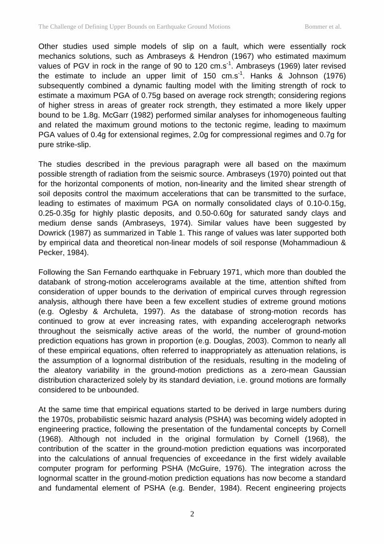
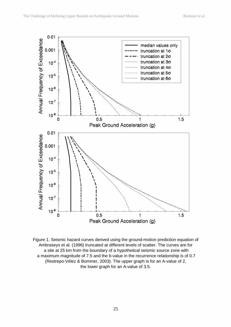
have shown the limitations of the lognormal formalism by extending PSHA to probability levels previously not explored, and thus given rise to the need to return to the issue of upper bounds on earthquake ground-motions. WHY UPPER LIMITS NEED TO BE DEFINED Upper limits on earthquake ground-motions have recently been identified as the “missing piece” from seismic hazard assessment, for both deterministic and probabilistic approaches (Bommer, 2002). Deterministic seismic hazard assessment (DSHA) is often interpreted to define the worst-case ground motion. DSHA should therefore be based on the least favorable combination of earthquake source characteristics and location, and the strongest ground-motion that could be generated by this scenario. In practice, DSHA generally uses the logarithmic mean or mean-plus-one-standard-deviation level of ground motion from predictive equations (e.g. Krinitzsky, 2002), which will generally be significantly below the worst-case scenario (Bommer, 2003). If DSHA is to be used to define the maximum earthquake loading to which a structure may be subjected, then an estimate of the upper limit on the ground motion that a particular scenario could generate is needed. Brune (1999) observed that PSHA using ground-motion prediction equations with untruncated lognormal scatter may overestimate ground motions with very long return periods. This inference was based on observations of the stability of precariously balanced rocks in the Mojave Desert. The need for defining upper limits on ground motions in PSHA only becomes clearly apparent when ground motions are calculated for very low annual frequencies of exceedance. For very long return periods, the hazard estimates are driven by the tails of the untruncated Gaussian distribution of the logarithmic residuals (Anderson & Brune, 1999; Abrahamson, 2000). The effect of truncating the distribution at different levels above the mean is illustrated in Figure 1. This figure indicates that for the situation analyzed therein, at the 10-4 level – which has been widely used as the basis for seismic safety analyses in nuclear installations in the past – the difference in the resulting hazard between truncating at 3 sigmas or 6 sigmas is almost negligible. Figure 1 also clearly shows that at annual frequencies of exceedance of the order of 10-7 or 10-8, the issue of whether the truncation level is at 3, 4, 5 or 6 sigma becomes a controlling factor on the computed hazard. The hazard curves shown in the figure are for one particular configuration and the sensitivity to the truncation level may not always be so high, particularly for sites closer to seismic source zones. Moreover, the two sets of curves indicate that the sensitivity to the truncation level is also related to the underlying seismicity rates. For most engineering projects, such long return periods are of no relevance, but for the rare situations where the risk analysis must consider such extreme cases, the definition of upper bounds becomes a necessity. The PSHA carried out for the nuclear waste repository at Yucca Mountain in the Nevada desert (Stepp et al., 2001) considered ground motions for annual frequencies of exceedance as low as 10-8, and as a result of not using truncations, extremely – and probably unphysically – high levels of ground


4

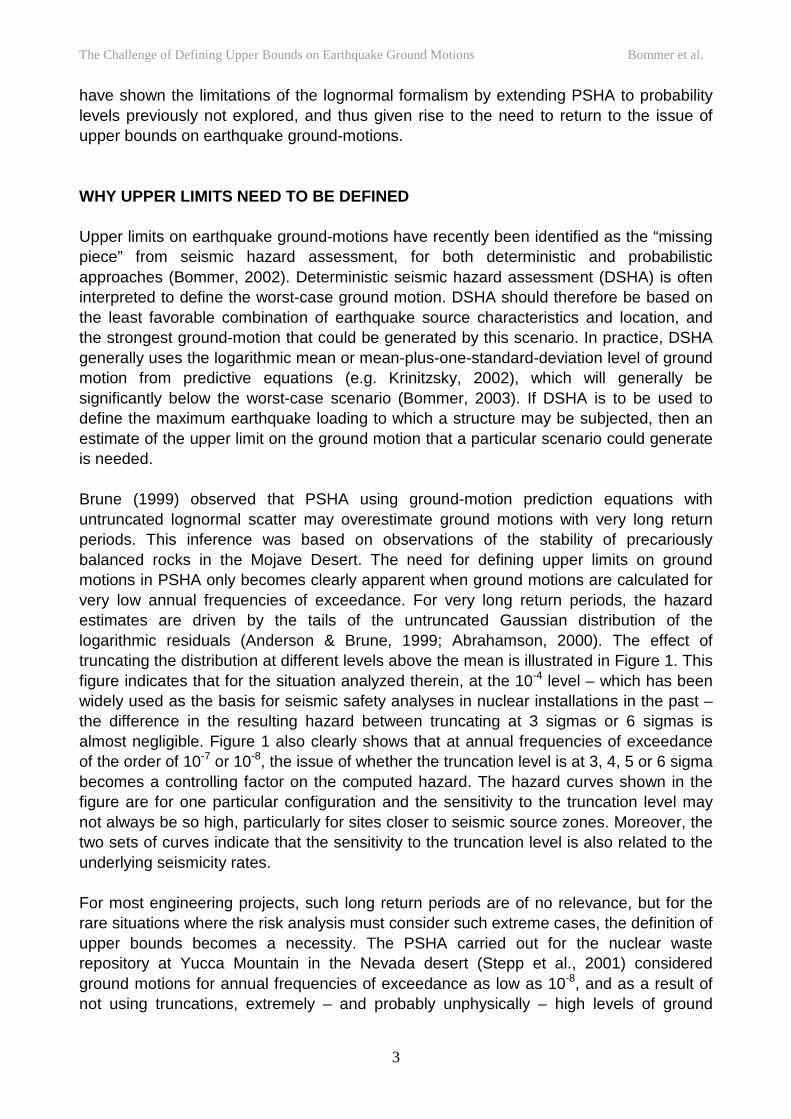
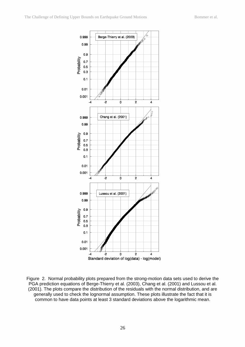
motion were computed: PGA values as high as 20g and PGV values that almost reached 18 m.s-1 (Corradini, 2003). The Yucca Mountain PSHA has been one of the first comprehensive applications of the SSHAC Level 4 procedures (Budnitz et al., 1997) for expert elicitation in seismic hazard assessment. A more recent application has been the PEGASOS project to perform a comprehensive seismic hazard assessment for nuclear power plants in Switzerland (Abrahamson et al., 2002)., which has considered annual frequencies of exceedance as low as 10-7. In large part due to the outcome of the Yucca Mountain PSHA, the PEGASOS project has required experts in both the ground motion and site response sub-projects – the latter being a feature not included in the Yucca Mountain study – to specify bounding values on the ground motions. Due to the sensitivity of the computed hazard to the truncation level, the critical point in the definition of this level is that it truly represents the boundary of physically acceptable ground motions and only excludes unphysical values. Romeo & Prestininzi (2000) proposed an upper bound at two standard deviations above the logarithmic mean of the prediction equation for PGA on the basis that “stronger motions are considered to be unlikely.” Since two standard deviations above the mean corresponds to the 97.7-percentile, it is not disputed that higher levels are indeed unlikely, but this does not mean that they are impossible. As Agathon pointed out, “It is a part of probability that many improbable things will happen”; the obvious corollary to this statement, in the context of upper bounds, is that impossible things will not happen. For an equation with homoscedastic scatter (i.e. constant sigma for all magnitude and distance combinations), the upper bound will generally lie at least 3 standard deviations above the mean (Figure 2). To distinguish between improbable and impossible levels of ground motion can only be achieved if the physical processes controlling ground motions are identified, and the interactions between these processes assessed. FACTORS DRIVING AND LIMITING EXTREME GROUND MOTIONS The maximum ground motions that can be experienced at the ground surface are controlled by three factors: the most intense seismic radiation that can emanate from the source of the earthquake; the interaction of radiation from different parts of the source and from different travel paths; and the limits on the strongest motion that can be transmitted to the surface by shallow geological materials. The maximum amplitude of seismic radiation from the earthquake source, for a given seismic moment, is controlled by the total energy release and the rate of energy release, which are dependent on factors describing the mechanics of the rupture process, such as the magnitude of the slip, its velocity (often approximated as a function of the source rise time and the final slip), and the velocity of rupture propagation. Although the average values of these quantities generally provide a good first-order approximation, it should be kept in mind that they possess a high degree of spatial variability, resulting from heterogeneities in material properties and stress conditions across the fault plane. This needs to be taken into account since in some instances it is the rate of change of these quantities rather than their absolute value that will influence the level of ground motion. In


5

particular, high-frequency ground motion results from abrupt changes in rupture velocity (Madariaga, 1977) whereas lower frequency motions are influenced more by the actual value of the rupture velocity. While it is fully acknowledged that slip, rise time, rupture velocity and their respective rates of change are highly interdependent variables, they are presented separately in the following discussion for the sake of clarity. For larger events, the energy release is often concentrated in small zones of the fault plane, called asperities (Aki, 1984). Asperities are characterized by having much larger slip than the average over the entire rupture plane; the asperity slip contrast, defined as the ratio of average slip on the asperity to the average overall slip (Somerville et al., 1999), provides a first-order estimate of the relative strength of the asperity. The amplitude of the ground motions generated by an asperity can be expected to increase with asperity size (relative to the rupture area) and asperity contrast. The constraints of geometry and energy conservation however imply that both these quantities are bounded and moreover that their maximum possible values are inversely correlated. This inverse correlation can be observed in practice: in the database of Somerville et al. (1999), the largest asperity slip contrast (3.42) corresponds to the 1984 Morgan Hill earthquake, which has one of the lowest ratios of asperity area to total rupture (0.14 compared to the average of 0.22). Conversely, the largest relative size of asperities (0.4) is identified for the 1983 Borah Peak earthquake, which has an asperity slip contrast of 1.62, well below the sample average of 2.01. As discussed previously, details of the slip distribution (e.g. the slip contrast between the edge of the asperity and the surrounding region) might also be important, in particular for the generation of high-frequency motions. However, the importance of these details decreases with increasing distance from the source. For sites located far enough away from the source, the effect of the source on ground motions can be satisfactorily estimated using the average value of slip velocity. While the slip distribution reflects spatial variations in the density of energy release, the distribution of the slip velocity gives an indication of the rate at which this energy is released. The velocity of fault rupture will also play a role in controlling the most extreme ground motions that can be generated, since rupture velocity affects the corner frequency of the radiated body waves. In a study of the 1906 San Francisco earthquake, Boore (1977) finds that a change of rupture velocity from 2 to 3 km/s led to a four-fold increase in computed ground motions at periods of about 5 seconds. Boore & Joyner (1978) investigate how the introduction of incoherence into the smooth propagation model of Boore (1977) affects the outcome and conclude that the sensitivity of near-field ground motions to rupture velocity and azimuth is preserved as long as the mean rupture velocity is the same. It should however be kept in mind that the figure quoted above is the result of a modeling exercise, rather than an observed quantity. If the spatial variability of rupture velocity across the fault plane is considered, the definition of the maximum permissible values of this quantity becomes even more of an issue. Das (2003) discusses the development of proposals regarding maximum permissible rupture speeds, addressing in particular the issue of whether rupture velocity


6

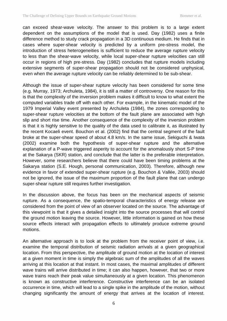
can exceed shear-wave velocity. The answer to this problem is to a large extent dependent on the assumptions of the model that is used. Day (1982) uses a finite difference method to study crack propagation in a 3D continuous medium. He finds that in cases where super-shear velocity is predicted by a uniform pre-stress model, the introduction of stress heterogeneities is sufficient to reduce the average rupture velocity to less than the shear-wave velocity, while local super-shear rupture velocities can still occur in regions of high pre-stress. Day (1982) concludes that rupture models including extensive segments of super-shear propagation should not be considered unphysical, even when the average rupture velocity can be reliably determined to be sub-shear. Although the issue of super-shear rupture velocity has been considered for some time (e.g. Murray, 1973; Archuleta, 1984), it is still a matter of controversy. One reason for this is that the complexity of the inversion problem makes it difficult to know to what extent the computed variables trade off with each other. For example, in the kinematic model of the 1979 Imperial Valley event presented by Archuleta (1984), the zones corresponding to super-shear rupture velocities at the bottom of the fault plane are associated with high slip and short rise time. Another consequence of the complexity of the inversion problem is that it is highly sensitive to the quality of the data used to calibrate it, as illustrated by the recent Kocaeli event. Bouchon et al. (2002) find that the central segment of the fault broke at the super-shear speed of about 4.8 km/s. In the same issue, Sekiguchi & Iwata (2002) examine both the hypothesis of super-shear rupture and the alternative explanation of a P-wave triggered asperity to account for the anomalously short S-P time at the Sakarya (SKR) station, and conclude that the latter is the preferable interpretation. However, some researchers believe that there could have been timing problems at the Sakarya station (S.E. Hough, personal communication, 2003). Therefore, although new evidence in favor of extended super-shear rupture (e.g. Bouchon & Vallée, 2003) should not be ignored, the issue of the maximum proportion of the fault plane that can undergo super-shear rupture still requires further investigation. In the discussion above, the focus has been on the mechanical aspects of seismic rupture. As a consequence, the spatio-temporal characteristics of energy release are considered from the point of view of an observer located on the source. The advantage of this viewpoint is that it gives a detailed insight into the source processes that will control the ground motion leaving the source. However, little information is gained on how these source effects interact with propagation effects to ultimately produce extreme ground motions. An alternative approach is to look at the problem from the receiver point of view, i.e. examine the temporal distribution of seismic radiation arrivals at a given geographical location. From this perspective, the amplitude of ground motion at the location of interest at a given moment in time is simply the algebraic sum of the amplitudes of all the waves arriving at this location at that instant. In most cases, the maximal amplitudes of different wave trains will arrive distributed in time; it can also happen, however, that two or more wave trains reach their peak value simultaneously at a given location. This phenomenon is known as constructive interference. Constructive interference can be an isolated occurrence in time, which will lead to a single spike in the amplitude of the motion, without changing significantly the amount of energy that arrives at the location of interest.


7

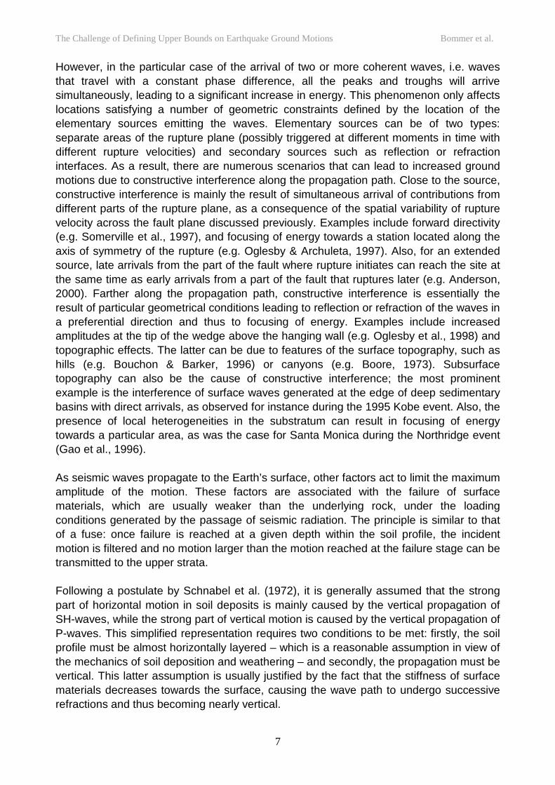
However, in the particular case of the arrival of two or more coherent waves, i.e. waves that travel with a constant phase difference, all the peaks and troughs will arrive simultaneously, leading to a significant increase in energy. This phenomenon only affects locations satisfying a number of geometric constraints defined by the location of the elementary sources emitting the waves. Elementary sources can be of two types: separate areas of the rupture plane (possibly triggered at different moments in time with different rupture velocities) and secondary sources such as reflection or refraction interfaces. As a result, there are numerous scenarios that can lead to increased ground motions due to constructive interference along the propagation path. Close to the source, constructive interference is mainly the result of simultaneous arrival of contributions from different parts of the rupture plane, as a consequence of the spatial variability of rupture velocity across the fault plane discussed previously. Examples include forward directivity (e.g. Somerville et al., 1997), and focusing of energy towards a station located along the axis of symmetry of the rupture (e.g. Oglesby & Archuleta, 1997). Also, for an extended source, late arrivals from the part of the fault where rupture initiates can reach the site at the same time as early arrivals from a part of the fault that ruptures later (e.g. Anderson, 2000). Farther along the propagation path, constructive interference is essentially the result of particular geometrical conditions leading to reflection or refraction of the waves in a preferential direction and thus to focusing of energy. Examples include increased amplitudes at the tip of the wedge above the hanging wall (e.g. Oglesby et al., 1998) and topographic effects. The latter can be due to features of the surface topography, such as hills (e.g. Bouchon & Barker, 1996) or canyons (e.g. Boore, 1973). Subsurface topography can also be the cause of constructive interference; the most prominent example is the interference of surface waves generated at the edge of deep sedimentary basins with direct arrivals, as observed for instance during the 1995 Kobe event. Also, the presence of local heterogeneities in the substratum can result in focusing of energy towards a particular area, as was the case for Santa Monica during the Northridge event (Gao et al., 1996). As seismic waves propagate to the Earth’s surface, other factors act to limit the maximum amplitude of the motion. These factors are associated with the failure of surface materials, which are usually weaker than the underlying rock, under the loading conditions generated by the passage of seismic radiation. The principle is similar to that of a fuse: once failure is reached at a given depth within the soil profile, the incident motion is filtered and no motion larger than the motion reached at the failure stage can be transmitted to the upper strata. Following a postulate by Schnabel et al. (1972), it is generally assumed that the strong part of horizontal motion in soil deposits is mainly caused by the vertical propagation of SH-waves, while the strong part of vertical motion is caused by the vertical propagation of P-waves. This simplified representation requires two conditions to be met: firstly, the soil profile must be almost horizontally layered – which is a reasonable assumption in view of the mechanics of soil deposition and weathering – and secondly, the propagation must be vertical. This latter assumption is usually justified by the fact that the stiffness of surface materials decreases towards the surface, causing the wave path to undergo successive refractions and thus becoming nearly vertical.


8

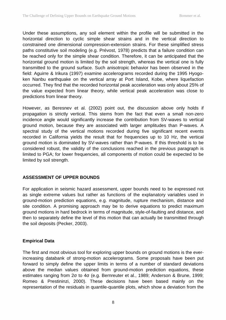
Under these assumptions, any soil element within the profile will be submitted in the horizontal direction to cyclic simple shear strains and in the vertical direction to constrained one dimensional compression-extension strains. For these simplified stress paths constitutive soil modeling (e.g. Prévost, 1978) predicts that a failure condition can be reached only for the simple shear condition. Therefore, it can be anticipated that the horizontal ground motion is limited by the soil strength, whereas the vertical one is fully transmitted to the ground surface. Such anisotropic behavior has been observed in the field: Aguirre & Irikura (1997) examine accelerograms recorded during the 1995 Hyogo-ken Nanbu earthquake on the vertical array at Port Island, Kobe, where liquefaction occurred. They find that the recorded horizontal peak acceleration was only about 25% of the value expected from linear theory, while vertical peak acceleration was close to predictions from linear theory. However, as Beresnev et al. (2002) point out, the discussion above only holds if propagation is strictly vertical. This stems from the fact that even a small non-zero incidence angle would significantly increase the contribution from SV-waves to vertical ground motion, because they are associated with larger amplitudes than P-waves. A spectral study of the vertical motions recorded during five significant recent events recorded in California yields the result that for frequencies up to 10 Hz, the vertical ground motion is dominated by SV-waves rather than P-waves. If this threshold is to be considered robust, the validity of the conclusions reached in the previous paragraph is limited to PGA; for lower frequencies, all components of motion could be expected to be limited by soil strength. ASSESSMENT OF UPPER BOUNDS For application in seismic hazard assessment, upper bounds need to be expressed not as single extreme values but rather as functions of the explanatory variables used in ground-motion prediction equations, e.g. magnitude, rupture mechanism, distance and site condition. A promising approach may be to derive equations to predict maximum ground motions in hard bedrock in terms of magnitude, style-of-faulting and distance, and then to separately define the level of this motion that can actually be transmitted through the soil deposits (Pecker, 2003). Empirical Data The first and most obvious tool for exploring upper bounds on ground motions is the ever-increasing databank of strong-motion accelerograms. Some proposals have been put forward to simply define the upper limits in terms of a number of standard deviations above the median values obtained from ground-motion prediction equations, these estimates ranging from 2 to 4 (e.g. Bernreuter et al., 1989; Anderson & Brune, 1999; Romeo & Prestininzi, 2000). These decisions have been based mainly on the representation of the residuals in quantile-quantile plots, which show a deviation from the


9

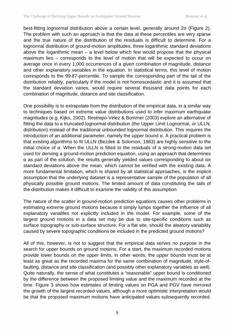
best-fitting lognormal distribution above a certain level, generally around 2 (Figure 2). The problem with such an approach is that the data at these percentiles are very sparse and the true nature of the distribution of the residuals is difficult to determine. For a lognormal distribution of ground-motion amplitudes, three logarithmic standard deviations above the logarithmic mean – a level below which few would propose that the physical maximum lies – corresponds to the level of motion that will be expected to occur on average once in every 1,000 occurrences of a given combination of magnitude, distance and other explanatory variables in the equation. In statistical terms, this level of motion corresponds to the 99.87-percentile. To sample the corresponding part of the tail of the distribution reliably, particularly if the model is not homoscedastic and it is assumed that the standard deviation varies, would require several thousand data points for each combination of magnitude, distance and site classification. One possibility is to extrapolate from the distribution of the empirical data, in a similar way to techniques based on extreme value distributions used to infer maximum earthquake magnitudes (e.g. Kijko, 2002). Restrepo-Vélez & Bommer (2003) explore an alternative of fitting the data to a truncated lognormal distribution (the Upper Limit Lognormal, or ULLN, distribution) instead of the traditional unbounded lognormal distribution. This requires the introduction of an additional parameter, namely the upper bound . A practical problem is that existing algorithms to fit ULLN (Bezdek & Solomon, 1983) are highly sensitive to the initial choice of . When the ULLN is fitted to the residuals of a strong-motion data set used for deriving a ground-motion prediction equation, using an approach that determines

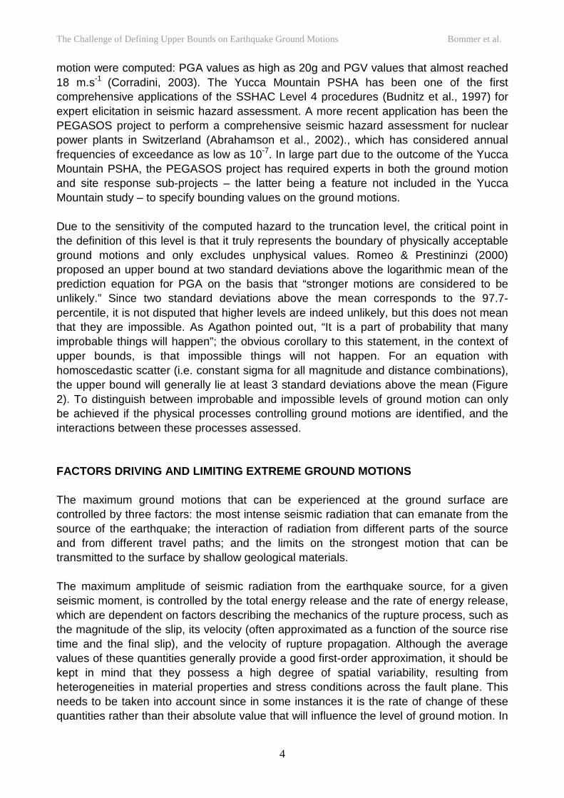
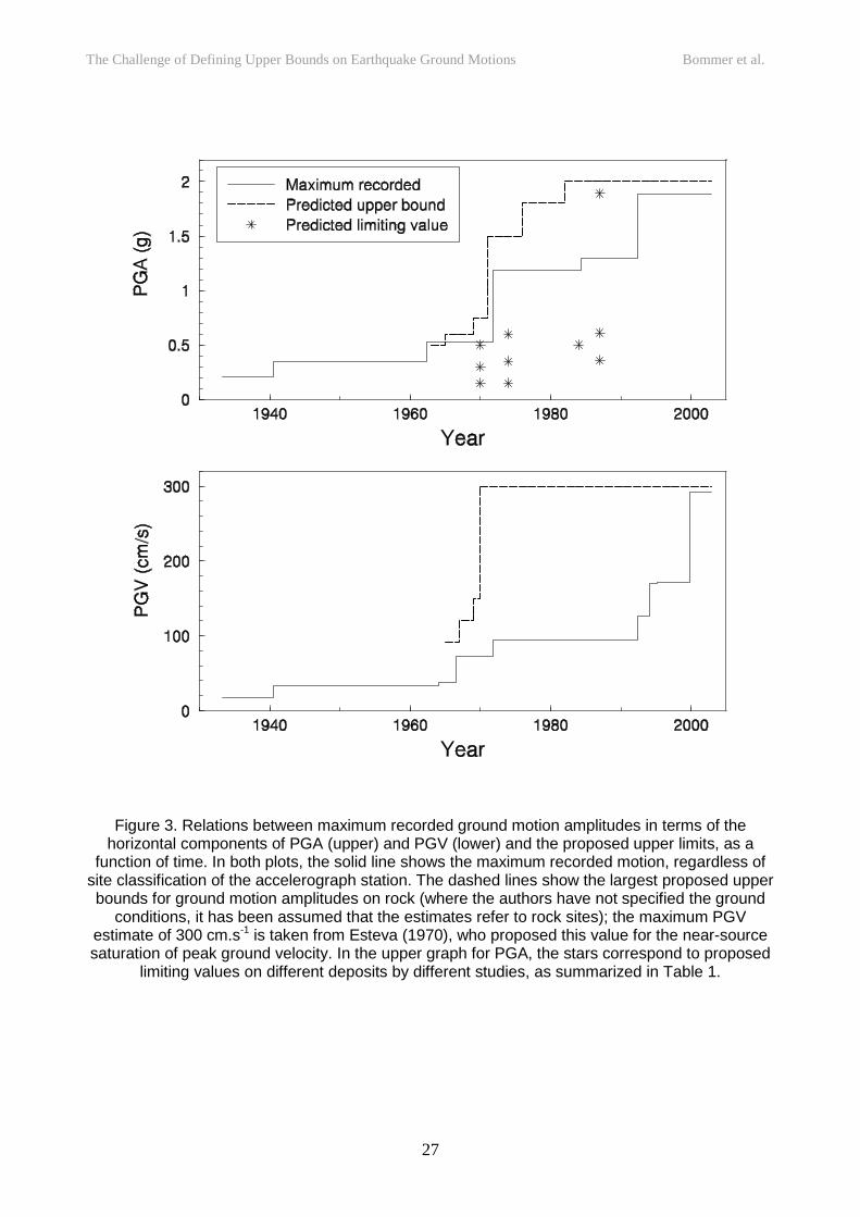
as part of the solution, the results generally yielded values corresponding to about six standard deviations above the mean, which cannot be verified with the existing data. A more fundamental limitation, which is shared by all statistical approaches, is the implicit assumption that the underlying dataset is a representative sample of the population of all physically possible ground motions. The limited amount of data constituting the tails of the distribution makes it difficult to examine the validity of this assumption. The nature of the scatter in ground-motion prediction equations causes other problems in estimating extreme ground motions because it simply lumps together the influence of all explanatory variables not explicitly included in the model. For example, some of the largest ground motions in a data set may be due to site-specific conditions such as surface topography or sub-surface structure. For a flat site, should the aleatory variability caused by severe topographic conditions be included in the predicted ground motions? All of this, however, is not to suggest that the empirical data serves no purpose in the search for upper bounds on ground motions. For a start, the maximum recorded motions provide lower bounds on the upper limits, in other words, the upper bounds must be at least as great as the recorded maxima for the same combination of magnitude, style-of-faulting, distance and site classification (and possibly other explanatory variables as well). Quite naturally, the sense of what constitutes a “reasonable” upper bound is conditioned by the difference between the proposed limiting value and the maximum recorded at the time. Figure 3 shows how estimates of limiting values on PGA and PGV have mirrored the growth of the largest recorded values, although a more optimistic interpretation would be that the proposed maximum motions have anticipated values subsequently recorded.


10

Most engineering seismologists would agree that the estimates of PGA obtained in the Yucca Mountain seismic hazard study are too high, being an order of magnitude greater than the largest recorded horizontal accelerations, but there is no consensus on how much they would need to be reduced to be considered physically realizable. Should an earthquake produce an accelerogram with a peak of, say, 3g in the near future, responses to this question would probably be modified. In passing it is important to note that the maximum ground motions shown in Fig. 3 correspond to those recorded on strong-motion accelerographs, which are therefore considered to be in the frequency range of interest to engineering applications. There are examples of much higher ground accelerations recorded from rock bursts in mines. In particular, McGarr et al. (1981) report that during a 0.72 ML tremor, a value of 7.7g corresponding to a single major S-wave arrival was recorded on a transverse component. The corresponding frequency is not given explicitly, but it can be inferred from the paper that it was probably of the order of 100 Hertz or more. The real value of the empirical data is in the insight it can provide into both the factors that create extreme levels of motion and those that limit the maximum surface amplitudes. Careful examination of the largest, and indeed the lowest, recorded amplitudes of motion can provide insight into the factors that tend to produce the strongest motions (e.g. Anderson et al., 2002), although it is important to always keep in mind that often a number of factors will be acting in unison to create the higher recorded amplitudes and the temptation must be resisted to assign the cause of the extreme motions to the current fashion, be it site amplification, Moho bounce, rupture directivity, or buried ruptures. Inversion of strong-motion recordings enables detailed pictures of the fault rupture process to be obtained and compared, such as has been done by Somerville et al. (1999) for a number of earthquakes producing significant accelerograms. All of this information is vital input to the only current possibility for identifying upper bounds of rock motions: estimates based on seismological source models. Source Models In the absence of large numbers of recordings from very dense accelerograph networks triggered by many earthquakes, the best possibility of constraining the likely maximum levels that ground-motion amplitudes can reach is through the use of models to generate synthetic accelerograms. The usefulness of any particular model in achieving this objective depends on the degree to which it explicitly includes each of the factors that tends to increase or to limit the most severe motions. However, even models that do not include all factors may still provide useful insight into the possible ranges of upper bound motions provided their results are carefully interpreted with respect to the effect of any missing factors. The theoretical modeling of ground motions is based on two fundamental results: Burridge & Knopoff (1964) establish the equivalence between a double-couple tensor and the shear force system acting on a fault plane in the so-called representation theorem,


11

and Aki (1967) found that the far-field radiation of seismic sources over a wide range of magnitudes could be approximated using an 2-model for the Fourier displacement spectrum. The first theoretical models presented for ground motion prediction were simple deterministic models. Haskell (1964) considered the problem of a propagating rupture on a rectangular fault plane, assuming constant rupture velocity along strike and instantaneous propagation along dip. Savage (1966) presents two models to calculate the far-field radiation of an elliptical fault, rupture being assumed to originate at one focus of the ellipse and then spread radially. In the first model, the slip is considered homogeneous across the fault surface, whereas in the second model it is variable and constrained to zero on the fault edge. Unlike Haskell’s model, Savage’s models include nucleation and rupture arrest features, leading to the simulated body waves exhibiting two stopping phases. Brune (1970,1971) considers a shear stress pulse on a circular fault and provides an estimate of the far-field spectrum that follows the 2-model and depends only on M0, the stress parameter measuring the average strength of the source (within this model), and wave propagation characteristics. The deterministic character of the models above implies that they can only predict coherent ground motions. This limits their applicability for high-frequency ground motions, which are strongly incoherent. Hanks & McGuire (1981) showed that high-frequency ground motions could be represented as finite-duration band-limited Gaussian white noise. Boore (1983) combined this result with Brune’s 2-model to obtain a widely used stochastic point-source model. The numeric implementation of this model, SMSIM (e.g. Boore 2000, 2003) also incorporates a theoretical propagation function accounting for path and site characteristics via a series of multiplicative filters. Beresnev & Atkinson (1998) extended the method to a finite source by dividing the fault plane into sub-faults, each represented as a stochastic point-source, and summing the contributions of the sub-events with appropriate time delays. Zeng et al. (1994) present a composite source model in which a great number of sub-events of various sizes are randomly distributed across the fault plane; the sub-event sizes are assumed to follow a fractal distribution (i.e. a power-law distribution with a fractional exponent) and are allowed to overlap. The radiation of each sub-event is assumed to follow the shape of the Brune (1970) model. The contributions from the sub-events are summed with appropriate time delays. This yields a complex source time function, which is convolved with a synthetic Green’s function obtained using the Zeng & Anderson (1994) algorithm to produce synthetic seismograms. The models above are all kinematic, i.e. the slip function is imposed. An alternative approach is to impose the stress conditions and derive the slip function from these, as is done in dynamic models. The distinct advantage offered by dynamic modeling is the fact that the limiting strength of the rock, in terms of the maximum sustainable stress, can be specified, thus allowing physical constraint on the radiated motions. In this respect, the upper bounds obtained from the kinematic source models are likely to be overestimates. Dynamic models are based on dislocation theory (Eshelby, 1957) and more precisely the


12

propagation of shear cracks. Madariaga (1976) introduced a very simple model based on a circular crack. This simple model was later revised to exclude stress singularities at the crack tip (Madariaga, 1977) and then evolved to a finite-fault model considering asperities (Madariaga, 1979), and more recently to 2D and 3D crack models (Madariaga et al., 1998; Tada & Madariaga, 2001) Aki and co-workers (e.g. Das & Aki, 1977; Aki, 1979; Papageorgiou & Aki 1983) explored the topic of spatial stress heterogeneity across the rupture surface using barriers and asperities. Although this model yields good results in backward modeling, it requires input parameters that are difficult to predict for future events, such as the location of asperities and barriers. This limitation is mainly related to the entirely deterministic character of the model and somewhat alleviated by the latest generation of dynamic models (Guatteri et al., 2003) that present a stochastic-dynamic model in which the characteristics of slip are allowed to vary across the fault plane, although the resulting model is so far applicable only for low frequencies. Whichever source model is chosen, the exploration of upper bounds requires, for each magnitude, mechanism and source-to-site distance combination, a large number of simulations to be run, varying each of the variables such as the location, size and strength of asperities, rupture velocity, and nucleation point. This task is onerous in terms of computational effort and time; the real challenge is to ensure that all of the combinations of rupture parameters are actually physical. There is little doubt that very extreme motions could be computed from a model including a large asperity, occupying about one third of the rupture plane, possessing a slip contrast of 3.0 and exhibiting variations of rupture velocity up to super-shear and a short rise time; there is also little doubt that such a situation is unlikely to be realizable. Herein, once again, lies the heart of the problem: the need to identify source characteristics that are not only unlikely (very small probability of realization) but actually impossible (zero probability). Another reason that the process of searching for extreme values is computationally intensive and very time-consuming is that for a given earthquake magnitude and source-to-site distance, there will be a large number of locations around the fault rupture that need to be considered. With relative ease, for a given velocity model, the least favorable locations could be identified, probably controlled by proximity to the major asperity and in the forward directivity position; lateral velocity variations would make this task considerably more difficult. However, there is also value in exploring the spatial variation of extreme motions around the fault rupture, since this can shed light on how likely the highest ground-motion recordings, invariably from sparse instrument networks, are to actually come close to the upper bounds, even if the rupture parameters represented a worst-case scenario. Strength of Surface Materials Several possibilities exist to account for the influence of the strength of surface materials on the maximum surface ground-motion. The first, and most natural, one consists in


13

running site response analyses with increasing amplitudes of the input bedrock motion (e.g. Mohammadioun & Pecker, 1984). As the input motion increases, the earthquake-induced shear stresses increase within the soil profile, eventually reaching the soil strength at some depth; at that stage, the incoming motion is no longer transmitted to the upper layers and the surface ground-motion is bounded to the value reached before saturation of the soil strength. Although attractive, the method suffers some drawbacks: it is time consuming, requires a genuinely non-linear algorithm (equivalent linear models are of limited usefulness for such calculations) and the results are very much dependent on the soil constitutive model and the accuracy of the parameters entering these models. On the other hand, using any finite element model, a great flexibility is offered to the analyst to model strongly heterogeneous profiles and even two dimensional geometries. Given the heavy burden put on the analyst for the implementation of the above approach, several attempts have been made to derive simplified estimates of the maximum surface ground-motion. So far, these estimates are limited to the evaluation of the maximum peak ground acceleration. Betbeder-Matibet (1993) has developed an expression for the maximum acceleration at the surface of a uniform soil layer overlying a rock half-space. This solution is based on the relationship between the maximum surface acceleration and the average soil column acceleration; this is obtained by the computation of a fundamental "non-linear" mode shape of the soil column. Although simple, this solution suffers from some limitations: the soil profile is assumed homogeneous with depth, which is seldom achieved in natural soil deposits, and the maximum ground surface acceleration does not depend on the frequency content of the input base motion. To overcome some of these limitations, Pecker (2003) has developed a simple but robust method for estimating the limiting value on PGA by deriving a solution for a heterogeneous soil profile in which the shear modulus varies with depth. The proposed method is supported by observations in California available at the ROSRINE web site (http://geoinfo.usc.edu/rosrine). The method is quite simple, relying mainly on the estimates of two quantities, the depth-dependent shear strength, and the yield shear strain of the soil. Of these two quantities, the former can be quite reliably measured under static conditions using well-defined procedures that may vary according to the soil type, along with the appropriate strength criterion, and variations in the latter do not affect the outcome significantly. However, this solution involves a number of issues that deserve further investigation, such as the margin of error introduced by using static measurement procedures to estimate dynamic quantities and by assuming a similar behavior at small and large strains. The possibilities for investigating the limitations on earthquake ground-motions imposed by soil strength through laboratory investigations may be limited. Since the strength and stiffness of soils are pressure dependent, shake table tests are limited by the fact that the samples are generally in a 1g environment and too small to reproduce realistic in situ stresses. Some geotechnical centrifuges, provided that they are able to reproduce


14

realistic seismic ground motions as the input to the soil samples, may, however, be able to provide some useful results. The existence of a well-defined physical limiting mechanism for ground accelerations on soil is encouraging, but it should be kept in mind that any method trying to capture the resulting limits requires bedrock motion as input, and therefore the problem cannot be entirely decoupled from the estimation of extreme bedrock motions. The limiting values on other parameters, such as peak ground velocity, which may be controlled by different mechanisms, also needs to be explored. A Framework for Comprehensive Definition of Upper Bounds As has been mentioned previously, the needs of seismic hazard assessment for critical facilities are not met by simply defining the maximum level of ground motion that could ever be achieved. Upper bounds need to be defined, possibly on a regional basis (and certainly separate definitions will be needed for crustal and for subduction earthquakes) as limiting surfaces defined by at least the following parameters: magnitude, style-of-faulting, depth of faulting, source-to-site distance and site conditions, which will almost definitely need to consider both the strength of the materials in the upper tens of meters at the site and the structure over a depth of several kilometers. In terms of the combinations of parameters for which the maximum ground-motion surface needs to be defined, it is worth making a passing comment on magnitudes, for which maximum attainable values are routinely specified in PSHA. Jackson (1996) argues for the occurrence of very large earthquakes, with magnitudes in excess of Mw 8, in crustal regions (specifically California), with recurrence intervals measured in thousands of years. Hough (1996) and Schwartz (1996) present convincing cases against the hypothesis that Jackson (1996) presents, but even if such earthquakes were feasible, they may not be of particular importance for the issue of the upper bound ground motions: A site near one end of a fault rupture extending over a length of 1,000 km will be blissfully unaware of the strong motion generated by the second half of the rupture. Another important point to be borne in mind is that to obtain the strongest possible ground motions at a particular distance from the fault rupture using seismological source models, the high spatial variability of ground motions needs to be considered. Oglesby & Archuleta (1997) argue that the very high amplitudes recorded at the Cape Mendocino station during the 1992 Petrolia earthquake were the result of its location at a specific point with respect to the radiation from the main fault asperity. In the preceding discussions a clear distinction has been made between the effects that contribute to creating and limiting extreme ground motions; although the separation is useful from an analytical point of view, the final model for upper bounds will need to consider the interaction between the two, since the nature of site response is dependent upon the base excitation. For the model of Pecker (2003), this can readily be accomplished because the proposed method properly takes into account the frequency content of the base motion through its elastic response spectrum. In addition, simple


15

transfer methods, which are standard practice in structural dynamics, can be used to compute not only the maximum ground acceleration but the whole surface response spectrum (Igusa & Der Kiureghian, 1985). There is a potential pitfall in determining upper bounds if analyses are performed for individual strong-motion parameters and then hazard analysis is carried out allowing each parameter to reach its maximum maximus value. The total energy liberated by a fault rupture will always be limited since the seismic energy released per unit of the source volume is approximately constant; extreme ground motions are therefore likely to be created not so much by generation of very high amounts of energy but rather by the focusing of the energy into particular period ranges. Source effects such as rupture directivity will generally affect longer period motions; site effects will often cause focusing of the energy into a narrow frequency band. Therefore, a vector approach may be needed, following the proposal of Bazzurro & Cornell (2002), in which PSHA is performed for two ground-motion parameters simultaneously, including a model for the covariance of the residuals of each parameter to calculate the joint probability distribution. As has been suggested by Restrepo-Vélez & Bommer (2003), this concept could be extended to the definition of upper bound ground-motions since the latter correspond to the maximum residuals. Another point that needs to be kept in mind is that although the definition of upper bounds on ground-motion amplitudes will always correspond to the largest absolute values, for source effects the most extreme ground motions, in a general sense, will probably correspond to the shortest possible duration of shaking for a given magnitude. There may be situations, particularly with regard to liquefaction hazard for example, where long duration of shaking will define the worst-case scenario, but for structural response (except for strongly degrading structures) the worst-case scenario is likely to be related to the amplitude of the ground motion even though it has shorter duration. Short duration of shaking, whereby the major part of the Arias intensity is accumulated in a short interval, can be driven by bi-lateral rupture and high rupture velocities (Bommer & Martínez-Pereira, 1999) and by forward directivity effects (Somerville et al., 1997). A final point worthy of mention is terminology, especially since engineering seismology is a field in which many ill-defined terms – such as attenuation relations and stress drop (Atkinson & Beresnev, 1997) – have become part of common usage. The generic term ‘upper bounds’ used in the title of this paper refers to the final effect of all of the factors that either increase or limit ground motions, whereas it could be helpful to use terminology that distinguishes between these influences. For the maximum amplitudes of ground motion that can be generated in rock due to the limiting values of source parameters and wave propagation effects, ‘bounding ground motion’ has been proposed as suitable term, whereas the surface amplitudes imposed by the limiting strength of near-surface strata could be referred to as ‘upper limits’ (C. Stepp, personal communication, 2003).


16

CONCLUDING REMARKS This paper has made the case for upper bounds on earthquake ground-motions to be defined, and offered some thoughts on ways in which the problem can be addressed and a framework for how the solutions may be expressed. A great deal of work remains to be done and this article is not intended to provide definitive answers: the intention of the authors is rather to issue a call to arms and encourage new research and exchanges of ideas and results on this problem. The number of engineering projects for which extreme motions are likely to be of relevance is limited, primarily by the fact that the importance – in terms of cost or consequences of failure or loss of function – of few projects is sufficient to warrant the expense of designing against the absolute worst-case ground motions. However, for those projects whose criticality and design life result in design for ground-motions with annual frequencies of exceedance smaller than 10-6, such as the Yucca Mountain waste repository, the issue of upper limits on ground motions requires urgent attention. And although research into this topic may be driven initially by the needs of seismic hazard assessments for critical facilities, the work can be expected to provide very useful insight into issues of more general applicability, defining the limits of the hazard space, identifying factors that increase or limit hazard levels, and improving, in the process, the capability to model ground motions and site response. ACKNOWLEDGEMENTS This paper, and ongoing work that it establishes the basis for, has arisen directly from the PEGASOS project in Switzerland, in which most of the authors participated as members of expert panels on ground-motion models (EG2) and site response (EG3). The Technical Facilitator Integrator of both groups was the second author of the paper, assisted by Dr Patrick Smit for EG2 and by Dr Martin Koller for EG3, bringing to the project the invaluable experience of the Yucca Mountain study. The authors are very grateful to all the organizers of the PEGASOS project who provided such a stimulating atmosphere to explore these challenging and exciting ideas: Philip Birkhäuser, Jim Farrington, René Graf, Andreas Hölker, Philippe Roth, and Christian Sprecher. We are also grateful to the resource experts, Dr Arben Pitarka and Dr Enrico Priolo, and their colleagues at URS Corporation and OGS, Trieste, respectively, for providing numerical simulations of ground motions that helped to guide our first attempts to define upper bounds on ground motions in bedrock. The authors wish to express gratitude to Luis Fernando Restrepo-Vélez for his assistance with Fig. 1, to Philippe Roth of Proseis for input to Fig. 2, and to David M. Boore for input to Fig. 3. The manuscript has been improved at different stages by constructive criticisms and helpful suggestions from the following individuals, to whom the authors are indebted: Nicholas N. Ambraseys, John G. Anderson, David M. Boore, John Douglas, Thomas C. Hanks, Susan E. Hough, Martin Koller, Art McGarr, Luis Fernando Restrepo-Vélez, Carl J. Stepp and Gabriel R. Toro.


17

REFERENCES Abrahamson, N.A. (2000). State of the practice of seismic hazard evaluation. Proceedings of GeoEng 2000, Melbourne, 19-24 November, vol. 1, 659-685. Abrahamson, N.A., P. Birkhauser, M. Koller, D. Mayer-Rosa, P. Smit, C. Sprecher, S. Tinic & R. Graf (2002). PEGASOS – a comprehensive probabilistic seismic hazard assessment for nuclear power plants in Switzerland. Proceedings of the Twelfth European Conference on Earthquake Engineering, London, Paper no. 633. Aki, K. (1967). Scaling law of seismic spectrum. Journal of Geophysical Research 73, 5359-5376. Aki, K. (1979). Characterization of barriers on an earthquake fault. Journal of Geophysical Research 74, 615-631. Aki, K. (1984). Asperities, barriers, characteristic earthquakes and strong motion prediction. Journal of Geophysical Research 89, 5867-5872. Aguirre, J. & K. Irikura (1997). Nonlinearity, liquefaction, and velocity variation of soft soil layers in Port Island, Kobe, during the Hyogo-ken Nanbu earthquake. Bulletin of the Seismological Society of America 87(5), 1244-1285. Ambraseys, N.N. (1969). Maximum intensity of ground movements caused by faulting. Proceedings of the Fourth World Conference on Earthquake Engineering, Santiago de Chile, vol. 1, 154. Ambraseys, N.N. (1970). Factors controlling the earthquake response of foundation materials. Proceedings of the Third European Symposium on Earthquake Engineering, Sofia, 309-317. Ambraseys, N.N. (1974). Dynamics and response of foundation materials in epicentral regions of strong earthquakes. Proceedings of the Fifth World Conference on Earthquake Engineering, Rome, vol. 1, cxxvi-cxlviii. Ambraseys, N.N. & A. Hendron (1967). Dynamic behaviour of rock masses. In: Rock Mechanics in Engineering Practice, K. Stagg & O. Zienkewicz eds., John Wiley, 203-236. Ambraseys, N.N., K.A. Simpson & J.J. Bommer (1996). Prediction of horizontal response spectra in Europe. Earthquake Engineering & Structural Dynamics 25, 371-400. Anderson, J.G. (2000). Expected shape of regressions for ground-motion parameters on rock. Bulletin of the Seismological Society of America 90, S43-S52. Anderson, J.G. & J.N. Brune (1999). Probabilistic seismic hazard assessment without the ergodic assumption. Seismological Research Letters 70(1), 19-28.


18

Anderson, J.G., J.N. Brune & S.G. Wesnousky (2002). Physical phenomena controlling high-frequency seismic wave generation in earthquakes. Proceedings of the Seventh US National Conference on Earthquake Engineering, 21-25 July, Boston, MA, Earthquake Engineering Research Institute. Archuleta, R. (1984). A faulting model for the 1979 Imperial Valley earthquake. Journal of Geophysical Research 89, 4559-4585. Atkinson, G.M. & I. Beresnev (1997). Don’t call it stress drop. Seismological Research Letters 68(1), 3-4. Bazzurro, P. & C.A. Cornell (2002). Vector-valued probabilistic seismic hazard analysis (VPSHA). Proceedings of the Seventh US National Conference on Earthquake Engineering, Boston, MA, 21-25 July, Earthquake Engineering Research Institute. Bender, B. (1984). Incorporating acceleration variability into seismic hazard analysis. Bulletin of the Seismological Society of America 74, 1451-1462. Beresnev, I. A. & G.M. Atkinson (1998). FINSIM: A FORTRAN program for simulating stochastic acceleration time histories from finite faults. Seismological Research Letters 69, 27-32. Beresnev, I.A., A.M. Nightengale & W.J. Silva (2002). Properties of Vertical Ground Motions. Bulletin of the Seismological Society of America 92(8), 3152-3164. Berge-Thierry, C., F. Cotton, O. Scotti, D-A. Griot-Pomnera & Y. Fukushima (2003). New empirical response spectral attenuation laws for moderate European earthquakes. Journal of Earthquake Engineering 7(2), 193-222. Bernreuter, D.L., J.B. Savy, R.W. Mensing & J.C. Chen (1989). Seismic hazard characterization of 69 nuclear power plant sites East of the Rocky Mountains. Report NUREG/CR-5250, US Nuclear Regulatory Commission. Betbeder-Matibet, J. (1993). Calcul de l'effet de site pour une couche de sol. Troisième Colloque National de Génie Parasismique, Saint-Rémy-lès-Chevreuse, vol 1, DS1-DS10. Bezdek, J. C. & K.H. Solomon (1983). Upper limit lognormal distribution for drop size data. ACSE Journal of Irrigation and Drainage Engineering 109 (1), 72-88. Bommer, J.J. (2002). Deterministic vs. probabilistic seismic hazard assessment: an exaggerated and obstructive dichotomy. Journal of Earthquake Engineering 6(special issue no. 1), 43-73. Bommer, J.J. (2003). Uncertainty about the uncertainty in seismic hazard analysis. Engineering Geology 70(1/2), 165-168. Bommer, J.J. & A. Martínez-Pereira (1999). The effective duration of earthquake strong motion. Journal of Earthquake Engineering 3(2), 127-172.


19

Boore, D.M. (1973). The effect of simple topography on seismic waves: Implications for the accelerations recorded at Pacoima Dam, San Fernando Valley, California. Bulletin of the Seismological Society of America 63, 1603-1609. Boore, D.M. (1977). Strong motion recordings of the California earthquake of April 18, 1906. Bulletin of the Seismological Society of America 67, 561-577. Boore, D. M. (1983). Stochastic simulation of high-frequency ground motions based on seismological models of the radiated spectra. Bulletin of the Seismological Society of America 73, 1865-1894. Boore, D. M. (2000). SMSIM Fortran programs for simulating ground motions from earthquakes:version 2.0: A revision of OFR 96-80-A. US Geological Survey Open-File Report OF 00-509, 55 pp. Boore, D. M. (2003). Prediction of ground motion using the stochastic method. Pure and Applied Geophysics 160(3-4), 635-676. Boore, D.M. & W.B. Joyner (1978). The influence of rupture incoherence on seismic directivity. Bulletin of the Seismological Society of America 68(2), 283-300. Bouchon, M. & J.S. Barker (1996). Seismic response of a hill: The example of Tarzana, California. Bulletin of the Seismological Society of America 86(1), 66-72. Bouchon, M. & M. Vallée (2003). Observations of long supershear rupture during the magnitude 8.1 Kunlunshan earthquake. Science 301, 824-826. Bouchon, M., M.N. Toksöz, H. Karabulut, M.-P. Bouin, M. Dietrich, M. Aktar & M. Edie (2002). Space and time evolution of rupture and faulting during the 1999 Izmit (Turkey) earthquake. Bulletin of the Seismological Society of America 92(1), 256-266. Brune, J. N. (1970). Tectonic stress and the spectra of seismic shear waves from earthquakes. Journal of Geophysical Research, 75, 4997-5009. Brune, J. N. (1971). Correction. Journal of Geophysical Research 76, 5002. Brune, J.N. (1999). Precarious rocks along the Mojave section of the San Andreas fault, California: constraints on ground motion from great earthquakes. Seismological Research Letters 70, 29-33. Budnitz, R.J., G. Apostolakis, D.M. Boore, L.S. Cluff, K.J. Coppersmith, C.A. Cornell & P.A. Morris (1997). Recommendations for probabilistic seismic hazard analysis: guidance on uncertainty and use of experts. NUREG/CR-6372, US Nuclear Regulatory Commission. Burridge, R. & L. Knopoff (1964). Body force equivalents for seismic dislocations. Bulletin of the Seismological Society of America 54, 1875-1888.


20

Chang, T., F. Cotton & J. Anglier (2001). Seismic attenuation and peak ground acceleration in Taiwan. Bulletin of the Seismological Society of America 91(5), 1229-1246. Cornell, C.A. (1968). Engineering seismic risk analysis. Bulletin of the Seismological Society of America 58, 1583-1606. Corradini, M.L. (2003). Letter from chairman of the US Nuclear Waste Technical Review Board to the Director of the Office of Civilian Radioactive Waste Management, available at http://www.nwtrb.gov/corr/mlc010.pdf. Das, S. (2003). Spontaneous complex earthquake rupture propagation. Pure and Applied Geophysics 160(3-4), 579-602. Day, S.M. (1982). Three-dimensional simulation of spontaneous rupture: the effect of nonuniform prestress. Bulletin of the Seismological Society of America. 73(6), 1881-1902. Das, S. & K. Aki (1977). Fault planes with barriers: A versatile earthquake model. Journal of Geophysical Research 82, 5648-5670. Douglas, J. (2003). Earthquake ground motion estimation using strong-motion records: a review of equations for the estimation of peak ground acceleration and response spectral ordinates. Earth Science Reviews 61, 43-104. Dowrick, D.J. (1987). Earthquake Resistant Design for Engineering and Architects. Second edition. John Wiley & Sons. Eshelby, J.D. (1957). The determination of the elastic field of an ellipsoidal inclusion, and related problems. Proceedings of the Royal Society of London, Series A, Mathematical and Physical Sciences 241(1226), 376-396. Esteva, L. (1970). Seismic risk and seismic design. In: Seismic Design for Nuclear Power Plants, ed. R. Hansen, MIT Press, Cambridge, 142-182. Gao, S., H. Liu, P.M. Davis & L. Knopoff (1996). Localized amplification of seismic waves and correlation with damage due to the Northridge earthquake. Bulletin of the Seismological Society of America 86(1B), S209-S230 Guatteri, M., P.M. Mai, G.C. Beroza & J. Boatwright (2003). Strong ground motion prediction from stochastic-dynamic source models. Bulletin of the Seismological Society of America 93(1), 301-313. Hanks, T.C. & D.A. Johnson (1976). Geophysical assessment of peak acceleration. Bulletin of the Seismological Society of America 66, 959-968. Hanks, T.C. & R.K. McGuire (1981). The character of high-frequency ground motion. Bulletin of the Seismological Society of America 71(6), 2071-2095.


21

Haskell, N.A. (1964). Total energy and energy spectral density of elastic wave radiation from propagating faults. Bulletin of the Seismological Society of America 54, 1811-1841. Hough, S.E. (1996). The case against huge earthquakes. Seismological Research Letters 67(3), 3-4. Housner, G.W. (1965). Intensity of ground shaking near the causative fault. Proceedings of the Third World Conference on Earthquake Engineering, Auckland, vol. 1, 81-94. Igusa, T. & A. Der Kiureghian (1985). Generation of floor response spectra including oscillator-structure interaction. Earthquake Engineering & Structural Dynamics 13, 661-676. Jackson, D.D. (1996). The case for huge earthquakes. Seismological Research Letters 67(1), 3-5. Kijko, A. (2002). Statistical estimation of maximum regional earthquake magnitude. Proceedings of the Twelfth European Conference on Earthquake Engineering, London, Paper no. 22, Elsevier. Krinitzsky, E.L. (2002). How to obtain earthquake ground motions for engineering design. Engineering Geology 65(1), 1-16. Lussou, P., P. Bard., F. Cotton & Y. Fukushima (2001). Seismic design regulation codes: contribution of K-Net data to site effect evaluation. Journal of Earthquake Engineering 5(1), 13-33. Madariaga, R. (1976). Dynamics of an expanding circular fault. Bulletin of the Seismological Society of America 66(3), 639-666. Madariaga, R. (1977). High-frequency radiation from crack (stress drop) models of earthquake faulting. Geophysical Journal of the Royal Astronomical Society 51, 625-651. Madariaga, R. (1979). On the relation between seismic moment and stress drop in the presence of stress and strength heterogeneities. Journal of Geophysical Research 84(B5), 2243-2250. Madariaga, R., K. Olsen & R. Archuleta (1998). Modeling dynamic rupture in a 3D earthquake fault model. Bulletin of the Seismological Society of America 88(5), 1182-1197. McGarr, A. (1982). Upper bounds on near-source peak ground motion based on a model of inhomogeneous faulting. Bulletin of the Seismological Society of America 72, 1825-1841. McGarr, A., R.W.E. Green & S.M. Spottiswoode (1981). Strong ground motion of mine tremors: some implications for near source ground motion parameters. Bulletin of the Seismological Society of America 71(1), 295-319.


22

McGuire, R.K. (1976). FORTRAN computer program for seismic risk analysis. US Geological Survey Open-File Report 76-67. Mohammadioun, B. & A. Pecker (1984). Low-frequency transfer of seismic energy by superficial soil deposits and soft rocks. Earthquake Engineering & Structural Dynamics 12, 537-564. Murray, G.F. (1973). Dislocation mechanism – the Parkfield 1966 accelerograms. Bulletin of the Seismological Society of America 63(5), 1539-1555. Newmark, N.M. (1965). Effects of earthquakes on dams and embankments. Géotechnique 15, 139-160. Newmark, N.M. & W.J. Hall (1969). Seismic design criteria for nuclear reactor facilities. Proceedings of the Fourth World Conference on Earthquake Engineering, Santiago de Chile, vol. 2, B4.37-B4.50. Newmark, N.M. & E. Rosenblueth (1971). Fundamentals of Earthquake Engineering. Prentice Hall. Oglesby, D.D. & R.J. Archuleta (1997). A faulting model for the 1992 Petrolia earthquake: can extreme ground accelerations be a source effect? Journal of Geophysical Research 102(B2), 11,877-11,897. Oglesby, D.D., R.J. Archuleta & S.B. Nielsen (1998). Earthquakes on dipping faults: the effects of broken symmetry. Science, 280(5366), 1055-1059. Papageorgiou, A. S. & K. Aki (1983). A specific barrier model for the quantitative description of inhomogeneous faulting and the prediction of strong ground motion. I: Description of the model. Bulletin of the Seismological Society of America 73, 693-722. Pecker, A. (2003). An estimate of maximum ground surface motion. Comptes Rendus de l'Académie des Sciences, Paris, in press. Prévost J.H. (1978). Plasticity theory for soil stress-strain behavior. ASCE Journal of Engineering Mechanics, 104(EM5), 1177-1194. Restrepo-Vélez, L.F. & J.J. Bommer (2003). An exploration of the nature of the scatter in ground-motion prediction equations and the implications for seismic hazard assessment. Journal of Earthquake Engineering 7(special issue no.1), 171-199. Romeo, R. & A. Prestininzi (2000). Probabilistic versus deterministic hazard analysis: an integrated approach for siting problems. Soil Dynamics & Earthquake Engineering 20, 75-84.


23

Savage, J.C. (1966). Radiation from a realistic model of faulting. Bulletin of the Seismological Society of America 56(2), 577-592. Schnabel P.E., J. Lysmer & H.B. Seed (1972). SHAKE - A computer program for earthquake response analysis of horizontally layered sites. Report EERC 72-12, Earthquake Engineering Research Center, University of California, Berkeley. Schwartz, D.P. (1996). Letter. Seismological Research Letters 67(3), 5-6. Sekiguchi, H. & T. Iwata (2002). Rupture process of the 1999 Kocaeli, Turkey, earthquake estimated from strong-motion waveforms. Bulletin of the Seismological Society of America 92(1), 300-311. Somerville, P., K. Irikura, R. Graves, S. Sawada, D. Wald, N. Abrahamson, Y. Iwasaki, T. Kagawa, N. Smith & A. Kowada (1999). Characterizing crustal earthquake slip models for the prediction of strong ground motion. Seismological Research Letters 70, 59-80. Somerville, P.G., N.F. Smith, R.W. Graves & N.A. Abrahamson (1997). Modification of empirical strong ground motion attenuation relations to include the amplitude and duration effects of rupture directivity. Seismological Research Letters 68(1), 199-222. Stepp, J.C., I. Wong, J. Whitney, R. Quittemeyer, N. Abrahamson, G. Toro, R. Youngs, K. Coppersmith, J. Savy, T. Sullivan and Yucca Mountain PSHA project members (2001). Probabilistic seismic hazard analyses for ground motions and fault displacements at Yucca Mountain, Nevada. Earthquake Spectra 17(1), 113-151. Tada, T. & R. Madariaga (2001). Dynamic modelling of the flat 2-D crack by a semi-analytic BIEM scheme. International Journal for Numerical Methods in Engineering 50(1), 227-251. Zeng, Y. & J.G. Anderson (1994). A method for direct computation of the differential seismogram with respect to the velocity change in a layered elastic solid. Bulletin of the Seismological Society of America 85, 300-307. Zeng, Y., J.G. Anderson & G. Yu (1994). A composite source model for computing realistic synthetic strong ground motions. Geophysical Research Letters 21(8), 725-728.


24

Table 1. Proposals for limiting values of PGA at soil sites.

Study PGA (g) Soil Type 0.15 Very soft marine deposits (PI=10) 0.30 Inorganic clays of low and medium plasticity (PI=50) Ambraseys (1970) 0.50 Deposits of high plasticity 0.15 Normally consolidated clays 0.35 Highly plastic clays Ambraseys (1974) 0.60 Saturated sandy clays and medium dense sands

Mohammadioun & Pecker (1984) 0.50 Near-source alluvial site 0.36 High plasticity normally consolidated clays 0.61 Medium dense sands and saturated sandy clays Dowrick (1987) 1.89 Overconsolidated clays


25

Figure 1. Seismic hazard curves derived using the ground-motion prediction equation of Ambraseys et al. (1996) truncated at different levels of scatter. The curves are for

a site at 25 km from the boundary of a hypothetical seismic source zone with a maximum magnitude of 7.5 and the b-value in the recurrence relationship is of 0.7

(Restrepo-Vélez & Bommer, 2003). The upper graph is for an A-value of 2, the lower graph for an A-value of 3.5.


26

Figure 2. Normal probability plots prepared from the strong-motion data sets used to derive the PGA prediction equations of Berge-Thierry et al. (2003), Chang et al. (2001) and Lussou et al. (2001). The plots compare the distribution of the residuals with the normal distribution, and are

generally used to check the lognormal assumption. These plots illustrate the fact that it is common to have data points at least 3 standard deviations above the logarithmic mean.


27

Figure 3. Relations between maximum recorded ground motion amplitudes in terms of the horizontal components of PGA (upper) and PGV (lower) and the proposed upper limits, as a

function of time. In both plots, the solid line shows the maximum recorded motion, regardless of site classification of the accelerograph station. The dashed lines show the largest proposed upper bounds for ground motion amplitudes on rock (where the authors have not specified the ground

conditions, it has been assumed that the estimates refer to rock sites); the maximum PGV estimate of 300 cm.s-1 is taken from Esteva (1970), who proposed this value for the near-source saturation of peak ground velocity. In the upper graph for PGA, the stars correspond to proposed

limiting values on different deposits by different studies, as summarized in Table 1.