Download - Stochastic Model to Determine the Expected Time to Recruitment with Three Sources of Depletion of Manpower under Correlated Interarrival Times

Bonfring International Journal of Industrial Engineering and Management Science, Vol. 4, No. 1, February 2014 34

ISSN 2277-5056 | © 2014 Bonfring

Abstract--- It is a common phenomenon that some personnel leave an organization after completing a certain period of services to that organization voluntarily or involuntarily due to death, retirement or termination. It usually happen that whenever the policy decisions regarding promotion and target of work or sales to be achieved are revised, then, there will be exit of personnel, which in other words called the attrition or wastage. In any organization like marketing, industrial, software, the depletion of manpower due to policy decisions is quite common. This results in manpower attrition and then recruitment becomes necessary. Frequent recruitment is not advisable due to the cost of the same. Hence recruitment is postponed till a point called the breakdown point of total depletion beyond which the normal activities cannot be continued due to shortage of manpower. This level of allowable manpower attrition is called threshold. In this paper a Stochastic model to determine expected time to recruitment with three sources of depletion of manpower attrition under correlated interarrival times has been derived. It provides the optimal solution because; it takes into consideration the cost of frequent recruitments, depletion of manpower and the cost of shortage of manpower. The Stochastic model discussed in the paper is not only applicable to industry as a whole but also in a wider context of other applicable areas.

Keywords--- Attrition, Threshold, Depletion of Manpower, Correlated, Interarrival Times, Optimal Solution

I. INTRODUCTION N any organization it usually happens that whenever the policy decisions regarding pay, perquisites, promotion and

targets of work or sales to be achieved are revised then there will be exit of personnel, which in other words is called the wastage. The concept of wastage is dealt in details by Barthlomew (1982). In the case of wastages has following i.i.d random variables and the threshold level of wastage being a random variable, the expected time to recruitment has already been derived by Sathiyamoorthi and Elangovan (1998). It is a common phenomenon that some personnel leave an

Dr. R. Elangovan, Professor, Department of Statistics, Annamalai University, Annamalainagar. E-mail: [email protected]

R. Arulpavai, Assistant Professor, Department of Statistics, Government Arts College, C.Mutlur, Chidambaram. E-mail: [email protected] DOI: 10.9756/BIJIEMS.4802

organization after completing a certain period of services to that organization voluntarily or involuntarily due to death, retirement or termination. It usually happen that whenever the policy decisions regarding promotion and target of work or sales to be achieved are revised, then, there will be exit of personnel, which in other words called the attrition or wastage. In any organization like marketing, industrial, software, the depletion of manpower due to policy decisions is quite common. This results in manpower attrition and then recruitment becomes necessary. Frequent recruitment is not advisable due to the cost of the same. Hence recruitment is postponed till a point called the breakdown point of total depletion beyond which the normal activities cannot be continued due to shortage of manpower. This level of allowable manpower attrition is called threshold. In this Chapter a Stochastic model to determine expected time to recruitment with three sources of depletion of manpower attrition under correlated interarrival times has been derived using the result of Gurland (1955) and Esary et al., (1973). Some quite interesting results cited in the recent literature by Arulpavai and Elangovan (2012, 2013). It provides the optimal solution because; it takes into consideration the cost of frequent recruitments, depletion of manpower and the cost of shortage of manpower. The Stochastic model discussed in the Chapter is not only applicable to industry as a whole but also in a wider context of other applicable areas.

II. ASSUMPTION • The depletion of manpower occurs whenever the

policy decisions are announced. • The interarrival times between decision epochs are

random variables are constantly correlated and exchangeable but not independent.

• The depletion of manpower also occurs due to transfer of personnel and the interarrival times between successive epochs of transfer are i.i.d. random variables having exponential distribution with parameter λ.

• The total depletion due to the above three assumptions crosses the threshold which itself is a random variable, recruitment becomes necessary.

• The three types of depletion are linear and additive.

Stochastic Model to Determine the Expected Time to Recruitment with Three Sources of Depletion of

Manpower under Correlated Interarrival Times R. Elangovan and R. Arulpavai

I


ISSN 2277-5056 | © 2014 Bonfring

III. NOTATIONS i. Xi - a continuous random variable representing the

amount of depletion of man hours due to the ith epoch of policy decisions having exponential distribution with parameter α.

• Yj – a continuous random variable representing the amount of depletion of man hours due to the jth event of transfer of personnel having exponential distribution with parameter µ.

• Zn – a continuous random variable representing the amount of depletion of man hours due to the nth event of transfer of personnel having with exponential distribution parameter is denoted as η.

• h – Probability density function of Xi, k – Probability density function of Yi and m – Probability density function of Zn

• Ui – Random variable denoting the interarrival times between the successive decision epochs. The ui’s are constantly correlated with exponential distribution with parameter a.

• Vj – Random variable representing the interarrival times between the successive epochs of transfer. vj’s are i.i.d. random variable with exponential distribution with parameter λ.

• Wn –Random variable representing the interarrival times between the successive epochs of transfer of nth event with parameter β.

• mXXXXX ++++= ....~321 ,

mYYYYY ++++= ....~321 an

mZZZZZ ++++= ....~321

• L(t) = P(T < t) =c.d.f of the time to recruitment of the system.

• S(t) = Survivor function P(T > t) • L*(S) = Laplace transform of L(t), h*(.) = Laplace

transform of h(.), k*(.)= • Laplace transform of k(.) and p*(.) = Laplace

transform of p(.) • f(.) = p.d.f. of ui, g(.) = p.d.f. of vi and s(.) = p.d.f. of

wn. The probability that the total depletion of manpower on

”m” occasions of decision making and ”n” and “q” occasions of transfer of personnel does not exceed the threshold level is given as,

[ ] daecaQAZYXP czzyx

−∞

++∫=<++0

~~~ )(~~~

daecaQ czzyx

−∞

++∫=0

~~~ )(

)(* ~~~ cCQ zyx ++= But we know that

)(1)( ** sfs

sF mm =

)(1)( ** sgs

sG nn =

)(1)( ** sss

sS qq =

But we know that

[ ]c

cqcAZYXP zyx

)(~~~*

~~~ ++=<++

)()()( ***~~~ cqcqcqzyx

=

[ ] [ ] [ ]qnmcqcqcq )()()( ***=

[ ] [ ] [ ]qnmcpckch )()()( ***= (1)

Since x, y and z are independent and xi, yj and zn

IV. RESULTS s(t)=P(T<t) Probability that there are exactly “m” occasions of policy making and “n”, “p” occasions of transfer and the total depletion does not cross the threshold A in (0, t).

)(1][)( tstTptL −=<=

( )( ) ( )

( )( ) ( )

( )( ) ( )⎪⎭

⎪⎬⎫

⎪⎩

⎪⎨⎧

⎟⎟

⎠

⎞

⎜⎜

⎝

⎛−−

⎪⎭

⎪⎬⎫

⎪⎩

⎪⎨⎧

⎟⎟⎠

⎞⎜⎜⎝

⎛−−

⎪⎭

⎪⎬⎫

⎪⎩

⎪⎨⎧

⎟⎟⎠

⎞⎜⎜⎝

⎛−−−=

∑

∑

∑

∞

=

−

∞

=

−

∞

=

−

1

1**

1

1**

1

1**

)(11

)(11

)(111

q

qq

n

nn

m

mm

cptscp

cktGck

chtFch

(2)

( )( ) ( ) ( )( ) ( )

( )( ) ( )

( )( ) ( )( ) ( ) ( )⎪⎩

⎪⎨⎧

⎜⎜⎝

⎛−−−

−+

−+−=

∑∑

∑

∑∑

∞

=

−−∞

=

−∞

=

−∞

=

−∞

=

1

1*1*

1

**

1*

1

*

1*

1

*1*

1

*

)()(11

)(1

)(1)(1

n

nn

m

mm

q

qq

n

nn

m

mm

cktGchtfckch

cptscp

cktgckchtfch

( ) ( )⎭⎬⎫

+ −∞

=

∞

=

− ∑∑ 1*

11

1* )()( n

nn

m

mm cktgchtF

( )( ) ( )( ) ( ) ( )⎪⎩

⎪⎨⎧

⎟⎟

⎠

⎞

⎜⎜

⎝

⎛

⎟⎟⎠

⎞⎜⎜⎝

⎛−−− ∑∑

∞

=

−∞

=

−

1

1*

1

1*** )()(11q

qq

m

mm cptschtfcpch

( ) ( )⎭⎬⎫

+ −∞

=

∞

=

− ∑∑ 1*

11

1* )()( q

qq

m

mm cptSchtF

( )( ) ( )( ) ( ) ( )⎪⎩

⎪⎨⎧

⎟⎟⎠

⎞⎜⎜⎝

⎛⎟⎠

⎞⎜⎝

⎛−−− ∑∑

∞

=

−∞

=

−

1

1*

1

1*** )()(11q

qq

n

nn cptscktgcpck

( ) ( ) ⎟⎟

⎠

⎞

⎜⎜

⎝

⎛

⎟⎟⎠

⎞⎜⎜⎝

⎛∑∑

∞

=

−∞

=

−

1

1*

1

1* )()(q

qq

n

nn cptscktG

( ) ( )⎭⎬⎫

+ −∞

=

∞

=

− ∑∑ 1*

11

1* )()( q

qq

n

nn cptscktG

( )( ) ( )( ) ( )( ) ( )⎪⎩

⎪⎨⎧

⎟⎟⎠

⎞⎜⎜⎝

⎛−−−+ ∑

∞

=

−

1

1**** )(111m

mm chtfcpckch


ISSN 2277-5056 | © 2014 Bonfring

( ) ( ) ( )∑ ∑∑∞

=

∞

=

−−∞

=

−+1 1

1*1*

1

1* )()()(m q

qq

n

nn

mm cptscktgchtF

( ) ( ) ( )∑ ∑∑∞

=

−∞

=

−∞

=

−

⎪⎭

⎪⎬⎫

++1

1*

1

1*

1

1* )()()(m

q

qq

n

nn

mm cptscktGchtF

( )( ) ( ) ( )( ) ( )

( )( ) ( )

( )( ) ( )( ) ( ) ( )

( ) ( )cktt

m

mm

cktt

tm

mm

cptt

ckttm

mm

eechtF

dteechtfckch

eecp

eeckchtfch

*

*

*

*

1

1*

0

1*

1

**

*

*1*

1

*

)(

)(11

1

1)(1

λλ

λλ

µµ

λλ

λ

λ

µ

λ

−∞

=

−

−−∞

=

−

−−∞

=

∑

∫∑

∑

+

−−−

−+

−+−=

( )( ) ( )( ) ( ) ( )

( ) ( )∑

∫∑∞

=

−−

−∞

=

−

+

−−−

1

1*

01

1***

*

*

)(

)(11

m

cpttmm

cptt

t

m

mm

eechtF

dteechtfcpch

µµ

µµ

µ

µ

( )( ) ( )( ) ( ) ( )

( ) ( )cpttcktt

t

tcpttcktt

eedtee

dteeeecpck

**

**

0

0

** 11

µµλλ

µµλλ

µλ

µλ

−−

−−

∫

∫

+

−−−

( )( ) ( )( ) ( )( ) ( )⎪⎩

⎪⎨⎧

−−−+ ∑∞

=

−

1

1**** )(111m

mm chtfcpckch

( ) ( )dteedteet

cpttcktt

t ∫∫ −−

00

** µµλλ µλ

( ) ( ) ( )∑ ∫∞

=

−−−+1 0

1* **)(

m

tcpttckttm

m dteeeechtF µµλλ µλ

( ) ( ) ( )∑ ∫∞

=

−−−+1 0

1* **)(

m

cpttcktt

tmm eedteechtF µµλλ µλ

( )( ) ( ) ( )( ) ( )( )

( )( ) ))(1(*

1*1*

1

*

*

*

1

1)(1

cpt

cktm

mm

ecp

eckchtfch

−−

−−−∞

=

−+

⎟⎟⎠

⎞⎜⎜⎝

⎛−+−= ∑

µ

λ

µ

λ

( )( ) ( ) ⎟⎠

⎞⎜⎝

⎛−−− −−−

∞

=∑ ))(1(1*

1

* *

1)(1 cktm

mm echtfch λ

( )( ) ( )( ) ( ) ⎟⎠

⎞⎜⎝

⎛−−− −−−

∞

=∑ ))(1(1*

1

** *

)(11 cktm

mm echtFckch λλ

( )( ) ( ) ( )

( )( ) ( )( ) ( ) ⎟⎟⎠

⎞⎜⎜⎝

⎛−−−

⎟⎟⎠

⎞⎜⎜⎝

⎛−−−

∑

∑∞

=

−

−−∞

=

−

−−

1

1***

))(1(

1

1**

))(*1(

*

)(11

1)(1

m

mm

cpt

m

mm

cptechtFcpch

echtfch

µµ

µ

( )( ) ( ) ( )( )( )( )( ) ⎟

⎠⎞

⎜⎝⎛ −−−

−−−−−−−

−−+−

))(*1(*

**

))(1(*

))(1(*

11

11cpt

eecp

eeck

ckt

cptcktt

µµ

λ

λ

µλλ

( )( ) ( ) ( )( ) ⎟

⎟⎟⎟

⎠

⎞

⎜⎜⎜⎜

⎝

⎛

−

−−+

−−

−−∞

=

−∑))(1(

))(1(

1

1**

*

*

1

1)(1

ckt

cpt

m

mm

e

echtfch

λ

µ

( )( ) ( )( ) ( ) ( )

( ) ⎟⎟⎟⎟

⎠

⎞

⎜⎜⎜⎜

⎝

⎛

−

−−+

−−

∞

=

+−−∑))(1(

1

1***

*

*

1

)(11

cpt

m

ckttmm

e

echtFckch

µ

λλλ

( )( ) ( )( ) ( ) ( )

( ) ⎟⎟⎟⎟

⎠

⎞

⎜⎜⎜⎜

⎝

⎛

−

−−+

−−

∞

=

+−−∑))(1(

1

1***

*

*

1

)(11

ckt

m

cpttmm

e

echtFcpch

λ

µµµ

(3) Taking Laplace Transform on both side

L[f(t)]=F(s)

( )( ) ( ) ( ) ( )( ) ( )( )( )( )( ) ( )))(1(*

1*

1

1**

*

*

1

1)(1

cpt

ckt

mm

m

eLcp

eLcktfLchch

−−

−−∞

=

−

−+

⎟⎟⎠

⎞⎜⎜⎝

⎛−+−= ∑

µ

λ

µ

λ

( )( ) ( ) ( )( )⎟⎠

⎞⎜⎝

⎛−−− ∑

∞

=

−−−

1

))(1(1** *

1)(1m

cktm

m etfLchch λ

( )( ) ( )( ) ( ) ( )⎟⎠

⎞⎜⎝

⎛−−− ∑

∞

=

−−−

1

))(1(1*** *

)(11m

cktm

m etFLchckch λλ

( )( ) ( ) ( )( )⎟⎠

⎞⎜⎝

⎛−−− ∑

∞

=

−−−

1

))(1(1** *

1)(1m

cptm

m etfLchch µ

( )( ) ( )( ) ( ) ( )( )( )⎟⎠

⎞⎜⎝

⎛−−− ∑

∞

=

−−−

1

11*** *

)(11m

cptm

m etFLchcpch µµ

( )( ) ( )( )( )( ) ( )( )( )( ) ( )( )( )⎟

⎟

⎠

⎞

⎜⎜

⎝

⎛ −+−−

−−−−−−

cptcktckt

eL

ckeLck **

*

11

*1* 1

1µλ

λ λλ

( )( ) ( )( )( )( ) ( )( )( )( ) ( )( )( )⎟

⎟

⎠

⎞

⎜⎜

⎝

⎛ −+−−

−−−−−−

cptcktcpt

eL

cpeLcp **

*

11

*1* 1

1µλ

µ µµ


ISSN 2277-5056 | © 2014 Bonfring

( )( ) ( ) ( ) ( )⎜⎝

⎛−−+ ∑ ∑

∞

=

∞

=

−−−

1 1

))(1(1** *

)()(1m m

cktmm

m etfLtfLchch λ

( )( )( ) ( )( ) ( )( )( )⎟⎠

⎞+− ∑∑

∞

=

−−−−∞

=

−−

1

11

1

1 ***

)()(m

cptcktm

m

cptm etfLetfL µλµ

( )( ) ( )( ) ( )

( )( )( ) ( )( ) ( )( )( )⎟⎟⎠

⎞⎜⎜⎝

⎛−

−−+

∑ ∑∞

=

∞

=

−−−−−−

−

1 1

111

1***

***)()(

11

m m

cptcktm

cktm

m

etFLetFL

chckch

µλλλ

( )( ) ( )( ) ( ) 1*** 11 −−−+ mchcpch

( )( )( ) ( )( ) ( )( )( )⎟⎟⎠

⎞⎜⎜⎝

⎛−∑ ∑

∞

=

∞

=

−−−−−−

1 1

111 ***)()(

m m

cptcktm

cptm etFLetFL µλµµ

…( 7)

( )[ ] ( ) ( )( ) ( ) ⎟⎟⎠

⎞⎜⎜⎝

⎛−== ∑

∞

=

−

1

*1*** )(1m

mm sfchchsltLL

( )( )( )( ) ⎟

⎟⎠

⎞⎜⎜⎝

⎛⎟⎟⎠

⎞⎜⎜⎝

⎛

−+−+

cksck *

*

111

λλ

( )( ) ( )( ) ⎟⎟⎠

⎞⎜⎜⎝

⎛⎟⎟⎠

⎞⎜⎜⎝

⎛−+

−+cps

cp **

111

µµ

( )( ) ( ) ( )⎟⎟

⎠

⎞⎜⎜⎝

⎛−− ∑

∞

=

−

1

1** )(1m

mm tfLchch

( )( ) ( ) ( ) ( )( )⎟⎟⎠

⎞⎜⎜⎝

⎛−+ ∑

∞

=

−−−

1

11** *)(1

m

cktm

m etfLchch λ

( )( ) ( )( ) ( )

⎟⎟⎟⎟

⎠

⎞

⎜⎜⎜⎜

⎝

⎛

⎟⎟

⎠

⎞

⎜⎜

⎝

⎛

−−

−∑ ∫

∞

=

−−

−

1

))(1(

0

1***

*)(

11

m

cktt

m

m

dtetfL

chckch

λλ

( )( ) ( ) ( )⎟⎠

⎞⎜⎝

⎛−− ∑

∞

=

−

1

1** )(1m

mm tfLchch

( )( ) ( ) ( )⎟⎟⎠

⎞⎜⎜⎝

⎛−+ ∑

∞

=

−−−

1

))(1(1** *)(1

m

cptm

m etfLchch µ

( )( ) ( )( ) ( )

( )( )⎟⎟⎟⎟

⎠

⎞

⎜⎜⎜⎜

⎝

⎛

⎟⎟

⎠

⎞

⎜⎜

⎝

⎛

−−

−∑ ∫

∞

=

−−

−

1 0

1

1***

*)(

11

m

tcpt

m

m

dtetfL

chcpch

µµ

( )( ) ( )( )( )( )( )( ) ( )( ) ( )( )( )( )( )tcpck

ckt

eLck

eLck**

*

11*

1*

1

1−+−−

−−

−+

−−µλ

λ

λ

λ

( )( ) ( )( )( )( )( )( ) ( )( ) ( )( )( )( )tcpck

cpt

eLcp

eLcp**

*

11*

1*

1

1−+−−

−−

−+

−−µλ

µ

µ

µ

( )( ) ( ) ( ) ( )( ) ( )

( )∑

∑∞

=

−−

−∞

=

− −−−+

1

))(1(

1**

1

1**

*)(

1)(1

m

cktm

m

mm

m

etfL

chchtfLchch

λ

( )( ) ( ) ( )( )( )∑∞

=

−−−−−1

11** *)(1

m

cptm

m etfLchch µ

( )( ) ( ) ( )( ) ( )( )( )( )∑∞

=

−+−−−−−1

111** **)(1

m

tcpckm

m etfLchch µλ

( )( ) ( )( ) ( ) ( )( )∑ ∫∞

=

−−−

⎟⎟⎠

⎞⎜⎜⎝

⎛−−+

1 0

11*** *

)(11m

tckt

mm dtetfLchckch λλ

( )( ) ( )( ) ( )

( )( ) ( )( )( )∑ ∫∞

=

−+−−

−

⎟⎟

⎠

⎞

⎜⎜

⎝

⎛

−−−

1 0

11

1***

**)(

11

m

ttcpck

m

m

dtetfL

chckch

µλλ

( )( ) ( )( ) ( ) ( )( )∑ ∫∞

=

−−−

⎟⎟⎠

⎞⎜⎜⎝

⎛−−+

1 0

11*** *

)(11m

tcpt

mm dtetfLchcpch µµ

( )( ) ( )( ) ( )

( )( ) ( )( )( )∑ ∫∞

=

−+−−

−

⎟⎟

⎠

⎞

⎜⎜

⎝

⎛

−−−

1 0

11

1***

**)(

11

m

ttcpck

m

m

dtetfL

chcpch

µλµ (4)

[ ] ( )( )( )( ) ( )( )[ ]

( )( )( )( ) ( )( )[ ] ⎟

⎟

⎠

⎞

⎜⎜

⎝

⎛

−+−+

−−+

⎟⎟

⎠

⎞

⎜⎜

⎝

⎛

−+−+

−−=

2**

*

2**

**

11

1

11

1)(

cpcks

cp

cpcks

cksldsd

µλ

µ

µλ

λ

( )( ) ( ) ( )( ) ( )( )( )∑∞

=

− −+−+−+1

***1** 111m

mm cpcksf

dsdchch µλ

( )( ) ( )( ) ( )

( )( ) ( )( )( )(( )( ) ( )( )( )( )

( )( ) ( )( )( ))( )( ) ( )( )( )∑

∞

=

−

−+−+

−+−+−

−+−+

−+−+

−−−1

2**

***

***

**

1***

11

11

11

11

11m

m

m

m

cpcks

cpcksf

cpcksfdsd

cpcks

chckchµλ

µλ

µλ

µλ

λ

( )( ) ( )( ) ( )

( )( ) ( )( )( )(( )( ) ( )( )( )( )

( )( ) ( )( )( ))( )( ) ( )( )( )∑

∞

=

−

−+−+

−+−+−

−+−+

−+−+

−−−1

2**

***

***

**

1***

11

11

11

11

11m

m

m

m

cpcks

cpcksf

cpcksfdsd

cpcks

chcpchµλ

µλ

µλ

µλ

µ

( 5)


ISSN 2277-5056 | © 2014 Bonfring

[ ] ( )( )( )( ) ( )( )[ ]

( )( )( )( ) ( )( )[ ] 2**

*

2**

*

0*

11

1

11

1)(

cpck

cp

cpck

cksldsd

s

−+−

−−

−+−

−−==

µλ

µ

µλ

λ

( )( ) ( ) ( )( )( )( )∑

∞

=

−

⎟⎟⎠

⎞⎜⎜⎝

⎛

−+

−−+

1*

**1**

1

11

mm

m

cp

ckf

dsdchch

µ

λ

( )( ) ( )( ) ( )

( )( ) ( )( )( ) ( )( ) ( )( )( )( )( )( ) ( )( )( )∑

∞

=

−

−+−

−+−−+−

−−−

12**

*****

1***

11

1111

11

m

m

m

cpck

cpckfdsdcpck

chckch

µλ

µλµλλ

( )( ) ( )( ) ( ) ( )( ) ( )( )( )( )( ) ( )( )( )∑

∞

=

−

−+−

−+−−−+

12**

***1***

11

1111

m

mm

cpck

cpckfchckch

µλ

µλλ

( )( ) ( )( ) ( )

( )( ) ( )( )( ) ( )( ) ( )( )( )( )( )( ) ( )( )( )∑

∞

=

−

−+−

−+−−+−

−−−

12**

*****

1***

11

1111

11

m

m

m

cpck

cpckfdsdcpck

chcpch

µλ

µλµλµ

( )( ) ( )( ) ( ) ( )( ) ( )( )( )( )( ) ( )( )( )∑

∞

=

−

−+−

−+−−−+

12**

***1***

11

1111

m

mm

cpck

cpckfchcpch

µλ

µλµ

(6)

))(1())(1(1)( ** cpck

TE−+−

=µλ

( )( ) ( ) ( )( ) ( )( )( )( )( ) ( )( )∑

∞

=

−

−+−

−+−−−

1**

***1**

1111

1m

mm

cpckcpckf

chchµλ

µλ

The expression for the c.d.f of the partial sum

Sm=u1+u2+…+um. when the random variables ui, i = 1, 2, 3, m are exchangeable, exponentially distributed and are with construct with correlation has derived that the c.d.f of

( )( ) ⎟⎟

⎠

⎞⎜⎜⎝

⎛+−

++=

)1()1(11

1*

bsRmRbsbs

sfm

m (7)

Where b=a(1-R), a being the parameter of the exponential distribution. Noting that the interarrival times between decision making epochs are constantly correlated exponential variables with parameter a.

( )( ) ( )[ ]⎟

⎟⎠

⎞⎜⎜⎝

⎛

++−++−

=MRbsbsRbs

bsRsf mm 11)1()1()1(*

( )( ) ( )( )( )=−+− cpckf m

*** 11 µλ

( ) ( )( ) ( )( )( )( )( )( ) ( )( )( ){ }

( ) ( )( ) ( )( )( )( ){( )( ) ( )( )( )} ⎟⎟

⎟⎟⎟⎟

⎠

⎞

⎜⎜⎜⎜⎜⎜

⎝

⎛

−+−+

−+−+−

−+−+

−+−+−

cpckMRb

cpckbR

cpckb

cpckbRm

**

**

**

**

11

1111

111

1111

µλ

µλ

µλ

µλ

(8)

))(1())(1(1)( ** cpck

TE−+−

=µλ

( )( ) ( )

( ) ( )( ) ( )( )( )( )( )( ) ( )( )( ){ }

( ) ( )( ) ( )( )( )( ){( )( ) ( )( )( )} ⎟⎟

⎟⎟⎟⎟

⎠

⎞

⎜⎜⎜⎜⎜⎜

⎝

⎛

−+−+

−+−+−

−+−+

−+−+−

−− −

cpckMRb

cpckbR

cpckb

cpckbR

chchm

m

**

**

**

**

1**

11

1111

111

1111

1

µλ

µλ

µλ

µλ

(9) h(.),k(.) and p(.) are exponentially distributed with

parameters α, µ, and η.

( )c

ch+

=α

α* , ( )c

ck+

=β

β* , ( )c

cp+

=η

η* ,

( )α+

=−c

cch*1 , ( )β+

=−c

cck*1 , ( )η+

=−c

ccp*1

ηµ

βλ

++

+

=

cc

cc

TE 1)(

( )

( ) ( )

⎟⎟⎟⎟⎟⎟⎟⎟⎟⎟⎟⎟

⎠

⎞

⎜⎜⎜⎜⎜⎜⎜⎜⎜⎜⎜⎜

⎝

⎛

⎟⎟⎠

⎞⎜⎜⎝

⎛+

++

+

⎟⎟⎠

⎞⎜⎜⎝

⎛+

++

−−

⎟⎟⎠

⎞⎜⎜⎝

⎛⎟⎟⎠

⎞⎜⎜⎝

⎛+

++

+−

++

+

⎟⎠⎞

⎜⎝⎛

+⎟⎠⎞

⎜⎝⎛

+−

∑∞

=

−−

ηµ

βλ

ηµ

βλ

ηµ

βλ

ηµ

βλ

αα

α

cc

ccmRb

cc

ccbRR

cc

ccbR

cc

cc

ccc

m

mm

11

111

11

In the case of three sources of manpower deletion assume that m=3, the resulting expression becomes,

ηµ

βλ

++

+

=

cc

cc

TE 1)(

( )

( ) ( )( )( )

( ) ( )⎪⎩

⎪⎨⎧

⎭⎬⎫

⎟⎟⎠

⎞⎜⎜⎝

⎛+

++

+⎟⎟⎠

⎞⎜⎜⎝

⎛+

++

−−

⎟⎟⎠

⎞⎜⎜⎝

⎛+

++

⎟⎟⎠

⎞⎜⎜⎝

⎛⎟⎟⎠

⎞⎜⎜⎝

⎛++

++++

−⎟⎠⎞

⎜⎝⎛

+⎟⎠⎞

⎜⎝⎛

+

−

−

ηµ

βλ

ηµ

βλ

ηµ

βλ

ηββµλη

αα

α

cc

ccRb

cc

ccbRR

cc

cc

ccccccb

Rcc

c

m

311

1

1

1

2

(10)


ISSN 2277-5056 | © 2014 Bonfring

( )

( )( ) ( )( ) ( )( )( )

( ) ( )

⎟⎟⎠

⎞⎜⎜⎝

⎛+

++⎭

⎬⎫

⎟⎟⎠

⎞⎜⎜⎝

⎛+

++

+

⎟⎟⎠

⎞⎜⎜⎝

⎛+

++

−−

⎟⎟⎠

⎞⎜⎜⎝

⎛++

++++++

−⎟⎠⎞

⎜⎝⎛

+⎟⎠⎞

⎜⎝⎛

+

−

++

+

=

−

ηµ

βλ

ηµ

βλ

ηµ

βλ

ηββµηληβ

αα

α

ηµ

βλ

cc

cc

cc

ccRb

cc

ccbRR

ccccccbcc

Rcc

c

cc

cc

m

3

11

1

1

1

2

(11)

( ) ( )( )( )( ) ( )( )( )

22

2 20

2

1 1s

dE T l sds k c p cλ µ

∗

= ∗ ∗= =

− + −

( )( ) ( ) ( )( ) ( )( )( )2

1 * * *2

1

1 1 1mm

m

dh c h c f k c p cds

λ µ∞

−∗ ∗

=

+ − − + −∑

( )( ) ( ) ( )( ) ( )( )( ) ( )( ) ( )( )( )( )( ) ( )( )( )

21 * * * * *

2

* *

1 1 1 1 1

1 1

mm

dh c h c f k c p c k c p cds

k c p c

λ µ λ µ

λ µ

−∗ ∗⎛ ⎞− − + − − + −⎜ ⎟

⎜ ⎟−⎜ ⎟− + −⎜ ⎟⎝ ⎠

( )( ) ( ) ( )( ) ( )( )( ) ( )( ) ( )( )( )( )( ) ( )( )( ) ( )( ) ( )( )( )( )( ) ( )( )( )

1 * * * * *

1

* * * * *

3* *

2 1 1 1 1 1

1 1 1 1

1 1

mm

m

m

dh c h c k c p c f k c p cds

f k c p c k c p c

k c p c

λ µ λ µ

λ µ λ µ

λ µ

∞−∗ ∗

=

⎛ ⎞− − + − − + −⎜ ⎟

⎜ ⎟⎜ ⎟− − + − − + −⎜ ⎟+⎜ ⎟− + −⎜ ⎟⎜ ⎟⎜ ⎟⎝ ⎠

∑

( )( )( ) ( )( )( )

22

2

1 1E T

k c p cλ µ∗ ∗=

− + −

( )( ) ( ) ( )( ) ( )( )( )( )( ) ( )( )( )

1 * * *

12* *

2 1 1 1

1 1

mm

mh c h c f k c p c

k c p c

λ µ

λ µ

∞−∗ ∗

=

⎛ ⎞− − + −⎜ ⎟⎜ ⎟−⎜ ⎟− + −⎜ ⎟⎝ ⎠

∑

( )2 2E Tc c

c cλ µ

β η

=⎛ ⎞

+⎜ ⎟+ +⎝ ⎠

( )

( )

11

1

21

1 1

1 1

2

mm

m

m

c cR bc c

c c c cR b mRbc c c cc

c c c cc c

λ µβ η

λ µ λ µβ η β ηα

α α λ µβ η

−−

− ∞

=

⎧ ⎫⎛ ⎞⎧ ⎫⎛ ⎞⎪ ⎪⎜ ⎟− + +⎨ ⎬⎜ ⎟⎪ ⎪+ +⎜ ⎟⎝ ⎠⎩ ⎭⎪ ⎪⎜ ⎟⎧ ⎫⎛ ⎞ ⎛ ⎞⎪ ⎪⎜ ⎟− + + + +⎨ ⎬⎜ ⎟ ⎜ ⎟⎪ ⎪⎜ ⎟+ + + +⎝ ⎠ ⎝ ⎠⎩ ⎭⎪ ⎪⎛ ⎞⎛ ⎞ ⎝ ⎠−⎨ ⎬⎜ ⎟⎜ ⎟+ +⎝ ⎠⎝ ⎠ ⎛ ⎞⎪ ⎪+⎜ ⎟⎪ ⎪+ +⎝ ⎠⎪ ⎪⎪ ⎪⎪ ⎪⎪ ⎪⎩ ⎭

∑

2c c

c cλ µ

β η

=⎛ ⎞

+⎜ ⎟+ +⎝ ⎠

( )

( )

1

1

1

1 111

1 1

m

m

m

c cR bc cc

c c c cc c c cR b mRbc cc c c c

λ µβ ηα

α α λ µλ µ λ µβ ηβ η β η

−

− ∞

=

⎧ ⎫⎛ ⎞⎧ ⎫⎛ ⎞ ⎛ ⎞⎪ ⎪⎜ ⎟− + +⎨ ⎬⎜ ⎟ ⎜ ⎟+ +⎪ ⎪⎜ ⎟⎝ ⎠⎛ ⎞⎛ ⎞ ⎩ ⎭ ⎜ ⎟−⎨ ⎬⎜ ⎟⎜ ⎟ ⎜ ⎟ ⎜ ⎟+ + ⎧ ⎫ ⎛ ⎞⎝ ⎠⎝ ⎠ ⎛ ⎞ ⎛ ⎞⎪ ⎪⎜ ⎟ +− + + + + ⎜ ⎟⎨ ⎬ ⎜ ⎟⎜ ⎟ ⎜ ⎟⎪ ⎪⎜ ⎟ + ++ + + + ⎝ ⎠⎝ ⎠ ⎝ ⎠ ⎝ ⎠⎩ ⎭⎝ ⎠⎩ ⎭

∑

put m=3

2 2( )E Tc c

c cλ µ

β η

=⎛ ⎞

+⎜ ⎟+ +⎝ ⎠

( ) ( )( )( ) ( ) ( ) ( )( )

( )

22

1 1

1 1 3

c cc Rc c c c b c c c c

c c c c c cR b Rbc c c c c c

β ηαα α β η λ η µ β

λ µ λ µ λ µβ η β η β η

⎛ ⎞⎛ ⎞+ +⎛ ⎞⎛ ⎞⎜ ⎟− − ⎜ ⎟⎜ ⎟⎜ ⎟ ⎜ ⎟⎜ ⎟+ + + + + + + +⎝ ⎠⎝ ⎠ ⎝ ⎠⎜ ⎟⎧ ⎫⎜ ⎟⎛ ⎞⎛ ⎞ ⎛ ⎞ ⎛ ⎞⎪ ⎪− + + + + +⎨ ⎬⎜ ⎟⎜ ⎟⎜ ⎟ ⎜ ⎟ ⎜ ⎟+ + + + + +⎝ ⎠ ⎝ ⎠ ⎝ ⎠⎜ ⎟⎪ ⎪⎝ ⎠⎩ ⎭⎝ ⎠

(12)

[ ]22 )()()( TETETV −=

2c c

c cλ µ

β η

=⎛ ⎞

+⎜ ⎟+ +⎝ ⎠

( ) ( )( )( ) ( ) ( ) ( )( )

( )

22

1 1

1 1 3

c cc Rc c c c b c c c c

c c c c c cR b Rbc c c c c c

β ηαα α β η λ η µ β

λ µ λ µ λ µβ η β η β η

⎛ ⎞⎛ ⎞+ +⎛ ⎞⎛ ⎞⎜ ⎟− − ⎜ ⎟⎜ ⎟⎜ ⎟ ⎜ ⎟⎜ ⎟+ + + + + + + +⎝ ⎠⎝ ⎠ ⎝ ⎠⎜ ⎟⎧ ⎫⎜ ⎟⎛ ⎞⎛ ⎞ ⎛ ⎞ ⎛ ⎞⎪ ⎪− + + + + +⎨ ⎬⎜ ⎟⎜ ⎟⎜ ⎟ ⎜ ⎟ ⎜ ⎟+ + + + + +⎝ ⎠ ⎝ ⎠ ⎝ ⎠⎜ ⎟⎪ ⎪⎝ ⎠⎩ ⎭⎝ ⎠

( ) ( )( )( )( ) ( ) ( )( )

( )

222

2

311

111

⎪⎪

⎭

⎪⎪

⎬

⎫

⎪⎪

⎩

⎪⎪

⎨

⎧

⎪⎩

⎪⎨⎧

⎭⎬⎫

⎟⎟⎠

⎞⎜⎜⎝

⎛+

++

+⎟⎟⎠

⎞⎜⎜⎝

⎛⎟⎟⎠

⎞⎜⎜⎝

⎛+

++

+−

⎟⎟⎠

⎞⎜⎜⎝

⎛++++++

++−⎟

⎠⎞

⎜⎝⎛

+⎟⎠⎞

⎜⎝⎛

+−

⎟⎟⎠

⎞⎜⎜⎝

⎛+

++

−

ηµ

βλ

ηµ

βλ

βµηληβηβ

αα

α

ηµ

βλ

cc

ccRb

cc

ccbR

ccccbccccR

ccc

cc

cc

(13)

V. NUMERICAL EXAMPLES The parameters such as R, α, µ, η, β and λ are taken in

different inputted data values and keeping c=0.2 and b=0.5 are fixed. The expected time to recruitment and its variance are shown in table 1 to table 6 and figure 1 to figure 6 respectively.

Table. 1: Variations in E(T) and V(T) for the Variations in R keeping α=1.0, λ=1.5, µ=2.0, η=3.6 and β=4.0 are fixed

R E(T) V(T) 0.2 0.4 0.6 0.8 1.0

5.1806 5.2224 5.2874 5.4021 5.6595

37.0942 52.1782 75.6130

116.9880 209.6770


ISSN 2277-5056 | © 2014 Bonfring

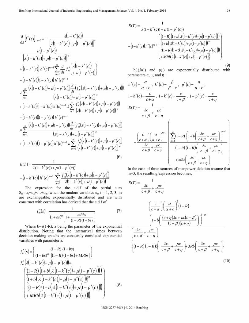
Fig. 1: Variations in E(T) and V(T) for the variations in R From table 1 it is observed that, if the value of R, which is

the parameter of the correlation between the inter-decision time increases and other inputted data values α=1.0, λ=1.5, µ=2.0, η=3.6 and β=4.0 are fixed, the expected time to recruitment and its variance increases, as shown in table 1 and figure 1 respectively.

Table. 2: Variations in E(T) and V(T) for the variations in α and µ=2.0, λ=1.5, R=0.6, η=3.6 and β=4.0

α E(T) V(T) 1.0 1.5 2.0 2.5 3.0

5.2874 5.36505 5.41798 5.45536 5.48294

75.613 75.6647 75.6931 75.7098 75.7203

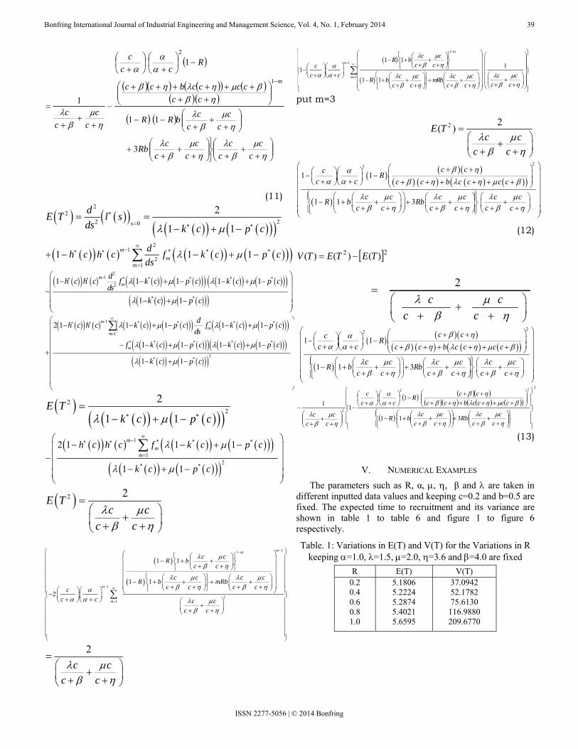
Fig. 2: Variations in E(T) and V(T) for the Variations in α

From table 2 it is observed that, if the value of α, which is the parameter of the random variable representing the amount of depletion at every epoch of policy decision increases and other inputted data values µ=2.0, λ=1.5, R=0.6, η=3.6 and β=4.0 are fixed, the expected time to recruitment and its

variance increases, as shown in table 2 and figure 2 respectively.

Table. 3: Variations in E(T) and V(T) for the Variations in µ and α=1.0, λ=1.5, R=0.6, η=3.6 and β=4.0

µ E(T) V(T) 1.2 1.4 1.6 1.8 2.0

6.8791 6.3956 5.9768 5.6105 5.2874

145.9590 121.9820 103.0620 87.9082 75.6130

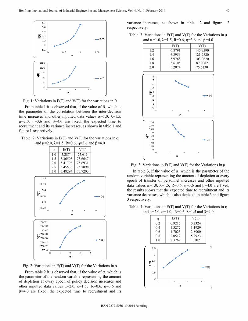
Fig. 3: Variations in E(T) and V(T) for the Variations in µ In table 3, if the value of µ, which is the parameter of the

random variable representing the amount of depletion at every epoch of transfer of personnel increases and other inputted data values α=1.0, λ=1.5, R=0.6, η=3.6 and β=4.0 are fixed, the results shows that the expected time to recruitment and its variance decreases, which is also depicted in table 3 and figure 3 respectively.

Table. 4: Variations in E(T) and V(T) for the Variations in η and µ=2.0, α=1.0, R=0.6, λ=1.5 and β=4.0

η E(T) V(T) 0.2 0.4 0.6 0.8 1.0

0.9217 1.3272 1.7023 2.0512 2.3769

0.2324 1.1929 2.8900 5.2923 3302


ISSN 2277-5056 | © 2014 Bonfring

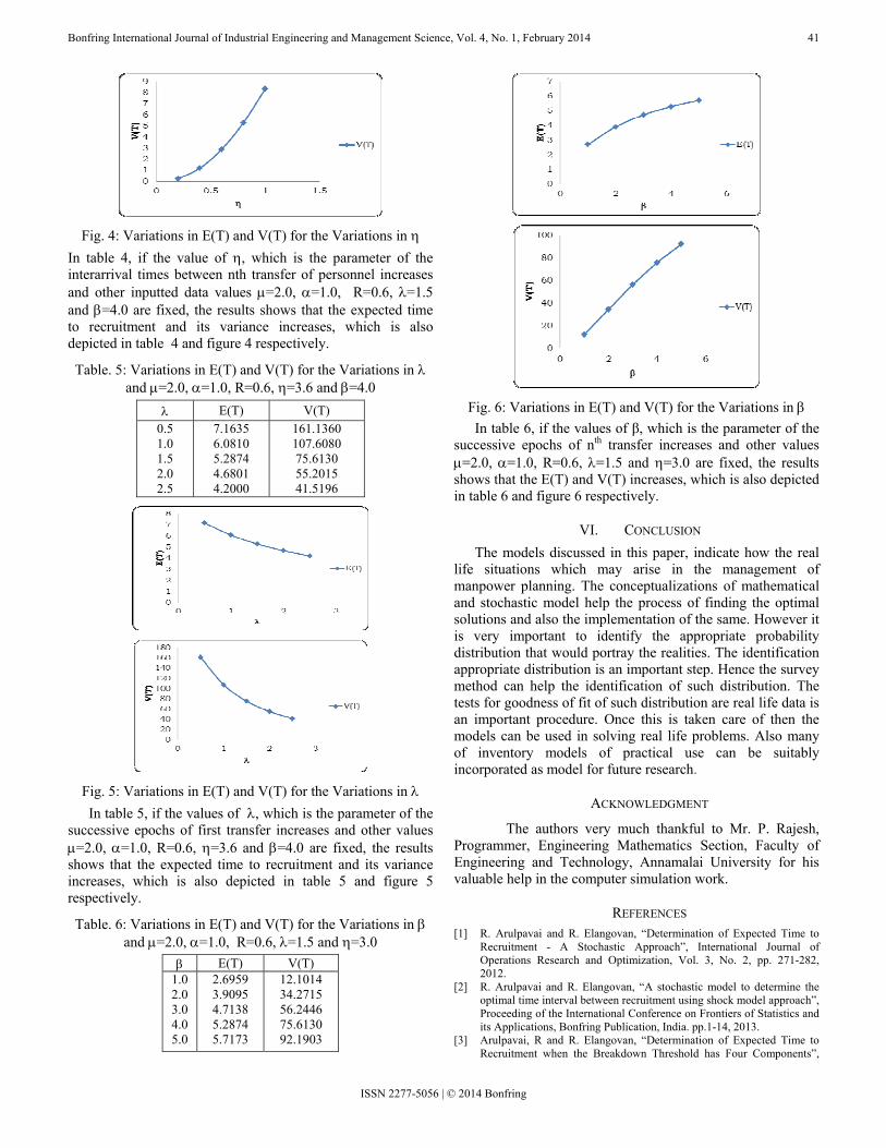
Fig. 4: Variations in E(T) and V(T) for the Variations in η

In table 4, if the value of η, which is the parameter of the interarrival times between nth transfer of personnel increases and other inputted data values µ=2.0, α=1.0, R=0.6, λ=1.5 and β=4.0 are fixed, the results shows that the expected time to recruitment and its variance increases, which is also depicted in table 4 and figure 4 respectively.

Table. 5: Variations in E(T) and V(T) for the Variations in λ and µ=2.0, α=1.0, R=0.6, η=3.6 and β=4.0

λ E(T) V(T) 0.5 1.0 1.5 2.0 2.5

7.1635 6.0810 5.2874 4.6801 4.2000

161.1360 107.6080 75.6130 55.2015 41.5196

Fig. 5: Variations in E(T) and V(T) for the Variations in λ In table 5, if the values of λ, which is the parameter of the

successive epochs of first transfer increases and other values µ=2.0, α=1.0, R=0.6, η=3.6 and β=4.0 are fixed, the results shows that the expected time to recruitment and its variance increases, which is also depicted in table 5 and figure 5 respectively.

Table. 6: Variations in E(T) and V(T) for the Variations in β and µ=2.0, α=1.0, R=0.6, λ=1.5 and η=3.0

β E(T) V(T) 1.0 2.0 3.0 4.0 5.0

2.6959 3.9095 4.7138 5.2874 5.7173

12.1014 34.2715 56.2446 75.6130 92.1903

Fig. 6: Variations in E(T) and V(T) for the Variations in β In table 6, if the values of β, which is the parameter of the

successive epochs of nth transfer increases and other values µ=2.0, α=1.0, R=0.6, λ=1.5 and η=3.0 are fixed, the results shows that the E(T) and V(T) increases, which is also depicted in table 6 and figure 6 respectively.

VI. CONCLUSION The models discussed in this paper, indicate how the real

life situations which may arise in the management of manpower planning. The conceptualizations of mathematical and stochastic model help the process of finding the optimal solutions and also the implementation of the same. However it is very important to identify the appropriate probability distribution that would portray the realities. The identification appropriate distribution is an important step. Hence the survey method can help the identification of such distribution. The tests for goodness of fit of such distribution are real life data is an important procedure. Once this is taken care of then the models can be used in solving real life problems. Also many of inventory models of practical use can be suitably incorporated as model for future research.

ACKNOWLEDGMENT

The authors very much thankful to Mr. P. Rajesh, Programmer, Engineering Mathematics Section, Faculty of Engineering and Technology, Annamalai University for his valuable help in the computer simulation work.

REFERENCES [1] R. Arulpavai and R. Elangovan, “Determination of Expected Time to

Recruitment - A Stochastic Approach”, International Journal of Operations Research and Optimization, Vol. 3, No. 2, pp. 271-282, 2012.

[2] R. Arulpavai and R. Elangovan, “A stochastic model to determine the optimal time interval between recruitment using shock model approach”, Proceeding of the International Conference on Frontiers of Statistics and its Applications, Bonfring Publication, India. pp.1-14, 2013.

[3] Arulpavai, R and R. Elangovan, “Determination of Expected Time to Recruitment when the Breakdown Threshold has Four Components”,


ISSN 2277-5056 | © 2014 Bonfring

The International Innovative Research Journal for Advanced Mathematics, Vol.1, No. 1, pp.1-21, 2013.

[4] R. Arulpavai and R. Elangovan, “Stochastic Model to Determine the Optimal Manpower Reserve at Four Nodes in Series”, International Journal of Ultra Scientist of Physical Sciences, Vol. 25(1) A, pp.139-155, 2013.

[5] D. J. Bartholomew, “The Stochastic Model for Social Processes”, 3nd ed., John Wiley and Sons, New York, 1982.

[6] D. J. Bartholomew, A. F. Forbes, and S. I. McClean, “Statistical Techniques for Manpower Planning”, Wiley, Chichester, 1991.

[7] D. J. Bartholomew and A. F. Forbes, “Statistical Techniques for Manpower Planning”, John Wiley and Sons, Chichester, 1979.

[8] J. D. Esary, W. Marshall and F. Prochan, “Shock Models and wear process”, Annals of probability, Vol.1, No.4, pp.627-650, 1973.

[9] J. Gurland, “Distribution of the Maximum of the Arithmetic Mean of Correlated Random Variables”, Annals of mathematical statistics, Vol. 26, pp. 294-300, 1955.

[10] R. Sathiyamoorthi and R. Elangovan, “A Stochastic Model for Optimum Training Duration”, Indian Association for Productivity, Quality and Reliability (IAPQR) Transactions, Vol. 23, No.2, pp. 127-131, 1998a.

[11] R. Sathiyamoorthi and R. Elangovan, “Shock Model Approach to Determine the Expected time for Recruitment”, Journal of Decision and Mathematical Science, Vol.3, No.1-3, pp. 67-78, 1998b.

Dr. R. Elangovan, is working as Professor, Department of Statistics, Annamalai University, Annamalainagar, Tamilnadu. He is having more than 22 years of P.G. teaching experience. He obtained his B.Sc., M.Sc., Degrees in Statistics from Annamalai University in 1982-1984, and M.Phil., Ph.D., degree from the same institution in 1988 and 2000. He obtained the B.Ed., and M.Ed., degrees also in Education from Annamalai

University in 1987 and 1994.He obtained the M.B.A. (H.R.M.) from the same institution during 2013. He has an excellent academic record of guiding 42 students for M.Phil. degree also and he has published 54 research papers in leading National and International journals, currently guiding 5 students for their Ph.D. programme in statistics. Five Students are already awarded Ph.D. degree under his guidance. He has attended nearly 46 International and 26 National level seminars and presenting papers. He is the editor of various reputed journals in India. He has written 3 books and written 5 lessons and reports for the Directorate of Distance Education of Annamalai University. He visited France, Hang Hong, Paris and USA and delivered invited talk and also chaired the technical session in the conference. He worked as a Statistician in Aravind Eye Hospital, Madurai from (1987-1988), as Assistant Technical Officer in Christian Medical College, Vellore (1988-1989) before joining Annamalai University (1990) as Lecturer. He has gained the reputation of being an excellent teacher. (E-mail: [email protected])

Mrs. R. Arulpavai, M.Sc., M.Phil., B.Ed., working as Guest Lecturer in the Department of Statistics, Government Arts College, C. Mutlur, Chidambaram since 2004 to till date (10 Year). She is currently pursuing Ph.D. degree in Statistics at Manonmaniyam Sundaranar University, Thirunelveli. She has published 7 papers in International and National level journals and published 3 books in statistics. She has participated and presented a papers in 7 National, International level

seminars and workshops. She has gained reputation of being a good teacher for teaching statistics to the graduate students. (E-mail: [email protected])