Selective Model Inversion and Adaptive Disturbance Observer forTime-varying Vibration Rejection on an Active-Suspension

BenchmarkXu Chen and Masayoshi Tomizuka

Abstract—This paper presents an adaptive control schemefor identifying and rejecting unknown and/or time-varyingnarrow-band vibrations. We discuss an idea of safely andadaptively inverting a (possibly non-minimum phase) plantdynamics at selected frequency regions, so that structureddisturbances (especially vibrations) can be estimated andcanceled from the control perspective. By taking advantageof the disturbance model in the design of special infinite-impulse-response (IIR) filters, we can reduce the adaptationto identify the minimum amount of parameters, achieveaccurate parameter estimation under noisy environments,and flexibly reject the narrow-band disturbances with cleartuning intuitions. Evaluation of the algorithm is performedvia simulation and experiments on an active-suspensionbenchmark.

Index Terms—adaptive regulation, loop shaping, inversecontrol, vibration rejection, active suspension

I. Introduction

The rejection of single and multiple narrow-band dis-turbances is a fundamental problem in many mechanicalsystems that involve periodic motions. For example,the shaking mechanism in active suspensions [1], therotating disks in hard disk drives [2], and the coolingfans for computer products [3], all generate vibrationsthat are composed of sinusoidal components in nature.Challenges of the problem are that we often do not haveaccurate knowledge of the disturbance frequencies, andthat in many applications the disturbance characteristicsmay even change w.r.t. time and/or among differentproducts (e.g., in the hard disk drive industry [4]).

In various situations, hardware limitations or exces-sive cost make it infeasible to re-design the hardwarefor reducing these disturbances, and it is only possibleto address the problem from the control-engineeringapproach. As narrow-band disturbances are composedof sinusoidal signal components, controllers can becustomized to incorporate the disturbance structure toasymptotically reject the vibrations. This internal-model-principle [5] based perspective has been investigated infeedback control algorithms in [1], [3], [6]–[8], amongwhich [6], [7] used state-space designs, and [1], [3], [8]applied Youla Parameterization, a.k.a. all stabilizing con-trollers, with a Finite Impulse Response (FIR) adaptiveQ filter. Alternatively, the disturbance frequency can befirstly estimated and then applied for controller design.

X. Chen and M. Tomizuka are with the Department of MechanicalEngineering, University of California, Berkeley, CA, 94720, USA (email:maxchen@me.berkeley.edu; tomizuka@me.berkeley.edu)

This indirect-adaptive-control perspective has been con-sidered in [9]–[11]. Indeed, frequency identification ofnarrow-band signals is a problem that receives greatresearch attention itself. Among the related literaturewe can find: (i) methods using nonparametric spectrumestimation or eigen analysis (subspace methods) [12],[13]; (ii) online adaptive identification approaches [14]–[20]. Spectrum estimation and eigen analysis in gen-eral require more expensive computation within thesampling interval, and have lower resolutions for non-stationary processes. Among references in group (ii), forthe identification of n frequency components, adaptivenotch filters in the orders of 5n− 1 [19], 2n + 6 [20], 3n[15]–[17], and 2n [14], have been discussed.

In this paper we discuss a new adaptive incorporationof the internal model principle for asymptotic rejectionof narrow-band disturbances. Different from the FIR-based adaptive algorithms, we construct the controllersand adaptation with Infinite Impulse Response (IIR)filters and inverse system models. Applying these con-siderations we are able to obtain a structured controllerparameterization that requires the minimum number ofadaptation parameters. An additional consideration isthat adaptation on IIR structures enables direct adaptivecontrol with adaptation algorithms that use the parallelpredictor, which is essential for accurate parameter con-vergence under noisy environments [21]. The importanceof this aspect can also be seen from the aforementionedliterature on frequency identification. Finally, with theinverse-model based design, the internal signals in theproposed algorithm have clear physical meanings. Thecontroller structure extends the idea in [2]. The mainresults of this paper, i.e., the design of inverse models,the derivation of the cascaded IIR filters, and the adap-tation algorithm for time-varying disturbance rejection,however, are all newly developed. An additional con-tribution is the application to a new class of systemsthat has characteristics quite different from the hard diskdrive in [2]. A short version of the paper appeared in[22]. This article is a substantially modified version withproofs and derivations of equations, extended analysisof the algorithms (especially the adaptive-control part),and implementation details as well as the full simulationand experimental results.

The algorithm is evaluated on an active suspensionsystem that has been described in [23]. Fig. 1 presents thefrequency response of the plant. It can be observed thatthe system has a group of resonant and anti-resonant

modes, especially at around 50 Hz and 100 Hz. Addi-tionally, the system is open-loop stable but has multiplelightly damped mid-frequency zeros and high-frequencynonminimum-phase zeros. These characteristics placeadditional challenges not just for adaptive disturbancerejection, but also for general feedback control [24].

50 100 150 200 250 300 350 400−80

−60

−40

−20

0

20

Gai

n (d

B)

50 100 150 200 250 300 350 400−180

−90

0

90

180

Pha

se (

degr

ee)

Frequency (Hz)

identified modelexperimental data

Figure 1: Frequency response of the plant

II. SelectiveModel InversionFig. 2 shows the proposed control scheme. We have

the following relevant signals and transfer functions:• P(z−1) and P(z−1): the plant and its identified model.

They are open-loop stable in the benchmark;• C(z−1): the baseline controller designed to provide a

robustly stable closed loop. For controlling a stable plant,we assume that C(z−1) is also stable;• d(k) and d(k): the actual (unmeasurable) disturbance

and its online estimate. To see this, note that

d(k) = P(q−1)u(k) + d(k)− P(q−1)u(k) ≈ d (k) ,

where q−1 is the one-step-delay operator (in this paper,P(z−1), P(q−1), and P(e− jω) are used to denote respectivelythe transfer function, the pulse transfer function, and thefrequency response of P(z−1)). d(k) is quite accurate asP(z−1) is identified quite accurately in the benchmark.The minimum requirement for P(z−1) is that is should beaccurate within the frequency region where disturbanceoccurs. The noise due to model mismatch, if any, can belater reduced by filtering in the adaptation scheme;• y(k): the measured residual errors;• P−1

m (z−1) and z−m: these are constructed such that:1) Pm(z−1) has a relative degree of zero (and hence

P−1m (z−1) is realizable);2) P−1

m (z−1) is stable; and3) within the frequency range of the possible distur-

bances, P(z−1)∣∣∣z=e jω ≈ z−mPm(z−1)

∣∣∣z=e jω , namely, P−1

m (z−1)is a nominal inverse model (without delays) of P(z−1).Indeed in Fig. 1, the dashed line depicts the frequencyresponse of z−mPm(z−1), which matches well with theexperimental frequency response up to around 350 Hz;

• Parameter adaptation algorithm: provides onlineinformation of the characteristics of d(k);• c (k): the compensation signal to asymptotically reject

the narrow-band disturbance in d (k).

+-

+-

+-

1( )Q z−

d(k)

C(z¡1)

c(k)

0

d(k)

u(k) + + y(k)

P (z¡1)

P (z¡1)

Disturbance source Mechanical path

z¡m

+-P

¡1

m(z¡1)

Parameter Adaptation

Algorithm (PAA)

Figure 2: Structure of the proposed control scheme

Ignoring first the shaded blocks (about parameteradaptation) in Fig. 2, we have

y (k) = d (k) + P(q−1)u (k)

u(k) = −C(q−1)y (k)− c(k)

c(k) = Q(q−1)[P−1m (q−1)y(k)− q−mu(k)]

from which we can derive the sensitivity function,namely, the transfer function from d(k) to y(k):

S(z−1) = Gd2y(z−1) =(1− z−mQ(z−1)

)/X(z−1) (1)

X(z−1) = 1 + P(z−1)C(z−1) + Q(z−1)(P−1m (z−1)P(z−1)− z−m)

(2)

From the frequency-response perspective (replace z−1

with e− jω), if P(e− jω) = e− jmωPm(e− jω) in (1) and (2), thenthe last term in X(e− jω) vanishes and

S(e− jω) =(1− e− jmωQ(e− jω)

)/(1 + P(e− jω)C(e− jω)

). (3)

If we design a Q-filter Q(z−1) with its frequency re-sponse as shown in Fig. 3, then 1− e−mjωQ(e− jω), andthus Gd2y(e− jω) in (1), will become zero at the centerfrequencies of Q(z−1), namely, disturbances occurring atthese frequencies will be strongly attenuated. Assumefirst that vibrations occur exactly at 60 Hz and 90 Hz.Q(z−1) will filter out all other frequency componentssuch that its output c(k) consists of signals only at thedisturbance frequencies. More specifically, c(k) is actuallyan estimated version of P−1(q−1)d(k) if d(k) contains justnarrow-band vibrations. To see this, notice in Fig. 2, thatthe control signal u (k) flows through two paths to reachthe summing junction before Q(z−1): one from the plantP(z−1) to the inverse P−1

m (z−1), and the other through z−m.Hence the effect of u(k) gets canceled at the summingjunction before Q(z−1), and only the filtered disturbanceP−1

m (q−1)d(k) enters Q(z−1).We remark that the shape of Q(z−1) in Fig. 3 is central

in the proposed design scheme. Uncertainties exist in

0 50 100 150 200 250 300 350 4000

0.5

1

1.5G

ain

1−z−mQ(z−1)

0 50 100 150 200 250 300 350 4000

0.5

1

1.5

Gai

n

Ferquency (Hz)

Q(z−1)

Figure 3: Frequency response of a Q-filter example

P(z−1) (particularly at high frequencies), no matter howaccurate Pm(z−1) is constructed (based on modeling orsystem identification). It is not practical (and is evendangerous) to invert P(z−1) over the entire frequencyregion. Keeping the magnitude of Q(z−1) small exceptat the interested disturbance frequencies forms a “lo-cal/selective” model inverse (SMI) of the plant dynam-ics, such that errors due to model mismatches do notpass through Q(z−1) and equation (3) remains a validapproximation of (1). In this way, closed-loop stabilitycan be readily preserved since 1/(1 + P(z−1)C(z−1)) is thesensitivity function of the baseline system (and henceis stable). A stable Q(z−1) in this case will assure thestability of S(z−1)≈ (1−z−mQ(z−1))/(1+P(z−1)C(z−1)). Un-der the above conditions, the proposed scheme becomesa special form of Youla parameterization [25], wherethe add-on stable Q parameterization does not alterthe closed-loop stability and focus on just disturbancecancellation. Of course, a prior assumption is that goodmodel information can be obtained at the disturbancefrequencies. If the system already has large uncertaintiesat the disturbance frequencies, it is best not to applylarge control effort there in the first place.

The full stability result is summarized as follows:

Theorem 1. Under the definitions listed at the beginningof this section, when there is no mismatch between P(z−1)and z−mPm(z−1), the closed loop in Fig. 2 is stable as long asQ(z−1) is stable. When there is (stable and bounded) model un-certainty ∆(z−1) such that P(z−1) = z−mPm(z−1)[1 + ∆(z−1)],the closed loop is stable if Q(z−1) is stable and∣∣∣Q(e− jω)

∣∣∣ < ∣∣∣∣∣∣1 + P(e− jω)C(e− jω)∆(e− jω)

∣∣∣∣∣∣ , ∀ω ∈ [0,π] . (4)

Proof: The nominal stability condition is a standardresult of Youla parameterization. For robust stability,noting that ∆(z−1) = P−1

m (z−1)P(z−1)−z−m, from (2), we canobtain the closed-loop characteristic polynomial:

1 + P(z−1)C(z−1) + z−mQ(z−1)∆(z−1) = 0 (5)

The system is thus robustly stable if ∀ ω ∈ [0,π]∣∣∣e− jmω∆(e− jω)Q(e− jω)∣∣∣ < ∣∣∣1 + P(e− jω)C(e− jω)

∣∣∣ . (6)

Noticing that the delay term e− jmω has unity magnitude,we can transform (6) to (4).

The benchmark system has visible uncertainties onlyat high frequencies (this is also the common case ingeneral mechanical systems). (4) then provides veryflexible design freedom for Q(z−1). More important, thestability condition in Youla parameterization also holdswhen Q(z−1) is made adaptive (but is still stable). Thisgreatly benefits the rejection of unknown and time-varying vibrations when we update the parameters ofQ(z−1).

In the next section, we propose an approach to obtainthe optimal inverse filter P−1

m (z−1). Following that, inSection IV we study the application of the internal modelprinciple to design a customized Q(z−1) that satisfies thefrequency response in Fig. 3 for SMI.

III. Design of The Inverse DynamicsIn the aforementioned analysis we have assumed

P−1m (z−1) to be stable. It is well known that nonminimum-

phase zeros in P(z−1) not only make P−1(z−1) unstable butalso cause control limitations. The benchmark system hasmultiple of such zeros. We discuss next an H∞ treatmentof the problem when designing P−1

m (z−1).Let S denote the set of all stable discrete-time rational

transfer functions. Recalling the ideal situation whereP(z−1) = z−mPm(z−1), we search among S to find M(z−1) =P−1

m (z−1) such that the following two criteria are satisfied:(i) model matching: to minimize the cost func-

tion ||W1(z−1)(M(z−1)P(z−1)− z−m

)||∞, namely, we mini-

mize the maximum magnitude of the model mismatchM(z−1)P(z−1)−z−m, weighted by W1(z−1). The ideal solu-tion, if P−1(z−1) is stable, is simply M(z−1) = z−mP−1(z−1).The weighting function determines the interested regionwhere we would like to have good model accuracy.

(ii) gain constraint: as the inverse is used for process-ing the measured output signal, we should be carefulnot to amplify the noises in y(k). Consider the problemof min ||W2(z−1)M(z−1)P(z−1)||∞, where the magnitude ofM(z−1)P(z−1) is scaled by the weight W2(z−1). The opti-mal solution for this part alone would be that M(z−1) = 0,i.e., M(z−1) will not amplify any of its input components.To make full use of this gain constraint, we combine itwith criterion (i) to form:

minM(z−1)∈S

∥∥∥∥∥∥[

W1(z−1)(M(z−1)P(z−1)− z−m

)W2(z−1)M(z−1)P(z−1)

]∥∥∥∥∥∥∞

. (7)

The optimization in (7) finds the optimal inverse thatpreserves accurate model information in the frequencyregion specified by W1(z−1), and in the meantime penal-izes excessive high gains of M(z−1) at frequencies whereW2(z−1) has high magnitudes. Typically W1(z−1) is a low-pass filter and W2(z−1) is a high-pass filter.

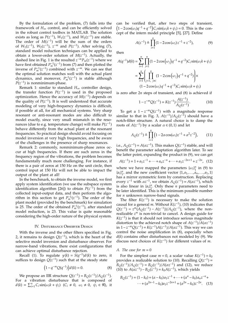
By the formulation of the problem, (7) falls into theframework of H∞ control, and can be efficiently solvedin the robust control toolbox in MATLAB. The solutionexists as long as P(z−1), W1(z−1), and W2(z−1) are stable.The order of M(z−1) will be the sum of the ordersof W1(z−1), W2(z−1), z−m and P(z−1). After solving (7),standard model reduction techniques can be applied toobtain a lower-order solution of M(z−1). Actually, thedashed line in Fig. 1 is the resulted z−mPm(z−1) where wehave first obtained P−1

m (z−1) from (7) and then plotted theinverse of P−1

m (z−1) combined with z−m. We can see thatthe optimal solution matches well with the actual plantdynamics, and moreover, P−1

m (z−1) is stable althoughP(z−1) is nonminimum-phase.

Remark 1: similar to standard H∞ controller design,the transfer function P(z−1) is used in the proposedoptimization. Hence the accuracy of M(z−1) depends onthe quality of P(z−1). It is well understood that accuratemodeling of very high-frequency dynamics is difficult,if possible at all, for all mechanical systems. Very sharpresonant or anti-resonant modes are also difficult tomodel exactly, since very small mismatch in the reso-nances (due to e.g. temperature change) will make P(z−1)behave differently from the actual plant at the resonantfrequencies. So practical design should avoid focusing onmodel inversion at very high frequencies, and be awareof the challenges in the presence of sharp resonances.

Remark 2: commonly, nonminimum-phase zeros oc-cur at high frequencies. If there are such zeros in thefrequency region of the vibrations, the problem becomesfundamentally much more challenging. For instance, ifthere is a pair of zeros at 150 Hz on the unit circle, thencontrol input at 150 Hz will not be able to impact theoutput of the plant at all!

In the benchmark, to obtain the inverse model, we firstapply system identification (we use the subspace systemidentification algorithm [26]) to obtain P(z−1) from thecollected input-output data, and then perform the algo-rithm in this section to get P−1

m (z−1). The order of theplant model (provided by the benchmark) for simulationis 25. The order of the obtained P−1

m (z−1), after standardmodel reduction, is 23. This value is quite reasonableconsidering the high-order nature of the physical system.

IV. Disturbance Observer Design

With the inverse and the other filters specified in Fig.2, it remains to design Q(z−1), which is the heart of theselective model inversion and disturbance observer. Fornarrow-band vibrations, there exist configurations thatcan achieve optimal disturbance rejection.

Recall (1). To regulate y (k) = S(q−1)d (k) to zero, itsuffices to design Q(z−1) such that at the steady state(

1− q−mQ(q−1))d (k) = 0. (8)

We propose an IIR structure Q(z−1) = BQ(z−1)/AQ(z−1).For a vibration disturbance that is composed ofd (k) =

∑ni=1 Ci sin(ωik + ψi) (Ci , 0, ωi , 0, ψi ∈ R), it

can be verified that, after two steps of transient,(1−2cos(ωi)q−1 + q−2

)Ci sin(ωik +ψi) = 0. This is the con-

cept of the intern model principle [5], [27]. Define

A(z−1) ,n∏

i=1

(1−2cos(ωi)z−1 + z−2), (9)

then

A(q−1)d(k) =

n∑i=1

n∏j=1

(1−2cos(ω j

)q−1 + q−2)Ci sin(ωik +ψi)

=

n∑i=1

n∏j=1, j,i

(1−2cos(ω j

)q−1 + q−2)

×(1−2cos(ωi)q−1 + q−2)Ci sin(ωik +ψi)

is zero after 2n steps of transient, and (8) is achieved if

1− z−mQ(z−1) = K(z−1)A(z−1)

AQ(z−1). (10)

To get a 1 − z−mQ(z−1) with a magnitude responsesimilar to that in Fig. 3, A(z−1)/AQ(z−1) should have anotch-filter structure. A natural choice is to damp theroots of A(z−1) by a scalar α ∈ (0,1) and let

AQ(z−1) ,n∏

i=1

(1−2αcos(ωi)z−1 +α2z−2

), (11)

i.e., AQ(z−1) = A(αz−1). This makes Q(z−1) stable, and willbenefit the parameter adaptation algorithm later. To seethe latter point, expanding the product in (9), we can get

A(z−1) = 1 + a1z−1 + · · ·+ anz−n + · · ·+ a1z−2n+1 + z−2n, (12)

where we have mapped the parameters ωin1 in (9) to

ain1 , and the new coefficient vector 1,a1, . . . ,an, . . . ,a1,1

has a mirror symmetric form by construction. Replacingevery z−1 with αz−1, we obtain AQ(z−1) = A(αz−1), whichis also linear in ai

n1 . Only these n parameters need to

be later identified. This is the minimum possible numberfor n unknown narrow-band signals.

The filter K(z−1) is necessary to make the solutioncausal for a general m. Without K(z−1), (10) indicates thatQ(z−1) = zm(AQ(z−1) − A(z−1))/AQ(z−1), where the non-realizable zm is non-trivial to cancel. A design guide forK(z−1) is that it should not introduce serious magnitudedistortion to the achieved notch shape of A(z−1)/A(αz−1)in 1−z−mQ(z−1) = K(z−1)A(z−1)/A(αz−1). This way we cancontrol the noise amplification in (8), especially whend(k) contains other disturbances not modeled by (9). Wediscuss next choices of K(z−1) for different values of m.

A. The case for m = 0For the simplest case m = 0, a scalar value K(z−1) = k0

provides a realizable solution to (10). Recalling Q(z−1) =BQ(z−1)/AQ(z−1) = BQ(z−1)/A(αz−1) and (12), we reduce(10) to A(αz−1)−BQ(z−1) = k0A(z−1), which yields

BQ(z−1) = (1− k0) + (α− k0)a1z−1 + · · ·+ (αn− k0)anz−n+

· · ·+ (α2n−1− k0)a1z−2n+1 + (α2n

− k0)z−2n. (13)

It can be shown (see Appendix) that k0 = αn leadsto the common factor 1−αz−2 in BQ(z−1), which placestwo symmetric zeros to Q(z−1) at ±

√α. This provides

balanced magnitude response for Q(z−1) at low and highfrequencies.

B. The case for m = 1Applying analogous analysis as in Section IV-A, if m =

1, we reduce (10) to A(αz−1)− z−1BQ(z−1) = k0A(z−1), thesolution of which is BQ(z−1) = (1− k0)z + (α− k0)a1 + · · ·+(αn−k0)anz−n+1 + · · ·+ (α2n−1

−k0)a1z−2n+2 + (α2n−k0)z−2n+1.

To let the term (1− k0)z vanish for realizability, werequire k0 = 1, which gives

BQ(z−1) =

2n∑i=1

(αi−1)aiz−i+1; ai = a2n−i, a2n = 1. (14)

As an example, when n = 1, (9), (12) and (14) yield a1 =−2cosω1 and

Q(z−1) =(1−α)

(2cosω1− (1 +α)z−1

)1−2αcosω1z−1 +α2z−2

.

Evaluating the frequency response at ω1 and usingthe identity 2cos(ω1) = e jω1 + e− jω1 , we can obtain thatQ(e− jω1 ) = e jω1 . Thus, Q(z−1) provides exactly one-stepadvance to counteract the one-step delay in 1−z−1Q(z−1)at the center frequency ω1, hence the zero magnituderesponse of 1− z−1Q(z−1) at ω1.

C. The case for an arbitrary mFor m > 1, assigning K(z−1) = k0 no longer gives a

realizable solution. Defining K(z−1) as a general FIR filtercan address the causality issue. This will give slightlyless control over the shape of K(z−1)A(z−1)/A(αz−1), asK(z−1) is now an FIR to be computed and its shape isnon-trivial until we have solved (10). Another way thatprovides additional design freedom is to consider an IIRdesign:

K(z−1) =

N∑i=0

ki

[A(z−1)

A(αz−1)

]i

, ki ∈ R. (15)

Namely, K(z−1) is chosen as a combination of N (≥ 0)filters that influence only the local loop shape (recallthat A(z−1)/A(αz−1) is a notch filter). Take the exampleof m = 2. When N = 1,1 (10) is

1− z−2Q(z−1) =

(k0 + k1

A(z−1)A(αz−1)

)A(z−1)

A(αz−1),

which gives

Q(z−1) = z2(1− k0

A(z−1)A(αz−1)

− k1A(z−1)2

A(αz−1)2

). (16)

Partitioning, we obtain

Q(z−1) , z2(1−ρ1

A(z−1)A(αz−1)

)(1−ρ2

A(z−1)A(αz−1)

). (17)

1If N = 0, the result is unrealizable since K(z−1) is a scalar again.

The numerator of Q(z−1) is given by BQ(z−1) =z2(A(αz−1)−ρ1A(z−1))(A(αz−1)−ρ2A(z−1)). Recalling (12),we have A(αz−1)−ρiA(z−1) =

(1−ρi

)+

(α−ρi

)a1z−1 + · · ·+

(α2n−ρi)z−2n. To make the z2 term vanish in BQ(z−1) for

realizability of Q(z−1), we must have 1−ρi = 0 for i = 1,2,yielding k0 = 2, k1 = −1 in (16). With these solved ρi andki, after simplification, (17) and (15) become

Q(z−1) =

∑2ni=1(αi

−1)aiz−i+1

A(αz−1)

2

; ai = a2n−i, a2n = 1 (18)

K(z−1) = 2−A(z−1)

A(αz−1). (19)

For a general integer m, when N = m−1, applying anal-ogous analysis, we get the following partitioned Q(z−1)from (15) and (10):

Q(z−1) = zmm∏

i=1

(1−ρi

A(z−1)A(αz−1)

).

The solution pair is thus obtained when ρi = 1 ∀i, and

Q(z−1) =

∑2ni=1(αi

−1)aiz−i+1

A(αz−1)

m

(20)

1− z−mQ(z−1) = 1−(1−

A(z−1)A(αz−1)

)m

(21)

=A(z−1)

A(αz−1)

m∑i=1

(mi

)[−

A(z−1)A(αz−1)

]i−1

. (22)

Here ai is as defined in (18); and from (21) to (22) we have

used the identity (1 + x)m = 1 +

(m1

)x + · · · +

(mm

)xm,

where(

mi

)= m!

i!(m−i)! is the binomial coefficient.

It can be observed that the general result obtained hereis essentially a cascaded version of the developed Q(z−1)in Section IV-B. For the sake of clarity, we denote nowthe Q filter for m = 0 and m = 1 respectively as Q0(z−1)and Q1(z−1). From the discussion at the end of SectionIV-B, Q1(z−1) provides one-step phase advance at thedisturbance frequencies ωi

n1 , to address the term z−1 in

1−z−1Q1(z−1). For a general m, we see that the cascadedQ(z−1) =

[Q1(z−1)

]min (20) works the same way since

1− z−mQ(z−1) = 1− (z−1Q1(z−1))m, i.e., each Q1(z−1) blockcompensates one z−1 term, to achieve 1− e− jmωQ(e− jω) =0 when ω ∈ ωi

n1 . Recall from Fig. 3, that Q(z−1) is

a special type of bandpass filter. Cascading multipleQ1(z−1) together not only provides the compensation forz−m, but also provides an enhanced bandpass frequencyresponse, as |Q(e− jω)|m ≤ |Q(e− jω)| if m≥ 1 and |Q(e− jω)|< 1(when ω is outside of the passband). If needed, we canadditionally cascade one or multiple blocks of Q0(z−1) toQ(z−1), which will further reduce the magnitude of thefilter outside the passband.

V. Parameter AdaptationThis section discusses the online adaptation of Q(z−1)

when the disturbance characteristics is not known. Recall

from Fig. 2, that the residual is

y (k) = Gd2y(q−1)d(k) = S(q−1)d(k) ≈1− q−mQ(q−1)

1 + P(q−1)C(q−1)d(k).

The beginning of Section II has discussed the obtainingof d(k) ≈ d(k). Letting w(k) , d(k)/(1 + P(q−1)C(q−1)) andrecalling the solution of 1−q−mQ(q−1) in (22), we get

y(k) ≈

m∑i=1

(mi

)[−

A(q−1)A(αq−1)

]i−1 A(q−1)A(αq−1)

w(k)

The direct dynamics between w(k) and y(k)is nonlinear w.r.t. the unknown coefficientsθ , [a1,a2, . . . ,an]T in Q(z−1). Noticing however the

filter∑m

i=1

(mi

)[−

A(q−1)A(αq−1)

]i−1is a linear combination of

(and actually also normalized) notch filters,2 we cansimply design to minimize

y(k) = A(q−1)/A(αq−1)w(k). (23)

Additional filtering can be applied on w(k) to improvethe signal-to-noise ratio. In the benchmark, the interesteddisturbance-rejection region is [50–95] Hz. A bandpassfilter in Fig. 4 can be used on w (k).

50 100 150 200 250 300 350 400−80

−60

−40

−20

0

Mag

nitu

de (

dB)

Frequency (Hz)

Figure 4: Example bandpass filter

The structure of (23) is special (and simplified) foradaptive control due to the close relationship betweenthe numerator and the denominator. For such type ofadaptation model, [2] has proposed a two-stage adap-tation scheme that combines recursive least squaresand output-error based parameter adaptation algorithms(PAA) for identification of θ. We list below only thecentral equations and then focus on applying the PAAfor identifying different time-varying vibrations.

Step one: recursive least squares (RLS) aiming at min-imizing A(q−1)w(k), where A(q−1) is given by (12):

εo (k) = −A(q−1)w(k) (24)

= −ψ (k−1)T θ (k−1)− (w (k) + w (k−2n)) (25)

θ (k) = θ (k−1) +P (k−1)ψ (k−1)εo (k)

1 +ψ (k−1)T P (k−1)ψ (k−1)(26)

P (k) =1λ (k)

[P(k−1)−

P(k−1)ψ(k−1)ψT(k−1)P(k−1)λ (k) +ψT(k−1)P(k−1)ψ(k−1)

]Here the regressor vector ψ(k − 1) = [ψ1(k −1), . . . ,ψn(k− 1)]T is computed from ψi (k−1) = w (k− i) +w (k−2n + i) ; i = 1, ...,n−1, and ψn (k−1) = w (k−n).

2In special case where m = 1, this summation term becomes identity.

Step two: parallel adaptation algorithm witha fixed compensator C(z−1) = 1 + c1αz−1 + · · · +cnαnz−n + · · · + c1α2n−1z−2n+1 + α2nz−2n, aiming atminimizing A(q−1)/A(αq−1)w(k). With the newlyintroduced denominator part, the regressor vectoris composed of φi (k−1) = w (k− i) + w (k−2n + i) −αie (k− i) − α2n−ie (k−2n + i) ; i = 1, ...,n − 1, andφn (k−1) = w (k−n)−αne (k−n). We have

e (k) = φ (k−1)T θ (k) + w (k) + w (k−2n)−α2ne (k−2n)

ν (k) = C(q−1)e(k) = e (k) +α2ne (k−2n) +ϕ (k−1)Tθc (27)

eo (k) = φ (k−1)T θ (k−1) + w (k) + w (k−2n)−α2ne (k−2n)

νo (k) = eo (k) +α2ne (k−2n) +ϕ (k−1)Tθc (28)

where e(k) and ν(k) are respectively the a posterioriestimation and adaptation errors; eo(k) and νo(k) arerespectively the a priori estimation and adaptation er-rors; and θc , [c1,c2, . . . ,cn] is the coefficient vector ofC(z−1). ϕ(k − 1) = [ϕ1 (k−1) ,ϕ2 (k−1) , . . . ,ϕn (k−1)]T in(27) and (28) are computed from: ϕi (k−1) = αie (k− i) +α2n−ie (k−2n + i) ; i = 1, ...,n−1, ϕn (k−1) = αne (k−n). Thefinal parameter adaptation equations are

θ (k) = θ (k−1) +P (k−1)

(−φ (k−1)

)νo (k)

1 +φ (k−1)T P (k−1)φ (k−1)(29)

P (k) =1λ (k)

[P(k−1)−

P(k−1)φ(k−1)φT(k−1)P(k−1)λ (k) +φT(k−1)P(k−1)φ(k−1)

]The RLS algorithm is globally convergent if the adap-

tation input contains pure narrow-band vibrations, butyields biased estimate if there are colored input noises.The parallel algorithm in Step two provides accuratelocal convergence but needs proper parameter initializa-tion. Steps one and two are therefore connected by usingthe final estimated parameter θo at Step one to initializeθc and θ in Step two. The switching between the twosteps can be made automatic [2] (after some tuning) orsimply by a fixed time window to run Step one.

To have good convergence under noisy environments,let α in Step two initialize from a relatively small value(e.g. 0.8) and converge gradually to a value that isclose to 1 (e.g. 0.99). The estimated θ(k) is then usedto construct the Q filter designed in the previous section(the coefficient α in the Q filter for implementation doesnot need to be the same as that used in parameteradaptation).

The forgetting factor λ(k) determines how much infor-mation is used for adaptation. In this article we suggestthe following tuning rules:

(i) rapid initial convergence: initialize the forgettingfactor to be exponentially increasing from λ0 to 1 inthe first several samples, where λ0 can be taken to bebetween [0.92,1)

(ii) adjustment for sudden parameter change: whenthe prediction error encounters a sudden increase, indi-cating a change of system parameters, switch from Steptwo to Step one, reduce λ (k) to a small value λ (e.g. 0.92

in the benchmark), and then increase it back to its steady-state value λ (usually close to 1), using the formulaλ(k) = λ−λrate(λ−λ(k−1)), with λrate [preferably in therange (0.9,0.995)] defining the speed of convergence.

(iii) adjustment for continuously changing parameters:when the parameters are changing, keep λ(k) strictlysmaller than one, using e.g., a constant λ(k) (< 1).

VI. ImplementationIn this section we provide some details about imple-

menting the algorithm:Obtaining the frequencies from the identified param-

eters: from (9) and (12), the vibration frequen-cies and the identified parameters are mapped by∏n

i=1

(1−2cos(ωi)z−1 + z−2

)= 1 + a1z−1 + · · · + anz−n + · · · +

a1z−2n+1 + z−2n. For the simplest case where n = 1, wehave a1 = −2cosω1, from which we can compute thevibration frequency ω1 = 2πΩ1Ts, where the unit of Ω1is Hz. The parameter a1 is online updated and Ω1 canbe computed offline for algorithm tuning. For n > 1, as(1−2cos(ωi)z−1 + z−2

)=

(1− e jωiz−1

)(1− e− jωiz−1

), ωi can

be computed offline via calculating the angle of the com-plex roots of 1+a1z−1 + · · ·+anz−n + · · ·+a1z−2n+1 +z−2n = 0.

Algorithm tuning: besides the above structural map-ping between the identified parameters and the vibrationfrequency, another property is also useful for algorithmtuning: the width of the attenuation bandwidth in Fig.3 is determined by the parameter α in (11). When α issmaller but very close to one, the magnitude of Q(z−1)is very small except at the vibration frequencies. Theclosed-loop robust stability will then be easy to satisfyfrom Theorem 1. This will however require very accurateinformation of the disturbance frequency. Designers cangradually reduce α to reach the desired attenuationbandwidth. Keep in mind, however, that the Q filtershould satisfy the gain constraint (4) for stability.

Baseline controller: the active suspension system isopen-loop stable. Since the benchmark is on narrow-band vibration rejection rather than motion control, weused a baseline controller (provided by the benchmark3)that has very small gains to achieve closed-loop robuststability. For general motion control problems, the base-line controller should also be carefully chosen to providethe standard loop-shaping performance (see, e.g., [2]).

VII. Simulation and Experimental ResultsWe apply in this section the proposed scheme to

the benchmark on active suspension. In this system,the plant delay m = 2 in the modeling of P(z−1)

∣∣∣z=e jω ≈

z−mPm(z−1)∣∣∣z=e jω . Hence two Q1(z−1) blocks are needed

in (20). Vibrations occur in the middle frequency regionbetween 50 Hz and 95 Hz. There are also other noisesat low and high frequencies. To enhance the bandpassproperty of Q(z−1), we added one additional Q0(z−1)

3See http://www.gipsa-lab.grenoble-inp.fr/~ioandore.landau/benchmark_adaptive_regulation/index.html

block designed in Section IV-A, and prefiltered the inputto the PAA by a bandpass filter as shown in Fig. 4to remove the bias and other high-frequency noises inthe estimated disturbance. Three levels of evaluationsare conducted. Within each level, three types of distur-bances are considered: the first with constant unknownfrequencies injected at a certain time (denoted as simplestep test), the second with sudden frequency changesat specific time instances, and the third with chirp-changing frequencies. The graphical and numerical dataare compared to other participants of the benchmark.

A. Level 1: rejection of single-frequency vibrationsFig. 5 shows the time trace of the residual errors

(experimental result) for a time-varying vibration withthe following characteristics: the disturbance frequencychanges in the pattern of null→ 75Hz→ 85Hz→ 75Hz→65Hz→ 75Hz→ null, occurring respectively at 5 sec, 8sec, 11 sec, 14 sec, 17 sec, and finally 32 sec, whenthe disturbance is turned off. In the presence of vari-ous frequency jumps, the algorithm is seen to providerapid and strong vibration compensation. Comparingthe data at 2 sec and 7 sec, we see that the steady-stateresidual errors with the compensation scheme (data at7 sec) has been reduced to be at the same magnitudeas the baseline case (at 2 sec) where no disturbance ispresent. Summarized in Table I are the simulation andexperimental results of a full set of evaluations coveringdifferent frequency values. The performance is evaluatedby two quantitative values: the 2-norm values of thetransient errors at the initial 3 seconds after disturbanceinjection (denoted as ||e||22 T©), and the maximum valuesof the residual error. It can be seen the performances atdifferent frequencies are all similar to that in Fig. 5.

0 5 10 15 20 25 30 35 40−0.02

0

0.02

Res

idua

l for

ce [V

]

Open loop

0 5 10 15 20 25 30 35 40−0.02

0

0.02

Time [sec]

Res

idua

l for

ce [V

]

Closed loopHz: 75 85 75 65 75

Figure 5: Experimental results of rejecting a narrow-band disturbance with step frequency changes.

At a particular frequency, Fig. 6 presents the steady-state error spectra when the system is subjected to a75-Hz disturbance. With the compensation scheme, thespectral peak at 75 Hz has been reduced from around−42 dB to −91 dB, indicating a disturbance attenuation ofabout 49 dB (the benchmark specification is 40 dB). Theseresults are directly reflected in Fig. 7, which presentsthe magnitude responses of the sensitivity functions

Table I: Results of rejecting vibrations with step changesin frequencies (level 1)

freq. (Hz) ||e||22 T© (×10−3V2) max |e| (×10−3V)

Sim

ulat

ion

Seq.

1 60→70 20.78 22.1070→60 11.21 19.8060→50 15.51 19.4050→60 10.39 20.98

Seq.

2 75→85 19.29 22.4385→75 10.12 17.3775→65 10.66 18.9665→75 9.09 19.17

Seq.

3 85→95 17.09 23.9395→85 12.13 23.0285→75 10.15 18.9675→85 8.64 16.93

Expe

rim

ent

Seq.

1 60→70 19.50 23.9570→60 13.51 20.2760→50 28.47 23.8550→60 15.62 22.62

Seq.

2 75→85 16.64 20.1685→75 9.93 16.6175→65 11.31 20.2865→75 10.11 18.93

Seq.

3 85→95 135.00 25.1895→85 16.07 19.0685→75 10.33 18.9475→85 8.56 15.26

(note the sharp notch at 75 Hz and small amplificationsat other regions). During actual experiments there arerandom noises that are time-dependent. Hence compar-ing to Fig. 6a, the open- and closed-loop spectra, atfrequencies other than the spectral peaks, look slightlymore different in Fig. 6b.

0 50 100 150 200 250 300 350 400−100

−90

−80

−70

−60

−50

−40

Frequency [Hz]

Pow

er S

pect

rum

Den

sity

(P

SD

) [d

B]

open loopclosed loop

(a) Simulation

0 50 100 150 200 250 300 350 400−100

−90

−80

−70

−60

−50

−40

Frequency [Hz]

Pow

er S

pect

rum

Den

sity

(P

SD

) [d

B]

PSDOL

PSDCL

(b) Experiment

Figure 6: Error spectra of rejecting a 75 Hz vibration

0 50 100 150 200 250 300 350 400−50

−40

−30

−20

−10

0

10

Hz

dB

w/o compensatorw/ compensator

Figure 7: Magnitude response of the sensitivity functionswith (w/) and without (w/o) the proposed compensator

The algorithm is additionally tested at frequenciesuniformly sampled between 50 Hz and 95 Hz. Table IIsummarizes, from the second to the last columns, theoverall 2-norm reduction of the errors (global attenuationGA), the disturbance attenuation (DA) at the vibrationfrequencies, the maximum spectral amplification, the3-sec transient value of ||e||22 T©, the residual value of||e||22 at the final 3 seconds (denoted as ||e||22 R©), themaximum of |e|, and lastly a scalar called transient ratio(T ratio). T ratio is the ratio between ||e||22 at two timewindows: the first from 7 sec to 10 sec (disturbancewas injected at 5 sec); the other at the final 3 seconds.It is a measure of whether the residual errors haveconverged to the steady-state values after two seconds(required specification from benchmark) of running theadaptive algorithm. If T ratio is less than 1.21, it isregarded that the algorithm has fully converged (100%satisfaction in the benchmark). The numbers indicatethat, similar to the case in Fig. 6, in all tests, the narrow-band disturbance has been greatly attenuated within ashort period of time. As the system has two pairs ofstrong resonant and anti-resonant modes neat 50 Hz and100 Hz (recall Fig. 1), we intentionally reduced the depthof attenuation at frequencies below 52 Hz and above 92Hz in the experiments. This is done by selecting α to becloser to 1, and hence a sharper notch shape in Fig. 3.The simulation results do not have this modification andreflect the best possible performance.

Fig. 8 shows a summary, in the same scale, of the level-1 time-domain results under different specifications. Thefirst subplot is the time-domain result corresponding tothe spectra in Fig. 6; and the second subplot is anotherexample with step frequency changes in the disturbance.The third one is for the case when the disturbance is achirp signal whose frequency sweeps between 50 Hz and95 Hz in the time windows [10–15], [20–25] sec. Undersuch time-varying vibrations, we see that the proposedalgorithm maintains its effectiveness of compensatingthe disturbance. For this time-varying vibration, we usedan aggressive forgetting factor to track the changingfrequency, to achieve a compensation result that is asgood as those in the first two subplots. Yet the parameterwas updated a bit too fast when the vibration stoppedchanging its frequency from 15 sec to 20 sec (recall that

Table II: Results of rejecting vibrations with unknown constant frequencies (level 1 simple step test)

freq. GA DA max. amp. ||e||22 T© ||e||22 R© max |e| T ratio(Hz) (dB) (dB) (dB) @(Hz) (×10−3V2) (×10−3V2) (×10−3V)

Sim

ulat

ion

50 34.55 51.18 3.10 60.94 10.09 3.62 18.29 1.057155 34.40 56.55 4.04 46.88 8.66 3.73 20.68 1.057460 34.40 52.22 3.33 50.00 8.17 3.71 20.53 1.068465 34.43 50.93 3.08 54.69 8.01 3.71 19.78 1.057570 34.44 55.44 2.79 81.25 8.03 3.83 20.00 1.051575 34.77 54.76 2.96 67.19 8.46 3.73 19.27 1.051180 34.99 46.99 3.74 100.00 8.89 3.67 21.64 1.060585 34.62 45.87 4.88 100.00 9.72 3.64 23.80 1.058890 32.53 45.83 4.25 101.56 10.78 3.81 27.15 1.044495 25.39 48.33 4.72 103.13 13.97 3.82 29.54 1.0753

Expe

rim

ent

50 35.80 46.61 7.58 62.50 14.79 6.20 29.21 0.999955 35.43 51.38 10.91 128.10 11.63 4.67 19.00 0.910660 35.51 52.10 8.89 128.10 11.26 4.02 19.00 1.098765 33.54 53.89 7.52 75.00 10.56 4.17 17.81 0.978470 31.42 48.37 8.02 117.20 10.33 4.45 19.03 1.018675 31.05 49.01 7.85 135.90 10.18 4.11 17.81 1.011980 31.44 49.04 9.29 289.10 10.71 3.79 20.28 0.990585 30.23 45.70 6.63 126.60 11.19 4.04 19.08 0.999390 29.40 42.62 8.20 129.70 12.33 3.89 21.49 0.993395 26.42 31.58 6.64 0.10 18.04 4.33 26.30 1.0434

95 Hz is close to the sharp resonant mode). In level twoand level three, the adaptation speed was reduced togive a smoother overall transient. Table III summarizes,for all three levels of evaluations, the maximum of theabsolute error and the mean square error value E(e2) forrejecting the chirp disturbances. These numbers are allwithin the benchmark specifications.

0 5 10 15 20 25 30

−0.05

0

0.05

Res

idua

l For

ce [V

]

Simple Step Test

Maximum value = 0.017813

Open LoopClosed Loop

0 5 10 15 20 25 30

−0.05

0

0.05

Res

idua

l For

ce [V

]

Step Changes in Frequency Test

Maximum value = 0.023945

0 5 10 15 20 25 30

−0.05

0

0.05

Time [sec]

Res

idua

l For

ce [V

]

Chirp Test

Maximum value = 0.028904

75 Hz

60 Hz 70 Hz 60 Hz 50 Hz 60 Hz

50 Hz95 Hz

50 Hz

Figure 8: Time-domain level-1 experimental results

Table III: Simulation (Sim.) and experimental (Exp.) re-sults of rejecting chirp disturbances

max |e| (×10−3V) E(e2

)(×10−6V2)

Freq.

Sim

. Level 1 8.8 5.3 3.83 2.91Level 2 34.4 96.5 87.5 407Level 3 38.0 38.5 197 193

Exp. Level 1 20.3 11.7 4.37 11.5

Level 2 31.5 33.9 79.8 61.5Level 3 33.6 41.2 102 111

B. Level-2: rejection of two narrow-band vibrations

In level 2 the complexity of the test was doubled. Figs.9 and 10 show, respectively, the frequency- and time-domain experimental results in one test. The algorithmis seen to have maintained its effectiveness and per-formance in rejecting the vibrations. Fig. 9 correspondsto the spectral comparison for the first subplot in Fig.10. The disturbances at 60 and 80 Hz are attenuated,respectively, by 41.91 dB and 39.05 dB, without introduc-ing large amplified errors at other frequencies. Indeed,the proposed algorithm has the property of maintainingvery small amplification of other disturbances, due to thefrequency-domain design criterion in Fig. 3. The full sim-ulation and experimental results at different frequenciesare summarized in Tables IV and V. Similar to level-1results, the performance is uniform in different tests.

0 50 100 150 200 250 300 350 400−90

−80

−70

−60

−50

−40

Frequency [Hz]

PS

D e

stim

ate

[dB

]

Power Spectral Density Comparison

PSDOL

PSDCL

Figure 9: Frequency-domain level-2 experimental results

C. Level 3: rejection of three narrow-band vibrations

In this section the disturbance is extended to containthree narrow-band vibrations. Not only the complexityof the problem has been much increased, but also theadaptation environment is much more challenging. It

Table IV: Results of rejecting vibrations with unknown constant frequencies (level 2 simple step test)

freq. GA DA max. amp. ||e||22 T© ||e||22 R© max |e| T ratio(Hz) (dB) (dB)-(dB) (dB) @(Hz) (×10−3V2) (×10−3V2) (×10−3V)

Sim

ulat

ion 50,70 39.87 (43.87)(49.81) 5.17 46.88 42.20 3.91 32.82 1.0542

55,75 40.00 (51.22)(50.18) 3.83 100.00 29.20 3.93 30.31 1.042760,80 40.35 (47.51)(42.28) 5.49 100.00 29.60 3.72 33.94 1.053365,85 40.38 (46.66)(42.15) 6.69 100.00 25.10 3.71 36.33 1.036870,90 39.66 (50.24)(41.23) 6.06 101.56 36.70 3.74 44.61 1.043775,95 37.33 (49.84)(43.08) 4.87 109.38 40.10 3.73 44.40 1.0525

Expe

rim

ent 50,70 37.56 (42.95)(45.04) 10.77 76.56 83.61 7.28 40.17 0.9276

55,75 38.56 (47.11)(44.71) 7.98 115.63 52.38 5.15 31.69 0.982860,80 39.83 (41.91)(39.05) 8.10 92.19 43.05 3.94 29.29 1.145265,85 35.31 (50.39)(38.52) 11.27 104.69 42.63 5.74 31.76 1.002170,90 37.05 (44.28)(37.33) 7.47 98.44 38.89 4.12 37.90 0.965275,95 35.31 (46.31)(33.15) 9.04 71.88 42.24 4.55 39.16 1.1808

0 5 10 15 20 25 30

−0.05

0

0.05

Res

idua

l For

ce [V

]

Simple Step Test

Maximum value = 0.029536

Open LoopClosed Loop

0 5 10 15 20 25 30

−0.05

0

0.05

Res

idua

l For

ce [V

]

Step Changes in Frequency Test

Maximum value = 0.042431

0 5 10 15 20 25 30

−0.05

0

0.05

Time [sec]

Res

idua

l For

ce [V

]

Chirp Test

Maximum value = 0.035906

60−80 Hz

55−75 60−80 55−75 50−70 55−75

50−70 Hz75−95 Hz

50−70 Hz

Figure 10: Time-domain level-2 experimental results

Table V: Results of rejecting vibrations with step changesin frequencies (level 2)

freq. (Hz) ||e||22 T© (×10−3V2) max |e| (×10−3V)

Sim

ulat

ion

Seq.

1 [55,75]→[60,80] 52.60 34.30[60,80]→[55,75] 55.40 34.50[55,75]→[50,70] 70.40 36.70[50,70]→[55,75] 60.50 40.00

Seq.

2 [70,90]→[75,95] 62.50 29.00[75,95]→[70,90] 53.60 36.40[70,90]→[65,85] 55.10 33.90[65,85]→[70,90] 45.60 31.80

Expe

rim

ent

Seq.

1 [55,75]→[60,80] 64.54 42.43[60,80]→[55,75] 72.71 39.68[55,75]→[50,70] 102.45 41.21[50,70]→[55,75] 70.79 38.76

Seq.

2 [70,90]→[75,95] 83.67 37.18[75,95]→[70,90] 56.23 40.02[70,90]→[65,85] 66.46 34.73[65,85]→[70,90] 85.89 38.80

appears the strong vibrations have excited other systemmodes at the beginning of all experiments (see thesmall side peaks in Fig. 11). Fig. 11 presents the errorspectra in the scheme where the disturbance frequen-cies are unknown but constant. Similar to the case inprevious sections, the narrow-band disturbances havebeen greatly attenuated. Some of the small side peaks,although not expected at the design stage, are actually at-tenuated in the experiments (similar result also appearsin Fig. 9), and the proposed algorithm correctly found

the largest peaks. Fig. 12 provides an example of thetime-domain results at each disturbance characteristics.The corresponding identified frequencies for the secondsubplot are shown in Fig. 13 (computed offline fromthe method in Section VI). With the correctly identifiedfrequencies, the algorithm rapidly reduces the residualerrors to the same magnitude as the case where novibrations are present.

0 50 100 150 200 250 300 350 400−90

−80

−70

−60

−50

−40

Frequency [Hz]

PS

D e

stim

ate

[dB

]Power Spectral Density Comparison

PSDOL

PSDCL

Figure 11: Error spectra in the rejection of three narrow-band vibrations (experimental result)

0 5 10 15 20 25 30

−0.05

0

0.05

Res

idua

l For

ce [V

]

Simple Step Test

Maximum value = 0.048526

Open LoopClosed Loop

0 5 10 15 20 25 30

−0.05

0

0.05

Res

idua

l For

ce [V

]

Step Changes in Frequency Test

Maximum value = 0.072771

0 5 10 15 20 25 30

−0.05

0

0.05

Time [sec]

Res

idua

l For

ce [V

]

Chirp Test

Maximum value = 0.051947

60−75−90 Hz

50−65−80 Hz 65−80−95 Hz 50−65−80 Hz

55−70−85 60−75−90 55−70−8550−65−8055−70−85

Figure 12: Time-domain level-3 experimental results

Table VI: Results of rejecting vibrations with unknown constant frequencies (level 3 simple step test)

freq. GA DA max. amp. ||e||22 T© ||e||22 R© max |e| T ratio(Hz) (dB) (dB)-(dB)-(dB) (dB) @(Hz) (×10−3) (×10−3) (×10−3)

Sim

. 50,65,80 43.91 (42.63)(39.54)(40.76) 6.57 101.56 108.90 3.70 44.70 1.083555,70,85 43.93 (47.93)(44.80)(40.36) 4.91 101.56 95.70 3.70 49.60 1.051860,75,90 43.48 (45.57)(47.12)(40.29) 4.88 110.94 75.90 3.70 52.80 1.048865,80,95 42.00 (44.58)(39.94)(41.39) 5.11 110.94 56.70 3.70 59.10 1.0422

Exp.

50,65,80 41.97 (38.48)(45.66)(42.86) 7.54 93.75 182.13 5.73 47.10 0.991155,70,85 39.59 (44.79)(44.41)(37.54) 9.46 46.88 127.86 6.08 51.98 0.967560,75,90 38.31 (42.65)(41.75)(35.95) 8.27 115.63 94.49 6.17 48.53 1.159365,80,95 39.01 (43.70)(37.90)(33.14) 8.26 54.69 98.87 5.01 54.64 1.0608

0 5 10 15 20 25 3050

60

70

80

90

100

Time (Sec)

Est

imat

ed fr

eque

ncy

(Hz)

Figure 13: Identified frequencies for the middle plot ofFig. 12 (vibrations injected at the fifth second)

The full summary of simulation and experimentalresults at different frequencies are shown in Tables VIand VII. In all cases, the achieved performance are atthe same level as those demonstrated in Figs. 11 to 13.

Table VII: Results of rejecting vibrations with stepchanges in frequencies (level 3)

freq. ||e||22 T© max |e|(Hz) (×10−3V2) (×10−3V)

Sim

ulat

ion

Seq.

1 [55,70,85]→[60,75,90] 72.60 48.90[60,75,90]→[50,70,85] 80.11 54.11[55,70,85]→[50,65,80] 109.84 52.47[50,65,80]→[55,70,85] 76.17 49.10

Seq.

2 [60,75,90]→[65,80,95] 60.81 44.51[65,80,95]→[60,75,90] 79.87 49.57[60,75,90]→[55,70,95] 93.96 56.69[55,70,85]→[60,75,90] 99.21 52.26

Expe

rim

ent

Seq.

1 [55,70,85]→[60,75,90] 149.24 56.84[60,75,90]→[50,70,85] 162.04 59.58[55,70,85]→[50,65,80] 242.40 59.58[50,65,80]→[55,70,85] 127.32 59.58

Seq.

2 [60,75,90]→[65,80,95] 162.60 51.94[65,80,95]→[60,75,90] 120.96 52.22[60,75,90]→[55,70,95] 158.29 59.58[55,70,85]→[60,75,90] 133.57 59.30

The benchmark has set up several evaluation quanti-ties about overall performance, robustness, and complex-ity. The proposed algorithm achieved 100% in the bench-mark specification index for transient performance;100%, 100%, and 99.78% respectively in steady-statesimulation performance; and ranked one, three, and two,respectively in experimental results. The recorded taskexecution time is also moderate among the benchmarkparticipants. Detailed summaries and discussions areprovided in the benchmark synthesis paper [23].

D. Remark about the simulation and experimental results

From the tables, the proposed algorithm is seen tobe effective under all tests. The experimental resultsmatch well with the simulations, and we can obtainquite good guidance from the offline simulation. Dueto the presence of system uncertainties and unmodelednoises, some experiments are slightly more difficult toperform, especially when the disturbance frequencies areclose to the resonances at around 50 Hz and 100 Hz inFig. 1. Actually, as the actual resonances have slightlydifferent frequencies than those in simulation, the initialrun of the experiments at 50 Hz and 95 Hz failed inthe parameter adaptation. To cope with the problem,we first used a weak baseline controller such that thegain between the disturbance and the control input isvery low at high frequencies and around the systemmodes (see Fig. 14). Additionally, two modifications canbe made on the Q-filter design. The first is to make theQ filter have sharper passbands in Fig. 3. The secondis to put a scalar gain that is smaller than one ahead ofQ(z−1). The effect of both modifications is to make Q(z−1)pass less noises in the band-pass process. Accompaniedby this increased robustness, is the requirement of moreaccurate parameter convergence in the first modification,or the loss of perfect disturbance property in the secondrelaxation. From an engineering point of view, perfectdisturbance rejection may however not always be neces-sary. For example, an attenuation of around 35 dB canalready make the error spectra relatively flat in Fig. 6.

0 50 100 150 200 250 300 350 400

−240

−220

−200

−180

−160

−140

−120

Hz

dB

w/o compensatorw/ compensator

Figure 14: Magnitude response of the closed-loop trans-fer function from the disturbance to the control input

VIII. ConclusionsIn this paper, an adaptive selective model inversion

(SMI) scheme has been introduced for multiple narrow-band disturbance rejection. This special Youla parameter-ization is constructed by a H∞-based inverse design andinternal-model-principle based IIR filters. Under com-prehensive tests, the proposed algorithm significantlyattenuated the disturbance. In particular, the propertiesof minimum adaptation parameters, small error ampli-fication, and intuitive tuning rules are useful for relatedcontrol problems.

IX. AcknowledgmentWe would like to thank Abraham Castellanos Silva for

his help on the experiments. We would also like to thankProfessor Landau for organizing the benchmark.

References[1] I.-D. Landau, M. Alma, J.-J. Martinez, and G. Buche, “Adaptive

suppression of multiple time-varying unknown vibrations usingan inertial actuator,” IEEE Transactions on Control Systems Technol-ogy, vol. 19, no. 6, pp. 1327–1338, 2011.

[2] X. Chen and M. Tomizuka, “A minimum parameter adaptiveapproach for rejecting multiple narrow-band disturbances withapplication to hard disk drives,” IEEE Transactions on ControlSystems Technology, vol. 20, pp. 408 – 415, March 2012.

[3] C. Kinney, R. de Callafon, E. Dunens, R. Bargerhuff, and C. Bash,“Optimal periodic disturbance reduction for active noise cancela-tion,” Journal of Sound and Vibration, vol. 305, no. 1-2, pp. 22–33,Aug. 2007.

[4] L. Guo and Y. Chen, “Disk flutter and its impact on hdd servoperformance,” in Proc. 2000 Asia-Pacific Magnetic Recording Conf.,2000, pp. TA2/1–TA2/2.

[5] B. Francis and W. Wonham, “The internal model principle ofcontrol theory,” Automatica, vol. 12, no. 5, pp. 457–465, 1976.

[6] Q. Zhang and L. Brown, “Noise analysis of an algorithm foruncertain frequency identification,” IEEE Transactions on AutomaticControl, vol. 51, no. 1, pp. 103–110, 2006.

[7] W. Kim, H. Kim, C. Chung, and M. Tomizuka, “Adaptive outputregulation for the rejection of a periodic disturbance with anunknown frequency,” IEEE Transactions on Control Systems Tech-nology, vol. 19, no. 5, pp. 1296–1304, 2011.

[8] F. Ben-Amara, P. T. Kabamba, and a. G. Ulsoy, “Adaptive sinu-soidal disturbance rejection in linear discrete-time systems–partI: Theory,” ASME Journal of Dynamics Systems, Measurement, andControl, vol. 121, no. 4, pp. 648–654, 1999.

[9] Y. Kim, C. Kang, and M. Tomizuka, “Adaptive and optimalrejection of non-repeatable disturbance in hard disk drives,” inProc. 2005 IEEE/ASME International Conf. on Advanced IntelligentMechatronics, vol. 1, 2005, pp. 1–6.

[10] Q. Jia and Z. Wang, “A new adaptive method for identificationof multiple unknown disturbance frequencies in hdds,” IEEETransactions on Magnetics, vol. 44, no. 11 Part 2, pp. 3746–3749,2008.

[11] X. Chen and M. Tomizuka, “An indirect adaptive approach toreject multiple narrow-band disturbances in hard disk drives,”in Proc. 2010 IFAC Symposium on Mechatronic Systems, Sept. 13-15,2010 Cambridge, Massachusetts, USA, 2010, pp. 44–49.

[12] R. Roy and T. Kailath, “Esprit-estimation of signal parameters viarotational invariance techniques,” IEEE Transactions on Acoustics,Speech, and Signal Processing, vol. 37, no. 7, pp. 984 –995, Jul. 1989.

[13] R. Schmidt, “Multiple emitter location and signal parameterestimation,” IEEE Transactions on Antennas and Propagation, vol. 34,no. 3, pp. 276 – 280, Mar. 1986.

[14] A. Nehorai, “A minimal parameter adaptive notch filter withconstrained poles and zeros,” IEEE Transactions on Acoustics,Speech, and Signal Processing, vol. 33, no. 4, pp. 983–996, Aug. 1985.

[15] G. Obregon-Pulido, B. Castillo-Toledo, and A. Loukianov, “Aglobally convergent estimator for n-frequencies,” IEEE Transac-tions on Automatic Control, vol. 47, no. 5, pp. 857 –863, May. 2002.

[16] L. Hsu, R. Ortega, and G. Damm, “A globally convergent fre-quency estimator,” IEEE Transactions on Automatic Control, vol. 44,no. 4, pp. 698 –713, Apr. 1999.

[17] M. Mojiri and A. Bakhshai, “An adaptive notch filter for fre-quency estimation of a periodic signal,” IEEE Transactions onAutomatic Control, vol. 49, no. 2, pp. 314 – 318, Feb. 2004.

[18] B. Wu and M. Bodson, “A magnitude/phase-locked loop approachto parameter estimation of periodic signals,” IEEE Transactions onAutomatic Control, vol. 48, no. 4, pp. 612 – 618, Apr. 2003.

[19] R. Marino and P. Tomei, “Global estimation of n unknown fre-quencies,” IEEE Transactions on Automatic Control, vol. 47, no. 8,pp. 1324 – 1328, Aug. 2002.

[20] R. Marino, G. L. Santosuosso, and P. Tomei, “Robust adaptivecompensation of biased sinusoidal disturbances with unknownfrequency,” Automatica, vol. 39, no. 10, pp. 1755 – 1761, 2003.

[21] L. Ljung, System Identification: Theory for the User, 2nd ed. PrenticeHall PTR, 1999.

[22] X. Chen and M. Tomizuka, “Selective model inversion and adap-tive disturbance observer for rejection of time-varying vibrationson an active suspension,” in 2013 European Control Conf., July 17-19(to appear).

[23] I.-D. Landau, A. C. Silva, T.-B. Airimitoaie, G. Buche, and M. Noe,“Benchmark on adaptive regulation – rejection of unknown/time-varying multiple narrow band disturbances,” in European Journalof Control, 2013 (to appear).

[24] S. Skogestad and I. Postlethwaite, Multivariable Feedback Control:Analysis and Design, 2nd ed. Wiley Chichester, UK, 2005.

[25] D. Youla, J. J. Bongiorno, and H. Jabr, “Modern wiener–hopfdesign of optimal controllers part i: The single-input-output case,”IEEE Transactions on Automatic Control, vol. 21, no. 1, pp. 3–13,1976.

[26] P. Overschee and B. Moor, Subspace Identification for Linear Systems:Theory-Implementation-Applications. Kluwer Academic Publishers,1996.

[27] E. Davison, “The robust control of a servomechanism problem forlinear time-invariant multivariable systems,” IEEE Transactions onAutomatic Control, vol. 21, no. 1, pp. 25–34, 1976.

AppendixThe Q-filter numerator in (13) can be partitioned into

BQ(z−1

)= bnz−n +

n−1∑i=0

(biz−i + b2n−iz−2n+i

), (30)

where bi = (αi− k)ai, a0 = 1, and ai = a2n−i. Letting k = αn

gives bn = 0 and

biz−i + b2n−iz−2n+i

=αnaiz−i[(αi−n−1

)+

(α−i+n

−1)z−2n+2i

](31)

We claim that biz−i + b2n−iz−2n+i always contains thefactor 1−αz−2. To see this, substituting in z−2 = α−1 to(31), we can observe that

[(αi−n−1

)+

(α−i+n

−1)z−2n+2i

]=[(

αi−n−1

)+

(α−i+n

−1)αi−n

]= 0, which proves that 1 −

αz−2 is a common factor of biz−i +b2n−iz−2n+i. Since bn = 0,BQ(z−1) in (30) thus contains the common factor 1−αz−2.