


Bahasa
Halaman
Hukum


1
SCALE VARIABILITY OF SURFACE FLUXES OF ENERGY AND
CARBON OVER A TROPICAL RAIN FOREST IN SOUTH-WEST
AMAZONIA. I. DIURNAL CONDITIONS
Celso von Randow, Leonardo D. A. Sá, Prasad S. S. D. Gannabathula and
Antonio O. Manzi
Laboratório Associado de Meteorologia e Oceanografia (LMO), Centro de Previsão de
Tempo e Estudos Climáticos (CPTEC), Instituto Nacional de Pesquisas Espaciais (INPE),
São José dos Campos, Brazil
2
Abstract
The aim of this study is to investigate the low-frequency characteristics of diurnal
turbulent scalar spectra and cospectra near the Amazonian rain forest. This is because the
available turbulent data are often non stationary and there is no clear spectral gap to
separate data in 'mean' and 'turbulent' parts. Daubechies-8 orthogonal wavelet is used to
scale project turbulent signals in order to provide scale variance and covariance estimations.
Based on the characteristics of the scale dependence of the scalar fluxes, the total scalar
covariance of each 4 hours data run was partitioned into 'turbulent', 'large eddy', and
'mesoscale' covariance contributions according to the method proposed by Sun et al. [1996].
This permits to study some of the statistical characteristics of the scalar turbulent fields in
each one of the classes above mentioned and thus, to have a insight to explain the origin of
the variability of the scalar fields close to Amazonian forest. The data were measured in a
60m height micrometeorological tower built in Rebio-Jaru Biological Reserve (10o 04' S;
61o 56' W), in brazilian north-western state of Rondonia during the LBA (Large Scale
Biosphere-Atmosphere Experiment in Amazonia) 1999 wet season campaign. 10.4 Hz fast
response turbulent measurements were performed at 62.7 m above the ground (27 m above
the top canopy mean height). The largest amount of the sensible heat, latent heat and CO2
covariance contributions occurred on 'turbulent' length scales. Larger scale eddy motions,
however, can contribute up to 30 % to the total covariances under weak wind conditions.
Analysis of scale correlation coefficient (r(Tq)) between temperature (T) and humidity (q)
signals show that the scale pattern of T and q variability are not similar, and r(Tq) < 1 for
all analysed scales.
3
1. Introduction
The discussions about the accuracy on turbulent fluxes estimations using the eddy-
correlation method are many times forgotten in scientific works, although their importance
are evident, as discussed by [Wyngaard, 1983; Shuttleworth et al., 1984; Mahrt, 1991a;
Vickers and Mahrt, 1997; Mahrt, 1998; Affre et al., 2000; McNaughton and Laubach,
2000], among others. It is an extremely complex problem and contains several uncertainties
associated with the nature of turbulence [Lumley and Panofsky, 1964; Chimonas, 1985;
Kaimal et al., 1989; Wyngaard, 1992; McNaughton and Laubach, 2000], which can be
aggravated when measurements are made under certain peculiar conditions, such as on
towers [Mahrt, 1998], on aircrafts [Mann and Lenschow; 1994; Réchou and Durand, 1997],
over complex surfaces [Mahrt, 1991a], or under transient conditions [Howell and Mahrt,
1994a; Mahrt, 1998], in the context of disturbed surface layers [McNaughton and Laubach,
2000] or disturbed wet tropical boundary layer [Garstang and Fitzjarrald, 1999]. Two main
sources of imprecision on turbulent fluxes estimations could be stressed: the first one is
result of all the errors associated with the measurements themselves, and the second comes
from the way in which eddy-correlation method is used. On this work we will discuss the
second aspect of the problem, by means of investigating questions related to the
measurement of turbulent fluxes under non-stationary conditions or over non-homogeneous
surfaces and the dependence of flux calculations to the choice of cutoff frequency (or
averaging period) used on these calculations [Réchou and Durand, 1997; Mahrt, 1998].
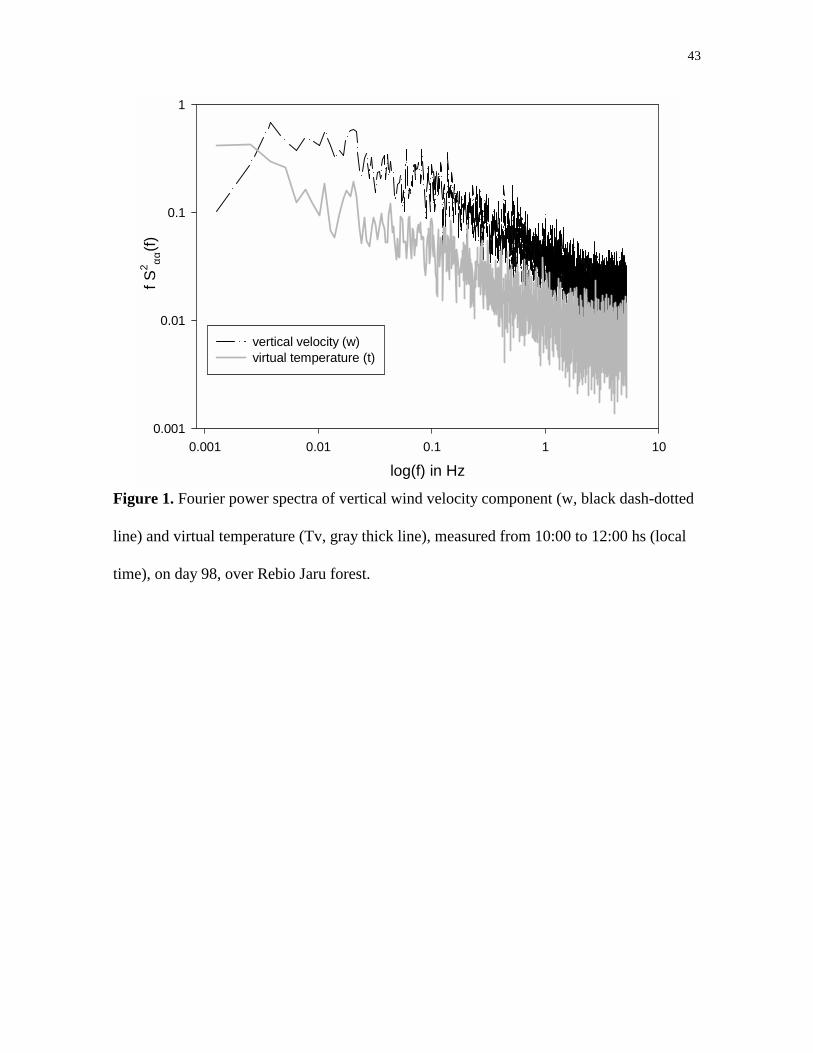
This imprecision on flux estimations appears when the power spectra of turbulent
variables, such as w (vertical wind velocity) do not show a clear spectral gap (Figure 1),
4
when sampled at one hour scale. This problem was discussed by several authors: Lumley
and Panofsky [1964, pg. 45], on their classical study about atmospheric turbulence
structure, identified scenarios where the autocorrelation function does not tend to zero with
increase on time (or on length) in such a way that the determination of integral scales
sometimes becomes particularly difficult. It is evident that turbulent signals under such
conditions led to difficulties on definition of averaging periods and fluctuations [Mahrt,
1989; Hildebrand, 1991; Mahrt,1991a, 1998].
According to Pasquill [1974], two major objections could be raised against the
current statement concerning the validity of the stationarity and homogeneity hypotheses on
atmospheric boundary layer (ABL) turbulent fields. The first one results from the fact that
the power spectra of turbulent fluctuations extend to larger scales of motion, such as
mesoscale ones, which existence is connected to perturbations introduced by low-frequency
motions [McNaughton and Laubach, 2000]. Consequently, turbulent variables calculated
statistically are strongly dependent on sampling period and often their variances do not
show a stable mean value along the data sampling, as detected by authors such as
Hildebrand [1991] and Mahrt [1991a], on studies about flux estimation over complex
terrain. According to Tennekes and Wyngaard [1972] this problem tends to be aggravated
in higher order moment evaluations. The second complication is associated to the factors
regarding the variability imposed to the flow, by external forcing such as the roughness of
the terrain [McNaughton and Laubacch, 2000], the existence of complex distributions of
sources or sinks of heat and moisture at the surface [Brutsaert, 1998; Desjardins et al.,
1997], the interaction of the ABL flow with gravity waves exterior to it [Nai-Ping et al.,
5
1983; Chimonas, 1985; Stull, 1988], the effects originated from the top of the ABL [Mahrt,
1991b], etc.
Trying to deal with the determination of scale dependent fluxes, Sun et al [1996],
based on the characteristics of this dependence, proposed to partition the total flux into
turbulent, large-eddy, and mesoscale fluxes due to motions on scales smaller than 1 km,
between 1 and 5 km, and bigger than 5 km, respectively. In order to explain these
characteristics of flux-scale dependence, McNaughton and Laubach [2000] have proposed a
different three class scheme based on the earlier ideas of Kader and Yaglom [1990] and
their attempt to find a generalization of the classical Monin-Obukhov Similarity Theory
(MOST). After McNaughton and Laubach [2000], three different scaling regimes could act
on the surface layer turbulent exchanges: an inner-layer scaling (ILS), an outer-layer scaling
(OLS) and a combined scaling (CS). Each one of these regimes would explain the
characteristics of turbulent power spectra and cospectra on specific regions and their
classification depends on height and frequency. They have associated OLS components
with "inactive" turbulence and ILS components with "active" turbulence in the sense
proposed by Townsend's hypothesis about turbulence atmospheric structure [Townsend,
1976; Högström, 1990]. Still after McNaughton and Laubach, if the power spectra of active
and inactive components of turbulence are separated by a spectral gap, there would be no
interactions between them. But, on the other hand, if there is no obvious spectral gaps, there
would be a matching region with -1 and no more -5/3 power law (for u, v, and scalar
variables, but not for w-wind velocity component) corresponding to the CS region.
Therefore, each one of these classes should have a specific parameterization to represent the
subgrid fluxes on models of simulations of ABL, what is particularly difficult for large
6
eddies and mesoscale motions situations. Other class-separation criteria have been
proposed, still. Howell and Mahrt [1994b] also studied the scale dependence of surface
fluxes using the Haar wavelet transform to decompose the turbulent signals in 4 classes,
including the three cited before, and the 'fine scale' class, corresponding to very small scale
motions, with nearly isotropic characteristics.
The classes established by Sun et al. [1996] refer to oceanic tropical boundary layer
which in some situations, in the vicinity of large cloud cluster systems, do not show a clear
gap in the power spectra [Williams et al, 1996] and present many affinities with the ABL
over Amazon rain forest on wet-season [Garstang and Fitzjarrald, 1999]. According to these
authors, the tropical wet season ABL could be characterized as a disturbed state of the
boundary layer, which presents peculiar inter-scale links properties. It has qualitatively
different characteristics than that observed on undisturbed boundary layers and exhibits
peculiar tropospheric phenomena, such as outflows, among others, which play important
roles on vertical transports and on defining vertical exchange processes time-scales. Under
these conditions, is hard to characterize a superior border for the ABL, whose
thermodynamic characteristics are strictly associated to the nature of the convection on the
humid troposphere. It is important to mention that, although not hardly studied, the
exchanges of heat and moisture on the top of ABL also appear to influence the variability of
turbulent scalar variables measured at surface [Mahrt, 1991b; Holtslag and Moeng 1991;
Smedman et al., 1995; Wiliams et al., 1996; Garstang and Fitzjarrald, 1999]. Mahrt [1991b]
showed that, depending on the ABL moisture regime, different characteristic scales of
potential virtual temperature and humidity are present on some close to surface turbulent
processes.
7
Even disregarding the top of ABL influence, at least four physically distinct factors
may contribute to the variability of measurements at surface: (i) local circulation induced by
horizontal heterogeneity of the terrain [Mahrt and Ek, 1993; Mahrt et al., 1994, Mahrt et al.,
1998], which is expected to exist in Rebio Jaru site (this study) due the existence of "fish-
bone pattern" trips of alternating forested/deforested areas surrounding the reserve [Dias et
al., 2001] and also due to the wavy pattern of the vegetated crown top; (ii) contribution
from updrafts and downdrafts to surface fluxes [Wyngaard and Moeng, 1992], associated
with the very strong convective activity present in Amazonia [Garstang and Fitzjarrald,
1999]; (iii) contributions due to the existence of coherent structures on turbulent flow
[Mahrt and Gibson, 1992; Mahrt and Howell, 1994; Hogström and Bergström, 1996], what
presents specific characteristics over vegetated covers [Paw U et al., 1992; Gao and Li,
1993; Collineau and Brunet, 1993; Lu and Fitzjarrald, 1994; Raupach et al., 1996; Brunet
and Irvine, 2000]; (iv) the effects of slow wind direction and wind strength variation on
scalar transport processes near the ground [McNaughton and Laubach, 2000]. Such
variations are identified with the concept of "inactive" turbulence [Townsend, 1976].
These factors can drive important contributions to the total fluxes by low frequency
motions, as reported by Sakai [personal communication, 2000]. The author found for a
summer-time signal, obtained above a midlatitude deciduos forest, that large eddies
presenting periods ranging from 4 to 30 minutes might contribute with about 17 % to total
surface fluxes of heat, water vapor and CO2. However, it is likely that these flux fractions
would not be taken into account if they were calculated by the current popular averaging-
periods procedures. This is because these usual sampling time intervals are too short to
resolve the larger eddies present in the flow [Mahrt, 1998]. Sakai [2000] has also found that
8
short-averaging periods might underestimate daytime CO2 fluxes at standard towers by 10-
40 %, depending on wind speed conditions. Most of research groups from the flux
measurement community use frequency response corrections suggested by Moore [1986],
and slightly corrected by Moncrieff et al. [1987]. However, Culf et al. [2001] highlight that
this correction scheme might generate large unrealistic low-frequency corrections under
certain circumstances (for instance, under unstable conditions and low wind speed).
In this work we use turbulent data measured at Amazon rain forest during LBA
1999 wet-season campaign. The measuring heights, 62m and 67 m, are likely to be in a
surface transition sub-layer. During daytime conditions, low-frequency contributions to
eddy-correlation turbulent fluxes were often present. We apply wavelet transform to project
the data on scales and calculate by scale covariances in a similar way to the one used by
Howell and Mahrt [1994b] and Katul and Parlange [1994]. To accomplish such
calculations, we use the Daubechies-8 wavelet transform [Daubechies, 1992] to decompose
turbulent signals of wind velocity (u,v,w), temperature (T), humidity (q) and CO2
concentration (c). In spite of some restrictions concerning the feasibility of its applications
[Treviño and Andreas, 1996], wavelet analysis is a powerful tool to analyze turbulent
signals [Farge, 1992; Katul and Parlange, 1994; Abry, 1997]. Using the scale projected
signals, we then calculate the fluxes partitioned into turbulent, large-eddy and mesoscale
classes.
2. Site description and instruments deployed
9
During the 1999 Wet Season in Amazonia, several activities of the LBA Project
(Large Scale Biosphere-Atmosphere Experiment in Amazonia) took place at the biological
reserve of Jaru (Rebio Jaru), located about 100 km North of Ji-Paraná, Rondonia, Brazil
[Dias et al., 2001]. Rebio Jaru is a terra firme forest reserve owned by the Brazilian
Environmental Protection Agency (IBAMA). As reported by Culf et al. [1996], in the
predominant wind direction (sector from the north west clockwise to south-south east), the
fetch condition is mainly of an undisturbed forest for tens of kilometers. However, in the
other directions, it is much less (about 800 m), where the Ji-Paraná river forms the western
boundary of the reserve. On the other side of the river the rain forest has been progressively
cleared during the last 25 years, following a very peculiar fish-bone pattern, which
alternates patches of forest and of degraded land are observed [Andreae et al., 2001].
The Rebio Jaru reserve canopy has a mean height of 35m; however, some of the
higher tree branches have heights up to 45m. Details of vegetation at this site are given by
McWilliam et al. [1996]. At the end of 1998, within the collaboration of LBA/AMC and
LBA/EUSTACH projects, a new 60 m tall micrometeorological tower was built at this site
(10o 4.706' S; 61o 56.027' W, at the height of 145 m A.S.L.). Details of instrumentation and
measurements at this tower are given by Dias et al. [2001] and Andreae et al. [2001].
Two datasets were used on this work. The first one (dataset A) is composed by
measurements made between days 93 (Apr. 3rd) and 99 (Apr. 9th) of 1999, with a 3-D sonic
anemometer (Solent A1012R, Gill Instruments), together with a infrared gas analyzer (LI-
6262, LICOR Inc.), both recording data at a sampling rate of 10.4 Hz.. , This data were
obtained at the height of 62.7 m, and is part of long term measurements of surface fluxes
10
supported by the LBA/EUSTACH project (Andreae et al., 2001). The second dataset (B) is
composed by turbulent data collected from day 31 (Jan. 31st) to 60 (Mar. 1st) of 1999,
during WETAMC campaign (Dias et al, 2001), with a different 3-D sonic anemometer
installed at the height of 67 m above the forest floor (CSAT3, Campbell Scientific Inc.), at
a sampling rate of 16 Hz. The sonic anemometers measure the three wind components
(u,v,w) and virtual air temperature (Tv), and the IRGA measures the concentration of water
vapor (q) and CO2 (c) on the air. Quality control was done using the QC pack software of
Vickers and Mahrt (1997). Records with bad data points, instrument dropouts, poor
resolution and abrupt changes are flagged and then examined visually. Bad data records
were not used in the analysis.
3. Methodology
a. Determination of power spectra and cospectra low-frequency ends of the turbulent
variables
The spectral gap, usually appears on power spectra of turbulent variables measured
at middle and high latitude sites over uniform terrain, and provide the necessary
information to a good choice of the sampling segment size (time of duration of
measurements to flux determination). This also supply information on the temporal scale
where the variables should be divided into mean and fluctuation parts [Stull, 1988].
Although is broadly accepted that the spectral gap exists at least on a statistical sense on
11
temporal scales close to 1 hour [Lumley and Panofsky, 1964; Stull, 1988], there are
situations when is hard to observe a clear gap, on intervals up to hundred of minutes [Sun et
al., 1996; Williams et al., 1996; Mahrt, 1998; Mc Naughton and Laubach, 2000]. Among
the several factors that may determine a non clear existence of the spectral gap, could be
highlighted: (a) the modulation of the turbulent fluxes by mesoscale motions [Sun et al,
1996; Williams et al, 1996]; (b) the existence of complex and horizontally heterogeneous
surfaces [Mahrt et al., 1994; McNaughton and Laubach, 2000]; (c) the existence of
mesoscale transient motions [Mahrt et al., 1994]; and (d) multiscale processes with a strong
non-linear interaction between the motions on several scales, what is typical of the humid
tropical boundary layer [Williams et al., 1996; Garstang and Fitzjarrald, 1999].
Most of the power spectra observed over Rebio Jaru during the wet season with data
measured during morning and afternoon times show variance spread over a wide range of
frequencies, without any obvious spectral gaps, even when the sampling sizes were
increased to several hundreds of minutes. This difficulty in determining a clear cutoff
frequency motivated the authors to use the methodology based on wavelet transforms, as
suggested by Howell and Mahrt [1994b]. Wavelet transforms allow the decomposition of
turbulent scalar fields into space and scale, and information related to the motions on a
particular scale can be extracted, even the spectra of signal of different scales. The Fourier
energy spectrum [Kaimal and Finnigan, 1994] has been one of the most popular techniques
for analysis of signals. Indeed, many of the traditional methods work in the Fourier space
for most of the time.
The Fourier energy spectrum E(k) of the real function f(x) is defined by
12
E(k) = | f(k) |2 for k ≥ 0 ( 1 )
where f(k) signifies Fourier transform.
The wavelet transform extends the concept of energy spectrum so that one can
define a local energy spectrum E(k, x) using the L2 norm wavelet [Farge, 1992]:
E(x, k) = C | F(x, k0/k) |2 for k ≥ 0 ( 2 )
where k0 is the peak wave number of the analysing wavelet, and C is a constant.
By measuring E(x, k) at different places in a flow field one can determine what parts
of the field contribute most to the overall Fourier energy spectrum and how the energy
spectrum depends on local conditions. For example, one can determine the type of energy
spectrum contributed by coherent structures, such as isolated vortices, and the type of
energy spectrum contributed by the unorganized part of the flow [Farge, 1992; Gao and Li,
1993].
Since the wavelet transform analyses the signal into wavelets rather than sine waves,
it is possible that the mean wavelet energy spectrum may not always have the same slope as
the Fourier energy spectrum. Perrier et al. [1995] have demonstrated the conditions on
which is possible to obtain spectral power law estimation by means of WT.
Howell and Mahrt [1994b] used also wavelet transform to develop an adaptive
method to divide the high frequency turbulent motions into turbulent and fine scale classes.
However, as our main goal is this study is to assess the low frequency contributions to the
13
total fluxes, we did not separate this fine scale class using Howell and Mahrt [1994b]
methodology.
b. Wavelet decomposition of turbulent data
The wavelet transform (WT) is a powerful analysis tool, that permits an
evolutionary spectral study of turbulent atmospheric signals [Daubechies, 1992; Farge,
1992]. WT is similar to, but an extension of Fourier analysis. WT is computationally
similar in principle to Fast Fourier Transform (FFT). The FFT uses cosines, sines and
exponentials to represent a signal, and is most useful for representing stationary functions.
Since many 1-D and 2-D signals display non-linear, chaotic, intermittent or fractal
behaviour, Fourier analysis is less suitable for analysing such signals. Wavelets offer a more
adequate method to analyse complex signals. The aim of the WT is to 'express' an input
signal into a series of coefficients of specified energy. The discrete numbers associated with
each coefficient contain all the information needed to completely describe the signal,
provided one knows which analysing wavelet was used for the decomposition. The WT
partitions a signal with respect to spatial frequency. This is achieved by filtering the signal
with a pair of dyadic orthogonal filters called a quadrature mirror filter (QMF). A QMF
comes in a pair: termed a 'father' wavelet and a 'mother' wavelet. The father wavelet
provides an approximate or blurred version of the signal at sucessive resolutions, while the
mother wavelet captures the detail at each resolution. In the wavelet transform certain
coefficients are large while others are negligible, and practically zero. This property can be
14
used to separate out the required information by suppressing out the coefficients close to
zero.
In this work we use the Daubechies-8 WT to project the turbulent signals on 16
scales. This WT is a discrete orthogonal wavelet and the cospectra based on this type of
wavelet can be interpreted as fluxes decomposed into values computed from moving
averages [Howell and Mahrt, 1997]. For analysis of turbulence measurements, discrete WT
are preferable since it is suitable to provide non redundant decomposition information and it
permits to obtain a inverse WT. Howell and Mahrt [1994b] also show that cospectra based
on the orthogonal Haar (multiresolution) decomposition are directly linked to varying the
Reynolds averaging length procedure.
The turbulent signals of horizontal (u) and vertical (w) wind velocity components,
virtual air temperature (Tv), specific humidity (q) and CO2 concentration (c) were divided
into overlapping intervals of 4 hours, and each of these intervals was decomposed into 16
scales (15 scales, in case of dataset B), using the wavelets subroutines of the software
package Matlab (The MathWorks, Inc.). The package performs the wavelet decomposition
of a turbulent signal similar to the methodology described by Katul and Parlange [1994].
The choice of the Daubechies-8 WT was, to some extent, arbitrary. This is because various
wavelets were tested, but the differences between scale variances or covariances calculated
with several wavelets were very small, result similar to the one obtained by Katul and
Parlange [1994], for turbulent data measured at atmospheric surface layer under unstable
and stable stability conditions.
15
3. Results and discussion
One of the main goals of this work is to investigate the scale contributions of
turbulent fluctuations to variances and covariances calculations. As was stressed by
Lenschow and Stankov [1986] an important consideration in observational studies of the
ABL is the length or time over which, on the average, a variable maintains some degree of
correlation with itself or with other physically significant variables. For fixed-point tower
measurements, accepting the Taylor's "frozen turbulence" assumption (Stull, 1988) a time
scale is specified in such a way that it can be related to a length scale by multiplying the
mean wind speed by the time scale. But to obtain flux measurements in tower-based
measurements is not an easy task. Mahrt [1998] has carried out a review of the main
problems which introduce errors in ABL turbulent flux measurements. One of these
problems is nonstationarity. As was discussed by him, nonstationarity of surface fluxes is
caused by diurnal trend, mesoscale motions, and passage of clouds. All these problems
probably are present in the tropical wet-season ABL [Garstang and Fitzjarrald, 1999].
Nonstationary mesoscale motions or mesoscale motions associated with heterogeneous
surfaces modulate the turbulent flux and sometimes lead to computed flux on scales larger
than turbulent motions [Mahrt et al., 1994; Mahrt, 1998]. After a variance analysis
performed by Mahrt et al. [1994] the momentum and ozone fluxes are more influenced by
transient mesoscale motions while fluxes of heat, moisture and carbon dioxide are more
influenced by surface heterogeneity. Updrafts and downdrafts sequence events sometimes
associated to well-organized convective cloud systems or to individual eddies motion also
contribute to introduce scale dependence on ABL fluxes [Sun et al., 1996]. As a tool for

16
displaying the scale dependence, we have computed the variances and covariances by
means of wavelet transform (WT) [Farge, 1992; Abry, 1997]. WT is suited to be a more
adequate tool to scale project nonstationary turbulent signals which present irregularly
spaced sharp transitions [Farge, 1992; Gao and Li, 1993; Collineau and Brunet, 1993;
Mahrt et al., 1994].
In order to project transient signals on selected scales, we apply the Daubechies-8
Wavelet transform to the turbulence time series of dataset A (B), divided on overlapping
records of 131072 (262144) data points, that correspond to approximately 3.5 (4.5) hours,
recovered from the datasets following a time step of one hour. These records lengths were
chosen to provide better analyses of low frequency motions, and because under diurnal
conditions, turbulent signals seldom presented spectra or cospectra low-frequency end at
frequencies higher than the ones corresponding to time scales of 2 to 3 hours. Variances and
covariances of the variables were then calculated for each projected time scale. Scale
variances represent the energy of the turbulent scalars (or wind component) contained on
each specific scale of variability [Gao and Li, 1993, Katul and Parlange, 1994].
On the following section we show the contribution of each scale to the total
variances and fluxes and assess the partition of these fluxes between turbulent, large eddies
and mesoscale classes, as proposed by Sun et al [1996]. In order to obtain useful
information about the scaling properties of the turbulent signals on the various selected
scales on which they have been projected, we also performed scale calculations of the
correlation coefficients between temperature (T) and specific humidity (q). This is because
De Bruin et al. [1999], based on the conclusions of Hill [1989] have shown that if the
correlation coefficient between T and q (r(Tq)) is equal to one, temperature and specific
17
humidity both will obey the Monin-Obukhov Similarity Theory (MOST). Further, under
such conditions, it is possible to determine the Bowen ratio from r(Tq). As examples of
situations in which r(Tq) ≠ 1, De Bruin et al. [1999] have mentioned: conditions of local
advection and conditions in which the entrainment of dry air at the top of the ABL is
stronger than surface evaporation, when large eddies are able to transport drier air from
ABL top towards the surface [Mahrt, 1991b]. In these situations, the MOST is expected to
be violated.
Scale variances and covariances partitioning
Once the wavelet coefficients are available, one can assess the energy contained in
each scale (scale variance). With this information, it is possible to investigate in which eddy
motion classes are partitioned the contributions from different physical processes to total
fluxes. One starting point to perform this analysis is by simply calculating the variances and
covariances of these coefficients and verifying whether they agree or not with some
classification proposed. In this work, we will analyse the feasibility of applying the
classification proposed by Sun et al. [1996] to explain our results. This is carried out in
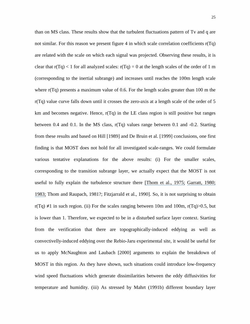
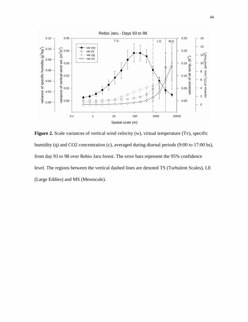
Figure 2. It shows the scale variances of w, Tv, q and c, averaged during diurnal periods
(9:00 to 17:00 hs), from day 93 to 98. The scales are presented as spatial scales of eddies,
which were estimated assuming the Taylor’s hypothesis [Stull, 1988]. The vertical dashed
lines indicate the scales that divide the three classes of motion:
Turbulent scales (TS) – main scales of vertical turbulent transport of mass and energy in the
atmospheric surface layer;
18
Large eddies (LE) – motions involving eddies of scales on the order of the height of the
ABL;
Mesoscale (MS) – motions on horizontal scales much larger than the height of the ABL,
involving processes not expected to be controlled only by ABL parameters.
Nevertheless, based only on the information provided by Figure 2, it is not easy to
assess specific scales that should separate the above classes. To have some more insight
about the end of each one of these classes, we depict also informations regarding: (i) the
scale covariance values, as a function of the scale itself, which are useful to better
understand the regions in which some properties of the eddy motions are present (Figure 3);
(ii) the scale correlation coefficients between Tv and q along a large range of scales (Figure
4); (iii) the mean values of H, λE, FCO2, var(w), var(Tv), var(q), and H/ λE, which are
presented in Table 1.
Figure 2 shows a broad peak for var(w) values ranging from scales around 50m to
500m (the peak corresponds to a 4.0min time-scale), while scalar variances grow up slowly
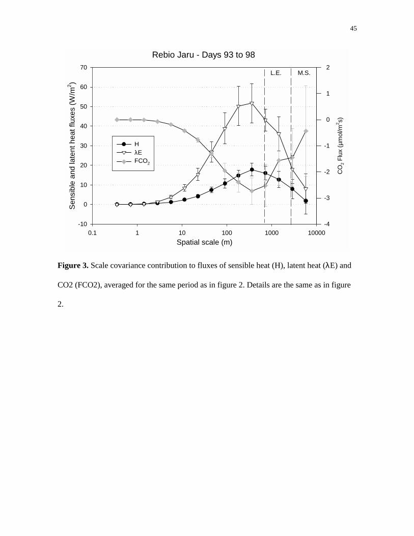
continuously in this region (without any local maximum). Figure 3 shows, still, broader
peaks than the former var(w) one, for scalar cospectrum peaks. Their local
maximum/minimum values are also inside the interval located between 50m to 500m: while
scalar H and λE show maximum values, FCO2 presentes a minimum value there. On scales
higher than 800 m, we see a continuous drop on <w'T>' and <w'q'> scale values and a
increase on <w'c'> scale values (Figure 3), as well as a continuous drop on the scale
correlation coefficient between Tv and q (Figure 4). Due to this factors, the scales around
300m, which corresponds to temporal scales around 3 minutes, present the more energetic
19
surface layer eddies and are associated with physical events whose role in tropical wet ABL
is essential to determine some important features of the structure of turbulence there.
Hence, this scale actually separetes two different classes of turbulent eddy patterns, as
discussed by Williams et al. [1996], and not three, as proposed by Sun et al. [1996] for the
tropical marine boundary layer. So, it appears that all the scales greater than the ones
associated with the spectral and cospectral peaks present similar physical characteristics.
However, the variances of Tv, q, and c increase considerably on scales higher than 3 km
(figure 2) and, despite the facts discussed above, the low frequency motions seems to
behave slightly different on scales ranging from 800 m to 3 km, and higher than 3 km (see
figure 5 discussed later, where we can see that these two classes present opposite signals).
Due to this fact, we choose the 3 km scale to separate the large eddy and mesoscale classes.
However, this and other criteria to split these low frequency scales in two different classes
should be investigated later.
It is interesting to note that most of the variance of w occur on turbulent scales (TS),
what explains the fact that most of the mass and energy exchange happen on these scales. It
shows a maximum on scales close to 300m, similar to results obtained by Howell and
Mahrt [1994b]. Due to the fact that large-scale motions are predominantly horizontal at
levels close to the surface, variances of w are low at LE and MS classes. McNaughton and
Laubach (2000) reported, however, that although w-spectrum is well scaled by Monin-
Obukhov Similarity, it still might present enhancement at low frequencies under disturbed
conditions, influenced by outside ABL parameters, such as updrafts and downdrafts.
Variances of Tv, q and c show the higher values at mesoscale, but is important to notice
that q still presents pronounced energy on turbulent processes, compared to higher scales.
20
The presence of the maximum variance at low frequency motions (except for w, which is
surface limited, as explained above) probably indicate the high influence of mesoscale
motions and convective systems that act on amazonian ABL. Several authors have also
reported high variability of turbulent scalars at low frequencies, such as Wiliams et al
[1996], Sun et al. [1996] and Réchou and Durand [1997].
In spite of the fact that the scalar variance curves present similar shapes, the var(q)
curve grows more quickly inside the TS range comparatively to the var(T) and var(c)
curves, which present enhancement in their scale variation rate at the separation border
between TS and LE regions, result which seems to be related with the concept of 'scale
surface heterogeneity' [Mahrt, 1996]. As discussed by Stull [1988], for 'classical' situations,
there are experimental and modeling evidences that var(T) is expected to be greater than
var(q) at the lower levels of the ABL. This is because close to the surface, there would be a
more intensive variation of sources and sinks of sensible heat, which generate more
intensive fluctuations of T in this region comparatively to humidity field. But our results do
not present such a difference. One first possible explanation for these results is that the
measurements were performed below the 'blending height', loosely defined as the level
above which the flow becomes horizontally homogeneous in the absence of other
influences [Mahrt, 1996]. One other possible explanation for these results is that in a rain
forest as the Rebio-Jaru reserve, the scale thermal and humidity heterogeneity strength
patterns are not the same. Besides, the former grows more slowly than the last when the
spatial scale increases. As stressed by McNaughton and Laubach [2000], 'advected variance'
has little effect on this kind of results, and since all scalars over the experimental field are
transported by the same velocity field, the main differences in scalar spectra must have had

21
their origin in differences in scalar sources at the ground. At the lower frequency range we
observe a clear variation on the values of d[var(S)]/ds (where S is a generic scalar and s, is
the spatial scale), except for d[var(q)]/ds.
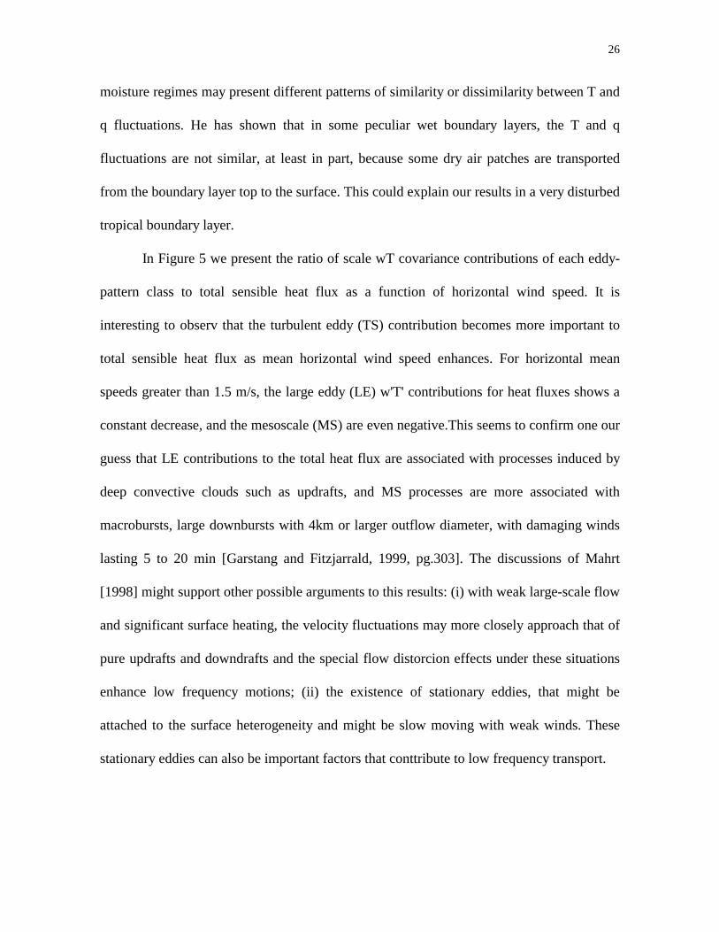
Figure 3 shows the scale dependence of fluxes of sensible and latent heat, and CO2,
averaged for the same period as in figure 2. On the smallest scales, that should involve
mainly isotropic motions [Howell and Mahrt, 1994], the fluxes are very small, but different
from zero. The fact that the fluxes are not always null in the inertial subrange, raises some
interesting questions discussed by Katul et al. [1997] concerning the inertial subrange eddy
motion contamination by the larger scale organized eddy motion. As they have stressed,
irrespective of the anisotropy source, if interactions between large scales and small scales
are significant, then it is possible that the anisotropy of the large scale persists in the inertial
subrange. In such situations, basic atmospheric surface layer assumptions as Kolmogorov's
hypotheses could be affected. From scale of 10m towards higher scales, the fluxes increase
significantly, characterizing well the high transports on the region of turbulent scales. Both
sensible and latent heat fluxes, as well as CO2 flux, reach a maximum at scales close to 400
m, corresponding to time scales of approximately 3 minutes, and then decrease to small
values at higher scales. It is interesting to guess about the physical origins for these 3min
maximum-energy eddies in the wet tropical boundary-layer. As was discussed by Gartang
and Fitzjarrald [1999, pg.16], horizontal gradients in temperature and humidity tend to
disappear in the lower tropical atmosphere. As they have stressed, in this context locally
produced horizontal gradients in temperature, moisture, and pressure are product of
perturbations of the velocity field and not a result of pre-existing gradients in those
quantities. Thus, we might expect that these local perturbations of the velocity field are the
22
main source for generation of turbulent kinectic energy (TKE) in the atmospheric surface
layer of tropical regions. Gu et al. [2001] have recently presented evidences of cloud
modulation of solar irradiance in a Amazonia pasture (located not far from our
experimental site) associated with cloud gap patterns which seems to be responsible for a
convective regime and a turbulence diffusion regime whose long time period fluctuations
are of the order of 3 min, the same time-scale order as we have obtained in our results.
Hence, we suggest that these cloud gap effects represent the main source of w-TKE in the
Amazon forest wet boundary layer and they could explain the physical origin of our 3min
energy-peaks.
Although the largest amount of the energy and mass fluxes occur on turbulent scales
below or of the order of the w-spectral peak, larger scale eddy motions could generate
important contributions to the total fluxes. In addition, according to our results, these low-
frequency contributions to surface fluxes also show large variation among the various
investigated data records, as we can see on Figure 3. This sohows up by the estimated large
sampling errors.
Two explanations for these results could be proposed: (i) one presented by
McNaughton and Laubach [1998, 2000] in their investigation about the consequences of the
unsteadiness of the wind field on the scalar fields. After them, the surface fluxes of
temperature and humidity do indeed vary in step with low-frequency variations in the wind
under certain non homogeneous surface conditions. By means of a theoretical treatment,
they showed that this would affect the values of the eddy-diffusivities for temperature and
humidity in different ways. It is interesting to note that this kind of low-frequency wind
velocity variability and that dissimilarity between T and q fluctuations were observed in
23
Rebio-Jaru turbulent data, too. It is important also to keep in mind that our experimental
site is in a rain forest strip which is surrounded by deforested areas in a very peculiar "fish-
bone" pattern. Such a non homogeneous boundary condition could generate mesoscale
circulations as the discussed by Sun et al. [1996] and Mahrt and Ek [1993], that would
explain our low-frequency scalar fluxes. (ii) one second explanation concerns, not the
heterogeneity surface conditions, but the peculiar complex characteristics of the 'disturbed
state' wet tropical ABL. According to Garstang and Fitzjarrald [1999, pg. 13], when deep
convective clouds are present in a moist convective tropical boundary layer, the links to the
surface in the vertical column of the atmosphere are complex. Besides, mean upward
motions may be present over a substantial area occupied by these systems, which
concentrate the vertical transport of heat, trace gases, and matter there. In such situations,
there is a failure of the familiar concept of planetary boundary layer, in which there is a
simple connection between the surface and some shallow horizontally homogeneous layer.
This is because the deep clouds operate as very effective mixers, leaving the atmosphere
much more nearly neutrally stratified than in the undisturbed ABL familiar state [Garstang
and Fitzjarrald, 1999, pg. 285]. We suggest that this peculiar behaviour of the wet tropical
boundary layer is responsible for our results concerning the low-frequency features of the
scalar covariances.
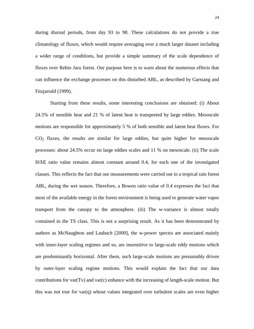
To provide quantitative information about the amount of flux contained in each
turbulence-pattern class earlier defined, we present Table 1. In this table we present the
mean by-class and total values of sensible heat flux (H, in W/m2), latent heat flux (λE, in
W/m2), the bowen ratio (H/λE), CO2 flux (FCO2, in µmol/m2/s), variance of w (in m2/s2),
variance of Tv (in K2), variance of q (in g2/kg2), and variance of c (in µmol2/mol) averaged
24
during diurnal periods, from day 93 to 98. These calculations do not provide a true
climatology of fluxes, which would require averaging over a much larger dataset including
a wider range of conditions, but provide a simple summary of the scale dependence of
fluxes over Rebio Jaru forest. Our purpose here is to warn about the numerous effects that
can influence the exchange processes on this disturbed ABL, as described by Garstang and
Fitzjarrald (1999).
Starting from these results, some interesting conclusions are obtained: (i) About
24.5% of sensible heat and 21 % of latent heat is transported by large eddies. Mesoscale
motions are responsible for approximately 5 % of both sensible and latent heat fluxes. For
CO2 fluxes, the results are similar for large eddies, but quite higher for mesoscale
processes: about 24.5% occur on large eddies scales and 11 % on mesoscale. (ii) The scale
H/λE ratio value remains almost constant around 0.4, for each one of the investigated
classes. This reflects the fact that our measurements were carried out in a tropical rain forest
ABL, during the wet season. Therefore, a Bowen ratio value of 0.4 expresses the fact that
most of the available energy in the forest environment is being used to generate water vapor
transport from the canopy to the atmosphere. (iii) The w-variance is almost totally
contained in the TS class. This is not a surprising result. As it has been demonstrated by
authors as McNaughton and Laubach [2000], the w-power spectra are associated mainly
with inner-layer scaling regimes and so, are insensitive to large-scale eddy motions which
are predominantly horizontal. After them, such large-scale motions are presumably driven
by outer-layer scaling regime motions. This would explain the fact that our data
contributions for var(Tv) and var(c) enhance with the increasing of length-scale motion. But
this was not true for var(q) whose values integrated over turbulent scales are even higher
25
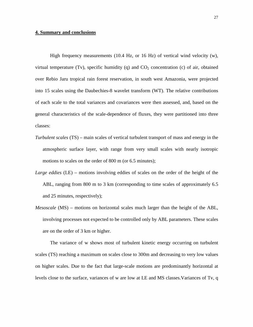
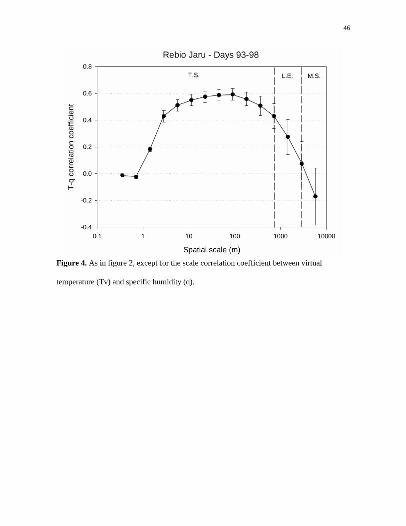
than on MS class. These results show that the turbulent fluctuations pattern of Tv and q are
not similar. For this reason we present figure 4 in which scale correlation coefficients r(Tq)
are related with the scale on which each signal was projected. Observing these results, it is
clear that r(Tq) < 1 for all analyzed scales: r(Tq) = 0 at the length scales of the order of 1 m
(corresponding to the inertial subrange) and increases until reaches the 100m length scale
where r(Tq) presents a maximum value of 0.6. For the length scales greater than 100 m the
r(Tq) value curve falls down until it crosses the zero-axis at a length scale of the order of 5
km and becomes negative. Hence, r(Tq) in the LE class region is still positive but ranges
between 0.4 and 0.1. In the MS class, r(Tq) values range between 0.1 and -0.2. Starting
from these results and based on Hill [1989] and De Bruin et al. [1999] conclusions, one first
finding is that MOST does not hold for all investigated scale-ranges. We could formulate
various tentative explanations for the above results: (i) For the smaller scales,
corresponding to the transition subrange layer, we actually expect that the MOST is not
useful to fully explain the turbulence structure there [Thom et al., 1975; Garratt, 1980;
1983; Thom and Raupach, 1981?; Fitzjarrald et al., 1990]. So, it is not surprising to obtain
r(Tq) ≠1 in such region. (ii) For the scales ranging between 10m and 100m, r(Tq)>0.5, but
is lower than 1. Therefore, we expected to be in a disturbed surface layer context. Starting
from the verification that there are topographically-induced eddying as well as
convectivelly-induced eddying over the Rebio-Jaru experimental site, it would be useful for
us to apply McNaughton and Laubach [2000] arguments to explain the breakdown of
MOST in this region. As they have shown, such situations could introduce low-frequency
wind speed fluctuations which generate dissimilarities between the eddy diffusivities for
temperature and humidity. (iii) As stressed by Mahrt (1991b) different boundary layer
26
moisture regimes may present different patterns of similarity or dissimilarity between T and
q fluctuations. He has shown that in some peculiar wet boundary layers, the T and q
fluctuations are not similar, at least in part, because some dry air patches are transported
from the boundary layer top to the surface. This could explain our results in a very disturbed
tropical boundary layer.
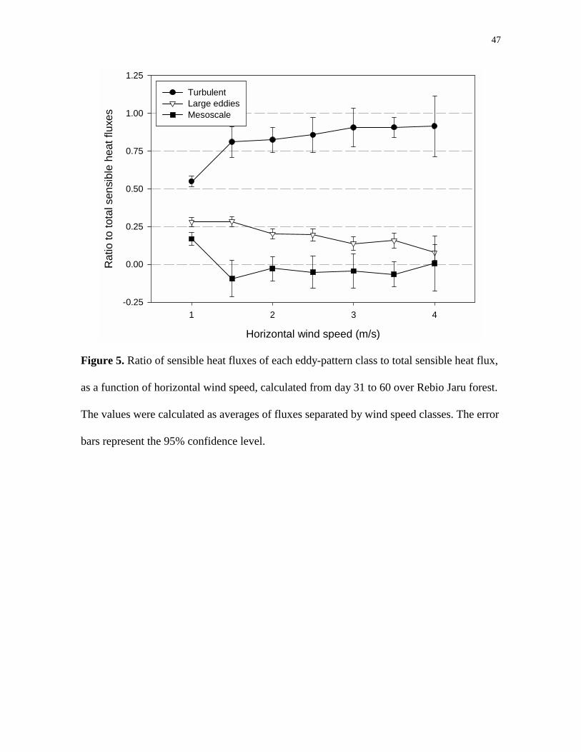
In Figure 5 we present the ratio of scale wT covariance contributions of each eddy-
pattern class to total sensible heat flux as a function of horizontal wind speed. It is
interesting to observ that the turbulent eddy (TS) contribution becomes more important to
total sensible heat flux as mean horizontal wind speed enhances. For horizontal mean
speeds greater than 1.5 m/s, the large eddy (LE) w'T' contributions for heat fluxes shows a
constant decrease, and the mesoscale (MS) are even negative.This seems to confirm one our
guess that LE contributions to the total heat flux are associated with processes induced by
deep convective clouds such as updrafts, and MS processes are more associated with
macrobursts, large downbursts with 4km or larger outflow diameter, with damaging winds
lasting 5 to 20 min [Garstang and Fitzjarrald, 1999, pg.303]. The discussions of Mahrt
[1998] might support other possible arguments to this results: (i) with weak large-scale flow
and significant surface heating, the velocity fluctuations may more closely approach that of
pure updrafts and downdrafts and the special flow distorcion effects under these situations
enhance low frequency motions; (ii) the existence of stationary eddies, that might be
attached to the surface heterogeneity and might be slow moving with weak winds. These
stationary eddies can also be important factors that conttribute to low frequency transport.
27
4. Summary and conclusions
High frequency measurements (10.4 Hz, or 16 Hz) of vertical wind velocity (w),
virtual temperature (Tv), specific humidity (q) and CO2 concentration (c) of air, obtained
over Rebio Jaru tropical rain forest reservation, in south west Amazonia, were projected
into 15 scales using the Daubechies-8 wavelet transform (WT). The relative contributions
of each scale to the total variances and covariances were then assessed, and, based on the
general characteristics of the scale-dependence of fluxes, they were partitioned into three
classes:
Turbulent scales (TS) – main scales of vertical turbulent transport of mass and energy in the
atmospheric surface layer, with range from very small scales with nearly isotropic
motions to scales on the order of 800 m (or 6.5 minutes);
Large eddies (LE) – motions involving eddies of scales on the order of the height of the
ABL, ranging from 800 m to 3 km (corresponding to time scales of approximately 6.5
and 25 minutes, respectively);
Mesoscale (MS) – motions on horizontal scales much larger than the height of the ABL,
involving processes not expected to be controlled only by ABL parameters. These scales
are on the order of 3 km or higher.
The variance of w shows most of turbulent kinetic energy occurring on turbulent
scales (TS) reaching a maximum on scales close to 300m and decreasing to very low values
on higher scales. Due to the fact that large-scale motions are predominantly horizontal at
levels close to the surface, variances of w are low at LE and MS classes.Variances of Tv, q
28
and c show the higher values at mesoscale, indicating a likely high influence of mesoscale
motions and convective systems that act on amazonian ABL on these data.
The largest amount of the sensible heat, latent heat and CO2 fluxes occur on
turbulent length scales below or of the order of the w-spectral peak scale. Larger scale eddy
motions could, however, generate important contributions to the total fluxes. In addition,
these low-frequency contributions to surface fluxes show large variation among the various
investigated data records, and can be either positive or negative irrespectively of mean ABL
gradient conditions. About 24.5% of sensible heat and 21 % of latent heat averaged during
diurnal periods from day 93 to 98 were transported by large eddies. Mesoscale motions
during the same period were responsible for approximately 5 % of both sensible and latent
heat fluxes. For CO2 fluxes, the results are similar for large eddies, but quite higher for
mesoscale processes: about 24.5% occur on large eddies scales and 11 % on mesoscale.
These calculations, however, do not provide a true climatology of fluxes, which would
require averaging over a much larger dataset including a wider range of conditions.
We also performed scale calculations of the correlation coefficients, r(Tq), between
temperature (T) and specific humidity (q). The results show that the turbulent fluctuations
pattern of T and q are not similar, and r(Tq) < 1 for all analysed scales.
29
5. Acknowledgments
This work is part of The Large Scale Biosphere-Atmosphere Experiment in Amazonia
(LBA) and was supported by the Fundação do Amparo à Pesquisa do Estado de São Paulo
(FAPESP)/Brazil-process 1997/9926-9. Thanks are due to Dr. Maria Assunção Faus da
Silva Dias who is the coordinator of this research project. The authors are also grateful to
INCRA/Ji-Paraná and to IBAMA/Ji-Paraná. C. von Randow, P. Gannabathula are
supported by a fellowship from Conselho Nacional de Pesquisa e Desenvolvimento
Tecnológico (CNPq).
6. References
Abry, P., Ondelettes et Turbulences, Diderot-Editeur, 292 pp., Paris, 1997.
Affre, C., A. Lopez, A. Carrara, A. Druilhet and J. Fontan, The analysis of energy and
ozone flux data from the LANDES 94 experiment, Atmospheric Environment, 32, 803-821,
2000.
Andreae, M. O. et al., Towards an understanding of the biogeochemical cycling of carbon,
water, energy, trace gases and aerosols in Amazonia: An overview of the LBA-EUSTACH
experiments, J. Geophys. Res., this issue, 2001.

30
Brunet, Y., and M. R. Irvine, The Control of Coherent Eddies in Vegetation Canopies:
Streamwise Structure Spacing, Canopy Shear Scale and Atmospheric Stability, Boundary
Layer Meteorol., 94 (1), 139-163, 2000.
Brutsaert, W., Land-surface water vapor and sensible heat flux: Spatial variability,
homogeneity, and measurement scales, Water Resources Res., 34 (10), 2433-2442, 1998.
Chimonas, G., Apparent Counter-gradient Heat Fluxes Generated by Atmospheric Waves,
Boundary Layer Meteorol., 31 (1), 1-12, 1985.
Collineau, S., and Y. Brunet, Detection of Turbulent Coherent Motions in a Forest Canopy.
Part II: Time-scales and Conditional Averages, Boundary Layer Meteorol., 66 (1-2), 49-73,
1993.
Culf, A. D., J. L. Esteves, A. O. Marques Filho and H. R. Rocha, Radiation, temperature
and humidity over forest and pasture in Amazonia, in Amazonian Deforestation and
Climate, edited by C. A. Nobre, J.H.C. Gash, J.M. Roberts and R.L. Victoria, pp. 175-191,
Wiley, Chichester, 1996.
Culf, A. D. et al., Errors arising from the correction of eddy correlation data under unstable
conditions, J. Geophys. Res., this issue, 2001.
Daubechies, I., Ten Lectures on Wavelets, 357 pp., SIAM, Philadelphia, 1992.
31
De Bruin, H. A. R., B. J. J. M. Van Den Hurk and L. J. M. Kroon, On the Temperature-
Humidity Correlation and Similarity, Boundary Layer Meteorol., 93, 453-468, 1999.
Desjardins, R. L., J. I. MacPherson, L. Mahrt, P. H. Schuepp, E. Pattey, H. Neumann, D.
Baldocchi, S. Wofsy, D. Fitzjarrald, H. McCaughey and D. W. Joiner, Scaling up flux
measurements for the boreal forest using aircraft-tower combinations, J. Geophys. Res., 102
(D24), 29125-29133, 1997.
Dias, M. A. F. S., S. Rutledge, P. Kabat, P. Silva Dias, C. Nobre, G. Fisch, H. Dolman, E.
Zipser, M. Garstang, A. Manzi, J. Fuentes, H. Rocha, J. Marengo, A. Plana-Fattori, L. D. A.
Sá, R. C. S. Avalá, M. Andreae, P. Artaxo, R. Gielow and L. Gatti, Clouds and rain
processes in a biosphere atmosphere interaction context in the Amazon Region, J. Geophys.
Res., this issue, 2001.
Farge, M., The Wavelet Transform and its Applications to Turbulence, Annu. Rev. Fluid
Mech., 24, 395-457, 1992.
Fitzjarrald, D. R., K. E. Moore, O. M. R. Cabral, J. Scolar, A. O. Manzi and L. D. A. Sá,
Daytime Turbulent Exchange Between the Amazon Forest and the Atmosphere, J. Geophys.
Res., 95 (D10), 16825-16838, 1990.
32
Gao, W., and B. L. Li, Wavelet Analysis of Coherent Structures at the Atmosphere-Forest
Interface, J. Appl. Meteorol., 32 (11), 1717-1725, 1993.
Garratt, J. R., Surface Influence upon Vertical Profiles in the Atmospheric near-surface
layer, Q. J. R. Meteorol. Soc., 106 (450), 803-819, 1980.
Garratt, J. R., Surface Influence upon Vertical Profiles in the Nocturnal Boundary Layer,
Boundary Layer Meteorol., 26 (1) 69-80, 1983.
Garstang, M., and D. R. Fitzjarrald, Observations of Surface to Atmosphere Interactions in
the Tropics, 405 pp., Oxford-University-Press, New York, 1999.
Gu, L., J. D. Fuentes, M. Garstang, J. Tota da Silva, R. Heitz, J. Sigler and H. H. Shugart,
Cloud Modulation of surface solar irradiance at a pasture site in southern Brazil, Agric.
Forest Meteorol., 106, 117-129, 2001.
Hildebrand, P. H., Error in Eddy Correlation Turbulence Measurements from Aircraft:
Application to HAPEX-MOBILHY, in Land Surface Evaporation - Measurement and
Parameterization, edited by T.J.Schmugge and J.-C. André., pp. 231-243, Springer-Verlag,
New York, 1991.
Hill, R. J., Implications of Monin-Obukhov Similarity Theory for Scalar Quantities, J.
Atmos. Sci., 46 (14), 2236-2244, 1989.
33
Holtslag, A. A. M., and C.-H. Moeng, Eddy Diffusivity and Countergradient Transport in
the Convective Atmospheric Boundary Layer, J. Atmos. Sci., 48 (14), 1690-1698, 1991.
Howell J. F., and L. Mahrt, An Adaptative Multiresolution Data Filter: Applications to
Turbulence and Climatic Time Series, J. Atmos. Sci., 51 (14), 2165-2178, 1994a.
Howell, J. F., and L. Mahrt, An Adaptative Decomposition: Application to Turbulence, in
Wavelets in Geophysics, edited by P. Kumar and Efi Foufoula-Georgiou, pp. 107-128,
Academic-Press, San Diego, 1994b.
Howell J. F., and L. Mahrt, Multiresolution Flux Decomposition, Boundary Layer
Meteorol., 83, 117-137, 1997.
Högström, U., Analysis of Turbulence Structure in the Surface Layer with a Modified
Similarity Formulation for Near Neutral Conditions, J. Atmos. Sci., 47 (16), 1949-1972,
1990.
Högström, U., and H. Bergström, Organised Turbulence in the Near-Neutral Atmospheric
Surface Layer, J. Atmos. Sci., 53 (17), 2452-2464, 1996.
Kader, B. A., and A. M. Yaglom, Mean fields and fluctuation moments in unstable
stratified turbulent boundary layers, J. Fluid Mech., 212, 637-662, 1990.
34
Kaimal, J. C., S. F. Clifford and R. J. Lataitis, Effect of Finite Sampling on Atmospheric
Spectra, Boundary Layer Meteorol., 47 (1-4), 337-347, 1989.
Katul, G. G., and M. B. Parlange, On the Active Role of Temperature in Surface-Layer
Turbulence, J. Atmos. Sci., 51 (15), 2181-2195, 1994.
Katul, G., C.-I. Hsieh and J. Sigmon, Energy-Inertial Scale interactions for Velocity and
Temperature in the Unstable Atmospheric Surface Layer, Boundary Layer Meteorol., 82
(1), 49-80, 1997.
Lenschow, D. H., and B. B. Stankov, Length scales in the convective boundary layer, J.
Atmos. Sci., 43, 1198-1209, 1986.
Lu, C.-H., and D. R. Fitzjarrald, Seasonal and Diurnal Variations of Coherent Structures
over a Deciduous Forest, Boundary Layer Meteorol., 69 (1-2), 43-69, 1994.
Lumley, J. L., and H. A. Panofsky, The Structure of Atmospheric Turbulence, 239 pp.,
Wiley, New York, 1964.
Mahrt, L., Intermittency of Atmospheric Turbulence, J. Atmos. Sci., 46 (1), 79-95, 1989.
35
Mahrt, L., Heat and Moisture Fluxes over the Pine Forest in HAPEX, in Land Surface
Evaporation - Measurement and Parameterization, edited by T. J. Schmugge, pp. 261-273,
Springer-Verlag, New York, 1991a.
Mahrt, L., Boundary-layer moisture regimes, Q. J. R. Meteorol. Soc., 117 (A), 497, 151-
176, 1991b.
Mahrt, L., and W. Gibson, Flux Decomposition into Coherent Structures, Boundary Layer
Meteorol., 60 (1-2), 143-168, 1992.
Mahrt, L., and M. Ek, Spatial Variability of Turbulent Fluxes and Roughness Lengths in
HAPEX-MOBILHY, Boundary Layer Meteorol., 65 (4), 381-400, 1993.
Mahrt, L., J. I. Macpherson and R. Desjardins, Observations of Fluxes over Heterogeneous
Surfaces, Boundary Layer Meteorol., 67, 345-367, 1994.
Mahrt, L., and J. F. Howell, The influence of coherent structures and microfronts on scaling
laws using global and local transforms, J. Fluid Mech., 260, 247-270, 1994.
Mahrt, L., The Bulk Aerodynamic Formulation for Surface Heterogeneity, Boundary Layer
Meteor., 78, 87-119, 1996.
36
Mahrt, L., Flux Sampling Errors for Aircraft and Towers, J. Atmos. Oceanic Tech., 15, 416-
429, 1998.
Mahrt, L., D. Vickers, J. Edson, J. Sun, J. Hojstrup, J. Hare and J. M. Wilczak, Heat Flux in
the Coastal Zone, Boundary Layer Meteorol., 86 (3), 421-446, 1998.
Mann, J., and D. H. Lenschow, Errors in airborne flux measurements, J. Geophys. Res., 99
(D7), 14519-14526, 1994.
McNaughton, K.G., and J. Laubach, Unsteadiness as a Cause of Non-Equality of Eddy
Diffusivities for Heat and Vapour at the Base of an Advective Invertion, Boundary Layer
Meteorol., 88 (3), 479-504, 1998.
McNaughton, K. G., and J. Laubach, Power Spectra and Cospectra for Wind and Scalars in
a Disturbed Surface Layer at the Base of an Advective Inversion, Boundary Layer
Meteorol., 96, 143-185, 2000.
Moncrieff, J. B., J. M. Massheder, H. A. R. de Bruin, J. Elbers, T. Friborg, B. Huesinkveld,
P. Kabat, S. Scott, H. Soegaard and A. Verhoef, A System to Measure Surface Fluxes of
Momentum, Sensible Heat, Water Vapour and Carbon Dioxide, J. Hydrol., 188-189, 589-
611, 1997.
37
Moore, C. J., Frequency Response Corrections for Eddy Correlation Systems, Boundary
Layer Meteorol., 37, 17-35, 1986.
Nai-Ping, L., W. D. Neff and J. C. Kaimal, Wave and Turbulence Structure in a Disturbed
Nocturnal Inversion, Boundary Layer Meteorol., 26 (2), 141-155, 1983.
Pasquill, F., Atmospheric Diffusion, Wiley, New York, 1974.
Paw U, K. T., Y. Brunet, S. Collineau, R. H. Shaw, T. Maitani, J. Qiu and L. Hipps, On
coherent structures in turbulence above and within agricultural plant canopies, Agric.
Forest Meteorol., 61 (1-2), 55-68, 1992.
Perrier, V., T. Philipovitch, C. Basdevant, Wavelet spectra compared to fourier spectra, J.
Math. Phys., 36, 1506-1519, 1995.
Raupach, M. R., and A. S. Thom, Turbulence in and above Plant Canopies, Annu. Rev.
Fluid Mech., 13, 97-129, 1981.
Raupach, M. R., J. J. Finnigan and Y. Brunet, Coherent Eddies and Turbulence in
Vegetation Canopies: The Mixing-layer Analogy, Boundary Layer Meteorol., 78 (3-4), 351-
382, 1996.
38
Réchou, A., and P. Durand, Conditional Sampling and Scale Analysis of the Marine
Atmospheric Mixed Layer - Sofia Experiment, Boundary Layer Meteorol., 82, 81-104,
1997.
Shuttleworth, J. W., J. H. C. Gash, C. R. Lloyd, C. J. Moore, J. Roberts, A. O. Marques
Filho, G. F. Fisch, V. P. Silva Filho, M. N. G. Ribeiro, L. C. B. Molion, L. D. A. Sá, C. A.
Nobre, O. M. R. Cabral, S. R. Patel and J. C. Moraes, Eddy correlation measurements of
energy partition for Amazonian forest, Q. J. R. Meteorol. Soc., 110, 466: 1143-1162, 1984.
Smedman, A.-S., H. Bergström and U. Högström, Spectra, Variances and Length Scales in
a Marine Stable Boundary Layer Dominated by a Low Level Jet, Boundary Layer
Meteorol., 76 (3), 211-232, 1995.
Stull, R. B., An Introduction to Boundary Layer Meteorology, 666 pp., Kluwer Academic,
Dordrecht, 1988.
Sun, J., J. F. Howell, S. K. Esbensen, L. Mahrt, C. M. Greb, R. Grossman and M. A.
LeMone, Scale Dependence of Air-Sea Fluxes over the Western Equatorial Pacific, J.
Atmos. Sci., 53 (21), 2997-3012, 1996.
Tennekes, H., and J. C. Wyngaard, The Intermittent Small-Scale Structure of Turbulence:
Data-processing Hazards, J. Fluid Mech., 55, 93-103, 1972.
39
Thom, A. S., J. B. Stewart, H. R. Oliver and J. H. C. Gash, Comparison of aerodynamic and
energy budget estimates of fluxes over a pine forest, Q. J. R. Meteorol. Soc., 101, 93-105,
1975.
Townsend, A. A., The Structure of Turbulent Shear Flow, 429 pp., C. U. Press, Cambridge,
1976.
Treviño, G., and E. L. Andreas, On Wavelet Analysis of Nonstationary Turbulence,
Boundary Layer Meteorol., 81 (3-4), 271-288, 1996.
Vickers, D., and L. Mahrt, Quality Control and Flux Sampling Problems for Tower and
Aircraft Data, J. Atmos. Oceanic Tech., 14 (3, Part 1), 512-526, 1997.
Williams, A. G., H. Kraus and J. M. Hacker, Transport Processes in the Tropical Wram
Pool Boundary Layer. Part I: Spectral Composition of Fluxes, J. Atmos. Sci., 53 (8), 1187-
1202, 1996.
Wyngaard, J. C., Lectures on the Planetary Boundary Layer, in Mesoscale Meteorology -
Theory, Observations and Models, edited by D.Lilly and T.Gal-Chen, pp. 603-650, Reidel,
Hingham, 1983.
Wyngaard, J. C., Atmospheric Turbulence, Annu. Rev. Fluid Mech., 24, 205-233, 1992.
40
Wyngaard, J. C., and C.-H. Moeng, Parameterizing Turbulent Diffusion through the Joint
Probability Density, Boundary Layer Meteorol., 60 (1-2), 1-13, 1992.
41
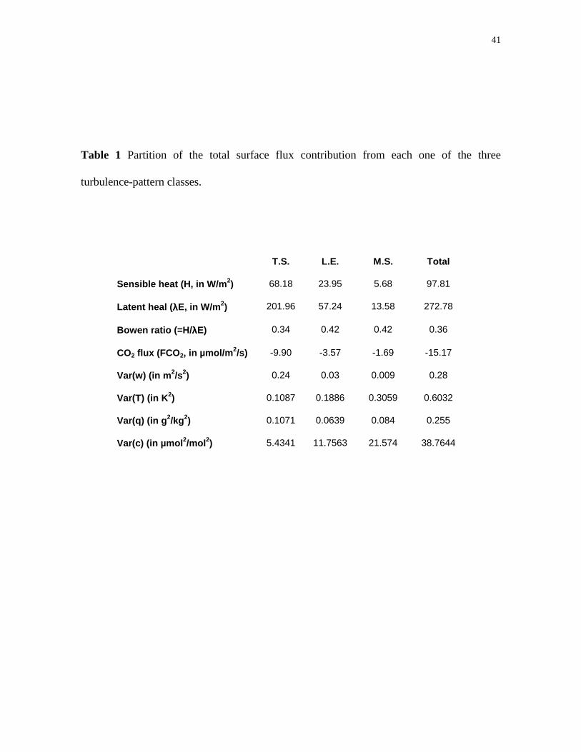
Table 1 Partition of the total surface flux contribution from each one of the three
turbulence-pattern classes.
T.S. L.E. M.S. Total
Sensible heat (H, in W/m2) 68.18 23.95 5.68 97.81
Latent heal (λλλλE, in W/m2) 201.96 57.24 13.58 272.78
Bowen ratio (=H/λλλλE) 0.34 0.42 0.42 0.36
CO2 flux (FCO2, in µmol/m2/s) -9.90 -3.57 -1.69 -15.17
Var(w) (in m2/s2) 0.24 0.03 0.009 0.28
Var(T) (in K2) 0.1087 0.1886 0.3059 0.6032
Var(q) (in g2/kg2) 0.1071 0.0639 0.084 0.255
Var(c) (in µmol2/mol2) 5.4341 11.7563 21.574 38.7644
42
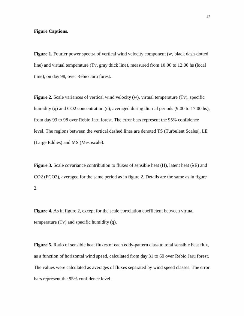
Figure Captions.
Figure 1. Fourier power spectra of vertical wind velocity component (w, black dash-dotted
line) and virtual temperature (Tv, gray thick line), measured from 10:00 to 12:00 hs (local
time), on day 98, over Rebio Jaru forest.
Figure 2. Scale variances of vertical wind velocity (w), virtual temperature (Tv), specific
humidity (q) and CO2 concentration (c), averaged during diurnal periods (9:00 to 17:00 hs),
from day 93 to 98 over Rebio Jaru forest. The error bars represent the 95% confidence
level. The regions between the vertical dashed lines are denoted TS (Turbulent Scales), LE
(Large Eddies) and MS (Mesoscale).
Figure 3. Scale covariance contribution to fluxes of sensible heat (H), latent heat (λE) and
CO2 (FCO2), averaged for the same period as in figure 2. Details are the same as in figure
2.
Figure 4. As in figure 2, except for the scale correlation coefficient between virtual
temperature (Tv) and specific humidity (q).
Figure 5. Ratio of sensible heat fluxes of each eddy-pattern class to total sensible heat flux,
as a function of horizontal wind speed, calculated from day 31 to 60 over Rebio Jaru forest.
The values were calculated as averages of fluxes separated by wind speed classes. The error
bars represent the 95% confidence level.
43
log(f) in Hz0.001 0.01 0.1 1 10
f S2 αα
(f)
0.001
0.01
0.1
1
vertical velocity (w)virtual temperature (t)
Figure 1. Fourier power spectra of vertical wind velocity component (w, black dash-dotted
line) and virtual temperature (Tv, gray thick line), measured from 10:00 to 12:00 hs (local
time), on day 98, over Rebio Jaru forest.
44
Rebio Jaru - Days 93 to 98
Spatial scale (m)
0.1 1 10 100 1000 10000
varia
nce
of v
ertic
al w
ind
vel.
(m2 /s
2 )
0.00
0.01
0.02
0.03
0.04
0.05
varia
nce
of a
ir te
mp.
(K2 )
0.00
0.05
0.10
0.15
0.20
0.25va
rianc
e of
spe
cific
hum
idity
(g2 /k
g2 )
0.00
0.02
0.04
0.06
0.08
0.10
0.12
varia
nce
of C
O2 c
onc.
(µm
ol2 /m
ol2 )
0
2
4
6
8
10
12
14
16
var (w)var (t)var (q)var (c)
T.S. L.E. M.S.
Figure 2. Scale variances of vertical wind velocity (w), virtual temperature (Tv), specific
humidity (q) and CO2 concentration (c), averaged during diurnal periods (9:00 to 17:00 hs),
from day 93 to 98 over Rebio Jaru forest. The error bars represent the 95% confidence
level. The regions between the vertical dashed lines are denoted TS (Turbulent Scales), LE
(Large Eddies) and MS (Mesoscale).
45
Rebio Jaru - Days 93 to 98
Spatial scale (m)0.1 1 10 100 1000 10000
Sens
ible
and
late
nt h
eat f
luxe
s (W
/m2 )
-10
0
10
20
30
40
50
60
70
CO
2 Flu
x (µ
mol
/m2 s)
-4
-3
-2
-1
0
1
2
HλEFCO2
L.E. M.S.
Figure 3. Scale covariance contribution to fluxes of sensible heat (H), latent heat (λE) and
CO2 (FCO2), averaged for the same period as in figure 2. Details are the same as in figure
2.
46
Rebio Jaru - Days 93-98
Spatial scale (m)
0.1 1 10 100 1000 10000
T-q
corre
latio
n co
effic
ient
-0.4
-0.2
0.0
0.2
0.4
0.6
0.8T.S. L.E. M.S.
Figure 4. As in figure 2, except for the scale correlation coefficient between virtual
temperature (Tv) and specific humidity (q).
47
Horizontal wind speed (m/s)
1 2 3 4
Rat
io to
tota
l sen
sibl
e he
at fl
uxes
-0.25
0.00
0.25
0.50
0.75
1.00
1.25
TurbulentLarge eddiesMesoscale
Figure 5. Ratio of sensible heat fluxes of each eddy-pattern class to total sensible heat flux,
as a function of horizontal wind speed, calculated from day 31 to 60 over Rebio Jaru forest.
The values were calculated as averages of fluxes separated by wind speed classes. The error
bars represent the 95% confidence level.
Top Related
Copyright © 2022 FDOKUMEN

