


Bahasa
Halaman
Hukum


This page intentionally left blank

Resource-Constrained Project Scheduling

This page intentionally left blank

Resource-ConstrainedProject Scheduling Models, Algorithms, Extensions and
Applications
Edited by Christian Artigues Sophie Demassey Emmanuel Néron
Series Editor Francis Sourd

First published in Great Britain and the United States in 2008 by ISTE Ltd and John Wiley & Sons, Inc.
Apart from any fair dealing for the purposes of research or private study, or criticism or review, as permitted under the Copyright, Designs and Patents Act 1988, this publication may only be reproduced, stored or transmitted, in any form or by any means, with the prior permission in writing of the publishers, or in the case of reprographic reproduction in accordance with the terms and licenses issued by the CLA. Enquiries concerning reproduction outside these terms should be sent to the publishers at the undermentioned address:
ISTE Ltd John Wiley & Sons, Inc. 6 Fitzroy Square 111 River Street London W1T 5DX Hoboken, NJ 07030 UK USA
www.iste.co.uk www.wiley.com
© ISTE Ltd, 2008
The rights of Christian Artigues, Sophie Demassey and Emmanuel Néron to be identified as the authors of this work have been asserted by them in accordance with the Copyright, Designs and Patents Act 1988.
Library of Congress Cataloging-in-Publication Data
Artigues, Christian. Resource-constrained project scheduling : models, algorithms, extensions and applications / edited by Christian Artigues, Sophie Demassey, Emmanuel Néron. p. cm. Includes bibliographical references and index. ISBN 978-1-84821-034-9 1. Production scheduling. I. Demassey, Sophie. II. Néron, Emmanuel. III. Title. TS157.5.A77 2008 658.5'3--dc22
2007043947
British Library Cataloguing-in-Publication Data A CIP record for this book is available from the British Library ISBN: 978-1-84821-034-9
Printed and bound in Great Britain by Antony Rowe Ltd, Chippenham, Wiltshire.
Table of Contents
Preface . . . . . . . . . . . . . . . . . . . . . . . . . . . . . . . . . . . . . . . . . 13Christian ARTIGUES, Sophie DEMASSEY and Emmanuel NÉRON
Part 1. Models and Algorithms for the Standard Resource-ConstrainedProject Scheduling Problem . . . . . . . . . . . . . . . . . . . . . . . . . . . . 19
Chapter 1. The Resource-Constrained Project Scheduling Problem . . . . 21Christian ARTIGUES
1.1. A combinatorial optimization problem . . . . . . . . . . . . . . . . . . . 211.2. A simple resource-constrained project example . . . . . . . . . . . . . . 231.3. Computational complexity . . . . . . . . . . . . . . . . . . . . . . . . . . 231.4. Dominant and non-dominant schedule subsets . . . . . . . . . . . . . . 261.5. Order-based representation of schedules and related dominant schedule
sets . . . . . . . . . . . . . . . . . . . . . . . . . . . . . . . . . . . . . . . 281.6. Forbidden sets and resource flow network formulations of the RCPSP . 311.7. A simple method for enumerating a dominant set of quasi-active sched-
ules . . . . . . . . . . . . . . . . . . . . . . . . . . . . . . . . . . . . . . . 34
Chapter 2. Resource and Precedence Constraint Relaxation . . . . . . . . . 37Emmanuel NÉRON
2.1. Relaxing resource constraints . . . . . . . . . . . . . . . . . . . . . . . . 382.2. Calculating the disjunctive subproblem . . . . . . . . . . . . . . . . . . 382.3. Deducing identical parallel machine problems . . . . . . . . . . . . . . 412.4. Single cumulative resource problem . . . . . . . . . . . . . . . . . . . . 452.5. Conclusion and perspectives . . . . . . . . . . . . . . . . . . . . . . . . . 47
Chapter 3. Mathematical Programming Formulations and Lower Bounds 49Sophie DEMASSEY
3.1. Sequence-based models . . . . . . . . . . . . . . . . . . . . . . . . . . . 50
5
6 Resource-Constrained Project Scheduling
3.1.1. Minimal forbidden sets . . . . . . . . . . . . . . . . . . . . . . . . 513.1.2. Resource flow . . . . . . . . . . . . . . . . . . . . . . . . . . . . . . 52
3.2. Time-indexed formulations . . . . . . . . . . . . . . . . . . . . . . . . . 533.2.1. Resource conflicts as linear constraints . . . . . . . . . . . . . . . 543.2.2. Feasible configurations . . . . . . . . . . . . . . . . . . . . . . . . 56
3.2.2.1. Combinatorial relaxations . . . . . . . . . . . . . . . . . . . . 583.2.2.2. Column generation and further improvements . . . . . . . . 593.2.2.3. Cutting planes for the preemptive relaxation . . . . . . . . . 60
3.3. Linear lower bounds and redundant resources . . . . . . . . . . . . . . . 61
Chapter 4. Constraint Programming Formulations and PropagationAlgorithms . . . . . . . . . . . . . . . . . . . . . . . . . . . . . . . . . . . . . . 63Philippe LABORIE and Wim NUIJTEN
4.1. Constraint formulations . . . . . . . . . . . . . . . . . . . . . . . . . . . 634.1.1. Constraint programming . . . . . . . . . . . . . . . . . . . . . . . . 634.1.2. Constraint-based scheduling . . . . . . . . . . . . . . . . . . . . . 64
4.2. Constraint propagation algorithms . . . . . . . . . . . . . . . . . . . . . 654.2.1. Temporal constraints . . . . . . . . . . . . . . . . . . . . . . . . . . 654.2.2. Timetabling . . . . . . . . . . . . . . . . . . . . . . . . . . . . . . . 664.2.3. Disjunctive reasoning . . . . . . . . . . . . . . . . . . . . . . . . . 674.2.4. Edge-finding . . . . . . . . . . . . . . . . . . . . . . . . . . . . . . 674.2.5. Energy reasoning . . . . . . . . . . . . . . . . . . . . . . . . . . . . 684.2.6. Precedence graph . . . . . . . . . . . . . . . . . . . . . . . . . . . . 704.2.7. Energy precedence . . . . . . . . . . . . . . . . . . . . . . . . . . . 704.2.8. Balance constraint . . . . . . . . . . . . . . . . . . . . . . . . . . . 71
4.3. Conclusion . . . . . . . . . . . . . . . . . . . . . . . . . . . . . . . . . . 72
Chapter 5. Branching Schemes for Branch-and-Bound . . . . . . . . . . . . 73Emmanuel NÉRON
5.1. Chronological branching scheme . . . . . . . . . . . . . . . . . . . . . . 755.1.1. Adding one activity to a partial solution . . . . . . . . . . . . . . . 75
5.1.1.1. Considering all relevant activities . . . . . . . . . . . . . . . 755.1.1.2. Delaying one activity . . . . . . . . . . . . . . . . . . . . . . 77
5.1.2. Dominance rule: left shift and global left shift . . . . . . . . . . . 785.1.3. Adding a subset of activities to a partial solution . . . . . . . . . . 79
5.1.3.1. Delaying alternatives . . . . . . . . . . . . . . . . . . . . . . 795.1.3.2. Building a solution using blocks . . . . . . . . . . . . . . . . 80
5.1.4. Dominance rule: cut-set . . . . . . . . . . . . . . . . . . . . . . . . 815.2. Specific branching schemes . . . . . . . . . . . . . . . . . . . . . . . . . 82
5.2.1. Fixing disjunction and parallel relationship . . . . . . . . . . . . . 825.2.2. Reducing time-windows of activities . . . . . . . . . . . . . . . . . 835.2.3. Resolving forbidden sets . . . . . . . . . . . . . . . . . . . . . . . 84
5.3. Conclusion and perspectives . . . . . . . . . . . . . . . . . . . . . . . . . 85
Table of Contents 7
Chapter 6. Heuristics . . . . . . . . . . . . . . . . . . . . . . . . . . . . . . . . 87Christian ARTIGUES and David RIVREAU
6.1. Schedule representation schemes . . . . . . . . . . . . . . . . . . . . . . 876.1.1. Natural date variables . . . . . . . . . . . . . . . . . . . . . . . . . 876.1.2. List schedule generation scheme representations . . . . . . . . . . 886.1.3. Set-based representations . . . . . . . . . . . . . . . . . . . . . . . 886.1.4. Resource flow network representation . . . . . . . . . . . . . . . . 89
6.2. Constructive heuristics . . . . . . . . . . . . . . . . . . . . . . . . . . . . 896.2.1. Standard list schedule generation scheme heuristics . . . . . . . . 896.2.2. A generic insertion-based list schedule generation scheme . . . . 916.2.3. Set schedule generation scheme heuristics . . . . . . . . . . . . . . 936.2.4. (Double-)justification-based methods . . . . . . . . . . . . . . . . 94
6.3. Local search neighborhoods . . . . . . . . . . . . . . . . . . . . . . . . . 946.3.1. List-based neighborhoods . . . . . . . . . . . . . . . . . . . . . . . 956.3.2. Set-based neighborhoods . . . . . . . . . . . . . . . . . . . . . . . 956.3.3. Resource flow-based neighborhoods . . . . . . . . . . . . . . . . . 966.3.4. Extended neighborhood for natural date variables . . . . . . . . . 96
6.4. Metaheuristics . . . . . . . . . . . . . . . . . . . . . . . . . . . . . . . . 976.4.1. Simulated annealing . . . . . . . . . . . . . . . . . . . . . . . . . . 976.4.2. Tabu search . . . . . . . . . . . . . . . . . . . . . . . . . . . . . . . 976.4.3. Population-based metaheuristics . . . . . . . . . . . . . . . . . . . 986.4.4. Additional methods . . . . . . . . . . . . . . . . . . . . . . . . . . 99
6.5. Conclusion . . . . . . . . . . . . . . . . . . . . . . . . . . . . . . . . . . 1006.6. Appendix . . . . . . . . . . . . . . . . . . . . . . . . . . . . . . . . . . . 101
6.6.1. Serial list schedule generation revisited . . . . . . . . . . . . . . . 1016.6.2. Parallel list schedule generation revisited . . . . . . . . . . . . . . 104
Chapter 7. Benchmark Instance Indicators and ComputationalComparison of Methods . . . . . . . . . . . . . . . . . . . . . . . . . . . . . . 107Christian ARTIGUES, Oumar KONÉ, Pierre LOPEZ, Marcel MONGEAU,Emmanuel NÉRON and David RIVREAU
7.1. Introduction . . . . . . . . . . . . . . . . . . . . . . . . . . . . . . . . . . 1077.2. Standard instance indicators . . . . . . . . . . . . . . . . . . . . . . . . . 1087.3. New instance indicators . . . . . . . . . . . . . . . . . . . . . . . . . . . 1127.4. State-of-the-art benchmark instances . . . . . . . . . . . . . . . . . . . . 1147.5. A critical analysis of the instance indicators . . . . . . . . . . . . . . . . 118
7.5.1. Indicator comparison between trivial and non-trivial instances . . 1187.5.2. Indicator stability and correlation . . . . . . . . . . . . . . . . . . . 120
7.6. Comparison of solution methods . . . . . . . . . . . . . . . . . . . . . . 1247.6.1. Selected methods and experimental framework . . . . . . . . . . . 1247.6.2. Results on the KSD30 instances . . . . . . . . . . . . . . . . . . . 1297.6.3. Results on the BL instances . . . . . . . . . . . . . . . . . . . . . . 131
8 Resource-Constrained Project Scheduling
7.6.4. Results on the KSD60 instances . . . . . . . . . . . . . . . . . . . 1327.6.5. Results on the Pack instances . . . . . . . . . . . . . . . . . . . . . 134
7.7. Conclusion . . . . . . . . . . . . . . . . . . . . . . . . . . . . . . . . . . 135
Part 2. Variants and Extensions . . . . . . . . . . . . . . . . . . . . . . . . . . 137
Chapter 8. Preemptive Activities . . . . . . . . . . . . . . . . . . . . . . . . . 139Jean DAMAY
8.1. Preemption in scheduling . . . . . . . . . . . . . . . . . . . . . . . . . . 1398.2. State of the art . . . . . . . . . . . . . . . . . . . . . . . . . . . . . . . . 140
8.2.1. Integral preemption for the RCPSP . . . . . . . . . . . . . . . . . . 1408.2.2. Rational preemption for parallel machine scheduling problems . . 141
8.3. Recent LP-based methods . . . . . . . . . . . . . . . . . . . . . . . . . . 1428.3.1. Reformulation . . . . . . . . . . . . . . . . . . . . . . . . . . . . . 1428.3.2. A specific neighborhood search algorithm . . . . . . . . . . . . . . 144
8.3.2.1. Descent approach . . . . . . . . . . . . . . . . . . . . . . . . 1448.3.2.2. Diversification techniques . . . . . . . . . . . . . . . . . . . . 1458.3.2.3. Experimental results . . . . . . . . . . . . . . . . . . . . . . . 145
8.3.3. Exact methods . . . . . . . . . . . . . . . . . . . . . . . . . . . . . 1468.3.3.1. Branch-and-bound . . . . . . . . . . . . . . . . . . . . . . . . 1468.3.3.2. Branch and cut and price . . . . . . . . . . . . . . . . . . . . 147
8.4. Conclusion . . . . . . . . . . . . . . . . . . . . . . . . . . . . . . . . . . 147
Chapter 9. Multi-Mode and Multi-Skill Project Scheduling Problem . . . 149Odile BELLENGUEZ-MORINEAU and Emmanuel NÉRON
9.1. Introduction . . . . . . . . . . . . . . . . . . . . . . . . . . . . . . . . . . 1499.2. Multi-Mode RCPSP . . . . . . . . . . . . . . . . . . . . . . . . . . . . . 150
9.2.1. Problem presentation . . . . . . . . . . . . . . . . . . . . . . . . . . 1509.2.2. Branching schemes for solving multi-mode RCPSP . . . . . . . . 1529.2.3. Dominance rules . . . . . . . . . . . . . . . . . . . . . . . . . . . . 153
9.3. Multi-Skill Project Scheduling Problem . . . . . . . . . . . . . . . . . . 1549.3.1. Problem presentation . . . . . . . . . . . . . . . . . . . . . . . . . . 1549.3.2. Branching scheme based on time-windows reduction . . . . . . . 1579.3.3. Lower bounds and time-bound adjustments . . . . . . . . . . . . . 1589.3.4. Dominance rule . . . . . . . . . . . . . . . . . . . . . . . . . . . . . 159
9.4. Conclusion and research directions . . . . . . . . . . . . . . . . . . . . . 160
Chapter 10. Project Scheduling with Production and Consumptionof Resources: How to Build Schedules . . . . . . . . . . . . . . . . . . . . . . 161Jacques CARLIER, Aziz MOUKRIM and Huang XU
10.1. Introduction . . . . . . . . . . . . . . . . . . . . . . . . . . . . . . . . . 16110.2. The precedence-constrained project scheduling problem . . . . . . . . 162
Table of Contents 9
10.2.1. Traditional precedence constraints . . . . . . . . . . . . . . . . . 16210.2.2. AND/OR precedence constraints . . . . . . . . . . . . . . . . . . 163
10.3. The resource-constrained project scheduling problem . . . . . . . . . 16410.3.1. Graph representation . . . . . . . . . . . . . . . . . . . . . . . . . 16410.3.2. The strict order algorithm . . . . . . . . . . . . . . . . . . . . . . 164
10.4. Scheduling problems with production and consumption ofa non-renewable resource . . . . . . . . . . . . . . . . . . . . . . . . . . 166
10.5. Discussion . . . . . . . . . . . . . . . . . . . . . . . . . . . . . . . . . . 170
Chapter 11. Activity Insertion Problem in a RCPSP with Minimumand Maximum Time Lags . . . . . . . . . . . . . . . . . . . . . . . . . . . . . 171Christian ARTIGUES and Cyril BRIAND
11.1. Introduction . . . . . . . . . . . . . . . . . . . . . . . . . . . . . . . . . 17111.2. Problem statement . . . . . . . . . . . . . . . . . . . . . . . . . . . . . 17211.3. Insertion positions . . . . . . . . . . . . . . . . . . . . . . . . . . . . . . 17611.4. Feasibility conditions under a makespan upper bound . . . . . . . . . 17611.5. Computational complexity of the insertion problem with minimum
and maximum time lags . . . . . . . . . . . . . . . . . . . . . . . . . . . 17811.6. A polynomial algorithm for the insertion problem with minimum time
lags only . . . . . . . . . . . . . . . . . . . . . . . . . . . . . . . . . . . . 18111.7. Conclusion . . . . . . . . . . . . . . . . . . . . . . . . . . . . . . . . . . 190
Chapter 12. Reactive Approaches . . . . . . . . . . . . . . . . . . . . . . . . . 191Christelle GUÉRET and Narendra JUSSIEN
12.1. Dynamic project scheduling . . . . . . . . . . . . . . . . . . . . . . . . 19112.2. Explanations and constraint programming for solving dynamic problems 192
12.2.1. Dynamic problems and constraint programming . . . . . . . . . 19212.2.2. Explanation-based constraint programming . . . . . . . . . . . . 193
12.3. An explanation-based approach for solving dynamic project scheduling 19412.3.1. The tree search to solve static instances . . . . . . . . . . . . . . 19512.3.2. Incrementally handling unexpected events . . . . . . . . . . . . . 196
12.4. Experimental results . . . . . . . . . . . . . . . . . . . . . . . . . . . . 19712.4.1. Stability measures . . . . . . . . . . . . . . . . . . . . . . . . . . 19712.4.2. Test set . . . . . . . . . . . . . . . . . . . . . . . . . . . . . . . . . 19712.4.3. Computational results . . . . . . . . . . . . . . . . . . . . . . . . 198
12.4.3.1. Analysis of the results in terms of cpu time . . . . . . . . . 19912.4.3.2. Analysis of the stability . . . . . . . . . . . . . . . . . . . . 200
12.5. Conclusion . . . . . . . . . . . . . . . . . . . . . . . . . . . . . . . . . . 201
Chapter 13. Proactive-reactive Project Scheduling . . . . . . . . . . . . . . 203Erik DEMEULEMEESTER, Willy HERROELEN and Roel LEUS
13.1. Introduction . . . . . . . . . . . . . . . . . . . . . . . . . . . . . . . . . 203
10 Resource-Constrained Project Scheduling
13.2. Solution robust scheduling under activity duration uncertainty . . . . . 20413.2.1. The proactive/reactive scheduling problem . . . . . . . . . . . . . 20413.2.2. Proactive scheduling . . . . . . . . . . . . . . . . . . . . . . . . . 205
13.2.2.1. Robust resource allocation . . . . . . . . . . . . . . . . . . . 20513.2.2.2. Buffer insertion . . . . . . . . . . . . . . . . . . . . . . . . . 206
13.2.3. Reactive scheduling . . . . . . . . . . . . . . . . . . . . . . . . . . 20713.3. Solution robust scheduling under resource availability uncertainty . . 209
13.3.1. The problem . . . . . . . . . . . . . . . . . . . . . . . . . . . . . . 20913.3.1.1. Proactive strategy . . . . . . . . . . . . . . . . . . . . . . . . 20913.3.1.2. Reactive strategy . . . . . . . . . . . . . . . . . . . . . . . . 210
13.4. Conclusions and suggestions for further research . . . . . . . . . . . . 21013.5. Acknowledgements . . . . . . . . . . . . . . . . . . . . . . . . . . . . . 211
Chapter 14. RCPSP with Financial Costs . . . . . . . . . . . . . . . . . . . . 213Laure-Emmanuelle DREZET
14.1. Problem presentation and context . . . . . . . . . . . . . . . . . . . . . 21314.2. Definitions and notations . . . . . . . . . . . . . . . . . . . . . . . . . . 214
14.2.1. Definitions . . . . . . . . . . . . . . . . . . . . . . . . . . . . . . . 21414.2.2. Notations . . . . . . . . . . . . . . . . . . . . . . . . . . . . . . . 21514.2.3. Classification . . . . . . . . . . . . . . . . . . . . . . . . . . . . . 216
14.3. NPV maximization . . . . . . . . . . . . . . . . . . . . . . . . . . . . . 21714.3.1. Unconstrained resources: MAXNPV and PSP . . . . . . . . . . . 21714.3.2. Constrained resources: RCPSPDC, CCPSP and PSP . . . . . . . 219
14.4. Resource-related costs . . . . . . . . . . . . . . . . . . . . . . . . . . . 22114.4.1. Resource Leveling Problem . . . . . . . . . . . . . . . . . . . . . 22114.4.2. Resource Investment Problem (RIP) and Resource Renting
Problem (RRP) . . . . . . . . . . . . . . . . . . . . . . . . . . . . . 22314.5. Conclusion . . . . . . . . . . . . . . . . . . . . . . . . . . . . . . . . . . 225
Part 3. Industrial Applications . . . . . . . . . . . . . . . . . . . . . . . . . . 227
Chapter 15. Assembly Shop Scheduling . . . . . . . . . . . . . . . . . . . . . 229Michel GOURGAND, Nathalie GRANGEON and Sylvie NORRE
15.1. The assembly shop scheduling problem . . . . . . . . . . . . . . . . . 22915.1.1. Mono shop problem . . . . . . . . . . . . . . . . . . . . . . . . . 230
15.1.1.1. Physical subsystem . . . . . . . . . . . . . . . . . . . . . . . 23015.1.1.2. Logical subsystem . . . . . . . . . . . . . . . . . . . . . . . 23015.1.1.3. Decisional subsystem . . . . . . . . . . . . . . . . . . . . . 231
15.1.2. Multi shop problem . . . . . . . . . . . . . . . . . . . . . . . . . . 23215.2. Link with the RCPSP . . . . . . . . . . . . . . . . . . . . . . . . . . . . 23315.3. Proposition of extensions . . . . . . . . . . . . . . . . . . . . . . . . . . 234
15.3.1. RCPSP with variable demand profile . . . . . . . . . . . . . . . . 23515.3.2. RCPSP with resource individualization . . . . . . . . . . . . . . . 237
Table of Contents 11
15.4. Proposition of solution methods . . . . . . . . . . . . . . . . . . . . . . 23915.5. Some results . . . . . . . . . . . . . . . . . . . . . . . . . . . . . . . . . 24015.6. Conclusion . . . . . . . . . . . . . . . . . . . . . . . . . . . . . . . . . . 242
Chapter 16. Employee Scheduling in an IT Company . . . . . . . . . . . . . 243Laure-Emmanuelle DREZET and Jean-Charles BILLAUT
16.1. Introduction . . . . . . . . . . . . . . . . . . . . . . . . . . . . . . . . . 24316.2. Problem presentation and context . . . . . . . . . . . . . . . . . . . . . 24416.3. Real life example . . . . . . . . . . . . . . . . . . . . . . . . . . . . . . 24716.4. Predictive phase . . . . . . . . . . . . . . . . . . . . . . . . . . . . . . . 250
16.4.1. Greedy algorithms . . . . . . . . . . . . . . . . . . . . . . . . . . 25016.4.2. Tabu search algorithm . . . . . . . . . . . . . . . . . . . . . . . . 251
16.5. Proactive phase . . . . . . . . . . . . . . . . . . . . . . . . . . . . . . . 25116.6. Reactive phase . . . . . . . . . . . . . . . . . . . . . . . . . . . . . . . 25216.7. Computational experiments . . . . . . . . . . . . . . . . . . . . . . . . 253
16.7.1. Predictive and proactive algorithms . . . . . . . . . . . . . . . . . 25316.7.2. Reactive algorithm . . . . . . . . . . . . . . . . . . . . . . . . . . 254
16.8. Conclusion . . . . . . . . . . . . . . . . . . . . . . . . . . . . . . . . . . 254
Chapter 17. Rolling Ingots Production Scheduling . . . . . . . . . . . . . . 257Christoph SCHWINDT and Norbert TRAUTMANN
17.1. Introduction . . . . . . . . . . . . . . . . . . . . . . . . . . . . . . . . . 25717.2. Project scheduling model . . . . . . . . . . . . . . . . . . . . . . . . . . 259
17.2.1. Activities and temporal constraints . . . . . . . . . . . . . . . . . 25917.2.2. Resource constraints . . . . . . . . . . . . . . . . . . . . . . . . . 26117.2.3. Production scheduling problem . . . . . . . . . . . . . . . . . . . 264
17.3. Solution method . . . . . . . . . . . . . . . . . . . . . . . . . . . . . . . 26417.4. Conclusions . . . . . . . . . . . . . . . . . . . . . . . . . . . . . . . . . 266
Chapter 18. Resource-Constrained Modulo Scheduling . . . . . . . . . . . 267Benoît DUPONT DE DINECHIN, Christian ARTIGUES and Sadia AZEM
18.1. Introduction . . . . . . . . . . . . . . . . . . . . . . . . . . . . . . . . . 26718.2. The resource-constrained modulo scheduling problem . . . . . . . . . 268
18.2.1. The resource-constrained cyclic scheduling problem . . . . . . . 26818.2.2. The resource-constrained modulo scheduling problem . . . . . . 26918.2.3. From modulo scheduling to software pipelining . . . . . . . . . . 270
18.3. Integer linear programming formulations . . . . . . . . . . . . . . . . . 27318.3.1. The RCMSP formulations by Eichenberger et al. . . . . . . . . . 27318.3.2. A new time-indexed RCMSP formulation . . . . . . . . . . . . . 274
18.4. Solving the RCMSP formulations . . . . . . . . . . . . . . . . . . . . . 27518.4.1. Reducing the size of the RCMSP formulations . . . . . . . . . . 27518.4.2. A large neighborhood search for the RCMSP . . . . . . . . . . . 275

12 Resource-Constrained Project Scheduling
18.4.3. Implementation and experiments . . . . . . . . . . . . . . . . . . 27618.5. Summary and conclusions . . . . . . . . . . . . . . . . . . . . . . . . . 277
Bibliography . . . . . . . . . . . . . . . . . . . . . . . . . . . . . . . . . . . . . 279
List of Authors . . . . . . . . . . . . . . . . . . . . . . . . . . . . . . . . . . . . 303
Index . . . . . . . . . . . . . . . . . . . . . . . . . . . . . . . . . . . . . . . . . . 307
Preface
Nowadays, material and human resource management is an increasingly importantissue for organizations. Thus, a careful management of projects is an absolute neces-sity to preserve the competitiveness of companies. Scheduling plays a major part inproject management. Indeed, the scheduling process amounts to deciding when theproject activities will start and how they will use the available resources. Such deci-sions can be expected to have a large impact on the total project duration (makespan),which is the main performance criterion we consider in this book. Note that estab-lishing a good schedule is necessary but not sufficient for actual project makespanminimization. As a comprehensive counter-example, let us consider the project thatconsisted of writing the present book. We expected a one year total duration but wemust admit that the realized makespan exceeded two years. In this case, the makespanincrease was clearly caused by an over-optimistic estimation of activity durations andresource availabilities while the schedule was correct.
Nevertheless, we focus in this book on the deterministic resource-constrainedproject scheduling problem (RCPSP). The standard RCPSP can be defined as acombinatorial optimization problem, i.e. in terms of decision variables, constraintsand objective functions, as follows. A set of activities and a set of resources of knowncharacteristics (activity durations, activity resource demands, resource availabilities,precedence restrictions) are given. The decision variables are the activity start timesdefined on integer time periods. The objective function which has to be minimizedis the makespan, i.e. the largest activity completion time, assuming the project startsat time 0. There are two types of constraints. The precedence constraints preventeach activity from starting before the completion of its predecessors. The resourceconstraints ensure that, at each time period and for each resource, the total activitydemand does not exceed the resource availability. Once started, an activity cannot beinterrupted.
Despite the simplicity of its definition, the RCPSP belongs to the class of NP-hard optimization problems [BLA 83] and is actually one of the most intractable
13
14 Resource-Constrained Project Scheduling
classical problems in practice. In the publicly available PSPLIB library [PSPib],the optimal makespan of randomly generated problems with 60 activities and 4resources is still unknown. For both its industrial relevance and its challenging dif-ficulty, solving the RCPSP has become a flourishing research theme. This becomesclear when observing the significant number of books that were published on thissubject [SLO 89, KOL 95a, JOZ 98, WEG 98, HAR 99, KLE 01, DOR 02, DEM 02c,NEU 03, BRU 06]. One might even legitimately ask why yet another book on theRCPSP is needed.
The aim of this book is to present the latest results in the field, not as a collectionof independent articles, but as a whole, in an integrated manner. Thus, it provides astate-of-the-art of the solution approaches for the standard RCPSP (Part 1) and forseveral of its variants (Part 2) and industrial applications (Part 3). The developmentson each approach type are investigated from the fundamentals to the most recent –even current – studies.
This book contains 18 chapters written by 28 authors who are all active researchersin the area. We describe hereafter the contents of the book, underlining the originalaspects for each chapter.
There are three parts. The first part is devoted to the standard RCPSP as statedabove and the various methods that have been proposed to solve it. More precisely,each chapter of this part focuses on a particular aspect of the solution process. Chap-ter 1, written by Christian Artigues, focuses on the models and describes the RCPSP asa combinatorial optimization problem. Different combinatorial models of the resourceconstraints and characterizations of dominant schedule sets are given. In particular,the properties of the order-based representation are studied. Chapter 2, written byEmmanuel Néron, considers the scheduling standard subproblems obtained by variousrelaxations. Solving these subproblems using specific scheduling methods generallyyields quickly computable lower bounds. However, extraction of a relevant subprob-lem may be a complex task. The chapter describes innovative concepts of redundantresources and redundant functions, designed with this aim in mind. Chapter 3, writ-ten by Sophie Demassey, is devoted to mathematical programming formulations ofthe RCPSP and to lower bounds resulting from their relaxations. Besides recalling themain sequence-based and time-indexed integer linear programming formulations, itdescribes the recent cutting-plane and column generation techniques making it possi-ble to obtain tight lower bounds when used in conjunction with constraint program-ming. A promising formulation based on the redundant resource concept and linearlower bounds is also introduced. Chapter 4, written by Philippe Laborie and Wim Nui-jten, is devoted to constraint programming approaches for scheduling and describesthe existing propagation algorithms relevant for the RCPSP. The by-now standard dis-junctive, edge-finding and energy reasoning rules are recalled. The original balanceand energy-precedence propagation algorithms are presented. Chapter 5, written by
Preface 15
Emmanuel Néron, presents the main branching schemes and associated dominancerules used to solve the RCPSP via exact methods. Indeed, a multitude of branch-and-bound methods can be derived by combining the presented branching schemeswith the lower bounds and constraint propagation algorithms presented in Chapters2, 3 and 4. Chapter 6, written by Christian Artigues and David Rivreau, describesthe main heuristics and metaheuristics that were proposed to approximate the RCPSP.The chapter reviews the literature and proposes a unifying framework based on theconcepts of events and resource flows for the two main constructive algorithms: theparallel and the serial scheduling schemes. Chapter 7, written by Christian Artigues,Oumar Koné, Pierre Lopez, Marcel Mongeau, Emmanuel Néron and David Rivreau,is devoted to extensive computational experiments. Its objective is twofold. First, aselection of representative exact and heuristic methods among those presented in theprevious chapters are tested and compared under a common experimental frameworkon four different instance sets. Second, classical and new instance difficulty indicatorsare evaluated through experiments and their discriminating power is discussed.
Part 2 of the book presents variants and extensions of the RCPSP. Clearly, thestandard model does not allow for modeling all the practical situations accurately.Each chapter of this part focuses on a particular variant or extension and presents thelatest advances made to tackle it. Most chapters present new and original methods.Chapter 8, written by Jean Damay, presents LP-based neighborhood search and exactmethods for the rational preemptive variant of the RCPSP. This variant has never beenconsidered before despite its practical interest. It considers the case where activitiescan be interrupted at any, not necessarily integer, time. Chapter 9, written by OdileBellenguez-Morineau and Emmanuel Néron, is devoted to the multi-mode RCPSPand the multi-skill RCPSP. The chapter reviews branching schemes and dominancerules for the multi-mode RCPSP. This extension introduces alternative activity execu-tion modes, differing by the resource requirements and the durations. The multi-skillRCPSP is a variant for which the modes are implicitly defined using the intermediateconcept of required and available skills. This model makes it possible to efficientlyrepresent the practical case of human resources while there would be an explosionof the number of modes in the multi-mode model. An exact method is proposed tosolve the problem. Chapter 10, written by Jacques Carlier, Aziz Moukrim and HuangXu, considers a RCPSP with renewable (as in the standard case) and non-renewableresources. Some activities consume a non-renewable resources while others produceit. They propose an enumeration method based on the concept of arbitrage and on thestrict order algorithm. They also show how AND/OR precedence constraints can beused to compute solutions. Chapter 11, written by Christian Artigues and Cyril Briand,considers the RCPSP with minimum and maximum time lags. They focus on the prob-lem of activity insertion in a schedule represented by a resource flow, which can occurin reactive scheduling (next chapter) or as a component of a local search method. Theyshow the problem is NP-hard and propose a polynomial algorithm when only mini-mum time lags are considered. Chapter 12, written by Christelle Guéret and Narendra
16 Resource-Constrained Project Scheduling
Jussien, proposes a reactive approach to solve a dynamic project scheduling problem,i.e. one that may change over time through unexpected events. Their method cantackle various events including the insertion of a new activity as in the previous chap-ter. They make use of explanation-based constraint programming, where explanationsallow for schedule repairing through the tree-search after each disruption. Chapter 13,written by Erik Demeulemeester, Willy Herroelen and Roel Leus, makes a step fur-ther in tackling project scheduling under uncertainty using proactive/reactive proce-dures. Uncertainty may affect activity durations and resource availabilities. Proactivescheduling methods aiming at anticipating disruptions through robust resource allo-cation and buffer insertion in a precomputed schedule are presented. Reactive strate-gies are carried out when the proactive schedule cannot absorb the disruptions. Theobjective is to minimize an instability function measuring the distance between theprecomputed schedule and the realized schedule. While the previous chapters mainlyconsider makespan minimization, Chapter 14, written by Laure-Emmanuelle Drezet,introduces several other objective functions dealing with financial aspects. The chapterreviews and classifies the existing work carried out on net present value maximizationand resource-related costs such as resource leveling and resource investment.
Part 3 of the book is devoted to industrial applications involving the RCPSP orits variants and extensions. Thereby, the reader may verify how the different modelsand methods presented in this book are actually applied in various and perhaps sur-prising situations. Chapter 15, written by Michel Gourgand, Nathalie Grangeon andSylvie Norre, considers an assembly shop problem in an automotive company. Spe-cial attention is paid to the modeling process which exhibits a RCPSP with variableresource profile and resource individualization, linked with the multimode aspectsdescribed in Chapter 9. The problem is solved by neighborhood search heuristics.Chapter 16, written by Laure-Emmanuelle Drezet and Jean-Charles Billaut, describesan employee scheduling problem in a IT company. The problem is modeled as a mixedproject scheduling and workforce assignment problem. It follows that work regulationconstraints are added to the standard RCPSP model. Since the considered projects(software developments) are highly likely to be disrupted, a proactive/reactive method(see Chapter 13) is proposed. Chapter 17, written by Christoph Schwindt and Nor-bert Trautmann, considers a rolling ingots production scheduling problem in the alu-minium industry. This industrial context gives rise to a complex multi-mode RCPSPwith minimum and maximum time lags, batching machines and sequence-dependentchangeover times. A filtered beam search version of a branch-and-bound method isproposed to solve the problem. Chapter 18, written by Benoit Dupont de Dinechin,Christian Artigues and Sadia Azem, presents an unusual application of the RCPSP,namely an instruction scheduling problem for very long instruction word processors.The specific characteristics of these processors and the cyclic nature of the problemyields a modulo RCPSP with minimum and maximum time lags. New integer linearprogramming formulations are proposed and an efficient large neighborhood searchtechnique is used to solve near-optimally large industrial problems in a few minutes.

Preface 17
We wish to warmly thank all the colleagues who kindly accepted to review one orseveral chapters of the book: Philippe Baptiste, Rainer Kolisch, Philippe Lacomme,Francis Sourd and Mario Vanhoucke.
Christian ARTIGUES, SOPHIE DEMASSEY and Emmanuel NÉRON

18
This page intentionally left blank

Part 1
Models and Algorithms for the StandardResource-Constrained Project
Scheduling Problem
19

20
This page intentionally left blank
Chapter 1
The Resource-Constrained ProjectScheduling Problem
1.1. A combinatorial optimization problem
Informally, a resource-constrained project scheduling problem (RCPSP) consid-ers resources of limited availability and activities of known durations and resourcerequests, linked by precedence relations. The problem consists of finding a scheduleof minimal duration by assigning a start time to each activity such that the precedencerelations and the resource availabilities are respected.
More formally, the RCPSP can be defined as a combinatorial optimization prob-lem. A combinatorial optimization problem is defined by a solution space X , which isdiscrete or which can be reduced to a discrete set, and by a subset of feasible solutionsY ⊆ X associated with an objective function f : Y → R. A combinatorial optimiza-tion problem aims at finding a feasible solution y ∈ Y such that f(y) is minimizedor maximized. A resource-constrained project scheduling problem is a combinatorialoptimization problem defined by a tuple (V, p,E,R, B, b).
Activities constituting the project are identified by a set V = {A0, . . . , An+1}.Activity A0 represents by convention the start of the schedule and activity An+1 sym-metrically represents the end of the schedule. The set of non-dummy activities is iden-tified by A = {A1, . . . , An}.
Durations are represented by a vector p in Nn+2 where pi is the duration of activity
Ai, with special values p0 = pn+1 = 0.
Chapter written by Christian ARTIGUES.
21
22 Resource-Constrained Project Scheduling
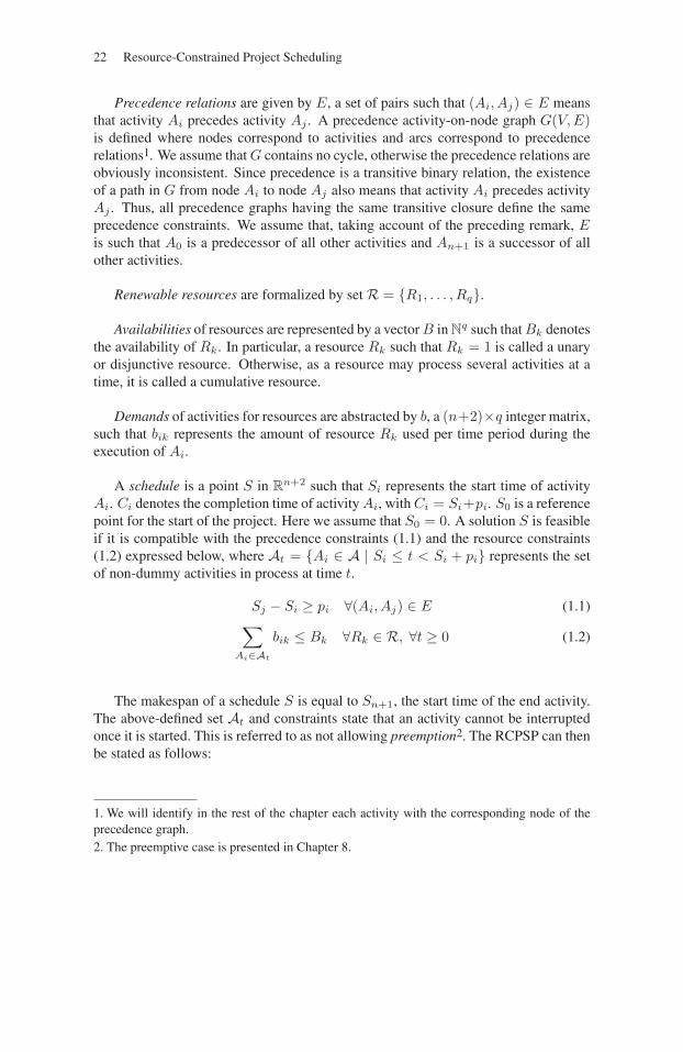
Precedence relations are given by E, a set of pairs such that (Ai, Aj) ∈ E meansthat activity Ai precedes activity Aj . A precedence activity-on-node graph G(V,E)is defined where nodes correspond to activities and arcs correspond to precedencerelations1. We assume that G contains no cycle, otherwise the precedence relations areobviously inconsistent. Since precedence is a transitive binary relation, the existenceof a path in G from node Ai to node Aj also means that activity Ai precedes activityAj . Thus, all precedence graphs having the same transitive closure define the sameprecedence constraints. We assume that, taking account of the preceding remark, Eis such that A0 is a predecessor of all other activities and An+1 is a successor of allother activities.
Renewable resources are formalized by setR = {R1, . . . , Rq}.
Availabilities of resources are represented by a vector B in Nq such that Bk denotes
the availability of Rk. In particular, a resource Rk such that Rk = 1 is called a unaryor disjunctive resource. Otherwise, as a resource may process several activities at atime, it is called a cumulative resource.
Demands of activities for resources are abstracted by b, a (n+2)×q integer matrix,such that bik represents the amount of resource Rk used per time period during theexecution of Ai.
A schedule is a point S in Rn+2 such that Si represents the start time of activity
Ai. Ci denotes the completion time of activity Ai, with Ci = Si+pi. S0 is a referencepoint for the start of the project. Here we assume that S0 = 0. A solution S is feasibleif it is compatible with the precedence constraints (1.1) and the resource constraints(1.2) expressed below, where At = {Ai ∈ A | Si ≤ t < Si + pi} represents the setof non-dummy activities in process at time t.
Sj − Si ≥ pi ∀(Ai, Aj) ∈ E (1.1)∑Ai∈At
bik ≤ Bk ∀Rk ∈ R, ∀t ≥ 0 (1.2)
The makespan of a schedule S is equal to Sn+1, the start time of the end activity.The above-defined set At and constraints state that an activity cannot be interruptedonce it is started. This is referred to as not allowing preemption2. The RCPSP can thenbe stated as follows:
1. We will identify in the rest of the chapter each activity with the corresponding node of theprecedence graph.2. The preemptive case is presented in Chapter 8.
The Resource-Constrained Project Scheduling Problem 23
DEFINITION 1.1.– The RCPSP is the problem of finding a non-preemptive scheduleS of minimal makespan Sn+1 subject to precedence constraints (1.1) and resourceconstraints (1.2).
An important preliminary remark is that, since durations are integers, we canrestrict ourselves to integer schedules without missing the optimal solution. A non-integer feasible schedule can be transformed into an integer feasible schedule withoutincreasing the makespan by recursively applying the following principle. Consider anon-integer schedule S and let Ai denote the first activity in the increasing start timeorder such that Si �∈ N. Then setting Si to its nearest lower integer Si does not vio-late any precedence constraints, since the completion time of the predecessors of Ai
are integers strictly lower than Si. Left shifting an activity can violate a resource con-straint only if it enters new sets At for Si ≤ t < Si. Since we have At ⊆ ASi
\ {i}for Si ≤ t < Si, no resource-constraint violation can appear by setting Si to Si.The set of integer schedules, containing at least one optimal solution, is said to bedominant.
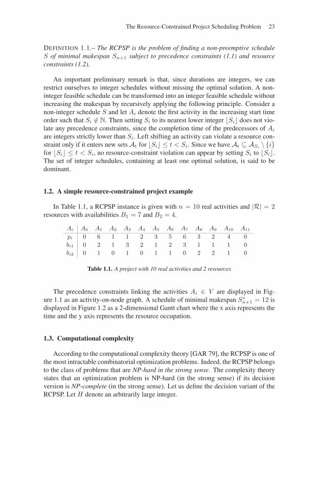
1.2. A simple resource-constrained project example
In Table 1.1, a RCPSP instance is given with n = 10 real activities and |R| = 2resources with availabilities B1 = 7 and B2 = 4.
Ai A0 A1 A2 A3 A4 A5 A6 A7 A8 A9 A10 A11
pi 0 6 1 1 2 3 5 6 3 2 4 0
bi1 0 2 1 3 2 1 2 3 1 1 1 0
bi2 0 1 0 1 0 1 1 0 2 2 1 0
Table 1.1. A project with 10 real activities and 2 resources
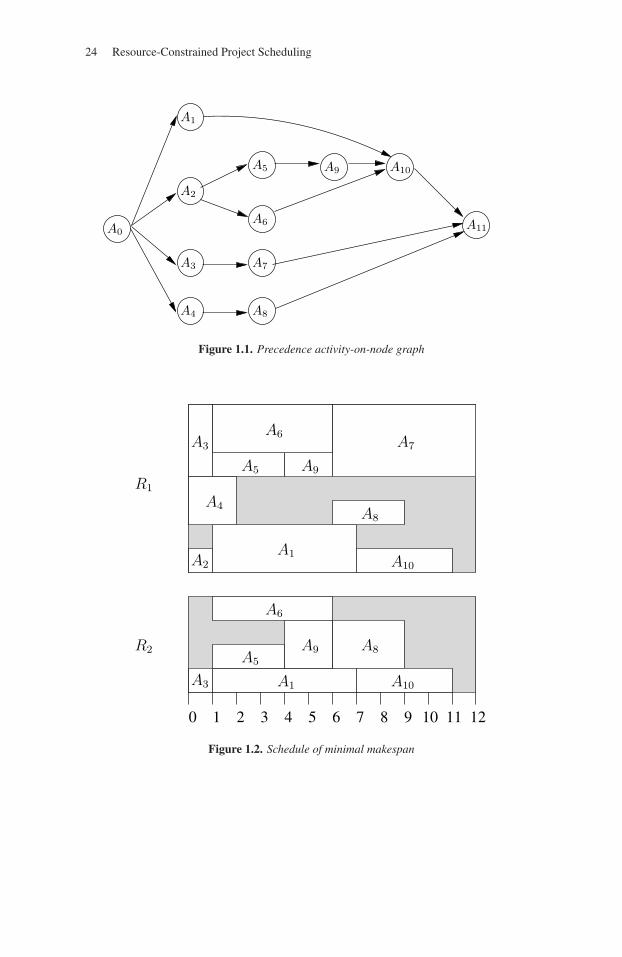
The precedence constraints linking the activities Ai ∈ V are displayed in Fig-ure 1.1 as an activity-on-node graph. A schedule of minimal makespan S∗
n+1 = 12 isdisplayed in Figure 1.2 as a 2-dimensional Gantt chart where the x axis represents thetime and the y axis represents the resource occupation.
1.3. Computational complexity
According to the computational complexity theory [GAR 79], the RCPSP is one ofthe most intractable combinatorial optimization problems. Indeed, the RCPSP belongsto the class of problems that are NP-hard in the strong sense. The complexity theorystates that an optimization problem is NP-hard (in the strong sense) if its decisionversion is NP-complete (in the strong sense). Let us define the decision variant of theRCPSP. Let H denote an arbitrarily large integer.
24 Resource-Constrained Project Scheduling
A9
A1
A2
A0
A3
A4
A7
A8
A10
A11
A5
A6
Figure 1.1. Precedence activity-on-node graph
R1
R2
21 3 4 5 6 7 8 9 10 11 120
A3
A2
A4
A5 A9
A7
A6
A8
A10
A6
A8
A10A1
A9A5
A3
A1
Figure 1.2. Schedule of minimal makespan
The Resource-Constrained Project Scheduling Problem 25
DEFINITION 1.2.– The decision variant of the RCPSP is the problem of determiningwhether a schedule S of makespan Sn+1 not greater than H subject to precedenceconstraints (1.1) and resource constraints (1.2) exists or not.
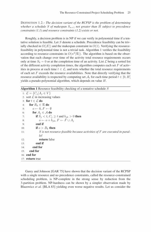
Roughly, a decision problem is in NP if we can verify in polynomial time if a ten-tative solution is feasible. Let S denote a schedule. Precedence feasibility can be triv-ially checked in O(|E|) and the makespan constraint in O(1). Verifying the resource-feasibility in polynomial time is not a trivial task. Algorithm 1 verifies the feasibilityaccording to resource-constraints in O(n2|R|). The algorithm is based on the obser-vation that each change over time of the activity total resource requirements occursonly at time S0 = 0 or at the completion time of an activity. List L being a sorted listof the different activity completion times, the algorithm computes each set F of activ-ities in process at each time t ∈ L, and tests whether the total resource requirementsof each set F exceeds the resource availabilities. Note that directly verifying that theresource availability is respected by computing set At for each time period t ∈ [0,H[yields a pseudo-polynomial algorithm, which depends on value H .
Algorithm 1 Resource feasibility checking of a tentative schedule S
1: L = {Cj |Aj ∈ V }2: sort L in increasing values3: for t ∈ L do4: for Rk ∈ R do5: o← 0, F ← ∅6: for Aj ∈ A do7: if Sj < t, Cj ≥ t and bjk > 0 then8: o← o + bjk, F ← F ∪Aj
9: end if10: if o > Bk then11: S is not resource-feasible because activities of F are executed in paral-
lel12: return false13: end if14: end for15: end for16: end for17: return true
Garey and Johnson [GAR 75] have shown that the decision variant of the RCPSPwith a single resource and no precedence constraints, called the resource-constrainedscheduling problem, is NP-complete in the strong sense by reduction from the3-partition problem. NP-hardness can be shown by a simpler observation made byBlazewicz et al. [BLA 83] yielding even worse negative results. Let us consider the
26 Resource-Constrained Project Scheduling
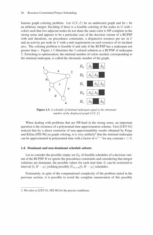
famous graph coloring problem. Let G(V, E) be an undirected graph and let c bean arbitrary integer. Deciding if there is a feasible coloring of the nodes in G with ccolors such that two adjacent nodes do not share the same color is NP-complete in thestrong sense and appears to be a particular case of the decision variant of a RCPSPwith unit durations, no precedence constraints, a disjunctive resource per arc in Eand an activity per node in V with a unit requirement on each resource of its incidentarcs. The coloring problem is feasible if and only if the RCPSP has a makespan notgreater than c. Figure 1.3 illustrates the 3 colored solution as a RCPSP of makespan3. Switching to optimization, the minimal number of colors needed, corresponding tothe minimal makespan, is called the chromatic number of the graph.
12
3
4
a
bc
d
e
A1 A2
A1 A3
A3 A2
A3A4
A4 A2
Ra
Rb
Rd
Rc
Re
Figure 1.3. A schedule of minimal makespan equal to the chromaticnumber of the displayed graph G(V, E)
When dealing with problems that are NP-hard in the strong sense, an importantquestion is the existence of a polynomial-time approximation scheme. Uetz [UET 01]noticed that by a direct extension of non-approximability results obtained by Feigeand Kilian [FEI 98] on graph coloring, it is very unlikely3 that the minimal makespancan be approximated in polynomial time with a factor of n1−ε for any constant ε > 0.
1.4. Dominant and non-dominant schedule subsets
Let us consider the possibly empty set SH of feasible schedules of a decision vari-ant of the RCPSP. If we ignore the precedence constraints and considering that integersolutions are dominant, the possible values for each start time Si can be restricted tointerval [0,H − pi[ yielding possibly ΠAi∈A[0,H − pi[ schedules.
Fortunately, in spite of the computational complexity of the problem stated in theprevious section, it is possible to avoid the complete enumeration of this possibly
3. We refer to [UET 01, FEI 98] for the precise conditions.

The Resource-Constrained Project Scheduling Problem 27
huge search space to find a feasible solution. It is possible to define subsets of sched-ules significantly smaller than SH that always contain a feasible solution if it exists,i.e. dominant subsets. These sets of schedules are the sets of semi-active and activeschedules, based on the concepts of local and global left shifts, respectively. Let usconsider a schedule S and an activity Ai. The global left shift operator LS(S,Ai,Δ)transforms schedule S into an identical schedule S′, except for S′
i = Si − Δ withΔ > 0. A left shift is local when, in addition, all schedules obtained by LS(S,Ai, ρ)with 0 < ρ ≤ Δ are also feasible. We define the set of semi-active and active sched-ules as follows.
DEFINITION 1.3.– A schedule is semi-active if it admits no feasible activity local leftshift.
From this definition, an integer schedule is semi-active if and only if for eachactivity Ai ∈ A, there is no feasible activity left shift of 1 time unit.
DEFINITION 1.4.– A schedule is active if it admits no feasible activity global left shift.
From this definition, an integer schedule is active if and only if for each activityAi ∈ A, there is no feasible left shift of Δ ∈ N
∗ time units. Note that the scheduledisplayed in Figure 1.2 is both semi-active and active.
Any solution of SH can obviously be transformed into a semi-active schedule byapplying a series of local left shifts. Any semi-active schedule can in turn be trans-formed into an active schedule by performing a series of global left shifts. It fol-lows that the semi-active schedule set Ssa
H and the active schedule set SaH are dom-
inant subsets of SH . More precisely we have SaH ⊆ Ssa
H ⊆ SH . These sets arealso dominant for the search of a solution of S minimizing a regular objective func-tion f : R
n+2 → R. A function f is regular if for all S, S′ ∈ Rn+2 such that
S ≤ S′ (where ≤ is meant componentwise), we have f(S) ≤ f(S′). In particu-lar, the makespan criterion considered in the standard RCPSP corresponds to a regularobjective function.
For practical reasons it can be relevant to consider non-dominant subsets of sched-ules, i.e. that may exclude the optimal solution. The non-delay scheduling concept islinked to the requirement that no resource is left idle while it could process an activ-ity. Although it may appear intuitively as efficient, this scheduling policy may leadonly to sub-optimal solutions. The set of non-delay schedules can be defined by con-sidering partial left shifts. A partial left shift consists of allowing preemption for theleft-shifted activity. An activity is preemptive if it can be interrupted at any (not neces-sarily integer) time-point (see Chapter 8). Thus, a partial left shift PLS(S,Ai,Δ,Γ)of an originally non-interrupted activity consists of a left shift of Δ > 0 time units ofthe first Γ > 0 units of the activity.
28 Resource-Constrained Project Scheduling
DEFINITION 1.5.– A schedule is non-delay if it admits no feasible activity partial leftshift.
For an integer schedule S, whenever a resource is left idle while it could startprocessing an activity, it is possible to globally left shift the first unit of this activityinto the idle period. From the above definition, the set Snd
H of semi-active schedulesof makespan not greater than H verifies Snd
H ⊆ SaH . The schedule displayed in Figure
1.2 is also a non-delay schedule .
Introduced for the job-shop problem by Baker [BAK 74], similar definitionsof semi-active, active and non-delay schedule sets for the RCPSP can be found in[SPR 95, NEU 00a].
1.5. Order-based representation of schedules and related dominant schedule sets
From the dominance property of the semi-active schedule set, we may derive arelevant representation of schedules. Let S be a feasible schedule. For any activityAj , if Sj > 0 and if there is no other activity Ai such that Si + pi = Sj , then activityAj can be left shifted and the schedule is not semi-active. Hence, in any semi-activeschedule S and for any activity Aj such that Sj > 0, there is an activity Ai such thatSj = Si+pi. It follows that it is intuitively relevant to represent a left-shifted scheduleby additional precedence constraints. Bartusch et al. [BAR 88] propose to considerthe decomposition of set S of feasible solutions into finitely many subsets, each oneincluding schedules satisfying the precedence constraints induced by a different strictorder. Formally, let P denote a strict order4 on the set of activities A and let S(P ) ={S|Sj − Si ≥ pi ∀(Ai, Aj) ∈ E ∪ P} denote the set of (not necessarily feasible)schedules that verify the precedence constraints given by E and the ones given by P .S(P ) is a polyhedron and so is S(∅) which is the set of time-feasible schedules. Bydefinition, a strict order P is time-feasible if S(P ) �= ∅ and is (resource- and time-)feasible if, in addition, S(P ) ⊆ S. A result established by Bartusch et al. [BAR 88]states that the set of schedules S is the union of the polyhedra S(P ) for all inclusion-minimal feasible strict orders P on the set of activities A. In the case of the searchfor a feasible solution in SH , or the minimization of a regular objective function inS, the minimal element of S(P ) dominates the other elements of this set. This is thepoint ES(P ) (earliest-start schedule) of S(P ) such that ∀S′ ∈ S(P ), ES(P ) ≤ S′.By definition, ES(P )i is equal to the length of the longest path from A0 to Ai ingraph G(V,E ∪ P ), each arc (Ai, Aj) ∈ E ∪ P being valuated by pi. It follows thatS(P ) �= ∅ if and only if G(V,E ∪ P ) is acyclic.
The RCPSP can be defined as the search for a feasible strict order P onA such thatES(P ) is of minimal makespan. Note that P is said to be feasible not only if ES(P )
4. A strict order is an irreflexive and transitive binary relation.
The Resource-Constrained Project Scheduling Problem 29
is feasible, but if and only if all schedules in S(P ) are feasible. We will see how thistype of feasibility can be checked in the next section to specify the strict order-basedRCPSP formulation.
To illustrate these concepts, let us consider schedule S displayed in Figure 1.2 andstrict orders
P1 = {(A2, A1), (A3, A1), (A3, A6), (A6, A7), (A3, A7), (A9, A7), (A9, A8)},P2 = P1 ∪ {(A3, A8), (A6, A8)} and P3 = P2 \ {A9, A8}.
Note that we have S = ES(P1) = ES(P2) = ES(P3). P1 and P2 are bothfeasible strict orders since any schedule in S(P1) or S(P2) is feasible. However, P3
is not a feasible strict order although ES(P3) is feasible. Indeed, consider scheduleS′ = S, except that S9 and S7 are both right shifted by 1 time unit. S′ is in S(P3) butis not resource-feasible since R2 is oversubscribed at time C9. As stated above, it isnot trivial to check the feasibility of a strict order, which corresponds here to see thatS(P1) ⊆ S and S(P2) ⊆ S. This is linked to the forbidden set concept described insection 1.6. However, this example shows that the above-defined feasibility conditionof a strict order is not a necessary condition for obtaining a feasible schedule. We canalso remark that the important arcs of a feasible strict order are the ones belonging toits transitive reduction. Let us consider P ′
1 = P1 \ (A3, A7), the transitive reductionof P1. We have S(P1) = S(P ′
1). Furthermore, P1 is an inclusion-minimal feasiblestrict order: if we remove any arc belonging to the transitive reduction of P1 (i.e. allarcs except (A3, A7)), ES(P1) becomes unfeasible. P2 is not an inclusion-minimalfeasible strict order since we have P2 ⊂ P1. This shows that several strict orders maylead to the same earliest-start schedule.
Another important remark is that despite the fact that the semi-active concept isintuitively related to the strict order concept, each earliest-start schedule with respectto a given strict order does not necessarily correspond to a semi-active schedule inthe sense of Definition 1.3 as noted by Sprecher et al. [SPR 95]. For instance, letus define strict order P4 = P1 ∪ {(A10, A8)}. The earliest start schedule ES(P4)is identical to the one displayed in Figure 1.2 except that the start time of activity8 is delayed up to the completion time of activity A10. Since a local left shift ofactivity A8 is made feasible, schedule ES(P4) is not semi-active. For that reason,Neumann et al. [NEU 00a] propose additional schedule sets related to the strict orderrepresentation: the quasi-active and the pseudo-active schedule sets. These sets arebased on the order-preserving and order-monotonic left shifts, respectively. These leftshifts are defined by reference to the interval order P (S) induced by a schedule Swhere P (S) = {(Ai, Aj) ∈ V 2|Sj ≥ Si + pi}. By definition, P (S) is the inclusionmaximal strict order P such that S ∈ S(P ). Since P (S) is inclusion maximal, eachantichain in graph G(V,E ∪ P (S)) represents a set of activities simultaneously inprocess.
30 Resource-Constrained Project Scheduling
An order-preserving left shift of an activity on S yields a feasible schedule S′
such that P (S) ⊆ P (S′). An order-monotonic left shift of an activity on S yields afeasible schedule S′ such that P (S) ⊆ P (S′) or P (S′) ⊆ P (S). From this definitionit follows that in an order-monotonic left shift from schedule S, either all chains ofG(V,E∪P (S)) or all antichains are preserved. Consequently, an order-preserving leftshift is also order-monotonic. Moreover, since the initial and final schedules belongto the same feasible order polyhedron S(P (S)) or S(P (S′)), an order-monotonic leftshift is also a local left shift.
DEFINITION 1.6.– A schedule is quasi-active if it admits no feasible order-preservingleft shift.
From a polyhedral point of view, a schedule S is quasi-active if for each activityAi ∈ V , S′ = LS(S,Ai,Δ) does not belong to S(P (S)), for all Δ > 0, i.e. if it isthe minimal point of S(P (S)).
We can show that schedule ES(P4) defined above is quasi-active since anyleft shift violates its interval order P (ES(P4)) = {(A1, A8), (A1, A10), (A2, A1),(A2, A5), (A2, A6), (A2, A7), (A2, A8), (A2, A9),(A2, A10), (A3, A1), (A3, A5),(A3, A6), (A3, A7), (A3, A8), (A3, A9), (A3, A10), (A4, A7), (A4, A8), (A4, A9),(A4, A10), (A5, A7), (A5, A8), (A5, A9), (A5, A10), (A6, A7), (A6, A8), (A6, A10),(A9, A7), (A9, A8), (A9, A10), (A10, A8)}.
Since each semi-active schedule is also a quasi-active schedule, we have the fol-lowing relations Ssa
H ⊆ SqaH ⊆ SH where Sqa
H denote the set of quasi-active schedules.
DEFINITION 1.7.– A schedule is pseudo-active if it admits no feasible order-monotonic left shift.
A schedule S is pseudo-active if for each activity Ai ∈ V , S′ = LS(S,Ai,Δ)does not belong to S(P ), for all Δ > 0 and for all strict orders P such that S ∈ S(P ),i.e. if it is the minimal point of all schedule sets S(P ) containing S.
Schedule ES(P4) is not pseudo-active since a local left shift of 1 unit on activ-ity A10 is order-monotonic: it removes (10, 8) and (1, 8) from P (ES(P4)) yieldinga necessarily feasible and non-worse schedule. In the terms of Definition 1.7, wecan also remark alternatively that ES(P4) belongs to the polyhedron S(P1) and thatactivity A10 can be locally left shifted while obtaining a schedule still in set S(P1).
Based on these definitions, the following theorem can be established.
THEOREM 1.1.– The set of semi-active schedules and the set of pseudo-active sched-ules are identical for the RCPSP.
The Resource-Constrained Project Scheduling Problem 31
Proof. Since there is no feasible local left shift from a semi-active schedule, the setof semi-active schedules is included in the set of pseudo-active schedules. We showthat, conversely, there is no feasible local left shift from a pseudo-active schedule.Suppose that there is a feasible local non-order-monotonic left shift LS(S,Ai,Δ)from a pseudo-active schedule S yielding schedule S′. Since LS(S,Ai,Δ) is notorder-monotonic, let (Aj , Ai) ∈ P (S), (Aj , Ai) �∈ P (S′), (Ai, Ak) �∈ P (S) and(Ai, Ak) ∈ P (S′). Let Δ′ = (Si + pi − Sk)/2. We have Δ > Δ′ and thenLS(S,Ai,Δ′) is feasible and does not create (Ai, Ak) while (Aj , Ai) is eitherremoved from or kept in P (S′). From S′, we can recursively apply this principleuntil obtaining a feasible order-monotonic left shift from S, which contradicts thehypothesis.
To sum up, we have the following relations between the presented dominant sched-ule sets: Sa
H ⊆ SsaH = Spa
H ⊆ SqaH ⊆ SH , where Spa
H denotes the set of pseudo-activeschedules. It should be mentioned that for the RCPSP with minimal and maximaltime lags, an extension of the problem considered in Chapter 11, it generally holdsthat Ssa
H ⊂ SpaH [NEU 00a].
1.6. Forbidden sets and resource flow network formulations of the RCPSP
From the order-based representation of dominant schedules, we can derive twoalternative formulations of the RCPSP restricting the search space to the dominant setof quasi-active schedules.
A forbidden set is a set F of activities that cannot be scheduled in parallel ina feasible solution because of resource limitations due to a resource Rk such that∑
Ai∈F bik > Bk. A forbidden set is minimal if any of its subsets of activities F ′
verifies, ∀Rk ∈ R,∑
Ai∈F ′ bik ≤ Bk. Let F denote the set of minimal forbiddensets. No element ofF can be an antichain of G(V,E∪P (S)) for any feasible scheduleS. Consequently, a necessary condition for feasibility of a schedule S is that ∀F ∈ F ,F 2∩P (S) �= ∅. A forbidden set F such that F 2∩P (S) �= ∅ is said to be broken up. If,in addition, S ∈ S(∅), we obtain a necessary and sufficient condition. Consequently,the RCPSP can be reformulated as follows.
DEFINITION 1.8.– The RCPSP aims at finding a strict order P such that G(V,E∪P )is acyclic, ∀F ∈ F , F 2 ∩ P �= ∅ and ES(P )n+1 is minimal.
The drawback of the preceding formulation is that the number of minimal forbid-den sets |F| can be extremely large. A significant number of forbidden sets are implic-itly broken up due to precedence relations. Indeed as soon as there is a path from Ai
to Aj in the precedence graph G(V,E), any precedence-feasible schedule breaks upany forbidden set including both Ai and Aj . Thus, we do not have to consider suchforbidden sets in F .
32 Resource-Constrained Project Scheduling
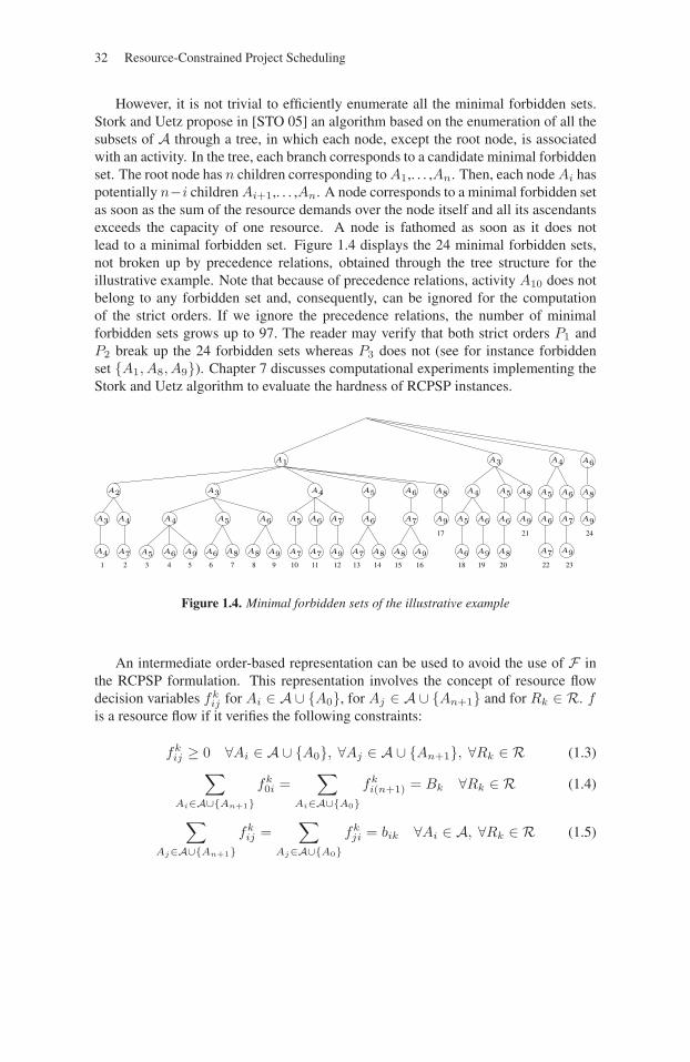
However, it is not trivial to efficiently enumerate all the minimal forbidden sets.Stork and Uetz propose in [STO 05] an algorithm based on the enumeration of all thesubsets of A through a tree, in which each node, except the root node, is associatedwith an activity. In the tree, each branch corresponds to a candidate minimal forbiddenset. The root node has n children corresponding to A1,. . . ,An. Then, each node Ai haspotentially n−i children Ai+1,. . . ,An. A node corresponds to a minimal forbidden setas soon as the sum of the resource demands over the node itself and all its ascendantsexceeds the capacity of one resource. A node is fathomed as soon as it does notlead to a minimal forbidden set. Figure 1.4 displays the 24 minimal forbidden sets,not broken up by precedence relations, obtained through the tree structure for theillustrative example. Note that because of precedence relations, activity A10 does notbelong to any forbidden set and, consequently, can be ignored for the computationof the strict orders. If we ignore the precedence relations, the number of minimalforbidden sets grows up to 97. The reader may verify that both strict orders P1 andP2 break up the 24 forbidden sets whereas P3 does not (see for instance forbiddenset {A1, A8, A9}). Chapter 7 discusses computational experiments implementing theStork and Uetz algorithm to evaluate the hardness of RCPSP instances.
A4
A6 A9 A6
A5
A8
A6
A8 A9 A7 A7
A5 A6 A7
A9 A7
A6
A5
A8 A8
A7
A6
A9A4
A2
A3
A3
A6
A5
A4
A7
A6
A7
A9
A9
A8
A6
A8
A9
A8
A5
A6
A6
A9
A4
A8
A6
A5
A9
14 15 16 18 19 20 2322
17 21 24
13
A1
A7
A4 A4
A5
A3
1 2 3 4 5 6 7 8 9 10 11 12
Figure 1.4. Minimal forbidden sets of the illustrative example
An intermediate order-based representation can be used to avoid the use of F inthe RCPSP formulation. This representation involves the concept of resource flowdecision variables fk
ij for Ai ∈ A ∪ {A0}, for Aj ∈ A ∪ {An+1} and for Rk ∈ R. fis a resource flow if it verifies the following constraints:
fkij ≥ 0 ∀Ai ∈ A ∪ {A0}, ∀Aj ∈ A ∪ {An+1}, ∀Rk ∈ R (1.3)∑Ai∈A∪{An+1}
fk0i =
∑Ai∈A∪{A0}
fki(n+1) = Bk ∀Rk ∈ R (1.4)
∑Aj∈A∪{An+1}
fkij =
∑Aj∈A∪{A0}
fkji = bik ∀Ai ∈ A, ∀Rk ∈ R (1.5)
The Resource-Constrained Project Scheduling Problem 33
A resource flow f induces the strict order P (f), the transitive closure of{(Ai, Aj) ∈ V 2 | fij > 0}. The following lemmas establish the link between flowsand strict orders.
LEMMA 1.1.– If f is a flow and G(V,E ∪ P (f)) is acyclic, then P (f) is a feasiblestrict order.
Proof. First, if G(V,E ∪ P (f)) is acyclic, then ES(P (f)) is time feasible. Second,suppose that a forbidden set F is not broken up by ES(P (f)) for a resource k. Sinceall activities of F are simultaneously in process during at least one time period, thereis a total incoming flow of F equal to
∑i∈F bik > Bk which violates the flow con-
servation conditions.
Consequently, a resource flow such that G(V,E ∪ P (f)) is acyclic is said to befeasible.
LEMMA 1.2.– For each feasible strict order P , there is a feasible resource flow f suchthat ES(P (f)) ≤ ES(P ).
Proof. Let us consider the feasible schedule S = ES(P ) and strict order P (S) ⊇ Pwith ES(P (S)) = S. By setting additional constraints fk
ij = 0 for all (Ai, Aj) �∈P (S) we show that there exists a flow verifying equations (1.3)-(1.5). This amountsto verifying that there exists a feasible flow in each network Gk(V,E ∪ P (S)), foreach resource Rk ∈ R with minimal and maximal node capacities bik for all activitiesAi ∈ A and node capacities Bk for nodes A0 and An+1. Let us transform this graphwith bounds on node flow into a graph with bounds on arc flows. We split each nodeAi ∈ V into two nodes Ai and A′
i linked by an arc of minimal and maximal capacitiesequal to the node capacity. All other arcs have null minimal capacities and infinitemaximal capacities. If we now ignore the maximal capacities, since P (S) is feasible,there is no A0−A′
n+1 cut of (minimal) capacity greater than Bk. Indeed suppose thatsuch a cut exists. Then, it includes a set of arcs (i, i′) that represents a non-brokenup forbidden set. Furthermore there is a A0 − A′
n+1 cut (reduced to arc (A0, A′0)) of
minimal capacity equal to Bk. Therefore, according to the min-flow max-cut theorem(see [NEU 03, LEU 04]), we have a minimal flow equal to Bk.
It follows from Lemmas 1.1 and 1.2 that the RCPSP can be defined as follows.
DEFINITION 1.9.– The RCPSP aims at finding a feasible flow f such thatES(P (f))(n+1) is minimal.
From a feasible flow f , a feasible schedule ES(P (f)) can be computed by longestpath computations in graph G(V,E ∪ P (f)) where all arcs (Ai, Aj) ∈ E ∪ P (f) arevaluated by pj .
34 Resource-Constrained Project Scheduling
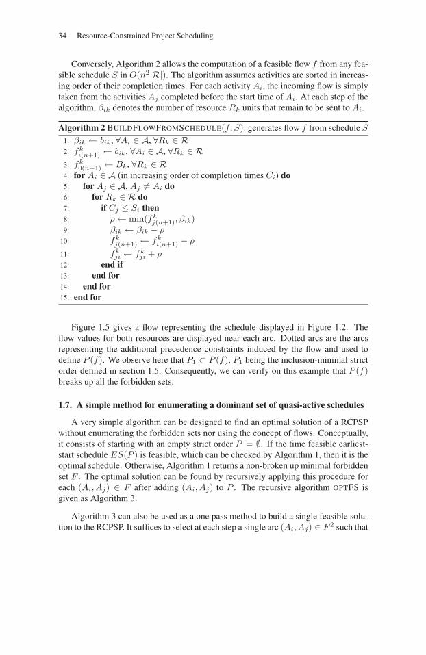
Conversely, Algorithm 2 allows the computation of a feasible flow f from any fea-sible schedule S in O(n2|R|). The algorithm assumes activities are sorted in increas-ing order of their completion times. For each activity Ai, the incoming flow is simplytaken from the activities Aj completed before the start time of Ai. At each step of thealgorithm, βik denotes the number of resource Rk units that remain to be sent to Ai.
Algorithm 2 BUILDFLOWFROMSCHEDULE(f, S): generates flow f from schedule S
1: βik ← bik, ∀Ai ∈ A, ∀Rk ∈ R2: fk
i(n+1) ← bik, ∀Ai ∈ A, ∀Rk ∈ R3: fk
0(n+1) ← Bk, ∀Rk ∈ R4: for Ai ∈ A (in increasing order of completion times Ci) do5: for Aj ∈ A, Aj �= Ai do6: for Rk ∈ R do7: if Cj ≤ Si then8: ρ← min(fk
j(n+1), βik)9: βik ← βik − ρ
10: fkj(n+1) ← fk
i(n+1) − ρ
11: fkji ← fk
ji + ρ12: end if13: end for14: end for15: end for
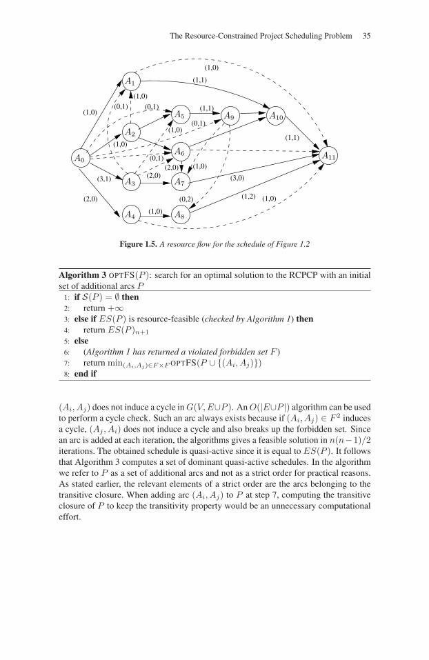
Figure 1.5 gives a flow representing the schedule displayed in Figure 1.2. Theflow values for both resources are displayed near each arc. Dotted arcs are the arcsrepresenting the additional precedence constraints induced by the flow and used todefine P (f). We observe here that P1 ⊂ P (f), P1 being the inclusion-minimal strictorder defined in section 1.5. Consequently, we can verify on this example that P (f)breaks up all the forbidden sets.
1.7. A simple method for enumerating a dominant set of quasi-active schedules
A very simple algorithm can be designed to find an optimal solution of a RCPSPwithout enumerating the forbidden sets nor using the concept of flows. Conceptually,it consists of starting with an empty strict order P = ∅. If the time feasible earliest-start schedule ES(P ) is feasible, which can be checked by Algorithm 1, then it is theoptimal schedule. Otherwise, Algorithm 1 returns a non-broken up minimal forbiddenset F . The optimal solution can be found by recursively applying this procedure foreach (Ai, Aj) ∈ F after adding (Ai, Aj) to P . The recursive algorithm OPTFS isgiven as Algorithm 3.
Algorithm 3 can also be used as a one pass method to build a single feasible solu-tion to the RCPSP. It suffices to select at each step a single arc (Ai, Aj) ∈ F 2 such that
The Resource-Constrained Project Scheduling Problem 35
(1,0)
(1,1)
(1,0)
(1,0)(1,1)
(0,1)
(1,2)(0,2)
(1,0)
(1,0)
(0,1)(1,0)
(3,0)
(2,0)(2,0)(3,1)
(1,1)(0,1)(0,1)(1,0)
(2,0) (1,0)
A1
A2
A6 A11
A10
A8A4
A3
A0
A9
A7
A5
Figure 1.5. A resource flow for the schedule of Figure 1.2
Algorithm 3 OPTFS(P ): search for an optimal solution to the RCPCP with an initialset of additional arcs P
1: if S(P ) = ∅ then2: return +∞3: else if ES(P ) is resource-feasible (checked by Algorithm 1) then4: return ES(P )n+1
5: else6: (Algorithm 1 has returned a violated forbidden set F )7: return min(Ai,Aj)∈F×F OPTFS(P ∪ {(Ai, Aj)})8: end if
(Ai, Aj) does not induce a cycle in G(V,E∪P ). An O(|E∪P |) algorithm can be usedto perform a cycle check. Such an arc always exists because if (Ai, Aj) ∈ F 2 inducesa cycle, (Aj , Ai) does not induce a cycle and also breaks up the forbidden set. Sincean arc is added at each iteration, the algorithms gives a feasible solution in n(n−1)/2iterations. The obtained schedule is quasi-active since it is equal to ES(P ). It followsthat Algorithm 3 computes a set of dominant quasi-active schedules. In the algorithmwe refer to P as a set of additional arcs and not as a strict order for practical reasons.As stated earlier, the relevant elements of a strict order are the arcs belonging to thetransitive closure. When adding arc (Ai, Aj) to P at step 7, computing the transitiveclosure of P to keep the transitivity property would be an unnecessary computationaleffort.

36
This page intentionally left blank
Chapter 2
Resource and Precedence ConstraintRelaxation
The RCPSP is one of the most complex scheduling problems. It can be consid-ered as a generalization of many standard scheduling subproblems. Relaxing an initialRCPSP instance in order to build relaxed subproblems may be useful for the resolutionof the initial instance. Relaxations are mainly used to compute efficient lower boundsof the project duration, but also to totally or partially build a solution of the initialinstance. For instance if we refer to the disjunctive problem relaxations (see section2.2), specific branching schemes have been designed to schedule machines. Directlyinspired by the large amount of work dedicated to job-shop scheduling, these branch-ing schemes consist of ordering all activities that require the same single machinefor solving the RCPSP. Ordering the single machines before applying any specifi-cally designed branching scheme for solving the RCPSP drastically improves the per-formance of the branch-and-bound methods. Thus, building relevant single machinescheduling instances, or parallel machine scheduling instance from a RCPSP instancemay be interesting to speed up the resolution and/or to get efficient lower bounds.
In this chapter, we present traditional critical path based lower bounds and meth-ods for bounding single resource problems that arise as relaxations of the RCPSP.Basically, these new problems are obtained either by relaxing the precedence relationsto time-windows for activities and/or by relaxing partially the resource constraints.Namely these problems are (1) the single machine problem (1|ri, qi|Cmax), (2) theidentical parallel machine problem (P |ri, qi|Cmax) and (3) the multiprocessor prob-lem (P |ri, qi, sizei|Cmax) also known as the Cumulative Scheduling Problem (CuSP).
Chapter written by Emmanuel NÉRON.
37
38 Resource-Constrained Project Scheduling
For these three relaxations, we first describe how they can be derived from an ini-tial RCPSP instance, and we present briefly how they can be used to compute lowerbounds for a RCPSP instance.
2.1. Relaxing resource constraints
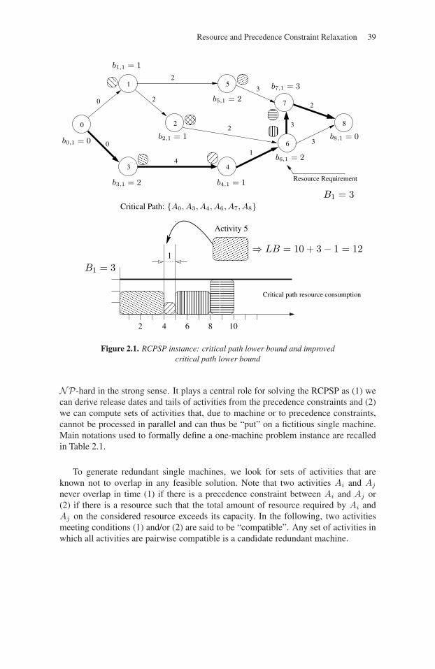
The most intuitive relaxation of the RCPSP consists of relaxing all the resourceconstraints. Then the corresponding problem is to find a critical path in a directedand acyclic graph that can be solved using, for instance, Bellman’s algorithm. Thisnotion of length in the precedence graph is also used to compute both earliest start-ing time (ESi) and tail (qi) of activities. Tail qi corresponds to the minimum durationbetween the end of activity Ai and the end of the project. ESi = L(A0, Ai) andqi = L(Ai, An+1)− pi, where L(Ai, Aj) denotes the longest path in the precedencegraph between Ai and Aj . This trivial relaxation, that consists of ignoring resourceconstraints to compute time-bounds for activities, plays an important role in the solv-ing methods (lower bound computation, adjusting time-windows of activities etc.).A RCPSP instance and a corresponding critical path are presented in the top part ofFigure 2.1.
Some improvements have been proposed in order to enforce critical path relaxation[STI 78, DEM 92b]. Authors consider an activity that cannot be processed simultane-ously (due to resource constraints) with activities of the critical path (CP). Let us con-sider an activity Ai with a time-window [ESi, LCi], and let us consider that activitiesof the critical path are scheduled at their earliest starting times. Then, if the amountof resources required by Ai are available only during ei time-units between ESi andLCi, with ei ≤ pi, the project completion will be delayed by at least pi−ei time-units,thus L = maxAi /∈CP (L(A0, An+1) + pi − ei) is a valid lower bound of the projectduration. Figure 2.1 shows the Gantt diagram associated with the activities of the crit-ical path. Notice that resource is not available to process activity A5 simultaneouslywith the ones of the critical path. Thus, a new lower bound can be calculated which isequal to 12.
2.2. Calculating the disjunctive subproblem
In this section we present a method to build such single machine problems froman initial RCPSP and we quickly present an overview of techniques either to computelower bounds of the makespan (maxi(Ci +qi), where Ci denotes the completion timeof the activity Ai) or to derive satisfiability tests, and time-window adjustments ofactivities.
In the single machine problem, a set of activities has to be processed on a singlemachine. Each activity, Ai has a release date ESi, a processing time pi, a tail qi ora deadline LCi if the decision variant is considered. This problem is known to be
Resource and Precedence Constraint Relaxation 39
1
0 2
3
6
7
8
4
5
Resource Requirement
0
0
41
2
2
3
2
3
3
2
Critical path resource consumption
Critical Path: {A0, A3, A4, A6, A7, A8}
Activity 5
b3,1 = 2
b1,1 = 1
b0,1 = 0b2,1 = 1
b4,1 = 1
b6,1 = 2
b5,1 = 2
b8,1 = 0
b7,1 = 3
B1 = 3
102 4 6 8
B1 = 31
⇒ LB = 10 + 3− 1 = 12
Figure 2.1. RCPSP instance: critical path lower bound and improvedcritical path lower bound
NP-hard in the strong sense. It plays a central role for solving the RCPSP as (1) wecan derive release dates and tails of activities from the precedence constraints and (2)we can compute sets of activities that, due to machine or to precedence constraints,cannot be processed in parallel and can thus be “put” on a fictitious single machine.Main notations used to formally define a one-machine problem instance are recalledin Table 2.1.
To generate redundant single machines, we look for sets of activities that areknown not to overlap in any feasible solution. Note that two activities Ai and Aj
never overlap in time (1) if there is a precedence constraint between Ai and Aj or(2) if there is a resource such that the total amount of resource required by Ai andAj on the considered resource exceeds its capacity. In the following, two activitiesmeeting conditions (1) and/or (2) are said to be “compatible”. Any set of activities inwhich all activities are pairwise compatible is a candidate redundant machine.
40 Resource-Constrained Project Scheduling
Notation Definition
A set of activity
n number of activities: |A|pi processing time of activity Ai
ESi earliest starting time of activity Ai (release date)
qi tail of activity Ai
(or LCi latest completion time of activity Ai (deadline))
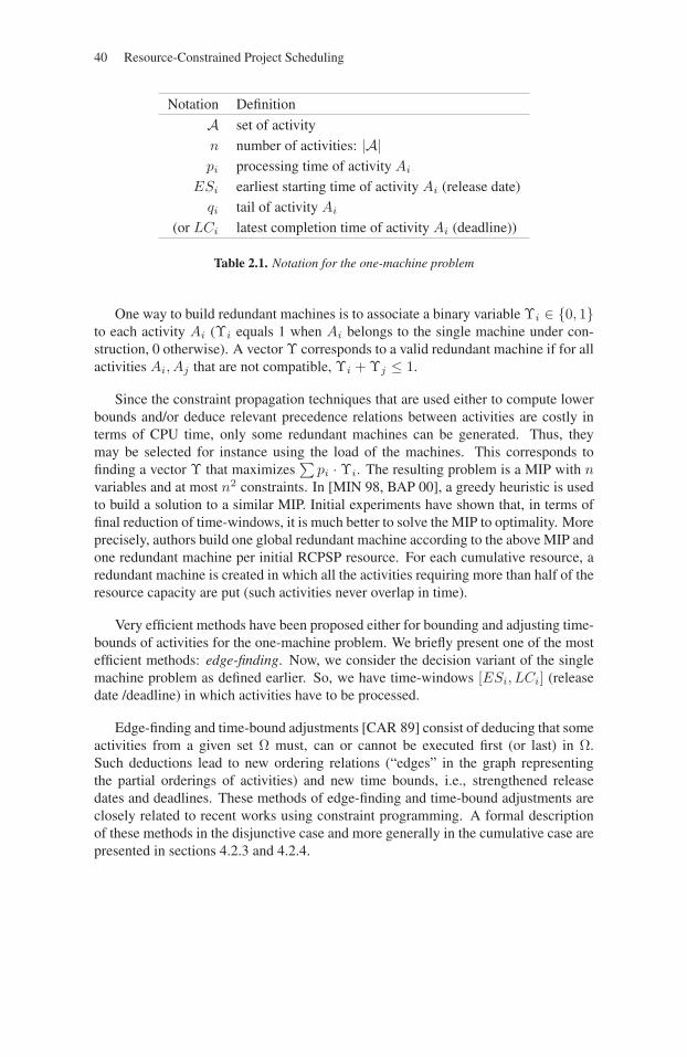
Table 2.1. Notation for the one-machine problem
One way to build redundant machines is to associate a binary variable Υi ∈ {0, 1}to each activity Ai (Υi equals 1 when Ai belongs to the single machine under con-struction, 0 otherwise). A vector Υ corresponds to a valid redundant machine if for allactivities Ai, Aj that are not compatible, Υi + Υj ≤ 1.
Since the constraint propagation techniques that are used either to compute lowerbounds and/or deduce relevant precedence relations between activities are costly interms of CPU time, only some redundant machines can be generated. Thus, theymay be selected for instance using the load of the machines. This corresponds tofinding a vector Υ that maximizes
∑pi · Υi. The resulting problem is a MIP with n
variables and at most n2 constraints. In [MIN 98, BAP 00], a greedy heuristic is usedto build a solution to a similar MIP. Initial experiments have shown that, in terms offinal reduction of time-windows, it is much better to solve the MIP to optimality. Moreprecisely, authors build one global redundant machine according to the above MIP andone redundant machine per initial RCPSP resource. For each cumulative resource, aredundant machine is created in which all the activities requiring more than half of theresource capacity are put (such activities never overlap in time).
Very efficient methods have been proposed either for bounding and adjusting time-bounds of activities for the one-machine problem. We briefly present one of the mostefficient methods: edge-finding. Now, we consider the decision variant of the singlemachine problem as defined earlier. So, we have time-windows [ESi, LCi] (releasedate /deadline) in which activities have to be processed.
Edge-finding and time-bound adjustments [CAR 89] consist of deducing that someactivities from a given set Ω must, can or cannot be executed first (or last) in Ω.Such deductions lead to new ordering relations (“edges” in the graph representingthe partial orderings of activities) and new time bounds, i.e., strengthened releasedates and deadlines. These methods of edge-finding and time-bound adjustments areclosely related to recent works using constraint programming. A formal descriptionof these methods in the disjunctive case and more generally in the cumulative case arepresented in sections 4.2.3 and 4.2.4.
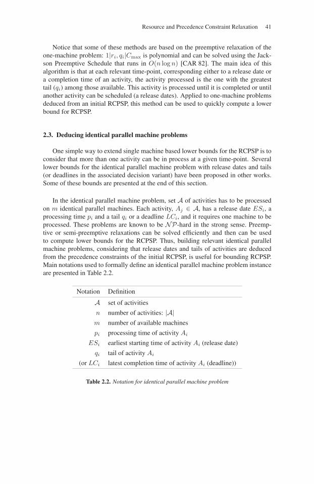
Resource and Precedence Constraint Relaxation 41
Notice that some of these methods are based on the preemptive relaxation of theone-machine problem: 1|ri, qi|Cmax is polynomial and can be solved using the Jack-son Preemptive Schedule that runs in O(n log n) [CAR 82]. The main idea of thisalgorithm is that at each relevant time-point, corresponding either to a release date ora completion time of an activity, the activity processed is the one with the greatesttail (qi) among those available. This activity is processed until it is completed or untilanother activity can be scheduled (a release dates). Applied to one-machine problemsdeduced from an initial RCPSP, this method can be used to quickly compute a lowerbound for RCPSP.
2.3. Deducing identical parallel machine problems
One simple way to extend single machine based lower bounds for the RCPSP is toconsider that more than one activity can be in process at a given time-point. Severallower bounds for the identical parallel machine problem with release dates and tails(or deadlines in the associated decision variant) have been proposed in other works.Some of these bounds are presented at the end of this section.
In the identical parallel machine problem, set A of activities has to be processedon m identical parallel machines. Each activity, Aj ∈ A, has a release date ESi, aprocessing time pi and a tail qi or a deadline LCi, and it requires one machine to beprocessed. These problems are known to be NP-hard in the strong sense. Preemp-tive or semi-preemptive relaxations can be solved efficiently and then can be usedto compute lower bounds for the RCPSP. Thus, building relevant identical parallelmachine problems, considering that release dates and tails of activities are deducedfrom the precedence constraints of the initial RCPSP, is useful for bounding RCPSP.Main notations used to formally define an identical parallel machine problem instanceare presented in Table 2.2.
Notation Definition
A set of activities
n number of activities: |A|m number of available machines
pi processing time of activity Ai
ESi earliest starting time of activity Ai (release date)
qi tail of activity Ai
(or LCi latest completion time of activity Ai (deadline))
Table 2.2. Notation for identical parallel machine problem
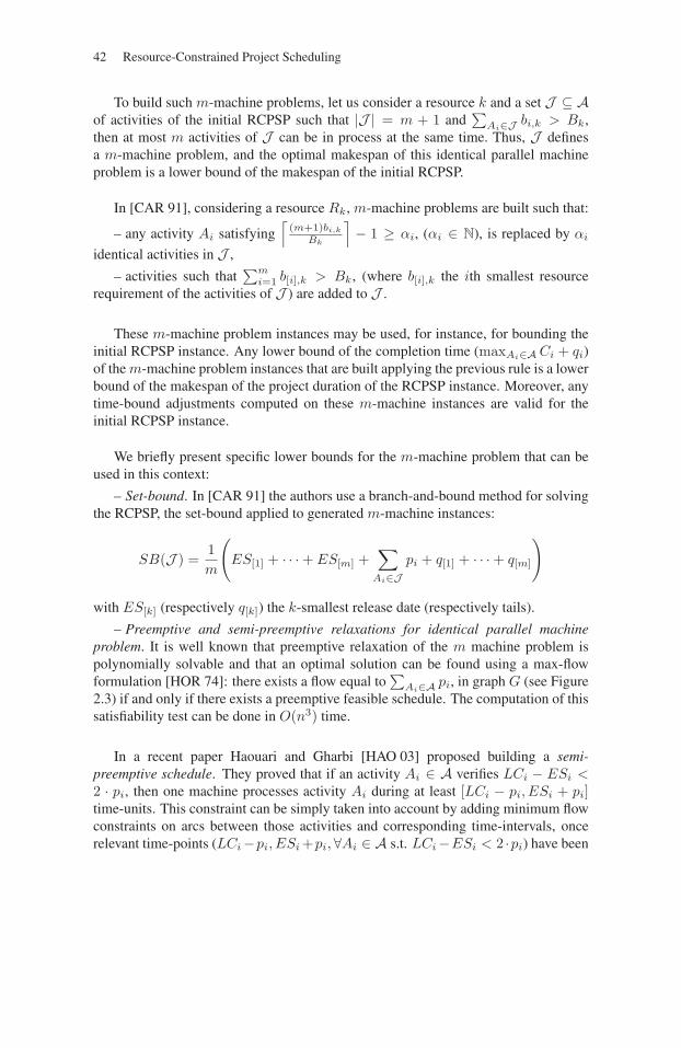
42 Resource-Constrained Project Scheduling
To build such m-machine problems, let us consider a resource k and a set J ⊆ Aof activities of the initial RCPSP such that |J | = m + 1 and
∑Ai∈J bi,k > Bk,
then at most m activities of J can be in process at the same time. Thus, J definesa m-machine problem, and the optimal makespan of this identical parallel machineproblem is a lower bound of the makespan of the initial RCPSP.
In [CAR 91], considering a resource Rk, m-machine problems are built such that:
– any activity Ai satisfying⌈
(m+1)bi,k
Bk
⌉− 1 ≥ αi, (αi ∈ N), is replaced by αi
identical activities in J ,
– activities such that∑m
i=1 b[i],k > Bk, (where b[i],k the ith smallest resourcerequirement of the activities of J ) are added to J .
These m-machine problem instances may be used, for instance, for bounding theinitial RCPSP instance. Any lower bound of the completion time (maxAi∈A Ci + qi)of the m-machine problem instances that are built applying the previous rule is a lowerbound of the makespan of the project duration of the RCPSP instance. Moreover, anytime-bound adjustments computed on these m-machine instances are valid for theinitial RCPSP instance.
We briefly present specific lower bounds for the m-machine problem that can beused in this context:
– Set-bound. In [CAR 91] the authors use a branch-and-bound method for solvingthe RCPSP, the set-bound applied to generated m-machine instances:
SB(J ) =1m
(ES[1] + · · ·+ ES[m] +
∑Ai∈J
pi + q[1] + · · ·+ q[m]
)
with ES[k] (respectively q[k]) the k-smallest release date (respectively tails).
– Preemptive and semi-preemptive relaxations for identical parallel machineproblem. It is well known that preemptive relaxation of the m machine problem ispolynomially solvable and that an optimal solution can be found using a max-flowformulation [HOR 74]: there exists a flow equal to
∑Ai∈A pi, in graph G (see Figure
2.3) if and only if there exists a preemptive feasible schedule. The computation of thissatisfiability test can be done in O(n3) time.
In a recent paper Haouari and Gharbi [HAO 03] proposed building a semi-preemptive schedule. They proved that if an activity Ai ∈ A verifies LCi − ESi <2 · pi, then one machine processes activity Ai during at least [LCi − pi, ESi + pi]time-units. This constraint can be simply taken into account by adding minimum flowconstraints on arcs between those activities and corresponding time-intervals, oncerelevant time-points (LCi−pi, ESi +pi,∀Ai ∈ A s.t. LCi−ESi < 2 ·pi) have been
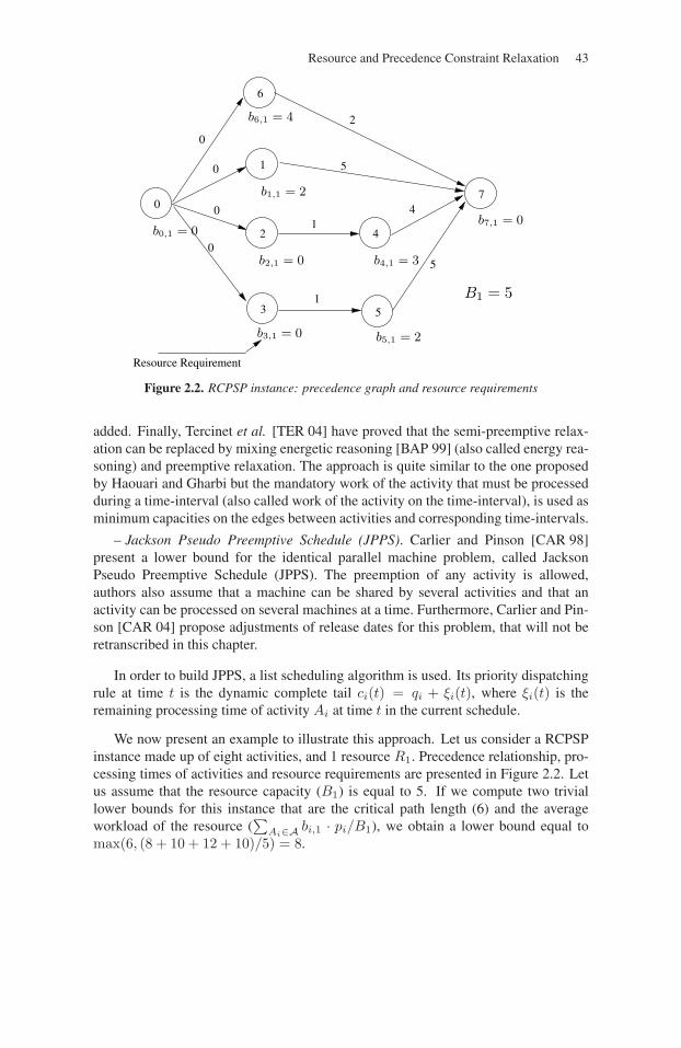
Resource and Precedence Constraint Relaxation 43
5
2
1
6
7
4
0
3
2
5
1
1
5
4
0
0
0
0
Resource Requirement
B1 = 5
b3,1 = 0
b7,1 = 0
b1,1 = 2
b2,1 = 0 b4,1 = 3
b5,1 = 2
b0,1 = 0
b6,1 = 4
Figure 2.2. RCPSP instance: precedence graph and resource requirements
added. Finally, Tercinet et al. [TER 04] have proved that the semi-preemptive relax-ation can be replaced by mixing energetic reasoning [BAP 99] (also called energy rea-soning) and preemptive relaxation. The approach is quite similar to the one proposedby Haouari and Gharbi but the mandatory work of the activity that must be processedduring a time-interval (also called work of the activity on the time-interval), is used asminimum capacities on the edges between activities and corresponding time-intervals.
– Jackson Pseudo Preemptive Schedule (JPPS). Carlier and Pinson [CAR 98]present a lower bound for the identical parallel machine problem, called JacksonPseudo Preemptive Schedule (JPPS). The preemption of any activity is allowed,authors also assume that a machine can be shared by several activities and that anactivity can be processed on several machines at a time. Furthermore, Carlier and Pin-son [CAR 04] propose adjustments of release dates for this problem, that will not beretranscribed in this chapter.
In order to build JPPS, a list scheduling algorithm is used. Its priority dispatchingrule at time t is the dynamic complete tail ci(t) = qi + ξi(t), where ξi(t) is theremaining processing time of activity Ai at time t in the current schedule.
We now present an example to illustrate this approach. Let us consider a RCPSPinstance made up of eight activities, and 1 resource R1. Precedence relationship, pro-cessing times of activities and resource requirements are presented in Figure 2.2. Letus assume that the resource capacity (B1) is equal to 5. If we compute two triviallower bounds for this instance that are the critical path length (6) and the averageworkload of the resource (
∑Ai∈A bi,1 · pi/B1), we obtain a lower bound equal to
max(6, (8 + 10 + 12 + 10)/5) = 8.
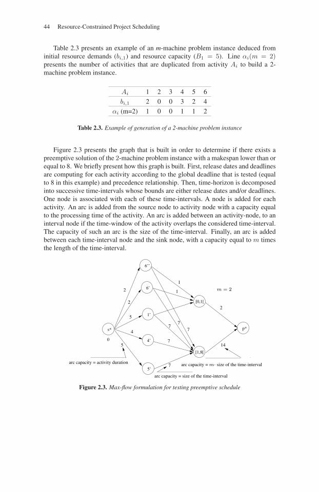
44 Resource-Constrained Project Scheduling
Table 2.3 presents an example of an m-machine problem instance deduced frominitial resource demands (bi,1) and resource capacity (B1 = 5). Line αi(m = 2)presents the number of activities that are duplicated from activity Ai to build a 2-machine problem instance.
Ai 1 2 3 4 5 6
bi,1 2 0 0 3 2 4
αi (m=2) 1 0 0 1 1 2
Table 2.3. Example of generation of a 2-machine problem instance
Figure 2.3 presents the graph that is built in order to determine if there exists apreemptive solution of the 2-machine problem instance with a makespan lower than orequal to 8. We briefly present how this graph is built. First, release dates and deadlinesare computing for each activity according to the global deadline that is tested (equalto 8 in this example) and precedence relationship. Then, time-horizon is decomposedinto successive time-intervals whose bounds are either release dates and/or deadlines.One node is associated with each of these time-intervals. A node is added for eachactivity. An arc is added from the source node to activity node with a capacity equalto the processing time of the activity. An arc is added between an activity-node, to aninterval node if the time-window of the activity overlaps the considered time-interval.The capacity of such an arc is the size of the time-interval. Finally, an arc is addedbetween each time-interval node and the sink node, with a capacity equal to m timesthe length of the time-interval.
4’
1’
6’
s*
5’
[0,1[
[1,8[
p*
6’’
05
m = 2
2
14
2
5
4
2
7
7
77
7
1
1
arc capacity = activity duration arc capacity = m· size of the time-interval
arc capacity = size of the time-interval
Figure 2.3. Max-flow formulation for testing preemptive schedule
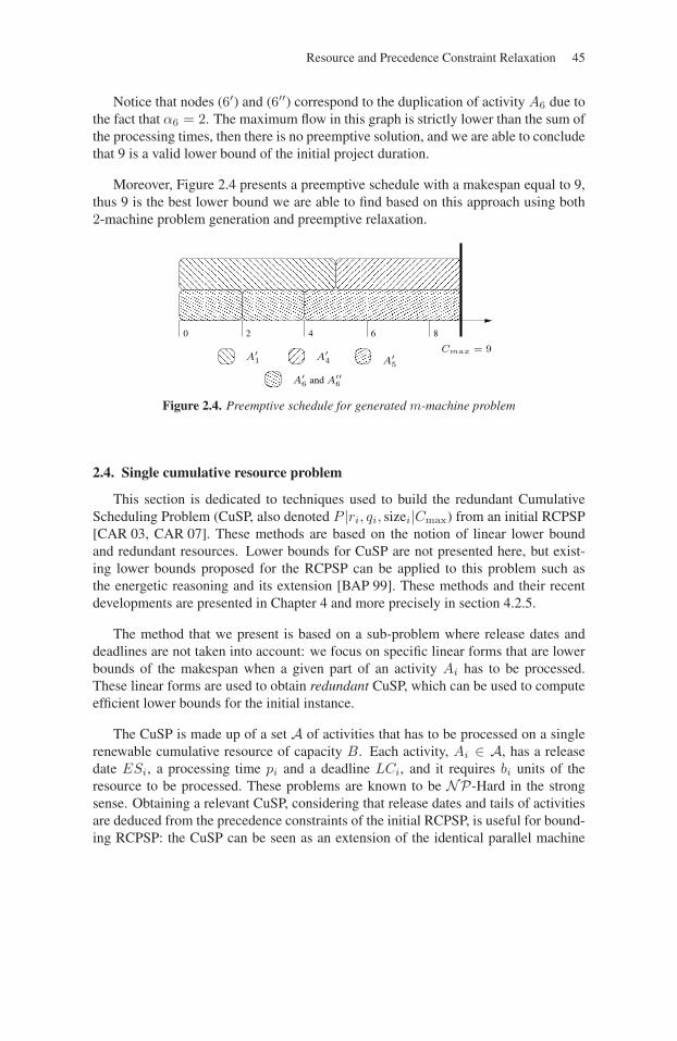
Resource and Precedence Constraint Relaxation 45
Notice that nodes (6′) and (6′′) correspond to the duplication of activity A6 due tothe fact that α6 = 2. The maximum flow in this graph is strictly lower than the sum ofthe processing times, then there is no preemptive solution, and we are able to concludethat 9 is a valid lower bound of the initial project duration.
Moreover, Figure 2.4 presents a preemptive schedule with a makespan equal to 9,thus 9 is the best lower bound we are able to find based on this approach using both2-machine problem generation and preemptive relaxation.
60 2 4 8
A′1 A′
4 A′5
A′6 and A′′
6
Cmax = 9
Figure 2.4. Preemptive schedule for generated m-machine problem
2.4. Single cumulative resource problem
This section is dedicated to techniques used to build the redundant CumulativeScheduling Problem (CuSP, also denoted P |ri, qi, sizei|Cmax) from an initial RCPSP[CAR 03, CAR 07]. These methods are based on the notion of linear lower boundand redundant resources. Lower bounds for CuSP are not presented here, but exist-ing lower bounds proposed for the RCPSP can be applied to this problem such asthe energetic reasoning and its extension [BAP 99]. These methods and their recentdevelopments are presented in Chapter 4 and more precisely in section 4.2.5.
The method that we present is based on a sub-problem where release dates anddeadlines are not taken into account: we focus on specific linear forms that are lowerbounds of the makespan when a given part of an activity Ai has to be processed.These linear forms are used to obtain redundant CuSP, which can be used to computeefficient lower bounds for the initial instance.
The CuSP is made up of a set A of activities that has to be processed on a singlerenewable cumulative resource of capacity B. Each activity, Ai ∈ A, has a releasedate ESi, a processing time pi and a deadline LCi, and it requires bi units of theresource to be processed. These problems are known to be NP-Hard in the strongsense. Obtaining a relevant CuSP, considering that release dates and tails of activitiesare deduced from the precedence constraints of the initial RCPSP, is useful for bound-ing RCPSP: the CuSP can be seen as an extension of the identical parallel machine
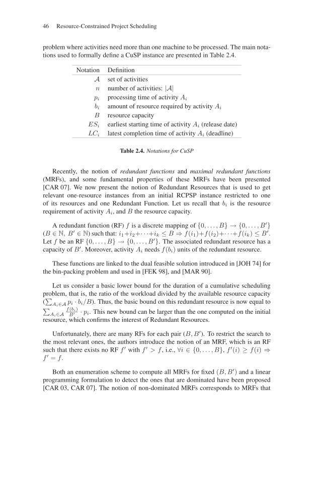
46 Resource-Constrained Project Scheduling
problem where activities need more than one machine to be processed. The main nota-tions used to formally define a CuSP instance are presented in Table 2.4.
Notation DefinitionA set of activitiesn number of activities: |A|pi processing time of activity Ai
bi amount of resource required by activity Ai
B resource capacityESi earliest starting time of activity Ai (release date)LCi latest completion time of activity Ai (deadline)
Table 2.4. Notations for CuSP
Recently, the notion of redundant functions and maximal redundant functions(MRFs), and some fundamental properties of these MRFs have been presented[CAR 07]. We now present the notion of Redundant Resources that is used to getrelevant one-resource instances from an initial RCPSP instance restricted to oneof its resources and one Redundant Function. Let us recall that bi is the resourcerequirement of activity Ai, and B the resource capacity.
A redundant function (RF) f is a discrete mapping of {0, . . . , B} → {0, . . . , B′}(B ∈ N, B′ ∈ N) such that: i1+i2+· · ·+ik ≤ B ⇒ f(i1)+f(i2)+· · ·+f(ik) ≤ B′.Let f be an RF {0, . . . , B} → {0, . . . , B′}. The associated redundant resource has acapacity of B′. Moreover, activity Ai needs f(bi) units of the redundant resource.
These functions are linked to the dual feasible solution introduced in [JOH 74] forthe bin-packing problem and used in [FEK 98], and [MAR 90].
Let us consider a basic lower bound for the duration of a cumulative schedulingproblem, that is, the ratio of the workload divided by the available resource capacity(∑
Ai∈A pi · bi/B). Thus, the basic bound on this redundant resource is now equal to∑Ai∈A
f(bi)B′ · pi. This new bound can be larger than the one computed on the initial
resource, which confirms the interest of Redundant Resources.
Unfortunately, there are many RFs for each pair (B,B′). To restrict the search tothe most relevant ones, the authors introduce the notion of an MRF, which is an RFsuch that there exists no RF f ′ with f ′ > f , i.e., ∀i ∈ {0, . . . , B}, f ′(i) ≥ f(i) ⇒f ′ = f .
Both an enumeration scheme to compute all MRFs for fixed (B,B′) and a linearprogramming formulation to detect the ones that are dominated have been proposed[CAR 03, CAR 07]. The notion of non-dominated MRFs corresponds to MRFs that
Resource and Precedence Constraint Relaxation 47
may lead to interesting lower bounds. The fact that f is a non-dominated MRF corre-sponds to the existence of a set of processing times of activities such that the best lowerbound for these processing times is given by the redundant resource corresponding tof .
The example presented below illustrates how MRFs can be used to compute lowerbounds on the instance presented in Figure 2.2. Table 2.5 presents two MRFs, andthe resource requirements of the activities for the redundant resources which have acapacity equal respectively to 1 and 2.
Aj ∈ A 1 2 3 4 5 6bi,1 2 0 0 3 2 4
f1 : {0, . . . , 5} → {0, 1}, f1(bi,1) 0 0 0 1 0 1f2 : {0, . . . , 5} → {0, 1, 2}, f2(bi,1) 1 0 0 1 1 2
Table 2.5. An example of redundant resources
Figure 2.5 presents an optimal schedule for the redundant resource based on f2.Thus, we are able to conclude that 11 is a valid lower bound of the initial projectduration.
0 2 4 6 8
Cmax = 11A′6A′
5A′4A′
1
10
Figure 2.5. Optimal schedule for redundant resource
2.5. Conclusion and perspectives
In this chapter we have presented how standard scheduling subproblems, namelythe one-machine problem, m-machine problem and CuSP, can be deduced from an ini-tial RCPSP instance. These subproblems are mainly used for computing lower boundsthat are an interesting trade-off between efficiency and computation time. Moreover,recent works have used these subproblems more explicitly, for instance, selecting dis-junctions of deduced one-machine problem in order to speed up the RCPSP resolution.One interesting issue is the use of these subproblem relaxations in heuristic methodssuch as a large neighborhood search: solving exactly and efficiently several subprob-lem instances in order to build a global solution for large size RCPSP instances.

48 Resource-Constrained Project Scheduling
Another research direction is the identification of interesting redundant resourcesfor a given RCPSP instance, i.e., the ones that may lead to tight lower bounds. More-over, these relevant redundant resources may be different during the time-horizon ofthe project, thus introducing redundant resources related to one given time-intervalmay be an interesting research direction. Finally, since redundant resource focuseson each initial resource of the initial RCPSP instance separately, then a promisingresearch direction consists of finding redundant resources that take, as accurately aspossible, at least two resources of the initial RCPSP instance into account.
Chapter 3
Mathematical Programming Formulationsand Lower Bounds
Most of the earliest studies [PRI 69, BAL 70, FIS 73, PAT 76, TAL 78, STI 78]devoted to the RCPSP relate to mathematical programming. Standard branch-and-bound approaches, using a relaxation of a mathematical programming formulation forthe computation of lower bounds, were proposed to solve the RCPSP at optimality.However, modeling the cumulative resource constraints within a mathematical pro-gram requires dealing with a large number of variables or inequalities. Therefore,solving the linear programming relaxation of any model for the RCPSP is too time-consuming – or just impossible – in practice. Branch-and-bound were implementedusing weaker combinatorial relaxations (they are presented in Chapter 2) and yieldedto an optimal solution for only small sized instances. Some research was carried outsince, to optimally solve problems of larger sizes by exploiting less drastic relax-ations. More sophisticated formulations together with suited solution techniques (col-umn generation, Lagrangean relaxation) were proposed, as well as a number of spe-cific valid linear inequalities to tighten the relaxations. Thus, the best lower boundsto date combine column generation and cutting planes with constraint programming-based preprocessing under a destructive approach. Even if, for medium size instances,such bounds require too much time to be computed at each node of a branch-and-bound, they may be particularly helpful to evaluate the quality of practical solutionapproaches such as metaheuristics for the RCPSP. Furthermore, the studies of thesebounds have greatly contributed to a better understanding of the RCPSP and, also, tothe development of combined solution techniques.
Chapter written by Sophie DEMASSEY.
49
50 Resource-Constrained Project Scheduling
In this chapter, we present the main mathematical programming formulations(either binary or mixed integer linear programs) and their relaxations proposed for thebasic RCPSP defined in Chapter 1.
These formulations consist of two main classes regarding the decision variables:sequence-based formulations focus on the ordering the activities are processed in,one compared to another; and time-indexed formulations focus on the assignmentof resources to activities at each time. Sequence-based models are presented in sec-tion 3.1 and time-indexed models are presented in section 3.2.
The mathematical programming approaches for the RCPSP reviewed in this chap-ter join up the numerous studies that have been published on the application of polyhe-dral approaches to scheduling problems. Most studies for the RCPSP derive from pre-vious studies on shop scheduling with disjunctive resources. We refer to the report byQueyanne and Schultz [QUE 94] for a comprehensive synthesis of these approaches.
In order to improve the readability of the formulations and to conform to a com-mon usage in mathematical programming, the notations are simplified in this chapter:activities Ai, Aj and resources Rk are denoted by their indices i, j and k.
3.1. Sequence-based models
Scheduling activities on a resource can be viewed as, first, determining a sequenceof activities satisfying the precedence constraints, and then fixing the processing timesof the activities following the sequence and according to other constraints such asresource availability, set-up times, release and due dates, etc. The sequence-basedmathematical programming formulations reflect this decomposition. They lie on twosets of decision variables: the Boolean linear ordering variables to determine the rel-ative ordering of each pair of activities, and the numerical natural date variables todetermine the processing, e.g. the start or the completion time, of each activity.
Formally, linear ordering variables (xij)(i,j)∈V ×V are defined for each pair ofactivities. Variable xij takes value 1 if activity j starts after the completion of activityi, and 0 otherwise. They are linked with the starting time variables (Si)i∈V as follows:
– i precedes j: xij = 1 ∧ xji = 0 ⇐⇒ Sj ≥ Si + pi
– j precedes i: xij = 0 ∧ xji = 1 ⇐⇒ Si ≥ Sj + pj
– i and j are in parallel: xij = 0 ∧ xji = 0 ⇐⇒ Si − pj < Sj < Si + pi
– xij = 1 ∧ xji = 1 is not allowed (no cycle).
Sequence-based models are often used in the context of shop scheduling with dis-junctive resources. For a problem with a single disjunctive machine and no additionaltemporal constraints, a minimum makespan schedule is uniquely determined by thesequence of the activities, then by the instantiation of the linear ordering variables. In
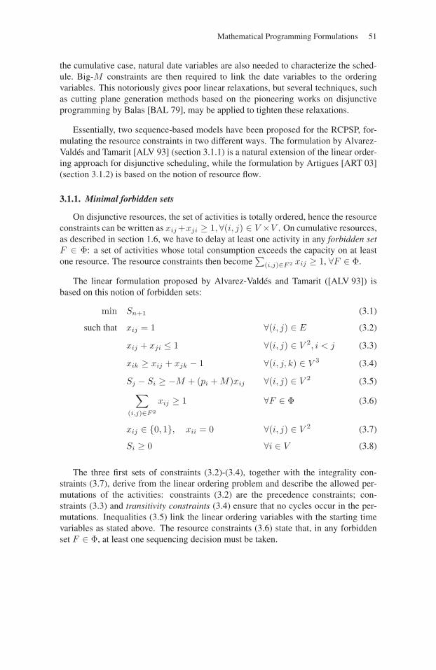
Mathematical Programming Formulations 51
the cumulative case, natural date variables are also needed to characterize the sched-ule. Big-M constraints are then required to link the date variables to the orderingvariables. This notoriously gives poor linear relaxations, but several techniques, suchas cutting plane generation methods based on the pioneering works on disjunctiveprogramming by Balas [BAL 79], may be applied to tighten these relaxations.
Essentially, two sequence-based models have been proposed for the RCPSP, for-mulating the resource constraints in two different ways. The formulation by Alvarez-Valdés and Tamarit [ALV 93] (section 3.1.1) is a natural extension of the linear order-ing approach for disjunctive scheduling, while the formulation by Artigues [ART 03](section 3.1.2) is based on the notion of resource flow.
3.1.1. Minimal forbidden sets
On disjunctive resources, the set of activities is totally ordered, hence the resourceconstraints can be written as xij +xji ≥ 1,∀(i, j) ∈ V ×V . On cumulative resources,as described in section 1.6, we have to delay at least one activity in any forbidden setF ∈ Φ: a set of activities whose total consumption exceeds the capacity on at leastone resource. The resource constraints then become
∑(i,j)∈F 2 xij ≥ 1, ∀F ∈ Φ.
The linear formulation proposed by Alvarez-Valdés and Tamarit ([ALV 93]) isbased on this notion of forbidden sets:
min Sn+1 (3.1)
such that xij = 1 ∀(i, j) ∈ E (3.2)
xij + xji ≤ 1 ∀(i, j) ∈ V 2, i < j (3.3)
xik ≥ xij + xjk − 1 ∀(i, j, k) ∈ V 3 (3.4)
Sj − Si ≥ −M + (pi + M)xij ∀(i, j) ∈ V 2 (3.5)∑(i,j)∈F 2
xij ≥ 1 ∀F ∈ Φ (3.6)
xij ∈ {0, 1}, xii = 0 ∀(i, j) ∈ V 2 (3.7)
Si ≥ 0 ∀i ∈ V (3.8)
The three first sets of constraints (3.2)-(3.4), together with the integrality con-straints (3.7), derive from the linear ordering problem and describe the allowed per-mutations of the activities: constraints (3.2) are the precedence constraints; con-straints (3.3) and transitivity constraints (3.4) ensure that no cycles occur in the per-mutations. Inequalities (3.5) link the linear ordering variables with the starting timevariables as stated above. The resource constraints (3.6) state that, in any forbiddenset F ∈ Φ, at least one sequencing decision must be taken.
52 Resource-Constrained Project Scheduling
Actually, the number of required constraints (3.6) can be restricted by consideringonly the minimal or undominated forbidden sets: a forbidden set F is undominatedif it is (i) minimum for the inclusion relation on (Φ,⊆) and (ii) an antichain for theprecedence relation on V . However, even with this restriction, the number of con-straints (3.6) may remain exponential in the number n of activities. As a consequence,it could be practically impossible to enumerate1 the minimal forbidden sets and thento directly solve the linear programming relaxation of problem (3.1)-(3.8). The pres-ence of big-M constraints (3.5), which make this relaxation weak, is another obviousdrawback of this formulation.
Despite these drawbacks, Demassey et al. [DEM 02a] have obtained tight lowerbounds on the KSD benchmark instances from this linear relaxation. They use a con-straint propagation module as preprocessing, to compute M values as small as possiblein constraints (3.5) and to generate all the minimal forbidden sets of cardinality 2 or3. The other resource constraints (3.6) of the mathematical programming formulationare then relaxed. In addition, many deductions made during the propagation mecha-nism are used in order to tighten the linear relaxation a priori. In fact, the two RCPSPmodels, of constraint programming and of linear programming, are very close: theyboth are based on natural date variables and distance between tasks variables. Somevariable domain reductions of the constraint processing correspond, for example, tothe deduction of new precedence constraints. They directly result in variable fixingor bounding in the mathematical programming formulation. Four families of struc-tural cutting planes for the linear relaxation are also proposed in [DEM 02a]. They arederived by translating redundant constraints deduced by constraint processing. Suchan approach extends prior works on the single machine problem by Balas [BAL 85]and Dyer and Wolsey [DYE 90], and on the job-shop problem by Applegate andCook [APP 91], who proposed effective cutting plane generation procedures for thesequence-based formulations of these problems.
3.1.2. Resource flow
Artigues [ART 03] proposed an alternative formulation of the resource constraintsfor the sequence-based model. The amount of resources in use during the process ofan activity is freed at the end of this process, and becomes available to start anotheractivity. For each resource, this transfer can be formulated as a flow over the activity-on-node precedence network G(V,E) from activity 0 (the source) to activity n + 1(the sink).
1. A pseudo-polynomial algorithm is given in [STO 05] to enumerate all the minimal forbiddensets of a RCPSP (see also sections 1.6 and 7.2).
Mathematical Programming Formulations 53
The mathematical programming formulation is identical to the previous model,except for resource constraints (3.6) that are replaced by the flow inequalities (3.9)-(3.11) of a flow model:∑
j∈V
fkij = bik ∀i ∈ V, ∀k ∈ R (3.9)
∑j∈V
fkji = bik ∀i ∈ V, ∀k ∈ R (3.10)
0 ≤ fkij ≤ min(bik, bjk)xij ∀(i, j) ∈ V 2, ∀k ∈ R (3.11)
Variable fkij gives the amount of resource k transferred from activity i at its com-
pletion, to activity j at its start. By constraints (3.11), this flow value is limited to thecapacity min(bik, bjk) of arc (i, j) if the arc exists (i.e. if i precedes j or xij = 1),and to 0 otherwise. Constraints (3.9) and (3.10) are the usual inequalities of flowconservation (respectively the outgoing flow and the incoming flow on node i). Notethat, in this model, the dummy consumptions b0k and b(n+1)k are fixed to Bk for eachresource k.
Compared to the previous model, this one contains mn2 float variables more, butonly a polynomial number of constraints and it does not require to compute the for-bidden sets at first. Still, this formulation induces many symmetries2 and its linearprogramming relaxation has not been exploited to date. However, this formulationwas applied in several dedicated algorithms relative to robust scheduling. Artiguesand Roubellat [ART 00] considered the problem of activity insertion in an existingschedule (see Algorithm 4). Schwindt [SCH 05] and Neumann et al. [NEU 03] con-sidered a variant of the RCPSP with sequence-dependant setup times and used thismodel as a feasibility test. Lastly, Leus and Herroelen [LEU 04] used the resourceflow as an indicator of the robustness of a schedule regarding the uncertainty of theprocessing times.
3.2. Time-indexed formulations
Many scheduling problem formulations are based on time discretization since theynaturally describe the usage of the resources and the processing of the activities overtime. In these models, we need to fix a planning horizon, denoted by T , which meansthat all jobs have to be completed by time T . Time from 0 to T is then divided intoelementary periods of one unit-length. For each activity j ∈ V and for each timeperiod t ∈ T = {0, . . . , T}, a Boolean variable yjt indicates whether activity j isprocessed at time t. The precise relation between these time-indexed variables andthe processing times of the activities differs sometimes from one model to another.
2. Consider two activities 1 and 2 (1 precedes 2) with consumption 2 on a resource of capacity3, then the two solutions (2, 0, 2, 0, 2) and (2, 1, 1, 1, 2) for vector (f01, f02, f12, f13, f23) areequivalent, i.e. they give the same schedule S1 = 0, S2 = p1, S3 = p1 + p2.
54 Resource-Constrained Project Scheduling
Usually, it is given by one of these 3 possible definitions:
– yjt = 1 if and only if Sj = t (activity j starts at time t);
– yjt = 1 if and only if Sj + pj = t (activity j finishes at time t);
– yjt = 1 if and only if Sj ≤ t (activity j starts before time t).
The resulting models are not significantly different and it is mostly trivial to trans-late a model into another following these definitions. In this section, the time-indexedformulations are given using the first definition above (also the most commonly used).Thus, we have relation:
Sj =T∑
t=0
yjt, for each activity j ∈ V.
Two different time-indexed modeling approaches have been proposed for theRCPSP and, again, the difference comes from the way the resource constraints areformulated. In a first formulation, one linear constraint for each time period is for-mulated to avoid resource conflicts (section 3.2.1). In the other formulation, resourceconflicts are resolved at first, then stipulated as binary variables (section 3.2.2).
3.2.1. Resource conflicts as linear constraints
By means of the time-indexed variables, the set At of activities which are pro-cessed at given time t is entirely characterized:
At =
{j ∈ A |
t+pj−1∑s=t
yjs = 1
}.
To avoid resource conflicts at time t, we have to ensure that, for each resource, thetotal consumption of the activities inAt does not exceed the resource capacity. One ofthe first mathematical programming formulations of the RCPSP was given by Pritskeret al. ([PRI 69]):
min∑t∈T
t · y(n+1)t (3.12)
such thatT∑
t=0
yit = 1 ∀i ∈ V (3.13)
T∑t=0
t · (yjt − yit) ≥ pi ∀(i, j) ∈ E (3.14)
∑i∈V
bik
t∑τ=t−pi+1
yiτ ≤ Bk ∀k ∈ R, ∀t ∈ T (3.15)
yit ∈ {0, 1} ∀i ∈ V, ∀t ∈ T (3.16)
Mathematical Programming Formulations 55
Constraints (3.13) impose that each activity is started exactly one time over theplanning horizon T . Inequalities (3.14) and (3.15) are the precedence and the resourceconstraints, respectively.
The size of this binary integer program grows with the value of the time horizonT and then may be very large. However, a simple preprocessing, computing tighttime-windows for the activities, makes it possible to greatly decrease the number ofvariables: yjt = 0 if t < ESj or t > LSj . The main drawback of this compactformulation is the low quality of the linear programming relaxation, as its solutionsare far from being integral.
In [CHR 87], Christofides et al. restate the precedence constraints (3.14) in a dis-aggregated manner as
T∑τ=t
yiτ +t+pi−1∑
τ=0
yj,τ ≤ 1 ∀(i, j) ∈ E, ∀t ∈ T . (3.17)
Replacing precedence constraints (3.13) by (3.17) makes the mathematical pro-gramming formulation theoretically stronger since inequalities (3.17) and (3.13) to-gether imply (3.14). Uetz [UET 01] shows on a specific instance of the RCPSP that,with disaggregated precedence constraints, the linear programming relaxation pro-vides lower bounds that may be 75% higher. Yet, in practice, the additional compu-tational time needed to solve this larger linear program does not seem to be coun-terbalanced by a significant improvement of the bound (see e.g. [CAV 01, MÖH 03,DEM 02a]).
Families of structural valid inequalities were proposed in [CHR 87, SAN 99,DEM 05] to tighten the time-indexed formulation. Among them, the clique cuts canbe particularly strong and easily identified by analyzing the problem a priori. Oneway of generating clique cuts for the RCPSP is to compute disjunctive subproblems(or redundant single machines, see section 2.2): if C is a set of activities that cannotoverlap in time pairwise, then at most one activity in C is in process at any time t.This statement can be formulated as
∑j∈C
t∑τ=t−pj+1
yjτ ≤ 1 ∀ t ∈ T . (3.18)
This cutting plane procedure is applied in [DEM 05]. In a preprocessing phase,disjunctive subproblems are generated from greedy heuristics and used to run someconstraint propagation techniques such as edge-finding. These algorithms detect newnon-overlapping relationships which help, in turn, to generate new disjunctive sub-problems of larger sizes, providing stronger clique inequalities for the linear program.
56 Resource-Constrained Project Scheduling
Fisher [FIS 73], Christofides et al. [CHR 87] and Möhring et al. [MÖH 03] con-sidered the Lagrangian relaxation of the Pritsker’s formulation, which is obtainedby dualizing resource constraints (3.15). The Lagrangian subproblem with the non-negative multipliers (λkt)k∈R,t∈T is
min∑t∈T
t · y(n+1)t +∑t∈T
∑i∈V
( ∑k∈R
bik
t+pi−1∑τ=t
λkτ
)yit −
∑t∈T
∑k∈R
λktBk
such that (3.13), (3.17), (3.16)
(3.19)
Since the polyhedron defined by inequalities (3.13), (3.17) and y ≥ 0 is integral,the optimum value of the Lagrangian dual is not greater than – and a fortiori it equals– the linear relaxation bound of the disaggregated formulation. Nevertheless, solvingthe Lagrangian dual with an incomplete iterative procedure, e.g. the subgradient algo-rithm, may yield a good approximation (from below) of this value, while, within thesame time, the linear programming relaxation cannot always be solved at all.
The Lagrangian subproblems are instances of the project scheduling problem with-out resource constraints and with start-time dependent costs. The polynomial timecomplexity (the polyhedron is integral) of this problem was first exploited by Möhringet al. [MÖH 03]. In their procedure, each Lagrangian subproblem is reduced to a min-imum cut problem in a directed graph and solved in time O(nmT 2 log(T )). This pro-cedure is a good trade-off between bound quality and computational time. Actually, inthe experiments, the results (bounds and times) are similar to the linear programmingrelaxation of the aggregated solution. However, the procedure has a second purposesince the solutions of the Lagrangian subproblems are used to derive, with small addi-tional efforts, feasible solutions for the RCPSP as well.
The paper by Möhring et al. [MÖH 03] is also a good reference for the compu-tational study of the time-indexed formulation. The quality of the lower bounds andthe computational times are compared for the linear programming relaxations (withaggregated or disaggregated precedence constraints, augmented or not with a familyof clique cuts, solved with the primal simplex or the barrier algorithms, etc.) andfor their own Lagrangian relaxation approach. In Chapter 7, extensive computationalexperiments are carried out to evaluate the quality of the lower bounds obtained bythe time-indexed formulations with and without constraint-propagation-based prepro-cessing.
3.2.2. Feasible configurations
Mingozzi et al. [MIN 98] built their model on the notion of a feasible set of activi-ties. A set φ ⊆ A of activities is a feasible set if all the activities in φ can be processed
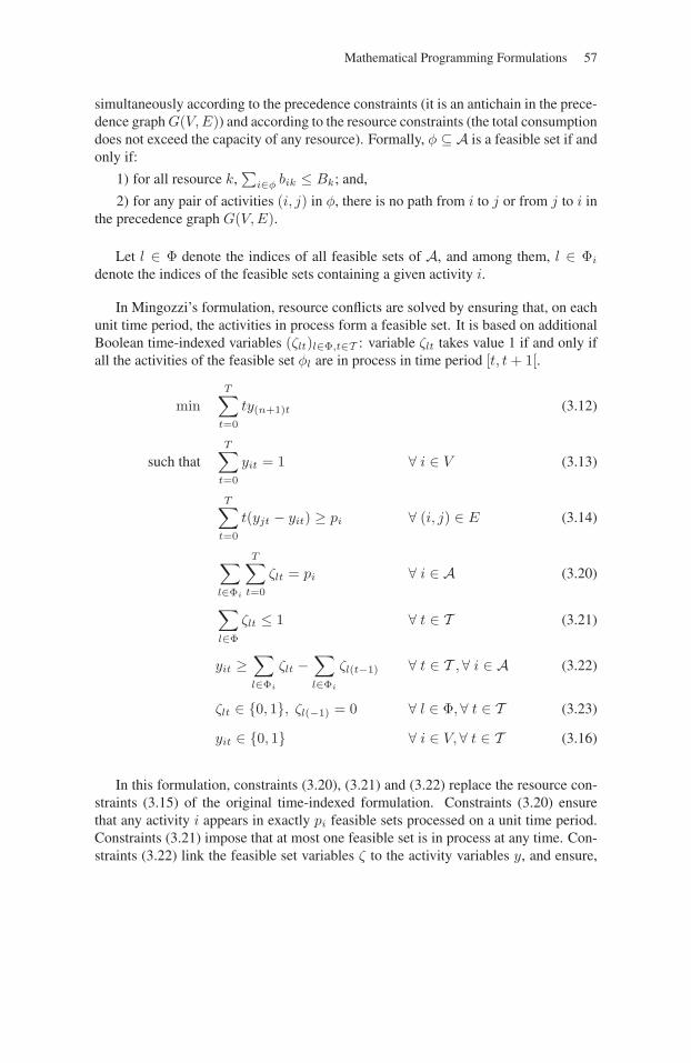
Mathematical Programming Formulations 57
simultaneously according to the precedence constraints (it is an antichain in the prece-dence graph G(V,E)) and according to the resource constraints (the total consumptiondoes not exceed the capacity of any resource). Formally, φ ⊆ A is a feasible set if andonly if:
1) for all resource k,∑
i∈φ bik ≤ Bk; and,
2) for any pair of activities (i, j) in φ, there is no path from i to j or from j to i inthe precedence graph G(V,E).
Let l ∈ Φ denote the indices of all feasible sets of A, and among them, l ∈ Φi
denote the indices of the feasible sets containing a given activity i.
In Mingozzi’s formulation, resource conflicts are solved by ensuring that, on eachunit time period, the activities in process form a feasible set. It is based on additionalBoolean time-indexed variables (ζlt)l∈Φ,t∈T : variable ζlt takes value 1 if and only ifall the activities of the feasible set φl are in process in time period [t, t + 1[.
minT∑
t=0
ty(n+1)t (3.12)
such thatT∑
t=0
yit = 1 ∀ i ∈ V (3.13)
T∑t=0
t(yjt − yit) ≥ pi ∀ (i, j) ∈ E (3.14)
∑l∈Φi
T∑t=0
ζlt = pi ∀ i ∈ A (3.20)
∑l∈Φ
ζlt ≤ 1 ∀ t ∈ T (3.21)
yit ≥∑l∈Φi
ζlt −∑l∈Φi
ζl(t−1) ∀ t ∈ T ,∀ i ∈ A (3.22)
ζlt ∈ {0, 1}, ζl(−1) = 0 ∀ l ∈ Φ,∀ t ∈ T (3.23)
yit ∈ {0, 1} ∀ i ∈ V,∀ t ∈ T (3.16)
In this formulation, constraints (3.20), (3.21) and (3.22) replace the resource con-straints (3.15) of the original time-indexed formulation. Constraints (3.20) ensurethat any activity i appears in exactly pi feasible sets processed on a unit time period.Constraints (3.21) impose that at most one feasible set is in process at any time. Con-straints (3.22) link the feasible set variables ζ to the activity variables y, and ensure,
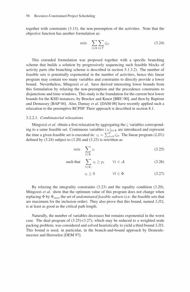
58 Resource-Constrained Project Scheduling
together with constraints (3.13), the non-preemption of the activities. Note that theobjective function has another formulation as:
min∑l∈Φ
∑t∈T
ζlt. (3.24)
This extended formulation was proposed together with a specific branchingscheme that builds a solution by progressively sequencing such feasible blocks ofactivity parts (the branching scheme is described in section 5.1.3.2). The number offeasible sets is potentially exponential in the number of activities, hence this linearprogram may contain too many variables and constraints to directly provide a lowerbound. Nevertheless, Mingozzi et al. have derived interesting lower bounds fromthis formulation by relaxing the non-preemption and the precedence constraints todisjunctions and time-windows. This study is the foundation for the current best lowerbounds for the KSD instances, by Brucker and Knust [BRU 00], and then by Baptisteand Demassey [BAP 04]. Also, Damay et al. [DAM 08] have recently applied such arelaxation to the preemptive RCPSP. Their approach is described in section 8.1.
3.2.2.1. Combinatorial relaxations
Mingozzi et al. obtain a first relaxation by aggregating the ζ variables correspond-ing to a same feasible set. Continuous variables (zl)l∈Φ are introduced and representthe time a given feasible set is executed in: zl =
∑Tt=0 ζlt. The linear program (LB1)
defined by (3.24) subject to (3.20) and (3.23) is rewritten as
min∑l∈Φ
zl (3.25)
such that∑l∈Φi
zl ≥ pi ∀i ∈ A (3.26)
zl ≥ 0 ∀l ∈ Φ (3.27)
By relaxing the integrality constraints (3.23) and the equality condition (3.20),Mingozzi et al. show that the optimum value of this program does not change whenreplacing Φ by Φmax the set of undominated feasible subsets (i.e. the feasible sets thatare maximum for the inclusion order). They also prove that this bound, named LB2,is at least as good as the critical path length.
Naturally, the number of variables decreases but remains exponential in the worstcase. The dual program of (3.25)-(3.27), which may be reduced to a weighted nodepacking problem, was considered and solved heuristically to yield a third bound LB3.This bound is used, in particular, in the branch-and-bound approach by Demeule-meester and Herroelen [DEM 97].
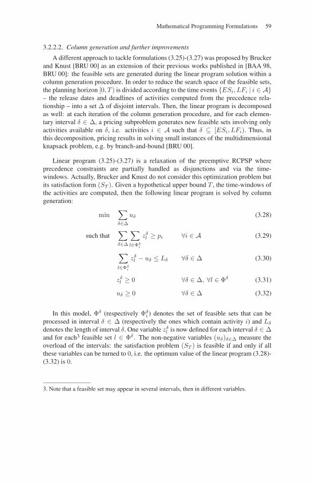
Mathematical Programming Formulations 59
3.2.2.2. Column generation and further improvements
A different approach to tackle formulations (3.25)-(3.27) was proposed by Bruckerand Knust [BRU 00] as an extension of their previous works published in [BAA 98,BRU 00]: the feasible sets are generated during the linear program solution within acolumn generation procedure. In order to reduce the search space of the feasible sets,the planning horizon [0, T ) is divided according to the time events {ESi, LFi | i ∈ A}– the release dates and deadlines of activities computed from the precedence rela-tionship – into a set Δ of disjoint intervals. Then, the linear program is decomposedas well: at each iteration of the column generation procedure, and for each elemen-tary interval δ ∈ Δ, a pricing subproblem generates new feasible sets involving onlyactivities available on δ, i.e. activities i ∈ A such that δ ⊆ [ESi, LFi). Thus, inthis decomposition, pricing results in solving small instances of the multidimensionalknapsack problem, e.g. by branch-and-bound [BRU 00].
Linear program (3.25)-(3.27) is a relaxation of the preemptive RCPSP whereprecedence constraints are partially handled as disjunctions and via the time-windows. Actually, Brucker and Knust do not consider this optimization problem butits satisfaction form (ST ). Given a hypothetical upper bound T , the time-windows ofthe activities are computed, then the following linear program is solved by columngeneration:
min∑δ∈Δ
uδ (3.28)
such that∑δ∈Δ
∑l∈Φδ
i
zδl ≥ pi ∀i ∈ A (3.29)
∑l∈Φδ
i
zδl − uδ ≤ Lδ ∀δ ∈ Δ (3.30)
zδl ≥ 0 ∀δ ∈ Δ, ∀l ∈ Φδ (3.31)
uδ ≥ 0 ∀δ ∈ Δ (3.32)
In this model, Φδ (respectively Φδi ) denotes the set of feasible sets that can be
processed in interval δ ∈ Δ (respectively the ones which contain activity i) and Lδ
denotes the length of interval δ. One variable zδl is now defined for each interval δ ∈ Δ
and for each3 feasible set l ∈ Φδ . The non-negative variables (uδ)δ∈Δ measure theoverload of the intervals: the satisfaction problem (ST ) is feasible if and only if allthese variables can be turned to 0, i.e. the optimum value of the linear program (3.28)-(3.32) is 0.
3. Note that a feasible set may appear in several intervals, then in different variables.
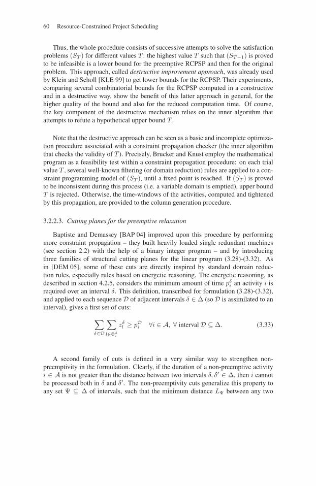
60 Resource-Constrained Project Scheduling
Thus, the whole procedure consists of successive attempts to solve the satisfactionproblems (ST ) for different values T : the highest value T such that (ST−1) is provedto be infeasible is a lower bound for the preemptive RCPSP and then for the originalproblem. This approach, called destructive improvement approach, was already usedby Klein and Scholl [KLE 99] to get lower bounds for the RCPSP. Their experiments,comparing several combinatorial bounds for the RCPSP computed in a constructiveand in a destructive way, show the benefit of this latter approach in general, for thehigher quality of the bound and also for the reduced computation time. Of course,the key component of the destructive mechanism relies on the inner algorithm thatattempts to refute a hypothetical upper bound T .
Note that the destructive approach can be seen as a basic and incomplete optimiza-tion procedure associated with a constraint propagation checker (the inner algorithmthat checks the validity of T ). Precisely, Brucker and Knust employ the mathematicalprogram as a feasibility test within a constraint propagation procedure: on each trialvalue T , several well-known filtering (or domain reduction) rules are applied to a con-straint programming model of (ST ), until a fixed point is reached. If (ST ) is provedto be inconsistent during this process (i.e. a variable domain is emptied), upper boundT is rejected. Otherwise, the time-windows of the activities, computed and tightenedby this propagation, are provided to the column generation procedure.
3.2.2.3. Cutting planes for the preemptive relaxation
Baptiste and Demassey [BAP 04] improved upon this procedure by performingmore constraint propagation – they built heavily loaded single redundant machines(see section 2.2) with the help of a binary integer program – and by introducingthree families of structural cutting planes for the linear program (3.28)-(3.32). Asin [DEM 05], some of these cuts are directly inspired by standard domain reduc-tion rules, especially rules based on energetic reasoning. The energetic reasoning, asdescribed in section 4.2.5, considers the minimum amount of time pδ
i an activity i isrequired over an interval δ. This definition, transcribed for formulation (3.28)-(3.32),and applied to each sequence D of adjacent intervals δ ∈ Δ (so D is assimilated to aninterval), gives a first set of cuts:
∑δ∈D
∑l∈Φδ
i
zδl ≥ pDi ∀i ∈ A, ∀ interval D ⊆ Δ. (3.33)
A second family of cuts is defined in a very similar way to strengthen non-preemptivity in the formulation. Clearly, if the duration of a non-preemptive activityi ∈ A is not greater than the distance between two intervals δ, δ′ ∈ Δ, then i cannotbe processed both in δ and δ′. The non-preemptivity cuts generalize this property toany set Ψ ⊆ Δ of intervals, such that the minimum distance LΨ between any two
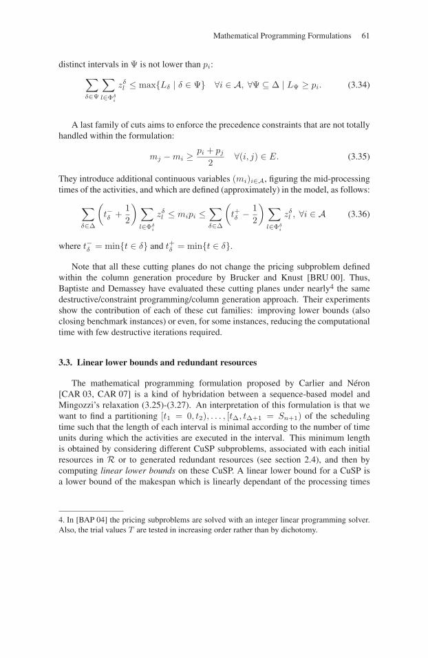
Mathematical Programming Formulations 61
distinct intervals in Ψ is not lower than pi:∑δ∈Ψ
∑l∈Φδ
i
zδl ≤ max{Lδ | δ ∈ Ψ} ∀i ∈ A, ∀Ψ ⊆ Δ | LΨ ≥ pi. (3.34)
A last family of cuts aims to enforce the precedence constraints that are not totallyhandled within the formulation:
mj −mi ≥pi + pj
2∀(i, j) ∈ E. (3.35)
They introduce additional continuous variables (mi)i∈A, figuring the mid-processingtimes of the activities, and which are defined (approximately) in the model, as follows:
∑δ∈Δ
(t−δ +
12
) ∑l∈Φδ
i
zδl ≤ mipi ≤
∑δ∈Δ
(t+δ −
12
) ∑l∈Φδ
i
zδl , ∀i ∈ A (3.36)
where t−δ = min{t ∈ δ} and t+δ = min{t ∈ δ}.
Note that all these cutting planes do not change the pricing subproblem definedwithin the column generation procedure by Brucker and Knust [BRU 00]. Thus,Baptiste and Demassey have evaluated these cutting planes under nearly4 the samedestructive/constraint programming/column generation approach. Their experimentsshow the contribution of each of these cut families: improving lower bounds (alsoclosing benchmark instances) or even, for some instances, reducing the computationaltime with few destructive iterations required.
3.3. Linear lower bounds and redundant resources
The mathematical programming formulation proposed by Carlier and Néron[CAR 03, CAR 07] is a kind of hybridation between a sequence-based model andMingozzi’s relaxation (3.25)-(3.27). An interpretation of this formulation is that wewant to find a partitioning [t1 = 0, t2), . . . , [tΔ, tΔ+1 = Sn+1) of the schedulingtime such that the length of each interval is minimal according to the number of timeunits during which the activities are executed in the interval. This minimum lengthis obtained by considering different CuSP subproblems, associated with each initialresources in R or to generated redundant resources (see section 2.4), and then bycomputing linear lower bounds on these CuSP. A linear lower bound for a CuSP isa lower bound of the makespan which is linearly dependant of the processing times
4. In [BAP 04] the pricing subproblems are solved with an integer linear programming solver.Also, the trial values T are tested in increasing order rather than by dichotomy.
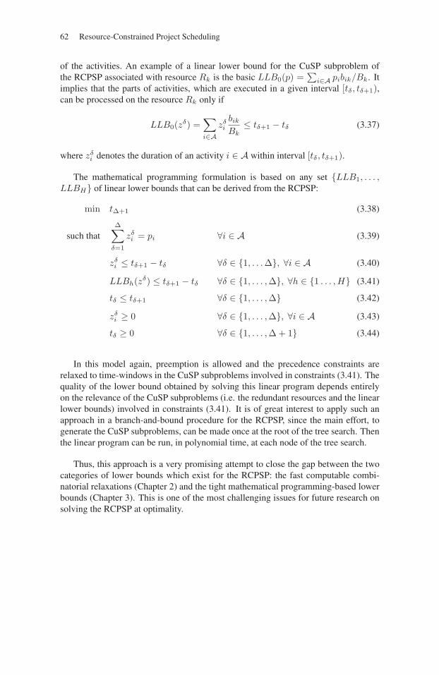
62 Resource-Constrained Project Scheduling
of the activities. An example of a linear lower bound for the CuSP subproblem ofthe RCPSP associated with resource Rk is the basic LLB0(p) =
∑i∈A pibik/Bk. It
implies that the parts of activities, which are executed in a given interval [tδ, tδ+1),can be processed on the resource Rk only if
LLB0(zδ) =∑i∈A
zδi
bik
Bk≤ tδ+1 − tδ (3.37)
where zδi denotes the duration of an activity i ∈ A within interval [tδ, tδ+1).
The mathematical programming formulation is based on any set {LLB1, . . . ,LLBH} of linear lower bounds that can be derived from the RCPSP:
min tΔ+1 (3.38)
such thatΔ∑
δ=1
zδi = pi ∀i ∈ A (3.39)
zδi ≤ tδ+1 − tδ ∀δ ∈ {1, . . . Δ}, ∀i ∈ A (3.40)
LLBh(zδ) ≤ tδ+1 − tδ ∀δ ∈ {1, . . . ,Δ}, ∀h ∈ {1 . . . , H} (3.41)
tδ ≤ tδ+1 ∀δ ∈ {1, . . . ,Δ} (3.42)
zδi ≥ 0 ∀δ ∈ {1, . . . ,Δ}, ∀i ∈ A (3.43)
tδ ≥ 0 ∀δ ∈ {1, . . . ,Δ + 1} (3.44)
In this model again, preemption is allowed and the precedence constraints arerelaxed to time-windows in the CuSP subproblems involved in constraints (3.41). Thequality of the lower bound obtained by solving this linear program depends entirelyon the relevance of the CuSP subproblems (i.e. the redundant resources and the linearlower bounds) involved in constraints (3.41). It is of great interest to apply such anapproach in a branch-and-bound procedure for the RCPSP, since the main effort, togenerate the CuSP subproblems, can be made once at the root of the tree search. Thenthe linear program can be run, in polynomial time, at each node of the tree search.
Thus, this approach is a very promising attempt to close the gap between the twocategories of lower bounds which exist for the RCPSP: the fast computable combi-natorial relaxations (Chapter 2) and the tight mathematical programming-based lowerbounds (Chapter 3). This is one of the most challenging issues for future research onsolving the RCPSP at optimality.
Chapter 4
Constraint Programming Formulationsand Propagation Algorithms
This chapter presents the classical representation of RCPSP in constraint-basedscheduling as well as the propagation algorithms for temporal constraints and resourcecapacity constraints (timetabling, disjunctive reasoning, edge-finding, energetic rea-soning, precedence energy and balance) used to solve the RCPSP through constraint-based scheduling.
4.1. Constraint formulations
4.1.1. Constraint programming
Constraint programming (CP) is based on a declarative description of a problem as(1) a set of decision variables with domains, i.e., sets of possible values, for instancethe start time of an activity with its possible time-windows; and (2) a set of constraintsrestricting the combinations of values the decision variables can take, for instance aprecedence constraint between the end time of activity A and the start time of activityB.
Constraints can be defined either explicitly as a set of compatible tuples of variableassignments or implicitly, for instance through an algebraic relation (e.g. x �= y). Asolution to a CP problem is a complete assignment of the variables satisfying all theconstraints.
Chapter written by Philippe LABORIE and Wim NUIJTEN.
63
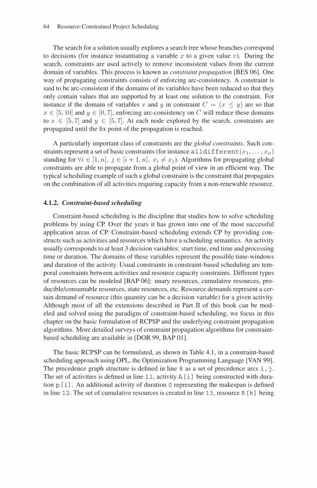
64 Resource-Constrained Project Scheduling
The search for a solution usually explores a search tree whose branches correspondto decisions (for instance instantiating a variable x to a given value v). During thesearch, constraints are used actively to remove inconsistent values from the currentdomain of variables. This process is known as constraint propagation [BES 06]. Oneway of propagating constraints consists of enforcing arc-consistency. A constraint issaid to be arc-consistent if the domains of its variables have been reduced so that theyonly contain values that are supported by at least one solution to the constraint. Forinstance if the domain of variables x and y in constraint C = (x ≤ y) are so thatx ∈ [5, 10] and y ∈ [0, 7], enforcing arc-consistency on C will reduce these domainsto x ∈ [5, 7] and y ∈ [5, 7]. At each node explored by the search, constraints arepropagated until the fix point of the propagation is reached.
A particularly important class of constraints are the global constraints. Such con-straints represent a set of basic constraints (for instance alldifferent(x1, . . . , xn)standing for ∀i ∈ [1, n], j ∈ [i + 1, n], xi �= xj). Algorithms for propagating globalconstraints are able to propagate from a global point of view in an efficient way. Thetypical scheduling example of such a global constraint is the constraint that propagateson the combination of all activities requiring capacity from a non-renewable resource.
4.1.2. Constraint-based scheduling
Constraint-based scheduling is the discipline that studies how to solve schedulingproblems by using CP. Over the years it has grown into one of the most successfulapplication areas of CP. Constraint-based scheduling extends CP by providing con-structs such as activities and resources which have a scheduling semantics. An activityusually corresponds to at least 3 decision variables: start time, end time and processingtime or duration. The domains of these variables represent the possible time-windowsand duration of the activity. Usual constraints in constraint-based scheduling are tem-poral constraints between activities and resource capacity constraints. Different typesof resources can be modeled [BAP 06]: unary resources, cumulative resources, pro-ducible/consumable resources, state resources, etc. Resource demands represent a cer-tain demand of resource (this quantity can be a decision variable) for a given activity.Although most of all the extensions described in Part II of this book can be mod-eled and solved using the paradigm of constraint-based scheduling, we focus in thischapter on the basic formulation of RCPSP and the underlying constraint propagationalgorithms. More detailed surveys of constraint propagation algorithms for constraint-based scheduling are available in [DOR 99, BAP 01].
The basic RCPSP can be formulated, as shown in Table 4.1, in a constraint-basedscheduling approach using OPL, the Optimization Programming Language [VAN 99].The precedence graph structure is defined in line 8 as a set of precedence arcs i,j.The set of activities is defined in line 11, activity A[i] being constructed with dura-tion p[i]. An additional activity of duration 0 representing the makespan is definedin line 12. The set of cumulative resources is created in line 13, resource R[k] being
Constraint Programming Formulations and Propagation Algorithms 65
of capacity B[k]. Discrete resources post a global capacity constraint on the set ofactivities that require the resource. The objective function (minimize end time ofmakespan activity) is specified in line 14 followed by the constraints of the problem.Each activity A[i] is constrained to finish before the makespan activity (line 17)and to require b[i][k] units of resource R[k] in line 19. Finally, the precedenceconstraints of the precedence graph G are posted in line 22.
1 // Data2 struct Precedence { int i; int j; };3 int q = ...; // Number of resources4 int n = ...; // Number of activities5 int p[1..n] = ...; // Processing times6 int B[1..q] = ...; // Resource capacities7 int b[1..n,1..q] = ...; // Resource requirements8 {Precedence} G = ...; // Precedence graph9
10 // Model11 Activity A[i in 1..n](p[i]);12 Activity makespan(0);13 DiscreteResource R[k in 1..q](B[k]);14 minimize makespan.end15 subject to {16 forall(i in 1..n) {17 A[i] precedes makespan;18 forall(k in 1..q : 0 < b[i][k])19 A[i] requires(b[i][k]) R[k];20 };21 forall(<i,j> in G)22 A[i] precedes A[j];23 };
Table 4.1. An OPL model of the basic RCPSP
The next section describes the principles of the classical algorithms for propagat-ing temporal constraints (section 4.2.1) and resource constraints (sections 4.2.2-4.2.8).
4.2. Constraint propagation algorithms
4.2.1. Temporal constraints
Temporal relations between activities can be expressed by linear constraintsbetween start and end variables of activities. For instance, a standard precedence
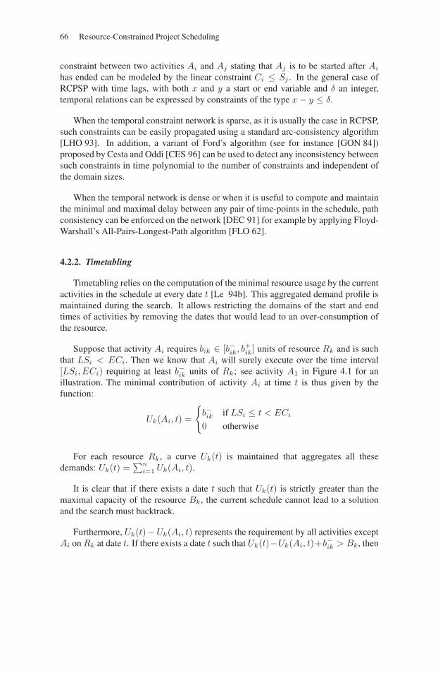
66 Resource-Constrained Project Scheduling
constraint between two activities Ai and Aj stating that Aj is to be started after Ai
has ended can be modeled by the linear constraint Ci ≤ Sj . In the general case ofRCPSP with time lags, with both x and y a start or end variable and δ an integer,temporal relations can be expressed by constraints of the type x− y ≤ δ.
When the temporal constraint network is sparse, as it is usually the case in RCPSP,such constraints can be easily propagated using a standard arc-consistency algorithm[LHO 93]. In addition, a variant of Ford’s algorithm (see for instance [GON 84])proposed by Cesta and Oddi [CES 96] can be used to detect any inconsistency betweensuch constraints in time polynomial to the number of constraints and independent ofthe domain sizes.
When the temporal network is dense or when it is useful to compute and maintainthe minimal and maximal delay between any pair of time-points in the schedule, pathconsistency can be enforced on the network [DEC 91] for example by applying Floyd-Warshall’s All-Pairs-Longest-Path algorithm [FLO 62].
4.2.2. Timetabling
Timetabling relies on the computation of the minimal resource usage by the currentactivities in the schedule at every date t [Le 94b]. This aggregated demand profile ismaintained during the search. It allows restricting the domains of the start and endtimes of activities by removing the dates that would lead to an over-consumption ofthe resource.
Suppose that activity Ai requires bik ∈ [b−ik, b+ik] units of resource Rk and is such
that LSi < ECi. Then we know that Ai will surely execute over the time interval[LSi, ECi) requiring at least b−ik units of Rk; see activity A1 in Figure 4.1 for anillustration. The minimal contribution of activity Ai at time t is thus given by thefunction:
Uk(Ai, t) =
{b−ik if LSi ≤ t < ECi
0 otherwise
For each resource Rk, a curve Uk(t) is maintained that aggregates all thesedemands: Uk(t) =
∑ni=1 Uk(Ai, t).
It is clear that if there exists a date t such that Uk(t) is strictly greater than themaximal capacity of the resource Bk, the current schedule cannot lead to a solutionand the search must backtrack.
Furthermore, Uk(t)−Uk(Ai, t) represents the requirement by all activities exceptAi on Rk at date t. If there exists a date t such that Uk(t)−Uk(Ai, t)+b−ik > Bk, then
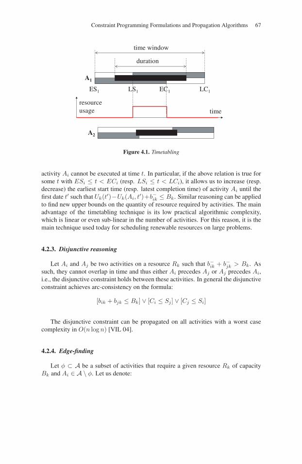
Constraint Programming Formulations and Propagation Algorithms 67
time window
duration
resourceusage time
A1
ES1 LS1 EC1 LC1
A2
Figure 4.1. Timetabling
activity Ai cannot be executed at time t. In particular, if the above relation is true forsome t with ESi ≤ t < ECi (resp. LSi ≤ t < LCi), it allows us to increase (resp.decrease) the earliest start time (resp. latest completion time) of activity Ai until thefirst date t′ such that Uk(t′)−Uk(Ai, t
′)+b−ik ≤ Bk. Similar reasoning can be appliedto find new upper bounds on the quantity of resource required by activities. The mainadvantage of the timetabling technique is its low practical algorithmic complexity,which is linear or even sub-linear in the number of activities. For this reason, it is themain technique used today for scheduling renewable resources on large problems.
4.2.3. Disjunctive reasoning
Let Ai and Aj be two activities on a resource Rk such that b−ik + b−jk > Bk. Assuch, they cannot overlap in time and thus either Ai precedes Aj or Aj precedes Ai,i.e., the disjunctive constraint holds between these activities. In general the disjunctiveconstraint achieves arc-consistency on the formula:
[bik + bjk ≤ Bk] ∨ [Ci ≤ Sj ] ∨ [Cj ≤ Si]
The disjunctive constraint can be propagated on all activities with a worst casecomplexity in O(n log n) [VIL 04].
4.2.4. Edge-finding
Let φ ⊂ A be a subset of activities that require a given resource Rk of capacityBk and Ai ∈ A \ φ. Let us denote:
68 Resource-Constrained Project Scheduling
– ESφ = minAj∈φ ESj , the earliest start time of all activities in φ;
– ECφ = minAj∈φ ECj , the earliest completion time of all activities in φ;
– LCφ = maxAj∈φ LCj , the latest completion time of all activities in φ;
– Wφ =∑
Aj∈φ pj · bjk, the global energy required by φ.
The basic idea of edge-finding and activity interval techniques is to ensure that forany subset of activities φ, resource Rk provides enough energy over the time interval[ESφ, LCφ) to allow the execution of all the activities of φ, that is: Wφ ≤ Bk ·(LCφ−ESφ). Constraint propagation is usually performed by applying the three followingdeduction rules:
1) If Bk · (LCφ−ESφ∪{i}) < Wφ∪{Ai}, then Ai must finish after all activities inφ, in particular ECi := max(ECi, ECφ).
2) If ESφ < ESi < ECφ and Bk ·(LCφ−ESφ) < Wφ+bik ·(min(LCφ, ECi)−ESi), then at least one activity Aj in φ must precede Ai, otherwise Ai would startbetween ESφ and ECφ and there would not be enough energy to execute φ ∪ {Ai}between ESφ and LCφ, thus ESi := max(ESi, ECφ).
3) If ESi < ESφ < ECi and Bk · (LCφ − ESφ) < Wφ + bik · (ECi − ESφ),then Ai must finish after all activities in φ, in particular ECi := max(ECi, ECφ).
These rules make it possible to update the earliest start or completion times ofactivities and symmetrical rules allow us to update the latest start and completiontimes. Edge-finding ([NUI 94]) and activity intervals propagation ([CAS 96]) are verysimilar techniques that mainly differ in the way the propagation rules are triggered:edge-finding algorithms are global algorithms that perform all updates on a givenresource whereas activity interval approaches are performed incrementally as soonas the time bound of a activity changes.
Note that specific edge-finding algorithms have been designed for the special caseof disjunctive resources (Bk = 1) [BAP 01]. These algorithms can be implementedwith a time complexity in O(n log n) [VIL 04].
4.2.5. Energy reasoning
Energy-based constraint propagation algorithms compare the amount of energyprovided by a resource over some interval [t1, t2) to the amount of energy requiredby activities that have to be processed over this interval. [ERS 91] proposes the fol-lowing definition of the required energy consumption that takes into account the factthat activities cannot be interrupted. Given a resource Rk, an activity Ai and a timeinterval [t1, t2),Wk(Ai, t1, t2), the left shift/right shift required energy consumptionof resource Rk by activity Ai over [t1, t2) is bik times the minimum of the three fol-lowing durations:
Constraint Programming Formulations and Propagation Algorithms 69
– the length of the interval: t2 − t1;
– the number of time units during which Ai executes after time t1 if Ai is leftshifted, i.e., scheduled as soon as possible: pL
i (t1) = max(0, pi−max(0, t1−ESi));– the number of time units during which Ai executes before time t2 if Ai is right
shifted, i.e., scheduled as late as possible: pRi (t2) = max(0, pi −max(0, LCi − t2)).
This leads to Wk(Ai, t1, t2) = bik ·min(t2 − t1, pLi (t1), pR
i (t2)).
The left shift/right shift overall required energy consumption Wk(t1, t2) over aninterval [t1, t2) is then defined as the sum over all activities Ai of Wk(Ai, t1, t2).
It is obvious that if there is a feasible schedule, then Bk ·(t2−t1)−Wk(t1, t2) ≥ 0for all t1 and t2 such that t2 ≥ t1.
It is shown in [BAP 01] how the values of Wk can be used to adjust activity timebounds. Given an activity Ai and a time interval [t1, t2) with t2 < LCi, it is examinedwhether Ai can end before t2. If there is a time interval [t1, t2) such that
Wk(t1, t2)−Wk(Ai, t1, t2) + bik · pLi (t1) > Bk · (t2 − t1),
then a valid lower bound of the end time of Ai is
t2 +1
bik(Wk(t1, t2)−Wk(Ai, t1, t2) + bik · pL
i (t1)−Bk · (t2 − t1)).
Similarly, when
Wk(t1, t2)−Wk(Ai, t1, t2) + bik ·min(t2 − t1, pLi (t1)) > Bk · (t2 − t1),
Ai cannot start before t1 and a valid lower bound of the start time of Ai is
t2 −1
bik(C(t2 − t1)−Wk(t1, t2) + Wk(Ai, t1, t2)).
[BAP 01] presents a O(n3) algorithm to compute these time bound adjustmentsfor all n activities. It is first shown there are O(n2) intervals [t1, t2) of interest. Givenan interval and an activity, the adjustment procedure runs in O(1). As such, the obvi-ous overall complexity of the algorithm is thus O(n3). An interesting open questionis whether there is a quadratic algorithm to compute all the adjustments on the O(n2)intervals under consideration. Another open question at this point is whether the char-acterization of the O(n2) time intervals in [BAP 01] can be sharpened in order toeliminate some intervals and reduce the practical complexity of the correspondingalgorithm. Finally, it seems reasonable to think that the time bound adjustments couldbe sharpened. Even though the energy tests can be limited (without any loss) to agiven set of intervals, it could be that the corresponding adjustment rules cannot.
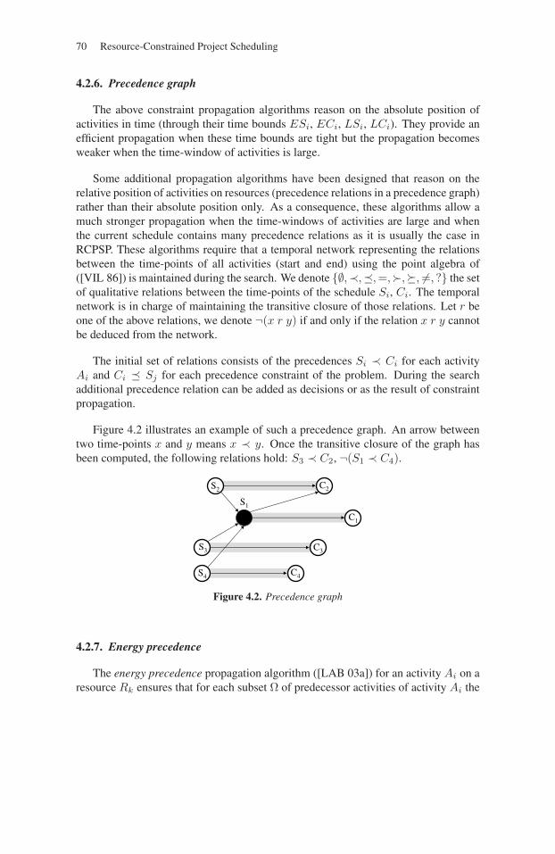
70 Resource-Constrained Project Scheduling
4.2.6. Precedence graph
The above constraint propagation algorithms reason on the absolute position ofactivities in time (through their time bounds ESi, ECi, LSi, LCi). They provide anefficient propagation when these time bounds are tight but the propagation becomesweaker when the time-window of activities is large.
Some additional propagation algorithms have been designed that reason on therelative position of activities on resources (precedence relations in a precedence graph)rather than their absolute position only. As a consequence, these algorithms allow amuch stronger propagation when the time-windows of activities are large and whenthe current schedule contains many precedence relations as it is usually the case inRCPSP. These algorithms require that a temporal network representing the relationsbetween the time-points of all activities (start and end) using the point algebra of([VIL 86]) is maintained during the search. We denote {∅,≺,�,=,�,�, �=, ?} the setof qualitative relations between the time-points of the schedule Si, Ci. The temporalnetwork is in charge of maintaining the transitive closure of those relations. Let r beone of the above relations, we denote ¬(x r y) if and only if the relation x r y cannotbe deduced from the network.
The initial set of relations consists of the precedences Si ≺ Ci for each activityAi and Ci � Sj for each precedence constraint of the problem. During the searchadditional precedence relation can be added as decisions or as the result of constraintpropagation.
Figure 4.2 illustrates an example of such a precedence graph. An arrow betweentwo time-points x and y means x ≺ y. Once the transitive closure of the graph hasbeen computed, the following relations hold: S3 ≺ C2, ¬(S1 ≺ C4).
S2
S1
S3
S4 C4
C3
C1
C2
Figure 4.2. Precedence graph
4.2.7. Energy precedence
The energy precedence propagation algorithm ([LAB 03a]) for an activity Ai on aresource Rk ensures that for each subset Ω of predecessor activities of activity Ai the
Constraint Programming Formulations and Propagation Algorithms 71
resource provides enough energy to execute all activities in Ω between ESΩ and Si.More formally, if ESΩ = minAj∈Ω ESj and WΩ,k =
∑Aj∈Ω pj · bik, it performs the
following deduction rule:
∀Ω ⊂ {Aj ∈ A, Cj � Si}, ESi := max(ESi, ESΩ + �WΩ,k/Bk�)
The propagation of the energy precedence constraint can be performed for all theactivities Ai on a resource and for all the subsets Ω with a total worst-case time com-plexity of O(n(p + log(n))), where n is the number of activities on the resource andp the maximal number of predecessors of a given activity in the temporal network(p < n).
4.2.8. Balance constraint
On a renewable resource, the balance constraint ([LAB 03a]) can be defined asfollows. The basic idea of the algorithm is to compute, for each activity Ai on aresource Rk, a lower bound on the resource usage at the start time of Ai (a symmetricalreasoning can be applied to perform some propagation based on a lower bound on theresource usage at the completion time of Ai). Using the temporal network a lowerbound on the resource utilization at date Si + ε just after the start time of Ai can becomputed assuming that all the resource requirements that do not necessarily overlapSi will not overlap it:
Lk(i) =∑
j/(Sj�Si)∧(Cj�Si)
bjk
Given this bound, the balance constraint is able to discover three types of informa-tion:
Dead ends. Whenever Lk(i) > Bk, the resource will surely be over-consumedjust after time-point Si so the search has reached a dead end.
New bounds on time variables. If LK(i) ≤ Bk, Δ(i) = Bk − LK(i) representsa slack of capacity that must not be exceeded by all the resource requirements that,currently, do not necessarily overlap Si but could overlap it. Let P (i) = {Aj/(Sj �Si) ∧ ¬(Cj � Si)}. We suppose the activities (Aj1 , . . . , Aju
, . . . , Ajp) in P (i) are
ordered by decreasing earliest completion time ECj . Let v be the index in [1, p] suchthat:
v−1∑u=1
bjuk ≤ Δ(x) <
v∑u=1
bjuk
If event Si is executed at a date Si < ECjv, not enough activities of P (i) will
be able to be completed strictly before Si in order to ensure the resource is not over-consumed just after Si as in this case, the consumed quantity will be at least LK(i) +∑v
u=1 bjuk > Bk. Thus, ECjvis a valid lower bound of Si.

72 Resource-Constrained Project Scheduling
New precedence relations. Suppose there exists activity Ay in P (i) such that:∑Az∈P (i),CzCy
bzk > Δ(x)
Then, if we had Si ≺ Cy , we would see that again there is no way to avoid aresource over-consumption as it would consume at least:
Lk(i) +∑
Az∈P (i),CzCy
bzk > Bk
Thus, the necessary precedence relation: Cy � Si can be deduced and added tothe current temporal network.
On the precedence graph of Figure 4.2, if all activities require 1 unit of the sameresource Rk of capacity 3, the balance constraint applied at time-point S1 would com-pute Lk(1) = b1k + b2k = 2 and deduce that min(EC3, EC4) ≤ S1.
The balance algorithm can be executed for all activities Ai with a global worst-case complexity in O(n2) if the propagation that discovers new precedence relationsis not turned on and in O(n3) for a full propagation. In practice, there are many ways toshortcut this worst case and in particular, it was noticed that the algorithmic cost of theextra-propagation that discovers new precedence relations was in general negligible.
4.3. Conclusion
Constraint-based scheduling provides a wide spectrum of propagation algorithmsfor renewable resources ranging from sub-linear to quadratic time complexities. Theselection of a combination of propagation algorithms clearly depends on the size ofthe problem being solved.
For small problems, up to a few tens of renewable resources and a few hundredactivities on each resource, a strong propagation scheme may be used. This is forinstance the case of the MCS method described in section 7.6 and experimented onsmall RCPSPs. It uses a combination of timetabling, disjunctive, edge-finding, energyprecedence and balance constraints.
Larger problems are generally solved using meta-heuristics. These methods, forinstance the LNS described in section 7.6, are usually less sensitive to constraint prop-agation than tree search methods and light propagation schemes can be used, typically,only using timetabling.
Chapter 5
Branching Schemes for Branch-and-Bound
In this chapter we present exact methods for solving the RCPSP, restrictingourselves to branch-and-bound methods. Linear programming based methods aredescribed in Chapter 3. Constraint Programming (CP) methods are close to the onesthat are presented in this section. For instance, many CP filtering methods used toadjust time-bounds of activities are used in branch-and-bound methods. Moreover inthis chapter, only branching schemes are presented: lower bounds, upper bounds andfiltering methods are respectively described in Chapters 2, 6 and 4.
Notice that exact methods, of course, are used to obtain an exact solution to theRCPSP but they are also helpful in obtaining efficient heuristic solutions. A searchtree can be truncated in order to limit the search to promising solutions, and recentlythey were also used as a part of a heuristic based on a large neighborhood search.
Branch-and-bound methods build a search tree in order to explore implicitly thesearch space. At each node of the search tree, two situations may occur: (1) a leaf nodeis reached and a feasible solution can be deduced, (2) after computing lower bounds,upper bounds and possibly time-bound adjustments, the search space correspondingto the current node is partitioned into subsets such that the union of these subsetscorresponds to the set of solutions of the current node. This operation of partitioningan area of the search space into sub-areas is called branching (see Figure 5.1).
Building a search tree that efficiently explores all relevant solutions is a challeng-ing problem. From the earliest works on the RCPSP [JOH 67], many authors haveproposed several branching schemes. Most of the time, linked to branching schemes,
Chapter written by Emmanuel NÉRON.
73
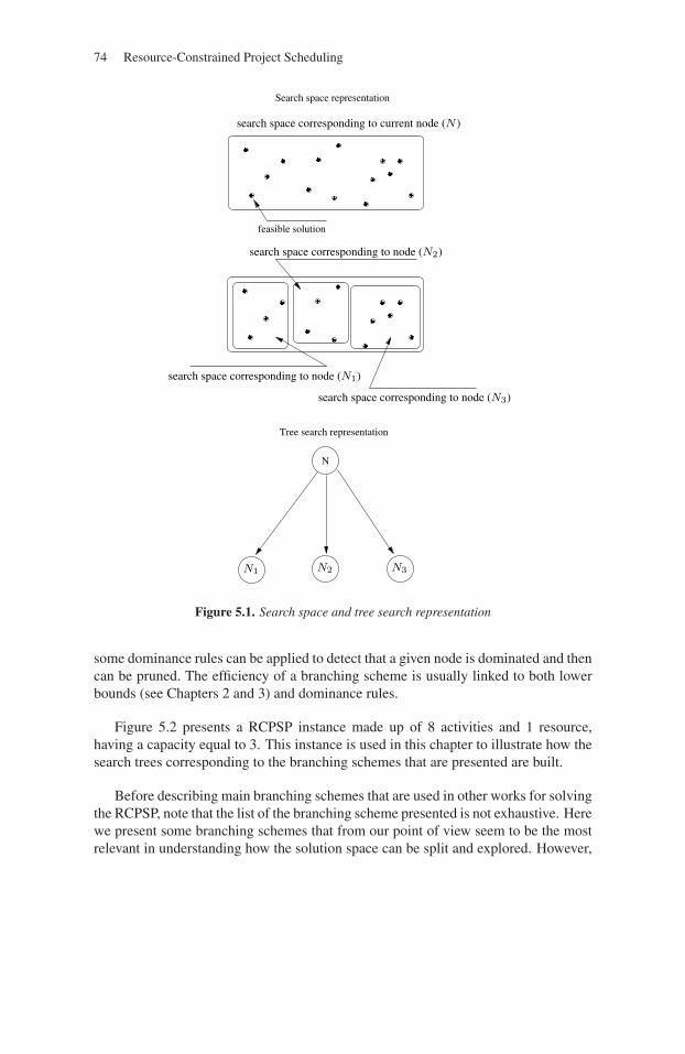
74 Resource-Constrained Project Scheduling
N
feasible solution
Search space representation
Tree search representation
search space corresponding to node (N3)
N1 N2 N3
search space corresponding to current node (N )
search space corresponding to node (N2)
search space corresponding to node (N1)
Figure 5.1. Search space and tree search representation
some dominance rules can be applied to detect that a given node is dominated and thencan be pruned. The efficiency of a branching scheme is usually linked to both lowerbounds (see Chapters 2 and 3) and dominance rules.
Figure 5.2 presents a RCPSP instance made up of 8 activities and 1 resource,having a capacity equal to 3. This instance is used in this chapter to illustrate how thesearch trees corresponding to the branching schemes that are presented are built.
Before describing main branching schemes that are used in other works for solvingthe RCPSP, note that the list of the branching scheme presented is not exhaustive. Herewe present some branching schemes that from our point of view seem to be the mostrelevant in understanding how the solution space can be split and explored. However,
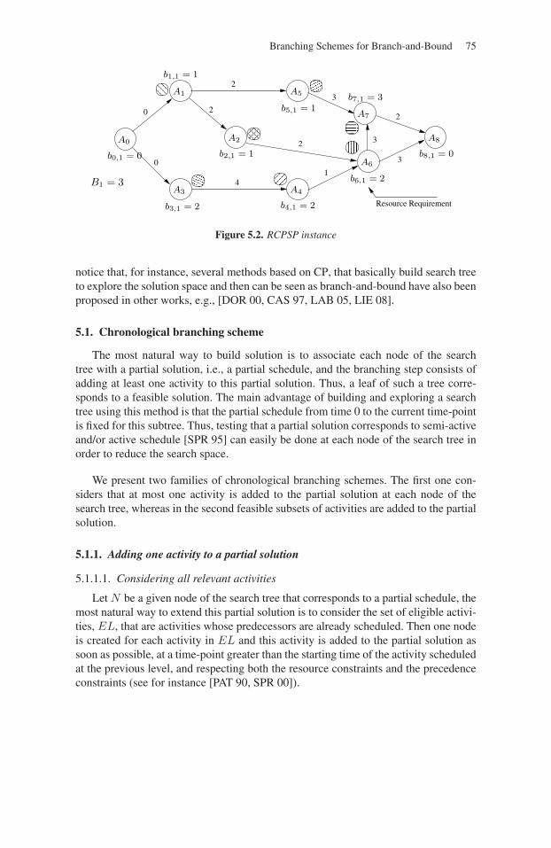
Branching Schemes for Branch-and-Bound 75
Resource Requirement
0
0
41
2
2
3
2
3
3
2 A7
b3,1 = 2
b1,1 = 1
b0,1 = 0 b2,1 = 1
b4,1 = 2
b6,1 = 2B1 = 3
b5,1 = 1
b8,1 = 0
b7,1 = 3A1 A5
A8
A6
A4
A2
A3
A0
Figure 5.2. RCPSP instance
notice that, for instance, several methods based on CP, that basically build search treeto explore the solution space and then can be seen as branch-and-bound have also beenproposed in other works, e.g., [DOR 00, CAS 97, LAB 05, LIE 08].
5.1. Chronological branching scheme
The most natural way to build solution is to associate each node of the searchtree with a partial solution, i.e., a partial schedule, and the branching step consists ofadding at least one activity to this partial solution. Thus, a leaf of such a tree corre-sponds to a feasible solution. The main advantage of building and exploring a searchtree using this method is that the partial schedule from time 0 to the current time-pointis fixed for this subtree. Thus, testing that a partial solution corresponds to semi-activeand/or active schedule [SPR 95] can easily be done at each node of the search tree inorder to reduce the search space.
We present two families of chronological branching schemes. The first one con-siders that at most one activity is added to the partial solution at each node of thesearch tree, whereas in the second feasible subsets of activities are added to the partialsolution.
5.1.1. Adding one activity to a partial solution
5.1.1.1. Considering all relevant activities
Let N be a given node of the search tree that corresponds to a partial schedule, themost natural way to extend this partial solution is to consider the set of eligible activi-ties, EL, that are activities whose predecessors are already scheduled. Then one nodeis created for each activity in EL and this activity is added to the partial solution assoon as possible, at a time-point greater than the starting time of the activity scheduledat the previous level, and respecting both the resource constraints and the precedenceconstraints (see for instance [PAT 90, SPR 00]).
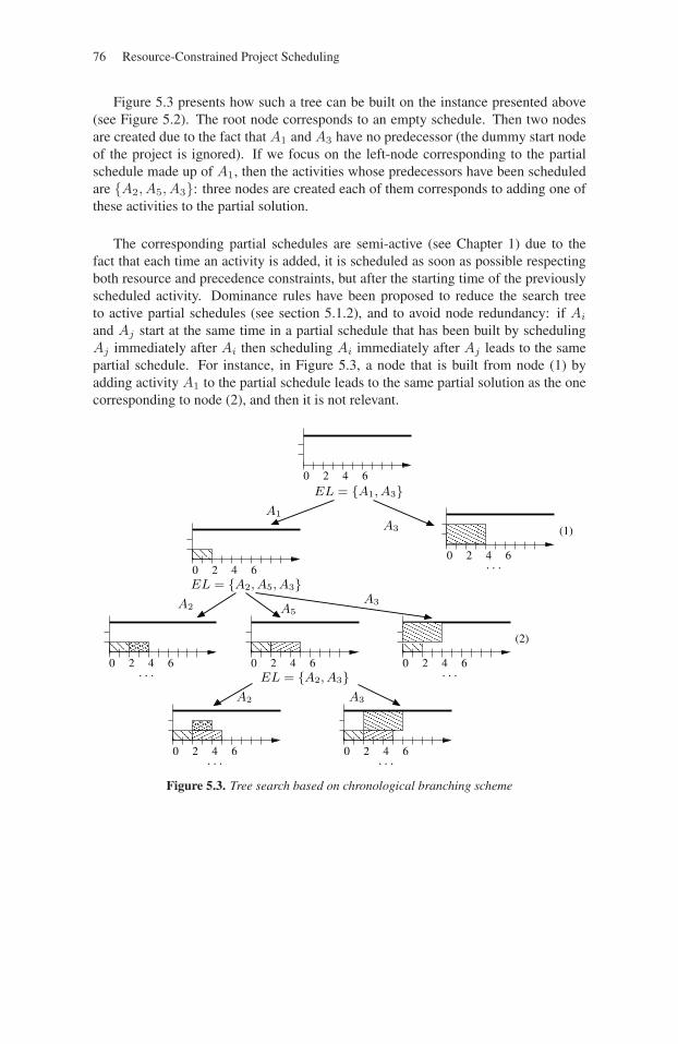
76 Resource-Constrained Project Scheduling
Figure 5.3 presents how such a tree can be built on the instance presented above(see Figure 5.2). The root node corresponds to an empty schedule. Then two nodesare created due to the fact that A1 and A3 have no predecessor (the dummy start nodeof the project is ignored). If we focus on the left-node corresponding to the partialschedule made up of A1, then the activities whose predecessors have been scheduledare {A2, A5, A3}: three nodes are created each of them corresponds to adding one ofthese activities to the partial solution.
The corresponding partial schedules are semi-active (see Chapter 1) due to thefact that each time an activity is added, it is scheduled as soon as possible respectingboth resource and precedence constraints, but after the starting time of the previouslyscheduled activity. Dominance rules have been proposed to reduce the search treeto active partial schedules (see section 5.1.2), and to avoid node redundancy: if Ai
and Aj start at the same time in a partial schedule that has been built by schedulingAj immediately after Ai then scheduling Ai immediately after Aj leads to the samepartial schedule. For instance, in Figure 5.3, a node that is built from node (1) byadding activity A1 to the partial schedule leads to the same partial solution as the onecorresponding to node (2), and then it is not relevant.
(1)
(2)
6420
64206420
6426426420 00
EL = {A1, A3}
EL = {A2, A3}
EL = {A2, A5, A3}
64 64220 0
A3
A1
A3A5
A2
A2 A3
. . .
. . . . . .
. . .
. . .
Figure 5.3. Tree search based on chronological branching scheme
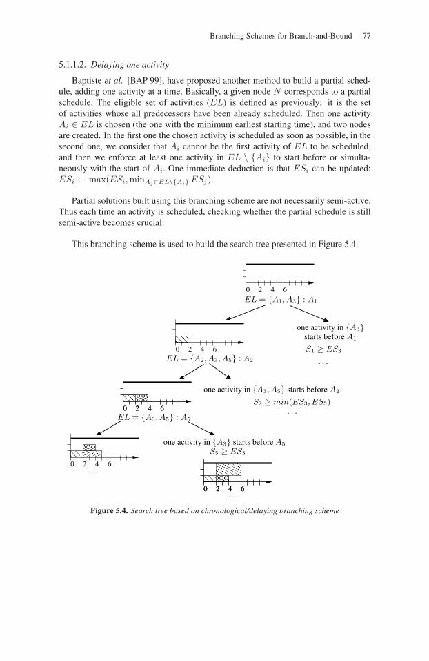
Branching Schemes for Branch-and-Bound 77
5.1.1.2. Delaying one activity
Baptiste et al. [BAP 99], have proposed another method to build a partial sched-ule, adding one activity at a time. Basically, a given node N corresponds to a partialschedule. The eligible set of activities (EL) is defined as previously: it is the setof activities whose all predecessors have been already scheduled. Then one activityAi ∈ EL is chosen (the one with the minimum earliest starting time), and two nodesare created. In the first one the chosen activity is scheduled as soon as possible, in thesecond one, we consider that Ai cannot be the first activity of EL to be scheduled,and then we enforce at least one activity in EL \ {Ai} to start before or simulta-neously with the start of Ai. One immediate deduction is that ESi can be updated:ESi ← max(ESi,minAj∈EL\{Ai} ESj).
Partial solutions built using this branching scheme are not necessarily semi-active.Thus each time an activity is scheduled, checking whether the partial schedule is stillsemi-active becomes crucial.
This branching scheme is used to build the search tree presented in Figure 5.4.
6420
6420
6420 6420
6420 6420
EL = {A1, A3} : A1
EL = {A2, A3, A5} : A2
one activity in {A3, A5} starts before A2
S2 ≥ min(ES3, ES5)
one activity in {A3} starts before A5
6420
EL = {A3, A5} : A5
S5 ≥ ES3
. . .
. . .
. . .
one activity in {A3}starts before A1
S1 ≥ ES3
. . .
Figure 5.4. Search tree based on chronological/delaying branching scheme
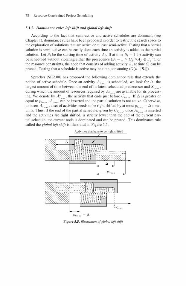
78 Resource-Constrained Project Scheduling
5.1.2. Dominance rule: left shift and global left shift
According to the fact that semi-active and active schedules are dominant (seeChapter 1), dominance rules have been proposed in order to restrict the search space tothe exploration of solutions that are active or at least semi-active. Testing that a partialsolution is semi-active can be easily done each time an activity is added to the partialsolution. Let Si be the starting time of activity Ai. If at time Si − 1 the activity canbe scheduled without violating either the precedence (Si − 1 ≥ Cj ,∀Aj ∈ Γ−1
i ), orthe resource constraints, the node that consists of adding activity Ai at time Si can bepruned. Testing that a schedule is active may be time-consuming (O(n · |R|)).
Sprecher [SPR 00] has proposed the following dominance rule that extends thenotion of active schedule. Once an activity Aimax is scheduled, we look for Δ, thelargest amount of time between the end of its latest scheduled predecessor and Simax ,during which the amount of resources required by Aimax are available for its process-ing. We denote by A∗
imax, the activity that ends just before Cimax . If Δ is greater or
equal to pimax , Aimax can be inserted and the partial solution is not active. Otherwise,to insert Aimax , a set of activities needs to be right shifted by at most pimax −Δ time-units. Thus, if the end of the partial schedule, given by Ci∗max
, once Aimax is insertedand the activities are right shifted, is strictly lower than the end of the current par-tial schedule, the current node is dominated and can be pruned. This dominance rulecalled the global left shift is illustrated in Figure 5.5.
Activities that have to be right shifted
Δ
Δ
pimax
pimax − Δ
Ci∗max
Figure 5.5. illustration of global left shift
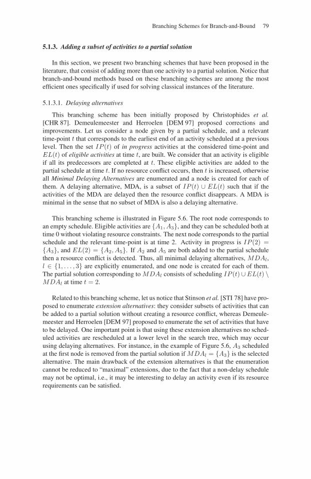
Branching Schemes for Branch-and-Bound 79
5.1.3. Adding a subset of activities to a partial solution
In this section, we present two branching schemes that have been proposed in theliterature, that consist of adding more than one activity to a partial solution. Notice thatbranch-and-bound methods based on these branching schemes are among the mostefficient ones specifically if used for solving classical instances of the literature.
5.1.3.1. Delaying alternatives
This branching scheme has been initially proposed by Christophides et al.[CHR 87]. Demeulemeester and Herroelen [DEM 97] proposed corrections andimprovements. Let us consider a node given by a partial schedule, and a relevanttime-point t that corresponds to the earliest end of an activity scheduled at a previouslevel. Then the set IP (t) of in progress activities at the considered time-point andEL(t) of eligible activities at time t, are built. We consider that an activity is eligibleif all its predecessors are completed at t. These eligible activities are added to thepartial schedule at time t. If no resource conflict occurs, then t is increased, otherwiseall Minimal Delaying Alternatives are enumerated and a node is created for each ofthem. A delaying alternative, MDA, is a subset of IP (t) ∪ EL(t) such that if theactivities of the MDA are delayed then the resource conflict disappears. A MDA isminimal in the sense that no subset of MDA is also a delaying alternative.
This branching scheme is illustrated in Figure 5.6. The root node corresponds toan empty schedule. Eligible activities are {A1, A3}, and they can be scheduled both attime 0 without violating resource constraints. The next node corresponds to the partialschedule and the relevant time-point is at time 2. Activity in progress is IP (2) ={A3}, and EL(2) = {A2, A5}. If A2 and A5 are both added to the partial schedulethen a resource conflict is detected. Thus, all minimal delaying alternatives, MDAl,l ∈ {1, . . . , 3} are explicitly enumerated, and one node is created for each of them.The partial solution corresponding to MDAl consists of scheduling IP (t)∪EL(t) \MDAl at time t = 2.
Related to this branching scheme, let us notice that Stinson et al. [STI 78] have pro-posed to enumerate extension alternatives: they consider subsets of activities that canbe added to a partial solution without creating a resource conflict, whereas Demeule-meester and Herroelen [DEM 97] proposed to enumerate the set of activities that haveto be delayed. One important point is that using these extension alternatives no sched-uled activities are rescheduled at a lower level in the search tree, which may occurusing delaying alternatives. For instance, in the example of Figure 5.6, A3 scheduledat the first node is removed from the partial solution if MDAl = {A3} is the selectedalternative. The main drawback of the extension alternatives is that the enumerationcannot be reduced to “maximal” extensions, due to the fact that a non-delay schedulemay not be optimal, i.e., it may be interesting to delay an activity even if its resourcerequirements can be satisfied.
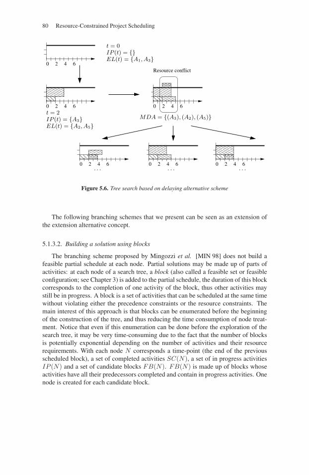
80 Resource-Constrained Project Scheduling
Resource conflict
6420
6420
6420. . .
6420. . .
6420
t = 0IP (t) = {}EL(t) = {A1, A3}
MDA = {(A3), (A2), (A5)}
6420
t = 2IP (t) = {A3}EL(t) = {A2, A5}
. . .
Figure 5.6. Tree search based on delaying alternative scheme
The following branching schemes that we present can be seen as an extension ofthe extension alternative concept.
5.1.3.2. Building a solution using blocks
The branching scheme proposed by Mingozzi et al. [MIN 98] does not build afeasible partial schedule at each node. Partial solutions may be made up of parts ofactivities: at each node of a search tree, a block (also called a feasible set or feasibleconfiguration; see Chapter 3) is added to the partial schedule, the duration of this blockcorresponds to the completion of one activity of the block, thus other activities maystill be in progress. A block is a set of activities that can be scheduled at the same timewithout violating either the precedence constraints or the resource constraints. Themain interest of this approach is that blocks can be enumerated before the beginningof the construction of the tree, and thus reducing the time consumption of node treat-ment. Notice that even if this enumeration can be done before the exploration of thesearch tree, it may be very time-consuming due to the fact that the number of blocksis potentially exponential depending on the number of activities and their resourcerequirements. With each node N corresponds a time-point (the end of the previousscheduled block), a set of completed activities SC(N), a set of in progress activitiesIP (N) and a set of candidate blocks FB(N). FB(N) is made up of blocks whoseactivities have all their predecessors completed and contain in progress activities. Onenode is created for each candidate block.
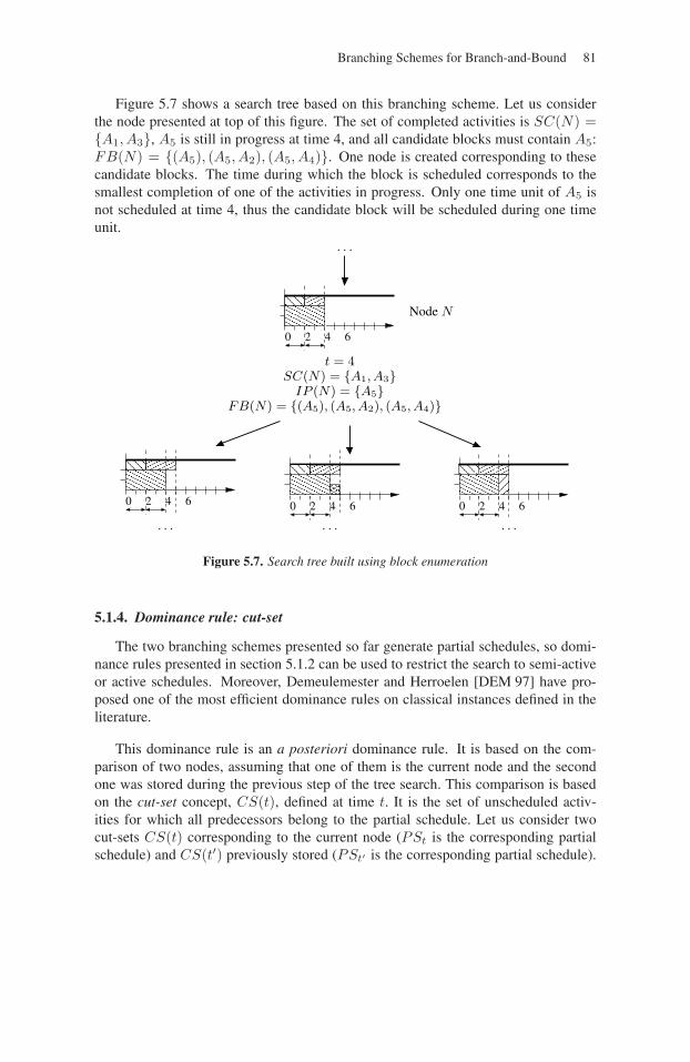
Branching Schemes for Branch-and-Bound 81
Figure 5.7 shows a search tree based on this branching scheme. Let us considerthe node presented at top of this figure. The set of completed activities is SC(N) ={A1, A3}, A5 is still in progress at time 4, and all candidate blocks must contain A5:FB(N) = {(A5), (A5, A2), (A5, A4)}. One node is created corresponding to thesecandidate blocks. The time during which the block is scheduled corresponds to thesmallest completion of one of the activities in progress. Only one time unit of A5 isnot scheduled at time 4, thus the candidate block will be scheduled during one timeunit.
FB(N) = {(A5), (A5, A2), (A5, A4)}
SC(N) = {A1, A3}t = 4
IP (N) = {A5}
. . .. . .. . .
. . .
6420
6420 6420 6420
Node N
Figure 5.7. Search tree built using block enumeration
5.1.4. Dominance rule: cut-set
The two branching schemes presented so far generate partial schedules, so domi-nance rules presented in section 5.1.2 can be used to restrict the search to semi-activeor active schedules. Moreover, Demeulemester and Herroelen [DEM 97] have pro-posed one of the most efficient dominance rules on classical instances defined in theliterature.
This dominance rule is an a posteriori dominance rule. It is based on the com-parison of two nodes, assuming that one of them is the current node and the secondone was stored during the previous step of the tree search. This comparison is basedon the cut-set concept, CS(t), defined at time t. It is the set of unscheduled activ-ities for which all predecessors belong to the partial schedule. Let us consider twocut-sets CS(t) corresponding to the current node (PSt is the corresponding partialschedule) and CS(t′) previously stored (PSt′ is the corresponding partial schedule).
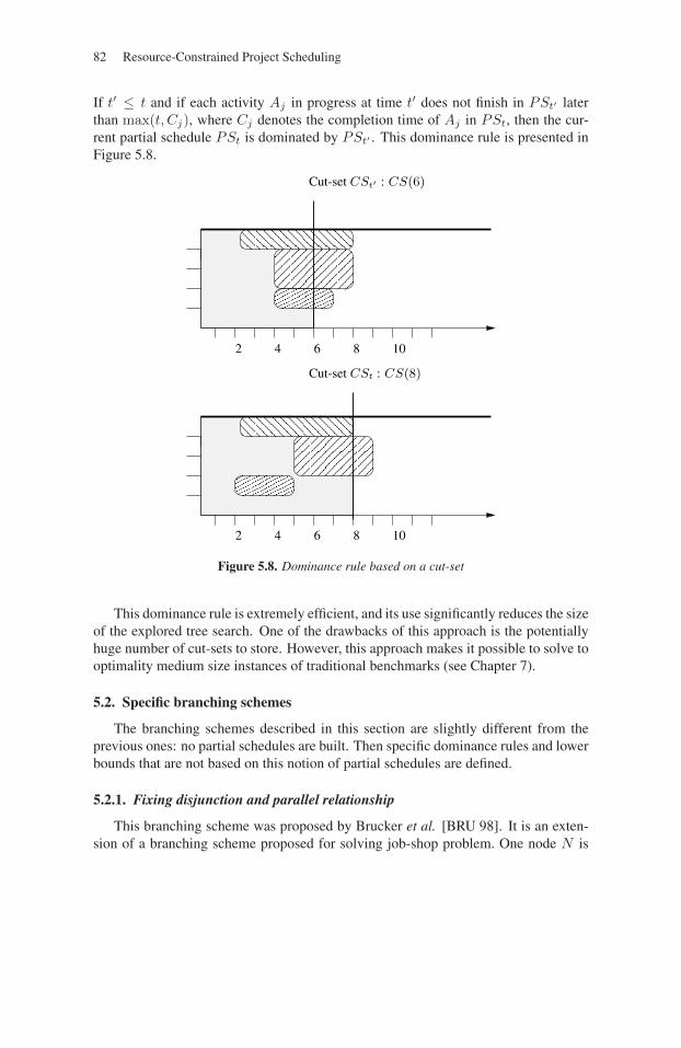
82 Resource-Constrained Project Scheduling
If t′ ≤ t and if each activity Aj in progress at time t′ does not finish in PSt′ laterthan max(t, Cj), where Cj denotes the completion time of Aj in PSt, then the cur-rent partial schedule PSt is dominated by PSt′ . This dominance rule is presented inFigure 5.8.
86
Cut-set CSt : CS(8)
102 4 6 8
Cut-set CSt′ : CS(6)
102 4
Figure 5.8. Dominance rule based on a cut-set
This dominance rule is extremely efficient, and its use significantly reduces the sizeof the explored tree search. One of the drawbacks of this approach is the potentiallyhuge number of cut-sets to store. However, this approach makes it possible to solve tooptimality medium size instances of traditional benchmarks (see Chapter 7).
5.2. Specific branching schemes
The branching schemes described in this section are slightly different from theprevious ones: no partial schedules are built. Then specific dominance rules and lowerbounds that are not based on this notion of partial schedules are defined.
5.2.1. Fixing disjunction and parallel relationship
This branching scheme was proposed by Brucker et al. [BRU 98]. It is an exten-sion of a branching scheme proposed for solving job-shop problem. One node N is
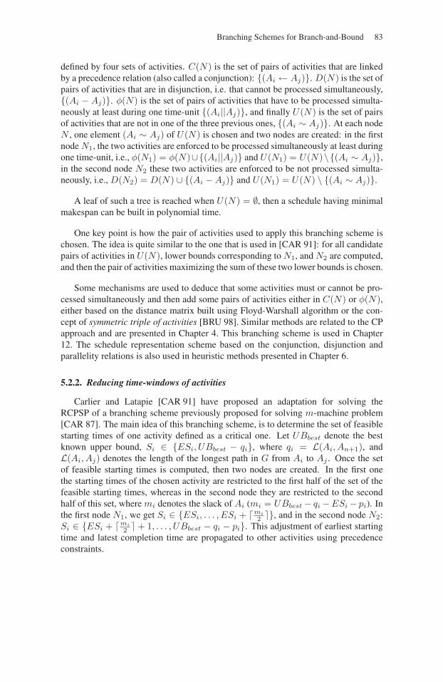
Branching Schemes for Branch-and-Bound 83
defined by four sets of activities. C(N) is the set of pairs of activities that are linkedby a precedence relation (also called a conjunction): {(Ai ← Aj)}. D(N) is the set ofpairs of activities that are in disjunction, i.e. that cannot be processed simultaneously,{(Ai − Aj)}. φ(N) is the set of pairs of activities that have to be processed simulta-neously at least during one time-unit {(Ai||Aj)}, and finally U(N) is the set of pairsof activities that are not in one of the three previous ones, {(Ai ∼ Aj)}. At each nodeN , one element (Ai ∼ Aj) of U(N) is chosen and two nodes are created: in the firstnode N1, the two activities are enforced to be processed simultaneously at least duringone time-unit, i.e., φ(N1) = φ(N)∪{(Ai||Aj)} and U(N1) = U(N)\{(Ai ∼ Aj)},in the second node N2 these two activities are enforced to be not processed simulta-neously, i.e., D(N2) = D(N) ∪ {(Ai −Aj)} and U(N1) = U(N) \ {(Ai ∼ Aj)}.
A leaf of such a tree is reached when U(N) = ∅, then a schedule having minimalmakespan can be built in polynomial time.
One key point is how the pair of activities used to apply this branching scheme ischosen. The idea is quite similar to the one that is used in [CAR 91]: for all candidatepairs of activities in U(N), lower bounds corresponding to N1, and N2 are computed,and then the pair of activities maximizing the sum of these two lower bounds is chosen.
Some mechanisms are used to deduce that some activities must or cannot be pro-cessed simultaneously and then add some pairs of activities either in C(N) or φ(N),either based on the distance matrix built using Floyd-Warshall algorithm or the con-cept of symmetric triple of activities [BRU 98]. Similar methods are related to the CPapproach and are presented in Chapter 4. This branching scheme is used in Chapter12. The schedule representation scheme based on the conjunction, disjunction andparallelity relations is also used in heuristic methods presented in Chapter 6.
5.2.2. Reducing time-windows of activities
Carlier and Latapie [CAR 91] have proposed an adaptation for solving theRCPSP of a branching scheme previously proposed for solving m-machine problem[CAR 87]. The main idea of this branching scheme, is to determine the set of feasiblestarting times of one activity defined as a critical one. Let UBbest denote the bestknown upper bound, Si ∈ {ESi, UBbest − qi}, where qi = L(Ai, An+1), andL(Ai, Aj) denotes the length of the longest path in G from Ai to Aj . Once the setof feasible starting times is computed, then two nodes are created. In the first onethe starting times of the chosen activity are restricted to the first half of the set of thefeasible starting times, whereas in the second node they are restricted to the secondhalf of this set, where mi denotes the slack of Ai (mi = UBbest − qi −ESi − pi). Inthe first node N1, we get Si ∈ {ESi, . . . , ESi + �mi
2 �}, and in the second node N2:Si ∈ {ESi + �mi
2 � + 1, . . . , UBbest − qi − pi}. This adjustment of earliest startingtime and latest completion time are propagated to other activities using precedenceconstraints.
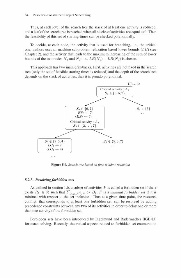
84 Resource-Constrained Project Scheduling
Thus, at each level of the search tree the slack of at least one activity is reduced,and a leaf of the search tree is reached when all slacks of activities are equal to 0. Thenthe feasibility of this set of starting-times can be checked polynomially.
To decide, at each node, the activity that is used for branching, i.e., the criticalone, authors uses m-machine subproblem relaxation based lower bounds (LB) (seeChapter 2), and the activity that leads to the maximum increasing of the sum of lowerbounds of the two nodes N1 and N2, i.e., LB(N1) + LB(N2) is chosen.
This approach has two main drawbacks. First, activities are not fixed in the searchtree (only the set of feasible starting times is reduced) and the depth of the search treedepends on the slack of activities, thus it is pseudo polynomial.
ES6 ← 7
Critical activity : A6
S6 ∈ {6, 7} S6 ∈ {5}
Critical activity : A5
S6 ∈ {5, 6, 7}
S5 ∈ {2, . . . , 7}
S5 ∈ {2, 3, 4}
(LC1 ← 4)
S5 ∈ {5, 6, 7}
. . .
UB = 12
LC5 ← 7 . . .
. . .
(ES7 ← 9)
Figure 5.9. Search tree based on time-window reduction
5.2.3. Resolving forbidden sets
As defined in section 1.6, a subset of activities F is called a forbidden set if thereexists Rk ∈ R such that
∑Aj∈F bj,k > Bk. F is a minimal forbidden set if it is
minimal with respect to the set inclusion. Thus at a given time-point, the resourceconflict, that corresponds to at least one forbidden set, can be resolved by addingprecedence constraints between any two of its activities in order to delay one or morethan one activity of the forbidden set.
Forbidden sets have been introduced by Ingelmund and Radermacher [IGE 83]for exact solving. Recently, theoretical aspects related to forbidden set enumeration
Branching Schemes for Branch-and-Bound 85
have been investigated by Stork and Uetz [STO 05]. Laborie [LAB 05] presented asimilar concept: minimal critical sets. More details about this method are presentedin Chapter 7.
5.3. Conclusion and perspectives
In this chapter we have presented main branching schemes that are used to obtainexact solutions of the classical RCPSP. Notice that the efficiency of exact methods isobviously linked to the way that the search space is explored, i.e, to the branchingscheme, but several works have proved that lower bound and time-bound reductiontechniques are also extremely useful to improve the search, both in terms of numberof explored nodes and time consumption. Thus, recent works that use cooperationbetween linear programming formulation and constraint programming are promisingresearch directions.
Exact methods are used more and more to obtain efficient heuristic methods. First,the search tree can be truncated using, for instance, traditional methods e.g., beamsearch or recovering beam search, or methods coming from the constraint program-ming community, e.g., limited discrepancy search. Exact methods are also used moreand more as a part of heuristics based on a large neighborhood search.

86
This page intentionally left blank
Chapter 6
Heuristics
This chapter describes the main heuristics proposed in the research for the RCPSP.Special attention is paid to simple constructive heuristics and a generic schedulegeneration scheme embedding the standard serial and parallel schedule generationsscheme is provided. For a complete description and experimental evaluation ofstandard heuristics and metaheuristics see [KOL 99a, KOL 06].
6.1. Schedule representation schemes
The fundamental goal of a heuristic algorithm is to generate a good solution in areasonable amount of time. As such, it is necessary to define a representation schemeof the solution itself. In this section we describe the representation schemes used inthe main heuristics within other works. Other formulations or encoding solutions canbe found in Chapters 3 and 4.
6.1.1. Natural date variables
Since we consider the makespan criterion in a non-preemptive environment, themost straightforward formulation of a RCPSP chooses variables representing eitherthe starting times or the completion times of activities. In fact, this representation isusually the final output of heuristics even when they operate on another internal encod-ing scheme. This formulation is in particular the core of the neighborhood procedureof Palpant et al. [PAL 04] described in section 6.4.4.
Chapter written by Christian ARTIGUES and David RIVREAU.
87
88 Resource-Constrained Project Scheduling
6.1.2. List schedule generation scheme representations
Typically, a heuristic process involves choosing between alternatives. A commonpractice to resolve this stage is to use a priority list as a decision maker. As a result thecombination of the heuristic (schedule generator) and the priority list can be consid-ered as solution provider for the RCPSP instance under investigation. In most casesthe heuristic is supposed to be known in advance, so the list itself is seen as a cod-ing for the solution. Due to its genericity and simplicity, the list representation is thebasic solution encoding used by many greedy heuristics such as the serial and paral-lel scheduling schemes, but also by more elaborated heuristics such as tabu search ormulti-pass methods (see section 6.2.1).
From the implementation point of view, the list either consists of activities in non-increasing order of priority, or is a vector of priority values such that the ith elementcorresponds to activity Ai. In the first case, we speak of an activity list whereas inthe second the encoding is called random key representation. For instance, activitylist (A2, A3, A4, A4) and random key vector (4.6, 1.2, 1.9, 3.4) represent the samepriority order in which activity A2 is preferred to activity A3, A3 is preferred to A4,and so on.
6.1.3. Set-based representations
The minimal forbidden sets defined in Chapter 1 can also be used as the basis ofan alternative encoding for solutions. We consider here that a forbidden set F can bedefined as a set of activities such that there is no path between any pair of activities inthe set and that there is a resource conflict on F . If no activity can be removed fromthat set without removing the conflict, then F is said to be a minimal forbidden set.Clearly, fixing Ai → Aj or Aj → Ai for (Ai, Aj) ∈ F×F solves the resource conflictrelated to F (and possibly some others). It follows that a solution to a RCPSP problemcan be characterized by a selection of a set of at most one pair of activities for eachminimal forbidden set such that all resource conflicts are resolved and there is no cyclein the augmented precedence graph. This is the strict-order representation defined inChapter 1. Note that this representation is also called a partial-order schedule by someauthors [GOD 05, POL 07].
Brucker et al. [BRU 98] devise a more sophisticated generation scheme represen-tation (see also section 5.2.1). For these authors, a schedule scheme (C,D, φ, U) isa set of disjoint relations between activities. Relations in C are called conjunctions,D defines disjunctions and φ and U are parallelity and flexibility relations. Moreprecisely, a schedule scheme characterizes the set of solutions with:
– Ai → Aj for all (Ai, Aj) ∈ C (Ai should precede Aj)
– Ai −Aj for all (Ai, Aj) ∈ D (Ai and Aj cannot be scheduled in parallel)
Heuristics 89
– Ai||Aj for all (Ai, Aj) ∈ φ (Ai and Aj should be processed in parallel)
– Ai∼Aj for all (Ai, Aj)∈U (there is no specific constraint between Ai and Aj)
When U = ∅, it can be proved that either no feasible solution satisfying all rela-tions exists or a dominating feasible schedule can be found. Thus, we can considera schedule scheme of the form (C,D, φ, ∅) as a solution. A branching scheme usingthis representation is described in section 5.2.1 (see also section 12.3.1).
6.1.4. Resource flow network representation
Feasible schedules can finally be modeled by a network flow based representation(see Chapter 1). This formalization allows us to define a strict order that destroysall forbidden sets without explicitly enumerating all minimal forbidden sets. In thismodel the flow decision variables fk
ij give the number of units of resource Rk directlytransferred from an activity Ai to an activity Aj (where Ai belongs to A ∪ {A0}, Aj
is inA∪{An+1} and Rk inR). As shown in Chapter 1, from a feasible resource flowf , a schedule ES(P (f)) can be obtained through longest path computations in graphG(V,E ∪ P (f)), where P (f) = {(Ai, Aj) ∈ V 2 | fij > 0} and each arc is valuatedby the duration of the origin activity. Conversely, a feasible flow can be built from anyfeasible schedule S by Algorithm 2.
6.2. Constructive heuristics
Constructive heuristics are often used to generate a first solution in a very reasona-ble amount of time. In this section, we review the main methods applied for a RCPSP.
6.2.1. Standard list schedule generation scheme heuristics
List schedules generation scheme (SGS) heuristics appear to be one of the mostwidely used. Typically two basic scheduling schemes are reported: the serial schedul-ing scheme and the parallel scheduling scheme. Both heuristics schedule activitiesaccording to a given priority list, selecting tasks one by one and determining a startingtime for each activity. Once a starting time is assigned to a particular task, this time ispermanent and may not be changed at a later stage of the procedure.
Let L denote a list of activities and let P (L) denote the strict (total) order inducedby L, i.e. (Ai, Aj) ∈ P (L) if and only if Ai is before Aj in the list. L is said tobe compatible with the precedence constraints whenever E ⊆ P (L). Both the serialand the parallel scheduling schemes assume the priority list is compatible with theprecedence constraints.
In the serial scheduling scheme proposed by Kelley [KEL 63], in each iteration thefirst available task in the list L is selected to be scheduled as soon as possible (withrespect to precedence and resource constraints). Note the serial scheduling scheme isidentical to the strict order algorithm proposed by Carlier (see [CAR 84] and Chapter10).
90 Resource-Constrained Project Scheduling
On the other hand, the parallel scheduling scheme ([BRO 65]) operates in chrono-logical fashion. At any period t, the set of schedulable activities, denoted by Lt,consists of all those unscheduled activities which have their predecessors completedand which can be processed at that time with respect to resource constraints. Let t bethe first time period such that Lt �= ∅ at a given step of the procedure. Following anon-delay policy, the first activity in the priority list that belongs to Lt is scheduled attime t and the process is iterated until all tasks are completed.
As pointed out by Debels et al. [DEB 06a], for both methods a single schedule canbe represented by different priority lists. For instance, if we consider the activity list(A5, A3, A6, A4, A2, A1) and that the corresponding solution start times are S5 = 0,S3 = 2, S6 = 0, S4 = 5, S2 = 8, S1 = 7, then activities A3 and A6 can clearly beswapped without changing the output. In order to eliminate this flaw, the authors pro-pose to use a standardized random key representation for schedules. The central ideaof Debels et al. consists of using rank values as priorities and applying a schedulingscheme to this random key distribution. This gives a starting time for each activity.The standardized random key representation is post-processed on this schedule byassigning the rank of the starting of activities as priorities. In case of ties, the lowestranking is attributed to all activities starting at the same time. With this convention,each list corresponds to a unique schedule. For example, the standardized random keyrepresentation of previous schedule is (5, 6, 3, 4, 1, 1) where priority values of A5 andA6 are equal to 1 since they have the same start time and they appear in first position.
Although serial and parallel scheduling schemes appear to be very similar at firstsight (which is confirmed by the fact that they can be embedded into the generic frame-work of the next section), their outputs do not share the same properties. Indeed wewill see that any schedule generated with the serial scheduling scheme belongs to theset of active schedules while only non-delay schedules are generated by the parallelscheduling scheme. From Sprecher et al. [SPR 95] it is also known that there is atleast one optimal schedule that is active whereas the set of non-delay schedules mayexclude all optimal solution1. These results are detailed in section 6.6.1.
From the operational point of view, list schedule generation scheme heuristics canbe applied as single or multi-pass heuristics. A single pass generally consists of com-puting a list through a priority rule as described above. The list is said to be a staticpriority rule when it can be computed before running the scheduling algorithm. On theother hand, the dynamic priority rules are updated while the schedule is in construc-tion. Typically, dynamic priority rules depend on the start time values. See [KOL 96]for a comprehensive survey of traditional priority rules for the RCPSP.
1. Active and non-delay schedules are defined more precisely in Chapter 1.
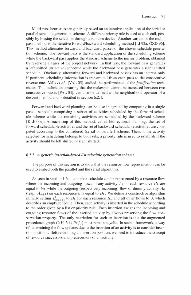
Heuristics 91
Multi-pass heuristics are generally based on an iterative application of the serial orparallel schedule generation scheme. A different priority rule is used at each call, pos-sibly by biasing the selection through a random device. Another variant of the multi-pass method is the iterative forward/backward scheduling method [LI 92a, ÖZD 96].This method alternates forward and backward passes of the chosen schedule genera-tion scheme. The forward pass is the standard application of the scheduling schemewhile the backward pass applies the standard scheme to the mirror problem, obtainedby reversing all arcs of the project network. In that way, the forward pass generatesa left shifted (or active) schedule while the backward pass generates a right shiftedschedule. Obviously, alternating forward and backward passes has an interest onlyif pertinent scheduling information is transmitted from each pass to the consecutivereverse one. Valls et al. [VAL 05] studied the performance of the justification tech-nique. This technique, ensuring that the makespan cannot be increased between twoconsecutive passes [PAL 04], can also be defined as the neighborhood operator of adescent method and is detailed in section 6.2.4.
Forward and backward planning can be also integrated by computing in a singlepass a schedule comprising a subset of activities scheduled by the forward sched-ule scheme while the remaining activities are scheduled by the backward scheme[KLE 00a]. At each step of this method, called bidirectional planning, the set offorward-schedulable activities and the set of backward-schedulable activities are com-puted according to the considered (serial or parallel) scheme. Then, if the activityselected for scheduling belongs to both sets, a priority rule is used to establish if theactivity should be left shifted or right shifted.
6.2.2. A generic insertion-based list schedule generation scheme
The purpose of this section is to show that the resource-flow representation can beused to embed both the parallel and the serial algorithms.
As seen in section 1.6, a complete schedule can be represented by a resource flowwhere the incoming and outgoing flows of any activity Ai on each resource Rk areequal to bik while the outgoing (respectively incoming) flow of dummy activity A0
(resp. An+1) on each resource k is equal to Bk. We define a constructive algorithminitially setting fk
0(n+1) to Bk for each resource Rk and all other flows to 0, whichdescribes an empty schedule. Then, each activity is inserted in the schedule accordingto the order given by a list or priority rule. Each insertion assigns the incoming andoutgoing resource flows of the inserted activity by always preserving the flow con-servation property. The only restriction for such an insertion is that the augmentedprecedence graph G(V,E ∪ P (f)) must remain acyclic. In such a framework, a wayof determining the flow updates due to the insertion of an activity is to consider inser-tion positions. Before defining an insertion position, we need to introduce the conceptof resource successors and predecessors of an activity.
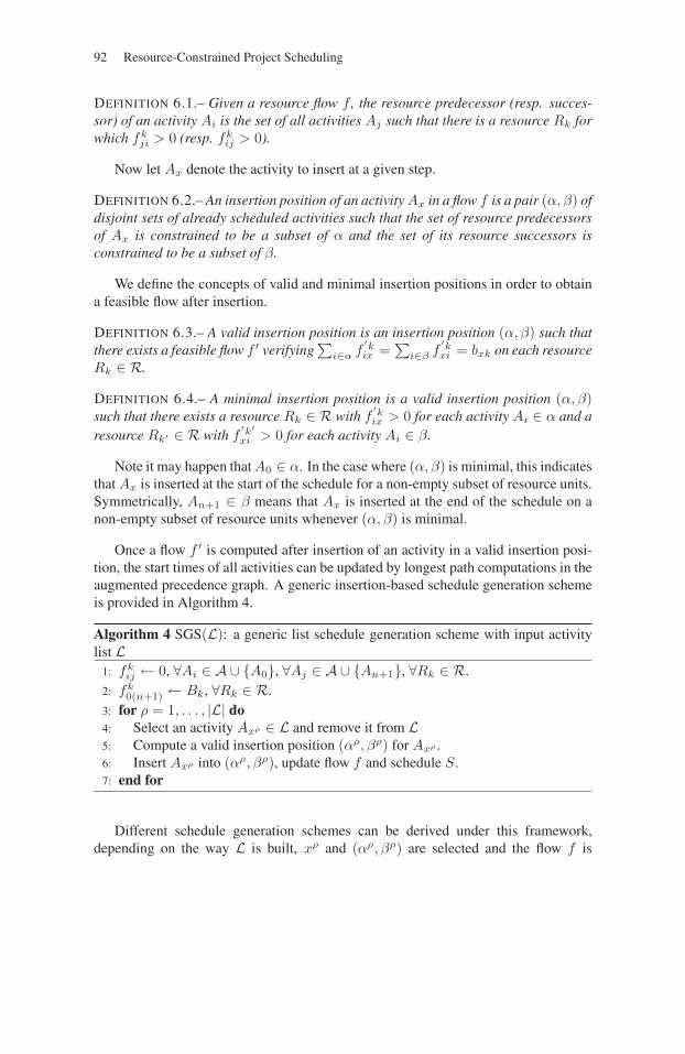
92 Resource-Constrained Project Scheduling
DEFINITION 6.1.– Given a resource flow f , the resource predecessor (resp. succes-sor) of an activity Ai is the set of all activities Aj such that there is a resource Rk forwhich fk
ji > 0 (resp. fkij > 0).
Now let Ax denote the activity to insert at a given step.
DEFINITION 6.2.– An insertion position of an activity Ax in a flow f is a pair (α, β) ofdisjoint sets of already scheduled activities such that the set of resource predecessorsof Ax is constrained to be a subset of α and the set of its resource successors isconstrained to be a subset of β.
We define the concepts of valid and minimal insertion positions in order to obtaina feasible flow after insertion.
DEFINITION 6.3.– A valid insertion position is an insertion position (α, β) such thatthere exists a feasible flow f ′ verifying
∑i∈α f
′kix =
∑i∈β f
′kxi = bxk on each resource
Rk ∈ R.
DEFINITION 6.4.– A minimal insertion position is a valid insertion position (α, β)such that there exists a resource Rk ∈ R with f
′kix > 0 for each activity Ai ∈ α and a
resource Rk′ ∈ R with f′k′xi > 0 for each activity Ai ∈ β.
Note it may happen that A0 ∈ α. In the case where (α, β) is minimal, this indicatesthat Ax is inserted at the start of the schedule for a non-empty subset of resource units.Symmetrically, An+1 ∈ β means that Ax is inserted at the end of the schedule on anon-empty subset of resource units whenever (α, β) is minimal.
Once a flow f ′ is computed after insertion of an activity in a valid insertion posi-tion, the start times of all activities can be updated by longest path computations in theaugmented precedence graph. A generic insertion-based schedule generation schemeis provided in Algorithm 4.
Algorithm 4 SGS(L): a generic list schedule generation scheme with input activitylist L
1: fkij ← 0, ∀Ai ∈ A ∪ {A0}, ∀Aj ∈ A ∪ {An+1}, ∀Rk ∈ R.
2: fk0(n+1) ← Bk, ∀Rk ∈ R.
3: for ρ = 1, . . . , |L| do4: Select an activity Axρ ∈ L and remove it from L5: Compute a valid insertion position (αρ, βρ) for Axρ .6: Insert Axρ into (αρ, βρ), update flow f and schedule S.7: end for
Different schedule generation schemes can be derived under this framework,depending on the way L is built, xρ and (αρ, βρ) are selected and the flow f is
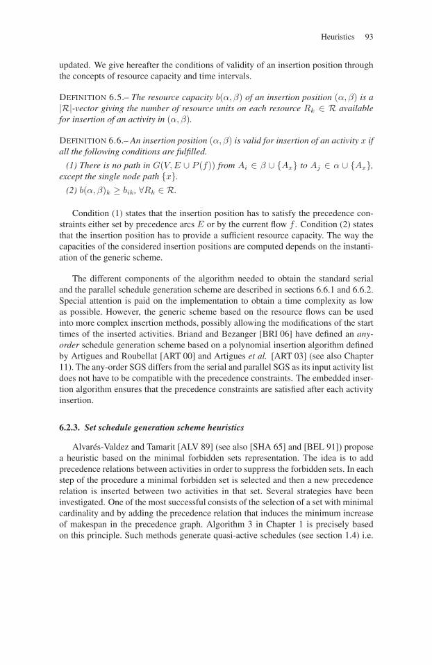
Heuristics 93
updated. We give hereafter the conditions of validity of an insertion position throughthe concepts of resource capacity and time intervals.
DEFINITION 6.5.– The resource capacity b(α, β) of an insertion position (α, β) is a|R|-vector giving the number of resource units on each resource Rk ∈ R availablefor insertion of an activity in (α, β).
DEFINITION 6.6.– An insertion position (α, β) is valid for insertion of an activity x ifall the following conditions are fulfilled.
(1) There is no path in G(V,E ∪ P (f)) from Ai ∈ β ∪ {Ax} to Aj ∈ α ∪ {Ax},except the single node path {x}.
(2) b(α, β)k ≥ bik, ∀Rk ∈ R.
Condition (1) states that the insertion position has to satisfy the precedence con-straints either set by precedence arcs E or by the current flow f . Condition (2) statesthat the insertion position has to provide a sufficient resource capacity. The way thecapacities of the considered insertion positions are computed depends on the instanti-ation of the generic scheme.
The different components of the algorithm needed to obtain the standard serialand the parallel schedule generation scheme are described in sections 6.6.1 and 6.6.2.Special attention is paid on the implementation to obtain a time complexity as lowas possible. However, the generic scheme based on the resource flows can be usedinto more complex insertion methods, possibly allowing the modifications of the starttimes of the inserted activities. Briand and Bezanger [BRI 06] have defined an any-order schedule generation scheme based on a polynomial insertion algorithm definedby Artigues and Roubellat [ART 00] and Artigues et al. [ART 03] (see also Chapter11). The any-order SGS differs from the serial and parallel SGS as its input activity listdoes not have to be compatible with the precedence constraints. The embedded inser-tion algorithm ensures that the precedence constraints are satisfied after each activityinsertion.
6.2.3. Set schedule generation scheme heuristics
Alvarés-Valdez and Tamarit [ALV 89] (see also [SHA 65] and [BEL 91]) proposea heuristic based on the minimal forbidden sets representation. The idea is to addprecedence relations between activities in order to suppress the forbidden sets. In eachstep of the procedure a minimal forbidden set is selected and then a new precedencerelation is inserted between two activities in that set. Several strategies have beeninvestigated. One of the most successful consists of the selection of a set with minimalcardinality and by adding the precedence relation that induces the minimum increaseof makespan in the precedence graph. Algorithm 3 in Chapter 1 is precisely basedon this principle. Such methods generate quasi-active schedules (see section 1.4) i.e.
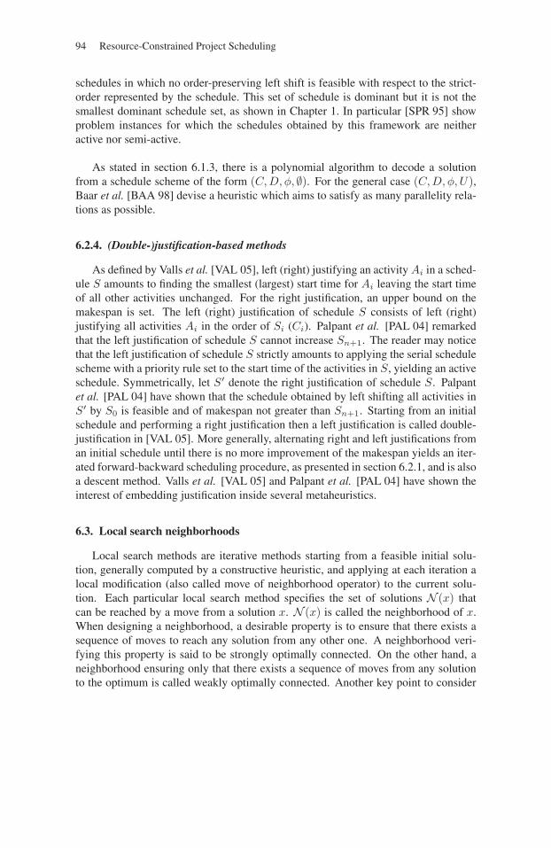
94 Resource-Constrained Project Scheduling
schedules in which no order-preserving left shift is feasible with respect to the strict-order represented by the schedule. This set of schedule is dominant but it is not thesmallest dominant schedule set, as shown in Chapter 1. In particular [SPR 95] showproblem instances for which the schedules obtained by this framework are neitheractive nor semi-active.
As stated in section 6.1.3, there is a polynomial algorithm to decode a solutionfrom a schedule scheme of the form (C,D, φ, ∅). For the general case (C,D, φ, U),Baar et al. [BAA 98] devise a heuristic which aims to satisfy as many parallelity rela-tions as possible.
6.2.4. (Double-)justification-based methods
As defined by Valls et al. [VAL 05], left (right) justifying an activity Ai in a sched-ule S amounts to finding the smallest (largest) start time for Ai leaving the start timeof all other activities unchanged. For the right justification, an upper bound on themakespan is set. The left (right) justification of schedule S consists of left (right)justifying all activities Ai in the order of Si (Ci). Palpant et al. [PAL 04] remarkedthat the left justification of schedule S cannot increase Sn+1. The reader may noticethat the left justification of schedule S strictly amounts to applying the serial schedulescheme with a priority rule set to the start time of the activities in S, yielding an activeschedule. Symmetrically, let S′ denote the right justification of schedule S. Palpantet al. [PAL 04] have shown that the schedule obtained by left shifting all activities inS′ by S0 is feasible and of makespan not greater than Sn+1. Starting from an initialschedule and performing a right justification then a left justification is called double-justification in [VAL 05]. More generally, alternating right and left justifications froman initial schedule until there is no more improvement of the makespan yields an iter-ated forward-backward scheduling procedure, as presented in section 6.2.1, and is alsoa descent method. Valls et al. [VAL 05] and Palpant et al. [PAL 04] have shown theinterest of embedding justification inside several metaheuristics.
6.3. Local search neighborhoods
Local search methods are iterative methods starting from a feasible initial solu-tion, generally computed by a constructive heuristic, and applying at each iteration alocal modification (also called move of neighborhood operator) to the current solu-tion. Each particular local search method specifies the set of solutions N (x) thatcan be reached by a move from a solution x. N (x) is called the neighborhood of x.When designing a neighborhood, a desirable property is to ensure that there exists asequence of moves to reach any solution from any other one. A neighborhood veri-fying this property is said to be strongly optimally connected. On the other hand, aneighborhood ensuring only that there exists a sequence of moves from any solutionto the optimum is called weakly optimally connected. Another key point to consider
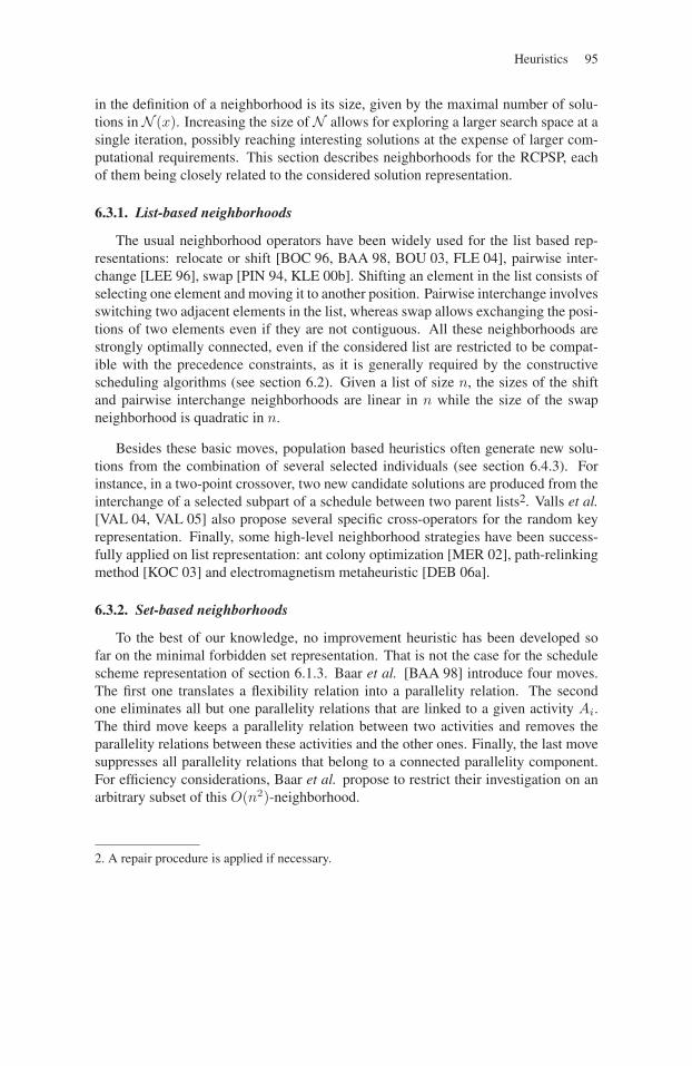
Heuristics 95
in the definition of a neighborhood is its size, given by the maximal number of solu-tions inN (x). Increasing the size ofN allows for exploring a larger search space at asingle iteration, possibly reaching interesting solutions at the expense of larger com-putational requirements. This section describes neighborhoods for the RCPSP, eachof them being closely related to the considered solution representation.
6.3.1. List-based neighborhoods
The usual neighborhood operators have been widely used for the list based rep-resentations: relocate or shift [BOC 96, BAA 98, BOU 03, FLE 04], pairwise inter-change [LEE 96], swap [PIN 94, KLE 00b]. Shifting an element in the list consists ofselecting one element and moving it to another position. Pairwise interchange involvesswitching two adjacent elements in the list, whereas swap allows exchanging the posi-tions of two elements even if they are not contiguous. All these neighborhoods arestrongly optimally connected, even if the considered list are restricted to be compat-ible with the precedence constraints, as it is generally required by the constructivescheduling algorithms (see section 6.2). Given a list of size n, the sizes of the shiftand pairwise interchange neighborhoods are linear in n while the size of the swapneighborhood is quadratic in n.
Besides these basic moves, population based heuristics often generate new solu-tions from the combination of several selected individuals (see section 6.4.3). Forinstance, in a two-point crossover, two new candidate solutions are produced from theinterchange of a selected subpart of a schedule between two parent lists2. Valls et al.[VAL 04, VAL 05] also propose several specific cross-operators for the random keyrepresentation. Finally, some high-level neighborhood strategies have been success-fully applied on list representation: ant colony optimization [MER 02], path-relinkingmethod [KOC 03] and electromagnetism metaheuristic [DEB 06a].
6.3.2. Set-based neighborhoods
To the best of our knowledge, no improvement heuristic has been developed sofar on the minimal forbidden set representation. That is not the case for the schedulescheme representation of section 6.1.3. Baar et al. [BAA 98] introduce four moves.The first one translates a flexibility relation into a parallelity relation. The secondone eliminates all but one parallelity relations that are linked to a given activity Ai.The third move keeps a parallelity relation between two activities and removes theparallelity relations between these activities and the other ones. Finally, the last movesuppresses all parallelity relations that belong to a connected parallelity component.For efficiency considerations, Baar et al. propose to restrict their investigation on anarbitrary subset of this O(n2)-neighborhood.
2. A repair procedure is applied if necessary.
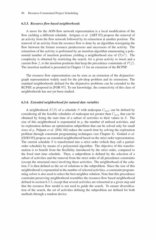
96 Resource-Constrained Project Scheduling
6.3.3. Resource flow-based neighborhoods
A move for the AON-flow network representation is a local modification of theflow yielding a different schedule. Artigues et al. [ART 03] propose the removal ofan activity from the flow network followed by its reinsertion at another position. Theremoval of an activity from the resource flow is done by an algorithm reassigning theflow between the former resource predecessors and successors of the activity. Thereinsertion of the activity is performed by an insertion algorithm enumerating a poly-nomial number of insertion positions yielding a neighborhood size of O(n3). Thecomplexity is obtained by restricting the search, for a given activity to insert and acurrent flow f , to the insertion positions that keep the precedence constraints of P (f).The insertion method is presented in Chapter 11 for an extension of the RCPSP.
The resource flow representation can be seen as an extension of the disjunctive-graph representation widely used for the job-shop problem and its extensions. Thestandard neighborhoods defined for the disjunctive problems can be extended to theRCPSP, as proposed in [FOR 97]. To our knowledge, the connectivity of this class ofneighborhoods has not yet been studied.
6.3.4. Extended neighborhood for natural date variables
A neighborhood N (S) of a schedule S with makespan Cmax can be defined byconsidering all the feasible schedules of makespan not greater than Cmax that can beobtained by fixing the start time of a subset of activities to their values in S. Thesize of this neighborhood is exponential in p, the number of unfixed activities, andits exploration defines an optimization subproblem that can be solved only for smallsizes of p. Palpant et al. [PAL 04] reduce the search time by solving the explorationproblem through constraint programming techniques (see Chapter 4). Godard et al.[GOD 05] propose an extended neighborhood based on the strict order representation.The current schedule S is transformed into a strict order (which they call a partial-order schedule) by means of a polynomial algorithm. The objective of this transfor-mation is to benefit from the flexibility introduced by the strict order, compared tothe fixed start time schedule. Then, a subproblem is defined by the selection of asubset of activities and the removal from the strict order of all precedence constraints(except the structural ones) involving these activities. The neighborhood of the solu-tion S is then defined as the set of solutions to the subproblem. Since the size of thisneighborhood is exponential in the number of selected activities, a constraint program-ming solver is also used to select the best neighbor solution. Note that this precedenceconstraint-preserving neighborhood resembles the resource-flow based neighborhooddefined in section 6.3.3, except that several activities are reinserted at a given step andthat the resource flow model is not used to guide the search. To ensure diversifica-tion of the search, the set of activities defining the subproblem are defined for bothmethods through a random device.
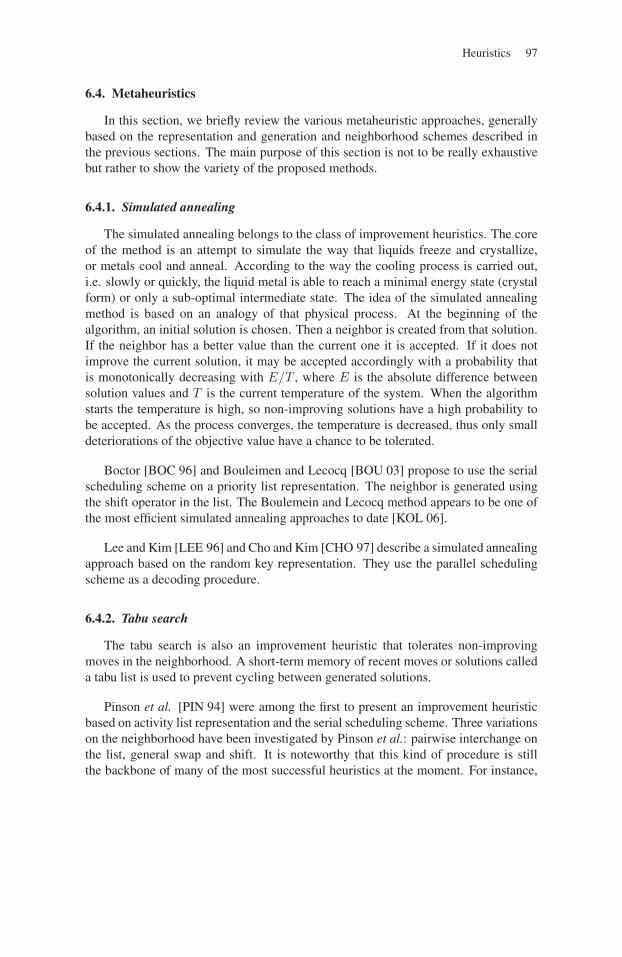
Heuristics 97
6.4. Metaheuristics
In this section, we briefly review the various metaheuristic approaches, generallybased on the representation and generation and neighborhood schemes described inthe previous sections. The main purpose of this section is not to be really exhaustivebut rather to show the variety of the proposed methods.
6.4.1. Simulated annealing
The simulated annealing belongs to the class of improvement heuristics. The coreof the method is an attempt to simulate the way that liquids freeze and crystallize,or metals cool and anneal. According to the way the cooling process is carried out,i.e. slowly or quickly, the liquid metal is able to reach a minimal energy state (crystalform) or only a sub-optimal intermediate state. The idea of the simulated annealingmethod is based on an analogy of that physical process. At the beginning of thealgorithm, an initial solution is chosen. Then a neighbor is created from that solution.If the neighbor has a better value than the current one it is accepted. If it does notimprove the current solution, it may be accepted accordingly with a probability thatis monotonically decreasing with E/T , where E is the absolute difference betweensolution values and T is the current temperature of the system. When the algorithmstarts the temperature is high, so non-improving solutions have a high probability tobe accepted. As the process converges, the temperature is decreased, thus only smalldeteriorations of the objective value have a chance to be tolerated.
Boctor [BOC 96] and Bouleimen and Lecocq [BOU 03] propose to use the serialscheduling scheme on a priority list representation. The neighbor is generated usingthe shift operator in the list. The Boulemein and Lecocq method appears to be one ofthe most efficient simulated annealing approaches to date [KOL 06].
Lee and Kim [LEE 96] and Cho and Kim [CHO 97] describe a simulated annealingapproach based on the random key representation. They use the parallel schedulingscheme as a decoding procedure.
6.4.2. Tabu search
The tabu search is also an improvement heuristic that tolerates non-improvingmoves in the neighborhood. A short-term memory of recent moves or solutions calleda tabu list is used to prevent cycling between generated solutions.
Pinson et al. [PIN 94] were among the first to present an improvement heuristicbased on activity list representation and the serial scheduling scheme. Three variationson the neighborhood have been investigated by Pinson et al.: pairwise interchange onthe list, general swap and shift. It is noteworthy that this kind of procedure is stillthe backbone of many of the most successful heuristics at the moment. For instance,
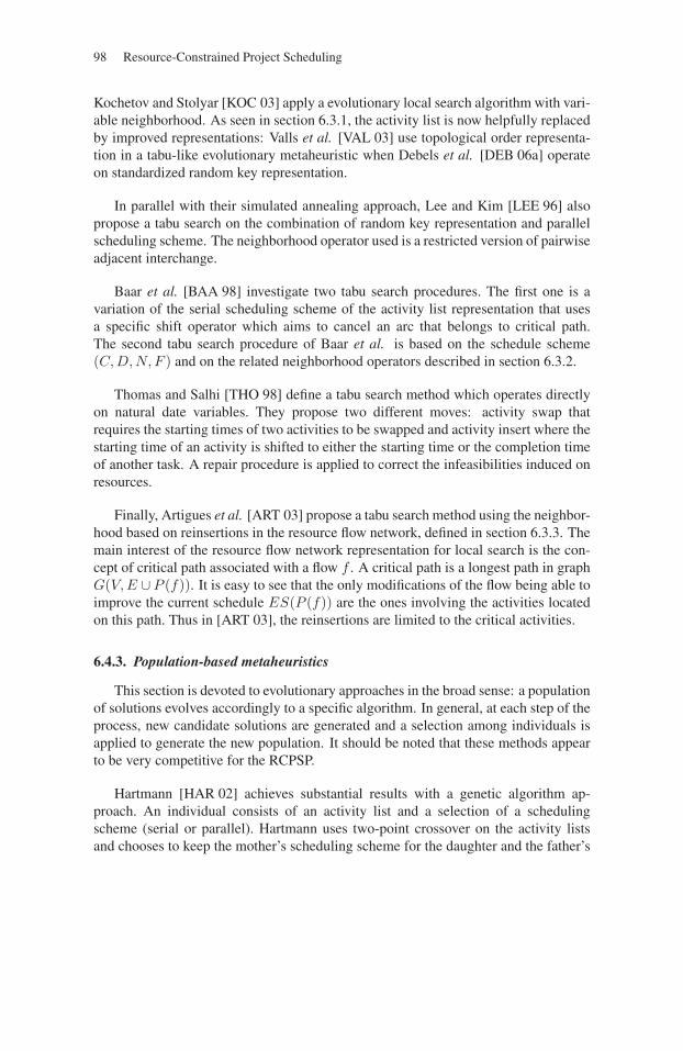
98 Resource-Constrained Project Scheduling
Kochetov and Stolyar [KOC 03] apply a evolutionary local search algorithm with vari-able neighborhood. As seen in section 6.3.1, the activity list is now helpfully replacedby improved representations: Valls et al. [VAL 03] use topological order representa-tion in a tabu-like evolutionary metaheuristic when Debels et al. [DEB 06a] operateon standardized random key representation.
In parallel with their simulated annealing approach, Lee and Kim [LEE 96] alsopropose a tabu search on the combination of random key representation and parallelscheduling scheme. The neighborhood operator used is a restricted version of pairwiseadjacent interchange.
Baar et al. [BAA 98] investigate two tabu search procedures. The first one is avariation of the serial scheduling scheme of the activity list representation that usesa specific shift operator which aims to cancel an arc that belongs to critical path.The second tabu search procedure of Baar et al. is based on the schedule scheme(C,D,N, F ) and on the related neighborhood operators described in section 6.3.2.
Thomas and Salhi [THO 98] define a tabu search method which operates directlyon natural date variables. They propose two different moves: activity swap thatrequires the starting times of two activities to be swapped and activity insert where thestarting time of an activity is shifted to either the starting time or the completion timeof another task. A repair procedure is applied to correct the infeasibilities induced onresources.
Finally, Artigues et al. [ART 03] propose a tabu search method using the neighbor-hood based on reinsertions in the resource flow network, defined in section 6.3.3. Themain interest of the resource flow network representation for local search is the con-cept of critical path associated with a flow f . A critical path is a longest path in graphG(V,E ∪ P (f)). It is easy to see that the only modifications of the flow being able toimprove the current schedule ES(P (f)) are the ones involving the activities locatedon this path. Thus in [ART 03], the reinsertions are limited to the critical activities.
6.4.3. Population-based metaheuristics
This section is devoted to evolutionary approaches in the broad sense: a populationof solutions evolves accordingly to a specific algorithm. In general, at each step of theprocess, new candidate solutions are generated and a selection among individuals isapplied to generate the new population. It should be noted that these methods appearto be very competitive for the RCPSP.
Hartmann [HAR 02] achieves substantial results with a genetic algorithm ap-proach. An individual consists of an activity list and a selection of a schedulingscheme (serial or parallel). Hartmann uses two-point crossover on the activity listsand chooses to keep the mother’s scheduling scheme for the daughter and the father’s
Heuristics 99
scheduling scheme for the son. Precedence-feasible shift-mutations are applied onlists and the scheduling scheme can also be reversed with a given probability.
Ant colony optimization together with local search has been used by Merkle et al.[MER 02]. In every generation, each of m ants builds a solution using a parallel ora serial scheduling scheme. The selection of activities for the scheduling algorithm isguided by a combination of pheromone information and heuristic evaluation.
Kochetov and Stolyar [KOC 03] create a hybrid evolutionary method based on pathrelinking, GRASP and tabu search (for an overview of these methods, see [GLO 97]).Solutions are represented by activity lists and an elaborated neighborhood is definedon starting time considerations. The main idea is to detect a set of resource concurrentactivities. Each of these sets belongs to a sub-part somewhere in the middle of theactivity list. The first and the last part of the list are scheduled according to a serialscheduling scheme. Activities in the second part are scheduled following an improvedparallel scheduling scheme which aims to select on each step a subset with maximumresource utilization.
Valls et al. present successful strategies in [VAL 03, VAL 04, VAL 05]. All of thesestrategies involve the use of a population based on a basic version of the standardizedrandom key representation. The various approaches of Valls et al. differ on the neigh-borhood moves or genetic operators used, the schedule generation scheme and theimplementation of the evolution process.
As mentioned earlier, Debels et al. [DEB 06a] devise the Standardized RandomKey representation and integrate an electromagnetism heuristic3 based on that repre-sentation into a scatter search method4.
6.4.4. Additional methods
Undoubtedly, there remain efficient methods that do not fall into the categoriesdescribed so far.
For instance, Schirmer [SCH 00a] uses a case based reasoning adaptive search.The idea is to analyze the effect of instance characteristics to select the appropriatescheduling scheme/priority rule combination.
3. The electromagnetic approach, based on the theory of physics, simulates attraction and repul-sion of sample points in order to move toward a promising solution.4. Citing Glover [GLO 99]:
Scatter search and path relinking contrast with other evolutionary procedures, such asgenetic algorithms, by providing unifying principles for joining solutions based on gen-eralized path constructions (in both Euclidean and neighborhood spaces) and by usingstrategic designs where other approaches resort to randomization.
100 Resource-Constrained Project Scheduling
Möring et al. [MÖH 03] developed a Lagrangian based heuristic. Their Lagrangianapproach relies on a time-indexed formulation in which the resource constraints arerelaxed. The Langragian dual is solved using a subgradient procedure where therelaxed problem reduces to a minimum cut computation in a graph. Consideringthat the violations of the resource constraints tend to be reduced during subgradientoptimization, and according to an idea inspired by approximation algorithms, Möringet al. propose to exploit the α-completion times of activities as input for the serialand parallel scheduling schemes.
Fkeszar and Hindi [FLE 04] implement the variable neighborhood search[HAN 99] metaheuristic upon the serial scheduling scheme with an improvedshift move neighborhood.
[PAL 04, GOD 05] propose randomized large neighborhood search methods basedon the extended neighborhoods presented in section 6.3.4. For these methods, ran-domization of the neighborhood definition prevents cycling and ensures diversifica-tion while the neighborhood large size allows intensification of the search. It followsthat, by contrast to the other successful methods described above, there is no needof a complex metaheuristic embedding the neighborhood search. As a counterpart,sophisticated search methods are necessary to explore the neighborhood.
Lastly, the exact methods described in Chapter 5 can be generally transformed intoheuristics by interrupting the search before reaching optimality as soon as a feasiblesolution has been found.
6.5. Conclusion
According to the experimental evaluation of Kolisch and Hartmann [KOL 06],the best metaheuristics on the set of RCPSP instances proposed by Kolisch et al.[KOL 97] are almost all hybrid methods, incorporating several components, like evo-lutionary algorithms and local search. The emergence of these methods has beenstrongly motivated by a competition to obtain the best results on the KSD instances.Kolisch and Hartmann [KOL 06] conclude that this competition has the drawback ofpromoting methods that associate existing results rather than test innovative ideas.Although it seems undeniable that hybrid methods are likely to obtain the best resultson real problems, there remains an urgent need to focus on the essential and indi-vidual aspects of the heuristics. This would make it possible to understand in whichcases some component should be used or not to solve particular problems. A smallcontribution of this chapter is to put a special emphasis on the schedule representationand generation schemes presenting a generic framework that could be used to pro-pose new insertion-based constructive and local search algorithms, as also suggestedin Chapter 11.
Heuristics 101
6.6. Appendix
In this appendix, we show that the serial and parallel scheduling schemes can beexpressed inside the generic insertion-based scheduling framework.
6.6.1. Serial list schedule generation revisited
For the serial schedule generation scheme , the input activity list L has to be com-patible with the precedence constraints such that no activity can be selected for inser-tion before any of its predecessors. The selected activity Aiρ is simply the ρth activityof list L. As stated in section 6.2.1, the principle of the serial SGS is to schedule thisactivity as soon as possible without delaying any already scheduled activity. Given apartial schedule involving the set {Ai1 , . . . , Aiρ−1} of already inserted activities, werepresent the insertion possibilities by means of a special structure: the event list EL.An event e is 4-tuple (t(e),S(e), C(e), (bk(e))k∈R):
– t(e) denotes the time period of the event,
– S(e) is the set of activities starting exactly at time t(e),– C(e) is the set of activities completing exactly at time t(e),– bk(e) represents the remaining capacity of resource k available during interval
[t(e), t(nexte)[ (nexte is the event immediately following e in EL).
The event list is sorted in increasing order of t(e) and all t(e) are assumedto be distinct. It follows that each capacity bk(e) remains constant during interval[t(e), t(nexte)[. A partial or complete schedule can be represented by an event listEL and an empty schedule is denoted by EL = ∅. To illustrate the concept of eventlist, consider the RCPSP example presented in Figure 6.1. Let us assume that activityAiρ = A6 has to be inserted as shown in the figure. We suppose here that activity A6
has no predecessor. The event list EL of the partial schedule is given in Table 6.1.
The insertion problem aims at finding the first event e such that the start time ofactivity Aiρ can be set to Siρ = t(e). Such an event is named a start event. The corre-sponding end event is the first event f after e in EL such that t(e)+piρ ≤ t(f). Aiρ isinserted between events e and f . Such events define unambiguously an insertion posi-tion (α, β) such that α is the set of activities completed exactly at or before t(e), i.e. theunions of sets C(g) with t(g) ≤ t(e) plus activity A0. β is the set of activities startingexactly at of after t(f) i.e. the union of sets S(g) with t(g) ≥ t(f) plus activity An+1.The capacity of the insertion position is the minimal resource capacity available dur-ing each interval [t(g), t(nextg)[ where g varies from e to the event preceding f in EL,denoted predf . In the example, the start event e1 = (1, {A1, A5}, {A2, A3}, (2, 2))and its end event e5 = (6, {A7, A8}, {A9}, (1, 1)) define insertion position (α, β) =({A0, A2, A3}, {A7, A8, A10}). The capacity of this insertion position is the mini-mum capacity available among intervals [t(e1) = 1, 2[, [2, 4[, [4, 6 = t(e5)[, i.e.b(α, β)1 = min(2, 4, 4) = 2 and b(α, β)2 = min(2, 2, 1) = 1.
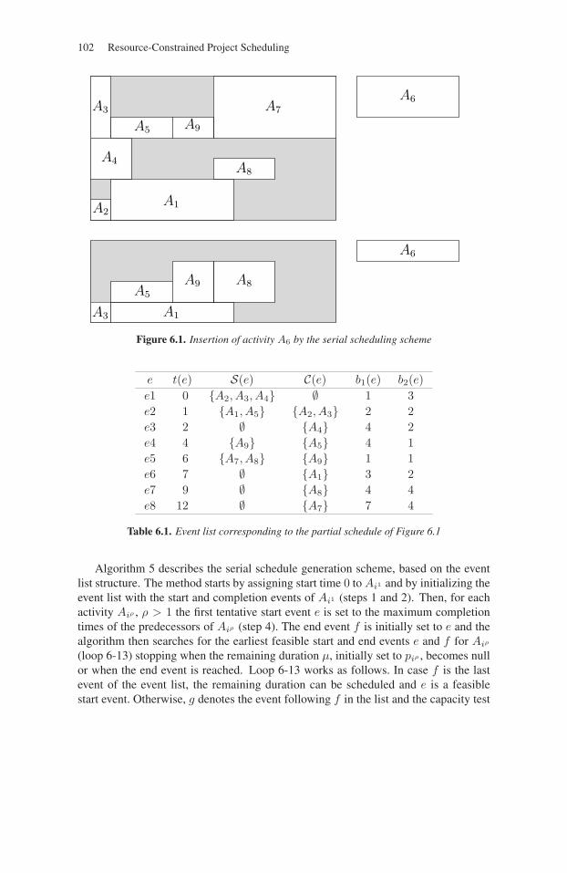
102 Resource-Constrained Project Scheduling
A1
A1
A2
A3
A3
A4
A5
A5
A6
A6
A7
A8
A8
A9
A9
Figure 6.1. Insertion of activity A6 by the serial scheduling scheme
e t(e) S(e) C(e) b1(e) b2(e)e1 0 {A2, A3, A4} ∅ 1 3e2 1 {A1, A5} {A2, A3} 2 2e3 2 ∅ {A4} 4 2e4 4 {A9} {A5} 4 1e5 6 {A7, A8} {A9} 1 1e6 7 ∅ {A1} 3 2e7 9 ∅ {A8} 4 4e8 12 ∅ {A7} 7 4
Table 6.1. Event list corresponding to the partial schedule of Figure 6.1
Algorithm 5 describes the serial schedule generation scheme, based on the eventlist structure. The method starts by assigning start time 0 to Ai1 and by initializing theevent list with the start and completion events of Ai1 (steps 1 and 2). Then, for eachactivity Aiρ , ρ > 1 the first tentative start event e is set to the maximum completiontimes of the predecessors of Aiρ (step 4). The end event f is initially set to e and thealgorithm then searches for the earliest feasible start and end events e and f for Aiρ
(loop 6-13) stopping when the remaining duration μ, initially set to piρ , becomes nullor when the end event is reached. Loop 6-13 works as follows. In case f is the lastevent of the event list, the remaining duration can be scheduled and e is a feasiblestart event. Otherwise, g denotes the event following f in the list and the capacity test
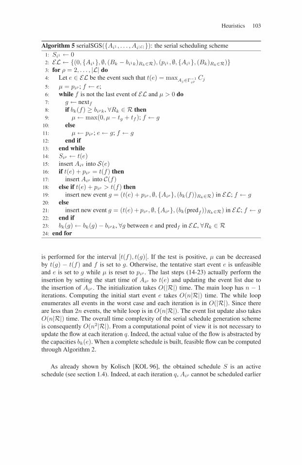
Heuristics 103
Algorithm 5 serialSGS({Ai1 , . . . , Ai|L|}): the serial scheduling scheme1: Si1 ← 02: EL ← {(0, {Ai1}, ∅, (Bk − bi1k)Rk∈R), (pi1 , ∅, {Ai1}, (Bk)Rk∈R)}3: for ρ = 2, . . . , |L| do4: Let e ∈ EL be the event such that t(e) = maxAj∈Γ−1
iρCj
5: μ = piρ ; f ← e;6: while f is not the last event of EL and μ > 0 do7: g ← nextf8: if bk(f) ≥ biρk, ∀Rk ∈ R then9: μ← max(0, μ− tg + tf ); f ← g
10: else11: μ← piρ ; e← g; f ← g12: end if13: end while14: Siρ ← t(e)15: insert Aiq into S(e)16: if t(e) + piρ = t(f) then17: insert Aiρ into C(f)18: else if t(e) + piρ > t(f) then19: insert new event g = (t(e) + piρ , ∅, {Aiρ}, (bk(f))Rk∈R) in EL; f ← g20: else21: insert new event g = (t(e) + piρ , ∅, {Aiρ}, (bk(predf ))Rk∈R) in EL; f ← g22: end if23: bk(g)← bk(g)− biρk, ∀g between e and predf in EL, ∀Rk ∈ R24: end for
is performed for the interval [t(f), t(g)[. If the test is positive, μ can be decreasedby t(g) − t(f) and f is set to g. Otherwise, the tentative start event e is unfeasibleand e is set to g while μ is reset to piρ . The last steps (14-23) actually perform theinsertion by setting the start time of Aiρ to t(e) and updating the event list due tothe insertion of Aiρ . The initialization takes O(|R|) time. The main loop has n − 1iterations. Computing the initial start event e takes O(n|R|) time. The while loopenumerates all events in the worst case and each iteration is in O(|R|). Since thereare less than 2n events, the while loop is in O(n|R|). The event list update also takesO(n|R|) time. The overall time complexity of the serial schedule generation schemeis consequently O(n2|R|). From a computational point of view it is not necessary toupdate the flow at each iteration q. Indeed, the actual value of the flow is abstracted bythe capacities bk(e). When a complete schedule is built, feasible flow can be computedthrough Algorithm 2.
As already shown by Kolisch [KOL 96], the obtained schedule S is an activeschedule (see section 1.4). Indeed, at each iteration q, Aiρ cannot be scheduled earlier
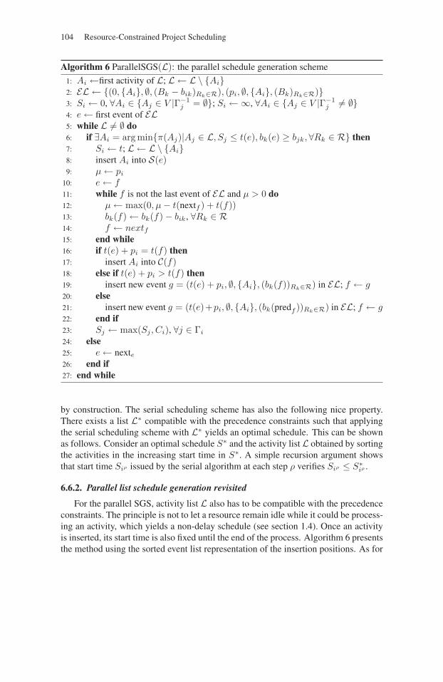
104 Resource-Constrained Project Scheduling
Algorithm 6 ParallelSGS(L): the parallel schedule generation scheme
1: Ai ←first activity of L; L ← L \ {Ai}2: EL ← {(0, {Ai}, ∅, (Bk − bik)Rk∈R), (pi, ∅, {Ai}, (Bk)Rk∈R)}3: Si ← 0, ∀Ai ∈ {Aj ∈ V |Γ−1
j = ∅}; Si ←∞, ∀Ai ∈ {Aj ∈ V |Γ−1j �= ∅}
4: e← first event of EL5: while L �= ∅ do6: if ∃Ai = arg min{π(Aj)|Aj ∈ L, Sj ≤ t(e), bk(e) ≥ bjk,∀Rk ∈ R} then7: Si ← t; L ← L \ {Ai}8: insert Ai into S(e)9: μ← pi
10: e← f11: while f is not the last event of EL and μ > 0 do12: μ← max(0, μ− t(nextf ) + t(f))13: bk(f)← bk(f)− bik, ∀Rk ∈ R14: f ← nextf15: end while16: if t(e) + pi = t(f) then17: insert Ai into C(f)18: else if t(e) + pi > t(f) then19: insert new event g = (t(e) + pi, ∅, {Ai}, (bk(f))Rk∈R) in EL; f ← g20: else21: insert new event g = (t(e)+pi, ∅, {Ai}, (bk(predf ))Rk∈R) in EL; f ← g22: end if23: Sj ← max(Sj , Ci), ∀j ∈ Γi
24: else25: e← nexte26: end if27: end while
by construction. The serial scheduling scheme has also the following nice property.There exists a list L∗ compatible with the precedence constraints such that applyingthe serial scheduling scheme with L∗ yields an optimal schedule. This can be shownas follows. Consider an optimal schedule S∗ and the activity list L obtained by sortingthe activities in the increasing start time in S∗. A simple recursion argument showsthat start time Siρ issued by the serial algorithm at each step ρ verifies Siρ ≤ S∗
iρ .
6.6.2. Parallel list schedule generation revisited
For the parallel SGS, activity list L also has to be compatible with the precedenceconstraints. The principle is not to let a resource remain idle while it could be process-ing an activity, which yields a non-delay schedule (see section 1.4). Once an activityis inserted, its start time is also fixed until the end of the process. Algorithm 6 presentsthe method using the sorted event list representation of the insertion positions. As for

Heuristics 105
the serial SGS, the first activity of the list is scheduled at time 0 and its start and endevents are created. The tentative start event e is set to the first event. At each iterationof the main loop (steps 5-27), the first activity Ai of list L that can be started at timet(e) is considered: at step 6, π(Aj) denotes the position of activity Aj in list L. Ifsuch an activity Ai exists, it is removed from L and inserted in the position definedby e, updating the event list as for the serial scheme (steps 7-22). The earliest starttimes of its successors are updated (step 23). If Ai does not exist, no more activitiescan be scheduled at event e and the next event of EL is considered. The main loophas less than 3n iterations since for each of them, either an activity is scheduled or anew event is considered. At step 6, the search for Ai is in O(n|R|) and the updateof the successor start times at step 23 takes only |Γi| iterations. The remaining com-putations are similar to those of the serial SGS. It follows that the complexity of theparallel SGS is also O(n2|R|). As underlined in section 6.2.1, since the parallel SGSgenerates only non-delay schedules there is no guarantee on the existence of a list Lyielding an optimal solution.

106
This page intentionally left blank
Chapter 7
Benchmark Instance Indicators andComputational Comparison of Methods
7.1. Introduction
If there exist some strongly NP-hard problems that can be solved reasonably wellin practice, the RCPSP belongs to the class of really hard optimization problems.To illustrate this, instances of the minimum lateness one-machine scheduling problemwith release dates with thousands of jobs can be solved to optimality by Carlier’s algo-rithm [CAR 82]. This is unfortunately not the case for the RCPSP for which today’sexact methods are still not able to solve problems dealing with more than 60 activities.
A way to compare several exact and heuristic methods proposed to solve an NP-hard optimization problem involves comparing the results they obtain in terms of con-sumed CPU time, memory requirement and objective-function value on a commonset of problem instances. Since the late 1960s, a wide variety of benchmark RCPSPinstances has been proposed. The design of such RCPSP instances must take intoaccount the following two major features that the RCPSP shares with many NP-hardproblems.
First, the RCPSP has a complex structure and can be decomposed into manycategories depending on the resource features, the activity requirements and theprecedence-constraint graph. To give an idea of this diversity, simply consider the factthat the job-shop scheduling problem (JSP) and the parallel machine problem (PMP)are both special cases of the RCPSP, both known for their hardness.
Chapter written by Christian ARTIGUES, Oumar KONÉ, Pierre LOPEZ, Marcel MONGEAU,Emmanuel NÉRON and David RIVREAU.
107
108 Resource-Constrained Project Scheduling
Second, as established by Herroelen and de Reyck [HER 99], the RCPSP admitsphase transitions. Indeed, consider a set of RCPSP instances with a single resource(|R| = 1), which allows us to drop the resource index in the notations. If B islarger than
∑Ai∈A bi, then there is no resource constraint and the problem amounts
to finding feasible start times with respect to precedence constraints only, which canbe performed in O(n2). The other extreme case is also trivial since if B is smallerthan maxAi∈A ri, then there is no solution to the problem, which can be checkedin O(n). For the intermediary values, Herroelen and de Reyck showed in [HER 99]that the computational requirement of the branch-and-bound procedure developed byDemeulemeester and Herroelen [DEM 97] varies as a function of B according to acontinuous bell-shaped easy-hard-easy complexity pattern.
The purpose of this chapter is twofold. First, we shall compare the performanceof state-of-the-art methods for solving the RCPSP. Secondly, we shall evaluate theability of several indicators to evaluate instance hardness. Indeed, an area of researchis devoted to the proposition of various indicators able to foresee the hardness of agiven instance. Section 7.2 is devoted to the presentation and the critical analysisof such indicators while section 7.3 proposes new instance indicators. The compu-tational experiments carried out in this chapter are performed on a selection of rep-resentative instance subsets. Section 7.4 refers to a presentation of the benchmarkinstances encountered in other works. Section 7.5 analyzes the stability of the indica-tors and underlines some pitfalls, focusing on a particular set of instances. Section 7.6first presents a sample of methods, also selected from other works and described inthe preceding chapters. Then, these methods are tested and compared on the selectedinstances under a common experimental framework. The results of these experimentsare analyzed and conclusions are drawn. We conclude our chapter in section 7.7.
7.2. Standard instance indicators
Since the 1960s, indicators have emerged to characterize the RCPSP instances.They can be roughly classified into four categories: precedence-oriented, time-ori-ented, resource-oriented and hybrid. In general, the correlation between an indicatorand the instance hardness is established experimentally as follows. We use an exactmethod to solve a series of groups of randomly generated instances with increasingindicator value and measures the average CPU time and its standard deviation foreach group. In this section, we list a selection of state-of-the-art indicators from eachcategory and recall the previously established relationships between the indicatorsvalue and the instance tractability.
We first consider the precedence-oriented indicators. Their objective is to evaluatethe complexity of the resource network. We concentrate here on the main precedence-oriented indicators (recently, other indicators of this category were proposed in[VAN 04]).
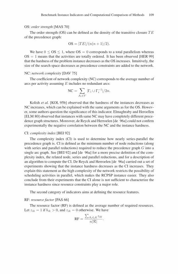
Benchmark Instance Indicators and Computational Comparison of Methods 109
OS: order strength [MAS 70]
The order strength (OS) can be defined as the density of the transitive closure TEof the precedence graph:
OS = |TE|/(n(n + 1)/2).
We have 0 ≤ OS ≤ 1, where OS = 0 corresponds to a total parallelism whereasOS = 1 means that the activities are totally ordered. It has been observed [HER 99]that the hardness of the problem instance decreases as the OS increases. Intuitively, thesize of the search space decreases as precedence constraints are added to the network.
NC: network complexity [DAV 75]
The coefficient of network complexity (NC) corresponds to the average number ofarcs per activity assuming E includes no redundant arcs:
NC =∑
Ai∈V
|Γi ∪ Γ−1i |/2n.
Kolish et al. [KOL 95b] observed that the hardness of the instances decreases asNC increases, which can be explained with the same arguments as for the OS. Howev-er, some authors question the significance of this indicator. Elmaghraby and Heroellen[ELM 80] observed that instances with same NC may have completely different prece-dence graph structures. Moreover, de Reyck and Herroelen [de 96a] could not confirmexperimentally the negative correlation between the NC and the instance hardness.
CI: complexity index [BEI 92]
The complexity index (CI) is used to determine how nearly series-parallel theprecedence graph is. CI is defined as the minimum number of node reductions (alongwith series and parallel reductions) required to reduce the precedence graph G into asingle arc graph. See [BEI 92] and [de 96a] for a more precise definition of the com-plexity index, the related node, series and parallel reductions, and for a description ofan algorithm to compute the CI. De Reyck and Herroelen [de 96a] carried out a set ofexperiments showing that the instance hardness decreases as the CI increases. Theyexplain this statement as the high complexity of the network restricts the possibility ofscheduling activities in parallel, which makes the RCPSP instance easier. They alsoconclude from their experiments that the CI alone is not sufficient to characterize theinstance hardness since resource constraints play a major role.
The second category of indicators aims at defining the resource features.
RF: resource factor [PAS 66]
The resource factor (RF) is defined as the average number of required resources.Let zik = 1 if bik > 0, and zik = 0 otherwise. We have
RF =
∑Ai∈A zik
n|R| .
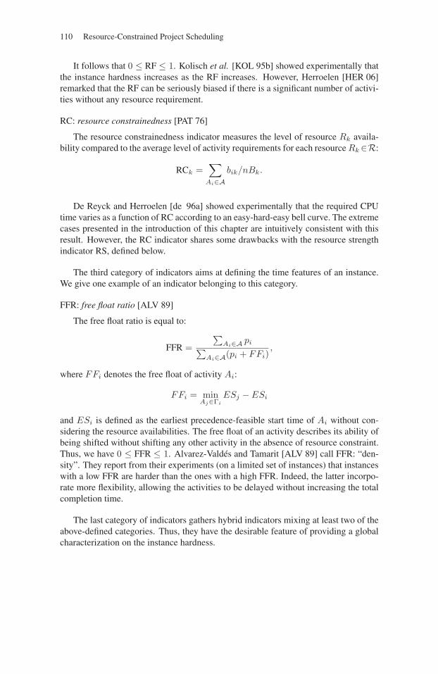
110 Resource-Constrained Project Scheduling
It follows that 0 ≤ RF ≤ 1. Kolisch et al. [KOL 95b] showed experimentally thatthe instance hardness increases as the RF increases. However, Herroelen [HER 06]remarked that the RF can be seriously biased if there is a significant number of activi-ties without any resource requirement.
RC: resource constrainedness [PAT 76]
The resource constrainedness indicator measures the level of resource Rk availa-bility compared to the average level of activity requirements for each resource Rk∈R:
RCk =∑
Ai∈Abik/nBk.
De Reyck and Herroelen [de 96a] showed experimentally that the required CPUtime varies as a function of RC according to an easy-hard-easy bell curve. The extremecases presented in the introduction of this chapter are intuitively consistent with thisresult. However, the RC indicator shares some drawbacks with the resource strengthindicator RS, defined below.
The third category of indicators aims at defining the time features of an instance.We give one example of an indicator belonging to this category.
FFR: free float ratio [ALV 89]
The free float ratio is equal to:
FFR =
∑Ai∈A pi∑
Ai∈A(pi + FFi),
where FFi denotes the free float of activity Ai:
FFi = minAj∈Γi
ESj − ESi
and ESi is defined as the earliest precedence-feasible start time of Ai without con-sidering the resource availabilities. The free float of an activity describes its ability ofbeing shifted without shifting any other activity in the absence of resource constraint.Thus, we have 0 ≤ FFR ≤ 1. Alvarez-Valdés and Tamarit [ALV 89] call FFR: “den-sity”. They report from their experiments (on a limited set of instances) that instanceswith a low FFR are harder than the ones with a high FFR. Indeed, the latter incorpo-rate more flexibility, allowing the activities to be delayed without increasing the totalcompletion time.
The last category of indicators gathers hybrid indicators mixing at least two of theabove-defined categories. Thus, they have the desirable feature of providing a globalcharacterization on the instance hardness.
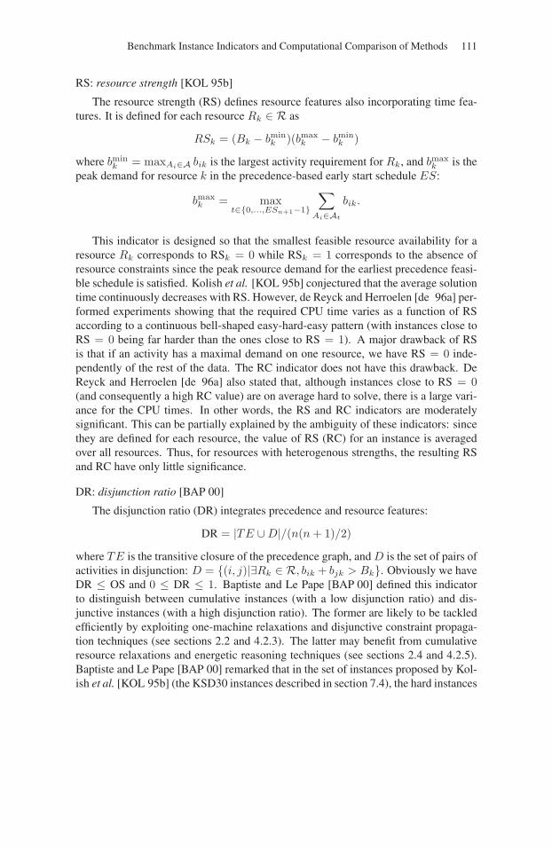
Benchmark Instance Indicators and Computational Comparison of Methods 111
RS: resource strength [KOL 95b]
The resource strength (RS) defines resource features also incorporating time fea-tures. It is defined for each resource Rk ∈ R as
RSk = (Bk − bmink )(bmax
k − bmink )
where bmink = maxAi∈A bik is the largest activity requirement for Rk, and bmax
k is thepeak demand for resource k in the precedence-based early start schedule ES:
bmaxk = max
t∈{0,...,ESn+1−1}
∑Ai∈At
bik.
This indicator is designed so that the smallest feasible resource availability for aresource Rk corresponds to RSk = 0 while RSk = 1 corresponds to the absence ofresource constraints since the peak resource demand for the earliest precedence feasi-ble schedule is satisfied. Kolish et al. [KOL 95b] conjectured that the average solutiontime continuously decreases with RS. However, de Reyck and Herroelen [de 96a] per-formed experiments showing that the required CPU time varies as a function of RSaccording to a continuous bell-shaped easy-hard-easy pattern (with instances close toRS = 0 being far harder than the ones close to RS = 1). A major drawback of RSis that if an activity has a maximal demand on one resource, we have RS = 0 inde-pendently of the rest of the data. The RC indicator does not have this drawback. DeReyck and Herroelen [de 96a] also stated that, although instances close to RS = 0(and consequently a high RC value) are on average hard to solve, there is a large vari-ance for the CPU times. In other words, the RS and RC indicators are moderatelysignificant. This can be partially explained by the ambiguity of these indicators: sincethey are defined for each resource, the value of RS (RC) for an instance is averagedover all resources. Thus, for resources with heterogenous strengths, the resulting RSand RC have only little significance.
DR: disjunction ratio [BAP 00]
The disjunction ratio (DR) integrates precedence and resource features:
DR = |TE ∪D|/(n(n + 1)/2)
where TE is the transitive closure of the precedence graph, and D is the set of pairs ofactivities in disjunction: D = {(i, j)|∃Rk ∈ R, bik + bjk > Bk}. Obviously we haveDR ≤ OS and 0 ≤ DR ≤ 1. Baptiste and Le Pape [BAP 00] defined this indicatorto distinguish between cumulative instances (with a low disjunction ratio) and dis-junctive instances (with a high disjunction ratio). The former are likely to be tackledefficiently by exploiting one-machine relaxations and disjunctive constraint propaga-tion techniques (see sections 2.2 and 4.2.3). The latter may benefit from cumulativeresource relaxations and energetic reasoning techniques (see sections 2.4 and 4.2.5).Baptiste and Le Pape [BAP 00] remarked that in the set of instances proposed by Kol-ish et al. [KOL 95b] (the KSD30 instances described in section 7.4), the hard instances
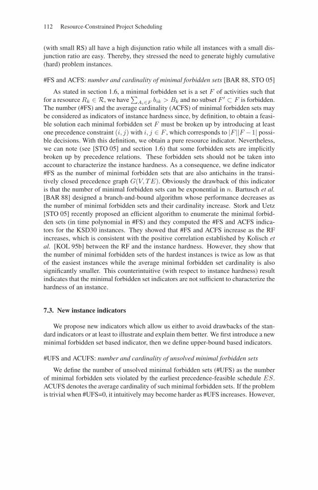
112 Resource-Constrained Project Scheduling
(with small RS) all have a high disjunction ratio while all instances with a small dis-junction ratio are easy. Thereby, they stressed the need to generate highly cumulative(hard) problem instances.
#FS and ACFS: number and cardinality of minimal forbidden sets [BAR 88, STO 05]
As stated in section 1.6, a minimal forbidden set is a set F of activities such thatfor a resource Rk ∈ R, we have
∑Ai∈F bik > Bk and no subset F ′ ⊂ F is forbidden.
The number (#FS) and the average cardinality (ACFS) of minimal forbidden sets maybe considered as indicators of instance hardness since, by definition, to obtain a feasi-ble solution each minimal forbidden set F must be broken up by introducing at leastone precedence constraint (i, j) with i, j ∈ F , which corresponds to |F ||F −1| possi-ble decisions. With this definition, we obtain a pure resource indicator. Nevertheless,we can note (see [STO 05] and section 1.6) that some forbidden sets are implicitlybroken up by precedence relations. These forbidden sets should not be taken intoaccount to characterize the instance hardness. As a consequence, we define indicator#FS as the number of minimal forbidden sets that are also antichains in the transi-tively closed precedence graph G(V, TE). Obviously the drawback of this indicatoris that the number of minimal forbidden sets can be exponential in n. Bartusch et al.[BAR 88] designed a branch-and-bound algorithm whose performance decreases asthe number of minimal forbidden sets and their cardinality increase. Stork and Uetz[STO 05] recently proposed an efficient algorithm to enumerate the minimal forbid-den sets (in time polynomial in #FS) and they computed the #FS and ACFS indica-tors for the KSD30 instances. They showed that #FS and ACFS increase as the RFincreases, which is consistent with the positive correlation established by Kolisch etal. [KOL 95b] between the RF and the instance hardness. However, they show thatthe number of minimal forbidden sets of the hardest instances is twice as low as thatof the easiest instances while the average minimal forbidden set cardinality is alsosignificantly smaller. This counterintuitive (with respect to instance hardness) resultindicates that the minimal forbidden set indicators are not sufficient to characterize thehardness of an instance.
7.3. New instance indicators
We propose new indicators which allow us either to avoid drawbacks of the stan-dard indicators or at least to illustrate and explain them better. We first introduce a newminimal forbidden set based indicator, then we define upper-bound based indicators.
#UFS and ACUFS: number and cardinality of unsolved minimal forbidden sets
We define the number of unsolved minimal forbidden sets (#UFS) as the numberof minimal forbidden sets violated by the earliest precedence-feasible schedule ES.ACUFS denotes the average cardinality of such minimal forbidden sets. If the problemis trivial when #UFS=0, it intuitively may become harder as #UFS increases. However,
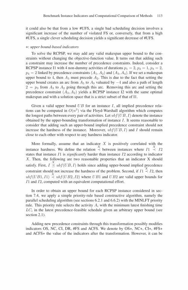
Benchmark Instance Indicators and Computational Comparison of Methods 113
it could also be that from a low #UFS, a single bad scheduling decision involves asignificant increase of the number of violated FS or, conversely, that from a high#UFS, a single clever scheduling decision yields a significant decrease of #UFS.
+: upper bound-based indicators
To solve the RCPSP, we may add any valid makespan upper bound to the con-straints without changing the objective-function value. It turns out that adding sucha constraint may increase the number of precedence constraints. Indeed, consider aRCPSP instance I1 with 4 non-dummy activities of durations p1 = 2, p2 = 1, p3 = 2,p4 = 2 linked by precedence constraints (A1, A2) and (A3, A4). If we set a makespanupper bound to 4, then A3 must precede A2. This is due to the fact that setting theupper bound creates an arc from A5 to A0 valuated by −4 and also a path of length2 = p3 from A3 to A2 going through this arc. Removing this arc and setting theprecedence constraint (A3, A2) yields a RCPSP instance I2 with the same optimalmakespan and with a solution space that is a strict subset of that of I1.
Given a valid upper bound UB for an instance I , all implied precedence rela-tions can be computed in O(n3) via the Floyd-Warshall algorithm which computesthe longest paths between every pair of activities. Let ubf(UB, I) denote the instanceobtained by the upper-bounding transformation of instance I . It seems reasonable toconsider that adding such an upper-bound implied precedence constraint should notincrease the hardness of the instance. Moreover, ubf(UB, I) and I should remainclose to each other with respect to any hardness indicator.
More formally, assume that an indicator X is positively correlated with the
instance hardness. We define the relationX≺ between instances where I1
X≺ I2states that instance I1 is significantly harder than instance I2 according to indicatorX . Then, the following are two reasonable properties that an indicator X should
satisfy. First, IX� ubf(UB, I) holds since adding upper-bound implied precedence
constraint should not increase the hardness of the problem. Second, if I1X≺ I2, then
ubf(UB1, I1)X≺ ubf(UB2, I2) where UB1 and UB2 are valid upper bounds for
I1 and I2, computed with an equivalent computational effort.
In order to obtain an upper bound for each RCPSP instance considered in sec-tion 7.4, we apply a simple priority-rule based constructive algorithm, namely theparallel scheduling algorithm (see sections 6.2.1 and 6.6.2) with the MINLFT priorityrule. This priority rule selects the activity Ai with the minimum latest finishing timeLCi in the latest precedence-feasible schedule given an arbitrary upper bound (seesection 2.1).
Adding new precedence constraints through this transformation possibly modifiesindicators OS, NC, CI, DR, #FS and ACFS. We denote by OS+, NC+, CI+, #FS+and ACFS+ the value of the indicators after the transformation. However, it can be
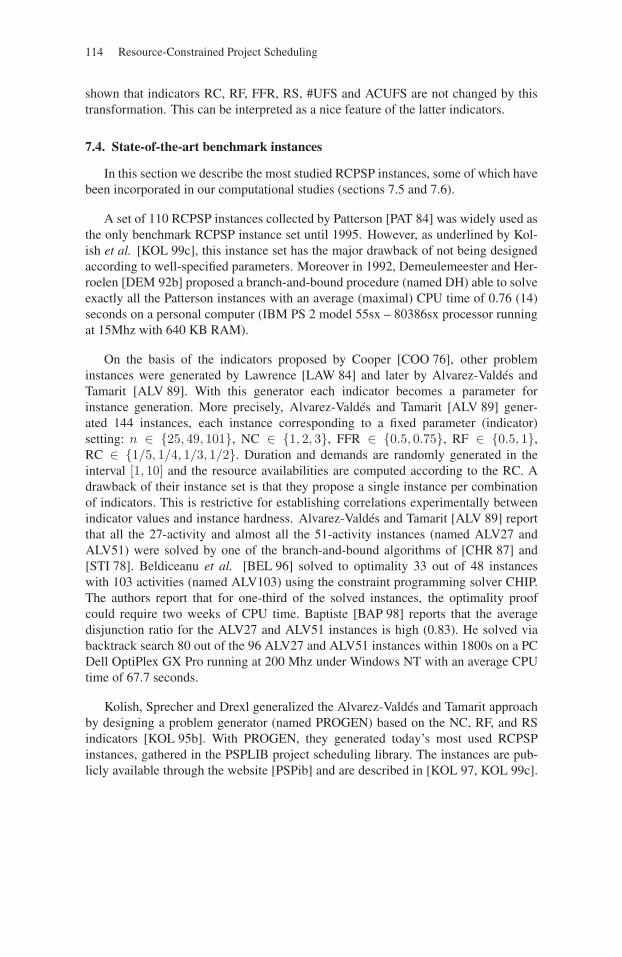
114 Resource-Constrained Project Scheduling
shown that indicators RC, RF, FFR, RS, #UFS and ACUFS are not changed by thistransformation. This can be interpreted as a nice feature of the latter indicators.
7.4. State-of-the-art benchmark instances
In this section we describe the most studied RCPSP instances, some of which havebeen incorporated in our computational studies (sections 7.5 and 7.6).
A set of 110 RCPSP instances collected by Patterson [PAT 84] was widely used asthe only benchmark RCPSP instance set until 1995. However, as underlined by Kol-ish et al. [KOL 99c], this instance set has the major drawback of not being designedaccording to well-specified parameters. Moreover in 1992, Demeulemeester and Her-roelen [DEM 92b] proposed a branch-and-bound procedure (named DH) able to solveexactly all the Patterson instances with an average (maximal) CPU time of 0.76 (14)seconds on a personal computer (IBM PS 2 model 55sx – 80386sx processor runningat 15Mhz with 640 KB RAM).
On the basis of the indicators proposed by Cooper [COO 76], other probleminstances were generated by Lawrence [LAW 84] and later by Alvarez-Valdés andTamarit [ALV 89]. With this generator each indicator becomes a parameter forinstance generation. More precisely, Alvarez-Valdés and Tamarit [ALV 89] gener-ated 144 instances, each instance corresponding to a fixed parameter (indicator)setting: n ∈ {25, 49, 101}, NC ∈ {1, 2, 3}, FFR ∈ {0.5, 0.75}, RF ∈ {0.5, 1},RC ∈ {1/5, 1/4, 1/3, 1/2}. Duration and demands are randomly generated in theinterval [1, 10] and the resource availabilities are computed according to the RC. Adrawback of their instance set is that they propose a single instance per combinationof indicators. This is restrictive for establishing correlations experimentally betweenindicator values and instance hardness. Alvarez-Valdés and Tamarit [ALV 89] reportthat all the 27-activity and almost all the 51-activity instances (named ALV27 andALV51) were solved by one of the branch-and-bound algorithms of [CHR 87] and[STI 78]. Beldiceanu et al. [BEL 96] solved to optimality 33 out of 48 instanceswith 103 activities (named ALV103) using the constraint programming solver CHIP.The authors report that for one-third of the solved instances, the optimality proofcould require two weeks of CPU time. Baptiste [BAP 98] reports that the averagedisjunction ratio for the ALV27 and ALV51 instances is high (0.83). He solved viabacktrack search 80 out of the 96 ALV27 and ALV51 instances within 1800s on a PCDell OptiPlex GX Pro running at 200 Mhz under Windows NT with an average CPUtime of 67.7 seconds.
Kolish, Sprecher and Drexl generalized the Alvarez-Valdés and Tamarit approachby designing a problem generator (named PROGEN) based on the NC, RF, and RSindicators [KOL 95b]. With PROGEN, they generated today’s most used RCPSPinstances, gathered in the PSPLIB project scheduling library. The instances are pub-licly available through the website [PSPib] and are described in [KOL 97, KOL 99c].
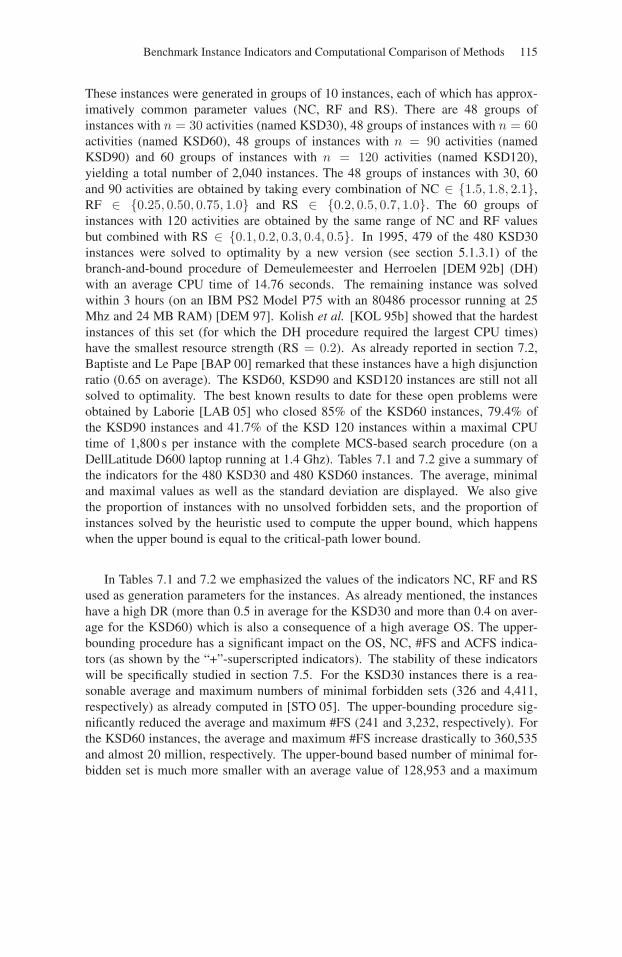
Benchmark Instance Indicators and Computational Comparison of Methods 115
These instances were generated in groups of 10 instances, each of which has approx-imatively common parameter values (NC, RF and RS). There are 48 groups ofinstances with n = 30 activities (named KSD30), 48 groups of instances with n = 60activities (named KSD60), 48 groups of instances with n = 90 activities (namedKSD90) and 60 groups of instances with n = 120 activities (named KSD120),yielding a total number of 2,040 instances. The 48 groups of instances with 30, 60and 90 activities are obtained by taking every combination of NC ∈ {1.5, 1.8, 2.1},RF ∈ {0.25, 0.50, 0.75, 1.0} and RS ∈ {0.2, 0.5, 0.7, 1.0}. The 60 groups ofinstances with 120 activities are obtained by the same range of NC and RF valuesbut combined with RS ∈ {0.1, 0.2, 0.3, 0.4, 0.5}. In 1995, 479 of the 480 KSD30instances were solved to optimality by a new version (see section 5.1.3.1) of thebranch-and-bound procedure of Demeulemeester and Herroelen [DEM 92b] (DH)with an average CPU time of 14.76 seconds. The remaining instance was solvedwithin 3 hours (on an IBM PS2 Model P75 with an 80486 processor running at 25Mhz and 24 MB RAM) [DEM 97]. Kolish et al. [KOL 95b] showed that the hardestinstances of this set (for which the DH procedure required the largest CPU times)have the smallest resource strength (RS = 0.2). As already reported in section 7.2,Baptiste and Le Pape [BAP 00] remarked that these instances have a high disjunctionratio (0.65 on average). The KSD60, KSD90 and KSD120 instances are still not allsolved to optimality. The best known results to date for these open problems wereobtained by Laborie [LAB 05] who closed 85% of the KSD60 instances, 79.4% ofthe KSD90 instances and 41.7% of the KSD 120 instances within a maximal CPUtime of 1,800 s per instance with the complete MCS-based search procedure (on aDellLatitude D600 laptop running at 1.4 Ghz). Tables 7.1 and 7.2 give a summary ofthe indicators for the 480 KSD30 and 480 KSD60 instances. The average, minimaland maximal values as well as the standard deviation are displayed. We also givethe proportion of instances with no unsolved forbidden sets, and the proportion ofinstances solved by the heuristic used to compute the upper bound, which happenswhen the upper bound is equal to the critical-path lower bound.
In Tables 7.1 and 7.2 we emphasized the values of the indicators NC, RF and RSused as generation parameters for the instances. As already mentioned, the instanceshave a high DR (more than 0.5 in average for the KSD30 and more than 0.4 on aver-age for the KSD60) which is also a consequence of a high average OS. The upper-bounding procedure has a significant impact on the OS, NC, #FS and ACFS indica-tors (as shown by the “+”-superscripted indicators). The stability of these indicatorswill be specifically studied in section 7.5. For the KSD30 instances there is a rea-sonable average and maximum numbers of minimal forbidden sets (326 and 4,411,respectively) as already computed in [STO 05]. The upper-bounding procedure sig-nificantly reduced the average and maximum #FS (241 and 3,232, respectively). Forthe KSD60 instances, the average and maximum #FS increase drastically to 360,535and almost 20 million, respectively. The upper-bound based number of minimal for-bidden set is much more smaller with an average value of 128,953 and a maximum
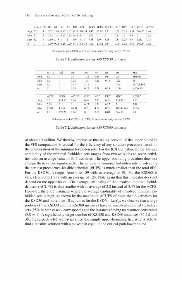
116 Resource-Constrained Project Scheduling
n + 2 |R| OS NC RF RS DR #FS ACFS #UFS ACUFS OS+ NC+ DR+ #FS+ ACFS+
Avg 32 4 0.52 1.81 0.63 0.62 0.56 326.24 3.45 17.01 2.2 0.58 2.15 0.61 241.77 3.44
Min 32 4 0.34 1.5 0.25 0.14 0.36 6 2.02 0 0 0.34 1.5 0.4 2 2.02
Max 32 4 0.69 2.13 1 1 0.9 4411 7.38 159 6.18 0.81 3.25 0.9 3232 7.73
σ 0 0 0.09 0.26 0.28 0.29 0.11 508.33 1.02 21.92 1.44 0.09 0.32 0.09 360.84 1.02
% instances with #UFS = 0: 25%, % instances trivially solved: 35.2%
Table 7.1. Indicators for the 480 KSD30 instances
n + 2 |R| OS NC RF RS DR #FS
Avg 62 4 0.4 1.81 0.63 0.6 0.41 360,535
Min 62 4 0.25 1.5 0.25 0.14 0.25 69
Max 62 4 0.57 2.11 1 1 0.68 19,723,866
σ 0 0 0.08 0.25 0.28 0.29 0.09 1,676,354
ACFS #UFS ACUFS OS+ NC+ DR+ #FS+ ACFS+
Avg 5.21 124.52 3.06 0.49 2.72 0.5 128,953 5.17
Min 2.38 0 0 0.27 1.5 0.27 31 2.38
Max 12.01 1,958 10.34 0.7 4.19 0.7 10,338,140 12.54
σ 1.9 227.28 2.16 0.1 0.62 0.09 646,581 1.9
% instances with #UFS = 0 : 25%, % instances trivially solved: 38.7%
Table 7.2. Indicators for the 480 KSD60 instances
of about 10 million. We thereby emphasize that taking account of the upper bound inthe #FS computation is crucial for the efficiency of any solution procedure based onthe enumeration of the minimal forbidden sets. For the KSD30 instances, the averagecardinality of the minimal forbidden sets ranges from two activities to seven activi-ties with an average value of 3.45 activities. The upper bounding procedure does notchange these values significantly. The number of minimal forbidden sets unsolved bythe earliest precedence-feasible schedule (#UFS) is much smaller than the total #FS.For the KSD30, it ranges from 0 to 159 with an average of 19. For the KSD60, itvaries from 0 to 1,958 with an average of 124. Note again that this indicator does notdepend on the upper bound. The average cardinality of the unsolved minimal forbid-den sets (ACUFS) is also smaller with an average of 2.2 instead of 3.45 for the ACFS.However, there are instances where the average cardinality of unsolved minimal for-bidden sets is high, as shown by the maximum ACUFS of more than 6 activities forthe KSD30 and more than 10 activities for the KSD60. Lastly, we observe that a largeportion of the KSD30 and the KSD60 instances have no unsolved minimal forbiddensets (25% in both cases), corresponding to the instances having no resource constraints(RS = 1). A significantly larger number of KSD30 and KSD60 instances (35.2% and38.7%, respectively) are trivial since the simple upper-bounding heuristic is able tofind a feasible solution with a makespan equal to the critical-path lower bound.
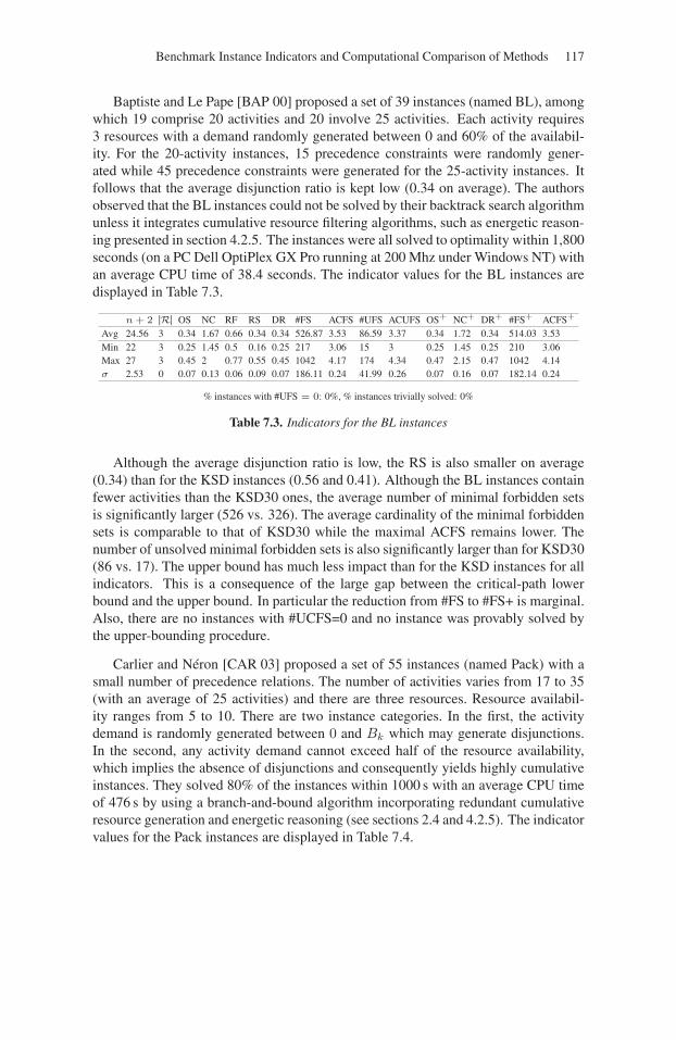
Benchmark Instance Indicators and Computational Comparison of Methods 117
Baptiste and Le Pape [BAP 00] proposed a set of 39 instances (named BL), amongwhich 19 comprise 20 activities and 20 involve 25 activities. Each activity requires3 resources with a demand randomly generated between 0 and 60% of the availabil-ity. For the 20-activity instances, 15 precedence constraints were randomly gener-ated while 45 precedence constraints were generated for the 25-activity instances. Itfollows that the average disjunction ratio is kept low (0.34 on average). The authorsobserved that the BL instances could not be solved by their backtrack search algorithmunless it integrates cumulative resource filtering algorithms, such as energetic reason-ing presented in section 4.2.5. The instances were all solved to optimality within 1,800seconds (on a PC Dell OptiPlex GX Pro running at 200 Mhz under Windows NT) withan average CPU time of 38.4 seconds. The indicator values for the BL instances aredisplayed in Table 7.3.
n + 2 |R| OS NC RF RS DR #FS ACFS #UFS ACUFS OS+ NC+ DR+ #FS+ ACFS+
Avg 24.56 3 0.34 1.67 0.66 0.34 0.34 526.87 3.53 86.59 3.37 0.34 1.72 0.34 514.03 3.53Min 22 3 0.25 1.45 0.5 0.16 0.25 217 3.06 15 3 0.25 1.45 0.25 210 3.06Max 27 3 0.45 2 0.77 0.55 0.45 1042 4.17 174 4.34 0.47 2.15 0.47 1042 4.14σ 2.53 0 0.07 0.13 0.06 0.09 0.07 186.11 0.24 41.99 0.26 0.07 0.16 0.07 182.14 0.24
% instances with #UFS = 0: 0%, % instances trivially solved: 0%
Table 7.3. Indicators for the BL instances
Although the average disjunction ratio is low, the RS is also smaller on average(0.34) than for the KSD instances (0.56 and 0.41). Although the BL instances containfewer activities than the KSD30 ones, the average number of minimal forbidden setsis significantly larger (526 vs. 326). The average cardinality of the minimal forbiddensets is comparable to that of KSD30 while the maximal ACFS remains lower. Thenumber of unsolved minimal forbidden sets is also significantly larger than for KSD30(86 vs. 17). The upper bound has much less impact than for the KSD instances for allindicators. This is a consequence of the large gap between the critical-path lowerbound and the upper bound. In particular the reduction from #FS to #FS+ is marginal.Also, there are no instances with #UCFS=0 and no instance was provably solved bythe upper-bounding procedure.
Carlier and Néron [CAR 03] proposed a set of 55 instances (named Pack) with asmall number of precedence relations. The number of activities varies from 17 to 35(with an average of 25 activities) and there are three resources. Resource availabil-ity ranges from 5 to 10. There are two instance categories. In the first, the activitydemand is randomly generated between 0 and Bk which may generate disjunctions.In the second, any activity demand cannot exceed half of the resource availability,which implies the absence of disjunctions and consequently yields highly cumulativeinstances. They solved 80% of the instances within 1000 s with an average CPU timeof 476 s by using a branch-and-bound algorithm incorporating redundant cumulativeresource generation and energetic reasoning (see sections 2.4 and 4.2.5). The indicatorvalues for the Pack instances are displayed in Table 7.4.
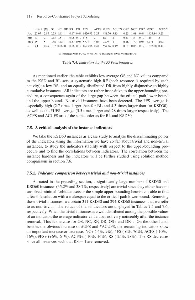
118 Resource-Constrained Project Scheduling
n + 2 |R| OS NC RF RS DR #FS ACFS #UFS ACUFS OS+ NC+ DR+ #FS+ ACFS+
Avg 25.07 2.85 0.23 1.61 1 0.17 0.44 1426.93 3.23 481.76 3.13 0.23 1.61 0.44 1425.84 3.23
Min 17 2 0.13 1.5 1 0.08 0.19 115 2 18 2 0.13 1.5 0.19 115 2
Max 35 5 0.48 1.72 1 0.53 0.94 5774 4.02 2399 4 0.48 1.72 0.94 5774 4.02
σ 5.1 0.49 0.07 0.06 0 0.08 0.19 1623.06 0.47 557.86 0.49 0.07 0.06 0.19 1623.28 0.47
% instances with #UFS = 0: 0%, % instances trivially solved: 0%
Table 7.4. Indicators for the 55 Pack instances
As mentioned earlier, the table exhibits low average OS and NC values comparedto the KSD and BL sets, a systematic high RF (each resource is required by eachactivity), a low RS, and an equally distributed DR from highly disjunctive to highlycumulative instances. All indicators are rather insensitive to the upper-bounding pro-cedure, a consequence again of the large gap between the critical-path lower boundand the upper bound. No trivial instances have been detected. The #FS average isespecially high (2.7 times larger than for BL and 4.3 times larger than for KSD30),as well as the #UFS average (5.5 times larger and 28 times larger respectively). TheACFS and ACUFS are of the same order as for BL and KSD30.
7.5. A critical analysis of the instance indicators
We take the KSD60 instances as a case study to analyze the discriminating powerof the indicators using the information we have so far about trivial and non-trivialinstances, to study the indicators stability with respect to the upper-bounding pro-cedure and to find the correlations between indicators. The correlation between theinstance hardness and the indicators will be further studied using solution methodcomparisons in section 7.6.
7.5.1. Indicator comparison between trivial and non-trivial instances
As noted in the preceding section, a significantly large number of KSD30 andKSD60 instances (35.2% and 38.7%, respectively) are trivial since they either have nounsolved minimal forbidden sets or the simple upper-bounding heuristic is able to finda feasible solution with a makespan equal to the critical-path lower bound. Removingthese trivial instances, we obtain 311 KSD30 and 294 KSD60 instances that we referto as non-trivial. The values of their indicators are displayed in Tables 7.5 and 7.6,respectively. When the trivial instances are well distributed among the possible valuesof an indicator, the average indicator value does not vary noticeably after the instanceremoval. This is the case for OS, NC, RF, DR, OS+ and DR+. On the other hand,besides the obvious increase of #UFS and #ACUFS, the remaining indicators showan important increase or decrease: NC+ (-4%,-9%), #FS (-6%,-76%), ACFS (-10%,-16%), #FS+ (+6%,-64%), ACFS+ (-10%,-16%), RS (-25%,-28%). The RS decreasessince all instances such that RS = 1 are removed.
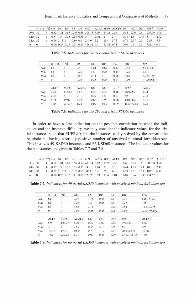
Benchmark Instance Indicators and Computational Comparison of Methods 119
n + 2 |R| OS NC RF RS DR #FS ACFS #UFS ACUFS OS+ NC+ DR+ #FS+ ACFS+
Avg 32 4 0.52 1.81 0.63 0.46 0.58 306.15 3.09 24.21 2.86 0.55 2.06 0.61 257.09 3.08Min 32 4 0.34 1.5 0.25 0.14 0.36 8 2.02 2 2 0.34 1.5 0.43 8 2.02Max 32 4 0.69 2.13 1 0.89 0.9 2,840 5.5 159 5.75 0.74 2.97 0.9 2,054 5.54σ 0 0 0.09 0.26 0.27 0.21 0.11 418.32 0.7 23.41 0.71 0.09 0.31 0.1 322.07 0.7
Table 7.5. Indicators for the 311 non-trivial KSD30 instances
n + 2 |R| OS NC RF RS DR #FSAvg 62 4 0.4 1.81 0.62 0.43 0.42 84,673.53Min 62 4 0.25 1.5 0.25 0.14 0.25 130Max 62 4 0.57 2.11 1 0.76 0.68 3,774,139σ 0 0 0.08 0.25 0.28 0.2 0.09 312,865.6
ACFS #UFS ACUFS OS+ NC+ DR+ #FS+ ACFS+
Avg 4.37 175.63 3.81 0.46 2.46 0.48 46,072.6 4.34Min 2.38 5 2 0.27 1.5 0.27 52 2.38Max 8.74 1958 7.42 0.66 3.9 0.68 1,609,652 8.71σ 1.26 250.97 1.22 0.09 0.59 0.09 157,472.18 1.25
Table 7.6. Indicators for the 294 non-trivial KSD60 instances
In order to have a first indication on the possible correlation between the indi-cators and the instance difficulty, we may consider the indicator values for the triv-ial instances such that #UFS �=0, i.e. the instances easily solved by the constructiveheuristic but having a strictly positive number of unsolved minimal forbidden sets.This involves 49 KSD30 instances and 66 KSD60 instances. The indicator values forthese instances are given in Tables 7.7 and 7.8.
n + 2 |R| OS NC RF RS DR #FS ACFS #UFS ACUFS OS+ NC+ DR+ #FS+ ACFS+
Avg 32 4 0.51 1.81 0.61 0.66 0.52 483.14 3.62 12.96 3.35 0.6 2.23 0.6 306.08 3.58Min 32 4 0.37 1.5 0.25 0.35 0.37 14 2.14 2 2 0.44 1.75 0.43 10 2.12Max 32 4 0.67 2.13 1 0.82 0.69 3413 6.4 55 6.18 0.74 2.81 0.75 1823 6.41σ 0 0 0.08 0.26 0.32 0.1 0.09 721.28 0.99 13.4 1.01 0.07 0.26 0.08 454.67 1
Table 7.7. Indicators for 49 trivial KSD30 instances with unsolved minimal forbidden sets
n + 2 |R| OS NC RF RS DR #FSAvg 62 4 0.39 1.78 0.66 0.67 0.39 826,181.59Min 62 4 0.27 1.5 0.25 0.5 0.27 136Max 62 4 0.53 2.11 1 0.72 0.54 12,630,775σ 0 0 0.08 0.25 0.28 0.08 0.08 2,324,982.02
ACFS #UFS ACUFS OS+ NC+ DR+ #FS+ ACFS+
Avg 5.9 123.27 5.29 0.52 3.09 0.52 394,420.7 5.82Min 3 6 2.55 0.35 2.18 0.35 55 2.93Max 10.34 1733 10.34 0.7 4.19 0.7 10,338,140 10.38σ 1.62 237.23 1.71 0.09 0.44 0.09 1,403,795.43 1.65
Table 7.8. Indicators for 66 trivial KSD60 instances with unsolved minimal forbidden sets

120 Resource-Constrained Project Scheduling
Compared to the non-trivial instances, the trivial ones with unsolved minimal for-bidden sets have higher NC+ (+8%,+25%), #FS (+57%,+875%), ACFS (+17%,+35%),#FS+(+19%,+756%), ACFS+(+16%;+34%), RS (+43%,+55%) and ACUFS (+17%,+38%), whereas they have a lower #UFS (-46%,-29%). Thus, we verify the counterin-tuitive result that easy instances may have a much larger number of minimal forbiddensets. On the other hand, the trivial instances have a significantly lower average numberof unsolved minimal forbidden sets than the non-trivial instances. However, it wouldbe rash to conclude that the #UFS is a good indicator for measuring instance hard-ness. Indeed, the number of unsolved minimal forbidden set remains relatively highfor these trivial instances.
7.5.2. Indicator stability and correlation
In order to evaluate the stability of the indicators, we compare each indicator withits upper-bound based counterpart, by means of a correlation coefficient, average andstandard deviation. We restrict this study to the KSD60 instance set. Since the num-ber of minimal forbidden sets can be exponential in n, we take the #FS and #FS+indicators to perform the evaluations. The results are summarized in Table 7.9.
NC/NC+ OS/OS+ DR/DR+ log#FS/log#FS+ ACFS/ACFS+
Correl. Coeff 0.25 0.75 0.75 0.98 1
Avg Dev (%) 52 23 23 6 1
Std Dev (%) 38 19 19 5 2
Table 7.9. Impact of upper bounding on the KSD60 indicators
The table shows that the NC indicator is the less stable indicator with importantdifferences between instances representing the same problems and a weak correlationbetween NC and NC+. On the other hand, the upper-bounding procedure has nosignificant effect on the average cardinality of the minimal forbidden sets.
We illustrate the instability of NC in Figure 7.1. The X-axis represents the 480KSD60 instances in the lexicographic order corresponding to increasing NC, thenRF and then RS. The Y-axis gives the values of NC, NC+ and RS. We observe inthe bottom part the variation of RS (0.2, 0.5, 0.7, 1.0) while the NC variation (1.5,1.8, 2.1) is displayed in the middle part. The effect of the upper bounding procedureis well illustrated by the observed relation between RS and NC+ (top part). WhenRS = 0.2, the gap between NC and NC+ is very narrow whereas it becomes high forthe other values of RS. As already mentioned, several studies consider that the hardestinstances are those with RS = 0.2. Thus, the upper bound obtained by the simpleheuristic greatly deviates from the critical-path lower bound which implies a smallernumber of additional precedence constraints.
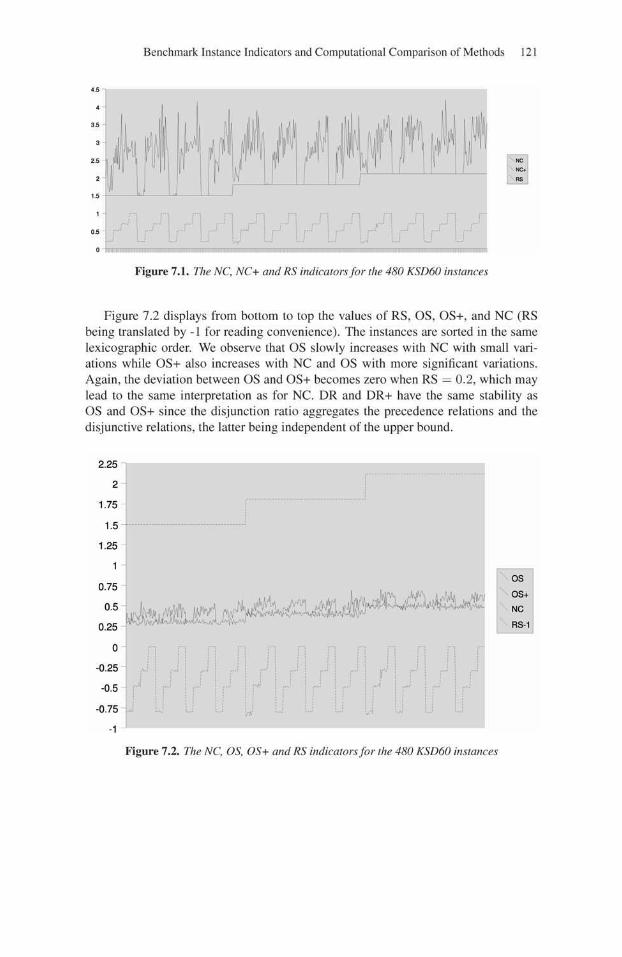
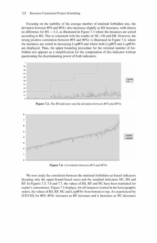
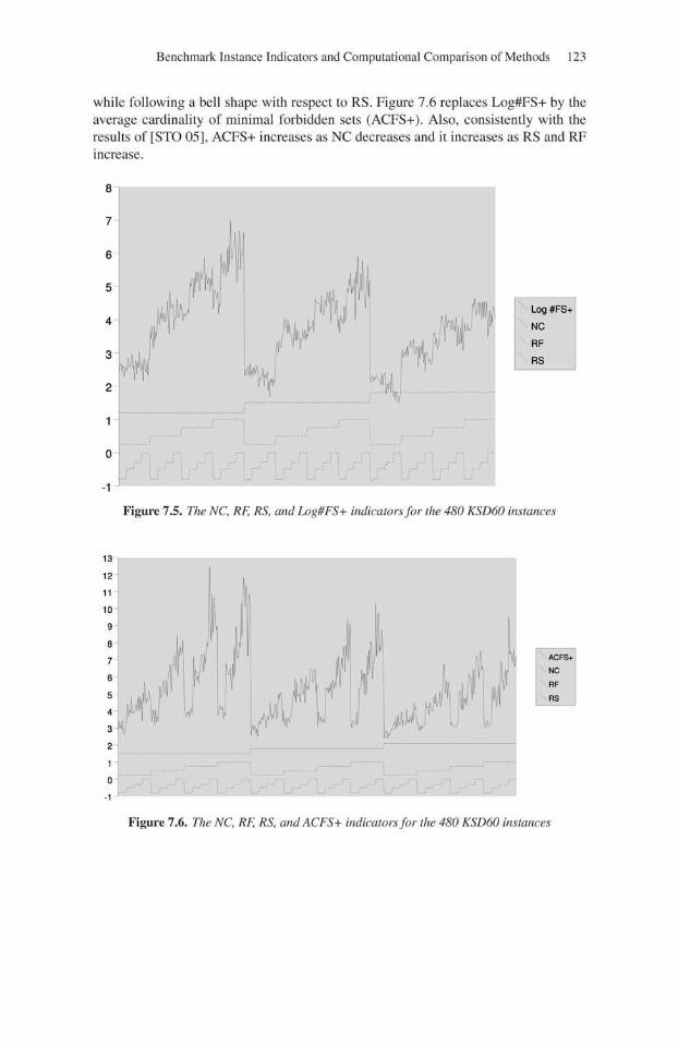
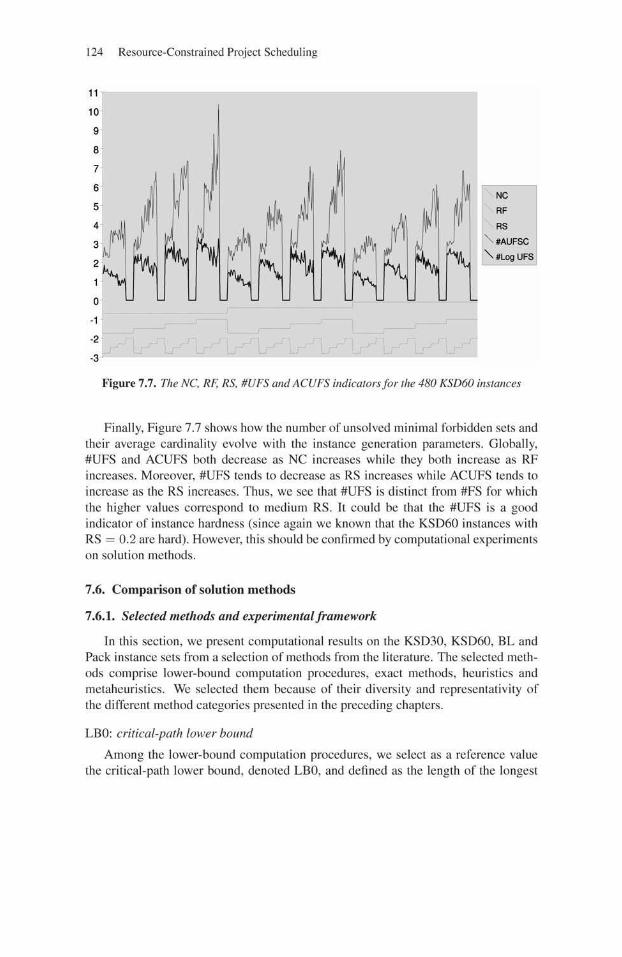
Benchmark Instance Indicators and Computational Comparison of Methods 125
path in the precedence graph. The bound is very fast to compute: O(|E|) with Bell-man’s longest-path algorithm. However, it can be expected to be far from the optimalmakespan since it ignores resource constraints (see also section 2.1).
DCP: disjunctive constraint-propagation based lower bound
We choose a second lower-bound computation procedure based on constraint-propagation algorithms mostly focusing on disjunctive subproblem relaxations. Wedenote this bound DCP and we describe how it is computed below. As stated in sec-tion 2.2, the disjunctive subproblem relaxation consists of generating one-machineproblems implied by the considered RCPSP instance. A one-machine problem con-sists of a set of pairwise disjunctive activities together with a time-window [ESi, LSi]associated with each activity Ai, where ESi (LSi) denotes the earliest (latest) starttime of Ai.
We set the time-windows as follows: for each activity Ai, the initial ESi is set tothe longest path from A0 to Ai in the precedence graph, while LSi is set to a certainupper bound minus the longest path from Ai to An+1. The upper bound, denoted UB,is obtained by the parallel scheduling algorithm with the MINLFT priority rule (seesections 6.2.1, 6.6.2 and 7.3).
The disjunction relation between two activities is established as follows: Ai andAj are in disjunction if they cannot be processed in parallel. This occurs when there isa precedence relation (Ai ≺ Aj or Aj ≺ Ai), when there is a resource Rk ∈ R suchthat bik + bjk > Bk or when the disjunction relation has been detected through thesymmetric triple rule designed by Brucker et al. [BRU 98]. The latter rule is based onthe following remark: suppose Ai, Aj , and Ak form a minimal forbidden set. Supposethat because of activity time-windows we know that (i) Ai and Ak must be processedin parallel from some non-zero time interval and (ii) Aj and Ak must be processedin parallel from some non-zero time interval. Then since {Ai, Aj , Ak} is a minimalforbidden set, (i) and (ii) implies that there is a disjunction relation between Ai andAj .
A one-machine problem corresponds to a clique in a graph where nodes corre-spond to activities and edges correspond to the disjunction relations. Unfortunately,there may be an exponential number of maximal cliques. To generate a limited num-ber of one-machine problems, we use a randomized version of the heuristic proposedin [BRU 98]. The heuristic generates maximal cliques by sorting the activities in arandom order and by generating greedily a maximal clique including the first activ-ity, then for the next activity not included in a maximal clique, etc. For each differentinitial random order, we obtain a different set of maximal cliques (one-machine prob-lems).
Then, for each one-machine problem, we apply the edge-finding constraint propa-gation technique to tighten the time-windows of the activity (see section 2.2). We also

126 Resource-Constrained Project Scheduling
apply a lower bounding procedure by finding for each maximal clique C of activitiesthe largest bound given by
LB(C) = maxC′⊆C
(min
Ai∈C′ESi +
∑Ai∈C′
pi + minAi∈C′
(UB − LCi)
), (7.1)
where LCi is the latest completion time of Ai. Obviously, the magnitude of time-window adjustments and the lower-bound quality highly depend on the disjunctivenature of the considered instance, and also on the quality of the upper bound UB. Wecoded the DCP procedure in C++.
PWW: linear programming lower bound [PRI 69]
The third lower bound that we shall test corresponds to the continuous relaxationof the ILP proposed by Pritsker et al. [PRI 69] and described in section 3.2.1. The ILPcomprises time indexed 0-1 variables representing the activities start times. We denotePWW the lower bound obtained by solving to optimality this LP relaxation. There isa pseudo-polynomial number of 0-1 variables since there is one binary variable perpossible start time of each activity: at most n(UB−pi), where UB is the upper boundused as scheduling horizon. There is also a pseudo-polynomial number of resourceconstraints.
CAT: linear programming lower bound [CHR 87]
The fourth lower bound that we shall evaluate is the continuous relaxation of theILP proposed by Christofides et al. [CHR 87]. This ILP mainly proposes a disag-gregated variant of the precedence constraints yielding a stronger relaxation at theexpense of a pseudo-polynomial number of precedence constraints (|E|UB in theworst case). We denote by CAT the lower bound obtained by solving to optimalitythis LP relaxation.
We coded all the linear programs using the C++ API of the ILOG CPLEX 10.2linear programming solver [ILO 07b]. We used the default CPLEX parameters forlinear programming.
DCP-PWW and DCP-CAT: constraint propagation/linear programming lower bound
The size of the PWW and CAT linear programs strongly depends on the number ofpossible activity start times. Thus, it seems natural to use the time-window reductionsperformed by constraint propagation as a preprocessing step of the LPs. This reducesthe number of 0-1 variables to LSi − ESi for each activity, and also the numberof precedence constraints in the disaggregated model. This also restricts the feasi-ble set of continuous solutions, which in turn possibly increases the optimal relaxedmakespan. Such preprocessing techniques and other CP-based valid inequalities havebeen studied in [DEM 02a, DEM 05] and also reported in section 3.2.1. We denote byDCP-PWW and DCP-CAT the solving of the Pritsker et al. [PRI 69] and Christofideset al. [CHR 87] LP relaxation after DCP preprocessing.

Benchmark Instance Indicators and Computational Comparison of Methods 127
MCS: complete minimal critical set lower bound [LAB 05]
The last lower bound computation method that we shall test is also an exactmethod: the complete MCS-based search proposed by Laborie [LAB 05], whereMCS stands for Minimal Critical Set, another designation of the minimal forbiddenset concept. Following the destructive framework, the method applies a completebacktrack search with constraint propagation to verify whether there exists a solutionsatisfying a tentative upper bound T , where T is initially set to a valid lower bound.If the search fails then T + 1 is a lower bound and the process can be iterated bysetting T ← T + 1. If the search succeeds, T is the optimal makespan. The backtracksearch proceeds by detection and resolution of minimal forbidden sets. A resolverof a minimal forbidden set is a precedence relation that breaks up the forbidden set.Namely, each node maintains a set of precedence relations between the activities.During node evaluation, we select a minimal forbidden set violated by the precedenceconstraints. Children nodes are created by generating for each of them a precedencerelation (a resolver) breaking up the forbidden set. The minimal forbidden set isselected so as to minimize an estimation of the remaining search space after itsresolution. The method also comprises a self-adapting shaving technique applied ateach node to strengthen constraint propagation. If all but one resolver of a minimalforbidden set yield a search failure after constraint propagation, then the precedenceconstraint of the remaining resolver must be verified. The constraint propagationtechniques used are the timetable, disjunctive, edge-finding, precedence-energy andbalance constraints (described in Chapter 4). A time limit is imposed to the backtracksearch so that the current lower bound is returned if the time limit is reached. If thetime limit is not reached, the optimal makespan is returned. The method, based on theILOG Constraint Programming solver was kindly provided by Philippe Laborie, as abinary executable file using ILOG CP 1.2 [ILO 07a] runtime license.
DH: branch-and-bound [DEM 97]
Our computational experiments also comprise the exact branch-and-bound methodproposed by Demeulemeester and Herroelen [DEM 97], denoted by DH. The methodis based on the delaying alternative branching scheme (see section 5.1.3.1) and usesthe local left shift dominance rule (see section 5.1.2), the powerful cut-set dominancerule (see section 5.1.4), and the weighted node packing bound inspired by Mingozziet al. [MIN 98] (see section 3.2.2). As stated in section 7.4, this method was the firstto solve all KSD30 instances to optimality. The method was kindly provided by ErikDemeulemeester and Willy Herroelen as C++ files.
PAR-LFT: parallel schedule scheme with the MINLFT priority rule
Besides lower-bound computation and exact methods, we shall also evaluate threeheuristics and metaheuristics. The first one is a simple call of the parallel schedulingscheme with the minimum latest finishing time priority rule. We used the method thatis described in detail in sections 6.2.1 and 6.6.2, to compute the upper-bound based
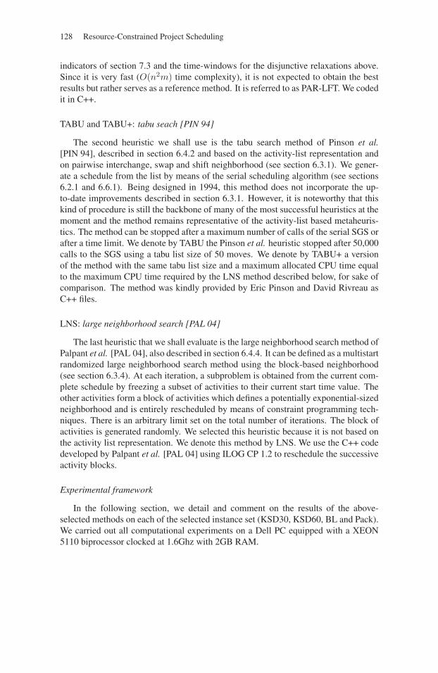
128 Resource-Constrained Project Scheduling
indicators of section 7.3 and the time-windows for the disjunctive relaxations above.Since it is very fast (O(n2m) time complexity), it is not expected to obtain the bestresults but rather serves as a reference method. It is referred to as PAR-LFT. We codedit in C++.
TABU and TABU+: tabu seach [PIN 94]
The second heuristic we shall use is the tabu search method of Pinson et al.[PIN 94], described in section 6.4.2 and based on the activity-list representation andon pairwise interchange, swap and shift neighborhood (see section 6.3.1). We gener-ate a schedule from the list by means of the serial scheduling algorithm (see sections6.2.1 and 6.6.1). Being designed in 1994, this method does not incorporate the up-to-date improvements described in section 6.3.1. However, it is noteworthy that thiskind of procedure is still the backbone of many of the most successful heuristics at themoment and the method remains representative of the activity-list based metaheuris-tics. The method can be stopped after a maximum number of calls of the serial SGS orafter a time limit. We denote by TABU the Pinson et al. heuristic stopped after 50,000calls to the SGS using a tabu list size of 50 moves. We denote by TABU+ a versionof the method with the same tabu list size and a maximum allocated CPU time equalto the maximum CPU time required by the LNS method described below, for sake ofcomparison. The method was kindly provided by Eric Pinson and David Rivreau asC++ files.
LNS: large neighborhood search [PAL 04]
The last heuristic that we shall evaluate is the large neighborhood search method ofPalpant et al. [PAL 04], also described in section 6.4.4. It can be defined as a multistartrandomized large neighborhood search method using the block-based neighborhood(see section 6.3.4). At each iteration, a subproblem is obtained from the current com-plete schedule by freezing a subset of activities to their current start time value. Theother activities form a block of activities which defines a potentially exponential-sizedneighborhood and is entirely rescheduled by means of constraint programming tech-niques. There is an arbitrary limit set on the total number of iterations. The block ofactivities is generated randomly. We selected this heuristic because it is not based onthe activity list representation. We denote this method by LNS. We use the C++ codedeveloped by Palpant et al. [PAL 04] using ILOG CP 1.2 to reschedule the successiveactivity blocks.
Experimental framework
In the following section, we detail and comment on the results of the above-selected methods on each of the selected instance set (KSD30, KSD60, BL and Pack).We carried out all computational experiments on a Dell PC equipped with a XEON5110 biprocessor clocked at 1.6Ghz with 2GB RAM.
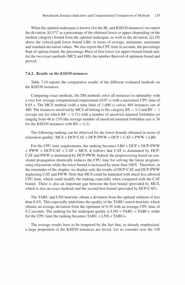
Benchmark Instance Indicators and Computational Comparison of Methods 129
When the optimal makespan is known (for the BL and KSD30 instances) we reportthe deviation ΔOPT as a percentage of the obtained lower or upper (depending on themethod category) bound from the optimal makespan, as well as the deviation ΔLB0above the critical-path lower bound LB0, in terms of average, minimum, maximumand standard-deviation values. We also report the CPU time in seconds, the percentage#opt of optima found, the percentage #best of best lower (or upper) bound found and,for the two exact methods (MCS and DH), the number #proved of optimum found andproved.
7.6.2. Results on the KSD30 instances
Table 7.10 reports the comparative results of the different evaluated methods onthe KSD30 instances.
Comparing exact methods, the DH methods solve all instances to optimality witha very low average computational requirement (0.07 s) with a maximum CPU time of8.65 s. The MCS method (with a time limit of 1,000 s) solves 469 instances out of480. The instances unsolved by MCS all belong to the category RS = 0.2 and RF = 1(except one for which RF = 0.75) with a number of unsolved minimal forbidden setranging from 48 to 159 (the average number of unsolved minimal forbidden sets is 36for the KSD30 instances with RS = 0.2).
The following ranking can be observed for the lower bounds obtained in terms ofrelaxation quality: MCS > DCP-CAT > DCP-PWW > DCP > CAT > PWW > LB0.
For the CPU time requirements, the ranking becomes LB0 < DCP < DCP-PWW< PWW < DCP-CAT < CAT < MCS. It follows that CAT is dominated by DCP-CAT and PWW is dominated by DCP-PWW. Indeed, the preprocessing based on con-straint propagation drastically reduces the CPU time for solving the linear program-ming relaxations while the lower bound is increased by more than 100%. Therefore, inthe remainder of the chapter, we display only the results of DCP-CAT and DCP-PWWneglecting CAT and PWW. Note that MCS could be launched with much less allowedCPU time, which could modify the ranking especially when compared with the CATbound. There is also an important gap between the best bound (provided by MCS,which is also an exact method) and the second best bound (provided by DCP-CAT).
The TABU and LNS heuristic obtain a deviation from the optimal solution of lessthan 0.4%. This especially underlines the quality of the TABU search heuristic whichobtains an average deviation from the optimum of 0.39 with an average CPU time of0.2 seconds. The ranking for the makespan quality is LNS < TABU < TABU+ whilefor the CPU time the ranking becomes TABU < LNS < TABU+.
The average results have to be tempered by the fact that, as already emphasized,a large proportion of the KSD30 instances are trivial. Let us consider now the 120
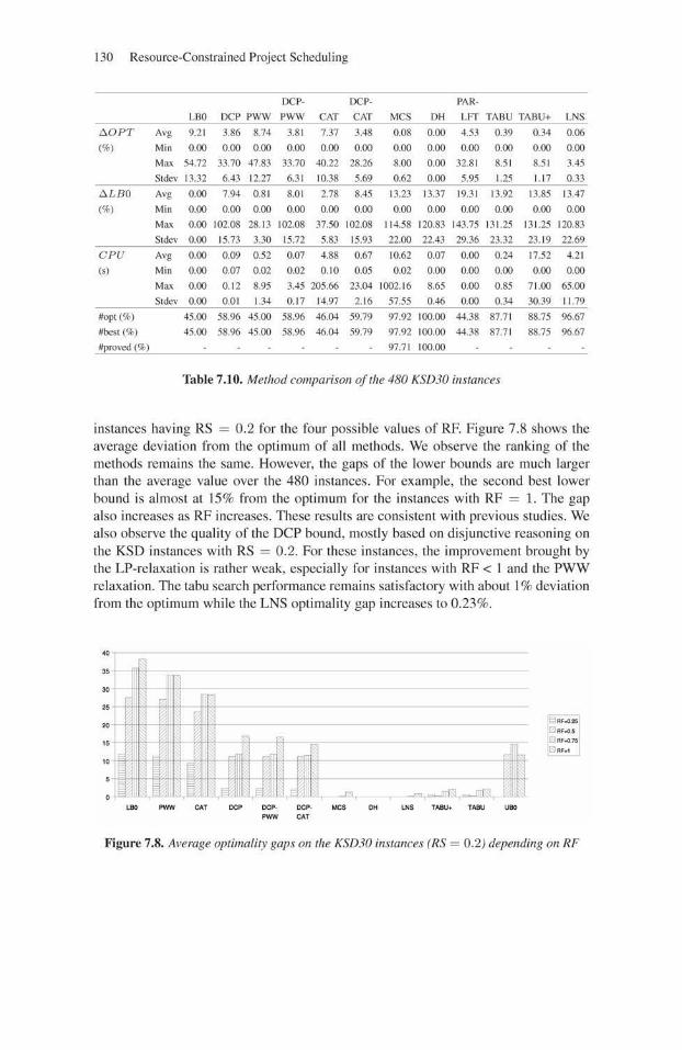
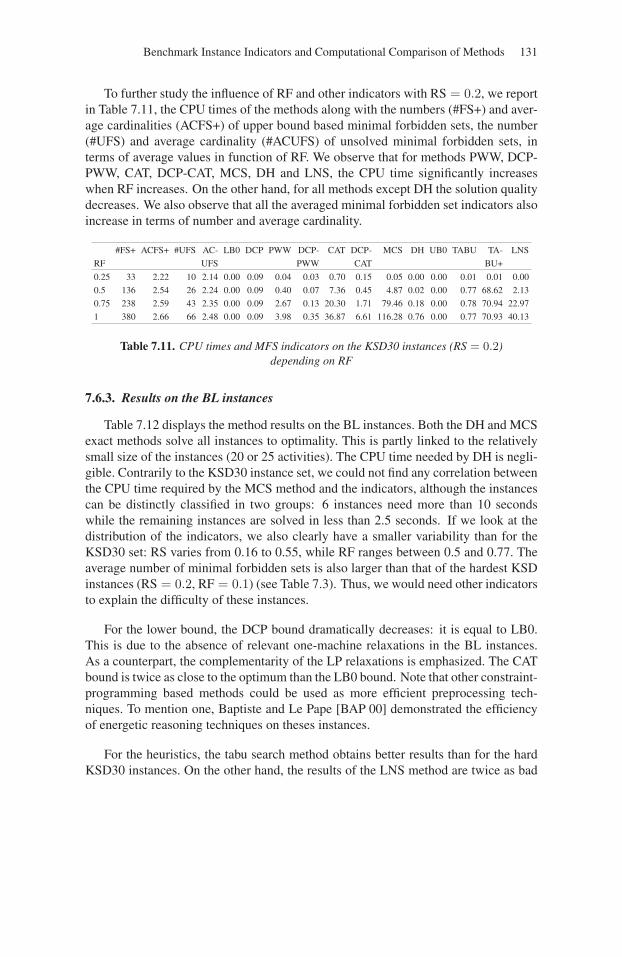
Benchmark Instance Indicators and Computational Comparison of Methods 131
To further study the influence of RF and other indicators with RS = 0.2, we reportin Table 7.11, the CPU times of the methods along with the numbers (#FS+) and aver-age cardinalities (ACFS+) of upper bound based minimal forbidden sets, the number(#UFS) and average cardinality (#ACUFS) of unsolved minimal forbidden sets, interms of average values in function of RF. We observe that for methods PWW, DCP-PWW, CAT, DCP-CAT, MCS, DH and LNS, the CPU time significantly increaseswhen RF increases. On the other hand, for all methods except DH the solution qualitydecreases. We also observe that all the averaged minimal forbidden set indicators alsoincrease in terms of number and average cardinality.
#FS+ ACFS+ #UFS AC- LB0 DCP PWW DCP- CAT DCP- MCS DH UB0 TABU TA- LNS
RF UFS PWW CAT BU+
0.25 33 2.22 10 2.14 0.00 0.09 0.04 0.03 0.70 0.15 0.05 0.00 0.00 0.01 0.01 0.00
0.5 136 2.54 26 2.24 0.00 0.09 0.40 0.07 7.36 0.45 4.87 0.02 0.00 0.77 68.62 2.13
0.75 238 2.59 43 2.35 0.00 0.09 2.67 0.13 20.30 1.71 79.46 0.18 0.00 0.78 70.94 22.97
1 380 2.66 66 2.48 0.00 0.09 3.98 0.35 36.87 6.61 116.28 0.76 0.00 0.77 70.93 40.13
Table 7.11. CPU times and MFS indicators on the KSD30 instances (RS = 0.2)depending on RF
7.6.3. Results on the BL instances
Table 7.12 displays the method results on the BL instances. Both the DH and MCSexact methods solve all instances to optimality. This is partly linked to the relativelysmall size of the instances (20 or 25 activities). The CPU time needed by DH is negli-gible. Contrarily to the KSD30 instance set, we could not find any correlation betweenthe CPU time required by the MCS method and the indicators, although the instancescan be distinctly classified in two groups: 6 instances need more than 10 secondswhile the remaining instances are solved in less than 2.5 seconds. If we look at thedistribution of the indicators, we also clearly have a smaller variability than for theKSD30 set: RS varies from 0.16 to 0.55, while RF ranges between 0.5 and 0.77. Theaverage number of minimal forbidden sets is also larger than that of the hardest KSDinstances (RS = 0.2, RF = 0.1) (see Table 7.3). Thus, we would need other indicatorsto explain the difficulty of these instances.
For the lower bound, the DCP bound dramatically decreases: it is equal to LB0.This is due to the absence of relevant one-machine relaxations in the BL instances.As a counterpart, the complementarity of the LP relaxations is emphasized. The CATbound is twice as close to the optimum than the LB0 bound. Note that other constraint-programming based methods could be used as more efficient preprocessing tech-niques. To mention one, Baptiste and Le Pape [BAP 00] demonstrated the efficiencyof energetic reasoning techniques on theses instances.
For the heuristics, the tabu search method obtains better results than for the hardKSD30 instances. On the other hand, the results of the LNS method are twice as bad
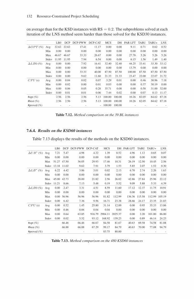
132 Resource-Constrained Project Scheduling
on average than for the KSD instances with RS = 0.2. The subproblems solved at eachiteration of the LNS method seem harder than those solved for the KSD30 instances.
LB0 DCP DCP-PWW DCP-CAT MCS DH PAR-LFT TABU TABU+ LNS
ΔOPT (%) Avg 22.62 22.62 17.41 11.17 0.00 0.00 9.11 0.71 0.62 0.52
Min 0.00 0.00 0.00 0.00 0.00 0.00 0.00 0.00 0.00 0.00
Max 46.67 46.67 33.33 26.67 0.00 0.00 27.78 5.26 5.26 5.26
Stdev 11.95 11.95 7.94 6.54 0.00 0.00 6.15 1.56 1.49 1.40
ΔLB0 (%) Avg 0.00 0.00 7.92 16.41 32.40 32.40 44.25 33.41 33.30 33.12
Min 0.00 0.00 0.00 0.00 0.00 0.00 13.79 0.00 0.00 0.00
Max 0.00 0.00 33.33 40.00 87.50 87.50 100.00 87.50 87.50 87.50
Stdev 0.00 0.00 9.62 11.60 21.33 21.33 23.47 22.00 22.07 21.72
CPU (s) Avg 0.00 0.04 0.02 0.07 3.29 0.01 0.00 0.46 30.96 7.18
Min 0.00 0.02 0.00 0.01 0.03 0.00 0.00 0.37 30.19 0.00
Max 0.00 0.06 0.05 0.28 35.71 0.08 0.00 0.58 31.00 32.00
Stdev 0.00 0.01 0.01 0.06 7.44 0.02 0.00 0.07 0.13 11.17
#opt (%) 2.56 2.56 2.56 5.13 100.00 100.00 10.26 82.05 84.62 87.18
#best (%) 2.56 2.56 2.56 5.13 100.00 100.00 10.26 82.05 84.62 87.18
#proved (%) - - - - 100.00 100.00 - - - -
Table 7.12. Method comparison on the 39 BL instances
7.6.4. Results on the KSD60 instances
Table 7.13 displays the results of the methods on the KSD60 instances.
LB0 DCP DCP-PWW DCP-CAT MCS DH PAR-LFT TABU TABU+ LNS
ΔUB∗ (%) Avg 7.21 5.47 4.98 4.22 1.39 0.52 4.96 1.12 0.65 0.07
Min 0.00 0.00 0.00 0.00 0.00 0.00 0.00 0.00 0.00 0.00
Max 51.27 47.50 36.05 29.93 17.46 10.31 26.19 12.50 10.45 2.56
Stdev 13.18 11.02 9.62 7.91 3.79 1.53 5.85 2.07 1.52 0.30
ΔLB∗ (%) Avg 6.22 4.42 3.86 3.01 0.02 2.13 6.70 2.74 2.26 1.63
Min 0.00 0.00 0.00 0.00 0.00 0.00 0.00 0.00 0.00 0.00
Max 45.00 42.73 28.00 21.82 2.56 26.02 42.86 27.84 25.96 22.12
Stdev 11.21 8.66 7.13 5.48 0.19 5.52 9.09 5.88 5.33 4.39
ΔLB0 (%) Avg 0.00 2.47 3.31 4.51 8.59 11.60 17.12 12.37 11.75 10.91
Min 0.00 0.00 0.00 0.00 0.00 0.00 0.00 0.00 0.00 0.00
Max 0.00 56.96 56.96 56.96 81.82 112.99 136.36 115.58 112.99 105.19
Stdev 0.00 6.42 7.36 9.56 16.71 23.38 28.66 24.17 23.35 21.83
CPU (s) Avg 0.00 0.52 1.45 25.80 31.14 12.89 0.00 0.95 35.33 13.86
Min 0.00 0.46 0.06 0.04 0.04 0.00 0.00 0.00 0.00 0.00
Max 0.00 0.64 63.85 916.79 2904.11 2025.37 0.00 2.20 101.00 86.00
Stdev 0.00 0.02 5.52 93.12 168.92 139.23 0.00 0.89 46.14 24.23
#opt (%) 66.46 66.46 66.67 84.58 81.67 40.63 69.58 74.58 81.88
#best (%) 66.88 66.88 67.29 99.17 84.79 40.63 70.00 77.08 94.79
#proved (%) - - - - 83.75 80.00 - - - -
Table 7.13. Method comparison on the 480 KSD60 instances
Benchmark Instance Indicators and Computational Comparison of Methods 133
For the exact methods, while the MCS method was clearly outperformed by theDH method for the KSD30 and BL instances, it obtains in turn better results on thisinstance set. Although MCS requires more CPU time than DH on average to solve theinstances to optimality (31 s vs. 13 s), it solves more instances (402 vs 384) within atime limit of 3,000 s for both methods. The compared results of MCS and DH pre-sented so far show the interest of developing new hybrid exact methods to solve theRCPSP. Combining the power of constraint propagation and self-adapting shavingwith efficient lower bounds and powerful dominance rules could be a way of improv-ing these results.
For the lower bounds, the results are consistent with those for the KSD30 set,although the CPU times of the linear programming relaxation become high. For theDCP-CAT lower bound, the CPU time can reach 916 seconds; it is 25.8 seconds onaverage. For the DCP-PWW lower bound the CPU time remains reasonable but isstill high (up to 64 s and 1.85 s on average). This obviously questions the relevance ofinteger linear programming branch-and-bound for solving the RCPSP. However, thereasonable quality of the best LP-based bound (combined with the DCP preprocess-ing) together with the recent success of column-generation-based [BRU 00, BAP 04]and Lagrangean relaxation-based lower bounds [MÖH 03] makes room for furtherimprovements, and again hybrid methods. Thus, combining constraint propagationwith branch-and-price and/or branch-and-cut techniques appears to be another promis-ing way of tackling the RCPSP.
For the heuristics, the best results are obtained according to the following rank withrespect to the average gap ΔUB∗ with the best upper bound LNS > DH > TABU+> TABU > PAR-LFT. We have to stress the excellent result of the DH method as aheuristic. However, we must here take into account the high average CPU time (600 s)obtained by incorporating instances for which the 3,000 s limit allocated to the DHmethod is reached (as for the exact methods, the tables display the average CPU timefor solved instances only). The TABU method definitely offers a good compromisebetween the quality of the solution (about 1% above the best upper bound on average,with a maximum of 12%) and the CPU time: less than one second. The TABU+method significantly improves the results of the TABU method with a rather highaverage CPU time (35 s) without reaching the result quality of the LNS method. TheLNS method is particularly successful on the KSD60 instance set: it obtains the bestresult in 94% of the cases and it is always below 2.6% from the best upper bound.However, LNS has a rather high average CPU time (13 s) and we have to emphasizethat state-of-the-art metaheuristics (see Chapter 6 and [KOL 06]) are able to reachcomparable results with much less required CPU time. Nevertheless, the table gives agood idea of today’s maximal gap between the best known lower bound and the bestknown upper bound on the KSD60 instances which reaches 22%.
Let us now use the fact that several instances are still unsolved in order to evaluatefurther the relevance of the different indicators with respect to instance difficulty. First,
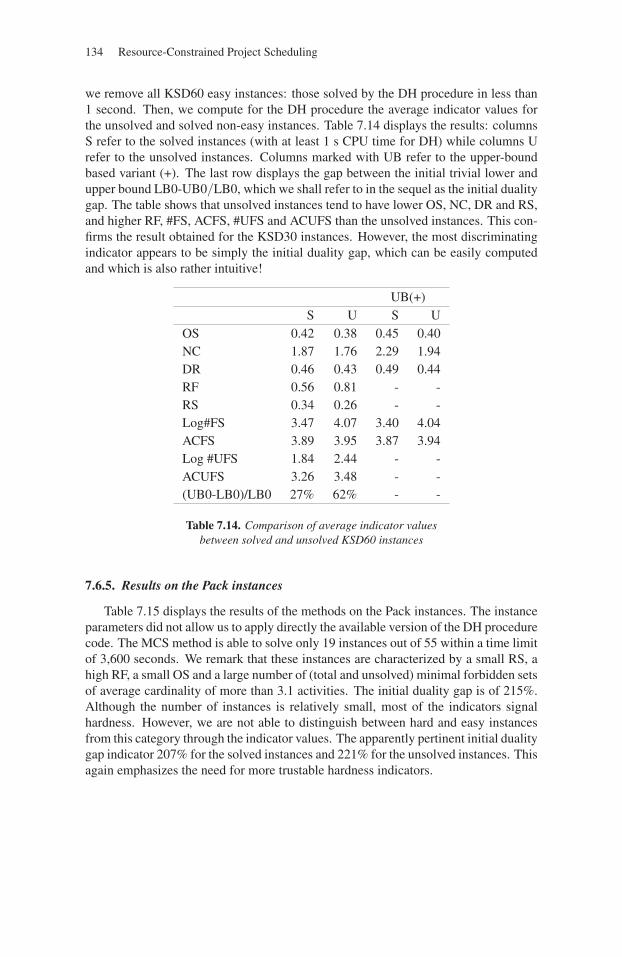
134 Resource-Constrained Project Scheduling
we remove all KSD60 easy instances: those solved by the DH procedure in less than1 second. Then, we compute for the DH procedure the average indicator values forthe unsolved and solved non-easy instances. Table 7.14 displays the results: columnsS refer to the solved instances (with at least 1 s CPU time for DH) while columns Urefer to the unsolved instances. Columns marked with UB refer to the upper-boundbased variant (+). The last row displays the gap between the initial trivial lower andupper bound LB0-UB0/LB0, which we shall refer to in the sequel as the initial dualitygap. The table shows that unsolved instances tend to have lower OS, NC, DR and RS,and higher RF, #FS, ACFS, #UFS and ACUFS than the unsolved instances. This con-firms the result obtained for the KSD30 instances. However, the most discriminatingindicator appears to be simply the initial duality gap, which can be easily computedand which is also rather intuitive!
UB(+)S U S U
OS 0.42 0.38 0.45 0.40NC 1.87 1.76 2.29 1.94DR 0.46 0.43 0.49 0.44RF 0.56 0.81 - -RS 0.34 0.26 - -Log#FS 3.47 4.07 3.40 4.04ACFS 3.89 3.95 3.87 3.94Log #UFS 1.84 2.44 - -ACUFS 3.26 3.48 - -(UB0-LB0)/LB0 27% 62% - -
Table 7.14. Comparison of average indicator valuesbetween solved and unsolved KSD60 instances
7.6.5. Results on the Pack instances
Table 7.15 displays the results of the methods on the Pack instances. The instanceparameters did not allow us to apply directly the available version of the DH procedurecode. The MCS method is able to solve only 19 instances out of 55 within a time limitof 3,600 seconds. We remark that these instances are characterized by a small RS, ahigh RF, a small OS and a large number of (total and unsolved) minimal forbidden setsof average cardinality of more than 3.1 activities. The initial duality gap is of 215%.Although the number of instances is relatively small, most of the indicators signalhardness. However, we are not able to distinguish between hard and easy instancesfrom this category through the indicator values. The apparently pertinent initial dualitygap indicator 207% for the solved instances and 221% for the unsolved instances. Thisagain emphasizes the need for more trustable hardness indicators.
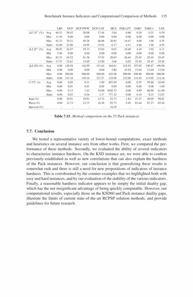
Benchmark Instance Indicators and Computational Comparison of Methods 135
LB0 DCP DCP-PWW DCP-CAT MCS PAR-LFT TABU TABU+ LNS
ΔUB∗ (%) Avg 60.53 26.42 20.98 17.44 3.84 6.60 0.38 0.21 0.39
Min 11.54 0.00 0.00 0.00 0.00 0.00 0.00 0.00 0.00
Max 83.33 70.31 49.28 46.88 20.83 16.67 4.60 1.96 4.55
Stdev 16.60 23.80 16.95 15.01 6.17 4.51 4.60 1.96 4.55
ΔLB∗ (%) Avg 58.92 24.57 18.73 15.03 0.63 10.40 4.10 3.92 4.11
Min 5.48 0.00 0.00 0.00 0.00 0.00 0.00 0.00 0.00
Max 83.33 65.52 41.38 37.93 20.83 26.44 25.45 25.45 25.45
Stdev 17.57 22.61 15.09 12.90 3.08 6.02 25.45 25.45 25.45
ΔLB0 (%) Avg 0.00 128.94 142.99 151.62 184.61 215.92 197.02 196.47 196.90
Min 0.00 0.00 0.00 0.00 5.80 15.94 13.04 13.04 13.04
Max 0.00 500.00 500.00 500.00 425.00 500.00 500.00 500.00 500.00
Stdev 0.00 141.18 130.16 127.57 110.96 123.06 114.45 114.05 114.18
CPU (s) Avg 0.00 0.05 0.21 1.90 493.50 0.00 0.55 59.86 24.96
Min 0.00 0.01 0.01 0.05 0.04 0.00 0.06 0.06 1.00
Max 0.00 0.12 1.42 18.00 3020.72 0.00 0.89 60.99 61.00
Stdev 0.00 0.03 0.36 3.17 777.32 0.00 0.16 8.21 12.87
#opt (%) 0.00 10.91 10.91 12.73 52.73 1.82 47.27 49.09 50.91
#best (%) 0.00 12.73 12.73 16.36 92.73 5.45 83.64 87.27 85.45
#proved (%) - - - - 34.55 - - - -
Table 7.15. Method comparison on the 55 Pack instances
7.7. Conclusion
We tested a representative variety of lower-bound computations, exact methodsand heuristics on several instance sets from other works. First, we compared the per-formance of these methods. Secondly, we evaluated the ability of several indicatorsto characterize instance hardness. On the KSD instance set, we were able to confirmpreviously-established as well as new correlations that can also explain the hardnessof the Pack instances. However, our conclusion is that generalizing these results issomewhat rash and there is still a need for new propositions of indicators of instancehardness. This is corroborated by the counter-examples that we highlighted both witheasy and hard instances, and by our evaluation of the stability of the various indicators.Finally, a reasonable hardness indicator appears to be simply the initial duality gap,which has the not insignificant advantage of being quickly computable. However, ourcomputational results, especially those on the KSD60 and Pack instance duality gaps,illustrate the limits of current state-of-the-art RCPSP solution methods, and provideguidelines for future research.

136
This page intentionally left blank

Part 2
Variants and Extensions
137

138
This page intentionally left blank
Chapter 8
Preemptive Activities
8.1. Preemption in scheduling
This chapter describes a classical extension of scheduling problems: the fact thatthe execution of an activity may be interrupted by the execution of another one, andcontinued later. Such an activity is called preemptive, and we assume here that nopenalty is given if any interruption occurs. A project in which all activities are pre-emptive is also called preemptive. Some contributions have treated derived cases ofpreemption: either interruption can occur only in favor of specific activities (selectivepreemption), or an activity can be interrupted most once or twice (limited preemption),or, in more recent works, only a subset of activities are preemptive. Allowing preemp-tion evidently improves the optimal objective value of a scheduling problem, as someconstraints are relaxed. But it also increases a lot the cardinality of the feasible solu-tion set.
In the following, we distinguish two specific kinds of preemption. Indeed, the veryfew approaches dealing with preemption for the RCPSP consider all integer dates ofthe project to interrupt the execution of some activities. This is called integral pre-emption and this can be done since all processing times are integer or can tolerate acommon discretization. For an industrial point of view, it seems to be convenient toschedule parts of activities for a given number of time units (CPU clock for micro-processor instructions, days or half-days of work on a project . . . ). For a theoreticalpoint of view, Baptiste et al. [BAP 05] claim that a wide class of scheduling prob-lems admits, for a lot of objective functions, an optimal preemptive solution such that
Chapter written by Jean DAMAY.
139
140 Resource-Constrained Project Scheduling
all interruptions occur at integral dates. This is not the case of makespan minimiza-tion, which will be considered hereafter. For example, consider the instance containingone resource with a capacity of two units and three incomparable activities (with noprecedence relations between them) of duration one time unit, and of requirement oneresource unit (q = 1, B1 = 2, n = 3, E = ∅, and ∀Ai ∈ A, bi1 = 1, pi = 1). Alloptimal solutions of this instance have their first interruption at time 0.5. Hence, analternative approach consists of considering rational preemption, for which all pre-emptive activities can be interrupted at any rational times during the project. The res-olution of such problems involves mathematical programming techniques, as it seemsdifficult to predict iteratively at what time the next preemption could occur.
Note that the exact resolution of any kind of preemptive version mentioned aboveprovides a lower bound of the optimal makespan of the non-preemptive version. Somemajor contributions [MIN 98, BRU 00, BAP 04] obtain high-quality lower bounds ofsuch values from a formulation that relaxes these non-preemption constraints, but alsopartially the precedence ones (see section 3.2.2). To our knowledge, no work had beendone to solve the rational preemptive version of the RCPSP.
8.2. State of the art
8.2.1. Integral preemption for the RCPSP
In several approaches dealing with the non-preemptive case, the algorithm con-sists of adding iteratively activities or a set of activities to partial schedules (cf. listalgorithms or chronological branching schemes of section 5.1), in order to build acomplete schedule. If this algorithmic scheme is applied for the preemptive case, it isnot sufficient only to consider the finishing times of each activity to enrich the partialschedule.
Le Pape and Baptiste present in [Le 98] a few constraint propagation techniquesto the preemptive version of some disjunctive scheduling problems. For cumulativeones (such as the RCPSP), we can clearly see that the propagation process would berather slow, since it prevents us from using some simple propagation techniques.
We will focus here on the main contribution for the integral preemptive RCPSP:the paper of Demeulemeester and Herroelen [DEM 96a]. Derived from their approachfor the non-preemptive version [DEM 92b] described in section 5.1.1.2, the methodthey implement is a branch-and-bound procedure in which each node corresponds toa partial feasible schedule composed of parts of activities scheduled before a date (ordecision point) t ∈ N. In the leaves of this tree, each activity is entirely processed, sothey correspond to complete schedules.
The branching scheme consists of extending a partial schedule, hence finding allsubsets of the so-called eligible activities that could be in process on the next timeinterval and lead to the optimal solution derived from this node. Indeed, the decision
Preemptive Activities 141
point of the child nodes is t + 1. Hence, it does not only correspond to the completiondate of the activities, like Kaplan suggested in [KAP 88]. Indeed, the authors spliteach activity Ai in pi unit duration activities and apply almost the same algorithm of[DEM 92b] for the non-preemptive version. Thus, they can adapt and provide somedominance rules to restrict the calculation of the next feasible subsets: because ofresource constraints, we can first identify activities that can be in process on the nextinterval(s) and lead to an optimal solution, and secondly determine all minimal (in thesense of inclusion) subsets of activities the execution of which can be delayed. Theyalso propose a simple comparison with previously saved nodes to eliminate some ofthem, and local lower bound processes: the most intuitive lower bound calculationcorresponds to t augmented by the length of the remaining critical path, and it is theonly one tested in practice.
The computational results of this algorithm are presented for the Patterson set of110 instances, which are all optimally solved within 5 minutes. Preliminary numericalresults of a recent reimplementation with new dominance rules may indicate that thisalgorithm requires too many CPU-time to provide the optimal solutions of a lot ofPSPLIB instances with 30 activities. Note that the Patterson instances are known tobelong to the set of “very easy” ones (cf. [KOL 95b]).
8.2.2. Rational preemption for parallel machine scheduling problems
Note first that research about preemption in scheduling problems mainly concernsthe machine scheduling problems (job-shop, flow-shop, parallel machine, etc.). Aclassical result comes from McNaughton [MCN 59] for the parallel machine schedul-ing problem and provides an algorithm to build an optimal schedule with at mostm − 1 interruptions when m incomparable activities have to be executed (such as inthe example mentioned in 8.1).
Derived from Papadimitriou and Yannakakis [PAP 79], we provide here the defi-nition of the interval orders in scheduling problems. We say that a precedence graphG(V,E, p) belongs to the interval order class if each vertex of V , that is to say eachactivity, can be associated with an interval in the real line such that (Ai, Aj) ∈ E iffevery interior point of the associated interval of Ai is strictly lower than every inte-rior point of the one associated with Aj . In practice, these intervals correspond to thesmallest closed time windows [ESi;LCi], Ai ∈ V . The authors provide a polyno-mial (linear) algorithm to solve the parallel machine instances with such a precedencegraph and unit-time tasks.
Sauer and Stone [SAU 89b] [SAU 89a] extend this polynomiality result to thepreemptive case of this problem. In [MOU 99], Moukrim introduces a new class oforders, called quasi-interval orders, the instances of which are solved by the algo-rithm described by Papadimitriou and Yannakakis in its preemptive version, and stillwith unit-time tasks.
142 Resource-Constrained Project Scheduling
However, the authors of [SAU 89b] use a rather new linear programming formu-lation, in which the variables are associated with Φ the set of all the so-called feasiblesubsets of activities (see section 3.2.2), i.e. the subsets of activities that can be simulta-neously in process during a feasible schedule (al ∈ Φ iff ∀Rk ∈ R,
∑Ai∈l bik ≤ Bk
and ∀Ai, Aj ∈ l, (Ai, Aj) /∈ TE and (Aj , Ai) /∈ TE, where TE is the transitiveclosure of E). The program, called P in this chapter, is presented in the next sectionas an adaptation of a relaxation of Mingozzi et al. [MIN 98] for the RCPSP (witharbitrary processing times). Sauer and Stone also define a precedence relation ≺ onΦ: ∀al, al′ ∈ Φ, al ≺ al′ iff ∃Ai ∈ al, Aj ∈ al′ such that (Ai, Aj) ∈ E and identifythat the lack of cycles in the graph Γ = (Φ,≺) is a crucial feasibility property. Sincethe interval orders verify this property, the solution of the linear program P providesthe optimal preemptive solution of the instances having such precedence graphs.
In [MOU 97, MOU 05], Moukrim and Quilliot identify another class, calledAm-order, of parallel machine instances for which the solution of P is equal tothe makespan of the optimal preemptive solution. They provide in [MOU 05] analgorithm to build such an optimal preemptive schedule from this solution of P , forthis class. In [MOU 97], the authors reuse this linear formulation to propose a descentalgorithm based on the Simplex pivoting for parallel machine problems (for both thepreemptive and non-preemptive case). Note that they reuse works on hypergraphsfrom Bendali and Quilliot [BEN 97]. All this is reconsidered in the next section forthe RCPSP.
8.3. Recent LP-based methods
In the following, our recent works dealing with the preemptive version of theRCPSP [DAM 08, DAM 05] are summarized. Indeed, the following results are ini-tially provided for a given subset of preemptive activities, but we assume here that theyall are preemptive, for sake of simplicity. The descent approach is derived from theworks of [MOU 97] mentioned in the previous section dedicated to parallel machinescheduling problems. Note that all propositions and theorems presented below aregiven without proof, but are intuitively assumable.
8.3.1. Reformulation
Let us introduce some notations dealing with the set Φ of feasible subsets of activ-ities, that we call valid antichains (the corresponding subset of vertices are antichainsof the precedence graph): ∀al, al′ ∈ Φ, al ≺ al′ iff ∃Ai ∈ al, Aj ∈ al′ such that(Ai, Aj) ∈ E. Note that ≺ is not an order relation, and we call antichain graph thegraph Γ = (Φ,≺). Let Φi be the set of all feasible subsets containing activity Ai.
Let σ = (a1, . . . , a|σ|) be a sequence of valid antichains, and for all Ai ∈ V , letσi = Φi∩σ be the set of antichains of σ containing Ai. σ is said ordered if the order of

Preemptive Activities 143
this sequence respects the partial order given by ≺, that is to say ∀l, l′ ∈ {1, . . . , |σ|},l < l′ ⇒ al′ �≺ al. In the following, the positive vector z ∈ R|σ|
+ will represent therespective amounts of time during which all activities of the feasible subsets of σ aresimultaneously executed in the associated schedule, as it is introduced in section 3.2.2.
PROPOSITION 8.1.– Let σ be a sequence of valid antichains, and z be a positivevector indexed on σ. The pair (σ, z) represents a preemptive schedule if and only if σis ordered and z verifies ∀Ai ∈ V ,
∑l∈σi
zl = pi. Its makespan is∑
l∈σ zl.
By a slight abuse of notations, a pair (σ, z) where σ is ordered and ∀Ai ∈ V ,∑a∈σi
za ≥ pi represents also a preemptive schedule, since it can be easily trans-formed into a regular one.
Mingozzi et al. [MIN 98] introduced the following linear program P that contains(only) n constraints and |Φ| variables, except that they efficiently restricted the vari-able set to the “undominated feasible subsets” (see section 3.2.2):
(P) : min Z = 1 · z, Mz ≥ p, z ∈ R|Φ|+ .
It is issued from the exact time-indexed mixed integer linear formulation of section3.2.2, with a much more higher number of variables and constraints. Some constraintsof this MIP were relaxed or partially relaxed and the time-indexation was avoidedthanks to the introduction of these real-valued “duration” variables z. Hence it is arelaxation, but not only in the sense of the traditional integrality constraint relaxation.
1 is the vector of |Φ| elements that are equal to 1. The incidence matrix M(n, |Φ|)is defined as follows: Mil = 1 if activity Ai belongs to antichain al, 0 otherwise.Thus these constraints ensure that for each activity Ai ∈ A the sum of the durationof the feasible subsets containing Ai is at least equal to its processing time pi. Thedefinition of the variables includes the resource and disjunctive constraints, that willbe taken into account in the pricing subproblem of the column generation resolution(see next subsection).
We say that an antichain al is active for a solution z of P if and only if zl > 0. Letus denote by ACT (z) the set of active antichains for z. We now define SP as the setof solutions z of P for which we can build an ordered sequence with exactly all theelements of ACT (z), and state the following theorem.
THEOREM 8.1.– Solving the preemptive version of the RCPSP consists of finding anelement of SP that minimizes Z.
Finally, a necessary and sufficient condition for a solution z of P to belong to SP
is the lack of oriented cycle in the antichain subgraph induced by ACT (z). Note thatan oriented sequence can be found through a simple topological order search in thissubgraph.
144 Resource-Constrained Project Scheduling
This theoretical formulation leads us to different approaches and algorithms,described in the next subsections.
8.3.2. A specific neighborhood search algorithm
8.3.2.1. Descent approach
We establish in [DAM 08] the two following theoretical results. The set of thebasis solutions (in the Simplex sense) of P in SP is dominant. Furthermore, the setSP is connected in the sense that two elements of SP are neighbors if and only if onecan be obtained from the other by exactly one Simplex pivoting on P . It follows thatwe may go from any solution of SP to any other by a sequence of Simplex pivotingsin P .
Thus, we devised a descent algorithm based on the Simplex. Indeed, if we haveinitially a solution z0 of SP (loaded in P from an initial feasible schedule provided bya simple list algorithm with random priorities), the idea of this algorithm is to checkat each step k if the switch of outing and entering variables (resp. zo and ze) proposedby the Simplex pivoting will lead to a basis solution zk\{zo}∪{ze} still in SP , that isto say that the antichain subgraph induced by ACT (z)\{ao} ∪ {ae} does not containany oriented cycle. If this test proves negative, the switch does not occur, and wetry another one proposed by the Simplex. Otherwise, the classical Simplex pivotingis computed. The process is iterated until no candidate variable verifies the test: thissituation corresponds to a local minimum of the problem. The incremental version ofthis test in the preemptive case corresponds to the detection of an oriented cycle in theantichain subgraph going through the new element ae. Note that the non-preemptiveversion of this test has far stronger constraints.
As the number of feasible subsets, i.e. the number of variables, is very large (expo-nential in n) and a few of them are interesting for our problem, we set up a columngeneration module (see section 3.2.2, without time discretization). Each dual variableπi is associated with activity Ai ∈ V and an entering column corresponds to a validantichain ae that also has to verify
∑Ai∈ae
πi > 1 due to our formulation ofP . Hence,the subproblem is a multidimensional knapsack-stable problem, in which each vertexAi has a unit profit πi and a multidimensional weight bik, Rk ∈ R. It is computedhere by a branch-and-bound procedure like in [BRU 00]. The disjunctions (Ai, Aj)are defined by some resource constraint violations (∃Rk ∈ R, bik +bjk > Bk) and theprecedence relations between activities ((Ai, Aj) ∈ TE or (Aj , Ai) ∈ TE), or canbe strengthened through constraint propagation techniques (see [BAP 04], [DEM 05],[BRU 98]), at least each time that the best known upper bound of the makespan isimproved. A specific preprocessing filtering step is added on this subproblem, to pre-vent from building trivial oriented cycles. This preprocessing is removed to check if alocal minimum is indeed reached.
Preemptive Activities 145
8.3.2.2. Diversification techniques
Diversification techniques were proposed to get out of the numerous local minima.The idea is to build from each of them a feasible solution for which it has been proventhat it can be reloaded in basis of the linear program, in order to reiterate the descent(intensification) process.
The first one, called reconstruction, consists of building, from the feasible subsetfamily associated with an optimal solution of the relaxation P , an ordered sequence,allowing some modifications in the subsets. In [MÖH 03], the authors generate suchschedules by applying list algorithms with priority lists derived from the order ofthe jobs in the solution of a Lagrangian relaxation. Here, the following methodis inspired by Moukrim and Quilliot [MOU 05], concerning the identical parallelmachine scheduling problem. The idea is to build step by step an ordered sequence offeasible subsets. By induction on the feasible subsets of the solution of P in its initialarbitrary order, we ensure through specific switches of activities that the subsequencefrom the beginning to the current antichain is an ordered sequence. Because of theseswitches, the subsets do not forcefully respect the resource constraints first, hence atthe end of this induction process, a postprocessing step is performed to make thesesubsets respect them and the sequence represent a feasible preemptive schedule. Theduration variables are provided by the reloading in P . Another reconstruction algo-rithm has also been designed in order to take into account the associated durations ofeach feasible subset in the solution of P .
The second diversification algorithm, called perturbation, was devised to avoid thefact that during the descent algorithm described above, a valid and Simplex candidateantichain ae is not allowed to enter the basis antichain family f because of an orientedcycle in the subgraph induced by f ∪ {ae}. The idea of this algorithm is to force theentering of ae. Indeed, ae may be present in “good” solutions, but some antichains off forbid ze from entering the basis through only one Simplex pivoting. It reuses thespecific switches of activities between the feasible subsets and provides a still orderedsequence of feasible subsets, containing ae, that do not forcefully respect the resourceconstraints. The postprocessing step explained above is also performed at the end ofthis feasible solution perturbation, to build another more “distant” feasible solution inSP .
8.3.2.3. Experimental results
The experiments were computed on a PC Duron 1GHz - 256 Mb RAM. The resultsof this specific neighborhood method (descents with 20 reconstructions and 5 pertur-bations between each reconstruction) on the PSPLIB instances (see [KOL 97] andChapter 7) with 30 activities, called KSD30, are very good, since the optimum wasobtained for 442 over 480 instances. The average and maximum gaps are respectively0.15% and 5.41%, in an average time of 9.9 s. Note that the optimal value is obtained
146 Resource-Constrained Project Scheduling
for these instances thanks to the branch-and-bound algorithm described in the follow-ing section. This is not the case for the instances with 60 activities, called KSD60,but we can assume that the experiments are still very good on them, since the averagegap with the lower bound given by the solution of P is similar to the one obtainedon KSD30 (respectively 2.38% and 2.15%). But for them the solutions are obtainedwithin an average time of 103.4 s.
8.3.3. Exact methods
8.3.3.1. Branch-and-bound
A branch-and-bound algorithm derived from the formulation of section 8.3.1 basedon P has been implemented and presented in [DAM 06b]. It was devised first toimprove our best known preemptive lower and upper bounds, and eventually to findthe optimal preemptive solutions of the KSD30 instances. The bounding process con-sists of solving P (with a few additional simple logical constraints) to get a local lowerbound z of the optimal makespan, whereas the branching process consists of forbid-ding the variables corresponding to the vertices of an oriented cycle in the antichainsubgraph induced by ACT (z).
Indeed, for each antichain al of such an identified oriented cycle, the current nodeof the search tree derives one subproblem in which the corresponding variable zl isnot allowed to appear in the associated solution of P . Hence, for any subproblem inthe search tree, there is a list L of forbidden feasible subsets. For an algorithmic pointof view, this is done by setting the corresponding duration variables zl, al ∈ L, to 0.If such a solution does not contain any circuit, then it corresponds to a feasible pre-emptive solution. In a best-first exploration of the search tree, the process is stoppedsince this solution has the minimum value, that is to say the minimum makespan.
The branching process has been first improved by only considering the orientedcycles of minimal length in the antichain subgraph. We proved that it is sufficient inour research only to consider the chordless oriented cycles, which are easier to iden-tify. Furthermore, the idea was then to detect more precisely the activities involvedin these antichain cycles. The forbidden list L became a list of forbidden couplesof activities, that is to say disjunctions. This latter point is of course implicitly welltreated in our column generation process, as the constraints deal with disjunctions ofactivities.
Finally, we may observe in our very first experiments that the main chordless ori-ented cycles are of length 2 for the KSD30 instances. Thus we proposed three filteringsteps in the branching process, in order to add even more disjunctions, so to forbideven more feasible subsets in the numerous subproblems of the search tree. One ofthese filtering steps has provided all optimal preemptive solutions of KSD30 in anaverage (resp. maximum) time of 11 minutes (resp. 9 hours) and an average (resp.maximum) number of treated nodes of 1,050 (resp. 25,717).
Preemptive Activities 147
8.3.3.2. Branch and cut and price
Another idea to use this formulation in an exact resolution is to build a MixedInteger Linear Program (MILP) [DAM 05] [DAM 06a] and to use the recent solv-ing techniques and frameworks dedicated to it. Indeed, if we add a binary presencevariable for each feasible subset in P which is equal to 1 when the feasible subsetis chosen in the solution and 0 otherwise, it is easy to formulate the non-circuit con-straints. This provides a MILP with an exponential number of variables (two for eachfeasible subset) and an exponential number of constraints (one for each activity likein P , plus one for each oriented cycle in the global antichain graph (Φ,≺), plus onefor each feasible subset, which is called the Big-M coupling constraint). However,these numbers of variables and constraints are far less large than for the other classicaltime-indexed formulations, in particular the one of Mingozzi et al. [MIN 98]. Suchworks are also likely to be done when not all activities are preemptive, and naturallyfor the non-preemptive case of the RCPSP.
8.4. Conclusion
In this chapter, we have focused on the high quality and promising results of recentworks for the resource constrained project scheduling problem, including its ratio-nal preemptive version. Our approach deals with a new formulation of this probleminvolving the feasible subsets of activities, but an important point is that it is not time-indexed and that the underlying linear program is quite easy to solve. This leads toseveral types of algorithms, such as an original generic iterated descent algorithm andexact methods that provide very good and original experimental results.
One of the latter methods deals with the very efficient and promising Branch andCut and Price techniques, for which the implementation and experiments are per-formed at the present time and are likely to provide really interesting and good resultsfor the RCPSP.
However, other interesting original theoretical results can derive from theseapproaches. Like for the parallel machine scheduling problem, a class of instancescan be found, for which the value of the optimal solution ofP is equal to the makespanof the optimal preemptive solution of the problem. A polynomial algorithm can alsobe devised to build an optimal schedule from any solution of P , called optimalreconstruction.

148
This page intentionally left blank
Chapter 9
Multi-Mode and Multi-Skill ProjectScheduling Problem
9.1. Introduction
This chapter deals with two different problems: the Multi-Mode Resource-Con-strained Project Scheduling Problem (MM-RCPSP) and the Multi-Skill ProjectScheduling Problem (MSPSP). What is particular about those two problems is thatresources can be assigned according to different ways, eventually impacting process-ing time of activities. For the first problem, activities may be processed according toseveral ways, that means different amounts of resources required and correspondingprocessing time. For the second problem, resources are able to be assigned to differentkinds of resource requirements. This major difference with the traditional RCPSP,that can be called resource flexibility, leads to a significant increase in the number offeasible solutions. To build a solution we have to fix (1) the way the activities haveto be processed and (2) the starting times of the activities. The latter problem is thenequivalent to solving a traditional RCPSP instance.
Section 9.2 deals with the MM-RCPSP, and section 9.3 with the MSPSP. Eachsection draws the specificities of its studied problem based on the presentation of asimple example, and then resolution methods are described. We focus on branch-and-bound methods (see Chapter 5), because those are significantly different from tradi-tional branch-and-bound for the RCPSP, exhibiting the structural difference betweenthese problems and the RCPSP. For MM-RCPSP, exact methods are based on partialschedules and at each node of the search tree both mode of execution and starting
Chapter written by Odile BELLENGUEZ-MORINEAU and Emmanuel NÉRON.
149
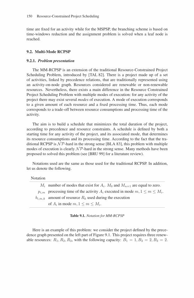
150 Resource-Constrained Project Scheduling
time are fixed for an activity while for the MSPSP, the branching scheme is based ontime-windows reduction and the assignment problem is solved when a leaf node isreached.
9.2. Multi-Mode RCPSP
9.2.1. Problem presentation
The MM-RCPSP is an extension of the traditional Resource-Constrained ProjectScheduling Problem, introduced by [TAL 82]. There is a project made up of a setof activities, linked by precedence relations, that are traditionally represented usingan activity-on-node graph. Resources considered are renewable or non-renewableresources. Nevertheless, there exists a main difference in the Resource ConstrainedProject Scheduling Problem with multiple modes of execution: for any activity of theproject there may exist several modes of execution. A mode of execution correspondsto a given amount of each resource and a fixed processing time. Thus, each modecorresponds to a trade-off between resource consumptions and processing time of theactivity.
The aim is to build a schedule that minimizes the total duration of the project,according to precedence and resource constraints. A schedule is defined by both astarting time for any activity of the project, and its associated mode, that determinesits resource consumptions and its processing time. According to the fact that the tra-ditional RCPSP isNP-hard in the strong sense [BLA 83], this problem with multiplemodes of execution is clearlyNP-hard in the strong sense. Many methods have beenproposed to solved this problem (see [BRU 99] for a literature review).
Notations used are the same as those used for the traditional RCPSP. In addition,let us denote the following.
Notation
Mi number of modes that exist for Ai. M0 and Mn+1 are equal to zero.
pi,m processing time of the activity Ai executed in mode m, 1 ≤ m ≤Mi.
bi,m,k amount of resource Rk used during the execution
of Ai in mode m, 1 ≤ m ≤Mi.
Table 9.1. Notation for MM-RCPSP
Here is an example of this problem: we consider the project defined by the prece-dence graph presented on the left part of Figure 9.1. This project requires three renew-able resources: R1, R2, R3, with the following capacity: B1 = 1, B2 = 2, B3 = 2.
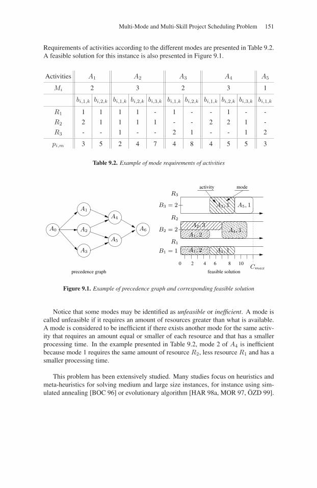
Multi-Mode and Multi-Skill Project Scheduling Problem 151
Requirements of activities according to the different modes are presented in Table 9.2.A feasible solution for this instance is also presented in Figure 9.1.
Activities A1 A2 A3 A4 A5
Mi 2 3 2 3 1
bi,1,k bi,2,k bi,1,k bi,2,k bi,3,k bi,1,k bi,2,k bi,1,k bi,2,k bi,3,k bi,1,k
R1 1 1 1 1 - 1 - - 1 - -
R2 2 1 1 1 1 - - 2 2 1 -
R3 - - 1 - - 2 1 - - 1 2
pi,m 3 5 2 4 7 4 8 4 5 5 3
Table 9.2. Example of mode requirements of activities
activity mode
feasible solution
2 4 8 106
precedence graph
0
A3, 1
A1, 2
A2, 3
A3, 1
A5, 1
A4, 1
A1, 2
A0
A1
A2
A3
A4
A5
A6
R3
R2
R1
B1 = 1
B2 = 2
B3 = 2
Cmax
Figure 9.1. Example of precedence graph and corresponding feasible solution
Notice that some modes may be identified as unfeasible or inefficient. A mode iscalled unfeasible if it requires an amount of resources greater than what is available.A mode is considered to be inefficient if there exists another mode for the same activ-ity that requires an amount equal or smaller of each resource and that has a smallerprocessing time. In the example presented in Table 9.2, mode 2 of A4 is inefficientbecause mode 1 requires the same amount of resource R2, less resource R1 and has asmaller processing time.
This problem has been extensively studied. Many studies focus on heuristics andmeta-heuristics for solving medium and large size instances, for instance using sim-ulated annealing [BOC 96] or evolutionary algorithm [HAR 98a, MOR 97, ÖZD 99].
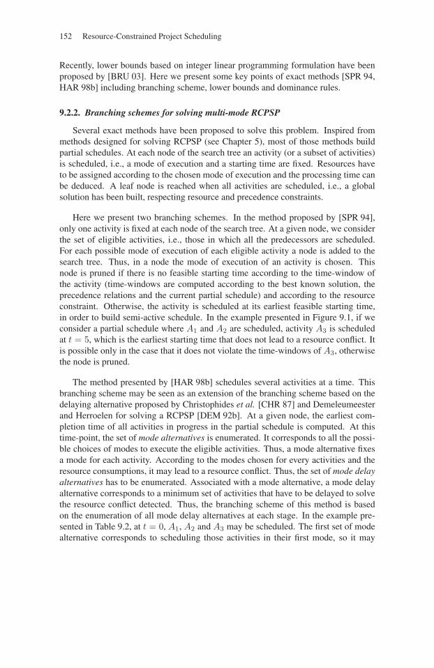
152 Resource-Constrained Project Scheduling
Recently, lower bounds based on integer linear programming formulation have beenproposed by [BRU 03]. Here we present some key points of exact methods [SPR 94,HAR 98b] including branching scheme, lower bounds and dominance rules.
9.2.2. Branching schemes for solving multi-mode RCPSP
Several exact methods have been proposed to solve this problem. Inspired frommethods designed for solving RCPSP (see Chapter 5), most of those methods buildpartial schedules. At each node of the search tree an activity (or a subset of activities)is scheduled, i.e., a mode of execution and a starting time are fixed. Resources haveto be assigned according to the chosen mode of execution and the processing time canbe deduced. A leaf node is reached when all activities are scheduled, i.e., a globalsolution has been built, respecting resource and precedence constraints.
Here we present two branching schemes. In the method proposed by [SPR 94],only one activity is fixed at each node of the search tree. At a given node, we considerthe set of eligible activities, i.e., those in which all the predecessors are scheduled.For each possible mode of execution of each eligible activity a node is added to thesearch tree. Thus, in a node the mode of execution of an activity is chosen. Thisnode is pruned if there is no feasible starting time according to the time-window ofthe activity (time-windows are computed according to the best known solution, theprecedence relations and the current partial schedule) and according to the resourceconstraint. Otherwise, the activity is scheduled at its earliest feasible starting time,in order to build semi-active schedule. In the example presented in Figure 9.1, if weconsider a partial schedule where A1 and A2 are scheduled, activity A3 is scheduledat t = 5, which is the earliest starting time that does not lead to a resource conflict. Itis possible only in the case that it does not violate the time-windows of A3, otherwisethe node is pruned.
The method presented by [HAR 98b] schedules several activities at a time. Thisbranching scheme may be seen as an extension of the branching scheme based on thedelaying alternative proposed by Christophides et al. [CHR 87] and Demeleumeesterand Herroelen for solving a RCPSP [DEM 92b]. At a given node, the earliest com-pletion time of all activities in progress in the partial schedule is computed. At thistime-point, the set of mode alternatives is enumerated. It corresponds to all the possi-ble choices of modes to execute the eligible activities. Thus, a mode alternative fixesa mode for each activity. According to the modes chosen for every activities and theresource consumptions, it may lead to a resource conflict. Thus, the set of mode delayalternatives has to be enumerated. Associated with a mode alternative, a mode delayalternative corresponds to a minimum set of activities that have to be delayed to solvethe resource conflict detected. Thus, the branching scheme of this method is basedon the enumeration of all mode delay alternatives at each stage. In the example pre-sented in Table 9.2, at t = 0, A1, A2 and A3 may be scheduled. The first set of modealternative corresponds to scheduling those activities in their first mode, so it may
Multi-Mode and Multi-Skill Project Scheduling Problem 153
be defined by: {A1, 1;A2, 1;A3, 1}, where any chosen activity is directly followedby the number of its chosen mode of execution. This alternative leads to a resourceconflict. According to the fact that no pair of activities can be executed in parallelwithout leading to a resource conflict, the distinct sets of mode delay alternative are:{A1, 1;A2, 1}, {A1, 1;A3, 1}, {A2, 1;A3, 1}. Thus, the created nodes, correspondingto the first set of mode alternative, are : {A3, 1}, {A2, 1}, {A1, 1}.
The strategy to explore the search tree is chosen according to a priority rule com-bined with a traditional depth-first strategy. This order may really change the efficiencyof the method. So, the activity is either sorted by the length of its minimum processingtime, maximum processing time, or even average processing time. Then for a givenactivity, modes are sorted according to an associated weight. This weight is inverselyproportional to the processing time associated with the mode: a mode with a heavyweight is chosen first because it corresponds to a small processing time.
9.2.3. Dominance rules
Dominance rules have been proposed in order to reduce the search tree that maybecome huge depending on the number of modes and the number of activities to con-sider [SPR 94], [HAR 98a]. Here we present a brief overview of such rules:
1) If an eligible activity cannot be scheduled without violating its latest finishingtime (computed according to the best known solution and precedence relations), inany mode, then the corresponding node can be pruned.
2) If, in a partial schedule, an activity can be left shifted without violating eitherthe resource or precedence constraints, then the node corresponding to this partialschedule can be pruned.
3) In a partial schedule, if no eligible activity can be scheduled before the end of anactivity Ai, executed in mode m, and if Ai may be executed in mode m′ with a shorterprocessing time without violating resource constraints, then the node correspondingto the schedule of Ai in mode m may be pruned.
4) If there exists a partial schedule where an activity Ai and an activity Aj areadded respectively in mode mi and mj with the same starting time, it is not necessaryto explore the node where, in the same partial schedule, activity Aj in mode mj andthen activity Ai in mode mi are added because they also will have the same startingtime, so the partial schedules are equivalent.
5) Consider that there exists a first partial schedule PS where an activity Ai inmode mi and an activity Aj in mode mj are added to get a first partial schedule PS1.Assume that the completion time of Ai in this first schedule, C1
i , is equal to the startingtime of Aj , S1
j . If, in another node, activities Aj in mode mj and Ai in mode mi areadded to the same partial schedule PS to get PS2, with C2
j =S2i and if the first activity
not yet scheduled cannot be scheduled earlier in PS2 than in PS1, then the secondpartial schedule PS2 should not be built, the corresponding node has to be pruned.

154 Resource-Constrained Project Scheduling
6) If a partial schedule PS has a completion time C, and if in another node thereexists a partial schedule containing the same activities that allows the next activityto start at a time t equal to or greater than C, the node corresponding to this secondpartial schedule should not be explored.
This extension of the traditional RCPSP allows taking into account time-cost trade-off. Thus, it may be used to represent many real problems. However, all resourcesconsidered are one-purpose, i.e., they may satisfy only one kind of resource require-ment. This is why another extension has been introduced: the MSPSP. In this problem,resources correspond to persons that master a subset of the skills required by the dif-ferent activities of the project.
9.3. Multi-Skill Project Scheduling Problem
The MSPSP has been proposed by Néron and Baptista [NÉR 02]. The main featureof this model is to consider resources that are staff members, thus renewable anddisjunctive, mastering several skills. Initially it has been proposed to model projectscheduling problems in IT companies.
9.3.1. Problem presentation
The MSPSP can be seen as an extension of the traditional RCPSP. In the MSPSP,the project to schedule is traditionally made up of a set of activities, linked byprecedence relations. The main difference is the resource considered and the way todefine resource requirements: resources are staff members assigned to the project.Thus, resources considered are renewable and disjunctive, i.e., a staff member canbe assigned at most to one requirement at a time. The way these resources are usedis a consequence of the skills they master among all those taken into account for theproject. Thus, for each person in the staff, we exactly know which skill he/she masters.Symmetrically, requirements of activities are defined in terms of skill requirements,i.e., the number of persons for each skill required to process the activity. Thus, thestaff members assigned to the execution of an activity are a subset of persons able tosatisfy its skill requirements.
The goal is to build a schedule to minimize the total project duration. This schedulehas to respect precedence and resource and skill constraints. According to the differentskills every person masters, there may exist many possible subsets of persons able tosatisfy the skill requirements of the activities. Thus, when the starting time of eachactivity is fixed, there may correspond many feasible schedules. Nevertheless, a validschedule has to respect the following constraints: a person cannot be assigned to morethan one unit of skill requirement at a time and not to a requirement correspondingto a skill he/she does not master. Moreover, all the persons who start an activity haveto be assigned to it all along its processing. Furthermore, the model used also takesinto account unavailability periods of the resources. Thus, a person cannot be assigned
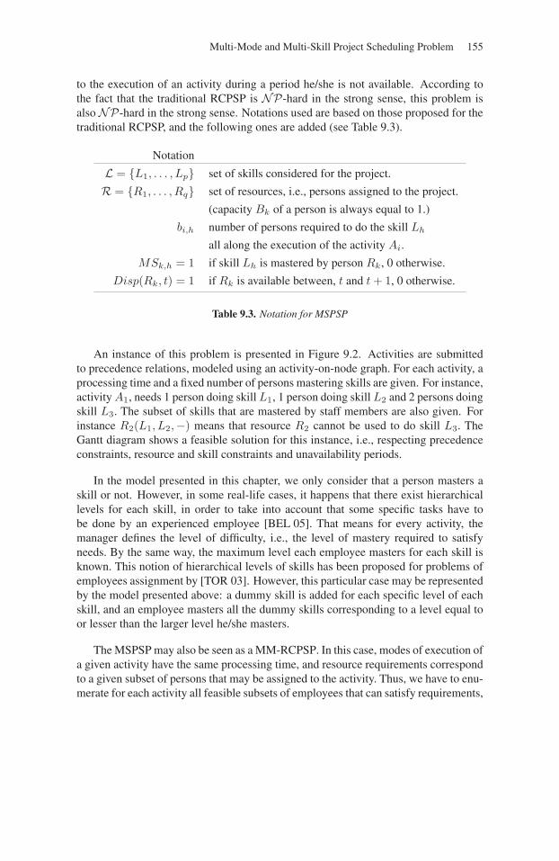
Multi-Mode and Multi-Skill Project Scheduling Problem 155
to the execution of an activity during a period he/she is not available. According tothe fact that the traditional RCPSP is NP-hard in the strong sense, this problem isalsoNP-hard in the strong sense. Notations used are based on those proposed for thetraditional RCPSP, and the following ones are added (see Table 9.3).
Notation
L = {L1, . . . , Lp} set of skills considered for the project.
R = {R1, . . . , Rq} set of resources, i.e., persons assigned to the project.
(capacity Bk of a person is always equal to 1.)
bi,h number of persons required to do the skill Lh
all along the execution of the activity Ai.
MSk,h = 1 if skill Lh is mastered by person Rk, 0 otherwise.
Disp(Rk, t) = 1 if Rk is available between, t and t + 1, 0 otherwise.
Table 9.3. Notation for MSPSP
An instance of this problem is presented in Figure 9.2. Activities are submittedto precedence relations, modeled using an activity-on-node graph. For each activity, aprocessing time and a fixed number of persons mastering skills are given. For instance,activity A1, needs 1 person doing skill L1, 1 person doing skill L2 and 2 persons doingskill L3. The subset of skills that are mastered by staff members are also given. Forinstance R2(L1, L2,−) means that resource R2 cannot be used to do skill L3. TheGantt diagram shows a feasible solution for this instance, i.e., respecting precedenceconstraints, resource and skill constraints and unavailability periods.
In the model presented in this chapter, we only consider that a person masters askill or not. However, in some real-life cases, it happens that there exist hierarchicallevels for each skill, in order to take into account that some specific tasks have tobe done by an experienced employee [BEL 05]. That means for every activity, themanager defines the level of difficulty, i.e., the level of mastery required to satisfyneeds. By the same way, the maximum level each employee masters for each skill isknown. This notion of hierarchical levels of skills has been proposed for problems ofemployees assignment by [TOR 03]. However, this particular case may be representedby the model presented above: a dummy skill is added for each specific level of eachskill, and an employee masters all the dummy skills corresponding to a level equal toor lesser than the larger level he/she masters.
The MSPSP may also be seen as a MM-RCPSP. In this case, modes of execution ofa given activity have the same processing time, and resource requirements correspondto a given subset of persons that may be assigned to the activity. Thus, we have to enu-merate for each activity all feasible subsets of employees that can satisfy requirements,
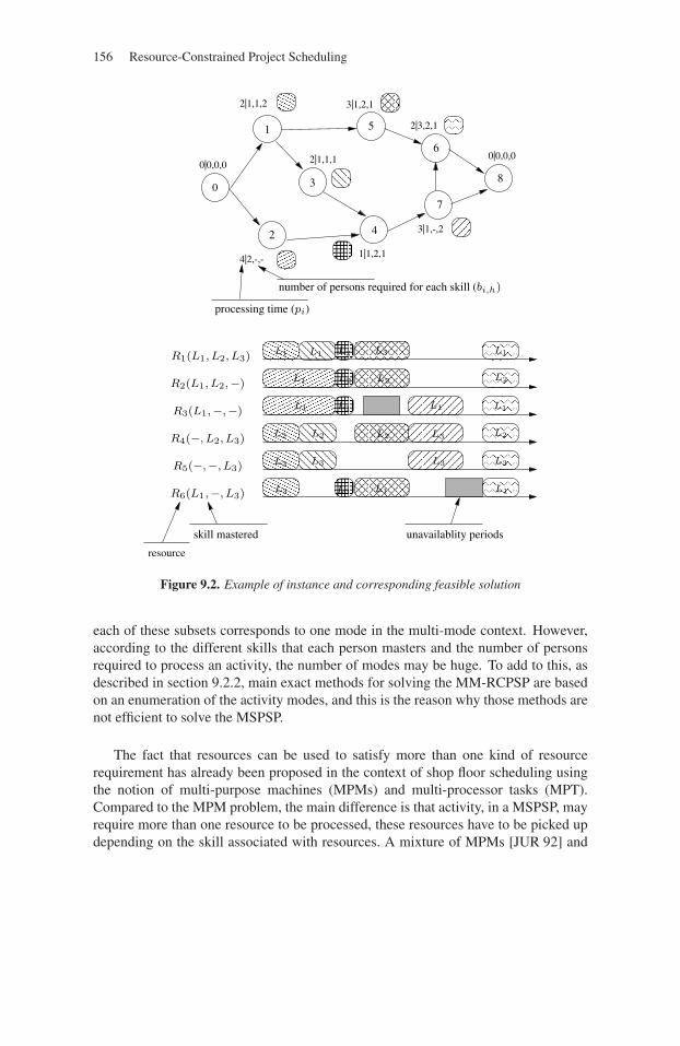
156 Resource-Constrained Project Scheduling
0
resource
8
1
2
3
4
1|1,2,1
5
6
7
4|2,-,-
2|1,1,2 3|1,2,1
2|3,2,1
3|1,-,2
2|1,1,10|0,0,00|0,0,0
R1(L1, L2, L3)
R6(L1,−, L3)
R5(−,−, L3)
R4(−, L2, L3)
R3(L1,−,−)
R2(L1, L2,−)
processing time (pi)
number of persons required for each skill (bi,h)
skill mastered unavailablity periods
L1
L3
L2
L1
L1
L2
L2
L3
L2
L2
L3
L1
L3
L3 L3
L2
L2
L1
L1
L1L1
L1
L2
L3
L3
L1
Figure 9.2. Example of instance and corresponding feasible solution
each of these subsets corresponds to one mode in the multi-mode context. However,according to the different skills that each person masters and the number of personsrequired to process an activity, the number of modes may be huge. To add to this, asdescribed in section 9.2.2, main exact methods for solving the MM-RCPSP are basedon an enumeration of the activity modes, and this is the reason why those methods arenot efficient to solve the MSPSP.
The fact that resources can be used to satisfy more than one kind of resourcerequirement has already been proposed in the context of shop floor scheduling usingthe notion of multi-purpose machines (MPMs) and multi-processor tasks (MPT).Compared to the MPM problem, the main difference is that activity, in a MSPSP, mayrequire more than one resource to be processed, these resources have to be picked updepending on the skill associated with resources. A mixture of MPMs [JUR 92] and
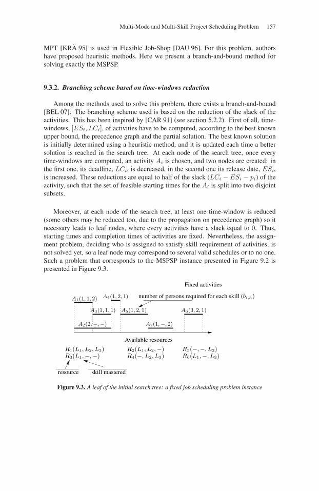
Multi-Mode and Multi-Skill Project Scheduling Problem 157
MPT [KRÄ 95] is used in Flexible Job-Shop [DAU 96]. For this problem, authorshave proposed heuristic methods. Here we present a branch-and-bound method forsolving exactly the MSPSP.
9.3.2. Branching scheme based on time-windows reduction
Among the methods used to solve this problem, there exists a branch-and-bound[BEL 07]. The branching scheme used is based on the reduction of the slack of theactivities. This has been inspired by [CAR 91] (see section 5.2.2). First of all, time-windows, [ESi, LCi], of activities have to be computed, according to the best knownupper bound, the precedence graph and the partial solution. The best known solutionis initially determined using a heuristic method, and it is updated each time a bettersolution is reached in the search tree. At each node of the search tree, once everytime-windows are computed, an activity Ai is chosen, and two nodes are created: inthe first one, its deadline, LCi, is decreased, in the second one its release date, ESi,is increased. These reductions are equal to half of the slack (LCi − ESi − pi) of theactivity, such that the set of feasible starting times for the Ai is split into two disjointsubsets.
Moreover, at each node of the search tree, at least one time-window is reduced(some others may be reduced too, due to the propagation on precedence graph) so itnecessary leads to leaf nodes, where every activities have a slack equal to 0. Thus,starting times and completion times of activities are fixed. Nevertheless, the assign-ment problem, deciding who is assigned to satisfy skill requirement of activities, isnot solved yet, so a leaf node may correspond to several valid schedules or to no one.Such a problem that corresponds to the MSPSP instance presented in Figure 9.2 ispresented in Figure 9.3.
Available resources
R3(L1,−,−)R1(L1, L2, L3) R2(L1, L2,−)
R4(−, L2, L3)R5(−,−, L3)R6(L1,−, L3)
resource skill mastered
A1(1, 1, 2)
A3(1, 1, 1) A6(3, 2, 1)
A7(1,−, 2)A2(2,−,−)
A5(1, 2, 1)
A4(1, 2, 1) number of persons required for each skill (bi,h)
Fixed activities
Figure 9.3. A leaf of the initial search tree: a fixed job scheduling problem instance
158 Resource-Constrained Project Scheduling
Determining if there exists a feasible assignment of persons to fixed activitiesrespecting skill constraints can be seen as a fixed job scheduling problem, which isNP-complete in the strong sense [KOL 91]. Thus, each leaf node is solved using aninteger linear programming formulation, in order to prune the node if it is unfeasible,or to find a solution if it exists. In this latter case, the solution to this assignmentproblem with fixed starting time is a solution for the global problem.
9.3.3. Lower bounds and time-bound adjustments
During the search, each node is evaluated by lower bounds in order to know if thenode may lead to a solution better than the best known one or if it has to be pruned.Two complementary methods are used for this evaluation. Those two methods aredestructive ones. That means a value D is fixed as an upper bound and tests areperformed to detect a contradiction. D is equal to the makespan of the best knownsolution minus one. If D cannot be respected as a global deadline, then the nodecannot lead to a solution strictly better than the best one, so it can be pruned.
The first method used to detect contradiction has been proposed by Bellenguezand Néron [BEL 05]. It is inspired from [BAP 99], [NÉR 01]. It is based on ener-getic reasoning. On a given time-interval, once every time-windows [ESi, LCi(D)]of activities are computed, it is necessary to compute the mandatory part of the activ-ities. The mandatory part w(i, t1, t2) of an activity Ai on an interval [t1; t2] is theminimum part of the activity that has to be processed on this interval to respect thetime-window of the activity and is computed:
w(i, t1, t2) = min(max(0, ESi + pi− t1),max(0, t2− (LCi(D)− pi)), pi, t2− t1).
PROPOSITION 9.1.– If there exists a time-interval [t1; t2[ where the assignment prob-lem of the mandatory parts of activity to staff members, respecting skills constraintshas no solution according to the resource constraint, then there exists no solution thatrespects the global deadline D.
Notice that this assignment problem can be solved in polynomial time.
The second lower bound is based on the graph of antichains, introduced for theRCPSP by [MIN 98]. This method is based on pairs of activity that may be in progressat the same time, without violating neither the precedence constraints nor the resourceconstraints. Thus, for each pair, it is necessary to check (1) if the two activities are notlinked by a precedence relation, (2) if their time-windows overlap and (3) if their exe-cution in parallel does not lead to a resource conflict. The compatibility graph is madeup of a node per activity, and two activities are linked if they can be in progress at thesame time, i.e., satisfying (1) (2) and (3). Weights associated with nodes are equal tothe duration of the corresponding activity. In this graph, a maximum weighted sta-ble set is computed, exactly using an ILP formulation, or heuristically using a greedy
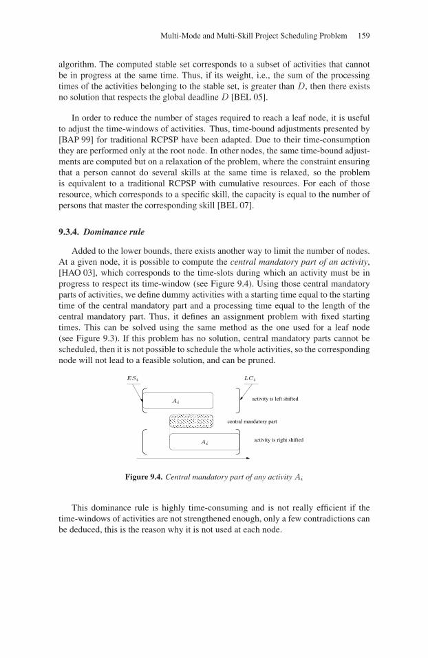
Multi-Mode and Multi-Skill Project Scheduling Problem 159
algorithm. The computed stable set corresponds to a subset of activities that cannotbe in progress at the same time. Thus, if its weight, i.e., the sum of the processingtimes of the activities belonging to the stable set, is greater than D, then there existsno solution that respects the global deadline D [BEL 05].
In order to reduce the number of stages required to reach a leaf node, it is usefulto adjust the time-windows of activities. Thus, time-bound adjustments presented by[BAP 99] for traditional RCPSP have been adapted. Due to their time-consumptionthey are performed only at the root node. In other nodes, the same time-bound adjust-ments are computed but on a relaxation of the problem, where the constraint ensuringthat a person cannot do several skills at the same time is relaxed, so the problemis equivalent to a traditional RCPSP with cumulative resources. For each of thoseresource, which corresponds to a specific skill, the capacity is equal to the number ofpersons that master the corresponding skill [BEL 07].
9.3.4. Dominance rule
Added to the lower bounds, there exists another way to limit the number of nodes.At a given node, it is possible to compute the central mandatory part of an activity,[HAO 03], which corresponds to the time-slots during which an activity must be inprogress to respect its time-window (see Figure 9.4). Using those central mandatoryparts of activities, we define dummy activities with a starting time equal to the startingtime of the central mandatory part and a processing time equal to the length of thecentral mandatory part. Thus, it defines an assignment problem with fixed startingtimes. This can be solved using the same method as the one used for a leaf node(see Figure 9.3). If this problem has no solution, central mandatory parts cannot bescheduled, then it is not possible to schedule the whole activities, so the correspondingnode will not lead to a feasible solution, and can be pruned.
activity is left shifted
activity is right shifted
central mandatory part
ESi LCi
Ai
Ai
Figure 9.4. Central mandatory part of any activity Ai
This dominance rule is highly time-consuming and is not really efficient if thetime-windows of activities are not strengthened enough, only a few contradictions canbe deduced, this is the reason why it is not used at each node.

160 Resource-Constrained Project Scheduling
9.4. Conclusion and research directions
In this chapter two extensions of the traditional RCPSP have been presented.Both are linked to resource flexibility. In the traditional RCPSP, resources neededand amounts of these resources required to process activities are known. In these twoextensions, there exist alternative resource requirements for activities. The main dif-ference lies in the fact that deciding what resource will be used and what amount ofthis resource is required, are decision variables that must be fixed during the resolutionprocess. Thus, resolution methods, especially exact methods, are much more complex.
Even if these two models, namely MM-RCPSP and MSPSP, are much harder tosolve in practice than traditional RCPSP, their practical interest is obvious: theseextensions mixing project definition and resource flexibility to process activity areone of the most promising research directions to solve real-life applications. Thus, thehuge amount of work in the literature dedicated to heuristics for these problems wouldbe used to obtain good solutions. Nevertheless, lower bounds, time-bound adjustmentsand also exact methods can be used to solve heuristically large size instances, usinglarge neighborhood search for instance (see Chapter 6).
Chapter 10
Project Scheduling with Productionand Consumption of Resources:
How to Build Schedules
Scheduling problems with resource constraints are NP-hard. Thus, methods arerequired for enumerating solutions. One method for the RCPSP is based on the notionof arbitrage, which is a preorder on the starting times of activities. An earliest schedulecan be computed using the strict order algorithm. We show here how to compute anearliest schedule using AND/OR precedence relations. We also generalize the notionof arbitrage to the more general case of activities producing and consuming a non-renewable resource.
10.1. Introduction
Project scheduling has attracted an increasingly growing interest in recent years,from both a scientific and a practical point of view, because it is an issue in almostevery area of the economy. We talk about optimizing codes in computer science, thejob-shop problem in industry, timetable development in administration and projectplanning in construction. Project scheduling is concerned with single-item or smallbatch production where scarce resources have to be allocated to dependent activitiesover time. Over the last 10 years scheduling problems with makespan minimizationhave been the subject of numerous papers. However, the only types of resources usu-ally considered are renewable and non-renewable. Renewable resources are required
Chapter written by Jacques CARLIER, Aziz MOUKRIM and Huang XU.
161

162 Resource-Constrained Project Scheduling
by activities at their starting times and given back at their completion times. Renew-able means that a pre-specified number of units of a resource are available for everyperiod of the planning horizon. One example of a renewable resource is the workforce.Non-renewable means that a number of units of a resource become available at sometime and then can be spent over the remaining planning horizon. Money is an exam-ple of a non-renewable resource. The project scheduling problem with non-renewableresources can be solved by the shifting algorithm [CAR 84], which calculates the lat-est schedules in polynomial time. Solutions to the RCPSP can be enumerated via thenotion of arbitrage using the strict order algorithm. We also show here how to com-pute these solutions using AND/OR precedence constraints. Nowadays, as demandsfrom the industrial sector increase, the integration of these two types of resources isbecoming crucial. Laborie [LAB 03b] put forward the concept of a Resource Tem-poral Network (RTN), which has a great expressive power and in which most of theresources used in scheduling can be modeled. Bouly et al. [BOU 04] developed amodel which allows resource production by tasks, and provided algorithms to solvethe problem with makespan minimization. Here we also discuss the project schedulingproblem with production and consumption of resources.
This chapter is composed of four sections. In section 10.2 we recall the graphrepresentation of a project scheduling problem with AND/OR precedence constraints.Section 10.3 will be devoted to the RCPSP, and section 10.4 to the project schedulingproblem in which activities can produce and consume resources.
10.2. The precedence-constrained project scheduling problem
A project consists of a number of activities or tasks that have processing timesand that need to be executed according to a set of precedence constraints. We beginby making the distinction between traditional precedence constraints and AND/ORprecedence constraints.
10.2.1. Traditional precedence constraints
The traditional precedence constraint is the AND precedence constraint. Eachactivity may have several predecessors and cannot start until all its predecessors arecompleted. A project network is given by a directed graph G = (V,E, v) where nodesin V model activities and arcs in E model precedence relations.
The classical objective is the makespan of the project which has to be minimized.Let us assume that the project consists of a set V = {A0, A1, . . . , An+1} of activitieswhere activity A0 (respectively An+1) is a fictitious beginning (respectively termina-tion) activity. It is represented by a directed graph G = (V,E, v). V is the node-set,|V | = n+2. E is the arc-set, |E| = m. vij is the length of the arc from Ai to Aj . Theproblem is to find the earliest starting time Sj , for all Aj ∈ V , satisfying the followingconditions:
Production and Consumption of Resources 163
1) Sj ≥ max{Si + vij | (Ai, Aj) ∈ E}2) Sj ≥ 0, for all Aj ∈ V
To solve the problem there exist several efficient algorithms, such as Bellman’salgorithm with a complexity of O(m) when there is no directed cycle, Dijkstra’s algo-rithm with a complexity of O(n2) when the values are non-negative and the Floyd-Warshall algorithm [LAW 76], with a complexity of O(n3) in the general case.
10.2.2. AND/OR precedence constraints
Basically, an AND/OR-network is a directed graph (or digraph for short). In con-trast to standard digraphs, an AND/OR-network has two different sorts of nodes,AND- and OR-nodes, which represent the following constraints. An AND-node issimply a normal node, meaning that the job it represents can be processed as soon asevery job preceding it in the graph has been completed. An OR-node, on the otherhand, can be scheduled as soon as at least one of its predecessors has completed, andthus represents a constraint. These generalized precedence constraints provide a goodmodel for a variety of applications. The input of the scheduling problem under consid-eration is a directed graph G = (V,E, v) with nodes of both types, V is the node-set,|V | = n + 2. E is the arc-set, |E| = m and vij is the arc length from Ai to Aj , whichmodels their time lags. We assume that V = A ∪ O, A being the set of AND-nodesand O the set of OR-nodes.
The problem is to find the earliest starting time Sj , for all Aj ∈ V , satisfying thefollowing conditions:
1) Sj ≥ max{Si + vij |(Ai, Aj) ∈ E}, ∀Aj ∈ A
2) Sj ≥ min{Si + vij |(Ai, Aj) ∈ E}, ∀Aj ∈ O
3) Sj ≥ 0, for all Aj ∈ V
It is easy to see that the problem is transformed into the critical path problem if theset O is empty, and the shortest-path problem if the set A is empty.
In the case where time lags are strictly positive, Möhring et al. [MÖH 04] haveproposed an O(|O| log |O| + |E| + |V |) algorithm to calculate the earliest startingtimes. Where there are arcs with zero values they have proposed an O(|V |+ |E| · |O|)algorithm. Adelson-Velsky and Levner [ADE 02] have also proposed an O(|V |+ |E| ·|O|) algorithm, a generalization of Dijkstra’s algorithm, to calculate the earliest start-ing times in this situation. Where negative arcs are allowed, pseudopolynomial algo-rithms can easily be obtained, but no one has yet proposed a polynomial algorithm.
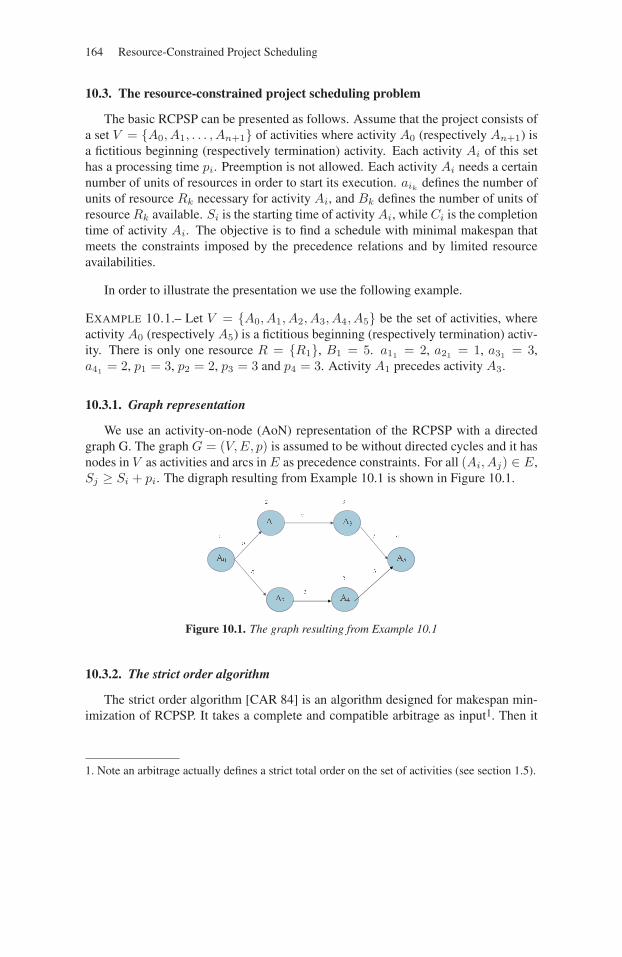
164 Resource-Constrained Project Scheduling
10.3. The resource-constrained project scheduling problem
The basic RCPSP can be presented as follows. Assume that the project consists ofa set V = {A0, A1, . . . , An+1} of activities where activity A0 (respectively An+1) isa fictitious beginning (respectively termination) activity. Each activity Ai of this sethas a processing time pi. Preemption is not allowed. Each activity Ai needs a certainnumber of units of resources in order to start its execution. aik
defines the number ofunits of resource Rk necessary for activity Ai, and Bk defines the number of units ofresource Rk available. Si is the starting time of activity Ai, while Ci is the completiontime of activity Ai. The objective is to find a schedule with minimal makespan thatmeets the constraints imposed by the precedence relations and by limited resourceavailabilities.
In order to illustrate the presentation we use the following example.
EXAMPLE 10.1.– Let V = {A0, A1, A2, A3, A4, A5} be the set of activities, whereactivity A0 (respectively A5) is a fictitious beginning (respectively termination) activ-ity. There is only one resource R = {R1}, B1 = 5. a11 = 2, a21 = 1, a31 = 3,a41 = 2, p1 = 3, p2 = 2, p3 = 3 and p4 = 3. Activity A1 precedes activity A3.
10.3.1. Graph representation
We use an activity-on-node (AoN) representation of the RCPSP with a directedgraph G. The graph G = (V,E, p) is assumed to be without directed cycles and it hasnodes in V as activities and arcs in E as precedence constraints. For all (Ai, Aj) ∈ E,Sj ≥ Si + pi. The digraph resulting from Example 10.1 is shown in Figure 10.1.
Figure 10.1. The graph resulting from Example 10.1
10.3.2. The strict order algorithm
The strict order algorithm [CAR 84] is an algorithm designed for makespan min-imization of RCPSP. It takes a complete and compatible arbitrage as input1. Then it
1. Note an arbitrage actually defines a strict total order on the set of activities (see section 1.5).

Production and Consumption of Resources 165
finds a schedule which is optimal for the defined preorder of activity starting times ifand only if the selected arbitrage is complete and compatible.
DEFINITION 10.1.– An arbitrage of resource Rk is a set of conjunctive arcs αk ={(i1, i2), . . . , (ip−1, ip)} with zero values, while Π = (i1, i2, . . . , ip) is a permutationon the set of activities requiring this resource.
DEFINITION 10.2.– A complete arbitrage α = ∪k∈Kαk is a union of arbitrages ofresources.
DEFINITION 10.3.– A complete arbitrage is compatible if there exists a schedule suchthat for each arc (i, j) in α, Sj ≥ Si.
The strict order algorithm is O(n2) [CAR 84]. It calculates an earliest schedulewhich respects a given preorder (Figure 10.2). Note that for efficiency, the algorithmdoes not necessarily respect the start time order set by the arbitrage and is thus identi-cal to the serial scheduling scheme (see Chapter 6).
(1) Initializationt = 0;
(2) Determination of the starting time of an activityfor an activity Ai which is not scheduled and whose predecessors in the graphG(α) = (V,E ∪ α) have all been scheduled, we set:ui = max{Sj + pj |(Aj , Ai) ∈ E}.t is the first time after ui when there are sufficient resources for activity Ai;if no such ui exists, go to (5).
(3) Assignment of the activitySi = t;if there are activities which are not scheduled, go to (2);otherwise, go to (4).
(4) Writing of the solutionreturn schedule S = {Si|Ai ∈ V }.
(5) Solution non-existentreturn (no feasible schedule).
Figure 10.2. The strict order algorithm
The strict order algorithm can be adapted to a graph G = (V,E, p) which containsnegative cycles [CAR 84], but it does not always converge. A negative arc from Ai toAj with a negative value vij implies that activity Ai has to start before time Sj + |vij |.A negative cycle is a cycle with a negative value.
We can apply the strict order algorithm to Example 10.1 with an arbitrage α =(A1, A2, A3, A4). We obtain the following schedule: S = {S1 = 0, S2 = 0, S3 =3, S4 = 3, S5 = 6}.
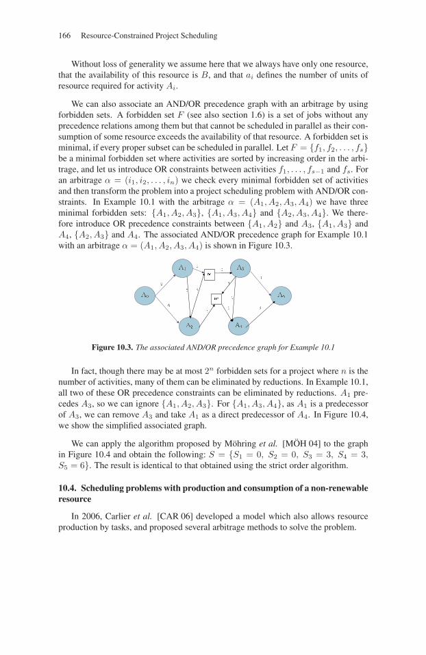
166 Resource-Constrained Project Scheduling
Without loss of generality we assume here that we always have only one resource,that the availability of this resource is B, and that ai defines the number of units ofresource required for activity Ai.
We can also associate an AND/OR precedence graph with an arbitrage by usingforbidden sets. A forbidden set F (see also section 1.6) is a set of jobs without anyprecedence relations among them but that cannot be scheduled in parallel as their con-sumption of some resource exceeds the availability of that resource. A forbidden set isminimal, if every proper subset can be scheduled in parallel. Let F = {f1, f2, . . . , fs}be a minimal forbidden set where activities are sorted by increasing order in the arbi-trage, and let us introduce OR constraints between activities f1, . . . , fs−1 and fs. Foran arbitrage α = (i1, i2, . . . , in) we check every minimal forbidden set of activitiesand then transform the problem into a project scheduling problem with AND/OR con-straints. In Example 10.1 with the arbitrage α = (A1, A2, A3, A4) we have threeminimal forbidden sets: {A1, A2, A3}, {A1, A3, A4} and {A2, A3, A4}. We there-fore introduce OR precedence constraints between {A1, A2} and A3, {A1, A3} andA4, {A2, A3} and A4. The associated AND/OR precedence graph for Example 10.1with an arbitrage α = (A1, A2, A3, A4) is shown in Figure 10.3.
Figure 10.3. The associated AND/OR precedence graph for Example 10.1
In fact, though there may be at most 2n forbidden sets for a project where n is thenumber of activities, many of them can be eliminated by reductions. In Example 10.1,all two of these OR precedence constraints can be eliminated by reductions. A1 pre-cedes A3, so we can ignore {A1, A2, A3}. For {A1, A3, A4}, as A1 is a predecessorof A3, we can remove A3 and take A1 as a direct predecessor of A4. In Figure 10.4,we show the simplified associated graph.
We can apply the algorithm proposed by Möhring et al. [MÖH 04] to the graphin Figure 10.4 and obtain the following: S = {S1 = 0, S2 = 0, S3 = 3, S4 = 3,S5 = 6}. The result is identical to that obtained using the strict order algorithm.
10.4. Scheduling problems with production and consumption of a non-renewableresource
In 2006, Carlier et al. [CAR 06] developed a model which also allows resourceproduction by tasks, and proposed several arbitrage methods to solve the problem.
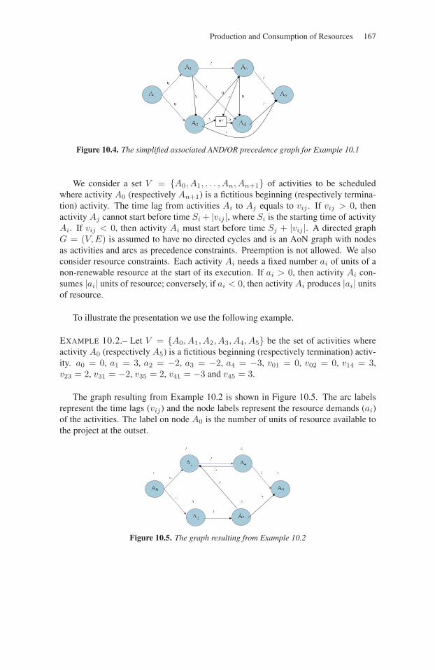
Production and Consumption of Resources 167
Figure 10.4. The simplified associated AND/OR precedence graph for Example 10.1
We consider a set V = {A0, A1, . . . , An, An+1} of activities to be scheduledwhere activity A0 (respectively An+1) is a fictitious beginning (respectively termina-tion) activity. The time lag from activities Ai to Aj equals to vij . If vij > 0, thenactivity Aj cannot start before time Si + |vij |, where Si is the starting time of activityAi. If vij < 0, then activity Ai must start before time Sj + |vij |. A directed graphG = (V,E) is assumed to have no directed cycles and is an AoN graph with nodesas activities and arcs as precedence constraints. Preemption is not allowed. We alsoconsider resource constraints. Each activity Ai needs a fixed number ai of units of anon-renewable resource at the start of its execution. If ai > 0, then activity Ai con-sumes |ai| units of resource; conversely, if ai < 0, then activity Ai produces |ai| unitsof resource.
To illustrate the presentation we use the following example.
EXAMPLE 10.2.– Let V = {A0, A1, A2, A3, A4, A5} be the set of activities whereactivity A0 (respectively A5) is a fictitious beginning (respectively termination) activ-ity. a0 = 0, a1 = 3, a2 = −2, a3 = −2, a4 = −3, v01 = 0, v02 = 0, v14 = 3,v23 = 2, v31 = −2, v35 = 2, v41 = −3 and v45 = 3.
The graph resulting from Example 10.2 is shown in Figure 10.5. The arc labelsrepresent the time lags (vij) and the node labels represent the resource demands (ai)of the activities. The label on node A0 is the number of units of resource available tothe project at the outset.
Figure 10.5. The graph resulting from Example 10.2
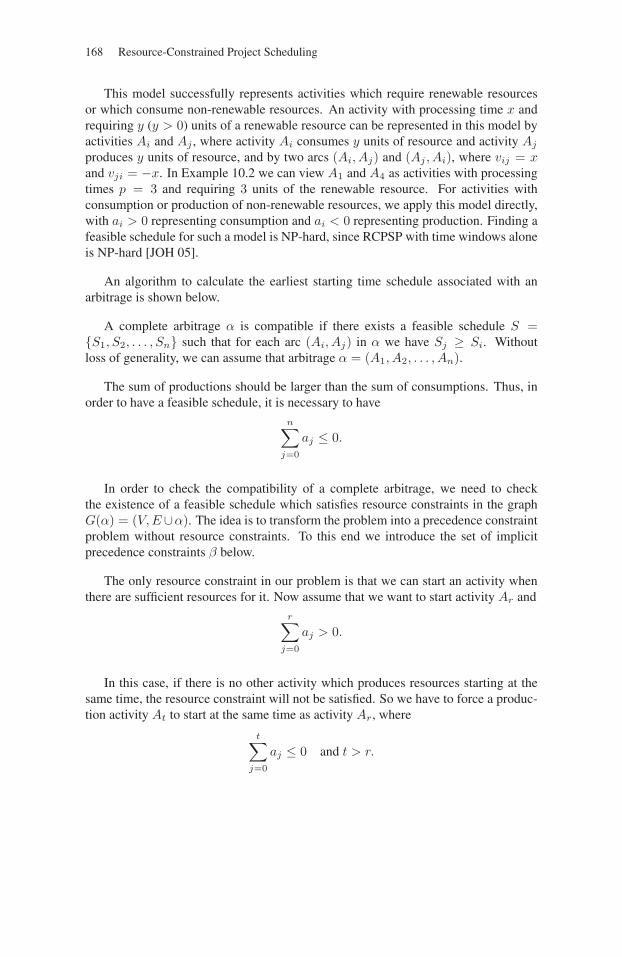
168 Resource-Constrained Project Scheduling
This model successfully represents activities which require renewable resourcesor which consume non-renewable resources. An activity with processing time x andrequiring y (y > 0) units of a renewable resource can be represented in this model byactivities Ai and Aj , where activity Ai consumes y units of resource and activity Aj
produces y units of resource, and by two arcs (Ai, Aj) and (Aj , Ai), where vij = xand vji = −x. In Example 10.2 we can view A1 and A4 as activities with processingtimes p = 3 and requiring 3 units of the renewable resource. For activities withconsumption or production of non-renewable resources, we apply this model directly,with ai > 0 representing consumption and ai < 0 representing production. Finding afeasible schedule for such a model is NP-hard, since RCPSP with time windows aloneis NP-hard [JOH 05].
An algorithm to calculate the earliest starting time schedule associated with anarbitrage is shown below.
A complete arbitrage α is compatible if there exists a feasible schedule S ={S1, S2, . . . , Sn} such that for each arc (Ai, Aj) in α we have Sj ≥ Si. Withoutloss of generality, we can assume that arbitrage α = (A1, A2, . . . , An).
The sum of productions should be larger than the sum of consumptions. Thus, inorder to have a feasible schedule, it is necessary to have
n∑j=0
aj ≤ 0.
In order to check the compatibility of a complete arbitrage, we need to checkthe existence of a feasible schedule which satisfies resource constraints in the graphG(α) = (V,E∪α). The idea is to transform the problem into a precedence constraintproblem without resource constraints. To this end we introduce the set of implicitprecedence constraints β below.
The only resource constraint in our problem is that we can start an activity whenthere are sufficient resources for it. Now assume that we want to start activity Ar and
r∑j=0
aj > 0.
In this case, if there is no other activity which produces resources starting at thesame time, the resource constraint will not be satisfied. So we have to force a produc-tion activity At to start at the same time as activity Ar, where
t∑j=0
aj ≤ 0 and t > r.
Production and Consumption of Resources 169
For As, At ∈ α where s < t, we say that the arc from At to As+1 of value 0 isimplied by α if and only if for every r where s < r < t the following conditions aresatisfied:
s∑j=0
aj ≤ 0 (10.1)
r∑j=0
aj > 0, ∀r ∈ ]s, t[ (10.2)
t∑j=0
aj ≤ 0. (10.3)
β is the set of all arcs implied by α in this way. In order to generate β, let
D =
{Aj |
j∑k=0
ak ≤ 0
}.
We suppose that there are m elements in D and D = {Aj1 , Aj2 , . . . , Ajm} such
that j1 ≤ j2 ≤ · · · ≤ jm. If j1 �= 0, we add the arc (Aj1 , A0) of zero value to β, andfor every s where js+1 > js + 1 we add the arc (Ajs+1 , Ajs+1) of zero value to β.
THEOREM 10.1.– A complete arbitrage α = {(A1, A2), (A2, A3), . . . , (An−1, An)}is compatible if and only if the directed graph G(α, β) = (V,E ∪ α ∪ β) containsno directed cycles of strictly positive value, where β contains all implicit precedenceconstraints deduced from α.
If the directed graph G(α, β) = (V,E ∪ α ∪ β) contains no positive directedcycles, we can apply the Floyd-Warshall algorithm [LAW 76] to obtain an optimalschedule. This schedule will satisfy all precedence and resource constraints, since agraph without strictly positive directed cycles is a sufficient condition for the Floyd-Warshall algorithm to find a feasible schedule. The arbitrage is therefore compatible.
Let us now suppose that the complete arbitrage α is compatible and that there is astrictly positive cycle (Av1 , Av2 , . . . , Avp
, Av1) in the graph G(α, β). So Sv1 > Sv1 ,which is a contradiction for the existence of a feasible schedule.
The algorithm yields the earliest starting time schedule if the given arbitrage iscompatible. Its complexity is O(n3). It works even where values are negative.

170 Resource-Constrained Project Scheduling
Input:A complete arbitrage α = {(Ai1 , Ai2), (Ai2 , Ai3), . . . , (Ain−1 , Ain
)}A conjunctive graph G = (V,E)Output:An Earliest Start Time Schedule S for the arbitrage α.(1) Generate β, which contains all implicit precedence constraints deduced from α;(2) Use the Floyd-Warshall algorithm to compute S in graph G(α, β)=(V,E∪α∪β).
Figure 10.6. Algorithm to compute the earliest starting time schedule of a complete arbitrage
10.5. Discussion
Using the complete arbitrage method for enumeration would be very costly. Forthis reason we have also proposed restricting the arbitrage to consumption activities[CAR 06]. We are now working on algorithms for computing earliest schedules inthis restricted case. We can also restrict the arbitrage to production activities whencomputing latest schedules. The arbitrages may then be used to construct both exactand approximate methods.
Chapter 11
Activity Insertion Problem in a RCPSP withMinimum and Maximum Time Lags
11.1. Introduction
In the standard RCPSP, the precedence relations are simple: an activity cannotstart before the end of all its predecessors. In other words, between the start timeof an activity Ai and the start time of its successor Aj there is a minimal distance(or minimum time lag) equal to the duration of Ai. The RCPSP with minimum andmaximum time lags (RCPSP/max) involves generalized precedence relations wherethe minimum time lag between Ai and Aj can be any non-negative value and wherethere is possibly a maximum allowed time lag between the start time of Ai and thestart time of Aj .
Independently of makespan minimization, simply finding a resource-feasibleschedule that respects both the minimum and maximum time lags is NP-hard[BAR 88] whereas, for the standard RCPSP, this problem is polynomial. For thatreason, the RCPSP/max problem has been extensively studied in the schedulingresearch. For a thorough analysis of this problem, we recommend the work of Neu-mann, Schwindt and Zimmermann [NEU 03]. In this chapter, unlike most approachesthat focused on finding a global schedule that minimizes the project duration, weillustrate the difficulties brought by the maximum time lags by considering theapparently simple problem of inserting a single activity inside an existing schedule.
Chapter written by Christian ARTIGUES and Cyril BRIAND.
171
172 Resource-Constrained Project Scheduling
This problem aims at finding an insertion position that is feasible with regards tothe min/max time lags and resource constraints and that preserves the partial schedulestructure. The objective is to minimize the project duration increase. Such a prob-lem arises in local search procedures for reinsertion neighborhoods that unschedulean activity and insert it at another position and also for reactive insertion of unex-pected activities. The interest of preserving the structure of the partial schedule istwofold. First, it makes it possible to decrease the size of the search space, which isnecessary for both neighborhood search and reactive scheduling. Second, this policytends to minimize the disturbances during the online project execution phase, whichis referred to as ensuring the schedule stability. We define the structure of the scheduleby means of resource flow networks, inducing additional precedence constraints. Theproblem has already been addressed for the standard RCPSP in [ART 00, ART 03]where an O(n2q) optimal solving procedure has been proposed where n is the numberof activities and q is the number of resources. Unfortunately, this procedure is unableto tackle minimum and maximum time lags. In [GRÖ 07], insertion problems in ageneral disjunctive scheduling framework capturing a variety of job shop schedulingproblems and insertion types are considered and lower and upper bound proceduresare developed. Since disjunctive scheduling is a particular case of the RCPSP where allresources have unit availability, the proposed procedures do not apply to the problemconsidered in this paper. We show that the considered insertion problem is NP-hardfor the RCPSP with minimum and maximum time lags. When maximum time lags areignored, a O(n2q) algorithm is provided by a direct extension of the one proposed in[ART 03].
11.2. Problem statement
As for the standard RCPSP (see Chapter 1), activities constituting the project areidentified by a set V = {A0, . . . , An+1}. Activity A0 represents by conventionthe start of the schedule and activity An+1 represents symmetrically the end of theschedule. The set of non-dummy activities is identified by A = {A1, . . . , An}. pi
denotes the duration of activity i with p0 = pn+1 = 0. We assume in this chapter thatpi > 0,∀Ai ∈ A.
A valued activity-on-node graph G(V,E, l) is defined where nodes correspondto activities and arcs correspond to precedence relations. Each arc (Ai, Aj) ∈ E isvalued by an integer time lag lij . lij ≥ 0 corresponds to a minimum time lag of lijunits stating that Aj has to start at least lij time units after the start time of Ai. Inthe standard RCPSP, only minimum time lags are considered and lij = pi for eacharc (Ai, Aj) ∈ E. lij ≤ 0 corresponds to a time lag of −lij units stating that Ai hasto start at the latest lij time units after the start time of Aj . Resource constraints aredefined as in the standard RCPSP.R = {R1, . . . , Rq} denotes the set of resources. Bk
denotes the availability of Rk. bik represents the amount of resource Rk used duringthe execution of i.
Activity Insertion Problem in a RCPSP with Minimum and Maximum Time Lags 173
We assume that we have at least the following arcs in E: an arc (A0, Ai) peractivity Ai ∈ A valuated by l0i ≥ 0 and an arc (Ai, An+1) per activity Ai ∈ Avaluated by li(n+1) = pi.
A solution S is a schedule giving the start time Si of each activity Ai. S is feasibleif it is compatible with the generalized precedence constraints (11.1) and the resourceconstraints (11.2) defined in Chapter 1 and recalled below where At = {i ∈ A |Si ≤t < Si + pi} represents the set of non-dummy activities in process at time t.
Sj − Si ≥ lij ∀(Ai, Aj) ∈ E (11.1)∑Ai∈At
bik ≤ Bk ∀Rk ∈ R,∀t ≥ 0 (11.2)
The makespan of a schedule S is equal to Sn+1, the start time of the end activity.The above-defined set At and constraints state that an activity cannot be interruptedonce it is started. This is referred to as not allowing preemption. The RCPSP withminimum and maximum time lags is the problem (P) of finding a non-preemptiveschedule S of minimal makespan Sn+1 such that S0 = 0 and subject to precedenceconstraints (11.1) and resource constraints (11.2). The problem does not necessarilyhave a solution. This can be due to an inconsistency of the precedence constraints(11.1), independently of the resource constraints. To verify the consistency of theprecedence constraints E, a distance matrix (δij)i,j∈V 2 can be computed where δij
is the length of the longest path between i and j in G(V,E, l). (δij) can be com-puted in O(n3) by the Floyd-Warshall algorithm. More precisely, there is no solutionif there is a cycle of positive length in G(V,E, l). In the case where the temporal con-straints are consistent, the problem does not necessarily have a solution either and thecorresponding decision problem is NP-complete [BAR 88].
We use the concept of resource-flow network (introduced in Chapter 1) to representthe solutions to (P) [FOR 97, ART 00, ART 03, LEU 04, NEU 03]. A resource flow fis a (n + 2)× (n + 2)×m matrix verifying equations (11.3-11.5) defined in Chapter1 and recalled below:
fijk ≥ 0 ∀Ai ∈ A ∪ {A0}, ∀Aj ∈ A ∪ {An+1}, ∀Rk ∈ R (11.3)
∑Ai∈A∪{An+1}
f0ik =∑
Ai∈A∪{A0}fi(n+1)k = Bk ∀Rk ∈ R (11.4)
∑Aj∈A∪{An+1}
fijk =∑
Aj∈A∪{A0}fijk = bik ∀Ai ∈ A,∀Rk ∈ R (11.5)

174 Resource-Constrained Project Scheduling
fkij denotes the number of resource Rk units transferred from activity Ai to activity
Aj . We define E(f) as the set of arcs induced by a resource flow1 f , i.e. E(f) ={(Ai, Aj) ∈ V 2 | ∃k ∈ R, fk
ij > 0}. E(f) can be seen as the set of precedenceconstraints represented by the flow. Consider graph Gf = G(V,E∪E(f), l(f)) wherel(f) is defined as follows. Each arc (i, j) ∈ E with (i, j) �∈ E(f) is valuated by lij .Each arc (i, j) ∈ E(f) with (i, j) �∈ E is valuated by pi. Each arc (i, j) ∈ E ∩ E(f)is valuated by max(pi, lij).
Let (δfij)Ai,Aj∈V denotes the distance matrix associated with flow f . δf
ij is thelength of the longest path from Ai to Aj in Gf . The precedence constraints inducedby the flow are consistent if and only if there is no cycle of positive length in Gf . Inparticular, δf
0i, ∀Ai ∈ V denotes the earliest start schedule associated with the flow f .We set δf
ij = −∞ if there is no path from Ai to Aj in Gf .
PROPOSITION 11.1.– (P ) can be defined as the problem of finding a resource flow fverifying (11.3-11.5), such that Gf does not admit a cycle of positive length and suchthat δf
0(n+1) is minimal.
Proof. The arguments used in Lemmas 1.1 and 1.2 (Chapter 1) and issued from[LEU 04] for the standard RCPSP can be easily transposed for the considered prob-lem. Similarly, the ones used in [NEU 03] (section 2.13) for the RCPSP with mini-mum/maximum time lags and sequence-dependent setup times hold.
We consider a partial solution in which all activities but one, denoted by activityAx (0 < x < n + 1), have been scheduled. This amounts to considering a completesolution to problem (Px) identical to (P) except that bxk = 0, ∀k ∈ R.
Consider an example comprising five real activities and a single resource of threeunits issued from ([NEU 03], Ch. 2, P. 26). Durations and resource demands are givenin Table 11.1.
Ai 0 1 2 3 4 5 6
pi 0 6 4 2 4 2 0
bi 0 1 2 2 2 3 0
Table 11.1. Durations and resource demands
1. In Chapter 1, a strict order P (f) is defined as the transitive closure of E(f).
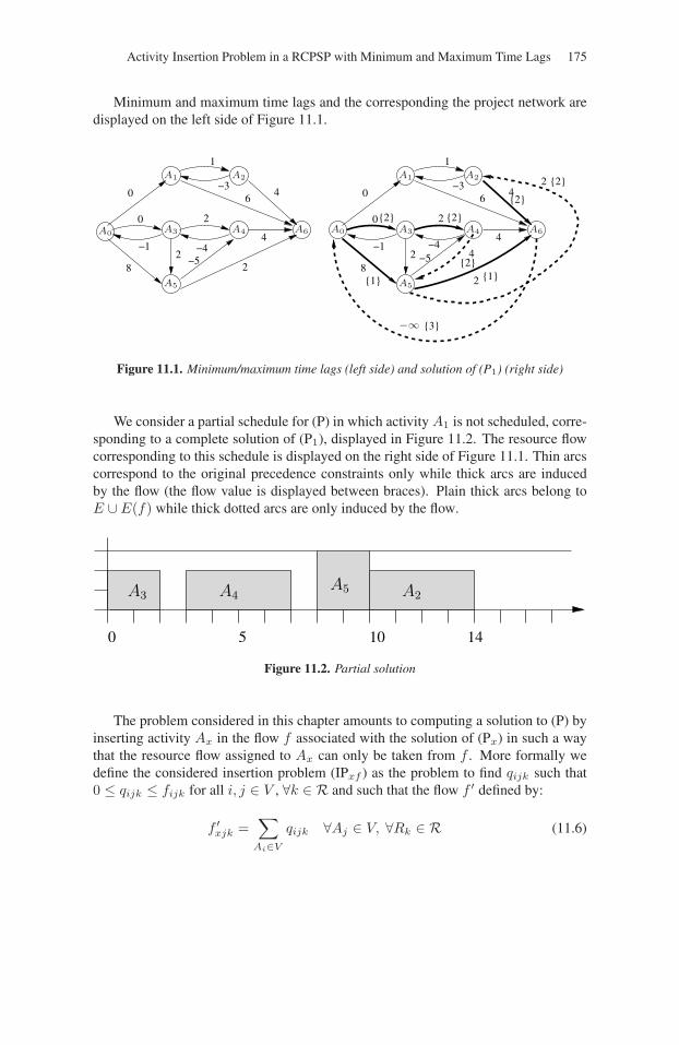
Activity Insertion Problem in a RCPSP with Minimum and Maximum Time Lags 175
Minimum and maximum time lags and the corresponding the project network aredisplayed on the left side of Figure 11.1.
0
−1
82
2
1
−36
40
4
{1}
{2} {2}0
−1
82
2
−4−5
2
1
−36
40
4
4{2}
2 {1}
{2}
−5−4
2 {2}
{3}−∞
A0
A1 A2
A3 A4
A5
A6 A0
A1 A2
A6A4A3
A5
Figure 11.1. Minimum/maximum time lags (left side) and solution of (P1) (right side)
We consider a partial schedule for (P) in which activity A1 is not scheduled, corre-sponding to a complete solution of (P1), displayed in Figure 11.2. The resource flowcorresponding to this schedule is displayed on the right side of Figure 11.1. Thin arcscorrespond to the original precedence constraints only while thick arcs are inducedby the flow (the flow value is displayed between braces). Plain thick arcs belong toE ∪ E(f) while thick dotted arcs are only induced by the flow.
0 5 10 14
A3 A4A5 A2
Figure 11.2. Partial solution
The problem considered in this chapter amounts to computing a solution to (P) byinserting activity Ax in the flow f associated with the solution of (Px) in such a waythat the resource flow assigned to Ax can only be taken from f . More formally wedefine the considered insertion problem (IPxf ) as the problem to find qijk such that0 ≤ qijk ≤ fijk for all i, j ∈ V , ∀k ∈ R and such that the flow f ′ defined by:
f ′xjk =
∑Ai∈V
qijk ∀Aj ∈ V, ∀Rk ∈ R (11.6)
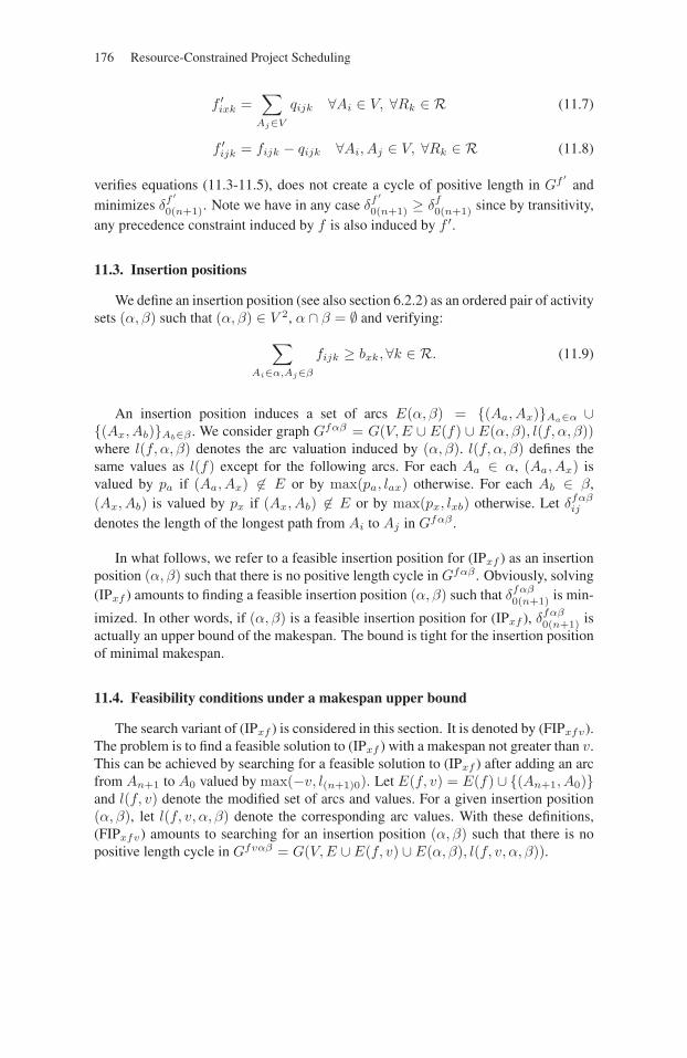
176 Resource-Constrained Project Scheduling
f ′ixk =
∑Aj∈V
qijk ∀Ai ∈ V, ∀Rk ∈ R (11.7)
f ′ijk = fijk − qijk ∀Ai, Aj ∈ V, ∀Rk ∈ R (11.8)
verifies equations (11.3-11.5), does not create a cycle of positive length in Gf ′and
minimizes δf ′
0(n+1). Note we have in any case δf ′
0(n+1) ≥ δf0(n+1) since by transitivity,
any precedence constraint induced by f is also induced by f ′.
11.3. Insertion positions
We define an insertion position (see also section 6.2.2) as an ordered pair of activitysets (α, β) such that (α, β) ∈ V 2, α ∩ β = ∅ and verifying:
∑Ai∈α,Aj∈β
fijk ≥ bxk,∀k ∈ R. (11.9)
An insertion position induces a set of arcs E(α, β) = {(Aa, Ax)}Aa∈α ∪{(Ax, Ab)}Ab∈β . We consider graph Gfαβ = G(V,E ∪ E(f) ∪ E(α, β), l(f, α, β))where l(f, α, β) denotes the arc valuation induced by (α, β). l(f, α, β) defines thesame values as l(f) except for the following arcs. For each Aa ∈ α, (Aa, Ax) isvalued by pa if (Aa, Ax) �∈ E or by max(pa, lax) otherwise. For each Ab ∈ β,(Ax, Ab) is valued by px if (Ax, Ab) �∈ E or by max(px, lxb) otherwise. Let δfαβ
ij
denotes the length of the longest path from Ai to Aj in Gfαβ .
In what follows, we refer to a feasible insertion position for (IPxf ) as an insertionposition (α, β) such that there is no positive length cycle in Gfαβ . Obviously, solving(IPxf ) amounts to finding a feasible insertion position (α, β) such that δfαβ
0(n+1) is min-
imized. In other words, if (α, β) is a feasible insertion position for (IPxf ), δfαβ0(n+1) is
actually an upper bound of the makespan. The bound is tight for the insertion positionof minimal makespan.
11.4. Feasibility conditions under a makespan upper bound
The search variant of (IPxf ) is considered in this section. It is denoted by (FIPxfv).The problem is to find a feasible solution to (IPxf ) with a makespan not greater than v.This can be achieved by searching for a feasible solution to (IPxf ) after adding an arcfrom An+1 to A0 valued by max(−v, l(n+1)0). Let E(f, v) = E(f) ∪ {(An+1, A0)}and l(f, v) denote the modified set of arcs and values. For a given insertion position(α, β), let l(f, v, α, β) denote the corresponding arc values. With these definitions,(FIPxfv) amounts to searching for an insertion position (α, β) such that there is nopositive length cycle in Gfvαβ = G(V,E ∪ E(f, v) ∪ E(α, β), l(f, v, α, β)).

Activity Insertion Problem in a RCPSP with Minimum and Maximum Time Lags 177
As a preliminary remark, if there is a positive length cycle in Gfv , there is obvi-ously no feasible solution to (FIPxfv). Again, this can be determined in O(n3) bythe Floyd-Warshall algorithm. However, according to the last remark of section 11.2,if f represents a feasible solution to (Px), there is a positive length cycle in Gfv ifand only if v < δf
0(n+1). In what follows, we assume v ≥ δf0(n+1) and we consider
(δfvij )Ai,Aj∈V defined as the distance matrix corresponding to the all-pairs longest
path lengths in Gfv .
The remainder of the section is devoted to the evaluation of the feasibility ofan insertion position (α, β) (without generating graph Gfvαβ or computing matrix(δfαβ
ij )). For this purpose, we define the following three categories of elementarycycles in Gfvαβ :
• An elementary cycle of type C1(v, α, β) involves an arc (Aa, Ax) with Aa ∈ αand l(f, v, α, β)ax = pa and no arc (Ax, Ab) with Ab ∈ β. Note that in Gfvαβ , alongest path from Ax to Aa not traversing any node of β is also a longest path fromAx to Aa in Gfv of length δfv
xa (since the path cannot traverse Ax again). Therefore,L1(v, α, β) = maxAa∈α(pa + δfv
xa) is the length of the cycles of C1(v, α, β) havingthe largest length.
• An elementary cycle of type C2(v, α, β) includes an arc (Ax, Ab) with Ab ∈ βand l(f, v, α, β)xb = px and no arc (Aa, Ax) with Aa ∈ α. Using the same argumentsas the ones use in the previous item, the length of the longest path from Ab to Ax inGfvαβ is equal to δfv
bx . Consequently, L2(v, α, β) = px + maxAb∈β(δfvbx ) denotes the
length of the cycle in C2(v, α, β) having the largest length.
• A cycle of type C3(v, α, β) involves two arcs (Aa, Ax), (Ax, Ab) withl(f, v, α, β)ax = pa and l(f, v, α, β)xb = px. Again, the longest path in Gfvαβ
passes only through arcs existing in G(V,E ∪ E(f, v), l(v, f)) and thus has lengthδfvba . Hence, let L3(v, α, β) = px + max(Aa,Ab)∈α×β(pa + δfv
ba ) be the length of thecycle of C3(v, α, β) having the largest length.
In what follows, Cq(v, α, β) and Lq(v, α, β) (q = 1, 2, 3) will be simply denotedCq and Lq when there is no ambiguity. Figure 11.3 illustrates the three consideredcategories of cycles.
δfvbx
max(pa, δfvax)
δfvxa
max(px, δfvxb )
δfvab
δfvba
Aa Ab
Ax
Figure 11.3. Cycle analysis after an activity insertion
178 Resource-Constrained Project Scheduling
THEOREM 11.1.– An insertion position (α, β) is feasible for (FIPxfv) if and only ifmax(L1, L2, L3) ≤ 0.
Proof. This amounts to showing that there is no cycle of positive length in Gfvαβ ifand only if max(L1, L2, L3) ≤ 0.
(⇒ part) If there is no positive length cycle in Gfvαβ , since each Li is not largerthan an actual cycle length, then L1, L2 and L3 are non-positive.
(⇐ part) We know that in a valued digraph there is no positive length cycle if andonly if there is no elementary positive length cycle. Thus, it is sufficient to show that ifmax(L1, L2, L3) ≤ 0, there is no elementary positive length cycle in Gfvαβ . Amongthe possible elementary cycles, we may restrict ourselves to the ones traversing atleast one arc (Aa, Ax) with Aa ∈ α and l(f, v, α, β)ax = pa (type (i) arc) or onearc (Ax, Ab) with Ab ∈ β and l(f, v, α, β)xb = px (type (ii) arc). Indeed, any cycletraversing none of these arcs has a length equal to the length of a cycle in Gfv whichis by hypothesis non-negative. Furthermore, at most one type (i) arc and at most onetype (ii) arc may be traversed by any elementary cycle.
Suppose now that C denotes an elementary cycle of Gfvαβ with the largest lengthbut not belonging any category among C1, C2, or C3. According to the presence oftype (i) and (ii) arcs there are three possibilities. If C traverses exactly one type (i) arcand no type (ii) arcs, the path in C from Ax to Aa is not larger than δfv
xa . Indeed, byconstruction, for any activities Ai, Aj , Ak we have δfv
ij ≥ δfvik + δfv
kj . Consequently,there exists in C1 a cycle not shorter than C. For the same reason, if C traverses exactlyone type (ii) arc and no type (i) arcs, the path in C from Ab to Ax is not larger thanδfvbx and there exists in C2 a cycle not shorter than C. Lastly, in the case C traverses
exactly one type (i) arc and one type (ii) arc, the path in C from Ab to Aa is not largerthan δfv
ba and there exists in C3 a cycle not shorter than C. It follows that there existsan elementary longest length cycle that belongs either to C1, C2 or C3.
11.5. Computational complexity of the insertion problem with minimum andmaximum time lags
In this section, we prove that (IPxf ) is NP-hard. We show that the decision problem(DIPxfv), stating whether there exists a feasible solution to (FIPxfv) or not, is NP-complete by reduction from the independent set problem. We recall that, given a graphG(V, E), where V is a set of vertices and E is a set of edges, and an integer k, theindependent set problem lies in finding a subset of vertices W ⊆ V of cardinality ksuch that ∀x, y ∈ W , (x, y) �∈ E (i.e. the vertices of W are pairwise independent).Such a problem is known to be NP-hard. Let p denote the number of vertices: p = |V|.
In what follows, we show how to associate with any independent set problem aninstance of the insertion problem with n = 2p + 1 non-dummy activities and a singleresource of availability B1 = p (the resource index can be omitted).
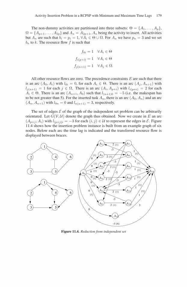
Activity Insertion Problem in a RCPSP with Minimum and Maximum Time Lags 179
The non-dummy activities are partitioned into three subsets: Θ = {A1, . . . , Ap},Ω = {Ap+1, . . . , A2p} and An = A2p+1, An being the activity to insert. All activitiesbut An are such that bi = pi = 1, ∀Ai ∈ Θ ∪ Ω. For An we have pn = 3 and we setbn to k. The resource flow f is such that
f0i = 1 ∀Ai ∈ Θ
fi(p+i) = 1 ∀Ai ∈ Θ
fj(n+1) = 1 ∀Aj ∈ Ω.
All other resource flows are zero. The precedence constraints E are such that thereis an arc (A0, Ai) with l0i = 0, for each Ai ∈ Θ. There is an arc (Aj , An+1) withlj(n+1) = 1 for each j ∈ Ω. There is an arc (Ai, Ap+i) with li(p+i) = 2 for eachAi ∈ Θ. There is an arc (An+1, A0) such that l(n+1)0 = −5 (i.e. the makespan hasto be not greater than 5). For the inserted task An, there is an arc (A0, An) and an arc(An, An+1) with l0n = 0 and ln(n+1) = 3, respectively.
The set of edges E of the graph of the independent set problem can be arbitrarilyorientated. Let G(V,U) denote the graph thus obtained. Now we create in E an arc(Ap+j , Ai) with l(p+j)i = −3 for each (i, j) ∈ U to represent the edges in E . Figure11.4 shows how the insertion problem instance is built from an example graph of sixnodes. Below each arc the time lag is indicated and the transferred resource flow isdisplayed between braces.
{1}
{1}
{1}
{1}
{1}
{1}
{1}
{1}{1}
{1}
{1}
{1}
{1}
{1}
{1}
{1}
{1}
−5 {6}
{1}
1
2
3
4
5
6
1
2
3
4
5
6
2
-3
2
2
2
2
2
1
1
1
1
1
1
A13
0
3
0
0
0
0
0
0
-3
-3
-3
A0
A1
A2
A3
A4
A5
A6
A7
A8
A9
A10
A11
A12
A14-3
-3
-3
Figure 11.4. Reduction from independent set
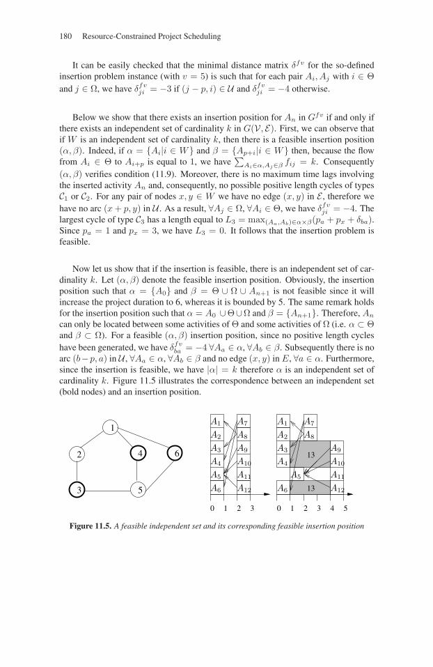
180 Resource-Constrained Project Scheduling
It can be easily checked that the minimal distance matrix δfv for the so-definedinsertion problem instance (with v = 5) is such that for each pair Ai, Aj with i ∈ Θand j ∈ Ω, we have δfv
ji = −3 if (j − p, i) ∈ U and δfvji = −4 otherwise.
Below we show that there exists an insertion position for An in Gfv if and only ifthere exists an independent set of cardinality k in G(V, E). First, we can observe thatif W is an independent set of cardinality k, then there is a feasible insertion position(α, β). Indeed, if α = {Ai|i ∈ W} and β = {Ap+i|i ∈ W} then, because the flowfrom Ai ∈ Θ to Ai+p is equal to 1, we have
∑Ai∈α,Aj∈β fij = k. Consequently
(α, β) verifies condition (11.9). Moreover, there is no maximum time lags involvingthe inserted activity An and, consequently, no possible positive length cycles of typesC1 or C2. For any pair of nodes x, y ∈ W we have no edge (x, y) in E , therefore wehave no arc (x + p, y) in U . As a result, ∀Aj ∈ Ω, ∀Ai ∈ Θ, we have δfv
ji = −4. Thelargest cycle of type C3 has a length equal to L3 = max(Aa,Ab)∈α×β(pa + px + δba).Since pa = 1 and px = 3, we have L3 = 0. It follows that the insertion problem isfeasible.
Now let us show that if the insertion is feasible, there is an independent set of car-dinality k. Let (α, β) denote the feasible insertion position. Obviously, the insertionposition such that α = {A0} and β = Θ ∪ Ω ∪ An+1 is not feasible since it willincrease the project duration to 6, whereas it is bounded by 5. The same remark holdsfor the insertion position such that α = A0 ∪Θ∪Ω and β = {An+1}. Therefore, An
can only be located between some activities of Θ and some activities of Ω (i.e. α ⊂ Θand β ⊂ Ω). For a feasible (α, β) insertion position, since no positive length cycleshave been generated, we have δfv
ba = −4 ∀Aa ∈ α, ∀Ab ∈ β. Subsequently there is noarc (b−p, a) in U , ∀Aa ∈ α, ∀Ab ∈ β and no edge (x, y) in E, ∀a ∈ α. Furthermore,since the insertion is feasible, we have |α| = k therefore α is an independent set ofcardinality k. Figure 11.5 illustrates the correspondence between an independent set(bold nodes) and an insertion position.
0 1 2 3 4
13
13
50 1 2 3
1
2
53
4 6
A1
A2
A3
A4
A5
A6 A12
A11
A10
A9
A8
A7 A1
A2
A3
A4
A6
A8
A7
A9
A10
A11
A12
A5
Figure 11.5. A feasible independent set and its corresponding feasible insertion position
Activity Insertion Problem in a RCPSP with Minimum and Maximum Time Lags 181
While for the standard RCPSP, Artigues et al. proposed a polynomial algorithmto solve the insertion problem [ART 00, ART 03], the introduction of minimum andmaximum time lags clearly makes the problem intractable despite its apparent sim-plicity. This illustrates the deep modifications of the problem structure brought by themaximum time lags. To confirm this, we exhibit in the following section a polynomialalgorithm to solve the insertion problem when only minimum time lags are consid-ered.
11.6. A polynomial algorithm for the insertion problem with minimum time lagsonly
We suppose in this section that all time lags are non-negative. We still assumethat f represents a feasible solution to (Px) of makespan δf
0(n+1) corresponding to the
length of the longest path between 0 and n + 1 in Gf . We show that in this case theinsertion problem (IPxf ) becomes polynomially solvable. First, let us prove that forany v ≥ δf
0(n+1), the following lemma holds.
LEMMA 11.1.– ∀Ai, Aj ∈ V 2, δfvij = max(δf
ij , δf0j + δf
i(n+1) − v).
Proof. Since δfvij is the length of the longest path in Gfv, let P denote such a longest
path. If P traverses arc (An+1, A0) (valued by −v since we have no maximum timelags), by definition of the longest paths we have δfv
ij = δfv0j + δfv
i(n+1) − v. Since Gfv
is obtained from Gf by adding arc (An+1, A0), we have δfv0i = δf
0i and δfvj(n+1) =
δfj(n+1). If P does not traverse arc (An+1, A0) it has, for the same reason, length δf
ij .
With this property, we subdivide each cycle type Cq(v, α, β) in Gfvαβ into twosubtypes, one being independent of v, as follows:
• C11(v, α, β) is the subset of elementary cycles C1(v, α, β) (traversing an arc
(Aa, Ax) with Aa∈α) such that δfvxa = δf
0a + δfx(n+1) − v. Consequently, the longest
cycle of this type has a length equal to L11(v, α, β)=maxAa∈α(δf
0a+pa)+δfx(n+1)−v.
• C21(α, β) is the subset of elementary cycles C1(v, α, β) such that δfv
xa = δfxa. The
longest cycle of this type is of length L21(α, β) = maxAa∈α(δf
xa + pa). Note that wehave L2
1(α, β) = −∞ if ∀Aa ∈ α, δfxa = −∞.
• C12(v, α, β) is the subset of elementary cycles C2(v, α, β) (traversing an arc(Ax, Ab) with Ab ∈ β) such that δfv
bx = δf0x + δf
b(n+1) − v. The longest cycle of
this type is of length L12(v, α, β) = δf
0x + px + maxAb∈β(δfb(n+1))− v.
• C22(α, β) is the subset of elementary cycles C2(v, α, β) such that δfvbx = δf
bx.The longest cycle of this type is of length L2
2(α, β) = maxAb∈β(δfbx) + px. We have
L22(α, β) = −∞ if ∀Ab ∈ β, δf
bx = −∞.
182 Resource-Constrained Project Scheduling
• C13(v, α, β) is the subset of elementary cycles C3(v, α, β) (traversing an arc(Aa, Ax) with Aa ∈ α and an arc (Ax, Ab) with Ab ∈ β) such that δfv
ba = δf0a +
δfb(n+1)−v. The longest cycle of this type is of length L1
3(v, α, β) = maxAa∈α(δf0a +
pa) + px + maxAb∈β(δfb(n+1))− v.
• C23(α, β) is the subset of elementary cycles C3(v, α, β) such that δfvba = δf
ba. Thelongest cycle of this type is of length L2
3(α, β) = maxAa∈α,Ab∈β(δfba + pa) + px. We
have L23(α, β) = −∞ if δf
ba = −∞.
We now consider the insertion problem (IPxf ) relative to its search variant. Aninsertion position (α, β) is feasible for (IPxf ) if there exists an arbitrary large valueM ≥ δf
0(n+1) such that (FIPxfM ) is feasible. (IPxf ) amounts to finding the small-
est M ≥ δf0(n+1) such that there exists a feasible insertion position for (FIPxfM ).
Remarking that L21, L2
2 and L23 do not depend on v, the following theorem can be
stated.
THEOREM 11.2.– An insertion position (α, β) is feasible for (IPxf ) if and only if itsatisfies constraints (11.9) and max
(L2
1(α, β), L22(α, β), L2
3(α, β))≤ 0.
Proof. Searching a feasible solution to (IPxf ) amounts to searching a feasible solutionto (FIPxf∞) where v = ∞. It follows that for any (α, β), L1
1(α, β) = L12(α, β) =
L13(α, β) = −∞. It follows that there is no positive length cycle in Gfαβ if and only
if the considered property holds.
Thus, the feasibility of an insertion position only depends on the type 2 cycles.
THEOREM 11.3.– If (α, β) is a feasible insertion position for (IPxf ), we have
δfαβ0(n+1) = max
(δf0(n+1), L
11(0, α, β), L1
2(0, α, β), L13(0, α, β)
). (11.10)
Proof. Since (α, β) is feasible for (IPxf ), we have L1(v, α, β) = L11(v, α, β),
L2(v, α, β) = L12(v, α, β) and L3(v, α, β) = L1
3(v, α, β), ∀v ≥ δf0(n+1). The
makespan of the solution represented by (α, β) is either equal to δf0(n+1) or to the
smallest value v such that max(L11(v, α, β), L1
2(v, α, β), L13(v, α, β)) ≤ 0 which
yields the expression.
The makespan of a feasible insertion position depends on the type 1 cycles. Below,we derive a necessary and sufficient condition for the existence of a feasible insertionposition and we define a feasible insertion position in the case the condition is verified.
Let γ0 = {Ai ∈ A|δfix = 0 and δf
xi = 0}. The constraint δfix = 0 and δf
xi = 0is called a synchronization constraint and γ0 is the set of non-dummy activities that
Activity Insertion Problem in a RCPSP with Minimum and Maximum Time Lags 183
are synchronized with Ax. Note that An+1 cannot be synchronized with Ax sincelx(n+1) = px. A0 can only be synchronized with Ax if l0x = 0. Note, that in thespecial case where l0x = lx0 = 0, dummy activity A0 does not belong to γ0. Conse-quently, for any activity Ai ∈ γ0 we cannot have Ai ∈ α (otherwise a cycle of lengthpa would be issued) nor Ai ∈ β (otherwise a cycle of length px would be issued).Furthermore, in any feasible schedule respecting the precedence constraints, the syn-chronized activities are constrained to start exactly at the same time. Consequently,there exists a solution to the insertion problem if the following inequalities hold:∑
Ai∈γ0
bik + bxk ≤ Bk ∀Rk ∈ R (11.11)
Let (α0, β0) be the insertion position such that α0 = {Ai ∈ V \ γ0|δfix ≥ 0} and
β0 = V \ (γ0 ∪ α0). It is easy to verify that (α0, β0) is a feasible insertion positionif and only if γ0 satisfies constraints (11.11). Moreover, if (α0, β0) is not feasiblethen there does not exist any feasible insertion position. Therefore, the existence of afeasible insertion position can be established and feasible insertion position (α0, β0)can be computed in O(n|R|). However, distance matrix δf
ij , needed as input of thesecomputations, is computed in O(n3). In the remaining of the section we present analgorithm to find an optimal insertion position.
Let (α, β) denote a feasible insertion position for (IPxf ). Let μ denotes the subsetof α such that μ = {Ai ∈ α|δ0i + pi = maxAa∈α(δ0a + pa)} and ν denotes thesubset of β such that ν = {Ai ∈ β|δf
i(n+1) = maxAb∈β(δfb(n+1))}. Due to the
expression of δfαβ0(n+1) given by equation (11.10), there is no other feasible insertion
position (α′, β′) such that Cmax(α′, β′) < Cmax(α, β), μ ⊆ α′ and ν ⊆ β′. Withthis property a branching scheme can be defined from the feasible insertion position(α0, β0) considering that any improving insertion position must verify either μ �⊆ α′
or ν �⊆ β′, or both conditions.
Algorithm 7 is based on this property. At step 1, the set γ0 is computed and step2 checks whether the feasibility condition 11.11 is verified. If this is the case, thefeasible insertion position (α0, β0) is generated at step 3. Starting with ρ = 0 aseries of insertion positions (αρ, βρ) is generated from step 5 to step 17 until the flowsent from αρ to βρ becomes insufficient for the insertion of x. For each consideredinsertion position (αρ, βρ), a sub-series of included insertion positions (α, βρ) suchthat α ⊂ αρ are evaluated in steps 7-13 starting with α = αρ while there remains asufficient amount of flow sent from α to βρ. At the end of loop 5-17, (α∗, β∗) is thebest encountered insertion position, i.e. the one with the smallest δfαβ
0(n+1). Given aninsertion position (α, βρ) with α ⊆ αρ, the next insertion sub-position is generatedby removing from set α the set μ presented above (steps 11-12). Given an insertionposition (αρ, βρ), the next insertion position (αρ+1, βρ+1) is generated from step 14
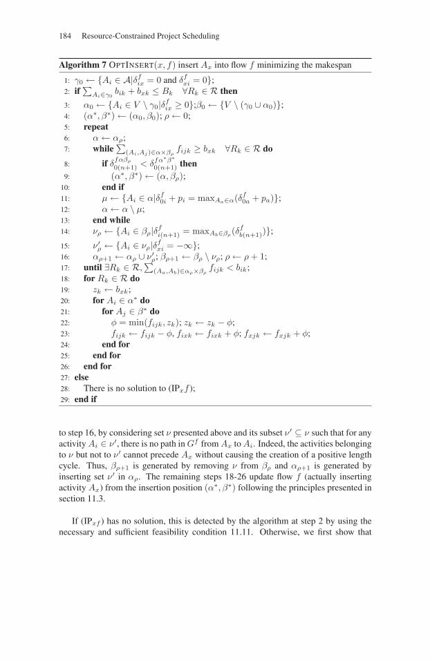
184 Resource-Constrained Project Scheduling
Algorithm 7 OPTINSERT(x, f) insert Ax into flow f minimizing the makespan
1: γ0 ← {Ai ∈ A|δfix = 0 and δf
xi = 0};2: if
∑Ai∈γ0
bik + bxk ≤ Bk ∀Rk ∈ R then
3: α0 ← {Ai ∈ V \ γ0|δfix ≥ 0};β0 ← {V \ (γ0 ∪ α0)};
4: (α∗, β∗)← (α0, β0); ρ← 0;5: repeat6: α← αρ;7: while
∑(Ai,Aj)∈α×βρ
fijk ≥ bxk ∀Rk ∈ R do
8: if δfαβρ
0(n+1) < δfα∗β∗
0(n+1) then9: (α∗, β∗)← (α, βρ);
10: end if11: μ← {Ai ∈ α|δf
0i + pi = maxAa∈α(δf0a + pa)};
12: α← α \ μ;13: end while14: νρ ← {Ai ∈ βρ|δf
i(n+1) = maxAb∈βρ(δf
b(n+1))};15: ν′
ρ ← {Ai ∈ νρ|δfxi = −∞};
16: αρ+1 ← αρ ∪ ν′ρ; βρ+1 ← βρ \ νρ; ρ← ρ + 1;
17: until ∃Rk ∈ R,∑
(Aa,Ab)∈αρ×βρfijk < bik;
18: for Rk ∈ R do19: zk ← bxk;20: for Ai ∈ α∗ do21: for Aj ∈ β∗ do22: φ = min(fijk, zk); zk ← zk − φ;23: fijk ← fijk − φ, fixk ← fixk + φ; fxjk ← fxjk + φ;24: end for25: end for26: end for27: else28: There is no solution to (IPxf );29: end if
to step 16, by considering set ν presented above and its subset ν′ ⊆ ν such that for anyactivity Ai ∈ ν′, there is no path in Gf from Ax to Ai. Indeed, the activities belongingto ν but not to ν′ cannot precede Ax without causing the creation of a positive lengthcycle. Thus, βρ+1 is generated by removing ν from βρ and αρ+1 is generated byinserting set ν′ in αρ. The remaining steps 18-26 update flow f (actually insertingactivity Ax) from the insertion position (α∗, β∗) following the principles presented insection 11.3.
If (IPxf ) has no solution, this is detected by the algorithm at step 2 by using thenecessary and sufficient feasibility condition 11.11. Otherwise, we first show that
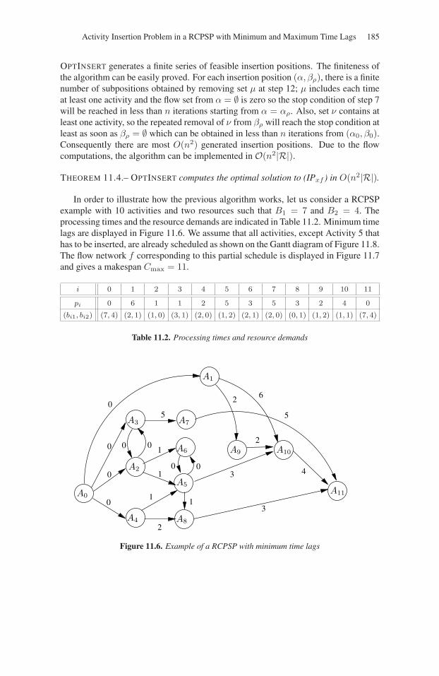
Activity Insertion Problem in a RCPSP with Minimum and Maximum Time Lags 185
OPTINSERT generates a finite series of feasible insertion positions. The finiteness ofthe algorithm can be easily proved. For each insertion position (α, βρ), there is a finitenumber of subpositions obtained by removing set μ at step 12; μ includes each timeat least one activity and the flow set from α = ∅ is zero so the stop condition of step 7will be reached in less than n iterations starting from α = αρ. Also, set ν contains atleast one activity, so the repeated removal of ν from βρ will reach the stop condition atleast as soon as βρ = ∅ which can be obtained in less than n iterations from (α0, β0).Consequently there are most O(n2) generated insertion positions. Due to the flowcomputations, the algorithm can be implemented in O(n2|R|).
THEOREM 11.4.– OPTINSERT computes the optimal solution to (IPxf ) in O(n2|R|).
In order to illustrate how the previous algorithm works, let us consider a RCPSPexample with 10 activities and two resources such that B1 = 7 and B2 = 4. Theprocessing times and the resource demands are indicated in Table 11.2. Minimum timelags are displayed in Figure 11.6. We assume that all activities, except Activity 5 thathas to be inserted, are already scheduled as shown on the Gantt diagram of Figure 11.8.The flow network f corresponding to this partial schedule is displayed in Figure 11.7and gives a makespan Cmax = 11.
i 0 1 2 3 4 5 6 7 8 9 10 11
pi 0 6 1 1 2 5 3 5 3 2 4 0
(bi1, bi2) (7, 4) (2, 1) (1, 0) (3, 1) (2, 0) (1, 2) (2, 1) (2, 0) (0, 1) (1, 2) (1, 1) (7, 4)
Table 11.2. Processing times and resource demands
0 0
00
11
0
0
0
5 5
1
1 3 4
3
2
02 6
2
A0
A10
A11
A2
A9
A3 A7
A1
A6
A5
A4 A8
Figure 11.6. Example of a RCPSP with minimum time lags
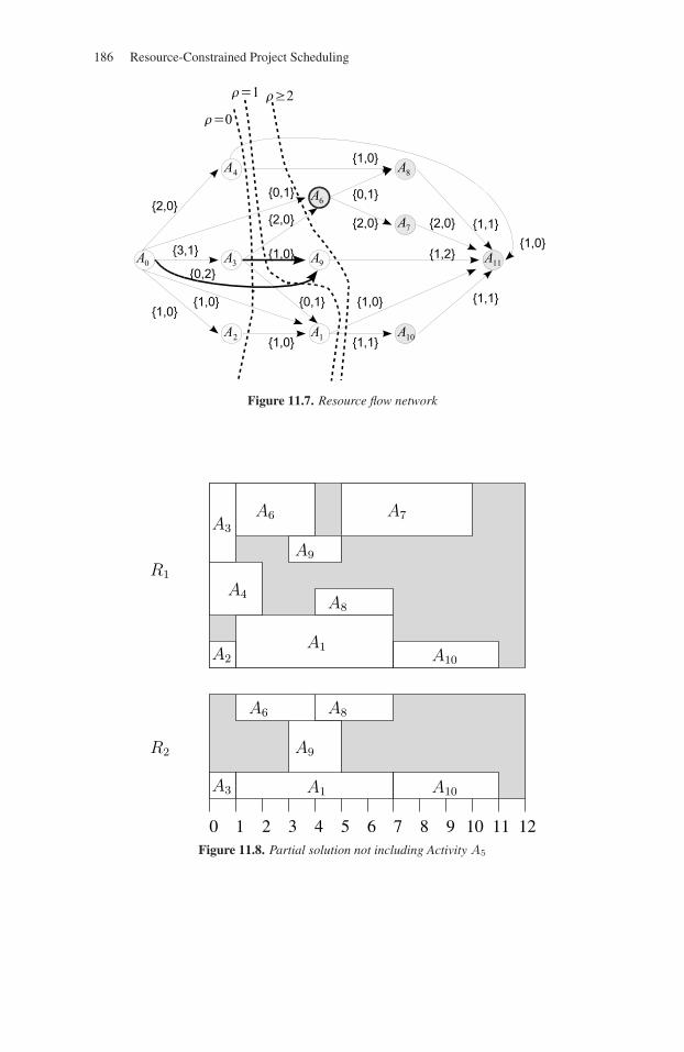
186 Resource-Constrained Project Scheduling
Figure 11.7. Resource flow network
R1
R2
21 3 4 5 6 7 8 9 10 11 120
A3
A2
A4
A10
A10A1A3
A1
A6
A6
A9
A9
A7
A8
A8
Figure 11.8. Partial solution not including Activity A5
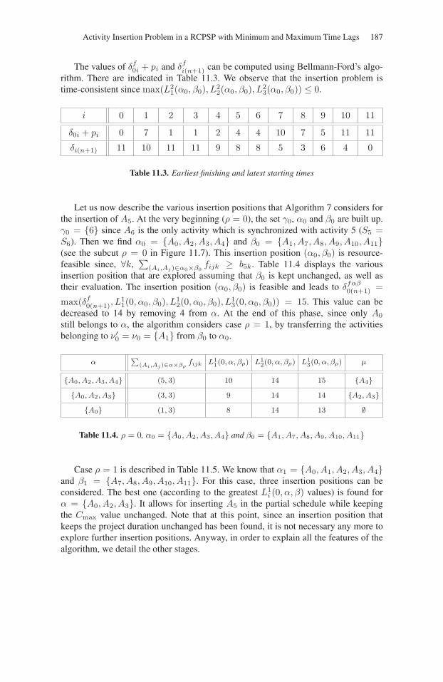
Activity Insertion Problem in a RCPSP with Minimum and Maximum Time Lags 187
The values of δf0i + pi and δf
i(n+1) can be computed using Bellmann-Ford’s algo-rithm. There are indicated in Table 11.3. We observe that the insertion problem istime-consistent since max(L2
1(α0, β0), L22(α0, β0), L2
3(α0, β0)) ≤ 0.
i 0 1 2 3 4 5 6 7 8 9 10 11
δ0i + pi 0 7 1 1 2 4 4 10 7 5 11 11
δi(n+1) 11 10 11 11 9 8 8 5 3 6 4 0
Table 11.3. Earliest finishing and latest starting times
Let us now describe the various insertion positions that Algorithm 7 considers forthe insertion of A5. At the very beginning (ρ = 0), the set γ0, α0 and β0 are built up.γ0 = {6} since A6 is the only activity which is synchronized with activity 5 (S5 =S6). Then we find α0 = {A0, A2, A3, A4} and β0 = {A1, A7, A8, A9, A10, A11}(see the subcut ρ = 0 in Figure 11.7). This insertion position (α0, β0) is resource-feasible since, ∀k,
∑(Ai,Aj)∈α0×β0
fijk ≥ b5k. Table 11.4 displays the variousinsertion position that are explored assuming that β0 is kept unchanged, as well astheir evaluation. The insertion position (α0, β0) is feasible and leads to δfαβ
0(n+1) =
max(δf0(n+1), L
11(0, α0, β0), L1
2(0, α0, β0), L13(0, α0, β0)) = 15. This value can be
decreased to 14 by removing 4 from α. At the end of this phase, since only A0
still belongs to α, the algorithm considers case ρ = 1, by transferring the activitiesbelonging to ν′
0 = ν0 = {A1} from β0 to α0.
α∑
(Ai,Aj)∈α×βρfijk L1
1(0, α, βρ) L12(0, α, βρ) L1
3(0, α, βρ) μ
{A0, A2, A3, A4} (5, 3) 10 14 15 {A4}{A0, A2, A3} (3, 3) 9 14 14 {A2, A3}
{A0} (1, 3) 8 14 13 ∅
Table 11.4. ρ = 0, α0 = {A0, A2, A3, A4} and β0 = {A1, A7, A8, A9, A10, A11}
Case ρ = 1 is described in Table 11.5. We know that α1 = {A0, A1, A2, A3, A4}and β1 = {A7, A8, A9, A10, A11}. For this case, three insertion positions can beconsidered. The best one (according to the greatest L1
i (0, α, β) values) is found forα = {A0, A2, A3}. It allows for inserting A5 in the partial schedule while keepingthe Cmax value unchanged. Note that at this point, since an insertion position thatkeeps the project duration unchanged has been found, it is not necessary any more toexplore further insertion positions. Anyway, in order to explain all the features of thealgorithm, we detail the other stages.
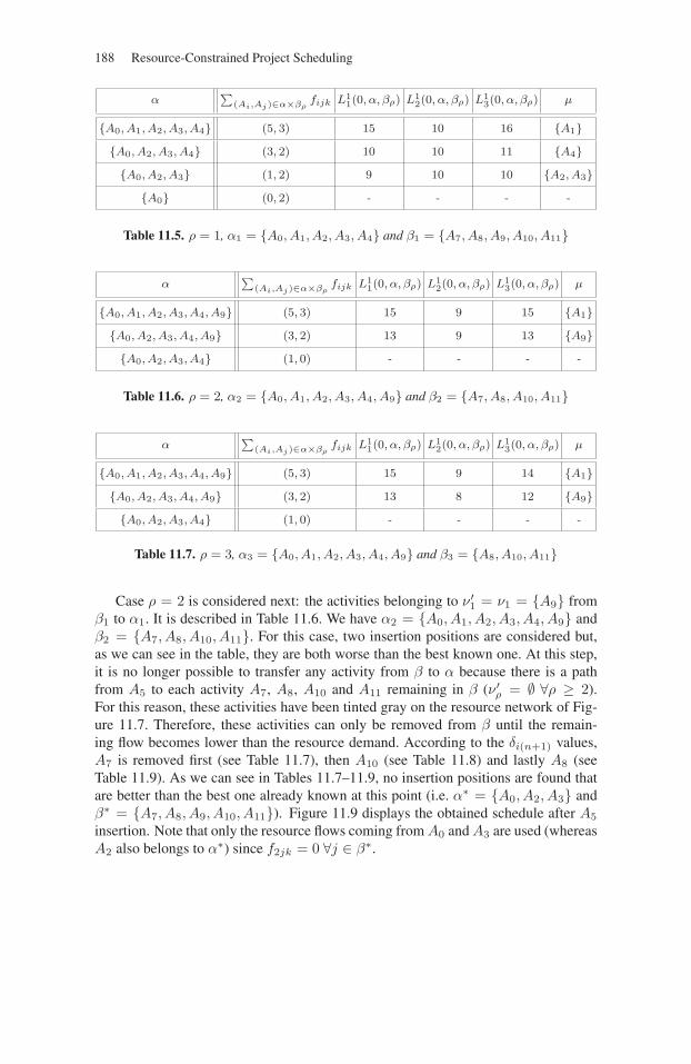
188 Resource-Constrained Project Scheduling
α∑
(Ai,Aj)∈α×βρfijk L1
1(0, α, βρ) L12(0, α, βρ) L1
3(0, α, βρ) μ
{A0, A1, A2, A3, A4} (5, 3) 15 10 16 {A1}{A0, A2, A3, A4} (3, 2) 10 10 11 {A4}{A0, A2, A3} (1, 2) 9 10 10 {A2, A3}
{A0} (0, 2) - - - -
Table 11.5. ρ = 1, α1 = {A0, A1, A2, A3, A4} and β1 = {A7, A8, A9, A10, A11}
α∑
(Ai,Aj)∈α×βρfijk L1
1(0, α, βρ) L12(0, α, βρ) L1
3(0, α, βρ) μ
{A0, A1, A2, A3, A4, A9} (5, 3) 15 9 15 {A1}{A0, A2, A3, A4, A9} (3, 2) 13 9 13 {A9}{A0, A2, A3, A4} (1, 0) - - - -
Table 11.6. ρ = 2, α2 = {A0, A1, A2, A3, A4, A9} and β2 = {A7, A8, A10, A11}
α∑
(Ai,Aj)∈α×βρfijk L1
1(0, α, βρ) L12(0, α, βρ) L1
3(0, α, βρ) μ
{A0, A1, A2, A3, A4, A9} (5, 3) 15 9 14 {A1}{A0, A2, A3, A4, A9} (3, 2) 13 8 12 {A9}{A0, A2, A3, A4} (1, 0) - - - -
Table 11.7. ρ = 3, α3 = {A0, A1, A2, A3, A4, A9} and β3 = {A8, A10, A11}
Case ρ = 2 is considered next: the activities belonging to ν′1 = ν1 = {A9} from
β1 to α1. It is described in Table 11.6. We have α2 = {A0, A1, A2, A3, A4, A9} andβ2 = {A7, A8, A10, A11}. For this case, two insertion positions are considered but,as we can see in the table, they are both worse than the best known one. At this step,it is no longer possible to transfer any activity from β to α because there is a pathfrom A5 to each activity A7, A8, A10 and A11 remaining in β (ν′
ρ = ∅ ∀ρ ≥ 2).For this reason, these activities have been tinted gray on the resource network of Fig-ure 11.7. Therefore, these activities can only be removed from β until the remain-ing flow becomes lower than the resource demand. According to the δi(n+1) values,A7 is removed first (see Table 11.7), then A10 (see Table 11.8) and lastly A8 (seeTable 11.9). As we can see in Tables 11.7–11.9, no insertion positions are found thatare better than the best one already known at this point (i.e. α∗ = {A0, A2, A3} andβ∗ = {A7, A8, A9, A10, A11}). Figure 11.9 displays the obtained schedule after A5
insertion. Note that only the resource flows coming from A0 and A3 are used (whereasA2 also belongs to α∗) since f2jk = 0 ∀j ∈ β∗.
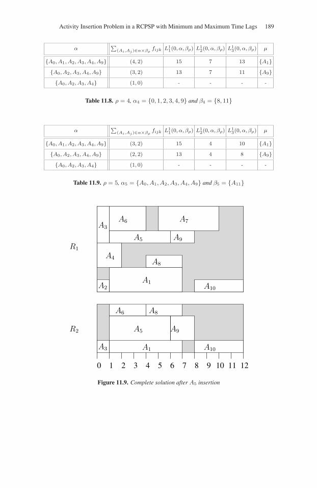
Activity Insertion Problem in a RCPSP with Minimum and Maximum Time Lags 189
α∑
(Ai,Aj)∈α×βρfijk L1
1(0, α, βρ) L12(0, α, βρ) L1
3(0, α, βρ) μ
{A0, A1, A2, A3, A4, A9} (4, 2) 15 7 13 {A1}{A0, A2, A3, A4, A9} (3, 2) 13 7 11 {A9}{A0, A2, A3, A4} (1, 0) - - - -
Table 11.8. ρ = 4, α4 = {0, 1, 2, 3, 4, 9} and β4 = {8, 11}
α∑
(Ai,Aj)∈α×βρfijk L1
1(0, α, βρ) L12(0, α, βρ) L1
3(0, α, βρ) μ
{A0, A1, A2, A3, A4, A9} (3, 2) 15 4 10 {A1}{A0, A2, A3, A4, A9} (2, 2) 13 4 8 {A9}{A0, A2, A3, A4} (1, 0) - - - -
Table 11.9. ρ = 5, α5 = {A0, A1, A2, A3, A4, A9} and β5 = {A11}
R1
R2
21 3 4 5 6 7 8 9 10 11 120
A3
A2
A4
A1A3
A1
A6
A6
A7
A8
A8
A5 A9
A10
A10
A9A5
Figure 11.9. Complete solution after A5 insertion
190 Resource-Constrained Project Scheduling
11.7. Conclusion
In this chapter, we considered the problem of inserting a single activity Ax insidean existing partial schedule while preserving its structure. The existence of minimumand maximum time lags between an activity pair is tackled. The objective is to mini-mize the project duration increase. This problem consists of selecting the best pair ofordered set (α∗, β∗) inside the resource flow network associated with the existing par-tial schedule, so that both the flow coming from α satisfies the resource demand of Ax
and the insertion does not cause a temporal inconsistency. We have shown how, givena pair (α, β), that the latter constraint can easily be checked by considering three cate-gories of elementary cycles. Moreover, we also show that the project duration increasecan also be computed by considering the length of these same elementary cycles.
Whereas the insertion problem is polynomially solvable for the standard RCPSP(where only precedence constraints are taken into account), we showed that the intro-duction of minimum and maximum time lags makes the problem NP-hard. Neverthe-less, when only minimum time lags are considered, the problem turns back polynomi-ally solvable and we exhibit an algorithm to solve it.
Once again, we observe that dealing with maximum time lag constraints is dif-ficult. It was already known that finding a resource-feasible schedule that respectsboth the minimum and maximum time lags is NP-hard. We saw here that, thoughapparently easier, even the problem of inserting a single activity in an already-existingresource-feasible and time-consistent schedule is NP-hard. Therefore, it might appearrelevant in some situations to relax maximum time lags, intending to find a schedulewhich minimizes the maximum time lag violation (a maximum makespan value beingpreliminary set). Indeed, in many schedule environments, maximum time lags corre-spond to user preferences and hence it makes sense to produce a schedule that does notrespect them. In this case, we can also define priorities in order to define a hierarchyamong maximum time lags. In this case, a possible objective function would be theminimization of the weighted sum of the time lag violations.
Chapter 12
Reactive Approaches
Project scheduling research often focuses its attention on providing efficient solu-tions assuming a static and deterministic environment. However, many disruptionsmay occur during the execution of a schedule. Several approaches exist for handlingthose disruptions: we will focus here on what is usually called predictive-reactiveapproaches.
12.1. Dynamic project scheduling
This chapter deals with a project scheduling problem in which disruptions mayoccur during execution: new incoming orders, order cancelations, missing raw mate-rials, power shortages, machine break-downs, etc. This problem is very general as itincludes many scheduling problems, and many types of unexpected events are consid-ered (addition, removal or modification of temporal constraints, resources and activ-ities). We propose a predictive-reactive approach for a situation where no stochasticmodel of the possible disruptions can be provided. As far as we know, the only workhandling this case is a flow-based heuristic proposed by Artigues et al. [ART 03] forthe addition of unexpected activities in a RCPSP. Chapter 13 addresses an alternativeand complementary proactive-reactive approach, aiming at anticipating disruptionsthrough the generation of a robust baseline schedule.
The idea of predictive-reactive approaches is to build a first operational solutionthat will be re-optimized when an unexpected event is to be handled. Two questionsmust be addressed:
Chapter written by Christelle GUÉRET and Narendra JUSSIEN.
191
192 Resource-Constrained Project Scheduling
– When is a new schedule needed? A new schedule can be computed each timean unexpected event occurs (e.g. [WU 93] and [BIE 99]); or, at predetermined timeintervals [CHU 92]; or, finally, when a given threshold in perturbation is reached[VIE 00]. Generally, rescheduling provides better performance because the overallsystem reacts quickly to unexpected events. However, a significant amount of com-puting time can be required and, moreover, highly varying consecutive solutions maybe computed.
– How is a new schedule to be computed? Computing a new schedule consists ofeither computing a new optimal solution or repairing the current unfeasible schedule.Generally, operational techniques repair the current solution in order to maximize thestability of successive solutions [AKT 99, BEA 91, BIE 99, WU 93]. Computing anew optimal solution is seldom applied. Indeed, the re-optimization problem is an NP-complete problem [PIC 95]. The worst case consists of computing from scratch a newschedule each time an unexpected event occurs. Moreover, generally the successiveobtained schedules are quite different one from another and computing time remainsquite prohibitive.
In this chapter, a new technique1 for computing successive optimal stable solutionseach time an unexpected event occurs is introduced. This technique uses a recentextension of constraint programming: explanation-based constraint programming.
12.2. Explanations and constraint programming for solving dynamic problems
Constraint programming [TSA 93] is the study of computational systems basedon constraints (see also Chapter 4). The idea of constraint programming is to solveproblems by stating constraints (conditions, properties) which must be satisfied by thesolution. Work in this area can be tracked back to research in Artificial Intelligenceand Computer Graphics in the 1960s and 1970s. Only in the last decade, however,has emerged a growing realization that these ideas provide the basis for a powerfulapproach to programming, modeling and problem solving and that different efforts toexploit these ideas can be unified under a common conceptual and practical frame-work: constraint programming.
12.2.1. Dynamic problems and constraint programming
The notion of dynamic constraint satisfaction has been first introduced in[DEC 88]. A dynamic constraint satisfaction problem (DCSP) is a sequence of con-straint satisfaction problems, each one resulting from some change in the definition ofthe previous one. These changes may affect any component in the problem definition:variables (addition or removal), domains (value addition or removal), constraints(addition or removal), constraint scopes (variable addition or removal) or constraint
1. This approach has been developed in the PhD dissertation of Abdallah Elkhyari.
Reactive Approaches 193
definitions (changes in the intensional definition, tuple addition or removal in caseof extensional definition). All these changes can basically be expressed in terms ofconstraint additions and removals because domains can be seen as unary constraints,because variables are implicitly added or removed with all the constraints that applyto them, and because any change in a component can be seen as a removal followedby an addition.
Constraint-based techniques for solving dynamic problems can be classified intotwo categories [VER 05]: proactive methods (which suppose an existing model ofthe possible modifications) and reactive methods. The latter were addressed with twomain approaches:
– solutions (complete solutions, partial instantiations, etc.) reuse techniques as in[VER 94] which are based on the assumption that the previous solution is a good basisfor finding a solution to the next problem;
– reasoning reuse techniques (as in [SCH 94], or in explanation-based constraintprogramming [JUS 03]) which prefer to keep track of the portions of the search spacethat have been set aside in previous resolutions and that can be still set aside in the newproblem, the idea behind being to learn from the past in order to avoid future failures.
Several constraint-based reactive scheduling systems arose at the end of the 1980sand in the 1990s [Le 94a]. Collinot and Le Pape [COL 91] introduced the SONIA sys-tem in order to compute acceptable solutions to “evolutive” scheduling problems, i.e.,problems whose data may be subject to variation. Their approach relies on an intel-ligent backtracking technique. Burke and Prosser also proposed a Truth MaintenanceSystem (TMS) based approach in the DAS system [BUR 91]. Finally, Smith [SMI 94]introduced the OPIS system based on two notions: conflicts and opportunity for pro-viding repairs and potential improvements of schedules upon handling an unexpectedevent. Those three systems build a compact description of the contradictions encoun-tered during search and use this information to perform a sophisticated (and thereforenot necessarily chronological) backtrack. Unfortunately these approaches are proneto the hazards of search compared to a from-scratch rescheduling as shown by Baker[BAK 94].
12.2.2. Explanation-based constraint programming
In constraint programming , the constraint solver’s main activity resides in comput-ing redundant information for the constraint network characterizing the solved prob-lem. This redundant information is, most of the time, far from direct and will allow toquickly prune the different possibilities for the variables of the problem. Such infor-mation can be of different kinds: domain reduction (value removal, bound adjust-ments, etc.), failure identification and new implicit constraint addition. Providing anexplanation in this context consists of justifying each new information computed bythe solver in order to be able to quickly evaluate the validity of this information in
194 Resource-Constrained Project Scheduling
another context. Such a justification is provided as a (precise) set of constraints whoseconjunction logically leads to the information being justified. Explanations can beseen as an explicit trace of the solver’s behavior as the whole set of interactionsbetween constraints that led the solver to provide the new information do appear inthe explanation.
Explanations have now clearly shown their interest for constraint programming[JUS 03]: constraint solvers are no longer black boxes only able to answer yes or nowhen solving a problem, they now initiate a real interaction with the final user, beingable, for example, to explain why a constraint network is unfeasible. Moreover, expla-nations are quite useful in a dynamic context as they can efficiently and incrementallyremove a constraint because they provide a direct access to its past effects [DEB 03].Finally, and this particularity will also be used for project scheduling, explanations canbe used to design new powerful search techniques that will replace classical backtrack-ing with a true repair of the decision path without an excessive loss of past information[GUÉ 00, JUS 02]. This substantial modification in classical search schema allows afruitful consideration of the information gathered through search: re-exploration ofsignificative portions of the search space is avoided and search, while remaining com-plete, is failure-driven and can overcome the somewhat arbitrary exploration inducedby backtracking techniques.
Using an explanation-based constraint solver induces two prerequisites:
– any used constraint needs to be able to explain any of the information it provides;
– the solving technique needs a branching scheme that involves basic (i.e. avail-able as is in the solver’s library of constraints) constraints whose negation is alsoa basic constraint. Indeed, in explanation-based constraint programming, decisions(traditionally a variable-value assignment) and their negations (traditionally a valueremoval) are explicitly handled as opposed to traditional backtracking-based approachwhere all negations are implicit (thanks to backtracking).
In the following, we will actively use the capability of such a system to take intoaccount a modification of the problem definition and to explain past decisions in orderto compute a new optimal solution when an unexpected event occurs.
12.3. An explanation-based approach for solving dynamic project scheduling
Our system is based upon:
– a tree-based search embedded within a constraint solver: in each node, deductionrules are applied in order to propagate the constraints of the problem2;
2. In the following, the word constraint will refer not only to initial constraints of the problems(precedence and resource constraints), but also to each decision made in the branching schemeand to each deduction made by propagation rules during a search.
Reactive Approaches 195
– the active use of explanations. These are provided by the constraints used forsolving the RCPSP and will be used to dynamically handle unexpected events. Indeed,as already mentioned, handling an unexpected event leads to removing, adding, ormodifying a constraint. Upon removing a constraint, a re-optimization is launchedfrom the previous feasible solution of the problem. For the other two cases, if thecurrent solution is not valid anymore, explanations can be of some help to determineconstraints responsible for the contradiction. The re-optimization is performed takinginto account the fact that at least one of these constraints needs to be removed (adding,for that, its negation).
We first present the explanation-based tree-search algorithm for solving staticRCPSP and then explain how to extend it to solve dynamic instances.
12.3.1. The tree search to solve static instances
The tree search we use is largely inspired from the one from Brucker et al.[BRU 98] and previously described in section 5.2.1 (see also section 6.1.3).
Each node in the search tree is defined by three disjoint sets: a set C of pairs ofactivities that are in conjunction, a set P of pairs of activities that are overlapping, aset F of pairs of activities that are said to be flexible:
– C = {(i, j) | (i→ j) ∨ (j → i)};– φ = {(i, j) | (i ‖ j)};– U = {(i, j) | (i, j) �∈ C ∧ (i, j) �∈ P}.
Branching consists of transferring a pair of activities from F to C (thus imposingi → j or j → i) or to φ (imposing i ‖ j). This branching is performed until Ubecomes empty. In each node, propagation rules add new implicit constraints andtherefore complete sets C and φ while removing pairs from U . Backtracks and repairsmade on the set of decisions taken so far may transfer back some pairs of activitiesfrom C or φ to U .
As already mentioned, our technique relies on the fact that decisions taken duringa search do possess an easily stated negation. However, for example, negating i → jleads to the disjunction j → i ∨ i ‖ j, and disjunctions adding non-determinism ina problem are generally poorly handled in constraint programming. This is why weintroduce the notion of distance.
DEFINITION 12.1.– Let Ai and Aj be two distinct activities. The distance dij betweenAi and Aj is the time lag between the end of activity Ai and the beginning of Aj .Therefore, we have: dij = Sj − Si − pi.
Stating sequencing constraints using this notion of distance is easy and leads to therelations reported in Table 12.1.
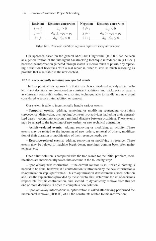
196 Resource-Constrained Project Scheduling
Decision Distance constraint Negation Distance constrainti→ j dij ≥ 0 i �→ j dij < 0j → i dij ≤ −pi − pj j �→ i dij > −pi − pj
i ‖ j dij · dji > 0 i↔ j dij · dji ≤ 0
Table 12.1. Decisions and their negation expressed using the distance
Our approach based on the general MAC-DBT algorithm [JUS 00] can be seenas a generalization of the intelligent backtracking technique introduced in [COL 91]because the information gathered through search is used as much as possible by replac-ing a traditional backtrack with a real repair in order to save as much reasoning aspossible that is reusable in the new context.
12.3.2. Incrementally handling unexpected events
The key point of our approach is that a search is considered as a dynamic prob-lem (new decisions are considered as constraint additions and backtracks or repairsas constraint removals) leading to a solving technique able to handle any new eventconsidered as a constraint addition or removal.
Our system is able to incrementally handle various events:
– Temporal events: adding, removing or modifying sequencing constraints(precedence, disjunction, overlapping between two activities including their general-ized cases – taking into account a minimal distance between activities). These eventsmay be related to the incoming of new orders, or new technical constraints.
– Activity-related events: adding, removing or modifying an activity. Theseevents may be related to the incoming of new orders, removal of others, modifica-tion of their duration or modification of their resource needs, etc.
– Resource-related events: adding, removing or modifying a resource. Theseevents may be related to machine break-down, machines coming back after main-tenance, etc.
Once a first solution is computed with the tree search for the initial problem, mod-ifications are incrementally taken into account in the following way:
– upon adding new information: if the current solution is still feasible, nothing isneeded to be done; however, if a contradiction is introduced by the new information are-optimization step is performed. This re-optimization starts from the current solutionand uses the explanations provided by the solver to, first, determine the set of decisionsresponsible for this contradiction, and, second, to dynamically remove from this setone or more decisions in order to compute a new solution;
– upon removing information: re-optimization is asked after having performed theincremental removal [DEB 03] of all the constraints related to this information;
Reactive Approaches 197
– upon modifying information: a removal (of the old information) followed by anaddition (of the new information) is performed.
Notice that adding or modifying a constraint may lead to an over-constrainedinstance (for which no solution exists). Thanks to explanations, our system is ableto provide a contradiction explanation that can be used by the user to select a con-straint to be removed or modified, or to allow a degradation of the makespan in orderto compute a new solution. Several tools can be designed to help the user to make hischoice in this context [JUS 01].
12.4. Experimental results
As no other technique exists for optimally solving RCPSP instances in a dynamiccontext, we compared our technique to a rescheduling from scratch after each event.As no real benchmark has been defined for this problem, we created benchmarks basedupon existing instances for the static case. We present here3 results both in terms ofexecution time and stability of successive solutions for adding and removing a set ofactivities.
12.4.1. Stability measures
Performance of dynamic scheduling systems can be measured both using comput-ing time and quality of the obtained solutions. The quality of successive solutions canbe measured comparing the new solution to the previous one or to the initial one. Weevaluated the performance of our approach by studying the evolution of this qualityover time.
Several stability measures were used: number of modified starting times, sum ofthe modifications, maximal modification, etc. and finally, the number of relative posi-tions between activities that have been modified. This is the measure reported in thefollowing as it seems the most relevant measure for scheduling problems. POSI(Sp,Sq) represents the number of relative positions that have changed when switchingfrom schedule Sp to schedule Sq. POSI(Sp, Sq) =
∑(i,j)∈A×A, i<j γi
j(Sp, Sq) where
γij(Sp, Sq) = 1 if the relative position of Ai and Aj has changed and 0 otherwise.
12.4.2. Test set
We use a data set generated thanks to ProGen from Kolisch et al. [KOL 95b]. Weuse the SMCP (Single-Mode Project Scheduling) series. In the following, P0 denotesthe original problem of the series and Pi the problem obtained after the ith perturba-tion.
3. Those results mainly come from the PhD dissertation of Abdallah Elkhyari [ELK 03a].
198 Resource-Constrained Project Scheduling
Problems used for studying the consequences of the addition of a series of activitiesare built in the following way:
– the initial problem P0 is a SMCP problem from which activities are removed,as well as the associated precedence constraints. In order to be sure that P0 is still aRCPSP, precedence constraints between the predecessors of the activity removed anddummy activity A0, and between its successors and dummy activity An+1 are added;
– problem Pi is obtained from problem Pi−1 by randomly adding one activityamong the ones that have been initially removed. Precedence constraints that hadbeen removed with this activity and that link it with other activities of problem Pi−1
are also added.
In order to study the consequences of the removal of a series of activities, eachseries of problems is constructed as follows:
– the initial problem P0 is a SMCP problem;
– problem Pi is obtained from problem Pi−1 by randomly removing one activityand its precedence constraints, and by adding the precedence constraints that connectits successors and predecessors to the dummy activities.
A large number of problems have been generated for each type of event. Thus,for the addition and the removal of a series of activities, 10 series of 10 problemseach have been constructed for each following size: 12 activities and 4 resources, 22activities and 4 resources, 32 activities and 1 resource, 32 activities and 2 resources,32 activities and 3 resources, and 32 activities and 4 resources. For coherence matters,the number of additions/removals of activities depends on the size of the problem: 2for problems with 12 activities, 3 for problems with 22 activities and 4 for the others.
12.4.3. Computational results
We only present here the results obtained for the addition and removal of activi-ties. The results are quite similar for the addition and the removal of precedence orgeneralized temporal constraints.
In the following, ppce represents our approach, and ropt corresponds to arescheduling from scratch.
Let Tppce(Pk) (respectively Tropt(Pk)) be the time needed (in seconds) to com-pute a solution for problem Pk with our system (respectively by a rescheduling fromscratch). The gain in time is defined by:
Gtime(Pi) = 1−∑
0≤k≤i Tppce(Pk)∑0≤k≤i Tropt(Pk)
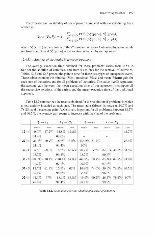
Reactive Approaches 199
The average gain in stability of our approach compared with a rescheduling fromscratch is:
GPOSI(Pi, Pj) = 1−∑
1≤k≤s POSI(Ski (ppce), Sk
j (ppce))∑1≤k≤s POSI(Sk
i (ropt), Skj (ropt))
where Ski (ropt) is the solution of the ith problem of series k obtained by a reschedul-
ing from scratch, and Ski (ppce) is the solution obtained by our approach.
12.4.3.1. Analysis of the results in terms of cpu time
The average execution time obtained for these problems varies from 2.5 s to61 s for the addition of activities, and from 5 s to 66 s for the removal of activities.Tables 12.2 and 12.3 present the gain in time for these two types of unexpected event.These tables contain: the minimal (Min), maximal (Max) and mean (Mean) gain foreach step of the series, and for all problems of the series. The value (AvG) representsthe average gain between the mean execution time of our approach to compute allthe successive solutions of the series, and the mean execution time of the traditionalapproach.
Table 12.2 summarizes the results obtained for the resolution of problems in whicha new activity is added at each step. The mean gain (Mean) is between 10.7% and78.2%, and the average gain (AvG) is very important for all problems: between 43.7%and 90.5%, the average gain seems to increase with the size of the problems.
P0 → P1 P1 → P2 P2 → P3 P3 → P4
Min/Max Mean Min/Max Mean Min/Max Mean Min/Max Mean AvG
12×4 -0.9% 37.7% -63.8% 32.2% – – – – 43.7%64.4% 69.6% – –
22×4 -34.6% 29.7% -208% 5.8% -155.2% 34.4% – – 78.9%94.4% 94.4% 96% –
32×1 30% 58.3% 18.2% 68.5% 40.7% 77% -66.1% 46.7% 83.8%98.7% 99.3% 98.7% 99.6%
32×2 -280.9% 10.7% -140.1% 57.8% -64.2% 68.7% -78.9% 62.8% 84.9%91.2% 97.1% 96.9% 97.6%
32×3 12.7% 61.4% 15.9% 66% 16.8% 74.6% 30.6% 78.2% 90.5%95.2% 98.2% 98.8% 96.3%
32×4 33.3% 57% -18.1% 63.5% -19.6% 60.7% 26.7% 78.2% 90%75.9% 97.4% 98.7% 99.2%
Table 12.2. Gain in time for the addition of a series of activities
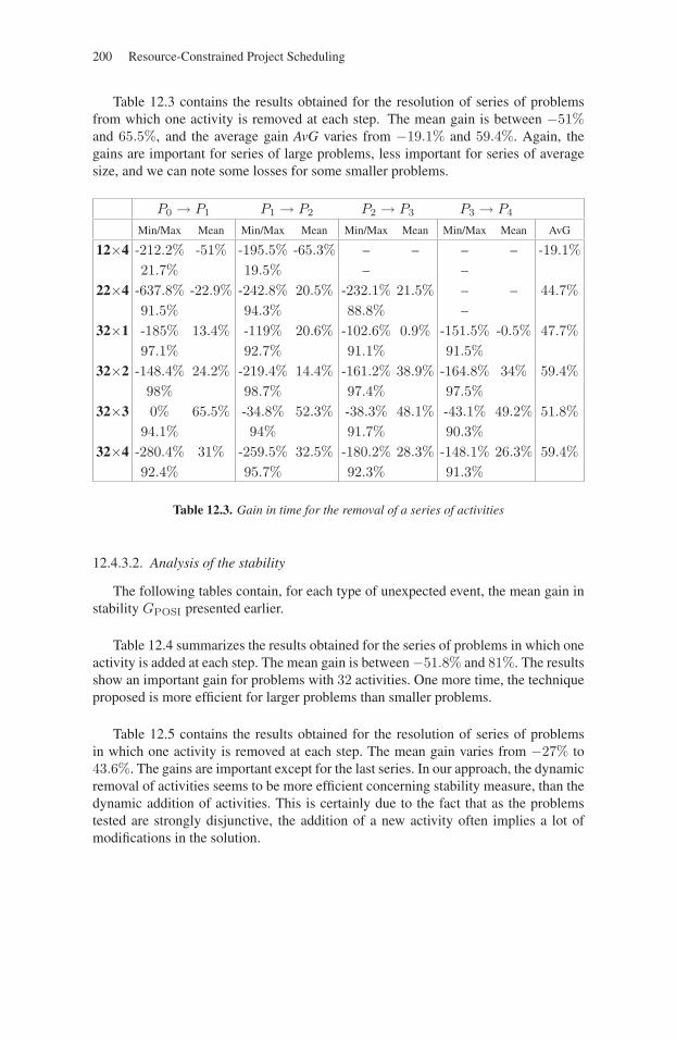
200 Resource-Constrained Project Scheduling
Table 12.3 contains the results obtained for the resolution of series of problemsfrom which one activity is removed at each step. The mean gain is between −51%and 65.5%, and the average gain AvG varies from −19.1% and 59.4%. Again, thegains are important for series of large problems, less important for series of averagesize, and we can note some losses for some smaller problems.
P0 → P1 P1 → P2 P2 → P3 P3 → P4
Min/Max Mean Min/Max Mean Min/Max Mean Min/Max Mean AvG
12×4 -212.2% -51% -195.5% -65.3% – – – – -19.1%21.7% 19.5% – –
22×4 -637.8% -22.9% -242.8% 20.5% -232.1% 21.5% – – 44.7%91.5% 94.3% 88.8% –
32×1 -185% 13.4% -119% 20.6% -102.6% 0.9% -151.5% -0.5% 47.7%97.1% 92.7% 91.1% 91.5%
32×2 -148.4% 24.2% -219.4% 14.4% -161.2% 38.9% -164.8% 34% 59.4%98% 98.7% 97.4% 97.5%
32×3 0% 65.5% -34.8% 52.3% -38.3% 48.1% -43.1% 49.2% 51.8%94.1% 94% 91.7% 90.3%
32×4 -280.4% 31% -259.5% 32.5% -180.2% 28.3% -148.1% 26.3% 59.4%92.4% 95.7% 92.3% 91.3%
Table 12.3. Gain in time for the removal of a series of activities
12.4.3.2. Analysis of the stability
The following tables contain, for each type of unexpected event, the mean gain instability GPOSI presented earlier.
Table 12.4 summarizes the results obtained for the series of problems in which oneactivity is added at each step. The mean gain is between−51.8% and 81%. The resultsshow an important gain for problems with 32 activities. One more time, the techniqueproposed is more efficient for larger problems than smaller problems.
Table 12.5 contains the results obtained for the resolution of series of problemsin which one activity is removed at each step. The mean gain varies from −27% to43.6%. The gains are important except for the last series. In our approach, the dynamicremoval of activities seems to be more efficient concerning stability measure, than thedynamic addition of activities. This is certainly due to the fact that as the problemstested are strongly disjunctive, the addition of a new activity often implies a lot ofmodifications in the solution.
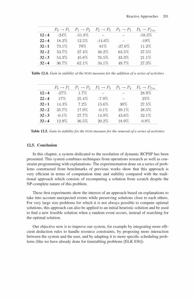
Reactive Approaches 201
P0 → P1 P1 → P2 P2 → P3 P3 → P4 P0 → Pfin
12×4 -24% -51.8% – – -58.3%22×4 18.2% 12.5% -14.6% – -19%32×1 73.1% 79% 81% -27.6% 11.2%32×2 53.7% 37.4% 38.2% 63.5% 37.5%32×3 54.3% 45.8% 76.5% 33.3% 21.1%32×4 36.7% 62.1% 34.1% 49.7% 27.3%
Table 12.4. Gain in stability of the POSI measure for the addition of a series of activities
P0 → P1 P1 → P2 P2 → P3 P3 → P4 P0 → Pfin
12×4 -27% 1.7% – – 28.9%22×4 17% 25.4% -7.9% – 25%32×1 14.3% 7.2% 15.6% 30% 27.5%32×2 35.7% 17.9% -0.1% 39.1% 38.5%32×3 -0.1% 27.7% 14.9% 43.6% 32.1%32×4 12.9% 36.5% 20.2% 18.9% 0.9%
Table 12.5. Gain in stability for the POSI measure for the removal of a series of activities
12.5. Conclusion
In this chapter, a system dedicated to the resolution of dynamic RCPSP has beenpresented. This system combines techniques from operations research as well as con-straint programming with explanations. The experimentation done on a series of prob-lems constructed from benchmarks of previous works show that this approach isvery efficient in terms of computation time and stability compared with the tradi-tional approach which consists of recomputing a solution from scratch despite theNP-complete nature of this problem.
These first experiments show the interest of an approach based on explanations totake into account unexpected events while preserving solutions close to each others.For very large size problems for which it is not always possible to compute optimalsolutions, this approach can also be applied to an initial heuristic solution and be usedto find a new feasible solution when a random event occurs, instead of searching forthe optimal solution.
Our objective now is to improve our system, for example by integrating more effi-cient deduction rules to handle resource constraints, by proposing more interactionbetween the system and the user, and by adapting it to more specific scheduling prob-lems (like we have already done for timetabling problems [ELK 03b]).

202
This page intentionally left blank
Chapter 13
Proactive-reactive Project Scheduling
13.1. Introduction
The vast majority of the project scheduling research efforts over the past severalyears have concentrated on the development of workable baseline schedules, assum-ing complete information and a static and deterministic environment. Such a baselineschedule (pre-schedule, predictive schedule) is traditionally constructed by solving theRCPSP. This problem (problem m, 1|cpm|Cmax in the notation of [HER 00]) involvesthe determination of activity starting times that satisfy both the zero-lag finish-startprecedence constraints and the renewable resource constraints under the objective ofminimizing the project duration (for reviews, see Part 1 of the present book along with[BRU 99, DEM 02b, HER 98a, KOL 99a, KOL 99b]).
During execution, however, a project may be subject to considerable uncertainty,which may lead to numerous schedule disruptions. Many types of disruptions havebeen identified in other works (see [YU 04, WAN 05, ZHU 05]). Activities can takelonger than primarily expected, resource requirements or availability may vary, readytimes and due dates may change, new activities may have to be inserted ([ART 00]),etc. In this chapter we focus on schedule disruptions that may be caused by uncer-tainty in the duration of the project activities and/or in the availability of the renewableresources.
Proactive/reactive project scheduling procedures try to cope with schedule disrup-tions that may occur during project execution through the combination of a proactive
Chapter written by Erik DEMEULEMEESTER, Willy HERROELEN and Roel LEUS.
203
204 Resource-Constrained Project Scheduling
scheduling procedure for generating a robust baseline schedule with a reactive proce-dure that is invoked when a schedule breakage occurs during project execution and theschedule needs to be repaired. By contrast, Chapter 12 addresses a predictive-reactiveapproach where all the effort is concentrated on the repair procedure, while the base-line schedule has not been constructed with a robustness objective.
Research in proactive/reactive project scheduling is growing steadily (for surveyssee [AYT 05, HER 04, HER 05, VIE 03]). The objective of this chapter is to dis-cuss promising proactive/reactive scheduling procedures that may be deployed at theoccurrence of disruptions that are caused by uncertain activity durations or uncertainresource availabilities.
The remainder of this chapter is organized as follows. In the next section weintroduce the solution robust project scheduling problem under activity durationuncertainty and discuss proactive and reactive scheduling policies. Section 13.3 thenpresents proactive and reactive procedures for dealing with disruptions that may becaused by resource breakdowns. Section 13.4 offers conclusions and suggestions forfurther research.
13.2. Solution robust scheduling under activity duration uncertainty
13.2.1. The proactive/reactive scheduling problem
The problem used as our vehicle of analysis can be described as follows. A projectnetwork G(V,E) is represented in activity-on-the-node representation with dummystart node A0 and dummy end node An+1. All non-dummy project activities havestochastic activity durations Pi and are subject to zero-lag finish-start precedence con-straints on the elements of E: we require Sj ≥ Si + Pi if (Ai, Aj) ∈ E, withSi the activity start times realized during project execution. Non-dummy activitiesrequire an integer per period amount bik of one or more renewable resource types Rk,k = 1, . . . , q, during their execution. All resource types Rk have a per-period capac-ity Bk. The activity weight wi denotes the marginal cost of a deviation between therealized start time Si of activity Ai and its planned start time si in the baseline sched-ule. These weights may include unforeseen storage costs, extra organizational costs,costs related to agreements with subcontractors or also just a cost that expresses thedissatisfaction of employees with schedule changes. We assume that w0 = 0, whilewn+1 denotes the cost of delaying the project completion beyond a predetermineddeterministic due date dn+1.
The proactive scheduling objective is to build a robust or stable precedence andresource feasible baseline schedule, the activity starting times of which are denotedby si. We assume in this chapter that stability is strived for by minimizing the stability
Proactive-reactive Project Scheduling 205
function∑
Ai∈V wiE (|Si − si|), the weighted sum of the expected absolute devia-tion between the realized activity start times Si and the planned activity start times si
(E is the expectation operator). Unfortunately, the evaluation of the objective func-tion
∑Ai∈V wiE (|Si − si|) is a cumbersome task: [HAG 88] has shown for projects
without resource constraints that even when every activity duration Pi can take onlytwo discrete values, then computing the expected project duration and computing theprobability that the project is finished by a given time instant, assuming an early-startschedule, isNP-complete. In our applications, we compute the stability cost throughsimulation. Finally, it should be mentioned that other stability objective functions andsurrogate stability measures have been proposed in other works ([Van 06a]).
13.2.2. Proactive scheduling
Several strategies can be followed for generating stable baseline schedules; in thischapter we assume that a two-phase procedure is used. In the first phase, an inputschedule is generated that is both precedence and resource feasible but is not inten-tionally protected against anticipated disruptions. Such a schedule can be generatedby solving the underlying RCPSP (problem m, 1|cpm|Cmax), using (deterministic)single-point estimates pi for each Pi.
Two strategies may then be used in the second phase to increase the stability of theinput schedule. One way is to aim at a robust resource allocation, i.e. to decide on aclever way in which the various resource units are transferred between the activities ofthe schedule. Another is to insert time buffers that should prevent as much as possiblethe propagation of distortions throughout the schedule.
Under the assumption that a single activity may deviate from its pre-schedule dura-tion (without knowing which) and a single disruption scenario per activity, [LEU 05]showed that the machine scheduling problem for stability is strongly NP-hard for asingle machine with unequal ready times or precedence constraints and for the case ofa free number of parallel machines; the single-machine problem without ready timesand precedence constraints is still ordinarily NP-hard.
13.2.2.1. Robust resource allocation
[LEU 03, LEU 04] study the problem of generating a robust resource allocationfor a given feasible baseline schedule. They explore the fact that the search for anoptimal resource allocation reduces to the search for a resource flow network (whichdescribes the routing of resources across the activities in the schedule; see section 1.6)that exhibits desirable robustness characteristics. A branch-and-bound algorithm isdeveloped that solves the robust resource allocation problem in exact and approximateformulations for the case of a single resource type and exponential activity durationdisruption lengths. For the general multi-resource type case, Deblaere et al. [DEB 06b]derive lower bounds on scheduling stability and propose three integer programming
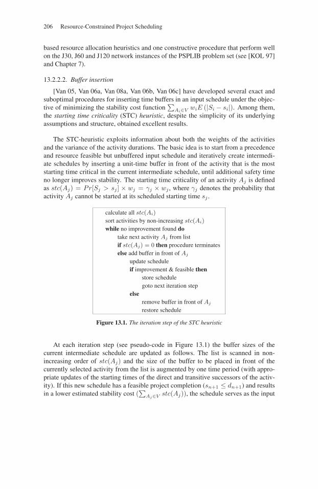
206 Resource-Constrained Project Scheduling
based resource allocation heuristics and one constructive procedure that perform wellon the J30, J60 and J120 network instances of the PSPLIB problem set (see [KOL 97]and Chapter 7).
13.2.2.2. Buffer insertion
[Van 05, Van 06a, Van 08a, Van 06b, Van 06c] have developed several exact andsuboptimal procedures for inserting time buffers in an input schedule under the objec-tive of minimizing the stability cost function
∑Ai∈V wiE (|Si − si|). Among them,
the starting time criticality (STC) heuristic, despite the simplicity of its underlyingassumptions and structure, obtained excellent results.
The STC-heuristic exploits information about both the weights of the activitiesand the variance of the activity durations. The basic idea is to start from a precedenceand resource feasible but unbuffered input schedule and iteratively create intermedi-ate schedules by inserting a unit-time buffer in front of the activity that is the moststarting time critical in the current intermediate schedule, until additional safety timeno longer improves stability. The starting time criticality of an activity Aj is definedas stc(Aj) = Pr[Sj > sj ] × wj = γj × wj , where γj denotes the probability thatactivity Aj cannot be started at its scheduled starting time sj .
calculate all stc(Ai)
sort activities by non-increasing stc(Ai)
while no improvement found dotake next activity Aj from listif stc(Aj) = 0 then procedure terminateselse add buffer in front of Aj
update scheduleif improvement & feasible then
store schedulegoto next iteration step
elseremove buffer in front of Aj
restore schedule
Figure 13.1. The iteration step of the STC heuristic
At each iteration step (see pseudo-code in Figure 13.1) the buffer sizes of thecurrent intermediate schedule are updated as follows. The list is scanned in non-increasing order of stc(Aj) and the size of the buffer to be placed in front of thecurrently selected activity from the list is augmented by one time period (with appro-priate updates of the starting times of the direct and transitive successors of the activ-ity). If this new schedule has a feasible project completion (sn+1 ≤ dn+1) and resultsin a lower estimated stability cost (
∑Aj∈V stc(Aj)), the schedule serves as the input
Proactive-reactive Project Scheduling 207
schedule for the next iteration step. If not, the next activity in the list is considered.When an activity Aj is reached for which stc(Aj) = 0 (all activities Aj with sj = 0are by definition in this case), the procedure terminates.
Regrettably, the probabilities γj are not easy to compute. STC makes two assump-tions in approximating γj : (a) predecessor Ai of activity Aj starts at its originallyplanned starting time when calculating the event that predecessor Ai disturbs theplanned starting time of activity Aj , and (b) only one activity at a time disturbs thestarting time of activity Aj .
13.2.3. Reactive scheduling
Proactive-reactive scheduling implies that the buffered baseline schedules gener-ated by the proactive procedures should be combined with reactive scheduling proce-dures that are deployed during project execution when disruptions occur that cannotbe absorbed by the baseline schedule.
The research concerning reactive project scheduling is virtually void. [YU 04] de-scribe an ILP model for the Multi-Mode RCPSP (problem m,1T |cpm, disc,mu|Cmax
in the notation of [HER 00]) and report on computational results obtained by a hybridmixed integer programming/constraint propagation approach for minimizing theschedule deviation caused by a single disruption induced by a known increase in theduration of a single activity. [Van 06c] developed and extensively evaluated a numberof exact and heuristic reactive procedures.
The reactive scheduling problem at decision point t when the baseline schedulebreaks can be viewed as a RCPSP with weighted earliness tardiness costs (problemm, 1|cpm|early/tardy in the notation of [HER 00]). Due dates are set equal to theactivity completion times si+pi in the predictive schedule. The earliness and tardinesscosts may be assumed to be symmetrical and chosen as the weights wi in the stabilityobjective function, with a possible exception for the earliness cost of the dummy endactivity, which can be set equal to zero.
Efficient exact procedures for solving problem m, 1|cpm|early/tardy havebeen proposed in the scheduling studies ([SCH 00b, VAN 01a, KÉR 05]). However,[Van 08a] found that calling an exact weighted earliness-tardiness procedure at eachschedule breakage point becomes computationally infeasible already for small net-works. [Van 06a] obtained excellent computational results with a sampling approachand an adapted version of the local search algorithm of [BAL 07]. The samplingapproach requires less computational time for similar stability cost performance.
The basic sampling approach ([Van 06a]) relies on different priority lists in combi-nation with different schedule generation schemes. It tries to make a suitable decisionat each decision time t as illustrated in Figure 13.2. Step 1 checks for new information
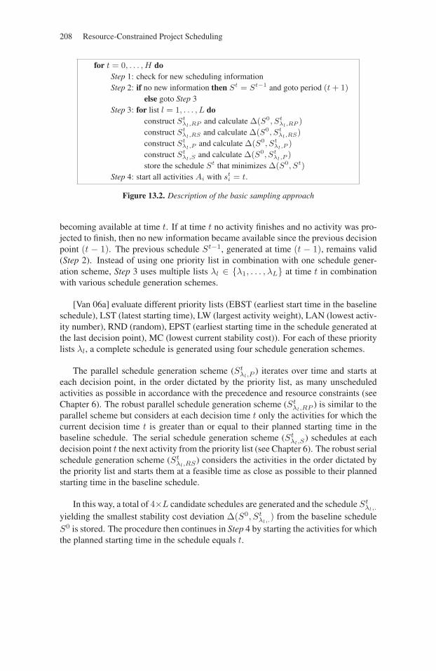
208 Resource-Constrained Project Scheduling
for t = 0, . . . , H doStep 1: check for new scheduling informationStep 2: if no new information then St = St−1 and goto period (t + 1)
else goto Step 3Step 3: for list l = 1, . . . , L do
construct Stλl,RP and calculate Δ(S0, St
λl,RP )
construct Stλl,RS and calculate Δ(S0, St
λl,RS)
construct Stλl,P
and calculate Δ(S0, Stλl,P
)
construct Stλl,S
and calculate Δ(S0, Stλl,P
)
store the schedule St that minimizes Δ(S0, St)
Step 4: start all activities Ai with sti = t.
Figure 13.2. Description of the basic sampling approach
becoming available at time t. If at time t no activity finishes and no activity was pro-jected to finish, then no new information became available since the previous decisionpoint (t − 1). The previous schedule St−1, generated at time (t − 1), remains valid(Step 2). Instead of using one priority list in combination with one schedule gener-ation scheme, Step 3 uses multiple lists λl ∈ {λ1, . . . , λL} at time t in combinationwith various schedule generation schemes.
[Van 06a] evaluate different priority lists (EBST (earliest start time in the baselineschedule), LST (latest starting time), LW (largest activity weight), LAN (lowest activ-ity number), RND (random), EPST (earliest starting time in the schedule generated atthe last decision point), MC (lowest current stability cost)). For each of these prioritylists λl, a complete schedule is generated using four schedule generation schemes.
The parallel schedule generation scheme (Stλl,P
) iterates over time and starts ateach decision point, in the order dictated by the priority list, as many unscheduledactivities as possible in accordance with the precedence and resource constraints (seeChapter 6). The robust parallel schedule generation scheme (St
λl,RP ) is similar to theparallel scheme but considers at each decision time t only the activities for which thecurrent decision time t is greater than or equal to their planned starting time in thebaseline schedule. The serial schedule generation scheme (St
λl,S) schedules at each
decision point t the next activity from the priority list (see Chapter 6). The robust serialschedule generation scheme (St
λl,RS) considers the activities in the order dictated bythe priority list and starts them at a feasible time as close as possible to their plannedstarting time in the baseline schedule.
In this way, a total of 4×L candidate schedules are generated and the schedule Stλl,.
yielding the smallest stability cost deviation Δ(S0, Stλl,.
) from the baseline scheduleS0 is stored. The procedure then continues in Step 4 by starting the activities for whichthe planned starting time in the schedule equals t.
Proactive-reactive Project Scheduling 209
13.3. Solution robust scheduling under resource availability uncertainty
The research on proactive/reactive project scheduling under resource availabil-ity uncertainties is virtually non-existent. [DRE 05] considers the problem of projectplanning subject to human resource constraints which have to do with job compe-tences, working hour limits, vacation periods and unavailability of employees. Shepresents a mathematical model as well as dedicated algorithms for robust schedulegeneration and schedule repair. [YU 04], in their above-mentioned ILP model forthe multi-mode problem, allow for (known) decreases in the resource availabilities incertain planning periods.
13.3.1. The problem
Contrary to section 13.2, activity durations are now assumed to be determinis-tic; uncertainty originates from the stochastic nature of renewable resource availabil-ity Bk (k = 1, . . . , q). This means that during schedule execution infeasibilities mayoccur due to renewable resource breakdowns, causing the schedule to need repair. Theproactive project scheduling problem then consists of generating a proactive schedulethat is protected as well as possible from such disruptions, subject to a project dead-line, finish-start, zero-lag precedence constraints and renewable resource constraints.A deterministic maximum resource availability Bk is considered for each renewableresource type Rk. Each of these Bk resource units initially allocated to the project issubject to breakdowns; some of the proposed models pre-suppose knowledge of themean time to failure and the mean time to repair. The objective function to be mini-mized is again
∑Ai∈V wiE (|Si − si|), the weighted expected deviation between the
planned and actually realized activity start times.
[LAM 06] develop and evaluate eight proactive and three reactive scheduling pro-cedures; one of the hypotheses that lie at the basis of their computations is that duringproject execution activities are not initiated before their baseline starting time. Thebest proactive and reactive strategies can be described as follows.
13.3.1.1. Proactive strategy
The best performing proactive strategy consists of the addition of time buffers to aschedule which is generated using resource buffering, and which places the activitieswith highest impact on total project stability earliest in time (largest CIW first).
Resource buffering boils down to planning the project subject to a deterministicnominal resource availability that is strictly below Bk. More precisely, the nominalavailabilities are set equal to E(Bk) =
∑Bk
m=0(Bk − m)πm, where πm denotes thesteady state probability that m resource units of resource type Rk are inactive. Whennecessary, this value is increased to maxAi∈V bik to allow for the activity with thehighest resource demand for resource type Rk to be scheduled.
210 Resource-Constrained Project Scheduling
The largest CIW first rule schedules the activities Ai in non-increasing order oftheir cumulative instability weight CIWi = wi +
∑Aj∈Γ∗
iwj , where Γ∗
i denotesthe set of direct and indirect successors of activity Ai. In the first step a precedencefeasible priority list is constructed in which precedence-unrelated activity pairs appearin non-increasing order of CIWi (lowest activity number as tie-breaker). Afterwardthis priority list is transformed into a precedence and resource feasible schedule usinga serial schedule generation scheme .
Time buffering implies that time buffers are inserted in front of activities inorder to absorb potential disruptions caused by earlier resource breakdowns and theresulting activity shifts. The procedure approximates Δi, the duration increase inactivity Ai caused by resource breakdowns, by maxRk∈R{ pi
MTTFkMTTRkrik},
where pi denotes the expected duration of activity Ai, and MTTFk and MTTRk,respectively denote the mean time to failure and mean time to repair for resourcetype Rk. The impact on the objective function that can be attributed to the dis-ruption of activity Aj caused by its predecessors i ∈ Γ∗−1
j is then estimated asIj =
∑Ai∈Γ∗−1
jwj max{0, si + pi + Δi − sj}. All non-dummy activities are placed
in a list L ordered by non-increasing impact estimates, with the lowest activity numberas tie-breaker. The first activity in list L is selected and right shifted by one timeunit. Affected activities are likewise right shifted by one time unit in order to keepthe schedule precedence and resource feasible. In case the resulting schedule alsorespects the project deadline constraint, the procedure moves to the next iteration byrecalculating the expected impacts for each activity in the new schedule and buildinga new list L′. In case the new schedule violates the deadline, the move is reverted andthe procedure examines the next activity in the list. If no such activity can be found,the procedure terminates.
13.3.1.2. Reactive strategy
When the baseline schedule breaks, i.e. when activities have to be interruptedbecause of a resource breakdown, the schedule needs to be repaired using a reactiveprocedure. Lambrechts et al. [LAM 06] investigate a preempt-repeat setting (inter-rupted activities have to be restarted anew); they generate a list L containing all activ-ities that are not yet completed at the time of interruption, ordered in non-decreasingorder of the baseline starting times. This list is then decoded into a feasible scheduleusing a serial schedule generation scheme that tries to schedule the interrupted activ-ities as early as possible; a tabu search algorithm to improve the generated reactiveschedule is also proposed in the same source.
13.4. Conclusions and suggestions for further research
Real-life projects are typically subject to considerable uncertainty. This chapterhas addressed proactive/reactive project scheduling procedures that may be deployedwhen the uncertainty pertains to the duration of activities or to the availability of

Proactive-reactive Project Scheduling 211
renewable resources. Proactive procedures have been described to generate a robustbaseline schedule that is appropriately protected against distortions that may occurduring project execution. The term “robustness” in this context refers to solutionrobustness or stability. Our aim has been to generate proactive precedence andresource feasible baseline schedules that minimize one particular stability cost func-tion, namely the weighted sum of the expected deviation between the actually realizedactivity start times during project execution and the planned activity start times in thebaseline. When distortions during project execution cause the baseline schedule tobecome infeasible, a reactive policy needs to be invoked to repair the schedule; thischapter has (to a lesser extent) also provided insights into this reactive issue.
For variable activity durations, [Van 05, Van 06a, Van 08a, Van 06b, Van 06c]have developed exact and heuristic proactive time buffer insertion strategies that canbe combined with effective reactive policies for (optimally or heuristically) solvingthe underlying weighted earliness-tardiness problem. These research efforts allow usto draw interesting and reassuring conclusions. It appears that the combination ofproactive and reactive scheduling techniques leads to significant stability improve-ment decreases in the planning nervousness, with only moderate (hence acceptable)increases in schedule makespan.
The unavailability of resources is a second potential but very realistic cause ofsubstantial deviations from the baseline schedule. Consequently, the development ofproactive/reactive scheduling procedures under stochastic resource availability is rel-evant from a theoretical and a practical point of view. Research in this area is justemerging. [LAM 06] have obtained excellent results with a dedicated procedure thatcombines a resource and time buffered proactive scheduling procedure with a listbased reactive schedule generation scheme.
These promising results justify the engagement in additional research. The devel-opment of a single-step (monolithic) proactive scheduling procedure for the generationof stable (solution robust) baseline schedules with acceptable makespan performance,which can be easily combined with effective reactive scheduling policies that are ableto operate under various types of schedule distortions, deserves priority. The explo-ration of robustness measures other than the weighted activity starting time devia-tions, which was explored in this chapter, constitutes another interesting area of futureresearch.
13.5. Acknowledgements
This research has been supported by Project OT/03/14 of the Research FundK.U. Leuven, Project G.0109.04 of the Research Foundation – Flanders (F.W.O.-Vlaanderen) and Project 06163 supported by the National Bank of Belgium.

212
This page intentionally left blank
Chapter 14
RCPSP with Financial Costs
A project is a complex system in which many different persons and several meansand actions interact to give an answer to a client’s request. As an answer, it has torespond to the client’s wishes in terms of time, quantity and costs. These three objec-tives are often incompatible and traditionally only one of them is taken into account.For the last 10 years, the project scheduling problem with makespan minimization hasbeen the subject of several papers. The studies on project scheduling with financialcosts received a little less interest. In this chapter, we focus on the way that financialaspects of project scheduling are treated in the studies. This chapter is inspired by[DRE 02, DRE 03].
14.1. Problem presentation and context
As shown in this book, the project scheduling problem is characterized byactivities, resources and an objective function. All activities of a project have to becompleted to achieve the project. Project activities have one or several executionmodes (see Chapter 9) associated with a duration and require the use of resources(this requirement can be constant or not). Activities can be linked with precedencerelations representing technological constraints and can also be associated withtime windows (release time, due dates or deadlines). Associated with an activity, acash flow may occur. To process activities, the project needs resources (workforce,capital, machine, etc.). Resources used by the project can be of four different types:renewable, non-renewable (as capital in special cases), doubly constrained and par-tially renewable. Costs can be caused by resources or by activities. When costs are
Chapter written by Laure-Emmanuelle DREZET.
213

214 Resource-Constrained Project Scheduling
generated by activities, the way activities are processed (execution mode, starting orfinishing time) generates costs that have to be minimized. When costs are generatedby resources, the scheduling of activities indirectly impacts on the budget of theproject via the resource. When costs are incurred by activity execution modes, we canconsider that costs are generated both by activities and resources. In fact, when thereare several execution modes for an activity, they are often characterized by differentlevels of resource consumption and by different durations, inversely proportional tothe resource requirements. As a consequence, we consider this type of costs as mixed.
This chapter is organized as follows. The next section provides several definitionsand notations used for project scheduling problems with financial objectives. Section14.3 presents problems for which costs are activity-related and the objective is themaximization of project benefits. Problems with resource-related costs are studied insection 14.4.
14.2. Definitions and notations
14.2.1. Definitions
The objective of the contractor and the client is to reduce costs and ideally to max-imize their profit. To maximize project profit is equivalent to maximize its Net PresentValue (NPV). The NPV is the most frequent criterion used in project scheduling whenthe project financial aspects are taken into account. This criterion is calculated withcash flows generated by project activities. A cash flow can be positive (cash inflow)or negative (cash outflow). For the contractor, cash outflows represent the expensescaused by manpower, equipment and raw materials while cash inflows represent theclient’s payments (they are often proportional to the project’s advancement).
The NPV was first introduced by Russell in 1970 ([RUS 70]). It is a non-regularobjective function, except in the case where cash flows are only positive. NPV rep-resents profit in actual value that will be earn after x years. NPV is defined as below(when project representation is a AOA (Activity-On-Arc1) graph where cash flows areassociated with the n events or n graph vertices):
NPV =∑n
i=1 Fie−αTi subject to: Sk + pk < Ck with data:
Fi cash-flow generated by event i,
Sk (respectively Ck) the event associated with the start (respectively the end) ofthe activity Ak and pk the duration of the activity Ak,
1. Contrarily to the Activity-On-Node representation of the project presented in Chapter 1, theActivity-On-Arc representation associates the activities with the arcs of the precedence graph,while the nodes represent events (i.e. activity start and completion times).
RCPSP with Financial Costs 215
e−α = (1 + r)−1 = β, the discount factor with r the discount rate, i.e. what weare going to lose or earn by investing some money in the project instead of keeping it,
Si and Ci, starting time and completion time of Ai.
The discount factor is used to take the discount (i.e. the money variation in time)into account. In fact, discounting consists of giving to different cash flows occurring atdifferent dates an actual value. A major difficulty consists of determining the adequatediscount factor.
14.2.2. Notations
From all existing scheduling problems notations, we use the notation proposed in[HER 98b] that uses the traditional notation of traditional production scheduling prob-lems. The α field describes resource characteristics, the β field specifies the activitycharacteristics and the γ field specifies the objective function. As β8 is used to describethe financial implications of the project activities, we only detail its possible values:
– cj if activities are associated with cash flows;
– c+j if cash flows associated with activities are positive;
– cj if cash flows are stochastic;
– per if cash flows are periodic;
– sched if both the amount and the timing of cash flows have to be determined;
– ∅ if no cash flows are specified.
In this chapter we use this notation to classify all of the studied problems. Forexample, the previous model can be noted cpm, cj |NPV : only one cash flow is asso-ciated with a graph node (cj) and resources are unconstrained (cpm).
To better fit the reality and to avoid ambiguity, some precisions about cash flowoccurrence must be made. First of all, cash flows have to be associated with activitiesinstead of events. In fact, associating cash flows with events generates confusionsbecause an event can correspond with the end of several activities and the beginning ofothers without adaptation of the classical AOA representation of projects (adaptationswere presented in [PAD 97, YAN 95, DAY 96]).
Several cash flows can be associated with one activity. When an activity is quitelong, discounting cash flows on one unique period can be inappropriate. A solutionmay consist of decomposing activities into subactivities to have only one cash flowassociated with an activity, but this decomposition increases the graph complexity.
As a consequence, some authors adopt another representation, allowing severalcash flows associated with one activity. This model was first introduced in [DOE 77].It supposes there are several cash flows associated with one activity and they are
216 Resource-Constrained Project Scheduling
inputted all together at the end of the activity. Time periods are defined by associ-ating a unique cash flow to a time period. This model also considers the loss generatedby the activity processing called opportunity costs. They also take capital constraintsinto account. It can be noted that Russell’s approach [RUS 70] is a particular case ofthe approach of Doersch and Patterson [DOE 77].
Another remark can yet be formulated: the last two models suppose that a cashflow generated by an activity is constant, i.e. its value does not depend on the startingtime of the activity. In [ETG 96] a new model is introduced where cash flows valuesare time dependent. This model considers that the amount of cash flows is a non-increasing linear time function. Vanhoucke et al. [VAN 01b] studied a similar problemand introduced another value for β8 : clin
j .
14.2.3. Classification
The two next sections present a review of different models found in other works.The presentation follows this classification:
– MAXNPV: NPV of the project has to be minimized, no resource constraints aretaken into account;
– RCPSPDC (Resource Constrained Project Scheduling Problem with DiscountedCash Flows) corresponds to the MAXNPV with resource constraints;
– CCPSP (Capital Constrained Project Scheduling Problem) is a RCPSPDC gen-eralization with additional constraints on capital;
– PSP (Payment Scheduling Problem): amount and occurrence of cash flows haveto be determined to maximize the project’s NPV.
When costs are generated by activities through their execution mode, we are facedwith the TCTP (Time/Cost Trade-off Problem). When costs are resource-related wecan distinguish three problems:
– RLP (Resource Leveling Problem): resource consumption has to be leveled fromone time period to another, or on each period the difference between resource usageand a target value has to be minimized;
– RIP (Resource Investment Problem) or RACP (Resource Availability CostsProblem) consists of minimizing the capacity of bought resources while respectingthe requirement of activities;
– RRP (Resource Renting Problem) consists of minimizing the capacity of rentedor bought resources while respecting activities requirements. Two different types ofresource costs are considered. RIP is a subproblem of RRP (Resource Renting Prob-lem).
See the classical three field notation of Herroelen et al. [HER 98b] for further de-tails. We recall basic notation that are used in this part. In field one (α-field) 1, 1 means
RCPSP with Financial Costs 217
that only one renewable resource is considered and m, 1, means that m renewableresources are taken into account simultaneously. In field two (β-field) cpm meansthat activities are submitted to traditional start-end precedence relation, gpr meansthat generalized precedence relation are considered. Notice that in most of the studiedproblems, whereas the objective function is related to costs, the project deadline isfixed, which is denoted by δn in the second filed of the traditional notation.
Notice that related to these problems TCTP (Time/Cost Tradeoff Problem) hasbeen the subject of many papers. For the TCTP, activities have several executionmodes, each mode corresponding to a pair: duration and cost (discrete TCTP). Eachactivity can also have its cost and duration linked by a continuous function (continuousTCTP). In this case, an upper and a lower bound are specified for cost and duration.The objective of TCTP can be either to minimize total costs generated by crashingsome activities, to minimize the project duration while respecting an upper bound ontotal project costs or to determine the whole Pareto optima curve. The TCTP com-plexity depends on the nature of the cost-duration relationship. Related to problemsdealing with costs without cash flows, De Dunne, Ghosh and Wells [DE 95] gave astate-of-the-art review on TCTP. To solve discrete TCTP, the project graph can besimplified by suppressing some activities execution modes or by changing the graphstructure ([BRU 83, SCH 80, MUL 89, BEI 92]). The majority of approaches dealingwith TCTP do not consider constraints on resources (except on the capital availablefor the project) and do not consider that cash flows can occur.
14.3. NPV maximization
In this section we focus on minimization of NPV of the project, without resourceconstraints (MAXNPV) denoted cpm, cj |NPV , and then adding resource constraints(RCPSPDC), denoted m, 1|cpm, cj |NPV .
14.3.1. Unconstrained resources: MAXNPV and PSP
MAXNPV is a polynomial problem that was first studied by Russell in 1970[RUS 70] with a model where cash flows are associated with events of an AOA projectgraph (cpm, cj |NPV ). The proposed resolution is based on the transformation of thenon-linear mathematical model of MAXNPV into a linear one with the help of Tay-lor series approximation. This transformation results in a linear program whose dualis a transshipment network flow problem. Russell based his resolution on the Ford andFulkerson algorithm (out-of-kilter) and found optimal solutions.
Grinold in [GRI 72] took the same model cpm, cj |NPV and added a project dead-line denoted by δn and showed that Russell’s non linear program can be linearizeddirectly with the use of particular structure of this non linear program. He providedtwo procedures, one with a fixed project deadline and the other having the projectdeadline as a parameter and showing relationship between project NPV and projectdeadline.

218 Resource-Constrained Project Scheduling
Elmaghraby and Herroelen [ELM 90] proposed a new approach to solvecpm, δn, cj |NPV and showed that the approaches of Grinold and Russell wereimperfect. In fact, in special cases, Russell and Grinold procedures can be deadlockedor cannot provide a coherent solution. Moreover, Elmaghraby and Herroelen point outthe complexity of Grinold and Russell approaches and propose an algorithm basedon a simpler concept: advancing as much as possible events associated with positivecash flows while delaying as much as possible those associated with negative cashflows. In [SEP 94], Sepil pointed out a flaw in Elmaghraby and Herroelen approach,corrected it and gave a computational evaluation of the modified procedure.
Schwindt and Zimmermann in [SCH 01] consider the unconstrained MAXNPVproblem with general temporal constraint. The method that they proposed is a steepestascent approach. Note that the efficiency of this algorithm is demonstrated on the basisof two randomly generated benchmark problem sets consisting of instances with up to1,000 activities.
Demeulemeester, Herroelen and Van Dommelen [DEM 96b] proposed an optimalresolution of cpm, δn, cj |NPV with an AON project representation where cash flowsare associated with completion time of some activities. This procedure was adaptedby De Reyck and Herroelen [de 96b] to be used on gpr, δn, cj |NPV . The main dif-ference between the two approaches is the necessary transformation of the generalizedprecedence relations into standard precedence relations (with transformation rulesdefined in [BAR 88]). Related to the same problem, Vanhoucke, Demeulemeester andHerroelen [VAN 03] present a branch-and-bound algorithm which computes upperbounds by making piecewise linear overestimations. The problem is relaxed into aweighted earliness-tardiness project scheduling problem.
cpm, (δn), clinj |NPV was studied by Etgar, Shtub and LeBlanc [ETG 96] (sim-
ulated annealing), Shtub and Etgar ([SHT 97] (branch-and-bound procedure) and[VAN 01b] (polynomial algorithm for the cpm, δn, clin
j |NPV based on an implicitenumeration and on the algorithm developed by Demeulemeester, Herroelen and VanDommelen [DEM 96b]).
Few stochastic models were developed and the stochastic characteristic isrelated to activities duration rather than cash flows (Buss and Rosenblatt [BUS 93],Elmaghraby et al. [ELM 00]).
In MAXNPV, the amount and timing of cash flows are known. However, theamount and timing of a client’s payments directly affect project benefits for both theclient and the contractor. The amount and timing of progress payments are one of themost important points in the negotiations between client and contractor. In fact, thecontractor’s ideal solution is to perceive one unique contractual payment at the begin-ning of the project. After receiving this payment, the contractor attempts to minimizecosts by scheduling activities associated with a large investment as late as possible.
RCPSP with Financial Costs 219
Of course, this is not the client’s ideal solution. The client prefers to give one uniquepayment at the end of the project. Thus, for the client, the schedule of activities is lessimportant than the completion time of the project.
The objective of negotiations between the contractor and the client is to obtain anequitable solution. An equitable solution is defined as a solution in which client andcontractor deviate from their ideal solutions with a same percentage.
PSP (Payment Scheduling Problem) can be studied from the contractor point ofview as from the client’s one. In this problem, the amount and occurrence of cashflows have to be determined to maximize the project NPV.
Dayanand and Padman studied PSP (cpm, sched|NPV ) from the contractor’spoint of view. In this problem both the amount and timing of cash flows have to bedetermined (denoted by sched) In [DAY 93], they gave an integer linear program andtested several heuristics.
14.3.2. Constrained resources: RCPSPDC, CCPSP and PSP
Here we consider NPV minimization subjected to resource constraints: m,1|cpm, cj |NPV .
The RCPSPDC and CCPSP problems are NP-hard as RCPSP generalizations. Themajority of procedures developed to solve this problem are heuristics but there existsome exact methods that are applicable on small size instances. The mathematicalmodel of this problem is similar to the MAXNPV model with supplementary con-straints on the resource capacities (see Chapter 3). For this problem, as far as weknow, the literature references only renewable resources.
Yang et al. [YAN 92] studied m, 1|cpm, δn, cj |NPV and assumed AOA networksin which an activity can be associated with several cash flows. Notice that δn denotesa project deadline. Authors add bonus and penalties for lateness or advances are asso-ciated with the project completion time. They used an implicit enumeration algorithmdeveloped by Talbot and Patterson [TAL 78] and gave two dominance rules to avoidenumerating all possible solutions. This procedure was evaluated on 20 problems andthe authors concluded that it can fail to find an optimal solution for problems made upof more than 30 activities or for specific problems (with tight resource constraints, adeadline higher than the project optimal duration for the makespan minimization).
Icmeli and Erenguc [ICM 96a] developed a branch-and-bound procedure forthe case where the resources may be available in variable amount (denoted by va):m, 1, va|cpm, δn, cj |NPV . Nodes correspond to complete solutions compatible withprecedence constraints but not with resource constraints. Initially, the lower boundis given by a heuristic procedure or set to −∞. The upper bound is calculated with

220 Resource-Constrained Project Scheduling
Grinold [GRI 72] procedure (see section 14.3.1) on the transformed problem (initialproblem without resource constraints). The branching scheme is the one developedin the DH-procedure [DEM 92b]. A node is cut off if it is associated with an upperbound lower than the lower bound or if it conducts to a solution whose completiontime is upper than the project deadline. When a node is associated with a feasiblesolution, the upper bound is updated. Tests on the Patterson set (50 problems) and thePROGEN set (40 problems) show that this procedure obtains better results than theprocedure given in [YAN 92] and described above. Baroum and Patterson [BAR 99]also developed a branch-and-bound procedure on the same branching scheme form, 1, va|cpm, c+
j |NPV but nodes of the searching tree correspond to feasible partialsolutions.
Vanhoucke, Demeulemeester and Herroelen [VAN 01c] introduce a depth-firstbranch-and-bound algorithm for which we make use of extra precedence relationsto resolve a number of resource conflicts. Upper bound for the MAXNPV problemis also proposed in this case based on the idea that positive cash flows should bescheduled as early as possible while negative cash flows should be scheduled as lateas possible within the precedence constraints.
Several heuristics were also proposed to solve the RCPSPDC, for example: Icmeliand Erenguc [ICM 94] used a Tabu search procedure to solve m, 1|cpm, δn, cj |NPVand Yang et al. [YAN 95] proposed procedure based on stochastic rules. Recent devel-opments on heuristic method for this problem have been proposed by Vanhoucke[VAN 06d], based on recursive procedure that can also be used as a part of moreglobal optimization method.
De Reyck and Herroelen [de 98] developed a branch-and-bound method for them, 1, va|gpr, ρj , δj , vr, cj |NPV , (ρj , means that ready times differ per activity andvr that the resource requirements may be variable discrete). Each node of the search-ing tree corresponds to a complete solution and the branching scheme is extractedfrom the DH-procedure [DEM 97]. They also proposed three dominance rules to avoidthe exploration of all the nodes of the searching tree. This branch-and-bound methodsolves problems with up to 50 activities and its truncated version also gives goodresults.
Suboptimal approaches to solve m, 1|cpm, cj |NPV are numerous. Russell[RUS 86] was the first to test standard priority rules for this problem. Several otherauthors developed procedures based on priority rules. Zhu and Padman [ZHU 97]used both neural networks and priority rules to solve this problem. Recently Mikaet al. [MIK 05], considered metaheuristics (simulated annealing and tabu search)for solving MM-RCPSP with discounted cash flows. They investigate four differentpayment models: lump-sum payment at the completion of the project, payments atactivities’ completion times, payments at equal time intervals and progress payments.
RCPSP with Financial Costs 221
Periodic cash flows (denoted by per) were studied in [SEP 97] in which the authorsadapted the model developed by Kazaz and Sepil [KAZ 96] for cpm, per|NPV totake resource constraints into account and to solve m, 1|cpm, per|NPV .
Buss and Rosenblatt [BUS 95] and Elmaghraby [ELM 00] present a model for theNPV maximization when activities duration are stochastic.
The CCPSP is a RCPSPDC generalization. It differs from the RCPSPDC by con-sidering constraints capital available for the projet.
Doersch and Patterson [DOE 77] introduced a binary integer linear programmingformulation to solve 1, 1, va|cpm, δn, cj |NPV . This model solves to optimalityprojects with 15 to 20 activities but fails to solve problems with more than 30activities. This approach was updated in [SMI 96].
Smith-Daniels and Smith-Daniels [SMI 87] extended the Doersch and Pat-terson model to take constraints on cost and on material into account: m, 1,va|cpm, δn, cj |NPV . This procedure allows solving small problems to optimality.
For the resource-constrained PSP with multiple modes of activity processing(denoted by mu), Ulusoy and Cebelli [ULU 00] proposed a double-loop geneticalgorithm to solve m, 1|cpm, δn,mu, sched|NPV . The objective is to determine anequitable solution for both the contractor and the client.
Some hybrid approaches can be found that combine TCTP with cash flows onactivities and discounting with constraints on resources: [TAL 82, ERE 93, ICM 96b].Other extensions are considered in [VAN 08b]: time/switch constraints, work conti-nuity constraints and net present value maximization. Authors present both an exactsolution approach for the work continuity version and a new meta-heuristic approach.
14.4. Resource-related costs
In the first section of this chapter we have presented a classification and a reviewof the research considering scheduling problems where costs are generated by activi-ties through their execution mode: the TCTP (Time/Cost Trade-off Problem). In thissection we assume that costs are resource-related then we can distinguish two mainclasses of problems: costs can be caused by sub-optimal use of the resource or thenecessary reservation of resources.
14.4.1. Resource Leveling Problem
This problem consists of minimizing the maximal resource utilization by avoidingpeaks in resource consumption either by limiting deviations between the resource con-sumption and a target value or by minimizing variations of resource utilization overtime. The complexity of the RLP depends on whether the resources are constrained ornot.
222 Resource-Constrained Project Scheduling
The objective function can consist of:
– minimizing the absolute value of the difference between resource usage and atarget value,
∑abs.dev;
– minimizing the square of the difference between resource usage and a targetvalue,
∑sq.dev;
– minimizing jumps in resource usage between two consecutive time periods,∑jump;
– minimizing the maximal resource usage, maxreq.
Ahuja [AHU 76], Easa [EAS 89], Bandelloni et al. [BAN 94] and Younis andSaad [YOU 96] proposed exact algorithms based on implicit enumeration, oninteger programming or on dynamic programming. Easa devised a procedure for1, 1|cpm, δn|
∑abs · dev and 1, 1|cpm, δn|
∑jump (δn means that the project
deadline is fixed). His procedure finds the optimal solution for small to medium-sizeprojects. Bandelloni’s dynamic programming approach solves 1|gpr, δn|
∑abs.dev
and leads to an optimal solution for small and medium projects.
Savin ([SAV 96, SAV 97]) used neural networks to solve the RLP.
Heuristic approaches were proposed by several authors, all of them consist of mov-ing some activities or in computing a priority for each activity.
Harris [HAR 90] showed that when a resource is leveled, and if the resourcedemands are uniform for all resources, other resources also tend to be leveled. Hedeveloped a heuristic procedure to level the utilization of a unique resource, with gen-eralized precedence relations. His procedure is easy to apply and is applicable on some1, 1|gpr, δn|
∑jump problems. The first step of his procedure consists of building the
base resource usage histogram by considering only critical activities. Others activitiesare placed with the help of three priority rules. An example is detailed but no test wascarried out.
For RLP with generalized precedence relations and general objective func-tion, Brinkmann and Neumann [BRI 96] devised two greedy algorithms to solvem, 1|gpr, δn|Cmax and m, 1|gpr, δn|γ (with γ =
∑jump or = maxreq). Their
procedure is based on implicit enumeration or on graph reduction (contraction). Testswere only carried out on m|gpr, δn|γ with γ =
∑jump or γ = maxreq with
unconstrained resources.
Neumann and Zimmermann [NEU 99] devised three polynomial heuristics form|gpr, δn|γ or m, 1|gpr, δn|γ with γ =
∑abs.dev,
∑sq ·dev,
∑jump or maxreq.
Problems composed of up to 500 activities and 5 resources can be efficiently solved.
The same authors (in [NEU 00b]) have developed a branch-and-bound method (forRLP with or without constrained resources) and a heuristic procedure, starting from a
RCPSP with Financial Costs 223
feasible solution of the resource-unconstrained RLP and enhance it to obtain a feasi-ble solution to the resource-constrained RLP. Solved problems are m|gpr, δn|γ withγ =
∑abs · dev,
∑sq · dev,
∑jump or maxreq. Neumann and Zimmermann also
developed an adaptation of their BB procedure with the filtered beam search method.
14.4.2. Resource Investment Problem (RIP) and Resource Renting Problem (RRP)
In the Resource Investment Problem (RIP), also denoted by the Resource Avail-ability Cost Problem (RACP), costs are generated by the reservation of a given amountof resource for the project. A solution of this problem consists of a set of activity start-ing times and a set of resource capacities, while respecting a project deadline. Thisproblem is NP-hard
Some authors argue that the RIP is a Resource Leveling Problem (RLP) subprob-lem. If the two problems are strongly related in the RLP, resource capacities are knownwhile they are variables and have to be determined in the RIP.
In the RIP the system has bought all the resources needed by the project. The costof a resource is proportional to the resource capacity, is not time-dependent and doesnot vary if the resource is used once or during all the project. In the RRP, resourcescan be rent and costs generated by a resource are of two types: fixed costs to have theresource Rk: cp
k, that are not time-dependent, and renting costs, crk. Though, disposing
of the resource Rk during t time periods costs cpk + t · cr
k. The RRP isNP-hard as anRIP generalization.
The objective of the RRP is to minimize resource total costs while respecting activ-ities requirements and deadline of the project. All the resources needed by the projectare known and there are renewable.
The RRP is denoted by m, 1|cpm, δn|rrc (rrc = resource renting costs). A RRPsolution is a 3-tuple composed by the activity starting times, the number of resourceunits added at each time period (αkt) and the number of resource k units removed ateach time period (ωkt).
Möhring [MÖH 84] was the first to define the RIP and to propose an algorithm form, 1|cpm, δn|rac (rac=resource availability costs). Möring’s approach is based onthe Radermacher [RAD 85] procedure for the RCPSP.
Demeulemeester [DEM 95] devised a procedure to solve the same problem, basedon a branch-and-bound procedure for the RCPSP developed by Demeulemeester[DEM 92a] (see Chapter 5). Two different strategies are presented, the first is basedon the progressive increase of resource capacity and the second is based on the
224 Resource-Constrained Project Scheduling
progressive decrease of resource capacities. The first strategy cannot guarantee theoptimality of the solution but a feasible solution can be obtained quickly. The secondstrategy is based on the decision problem associated with RCPSP: the RCPSDP,solved for an adaptation of the initial problem. This adaptation considers only twoconstrained resources, other resource capacities are supposed to be infinite. The min-imal resource capacities can be computed. This resolution allows the construction ofnon-strict Pareto optima set. Within this set, the Pareto optimum associated with thelowest cost is chosen and the RCPSDP associated with this vector is solved. If nofeasible solution exists, the optima Pareto set is updated with new points. This strat-egy guarantees that the first feasible solution found is an optimal one. If the decisionproblem included in [DEM 95] procedure is changed, other RIP problems can besolved by this procedure: the RIP with general precedence constraints on activities orthe RIP with activity preemption. The method proposed in [DEM 95] obtains betterresults than the method proposed in [MÖH 84] because the procedure to solve theRCPSP developed in [DEM 92a] outperforms the procedure developed in [RAD 85].
Two approaches were proposed by Kimms in [KIM 01], for m, 1|cpm, δn|rac, onebased on Lagrangean relaxation, the other one on column generation. Computationaltests show that Lagrangean relaxation obtains worse results than column generationbut needs less computational time. For 64% of the instances, the Lagrangean relax-ation leads to solutions close to optimal solution (less than 10%).
The RIP can be used to solve staff management problems. In fact, the problem ofthe workforce size determination can be modeled as an RIP. For example, Kane andBaptiste [KAN 01] solved 3, 1, va|cpm, δn|rac. They aim at determining the opti-mal numbers of interim workers and of supplementary hours to minimize salary costswhile respecting workload. The objective function takes the French legislation onmaximal weekly working hours into account by allowing the definition of two dif-ferent prices for supplementary hours.
For the RRP, Nübel in [NÜB 01] developed an exact procedure to determine anoptimal renting policy, knowing a feasible schedule of project activities. He also gavea “depth-first” branch-and-bound method that enumerates all quasi-stable schedulesand determines an optimal renting location (Nübel shows that the set of quasi-stableschedules is dominant). Each node of the searching tree corresponds to a partial solu-tion. If at a node p all the activities starting times are fixed, an optimal renting policyis computed, the upper bound is updated and the backtrack occurs. Otherwise, nodesare created by fixing a new activity. The authors also gave three lower bounds. Theytest their procedure on 10,800 problems from ProGen/max, showing that their branch-and-bound is efficient on small size instances (up to 10 activities). They concludedthat the RRP difficulty is proportional to the ratio cr
k/cpk. A branch-and-bound method
for the RRP is also given in [NEU 03].

RCPSP with Financial Costs 225
14.5. Conclusion
Figure 14.1 presents a synthesis of the studied problems. For further reading, andpossibly missing references we refer to Drezet (2002). This figure highlights the het-erogenity of the interest researchers have on the financial aspect in project scheduling.
Nevertheless, the vast majority of these approaches remain quite far from the pre-occupation of the project managers in industries. None of the proposed models areavailable in standard project scheduling software. The gap between theoretical andpragmatic solutions is still present. It is probably due to the complexity to determinethe right discount rate or to estimate the requirements of resources or costs generatedby the booking of these resources.
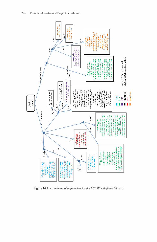
226 Resource-Constrained Project Scheduling
Figure 14.1. A summary of approaches for the RCPSP with financial costs

Part 3
Industrial Applications
227

228
This page intentionally left blank
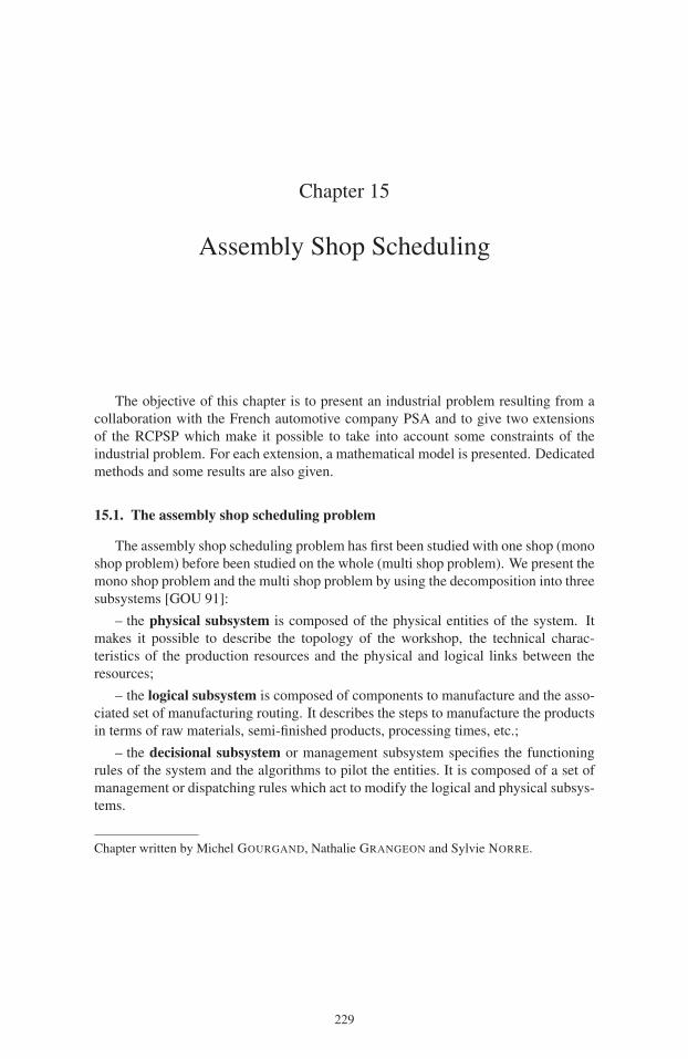
Chapter 15
Assembly Shop Scheduling
The objective of this chapter is to present an industrial problem resulting from acollaboration with the French automotive company PSA and to give two extensionsof the RCPSP which make it possible to take into account some constraints of theindustrial problem. For each extension, a mathematical model is presented. Dedicatedmethods and some results are also given.
15.1. The assembly shop scheduling problem
The assembly shop scheduling problem has first been studied with one shop (monoshop problem) before been studied on the whole (multi shop problem). We present themono shop problem and the multi shop problem by using the decomposition into threesubsystems [GOU 91]:
– the physical subsystem is composed of the physical entities of the system. Itmakes it possible to describe the topology of the workshop, the technical charac-teristics of the production resources and the physical and logical links between theresources;
– the logical subsystem is composed of components to manufacture and the asso-ciated set of manufacturing routing. It describes the steps to manufacture the productsin terms of raw materials, semi-finished products, processing times, etc.;
– the decisional subsystem or management subsystem specifies the functioningrules of the system and the algorithms to pilot the entities. It is composed of a set ofmanagement or dispatching rules which act to modify the logical and physical subsys-tems.
Chapter written by Michel GOURGAND, Nathalie GRANGEON and Sylvie NORRE.
229
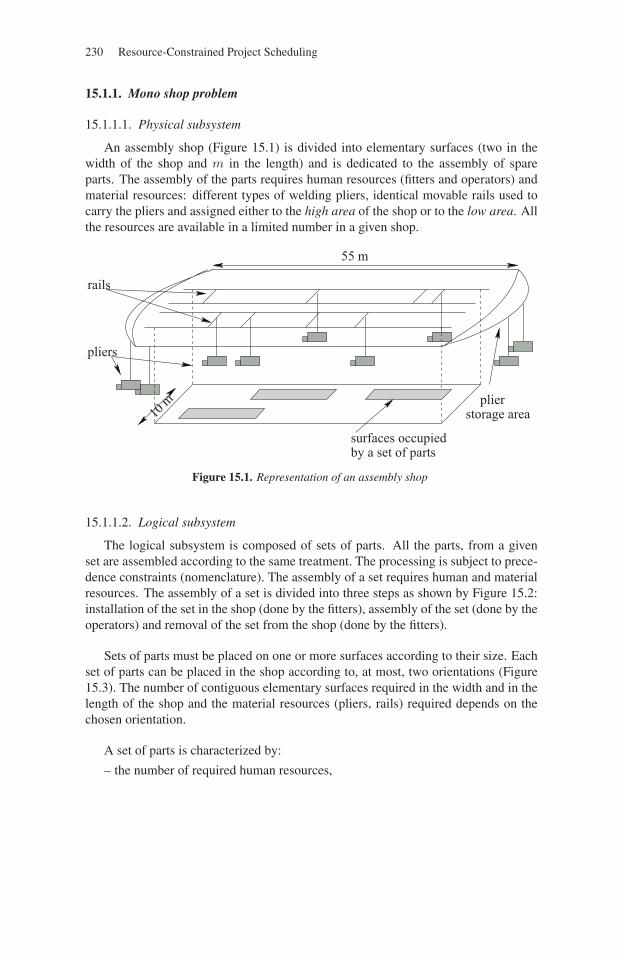
230 Resource-Constrained Project Scheduling
15.1.1. Mono shop problem
15.1.1.1. Physical subsystem
An assembly shop (Figure 15.1) is divided into elementary surfaces (two in thewidth of the shop and m in the length) and is dedicated to the assembly of spareparts. The assembly of the parts requires human resources (fitters and operators) andmaterial resources: different types of welding pliers, identical movable rails used tocarry the pliers and assigned either to the high area of the shop or to the low area. Allthe resources are available in a limited number in a given shop.
pliers
rails
surfaces occupied
55 m
plierstorage area
by a set of parts
10 m
Figure 15.1. Representation of an assembly shop
15.1.1.2. Logical subsystem
The logical subsystem is composed of sets of parts. All the parts, from a givenset are assembled according to the same treatment. The processing is subject to prece-dence constraints (nomenclature). The assembly of a set requires human and materialresources. The assembly of a set is divided into three steps as shown by Figure 15.2:installation of the set in the shop (done by the fitters), assembly of the set (done by theoperators) and removal of the set from the shop (done by the fitters).
Sets of parts must be placed on one or more surfaces according to their size. Eachset of parts can be placed in the shop according to, at most, two orientations (Figure15.3). The number of contiguous elementary surfaces required in the width and in thelength of the shop and the material resources (pliers, rails) required depends on thechosen orientation.
A set of parts is characterized by:
– the number of required human resources,
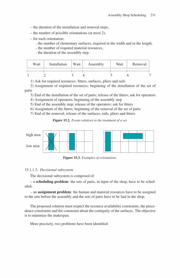
Assembly Shop Scheduling 231
– the duration of the installation and removal steps,
– the number of possible orientations (at most 2),
– for each orientation:- the number of elementary surfaces, required in the width and in the length,- the number of required material resources,- the duration of the assembly step.
InstallationWait
1 2
Assembly Wait Removal
3 4 5 6 7
Wait
1) Ask for required resources: fitters, surfaces, pliers and rails2) Assignment of required resources; beginning of the installation of the set of
parts3) End of the installation of the set of parts; release of the fitters; ask for operators4) Assignment of operators; beginning of the assembly step5) End of the assembly step; release of the operators; ask for fitters6) Assignment of the fitters; beginning of the removal of the set of parts7) End of the removal; release of the surfaces, rails, pliers and fitters
Figure 15.2. Events relatives to the treatment of a set
high area
low area
Figure 15.3. Examples of orientations
15.1.1.3. Decisional subsystem
The decisional subsystem is composed of:
– a scheduling problem: the sets of parts, in input of the shop, have to be sched-uled;
– an assignment problem: the human and material resources have to be assignedto the sets before the assembly and the sets of parts have to be laid in the shop.
The proposed solution must respect the resource availability constraints, the prece-dence constraints and the constraint about the contiguity of the surfaces. The objectiveis to minimize the makespan.
More precisely, two problems have been identified:
232 Resource-Constrained Project Scheduling
– Problem 1: mono shop problem with an unlimited number of material andhuman resources. The objective is to find a schedule of the sets and an assignmentof the surfaces to the sets which respect the precedence constraints, the constraintabout the contiguity of the surfaces and to minimize the makespan. Solving this prob-lem makes it possible to estimate the performance of the shop with only the limitationof the number of available elementary surfaces.
– Problem 2: mono shop problem with a limited number of material and humanresources. The objective is to find a schedule of the sets and an assignment of theresources to the sets which respect the availability and the precedence constraints, theconstraint about the contiguity of the surfaces and to minimize the makespan. Thisproblem helps us to study the impact of the limited number of resources. Solvingthis problem makes it possible to evaluate the opportunity to increase or decrease thenumber of resources of each type.
15.1.2. Multi shop problem
The physical subsystem is composed of many shops. The resources of each shop,called local resources, are completed with global resources, which can be used in anyshop. Global resources are pliers, fitters and operators, and are also available in alimited number. The logical subsystem is the same as in the mono shop problem, buta set of parts can be assembled in any shop. The decisional subsystem is the same asin the mono shop problem, but an assignment problem of the sets of parts and of theglobal resources to the shops is added. The proposed solution must respect the localand global resource availability constraints and the constraint about the contiguity ofthe surfaces. The objective is to minimize the makespan.
More precisely, two problems have been identified:
– Problem 3: multi shop problem without set distribution. The distribution of thesets in the shops is supposed to be established, the objective is to find a schedule ofthe sets of parts in each shop and an assignment of global and local resources to thesets which respect the availability and the precedence constraints, the constraint aboutthe contiguity of the surfaces and to minimize the makespan.
– Problem 4: multi shop problem with set distribution. This problem is the wholeproblem. The objective is not only to determine a schedule of the sets in each shop andan assignment of global and local resources to the sets, but also to distribute the setsamong the shops in order to respect the availability and the precedence constraints,the constraint about the contiguity of the surfaces and to minimize the makespan.
The impact of global resources can be analyzed by comparing separate studies(Problem 2) for many shops with a multi shop study (Problem 3).
Figure 15.4 represents the four identified problems and Table 15.1 describes thecharacteristics.
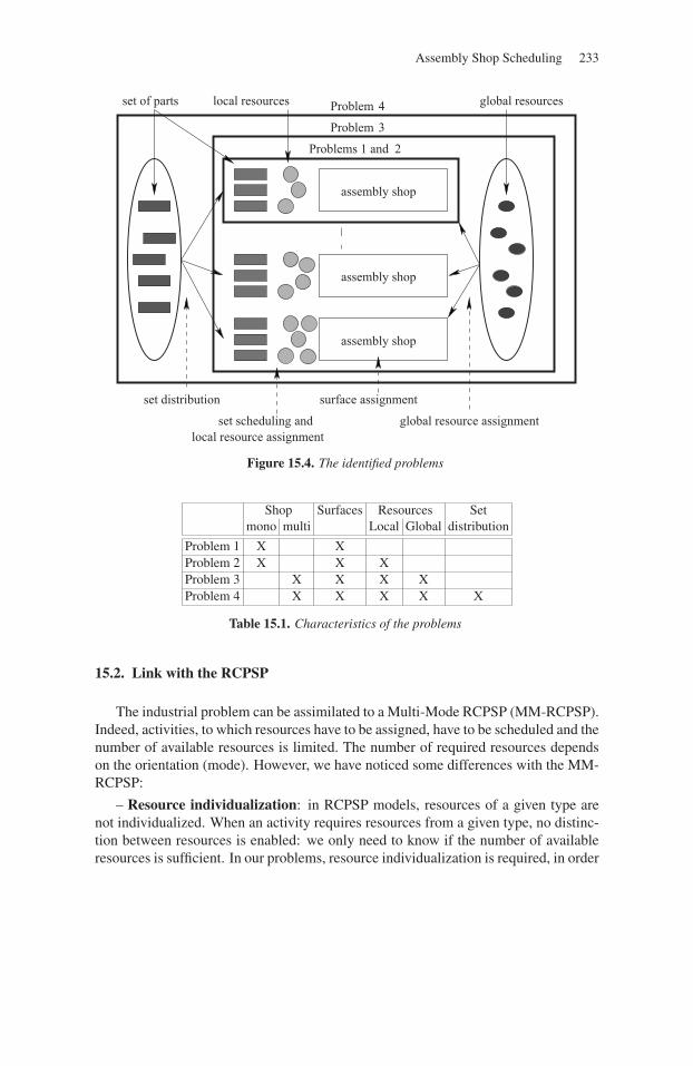
Assembly Shop Scheduling 233
Problem 4
Problem 3
Problems 1 and 2
assembly shop
assembly shop
assembly shop
set distribution surface assignment
set scheduling and local resource assignment
global resource assignment
global resourceslocal resourcesset of parts
Figure 15.4. The identified problems
Shop Surfaces Resources Setmono multi Local Global distribution
Problem 1 X XProblem 2 X X XProblem 3 X X X XProblem 4 X X X X X
Table 15.1. Characteristics of the problems
15.2. Link with the RCPSP
The industrial problem can be assimilated to a Multi-Mode RCPSP (MM-RCPSP).Indeed, activities, to which resources have to be assigned, have to be scheduled and thenumber of available resources is limited. The number of required resources dependson the orientation (mode). However, we have noticed some differences with the MM-RCPSP:
– Resource individualization: in RCPSP models, resources of a given type arenot individualized. When an activity requires resources from a given type, no distinc-tion between resources is enabled: we only need to know if the number of availableresources is sufficient. In our problems, resource individualization is required, in order
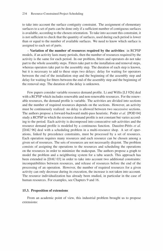
234 Resource-Constrained Project Scheduling
to take into account the surface contiguity constraint. The assignment of elementarysurfaces to a set of parts can be done only if a sufficient number of contiguous surfacesis available, according to the chosen orientation. To take into account this constraint, itis not sufficient to check that the quantity of surfaces, used during each period is lowerthan or equal to the number of available surfaces. We need to know which surface isassigned to each set of parts.
– Variation of the number of resources required by the activities: in RCPSPmodels, if an activity lasts many periods, then the number of resources required by theactivity is the same for each period. In our problem, fitters and operators do not takepart to the whole assembly steps. Fitters take part to the installation and removal steps,whereas operators take part to the assembly step. The duration of each step is known,but it is necessary to add to these steps two delays: delay for waiting for operatorsbetween the end of the installation step and the beginning of the assembly step anddelay for waiting for fitters between the end of the assembly step and the beginning ofthe removal step. The duration of the delay is unknown.
Few papers consider variable resource demand profile. Li and Willis [LI 92b] dealwith a RCPSP which includes renewable and non-renewable resources. For the renew-able resources, the demand profile is variable. The activities are divided into sectionsand the number of required resources depends on the sections. However, an activitymust be continuously realized: no delay is allowed between two successive sections.The authors propose a forward-backward multi-pass heuristic. Poder et al. [POD 04]study a RCPSP in which the resource demand profile is not constant but varies accord-ing to the period. Each activity is decomposed into consecutive sub activities and theresource demand profile is modeled by a continuous function. Dauzère-Pérès et al.[DAU 96] deal with a scheduling problem in a multi-resource shop. A set of oper-ations, linked by precedence constraints, must be processed by a set of resources.Each operation requires many resources and each resource can be chosen among agiven set of resources. The sets of resources are not necessarily disjoint. The problemconsists of assigning the operations to the resources and scheduling the operationson the resources in order to minimize the makespan. The authors propose a graph tomodel the problem and a neighboring system for a tabu search. This approach hasbeen extended in [DAU 03] in order to take into account two additional constraints:incompatibilities between resources, and release of resources before the end of theprocessing of an operation. However, the number of required resources for a givenactivity can only decrease during its execution, the increase is not taken into account.The resource individualization has already been studied, in particular in the case ofhuman resources. For examples, see Chapters 9 and 16.
15.3. Proposition of extensions
From an academic point of view, this industrial problem brought us to proposeextensions:

Assembly Shop Scheduling 235
– RCPSP with variable demand profile: an activity is divided into steps. Twoconsecutive steps require a different number of resources of a given type. This varia-tion of the number of resources required during the treatment of an activity may causewaiting time between the steps (because of the possible unavailability of resources).Thus, the duration of an activity is not known in advance.
– RCPSP with resource individualization: this extension makes it possible togive, for each activity, not only the starting time of the activity but also one or moreaccurate assigned resources.
15.3.1. RCPSP with variable demand profile
The considered hypotheses are the following:
– there are different types of resources and they are renewable ; for each type andeach period, the number of resources is limited;
– the activities are subject to precedence constraints such as: activity j cannot startbefore the completion of activity i;
– the activities are not preemptive;
– each activity is composed of at least one step;
– for each step, the duration is known, as well as the required quantity of resourcefrom each type (constant during the process of the step);
– two successive steps have different resource requirements at least for one typeof resource;
– it is not compulsory to process continuously two successive steps. They can beseparated by a waiting time due to the unavailability of a resource;
– if two successive steps require the same resources, their resources are notreleased during the waiting time and cannot be used for another activity.
To the definitions already defined in Chapter 1, we add the following ones:
– Steps:Ei number of steps in activity Ai
pi,j processing time of step j of activity Ai
bi,j,k amount of resource Rk used during the execution of step j of activity Ai
Ci,j completion time of step j of activity Ai
ECi,j earliest completion time of step j of activity Ai
LCi,j latest completion time of step j of activity Ai
– Variables:yijt = 1⇔ Ci,j = t, step j of activity Ai finishes during period t.
We assume that activities A0, and An+1 are composed of only one step: E0 = 1,En+1 = 1.
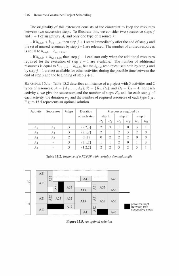
236 Resource-Constrained Project Scheduling
The originality of this extension consists of the constraint to keep the resourcesbetween two successive steps. To illustrate this, we consider two successive steps jand j + 1 of an activity Ai and only one type of resource k:
– if bi,j,k > bi,j+1,k, then step j + 1 starts immediately after the end of step j andthe set of unused resources by step j+1 are released. The number of unused resourcesis equal to bi,j,k − bi,j+1,k.
– if bi,j,k < bi,j+1,k, then step j + 1 can start only when the additional resourcesrequired for the execution of step j + 1 are available. The number of additionalresources is equal to bi,j+1,k − bi,j,k, but the bi,j,k resources used both by step j andby step j +1 are not available for other activities during the possible time between theend of step j and the beginning of step j + 1.
EXAMPLE 15.1.– Table 15.2 describes an instance of a project with 5 activities and 2types of resources: A = {A1, . . . , A5}, R = {R1, R2}, and B1 = B2 = 4. For eachactivity i, we give the successors and the number of steps Ei, and for each step j ofeach activity, the duration pij and the number of required resources of each type bijk.Figure 15.5 represents an optimal solution.
Activity Successor #steps Duration #resources required by
of each step step 1 step 2 step 3
R1 R2 R1 R2 R1 R2
A1 A5 3 {2,2,3} 2 3 1 0 3 1
A2 A4 3 {2,1,2} 2 1 2 3 2 0
A3 A5 2 {1,2} 0 2 2 2 0 0
A4 - 3 {2,1,2} 1 1 2 0 1 3
A5 - 3 {1,2,2} 2 2 3 2 3 1
Table 15.2. Instance of a RCPSP with variable demand profile
resource keptbetween twosuccessive steps
A41
A41
A11
A11
A21
A21
A22
A22
A31
A23
A32
A32
A12
A13
A13
A42
A51
A51
A52
A52 A53
A53
A43
A43
R2
R1
Figure 15.5. An optimal solution
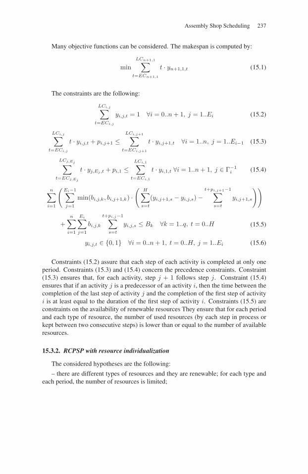
Assembly Shop Scheduling 237
Many objective functions can be considered. The makespan is computed by:
minLCn+1,1∑
t=ECn+1,1
t · yn+1,1,t (15.1)
The constraints are the following:
LCi,j∑t=ECi,j
yi,j,t = 1 ∀i = 0..n + 1, j = 1..Ei (15.2)
LCi,j∑t=ECi,j
t · yi,j,t + pi,j+1 ≤LCi,j+1∑
t=ECi,j+1
t · yi,j+1,t ∀i = 1..n, j = 1..Ei−1 (15.3)
LCj,Ej∑t=ECj,Ej
t · yj,Ej ,t + pi,1 ≤LCi,1∑
t=ECi,1
t · yi,1,t ∀i = 1..n + 1, j ∈ Γ−1i (15.4)
n∑i=1
(Ei−1∑j=1
min(bi,j,k, bi,j+1,k) ·(
H∑s=t
(yi,j+1,s − yi,j,s)−t+pi,j+1−1∑
s=t
yi,j+1,s
))
+n∑
i=1
Ei∑j=1
bi,j,k
t+pi,j−1∑s=t
yi,j,s ≤ Bk ∀k = 1..q, t = 0..H (15.5)
yi,j,t ∈ {0, 1} ∀i = 0..n + 1, t = 0..H, j = 1..Ei (15.6)
Constraints (15.2) assure that each step of each activity is completed at only oneperiod. Constraints (15.3) and (15.4) concern the precedence constraints. Constraint(15.3) ensures that, for each activity, step j + 1 follows step j. Constraint (15.4)ensures that if an activity j is a predecessor of an activity i, then the time between thecompletion of the last step of activity j and the completion of the first step of activityi is at least equal to the duration of the first step of activity i. Constraints (15.5) areconstraints on the availability of renewable resources They ensure that for each periodand each type of resource, the number of used resources (by each step in process orkept between two consecutive steps) is lower than or equal to the number of availableresources.
15.3.2. RCPSP with resource individualization
The considered hypotheses are the following:
– there are different types of resources and they are renewable; for each type andeach period, the number of resources is limited;
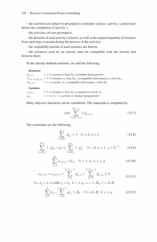
238 Resource-Constrained Project Scheduling
– the activities are subject to precedence constraints such as: activity j cannot startbefore the completion of activity i;
– the activities are not preemptive;
– the duration of each activity is known, as well as the required quantity of resourcefrom each type (constant during the process of the activity);
– the availability periods of each resource are known;
– the resources used by an activity must be compatible with the activity andbetween them.
To the already-defined notations, we add the following:
– Resources:
σk,u,t = 1 ⇔ resource u from Rk is available during period t
λrk1,u1,k2,u2 = 1 ⇔ resource u1 from Rk1 is compatible with resource u2 from Rk2
λai,k,u = 1 ⇔ activity Ai is compatible with resource u from Rk
– Variables:
ωi,k,u = 1 ⇔ resource u from Rk is assigned to activity Ai
y′i,t = 1 ⇔ Ci = t, activity Ai finishes during period t
Many objective functions can be considered. The makespan is computed by:
minLCn+1∑
t=ECn+1
t.y′n+1,t (15.7)
The constraints are the following:
LCi∑t=ECi
y′i,t = 1 ∀i = 0..n + 1 (15.8)
LCj∑t=ECj
t · y′j,t + pi ≤
LCi∑t=ECi
t · y′i,t ∀i = 0..n + 1, j ∈ Γ−1
i (15.9)
Bk∑u=1
ωi,k,u = bi,k ∀i = 1..n, k = 1..q (15.10)
ωi1,k,u + ωi2,k,u +t+pi1−1∑
s=t
y′i1,s +
t+pi2−1∑t2=t
y′i2,t2 ≤ 3
∀i1, i2 = 1..n with i1 < i2, k = 1..q, u = 1..Bk, t = 0..H
(15.11)
k∑i=1
bi,k ·t+pi−1∑
s=t
y′i,t ≤ Bk ∀ t = 0..H, k = 1..q (15.12)
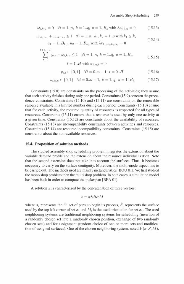
Assembly Shop Scheduling 239
ωi,k,u = 0 ∀i = 1..n, k = 1..q, u = 1..Bk with λai,k,u = 0 (15.13)
ωi,k1,u1 + ωi,k2,u2 ≤ 1 ∀i = 1..n, k1, k2 = 1..q with k1 ≤ k2,
u1 = 1..Bk1 , u2 = 1..Bk2 with λrk1,u1,k2,u2 = 0(15.14)
t+pi−1∑s=t
yi,t + ωi,k,u ≤ 1 ∀i = 1..n, k = 1..q, u = 1..Bk,
t = 1..H with σk,u,t = 0
(15.15)
yi,t ∈ {0, 1} ∀i = 0..n + 1, t = 0..H (15.16)
ωi,k,u ∈ {0, 1} ∀i = 0..n + 1, k = 1..q, u = 1..Bk (15.17)
Constraints (15.8) are constraints on the processing of the activities; they assurethat each activity finishes during only one period. Constraints (15.9) concern the prece-dence constraints. Constraints (15.10) and (15.11) are constraints on the renewableresource available in a limited number during each period. Constraints (15.10) ensurethat for each activity, the required quantity of resources is respected for all types ofresources. Constraints (15.11) ensure that a resource is used by only one activity ata given time. Constraints (15.12) are constraints about the availability of resources.Constraints (15.13) are incompatibility constraints between activities and resources.Constraints (15.14) are resource incompatibility constraints. Constraints (15.15) areconstraints about the non-available resources.
15.4. Proposition of solution methods
The studied assembly shop scheduling problem integrates the extension about thevariable demand profile and the extension about the resource individualization. Notethat the second extension does not take into account the surfaces. Thus, it becomesnecessary to carry on the surface contiguity. Moreover, the multi-mode aspect has tobe carried out. The methods used are mainly metaheuristics [BOU 01]. We first studiedthe mono shop problem then the multi shop problem. In both cases, a simulation modelhas been built in order to compute the makespan [BEA 01].
A solution x is characterized by the concatenation of three vectors:
x = σ&S&M
where σi represents the ith set of parts to begin its process, Si represents the surfaceused by the top left corner of set σi and Mi is the used orientation for set σi. The usedneighboring systems are traditional neighboring systems for scheduling (insertion ofa randomly chosen set into a randomly chosen position, exchange of two randomlychosen sets) and for assignment (random choice of one or more sets and modifica-tion of assigned surfaces). One of the chosen neighboring system, noted V (σ, S,M),
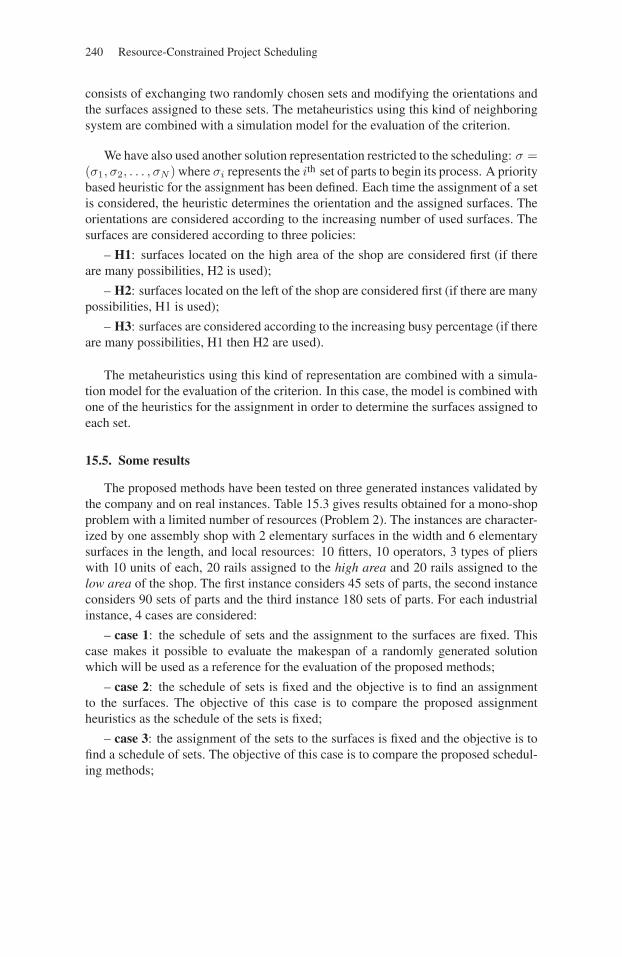
240 Resource-Constrained Project Scheduling
consists of exchanging two randomly chosen sets and modifying the orientations andthe surfaces assigned to these sets. The metaheuristics using this kind of neighboringsystem are combined with a simulation model for the evaluation of the criterion.
We have also used another solution representation restricted to the scheduling: σ =(σ1, σ2, . . . , σN ) where σi represents the ith set of parts to begin its process. A prioritybased heuristic for the assignment has been defined. Each time the assignment of a setis considered, the heuristic determines the orientation and the assigned surfaces. Theorientations are considered according to the increasing number of used surfaces. Thesurfaces are considered according to three policies:
– H1: surfaces located on the high area of the shop are considered first (if thereare many possibilities, H2 is used);
– H2: surfaces located on the left of the shop are considered first (if there are manypossibilities, H1 is used);
– H3: surfaces are considered according to the increasing busy percentage (if thereare many possibilities, H1 then H2 are used).
The metaheuristics using this kind of representation are combined with a simula-tion model for the evaluation of the criterion. In this case, the model is combined withone of the heuristics for the assignment in order to determine the surfaces assigned toeach set.
15.5. Some results
The proposed methods have been tested on three generated instances validated bythe company and on real instances. Table 15.3 gives results obtained for a mono-shopproblem with a limited number of resources (Problem 2). The instances are character-ized by one assembly shop with 2 elementary surfaces in the width and 6 elementarysurfaces in the length, and local resources: 10 fitters, 10 operators, 3 types of plierswith 10 units of each, 20 rails assigned to the high area and 20 rails assigned to thelow area of the shop. The first instance considers 45 sets of parts, the second instanceconsiders 90 sets of parts and the third instance 180 sets of parts. For each industrialinstance, 4 cases are considered:
– case 1: the schedule of sets and the assignment to the surfaces are fixed. Thiscase makes it possible to evaluate the makespan of a randomly generated solutionwhich will be used as a reference for the evaluation of the proposed methods;
– case 2: the schedule of sets is fixed and the objective is to find an assignmentto the surfaces. The objective of this case is to compare the proposed assignmentheuristics as the schedule of the sets is fixed;
– case 3: the assignment of the sets to the surfaces is fixed and the objective is tofind a schedule of sets. The objective of this case is to compare the proposed schedul-ing methods;
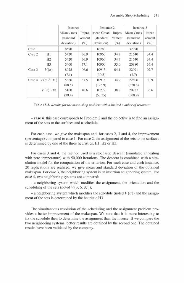
Assembly Shop Scheduling 241
Instance 1 Instance 2 Instance 3
Mean Cmax Impro Mean Cmax Impro Mean Cmax Impro
(standard vement (standard vement (standard vement
deviation) (%) deviation) (%) deviation) (%)
Case 1 8590 16780 32990
Case 2 H1 5420 36.9 10960 34.7 21640 34.4
H2 5420 36.9 10960 34.7 21640 34.4
H3 5400 37.1 10900 35.0 20980 36.4
Case 3 V (σ) 8025 06.6 10913 04.1 32091 02.7
(7.1) (30.5) (2.7)
Case 4 V (σ, S, M) 5366 37.5 10916 34.9 22806 30.9
(88.5) (125.9) (328.8)
V (σ), H3 5100 40.6 10279 38.8 20927 36.6
(39.4) (57.35) (308.9)
Table 15.3. Results for the mono-shop problem with a limited number of resources
– case 4: this case corresponds to Problem 2 and the objective is to find an assign-ment of the sets to the surfaces and a schedule.
For each case, we give the makespan and, for cases 2, 3 and 4, the improvement(percentage) compared to case 1. For case 2, the assignment of the sets to the surfacesis determined by one of the three heuristics, H1, H2 or H3.
For cases 3 and 4, the method used is a stochastic descent (simulated annealingwith zero temperature) with 50,000 iterations. The descent is combined with a sim-ulation model for the computation of the criterion. For each case and each instance,20 replications are realized, we give mean and standard deviation of the obtainedmakespan. For case 3, the neighboring system is an insertion neighboring system. Forcase 4, two neighboring systems are compared:
– a neighboring system which modifies the assignment, the orientation and thescheduling of the sets (noted V (σ, S,M));
– a neighboring system which modifies the schedule (noted V (σ)) and the assign-ment of the sets is determined by the heuristic H3.
The simultaneous resolution of the scheduling and the assignment problem pro-vides a better improvement of the makespan. We note that it is more interesting tofix the schedule then to determine the assignment than the inverse. If we compare thetwo neighboring systems, better results are obtained by the second one. The obtainedresults have been validated by the company.

242 Resource-Constrained Project Scheduling
15.6. Conclusion
The objective of this chapter was to present an industrial problem which can belinked to a MM-RCPSP and the methods proposed to solve it. From an academic pointof view, the study of this problem led us to propose two extensions: RCPSP withvariable demand profile and RCPSP with resource individualization. Mathematicalmodels for these extensions have been presented for the Single Mode. Similar workson the Multi-Mode are in progress.
In the future, we plan to use the proposed extensions in other domains, such as inthe healthcare systems for the scheduling of surgical operations in operating theaters.

Chapter 16
Employee Scheduling in an IT Company
This chapter describes a project scheduling problem of a French Information Tech-nology company called Eskape. In this company, a project typically corresponds tosoftware development. Resources required for the execution of the project activi-ties are the employees. We consider that the requirements of the activities are time-dependent, that employees have different skills and that the legal constraints dictatedby the French workforce legislation have to be respected. The problem is studied usinga global approach, dealing first with the predictive phase, where the project activitiesare scheduled and the employees planning are constructed. Under some hypothesesconcerning unexpected events, a proactive approach and finally a reactive approachare proposed.
16.1. Introduction
We consider projects where activities only need human resources to be performed.In Eskape these resources correspond to developers and a project corresponds to asoftware development. Activities correspond to the analysis of the client requirements,development of the application, tests, etc. Each activity needs particular skills to beperformed, depending on the project requirements: analysis method, language devel-opment (C++, Java, etc.), etc. Moreover, since resources are human, specific con-straints dictated by the workforce legislation have to be taken into account.
The problem consists of finding a feasible solution, i.e. an assignment of theproject activities to the employees, without violating legal constraints or project con-straints and optimizing a given criterion.
Chapter written by Laure-Emmanuelle DREZET and Jean-Charles BILLAUT.
243
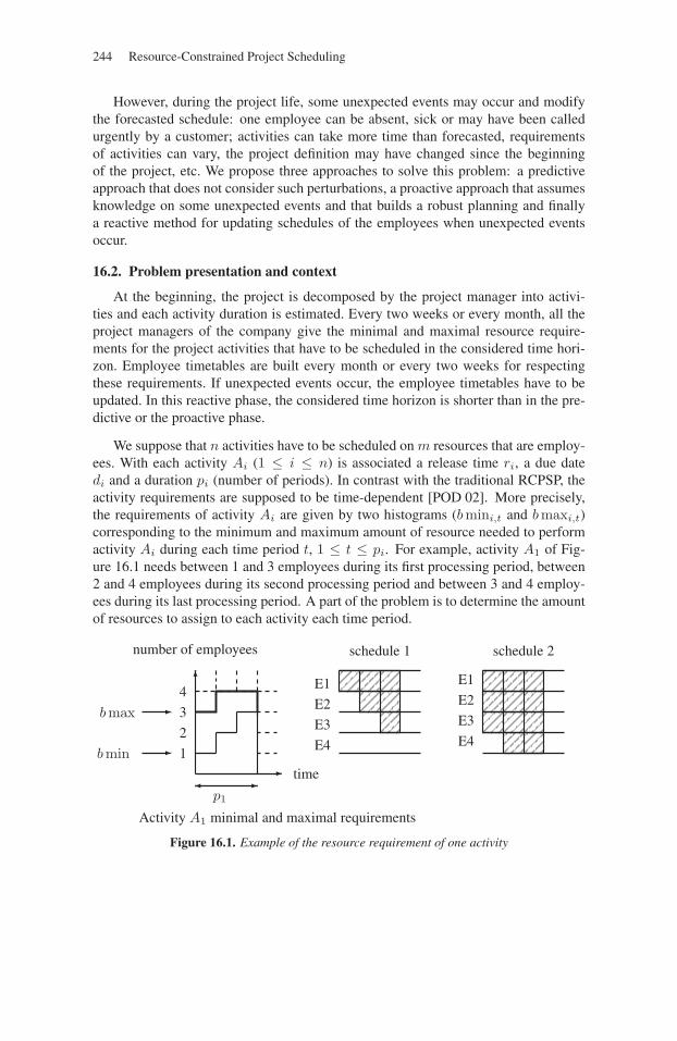
244 Resource-Constrained Project Scheduling
However, during the project life, some unexpected events may occur and modifythe forecasted schedule: one employee can be absent, sick or may have been calledurgently by a customer; activities can take more time than forecasted, requirementsof activities can vary, the project definition may have changed since the beginningof the project, etc. We propose three approaches to solve this problem: a predictiveapproach that does not consider such perturbations, a proactive approach that assumesknowledge on some unexpected events and that builds a robust planning and finallya reactive method for updating schedules of the employees when unexpected eventsoccur.
16.2. Problem presentation and context
At the beginning, the project is decomposed by the project manager into activi-ties and each activity duration is estimated. Every two weeks or every month, all theproject managers of the company give the minimal and maximal resource require-ments for the project activities that have to be scheduled in the considered time hori-zon. Employee timetables are built every month or every two weeks for respectingthese requirements. If unexpected events occur, the employee timetables have to beupdated. In this reactive phase, the considered time horizon is shorter than in the pre-dictive or the proactive phase.
We suppose that n activities have to be scheduled on m resources that are employ-ees. With each activity Ai (1 ≤ i ≤ n) is associated a release time ri, a due datedi and a duration pi (number of periods). In contrast with the traditional RCPSP, theactivity requirements are supposed to be time-dependent [POD 02]. More precisely,the requirements of activity Ai are given by two histograms (bmini,t and bmaxi,t)corresponding to the minimum and maximum amount of resource needed to performactivity Ai during each time period t, 1 ≤ t ≤ pi. For example, activity A1 of Fig-ure 16.1 needs between 1 and 3 employees during its first processing period, between2 and 4 employees during its second processing period and between 3 and 4 employ-ees during its last processing period. A part of the problem is to determine the amountof resources to assign to each activity each time period.
�
�
1
2
3
4
Activity A1 minimal and maximal requirements
time
number of employees
��p1
schedule 1 schedule 2
E1
E2
E3
E4
E1
E2
E3
E4�
�
bmin
bmax
Figure 16.1. Example of the resource requirement of one activity
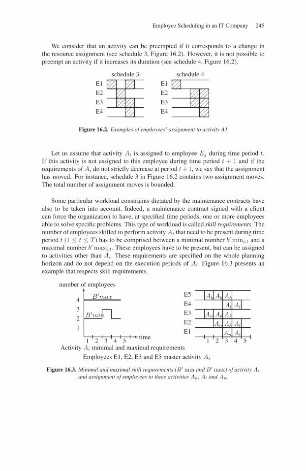
Employee Scheduling in an IT Company 245
We consider that an activity can be preempted if it corresponds to a change inthe resource assignment (see schedule 3, Figure 16.2). However, it is not possible topreempt an activity if it increases its duration (see schedule 4, Figure 16.2).
schedule 3
E1
E2
E3
E4
schedule 4
E1
E2
E3
E4
Figure 16.2. Examples of employees’ assignment to activity A1
Let us assume that activity Ai is assigned to employee Ej during time period t.If this activity is not assigned to this employee during time period t + 1 and if therequirements of Ai do not strictly decrease at period t + 1, we say that the assignmenthas moved. For instance, schedule 3 in Figure 16.2 contains two assignment moves.The total number of assignment moves is bounded.
Some particular workload constraints dictated by the maintenance contracts havealso to be taken into account. Indeed, a maintenance contract signed with a clientcan force the organization to have, at specified time periods, one or more employeesable to solve specific problems. This type of workload is called skill requirements. Thenumber of employees skilled to perform activity Ai that need to be present during timeperiod t (1 ≤ t ≤ T ) has to be comprised between a minimal number b′ mini,t and amaximal number b′ maxi,t. These employees have to be present, but can be assignedto activities other than Ai. These requirements are specified on the whole planninghorizon and do not depend on the execution periods of Ai. Figure 16.3 presents anexample that respects skill requirements.
�
�
1
2
3
4
Activity Ai minimal and maximal requirements
time
number of employees
E1
E2
E3
E4
E5B′max
B′min
Ak Ak Ak
Ak Ak
Ak
Am
Al Al
Al
Al
Am
Am
Employees E1, E2, E3 and E5 master activity Ai
1 2 3 4 5 1 2 3 4 5
Figure 16.3. Minimal and maximal skill requirements (B′ min and B′ max) of activity Ai
and assignment of employees to three activities Ak, Al and Am
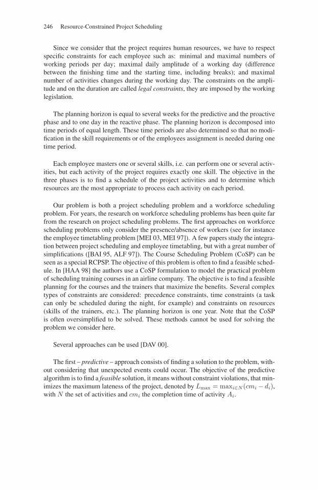
246 Resource-Constrained Project Scheduling
Since we consider that the project requires human resources, we have to respectspecific constraints for each employee such as: minimal and maximal numbers ofworking periods per day; maximal daily amplitude of a working day (differencebetween the finishing time and the starting time, including breaks); and maximalnumber of activities changes during the working day. The constraints on the ampli-tude and on the duration are called legal constraints, they are imposed by the workinglegislation.
The planning horizon is equal to several weeks for the predictive and the proactivephase and to one day in the reactive phase. The planning horizon is decomposed intotime periods of equal length. These time periods are also determined so that no modi-fication in the skill requirements or of the employees assignment is needed during onetime period.
Each employee masters one or several skills, i.e. can perform one or several activ-ities, but each activity of the project requires exactly one skill. The objective in thethree phases is to find a schedule of the project activities and to determine whichresources are the most appropriate to process each activity on each period.
Our problem is both a project scheduling problem and a workforce schedulingproblem. For years, the research on workforce scheduling problems has been quite farfrom the research on project scheduling problems. The first approaches on workforcescheduling problems only consider the presence/absence of workers (see for instancethe employee timetabling problem [MEI 03, MEI 97]). A few papers study the integra-tion between project scheduling and employee timetabling, but with a great number ofsimplifications ([BAI 95, ALF 97]). The Course Scheduling Problem (CoSP) can beseen as a special RCPSP. The objective of this problem is often to find a feasible sched-ule. In [HAA 98] the authors use a CoSP formulation to model the practical problemof scheduling training courses in an airline company. The objective is to find a feasibleplanning for the courses and the trainers that maximize the benefits. Several complextypes of constraints are considered: precedence constraints, time constraints (a taskcan only be scheduled during the night, for example) and constraints on resources(skills of the trainers, etc.). The planning horizon is one year. Note that the CoSPis often oversimplified to be solved. These methods cannot be used for solving theproblem we consider here.
Several approaches can be used [DAV 00].
The first – predictive – approach consists of finding a solution to the problem, with-out considering that unexpected events could occur. The objective of the predictivealgorithm is to find a feasible solution, it means without constraint violations, that min-imizes the maximum lateness of the project, denoted by Lmax = maxi∈N (cmi − di),with N the set of activities and cmi the completion time of activity Ai.
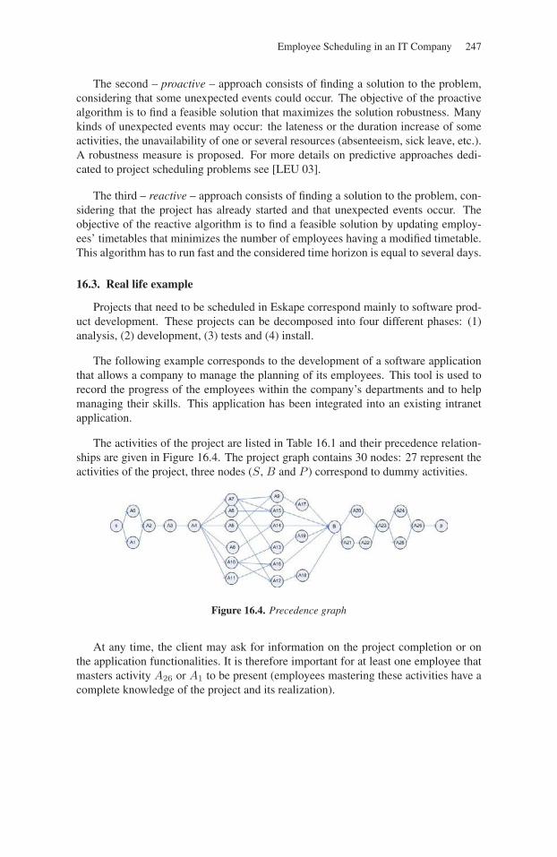
Employee Scheduling in an IT Company 247
The second – proactive – approach consists of finding a solution to the problem,considering that some unexpected events could occur. The objective of the proactivealgorithm is to find a feasible solution that maximizes the solution robustness. Manykinds of unexpected events may occur: the lateness or the duration increase of someactivities, the unavailability of one or several resources (absenteeism, sick leave, etc.).A robustness measure is proposed. For more details on predictive approaches dedi-cated to project scheduling problems see [LEU 03].
The third – reactive – approach consists of finding a solution to the problem, con-sidering that the project has already started and that unexpected events occur. Theobjective of the reactive algorithm is to find a feasible solution by updating employ-ees’ timetables that minimizes the number of employees having a modified timetable.This algorithm has to run fast and the considered time horizon is equal to several days.
16.3. Real life example
Projects that need to be scheduled in Eskape correspond mainly to software prod-uct development. These projects can be decomposed into four different phases: (1)analysis, (2) development, (3) tests and (4) install.
The following example corresponds to the development of a software applicationthat allows a company to manage the planning of its employees. This tool is used torecord the progress of the employees within the company’s departments and to helpmanaging their skills. This application has been integrated into an existing intranetapplication.
The activities of the project are listed in Table 16.1 and their precedence relation-ships are given in Figure 16.4. The project graph contains 30 nodes: 27 represent theactivities of the project, three nodes (S, B and P ) correspond to dummy activities.
Figure 16.4. Precedence graph
At any time, the client may ask for information on the project completion or onthe application functionalities. It is therefore important for at least one employee thatmasters activity A26 or A1 to be present (employees mastering these activities have acomplete knowledge of the project and its realization).
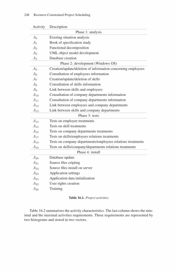
248 Resource-Constrained Project Scheduling
Activity Description
Phase 1: analysis
A0 Existing situation analysisA1 Book of specification studyA2 Functional decompositionA3 UML object model developmentA4 Database creation
Phase 2: development (Windows OS)
A5 Creation/update/deletion of information concerning employeesA6 Consultation of employees informationA7 Creation/update/deletion of skillsA8 Consultation of skills informationA9 Link between skills and employeesA10 Consultation of company departments informationA11 Consultation of company departments informationA12 Link between employees and company departmentsA13 Link between skills and company departments
Phase 3: tests
A14 Tests on employee treatmentsA15 Tests on skill treatmentsA16 Tests on company departments treatmentsA17 Tests on skills/employees relations treatmentsA18 Tests on company departments/employees relations treatmentsA19 Tests on skills/company/departments relations treatments
Phase 4: install
A20 Database updateA21 Source files criptingA22 Source files install on serverA23 Application settingsA24 Application data initializationA25 User rights creationA26 Training
Table 16.1. Project activities
Table 16.2 summarizes the activity characteristics. The last column shows the min-imal and the maximal activities requirements. These requirements are represented bytwo histograms and stored in two vectors.
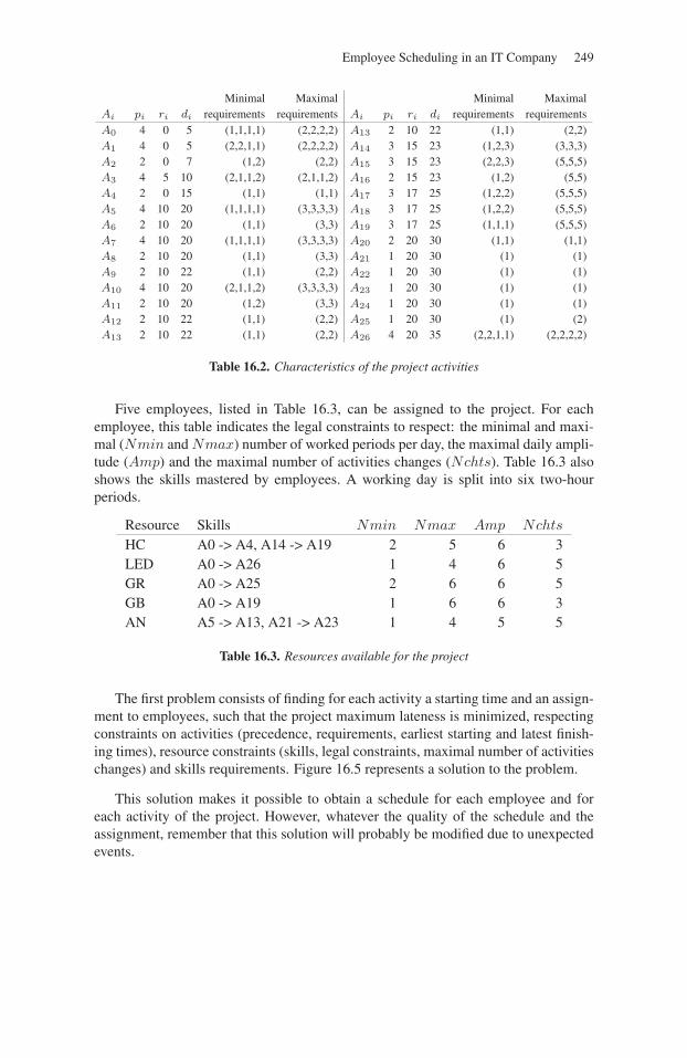
Employee Scheduling in an IT Company 249
Minimal Maximal Minimal MaximalAi pi ri di requirements requirements Ai pi ri di requirements requirementsA0 4 0 5 (1,1,1,1) (2,2,2,2) A13 2 10 22 (1,1) (2,2)A1 4 0 5 (2,2,1,1) (2,2,2,2) A14 3 15 23 (1,2,3) (3,3,3)A2 2 0 7 (1,2) (2,2) A15 3 15 23 (2,2,3) (5,5,5)A3 4 5 10 (2,1,1,2) (2,1,1,2) A16 2 15 23 (1,2) (5,5)A4 2 0 15 (1,1) (1,1) A17 3 17 25 (1,2,2) (5,5,5)A5 4 10 20 (1,1,1,1) (3,3,3,3) A18 3 17 25 (1,2,2) (5,5,5)A6 2 10 20 (1,1) (3,3) A19 3 17 25 (1,1,1) (5,5,5)A7 4 10 20 (1,1,1,1) (3,3,3,3) A20 2 20 30 (1,1) (1,1)A8 2 10 20 (1,1) (3,3) A21 1 20 30 (1) (1)A9 2 10 22 (1,1) (2,2) A22 1 20 30 (1) (1)A10 4 10 20 (2,1,1,2) (3,3,3,3) A23 1 20 30 (1) (1)A11 2 10 20 (1,2) (3,3) A24 1 20 30 (1) (1)A12 2 10 22 (1,1) (2,2) A25 1 20 30 (1) (2)A13 2 10 22 (1,1) (2,2) A26 4 20 35 (2,2,1,1) (2,2,2,2)
Table 16.2. Characteristics of the project activities
Five employees, listed in Table 16.3, can be assigned to the project. For eachemployee, this table indicates the legal constraints to respect: the minimal and maxi-mal (Nmin and Nmax) number of worked periods per day, the maximal daily ampli-tude (Amp) and the maximal number of activities changes (Nchts). Table 16.3 alsoshows the skills mastered by employees. A working day is split into six two-hourperiods.
Resource Skills Nmin Nmax Amp Nchts
HC A0 -> A4, A14 -> A19 2 5 6 3LED A0 -> A26 1 4 6 5GR A0 -> A25 2 6 6 5GB A0 -> A19 1 6 6 3AN A5 -> A13, A21 -> A23 1 4 5 5
Table 16.3. Resources available for the project
The first problem consists of finding for each activity a starting time and an assign-ment to employees, such that the project maximum lateness is minimized, respectingconstraints on activities (precedence, requirements, earliest starting and latest finish-ing times), resource constraints (skills, legal constraints, maximal number of activitieschanges) and skills requirements. Figure 16.5 represents a solution to the problem.
This solution makes it possible to obtain a schedule for each employee and foreach activity of the project. However, whatever the quality of the schedule and theassignment, remember that this solution will probably be modified due to unexpectedevents.
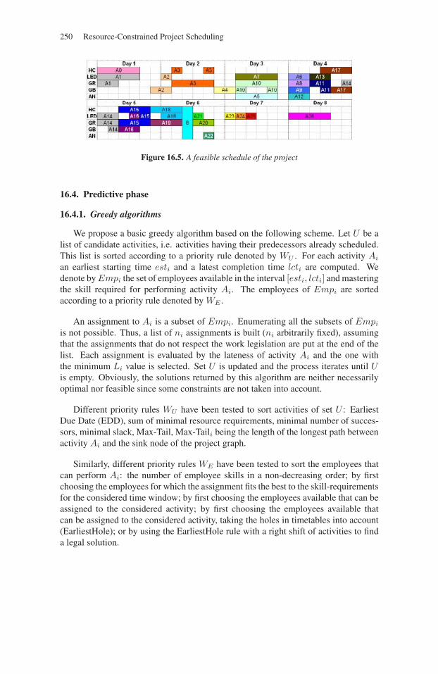
250 Resource-Constrained Project Scheduling
Figure 16.5. A feasible schedule of the project
16.4. Predictive phase
16.4.1. Greedy algorithms
We propose a basic greedy algorithm based on the following scheme. Let U be alist of candidate activities, i.e. activities having their predecessors already scheduled.This list is sorted according to a priority rule denoted by WU . For each activity Ai
an earliest starting time esti and a latest completion time lcti are computed. Wedenote by Empi the set of employees available in the interval [esti, lcti] and masteringthe skill required for performing activity Ai. The employees of Empi are sortedaccording to a priority rule denoted by WE .
An assignment to Ai is a subset of Empi. Enumerating all the subsets of Empi
is not possible. Thus, a list of ni assignments is built (ni arbitrarily fixed), assumingthat the assignments that do not respect the work legislation are put at the end of thelist. Each assignment is evaluated by the lateness of activity Ai and the one withthe minimum Li value is selected. Set U is updated and the process iterates until Uis empty. Obviously, the solutions returned by this algorithm are neither necessarilyoptimal nor feasible since some constraints are not taken into account.
Different priority rules WU have been tested to sort activities of set U : EarliestDue Date (EDD), sum of minimal resource requirements, minimal number of succes-sors, minimal slack, Max-Tail, Max-Taili being the length of the longest path betweenactivity Ai and the sink node of the project graph.
Similarly, different priority rules WE have been tested to sort the employees thatcan perform Ai: the number of employee skills in a non-decreasing order; by firstchoosing the employees for which the assignment fits the best to the skill-requirementsfor the considered time window; by first choosing the employees available that can beassigned to the considered activity; by first choosing the employees available thatcan be assigned to the considered activity, taking the holes in timetables into account(EarliestHole); or by using the EarliestHole rule with a right shift of activities to finda legal solution.
Employee Scheduling in an IT Company 251
When all the activities have been scheduled, a repairing phase is executed toincrease the number of employees assigned to each activity of the project. The aim isto decrease the number of skill-requirements violations without increasing the numberof violated legal constraints. This is done by assigning some additional employees toactivities when it is both possible and required.
16.4.2. Tabu search algorithm
The aim of the tabu search algorithm is to enhance the solution returned by thegreedy algorithm. A state in this tabu search algorithm is composed of a vector giv-ing for each activity of the project its starting and ending time periods, and by theassignment matrix of employees to activities, for each time period.
Four types of move are used in this method, based on activity moves and swaps oron employee assignments moves or swaps: (1) the change of the assignment of oneemployee on one time period; (2) the swap between the assignments of two employeesover the same time period; (3) the left or right shift of the starting time of one activityfor one or several time periods; and (4) the swap between two activities.
In a given state, the generated moves are those that lead to neighbors respectingprecedence constraints between activities and skill constraint. As the size of the gen-erated neighborhood may be very large, all the neighbours of the current solution arenot generated at each iteration: moves based on employees are only generated froma selected time period and the number of time periods of the right and left shifts arebounded.
A solution S is evaluated using two criteria: the number of violated constraintsand the maximum lateness. These two objectives are considered in the lexicographicorder.
16.5. Proactive phase
In a proactive approach, the schedule is built considering some knowledge on theunexpected events that could occur and modify the current schedule. In our problem,we consider several types of unexpected events. Moreover, the company is not neces-sarily interested to have a solution optimizing the maximum lateness, if this solutionhas to be totally recomputed when the first unexpected event occurs. Thus, we searchfor solutions minimizing the total number of violated constraints and among all thesesolutions, we search for the most robust solution. For more details on robust schedul-ing see [BIL 05].
The unexpected events that may occur concern both employees and activities. Twomain types of perturbations can be distinguished: the absenteeism of employees andthe modification of the duration of activities. We consider that each employee maybe absent. This unavailability can correspond to the assignment of these employees
252 Resource-Constrained Project Scheduling
to activities belonging to other projects or to unexpected leaves. Two data can beassociated with each employee: a probability of absenteeism and a maximal absenceduration. When perturbations affect an activity, we consider that the duration of thisactivity is modified. In reality, when this kind of perturbation occurs, it correspondsto an increase of the duration of the activity. This perturbation is often due to mistakesmade by the project manager when he/she estimates the duration of the activities.Thus, we consider here that the duration of the perturbated activity is greater than thenormal duration. Therefore, two pieces of data are associated with each activity: aprobability of perturbation and a maximal duration of perturbation.
We define two robustness measures for a schedule S: ρPS which is based on
employees, and ρAS which is based on activities. ρP
S is computed using some informa-tion on each employee j, as the absence probability pindj
and the maximal durationof absence dindj
. ρAS is computed using some knowledge on the possible disturbances
for each activity: the probability of perturbation and the maximal duration of pertur-bation. The total robustness of schedule S is given by a linear combination of ρA
S andρP
S (with α = 0.5).
ρPS = min
j∈J−(workloadj + dindj
)× pindj
ρAS = min
i∈I(slacki − dalli)× palli
ρS = −(1− α)× ρAS − α× ρP
S
It is important to note that the robustness metric and the maximum lateness cri-terion are conflicting in this context. The predictive algorithm has been adapted andtwo new priority rules have been defined: ROBACT based on the slack of activityAi and the probability of perturbation, and RobEmp based on the load of employeeEj and the probability of absenteeism. The selection of the best assignment uses therobustness measure instead of the lateness measure.
The predictive tabu search algorithm has also been adapted to evaluate the qualityof each neighbor with its number of violated constraints and its robustness.
16.6. Reactive phase
In this phase, the company must face absenteeism of some employees or modifica-tion of the duration of some activities. It is supposed that the timetables of employeesare known and that due to unforeseen events we have to modify some of these timeta-bles. Since the algorithm has to return a solution quite quickly, the considered timehorizon has been reduced to one day. On the other hand, since more information isavailable during this phase than during the previous one (predictive or proactive), wecan be more precise and the length of each time period has been reduced in the reac-tive phase. As beginning and ending periods of activities are the data of this problem,
Employee Scheduling in an IT Company 253
precedence relationships between activities are implicitly known and are not explicitlyconsidered in this phase.
A weight is associated with each employee if his timetable has already been modi-fied recently. The aim is to ensure ourselves that the modifications do not always con-cern the same employees. The objective of the problem is to update timetables, suchthat the new constraints are satisfied and the weighted number of modified timetablesis minimized.
A tabu search algorithm has been developed for this problem, inspired by the tabusearch algorithm of [MUS 04]. The initial solution of the method corresponds to theinitial employee timetables. This solution can violate either the skill requirements orthe activity requirement constraints. As for the predictive tabu search algorithm, crite-ria are minimized in a lexicographical order: first the number of violated constraintsand then the number of modified timetables. The tabu list contains moves that wereselected during the previous iterations. As the size of the neighborhood may be verylarge, only a reduced number of neighbors (limited by a parameter) are generated. Themoves depend on the kind of violated constraints and different diversification methodshave been tested.
16.7. Computational experiments
16.7.1. Predictive and proactive algorithms
To evaluate the performances of the algorithms, we have adapted the instancesof the PSPLIB (see [KOL 97, PSPib] and Chapter 7). The modified instances aregenerated using the precedence graph of the PSPLIB to link activities and to findtheir release times and due dates. The activities requirements are computed using theoriginal requirement of activities and the number of employees skilled to perform theactivities. We assume that each employee masters 70% of the skills in all the instanceswe consider.
Depending on the priority rules, 32 heuristic algorithms have been tested in fourcategories (some heuristic algorithms use a second priority-rule to break ties). Theresults show that two heuristic algorithms outperform the others for the robustnessmeasure. We can also notice that the robust algorithms make it possible to respectmore constraints (only legal and skill-requirements constraints may be violated) thanthe predictive algorithms. All the problem instances have been solved by the heuristicalgorithms in less than one second.
The predictive and the proactive tabu search algorithms have also been evaluated,using the results given by the heuristic algorithms. Initial solutions of the predictivetabu search algorithm are provided by the best predictive greedy heuristic. Table 16.4presents the results of the tabu search algorithms. Column “# of viol. constr.” is theaverage number of violated constraints, columns Lmax and ρS indicate the averagevalue of these criteria.
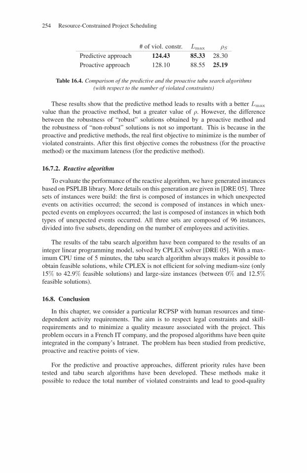
254 Resource-Constrained Project Scheduling
# of viol. constr. Lmax ρS
Predictive approach 124.43 85.33 28.30
Proactive approach 128.10 88.55 25.19
Table 16.4. Comparison of the predictive and the proactive tabu search algorithms(with respect to the number of violated constraints)
These results show that the predictive method leads to results with a better Lmax
value than the proactive method, but a greater value of ρ. However, the differencebetween the robustness of “robust” solutions obtained by a proactive method andthe robustness of “non-robust” solutions is not so important. This is because in theproactive and predictive methods, the real first objective to minimize is the number ofviolated constraints. After this first objective comes the robustness (for the proactivemethod) or the maximum lateness (for the predictive method).
16.7.2. Reactive algorithm
To evaluate the performance of the reactive algorithm, we have generated instancesbased on PSPLIB library. More details on this generation are given in [DRE 05]. Threesets of instances were build: the first is composed of instances in which unexpectedevents on activities occurred; the second is composed of instances in which unex-pected events on employees occurred; the last is composed of instances in which bothtypes of unexpected events occurred. All three sets are composed of 96 instances,divided into five subsets, depending on the number of employees and activities.
The results of the tabu search algorithm have been compared to the results of aninteger linear programming model, solved by CPLEX solver [DRE 05]. With a max-imum CPU time of 5 minutes, the tabu search algorithm always makes it possible toobtain feasible solutions, while CPLEX is not efficient for solving medium-size (only15% to 42.9% feasible solutions) and large-size instances (between 0% and 12.5%feasible solutions).
16.8. Conclusion
In this chapter, we consider a particular RCPSP with human resources and time-dependent activity requirements. The aim is to respect legal constraints and skill-requirements and to minimize a quality measure associated with the project. Thisproblem occurs in a French IT company, and the proposed algorithms have been quiteintegrated in the company’s Intranet. The problem has been studied from predictive,proactive and reactive points of view.
For the predictive and proactive approaches, different priority rules have beentested and tabu search algorithms have been developed. These methods make itpossible to reduce the total number of violated constraints and lead to good-quality

Employee Scheduling in an IT Company 255
solutions. For the reactive phase, a tabu search algorithm and a MILP have beendeveloped. The heuristic method leads quickly to feasible solutions, while the MILPis quite inefficient.
Our future work will consist of developing new robustness measures, consider-ing explicitly the resource constraints when computing slacks, for example. All theheuristic algorithms can also be used to generate a part of an initial population for agenetic algorithm that may reach a better compromise between the number of violatedconstraints and the robustness of the solution (for the proactive phase) or the numberof modified timetables (for the reactive phase).

256
This page intentionally left blank
Chapter 17
Rolling Ingots Production Scheduling
In this chapter we study a real-world scheduling problem arising in the contextof rolling ingots production in aluminium industry. In the first part of the chapter wereview the production process and discuss the constraints that have to be observedwhen scheduling a given set of production orders on the production facilities. We thenshow how this problem can be modeled as a RCPSP with minimal and maximal timelags between activities and different kinds of renewable resources. A solution pro-cedure of type branch-and-bound is sketched in the second part. The basic principleconsists of relaxing the resource constraints by assuming infinite resource availability.Resulting resource conflicts are iteratively resolved by introducing precedence rela-tionships among activities competing for the same resources.
17.1. Introduction
We consider the production of rolling ingots, i.e. ingots of a certain aluminiumalloy in rectangular form. These ingots are the starting material for the rolling of sheet,strip and foil. The production process can be described as follows (see section 1.4 in[KAM 99] and Figure 17.1).
In a melting furnace, which is called a potroom, the ingredients composing thealloy are smelted in an electrolytical process. In general, several different potroomsare available at a production plant. One or several casting units belong to each pot-room. A casting unit consists of a holding fixture for a mould, a retractable hydrauliccylinder named stool, and a stool-cap, which closes the bottom of the mould at the
Chapter written by Christoph SCHWINDT and Norbert TRAUTMANN.
257
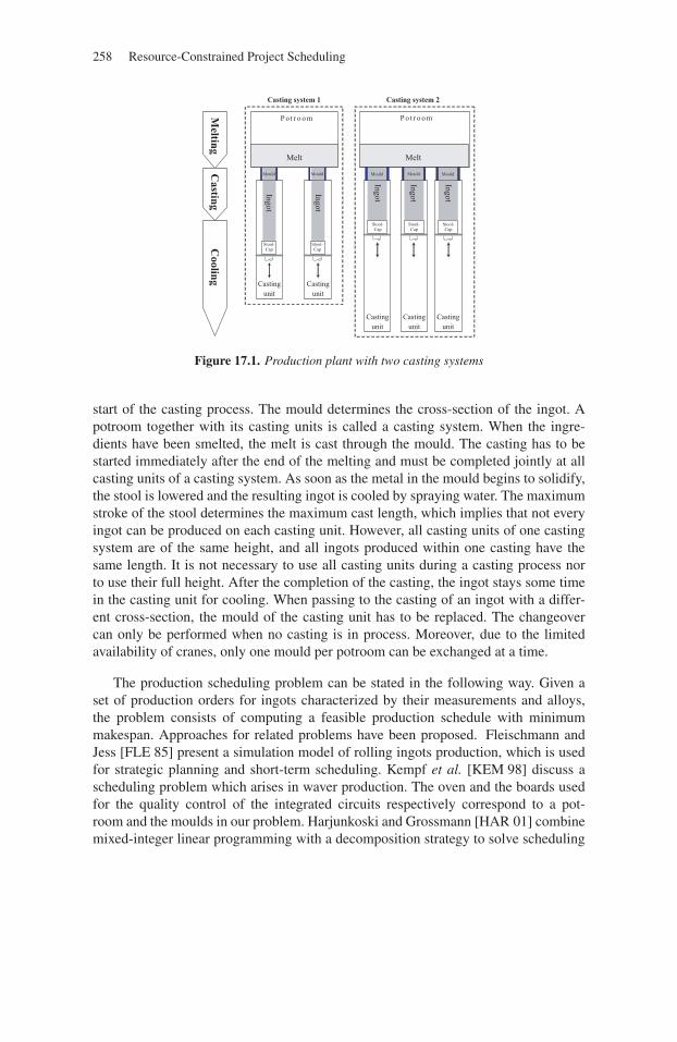
258 Resource-Constrained Project Scheduling
P o t r o o m
Mould Mould
P o t r o o m
Mould Mould Mould
Casting system 1 Casting system 2
Melting
Casting
Cooling
Castingunit
Castingunit
Castingunit
Castingunit
Castingunit
Melt Melt
Ingot
Ingot
Ingot
Ingot
Ingot
Stool-Cap
Stool-Cap
Stool-Cap
Stool-Cap
Stool-Cap
Figure 17.1. Production plant with two casting systems
start of the casting process. The mould determines the cross-section of the ingot. Apotroom together with its casting units is called a casting system. When the ingre-dients have been smelted, the melt is cast through the mould. The casting has to bestarted immediately after the end of the melting and must be completed jointly at allcasting units of a casting system. As soon as the metal in the mould begins to solidify,the stool is lowered and the resulting ingot is cooled by spraying water. The maximumstroke of the stool determines the maximum cast length, which implies that not everyingot can be produced on each casting unit. However, all casting units of one castingsystem are of the same height, and all ingots produced within one casting have thesame length. It is not necessary to use all casting units during a casting process norto use their full height. After the completion of the casting, the ingot stays some timein the casting unit for cooling. When passing to the casting of an ingot with a differ-ent cross-section, the mould of the casting unit has to be replaced. The changeovercan only be performed when no casting is in process. Moreover, due to the limitedavailability of cranes, only one mould per potroom can be exchanged at a time.
The production scheduling problem can be stated in the following way. Given aset of production orders for ingots characterized by their measurements and alloys,the problem consists of computing a feasible production schedule with minimummakespan. Approaches for related problems have been proposed. Fleischmann andJess [FLE 85] present a simulation model of rolling ingots production, which is usedfor strategic planning and short-term scheduling. Kempf et al. [KEM 98] discuss ascheduling problem which arises in waver production. The oven and the boards usedfor the quality control of the integrated circuits respectively correspond to a pot-room and the moulds in our problem. Harjunkoski and Grossmann [HAR 01] combinemixed-integer linear programming with a decomposition strategy to solve scheduling
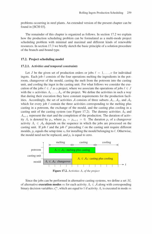
Rolling Ingots Production Scheduling 259
problems occurring in steel plants. An extended version of the present chapter can befound in [SCH 03].
The remainder of this chapter is organized as follows. In section 17.2 we explainhow the production scheduling problem can be formulated as a multi-mode projectscheduling problem with minimal and maximal and different kinds of renewableresources. In section 17.3 we briefly sketch the basic principle of a solution procedureof the branch-and-bound type.
17.2. Project scheduling model
17.2.1. Activities and temporal constraints
Let J be the given set of production orders or jobs � = 1, . . . , ν for individualingots. Each job � consists of the four operations melting the ingredients in the pot-room, changeover of the mould, casting the melt from the potroom into the castingunit, and cooling the ingot in the casting unit. For what follows we consider the exe-cution of the jobs � ∈ J as a project, where we associate the operations of jobs � ∈ Jwith the n activities A1 . . . , An of the project. We define the activities in such a waythat during their execution they have constant requirements for the production facil-ities. Accordingly, the set of activities A consists of three subsets A1, A2, and A3
which for every job � contain the three activities corresponding to the melting pluscasting in a potroom, the exchange of the mould, and the casting plus cooling in acasting unit of the casting system (see Figure 17.2). The dummy activities A0 andAn+1 represent the start and the completion of the production. The duration of activ-ity Ai is denoted by pi, where p0 = pn+1 = 0. The duration pi of a changeoveractivity Ai ∈ A2 depends on the sequence in which the jobs are processed on thecasting unit. If job � and the job �′ preceding � on the casting unit require differentmoulds, pi equals the setup time s� for installing the mould belonging to �. Otherwise,the mould need not be replaced, and pi is equal to zero.
� �melting � �casting � �cooling
mould
casting unit
potroom
�
�
tAi ∈ A2: changeover
Ai ∈ A3: casting plus cooling
Ai ∈ A1: melting plus casting
Figure 17.2. Activities Ai of the project
Since the jobs can be performed in alternative casting systems, we define a set Mi
of alternative execution modes m for each activity Ai ∈ A along with correspondingbinary decision variables xm
i , which are equal to 1 if activity Ai is executed in mode m
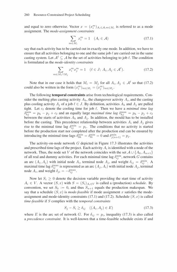
260 Resource-Constrained Project Scheduling
and equal to zero otherwise. Vector x = (xmi )Ai∈A,m∈Mi
is referred to as a modeassignment. The mode-assignment constraints∑
m∈Mi
xmi = 1 (Ai ∈ A) (17.1)
say that each activity has to be carried out in exactly one mode. In addition, we have toensure that all activities belonging to one and the same job � are carried out in the samecasting system. Let A� ⊆ A be the set of activities belonging to job �. The conditionis formulated as the mode-identity constraints∑
m∈Mi∩Mj
xmi xm
j = 1 (� ∈ J ; Ai, Aj ∈ A�). (17.2)
Note that in our case it holds that Mi = Mj for all Ai, Aj ∈ A� so that (17.2)could also be written in the form (xm
i )m∈Mi= (xm
j )m∈Mj.
The following temporal constraints arise from technological requirements. Con-sider the melting plus casting activity Ah, the changeover activity Ai, and the castingplus cooling activity Aj of a job � ∈ J . By definition, activities Ah and Aj are pulledtight. Let c� denote the cooling time for job �. Then we have a minimal time lagδminhj = ph − pj + c� and an equally large maximal time lag δmax
hj = ph − pj + c�
between the starts of activities Ah and Aj . In addition, the mould has to be installedbefore the casting. This precedence relationship between activities Ai and Aj givesrise to the minimal time lag δmin
ij = pi. The conditions that no activity is startedbefore the production start nor completed after the production end can be ensured byintroducing the minimal time lags δmin
0h = δmin0i = 0 and δmin
j(n+1) = pj .
The activity-on-node network G depicted in Figure 17.3 illustrates the activitiesand prescribed time lags of the project. Each activity Ai is identified with a node of thenetwork. Thus, the node set V of the network coincides with the set A∪ {A0, An+1}of all real and dummy activities. For each minimal time lag δmin
ij , network G containsan arc (Ai, Aj) with initial node Ai, terminal node Aj , and weight δij = δmin
ij . Amaximal time lag δmax
ij is represented as an arc (Aj , Ai) with initial node Aj , terminalnode Ai, and weight δji = −δmax
ij .
Now let Si ≥ 0 denote the decision variable providing the start time of activityAi ∈ V . A vector (S, x) with S = (Si)Ai∈V is called a (production) schedule. Byconvention, we set S0 := 0, and thus Sn+1 equals the production makespan. Wesay that a schedule (S, x) is mode-feasible if mode assignment x satisfies the mode-assignment and mode-identity constraints (17.1) and (17.2). Schedule (S, x) is calledtime-feasible if S complies with the temporal constraints
Sj − Si ≥ δij ((Ai, Aj) ∈ E) (17.3)
where E is the arc set of network G. For δij = pi, inequality (17.3) is also calleda precedence constraint. It is well-known that a time-feasible schedule exists if and
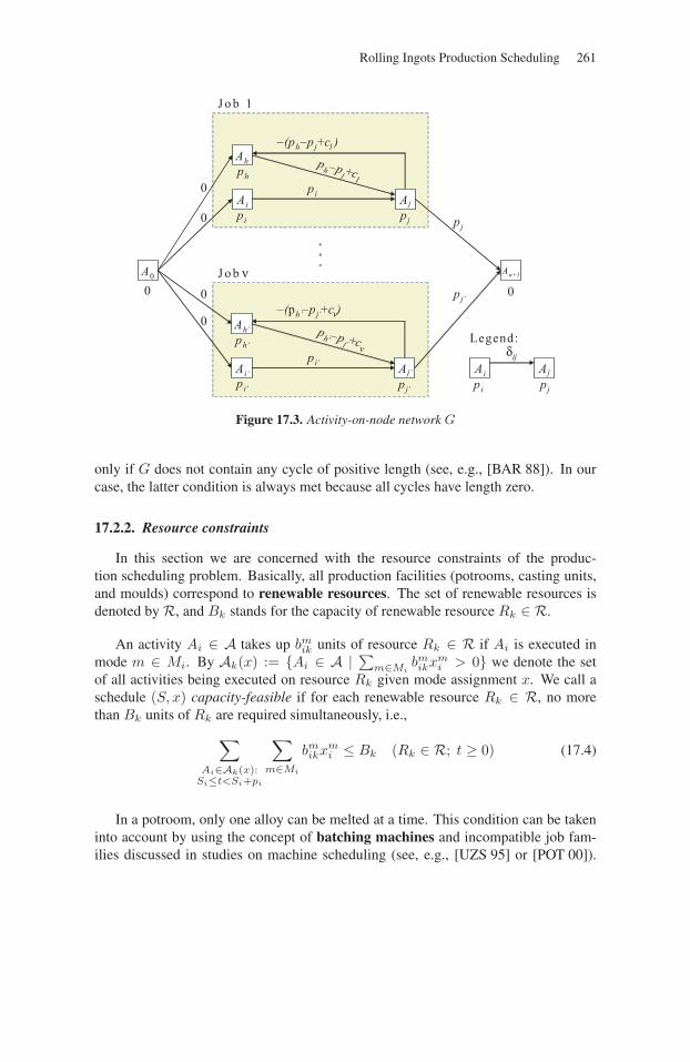
Rolling Ingots Production Scheduling 261
Ai Aj
Ah ph–pj+c1pi
ph
pi pj
Ai Ajδij
pi pjAj‘
A0 An+1
0
0
0
0
pj
pj‘0 0
Legend:
–(ph–pj+c1)
Ai‘
Ah‘ph‘
pi‘ pj‘
ph‘–pj‘+cνpi‘
–(ph‘–pj‘+cν)
J o b 1
J o b ν
Figure 17.3. Activity-on-node network G
only if G does not contain any cycle of positive length (see, e.g., [BAR 88]). In ourcase, the latter condition is always met because all cycles have length zero.
17.2.2. Resource constraints
In this section we are concerned with the resource constraints of the produc-tion scheduling problem. Basically, all production facilities (potrooms, casting units,and moulds) correspond to renewable resources. The set of renewable resources isdenoted byR, and Bk stands for the capacity of renewable resource Rk ∈ R.
An activity Ai ∈ A takes up bmik units of resource Rk ∈ R if Ai is executed in
mode m ∈ Mi. By Ak(x) := {Ai ∈ A |∑
m∈Mibmikxm
i > 0} we denote the setof all activities being executed on resource Rk given mode assignment x. We call aschedule (S, x) capacity-feasible if for each renewable resource Rk ∈ R, no morethan Bk units of Rk are required simultaneously, i.e.,∑
Ai∈Ak(x):Si≤t<Si+pi
∑m∈Mi
bmikxm
i ≤ Bk (Rk ∈ R; t ≥ 0) (17.4)
In a potroom, only one alloy can be melted at a time. This condition can be takeninto account by using the concept of batching machines and incompatible job fam-ilies discussed in studies on machine scheduling (see, e.g., [UZS 95] or [POT 00]).
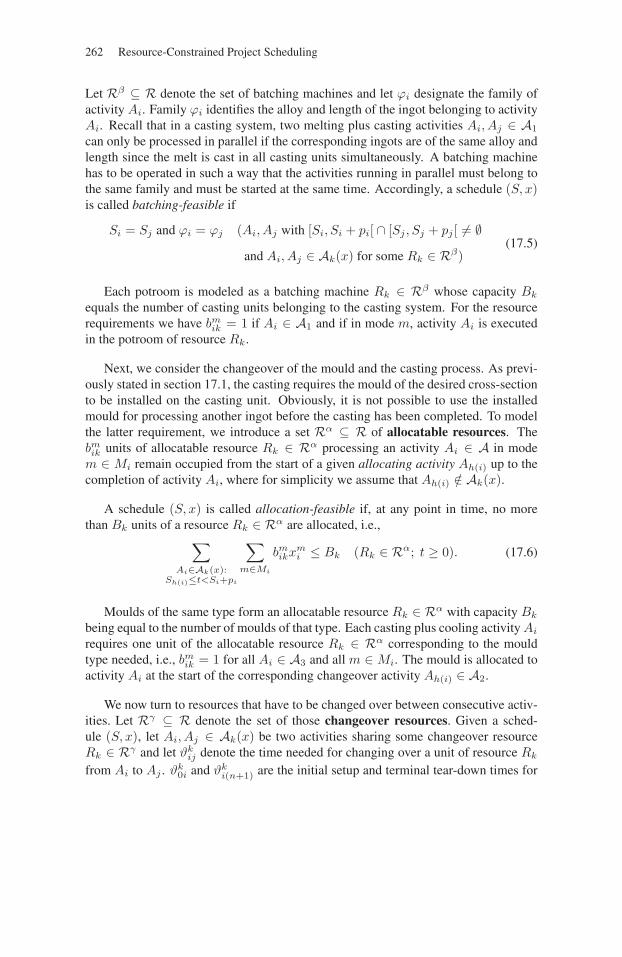
262 Resource-Constrained Project Scheduling
Let Rβ ⊆ R denote the set of batching machines and let ϕi designate the family ofactivity Ai. Family ϕi identifies the alloy and length of the ingot belonging to activityAi. Recall that in a casting system, two melting plus casting activities Ai, Aj ∈ A1
can only be processed in parallel if the corresponding ingots are of the same alloy andlength since the melt is cast in all casting units simultaneously. A batching machinehas to be operated in such a way that the activities running in parallel must belong tothe same family and must be started at the same time. Accordingly, a schedule (S, x)is called batching-feasible if
Si = Sj and ϕi = ϕj (Ai, Aj with [Si, Si + pi[ ∩ [Sj , Sj + pj [ �= ∅
and Ai, Aj ∈ Ak(x) for some Rk ∈ Rβ)(17.5)
Each potroom is modeled as a batching machine Rk ∈ Rβ whose capacity Bk
equals the number of casting units belonging to the casting system. For the resourcerequirements we have bm
ik = 1 if Ai ∈ A1 and if in mode m, activity Ai is executedin the potroom of resource Rk.
Next, we consider the changeover of the mould and the casting process. As previ-ously stated in section 17.1, the casting requires the mould of the desired cross-sectionto be installed on the casting unit. Obviously, it is not possible to use the installedmould for processing another ingot before the casting has been completed. To modelthe latter requirement, we introduce a set Rα ⊆ R of allocatable resources. Thebmik units of allocatable resource Rk ∈ Rα processing an activity Ai ∈ A in mode
m ∈ Mi remain occupied from the start of a given allocating activity Ah(i) up to thecompletion of activity Ai, where for simplicity we assume that Ah(i) /∈ Ak(x).
A schedule (S, x) is called allocation-feasible if, at any point in time, no morethan Bk units of a resource Rk ∈ Rα are allocated, i.e.,∑
Ai∈Ak(x):Sh(i)≤t<Si+pi
∑m∈Mi
bmikxm
i ≤ Bk (Rk ∈ Rα; t ≥ 0). (17.6)
Moulds of the same type form an allocatable resource Rk ∈ Rα with capacity Bk
being equal to the number of moulds of that type. Each casting plus cooling activity Ai
requires one unit of the allocatable resource Rk ∈ Rα corresponding to the mouldtype needed, i.e., bm
ik = 1 for all Ai ∈ A3 and all m ∈ Mi. The mould is allocated toactivity Ai at the start of the corresponding changeover activity Ah(i) ∈ A2.
We now turn to resources that have to be changed over between consecutive activ-ities. Let Rγ ⊆ R denote the set of those changeover resources. Given a sched-ule (S, x), let Ai, Aj ∈ Ak(x) be two activities sharing some changeover resourceRk ∈ Rγ and let ϑk
ij denote the time needed for changing over a unit of resource Rk
from Ai to Aj . ϑk0i and ϑk
i(n+1) are the initial setup and terminal tear-down times for
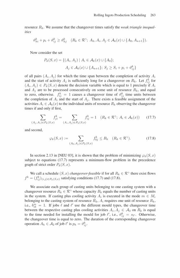
Rolling Ingots Production Scheduling 263
resource Rk. We assume that the changeover times satisfy the weak triangle inequal-ities
ϑkhi + pi + ϑk
ij ≥ ϑkhj (Rk ∈ Rγ ; Ah, Ai, Aj ∈ Ak(x) ∪ {A0, An+1}).
Now consider the set
Pk(S, x) = {(Ai, Aj) | Ai ∈ Ak(x) ∪ {A0};
Aj ∈ Ak(x) ∪ {An+1}; Sj ≥ Si + pi + ϑkij}
of all pairs (Ai, Aj) for which the time span between the completion of activity Ai
and the start of activity Aj is sufficiently long for a changeover on Rk. Let fkij for
(Ai, Aj) ∈ Pk(S, x) denote the decision variable which is equal to 1 precisely if Ai
and Aj are to be processed consecutively on some unit of resource Rk, and equalto zero, otherwise. fk
ij = 1 causes a changeover time of ϑkij time units between
the completion of Ai and the start of Aj . There exists a feasible assignment of theactivities Ai ∈ Ak(x) to the individual units of resource Rk observing the changeovertimes if and only if first,∑
(Aj ,Ai)∈Pk(S,x)
fkji =
∑(Ai,Aj)∈Pk(S,x)
fkij = 1 (Rk ∈ Rγ ; Ai ∈ Ak(x)) (17.7)
and second,
ϕk(S, x) :=∑
(A0,Aj)∈Pk(S,x)
fk0j ≤ Bk (Rk ∈ Rγ). (17.8)
In section 2.13 in [NEU 03], it is shown that the problem of minimizing ϕk(S, x)subject to equations (17.7) represents a minimum-flow problem in the precedencegraph of strict order Pk(S, x).
We call a schedule (S, x) changeover-feasible if for all Rk ∈ Rγ there exist flowsfk = (fk
ij)(i,j)∈Pk(S,x) satisfying conditions (17.7) and (17.8).
We associate each group of casting units belonging to one casting system with achangeover resource Rk ∈ Rγ whose capacity Bk equals the number of casting unitsin the system. If casting plus cooling activity Ai is executed in the mode m ∈ Mi
belonging to the casting system of resource Rk, Ai requires one unit of resource Rk,i.e., bm
ik = 1. If jobs � and �′ use the different mould types, the changeover timebetween the respective casting plus cooling activities Ai, Aj ∈ A3 on Rk is equalto the time needed for installing the mould for job �′, i.e., ϑk
ij = s�′ . Otherwise,the changeover time is equal to zero. The duration of the corresponding changeoveroperation Ah ∈ A2 of job �′ is ph = ϑk
ij .
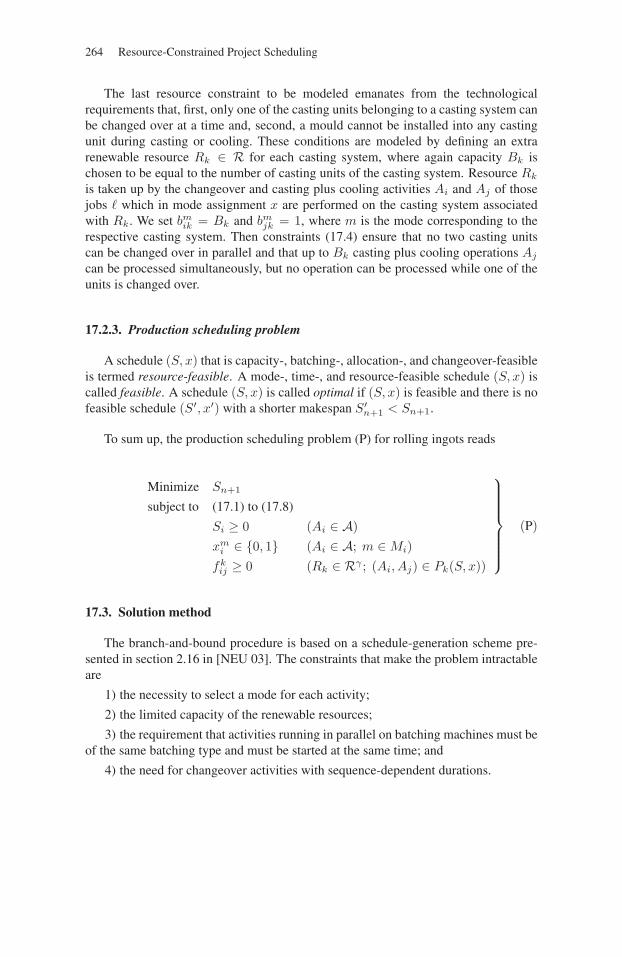
264 Resource-Constrained Project Scheduling
The last resource constraint to be modeled emanates from the technologicalrequirements that, first, only one of the casting units belonging to a casting system canbe changed over at a time and, second, a mould cannot be installed into any castingunit during casting or cooling. These conditions are modeled by defining an extrarenewable resource Rk ∈ R for each casting system, where again capacity Bk ischosen to be equal to the number of casting units of the casting system. Resource Rk
is taken up by the changeover and casting plus cooling activities Ai and Aj of thosejobs � which in mode assignment x are performed on the casting system associatedwith Rk. We set bm
ik = Bk and bmjk = 1, where m is the mode corresponding to the
respective casting system. Then constraints (17.4) ensure that no two casting unitscan be changed over in parallel and that up to Bk casting plus cooling operations Aj
can be processed simultaneously, but no operation can be processed while one of theunits is changed over.
17.2.3. Production scheduling problem
A schedule (S, x) that is capacity-, batching-, allocation-, and changeover-feasibleis termed resource-feasible. A mode-, time-, and resource-feasible schedule (S, x) iscalled feasible. A schedule (S, x) is called optimal if (S, x) is feasible and there is nofeasible schedule (S′, x′) with a shorter makespan S′
n+1 < Sn+1.
To sum up, the production scheduling problem (P) for rolling ingots reads
Minimize Sn+1
subject to (17.1) to (17.8)
Si ≥ 0 (Ai ∈ A)xm
i ∈ {0, 1} (Ai ∈ A; m ∈Mi)fk
ij ≥ 0 (Rk ∈ Rγ ; (Ai, Aj) ∈ Pk(S, x))
⎫⎪⎪⎪⎪⎪⎪⎬⎪⎪⎪⎪⎪⎪⎭
(P)
17.3. Solution method
The branch-and-bound procedure is based on a schedule-generation scheme pre-sented in section 2.16 in [NEU 03]. The constraints that make the problem intractableare
1) the necessity to select a mode for each activity;
2) the limited capacity of the renewable resources;
3) the requirement that activities running in parallel on batching machines must beof the same batching type and must be started at the same time; and
4) the need for changeover activities with sequence-dependent durations.
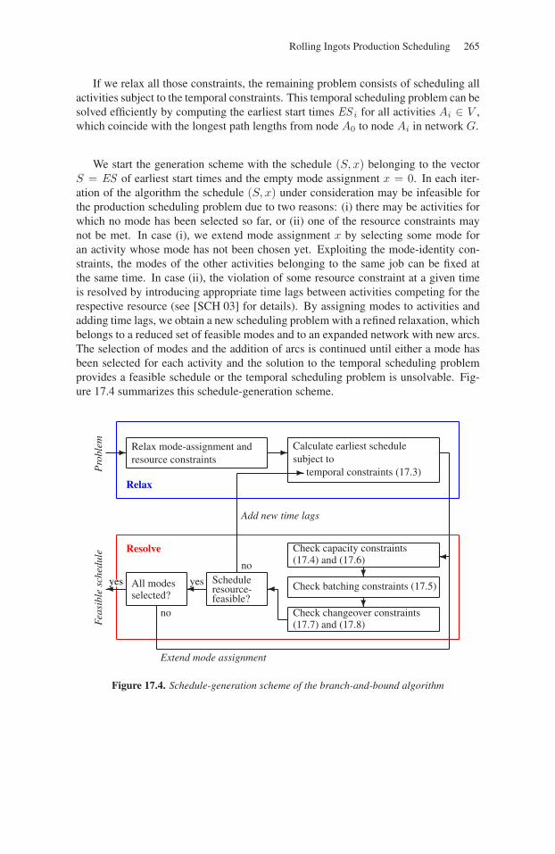
Rolling Ingots Production Scheduling 265
If we relax all those constraints, the remaining problem consists of scheduling allactivities subject to the temporal constraints. This temporal scheduling problem can besolved efficiently by computing the earliest start times ES i for all activities Ai ∈ V ,which coincide with the longest path lengths from node A0 to node Ai in network G.
We start the generation scheme with the schedule (S, x) belonging to the vectorS = ES of earliest start times and the empty mode assignment x = 0. In each iter-ation of the algorithm the schedule (S, x) under consideration may be infeasible forthe production scheduling problem due to two reasons: (i) there may be activities forwhich no mode has been selected so far, or (ii) one of the resource constraints maynot be met. In case (i), we extend mode assignment x by selecting some mode foran activity whose mode has not been chosen yet. Exploiting the mode-identity con-straints, the modes of the other activities belonging to the same job can be fixed atthe same time. In case (ii), the violation of some resource constraint at a given timeis resolved by introducing appropriate time lags between activities competing for therespective resource (see [SCH 03] for details). By assigning modes to activities andadding time lags, we obtain a new scheduling problem with a refined relaxation, whichbelongs to a reduced set of feasible modes and to an expanded network with new arcs.The selection of modes and the addition of arcs is continued until either a mode hasbeen selected for each activity and the solution to the temporal scheduling problemprovides a feasible schedule or the temporal scheduling problem is unsolvable. Fig-ure 17.4 summarizes this schedule-generation scheme.
Pro
blem � Relax mode-assignment and
resource constraints� Calculate earliest schedule
subject totemporal constraints (17.3)
Relax
Add new time lags
Extend mode assignment
�
�
�Check changeover constraints(17.7) and (17.8)
Check batching constraints (17.5)
Check capacity constraints(17.4) and (17.6)
�Scheduleresource-feasible?
no
�
�yesAll modesselected?
no
�yes
Feas
ible
sche
dule Resolve
Figure 17.4. Schedule-generation scheme of the branch-and-bound algorithm
266 Resource-Constrained Project Scheduling
In the branch-and-bound algorithm, the enumeration is performed as follows. Inthe case of a mode selection for some activity Ai we generate one enumeration nodefor each mode m ∈ Mi. When dealing with a violation of a resource constraint, weenumerate the alternatives of choosing two activities Ai, Aj among the activities caus-ing the conflict and define an appropriate minimal time lag δmin
ij between Ai and Aj .Each time we have reached a feasible schedule or the temporal scheduling problemhas become unsolvable, we perform backtracking and proceed with the investigationof unexplored enumeration nodes.
Due to the sequence-dependent need for changeovers, the resource demands overtime arising from the changeover activities are not known until the activity sequenceson the changeover resources have been established. That is why we follow a heuristictwo-phase approach where in the first phase, while observing the changeover times,we assume that changeover activities do not require resources for their execution.In the terms of our production scheduling problem the latter assumption means thatwe allow for parallel changeovers on casting units belonging to one and the samecasting system. When we have obtained a feasible schedule for this subproblem,we fix the activity sequences on the changeover resources (and thus the durationsof the changeover activities) by introducing a precedence constraint between any twoconsecutive activities. We then proceed with the second phase, where we apply thebranching process subject to the time lags introduced.
We have evaluated the performance of a filtered beam search version of the branch-and-bound algorithm. The tests have been performed based on 15 instances includingup to 50 jobs. The results for the larger instances indicate that the algorithm scaleswell. In particular, the makespan-per-job ratio seems to be independent of the problemsize, though the CPU time limit has not been varied. Details of the performanceanalysis can be found in [SCH 03].
17.4. Conclusions
In this chapter we have considered the problem of scheduling the casting of rollingingots on a production plant consisting of several casting systems. The problem ischaracterized by specific technological constraints such as cooling times, incompati-bilities between production orders, and changeovers whose necessity depends on thesequence in which the production orders are processed on the casting units. We haveformulated the problem as a resource-constrained project scheduling model with min-imal and maximal time lags between the activities and different types of resources.For solving the problem, we have proposed a branch-and-bound algorithm where werelax the resource constraints and enumerate the different alternatives of assigningexecution modes to the activities and resolving resource conflicts between activitiescompeting for the same resources. An experimental performance analysis shows thata truncated version of the algorithm is able to find good schedules within a reasonableamount of computation time.
Chapter 18
Resource-Constrained Modulo Scheduling
18.1. Introduction
Modulo scheduling is an effective instruction scheduling framework for optimiz-ing innermost program loops, especially when compiling for Very Long InstructionWord (VLIW) processors. VLIW processors are instruction-level parallel processors[RAU 93] where the compiler is the only responsible for instruction scheduling. Bycomparison, superscalar processors like the Intel Pentium series dynamically resched-ule instructions by hardware, based on the linear order of instructions produced by thecompiler. The Lx [FAR 00] is an example of modern VLIW architecture jointly devel-oped by Hewlett-Packard Laboratories and STMicroelectronics. This architecture isimplemented by the STMicroelectronics ST200 VLIW processor family.
Modern VLIW processors are mainly used for media processing in embeddeddevices such as mobile, automotive and consumer electronics. For such applications,the time taken by compiler optimizations is not an issue. Rather, the quality of theinstruction schedules produced has a direct impact on the overall system cost andenergy consumption, as high-quality instruction schedules enable to reduce the oper-ating frequency given the real-time processing requirements. This allows for the useof optimal instruction scheduling techniques for VLIW processors, in particular oninner loop code where most of the processing time is spent.
Instruction scheduling for inner loops is also known as software pipelining[ALL 95]. Among the different software pipelining frameworks, modulo scheduling[RAU 96] is the most successful in production compilers. The modulo schedulingframework is distinguished by its focus on 1-periodic cyclic schedules with integral
Chapter written by Benoît DUPONT DE DINECHIN, Christian ARTIGUES and Sadia AZEM.
267
268 Resource-Constrained Project Scheduling
period, which leads to simplifications compared to the classic formulation of cyclicscheduling [HAN 95].
In this chapter, we define the resource-constrained modulo scheduling problem(RCMSP) as a modulo scheduling problem where the resource constraints are adaptedfrom the renewable RCPSP. We then introduce a new time-indexed integer linear pro-gramming formulation of the RCMSP, along with the one proposed earlier by Eichen-berger et al. [EIC 95, EIC 97]. Finally, we propose a large neighborhood search heuris-tic to solve difficult instances of these formulations.
18.2. The resource-constrained modulo scheduling problem
18.2.1. The resource-constrained cyclic scheduling problem
A basic cyclic scheduling [HAN 95] is defined by a set of generic operations A ={Ai}1≤i≤n to be executed repeatedly, thus defining a set of operation instances
{Ali}l∈N
1≤i≤n.
We call iteration l the set of operation instances {Ali}1≤i≤n. For any i ∈ [1, n]
and l ∈ N, let σli denote the schedule date of operation instance Al
i. Basic cyclicscheduling problems are constrained by uniform dependencies denoted
Aiθj
i ,ωji−→ Aj ,
where the latency θji and the distance ωj
i are non-negative integers:
Aiθj
i ,ωji−→ Aj =⇒ σl
i + θji ≤ σ
l+ωji
j ∀l ∈ N (18.1)
In the case of cyclic scheduling on parallel processors [HAN 95], basic cyclicscheduling problems are augmented with resource constraints. Each generic operationAi has a processing time pi and there are m identical processors available. Each Al
i
requires one of the processors to be available between dates [σli, σ
li + pi − 1].
For instruction scheduling applications, we are interested in resource-constrainedcyclic scheduling problems, whose resource constraints are adapted from the standardRCPSP. Precisely, a set of q renewable resources is defined with availabilities Bk >0,∀Rk ∈ R. Assume Resk
i is a set of non-negative integers such that c ∈ Reski means
operation Ali requires bik units of resource Rk exactly c time periods after starting its
execution. In RCPSP, an operation requires its resources during all its processing timeand in such cases Resk
i = {0, . . . , pi − 1} for any resource Rk and any operation Ali.
The cyclic scheduling resource constraints can be written as:
∀Rk ∈ R,∀t ≥ 0 :∑
Ali∈Atk
bik ≤ Bk (18.2)
where Atk = {Ali | ∃l ≥ 0, ∃c ∈ Resk
i , σli + c = t}.
Resource-Constrained Modulo Scheduling 269
18.2.2. The resource-constrained modulo scheduling problem
Modulo scheduling is a specialization of cyclic scheduling where any cyclic sched-ule {σl
i}l∈N
1≤i≤n must be 1-periodic with integral period λ ≥ 1, traditionally called theinitiation interval. By definition, a 1-periodic cyclic schedule satisfies:
∀i ∈ [1, n], ∀l ≥ 0 : σli = σ0
i + lλ. (18.3)
Restricting cyclic scheduling to 1-periodic schedules allows significant simplifi-cations in the problem formulation. Let us define σi
def= σ0i . The values {σi} can be
considered as the schedule dates of the generic operations {Ai}. A solution is fullycharacterized by the initiation interval λ and the generic schedule {σi}. Each uniformdependence constraint becomes:
σi + θji − ωj
i λ ≤ σj ∀(i, j) ∈ Edep. (18.4)
For resource constraints (18.2), the definition of Atk becomes Atk = {Ai | ∃c ∈Resk
i , σi = (t−c)mod λ}. It follows from this definition that all resource constraints(18.2) such that t ≥ λ are redundant. Thus, the number of resource constraints can bereduced. They are now defined as:∑
Ai∈Atk
bik ≤ Bk ∀Rk ∈ R,∀t ∈ [0, λ− 1]. (18.5)
The primary objective of modulo scheduling is to find a 1-periodic schedule witha minimal period λ, in order to maximize the throughput. A secondary objectiveof modulo scheduling is often considered, such as minimizing the generic schedulelength Cmax = maxi=1,...,n σi + pi or minimizing the cumulative lifetime of regis-ters [Dup 94, Dup 96, EIC 97, Dup 04]. Both objectives are linear with the genericschedule dates so we take as the secondary objective of modulo scheduling some lin-ear expression
∑wiσi. Moreover, we assume the existence of modulo scheduling
relaxations that provide deadlines di for each generic operation Ai, so we will includeconstraints σi + pi ≤ di in the integer programming formulations discussed here.
In the traditional modulo scheduling framework [RAU 96], two lower bounds onthe initiation interval λ are computed: λrec is the minimum λ such that there are nopositive length circuits in the dependence graph; λres is the minimum λ such that therenewable resourcesR are not over-subscribed:
λrecdef= max
C
⌈ ∑C θj
i∑C ωj
i
⌉: C dependence circuit
λresdef= max
1≤k≤q
⌈∑ni=1 pibik
Bk
⌉: q = |R|
Given λmindef= max(λrec, λres), the classic modulo scheduling framework finds
a minimal value of the period λ by dichotomy search such that (18.4–18.5) are
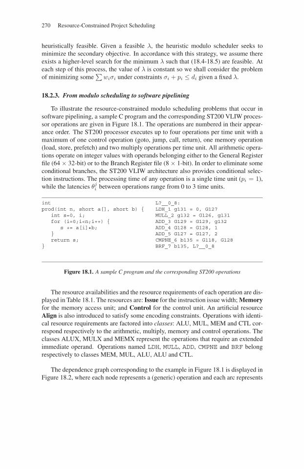
270 Resource-Constrained Project Scheduling
heuristically feasible. Given a feasible λ, the heuristic modulo scheduler seeks tominimize the secondary objective. In accordance with this strategy, we assume thereexists a higher-level search for the minimum λ such that (18.4-18.5) are feasible. Ateach step of this process, the value of λ is constant so we shall consider the problemof minimizing some
∑wiσi under constraints σi + pi ≤ di given a fixed λ.
18.2.3. From modulo scheduling to software pipelining
To illustrate the resource-constrained modulo scheduling problems that occur insoftware pipelining, a sample C program and the corresponding ST200 VLIW proces-sor operations are given in Figure 18.1. The operations are numbered in their appear-ance order. The ST200 processor executes up to four operations per time unit with amaximum of one control operation (goto, jump, call, return), one memory operation(load, store, prefetch) and two multiply operations per time unit. All arithmetic opera-tions operate on integer values with operands belonging either to the General Registerfile (64 × 32-bit) or to the Branch Register file (8 × 1-bit). In order to eliminate someconditional branches, the ST200 VLIW architecture also provides conditional selec-tion instructions. The processing time of any operation is a single time unit (pi = 1),while the latencies θj
i between operations range from 0 to 3 time units.
intprod(int n, short a[], short b) {
int s=0, i;for (i=0;i<n;i++) {
s += a[i]*b;}return s;
}
L?__0_8:LDH_1 g131 = 0, G127MULL_2 g132 = G126, g131ADD_3 G129 = G129, g132ADD_4 G128 = G128, 1ADD_5 G127 = G127, 2CMPNE_6 b135 = G118, G128BRF_7 b135, L?__0_8
Figure 18.1. A sample C program and the corresponding ST200 operations
The resource availabilities and the resource requirements of each operation are dis-played in Table 18.1. The resources are: Issue for the instruction issue width; Memoryfor the memory access unit; and Control for the control unit. An artificial resourceAlign is also introduced to satisfy some encoding constraints. Operations with identi-cal resource requirements are factored into classes: ALU, MUL, MEM and CTL cor-respond respectively to the arithmetic, multiply, memory and control operations. Theclasses ALUX, MULX and MEMX represent the operations that require an extendedimmediate operand. Operations named LDH, MULL, ADD, CMPNE and BRF belongrespectively to classes MEM, MUL, ALU, ALU and CTL.
The dependence graph corresponding to the example in Figure 18.1 is displayed inFigure 18.2, where each node represents a (generic) operation and each arc represents
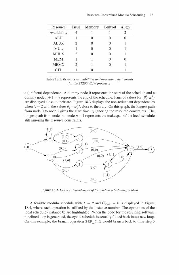
Resource-Constrained Modulo Scheduling 271
Resource Issue Memory Control AlignAvailability 4 1 1 2
ALU 1 0 0 0
ALUX 2 0 0 1
MUL 1 0 0 1
MULX 2 0 0 1
MEM 1 1 0 0
MEMX 2 1 0 1
CTL 1 0 1 1
Table 18.1. Resource availabilities and operation requirementsfor the ST200 VLIW processor
a (uniform) dependence. A dummy node 0 represents the start of the schedule and adummy node n+1 = 8 represents the end of the schedule. Pairs of values for (θj
i , ωji )
are displayed close to their arc. Figure 18.3 displays the non-redundant dependencieswhen λ = 2 with the values θj
i −ωji λ close to their arc. On this graph, the longest path
from node 0 to node i gives the start time σi ignoring the resource constraints. Thelongest path from node 0 to node n + 1 represents the makespan of the local schedulestill ignoring the resource constraints.
(3,0)
(1,1)
(1,1)
(3,0)
(1,1)(0,0)
(0,0)
(0,0)
(0,0)
(0,0)
(0,1)(1,0)
(0,0)
(0,0)
(1,4)
(1,1)
4
2
5
6
3
7
1
08
(1,0)
Figure 18.2. Generic dependencies of the modulo scheduling problem
A feasible modulo schedule with λ = 2 and Cmax = 6 is displayed in Figure18.4, where each operation is suffixed by the instance number. The operations of thelocal schedule (instance 0) are highlighted. When the code for the resulting softwarepipelined loop is generated, the cyclic schedule is actually folded back into a new loop.On this example, the branch operation BRF_7.1 would branch back to time step 5
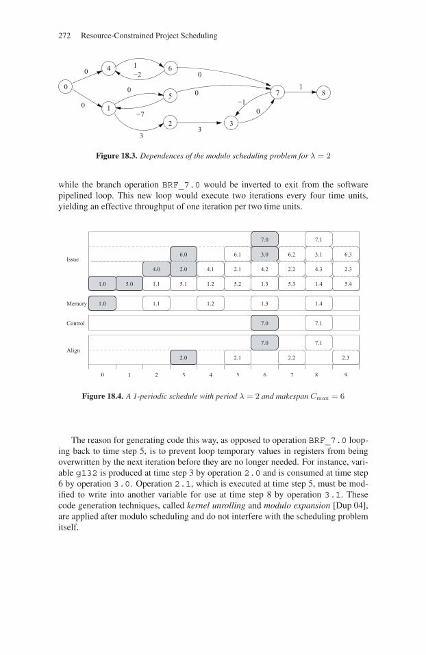
272 Resource-Constrained Project Scheduling
−21
0
−7
0
−10
0
33
0
0
0
1
4 6
5
2 3
7 81
Figure 18.3. Dependences of the modulo scheduling problem for λ = 2
while the branch operation BRF_7.0 would be inverted to exit from the softwarepipelined loop. This new loop would execute two iterations every four time units,yielding an effective throughput of one iteration per two time units.
0 1 2 3 4 5 6 7 8 9
1.0
1.0
5.0
2.0
7.0
7.0
4.0
6.0
2.0
1.1 1.2 1.35.1
4.1 4.22.1
6.1
5.2
1.1 1.2 1.3
2.1
1.4
2.2 2.3
7.1
7.1
7.1
4.32.2 2.3
6.2 6.33.0
7.0
3.1
5.3 5.41.4
Memory
Control
Align
Issue
Figure 18.4. A 1-periodic schedule with period λ = 2 and makespan Cmax = 6
The reason for generating code this way, as opposed to operation BRF_7.0 loop-ing back to time step 5, is to prevent loop temporary values in registers from beingoverwritten by the next iteration before they are no longer needed. For instance, vari-able g132 is produced at time step 3 by operation 2.0 and is consumed at time step6 by operation 3.0. Operation 2.1, which is executed at time step 5, must be mod-ified to write into another variable for use at time step 8 by operation 3.1. Thesecode generation techniques, called kernel unrolling and modulo expansion [Dup 04],are applied after modulo scheduling and do not interfere with the scheduling problemitself.

Resource-Constrained Modulo Scheduling 273
18.3. Integer linear programming formulations
18.3.1. The RCMSP formulations by Eichenberger et al.
Eichenberger et al. [EIC 95, EIC 97] introduce a class of integer linear program-ming formulations for the RCMSP, based on the decomposition of the generic sched-ule dates {σi} into a quotient and a remainder:
σi = λli + τi : li ∈ N ∧ τi ∈ [0, λ− 1].
For the integer linear programming formulations, 0-1 time indexed variables yτi
are used to represent the remainders τi = σi mod λ, i.e. yτi = 1 ⇐⇒ τi = τ , while
the quotients li = σi
λ are directly defined as integer variables:
(ED)∑
i∈[1,n]
wi
(λ−1∑τ=0
τyτi + liλ
): minimize
λ−1∑τ=0
yτi = 1 i ∈ [1, n] (18.6)
λ−1∑τ=0
τyτi + liλ + θj
i − λωji ≤
λ−1∑τ=0
τyτj + ljλ (i, j) ∈ Edep (18.7)
n∑i=1
∑c∈Resk
i
y(τ−c)mod λi bik ≤ Bk τ ∈ [0, λ− 1], Rk ∈ R (18.8)
li ∈{
0, . . . ,
⌊di − pi
λ
⌋}i ∈ [1, n] (18.9)
yτi ∈ {0, 1} i ∈ [1, n], τ ∈ [0, λ− 1] (18.10)
Eichenberger and Davidson [EIC 97] report that constraints (18.6–18.7) wereinitially proposed by Govindarajan et al. [GOV 94]. Constraints (18.6) state thateach generic operation has to be started exactly once in time window [0, λ − 1].We have σi = λli + τi and τi =
∑λ−1τ=0 τyτ
i , so constraints (18.7) correspondexactly to constraints (18.4). Likewise, the economic function
∑i∈[1,n] wiσi becomes∑
i∈[1,n] wi(∑λ−1
τ=0 τyτi + liλ). Resource constraints (18.8) with bik = 1 were
introduced in [EIC 95] as a linear form of constraints (18.5). Note that we allowinteger values for bik, making the problem considered by [EIC 97] a particular caseof the RCMSP considered here. Conversely, we do not include the register pressureequations of [EIC 95] in the above formulation, as they correspond to a specific casewhere the secondary objective of modulo scheduling is not linear with the genericschedule dates.
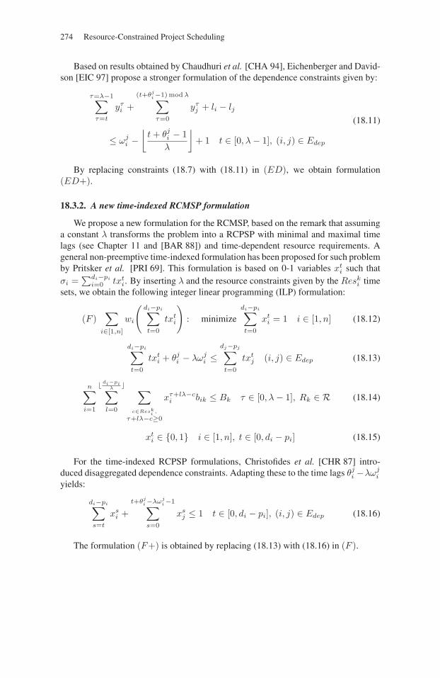
274 Resource-Constrained Project Scheduling
Based on results obtained by Chaudhuri et al. [CHA 94], Eichenberger and David-son [EIC 97] propose a stronger formulation of the dependence constraints given by:
τ=λ−1∑τ=t
yτi +
(t+θji−1) mod λ∑τ=0
yτj + li − lj
≤ ωji −
⌊t + θj
i − 1λ
⌋+ 1 t ∈ [0, λ− 1], (i, j) ∈ Edep
(18.11)
By replacing constraints (18.7) with (18.11) in (ED), we obtain formulation(ED+).
18.3.2. A new time-indexed RCMSP formulation
We propose a new formulation for the RCMSP, based on the remark that assuminga constant λ transforms the problem into a RCPSP with minimal and maximal timelags (see Chapter 11 and [BAR 88]) and time-dependent resource requirements. Ageneral non-preemptive time-indexed formulation has been proposed for such problemby Pritsker et al. [PRI 69]. This formulation is based on 0-1 variables xt
i such thatσi =
∑di−pi
i=0 txti. By inserting λ and the resource constraints given by the Resk
i timesets, we obtain the following integer linear programming (ILP) formulation:
(F )∑
i∈[1,n]
wi
(di−pi∑t=0
txti
): minimize
di−pi∑t=0
xti = 1 i ∈ [1, n] (18.12)
di−pi∑t=0
txti + θj
i − λωji ≤
dj−pj∑t=0
txtj (i, j) ∈ Edep (18.13)
n∑i=1
� di−piλ �∑
l=0
∑c∈Resk
i,
τ+lλ−c≥0
xτ+lλ−ci bik ≤ Bk τ ∈ [0, λ− 1], Rk ∈ R (18.14)
xti ∈ {0, 1} i ∈ [1, n], t ∈ [0, di − pi] (18.15)
For the time-indexed RCPSP formulations, Christofides et al. [CHR 87] intro-duced disaggregated dependence constraints. Adapting these to the time lags θj
i −λωji
yields:
di−pi∑s=t
xsi +
t+θji−λωj
i −1∑s=0
xsj ≤ 1 t ∈ [0, di − pi], (i, j) ∈ Edep (18.16)
The formulation (F+) is obtained by replacing (18.13) with (18.16) in (F ).
Resource-Constrained Modulo Scheduling 275
18.4. Solving the RCMSP formulations
18.4.1. Reducing the size of the RCMSP formulations
In terms of variable numbers, formulations (ED) and (ED+) comprise nλbinary variables yτ
i and n integer variables li. Formulations (F ) and (F+) comprise∑ni=1(di − pi + 1) binary variables. Since we can assume that di ≥ λ, the new
formulation has potentially a greater number of variables.
Formulation (F+) involves variables and constraints in numbers that are directlyrelated to any assumed earliest {ESi}1≤i≤n and latest {LSi}1≤i≤n schedule dates(margins). Indeed, the number of variables is
∑ni=1 LSi − ESi + 1. Most of the
constraints are the dependence equations (18.16), and edef= |Edep| non-transitively
redundant dependencies appear to generate eT equations with Tdef= max1≤i≤n LSi +
pi. However, the first sum of (18.16) is 0 if t > LSi. Likewise, the second sum of(18.16) is 0 if t + θj
i − λωji − 1 < ESj . (18.16) is actually equivalent to:
di−pi∑s=t
xsi +
t+θji−λωj
i −1∑s=0
xsj ≤ 1 t ∈ [ESj − θj
i + λωji + 1, LSi], (i, j) ∈ Edep
(18.17)
Therefore, (18.17) is redundant whenever ESj − θji + λωj
i ≥ LSi.
Due to the decrease in the number for variables and equations, formulation (F+) islikely to become more tractable after reducing the assumed margins. By comparison,the number of variables in formulation (ED+) only decreases when some LSi −ESi ≤ λ, while most dependence equations (18.11) remain.
For the RCPSP, the basic technique to reduce the margins is to initialize ESi = ri
and LSi = di − pi, with {ri}1≤i≤n and {di}1≤i≤n being the release dates and thedeadlines, then propagate the dependence constraints using a label-correcting algo-rithm. More elaborate constraint propagation techniques have been proposed for theRCPSP (see Chapter 4 and [DEM 05]). Ultimately, all these margins reduction tech-niques rely on some effective upper bounding of the deadlines {di}1≤i≤n.
18.4.2. A large neighborhood search for the RCMSP
In the case of the modulo scheduling, the primary objective is the period mini-mization. Heuristics build modulo schedules at some period λ that is often greaterthan the lower bound λmin
def= max(λrec, λres). When this happens, the feasibility ofmodulo scheduling at period λ − 1 is open. Moreover, it is not known how to boundthe makespan at period λ− 1 given a makespan at period λ. This means that effectiveupper bounding of the due dates in RCMSP instances is not available either.
276 Resource-Constrained Project Scheduling
To compensate for this lack of upper bounding, we propose a large neighborhoodsearch (LNS) for the RCMSP formulations, based on adaptive margins reduction andimplicit enumeration of the resulting time-indexed integer programs (using a MIPsolver). The LNS (see [PAL 04] and Chapters 6 and 7) is a meta-heuristic where alarge number of solutions in the neighborhood of an incumbent solution are searchedby means of branch-and-bound, constraint programming, or integer programming.The large neighborhood is obtained by fixing some variables of the incumbent solutionwhile releasing others.
In the setting of time-indexed formulations, we consider as the neighborhood of anincumbent solution {σi}1≤i≤n some margins {ESi, LSi : σi ∈ [ESi, LSi]}1≤i≤n,which are made consistent under dependence constraint propagation. For each xσi
i =1, we fix variables xri
i · · ·xESi−1i , xLSi+1
i · · ·xdi−pi
i to zero and release variablesxESi
i · · ·xLSii . The fixed variables and the dependence constraints (18.17) found
redundant given the margins are removed from the integer program.
We adapt the generic LNS algorithm of [PAL 04] by using margins to define theneighborhoods and by starting from a heuristic modulo schedule. The period λ is keptconstant while our LNS searches increasingly wider margins under a time budget inorder to minimize the makespan. The key innovation is to replace the diversificationoperator of [PAL 04] by a decrement of the period to λ−1 while keeping the scheduledates of the former period λ. This yields a pseudo-solution that may no longer be fea-sible due to the period change. Computational experience shows that a new solution atperiod λ−1 can often be found in the neighborhood of this pseudo-solution, wheneverthe problem instance is feasible at period λ− 1. In the case where a solution at periodλ− 1 is found, our LNS goes back to the makespan minimization.
18.4.3. Implementation and experiments
We implemented the two time-indexed formulations of RCMSP (ED+) and (F+)in the production compiler for the STMicroelectronics ST200 VLIW processor family[Dup 04], along with the proposed LNS heuristic, then used the CPLEX 9.0 CallableLibrary to solve the resulting MIPs.
Table 18.2 reports LNS experimental data for the largest loops that could not bedirectly solved with these formulations, assuming a timeout of 300 s and a time hori-zon of 4λmin. Column #O,#D gives the number of operations and non-redundantdependencies. Column Heuristic λ,M displays the period and makespan computedby the ST200 production compiler insertion scheduling heuristic [Dup 04]. The col-umn groups (F+) 300, (F+) 30, (ED+) 300, correspond to the proposed LNS usingour formulation and Eichenberger et al. formulation for timeout values of 300 s, 30 s,300 s. In each group, column #V,#C gives the number of variables and constraints ofthe integer program sent to CPLEX 9.0 by the last successful LNS step. In all thesecases, the (F+) LNS reached the λmin, thus ensuring optimality of the period λ.

Resource-Constrained Modulo Scheduling 277
Heuristic (F+) 300 (F+) 30 (ED+) 300
Loop #O,#D λ, M λ, M #V,#C λ, M #V,#C λ, M #V,#C
q_plsf_5.0_215 231,313 81,97 75,77 1114,1236 75,78 1873,2042 *,* 18942,25989
q_plsf_5.0_227 121,163 42,92 39,46 982,1228 39,46 1378,1685 39,47 4840,6673
q_plsf_5.0_201 124,168 42,92 40,47 1086,1340 40,65 1197,1421 41,50 5208,7217
q_plsf_5.2_11 233,317 82,100 75,78 1113,1216 75,79 1897,2045 *,* 19339,26637
subbands.0_196 130,234 44,65 35,49 718,906 35,48 1008,1248 *,* 5850,10778
transfo.IMDCT_L 232,370 71,109 58,58 1133,1075 58,58 1985,1961 70,74 16472,26482
Table 18.2. Large-scale neighborhood search experimental data
18.5. Summary and conclusions
High-quality instruction scheduling for VLIW processors, in particular the soft-ware pipelining of inner loops, is a significant contributor to the performance of mediaprocessing applications. Modern software pipelining techniques operate under theframework of modulo scheduling [RAU 96], which simplifies the cyclic schedulingproblems by focusing on 1-periodic cyclic schedules with integral period. In additionto minimizing the period, modulo schedulers seeks to reduce a secondary objectivethat can be expressed as a weighted linear sum of the generic schedule dates.
In this chapter, we formalize the resource-constrained modulo scheduling prob-lem and we focus on two integer programming formulations of this problem. Thefirst formulation is based on work by Eichenberger et al. [EIC 95, EIC 97]. The sec-ond formulation is generalized from the classic non-preemptive time-indexed integerprogramming formulation of Pritsker et al. [PRI 69] for the RCPSP with time-lags.For both formulations, we consider the variants where the dependence constraints aredisaggregated.
Our computational experience shows that, while the formulation of Eichenbergeret al. generates fewer variables than our formulation generalized from Pritsker et al.,both techniques are intractable in practice for modulo scheduling problems with morethan a few dozen generic operations. However, when combined with a simple large-scale neighborhood search, only the new formulation with disaggregated dependenceequations makes it possible to solve near-optimally modulo scheduling problems withhundreds of generic operations and uniform dependencies in a matter of minutes.

278
This page intentionally left blank
Bibliography
[ADE 02] G.M. ADELSON-VELSKY and E. LEVNER, “Project scheduling in AND-ORgraphs: A generalization of Dijkstra’s algorithm”, Mathematics of Operations Research,vol. 27, num. 3, p. 504–517, 2002.
[AHU 76] H. AHUJA, Construction Performance Control by Networks, Wiley & Sons, 1976.
[AKT 99] M. AKTURK and E. GORGULU, “Match-up scheduling under a machine break-down”, European Journal of Operational Research, vol. 112, num. 1, p. 81–97, 1999.
[ALF 97] H.K. ALFARES and J. BAILEY, “Integrated project task and manpower scheduling”,IIE Transactions, vol. 29, num. 9, p. 711–717, 1997.
[ALL 95] V.H. ALLAN, R.B. JONES, R.M. LEE and S.J. ALLAN, “Software pipelining”,ACM Computing Surveys, vol. 27, num. 3, p. 367–432, 1995.
[ALV 89] R. ALVAREZ-VALDÉS and J.M. TAMARIT, “Heuristic algorithms for Resource-Constrained Project Scheduling: a review and an empirical analysis”, SLOWINSKI R. andWEGLARZ J., Eds., Advances in Project Scheduling, p. 113–134, Elsevier, 1989.
[ALV 93] R. ALVAREZ-VALDÉS and J.M. TAMARIT, “The project scheduling polyhedron:dimension, facets and lifting theorems”, European Journal of Operational Research,vol. 67, num. 2, p. 204–220, 1993.
[APP 91] D. APPLEGATE and W. COOK, “A computational study of job-shop scheduling”,ORSA Journal on Computing, vol. 3, num. 2, p. 149–156, 1991.
[ART 00] C. ARTIGUES and F. ROUBELLAT, “A polynomial activity insertion algorithm in amulti-resource schedule with cumulative constraints and multiple modes”, European Jour-nal of Operational Research, vol. 127, num. 2, p. 297–316, 2000.
[ART 03] C. ARTIGUES, P. MICHELON and S. REUSSER, “Insertion techniques for staticand dynamic Resource-Constrained Project Scheduling”, European Journal of OperationalResearch, vol. 149, num. 2, p. 249–267, 2003.
[AYT 05] H. AYTUG, M. LAWLEY, K. MCKAY, S. MOHAN and R. UZSOY, “Executingproduction schedules in the face of uncertainties: A review and some future directions”,European Journal of Operational Research, vol. 161, num. 1, p. 86–110, 2005.
279
280 Resource-Constrained Project Scheduling
[BAA 98] T. BAAR, P. BRUCKER and S. KNUST, “Tabu search algorithms and lower boundsfor the Resource-Constrained Project Scheduling Problem”, S. VOSS, S. MARTELLO, I.OSMAN and C. ROUCAIROL, Eds., Meta-Heuristics: Advances and Trends in Local SearchParadigms for Optimization, p. 1–18, Kluwer Academic Publishers, 1998.
[BAI 95] J. BAILEY, H.K. ALFARES and W.Y. LIN, “Optimization and heuristic models tointegrate project task and manpower scheduling”, Computers and Industrial Engineering,vol. 29, num. 1, p. 473–376, 1995.
[BAK 74] K.R. BAKER, Introduction to Sequencing and Scheduling, Wiley & Sons, New-York, 1974.
[BAK 94] A.B. BAKER, “The hazards of fancy backtracking”, Twelfth National Conferenceon Artificial Intelligence (AAAI-94), Seattle, WA, USA, AAAI Press, p. 288–293, 1994.
[BAL 70] E. BALAS, “Project scheduling with resource constraints”, E.M.L. BEALE, Ed.,Applications of Mathematical Programming Techniques, p. 187–200, American Elsevier,1970.
[BAL 79] E. BALAS, “Disjunctive programming”, Annals of Discrete Mathematics, vol. 5,p. 3–51, 1979.
[BAL 85] E. BALAS, “On the facial structure of scheduling polyhedra”, Mathematical Pro-gramming Study, vol. 24, p. 179–218, 1985.
[BAL 07] F. BALLESTÍN and N. TRAUTMANN, “An iterated-local-search heuristic for theresource-constrained weighted earliness-tardiness project scheduling problem”, Interna-tional Journal of Production Research, 2007, forthcoming.
[BAN 94] M. BANDELLONI, M. TUCCI and R. RINALDI, “Optimal resource leveling usingnon-serial dynamic programming”, European Journal of Operational Research, vol. 78,num. 2, p. 162–177, 1994.
[BAP 98] P. BAPTISTE, Une étude théorique et expérimentale de la propagation de contraintesde ressources, PhD thesis, Université de Technologie de Compiègne, France, 1998.
[BAP 99] P. BAPTISTE, C. LE PAPE and W. NUIJTEN, “Satisfiability tests and time-boundadjustments for cumulative scheduling problems”, Annals of Operations Research, vol. 92,p. 305–333, 1999.
[BAP 00] P. BAPTISTE and C. LE PAPE, “Constraint propagation and decomposition tech-niques for highly disjunctive and highly cumulative project scheduling problems”, Con-straints, vol. 5, num. 1–2, p. 119–139, 2000.
[BAP 01] P. BAPTISTE, C. LE PAPE and W. NUIJTEN, Constraint-Based Scheduling: Apply-ing Constraint Programming to Scheduling Problems, Kluwer Academic Publishers, 2001.
[BAP 04] P. BAPTISTE and S. DEMASSEY, “Tight LP bounds for Resource-ConstrainedProject Scheduling”, OR Spectrum, vol. 26, num. 2, p. 251–262, 2004.
[BAP 05] P. BAPTISTE, J. CARLIER, A. KONONOV, M. QUEYRANNE, S. SEVASTIANOV
and M. SVIRIDENKO, “Structural properties of preemptive schedules”, submitted for pub-lication, 2005.
Bibliography 281
[BAP 06] P. BAPTISTE, P. LABORIE, C. LE PAPE and W. NUIJTEN, “Constraint-basedscheduling and planning”, F. ROSSI, P. VAN BEEK AND T. WALSH, Ed., Handbook ofConstraint Programming, p. 759–798, Elsevier, 2006.
[BAR 88] M. BARTUSCH, R.H. MÖHRING and F.J. RADERMACHER, “Scheduling projectnetworks with resource constraints time windows”, Annals of Operations Research, vol. 16,p. 201–240, 1988.
[BAR 99] S. BAROUM and J. PATTERSON, “An exact solution procedure for maximizing thenet present value of cash flows in a network”, J. WEGLARZ, Ed., Handbook on RecentAdvances in Project Scheduling, p. 107–134, Kluwer Academic Publishers, 1999.
[BEA 91] J. BEAN, J. BIRGE, J. MITTENTHAL and C. NOON, “Match-up scheduling withmultiple resources, release dates and disruptions”, Operations Research, vol. 39, num. 3,p. 470–483, 1991.
[BEA 01] M. BEAUSEIGNEUR, C. BOUTEVIN, M. GOURGAND and S. NORRE, “A genericsimulation model for an industrial problem”, N. GIAMBIASI and C. FRYDMAN, Eds., 13thEuropean Simulation Symposium (ESS 2001), Marseille, France, p. 182–186, 2001.
[BEI 92] W. BEIN, J. KAMBUROWSKI and M. STALLMANN, “Optimal reduction of two-terminal directed acyclic graphs”, SIAM Journal on Computing, vol. 21, num. 6, p. 1112–1129, 1992.
[BEL 91] C.E. BELL and J. HAN, “A new heuristic solution method in Resource-ConstrainedProject Scheduling”, Naval Research Logistics, vol. 38, num. 3, p. 315–331, 1991.
[BEL 96] N. BELDICEANU, E. BOURREAU, D. RIVREAU and H. SIMONIS, “SolvingResource-Constrained Project Scheduling with CHIP”, The Fifth International Workshopon Project Management and Scheduling (PMS’1996), Poznan, Poland, 1996.
[BEL 05] O. BELLENGUEZ and E. NÉRON, “Lower bounds for the multi-skill ProjectScheduling Problem with hierarchical levels of skills”, E.K. BURKE and M. TRICK, Eds.,Practice and Theory of Automated Timetabling V, vol. 3616 of Lecture Notes in ComputerScience, Springer-Verlag, p. 229–243, 2005.
[BEL 07] O. BELLENGUEZ-MORINEAU and E. NÉRON, “A branch-and-bound method forsolving multi-skill project scheduling problem”, RAIRO – Operations Research, vol. 41,num. 2, p. 155–170, 2007.
[BEN 97] F. BENDALI and A. QUILLIOT, “Representation of ordered families of intervals,and applications”, RAIRO – Operations Research, vol. 31, num. 1, p. 73–101, 1997.
[BES 06] C. BESSIÈRE, “Constraint propagation”, F. ROSSI, P. VAN BEEK AND T. WALSH,Ed., Handbook of Constraint Programming, p. 27–82, Elsevier, 2006.
[BIE 99] C. BIERWIRTH and D. MATTFELD, “Production scheduling and rescheduling withgenetic algorithms”, Evolutionary Computation, vol. 7, num. 1, p. 1–17, 1999.
[BIL 05] J.-C. BILLAUT, A. MOUKRIM and E. SANLAVILLE, Eds., Flexibilité et Robustesseen Ordonnancement, Hermes, 2005.

282 Resource-Constrained Project Scheduling
[BLA 83] J. BLAZEWICZ, J. LENSTRA and A.R. KAN, “Scheduling subject to resource con-straints: Classification and complexity”, Discrete Applied Mathematics, vol. 5, num. 1,p. 11–24, 1983.
[BOC 96] F. BOCTOR, “Resource-Constrained Project Scheduling by simulated annealing”,International Journal of Production Research, vol. 34, num. 8, p. 2335–2351, 1996.
[BOU 01] C. BOUTEVIN, M. GOURGAND and S. NORRE, “Coupling heuristics, metaheuris-tics and simulation model for an industrial problem similar to RCPSP”, International Con-ference on Industrial Engineering and Production Management (IEPM’2001), Québec,Canada, 2001.
[BOU 03] K. BOULEIMEN and H. LECOCQ, “A new efficient simulated annealing algorithmfor the Resource-Constrained Project Scheduling Problem and its multiple mode version”,European Journal of Operational Research, vol. 149, num. 2, p. 268–281, 2003.
[BOU 04] H. BOULY, Généralisation d’algorithmes d’ordonnancement à la production deressources par les tâches, Master’s thesis, Université de Technologie de Compiègne - EcoleSupérieure d’Ingénieurs en Electrotechnique et Electronique d’Amiens, 2004.
[BRI 96] K. BRINKMANN and K. NEUMANN, “Heuristic procedures for Resource-Constrained Project Scheduling with minimal and maximal time lags: the resource-levelingand minimum project duration problems”, Journal of Decision Systems, vol. 5, p. 129–155,1996.
[BRI 06] C. BRIAND and J. BEZANGER, “An any-order SGS for project scheduling withscarce resources and precedence constraints”, 10th International Workshop on Project Man-agement and Scheduling (PMS’2006), Poznan, Poland, p. 95–100, 2006.
[BRO 65] G. BROOKS and C. WHITE, “An algorithm for finding optimal or near optimalsolutions to the production scheduling problem”, Journal of Industrial Engineering, vol. 16,p. 34–40, 1965.
[BRU 83] H. BRUER and R. MÖHRING, “A fast algorithm for the decomposition of graphsand posets”, Mathematics of Operations Research, vol. 8, p. 170–184, 1983.
[BRU 98] P. BRUCKER, S. KNUST, A. SCHOO and O. THIELE, “A branch and bound algo-rithm for the Resource-Constrained Project Scheduling Problem”, European Journal ofOperational Research, vol. 107, p. 272–288, 1998.
[BRU 99] P. BRUCKER, A. DREXL, R. MÖHRING, K. NEUMANN and E. PESCH, “Resource-constrained project scheduling: notation, classification, models, and methods”, EuropeanJournal of Operational Research, vol. 112, num. 1, p. 3–41, 1999.
[BRU 00] P. BRUCKER and S. KNUST, “A linear programming and constraint propagation-based lower bound for the RCPSP”, European Journal of Operational Research, vol. 127,p. 355–362, 2000.
[BRU 03] P. BRUCKER and S. KNUST, “Lower bounds for the Resource-Constrained ProjectScheduling Problems”, European Journal of Operational Research, vol. 149, p. 302–313,2003.
[BRU 06] P. BRUCKER and S. KNUST, Complex Scheduling, Springer-Verlag, 2006.
Bibliography 283
[BUR 91] P. BURKE and P. PROSSER, “A distributed asynchronous system for predictive andreactive scheduling”, International Journal for Artificial Intelligence in Engineering, vol. 6,num. 3, p. 106–124, 1991.
[BUS 93] A. BUSS and M. ROSENBLATT, Activity delay in stochastic project networks,Report , Washington University, 1993.
[BUS 95] A. BUSS and M. ROSENBLATT, “Resource-constrained scheduling in stochasticproject networks”, INFORMS International Singapore Meeting, 1995.
[CAR 82] J. CARLIER, “The one-machine sequencing problem”, European Journal of Opera-tional Research, vol. 11, num. 1, 1982.
[CAR 84] J. CARLIER, Problèmes d’ordonnancements à contraintes de ressources: algo-rithmes et complexité, Doctorat d’état, PhD thesis, Université Pierre et Marie Curie (ParisVI), France, 1984.
[CAR 87] J. CARLIER, “Scheduling jobs with release dates and tails on identical machines tominimize the makespan”, European Journal of Operational Research, vol. 29, p. 298–306,1987.
[CAR 89] J. CARLIER and E. PINSON, “An algorithm for solving the job-shop problem”,Management Science, vol. 35, p. 164–176, 1989.
[CAR 91] J. CARLIER and B. LATAPIE, “Une méthode arborescente pour résoudre les prob-lèmes cumulatifs”, RAIRO – Recherche Opérationnelle, vol. 25, num. 3, p. 311–340, 1991.
[CAR 98] J. CARLIER and E. PINSON, “Jackson’s pseudo preemptive schedule for the Pm/ri, qi/Cmax scheduling problem”, Annals of Operations Research, vol. 83, p. 41–48, 1998.
[CAR 03] J. CARLIER and E. NÉRON, “On linear lower bounds for the Resource ConstrainedProject Scheduling Problem”, European Journal of Operational Research, vol. 149, p. 314–324, 2003.
[CAR 04] J. CARLIER and E. PINSON, “Jackson’s pseudo preemptive schedule and cumula-tive scheduling problems”, Discrete Applied Mathematics, vol. 145, p. 80–94, 2004.
[CAR 06] J. CARLIER, A. MOUKRIM and H. XU, “Arbitrage methods for scheduling prob-lems with production and consumption of a non-renewable resource”, Workshop Interna-tional Logistique and Transport, Hammamet, Tunisia, p. 100–112, 2006.
[CAR 07] J. CARLIER and E. NÉRON, “Computing redundant resources for the ResourceConstrained Project Scheduling Problem”, European Journal of Operational Research,vol. 176, p. 1452–1463, 2007.
[CAS 96] Y. CASEAU and F. LABURTHE, “Cumulative scheduling with task intervals”, Pro-ceedings of the Joint International Conference and Symposium on Logic Programming,p. 363–377, 1996.
[CAS 97] Y. CASEAU and F. LABURTHE, “A constraint based approach to the RCPSP”, Pro-ceeding of the International Conference on Principles and Practice of Constraint Program-ming, (CP’97), vol. 1330 of Lecture Notes in Computer Science, Springer-Verlag, 1997.
284 Resource-Constrained Project Scheduling
[CAV 01] C. CAVALCANTE, C. DE SOUZA, M. SAVELSBERGH, Y. WONG and L. WOLSEY,“Scheduling Projects with Labor Constraints”, Discrete Applied Mathematics, vol. 112,p. 27–52, 2001.
[CES 96] A. CESTA and A. ODDI, “Gaining efficiency and flexibility in the simple tempo-ral problem”, Third International Conference on Temporal Representation and Reasoning(TIME-96), Key-West, Florida, USA, 1996.
[CHA 94] S. CHAUDHURI, R.A. WALKER and J.E. MITCHELL, “Analyzing and exploitingthe structure of the constraints in the ILP approach to the scheduling problem”, IEEE Trans-actions on Very Large Scale Integration Systems, vol. 2, num. 4, p. 456–471, 1994.
[CHO 97] J.-H. CHO and Y.-D. KIM, “A simulated annealing algorithm for the Resource-Constrained Project Scheduling Problems”, Journal of the Operational Research Society,vol. 48, p. 736–744, 1997.
[CHR 87] N. CHRISTOFIDES, R. ALVAREZ-VALDÉS and J.M. TAMARIT, “Project schedul-ing with resource constraints: a branch-and-bound approach”, European Journal of Opera-tional Research, vol. 29, num. 3, p. 262–273, 1987.
[CHU 92] L. CHURCH and R. UZSOY, “Analysis of periodic and event-drive reschedulingpolicies in dynamic shops”, International Journal of Computer Integrated Manufacturing,vol. 5, p. 153–163, 1992.
[COL 91] A. COLLINOT and C. LE PAPE, “Adapting the behavior of a job-shop schedulingsystem”, International Journal for Decision Support Systems, vol. 7, num. 3, p. 341–353,1991.
[COO 76] D.F. COOPER, “Heuristics for scheduling resource-constrained projects: an experi-mental investigation”, Management Science, vol. 22, num. 11, p. 1186–1194, 1976.
[DAM 05] J. DAMAY, Techniques de résolution basées sur la programmation linéaire pourl’ordonnancement de projet, PhD thesis, Blaise Pascal University, Clermont-Ferrand,France, 2005.
[DAM 06a] J. DAMAY and P. FOUILHOUX, “Un algorithme de Branch and Cut and Price pourle RCPSP préemptif”, 7ème congrès de la société Française de Recherche Opérationnelleet d’Aide à la Décision (ROADEF’06), Lille, 2006.
[DAM 06b] J. DAMAY and E. SANLAVILLE, “Méthode par Séparation/Evaluation pour leRCPSP préemptif”, 7ème congrès de la société Française de Recherche Opérationnelle etd’Aide à la Décision (ROADEF’06), Lille, Presses Universitaires de Valenciennes, p. 207–218, 2006.
[DAM 08] J. DAMAY, A. QUILLIOT and E. SANLAVILLE, “Linear programming based algo-rithms for preemptive and non-preemptive RCPSP”, European Journal of OperationalResearch, forthcoming, 2008.
[DAU 96] S. DAUZÈRE-PÉRÈS, W. ROUX and J. LASSERRE, “Multi-resource shop schedul-ing with resource flexibility”, European Journal of Operational Research, vol. 107, p. 289–305, 1996.
Bibliography 285
[DAU 03] S. DAUZÈRE-PÉRÈS and C. PAVAGEAU, “Extension of an integrated approach formulti-resource shop flexibility”, IEEE Transactions on Systems, Man and Cybernetics, PartC, vol. 33, num. 2, 2003.
[DAV 75] E.W. DAVIS, “Project network summary measures and constrained-resourcescheduling”, AIIE Transactions, vol. 7, num. 2, p. 132–142, 1975.
[DAV 00] A. DAVENPORT and J. BECK, A survey of techniques for scheduling with uncer-tainty, http://www.eil.utoronto.ca/profiles/chris/chris.papers.html, 2000.
[DAY 93] N. DAYANAND and R. PADMAN, Payments in projects: a contractor’s model,Report num. 93-71, Carnegie Mellon University, 1993.
[DAY 96] N. DAYANAND, Scheduling payments in projects: an optimization-based approach,PhD thesis, Carnegie Mellon University, USA, 1996.
[de 96a] B. DE REYCK and W. HERROELEN, “On the use of the complexity index as ameasure of complexity in activity networks”, European Journal of Operational Research,vol. 91, num. 2, p. 347–366, 1996.
[de 96b] B. DE REYCK and W. HERROELEN, An optimal procedure for the uncon-strained max-npv project scheduling problem with generalized precedence relations, Reportnum. 9642, Department of Applied Economics, Katholieke Universiteit Leuven, Belgium,1996.
[de 98] B. DE REYCK and W. HERROELEN, “An optimal procedure for the Resource-Constrained Project Scheduling Problem with discounted cash flows and generalized prece-dence relations”, Computers and Operations Research, vol. 25, num. 1, p. 1–17, 1998.
[DE 95] P. DE, E. DUNNE, J. GHOSH and C. WELLS, “The discrete time-cost tradeoff prob-lem revisited”, European Journal of Operational Research, vol. 81, p. 225–238, 1995.
[DEB 03] R. DEBRUYNE, G. FERRAND, N. JUSSIEN, W. LESAINT, S. OUIS and A.TESSIER, “Correctness of constraint retraction algorithms”, Sixteenth International FloridaArtificial Intelligence Research Society Conference (FLAIRS’03), St. Augustine, Florida,USA, AAAI Press, p. 172–176, 2003.
[DEB 06a] D. DEBELS, B. DE REYCK, R. LEUS and M. VANHOUCKE, “A hybrid scattersearch/electromagnetism meta-heuristic for project scheduling”, European Journal of Oper-ational Research, vol. 169, num. 2, p. 638–653, 2006.
[DEB 06b] F. DEBLAERE, E. DEMEULEMEESTER, W. HERROELEN and S.V. DE VONDER,Proactive resource allocation heuristics for robust project scheduling, Report num. KBI0608, Department of Decision Sciences & Information Management, Katholieke Univer-siteit Leuven, Belgium, 2006.
[DEC 88] R. DECHTER and A. DECHTER, “Belief maintenance in dynamic constraint net-works”, Proc. of the 7th National Conference on Artificial Intelligence (AAAI-88), St. Paul,MN, USA, p. 37–42, 1988.
[DEC 91] R. DECHTER, I. MEIRI and J. PEARL, “Temporal constraint networks”, ArtificialIntelligence, vol. 49, num. 1-3, p. 61–96, 1991.
286 Resource-Constrained Project Scheduling
[DEM 92a] E. DEMEULEMEESTER, Optimal algorithms for various classes of multipleresource-constrained project scheduling problems, PhD thesis, Katholieke Universiteit Leu-ven, Belgium, unpublished, 1992.
[DEM 92b] E. DEMEULEMEESTER and W. HERROELEN, “A branch-and-bound procedurefor the multiple-resource constrained single project scheduling problem”, Management Sci-ence, vol. 38, num. 12, p. 1803–1818, 1992.
[DEM 95] E. DEMEULEMEESTER, “Minimizing resource availability costs in time-limitedproject networks”, Management Science, vol. 41, p. 1590–1598, 1995.
[DEM 96a] E. DEMEULEMEESTER and W. HERROELEN, “An efficient optimal solution pro-cedure for the preemptive Resource-Constrained Project Scheduling Problem”, EuropeanJournal of Operational Research, vol. 90, num. 2, p. 334–348, 1996.
[DEM 96b] E. DEMEULEMEESTER, W. HERROELEN and P.V. DOMMELEN, An optimalrecursive search procedure for the deterministic unconstrained max-NPV project schedul-ing problem, Report num. 9603, Department of Applied Economics, Katholieke UniversiteitLeuven, Belgium, 1996.
[DEM 97] E. DEMEULEMEESTER and W. HERROELEN, “New benchmark results forthe Resource-Constrained Project Scheduling Problem”, Management Science, vol. 43,num. 11, p. 1485–1492, 1997.
[DEM 02a] S. DEMASSEY, C. ARTIGUES and P. MICHELON, “A hybrid constraintpropagation-cutting plane algorithm for the RCPSP”, Proceedings of the 4th InternationalWorkshop on Integration of AI and OR Techniques in Constraint Programming for Combi-natorial Optimization Problems (CPAIOR’02), Le Croisic, France, p. 321–331, 2002.
[DEM 02b] E. DEMEULEMEESTER and W. HERROELEN, Project Scheduling – A ResearchHandbook, vol. 49 of International Series in Operations Research & Management Science,Kluwer Academic Publishers, 2002.
[DEM 02c] E. DEMEULEMEESTER and W. HERROELEN, Project Scheduling: a ResearchHandbook, vol. 49 of International Series in Operations Research and Management Sci-ence, Kluwer Academic Publishers, 2002.
[DEM 05] S. DEMASSEY, C. ARTIGUES and P. MICHELON, “Constraint propagation basedcutting planes: an application to the resource-constrained project scheduling problem”,INFORMS Journal on Computing, vol. 17, num. 1, p. 52–65, 2005.
[DOE 77] R. DOERSCH and J. PATTERSON, “Scheduling a project to maximize its presentvalue: a zero-one programming approach”, Management Science, vol. 23, p. 882–889,1977.
[DOR 99] U. DORNDORF, T. PHAN-HUY and E. PESCH, “A survey of interval capacity con-sistency tests for time- and resource-constrained scheduling”, J. WEGLARZ, Ed., ProjectScheduling – Recent Models, Algorithms and Applications, p. 213–238, Kluwer AcademicPublishers, 1999.
[DOR 00] U. DORNDORF, E. PESCH and T. PHAN-HUY, “A branch-and-bound algorithm forthe Resource-Constrained Project Scheduling Problem”, Mathematical Methods of Opera-tions Research, vol. 52, p. 413–439, 2000.
Bibliography 287
[DOR 02] U. DORNDORF, Project Scheduling with Time Windows – From Theory to Applica-tions, Physica-Verlag, 2002.
[DRE 02] L.-E. DREZET, “Suivi et planification de projets complexes”, Mémoire de DEA,Laboratoire d’Informatique, University of Tours, France, 2002.
[DRE 03] L. DREZET and C. TACQUARD, “Survey of financial aspects in project scheduling”,International Conference on Industrial Engineering and Production Management (IEPM2003), Porto, Portugal, 2003.
[DRE 05] L.-E. DREZET, Résolution d’un problème de gestion de projets sous contraintes deressources humaines: de l’approche prédictive à l’approche réactive, PhD thesis, UniversitéFrançois Rabelais, Tours, France, 2005.
[Dup 94] B. DUPONT DE DINECHIN, “An Introduction to Simplex Scheduling”, IFIP WG10.3Working Conference on Parallel Architectures and Compilation Techniques, p. 327–330,1994.
[Dup 96] B. DUPONT DE DINECHIN, “Parametric Computation of Margins and of MinimumCumulative Register Lifetime Dates”, Languages and Compilers for Parallel Computing,vol. 1239/1997 of Lecture Notes in Computer Science, p. 231–245, 1996.
[Dup 04] B. DUPONT DE DINECHIN, “From machine scheduling to VLIW instructionscheduling”, ST Journal of Research, vol. 1, num. 2, 2004.
[DYE 90] M.E. DYER and L.A. WOLSEY, “Formulating the single machine sequencing prob-lem with release dates as a mixed integer program”, Discrete Applied Mathematics, vol. 26,p. 255–270, 1990.
[EAS 89] S. EASA, “Resource leveling in construction by optimization”, Journal of Construc-tion and Management, vol. 115, p. 302–316, 1989.
[EIC 95] A.E. EICHENBERGER, E.S. DAVIDSON and S.G. ABRAHAM, “Optimum moduloschedules for minimum register requirements”, International Conference on Supercomput-ing Proceedings (ICS’95), Barcelona, Spain, p. 31–40, 1995.
[EIC 97] A.E. EICHENBERGER and E.S. DAVIDSON, “Efficient formulation for optimal mod-ulo schedulers”, ACM SIGPLAN Conference on Programming Language Design and Imple-mentation, Las Vegas, Nevada, p. 194–205, 1997.
[ELK 03a] A. ELKHYARI, Outils d’aide à la décision pour des problèmes d’ordonnancementdynamiques, PhD thesis, University of Nantes, Nantes, France, 2003.
[ELK 03b] A. ELKHYARI, C. GUÉRET and N. JUSSIEN, “Solving dynamic timetabling prob-lems as dynamic resource constrained project scheduling problems using new constraintprogramming tools”, E.K. BURKE and P.D. CAUSMAECKER, Eds., Practice and Theoryof Automated Timetabling IV, num. 2740 Lecture Notes in Computer Science, Springer-Verlag, p. 39–59, 2003.
[ELM 80] S.E. ELMAGHRABY and W. HERROELEN, “On the measurement of complexity inactivity networks”, European Journal of Operational Research, vol. 5, num. 4, p. 223–234,1980.
288 Resource-Constrained Project Scheduling
[ELM 90] S. ELMAGHRABY and W. HERROELEN, “The scheduling of activities to maximizethe net present value of projects”, European Journal of Operational Research, vol. 49,p. 35–49, 1990.
[ELM 00] S. ELMAGHRABY, A. FERREIRA and L. TAVARES, “Optimal start times understochastic activity durations”, International Journal of Production Economics, vol. 64,p. 153–164, 2000.
[ERE 93] S. ERENGUC, S. TUFEKCI and C. ZAPPE, “The solution of the time/cost trade-off problem with discounted cash flows using generalized Benders decomposition”, NavalResearch Logistics, vol. 40, p. 25–50, 1993.
[ERS 91] J. ERSCHLER, P. LOPEZ and C. THURIOT, “Raisonnement temporel sous con-traintes de ressources et problèmes d’ordonnancement”, Revue d’Intelligence Artificielle,vol. 5, p. 7–32, 1991.
[ETG 96] R. ETGAR, A. SHTUB and L. LEBLANC, “Scheduling projects to maximize netpresent value – the case of time-dependent, contingent cash flows”, European Journal ofOperational Research, vol. 96, p. 90–96, 1996.
[FAR 00] P. FARABOSCHI, G. BROWN, J.A. FISHER, G. DESOLI and F. HOMEWOOD, “Lx:a technology platform for customizable VLIW embedded processing”, The 27th AnnualInternational Symposium on Computer architecture, New York, NY, USA, ACM Press,p. 203–213, 2000.
[FEI 98] U. FEIGE and J. KILIAN, “Zero-knowledge and the chromatic number”, Journal ofComputer and System Sciences, vol. 187, num. 57, p. 187–199, 1998.
[FEK 98] S.P. FEKETE and J. SCHEPERS, “New classes of lower bounds for bin packing prob-lems”, Lecture Notes in Computer Science, vol. 1412, p. 257–270, 1998.
[FIS 73] M. FISHER, “Optimal solution of scheduling problems using lagrange multipliers,Part I”, Operations Research, vol. 21, num. 5, 1973.
[FLE 85] B. FLEISCHMANN and H. JESS, “Erfahrungen mit einem Simulationsmodell in einerAluminiumgießerei”, OR Spektrum, vol. 7, p. 175–185, 1985.
[FLE 04] K. FLESZAR and K. HINDI, “Solving the Resource-Constrained Project SchedulingProblem by a variable neighborhood search”, European Journal of Operational Research,vol. 155, p. 402–413, 2004.
[FLO 62] R.W. FLOYD, “Algorithm 97: shortest path”, Communications of the ACM, vol. 5,num. 6, p. 345–345, 1962.
[FOR 97] P. FORTEMPS and M. HAPKE, “On the disjunctive graph for project scheduling”,Foundations on Computing and Decision Sciences, vol. 22, p. 195–209, 1997.
[GAR 75] M. GAREY and D. JOHNSON, “Complexity results for multiprocessor schedulingunder resource constraints”, SIAM Journal on Computing, vol. 4, num. 4, p. 397–411, 1975.
[GAR 79] M.R. GAREY and D.S. JOHNSON, Computers and Intractability. A Guide to theTheory of NP-Completeness, W.H. Freeman and Company, New York, 1979.
[GLO 97] F. GLOVER and M. LAGUNA, Tabu Search, Kluwer Academic Publishers, 1997.
Bibliography 289
[GLO 99] F. GLOVER, “Scatter search and path relinking”, D. CORNE, M. DORIGO and F.GLOVER, Eds., New Ideas in Optimization, p. 297–316, McGraw-Hill, 1999.
[GOD 05] D. GODARD, P. LABORIE and W. NUIJTEN, “Randomized large neighborhoodsearch for cumulative scheduling”, Proceedings of the International Conference on Auto-mated Planning and Scheduling (ICAPS-05), Monterey, California, USA, 2005.
[GON 84] M. GONDRAN and M. MINOUX, Graphs and Algorithms, John Wiley & Sons,1984.
[GOU 91] M. GOURGAND and P. KELLERT, “Conception d’un environnement de modélisa-tion de systèmes de production”, 3ème congrès international de Génie industriel, Tours,France, 1991.
[GOV 94] R. GOVINDARAJAN, E.R. ALTMAN and G.R. GAO, “Minimizing register require-ments under resource-constrained rate-optimal software pipelining”, 27th Annual Interna-tional Symposium on Microarchitecture, p. 85–94, 1994.
[GRI 72] R. GRINOLD, “The payment scheduling problem”, Naval Research Logistics Quar-terly, vol. 19, p. 123–136, 1972.
[GRÖ 07] H. GRÖFLIN and A. KLINKERT, “Feasible insertions in job shop scheduling, shortcycles and stable sets”, European Journal of Operational Research, vol. 177, num. 2,p. 763–785, 2007.
[GUÉ 00] C. GUÉRET, N. JUSSIEN and C. PRINS, “Using intelligent backtracking to improvebranch and bound methods: an application to open-shop problems”, European Journal ofOperational Research, vol. 127, num. 2, p. 344–354, 2000.
[HAA 98] K. HAASE, J. LATTEIER and A. SCHIRMER, “The course scheduling problem atLuftansa technical training”, European Journal of Operational Research, vol. 110, p. 441–456, 1998.
[HAG 88] J. HAGSTROM, “Computational complexity of PERT problems”, Networks, vol. 18,p. 139–147, 1988.
[HAN 95] C. HANEN and A. MUNIER, “Cyclic scheduling problem on parallel processors”,DAMATH: Discrete Applied Mathematics and Combinatorial Operations Research andComputer Science, vol. 57, 1995.
[HAN 99] P. HANSEN and N. MLADENOVIC, “An introduction to variable neighborhoodsearch”, S. VOSS, S. MARTELLO, I.H. OSMAN and C. ROUCAIROL, Eds., Metaheuris-tics: Advances and Trends in Local Search Paradigms for Optimization, p. 433–458, KluwerAcademic Publishers, 1999.
[HAO 03] M. HAOUARI and A. GHARBI, “An improved max-flow-based lower bound forminimizing maximum lateness on identical parallel machines”, Operations Research Let-ters, vol. 31, p. 49–52, 2003.
[HAR 90] R. HARRIS, “Packing method for resource leveling (pack)”, Journal of Construc-tion Engineering and Management, vol. 116, p. 39–43, 1990.
[HAR 98a] S. HARTMANN, “A competitive genetic algorithm for Resource-ConstrainedProject Scheduling”, Naval Research Logistics, vol. 45, p. 733–750, 1998.
290 Resource-Constrained Project Scheduling
[HAR 98b] S. HARTMANN and A. DREXL, “Project scheduling with multiple modes: a com-parison of exact algorithms”, Networks, vol. 32, p. 283–297, 1998.
[HAR 99] S. HARTMANN, Project Scheduling Under Limited Resources – Models, Methods,and Applications, Springer-Verlag, 1999.
[HAR 01] I. HARJUNKOSKI and I.E. GROSSMANN, “Decomposition techniques for mul-tistage scheduling problems using mixed-integer and constraint programming methods”,Computers and Chemical Engineering, vol. 25, p. 1647–1660, 2001.
[HAR 02] S. HARTMANN, “A self-adapting genetic algorithm for project scheduling underresource constraints”, Naval Research Logistics, vol. 49, p. 433–448, 2002.
[HER 98a] W. HERROELEN, B. DE REYCK and E. DEMEULEMEESTER, “Resource-constrained scheduling: A survey of recent developments”, Computers and OperationsResearch, vol. 25, p. 279–302, 1998.
[HER 98b] W. HERROELEN, E. DEMEULEMEESTER and B. DE REYCK, “A classificationscheme for project scheduling”, WEGLARZ J., Ed., Handbook on Recent Advances inProject Scheduling, p. 1–26, Kluwer Academic Publishers, 1998.
[HER 99] W. HERROELEN and B. DE REYCK, “Phase transitions in project scheduling”, Jour-nal of the Operational Research Society, vol. 150, p. 148–156, 1999.
[HER 00] W. HERROELEN, B. DE REYCK and E. DEMEULEMEESTER, “On the paper‘Resource-constrained project scheduling: Notation, classification, models and methods’by Brucker et al.”, European Journal of Operational Research, vol. 128, p. 221–230, 2000.
[HER 04] W. HERROELEN and R. LEUS, “Robust and reactive project scheduling: A reviewand classification of procedures”, International Journal of Production Research, vol. 42,num. 8, p. 1599–1620, 2004.
[HER 05] W. HERROELEN and R. LEUS, “Project scheduling under uncertainty – Survey andresearch potentials”, European Journal of Operational Research, vol. 165, p. 289–306,2005.
[HER 06] W. HERROELEN, “Project scheduling–theory and practice”, Production and Oper-ations Management, vol. 14, num. 4, p. 413–432, 2006.
[HOR 74] W. HORN, “Some simple scheduling algorithms”, Naval Research Logistic Quar-terly, vol. 21, p. 177–185, 1974.
[ICM 94] O. ICMELI and S. ERENGUC, “A Tabu search procedure for Resource ConstrainedProject Schedule to improve project scheduling with discounted cash flows”, Computersand Operations Research, vol. 21, p. 841–853, 1994.
[ICM 96a] O. ICMELI and S. ERENGUC, “A branch and bound procedure for the ResourceConstrained Project Scheduling Problem with discounted cash flows”, Management Sci-ence, vol. 42, p. 1395–1408, 1996.
[ICM 96b] O. ICMELI and S. ERENGUC, “The resource constrained time/cost tradeoff projectscheduling problem with discounted cash flows”, Journal of Operations Management,vol. 14, p. 255–275, 1996.
Bibliography 291
[IGE 83] G. IGELMUND and F. RADERMACHER, “Algorithmic approaches to preselectivestrategies for stochastic scheduling problem”, Network, vol. 13, p. 29–48, 1983.
[ILO 07a] ILOG SA, ILOG CP 1.2 Reference Manual, March 2007.
[ILO 07b] ILOG SA, ILOG CPLEX C++ API 10.2 Reference Manual, March 2007.
[JOH 67] T. JOHNSON, An algorithm for the Resource-Constrained Project Scheduling Prob-lem, PhD thesis, M.I.T, Boston, USA, 1967.
[JOH 74] D.S. JOHNSON, A.J. DEMERS, J.D. ULLMAN, M.R. GAREY and R.L. GRAHAM,“Worst case performance bounds for simple one-dimensional packing algorithms”, SIAMJournal on Computing, vol. 3, p. 299–325, 1974.
[JOH 05] B. JOHANNES, “On the complexity of scheduling unit-time jobs with OR-precedence constraints”, Operations Research Letters, vol. 33, p. 587–596, 2005.
[JOZ 98] J. JOZEFOWSKA and J. WEGLARZ, Eds., Perspectives in Modern Project Schedul-ing, Springer-Verlag, 1998.
[JUR 92] B. JURISCH, Scheduling jobs in shops with multi-purpose machines, PhD thesis,University of Osnabrück, Germany, 1992.
[JUS 00] N. JUSSIEN, R. DEBRUYNE and P. BOIZUMAULT, “Maintaining arc-consistencywithin dynamic backtracking”, Principles and Practice of Constraint Programming (CP2000), num. 1894 Lecture Notes in Computer Science, Singapore, Springer-Verlag, p. 249–261, 2000.
[JUS 01] N. JUSSIEN and S. OUIS, “User-friendly explanations for constraint program-ming”, ICLP’01 11th Workshop on Logic Programming Environments (WLPE’01), Paphos,Chypre, 2001.
[JUS 02] N. JUSSIEN and O. LHOMME, “Local search with constraint propagation andconflict-based heuristics”, Artificial Intelligence, vol. 139, num. 1, p. 21–45, 2002.
[JUS 03] N. JUSSIEN, “The versatility of using explanations within constraint programming”,Habilitation à Diriger des Recherches, University of Nantes, Nantes, France, 2003, alsoavailable as Research Report RR-03-04 at École des Mines de Nantes.
[KAM 99] C. KAMMER, Aluminium Handbook Volume 1: Fundamentals and Materials, Alu-minium, Düsseldorf, 1999.
[KAN 01] H. KANE and P. BAPTISTE, “Adjustement of the capacity to the loading rate: adynamic model to analysis the workforce costs”, Industrial Engineering and ProductionManagement (IEPM 2001), Quebec, Canada, 2001.
[KAP 88] L. KAPLAN, Resource-Constrained Project Scheduling with preemption of jobs,PhD thesis, University of Michigan, Ann Arbor, MI, USA, 1988.
[KAZ 96] B. KAZAZ and C. SEPIL, “Project scheduling with discounted cash flows andprogress payments”, Journal of the Operational Research Society, vol. 47, p. 1262–1272,1996.
292 Resource-Constrained Project Scheduling
[KEL 63] J.E.J. KELLEY, “The critical-path method: resources planning and scheduling”,J.F. MUTH and G.L. THOMPSON, Eds., Industrial Scheduling, p. 347–365, Prentice Hall,1963.
[KEM 98] K.G. KEMPF, R. UZSOY and C.S. WANG, “Scheduling a single batch processingmachine with secondary resource constraints”, Journal of Manufacturing Systems, vol. 17,p. 37–51, 1998.
[KÉR 05] A. KÉRI and T. KIS, “Primal-dual combined with constraint propagation for solvingRCPSPWET”, Proceedings of 2nd Multidisciplinary International Conference on Schedul-ing: Theory and Applications (MISTA’05), New York, USA, 2005.
[KIM 01] A. KIMMS, Mathematical Programming and Financial Objectives for SchedulingProjects, Operations Research and Management Science, Kluwer Academic Publishers,2001.
[KLE 99] R. KLEIN and A. SCHOLL, “Computing lower bound by destructive improvement:An application to resource-constrained project scheduling”, European Journal of Opera-tional Research, vol. 112, p. 322–346, 1999.
[KLE 00a] R. KLEIN, “Bidirectional planning: improving priority rule-based heuristics forscheduling resource-constrained projects”, European Journal of Operational Research,vol. 127, p. 619–638, 2000.
[KLE 00b] R. KLEIN, “Project scheduling with time-varying resource constraints”, Interna-tional Journal of Production Research, vol. 38, num. 16, p. 3937–3952, 2000.
[KLE 01] R. KLEIN, Scheduling of resource-constrained projects, Kluwer Academic Publish-ers, 2001.
[KOC 03] Y. KOCHETOV and A. STOLYAR, “Evolutionary local search with variable neigh-borhood for the Resource-Constrained Project Scheduling Problem”, Proceedings of the3rd International Workshop of Computer Science and Information Technologies (CSIT’03),2003.
[KOL 91] A. KOLEN and L. KROON, “On the computational complexity of (maximum) classscheduling”, European Journal of Operational Research, vol. 54, p. 23–28, 1991.
[KOL 95a] R. KOLISCH, Project scheduling under resource constraints – Efficient heuristicsfor several problem classes, Physica, 1995.
[KOL 95b] R. KOLISCH, A. SPRECHER and A. DREXL, “Characterization and generationof a general class of Resource-Constrained Project Scheduling Problems”, ManagementScience, vol. 41, p. 1693–1703, 1995.
[KOL 96] R. KOLISCH, “Serial and parallel Resource-Constrained Project Scheduling meth-ods revisited: Theory and computation”, European Journal of Operational Research,vol. 90, num. 2, p. 320–333, 1996.
[KOL 97] R. KOLISCH and A. SPRECHER, “PSPLIB – A project scheduling library”, Euro-pean Journal of Operational Research, vol. 96, num. 1, p. 205–216, 1997.
Bibliography 293
[KOL 99a] R. KOLISCH and S. HARTMANN, “Heuristic algorithms for solving the Resource-Constrained Project Scheduling Problem: classification and computational analysis”, J.WEGLARZ, Ed., Handbook on Recent Advances in Project Scheduling, Kluwer AcademicPublishers, 1999.
[KOL 99b] R. KOLISCH and R. PADMAN, “An integrated survey of deterministic projectscheduling”, Omega, vol. 49, p. 249–272, 1999.
[KOL 99c] R. KOLISCH, C. SCHWINDT and A. SPRECHER, “Benchmark instances for projectscheduling problems”, J. WEGLARZ, Ed., Handbook on Recent Advances in ProjectScheduling, p. 197–212, Kluwer Academic Publishers, 1999.
[KOL 06] R. KOLISCH and S. HARTMANN, “Experimental investigation of heuristics forResource-Constrained Project Scheduling: An update”, European Journal of OperationalResearch, vol. 174, num. 1, p. 23–37, 2006.
[KRÄ 95] A. KRÄMER, Scheduling multiprocessor tasks on dedicated processors, PhD thesis,University of Osnabrück, Germany, 1995.
[LAB 03a] P. LABORIE, “Algorithms for propagation resource constraints in AI planning andscheduling: Existing approaches and new results”, Artificial Intelligence, vol. 143, p. 151–188, 2003.
[LAB 03b] P. LABORIE, Resource temporal networks: definition and complexity, Report ,ILOG, 2003.
[LAB 05] P. LABORIE, “Complete MCS-based search: Application to Resource-ConstrainedProject Scheduling”, Proceedings of the International Joint Conference on Artificial Intel-ligence, (IJCAI’05), Edinburgh, Scotland, 2005.
[LAM 06] O. LAMBRECHTS, E. DEMEULEMEESTER and W. HERROELEN, Proactive andreactive strategies for the Resource-Constrained Project Scheduling Problem with uncer-tain resource availabilities, Report num. KBI 0606, Department of Decision Sciences andInformation Management, Katholieke Universiteit Leuven, Belgium, 2006.
[LAW 76] E. LAWLER, Combinatorial Optimization: Networks and Matroids, Holt, Rinehartand Winston, New York, 1976.
[LAW 84] S.R. LAWRENCE, Resource-Constrained Project Scheduling: an experimentalinvestigation of heuristic scheduling techniques, Report , Graduate School of IndustrialAdministration, Carnegie-Mellon University, Pittsburgh, PA, USA, 1984.
[Le 94a] C. LE PAPE, “Constraint-based programming for scheduling: an historical perspec-tive”, Operations Research Society Seminar on Constraint Handling Techniques, 1994.
[Le 94b] C. LE PAPE, “Implementation of resource constraints in ILOG Schedule: a libraryfor the development of constraint-based scheduling systems”, Intelligent Systems Engineer-ing, vol. 3, num. 2, p. 55–66, 1994.
[Le 98] C. LE PAPE and P. BAPTISTE, “Resource constraints for preemptive job-shopscheduling”, Constraints, vol. 3, num. 4, p. 263–287, 1998.
[LEE 96] J.-K. LEE and Y.-D. KIM, “Search heuristics for Resource-Constrained ProjectScheduling”, Journal of the Operational Research Society, vol. 47, p. 678–689, 1996.
294 Resource-Constrained Project Scheduling
[LEU 03] R. LEUS, The generation of stable project plans. Complexity and exact algorithms,PhD thesis, Department of applied economics, Katholieke Universiteit Leuven, Belgium,2003.
[LEU 04] R. LEUS and W. HERROELEN, “Stability and resource allocation in project plan-ning”, IIE Transactions, vol. 36, num. 7, p. 1–16, 2004.
[LEU 05] R. LEUS and W. HERROELEN, “The complexity of machine scheduling for stabilitywith a single disrupted job”, Operations Research Letters, vol. 33, p. 151–156, 2005.
[LHO 93] O. LHOMME, “Consistency techniques for numeric CSPs”, Proc. 13th InternationalJoint Conference on Artificial Intelligence (IJCAI’93), Chambéry, France, 1993.
[LI 92a] K. LI and Y.-D. KIM, “An iterative scheduling technique for Resource-ConstrainedProject Scheduling”, European Journal of Operational Research, vol. 56, p. 370–379, 1992.
[LI 92b] K. LI and R. WILLIS, “An iterative scheduling technique for Resource-ConstrainedProject Scheduling”, European Journal of Operational Research, vol. 56, p. 370–379, 1992.
[LIE 08] O. LIESS and P. MICHELON, “A constraint programming approach for the Resource-Constrained Project Scheduling Problem”, Annals of Operations Research, forthcoming,2008.
[MAR 90] S. MARTELLO and P. TOTH, “Lower bound and reduction procedure for the bin-packing problem”, Discrete Applied Mathematics, vol. 28, p. 59–70, 1990.
[MAS 70] A. MASTOR, “An experimental and comparative evaluation of production line bal-ancing techniques”, Management Science, vol. 16, num. 11, p. 728–746, 1970.
[MCN 59] R. MCNAUGHTON, “Scheduling with deadlines and loss functions”, ManagementScience, vol. 6, p. 1–12, 1959.
[MEI 97] A. MEISELS, E. GUDES and G. SOLOTOREVSKY, “Combining rules and con-straints for employee timetabling”, International Journal of Intelligent Systems, vol. 12,p. 419–439, 1997.
[MEI 03] A. MEISELS and A. SCHAERF, “Modeling and solving employee timetabling prob-lems”, Annals of Mathematics and Artificial Intelligence, vol. 39, p. 41–59, 2003.
[MER 02] D. MERKLE, M. MIDDENDORF and H. SCHMECK, “Ant colony optimization forResource-Constrained Project Scheduling”, IEEE Transactions on Evolutionary Computa-tion, vol. 6, p. 333–346, 2002.
[MIK 05] M. MIKA, G. WALIGORA and J. WEGLARZ, “Simulated annealing and tabu searchfor multi-mode Resource-Constrained Project Scheduling with positive discounted cashflows and different payment models”, European Journal of Operational Research, vol. 164,p. 639–668, 2005.
[MIN 98] A. MINGOZZI, V. MANIEZZO, S. RICCIARDELLI and L. BIANCO, “An exact algo-rithm for the Resource-Constrained Project Scheduling Problem based on a new mathemat-ical formulation”, Management Science, vol. 44, num. 5, p. 714–729, 1998.
[MÖH 84] R. MÖHRING, “Minimizing costs of resource requirements in project networkssubject to a fixed completion time”, Operations Research, vol. 32, p. 89–120, 1984.
Bibliography 295
[MÖH 03] R. MÖHRING, A. SCHULZ, F. STORK and M. UETZ, “Solving project schedulingproblems by minimum cut computations”, Management Science, vol. 49, num. 3, p. 330–350, 2003.
[MÖH 04] R.H. MÖHRING, M. SKUTELLA and F. STORK, “Scheduling with AND/OR prece-dence constraints”, SIAM Journal on Computing, vol. 33, p. 393–415, 2004.
[MOR 97] M. MORI and C. TSENG, “A genetic algorithm for multi-mode Resource-Constrained Project Scheduling Problem”, European Journal of Operational Research,vol. 100, p. 134–141, 1997.
[MOU 97] A. MOUKRIM and A. QUILLIOT, “A relation between multiprocessor schedulingand linear programming”, Order, vol. 14, num. 3, p. 269–278, 1997.
[MOU 99] A. MOUKRIM, “Optimal scheduling on parallel machines for a new order class”,Operations Research Letters, vol. 24, p. 91–95, 1999.
[MOU 05] A. MOUKRIM and A. QUILLIOT, “Optimal preemptive scheduling on a fixed num-ber of identical parallel machines”, Operations Research Letters, vol. 33, p. 143–150, 2005.
[MUL 89] J. MULLER and J. SPINRAD, “Incremental modular decomposition”, Journal of theACM, vol. 36, p. 1–19, 1989.
[MUS 04] N. MUSLIU, A. SCHAERF and W. SLANY, “Local search for shift design”, Euro-pean Journal of Operational Research, vol. 153, p. 51–64, 2004.
[NÉR 01] E. NÉRON, P. BAPTISTE and J.N. GUPTA, “Solving hybrid flow shop problemusing energetic reasoning and global operations”, Omega, vol. 29, num. 6, p. 501–511,2001.
[NÉR 02] E. NÉRON and D. BAPTISTA, “Heuristics for the multi-skill project schedulingproblem”, International Symposium on Combinatorial Optimization (CO’2002), Paris,France, 2002.
[NEU 99] K. NEUMANN and J. ZIMMERMANN, “Resource leveling for projects withschedule-dependent time windows”, European Journal of Operational Research, vol. 117,p. 591–605, 1999.
[NEU 00a] K. NEUMANN, H. NÜBEL and C. SCHWINDT, “Active and stable project schedul-ing”, Mathematical Methods of Operational Research, vol. 52, p. 441–465, 2000.
[NEU 00b] K. NEUMANN and J. ZIMMERMANN, “Procedures for resource leveling and netpresent value problems in project scheduling with general temporal and resource con-straints”, European Journal of Operational Research, vol. 127, p. 425–443, 2000.
[NEU 03] K. NEUMANN, C. SCHWINDT and J. ZIMMERMANN, Project Scheduling with TimeWindows and Scarce Resources (2nd edition), Springer-Verlag, Berlin, 2003.
[NÜB 01] H. NÜBEL, “The resource renting problem subject to temporal constraints”, ORSpektrum, vol. 23, p. 359–381, 2001.
[NUI 94] W. NUIJTEN, Time and Resource Constrained Scheduling: A constraint satisfactionapproach, PhD thesis, Eindhoven University of Technology, The Netherlands, 1994.
296 Resource-Constrained Project Scheduling
[ÖZD 96] L. ÖZDAMAR and G. ULUSOY, “A note on an iterative forward/backward schedul-ing technique with reference to a procedure by Li and Willis”, European Journal of Opera-tional Research, vol. 89, p. 400–407, 1996.
[ÖZD 99] L. ÖZDAMAR, “A genetic algorithm approach to a general category project schedul-ing problem”, IEEE Transactions on Systems, Man and Cybernetics, vol. 29, p. 44–69,1999.
[PAD 97] R. PADMAN, D. SMITH-DANIELS and V. SMITH-DANIELS, “Heuristic schedul-ing of Resource-Constrained Projects with cash flows”, Naval Research Logistics, vol. 44,p. 365–381, 1997.
[PAL 04] M. PALPANT, C. ARTIGUES and P. MICHELON, “LSSPER: solving the Resource-Constrained Project Scheduling Problem with large neighbourhood search”, Annals ofOperations Research, vol. 131, num. 1-4, p. 237–257, 2004.
[PAP 79] C.H. PAPADIMITRIOU and M. YANNAKAKIS, “Scheduling interval-ordered tasks”,SIAM Journal on Computing, vol. 8, num. 3, p. 405–409, 1979.
[PAS 66] T.L. PASCOE, “Allocation of resources – CPM”, Revue Française de Rechercheopérationnelle, vol. 38, p. 31–38, 1966.
[PAT 76] J.H. PATTERSON and G.W. ROTH, “Scheduling a project under multiple resourceconstraints: a zero-one programming approach”, AIIE Transactions, vol. 8, p. 449–455,1976.
[PAT 84] J.H. PATTERSON, “A comparison of exact approaches for solving the multiple con-strained Resource Project Scheduling Problem”, Management Science, vol. 30, num. 7,p. 854–867, 1984.
[PAT 90] J. PATTERSON, R. SLOWINSKI, F. TALBOT and J. WEGLARZ, “Computationalexperience with a backtracking algorithm for solving a general class of precedence andresource constrained scheduling problems”, European Journal of Operational Research,vol. 49, p. 68–79, 1990.
[PIC 95] C. PICOULEAU, “New complexity results on scheduling with small communicationdelays”, Discrete Applied Mathematics, vol. 60, p. 331–342, 1995.
[PIN 94] E. PINSON, C. PRINS and F. RULLIER, “Using tabu search for solving the Resource-Constrained Project Scheduling Problem”, Proceedings of the Fourth International Work-shop on Project Management and Scheduling (PMS’94), Leuven, Belgium, 1994.
[POD 02] E. PODER, Programmation par contraintes et ordonnancement de tâches avec con-sommation variable de ressource, PhD thesis, Blaise Pascal University, Clermont-Ferrand,France, 2002.
[POD 04] E. PODER, N. BELDICEANU and E. SANLAVILLE, “Computing a lower approx-imation of the compulsory part of a task with varying duration resource consumption”,European Journal of Operation Research, vol. 153, p. 239–254, 2004.
[POL 07] N. POLICELLA, A. CESTA, A. ODDI and S. SMITH, “From precedence constraintposting to partial order schedules: A CSP approach to robust scheduling”, AI Communica-tions, vol. 20, num. 3, p. 163–180, 2007.
Bibliography 297
[POT 00] C. POTTS and M. KOVALYOV, “Scheduling with batching: a review”, EuropeanJournal of Operational Research, vol. 120, p. 228–249, 2000.
[PRI 69] A.A. PRITSKER, L.J. WATTERS and P.M. WOLFE, “Multi-project scheduling withlimited resources: a zero-one programming approach”, Management Science, vol. 16,p. 93–108, 1969.
[PSPib] “Project Scheduling Problem Library”, http://www.bwl.uni-kiel.de/Prod/psplib.
[QUE 94] M. QUEYRANNE and A. SCHULZ, Polyhedral approaches to machine scheduling,Report num. 408/1994, Technischen Universität Berlin, 1994.
[RAD 85] F. RADERMACHER, “Scheduling of project networks”, Annals of OperationsResearch, vol. 4, p. 227–252, 1985.
[RAU 93] B. RAU and J. FISHER, “Instruction-level parallel processing: history, overview,and perspective”, Journal of Supercomputing, vol. 7, num. 1-2, p. 9–50, 1993.
[RAU 96] B.R. RAU, “Iterative modulo scheduling”, International Journal of Parallel Pro-cessing, vol. 24, num. 1, p. 3–64, 1996.
[RUS 70] A. RUSSELL, “Cash flows in networks”, Management Science, vol. 16, p. 357–373,1970.
[RUS 86] R. RUSSELL, “A comparison of heuristics for scheduling projects with cash flowsand resource restrictions”, Management Science, vol. 32, p. 1291–1300, 1986.
[SAN 99] J.K. SANKARAN, D.L. BRICKER and S.-H. JUANG, “A strong fractional cutting-plane algorithm for Resource-Constrained Project Scheduling”, International Journal ofIndustrial Engineering: Applications and Practice, vol. 6, num. 2, p. 99–111, 1999.
[SAU 89a] N. SAUER and M. STONE, “Preemptive scheduling”, I. RIVAL, Ed., Algorithmsand order, p. 307–323, Kluwer Academic Publishers, 1989.
[SAU 89b] N. SAUER and M. STONE, “Preemptive scheduling of interval orders is polyno-mial”, Order, vol. 5, num. 4, p. 345–348, 1989.
[SAV 96] D. SAVIN, S. ALKASS and P. FAZIO, “Construction resource leveling using neuralnetworks”, Canadian Journal of Civil Engineering, vol. 23, p. 917–925, 1996.
[SAV 97] D. SAVIN, S. ALKASS and P. FAZIO, “A procedure for calculating the weight-matrixof a neural network for resource leveling”, Advances in Engineering Software, vol. 28,p. 277–283, 1997.
[SCH 80] J. SCHWARZE, “An algorithm for hierarchical reduction and decomposition of adirected graph”, Computing, vol. 25, p. 47–57, 1980.
[SCH 94] T. SCHIEX and G. VERFAILLIE, “Nogood recording for static and dynamic con-straint satisfaction problems”, International Journal of Artificial Intelligence Tools, vol. 3,num. 2, p. 187–207, 1994.
[SCH 00a] A. SCHIRMER, “Case-based reasoning and improved adaptive search for projectscheduling”, Naval Research Logistics, vol. 47, p. 201–222, 2000.

298 Resource-Constrained Project Scheduling
[SCH 00b] C. SCHWINDT, “Minimizing earliness-tardiness costs of resource-constrainedprojects”, K. INDERFURTH, G. SCHWÖDIAUER, W. DOMSCHKE, F. JUHNKE, P. KLEIN-SCHMIDT and G. WÄSCHER, Eds., Operations Research Proceedings, Springer-Verlag,2000.
[SCH 01] C. SCHWINDT and J. ZIMMERMANN, “A steepest ascent approach to maximizingthe net present value of projects”, Mathematical Methods of Operations Research, vol. 53,p. 435–450, 2001.
[SCH 03] C. SCHWINDT and N. TRAUTMANN, “Scheduling the production of rolling ingots:Industrial context, model, and solution method”, International Transactions in OperationalResearch, vol. 10, p. 547–563, 2003.
[SCH 05] C. SCHWINDT, Resource Allocation in Project Management, GOR-Publications,2005.
[SEP 94] C. SEPIL, “Comment on Elmaghraby and Herroelen’s ‘The scheduling of activitiesto maximize the net present value of projects”’, European Journal of Operational Research,vol. 73, p. 185–187, 1994.
[SEP 97] C. SEPIL and N. ORTAÇ, “Performance of the heuristic procedure for constrainedprojects with progress payments”, Journal of the Operational Research Society, vol. 48,p. 1123–1130, 1997.
[SHA 65] L. SHAFFER, J. RITTER and W. MEYER, The Critical–Path Method, McGraw-Hill,New York, 1965.
[SHT 97] A. SHTUB and R. ETGAR, “A branch-and-bound algorithm for scheduling projectsto maximize net present value : the case of the time dependent, contingent cash flows”,International Journal of Production Research, vol. 35, p. 3367–3378, 1997.
[SLO 89] R. SLOWINSKI and J. WEGLARZ, Eds., Advances in Project Scheduling, Elsevier,1989.
[SMI 87] D. SMITH-DANIELS and V. SMITH-DANIELS, “Maximizing the net present value ofa project subject to materials and capital constraints”, Journal of Operations Management,vol. 7, p. 33–45, 1987.
[SMI 94] S.F. SMITH, “Reactive scheduling systems”, D. BROWN and W. SCHERER, Eds.,Intelligent Scheduling Systems, Kluwer Academic Publishers, 1994.
[SMI 96] D. SMITH-DANIELS, R. PADMAN and V. SMITH-DANIELS, “Heuristic schedulingof capital constrained projects”, Journal of Operations Management, vol. 14, p. 241–254,1996.
[SPR 94] A. SPRECHER, “Resource-Constrained Project Scheduling: exact methods for themulti-mode case”, Lecture Notes in Economics and Mathematical Systems, vol. 409, 1994.
[SPR 95] A. SPRECHER, R. KOLISCH and A. DREXL, “Semi-active, active, and non-delayschedules for the Resource-Constrained Project Scheduling Problem”, European Journal ofOperational Research, vol. 80, num. 1, p. 94–102, 1995.
[SPR 00] A. SPRECHER, “Scheduling resource-constrained projects competitively at modestmemory requirements”, Management Science, vol. 46, p. 710–723, 2000.
Bibliography 299
[STI 78] J.P. STINSON, E.W. DAVIS and B.M. KHUMAWALA, “Multiple resource-constrained scheduling using branch-and-bound”, AIIE Transactions, vol. 10, num. 3,p. 252–259, 1978.
[STO 05] F. STORK and M. UETZ, “On the generation of circuits and minimal forbidden sets”,Mathematical Programming, vol. 102, num. 1, p. 185–203, 2005.
[TAL 78] F. TALBOT and J.H. PATTERSON, “An efficient integer programming algorithm withnetwork cuts for solving RCSP”, Management Science, vol. 24, num. 11, p. 1163–1174,1978.
[TAL 82] F. TALBOT, “Resource-Constrained Project Scheduling with time-resource trade-offs: the non preemptive case”, Management Science, vol. 28, p. 1197–1210, 1982.
[TER 04] F. TERCINET, C. LENTÉ and E. NÉRON, “Mixed satisfiability tests for multipro-cessor scheduling with release dates and deadlines”, Operations Research Letters, vol. 32,num. 11, p. 326–330, 2004.
[THO 98] P. THOMAS and S. SALHI, “A tabu search approach for the Resource-ConstrainedProject Scheduling Problem”, Journal of Heuristics, vol. 4, p. 123–139, 1998.
[TOR 03] I. TOROSLU, “Personnel assignment problem with hierarchical ordering con-straints”, Computers and Industrial Engineering, vol. 45, p. 493–510, 2003.
[TSA 93] E. TSANG, Foundations of Constraint Satisfaction, Academic Press, 1993.
[UET 01] M. UETZ, Algorithms for deterministic and stochastic scheduling, PhD thesis, Tech-nische Universität, Berlin, Germany, 2001.
[ULU 00] G. ULUSOY and S. CEBELLI, “An equitable approach to the payment schedulingproblem in project management”, European Journal of Operational Research, vol. 127,p. 262–278, 2000.
[UZS 95] R. UZSOY, “Scheduling batch processing machines with incompatible job families”,International Journal of Production Research, vol. 33, p. 2685–2708, 1995.
[VAL 03] V. VALLS, M. QUINTANILLA and F. BALLESTIN, “Resource-Constrained ProjectScheduling: A critical reordering heuristic”, European Journal of Operational Research,vol. 149, p. 282–301, 2003.
[VAL 04] V. VALLS, M. QUINTANILLA and F. BALLESTIN, “A population-based approachto the Resource-Constrained Project Scheduling Problem”, Annals of Operations Research,vol. 131, p. 305–324, 2004.
[VAL 05] V. VALLS, F. BALLESTIN and M. QUINTANILLA, “Justification and RCPSP: Atechnique that pays”, European Journal of Operational Research, vol. 165, p. 375–386,2005.
[VAN 99] P. VAN HENTENRYCK, The OPL Optimization Programming Language, MIT Press,1999.
[VAN 01a] M. VANHOUCKE, E. DEMEULEMEESTER and W. HERROELEN, “An exact proce-dure for the resource-constrained weighted earliness-tardiness project scheduling problem”,Annals of Operations Research, vol. 102, p. 179–196, 2001.
300 Resource-Constrained Project Scheduling
[VAN 01b] M. VANHOUCKE, E. DEMEULEMEESTER and W. HERROELEN, “Maximizing thenet present value of a project with linear time-dependent cash flows”, International Journalof Production Research, vol. 39, p. 3159–3181, 2001.
[VAN 01c] M. VANHOUCKE, E. DEMEULEMEESTER and W. HERROELEN, “On maximiz-ing the net present value of a project under renewable resource constraints”, ManagementScience, vol. 47, p. 1113–1121, 2001.
[VAN 03] M. VANHOUCKE, E. DEMEULEMEESTER and W. HERROELEN, “Progress pay-ments in project scheduling problems”, European Journal of Operational Research,vol. 148, p. 604–620, 2003.
[VAN 04] M. VANHOUCKE, J. COELHO, D. DEBELS and L.V. TAVARES, On the morpho-logical structure of a network, Vlerick Leuven Gent Working Paper Series, num. 2004/9,Vlerick Leuven Gent Management School, Belgium, 2004.
[Van 05] S. VAN DE VONDER, E. DEMEULEMEESTER and W. HERROELEN, Heuristic pro-cedures for generating stable project baseline schedules, Report num. 0516, Department ofApplied Economics, Katholieke Universiteit Leuven, Belgium, 2005.
[Van 06a] S. VAN DE VONDER, F. BALLESTÍN, E. DEMEULEMEESTER and W. HERROELEN,Heuristic procedures for reactive project scheduling, Report num. KBI 0605, Department ofDecision Sciences & Information Management, Katholieke Universiteit Leuven, Belgium,2006.
[Van 06b] S. VAN DE VONDER, E. DEMEULEMEESTER, W. HERROELEN and R. LEUS, “Thetrade-off between stability and makespan in Resource-Constrained Project Scheduling”,International Journal of Production Research, vol. 44, num. 2, p. 215–236, 2006.
[Van 06c] S. VAN DE VONDER, E. DEMEULEMEESTER, R. LEUS and W. HERROELEN,“Proactive-reactive project scheduling – trade-offs and procedures”, J. WEGLARZ and J.JOZEFOWSKA, Eds., Perspectives in Modern Scheduling, vol. 92 of International Series inOperations Research & Management Science, Springer-Verlag, 2006.
[VAN 06d] M. VANHOUCKE, “An efficient hybrid search procedure for various optimizationproblems”, Lecture Notes in Computer Science, vol. 3906, p. 272–283, 2006.
[Van 08a] S. VAN DE VONDER, E. DEMEULEMEESTER and W. HERROELEN, “An investiga-tion of efficient and effective predictive-reactive project scheduling procedures”, Journal ofScheduling, forthcoming, 2008.
[VAN 08b] M. VANHOUCKE and D. DEBELS, “The discrete time/cost trade-off problem:extensions and heuristic procedures”, Journal of Scheduling, forthcoming, 2008.
[VER 94] G. VERFAILLIE and T. SCHIEX, “Solution reuse in dynamic constraint satisfac-tion problems”, Proc. of the 12th National Conference on Artificial Intelligence (AAAI-94),Seattle, WA, USA, p. 307–312, 1994.
[VER 05] G. VERFAILLIE and N. JUSSIEN, “Constraint solving in uncertain and dynamicenvironments – a survey”, Constraints, vol. 10, num. 3, p. 253–281, 2005.
[VIE 00] G. VIEIRA, J. HERRMANN and E. LIN, “Analytical models to predict the perfor-mance of a single-machine system under periodic and event-driven rescheduling strategies”,International Journal of Production Research, vol. 38, num. 8, p. 1899–1915, 2000.
Bibliography 301
[VIE 03] G. VIEIRA, J. HERRMANN and E. LIN, “Rescheduling manufacturing systems: Aframework of strategies, policies, and methods”, Journal of Scheduling, vol. 6, num. 1,p. 35–58, 2003.
[VIL 86] M. VILAIN and H. KAUTZ, “Constraint propagation algorithms for temporal rea-soning”, Proceedings of Fifth National Conference on Artificial Intelligence, p. 377–382,1986.
[VIL 04] P. VILIM, “O(n log n) Filtering Algorithms for Unary Resource Constraint”, Pro-ceedings of the 3th International Workshop on Integration of AI and OR Techniques in Con-straint Programming for Combinatorial Optimization Problems, CPAIOR’04, p. 319–334,2004.
[WAN 05] J. WANG, “Constraint-based schedule repair for product development projects withtime-limited constraints”, International Journal of Production Economics, vol. 95, p. 399–414, 2005.
[WEG 98] J. WEGLARZ, Ed., Project Scheduling – Recent Models, Algorithms and Applica-tions, Springer-Verlag, 1998.
[WU 93] S.D. WU, R.H. STORER and P.C. CHANG, “One-machine rescheduling heuristicswith efficiency and stability as criteria”, Computers and Operations Research, vol. 20, p. 1–14, 1993.
[YAN 92] K. YANG, F. TALBOT and J. PATTERSON, “Scheduling a project to maximize itsnet present value: an integer programming approach”, European Journal of OperationalResearch, vol. 64, p. 188–198, 1992.
[YAN 95] K. YANG, L. TAY and C. SUM, “A comparison of stochastic scheduling rules formaximizing project net present value”, European Journal of Operational Research, vol. 85,p. 327–339, 1995.
[YOU 96] M. YOUNIS and B. SAAD, “Optimal resource leveling of multi-resource projects”,Computers and Industrial Engineering, vol. 31, p. 1–4, 1996.
[YU 04] G. YU and X. QI, Disruption management – framework, models and applications,World Scientific, New Jersey, 2004.
[ZHU 97] D. ZHU and R. PADMAN, “Connectionist approaches for solver selection in con-strained project scheduling”, Annals of Operations Research, vol. 72, p. 265–298, 1997.
[ZHU 05] G. ZHU, J. BARD and G. YU, “Disruption management for Resource-ConstrainedProject Scheduling”, Journal of the Operational Research Society, vol. 56, p. 365–381,2005.

302
This page intentionally left blank
List of Authors
Christian Artigues, University of Toulouse, LAAS-CNRS,7 avenue du Colonel Roche, 31077 Toulouse Cedex 4, France.
Sadia Azem École des Mines de Saint-Etienne1 and University of Luxembourg2
1 École des Mines de Saint-Etienne, CMP Georges Charpak, Avenue des Anémones -Quartier Saint-Pierre, 13541 Gardanne- France.2University of Luxembourg, Faculté des Sciences, de la Technologie et de la Commu-nication, 6, rue Richard Coudenhove-Kalergi, L-1511 Luxembourg.
Odile Bellenguez-Morineau Université François Rabelais Tours1 and Ecole desMines de Nantes, IRCCyN2
1 Laboratoire d’Informatique, Polytech’Tours, 64 avenue Jean Portalis 37200, Tours,France2 Ecole des Mines de Nantes – Dep. d’Automatique et Productique, 4 rue AlfredKastler, La Chantrerie, BP 20722 44307 Nantes Cedex 3, France (present address).
Jean-Charles Billaut, Université François Rabelais Tours,Laboratoire d’Informatique, Polytech’Tours, 64 avenue Jean Portalis, 37200 Tours,France.
Cyril Briand, University of Toulouse, LAAS-CNRS,7 avenue du Colonel Roche, 31077 Toulouse Cedex 4, France.
Jacques Carlier, Université de Technologie de Compiègne,HeuDiaSyC, UMR CNRS 6599, Génie Informatique, BP 20529, 60205 CompiègneCedex, France.
Jean Damay, Blaise Pascal University, LIMOS1 and CIRRELT2
1LIMOS, Complexe scientifique des Cézeaux, 63177 Aubière Cedex, France,2CIRRELT, University of Montreal C.P. 6128, succ. Centre-ville Montreal, QC H3C3J7 Canada (present address).
303

304 Resource-Constrained Project Scheduling
Sophie Demassey, École des Mines de Nantes,4 rue Alfred Kastler, BP 20722, 44307 Nantes Cedex 03, France.
Erik Demeulemeester, Katholieke Universiteit Leuven,Faculty of Business and Economics, Department of Decision Sciences and Informa-tion Management, Research Center for Operations Management, Naamsestraat 69,B-3000 Leuven, Belgium.
Laure-Emmanuelle Drezet, Université François Rabelais Tours,Laboratoire d’Informatique, Polytech’Tours, 64 avenue Jean Portalis, 37200 Tours,France.
Benoît Dupont de Dinechin, STMicroelectronics STS/CEC,12, rue Jules Horowitz – BP 217, 38019 Grenoble, France.
Michel Gourgand, Blaise Pascal University, LIMOS,ISIMA, Campus des Cézeaux, 63173 Aubière Cedex, France.
Nathalie Grangeon, Blaise Pascal University, LIMOS,IUT de Montluçon, Avenue Aristide Briand, 03100 Montluçon, France.
Christelle Guéret, École des Mines de Nantes, IRCCyN,4 rue Alfred Kastler, BP 20722, 44307 Nantes Cedex 03, France.
Willy Herroelen, Katholieke Universiteit Leuven,Faculty of Business and Economics, Department of Decision Sciences and Informa-tion Management, Research Center for Operations Management, Naamsestraat 69,B-3000 Leuven, Belgium.
Narendra Jussien, École des Mines de Nantes, LINA-CNRS,4 rue Alfred Kastler, BP 20722, 44307 Nantes Cedex 03, France.
Oumar Koné, University of Toulouse, LAAS-CNRS,7 avenue du Colonel Roche, 31077 Toulouse Cedex 4, France.
Philippe Laborie, ILOG,9 rue de Verdun, 94253 Gentilly Cedex, France.
Roel Leus, Katholieke Universiteit Leuven,Faculty of Business and Economics, Naamsestraat 69, B-3000 Leuven, Belgium.
Pierre Lopez, University of Toulouse, LAAS-CNRS,7 avenue du Colonel Roche 31077 Toulouse Cedex 4, France.

List of Authors 305
Marcel Mongeau, University of Toulouse, UPS, Institut de Mathématiques,31062 Toulouse Cedex 9, France.
Aziz Moukrim, Université de Technologie de Compiègne,HeuDiaSyC, UMR CNRS 6599, Génie Informatique, BP 20529, 60205 CompiègneCedex, France.
Emmanuel Néron, Université François Rabelais Tours,Laboratoire d’Informatique, Polytech’Tours, 64 avenue Jean Portalis 37200, Tours,France.
Sylvie Norre, Blaise Pascal University, LIMOS,IUT de Montluçon, Avenue Aristide Briand, 03100 Montluçon, France.
Wim Nuijten, ILOG,9 rue de Verdun, 94253 Gentilly Cedex, France.
David Rivreau, Institut de Mathématiques Appliquées – Université Catholique del’Ouest,3 place André-Leroy-BP 10808 – 49008 Angers Cedex 01, France.
Christoph Schwindt, Clausthal University of Technology, Institute of Managementand Economics,Julius-Albert-Str. 2, 38678 Clausthal-Zellerfeld, Germany.
Norbert Trautmann, University of Bern,Departement Betriebswirtschaftslehre, Schuetzenmattstrasse 14, 3012 Bern, Switzer-land.
Huang Xu, Université de Technologie de Compiègne,HeuDiaSyC, UMR CNRS 6599, Génie Informatique, BP 20529, 60205 CompiègneCedex, France.

306
This page intentionally left blank
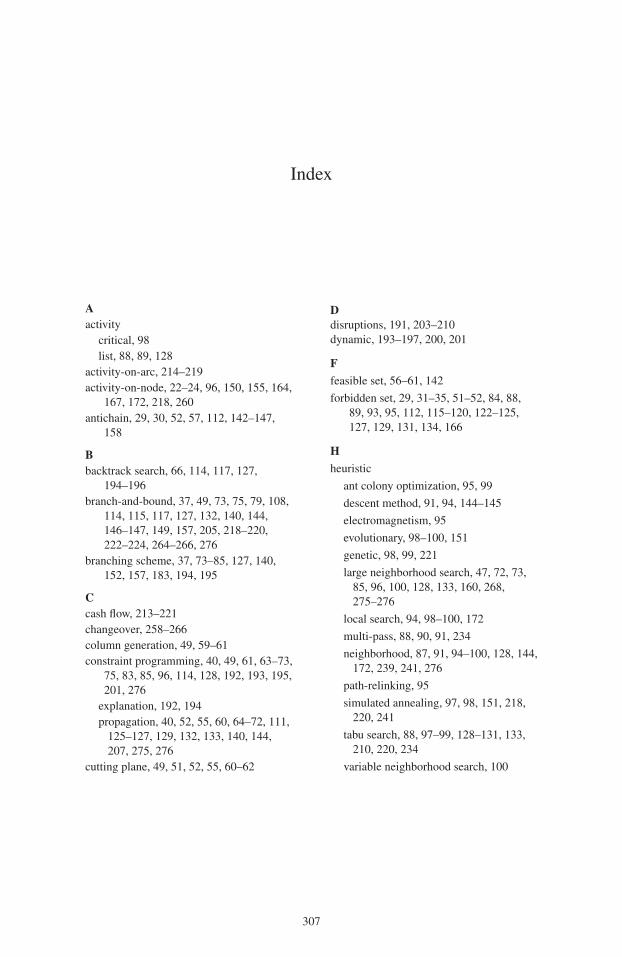
Index
Aactivity
critical, 98list, 88, 89, 128
activity-on-arc, 214–219activity-on-node, 22–24, 96, 150, 155, 164,
167, 172, 218, 260antichain, 29, 30, 52, 57, 112, 142–147,
158
Bbacktrack search, 66, 114, 117, 127,
194–196branch-and-bound, 37, 49, 73, 75, 79, 108,
114, 115, 117, 127, 132, 140, 144,146–147, 149, 157, 205, 218–220,222–224, 264–266, 276
branching scheme, 37, 73–85, 127, 140,152, 157, 183, 194, 195
Ccash flow, 213–221changeover, 258–266column generation, 49, 59–61constraint programming, 40, 49, 61, 63–73,
75, 83, 85, 96, 114, 128, 192, 193, 195,201, 276
explanation, 192, 194propagation, 40, 52, 55, 60, 64–72, 111,
125–127, 129, 132, 133, 140, 144,207, 275, 276
cutting plane, 49, 51, 52, 55, 60–62
Ddisruptions, 191, 203–210dynamic, 193–197, 200, 201
F
feasible set, 56–61, 142
forbidden set, 29, 31–35, 51–52, 84, 88,89, 93, 95, 112, 115–120, 122–125,127, 129, 131, 134, 166
H
heuristic
ant colony optimization, 95, 99
descent method, 91, 94, 144–145
electromagnetism, 95
evolutionary, 98–100, 151
genetic, 98, 99, 221
large neighborhood search, 47, 72, 73,85, 96, 100, 128, 133, 160, 268,275–276
local search, 94, 98–100, 172
multi-pass, 88, 90, 91, 234
neighborhood, 87, 91, 94–100, 128, 144,172, 239, 241, 276
path-relinking, 95
simulated annealing, 97, 98, 151, 218,220, 241
tabu search, 88, 97–99, 128–131, 133,210, 220, 234
variable neighborhood search, 100
307
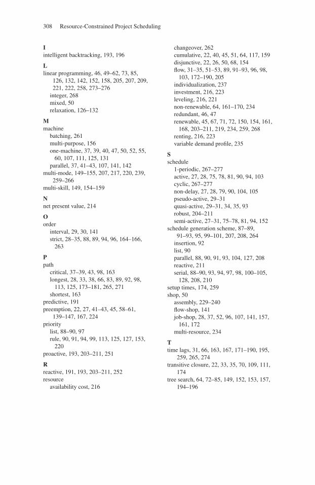
308 Resource-Constrained Project Scheduling
Iintelligent backtracking, 193, 196
Llinear programming, 46, 49–62, 73, 85,
126, 132, 142, 152, 158, 205, 207, 209,221, 222, 258, 273–276
integer, 268mixed, 50relaxation, 126–132
Mmachine
batching, 261multi-purpose, 156one-machine, 37, 39, 40, 47, 50, 52, 55,
60, 107, 111, 125, 131parallel, 37, 41–43, 107, 141, 142
multi-mode, 149–155, 207, 217, 220, 239,259–266
multi-skill, 149, 154–159
Nnet present value, 214
Oorder
interval, 29, 30, 141strict, 28–35, 88, 89, 94, 96, 164–166,
263
Ppath
critical, 37–39, 43, 98, 163longest, 28, 33, 38, 66, 83, 89, 92, 98,
113, 125, 173–181, 265, 271shortest, 163
predictive, 191preemption, 22, 27, 41–43, 45, 58–61,
139–147, 167, 224priority
list, 88–90, 97rule, 90, 91, 94, 99, 113, 125, 127, 153,
220proactive, 193, 203–211, 251
Rreactive, 191, 193, 203–211, 252resource
availability cost, 216
changeover, 262cumulative, 22, 40, 45, 51, 64, 117, 159disjunctive, 22, 26, 50, 68, 154flow, 31–35, 51–53, 89, 91–93, 96, 98,
103, 172–190, 205individualization, 237investment, 216, 223leveling, 216, 221non-renewable, 64, 161–170, 234redundant, 46, 47renewable, 45, 67, 71, 72, 150, 154, 161,
168, 203–211, 219, 234, 259, 268renting, 216, 223variable demand profile, 235
Sschedule
1-periodic, 267–277active, 27, 28, 75, 78, 81, 90, 94, 103cyclic, 267–277non-delay, 27, 28, 79, 90, 104, 105pseudo-active, 29–31quasi-active, 29–31, 34, 35, 93robust, 204–211semi-active, 27–31, 75–78, 81, 94, 152
schedule generation scheme, 87–89,91–93, 95, 99–101, 207, 208, 264
insertion, 92list, 90parallel, 88, 90, 91, 93, 104, 127, 208reactive, 211serial, 88–90, 93, 94, 97, 98, 100–105,
128, 208, 210setup times, 174, 259shop, 50
assembly, 229–240flow-shop, 141job-shop, 28, 37, 52, 96, 107, 141, 157,
161, 172multi-resource, 234
Ttime lags, 31, 66, 163, 167, 171–190, 195,
259, 265, 274transitive closure, 22, 33, 35, 70, 109, 111,
174tree search, 64, 72–85, 149, 152, 153, 157,
194–196
Top Related
Copyright © 2022 FDOKUMEN

