


Bahasa
Halaman
Hukum


Information Sciences 166 (2004) 105–125
www.elsevier.com/locate/ins
Relative information of type s, Csisz�ar’sf -divergence, and information inequalities q
Inder Jeet Taneja a,*, Pranesh Kumar b
a Departamento de Matem�atica, Universidade Federal de Santa Catarina, 88040-900 Florian�opolis,SC, Brazil
b Department of Mathematics, College of Science and Management, University of Northern
British Columbia, Prince George, BC, Canada V2N4Z9
Received 16 June 2003; received in revised form 28 October 2003; accepted 10 November 2003
Abstract
During past years Dragomir has contributed a lot of work providing different kinds
of bounds on the distance, information and divergence measures. In this paper, we have
unified some of his results using the relative information of type s and relating it with the
Csisz�ar’s f -divergence.� 2003 Elsevier Inc. All rights reserved.
Keywords: Relative information; Csisz�ar’s f -divergence; v2-divergence; Hellinger’s
discrimination; Relative information of type s; Information inequalities
1. Introduction
Let ( � )
qTh
Counc*Co
E-m
UR
0020-0
doi:10.
Dn ¼ P ¼ ðp1; p2; . . . ; pnÞ pi���� > 0;
Xni¼1
pi ¼ 1 ; nP 2;
be the set of complete finite discrete probability distributions.
is research is partially supported by the Natural Sciences and Engineering Research
il’s Discovery Grant to Pranesh Kumar.
rresponding author.
ail addresses: [email protected] (I.J. Taneja), [email protected] (P. Kumar).
L: http://www.mtm.ufsc.br/~taneja.
255/$ - see front matter � 2003 Elsevier Inc. All rights reserved.
1016/j.ins.2003.11.002
106 I.J. Taneja, P. Kumar / Information Sciences 166 (2004) 105–125
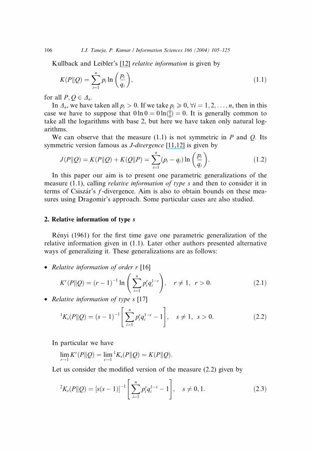
Kullback and Leibler’s [12] relative information is given by
KðPkQÞ ¼Xni¼1
pi lnpiqi
� �; ð1:1Þ
for all P ;Q 2 Dn.
In Dn, we have taken all pi > 0. If we take pi P 0, 8i ¼ 1; 2; . . . ; n, then in this
case we have to suppose that 0 ln 0 ¼ 0 lnð00Þ ¼ 0. It is generally common to
take all the logarithms with base 2, but here we have taken only natural log-
arithms.
We can observe that the measure (1.1) is not symmetric in P and Q. Itssymmetric version famous as J-divergence [11,12] is given by
JðPkQÞ ¼ KðPkQÞ þ KðQkP Þ ¼Xni¼1
ðpi � qiÞ lnpiqi
� �: ð1:2Þ
In this paper our aim is to present one parametric generalizations of the
measure (1.1), calling relative information of type s and then to consider it in
terms of Csisz�ar’s f -divergence. Aim is also to obtain bounds on these mea-
sures using Dragomir’s approach. Some particular cases are also studied.
2. Relative information of type s
R�enyi (1961) for the first time gave one parametric generalization of the
relative information given in (1.1). Later other authors presented alternative
ways of generalizing it. These generalizations are as follows:
• Relative information of order r [16]
KrðPkQÞ ¼ ðr � 1Þ�1ln
Xni¼1
pri q1�ri
!; r 6¼ 1; r > 0: ð2:1Þ
• Relative information of type s [17]
1KsðPkQÞ ¼ ðs� 1Þ�1Xni¼1
psi q1�si
"� 1
#; s 6¼ 1; s > 0: ð2:2Þ
In particular we have
limr!1
KrðPkQÞ ¼ lims!1
1KsðPkQÞ ¼ KðPkQÞ:
Let us consider the modified version of the measure (2.2) given by
2KsðPkQÞ ¼ ½sðs� 1Þ��1Xni¼1
psi q1�si
"� 1
#; s 6¼ 0; 1: ð2:3Þ
I.J. Taneja, P. Kumar / Information Sciences 166 (2004) 105–125 107
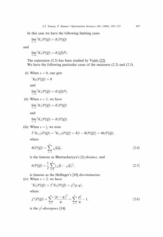
In this case we have the following limiting cases
lims!1
2KsðPkQÞ ¼ KðPkQÞ
and
lims!0
2KsðPkQÞ ¼ KðQkP Þ:
The expression (2.3) has been studied by Vajda [22].
We have the following particular cases of the measures (2.2) and (2.3).
(i) When s ¼ 0, one gets
1K0ðPkQÞ ¼ 0
and
lims!0
2KsðPkQÞ ¼ KðQkP Þ:
(ii) When s ¼ 1, we have
lims!1
1KsðPkQÞ ¼ KðPkQÞ
and
lims!1
2KsðPkQÞ ¼ KðPkQÞ:
(iii) When s ¼ 12, we note
2 1K1=2ðPkQÞ ¼ 2K1=2ðPkQÞ ¼ 4½1� BðPkQÞ� ¼ 4hðPkQÞ;
where
BðPkQÞ ¼Xni¼1
ffiffiffiffiffiffiffipiqi
p; ð2:4Þ
is the famous as Bhattacharyya’s [1] distance, and
hðPkQÞ ¼ 1
2
Xni¼1
ð ffiffiffiffipi
p � ffiffiffiffiqi
p Þ2; ð2:5Þ
is famous as the Hellinger’s [10] discrimination.
(iv) When s ¼ 2, we have
1K2ðPkQÞ ¼ 21K2ðPkQÞ ¼ v2ðp; qÞ;where
v2ðPkQÞ ¼Xni¼1
ðpi � qiÞ2
qi¼Xni¼1
p2iqi
� 1; ð2:6Þ
is the v2-divergence [14].
108 I.J. Taneja, P. Kumar / Information Sciences 166 (2004) 105–125
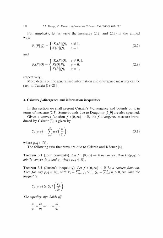
For simplicity, let us write the measures (2.2) and (2.3) in the unified
way:
WsðPkQÞ ¼1KsðPkQÞ; s 6¼ 1;KðPkQÞ; s ¼ 1
�ð2:7Þ
and
UsðPkQÞ ¼2KsðPkQÞ; s 6¼ 0; 1;KðQkP Þ; s ¼ 0;KðPkQÞ; s ¼ 1;
8<: ð2:8Þ
respectively.
More details on the generalized information and divergence measures can be
seen in Taneja [18–21].
3. Csisz�ars f -divergence and information inequalities
In this section we shall present Csisz�ar’s f -divergence and bounds on it in
terms of measure (2.3). Some bounds due to Dragomir [5–9] are also specified.
Given a convex function f : ½0;1Þ ! R, the f -divergence measure intro-
duced by Csisz�ar [3] is given by
Cf ðp; qÞ ¼Xni¼1
qifpiqi
� �; ð3:1Þ
where p; q 2 Rnþ.
The following two theorems are due to Csisz�ar and K€orner [4].
Theorem 3.1 (Joint convexity). Let f : ½0;1Þ ! R be convex, then Cf ðp; qÞ isjointly convex in p and q, where p; q 2 Rn
þ.
Theorem 3.2 (Jensen’s inequality). Let f : ½0;1Þ ! R be a convex function.Then for any p; q 2 Rn
þ, with Pn ¼Pn
i¼1 pi > 0, Qn ¼Pn
i¼1 pi > 0, we have theinequality
Cf ðp; qÞPQnfPnQn
� �:
The equality sign holds iff
p1q1
¼ p2q2
¼ � � � ¼ pnqn
:
I.J. Taneja, P. Kumar / Information Sciences 166 (2004) 105–125 109
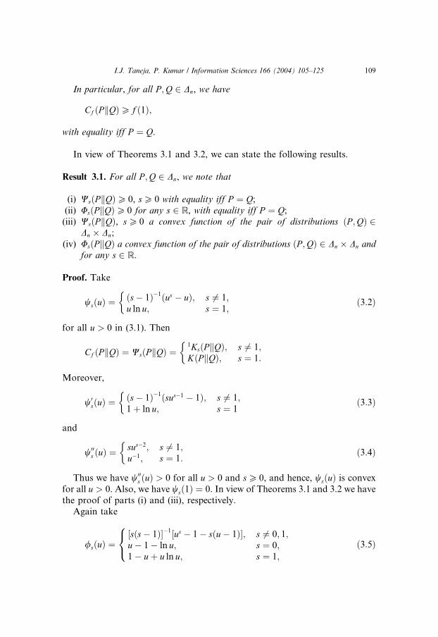
In particular, for all P ;Q 2 Dn, we have
Cf ðPkQÞP f ð1Þ;
with equality iff P ¼ Q.
In view of Theorems 3.1 and 3.2, we can state the following results.
Result 3.1. For all P ;Q 2 Dn, we note that
ii(i) WsðPkQÞP 0, sP 0 with equality iff P ¼ Q;i(ii) UsðPkQÞP 0 for any s 2 R, with equality iff P ¼ Q;(iii) WsðPkQÞ, sP 0 a convex function of the pair of distributions ðP ;QÞ 2
Dn � Dn;(iv) UsðPkQÞ a convex function of the pair of distributions ðP ;QÞ 2 Dn � Dn and
for any s 2 R.
Proof. Take
wsðuÞ ¼ðs� 1Þ�1ðus � uÞ; s 6¼ 1;u ln u; s ¼ 1;
�ð3:2Þ
for all u > 0 in (3.1). Then
Cf ðPkQÞ ¼ WsðPkQÞ ¼1KsðPkQÞ; s 6¼ 1;KðPkQÞ; s ¼ 1:
�
Moreover,
w0sðuÞ ¼
ðs� 1Þ�1ðsus�1 � 1Þ; s 6¼ 1;1þ ln u; s ¼ 1
�ð3:3Þ
and
w00s ðuÞ ¼
sus�2; s 6¼ 1;u�1; s ¼ 1:
�ð3:4Þ
Thus we have w00s ðuÞ > 0 for all u > 0 and sP 0, and hence, wsðuÞ is convex
for all u > 0. Also, we have wsð1Þ ¼ 0. In view of Theorems 3.1 and 3.2 we have
the proof of parts (i) and (iii), respectively.
Again take
/sðuÞ ¼½sðs� 1Þ��1½us � 1� sðu� 1Þ�; s 6¼ 0; 1;u� 1� ln u; s ¼ 0;1� uþ u ln u; s ¼ 1;
8<: ð3:5Þ
110 I.J. Taneja, P. Kumar / Information Sciences 166 (2004) 105–125
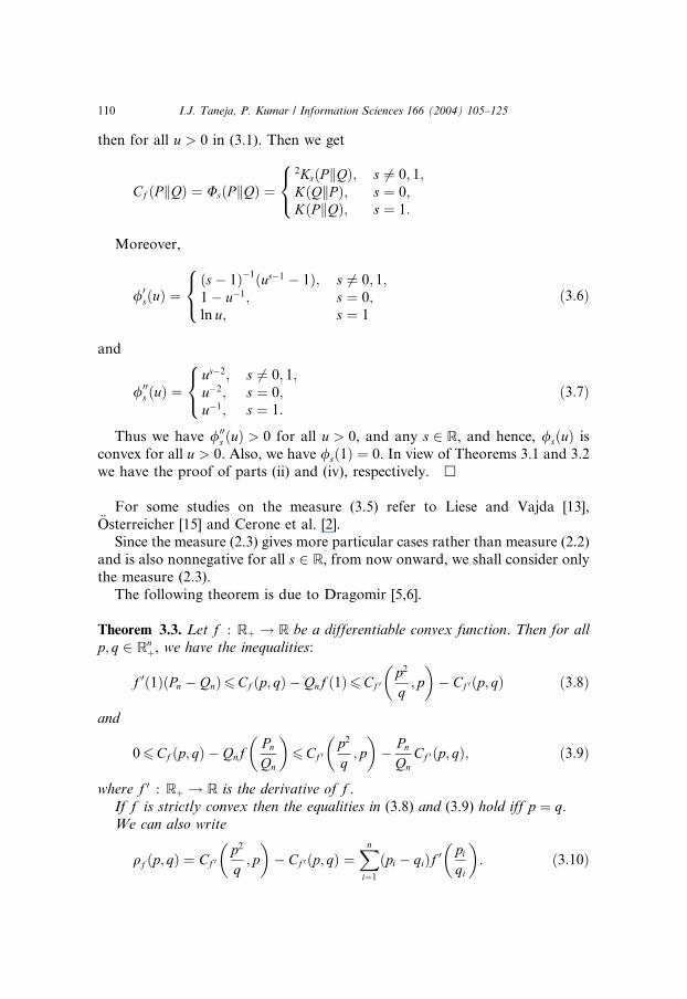
then for all u > 0 in (3.1). Then we get
Cf ðPkQÞ ¼ UsðPkQÞ ¼2KsðPkQÞ; s 6¼ 0; 1;KðQkP Þ; s ¼ 0;KðPkQÞ; s ¼ 1:
8<:
Moreover,
/0sðuÞ ¼
ðs� 1Þ�1ðus�1 � 1Þ; s 6¼ 0; 1;1� u�1; s ¼ 0;ln u; s ¼ 1
8<: ð3:6Þ
and
/00s ðuÞ ¼
us�2; s 6¼ 0; 1;u�2; s ¼ 0;u�1; s ¼ 1:
8<: ð3:7Þ
Thus we have /00s ðuÞ > 0 for all u > 0, and any s 2 R, and hence, /sðuÞ is
convex for all u > 0. Also, we have /sð1Þ ¼ 0. In view of Theorems 3.1 and 3.2
we have the proof of parts (ii) and (iv), respectively. h
For some studies on the measure (3.5) refer to Liese and Vajda [13],€Osterreicher [15] and Cerone et al. [2].
Since the measure (2.3) gives more particular cases rather than measure (2.2)
and is also nonnegative for all s 2 R, from now onward, we shall consider only
the measure (2.3).
The following theorem is due to Dragomir [5,6].
Theorem 3.3. Let f : Rþ ! R be a differentiable convex function. Then for allp; q 2 Rn
þ, we have the inequalities:
f 0ð1ÞðPn � QnÞ6Cf ðp; qÞ � Qnf ð1Þ6Cf 0p2
q; p
� �� Cf 0 ðp; qÞ ð3:8Þ
and
06Cf ðp; qÞ � QnfPnQn
� �6Cf 0
p2
q; p
� �� PnQn
Cf 0 ðp; qÞ; ð3:9Þ
where f 0 : Rþ ! R is the derivative of f .If f is strictly convex then the equalities in (3.8) and (3.9) hold iff p ¼ q.We can also write
qf ðp; qÞ ¼ Cf 0p2
q; p
� �� Cf 0 ðp; qÞ ¼
Xni¼1
ðpi � qiÞf 0 piqi
� �: ð3:10Þ
I.J. Taneja, P. Kumar / Information Sciences 166 (2004) 105–125 111
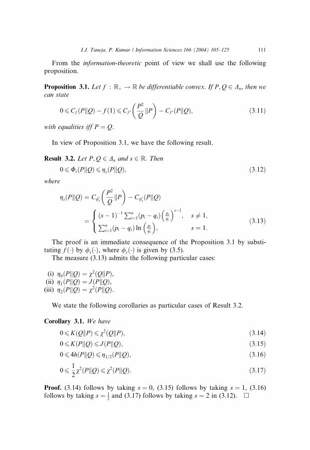
From the information-theoretic point of view we shall use the following
proposition.
Proposition 3.1. Let f : Rþ ! R be differentiable convex. If P ;Q 2 Dn, then wecan state
06Cf ðPkQÞ � f ð1Þ6Cf 0P 2
QkP
� �� Cf 0 ðPkQÞ; ð3:11Þ
with equalities iff P ¼ Q.
In view of Proposition 3.1, we have the following result.
Result 3.2. Let P ;Q 2 Dn and s 2 R. Then
06UsðPkQÞ6 gsðPkQÞ; ð3:12Þ
wheregsðPkQÞ ¼ C/0s
P 2
QkP
� �� C/0
sðPkQÞ
¼ðs� 1Þ�1Pn
i¼1ðpi � qiÞ piqi
� �s�1
; s 6¼ 1;Pni¼1ðpi � qiÞ ln pi
qi
� �; s ¼ 1:
8<: ð3:13Þ
The proof is an immediate consequence of the Proposition 3.1 by substi-
tuting f ð�Þ by /sð�Þ, where /sð�Þ is given by (3.5).
The measure (3.13) admits the following particular cases:
ii(i) g0ðPkQÞ ¼ v2ðQkP Þ,i(ii) g1ðPkQÞ ¼ JðPkQÞ,(iii) g2ðPkQÞ ¼ v2ðPkQÞ.
We state the following corollaries as particular cases of Result 3.2.
Corollary 3.1. We have
06KðQkP Þ6 v2ðQkP Þ; ð3:14Þ06KðPkQÞ6 JðPkQÞ; ð3:15Þ06 4hðPkQÞ6 g1=2ðPkQÞ; ð3:16Þ
061
2v2ðPkQÞ6 v2ðPkQÞ: ð3:17Þ
Proof. (3.14) follows by taking s ¼ 0, (3.15) follows by taking s ¼ 1, (3.16)
follows by taking s ¼ 12and (3.17) follows by taking s ¼ 2 in (3.12). h
112 I.J. Taneja, P. Kumar / Information Sciences 166 (2004) 105–125
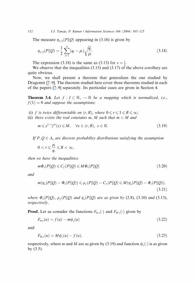
The measure g1=2ðPkQÞ appearing in (3.16) is given by
g1=2ðPkQÞ ¼1
2
Xni¼1
ðqi � piÞffiffiffiffiqipi
r: ð3:18Þ
The expression (3.18) is the same as (3.13) for s ¼ 12.
We observe that the inequalities (3.15) and (3.17) of the above corollary are
quite obvious.
Now, we shall present a theorem that generalizes the one studied by
Dragomir [7–9]. The theorem studied here cover three theorems studied in each
of the papers [7–9] separately. Its particular cases are given in Section 4.
Theorem 3.4. Let f : I � Rþ ! R be a mapping which is normalized, i.e.,f ð1Þ ¼ 0 and suppose the assumptions:
i(i) f is twice differentiable on ðr;RÞ, where 06 r6 16R61;(ii) there exists the real constants m, M such that m < M and
m6 x2�sf 00ðxÞ6M ; 8x 2 ðr;RÞ; s 2 R: ð3:19Þ
If P ;Q 2 Dn are discrete probability distributions satisfying the assumption
0 < r6piqi
6R < 1;
then we have the inequalities:
mUsðPkQÞ6Cf ðPkQÞ6MUsðPkQÞ ð3:20Þ
and
mðgsðPkQÞ � UsðPkQÞÞ6 qf ðPkQÞ � Cf ðPkQÞ6MðgsðPkQÞ � UsðPkQÞÞ;ð3:21Þ
where UsðPkQÞ, qf ðPkQÞ and gsðPkQÞ are as given by (2.8), (3.10) and (3.13),respectively.
Proof. Let us consider the functions Fm:sð�Þ and FM :sð�Þ given by
Fm;sðuÞ ¼ f ðuÞ � m/sðuÞ ð3:22Þ
and
FM ;sðuÞ ¼ M/sðuÞ � f ðuÞ; ð3:23Þ
respectively, where m andM are as given by (3.19) and function /sð�Þ is as givenby (3.5).
I.J. Taneja, P. Kumar / Information Sciences 166 (2004) 105–125 113
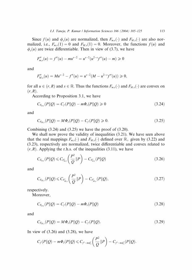
Since f ðuÞ and /sðuÞ are normalized, then Fm:sð�Þ and FM :sð�Þ are also nor-
malized, i.e., Fm:sð1Þ ¼ 0 and FM :sð1Þ ¼ 0. Moreover, the functions f ðuÞ and
/sðuÞ are twice differentiable. Then in view of (3.7), we have
F 00m;sðuÞ ¼ f 00ðuÞ � mus�2 ¼ us�2ðu2�sf 00ðuÞ � mÞP 0
and
F 00M ;sðuÞ ¼ Mus�2 � f 00ðuÞ ¼ us�2ðM � u2�sf 00ðuÞÞP 0;
for all u 2 ðr;RÞ and s 2 R. Thus the functions Fm:sð�Þ and FM :sð�Þ are convex on
ðr;RÞ.According to Proposition 3.1, we have
CFm;sðPkQÞ ¼ Cf ðPkQÞ � mUsðPkQÞP 0 ð3:24Þ
and
CFM ;sðPkQÞ ¼ MUsðPkQÞ � Cf ðPkQÞP 0: ð3:25Þ
Combining (3.24) and (3.25) we have the proof of (3.20).
We shall now prove the validity of inequalities (3.21). We have seen above
that the real mappings Fm:sð�Þ and FM :sð�Þ defined over Rþ given by (3.22) and
(3.23), respectively are normalized, twice differentiable and convex related to
ðr;RÞ. Applying the r.h.s. of the inequalities (3.11), we have
CFm;sðPkQÞ6CF 0m;s
P 2
QkP
� �� CF 0
m;sðPkQÞ ð3:26Þ
and
CFM ;sðPkQÞ6CF 0M ;s
P 2
QkP
� �� CF 0
M ;sðPkQÞ; ð3:27Þ
respectively.
Moreover,
CFm;sðPkQÞ ¼ Cf ðPkQÞ � mUsðPkQÞ ð3:28Þ
and
CFM ;sðPkQÞ ¼ MUsðPkQÞ � Cf ðPkQÞ: ð3:29Þ
In view of (3.26) and (3.28), we have
Cf ðPkQÞ � mUsðPkQÞ6Cf 0�m/0s
P 2
QkP
� �� Cf 0�m/0
sðPkQÞ:
114 I.J. Taneja, P. Kumar / Information Sciences 166 (2004) 105–125
Thus,
Cf ðPkQÞ � mUsðPkQÞ6Cf 0P 2
QkP
� �� mC/0
s
P 2
QkP
� �� Cf 0 ðPkQÞ
þ mC/0sðPkQÞ:
Equivalently,
m C/0s
P 2
QkP
� ��� C/0
sðPkQÞ � UsðPkQÞ
6Cf 0P 2
QkP
� �� Cf 0 ðPkQÞ � Cf ðPkQÞ:
This gives,
mðgsðPkQÞ � UsðPkQÞÞ6 qf ðPkQÞ � Cf ðPkQÞ:
Thus, we have the l.h.s. of the inequalities (3.23).
Again in view of (3.27) and (3.29), we have
MUsðPkQÞ � Cf ðPkQÞ6CM/0s�f 0
P 2
QkP
� �� CM/0
s�f 0 ðPkQÞ:
Thus,
MUsðPkQÞ � Cf ðPkQÞ6MC/0s
P 2
QkP
� �� Cf 0
P 2
QkP
� ��MC/0
sðPkQÞ þ Cf 0 ðPkQÞ:
This gives,
Cf 0P 2
QkP
� �� Cf 0 ðPkQÞ � Cf ðPkQÞ
6M C/0s
P 2
QkP
� ��� C/0
sðPkQÞ � UsðPkQÞ
:
Finally,
qf ðPkQÞ � Cf ðPkQÞ6MðgsðPkQÞ � UsðPkQÞÞ:
Thus we have the r.h.s. of the inequalities (3.22) h
Remark 3.1. The above theorem unifies and generalizes the three different
theorems studied by Dragomir in three different papers [7] (for s ¼ 2), [8] (for
s ¼ 1) and [9] (for s ¼ 12). These particular cases will appear in the next section.
Moreover, we have one more particular case for s ¼ 0 which was not studiedbefore. The above theorem also admits one more interesting case for s ¼ 3, and
it shall be studied elsewhere.
I.J. Taneja, P. Kumar / Information Sciences 166 (2004) 105–125 115
4. Information inequalities
In this section, we shall present particular cases of Theorem 3.4. Some of
these particular cases include the results due to Dragomir [7–9].
4.1. Information bounds in terms of v2-divergence
The case s ¼ 2 of Theorem 3.4 gives:
Proposition 4.1. Let f : I � Rþ ! R be a mapping which is normalized, i.e.,f ð1Þ ¼ 0 and suppose the assumptions:
i(i) f is twice differentiable on ðr;RÞ, where 06 r6 16R61;(ii) there exists the real constants m, M such that m < M and
m6 f 00ðxÞ6M ; 8x 2 ðr;RÞ:
If P ;Q 2 Dn are discrete probability distributions satisfying the assumption0 < r6piqi
6R < 1;
then we have the inequalities:
m2v2ðPkQÞ6Cf ðPkQÞ6
M2v2ðPkQÞ ð4:1Þ
and
m2v2ðPkQÞ6 qf ðPkQÞ � Cf ðPkQÞ6
M2v2ðPkQÞ; ð4:2Þ
where qf ðPkQÞ and v2ðPkQÞ are as given by (3.10) and (2.6), respectively.
In view of Proposition 4.1 we can state the following result.
Result 4.1. Let P ;Q 2 Dn and s 2 R. Let there exists r, R such that r < R and
0 < r6piqi
6R < 1; 8i 2 f1; 2; . . . ; ng;
then Proposition 4.1 yields
Rs�2
2v2ðPkQÞ6UsðPkQÞ6
rs�2
2v2ðPkQÞ; s6 2; ð4:3Þ
rs�2
2v2ðPkQÞ6UsðPkQÞ6
Rs�2
2v2ðPkQÞ; sP 2; ð4:4Þ
Rs�2
2v2ðPkQÞ6 gsðPkQÞ � UsðPkQÞ6
rs�2
2v2ðPkQÞ; s6 2; ð4:5Þ

116 I.J. Taneja, P. Kumar / Information Sciences 166 (2004) 105–125
rs�2
2v2ðPkQÞ6 gsðPkQÞ � UsðPkQÞ6
Rs�2
2v2ðPkQÞ; sP 2: ð4:6Þ
Proof. According to expression (3.7), we have
/00s ðuÞ ¼ us�2:
Now if u 2 ½a; b� � ð0;1Þ, then we have
bs�26/00
s ðuÞ6 as�2; s6 2;
or accordingly,
/00s ðuÞ
6 rs�2; s6 2;P rs�2; sP 2
�ð4:7Þ
and
/00s ðuÞ
6Rs�2; sP 2;PRs�2; s6 2;
�ð4:8Þ
where r and R are as defined above.
Thus in view of (4.7), (4.8) and (4.1), we get the inequalities (4.3) and (4.4).
Again, in view of (4.7), (4.8) and (4.2), we get the inequalities (4.5) and(4.6). h
In view of Result 4.1, we obtain the following corollary.
Corollary 4.1. Under the conditions of Result 4.1, we have
1
2R2v2ðPkQÞ6KðQkPÞ6 1
2r2v2ðPkQÞ; ð4:9Þ
1
2Rv2ðPkQÞ6KðPkQÞ6 1
2rv2ðPkQÞ; ð4:10Þ
1
8ffiffiffiffiffiR2
p v2ðPkQÞ6 hðPkQÞ6 1
8ffiffiffiffir3
p v2ðPkQÞ; ð4:11Þ
Rþ 1
2R2v2ðPkQÞ6 JðPkQÞ6 r þ 1
2r2v2ðPkQÞ: ð4:12Þ
Proof. (4.9) follows by taking s ¼ 0, (4.10) follows by taking s ¼ 1 and (4.11)follows by taking s ¼ 1
2in (4.3). (4.12) follows by adding (4.9) and (4.10). While
for s ¼ 2, we have equality sign. h
I.J. Taneja, P. Kumar / Information Sciences 166 (2004) 105–125 117
Corollary 4.2. Under the conditions of Result 4.1, one gets
1
2R2v2ðPkQÞ6 v2ðQkP Þ � KðQkPÞ6 1
2r2v2ðPkQÞ; ð4:13Þ
1
2Rv2ðPkQÞ6KðQkPÞ6 1
2rv2ðPkQÞ; ð4:14Þ
1
8ffiffiffiffiffiR3
p v2ðPkQÞ6 1
4g1=2ðPkQÞ � hðPkQÞ6 1
8ffiffiffiffir3
p v2ðPkQÞ: ð4:15Þ
Proof. (4.13) follows by taking s ¼ 0, (4.14) follows by taking s ¼ 1 and (4.15)
follows by taking s ¼ 12in (4.5). While for s ¼ 2, we have equality sign. h
4.2. Information bounds in terms of Kullback–Leibler relative information
The case s ¼ 1 of Theorem 3.4 gives:
Proposition 4.2. Let f : I � Rþ ! R be a mapping which is normalized, i.e.,f ð1Þ ¼ 0 and suppose the assumptions:
i(i) f is twice differentiable on ðr;RÞ, where 06 r6 16R61;(ii) there exists the real constants m, M such that m < M and
m6 xf 00ðxÞ6M ; 8x 2 ðr;RÞ:
If P ;Q 2 Dn are discrete probability distributions satisfying the assumption0 < r6piqi
6R < 1;
then we have the inequalities:
mKðPkQÞ6Cf ðPkQÞ6MKðPkQÞ ð4:16Þ
andmKðQkP Þ6 qf ðPkQÞ � Cf ðPkQÞ6MKðQkP Þ; ð4:17Þ
where qf ðPkQÞ and KðPkQÞ are as given by (3.10) and (1.1), respectively.
In view of Proposition 4.2 we have the following result.
Result 4.2. Let P ;Q 2 Dn and s 2 R. Let there exists r, R such that r < R and
0 < r6piqi
6R < 1; 8i 2 f1; 2; . . . ; ng;
then Proposition 4.2 yields
rs�1KðPkQÞ6UsðPkQÞ6Rs�1KðPkQÞ; sP 1; ð4:18Þ
118 I.J. Taneja, P. Kumar / Information Sciences 166 (2004) 105–125
Rs�1KðPkQÞ6UsðPkQÞ6 rs�1KðPkQÞ; s6 1; ð4:19Þrs�1KðQkPÞ6 gsðPkQÞ � UsðPkQÞ6Rs�1KðQkP Þ; sP 1; ð4:20ÞRs�1KðQkP Þ6 gsðPkQÞ � UsðPkQÞ6 rs�1KðQkP Þ; s6 1: ð4:21Þ
Proof. According to expression (3.7), we have
/00s ðuÞ ¼ us�2:
Let us define the function g : ½r;R� ! R such that gðuÞ ¼ u/00s ðuÞ ¼ us�1,
then
supu2½r;R�
gðuÞ ¼ Rs�1; sP 1;rs�1; s6 1
�ð4:22Þ
and
infu2½r;R�
gðuÞ ¼ rs�1; sP 1;Rs�1; s6 1:
�ð4:23Þ
In view of (4.22), (4.23) and (4.16), we have the proof of the inequalities
(4.18) and 4.19. Again in view of (4.22), (4.23) and (4.17) we have the proof of
the inequalities (4.20) and (4.21). h
In view of Result 4.2, we state the following corollaries.
Corollary 4.3. Under the conditions of Result 4.2, one gets
1
RKðPkQÞ6KðQkPÞ6 1
rKðPkQÞ; ð4:24Þ
1
4ffiffiffiR
p KðPkQÞ6 hðPkQÞ6 1
4ffiffir
p KðPkQÞ; ð4:25Þ
2rKðPkQÞ6 v2ðPkQÞ6 2RKðPkQÞ: ð4:26Þ
Proof. (4.24) follows by taking s ¼ 0, (4.25) follows by taking s ¼ 12in (4.19)
and (4.26) follows by taking s ¼ 2 in (4.18). For s ¼ 1, we have equality
sign. h
Corollary 4.4. Under the conditions of Result 4.2, we obtain
1
RKðQkP Þ6 v2ðPkQÞ � KðQkP Þ6 1
rKðQkP Þ; ð4:27Þ
1
4ffiffiffiR
p KðPkQÞ6 1
4g1=2ðPkQÞ � hðPkQÞ6 1
4ffiffir
p KðQkPÞ; ð4:28Þ
I.J. Taneja, P. Kumar / Information Sciences 166 (2004) 105–125 119
2rKðQkP Þ6 v2ðPkQÞ6 2RKðQkP Þ: ð4:29Þ
Proof. (4.27) follows by taking s ¼ 0, (4.28) follows by taking s ¼ 12in (4.21)
and (4.29) follows by taking s ¼ 2 in (4.20). For s ¼ 1, we have equality
sign. h
The following corollary is a consequence of the Corollaries 4.3 and 4.4.
Corollary 4.5. Under the conditions of Result 4.2, one gets
r6KðPkQÞKðQkPÞ 6R; ð4:30Þ
4ffiffir
p6
KðPkQÞhðPkQÞ 6 4
ffiffiffiR
p; ð4:31Þ
2r6v2ðPkQÞKðPkQÞ 6 2R: ð4:32Þ
The inequalities given in Corollary 4.5 can also be written in different forms
given below.
Corollary 4.6. Under the conditions of Result 4.2, we obtain
1þ RR
KðPkQÞ6 JðPkQÞ6 1þ rr
KðPkQÞ; ð4:33Þ
4ffiffir
pð1� BðPkQÞÞ6KðPkQÞ6 4
ffiffiffiR
pð1� BðPkQÞÞ; ð4:34Þ
1� 1
4ffiffir
p KðPkQÞ6BðPkQÞ6 1� 1
4ffiffiffiR
p KðPkQÞ; ð4:35Þ
1
Rv2ðPkQÞ6 JðPkQÞ6 1
rv2ðPkQÞ; ð4:36Þ
1
2Rv2ðPkQÞ6KðPkQÞ6 1
2rv2ðPkQÞ: ð4:37Þ
Inequalities (4.34) and (4.35) are equivalent but are written in different
forms.
In particular for s ¼ 0 in Theorem 3.4, we can state the following propo-
sition.
Proposition 4.3. Let f : I � Rþ ! R be a mapping which is normalized, i.e.,f ð1Þ ¼ 0 and suppose the assumptions:
i(i) f is twice differentiable on ðr;RÞ, where 06 r6 16R61;(ii) there exists the real constants m, M such that m < M and
120 I.J. Taneja, P. Kumar / Information Sciences 166 (2004) 105–125
m6 x2f 00ðxÞ6M ; 8x 2 ðr;RÞ:
If P ;Q 2 Dn are discrete probability distributions satisfying the assumption
0 < r6piqi
6R < 1;
then we have the inequalities:
mKðQkP Þ6Cf ðPkQÞ6MKðQkP Þ ð4:38Þ
andmðv2ðQkP Þ � KðQkP ÞÞ6 qf ðPkQÞ � Cf ðPkQÞ6Mðv2ðQkPÞ � KðQkP ÞÞ; ð4:39Þ
where qf ðPkQÞ, v2ðPkQÞ and KðPkQÞ as given by (3.10), (2.6) and (1.1),respectively.
Inequalities (4.38) and (4.39) are new and were not studied before.
In view of Proposition 4.3, we obtain the following result.
Result 4.3. Let P ;Q 2 Dn and s 2 R. Let there exists r, R such that r < R and
0 < r6piqi
6R < 1; 8i 2 f1; 2; . . . ; ng;
then Proposition 4.3 yields
rsKðQkP Þ6UsðPkQÞ6RsKðQkP Þ; sP 0; ð4:40ÞRsKðQkP Þ6UsðPkQÞ6 rsKðQkP Þ; s6 0; ð4:41Þrsðv2ðQkP Þ � KðQkP ÞÞ6 gsðPkQÞ � UsðPkQÞ
6Rsðv2ðQkP Þ � KðQkPÞÞ; sP 0; ð4:42Þ
Rsðv2ðQkP Þ � KðQkP ÞÞ6 gsðPkQÞ � UsðPkQÞ6 rsðv2ðQkP Þ � KðQkP ÞÞ; s6 0: ð4:43Þ
Proof. According to expression (3.7), we can write
/00s ðuÞ ¼ us�2:
Let us define the function g : ½r;R� ! R such that gðuÞ ¼ u2/00s ðuÞ ¼ us, then
supu2½r;R�
gðuÞ ¼ Rs; sP 0;rs; s6 0
�ð4:44Þ
I.J. Taneja, P. Kumar / Information Sciences 166 (2004) 105–125 121
and
infu2½r;R�
gðuÞ ¼ rs; sP 0;Rs; s6 0:
�ð4:45Þ
In view of (4.44), (4.45) and (4.38) we have the inequalities (4.40) and (4.41).
Again in view of (4.44), (4.45) and (4.39) we have the inequalities (4.42) and(4.43). h
In view of Result 4.3, we get the following corollaries.
Corollary 4.7. Under the conditions of Result 4.3, we have
rKðQkP Þ6KðPkQÞ6RKðQkP Þ; ð4:46Þ1
4
ffiffir
pKðQkP Þ6 hðPkQÞ6 1
4
ffiffiffiR
pKðQkPÞ; ð4:47Þ
2r2KðQkP Þ6 v2ðPkQÞ6 2R2KðQkP Þ: ð4:48Þ
Proof. (4.46) follows by taking s ¼ 1, (4.47) follows by taking s ¼ 12and (4.48)
follows by taking s ¼ 2 in (4.40). For s ¼ 0, we have equality sign. h
Corollary 4.8. Under the conditions of Result 4.3, we obtain
1þ RR
KðQkP Þ6 v2ðQkP Þ6 1þ rr
KðQkP Þ; ð4:49Þ
1
4
ffiffir
pðv2ðQkP Þ � KðQkP ÞÞ6 1
4g1=2ðPkQÞ � hðPkQÞ
61
4
ffiffiffiR
pðv2ðQkP Þ � KðQkP ÞÞ; ð4:50Þ
2r2ðv2ðQkP Þ � KðQkP ÞÞ6 v2ðPkQÞ6 2R2ðv2ðQkPÞ � KðQkP ÞÞ: ð4:51Þ
Proof. (4.49) follows by taking s ¼ 1, (4.50) follows by taking s ¼ 12and (4.51)
follows by taking s ¼ 2 in (4.42). For s ¼ 0, we have equality sign. h
4.3. Information bounds in terms of Hellinger’s discrimination
The case s ¼ 12of Theorem 3.4 gives:
Proposition 4.4. Let f : I � Rþ ! R the generating mapping is normalized, i.e.,f ð1Þ ¼ 0 and satisfy the assumptions:
i(i) f is twice differentiable on ðr;RÞ, where 06 r6 16R61;(ii) there exists the real constants m, M such that m < M and
122 I.J. Taneja, P. Kumar / Information Sciences 166 (2004) 105–125
m6 x3=2f 00ðxÞ6M ; 8x 2 ðr;RÞ:
If P ;Q 2 Dn are discrete probability distributions satisfying the assumption
0 < r6piqi
6R < 1;
then we have the inequalities:
4mhðPkQÞ6Cf ðPkQÞ6 4MhðPkQÞ ð4:52Þ
and
4m1
4g1=2ðPkQÞ
�� hðPkQÞ
�6 qf ðPkQÞ � Cf ðPkQÞ
6 4M1
4g1=2ðPkQÞ
�� hðPkQÞ
�; ð4:53Þ
where hðPkQÞ is the Hellinger’s divergence given by (2.5), qf ðPkQÞ is as given by(3.10) and g1=2ðPkQÞ is as given by (3.18).
In view of Proposition 4.4, we state the following result.
Result 4.4. Let P ;Q 2 Dn and s 2 R. Let there exists r, R such that r < R and
0 < r6piqi
6R < 1; 8i 2 f1; 2; . . . ; ng;
then Proposition 4.4 yields
4r2s�12 hðPkQÞ6UsðPkQÞ6 4R
2s�12 hðPkQÞ; sP 1
2; ð4:54Þ
4R2s�12 hðPkQÞ6UsðPkQÞ6 4r
2s�12 hðPkQÞ; s6 1
2; ð4:55Þ
4r2s�12
1
4g1=2ðPkQÞ
�� hðPkQÞ
�6 gsðPkQÞ � UsðPkQÞ
6 4R2s�12
1
4g1=2ðPkQÞ
�� hðPkQÞ
�; sP
1
2; ð4:56Þ
4R2s�12
1
4g1=2ðPkQÞ
�� hðPkQÞ
�6 gsðPkQÞ � UsðPkQÞ
6 4r2s�12
1
4g1=2ðPkQÞ
�� hðPkQÞ
�; s6
1
2: ð4:57Þ
Proof. Let the function /sðuÞ given by (3.5) is defined over ½r;R�. Defining
gðuÞ ¼ u3=2/00s ðuÞ ¼ u3=2us�2 ¼ u
2s�12 , we get
I.J. Taneja, P. Kumar / Information Sciences 166 (2004) 105–125 123
supu2½r;R�
gðuÞ ¼ R2s�12 ; sP 1
2;
r2s�12 ; s6 1
2
(ð4:58Þ
and
infu2½r;R�
gðuÞ ¼ r2s�12 ; sP 1
2;
R2s�12 ; s6 1
2:
(ð4:59Þ
In view of (4.58), (4.59) and (4.52) we get the proof of the inequalities (4.54)and (4.55). Again in view of (4.58), (4.59) and (4.53) we get the proof of the
inequalities (4.56) and (4.57). h
In view of Result 4.4, we obtain the following corollary.
Corollary 4.9. Under the conditions of Result 4.4, one gets
4ffiffiffiR
p hðPkQÞ6KðQkPÞ6 4ffiffir
p hðPkQÞ; ð4:60Þ
4ffiffir
phðPkQÞ6KðPkQÞ6 4
ffiffiffiR
phðPkQÞ; ð4:61Þ
8ffiffiffiffir3
phðPkQÞ6 v2ðPkQÞ6 8
ffiffiffiffiffiR3
phðPkQÞ: ð4:62Þ
Proof. (4.60) follows by taking s ¼ 0 in (4.55). (4.61) follows by taking s ¼ 1
and (4.62) follows by taking s ¼ 2 in (4.57). For s ¼ 12, we have equality
sign. h
Corollary 4.10. Under the conditions of Result 4.4, we have
4ffiffiffiR
p 1
4g1=2ðPkQÞ
�� hðPkQÞ
�6 v2ðQkPÞ � KðQkPÞ
64ffiffir
p 1
4g1=2ðPkQÞ
�� hðPkQÞ
�; ð4:63Þ
4ffiffir
p 1
4g1=2ðPkQÞ
�� hðPkQÞ
�6KðPkQÞ6 4
ffiffiffiR
p 1
4g1=2ðPkQÞ
�� hðPkQÞ
�;
ð4:64Þ
8ffiffiffiffir3
p 1
4g1=2ðPkQÞ
�� hðPkQÞ
�6 v2ðPkQÞ6 8
ffiffiffiffiffiR3
p 1
4g1=2ðPkQÞ
�� hðPkQÞ
�:
ð4:65Þ
Proof. (4.63) follows by taking s ¼ 0, (4.64) follows by taking s ¼ 1 and (4.65)
follows by taking s ¼ 2 in Result 4.4. For s ¼ 12, we have equality sign. h

124 I.J. Taneja, P. Kumar / Information Sciences 166 (2004) 105–125
Acknowledgements
Authors wish to express their sincere thanks to the referee for the valuable
suggestions which helped in improving the presentation and quality of the
paper.
References
[1] A. Bhattacharyya, Some analogues to the amount of information and their uses in statistical
estimation, Sankhya 8 (1946) 1–14.
[2] P. Cerone, S.S. Dragomir, F. €Osterreicher, Bounds on extended f -divergences for a variety of
classes, RGMIA Research Report Collection, 6(1), Article 7, 2003.
[3] I. Csisz�ar, Information type measures of differences of probability distribution and indirect
observations, Studia Math. Hungarica 2 (1967) 299–318.
[4] I. Csisz�ar, J. K€orner, Information Theory: Coding Theorems for Discrete Memoryless
Systems, Academic Press, New York, 1981.
[5] S.S. Dragomir, Some inequalities for the Csisz�ar U-divergence, Inequalities for Csisz�ar f -Divergence in Information Theory. Available from <http://rgmia.vu.edu.au/monographs/
csiszar.htm>.
[6] S.S. Dragomir, A converse inequality for the Csisz�ar U-divergence, Inequalities for Csisz�ar f -Divergence in Information Theory. Available from <http://rgmia.vu.edu.au/monographs/
csiszar.htm>.
[7] S.S. Dragomir, Some inequalities for ðm;MÞ-convex mappings and applications for the Csisz�ar
U-divergence in information theory, Inequalities for Csisz�ar f -Divergence in Information
Theory. Available from <http://rgmia.vu.edu.au/monographs/csiszar.htm>.
[8] S.S. Dragomir, Upper and lower bounds for Csisz�ar f -divergence in terms of the Kullback–
Leibler distance and applications, Inequalities for Csisz�ar f -Divergence in Information
Theory. Available from <http://rgmia.vu.edu.au/monographs/csiszar.htm>.
[9] S.S. Dragomir, Upper and lower bounds for Csisz�ar f -divergence in terms of Hellinger
discrimination and applications, Inequalities for Csisz�ar f -Divergence in Information Theory.
Available from <http://rgmia.vu.edu.au/monographs/csiszar.htm>.
[10] E. Hellinger, Neue Begr€undung der Theorie der quadratischen Formen von unendlichen vielen
Ver€anderlichen, J. Reine Aug. Math. 136 (1909) 210–271.
[11] H. Jeffreys, An invariant form for the prior probability in estimation problems, Proc. Roy.
Soc. Lond., Ser. A 186 (1946) 453–461.
[12] S. Kullback, R.A. Leibler, On information and sufficiency, Ann. Math. Stat. 22 (1951) 79–86.
[13] F. Liese, I. Vajda, Convex Statistical Decision Rules, Teubner-Texte zur Mathematick, Band
95, Leipzig, 1987.
[14] K. Pearson, On the Criterion that a given system of deviations from the probable in the case of
correlated system of variables is such that it can be reasonable supposed to have arisen from
random sampling, Philos. Mag. 50 (1900) 157–172.
[15] F. €Osterreicher, Csisz�ar’s f -Divergence, Basic Properties, pre-print, 2002. Available from
<http://rgmia.vu.edu.au>.
[16] A R�enyi, On measures of entropy and information, in: Proc. 4th Berk. Symp. Math. Stat.
Probl., vol. 1, University of California Press, 1961, pp. 547–561.
[17] B.D. Sharma, R. Autar, Relative information function and their type ða; bÞ generalizations,
Metrika 21 (1974) 41–50.

I.J. Taneja, P. Kumar / Information Sciences 166 (2004) 105–125 125
[18] I.J. Taneja, Some contributions to information Theory––I (a survey: on measures of
information), J. Comb. Inf. Syst. Sci. (India) 4 (1979) 253–274.
[19] I.J. Taneja, On generalized information measures and their applications, in: P.W. Hawkes
(Ed.), Advances in Electronics and Electron Physics, 76, Academic Press, USA, 1989, pp. 327–
413.
[20] I.J. Taneja, New developments in generalized information measures, in: P.W. Hawkes (Ed.),
Advances in Imaging and Electron Physics, 91, 1995, pp. 37–135.
[21] I.J. Taneja, Generalized Information Measures and their Applications, 2001. On line book:
http://www.mtm.ufsc.br/~taneja/book/book.html.
[22] I. Vajda, Theory of Statistical Inference and Information, Kluwer Academic Press, London,
1989.
Top Related
Copyright © 2022 FDOKUMEN

