


Bahasa
Halaman
Hukum

SPECIAL REVIEW
Reconceptualising the beta diversity-environmentalheterogeneity relationship in running water systems
JANI HEINO*, ADRIANO S. MELO† AND LUIS M. BINI†
*Finnish Environment Institute, Natural Environment Centre, Biodiversity, Oulu, Finland†Departamento de Ecologia, Universidade Federal de Goias, Goiania, Brazil
SUMMARY
1. Beta diversity modelling has received increased interest recently. There are multiple definitions of
beta diversity, but here, we focus on variability in species composition among sampling units within
a given area. This facet can be described using various approaches. Some approaches ignore the spa-
tial scale of the area considered (i.e. region limits), while some consider different region limits as a
starting point for the analysis of beta diversity.
2. We focused specifically on the beta diversity–environmental heterogeneity relationship in running
waters. First, we present two conceptual models, which assume either (1) strong environmental con-
trol among localities (riffle sites in our case) within each region unit (a region unit encompasses a
species pool and can be a stream or a basin or an ecoregion) or (2) that the spatial level of a region
unit affects the relative importance of mechanisms affecting variability in species composition among
localities (i.e. among riffle sites) within each region unit. Second, we compared three recent studies
that used similar methods to examine the beta diversity–environmental heterogeneity relationship,
but which were based on different region units, comprising sets of streams or sets of basins or sets of
ecoregions.
3. Our conceptual framework assumes that environmental control is not likely to be the sole mecha-
nism affecting variability in community composition among localities within each region unit, but it
is likely to be most important when dispersal rates are intermediate (i.e. among localities within a
basin). In contrast, if dispersal rates are very high (i.e. among localities within a stream) or very low
(i.e. among localities within an ecoregion), environmental control is in part masked by high dispersal
rates or is prevented from occurring because not all species can reach all localities, respectively. Such
scale dependency in the relative strength of environmental control might therefore transcend spatial
scales from individual region units to the strength of the beta diversity–environmental heterogeneity
relationship. We emphasise that the beta diversity–environmental heterogeneity relationship can only
be tested across multiple region units. The results of three case studies are consistent with these pre-
dictions. Specifically, the beta diversity–environmental heterogeneity regression was highly signifi-
cant across multiple basins, but not across multiple streams or across multiple ecoregions.
4. We suggest that researchers take spatial scale and region unit level explicitly into account when
inferring the mechanisms structuring ecological communities and mapping variation in beta diver-
sity. We also propose a unified terminology for studies examining the beta diversity–environmental
heterogeneity relationship in running waters because inconsistent terminology is likely to hamper
the progress of our science.
Keywords: average distance to centroid, dispersal, spatial scale, species sorting, terminology
Correspondence: Jani Heino, Finnish Environment Institute, Natural Environment Centre, Biodiversity, Paavo Havaksen Tie 3, FI-90014
Oulu, Finland.
E-mail: [email protected]
© 2014 John Wiley & Sons Ltd 223
Freshwater Biology (2015) 60, 223–235 doi:10.1111/fwb.12502
Introduction
Species diversity can be described by three components:
local species richness (a-diversity), regional richness
(c-diversity) and differences in species composition
between localities (b-diversity) (Whittaker, 1960). While
a large number of studies have focused on local or
regional species richness patterns in the past, ecological
research has shifted much of its recent focus to beta
diversity patterns (Anderson et al., 2011; Melo et al.,
2011). There are various beta diversity concepts (Tuom-
isto, 2010; Anderson et al., 2011), but in this paper, we
favour the one proposed by Anderson, Ellingsen &
McArdle (2006) owing to its simplicity: ‘Beta diversity
can be defined as the variability in species composition
among sampling units for a given area’.
In the context of studying beta diversity, the concepts of
‘region unit’ and ‘locality’ are important (Table 1).
Among the factors accounting for variation in beta diver-
sity across multiple region units, environmental heteroge-
neity (here defined as the variation in abiotic conditions
among the same set of localities where beta diversity was
estimated within a region unit; Fig. 1) is often hypothes-
ised as being of paramount importance (Anderson et al.,
2006). One could expect a positive beta diversity–environ-
mental heterogeneity relationship (BDEHR) because an
increase in the latter incorporates an increase in the vari-
ety of environmental conditions to which different species
are adapted, hence producing greater variation in species
composition among localities within a region unit (Chase
& Leibold, 2003; Leibold et al., 2004). Despite its intuitive
appeal, however, this explanation has not gained
unequivocal empirical support. As with the alpha diver-
sity–environmental heterogeneity relationship (Bar-Mass-
ada & Wood, 2014), the BDEHR may also show multiple
forms. The potential reasons underlying different
BDEHRs centre on issues of (1) spatial level of a region
unit, (2) environmental gradient length and (3) ecological
mechanisms, the importance of which may be determined
by a combination of (1) and (2). These differences may
also be affected by (4) statistical choices. Furthermore,
communication of research findings is hampered by
inconsistent terminology and, hence, we propose a uni-
fied terminology for this field of research (Table 1).
Table 1 Definitions of the common terms used throughout this paper
Term Definition
Spatial scale Spatial scale has two components: grain and extent (Wiens, 1989)
Spatial grain Spatial grain refers to the size of the sampling unit used in a study (Wiens, 1989). In running water research, spatial
grain typically refers to the local arena, such as a riffle site, in macroecological studies (Heino, 2011)
Spatial extent Spatial extent refers to the size of the region encompassing all localities in a region unit (Wiens, 1989). Spatial
extent can be measured as the distance between the localities situated furthest from each other or as a convex
polygon encompassing all localities in a region unit
Overall spatial level Overall spatial level describes the whole geographic area encompassing all region units in a study. It may be a
landscape, a biogeographic region or an entire continent
Region unit level A region unit encompasses a regional species pool. In running waters, a region unit may be a stream (Gr€onroos &
Heino, 2012), a drainage basin (Landeiro et al., 2012) or an ecoregion (Bini et al., 2014)
Locality A locality is a local arena within which biotic interactions and responses of species to environmental conditions
occur. A locality harbours a biological community. In running water research, a typical locality is a riffle site
(Heino, 2011)
Environmental
conditions
Environmental features of a locality. Environmental factors are agents of species sorting (Leibold et al., 2004)
Community
composition
Biological features of a locality. Community composition is made up of species found at a locality at a given point
in time
Environmental
heterogeneity
Environmental differences among two or more localities. In this study, we define environmental heterogeneity as
variability in abiotic conditions among localities within a region unit (Anderson et al., 2006)
Beta diversity Biological differences among two or more localities. In this study, we define beta diversity as variability in species
composition among localities within a region unit (Anderson et al., 2006)
Species sorting Species are filtered by environmental factors to occur at environmentally suitable sites. Adequate dispersal rates are
necessary so that species can track variation in environmental conditions among localities (Leibold et al., 2004)
Mass effects High dispersal rates homogenise community structure at adjacent localities irrespective of their environmental
conditions and obscure species sorting (Leibold et al., 2004)
Dispersal limitation Some species are precluded from occurring at suitable localities because the nearest occupiable sites are too far
away. Dispersal limitation prevents perfect species sorting from occurring because species cannot reach all
environmentally suitable localities (Leibold et al., 2004)
Dispersal barrier Any factor (e.g. geomorphological, hydrological) that prevents species from dispersing to all localities within a
region unit
© 2014 John Wiley & Sons Ltd, Freshwater Biology, 60, 223–235
224 J. Heino et al.
Spatial scale is a key issue in ecology because most
patterns and underlying processes are scale dependent
(Levin, 1992; Wu & Loucks, 1995). Spatial scale com-
prises ‘grain’, which refers to the resolution or size of
the sampling unit, and ‘extent’, which refers to the size
of the region encompassing all sampling units of a study
(Wiens, 1989). A change in either grain or extent is
expected to change beta diversity patterns (Barton et al.,
2013), and a number of studies have shown that beta
diversity is strongly dependent on the grain size and the
spatial extent of a study (Gering & Crist, 2002; Hepp &
Melo, 2013).
Along with increasing spatial extent, ranges in envi-
ronmental variables are also likely to increase (e.g.
Jackson, Peres-Neto & Olden, 2001), so ecologists have
also used spatial extent or geographic distances between
sites as surrogates for environmental heterogeneity (e.g.
Harrison, Ross & Lawton, 1992). Increasing lengths of
environmental gradients are likely to increase the
strength of environmental filtering (i.e. species sorting),
and one may expect to find increasingly large variation
in species composition with increasing spatial extent
due to the increased importance of species sorting (e.g.
Heino, 2011). Thus, although dispersal rates are also
likely to be scale dependent (e.g. Ng, Carr & Cottenie,
2009), their effects may go unnoticed because the lengths
of environmental gradients may increase with increasing
spatial extent.
Our definition of region unit is a key issue in this con-
text. In running water research, a region unit of analysis
may refer to a stream encompassing multiple riffle sites
(Gr€onroos & Heino, 2012; Al-Shami et al., 2013), a drain-
age basin encompassing multiple stream riffle sites
(Landeiro et al., 2012; G€othe, Angeler & Sandin, 2013) or
an ecoregion encompassing multiple stream riffle sites
from different drainage basins (Mykr€a, Heino & Muotka,
2007; Bini et al., 2014). In all these studies in running
waters, grain size was a riffle site, whereas the region
unit of analysis varied among studies, being a stream, a
drainage basin or an ecoregion, respectively. In the fol-
lowing, we will refer explicitly to grain size as a locality
(riffle site) and the three levels as region units. We
emphasise that ‘spatial level of a region unit’ and ‘spa-
tial extent’ are not exactly the same thing. Although spa-
tial extent does increase from the stream level to the
ecoregion level, spatial extent may also vary within each
region unit level (e.g. ecoregions of different sizes; Bini
et al., 2014).
Two different conceptual models can be used to illus-
trate the scale dependency of the BDEHR. First, ‘the
environmental control model’ underlying variation in
beta diversity across multiple region units assumes that
the spatial level of a region unit has no effect on the
mechanisms underlying the BDEHR (Fig. 2). This model
starts from within each region unit, where species sort-
ing is occurring among localities. Species are assumed to
be able to disperse to all localities within a region unit
and, hence, environmental conditions determine which
species are able to occur at a locality (Leibold et al.,
2004). Species sorting should be the more important the
wider the differences in environmental conditions are
among localities within a region unit. If this model holds
within each region unit, one may also expect a positive
BDEHR that can only be detected across multiple region
units. An important consideration in this context is,
however, that the region unit level within which both
beta diversity and habitat heterogeneity are measured
typically varies among studies (Fig. 1).
Simultaneous consideration of the spatial level of a
region unit, dispersal rates, spatial extent and environ-
mental gradient lengths is important because these fac-
tors determine the relative roles of the mechanisms
structuring ecological communities (Leibold et al., 2004;
Gravel et al., 2006; Thompson & Townsend, 2006; Brown
et al., 2011; Altermatt, 2013; Bini et al., 2014; Datry et al.,
2014). The main general mechanisms causing variation
in community composition among localities within a
region unit include not only species sorting but also
mass effects at small spatial extents and dispersal limita-
tion at large spatial extents (Table 1). These two dis-
persal-related mechanisms may obscure species sorting
effects by disassociating species and the environment
owing to either very high or very low dispersal rates
(Leibold et al., 2004; Ng et al., 2009; Winegardner et al.,
2012; Heino & Peckarsky, 2014). Species sorting has been
shown to be the most important mechanism structuring
ecological communities at various spatial extents (Cottenie,
2005; Van der Gucht et al., 2007), including stream
systems ranging from riffle to catchment extents (Robson,
1996; Downes et al., 1998; Robson & Chester, 1999;
Landeiro et al., 2012). However, the potential scale
dependencies of species sorting, mass effects and dis-
persal limitation have received little explicit consider-
ation in running waters (Heino, 2013; Heino &
Peckarsky, 2014), although some studies have considered
those mechanisms at very small extents within and
among riffles in a stream (Robson & Chester, 1999;
Downes & Reich, 2008; Downes & Lancaster, 2010).
Furthermore, those dispersal-related mechanisms acting
among localities within each region unit are likely to
affect the BDEHR. For example, mass effects may mask
the effects of species sorting among localities within
© 2014 John Wiley & Sons Ltd, Freshwater Biology, 60, 223–235
Beta diversity and environmental heterogeneity 225
small region units (i.e. within a stream), decoupling the
match between variation in species composition and var-
iation in habitat conditions (Heino & Gr€onroos, 2013).
Correspondingly, within very large region units (i.e.
within a large ecoregion), dispersal limitation may partly
prevent species sorting from occurring, leading to less
clear relationships between variation in species composi-
tion and variation in environmental conditions among
Basin-1 Basin-10Basin-2
...
...Ecoregion-1 Ecoregion-2 Ecoregion-10
Reg
ion
unit:
Stre
amR
egio
nun
it: B
asin
Reg
ion
unit:
Eco
regi
on
BDEHR (across 10 streams)
...Stream-1 Stream-10Stream-2
Beta diversityHabitat heterogeneity
Beta diversityHabitat heterogeneity
Beta diversityHabitat heterogeneity
BDEHR (across 10 basins)
Beta diversityHabitat heterogeneity
Beta diversityHabitat heterogeneity
Beta diversityHabitat heterogeneity
BDEHR (across 10 ecoregions)
Beta diversityHabitat heterogeneity
Beta diversityHabitat heterogeneity
Beta diversityHabitat heterogeneity
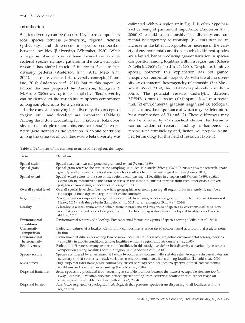
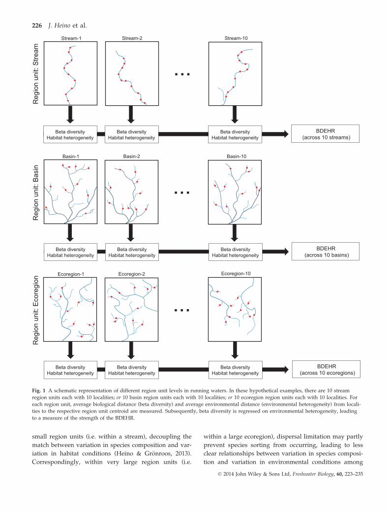
Fig. 1 A schematic representation of different region unit levels in running waters. In these hypothetical examples, there are 10 stream
region units each with 10 localities; or 10 basin region units each with 10 localities; or 10 ecoregion region units each with 10 localities. For
each region unit, average biological distance (beta diversity) and average environmental distance (environmental heterogeneity) from locali-
ties to the respective region unit centroid are measured. Subsequently, beta diversity is regressed on environmental heterogeneity, leading
to a measure of the strength of the BDEHR.
© 2014 John Wiley & Sons Ltd, Freshwater Biology, 60, 223–235
226 J. Heino et al.
localities. In contrast, if dispersal rates are neither too
high nor clearly limiting among localities (i.e. within a
drainage basin), species sorting should lead to strong
associations between species composition and habitat
conditions. This is ‘the dispersal-environmental control
model’ underlying the BDEHR tested across multiple
region units (Fig. 3). This model also starts from the
individual region unit level, where species sorting
occurs among localities. However, in contrast to the
environmental control model, high or low dispersal rates
BD
Environmental dissimilarity
EH
Com
posi
tiona
l di
ssim
ilarit
y
Environmental dissimilarity
Com
posi
tiona
l di
ssim
ilarit
y
BDEHR (across 10 basins)
‘Species sorting’within the blue basin
‘Species sorting’within the red basin
Incr
easi
ng e
nviro
nmen
tal h
eter
ogen
eity
with
in e
ach
regi
on u
nit
Reg
ion
unit:
Stre
am
Reg
ion
unit:
Bas
in
Reg
ion
unit:
Eco
regi
on
BD
Environmental dissimilarity
EH
Com
posi
tiona
l di
ssim
ilarit
y
Environmental dissimilarity
Com
posi
tiona
l di
ssim
ilarit
yBDEHR
(across 10 streams)
‘Species sorting’within the blue stream
‘Species sorting’within the red stream
BD
Environmental dissimilarity
EH
Com
posi
tiona
l di
ssim
ilarit
y
Environmental dissimilarity
Com
posi
tiona
l di
ssim
ilarit
y
BDEHR (across 10 ecoregions)
‘Species sorting’within the blue ecoregion
‘Species sorting’within the red ecoregion
Incr
easi
ng b
eta
dive
rsity
with
in e
ach
regi
on u
nit
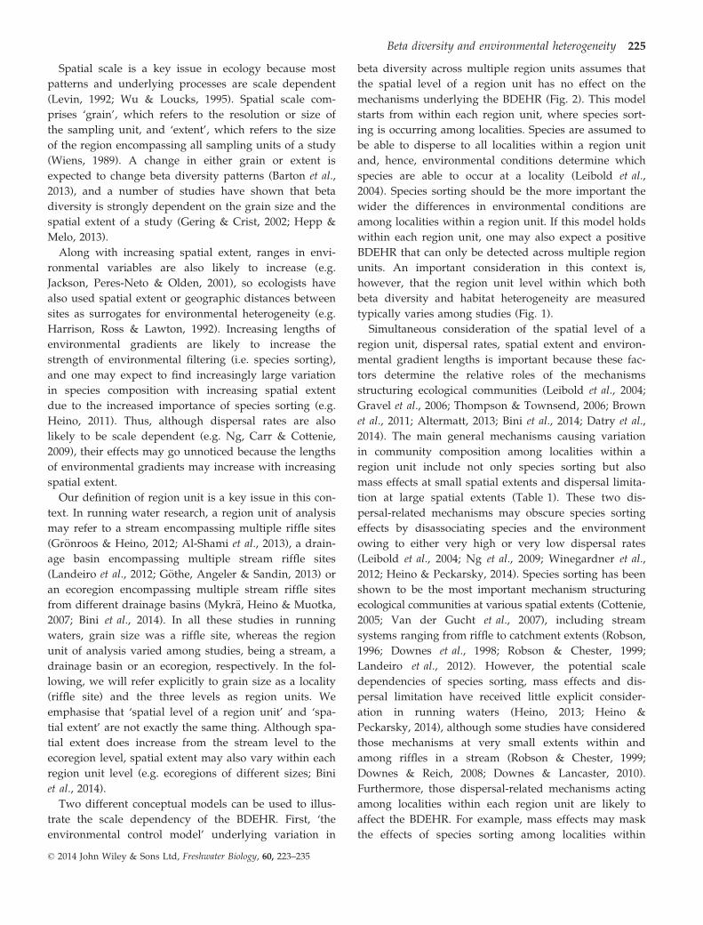
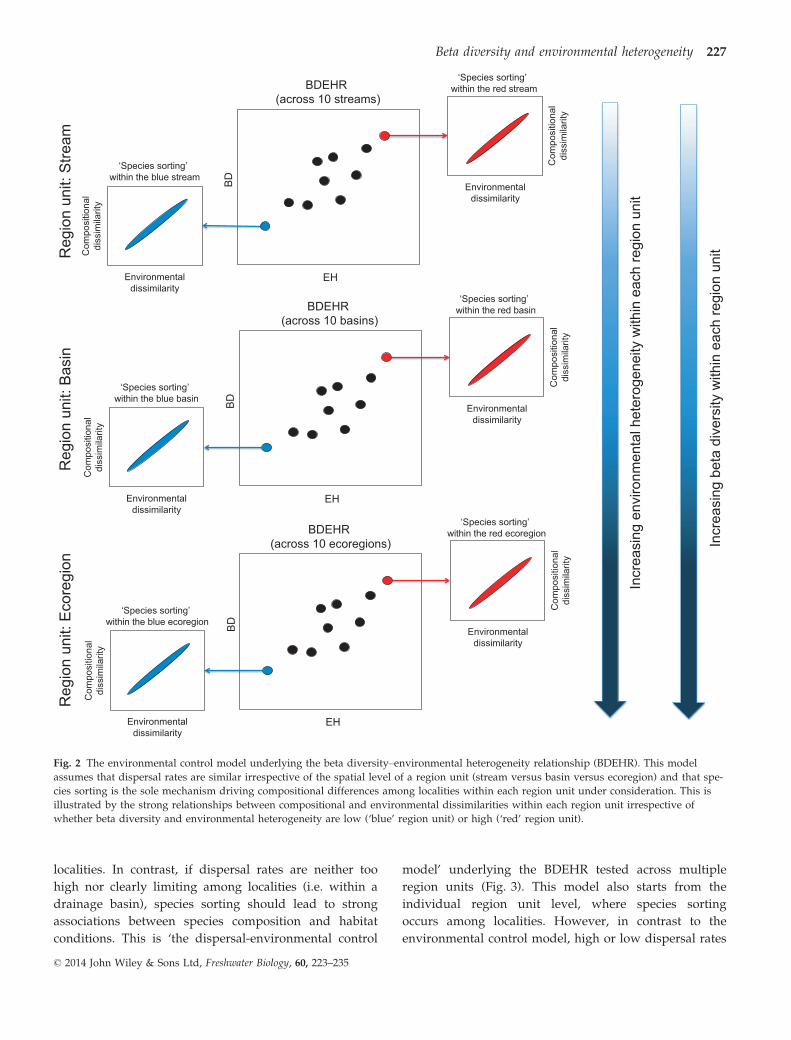
Fig. 2 The environmental control model underlying the beta diversity–environmental heterogeneity relationship (BDEHR). This model
assumes that dispersal rates are similar irrespective of the spatial level of a region unit (stream versus basin versus ecoregion) and that spe-
cies sorting is the sole mechanism driving compositional differences among localities within each region unit under consideration. This is
illustrated by the strong relationships between compositional and environmental dissimilarities within each region unit irrespective of
whether beta diversity and environmental heterogeneity are low (‘blue’ region unit) or high (‘red’ region unit).
© 2014 John Wiley & Sons Ltd, Freshwater Biology, 60, 223–235
Beta diversity and environmental heterogeneity 227
may partly disassociate communities from environmen-
tal control at small (i.e. within a stream) and large (i.e.
within an ecoregion) spatial extents, respectively. If this
model holds within each region unit, one should see dif-
ferent BDEHRs depending on the spatial level of the
region units where beta diversity and environmental
heterogeneity are measured (i.e. stream versus drainage
basin versus ecoregion).
Ecologists have recently broadened their focus to not
only quantify patterns of beta diversity across spatial
scales, but also explain variation or dissimilarities in
species composition using environmental variables or
environmental dissimilarities, respectively (Legendre,
Borcard & Peres-Neto, 2005; Tuomisto & Ruokolainen,
2006; Melo, Rangel & Diniz-Filho, 2009; Anderson et al.,
2011). Various statistical approaches have hence been
BD
Com
posi
tiona
l di
ssim
ilarit
y
Environmental dissimilarity
EH
Com
posi
tiona
l di
ssim
ilarit
y
Environmental dissimilarity
BDEHR (across 10 streams)
‘Species sorting’within the blue stream
‘Species sorting’within the red stream
BD
Environmental dissimilarity
EH
Com
posi
tiona
l di
ssim
ilarit
y
Environmental dissimilarity
Com
posi
tiona
l di
ssim
ilarit
y
BDEHR (across 10 basins)
‘Species sorting’within the blue basin
‘Species sorting’ within the red basin
BD
Com
posi
tiona
l di
ssim
ilarit
y
EH
Com
posi
tiona
l di
ssim
ilarit
y
BDEHR (across 10 ecoregions)
‘Species sorting’within the blue ecoregion
‘Species sorting’within the red ecoregion
Incr
easi
ng e
nviro
nmen
tal h
eter
ogen
eity
with
in e
ach
regi
on u
nit
Incr
easi
ng d
ispe
rsal
rate
s w
ithin
eac
h re
gion
uni
tReg
ion
unit:
Stre
am
Reg
ion
unit:
Bas
in
Reg
ion
unit:
Eco
regi
on
Environmental dissimilarity
Com
posi
tiona
l di
ssim
ilarit
y
Environmental dissimilarity
Com
posi
tiona
l di
ssim
ilarit
y
Incr
easi
ng b
eta
dive
rsity
with
in e
ach
regi
on u
nit
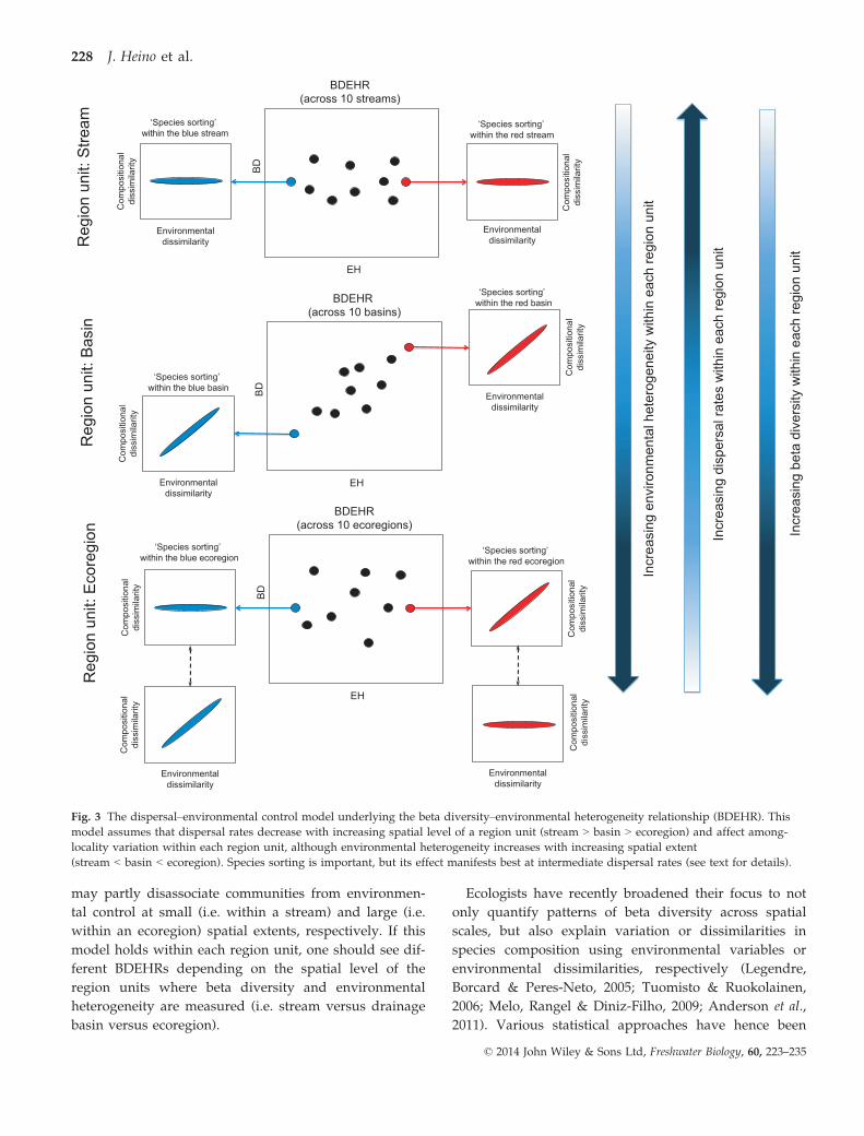
Fig. 3 The dispersal–environmental control model underlying the beta diversity–environmental heterogeneity relationship (BDEHR). This
model assumes that dispersal rates decrease with increasing spatial level of a region unit (stream > basin > ecoregion) and affect among-
locality variation within each region unit, although environmental heterogeneity increases with increasing spatial extent
(stream < basin < ecoregion). Species sorting is important, but its effect manifests best at intermediate dispersal rates (see text for details).
© 2014 John Wiley & Sons Ltd, Freshwater Biology, 60, 223–235
228 J. Heino et al.
proposed to disentangle the effects of spatial processes
and species sorting on community structure, including
(1) variation partitioning in constrained ordination
analysis (Legendre et al., 2005), (2) partial regression of
distance matrices (Tuomisto & Ruokolainen, 2006) and
(3) test of the homogeneity of multivariate dispersions
(Anderson et al., 2006). This latter test also provides a
measure of beta diversity for each region unit (i.e. aver-
age distance from localities to a region unit centroid)
that can be used in further analyses (Anderson et al.,
2011). These three methods are intended to (1) model
variation in raw community composition among sites as
functions of environmental and spatial predictors, (2)
model compositional dissimilarities between sites using
geographical and environmental distance matrices and
(3) quantify community compositional variation or envi-
ronmental heterogeneity among localities within a
region unit. Subsequently, a relationship between the
resulting beta diversity and environmental heterogeneity
values (obtained using the third method) can be tested
across multiple region units (Anderson et al., 2006).
While most studies examining running water systems
have used (1) and (2) to infer the relative roles of spatial
processes and environmental filtering for variation in
community composition (Landeiro et al., 2012; G€othe
et al., 2013; Gr€onroos et al., 2013), few studies have
applied (3) to tackle basically the same question but
from a different point of view (Heino et al., 2013; Astor-
ga et al., 2014; Bini et al., 2014).
We focus on unifying the terminology and reconciling
the different patterns of the BDEHR by considering the
spatial level of a region unit and underlying mecha-
nisms in running waters. We describe the two concep-
tual models (i.e. the environmental control model and
the dispersal-environmental control model), akin to the
previous ideas of Leibold et al. (2004) of metacommunity
organisation, and adapt those ideas to studying the
BDEHR in running water systems. We illustrate the
scale dependency of the mechanisms underlying this
relationship by comparing the predictions of the two
conceptual models with the findings of three recent
BDEHR studies from stream systems (Heino et al., 2013;
Astorga et al., 2014; Bini et al., 2014). These three studies
used the same spatial grain (i.e. a riffle site), but were
based on distinct spatial levels of the region units (i.e.
stream versus basin versus ecoregion). Also, they
employed basically the same analytical methods, which
involved a regression between average biological dis-
tance from riffle sites to region unit centroid (i.e. beta
diversity, the response variable) and average environ-
mental distance from riffle sites to region unit centroid
(i.e. environmental heterogeneity, the predictor variable)
across multiple region units (see Table S1 in Supporting
Information). They pursued the same question, but
ended up with different conclusions. We suggest that
the different patterns are probably due to the fact that
underlying mechanisms vary with the spatial level of a
region unit or, more specifically, from the stream level
through the drainage basin level to the ecoregion level.
We first consider potential analytical differences among
the studies of Heino et al. (2013), Astorga et al. (2014)
and Bini et al. (2014) and then provide two hypotheses
regarding the effects of spatial scale on beta diversity
patterns and underlying community assembly mecha-
nisms.
Analytical details
The detection of beta diversity patterns may be affected
by statistical choices regarding how to quantify beta
diversity and environmental heterogeneity, and what
biological and environmental variables to include in the
analyses. First, if a study omits a diverse taxonomic
group (e.g. Diptera: Chironomidae) from the analyses,
the results may not be strictly comparable to those of
other studies. Second, the choices of how many and
which environmental variables are used for quantifying
environmental heterogeneity may affect the comparabil-
ity of the results. Although the measures of beta diver-
sity and environmental heterogeneity were derived
using the same approach (i.e. average distance from
localities to a region unit centroid) and distance mea-
sures (i.e. Sørensen dissimilarity coefficient for presence–
absence data and standardised Euclidean distance for
environmental data), there were some differences in the
methodological choices and data set characteristics
(Table S1) between the studies of Heino et al. (2013), Ast-
orga et al. (2014) and Bini et al. (2014). For example, Ast-
orga et al. (2014) omitted chironomid midges and
focused only on selected key environmental variables
for calculating environmental heterogeneity, whereas
Heino et al. (2013) and Bini et al. (2014) included midges
and tested the effect of overall environmental heteroge-
neity on beta diversity.
We re-analysed the data of Heino et al. (2013) by (1)
omitting chironomid midges that are rarely included in
these types of studies and (2) by calculating environmen-
tal heterogeneity based only on five key variables. These
additional analyses were also based on average Sørensen
distance from localities to centroid for biological data and
average standardised Euclidean distance from localities
to centroid for environmental data, following exactly the
© 2014 John Wiley & Sons Ltd, Freshwater Biology, 60, 223–235
Beta diversity and environmental heterogeneity 229
same statistical methodology as in the three original stud-
ies. Key environmental variables measured for each local-
ity included channel width, shading, current velocity,
depth and moss cover, which often influence stream
invertebrate communities at this combination of spatial
grain and spatial extent in boreal regions (Heino & Korsu,
2008; Gr€onroos & Heino, 2012; Heino et al., 2013) and
elsewhere (Robson & Barmuta, 1998; Robson & Chester,
1999; Rackemann et al., 2013). We found no differences in
relation to the patterns originally detected by Heino et al.
(2013), and the BDEHRs remained far from significant in
all cases (see Fig. S1 in Supporting Information). Finally,
the ranges in average environmental distance from locali-
ties to a region unit centroid were similar among the three
studies, being 2.42–3.74, 1.44–2.75 and 2.74–5.40 for Heino
et al. (2013), Astorga et al. (2014) and Bini et al. (2014),
respectively. The small differences in these figures are
unlikely to account for the different BDEHR patterns. The
reason for different findings among the studies of Heino
et al. (2013), Astorga et al. (2014) and Bini et al. (2014) is
hence unlikely to be related to statistical choices or data
set characteristics. More likely explanations for the
differences among studies are related to differences in the
spatial level of the region units and scale dependency in
the mechanisms underlying spatial variation of beta
diversity.
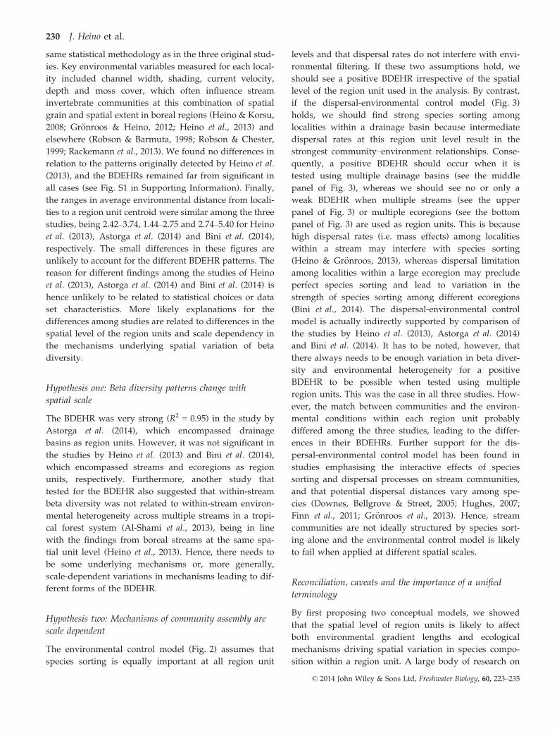
Hypothesis one: Beta diversity patterns change with
spatial scale
The BDEHR was very strong (R2 = 0.95) in the study by
Astorga et al. (2014), which encompassed drainage
basins as region units. However, it was not significant in
the studies by Heino et al. (2013) and Bini et al. (2014),
which encompassed streams and ecoregions as region
units, respectively. Furthermore, another study that
tested for the BDEHR also suggested that within-stream
beta diversity was not related to within-stream environ-
mental heterogeneity across multiple streams in a tropi-
cal forest system (Al-Shami et al., 2013), being in line
with the findings from boreal streams at the same spa-
tial unit level (Heino et al., 2013). Hence, there needs to
be some underlying mechanisms or, more generally,
scale-dependent variations in mechanisms leading to dif-
ferent forms of the BDEHR.
Hypothesis two: Mechanisms of community assembly are
scale dependent
The environmental control model (Fig. 2) assumes that
species sorting is equally important at all region unit
levels and that dispersal rates do not interfere with envi-
ronmental filtering. If these two assumptions hold, we
should see a positive BDEHR irrespective of the spatial
level of the region unit used in the analysis. By contrast,
if the dispersal-environmental control model (Fig. 3)
holds, we should find strong species sorting among
localities within a drainage basin because intermediate
dispersal rates at this region unit level result in the
strongest community–environment relationships. Conse-
quently, a positive BDEHR should occur when it is
tested using multiple drainage basins (see the middle
panel of Fig. 3), whereas we should see no or only a
weak BDEHR when multiple streams (see the upper
panel of Fig. 3) or multiple ecoregions (see the bottom
panel of Fig. 3) are used as region units. This is because
high dispersal rates (i.e. mass effects) among localities
within a stream may interfere with species sorting
(Heino & Gr€onroos, 2013), whereas dispersal limitation
among localities within a large ecoregion may preclude
perfect species sorting and lead to variation in the
strength of species sorting among different ecoregions
(Bini et al., 2014). The dispersal-environmental control
model is actually indirectly supported by comparison of
the studies by Heino et al. (2013), Astorga et al. (2014)
and Bini et al. (2014). It has to be noted, however, that
there always needs to be enough variation in beta diver-
sity and environmental heterogeneity for a positive
BDEHR to be possible when tested using multiple
region units. This was the case in all three studies. How-
ever, the match between communities and the environ-
mental conditions within each region unit probably
differed among the three studies, leading to the differ-
ences in their BDEHRs. Further support for the dis-
persal-environmental control model has been found in
studies emphasising the interactive effects of species
sorting and dispersal processes on stream communities,
and that potential dispersal distances vary among spe-
cies (Downes, Bellgrove & Street, 2005; Hughes, 2007;
Finn et al., 2011; Gr€onroos et al., 2013). Hence, stream
communities are not ideally structured by species sort-
ing alone and the environmental control model is likely
to fail when applied at different spatial scales.
Reconciliation, caveats and the importance of a unified
terminology
By first proposing two conceptual models, we showed
that the spatial level of region units is likely to affect
both environmental gradient lengths and ecological
mechanisms driving spatial variation in species compo-
sition within a region unit. A large body of research on
© 2014 John Wiley & Sons Ltd, Freshwater Biology, 60, 223–235
230 J. Heino et al.
community patterns of stream organisms suggests that
species sorting mainly drives spatial variation in com-
munity composition among localities within a drainage
basin (Clarke et al., 2008; Landeiro et al., 2012; Siqueira
et al., 2012; G€othe et al., 2013; Gr€onroos et al., 2013).
However, a growing body of work on small (i.e. within
localities) to medium (i.e. among localities or among
streams) scale processes, including dispersal and coloni-
sation processes, shows that stream invertebrates may
actually be more dispersal limited than has been com-
monly believed (Hughes, 2007; Hughes, Schmidt & Finn,
2009). Furthermore, recent empirical studies have
increasingly shown that other processes, such as oviposi-
tion choices, can leave lasting effects on distribution pat-
terns of stream invertebrates at the among-localities
scale within a stream (Lancaster, Downes & Arnold,
2011; Heino & Peckarsky, 2014). It is also likely, how-
ever, that the importance of dispersal limitation
increases when a study spans localities of many drain-
age basins within an ecoregion (Hoeinghaus, Winemiller
& Birnbaum, 2007; Mykr€a et al., 2007; Jacquemin &
Pyron, 2011; Maloney & Munguia, 2011; Astorga et al.,
2012). In addition, while some empirical studies from
stream systems have shown that high dispersal rates do
not necessarily interfere with species sorting at small
microhabitat scales (Robson & Chester, 1999; Heino &
Korsu, 2008), theory and other empirical studies suggest
that the match between community composition and
environmental conditions is weakened by high dispersal
rates among localities within a stream (Leibold et al.,
2004; Heino & Gr€onroos, 2013).
If scale dependencies are general phenomena, one
should first find the strongest role for species sorting
among localities within a drainage basin, species sorting
masked by high dispersal rates among localities within a
stream, and the strength of species sorting weakened
within a large ecoregion (see the bottom panel of Fig. 3),
leading to wide variation in the strength of species sort-
ing among different ecoregions (Bini et al., 2014). These
differences in the underlying mechanisms active within
each region unit should lead to differences in the
BDEHR that can only be tested using multiple region
units, reconciling the different findings from running
water systems.
We emphasise, however, that the two conceptual
models we present are idealistic, and the fit of empirical
data with the models is likely to be affected by contin-
gencies in regional history, landscape characteristic, spe-
cies pools and the dispersal abilities of the organisms
studied. For example, genetic studies have suggested
that dispersal distances vary considerably among species
of aquatic insects (Hughes, 2007; Finn et al., 2011),
implying that dispersal is a key factor affecting BDEHRs.
Furthermore, different organismal groups show different
dispersal modes, distances and rates (Beisner et al., 2006;
Hugueny, Oberdorff & Tedesco, 2010; Maloney &
Munguia, 2011; Astorga et al., 2012; De Bie et al., 2012;
Heino et al., 2012), which is likely to affect the spatial
level of a region unit where species sorting is manifested
most strongly (Heino & Peckarsky, 2014). We may
assume that, for organisms showing very limited dis-
persal rates and short dispersal distances, the strongest
BDEHRs may be detected when tested using multiple
stream region units. On the other hand, for organismal
groups with very high dispersal rates and large
dispersal distances, the strongest BDEHRs might be
expected to occur when tested using multiple ecoregion
region units. Accordingly, we encourage freshwater
ecologists to consider spatial scale explicitly in their
studies. Such a consideration is important because not
only environmental gradient lengths, but also the mech-
anisms affecting ecological communities and the spatial
variation of beta diversity vary with the spatial level of
a region unit and organismal group (Shurin, Cottenie &
Hillebrand, 2009; Angeler & Drakare, 2013; Heino, 2013).
These mechanisms may thus be better inferred if we
acquire more knowledge on the life histories of aquatic
organisms, which should elucidate the processes that
underpin BDHERs across multiple spatial scales.
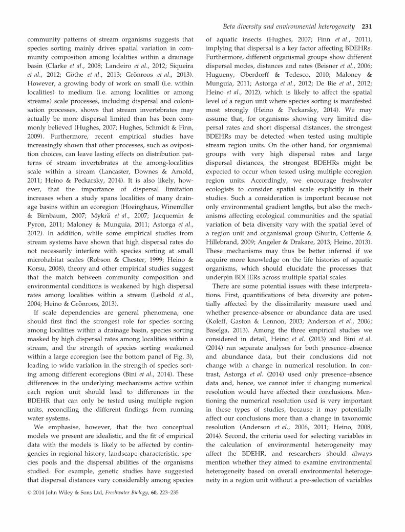
There are some potential issues with these interpreta-
tions. First, quantifications of beta diversity are poten-
tially affected by the dissimilarity measure used and
whether presence–absence or abundance data are used
(Koleff, Gaston & Lennon, 2003; Anderson et al., 2006;
Baselga, 2013). Among the three empirical studies we
considered in detail, Heino et al. (2013) and Bini et al.
(2014) ran separate analyses for both presence–absence
and abundance data, but their conclusions did not
change with a change in numerical resolution. In con-
trast, Astorga et al. (2014) used only presence–absence
data and, hence, we cannot infer if changing numerical
resolution would have affected their conclusions. Men-
tioning the numerical resolution used is very important
in these types of studies, because it may potentially
affect our conclusions more than a change in taxonomic
resolution (Anderson et al., 2006, 2011; Heino, 2008,
2014). Second, the criteria used for selecting variables in
the calculation of environmental heterogeneity may
affect the BDEHR, and researchers should always
mention whether they aimed to examine environmental
heterogeneity based on overall environmental heteroge-
neity in a region unit without a pre-selection of variables
© 2014 John Wiley & Sons Ltd, Freshwater Biology, 60, 223–235
Beta diversity and environmental heterogeneity 231
(Heino et al., 2013) or whether they examined various
subsets of environmental variables separately for calcu-
lating environmental heterogeneity (Bini et al., 2014) or,
finally, whether they directly focused on a set of key
environmental variables known to have strong effects on
the biota (Astorga et al., 2014). We recommend that
researchers use both a measure of overall heterogeneity
and a measure of environmental heterogeneity based on
a set of key environmental variables. Although our
additional analyses did not reveal differences in the
BDHERs based on either measure of environmental
heterogeneity (Fig. S2), differences among the measures
are also possible.
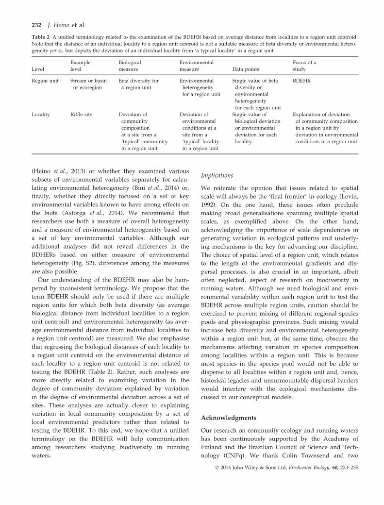
Our understanding of the BDEHR may also be ham-
pered by inconsistent terminology. We propose that the
term BDEHR should only be used if there are multiple
region units for which both beta diversity (as average
biological distance from individual localities to a region
unit centroid) and environmental heterogeneity (as aver-
age environmental distance from individual localities to
a region unit centroid) are measured. We also emphasise
that regressing the biological distances of each locality to
a region unit centroid on the environmental distance of
each locality to a region unit centroid is not related to
testing the BDEHR (Table 2). Rather, such analyses are
more directly related to examining variation in the
degree of community deviation explained by variation
in the degree of environmental deviation across a set of
sites. These analyses are actually closer to explaining
variation in local community composition by a set of
local environmental predictors rather than related to
testing the BDEHR. To this end, we hope that a unified
terminology on the BDEHR will help communication
among researchers studying biodiversity in running
waters.
Implications
We reiterate the opinion that issues related to spatial
scale will always be the ‘final frontier’ in ecology (Levin,
1992). On the one hand, these issues often preclude
making broad generalisations spanning multiple spatial
scales, as exemplified above. On the other hand,
acknowledging the importance of scale dependencies in
generating variation in ecological patterns and underly-
ing mechanisms is the key for advancing our discipline.
The choice of spatial level of a region unit, which relates
to the length of the environmental gradients and dis-
persal processes, is also crucial in an important, albeit
often neglected, aspect of research on biodiversity in
running waters. Although we need biological and envi-
ronmental variability within each region unit to test the
BDEHR across multiple region units, caution should be
exercised to prevent mixing of different regional species
pools and physiographic provinces. Such mixing would
increase beta diversity and environmental heterogeneity
within a region unit but, at the same time, obscure the
mechanisms affecting variation in species composition
among localities within a region unit. This is because
most species in the species pool would not be able to
disperse to all localities within a region unit and, hence,
historical legacies and unsurmountable dispersal barriers
would interfere with the ecological mechanisms dis-
cussed in our conceptual models.
Acknowledgments
Our research on community ecology and running waters
has been continuously supported by the Academy of
Finland and the Brazilian Council of Science and Tech-
nology (CNPq). We thank Colin Townsend and two
Table 2 A unified terminology related to the examination of the BDEHR based on average distance from localities to a region unit centroid.
Note that the distance of an individual locality to a region unit centroid is not a suitable measure of beta diversity or environmental hetero-
geneity per se, but depicts the deviation of an individual locality from ‘a typical locality’ in a region unit
Level
Example
level
Biological
measure
Environmental
measure Data points
Focus of a
study
Region unit Stream or basin
or ecoregion
Beta diversity for
a region unit
Environmental
heterogeneity
for a region unit
Single value of beta
diversity or
environmental
heterogeneity
for each region unit
BDEHR
Locality Riffle site Deviation of
community
composition
at a site from a
‘typical’ community
in a region unit
Deviation of
environmental
conditions at a
site from a
‘typical’ locality
in a region unit
Single value of
biological deviation
or environmental
deviation for each
locality
Explanation of deviation
of community composition
in a region unit by
deviation in environmental
conditions in a region unit
© 2014 John Wiley & Sons Ltd, Freshwater Biology, 60, 223–235
232 J. Heino et al.
anonymous reviewers for excellent comments that
improved this paper.
References
Al-Shami S.A., Heino J., Che Salmah M.R., Ahmad A.H.,
Hamid S.A. & Madrus M.R. (2013) Drivers of beta diver-
sity of macroinvertebrate communities in tropical forest
streams. Freshwater Biology, 58, 1126–1137.
Altermatt F. (2013) Diversity in riverine metacommunities:
a network perspective. Aquatic Ecology, 47, 365–377.
Anderson M.J., Crist T.O., Chase J.M., Vellend M., Inouye
B.D., Freestone A.L. et al. (2011) Navigating the multiple
meanings of b diversity: a roadmap for the practicing
ecologist. Ecology Letters, 14, 19–28.
Anderson M.J., Ellingsen K.E. & McArdle B.H. (2006) Multi-
variate dispersion as a measure of beta diversity. Ecology
Letters, 9, 683–693.
Angeler D.G. & Drakare S. (2013) Tracing alpha, beta and
gamma diversity responses to environmental change in
boreal lakes. Oecologia, 172, 1191–1202.
Astorga A., Death R., Death F., Paavola R., Chakraborty M.
& Muotka T. (2014) Habitat heterogeneity drives the geo-
graphical distribution of beta diversity: the case of New
Zealand stream invertebrates. Ecology and Evolution, 4,
2693–2702.
Astorga A., Oksanen J., Soininen J., Virtanen R., Luoto M.
& Muotka T. (2012) Distance decay of similarity in stream
communities: do macro- and microorganism follow the
same rules? Global Ecology and Biogeography, 21, 365–375.
Bar-Massada A. & Wood E.M. (2014) The richness-heteroge-
neity relationship differs between heterogeneity measures
within and among habitats. Ecography, 37, 528–535.
Barton P.S., Cunningham S.A., Manning A.D., Gigg H., Lin-
denmayer D.B. & Didham R.K. (2013) The spatial scaling
of beta diversity. Global Ecology and Biogeography, 22,
639–647.
Baselga A. (2013) Multiple site dissimilarity quantifies com-
positional heterogeneity among several sites, while aver-
age pairwise dissimilarity may be misleading. Ecography,
36, 124–128.
Beisner B.E., Peres-Neto P.R., Lindstrom E., Barnett A. &
Longhi M.L. (2006) The role of dispersal in structuring lake
communities from bacteria to fish. Ecology, 87, 2895–2991.
Bini L.M., Landeiro V.L., Padial A.A., Siqueira T. & Heino
J. (2014) Nutrient enrichment is related to two facets of
beta diversity for stream invertebrates across the United
States. Ecology, 95, 1569–1578.
Brown B.L., Swan C.M., Auerbach D.A., Grant E.H.C., Hitt
N.P., Maloney K.O. et al. (2011) Metacommunity theory
as a multispecies, multiscale framework for studying the
influence of river network structure on riverine
communities and ecosystems. Journal of the North Ameri-
can Benthological Society, 30, 310–327.
Chase J.M. & Leibold M.A. (2003) Ecological Niches. Chicago
University Press, Chicago.
Clarke A., Mac Nally R., Bond N. & Lake P.S. (2008) Macro-
invertebrate diversity in headwater streams: a review.
Freshwater Biology, 53, 1707–1721.
Cottenie K. (2005) Integrating environmental and spatial
processes in ecological community dynamics. Ecology Let-
ters, 8, 1175–1182.
Datry T., Larned S.T., Fritz K.M., Bogan M.T., Wood P.J.,
Meyer E.I. et al. (2014) Broad-scale patterns of inverte-
brate richness and community composition in tempo-
rary rivers: effects of flow intermittence. Ecography, 37,
94–104.
De Bie T., De Meester L., Brendonck L., Martens K.,
Goddeeris B., Ercken D. et al. (2012) Body size and dis-
persal mode as key traits determining metacommunity
structure of aquatic organisms. Ecology Letters, 15, 740–747.
Downes B.J., Lake P.S., Schreiber E.S.G. & Glaister A. (1998)
Habitat structure and the regulation of local species
diversity in a stony upland stream. Ecological Monographs,
68, 237–257.
Downes B.J., Bellgrove A. & Street J.L. (2005) Drifting or
walking? Colonisation routes used by different instars
and species of lotic, macroinvertebrate filter-feeders. Mar-
ine & Freshwater Research, 56, 815–824.
Downes B.J. & Lancaster J. (2010) Does dispersal control
population densities in advection dominated systems?
Journal of Animal Ecology, 79, 235–248.
Downes B.J. & Reich P. (2008) What is the spatial structure
of stream insect populations? Dispersal behaviour at dif-
ferent life-history stages. In: Aquatic Insects: Challenges to
Populations. (Eds J. Lancaster & R.A. Briers), pp. 184–203.
CAB International Publishers, Wallingford.
Finn D.S., Bonada N., Murria C. & Hughes J.M. (2011)
Small but mighty: headwaters are vital to stream network
biodiversity at two levels of organization. Journal of North
American Benthological Society, 30, 963–980.
Gering J.C. & Crist T.O. (2002) The alpha-beta-regional rela-
tionship: providing new insights into local-regional pat-
terns of species richness and scale dependence of
diversity components. Ecology Letters, 5, 433–444.
G€othe E., Angeler D.G. & Sandin L. (2013) Metacommunity
structure in a small boreal stream network. Journal of Ani-
mal Ecology, 82, 449–458.
Gravel D., Canham C.D., Beaudet M. & Messier C. (2006)
Reconciling niche and neutrality: the continuum hypothe-
sis. Ecology Letters, 9, 399–409.
Gr€onroos M. & Heino J. (2012) Species richness at the guild
level: effects of species pool and local environmental con-
ditions on stream macroinvertebrate communities. Journal
of Animal Ecology, 81, 679–691.
Gr€onroos M., Heino J., Siqueira T., Landeiro V.L., Kotanen
J. & Bini L.M. (2013) Metacommunity structuring in
stream networks: roles of dispersal mode, distance type
© 2014 John Wiley & Sons Ltd, Freshwater Biology, 60, 223–235
Beta diversity and environmental heterogeneity 233
and regional environmental context. Ecology and Evolu-
tion, 3, 4473–4487.
Harrison S., Ross S.J. & Lawton J.H. (1992) Beta diversity
on geographic gradients in Britain. Journal of Animal Ecol-
ogy, 61, 151–158.
Heino J. (2008) Influence of taxonomic resolution and data
transformation on biotic matrix concordance and assem-
blage-environment relationships in stream macroinverte-
brates. Boreal Environment Research, 13, 359–369.
Heino J. (2011) A macroecological perspective of diversity
patterns in the freshwater realm. Freshwater Biology, 56,
1703–1722.
Heino J. (2013) The importance of metacommunity ecology
for environmental assessment research in the freshwater
realm. Biological Reviews, 88, 166–178.
Heino J. (2014) Taxonomic surrogacy, numerical resolution
and responses of stream macroinvertebrate communities
to ecological gradients: are the inferences transferable
among regions? Ecological Indicators, 36, 186–194.
Heino J. & Gr€onroos M. (2013) Does environmental hetero-
geneity affect species co-occurrence in ecological guilds
across stream macroinvertebrate metacommunities? Ecog-
raphy, 36, 926–936.
Heino J., Gr€onroos M., Ilmonen J., Karhu T., Niva M. &
Paasivirta L. (2013) Environmental heterogeneity and beta
diversity of stream macroinvertebrate communities at
intermediate spatial scales. Freshwater Science, 32, 142–154.
Heino J., Gr€onroos M., Soininen J., Virtanen R. & Muotka T.
(2012) Context dependency and metacommunity structur-
ing in boreal headwater streams. Oikos, 121, 537–544.
Heino J. & Korsu K. (2008) Testing species-stone area and
species-bryophyte cover relationships in riverine macroin-
vertebrates at small scales. Freshwater Biology, 53, 558–568.
Heino J. & Peckarsky B.L. (2014) Integrating behavioral,
population and large-scale approaches for understanding
stream insect communities. Current Opinion in Insect Sci-
ence, 2, 7–13.
Hepp L.U. & Melo A.S. (2013) Dissimilarity of stream insect
assemblages: effects of multiple scales and spatial dis-
tances. Hydrobiologia, 703, 239–246.
Hoeinghaus D.J., Winemiller K.O. & Birnbaum J.S. (2007)
Local and regional determinants of stream fish assem-
blage structure: inferences based on taxonomic versus
functional groups. Journal of Biogeography, 34, 324–338.
Hughes J.M. (2007) Constraints on recovery: using molecu-
lar methods to study connectivity of aquatic biota in riv-
ers and streams. Freshwater Biology, 52, 616–631.
Hughes J.M., Schmidt D.J. & Finn D.S. (2009) Genes in
streams: using DNA to understand the movement of
freshwater fauna and their riverine habitat. BioScience, 59,
573–583.
Hugueny H., Oberdorff T. & Tedesco P.A. (2010) Commu-
nity ecology of river fishes: a large scale perspective.
American Fisheries Society Symposium, 73, 29–62.
Jackson D.A., Peres-Neto P.R. & Olden J.D. (2001) What
controls who is where in freshwater fish communities –
the roles of biotic, abiotic and spatial factors. Canadian
Journal of Fisheries and Aquatic Sciences, 58, 157–170.
Jacquemin S.J. & Pyron M. (2011) Impact of past glaciations
events on contemporary fish assemblages of the Ohio
River basin. Journal of Biogeography, 38, 982–991.
Koleff P., Gaston K.J. & Lennon J.J. (2003) Measuring beta
diversity for presence-absence data. Journal of Animal
Ecology, 72, 367–382.
Lancaster J.Downes B.J. & Arnold A. (2011) Lasting effects
of maternal behaviour on the distribution of a disper-
sive stream insect. Journal of Animal Ecology, 80, 1061–
1069.
Landeiro V.L., Bini L.M., Melo A.S., Pes A.M.O. & Magnus-
son W.E. (2012) The roles of dispersal limitation and
environmental conditions in controlling caddisfly (Tri-
choptera) assemblages. Freshwater Biology, 57, 1554–1564.
Legendre P., Borcard D. & Peres-Neto P.R. (2005) Analyzing
beta diversity: partitioning the spatial variation of
community composition data. Ecological Monographs, 75,
435–450.
Leibold M.A., Holyoak M., Mouquet N., Amarasekare P.,
Chase J.M., Hoopes M.F. et al. (2004) The metacommunity
concept: a framework for multi-scale community ecology.
Ecology Letters, 7, 601–613.
Levin S.A. (1992) The problem of pattern and scale in ecol-
ogy. Ecology, 73, 1943–1967.
Maloney K.O. & Munguia P. (2011) Distance decay of simi-
larity in temperate aquatic communities: effects of envi-
ronmental transition zones, distance measure, and life
histories. Ecography, 34, 287–295.
Melo A.S., Rangel T.F.L.V.B. & Diniz-Filho J.A.F. (2009)
Environmental drivers of beta diversity patterns in New-
World birds and mammals. Ecography, 32, 226–236.
Melo A.S., Schneck F., Hepp L.U., Sim~oes N.R., Siqueira T.
& Bini L.M. (2011) Focusing on variation: methods and
applications of the concept of beta diversity in aquatic
ecosystems. Acta Limnologica Brasiliensia, 23, 318–331.
Mykr€a H., Heino J. & Muotka T. (2007) Scale-related pat-
terns in the spatial and environmental components of
stream macroinvertebrate assemblage variation. Global
Ecology and Biogeography, 16, 149–159.
Ng I.S.Y., Carr C. & Cottenie K. (2009) Hierarchical zoo-
plankton metacommunities: distinguishing between high
and limiting dispersal mechanisms. Hydrobiologia, 619,
133–143.
Rackemann S., Robson B. & Matthews T. (2013) Conserva-
tion value of waterfalls as habitat for lotic insects of wes-
tern Victoria, Australia. Aquatic Conservation: Marine and
Freshwater Ecosystems, 23, pages 171–178.
Robson B.J. (1996) Habitat architecture and trophic interac-
tion strength in a river: riffle-scale effects. Oecologia, 107,
411–420.
© 2014 John Wiley & Sons Ltd, Freshwater Biology, 60, 223–235
234 J. Heino et al.
Robson B.J. & Barmuta L.A. (1998) The effect of two scales
of habitat architecture on benthic grazing in a river. Fresh-
water Biology, 39, 207–220.
Robson B.J. & Chester E.T. (1999) Spatial patterns of inver-
tebrate species richness in a river: the relationship
between riffles and microhabitats. Austral Ecology, 24,
599–607.
Shurin J.B., Cottenie K. & Hillebrand H. (2009) Spatial auto-
correlation and dispersal limitation in freshwater organ-
isms. Oecologia, 159, 151–159.
Siqueira T., Bini L.M., Roque F.O., Pepinelli M., Ramos
R.C., Marques Couceiro S.R. et al. (2012) Common and
rare species respond to similar niche processes in macro-
invertebrate metacommunities. Ecography, 35, 183–192.
Thompson R.M. & Townsend C.R. (2006) A truce with neu-
tral theory: local deterministic factors, species traits and
dispersal limitation together determine patterns of diver-
sity in stream invertebrates. Journal of Animal Ecology, 75,
476–484.
Tuomisto H. (2010) A diversity of beta diversities: straight-
ening up a concept gone awry. Part 1. Defining beta
diversity as a function of alpha and gamma diversity.
Ecography, 33, 2–22.
Tuomisto H. & Ruokolainen K. (2006) Analyzing or explain-
ing beta diversity? Understanding the targets of different
methods of analysis. Ecology, 87, 2697–2708.
Van der Gucht K., Cottenie K., Muylaert K., Vloemans N.,
Cousin S., Declerck S. et al. (2007) The power of species
sorting: local factors drive bacterial community composi-
tion over a wide range of spatial scales. Proceedings of the
National Academy of Sciences, 104, 20404–20409.
Whittaker R.H. (1960) Vegetation of the Siskiyou Moun-
tains, Oregon and California. Ecological Monographs, 30,
279–338.
Wiens J.A. (1989) Spatial scaling in ecology. Functional Ecol-
ogy, 3, 385–397.
Winegardner A.K., Jones B.K., Ng I.S.Y., Siqueira T. &
Cottenie K. (2012) The terminology of metacommunity
ecology. Trends in Ecology and Evolution, 27, 253–254.
Wu J. & Loucks O.L. (1995) From balance of nature to hier-
archical patch dynamics: a paradigm shift in ecology. The
Quarterly Review of Biology, 70, 439–466.
Supporting Information
Additional Supporting Information may be found in the
online version of this article:
Table S1. Comparisons of three recent empirical studies
on the BDEHR in stream invertebrates.
Figure S1. A test of the effect of using all environmental
variables and key environmental variables only for
calculating environmental heterogeneity among sites.
(Manuscript accepted 11 October 2014)
© 2014 John Wiley & Sons Ltd, Freshwater Biology, 60, 223–235
Beta diversity and environmental heterogeneity 235
Top Related
Copyright © 2022 FDOKUMEN

