Download - Quantitative comparisons of forward problems in MEEG

Quantitative comparisons of forward problems in

MEEG.

Emmanuel Olivi, Maureen Clerc, Mariette Yvinec, Theodore Papadopoulo

To cite this version:

Emmanuel Olivi, Maureen Clerc, Mariette Yvinec, Theodore Papadopoulo. Quantitative com-parisons of forward problems in MEEG.. [Research Report] RR-6364, 2007, pp.32. <inria-00189515v3>

HAL Id: inria-00189515

https://hal.inria.fr/inria-00189515v3

Submitted on 9 Jan 2010

HAL is a multi-disciplinary open accessarchive for the deposit and dissemination of sci-entific research documents, whether they are pub-lished or not. The documents may come fromteaching and research institutions in France orabroad, or from public or private research centers.

L’archive ouverte pluridisciplinaire HAL, estdestinee au depot et a la diffusion de documentsscientifiques de niveau recherche, publies ou non,emanant des etablissements d’enseignement et derecherche francais ou etrangers, des laboratoirespublics ou prives.

https://hal.archives-ouvertes.fr

https://hal.inria.fr/inria-00189515v3

appor t de r ech er ch e

ISS

N02

49-6

399

ISR

NIN

RIA

/RR

--63

64--

FR+E

NG

Thème NUM

INSTITUT NATIONAL DE RECHERCHE EN INFORMATIQUE ET EN AUTOMATIQUE

Quantitative comparisons offorward problems in MEEG.

Emmanuel Olivi, Mariette Yvinec, Maureen Clerc and Theodore Papadopoulo

N° 6364

Novembre 2008

Centre de recherche INRIA Sophia Antipolis – Méditerranée2004, route des Lucioles, BP 93, 06902 Sophia Antipolis Cedex (France)

Téléphone : +33 4 92 38 77 77 — Télécopie : +33 4 92 38 77 65

Quantitative comparisons offorward problems in MEEG.

Emmanuel Olivi, Mariette Yvinec∗, Maureen Clerc and TheodorePapadopoulo†

Theme NUM — Systemes numeriquesEquipes-Projets GEOMETRICA And ODYSSEE

Rapport de recherche n° 6364 — Novembre 2008 — 29 pages

Abstract: This document gives comparisons between several methods thatsolve the forward problem in MEEG by comparing their precision on a 3-layerspherical model. These methods are based on finite elements which either usesurfacic meshes with triangles, volumic meshes with tetrahedra, or implicit ele-ments deduced from levelsets.

Key-words: MEG, EEG, MEEG, forward problem, CGAL, FEM, BEM,implicit finite elements, mesh generation, Boundary element method, sphericalmodel

∗ GEOMETRICA† ODYSSEE

Comparaisons quantitatives de resultats deproblemes directs en MEEG.

Resume : Ce document fournit des comparaisons de plusieurs methodes deresolution du probleme direct en MEEG en comparant leur precision sur unmodele de tete spherique a trois couches. Les methodes exposees sont deselements finis de trois types : surfaciques (BEM), volumiques tetraedriques(FEM), volumiques implicites bases sur des level-sets (implicit FEM).

Mots-cles : MEG, EEG, MEEG, probleme direct, CGAL, elements finis,elements finis implicites, maillage, elements frontiere, modele spherique

Comparisons of forward problems in MEEG 3

Contents

1 Introduction 4

2 The mesh generation 62.1 The three-layer spherical model . . . . . . . . . . . . . . . . . . . 6

2.1.1 Volumic meshes using Head mesher . . . . . . . . . . . . 62.1.2 Surfacic meshes using Surface mesher . . . . . . . . . . . 8

2.2 Realistic model . . . . . . . . . . . . . . . . . . . . . . . . . . . . 92.2.1 Volumic meshes using Head mesher . . . . . . . . . . . . 92.2.2 Surfacic meshes extracted from the volumic meshes . . . . 11

3 Different ways of solving the forward problem in MEEG 123.1 The symmetric Boundary Element Method . . . . . . . . . . . . 12

3.1.1 sBEM for EEG . . . . . . . . . . . . . . . . . . . . . . . . 123.1.2 sBEM for MEG . . . . . . . . . . . . . . . . . . . . . . . . 16

3.2 The tetrahedral Finite Element Method . . . . . . . . . . . . . . 173.3 The implicit Finite Element Method . . . . . . . . . . . . . . . . 18

3.3.1 iFEM for EEG . . . . . . . . . . . . . . . . . . . . . . . . 183.3.2 iFEM for MEG . . . . . . . . . . . . . . . . . . . . . . . . 18

3.4 Benefits and drawbacks of each methods . . . . . . . . . . . . . . 19

4 Quantitative comparisons of the results 204.1 The spherical model . . . . . . . . . . . . . . . . . . . . . . . . . 204.2 Precisions of iFEM and tFEM . . . . . . . . . . . . . . . . . . . . 224.3 Precision of the sBEM . . . . . . . . . . . . . . . . . . . . . . . . 24

4.3.1 results for the EEG problem . . . . . . . . . . . . . . . . 244.3.2 results for the MEG problem . . . . . . . . . . . . . . . . 25

4.4 Realistic model and trials . . . . . . . . . . . . . . . . . . . . . . 264.5 Summary, for the spherical model, of all methods solving the

forward EEG problem . . . . . . . . . . . . . . . . . . . . . . . . 27

5 Conclusion 28

RR n° 6364

4Emmanuel Olivi, Mariette Yvinec, Maureen Clerc and Theodore Papadopoulo

1 Introduction

MEEG, which stands for Magneto-Electro EncephaloGraphy, is a non-invasivetechnique very useful in studying brain functional activity. Its high temporalresolution is order of magnitude higher than that of the functional MRI. Dataacquisition in EEG and MEG gives respectively the electric potential and onecomponent of the magnetic field on sensors located around the scalp. Fromthese acquisitions, one can wish to recover the electrical sources inside the brainthat are responsible of the electromagnetic field measured. This problem is aninverse problem of localization whose resolution requires the resolution of theforward problem. Forward problem consists in simulating sources inside thebrain and computing the resulting field at the sensor positions. This resolutionis done by solving Maxwell’s equations in their quasi-static approximation ona geometry that depends on the patient. Hence, this problem depends on thesubject, meaning that for each patient one needs the definition of the tissues,i.e. the geometry of the different layers and their conductivities. Most of thelayers of the head can be extracted from anatomical MRI (Magnetic ResonanceImaging); the skull still present some difficulties to be extracted and is oftenguessed by inflating the brain. Conductivities of the layers can be evaluated bydifferent ways ; one can use reference conductivities that have been measuredin vivo on test subjects, or one can wish to estimate the conductivity for eachsubject using Electrical Impedance Tomography [2]. The skull conductivity isanisotropic, the tangential conductivity can be ten times higher than the radialone. It has been shown that this anisotropy has an important influence on theresults of the forward (and hence inverse) problem [7]. Several methods forsolving the forward problem have been proposed. Two of them require a meshof the geometry of the specific patient’s head in order to do the computationswhereas the other one avoids this time and memory consuming step by doing sothe computation on the grid given by the MRI. This document gives comparisonsbetween three different methods for solving the forward problem:

the boundary element method (BEM), which comes from an integralformulation of Maxwell’s equations, it needs a surfacic mesh of the sur-faces defining the computational domain. This method cannot take intoaccount the anisotropy of the skull and can only handle piecewise constantconductivities.

the tetrahedral finite element method (tFEM), which arises froma variational formulation of our problem, needs a volumic mesh (made oftetrahedra) of all the computational domain. It can handle anisotropy.

the implicit finite element method (iFEM), which also comes fromthe variational formulation but uses implicit elements given by the voxelsof the MRI. It can also handle anisotropy.

In order to compare the precision of these methods, we have used the very pop-ular spherical model for which an analytical solution exists.

INRIA


We first present the mesh generation using the Computational Geometry Algo-rithms Library (CGAL), then we explain the differences between the methodsused to solve the forward problem, and we finally show the comparisons made.

RR n° 6364


2 The mesh generation

CGAL1 is a library developed by an European consortium in which GEOMET-RICA team takes part. CGAL provides an automatic mesh generation of eithervolumic or surfacic objects. These objects can be defined through gray-levelimages or equations to be satisfied.

2.1 The three-layer spherical model

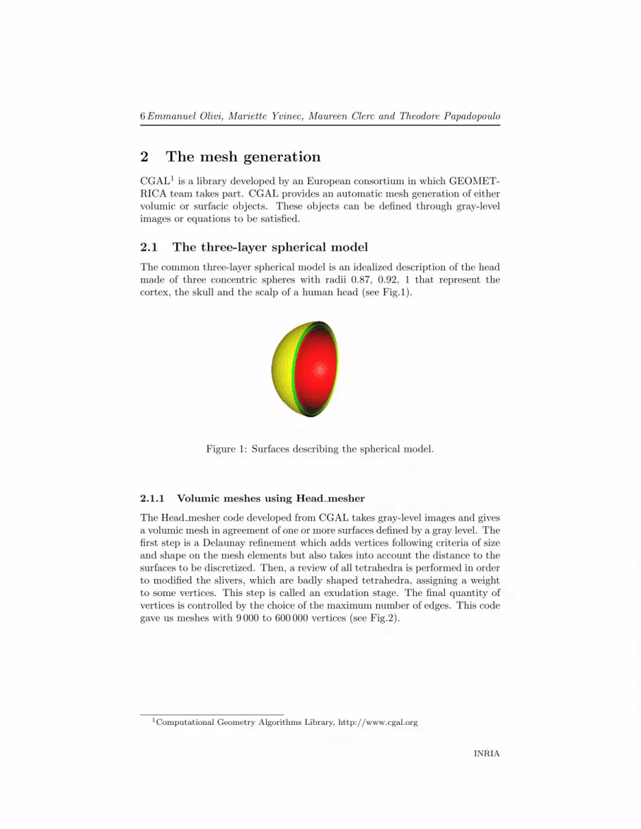
The common three-layer spherical model is an idealized description of the headmade of three concentric spheres with radii 0.87, 0.92, 1 that represent thecortex, the skull and the scalp of a human head (see Fig.1).

Figure 1: Surfaces describing the spherical model.

2.1.1 Volumic meshes using Head mesher

The Head mesher code developed from CGAL takes gray-level images and givesa volumic mesh in agreement of one or more surfaces defined by a gray level. Thefirst step is a Delaunay refinement which adds vertices following criteria of sizeand shape on the mesh elements but also takes into account the distance to thesurfaces to be discretized. Then, a review of all tetrahedra is performed in orderto modified the slivers, which are badly shaped tetrahedra, assigning a weightto some vertices. This step is called an exudation stage. The final quantity ofvertices is controlled by the choice of the maximum number of edges. This codegave us meshes with 9 000 to 600 000 vertices (see Fig.2).

1Computational Geometry Algorithms Library, http://www.cgal.org

INRIA


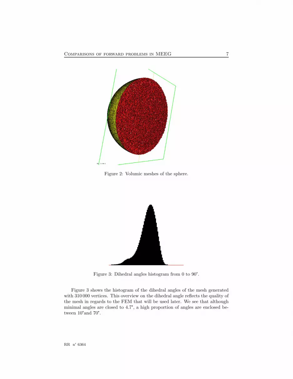
Figure 2: Volumic meshes of the sphere.

Figure 3: Dihedral angles histogram from 0 to 90°.

Figure 3 shows the histogram of the dihedral angles of the mesh generatedwith 310 000 vertices. This overview on the dihedral angle reflects the quality ofthe mesh in regards to the FEM that will be used later. We see that althoughminimal angles are closed to 4.7°, a high proportion of angles are enclosed be-tween 10°and 70°.

RR n° 6364


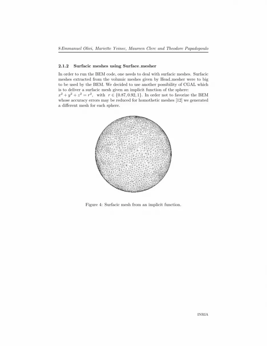
2.1.2 Surfacic meshes using Surface mesher

In order to run the BEM code, one needs to deal with surfacic meshes. Surfacicmeshes extracted from the volumic meshes given by Head mesher were to bigto be used by the BEM. We decided to use another possibility of CGAL whichis to deliver a surfacic mesh given an implicit function of the sphere:x2 + y2 + z2 = r2, with r ∈ 0.87, 0.92, 1. In order not to favorize the BEMwhose accuracy errors may be reduced for homothetic meshes [12] we generateda different mesh for each sphere.

Figure 4: Surfacic mesh from an implicit function.

INRIA


2.2 Realistic model

2.2.1 Volumic meshes using Head mesher

Number of vertices 57 000 320 000 584 000Total Time 6.62 205.34 615.46Refining Time 0.71 7.08 17.32Exudation Time 4.94 183.28 544.20Validation Time 0.20 1.25 2.31Writing Time 0.75 13.57 51.34

Table 1: Meshing steps time in minute.

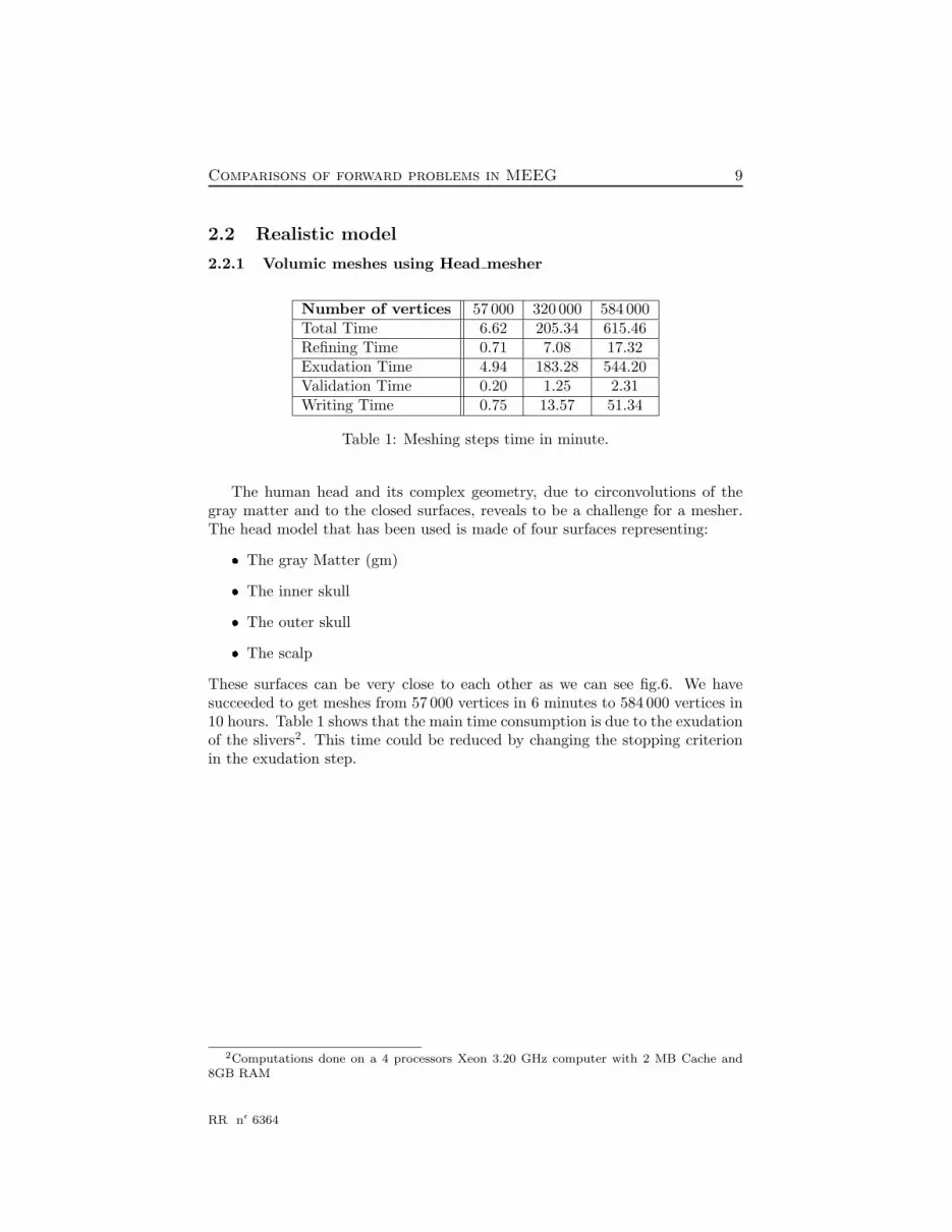
The human head and its complex geometry, due to circonvolutions of thegray matter and to the closed surfaces, reveals to be a challenge for a mesher.The head model that has been used is made of four surfaces representing:

The gray Matter (gm)

The inner skull

The outer skull

The scalp

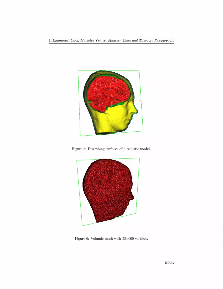
These surfaces can be very close to each other as we can see fig.6. We havesucceeded to get meshes from 57 000 vertices in 6 minutes to 584 000 vertices in10 hours. Table 1 shows that the main time consumption is due to the exudationof the slivers2. This time could be reduced by changing the stopping criterionin the exudation step.

2Computations done on a 4 processors Xeon 3.20 GHz computer with 2 MB Cache and8GB RAM

RR n° 6364


Figure 5: Describing surfaces of a realistic model.

Figure 6: Volumic mesh with 584 000 vertices.

INRIA


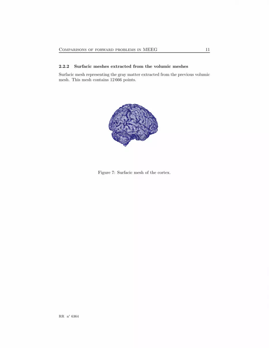
2.2.2 Surfacic meshes extracted from the volumic meshes

Surfacic mesh representing the gray matter extracted from the previous volumicmesh. This mesh contains 12 666 points.

Figure 7: Surfacic mesh of the cortex.

RR n° 6364


3 Different ways of solving the forward problemin MEEG

Neuronal activity inside the cortex creates an electromagnetic field outside thehead that can be measured using sensors as electrodes for the electric potentialor SQUIDS (superconducting quantum magnetic sensors) for the magnetic field.From the Maxwell equations, one can obtain formulas that give the potentialand the magnetic field due the parameters of a source f . In our study, we havemodeled the primary current source as a current dipole Jp which has a discreteposition r0 and a moment q so that Jp = q δ(r0). The so called forward problem,computes the resulting field on the scalp for a known source within the brain.One can derive from the quasi-static approximation of Maxwell’s equations theequation for the electric potential: ∇ · (Σ∇V ) = f = ∇ · Jp in Ω

(Σ ∇V ) · n = 0 on Γ,(1)

where Ω represents the conductive domain of the head and Γ its boundary. Andthe Biot-Savart law for the magnetic field:

B(r) = B0(r)− µ0

4π

∫Ω

Σ∇V ×∇(

1‖r− r′‖

)dr′ (2)

B0(r) =µ0

4π

∫Ω

Jp ×∇(

1‖r− r′‖

)dr′

In this document, we will present three methods to solve the forward EEG andtwo for the MEG forward problem.

3.1 The symmetric Boundary Element Method

3.1.1 sBEM for EEG

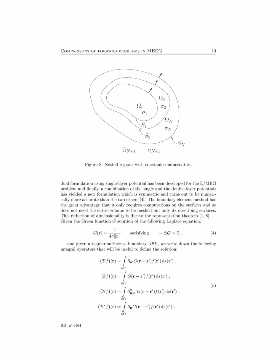
The boundary element method only works with piecewise constant conductivi-ties i.e. constant conductivity in each volume Ωi as shown figure 8. Let us addthat the symmetric BEM can also handle non-nested volumes [6] but for sakeof simplicity we will deal with the nested volume formulation. The equation 1now becomes:

σi∆V = f in Ωi, for all i = 1, . . . , N (3)∆V = 0 in ΩN+1[

V]j

=[σ∂nV

]j

= 0 on Sj , for all j = 1, . . . , N

The boundary element method is based on an integral formulation of theprevious equations. The classical integral formulation has been derived byGeselowitz [3] and is a double-layer potential approach. This classical formu-lation suffers from numerical errors when applied to the E/MEG problem. A

INRIA


Figure 8: Nested regions with constant conductivities.

dual formulation using single-layer potential has been developed for the E/MEGproblem and finally, a combination of the single and the double-layer potentialshas yielded a new formulation which is symmetric and turns out to be numeri-cally more accurate than the two others [4]. The boundary element method hasthe great advantage that it only requires computations on the surfaces and sodoes not need the entire volume to be meshed but only its describing surfaces.This reduction of dimensionality is due to the representation theorem [1, 8].Given the Green function G solution of the following Laplace equation:

G(r) =1

4π‖r‖satisfying −∆G = δ0 , (4)

and given a regular surface as boundary (∂Ω), we write down the followingintegral operators that will be useful to define the solution:(

Df)(r) =

∫∂Ω

∂n′G(r− r′)f(r′) ds(r′) ,

(Sf)(r) =

∫∂Ω

G(r− r′)f(r′) ds(r′) ,

(Nf)(r) =

∫∂Ω

∂2n,n′G(r− r′)f(r′) ds(r′) ,

(D∗f

)(r) =

∫∂Ω

∂nG(r− r′)f(r′) ds(r′) .

(5)

RR n° 6364


Then, one can derive from these formulas a symmetric formulation, in asimilar way that Nedelec [8] did. The symmetric approach, uses both the singleand double-layer potentials. In this approach, we consider in each Ω1, . . . ,ΩN

the function:

uΩi=

V − vΩi/σi in Ωi

−vΩi/σi in R3\Ωi .

Each uΩiis harmonic in R3\∂Ωi. Considering the nested volume model (Fig.

8), the boundary of Ωi is ∂Ωi = Si−1 ∪ Si. With respect to the orientations ofnormals indicated, the jumps of uΩi across Si satisfy the relations:

[uΩi]i = VSi

, [uΩi]i−1 = −VSi−1 , (6a)

and the jumps of their derivatives:

[∂nuΩi ]i = (∂nV )−Si, [∂nuΩi ]i−1 = −(∂nV )+

Si−1. (6b)

We define pSi = σi[∂nuΩi ]i = σi(∂nV )−Si. Note that since [σ∂nV ] = 0, we have

pSi= σi(∂nV )−Si

= σi+1(∂nV )+Si

at the interface Si.Applying the representation theorem to the harmonic function uΩi

, we getthe following for i = 1, . . . , N :

σ−1i+1(vΩi+1)Si

− σ−1i (vΩi

)Si=

Di,i−1VSi−1 − 2DiiVSi + Di,i+1VSi+1 − σ−1i Si,i−1pSi−1

+ (σ−1i + σ−1

i+1)SiipSi− σ−1

i+1Si,i+1pSi+1 , (7)

Using the same approach, we evaluate the quantities(σi∂nuΩi

)−Si

=(p −

∂nvΩi

)−Si

and(σi+1∂nuΩi+1

)+Si

=(p− ∂nvΩi+1

)+Si

and subtracting the resultingexpressions yield to:

(∂nvΩi+1)Si − (∂nvΩi)Si =σiNi,i−1VSi−1 − (σi + σi+1)NiiVSi + σi+1Ni,i+1VSi+1−

D∗i,i−1pSi−1 + 2D∗iipSi −D∗i,i+1pSi+1 , (8)

for i = 1, . . . , N . Here (and in (7)) the terms corresponding to non-existingsurfaces S0, SN+1 are to be set to zero. Terms involving pSN

must also be setto zero, since σN+1 = 0 implies pSN

= 0.Observe that, unlike in the previous approaches, each surface only interacts

with its neighbors, at the cost of considering two sets of unknowns, VSiand pSi

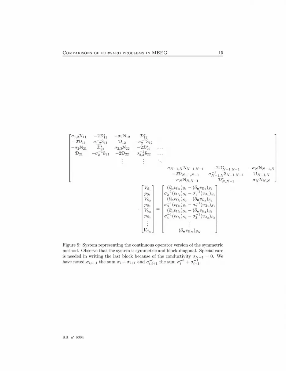
.Equations (7) and (8) thus lead to a block-diagonal symmetric operator matrix(see fig.9). Note that the vanishing conductivity σN+1 = 0 is taken into accountby effectively chopping off the last line and column of the matrix.

INRIA


σ1,2N11 −2D∗11 −σ2N12 D∗12

−2D11 σ−11,2S11 D12 −σ−1

2 S12

−σ2N21 D∗21 σ2,3N22 −2D∗22 . . .D21 −σ−1

2 S21 −2D22 σ−12,3S22 . . .

......

. . .σN−1,NNN−1,N−1 −2D∗N−1,N−1 −σNNN−1,N

−2DN−1,N−1 σ−1N−1,NSN−1,N−1 DN−1,N

−σNNN,N−1 D∗N,N−1 σNNN,N

·

VS1

pS1

VS2

pS2

VS3

pS3

...VSN

=

(∂nvΩ1)S1 − (∂nvΩ2)S1

σ−12 (vΩ2)S1 − σ−1

1 (vΩ1)S1

(∂nvΩ2)S2 − (∂nvΩ3)S2

σ−13 (vΩ3)S2 − σ−1

2 (vΩ2)S2

(∂nvΩ3)S3 − (∂nvΩ4)S3

σ−14 (vΩ4)S3 − σ−1

3 (vΩ3)S3

...(∂nvΩN

)SN

Figure 9: System representing the continuous operator version of the symmetricmethod. Observe that the system is symmetric and block-diagonal. Special careis needed in writing the last block because of the conductivity σN+1 = 0. Wehave noted σi,i+1 the sum σi + σi+1 and σ−1

i,i+1 the sum σ−1i + σ−1

i+1.

RR n° 6364


3.1.2 sBEM for MEG

As one can note from equation 2, the magnetic field B can be fully deduced fromthe knowledge of V on the interfaces. With the piecewise-constant conductivitymodel, the ohmic term can be decomposed as a sum over volumes of constantconductivity:∫

σ∇V × r− r′

‖r− r′‖3dr′ =

∑i

σi

∫Ωi

∇V × r− r′

‖r− r′‖3dr′ =

∑i

σiIi (9)

In the above identity, note that the conductivities must not only be assumedconstant in each domain Ωi but, but also isotropic, in order to take σi out of theintegral over Ωi. The volume integral Ii can be expressed as a surface integralon ∂Ωi = Si−1 ∪ Si. With this in view, we use the Stokes formula, and theidentity:

∇× (V∇g) = ∇V ×∇g

Thus,

Ii =∫

Ωi

∇×(V (r′)

r− r′

‖r− r′‖3

)dr′ =

∫∂Ωi

n× V (r′)r− r′

‖r− r′‖3ds

=∫

Si

n× V (r′)r− r′

‖r− r′‖3ds−

∫Si−1

n× V (r′)r− r′

‖r− r′‖3ds

This expression is then inserted in 9 ans recalling, that σN+1 = 0,

B(r) = B0(r) +µ0

4π

N∑i=1

(σi − σi+1)∫

Si

V (r′)n′ ×∇(

1‖r− r′‖

)ds′(r′).

INRIA


3.2 The tetrahedral Finite Element Method

The Finite Element Method developed for the forward problem in EEG, dealswith the weak formulation of equation 1. This equation is obtain by choosinga solution in a discretized space, multiplying both sides by a test function φand then integrating over the all computational domain. Using the divergencetheorem we get the following equivalences:∫

Ω

∇ · (σ∇V )φdΩ =∫

Ω

∇ · Jp φdΩ∫∂Ω

(φσ∇V ) · n d∂Ω−∫

Ω

σ∇V · ∇φdΩ = −∫

Ω

Jp · ∇φdΩ +∫

∂Ω

Jp φ · n d∂Ω∫Ω

σ∇V · ∇φdΩ =∫

Ω

Jp · ∇φdΩ (10)

We then discretize our solution V decomposing its values at the nodes lo-cation using the finite basis function φi as V =

∑ni=1 Viφi on the discretized

computational domain Ωh. Using Galerkin method, which uses the same basisfunctions as test functions, we can decompose these integrals on each elementwhich in the tFEM, are tetrahedra. The integrals are then performed on tetra-hedra of different shapes with constant conductivity inside. The mesh is comingfrom our volumic mesh generator and must have several properties as discussedin the section 2.1.1. Finally, we get the matricial equation that has to be solved:

Ax = b, (11)

where x is the vector of the unknowns, the potential Vi at the grid point i— and A the matrix such that:

Ai,j =∫

Ωh

σ(r)∇φi(r) · ∇φj(r) dr

=∑

Tk∈T

∑k:Vi,Vj∈Tk

σk

∫Tk

∇φi(r) · ∇φj(r) dr

where T represents the triangulation of Ωh, and Vk the vertices of the tetrahe-dron Tk, and finally the right hand side of 11 is:

bi =∫

Ωh

Jp · ∇φi dr =∫

Ωh

qδ(r0) · ∇φi dr = q · ∇φi(r0)

RR n° 6364


3.3 The implicit Finite Element Method

3.3.1 iFEM for EEG

The implicit FEM works with the same formulation as the tFEM (10) butcomputes the integrals present in the stiffness matrix and the source term in adifferent manner. The integrals are evaluated on the voxels of the image, andso this method does not need any mesh generation and uses directly the gridprovided by the MRI. In order to distinguish the different volumes that canhave different conductivities, a level-set method is used to extract the surfacesfrom the MRI.The computation of the stiffness matrix is then:

Ai,j =∑

k:Pi∈Vk,Pj∈Vk

∫Vk

σ(r)∇φik(r) · ∇φj

k(r) dr

The Cartesian grid cannot match perfectly the geometry of the domains, andas domains can have different conductivities, we must split the integral in orderto take into account each domains:∫

Vk

σ(r)∇φik(r)·∇φj

k(r) dr =∫

V 1k

σ1k∇φi

k(r)·∇φjk(r) dr+

∫V 2

k

σ2k∇φi

k(r)·∇φjk(r) dr

Integration over a voxel crossing an interface is done thanks to the level-sets [9].

3.3.2 iFEM for MEG

A method for solving the forward problem in MEG has been developed by [11]using the adjoint approach. We refer to this article for further explanations.

INRIA


3.4 Benefits and drawbacks of each methods

The symmetric BEM constructs a symmetric matrix, which is dense and can bestored; a direct solver is used to inverse it. The main drawback of this methodis that it has to work on isotropic media with piecewise constant conductivities.On the other hand, we have the FEM:s that create huge but sparse matrices thatcannot be inverted, the solution is obtained thanks to iterative solvers; here apreconditioned conjugated gradient. A significant advantage is that anisotropyand inhomogeneous media can be taken into account.

RR n° 6364


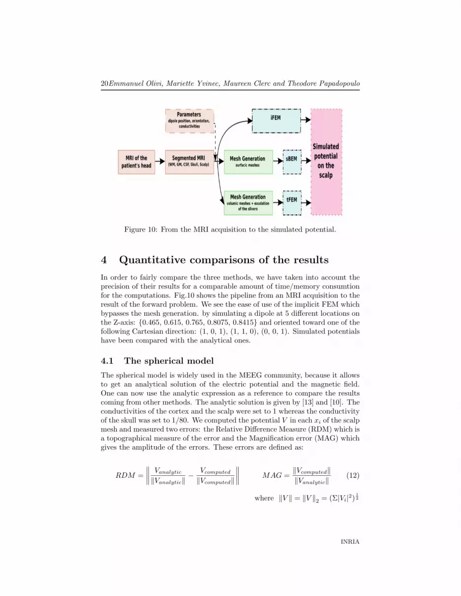
Figure 10: From the MRI acquisition to the simulated potential.

4 Quantitative comparisons of the results

In order to fairly compare the three methods, we have taken into account theprecision of their results for a comparable amount of time/memory consumtionfor the computations. Fig.10 shows the pipeline from an MRI acquisition to theresult of the forward problem. We see the ease of use of the implicit FEM whichbypasses the mesh generation. by simulating a dipole at 5 different locations onthe Z-axis: 0.465, 0.615, 0.765, 0.8075, 0.8415 and oriented toward one of thefollowing Cartesian direction: (1, 0, 1), (1, 1, 0), (0, 0, 1). Simulated potentialshave been compared with the analytical ones.

4.1 The spherical model

The spherical model is widely used in the MEEG community, because it allowsto get an analytical solution of the electric potential and the magnetic field.One can now use the analytic expression as a reference to compare the resultscoming from other methods. The analytic solution is given by [13] and [10]. Theconductivities of the cortex and the scalp were set to 1 whereas the conductivityof the skull was set to 1/80. We computed the potential V in each xi of the scalpmesh and measured two errors: the Relative Difference Measure (RDM) which isa topographical measure of the error and the Magnification error (MAG) whichgives the amplitude of the errors. These errors are defined as:

RDM =∥∥∥∥ Vanalytic

‖Vanalytic‖− Vcomputed

‖Vcomputed‖

∥∥∥∥ MAG =‖Vcomputed‖‖Vanalytic‖

(12)

where ‖V ‖ = ‖V ‖2 = (Σ|Vi|2)12

INRIA


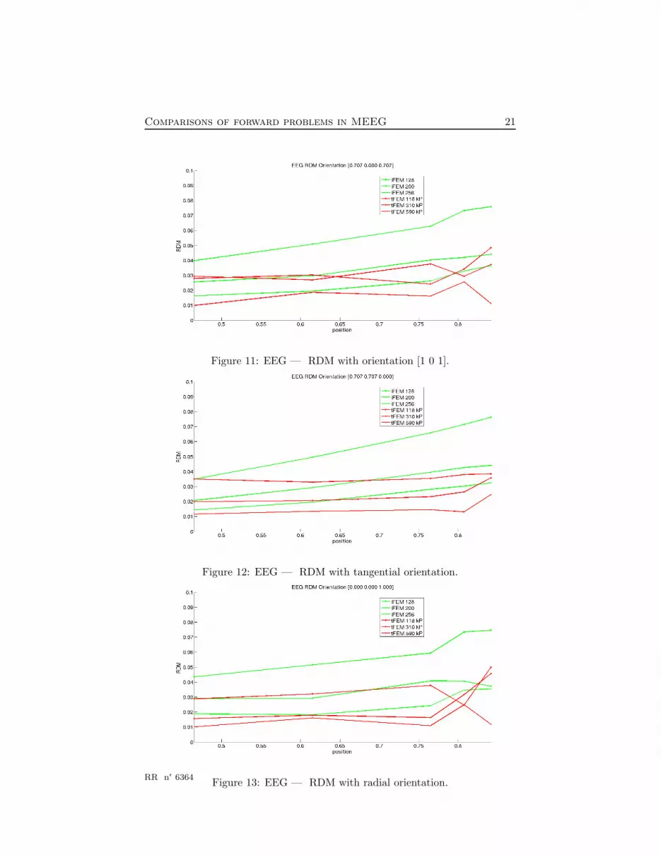
Figure 11: EEG — RDM with orientation [1 0 1].

Figure 12: EEG — RDM with tangential orientation.

Figure 13: EEG — RDM with radial orientation.RR n° 6364


4.2 Precisions of iFEM and tFEM

We have tested the precision of the two FE codes comparing them with theanalytical solution. To do so, we have tested three meshes for the tFEMwith: 118 000, 310 000, 590 000 points, and worked on images with dimensions:128x128x128, 200x200x200, 256x256x256 for the iFEM.

Fig. 11 to 13 show a higher precision of the tFEM (in red) compared withthe iFEM (in green) for the same amount of memory used. Computations madeon the 590 000-points mesh has required 2.4 GB of RAM for the tFEM, andas well for the finest grid 256x256x256 used by the iFEM. Table.2 gives thetimes needed for computations. We have not yet solved an issue regarding theMAG of the iFEM, so it is not plotted; the MAG of the tFEM, will be shownin section 4.5. In exchange, one can see that results coming from the iFEM aremore linear regarding the location of the dipoles for all orientations.

Methods NbPts — Dim Assembling time Iterations time NbIterationstetrahedric 118 000 16 s 121 s 291

310 000 45 s 702 s 416590 000 94 s 1852 s 509

implicit 128x128x128 82 s 338 s 337200x200x200 217 s 1728 s 509256x256x256 366 s 3824 s 579

Table 2: Computation time depending on the mesh size.

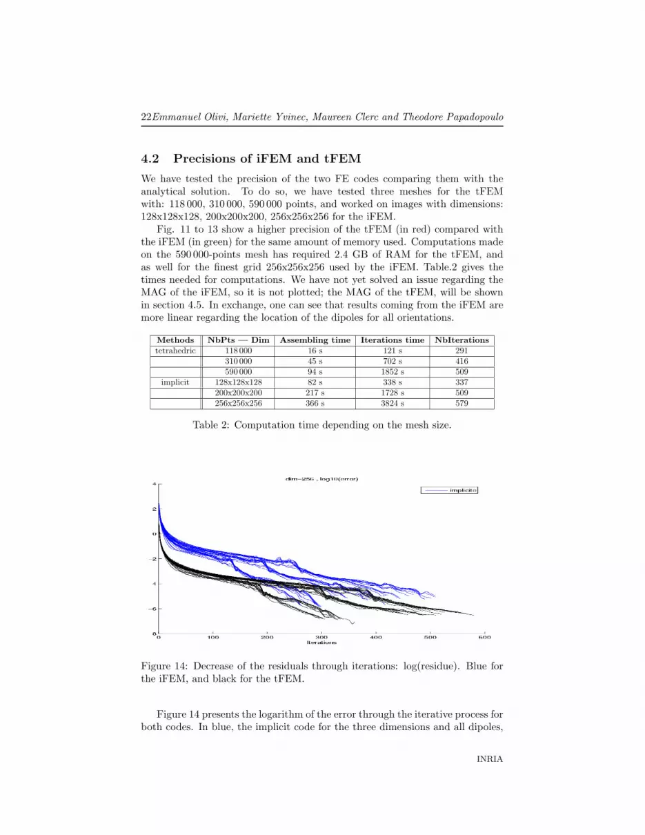
Figure 14: Decrease of the residuals through iterations: log(residue). Blue forthe iFEM, and black for the tFEM.

Figure 14 presents the logarithm of the error through the iterative process forboth codes. In blue, the implicit code for the three dimensions and all dipoles,

INRIA


and in black the tetrahedral one. One can see a ratio between the errors of theiFEM and tFEM. In order to speed up computations one could also stop earlier.

RR n° 6364


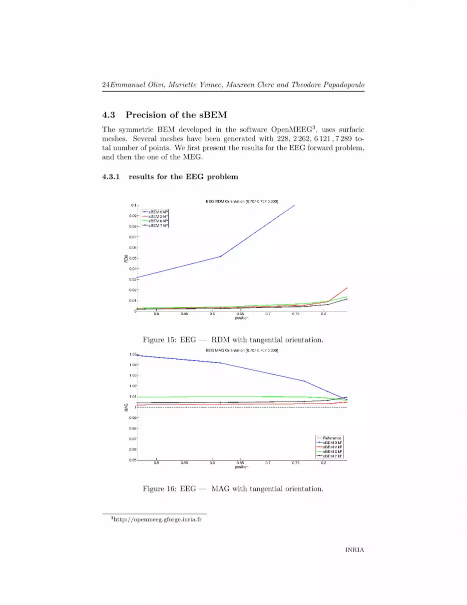
4.3 Precision of the sBEM

The symmetric BEM developed in the software OpenMEEG3, uses surfacicmeshes. Several meshes have been generated with 228, 2 262, 6 121 , 7 289 to-tal number of points. We first present the results for the EEG forward problem,and then the one of the MEG.

4.3.1 results for the EEG problem

Figure 15: EEG — RDM with tangential orientation.

Figure 16: EEG — MAG with tangential orientation.

3http://openmeeg.gforge.inria.fr

INRIA


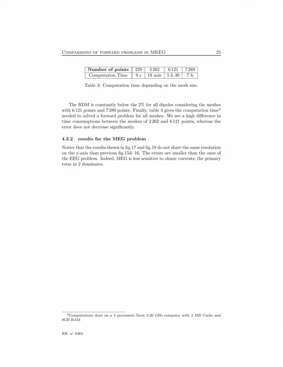
Number of points 228 2 262 6 121 7 289Computation Time 9 s 18 min 5 h 30 7 h

Table 3: Computation time depending on the mesh size.

The RDM is constantly below the 2% for all dipoles considering the mesheswith 6 121 points and 7 289 points. Finally, table 3 gives the computation time4

needed to solved a forward problem for all meshes. We see a high difference intime consumptions between the meshes of 2 262 and 6 121 points, whereas theerror does not decrease significantly.

4.3.2 results for the MEG problem

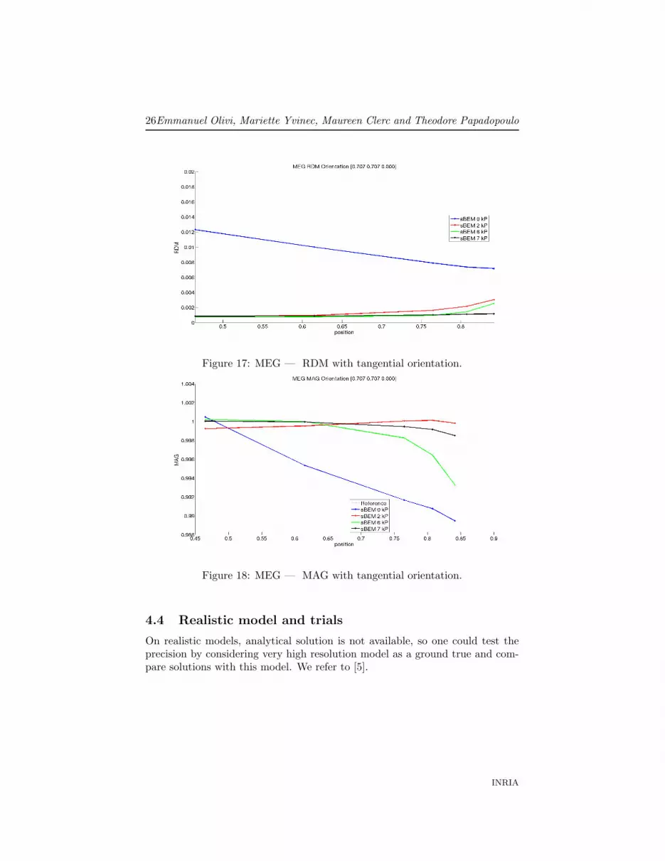
Notice that the results shown in fig.17 and fig.18 do not share the same resolutionon the y-axis than previous fig.15& 16. The errors are smaller than the ones ofthe EEG problem. Indeed, MEG is less sensitive to ohmic currents; the primaryterm in 2 dominates.

4Computations done on a 4 processors Xeon 3.20 GHz computer with 2 MB Cache and8GB RAM

RR n° 6364


Figure 17: MEG — RDM with tangential orientation.

Figure 18: MEG — MAG with tangential orientation.

4.4 Realistic model and trials

On realistic models, analytical solution is not available, so one could test theprecision by considering very high resolution model as a ground true and com-pare solutions with this model. We refer to [5].

INRIA


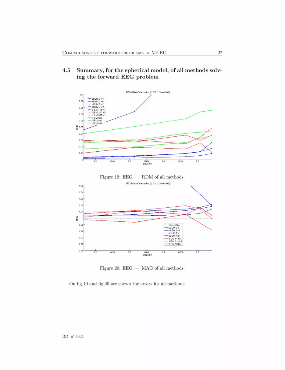
4.5 Summary, for the spherical model, of all methods solv-ing the forward EEG problem

Figure 19: EEG — RDM of all methods.

Figure 20: EEG — MAG of all methods.

On fig.19 and fig.20 are shown the errors for all methods.

RR n° 6364


5 Conclusion

In this document, we have seen how from a segmented MRI one could solve theMEEG forward problem. The sBEM gives the best results for the same amountof time spent in computations compared with the tetrahedric FEM, but themeshing step is still expensive. Furthermore, the sBEM is limited with thenumber of elements, and on realistic shape, it cannot provide a very detaileddescription of the geometry. Future computations on realistic model shouldclarify this point.Even if the tFEM gives slightly better results, the iFEM remains easy to useand could be easy to parallelize.The code Head mesher could be optimized by reducing the time spent in theexudation of the slivers which in our case was responsible for 90% of the meshingtime.Finally, we recall that the sBEM cannot take into account anisotropy, such asthe one of the skull.

INRIA


References

[1] Marc Bonnet. Equations integrales et elements de frontiere. CNRS Edi-tions, Eyrolles, 1995.

[2] M. Clerc, G. Adde, J. Kybic, T. Papadopoulo, and J.-M. Badier. In vivoconductivity estimation with symmetric boundary elements. In JaakkoMalmivuo, editor, International Journal of Bioelectromagnetism, volume 7,pages 307–310, 2005.

[3] D. B. Geselowitz. On bioelectric potentials in an homogeneous volumeconductor. Biophysics Journal, 7:1–11, 1967.

[4] J. Kybic, M. Clerc, T. Abboud, O. Faugeras, R. Keriven, and T. Pa-padopoulo. Integral formulations for the eeg problem. Technical Report4735, INRIA, feb 2003.

[5] J. Kybic, M. Clerc, T. Abboud, O. Faugeras, R. Keriven, and T. Pa-padopoulo. A common formalism for the integral formulations of the for-ward EEG problem. IEEE Transactions on Medical Imaging, 24:12–28, jan2005.

[6] J. Kybic, M. Clerc, O. Faugeras, R. Keriven, and T. Papadopoulo. Gen-eralized head models for MEG/EEG: boundary element method beyondnested volumes. Physics in Medicine and Biology, 51:1333–1346, 2006.

[7] Gildas Marin, Christophe Guerin, Sylvain Baillet, Line Garnero, andGerard Meunier. Influence of skull anisotropy for the forward and inverseproblems in EEG: simulation studies using FEM on realistic head models.Human Brain Mapping, 6:250–269, 1998.

[8] Jean-Claude Nedelec. Acoustic and Electromagnetic Equations. SpringerVerlag, 2001.

[9] Theodore Papadopoulo and Sylvain Vallaghe. Implicit meshing for finiteelement methods using levelsets. In Proceedings of MMBIA 07, 2007.

[10] Jukka Sarvas. Basic mathematical and electromagnetic concepts of thebiomagnetic inverse problem. Phys. Med. Biol., 32(1):11–22, 1987.

[11] S. Vallaghe, T. Papadopoulo, and M. Clerc. The adjoint method for generalEEG and MEG sensor-based lead field equations. Physics in Medicine andBiology, 54:135–147, 2009.

[12] B. Yvert, O. Bertrand, J.-F. Echallier, and J. Pernier. Improved forward eegcalculations using local mesh refinement of realistic head geometries. Elec-troencephalography and Clinical Neurophysiology, 95:381–392, may 1995.

[13] Zhi Zhang. A fast method to compute surface potentials generated bydipoles within multilayer anisotropic spheres. Phys. Med. Biol., 40:335–349, 1995.

RR n° 6364

Centre de recherche INRIA Sophia Antipolis – Méditerranée2004, route des Lucioles - BP 93 - 06902 Sophia Antipolis Cedex (France)

Centre de recherche INRIA Futurs : Parc Orsay Université - ZAC des Vignes4, rue Jacques Monod - 91893 ORSAY Cedex

Centre de recherche INRIA Nancy – Grand Est : LORIA, Technopôle de Nancy-Brabois - Campus scientifique615, rue du Jardin Botanique - BP 101 - 54602 Villers-lès-Nancy Cedex

Centre de recherche INRIA Rennes – Bretagne Atlantique : IRISA, Campus universitaire de Beaulieu - 35042 Rennes CedexCentre de recherche INRIA Grenoble – Rhône-Alpes : 655, avenue de l’Europe - 38334 Montbonnot Saint-Ismier

Centre de recherche INRIA Paris – Rocquencourt : Domaine de Voluceau - Rocquencourt - BP 105 - 78153 Le Chesnay Cedex

ÉditeurINRIA - Domaine de Voluceau - Rocquencourt, BP 105 - 78153 Le Chesnay Cedex (France)

http://www.inria.fr

ISSN 0249-6399