


Bahasa
Halaman
Hukum


Proceedings of the Open
University Geological SocietyVolume 2 2016
Including lecture articles from the AGM 2015, the Newcastle Symposium 2015,
OUGS Members’ field trip reports, the Annual Report for 2015,
and the 2015 Moyra Eldridge Photographic Competition winning
and highly commended photographs
Edited and designed by:Dr David M. Jones41 Blackburn Way,
Godalming, Surrey GU7 1JYe-mail: [email protected]
The Open University Geological Society (OUGS) and its Proceedings Editor accept no
responsibility for breach of copyright. Copyright for the work remains with the
authors, but copyright for the published articles is that of the OUGS.
ISSN 2058-5209© Copyright reserved
Proceedings of the OUGS 2 2016; published 2016; printed by Hobbs the Printers Ltd, Totton, Hampshire

1973–74 Prof. Ian Gass1975–76 Dr Chris Wilson1977–78 Mr John Wright1979–80 Dr Richard Thorpe1981–82 Dr Dennis Jackson
1983–84 Prof. Geoff Brown1985–86 Dr Peter Skelton1987–88 Mr Eric Skipsey1989–90 Dr Sandy Smith1991–92 Dr Dave Williams
1993–94 Dr Dave Rothery1995–96 Dr Nigel Harris1997–98 Dr Dee Edwards1999–00 Dr Peter Sheldon2001–02 Prof. Bob Spicer
2003–04 Prof. Chris Wilson2005–06 Dr Angela Coe2007–08 Dr Sandy Smith2011–12 Dr Dave McGarvie2012–13 Dr Nick Rogers
Past Presidents
ii
Committee of the Open University Geological Society 2016Society Website: ougs.org
Executive CommitteePresident: Dr Tom Argles, Department of Earth Sciences, The Open University, Milton Keynes MK7 6AA; [email protected]: Sue Vernon: 01895 678932; [email protected]: Don Cameron, BGS, Environmental Science Centre, Keyworth, Nottingham, NG2 5JD; 01159 142050; [email protected]: John Gooch: 01257 266288; [email protected] Secretary: Phyllis Turkington: 02890 817470; [email protected] Editor: Lyn Relph: 01758 750398; [email protected] Officer: Pauline Kirtley: 07506 692369; [email protected]
Branch OrganisersEast Anglia (EAn): Richard Kirkham: 07974 339917; [email protected] Midlands (EMi): Sue Atkinson: [email protected] Scotland (ESc): Stuart Swales: 01887 840377; [email protected] (Ire): Susan Pyne: 00353 1 456 2301; [email protected] (Lon): John Lonergan: 01903 740432; [email protected] Europe (Eur): Elisabeth d'Eyrames: [email protected] (Nor): Paul Williams: [email protected] West (NWe): Jane Schollick: [email protected] (Oxf): Sally Munnings: 01635 821290; [email protected] (Ssi): Janet Hiscott: 01633 781557; [email protected] East (SEa): Geoff Downer: [email protected] West (SWe): Rich Blagden: [email protected] Hall (WHa): Dr Zbig Towalski: [email protected] (Wsx): Sheila Alderman: 01935 825379; [email protected] Midlands (WMi): Sandra Morgan: 01543 410781; [email protected] Scotland (WSc): John Tweedie: [email protected] (Yor): Ricky Savage: 07786 536219; [email protected] Organisers Representative: Sally Munnings: 01635 821290, 07867 123273; [email protected]
Other officers(non-OUGSC voting)
Sales Administrator: John Lonergan: 01903 740432; [email protected] Secretary: Linda McArdell: 01707 339450; Heather Rogers; [email protected] Editor: Dr David M. Jones, 41 Blackburn Way, Godalming, Surrey GU7 1JY; 01483 424308; [email protected]/Reviews: Jane Michael: 07917 434598; [email protected]: Stuart Swales: 01887 840377; [email protected] Webmaster: Martin Bryan: 01452 859991; [email protected] and Forum Moderator: Linda Fowler; [email protected] Aid Officer: Ann Goundry: 01132 829798; [email protected]
Vice PresidentsDr Evelyn Brown, Dr Michael Gagan and Norma Rothwell: [email protected]

OUGS Committee
Policy-making body
Executive Committee
Sales Administrator
Executive Committee
management
President Treasurer
Chairman Membership Secretary
Secretary Information Officer
BOs’ Rep. Newsletter Editor
Branch Organisers
MembershipMembers can contact any
officer at any time, normally
through their BO and/or
through the BOs’ Rep.
Gift Aid Officer
DISSEMINATION OF INFORMATION PATHWAYS
Archivist/Reviews
Proceedings Editor
other co-opted officers
iii
Webmaster
iv
Editorial:
Dear readers,
I would like to begin this editorial by
thanking all members who filled out the
OUGS Executive Committee’s most recent
survey, and for the many kind comments
people made about our publication in its
new guise as the Proceedings of the OUGS. One of you even
commented, “Zealot high quality product”! I’ve never quite
thought of myself as, “a person who is zealous, especially to an
extreme or excessive degree; a fanatic,” but I do strive to give
you a decent publication.
This issue comprises articles from the speakers at our Annual
General Meeting weekend in April 2015 and at our Symposium
in July 2015 in Newcastle upon Tyne, entitled, ‘Pangaea: Life
and Times on a Super Continent: a celebration of Britain’s
unique marine Permian strata’.
First we are given a new perspective on the great Permo-
Triassic mass extinction, new thoughts about recovery after
mass extinction and new discoveries from Chinese fossil sites,
by Prof. Mike Benton of Bristol University, who has delivered
lectures to us many times at OUGS weekends.
Our Geoff Brown Memorial Lecture for 2015 was given by
Prof. Kathy Cashman, also of Bristol University, on the ever
fascinating research on volcanic eruptions and their effects
on society.
Our Symposium in Newcastle has produced a host of articles
ranging from a detailed and informative summary of Pangaea
and the Permian geology of north-east England by Dr Paul
Williams, to a summing up of the lectures by our President, Dr
Tom Argles. In between are articles on recent research and
interpretations of the North Pennines Orefield, on Zechstein
carbonates and the Permian Rotliegend sandstones, and on the
mining of Zechstein evaporites.
Then you can read a sweeping history of geological
research through more than a century on the Permian in
north-east England, followed by two final articles demon-
strating the increasing engagement of geologists and the pub-
lic. The Limestone Landscapes Project and outreach pro-
grammes in geoconservation and geodiversity are two exam-
ples of how the public, both UK and foreign visitors, are
becoming more engaged with there landscapes and local
building traditions.
There follow four field trip reports at home and abroad. And
interestingly, thinking of the increasing engagement of the
public with geology and geography just alluded to, on our final
field day of Tom Argles’s Presidential Field Trip, ‘Mantle in the
Mountains’ to Andalucía, Spain, we ‘met’ hundreds of seemingly
eager Spaniards from very young to quite elderly out on the
Nigüelas Fault east of Granada enjoying Spain’s national
‘Geolodía’ (Geology Day)! There follow several further field
trip reports, including one from the Newcastle Symposium, and
another field excursion to a Welsh locality by the seemingly
indefatigable John Downes.
Also included is a short report on a field trip dedicated to vis-
iting the final resting place of the ‘Father of English Geology’
William Smith, and a useful article on a crystallography and
mineralogy workshop/study weekend hosted last year by the
Severnside Branch.
Articles in this issue finish with an unusual twist and twill in a
report by Michael Perkins of the East of Scotland Branch on a
visit to see the Great Tapestry of Scotland. Michael picks out
the geological elements woven into the tapestry and describes
them to us with colourful (fabriculous!) photographs inter-
twined with his text.
One of the privileges and perils of editorship of a society publi-
cation and an ‘Editorial’ blank page is that you may, within rea-
son, ‘say things about people’. Theoretically speaking, a final
offering in this issue is a salutory note from Diana Smith, for-
mer OUGS Chairman and OUGS Tutor (to which I would add
the epithet ‘extraordinaire!’). Incidentally, Diana, for better or
worse, is hugely responsible for my becoming OUGS NewsletterEditor earlier this century, and now your Proceedings (formerly
Journal) Editor.
Diana attended a GS London meeting last June on ‘Higher
Education network and University Geosciences in the UK’ and
wrote a précis of each speaker’s address. The message is inter-
esting and informative, and it comes not only from UK shores,
but is an international one. It is the opinion of this editor that
we should definitely heed Diana’s final advice.
Last, but certainly not least, I want to express my gratitude to
all those who help me produce this publication for you. Thank
you to all you worthy transcribers who toil through our AGM
and Symposium lecture recordings to provide transcriptions for
the speakers to help them in writing up their articles for us to
publish: Philip Clark, Maggie Deytrikh, Averil Leaver, Dick
Millard, Sally Munnings, Isabel O’Brien, Jenny Parry and
Norma Rothwell.
Thank you also to Linda Fowler, Don Cameron and Sue
Vernon for your continued support and advice and proofread-
ing. A special thank you to Sue Hughes who has become our
proofreader (assuming the experience hasn’t put her off!).
And thank you to Professor Jose Benavente and to Dr Carlos
Sanz de Galdeano of the University of Granada for their wel-
come at the Nigüelas Fault, Andalucía, and for providing the
photographs for the figures on pages 113 and 114.
Finally, I’d like to explain the charming little vignettes that you
will find next to the titles of the articles beginning on pages 33,
39, 55 and 63. These are character sketches by our very own
Thalia, drawn as she listened to the lectures at the Newcastle
Symposium. Linda McArdell and I were able to persuade Thalia
to let us use them, and to which the authors readily agreed as
well. (And just for the record, in Greek mythology Thalia
[Θάλεια] is one of the Three Graces, the Muse for comedy and
idyllic poetry, and a Nereid [a sea nymph]!)
As always, I wish you happy reading.
— David M. Jones, OUGS Proceedings Editor

1Proceedings of the OUGS 2 2016, 1–8© OUGS ISSN 2058-5209
Evolutionary recovery after mass extinctions
Mike Benton(University of Bristol)
Introduction
Iwant to talk about recovery rather than about the extinctionevent itself, other than in the briefest terms. I’m interested
here in talking about recovery because of course we often focuson mass extinctions only in negative terms, and yet, clearly, lifesurvived and life came back, and in fact this particular event, aswas the case with many of the others, punctuated the trajectoryof life and probably had an important influence on life as we seeit today.
This is a rough outline of what I want to talk about:
• a little bit about China, where I’ve had the great privilege andpleasure to do field work over a number of years now, and
• a little bit about methods and ways that palaeontologists cantry to extract evolutionary information from the fossiloccurrences
If you read about the Permo-Triassic mass extinction you maysee a diagram like this (Fig. 1). This is a classic kind of rangechart and you’ve all seen them I know. The detail doesn’t matter,but this is well documented in China because the quality ofstratigraphy is very good across the boundary. Not only are theregood fossil occurrences that allow them to divide up the succes-sion into many, many zones, they believe that it’s very complete,that there’s not a lot of time missing, and it is very fossil rich; andas well as the paleontological evidence there are volcanic ashbeds, from which we can get a number of radiometric datesthrough the sequence.
The extinction event and sitesSo, in this diagram you are looking at more than 500 species ofinvertebrates; they’re plotted in sequence according to the timesof their extinctions, so it is a sort of step-wise pattern of extinc-tions. The stratigraphy is based mainly on conodonts and thePermo–Triassic boundary is here [pointing]; and the two extinc-tion levels bracket that boundary. And people debate back andforwards about whether there is there a single level of extinctionor two levels? It’s the sort of semantic question, whether youwish to call Level B a separate extinction event, but for themoment we’ll just do that. What’s been argued from this evidenceis that numerous species come and go through time, as you wouldexpect, and then at Level A 90% of species disappear at that onelevel. Then there is an episode up to Level B of rather strangeevolution, which I’ll say something about in a moment, and thenat Level B there appears to be another extinction where some-thing like 80% or 90% of species disappear. Various versions ofthis diagram have been published — this is the latest one fromNature Geoscience in 2013.
Now, what’s this episode between A and B? First of all,because of radiometric dating, and now the quality of the dating,we are able to say that the spacing is something like 180,000years. So there are exact radiometric age dates here, here, andthen at different points up and down because of these ash beds;so 180,000 years, that’s the level of precision that we wouldn’thave expected a number of years ago; and the other curious thingto notice is that something changes between Levels A and B:there are lots of steps of extinction, but almost all of the speciesgoing extinct are very short lived. So up to Level A there is a sortof random selection of long-lived and short-lived species, and
then that pattern returns again in theTriassic after Level B; but in thatspace in between the steps of extinc-tion are mainly very short-livedspecies so that they originate and goextinct within an increment of thatstratigraphic column — and these aretypically what people would call dis-aster species. They struggle into exis-tence, they do what they do, theyquickly go extinct and something elsecomes along and they’re a sort ofquick turn-over. And another point is,for the moment at least, that we seemto be calling this the Permo–Triassicextinction rather than the end-Permianextinction because the first level, A,was before the end of the Permian ifyou’re being very exact, and if you
OUGS AGM 2015 Keynote Lecture
Figure 1 A typical diuagram of Permo-Triassic mass extinction.
[OUGS AGM 2015; original transcription by Sandy Colville-Stewart and Helen Coombs from the symposium recording; edited byProf. Benton and POUGS Editor David M. Jones.]

regard Level B as another part of the extinction that’s alreadyinto the Triassic.
The other fact to be aware of is that physical conditions on theEarth apparently did not return to normal for five or six millionsyears after the P–T boundary, and so some of you will be famil-iar with this diagram (Fig. 2). It’s a very famous summary of car-bon isotopic values through the Permo–Triassic boundary, all theway through the early Triassic and into the middle Triassic.These data are from work by Jonathan Payne published inScience in 2004, and what he found was that not only was therethe well-known carbon spike or excursion at the P–T boundary,but also, importantly, that this was repeated several times,maybe three more times at different points during the earlyTriassic. When that was first published people thought, oh well,maybe this isn’t quite right but a great deal of effort has goneinto measuring and comparing other sections and so this seemsto be real and then you can see that once you’re into the middleTriassic it kind of settles down at a fairly steady level. Thosesorts of perturbations, each of these peaks, represents a time offlash heating, global warming on a dramatic scale. So in termsof the recovery, we need to be aware of the fact that conditionson the Earth didn’t just return to normal immediately.
Some of you may know that the global strata of type for thePermo–Triassic boundary is indeed in China, in Meishan. It’sworth a visit if you enjoy visiting geoparks — this is a real geop-ark in the sense that they’ve made a kind of park and funfair outof it. It’s not at all popular but the effort that’s gone into it is fan-tastic, with a huge car park, cafeterias and stuff that you’d expect;and there’s a ‘sensuround’ cinema of four dimensional experiencein which you can actually walk up the steps and the boundary islabelled, so they point you right at it. There’s no doubt and every-body’s encouraged to visit … but there we are, they do thingsproperly. Around the corner you can see why perhaps it was cho-sen, as it’s a very complete succession: great volumes of marinesediments enable you to track through the uppermost Permiancontinuously into the Triassic, so that it’s been possible to collectcentimetre by centimetre, as you can see, to do those stable-iso-tope measurements, document fossil occurrences and all the othersorts of evidence that help you to try to understand what’s goingon. It’s not only close to the boundary, which is well documented,
Evolutionary recovery after mass extinction / Benton
2
but in fact the marine sections in southChina continue right up through theTriassic into the late Triassic. [Pointed outon his slide] So Meishan is over here nearNanjing, and Shanghai is somewhere inthere; there’s Hong Kong and YunnanProvince, I’ll show you some pictures fromthere; and Beijing is up here, so all acrossSouth China this great basin — somethinglike 2,000km wide — all of it, or almost allof it, marine Triassic. When I started myinterest in this [extinction event] a numberof years ago, the thought of visiting theseplaces was just impossible. Now it is easy— anybody can go. The point of this dia-gram, and again the details don’t matter, isthat not only do you have good documen-tation of the transition at Meishan, but
there are also many other sections that give you the rest of thatsuccession; so several kilometres of continuous sedimentationcan be documented.
Luoping, Xingyi and GuanlingWe’ve spent some time in different locations, but one locationthat took me there and why I was first invited is this site ofLuoping, which is in Yunnan Province. Here a team of geologistsin China found exceptionally preserved fossils and with the helpof students and farmers they effectively dug away half a hill(Fig. 3, opposite). What you are looking at is a hill that has justbeen dug away and they were able to step up through the wholesuccession collecting tons of rock and fossils at each level. Andthe reason that they were excited about this Luoping site, or setof sites really, is the exceptional marine, shallow marine, fauna ofmainly the vertebrates, which I suppose attracted their attention.There are ichthyosaurs, some other isolated marine reptiles, andthere are many fish, including Saurichthys, a common well-known middle Triassic fish something like a pike, a predatoryfish, plus lots of other heavily-scaled fishes; there are also arthro-pods, Limulus; there are lobsters; and rather well-preserved sea-urchins with all their spines in place. There are also terrestrialthings that got washed in, bits of plants, insects, teeth ofdinosaurs or dinosaur-like creatures, a millipede — all sorts ofodd and strange creatures — and so in the collection, just over asummer, they collected 20,000 identifiable, exceptional fossilsfrom the site.
Working with our Chinese colleagues, and with a wonderfulAustralian artist named Brian Choo, we were able to ‘recon-struct’ this ancient world. Brian did these fantastic reconstruc-tions of a series of marine Triassic fossil lagerstätten — they callthem exceptional biotas in China — with lots of fish,ichthyosaurs, a placodont, a lobster here fighting placodonts, andall sorts of other wonderful creatures (Fig. 4, page 4).
At a slightly younger site — that’s Middle Anisian, Ladinian —Xingyi is another lägerstatte particularly well-known for thesauropterygians, the nothosaurs and the pachypleurosaurs, aswell as for the placodonts; and there are ichthyosaurs, lots ofammonites, fish and other things there as well.
Guanling is probably the most famous of these lagerstätten fromTriassic China, and is particularly known for the giant crinoids.Some of you may be familiar with these creatures from the
Figure 2 Permo-Triassic environmental change.

Posidonienschiefer of Germany, but Guanling has just the same,where you can see them fossilised and lying flat-out on the marinesediments, logs with these enormous long crinoids, maybe four orfive metres long trailing behind some kind of plankton sieving,pseudo-planktonic system; and living among these would be allkinds of fish and marine reptiles and other vertebrates.
So it’s no wonder that these sites have led to a lot of excitementand this is one of the many sets of lagerstätten that are producingwonderful fossils in China at the moment. Obviously they arerather over-written or less-famous than the Jehol biotas of earlyCretaceous age with feathered dinosaurs, but these have attracteda lot of attention too.
Recovery of lifeWe were interested in aspects of the recovery of life, and you cansee this in a very simple way if you compare a succession of ear-liest Triassic, next level up, next level up — and as you get intothe Triassic you can see the way the ecosystem is kind of build-ing. The important point to note is that in these marine succes-sions a lot of the fishes were inherited from the Permian, so manyof those continue, as do many of the invertebrates, but in very dif-ferent proportions. You all know, of course, that thePermo–Triassic mass extinction dealt the death knell to trilobites,and to rugose and tabulate corals; and that various other groupsentirely disappeared, and then that those ecological roles had tobe recovered slowly and eventually by other groups of corals andthe crustaceans such as lobsters and shrimps. As these animalsrose to prominence in the Triassic, obviously the brachiopodsnever recovered; and bivalves and various other groups tookover. But wholly new are the marine reptiles. There is not a hintof these marine reptile groups in the Permian and yet theyemerge, certainly by the Olenekian — maybe some were even inthe Induan — in the early Triassic, certainly by the end of theearly Triassic. So within three or four million years of the extinc-tion we already have the first representatives of these several dif-ferent groups of marine reptiles; and by the time of Luoping in
3
the middle Triassic they’vediversified further and you havethe shell-crushing placodontsand even large ichthyosaurs andthalattosaurs, some types ofwhich are getting to be manymetres in length. By the lateTriassic ichthyosaurs reachedgigantic size, the biggest marinereptiles ever; and some of theshonisaurs and shastasaurs weremaybe seven or eight metres inlength. So they’re more whale-like in size than anything else.
In attempting to document therecovery the first approach ofcourse is simply understandingthe succession: which groupsappear, when do they appear andthat kind of thing. One thingbecomes rather evident whenyou do that simple stratigraphicapproach: that the first phase ofthe recovery was a very difficult
time and most of the evidence suggests rather rapid recovery —somewhat debated, but I think the debate is rather semanticbecause of course certain groups like ammonoids and conodontsrecovered quickly in Induan in the beginning of the Triassic butthey were hit again by these repeated isotopic excursions, whichrepresent repeated, dramatic environmental change. So in a clas-sic ‘spindle’ diagram [as in Jonathan Payne’s work, mentioned
above — Ed.] we can almost separate this block of time acrossthe Permo–Triassic boundary. You can see the extinction of vari-ous groups at that point in these marine and terrestrial environ-ments, lots of groups entirely wiped out, some just surviving andrecovering, but during this time of six million years of rapid iso-topic fluctuation there are certain groups that did not recover.
It’s very easy to remember: the coal gap, the coral gap, thechert gap — three Cs. In deep seas there were no cherts beingformed, the siliceous organisms that would have formed thosecherts in a normal-functioning ocean just weren’t there and socherts are not accumulating. Secondly, no coral reefs because, ofcourse, the corals have been killed off, or at least if any survivedthey were minor, hidden parts of the ecosystems. Corals onlycame back rather later, the modern scleractinian corals.
On land there was the coal gap. Of course that’s an observationof the distribution of sedimentary rocks, but it’s an implicationthat there just weren’t any trees around — and maybe that thatwas part of the extinction.
More ways of looking at recoveryLet’s look at other ways of trying to understand the recovery. Thisis important because you then can see very probable linksbetween the physical environment as documented by the sedi-ments and the isotopes, delaying recovery and impacting on thenature of the evolutionary process, but also that it is dependant ondocumenting occurrences of fossils as point occurrences, wherewe can do it, to look at the fossils in a phylogenetic context, anevolutionary context. With colleagues in China we’re pushingthis approach forward — this is the beginning if you like, and we
Proceedings of the OUGS 2 2016
Figure 3 The Luoping fossil site in Yunnan Province.

have quite a way to go in trying to adopt these approaches, butthis is what we’ve been able to do here.
I want to take you, maybe for some of you, further from yourcomfort zone in later parts of the lecture by talking about macro-evolution; how we can use an improved stratigraphic time-scale
4
and a thorough and careful documentation of the fossils to try tocalculate certain aspects of evolution from that information. Notleast are things like rates of change — that’s a relatively straight-forward thing. Here, macro-evolution is just evolution above thespecies level.
Evolutionary recovery after mass extinction / Benton
Figure 4 A reconstruction of a marine Triassic fossil lagerstätten, or ‘exceptional biota’ by Australian artist Brian Choo, based on the Luopingfossil site in Yunnan Province, China.

5
What are the different components we need? One of these is thephylogenetic tree. Phylogenetic trees are a very important aspectof much of what I am going to talk about. You’re all familiar withthese, you may be aware that the production of ever bigger treesis feasible these days and can be done using a variety of differentmethods and a variety of different sources of information, andsome of you will have seen some that are absolutely huge. Theymay be for modern organisms compiled from genomic data, fromDNA, or in our cases we’re going to be doing it from the fossils;in some cases you can do a combined effort.
I’ll try not to go too far with this idea, just enough to introducesome of the concepts. When you’re talking about evolution in amathematical sense you’re looking for patterns, and the simplestway to find patterns, in a statistical sense, is to demonstrate some-thing that diverges from random, something that cannot beexplained by a random process. Statisticians use two terms in thiscase: they will often say that the random pattern is either a ran-dom walk or sometimes they use this term ‘Brownian Motion’.You’ll be familiar with both of these. In an earlier version thingsmoved, all these little particles jumped about, so BrownianMotion is that classical image of atoms bouncing around andmoving in an apparently kind of random way.
There are different kinds of patterns of evolution, and may bea little easier to follow where time is, as usual, on the y-axis anda character or a trait on the x-axis, and so the random model ofevolution, Brownian Motion, is shown by this kind of tree wheresplitting is just happening more or less equally to left and right.In contrast, in the trend case there is more splitting happening inthis direction so the whole population, the whole group, is head-ing off in that particular direction.
The final method or terminology I just want to remind you ofis the distinction between diversity and disparity. Normally,palaeontologists will use the word diversity simply to mean num-ber of species, or number of families, or number of genera;whereas disparity is the morphological diversity — but just toavoid that possible confusion of use of the word ‘diversity’ wetend to call it ‘disparity’. So disparity, then, is the amount of dif-ference in terms of morphological difference, forgetting the tax-onomy. Putting these two together, how do diversity and dispari-ty change through time? This is where we get to the surprisingdiscovery. The null expectation would be that the two are cou-pled, meaning that as diversity increases disparity increases at thesame rate; and if you prefer to look at this as a tree here it is(Fig. 5); it’s just a normal Brownian Motion kind of tree that’sexpanding at a kind of regular rate in time and as the speciessplit the range of morphology keeps increasing; and if youprefer to plot it with amount of change on the x-axis andtime on the y-axis, disparity and diversity more or lessincrease in parallel, so that’s implying they are coupled andthat makes sense, that would be the sort of basic common-sense expectation: that as the species split they get evermore different.
The other two possibilities are that diversity and disparityare decoupled, meaning that each follows its own course —that they are not connected exactly. You could have a patternof diversity first, where speciation rate is the same but theamount of morphology is quite limited, and so disparity isincreasing very slowly, whereas diversity is increasing at thesame rate — so here we have the diversity rising and the dis-parity coming rather later. Or, you could have this kind of
early burst type of model where it’s disparity first, so morpholo-gy expands fast and then speciation fills up that amount of spacethrough the same span of time. In all these three trees at the topthe rate of species-splitting is the same in each case. If we canidentify which of these is the commonest pattern in nature, wemight be discovering something important about how evolutionworks and entirely from fossil data.
This is nothing to do with any of the modern areas of biologythat normally would be used — making use of genomics as a wayof getting at the process of evolution; there are other patterns aswell. I can tell you, first of all, that this is the dominant patternfrom the fossil record; however you measure the disparity, itdoesn’t matter, that’s how it is, predominantly, in the fossilrecord, and that’s telling us something quite extraordinary — it’stelling us that we don’t really see much difference in post-extinc-tion times and normal times because often people have thought‘you clear the world, you empty the world of life, and in this post-extinction world somehow the normal rules of evolution will runawry’ and that evolution would then run very fast because there’sso much opportunity, there’s so little competition.
Maybe that’s true, but we don’t really see any difference fromgroups that radiate in other times. If you compare the pattern ofexpansion of birds, the normal assumption is that the early evo-lution of birds was not triggered by a preceding mass extinction,that you have Archaeopteryx, you then have all these amazingbirds from the Cretaceous of China. That sort of explosion ofearly birds was in no way, I don’t think, triggered by any pre-ceding mass extinction; whereas in the Triassic, which we aregoing to look at in a bit more detail, clearly was and yet you stillseem to get the same pattern, so far — and that’s based now onhundreds of studies where people have tried to look at many dif-ferent groups in many different ways — so morphology firstthen diversity.
Macro-evolutionThat gives a very clear steer of how we should understand one ofthe most fascinating parts of macro-evolution, that is, the adap-tive radiation. Think back to G. G. Simpson in 1944 [Tempo and
Mode in Evolution, Columbia UP — Ed.], when he presented adiagrammatic way to marry palaeontology and modern biologyand gave a model of adaptive radiation that fits this kind of expla-nation. It seems that, for whatever reason — whether it’s the
Proceedings of the OUGS 2 2016
Figure 5 Diversity and disparity ‘decouled’.

opportunity after a mass extinction, or the opportunity of a newcharacter — whatever it is that makes birds successful, the groupwill then explode, it will do everything that is possible, to the lim-its, and then after that the group is successful, it fills up the space.
Let’s have a look at a couple of case studies of groups thatrecovered in the Triassic and see what they show. Here is a niceexample of what could be called ‘an evolutionary bottleneck’ —the dicynodonts. They were very important herbivores on land atthe end of the Permian, then they were nearly wiped out. I thinkthree or four species survived, including, famously, Lystrosaurus,and then for a span of time — indeed this particular time of envi-ronmental awkwardness or ghastliness — they didn’t recovermuch at all. And then they kind of explosively radiated in theMiddle Triassic and eventually tailed off and disappeared in theLate Triassic. This is a spindle diagram (Fig. 6A), meant to rep-resent the number of species, more or less; and at one time thatwould have been all you could have done, and said, ‘Oh rightthat’s interesting’; and that’s it. But now you can go a lot further,and I’ll show you how we were able to try to marry together astudy of the diversity, but also the disparity, to try to understandwhat was going on.
Lystrosaurus is a famous fossil for all sorts of reasons. Thediversity data are quite rich, this is a range chart compiled by JörgFröbisch a number of years ago (Fig. 6B) and these are very com-mon fossils — they were bulky creatures, and so were easily fos-silised; they’re well known from the Karoo in Southern Africa,from the Permo–Triassic red beds of Russia, from China, andfrom various other parts of the world.
In terms of the phylogeny, there is the Permo–Triassic bound-ary here; and here are all the Late Permian forms, those MiddleTriassic forms, and the survivors: one, two, three, four. So this isLystrosaurus, this is Myosaurus and these two we don’t know,but these are leading up to these particular groups here, so wedon’t have any fossils here, but we know that there must havebeen precursors of those surviving across the boundary. So four,only two of which actually led to the explosion of diversity; andthese two — Lystrosaurus and Myosaurus — they are examplesof what has come to be known as ‘dead clade walking’. They areorganisms that survived but they shouldn’t really have becausethey don’t lead to anything at all, and it is important just to keepthat in mind briefly.
Evolutionary recovery after mass extinction / Benton
So what we then tried todo was to measure the rangeof morphology of all thesedicynodonts through thePermo–Triassic boundary.And it kind of confirmedwhat we thought we mightfind. First of all let meexplain: this diagram is ageometrical representationof all of the different aspectsof morphology that we wereable to measure, sum-marised and simplified intoa simple x/y plot. It is a verystandard sort of output froma variety of kinds multi-vari-ant statistical summaries,examples of which I am sure
you will have seen these in many different contexts. You can readthem in a very exact geometric way in terms of the area occupied,so you can say for these Permian forms, these are maybe MiddlePermian, these are maybe Late Permian — so you can actuallyplot and see where they sit, and the points that are closest are themost physically similar, while those that are farthest apart are —in terms of morphology — the most different. And then you canlook at the areas occupied through time — so in the late Permianthey occupy a large area of this morphospace, in the Triassicshown in blue they occupy a rather smaller area; and we were abit honest when we published this because we included over hereMyosaurus, but remember that it was a ‘dead clade walking’, andwe should have removed it for that reason. The Middle Triassicforms are just over here, so the effect of the bottleneck was,again, that disparity and diversity are decoupled, and althoughdiversity recovered more or less to something like the pre-extinc-tion level, morphology never did.
So this is evidence of a complex effect of the extinction eventand that something in the survivors is very different. The eventhad massively reduced their adaptive possibilities, or somethinglike that.
The rise of dinosaursMy third and final example is the origin of dinosaurs, which untilrecently I wouldn’t have linked, most people wouldn’t havelinked, with the Permo–Triassic mass extinction. But in a waynow perhaps we can. Normally, you may recall, we would under-stand that the dinosaurs originated in the Late Triassic — the old-est dinosaurs are typically from South America, the IschigualastoFormation of Argentina for example — and the oldest body fos-sils occur c. 230Mya; and here is the Permo–Triassic massextinction. However, in the last five or six years quite a lot of evi-dence has been found that pulls the origin of dinosaurs from theLate Triassic down into the end of the Early Triassic. So, at firstthat was quite a hard thing to swallow, that was quite difficult toaccept; and certainly the first inkling of this came from fossiltracks. Of course tracks are always something you have got to bea little bit careful about because people will hypothesise fromtracks, but it is often not absolutely defensible. I am sure many ofyou will know examples. However, soon after these tracksdinosaur-like from Poland were announced, also other fossils
6
Figure 6 (A) A classic ‘spindle’ diagram of species fluctuation through time. (B) Lystrosaurus range chart through
Triassic and Permian times, compiled by Jörg Fröbisch.

came from the Middle Triassic of Tanzania; and although theTanzanian examples were not dinosaurs, they were the nearestrelatives of dinosaurs — in terms of the evolutionary tree, the sis-ter group, the nearest relatives. If you’ve got them down here inthe Middle Triassic, dinosaurs must have come down there aswell because they shared a common ancestor and you can onlyhave one common ancestor.
[Here a ‘gratuitous picture of early dinosaurs’ was shown ‘just
to cheer you up a bit’ — Ed.] Here are some of the earlydinosaurs: this is Coelophysis and these are Late Triassic, ofcourse, so we don’t know exactly what these very first dinosaurslooked like. Even if they originated at that time, they were notabundant, they were not common, so we’ve not quite been ableto track them back yet in detail.
Well, we’ve used these numerical methods to try to understanda little bit more about the macroevolution of the origin of thedinosaurs. When I came into the business many years ago thecommon assumption was that, the common argument was, thatlife was so knocked sideways by the extinction event that the var-ious groups that were around in the Early and Middle Triassicwere kind of struggling to survive — and there may be some truthin that, I don’t know. It did actually connect the origin ofdinosaurs to the Permo–Triassic mass extinction.
But nonetheless, eventually the dinosaurs succeeded by bruteforce. It was very much a kind of competitive scenario, and theargument was that the dinosaurs were warm-blooded, or they hadbig sharp teeth, or they stood upright and could run fast, or a vari-ety of other explanations were given for why they were better,why they survived.
So a number of years ago we did one of the first of these kindsof studies, where the student Steven Brusatte (now on the staff atU Edinburgh), a very active young American, tried to find a wayto explore how the first dinosaurs may or may not have interact-ed with their supposed competitors. And so this is where we didthe first effort to try to establish disparity, and the relativeamounts of morphospace they were occupying.
So for the Late Triassic, first of all in this cartoon (Fig. 7), wehave the dinosaurs shown in this sort of green colour and we havetheir supposed competitors — the Crurotarans, whichare things like phytosaurs, ornithosuchids andrauisuchids, and all these strange toothy creatures thatI showed you a moment ago. These were still thebiggest creatures, the top predators. They were feed-ing on these earliest dinosaurs. And the previous ideathen would have been that when the dinosaurs cameon the scene they would have taken over and theywould have had a negative effect on their competitors.
So there is the disparity where Crurotarsans weredominant and we get into the early Jurassic and bythis point a lot of Crurotarsans have gone extinct andwe only have the precursors of crocodiles left, and yetthe dinosaurs are still more or less just pottering, theyare not doing much, they are just sitting there in thesame area of morphospace more or less, and it looksas if they are not actually even responding to theextinction of their supposed competitors.
Then, comparing change in disparity through time— through the Middle Triassic, through the LateTriassic into the Jurassic — the amount of disparity ofCrurotarsans was rising and then plummeted because,
of course, across the boundary they went down to very little;while for the dinosaurs (shown in this greenish colour) disparityrises and rises and then sort of levels across the boundary. Wehaven’t taken this research further forward, but the disparityprobably then picks up and rises again.
The conclusion from this analysis, it’s a slightly differentaspect than the decoupling, was that we couldn’t really see evi-dence that the dinosaurs as a whole were somehow having a neg-ative impact on the Crurotarsans as a whole, and the extinction ofthe Crurotarsans at the end of the Triassic was due to that massextinction event, which probably or possibly followed a similarmodel to the end-curve in involving global warming, acid rain,ocean stagnation and all those sorts of things. So this was anattempt to try to read more into the kinds of macro-ecologicalinteractions that people would have talked about.
Some concluding remarksI can’t show you finished results for these ideas about evolution-ary diversity and disparity, but the above are a few illustrations ofcertain approaches that can be used, showing that there are manyways of describing ‘recovery’; and I think there is an increasinginterest in it. The Triassic recovery is one of the most fascinatingnow, because of the Chinese deposits, it can be really well docu-mented in a way that maybe 10 or 20 years ago people wouldhave said was impossible, that our knowledge is too limited. InEurope for example you can’t really do this because thePermo–Triassic boundary in, for example, Germany is mainlywithin terrestrial red beds and then switches in the MiddleTriassic to marine and then in the Late Triassic switches back toterrestrial; and in Britain it is as complex or more complex, soregrettably in much of Europe, and similarly in North America, itis actually very difficult to get a good continuous succession.
So, there are different aspects, and diversity through time isobviously one approach — succession, which I described earlier,at the beginning and up to a certain point, was about the limit of
7
Figure 7 Cartoon of Late Triassic dinosaurs and their supposed com-
petitors, the Crurotarans.
Proceedings of the OUGS 2 2016

Evolutionary recovery after mass extinction / Benton
what palaeontologists would have done; or they might have talkedabout major clades, brachiopods declining, bivalves increasing,that kind of thing. Gills, for example, were seen as a way of try-ing to identify the diets and modes of life of different groups —and it can be done not considering taxonomy at all, just trying todocument different types of predators; and of course through thistime the range of gills changed. That may be linked to ecologicalstructure, the sort of food-web reconstruction approach.
I’ve talked, then, about disparity. I’ve been a little bit vagueabout how we collect the data, but there are several differenttypes of data that we can use in these plots. I have to say, our stu-dents now are very bright — they quickly learn all this stuff andcollect vast amounts of data. They seem to be very well able tounderstand and do these calculations so that you can use thecladistic data sets, which is what we have done, as a quick, easyway to get a lot of data without doing a lot of measurements.Morphometric would be measuring aspects of the structure,including lengths with ratios or indeed landmark measurements— some of you may be familiar with the idea of landmarks,where you have photographs of a trilobite or a skull or some-thing, and dot your way round it in exact spots and then you cancompare shapes. In dong this one of the most interesting is theidea of functional disparity, that is, trying to document aspects offeeding or locomotion in repeatable ways so you can actually tryto determine whether the range of diets has increased ordecreased — that sort of thing.
I have really not talked about the phylogenetic methods anddiversification shifts other than to introduce you to the idea ofrandom walks, but there are ways that we’ve not yet applied inthese examples too. For example, take an evolutionary tree, takea simple measurement of body size and then do calculations ofthe ancestral states and that enables you to track back to the bot-tom of the tree. Then you can calculate rates of change throughtime, and the hope is to find points at which they go beyond theexpectations of a random walk — then they increase at a morerapid rate, for example.
One plot that we did, just a very quick rough effort for theChinese vertebrates, tracking, the numbers of feeding gills of fish-es in blue, and remains fairly constant through the Triassic. Butfeeding gills of reptiles, they increase rather dramatically from theEarly Triassic, then in the Middle Triassic plummet and rise again.So these are wholly new feeding styles of these marine reptilesand they get bigger through time, so again this is the roughlyTriassic timescale against the Chinese biotas and these are thesmall ones, the medium ones and the large ones. That’s a progres-sion in size change through time, a very simple demonstration.
So to summarize, I think I have shown you some differentapproach, starting with the familiar kind of field work but thenmaybe just open it out a bit to show how you can use those rawdata to try to read a lot more than you might have thought youcould get out of the fossils. I think there’s a very importantresearch area here. It is enabled by improvements in the methods,because now there are methods available that were not available10 or so years ago; but at the same time, improvements in ourknowledge of the fossil record, of course, and, very importantly,improvements in the time scale. We all know that the quality oftime scales is crucial, particularly because of improvements inradiometric dating; and indeed so is simple access to the locali-ties that we couldn’t get at before. That’s very important because
if you are going to do any study of evolution you have to have agood-quality time scale, of course.
Making large phylogenetic trees has become a sort of game —people who churn them out; they want to make ever bigger andmore complex trees, and it becomes a sort of object of pride thatyou can wrestle a result out of a massive data set. Good for them.We can then use them because once they’ve cracked it you’ve gota very valuable research tool to use.
All of these new numerical techniques are really transformingthe field. All of the young palaeontologists in Bristol are learningthis stuff, I’m teaching it to our third years. For those who did[OU course] S364 there was a very strong component aboutclades from Peter Skelton and Peter Sheldon. They were on to it,it has now been around for a while, but there are now theseimproved methods that make it even easier to do.
I also think it is interesting, as a final point, to remind ourselvesthat the role of palaeontology in understanding evolution, inunderstanding biology, and that this role has often been quite sub-servient — palaeontologists are an apologetic lot and so we arealways saying, “Yes, I am sorry the fossil record isn’t very good,it is very incomplete.” We are always beating our breasts aboutthe inadequacies of the data, which is correct of course — onemustn’t pretend things are what they are not — but if these twopoints are true then here are two examples (and there are manymore that you can think of I am sure) of discoveries about evolu-tion that we didn’t know a few years ago and that I don’t thinkyou could get at without the kind of quality data methods that Ihave described.
So if this is true that in all groups — plants, animals, plankton-ic organisms, dinosaurs, everything pretty much — then that istelling us something about a key aspect of evolution. For, obvi-ously, even people who don’t care about palaeontology at all willstill ask a question like, “Why are birds so successful?” Thinkabout it, there are 10,000 species of birds around us today and thesister group of birds is crocodiles (23 species). Crocodiles andbirds have evolved in parallel since the Early Triassic. They splitat that time, they have shared the Earth for that span of time, theyhave lived through the same climate changes, the same massextinctions — 23 species vs 10,000 species. And the only differ-ence then has to be to do with their novelties, their characters,their morphologies, their adaptability, and that’s an example ofwhy it matters to understand adaptive radiations, diversifications,whatever you want to call them. Therefore we collectively aspalaeontologists over the last 20 or 30 years have been doingthese calculations in different ways, and it doesn’t matter whereyou get your morphological data from, you find you can say toyourself, ‘disparity first and diversity second — interesting.
And secondly, although not yet been thoroughly demonstrated,but seemingly broadly true, is that the periods of recovery of lifein times following mass extinctions don’t actually seem to bespecial times. They are special in the sense that so many groupsare radiating, of course — and in the case of the Triassic the timeswere special in terms of the continuing grim physical conditions(seriously perturbed oceans and atmospheres for five or six mil-lion years — kind of unexpected but seemingly confirmed).
Until recently, it has been commonplace to assume that thesetimes after mass extinctions must have been unusual or strange;and that evolution must have sort of run wild. But we don’t findany evidence of that, so this may be an important discovery.Thank you very much.
8

Introduction
In many parts of the world humans live in the shadow of neigh-bouring volcanoes. It is estimated that around the world, c. 800
million people live within 100km of an active volcano (Fig. 1).This proximity has its benefits: Italian wines, Iceland’s geother-mal energy, Chile’s copper deposits and many of Hawaii’s richoral traditions derive from the volcanoes that create these land-scapes. Living close to volcanoes also presents problems thatrange from the nuisance caused by small and/or low-intensityeruptions to major disruption, or even mass migration, caused bylarge explosive eruptions. Here I explore the impact of volcanismon human societies, using examples from both the present and thepast. My goals are first, to introduce a few of the most commonvolcanic hazards, and second, to explore the range of impactsgenerated by volcanic processes, particularly from the perspec-tive of temporal (immediate vs long-lived) and spatial (local vsregional vs global) perspectives on volcano-human interactions.
One of the more benign forms of volcanic activity compriseseffusive outpourings of lava. Most common are lava flowsformed from basaltic magma (Fig. 2), generated as a consequenceof melting the Earth’s mantle. The simple phase diagram inFigure 3 shows two common causes of mantle melting. One wayto melt the mantle is by heating, or increasing the temperature.Melting by heating is common in hot spot environments such asHawaii. Figure 3 also shows, however, that decompression cancause melting. Decompression-driven melting supplies basalticmagma to the mid-ocean ridges, and therefore helps to create theoceanic crust that covers c. 70% of the Earth’s surface. Basalticlava flows in Iceland, which is located over a hot spot on a mid-ocean ridge, are created by a combination of melting by heatingand melting by decompression.
A basaltic laboratoryHawaii has long been used as a laboratory for studying basalticlava flows, because here they are both frequent and commonlylong-lived. In fact, the current eruption of Kilauea volcanostarted in 1983, and thus has lasted for more than 30 years.Since 1800, frequent lava flows have erupted from Kilauea andMauna Loa volcanoes; in the early 19th century, the volcanoHualalai (near the tourist area Kailua-Kona) also showed lava
Figure 2 Photographs of basaltic lava flows: (A) lava flowing through a
lava tube in Hawaii; (B) Hawaiian pāhoehoe lava ʻbreaking outʻ
from a thin solid crust; (C) a rough-surface ʻāʻa flow from Mount
Etna, Italy; (D) solidified pāhoehoe ʻropesʻ in Hawaii.
9Proceedings of the OUGS 2 2016, 9–16© OUGS ISSN 2058-5209
OUGS AGM 2015 Geoff Brown Memorial Lecture
Volcanoes and human societies
Katharine V. Cashman
(School of Earth Sciences, University of Bristol)
Figure 1 Volcanoes of the world (map originally sourced from the Global
Volcanism Program, Smithsonian Institution. http://volcano.si.edu/).
Figure 3 Two ways to melt the Earth’s mantle, shown as a phase dia-
gram, where grey is solid rock and orange is rock plus melt. The
solid line labelled geotherm shows the normal increase in tempera-
ture with increasing depth (pressure) in the Earth. Within this simple
framework, melting the mantle requires diverging from the geotherm
either by heating at constant depth (pressure) or decompressing at
constant temperature, or some combination of both.

recently in late 2014/early 2015, when lava flows threat-ened the town of Pahoa on the eastern side of the island.At these times, volcanologists are asked to answer veryspecific questions, such as where the flows will go, andhow far and fast they will travel. Answering these ques-tions requires a detailed understanding of how lavamoves across, and interacts with, the landscape.
One approach to studying lava flows is to see howthey have behaved in the past. Figure 5 shows two com-pilations from Hawaii, one that examines the speed(velocity) of lava flows (dashed lines in Fig. 5A) andone that shows how far different lava flows have trav-elled (Fig. 5B). Note that both the flow velocity and theflow length (distance travelled) tend to increase withincreases in the effusion rate, or mass eruption rate(MER). When viewed in detail, however, it is clear thatlava flow length, in particular, can vary by an order ofmagnitude for the same MER. Thus these compilationplots provide broad guidelines for hazard assessment,but do not provide specific hazard information.
A clue to the variability of lava flow length comesfrom the outlines of individual lava flows. A simpleexample is shown in Figure 6 (opposite). This figureshows a single lava flow erupted from Kilauea’s Puu Oovent in 1983. Note that this lava ‘flow’ actually com-prises three separate flow lobes from the Puu Oo vent.
Moreover, the longest flow lobe, which travelled first north-eastand then north-north-east, splits to form two separate branches.The velocity of this flow was measured by tracking the locationof the flow front(s) over time. Importantly, when the flow split,the advance rate of each of the two branches dropped to approx-imately half of the original advance rate (Fig. 6A). A compilationof data from several different individual Puu Oo lava flowsshows this generally to be the case, as illustrated by the locationof points along the 2:1 line, which shows that the advance ratebefore splitting was twice as fast as the advance rate after split-ting (Fig. 6B). Exceptions represent flows that split as theycrossed over the Hilina Pali fault scarp, where the abrupt slopeincrease caused them to speed up even as they split.
Volcanoes and human societies / Cashman
flow activity (Fig. 4). The long-term activity of Hawaiian volca-noes has required the local population to adapt to volcanic erup-tions. One important step toward hazard mitigation has been thecreation of the Hawaiian Volcanoes National Park, which con-tains much of the volcanic activity within its borders. Of course,volcanic activity does not recognise political boundaries, andthus there are times when lava flows approach human settle-ments. This occurred in 1993, when lava flows overran the smallsettlement of Kalapana on Kilauea’s south-east coast, and most
Figure 4 Historic (since AD 1800) lava flows from the three active vol-
canoes in Hawaii (denoted by colour). Flow dates are labeled
(Cashman and Mangan 2014).
10
Figure 5 Lengths and advance rates of Hawaiian lava flows: (A) variations in distance as a function of time for recent lava flows — colours denote
different effusion rates (labelled); plot is contoured to show average rates of flow advance in metres per hour; (B) variations in lava flow length
as a function of effusion rate — note that most lava flows in Hawaii travel ≤ 25 km from the source, even when a wide range of average effusion
rate is considered (modified from Cashman and Mangan 2014).
A B
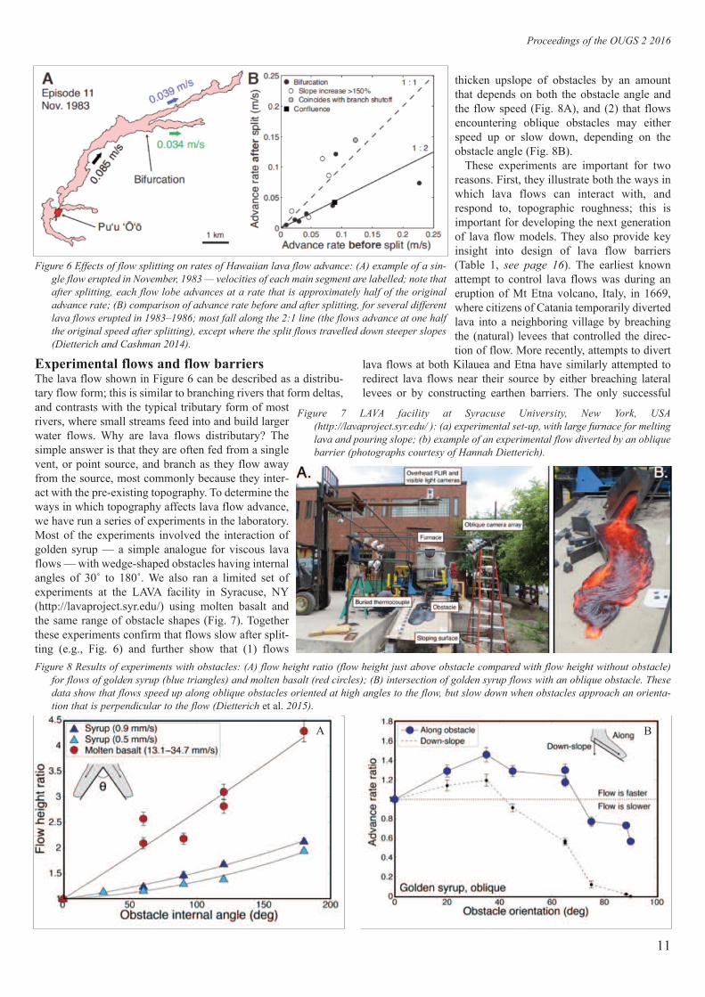
thicken upslope of obstacles by an amountthat depends on both the obstacle angle andthe flow speed (Fig. 8A), and (2) that flowsencountering oblique obstacles may eitherspeed up or slow down, depending on theobstacle angle (Fig. 8B).
These experiments are important for tworeasons. First, they illustrate both the ways inwhich lava flows can interact with, andrespond to, topographic roughness; this isimportant for developing the next generationof lava flow models. They also provide keyinsight into design of lava flow barriers(Table 1, see page 16). The earliest knownattempt to control lava flows was during aneruption of Mt Etna volcano, Italy, in 1669,where citizens of Catania temporarily divertedlava into a neighboring village by breachingthe (natural) levees that controlled the direc-tion of flow. More recently, attempts to divert
lava flows at both Kilauea and Etna have similarly attempted toredirect lava flows near their source by either breaching laterallevees or by constructing earthen barriers. The only successful
Figure 6 Effects of flow splitting on rates of Hawaiian lava flow advance: (A) example of a sin-
gle flow erupted in November, 1983 — velocities of each main segment are labelled; note that
after splitting, each flow lobe advances at a rate that is approximately half of the original
advance rate; (B) comparison of advance rate before and after splitting, for several different
lava flows erupted in 1983–1986; most fall along the 2:1 line (the flows advance at one half
the original speed after splitting), except where the split flows travelled down steeper slopes
(Dietterich and Cashman 2014).
11
Proceedings of the OUGS 2 2016
Figure 8 Results of experiments with obstacles: (A) flow height ratio (flow height just above obstacle compared with flow height without obstacle)
for flows of golden syrup (blue triangles) and molten basalt (red circles); (B) intersection of golden syrup flows with an oblique obstacle. These
data show that flows speed up along oblique obstacles oriented at high angles to the flow, but slow down when obstacles approach an orienta-
tion that is perpendicular to the flow (Dietterich et al. 2015).
Experimental flows and flow barriersThe lava flow shown in Figure 6 can be described as a distribu-tary flow form; this is similar to branching rivers that form deltas,and contrasts with the typical tributary form of mostrivers, where small streams feed into and build largerwater flows. Why are lava flows distributary? Thesimple answer is that they are often fed from a singlevent, or point source, and branch as they flow awayfrom the source, most commonly because they inter-act with the pre-existing topography. To determine theways in which topography affects lava flow advance,we have run a series of experiments in the laboratory.Most of the experiments involved the interaction ofgolden syrup — a simple analogue for viscous lavaflows — with wedge-shaped obstacles having internalangles of 30˚ to 180˚. We also ran a limited set ofexperiments at the LAVA facility in Syracuse, NY(http://lavaproject.syr.edu/) using molten basalt andthe same range of obstacle shapes (Fig. 7). Togetherthese experiments confirm that flows slow after split-ting (e.g., Fig. 6) and further show that (1) flows
Figure 7 LAVA facility at Syracuse University, New York, USA
(http://lavaproject.syr.edu/ ): (a) experimental set-up, with large furnace for melting
lava and pouring slope; (b) example of an experimental flow diverted by an oblique
barrier (photographs courtesy of Hannah Dietterich).
A B

12
diversion by levee breaching, however, was in Italy in 1992,when breaching was accompanied by construction of a diversionchannel. Earthen barriers work to slow flow advance, but areoften overtopped. The outcomes of barrier construction are con-sistent with our experimental results, where flow thickening (andovertopping) are a direct consequence of obstacle con-struction. During the 1973 eruption of Heimaey, Iceland,local scientists and engineers devised an unusual meansof obstacle construction that involved forced rapid cool-ing of the lava flow. Here the goal was to save a harbour;that goal was successfully met by spraying the advancinglava flow with seawater. As a consequence of lava con-finement at the flow front, however, lava backed up(thickened) and then broke out to spread over parts of thetown. In summary, our results, when combined withobservations of lava flow diversion attempts around theworld, suggest that the most effective flow barriers arethose that split (and thus slow) individual lava flows, par-ticularly when the barrier forms an oblique angle (Fig. 9).Under these conditions, flow splitting will slow the rateof advance, while the oblique angle of diversion willlimit both the increase in flow width caused by the splitand the flow thickening that allows barrier overtopping.
Short- and long-term flow impactsThe local impacts of lava flows — particularly inundation ofland areas and consequent devastation of plants and the builtenvironment — are obvious, but large lava flow eruptions canalso have more far-reaching effects. Over the past three decades,regions downwind of the Kilauea vent have been plagued with‘vog’, or volcanic fog, a consequence of the acidic gases emittedfrom the volcano as they are released from the magma. Thedetrimental effects of volcanic gas emissions were highlightedduring the 2014–15 Holuhraun eruption in Iceland, when a volu-minous (more than one cubic kilometre) lava flow eruptionreleased 11 million tonnes of sulphur dioxide (SO2) into theatmosphere over the six-month duration of eruptive activity(Fig. 10). During this time period, SO2 levels were sufficientlyhigh to cause respiratory problems in some Icelandic communi-ties. The effects of these large SO2 emissions could have beenworse, except that most of the eruption occurred over the winter,when strong winds rapidly dispersed the gas and winter darknessslowed the conversion of SO2 to harmful sulphuric acid. The sit-uation was different in June of 1783, when even larger volumes(c. 15 cubic kilometres) of lava poured over southern Icelandfrom Lakigigur (Fig. 10), and released an estimated 122 milliontonnes of SO2 to the atmosphere over the subsequent eightmonths. The local impacts of the eruption were described by JónSteingrímsson, a pastor living in southern Iceland, and provide agripping account of the terrifying effect of this eruption on thelocal population (Steingrímsson 1998):
“All week long neither sun nor sky could be seen for thethick clouds of fumes and smoke which blanketed the area.“Whenever the sun or moon could be seen on that part of thesky where the fire vapours swirled about, each appeared redas blood.“... more poison fell from the sky than words can describe:ash, volcanic hairs, rain full of sulphur and saltpeter, all of itmixed with sand.“All water went tepid and light blue in colour and rocks andgravel slides turned grey. All the earth’s plants withered andturned grey ...”
Figure 9 Example of an oblique-angle barrier constructed upslope of
the NOAA Observatory, high on the slopes of Mauna Loa volcano
(image from Google Earth).
Figure 10 Map of Iceland showing the glaciers (in white), the active
volcanic zones (in dark gray) and the volcanoes (black triangles).
All locations mentioned in the text are shown on the map.
Volcanoes and human societies / Cashman

Proceedings of the OUGS 2 2016
13
The impact of this eruption on the Icelandic population was dis-astrous, causing a Haze Famine (Móðuharðindin) that causedcrops to fail and killed >50% of the livestock and, as a conse-quence, 20% of the Icelandic population. Moreover, the com-bined effect of the high eruption rates, large SO2 emissions andsummer daylight and weather patterns meant the that effects ofthe eruption were felt much farther afield. For example, a per-sistent atmospheric haze caused by the eruption lingered over theUK and France for several months, causing respiratory problems,crop failures and high mortality rates. The haze was vividlydescribed by British naturalist Gilbert White (1789), who noted:“The sun, at noon, looked as blank as a clouded moon, and sheda rust-coloured ferruginous light on the ground, and floors ofrooms; but was particularly lurid and blood-coloured at rising andsetting… the country people began to look with a superstitiousawe, at the red, louring aspect of the sun.”
Summer in the arctic was unusually cold, and remained so forthe following two or three years. The eruption may even haveaffected the flow of the jet stream, which controls weather pat-terns throughout the northern hemisphere, and disrupted theAsian monsoon, prompting famine in Egypt.
More recently, Europe has experienced a different manifesta-tion of volcanic hazard from Iceland. The 2010 explosive erup-tion of Eyjafjallajökull volcano dispersed volcanic ash towardnorthern Europe; one consequence was extensive closure of air-ports (Fig. 11A), a disruption that caused losses of c. £1 billion.Why was Europe caught off guard? The hazards of ash fromexplosive eruptions in Iceland were well known, as outlined in apaper by the famous Icelandic volcanologist S. Thorarinsson thathe titled ‘Greetings from Iceland’ (Thorarinsson 1981) and inwhich he documented ash from several eruptions in Iceland thathad reached Sweden. In addition to the effects of the Laki erup-tion, Thorarinsson provides accounts of ash fall from the large1875 eruption of Askja volcano, where severe impacts in north-east Iceland contributed to a mass emigration to North America,
and the 1947 explosive eruption of Hekla volcano. Ash hazardsto civil aviation were also well understood, as summarised in a2010 paper by USGS geologists that compiles information on 94confirmed encounters of aircraft with volcanic ash cloudsbetween 1953 and 2009 (Guffanti et al. 2009) (Fig. 11B). Until2010, however, Icelandic volcanoes had not sent extensive ashclouds toward Europe since the rise of the airline industry.
Other parts of the world have experienced more recent disrup-tions because of volcanic ash. Ash hazards are particularly preva-lent in the Americas, where the volcanoes lie along the westernmargin (the eastern edge of the Pacific ‘Ring of Fire’; see Fig. 1)and prevailing winds from the west transport ash clouds over thecontinental landmass to the east (Fig. 12). During the 1980 erup-tion of Mount St Helens, USA, ash fall extended more than600km. They are described in a poem by Gary Snyder (2004):
Figure 11 Aircraft encounters with volcanic ash plumes: (A) reduction in flights over Eruopean airspace caused by the April 2010 eruption of
Eyjafjallajökull volcano in Iceland (re-drafted from BBC Website); (B) number of aircraft encounters with volcanic ash plumes between 1970 and 2010
— serious encounters are shown in red. Peak in serious encounters in 1980 is related to the eruption of Mount St Helens; peak in total number of
encounters in 1991 is related to two major eruptions that year, of Pinatubo, Philippines, and of Hudson, Chile (redrafted from Guffanti et al. 2010).
A B
Figure 12 Volcanic ash plume from the 1980 eruption of Mount St
Helens (location indicated by yellow star). The plume traversed the
states of Washington (WA), Idaho (ID) and Montana (MT), a dis-
tance of more than 600km (original photo from NOAA).

Volcanoes and human societies / Cashman
“roiling earth-gut-trash cloud tephra twelve miles highash falls like snow on wheatfields and orchards to the east
five hundred Hiroshima bombs”
“in Yakima, darkness at noon”
Distal impacts are particularly disturbing because the source can-not be seen and, before the days of rapid long-distance commu-nication, could not even be identified. As a result, rumoursabounded in 1980, including fears that the ash was radioactive.This fear stemmed directly from an incident just one year before,when a reactor meltdown at a nuclear power plant in Three MileIsland, Pennsylvania, had caused the most serious commercialnuclear power plant accident in US history.
Going back in time, oral traditions from Native American com-munities north-east of Mount St Helens record responses to anearlier explosive eruption in 1800 that underline the fear invokedby distal ash fall when the source is completely unknown (Ray1980): “When my grandmother was a little girl a heavy rain ofwhite ashes fell. The people called it snow... The ashes fell sev-eral inches deep all along the Columbia and far on both sides.Everybody was so badly scared that the whole summer was spentin praying. The people even danced — something they never didexcept in winter. They didn’t gather any food but what they hadto live on. That winter many people starved to death.”
fall in 1809–10. Analyses of ice cores from both Greenland(northern hemisphere) and Antarctica (southern hemisphere)show evidence for a sulphur layer in 1809, which has led to thespeculation that an ‘unknown’ eruption helped to trigger the colddecade. How could there be no historic record of such an event?
To address this question, we teamed up with an historian ofcolonial Latin America. She searched archival documents anddiscovered two records that shed some light on the puzzle. Thefirst comes from Francisco José de Caldas, Director of theAstronomical Observatory of Santa Fe de Bogotá, Colombia. Areport published by Caldas in February of 1809 described anupper atmospheric stratospheric cloud that had appeared on 11December 1808 and persisted until the time of the report (Caldas,translated in Guevara-Murua et al. 2004): “As of 11 December oflast year, the disk of the sun has appeared devoid of irradiance, itslight lacking that strength which makes it impossible to observeit easily and without pain. Its natural fiery colour has changed tothat of silver, so much so that many have mistaken it for themoon... The stars of the first, second and even third magnitudehave appeared somewhat dimmed, and those of the fourth andfifth have completely disappeared, to the observer’s naked eye.This veil has been constant both by the day and by night...”
Caldas noted that this atmospheric phenomenon was notrestricted to Bogotá, but instead was also reported from otherparts of Colombia, consistent with the presence of a widespread
volcano-induced stratospheric haze.Caldas also reported uncharacteristi-cally cold mornings, with widespreadice and resulting crop damage.Importantly, at exactly the same timethe Peruvian physician HipólitoUnanue reported unusual opticaleffects at sunset (Unanue, translatedin Guevara-Murua et al. 2004): “Atsundown in the middle of the monthof December, there began to appeartoward the S.W., between cerro de losChorillos and the sea, an evening twi-
light that up the atmosphere. From a N.S. direction on the hori-zon, it rose towards its zenith in the form of a cone, [and] shonewith a clear light until eight [o’clock] at night, when it faded.This scene was repeated every night until the middle of February,when it vanished.”
This phenomenon is known as twilight glow; it is caused bylight scattering by stratospheric aerosols and has been observedafter other large eruptions. Together, these accounts from bothnorth (Colombia) and south (Peru) of the equator, at exactly thesame time, provide strong evidence of a large tropical eruption,most likely in early December of 1808. Although we have notbeen able to identify the volcano, the most likely location forsuch an eruption is Indonesia, with its high density of frequentlyactive volcanoes.
The climate disturbance initiated by the 1808 eruption wasmagnified by the eruption of Tambora in 1815, an enormouseruption that created a stratospheric veil observed throughout theUnited States. The following year, extreme cold throughout thenorthern hemisphere (Fig. 13B) caused the ‘Year Without aSummer’, when failed harvests throughout Europe caused wide-spread famine, and failed harvests and famine in India accompa-nied resultant changes to the Asian monsoon. The dreariness of
14
Figure 13 Effect of large volcanic eruptions on global temperatures: (A)
decadal variations in average global temperature since 1800 — the
decade from 1810–1820 was the coldest of the past two centuries,
probably because of two large volcanic eruptions, the ‘unknown’
eruption of 1808 and the 1815 eruption of Tambora, Indonesia (from
Berkeleyearth.org); (B) anomalies in 1816 summer temperatures in
Europe caused by the Tambora eruption — the average temperatures
in France and the UK were up to 1.5˚C lower than normal (figure
from http:// en.wikipedia.org/wiki/Year_Without_a_Summer).
Impacts on temperatureLarge volcanic eruptions can have global impacts in the form oftemporary perturbations of Earth’s temperature. Large explosivesinject both fine ash and gases into the stratosphere, where sulphurdioxide gas is oxidised to sulphuric acid, which then condensesto form sulphate aerosols. These aerosols reflect solar radiationback into space, and thus cool the lower atmosphere. A dramaticexample comes from the decade of 1810–20, when averageglobal temperatures reached their lowest point in the past twocenturies (Fig. 13A). In large part, this temperature anomaly canbe attributed to the 1815 eruption of Tambora volcano inIndonesia, the largest eruption of the past several centuries.Interestingly, however, global temperatures had already started to
A B

Proceedings of the OUGS 2 2016
the summer weather is recorded in Lord Byron’s poem‘Darkness’ (1816):
“I had a dream, which was not all a dream.The bright sun was extinguish’d, and the stars
Did wander darkling in the eternal space,Rayless, and pathless, and the icy earth
Swung blind and blackening in the moonless air;Morn came and went — and came, and brought no day,
And men forgot their passions in their dreadOf this their desolation; and all hearts
Were chill’d into a selfish prayer for light...”
Accounts of similar stratospheric dust veils can be traced backthrough time, and along with them evidence for severe globalimpacts of past eruptions. For example, the atmospheric effectsof a large eruption of Ilopango volcano, El Salvador, in AD 536are described by the Roman official Cassiodorus in Ravenna,Italy, who describes a “blue-coloured sun” and a “summer with-out heat” and with both “perpetual frost and unnatural drought”(quoted in Graslund and Price 2012). In fact, tree ring recordsfrom North America suggest that the entire decade from AD 536to 545 was unusually cold, with one severe temperature pertur-bation in 536 and another in 540–542. This decade of cold withtwo obvious cool spikes suggests another example of paired largeeruptions.
Archaeologists have connected severe weather in the mid-6thcentury AD to a major collapse of Viking settlements in east cen-tral Sweden (Fig. 14) and, as a result, initiation of the MigrationPeriod and Viking diaspora (Graslund and Price 2012). They fur-ther suggest that oral traditions of this time are preserved in theIcelandic sagas, specifically in tales of Ragnarök (commonlytranslated as the Twilight of the Gods) that are found in the 13th-century Eddas of Snorri Sturluson. Ragnarök is forecast for thefuture but appears to be derived from memory of a past event,when (Sturluson, translated in Scudder 2001):
“[The wolf] smears with red bloodthe gods’ heavenly sitethe sunshine was blackfor summers afterthe weather treacherous”
This is only the start of Ragnarök, which manifests as: “a win-ter… called Fimbulwinter. Then snow will drift from all direc-tions. There will then be great frosts and keen winds. The sun willdo no good. There will be three of these winters together and nosummer between.” (in Graslund and Price 2012; from Faulkes1987):
This sequence of harsh winters is followed by another event,when (Sturluson, translated in Scudder 2001):
“The sun turns black,land sinks into the sea,the bright starts vanish from the sky.Fire rages forthat the life-giving tree,high flame will lickat heaven itself.”
This imagery is much more immediate, and may well recall anenormous Icelandic eruption three centuries before the Poetic
Edda were collected in writing. The AD 934 eruption of Eldgjá(which loosely translates as ‘Fire chasm’) sent 25% more lavathan the 1783 Laki eruption into Iceland’s south-central coastalplains. Although there is no written record from Iceland duringthis time period, an account from northern Germany appears torecord this event (quoted in Stothers 1998): “Indeed before thedeath of King Henry [2 July 936] many prodigies occurred, suchas: The brightness of the Sun outdoors in a cloudless skyappeared almost nil, but it streamed indoors, red as blood,through the windows of the houses. Likewise for the mountainwhere the overlord of the states was buried, according to report,because the mountain erupted in flames in many places.”
Although the identity of the ‘overlord of the states’ is unclear,it could be a direct reference to Iceland with the overlord beingÚlfljótr, who held the position of the first lawspeaker of the unit-ed Icelandic parliamentary body (the Alþingi), which was formedin the last year of settlement. Not surprisingly, the Eldgjá erup-tion apparently brought the Icelandic settlement period to anabrupt end, only 60 years after it started.
SummaryTo summarise, volcanic eruptions occur frequently around theworld. Where eruptions are common and of relatively low inten-sity (e.g., lava flows), humans not only co-exist with their rest-less environment but may also attempt to control it. Larger erup-tions are less frequent, but have much greater impacts. Unlikeearthquakes or floods, where impacts are local to regional inscale, the impacts of volcanic eruptions span from local toregional to even global. The far-reaching impacts have had sub-stantial impacts on past societies, impacts that have caused cropfailures and famines. These extreme impacts have provoked
15
Figure 14 Settlement patterns in east central Sweden. Note precipitous
drop in settlement numbers before AD 600, coincident with (and
inferred to be driven by) a documented cold period in the mid-6th
century caused by the AD 536 eruption of Ilopango volcano, El
Salvador, and possibly a second eruption c. AD 540 (redrafted from
Graslund and Price 2012).

Volcanoes and human societies / Cashman
extreme responses in societies substantially affected by famine,or even those seeking explanations for the ‘portents’ of fallingdistal ash or stratospheric veils that caused the sun to appear dimand without heat.
Today, many volcanoes in the world are monitored, eitherlocally via networks of seismometers, GPS sensors and gasdetection instruments, or globally using satellites. Satellite-basedsystems, in particular, provide a global means of monitoring pre-cursory changes in the Earth’s surface, early release of volcanicgases before eruption onsets, and movement of clouds of vol-canic ash and gas as they are dispersed from volcanic vents. Notonly news, but also hundreds of photos of eruptive activity flyaround the Internet, providing instant global updates of volcaniccrises. Modern technology cannot, however, change the nature ofvolcanic eruptions, and our highly interconnected world is alsohighly susceptible to disruption by volcanic activity, as illustrat-ed by the 2010 eruption of Eyjafjallajökull volcano in Iceland.Moreover, it is clear that the far-reaching effects of very largeeruptions — including decreases in global temperatures and con-sequent impacts on regional food and water supplies — wouldstill reverberate around the globe. For this reason, the challengefor both volcanologists and people living in regions with thepotential to be affected by volcanic activity is to develop strate-gies to improve resilience to the local, regional and global effectsof volcanic eruptions.
ReferencesCashman, K. V., and Mangan, M. T. 2014 ‘A century of studies of effu-
sive eruptions in Hawai‘i’. USGS Professional Paper 1801, 357–94Dietterich, H. R., and Cashman, K. V. 2014 ‘Channel networks within
lava flows: Formation, evolution and implications for flow behav-ior’. J Geophys Res Earth Surfaces 119 doi:10.1002/2014JF003103
Dietterich, H. R., Cashman, K. V., Rust, A. C., and Lev, E. 2015‘Diverting lava flows in the lab’. Nature Geoscience 8, 494–6
Faulkes, A. (trans.) 1987 Snorri Sturlson, Edda: Prologue and
Gylfaginning. Oxford: Oxford University PressGraslund, B., and Price, N. 2012 ‘Twilight of the gods? The ‘dust veil
event’ of AD 536 in critical perspective’. Antiquity 86, 428–43Guevara-Murua, A., Williams, C. A., Hendy , E. J., Rust, A. C., and
Cashman, K. V. 2004 ‘Observations of a stratospheric aerosol veilfrom a tropical volcanic eruption in December 1808: is this theUnknown ~1809 eruption?’. Climate of the Past 10, 1707–22
Guffanti, M., Casadevall, T. J., and Budding, K. 2010 ‘Encounters ofAircraft with Volcanic Ash Clouds: A Compilation of KnownIncidents, 1953–2009’. USGS Data Series 545
http://pubs.usgs.gov/ds/545/DS545.pdfGuffanti, M., Mayberry, G. C., Casadevall, T., and Wunderman, R. 2009
‘Volcanic ash hazards to airports’. Natural Hazards 51, 287–302Lord Byron 1816 ‘Darkness’.
http://www.poetryfoundation.org/poem/173081Ray V. F. 1980 The Sanpoil and Nespelem: Salishan Peoples of
Northeastern Washington. New York: AMS PressScudder, B. (trans.) 2001 The Prophecy. Iceland: Oddi Ltd Printing PressSteingrímsson, Jon 1998 Fires of the Earth. Iceland UPSnyder, Gary 2004 ‘1980: Letting Go’, in Snyder, G. Danger on Peaks.
San Francisco: Shoemaker and HoardStothers, R. B. 1998 ‘Far reach of the tenth century Eldgjá eruption,
Iceland’. Climate Change 39, 715–26Sturluson, Snorri (attrib.) [13th-cent.] ‘Völuspá’, in Scudder 2001 (qv)Thorarinsson, S. 1981 ‘Greetings from Iceland: ash-falls and volcanic
aerosols in Scandinavia’. Geografiska Annaler Ser A, Physical
Geography 63, 109–18White, Gilbert 1789 The Natural History and Antiquities of Selbourne.
London
16
Table 1 Summary of historical diversion attempts
year location style effect
1669 Mount Etna, Italy levee breach by excavation incomplete attempt
1935 Mauna Loa, USA aerial bombing of lava tube minor breakouts, eruption ceased soon after
1942 Mauna Loa, USA aerial bombing of levees created a temporary branch that rejoined the mainflow after a short distance
1955 Kilauea, USA earthen barriers partly successful at detection
1960 Kilauea, USA earthen barriers barriers overtopped or undermined
1973 Heimaey, Iceland water-cooling flow front stalled and thickened, habour saved
1983 Mount Etna, Italy earthen barriers, barriers diverted the flow but were overtopped; levee breach by explosives levee breach failed but debris created in the attempt
did cause significant overflows
1991–3 Mount Etna, Italy earthen barriers, barriers delayed flow advance but were overtopped; levee breach by explosives levee breach was successful
2001 Mount Etna, Italy earthen barriers numerous barriers delayed advance and diverted the flows; many overtopped
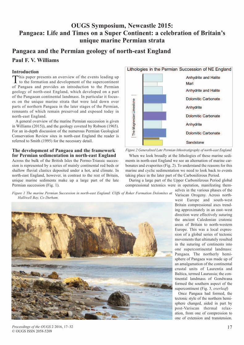
17
Introduction
This paper presents an overview of the events leading upto the formation and development of the supercontinent
of Pangaea and provides an introduction to the Permiangeology of north-east England, which developed on a partof the Pangaean continental landmass. In particular it focus-es on the unique marine strata that were laid down overparts of northern Pangaea in the later stages of the Permian,remnants of which remain preserved and exposed today innorth-east England.
A general overview of the marine Permian succession is givenin Williams (2015)), and the geology covered by Robson (1965).For an in-depth discussion of the numerous Permian GeologicalConservation Review sites in north-east England the reader isreferred to Smith (1995) for the necessary detail.
The development of Pangaea and the frameworkfor Permian sedimentation in north-east EnglandAcross the bulk of the British Isles the Permo-Triassic succes-sion is represented by a series of mainly continental red beds orshallow fluvial clastics deposited under a hot, arid climate. Innorth-east England, however, in contrast to the rest of Britain,unique marine sediments make up a large part of the latePermian succession (Fig. 1).
When we look broadly at the lithologies of these marine sedi-ments in north-east England we see an alternation of marine car-bonates and evaporites (Fig. 2). To understand the reasons for thismarine and cyclic sedimentation we need to look back to eventstaking place in the later part of the Carboniferous Period.
During a large part of the Upper Carboniferous Period globalcompressional tectonics were in operation, manifesting them-
selves in the various phases of theVariscan Orogeny. Across north-west Europe and south-westBritain compressional axes trend-ing approximately in an east–westdirection were effectively suturingthe ancient Caledonian cratonicareas of Britain to north-westernEurope. This was a local expres-sion of a global series of tectonicmovements that ultimately resultedin the suturing of continents intoone supercontinental landmass:Pangaea. The northerly hemi-sphere of Pangaea was made up ofan amalgamation of the continentalcrustal units of Laurentia andBaltica, termed Laurussia; the con-tinental landmass of Gondwanaformed the southern aspect of thesupercontinent (Fig. 3, overleaf)
Once Pangaea had formed, thetectonic style of the northern hemi-sphere changed, aided in part bypost-Variscan thermal relax-ation, from one of compression toone of extension and transtension.
Figure 1 The marine Permian Succession in north-east England: Cliffs of Roker Formation Dolomites at
Halliwell Bay, Co Durham.
Figure 2 Generalised Late Permian lithostratigraphy of north-east England.
OUGS Symposium, Newcastle 2015: Pangaea: Life and Times on a Super Continent: a celebration of Britain’s
unique marine Permian strata
Pangaea and the Permian geology of north-east England
Paul F. V. Williams
Proceedings of the OUGS 2 2016, 17–32© OUGS ISSN 2058-5209

Pangaea and Permian geology of north-east England / Williams
18
This resulted in the formation of a number of rift and strike-slip sub-siding basins across Laurussia (Fig. 4). It also facilitated widespreaddecompressive mantle melting to source mafic magmas, whichwere emplaced across many parts of Laurussia. Mafic sill suitesdeveloped across Scandinavia (the Oslo Rift) and, closer to home,sourced the Scottish Midland Valley sill and dyke complex and theWhin Sill complex of northern England (McCann et al. 2006).
As a result of the continuing Pangaean extensional tectonicregime a number of subsiding intracratonic strike-slip basins devel-oped in the area that was to become Britain and the surrounding
North Sea region. These basins depressed the Pangaean land surfacebelow general sea level, and these areas are identified in Figure 5.
For much of the early Permian continental desert sedimentationensued across the landlocked hot, arid plains and depressedbasins of Laurussia; and in the area that was to become Britain,then situated at around latitude 20˚ north, a series of red conti-nental clastics developed. In present-day north-east England aseries of linear dunal sand ridges can be identified within the ear-liest Permian deposits. These oldest units of the Yellow SandsFormation overlie the Carboniferous strata (Fig. 6, opposite left)and form a narrow NNW–SSE outcrop at the westerly edge of thePermian strata in north-east England. They comprise a series ofpoorly cemented sands of Early Permian age with rounded, ‘mil-let seed’ sand grains which characterise their desert origins. Theyshow classic dune bedding structures and are never more than c.
60m thick, although the formation is very variable in thicknesslocally. By mapping these thickness variations the morphology ofthe dunal sand ridges can be identified and are found to align withthe prevailing east-north-easterly palaeo-wind direction, givingclues to the earlier Permian palaeogeography of the region.
By late Permian times, global sea levels were rising due tosouthern hemisphere deglaciation. As a result of this sea level rise— coupled with continuing extensional tectonics, rifting and sub-sidence in the northern part of northern Pangaea — a connectionwas eventually established between the low-lying intracratonicPermian basins and the northerly Boreal Ocean through a narrow,restricted seaway (Fig. 7, opposite right). These interconnectingstraits were likely to have had a silled connection with the openocean. Rapid flooding ensued across these low-lying Permianbasins, creating a shallow land-locked epicontinental sea, the
Figure 3 The assembly of Pangaea after the Variscan Orogeny and the
position of Laurussia in the Northern Hemisphere (after Kroner and
Romer 2013, with permission; this image was published in Kroner,
U., and Romer, R. L. 2013 ‘Two plates — many subduction zones: the
Variscan orogeny reconsidered’. Gondwana Res 24, 298–329, fig. 1
— © Elsevier 2013)
Figure 4 Development of the Early Permian Extensional Tectonic
Province over Laurussia (after Kroner and Romer 2013, with
permission; this image was published in Kroner, U., and
Romer, R. L. 2013 ‘Two plates — many subduction zones: the
Variscan orogeny reconsidered’. Gondwana Res 24, 298–329,
fig.10 — © Elsevier 2013).
Figure 5 Tectonic map of north-west Europe in the early Permian show-
ing the development of subsiding intracratonic strike-slip basins over
the Pangaean continental land surface (after Gast and Gundlach
2006, fig. 1, with permission; © ZDGG 2006; www.schweizerbart.de).

19
Zechstein Sea, with two distinct, defined South and NorthPermian Basins (Fig. 8). The scene was now set for marine sedi-ments to accumulate in the Permian basins, and along the easternedge of the developing British mainland.
Another intriguing aspect of the late Permian sedimentary his-tory of north-east England is the cyclic nature of the deposits,with alternations of marine carbonates and evaporites formingthree major, well-defined cycles. The explanation for this lies inthe unique combination of climate, ongoing tectonic changesand continuing oscillations of global sea level operating in thelate Permian and affecting depositional conditions over theZechstein Basin.
The silled connection between the Zechstein Sea and theBoreal Ocean was sensitive to fluctuations in sea level and bathy-metric changes at the mouth. A fall in sea level or tectonic upliftcould bring about isolation of the basin from oceanic circulationand recharge. During the Late Permian a greenhouse climate pre-dominated with elevated surface temperatures. Under this hot,arid climate evaporative drawdown resulted in the developmentof hypersalinity of Zechstein seawater, and the precipitation ofevaporites. Further rifting and subsidence at the mouth of thebasin, on the other hand, or sea level rise resulted in re-establish-ment of the connection to the open ocean, recharge of the basinand restoration of more normal salinity terminating evaporitedeposition and a return to carbonate sedimentation. Studies ofcarbon and oxygen isotopes in Zechstein carbonates suggest thatpalaeoclimatic instability may also have been a contributing fac-tor, with periods of wetter climate and precipitation increasecoincident with some of the carbonate horizons in some parts ofthe Zechstein Basin (Gasiewicz 2013). Periodic oscillations inglobal sea level and bathymetry at the mouth of the interconnect-ing seaway produced episodes of basin isolation, during whichtime evaporite deposition occurred, resulting in repeated carbon-ate-evaporite cycles.
The final major intrigue of Late Permian sedimentation innorth-east England is the dominance of dolomitic rocks in thecarbonate succession. The vast majority of the carbonate rocksare dolomites and dolomitic limestones, with true limestones
Proceedings of the OUGS 2 2016
Figure 6 Unconformity between Upper Carboniferous sandstones, part-
ly desert-reddened, and early Permian Yellow Sands Formation;
exposures at Castletown on the banks of the River Wear. Hammer
lies on the undulating unconformity surface. Carboniferous strata
dip downwards to left of picture.
Figure 7 Map of the northerly Pangaean land surface in the Late Permian
with present-day continental margins of north-west Europe included
for reference, showing the formation of the Zechstein Sea and position
of Sub-Basins and Highs. Cratonic areas of Scandinavia and
Greenland in approximate Late Permian positions.
Figure 8 Map of north-west Europe in the Late Permian showing the posi-
tion of the Southern Permian and Northern Permian Zechstein Basins
and their palaeogeography (modified after Slowakiewicz et al. 2013,
fig. 1, with permission; original figure AAPG©2013, reprinted by per-
mission of the AAPG whose permission is required for further use).

20
Pangaea and Permian geology of north-east England / Williams
poorly represented, although some of the original dolomites havebeen converted to limestones (technically de-dolomites) by laterchanges. During the Permian the oceans surrounding thePangaean continent had magnesium concentrations much higherthan those of more normal oceanic waters. (Lowenstein et al.2005). In these ‘aragonite seas’, as they are known, aragonitewould be the primary carbonate precipitated, and further increas-es in salinity reflected by dolomite or high-Mg calcite formationrather than ordinary calcite. It is believed that the establishmentof aragonite seas with elevated Mg concentrations reflected theabsence of major global sea floor spreading activity over the vastsupercontinent, since rapid sea floor spreading is the site wheremagnesium is usually recycled. Once the rifting and break-up ofPangaea ensued, sea floor spreading activity would have
increased again, leading to magnesium recycling through vol-canic processes and return of oceans to less extreme Mg levels.Climate, temperature and sea level are also known to affect seawater ionic compositions, with cool icehouse conditions alsofavouring aragonite precipitation, precisely the conditions preva-lent during the early Permian, especially at southern latitudes.
The marine Permian succession of north-east EnglandIt was thus a chance combination of factors that facilitated thedeposition of north-east England’s unique marine Permian suc-cession. The area of land that was eventually to become north-east England was situated on the extreme western edge of theZechstein Basin, and where it is preserved today in the sediments,it is a record of the history of the shelf-edge and basin-slope envi-ronments of the Zechstein Sea.
Variations in sedimentaryfacies are recognised across thePermian exposures of north-eastEngland, reflecting Permianbasin margin bathymetry.Shallow water shelf and shelf-edge sediments found morewesterly, with deeper basin-slope sediments developed tothe east (diagram, Fig. 9).
The general sedimentary suc-cession for north-east Englandshown in Figure 10 comprisesseveral well developed, thickdolomitic carbonate horizonsknown locally and collectivelyin older terminology as ‘TheMagnesian Limestone’ (shownin dark blue in Fig, 10).
This generalised successionis, however, only seen in off-shore boreholes. For all onshoresuccessions the interveningevaporite horizons have allbeen lost either due to later dis-solution — and are now only
Figure 9 Facies variations in Zechstein sediments across north-east
England delimiting shelf, shelf edge, and basin downslope deposition-
al palaeoenvironments at the western margins of the Zechstein Sea.
Figure 10 The Permian Succession in north-east England — dark blue
ornament represents carbonate facies (not to scale).
Figure 11 Collapse breccia composed of blocks of Roker Formation Dolomite, resulting from dissolution of
underlying evaporite horizons, Roker Formation, Halliwell Bay, Co Durham (walking pole is 1m high).

21
represented by centimetre-scale thicknesses of ‘disso-lution residue’ — or were never deposited shorewardsin the first place. The loss of many tens of metres ofsediment has had profound effects on the overlyingPermian strata, which have foundered and collapsed,and are represented in many places by spectacularcollapse breccias (Fig. 11, previous page).
The full succession nomenclature and strata thick-ness is given in Figure 12, and extent of the Permianrocks outcropping in north-east England is shown inFigure 13, overleaf).
All the formations dip gently eastwards over theeroded pre-Permian land surface and form a prominentwest-facing escarpment where the Permian sedimentsrise from an eroded clay vale of soft upperCarboniferous rocks. Thus the younger, upperPermian, beds are found closer eastwards towards thepresent-day coast. This is demonstrated in the sectionsuperimposed on the landscape image in Figure 14.
The initial deposits of the new Zechstein Sea,formed over the early Permian continental clastics ofthe Yellow Sands Formation, were the fine-grainedlaminated dolomitic siltstones of the Marl SlateFormation. The Zechstein transgression reworked thetop surface of the earlier Permian sands and planed-offthe sand dunes formed on the desert basin. In someplaces the Marl Slate is banked over the dunal sandridges, and in other areas it is attenuated over them.
The grain-size of the sedimentary particles and con-sistent parallel planar lamination suggests an environ-ment that was free of currents, meaning that thesedeposits were below wave base; and also probablypoints to an almost tideless sea. The sediments arealso bituminous, and contain abundant well-pre-served fossil fishes, indicative of anoxic bottom-con-ditions and a stratified water column. Basin morphol-ogy is likely to have facilitated stratification of thewater column, and a barred basin is suggested, withwater depth of possibly up to 300m.
The Marl Slate outcrop follows the line of outcropof the Yellow Sands (Fig. 13), and is never more than6m thick; and occasionally not present at all. It hasyielded a rich fauna of early fossil fish (Fig. 15) andland plants, and a unique gliding reptile —Coelurosauravus jaekeli — thought to be a forerun-ner of flighted animals (Fig. 16).
Proceedings of the OUGS 2 2016
Figure 12 Permian stratigraphy and nomenclature for north-east England, and thick-
ness of stratigraphic units.
Figure 14 Permian strata forming landscape and topography in Co Durham: view look-
ing north with general geological section superimposed; west-facing escarpment
edge clearly visible to west (surmounted by Penshaw Monument), together with the
surface expression of the Ford Formation reef facies farther east; foreground is
composed of drift and coal measures sediments.
Figure 15 Fossil fish with jawbone, Marl Slate Formation. Pygopterussp., Quarrington Quarry, Co Durham.
Figure 16 Coelurosauravus jaekeli, a gliding reptile, thought to be the
forerunner of flighted creatures — Marl Slate Formation, Eppleton
Quarry, Co Durham (specimen in Sunderland Museum).

Pangaea and Permian geology of north-east England / Williams
22
Figure 13 Distribution of the Permian outcrops in north-east England (after Robson 1995, fig. 10, with permission; original
figure © Natural History Society of Northumbria 1995).
The first marine carbonates of the Zechstein Sea aredeposited over the Marl Slate Formation, heralding the start ofthe ‘Magnesian Limestone’ succession. In recognition of thecyclic nature of the carbonate/ evaporite units in the Permiansuccession of north-east England, a terminology has been
developed to classify and identify individual cycles, as detailedin Figure 17 (opposite).
The first carbonate unit of the Zechstein Sea, the RaisbyFormation (EZ1a stage — ‘Lower Magnesian Limestone’) formsa prominent west-facing escarpment, which is a major topo-

23
graphic feature running north-north-west through Co Durham.Deposition of these earliest carbonate units was accompanied byerosion, and the Raisby dolomites are deposited over the MarlSlate, which is thinned and cut out locally by pre-Raisby erosion.They are generally well-bedded, pale-cream-to-buff coloureddolomites displaying parallel bedding on a scale of 100–200mm,
and show dissolution cavities in places (Fig. 18). The Raisbybeds show evidence of uniform low-energy, tranquil condit-ions, with little current or wave activity, suggesting a moderate-depth, distally-steepened carbonate ramp into a more basinal,depositional environment. The more thin-bedded finely laminat-ed dolomitic horizons within the formation point to a deeperwater, significantly more basinal setting at the far distal end ofthe ramp.
The formation presents a narrow outcrop width at the westernedge of the Magnesian Limestone strata and is developed to amaximum of c. 76m, and contains a sparse, shelly marine fauna.Basin submarine slope-failures and gravity debris-slides arerecognised at horizons within the Raisby Formation, evidencedfrom the presence of jumbled units of relatively shallow-watershelf facies surrounded by finer-grained, laminated deeper-water sediments.
More massive-scale events at the end of Raisby times are alsorecorded, in which the whole thickness of both Raisby and under-lying Permian strata has been involved in wholesale movement.The ‘Downhill Slide’, as it is known, is named from its recogni-tion in the former Downhill Quarry near Sunderland, and it gen-erally affected the more northerly outcrops of the formation,which were involved in the north-eastwards downslope move-ment of Raisby and underlying units, creating massive submarineslide canyons on the Zechstein seabed. The resultant olistolithscan be seen in the exposures at Trow Point, and also low in thesection at Claxheugh Rock, where ‘grooves’ in the underlyingsediments are probably preserved remains of the slide base. Thepresence and preservation of these slide units and submarine
Figure 17 English Zechstein Cycles terminology.
Figure 18 Raisby Formation overlying dune-bedded Yellow Sands, Coldknuckles Quarry.
Proceedings of the OUGS 2 2016

canyons is regarded as unique, both in Britain and in the marinePermian geology of Europe.
Overlying the dolomites of the Raisby Formation is a series ofrocks belonging to the Ford Formation, deposited in the EZ1bcycle. This series is another predominantly dolomitic carbonateunit attaining a maximum thickness of c. 116m. The formationshows a wide extent of outcrop from west of Sunderland acrossmuch of the East Durham Plateau, outcropping along the coastsouth of Seaham, Three main facies units can be identified in theFord Formation across a west-to-east transect of the outcrop,facilitating the interpretation of the depositional environment forthe whole unit.
Strata of the Ford Formation developed in the more westerlyparts of the region show the presence of ooidal carbonate grain-stones, with cross-stratified units and generally an overall coarsegrain size, indicating a relatively shallow, higher-energy environ-
Pangaea and Permian geology of north-east England / Williams
ment, and points to a shallow lagoonal/marginal shelf setting.Farther east, however, the formation is represented by a series
of more erosion-resistant, unstratified framestones and bound-stones with a rich fossil biota, the outcrop of which forms a majortopographic feature. These units have been identified as formingthe core of a remarkable barrier reef structure. The reef developedon the western margins of the Zechstein Sea shelf area, and itsremnants are well defined in north-east England as a prominenttopographic ridge. It forms a discontinuous feature runningNNW–SSE through Co Durham close to the present-day coast-line as a series of linked knolls in the landscape (Fig. 19). Theextent of the present-day reef outcrop is shown in Figure 20.
In Permian times the shelf-edge barrier reef is likely to havebeen a continuous feature running for over 30 km along the mar-gins of the Zechstein Sea basin, with the back-reef shelf areaprobably stretching westwards for between 5 and 10 km.
Eastwards of the main reef structurethe formation is represented by muchthinner, finer-grained planar beddedand thinly laminated dolomites,which in places contain broken andjumbled reef blocks and fossil debrischaracteristic of the Ford Formation.This is regarded as reef talus deposit-ed downslope in a fore-reef setting,with reef material eroded from thereef crest by wave action. It is thoughtthat water depths here in the fore-reefenvironment were possibly c. 100mdeep, compared with the 5m or soover the reef crest.
The reef facies is developed overplanar stratified dolomitic mud-stones/wakestones, and in someplaces the transition from pre-reef toreef facies can be well seen, particu-larly at Humble-don Hill Quarry SSSI(Fig. 21). Some sections at the base ofthe reef show it to be founded on ashell-bed coquina, pointing to pre-reef shell banks and an already-shal-lowed marine shelf bathymetry prior
24
Figure 20 Position of the Ford Formation Barrier Reef crest and associated facies in north-east England.
Figure 19 Tunstall Hill and the Ford Formation reef crest above
Sunderland suburbs
Figure 21 Pre-reef to reef transition — Ford Formation, Humbledon Hill
Quarry SSSI.

25
Proceedings of the OUGS 2 2016
the reef crest, to bedded off-reef deposits, as at the type-localityof Ford Quarry in Sunderland.
Westward of the reef core, generally, the outcrops of off-reefbedded strata are ooidal grainstones displaying cross-stratifica-tion indicative of deposition under strong current and wave action.Where they are at similar stratigraphic level as the reef crest,these bedded dolomites are interpreted as back-reef deposits onthe shallow landward side of the main reef. As the reef grewthe back-reef lagoons continued to build upwards too, main-taining a difference in height of c. 5m between reef crest andlagoon floor.
Exposures of the massive reef-rock have in the past yieldednumerous fossils, in particular at Humbledon Hill Quarry (Fig.22), Tunstall Hill and Ford Quarry. The Humbledon Hill site ishistorically significant for the many unique figured and cited fos-sil specimens collected by the Victorian pioneers of Permiangeology in north-east England, in particular King, Howse andKirkby (Egeland-Eriksen 2016).
Among what appears to be a relative uniformity in the threemajor facies units of the Ford Formation described above, anoth-er more localised, but distinctive, unit also needs mention. Alongthe coast of South Shields from Frenchmans Bay to Trow Pointare a series of intriguing exposures of undoubtedly FordFormation lithologies. The Trow Point Bed is a basin floordeposit of no more than 0.6m maximum thickness, comprised oflaminated dolomitic beds containing columnar algal stromato-lites. This remarkable unit is widespread and persistent, being
to reef development. It also suggests that there was a transitionfrom the very hypersaline waters of the Raisby beds to one oflower salinity, allowing a wider faunal range to develop.
The unbedded unit of the Ford Formation comprising the reef-core is massive and much harder than the underlying stratifieddolomites. On examination it is found to be composed of theremains of numerous shelly organisms, and is richly fossilifer-ous. The sediments are mainly represented by framestones andboundstones (Fig. 22), and the main reef-building organisms ofthis remarkable structure were bryozoa, The Permian reef sup-ported a vast array of species, particularly gastropods, bivalves,brachiopods and echinoderms, and fossils of these creatures areabundant in the reef rock (Figs 23 and 24). Some of the reefmaterial shows isolated units of finely laminated horizons, on ascale of tens of centimetres, identified as algal laminites. Thesealso lived encrusted on and around the reef, contributing to thereef structure; and laminites are locally abundant in the reef-crest sediments in several places. During its life the reef wasprobably in the order of 100m high at its margins, with the deep-er, more easterly parts of the basin. At some localities a lateraltransition can be seen from the unbedded massive reef-rock of
Figure 22 Unstratified Ford Formation reef boundstone, Humbledon
Hill Quarry SSSI.
Figure 23 Fenestellid reef-forming bryozoan, Ford Formation reef
facies, Beacon Hill.
Figure 24 Ford Formation reef fossils: top — gastropods, Ford Quarry;
bottom — reef biota. Humbledon Hill Quarry SSSI (scale-bar for
each in lower image).
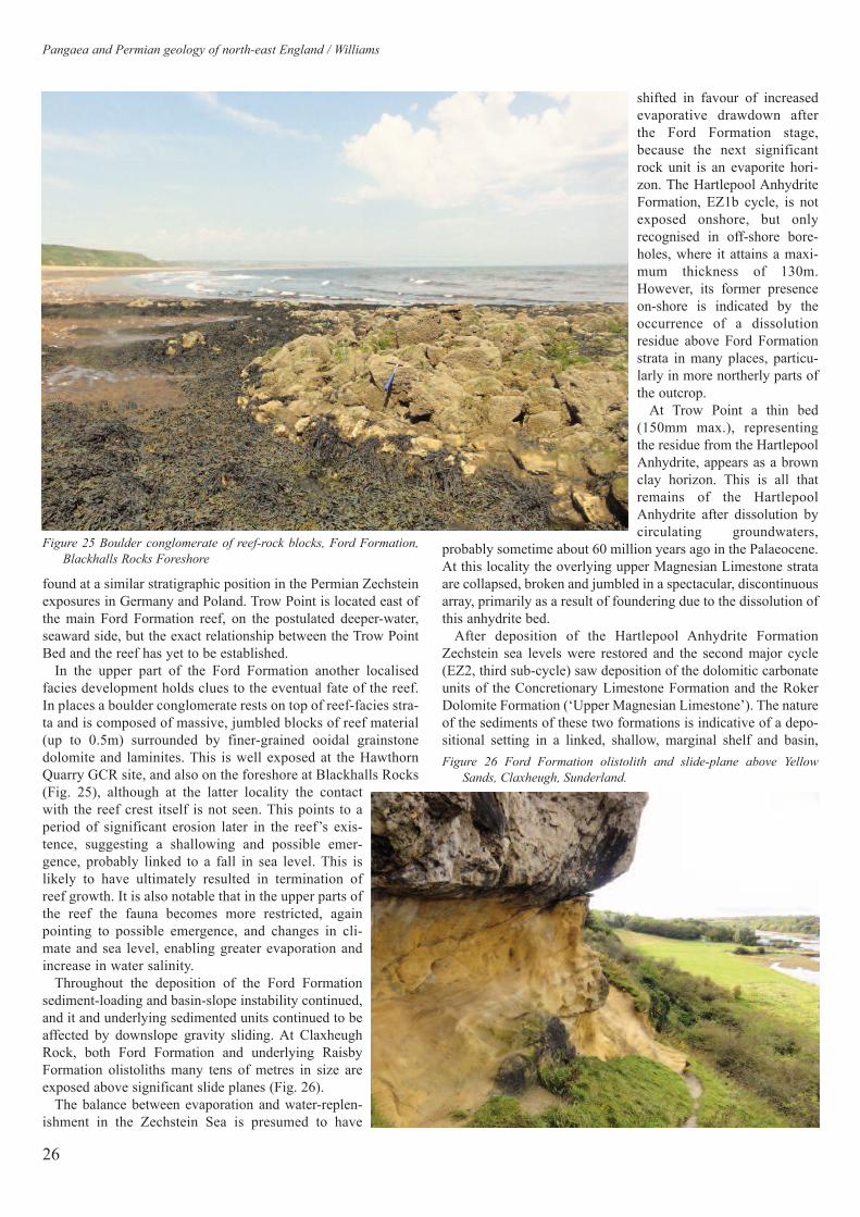
Pangaea and Permian geology of north-east England / Williams
26
found at a similar stratigraphic position in the Permian Zechsteinexposures in Germany and Poland. Trow Point is located east ofthe main Ford Formation reef, on the postulated deeper-water,seaward side, but the exact relationship between the Trow PointBed and the reef has yet to be established.
In the upper part of the Ford Formation another localisedfacies development holds clues to the eventual fate of the reef.In places a boulder conglomerate rests on top of reef-facies stra-ta and is composed of massive, jumbled blocks of reef material(up to 0.5m) surrounded by finer-grained ooidal grainstonedolomite and laminites. This is well exposed at the HawthornQuarry GCR site, and also on the foreshore at Blackhalls Rocks(Fig. 25), although at the latter locality the contactwith the reef crest itself is not seen. This points to aperiod of significant erosion later in the reef’s exis-tence, suggesting a shallowing and possible emer-gence, probably linked to a fall in sea level. This islikely to have ultimately resulted in termination ofreef growth. It is also notable that in the upper parts ofthe reef the fauna becomes more restricted, againpointing to possible emergence, and changes in cli-mate and sea level, enabling greater evaporation andincrease in water salinity.
Throughout the deposition of the Ford Formationsediment-loading and basin-slope instability continued,and it and underlying sedimented units continued to beaffected by downslope gravity sliding. At ClaxheughRock, both Ford Formation and underlying RaisbyFormation olistoliths many tens of metres in size areexposed above significant slide planes (Fig. 26).
The balance between evaporation and water-replen-ishment in the Zechstein Sea is presumed to have
shifted in favour of increasedevaporative drawdown afterthe Ford Formation stage,because the next significantrock unit is an evaporite hori-zon. The Hartlepool AnhydriteFormation, EZ1b cycle, is notexposed onshore, but onlyrecognised in off-shore bore-holes, where it attains a maxi-mum thickness of 130m.However, its former presenceon-shore is indicated by theoccurrence of a dissolutionresidue above Ford Formationstrata in many places, particu-larly in more northerly parts ofthe outcrop.
At Trow Point a thin bed(150mm max.), representingthe residue from the HartlepoolAnhydrite, appears as a brownclay horizon. This is all thatremains of the HartlepoolAnhydrite after dissolution bycirculating groundwaters,
probably sometime about 60 million years ago in the Palaeocene.At this locality the overlying upper Magnesian Limestone strataare collapsed, broken and jumbled in a spectacular, discontinuousarray, primarily as a result of foundering due to the dissolution ofthis anhydrite bed.
After deposition of the Hartlepool Anhydrite FormationZechstein sea levels were restored and the second major cycle(EZ2, third sub-cycle) saw deposition of the dolomitic carbonateunits of the Concretionary Limestone Formation and the RokerDolomite Formation (‘Upper Magnesian Limestone’). The natureof the sediments of these two formations is indicative of a depo-sitional setting in a linked, shallow, marginal shelf and basin,
Figure 25 Boulder conglomerate of reef-rock blocks, Ford Formation,
Blackhalls Rocks Foreshore
Figure 26 Ford Formation olistolith and slide-plane above Yellow
Sands, Claxheugh, Sunderland.

27
Proceedings of the OUGS 2 2016
downslope into a deeper-water environment.Recognising the lateral equivalence of thesetwo previously separate formations, the term‘Roker Formation’ is now common usagenomenclature for incorporating both these con-tiguous facies-units into one Formation unit.
The Roker Formation occupies the groundunderlying the East Durham Plateau to thecoast. While the outcrop is generally much lessextensive than that of the Ford Formation, itdoes, however, form extensive coastal expo-sures southwards from South Shields. NearSeaham, the formation is generally c. 80–100mthick, while in off-shore boreholes its maxi-mum recorded thickness is c. 200m.
The shallower-water ‘Roker Dolomite’ shelffacies (Fig. 27) is much less variable in char-acter than the preceding Ford Formation, andis generally a buff to cream-coloured, well-bedded dolomite to dolomitic limestone withbedding on a scale of tens of centimetres,together with more thinly laminated paledolomite horizons. Some of the more thinly laminated units arecomposed of fine dolomite particles, whereas the more thicklybedded horizons are coarser-grained dolomites. The morecoarse-grained dolomite units are characteristically ooidal intexture and show cross-stratification (Fig. 28). These featuresare indicative of higher-energy deposition, and are consistentwith a shallower, marginal shelf environment, albeit one close tothe basin slope because debris slide units are also a feature of theRocker dolomites. The more finely laminated dolomite mud-stone horizons are recognised as sub-tidal units, and some showevidence of storm and sub-tidal channel deposition. In thecoastal outcrops the shelf facies is developed in the Sunderlandarea around its type-locality at Roker (Fig. 27), and in the moresoutherly coastal areas south of Seaham.
In the southern area of outcrop a localised and unique facies ofthe Roker Formation developed. In the area around Hesleden
Dene and Blackhalls Rocks in south Co Durham, the HesledenDene Stromatolite Biostrome is exposed. It is a microbial-laminated, pale-cream-coloured dolomitic limestone composedof laminated microbialites, in its lower part (Fig. 29, overleaf),and huge columnar stromatolites in its upper parts (Fig. 30,overleaf). This unit occurs within a dolomitic limestone hori-zon c. 25m thick and overlies an erosion surface above the FordFormation boulder conglomerate mentioned above. The stroma-tolites are in the form of large microbial domes up to 20m acrossand 3m high, which are spectacularly displayed on the shore atBlackhalls Rocks. Structures of this size are currently unique inthe UK, and in marine Permian (Zechstein) strata generally. Thestromatolite domes would have formed in shallow tidal waters,and are likely to reflect the reestablishment of lower-salinitywaters after the evaporative EZ1b stage and re-establishment ofan environment less hostile to life.
Fine-grained laminated dolomites of the‘Concretionary Limestone’ strata represent the equiva-lent basin-slope and deeper -water facies deposits of theRoker Formation. The presence of bituminous fish beds(Fulwell Fish Bed) occurring in parts of the formationsuggest that this was an anoxic environment below wavebase, in a stratified body of water. The basin slope insta-bility that characterised earlier formations was stillaffecting EZ2 sedimentation, with horizons of debrisslide units representing slope failures and mass down-slope movement of already deposited material alsooccurring in this cycle. Sediment loading on the shelfedges was thus still evident, and this record of slopeinstability enabled the establishment of the depositionalsetting of a basin-margin slope.
Variability in bed thicknesses is recognised in the deep-er-water facies, with some thinly bedded dolomites on ascale of tens of centimetres, and some very thinly lami-nated horizons of pale-cream, fine-grained dolomite mud-stone. These latter beds tend to predominate at exposure.
Figure 27 Cliffs of Roker Formation Dolomites — type-locality, Roker
Park, Sunderland.
Figure 28 Roker Formation cross-stratified ooidal shelf grainstones,
Roker Park, Sunderland.

Pangaea and Permian geology of north-east England / Williams
tions, which occur at certain horizons, and have led tothe local name of ‘Cannon-Ball Limestone’ for thisbed. The concretions are spherical masses of calcitecrystals, in a range of sizes, which are believed to haveformed by later conversion of dolomite and growth ofcalcite crystals after the rock had been deposited(Braithwaite 1988). In some of the concretions, whichare rarely up to 300–500mm across, the original bed-ding lamination can still be seen; in other concretionsthe later calcite growth has obliterated any primarybedding structure. When exposed in section, many ofthe concretions show radiating calcite spherulites,which are particularly well developed at Hendon beachand promenade, and inland at the Carley Hill Quarrycomplex on the outskirts of Sunderland (Fig. 31, oppo-
site). The best exposures of the concretions themselves,however, are found at the ‘Cannon-Ball Rocks’ onRoker beach (Fig. 32, opposite), where they have beena tourist attraction since Victorian times. Later dissolu-tion of dolomite around the concretions, and in thedolomite strata generally, has produced a number ofinteresting textures in the rock strata, appearing as‘nets’ or ‘coral-like’. These ‘coralline or ‘reticulate’dissolution patterns are well displayed in outcrops gen-erally, and also in local building stones, particularly inand around the City of Sunderland.
Many of the Concretionary Limestone strata are fine-grained, with occasional horizons of harder recrys-tallised limestone where dolomite conversion has
28
Figure 29 Roker Formation microbial laminites, Blackhalls Rocks.
Figure 30 Microbial domes, Hesleden Dene stromatolite biostrome,
Roker Formation, Blackhalls Rocks.
The correlation of these strata between sections is complicated bythe absence of any notable marker-beds, although a reasonablyconsistent unit of thin-bedded, laminated dolomite known as the‘Flexible Limestone’ — because of its mechanical properties —can be traced through some sections. However, the most notablefeature of this unit is the presence of numerous spherical concre-

taken place. These occur in prominent bands, usuallybetween 100mm and 500mm thick. Some units alsoshow areas of jumbled strata on a scale of tens of cen-timetres, being attributed to debris slides of unconsol-idated and partly consolidated sediments off unstablesubmarine slopes. There is also more large-scale dis-ruption to the strata in places, and foundering on amassive scale and collapse-brecciation as a result ofdissolution of the underlying Hartlepool Anhydrite(see Fig. 11).
The carbonate sedimentation of the RokerFormation was terminated by an inferred fall inZechstein sea level and return to hypersalinity sincethe next stratigraphic unit is the Fordon evaporite hori-zon at the top of the EZ2 cycle. The Fordon Formationis not represented as an evaporite horizon onshore, butin offshore boreholes is developed to c. 30m thicknessof anhydrite beds. Onshore its dissolution residue isrepresented sporadically by a maximum of c. 10m ofvariable sediments, mainly clayey and dolomitic withlimestone and anhydrite blocks. The residue is particu-larly well displayed in the cliffs at Seaham, where itappears in contorted layers (Fig. 33).
The final carbonate phase of Zechstein sedimenta-tion is represented by the Seaham Formation, EZ3cycle. The Seaham Formation, named from its type-locality in Seaham Harbour, is more restricted in extentthan the preceding groups of Zechstein carbonates,occurring on-shore only in the vicinity of Seaham (Fig.34, overleaf). As a whole, the formation shows muchless lateral facies variations than any of the precedingZechstein carbonate horizons and is also relatively uni-form vertically. It reaches a maximum thickness of c.30m, and is generally a thin-bedded, pale-buff-coloured dolomite to dolomitic limestone in its lowerpart, but containing less dolomite higher up the succes-sion, where limestones are plentiful. Many of the thin-bedded units show preserved ripple structures, andcross-lamination is abundant, as is graded beddingindicative of a relatively moderate energy environmentin relatively shallow water. At some horizons low inthe succession significant cross-stratification andcoarser grain size points to storm deposits.
The calcareous alga Calcinema is plentiful through-out much of the formation, but at certain horizons ittakes on rock-forming proportions in the ‘Calcinema
Beds’. Microbial laminites are also developed andoccur higher up, near the top of the succession.Throughout much of the unit calcite concretions aredeveloped, and are plentiful higher in the successionwhere dedolomitisation and replacement by calcite hasconverted many horizons to limestone packed withspherulites. At their maximum development the con-cretions attain a size of c. 200mm diameter, with com-plete loss of original sedimentary bedding observed inmany places.
Like many of the preceding formations the SeahamFormation also shows brecciation and disruption ofstrata by foundering, due to the later dissolution of theunderlying Fordon evaporite beds. These features are
Proceedings of the OUGS 2 2016
29
Figure 31 Calcite spherulites, concretionary limestone facies of Roker Formation,
Carley Hill Quarry, Sunderland.
Figure 32 Cannon-Ball Rocks, Roker — calcite concretions in concretionary limestone
facies, Roker Formation.
Figure 33 Seaham residue of the Fordon Evaporite, Fordon Formation, Seaham.

Pangaea and Permian geology of north-east England / Williams
carbonate production. Increasing Zechstein Basin isolation islikely to reflect global-scale Late Permian lowering of sea level,although tectonic modifications at the restricted interconnectingseaway with the open ocean may also have contributed.
Above the Seaham Formation the later Permian Billinghamand Boulby Halites, Rotten Marl,and Sherburn AnhydriteEZ3/EZ4 strata are mainly evaporites and minor dolomitic marls.They are mainly developed offshore under the present-day NorthSea basin. When studied as a group they give an interestinginsight into the later development and palaeogeopgraphy of theZechstein Basin.
The Billingham Anhydrite Formation is found onshore only inthe area around Teesside and is developed to a maximum thick-ness of c. 8m. It is generally a dolomitic mudstone and laminat-ed dolomite in its lowest parts with anhydrite — nodular in places— and with abundant microbial laminites in the upper parts. It iswholly a shallow-water deposit, with the laminites and anhydritebeds likely to have been formed in a sabkha setting on aridcoastal plains, and represents a lowering of Zechstein sea leveland a return to evaporative drawdown and hypersalinity after theSeaham Formation.
The succeeding Boulby Halite Formation is again only devel-oped onshore in the Teesside area, but is well developed offshore,where boreholes show it to be c. 60m thick. It is mainly a coarsecrystalline halite deposit with halitic dolomite in the lower parts,and is again believed to have formed on shallow coastal fringesin an extensive sabkha environment.
particularly well developed in coastal sections in the Seaham area(Fig. 35, opposite).
The absence of major lateral variations in lithology that char-acterised the earlier Zechstein units, suggest that marked differ-ences in the depth of the sea basin, or shelves around its edgewere no longer exerting a significant control on sedimentation inthe latest Permian. The absence of deep-water facies dolomiticmudstones and lack of extensive biota both point to a deposition-al setting as a large, stable, arid shelf area for the SeahamFormation. This suggests that by these later Permian times shelfmargins had increased significantly, and that by now the deeperbasinal areas of the Zechstein Sea lay farther eastwards, wellbeyond the present-day land area of Britain. This suggestedincrease in shelf area probably relates to lowering of Zechsteinsea levels generally.
This inferred change in morphology of the basin and its mar-gins is likely to have been a contributing factor in bringing to aclose the major deposition of Zechstein carbonate sediments atthe end of the Permian. Sediments above the Seaham Formationare no longer characterised by alternations of carbonates andevaporites, and only evaporites and marls are represented in thesuccession. Halite deposition also appears in the later evaporites,suggesting increasing hypersalinity, and points to progressiveincreases in drawdown and isolation of the basin. After theSeaham Formation, with lowering Zechstein sea levels andincreasing hypersalinity, the depositional environment had thusevolved to one where evaporite deposition became favoured over
30
Figure 34 The Seaham Formation, Seaham Harbour.

Proceedings of the OUGS 2 2016
31
The Rotten Marl Formation is at a maximum of c. 10m thick,and is a silty mudstone with halite and gypsum crystals, the haliteabundant generally. Again, it is only developed in the south of thearea, and onshore appears to pass westwards into red sandstones.
The Sherburn Anhydrite Formation is again only found in thesouth of the area and is a dolomitic anhydrite c. 4m thick.
This group of sediments indicates that major changes indepositional conditions were occurring by the Late Permian,with the establishment of extensive shallow-water shelves anda sabkha environment under a generally hot, arid climate andhypersaline waters.
Sequence stratigraphy of Zechstein sedimentsWhile the English Zechstein Cycles nomenclature (see Fig. 17)remains the standard terminology, it has also been appropriateto apply sequence stratigraphic analysis to the north-eastEngland marine Permian succession (Tucker 1991). The tradi-tional view of English Zechstein cyclicity has each cyclebeginning with a carbonate unit and ending with an evaporitehorizon. However, sequence stratigraphic analysis places thecarbonate unit in the highstand systems tract (HST) and evap-orite deposition as the lowstand systems tract (LST), withthe sequence boundary (SB) at the start of the regressivephase heralding the onset of evaporite unit deposition as alowstand wedge.
The first sequence, ZS1 (Fig. 36), has the Raisby carbonatesdeposited as a HST. The sequence boundary terminating the first
Figure 35 Contorted Seaham Formation strata resulting from dissolution of underlying Fordon Formation evaporite units — Cciffs north
of Seaham Harbour, Seaham.
Figure 36 Sequence stratigraphy of the Zechstein carbonate-evaporite
succession of north-east England (based in part on data from
Tucker 1991).
sequence, ZS1, is placed at the start of the Raisby Downhill Slidebreccias (see Fig. 35), with the Ford Formation EZ1b carbonatesforming the TST and HST of ZS2. The sequence boundary forZS2 is placed at the regressive stage of Ford reef erosion, givingthe boulder conglomerates, followed by the lowstand deposition

Pangaea and Permian geology of north-east England / Williams
industry training, education and research, attracting participantson a worldwide basis. And recent investigations have now iden-tified new petroleum source rocks within the Permian successionand potential new targets for future development. It might onlybe a tiny corner of north-east England, but it certainly now hasglobal significance!
ReferencesBraithwaite, C. J. R. 1988 ‘Calcitization and compaction in the Upper
Permian Concretionary Limestone and Seaham formations of North-east England’. Proc Yorks Geol Soc 47, 33–45
Egeland Eriksen, K. 2016 ‘The History of Permian GeologicalInvestigation in north-east England’. Proc OUGS 2, 63–71
Gasiewicz, A. 2013 ‘Climatic control on the Late Permian MainDolomite (Ca2) deposition in northern margin of the SouthernPermian Basin and implications to its internal cyclicity’. London:Geol Soc Spec Publ 376, 475–521
Gast, R., and Gundlach, T. 2006 ‘Permian strike-slip and extensional tec-tonics in Lower Saxony, Germany’. Zeitschr Deutsch Gesellsch
Geowissenschaften 157, 41–56Kroner, U., and Romer, R. L. 2013 ‘Two plates — many subduction
zones: the Variscan orogeny reconsidered’. Gondwana Res 24,298–329. Amsterdam and Beijing: Elsevier
Lowenstein, T. K., Timofeeff, M. N., Kovalevych, V., and Horita, J. 2005‘The major-ion composition of Permian seawater’. Geochim
Cosmochim Acta 69 1701–19McCann, T., Pascal, C., Timmerman, M. J., Krzywiec, P., Lopez-Gomez,
J., Wetzel, A., Krawczyk, C. M., Rieke, H., and Lamarche, J. 2006‘Post Variscan late Carb – early Permian basin evolution in centraland western Europe’, in Gee, D. G., and Stephenson, R. A. (eds)European Lithosphere Dynamics. London: Geol Soc Lon Memoirs32, 355–388
Robson, D. A. 1995, in Johnson, G. A. L. (ed) Robson’s Geology of
North East England. Newcastle upon Tyne: Trans Nat Hist Soc
Northumbria 56/5
Slowakiewicz, M., Tucker, M. E., Pancost, R. D., Perri, E., and Mawson,M. 2013 ‘Upper Permian (Zechstein) Microbialites: Supratidalthrough deep sub-tidal deposition, source rock, and reservoir poten-tial’. Bull Amer Assoc Petroleum Geol 11, 1921–36
Smith, D. B. 1995 Marine Permian of England. Geol Conserv Rev Ser8, London: Chapman and Hall
Strohmenger, C., Voigt, E., and Zimdars, J. 1996 ‘Sequence stratigraphyand cyclic development of Basal Zechstein carbonate-evaporitedeposits (Upper Permian, northwest Germany)’. Sedimentary Geol
102, 33–54Tucker, M. E. 1991 ‘Sequence stratigraphy of carbonate-evaporite
basins: models and application to the Upper Permian (Zechstein) ofnortheast England and adjoining North Sea’. J Geol Soc London
148, 1019–36Williams P. F. V. 2015 ‘Permian rocks: a very special geology’, in
Durkin, J., Hammond, N., Picket, E., and Williams, P. Built on an
Ancient Sea: the Magnesian Limestone Landscapes of North East
England. Bishop Auckland: Groundwork NE & Cumbria, 27-–43
of the Hartlepool Anhydrite of the classic EZ1b cycle. Hence insequence stratigraphic terms each cycle starts with an evaporiteunit in contrast to the traditional cycle definition which startswith a carbonate unit.
However, in studies of Zechstein successions from the NorthGerman Basin alternative interpretations are possible.Strohmenger and co-workers (1996) identify karstic erosionsurfaces within the ZC1 carbonates (Raisby equivalents), indi-cating an erosive sequence boundary, with overlying carbon-ates representing the next cycle as lowstand and TST deposits,with the maximum flooding surface placed at the top of theirZC1 carbonate deposition and overlying evaporites occurringas the HST.
This apparent contradiction emphasises the difficulties,firstly, in attempting to apply sequence stratigraphic modelsdeveloped for marine systems to carbonate-evaporite succes-sions generally, which often have significant magnitudechanges of relative sea level. Secondly, it emphasises the dif-ficulties in attempting to apply the approach to different loca-tions within a basin and its margins, which have differentlocalised sedimentary successions and are only poorly compa-rable. More work is needed before a full and meaningfulsequence stratigraphic analysis can be applied to Zechsteincarbonate-evaporite successions generally.
EpilogueStudies of the onshore marine Permian deposits of north-eastEngland enable us to reconstruct the morphology, and understandthe development and evolution of the western margins of theZechstein Permian basin.
Evidence from the British sections complements and expandsthat derived from German and Polish sections of the basin, andlead to a much more comprehensive understanding of the dynam-ics and evolution of the basin as a whole. This in turn enables usto better understand the tectonic and sedimentological evolutionand development of the northern sub-polar regions of thePangaean supercontinent itself.
The recognition of favourable geological structure in thePermian deposits under the North Sea, coupled with the discov-ery of oil in east Yorkshire, prompted the search for offshore oil.In 1965 gas was discovered in the southern North Sea Basin, anda year later the West Sole platform went into production. Thusbegan the exploitation of North Sea oil and gas fields, driven byour increasing understanding of north-east England marinePermian geology.
A study of the UK marine Permian sections has also provideda better understanding of the nature of the oil and gas provincesacross the southern Permian basin in general, and has greatlyassisted in the search for hydrocarbon reserves across the wholeof the North Sea Basin. The technological developments intro-duced initially for North Sea exploration and production are nowused worldwide. The onshore marine Permian sections of north-east England now form an international focus for petroleum
32

Introduction
Basically my title means, ‘The North Pennines Orefield, it’s notwhat we thought it was’. For anyone who is not familiar with
it, The North Pennines Orefield is situated in this part of NorthernEngland [pointed out on a PowerPoint slide — Ed.], standing outfairly well on a topographic map and a regular road map. TheAlston Block is bounded by the A66 to the South and by the A69to the north, and within this area sits our North Pennines Orefield.To the north of The Alston Block is the Stublick Fault, which asyou come out towards the coast, turns into the Ninety FathomFault; and to the south, you have the Lunedale Fault, which turnsinto the Butterknowle Fault. To the west of the Alston Block is thePennine Escarpment, with the Pennine faults. The Alston Blockitself is largely composed of Carboniferous rocks, and althoughthis symposium is about the Permian, I am going to spend most ofmy time in the Carboniferous, Period — but trust me I’ll get therewith the Permian!
In addition to all of the Carboniferous rocks, we do have theseyellow ones here — the Whin Sill [pointed out on a PowerPoint
slide — Ed.], which will become important as we go on throughthis talk. Stratigraphically we are dealing with Carboniferous andwe are largely in limestones and sandstones, and some muds.Where the veins of The North Pennines Orefield are bestexpressed, is where there are good thick limestones, as thesemake really good wall rocks, which break open easily so that youget one big clean fracture through it, and nice thick veins. Whereit is a bit more muddy, the deformation becomes a bit more dif-fuse and veins do not form quite as well.
Specifically, these are the Upper Limestone and the MiddleLimestone — particularly the Three-Yard Limestone, the Six-Fathom Hazle and The Great Limestone. When you drive throughthe North Pennines, The Great Limestone is the outcrop that youwill see again and again, and it is one of the best limestones tomine as well.
Early researchThe North Pennine Block is fault-bounded. Why it became fault-bounded was a matter of controversy for a long time, as geolo-gists could not understand why it had positive structural highs.So, there were several theories proposed, involving normal rift-ing with horsts and grabens; but once geologists did some geo-physical surveys, they found an anomaly underneath, which wasthe Weardale granite. The Weardale granite does not actually out-crop anywhere, and it was only through these geophysical sur-veys that geologists figured out that it was there, and that it liesunderneath the Alston Block. Up to this point in fieldworknobody really knew why the orefield was there, then the granitewas discovered underneath and everyone went ‘Bingo! Graniteintrusion underneath, lots of ores came up, sorted! I wonder whatthe granite looks like, let’s drill a bore hole.’ They drilled downinto it, and they found that the limestones were sitting uncon-formably on top of the granite. The granite was not intruded. Thegranite turned out to be a Caledonian granite, which had beenuplifted and eroded before any limestones had been deposited onit. So, therefore the mineral veins that are in the limestones can-not be related to the formation of this granite. So that put the catamong the pigeons for a little while!
But others kept looking at it, and could see that there is this pur-ple zone in the ore field [pointed out on a PowerPoint slide —
Ed.]. That’s the outer limit of the fluorite zone. Outside this, thereis a lot of barite, with the green line representing the inner limit ofthe barite zone. There is some overlap and in some places thereare gaps, but the fluorite zone is very much centred on the granite.So people really thought that the granite has to have something todo with this, which has been our thinking for a long time.
We can see this stratigraphy in Figure 1. The red lines representour mineral veins. It is not just broad mineralisation, it is focusedin veins, and that is quite important. We have three distinct sets ofveins, three different colours: red, green and blue. Red veins run
east–west; they are generally thelongest and biggest veins in the sys-tem. In addition, we have north-westto south-east veins — green; and east-north-east to west-south-west veins— blue. It is quite a complex story.
Part of trying to understand theorigin of this stratigraphy is toexamine the veins and to try to datethe material; the North Pennines wasa big area for lead mining, and thusuranium-lead and lead dating wasthe obvious option. Many peoplehave attempted such dating, andhave achieved dates of 280 +/-30myaand of 250–150mya. A lot of thedates are around the 200mya mark,so no real agreement whatsoever.
33
[OUGS Newcastle Symposium: Pangaea: Life and Times; original transcription by Maggie Deytrikhfrom the Symposium recording; edited by Dr Dempsey and POUGS Editor David M. Jones.]
Proceedings of the OUGS 2 2016, 33–7© OUGS ISSN 2058-5209
The North Pennines Orefield: a major regional phase of mantle sourcedmineralisation, magmatism and transtension during the earliest Permian
Eddie Dempsey
Figure 1 Mineral veins of the North Pennine Orefield, based upon Dunham 1990.
Thalia © 2015

North Pennines Orefield / Dempsey
34
Cann and Banks (2001) reckon that there were two differentpulses of mineralisation, one c. 250mya and then a much biggerone at c. 210mya.
Looking at the granitesHowever, many thought that this interpretation was not quite goodenough. We wanted to know why the veins are there. Why they sitover a granite; and the dating does not really mean anything, aswhen there is that much of a spread, it is hard to trust them.
People continued to analyse the data and have come up withseveral different hypotheses of the geological histories of thearea. One of the most widely accepted is that of Johnson andDunham (2001) — that during the Carboniferous there wasextensive deformation and extension forming our northernEnglish big basins. Then at the start of the Permian the Whin Sillwas emplaced, with some compression. A few million years afterthe Whin Sill emplacement the mineral veins were emplaced,over quite a large time period (anything up to 100 million years),a long time for what is not that big an orefield to form.
Looking back to the granites, if you have ever been up to theore field, you will have seen this model up on the bill boards(Fig. 2). Geologists have been thinking that the granite has tohave something to do with the emplacement of the orefield. Sothey looked at the fluids inside fluorite and calcite. They foundthat these fluids were quite similar to Zechstein seawater and toZechstein sediments. What we reckon is happening is that thegranite is still quite warm through radioactive decay; the granitehas kept its heat and has caused what is called a ‘chimney effect’.Any water in it is rising up, sucking water in from the sides,where we have large sedimentary basins on either side of thegranite. The granite is sucking water from the sides and bringingit up (see Fig. 2), along with any minerals in it to deposit themabove the granite when the liquid cools down. This model fits inwith there being some type of Mississippi Valley deposit, inwhich fluids flowing through sediments leach out the metals inthe sediments and redeposit them somewhere else in the sedi-ment. Anytime you see someone showing you this diagram now,I want you to tell them it’s wrong! I’m going to show you.
So, we need to look at the mineralisation. This is my favouritehand specimen from the North Pennines [shown in a
PowerPoint slide — Ed.]. It sums up the North Pennines in one
small rock: it has fluorite, galena, pyrite, quartz, a mixture ofchalco-pyrite and haematite, and some more fluorite.
All of the mineralisation is vein-hosted, so if you look on theBGS Digi-map website, you can look at all the mineral veins andyou get nice linear vein sets parallel to the main structures in thearea. If you go back to Kingsley Dunham’s early work, heshowed that the mineralisation is all at these veins, but also thatthere are some ‘flats’, where some sediments have been alteredand mineralised. If you look at Dunham’s maps, these flat miner-alisations are always adjacent to the veins. So, what is happeningis that the fluids are coming up along the faults, forming veins,and every so often, spreading out into the adjacent rocks. So weget some replacement of the rocks, and some enrichment ofthings like iron, particularly, ironstone. When we mine them wewant to focus on the veins themselves, because there are fewercontaminants in them, and you do nit have to pick out all the cal-cite and sand and things like that.
There are nice clear galena veins, choc-a-block with quartz.These ones are a mixture of quartz, calcite, galena and pyrite(Fig. 3). As you can see, they have quite complex fracture net-works. It is not a case of just saying ‘that’s the orientation of ourfaults and our fractures, and this is what happened.’ It is morecomplex — a bit of a mess!
So, when we’re looking at our minerals, we know that they’resitting over the Alston Block, they’re in the veins. We really wantto focus upon which minerals. We want to focus upon when theminerals got there, but more importantly, why did the mineralsget there?
So, have quartz, fluorites carbonates, a metalliferous sulphideand our metalliferous supergene minerals. Metalliferous sul-phides include everything from galena, lead, chalcopyrite to cop-per and iron, pyrite, marcasite, even some pyhrrotite (magneticpyrite). We also want to see if there is any consistency in the agerelationship. Is there a pattern to the mineralisation? Were theresome minerals that came in first, then another, then another, in aconsistent sequence Not really. They all seem to be fairly coeval,mostly coming in at the same time, apart from the sulphides,brownish-gold in colour. Sulphides always seem to be the earli-est stage of mineralisation in the veins, and the final mineralisa-tion was the supergene metals — but much later than the currentprocesses, when metals move around. The fluorite is often in thelast dregs of mineralisation. This is why we wanted to focus onthe sulphides, which were there when the metal mineralisationsbegan. So, when did it start.
Figure 2 Artists’ impression of ‘Chimney Effect’ explanation of North
Pennines mineralisation.
Figure 3 Representative hand specimen with a mixture of quartz, calcite,
galena and pyrite.

Re-examining the datingWe have seen that a wide range of dates have been determinedfrom radiometric dating. So, if you go to Cann and Banks work(2001), they say that the main phase of mineralisation was from250 million years on. To do that, they looked at fluorites in par-ticular, and at barites. They wanted to know what fluids wereinside these minerals. What information does that tell us aboutthe age and the origin of these minerals? When we look at a typ-ical fluorite crystal we can see that there are a lot of fluid trails.
The main technique for analysing these is crush-leach extrac-tion. Basically, you crush up the rock, wash out whatever fluidsare in it, and analyse them. But this process is indiscriminate. Thecrystal will have multiple phases, initial growth zones when themineral was first grown and where the fluid was included in it.Afterwards, the rocks were fractured, several times and in manyorientations. There are also little healed fractures with fluid inclu-sions on those. Thus, if you crush the rock indiscriminately youget fluids from all of those different sources; you get fluids fromthe original growth, but also fluids from the time when the frac-turing happened. We do not know if all the fracturing happenedat one time; some fractures could have occurred as mush as 100million years apart. However, we cannot know because we havemixed all the fluids together; and therefore you get somethingapproaching an average, which really does not tell you anything.
We also found that there is much evidence for remobilisationand replacement of these ore bodies. You can see what wouldhave been originally cubes of fluorite, which are now replaced byquartz and chalcedony [shown in a PowerPoint slide of a thin
section — Ed.]. So, by analysing the fluid inclusions after theprocess described above, you do not know whether you are look-ing at the initial fluids or the fluids that have caused this laterremobilisation and replacement. There is a good chance that whatyou are looking at is that later event, that your initial fluids aregoing to be so washed out and gone, that you are not really goingto see them anymore. So, the research that Cann and Banks pub-lished may not have been the origin of the North PenninesOrefield, it may have been a subsequent event. Current researchat Durham University suggests that this event is more to do withthe barite mineralisation around it, rather than the initiation of theore zone itself.
Sulphides are the keyCopper and iron sulphides contain two isotopes: rhenium andosmium. The only way that these isotopes can go into pyrite isduring formation and once they are in the pyrite, they are lockedin. During remobilisation, nothing happens — the rhenium andosmium stay the same. If found, rhenium and osmium are com-monly chalcophilic, siderophilic and organophilic elements. Sothe pyrite is a chalcopyrite, and if we had any bitumen from thesame source, we could analyse it in the same way, but unfortu-nately there is none.
Rhenium and osmium are intrinsic to the isotopic compositionof the mineralising fluids. What I really mean by this statement isthat when a pyrite crystal forms, once it crystallises, it takes onan identical isotopic composition to that of the fluid that it camefrom — and that composition will be recorded and will notchange through the evolution of that orefield.
The other important aspect is that we can date it. Rheniumdecays into osmium and we can do fairly simple mathematics toderive the age by measuring the absolute quantities of osmium
isotopes and rhenium isotopes; so we did (Fig. 4). We collect-ed a lot of samples and analysed any that had enough rheniumand osmium in them. The concentrations that we were dealingwith, for rhenium, we were down to c. 1–3 parts per billion.For the osmium, we were down to 10 parts per trillion. To getan age from concentrations that low was a bit of a ‘miracle’,but we did get an age out, and it has quite a high uncertainty —of 37 million years — which is purely down to the low con-centrations. There is nothing we can do about that. The age wegot is 308mya.
We also calculated the initial osmium composition. The osmi-um composition in the fluids that formed these pyrites is a bituncertain. There is a ratio of different isotopes of c. 0.2 +/- 0.1, abit of a ‘wishy-washy’ result, but we looked at each sample andworked out an average. We could see we had two clear outliersthat just did not fit with everything else, so we re-ran the analy-sis with the two outliers removed, assuming that there was some-thing wrong with them. [Showing figures in a PowerPoint dia-
gram slide — Ed.] This figure here of ‘3.7’ is high — we wantthat number to be below ‘1’. Anything below 1 for the MSWD(Mean Square Weighted Deviation) indicates that it is naturalscatter. Anything above 1 is really telling you that there is some-thing wrong, that there is something causing scatter.
As we thought that these results were being caused by the twooutlying samples, we re-ran the analysis, but got basically thesame age; however, the uncertainty value was less — down to anerror of 20 million years. And our initial osmium ratio is a lotmore refined. So, now we have a value of 0.15 +/- 0.01, a num-ber we think we can trust, because our MSWD is within anacceptable range.
Then we looked again at the initial osmium and decided that wecould probably divide this into two groups, one with a very lowinitial osmium and one with a slightly higher one. When we cal-culated these ages we ended up with ages of 295mya and 294mya+/-30–40Ma. Once again, this represents a high uncertaintybecause of the low concentrations. What is important about theseages, however, trying to understand why the uncertainty is there?
35
Proceedings of the OUGS 2 2016
Figure 4 Initial osmium ratios; the black stars represent samples with
the low initial osmium and the blue stars represent the slightly high-
er initial osmium ratios.

North Pennines Orefield / Dempsey
36
Reviewing the graphs again, we find the initial osmium value at0.15. Any fluids that come from the mantle have very low initialosmium ratios and we have calculated that our fluids should beabout 295mya +/- 30Ma. What mantle source could there be at thattime that could be related to these sulphides? There was only oneoption — the Whin Sill, which has been dated fairly accurately at297mya. We therefore collected some samples of the Whin Sill andanalysed them for their initial osmium composition, and it cameout bang on the exact same result. So the red line (which also rep-resents the Mantle) on the Figure 5 diagram is our average WhinSill composition; and the dashed black line on the graph are thesulphides from the North Pennines Orefield. We regard this as a bitof a ‘smoking gun’. As said, we have two groups: one group that isbasically spot-on mantle source, spot on the Whin Sill; and a sec-ond group that is a bit higher. When we look at the two groups spa-tially, the low value ones (black stars on Fig. 4) and the highervalue ones (blue stars on Fig. 4) group separately.
So, we suggest the thick blue, north–south line on Figure 4 isthe Burtreeford disturbance, which is a large east-facing mono-cline that cuts right through the orefield. That is the fluid conduit— the fault line where the ores come up, and from there spreadinto all the other veins and fractures in the orefield. That is whyit is here that we get the purest mantle signature. But as the veinsand fractures spread east and west they have started to react withthe sediments, picking up a slight signature from them.
If the metals from the North Pennines Orefield were derivedfrom the surrounding sediments they would retain the same ini-tial osmium values as those sediments. If the metals were sourcedfrom the Zechstein brines we would see an iOs ratio of c. 0.6 andif they were sourced from the carboniferous sediments in thebasins adjacent to the Alston Block they would have an evenhigher iOs ratio of 0.7 or higher (see Fig. 5).
There is no way that the metals in the North Pennine Orefieldhave come from leaching the sediments, because of the hot gran-ite lying beneath it. The only way that the orefield could havemineralised these metals is if they come from a mantle source —and the only mantle source available at that time is the Whin Sill.
So, I am not saying that our metals are actually coming out ofthe Whin Sill itself, but that the process that led to the Whin Sillbeing intruded was the same process that let the hot fluids —the hot metalliferous brines — come up from the mantle andstart mineralising.
Again, the red line Figure 5 is the Whin Sill and there are ourtwo group averages. So, why are there these intrusions of largeigneous bodies at this time? Why this extensive mineralisation?We come back to the structural side of things. As we saw, all themineralisation is associated with veins, it is not an overallreplacement; rather, it is structurally controlled. It was time to getout and do some proper, traditional structural geology. We meas-ured strikes and dips, and as many lineations as possible. We plot-ted them all and then did some palaeo-stress analysis to find outwhat was going on at this time.
Our palaeo-stress analysis produced this nice diagram Fig. 6,opposite), with an east–west compression and a north–southextension. And such compression and extension agree with whatmany people had said earlier about the structure in the area.
We also did some Mohr’s circle analysis. In a plot of this analy-sis, each dot [shown in a PowerPoint slide graph — Ed.] repre-sents one of our faults or one of our veins. The closer you are tothis area [pointed out on the PowerPoint slide — Ed.] in thisstress field, the more likely you are to fail. So it is quite clear thatone group was ‘unhappy’ with that stress field. Back in the lab wereanalysed this group separately, and it turned out that the north-west–south-east veins, which in the field were regularly cross-cutby every other structure, were likely to be older. Indeed when wedid the stress analysis on the north-west–south-east group ofveins we got a completely different stress field. We found thatthese veins had north–south compression, and east–west exten-sion. These tectonics fit in perfectly with Variscan-age shorteningat that time.
So, at the very end of the Carboniferous Period, this areashould have been undergoing north–south shortening. The earlystructures and faults record this. The bulk of the mineralisationwas on every other structure. When we looked at that, we hadnorth-south extension, but east-west compression.
The whole tectonic framework has shifted at this point in time.The rocks were squeezed and squeezed, and then suddenly exten-sion began. These processes created the stress field at the end ofthe Carboniferous.
Permian meltingAnd finally to the Permian, and the start of the extension. Asextension began, so too did all of the mineralisation, and the mag-matism.
This structural story fits in with all the work that has been donearound the northern England on the structural history of thesetroughs and highs. Work by Nic De Paola and colleagues (DePaola et al. 2005) shows that at some point after the Variscanthere occurred a phase of transtension — strike-slip with anextensional component. De Paola was unable to put a date on thisextension, but he shows that it had to have been after theVariscan, and it affected the whole area.
The same story is recorded by Underhill et al. (1988) in theirstudy of the Dent Line just to the south of the Alston Block, form-ing the western edge of the Askrigg Block. The story is clearlyregional at this time, and we have finally been able to date theswitch from compression to extension through the mineralisationof the North Pennines.
Nic De Paola’s, however, shows that all of these tectonics werecontrolled by the structures and that their orientation east-north-east–west-south-west shows them to be Caledonian structures.So, were back to the underlying granite again.
Figure 5 Osmium isotopes fluids weighted averages.

The granite was not the controlling factor here, the tectonicsthat actually led to the granite emplacement — those Caledoniantectonics were still influential in the Permian because all of thefaults that propagated through the orefield and other coastalsections [many of which were visited on Symposium field trips
— Ed.] were controlled by the deep-rooted Caledonian structuresthat are buried underneath.
So, while the granite is not important, the process that led tothe granite is. The Caledonian lineament was in place, and theNorth Pennine Orefield was superimposed on the granite anddefined by it. This interpretation fits perfectly with the modelsput forward by Nic De Paola et al. (2005) So, what was reallygoing on at this time? Stepping right back to the Caledonian,compression was taking place, mashing and sliding the rocksalong large sinistral strike-slip faults and continuing into theCarboniferous, with some back-arc extension, but overall contin-ued compression After something like 100Ma of compression,suddenly, in the Permian, the tectonic processes in the crust‘relaxed’ with decompressional melting. After such continuouscompression, melting began. The rocks in the whole of northernEurope started to melt, from the Oslo Graben into Scotland and
Proceedings of the OUGS 2 2016
down into northern England, creating the Whin Sill. There wasdecompressional melting, and because of this melting theMantle was able to up-well into the area, heating the rocks andcausing extra hot briny fluids to develop, creating the NorthPennines Orefield.
Concluding remarksTo recap, the North Pennines Orefield is structurally controlled.It formed at the time of the significant switch point betweennorth–south compression and north–south extension. The miner-alisation that occurred c. 295mya — the Whin Sill magmatism(not the Whin Sill itself) — is the key to the North PenninesOrefield. Structures that are associated with the Weardale Granitestill control and influence the orefield, but this granite is too oldand too cold. Rather, the orefield metals are coming from theWhin Sill Permain magmatism.
So, the Permian in Northern England, didn’t exactly kick off witha bang, but with a fizz.
AcknowledgementDr Dempsey would like to acknowledge and thank his colleaguesfor their help in the research reported in this article:
R. E. Holdsworth, D. Selby, C. LeCornu and B. Young.
ReferencesCann J. R., and Banks, D. A. 2001 ‘Constraints on the genesis of the
mineralization of the Alston Block, Northern Pennine Orefield,northern England’. Proc Yorks Geol Soc 53, 187–96
De Paola, N., Holdsworth, R. E, McCaffrey, K. J. W., and Barchi, M. R.2005 ‘Partitioned transtension: an alternative to basin inversionmodels’. J Struct Geol 27, 607–25
Dunham, K. C. 1990 Geology of the Northern Pennine Orefield Vol I —
Tyne to Stainmore (2nd edn). London : BGS, 200–1, 209, 212Johnson G. A. L, and Dunham, K. C. 2001 ‘Emplacement of the Great
Whin Dolerite Complex and the Little Whin Sill in relation to thestructure of northern England’. Proc Yorks Geol Soc 53, 177–86
Underhill, J. R., Gayer, R. A., Woodcock, N. H., Donnelly, R., Jolley, E.,and Stimpson, I. G. 1988 ‘The Dent Fault, northern England — rein-terpreted as a major oblique slip fault zone’. J Geol Soc 145, 313–16
Figure 6 Phase model of faulting and folding of the Pennines Block.
37

Book reviewHarlow, Dilys 2014 The Land of the Beacons Way: Scenery and
geology across the Brecon Beacons National Park. GeologistsAssociation, South Wales Group (ISBN 978-0-90322-202-0;paperback, 128pp; £7.95)
The Brecon Beacons have always been quite a special place forme and were the place where, quite by coincidence, I becameinterested in geology. I was taking a mountaineering assessmentthere and we were all given a mountainous subject to researchover the course of an evening, to be turned into a five-minute talk‘on the hill’ the following day. I was given ‘the geology of theBrecon Beacons’, and I never looked back!
If I’d had this guide to hand back then, I might not have need-ed to spend quite so much time researching. After a brief intro-duction to geology, about 20 pages are devoted to ‘The BigPicture’, giving a geological overview of the area form theCambrian right up to the effects of recent landslips. I often findintroductory sections are either much too short, giving too littledetail, or too long, losing the weekend visitor in masses of detail,but here just the right amount of information is presented withclear diagrams and illustrative photographs.
The meat of the book is the descriptions of the geology alongthe Beacons Way, a 152km (94.5 mile) walking route that cross-es the Brecon Beacons from east to west (as presented here) andnormally completed in eight days. The geology follows the route
Book reviews
closely and is divided into chapters that correspond to each day,the intention being that this is a companion volume to more gen-eral walking routes and maps. To an extent, this is a mistake,because the book cannot stand alone in any sense. You couldn’tspend a couple of days in the area and use this book to plan anygeological walks without also having to take at least an OS map.Some basic information is missing, such as the length of eachwalking day and public transport options for those wanting toreturn to base at the end of each day.
This is a minor complaint, though, and missing practical detailsare more than made up for by the geological detail. You can bepretty sure that any time you cross from one bedrock to anotherit will be mentioned in the text, and geological features at allscales are described, photographed and illustrated so that youcan’t miss them. Dilys Harlow’s writing style is compact butcomprehensive and engaging and it’s a good guide even for thearmchair reader. Each day has 10 pages or so devoted to it; Ihaven’t used this book in the field, but can easily imagine how itwould enrich a walk.
If you are visiting the Brecon Beacons and planning on doingany walking, I heartily recommend this book. You’ll need othersources to plan the walks, but this really is a treasure trove of geo-logical information, and for most visitors it contains everythingyou need to know.
— Rich Blagden, BSc Hons (Open) Nat Sci (Earth Sciences)
38
Book reviewRichardson, Alan 2015 A Pocket Guide to Geological Field
Recording. Alan Richardson (no ISBN given — this is a web /print-on-demand publication; paperback, iv + 40pp; £4.99)
As the author says — this book is a quick reference guide withbare essentials, and assumes that the reader has already stud-ied geological theory. Thirty-nine numbered pages may seemvery brief, but the book is packed with information, much ofit diagrammatic.
The back cover illustrates sedimentary grain size and sorting;and there are convenient centimetre scales on each long edge.
After the introduction comes a summary of method, then thecode of conduct and lists of essential equipment. There is anextremely useful section on the correct way to use a compass cli-nometer and a separate compass.
The first main section, on igneous rocks, has separate sections onrecording and classifying, including texture, colour and minerals.
The sedimentary section suggests the use of dilute hydrochlo-ric acid (0.1M solution).
Grain size is used as a main starting point for classification,through numbered sections with multiple diagrams.
Sedimentary structures are illustrated, together with a table ofgraphic log, fossils and mapping symbols.
The metamorphic section is short but comprehensive, and isfollowed by a section on folds, faults and cleavage.
This slim A5-format booklet is just right for the pocket or ruck-sack and the list of contents helps as an index for quick referencein the field.
— Rosemary Darby, BA (Open), BSc Hons (Open),
Certs Ed: UK & NZ

Introduction
The UK’s first offshore oil production began in June 1975from the Argyll Field. In a 17-year period the field produced
72.6 million barrels of sweet, light crude. In 1992 productionfrom the field became uneconomic, the field was abandoned, allwells were plugged and the facilities removed.
Ten years later in January 2002 two new oil companies, TuscanEnergy, and Acorn Oil and Gas were awarded the licence to rede-velop the Argyll Field — renamed Ardmore. The first Ardmorewell was drilled in the summer of 2003 and ‘second’ oil flowedin September 2003. However, this second phase of productionfrom the field lasted only two years before the field was aban-doned for a second time. Although the redevelopment of the fieldproved to be a technical success the two start-up companies wereunder-capitalised and as a conse-quence were unable to fund contin-ued development drilling.
This case history compares theoriginal Argyll production phase andthe later Ardmore production intervaland examines the viability of oil fieldredevelopment.
Location and historyThe Ardmore/Argyll Field is locatedin a large tilted fault block in an ele-vated position on the western edge ofthe Central Graben of the North SeaHigh (Fig. 1). Argyll was discoveredin 1969 with well 30/24-1 byHamilton Brothers and partners.However, this well was not initiallyrecognised to be an oil discovery andit was abandoned. As a consequence30/24-2 was drilled close to the firstwell. It tested at 4,314bopd (barrelsof oil per day) from PermianZechstein carbonates. The same wellalso flowed 1,446bopd from a deepersandstone reservoir, believed at thetime to be the Rotliegend (thereforePermian in age), but later proved asDevonian. Appraisal followed and inJune 1975 the Argyll Field becamethe first oil field on stream on the UKcontinental shelf (Pennington 1975).
A converted drill-ship theTransworld 58 was used as the pro-duction vessel and crude oil was tran-shipped via offshore loading.Initially the field produced light,sweet oil at high rate. However, itwas clear from the outset that thegeology of the Argyll Field was com-plex. Most of the early production
came from wells that were completed in vuggy Permian,Zechstein carbonates. The deeper, oil-bearing sandstones thoughdescribed as Rotliegend were unlike those seen in the SouthernNorth Sea Gas Basin and onshore England. Not until severalyears after field start up were these red beds beneath theZechstein recognised to be a combination of Permian Rotliegendsandstones and Devonian (Old Red) sandstones and siltstones(Heward et al. 2003). The difficulty of distinguishing betweentwo, barren, red-bed sequences was not the only geological prob-lem to be addressed. Small quantities of oil were found in a laterwell (30/24-6) in shallow marine Jurassic sandstones, which only
39
Zechstein carbonates as a petroleum reservoir, Argyll/ArdmoreField, UK Continental Shelf
Jon Gluyas
Figure 1 Location map of the Argyll/Ardmore and adjacent fields and
showing the license acreage of Acorn and Tuscan in 2003.
Proceedings of the OUGS 2 2016, 39–45© OUGS ISSN 2058-5209
Thalia © 2015

of the Central Graben and above a significant transfer zone. It islikely that movement on this system has caused repeated inver-sions of the fault block that contains Ardmore leading to thecomplex, residual stratigraphy seen in the area with multipleand composite unconformities (Fig. 3, opposite). The mostrecent inversion appears to have occurred in the early Neogene,giving Ardmore its characteristic elongate NE–SW trapgeometry (Fig. 4, opposite).
The main stratigraphic intervals are described below.
Devonian
The oldest rocks penetrated in the area of the Ardmore Field areDevonian, Kyle Group limestones, informally referred to as the‘Mid Devonian Limestone’. The reservoir section in theArdmore Field occurs within the Buchan Formation of the UpperOld Red Group, a thick succession of continental red-beds thatoverlie the limestone.
The Devonian dips at 7–10° to the south-west such that the old-est rock penetrated is in the north-east corner of the ArdmoreField while progressively younger Devonian sub-crops the basePermian Unconformity to the south-west (Fig 5, page 42). It ispossible that the Devonian interval contains subtle angularunconformities and considerable missing section althoughunequivocal evidence of such is lacking.
Permian — Rotliegend and Zechstein
Above what can confidently be identified as Devonian sandstones,well 30/24-10 in the north of Ardmore, contains what has beendescribed as weathered olivine basalt beneath 30m of white sand-stone. In the south-west of the field 30/24-39 includes weatheredvolcanics or volcaniclastics beneath the Zechstein carbonates.Both intervals may be lowermost Permian Karl Formation.
Late Permian, Rotliegend, Auk Formation sandstone overliesthe Devonian. Rotliegend sandstones in Ardmore are confined toa low relief NW–SE syn-depositional valley through the centreof the field (Robson 1991; see Fig. 4). These sandstones are typ-ical Rotliegend aeolian and non-fluvial, water-laid facies.Beyond the immediate area of the Ardmore Field, the Rotliegendsandstones are widespread and thicker with a greater range of
facies (including fluvialsandstones).
The Kupferschiefermudstone and Zechsteincarbonates overstep theRotliegend sandstones andrest directly upon theDevonian strata (see Fig.5). Halibut Bank For-mation carbonates overliethe Kupferschiefer and arein turn overlain by theSapropelic Dolomite andTurbot Bank Formationcarbonates.
The original fabric ofthe Halibut and Turbotformations is difficult dueto pervasive dolomitisa-tion. The Halibut Bankinterval has a transitional
40
occur on the western flank of the field. Further surprises wereencountered. In the north-east of the field the Zechstein reservoiris completely eroded and Upper Cretaceous Chalk seals variablyfractured but otherwise tight Devonian sandstones that wereproven productive by well 30/25a-2 (1982, tested at 2,280bopd)but never completed as a producer. Core from 30/24-20 (1982)revealed a conglomerate facies of Upper Jurassic age containingpebbles of Zechstein dolomite and oil-bearing matrix that had notbeen described previously. Even the final well drilled byHamilton on the southern edge of the field (30/24-39, 1989)delivered a further puzzle when volcanic rock (probably lower-most Permian Karl Formation) was encountered at the levelwhere Rotliegend sandstones were expected.
Production peaked just one year after field start-up in 1976(Fig. 2) with a half-year average of c. 28,000bopd. At this timeonly the Zechstein interval was on production Rotliegend andDevonian interval completions were added in 1979 and 1982,respectively, giving two lesser peaks in production of just over20,000bopd in the first halves of 1979 and 1982.
A second field, Duncan, was brought on stream in Block 30/24in 1984. The Duncan Field (see Fig. 1) with a Jurassic Fulmarsandstone reservoir began production and in so doing the com-bined output from the two fields surpassed 27,000bopd as a half-yearly average. In 1985 the Innes Field began production from aRotliegend sandstone reservoir where total production reached33,000bopd in the first half of 1985. As the Innes crude had asignificantly higher gas–oil ratio than that from Argyll orDuncan it was possible to install gas lift on the Argyll wells,thereby extending field life. However, production from all threefields continued to decline and by 1992 the rate was 6,000bopd,which was limited by the 70% field water cut and the fluid han-dling capacity of the production vessel that was then on station(20,000bfpd [barrels of fluid per day]). All three fields wereabandoned in 1992.
Structure and stratigraphyBlock 30/24 is at the southern end of the Central Graben andnorth of the Mid-North Sea High. It lies largely on the rift shoul-der straddling the major bounding fault to the southernmost part
Zechstein carbonates as a petroleum reservoir, Argyll/Ardmore Field / Gluyas
Figure 2 Production history for the four reservoir intervals in the Argyll/Ardmore Field. The Jurassic reservoir is minor.

41
boundary with the Kupfer-schiefer. It comprises friableand argillaceous dolomite inter-laminated on a centimetre scalewith non-porous dolomite. Thisis overlain by an upward-coars-ening, poorly sorted, clast sup-ported dolomite breccia.
The Halibut Bank Formationpasses transitionally upwardsinto the basal unit of TurbotBank Formation (SapropelicDolomite). It is a laminateddolomitic argillaceous mudstonewith thin (mm-scale) gradeddolomitised beds.
The Turbot Formation passestransitionally upwards from thelaminated carbonate slope faciesat the top of the SapropelicDolomite into a meso- to finelycrystalline dolomite with possi-ble biomoulds.
Upper Jurassic Humber Group
The best development of UpperJurassic Fulmar sandstonesoccurs in a N–S strip, across thecentre of the field. Here it onlypoorly developed as a combina-tion of basal breccia with peb-bles of Zechstein dolomite over-lain by clean quartzose sand-stone. On the western flank of Ardmore the shallow marine,Fulmar sandstone is better developed. Well 30/24-6 producedabout a 0.4 million barrels of oil from this interval.
Upper Cretaceous — Palaeocene Chalk Group
The Chalk is present across the whole of greater Ardmore area,indicating that by Upper Cretaceous times the area was finallysubmerged. Oil shows occur throughout much of this sequencearound Ardmore, although the same interval acts as the ultimatetop seal to the north-eastern corner of the field.
Palaeocene/Eocene — Recent Stronsay, Westray and Nordland
Groups
The Tertiary section that overlies Ardmore is largely argillaceousand it is not considered to be prospective.
ReservoirsArdmore contains four reservoir units (Devonian, Rotliegend,Zechstein and Jurassic, see Fig. 3). The three oldest are in pres-sure and fluid communication and the fourth, youngest and minorunit (Jurassic) is independent.
Upper Devonian
The oil-bearing section of the Buchan Formation contains sand-stones and siltstones with subordinate mudstones, conglomeratesand rare coaly mudstones. The log trends and core exhibit acyclicity of sandstone and finer sediments for the whole of the
Figure 4 Map of the Ardmore Field (2003-vintage and based on inter-
pretation of 3D seismic data). The blue contour line is the oil–water
contact and the area within the red, hatched line bounds the distri-
bution of Permian Rotliegend reservoir.
Figure 3 Stratigraphy of the Argyll/Ardmore Field. The multiple unconformities that occur both within the
reservoir intervals and in the overburden demonstrate the frequency of tectonic activity in the area.
Proceedings of the OUGS 2 2016

interval, but there is also a clear overall upward trend to cleanerbetter sorted sandstones interbedded with mudstones from arather homogenous and monotonous collection of silty sand-stones and sandy siltstones at the base. The Buchan Formation isbeen divided into intervals interpreted to have been deposited ineither arid or humid environments and then wells are correlatedusing the humid to arid cyclicity (see Fig. 5).
The ranges in porosity and permeability for the sandstoneswithin the Devonian section are large, from 5–28% and <1mD to>1D respectively.
Rotliegend
Five reservoir zones consist of different proportions of four mainfacies associations, which infill topogra-phy and onlap the Argyll high of theRotliegend Auk Formation of Ardmore(Fig. 6; Heward et al. 2003). The fourfacies associations include:
• aeolian slipface sandstones;• aeolian, ripple-laminated sandstones;• water-laid sandstones; and• water-laid conglomerates and breccias.
The most permeable reservoirs within theRotliegend are the coarse water-laid sand-stones (Weissliegend) that dominate Unit1. The most porous reservoirs are themedium-grained dune slipface sandstones,most abundant in Unit 3. Units 2 and 4,dominated by wind ripple-laminatedsands, are relatively tight and have charac-teristically high-water saturations.
Zechstein carbonates as a petroleum reservoir, Argyll/Ardmore Field / Gluyas
Permeability in the water-laid sandstones of Unit 1 and aeoliansandstones is high, typically 1-5D.
Production logs run during the completion of Argyll wells30/24-11 and Innes well 30/24-24 confirm that the bulk of pro-duction was from Unit 1. Seven wells produced oil from theRotliegend reservoir in Argyll. However, material balance esti-mates indicate that the Auk Formation was not just an oil pro-ducer. It alone among the reservoirs of Argyll has a substantialaquifer. Aquifer size has been calculated to be c. 10 billion bar-rels based both on the material balance calculations and also
42
Figure 5 SW–NE section through the Argyll/Ardmore Field showing multiple unconformities in the reservoir and overburden intervals (line of
section shown on Fig. 4). The internal stratigraphy of the Devonian interval is also illustrated.
Figure 6 Distribution of lithofacies within the Rotliegend of the
Argyll/Ardmore Field, SW–NE cross-section.

from pressure data gathered from exploration wells drilled tothe north and west of Argyll after production began.
Zechstein
The Zechstein reservoir comprises a dual porosity system of largepores visible to the naked eye and micropores measured duringcore analysis. The large-scale macro pores visible in core com-prise fractures and vugs. Some of the fractures are of tectonic ori-gin, but most comprises anastomosing fracture systems withincollapse breccias (Fig. 7). Vugs include irregular 100μm to 5mmdiameter pores formed by dissolution of allochems duringdolomitisation and evaporite dissolution. Some vugs also formedby non-fabric selective dissolution.
Core plug measurements from the Zechstein reservoir are fewbecause much of the core is fragmented. In consequence the datamay be biased towards the poorer-quality reservoir. The highestporosities have been measured in the collapse breccias, whichhave both intercrystalline and mesovuggy porosity. These haveporosities of up to 20% and permeability up to 1D, although per-meability and porosity are poorly correlated. Indeed, many plugshave only c. 5% porosity, while permeability values measured inhundreds of millidarcies have been recorded. The cause of thehigh permeability at low porosity is fracturing. This appears to benatural and not core induced.
Given the difficulty of quantifying the reservoir quality of theZechstein from the existing conventional core analysis data, sup-plementary information has been gathered from the drillingreports. Mud losses were common during drilling of the karsticlayers in both the Turbot and Halibut Formations with reportedrates ranging from 60–200 barrels per minute. The effects of thismud invasion are readily seen in both fractures and vugs withinthe core. Drilling of the Zechstein was also typified by erraticdrilling breaks and frequent jamming of the core barrel.
Upper Jurassic
The Upper Jurassic FulmarFormation reservoir is poorly devel-oped on the west flank of Ardmore,where it comprises fine- to medium-grained clean to argillaceous sand-stones. Net to gross is typically high(80–100%) and porosity in therange 16–21%. Permeability varieswidely from a few millidarcies inthe more argillaceous intervals to afew hundred millidarcies in thecleanest sandstones.
SourceThe Upper Jurassic KimmeridgeClay Formation is the source rockfor oil within each of the threefields on Block 30/24.
STOIIP (stock tank oil initial-ly-in-place) and reserves
Initial oil in place and reserves hasbeen calculated many times forArdmore and its predecessor
Proceedings of the OUGS 2 2016
Argyll since the field was discovered in 1969. More than 10sets of STOIIP calculations from internal company recordsbetween 1985 and 2003 have been collated. These rangefrom 200 to 430MMstb (million stock tank barrels) for thefour reservoirs combined. A significant uncertainty affectinggross rock volume is the depth of the initial oil water con-tact. There are few penetrations of a proper contact, with themost common value being c. 9360ft TVDSS (true verticaldepth sub-sea) as seen in the central and south-western partsof the field. Projection of a deeper contact (9430ft TVDSS)on a field-wide basis certainly accounts for most of the addi-tional oil in the highest STOIIP figure, with most increaseoccurring in the Devonian reservoir. In the north-eastern partof the field the quality of the Devonian reservoir diminishesand in most instances only ‘oil down to’ depths that havebeen measured.
The P50 STOIIP estimate is 375MMstb (summed means). Thesubdivision by reservoir gives 33MMStb in the Jurassic,42MMstb in the Zechstein, 50MMstb in the Rotliegend and250MMstbl in the Devonian.
The Argyll Field produced 72.6MMstb with 41.1MMstb fromthe Zechstein reservoir, 18.2MMstb from the Rotliegend reser-voir and 12.8MMstb from the Devonian reservoir. The Fulmarsandstone produced c. 0.4MMstb from one well. Comparison ofSTOIIP and produced reserves appears to indicate that recoveryfactor for the Zechstein was almost 100% and c. 37% for theRotliegend, while only 5% of the in-place volume of Devonianoil recovered. Clearly the recovery factor for the Zechstein isunreasonable. It is known from the pressure data that theZechstein, Rotliegend and Devonian reservoirs are in pressurecommunication and therefore it is concluded that some of the oilproduced from the Zechstein was originally reservoired in eitherthe Rotliegend or Devonian.
43
Figure 7 Collapse breccia in Zechstein carbonates, Durham coast, UK. Note vuggy porosity and fractures.
These rocks are comparable to the Zechstein reservoir in the Argyll/Ardmore Field.

the benefit of being able to place the wellon the basis of interpreted 3D seismicdata, while only a sparse 2D data set wasavailable to Hamilton. T1 was expected topenetrate Zechstein carbonates lyingabove Devonian sandstones. It was antici-pated that flushed horizons could occuranywhere in the section, although on thebasis of the old wells it was thought prob-able that the base of the Zechstein, or topof the Devonian — which was coincidentwith the top perforations in the old wellnear by — would be the most likelyflushed section.
Given the limited funds available to thetwo companies, it was deemed necessaryto produce the well at the highest ratepossible, that is, from the combinedZechstein and Devonian. It was recog-nised that water ingress to the Zechstein
was likely to be rapid and to this end a complex completionstrategy was employed. A sliding sleeve was used as part ofthe completion over the Zechstein interval. The idea was thatwater could be shut off from Zechstein leaving only theDevonian producing.
Well 30/24-T1 was drilled in August 2003. Petrophysicalanalysis revealed a full oil column. No water was encountered.The Zechstein was high quality as was the underlying uppermostDevonian. Pressure data indicated that the field had recoveredabout two-thirds of the way between the virgin pressure and thefield abandonment pressure. All looked good.
In October 2003 production began. The choke was progres-sively opened and under natural flow the rate increased to morethan 20,000bopd — miracle. The rate was c. 30% higher thanany previous well had ever managed during the Argyll produc-tion phase. A production rate in excess of 20,000bopd wasmaintained for two months without resort to switching on theelectro-submersible pump. During these two months a secondwell T2 was drilled in the mid-part of the field. Petrophysicalanalysis of this well indicated that some intervals were water-flushed and in line with prognosis an initial water:oil ratio of c.1 was anticipated. Preparation was made to bring T2 on stream.However, in the days just before T2 came on, BS&W (basesolids and water) in T1 began to rise from near zero to a fewpercent. Clearly water breakthrough had begun to occur. T2came on stream and despite a 50% water-cut the field produc-tion rose to 28,000bopd — just for one day. Then the unexpect-ed happened. Although the production equipment had beendesigned to handle 50,000bwpd it could not handle a total fluidof 20,000bpd — disaster. Day after day the water:oil ratioincreased and day after day the production system tripped.Efforts to reduce the water-cut by closing the sliding sleevefailed. Could water be flowing through the Devonian at suchhigh rate?
Two problems with production kit were eventually identifiedand remedial work was begun to correct the equipment, whichhad not been built to specification. However, it took about sixmonths before the production system could handle the50,000bwpd as designed, and an enormous quantity of oil pro-duction had been lost.
Zechstein carbonates as a petroleum reservoir, Argyll/Ardmore Field / Gluyas
The remaining reserves for Ardmore have been calculated bothby extrapolating the water-cut trend for the Ardmore Field and bymodelling the reservoir. Both methods give similar results. WhenArgyll was abandoned it was producing c. 6,000bopd. The totaldaily fluid rate was 20,000bfpd, a figure constrained by the pro-duction facility then available. Thus at abandonment the water:oilratio was c. 2, and extrapolation of the water:oil ratio to 5 (Fig. 8)yields a remaining oil reserve of about 25MMstb.
Ardmore development and productionFor the Ardmore development, three firm and one contingentwells were planned for the first phase of field redevelopment toaccess the remaining 25MMstb of oil reserves. A further threesub-surface locations were identified as possible future welllocations dependent upon the outcome of initial drilling and pro-duction. By the time the field was abandoned for a second timethree new wells had been drilled and two of these new wellswere sidetracked.
Two types of target were identified for the Ardmore wells. Thelow risk targets are Devonian reservoired oil, proven during theArgyll phase but never produced. The reservoir quality is variablefrom poor to good and well rates were expected to be modest rel-ative to the rate that could be achieved from Rotliegend andZechstein completions. The most likely initial water-cut in suchwells is zero.
The higher-risk targets were the Zechstein and Rotliegendreservoirs, where because of their excellent properties uncon-strained well rates could exceed 20,000bopd. The prediction ofthe initial water-cut in such wells and the rate at which water-cutwould increase was the major risk.
Oil production from Ardmore was not as expected, although ittook some while to understand that this was not owing to errorsin the reservoir description, but rather failure to execute drillingand completions as planned. This error was compounded byproblems with the production facility, which was unable to meetthe design criterion and handle 50,000bwpd.
The first well drilled for the Ardmore production phase(30/24-T1) was located updip of one of the best wells fromthe Argyll production period (30/24-9). Tuscan and Acorn had
44
Figure 8 Extrapolation of the water:oil ratio at Ardmore.

The problem with T1 remained and as water-cut increased, sooil production decreased. By late 2003 the field was producingonly 5,000bopd and at that rate it was failing to return sufficientrevenue to pay of the loans made to the two companies.Problems with the flow multimeter also meant that it was notpossible to be confident about the relative proportions of oil andwater production from the two wells. In the meantime, T3 wasbeing drilled.
Eventually the decision was made to work over T1 and try toshut off the water. In doing so the source of the water wasrevealed. It was coming from the Zechstein, but an error in plac-ing the sliding sleeve meant that even when in the closed positionit was covering the perforated interval. Moreover, it was also dis-covered that the Devonian section was completely filled with lostcirculation material. It had not produced a barrel of oil. TheDevonian interval was cleaned and the Zechstein sectionblanked-off. When the well was brought back into production itflowed at 11,000bopd from the Devonian alone; a rate three timesbetter than had ever been seen from the Devonian during theArgyll production period — miracle.
Had well 30/24-T1 been drilled and completed correctly itwould have produced more than 30,000bopd and history wouldhave been different. However, the damage was done and despitea further well and two sidetracks being drilled the field was lit-tle more than breaking even. The two companies had insufficientfunds to drill their way out of the problem. By mid-2005 Tuscanceased trading, leaving Acorn to limp on. Acorn did raise suffi-cient funds to continue, but in an environment of rapidly risingoil price and consequential hike in day-rates for contractors,contracts were terminated. Acorn oversaw the abandonment ofthe three wells and closed the second chapter in theArgyll/Ardmore production history. Ardmore produced aboutfive million barrels.
Proceedings of the OUGS 2 2016
ConclusionsTwo small companies with very limited resources brought theabandoned Argyll Field back to life as the Ardmore Field. At first,oil was achieved in less than two years from the acquisition of thelicence. The limited resources meant that there was no margin forerror with the development. However, there were errors anddespite those being small relative to many other field start-ups,the two small companies were unable to continue to produce thefield. Ardmore was not a commercial success, although the pro-duction proved beyond doubt that there are c. 20mmbbl remain-ing, which for a properly capitalised company should make anattractive development.
PostscriptIn December 2010 the area containing the Ardmore Field wasrelicensed; this time to a far more financially robust company,Enquest plc. Their plans for a second redevelopment of theArdmore Field contain, for the first time, water injection andpressure support. The field, renamed for a second time and nowcalled Alma, came on stream on October 28th 2015.
ReferencesHeward, A. P., Schofield, P., and Gluyas, J. G. 2003 ‘The Rotliegend
reservoir in Block 30/24, U.K. Central North Sea: including theArgyll (renamed Ardmore) and Innes fields’. Petroleum Geoscience
9, 295–307Pennington, J. J. 1975 ‘The geology of the Argyll field’, in Woodland, A.
W. (ed) Petroleum and the Continental Shelf of North West Europe.Applied Science Publishers, Barking, 1, 285–91
Robson, D. 1991 ‘The Argyll, Duncan and Innes fields, Blocks 30/24and 30/25a, UK North Sea’, in Abbotts, I. L. (ed) United KingdomOil and Gas Fields: 25 Years Commemorative Volume. GeologicalSociety of London, Memoir 14, 219–25
45
46
Book review
Book reviewSimpson, Morven, and Broadhurst, Fred; del Strother, Peter andRhodes, Jennifer (rev) 2014 A Building Stones Guide to Central
Manchester (3rd edn). Manchester Geological Association /PJDS Consulting Ltd (ISBN 978-0-99287-131-4; paperback,67pp; £9.95 [£4.50 to members of the Manchester GeologicalAssociation])
This A5 size booklet provides a much welcome update to thispublication, which first appeared in 1975. Produced by theManchester Geological Association, the revisers have takenadvantage of full colour for this edition, illustrating many of thestones and buildings with good-quality images, often showingfeatures explained in the text. Spiral binding is proving a popularfeature for ‘field guides’, and for this publication helps to makeit easier to handle when walking in a busy city centre. The mapsare on the inside covers in pull-out sections. This enables the mapand the text to be read as a ‘single page’, another very helpful fea-ture. The maps are clear and easy to use and not cluttered withsuperfluous information. Four walks are detailed in the text andeach map covers an area of the city centre with between 15 and23 locations to visit on each walk.
The attractive cover, front and back, highlights key buildingsand a range of stones to be seen en route, and gives a strong visu-al appeal to the publication. Manchester clearly has a good rangeof building stones from the British Isles and from abroad, and thispublication illustrates them very well. Often, both the trade nameand the geological name are given for the modern claddingstones, together with a place of origin, where known.
The text is limited, but that is perhaps how it should be in sucha publication. The balance of text and images is good and the fontsize readable. However, it is a strange editorial decision that alarge section of text from an inscription, which can be read on thewalk, should occupy over half a page — while of general inter-est, the words have no geological significance.
Personally, I would have liked the route directions betweenthe stone descriptions to be more distinct from the narrative —while a slightly smaller font size has been used, a differentcolour or indent may have made navigation through the textmore user-friendly, especially when looking at the pages ‘inthe field’.
The seven-page glossary explains the geological terms men-tioned in the main text. A small criticism is that: having read thatcrystals of feldspar in larvikite change in colour and brightnesswhen viewed from slightly different directions — a propertyknown as the Schiller effect — I turned to the glossary to learnthat the Schiller effect is a “…lustre changing with the angle ofincident light. Best seen in plagioclase crystals found inlarvikite”. I left the glossary none the wiser.
There is also a link at the end of each walk to the ManchesterGeological Association’s website (including a QR code) forfurther information about the building stones of Manchester.This should prove an excellent way to keep the reader up todate with any changes to the itineraries. However, at the timeof writing this review there was no reference on the website tothe publication. Today, in any busy city centre, buildings comeand go and their façades can be altered considerably on thewhim of a new landlord, sometimes destroying the facing stoneand leaving the guide holder scratching his or her head as towhat they should be looking at. This can make a walking pub-lication out of date very quickly, but hopefully the ManchesterGeological Association has found a practical solution to thisperennial problem.
There is no price on my review copy, but the internet informsme the purchase price is £9.95. For a few hours of gently-pacedgeology and a handy reference tool this booklet should make auseful addition to a geologist’s bookshelf for when next visitingManchester’s city centre.
— Geoff Downer, BSc Hons (Open)

47Proceedings of the OUGS 2 2016, 47© OUGS ISSN 2058-5209
AbstractAs with all the ‘Big Five’ mass extinctions, no single factor or event can be held responsible for the most catastrophic and irreversibledevastation of life on Earth that occurred c. 250mya. Nor is it likely that one single event can be described as the Permo-Triassic MassExtinction — rather pulses or cumulative episodes with a final great spike in species mortality at the Permian–Triassic geological andtemporal boundary. Each event compounded the effects of the others. Some possible contributing factors are controversial and remaincontentious. In the light of Walter Alverez’s work on the Cretaceous-Tertiary (K-T) Mass Extinction and the identity of the ChicxulbCrater as ground zero for the Extinction Level Event (ELE) that saw off the dinosaurs and much else, Dr Mike Rampino’s suggestionof a similar bolide event at c. 252mya is a great deal more plausible than it might have been if theorised before 1980. The lack of a guiltycrater remnant with a convenient iridium indicator in the rock record does not necessarily rule it out as a possible contributing event.
The vast Siberian Traps, the great terraces of basalts originally covering up to 7 million square kilometres, and 2–3km deep at thevolcanic centres must certainly have accelerated the demise of genera during this time. The Large Igneous Province (LIP) event andits CO2, SO2 and fluorine output would have had worldwide implications. As an agent for disruption to methane and methane hydratestores, and over so prolonged a period, this great extrusive episode in Earth history must also have led to loss of marine and terrestri-al life, almost to the point of no return. What remained carried genetic material enough to ensure that basic body plans and [biologi-cal] Kingdoms survived, but only just. There were no fern spikes, no explosion of diversification, visible in the strata above thePermian-Trassic boundary, but succession after succession of barren rocks, lifeless braided river sediments, and great aeolian tractswith no inhabitants. Life took up to 10 million years to begin again in earnest. It took much longer before the Earth saw again thefecundity and diversity of the Carboniferous Period. Other factors have been suggested to account for the devastation: a gamma raypulse from a proximal neutron star, a solar event, or, like the Lunar Mares, the Traps are possibly a result of a meteor strike — withany resultant crater overwhelmed by basalt floods triggered by the bolide.
There is much yet to discover and the definitive story of the ‘Great Dying’ has yet to be written. Discussion and research continue.
The end-Permian mass extinction event
Paul Goodrich
[Unfortunately, Paul Goodrich was unable to write up his lecture as an article for the OUGS Proceedings. Although we provided a
near verbatim transcription of his lecture recording to him there were many queries in the text and it was not possible to produce an
acceptable article from the transcription text. Therefore we are able only to publish an abrstract from the Symposium brochure — Ed.]
Book review
48
Book reviewGill, Robin 2015 Chemical Fundamentals of Geology and
Environmental Geoscience (3rd edn). Oxford: Wiley Blackwell(ISBN 978-0-47065-665-5, 267pp; paperback, £32.50)
Geology is primarily an observational science. Some observa-tions may be explained by comparison with present dayprocesses. Other observations, those where there are no compa-rable present-day processes, or where the process took placewithin the Earth, may be explained by assuming that the laws ofphysics and chemistry apply uniformly in space and time. Forthese reasons the geoscientist needs to study the principles ofphysics and chemistry.
This outstanding book provides an excellent introduction to thechemical principles relevant to the geosciences. Although writtenat a relatively elementary level, the explanations provided arenon-trivial and complete, thus providing a secure foundation formore advanced studies.
The first four chapters concentrate on the ‘bulk properties’ ofmatter. Chapters 1 and 2 explain thermodynamic principles andapply these to discuss equilibrium in geological systems. Chapter3 concentrates on kinetics: the rates at which processes proceed.Chapter 4, on aqueous solution chemistry, contains an excellentexplanation of non-ideality and applies this to natural waters ofincreasing ionic strength.
In contrast, the following four chapters concentrate on matterat the atomic and molecular scale. Chapter 5 introduces atomic
structure using modern wave-mechanics concepts at an elemen-tary, but non-trivial, level — I wish that I had had access to thismaterial as a first year undergraduate! The link between the shapeof electronic orbitals, the shape of molecules and molecular prop-erties is clearly explained. Chapter 6 concentrates on the PeriodicTable by linking chemical properties to electronic structure,while Chapter 7 introduces bonding. Chapter 8 discusses thestructure and properties of silicate crystals and melts, includingan explanation of how the optical properties of minerals relate tostructure and bonding.
The final three chapters build on the previous chapters. Chapter9 reviews some geologically important elements. This chapter isnot a mere catalogue, but contains much useful material (in sep-arate boxes) that explains general concepts such as elementincompatibility, the behaviour of metals in aqueous solutions andthe link between transition metal chemistry and the colour ofminerals. Chapter 10 is devoted to radiogenic and stable isotopegeochemistry, while Chapter 11 considers the formation and rel-ative abundance of the elements in the universe.
The book is beautifully produced with clear text, together withwell-drawn and informative diagrams. It has been well proofread— I encountered very few errors, most of which are minor, easi-ly spotted and quickly corrected. All chapters have a set of exer-cises with full answers provided in an appendix. All in all, thisbook is excellent and highly recommended.— Duncan Woodcock, BSc Hons (Open), part-time PhD student
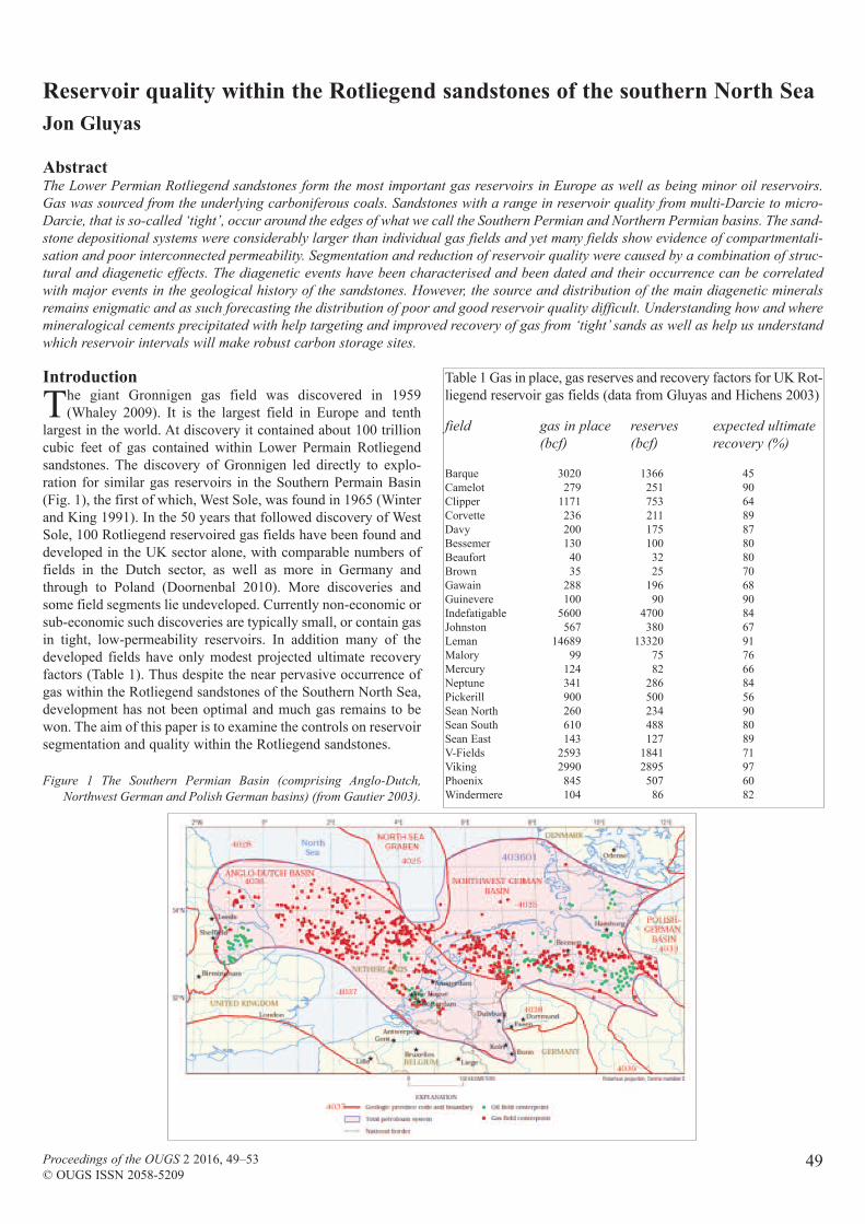
Introduction
The giant Gronnigen gas field was discovered in 1959(Whaley 2009). It is the largest field in Europe and tenth
largest in the world. At discovery it contained about 100 trillioncubic feet of gas contained within Lower Permain Rotliegendsandstones. The discovery of Gronnigen led directly to explo-ration for similar gas reservoirs in the Southern Permain Basin(Fig. 1), the first of which, West Sole, was found in 1965 (Winterand King 1991). In the 50 years that followed discovery of WestSole, 100 Rotliegend reservoired gas fields have been found anddeveloped in the UK sector alone, with comparable numbers offields in the Dutch sector, as well as more in Germany andthrough to Poland (Doornenbal 2010). More discoveries andsome field segments lie undeveloped. Currently non-economic orsub-economic such discoveries are typically small, or contain gasin tight, low-permeability reservoirs. In addition many of thedeveloped fields have only modest projected ultimate recoveryfactors (Table 1). Thus despite the near pervasive occurrence ofgas within the Rotliegend sandstones of the Southern North Sea,development has not been optimal and much gas remains to bewon. The aim of this paper is to examine the controls on reservoirsegmentation and quality within the Rotliegend sandstones.
49Proceedings of the OUGS 2 2016, 49–53© OUGS ISSN 2058-5209
Reservoir quality within the Rotliegend sandstones of the southern North Sea
Jon Gluyas
AbstractThe Lower Permian Rotliegend sandstones form the most important gas reservoirs in Europe as well as being minor oil reservoirs.
Gas was sourced from the underlying carboniferous coals. Sandstones with a range in reservoir quality from multi-Darcie to micro-
Darcie, that is so-called ‘tight’, occur around the edges of what we call the Southern Permian and Northern Permian basins. The sand-
stone depositional systems were considerably larger than individual gas fields and yet many fields show evidence of compartmentali-
sation and poor interconnected permeability. Segmentation and reduction of reservoir quality were caused by a combination of struc-
tural and diagenetic effects. The diagenetic events have been characterised and been dated and their occurrence can be correlated
with major events in the geological history of the sandstones. However, the source and distribution of the main diagenetic minerals
remains enigmatic and as such forecasting the distribution of poor and good reservoir quality difficult. Understanding how and where
mineralogical cements precipitated with help targeting and improved recovery of gas from ‘tight’ sands as well as help us understand
which reservoir intervals will make robust carbon storage sites.
Figure 1 The Southern Permian Basin (comprising Anglo-Dutch,
Northwest German and Polish German basins) (from Gautier 2003).
Table 1 Gas in place, gas reserves and recovery factors for UK Rot-liegend reservoir gas fields (data from Gluyas and Hichens 2003)
field gas in place reserves expected ultimate
(bcf) (bcf) recovery (%)
Barque 3020 1366 45Camelot 279 251 90Clipper 1171 753 64Corvette 236 211 89Davy 200 175 87Bessemer 130 100 80Beaufort 40 32 80Brown 35 25 70Gawain 288 196 68Guinevere 100 90 90Indefatigable 5600 4700 84Johnston 567 380 67Leman 14689 13320 91Malory 99 75 76Mercury 124 82 66Neptune 341 286 84Pickerill 900 500 56Sean North 260 234 90Sean South 610 488 80Sean East 143 127 89V-Fields 2593 1841 71Viking 2990 2895 97Phoenix 845 507 60Windermere 104 86 82

Reservoir quality within the Rotliegend sandstones of the southern North Sea / Gluyas
50
The sandstone-dominated facies belts are enormous and covermany thousands of square kilometres. These facies belts are sub-stantially larger than the footprints of even the biggest fields(Fig. 3), although some fields cross-cut the facies belt bound-aries (Fig. 4, opposite).
Reservoir segmentationMany of the Rotliegend reservoired fields are segmented. Thiswas often noticed in the early developed fields as a mismatchbetween the volume of gas as calculated form geological andfrom geophysical analysis of the mapped field volume, whichmost often was larger than that derived by reservoir engineers
from decline analysis of the production wells.Moreover, wells drilled only short distances apartcommonly displayed different pressures. Theassumption was that many fields were faulted, withthe faults acting as barriers to fluid flow. Other thana few small clues seen in cores and granulationseams we had little evidence as to what was caus-ing the compartmentalisation. Only when 3D seis-mic surveys became common were the faultsrevealed (Fig. 5, opposite).
Fault lineaments trending SW–NE can be mappedfrom the 3D seismic data. The trend of these strikeslip features is co-incident with structures in theunderlying Caledonian basement. Within theRotliegend the zones are characterised by quartzcemented granulation seams with negligible cross-seam permeability (Barr 2007). Barr dates the seal-ing fractures to the end Jurassic, when faulting athigh temperature and pressure gave rise to the cata-clasite rocks.
Barr (2007) also points to uplift in the Tertiary ascausing the then brittle rocks to fracture, leavingopen transmissive faults. These processes, however,might not always have been the case. Gluyas et al.
(1997a) report on findings from an investigation of diagen-esis within the Rotliegend reservoir of the Amethyst Field.Many of the Tertiary inversion faults in Amethyst arecemented by barite. Isotope evidence was used to show thatthe source of the sulphate was the overlying Zechstein,while the barium was inferred to have been derived formthe formation waters within the underlying Coal Measures.The barite precipitated when the two sets of formationwaters mixed during uplift. This same barite cement can beseen at Cullercoats on the north-east coast of the UK, wherea heavily fractured zone adjacent to the Ninety FathomFaults is pervasively barite cemented (Fig. 6, opposite).
The presence of cemented fractures means that thedrainage volumes per wells in Rotliegend fields are com-monly modest (Fig. 7, page 52).
Reservoir diagenesisThe diagenetic mineralogy of the Rotliegend sandstones isunusual in that it is dominated by illite. The illite occurs ashairy projections from the quartz grains and may form in
Figure 2 Subcrop to the Base Permian Unconformity in the Southern North Sea (from
Underhill 2003; reproduced with permission from the Geological Society).
Depositional systemIn broad terms the Southern Permian Basin of Europe compriseda large non-marine basin (1,500km E–W ¥ 500km N–S) the cen-tre of which was occupied by an ephemeral lake called the SilverPit Lake. Fringing the lake and to the edge of the basin weresands with subordinate muds deposited as aeolian dunes, fluvialsandbodies and sabkha mixed sandstones and mudstones. Thesubstrate to the basin was an eroded but not peneplaned terrain ofCarboniferous and Devonian strata (Fig. 2). Local topography inthe basin gave rise to the presence of isolated patches of basalRotliegend sandstone in the basin centre in what otherwise wasthe mud dominated Silver Pit lake.
Figure 3 Major facies belts within the Southern North Sea with
superimposed field outlines — upper part of the Slochteren
Formation and its equivalents (Rotliegend, Late Permian)
(from Doornenbal and Stevenson 2010).
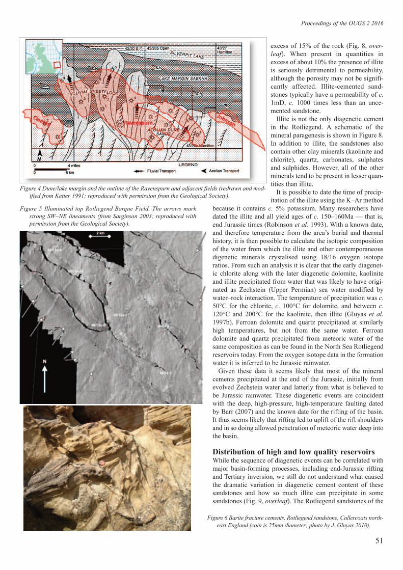
excess of 15% of the rock (Fig. 8, over-
leaf). When present in quantities inexcess of about 10% the presence of illiteis seriously detrimental to permeability,although the porosity may not be signifi-cantly affected. Illite-cemented sand-stones typically have a permeability of c.
1mD, c. 1000 times less than an unce-mented sandstone.
Illite is not the only diagenetic cementin the Rotliegend. A schematic of themineral paragenesis is shown in Figure 8.In addition to illite, the sandstones alsocontain other clay minerals (kaolinite andchlorite), quartz, carbonates, sulphatesand sulphides. However, all of the otherminerals tend to be present in lesser quan-tities than illite.
It is possible to date the time of precip-itation of the illite using the K–Ar method
because it contains c. 5% potassium. Many researchers havedated the illite and all yield ages of c. 150–160Ma — that is,end Jurassic times (Robinson et al. 1993). With a known date,and therefore temperature from the area’s burial and thermalhistory, it is then possible to calculate the isotopic compositionof the water from which the illite and other contemporaneousdigenetic minerals crystalised using 18/16 oxygen isotoperatios. From such an analysis it is clear that the early diagenet-ic chlorite along with the later diagenetic dolomite, kaoliniteand illite precipitated from water that was likely to have origi-nated as Zechstein (Upper Permian) sea water modified bywater–rock interaction. The temperature of precipitation was c.50°C for the chlorite, c. 100°C for dolomite, and between c.120°C and 200°C for the kaolinite, then illite (Gluyas et al.
1997b). Ferroan dolomite and quartz precipitated at similarlyhigh temperatures, but not from the same water. Ferroandolomite and quartz precipitated from meteoric water of thesame composition as can be found in the North Sea Rotliegendreservoirs today. From the oxygen isotope data in the formationwater it is inferred to be Jurassic rainwater.
Given these data it seems likely that most of the mineralcements precipitated at the end of the Jurassic, initially fromevolved Zechstein water and latterly from what is believed tobe Jurassic rainwater. These diagenetic events are coincidentwith the deep, high-pressure, high-temperature faulting datedby Barr (2007) and the known date for the rifting of the basin.It thus seems likely that rifting led to uplift of the rift shouldersand in so doing allowed penetration of meteoric water deep intothe basin.
Distribution of high and low quality reservoirsWhile the sequence of diagenetic events can be correlated withmajor basin-forming processes, including end-Jurassic riftingand Tertiary inversion, we still do not understand what causedthe dramatic variation in diagenetic cement content of thesesandstones and how so much illite can precipitate in somesandstones (Fig. 9, overleaf). The Rotliegend sandstones of the
Proceedings of the OUGS 2 2016
51
Figure 4 Dune/lake margin and the outline of the Ravenspurn and adjacent fields (redrawn and mod-
ified from Ketter 1991; reproduced with permission from the Geological Society).
Figure 5 Illuminated top Rotliegend Barque Field. The arrows mark
strong SW–NE lineaments (from Sarginson 2003; reproduced with
permission from the Geological Society).
Figure 6 Barite fracture cements, Rotliegend sandstone, Cullercoats north-
east England (coin is 25mm diameter; photo by J. Gluyas 2010).

Reservoir quality within the Rotliegend sandstones of the southern North Sea / Gluyas
52
Ravenspurn fields have abundant illite, while those fromthe adjacent Cleeton Field are almost wholly uncemented(Fig. 10, opposite). Moreover, those sandstones withabundant illite appear to have imported silica, potash andalumina. Silica can be derived locally from stylolites andpotash is a component of the formation water, but move-ment of large quantities of alumina is not feasible andgeochemical analysis indicates that dissolution offeldspars in the sandstones could not have supplied suffi-cient alumina (Gluyas and Leonard 1995). Research iscurrently underway to determine why some fields carryalmost no diagentetic cement while other fields have sub-stantial quantities, as well as ongoing work to determinethe origin of the illite cement.
ConclusionsThe Lower Permian Rotliegend sandstones form the mostimportant gas reservoirs in Europe and they have beenexploited for almost 60 years. Despite their importancethey are of variable quality. Some fields are heavily com-partmentalized, while in others the reservoir, thoughporous, is often of low permeability; and because of theselimitations on quality, recovery factors can in someinstances be as low as 50%.
These same Rotliegend reservoirs, and in particular thedepleted gas fields, are likely to be important for storageof CO2.
In order to continue to exploit the remaining gasresource as well as to develop some fields for CO2 injec-tion it is important to better understand the diagenetic his-tory of the sandstones. Work continues.
Figure 7 Drainage volume per well calculated for Southern North Sea
gas fields. The data were calculated by dividing the total field pro-
duction to end 2012 by the number of wells in each field (units = mil-
lion cubic meters reservoir volume).
Figure 8 Pore bridging (A) hairy illite (grain diameters c. 150 microm-
eters), scanning electron microscope photomicrograph, Ravenspurn
Field (photo by J. Gluyas 1983).
Figure 9 Diagenetic history of the Rotliegend sandstones within the
Ravenspurn Field (from Gluyas et al. 1997b).

ReferencesBarr, D. 2007 ‘Conductive faults and sealing fractures in the West Sole
gas fields Southern North Sea’. Geol Soc Spec Publ 292, 431–51Doornenbal, J. C., and Stevenson, A. G. (eds) 2010 Petroleum
Geological Atlas of the Southern Permian Basin Atlas. Houten:EAGE Publications b.v.
Gluyas, J. G., and Hichens, H. 2003 The United Kingdom Oil and Gas
Fields. London: Commemorative Millennium Volume Geol SocMem 20
Proceedings of the OUGS 2 2016
53
Gautier, D. L. 2003 ‘Carboniferous Rotliegend total petroleum system,systematic description and assessment results and summary’. US
Geol Survey Bull 2211
Gluyas, J. G. Jolley, E. J., and Primmer, T. J. 1997a ‘Element mobilityduring diagenesis: sulphate cementation of the Rotliegend sand-stones, Southern North Sea’. Marine Petrol Geol 14, 1001–12
Gluyas, J. G., and Leonard, A. J. 1995 ‘Diagenesis of the Rotliegendsandstone: the answer ain’t blowin’ in the wind’. Marine Petrol Geol
12, 491–7Gluyas, J. G., Robinson, A. G., and Primmer, T. P. 1997b ‘Rotliegend
sandstone diagenesis: a tale of two waters’, in Hendry, J., Carey, P.,Parnell, J., Ruffel, A., and Worden, R. (eds) 1997 Geofluids II ’97.Belfast, March 1997, 291–4
Ketter, F. 1991 ‘The Ravenspurn North Field, Blocks 42/30, 43/26a, UKNorth Sea’, in Abbots, I. 1991 UK Oil and Gas Fields. London: GeolSoc Mem 14, 459–67
Robinson, A. G., Coleman, M. L., and Gluyas, J. G. 1993 ‘The age andcause of illite cement growth, Village Fields area, Southern NorthSea: Evidence from K–Ar ages and 18O/16O ages’. AAPG 77
Sarginson, M. J. 2003 ‘The Barque Field, Blocks 48/13a, 48/14, UKNorth Sea’, in Gluyas, J. G., and Hichens, H. (eds) 2003 The United
Kingdom Oil and Gas Fields. London: Commemorative MillenniumVolume Geol Soc Mem 20, 663–70
Underhill, J. R. 2003 ‘The tectonic and stratigraphic framework of theUK’s Oil and Gas fields’, in Gluyas, J. G., and Hichens, H. (eds)2003 The United Kingdom Oil and Gas Fields. London:Commemorative Millennium Volume Geol Soc Mem 20, 17–59
Whaley, J. 2009 ‘The Gronnigen Gas Field’. GEO ExPro 6 (part 4)Winter, D. A., and King, B. 1991 ‘The West Sole Field, Block 48/6, UK
North Sea’, in Abbots, I. (ed) 1991 UK Oil and Gas Fields. London:Geol Soc Mem 14, 517–23
Figure 10 the Rotliegend reservoir within the Cleeton Filed is largely
uncemented and has permeabilities in excess of 1D (photo by A.
Leonard 1994).

Book reviews
54
Book reviewHarvey, Adrian M., and Mather, Anne E. 2015 Classic Geology
in Europe 12: Almeria. Edinburgh: Dunedin Academic Press Ltd(ISBN paperback 978-1-78046-037-6; e-pub 978-1-78046-527-2; Kindle 978-1-78046-528-9; paperback and e-book £24.99,Kindle £21.25)
I was excited when I saw this was available, as it is the third iter-ation of Anne Mather’s guides to this area, succeeding the BSRGField Meeting Guide Book she wrote with Martin Stokes (1999)and the Blackwell’s Field Guide to the Neogene SedimentaryBasins (with Martin, Harvey and Braga), which was an expand-ed version of the 1999 publication, in 2001. I have used these twoformer two guides, plus experience from other visits to the areato run field trips there over the last 15 years.
The Dunedin book is an improvement on previous versions interms of colour plates and figures: these are a great help, particu-larly for a newcomer to the area. A gripe I have is that some fig-ures have been scaled down to the extent that the labels and leg-ends on them are hardly legible, even for my myopic vision. Thisnew guide has also been reduced in length to about two-thirds ofthe previous version, so something has had to go and, in terms ofmaterial covered, where the Blackwell’s book stretched its wingsand flew out into the heady realms of the older Nevado-Filabride,Maláguide and Alpujárride basement complexes, the Dunedinversion returns to its Neogene Basin roots.
Don’t get me wrong: the Neogene Basins of Almeria areworld-class examples of these marginal features and, becauseof the semi-desert climate and lack of vegetation, have won-derful exposure, making them a real luxury in terms of fieldwork localities. However, I was disappointed to find that thebasement rocks, and even the wonderful Neogene volcanics,only have cursory cover. Perhaps these aspects should have aguide in their own right, but they are so much a part of theoverall geology of the area that I feel they warrant more cov-erage here, especially since the title of the book has mislead-ingly been changed from ‘Neogene Basins’ to the all-encom-passing ‘Almeria’.
The book is divided into two main sections: Part I covers‘The main themes in the geology and geomorphology ofAlmeria’ and Part II includes details of keynote sites and sevenitineraries. There are also useful appendices, including aGeological, Neogene and Quaternary timescales, a glossaryand a short section on logistics, which would be useful forsomeone new to the area. And indeed, for anyone who is newto the area, there is plenty to go and look at — it is aimed at theundergraduate or the enthusiastic amateur, so if you are plan-ning to go there, don’t reject it out of hand because of its lackof hard-rock interest! I won’t be throwing out my previousguides though.
— Linda Fowler, BSc (Open)
Book reviewUpton, Brian 2015 Volcanoes and the Making of Scotland (2ndedn). Edinburgh: Dunedin Academic Press Ltd (ISBN 978-1-78046-056-7; hardback, 248pp; £24.99)
This is a well-produced book, 240mm ¥ 160m and 20mm thick,but quite heavy so you probably wouldn’t carry it in your ruck-sack! Printed on shiny paper, reading some of the diagrams canbe a bit tricky in certain light.
The book comprises 12 chapters, a bibliography and an index.I thought that having no glossary would be a problem, but tech-nical terms are explained at least once within the text. They canbe found in the index, though you then have to turn to the partic-ular page for definitions — just a niggle really. The first fourchapters give an introduction as to what to expect from the book:information on how volcanoes form, plate tectonics, geologictime, mantle plumes, magmas, pyroclastics, lava and igneousrocks. I found these chapters a really good revision of basics,with some new information too. Upton uses modern analogiestoo. There are lots of diagrams, although references to them aresometimes not as clear as they might be. The photos are general-ly of good quality.
The next seven chapters go into detail about the variousvolcanoes that have formed in ‘Scotland’. And this is where thebook becomes somewhat unusual (which Brian Uptonadmits!). He takes the formation of the various igneous centreschronologically, but from the most recent backwards. This is
not something I am used to — I tend to think in terms of old-to-young, in geological chronology, not vice versa. Also, whenmaking something, you usually start at the beginning not theend. However, his point is that there is more evidence availablefrom the most recent volcanoes about their formation and his-tory. He then applies this to the more limited evidence of theolder areas, ‘imagining’ what might have happened, say, in theDevonian, while pointing out that it is ‘informed guesswork’and that we will probably never know: so much time, so mucherosion, so little left! There is a comprehensive section on theEdinburgh volcanics, with very specific examples. Chapter 11concerning the Pre-Cambrian is particularly fascinating, andshows the information available through geochemical analysis.Chapter 12 contains a summary. In a nutshell, Scotland is agraveyard of volcanoes.
The book took very careful reading. Rereading of some sec-tions was needed, as the story is very complicated — I think Iknew it was, but not quite that complicated. While this is aserious book, Brian Upton’s style includes the colloquial andhe does add humour on occasions (but I’ll leave the reader tofind these!).
Overall, I thoroughly enjoyed the book and I think it would bea valuable addition to your bookshelf, especially if you are inter-ested in Scottish geology. I will take it with me every time I amin Scotland, albeit not in my rucksack.
— Jane Michael, BSc Hons (Open) Nat Sci (Earth Sciences)

Introduction and history
Boulby mine is situated on the North Yorkshire coast betweenTeeside and Whitby, near the village of Staithes. The
Permian and Zechstein are overlain by some 1,000m of youngerrocks at this point (Fig. 1).
The deposits of potash were found during exploration for oiland gas in the 1930s. Previous speakers have described whypetroleum engineers are very interested in our halite rocks, asthey form a really good cap rock for migrating oil and gas. Mostof you have had chance to examine the samples of these haliterocks [on display at the Symposium — Ed.]. Initial impressionsare that these rocks are very friable — they will shatter easilywhen struck with a hammer; however, if halite rocks are com-pressed by burial deep within the strata, they show very plasticproperties and form a really good seal. We see this plastic flowreadily in our mine workings. When we make a tunnel in theserocks, the floor rises up within weeks of exposure. It actuallymoves in a fluid-like way — a very interesting rock.
The potash produced at the mine almost all goes to make fer-tilizer. In the 1960s ICI was a big producer of fertilizer and madethe brave decision to invest in this large new mine to exploit these
55
reserves. Such projects are not cheap, and their initial investmentwould have been in the region of £800,000,000, in modern-dayequivalent. The shafts were reported as being the deepest inEurope at the time. The railway line needed to be reinstated, anda large processing plant built— all high cost items.
Things didn’t go well in the early years; production didn’t pickup as well as had been hoped, conditions in the mine were diffi-cult and accidents were common.
ICI made the decision to let the mine go in the late 1970s, anddespite their large investment they sold it for a nominal sum toAnglo American, who had been one of their partners during themine construction.
The mine continued in Anglo American ownership right up to2002. During this period the mine was finding it difficult to makea profit owing to the low world price of potash and the ever-increasing distance of the mine workings from the shafts.
In 2002 Anglo put the mine up for sale and it was bought byICL who have invested heavily in the mine and who have bene-fitted from a steep rise in the world price for potash products.Current indications are that the mine should have several good
Mining in the Zechstein evaporites at Boulby Mine
Neil Rowley MSc C Eng FIMMM
Proceedings of the OUGS 2 2016, 55–61© OUGS ISSN 2058-5209
Figure 1 ICL Fertilizers Boulby Mine.
Thalia © 2015

years of life remaining, but it will need to be flexible to cope withthe ever-changing world in which we exist.
You will probably be aware that there is currently an applica-tion for permission to build a new mine to the south of Whitby.This is not from ICL, but rather from Sirius Minerals, a competi-tor company. Both Boulby and the proposed new mine are locat-ed within the North York Moors National Park.
Any such developments are understandably subject to verytight planning restrictions. The landscaping and architecturalstandards that were applied to Boulby will not be sufficient in thismodern age to gain permission. The new mine will need to bepretty much invisible.
However, the economics show a good case for allowing a tight-ly controlled development. Boulby employs more than 1,000people and makes a contribution of well over £100 million peryear into the local economy. A similar new mine would be ofgreat economic benefit to the local area.
Minerals mined at BoulbyThe main potash ore that we mine is called sylvinite. Sylvinite isa mixture of potassium chloride (KCl), sodium chloride (NaCl)and clay. The ratio of the minerals does vary greatly. We aim tomine ore with a KCL grade of higher than 30%, but the depositcan vary from 0 to 60% KCL, so much exploration drilling isrequired to identify the best areas to mine (Fig. 2).
Mining in the Zechstein evaporites at Boulby Mine / Rowley
56
There is currently a lot of interest in sulphate fertilizers, one ofthe factors being that in the past coal-fired power stations havebeen putting sulpher dioxide into the atmosphere, which thenadds sulphates to the soil during rainfall. Now the farmer needsto buy sulphate fertilizers to maintain the level of essential sul-phate in soil.
The world market for polyhalite is currently only 130,000tonnes per year. We are at the moment the only producer and thatis what we mined last year. We expect that the market will devel-op steadily over the coming years. The new mine proposed to thesouth of Whitby is being primarily designed to produce poly-halite, due to the difficulties of mining sylvinite at depth, and willbe aiming to produce several million tonnes per year veryquickly. It will be interesting to see if the world market willdevelop at a pace sufficient to accommodate this supply level.
Some statisticsTypically Boulby produces c. 2.5 million tonnes a year of sylvi-nite. This is refined down to yield c. 750,000 tonnes of finishedpotash products.
Rock salt: I think that the most salt that the mine has sold in ayear was one million tonnes. In recent years the winters havebeen quite mild and we have been able to get by on lower salt dri-veage. Last year production was < 0.5 million tones.
Polyhalite: Production was 130,000 tonnes last year and willbe 250,000 tonnes this year [2015]. It is expected to rise to500,000 tonnes next year. Future tonnages depend very much onthe development of the world market for the product.
The mine generally can produce 10,000 to 12,000 tonnes aday. The limit on the mine is what can be raised up the shafts. Ibelieve that the record for tonnage up the shaft in one day ismore than 14,000 tonnes, but the need for time to be spent onshaft maintenance means that this amount cannot be achieved ona regular basis.
People: There are 1,100 direct employees, and another100–200 contractors. There are also many more people in thecommunity who have their livelihoods connected to the mine. Itis a very big employer in the Northeast of England.
ICL doesn’t just own the mine, it also owns part of the railway.Being in the National Park we are limited regarding how manyroad wagons can get out, and hence the great majority of productgoes by train. Our responsibility for the track extends as far asSkinningrove Steelworks.
The company also operates a dock on the River Tees. This dockis crucial to the business, facilitating distribution of bulk cargoesworldwide. Half of the product sold goes within the UK, the otherhalf can go almost anywhere in the world. A lot of it is going intonorthern Europe at the moment.
Potash is applied to the land in the spring. There are twosprings in the year. The Southern Hemisphere has its spring at atime when the market is quiet in the Northern Hemisphere. Shipsto Brazil in the summer certainly help to even out supply throughthe year (Fig. 3, opposite).
The dock is also used for the distribution of the de-icing saltthat we mine. Most of the salt is for use within the UK, butcoastal sea transport provides an environmentally sustainablemeans of moving large tonnages. Many cargoes go to the eastcoast of Scotland, but also much of south-east England is alsosupplied by sea via the Thames or Shoreham. The occasionalcargo will go to the east coast of the USA.
Figure 2 Minerals mined at Boulby.
We also mine substantial quantities of de-icing salt. This is arelatively low-value product in relation to potash, but it is essen-tial to mine the salt in order to make the long-term tunnels in themine. Halite and sylvinite have similar compressive strengths,but it was found early in the life of the mine that a tunnel madein sylvinite will start to fail very quickly. It may last for four orfive years in the shallower parts of the mine, but the tunnels inthe deeper parts of the mine can only remain of use for one ortwo years. A tunnel in the halite will, however, remain open for30 or 40 years if properly engineered. So wherever we go tomine the sylvinite we will follow the development with two tun-nels in the halite to provide long-term access. This produces thesalt that can be sized and graded to sell for de-icing roads duringthe winter months.
More recently we have been developing some 150m below thesylvinite to access polyhalite (K2SO4.MgSO4.2CaSO4.2H2O). Itis quite a new product for us. Geologically it is perhaps bestdescribed as a naturally modified anhydtite. This can be used asfertilizer directly, without the need for extensive processing.

Proceedings of the OUGS 2 2016
57
Operation of the mineBoulby has two principal shafts, each 1,100m deep and 5.5m indiameter. To ventilate the mine the air is forced into the ‘down-cast’ shaft by the surface fans. The air travels all around theunderground workings and emerges at the other shaft, whichunsurprisingly is referred to as the ‘upcast’ shaft.
The downcast shaft is used to transport men and materials. It isfitted out with a large three-deck cage and a small counterweightcage. The main cage can accommodate 65 men. This enablespretty much a full shift of men to enter and leave the mine togeth-er. Materials are also transported on this cage, principally on pal-lets handled on and off by fork lift truck. Larger items can be sus-pended inside the cage if the decks are removed. A Ford Transitvan can just fit inside the cage, suspended by its back end.
The upcast shaft is used to hoist the rock to the surface, but italso carries the hot, damp, salty air out of the mine. There is quitea significant corrosion threat in this area, which needs to be care-fully controlled. The shaft is shut down at seven o’clock everymorning for inspection and maintenance, and this work usuallycontinues to around mid-day.
The mine works 24 hours a day, seven days a week, and pro-duction doesn’t stop during shaft maintenance periods. There areseveral large bunkers underground that can store up to 30,000tonnes of rock. Production continues into these bunkers duringshaft maintenance periods. Once the shaft does resume its nor-mal work then it operates with two 23-tonne skips at a rate of 32skips per hour. This gives a winding rate of more than 700tonnes per hour, which can generally cope with normal produc-tion and clear the bunkers before maintenance needs to startagain the next day.
EconomicsPotash is essential to maintain world food supplies. Some of thegreatest users are Brazil, China and India. They have big popula-tions and big agriculture, but little indigenous potash. If thepotash in the ground is not replaced after crops have been har-vested then yields will decrease. There should be a good long-term market for potash products for many years to come.
We are a fairly small player. We don’t have much say aboutwhat happens to the world price. As you know, commodityprices can vary greatly. All we can do is mine as efficiently aswe can at Boulby.
If world price is low, then we can defer capital expenditure andconcentrate on the products that offer the best value return.However, as the distance from the shafts to the working areaincreases over time, then the fixed costs rise. The limit of eco-nomic working is a difficult thing to predict. Hopefully, with ourrange of products we may be able to continue mining for manyyears yet.
Capital does need to be spent, however, to maintain the integri-ty of the mine and to produce a good quality product.
Possibly the most noticeable capital project in recent years hasbeen the replacement of one of the head towers at the shaft top.This was a major civil engineering exercise. The old tower wasstarting to show signs of structural deterioration and replacementwas essential to maintain the production capacity of the mine.The mine had to remain operational throughout as much of theconstruction phase a possible, so it was planned to build the newtower alongside the old one and then remove the old tower andslide the new one into position during a three-week summer shut-down period. This was a noteworthy feat of engineering (Fig. 4).
The operation was very successful, and the new tower was upand running within the allotted time. As you will see from thephotographs the appearance of the new headframe was initiallyvery much more like the traditional coal mining structures thatwe have been used to in Britain. However, in order to complywith the requirements of the National Park planning authoritiesand to make the shaft top area more weather resistant, the steelframe has now been enclosed in a concrete shell, which maintainsthe visual appearance of the original design.
Other major capital projects have involved making the refineryprocess more efficient and in developing the facilities to dealwith the production of polyhalite.
Figure 3 Ship loading de-icing salt at Tees Dock.
Figure 4 The new headframe alongside the old ready for the changeover.

Mineral processingAs the sylvinite rock is hoisted to the surface conveyors transportit into the processing plant. The primary aim of the plant is to sep-arate the KCl from the associated NaCl and clay (Fig. 5).
The material is initially crushed to physically separate themineral particles. It then passes to the froth flotation cells. Herean agent is added to produce bubbles. The choice of frothingagent is critical because the process depends on the surface ten-sion of the bubbles attracting potash to stick to them, but notattract the salt or the clay particles. At Boulby, guar gum is usedin combination with an amine. You will see from the photo-graph that this works well and the potash coated bubbles rise tothe top of the cells while the salt and the clay sink to the bot-tom. The potash flows over from the cells into centrifuges,which reduce the moisture and then on into gas-fired dryingkilns to produce a completely dry KCl product, which can bepressed into cakes and then broken-up to form a granular prod-uct. The moisture from the dryers forms the plume that you seeemerging from the chimney.
Some of the KCl goes into solution and this is recovered bycrystallisation. The resultant white crystals are 99% pure KCl andare sold into the industrial market.
But remember, only one-third of the rock is potash; two-thirdsare rock salt and clay. Because the material has been pulveriseddown, it is too fine for use as de-icing salt and too dirty to berefined economically into the food market. As with all the otherpotash mines in the world it becomes a waste product. Our loca-tion by the sea is ideal for disposal. The brine and clay mineralscan be pumped under permit into the sea about one mile offshorewith very little environmental impact. Some sedimentation of theclay particles does occur on the seabed in the outfall area, butsalinity levels recover to normal marine levels within meters ofthe discharge. The Environment Agency monitors the wholeprocess closely, as do other external bodies.
Some of the sylvinite ore bypasses the separation process tobe sold directly as fertilizer. Certain crops, such as sugar beet,have a marine ancestry and can tolerate some salt. The lack of
Mining in the Zechstein evaporites at Boulby Mine / Rowley
58
processing makes it possible to designate this product as suitablefor organic farming.
De-icing salt is relatively simple to process. As the salt fromthe development roads arrives at the surface it is crushed andscreened to a size to suit the individual customer. A chemicalanti-caking agent is added and the product is sent off to the dockby rail for onward distribution.
Polyhalite is also simple to process. The whole of the rock issaleable, so it just needs to be crushed to a size to suit the cus-tomer. Currently this is done using the same crushers and screensthat process the salt, but a new, dedicated plant is under con-struction and will come into operation in 2016, enabling a muchgreater throughput of the product.
GeologyThe shaft section gives an excellent introduction to the geology ofthe mine. The illustration is the original section drawn in the1970s, so some of the terminology is now out of date, but I’m surethat you will have little trouble understanding it (Fig. 6, opposite).
The mine is built on the site of earlier ironstone mines. TheCleveland Ironstone main seam is not present in the Boulbyshafts, but was extensively worked in the late 19th and early 20thcenturies in the area immediately to the north of the current shafts.
To the mining engineer the main area of difficulty in shaft sink-ing was the Bunter (now Sherwood) Sandstone. This water-filled,loosely bonded sandstone forms one of Britain’s main aquifersand presents obvious problems to anyone trying to sink a shaftthrough it. At Boulby two different techniques were used, one ineach shaft.
The down-cast shaft was sunk using a cement injection tech-nique. As the aquifer is approached, rings of holes are drilled andfine liquid cement is pumped into the strata, effectively blockingup the pore spaces and bonding the particles together. As sinkingproceeds, further rings of holes need to be drilled to maintain thegrout curtain ahead of the sinking. A water-tight lining is installedthroughout the area. This can be something of a stop-start processand engineers often favour the freezing technique, which wasused on the up-cast shaft.
In the freeze technique, holes are drilled from surface andrefrigerated brine is circulated, turning the strata water into ice.Explosives are then used to blast through this mixture of rock andice forming the shaft, and again a water-tight lining is installed.Once the lower limit of the aquifer is reached the freeze plant canbe switched off, and the water will be held back by the newlyinstalled lining. This technique can generally lead to quickerprogress in the sinking of a shaft; however, in the case of Boulbythe freeze plant was found to be underpowered and needed to beupgraded, causing the up-cast shaft to be completed almost a yearlater than the down-cast shaft.
Permian geologyI’m sure that you will all be familiar with the flooding and evap-oration cycles of the Zechstein Sea during this period. The areathat Boulby mines is part of the Z3 cycle. As the sea evaporatedthe various minerals crystallised out in order of solubility. First tocrystallise was the calcium sulphate, forming gypsum/anhydrite,then the sodium chloride, creating a bed of salt some 60m thickbeneath our normal potash horizon; and finally the potassiumchloride, forming a layer of varying thickness — usually between4m and 10m.
Figure 5 Froth flotation.

Proceedings of the OUGS 2 2016
59
The potassium chloride was probably initially in the form ofcarnallite (KClMgCL26H2O +NaCl), but subsequent recrytallisa-tion converted large areas to sylvinite (KCl +NaCl) (Fig. 7).
We see both forms of the ore in different areas of the mine, butsylvinite is the form of greatest economic significance. The car-nallite has lower KCl content and has poor rock mechanics prop-erties, making it unsuitable to work with our existing equipment.Sylvite is the name given to the pure white KCl that can occurwithin the sylvinite seam (Fig. 8).
Various inclusions can be found within the potash seam. Themost problematic being boracite, which occurs in the form ofhard, insoluble nodules that can quickly damage the cutting headsof the machines. Therefore, we try to avoid mining in areas withhigh boracite content.
The sylvinite is overlain by a very weak carnallitic marl. Thisgives great problems in controlling the mine roof if we get tooclose to it and so we leave 2m of sylvinite in the roof to ensurethe stability of the workings.
In theory the potash seam should extend all the way across theNorth Sea. The Germans are working the same seam on the otherside. However, as we have seen, the presence of carnallite andboracite, and the very variable thickness and grade of thesylvinite means that we need an extensive drilling programme toidentify the best areas to work economically.
Polyhalite is a modified anhydrite found some 150m below ournormal working horizon. It has the formulaK2SO4.MgSO4.2CaSO4.2H2O. This rock is much stronger thansylvinite and can be mined at greater depth. It forms a good nat-ural fertilizer and may well be the future of the mine.
Figure 6 Shaft section.
Figure 7 Common forms of potash at Boulby Mine.
Figure 8 Sylvinite rock.

Mining in the Zechstein evaporites at Boulby Mine / Rowley
60
The general dip of the strata is from north-west to south-east.Depth to the potash at the shafts is 1,100m. In the northern min-ing areas it is 800m and in the south 1,350m.
The geothermal gradient is steep in this area and this gives arock temperature of 45–46˚ C in the deeper parts of the mine.Humidity is low due to the halites absorbing the moisture in theair as it flow through the mine.
ExplorationEach year Boulby drills 100km of horizontal exploration holes.Each hole is c. 2km long. The holes generally start in the saltbelow the potash, but are deflected up at intervals to take sectionsthrough the potash seam. After each section is finished, a bore-hole survey is completed to ensure that the exact location of thesection is known. All holes are fully cored using reverse circula-tion of saturated brine to flush the cores out of the tail end of thedrill string. The drillers lay the cores out on corrugated sheets forlater examination by the geologists, with samples being sent forlaboratory analysis to determine grade (Fig. 9).
Much offshore seismic work has also been completed to give acomprehensive picture of the geological structure.
MiningThe standard machine that we use to excavate the various miner-als is the ‘Continuous Miner’.
These machines weigh approximately 100 tonnes and a newone currently costs more than £3 million. The mine operates afleet of 10 or 12 of these machines. They are electrically pow-ered, operating on 3.3KV and are remotely controlled by an oper-ator who stands some 20m away (Fig. 10).
The machines cut tunnels 3.8m high and 8m wide. The rockthat is excavated is loaded by the continuous miners into shuttlecars, which transport the mineral to the conveyor belt, which isusually maintained to within a distance of 100m of the face.
In the potash seam the production layout is a modified room-and-pillar system, but with surprisingly narrow pillars, whichyield, encouraging the roof beam to flex in the critical areasrather than to break. Reinforcing bolts 1.5m long are used sys-tematically to add strength to the roof beam. Movement of theroof is continuously monitored using ‘tell-tale’ extensometer sta-tions. Should an area be seen to be in danger of failing, addition-al steel and timber supports will be set to stabilise the roadway.
A 2m beam of good potash is maintained in the roof to avoidroof collaspse due to the weak carnallitic marl above. This is con-trolled by the geologists, who probe forward after each 8m cutinserting a gamma radiation sensor into a small-diameter drillhole. Each of the different minerals encountered emits differingamounts of gamma and so the geologist can build up a picture ofthe strata immediately ahead of the working face and apply gradelines accordingly to keep the working face a safe distance belowthe marl.
Because of the high closure rates within the potash workings,two roadways are advanced into each area of the mine in themore resilient salt horizon c. 10m below the potash. This is doneby a second machine and crew to form the long-life infrastructureroadways of the mine. When the potash roads have deformed tosuch an extent that it is no longer economical to maintain them,they are abandoned and sealed off. New potash districts are thendeveloped from the salt roadways (Fig. 11, opposite).
Each machine is operated by a team of approximately 10 peo-ple. The overseer is in charge of both safety and production. Hewill usually have a fitter and an electrician and six or seven men
to operate the machines. Shifts are 9.5hours long and the crew work a cycle oftwo day shifts, two afternoon shifts andtwo night shifts followed by four days off.In this way the machine can be kept run-ning 24 hours a day seven days a week.Two-day maintenance periods are sched-uled into the programme and the produc-tion crew will be redeployed to an alterna-tive district while the specialist mainte-nance crew ensures that the machines areserviced and repaired.
The six or so potash production districtsare located in different areas of the mine soas to give more chance of producing aneven grade once the products from the dif-ferent districts are blended together on theconveyor belts. The farthest productionpanels are currently operating at a distanceof more than seven miles from the shafts.
Figure 9 Exploration boreholes in the north section of the mine.
Figure 10 Joy Continuous Miner.

As with all mines, there are hazards that need to be controlled.Particularly important at Boulby is the potential to mine intopockets of high-pressure gas. If this occurs, then the resultant dis-charge can result in several hundred tons of rock being ejectedalong with a variety of gasses, including methane and the higherhydrocarbons. Such areas of potential outburst can, to someextent, be predicted by the geologists, and in such areas a modi-fied mining procedure is employed that relies on removing per-sonnel from the danger area while cutting is taking place. Largeventilation quantities are generally able to quickly dilute gassesemitted, but in such circumstances additional oxygen sets areavailable to the crews should they be needed.
Water is another potential hazard and the design of the mine issuch that rock mechanics stresses on the aquifer should not behigh enough to promote water ingress. The great majority of themine is desert-like in its dryness but there are a few places, usu-ally associated with fault planes that make significant quantitiesof water. Almost 1,000 gallons of water per minute are continu-ously pumped out of the mine.
PolyhaliteThere would appear to be very extensive reserves of polyhaliteaccessible within the current mining area. Two access drifts weredriven from the northern part of the mine into the polyhalite in2010. Trial workings have been progressing steadily since thengathering information on consistency of grade, machine suitabil-ity and roof support.
The current world market for this material is small, but thepotential is great.
It is expected that production will increase quickly as the cus-tomers become acquainted with the product and we learn themost efficient ways to mine it.
Proceedings of the OUGS 2 2016
61
ConclusionBoulby is a fascinating mine with many challenges, but also withmany years of experience in how these challenges can be over-come. The availability of salt, sylvinite and polyhalite within themining area gives some flexibility to help cope with changingworld markets in years to come.
This has been just a lightening tour of what goes on at the mine,but hopefully you will have learned a little of the many skills andprofessions that are needed to operate a large mine.
Any views expressed in this talk are those of the author and donot necessarily represent the views of the Company.
Figure 11 The relationship between the potash and salt roadways.

Book review
62
the Brazilian Rifts (zone 2), the North Atlantic Passive Margin(zone 3), the Eastern North American Rift System (zone 1), andthe Rhine Graben (zone 4).5 Role of Lithosphere Rheology on Rift Architecture (53–60),which discusses ‘extensional geodynamics’, ‘lithosphericstrength’, and ‘temperature and strain rates’. This chapter is tech-nical but free of formulae, and includes several detailed and com-plex ‘modelling prediction diagrams’ and comparative ‘correla-tion illustrations’.6 Lessons from Analogue Models (61–2), self-evidently, dis-cusses issues, accuracy and the predictability of models.7 Summary (63–5) The summary and opening Abstract (xi–xii)make similar points, although they also complement each other,and the summary mentions the zones studied.An Appendix on page 67 is a technical explanation of ‘effectiveelastic thickness’, ‘lithospheric strength profiles’ and ‘thermalage’, with a rock diagram.
Multiple citations are frequent throughout the book on almostevery topic mentioned; the authors are clearly well read.However, there are sometimes so many citations within a givensentence that the actual text is hard to follow. The References atthe end occupy 18 pages — comprising 20.45% of the book.
There is a two-page Index, mostly of place names rather thanof subjects.
Despite its short extent, this is a technically challenging book.The text is specialised. It is not a book for geology ‘first years’,but is a useful resource for discussions of some of the famed riftsystems and plate margin zones around the globe; and theextensive reference list provides a good place for keen studentsto pursue further detail.
Finally, although unlikely, unless there is an error on theSpringer website and/or on the Amazon page, the price of thisbook is exorbitant for an 88-page book, even if a most technicaland informative one. Springer does not appear to publish any-thing other than books of this nature and pricing.— David M. Jones, BA Hons (UC Berkeley), MA (Inst Archeeol
London), PhD (UC London), BSc Hons (Open),
OUGS Proceedings Editor
Book reviewMisra, Achyuta Ayan, and Mukherjee, Soumyajit 2015 Tectonic
Inheritance in Continental Rifts and Passive Margins. Cham,Heidleberg, New York, Dordrecht, London: Springer (ISBN 978-3-31920-575-5; paperback, xii + 88pp; €51.99, Amazon price£34.37; ebook €41.64)
Misra and Mukherjee are in the Department of Earth Sciences atthe Indian Institute of Tehnology, Mumbai (Bombay). Both areaccomplished authors in the field of continental plates and platemargin geology, especially Soumyajit Mukherjee.
Tectonic Inheritance is one in a series called ‘Springer Briefs inEarth Sciences’. Springer’s website [accessed 15-1-16] lists 44titles in the series, ranging from ‘general’ geological topics suchas this one to specific past geological event and region titles. Allare at this or a similar price, so assumed to be similarly ‘brief’.
Tectonic Inheritance has seven brief chapters:
1 Introduction (1–6), which describes the subject matter, includ-ing informative cartoons and a map (Fig. 1.3) of the rift systemsand passive margins discussed in detail in the book.2 General Aspects (7–8), which, although curiously also the titleof the first subsection of the Introduction, principally defineswhat the authors mean by ‘inheritance’.3 Influence of Pre-existing Anisotropics on Fault Propagation
(9–20), which begins to get into the real ‘meat’ of the subject.There are several numbered formulae, and many technical dia-grams and cartoons.4 Pre-existing Fabrics (21–52), which describes and discussesthe eight rift systems and margin zones shown on the map in theIntroduction. These range around the world and include all thecontinents except Antarctica. There are 24 well-drawn, complexand useful maps, diagrams and schematics, many in colour. Therift systems and margin zones included are divided into‘Pervasive Fabrics’ and ‘Discrete Fabrics’ (in both of which somezones are discussed): the East African Rift System (zone 5 onFig. 1.3 map), the Thailand Tertiary Rift System (zone 8),theSouth Atlantic Passive Margins (not actually figured on themap), the East and West Indian Passive Margins (zones 6 & 7),

63
Background
Recorded investigations into the geology of the area we nowknow as the Permian of north-east England begin around the
end of the 18th century, but I will begin my story back in antiq-uity in the Mediterranean. The region of Thessaly on the eastcoast of Greece has historically been a source of the mineralknown as lodestone. Its natural magnetism made it a valuablecommodity. According to Greek mythology, part of Thessaly wasruled by Magnes, one of the sons of Zeus. The region he gov-erned was called Magnesia and his subjects the Magnetes (Fig. 1).It is from this that the name magnet is derived and also the min-eral magnetite. In addition to lodestone there were two other min-erals from the region that were of value. Together these mineralswere known as Magnitis lithos or ‘stones of Magnesia’. One wasa black mineral used in glass-making and was called Magnesia
nigra (pyrolusite), the other a white mineral used as a cosmeticand called Magnesia alba; the latter also had another name,Magnesia carneus (‘flesh magnet’), because of the way it wouldstick to the lips.
Another property of Magnesia alba was that it appeared to bebeneficial to health. At the start of the 17th century a compoundknown as Conte di Palma’s powder was being sold by the RomanCount Di Palma as a panacea. He kept its source a closely guard-ed secret, but in 1707 the German physician Michael BernhardValentini (1657–1729) revealed that it was Magnesia alba anddescribed a process for its manufacture (Fig. 2).
In 1722 another German physician, Friedrich Hoffmann(1660–1742; Fig. 3, overleaf), described its medicinal effects andreported on the properties of Magnesia alba in his bookObservationum physic-chymicarum. One of his key observationswas that it did not effervesce with the application of dilute acid.
The story now moves to Britain where the Scottish physicianand chemist, Joseph Black (1728–1799; Fig. 4, overleaf) wrote athesis on experiments on Magnesia alba, which was publishedin 1756 in the journal Essays and Observations, Literary and
Philosophical. As it was a medical thesis he covered its curativeproperties, but he also looked into its chemical properties. Hereferred to Hoffman’s earlier work and verified the latter’sfindings. In addition, he carried out a number of experimentscomparing Magnesia with lime. His conclusion was that as it hadmany properties that differed: Magnesia was not simply anothercalcareous earth, but must be a compound of a different element— a carbonate of Magnesia. Black is now credited with the dis-covery of magnesium along with that of ‘fixed air’ (carbondioxide). He also went on to propose the idea of latent heat.
The history of Permian geological investigation in north-east England
Karl Egeland-Eriksen
Proceedings of the OUGS 2 2016, 63–71© OUGS ISSN 2058-5209
Figure 1 ‘Thessalia in Greece’ by TUBS — redrawn by author. (This vec-
tor graphics image was created with Adobe Illustrator. The file was
uploaded with Commonist, and the vector image includes elements
taken or adapted from this source: Greece location map.svg (by
Lencer). Licensed under CC BY-SA 3.0 via Commons:
https://commons.wikimedia.org/wiki/File:Thessalia_in_Greece.svg#
/media/File:Thessalia_in_Greece.svg).
Figure 2 ‘Michael Bernhard Valentini’ (artist unknown;
http://ihm.nlm.nih.gov/images/B25184. Licensed under Public
Domain via Commons:
https://commons.wikimedia.org/wiki/File:Michael_Bernhard_Valent
ini.jpg#/media/File:Michael_Bernhard_Valentini.jpg).
Thalia © 2015

History of Permian geological investigation in north-east England / Egeland-Eriksen
64
Early investigations in north-east EnglandHaving established that Magnesia alba is magnesium carbonatethe story moves back to the continent and to France where thearistocrat Déodat de Dolomieu (1750–1801; Fig. 5), having hada military career from the age of 12, became a member of theirRoyal Academy of Sciences. His main interests were mineralogy,volcanoes and mountain formation and he went on many scien-tific excursions throughout Europe, collecting minerals. On histravels he had noted that among the ancient marble statues ofRome there were many that had suffered corrosion from theforces of nature, but others seemed to be more resistant to ero-sion. These were made of a hard Greek marble, which he notedeffervesced little in acid. In 1791 he wrote about a tour he madeof the Tyrolean Alps, where he discovered ‘calcareous’ rockswith similar properties to the Roman statues (Observations et
Memoires sur La Physique). This stone was hard and did noteffervesce with acid. He also noted rhombic crystals within cav-ities in the rock. The following year Nicolas-Théodore deSaussure named the rock Dolomite after Dolomieu. The majormineral constituent is also called dolomite (CaMg(CO3)2) andthe mountain region is named the Dolomites.
At this time the rocks in the Durham coast area had been littlestudied as, unlike the nearby coalfields and north-Pennine ore-field, they had little economic value. There is evidence that IronAge farmers knew that crops grew better on what we now knowto be magnesian grassland than on other areas. The Romans usedthe stone for building places like Arbeia (South Shields, AD 120;Fig. 6, opposite), and it was used in the building of York Minster(1230) and the Newcastle Exchange building (1658). It alsofound use in the construction of more industrial buildings such as
Figure 3 ‘Friedrich Hoffmann’ by Johann Georg Wolfgang —
http://www.sil.si.edu/digitalcollections/hst/scientific-identi-
ty/CF/display_results.cfm?alpha_sort=h. Licensed under
Public Domain via Commons:
https://commons.wikimedia.org/wiki/File:Friedrich_Hoffm
ann.jpg#/media/File:Friedrich_Hoffmann.jpg).
Figure 4 Joseph Black (© The University of Glasgow; without
further permission, you may access, download and/or print
contents for non-commercial private research and study
purposes).
Figure 5 ‘Deodat de Dolomieu’ by Déssiné d’apres le Portrait
par M. Cordier, gravé par Ambroise Tardieu —
http://ihm.nlm.nih.gov/images/B06032. Licensed under
Public Domain via Commons:
https://commons.wikimedia.org/wiki/File:Deodat_de_Dol
omieu2.jpg#/media/File:Deodat_de_Dolomieu2.jpg).
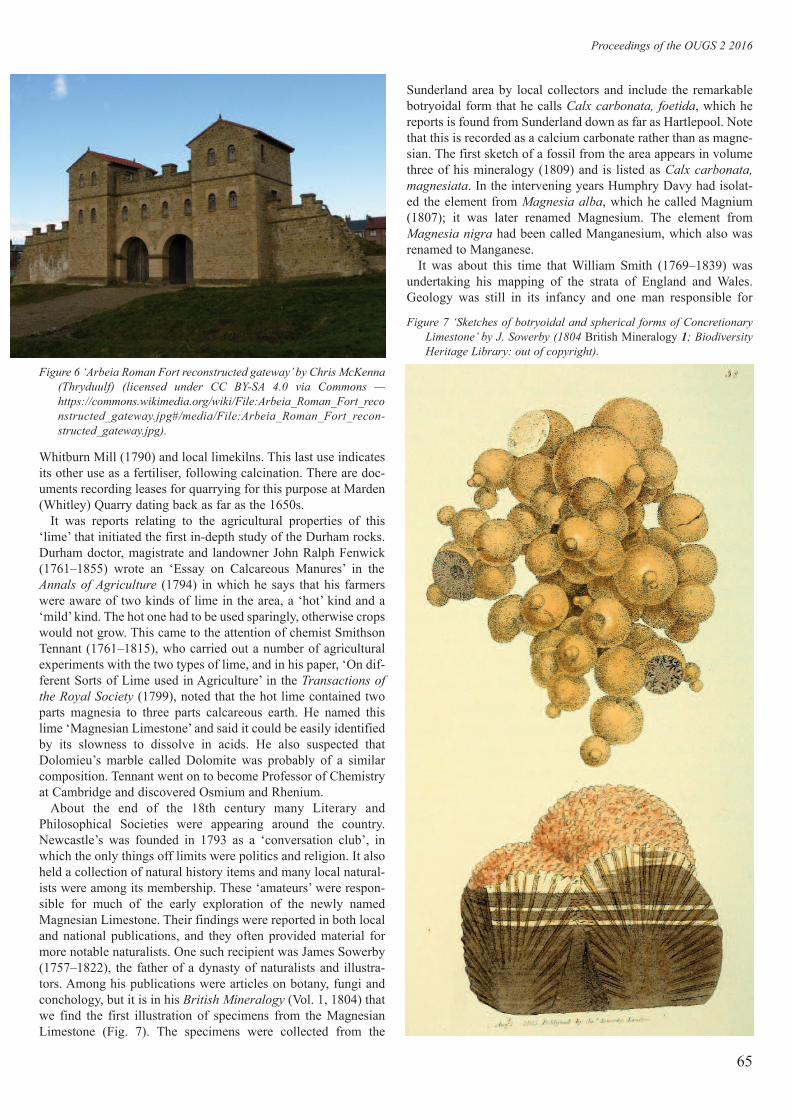
Whitburn Mill (1790) and local limekilns. This last use indicatesits other use as a fertiliser, following calcination. There are doc-uments recording leases for quarrying for this purpose at Marden(Whitley) Quarry dating back as far as the 1650s.
It was reports relating to the agricultural properties of this‘lime’ that initiated the first in-depth study of the Durham rocks.Durham doctor, magistrate and landowner John Ralph Fenwick(1761–1855) wrote an ‘Essay on Calcareous Manures’ in theAnnals of Agriculture (1794) in which he says that his farmerswere aware of two kinds of lime in the area, a ‘hot’ kind and a‘mild’ kind. The hot one had to be used sparingly, otherwise cropswould not grow. This came to the attention of chemist SmithsonTennant (1761–1815), who carried out a number of agriculturalexperiments with the two types of lime, and in his paper, ‘On dif-ferent Sorts of Lime used in Agriculture’ in the Transactions of
the Royal Society (1799), noted that the hot lime contained twoparts magnesia to three parts calcareous earth. He named thislime ‘Magnesian Limestone’ and said it could be easily identifiedby its slowness to dissolve in acids. He also suspected thatDolomieu’s marble called Dolomite was probably of a similarcomposition. Tennant went on to become Professor of Chemistryat Cambridge and discovered Osmium and Rhenium.
About the end of the 18th century many Literary andPhilosophical Societies were appearing around the country.Newcastle’s was founded in 1793 as a ‘conversation club’, inwhich the only things off limits were politics and religion. It alsoheld a collection of natural history items and many local natural-ists were among its membership. These ‘amateurs’ were respon-sible for much of the early exploration of the newly namedMagnesian Limestone. Their findings were reported in both localand national publications, and they often provided material formore notable naturalists. One such recipient was James Sowerby(1757–1822), the father of a dynasty of naturalists and illustra-tors. Among his publications were articles on botany, fungi andconchology, but it is in his British Mineralogy (Vol. 1, 1804) thatwe find the first illustration of specimens from the MagnesianLimestone (Fig. 7). The specimens were collected from the
65
Sunderland area by local collectors and include the remarkablebotryoidal form that he calls Calx carbonata, foetida, which hereports is found from Sunderland down as far as Hartlepool. Notethat this is recorded as a calcium carbonate rather than as magne-sian. The first sketch of a fossil from the area appears in volumethree of his mineralogy (1809) and is listed as Calx carbonata,
magnesiata. In the intervening years Humphry Davy had isolat-ed the element from Magnesia alba, which he called Magnium(1807); it was later renamed Magnesium. The element fromMagnesia nigra had been called Manganesium, which also wasrenamed to Manganese.
It was about this time that William Smith (1769–1839) wasundertaking his mapping of the strata of England and Wales.Geology was still in its infancy and one man responsible for
Proceedings of the OUGS 2 2016
Figure 6 ‘Arbeia Roman Fort reconstructed gateway’ by Chris McKenna
(Thryduulf) (licensed under CC BY-SA 4.0 via Commons —
https://commons.wikimedia.org/wiki/File:Arbeia_Roman_Fort_reco
nstructed_gateway.jpg#/media/File:Arbeia_Roman_Fort_recon-
structed_gateway.jpg).
Figure 7 ‘Sketches of botryoidal and spherical forms of Concretionary
Limestone’ by J. Sowerby (1804 British Mineralogy 1; Biodiversity
Heritage Library: out of copyright).
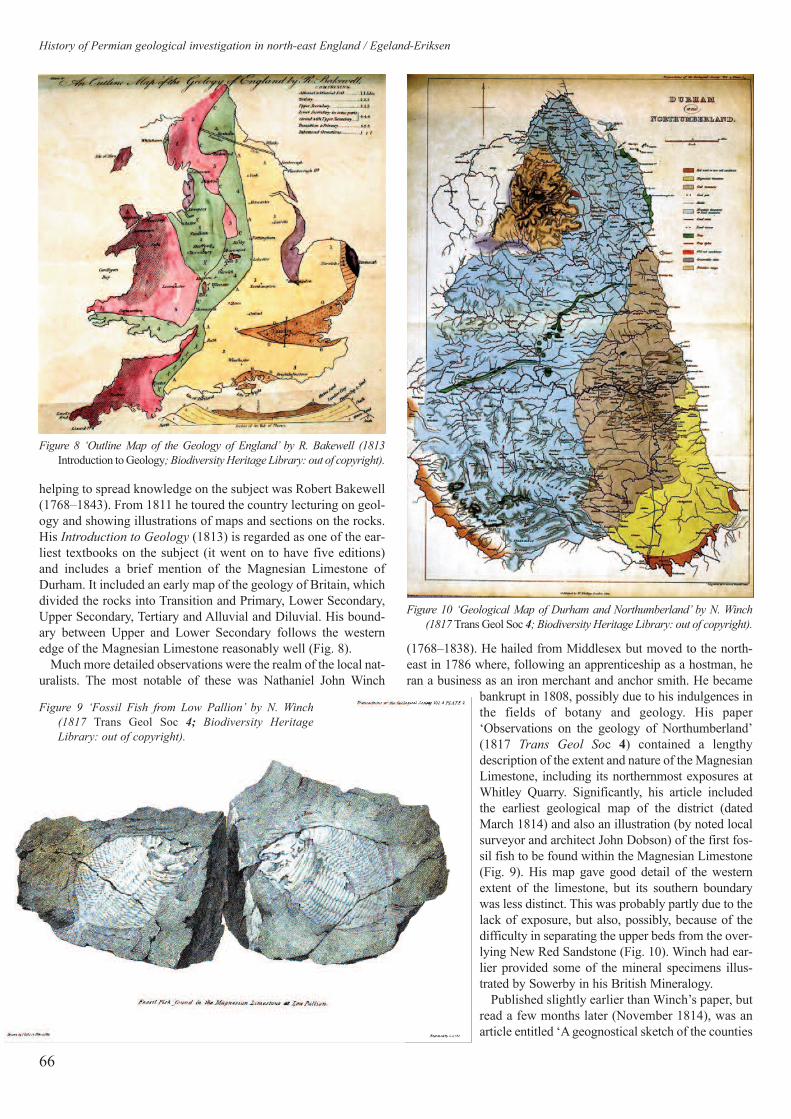
helping to spread knowledge on the subject was Robert Bakewell(1768–1843). From 1811 he toured the country lecturing on geol-ogy and showing illustrations of maps and sections on the rocks.His Introduction to Geology (1813) is regarded as one of the ear-liest textbooks on the subject (it went on to have five editions)and includes a brief mention of the Magnesian Limestone ofDurham. It included an early map of the geology of Britain, whichdivided the rocks into Transition and Primary, Lower Secondary,Upper Secondary, Tertiary and Alluvial and Diluvial. His bound-ary between Upper and Lower Secondary follows the westernedge of the Magnesian Limestone reasonably well (Fig. 8).
Much more detailed observations were the realm of the local nat-uralists. The most notable of these was Nathaniel John Winch
History of Permian geological investigation in north-east England / Egeland-Eriksen
66
(1768–1838). He hailed from Middlesex but moved to the north-east in 1786 where, following an apprenticeship as a hostman, heran a business as an iron merchant and anchor smith. He became
bankrupt in 1808, possibly due to his indulgences inthe fields of botany and geology. His paper‘Observations on the geology of Northumberland’(1817 Trans Geol Soc 4) contained a lengthydescription of the extent and nature of the MagnesianLimestone, including its northernmost exposures atWhitley Quarry. Significantly, his article includedthe earliest geological map of the district (datedMarch 1814) and also an illustration (by noted localsurveyor and architect John Dobson) of the first fos-sil fish to be found within the Magnesian Limestone(Fig. 9). His map gave good detail of the westernextent of the limestone, but its southern boundarywas less distinct. This was probably partly due to thelack of exposure, but also, possibly, because of thedifficulty in separating the upper beds from the over-lying New Red Sandstone (Fig. 10). Winch had ear-lier provided some of the mineral specimens illus-trated by Sowerby in his British Mineralogy.
Published slightly earlier than Winch’s paper, butread a few months later (November 1814), was anarticle entitled ‘A geognostical sketch of the counties
Figure 8 ‘Outline Map of the Geology of England’ by R. Bakewell (1813
Introduction to Geology; Biodiversity Heritage Library: out of copyright).
Figure 9 ‘Fossil Fish from Low Pallion’ by N. Winch
(1817 Trans Geol Soc 4; Biodiversity Heritage
Library: out of copyright).
Figure 10 ‘Geological Map of Durham and Northumberland’ by N. Winch
(1817 Trans Geol Soc 4; Biodiversity Heritage Library: out of copyright).

of Northumberland, Durham and part of Cumberland’ (Annal
Philos 4) by Scottish chemist and mineralogist Thomas Thomson(1773–1852). It also contained a map of the region, with far lessdetail but mentioned his visit to the area in August 1814 when hevisited four hills. He gave the first report on the fossils ofHumbledon Hill and the unusual limestone balls of FulwellQuarry, as well as the results of his chemical analysis of therocks. His article also includes the first mention of the so-called‘flexible limestone’ of Marsden.
In the Annals of Philosophy (1815, 6), Dr William Reid Clanny(1776–1850) of Bishopwearmouth gave an account of the‘Sunderland Limestone Formation’. He apologises to Thomsonfor not having taken him to Pallion lime-works on his visit of1814 and goes on to give a detailed section through the rocksthere noting layers with and without magnesia and those with fishfossils. He also reports the sinking of a shaft through the lime-stone in 1787 in search of coal, but no workable seams beingfound. Clanny invented a miner’s safety lamp predating Davy’sversion. He was also Head Physician at Sunderland Infirmary in1831 during the first outbreak of cholera in the British Isles anddid much to help prevent spread of the disease.
The professional geolgistsIt was, of course, also in 1815 that William Smith published hismap of the Strata of England and Wales. This was less accuratethan Winch’s map with respect to the Magnesian Limestone, withboth the western and southern limits ill-defined. Smith subse-quently went on to produce more detailed maps on a county basis.
In the southern part of the district the width of the MagnesianLimestone placed the working coalfields some distance from thecoast. About 1819 a committee chaired by John Fenwick wasformed to discuss how to improve the movement of coal from theDurham coalfields to the port at Stockton. The possibility of acanal was suggested, but the committee finally settled on a rail-way for horse-drawn carriages. Approval was finally obtained in1821, at which time George Stephenson became involved andconvinced them to use steam-powered locomotives instead ofhorses. So began the building of the Stockton to DarlingtonRailway. It did not, however, stop at Darlington, as this was stillsome way from the coalfields. It continued north-west to Shildonon the edge of the coal measures (Fig. 11). Construction involvedthe opening of quarries to provide materials. Two such quarrieswere at East Thickley and Middridge, just east of Shildon.
During the summers of 1821, 1822 and 1823 Adam Sedgwick(1785–1873), then the Woodwardian Professor of Geology atCambridge, visited the region to carry out fieldwork. On his wayto the area in 1821 he stopped at Robin Hood’s Bay. While ham-mering rocks in the bay he was hit in the eye by a splinter, leav-ing him virtually blind in that eye for the rest of his life. He con-tinued with his trip and made visits to East Thickley andMiddridge Quarries as well as meeting local naturalists, who pro-vided him with specimens from their collections. Publication ofhis findings was not immediate, however. His papers were read atthe Geological Society of London in 1826, 1827 and 1828, andwere finally published in their Transactions in 1829 in an 88-page piece entitled ‘On the geological relations and internalstructure of the Magnesian Limestone’. In it he describes the for-mations within the Magnesian Limestone and draws similaritiesbetween it and formations on the Continent. This proved to be themost important work on the subject for over a century.
67
Between Sedgwick’s visit and publication of his work two otherpublications appeared. In the Annals of Philosophy (1821, 1),William Buckland’s paper on the ‘Structure of the Alps, andadjoining parts of the Continent’ compared the MagnesianLimestone of England with the Elder Alpine Limestone, in partic-ular he mentioned the oolitic concretions in both, with those atSunderland being the size of a ‘cannon-ball’. I have found norecord of him visiting the area himself, so assume that he hasbased his description on communications from fellow geologists.That name has stuck and Sedgwick gave the same description inhis paper. Of course, they are not oolites. When Smith’s countymap of Durham was published in 1824 both his western andsouthern boundaries for the Magnesian Limestone were disputedby Sedgwick. Sedgwick also included sketches of notable sectionsat Claxheugh and at Tynemouth, as well as plates of fish fossilsfrom the Marl Slate at East Thickley and Middridge (Fig. 12).Some of these specimens were not identified by Sedgwick.
Proceedings of the OUGS 2 2016
Figure 11 Plan of intended Stockton and Darlington Railway by The Committee
of The Stockton and Darlington Railway — Report of the intended Rail or
Tram Road from Stockton to Darlington 1821 (1821 Tracts 57, 252;
Licensed under Public Domain via Commons: https://commons.wikime-
dia.org/wiki/File:Tracts_vol_57_p252_1821_Plan_of_intended_Stockton
_and_Darlington_Railway.jpg#/media/File:Tracts_vol_57_p252_1821_P
lan_of_intended_Stockton_and_Darlington_Railway.jpg).
Figure 12 ‘Marl-slate fossils from Middridge and East Thickley
Quarries’ (Sedgwick, A. 1829 Trans Geol Soc Ser 2, 3, Pl 12;
Biodiversity Heritage Library: out of copyright).

Sedgwick passed on specimens to Swiss biologist and geolo-gist Louis Agassiz (1807–1873). He had recently started workingon fossil fishes, drawing up a new system of classification. Hisfirst volume of Research on Fossil Fishes (1833) includes a spec-imen from East Thickley, which he determined to be from a newgenus which he called Coelocanthus, the world’s first-discoveredfossil Coelocanth (Fig. 13).
In 1841, following his expeditions in Russia, RoderickMurchison (1792–1871) determined that strata exposed in theregion of Perm above the Carboniferous, although unlike theMagnesian Limestone in a similar position in England andGermany, these strata were of a new system, distinct from theNew Red Sandstone. Murchison proposed the name of ‘PermianSystem’ to these rocks, and his geological map of England andWales in 1843 is probably the first to depict the Permian System.
Newcastle Museum curatorsThe emphasis on research into the Magnesian Limestone nowreturned to local natural historians. In 1840 the NewcastleMuseum found sufficient funds to employ its first paid curator.His name was William King (1809–1886), born in Sunderlandand previously curator of what is now the Sunderland Museum,and he specialised in fossils from the Magnesian Limestone. Anavid collector, he was helped enormously by the efforts of fellowcollector, schoolteacher Richard Howse (1821–1901) of SouthShields. Indeed, he frequently urged Howse to go out to keylocalities such as Tunstall and Humbledon Hills to collect speci-mens from the so-called ‘shell-beds’ to pass on to him. Throughcareful study of their anatomy he was able to describe many newgenera and species, including a bivalve he named Bakevelliaafter Robert Bakewell, whose books on geology had inspired himfrom an early age. Bakevellia is now the name attributed to aPermian sea that formerly covered an area to the west of thePennines with a fossil fauna rich in Bakevellia. King drew up acatalogue of the Permian fossils, which he presented to theTyneside Naturalists’ Field Club, which, at King’s request, adver-tised it in the London Geological Journal (1847, II). In May ofthat year, however, King withdrew his catalogue from the print-ers without giving any notice to the Field Club. His actions maywell have been in response to a dispute he was having with hisemployers. It transpired that King was selling Museum speci-mens, which he argued were his but which the Museum gover-nors believed belonged to the museum collections on the grounds
History of Permian geological investigation in north-east England / Egeland-Eriksen
68
that King was employed by them as curator during the period inwhich the specimens were collected. This disputed resulted inKing losing his job in November 1847, and appears to have beena blessing in disguise, for in 1849 King became a Fellow of theGeological Society of France and later, with a reference fromCharles Lyell, was appointed to the Chair of Mineralogy andGeology at Queen’s College, Galway, Ireland. In 1850 he pro-duced his most noted publication, A Monograph of the Permian
Fossils of England, with sketches by G. B. Sowerby (Fig. 14).His other claim to fame is that after examining bones discoveredin the Neander valley, Germany in 1856, he determined that theywere different from those of modern man and propose the nameHomo neanderthalensis for this new species.
On the departure of King from the Newcastle MuseumRichard Howse was appointed its new curator. His first task wasto produce a catalogue of the Permian fossils for publication —the Field Club felt obliged to publish one as it had advertisedone. They knew Howse had extensive notes and specimens onthe subject and he was willing to oblige. In due course hisCatalogue of the Fossils of the Permian System of the Counties
of Northumberland and Durham was advertised in the
Newcastle Chronicle of August 11, 1848 and published on 17August 1848. As soon as the advertisement appeared Kingrushed his catalogue back to the printers to have it published pri-vately. He did not wish to lose priority over the naming of newspecies, many of which had come from Howse’ collection. Hisefforts were in vain however, as Howse’ catalogue appeared twodays before that of King’s. Both were overshadowed by King’s
Figure 13 Coelocanthus granulatus Agass (Agassiz, L. 1831 Rechercessur les Poissons Fossiles, vol. 1; Biodiversity Heritage Library: out
of copyright).
Figure 14 Plate III from W. King 1850 The Permian Fossils of England(author scan).

1850 monograph. Howse produced an update of his catalogue in1857 addressing inaccuracies in earlier publications but alsogoing to great length to prove his rite to priority over naming ofspecies including correspondence from King regarding acquisi-tion of specimens.
In the Annals and Magazine of Natural History (1857, 19),Howse give a detailed description of the formations within thePermian and included a section across them (Fig. 15). At thispoint in time he included the Yellow Sands in the Carboniferous,and opinion that was challenged by Daglish and Forster in 1863in their Report for the British Association for the Advancement of
Science, in which they argued that the Yellow Sands were uncon-formable over the Carboniferous, but conformable to the overly-ing Magnesian Limestone. In another Tyneside Naturalists’ FieldClub Publication (A Synopsis of the Geology of Durham, 1863)Howse, along with fellow natural historian, James Kirkby(1834–1902) of Sunderland, reluctantly agreed to this placementof the Yellow Sands in the Permian.
Kirkby also made significant discoveries of new Chitons andEntomostraca within the shelly limestone at Humbleton Hill andfound a new bed rich in fish fossils within Fulwell Quarry. This bedwas somewhat higher than the Marl Slate and he termed it theFulwell Fish-bed. In 1866 Kirkby, along with E. J. J. Browell pub-lished the first complete chemical analysis of the MagnesianLimestone Series in the Transactions of the Natural History
Society of Northumberland, Durham and Newcastle upon Tyne.They showed that the Ca:Mg composition varied from 96.94:1.66to 42.48:49.86 with an absence of magnesia within the concretions.
Further confirmation of the boundary between theCarboniferous and Permian was established by J. Clifton Ward(1843–1880) in 1869 in the Quarterly Journal of the Geological
Society (QJGS) firmly placing the Rothliegende with theMillstone Grit in contrast to Sedgwick, Phillips and Murchison,all of whom placed the Rothliegende in the Permian. These pub-lications helped define the western boundary of the Permian inthe region.
In the late 1860s the railway at Shildon was being widened.This led to further fossil discoveries at Middridge Quarry by a
Proceedings of the OUGS 2 2016
69
local man, Joseph Duff, whose finds were reported by Howseand Albany Hancock (1806–1873) in the QJGS in 1870).Duff’s finds included the first British specimens of teeth andskin from Janessa, a new Labyrinthodont, namedLepidotosaurus duffi (Fig. 16), another new species, namedProterosaurus huxleyi, and the first four British specimens ofthe fish Dorypterus hofmanni.
In 1871 Andrew Crombie Ramsay (1814–1891) — famous forhis studies of the geology of Arran and other work — wrote aboutthe pre-Triassic red rocks in the Proceedings of the Geological
Society, arguing that the Magnesian Limestone could only havebeen produced by evaporation in a salt lake or inland sea, which,perhaps, had had a previous connection to the open sea. Up to thistime the Magnesian Limestone had been thought to derive fromerosion of magnesium-rich rocks.
By 1884 the Newcastle Museum had found a new home for itscollections. Richard Howse was still the curator and was respon-sible for organising the new geological display at the HancockMuseum, St. Mary’s Place, Newcastle upon Tyne (named afterbothers John and Albany Hancock).
Figure 15 ‘Section across the Magnesian Limestone’ (Howse, R. 1857 Annals and Magazine of Natural History; Biodiversity Heritage Library: out
of copyright.
Figure 16 ‘Lepdotosaurus from Middridge Quarry’ (Hancock A., and
Howse, R. 1870 Quart J Geol Soc 26; Biodiversity Heritage Library:
out of copyright).

The academicsThe College of Physical Science (now Newcastle University) hadbeen established 1871 and in 1879 G. A. Lebour (1847–1918)became its Professor of Geology. His Outlines of the Geology
and Natural History of Northumberland and Durham (1886)summarised the knowledge of the area, including his own find-ings. In it he comments on how Sedgwick’s paper of 60 years ear-lier was still valuable. He reports that the Yellow Sands arealways unconformable on the lower beds and, although non-fos-siliferous, are undoubtedly Carboniferous. Like Sedgwick, heincludes the sections at Claxheugh and Tynemouth (Fig. 17), andalso describes the ‘breccia gashes’ at Marsden, and drew his ownmap of the Geology of Northumberland.
The following year Howse remarked, in the Transactions of the
Natural History Society of Northumberland and Durham that theYellow Sands were an inconsistent bed absent in places. He statesthat they comprise gritty, incoherent, strongly false-bedded sandlikely to be of eolian deposition, the first time this had been sug-gested; Lebour supported this conclusion in his contribution tothe Victoria History of the County of Durham (1905).
History of Permian geological investigation in north-east England / Egeland-Eriksen
70
With much of the general complexity of the MagnesianLimestone in terms of its extent, upper and lower boundaries anddepositional environment thus explained, research movedtowards investigating some of the structural peculiarities. Formerstudent of Lebour, David Woolacott (1872–1924), a lecturer atNewcastle, published many papers in the local SocietyTransactions between 1903 and 1919, and revised the classifica-tion of the Permian rocks. He was particularly interested in thesections at Claxheugh and Trow Point. He identified a thrustplane at Trow Point and suggested thrusting from the north. Heused this to explain the sequence at Claxheugh with the LowerLimestone thrust over the Yellow Sands (not as Howse andLebour had concluded years earlier), and also that the brecciagashes were caused by roof collapse into caverns where theshelly limestone had been removed (Fig. 18).
Woolacott was helped in his investigations by his friend, theeccentric ‘amateur’ geologist, C. T. Trechmann (1884–1964).Trechmann’s family owned a cement works at Hartlepool,located on the Magnesian Limestone, and he had the means tocarry out his own research. He travelled widely and whilestudying in Zurich in 1907 he became aware of reports of bry-ozoan reefs within the Permian rocks in Germany. He states thatWoolacott was reaching the same conclusion regarding the so-called ‘shell beds’ in the Durham Permian. The sources of thefossils featured in Howse’s and King’s catalogues of 60 yearsearlier were part of this reef and included places such as thehills at Tunstall and Humbledon.
In the Quarterly Journal of the Geological Society (1913)Trechmann reported on a 265-foot thick mass of anhydrite dis-covered in a boring done in 1888 at the family’s Warren CementWorks in Hartlepool. He determined that this lay within theMagnesian Limestone due to the fossils found in beds above andbeneath it. Anhydrite of this thickness had not been found inother borings through the limestone, and he concluded that it haddissolved out elsewhere and that the dissolution of this greatthickness was responsible for the subsequent collapse of theoverlying beds, resulting in the collapse breccias as seen atMarsden (Fig. 19, opposite).
Figure 18 ‘Section at Claxheugh’ by D. Woolacott (1918 Trans Nat HistSoc Northumberland, Durham, and Newcastle upon Tyne;
Biodiversity Heritage Library: out of copyright).
Figure 17 ‘Sketches of sections at Claxheugh, Tynemouth and Marsden’
by G. A. Lebour (1886 Outlines of the Geology of Northumberlandand Durham; author scan).

71
Woolacott revised his theories on the sections at Claxheugh andTrow Point and in the 1918 Transactions of the Natural History
Society of Northumberland, Durham and Newcastle describedthe bryozoan reef and confirmed the unconformable relationshipbetween the Yellow Sands and the Magnesian Limestone. He alsocorrected his explanation for the breccia gashes, but confirmedthe existence of horizontal movements below the anhydrite layerat Claxheugh, Trow Point and Down Hill. This is now known tobe due to a massive submarine slide within the Lower Limestone(Raisby Formation) called the Downhill Slide.
Trechmann continued to research and collect specimens untilthe 1930s and found several new fossil species from places suchas East Thickley, but in his later years spent much of his life
exploring the geology of the West Indies and of New Zealand.Little further work was done on these areas until the arrival ofDenys Barker Smith (1929–2007) in the mid-1960s. Smith essen-tially rewrote the story of the Magnesian Limestone using all theearlier work outlined here, coupled with his own extensiveresearch, which has earned him the title of ‘Mr. Permian’.
My own investigations into the history of geological researchin north-east England continue. I am still trying to determine bywhom and when the term ‘Zechstein Sea’ was first used. In theearly 1900s Lebour referred to the ‘Permian Sea’, but this namehad been replaced by the Zechstein Sea by the 1960s. If anyoneout there knows the answer I would be grateful if they could letme know (e-mail address after title).
Figure 19 ‘Anhydrite at Warren Cement Works, Hartlepool’ (Trechmann, C. T. 1913 Quart J Geol Soc; Biodiversity Heritage Library:
out of copyright).
Proceedings of the OUGS 2 2016

Book reviews
72
Book reviewMason, John 2015 Introducing Mineralogy. Edinburgh: DunedinAcademic Press Ltd (ISBN 978-1-78046-028-4; paperback,118pp; £14.99)
In his prologue to Introducing Mineralogy John Mason describeshow he found a nugget of gold in a Welsh stream, which imme-diately drew me in and encouraged me to read the rest of thebook. Who wouldn’t want to be a mineralogist and find a nuggetof gold?
Mason begins with a chapter on the basics of mineralogy, whichis concise, readable and understandable, giving a crash course inthe chemistry of the elements, including chemical bonding, crys-tallisation, crystal systems and the properties of minerals. He fol-lows with two chapters on mineral occurrences, one describingrock forming minerals in igneous, sedimentary and metamorphicsettings in the Earth’s crust, together with meteorites from space,and rocks brought up from the mantle by geological processes.The other is on atypical occurrences where minerals are concen-trated in higher proportions and the processes leading to such con-centrations. Chapter 4 is about the dangers and ethics of mineral
collecting, while Chapter 5 covers the study of mineral assem-blages, including the use of petrography. Chapter 6 covers theminerals industry, the extraction of minerals from ore deposits andthe uses minerals can be put to, both industrial and ornamental.Mason ends by looking at the environmental issues associatedwith mineral extraction, both detrimental, such as pollution, andbeneficial, such as the place of minerals in soils.
There are copious colour illustrations of minerals, rocks androcks in thin section. The few graphs and diagrams enhance thetext, and there is a comprehensive glossary of defined termswhose first occurrences in the text are in bold blue. I found thisat first a little off-putting, my eyes tending to skip over the bluewords, but I got used to it.
The book is affordable, a good book for the beginner and willbe of interest to those who already know something of mineralo-gy. I found his distillation of elemental chemistry masterly andwill be glad to have it to hand if I ever have to explain it to mygrandchildren.
— Suzanne Grain, MSc (Open), BSc Hons (Open),
BA Hons (Wales)
Book reviewJones, Stuart J. 2015 Introducing Sedimentology. Edinburgh:Dundin Academic Press Ltd (ISBN paperback 978-1-78046-017-8; e-pub 978-1-78046-531-9; Kindle 978-1-78046-532-6; paper-back and e-book; £12.99, Kindle edition £12.34.)
Dr Jones states at the beginning of the book, “this book is intend-ed to provide some insight into sedimentology and the study of‘soft rocks’ in different environmental settings and identify whysediments are so important” — a lot to squeeze into 86 pages. Hebegins with very simple explanations of how grains of rock arerounded and transported to the basins to be deposited as beds,before developing the concept of facies and sequence stratigraphy.I liked his sub-title — ‘The hole in the ground to place the dirt’ —when describing sediment deposition in basins; so down to earth!
Chapter two ‘Sediment to sedimentary rock’ begins with a flowdiagram of the rock cycle followed by grain sorting. There followphotographs of various types of rock with brief descriptions ofhow they were formed.
Chapter three is about sedimentary structures and what theycan tell us about how and where the rocks formed, as well as‘way up’ in which they were deposited. This chapter is well illus-trated with diagrams and photographs that illustrate the topicbeing discussed.
Chapter four discusses sedimentary environments that con-trol the types of sediment deposited and the structures con-
tained within them. For example glaciers pluck lumps of angu-lar rock, which tend to form poorly sorted, coarse sedimentsclose to the mountain front; whereas lakes deposit fine layersof mud and silt.
Chapter five is a short chapter about fossils and their use indetermining past environments and the age of the rocks that con-tain them — biostratigraphy.
The final chapter is called ‘The riches from sedimentary rocks’and covers everything from water to oil and gas.
Throughout the book, terms are highlighted and defined in theGlossary at the end; this is followed by a short list for furtherreading.
Although a short book, it packs a lot of information into a smallspace and still manages to explain the basic concepts. I liked theuse of photographs showing sediments being deposited in pres-ent-day environments alongside photographs of similar rocksmany millions of years older. The use of photographs with dia-grams works very well. Some of the material is quite advanced,but it is introduced in a way that leads the reader in easy-to-understand steps. The other thing I liked is the list of illustrationswith their pages at the beginning of the book.
This is a book that anyone with an interest in geology wouldfind interesting, and for the more serious student it is a usefulreminder and means of clarifying concepts.
Lyn Relph, BSc Hons (Open), BSc Hons (Bangor)

Introduction
This paper describes the Limestone Landscapes Project. Theauthor, along with other colleagues has been involved in this
project since its planning and inception in 2007. The LandscapePartnership Scheme was completed at the end of 2015.
The Project is a landscape-scale initiative, and we have usedNational Character Areas as a coherent landscape scale. Thereare 159 National Character Areas in England. They are whatNatural England uses to describe landscape — the areas arebased on the geology, the ecology, the hydrology and the historicenvironment of a place. In the example of the LimestoneLandscapes area, this is National Character Area 15, the DurhamMagnesian Limestone Plateau (Fig. 1), the geology of which isthe focus of this OUGS Symposium.
73
The whole programme submitted was worth a total of £2.8 mil-lion: £1.9 million came from the Lottery Fund and other sourcescontributed £705,529 in cash contributions, plus £220,000 of in-kind contributions and volunteer time. Actually, we have hadabout £400,000-worth of volunteer time contributed, which hasbeen significant in the delivery of the programme.
The Limestone Landscapes Partnership includes:
• the four local authorities (South Tyneside, Sunderland, Durhamand Hartlepool),
• the Durham Wildlife Trust,• the National Trust,• the Grassland Trust (which unfortunately went into liquidation
halfway through the project),• Groundwork NE & Cumbria,• the North of England Civic Trust, and• a number of educational charities.
Proceedings of the OUGS 2 2016, 73–80© OUGS ISSN 2058-5209
The Limestone Landscapes Project: linking the Permian geology to its landscape within a Landscapes Partnership Scheme
Tony Devos
Figure 1 National Character Area 15, the Durham Magnesian
Limestone Plateau.
The project uses Landscape Character Assessment; DurhamCounty Council is particularly enthusiastic about this technique,and the Durham Council has encouraged the four other localauthorities involved — Hartlepool, Darlington, South Tynesideand Sunderland — to use the same approach. This has given us acombined landscape character for the whole of the area, includ-ing the coast, the escarpment, the clay inlands and the limestonegorges cutting across them. In Figure 2 you can also see wherethe Magnesian Limestone outcrops.
In terms of landscape, I don’t mean just the view. The termincludes the geology and soils, the biodiversity, the way in whichit has been used in the past as well as the way in which we expe-rience it today. These facets of landscape interact over time giv-ing it its unique character.
Starting in 2007, it took three years to put together the fundingbid for a Heritage Lottery Fund Landscape Partnership Scheme.
Figure 2 New Limestone character typology — limestone outcrops
(shown in red) in the area defined in Figure 1.

At the beginning of the project, the British GeologicalSurvey carried out a geological audit of the area. This is nowon the project website. The audit was followed by an ‘ActionPlan’ of what would be delivered through the project. We pro-duced a ‘Historic Environment Audit and Action Plan’, a‘Learning, Access and Community Engagement Plan,’ and a‘Biodiversity Opportunity Mapping Plan’. These plans identi-fied nearly £35 million-worth of projects, but given that thebudget was only £2.8 million, we cherry-picked the easiest andmost important of these. Our focus in prioritising was on pre-serving things that would be gone if we did not act now.Another important consideration was projects that were in‘friendly’ land ownership and would be more likely to succeedand have the benefits maintained.
Geology-related projects were identified in many places rightacross the landscape, which you can see marked by stars on theFigure 3 map.
We split projects into a number of different objectives, derivedfrom the Heritage Lottery Fund’s criteria:
• conserving and restoring• increasing access to, and learning about, geodiversity• increasing community participation in the geology of the area • developing training and skills
The Limestone Landscapes Project / Devos
74
Conserving and restoringThere are three sites we have worked on. I think many of thosewho took part in the Symposium field trips will have visited someof them:
• Tunstall Hills and Ryhope Cut, which is part of the reef in theSunderland area
• Marsden Old Quarry in South Tyneside• Fullwell and Carley Hill quarries
The Fullwell and Carley Hill quarries are a geological SSSI, andas you can see in Figure 4 the site was not in a favourable condi-tion at the start of the project. You could not get to it easily with-out a machete, and it was almost impossible to see anything of thespecial features of the area.
We spent a fair amount of money — about £35,000 — clearingthe area, and bringing it back into favourable condition. We hadpeople on ropes coming down from above to remove ivy andtrees off the faces, as well as cherry pickers and bulldozers tolevel some parts of the area. This was necessary partly becausethere was a lot of anti-social behaviour on the site, especially inthe woodlands. The exposure is now much more open (Fig. 5)and you can clearly see the strata including the Cannonball Rock(Fig. 6, opposite). We have also made visible some of the amaz-ing patterns in the Concretionary Limestone. There are threefaces in this exposure — east, west and north — all of which arenow visible and accessible.
Figured 3 Map of potential site-specific geodiversity projects: geology-
related projects (marked by stars) in the area defined in Figure 1.
Figure 4 Carley Hill SSSI before any restoration work was started.
Figure 5 Carley Hill SSSI cliff face cleared, exposing the Cannonball
Rock stratum (see Fig. 6, opposite).
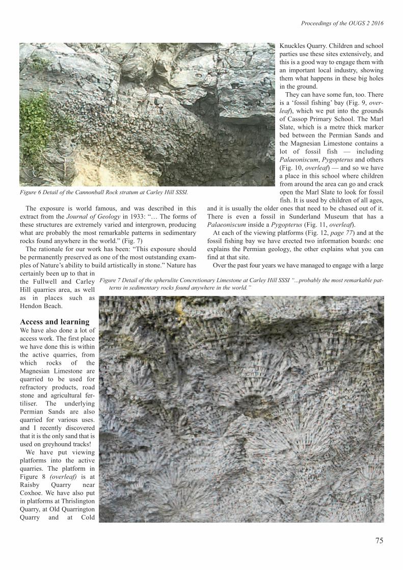
75
Proceedings of the OUGS 2 2016
The exposure is world famous, and was described in thisextract from the Journal of Geology in 1933: “… The forms ofthese structures are extremely varied and intergrown, producingwhat are probably the most remarkable patterns in sedimentaryrocks found anywhere in the world.” (Fig. 7)
The rationale for our work has been: “This exposure shouldbe permanently preserved as one of the most outstanding exam-ples of Nature’s ability to build artistically in stone.” Nature hascertainly been up to that inthe Fullwell and CarleyHill quarries area, as wellas in places such asHendon Beach.
Access and learningWe have also done a lot ofaccess work. The first placewe have done this is withinthe active quarries, fromwhich rocks of theMagnesian Limestone arequarried to be used forrefractory products, roadstone and agricultural fer-tiliser. The underlyingPermian Sands are alsoquarried for various uses.and I recently discoveredthat it is the only sand that isused on greyhound tracks!
We have put viewingplatforms into the activequarries. The platform inFigure 8 (overleaf) is atRaisby Quarry nearCoxhoe. We have also putin platforms at ThrislingtonQuarry, at Old QuarringtonQuarry and at Cold
Knuckles Quarry. Children and schoolparties use these sites extensively, andthis is a good way to engage them withan important local industry, showingthem what happens in these big holesin the ground.
They can have some fun, too. Thereis a ‘fossil fishing’ bay (Fig. 9, over-
leaf), which we put into the groundsof Cassop Primary School. The MarlSlate, which is a metre thick markerbed between the Permian Sands andthe Magnesian Limestone contains alot of fossil fish — includingPalaeoniscum, Pygopterus and others(Fig. 10, overleaf) — and so we havea place in this school where childrenfrom around the area can go and crackopen the Marl Slate to look for fossilfish. It is used by children of all ages,
and it is usually the older ones that need to be chased out of it.There is even a fossil in Sunderland Museum that has aPalaeoniscum inside a Pygopterus (Fig. 11, overleaf).
At each of the viewing platforms (Fig. 12, page 77) and at thefossil fishing bay we have erected two information boards: oneexplains the Permian geology, the other explains what you canfind at that site.
Over the past four years we have managed to engage with a large
Figure 6 Detail of the Cannonball Rock stratum at Carley Hill SSSI.
Figure 7 Detail of the spherulite Concretionary Limestone at Carley Hill SSSI “...probably the most remarkable pat-
terns in sedimentary rocks found anywhere in the world.”

The Limestone Landscapes Project / Devos
76
number of children. We have had [at the time of the lecture — Ed.]
4,800 children from 203 schools looking at the geology of the area,using both live and former quarries; and 613 secondary schoolpupils from 12 schools.
We have also produced a series of five Geotrail leaflets (Fig.13, opposite) as part of the Trails and Tribulations Project. Theseleaflets are available as hard copies and are also downloadablefrom the Limestone Landscapes website at http://www.lime-stonelandscapes.info/Pages/TrailsandTribulations.aspx. All theleaflets are well illustrated, and link the ecology, historic envi-ronment and the geology of the area.
• The Geotrail in South Tyneside, Cliffs, quarries and mills, hasa lot of information about the anhydrite dissolution, the DownHill Slide, and the formation of the reef and other localMagnesian Limestone rocks.
• The Rock in the city leaflet covers the centre of Sunderland,based on a walk conducted by local geologist Andy Lane.
• On top of the tropical reef tells you about the bryozoan equiva-lent of the Great Barrier Reef, and this leaflet looks at theTunstall Hills area where you can see the reef from the begin-ning of reef formation in the coquina all the way through tothe top and the end of the reef.
• Cliffs, caves and curious rocks looks at a number of differentrocks running down from the south side of Seaham in
Figure 8 Raisby Quarry viewing platform.
Figure 9 ‘Fossil fishing’ bay at Cassop Primary School.
Figure 10 Fossil fish from the Marl Slate: Pygopterus (above) and
Palaeoniscum (below).
Figure 11 Fossil fish from the Marl Slate: tail of Palaeoniscum inside the
body of a Pygopterus.
Dawdon to Hawthorn Dene. There are bits of reef and otherrocks formed again through the Magnesian Limestone on thecoast, along with the Easington Raised Beach.
• And last, Coal, clay and quarries features the back reef and thePermian Sands around Coxhoe, near some of the quarries there.
At the time of speaking we are just finishing a pair of interpreta-tion boards in Mowbray Park, right in the centre of the city oppo-site the Civic Centre. These replace signs saying “Danger fallingrocks” with “Danger! World class geology!” (Fig. 14, page 78),and act as signposts to the special Magnesian Limestone rocksfrom the heart of Sunderland City to elsewhere in the area.
There are a further three leaflets which look at the features offormer quarries that are now used for recreation and nature con-servation. These leaflets are part of the Kingdom of Quarries
Project and can be found on the Limestone Landscapes website athttp://www.limestonelandscapes.info/Pages/KingdomofQuarries.aspx
• Fulwell Quarry looks at the Concretionary Limestone again,and links it to a World War I ‘acoustic mirror’, which we havejust restored in the Quarry. Acoustic mirrors — a pre-cursorof radar — listened for Zeppelins, as there was a problem inSunderland (one of the major ship building areas) withZeppelin bombing during World War I. As soon as thisacoustic mirror was installed it put a stop to the bombingbecause its warning gave pilots 15 to 20 minutes extra time to

Proceedings of the OUGS 2 2016
77
get the aircraft up to shoot down the Zeppelins. The ‘mirror’was made from concrete from the local quarries.
• Marsden Old Quarry is a site visited as part of one of theSymposium field excursions. It contains two types ofConcretionary Limestone, along with some excellentMagnesian Limestone grasslands.
• The Kingdom of Quarries leaflet looks at four sites in the south-west of the area, all of which have now become DurhamWildlife Trust sites. The sites are now largely very importantMagnesian Limestone grasslands as a result of the quarrying.
Some sites are still Primary Magnesian Limestone grasslands,as they were not quarried at all; others, where quarrying hastaken place, are Secondary Magnesian Limestone Grasslands.
We also plan to publish a 190-page book called Built on an
Ancient Sea (Fig. 15, overleaf), about the Magnesian Limestonearea, showing how the geology links with the historic environ-ment and the ecology. It retails at £12 and will be available fromAmazon, or by contacting the Durham GeoHeritage Group byEmail at [email protected]
Figure 12 Interpretation panel explainingmt Permian Geology.
Figure 13 The Geotrail leaflets.

The Limestone Landscapes Project / Devos
78
Community participationWe have also done a great deal of community engagement ingeology. At former quarry sites such as Marsden Old Quarrymany of the geological features have been uncovered, such as theconcretionary limestones. Alongside the geology you can see theorchid-rich Magnesian Limestone grasslands. This helps to getlocal people with a variety of interests engaged with the sites.Local artist Ant Bryant, as his own initiative, talked to OwenPugh who owned a quarry just up the road and they gave him anyMagnesian Limestone he wanted for carving. Ant did this free ofcharge and we just had to pay to move the carvings. Figure 16shows an example of Ant’s work — a two-ton rock carving of thelizard of Lizard Lane. He also sculpted a sofa from MagnesianLimestone and an abstract piece. Ant did miniatures of each ofthese and turned them into treasure hunts round the quarry forlocal families, who could keep any miniatures of the MagnesianLimestone sculptures they found.
We have also carried out a project called the ‘Village Atlas’, inwhich both Paul Williams and Lesley Dunlop have been involved.The original Village Atlas concept came from theNorthumberland National Park. Initially they investigated thehistoric environment of each settlement to see how it developedover time, to find out what is left of the architecture and thearchaeology, and to identify what is important and why within thearea. This was done as the basis of developing ConservationAreas within the National Park. We thought, as a landscape part-nership, that we would like to take this concept further, so weincluded the geology, the ecology and the hydrology of the set-tlements, and worked with the local communities and schools to
study them. To date we have completed six Village Atlas projects:Wheatley Hill and Thornley; Elwick; Hetton-le-Hole; Ferryhill;Easington; and Cleadon.
The main Village Atlas is a document c. 400 pages long. Formany of the settlements we have also completed 40-page sum-maries, which we printed out and distributed in batches of 1,000to schools and members of the communities. These summariesare now all on our website.
The Village Atlas has been a really successful project, and wenow have a bid in to the Lottery Fund to do another 10 of themaround the Magnesian Limestone area. We have already hadapproaches from all the targeted communities wanting to dothem. There is a limit to what the records office can cope with interms of excited local people wanting to find out about the natu-ral and social history of their area.
From the Village Atlas projects there were a number of waysin which people were involved in their local geology. The firstand main route was to look at the maps of the settlements and
Figure 14 Panel 1 in situ in Mowbray Park.
Figure 15 Cover of Built on an Ancient Sea.
Figure 16 Lizard sculpture carved on Magnesian Limestone
by Owen Pugh in Marsden Old Quarr.

79
then visit key sites that illustrated important aspects of theirgeology. In Easington, Paul Williams took members of the localcommunity out to visit the site of the Easington Raised Beach(Fig. 17), which is now c. 50m above sea level and 30,000 yearsold. As part of the same project he led groups to Warren HouseGill to look at erratics from Iceland, part of an Earth HeritageSSSI in that area.
Another way that we have engaged communities is to look atthe stones used in the buildings and structures within their settle-ment. In Elwick, Lesley Dunlop led a tour of rocks from a vari-ety of different sources that had been used in the houses (Fig. 18).Alongside the Village Atlas projects we held a large number ofday-schools, looking at the elements of geodiversity outside thesix study settlements:
• Brian Young, the former BGS Area Officer, led a tour thatlooked at a variety of sites around Sunderland, including thetufa in Sunderland harbour (Fig. 19).
• Andy Lane, a local geologist, led a walk around the centre ofSunderland looking at the rocks in the buildings and Parks.
• Paul Williams has led a number of tours at Old Quarrington.Before we built the fossil fishing bay we used to do freelancefossil fishing at the edge of quarries.
• Paul also led a day-school looking at the Cannonball Rocks atRoker (Fig. 20).
All of these events have been well attended, and we have had torepeat them a number of times to cope with demand over a threeto four year period. We have also linked events to the historicenvironment, to biodiversity and to geodiversity, so that the audi-ence can see how these facets of landscape interact.
Training and skillsIn terms of the training and skills we have delivered professionaldevelopment for teachers. We ran a geocaching course to try andenthuse them, and there was also site-specific training, which gotthem out to a number of the geodiversity, biodiversity and his-toric environment sites. This was to show how they could use thespecial nature of this area in their teaching; 98 different teachershave participated.
We have also established geodiversity links to other projects.We restored coastal grasslands from Hawthorn Dene all the waydown to Crimdon Dene, which links to geodiversity. The inter-pretation there also supports geodiversity.
On the escarpment spurs, we did a lot of grassland restora-tion around Raisby Quarry, up into Coxhoe and Kelloe. Again,this involved a lot of rock work. The staff at Hope Constructionat Raisby Quarry were very helpful at involving children andpaying for fencing for grazing. We have rare-breed longhorn
Figure 17 Paul Williams leading a field trip to Easington
Raised Beach.
Figure 18 Lesley Dunlop explaining the stones used in the
buildings of Elwick Village.
Figure 19 Brian Young leading a Day School at the Tufa expo-
sures on Sunderland Marina.
Figure 20 Paul Williams leading a field trip to look at the Cannonball
Rock on Roker Beach.
Proceedings of the OUGS 2 2016

The Limestone Landscapes Project / Devos
80
cattle on that particular site, which graze the MagnesianLimestone grassland after the wildflowers have flowered andproduced seed.
The ‘Relics Rising’ project restored a number of the historicbuildings of the area, including limekilns (which obviously arehere because of the limestone), a blacksmith’s building atHetton-le-Hole and the Seaham Lifeboat House. These all usedlime pointing, and local geology provided material for thestructures.
We taught children about it all through Children’s Clubs, run-ning clubs at Cassop Primary School, in Castle Eden DeneNational Nature Reserve, and at Seaham. Geology figured in allof them.
Further, we have provided heritage skills training for local peo-ple in stone carving and lime pointing.
We advertise this material widely through websites and throughFacebook. We have an active community of viewers and contrib-utors; and we have produced newsletters, project updates, publi-cations and books.
I hope that this talk has given you an insight into how we at theLimestone Landscapes Project have been working with the geol-ogy of the area and what we have achieved. We hope to achievemore in the future. We would like to get all of the geologicalSSSIs in the area back into favourable condition. Of these, two orthree will be quite a challenge, but we’re up for the challenge!

81
Geoconservation and geodiversity — why it matters: examples from thePermian of the North East
Lesley Dunlop
[OUGS Newcastle Symposium: Pangaea: Life and Times; unfortunately, Lesley Dunlop was unable to write up her lecture as an arti-cle for the OUGS Proceedings. Therefore what follows is an edited transcription of the recording of the lecture. Transcription was com-pleted by Sally Munnings; editing is by POUGS Editor David M. Jones.]
Thank you for asking me to give this talk.
Geoconservation and geodiversityI am going to talk generally about the geoconservation and geo-diversity issues in England and then focus on the North EastPermian. There is some overlap with the subject matter present-ed by Tony Devos in the previous lecture. It is difficult to followsuch an inspiring project as the Limestones Landscapes Project;I just hope they get funding to continue it.
I will start by explaining the word ‘geodiversity’, as it is one ofthose words that has crept into our vocabulary over the last 20years in order to match the term ‘biodiversity’. Everybody iscomfortable talking about biodiversity, but geodiversity, as aterm, is relatively new. It is a good term because basically itincludes everything: rocks, minerals, landforms, soils and any-thing else we can talk about [that affects the landscape].Geodiversity is what everything else is built upon, so it is thefoundation for life, society and people. Also it gives that sense ofplace, which is what a lot of the Limestones Landscapes Projectis about — about the appreciation of where you are.
Those of you from this area are well aware that if you trav-elled around the places that Tony Devos discusses 30, 40 or 50years ago, they were entirely different. When I used to go onholiday down to Blackhall Rocks it really wasn’t as nice as itis today. For example, there were people carrying coal up fromthe beach.
The Geodiversity Charter for England was launched inOctober 2014. You can read about it on the websitewww.englishgeodiversityforum.org. Scotland also got anexcellent charter, which has been in use for about four years,including many spin off activities. You can even join thesite’s forum. We decided in England that what we needed wassomething just to promote geodiversity, just a ‘handle’, snap-shots and an explanations of how people could get involvedin conserving geodiversity.
The one message, especially true in the north-east ofEngland, but applicable to the country as a whole, is that thesecharters are ‘world class’. For example, if you travel throughFrance, most of the way down to mid-France, you will be inCretaceous and Jurassic rock for all of that journey. Suchhomogeneity is not the case if you travel around England —every few miles there is some totally different rock; and thisvariation is why we decided to work on the Charter. It gives anaim for promoting ways that people can take action and dosomething about geodiversity.
[Showing a PowerPoint (PP) slide of the West MidlandsDudley limestone caverns] You can see here that the youngster’svisiting them don’t engage with much. They live on the localestates, on the fringes of everything. So the project is aimed atgetting them to do something that engages withthe caverns andwhat they represent. Because the site is a cavern, and becauseyoung vistors can dress up and be ‘something different’, ourwork inspired them to become involved in a community project.
AbsractGeodiversity underpins and includes biodiversity. It is our rocks, soils, subsoils, landforms, landscape, water and minerals on land
and under the sea. It is important that this aspect is valued and promoted with the general population and there are a number of ways
that this can be done locally and nationally. The Permian strata of Co. Durham are important resources for local, national and inter-
national purposes. Locally the area is used for leisure and educational purposes, with many sites of open access and close to major
urban settlements. Nationally and internationally the stratsa are studied for their scientific value to help understand past environments,
and by industry — especially the oil industry — to better understand sequences seen in core samples. For these reasons it is impor-
tant that sites are conserved and maintained. Within the region there are many statutory and non-statutory sites, and recent project
work has enabled these to be brought into improved condition. This talk focused on some of the recent conservation work and chal-
lenges in the region, and also linked [the issues] to wider UK examples and initiatives, such as the English and Scottish Geodiversity
Charters and work done by local geoconservation groups within GeoConservationUK.
Collaboration among the Limestone Landscapes Project [see Tomy Devos, pages 73–80], Sunderland County Council and local
geologists has enabled, for example, the quarry at Carley Hill, part of the Fullwell and Carley Hill SSSI, to be cleared and improved,
thereby enabling study of a long section of concretionary limestone. Other work on an adjacent ‘acoustic mirror’ now means there is
much for visitors to see. There are many similar projects to improve local appreciation of the geological environment.
The coastal environment and instability of some of the Permian strata does provide challenges for conservation and compromises
need to be made between conservation of geologicasl exposures and public access and safety.Recent work at Hartlepool Headland to
reinforce the sea wall defences with rock armour has involved covering part of a Local Geological Site. While this is unfortunate, the
local authority was able to ensure that an assessment and record was made of the area under threat and to limit the effects as much
as possible. Other examples from the region were considered to show partnership and knowledge benfits.
If there is no engagement with geodiversity, then sites, landscapes and aspects of local character can be lost. Projects such as the
Village Atlases can make geology more accessable and relevant. Funding of site auditing means geodiversity can contribute more to
tourism, lifelong learning and health through walks and site conservation work, as has happened withing such local geodiversity audits.
Proceedings of the OUGS 2 2016, 81–4© OUGS ISSN 2058-5209

Geoconservation and geodiversity — why it matters / Dunlop
82
So the Charter’s principal aim it to promote ways to share goodpractice and raise local awareness. It is set out in a way that dif-ferent groups can appoach it in different ways.
[Referring to a PP slide of the Sunderland North Dock Tufa]This woman is from Estonia. She has come specifically to lookat this site, which many people might think is not particularlyinteresting. However, her group of international visitors cameespecially to look at this Sunderland site, having learned aboutit from our work on the Charter. We used the Sunderland NorthDock Tufa as an example of how you can work with localdevelopers and industry in order to preserve geodiversitybecause rock protrudes out of a wall where developers wantedto put a building. They could have easily just destroyed theexposure and built in a nice, normal, square fashion. What theydid, however, was to construct the building with a cavity in it sothat all of us can go and peer at this bit of tufa ‘growing’ out ofthe wall. This is a good example of working together — and ifyou take nothing else from tis article, please realise that every-thing about preserving and getting the message out on geodi-versity is working with people. If anybody wants me to comeand talk about geology, I will.
We owe Natural England for much of the funding to producethe Charter, and also the British Geological Survey who, free ofcharge, provided the designs.
NE England and the geodiversity partnershipReferring to north-east England, the English geodiversity forumis a partnership; it includes any organisation that wants to be partof it. There are big players and there are the small players. Forexample, one of the groups in the forum is Natural England.Natural England is responsible for the SSSI network, of whichthere are c. 1,200 in England. SSSIs provide a good link betweenbiodiversity and geodiversity.
Other sites [shown in a PP slide] are part of the geological con-servation review, of which there are c. 600 that are not SSSIs.Although they are nationally important sites they are not desig-nated as SSSIs because to take them through that process is cost-ly and time consuming. So one of the things we need to work onis to get such sites into SSSI statutory protection — because atthe moment they have no protection.
There is also a network of local geological sites, formerlycalled RIGS. There are c. 3,700 such sites, largely looked after bycounty groups and an organisation called GeoConservationUK,which coordinates the county groups.
[Showing a PP slide of Marsden Quarry] This slide focuses onits flowers rather than its rocks because this quarry is fantastic forits biodiversity. There are rock faces and fabulous sculptures, andwhat is important is to make links among biodiversity, the geodi-versity and any other diversity we wish to bring into it.
Co. Durham, particularly the coastline, has a set of world classsites. The vast majority of it is covered by some designation orother, whether it is a SSSI or other classification.
Tony Devos has already mentioned Carley Hill, and I willnow highlight what is happening with conservation at a fewother sites. Tony discribed the geodiversity audit for theLimestone Landscapes Project. There is also a Durham geodi-versity audit, which encompasses some of the main sites —SSSIs and local geological sites. It is worth reiterating Tony’scomment that this is just Co. Durham and that there are otherlocal authorities involved in this coastline conservation —
South Tyneside, Sunderland, Hartlepool just to mention a few.Thus our work is collaborative.
For the Limestone Landscapes audit they put out a gooddescriptive document, worth looking at alongside the BGS docu-ment and the sites described in it.
The conservation work at the Carley Hill and Fulwell SSSIswas funded as part of a scheme by Natural England.Unfortunately, most of the funding for the scheme has disap-peared and we are having to make applications for new funding,but all is not lost I think. In the Geodiversity Charter Report thegeology of Carley Hill and Fulwell is described as being,“famous for its bewildering array of bizarre calcite concre-tions”. As well as being a geodiversity site it is also of historicinterest to the local environment. Parts of the site are covered byhousing estates, so residents constantly walk around on thefootpaths through these SSSIs. Much of the quarried materialwas for lime burning and was taken out along a wagon track atthe Fulwell SSSI.
[Showing a PP slide of the site] The condition of the site washorrendous before it was cleared. The work by the LimestoneLandscape Project and the Local Council up to December 2013removed the trees and made the rock faces safe. This was noteasy because the rock strength is not great and there are manysmall faults in it, as well as folding and undulations along theface. The first bit of clearance left the corner with a whackingcrack running down through it. The site has open access, so it wasnecessary to knock off a bit of the corner so that visitors wouldnot stand underneath it and risk three tons of rock falling on them.Working with the Magnesium Limestone is not easy. To preventvisitors from climbing on top the rock faces, fencing was erectednext to the football field. The site looks much better now, as wellas being safer.
Hartlepool HeadlandAnother site I have been involved with recently is at HartlepoolHeadland. It is a local geological site on the foreshore on one sideof the headland. When the tide is in there is not a lot to see. Thelocal council needed to do urgent repairs on the sea wall, butbecause it is a local geological site there was the question of howthe repairs would affect geological exposures. The rocks areRoker Dolomites, but this site does not have the ‘cannon ball’features that you can see at Roker itself.
At the Hartlepool Headland site the dolomite is thinly beddedand there are some oolitic textures. It is cream-coloured, a longsection of which can be seen when the tide is out, and which youcan walk across to see a good sequence. My examination of itwas to see what would be lost from the geological site becausethe repairs of the sea wall decided by the local council.
The Hartlepool Star reported that, “The existing sea wall is ina really bad state of repair. If they don’t do anything about it overthe next 100 years and if it were to fail, [more than] 500 com-mercial and residential properties would be at risk of being erod-ed.” The projected cost was c. £9M. I would debate the sugges-tion of “the next 100 years”, as I think the coastal erosion will notbe gradual but will happen more suddenly due to a big storm orother such event; I do not think you can project over 100 years inthat sort of environment.
When I visited the site part of the wall had indeed collapsed,and there was a hole farther back on the promenade that need-ed urgent repair. Most of the wall had been patched piecemeal

Proceedings of the OUGS 2 2016
83
over the last 150 years and had large blocks that were begin-ning to collapse. The headland itself is also of historic interest.It has [the Norman church of St Hilda], largely built out of theMagnesium Limestone. It has a C20 gun battery, and a sculp-ture of a hanging monkey linked to the Napoleanonic Wars andlocal fishermen].
The proposed work to repair the sea wall will likely extend c.
12m, and will cover much of the geological exposure in someareas. It is always a difficult decision to make, and geoconserva-tion is always a compromise. But in reality the features that willbe covered can still be picked up elsewhere along the seafronthere. The bottom line is that, apart from one bit, when the tide isout you can get sufficiently far out to see the features [payingcareful attention to the tide times!]
Comparing this site with Roker, at Hartlepool there are fairlythin bedded units with muddy layers within them, some gyp-sum, and many small cracks on the surfaces of the beds. Thereare many conjugate joint sets that run out across the foreshore,which are the reason for the erosion. One feature that I was par-ticularly concerned about is the stack, because however I meas-ured it, the edge of the stack is within 12m of the existing wall.So I had to make a recommendation about being careful to pre-serve the stack.
A number of repair proposals were considered: one minimaland cheap and one with a bit more extensive armour. The geolo-gy consultation was considered last — isn’t it always?
The conclusion was an option to construct pinning over thewall because the wall is in such a bad state of repair. The rockarmour will not be a continuous neat block, but will be spreadout. It will give us geologists an opportunity to look at someScandinavian metamorphics.The repair rock is labelled as beinggranite, but it is not like any granite I have ever seen — perhapsgranite in a stonemason’s terminology. The work is ongoing atthe time of this lecture.
Marsden BayAnother area I have been looking at recently is Marsden Bay.Marsden Grotto is in this area and the bit I am interested inextends from the northern part almost down to SouterLighthouse. This project is another civil engineering project.
The Council is worried about the road that runs up the coastbecause there are various bits of erosion occurring, particularly inits southern section. I was asked to look at the geological aspects.In a PP slide Lesley pointed out a major fault with various otherfaults coming off at an angle. The area has been described as oneof the most complex stratigraphically and from an engineeringpoint of view.
It is the southern section of the bay that we are interested in, thegeology close to the road. Every month my colleagues are mak-ing 3D laser scans of the cliffs. They superimpose each month’sscans to see if there are any differences. They are looking to seehow the cliff is evolving over two years; presently they are aboutnine months into this project.
The rock strength is weak. A big problem is the dissolutionof the anhydrites; there is a lot of disturbance from collapsedbreccias and erosion, which, when it gets back to a criticalpoint, will collapse the rock face. In some places there arecemented breccias — different from the collapsed breccias —that occur just where you expect the fault to come along. Thisanalysis is ongoing.
The underlying geology, which on the map looks as if it is allone thing, has a number of other factors coming into play at thissouthern end. Marsden Quarry is still a working quarry, where thetop layers have been stripped, which changes the water flowthrough some of the faults and cavities. Farther south an old quar-ry was infilled, but a large hole has developed, also affectinggroundwater movement, and the quarry above it will be a factorin some of the erosion. It may even be necessary eventually to re-route the road through the quarry.
Middridge Quarry partnershipMiddridge Quarry, which has exposed down to theCarboniferous, has several things of geological interest: someof the oldest plants, and tetrapods. And owing to the ongoingpartnerships there is a 3m-wide open access footpath adjacentto it. Anyone travelling between Newton Aycliffe and Shildoncan use this footpath, which goes through rocks dating from thePermian to the Carboniferous and passes by the entrance to thequarry. There are steps and access into the quarry and an inter-pretation board is planned, a good example of what has comeout of the partnership.
The footpath was opened in October 2014 and people withpushchairs, people in wheelchairs and the blind can all get alongthe path safely due to the wide access. An interesting follow-onfrom this arrangement is that a group of the blind people haveexpressed interest in other geology walks suitable for blind peo-ple’s access. (I also work a lot in Berkshire, where you can’t see thegeology, so I am used to talking about things you cannot see.)
The Elwick Village AtlasTony Devos described the Elwick Village Atlas. Elwick is a vil-lage near Hartlepool. My involvement was solely just to talkabout the geology [showing a PP slide of a ‘typical wall inElwick’ and pointing out a bit of the local Magnesium Limestone,a bit of the Whin Sill, and other different materials].
The local people recognised that they were on the MagnesiumLimestone, with a large fault running just to the south and pro-viding good views toward Teesside, but initially they did notthink they had any of the bedrock in their local buildings as it iscovered by superficial material in the local area. So at first theyexpressed little interest in a project on their local buildingstones. We showed them that the till coating the local bedrockhad in fact brought in most of the locally used building stones;that there were bits of the Whin Sill, igneous rock probably fromthe Cheviots and other stone types. Materials had been broughtdown the coast from the Tyne, from the Cheviots, and a lot fromthe Midland Valley; possibly even some material from theAberdeen area.
So the hotchpotch of materials in their walls suddenly mademore sense. Their local church is built largely out of MagnesiumLimestone. We also showed them that bits of MagnesiumLimestone in local buildings still looks good, that but the sand-stones in the area are really poor, possibly due to pollution creep-ing up from Teesside. For example, the churchyard gravestonesandstones are horribly eroded. That was something else wecould make them appreciate.
North Dock TufaA final examle of partnership work with local people is the NorthDock Tufa. We hope to get this site designated a SSSI in the near

Geoconservation and geodiversity — why it matters / Dunlop
84
future. Natural England is working with a group of people to des-ignate, in particular, some local currently depositing tufa sites aspart of the geological geoconservation review.
There are two sites in the north-east of this area that are likelyto be put forward. One is a site at Dipton, where a small streamhas currently depositing tufa, depositing over 89 cascades of thesteam — absolutely fabulous. The stream is, however, certainlynot depositing calcium-rich water coming from farther up the
hill, as these are sandstones (which would be acid). Instead, it isdeep water that is bringing that material up.
The reason that North Dock and its tufa are important is that thearea is a rare habitat. For example, crayfish like to live in amongthe tufa and there are several fly species and other invertebratesthat only live in this particular type of habitat. It is likely thatthese two sites will be incorporated into the Geodiversity CharterReport and therefore put forward for SSSI designation.

85
Before I start the summing up, while I get a chance to do this,I would like to offer a vote of thanks to the organisers of this
weekend, which I have thoroughly enjoyed and I am sure thatyou have too. So thanks to Paul, Karl, John, Olwyn, John,Andrew and Steve.
I have never lived on the Permian in the UK; I have neverworked on the Permian at all. So this weekend has been some-what of a revelation for me, but great fun. There have been a widevariety of speakers plus a field trip today. It has really given mesome fantastic insights into both the Period [and] the time, [andinto] its paleogeography and also its place in the North East, andparticularly latterly, as Lesley [Dunlop] mentions, the landscapeand the sense of place that geology brings to a landscape. That isvery important as well as just the geology.
But, we will start with the geology, and I must mention that Ihave a train to catch as well, so this will be relatively brief I think,although I think that we have enough time. Anyone else who hasa train to catch, please feel free to leave at any time, and I won’thold it against you, as I may in fact be leaving as well, quite pos-sibly before I’ve finished!
Paul WilliamsOn Friday evening Paul Williams was presented to us, fullyclothed, which is a bonus! And he gave a lovely introduction toPangaea and the Permian geology of north-east England; a real-ly good introduction, particularly good as he confessed thathe’d spared us the sequence stratigraphy, so that was a realbonus as well.
We learned that the North East was a marine basin, while therest of Britain he describes by this lovely phrase as ‘not somarine’. And because it was a marine basin, you have all thosewonderful scenarios that before the Permian there was theVariscan deformation, which set up the particular tectonic con-figuration of this very restricted basin with a very narrow outletto the north.
So, first of all in the Permian. You had an arid environment,not a basin environment, a fairly low-lying environment, but anarid desert of those famous yellow sands, the RotliegendGroup. Some of it was so low-lying that it was even below sealevel, so it was described by Paul as a ‘depressed area’. So, abit of history there as well. Then there was the Zechstein Seatransgression over this very low sill in the basin at the northernend, with a transgression of the marine waters into that basinand the marl slate being deposited with its fabulous fossil fish-es in that very odd euxinic environment, just while the basinfilled up. And then as you move on up through the succession,you go up into the Magnesian Limestone, although we’re notallowed to call it the Magnesian Limestone anymore, so wehave to call it the Zechstein Group. But I’m going to keep call-ing it the Magnesian Limestone, with all its wonderful differ-ent facies, the barrier reefs, the back reef, the shelf, the slope
Newcastle Symposium 2015: Summing up
Dr Tom Argles, OUGS President
(Senior Lecturer in Earth Sciences, The Open University)
[OUGS Newcastle Symposium: Pangaea: Life and Times; original transcription by Norma Rothwell and Maggie Deytrikh from theSymposium recording; edited by Dr Argles and POUGS Editor David M. Jones.]
apron, all those sorts of things, with a cross-section right acrossthat Permian basin margin, which has given us such a lovelyvariety of rocks, particularly to look at today. That concludesFriday evening.
Eddie DempseySo we move on to Saturday morning, fortified by breakfast, formost of us, and we move onto the North Pennine Orefield. Eddietold us about his work, which is really cutting-edge, up to theminute stuff, in review, so it’s not even published as yet. Heexplained it as, “It’s not what we thought it was”; which, ofcourse, is what all good new work should be.
Throw out the old stuff, they are all talking rubbish, we’ve gota new theory that we are going to put forward. So we learnedthat the orefield and the mineralisation was not due to this chim-ney effect of drawing in the fluids from the Zechstein into thevicinity of the still warm Weardale Granite and then taking thosefluids through the granite, picking up all those lovely elementsand redepositing them above. This is apparently wrong. It is infact much more to do with a much more complicated successionof events that he mapped out for us. And he went back to somevery detailed work on rhenium-osmium isotopes (Re-Os), whichI thought was really nice. I’ve worked very briefly and tenta-tively on Re-Os isotopes, with some colleagues in the OpenUniversity and it is rather butch chemistry I have to tell you. Itinvolves flame throwing. You have these sealed tubes of aqua
regia, if you know what that is?You have to flame the top off so you score around with a
scalpel type of thing and then you flame with a flame torcharound, and it pings off, usually into your colleagues face, andthen you pull this stuff out and commit more unspeakable actson it. This is Re-Os chemistry, but I didn’t do that for long at all,so my opinion of Eddie was raised dramatically as he’s obvious-ly a guy who knows what he’s doing. So the Re-Os told us thatthese minerals were deposited and [that] they have [a] similarage to the Whin Sill, about 295Mya and they also have a similarsort of source, a mantle source, which was quite nice; that’s fromthe initial Re-Os ratio.
So a Mantle source, something connected to the Whin Sill, bothin time and geochemistry, [and] so apparently not much to dowith the Weardale Granite at all. And he also pointed out from thestructural orientation of these veins that you can see differentgenerations, earlier generations are more aligned to the VariscanN–S compression, and then later veins in the Permian, which aremore to do with the N–S transtensional event. So this is when thePermian basin, having been compressed for several hundreds ofmillennia, then finally got the chance to relax and extend, andthen, as Eddie said, it can then start to melt. So that was the storyof the Permian basin there.
You will be able to track the progress of this through how manysheets I tear off! [Tears one sheet off his notepad — Ed.]
Proceedings of the OUGS 2 2016, 85–8© OUGS ISSN 2058-5209
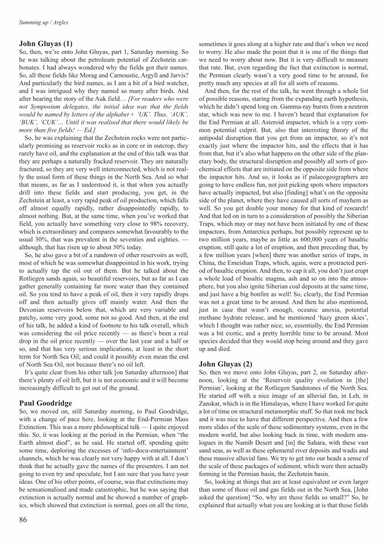
Summing up / Argles
86
John Gluyas (1)So, then, we’re onto John Gluyas, part 1, Saturday morning. Sohe was talking about the petroleum potential of Zechstein car-bonates. I had always wondered why the fields got their names.So, all these fields like Morag and Carnoustie, Argyll and Jarvis?And particularly the bird names, as I am a bit of a bird watcher,and I was intrigued why they named so many after birds. Andafter hearing the story of the Auk field… [For readers who were
not Symposium delegates, the initial idea was that the fields
would be named by letters of the alphabet + ‘UK’. Thus, ‘AUK’,
‘BUK’, ‘CUK’… Until it was realised that there would likely be
more than five fields! — Ed.]
So, he was explaining that the Zechstein rocks were not partic-ularly promising as reservoir rocks as in core or in outcrop, theyrarely have oil, and the explanation at the end of this talk was thatthey are perhaps a naturally fracked reservoir. They are naturallyfractured, so they are very well interconnected, which is not real-ly the usual form of these things in the North Sea. And so whatthat means, as far as I understood it, is that when you actuallydrill into these fields and start producing, you get, in theZechstein at least, a very rapid peak of oil production, which fallsoff almost equally rapidly, rather disappointedly rapidly, toalmost nothing. But, at the same time, when you’ve worked thatfield, you actually have something very close to 98% recovery,which is extraordinary and compares somewhat favourably to theusual 30%, that was prevalent in the seventies and eighties. —although, that has risen up to about 50% today.
So, he also gave a bit of a rundown of other reservoirs as well,most of which he was somewhat disappointed in his work, tryingto actually tap the oil out of them. But he talked about theRotliegen sands again, so beautiful reservoirs, but as far as I cangather generally containing far more water than they containedoil. So you tend to have a peak of oil, then it very rapidly dropsoff and then actually gives off mainly water. And then theDevonian reservoirs below that, which are very variable andpatchy, some very good, some not so good. And then, at the endof his talk, he added a kind of footnote to his talk overall, whichwas considering the oil price recently — as there’s been a realdrop in the oil price recently — over the last year and a half orso, and that has very serious implications, at least in the shortterm for North Sea Oil; and could it possibly even mean the endof North Sea Oil, not because there’s no oil left.
It’s quite clear from his other talk [on Saturday afternoon] thatthere’s plenty of oil left, but it is not economic and it will becomeincreasingly difficult to get out of the ground.
Paul GoodridgeSo, we moved on, still Saturday morning, to Paul Goodridge,with a change of pace here, looking at the End-Permian MassExtinction. This was a more philosophical talk — I quite enjoyedthis. So, it was looking at the period in the Permian, when “theEarth almost died”, as he said. He started off, spending quitesome time, deploring the excesses of ‘info-docu-entertainment’channels, which he was clearly not very happy with at all. I don’tthink that he actually gave the names of the presenters. I am notgoing to even try and speculate, but I am sure that you have yourideas. One of his other points, of course, was that extinctions maybe sensationalised and made catastrophic, but he was saying thatextinction is actually normal and he showed a number of graph-ics, which showed that extinction is normal, goes on all the time,
sometimes it goes along at a higher rate and that’s when we needto worry. He also made the point that it is one of the things thatwe need to worry about now. But it is very difficult to measurethat rate. But, even regarding the fact that extinction is normal,the Permian clearly wasn’t a very good time to be around, forpretty much any species at all for all sorts of reasons.
And then, for the rest of the talk, he went through a whole listof possible reasons, staring from the expanding earth hypothesis,which he didn’t spend long on. Gamma-ray bursts from a neutronstar, which was new to me. I haven’t heard that explanation forthe End Permian at all. Asteroid impactor, which is a very com-mon potential culprit. But, also that interesting theory of theantipodal disruption that you get from an impactor, so it’s notexactly just where the impactor hits, and the effects that it hasfrom that, but it’s also what happens on the other side of the plan-etary body, the structural disruption and possibly all sorts of geo-chemical effects that are initiated on the opposite side from wherethe impactor hits. And so, it looks as if palaeogeographers aregoing to have endless fun, not just picking spots where impactorshave actually impacted, but also [finding] what’s on the oppositeside of the planet, where they have caused all sorts of mayhem aswell. So you get double your money for that kind of research!And that led on in turn to a consideration of possibly the SiberianTraps, which may or may not have been initiated by one of theseimpactors, from Antarctica perhaps, but possibly represent up totwo million years, maybe as little as 600,000 years of basalticeruption, still quite a lot of eruption, and then preceding that, bya few million years [when] there was another series of traps, inChina, the Emeishan Traps, which, again, were a protracted peri-od of basaltic eruption. And then, to cap it all, you don’t just erupta whole load of basaltic magma, ash and so on into the atmos-phere, but you also ignite Siberian coal deposits at the same time,and just have a big bonfire as well! So, clearly, the End Permianwas not a great time to be around. And then he also mentioned,just in case that wasn’t enough, oceanic anoxia, potentialmethane hydrate release, and he mentioned ‘hazy green skies’,which I thought was rather nice; so, essentially, the End Permianwas a bit exotic, and a pretty horrible time to be around. Mostspecies decided that they would stop being around and they gaveup and died.
John Gluyas (2)So, then we move onto John Gluyas, part 2, on Saturday after-noon, looking at the ‘Reservoir quality evolution in [the]Permian’, looking at the Rotliegen Sandstones of the North Sea.He started off with a nice image of an alluvial fan, in Leh, inZanskar, which is in the Himalayas, where I have worked for quitea lot of time on structural metamorphic stuff. So that took me backand it was nice to have that different perspective. And then a fewmore slides of the scale of these sedimentary systems, even in themodern world, but also looking back in time, with modern ana-logues in the Namib Desert and [in] the Sahara, with these vastsand seas, as well as these ephemeral river deposits and wadis andthese massive alluvial fans. We try to get into our heads a sense ofthe scale of these packages of sediment, which were then actuallyforming in the Permian basin, the Zechstein basin.
So, looking at things that are at least equivalent or even largerthan some of those oil and gas fields out in the North Sea, [Johnasked the question] “So, why are those fields so small?” So, heexplained that actually what you are looking at is that those fields

are segmented; they might be broken up by later faulting, theymight be domed up by salt domes, for example. But equally, theymight have smaller scale things like faults and granulation seamscutting through them, and each of those is potentially segmentingthat large sedimentary package into much smaller pieces, whichcan then act as individual segmented reservoirs. And he had anice exposition of the role of baryte, as a cement, which is a bitstrange, considering that they pump it down the hole to get the oilout in the first place. So that’s one way he explained of cloggingup a hole, pump the baryte down, cement it all off, that’s it, thenyou’re not going to get anything out of it. Then he looked close-ly at different cements in these Rotliegen Sandstones: illite claycements, carbonate cements, maybe baryte cements and dolomitecements. He’d looked into the source of the illite recently. Thepore water for those Rotliegen Sandstones is Jurassic rainwater,but he was puzzled by where the aluminium for that clay miner-al came from? And his thesis at the moment is that, along with theiron oxide, if you think of a desert varnish type environment,there’s bauxite dust, there’s actually aluminium dust around inthe very deep tropical weathering that you would have at thattime, in that arid environment. So, you have bauxite dust, whichis, of course, mostly aluminium oxide, and that coats some of thegrains as well as the iron oxide. So, that could provide an in situ
source for the aluminium, rather than invoking all sorts of weirdfluids as something [that] would have been able to bring the alu-minium in, from farther away.
And just as a last aside from John’s talks, which I reallyenjoyed actually, I am looking forward very much to his forth-coming paper ‘Pyrites of Penzance’. I had to make that jokeagain, too good to miss!
Neil RowleySo, Saturday afternoon, with Neil Rowley and we had a slightchange of scene again — and we were looking at mining in theZechstein evaporates at Boulby. Now, I’ve never been downBoulby, I’d love to go. It seems to be a shame as they’re think-ing of scaling down those visits, which is a real shame. Amazingengineering that’s required to mine these potash salts, from notjust under the ground, but seven miles out into the North Sea;and presumably ‘fingering’ out all these different roadwaysunder the North Sea, and keeping those markets supplied. But,also interesting, apart from the engineering, was the recent pricerise, which saved Boulby in the late 2000s [c. 2006–7]. So, [Neilthen] explained that the company was spending money “like adrunken sailor”, which was rather nice for this part of the world.So, that fantastic description of, “We need a new shaft”; “Let’sjust do it”; “It doesn’t matter how much it costs, but how are wegoing to do it?”; “We can’t close the mine down for more thanabout three weeks”; “Can you do it in that time?”; “Oh, proba-bly, yes, we’ll draw some plans up and see what we can do?” Butthen, I thought that was absolutely extraordinary: you just cut itoff at the base. This is like primary school engineering. You justcut it off at the base, shift it over there, and then we’ll have thenew one and we’ll just put that in; ‘Bobs your uncle!’ — and itworked; extraordinary!
A fantastic story. I loved that talk, I could have gone on aboutthat talk forever. The last thing that I learnt from [Neil’s talk] thatI wanted to just remind you of, was that I now know why theNorth Sea is so salty? It’s because of all the amount of saltpumped out of Boulby!
87
Karl Egeland-EriksenSo, finally on Saturday, we came to Karl [and] ‘The history ofPermian geological investigation in north-east England’. Therewas an early slide of an old portrait of an old geological gentle-man, but he didn’t have a beard! This took me back to writing OUcourses over a number of years, where each first time, we’d sitdown for the first time with the module team and think about thecontent. First thing; how can we introduce the subject? And sooften, we would look back at the old books and we have a wholesuccession of photographs of ancient geological gentlemen withbeards. They all had to have beards. So, it’s actually quite a nicechange to see a whole succession of geological gentlemen, veryfew of whom had beards! Some of them had quite impressivesideboards but not beards. So, that was a nice change.
So, Karl mapped out for us beautifully this voyage of discov-ery of these various geological gentleman, or not even geologi-cal, as most of them actually were medical early on, which isslightly alarming. Mapping this journey of the MagnesianLimestone, from magnesia alba through to, what was describedas ‘calcareous manures’ — an interesting thought, although wedid see some peloidal mudstones today [on the field trip], so Iguess they are, kind of, ‘calcareous manures’ — through to ‘hotlime’, which sounds like some kind of pop group.And then we went through all these different characters. I am notgoing to name then all [but they included] Smithson, Tenant, andJames Sowerby, via some real giants’ names — Sedgewick,Buckland, Murchison, the giants of geology, [and] Louis Agassiz.And then through some local characters, such as King, Howseand Kirkby, who had these slightly tricky relationships at times inthe local community, fighting to be curator of the local museum.Interesting thought. And then right up to Dennis Smith, who wasdescribed as ‘Mr Permian’. You’ve heard about Mr Smith, butthat will have to wait for another time.
So, thank you to Karl for that, it was a really nice change ofpace at the end of the day.
We then had an excellent dinner. That was very good, followedby the ceilidh and I think that the less said about that the better.I am sure that you all enjoyed yourselves. And then, we came onto today. We had the Sunday field trips. I remember this morn-ing, lying in bed for a few minutes, thinking ‘Is that the showeror is it rain?’ As it turned out, it really worked out fairly well. Ithink that we only got rained on very slightly, no more than arefreshing sprinkle, so that worked fine. I had a great time. Youcan’t really ask for much more than spending a day on the beachin the sunshine and ending up in a pub, a very well-designed trip,in the true traditions of geological fieldtrips! “Did nobody elsego for a pint?”
Tony DevosThen finally, we ended up back here and we listened to a love-ly couple of talks with a slightly different emphasis this after-noon. Tony, on the limestones landscapes project, national char-acter areas, which I’ve read quite a bit about actually, whiletrawling through the internet for ridiculous facts to put into OUcourses to wake the students up. So, a really nice rundown ofwhat they’re doing — and they’re obviously doing a hugeamount of work. So, yes, they got a fair amount of money fromthe lottery and a lot of help from partners, but they are doing ahuge amount.
Proceedings of the OUGS 2 2016

They’ve done a geological audit with the BGS, conserving andrestoring the quarries. I did like the description of one of the quar-ries, prior to their work, as a ‘Bring your own machete quarry’!Access to live quarries as well, both for adults and school chil-dren. ‘Fossil fishing’, that was a brilliant idea, absolute genius.I’ve been to Quarrington and done the Quarrington experienceand done my own fossil fishing experience, but having it in a pri-mary school is just a genius idea I think. And some of the engage-ment figures that he was coming up with; nearly 5,000 primarypupils engaged in this project from 200 or so schools. That’s justamazing. And the trails and tribulations pamphlets. The bookthat’s coming out, which I might just do a quick plug for again,in October, village atlases, more field trips, an amazing amountof work that’s been going on, really inspiring. And good to hearthat he’s still up for further challenges.
Lesley DunlopAnd, finally, we come to Lesley Dunlop, at the end of the day:Geoconservation and Geodiversity, why it matters.
I have a couple of quotes here: “Geoconservation is always acompromise”. I did like that. The feeling that you are constantly,not quite treading on eggshells, but constantly jockeying posi-tion, constantly manoeuvring, with both partners and the opposi-tion — [with] everybody involved, I suppose the name youwould call them nowadays would be ‘stakeholders’. So, geocon-servation, quite a tricky subject. We tend to think of maybe any-one who’s involved with any kind of conservation just wantstheir bit. We want to make it the way we want it, but it’s not aseasy as that; as you’ve always got lots of other people involved.And her idea is that geodiversity is the foundation and that notjust geology as the foundation of the landscape in the physical
Summing up / Argles
88
sense, but also in a historical and cultural sense, and it gives itthat sense of place. And I don’t know if this kind of thing is hap-pening in any other country? These character areas, if you like —because it’s certainly something that I think is almost unique tothe UK, certainly on that smaller scale, that you get such a dif-ference as you drive or go by train from district to district,because of the changing geology and the changing biodiversitythat goes with that. It’s a lovely country to live in and it’s won-derful to come to a place like the North East, which is, I thinkunique in Europe and has some of the best — Paul [Williams]mentioned this a couple of times — some of the best geology inEurope, some of it absolutely world-beating. I just thought thatI’d throw that in again.
So, Lesley is talking about saving tufa sculptures, such avariety of things, making quarries safe and making quarriesvisible, which is always nice. And the bewildering array of cal-cite concretions in some of those quarries, but she’s [also] deal-ing with things like rock armour coastal defences, laser scan-ning of cliffs, which we’ve done a bit with laser scanning ofinland sites for virtual field trips. It’s quite fruitful work attimes. And then looking again, back to the villages and thebuilding stones in the villages.
So, I think a wonderful span and scope of different talks, allthrough the weekend. I’ll leave you with the last thing I learnedfrom Lesley’s talk which was — it kind of overturned a myth thatI’d had in my mind for pretty much forever from OU studies —that “sandstone is not always more durable than limestone”, andI think that it’s quite a nice note to end on for our weekend withthe Magnesian Limestone.
So thank you very much.

89
OUGS Field Trip Reports
Introduction
The OUGS President traditionally leads a field trip in his orher second year in the position and Tom suggested that revis-
iting his PhD area in southern Spain would be an interestingfocus for his trip. Jan Ashton-Jones, aided by Linda Fowler,offered to organise the event and loaned their holiday cottagebetween Antequera and Granada to Tom and his family for areccy in the preceding October.
The Betic Cordillera is a geological domain distinct from therest of Iberia and lacks the older basement terranes andHercynian deformation found elsewhere in Spain. It lies at thewestern end of the Tertiary Alpine-Himalayan mountain beltand is dominated by folding and thrusting resulting from com-pressional tectonic processes. Locations visited were mainly inthe Internal Zone between Ronda and the coast, in the ExternalThrust Belt near Antequera, and in the Internal Zone south ofGranada. Much of the trip was based around the large peridotitebodies exposed in the western Betic Mountains. These havebeen Rh-Os dated at 1.36Ga, the date when the material movedfrom mantle to continental crust. This article is an account ofthe trip by those who took part and, while it describes the loca-tions we visited, does not attempt to explain the overall geolo-gy in any detail.
Day 1 — Wednesday 29 AprilOverview from Málaga to Ronda
Linda Fowler
Our group of 20 met up at Málaga Airport during the morning ofWednesday April 29, picked up rental cars and set off towardsRonda, the first base, where we stayed at a traditionally Spanishhotel, centrally located between the Puente Nueva and the his-toric bull ring.
Our route from the airport initially took us south-west abovethe coast and then inland from San Pedro de Alcántara toRonda. We made an incidental first stop for coffee and tapas
at the Arroyo de Miel service area on the AP-7 toll road andtook this opportunity to ‘get our eye in’ on the Palaeozoic mar-ble exposed in the cutting behind the restaurant before head-ing up the 1970s ‘tourist’ road (A-396) from the coast toRonda. This road was upgraded from a ‘C’ road to take coachtour traffic, and is unusual in that it does not pass through anytowns or villages.
At a cutting near Km 34 [36.558176, –5.052443] we stoppedfor a view over the coast and had our first lesson in spottingperidotite locations — they are covered in pine trees, whichseem to prefer this substrate. Rock fragments at the roadsideincluded carbonates from nearby quarries, the local peridotite,metagranite (which has black specks of chromite and spinel onjoint surfaces) from below the peridotite sheet, and apparentlywaterworn pebbles of migmatitic breccia (aka lithoclasticgneiss), some of which contained post-kinematic garnets (Fig.1.1). We found various examples of this stretched, flattened,folded and refolded material containing blobs of quartz andlithic clasts (Fig. 1.2, overleaf).
At a second stop on this road, just past the Pujerra turn at Km24.5 [36.614832, –5.070215], we were able to see the remarkablyclear surface vegetation expression of the junction between thepine-tree-covered peridotite and the bare hillside of Dorsale
Limestone (Fig. 1.3, overleaf).
Mantle in the Mountains: a geological excursion to the Betic Cordillera inMálaga and Granada Provinces, Andalucía, Spain
OUGS President’s Trip 2015: Leader Dr Tom Argles, Organiser Jan Ashton-Jones
Authors: Jane Browning, Sam Capstick, Caroline Deans, Linda Fowler (and editor),
Mellissa Freeman, Chris Hodgson, Terri Newton, Michael Perkins, Bernard Skillerne de
Bristow, Paul Speak, Oliver Strimpel and Stuart Swales
Other participants: Pete Hodgkinson, David M. Jones, John Lamont, Margaret Poole,
Muriel Rogers and Paul Taylor
Latitude and longitude of locations are indicated in degrees decimal; images are by the individual authors except where other-
wise indicated.
Figure 1.1 Post-kinematic garnets have grown across the fabric of the
lithoclastic gneiss in this hand specimen.
Proceedings of the OUGS 2 2016, 89–114© OUGS ISSN 2058-5209

Mantle in the Mountains ... Andalucía, Spain / Browning et al.
90
Day 2 — Thursday 30 AprilSierra Bermeja peridotite and underlying gneiss
Linda Fowler
On the following morning we headed back down to Estepona onthe coast and then took the MA-557 towards the Sierra Bermeja
peridotite massif, where we stopped initially in a car park atPuerto de Peñas Blancas before heading off for the main loca-tions along a forestry track. Los Reales de Sierra Bermeja is aParaje Natural (Protected Natural Site) important for being oneof the largest outcrops of peridotite in the area. This rock givesthe mountains their characteristic colour and their name: Bermeja
translates as ‘ginger or russet coloured’, which is certainly true ofperidotite hills.
Puerto de Peñas Blancas [36.480193, –5.200316]: In theback wall of the parking area we found a leucocratic dyke,almost horizontal in aspect (Fig. 2.1). This quartz- and plagio-clase-rich dyke has an annealed fabric with brittle fractures,which are a response to post-cooling stress and containsdiopside and blue-green chromite (Fig. 2.2). It has probablybeen injected from below into the country rock, which at thispoint is plagioclase peridotite indicating shallow mantle ori-
gins. Farther up the hill the country rock is granular, spinelperidotite with garnets and tectonic foliation; although it ini-tially appears odd that the higher-pressure rocks are topo-graphically higher, they represent different time steps in thestory. The peridotite sheet was thrust over material that wasoriginally a breccia, and heated the latter to the point whereshallow partial melting took place to produce a matrix of low-pressure granitic melt.
From here we drove down the hill and then some 2–3km alonga forestry track [36.498060, –5.198620 to 36.513400,–5.207472], which contoured around the hillside to the north ofPico de los Reales, to explore the distribution of mafic layerswithin the peridotite (Figs 2.3, 2.4, 2.5, opposite). In some maficlayers the garnets are small swells in the thin layers of ‘marginalmylonites’, which also include a lineation of aligned, elongateorthopyroxene crystals (Fig. 2.6, opposite).
Figure 1.3 View NW from Km 24.5 to the steep, faulted junction between
pine-clad peridotite and poorly vegetated limestone.
Figure 1.2 Folding seen in a hand specimen of lithoclastic gneiss.
Figure 2.1 The leucocratic
dyke at Puerto de Peñas
Blanca is almost flat
lying.
Figure 2.2 Close up of leuco-
cratic rock in dyke at
Puerto de Peñas Blancas.
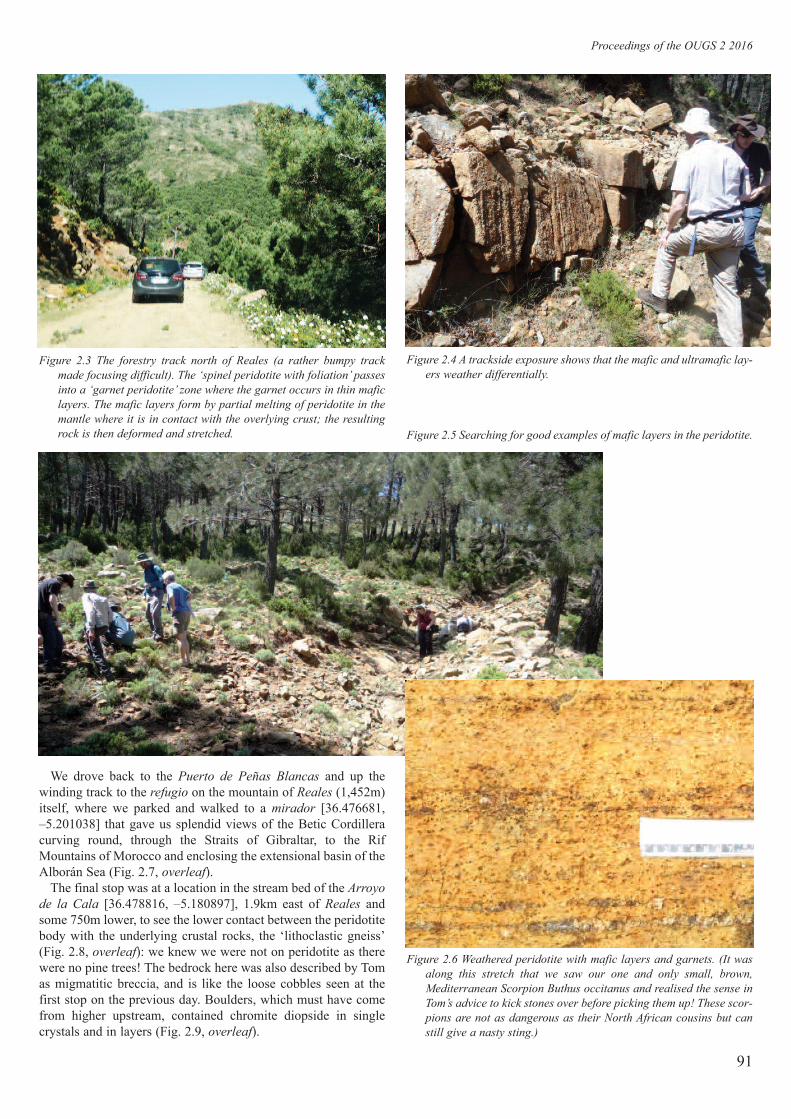
Proceedings of the OUGS 2 2016
91
Figure 2.5 Searching for good examples of mafic layers in the peridotite.
Figure 2.3 The forestry track north of Reales (a rather bumpy track
made focusing difficult). The ‘spinel peridotite with foliation’ passes
into a ‘garnet peridotite’ zone where the garnet occurs in thin mafic
layers. The mafic layers form by partial melting of peridotite in the
mantle where it is in contact with the overlying crust; the resulting
rock is then deformed and stretched.
Figure 2.4 A trackside exposure shows that the mafic and ultramafic lay-
ers weather differentially.
Figure 2.6 Weathered peridotite with mafic layers and garnets. (It was
along this stretch that we saw our one and only small, brown,
Mediterranean Scorpion Buthus occitanus and realised the sense in
Tom’s advice to kick stones over before picking them up! These scor-
pions are not as dangerous as their North African cousins but can
still give a nasty sting.)
We drove back to the Puerto de Peñas Blancas and up thewinding track to the refugio on the mountain of Reales (1,452m)itself, where we parked and walked to a mirador [36.476681,–5.201038] that gave us splendid views of the Betic Cordilleracurving round, through the Straits of Gibraltar, to the RifMountains of Morocco and enclosing the extensional basin of theAlborán Sea (Fig. 2.7, overleaf).
The final stop was at a location in the stream bed of the Arroyo
de la Cala [36.478816, –5.180897], 1.9km east of Reales andsome 750m lower, to see the lower contact between the peridotitebody with the underlying crustal rocks, the ‘lithoclastic gneiss’(Fig. 2.8, overleaf): we knew we were not on peridotite as therewere no pine trees! The bedrock here was also described by Tomas migmatitic breccia, and is like the loose cobbles seen at thefirst stop on the previous day. Boulders, which must have comefrom higher upstream, contained chromite diopside in singlecrystals and in layers (Fig. 2.9, overleaf).

92
Figure 2.8 Arroyo de la Cala: a stream section through the unit below
the base of the peridotite sheet.Figure 2.9 (a), (b) Peridotite with layering and chrome diopside crystals
from Arroyo de la Cala. ((b) SS).
Figure 2.7 Clear weather at the mirador at Reales enabled us to see the splendid views south and south west to Gibraltar and Jebl Musa:
the Pillars of Hercules, and even round to the Rif Mountains of North Africa.

93
Day 3 — Friday 1 MayCueva de la Pileta
Jane Browning
We set off in good time to be at the Cueva de La Pileta
[36.691345, –5.268587] promptly, as there are no set times fortours, so the guide waits until there is a sufficiently large group tobegin. Pileta can mean bowl, sink or trough, a bit of a misnomeras there was quite a climb up a rocky path from the car park tothe entrance of the cave, on the side of the Guadiaro Valley some670m above sea level. The caves are a nationally protected site.They are still owned by the descendants of the family who foundthe caves in 1905 and are totally uncommercialised. Lighting waspurely by torchlight, but there were handrails to help negotiatethe more tricky parts of the route. Note-taking was impossible inthose conditions and the guide asked that no photos be taken.
The limestone caves and the associated stalactites and stalag-mites were impressive and I am afraid I could not do justice whenattempting to describe the tremendous variety of formations thatwe saw. There was one particular wall that was akin to huge organpipes extending way up to the heights and, just as it appeared thatwe had surely reached the end, another cavern would appear. Wewere told that there were many other caves, on different levels, inaddition to those we visited. There are two prehistoric ‘schools ofart’ in the caves. The first dates from Cro-Magnon man, approxi-mately 25,000 years ago in the Upper Palaeolithic Period, withpaintings of horses, goats and fish (Figs 3.1 and 3.2). The morecommon charcoal scratchings are attributed to the MesolithicLevantine School and contain a number of zigzags and stick men;many of these are of archers hunting their prey.
Figure 3.1 The painting known as the Yegua preñada ‘pregnant mare’ is
a symbol of the Serrania de Ronda. This photo was taken of the
information board at the entrance (LF).
Figure 3.2 Pileta’s most famous drawing: a large fish (thought to be a
halibut), about 1.5m in length, with what appears to be the outline of
a seal inside it, is at the end of the longest gallery in the deepest part
of the cave, the ‘Fish Chamber’. This photo was taken of the infor-
mation board at the entrance (LF).
Low grade Alpujárride cover of peridotites, Internal Subbetic
Sam Capstick
We then headed through the valley in Subbetic formations andclimbed over a ridge passing the contact of the Mesozoic DorsaleLimestone. Stopping near Benalauría [36.594572, –5.270558] wesaw beautiful chevron folds (Fig. 3.3, overleaf) and fault breccia inpelitic carbonaceous Maláguide rocks: these are Silurian orCarboniferous in age. The pelitic rocks were interbedded withcoarse sandstones rich in mica and quartz clasts (up to 10mm); thesewere more resistant to folding and, instead of forming chevronsthey faulted and fractured (Fig. 3.4 overleaf), with fault brecciaswhere striking hematite and calcite crystals had also formed.
After a picnic lunch we drove down the road towards Jubriqueto a contact between the Maláguide and Alpujárride units withschists and phyllites [36.567001, –5.228095]. The jump from verylow grade to significantly higher-grade metamorphism proves thatit is an extensional contact and part of the section has been lost.The Alpujárride unit is rich in deformed quartz veins, which youwould expect to have been intruded post-kinematically. This is notthe case as they directly link to the metamorphism, during thepulse of heat caused by crustal thinning that placed the body ofperidotite closer to the crustal rocks. The minerals that surround orreplace the quartz give an insight into the metamorphic conditions
acting as a field barometer of temperature and pressure. Feldsparand mica were found but, more importantly, andalusite formed,which shows that the elements needed to form aluminium and sil-ica have diffused out of the local rock, enabling these minerals tocrystallise on the outer edges of the quartz veins (Fig. 3.5, page
95). In addition, this diffusion picks up graphite from the localrock, which gives the andalusite its pale pinkish-red colour.
On the return journey we stopped at Atajate mirador
[36.642465, –5.237236]: this provides a viewpoint of the threemain units: peridotite, Maláguide and the Dorsale Limestone.The road-cutting exposes red and white striped Cretaceous marlswhere a block of this has been down faulted into the olderDorsale Limestone. The red beds are muddier and take up thestrain, while the white is more lime-rich and does not warp in thesame way (Fig. 3.6, page 95).
Day 4 — Saturday 2 MayMiocene (Tortonian) clastic sediments of the Ronda Basin in
the Cerro Tajo Gorge
Terri Newton
The majority of the group met up outside our hotel and set offon foot to El Tajo gorge, to view some fantastic exposures ofMiocene (Tortonian) clastic sediments of the Ronda Basin.
Proceedings of the OUGS 2 2016

94
Mantle in the Mountains ... Andalucía, Spain / Browning et al.
Figure 3.3 (a, above) and (b, right) Clear chevron folds in the Maláguide
rocks at Benalauria (SC).
Figure 3.4 (below) Brittle deformation in the Maláguide rocks at
Benalauria (LF).

dewatering and erosion structures (e.g. channels) in the sides ofthe cliff face. We also searched for marine fossils, as Tom saidthey are abundant in the Miocene sediments of the Ronda Basin,although all we managed to find were some scarce trace fossils inthe path down the gorge (Fig. 4.2) and some isolated fragmentsof bivalve body fossils in a man-made wall at the end of the trail:thus the bivalve fossils were likely not in situ but brought in fromelsewhere. At the bottom of the gorge, to our delight and surprise,we found a café where we rested for a short while before makingthe somewhat harder hike back up.
95
Proceedings of the OUGS 2 2016
The Ronda Basin forms one of several late Miocene embaymentsbordering the southern edge of the Guadalquivir Basin, which atthis time was under Atlantic cool-water influence. The UpperMiocene clastic sediments of the Ronda Basin now exposed inthe Cerro Tajo Gorge are divided into three depositionalsequences within a ramp system:
• Sequence 1: Tortonian conglomerates and marls• Sequence 2: Late Tortonian to Early Messinian carbonates
(inner ramp) and siliciclastics (middle and outer ramp)• Sequence 3: Messinian carbonates (inner ramp) and siliciclas-
tics (middle and outer ramp) (Gibbons and Morena 2002).
El Tajo gorge is steep, narrow (68m at its widest) and deep (up to120m), and was incised by the constant erosion of the GuadalevinRiver, which is fed by mountain streams and snow-melt fromhigh in the Sierra de Las Nieves. The gorge divides the city ofRonda into two sections: the old Moorish area, La Ciudad (‘thecity’) and the new town, El Mercadillo (‘the little market’). In1793, after 40 years in construction, Ronda’s ‘new bridge’ thePuente Nuevo was completed, providing a connection betweenthe old and new towns.
The trail down El Tajo begins on the north side of the Puente
Nuevo; the main path takes a zigzag course and is made up of aseries of wide stone steps that eventually give way to a regulardirt track. As we hiked down the track the views of the gorge andPuente Nuevo in the distance became ever more spectacular(Fig. 4.1) and we observed soft-sediment structures formed by
Figure 3.5 (above) Pink andalusite in situ on the edge of a boudinaged
quartz vein, the boudins are c. 50mm long (LF).
Figure 3.6 (right) Tectonic structures in Cretaceous sediments at the
Mirador de Atajate (LF).
Figure 4.1 Tortonian sediments exposed in El Tajo gorge by Ronda’s
Puente Nueva (SS).
Figure 4.2 (above) Trace fossil in Tortonian sediments by the path
down El Tajo gorge (SS); and (below) a bivalve fossil (DMJ).
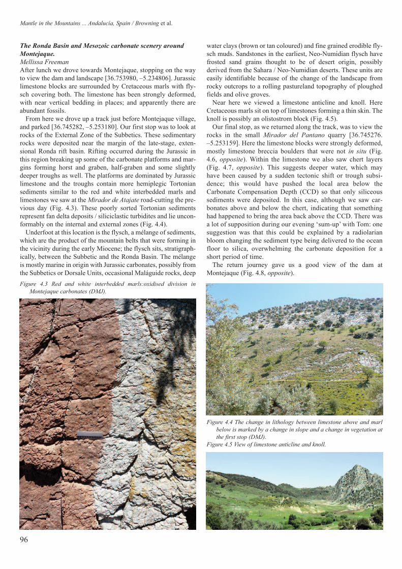
The Ronda Basin and Mesozoic carbonate scenery around
Montejaque.
Mellissa Freeman
After lunch we drove towards Montejaque, stopping on the wayto view the dam and landscape [36.753980, –5.234806]. Jurassiclimestone blocks are surrounded by Cretaceous marls with fly-sch covering both. The limestone has been strongly deformed,with near vertical bedding in places; and apparently there areabundant fossils.
From here we drove up a track just before Montejaque village,and parked [36.745282, –5.253180]. Our first stop was to look atrocks of the External Zone of the Subbetics. These sedimentaryrocks were deposited near the margin of the late-stage, exten-sional Ronda rift basin. Rifting occurred during the Jurassic inthis region breaking up some of the carbonate platforms and mar-gins forming horst and graben, half-graben and some slightlydeeper troughs as well. The platforms are dominated by Jurassiclimestone and the troughs contain more hemiplegic Tortoniansediments similar to the red and white interbedded marls andlimestones we saw at the Mirador de Atajate road-cutting the pre-vious day (Fig. 4.3). These poorly sorted Tortonian sedimentsrepresent fan delta deposits / siliciclastic turbidites and lie uncon-formably on the internal and external zones (Fig. 4.4).
Underfoot at this location is the flysch, a mélange of sediments,which are the product of the mountain belts that were forming inthe vicinity during the early Miocene; the flysch sits, stratigraph-ically, between the Subbetic and the Ronda Basin. The mélangeis mostly marine in origin with Jurassic carbonates, possibly fromthe Subbetics or Dorsale Units, occasional Maláguide rocks, deep
water clays (brown or tan coloured) and fine grained erodible fly-sch muds. Sandstones in the earliest, Neo-Numidian flysch havefrosted sand grains thought to be of desert origin, possiblyderived from the Sahara / Neo-Numidian deserts. These units areeasily identifiable because of the change of the landscape fromrocky outcrops to a rolling pastureland topography of ploughedfields and olive groves.
Near here we viewed a limestone anticline and knoll. HereCretaceous marls sit on top of limestones forming a thin skin. Theknoll is possibly an olistostrom block (Fig. 4.5).
Our final stop, as we returned along the track, was to view therocks in the small Mirador del Pantano quarry [36.745276.–5.253159]. Here the limestone blocks were strongly deformed,mostly limestone breccia boulders that were not in situ (Fig.4.6, opposite). Within the limestone we also saw chert layers(Fig. 4.7, opposite). This suggests deeper water, which mayhave been caused by a sudden tectonic shift or trough subsi-dence; this would have pushed the local area below theCarbonate Compensation Depth (CCD) so that only siliceoussediments were deposited. In this case, although we saw car-bonates above and below the chert, indicating that somethinghad happened to bring the area back above the CCD. There wasa lot of supposition during our evening ‘sum-up’ with Tom: onesuggestion was that this could be explained by a radiolarianbloom changing the sediment type being delivered to the oceanfloor to silica, overwhelming the carbonate deposition for ashort period of time.
The return journey gave us a good view of the dam atMontejaque (Fig. 4.8, opposite).
96
Mantle in the Mountains ... Andalucía, Spain / Browning et al.
Figure 4.3 Red and white interbedded marls:oxidised division in
Montejaque carbonates (DMJ).
Figure 4.4 The change in lithology between limestone above and marl
below is marked by a change in slope and a change in vegetation at
the first stop (DMJ).
Figure 4.5 View of limestone anticline and knoll.

97
Proceedings of the OUGS 2 2016
Figure 4.6 Calcite crystals found in the limestone at the Mirador del
Pantano quarry (DMJ).
Figure 4.7 (above) Looking at the chert layers at the Mirador del
Pantano quarry (MF); and (left) a detail of the chert layering
(DMJ).
Figure 4.8 The dam at Montejaque is built across the gap between two
blocks of limestone (LF).

98
Mantle in the Mountains ... Andalucía, Spain / Browning et al.
Day 5 — Sunday 3 MayThe peridotite/limestone contact, the gneiss/peridotite contact,
gneisses near Pujerra, peridotite and kinzigites on the track
towards Peñas Blancas
Oliver Strimpel
Retracing our first day’s route from Málaga to Ronda, we drovesouth on the A-397 to investigate another exposed boundary ofthe Sierra Bermeja peridotite massif, this time with Mesozoiclimestones [36.626028, –5.077827]. The road-cut presented thebest exposure, both of the contact itself, and of the progressionof increasing impact of the peridotite emplacement on the lime-stone country rock (Fig. 5.1). Approaching the contact, over ascale of a few metres, undisturbed limestone gave way to asheared, but not a recrystallised section, then to a partiallymylonitised strip, and finally, within a few tens of centimetresfrom the contact, to an intensely mylonitised, sheared, andstretched fabric (Fig. 5.2).
Darker layers from compositional variations in the originalbedding helped to highlight deformation. The peridotite, heavilyserpentinised near the contact, showed only brittle faulting,implying that the whole crustal section had already cooled whenit was emplaced over the limestone, and suggesting a fairly shal-low level of emplacement.
We speculated as to the sense of the fault, but the lack of larg-er-scale shear sense indicators made it hard to corroborate thecontact as the steeply dipping thrust fault shown on the IGMEgeological map. Small-scale indicators probably only reflectedpost-emplacement movements, perhaps associated with exhu-mation. Since the rocks had already cooled, this may be a latestage fault. But its age is difficult to determine because no min-erals in either the peridotite or the carbonates are readily amend-able to dating.
To reach our second contact of the day, we turned west off theA-397 towards Pujerra, where we found a contact between theperidotite and the structurally overlying Alpujárride gneiss(unlike the gneisses we saw earlier near Estepona, which wereunderneath the peridotite) [36.599652, –5.116209]. The extent ofthe peridotite was clearly delineated by the tree cover: almostexclusively pine on peridotite; and chestnut, cork, and other veg-etation on the surrounding gneisses. The peridotite was not asheavily serpentinised at the contact as we had seen elsewhere,probably owing to a shortage of available water. What water therewas probably originated from metamorphic reactions in crustalrocks — mainly from the micas.
Within the crustal rocks, a layer of highly metamorphosedgneiss next to the contact had been thoroughly dehydrated by oneor more regional thermal events, in addition to any heating asso-ciated with the juxtaposition of the peridotite and the gneiss.
Figure 5.1 Investigating the contact between peridotite (weathered
brown foreground rocks) and Mesozoic limestones (white-grey)
along the A-397 South of Ronda.
Figure 5.2 Intensely mylonitized limestones adjacent to the peridotite
contact.

99
What remained is a restitic rock called kinzigite (Fig. 5.3). Notonly is it an attractive rock, dappled with garnets and glintingwith graphite flecks, but it also encapsulates a lot of metamorphicpetrology, revealing evidence of both prograde and retrogrademetamorphism that probably reflect burial to the base of thecrust, followed by exhumation. It contains abundant garnet por-phyroblasts, some with included kyanite, the garnet being sur-rounded by a fabric of biotite + sillimanite + K-feldspar. Throughthe lens it was arguably possible to see cordierite formed as a rimreaction with biotite around the garnet, as well as kyanite pseudo-morphs altered to sillimanite.
We also identified centimetre- to meter-scale light-colouredlenses of quartz and feldspar within the gneisses (Fig. 5.4); theseare granulitic leucosomes, which imply that the regional thermalevent heated the gneiss enough to partially melt it and dehydratethe micas, leaving behind only anhydrous minerals. The releasedwater may have been assimilated into nearby leucocratic dykes,or used in serpentinisation of peridotite. Driving north-west fromthe contact, [36.598907, –5.142078] we moved into layers withsignificantly fewer garnets, the rocks grading through progres-sively lower Barrovian isograds. In the sillimanite zone, we wereable to spot some sillimanite crystals (Fig. 5.5), as well as themuch more ubiquitous fibrous form.
At our last stop in Igualeja (endowed with a much-needed barfor refreshment), we were back in limestone country where theRiver Genal emerges from a cave as a ‘karst upwelling’, accord-ing to a sign for visitors [36.632859, –5.118265].
Day 6 — Monday 4 MayNeo-Numidian flysch, Alozaina unit, peridotite/gneiss contact
zone, Valtocado and gneisses in the Sierra Alpujata
Stuart Swales
Bidding farewell to Ronda, our convoy crossed eastwards over theSerranía de Ronda on the A-366 through a lovely landscape ofpine forest and steep Jurassic and Cretaceous Subbetic carbonatehills, and through the village of El Burgo. South of El Burgo[36.774770, –4.937859] we stopped to examine a knoll of greylimestone. Within the mainly metre-scale beds of carbonate weobserved thin beige-coloured, very finely laminated horizons,some containing organic-rich laminae, with faint traces suggestiveof rootlets cutting c. 10mm or so down from the organic-rich lam-inae into the underlying sediment. The yellowish-beige layershave been interpreted as calcrete palaeosols, indicating cyclicemergence of the shallow-water carbonates (Fig. 6.1, overleaf).This whole block is an olistolith of Microcodium limestone, prob-ably late Cretaceous to Palaeogene, within the Neo-Numidian fly-sch. Various theories have been proposed about the exact nature ofMicrocodium, one being that they are calcite structures secretedby symbiotic bacteria around mycorrhizal hairs.
Farther down the A-366, just south of the town of Alozaina, westopped at an old bridge over a steep, deep arroyo, which has cutdown through the Alozaina Formation (Miocene, earliestAquitanian) [36.719891, –4.871557]. South of the bridge, thelowest part of the Alozaina Formation was seen to be a series ofpoorly sorted conglomerate and breccia beds, with randomly ori-ented clasts from millimetre up to metre scale, some very wellrounded, others angular, in a poorly sorted matrix that rangedfrom silt up to medium sand grade. A number of the less chaoticbeds could be seen to fine upwards and some of the bedsappeared to be small channels. Silvery schist clasts containedblack andalusite with rinds of alteration to muscovite — these aretypical low-grade Alpujárride rocks, as were clasts with quartzveins that contained pink andalusite. All the clasts appear to be
Figure 5.3 Kinzigite near the Alpujárride gneiss contact with peri-
dotite near Pujerra. As an indication of scale. the largest garnets
are c. 10mm across.
Figure 5.4 Granulite leucosome within the kinzigite, with quartz,
feldspar, and some remnant biotite in the fabric. The largest garnet
is c. 10mm across.
Figure 5.5 Sillimanite crystals in the gneiss, several hundred meters
from the contact.
Proceedings of the OUGS 2 2016

100
Mantle in the Mountains ... Andalucía, Spain / Browning et al.
derived from the directly underlying Maláguide and Alpujárriderocks. Tom pointed out the absence of any lower-level peridotitesor higher-grade Alpujárride rocks here, even though they both arecurrently proximal to this deposit.
On the north bank of the arroyo the matrix was clearly coars-er and more angular but the clasts themselves, while largelysimilar in composition to those across the arroyo, were smaller.One clast found there was typical lowest-grade Alpujárride, ahigh-sheen chloritic phyllite. We also found some smaller clastsof red sandstone.
Moving farther north to the new road-cutting, we foundclasts with more feldspar, suggestive of derivation from a high-er-grade Alpujárride source. As we walked north-east up theroad-cut we observed clasts derived from metamorphic sourcerocks of increasing grade: we successively found small clastswith biotite and fibrolite, then sillimanite schists, some withhotter ‘foxy’ biotite (Fig. 6.2); then we found fibrolitic schistswith albite/oligoclase feldspar porpyroblasts, eventually spot-ting migmatite clasts with strongly folded leucosomes andkinzigite clasts of deep origin. (An aside: Tom’s illustratedword-of-the-day was faserkiesel: millimetre-scale quartz knotsor pods containing fine sillimanite). This succession was seento be covered everywhere by flysch in an angular unconformi-ty. The flysch had what Tom described as a ‘sensuous’ — to thetouch — fine matrix, breaking down readily to very coarsesand, which had periodically avalanched downslope formingmini-fans in the roadside drainage channel (Fig. 6.3, opposite)— an interesting parallel to the much larger-scale process inthe deposit below!
Figure 6.1 Michael Perkins examining the yellowish-beige coloured layer of Microcodium Limestone at the first stop south of El Burgo.
Figure 6.2 A clast of sillimanite schist in the Alozaina Formation con-
glomerate; road-cut south east of Alozaina.
The Alozaina Formation has been interpreted as a sequence offast-flowing, mass-flow deposits from flash floods, and cata-strophic rock-slides, into an extensional basin during the firstepisode of the collapse of the Alborán Domain. Zircons in thegneisses have been dated as growing in the middle crust at 21Ma— only just before their early Miocene exhumation. This rela-tively short roadside exposure is a spectacular witness to the pro-gressive, yet rapid, unroofing of an orogen (Fig. 6.4, opposite).
South of Alhaurín el Grande we turned off the A7053 atValtocado, parking by an entirely redundant roundabout[36.596173, –4.705536]. In road-cuttings just north of this location

20mm wide fault gouge composed of ground-up gneiss.However, at the northern boundary, subsequent multiple episodes
of faulting had displaced theinclined junction and chunksof gneiss could be seendetached in this fault zone. Inthe nearby old road-cut, brittlefaulting was seen perpendicu-lar to the foliation (Fig. 6.5)
Travelling onwards, weheaded up the Guadalhorcevalley to Álora, from where wewent cross-country on the A-343 via Valle de Abdalajís,heading for our new base atAntequera. The countrysidewe passed through (no time forstops) was in the EarlyMiocene La JoyaOlistostromic Complex, whichseals the Internal / ExternalZone boundary and is strati-graphically above the AlozainaFormation seen earlier thisday. This mélange has many
101
Proceedings of the OUGS 2 2016
we could see brown migmatites with pale leucosomes sittingunder a peridotite mass. This is a fault block of the SierraAlpujata. Here we encountered our old friends, peridotite andgneiss, in close contact — a 20m or so wide chunk of gneiss wasbounded to the north and south by seemingly little-altered peri-dotite with few thin serpentinite veins. At both boundaries theperidotite had altered to a yellow serpentinite. Freshly brokengneiss blocks found in the float were mid-grey with a strong foli-ation defined by a biotite fabric wrapping abundant plagioclaseand K-feldspars — this was not the same as the ‘lithoclasticgneiss’ we had seen at our first peridotite/gneiss contact.
The southern boundary was sub-vertical, and within one metreof this boundary we could see the inclined foliation of the gneissbeing progressively rotated to become aligned parallel with theboundary. Similarly, feldspars in the gneiss were seen to progres-sively thin and become extended in this ductile deformation. Asthe boundary was approached, a mylonite derived from the gneisshad no discernible feldspars, having been recrystallised, then a
Figure 6.3 An example of a miniature avalanche forming a ‘mini-fan’
(scale is 100mm long; DMJ).
Figure 6.4 We examined progressive Alpujárride exhumation during earliest Aquitanian in the Alozaina road-cut
where clasts in the conglomerate went from lowest- to highest-grade in just 200m, indicating that the source
rocks were progressively deeper as the area was unroofed.
Figure 6.5 At Valtocado the southern contact between the gneiss body
(left) and peridotite is relatively planar with the gneiss foliation
stretched parallel to the contact plane. The gneiss is mylonitic at this
contact; the yellow serpentinised gouge is derived from the peridotite.

102
Mantle in the Mountains ... Andalucía, Spain / Browning et al.
very large (individually map-able) olistoliths of Subbetic carbon-ates and flysch clastics, some being hundreds of metres in heightand several square kilometres in area, hence the lumpy-bumpyappearance of the terrain!
More lovely scenery passed rapidly by, the road being flankedby more steep Jurassic and Cretaceous Subbetic limestonemountains. We had planned to return along this road the next dayto look at the flysch and multi-coloured marls but it proved to bea bit too winding for some of the group, so we decided that wewould not go back that way — we had actually seen enoughfrom the cars!
Looking south the different rock types stood out with their char-acteristic landscape, the peridotite close by and in the far dis-tance. Sandwiched between them cultivated land and housesindicated the gneiss, phyllites and schists of the AlpujárrideComplex and some superficial deposits (Fig. 7.1).
Next stop [36.853809, –4.812756], on a track off the roaddown to Carratraca (Fig. 7.2), we saw exposures of migmatitewith shear zones of gneiss, separated into light and dark miner-al layers containing garnets with tails which are kinematic indi-cators, indicating shearing and main foliation occurring at thesame time as metamorphism (Fig. 7.3, opposite). These rocks
were thinned and heatedfrom below, as well as bythe peridotite mass. Alsothere were shear zonescutting through the fabric:these were discrete shearsets, which deflected thefoliation, indicating thatthe rock was half-way tobeing brittle. Pure shearflattening in mylonitezones is due to the north-east thrusting during theemplacement of the peri-dotite. We hoped to findkinzigite in situ butfailed, although there wasevidence in pebbleswashed down from higherup the slope, and in thestream bed.
In the afternoon weinvestigated the CerroTajo fault [36.821643,
–4.795731]. This is a major, later fault exposed in a high-sidedroad-cutting on the A-357 (Fig. 7.4, opposite): the gneiss is down-thrown at the southern end and separated from peridotite to thenorth by fault gouge. We used the slickensides to give the direc-tion of movement on the fault (smooth upwards, rough down-wards on the gneiss), which indicated that this was a normal fault.The peridotite had been highly serpentinised, the fabric showedfault drag, as did a leucogranite dyke. The gneiss was rotting with
Figure 7.1 View south from the top of the Sierra de Aguas. In the distance is the Sierra Alpujata (peridotite) with a
quarry in the underlying marble at the left-hand end, above the town of Coín. In the middle distance the Sierra de
la Roble is also peridotite, but with gneiss lower down below the houses (LF).
Day 7 — Tuesday 5 MaySierra de Aguas peridotites (the smallest peridotite massif),
gneisses, migmatites and granites
Caroline Deans
The car convoy set out from the Hotel Lozano in Antequerathrough a maze of roundabouts, up to the top of the town and outon the A-343 towards Álora. On the journey, thanks to the two-way radios, Tom interpreted the landscape for us, pointing out therelationship between the flysch and the peridotite massif andidentifying the classic flysch landscape of green fields with theirrocky olistrostrome exposures. These vary in size, from a fewmetres up to as big as 5km sandstone blocks. In the distance onthe skyline we saw grey-brown flat-topped hills of Mid-UpperMiocene clastic sedimentary rocks.
At Álora we turned up into the hills, each with its castle. Thesehills are large blocks of Tortonian age set in the gentle farmlandslopes of the flysch, which laps up to the pine-covered peridotitemassif. As we climbed the tortuous road and then rough track,we stopped briefly to inspect white leucocratic dykes. At thesummit view point [36.855202, –4.791515] we looked outtowards Carratraca to the west; to the north-west a fault-bound-ed block of Jurassic limestone was marked by a wooded ridgeand in the distance were cultivated fields overlying gneissesof the Aljibe unit, which in turn overlies the peridotite. In thefar distance is a large olistostrome block of limestone.
Figure 7.2 The migmatite and gneiss locality near Carratraca (LF).

present in the peridotite, similarly deformed, also some largegarnets. Large almandine garnets were present in the kinzigite,while there were small, abundant, Mg-rich spessartine garnets,together with tourmaline, in the leucogranite, which grew inthe melt. These indicate S-granite (crustal melt) with a marinesedimentary origin, which was then metamorphosed andmigmatised (Fig. 7.6).
We made a final stop on the A-357 just south of Carratraca atthe Punto de interes geologico — Sierra de Alcaparaín, one ofthe stops on the Guadalteba Ruta Geológica. This was betweentwo peridotite blocks, which showed lots of deformation, clearlyseen in the white leucogranite and quartzite veins, which wereintruded while the host rocks were still undergoing deformation.
103
Proceedings of the OUGS 2 2016
muscovite and chlorite present in cross-cutting veins; it containedgarnets in the folded and twisted lenses, also chlorite, feldsparand quartz. The garnets were not the type associated with gneissformation, so the fault was not an original contact between theperidotite and the gneiss, but rather a tectonic one. The peridotitecontained large clasts of crustal gneiss, quartz and feldspar-richwith metasomatic rodingitised biotite due to Ca-rich fluids circu-lating during serpentinisation. This is a locality for the mineralxonotlite, a hydrous calcium silicate that occurs in serpentine andin contact zones (Fig. 7.5).
Our fourth stop was the Arroyo de la Cala (a different onefrom Day 2!) [36.810835, –4.782613]: at this location a peri-dotite-gneiss fault was examined, normal, brittle with serpentin-isation between and around the fault. There were white bands ofleucogranite dragged parallel to the fault. Quartz veins were
Figure 7.3 Impromptu explanation of σ-type and δ-type shear by Tom. σ-
type are porphyroclasts with wings of smeared off material; δ-type
clasts are less common than sigma-clasts but good, unambiguous
shear indicators. They develop from sigma-clasts when the clast
rotates significantly (LF).
Figure 7.4 The Cerro Tajo fault exposed in a road-cutting on the south-
west side of the A-357 south of Carratraca (LF).
Figure 7.5 Very rare acicular xonotlite crystals on serpentinised peri-
dotite (largest crystal 3mm) found at the Cerro Tajo fault. Xonotlite
is a hydrous calcium silicate (Ca6Si6O17(OH)2), which occurs in the
late veinlets associated with the cordierite granitic dykes from the
Ronda peridotites. The presence of xonotlite is typical of the rodin-
gitisation process, which caused Ca-metasomatism of the granitic
dykes during serpentinisation. This mineral is found in less than 20
localities across Europe so it was great pleasure seeing it in hand
specimen (SC).
Figure 7.6 Large almandine and smaller spessartine garnets at Arroyo
de la Cala (LF).

Variscan Orogeny, as it was not detected in the later Triassic-Cretaceous strata.
After lunch in a pine forest we drove on to a nearby bar for cof-fees etc. and noticed lots of Griffon Vultures; about 25 sat on aledge some 60m above the bar while another 50 or so circledabove the ridge. A pale yellow gecko came out of its hiding-placeunder the roof to observe the proceedings.
We then continued east to the Arroyo de Colmenar [36.894578,–4.752534]. As the temperature continued to rise we walkeddown a track to the river, disturbing a Great Egret from its feed-ing spot. Under the road and a little way up the arroyo, the firstexposure was a grey rock with much small-scale folding, con-taining biotite and small garnets. It is a strongly foliated phyllitewith visible bedding, which picked out beautiful Z-folds, allverging to the north-east as might be expected in the Alpujárridenappe (Fig. 8.1).
Another 50m up the dry arroyo we found small garnets in sandylayers with andalusite in the more pelitic layers. Farther alongthere was some evidence of staurolite with garnets in the schists.This evidence all indicates that the metamorphic grade increasesfarther down the succession, confirmed by finding fibrous silli-manite farther along. Sam found a large (c. 20mm) pink andalusitecrystal in the scree beneath a higher exposure (Fig. 8.2).
104
Mantle in the Mountains ... Andalucía, Spain / Browning et al.
Day 8 — Wednesday 6 MaySierra de Aguas cover, metamorphic schists, phyllites and
lower-grade lithologies
Paul Speak
We headed towards Ardales and then took the MA444 easttowards the reservoir to the first stop at the Arroyo de la Zahuda
[36.896847, –4.826426] to walk up a section of Palaeozoic andMesozoic sediments, part of the Maláguide nappe.
A road-cut near the bridge revealed greyish-white UpperCretaceous (Cenomanian/Turonian) marls, dipping north. It com-prised fine-grained carbonates and clays with no visible fossils,suggesting a shallow marine platform environment. The descrip-tion ‘pretty well mashed up’ summed it up, with signs of ductiledeformation before brittle fracturing. There was no sign of anylower Cretaceous rocks, which may have been eroded or notdeposited here. Across the arroyo, on the ridge, were exposuresof the underlying mid-Jurassic limestones, also dipping north.While the Cretaceous marls were much deformed, the more com-petent Jurassic limestones were not.
We walked up the arroyo, soon reaching a series of Triassicred beds: a variety of mature conglomerates consisting of round-ed clasts of sandstone pebbles and much quartz, as well as ter-restrial sandstones and mudstones. This suggested a wadi-typedepositional environment with flash floods. Also visible were aseries of red marls, indicating an oxidised state with ferrousFe(III) iron. There were pale green spots and bands causedwhere organic matter had been broken down by oxygen-scav-enging bacteria, which reduced the Fe(III) to Fe(II). We alsofound a caliche layer: a hard pan formed by calcareous concre-tions below the surface. Suggested environments included apalaeosol or a coastal lagoon.
Continuing up the arroyo, and hence down the stratigraphicsequence into the Carboniferous, the next exposure was a grey,gravelly conglomerate interbedded with siltstones and fine sand-stones; there were no fossils, but there was some evidence ofcross-stratification. Faulting and warping of the finer sedimentsgave evidence of deformation. The bedding was very steep, muchmore so than in the Triassic beds. The stratigraphic column sup-plied in our field notes indicated an unconformity in the area. Aweak tectonic fabric was detected in the conglomerate, with aspaced dissolution cleavage. This was thought to be related to the
Figure 8.1 Z-fold in phyllite, offset c. 50mm.
Figure 8.2 Andalusite crystal found by Sam Capstick (SC).
Close examination revealed that the garnets were pre-tectonic(the foliation wraps around them), the biotite and sillimanite weresyn-tectonic and the andalusite post-tectonic as the crystals arerandomly oriented and overgrow the tectonic foliation. The inter-pretation is that, as the crust thinned, the hot mantle got closer,increasing the metamorphic grade. In quartz veins near the top ofthe arroyo, early (deformed) kyanite crystals were found, somereplaced by later andalusite.
Returning the way we had come, a convenient lay-by [36.910369,–4.767218] gave us a good view towards the Desfiladero de los
Gaitanes, the spectacular gorge near El Chorro (Fig. 8.3, oppo-
site). We noted that there were large outcrops of vertically bed-ded limestone visible to the south-east, close to the sub-horizon-tal sediments on which the Griffon Vultures were perched. Thecontact could not be seen, but it was described as a verticalunconformity, where the Betic deformation had folded the lime-stones into vertical structures, which later became a sea cliff. Thelater Tortonian or Messinian high-energy marine sediments werelaid down horizontally against the cliff in a shallow marine basin.This was thought to have been one of the last narrow seawaysfrom the Atlantic to the Mediterranean (Martín et al. 2001).

up to 130˚ since emplacement. Theintrusive material itself probablyoriginated from a mantle partial meltassociated with a thermal pulseresulting from the hypothesised man-tle delamination event.
Walking a little farther up the trackgave us an excellent opportunity toidentify shear sense indicators withinthe Maláguide (Fig. 9.2, overleaf).These rocks are Palaeozoic in age,with the fabric most likely represent-ing the Variscan orogenic event, andmetamorphic minerals are limited tochlorite and white mica. The rocksare filled with strongly folded quartzveins. With Tom’s help, we identifiedquartz veins that pinched out parallelto the fabric where, in some cases, thefold hinges have detached completelyto form lozenges (Fig. 9.3, overleaf).We also found conjugate fracturesets, cutting through the Maláguidefabric. Stretching lineations could befound on some surfaces, while Tomexplained how we might distinguish
these from similar bedding-cleavage intersection lineations orwavier crenulation lineations.
105
Proceedings of the OUGS 2 2016
Day 9 — Thursday 7 MayMálaga dykes; El Torcal de Antequera-Dorsale unit limestones
Michael Perkins
Following on from the previous day’s excursion to the Ardalesarea, our morning locality in the Guadalmedina Valley enabled usto inspect a different relationship between the Maláguide unit andyounger rocks. After driving south from Antequera and parkingthe cars by the A-45 junction just south of Casabermeja, wewalked some 200m up a side road with some excellent exposureon its northern side [36.879575, –4.427819]. Here we could seesome fine-grained rocks with a well-developed cleavage. Beforelong, though, we found a different lithology: a clearly crystallineunit, which cut diagonally upwards to the west through the coun-try rock.
This dyke appeared to be composed of several distinct units,perhaps corresponding to multiple intrusion events. The unit far-thest to the west remained relatively fresh. The next was verybadly weathered to a brown colour, while the right-most unitbefore the country rock was again less altered. Faults were seento cut the dykes and country rock, offsetting the contacts. Thefresher rock showed no fabric (suggesting that the intrusion wassubsequent to metamorphism of the country rock) and appearedto contain abundant white feldspar and putative amphibole.Studies on the rock have confirmed a tholeiitic composition, con-taining hornblende and pyroxene, with an Ar-Ar date of 23Mathat places them at the end of the Oligocene.
The boundaries of the intrusion revealed two things. Firstly, theintrusion cut cleanly across the fabric of the country rock.Secondly, a chilled margin could be discerned, and the countryrock appeared to be baked, implying intrusion at relatively shal-low crustal levels (Fig. 9.1). These rocks have provided insightinto regional tectonics, since measurement of the magnetic orien-tation locked into component minerals at the time of crystallisa-tion indicates that the area has undergone clockwise rotation by
Figure 8.3 The Desfiladero de los Gaitanes, eroded through the vertical bed of limestone (LF).
Figure 9.1. The contact between the Oligocene dyke and the Palaeozoic
Maláguide country rock.

Most of the beds are not fossiliferous to the naked eye.However, there are some exposures of the ammonitico rosso bed,distinctive for its nodules and mottled pink tones. My groupfound two ammonites of different sizes (one c. 200mm diameter,the other about 5mm), and abundant belemnites. Other groupsfound other marine fossils including coral, crinoid stems,bivalves and bryozoa (Fig. 9.6, opposite, and page 108).
Day 10 — Friday 8 MayMorning: Sightseeing in Antequera
Chris Hodgson
Before setting off for Granada, the group took the opportunity tovisit the nearby archaeological site of the Viera and Menga dol-mens. Local geology contributed to favourable conditions forprehistoric settlement: the Antequera Basin was one of the lateMiocene embayments along the southern edge of theGuadalquivir Basin. It became filled mostly by platform temper-ate carbonates and mixed siliciclastic-carbonate deposits interfin-gering laterally with basinal marls. With later flysch deposits andsome uplift, a low lying plain with a river network developed inthe area of the present town of Antequera.
106
Mantle in the Mountains ... Andalucía, Spain / Browning et al.
We drove across country, through Villanueva de la Concepción,to reach our afternoon stop, which was a leisurely excursion to theParaje Natural (Protected Natural Site) of El Torcal de Antequera
[36.952532, –4.545014]. A Torcal is an area where torcas, ordolines, are found, circular depressions around sink holes in karst.The Torcal of Antequera comprises a Subbetic Jurassic limestonemassif rising to more than 1,300m, some 700m above the town,and is rightly famous for its spectacular karstic landscape, a prod-uct of the erosion of the sub-horizontal beds of limestone. This ismost dramatically displayed in the national monument El Tornillo,named for its resemblance to a screw (Fig. 9.4).
Our group split up to be free to explore the park at our leisure(and to try to avoid the bus-loads of school children!). In fact, itdoes not take a long walk to find tranquil spots, even on the well-trodden paths that lead off from the information centre. My groupexplored the yellow path, which winds its way 3km into the parkand takes in spectacular scenery including overhanging cliffs,caves, platforms and gullies.
The differential erosion of the limestone, giving rise to the‘stacked-pancake’ landscape, is formed by the different solubili-ty of the component beds. These beds comprise oolites, pseudo-breccia beds (these are partially dolomitised to give a brecciatedappearance), nodular beds and more massive units. Each litholo-gy is eroded and dissolved in a distinctive manner, producing alandscape of many contrasts (Fig. 9.5, opposite).
Figure 9.2. Tom explains various shear sense indicators. From top, left
to right: folded quartz veins thicken in the hinge and thin parallel to
cleavage; quartz lozenges where thickened fold hinges become
detached; more competent beds form lozenges or fold boudins; foli-
ation becomes boudinaged, with quartz in-filled in boudin neck;
shear fractures form a conjugate set; wavy crenulation lineations
(left) and straighter stretching lineations (right).
Figure 9.3. Folding of the quartz veins, thinning or pinching out paral-
lel to the metamorphic fabric.
Figure 9.4. El Tornillo (‘The Screw’), an eroded tower in the Jurassic
limestone of El Torcal. (https:// apbvigo.wordpress.com/2014/04/22/el-tornillo-torcal-de-antequera/_4140452-od/ under Creative
Commons Licence).

107
Proceedings of the OUGS 2 2016
Figure 9.5. The landscape of El Torcal.
Figure 9.6. Fossiliferous horizons
in the limestone of El Torcal
yielded:
ammonites (a – MF; b–d – DMJ),
(e) belemnites (MP)
and (f) crinoids (MP/DMJ).
a b
c
d

108
Mantle in the Mountains ... Andalucía, Spain / Browning et al.
The main building stone required was near by: we could see thedisused hillside quarry believed to be the source. Blocks werequarried using fire and water; they were cut and shaped usingflint tools and transported on rollers to the prepared site. Theorthostats (uprights) were raised up ramps (which could laterbecome the base of the tomb covering) and manoeuvred to fallinto position in the cut channel dug down to the bedrock. Theslabs were made vertical, wedged in place with boulders and sta-bilised. We noted their precision fit, with only a few wedges andfilling blocks used, and no mortar (Fig. 10.2). Additionally inMenga, central pillars were also emplaced (see below and Fig.10.3, opposite). The whole interior would then have been filledwith rubble up to the height of the orthostats to enable roofingwith capstones before clearing the internal space and completingthe tumuli with layers of various materials, including rocks andminerals brought from a distance. Domes were up to 50m diam-eter and 15m high. At this site the domes have been seeded withplant species identified by analysing Neolithic pollen.
At the ruined entrance to the Viera dolmen, missing capstonesallowed enough light to study an orthostat decorated with cavitiesknown as ‘cups’, a common motif in Iberian prehistoric art.Lying on the floor was part of one door and farther inside was‘hinge’ evidence of another. The doors and dimensions of the cor-ridor would symbolically prolong the passage to the burial cham-ber. Essential restoration, for safe access, involved replacingsome missing capstones, but the final quadrangular chamber isthe completely original funerary area.
The fertile soil conditions in Antequera, coupled with thewarm wet prehistoric climate, plus availability of timber forshelter to augment the many surrounding cave dwellings (El
Torcal de Antequera, La Peña de los Enamorados, etc),encouraged human habitation. These Neolithic structures wereprobably erected between the end of the 4th and the beginningof the 3rd millennium BC (carbon dating). They were not builtas astronomical observatories, although they do suggest astro-logical interest; rather they were community ritual gatheringplaces. For these animist societies death was just another riteof passage and skeletal remains and grave goods are found inmegalithic buildings.
The Archaeological Site, on a small hill near our hotel, protectsthe Viera and Menga dolmens, correctly so called, as they arecorridor tombs. Their substantial covering creates the domedtumuli still seen today (Fig. 10.1). From the El Caminante
‘Observatory’, we could appreciate the spatial relationshipbetween natural formations of the surrounding countryside andthe tumuli. The linked ‘Solar Centre’ shows the orientations ofthe most important dolmens of the Iberian Peninsula. MostEuropean megalithic monuments have their entrances orientedmore or less to the summer sunrise. Here Viera follows this pat-tern whereas Menga faces north.
e
f
Figure 9.6 (cont’d) (e) belemnite (MP) and (f) crinoid (MP/DMJ).
Figure 10.1 A domed tumulus covers the Viera dolmen. The iconic lime-
stone peak, La Peña de los Enamorados, towards which the Menga
dolmen is orientated is seen in the distance (DMJ).
Figure 10.2 Careful fitting and packing of stones, Menga dolmen (DMJ).

109
The Menga dolmen did not fail to impress. The trapezoidalshaped, unroofed atrium fronts the iconic trilithon (Fig. 10.4).This inner part of the lintel-like construction is unparalleled in theIberian Peninsula. The 250-ton capstone is one of the two thatoriginally covered the entrance corridor (2.5m wide and 2.7mhigh, 6m long). Following into the funerary chamber (6m wideand to 3.5m height at the head, 20m long) there are four similar-ly huge blocks spanning the roof between 13 orthostats. A veryunusual feature in European megalithic structures is the presenceof internal pillars as found here. Three large pillars are alignedalong this chamber’s longitudinal axis (see Fig. 10.3). As thesecoincide with the joins of the four capstones it seems likely theywere to installed support the roof. The lower parts of the pillarsare slimmer and although the medium-grained sandstone appears
Figure 10.3 Line of supporting
pillars along the central
axis of the Menga dolmen
(DMJ).
Figure 10.4 Entrance to Menga dolmen, showing
trilithon (DMJ); inset, Dr Jones atop the
dolmen, for scale (CH).
Figure 10.5 La Peña de los Enamorados, the peak from which a pair of
lovers, a Moorish princess and a Christian man are said to have
escaped capture by leaping to their deaths. It is also known as the
Montaña del Indio because of its supposed resemblance to a sleep-
ing Native American’s face (DMJ).
well cemented, later abrasion could be responsible. Still visibleon one orthostat are more typical motifs of megalithic art: cruci-form shapes and star-shaped engravings in the coarse-grained,gritty, sandstone.
The final amazement of this monument is the view looking outof the dolmen — a direct view of the famous hill that resemblesa recumbent head, La Peña de los Enamorados (Fig. 10.5). Wedid not visit the nearby, later, dolmen of El Romeral, which hasan equally interesting and unusual alignment towards the high-point of La Sierra del Torcal.
Proceedings of the OUGS 2 2016

was not evident in the road section. Later in the afternoon three ofus returned to the locality and looked at the rocks in the hill abovethe road. There we found a strongly magnetic, green garnet-bear-ing rock that appeared to be of high density, which we tentativelyidentified as a pod of the disrupted eclogite, and which had beensubject to significant retrograde metamorphism.
110
Mantle in the Mountains ... Andalucía, Spain / Browning et al.
Day 11 — Saturday 9 MaySierra Nevada metamorphic rocks
Linda Fowler
A drive up the A-395 Sierra Nevada road gave us several oppor-tunities to examine rocks of the Nevado-Filabrides Complex,which dominates this range of mountains as well as the Sierra delos Filabres.
We first stopped a short way uphill from a Jardín Botánico
parking area [37.112060, –3.431919]. Up to this point we hadnoticed roadside exposures of Triassic carbonates of theAlpujárride nappe, but now found schist of thePalaeozoic/Triassic Mulhacen Complex — because of the geom-etry of the thrust sheets, as we drove uphill we were movingdown the sequence into older rocks. Structurally above theschists we observed carbonate rocks with patches of a white, aci-cular mineral, which at first glance looked like some kind of veg-etation. Further inspection showed this to be gypsum in the satin-spar type of habit in which fibres grow in parallel. In this case thefibres were very coarse, 2–4mm in thickness and up to 300mm inlength (Fig. 11.1).
Figure 11.1 Satin spar gypsum at first stop, walking pole for scale (LF).
Bernard Skillerne de Bristow
We drove on uphill and examined a roadside section [37.098258,–3.390624], where we found a sequence of pelitic schists andleucogranites of the Proterozoic/Palaeozoic Veleta Complex. Thepelites contained a Grt+St?+Pl+Qtz assemblage typical of loweramphibolite facies, but only the garnet was clearly identifiable;we only saw the staurolite as occasional stubby brown prismaticcrystals. Texturally, the leucogranite was highly sheared with aproto-mylonitic fabric, which had overprinted the originaligneous texture (Fig. 11.2); it contained tourmaline similar to thatseen on previous days. The most spectacular feature of the expo-sure was the range of microstructures. This included σ-type (Fig.11.3) and δ-type (Fig. 11.4) chlorite-mantled porphyroclasts,which can be used as kinematic indicators, and foliation boudi-nage (Fig. 11.5, opposite). Isolated fold hinges showed that therocks had been isoclinally folded. A later series of tight uprightfolds have folded the F1 foliation and produced a well-developedstretching lineation parallel to the F2 axial plane. This suggeststhat the maximum transport direction is not given by the vergenceof the folds.
We had hoped to see evidence of the mafic/ultramafic body thathas been interpreted as a disrupted eclogitised ophiolite but this
Figure 11.2 Sheared protomylonitic fabric in leucogranite overprinting
original igneous texture at second stop.
Figure 11.3 (above) σ-type kinematic indicator seen at second stop.
Figure 11.4 (below) δ-type kinematic indicator seen at second stop.

and subduction/exhumation of the Nevado-Filábride Complex. The sediments withinthe Granada Basin are flat-lying and arefault-bounded with the sediments on-lap-ping the fault surfaces. Only the youngestsediments are seen at surface outcrop.
We parked above Nigüelas village[36.982136, –3.536371] and close to theparking area we could see a small faultbounded rift that has formed on this easternedge of the Granada Basin (Fig. 12.2, over-
leaf) The Nigüelas Fault lies close to oneside of this rift and is one of the boundingnormal faults of the Granada Basin. It dipsinward at an angle of c. 40–45° degrees,south-west towards the centre of the basin,and the fault plane is well exposed as a pol-
ished surface with well-defined slickensides (Fig. 12.3, over-
leaf). In Figure 12.4 (overleaf) it can be seen that the overlyingsediments dip in towards the fault plane. This could suggest thatthe fault is listric at depth and that sedimentation was syntecton-ic, resulting in a thickened wedge of sediment close to the fault.Alternatively, or in addition, the originally flat-lying basinal sed-iments could have undergone extension, resulting in an anticli-nal roll-over fold with it axis running parallel with the fault.
In the car park where we stopped to see this fault, ProfessorJose Benavente and Dr Carlos Sanz de Galdeano (geologists fromthe University of Granada) were setting up mirror stereoscopes toenable the public to view aerial photographic pairs (Fig. 12.5,page 113). We introduced ourselves and were kindly invited tojoin in! Photo-geology has gone a bit out of fashion these days,but it is still a valuable tool for regional geological mapping.
111
Proceedings of the OUGS 2 2016
Day 12 — Sunday 10 MayNigüelas Fault; Padul Basin; Nerja conglomerates; Torrox gneiss
Bernard Skillerne de Bristow
We had not realised that our last day in the Betics was theGeological Society of Spain’s (SGE) Geolodía (‘Geology Day’),when they organise events across the country for the generalpublic. Our visit to the Nigüelas Fault coincided with one ofthese events.
As we drove to Nigüelas we got good views of the GranadaBasin (Fig. 12.1) This is one of the many Neogene sedimentarybasins that have formed around the Betics during the later stagesof orogenesis at around the same time as the thrusting in theExternal Zone, extensional thinning of the Alborán Domain units,
Figure 11.5 Boudinaged foliation seen at the second stop.
Figure 12.1 View of the Granada Basin: flat lying sediments are bounded by steep fault contacts with the older rocks of the Sierra Nevada.

facies graphitic schists. The latest metamorphic/deformationalevent has resulted in a mylonitic fabric (D2). The age of the unitand the date of the metamorphism are uncertain. Some dataappear to support Variscan deformation, while others Alpine. Itis also possible that this was a Variscan tract that has beenreworked during the Alpine Orogeny. Mineral assemblage datafrom the overlying schists suggests Barrovian metamorphismwith a clockwise rotation of the PTt path.(Garcia-Casco et al.
1993). Micro-diamond inclusions have been found in the garnetindicating that the rocks have suffered ultra-high pressure meta-morphism (Coleman and Wang 1995). As the presence of dia-mond requires pressures equivalent to a depth of burial of120–150km it is generally thought that the presence of diamondindicates that crustal rocks must have been subducted to thesedepths and rapidly exhumed.
112
Mantle in the Mountains ... Andalucía, Spain / Browning et al.
Using pairs of photographs that partially overlap, the minor stere-oscope enables us to see the topography of the fault area in 3D.Geological features such as bedding planes and faults could beeasily recognised. Dr Sanz de Galdeano was also kind enough tosend two images of the area (Fig. 12.6(a), opposite, (b) and (c),page 114) to use in this account.
We broke for lunch in Nerja on the coast where some of the grouptook the opportunity to inspect exposures of Pleistocene conglom-erate on the beach (Fig. 12.7, page 114) [36.746470, –3.872575].
Our final stop was to see the Torrox gneiss exposed in a road-cutting on an abandoned housing development. The Torroxgneiss complex is a heterogeneous gneissic body that is locatedin the central segment of the Betic Cordilleras c. 50km east ofMálaga. It is stratigraphically at the base of the AlpujárrideComplex in this area, beneath a thick sequence of amphibolite
Figure 12.2 At Nigüelas the main fault at the basin edge is cut by a small
fault bounded rift running east–west into the Granada Basin.
Figure 12.3 The impressively steep, polished Nigüelas fault plane provided a slide for young geologists.
Figure 12.4 Syntectonic sediments dipping in towards the Nigüelas fault
plane with onlap.

113
Within the Torrox gneiss itself, the main rock type isa medium-grained granitic leucogneiss containingQtz+Na–Plag+Kfd+Ms+Bi with accessory minerals suchas tourmaline typical of S-type granites. The gneiss ismigmatic and contains cm-scale enclaves of aluminousminerals, which are interpreted as restites. Owing to thecomplex nature of the deformation and partial melting, theorigin of the Torrox gneiss is uncertain (Fig. 12.8, overleaf).
ConclusionWe arrived back in Málaga on Sunday evening, at theMálaga Nostrum hotel close to the airport, and enjoyedusing their outside bar area for the final debriefing beforehaving dinner together and thanking Tom for leading suchan excellent trip, and Jan who had organised it so meticu-lously (with some back up from Linda). All that remainedwas a final run to the airport in the morning to fill up withfuel, return cars and to check in for flights home when,hopefully, some of the group were able to appreciate thecountryside from the air that they had so recently exploredon the ground!
Figure 12.5 Mirror stereoscopes being used by staff from Granada University to
demonstrate 3D stereo models of the Nigüelas Fault.
Figure 12.6 (a), (b) (overleaf) and (c) (overleaf) The Nigüelas or Padul-Dúrcal Fault — distant and aerial views. The line of the fault can be easily
followed and also the alluvial fans. The rocks in which the quarries are situated are Alpine marbles (former Triassic carbonates) and belong to
the Alpujárride Complex. The snow-covered rocks of the Nevado-Filabride Complex, mainly dark schists and quartzites. Tectonically, the Nevado
Filabride is under the Alpujárride Complex. The high peak (centre-left) is ‘El Caballo’ (photos – courtesy of Dr Carlos Sanz de Galdeano Equiza,
University of Granada).
Proceedings of the OUGS 2 2016
a
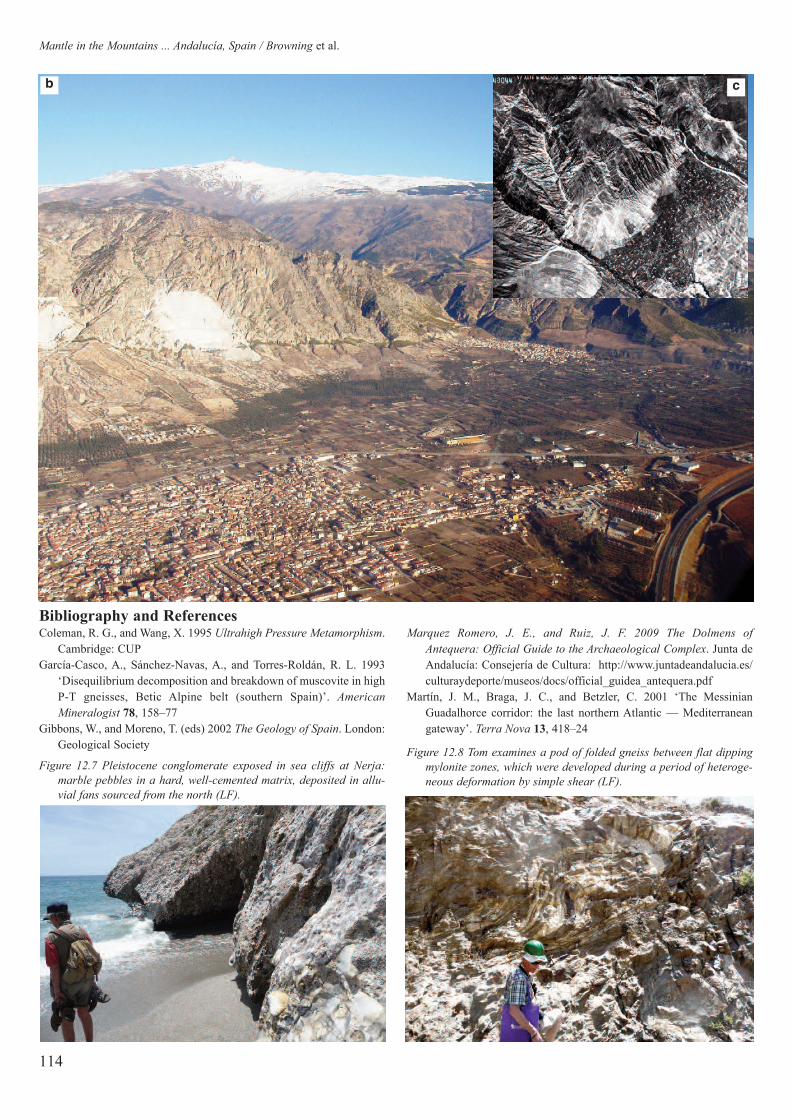
Mantle in the Mountains ... Andalucía, Spain / Browning et al.
114
Bibliography and ReferencesColeman, R. G., and Wang, X. 1995 Ultrahigh Pressure Metamorphism.
Cambridge: CUPGarcía-Casco, A., Sánchez-Navas, A., and Torres-Roldán, R. L. 1993
‘Disequilibrium decomposition and breakdown of muscovite in highP-T gneisses, Betic Alpine belt (southern Spain)’. American
Mineralogist 78, 158–77Gibbons, W., and Moreno, T. (eds) 2002 The Geology of Spain. London:
Geological Society
Marquez Romero, J. E., and Ruiz, J. F. 2009 The Dolmens of
Antequera: Official Guide to the Archaeological Complex. Junta deAndalucía: Consejería de Cultura: http://www.juntadeandalucia.es/culturaydeporte/museos/docs/official_guidea_antequera.pdf
Martín, J. M., Braga, J. C., and Betzler, C. 2001 ‘The MessinianGuadalhorce corridor: the last northern Atlantic — Mediterraneangateway’. Terra Nova 13, 418–24
Figure 12.7 Pleistocene conglomerate exposed in sea cliffs at Nerja:
marble pebbles in a hard, well-cemented matrix, deposited in allu-
vial fans sourced from the north (LF).
Figure 12.8 Tom examines a pod of folded gneiss between flat dipping
mylonite zones, which were developed during a period of heteroge-
neous deformation by simple shear (LF).
b c

It is a small urban site measuring c. 400m by 100m along anorth–south axis, and consists of steep-sided woodland. RecentlyTorbay Council has begun a three-year management plan of thin-ning non-native trees to improve access to the geology and viewsfrom the chapel (Herald Express 2015). Very little has been writ-ten about Chapel Hill in the geological literature and the exactposition of the limestone within the local stratigraphy is open toconjecture. The British Geological Survey map (BGS 2004)marks the locality as part of the Nordon Formation, more specif-ically one of two possible strata either side of the MarldonLimestone Member. We did not feel that it would be time-effi-cient, or within our skill set, to attempt to tie the limestone downto a narrower time period than this. The limestone itself has beenextensively quarried on its western side.
The source of the Permian breccia that abut the western side ofthe limestones is clearer. The Sticklepath Fault runs underneathTorre railway station immediately to the west of the site (BGS2004) and this has moved breccia that was originally several kilo-metres to the south-east to rest alongside these limestones. It isbelieved that the contact is fault-controlled (English RivieraGeopark 2015b). However, our survey of the site did not revealanywhere we could definitively see the contact between the tworock types so we were unable to confirm this.
Visitor information
Although the busy A3022 passes directly to the west, the closestparking is on the opposite side of the site, near the north-eastentrance, on Barton Road and other nearby streets. Torre railwaystation is 50m from the south-west entrance to the site and nearthe north-west entrance there is a bus stop for the No. 12 service,which runs from Newton Abbot to Torquay, Paignton andBrixham regularly through the daytime. There are no public toi-lets near by; cafés and shops are c. 1km from the site in Torre.
115
Introduction
This field guide has been put together by a small group of cur-rent and former undergraduate Earth Science students from
the Open University. In June 2015 we visited Chapel Hill on anOU Geological Society field trip to explore the site and to prac-tise our field skills, and this guide has been put together as aresult of our work. Unless referenced otherwise, the work here isthe result of primary research and we welcome any feedback thatwould improve it. Please note that no risk assessment is provid-ed and if you wish to use this guide to explore the site you willneed to make your own common-sense assessment of the risksinvolved (Richard Blagden, editor: [email protected]).
Site overviewChapel Hill (OS grid reference SX9065) is a small geological sitesituated about 1km from the centre of Torquay (Fig. 1). TheEnglish Riviera was designated as a Global Geopark in 2007(English Riviera Geopark 2015a). Chapel Hill is one of itsgeosites, and is also designated as a County Geological Site(CGS) and as a Regionally Important Geological Site (RIGS)(English Riviera Geopark 2015b). It is noted for its Devonianlimestone and Permian breccia, and for the relationship betweenthe two (English Riviera Geopark 2015b), and is known locallyfor the c. 13–14th century chapel, St Michael’s, that tops thelimestone (Fig. 2; Crowson 2015).
Chapel Hill, Torquay
Richard Blagden, Martin Broadbent, Annie Kitto, Gina Little and Trevor Ryder
Proceedings of the OUGS 2 2016, 115–18© OUGS ISSN 2058-5209
Figure 1 Sketch map of Chapel Hill — OS grid reference SX9065
(Martin Broadbent).
Figure 2 St Michael’s, Chapel Hill.

Devonian LimestoneWe started work at the northern end of the quarry (Face 1) andwere able to identify a bedding plane by the presence of stro-matoporoids. From here we worked upwards through the suc-cession and recorded details of six surfaces in total. The succes-sion is massively bedded and rather featureless, and beddingplanes were identified for the most part by coincidence of angleof dip. Although the rocks had recently been cleared of vegeta-tion the surfaces were well weathered (more so towards thesouthern end) and some hammering was needed to reveal thedetail. Hand lenses were used to identify fossils. Table 1 sum-marises each of the beds studied.
Table 1Bed Vertical distance Dip Notes
(from Bed 1)*
1 N/A 60º SW stomatoporoids and corals onsurface; rocks at top dipping60º, possibly by fault action;Permian material at base
2 5m variable, 50–75º no fossils eviden
3 2m 70º SW pink limestone with abunant corals
4 2m 60º SW abundant corals, possiblefault in corner between Face 3 and Face 4
5 unknown 60º SW no fossils; well-faulted, rubblysurface; well weathered
6 unknown 60–70º SW no fossils
* Measurement perpendicular to the bedding plane, i.e. directly upwards
through the strata.
In general we found most bedding surfaces dipping at 60–70º tothe south-west, which was a close approximation to the RIGScitation (English Riviera Geopark 2015b). However, at least twofaces were clearly dipping south and some of the higher parts,inaccessible to us, appeared to abut the SW-dipping faces.Quarrying has removed much of the crucial evidence, but we sus-pect that more than one phase of deformation took place, as inplaces the S-dipping beds appeared to overprint the SW-dippingbeds (Figs 3 and 4).
At first glance the limestone appeared to be dull, grey and fea-tureless, but judicious hammering revealed more details. Face 3in particular was a striking pink colour and Figure 5 (opposite)
shows a rugose coral extracted from Bed 1.One interesting feature was the appearance of a reddish con-
glomerate material at the base of Face 1, and this is discussed atlength in the description of the Sticklepath Fault, below.
The ruin of a limekiln can be seen just between the northernand southern quarries, and it would be interesting to research thestory of the industry at Chapel Hill, with the railway station insuch close proximity.
116
Chapel Hill, Torquay / Blagden et al.
Figure 3 View of the northern quarries.
Figure 4 Sketch of the northern quarry faces, northernmost to the far
left. Beds 5 and 6 continue to the south — for explanation see Table
1 (Richard Blagden).

coarser matrix (fine- to medium-grained angular sand) and moreflattened clasts, including some red shales and mudstones, whichare possibly re-worked local Permian sediments. Although moredetailed analysis is required, there is a visual impression thatthese flattened clasts show signs of imbrication, indicating apalaeocurrent direction towards the north-west, in a similar direc-tion to the dip. This layer possibly represents a small temporarychannel on the surface of a larger alluvial fan. Above this unit isa variable thickness (0.8–2.1m) of the bedded breccias describedin the second paragraph of Permian Conglomerate (above),which form the dominant lithology of the whole exposure.
Section 2 is approximately in the centre of the exposure and isshown in Figure 5. It is dominated by beds of varying thicknessof breccia (200–400mm), in which the number and size of clastsshow a tendency to decrease from the base upwards. This may beconsistent with deposition by flash-flood events; and c. 1.5mfrom the base of this section (the base being the pavement) is abed with fewer clasts that show more obvious signs of imbrica-tion than elsewhere on the exposure. The palaeocurrent directionindicated here is ‘into’ the face, or towards the north-east, whichis possible evidence for variations in current directions consistentwith shifting channels on the surface of a fan.
Section 3 The final section chosen for more detailed examinationis located c. 30m from the ‘top’ (northernmost end) of the expo-sure, close to another direction sign by the side of Newton Road
(Fig. 7). This site was examined because it may show asection through a large palaeochannel eroded into lay-ered breccias. Apart from the possible channel marginsmarked by abrupt lateral changes in lithology, the unitswithin the ‘channel’ are also more varied, containinglenses of reworked red shale and mudstone clasts set ina fine, silty matrix. These are visible as darker areas inFigures 7 and 8 (overleaf).
The Sticklepath FaultThe most intriguing structural discovery on the site wasat the base of limestone quarry Face 1. Here, adjoiningthe base of the limestone, we discovered a very smallamount of red sandstone with rock fragments, similar tothe Permian deposits at the bottom of the hill. This pro-voked considerable discussion and two theories wereraised to account for its appearance.
It is not in dispute that the Sticklepath Fault runs alongthe western edge of the site, and that it was responsiblefor bringing the Permian rocks into contact with the
117
Proceedings of the OUGS 2 2016
Permian ConglomerateThe exposure of Permian Strata at Chapel Hill Woods is locatedin a road cut by the side of Newton Road, which marks the west-ern boundary of the site. The length of this exposure is c. 200m.
The general nature of the lithology of these rocks is a series ofconglomerates or breccias dipping at c. 9º in a direction appar-ently towards the north-west, although this may not represent thetrue dip (Fig. 6). The breccias are interbedded with lenses of finermaterial, most commonly of fine to medium sand. The thicknessof beds shows considerable variation from 100mm to 0.5m and,in places, poorly defined, graded bedding is visible — finingupwards. The majority of clasts in the breccias consist ofDevonian limestones (up to 200mm in diameter), which containfrequent fossil fragments, including corals and brachiopods.Other, less common, clasts include quartz and very darkcoloured, often black, fine-grained crystalline volcanics. Thematrix of the breccias varies from silt to fine sand. The sandgrains examined by hand lens were mostly angular and glassy.This lithology would be consistent with deposition in an alluvialfan environment.
The original aim had been to construct a generalised graphiclog from the base of the exposure (at its southern end) to theyounger units (at the northern end) by tracing the topmost beds inone location and following them to where they ‘disappear’ intothe pavement, from which point the log could be continuedupwards. However, this proved impractical, as many ‘beds’ arelaterally discontinuous lenses. Therefore, only three sections aredescribed here in more detail.
Section 1 The oldest exposure is located at the southern end ofthe road-cut, and the following description is of a section locatedclose to the lower road direction sign c. 30m from the southern-most end of the exposure. The lowest unit in this section com-prises c. 1.1m of matrix-supported breccia with clasts up to200mm in diameter. The clasts are evenly distributed throughoutthe unit and the matrix is predominantly of silt size. As through-out the exposure, the clasts are predominantly of Devonian lime-stones with some quartz and dark volcanic rocks. Above thislayer is a unit of variable thickness (typically c. 0.5m), with a
Figure 5 Rugose coral, from lime-
stone Face 1 at Chapel Hill.
Figure 6 Roadside cutting of the Permian rocks

Due to the small size of the deposit and the lack of corroborat-ing evidence we were unable to adequately answer this question,but it would make an interesting focus for future research.
SummaryChapel Hill is an interesting geological site showing good expo-sures of Devonian limestone and Permian breccias. It is an urbansite with good transport links and can easily be explored fromTorquay.
The underlying geology of the area is revealed very nicelyfrom the chapel itself, with the limestone plateau of Torquay par-ticularly prominent.
The Permian rocks exposed in the road cutting and the quar-ried Devonian limestone cliffs are each worthy of explorationin their own right and may reveal features not described here.The Sticklepath Fault runs through, or adjacent to, the site.It was not clear on our visit whether or not the boundary itselfis exposed (see The Sticklepath Fault), but the relative posi-tions of the rocks at least suggest that an unconformity is pres-ent, if not the fault itself.
ReferencesBritish Geological Survey 2004 England and Wales Sheet 350
Torquay Solid and Drift [map] (scale 1:50,000). London: NERCCrowson, T. 2015 ‘Work continues to reveal historic secretchapel at heart of Torquay’. Herald Express [on-line] 22February 2015: www.torquayheraldexpress.co.uk/STUNNING-video-Work-continues-reveal-historic/story-26065130-detail/story.html [accessed 9 July 2015]English Riviera Geopark 2015) About the Geopark. [on-line]www.englishrivierageopark.org.uk/section_main.cfm?sec-tion=101 [accessed 10 June 2015]English Riviera Geopark 2015b) Chapel Hill, Torre. [on-line]www.englishrivierageopark.org.uk/section_sub.cfm?sec-tion=13&sub=56 [accessed 10 June 2015]Herald Express 2015 ‘Council clearing trees to restore historicviews’. Herald Express [on-line] 28 January 2015: www.torquay-heraldexpress.co.uk/Council-clearing-trees-restore-historic-views/ story-25929822-detail/story.html [accessed 5 July 2015]
118
Chapel Hill, Torquay / Blagden et al.
Devonian Limestone (Fig. 9). However, the actual contactbetween the two is hidden by the extensive slope of talus, soil andquarried waste that forms the hillside. By definition, any point atwhich the Permian comes into contact with the Devonian herelies on the fault, and it was suggested that the deposit at the baseof Face 1 must therefore be a very small part of the SticklepathFault. This would require the fault to dip c. 30-45°, but we havenot been able to establish whether this is reasonable.
There were, however, issues with this argument. Limestonemust surely have been quarried away from ‘in front’ of thedeposit, so it is unlikely that this material abutted the leadingedge of the limestone. The deposit did not appear in distinctstrata as it did at the bottom of the site, so was probably notformed by the same actions — although it may have beenreworked by fault movements. It was considered more likelythat this material dropped or was squeezed up into a crack,either during the Permian or more recently, and does not there-fore mark the line of the fault.
Figure 7 Section at northern end of exposure showing what may be a
paleochannel.
Figure 8 Typical cross-section of a Permian rock.
Figure 9 Chapel Hill seen from the southern approach along Newton
Road. St. Michael’s Chapel itself can be seen on the skyline top right,
and the Sticklepath Fault runs through the valley on the far left.

Introduction
As one of the events marking the 200th anniversary of thepublication of William Smith’s 1815 Geological Map, it was
appropriate that a group of geologists should visit his grave andmemorial at St. Peter’s Church in Northampton. This idea wassuggested to me at the OUGS 40th Anniversary Symposium in2012, held in Northampton, by Dave Williams, one of the OUGSspeakers. Dave mentioned that he was on a Geological Societycommittee planning events for the anniversary year, and that hethought something should be organised for Northampton. Hesuggested that as I live near Northampton perhaps I could makethe arrangements, hence my involvement..
So on September 6, 2015, a group of 10 of us made up ofGeological Society and OUGS members, assembled outside theIbis Hotel, Marefair, Northampton, to meet Dr Diana Sutherland,our guide for the day. Diana is the author of Northamptonshire
Stone (2003) and an expert on Northamptonshire geology.
Hazelrigg House, 33 MarefairOur first stop was just across the road from the Ibis, at HazelriggHouse (Fig. 1), which is where William Smith died in 1839. Whatwas Smith doing in Northamptonshire? According to Rev. R. M.Serjeantson in his History of the Church of St. Peter (1904):
In August 1839, he [Smith] was specially invited to attendthe meeting of the British Association in Birmingham. Onhis way he stayed with his friend, Mr G. Baker, the anti-quary, and with him made several excursions into theneighbouring country. On one of these expeditions he con-tracted a chill, which led to serious complications, and ina few days put an end to his life. He died on August 28th.At the suggestion of Dr Buckland, a tablet and bust waserected at St. Peter’s, the cost having been defrayed by asubscription amongst geologists.
It is not known how long Smith had been friends with GeorgeBaker and his sister Anne, or how often he came to Northampton.His county map of Northamptonshire is unfinished, so perhaps hewas working on this as part of his visit.
Hazelrigg House is a Tudor town house, dating from1570–1580, which is built of dark brown sandstone and ironstonefrom the Northampton Sand Formation. The doorcase isCotswold (Taynton?) Limestone. There is a local tradition thatCromwell stayed at the house on his way to Naseby (1645). Thehouse survived the Great Fire of Northampton in 1675. TheBakers, who bought the house in 1831, wrote a large, two-volumehistory of Northamptonshire.
119
William Smith’s last resting place
A joint OUGS and Geological Society visit to St. Peter’s Church, Northampton, followed
by a tour of All Saints Church, Brixworth (6 September 2015)
Ian Clarke
Proceedings of the OUGS 2 2016, 119–21© OUGS ISSN 2058-5209
Figure 1 Hazelrigg House, Marefair, Northampton.

As well as looking at the front of the house, later in the morn-ing we were able to peer into the rooms at the rear of the build-ing. This was much to the consternation of the Through theLooking Glass Theatre Company, whose members were rehears-ing inside. So much so that one of their leaders came out to seewhat we were up to. We explained who we were and gave him aninformation sheet about William Smith. He was very pleasedwith this, as the theatre group want to perform works that bringthe history of the building to life. So perhaps William Smith’sdramatic story will inspire a play (but hopefully not WilliamSmith — the musical!).
St. Peter’s ChurchJust a short way from Hazelrigg House is St. Peter’s Church,described in the recent new edition of Pevsner’sNorthamptonshire (Bailey et al. 2013) as “The most interestingNorman church in Northamptonshire and indeed one of the mostexceptional Norman churches in the country”.
Diana led us to William Smith’s grave in the churchyard(Fig. 2). Here she read out the details of his death certificateand the obituary notice from the local newspaper, theNorthampton Mercury. John Phillips, Smith’s nephew, hadarrived before Smith died and was present at the funeral. Thegravestone is made of very weathered sandstone (New RedSandstone, not local, source unknown) and the inscription ofWilliam Smith’s name is now barely legible.
St. Peter’s dates from AD 1160 and occupies the site of an ear-lier Saxon church. It is built of local brown sandstone and iron-stone of the Northampton Sand Formation, with decorative fea-tures of Blisworth Limestone, giving a typical Northamptonshirepolychrome effect. Inside the church, there is a memorial bust ofWilliam Smith (Fig. 3), by Matthew Noble. The inscription onthe marble plinth reads:
To honour the name of William Smith, LL.D. This monu-ment is erected by Friends and Fellow-labourers in thesame field of British Geology. Born 23rd March, 1769, atChurchill in Oxfordshire, and trained to the Profession of aCivil Engineer and Mineral Surveyor. He began, in 1791,to survey collieries and plan canals in the vicinity of Bath,and having observed that several strata of that district were
characterised by peculiar groups of organic remains headopted this fact as a principle of comparison, and was byit enabled to identify the strata in distant parts of thisisland, to construct sections, and to complete and publishin 1815 a Geological Map of England and Wales. By thusdevoting, during his whole life, all the power of an observ-ing mind to the advancement of one branch of Science, hegained the title of the “Father of English Geology”.
Inside the church, Diana spoke about the building’s architecturalhistory, including the many Norman alterations and its partialrebuilding by George Gilbert Scott in 1850, the building stonesand stone carvings — in particular a magnificent Anglo-Saxontomb-slab decorated with a Green Man and fantastic birds andbeasts. This tomb dates from the 10th or 11th century and is reput-ed to be the grave slab of St. Ragener, a little-known Anglo-Saxonprince, soldier and martyr (Sargant, accessed 29-12-2015).
All Saints’ Church, BrixworthAfter lunch, we continued to explore the Saxon theme by visit-ing All Saints’ Church, Brixworth, a few miles north ofNorthampton (Fig. 4, opposite). All Saints’ is one of the mostoutstanding examples of Anglo-Saxon architecture in England.It dates from the 8th and 9th centuries. Diana has spent manyyears working on identifying the many building stones used inits construction, especially in the Saxon parts of the church, andtracing the history of the building’s development. We began ourtour inside the church and she told us about the main points inthe building’s history: Saxon, later medieval and especially the19th century restoration by Rev. C. F. Watkins. Watkins did awonderful job in restoring Anglo-Saxon features, rebuilding thepolygonal apse and revealing the ambulatory that had been cov-ered by medieval stonework. The ambulatory, a walkway forpilgrims, is a semi-circular, sunken, outer ring-crypt surround-ing the apse. A highlight of the tour was to be able to go up intothe stair turret and see the use of tufa in the construction of theturret’s stair vault.
120
William Smith’s Last Resting Place / Clarke
Figure 2 William Smith’s grave, St. Peter’s Church cemetery, Marefair
Figure 3 William Smith memorial in St. Peter’s Church

Sargant, D. (ed) [accessed 29-12-2015] St. Ragener of Northampton
Prince, Soldier, Martyr by the Venerable Bazil Marsh, BA MLittFormerly Rector of St Peter’s, Northampton:www.fostp.org.uk/uploads/St%20Ragener%20(M)%20of%20Northampton.pdf
Serjeantson, Rev. R. M. 1904. History of the Church of St. Peter,
Northampton. Northampton: W. MarkSutherland, D. S. 2003 Northamptonshire Stone. Wimbourne: Dovecote
PressSutherland, D. S. 2014. The Building of Brixworth Church. Brixworth:
The Friends of All Saints Church, BrixworthWinchester, S. 2001 The Map that Changed the World: The Tale of
William Smith and the Birth of a Science. London: Penguin Books
121
Outside, Diana treated us to a geologi-cal feast, as we examined some of thebuilding stones around a small door onthe south side of the tower (Fig. 5). Theseinclude bedded tuffs, diorite,Markfieldite, granite, mica hornfels,Swithland Slate, grey and red Triassicsandstones, and many Roman bricks(Fig. 6). None of these stones is local, alloriginating in Leicestershire, and theyare thought to have been reclaimed fromRoman buildings in Leicester (Romanname Ratae) and brought about 35km toBrixworth for use in building this veryprestigious church.
However, as well as these importedigneous rocks and sandstones, there isplenty of Northamptonshire stone. Thisincludes eight types of NorthamptonSand, Blisworth Limestone and tufa.Northampton Sand was quarried locally,but the Blisworth Limestone may comefrom Towcester, 25km away. The tufa could have been foundlocally, but, like much of the church’s stone, could have comefrom a Roman site.
This was a fascinating day of geology, history and architectur-al delights. Thank are due to Diana Sutherland for showing ussuch wonderful buildings and explaining everything so well; andto The Churches Conservation Trust for allowing us access to St.Peter’s and to the Friends of All Saints’ Church, Brixworth, whoenabled us to go up into the stair turret.
Further readingBailey, B., Pevsner, N., Cherry, B. 2013 Northamptonshire, The
Buildings of England. London: Yale UP
Proceedings of the OUGS 2 2016
Figure 4 All Saints’ Church, Brixworth.
Figure 6 Brixworth Church’s patchwork of building stone and arch of
Northampton Sand.
Figure 5 Dr Diana Sutherland showing the mixture of building stones at
the small door, All Saints’ Church.and Brixworth.

Group: these quartzite pebbles were eroded from the Variscanuplands of Brittany, and were carried northward by a large, braid-ed river system. Next the author turns his attention to the problemof identifying rock used as building stone, and in particular theproblem of distinguishing between building stones that looksuperficially similar. In Staffordshire, sandstone is used widely asa building stone, but there are many different sandstone forma-tions; and for those involved in restoration it is critically impor-tant to identify the original stone and to locate the source quarry.Emphasising that visual inspection is often not sufficient fordefinitive identification, the author outlines the differences thatcan be observed by visual inspection in the field, the differencesthat can be seen in thin section, and the geochemical differencesbetween different formations, using a combination of textualexplanation, tables, graphs, and photographs.
The third and longest part of the book (nearly 200 pages) isdevoted to individual descriptions of stone buildings inStaffordshire. As the author notes in the Preface, this was one ofthe main aims of the book. This part deals in turn with fortifica-tions, churches, halls and country houses, and vernacular build-ings. Each section begins with an overview followed by anaccount of individual buildings, detailing location, historicalaspects, architectural features, and building stone, together withimages, which typically include an overall view of each buildingand a close-up view of its building stone. There are also a fewhistorical images and some close-ups of architectural features.Altogether the author identifies and describes more than 100 indi-vidual stone buildings, and he is able within his scheme ofdescription to incorporate interesting snippets of non-geologicalinformation such as archaeological finds, information about theowners, or architectural decorations. This part of the book ismore accessible, using less technical language than Parts 1 and 2,making this a good starting point for non-specialist readers.
The different parts of the book are suited to different audiences.For example, sections from Part 2 would be particularly relevantto readers who might be involved in stone building restoration, orstudents who are interested in finding out about the geochemistryof local sandstone, while Part 3 is more accessible to a generalaudience. Most readers are unlikely to read the book sequential-ly — they are more likely to pick out areas of interest. To addressthe different needs of these varied audiences I would have likedto see the addition of a glossary, and full referencing of the web-sites, which are provided in the Reference section simply as a listof website addresses.
Overall, this is a unique resource, gathering together a widerange of information relating to the building stones, stone build-ings and geology of Staffordshire.
— Sandra Morgan, OUGS West Midlands Branch Organiser
122
Book review
Book reviewFloyd, Peter A. 2015 Building Stones and Stone Buildings of
Staffordshire. Ilfracombe: Arthur H. Stockwell Ltd (ISBN 978-0-72234-543-6; paperback ; £14.95)
This book, written by Dr Peter Floyd (a Reader in Geochemistryat the University of Keele until his retirement), focuses onbuilding stone obtained from Staffordshire and buildings in thecounty that utilise this. The author tells us in his Preface that thebook is aimed at people who are interested in natural history andearth science, rather than professionals, but he also expects it tobe useful to a very specific group: people involved in stonebuilding restoration.
The book is divided into three parts, each part having a nar-rower focus than the preceding one. The scope of the first part ofthe book is very wide. It begins with a brief overview of stonebuilding in Staffordshire from the Stone Age to the present andan overview of studies and databases of local building stone. Weare then introduced to igneous, metamorphic and sedimentaryrock types, to geological time and to the geology of the UK, withparticular reference to the origin and some of the geologicalprocesses associated with various types of rocks used as buildingstone. Next there is a section on conservation and restoration,which includes an overview of physical, chemical and biologicalweathering processes as they affect building stone. The authorthen goes on to discuss restoration and the problems of sourcingsuitable stone with properties that are as close as possible to theoriginal. This is followed by a very brief introduction to archi-tectural styles, with guidance to the reader on how to find outmore. Next there is a short section on masonry, which is helpfulin showing how building stone may be oriented and dressed; andfinally there is a section on the terminology of architectural fea-tures found in churches, castles and country houses.
Thus the first part of the book gives us condensed introductionsto various topics, supported by many references to printed mate-rial and websites so that the reader can readily explore any ofthese topics in greater detail. Part 1, like the rest of the book, iscopiously illustrated by photographs and diagrams, althoughsome images would have benefited from improved resolution.
The second part of the book discusses the geology ofStaffordshire: the majority of the county has Triassic bedrock,with some significant areas of Carboniferous rock and smallerareas from the Permian and Silurian. The author provides a sim-plified geological map of the county and a comparison of activequarry sites in 1851 and 1994. He then outlines Carboniferous,Permian and Triassic geological processes and the stratigraphy ofthe area. Those who have walked around Staffordshire will bepleased to learn the origin of the rounded, liver-coloured pebblesfound in several of the formations of the Sherwood Sandstone

123
Introduction
The Afon Cleddau has two main headwaters, the western andthe eastern branches, which have their confluence at Picton
Point; south of this locality the main river is known as theDaugleddau (Fig. 1). North of Haverfordwest, the WesternCleddau flows through the spectacular Treffgarne Gorge, whichrepresents a glacial overflow channel, and the nearby rhyoliticcrags of Maiden Castle rise above the western side of the gorge.The main river neatly bisects the Pembrokeshire Coalfield and inthe 19th century it provided a natural outlet for local anthraciterequired for iron making and lime burning. Hook on the WesternCleddau and Landshipping Quay on the Daugleddau were busyriver ports exporting coal at that time.
The southern margin of the coalfield is marked by a linear outcropof Carboniferous Limestone, which has been quarried extensivelyfor building stone and more recently for limestone aggregate. Thequarries at West Williamston on the Carew River were worked inthe 19th century and the stone was transported downstream on sail-ing barges. Pembroke Castle and many of the numerous forts anddefensive works that line the Lower Haven were built from locallyquarried Carboniferous Limestone. The whitewashed tower ofBenton Castle is a conspicuous landmark rising above the woods onthe western side of the Daugleddau. Geologically this building issignificant in that it gives its name to the Benton Castle Fault, amajor thrust produced by the Caledonian Orogeny and later reacti-vated during the Variscan earth movements.
The river gets significantly wider below the Cleddau Bridge andthe presence of docking facilities, oil refineries and oil terminals(jetties) makes considerable impact on the natural environment.Despite these industrial developments along the Lower Haven,there are numerous small, unspoilt bays, including Sandy Haven,Lindsway Bay and Dale Roads, where interesting geologicallocalities can be accessed.
The Cleddau is a classic example of a drowned river valley orria produced by the late Flandrian rise in sea level less than10,000 years ago. The branching pattern of drowned tributarystreams provides an ideal environment for mooring small fishingand pleasure boats. These tributary valleys are locally known aspills (e.g. Cosheston Pill, Sandyhaven Pill), the sides of which areoften wooded while the silted headwaters are colonised by saltmarsh, providing a haven for wild life.
Localities to visitStarting in the upper reaches of the Western Cleddau, the itiner-ary follows the river downstream to its estuary as it crosses asequence of geological outcrops.
1. Maiden Castle [SM 955248] and the Treffgarne Gorge
[SM 958250]
The crags of Maiden Castle and neighbouring Poll Carn formprominent outcrops of the Roch rhyolite on the west side of theTreffgarne gorge (Fig. 2, overleaf). This locality is c. 9km northof Haverfordwest on the A40 Fishguard road. Park in the lay-byat Nant-y-Coy Mill where there is an excellent tearoom and craftshop. Walk up the narrow lane on the south side of the mill andafter c. 100m take the footpath that leads to Maiden Castle andbeyond to Poll Carn. These rugged tors are formed of flow-band-ed rhyolitic lavas that are also nodular and brecciated in places(Fig. 3, overleaf). The viscous, silica-rich lava flow would havehad a congealed crust, which was broken up and fragmented bythe continued movement of the molten lava underneath the crust.This autobrecciated lava can be recognised in the outcrop by itsfractured appearance that is recrystallised on some surfaces. Therocks at this locality belong to the Roch Volcanic Formation thatextends south-westwards c. 8km in a prominent line throughPlumstone Rocks and Cuffern Mountain to Roch Castle [SM
880211]. Although these RochVolcanics have long been consid-ered to be of Precambrian age, theBGS now assign them to theArenig Series of the Ordovician.
Maiden Castle and Poll Carn areimportant geomorphological sitesfor the study of the formation oftors. The physical appearance ofthe tors can be described asupstanding irregular masses of rhy-olitic lavas surrounded by block-field slopes (Fig. 4, overleaf). Thelarge blocks that litter the slopeshave clearly been detached fromthe main outcrop. Many researchersconsider that the tors evolved underperiglacial conditions during thelate Devensian, when the area isthought to have been just beyondthe maximum ice limit. On the
Exploring the Afon Cleddau Valley in Pembrokeshire: a geological itinerary
John Downes
Proceedings of the OUGS 2 2016, 123–31© OUGS ISSN 2058-5209
Figure 1 The Cleddau Valley and surrounding area.
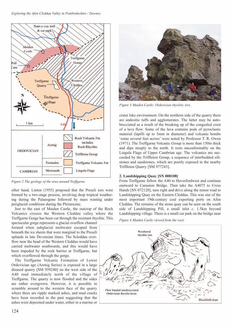
124
Exploring the Afon Cleddau Valley in Pembrokeshire / Downes
other hand, Linton (1955) proposed that the Preseli tors wereformed by a two-stage process, involving deep tropical weather-ing during the Palaeogene followed by mass wasting underperiglacial conditions during the Pleistocene.
Just to the east of Maiden Castle, the outcrop of the RochVolcanics crosses the Western Cleddau valley where theTreffgarne Gorge has been cut through the resistant rhyolite. Thisspectacular gorge represents a glacial overflow channelformed when subglacial meltwater escaped frombeneath the ice sheets that were marginal to the Preseliuplands in late Devensian times. The Scleddau over-flow near the head of the Western Cleddau would havecarried meltwater southwards, and this would havebeen impeded by the rock barrier at Treffgarne, butwhich overflowed through the gorge.
The Treffgarne Volcanic Formation of LowerOrdovician age (Arenig Series) is exposed in a largedisused quarry [SM 959240] on the west side of theA40 road immediately north of the village ofTreffgarne. The quarry is now flooded and the sidesare rather overgrown. However, it is possible toscramble around to the western face of the quarrywhere there are ripple marked ashes, and mud crackshave been recorded in the past suggesting that theashes were deposited under water, either in a marine or
crater lake environment. On the northern side of the quarry thereare andesitic tuffs and agglomerates. The latter may be auto-brecciated as a result of the breaking up of the congealed crustof a lava flow. Some of the lava contains pods of pyroclasticmaterial (lapilli up to 5mm in diameter) and volcanic bombs‘some several feet across’ were noted by Professor T. R. Owen(1971). The Treffgarne Volcanic Group is more than 150m thickand dips steeply to the north. It rests unconformably on theLingula Flags of Upper Cambrian age. The volcanics are suc-ceeded by the Triffleton Group, a sequence of interbedded silt-stones and sandstones, which are poorly exposed in the nearbyTriffleton Quarry [SM 977243].
2. Landshipping Quay [SN 008108]
From Treffgarne follow the A40 to Haverfordwest and continueeastward to Canaston Bridge. Then take the A4075 to CrossHands [SN 072120]; turn right and drive along the minor road toLandshipping Quay on the Eastern Cleddau. This was one of themost important 19th-century coal exporting ports on AfonCleddau. The remains of the stone quay can be seen on the southside of Landshipping Pill, a small inlet c. 1.5km beyondLandshipping village. There is a small car park on the bridge near
Figure 2 The geology of the area around Treffgarne.
Figure 3 Maiden Castle: Ordovician rhyolitic tors.
Figure 4 Maiden Castle viewed from the west.

125
Proceedings of the OUGS 2 2016
the quay and near by is a memorial at to the 40 miners who losttheir lives in the infamous Garden Pit disaster in 1844 when mineworkings were flooded by river water (Fig. 5).
At low tide, walk along the foreshore below the low rivercliffs on the north side of the pill, where you will see the MiddleCoal Measures exposed (Fig. 6). Thin coal seams and seatearths containing plant remains within the Timber Vein Groupcrop out at the western end of the section, but they are muchcontorted by Variscan folding and thrusting. There are examplesof cross-cutting, sandstone-filled channels (Fig. 7), wedging-out structures and numerous bedded ironstone nodules. At thefar end of the section there is a distinctive 2m-thick bed oforange coloured ironstone concretions. A large shallow anti-cline on the foreshore shows rectilinear jointing, ripple beddingand evidence of polygonal mudcracks.
Figure 5 Memorial to the miners killed in the Garden Pit disaster of 1844.
Figure 6 Stratigraphical Column for the Cleddau Valley south of
Haverfordwest.
Figure 7 Sandstone-filled channel cross-cutting shales in Middle Coal
Measures.
About 300m south of the ruined quay, the foreshore exposescyclothem units of the Lower Coal Measures dipping c. 50º SE.However, there is considerable evidence of northward propa-gating Variscan thrust movements in the folded strata. Oneexample at SN 105005 shows a thrust fault where the upper halfof a fold has been carried northward along the thrust plane.There are several folds showing spaced cleavage in the silt-stones between the more competent sandstone layers. The foldaxes generally trend NW–SE as in the synclinal structure out-lined by sandstone ribs on the foreshore near to the southernend of the section. The foreshore rock exposures are cut off bya major E–W fault at SN 003101 and south of this point thereare no further coal measure outcrops.
3. West Williamston Quarries [SN 025061]
From Landshipping return to the A4075 and drive to the junctionat SN 057054, just south of Cresselly; turn right along the lane toWest Williamston. The disused Point Quarries can be accessed bya footpath from the west side of the village. The quarries weremajor producers of limestone in the early 19th century when theirtidewater location enabled the stone to be transported around theWelsh coast. Barges of 15–20 tons were loaded in the tidal chan-nels that joined the quarries to the river (Fig. 8, overleaf), andthen moved to Lawrenny quay to be transhipped on to coastalvessels. The limestone was in great demand at the time for use in

126
Exploring the Afon Cleddau Valley in Pembrokeshire / Downes
limekilns to produce agricultural lime, mortar and whitewash forhouses. Records show that in 1839, a 40-ton sloop called Ranger
carried 10 cargoes of limestone from Lawrenny to Abercastle onthe north coast of Pembrokeshire. At the time of the Napoleonicwars there was a great demand for stone to build the complex offortifications to protect the Milford Haven. West Williamstonquarries were ideally located to supply limestone blocks fortransport by barge direct to the forts. Many of the Admiraltybuildings in Pembroke Dock were also constructed of limestonefrom these quarries.
You can get to the old quarries from the A4075 road at Carewby following the narrow lane past Carew mill pond to WestWilliamston. There is a small car park at SN 033059. Follow thedriveway to Williamston Park, from where a public footpathleads down to the salt marsh alongside the Carew River. The siteis on a promontory at the confluence of the Carew and Cresswellrivers. About 200m before reaching the north-west end of the site,there is a footpath leading through the trees to Point Quarrywhere the limestone is exposed (Fig. 9). Today the quarries arelargely overgrown, but they provide a haven for wildlife and nat-ural vegetation protected as a designated SSSI and managed bythe Wildlife Trust of South and West Wales.
The Lower Carboniferous succession at West Williamston isc. 300m thick and the strata lie on the flank of the CarewAnticline, dipping c. 25° NE. The fine-grained grey oolite atPoint Quarry belongs to the Black Rock Limestone and itshomogeneous texture make it an excellent building stone. Onthe top of the ridges between the tidal creeks there are several
The most interesting geological aspects of this locality are thesoft sediment deformation structures in the Cosheston Group ofthe Lower Old Red Sandstone. On reaching the river take thepath to the left and walk c. 300m to where a set of steps leadsdown to the rocky foreshore at SN 999050. Look carefully at thelow cliff face and you will see classic ball-and-pillow structures
below the base of a sandstone bed. This occurs whererounded masses of sandstone have sunk into the under-lying mudstone when it was still soft and unconsoli-dated (Fig. 10). It has also been argued that seismicshocks may convert overlying sediments into quick-sand that then founders into the mud. There are exam-ples of soft sediment deformation on the rock fore-shore where sandstone pillows are enclosed inslumped sediment. About 200m to the west there is abeautiful example of an anticlinal fold that has beencut by a reverse fault, while the whole structure isunderlain by slumped mudstones.
Figure 8 Tidal channels formerly used by barges entering Point Quarry.
Figure 9 Point Quarry at West Williamston.
metres of ‘rotten beds’ that are deeply weathered. This is apalaeokarst horizon where the limestone is pitted by chemicalweathering and some faces show solution hollows up to300mm in diameter. There are also numerous infilled fissures.The reddish clay infill appears to represent a weatheringresidue of insoluble clay minerals in which there are roundedfragments of unweathered limestone. The deeply weatheredbeds were probably formed as ground water percolated throughbedding planes and joints resulting in solution of the limestoneat depth. During Lower Carboniferous times, the hot, wet trop-ical conditions would have been ideal for the development ofthese palaeokarst features.
4. Mill Bay [SN 002049]
From West Williamston return to the A4075 and drive south tothe A477; turn right through Milton and continue on the mainroad towards Pembroke Dock. Turn left into Cosheston; at thevillage crossroads continue northward c. 1km to RosehillCottage. On the west side of the road there is a wooden gate thatgives access to a track leading down through a wooded valley toMill Bay. This is a permissive path that is closed to the publicduring December and January. It is best to approach Mill Bay atlow tide in order to gain access to the rocks in safety.
Figure 10 Ball-and-pillow structures in the Cosheston beds (Lower
ORS) in Mill Bay.
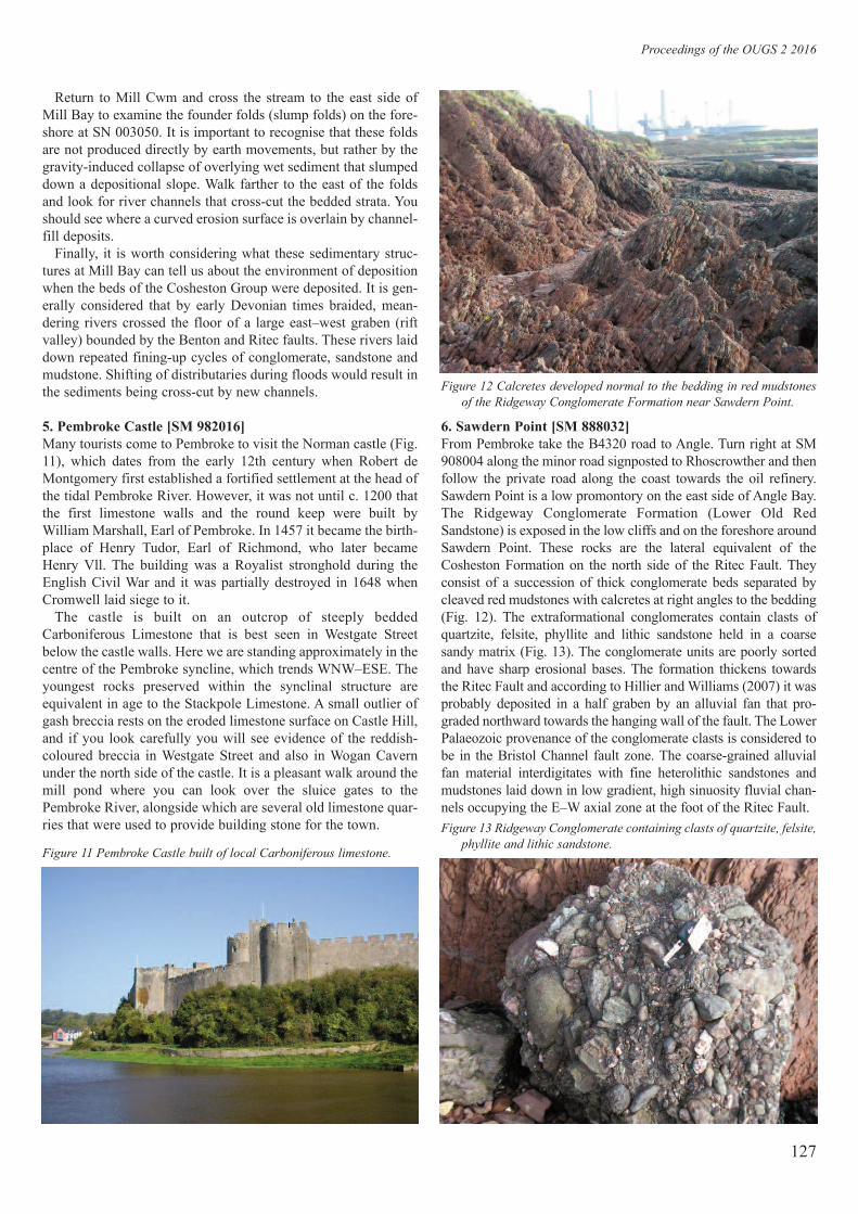
Return to Mill Cwm and cross the stream to the east side ofMill Bay to examine the founder folds (slump folds) on the fore-shore at SN 003050. It is important to recognise that these foldsare not produced directly by earth movements, but rather by thegravity-induced collapse of overlying wet sediment that slumpeddown a depositional slope. Walk farther to the east of the foldsand look for river channels that cross-cut the bedded strata. Youshould see where a curved erosion surface is overlain by channel-fill deposits.
Finally, it is worth considering what these sedimentary struc-tures at Mill Bay can tell us about the environment of depositionwhen the beds of the Cosheston Group were deposited. It is gen-erally considered that by early Devonian times braided, mean-dering rivers crossed the floor of a large east–west graben (riftvalley) bounded by the Benton and Ritec faults. These rivers laiddown repeated fining-up cycles of conglomerate, sandstone andmudstone. Shifting of distributaries during floods would result inthe sediments being cross-cut by new channels.
5. Pembroke Castle [SM 982016]
Many tourists come to Pembroke to visit the Norman castle (Fig.11), which dates from the early 12th century when Robert deMontgomery first established a fortified settlement at the head ofthe tidal Pembroke River. However, it was not until c. 1200 thatthe first limestone walls and the round keep were built byWilliam Marshall, Earl of Pembroke. In 1457 it became the birth-place of Henry Tudor, Earl of Richmond, who later becameHenry Vll. The building was a Royalist stronghold during theEnglish Civil War and it was partially destroyed in 1648 whenCromwell laid siege to it.
The castle is built on an outcrop of steeply beddedCarboniferous Limestone that is best seen in Westgate Streetbelow the castle walls. Here we are standing approximately in thecentre of the Pembroke syncline, which trends WNW–ESE. Theyoungest rocks preserved within the synclinal structure areequivalent in age to the Stackpole Limestone. A small outlier ofgash breccia rests on the eroded limestone surface on Castle Hill,and if you look carefully you will see evidence of the reddish-coloured breccia in Westgate Street and also in Wogan Cavernunder the north side of the castle. It is a pleasant walk around themill pond where you can look over the sluice gates to thePembroke River, alongside which are several old limestone quar-ries that were used to provide building stone for the town.
127
6. Sawdern Point [SM 888032]
From Pembroke take the B4320 road to Angle. Turn right at SM908004 along the minor road signposted to Rhoscrowther and thenfollow the private road along the coast towards the oil refinery.Sawdern Point is a low promontory on the east side of Angle Bay.The Ridgeway Conglomerate Formation (Lower Old RedSandstone) is exposed in the low cliffs and on the foreshore aroundSawdern Point. These rocks are the lateral equivalent of theCosheston Formation on the north side of the Ritec Fault. Theyconsist of a succession of thick conglomerate beds separated bycleaved red mudstones with calcretes at right angles to the bedding(Fig. 12). The extraformational conglomerates contain clasts ofquartzite, felsite, phyllite and lithic sandstone held in a coarsesandy matrix (Fig. 13). The conglomerate units are poorly sortedand have sharp erosional bases. The formation thickens towardsthe Ritec Fault and according to Hillier and Williams (2007) it wasprobably deposited in a half graben by an alluvial fan that pro-graded northward towards the hanging wall of the fault. The LowerPalaeozoic provenance of the conglomerate clasts is considered tobe in the Bristol Channel fault zone. The coarse-grained alluvialfan material interdigitates with fine heterolithic sandstones andmudstones laid down in low gradient, high sinuosity fluvial chan-nels occupying the E–W axial zone at the foot of the Ritec Fault.
Proceedings of the OUGS 2 2016
Figure 11 Pembroke Castle built of local Carboniferous limestone.
Figure 12 Calcretes developed normal to the bedding in red mudstones
of the Ridgeway Conglomerate Formation near Sawdern Point.
Figure 13 Ridgeway Conglomerate containing clasts of quartzite, felsite,
phyllite and lithic sandstone.

The Skrinkle Sandstone Group (Upper Old RedSandstone) is faulted against the RidgewayConglomerate Formation c. 400m ESE of SawdernPoint. Here mudstones, medium-grained sandstonesand thin conglomeritic units are present on thedownthrow side of the fault. An alternating sequenceof red and grey mudstones and sandstones is wellexposed on the foreshore around SM 897026, andthe grey calcareous mudstones record evidence of anincreasing marine influence, heralding the onset ofthe Lower Carboniferous marine transgression.
7. West Angle Bay [SM 855033]
Return to the B4320 and follow this road through Angle villageto the large car park adjacent to the beach in West Angle Bay.There is a café open during the tourist season and there are toiletsnext to the car park. The Hibernia pub in the village serves excel-lent refreshments.
At low tide, when the rocks are fully exposed, I suggest thatyou stand on the low sea wall near to the café and look out acrossthe bay and the entrance to the Milford Haven. Large oil tankersand the new LNG vessels have to negotiate this relatively narrowstretch of water between West Angle and St. Ann’s Head and itwas here that the ill fated Sea Empress was grounded in 1996with the loss of 72,000 tonnes of crude oil that polluted the coast-line for miles around. This is part of the environmental price wehave to pay for relying on imported oil and gas, but also from anaesthetic point of view, the existence of the three large oil refiner-ies on the Haven is an ever-present blot on the landscape, espe-cially in a National Park!
From your viewpoint you will also be able to observe the lineof the synclinal axis that trends WNW–ESE on the south side ofWest Angle Bay (Fig. 14). You will see the dark grey limestonesand shales of the Avon Group outcropping on either side of thebay, with the younger Black Rock Limestone occupying much of
Exploring the Afon Cleddau Valley in Pembrokeshire / Downes
128
the area beneath the sandy beach. Now walk along the foreshoreto the first cove that lies below a ruined limekiln on the north sideof the bay. Here you should be able to see the Avon Group strata
dipping towards the south and resting discordant-ly upon the almost vertical beds of Black RockLimestone. Here there has been a strong thrustmovement pushing the Avon Group rocks north-ward over Black Rock Limestone. The line ofthis thrust fault can be traced through Cove 2 andinto the south side of Cove 3 where a narrowzone of brecciated limestone marks the lowerside or footwall of the thrust (Fig. 15). These bro-ken and shattered rocks are the result of move-ment along the thrust fault during the Variscanearth movements (Fig. 16).
Walk over the rocks into Cove 3, where youwill see several other interesting geological struc-tures on the foreshore, including two periclinalfolds that appear as shallow elongated domesrather like the upturned hull of a boat. The axes ofthe folds are orientated parallel to the main syn-clinal axis of West Angle Bay. The rocks are alsocut by a series of en échelon veins that are wherethe rock has been sheared and the resulting ten-sion gashes have later been filled with the miner-al calcite. You may also notice some small circu-lar holes with radiating fractures c. 300mm long.
Figure 14 The geology of the northern shoreline of West Angle Bay.
Figure 15 View across the north shore of West Angle Bay.
Figure 16 Thrust plane between the Avon Group and the underlying ver-
tically bedded Black Rock Limestone in West Angle Bay.
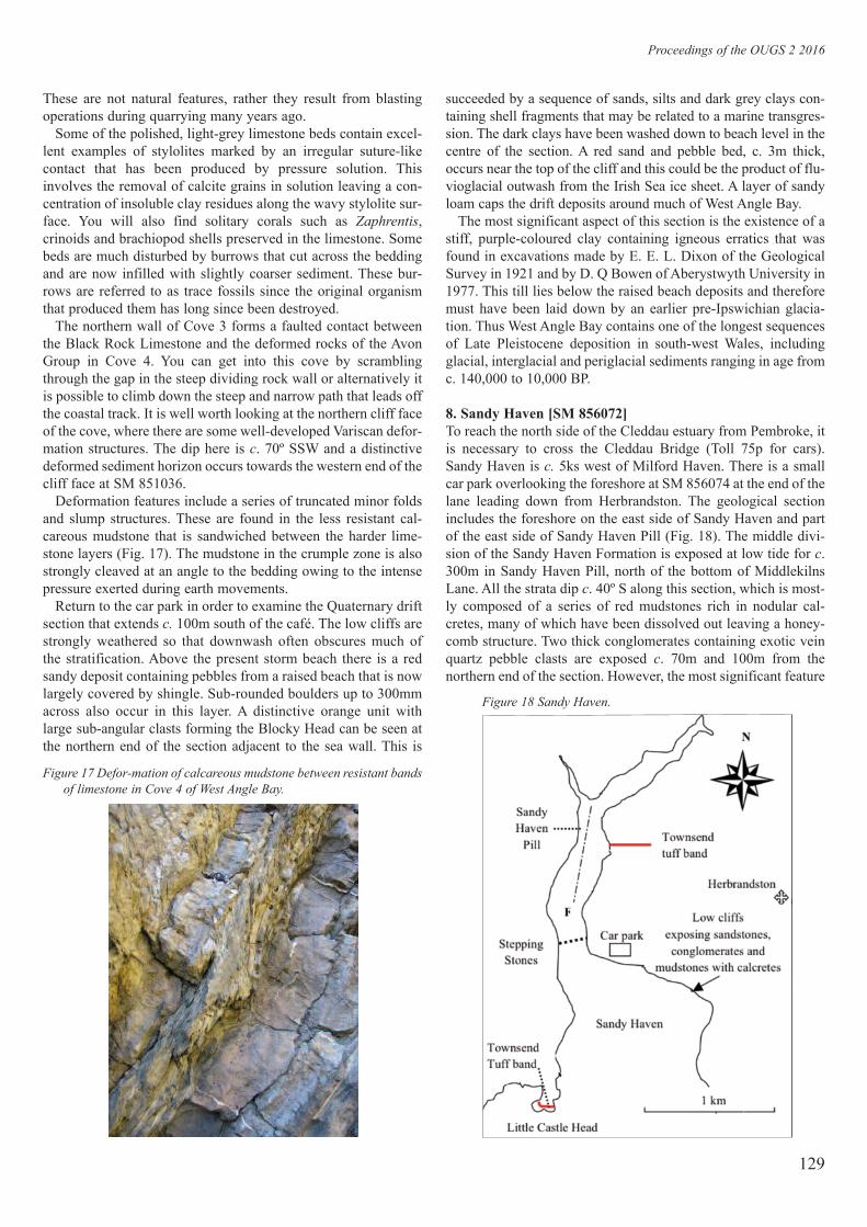
These are not natural features, rather they result from blastingoperations during quarrying many years ago.
Some of the polished, light-grey limestone beds contain excel-lent examples of stylolites marked by an irregular suture-likecontact that has been produced by pressure solution. Thisinvolves the removal of calcite grains in solution leaving a con-centration of insoluble clay residues along the wavy stylolite sur-face. You will also find solitary corals such as Zaphrentis,crinoids and brachiopod shells preserved in the limestone. Somebeds are much disturbed by burrows that cut across the beddingand are now infilled with slightly coarser sediment. These bur-rows are referred to as trace fossils since the original organismthat produced them has long since been destroyed.
The northern wall of Cove 3 forms a faulted contact betweenthe Black Rock Limestone and the deformed rocks of the AvonGroup in Cove 4. You can get into this cove by scramblingthrough the gap in the steep dividing rock wall or alternatively itis possible to climb down the steep and narrow path that leads offthe coastal track. It is well worth looking at the northern cliff faceof the cove, where there are some well-developed Variscan defor-mation structures. The dip here is c. 70º SSW and a distinctivedeformed sediment horizon occurs towards the western end of thecliff face at SM 851036.
Deformation features include a series of truncated minor foldsand slump structures. These are found in the less resistant cal-careous mudstone that is sandwiched between the harder lime-stone layers (Fig. 17). The mudstone in the crumple zone is alsostrongly cleaved at an angle to the bedding owing to the intensepressure exerted during earth movements.
Return to the car park in order to examine the Quaternary driftsection that extends c. 100m south of the café. The low cliffs arestrongly weathered so that downwash often obscures much ofthe stratification. Above the present storm beach there is a redsandy deposit containing pebbles from a raised beach that is nowlargely covered by shingle. Sub-rounded boulders up to 300mmacross also occur in this layer. A distinctive orange unit withlarge sub-angular clasts forming the Blocky Head can be seen atthe northern end of the section adjacent to the sea wall. This is
129
succeeded by a sequence of sands, silts and dark grey clays con-taining shell fragments that may be related to a marine transgres-sion. The dark clays have been washed down to beach level in thecentre of the section. A red sand and pebble bed, c. 3m thick,occurs near the top of the cliff and this could be the product of flu-vioglacial outwash from the Irish Sea ice sheet. A layer of sandyloam caps the drift deposits around much of West Angle Bay.
The most significant aspect of this section is the existence of astiff, purple-coloured clay containing igneous erratics that wasfound in excavations made by E. E. L. Dixon of the GeologicalSurvey in 1921 and by D. Q Bowen of Aberystwyth University in1977. This till lies below the raised beach deposits and thereforemust have been laid down by an earlier pre-Ipswichian glacia-tion. Thus West Angle Bay contains one of the longest sequencesof Late Pleistocene deposition in south-west Wales, includingglacial, interglacial and periglacial sediments ranging in age fromc. 140,000 to 10,000 BP.
8. Sandy Haven [SM 856072]
To reach the north side of the Cleddau estuary from Pembroke, itis necessary to cross the Cleddau Bridge (Toll 75p for cars).Sandy Haven is c. 5ks west of Milford Haven. There is a smallcar park overlooking the foreshore at SM 856074 at the end of thelane leading down from Herbrandston. The geological sectionincludes the foreshore on the east side of Sandy Haven and partof the east side of Sandy Haven Pill (Fig. 18). The middle divi-sion of the Sandy Haven Formation is exposed at low tide for c.300m in Sandy Haven Pill, north of the bottom of MiddlekilnsLane. All the strata dip c. 40º S along this section, which is most-ly composed of a series of red mudstones rich in nodular cal-cretes, many of which have been dissolved out leaving a honey-comb structure. Two thick conglomerates containing exotic veinquartz pebble clasts are exposed c. 70m and 100m from thenorthern end of the section. However, the most significant feature
Proceedings of the OUGS 2 2016
Figure 17 Defor-mation of calcareous mudstone between resistant bands
of limestone in Cove 4 of West Angle Bay.
Figure 18 Sandy Haven.

is the abundance of air-fall tuffs of variegated colours, whichwere called the ‘magenta beds’ when Cantrill et al. of theGeological Survey first surveyed the area in 1916. Most of thetuff beds are a few centimetres thick, but the Townsend tuff,which crops out in the middle of the section, is almost 4m thick.This distinctive regional marker horizon extends across SouthWest Wales and comprises three graded air-fall units, each finingupwards. The light-coloured porcellanite (silicified dust tuff)contrasts with the darker, magenta-coloured, medium-grained,crystal-lithic tuff at the base of each fall. Note that there is alsoan excellent section in the Townsend tuff at Little Castle Head onthe west side of Sandy Haven (see OUGS Journal 35, 26–7).
The foreshore and cliffs of Sandy Haven to the south of the carpark provide a representative section through the upper part of theSandy Haven Formation. At the western end of the foreshore nearsteps giving access to the beach, there is a distinctive grey con-glomerate, steeply bedded and overlain by red mudstones. Farthereast, the sequence is dominated by a 3m multi-storey unit of cross-stratified, medium-grained sandstones dipping c. 40º NE. Theseare overlain by thick mudstones festooned with calcretes and hon-eycombed where the calcareous material has been dissolved out.The mudstones are cleaved at a high angle to the bedding and thecalcretes have been elongated along the cleavage planes. Near theeastern end of the foreshore the effect of Variscan deformation canbe seen where interbedded mudstones and grey conglomerateshave been tilted to a near vertical position.
The succession in Sandy Haven shows a series of fining-upward cycles, typical of deposition in a meandering river envi-ronment, where cross-stratified fine- to medium-grained sand-stones represent point bar sediments and finer-grained mudstonesrepresent alluvial flood plain deposits. Traditionally, these sedi-ments have been considered as overbank deposits, but they arenow thought to be laid down by ephemeral, sinuous streams thatreworked the flood plain during seasonal flooding. Modernanalogies for mudstone deposition within the Old Red Sandstonecan be seen in the Channel Country of central Australia.
Coarse sandstones or conglomerates (lag gravels) rest on an ero-sion surface at the base of each cycle and the overlying mudstonesare often calcretised and contain mud cracks. The calcretes in themudstones are white, cylindrical or irregular-shaped masses thatare several millimetres across and elongated normal to beddingand parallel to the cleavage. These masses are carbonate-rich, sothey weather out easily. Calcretes represent fossil soils producedin a hot savannah climate of alternating dry and rainy seasons. Inthe wet seasons, ground water percolated down through the mud-stone and picked up calcium carbonate and other minerals. In thedry seasons, the waters were drawn up by evaporation anddeposited much of their mineral load, commonly replacing or fill-ing rootlets or making irregular nodular masses within the soil.
9. Lindsway Bay [SM 843067]
From Sandy Haven drive back to Herbrandston and around thehead of Sandy Haven Pill to St Ishmaels. There is a small car parkand toilets [SM 839072] adjacent to the sports field on the eastside of the village. Lindsway Bay is a beautiful, quiet and little-known bay, despite the fact that it lies within 2km of the LNG ter-minal at South Hook. You should follow the footpath that leadsfrom the car park to the coast path, then turn left and take thecoastal track c. 200m to the steep steps that lead down to thebeach in Lindsway Bay (Fig. 19). Care should be taken when
Exploring the Afon Cleddau Valley in Pembrokeshire / Downes
130
descending the steps, as there are no safety rails. Walk across thebeach to Sprat’s Point on the west side of the bay, where the alter-nating sandstones and mudstones of the Gray Sandstone Groupcan be seen dipping c. 70º SW (Fig. 20). These beds pass con-formably upwards into the basal Old Red Sandstone marls (RedCliff Formation) on the north-east side of Sprat’s Point, where thefaulted junction is marked by a steep gully.
The Silurian rocks in Lindsway Bay form the most easterlyexposure of the fault-bounded Marloes inlier. They also form thecliffs along the coast to the west, as far as Watch House Bay, but itis difficult to access the foreshore without using a boat. Even so, itis well worth walking along the coast path to observe the cliffstructures from above. Longberry Point can be easily recognisedby its massive sandstone beds that dip inland at a high angle. FurzyPoint and Watch House Bay are formed of calcareous mudstonesbelonging to the Coralliferous Series that are folded into a majoranticline, the axis of which runs roughly N–S through Furzy Point.
Figure 19 The geology of the coast between Watch House Point and
Lindsway Bay.
Figure 20 Gray Sandstone Group (Upper Silurian) at Sprat’s Point,
Lindsway Bay.

10. Mullock Bridge [SM 811080] & Townsend [SN 812060]
This locality is on the B4327 c. 3km west of St Ishmaels. It is ofconsiderable geomorphological interest, as it provides a magnif-icent example of a kame terrace on the western side of the Gannestuary. This feature is a flat-topped mound of fluvioglacial sandand gravel that was deposited by meltwater at the junction of thewasting Irish Sea ice front and the valley side. The drift sequence,which was exposed in a large gravel pit c. 400m south of MullockBridge, was recorded in detail by Gareth George in the early1970s. Unfortunately the pit has since been infilled and land-scaped and is now entirely overgrown. However, the topographyof the kame terrace can be appreciated by viewing it from thesouth in the vicinity of Pickleridge, where there is a car park [SM809067] (Fig. 21).
Walk along the shingle ridge past the flooded pits that are nowlagoons supporting a variety of wild life. In the banks of thelagoons there are exposures of fluvioglacial outwash sands andgravel. Pickleridge is a shingle ridge that has developed in anorth-westerly direction along the high-water mark across theGann estuary. This shingle barrier impedes the drainage on themarshy flood plain of Afon Gann that is inundated by the seawhen there are spring tides. You will notice that there is a strongcontrast in the natural vegetation between the dense colonies ofreed mace (bullrushes) on the wet flood-plain of Afon Gann andthe abundance of gorse and Scots pine that cover the dry sandyslopes of the kame terrace.
Continue along the road to Dale village where there is a carpark alongside the beach [SM 811058]. Walk back along theroad to the small group of houses at Townsend and descend tothe foreshore near Black Rock. The Sandy Haven Formationforms the rocky foreshore here and it consists of alternations ofthick vein quartz conglomerates, medium grained sandstonesand red mudstones with calcretes. Immediately south of BlackRock the Townsend Tuff Bed can be seen cutting across the fore-shore and following the strike of the sandstones (Fig. 22). Thetuff outcrop is c. 4m thick and consists of three fining-upwards,graded air-fall units. The light coloured porcellanite (silicifieddust tuff) contrasts with the darker, magenta-coloured, medium-grained, crystal-lithic tuff (crystal debris and rock fragments) atthe base of each fall. Townsend is by far the most accessibleplace where you can examine the tuff bed in south-west Wales,and it is of course, named after this locality.
Proceedings of the OUGS 2 2016
131
Sources cited and consultedAllan, J. R. L., Thomas, R. G., and Williams, B. P. J. 1982
‘The Old Red Sandstone north of Milford Haven’, in
Bassett, M. G. (ed.) Geological Excursions in Dyfed,
South West Wales. Cardiff: Nat Mus Wales, 123–49Bloxham, T. W. 1971 ‘Haverfordwest, Strumble Head and
Abereiddy Bay’, in Bassett, D. A., and Bassett, M. G.(eds) Geological Excursions in South Wales and The
Forest of Dean. Cardiff: Geol Assoc, 199–205Brown, E., Coe, A., and Skelton, P. 1999 Surface Processes,
S260, Block 4, Open University, 156–7Campbell, S., and Bowen, D. Q. 1989 ‘The Quaternary of
Wales’. Geol Conserv Rev Ser 2, 76–98Cantrill, T. C., Dixon, E. E. L., Thomas, H. H., and Jones, O.
T. 1916 The geology of the South Wales Coalfield. Part
XII. The country around Milford. Mem BGS (Englandand Wales). London: HMSO
Downes, J. 2009 Treffgarne Quarry RIGS report No. 562, Ordovician
Igneous Geology. South West Wales RIGS GroupDownes, J. 2008 Sandy Haven RIGS Report No. 479 Old Red Sandstone
Stratigraphy. South West Wales RIGS GroupHancock, P. L., Dunne, W. M., and Tringham, M. E. 1982 ‘Variscan
structures in SW Dyfed’, in Bassett, M. G. (ed.) Geological
Excursions in Dyfed, South West Wales. Cardiff: Nat Mus Wales,239–48
Hillier, R. D., and Williams, B. P. J. 2007 ‘The Ridgeway ConglomerateFormation of SW Wales, and its implications. The end of the LowerOld Red Sandstone?’. Geol J 42, 55–83
Linton, D. L. 1955 ‘The problem of tors’. Geograph J 121, 470–87Marriott, S. B., and Wright, V. P. 2004. ‘Mudrock deposition in an
ancient dryland system. Moor Cliffs Formation, Lower Old RedSandstone, South West Wales, UK’. Geol J 39, 277–98
Owen, T. R. 1973 Geology Explained in South Wales. Newton Abbot:David & Charles, 35–7
Thomas, R. G., Williams, B. P., Morrisey, L. B., Barclay, W. J., andAllen, K. C. 2006 ‘Enigma variations: the stratigraphy, provenance,palaeoseismicity and depositional history of the Lower Old RedSandstone, Cosheston Group, South Pembrokeshire, Wales’. Geol J
41, 481–536
Figure 21 View looking northward to the Mullock Bridge Kame Terrace.
Figure 22 Townsend Tuff Bed on the foreshore near Black Rock.

Book reviewSchmidt, Anja , Fristad, Kirsten E and, Elkins-Tanton, Linda T.2015 Volcanism and Global Environmental Change. CambridgeUniversity Press (ISBN 978-1-10705-837-8; hardback, 324pp; £75)
Volcanic eruptions have the potential to produce profound globalenvironmental effects, yet ascertaining the nature, magnitude andtimescale of these events from the geological record has provedchallenging. Volcanism and Global Environmental Changebrings together European, Russian and US geologists, volcanolo-gists, climate and atmospheric scientists and palaeobiologists toprovide an invaluable update on the state of knowledge in thiscomplex but intriguing area.
The volume is divided into three parts: Part One exploreslarge-volume volcanism, including origins, features and dura-tion; Part Two covers the assessment of gas and tephra releasein the present-day and geological record; Part Three considersmodes of volcanically-induced global environmental change.As each ‘chapter’ is the work of one or more different authors,the volume is inevitably more akin to a collection of papers thanto a textbook.
Part One explores the potential for global environmentalchange produced by large igneous provinces (LIPs) and consid-ers LIPs’ connection with mantle-core dynamics and deep mantleplumes. So-called ‘super eruptions’ and their potentially cata-strophic environmental consequences are also examined.
Part Two describes the increasingly sophisticated methods ofmonitoring current emissions. It further considers the role of
Book review
132
volcanic emissions in the Permian-Triassic extinction, includingthe release of volatiles in LIPs, which may not only affect climatebut also cause stratospheric ozone destruction, which is poten-tially harmful to life. Evidence of violent and surprisingly rapidrelease of sulfur-, carbon- and halogen-rich gases from sedimen-tary country rocks during contact metamorphism is discussed. InSiberia, for example, pipe structures with explosion cratersexceeding 1km diameter suggest rapid mobilisation of large vol-umes of carbon and sulfur from sediments following theemplacement of sills and dykes. Contact metamorphism oforganic material in offshore Norway might have been a cause ofenvironmental change during the Paleocene-Eocene ThermalMaximum (PETM).
Part Three includes a review of modes of volcanically-inducedenvironmental change, including halogen release and ozonedepletion resulting from Plinian eruptions, volcanic ash deposi-tion, Permian-Triassic ocean anoxia and ocean acidification. Itconcludes with a chapter on the environmental effects of LIPmagmatism from the Siberian perspective that highlights themany challenges that remain for modelling volcanism.
Each chapter is comprehensively referenced, making the vol-ume an excellent source for further reading. Unfortunately, theclarity of some colour figures is compromised by the small sizeof reproduction. Notwithstanding this, Volcanism and Global
Environmental Change provides in a single volume a highlyreadable selection of recent material from scientists working inthis important and fascinating field.
— Caroline Peters, BSc Hons (Open) Geoscience

Introduction
If you find the very notion of crystallography, with all thoseaxes, angles and planes of symmetry to be daunting, then this
workshop was the answer. We used the Aberystwyth Park Hotel’sconference room, which although lacking the facilities and spec-imens of the university lab, made hearing and seeing our instruc-tors much easier. Bill and Charlie brought all the necessary kit,and we had excellent instruction.
On January 30 we were introduced to crystal structure, formand symmetry. By the end of the day, we were discussing variousminerals and their crystal forms. We had a guest lecturer in theearly evening — Prof. Nick Pearce, ably assisted by Amy (hisdaughter) and Jack (his son). He spoke on the latest diagnostictechniques for determining the sources of lavas from major erup-tions. Prehistoric stone tools can also be dated using far lessdestructive methods; and how they fit in the archaeologicalsequences can tell us about the impact of such eruptions onhuman evolution.
January 31 was dedicated to using the petrological microscope— how it works and how to interpret what can be seen in thinsections.
Basic definitionsWe began with some basic definitions. Not all minerals are crys-tals. A mineral can be defined as a naturally occurring inorganicsubstance having a regular characteristic chemical compositionand crystalline molecular structure. A crystal is a solid bound bya series of plane faces. A piece of quartz with six sides and a pointat one or both ends is a crystal. A rounded sand grain of quartzwould not be called a crystal, although its internal structure maybe that of crystalline quartz.
Unit cells are the basic building blocks of crystals (Fig. 1). Youmay notice that the unit cell in Figure 1 is not so much NaCl asNa14Cl13. However, each atom on each face of the unit cell canshare with one or more adjoining unit cells. The central atom ona face can share between two cells, the centre atoms on the edgescan share between four, and the corner atoms can share betweeneight (Fig. 2). Consequently, by the time you get toNatrillionCltrillion&1 it does work within the lattice; besides, theodd ion does not matter that much!
133Proceedings of the OUGS 2 2016, 133–7© OUGS ISSN 2058-5209
OUGS crystallography and mineralogy workshop (Aberystwyth, 30–31 January 2015)
led by Charlie Bendall and Bill Perkins
text and diagrams by Elizabeth Edmundson
[This article was originally published in the Severnside Branch Newsletter, Sabrina Times, in May 2015. It is hoped that this slightly
edited version will prove useful to members. —Ed.]
Figure 1 A unit cell of halite — NaCl.
Figure 2 The building blocks and how they stack.
There are several rules governing unit cells:
r Each must be the same shape and size.r Each contains atoms in proportion and can share atoms in
faces.r Edges are straight lines.r Each shares atomic relationship.r Lattices are formed by stacks of unit cells.r There are no gaps between unit cells.r Unit cells can join by equal translation of all lattice points
without rotation.
From these criteria we can to determine what shapes fulfil these rules.To build unit cells into lattices, it is best to start at the begin-
ning; with two-dimensional shapes (Fig. 3). What we are lookingfor are shapes that:
r are the same;r can fit together along all their edges, and join points;r have no gaps in the lattice;r and have not been rotated.
Figure 3 2D strsaight-edged shapes.

In Figure 4 we see that the square (b), the rectangle (c), the par-allelogram (e), the rhombus (f) and the hexagons (h, i and j) allform 2D lattices without gaps. The pentagon (g), the heptagonand the octagon cannot join without gaps. The equilateral trian-gle (a), the right-angle triangle and the trapezoid (d) cannot joinwithout 180° rotations, which would invert the molecular struc-ture. So unit cell shapes must have:
r an equal number of sides;r opposite sides parallel;r and internal angles divisible by 360°.
Crystallography and mineralogy workshop / Edmundson
134
However, crystals are three-dimensional: 3D unit cells areextensions of their 2D counterparts and obey the same rulesregarding opposite faces parallel, opposite internal angles equal,straight lines, no rotation, etc. The four basic 2D shapes extendinto seven basic 3D shapes: cubic (isometric), tetragonal,orthorhombic, monoclinic, triclinic, trigonal and hexagonal (Fig.6). Cubic is the extension of the square; tetragonal andorthorhombic are extensions of the rectangle; monoclinic(skewed orthorhombus) and triclinic (orthorhombus skewedmore than once) are extensions of the parallelogram; and trigonaland hexagonal are extensions of the rhombus.
Figure 4 Fitting 2D chapes into lattices of unit cells.
Regular polygons can be distorted provided opposite sidesremain parallel and opposite angles are equal. Further, a rhom-boid lattice can overlay a hexagonal lattice (Fig. 5), showing thesame internal structure in each rhombus. Squares and rectanglesdo not work on the hexagonal lattice, because the internal struc-tures do not repeat in each unit. The parallelogram does not workunless it is the length of two rhombi — in which case it is tworhombi, not a parallelogram. This restricts the number of basic2D unit cell shapes to the square, the rectangle, the parallelogramand the rhombus.
Figure 5 The regular hexagonal lattice can be expressed
as a rhomboid latitce.
Figure 6 The seven basic 3D unit shapes.
3D symmetryWe spent the afternoon coming to terms with 3D symmetry —axes and mirror planes. After dividing a few 2D shapes into equalparts through their centres (Fig. 7), we started on the seven 3Dunit cells. One of the elements of symmetry is axial symmetry,which involves putting an axis through the central points ofopposing faces or edges, or through opposing corners. The rota-tion around any axis must present the same aspect to be countedas so many ‘-fold’. For example, a cube (Fig. 8) has six faces,eight corners and 12 edges. If you cut a cube of cheese, put atoothpick through the opposing faces and turn it around, the sameview of it happens four times — you can do this three differenttimes before you run out of punctured faces, so a cube has three
Figure 7 Rotational symmetry.
Figure 8 The axial symmetry of a cube.

four-fold axes through its faces. If the toothpick is corner to cor-ner, you can do this four times; turning it gives the same viewthree times — four three-fold axes. Edge-to-edge can be done sixtimes, but the view is the same only twice — six two-fold axes.
Crystallographic axes intersect the centres of the faces of thebasic shapes (Fig. 9). By convention, the vertical axis is c inFigure 9. The two axes horizontal to c, are b and a. In the case ofhexagonal crystals, there are three horizontal axes, a1, a2 and a3.Lengths of axes relative to each other, as well as the anglesbetween axes define shape:
r isometric: lengths a = b = c; angles ca = cb = ab = 90° —includes halite, garnet, fluorite, pyrite, galena and mag-netite, as well as diamond, gold and several other ele-mental minerals.
r tetragonal: lengths a = b ≠ c; angles ca = cb = ab = 90°— includes zircon, cassiterite, rutile, wulfenite and chal-copyrite.
r orthorhombic: lengths a ≠ b ≠ c; angles ca = cb = ab =
90° — includes olivine, barite, sulfur, topaz, staurolite,andalusite and the pyroxene enstatite.
r monoclinic: lengths a ≠ b ≠ c; angles ca = cb = 90°, ab ≠90°— includes the feldspar orthoclase, amphibole, epi-dote, gypsum, azurite, malachite and the pyroxenes diop-side and augite. Sugar (sucrose) also forms monocliniccrystals.
r triclinic: lengths a ≠ b ≠ c; angles ca ≠ cb ≠ ab ≠ 90° —includes the feldspars plagioclase and microcline,rhodonite and axinite.
r trigonal: lengths a = b = c; angles ca = cb = 90°, ab ≠ 90°— includes calcite, dolomite and tourmaline (hexagonalditrigonal).
r hexagonal: lengths a1 = a2 = a3; angles a1a2 = a2a3 =
a1a3 = 120°, ca1,2or3 = 90° — includes quartz, apatite,beryl (emerald, aquamarine), corundum (ruby, sapphire)and arsenic.
We had a brief discussion on mirror planes. Imagine a mirror inter-secting a cube in a plane of two of its axes. If the reflection lookslike the whole cube, then that plane is a mirror plane. We alsolooked at zones — areas of a crystal shared by parallel edges.
A major factor in a crystal shape will be its chemical compo-sition. Halite and garnet are both isometric, but the molecular
Proceedings of the OUGS 2 2016
135
lattice of halite (NaCl) is far less complex than that of garnet(Fe3Al2Si3O12), so halite crystallises as a cube, while garnetgrows a few extra faces.
Of course, real mineral crystals are not all basically shaped —axes can intersect just about anywhere on faces, edges and cor-ners. So, Charlie and Bill introduced us to ‘Miller indices’, whichdefine crystal faces, points and/or edges as the axes intersectthem. If a face cuts three axes, then the distances from the centreon the axes — e.g. a = 2 units, b = 2 units, c = 1 unit — are con-verted to their reciprocals — ½, ½, 1; then these are multiplied bythe lowest integer. In this example 2 — to give lowest integers.This would give indices of 1 1 2.
Where a face intersects only one axis, the default unit is 1 andthe other two axes, which never intersect the same face, are giventhe value ∞ (infinity). Their reciprocals are 1/1 (=1), 1/∞ (whichpretty much equals 0) and 1/∞ (0 again). So if it is the a axisintersected, then the Miller indices are 1 0 0. As a matter of inter-est, a hexagonal crystal gets four Millers!
Miller indices take some getting used to. A glance at such a setof figures conveys plenty of information as to the variations onbasic shapes to a practised eye. It is amazing that Bill and Charliemanaged to get across as much as they did on this point in abouthalf an hour!
All of these factors — shapes, axes, angles, mirror planes,zones and Miller indices — are diagnostics for mineral identifi-cation, along with colour, lustre, hardness, etc.
Thin section dayWe began by familiarising ourselves with the polarising micro-scopes: how to work them, which knobs do what, and what not totwiddle. We then went through a few definitions:
r polarised light: light waves made to vibrate along oneplane. In the microscope, a single polarising lens is the‘plane polarised light’ setting, and is below the thin sec-tion.
r crossed polars: a polarising lens set above the thin sec-tion. The upper lens can be rotated in relation to thelower lens. If two planes of polarised light are at rightangles to each other, non-refracted light blacks out, whilerefracted light shows in a range of intensities andcolours.
r refraction: the change in deflection of light passing fromone medium to another. The refractive index is the ratioof V1 over V2, with V = the speed of light and 1 and 2 =the speed of light through medium 1 and medium 2.
r birefringence: the difference between refractive indices.In thin section under crossed polars, it shows as interfer-ence colours (Fig. 10).
Figure 9 Chrystallographic axes.
Figure 10 The Birefringence Chart with the first three orders of
interfernece colours.

r interference colours (under crossed polars): causedby polarised light splitting and travelling at dif-ferent velocities as it comes up through the crys-tal, then recombining through the upper polaris-ing lens. Generally, if the light is out of phase bya wavelength, you get ‘first-order colours’; twowavelengths get ‘second-order colours’; threewavelengths, ‘third-order’.
r extinction (under crossed polars): the point atwhich the light coming through the crystal blacksout. Extinction occurs at every 90° (the crosshairs in the field of view). Extinction of a crystalaligning with the cross hairs is ‘parallel’ (or‘straight’); extinction at an angle to the crosshairs is ‘inclined’ (or ‘oblique’).
We began by viewing thin sections by eye. You can see how thesample is structured, grain size and some colour. Under themicroscope, using plane polarised light (ppl) you can see severaldiagnostic features:
r colour: Most show no colour, but some do; e.g. amphi-bole (green or brown), biotite (brown) and garnet (palepink).
r pleochroism: a wavy effect in a crystal as the stage isturned.
r relief: how well the mineral shows its shape. Mineralswith higher refractive indices tend to have higher relief.
r shape: often the crystals show their growth shapes.r cleavage: If a mineral has cleavage planes, these often
show up in thin section. Some minerals have characteris-tic cracks and fractures.
Under crossed polars (xp), shapes and cleavages of low reliefcrystals become visible, plus:
r interference colours: it is difficult to resist the visualimpact of the interference colours. Those peacock blues,golden yellows, flaming magentas, emerald greens andstriking black and white patterns are actually good diag-nostic indicators. Crystals that stay black at any positionof the stage are isotropic, and are inevitably isometric.
r extinction: relates to cleavage. Quartz, which has nocleavage, shows wavy extinction.
r twinning: some minerals grow distinct twins, which showup well under xp. Occasionally, twinning can be seenunder ppl, but is usually quite faint.
r alteration: shows up as a mishmash of ‘dirt’ around thecrystal, indicating breakdown of the crystallinestructure.
The rest of thin section day was spent viewing mineralswithin rocks in thin section. Figures 11, 12 and 13 showsome of the results. Some of the minerals we looked at were:
r quartz: under ppl there is little to see — no colour,no pleochroism, no cleavage, low relief and notmuch to show in shape, except where other miner-als start. Under xp, grains become very distinct,with first-order colours of white to grey to black(extinction). There is not much alteration, but grainscan show undulose extinction, caused by strain.
Crystallography and mineralogy workshop / Edmundson
136
r plagioclase: again, there is no colour or pleochroismunder ppl; and with low relief, shape and cleavage areonly faint. Under xp — shapes and cleavage show, withfirst-order greys and lamellar twinning — the character-istic ‘pyjama stripes’.
r orthoclase: ppl — no colour or pleochroism, low relief,but some messiness (exsolution into clays), the alterationindicating elongated shapes with a few striations but nocleavage. Under xp — first-order greys, several simpletwins, slight wavy extinction in some crystals.
r calcite (marble): ppl — colourless and no pleochroism;moderate relief; irregular shapes with definite cleavagesrunning at c. 120° to each other. Under xp the interfer-ence colours are very high-order (for example, off thescale in Figure 10), appearing as a variety of dullish pas-tels. Lamellar twinning shows along cleavage lines.
Figure 11 (a) A thin section under plane polarised light, showing the difference
between high and low relief; (b) under cross polars, the featureless areas either
side of the crystal show the ‘pyjama stripes’ of palgioclase (photos by E.
Edmundson).
Figure 12 An olivine crystal under crossed
polars (photo by Rebecca Pike).
Figure 13 Twinning in a clinopyroxene crystal under (a) polarised light and (b)
crossed polars (photo by Linda Fowler).

r olivine: ppl — faint (almost no) colour, no pleochroism,high relief; shapes are fairly regular and usually criss-crossed with fractures (no cleavage). Under xp — differ-ent brilliant colours of the second-order; the fracturesoften show alteration products.
r biotite: ppl — browns, very pleochroic; high relief, tabu-lar shape with lengthwise cleavage. Under xp — second-order colours tinted by brown.
r pyroxene (clino-): ppl — very pale brown, may showslight pleochroism; high relief, regular and irregularshapes, two cleavages at c. 90°. Under xp — strong first-to second-order colours (blues, yellows, rich browns,greys); twinning, when it happens, is simple.
We could have spent much longer viewing and picking out crys-tals in thin sections, but the weekend came to an end. There wasa lot of information given to us during the two days and we allappreciated Charlie and Bill for explaining it all to us.
Proceedings of the OUGS 2 2016
137
References consultedwww.geologyin.com/2014/11/crystal.structure.and.crystal.system.html
— an online article on crystallographyPough, Frederick H. 1998 A Field Guide to Rocks and Minerals (5th
edn). Peterson Field Guides Series: New York: Houghton MifflinMacKenzie, W. S., and Guilford, C. 1980 Atlas of Rock-forming
Minerals in Thin Section. Harlow: Longman
OUGS Chairman Linda Fowler attended and has posted photosfrom the weekend on her ‘Rocks and Olives’ blog.

Confronting barriers to inclusion / Smith
Held on June 26, 2015, the meeting was organised by theGeological Society of London, Higher Education network
and University Geosciences in the UK, and held in theGeological Society, Burlington House, Piccadilly, London.
Edmund Nickless (former Executive Secretary of the GeologicalSociety) introduced the conference and posed three questions forconsideration, as follows:
1. Does the emphasis on fieldwork in geoscience education dis-courage the participation of people with disabilities?
2. How can we design and deliver fieldwork that is inclusive andaccessible for people with disabilities?
3. How can we ensure that geoscience education and professionsattract and develop the talents of people with diverse abilities?
Alhough the questions appeared to focus on professional andhigher education, speakers from schools, Further Education andorganisations for both formal and informal geoscience educationtook part. The OUGS falls into this category.
The meeting discussed the perceived ‘macho’ image of field-work, which is critical to professional geological practice and thedevelopment of field skills, in the past seen to appeal, in the main,to young, male ‘outdoor’ types who can cope with a rigorousschedule of fieldwork. On the other hand, talented learners withdisabilities can be deterred, because it makes both physical andphysiological challenges that are too difficult for them to copewith. This discussion prompted consideration of geoethics:should we have a culture of disclosure (already we ask people ifthey have ‘dietary requirements’; should we ask if they have‘other requirements’ also?); and a consideration of the type ofleadership we need to encourage ethical and inclusive behaviour— do we need ‘enforcement’ or ‘encouragement’?
Keynote speaker: Chris Atchison (University of Cincinnati, andDirector of the International Association for Geoscience Diversity)His work has involved developing a programme to “encouragethe use of a wide spectrum of experiences in the field and lab toencourage retention” rather than use the previous ‘rigorous’,field-based instruction that discourages those with disabilitiesfrom active engagement.
Stressing ‘positive disclosure’, where learners explain whathelp they need, without the need to explain why, should be seenas of paramount importance. It is also important that the ‘edu-cators’ should be aware of the learners’ abilities, rather thantheir disabilities.
Once you have that knowledge, ‘flexibility’ is the great key.That emphasis must be coupled with the availability of adequatehelp in the field. The old adage ‘many hands make light work’was quoted — personnel to act as an ‘enablers’ are crucial.
As Chris was speaking, I felt that this work was almost ‘rein-venting the wheel’. The OU has already done this, to great andsuccessful outcome, in the work that our ‘special needs’ weeks atSummer School did for both 2nd- and 3rd-level courses!
Miguel Gomez-Heras (Instituto de Geociencias y Ciencia sinBarreras) told us about fieldwork they have been doing insouthern Spain with deaf and sight-impaired people, using theturbidite successions. Miguel’s presentation stressed the factthat such experience worked well, but needs two helpers foreach participant. The enjoyment of the participants was evidentin the presentation.
Angela Bentley (ESTA — Earth Science Teachers Association)and Aquinas College) presented three case studies from theschool, all of which showed how important ‘disclosure’ was — inorder that the necessary arrangements can be made for keepingstudents with mental health issues able to participate safely. Acouple of the cases could easily have ended in disaster.
Alison Stokes (Plymouth University and Geological SocietyHigher Education Network) backed up the previous speakersand finished with the maxim that [paraphrasing] “anybody[who] gets into geosciences, regardless of age or limitations,must have the opportunity to learn and not be judged”, whichwas based on what some of her students had said when given theopportunity to complete work at their own rate, rather than understressed conditions.
Jacqueline Houghton (University of Leeds) and colleagueshave been developing material for learning field skills in the vir-tual world. They use landscapes and outcrops specificallydesigned so that students can use these to get training in map-ping skills before they venture out in the field. Technology hasmoved on since the OU first designed the ‘virtual field trip’, andthis looks like a promising way forward. She stressed that suchwork was in no way a replacement for fieldwork, but that it wasa technical aid to fieldwork.
Gary Nichols and Wayne Gladwin (Nautilus Ltd) looked at howplanning and proper risk assessment was crucial in any field worksituation. Their work was particularly targeting continuing pro-fessional development (CPD), and showed how important it wasthat the planning put the participant at the centre of the process,asking what learning outcomes did they expect, what limitationsdid they have (disclosure again, but done by detailed discussion),what extra support was needed, and what insurance needed to bein place to cover it all.
General session of discussion
Further discussion then ranged widely over the ideas presentedabove. It was decided that there should be a follow-up meetinglater in the year. Discussion at the reception afterwards was mostinteresting and enabled me to make contact with participantsfrom Cardiff, Swansea and Plymouth. It appears that we are try-ing to sing from the same hymn sheet.
The OUGS is already well placed to address these issues, but Ifeel that we need to contribute to future meetings and use theexperience we have for the benefit of others.
Confronting barriers to inclusion: opening the gate to accessible geologicalfieldwork
Diana Smith, BA, BSc (Hons)
Proceedings of the OUGS 2 2016, 138© OUGS ISSN 2058-5209

Our small group collected promptly to leave for the drive to acar park on the banks of the Weir, a few miles west ofSunderland, where we were to meet our leader. We had come tothis area to examine the Lower Permian Yellow Sands and theFord Formation reef facies and associated features.
As the clouds started to clear we walked down to the riverbankto look across the river to the unconformity. Here the BasalPermian Sands can be seen sitting on an uneven erosional surfaceof the Carboniferous Upper Coal Measures, nearly masked bypurple staining due to deep weathering (Fig. 1). The riverbankstill shows evidence of its industrial past, with the remains of acoal staithe, a lime kiln and, farther downriver, the abandonedconcrete hulk of an experiment in shipbuilding.
139
We turned back to look south at the mass of Claxheugh Rock(Fig. 2) and Dr Lane pointed out the deep recession at the top ofthe tree-covered, sloping foreground. This weakness is the mark-er of the Downhill Slide, a massive submarine landslip thatremoved the majority of the Raisby Formation, leaving thin seg-ments of Marl Slate and the Lower Magnesium Limestone. Therock structure represents the seaward section of a reef, whichbuilt on top of the slide at the shelf edge of Zechstein Sea — theFord Formation.
We walked up to the east end of the rock where a mass ofPermian Yellow Sand is in contact with the Ford Formation.Those of us who managed the steep slope were rewarded with aclose inspection of the slide surface within the recess and thecross-bedding of the Yellow Sand (Fig. 3, overleaf).
A short bus ride and walk took us to Ford Quarry, a disusedMagnesium Limestone quarry that is now preserved as a Site ofSpecial Scientific Interest (SSSI) because of its geology. It wassurrounded by a protective fence! But we walked around the endof it and entered a delightful meadow studded with commonorchids (Fig. 4, overleaf). The mass of the Ford Formation reef isevident, with some stratification on the top indicating that thiswas the top surface of the reef and that talus had been moved bythe waves. Farther west down the quarry Dr Lane pointed out theback edge of the reef, where debris had fallen into the lagoon andformed further stratified backreef deposits (Fig. 5, overleaf). Wedid not look for any fossils in this locality as the high level ofdolomitization would have destroyed any evidence. The shortshowers of rain did not dampen are enthusiasm as we were sur-rounded by some beautiful examples of the flora of this lime-richenvironment (Fig. 6, overleaf).
Claxheugh, Ford Quarry and Tunstall Hill, led by Dr Andy Lane (Trip 2 atthe OUGS Newcastle Symposium 2015)
Averil Leaver
Figure 1 The unconformity between the Permian and the Carboniferous
on the bank of the River Weir at Claxheugh.
Figure 2 Claxheugh Rocks, Upper Permian Ford Formation reef limestone sitting on the surface left by the Downhill
Slide (marked by deep recession).
Proceedings of the OUGS 2 2016, 139–40© OUGS ISSN 2058-5209

Next, we returned to the bus for the ride to Tunstall Hill. This isnow a nature reserve, SSSI and the subject of a Geotrail walk leafletproduced by Limestone Landscapes, the subject of one of the after-noon talks by Tony Devos. A short walk past the allotments broughtus to one of the ‘Maiden’s Paps’ (named by homecoming sailorsbecause of their shape). Here we were able to examine an exposureand found some bryozoans, crinoids and algal mats (Fig. 7), an indi-cation that we were near the top of the reef.
We also had time to walk along the top of the hill to anotherquarry, to the side of an old railway track. Here our searchesrevealed a few similar fossils, including a branching sponge.
Back at the car park Andy thanked us for the interest we hadshown and expressed his admiration of us as representatives ofthe OU. It had been his first encounter with the ‘species’! We inour turn thanked him for an informative morning, which had notbeen blighted by the few short showers.
Claxheugh, Ford Quarry and Tunstall Hill / Leaver
140
Figure 3 Slide surface between the Ford Formation reef limestone and
deeply recessed Permian Yellow Sand.
Figure 4 Ford Quarry enclosing grass and flower meadow: an SSSI.
Figure 5 Ford Quarry showing landward side of reef core (left) and stratified backreef deposits (right).
Figure 6 Common Orchid found in
the meadow within Ford
Quarry.
Figure 7 Tunstall Hill Reef, part of Ford Formation showing part of an
algal mat.

Irecently had the opportunity to visit the Great Tapestry ofScotland, which was being exhibited at Stirling Castle in
February [2015]. The tapestry represents, in about 160 panels, thehistory (and prehistory) of Scotland, embroidered by a collabora-tion of hundreds of amateurs. The tapestry aims to cover not onlythe history of Scotland in terms of kings, queens and battles, butalso represents cultural development and achievements. I had agood feeling that geology would be represented in this hugework, and indeed it is represented generously.
The panels are ordered chronologically, so the first, and largestpanel we come across represents the geological history ofScotland (Figs 1 and 2). Though somewhat schematic, the major
141
events we know and love are all present and correct: the forma-tion and closure of Iapetus Ocean, the Caledonian Orogeny,Carboniferous and Palaeogene volcanism. All this is displayed inan extravagance of textures and colours, providing lots of funattempting to unravel three billion years of geological historyfrom a single two-dimensional design.
Geology takes a back seat for a while as we move through pre-history (including Scotland’s first house at our favourite fossillocality, Barn’s Ness), and the kings and queens era. All this is fas-cinating (each embroidered panel comes with a short descriptionof the history being represented, with much of the history beingunknown to me) but the geology doesn’t start again until we reach
Geology and the Great Tapestry of Scotland
Michael Perkins
Figure 1 The geological beginnings of Scotland.
Figure 2 Detail of Carboniferous volcanism.
Proceedings of the OUGS 2 2016, 141–3© OUGS ISSN 2058-5209
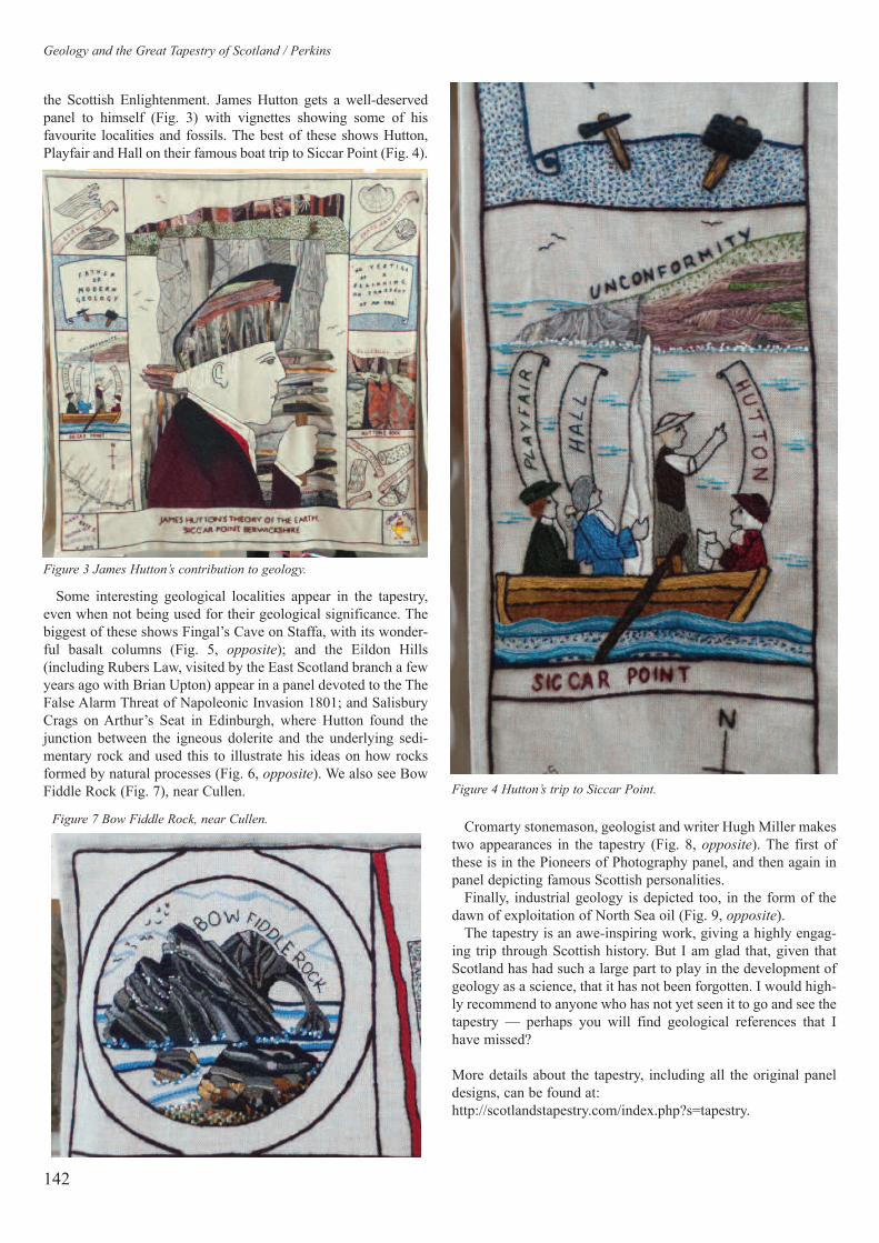
the Scottish Enlightenment. James Hutton gets a well-deservedpanel to himself (Fig. 3) with vignettes showing some of hisfavourite localities and fossils. The best of these shows Hutton,Playfair and Hall on their famous boat trip to Siccar Point (Fig. 4).
Geology and the Great Tapestry of Scotland / Perkins
142
Figure 3 James Hutton’s contribution to geology.
Figure 4 Hutton’s trip to Siccar Point.
Some interesting geological localities appear in the tapestry,even when not being used for their geological significance. Thebiggest of these shows Fingal’s Cave on Staffa, with its wonder-ful basalt columns (Fig. 5, opposite); and the Eildon Hills(including Rubers Law, visited by the East Scotland branch a fewyears ago with Brian Upton) appear in a panel devoted to the TheFalse Alarm Threat of Napoleonic Invasion 1801; and SalisburyCrags on Arthur’s Seat in Edinburgh, where Hutton found thejunction between the igneous dolerite and the underlying sedi-mentary rock and used this to illustrate his ideas on how rocksformed by natural processes (Fig. 6, opposite). We also see BowFiddle Rock (Fig. 7), near Cullen.
Figure 7 Bow Fiddle Rock, near Cullen. Cromarty stonemason, geologist and writer Hugh Miller makestwo appearances in the tapestry (Fig. 8, opposite). The first ofthese is in the Pioneers of Photography panel, and then again inpanel depicting famous Scottish personalities.
Finally, industrial geology is depicted too, in the form of thedawn of exploitation of North Sea oil (Fig. 9, opposite).
The tapestry is an awe-inspiring work, giving a highly engag-ing trip through Scottish history. But I am glad that, given thatScotland has had such a large part to play in the development ofgeology as a science, that it has not been forgotten. I would high-ly recommend to anyone who has not yet seen it to go and see thetapestry — perhaps you will find geological references that Ihave missed?
More details about the tapestry, including all the original paneldesigns, can be found at:http://scotlandstapestry.com/index.php?s=tapestry.
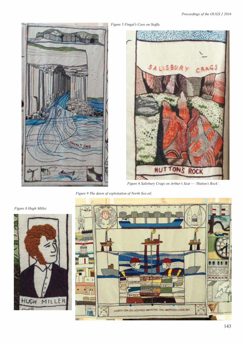
Proceedings of the OUGS 2 2016
143
Figure 5 Fingal’s Cave on Staffa.
Figure 8 Hugh Miller.
Figure 9 The dawn of exploitation of North Sea oil.
Figure 6 Salisbury Crags on Arthur’s Seat — ‘Hutton’s Rock’.

144
Editor’s notes to contributorsFollowing are guidelines for the submission of articles to theProceedings of the OUGS. The principal theme encompassedwithin these guidelines is ‘please keep it simple’. Let your editordo his job and please do not try to simulate, emulate or reproducethe page layout of the Proceedings. I have dedicated page-layoutsoftware (QuarkXPress) to do this and any special formatting,special characters and embedded illustrations that you include ina word-processing document can be lost (at best) or seriouslyconfuse and crash (at worst) my iMac or the QuarkXPress soft-ware when I import it into the layout.
If your article contains special characters (such as mathemati-cal symbols), please draw these to my attention — I will proba-bly spot them anyway — so that I can import them properly withthe glyphs menu in QuarkXPress.
Here are the basic guidelines. I will contact you about anyqueries that arise when I read your article. I will send you anedited version, showing you any changes that I have made andraising any queries or requesting any missing information.
Guidelines for OUGS Proceedings articlesAs OUGS Proceedings Editor I do not want the publication ofyour article to be more work than is necessary for you (or forme!). Your article need not be more than about 1,500 to 4,000words in general, but I leave the length up to you to suit thematerial you are writing about.
Regarding articles from the presenters of lectures at the OUGSSymposium, all OUGS members are grateful to you for present-ing a talk at the OUGS Annual Symposium, and for agreeing tosubmit a version of your talk for publication in the Proceedings.The purpose of this is to make your information available toOUGS members and others who could not attend the symposium.As OU students and OUGS members we enjoy hearing and learn-ing the information these symposia bring to us.
All that is necessary are:
• A Word (or compatible) file of the text: There is no need for youto attempt to format the text in any way using tools in Word orother word-processing software. I will do the page layout format inthe Proceedings house style, using dedicated publication-industry-standard page-layout software (QuarkXPress). However, feel free,if you wish, to use bold and/or italics to indicate headings and sub-headings so that I can set these into house style.
I do not require a hard copy, but if you need to point out spe-cial characters or attributes in your paper, it may be a good ideato send one with these items marked up or otherwise highlighted.Otherwise I can accept electronic files attached to an e-mail, orfiles on a CD.
• Each illustration, chart, graph, map or other illustration as
a separate digital file in high resolution: 300dpi minimum forcolour or half-tone images; 1200dpi for line illustrations. Tablescomposed in Word or Excel are fine, as they are just text. A roughguide to the number of figures in an article is 10 to 30. Obviouslyas a symposium presentation speaker you might have shownnumerous slides, so please use your best judgement on the num-ber to include with the paper to be published — again usually 10to 30 is only a rough guide.
• Please be sure that we have permission to publish any illus-
trations that are not yours: Also, please give me the appropri-ate information to cite in acknowledgement in the figure caption;and please tell me in writing or in an e-mail message that youhave obtained the permission necessary for each illustration inyour article that is not yours. As the author, this responsibility is yours.
• Please do not embed your illustrations in Word picture
boxes within the text: All that is necessary is to indicate, by areference within ( ) or within [ ] in your text, where the illustra-tion should go.
• You can submit the material as attachments to e-mails to me
or send it to me on a CD: I am on BT Broadband, so I canreceive large files. It is usually best to attach only a few illustra-tion files each to several e-mails. This applies especially to largefiles of photographs, charts and graphs. Alternatively, a digitalsharing package can be used, such as Dropbox or similar.
• Where appropriate, cite your sources, or make it clear that a
statement is a supposition, or solely your own view or opinion.
We use Harvard style citations in the text: (author date, pages),e.g. (Jones 2004, 51–3); and your sources or references should belisted in alphabetical order by author and date at the end of yourarticle. You need to list the author, date of publication (or ofaccess to a website), full title, periodical volume and number, orplace of publication and publisher, and page numbers.
If you miss out anything, I will ask you for it.If your list includes items not cited in your text, it will be called
‘Sources’; if all items in your list have been cited in your text, itwill be called ‘References’.
That really is it! The editing and page layout are my job, so let medo it for you. I will communicate with you as necessary as I dothis, with queries or difficulties with any formats, special sym-bols, characters, etc, as is the task of any editor.
For you really keen authors, regarding grammar and spelling I use:
Butcher, J. 1992 Copy-Editing: The Cambridge Handbook for Editors,
Authors and Publishers (3rd edn). Cambridge: Cambridge UPThe Oxford English Dictionary
The Penguin Spelling Dictionary 1990. London: Penguin Books LtdRitter, R. M. (ed and comp.) 2000 The Oxford Dictionary for Writers and
Editors (2nd edn). Oxford: Oxford UPRitter, R. M. (ed and comp.) 2002 The Oxford Manual of Style. Oxford:
Oxford UP
Please contact me at any time about your paper:
Dr David M. Jones, OUGS Proceedings Editor, 41 BlackburnWay, Godalming, Surrey GU7 1JY; 01483 424308;[email protected] OR [email protected]
The Open University Geological Society (OUGS) or its
Proceedings Editor, accept no responsibility for breach of copyright.
Copyright for the work remains with the author but copyright for
the published article will be that of the OUGS.
Editor’s notes to contributors

OUGS Moyra Eldridge Photographic Competition 2015
Winning and Highly Commended photographs
Popular Vote, Winner — Linda McArdell; also Geological Feature or Structure Winner
Liesegang rings in the ferruginous sands of the Vectis Formation, Sandown Bay, I.O.W.

Geo
logica
lly Insp
ired L
an
dsca
pe, W
inn
er — L
eon
An
gra
ve; also
Popu
lar V
ote H
igh
ly Com
men
ded
Panorama of A
lpine glaciers from G
ornergrat, above Zerm
att, Switzerland, w
ith the iconic Matterhorn on the far right.
Geo
logica
lly Insp
ired L
an
dsca
pe, H
igh
ly Com
men
ded
— L
inda M
cArd
ell
Salt Pans, Maras, V
alley of the Incas, high in the A
ndes, Peru.

Geologically Inspired Landscape, Highly Commended — Anna Saich
Sandstone Cliffs, Hastings. The cliffs to the east of Rock-a-Nore Road in Hastings Old Town are LowerCretaceous rocks. Sandstones of the Ashdown Formation form the lower part of the cliffs, with the sand-
stones and shales of the Wadhurst Formation above.
Geologically Inspired Landscape, Highly Commended — Linda McArdell
Castle Rock, vertical Oligocene limestone in the Torlesse Range west of Christchurch, New Zealand.

Geological Feature or Structure, Winner — Linda McArdell
Liesegang rings in the ferruginous sands of the Vectis Formation, Sandown Bay, I.O.W.[see Popular Vote, Winner]
Geological Feature or Structure, Highly Commended — Sarah Clark
Pahoehoe and lava rafts: a river of fast-flowing and very fluid lava issuing from a basalticfissure eruption, showing formation of pahoehoe at a slower ‘breakout’. Note the lava ‘rafts’
in the main course of the flow. Holuhraun, Iceland, September 2014.
Geological Feature or Structure, Highly Commended — Linda McArdell
Moeraki Boulders, Moeraki, New Zealand: the largest septarian nodules in the world.
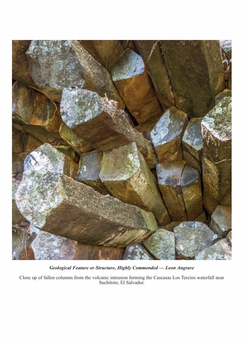
Geological Feature or Structure, Highly Commended — Leon Angrave
Close up of fallen columns from the volcanic intrusion forming the Cascasas Los Tercios waterfall nearSuchitoto, El Salvador.

Industrial Geology, Winner — Anna Saich
Marehill Sand Mines — local sandstones, including the Sandgate Formation seen at Marehill, were used in anumber of the medieval churches around Pulborough.
Industrial Geology, Highly Commended — Linda McArdell
Salt Pans of Maras, Valley of the Incas, high in the Andes, Peru.
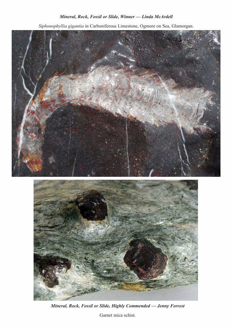
Mineral, Rock, Fossil or Slide, Winner — Linda McArdell
Siphonophyllia gigantia in Carboniferous Limestone, Ogmore on Sea, Glamorgan.
Mineral, Rock, Fossil or Slide, Highly Commended — Jenny Forrest
Garnet mica schist.

Mineral, Rock, Fossil or Slide, Highly Commended — James JonesQuartz crystals.
Top Related
Copyright © 2022 FDOKUMEN

