


Bahasa
Halaman
Hukum

PERMEABILITY AND SEEPAGE
GEOTC1 414 – Soil Mechanics
• In its natural occurrence, water and soil interacts with each other or shall we say they do affect each other.
• Water is a continuous phase of matter while soil (in a mass) is the opposite.
• And due to this interconnected voids, water can flow through this voids from points of higher energy to points of lower energy making soil a permeable media.
• The rate of which vary depending on the soil type and physical properties.
• It is necessary for determining or estimating the quantity of underground seepage under various hydraulic conditions, for investigating problems involving the pumping of water for underground construction and for making stability analyses of earth dams, hydraulic dams and other earth-retaining structures that are subject to seepage forces.
Introduction

According to Bernoulli’s principle, the total energy head at a point in water under motion can be given by the sum of the pressure head, velocity head and elevation head, or
If Bernoulli’s equation is applied to the flow of water through a porous soil medium, the flow of water or the seepage velocity is very small, thus the term expressing the velocity head can be negligible, and the total head at the point can be represented by
A. BERNOULLI’S EQUATION
Zg
vuhw
22
Zuhw
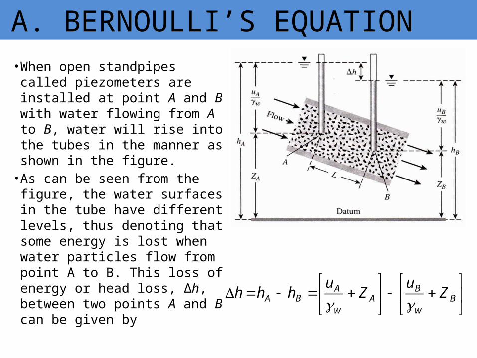
•When open standpipes called piezometers are installed at point A and B with water flowing from A to B, water will rise into the tubes in the manner as shown in the figure.•As can be seen from the figure, the water surfaces in the tube have different levels, thus denoting that some energy is lost when water particles flow from point A to B. This loss of energy or head loss, Δh, between two points A and B can be given by
A. BERNOULLI’S EQUATION
B
w
BA
w
ABA ZuZuhhh
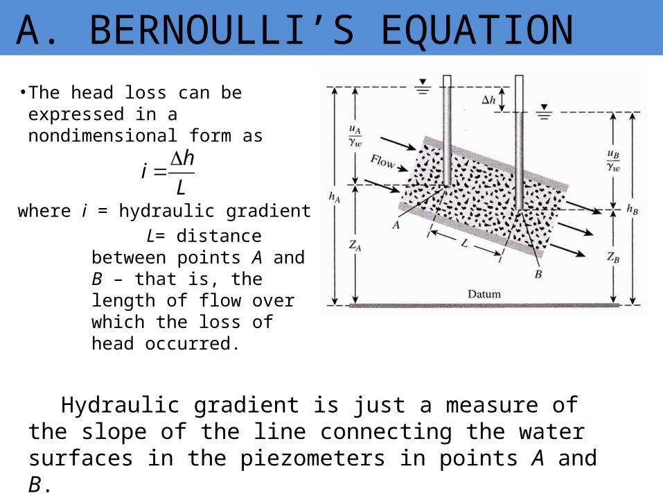
•The head loss can be expressed in a nondimensional form as
where i = hydraulic gradient L= distance
between points A and B – that is, the length of flow over which the loss of head occurred.
A. BERNOULLI’S EQUATION
Hydraulic gradient is just a measure of the slope of the line connecting the water surfaces in the piezometers in points A and B.
Lhi
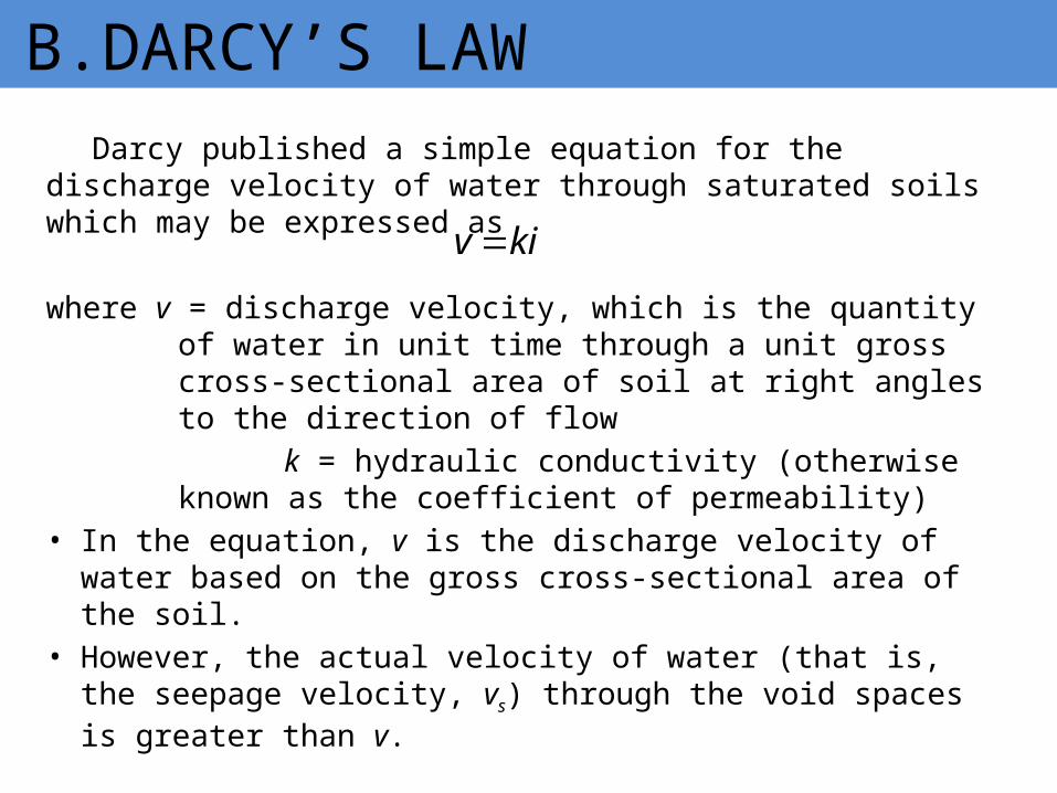
Darcy published a simple equation for the discharge velocity of water through saturated soils which may be expressed as
where v = discharge velocity, which is the quantity of water in unit time through a unit gross cross-sectional area of soil at right angles to the direction of flow
k = hydraulic conductivity (otherwise known as the coefficient of permeability)
• In the equation, v is the discharge velocity of water based on the gross cross-sectional area of the soil.
• However, the actual velocity of water (that is, the seepage velocity, vs) through the void spaces is greater than v.
B.DARCY’S LAW
kiv
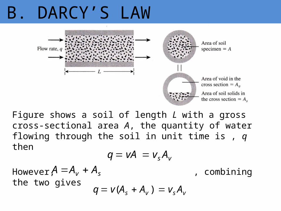
Figure shows a soil of length L with a gross cross-sectional area A, the quantity of water flowing through the soil in unit time is , q then
However, , combining the two gives
B. DARCY’S LAW
vs AvvAq
sv AAA
vsvs AvAAvq )(
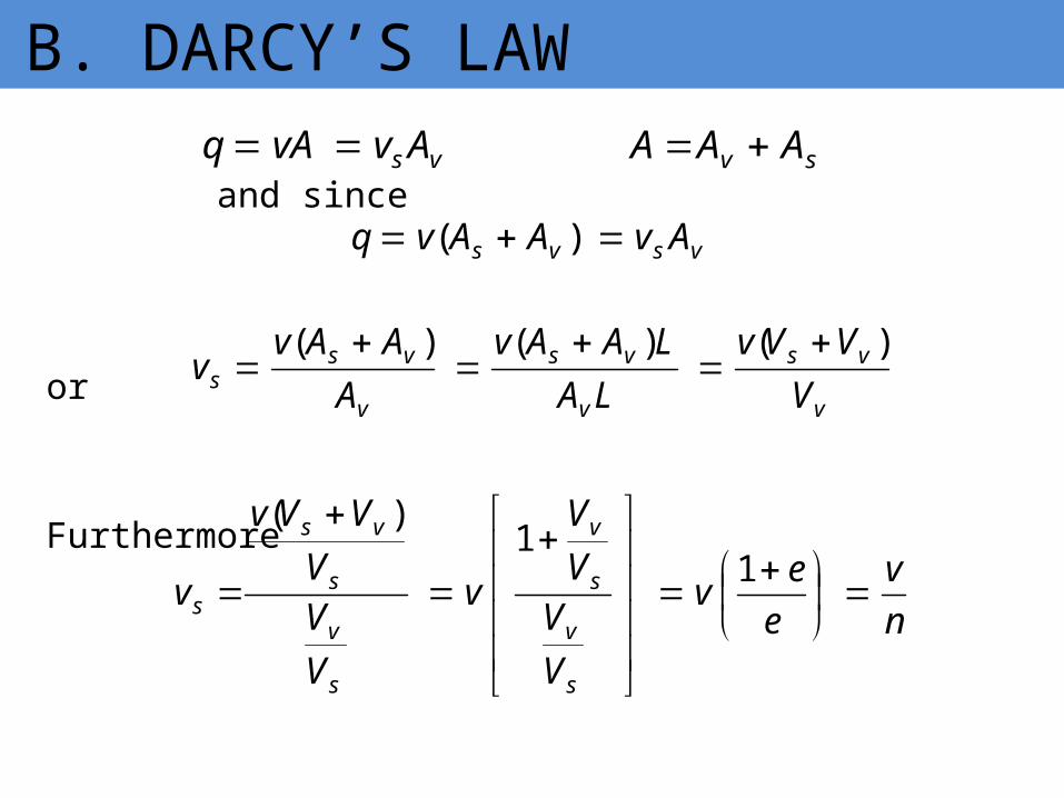
and since
or
Furthermore
B. DARCY’S LAWvs AvvAq sv AAA
vsvs AvAAvq )(
v
vs
v
vs
v
vss V
VVvLA
LAAvA
AAvv )()()(
nv
eev
VV
VV
v
VVV
VVv
v
s
v
s
v
s
v
s
vs
s
1
1)(
Hydraulic conductivity, k, is the measure of the conducting capability of soil to permit water to flow into it and it is expressed in cm/sec or m/sec in SI units and in ft/min or ft/day in English units and the values varies widely for different soils.
The hydraulic conductivity of soil generally depends on several factors:
•fluid viscosity•pore-size distribution•grain-size distribution•void ratio•roughness of mineral particles•degree of soil saturation
C. HYDRAULIC CONDUCTIVITY
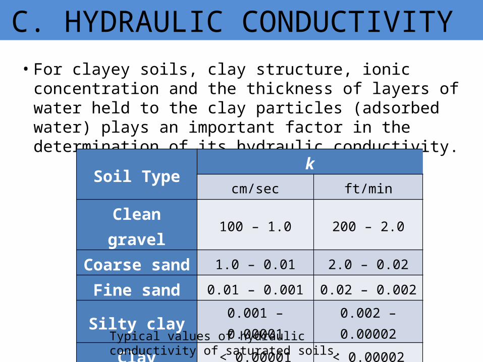
•For clayey soils, clay structure, ionic concentration and the thickness of layers of water held to the clay particles (adsorbed water) plays an important factor in the determination of its hydraulic conductivity.
C. HYDRAULIC CONDUCTIVITY
Soil Type kcm/sec ft/min
Clean gravel
100 – 1.0 200 – 2.0
Coarse sand 1.0 – 0.01 2.0 – 0.02Fine sand 0.01 – 0.001 0.02 – 0.002
Silty clay 0.001 – 0.00001
0.002 – 0.00002
Clay < 0.00001 < 0.00002Typical values of hydraulic conductivity of saturated soils.
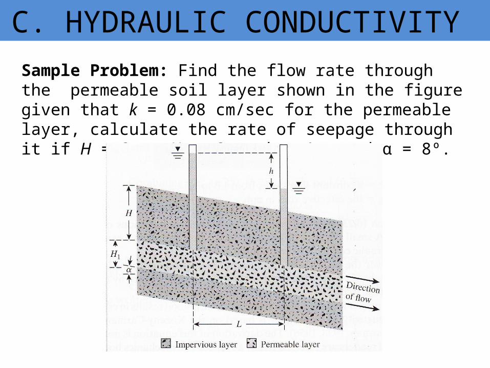
Sample Problem: Find the flow rate through the permeable soil layer shown in the figure given that k = 0.08 cm/sec for the permeable layer, calculate the rate of seepage through it if H = 8 m, H1 = 3 m, h = 4 m and α = 8º.
C. HYDRAULIC CONDUCTIVITY
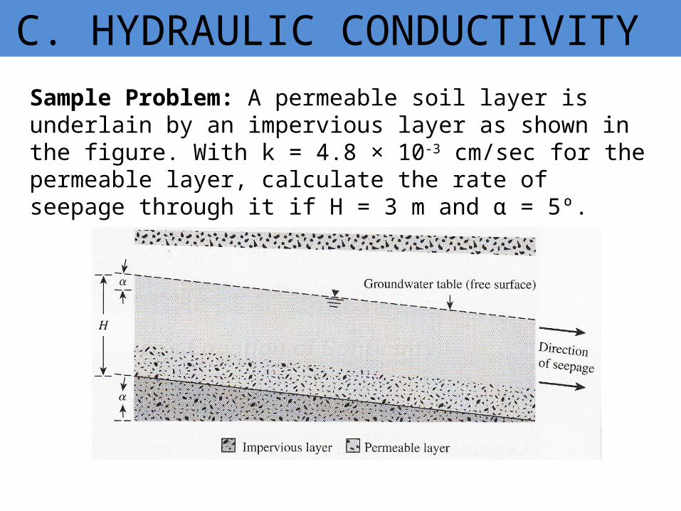
Sample Problem: A permeable soil layer is underlain by an impervious layer as shown in the figure. With k = 4.8 × 10⁻³ cm/sec for the permeable layer, calculate the rate of seepage through it if H = 3 m and α = 5º.
C. HYDRAULIC CONDUCTIVITY
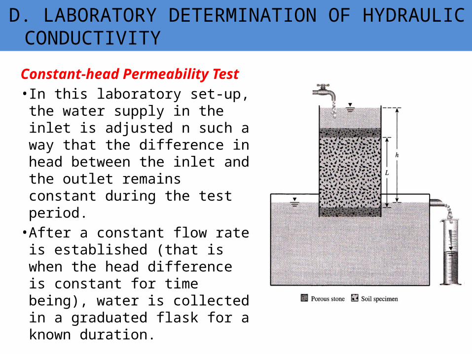
Constant-head Permeability Test•In this laboratory set-up, the water supply in the inlet is adjusted n such a way that the difference in head between the inlet and the outlet remains constant during the test period.•After a constant flow rate is established (that is when the head difference is constant for time being), water is collected in a graduated flask for a known duration.
D. LABORATORY DETERMINATION OF HYDRAULIC CONDUCTIVITY

Constant-head Permeability Test• The total volume collected may be expressed as
where V = volume of water collected
A = cross sectional area of the specimen perpendicular to the flow
t = duration of water collection
D. LABORATORY DETERMINATION OF HYDRAULIC CONDUCTIVITY
tkiAAvtV )(
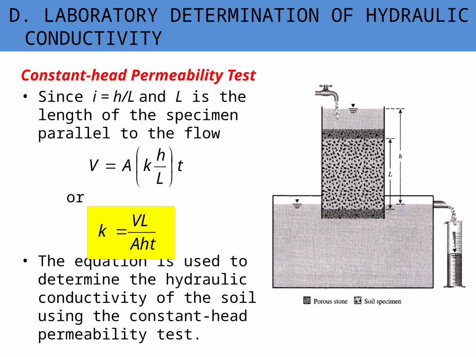
Constant-head Permeability Test• Since i = h/L and L is the length of the specimen parallel to the flow
or
• The equation is used to determine the hydraulic conductivity of the soil using the constant-head permeability test.
D. LABORATORY DETERMINATION OF HYDRAULIC CONDUCTIVITY
tLhkAV
AhtVLk

Falling-head Permeability Test• Water from a standpipe permitted to flow through the soil. The initial head difference h1 at time t1, usually taken as zero, is recorded and is water is allowed to flow through the soil specimen.
• As the flow continues, water in the standpipe drops to a head difference h2 at time t2 is then recorded.
D. LABORATORY DETERMINATION OF HYDRAULIC CONDUCTIVITY

Falling-head Permeability TestThe rate of flow of water
through the specimen can be given by
where q = flow rate (discharge) a = cross
sectional area of the standpipe
A = cross sectional area of the soil specimen perpendicular to the flow
D. LABORATORY DETERMINATION OF HYDRAULIC CONDUCTIVITY
dtdhaA
Lhkq

Falling-head Permeability Test
From the above equation,
Integrating
D. LABORATORY DETERMINATION OF HYDRAULIC CONDUCTIVITY
dtdhaA
Lhkq
hdh
AkaLdt
2
1
2
1
t
t
h
h hdh
AkaLdt
)ln( 1212 hhAkaLtt
)ln( 2112 hhAkaLtt
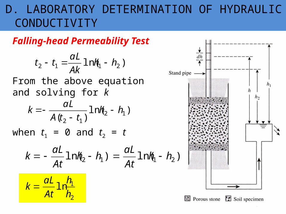
Falling-head Permeability Test
From the above equation and solving for k
when t1 = 0 and t2 = t
D. LABORATORY DETERMINATION OF HYDRAULIC CONDUCTIVITY
)ln( 2112 hhAkaLtt
)ln()( 1212
hhttA
aLk
)ln()ln( 2112 hhAtaLhh
AtaLk
2
1lnhh
AtaLk
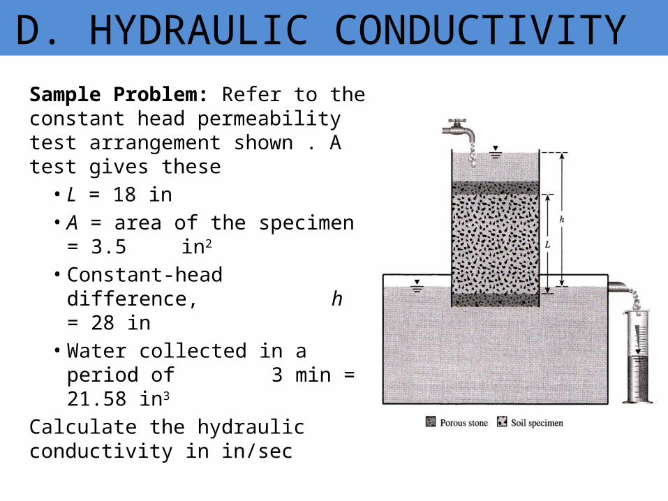
Sample Problem: Refer to the constant head permeability test arrangement shown . A test gives these• L = 18 in• A = area of the specimen = 3.5 in2
•Constant-head difference, h = 28 in
•Water collected in a period of 3 min = 21.58 in3
Calculate the hydraulic conductivity in in/sec
D. HYDRAULIC CONDUCTIVITY
Sample Problem: For a falling-head permeability test, the following values are given:•Length of the specimen = 200 mm•Area of the soil specimen = 1000 mm2
•Area of the standpipe = 40 mm2
•Head difference at time t = 0 is 500 mm•Head difference at time t = 180 sec is 300 mm
Determine the hydraulic conductivity of the soil in cm/sec.
D. HYDRAULIC CONDUCTIVITY

•For fairly uniform sand (that is, sand with small uniformity coefficient), Hazen (1930) proposed an empirical relationship for hydraulic conductivity in the form
where c = a constant that varies from 1.0 to 1.5 D10 = effective size, in mm
The equation is based primarily on observations on loose, clean filter sands. A small quantity of silts and clays, when present in a sandy soil, may change the hydraulic conductivity substantially.
E. RELATIONSHIPS FOR HYDRAULIC CONDUCTIVITY – GRANULAR SOIL
210sec)/cm( cDk
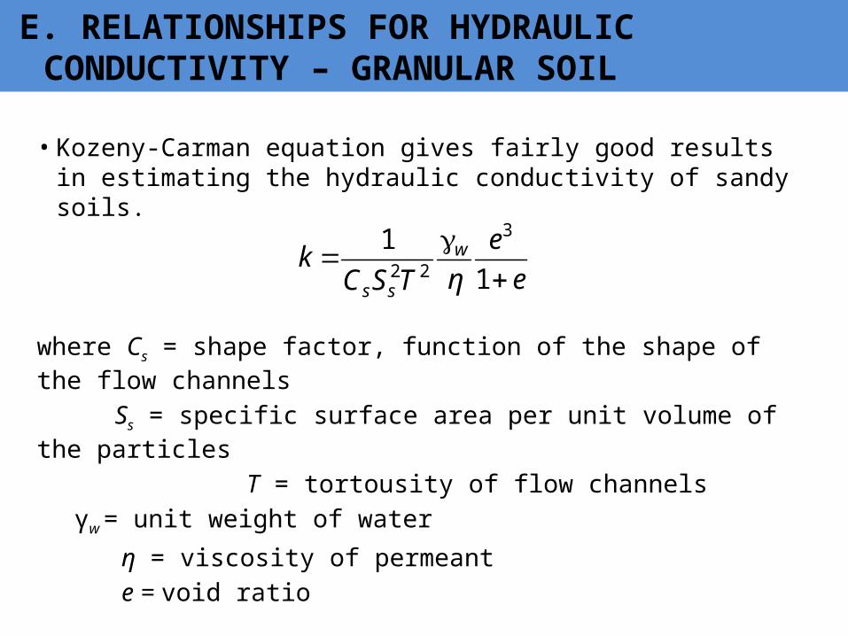
•Kozeny-Carman equation gives fairly good results in estimating the hydraulic conductivity of sandy soils.
where Cs = shape factor, function of the shape of the flow channels Ss = specific surface area per unit volume of the particles T = tortousity of flow channels
γw = unit weight of water η = viscosity of permeant e = void ratio
E. RELATIONSHIPS FOR HYDRAULIC CONDUCTIVITY – GRANULAR SOIL
ee
ηTSCk w
ss
11 3
22
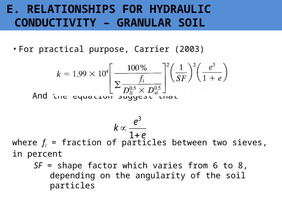
•For practical purpose, Carrier (2003)
And the equation suggest that
where fi = fraction of particles between two sieves, in percent SF = shape factor which varies from 6 to 8,
depending on the angularity of the soil particles
E. RELATIONSHIPS FOR HYDRAULIC CONDUCTIVITY – GRANULAR SOIL
eek
13
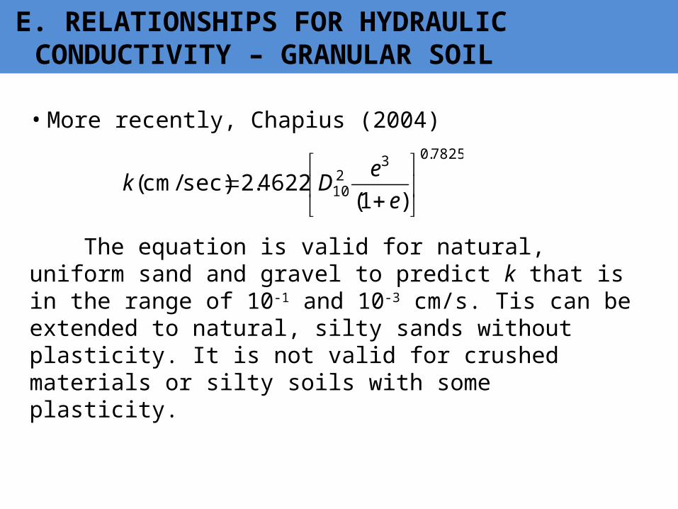
•More recently, Chapius (2004)
The equation is valid for natural, uniform sand and gravel to predict k that is in the range of 10-1 and 10-3 cm/s. Tis can be extended to natural, silty sands without plasticity. It is not valid for crushed materials or silty soils with some plasticity.
E. RELATIONSHIPS FOR HYDRAULIC CONDUCTIVITY – GRANULAR SOIL
7825.03210 )1(4622.2sec)/cm(
e
eDk
Sample Problem:The hydraulic conductivity of sand at a void ratio of 0.62 is 0.03 cm/sec. Estimate the hydraulic conductivity at a vid ratio of 0.48.
E. RELATIONSHIPS FOR HYDRAULIC CONDUCTIVITY – GRANULAR SOIL
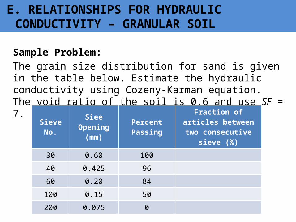
Sample Problem:The grain size distribution for sand is given in the table below. Estimate the hydraulic conductivity using Cozeny-Karman equation. The void ratio of the soil is 0.6 and use SF = 7.
E. RELATIONSHIPS FOR HYDRAULIC CONDUCTIVITY – GRANULAR SOIL
Sieve No.
Siee Opening (mm)
Percent Passing
Fraction of articles between two consecutive
sieve (%)30 0.60 10040 0.425 9660 0.20 84100 0.15 50200 0.075 0
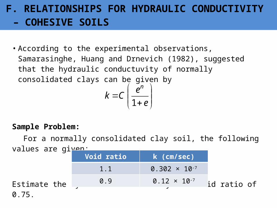
•According to the experimental observations, Samarasinghe, Huang and Drnevich (1982), suggested that the hydraulic conductuvity of normally consolidated clays can be given by
Sample Problem: For a normally consolidated clay soil, the following
values are given:
Estimate the hydraulic conductivity at a void ratio of 0.75.
F. RELATIONSHIPS FOR HYDRAULIC CONDUCTIVITY – COHESIVE SOILS
Void ratio k (cm/sec)1.1 0.302 × 10⁻⁷
0.9 0.12 × 10⁻⁷
e
eCkn
1
• As been stated previously that different soil have different hydraulic conductivity.
• It is also good to note that even a single soil could have different conductivity with respect to the flow direction.
• It means that a soil have a different conductivity when the flow if horizontal than when the flow is vertical.
• In terms of conductivity, a soil with the same value of hydraulic conductivity is referred to as isotropic soil and the soil with different values of hydraulic conductivities in the horizontal and vertical direction is referred to as anisotropic soil.
• In its natural state, soil might be composed stratified layers of soil with differing hydraulic conductivity for flow in a given direction.
• Nevertheless, an equivalent hydraulic conductivity can be computed to simplify conductivity calculations.
G. EQUIVALENT HYDRAULIC CONDUCTIVITY IN STRATIFIED SOIL
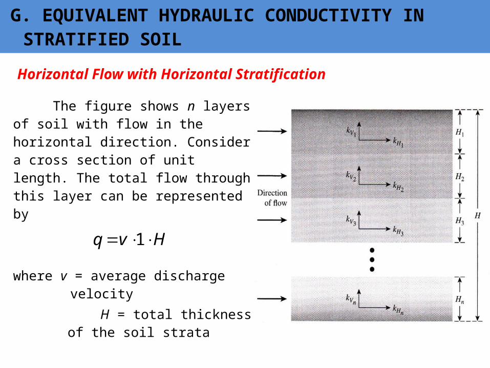
Horizontal Flow with Horizontal Stratification
G. EQUIVALENT HYDRAULIC CONDUCTIVITY IN STRATIFIED SOIL
The figure shows n layers of soil with flow in the horizontal direction. Consider a cross section of unit length. The total flow through this layer can be represented by
where v = average discharge velocity
H = total thickness of the soil strata
Hvq 1

Horizontal Flow with Horizontal Stratification
G. EQUIVALENT HYDRAULIC CONDUCTIVITY IN STRATIFIED SOIL
• Since the total flow or water passing through the cross section is equal to the sum of the water or flow through the individual layers then
where v1, v2, v3,…,vn = individual discharge velocities in the respective layers denoted by the subscript
H1, H2 , H3,..., Hn = individual thickness in the respective layers denoted by the subscript
nqqqqq 321
nn HvHvHvHvHv 11111 332211
Horizontal Flow with Horizontal Stratification
G. EQUIVALENT HYDRAULIC CONDUCTIVITY IN STRATIFIED SOIL
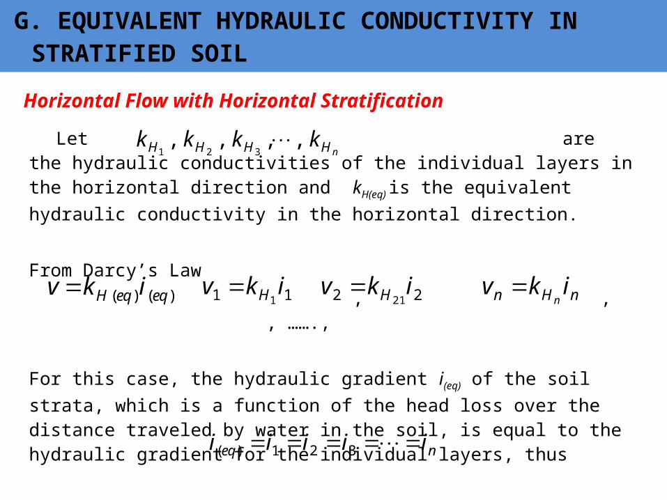
Let are the hydraulic conductivities of the individual layers in the horizontal direction and kH(eq) is the equivalent hydraulic conductivity in the horizontal direction.
From Darcy’s Law , , , …….,
For this case, the hydraulic gradient i(eq) of the soil strata, which is a function of the head loss over the distance traveled by water in the soil, is equal to the hydraulic gradient for the individual layers, thus
nHHHH kkkk ,,,,321
)()( eqeqH ikv 11 1ikv H 22 21
ikv H nHn ikvn
neq iiiii 321)(
Horizontal Flow with Horizontal Stratification
G. EQUIVALENT HYDRAULIC CONDUCTIVITY IN STRATIFIED SOIL
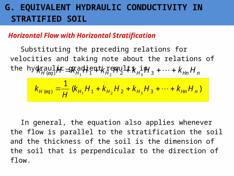
Substituting the preceding relations for velocities and taking note about the relations of the hydraulic gradient results in
In general, the equation also applies whenever the flow is parallel to the stratification the soil and the thickness of the soil is the dimension of the soil that is perpendicular to the direction of flow.
nHnHHHeqH HkHkHkHkHk 321)( 321
)(1321)( 321 nHnHHHeqH HkHkHkHk
Hk

Vertical Flow with Horizontal Stratification
G. EQUIVALENT HYDRAULIC CONDUCTIVITY IN STRATIFIED SOIL
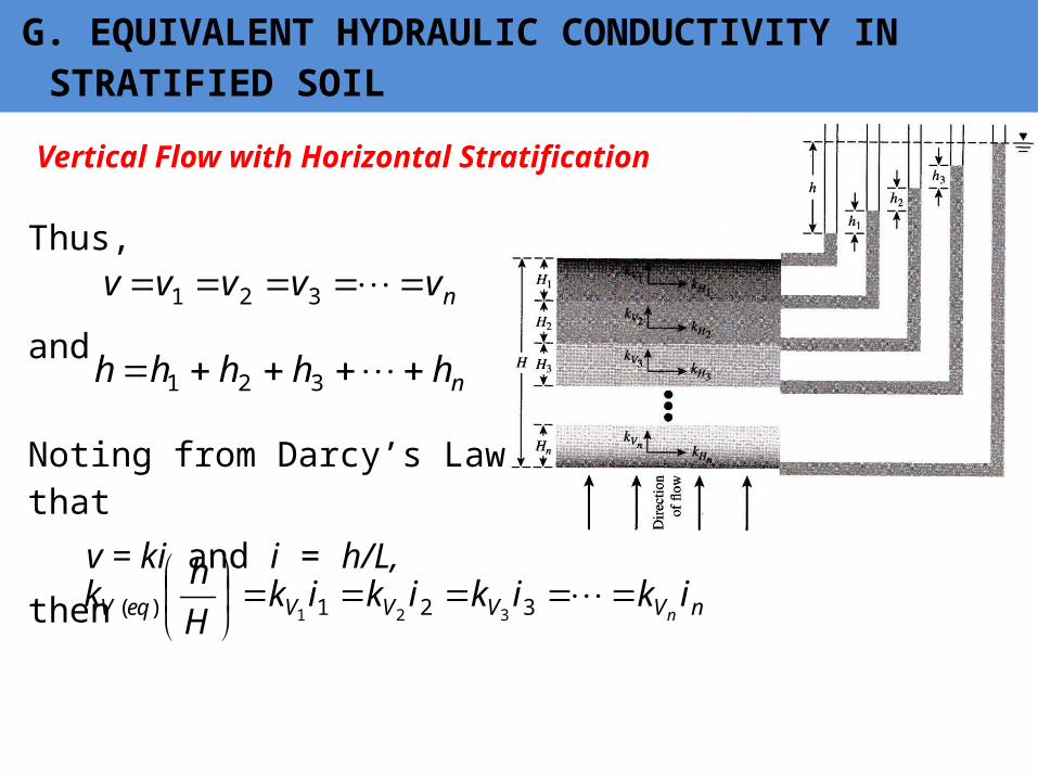
The figure shows n layers of soil with flow in the horizontal direction. • In this case the velocity of flow through all the layers is the same.
• However, as the soil travels over a layer, head loss occurs.• As it again passes through another layer, head loss occurs, though it does not connote that the magnitude of the head losses are equal for every layer.
• Therefore, every layer of the soil strata contributes to the total head loss, h, as water passes through the whole stratum
Vertical Flow with Horizontal Stratification
G. EQUIVALENT HYDRAULIC CONDUCTIVITY IN STRATIFIED SOIL
Thus,
and
Noting from Darcy’s Law that
v = ki and i = h/L, then
nvvvvv 321
nhhhhh 321
nVVVVeqV ikikikikHhk
n
321)( 321
Vertical Flow with Horizontal Stratification
G. EQUIVALENT HYDRAULIC CONDUCTIVITY IN STRATIFIED SOIL
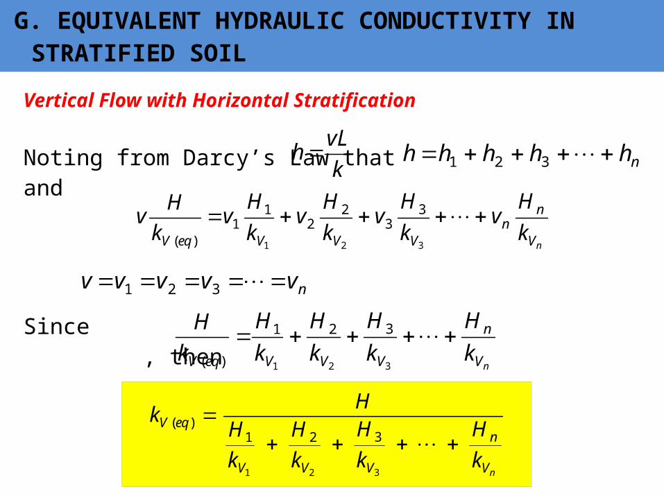
Noting from Darcy’s Law that and
Since , then
nvvvvv 321
nhhhhh 321
nV
nn
VVVeqV kHv
kHv
kHv
kHv
kHv
321
33
22
11
)(
kvLh
nV
n
VVVeqV kH
kH
kH
kH
kH
321
321
)(
nV
n
VVV
eqV
kH
kH
kH
kH
Hk
321
321)(

Vertical Flow with Horizontal Stratification
G. EQUIVALENT HYDRAULIC CONDUCTIVITY IN STRATIFIED SOIL
In general, equation also applies to compute the equivalent hydraulic conductivity when the flow is perpendicular to the soil stratification and the thickness of the soil is that dimension of the soil that parallel to the flow. nV
n
VVV
eqV
kH
kH
kH
kH
Hk
321
321)(

Figure shows layers of soils in a tube that is 100 mm × 100 mm in cross section. Water is supplied to maintain a constant head difference of 400 mm across the sample. The hydraulic conductivities of the soils in the direction of the flow through them are as follows:
Calculate the equivalent k, rate of water supply, seepage velocity through soil C.
Sample Problem
Soil k (cm/sec)
Porosity, n
A 1 × 10⁻² 25%B 3 × 10⁻³ 32%C 4.9 × 10⁻⁴ 22%

Given the stratified soil shown with a constant head difference of 1.8 m. The properties of each soil are as follows: Coefficient of permeability: k1 = 6.25 cm/hr; k2 = 5.75 cm/hr; k3 = 4.50 cm/hr; k4 = 6.25 cm/hr; k5 = 8.15 cm/hr; k6 = 3.60 cm/hr Thickness: H = 1.20 m, H3 = 0.30 m, H4 = 0.50 m, H5 = 0.40 m Length: L1 = 0.80 m, L2 = 0.70 m, L3 = 1.50 m, L6 = 0.90 mDetermine the total flow per meter width and the equivalent coefficient of permeability.
Sample Problem
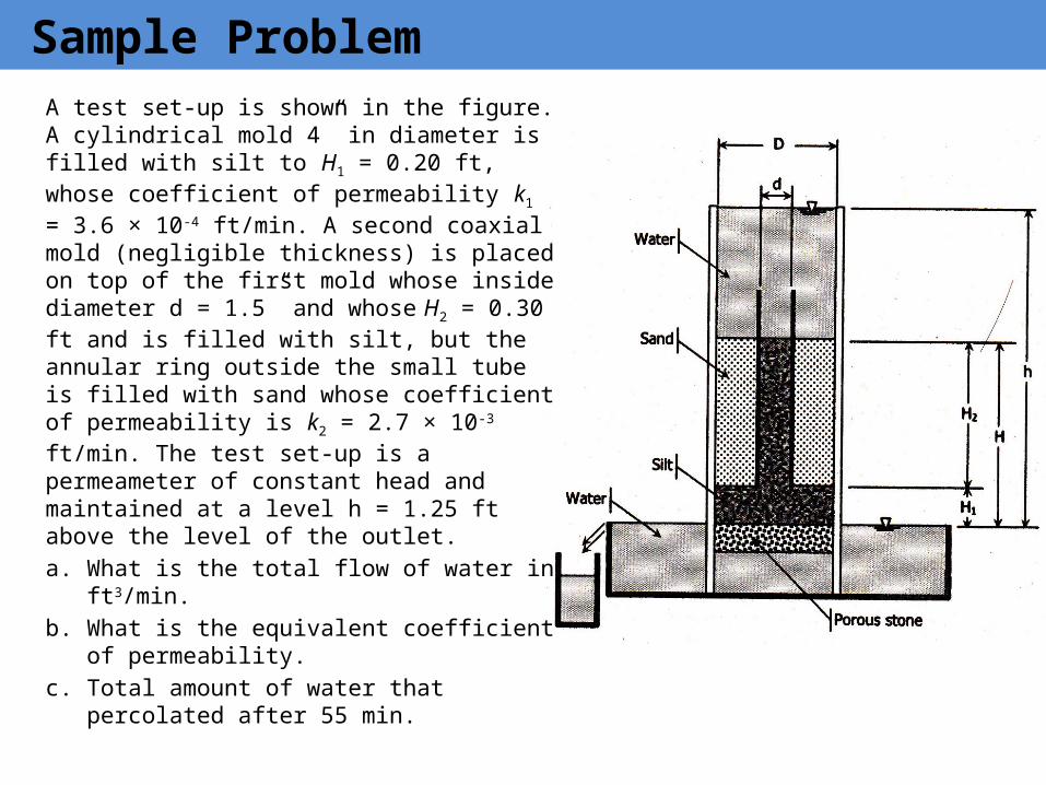
A test set-up is shown in the figure. A cylindrical mold 4” in diameter is filled with silt to H1 = 0.20 ft, whose coefficient of permeability k1 = 3.6 × 10⁻⁴ ft/min. A second coaxial mold (negligible thickness) is placed on top of the first mold whose inside diameter d = 1.5” and whose H2 = 0.30 ft and is filled with silt, but the annular ring outside the small tube is filled with sand whose coefficient of permeability is k2 = 2.7 × 10⁻³ ft/min. The test set-up is a permeameter of constant head and maintained at a level h = 1.25 ft above the level of the outlet. a. What is the total flow of water in
ft3/min.b. What is the equivalent coefficient
of permeability.c. Total amount of water that
percolated after 55 min.
Sample Problem
Top Related
Copyright © 2022 FDOKUMEN

