


Bahasa
Halaman
Hukum

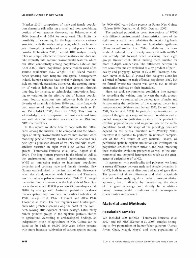
Investigating sex-specific dynamics using uniparentalmarkers: West New Guinea as a case studyStefano Mona1,2, Ernest Mordret1,2, Michel Veuille1,2 & Mila Tommaseo-Ponzetta3
1Laboratoire Biologie integrative des populations, Ecole Pratique des Hautes Etudes, 46 rue de Lille, 75007 Paris, France2CNRS UMR 7205, Museum National d’Histoire Naturelle, Rue Buffon, 75005 Paris, France3Department of Biology, University of Bari, 70100 Bari, Italy
Keywords
Gene genealogy, metapopulation,
patrilocality, spatial simulation, West New
Guinea.
Correspondence
Stefano Mona, UMR 7205, Museum National
d’Histoire Naturelle, Batiment 39 - 16 rue
Buffon, 75005 Paris, France.
Tel: +33-0-140798166;
Fax: +33-0-140793337;
E-mail: [email protected]
Funding information
No funding information provided.
Received: 13 March 2013; Revised: 27 May
2013; Accepted: 31 May 2013
Ecology and Evolution 2013; 3(8): 2647–
2660
doi: 10.1002/ece3.660
Abstract
Mitochondrial DNA (mtDNA) and Y chromosome (NRY) genetic markers have
been often contrasted to investigate sex-specific dynamics. Traditionally, isola-
tion by distance, intrapopulation genetic diversity and population differentia-
tion are estimated from both markers and compared. Two possible sources of
bias are often neglected. First, kilometric distances are frequently used as
predictor of the connectivity between groups, hiding the role played by envi-
ronmental features at a microgeographic scale. Second, the comparison of intra-
population diversity and population differentiation between mtDNA and NRY
is hampered by their different mutational mechanisms and rates. Here, we show
how to account for these biases by analyzing from a different perspective a pub-
lished dataset of eight West New Guinea (WNG) populations for which
mtDNA control region sequences and seven linked NRY microsatellites had
been typed. First, we modeled the connectivity among sampled populations by
computing the number of days required to travel between groups. Then, we
investigated the differences between the two sexes accounting for the molecular
characteristics of the markers examined to obtain estimates on the product of
the effective population size and the migration rate among demes (Nm). We
achieved this goal by studying the shape of the gene genealogy at several sam-
pling levels and using spatial explicit simulations. Both the direction and the
rate of migration differ between male and females, with an Nm estimated to be
>6 times higher in the latter under many evolutionary scenarios. We finally
highlight the importance of applying metapopulation models when analyzing
the genetic diversity of a species.
Introduction
Sex-specific demographic patterns are traditionally inves-
tigated in humans by using uniparentally inherited mark-
ers, namely mitochondrial DNA (mtDNA) for females
and Y chromosome (NRY) for males. Reports usually
focus mainly on three classes of analysis, whose results
are compared between the two markers: (i) isolation by
distance (IBD) (Seielstad et al. 1998; Wood et al. 2005;
Delfin et al. 2012; Kemp et al. 2012); (ii) intrapopulation
diversity levels (Oota et al. 2001; Kayser et al. 2003; Gun-
narsdottir et al. 2012); (iii) extent of population differen-
tiation (Seielstad et al. 1998; Oota et al. 2001; Nasidze
et al. 2004). Most of the evidences presented so far suggest
that paternal and maternal histories differ heavily, probably
as a consequence of cultural behaviors related to postmar-
ital residential pattern and variance in reproductive suc-
cess (see Heyer et al. [2012] and references therein).
However, different conclusions have been drawn depend-
ing on the region investigated (Seielstad et al. 1998; Oota
et al. 2001; Fuselli et al. 2003; Kayser et al. 2003; Nasidze
et al. 2004; Kemp et al. 2012), on the geographic scale
of the study (Wilder et al. 2004; Wilkins and Marlowe
2006) and on the specific locus ascertained on both
mtDNA and NRY (Wilder et al. 2004; Gunnarsdottir
et al. 2012).
There are several pitfalls when investigating male and
female population genetics patterns. First, despite the
advances in next generation sequencing technologies
which allow access to an incredibly large amount of data
ª 2013 The Authors. Ecology and Evolution published by John Wiley & Sons Ltd.
This is an open access article under the terms of the Creative Commons Attribution License, which permits use,
distribution and reproduction in any medium, provided the original work is properly cited.
2647
(Metzker 2010), comparison of male and female popula-
tion dynamics still relies on a small and nonrecombining
portion of our genome (however, see Balaresque et al.
2006; Segurel et al. 2008 for exceptions). This limits the
possibility of accounting for the large stochastic variance
associated with the coalescent process, which can be miti-
gated through the analysis of as many independent loci as
possible (Felsenstein 2006). Second, IBD analysis usually
relies on simple kilometric distance matrices and does not
take explicitly into account environmental features, which
can affect connectivity among populations (McRae and
Beier 2007). Third, population genetic models used often
assume equilibrium (i.e., Wright [1931] island model),
hence ignoring both temporal and spatial heterogeneity.
Indeed, human societies have probably changed their life-
style on multiple occasions. Moreover, the carrying capac-
ity of various habitats has not been constant through
time due, for instance, to technological innovations, lead-
ing to variation in the effective size of human popula-
tions. Fourth, mutation rate influences both the gene
diversity of a sample (Hudson 1990) and many frequently
used measure of population differentiation such as Fst
and Rst (Hedrick 2005; Meirmans 2006). This must be
acknowledged when comparing the results obtained from
loci with different mutation rates such as mtDNA and
NRY microsatellites.
In this report, we show how to cope with the differ-
ences among the markers to be compared and the advan-
tages of taking environmental features into account when
modeling genetic diversity. To this end, we analyzed in a
new light a published dataset of mtDNA and NRY micro-
satellites variation in eight West New Guinea (WNG)
groups (Tommaseo-Ponzetta et al. 2002; Kayser et al.
2003). The long human presence in the island as well as
the environmental and temporal heterogeneity makes
WNG an interesting region to investigate population
dynamics and contrast male and female histories. New
Guinea was colonized in the last part of the Pleistocene
when the island, together with Australia and Tasmania,
was part of one paleocontinent called “Sahul”. Although
the earliest human presence in the highlands of New Gui-
nea is documented 49,000 years ago (Summerhayes et al.
2010), by analogy with Australian prehistoric evidence
this occupation may have been even earlier (Roberts et al.
1990; Fullagar et al. 1996; O’Connell and Allen 1998;
Thorne et al. 1999). The first migrants were hunter–gath-erers who probably spread along the coast of the conti-
nent, leaving little evidence of their passage. Later, many
hunter–gatherer groups in the highland plateaus shifted
to agriculture. According to archaeological findings, an
independent origin of agriculture in New Guinea can be
dated as far back as 10,000–9000 years before present,
with more intensive cultivation of various species starting
by 7000–6500 years before present in Papua New Guinea
(Golson 1990; Denham et al. 2003; Denham 2005).
The analyzed populations cover two regions of WNG
with different environmental characteristics: three of the
eight groups are farmers, inhabiting the interior highlands,
whereas the remaining five are hunter/fisher–gatherers(Tommaseo-Ponzetta et al. 2002), inhabiting the low-
lands. A reduced NRY diversity compared with mtDNA
was already put forward when analyzing these eight
groups (Kayser et al. 2003), making them suitable for
more in-depth comparison. The differences between the
two sexes were mostly explained as a by-product of patril-
ocality and polygyny (Kayser et al. 2003) (recently, how-
ever, Heyer et al. [2012] showed that polygyny alone has
a limited influence on male effective population size), but
no formal hypothesis testing was carried out to obtain
quantitative estimate on their intensities.
Here, we took environmental conditions into account
by recording the walking time between the eight groups.
Furthermore, we compared the demography of males and
females using the prediction of the sampling theory in a
metapopulation (Wakeley and Lessard 2003; De and Durrett
2007; Stadler et al. 2009). In particular, we investigated the
shape of the gene genealogy within each population and in
pooled samples to qualitatively estimate the product of
effective population size and migration rate of the meta-
population (Nm). The shape of the genealogy does not
depend on the neutral mutation rate (Wakeley 2008),
therefore it is possible to perform an unbiased compari-
son of the Nm values of any markers. Finally, we
performed spatially explicit simulations to investigate the
population structure at both mtDNA and NRY, modeling
their molecular evolution properties as well as the envi-
ronmental and temporal heterogeneity (such as the emer-
gence of agriculture) of WNG.
In agreement with patrilocality and polygyny, we found
a strong difference between male and female dynamics in
WNG, both in terms of direction and rate of gene flow.
The pattern of those differences and their magnitude
emerged when analyzing data under a metapopulation
approach, both indirectly by investigating the shape
of the gene genealogy and directly by simulations
taking environmental conditions and locus-specific
characteristics into account.
Material and Methods
Population samples
We included 200 mtDNA (Tommaseo-Ponzetta et al.
2002) and 163 NRY (Kayser et al. 2003) samples belong-
ing to five populations of hunter/fisher gatherers (Asmat,
Awyu, Citak, Mappi, Muyu) and three populations of
2648 ª 2013 The Authors. Ecology and Evolution published by John Wiley & Sons Ltd.
Sex-specific Dynamic in New Guinea S. Mona et al.
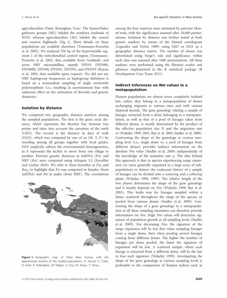
agriculturalists (Dani, Ketengban, Una). The hunter/fisher
gatherers groups (HG) inhabit the southern lowlands of
WNG whereas agriculturalists (AG) inhabit the central
and western highlands (Fig. 1). More details on these
populations are available elsewhere (Tommaseo-Ponzetta
et al. 2002). We analyzed 350 bp of the hypervariable seg-
ment 1 of the mitochondrial control region (Tommaseo-
Ponzetta et al. 2002; data available from GenBank) and
seven NRY microsatellites, namely DYS19, DYS389I,
DYS389II, DYS390, DYS391, DYS392, and DYS393 (Kayser
et al. 2003, data available upon request). We did not use
NRY haplogroup frequencies as haplogroup definition is
based on a nonrandom sampling of single nucleotide
polymorphism (i.e., resulting in ascertainment bias with
unknown effect on the estimation of diversity and genetic
distances).
Isolation by distance
We computed two geographic distance matrices among
the sampled populations. The first is the great circle dis-
tance, which represents the shortest line between two
points and takes into account the curvature of the earth
(GEO). The second is the distance in days of walk
(DAY), which was computed by one of us (M. T.-P.) by
traveling among all groups together with local guides.
DAY implicitly reflects the environmental heterogeneities,
as it represents the facility to move from one village to
another. Pairwise genetic distances at mtDNA (Fst) and
NRY (Rst) were computed using Arlequin 3.5 (Excoffier
and Lischer 2010). We refer to them hereafter as FstF and
RstM to highlight that Fst was computed in females (from
mtDNA) and Rst in males (from NRY). The correlations
among the four matrices were estimated by pairwise Man-
tel tests, with the significance assessed after 10,000 permu-
tations. Isolation by distance was further tested at both
genetic markers by means of the Mantel correlogram
(Legendre and Fortin 1989) using GEO or DAY as a
geographic distance matrix. The number of classes was
determined using Surge’s rule and significance within
each class was assessed after 1000 permutations. All these
analyses were performed using the libraries ecodist and
gdistance implemented in the R statistical package (R
Development Core Team 2011).
Indirect inferences on Nm values in ametapopulation
Human populations are almost never completely isolated
but, rather, they belong to a metapopulation of demes
exchanging migrants at various rates and with various
dispersal kernels. The gene genealogy relating a sample of
lineages extracted from a deme belonging to a metapopu-
lation, as well as that of a pool of lineages taken from
different demes, is mostly determined by the product of
the effective population size N and the migration rate
m (Wakeley 1999, 2001; Ray et al. 2003; Stadler et al. 2009).
Contrasting the shape of the genealogy at various sam-
pling level (i.e., single deme vs. a pool of lineages from
different demes) provides indirect information on the
absolute Nm value (Stadler et al. 2009) independently of
the knowledge of the mutation rate l. The idea behind
this approach is that in species experiencing range expan-
sion (or more generally organized in a large array of sub-
populations or demes) the coalescent history of a sample
of lineages can be divided into a scattering and a collecting
phase (Wakeley 1998, 1999). The relative length of the
two phases determines the shape of the gene genealogy
and it mostly depends on Nm (Wakeley 1999; Ray et al.
2003). This holds true for lineages sampled within a
deme, scattered throughout the range of the species or
pooled from various demes (Stadler et al. 2009). Con-
trasting the shape of a gene genealogy in a metapopula-
tion at all these sampling intensities can therefore provide
information on Nm. High Nm values will determine sig-
nature of population growth at all sampling levels (Stadler
et al. 2009). For decreasing Nm, the signature of the
range expansion will be lost first when sampling lineages
from a single deme, then when pooling several lineages
coming from different demes. The higher the number of
lineages per deme pooled, the faster the signature of
expansion will be lost. A scattered sample, where each
lineage is extracted from a different deme, will be the last
to lose such signature (Wakeley 1999). Investigating the
shape of the gene genealogy at various sampling levels is
preferable to the comparison of fixation indices such as
Figure 1. Geographic map of West New Guinea with the
approximate location of the studied populations. A: Asmat; C: Citak;
D: Dani; K: Ketengban; M: Mappi; U: Una; W: Awyu; Y: Muyu.
ª 2013 The Authors. Ecology and Evolution published by John Wiley & Sons Ltd. 2649
S. Mona et al. Sex-specific Dynamic in New Guinea
Fst (Excoffier et al. 1992) and Rst (Slatkin 1995), com-
monly used to estimate Nm. These fixation indices are
dependent on l and on the molecular evolutionary char-
acteristic of the markers under examination (Hedrick
2005). Moreover, they are based on simplifying assump-
tions which do not always hold in real settings (Whitlock
and McCauley 1999), while metapopulation and sampling
theory is robust to various population genetic models
(Wakeley 1999, 2004; Ray et al. 2003; Wilkins 2004; Sta-
dler et al. 2009).
To determine the shape of the genealogy, we used a
Bayesian-based coalescent approach and compared differ-
ent demographic models by means of Bayes Factors (BF).
We used BEAST (Drummond et al. 2012) to contrast a
constant size model versus the extended Bayesian skyline
plot (Heled and Drummond 2008) for mtDNA, and
Batwing (Wilson et al. 2003) to contrast a constant size
model versus a constant population starting an expansion
T generations before present for NRY. Default priors were
used in BEAST, whereas priors as in Mona et al. (2007)
were set in Batwing. We ran all datasets with both soft-
ware for 100,000,000 iterations with a 10% burn-in and a
thinning of 1000. Convergence was checked by running
each dataset twice and by reaching an effective sample
size higher than 200 for all parameters in each analysis.
Marginal likelihood was evaluated using the harmonic
mean estimator (Kass and Raftery 1995). BF were com-
puted as twice the difference of the natural logarithm
of the marginal likelihoods and interpreted using the
Jeffrey scale as reported in Kass and Raftery (1995). The
harmonic mean is a simple estimator of the marginal like-
lihood and some concerns have recently emerged on its
performance (Baele et al. 2012). The advantage of using
the harmonic mean is its computational efficiency, which
is important because we run a large number of model
comparison analyses. The analyses were performed in: (i)
each of the eight groups; (ii) the total pooled sample; (iii)
100 datasets of (a) 16 lineages obtained by resampling
two lineages per village (group 2L); (b) 24 lineages
obtained by resampling three lineages per village (group
3L); (c) 32 lineages obtained by resampling four lineages
per village (group 4L). In total, we analyzed 309 datasets
under two different models for the two markers, amount-
ing to 1236 coalescent analyses. The reasoning behind
resampling 100 times two, three, or four lineages per
village was to obtain a BF distribution at each sampling
intensity to assess the impact of stochastic variance in the
coalescent process.
Spatial explicit simulations
We performed a set of spatial explicit simulations of the
demographic history of males and females in WNG using
the software SPLATCHE (Currat et al. 2004). SPLATCHE
allows the simulation of a range expansion of haploid
individuals over a two-dimensional array of demes
arranged on a lattice and exchanging migrants with their
four nearest neighbors. Simulations are done in two con-
secutive steps, namely the forward (demographic) and the
backward (coalescent) steps. The forward simulation
starts from an ancestral deme, which sends migrants to
its neighboring demes. Migrations to empty demes repre-
sent new colonization events. Each deme has an intrinsic
growth rate g and its density is logistically regulated by its
carrying capacity (N) (Ray et al. 2003). SPLATCHE uses
a map of N values which can be also changed at user-
defined time points. In this way, it is possible to model
both spatial and temporal heterogeneity, by varying habi-
tat quality (the N values) in space and time. After the
regulation step, migrants are sent to the four neighboring
demes at rate m. The process is repeated for successive
generations for each nonempty deme, resulting in a wave
of advance of the whole population. At equilibrium, each
deme will send Nm migrants per generation to its
surrounding demes. At each generation, the demographic
and migration histories of every deme are stored in a
database, which is then used in the backward coalescent
step. The second phase of the algorithm then starts at the
present generation, proceeding backward in time. The
effective number of individuals present in a deme is used
to compute the probability of a coalescent event, and the
migration rates determine the probability of each sampled
gene to emigrate, backwards in time, to the surrounding
demes. The coalescent process stops after all genes have
coalesced.
Spatial simulations were used to investigate under
which demographic conditions we could reproduce the
RstM/FstF ratio observed in our data. Three of eight popu-
lations practice agriculture (AG groups), whereas the
remaining five are hunter/fisher–gatherers (HG groups).
Differences in Nm values between males (NmM) and
females (NmF) can be due (among other factors) to differ-
ent marital residence pattern and variance in reproductive
success (e.g., due to polygyny). It is not known when
these cultural behaviors arose in human populations and
if they differ markedly between AG and HG groups (Mar-
lowe 2004). For this reason, we devised six evolutionary
scenarios and tested a number of demographic parameters
under each of them, considering also the possible increase
in the carrying capacity of AG due to agriculture. The six
scenarios are listed in Table 1: (i) Scenario 1: differences
between NmM and NmF in HG, but not in AG. Postagri-
culture demographic expansion in AG; (ii) Scenario 2:
differences between NmM and NmF in AG, but not in HG.
Postagriculture demographic expansion in AG; (iii) Sce-
nario 3: reduction in NmM compared with NmF in both
2650 ª 2013 The Authors. Ecology and Evolution published by John Wiley & Sons Ltd.
Sex-specific Dynamic in New Guinea S. Mona et al.
AG and HG. Postagriculture demographic expansion in
AG; (iv) Scenario 4: differences between NmM and NmF in
both AG and HG. No postagriculture demographic expan-
sion in AG; (v) Scenario 5: reduction in NmM compared
with NmF in both AG and HG. These differences arose in
all demes only after the emergence of agriculture. Postag-
riculture demographic expansion in AG; (vi) Scenario 6:
reduction in NmM compared with NmF in HG. These
differences arose in HG only after the emergence of agri-
culture. Postagriculture demographic expansion in AG.
We set the beginning of the range expansion into New
Guinea at 2000 generations ago, which roughly corre-
sponds to the first human presence in the interior high-
lands at 49,000 years b.p. (Summerhayes et al. 2010)
assuming a generation time of 25 years (Fenner 2005).
For simplicity and because of the lack of data specific to
New Guinea, we assumed the same generation time for
males and females even though Fenner (2005) suggested
the value of 31 and 25, respectively, for ancient popula-
tions. For all scenarios and all demographic parameters,
we first modeled a rapid colonization of the whole of
WNG in approximately 100 generations and changed the
Nm thereafter. This choice was made for two reasons:
first, to ensure the same colonization time for both sexes,
and second, to cope with the earliest human remains in
Australia. Human remains are as old as 46,000 years b.p.
(Hudjashov et al. 2007), implying that the wave of
advance through New Guinea must have been fast. We
assumed the origin of the range expansion in the Bird’s
Head region (North West of New Guinea) as it was pro-
posed to be one of the possible arrival areas of modern
humans (Birdsell 1977). We also ran a set of simulations
placing the origin of the expansion in the southern region
of West New Guinea, obtaining similar results. To cali-
brate N values, we used density data available from mod-
ern and ancient hunter–gatherers group (Steele et al.
1998; Bocquet-Appel and Demars 2000; Binford 2001). By
fixing the carrying capacity of HG groups to 40 (Currat
and Excoffier 2004), we varied the total number of demes
of WNG in order to obtain a density of 0.16, 0.34, and 1
per square kilometer. These densities refer to the popula-
tion size before agriculture, when all demes had the same
carrying capacity (no difference between HG and AG
groups). The value of 1 has been used as an upper bound
as it exceeds the density range proposed for hunter–gath-erer groups (Binford 2001). All results presented are
based on a density of 0.16, but no significant differences
were obtained in the other two cases. Briefly, a density of
0.16 corresponds to 448 demes and a total effective male
or female size of 17,920 (leading to a total number of
inhabitants of 17,920 9 4 = 71,680 following the compu-
tation of Currat and Excoffier [2004]). Altitudinal values
were used to approximately define the number of AG
demes (as agriculture is mostly practiced in the interior
highlands), which we set to 90 for the 0.16 density map.
The effect of agriculture (scenarios 1, 2, 3, 5, and 6) was
simulated by suddenly increasing the carrying capacity
of AG demes at 8000 years b.p. (Denham et al. 2003;
Denham 2005). The migration rates m were set to obtain
an NmM and NmF ranging from 0.6 to 20 for HG and
from 10 to 150 for AG (in scenarios involving an effect of
agriculture). Mutation rate for the hypervariable region of
mtDNA was set according to Soares et al. (2009), whereas
for NRY we used an average value of 0.002 per generation
per locus, according to the median posterior distribution
obtained after the runs in Batwing. We simulated genetic
data from eight demes with the sample size and coordi-
nate position of our eight populations (therefore, three
AG and five HG groups). For each parameter combina-
tion under each scenario we performed 1000 coalescent
simulations. FstF and RstM were computed with Arlsum-
stat (Excoffier and Lischer 2010) and the averages were
visualized by means of a contour plot. The maps corre-
sponding to the three densities used are available upon
request as raster map which can be imported in R using
the adehabitat library.
Table 1. The evolutionary scenario tested.
Model Nm HG Nm AG Agriculture1 Description
1 NmM 6¼ NmF NmM = NmF Yes Sex differences in HG but not in AG. Increased carrying capacity in AG due to agriculture.
2 NmM = NmF NmM 6¼ NmF Yes Sex differences in AG but not in HG. Increased carrying capacity in AG due to agriculture.
3 NmM < NmF NmM < NmF Yes Sex differences in both AG and HG. Increased carrying capacity in AG due to agriculture.
4 NmM 6¼ NmF NmM 6¼ NmF No Sex differences in both AG and HG. No effect of agriculture
5 NmM < NmF2 NmM < NmF Yes Sex differences in both AG and HG. These differences appeared only after the beginning
of agriculture. Increased carrying capacity in AG due to agriculture
6 NmM < NmF2 NmM = NmF Yes Sex differences in HG. These differences appeared only after the beginning of agriculture.
Increased carrying capacity in AG due to agriculture
We assumed agriculture started 8000 years B.P. Before agriculture, there is no difference in Nm between AG and HG.1Agriculture increased (“Yes”) or not (“No”) the carrying capacity in AG, but not in HG.2Difference between NmM and NmF begins only after the emergence of agriculture.
ª 2013 The Authors. Ecology and Evolution published by John Wiley & Sons Ltd. 2651
S. Mona et al. Sex-specific Dynamic in New Guinea
Results
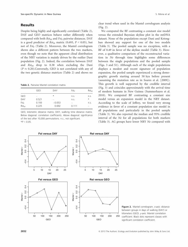
Despite being highly and significantly correlated (Table 2),
DAY and GEO matrices behave rather differently when
compared with both RstM and FstF pairwise distances. DAY
is a good predictor of RstM matrix (0.693, P < 0.05), but
not of FstF (Table 2). Moreover, the Mantel correlogram
shows also a different pattern between the two markers,
even though we note that the apparent clinal distribution
of the NRY variation is mainly driven by the outlier Dani
population (Fig. 2). Indeed, the correlation between DAY
and RstM drop to 0.38 when excluding the Dani
(P � 0.20).Conversely, GEO is not correlated with any of
the two genetic distance matrices (Table 2) and shows no
clear trend when used in the Mantel correlogram analysis
(Fig. 2).
We computed the BF contrasting a constant size model
versus the extended Bayesian skyline plot in the mtDNA
dataset. None of the populations except Dani and Keteng-
ban showed any support for one of the two models
(Table 3). The pooled sample was no exception, with a
BF of 0.49 in favor of the skyline model (Table 3). How-
ever, a qualitative comparison of the reconstructed varia-
tion in Ne through time highlights some differences
between the single populations and the pooled sample
(Figs. 3 and S1). Although each of the single populations
displays a modest and recent signature of population
expansion, the pooled sample experienced a strong demo-
graphic growth starting around 50 kya before present
(assuming the mutation rate as in Soares et al. [2009]).
This growth is well supported by the credible interval
(Fig. 3) and coincides approximately with the arrival time
of modern humans in New Guinea (Summerhayes et al.
2010). We computed BF contrasting a constant size
model versus an expansion model in the NRY dataset.
According to the scale of Jeffrey, we found very strong
evidence in favor of a constant population size model in
all populations and particularly in the pooled sample
(Table 3). We also reported the median and 95% credible
interval of the Ne for all populations for both markers
(Table 3). AG groups have lower NRY Ne compared with
Table 2. Pairwise Mantel correlation matrix.
GEO DAY FstF RstM
GEO – * n.s. n.s.
DAY 0.521 – n.s. *
FstF 0.193 �0.053 – n.s.
RstM 0.225 0.692 0.111 –
GEO, kilometric distance matrix; DAY, walking time distance matrix.
Below diagonal: correlation coefficients. Above diagonal: significance
of the test after 10,000 permutations. n.s., not significant.
*P < 0.05.
5 10 15 20 25
−0.
40.
00.
20.
4
Fst versus DAY
DAY
Man
tel r
5 10 15 20 25
−0.
40.
00.
20.
4
Rst versus DAY
DAY
Man
tel r
50 100 150 200 250
−0.
40.
00.
20.
4
Fst versus GEO
GEO
Man
tel r
50 100 150 200 250
−0.
40.
00.
20.
4
Rst versus GEO
GEO
Man
tel r
Figure 2. Mantel correlogram. x-axis: distance
between groups in days of walking (DAY) or
kilometers (GEO). y-axis: Mantel correlation
coefficient. Black dots represent classes with
significant correlation coefficient.
2652 ª 2013 The Authors. Ecology and Evolution published by John Wiley & Sons Ltd.
Sex-specific Dynamic in New Guinea S. Mona et al.
HG groups, while there is no trend in the mtDNA data
(Table 3).
We computed the BF in the resampled dataset and
present the results in Table 4. At all sampling intensities,
there are approximately the same number of dataset sup-
porting a constant or Bayesian skyline model in mtDNA.
Accordingly, the mean BF shows no correlation with the
number of lineages sampled per population and in any
case supports one of the demographic models tested
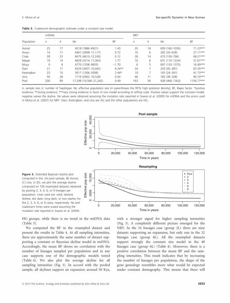
(Table 4). We also plot the average skyline for all
sampling intensities (Fig. 3). In accord with the pooled
sample, all skylines support an expansion around 50 Kya,
with a stronger signal for higher sampling intensities
(Fig. 3). A completely different picture emerged for the
NRY. In the 16 lineages case (group 2L) there are nine
datasets supporting an expansion, but only one in the 32
lineages case (group 4L). All the resampled datasets
support strongly the constant size model in the 48
lineages case (group 6L) (Table 4). Moreover, there is a
positive correlation between the mean BF and the sam-
pling intensities. This result indicates that by increasing
the number of lineages per population, the shape of the
gene genealogy resembles more what would be expected
under constant demography. This means that there will
Table 3. Coalescent demographic estimate under a constant size model.
Population
mtDNA NRY
n k Ne BF n k Ne BF
Asmat 25 17 4218 (1886–6921) 1.43 20 14 609 (160–1050) 71.23***
Awyu 14 11 6461 (2608–11,117) 0.72 10 6 282 (33–628) 27.11***
Citak 39 23 8475 (4610–12,240) 0.12 28 14 473 (130–796) 68.21***
Mappi 19 14 6628 (3214–11,063) 1.77 10 6 631 (114–1224) 51.61***
Muyu 9 8 4770 (1358–9655) �1.70 6 5 697 (133–1375) 16.49***
Dani 21 17 6529 (3057–10,442) 6.24** 24 7 203 (45–387) 65.35***
Ketengban 23 10 3017 (1306–5098) 2.44* 19 7 165 (24–341) 41.73***
Una 50 28 7119 (4362–10,528) 0.04 46 11 182 (38–328) 90.10***
Pool 200 89 17,298 (10,566–21,242) 0.49 163 56 928 (468–1302) 1156.77***
n, sample size; k, number of haplotype; Ne, effective population size (in parentheses the 95% high posterior density); BF, Bayes factor. *positive
evidence; **strong evidence; ***very strong evidence in favor of one model according to Jeffrey scale. Positive values support the constant model,
negative values the skyline. Ne values were obtained assuming the mutation rate reported in Soares et al. (2009) for mtDNA and the priors used
in Mona et al. (2007) for NRY. Dani, Ketengban, and Una are AG and the other populations are HG.
0 20,000 40,000 60,000 80,000 100,000 120,000
020
,000
40,0
00
Pool sample
Time in years
Effe
ctiv
e po
p si
ze
0 20,000 40,000 60,000 80,000 100,000 120,000
050
0015
,000
Resampling
Time in years
Effe
ctiv
e po
p si
ze Pool23469
Figure 3. Extended Bayesian skyline plot
computed in the: (A) pool sample; (B) Asmat;
(C) Una. In (D), we plot the average skyline
computed on 100 resampled datasets obtained
by pooling 2, 3, 4, 6, or 9 lineages per
population. Lines used are: solid, dashed,
dotted, dot dash, long dash, or two dashes for
the 2, 3, 4, 6, or 9 cases, respectively. Ne and
coalescent times were scaled assuming the
mutation rate reported in Soares et al. (2009).
ª 2013 The Authors. Ecology and Evolution published by John Wiley & Sons Ltd. 2653
S. Mona et al. Sex-specific Dynamic in New Guinea
be more coalescence during the scattering phase, which is
what we expect for small Nm value. The difference in the
shape of the gene genealogy between mtDNA and NRY is
therefore consistent with an NmM much smaller than
NmF.
We computed an RstM of 0.488 (P < 0.001) and an FstFof 0.116 (P < 0.001) among the sampled populations.
The RstM/FstF ratio is 4.2 which correspond approxi-
mately to an NmF/NmM ratio of 7.26 assuming the
Wright (1931) island model. We tested more realistic and
complex demographic scenarios by means of spatial expli-
cit simulations. We aimed to determine under each evo-
lutionary scenarios which values of NmF and NmM could
reproduce an RstM/FstF ratio around 4.2. Contour plots
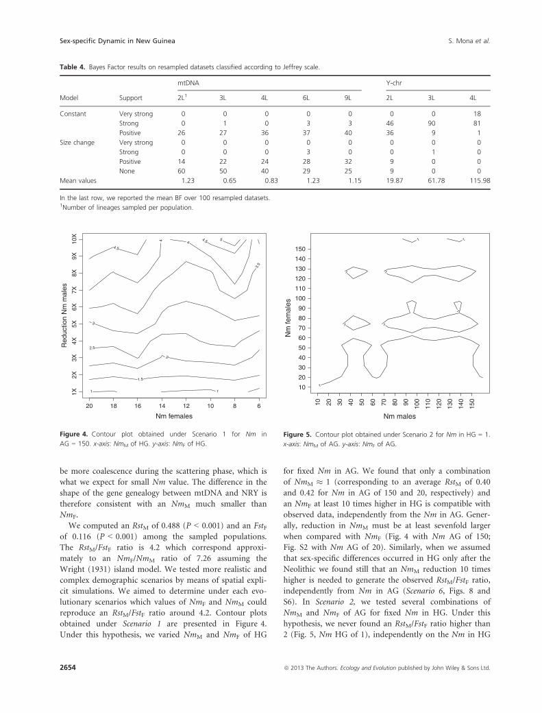
obtained under Scenario 1 are presented in Figure 4.
Under this hypothesis, we varied NmM and NmF of HG
for fixed Nm in AG. We found that only a combination
of NmM � 1 (corresponding to an average RstM of 0.40
and 0.42 for Nm in AG of 150 and 20, respectively) and
an NmF at least 10 times higher in HG is compatible with
observed data, independently from the Nm in AG. Gener-
ally, reduction in NmM must be at least sevenfold larger
when compared with NmF (Fig. 4 with Nm AG of 150;
Fig. S2 with Nm AG of 20). Similarly, when we assumed
that sex-specific differences occurred in HG only after the
Neolithic we found still that an NmM reduction 10 times
higher is needed to generate the observed RstM/FstF ratio,
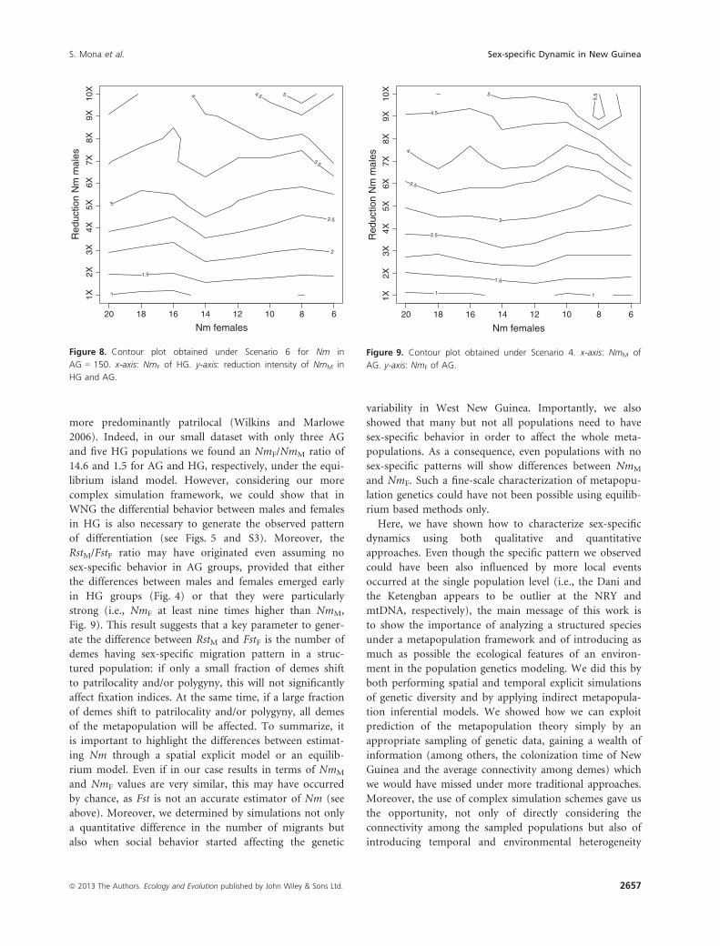
independently from Nm in AG (Scenario 6, Figs. 8 and
S6). In Scenario 2, we tested several combinations of
NmM and NmF of AG for fixed Nm in HG. Under this
hypothesis, we never found an RstM/FstF ratio higher than
2 (Fig. 5, Nm HG of 1), independently on the Nm in HG
Table 4. Bayes Factor results on resampled datasets classified according to Jeffrey scale.
Model Support
mtDNA Y-chr
2L1 3L 4L 6L 9L 2L 3L 4L
Constant Very strong 0 0 0 0 0 0 0 18
Strong 0 1 0 3 3 46 90 81
Positive 26 27 36 37 40 36 9 1
Size change Very strong 0 0 0 0 0 0 0 0
Strong 0 0 0 3 0 0 1 0
Positive 14 22 24 28 32 9 0 0
None 60 50 40 29 25 9 0 0
Mean values 1.23 0.65 0.83 1.23 1.15 19.87 61.78 115.98
In the last row, we reported the mean BF over 100 resampled datasets.1Number of lineages sampled per population.
Nm females
Red
uctio
n N
m m
ales
1 1
1.5
2
2.5
3
3.5
4
4 4.5
4.5 5
1X2X
3X4X
5X6X
7X8X
9X10
X
20 18 16 14 12 10 8 6
Figure 4. Contour plot obtained under Scenario 1 for Nm in
AG = 150. x-axis: NmM of HG. y-axis: NmF of HG.
Nm males
Nm
fem
ales
1
1
1
1
1
1 1
1
10
20
30
40
50
60
70
80
90
100
110
120
130
140
150
10 20 30 40 50 60 70 80 90 100
110
120
130
140
150
Figure 5. Contour plot obtained under Scenario 2 for Nm in HG = 1.
x-axis: NmM of AG. y-axis: NmF of AG.
2654 ª 2013 The Authors. Ecology and Evolution published by John Wiley & Sons Ltd.
Sex-specific Dynamic in New Guinea S. Mona et al.
(Fig. S3, Nm HG of 20). This result suggests that different
behavior between males and females in West New Guinea
are not (only) related to the emergence of agriculture as
they must be present in HG as well in order to obtain
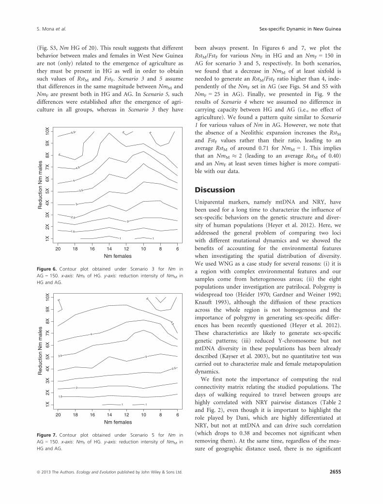
such values of RstM and FstF. Scenario 3 and 5 assume
that differences in the same magnitude between NmM and
NmF are present both in HG and AG. In Scenario 5, such
differences were established after the emergence of agri-
culture in all groups, whereas in Scenario 3 they have
been always present. In Figures 6 and 7, we plot the
RstM/FstF for various NmF in HG and an NmF = 150 in
AG for scenario 3 and 5, respectively. In both scenarios,
we found that a decrease in NmM of at least sixfold is
needed to generate an RstM/FstF ratio higher than 4, inde-
pendently of the NmF set in AG (see Figs. S4 and S5 with
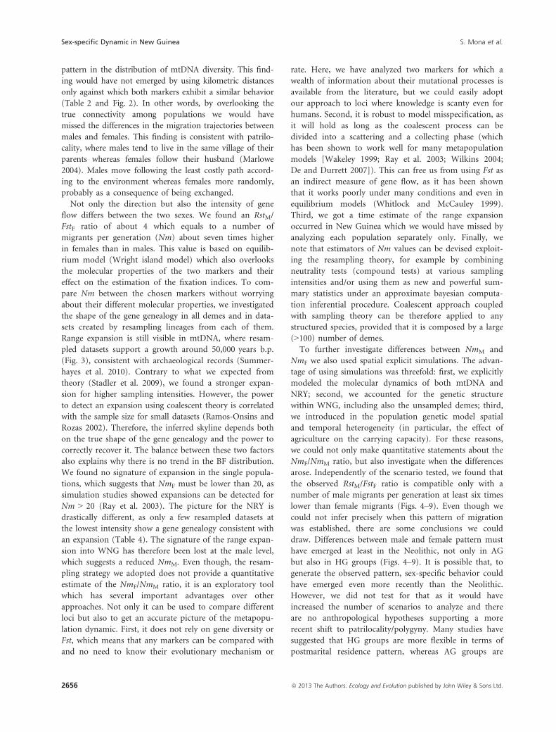
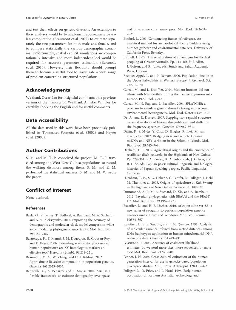
NmF = 25 in AG). Finally, we presented in Fig. 9 the
results of Scenario 4 where we assumed no difference in
carrying capacity between HG and AG (i.e., no effect of
agriculture). We found a pattern quite similar to Scenario
1 for various values of Nm in AG. However, we note that
the absence of a Neolithic expansion increases the RstMand FstF values rather than their ratio, leading to an
average RstM of around 0.71 for NmM = 1. This implies
that an NmM � 2 (leading to an average RstM of 0.40)
and an NmF at least seven times higher is more compati-
ble with our data.
Discussion
Uniparental markers, namely mtDNA and NRY, have
been used for a long time to characterize the influence of
sex-specific behaviors on the genetic structure and diver-
sity of human populations (Heyer et al. 2012). Here, we
addressed the general problem of comparing two loci
with different mutational dynamics and we showed the
benefits of accounting for the environmental features
when investigating the spatial distribution of diversity.
We used WNG as a case study for several reasons: (i) it is
a region with complex environmental features and our
samples come from heterogeneous areas; (ii) the eight
populations under investigation are patrilocal. Polygyny is
widespread too (Heider 1970; Gardner and Weiner 1992;
Knauft 1993), although the diffusion of these practices
across the whole region is not homogenous and the
importance of polygyny in generating sex-specific differ-
ences has been recently questioned (Heyer et al. 2012).
These characteristics are likely to generate sex-specific
genetic patterns; (iii) reduced Y-chromosome but not
mtDNA diversity in these populations has been already
described (Kayser et al. 2003), but no quantitative test was
carried out to characterize male and female metapopulation
dynamics.
We first note the importance of computing the real
connectivity matrix relating the studied populations. The
days of walking required to travel between groups are
highly correlated with NRY pairwise distances (Table 2
and Fig. 2), even though it is important to highlight the
role played by Dani, which are highly differentiated at
NRY, but not at mtDNA and can drive such correlation
(which drops to 0.38 and becomes not significant when
removing them). At the same time, regardless of the mea-
sure of geographic distance used, there is no significant
Nm females
Red
uctio
n N
m m
ales
1 1
1.5
2
2.5
3
3.5
4
4.5
5
5
5 5.5
1X2X
3X4X
5X6X
7X8X
9X10
X
20 18 16 14 12 10 8 6
Figure 6. Contour plot obtained under Scenario 3 for Nm in
AG = 150. x-axis: NmF of HG. y-axis: reduction intensity of NmM in
HG and AG.
Nm females
Red
uctio
n N
m m
ales
1 1
1.5
2
2.5
3 3.5
4
4.5
5
5
1X2X
3X4X
5X6X
7X8X
9X10
X
20 18 16 14 12 10 8 6
Figure 7. Contour plot obtained under Scenario 5 for Nm in
AG = 150. x-axis: NmF of HG. y-axis: reduction intensity of NmM in
HG and AG.
ª 2013 The Authors. Ecology and Evolution published by John Wiley & Sons Ltd. 2655
S. Mona et al. Sex-specific Dynamic in New Guinea
pattern in the distribution of mtDNA diversity. This find-
ing would have not emerged by using kilometric distances
only against which both markers exhibit a similar behavior
(Table 2 and Fig. 2). In other words, by overlooking the
true connectivity among populations we would have
missed the differences in the migration trajectories between
males and females. This finding is consistent with patrilo-
cality, where males tend to live in the same village of their
parents whereas females follow their husband (Marlowe
2004). Males move following the least costly path accord-
ing to the environment whereas females more randomly,
probably as a consequence of being exchanged.
Not only the direction but also the intensity of gene
flow differs between the two sexes. We found an RstM/
FstF ratio of about 4 which equals to a number of
migrants per generation (Nm) about seven times higher
in females than in males. This value is based on equilib-
rium model (Wright island model) which also overlooks
the molecular properties of the two markers and their
effect on the estimation of the fixation indices. To com-
pare Nm between the chosen markers without worrying
about their different molecular properties, we investigated
the shape of the gene genealogy in all demes and in data-
sets created by resampling lineages from each of them.
Range expansion is still visible in mtDNA, where resam-
pled datasets support a growth around 50,000 years b.p.
(Fig. 3), consistent with archaeological records (Summer-
hayes et al. 2010). Contrary to what we expected from
theory (Stadler et al. 2009), we found a stronger expan-
sion for higher sampling intensities. However, the power
to detect an expansion using coalescent theory is correlated
with the sample size for small datasets (Ramos-Onsins and
Rozas 2002). Therefore, the inferred skyline depends both
on the true shape of the gene genealogy and the power to
correctly recover it. The balance between these two factors
also explains why there is no trend in the BF distribution.
We found no signature of expansion in the single popula-
tions, which suggests that NmF must be lower than 20, as
simulation studies showed expansions can be detected for
Nm > 20 (Ray et al. 2003). The picture for the NRY is
drastically different, as only a few resampled datasets at
the lowest intensity show a gene genealogy consistent with
an expansion (Table 4). The signature of the range expan-
sion into WNG has therefore been lost at the male level,
which suggests a reduced NmM. Even though, the resam-
pling strategy we adopted does not provide a quantitative
estimate of the NmF/NmM ratio, it is an exploratory tool
which has several important advantages over other
approaches. Not only it can be used to compare different
loci but also to get an accurate picture of the metapopu-
lation dynamic. First, it does not rely on gene diversity or
Fst, which means that any markers can be compared with
and no need to know their evolutionary mechanism or
rate. Here, we have analyzed two markers for which a
wealth of information about their mutational processes is
available from the literature, but we could easily adopt
our approach to loci where knowledge is scanty even for
humans. Second, it is robust to model misspecification, as
it will hold as long as the coalescent process can be
divided into a scattering and a collecting phase (which
has been shown to work well for many metapopulation
models [Wakeley 1999; Ray et al. 2003; Wilkins 2004;
De and Durrett 2007]). This can free us from using Fst as
an indirect measure of gene flow, as it has been shown
that it works poorly under many conditions and even in
equilibrium models (Whitlock and McCauley 1999).
Third, we got a time estimate of the range expansion
occurred in New Guinea which we would have missed by
analyzing each population separately only. Finally, we
note that estimators of Nm values can be devised exploit-
ing the resampling theory, for example by combining
neutrality tests (compound tests) at various sampling
intensities and/or using them as new and powerful sum-
mary statistics under an approximate bayesian computa-
tion inferential procedure. Coalescent approach coupled
with sampling theory can be therefore applied to any
structured species, provided that it is composed by a large
(>100) number of demes.
To further investigate differences between NmM and
NmF we also used spatial explicit simulations. The advan-
tage of using simulations was threefold: first, we explicitly
modeled the molecular dynamics of both mtDNA and
NRY; second, we accounted for the genetic structure
within WNG, including also the unsampled demes; third,
we introduced in the population genetic model spatial
and temporal heterogeneity (in particular, the effect of
agriculture on the carrying capacity). For these reasons,
we could not only make quantitative statements about the
NmF/NmM ratio, but also investigate when the differences
arose. Independently of the scenario tested, we found that
the observed RstM/FstF ratio is compatible only with a
number of male migrants per generation at least six times
lower than female migrants (Figs. 4–9). Even though we
could not infer precisely when this pattern of migration
was established, there are some conclusions we could
draw. Differences between male and female pattern must
have emerged at least in the Neolithic, not only in AG
but also in HG groups (Figs. 4–9). It is possible that, to
generate the observed pattern, sex-specific behavior could
have emerged even more recently than the Neolithic.
However, we did not test for that as it would have
increased the number of scenarios to analyze and there
are no anthropological hypotheses supporting a more
recent shift to patrilocality/polygyny. Many studies have
suggested that HG groups are more flexible in terms of
postmarital residence pattern, whereas AG groups are
2656 ª 2013 The Authors. Ecology and Evolution published by John Wiley & Sons Ltd.
Sex-specific Dynamic in New Guinea S. Mona et al.
more predominantly patrilocal (Wilkins and Marlowe
2006). Indeed, in our small dataset with only three AG
and five HG populations we found an NmF/NmM ratio of
14.6 and 1.5 for AG and HG, respectively, under the equi-
librium island model. However, considering our more
complex simulation framework, we could show that in
WNG the differential behavior between males and females
in HG is also necessary to generate the observed pattern
of differentiation (see Figs. 5 and S3). Moreover, the
RstM/FstF ratio may have originated even assuming no
sex-specific behavior in AG groups, provided that either
the differences between males and females emerged early
in HG groups (Fig. 4) or that they were particularly
strong (i.e., NmF at least nine times higher than NmM,
Fig. 9). This result suggests that a key parameter to gener-
ate the difference between RstM and FstF is the number of
demes having sex-specific migration pattern in a struc-
tured population: if only a small fraction of demes shift
to patrilocality and/or polygyny, this will not significantly
affect fixation indices. At the same time, if a large fraction
of demes shift to patrilocality and/or polygyny, all demes
of the metapopulation will be affected. To summarize, it
is important to highlight the differences between estimat-
ing Nm through a spatial explicit model or an equilib-
rium model. Even if in our case results in terms of NmM
and NmF values are very similar, this may have occurred
by chance, as Fst is not an accurate estimator of Nm (see
above). Moreover, we determined by simulations not only
a quantitative difference in the number of migrants but
also when social behavior started affecting the genetic
variability in West New Guinea. Importantly, we also
showed that many but not all populations need to have
sex-specific behavior in order to affect the whole meta-
populations. As a consequence, even populations with no
sex-specific patterns will show differences between NmM
and NmF. Such a fine-scale characterization of metapopu-
lation genetics could have not been possible using equilib-
rium based methods only.
Here, we have shown how to characterize sex-specific
dynamics using both qualitative and quantitative
approaches. Even though the specific pattern we observed
could have been also influenced by more local events
occurred at the single population level (i.e., the Dani and
the Ketengban appears to be outlier at the NRY and
mtDNA, respectively), the main message of this work is
to show the importance of analyzing a structured species
under a metapopulation framework and of introducing as
much as possible the ecological features of an environ-
ment in the population genetics modeling. We did this by
both performing spatial and temporal explicit simulations
of genetic diversity and by applying indirect metapopula-
tion inferential models. We showed how we can exploit
prediction of the metapopulation theory simply by an
appropriate sampling of genetic data, gaining a wealth of
information (among others, the colonization time of New
Guinea and the average connectivity among demes) which
we would have missed under more traditional approaches.
Moreover, the use of complex simulation schemes gave us
the opportunity, not only of directly considering the
connectivity among the sampled populations but also of
introducing temporal and environmental heterogeneity
Nm females
Red
uctio
n N
m m
ales
1
1.5
2
2.5
3
3.5
4
4.5 5
1X2X
3X4X
5X6X
7X8X
9X10
X
20 18 16 14 12 10 8 6
Figure 8. Contour plot obtained under Scenario 6 for Nm in
AG = 150. x-axis: NmF of HG. y-axis: reduction intensity of NmM in
HG and AG.
Nm females
Red
uctio
n N
m m
ales
1 1
1.5
2.5
3
3.5
4
4.5
5
5.5
1X2X
3X4X
5X6X
7X8X
9X10
X
20 18 16 14 12 10 8 6
Figure 9. Contour plot obtained under Scenario 4. x-axis: NmM of
AG. y-axis: NmF of AG.
ª 2013 The Authors. Ecology and Evolution published by John Wiley & Sons Ltd. 2657
S. Mona et al. Sex-specific Dynamic in New Guinea
and test their effects on genetic diversity. An extension to
these analyses would be to implement approximate Bayes-
ian computation (Beaumont et al. 2002) to estimate sepa-
rately the two parameters for both male and female, and
to compare statistically the various demographic scenar-
ios. Unfortunately, spatial explicit simulations are compu-
tationally intensive and more independent loci would be
required for accurate parameter estimation (Bertorelle
et al. 2010). However, their flexibility should prompt
them to become a useful tool to investigate a wide range
of problem concerning structured populations.
Acknowledgments
We thank Oscar Lao for insightful comments on a previous
version of the manuscript. We thank Annabel Whibley for
carefully checking the English and for useful comments.
Data Accessibility
All the data used in this work have been previously pub-
lished in Tommaseo-Ponzetta et al. (2002) and Kayser
et al. (2003).
Author Contributions
S. M. and M. T.-P. conceived the project. M. T.-P. trav-
elled among the West New Guinea populations to record
the walking distances among them. S. M. and E. M.
performed the statistical analyses. S. M. and M. V. wrote
the paper.
Conflict of Interest
None declared.
References
Baele, G., P. Lemey, T. Bedford, A. Rambaut, M. A. Suchard,
and A. V. Alekseyenko. 2012. Improving the accuracy of
demographic and molecular clock model comparison while
accommodating phylogenetic uncertainty. Mol. Biol. Evol.
29:2157–2167.
Balaresque, P., F. Manni, J. M. Dugoujon, B. Crousau-Roy,
and E. Heyer. 2006. Estimating sex-specific processes in
human populations: are XY-homologous markers an
effective tool? Heredity (Edinb). 96:214–221.
Beaumont, M. A., W. Zhang, and D. J. Balding. 2002.
Approximate Bayesian computation in population genetics.
Genetics 162:2025–2035.
Bertorelle, G., A. Benazzo, and S. Mona. 2010. ABC as a
flexible framework to estimate demography over space
and time: some cons, many pros. Mol. Ecol. 19:2609–
2625.
Binford, L. 2001. Constructing frames of reference. An
analytical method for archaeological theory building using
hunther-gatherer and environmental data sets. University of
California Press, Berkeley.
Birdsell, J. 1977. The recalibration of a paradigm for the first
peopling of Greater Australia. Pp. 113–168 in J. Allen,
J. Golson, and R. Jones, eds. Sunda and Sahul. Academic
Press, London.
Bocquet-Appel, J., and P. Demars. 2000. Population kinetics in
the Upper Palaeolithic in Western Europe. J. Archaeol. Sci.
27:551–570.
Currat, M., and L. Excoffier. 2004. Modern humans did not
admix with Neanderthals during their range expansion into
Europe. PLoS Biol. 2:e421.
Currat, M., N. Ray, and L. Excoffier. 2004. SPLATCHE: a
program to simulate genetic diversity taking into account
environmental heterogeneity. Mol. Ecol. Notes 4:139–142.
De, A., and R. Durrett. 2007. Stepping-stone spatial structure
causes slow decay of linkage disequilibrium and shifts the
site frequency spectrum. Genetics 176:969–981.
Delfin, F., S. Myles, Y. Choi, D. Hughes, R. Illek, M. van
Oven, et al. 2012. Bridging near and remote Oceania:
mtDNA and NRY variation in the Solomon Islands. Mol.
Biol. Evol. 29:545–564.
Denham, T. P. 2005. Agricultural origins and the emergence of
rectilinear ditch networks in the Highlands of New Guinea.
Pp. 329–361 in A. Pawley, R. Attenborough, J. Golson, and
R. Hide, eds. Papuan pasts: cultural, linguistic and biological
histories of Papuan speaking peoples. Pacific Linguistics,
Canberra.
Denham, T. P., S. G. Haberle, C. Lentfer, R. Fullagar, J. Field,
M. Therin, et al. 2003. Origins of agriculture at Kuk Swamp
in the highlands of New Guinea. Science 301:189–193.
Drummond, A. J., M. A. Suchard, D. Xie, and A. Rambaut.
2012. Bayesian phylogenetics with BEAUti and the BEAST
1.7. Mol. Biol. Evol. 29:1969–1973.
Excoffier, L., and H. E. Lischer. 2010. Arlequin suite ver 3.5: a
new series of programs to perform population genetics
analyses under Linux and Windows. Mol. Ecol. Resour.
10:564–567.
Excoffier, L., P. E. Smouse, and J. M. Quattro. 1992. Analysis
of molecular variance inferred from metric distances among
DNA haplotypes: application to human mitochondrial DNA
restriction data. Genetics 131:479–491.
Felsenstein, J. 2006. Accuracy of coalescent likelihood
estimates: do we need more sites, more sequences, or more
loci? Mol. Biol. Evol. 23:691–700.
Fenner, J. N. 2005. Cross-cultural estimation of the human
generation interval for use in genetics-based population
divergence studies. Am. J. Phys. Anthropol. 128:415–423.
Fullagar, R., D. Price, and L. Head. 1996. Early human
occupation of northern Australia: archaeology and
2658 ª 2013 The Authors. Ecology and Evolution published by John Wiley & Sons Ltd.
Sex-specific Dynamic in New Guinea S. Mona et al.
thermoluminescence dating of Jinmium rock-shelter,
Northern Territory. Antiquity 70:751–773.
Fuselli, S., E. Tarazona-Santos, I. Dupanloup, A. Soto,
D. Luiselli, and D. Pettener. 2003. Mitochondrial DNA
diversity in South America and the genetic history of
Andean highlanders. Mol. Biol. Evol. 20:1682–1691.
Gardner, D., and J. Weiner. 1992. Social anthropology in
Papua New Guinea. Pp. 119–135 in R. Attenborough and
M. Alpers, eds. Human biology in Papua New Guinea: the
small cosmos. Clarendon Press, Oxford.
Golson, J. 1990. Kuk and the development of agriculture in
New Guinea retrospection and introspection. Pp. 139–147 in
D. Yen and J. Mummery, eds. Pacific production systems:
approaches to economic prehistory. Australian National
University, Canberra.
Gunnarsdottir, E. D., M. R. Nandineni, M. Li, S. Myles,
D. Gil, B. Pakendorf, et al. 2012. Larger mitochondrial DNA
than Y-chromosome differences between matrilocal and
patrilocal groups from Sumatra. Nat. Commun. 2:228.
Hedrick, P. W. 2005. A standardized genetic differentiation
measure. Evolution 59:1633–1638.
Heider, K. 1970. The Dugum Dani: a Papuan Culture in the
Highlands of West New Guinea. Aldine Publishing, Chicago,
IL.
Heled, J., and A. J. Drummond. 2008. Bayesian inference of
population size history from multiple loci. BMC Evol. Biol.
8:289.
Heyer, E., R. Chaix, S. Pavard, and F. Austerlitz. 2012.
Sex-specific demographic behaviours that shape human
genomic variation. Mol. Ecol. 21:597–612.
Hudjashov, G., T. Kivisild, P. A. Underhill, P. Endicott,
J. J. Sanchez, A. A. Lin, et al. 2007. Revealing the prehistoric
settlement of Australia by Y chromosome and mtDNA
analysis. Proc. Natl Acad. Sci. USA 104:8726–8730.
Hudson, R. 1990. Gene genealogies and the coalescent process.
Pp. 1–44 in D. Futuyma and J. Antonovics, eds. Oxford surveys
in evolutionary biology. Oxford University Press, New York.
Kass, R., and A. Raftery. 1995. Bayes Factors. J. Am. Stat.
Assoc. 90:773–795.
Kayser, M., S. Brauer, G. Weiss, W. Schiefenhovel,
P. Underhill, P. Shen, et al. 2003. Reduced Y-chromosome,
but not mitochondrial DNA, diversity in human populations
from West New Guinea. Am. J. Hum. Genet. 72:281–302.
Kemp, B. M., A. Gonzalez-Oliver, R. S. Malhi, C. Monroe,
K. B. Schroeder, J. McDonough, et al. 2012. Evaluating the
Farming/Language Dispersal Hypothesis with genetic
variation exhibited by populations in the Southwest and
Mesoamerica. Proc. Natl Acad. Sci. USA 107:6759–6764.
Knauft, B. 1993. South Coast New Guinea Cultures. History,
comparison, dialectic. Cambridge University Press,
Cambridge.
Legendre, P., and M. Fortin. 1989. Spatial pattern and
ecological analysis. Vegetatio 80:107–138.
Marlowe, F. W. 2004. Marital residence among foragers. Curr.
Anthropol. 45:277–284.
McRae, B. H., and P. Beier. 2007. Circuit theory predicts gene
flow in plant and animal populations. Proc. Natl Acad. Sci.
USA 104:19885–19890.
Meirmans, P. G. 2006. Using the AMOVA framework to
estimate a standardized genetic differentiation measure.
Evolution 60:2399–2402.
Metzker, M. L. 2010. Sequencing technologies – the next
generation. Nat. Rev. Genet. 11:31–46.
Mona, S., M. Tommaseo-Ponzetta, S. Brauer, H. Sudoyo,
S. Marzuki, and M. Kayser. 2007. Patterns of Y-chromosome
diversity intersect with the Trans-New Guinea hypothesis.
Mol. Biol. Evol. 24:2546–2555.
Nasidze, I., E. Y. Ling, D. Quinque, I. Dupanloup, R. Cordaux,
S. Rychkov, et al. 2004. Mitochondrial DNA and
Y-chromosome variation in the caucasus. Ann. Hum. Genet.
68:205–221.
O’Connell, J., and J. Allen. 1998. When did humans first arrive
in Greater Australia and why is it important to know? Evol.
Anthropol. 6:132–146.
Oota, H., W. Settheetham-Ishida, D. Tiwawech, T. Ishida, and
M. Stoneking. 2001. Human mtDNA and Y-chromosome
variation is correlated with matrilocal versus patrilocal
residence. Nat. Genet. 29:20–21.
R Development Core Team. 2011. R: a language and
environment for statistical computing. R Foundation for
Statistical Computing, Vienna, Austria. ISBN 3-900051-07-0.
Avalable at http://www.R-project.org/.
Ramos-Onsins, S. E., and J. Rozas. 2002. Statistical properties
of new neutrality tests against population growth. Mol. Biol.
Evol. 19:2092–2100.
Ray, N., M. Currat, and L. Excoffier. 2003. Intra-deme
molecular diversity in spatially expanding populations. Mol.
Biol. Evol. 20:76–86.
Roberts, R., R. Jones, and M. Smith. 1990.
Thermoluminescence dating of a 50,000-year-old human
occupation site in northern Australia. Nature 345:153–156.
Segurel, L., B. Martinez-Cruz, L. Quintana-Murci, P. Balaresque,
M. Georges, T. Hegay, et al. 2008. Sex-specific genetic structure
and social organization in Central Asia: insights from a
multi-locus study. PLoS Genet. 4:e1000200.
Seielstad, M. T., E. Minch, and L. L. Cavalli-Sforza. 1998.
Genetic evidence for a higher female migration rate in
humans. Nat. Genet. 20:278–280.
Slatkin, M. 1995. A measure of population subdivision based
on microsatellite allele frequencies. Genetics 139:457–462.
Soares, P., L. Ermini, N. Thomson, M. Mormina, T. Rito,
A. Rohl, et al. 2009. Correcting for purifying selection: an
improved human mitochondrial molecular clock. Am. J.
Hum. Genet. 84:740–759.
Stadler, T., B. Haubold, C. Merino, W. Stephan, and P.
Pfaffelhuber. 2009. The impact of sampling schemes on the
ª 2013 The Authors. Ecology and Evolution published by John Wiley & Sons Ltd. 2659
S. Mona et al. Sex-specific Dynamic in New Guinea

site frequency spectrum in nonequilibrium subdivided
populations. Genetics 182:205–216.
Steele, J., J. Adams, and T. Sluckin. 1998. Modelling
Paleoindian dispersals. World Archaeol. 30:286–305.
Summerhayes, G. R., M. Leavesley, A. Fairbairn, H. Mandui,
J. Field, A. Ford, et al. 2010. Human adaptation and plant
use in highland New Guinea 49,000 to 44,000 years ago.
Science 330:78–81.
Thorne, A., R. Grun, G. Mortimer, N. A. Spooner,
J. J. Simpson, M. McCulloch, et al. 1999. Australia’s oldest
human remains: age of the Lake Mungo 3 skeleton.
J. Hum. Evol. 36:591–612.
Tommaseo-Ponzetta, M., M. Attimonelli, M. De Robertis, F.
Tanzariello, and C. Saccone. 2002. Mitochondrial DNA
variability of West New Guinea populations. Am. J. Phys.
Anthropol. 117:49–67.
Wakeley, J. 1998. Segregating sites in Wright’s island model.
Theor. Popul. Biol. 53:166–174.
Wakeley, J. 1999. Nonequilibrium migration in human history.
Genetics 153:1863–1871.
Wakeley, J. 2001. The coalescent in an island model of
population subdivision with variation among demes. Theor.
Popul. Biol. 59:133–144.
Wakeley, J. 2004. Metapopulation models for historical
inference. Mol. Ecol. 13:865–875.
Wakeley, J. 2008. Coalescent Theory: an Introduction. Roberts
& Company, Greenwood Village, Colorado.
Wakeley, J., and S. Lessard. 2003. Theory of the effects of
population structure and sampling on patterns of linkage
disequilibrium applied to genomic data from humans.
Genetics 164:1043–1053.
Whitlock, M. C., and D. E. McCauley. 1999. Indirect measures
of gene flow and migration: FST not equal to 1/(4Nm + 1).
Heredity 82(Pt 2):117–125.
Wilder, J. A., S. B. Kingan, Z. Mobasher, M. M. Pilkington,
and M. F. Hammer. 2004. Global patterns of human
mitochondrial DNA and Y-chromosome structure are not
influenced by higher migration rates of females versus
males. Nat. Genet. 36:1122–1125.
Wilkins, J. F. 2004. A separation-of-timescales approach to the
coalescent in a continuous population. Genetics 168:
2227–2244.
Wilkins, J. F., and F. W. Marlowe. 2006. Sex-biased migration
in humans: what should we expect from genetic data?
BioEssays 28:290–300.
Wilson, I. J., M. Weale, and D. J. Balding. 2003. Inferences
from DNA data: population histories, evolutionary processes
and forensic match probabilities. J. R. Stat. Soc. Ser. A
166:155–188.
Wood, E. T., D. A. Stover, C. Ehret, G. Destro-Bisol,
G. Spedini, H. McLeod, et al. 2005. Contrasting patterns of
Y chromosome and mtDNA variation in Africa: evidence for
sex-biased demographic processes. Eur. J. Hum. Genet.
13:867–876.
Wright, S. 1931. Evolution in Mendelian Populations. Genetics
16:97–159.
Supporting Information
Additional Supporting Information may be found in the
online version of this article:
Figure S1. Extended Bayesian skyline plot computed in
the each population. Ne and coalescent times were scaled
assuming the mutation rate reported in Soares et al.
(2009).
Figure S2. Contour plot obtained under Scenario 1 for
Nm in AG = 20. x-axis: NmM of HG. y-axis: NmF of HG.
Figure S3. Contour plot obtained under Scenario 2 for
Nm in HG = 20. x-axis: NmM of AG. y-axis: NmF of AG.
Figure S4. Contour plot obtained under Scenario 3 for
Nm in AG = 25. x-axis: NmF of HG. y-axis: reduction
intensity of NmM in HG and AG.
Figure S5. Contour plot obtained under Scenario 5 for
Nm in AG = 25. x-axis: NmF of HG. y-axis: reduction
intensity of NmM in HG and AG.
Figure S6. Contour plot obtained under Scenario 6 for
Nm in AG = 25. x-axis: NmF of HG. y-axis: reduction
intensity of NmM in HG and AG.
2660 ª 2013 The Authors. Ecology and Evolution published by John Wiley & Sons Ltd.
Sex-specific Dynamic in New Guinea S. Mona et al.
Copyright © 2022 FDOKUMEN

