


Bahasa
Halaman
Hukum


1
Optimal hedge ratio with moving least squares – an empirical study using
Indian single stock futures data
Sukanto Bhattacharya1
Harminder Singh2
Renato M. Alas3
Abstract
________________________________________________________________
The use of commodity, currency and stock index futures to hedge risky exposures in the underlying
assets is well documented in financial literature. However single stock futures are a relatively new
addition to the family of futures and as such, academic research on its use as a hedging tool is
relatively thin. In this study we have explored the efficacy of two different methodological approaches
that may be applied when hedging a long position in the underlying stock with a single stock future.
We use daily trading data covering years 2002 to 2007 from the Indian market, where single stock
futures have been really thriving in terms of volume of trade, to extract the optimal hedge ratios using
both static OLS as well as 30-day, 60-day and 90-day moving least squares. The method of moving
least squares has been in use by market practitioners for some time primarily as a trend analysis and
charting tool. Our results indicate that the moving least squares approach outperforms the static OLS
in terms of the hedging efficiency, which has been measured by the root mean square hedging error.
________________________________________________________________
JEL classification: C40, G11, G13
Keywords: Single stock futures, optimal hedge ratio, moving least squares
Corresponding author
1 Deakin Graduate School of Business, Deakin University, Burwood 3125, Australia, [email protected]
2 School of Accounting, Economics and Finance, Deakin University, Burwood 3125, Australia
3 School of Business, Bond University, Australia

2
1. Introduction
Silber (1985) had concluded that the futures markets perform the main functions of risk transfer and
price discovery. However, futures markets not only provide an important vehicle for price discovery
but they also offer an alternative way to take equity positions. Furthermore, the use of commodity,
currency and index futures to hedge risky exposures in the underlying assets is well documented in
financial literature. However single stock futures are a relatively new addition to the family of futures
and as such, research on its use as a hedging tool is relatively thin. Our objective here is to explore the
efficacy of two different methodological approaches that may be applied when hedging a long
position in the underlying stock with a single stock future. While the time to delivery of a futures
contract affects the volume of trading and possibly also the price (Sun, 2003), it is however not a
relevant factor in our study as we used data from the Indian single stock futures market, where single
stock futures contracts are cash-settled and hence do not end in delivery on expiry of the contract.
India has the oldest stock market amongst the developing markets - Bombay Stock Exchange (BSE),
which was established in 1875. There are two major stock exchanges in India - BSE and NSE
(National Stock Exchange of India), the latter being recognised as a stock exchange in April, 1993.
Especially, BSE is the world’s largest in terms of the number of listed companies (BSE, 20094). India
is one of the strongest emerging economies in terms of a market for exchange-traded derivatives with
wholesome characteristics like nationwide access, anonymous electronic trading, and a developed
retail market. India’s tryst with equity derivatives began in the year 2000 on both the NSE and the
BSE. Trading first commenced in Index futures contracts, followed by index options in June 2001,
options in individual stocks in July 2001 and futures on single stocks in November 2001. Since then,
4 http://www.bseindia.com/about/introbse.asp, retrieved October 18, 2009.
3
derivatives in India have come a long way - NSE derivatives turnover increasing from Rs. 23,654
million (US$ 207 million) in 2000-01 to Rs. 110,104,821 million (US$2,161 billion)5 in 2008-09.
In particular, India is among the few countries where trading in single stock futures has shown a
tremendous upward trend. Single stock futures on NSE are traded in monthly series; the expiration
date for each series being the last Thursday of the month. At any point in time, three monthly series
(current month expiry, two month and three month expiry) are traded side by side. These contracts are
spot settled and can be exercised either at expiration or before expiration. The stock selection criteria
for derivatives trading in India ensure that stock is large in terms of market capitalization and has
sufficient liquidity in the underlying market and there are no adverse issues related to market
manipulation. Like elsewhere in the world, the major factors that have been driving the growth of
financial derivatives in India are increased volatility in asset prices in the financial markets, increased
integration of national financial markets with international markets; and the development of more
sophisticated risk management tools that provide economic agents with a much wider choice of risk
management strategies that can be tailored to fit the “budget” for risk control. The single stock futures
provide a unique set up that may help in the dissemination of information in both spot as well as
futures contracts in the context of the Indian market. The introduction of single stock futures reduces,
if not eliminates, any short-selling constraints that were faced by traders wanting to short the
underlying stock. Entering into a short position in single stock futures is as convenient as acquiring a
long position. Another advantage is that it affords investors greater leverage because futures contracts
require less capital upfront. Also, they may be used as a hedging tool in lieu of a protective put option.
In terms of number of single stock futures contracts traded in 2007 and 2008, NSE held the second
position worldwide during both these years. The rankings shown in Fig. 1 as follows are drawn from
World Federation of Exchanges (WFE) Annual Report and Statistics 2008.
Fig. 1: 2008 WFE rankings of largest volume of single stock futures trades
5 http://www.nse-india.com/content/us/ismr2009ch7.pdf, retrieved October 18, 2009.

4
2. Brief review of relevant literature
Johnson (1960) observed that hedgers preferred to hedge risky exposure in an underlying asset via the
futures market because of the convenience of cash settlement rather than having to take actual
delivery. He offered the first modern academic research on application of futures as a hedging tool.
Johnson’s methodological approach was further extended and refined by subsequent works of Stein
(1961), Ederington (1979), Franckle (1980), Dale (1981) and Herbst, Kare and Marshall (1993).
Nageswara Rao and Thakur (2008) empirically investigated the Indian derivatives market via a study
of hedging efficiency and calculation of optimal hedge ratio using alternative computational schemes.
However the above-mentioned works were based on commodity, currency or stock index futures and
not single stock futures. McKenzie, Brailsford and Faff (2001) studied the impact of introduction of
stock futures trading on stock price volatility. Lascelles (2002) noted the multiple benefits of single
stock futures as an exchange-traded derivative. Dutt and Wein (2003) commented on the adequacy of
margining requirements of single stock futures. Hung, Lee and So (2003) studied the impact of
foreign-listed single stock futures on the domestic underlying stock markets. McKenzie and Brooks
(2003) analyzed the single stock futures market of Hong Kong. Their empirical analysis of
information flows proxied by spot market volume and stock futures volume provided evidence that
suggests that it is not the arrival of news to the market which motivates derivatives trading. However
it was Brooks, Davies and Kim (2007) who directly addressed methodological issues related to

5
hedging with single stock futures. In particular, they proposed a methodology for hedging exposure to
an individual stock that does not have an exchange-traded single stock futures contract available on it.
While our work is motivated to a degree by the work of Brooks, Davies and Kim (2007), our research
question is different - we have sought to address the issue of hedging a long position in an underlying
stock with an exchange-traded single stock future in the Indian market using two alternative
approaches; one being akin to that originally posited by Johnson using a static linear regression and
another one which we have proposed; using the methodological tool of moving least squares. Our
results indicate that the moving least squares approach performs favourably against static OLS
regression in terms of the hedging efficiency (minimum root mean square error) in the test data set.
3. Data and methodology
The methodologies developed in previous literature for estimation of the optimal hedge ratio can be
categorized under one of the following groups of models: (a) Ordinary Least Squares (OLS) (b) Error
Correction (ECM) and (c) Autoregressive Conditional Heteroskedasticity (ARCH). Although very
simple to use in a practical sense, the OLS has been criticised for not taking into account important
statistical considerations like serial correlation, heteroskedasticity and cointegration (Hatemi-J and
Roca, 2006). However, Holmes (1995) had found that the OLS hedge ratio estimated ex-ante
outperformed naive hedge ratios. Lien et al (2002) observed that the OLS hedge ratio performed
better than a GARCH-based hedge ratio in currency, commodity and index futures markets. In a more
recent evidence of the efficacy of the OLS method, Bystrom (2003) reported that OLS marginally
outperformed more complex hedge ratio estimation models in Norwegian electricity futures market.
We have chosen to use the least squares hedge ratio because it is quite intuitive and relatively simple
to implement by market practitioners in a real-world hedging problem involving single stock futures.
The data for our study consists of end of day stock prices and the corresponding settlement prices on
the single stock futures between 1st January 2002 and 23
rd November 2007, for daily trading on 15

6
blue chip stocks listed on NSE that also have single stock futures contracts available on them. (For
one stock, due to data availability issues, the period is between 1st January 2002 and 23
rd July 2007).
The stocks are spread over a number of sectors ranging from manufacturing to finance & banking.
Last 30 days of data is used as the “test set” to compare the performance of the different approaches.
We have first of all fitted a best-fitting straight line to the data applying the ordinary least squares
method and used the slope of that line as an estimate of the optimal hedge ratio in accordance with
previous literature. Thereafter we have obtained 30-day, 60-day and 90-day moving least squares
estimates of the hedge ratio with the same data set and have compared their hedging performances.
With the static OLS approach, the objective is to minimize the sum of squared hedging errors for a
hedged position involving a long position in the underlying stock and a short position in the
corresponding single stock futures. The objective function to be minimized is obtained as follows:
e = (ΔS – γΔF) 2
... (i)
Here in our case, e is the hedging error, ΔS is the change in daily price of the underlying stock, ΔF is
the change in daily price of the corresponding single stock futures and γ is the applicable hedge ratio.
By the necessary first-order condition of minimization therefore:
γ’(e) = (2γΔF2 – 2ΔSΔF) = 0 ... (ii)
Solving (ii) for γ yields:
γ* = (2ΔSΔF)/(2ΔF2) = ΔS/ΔF ... (iii)

7
It is readily construed that γ* may be interpreted as the slope of the OLS regression of S on F.
Although not subjected to a great deal of academic research, the methodology of moving least squares
has been in use by market practitioners for some time primarily as a trend analysis and charting tool.
Although similar to a moving average trend, the moving linear regression is much more responsive to
changes in the end-of-day prices and as such, can be used as a simple way of addressing the time-
varying characteristic of the hedge ratio that is not adequately addressed using static OLS regression.
Like fitting a moving average trend, fitting a moving linear regression involves application of the least
squares methodology over the sample period using a “sliding scale” whereby with each passing day of
trade, the sample period is updated with the price movement data becoming available at the end of
that day while the earliest piece of data is dropped to retain the absolute size of the sample period. The
slope of the best-fitting least squares trend line is re-calculated at the end of each day to obtain a new
hedge ratio (in case of daily management of the hedged position). However in practice, transaction
costs can dictate a longer hedge management interval e.g. weekly, fortnightly or even monthly. We
have chosen to ignore transaction costs in our study and so have used daily intervals – but our posited
methodological approach may be easily extended to a longer interval to account for transaction costs.
4. Results and discussion
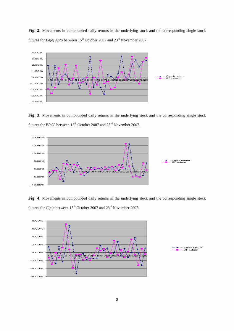
Fig. 2 to Fig. 16 depicts the movements in compounded daily returns in the underlying stock and the
corresponding single stock futures in the “test set” (12th June 2007 – 23
rd July 2007 for Gujarat
Ambuja, 15th October 2007 – 23
rd November 2007 for the other fourteen). In Table 1 we have first
reported the results of the static OLS model for each of the fifteen selected companies. Following this,
in Table 2 we depicted comparative hedging performances (in terms of root mean square hedging
error) for the static OLS model against each of the 30-day, 60-day and 90-day moving least squares.
8
Fig. 2: Movements in compounded daily returns in the underlying stock and the corresponding single stock
futures for Bajaj Auto between 15th
October 2007 and 23rd
November 2007.
Fig. 3: Movements in compounded daily returns in the underlying stock and the corresponding single stock
futures for BPCL between 15th
October 2007 and 23rd
November 2007.
Fig. 4: Movements in compounded daily returns in the underlying stock and the corresponding single stock
futures for Cipla between 15th
October 2007 and 23rd
November 2007.

9
Fig. 5: Movements in compounded daily returns in the underlying stock and the corresponding single stock
futures for Dr. Reddy’s between 15th
October 2007 and 23rd
November 2007.
Fig. 6: Movements in compounded daily returns in the underlying stock and the corresponding single stock
futures for Grasim between 15th
October 2007 and 23rd
November 2007.
Fig. 7: Movements in compounded daily returns in the underlying stock and the corresponding single stock
futures for Gujarat Ambuja between 12th
June 2007 and 23rd
July 2007.

10
Fig. 8: Movements in compounded daily returns in the underlying stock and the corresponding single stock
futures for HDFC between 15th
October 2007 and 23rd
November 2007.
Fig. 9: Movements in compounded daily returns in the underlying stock and the corresponding single stock
futures for Hindustan Petroleum between 15th
October 2007 and 23rd
November 2007.
Fig. 10: Movements in compounded daily returns in the underlying stock and the corresponding single stock
futures for Infosys between 15th
October 2007 and 23rd
November 2007.

11
Fig. 11: Movements in compounded daily returns in the underlying stock and the corresponding single stock
futures for ITC between 15th
October 2007 and 23rd
November 2007.
Fig. 12: Movements in compounded daily returns in the underlying stock and the corresponding single stock
futures for Mahindra & Mahindra between 15th
October 2007 and 23rd
November 2007.
Fig. 13: Movements in compounded daily returns in the underlying stock and the corresponding single stock
futures for MTNL between 15th
October 2007 and 23rd
November 2007.

12
Fig. 14: Movements in compounded daily returns in the underlying stock and the corresponding single stock
futures for Satyam between 15th
October 2007 and 23rd
November 2007.
Fig. 15: Movements in compounded daily returns in the underlying stock and the corresponding single stock
futures for SBIN between 15th
October 2007 and 23rd
November 2007.
Fig. 16: Movements in compounded daily returns in the underlying stock and the corresponding single stock
futures for Tata Power between 15th
October 2007 and 23rd
November 2007.

13
Table 1: OLS estimate of γ* for each of the fifteen selected blue chip Indian companies traded on the NSE
with single stock futures contracts available. The table also shows the t statistic, p-value and the Durbin-Watson
statistic for presence of serial correlation for each of the estimated hedge ratio values. Conventionally, statistical
significance for p-values at 1% is depicted by “***”, 5% is depicted by “**” and 10% is depicted by “*”.
γ* t statistic p-value Durbin-Watson statistic
Bajaj Auto 0.5503 26.07 0.0000*** 1.954
BPCL 0.6562 34.16 0.0000*** 2.807
Cipla 0.7236 40.07 0.0000*** 2.731
Dr Reddy's 0.3447 13.95 0.0000*** 2.487
Grasim 0.1045 4.03 0.0000*** 2.140
Gujarat Ambuja 0.0443 1.84 0.0660* 2.111
HDFC 0.7260 39.71 0.0000*** 2.747
Hindustan Petroleum 0.6191 31.58 0.0000*** 2.710
Infosys 0.7677 45.06 0.0000*** 2.940
ITC 0.0273 1.05 0.2960 2.055
Mahindra & Mahindra 0.2342 11.75 0.0000*** 2.234
MTNL 0.5839 27.59 0.0000*** 2.126
Satyam 0.3256 15.75 0.0000*** 2.045
SBIN 0.5965 29.57 0.0000*** 2.646
Tata Power 0.5299 25.80 0.0000*** 2.040
Table 2: Comparative hedging performances (in terms of root mean square hedging error)
Static OLS 30-day MLS 60-day MLS 90-day MLS
Bajaj Auto 1.82% 1.80% 1.76% 1.70%
BPCL 4.69% 4.27% 4.26% 4.27%
Cipla 2.65% 2.25% 2.27% 2.25%
DrReddy 1.57% 1.47% 1.45% 1.45%
Grasim 2.22% 2.24% 2.24% 2.24%
Gujrat Ambuja 1.99% 2.27% 2.27% 2.25%
HDFC 3.47% 2.85% 2.87% 2.84%
Hind-Petro 4.47% 4.02% 4.00% 3.99%
Infosys 2.72% 2.25% 2.24% 2.24%
ITC 2.86% 2.94% 2.89% 2.89%
Mahindra & Mahindra 2.72% 2.75% 2.73% 2.74%
MTNL 4.03% 3.49% 3.46% 3.46%
Satyam 2.05% 1.93% 1.92% 1.92%
SBIN 3.90% 3.77% 3.76% 3.73%
Tata Power 5.29% 4.51% 4.35% 4.29%
Count 15 15 15 15
Average 3.10% 2.85% 2.83% 2.82%
Maximum 5.29% 4.51% 4.35% 4.29%
Minimum 1.57% 1.47% 1.45% 1.45%
Range 3.72% 3.04% 2.90% 2.84%
Standard Deviation 1.15% 0.95% 0.93% 0.93%

14
We conduct the following test of hypothesis to better illustrate the comparative performances:
H0: Mean RMHSE obtained is equal to the desired RMHSE
HA: Mean RMHSE obtained is larger than the desired RMHSE
The results of the above test of hypothesis are tabulated in Tables 3 – 6 below.
Table 3: One-tailed t-test for equality of mean RMHSE of static OLS with a range of desired RMHSE values
Static OLS
Desired RMHSE t statistic One-tailed p-value
0.000% 10.4389 0.0000***
0.125% 10.0175 0.0000***
0.250% 9.5961 0.0000***
0.375% 9.1748 0.0000***
0.500% 8.7534 0.0000***
0.625% 8.3320 0.0000***
0.750% 7.9106 0.0000***
0.875% 7.4893 0.0000***
1.000% 7.0679 0.0000***
1.125% 6.6465 0.0000***
1.250% 6.2251 0.0000***
1.375% 5.8037 0.0000***
1.500% 5.3824 0.0000***
1.625% 4.9610 0.0001***
1.750% 4.5396 0.0002***
1.875% 4.1182 0.0005***
2.000% 3.6969 0.0012***
2.125% 3.2755 0.0028***
2.250% 2.8541 0.0064***
2.375% 2.4327 0.0145**
2.500% 2.0114 0.0320**
2.625% 1.5900 0.0671*
2.750% 1.1686 0.1310
2.875% 0.7472 0.2336
3.000% 0.3259 0.3747
Table 4: One-tailed t-test for equality of mean RMHSE of 30-day MLS with a range of desired RMHSE values
30-day MLS
Desired RMHSE t statistic One-tailed p-value
0.000% 11.6070 0.0000***
0.125% 11.0986 0.0000***
0.250% 10.5903 0.0000***
0.375% 10.0819 0.0000***
0.500% 9.5736 0.0000***
0.625% 9.0652 0.0000***
0.750% 8.5568 0.0000***
0.875% 8.0485 0.0000***
1.000% 7.5401 0.0000***

15
1.125% 7.0317 0.0000***
1.250% 6.5234 0.0000***
1.375% 6.0150 0.0000***
1.500% 5.5066 0.0000***
1.625% 4.9983 0.0001***
1.750% 4.4899 0.0003***
1.875% 3.9815 0.0007***
2.000% 3.4732 0.0019***
2.125% 2.9648 0.0051***
2.250% 2.4564 0.0138**
2.375% 1.9481 0.0359**
2.500% 1.4397 0.0860*
2.625% 0.9313 0.1837
2.750% 0.4230 0.3394
2.875% -0.0854 -
3.000% -0.5938 -
Table 5: One-tailed t-test for equality of mean RMHSE of 60-day MLS with a range of desired RMHSE values
60-day MLS
Desired RMHSE t statistic One-tailed p-value
0.000% 11.7459 0.0000***
0.125% 11.2273 0.0000***
0.250% 10.7087 0.0000***
0.375% 10.1902 0.0000***
0.500% 9.6716 0.0000***
0.625% 9.1530 0.0000***
0.750% 8.6345 0.0000***
0.875% 8.1159 0.0000***
1.000% 7.5973 0.0000***
1.125% 7.0788 0.0000***
1.250% 6.5602 0.0000***
1.375% 6.0416 0.0000***
1.500% 5.5231 0.0000***
1.625% 5.0045 0.0001***
1.750% 4.4859 0.0003***
1.875% 3.9674 0.0007***
2.000% 3.4488 0.0020***
2.125% 2.9302 0.0055***
2.250% 2.4117 0.0151**
2.375% 1.8931 0.0396**
2.500% 1.3745 0.0954*
2.625% 0.8560 0.2032
2.750% 0.3374 0.3704
2.875% -0.1812 -
3.000% -0.6997 -
Table 6: One-tailed t-test for equality of mean RMHSE of 90-day MLS with a range of desired RMHSE values
90-day MLS
Desired RMHSE t statistic One-tailed p-value

16
0.000% 11.7149 0.0000***
0.125% 11.1952 0.0000***
0.250% 10.6754 0.0000***
0.375% 10.1556 0.0000***
0.500% 9.6359 0.0000***
0.625% 9.1161 0.0000***
0.750% 8.5963 0.0000***
0.875% 8.0765 0.0000***
1.000% 7.5568 0.0000***
1.125% 7.0370 0.0000***
1.250% 6.5172 0.0000***
1.375% 5.9975 0.0000***
1.500% 5.4777 0.0000***
1.625% 4.9579 0.0001***
1.750% 4.4382 0.0003***
1.875% 3.9184 0.0008***
2.000% 3.3986 0.0022***
2.125% 2.8788 0.0061***
2.250% 2.3591 0.0167**
2.375% 1.8393 0.0436**
2.500% 1.3195 0.1041
2.625% 0.7998 0.2186
2.750% 0.2800 0.3918
2.875% -0.2398 -
3.000% -0.7596 -
It may be observed from the above tables that H0 may be rejected at 1% level of significance for the
static OLS hedge performances for a desired hedging error of 2.25%; meaning that it may be stated
with 99% confidence that the mean RMHSE obtained using static OLS is larger than this (and any
lower) level of desired hedging error. For the each of the 30-day, 60-day and 90-day MLS, this cut-off
level goes down to 2.125%. Also H0 may be rejected at 5% level of significance for the static OLS
hedge performances for a desired hedging error of 2.50%; meaning that it may be stated with 95%
confidence that the mean RMHSE obtained using static OLS is larger than this (and any lower) level
of desired hedging error. For the each of the 30-day, 60-day and 90-day MLS, this cut-off level is
observed to go down to 2.375%. Also H0 may be rejected at 10% level of significance for the static
OLS hedge performances for a desired hedging error of 2.625%; meaning that it may be stated with
90% confidence that the mean RMHSE obtained using static OLS is larger than this (and any lower)
level of desired hedging error. For the each of the 30-day and 60-day MLS, this cut-off level is
observed to go down to 2.50%. For the 90-day MLS, this level is observed to go down even further.

17
The above empirical results indicate that the moving least squares approach outperforms that of static
OLS in terms of the achievable minimum level of root mean square hedging error with daily hedging.
As noted before, if transaction costs are to be considered then we can easily extend this approach
simply by appropriately increasing the length of the hedging interval thus accommodating such costs.
5. Conclusion and scope of future research
In the world of derivatives, single stock futures are a relatively new addition to the family of futures.
The existing literature is thin on the specific issue of using single stock futures as a hedging tool. In
this paper we have used data from the burgeoning single stock futures market in India and have
illustrated the derivation of an optimal hedge ratio using standard static OLS method as well as a
moving least squares method with 30-day, 60-day and 90-day periodicities.
Our results indicate that the moving least squares approach outperforms that of static OLS in terms of
the hedging efficiency. While we have selected the moving least squares periodicities somewhat
arbitrarily in our study, a potentially productive direction of future research could aim at attempting to
find an optimal periodicity for running the moving least squares given the nature of the asset returns
data distribution. We are also hopeful that our paper will help to generate interest amongst
contemporary researchers, thereby directing more academic research focused towards single stock
futures markets in general and the hedging issues associated with single stock futures in particular.
References
[1] Brooks, C., Davies, R. J. and Kim, S. S. (2007) Cross Hedging With Single Stock Futures.
Assurances et Gestion des Risques 74(4), pp. 473–504
[2] Bystrom, H. N. E. (2003) The Hedging Performance of Electricity Futures on the Nordic Power
Exchange. Applied Economics 1, pp. 1–11
[3] Dale, C. (1981) The Hedging Effectiveness of Currency Futures Markets. Journal of Futures
Markets [serial online] 1(1), pp. 77–88
[4] Dutt, H. R. and Wein, I. L. (2003) On the Adequacy of Single Stock Futures Margining
requirements. Journal of Futures Markets 23(10), pp. 989–1002
[5] Ederington, L. H. (1979) The Hedging Performance of the New Futures Markets. Journal of
Finance 34(1), pp. 157–170
18
[6] Franckle, C. T. (1980) The Hedging Performance of the New Futures Markets: Comment. The
Journal of Finance 35(5), pp. 1273–1279
[7] Hatemi-J, A. and Roca, E. (2006) Calculating the Optimal Hedge Ratio: Constant, Time Varying
and the Kalman Filter Approach, pp. Applied Economics Letters 13(5), pp. 293–299
[8] Herbst, A. F., Kare, D. D. and Marshall, J. F. (1993) A Time Varying, Convergence Adjusted,
Minimum Risk Futures Hedge Ratio. Advances in Futures and Options Research 6, pp. 137–155
[9] Holmes, P. (1995) Ex Ante Hedge Ratios and the Hedging Effectiveness of the FTSE-100 Stock
Index Futures Contract. Applied Economics Letters 2, pp. 56–59
[10] Hung, M. W., Lee, C. F. and So, L. C. (2003) Impact of foreign-listed single stock futures on the
domestic underlying stock markets. Applied Economics Letters 10(9), pp. 567–574
[11] Johnson, L. L. (1960) The Theory of Hedging and Speculation in Commodity Futures. Review of
Economic Studies 27(3), pp. 139–151
[12] Lascelles, D. (2002) Single Stock Futures, the Ultimate Derivative. CSFI Publications, No. 52
[13] Lien, D., Tse, Y. K. and Tsui, A. K. C. (2002) Evaluating the Hedging Performance of the
Constant-Correlation GARCH Model. Applied Financial Economics 12, pp. 791–798
[14] Mckenzie, M. D. and Brooks, R. D. (2003) The role of information in Hong Kong individual
stock futures trading. Applied Financial Economics 13, pp. 123–131
[15] McKenzie, M. D., Brailsford, T. J. and Faff, R.W. (2001) New Insight into the Impact of the
Introduction of Futures Trading on Stock Price Volatility. Journal of Futures Markets 21(3), pp. 237–
255
[16] Nageswara Rao, S. V. D. and Thakur, S. K. (2008) Optimal Hedge Ratio and Hedge Efficiency:
An Empirical Investigation of Hedging in Indian Derivatives Market.
http://www.ermsymposium.org/2008/pdf/papers/Thakur.pdf, last retrieved 8th Nov. 2010
[17] Silber, G. W. (1985) The Economic Role of Financial Futures. In: Anne E. Peck (ed.) Futures
Markets: Their Economic Role, Washington, DC: American Enterprise Institute for Public Policy
Research
[18] Stein, J. L. (1961) The Simultaneous Determination of Spot and Futures Prices. The American
Economic Review 51(5), pp. 1012–1025
[19] Sun, W. (2003) Relationship between Trading Volume and Security Prices and Return. Technical
Report, P-2638, http://ssg.mit.edu/~waltsun/docs/AreaExamTR2638.pdf, last retrieved 8th Nov. 2010
Top Related
Copyright © 2022 FDOKUMEN

