


Bahasa
Halaman
Hukum

•
P?8t-1l6166
REPORT NO. FRA/ORD-80/2l
OPERATIONAL PARAMETERS IN ACOUSTIC SIGNATUREINSPECTION OF RAILROAD WHEELS
D. DousisR.D. Finch
UNIVERSITY OF HOUSTONDepartment of Mechanical Engineering
Houston TX 77004
. .
'A"•
APRIL 1980FINAL REPORT
DOCUMENT IS AVAILABLE TO THE PUBLICTHROUGH THE NATIONAl- TECHNICALINFORMATION SERVICE, SPRINGFIELD,VIRGINIA 22161
Prepared for
U.S. DEPARTMENT OF TRANSPORTATIONFEOERAL RAILROAD ADMINISTRATION
Office of Research and DevelopmentWashington DC 20590
REPRODUCED BYNATIONAL TECHNICALINFORMATION S.ERVICE
u.s. UEPAR11!\Kl U1 CUMMERCESPRINGFIEIU, VA 22161

NOTICE
This document is disseminated under the sponsorshipof the Department of Transportation in the interestof information exchange. The United States Government assumes no liability for its contents or usethereof.
NOTICE
The United States Government does not endorse products or manufacturers. Trade or manufacturers'names appear herein solely because they are considered essential to the object of this repert.
Technical Report Documentation Page
1. Report No. 2. Government Accession No. 3. Recipient's Cotolog No,
FRA/ORD-80/21 PU81 1 167664. Title and Subtitle 5. Report Dote
OPERATIONAL PARAMETERS IN ACOUSTIC April 1980SIGNATURE INSPECTION OF RAILROAD WHEELS 6. Performing. Orgoni lotion Coie
B. Performing Orgoni:.otion Report No.7. Author's)
n nn,," i " R • FinchDOT-TSC-FRA-80-9
D9. Performing Organization Nome and Address 10. Work Unit No. (TRA1S)
University of Hous toni, RR031!R0312Department of Mechanical Engineering 11. Contract Of Grant No.
Houston TX 77004 DOT-TSC-ll8713. Type of Repol! and Period Covered
12. Sponsoring Agency Nome ona Address Final ReportU.S. Department of Transportation March 1976-0ct. 1978Federal Railroad AdministrationOffice of Research and Development 14. Sponsoring Agency Code
Washington DC 20590
15. Supplementary Notes U.S. Department of TransportationResearch- and Special Programs Administration
*under contract to: Transportation Systems CenterCambridge MA 02142
16. Abstract
A brief summary is ,given of some prior studies which established the feas ib il i ty ofusing acoustic signatures for inspection of railroad wheels. The purpose of thepresent work was to elucidate operational paramete-r;,s which would be of importancefor the development of a prototype system. Experimental and theoretical investiga-tions were conducted to obtain more information on the effects on wheel vibrationsof geometrical variations, wear, internal stress etc. Hardware improvements andinterfacing were carried out for a ways ide installation, in addition to softwaredevelopment for real time data acquisition and processing. Field tests were madeto evaluate sys tern performance, to permit follow-up on certain wheels and to obtaintape recordings from a sample of axle sets in service. These tape recordings wereused to optimize the data processing software and to attempt to correlate identifi-able wheel conditions with characteristics of the acoustic signature. The greatestsignature differences were obtained when one of a pair of wheels was cracked.Differential wear was found to be a major cause of differences in the signatures ofgood wheel pairs. It is claimed that the knowledge gained from this study issufficient to warrant the installation of a prototype system with a reasonablelikelihood of success. Another important finding is that the frequencies of certainresonant modes shift slightly.with changes in residual stress.
17. Key Words lB. Distribution Statement
Railroad WheelsDOCUMENT IS AVAILABLE TO THE PUBLIC
Acoustic Signature iHROUGH THE NATIONAL TECHNICAL
Inspection Systems INFORMATiON SERVICE, SPRINGFIELD,VIRGINIA 22161
Residual Stress
19. Security Clo$$d, (of this. report) 20. Security Clossif, (of this page) 21. No. of Poges 22. Price
Unc1assi fied Unc1as s i fi ed
,,--- DOT F 1700.7 (B_72) Reproduction of completed poge authorized

i
o
"
o
"
~• 0
.::
"~.r~"~d
.... i!H
; "."i~~- . ,HH
•; 3• •°oc •. ~
;. .~ i
"'rT'T!' "'1"'1"'1'1' 'IT'T'TI' '1'1'1'1"'1'1' '1'1"'1"'1'" '1'1"'1"'1'1' 'ITIT'T" '1'1'1'1"'1'" "'1"'1"'1'1'
tt U II 101: 61 II LI " " ... tl U II 01 6 • L 9 ~ ,t t 1: : 1
, I "'~
11111111111111111111111111111111111111",11111111111111111111111111111111111111111111111111111111111 111111111 111111111 111111111 111111111 IIILIl IIlIillll 111111111 1111111111111111111 11111111111 11111111111111111
.., -•1:;
zCOinCO~
~COU
ua:...~
:E
encoco...u..-
····••,.
.... ~
Ii!~-:i-~~ _ ... E
ii
PREFACE
The authors would like to express their sincere
appreciation and thanks to the following:
Mr. P. Higgins for the management of the project
until February 1977, the study of different types of
excitation mechanisms and the modification of the
mechanical hammer type exciter, and for his assistance
and efforts during the Pueblo and Bessemer tests.
Mr. A. Chaudhari for the frequency analysis of the
railroad wheel vibrations using finite element analysis.
Mr. J. Herbster for the data transfer between the
computer and diskette written software.
Mr. K. Gates for his assistance with the electronic
experiment equipment.
Mr. W. Kucera, and the superintendent and personnel
of the Griffin Wheel Manufacturing Plant at Bessemer,
Alabama for their assistance during the residual stress
measurements at the Bessemer Plant.
Mr. W. McCutchan and the personnel at TTC in
Pueblo, Colorado for their assistance during the field
tests at Pueblo.
Messrs R. GilL B. Shewmake, J. Balusek and the
personnel of the Southern Pacific Transportation Company
for their assistance during the six weeks field tests at
the Englewood classification yard in Houston.
iii

Messrs R. Ehrenbeck, E. Sarkisian, J. Ferguson,
P. Rhine, W. Kucera and B. Shewmake, members of the
Project Advisory Committee, for their advice and valuable
comments.
The Union Pacific Railroad Company for the loan
of a Real Time Analyzer, and for their invitation to
participate in their dynamometer tests. Thanks are due
in particular to Mr. F. D. Acord, Mr. F. D. Bruner and
Dr. P. E. Rhine.
Dr. O. Crenwelge and Shell Oil Company for the
use of a Real Time Analyzer.
Dr. B. N. Nagarkar for his assistance during the
Englewood field test.
The Association of American Railroads for assuming
part of the funding and last but not least the Department
of Transportation for providing the majority of the
project funds.
iv
TABLE OF CONTENTSSection
1. INTRODUCTION
1.1 Background
1.2 Types of Defects
1.3 Elements of Acoustic Signature Analysis
1.4 Theory
1.5 Experiments on Excitation and DetectionMethods
1.6 Variables in the Acoustic Signature
1.7 Laboratory Demonstration System forFinding Cracks
1.8 Preliminary Field Tests
1.9 Objectives of the Present Study
2. THEORY OF RAILROAD WHEEL VIBRATIONS
2.1 Introduction
2.2 Stappenbeck's Ring Model of WheelVibrations
2.3 The Effect of Uneven Wear on WheelsAcross the Axle
2.4 The Effect of Residual Stress
3. EXPERIMENTS ON WHEEL GEOMETRY AND MINIMUMDETECTABLE CRACK SIZE
3.1 Introduction
3.2 Data Bank of Wheel Types
v
Page
1
1
3
6
8
12
13
16
19
21
25
25
27
32
34
37
37
37
CONTENTS (Cont'd)
Section
3.3 Results from Data Bank Tests
3.4 Investigation of Minimum DetectableCrack Size
4. RESIDUAL STRESS EVALUATION IN RAILROADWHEELS USING ACOUSTIC SIGNATURE ANALYSIS
4.1 Introduction
4.2 Test on Wheels with Different HeatTreatment in the Griffin WheelManufacturing Plant at Bessemer, Alabama
4.3 Dynamometer Tes~s at Wilmerding,Pennsylvania
4.3.1 Description of Tests
4.3.2 Data Processing
4.3.3 Results
5. SYSTEM COMPONENT DESIGN
5.1 Wheel Exciter
5.1.1 Mechanically Powered Excitation
5.1. 2 Electrically Powered Excitation
5.1. 3 Pneumatic Powered Excitation
5.1. 4 Comparison of Exciter Types
5.2 Wheel Sensor
5.3 Microphones
5.4 Spectrum Analyzer, Computer andDiskette Interfacing
5.5 System Description and SoftwareDevelopment
6. WAYSIDE TESTS
6.1 Tests at TTC Pueblo, Colorado
6.2 First Pueblo Test
6.3 Second Pueblo Test
vi
38
45
54
54
57
73
73
77
77
90
90
91
94
96
99
99
102
105
109
127
127
127
133
CONTENTS (Cont'd)
Section
6.4 Tests at the Southern PacificEnglewood Yard, Houston
6.5 Englewood Test Site and Equipment
6.6 Performance of the Hardware duringthe Englewood Test
6.7 Performance of Software during theEnglewood Test
7. SENSITIVITY ANALYSIS
7.1 Introduction
7.2 Identification and Correction ofSystem Problems
7.3 Optimizing the DI Equation
7.4 The Effect of Wheel Conditions
7.4.1 Introduction
7.4.2 Data Reduction
7.4.3 Laboratory Measurement ofWear
8. CONCLUSIONS AND SUGGESTIONS FOR FURTHER WORK
8.1 Conclusions
8.1.1 Advances in Scientific Understanding
8.1.2 System Improvements
8.1.3 Software and Signature RecognitionImprovements
8.2 Suggestions for Further Work
8.2.1 Installation of a PrototypeASI System
8.2.2 System Interaction Studies
8.2.3 Further Research on Residual Stress,Crack Growth and Wheel RemovalCriteria
vii
139
140
148
155
160
160
161
166
173
173
175
183
189
189
189
190
192
194
195
198
199

CONTENTS (Cont'd)
Section
REFERENCES-
APPENDIX A - List of Wheels on Inventory at Universityof Houston
APPENDIX B - Equipment List Used in the Englewood YardTests
APPENDIX C - Software for computer Interfacing and DataProcessing
204
209
210
211
211Col Pin Assignment
C o2 List of the Assembler Software Used for 214Digital Control of the Real Time Analyzerand Data Transfer to Computer/Diskette
Co3 List of the BASIC Software Used in theEnglewood Yard Field Tests
APPENDIX D - Resonances of the Wheels Tested at theGriffin Wheel Plant in Bessemer, Alabama
APPENDIX E - Dynamics of a Hammer Exciter
APPENDIX F - Finite Element Analysis
Fol Finite Element Analysis ofthe Rail'fay Wheel
Fo2 Mode Frequency Analysis
APPENDIX G - Relationship Among OperatingParameters
APPENDIX H - Report of New Technology
viii
247
253
256
260
260
261
274
277
Figure
1. 2.1
1. 3.1
1.4.1
LIST OF ILLUSTRATIONS
Wheel Showing Typical Cracks
Schematic of Acoustic SignatureInspection System Components
Mode Shapes Obtained with Finite ElementProgram for 33" Good Wheel. Note: TheHub Is Fixed for All Mode Shapes
4
7
10
1. 4. 2
1. 4. 3
Line Spectra of Resonances Obtained fromthe ANSYS Program, Compared withExperimental Spectra for 33" Good WheelsObtained by Us\ng a Rail-mountedAccelerometer 10
Mode Shapes Obtained with ANSYS Program for33" Wheel with Plate Crack 11
1.4.4
1. 6.1
1. 6.2
1. 6.3
1.6.4
1. 6. 5
1. 6. 6
1.8.1
1.8.2
Line Spectra of Resonances Obtained fromthe ANSYS Program for 33" Good andFlawed Wheels
Drawing of Impacter Used in First Test
Fixed Band Spectra of Impact on Good33" Wheels on Either End of theSame Axle
Fixed Band Spectra of Impact on Two Good33" Wheels, One a Griffin 9 Riser, One anARMCO Wrought
Fixed Band Spectra of Impact on 33"Southern wheels, One with a Large ThermalCrack
Fixed Band Spectra of Impact on Two 33"Southern Wheels, One with a Thick Layerof Grease
variation of Wheel Signature with Loadfor Wheel 3G (Accelerometer Pickup)
Train Consist for Second Test
Computer Output for an Eastbound Run at6 MPH. Reliability Was 100%. Engine IsCar 5. Decision Limit Is 11.
ix
11
14
15
15
17
17
18
22
22

ILLUSTRATIONS (Co~t'd)
Figure
2.1.1 Assumed and Actual Wheel Cross Sections 26
2.2.1 Cross Sections for Ring Model 31
3.2.1a Wheel Information and Test Description Form 39
3.2.1b Acoustic Signature Plot Form 39
3.2.2 Rolling Ball Apparatus 40
3.3.1 Signatures of Impact on Two Wheels on the Same 44Axle with Unevenly Worn Flanges
3.4.1 View of Wheel 15A 49
3.4.2a View of Wheel 15C (Front Side) 50
3.4.2b View of Wheel 15C (Back Side) 50
3.4.3 Signatures of Wheels, 15C with a Partial Plate 52Crack and 15A with a Full Plate Crack
3.4.4 Spectral Line Comparison Tests Among a 53Wheel with a Partial Plate Crack (15C), a Wheelwith a Full Plate Crack (15A) and Two GoodWheels of the Same Type (IG and 4G)
4.2.1 Strain Test on a 33" One Wear 70 Ton Griffin 58Wheel
4.2.2 View of the Hammer with a PZT Disk Between 60Hammer and Cylinder to Provide the TriggeringPulse on Impact with the Test Object
4.2.3 Schematic Diagram of Cast Wheel Manufacturing 62
4.2.4
4.2.5
4.2.6
4. 3.1
4.3.2
4. 3.3
Spectra Plots for CJ36 Wheels with DifferentInternal Stress Distribution, Between 2400 and2500 Hz
Differences in Resonant Frequency for CJ36Wheels
Differences in Resonant Frequency for CJ33Wheels
Setup for Acoustic Signature Recording
Strain Gauge Arrangement
Acoustic Signature of a CJ33 Wheel from0-6.4kHz
x
67
68
69
75
76
82

ILLUSTRATIONS (Cont'd)
Figure
4.3.4
4.3.5
4.3.6
4.3.7
4.3.8
4.3.9
Wheel UP 28, Acoustic Signature at 3 kHzbefore the Drag Braking Test
Wheel UP 28, Acoustic Signature at 3 kHzafter the First Drag Braking Stop
Wheel UP 28, Acoustic Signature at 3 kHzafter the Second Drag Braking Stop
Wheel UP 28, Acoustic Signature at 3 kHzafter the Third Drag Braking Stop
Wheel UP 28, Acoustic Signature at 3 kHzafter the Fourth Drag Braking Stop
Wheel UP 28, Acoustic Signature at 3 kHzafter the Fifth Drag Braking Stop
83
83
84
84
85
85
4.3.10 Frequency shift, Lf, Versus Strain Change,LE, at 3 kHz for Wheel UP 27 (Five DragBraking Stops)
4.3.11 Frequency Shift, Lf, Versus Strain Change,LE, at 3 kHz for Wheel UP 28 (Five DragBraking Stops)
87
88
5.1.1 Drawing of the Modified Mechanical Wheel 93Exciter
5.1.2 Motor Exciter, Rotary 95
5.1.3 Pneumatic Leaf Spring Exciter 98
5.2.1 Output Voltage Circuit of the Wheel Sensor 103
5.3.1a Assembly of Weatherproof Microphone 104
5.3.1b Directional Response Patterns for the 104GR 1/2" Electret-Condenser Microphone
5.5.1 Schematic of Data Collection and Processing 110Hardware
5.5.2 Flow Diagram for the Series of Computer 116Programs used in the SP Englewood Yard,Houston Tests
5.5.3 Flow Diagram of the Read Acoustic Signatures 120Part of the Main Program
xi
ILLUSTRATIONS (Cont'd)
Figure
5.5.4
5.5.5
5.5.6
5.5. 7
Flow Diagram of the Data Processing Sectionof the Main Program
Sample Output of the Main Program
Distribution of Difference Index for Run #21and Run #23 from the Field Tests atEnglewood Yard, 18 June 1975
Distribution of Difference Index for Run #10,Three Different Sampling Time Intervals, fromthe Field Tests at Englewood Yard, 18 June1975
121
123
125
126
6.2.1 Modified Mechanical Ha~mer Exciter used at 129TTC, Pueblo
6.2.2a View of the Exciter-Wheel Sensor 131
6.2.2b View of the Microphones, Exciter and Wheel 131Sensor on the Bypass Section of the FASTtrack at TTC, Pueblo
6.2.3a View of the Setup and Equipment used at TTC, 132Pueblo, Colorado
6.2.3b Schematic of the System used at TTC, Pueblo, 132Colorado
6.3.1
6.3.2
6. 3.3
Distribution of Difference Index for theTests 5/6. 6/9. 14/18 at TTC, Pueblo,Colorado
Distribution of Difference Index for the Tests14/18, 6/3, 13/13 at TTC, Pueblo, Colorado
Distribution of Difference Index for the Tests13/17, 17/18, 13/14 at TTC, Pueblo, Colorado
135
136
137
6.5.1 outline of the Southern Pacific's Classification 141Yard in Houston
6.5.2a View of the Inspection System 145
6.5.2b Schematic of the System Layout 145
6.5.3 View of the Microphones, Exciters and Wheel 146Sensors Through the Window of the Trailer
6.5.4a View of the East Side of the Hump. Inspection 147pits are Indicated by Arrow
6.5.4b View of the Microphones, Exciters and Wheel 147Sensors
xii
ILLUSTRATIONS (Cont'd)
Figure
6.6.1a Typical Performance of the Exciters during 151the Late Tests
6.6.1b Typical Performance of the Exciters during 151the Early Tests Sweep Speed 500 ms/div
6.6.2a Exciter Performance, Double Impact 152
6.6.2b Exciter Performance, New Wheels, Low or No 152Impact; Sweep Speed 500 mS/div
6.6.3a Impacts on Wheels with High Flanges, Followed 153by Impacts on Wheels with Low Flanges
6.6.3b Uneven Impact on Wheels Across the Axle 153
6.6.4a Timing Relation, South Exciter, Impact 154about 40 ms after the Timing Pulse
6.6.4b Timing Relation, North Exciter, Impact about 154110 ms after the Timing Pulse; Sweep Speed50 ms/div
6.7.1 Distribution of Difference Index for the LastTen Days of Field Tests at the SouthernPacific Yard (July 1977)
159
7.2.1 Distribution of Difference Index Values 163DI ~ Cl SD, Sample Size: 137, Frequency Range:0-10 kHz (No Correction for Timing PulseDifference)
7.2.2
7. 3.1
7.3.2
7.3.3
7.3.4
Distribution of Difference Index ValuesDI ~ C
lSD, Sample Size: 168, Frequency
Range: 0-10 kHz (With Correction for TimingPulse Difference)
Distribution of Difference Index ValuesDI ~ C
1SD, Sample Size: 372, Frequency
Range:~ 0-10 kHz
Distribution of Difference Index ValuesDI ~ Cl SD, Sample Size: 369, FrequencyRange: 0-7200 Hz
Distribution of Number of Common Resonances,NC, Sample Size: 313, Frequency Range:0-10 kHz
Distribution of Difference Index Values.DI ~ Cl SD - C2 (NC) 2, Sample Size: 371Frequency Range: 0-7200 Hz
xiii
164
168
169
171
172
ILLUSTRATIONS (Cont'd)
Figure
7.4.1 Signatures of Wheels with Uneven Impact 176
7.4.2 Timing Pulses and Sound Signals from Two 177Unevenly Impacted Wheels.
7.4.3 Signatures of Wheels on Axle 3, Car GTAX 17813286, Progressive Frequency Shifts
7.4.4 Typical Timing Pulses and Sound Signals from 179a Pair of Wheels Tested at the Englewood Yard
7.4.5 Frequency shift ~fn of a Pair of Unevenly Worn 180Wheels, versus Frequency f
7.4.6 Actual Cross Section of a Wheel Showing How 184the Tread and Flange Thickness Were Measured
7.4.7 Signature of Wheels IIa and IIC 186
7.4.8 Signature Differences at the Resonant 188Modes for Wheels IIA/C, due to Uneven Wear
C.1.2 SD 300A Digital Output Timing 213
F.2.1 View of a 33" Wheel with One Small Radial 265Flange Crack - ANSYS Geometry
F.2.2 View of a 33" Wheel with One Complete Flange 265and Tread Crack - ANSYS Geometry
F.2.3 View of a 33" Wheel with One Complete Radial 266Crack - ANSYS Geometry
F.2.4 View of a 33" Wheel with One Large Plate 266Crack - ANSYS Geometry
F.2.5 Comparison of Natural Modes for 33" Wheels 269
F.2.6a 33" Good Wheel Modal Analysis, Single Pulse on 270the Load Line
F.2.6b 33" Good Wheel Modal Analysis, Single pulse 30° 270from the Load Line
F.2.7
F.2.8
Modal Analysis of a 33" Wheel with One SmallRadial Flange Crack - Single Pulse Applied(Radial)
Nodal Analysis of a 33" Wheel with One SmallFlange Crack - Single Pulse Applied (Axial)
xiv
271
272

Table
1.1.1
1. 7.1
LIST OF TABLES
List of Wheel Failures for 1976
Sums of Differences of Wheel Spectrafrom Average Good Wheel Spectrum (ImpactExcitation)
2
20
2.2.1 List of Resonances calculated with the Ring 30Model Compared with ANSYS Results andExperimental Data
3.2.1
3.4.1
4.2.1
4.2.2
4.2.3
4.3.1
4.3.2
4.3.3
5.1.1
5.5.1
5.5.2
Inventory of Wheels Tested at SouthernPacific Englewood Yard 18 June 1976
Range of Deviations from Good WheelSpectral Averages in Experimentswith Thermal Cracks
List of Wheels Tested at the GriffinWheel Manufacturing Plant in Bessemer,Alabama for Residual Stress Evaluation
Preliminary Results - Residual StressTests, Bessemer, Alabama
Error Evaluation for Strong Resonanceson CJ33 and CJ36 Wheels
Strain Gauge Indication Versus AcousticSignature Changes from Drag BrakingTests on Wheel UP 28
Strain Gauge Indication Versus AcousticSignature Changes from Drag BrakingTests on Wheel UP 27
Setup State on HP 5445 Real TimeAnalyzer
Rating of 3 Exciter Types against IdealSpecifications
Summary of the Line Spectra Analysis(Results Obtained Manually from SpectraPlots)
Summary of the Line Spectra Analysis(Tests were Computer Controlled)
.xv
41
47
64
65
72
78
79
81
100
113
114

Table
6.5.1
6.7.1
7.4.1
7.4.2
C.l.l
D.l
D.2
F.2.l
TABLES (Cont'd)
Difference Index Values from WheelsTested in the Laboratory, forDiscrimination Level Selection
Summary of the Last Ten Days of Testsat the Southern Pacific Englewood Yard,Houston
Theoretical Estimate of DifferentialWear on Wheels with High DI Values
Tread and Flange Thickness of Wheelsat the University of Houston Laboratory
Computer-Analyzer Interfacing
Resonances of CJ33 Type Wheelswith Different Internal Stresses
Resonances of CJ36 Type Wheelswith Different Internal Stresses
Summary of Analysis
xvi
143
156
182
185
212
254
255
268
1. INTROr,UCTION
1.1 Background
The impetus to the work covered in this report came
from a feasibility study on the use of acoustic signatures
for inspection of railroad wheels [1]. The basic idea was
to see if it would be possible to automate the art of the
carman, who by banging wheels with a hammer, can tell a
defective one by its sound. There is a need for a fUlly
automatic testing system to inspect freight car wheels.
At present the standard way of finding cracked or over
heated wheels depends on the visual acuity of inspectors
stationed in pits at switching yards. These men have to
watch for a variety of possible mechanical defects as the
cars move past the pit. Although the inspectors are
remarkably adept at finding problems there are still a
number of mechanical defects which are not readily
apparent and subsequently can result in derailments.
Table 1.1.1 shows the AAR list of wheel failures for
1976 indicating the relative importance of different
defects.
Having indicated the motivation for the research it is
appropriate to proceed to summarize the findings of the earlier
feasibility study [1]. The present work had the general
objective of improving the laboratory demonstration system
to the point that actual operating parameters could be
TABLE 1.1.1 LIST OF WHEEL FAILURES FOR 1976
From: Association of American RailroadsMechanical Division Circular D.V. 1895
2
CAUSE - INTERCHANGE RULE 41 - SEC. F 6g; (I)s:: S .j.JIII -.-I IIIrl p:; M
.j.JIi, p.,Ul s:: S Ul 'r:J u
REPORT OF (I) s:: (I) •.-1 ~ (I) s:: (I)
!-< (lJ ~ p:; S U M .a (I) lI-<AAR WHEEL ,:; ~ 0 •.-1 III M ,:; ~
(I)
FAILURES FOR M 0 M 'r:J p:; !-< (lJ II: 0 Q•.-1
~(I) 0 ~ !-<
YEAR 1976 I1l !-< 'r:J Ul .j.J ill (I)Ii, !-< (I) I1l M Ul U
!-< 0 .j.J (I) I1l 'r:J !-< !-< I1lM 0 .j.J !-< S III ,:; 0 lI-<IIJ 'r:J IIJ Pi !-< (I) ill !-<
.j.J '0 (I) ~ 00 (I) !-< 'r:J ,:;0 (I) ~ 00 ~ E-t (I) UlE-! ~ u E-t ~ .a
u I1l U ,:;I1l !-< I1l 00H 0 r~0
66 68 71 72 74 75 82 83 88
28 "
lW - CS 21 18 1 2lW - WS 36 1 16 6 13
2W & MW - CS2W & MW - WS 1 1
TOTAL 58 20 16 7 2 13
33 "
lW - CS 273 3 30 17 176 25 1 20 1lW - WS 255 5 63 75 1 25 22 1 63
2W & MW - CS 16 1 3 9 2 12W & MW - WS 87 2 12 30 26 7 1 9
TOTAL 631 11 108 122 1 236 56 3 93 1
36 "
lW - CS 69 8 2 17 37 1 4lW - WS 367 4 47 211 18 71 16
2W & MW - CS 25 1 4 12 7 12W & MW - WS 94 2 12 27 1 15 22 15
TOTAL 555 14 60 244 1 62 137 1 36
38 "
lW - CSlW - WS 7 2 2 2 1
2W & MW - cs2W & MW - WS 3 1 2
TOTAL 10 1 2 4 2 1GRAND TOTAL 1254 25 189 384 2 309 197 4 143 1
lW = Single Wear
~m = Multiple Wear
CS = Cast Steel
WS = Wrought Steel

3
established and a secondary objective was to find if residual
stresses could change the acoustic signature and in what
manner. The specific objectives of the present program will
be defined after the summary of the feasibility study.
1.2 Types of Defects
It is appropriate to summarize the principal in-service
*defects of wheels, and their causes. A good summary of
this subject has been given by Carter and Caton [30J. At
present one of the most frequently occurring classes of
defect is the thermal crack, due to extended periods of
brake shoe application and rapid cooling. The cracks may
be found on only one or both wheels of an axle set. The
cracks appear as hair lines on the tread or flange and
there are frequently numerous cracks around the circum-
ference of the wheel. Despite the barely visible exterior
manifestation of this type of crack, below the surface it
may occupy a sizeable fraction of the rim cross section.
When a wheel with thermal cracks is withdrawn from service
and subjected to metallurgical examination the cracks are
typically found to extend over about a square inch in area
perpendicular to the surface (see Fig. 1.2.1). This area
is usually blackened, suggesting that the cracks may persist
for long periods before progressing through the plate to
cause a catastrophic failure. This final stage of the failure
is surmised to be a result of changes in the internal state
*The Association of American Railroads standard nomenclaturefor the parts of a wheel is illustrated in Fig. 1.2.1.

THERMALCRACI<
TREADPLATE
PLATECRACK
FIG. 1.2.1 WHEEL SHOWING TYPICAL CRACKS
4
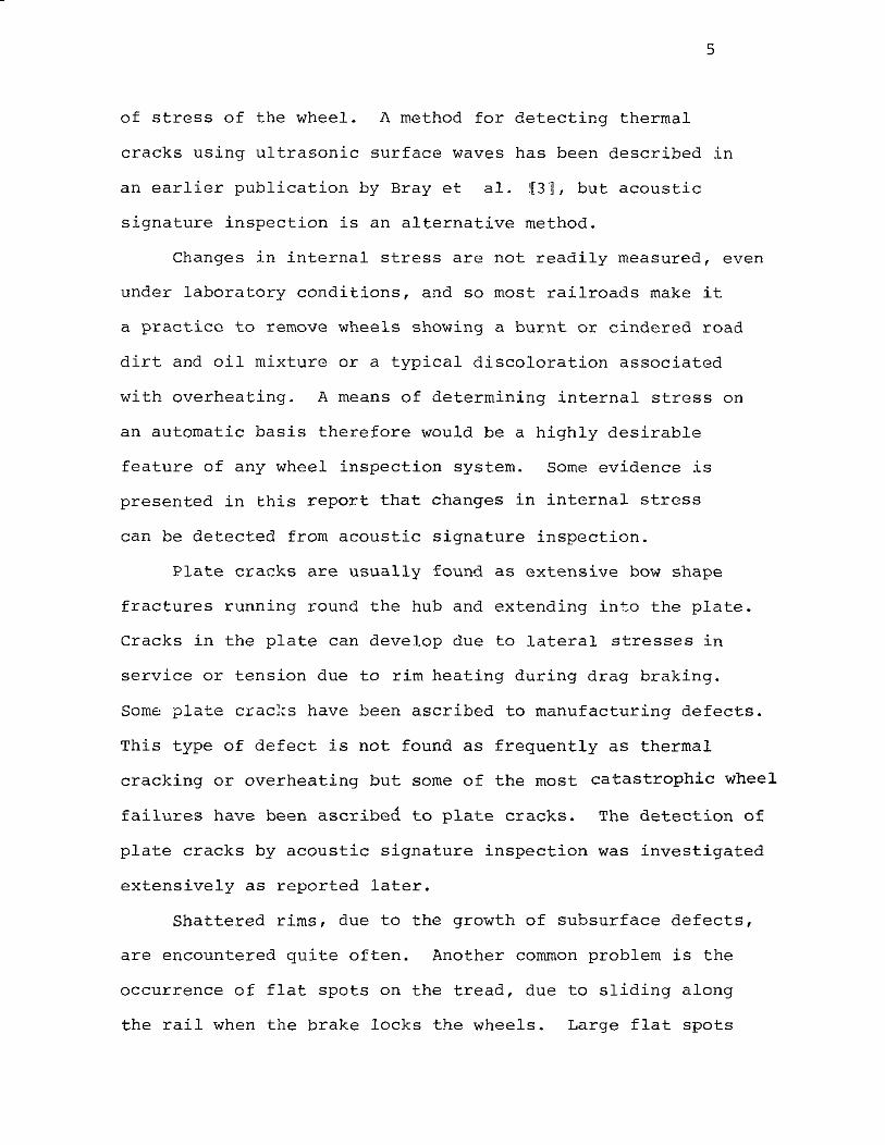
5
of stress of the wheel. A method for detecting thermal
cracks using ultrasonic surface waves has been described in
an earlier publication by Bray et al. 131, but acoustic
signature inspection is an alternative method.
Changes in internal stress are not readily measured, even
under laboratory conditions, and so most railroads make it
a practice to remove wheels showing a burnt or cindered road
dirt and oil mixture or a typical discoloration associated
with overheating. A means of determining internal stress on
an automatic basis therefore would be a highly desirable
feature of any wheel inspection system. Some evidence is
presented in this report that changes in internal stress
can be detected from acoustic signature inspection.
Plate cracks are usually found as extensive bow shape
fractures running round the hub and extending into the plate.
Cracks in the plate can develop due to lateral stresses in
service or tension due to rim heating during drag braking.
Some plate cracks have been ascribed to manufacturing defects.
This type of defect is not found as frequently as thermal
cracking or overheating but some of the most catastrophic wheel
failures have been ascribed to plate cracks. The detection of
plate cracks by acoustic signature inspection was investigated
extensively as reported later.
Shattered rims, due to the growth of subsurface defects,
are encountered quite often. Another cornmon problem is the
occurrence of flat spots on the tread, due to sliding along
the rail when the brake locks the wheels. Large flat spots
6
cause repeated impacting which results in further damage to
both the rail and the wheels. These tread surface defects
can be detected using very simple acoustic signature inspection.
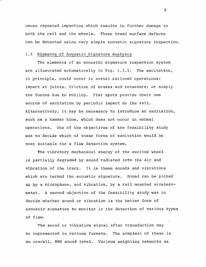
1.3 Elements of Acoustic Signature Analysis
The elements of an acoustic signature inspection system
are illustrated schematically in Fig. 1.3.1. The excitation,
in principle, could occur in normal railroad operations:
impact at joints, friction of brakes and retarders; or simply
the forces due to rolling. Flat spots provide their own
source of excitation by periodic impact on the rail.
Alternatively, it may be necessary to introduce an excitation,
such as a hammer blow, which does not occur in normal
operations. One of the objectives of the feasibility study
was to decide which of these forms of excitation would be
most suitable for a flaw detection system.
The vibratory mechanical energy of the excited wheel
is partially degraded by sound radiated into the air and
vibration of the track. It is these sounds and vibrations
which are termed the acoustic signature. Sound can be picked
up by a microphone, and vibration, by a rail mounted accelero
meter. A second objective of the feasibility study was to
decide whether sound or vibration is the better form of
acoustic signature to monitor in the detection of various types
of flaw.
The sound or vibration signal after transduction may
be represented in various formats. The simplest of these is
an overall, RMS sound level. Various weighting networks as
MIC
RO
PH
ON
EI)
EX
CIT
AT
ION
WH
EE
LD
ATA
PR
OC
ES
SO
R
\..../
0I
IIF
LA
WIN
DIC
AT
OR
TR
AC
K(D
ISP
LA
Y)
AC
CE
LE
RO
ME
TE
R
FIG
.1.
3.1
SC
HE
MA
TIC
OF
AC
OU
ST
ICS
IGN
AT
UR
EIN
SP
EC
TIO
NS
YS
TE
MC
OM
PO
NE
NT
S
"
8
well as band-pass filtering may be used to attenuate or
exclude noise components in the signal. The frequency
spectrum of the signal is a function of the filtering method
employed. Both one-third octave band and constant bandwidth
(250 channels per 10 kHz) analyzers were used in the
feasibility study. Railroad wheel sound spectra were found
to be dominated by high frequency components in the range of
1 to 5 kHz. One-third octave bands in this frequency range
are wide, so that all the information from a wheel's acoustic
signature is compressed into a few bands. Changes in the
acoustic signature result in relatively small level changes
in these 1/3 octave bands. However, when narrow constant
bandwidth analyzers are used, the wheel signature is represented
by more bands, thus perception of signature changes is
considerably improved. The disadvantage is increased
analysis time due to the increased amount of data.
The spectrum of a given signal can be processed with
a minicomputer by comparison to reference spectra. Various
possible comparison schemes were considered and are discussed
later. Finally if the comparisons show that a wheel is
defective, some form of flaw indicator is actuated. In the
present research system this indication is made with a
teletype.
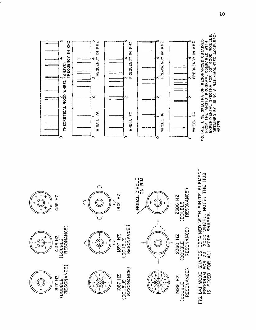
1.4 Theory
A completely theoretical design procedure could be
envisaged. The railroad wheel could be modelled using finite
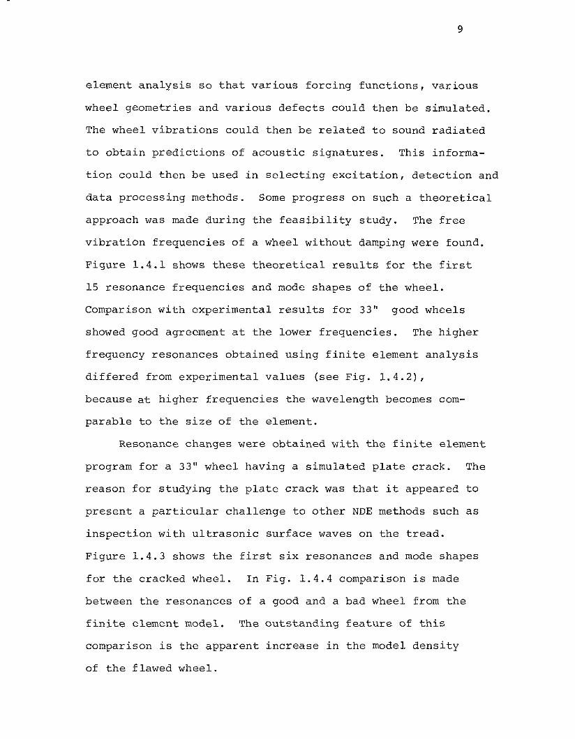
9
element analysis so that various forcing functions, various
wheel geometries and various defects could then be simulated.
The wheel vibrations could then be related to sound radiated
to obtain predictions of acoustic signatures. This informa
tion could then be used in selecting excitation, detection and
data processing methods. Some progress on such a theoretical
approach was made during the feasibility study. The free
vibration frequencies of a wheel without damping were found.
Figure 1.4.1 shows these theoretical results for the first
15 resonance frequencies and mode shapes of the wheel.
Comparison with experimental results for 33" good wheels
showed good agreement at the lower frequencies. The higher
frequency resonances obtained using finite element analysis
differed from experimental values (see Fig. 1.4.2),
because at higher frequencies the wavelength becomes com
parable to the size of the element.
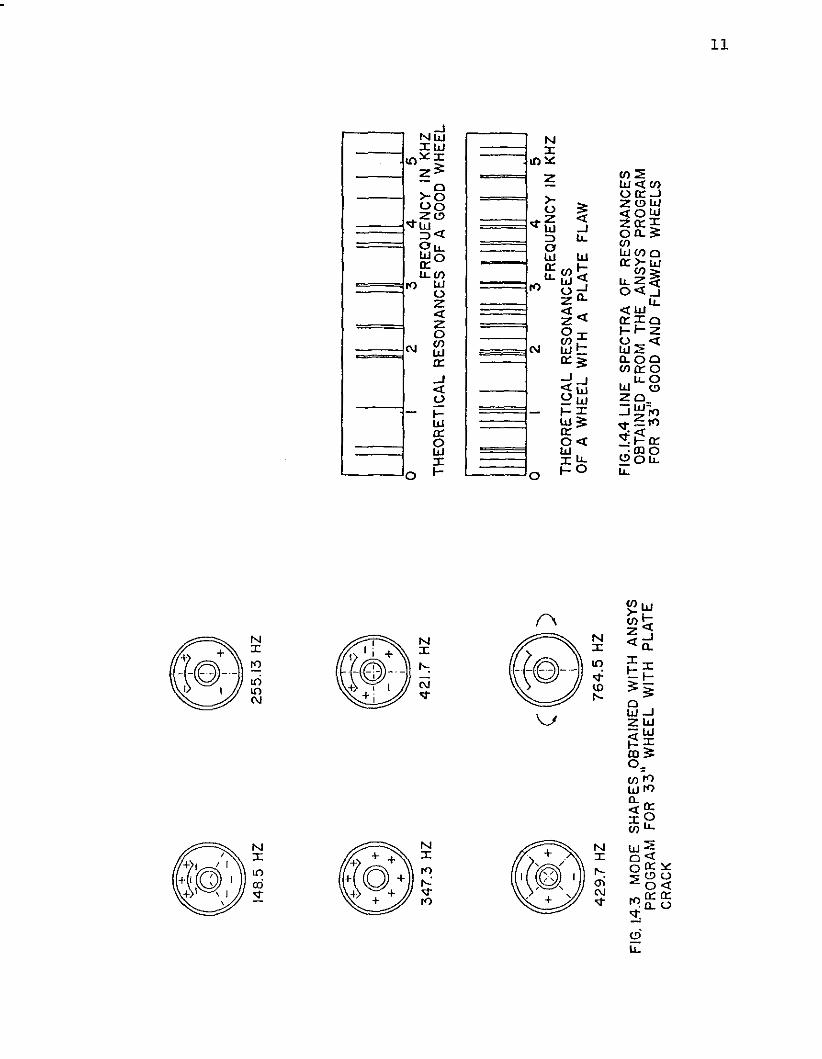
Resonance changes were obtained with the finite element
program for a 33" wheel having a simulated plate crack. The
reason for studying the plate crack was that it appeared to
present a particular challenge to other NDE methods such as
inspection with ultrasonic surface waves on the tread.
Figure 1.4.3 shows the first six resonances and mode shapes
for the cracked wheel. In Fig. 1.4.4 comparison is made
between the resonances of a good and a bad wheel from the
finite element model. The outstanding feature of this
comparison is the apparent increase in the model density
of the flawed wheel.
""
tV(@
)
FIG
.1.
4.1
MO
DE
SH
AP
ES
OB
TA
INE
DW
ITH
FIN
ITE
EL
EM
EN
TP
RO
GR
AM
FOR
33
"G
OO
DW
HE
EL
.N
OT
E:
TH
EH
UB
ISF
IXE
DFO
RA
LL
MO
DE
SH
AP
ES
.23
86
HZ
(DO
UB
LE
RE
SO
NA
NC
E)
317
HZ
(DO
UB
LER
ES
ON
AN
CE
)
1087
HZ
(DO
UB
LE
RE
SO
NA
NC
E)
1999
HZ
(DO
UB
LE
RE
SO
NA
NC
E)
44
3H
Z(D
OU
BL
ER
ES
ON
AN
CE
)
'J
1897
HZ
(DO
UB
LE
RE
SO
NA
NC
E)
I
-(@O-
-")-
\/
.......
----
..."'"
t2
36
0H
Z(D
OU
BLE
RE
SO
NA
NC
E)
45
5H
Z
v19
12H
Z
NO
DA
LC
IRC
LEO
NR
IM
®
[]JW
UJL
J]o
I2
34
5T
HE
OR
ET
ICA
LG
OO
DW
HE
EL
IAN
SY
S)
FR
EQ
UE
NC
YIN
KH
Z
WLU
LUI
Io
I2
34
5W
HE
EL
7A
FRE
QU
EN
CY
INK
HZ
WIU
lliI
Io
I2
34
5W
HE
EL
7CF
RE
QU
EN
CY
INK
HZ
[J.1
I.IL
l.0
oI
23
45
WH
EE
LIG
FR
EQ
UE
NC
YIN
KH
Z
WU
llWI.
Io
I2
34
5W
HE
EL
4GF
RE
QU
EN
CY
INK
HZ
FIG
.1.
4.2
LIN
ES
PE
CT
RA
OF
RE
SO
NA
NC
ES
OB
TA
INE
DFR
OM
TH
EA
NS
YS
PR
OG
RA
M.
CO
MP
AR
ED
WIT
HE
XP
ER
IME
NT
AL
SP
EC
TR
AFO
R3
3"
GO
OD
WH
EE
LS
,O
BT
AIN
ED
BY
US
ING
AR
AIL
-MO
UN
TE
DA
CC
ELE
RO
M
ETE
RI-
'o
@~:':
f\(O
J~-~
148.
5H
Z25
5.13
HZ
34
7.3
HZ
42
1.7
HZ
[JlJ
WJlL
WJ
oI
23
45
FR
EQ
UE
NC
YIN
KH
ZT
HE
OR
ET
ICA
LR
ES
ON
AN
CE
SO
FA
GO
OD
WH
EE
L
42
9.7
HZ
(((m
)))7
64
.5H
Z
iiliJi
illllU
Ull
oI
23
45
FR
EQ
UE
NC
YIN
KH
ZT
HE
OR
ET
ICA
LR
ES
ON
AN
CE
SO
FA
WH
EE
LW
ITH
AP
LA
TE
FL
AW
FIG
.1.
4.3
MO
DE
SH
AP
ES
OB
TA
INE
DW
ITH
AN
SY
SP
RO
GR
AM
FOR
33
"W
HE
EL
WIT
HP
LA
TE
CR
AC
K
FIG
./.4.
4L
INE
SP
EC
TR
AO
FR
ES
ON
AN
CE
SO
BT
AIN
ED
FRO
MT
HE
AN
SY
SP
RO
GR
AM
FOR
33
"G
OO
DA
ND
FLA
WE
DW
HE
ELS
t-'
t-'
12
1.5 Experiments on Excitation and Detection Methods
In order to determine which of the various excitation
methods would be most suitable a series of experiments were
performed, during the feasibility study, both in the lab
oratory and in the field. Rolling noise was found to be
predominantly low frequency sound from many sources and to
mask the response of the wheel. Impact at a rail joint
masks the wheel signature and even though some of the higher
wheel resonances seem to be excited the response varies
from wheel to wheel and with train speed. When passing
through a retarder a wheel sometimes emits an intense
screeching sound. It was found in this situation that
only a few resonances of the wheel were excited, and dif
ferent resonances were excited during successive passages
of the wheel through the retarder. This lack of repeatability
and the excitation of only one or two resonances ruled out
the retarder as a choice of excitation.
When using active excitation methods, energy is
imparted to the wheel from a device which is not part of
normal railroad operations. In the feasibility study an
electrodynamic shaker was used with random noise and sine
wave inputs. This method of excitation does not appear to
be feasible for field use. Tapping with a steel
pendulum or a hammer excites a rich spectrum of wheel
resonances (see Figs. 1.6.2 - 1.6.5). To obtain repeatab
ility with this mode of excitation, it was found that there
must be a good control of the momentum of the impacting
hammer.
13
Various microphone ane accelerometer configurations were
experimented with. Except in the detection of flat spots [4],
rail mounted accelerometers are not regarded as the best
choice, the reason being that there are natural modes of vibra
tion of the rail in the same frequency range as the wheel modes.
These rail modes can be superimposed on the wheel signature
thus compounding the difficulties of data processing. When a
microphone is used only the sound from the wheel is detected
because of the relatively small radiating area of the rail
and its weak coupling to the wheel. Regulations permit installa
tion of devices at ground level so that the microphone to
receive airborne sound is best located close to the rails.
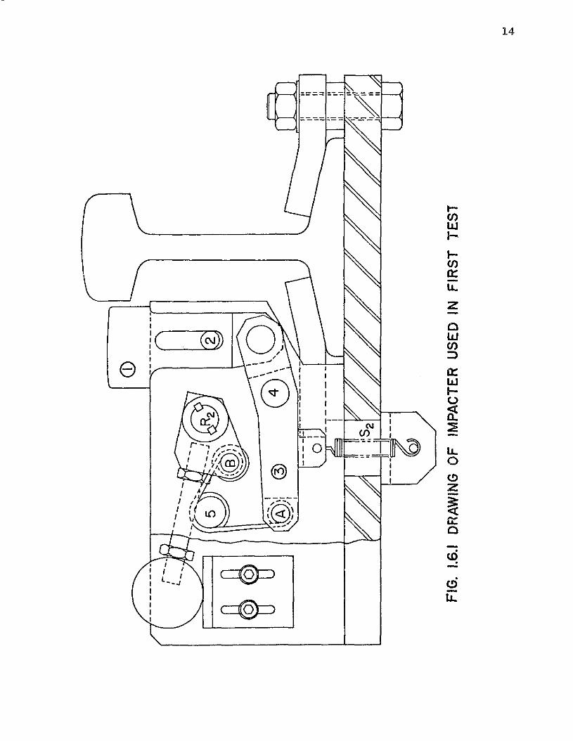
1.6 Variables in the Acoustic Signature
As part of the feasibility study wheel and axle sets
were rolled over an automatic impacter (see Fig. 1.6.1) on
the laboratory track. Unfortunately at the time this data
was taken there was no provision in the system for a triggering
pulse so that the timing of the scan made by the instrument
could not be controlled relative to the duration of the
impact sound. Even with this difficulty several interesting
features were discovered.
Figure 1.6.2 shows the superposition of impact spectra
from two good and equally worn Griffin 9 riser 33" wheels
on either end of the same axle. The signal amplitudes differ
somewhat but the values of the resonance frequencies
are very closely reproduced. In contrast Fig. 1.6.3 shows
the spectrum of one of these same wheels in comparison with
the spectrum of a good Armco Wrought 33" wheel. There are
:ome pronounced differences in the resonance frequencies.
:ven more differences in the resonance frequencies are
e
,II
;cIIII
--_"':.::--rr.v:~--~
I~-,IIIIIIIII I:1. _
:0I I ""''F~I
l-
~l-
IC/)0::LL
Z
awC/)::::>0::wI(.)
~:E
LLo(!)z
~0::o.
tQ-
14

t15
~zl1J0::l1JIJ..l1J0::
>-0::<t0::I-m0::<t
m :\"'Cl f\~
I;?'. i
l1Jo::> f;I- '
~ \ "\~ i r
"', Ii
~\ iW\'VJ1. :, .' !. _.".! -' of :.-!
o 2
,:.I\J. \/3 4
:;f:i\ :.
) i I \ ; , \ .. ' !\.J "'-; ~ '.,,",-'
5 6 7 8FREQUENC Y(kHz) ----0..._
r·.,.;' \. .....:....9 10
FIGURE 1.6.2 FIXED BAND SPECTRA OF IMPACT ON GOOD 33"WHEELS ON EITHER END OF THE SAME AXLE
-GRIFFIN 9 RISER·········ARMCO WROUGHT
5 6 7 8 9FREQUENCY (kHz) ~
SPECTRA OF IMPACT ON TWO GOOD 33"RISER, ONE AN ARMCO WROUGHT
4
~.'.,..
1~ \ \v :~.; .........
3
nn:!,., iI·1,i
FIGURE 1.6.3 FIXED BANDWHEELS ONE A GRIFFIN 9
{\i: f:I ~ i\; i i:,"": ..: ii : ; i
i!! . ! t :".\t'v\ I (. II···\.JJ \v0 \.V012
16
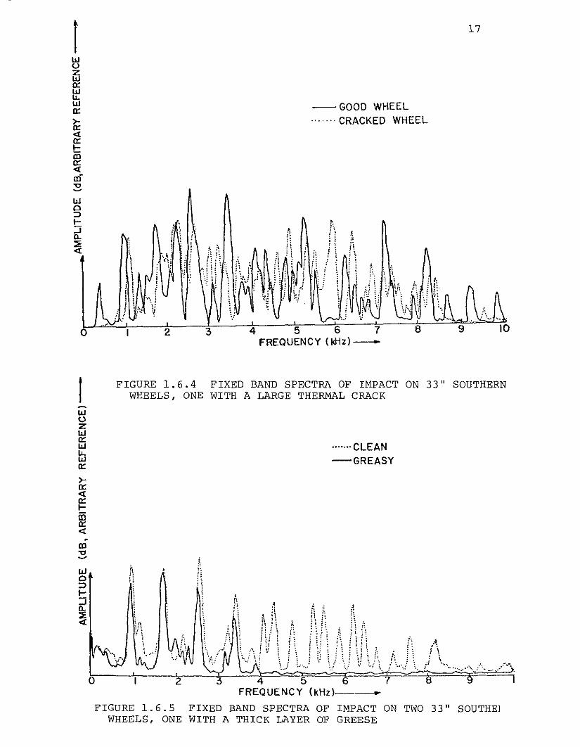
found between the spectra displayed in Fig. 1.6.4. These
were obtained from two Southern 33" wheels on the same
axle. One of them/however, has a thermal crack which has
propagated clear through to the hub. Finally, Fig. 1.6.5
shows the comparison of the spectra of two identical good wheels
(33" Southern), one of which has a heavy layer of grease.
The most interesting aspect of the spectrum of the greasy
wheel is the complete absence of sound above about 4 kHz.
This was presumably due to damping of the plate vibrations.
This feature, i.e., the damping of high frequency resonances,
could be used as a means of identifying the spectra of greasy
wheels, which might otherwise be mistaken for cracked
wheels and give rise to a false alarm.
Also as a part of the feasibility study some labora
tory exper~ments were performed with wheel pairs in a
stationary load frame using a hydraulic jacking system to
simulate loads up to 20 tons. Figure 1.6.6 shows a series
of spectral analyses, each with increasing load. The
traces are superimposed on one another but slightly offset
to give a three dimensional perspective. Some resonances
are enchanced by the load; some are diminished. Most shift
slightly in frequency and some split into two separate
resonance peaks. On the other hand, if one does not use
too fine discrimination, it is clear that the changes do
not produce complete disorder in the three-dimensional plot.
1.7 Laboratory Demonstration System for Finding Cracks
As the last part of the feasibility study a laboratory
demonstration system was assembled to simulate field opera-
r17
wuffiII::Wl1..WII::
f<tII::!::roII::<troO~
-- GOOD WHEEL....... CRACKED WHEEL
o I 2 3 4 5 6 7FREQUENCY (kHzl-
8 9 10
fFIGURE 1.6.4 FIXED BAND SPECTRA OF IMPACT ON 33" SOUTHERN
WHEELS, ONE WITH A LARGE THERMAL CRACK
wuzWII::Wl1..WII::
>II::<tII::I-
~<t
..·····CLEAN-GREASY
TWO 33 n SOUTHE]
/~, \
! \,'} ' .. ~ ,', ,', ..~..-.
: ~ ~.' .
:: ::
".! ':." } ~
,; ".
~n :~ .
•i~... ••.,n..:..,.n." . n1\{j l' Anil, .!~. .' t'..',: i ~ : ." , j:".....: , ...i} : J \/ ~: \i\.
~.
i\;
3 4 5 6 7FREQUENCY (kHzl-_
FIXED BAND SPECTRA OF IMPACT ONWITH A THICK LAYER OF GREESE
,
FIGURE 1. 6.5WHEELS, ONE
o 2
o
ro"Cl~
wo:::II:J
~

GO
OD
WH
EE
L:3
G
(J) z ~ z - o g ...
J
w10
o ::J(J
)
!:::
z~..
.J-o
~>
~0
2:3
45
FR
EQ
UE
NC
YIN
KH
Z
FIG
. 1.6
.6V
AR
IAT
ION
OF
WH
EE
LS
IGN
AT
UR
EW
ITH
LOA
DFO
RW
HE
EL
:3G
.(A
CC
EL
ER
OM
ET
ER
PIC
KU
P)
I-'
OJ
19
tions as far as possible. For this phase of the work only
the third octave band analyzer was available. This was
interfaced with the NOVA minicomputer. The minicomputer
was programmed to read a given spectrum, generated by
impact of a hammer or pendulum, and to compare this spectrum
with either: 1) a standard spectrum,i.e., the average•
spectrum of good wheels, continuously averaged on a weighted
basis, or 2) the spectrum of the mating wheel on the same
axle. The output of the program was a number which is the
sum of the squares of the differences in dB between the
two spectra in the various third octave bands.
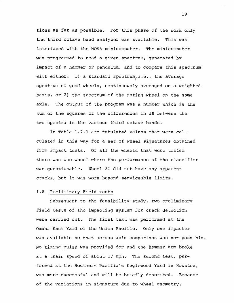
In Table 1.7.1 are tabulated values that were cal-
culated in this way for a set of wheel signatures obtained
from impact tests. Of all the wheels that were tested
there was one wheel where the performance of the classifier
was questionable. Wheel 8G did not have any apparent
cracks, but it was worn beyond serviceable limits.
1.8 Preliminary Field Tests
Subsequent to the feasibility study, two preliminary
field tests of the impacting system for crack detection
were carried out. The first test was performed at the
Omaha East Yard of the Union Pacific. Only one impacter
was available so that across axle comparison was not possible.
No timing pulse was provided for and the hammer arm broke
at a train speed of about 17 mph. The second test, per-
formed at the Southern Pacific's Englewood Yard in Houston,
was more successful and will be briefly described. Because
of the variations in signature due to wheel geometry,
20
TABLE 1.7.1 SUMS OF DIFFERENCES OF WHEEL SPECTRA FROM AVERAGEGOOD WHEEL SPECTRUM (IMPACT EXCITATION)
NOTE: a) Good wheel average based on all good wheels,
b) Summing of differences in dB for 1/3 octave bandswith center frequencies of 1.6 KHz to 8 KHz,
c) All spectra for this table were obtained by tappingon the rim of the wheels with a steel bar.
CONDITIONDIFFERENCE
DIFFERENCE
ACTUALINDICATED BY
FROM BETWEENWHEELS
CONDITION CLASSIFIERAVERAGE SIGNATURES
WITH DISCRIMINA- OF WHEELSTION LEVEL=70 SIGNATURE
ON SAME AXLE
lG Good Good 27 157
lB Flawed Flawed 184
3G Good Good 35 49
3B Flawed Flawed 84
4G Good Good 41 82
4B Flawed Flawed 123
8G Good Flawed 128 7*Mispick Badly Worn
8B Flawed Flawed 121
7A Good Good 42 4
7C Good Good 38
9A Good Good 51 100
9C Flawed Flawed 151
lOA Good Good 63 4
10C Good Good 67
llA Good Good 28 26
llC Good Good 54

21
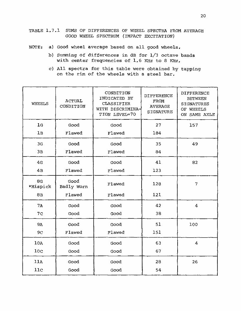
load, grease etc., the basis of this test was a comparison
of spectra from wheels at either end of axle. Figure 1.8.1
shows the train consist in the test. Identical impacters
were installed on the two rails, one train length apart.
There were two defective wheels. Wheel N15 had a larger thermal
crack and wheel S12, a shattered rim. The train was run
forward and backward in successive runs and the sound
tape recorded for laboratory processing.
Figure 1.8.2 shows typical printout using cross axle
comparison with third octave band analysis. Car 5 is the
engine. The numbers in the column labelled "Across Axle
Comparison" are the sums of the algebraic differences in
third octave band spectra of the two wheels. The decision
that a wheel is bad is based upon this number exceeding 10.
1.9 Objectives of the Present study
It was concluded from the feasibility study that it
should be possible to use acoustic signature inspection
for detection of thermal and plate cracks in railroad
wheels. It appeared that the best form of excitation for
detecting cracks is by impact and that the best sensor
is a microphone. The cracks cause shifts in resonance
frequencies and these shifts can be observed best in narrow
band analysis but are also manifest in third octave band
analysis. Grease layers cause damping of resonance lines
above about 5 kHz. Recognition of defective wheels can
be carried out by comparing sound spectra with a standard
or by comparing the sound spectra of wheels on either end
of an axle.
EA
ST
to-.
IMP
AC
TE
RI..
¢J
WW
ES
T
*NIM
PAC
TE
R
S<P
'\t
EI
t
.E{#
22
99
)1
IE
NG
IN
II
§N
I)
""."
,51
\I
IN
2S
2I
MW
~~4
64
64
0
~.
~R
EC
OR
DE
R
53
\1I
N4
54
I
IN
5
]",,
,""::I
:1
N6
MW
~~4
65
55
3
IN7
5711
INS
saf
IN
91
HO
PPE
RC
AR
5911
JN
rQM
W
SP
46
512
8
SJO
.l
IN
ilIW
511II
IN
il--
Sll
I
"''']
GO
ND
OL
AC
AR
51
>I
IN
I4I
IW
SP
3011
17
51
4I
tN
J5*
51
5I
IN
IGt
51
6I
l·-~·_·_---
----
----
----
--1
11
1A
VE
RA
GE
SP
EC
TR
UM
CO
HP
AA
ISO
N'
IA
CR
OS
SI
II
CAR
IA
XLE
1-----------------1
-----------------1
AX
LE1
DE
CIS
ION
l1
I1
TIR
ST
SID
EI
SE
CO
ND
SID
E1
CO
MP
.I
1
I---
----
----
----
----
----
----
----
----
----
----
----
----
----
----
----
----
(1
I1
11
34.
I2
41
BI
G0
0D
I1
1I
2t
111
20
I11
IBA
D1
11
I3
16
16
I4.
1G
e0D
11
II
4.I
9I
61
31
G0
eDI
I---
----
----
----
----
----
----
----
----
-~--
----
----
----
----
----
----
----
1I
2I
1I
6I
4.1
12.
1B
AD
II
21
2I
I1
1I
71
G0
eD1
I2
I3
I13
12
I04
1G
0"0
II
2I
I/ot"
11
12
1G
00
01
1---
----
---
---.-
----
----
-1I
J1
lI
11G
Il
IG
0eD
[I
JI
2I"
I3
13
IG
00
0I
t3
I:)
11
I1
I1
0I
Gee
DI
I:)
I4
I"
I2
II
IG
eeD
1
J---
----
----
----
----
----
----
----
----
----
----
----
----
----
----
----
----
1I
4;
II
I3
I1
I7
IG
00
DI
14.
I2
I3
1"
16
1G
00
DI
I4
I:)
II
I"
I2
1G
00D
I1
41
4I
2I
"t
41
Ge0
DI
1--------------------------------------------------------·-
---------1
I5
I1
I2
I"
I1
IG
00D
II
5I
2I
2I
15
I1
0I
G0
00
1I
5I:)
12
I:)
I1
IG
e0D
II
51
4.I
13
I5
I:)
IG
eGD
I
t---
----
----
----
----
----
----
----
----
----
----
----
----
----
----
----
----
1.
,
-1 "j MW
{
IW
-* -{
\E
NG
INE
WH
EE
LS
40
",A
LL
OT
HE
R3
3"
MW~MUlTrwEAR
IW::
SIN
GlE
WE
AR
*B
AD
WH
EE
LS
IG
RE
AS
YW
HE
EL
S
FIG
.1
.8.2
CO
MPU
TER
OU
TPU
TFO
RA
NEA
STB
OU
ND
RU
NA
T6
MPH
.R
EL
IAB
ILIT
YW
AS
lOO
Vo.
EN
GIN
EIS
CA
R5
.D
EC
ISIO
NL
IMIT
IS1
1.
tv tv
FIG
.1
.8.1
TR
AIN
CO
NSI
STFO
RSE
CO
ND
TE
ST
23
It was with this background that the present project
was formulated. The overall objective was to obtain infor
mation on the parameters that might affect or limit the
performance of an acoustic signature inspection in actual
operation, as opposed to laboratory operation or operation
in controlled field tests. To achieve this end the program
was divided into three parts: first, to improve and expand
scientific knowledge of the wheel's acoustic signatures~
second, to improve the design of various system compo
nents~ third, to test the improved system for an extended
period under actual operating conditions.
Regarding the first part of the program, improvement
of scientific knowledge, both experimental and theoretical
studies were planned. The intention was to obtain a
better grasp of the effect on signatures of wheel geometry,
wheel wear, the wheel's internal state of stress, and
various environmental conditions. Some of these studies
were carried out at the DOT's Transportation Test Center
at Pueblo, Colorado, some at the Griffin Wheel Company's
plant at Bessemer, Alabama, and some at the Westinghouse
plant at Wilmerding, Pennsylvania. It was decided to
extend the theory of wheel vibrations to gain additional
insight into the effects of a) variations in wheel geometry,
b) variations in crack sizes and locations, c) various forc
ing functions and d) variation in internal stress.
Under the second part of the program, improvements
in system component design, there were several major
24
developments. Firstly, the design of the excitation
mechanism was sUbjected to some scrutiny, with a view to
improving its reliability and operating speed range. The
second major change was the acquisition of a narrow band
RTA, its interfacing with the existing NOVA computer and
the addition and interfacing of a diskette memory unit.
Finally, reliable commercially made microphones and wheel
sensors were acquired.
The final system test, the third part of the program,
was carried out at the Southern Pacific's Englewood Yard
in Houston. The objectives of this test were to elucidate
remaining problems with the system and to ascertain, if
possible, information on false alarm rates.
The study was concluded with a sensitivity analysis
of the data recorded during the field tests. System problems
were elucidated, an optimum form of the difference index
(Dr) equation was ascertained and the major cause of high
Dr values in uncracked wheels was determined.
25
2. THEORY OF RAILROAD WHEEL VIBRATIONS
2.1 Introduction
A brief summary of previous work on wheel vibrations
was presented in Section 1. In these earlier studies a
number of elementary models were considered and commercially
available computer programs were used to simulate the
vibrations of good and defective wheels. The cross section
of a typical railroad wheel is shown in Figure 2.1.1.
Ring or circular plate models are the simplest approxima
tions that can be used. In the feasibility study of flaw
detection in wheels using acoustic signatures, Nagy modeled
the one-fourth scale model wheels and later full size
wheels as flat annular plates. He also reviewed the
literature on these subjects and concluded that the ring
model gave a better fit to wheel data. The most accurate
theoretical approach is to analyze the actual wheel
geometry using finite element analysis. Nagy used the
ANSYS program to study the vibrations of a good 33-inch
wheel and compared those with the response of a defective
wheel having a plate crack. His work was extended later
by Chaudhari who studied the vibrations of wheels with
different types and sizes of cracks, applying single or
repetitive impulse excitation. Chaudhari's work improved
on Nagy's by using more elements and more realistic
boundary conditions. (The wheels were fixed at the hub and

ACTUAL WHEELCROSS SECTION
h
AS SlJ"ED WHEEL --,CROSS SECTI ONFOR FLAT PLATEt'ODEL
I Jz ---1-..
,
I
26
ASSiJ"ED WHEELCROSS SECTIONFOR RING MODEL
WHERE; s- 16.5"b- 4.12"r= 15.92"_ 5.75"h- 1. 2"Hm 1.21t
r a
Fig. 2.1.1 Assumed and Actual Wheel Cross Sections
27
in addition at one node on the tread to simulate the con-
tact of the wheel with the rail.) An abbreviated version
of Chaudhari's work is presented in Appendix F.
Although the finite element approach is ultimately
the most accurate it is expensive and time consuming.
The more elementary models, especially Stappenbeck's [17]
ring theory, can be used to gain an insight into certain
effects, as explained in later sections, with comparative
ease.
2.2 Stappenbeck's Rinq Model of Wheel Vibrations
Stappenbeck [17] showed that the well known theory
of the vibrations of rings could give a good explanation
of the sounds emitted by a vibrating railroad wheel. To
see why this is so it is appropriate to review his reason-
ing. The vibration of rings was first treated in 1890
by Mitchell [52], as an extension of the theory of bars,
by regarding the ring as a curved bar whose two ends are
joined together. Flexural modes of vibration, with
displacements either in the plane of the ring or out of
the plane, are the most readily excited.
For out-of-p1ane flexure the resonant frequencies
are given by:
where
2 2 2] 1/2n (n - 1) f2 or
(n + 1 + v)n=l,2,3, .. (2.2.1)
28
E = Young's modulus
A = the cross sectional area,
I = the moment of inertia of cross section wi -thx
respect to an axis in the plane of the ring,
r = the radius of the ring,
\! = Poisson's ratio,
n = the ratio of the number of wavelengths to the
circumference,
and p = the density of the ring.
It should be noted that the case for n = 1 yields a zero
resonant frequency. This is not a vibrational mode and the
motion consists of a free rotation about a diameter. The
lowest vibrational mode occurs when n = 2, in which case
there are four nodal points on the ring.
Now consider the addition of a thin circular plate
within the ring. Again, in the case of a plate, the most
readily excited modes are flexural. Thus when the coupling
of ring and plate modes is considered, it may be seen that
the out-of-plane flexure of the ring will readily couple
with plate modes having an integral number of nodal dia-
meters. Because the wheel rim is massive in comparison
to the plate this was the model Stappenback proposed for
the vibrations of the wheel and he demonstrated that the
sound radiated from 765 mm diameter streetcar wheels con
tained a series of prominent resonances whose frequency
ratios corresponded closely to values obtained from
eqn (2. 2. 1) . (Assuming the fundamental mode occurs
when n = 2, the ratios of the frequencies of the higher
order modes to the fundamental are 2.87, 5.53, 8.98,

29
13.2, .... for n = 3, 4, 5, 6, .... respectively). with
this viewpoint in mind the massive rim forces the plate
into vibration, and the plate is then the primary sound
source because of its larger radiating surface. An alter
native model, in which the plate forces the rim into vibration,
was investigated by Nagy [1]. The ratios of the prominent
resonance frequencies did not fit the experimental results.
The conclusion is then that the prominent resonances
in the acoustic spectrum are due to wheel modes with two,
three, four or more nodal diameters. This does not imply
that other modes of vibration canno~ be excited. Indeed
the author has been able to excite the wheel in a vibratory
mode with a single nodal diameter. (The hub of the wheel
rrovides a stiffness for this mode which would not exi,-,t
for an unconstrained plate.) Such a mode is also revealed
by thE, finite element analysis. Numerical results for EUef.
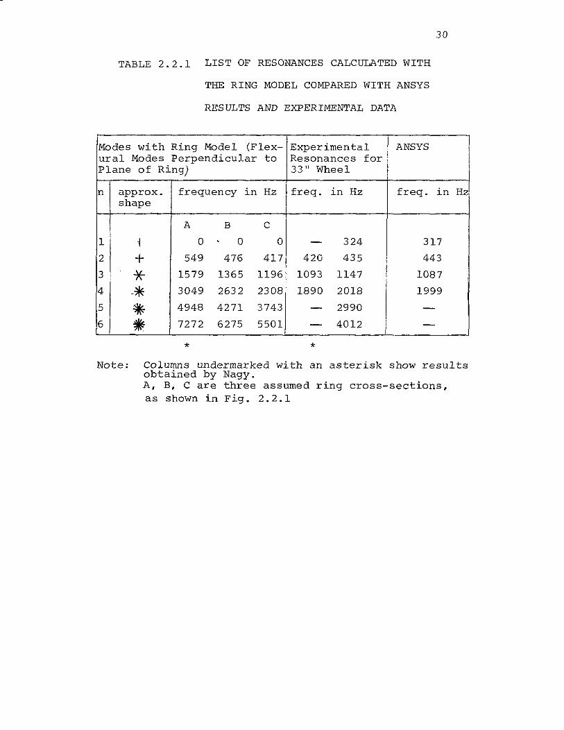
experiments are shown in Table 2.2.1. ThE> two columns
showing the experimental results are for two different
types of 33-inch wheel. The left'-hand column corresponds
to a wheel having the sarr\e cross-section as in Fig. 2.1.1,
and the right"'hand column corresponds to a 33-inch Griffin
wheel having cross section as in Fig. 4.2.1. Three
variations of calculations using the ring model are
given. In column A the results are those given by Nagy.
An attempt to improve these results was made by modeling
the wheel as a ring with cross section identical to the
30
TABLE 2.2.1 LIST OF RESONANCES CALCULATED WITH
THE RING MODEL COMPARED WITH ANSYS
RESULTS AND EXPERIMENTAL DATA
Modes with Ring Model (Flex- Experimental ANSYSural Modes Perpendicular to Resonances forPlane of Ring) 33" Wheel
n approx. frequency in Hz freq. in Hz freq. in Hz,shape
A B C:
1 i 0 . 0 0 - 324 317
2 + 549 476 417 420 435 443
3 ! * 1579 1365 1196 1093 1147 1087
4 -* 3049 2632 2308 1890 2018 1999
5
'*"4948 4271 3743 - 2990 -
6 ~ 7272 6275 5501 4012i- I -
* *Note: Columns undermarked with an asterisk show results
obtained by Nagy.A, B, C are three assumed ring cross-sections,as shown in Fig. 2.2.1
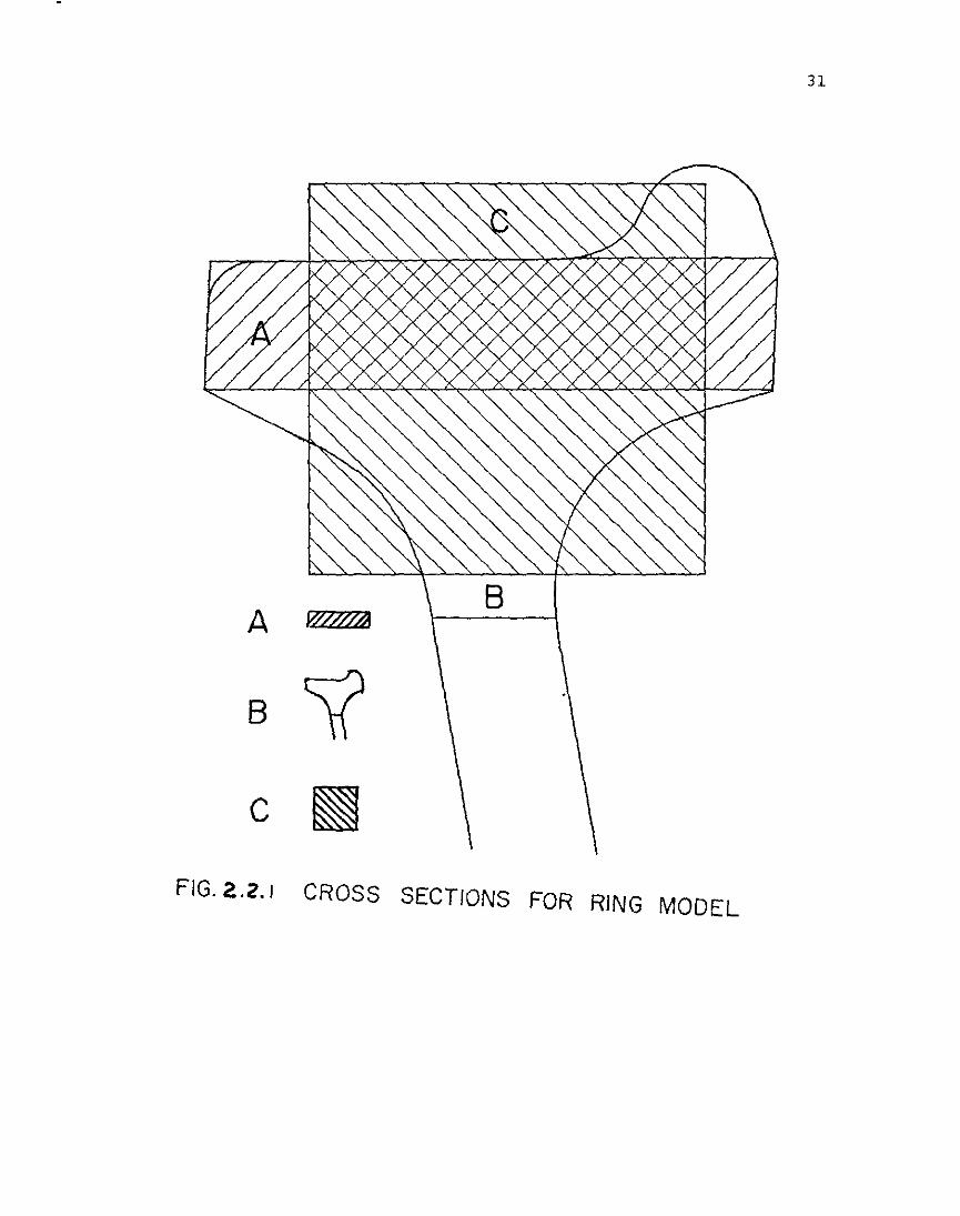
31
A W///4lB
c
B
FIG. 2..Z. J CROSS SECTIONS FOR RING MODEL
32
rim. The radius of the ring was estimated after evaluating
the centroid of the cross section by numerical-graphic
integration. The area moment of ine rtia about the neutral
axis was evaluated in a similar way. The results, shown in
column B, are a much closer fit to experimental measurements
than obtained from the rectangular cross section (see
Fig. 2.2.1) model used by Nagy. Even better results are
obtained using an "equivalent" square cross section. The
optimum selection was a 4" x 4" cross section with cor
responding radius of 15.1". The mode evaluation based on
this model shows almost identical frequencies for the
two nodal diameter mode and reasonable correspondence with
experiment for the other nodal diameter modes. Comparison
with the results from the ANSYS program also shows good
agreement. The major point to be made is that Stappenbeck's
ring mOdel is a surprisingly good predictor of the prominent
resonances of the acoustic spectrum of actual wheels.
2.3 The Effect of Uneven Wear on Wheels Across the Axle
A theoretical explanation of the effect of uneven wear
can be given in terms of Stappenbeck's simple theory of
wheel vibrations. The series of resonant frequencies
is given by the expression (2.2.1). It is clear that
uneven wear on a wheel pair will result in differences
for Ix' A and r for the two wheels. Rewriting eqn. (2.2.1)
to break out these factors, which are related to the wheel
geometry, we have:
33
or
[
I J1/2l 2 2 2] 1/2f ~ B ~ n (n - 1)n 4 2Ar n + 1 + v
where B is a constant dependent on the material properties
of the wheel. We shall assume that these properties are
unaffected by wear. Assuming that the rim can be modelled
as a ring of rectangular cross section (see Fig. 2.2.1),
with width wand thickness h,
A ~ hw
and
Hence,
fn ~
2 2 2J 1/2B w n en - 1)
~ 112 ~2 n 2 + 1 + v(2.3.1)
The effect of wear will be to reduce the effective radius
r, but not the rim width w. Hence the change in frequency
of the nth mode will be:
1M
1= 11L [n 2 (n2
- 1)~ll/2wflrn /f2 ~2 + 1 + v j r 3
= (2 fir) fr n
Finally, since a change in the effective radius is
approximately one half of a change in rim thickness, lIh,
for small changes,
(2.3.2)
34
Thus, for a given wheelset, a difference in wear on the
two wheels, in the amount ~h, should result in frequency
shifts proportional to the resonant frequencies. Experi-
mental results which are in agreement with this finding, to
a first approximation, are given in Section 7.
2.4 The Effect of Residual Stress*
The current interest in residual stress and its
influence on the creation and propagation of cracks in wheels
can be seen from the number of recent papers on this topic.
Bray [18] cited 15 papers related to the SUbject at the
5th International Wheelset Conference in 1976. Wetenkamp
and Kipp [19] and Yavelak and Scott [53] have also given
papers on this subject recently.
The most general treatment of the dynamics of elastic
media under intial stress was given by Biot [20, 21] who
concluded that the presence of an initial stress tends to
modify the effective rigidity of the medium. In general,
tension tends to increase the rigidity, whereas compression
tends to decrease it. The result is a corresponding increase
or decrease in the frequency of the natural modes of a
finite body. There are a number of well known examples of
such effects, the vibrations of strings under tension and
rods under load being among the best known.
*The definition of residual stress in this context refersto the system of stresses which can exist in a body whenit is free from external forces, temperature aradients androtational motion. In the case of a wheel these stressesare located in manufacture and may be modified In serVlce.
35
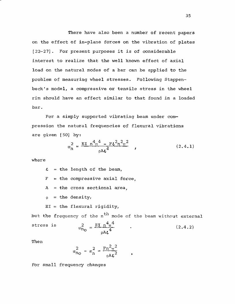
There have also been a number of recent papers
on the effect of in-plane forces on the vibration of plates
[22-27]. For present purposes it is of considerable
interest to realize that the well known effect of axial
load on the natural modes of a bar can be applied to the
problem of measuring wheel stresses. Following Stappen-
beck's model, a compressive or tensile stress in the wheel
rim should have an effect similar to that found in a loaded
bar.
For a simply supported vibrating beam under com-
pression the natural frequencies of flexural vibrations
are given [50] by:
where
, (2.4.1)
-L the length of the beam,
F = the compressive axial force,
A = the cross sectional area,
p = the density,
EI = the flexural rigidity,
but the frequency of the nth mode of the beam without external
stress is
Then
•
(2.4.2)
For small frequency changes

36
Thus
or
(2.4.3)
This result implies that the frequency shifts are the
same for all modes and are proportional to the applied
force. Since the ring model simply assumes that the rim
is a circular bar, flexural vibrations of wheels with uniform
compressive or tensile residual stresses in the rim should
show similar effects; i.e., if a uniform stress is induced in the
rim, all modes should show the same numerical change in
resonant frequency. Some experimental results which appear
to be consistent with this concept are presented in
Section 4.
37
3. EXPERIMENTS ON WHEEL GEOMETRY
AND MINIMUM DETECTABLE CRACK SIZE
3.1 Introduction
There were certain questions which could not be
readily answered from the theoretical study and it
was decided to tackle these by obtaining experimental
data. There were two main tasks in this work: firstly,
the compilation of a data bank of signatures of wheels
with different geometries and from various manufacturers, and
secondly, a study of the minimum detectable crack size.
3.2 Data Bank of Wheel Types
In brief, the idea behind this study was that the
acoustic signatures of all types of good wheels and the
signatures of all types of defective wheels might belong
in two different clusters and there might be no over
lapping in their characteristics. If this were the case
a decision scheme for flaw detection could be based on
the comparison of the signature of the wheel under test
with a set of good wheel signatures. If the signature
matched any of the good wheel signatures it would
be declared a good wheel of a certain type, and if
not, defective. A computer or other type of file that
has the signatures of all geometrical variations of good
wheels would house the data bank.
38
In order to develop the data bank. the Southern
Pacific Transportation Company provided a number of new
and used wheels for testing in their Houston repair shop
facilities. A total of 34 wheels were tested and 136
wheel signatures were obtained. The sample included
wheels of cast and wrought construction. having flat
and dished plate configurations. Single wear and multiple
wear rims were also encountered. The information acquired
was kept in a data bank book, in the form of a series of
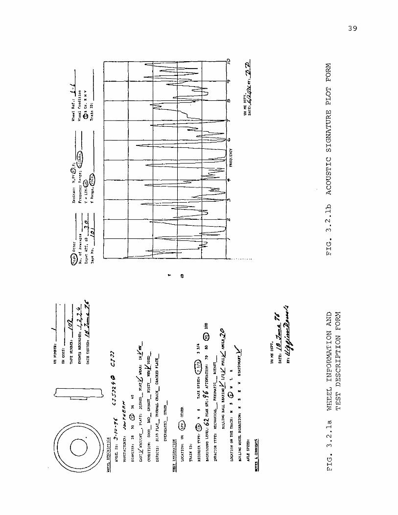
description sheets as shown in Fig. 3.2.1a, accompanied
by the signature plots. one of which is shown in Fig.
3.2.1b. For these tests an inclined guideway was
constructed (see Fig. 3.2.2) and was used as a path
guide for a 1.5 inch steel ball. Near the bottom end
of the incline a photosensor unit was installed to detect
the presence of the ball immediately before the impact.
The photosensor's signal was recorded on the triggering
pulse channel of a dual channel GR* recorder for later
acoustic signature analysis in the laboratory. The
design assured reproducible and constant force impact on
the lower inner rim of the wheel. Acoustic signature
tests were conducted on the wheels listed in Table 3.2.1.
3.3 Results from Data Bank Tests
About ten different types of wheels were tested
in the SP shops. Another 14 axles having good/good and
*General Radio
UHtn
JX1l
DI_-<
,_
UHCO
D!':
:,.
...,
-__
'rAPE~Dt
/02
tvn
I'T
Skl
CO
RD
tDl~~
OA
T!t~TEtlI
It!
.7.,.
...",
l'~
eO
thH
_
No.
ofAv~u.ges
In~ut
....n
.d
B--3
..2
tap
eN".
-l..t
2..l
Ex
e1te
r:~.PVe.R:=~
_F
req
uen
cyR
ange
;<
GIo
§)
_
Y•
LIS
/@)
1"RlInse,~,
_
Whe
elR
ef.
:1..:
:..1Y
hee
l;'
on
dl.
tio
n
c:!
:>8
Cr.
II.N
Vtr
ain
10
:_
lo'H
EI:l
..o!:SclUrnc~
DE
fEC
TS
:S
LID
rur_
l1lE
:RH
AL
CM
CIC
_C
RA
CU
Dp
u.r
r:_
OV
tRH
E.A
TE
!J_
O1
1lf
R_
<>~EQt;EllCY
NI
1/~
~.
l~y\
V
\~~~
V
1\I
2.3
..,
7A
~
f ..
CoT
:7:7
'jS.72~(;
\IIl
tEl.
fD::J~/()·1(
HA
HU
TAC
TUIlE
ll:./
"'"rl(~"""
Oll
lXE
TtR
:~8
30(l
tl36
~O
CA
ST
j{II
RO
IJG
IIT
_,P
LA
Tt:
DIS
HlD
_YL
AtZiIl
.A.R
:lW
.1("
,,_
CO
!QlIT
IOIf
:G
OO
Il_
!AD
_C
-.E
AS
T_
RU
ST
Y_
lfE
Wj(
US
lO_
TE
S'r
INFO
P_"',
ATI
ON
LO
C"n
C!!
1tm
@Q
T\l
.tt
TR
AIN
10
:
REC
OR
DER
TY
PIt
,@
M9
tAP
!S
PE
eD,@
3".
BACK
GRO
UN
DL
lVE
L:62
ptA
J(S
PL
:'16
A'fT
£N'U
AnO
M:
70
SO®
10
0
[KPA
CT
OR
TY
PE
'K
EC
HA
HIC
AL
_P
KE
IlX
A.T
lC_
RO
TA
R1
_
RO
L1.lW
C!A
LL
!!A
IlIN
GV
In.J
t..
nn.r.J:
::::M
fCU
..::l.
0
LOC
ATI
ON
ONT
IlEtt
AC
KI
If5
(i)
WL
R
ItOL
LIN
GW
ElL
DIU
CT
IOfl
I"
SI
WS
'IA
tto
tl.U
TY
AX
LES
PE
tD:
IlQ
T!:
!,
<:X
ltfllH
rS
t1HPI
En
ttT
.O"'TE'~~YI~
UH
Kt
DO
T.
DA
TEI
/8:I
t-4
74'
n,"'1
1'..../
h-
4
FIG
.3
.2.la
WH
EEL
INFO
RM
AT
ION
AN
DT
ES
TD
ES
CR
IPT
ION
FOR
MF
IG.
3.2
.1b
AC
OU
ST
ICSI
GN
AT
UR
EPL
OT
FOR
M
w \D
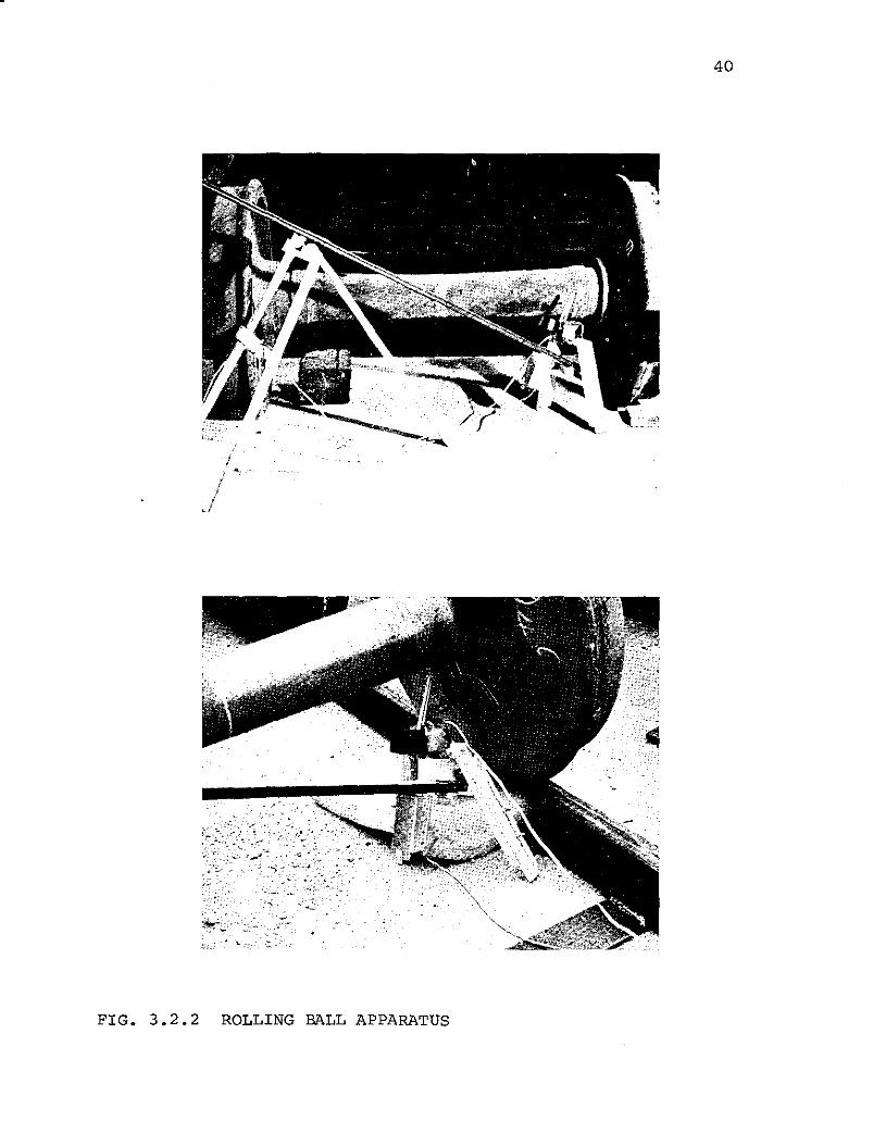
FIG. 3.2.2 ROLLING BALL APPARATUS
40
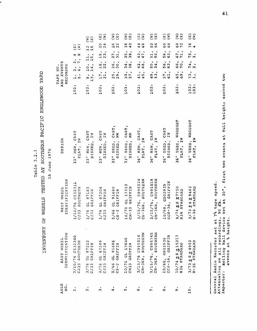
Tab
le3
.2.1
INV
EN
TO
RY
OF
WH
EELS
TE
STE
DA
TSO
UT
HE
RN
PA
CIF
ICEN
GLE
WO
OD
YA
RD
18
Ju
ne
19
76
TA
PE
NO
.A
XL
EE
AS
TW
HE
EL
WE
STW
HE
EL
DE
SIG
NA
ND
EV
EN
TS
NO
.ID
EN
TIF
ICA
TIO
NID
EN
TIF
ICA
TIO
NR
EC
OR
DE
D
l.
3/1
0/7
6C
53
23
40
3/1
0/7
6C
53
23
11
33
"N
EW
,C
AS
T1
02
,1
,2
,3
,4
(E)
CJ
3)
SO
UT
HE
RN
CJ
33
SO
UT
HE
RN
FL
AT
,IW
5,
6,
7,
8(W
)
2.
3/7
6G
L8
70
22
3/7
6G
L8
71
83
33
"N
EW
,C
AS
T1
02
:9
,1
0,
11
,1
2(W
lC
J33
GR
IFF
INC
J33
GR
IFF
IND
ISH
ED
,IW
13
,1
4,
15
,1
6(E
l
3.
3/7
6G
L6
72
49
3/7
6G
L8
72
04
33
"N
EW
,C
AS
T1
02
,1
7,
18
.1
9.
20(E
)C
J3
3G
RIF
FIN
CJ3
3G
RIF
FIN
DIS
HE
D,
IW2
1,
22
,2
3,
24
(Wl
4.
5/6
6G
L9
16
86
5/6
6G
L9
16
90
33
"U
SE
D,
CA
ST
,1
02
:2
5,
26
,2
7,
28
(W)
CS
-2G
RIF
FIN
CS
-2G
RIF
FIN
DIS
HE
D,
MW
29
,3
0,
31
,3
2(E
)
5.
10
/70
GL
17
64
61
0/7
0G
L1
75
22
33
"U
SE
D,
CA
ST
,1
02
,3
3,
34
,3
5,
36
(Wl
CM
33G
RIF
FIN
CM
-33
GR
IFF
IND
ISH
ED
,M
W3
7,
38
,3
9,
40
(El
6.
3/1
5/7
6C
99
55
14
3/1
5/7
6,
C9
95
52
43
6"
NE
W,
CA
ST
,1
02
,4
1,
42
,4
3.
44
(E)
CH
-36
B,
SOU
TH
ER
NC
H-3
6B
,SO
UT
HE
RN
FL
AT
,IW
45
,4
6,
47
,4
8(W
)
7.
3/1
5/7
6.
C9
95
74
53
/15
/76
,C
99
55
18
36
"N
EW
,C
AS
T1
02
,4
9,
50
,5
1,
52
(W)
eH-3
GB
,S
OU
TH
ER
NC
H-3
6B
,SO
UT
HE
RN
FL
AT
,IW
53
,5
4,
55
,5
6(E
)
8.
10
/68
,G
B0
29
36
10
/68
,G
B0
29
39
36
"U
SE
D,
CA
ST
10
2,
57
,5
8,
59
,6
0(E
lC
CH
-36
,G
RIF
FIN
CC
H-3
6,
GR
IFF
IND
ISH
ED
,IW
61
,6
2,
63
,6
4(W
l
9.
10
/74
;t.S
j;1
52
17
9/7
4j;
Sj;
77
50
36
"U
SE
D,
WR
OU
GH
T1
02
,6
5,
66
.,6
7,
68
(W)
H3
6ST
AN
DA
RD
H3
6ST
AN
DA
RD
FL
AT
,IW
69
,7
0,
71
,7
2(E
)
10
.3
/73
j;S
.t8
95
23
/73
.tS
j;9
48
23
6"
US
ED
,W
RO
UG
HT
10
2,
73
,7
4,
75
,7
6(E
lH
-36
STA
ND
AR
DH
-36
STA
ND
AR
DF
LA
T,
IW1
03
,1
.2
.3
,4
(Wl
Gen
era
lR
ad
ioR
eco
rd
er
set
at
7~
tap
esp
eed
.A
tten
ua
tio
no
na
llreco
rd
ing
s,
90
dB.
Imp
acto
r:
Ro
llin
gB
all
dev
ice
set
at
30
°,
fir
st
two
ev
en
tsa
tfu
llh
eig
ht;
seco
nd
two
ev
en
tsa
t7
heig
ht.
*"I-'
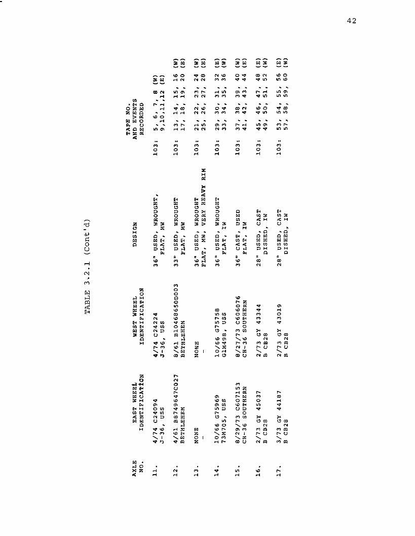
TA
BL
E3
.2.1
(Co
nt'
d)
TA
PE
NO
.A
XL
EE
AST
WH
EEL
WES
TW
HEE
LD
ES
IGN
AN
DE
VE
NT
SN
O.
IDE
NT
IFIC
AT
ioN
IDE
NT
IFIC
AT
ION
RE
CO
RD
ED
11
.4
/74
C2
40
94
4/7
4C
24
22
43
6"
US
ED
,W
RO
UG
HT
,1
03
,5
,6
,7
,8
(W)
J-3
6,
USS
J-3
6,
USS
FL
AT
,M
W9
,10
,11
,12
(E)
12
.4
/61
B8749647CO~7
8/6
1B
I04
68
65
0D
00
33
311
US
ED
,W
RO
UG
HT
10
3:
13
,1
4,
15
,1
6(W
)B
ET
HL
EH
EM
BE
TH
LE
HE
MF
LA
T,
MW
17
,1
8,
19
,2
0(E
)
13
.N
ON
EN
ON
E3
6"
US
ED
,W
RO
UG
HT
10
3,
21
,2
2,
23
,2
4(W
)F
LA
T,
MW
,V
ERY
HEA
VY
RIM
25
,2
6,
27
,2
8(E
)
14
.1
0/6
6G
75
96
91
0/6
6G
75
75
83
6"
US
ED
,W
RO
UG
HT
10
3,
29
,3
0,
31
,3
2(E
)7
3M
70
5,
USS
G1
M4
98
,U
SSF
LA
T,
IW3
3,
34
,3
5,
36
(W)
15
.8
/29
/73
C6
07
15
38
/27
/73
C6
06
07
63
6"
CA
ST
,U
SED
10
3:
37
,3
8,
39
,4
0(W
)C
H-3
6SO
UT
HE
RN
CH
-36
SOU
TH
ER
NF
LA
T,
IW4
1,
42
,4
3,
44
(E)
16
.2
/73
GY
45
03
72
/73
GY
43
34
42
811
US
ED
,C
AST
10
3:
45
,4
6,
47
,4
8(E
)B
CB
28B
CB
28D
ISH
ED
,IW
49
,5
0,
51
,5
2(W
)
17
.3
/73
GY4
41
87
2/7
3G
Y4
30
19
28
11U
SE
D,
CA
ST1
03
,5
3,
54
,5
5,
56
(E)
BC
B28
BC
B28
DIS
HE
D?
IW5
7,
58
,5
9,
60
(W)
*" '"
43
good/defective wheels were tested in the University
laboratory (hammer impact testing). The conclusions
from these tests were as follows:
a. The relative amplitude of the wheel resonances
depends on the magnitude of the impact.
b. The relative amplitude of the wheel resonances
depends on the direction of the impact.
c. Each type of wheel has a characteristic signature.
d. Signature changes with wear. An axle with wheels
whose flanges show different amounts of wear has
spectral differences mostly above 4 kHz (see
Fig. 3.3.1). The importance of this finding was
not completely appreciated at the time of the earlier
laboratory tests. After the field test it was
realized that differential wear is a major cause of
signature differences and further work on the
subject was performed (see Section 7).
e. The signature of a used worn wheel compared to
the signatures of standard new wheels may show
spectral differences of the same order as a cracked
wheel.
It was already known that load on wheels has some
effect on wheel signature, (see Fig. 1.6.6). Variations
with wear and load are enough to exclude the use of the
data bank as a classifier for the decision process in
field tests. Another important reason is the extremely
lengthy processing that would be necessary due to the

I ~ LLI
0 Z LLI a:: LLI
Ll-
LLI a:: ~ ~
30
a:: ~ iii a:: ~ ~
lD2
0"C
l - LLI
0 ;:)~ :J
10Q
.
:::E ~
WH
EE
LlO
A__
____
_W
HE
EL
10C
A "ft
"
",\
I
"
,,
I',
,,
,I
,,
I\
:~:
A':
,4"
I
"I
I"
",
"•
I'.
I,"
II•
,II
~"
III
"I
I,I
II
,I
I'
,I
',I
II
III
II
III
",
II
II
II
II
II
I"
I,
,I
II
II,
I\
II
II
,I
I1
II
I,
I,
II
II
II
II
I'
,,
I,
,, I
:;
IJ
I)
II
I,
II
I''I
f',
II
II
"I
II
,I
I\
IIII
"'
II
I,
I'\
II
'1/
•f
II
III
I,
II,
1\
,,
I'
II
II
III
,II
I
•I
II'
I.,,
I"
'I
~.
\,
.',
,,.
I,
,\.
I,
,I
I\
,,
,•
•
o/1
23
45
FRE
QU
EN
CY
6 (kH
z)7
-8
910
01> 01>
FIG
UR
E3
.3.1
SIG
NA
TU
RE
SO
FIM
PAC
TO
NTW
OW
HEE
LSO
NTH
ESA
ME
AX
LEW
ITH
UN
EVEN
LYW
ORN
FLA
NG
ES

45
large number of comparisons between the signature of an
unknown wheel type and the standard signatures. One
single comparison takes about 30 seconds, and there are
over 40 different types of wheel in use. It was concluded
that across the axle comparison is therefore the only
practical scheme.
3.4 Investigation of Minimum Detectable Crack Size
As mentioned earlier, one of the questions which
arose from the feasibility study was the issue of the
smallest crack that could be detected by signature analysis.
In Appendix F it is shown on a theoretical basis that a
single crack, not much larger than a dormant thermal
crack,willchange the signature slightly. The doubt
remained however as to whether an experimental system
would be capable of finding such a slight change.
Consequently it was decided to perform some experiments
to address this issue. As discussed in section 4
the critical crack length is at least one tenth of an inch. The
key question is therefore whether or not the system can
detect the presence of cracks of critical size. This
leads to the difficulty that there is little agreement on
what this size is. In practice cracked wheels are
removed from service when they are found by visual
inspection and thus it was decided to investigate wheel
sets with the smallest cracks discovered in this way.
46
Firstly, it was decided to investigate the
chances of finding thermal cracks. Some experiments
were performed on a 36" wheel and axle set. One of these
wheels had eight thermal cracks visible on the front
face of the rim and extending onto the treadfi.e., at
about the same location as that of the crack illustrated
in Fig. 1.2.1. No cracks were visible on the other wheel.
The experiments were performed using a 1.5" hard steel
ball bearing on the end of a 3 ft. pendulum string.
Analysis was performed in real time, using the third octave
band RTA*. At a given site on the wheel, five impacts
were made, the starting point of the pendulum's fall
being accurate to about 1 mm and the maximum overall
sound level of the impact being reproducible to about
1 dB. The RTA was set to read the maximum level in
each spectral band and these values were transferred to
the computer and stored after each impact. Two impact
sites on the good wheel were chosen, one on the front
face of the rim and one on the plate. The precisely
equivalent locations on the bad wheel were then impacted.
For each set of 5 impacts on the good wheel an average
spectrum was computed. Each of the individual spectra
for a given location on either wheel was then compared
with the appropriate good wheel average. The algebraic
sum of the deviations in dB in each spectral band was
then calculated. The results are shown in Table 3.4.1.
*RTA (Real Time Analyzer)
TABLE 3.4.1
RANGE OF DEVIATIONS FROM GOOD WHEEL SPECTRALAVERAGES IN EXPERIMENTS WITH THERMAL CRACKS
47
Run Good Wheel Bad WheelNumber
Flange Plate Flange PlateImpact Impact Impact Impact
1 200-500 300-800 1300-2800 700-1000
2 200-650 250-650 1100-2600 700-1400

48
The conclusion was reached that there was a definite
difference between the good and bad wheel spectra.
Some measurements were also made of decay times of
impact sound levels, but no significant differences
were found in that case.
These results indicate that the wheel with the
thermal cracks should be readily distinguished from its
mating wheel. The point should be made that the wheel
under test had a large number of cracks, although each
one is presumably not much greater than a square
inch in area. However, the occurrence of dormant
thermal cracks in such numbers on a wheel is probably
the normal way for such cracks to appear, so it was con
cluded that there is a good chance of detecting them
in the field.
It was also of some interest to know the smallest
plate crack which could be detected. Railroad repre
sentatives were asked for help to find a small plate
crack. The closest approximation that has come to our
attention so far is a wheelset where One wheel (UH
inventory number lSA) has a typical large plate crack as
shown in Fig. 3.4.1 and wheel lSC, its mate, has a crack
on the front plate near the hub (see Fig. 3.4.2a)
which is not visible on the back side of the plate
(see Fig. 3.4.2b). To be sure about the extent of the
crack, a liquid penetrant test was performed on the
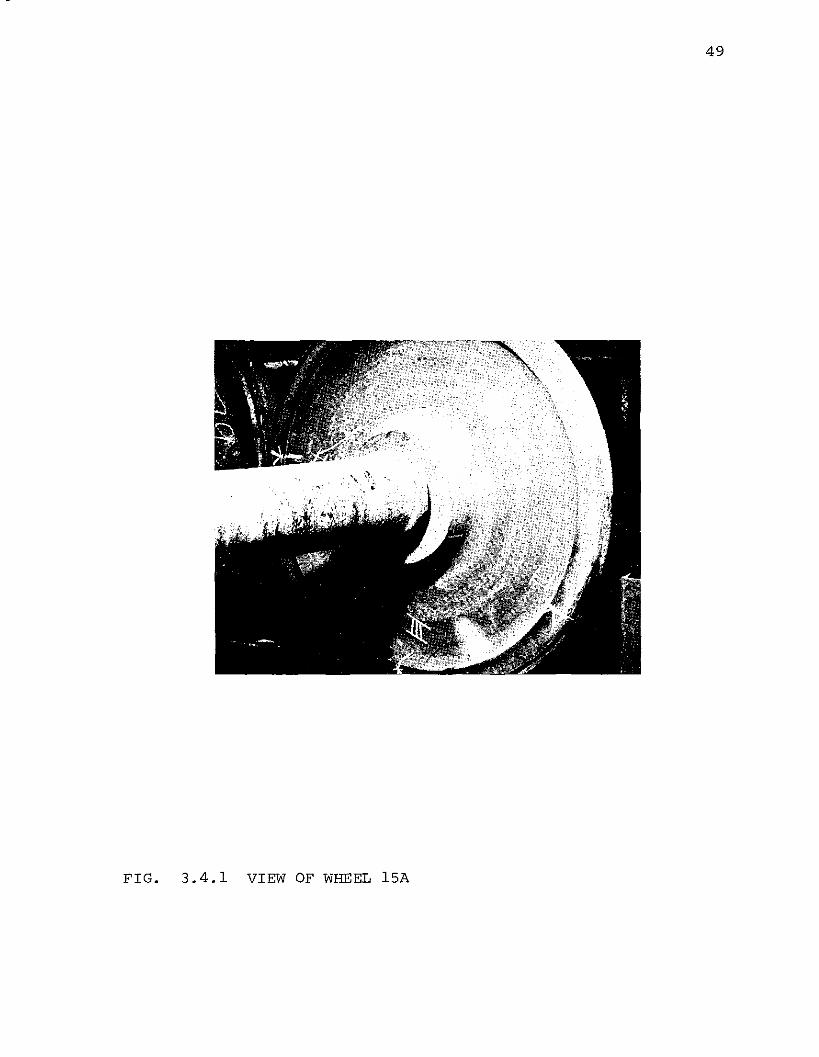
FIG. 3.4.1 VIEW OF WHEEL 15A
49
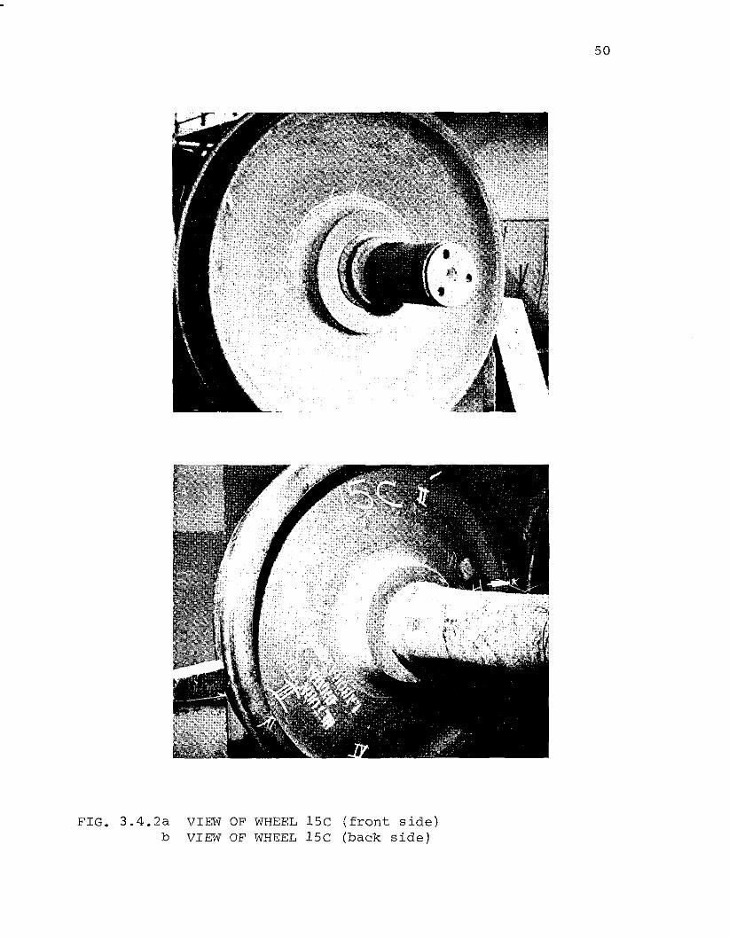
FIG. 3.4.2ab
VIEW OF WHEEL 15C (front side)VIEW OF WHEEL 15C (back side)
50
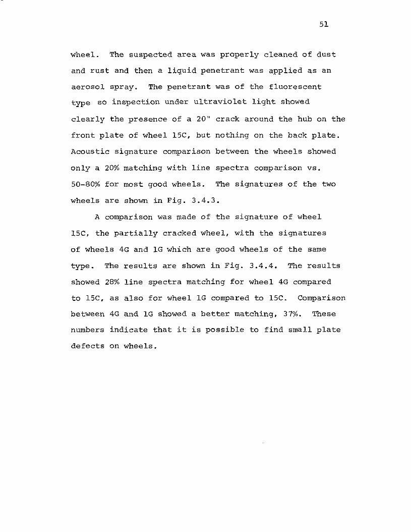
51
wheel. The suspected area was properly cleaned of dust
and rust and then a liquid penetrant was applied as an
aerosol spray. The penetrant was of the fluorescent
type so inspection under ultraviolet light showed
clearly the presence of a 20" crack around the hub on the
front plate of wheel l5C, but nothing on the back plate.
Acoustic signature comparison between the wheels showed
only a 20% matching with line spectra comparison vs.
50-80% for most good wheels. The signatures of the two
wheels are shown in Fig. 3.4.3.
A comparison was made of the signature of wheel
l5C, the partially cracked wheel, with the signatures
of wheels 4G and IG which are good wheels of the same
type. The results are shown in Fig. 3.4.4. The results
showed 28% line spectra matching for wheel 4G compared
to l5C, as also for wheel lG compared to l5C. Comparison
between 4G and IG showed a better matching, 37%. These
numbers indicate that it is possible to find small plate
defects on wheels.
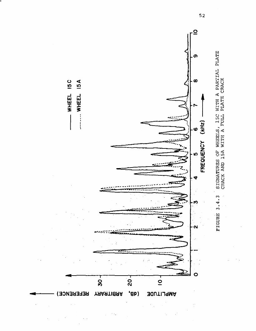
1 - UJ 0 Z UJ
Q:
UJ
lL.
UJ
Q:
~3
0cs: Q
:~ iii Q
: cs: •2
0CD "C
I - UJ
0 ::)~
10:J 0.
.:::E cs:
WH
EE
L15
C
.---
----
WH
EE
L15
A
-~ .. ..
," "
'..,
:',
.:,, "
,•
",
\,
I,
,•
•,
,,
,,
,,
,,
,,
-0
1•
,,
,•
•0
,,
•••
0,
,•
,.,
,,
•·,
,,
••
00
,:
,)
0,.
•,
0•
:,
•;
••
,•
,.
•0
•,
,0
,,
,,
•0
"·•
~,
•,
••
,•
•,
•f.
•,
•,
•-
•,
•,
,,
·I
\,
·-y'
0,
,l
,,
,•
•I
.:
••
0•
\~1
.,....
.,'~
'0
,"
~•
•0
•,
I'
ft0
,,..
:•
.,\.V
I.:•
••
.,"
••
00
0•
•:
,..
.:
...,
.,.
,•
·0..
''-J
..•
0
,~
4't
v,
•0
\!
.'W
0J
',
0,
o'•
•\~
V0
'.
,,.'I..
\,J,
'.....
....1•
\.'
~..
./
I~...~
....
...
OJ\t.
;•.
•.•.
.'~
..'
o2
34
5FR
EQUE
NCY
6(k
Hz)
7B
910
()l
IV
FIGU~E
3.4
.3SI
GN
AT
UR
ES
OF
WH
EE
LS,
15
CW
ITH
APA
RT
IAL
PLA
TE
CR
AC
KA
ND
15A
WIT
HA
FUL
LPL
AT
EC
RA
CK

53
Percentage of Matching Lines
15A
15C
20'/0
28"/0
/
15C
28"/0
o4G
37"/0
FIG. 3.4.4 SPECTRAL LINE COMPARISON TESTS BETWEEN A WHEELWITH A PARTIAL PLATE CRACK (15C), A WHEEL WITHA FULL PLATE CRACK (15A) AND TWO GOOD WHEELS OFTHE SAME TYPE (lG AND 4G)
54
4. RESIDUAL STRESS EVALUATION IN RAILROAD WHEELS
USING ACOUSTIC SIGNATURE ANALYSIS
4.1 Introduction
The residual stress in a wheel may be as important
in influencing wheel failure as the presence of an
incipient crack. The reason for this, in terms of fracture
mechanics, is apparent from the relationship
K = A (J c l / 2IC
where KIC is the fracture toughness parameter, a property
of the material. Carter and Caton [30] give values of KIC
ranging from 25 to 40 Ksi in l / 2 , depending on the wheel
class. A is a constant which Carter and Caton found to
vary from 0.9 to 1.98 for different crack locations.
(J is the applied tension needed to cause the crack to
grow and c is the surface length of the crack. Carter
and Caton quote 55 Ksi tensile stress as being representa-
tive of the peak of the stress generated during drag
braking and hence conclude that critical crack lengths
are a minimum of 0.1 inch for corner cracks in class U
wheels to 0.65 inch for surface cracks in class A wheels.
However it does not follow that such cracks will
cause a wheel to break. New wheels are manufactured with
a residual compressive stress in the rim, which is usually
in the range 20-25 Ksi according to Wandrisco and Dewez
[31] . The plate of a new wheel is in tension. Extended
periods of brake application can overheat the wheel and
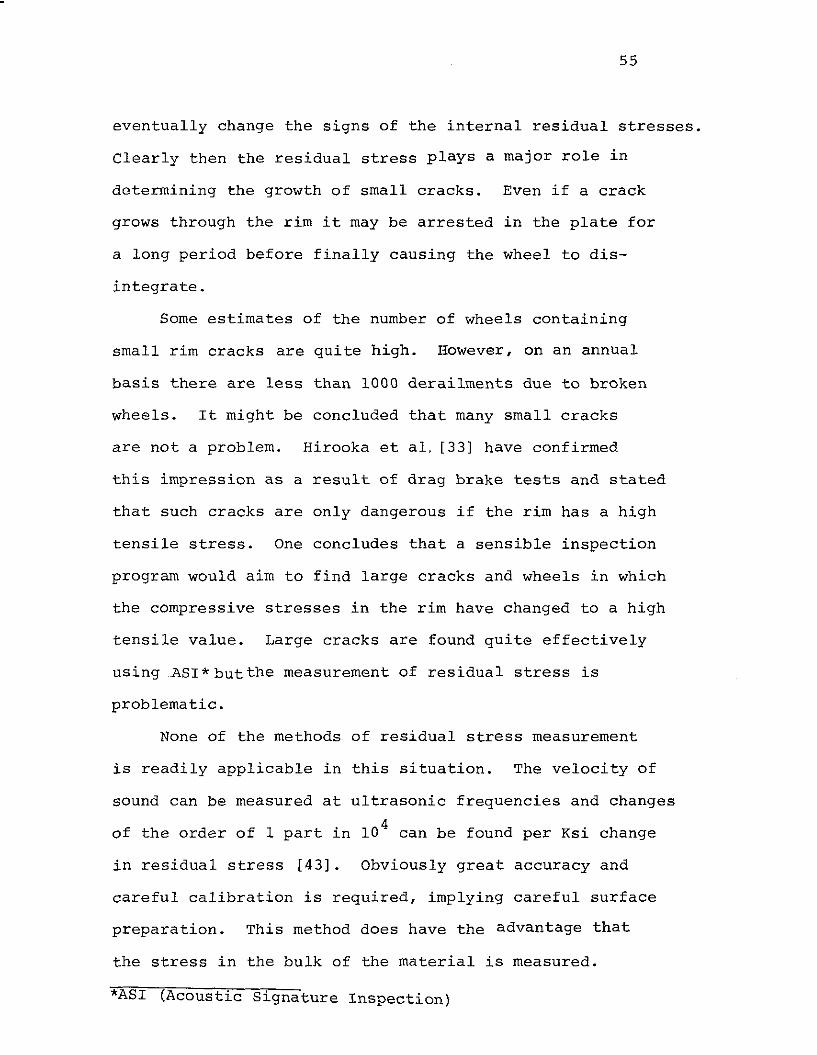
55
eventually change the signs of the internal residual stresses.
Clearly then the residual stress plays a major role in
determining the growth of small cracks. Even if a crack
grows through the rim it may be arrested in the plate for
a long period before finally causing the wheel to dis-
integrate.
Some estimates of the number of wheels containing
small rim cracks are quite high. However, on an annual
basis there are less than 1000 derailments due to broken
wheels. It might be concluded that many small cracks
are not a problem. Hirooka et aI, [33] have confirmed
this impression as a result of drag brake tests and stated
that such cracks are only dangerous if the rim has a high
tensile stress. One concludes that a sensible inspection
program would aim to find large cracks and wheels in which
the compressive stresses in the rim have changed to a high
tensile value. Large cracks are found quite effectively
using ASI*butthe measurement of residual stress is
problematic.
None of the methods of residual stress measurement
is readily applicable in this situation. The velocity of
sound can be measured at ultrasonic frequencies and changes
4of the order of 1 part in 10 can be found per Ksi change
in residual stress [43]. Obviously great accuracy and
careful calibration is required, implying careful surface
preparation. This method does have the advantage that
the stress in the bulk of the material is measured.
*ASI (Acoustic Signature Inspection)

56
X-rays can be used in evaluation of lattice dimensions in
homogeneous materials. Residual stresses can be deduced
by evaluating strain from lattice dimensions. The method
is restricted to surface stress-evaluation over a small
area and careful surface preparation is necessary [321.
Barkhausen noise can also be used in residual stress
evaluation [341. Again in this case the most obvious
limitation is surface preparation of the test material
and only surface stress evaluation can be made. In the
case of a wheel in service surface residual stresses on
the tread, front and back rim are different from the
"bulk" rim stresses due to braking action from retarders
and the high local loading on the tread of a rolling wheel.
The objective of the work reported here was to
investigate the possibility of using acoustic signatu~e
inspection to evaluate residual stress. The basic idea
is that applied stress changes the natural frequencies of
flexural vibrations in an object. The simplest example
is the change of the natural modes of a string under dif
ferent tension. For rigid bodies such as a beam, or column~
there is a well known theoretical treatment and experimental
evidence that the response changes with load, which has
to be allowed for in the design of chimney stacks and the
like. A similar effect occurs in the case of high speed
turbine blades where the frequencies of the natural modes
changes with speed. This question has been discussed in
Section 2.

57
Nagy [1] showed that changes in resonant frequencies
of wheels occurred under load. This gave rise to the idea
that change in residual stress might be detectable from
changes in resonant frequencies.
4.2 Test on Wheels with Different Heat Treatment in the
Griffin Wheel Manufacturing Plant at Bessemer, Alabama
A first attempt to study this problem was made in
the Griffin Wheel Manufacturing Plant at Bessemer, Alabama.
A variety of manufacturing treatments had been applied to
the wheels to generate a wide range of residual stresses.
Acoustic signatures were recorded from 33-and 36-inch
wheels that had normal treatment, and also from wheels
that had high internal tension stresses. The standard
procedure for measuring residual stresses is destructive
testing by saw cut described in the manual of standards
and recommended practices of the Association of American
Railroads (AAR) [36]. In ,Fig •. 4.2.1are shown the results
of strain test on a 33 inch one wear Griffin wheel. This
figure was obtained from the' car' and Locomotive
Cyclopedia [37].
All wheels tested were sitting on their hubs on a
concrete floor, so the plates and rims were free of contact.
The.following measurem~nt5 were taken~.
1. Hammer impacts on each wheel.
a. Ten impacts were made on three different points
on the circumference of the front rim of the
wheel. The relative location of the impact
points were approximately 120 0 apart.
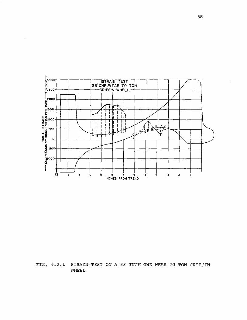
58
~ooo~~500I-
~OOO~,",500
~
~~OOOo:uI-Z"'- 500-,0<5oi<, 0O:z
ou; 500tl0:..~IOOOou
i
---,STRAIN- TEST-1 ----- --- -
1/33"ONE.WEAR 70· TONRtFFtNWHEEL
/- /Vi f ~
,..-(1 [ , I I I i) V, : [ : I I II
, [ I I I I I II V}!~,I,
I ! 1 I I I 11..........- 17 ,I I ,
"'-- i : I i 1 llJ,-1 I
~14 " NI "'"• T 6 5 A I\..
--- l.-----' "----1/
II
13 12 " 10 9 a 7 6 5'NCHES FROM TREAD
4
FIG. 4.2.1 STRAIN TEST ON A 33-INCH ONE WEAR 70 TON GRIFFINWHEEL

59
b. Five impacts on the plate, midway from the center
to the rim of the wheel.
c. Five impacts on the flange, along a radius.
For steps la, b, and c sound was detected by a
microphone. The hammer is shown in Fig. 4.2.2. This
design provides a triggering pulse simultaneously with
the impact. Signals were recorded on a dual channel
recorder.
2. Shaker excitation. In this series of tests a shaker
was used as an exciter and the vibrations were picked
up by a GR type 1560-P52 accelerometer. Input
signals were:
a. random noise,
and b. slowly sweeping sine signal from a Wavetek
Model 134 signal generator, in the range from
400 to 2000 Hz.
Most of the analyses were made from impact recordings.
The wheel manufacturing steps are as follows:
1. Pressure Pouring pit: Steel wheels are formed as
air pressure forces molten steel up from a sealed
chamber into graphite molds. A mold is filled in
20 seconds.
2. Wheel Transfer: Depending upon the metal temperature
at pouring, the wheel casting will solidify in five
to seven minutes. The cope (top) of the mold is
removed, and the wheel is lifted by the hub and
conveyed to the final finishing and inspection stations.
60
.~.
FIG. 4. 2. 2 VIEW OF THE HAMMER WITH A PZT DISK BETWEEN HAMMERAND CYLINDER TO PROVIDE THE TRIGGERING PULSE ONIMPACT WITH THE TEST OBJECT
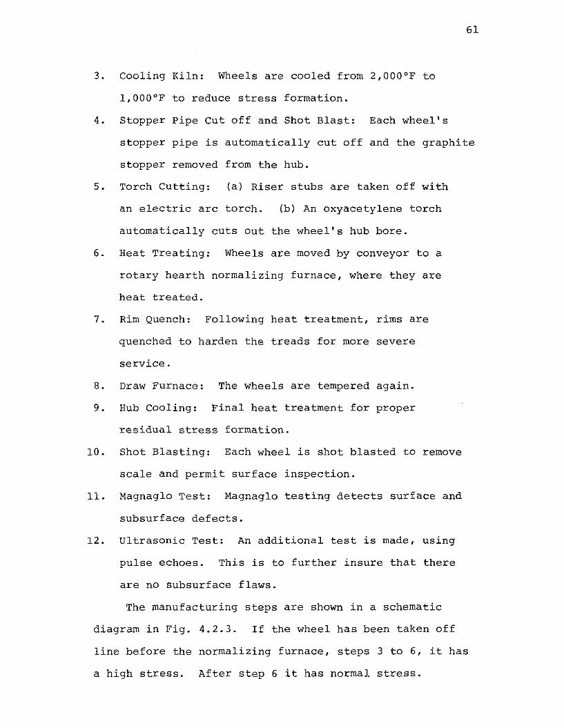
61
3. Cooling Kiln: Wheels are cooled from 2,000°F to
1,000oF to reduce stress formation.
4. Stopper Pipe Cut off and Shot Blast: Each wheel's
stopper pipe is automatically cut off and the graphite
stopper removed from the hub.
5. Torch Cutting: (a) Riser stubs are taken off with
an electric arc torch. (b) An oxyacetylene torch
automatically cuts out the wheel's hub bore.
6. Heat Treating: Wheels are moved by conveyor to a
rotary hearth normalizing furnace, where they are
heat treated.
7. Rim Quench: Following heat treatment, rims are
quenched to harden the treads for more severe
service.
8. Draw Furnace: The wheels are tempered again.
9. Hub Cooling: Final heat treatment for proper
residual stress formation.
10. Shot Blasting: Each wheel is shot blasted to remove
scale and permit surface inspection.
11. Magnaglo Test: Magnaglo testing detects surface and
subsurface defects.
12. Ultrasonic Test: An additional test is made, using
pulse echoes. This is to further insure that there
are no subsurface flaws.
The manufacturing steps are shown in a schematic
diagram in Fig. 4.2.3. If the wheel has been taken off
line before the normalizing furnace, steps 3 to 6, it has
a high stress. After step 6 it has normal stress.
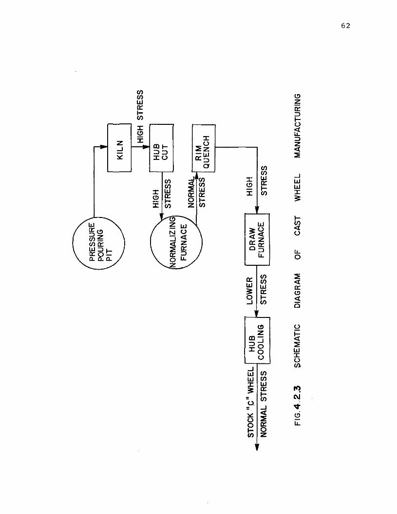
---I
PR
ES
SU
RE
'P
OU
RIN
G+
PIT
KIL
N HIG
H
HIG
HH
UB
NO
RM
ALI
ZIN
dS
TR
ES
SC
UT
FU
RN
AC
E;
NO
RM
AL
./
ST
RE
SS
RIM
QU
EN
CH
STO
CK
"e"W
HE
EL
HU
BLO
WE
RD
RA
WH
IGH
NO
RM
AL
ST
RE
SS
CO
OLI
NG
ST
RE
SS
FU
RN
AC
ES
TR
ES
S
ST
RE
SS
FIG
.4.2
.3S
CH
EM
AT
ICD
IAG
RA
MO
FC
AS
TW
HE
EL
MA
NU
FA
CT
UR
ING
Cl' '"

63
Between steps 7 and 8 it has high stress. After step 8
it has lower stress and after step 9 it has the normal
stress configuration. A list of wheels tested at the
Griffin Wheel Plant in Bessemer, Alabama is presented in
Table 4.2.1. The first column has the wheel identification,
type and number. The second column has the tape numbers
of tests as recorded. The third column has the
description of the manufacturing treatment and the last
column the estimated stress according to the treatment.
Preliminary results from comparisons between the
acoustic signatures of the wheels are listed in Table 4.2.2.
The difference index is based on a decision scheme which
is a combination of line spectra and sum of the differences
comparison between two spectra. There were only two
conflicting results out of 25 tests. In run No.5, the
Difference Index for high/normal stressed wheels is small.
In run No.9, although wheels CJ36 26 425 and CJ 36 26 171
had the same heat treatment, history, and structure, they have
a Difference Index of 10. One possible explanation is
the existence of small geometric differences indicated
by the rough surface appearance (the wheels were removed
from the line before step 4).
A detailed study of the acoustic signatures was made
using a spectrum translator to measure small shifts in
resonance frequencies. This instrument was used in con
junction with the SD330 RTA. The spectrum translator can
separate frequency bands from a spectrum and expand them,
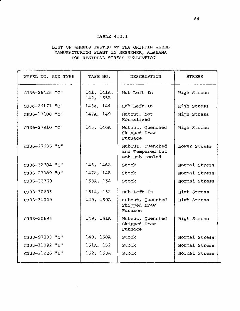
TABLE 4.2.1
LIST OF WHEELS TESTED AT THE GRIFFIN WHEELMANUFACTURING PLANT IN BESSEMER, ALABAMA
FOR RESIDUAL STRESS EVALUATION
64
WHEEL NO. AND TYPE TAPE NO. DESCRIPTION STRESS
CJ36-26425 II ell 141, 141A, Hub Left In High Stress142, 155A
CJ36-26171 "e" 143A, 144 Hub Left In High Stress
CH36-17180 II ell 147A, 149 Hubcut, Not High StressNormalized
CJ36-27910 "ell 145, 146A Hubcut, Quenched High StressSkipped DrawFurnace
CJ36-27636 II ell Hubcut, Quenched Lower Stressand Tempered butNot Hub Cooled
CJ36-32784 II ell 145, 146A Stock Normal Stress
CJ36-23089 "U ll 147A, 148 Stock Normal Stress
CJ36-32769 153A, 154 Stock Normal Stress
CJ33-30695 151A, 152 Hub Left In High Stress
CJ33-31029 149, 150A Hubcut, Quenched High StressSkipped DrawFurnace
CJ33-30695 149, 151A Hubcut, Quenched High StressSkipped DrawFurnace
CJ33-97803 II ell 149, 150A Stock Normal Stress
CJ33-11092 "U" 151A, 152 Stock Normal Stress
CJ33-21226 IIUII 152, 153A stock Normal Stress
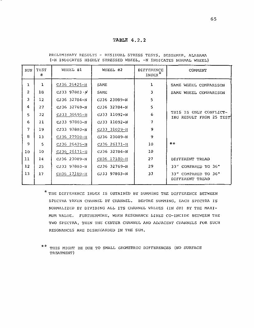
65
TABLE 4.2.2
PRI:[,HIlNI\RY RESULTS - HESIIJUI\L STRESS n;STS, DESSEMER, I\LI\lllIMI\(-Ii INlJlCATES IllGIILY STRESSED WHEEL, -N INDICATES NOIU>II\L WHEEL)
RUN TEST WHEEL #1 WHEEL #2 DIFFEltEtlCE COMMENT# INDEX*
1 1 C~J 36 2(,425-11 SAME 1 SAME WIIEEL COIWJ\IUSON
2 18 CJ33 97803-{'J SAME 3 SJ\ME WHEEL CQMPAIUSON
3 12 CJ36 32784-N CJ36 23089-N 5
4 27 CJ36 32769-N CJ36 32784-N 5
5 22 CJ33 JO()9S-11 CJ33 1l092-N 6TillS IS ONLY CONFLICT-ING RESULT FROM 25 TEST
6 21 CJ33 97003-N CJ33 1l092-N 7
7 19 CJ33 97803-N CJ33 31029-11 9
8 13 eT36 27910-1l CJ36 23089-N 9
9 5 CJ36 26~25-11 CJ36 26171-11 10 **
10 10 CJ36 26171-11 CJ36 32704-N 10
II 14 CJ36 23089-N C1I36 17180-11 27 DIfFERENT TREIID
12 25 CJ33 97803-N CJ36 32769-N 29 33'1 COMPARED TO 36"
13 17 CII36 17100-11 CJ33 97803-N 33 33" COMI'AHED TO 36"DIfFERENT TREIID
* TilE DIFFEHENCE INlJEX IS OBTAINED BY SUI1MING TIlE DIffERENCE BETWEEN
SPECTRA TAKEN ClllltlNEL IlY CIIJ\NNEL. IlEFORE SUMMING, EI\CH SPECTRA IS
NOIU>ll\LIZED DY DIVIDING ALL ITS CHANNEL VALUES (III dB) BY TilE MAXI
MUM VAI>UE. FURTm;RMORE, WilEN RESONANCE LINES C0-INCIDE BETWEEN TilE
TWO SI'ECTltJI, Til EN TIlE CENTER CIIIINNEL AND ADJACENT CIIIINNI:;LS FUR SUCII
RESONANCES AHE DISREGIIRDI:;D IN TIlE SUM.
** THIS MIGHT BE DUE TO SMALL GEOMETRIC DIFFERENCES (NO SURFACETREATMENT)
66
thus improving the frequency resolution. In the range
of 10 kHz the analyzer has a 40 Hz resolution. With the
spectrum translator, translated bands had a 100 Hz range
and 0.4 Hz resolution. In the range of 10 kHz the sampling
period is 50 ms, for the 100 Hz range it is 2500 ms, hence
only slowly decaying signals (resonances) can be analyzed.
With the use of a spectrum translator significant dif
ferences in the resonant frequencies were revealed.
Spectral plots were obtained for most of the strong wheel
resonances. An example is shown in Fig. 4.2.4. The
resonances of the normally stressed wheels were separated
from those of the highly stressed wheels by more than
8 Hz. The estimated frequency shift for those resonances
due to geometrical tolerance in manufacturing is I Hz.
A list of the measurements taken is presented in
Table D.I in Appendix D.l. The results are also shown in
Fig. 4.2.5 for CJ36 type wheels and in Fig. 4.2.6 for CJ33
type wheels. These are rather unusual presentations and
some explanation is needed. The points on the plot repre
sent resonant frequencies. All the points lie on lines
parallel to the Y axis. For example, the line AA' in
Fig. 4.2.5 has the resonances of the CJ36 type wheels near
390 Hz. Dots represent resonances of normally stressed
wheels and asterisks represent highly stressed wheels. At each
wheel resonance, the value for the normally stressed wheel
was set on the X-axis. The intersection of AA' and the
x-axis represents the resonance of the wheel CJ 36 32784
at 390.8 Hz. The rest of the indications on AA' show the

---.--
-----
f\ II.
NO
RM
AL
ST
RE
SS
(24
65
.6H
z)-------
NO
RM
AL
ST
RE
SS
(24
68
.8H
z)-'--'
NO
RM
AL
ST
RE
SS
(24
70
.0H
z)
---H
IG
HS
TR
ES
S{2
47
8.8
Hzl
......
......
.....
HIG
HS
TR
ES
S(H
UB
IN-
24
83
.2H
z)
0'
-.J
...... 102
50
0H
z9
8A~
I'
::
I\q
I\
~~
nlll
!L~
...
\,~'
I:
:/.
...,
\\
i:!
.
7A ii ii ii ii ji !i Ii hi
,..
,II
I'.
,r,I
'i'i
'I.
'iII~
'.I
i;i
"I
I'
t.I
\\
.-",
.
45
6F
RE
QU
EN
CY
(Hz)
..
32
t - !oJ U Z !oJ
lr !oJ "- !oJ
30
lr >- lr c:(
lr ... iii2
0lr c:
( .CD ".- !o
J10
0 :::> ... :J Il. :::E c:(
o1
/..-
....
....
•
24
00
Hz
FIG
UR
E4
.2.4
SPE
CT
RA
PLO
TS
FOR
CJ3
6W
HEE
LSW
ITH
DIF
FE
RE
NT
INT
ER
NA
LS
TR
ES
SD
IST
RIB
UT
ION
,B
ETW
EEN
24
00
an
d2
50
0H
z

68
10
5
-N:I:~
Q)0uc
Q)~Q)........i5
-5>.ucQ)::I17Q)~
II..
-10
-/5
A'
f~
! f •• ~ ~ ,I
i~ F r
t 1-4
rl
tA
I 2 3 4 5
Resonant Frequency (kHz)
FIG.4.2.5 DIFFERENCES IN RESONANT FREQUENCY FOR CJ36WHEELS• NORMALLY STRESSED WHEELS;lIE HIGHLY STRESSED WHEELS
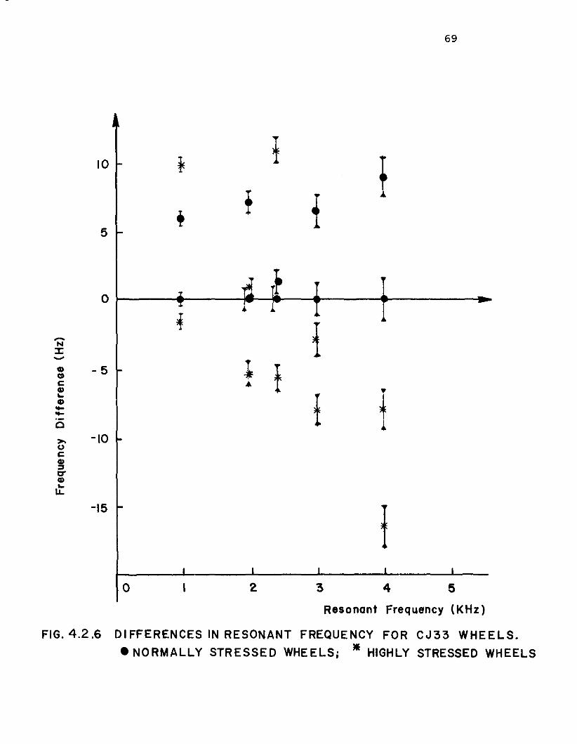
10 I-
5 - +
69
~ ~ r0 y ~.
1~
N:J:-- fCD -5 l- t«:I)
cCD ,....
+CD--0 J.,.. -10 I-0cCD:;,0-CD...\.L
-15 l-
fI I I I I
0 2 3 4 5
Resonant Frequency (KHz)
FIG. 4.2.6 01 FFERENCES IN RESONANT FREQUENCY FOR CJ33 WHEELS.
• NORMALLY STRESSED WHEELS; " HIGHLY STRESSED WHEELS
70
frequency deviation from that value of the corresponding
resonance for other wheels in Hz. Positive deviations
correspond to resonances above 390.8 Hz and negative
deviations to lower values. In some cases the resonance
of a highly stressed wheel lies among the resonances of
the normally stressed wheels, but in other cases it is
above or below. Thus, although the shift may be to higher
or lower frequencies, in general there is a separation
between the resonances of normally and highly stressed
wheels. Hence a known type of wheel with unknown stress
could be checked for stress distribution by comparing a
few small portions of its signature with the same signature
portions of normally stressed wheels. These frequency
shifts could conceivably be due to variations in the
geometry of the wheels because of dimensional tolerances.
For this reason it was decided to estimate frequency
shifts due to extreme variations in the dimensional
tolerances.
The manufacturing error for a 36" wheel is about 5 lb
or about 0.5% in weight; hence the volume error, £v,is
also 0.5%
i. e. £ = 0.5%.v
Approximating the wheel to a disk, the volume of the
wheels is
2v = 1Tr h.
Differentiating (4.2.2)
(4.2.1)
(4.2.2)
71
dv = 2rrrhdr + rrr2dh,
or,
dvv
2rrrh=rrr 2h
dr + dh (4.2.3)
2dr + dh = ~= r 11 c.. r + ch
where Er is the error due to the change in the radial
direction and Eh is the error due to the change in the
thickness. Assuming E =r
Er = 2.5 x 10⁻⁴ and
or
for the sake of argument,
(4.2.4)
The resonance frequencies are given by
or
fn
= n(n-l) 12 ~2rr
(n +\1) 2
Thus
fn
C-Z (4.2.5) , C = constant.r
3C= 3 f>r,r
(4,2,5)
(4,2.6)
and finally from (4,2,4), (4,2,5) and (4,2,6) the frequency
error is
(4.2.7)
In Table 4.2.3 the estimated frequency error is given
in Hz for the main resonances of the CJ33 and CJ36 type
wheels. The estimated frequency shifts due to geometrical
variations are much less than those measured.
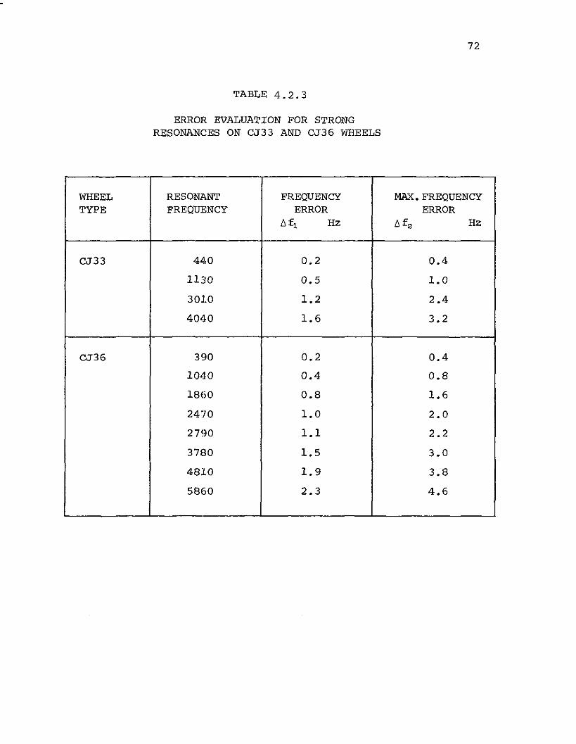
TABLE 4.2.3
ERROR EVALUATION FOR STRONGRESONANCES ON CJ33 AND CJ36 WHEELS
72
WHEEL RESONANT FREQUENCY MAX. FREQUENCYTYPE FREQUENCY ERROR ERROR
[, f 1 Hz [, f 2 Hz
CJ33 440 0.2 0.4
1130 0.5 1.0
3010 1.2 2.4
4040 1.6 3.2
CJ36 390 0.2 0.4
1040 0.4 0.8
1860 0.8 1.6
2470 1.0 2.0
2790 1.1 2.2
3780 1.5 3.0
4810 1.9 3.8
5860 2.3 4.6
73
4.3 Dynamometer Tests at Wilmerding, Pennsylvania
An opportunity to correlate numeri~al stress indica
tions with changes in the acoustic signature was offered
by the union Pacific Railroad Company (UPRR) who invited the
University to participate in a series of dynamometer
tests in the Westinghouse Plant at Wilmerding, Pennsylvania.
4.3.1 Description of Tests
The objective of the Union Pacific's test team was
to study the thermal damage and premature wear to the
tread and flange portion of the wheel. Preliminary
internal study of the problem by the UPRR focused attention
on three potential causes of the phenomena:
1. misalignment of the brake shoe with respect to the
wheel center line,
2. misapplied brake shoe,
and 3. high energy drag braking applications.
SUbsequent discussion and correspondence between repre
sentatives of the Union Pacific Railroad and
Westinghouse Air Brake Division (WABD) resulted in a
proposal to conduct a dynamometer research test program to
investigate the possible effect of these factors on
usable wheel life. This program was conducted by WABD
under contract to UPRR.
The dynamometer test program consisted of both stop
tests and drag tests. The stop tests were emergency
stops from 80 mph. Five stops were made on each wheel
used. The drag test was run at a speed of 60 mph with a
74
shoe force simulat:ing a 15 psi brake pipe reduction. Five
drag tests were made on each wheel. Two different positions
of the shoe on the wheel were tested: in the center of
the tread, with the shoe overriding the outer edge of the
tread, and with the shoe riding on the flange. Several
types of brake shoes were used.
The acoustic signature of the wheel after each stop
was obtained using the setup shown in Fig. 4.3.1. For
excitation of the wheel a 16 oZ,standard hammer was used
and the wheel was impacted five times. In a few tests a
32 OZ. hammer in addition to the 16 OZ. one was used. The
stress readings were obtained from three SR-4 foil strain
gauges (BLH Electronics) welded on the wheel as shown in
Fig. 4.3.2. The strain readings were obtained using two
types of strain indicators. The first device was a
multichannel indicator with an internal calibration to zero
the initial reading, so that any subsequent reading indi
cated the change in strain directly. The second device
gave indications whereby any strain change could be
evaluated by sUbtracting the indication from the initial
reading. In the following description the three gauges
will be referred to as A, B, and C (see Fig. 4.3.2). The
SR-4 gauge specifications indicate that the maximum
advisable operational temperature without special coating
is 705°F.
Acoustic signatures from a total of six wheels were
obtained. All wheels tested were Griffin CJ33 and were
75
Wheel Microphone NAGRA----, I 2 1 TAPE500 HP
DC MOTOR ~ i H I
BACKGROUND NOISE: 88 dBAIMPACT LEVEL : 113 dBA on fast at 2 feetSLM : GRTAPE RECORDER :NAGRA IV
FIG. 4.3.1 SETUP FOR ACOUSTIC SIGNATURE RECORDING

- --
o= = +0.25"
Back Face of the Wheel
76
B_ _ _ _ 1 0 25 11-- - - T .A I _ 1. 1.50"o f Front Face of the Wheel
FIG. 4.3.2 STRA~N GAUGE ARRANGEMENT
77
identified as UP 12, 19, 20, 17, 27, and 28. In wheels
UP 12, 19, 20 and 17 emergency braking tests were per
formed with different brake shoes and shoe positions. On
wheels UP 27 and 28 drag braking tests were performed
applying COBRA composition brake shoes. As was expected
the highest stress changes occurred in the drag braking
tests because of the high final wheel tread temperature of
600°F to 1100°F, as compared to emergency stops in which
final temperatures are generally in the range of 150°F to
550°F.
4.3.2 Data processing
The tape recordings were returned to the University
for processing. An attempt to see changes in the signature
using the SD 330 A RTA failed because of the low frequency
resolution of 20-40 Hz while the range of interest is
0-10 Hz. By courtesy of the Shell oil Co., a Hewlett
Packard (HP 5445) real-time spectrum analyzer was made
available. This instrument has a variety of features and
options for optimum signal processing. Identification of
the important resonances was achieved in a preliminary run
shown in Fig. 4.3.3. Because of limited access time with
the analyzer only signatures from wheels UP 27 and 28
(drag braking) could be obtained.
4.3.3 Results
The results are summarized in Table 4.3.1 and 4.3.2.
These tables contain: in column 1, the test number; in
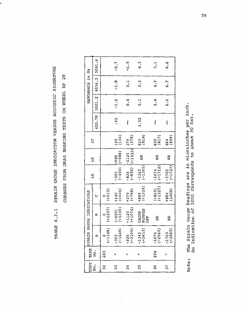
TAB
LE4
.3.1
ST
RA
ING
AU
GE
IND
ICA
TIO
NV
ER
SUS
AC
OU
STIC
SIG
NA
TU
RE
CH
AN
GES
FRO
MD
RA
GB
RA
KIN
GT
ES
TS
ON
WH
EEL
UP
28
II
TA
PE~TRAIN
GA
UG
EIN
DIC
AT
ION
SI
II
I,
TE
ST
RES
ON
AN
CE
inH
z
No
.N
o.
6A6B
6CA
BC
42
0.7
03
00
1.
24
03
4.3
50
91
.4
32
20
30
00
(-1
24
8)
(+2
22
7)
(+5
10
)
33
"-3
92
(-9
80
)+
14
0-3
92
-98
01
40
.62
-1.2
-1.8
-2.7
(-1
64
8)
(+1
23
9)
(+6
46
)(-
40
0)
(-9
88
)(1
36
)
34
"-8
26
-11
25
+2
79
-82
6-1
12
52
79
-0
.40
.1-1
.5
(-2
10
4)
(+1
07
4)
(+7
88
)(-
85
6)
(-1
15
3)
(27
8)
35
"-1
34
2G
AU
GE
+8
09
-13
42
81
03
.52
5.1
5.2
4.3
(-2
61
3)
BU
RN
ED(+
13
29
)(-
13
65
)N
R(8
19
)O
FF
36
20
4-1
67
4N
R(+
82
5)
-16
74
NR
82
5-
5.4
4.7
5.1
(-2
96
0)
(+1
32
7)
(-1
71
2)
(81
7)
37
"-1
70
3+
88
4-1
70
38
84
-6
.06
.76
.6(-
29
85
)N
R(1
40
9)
(-1
73
7)
NR
(89
9)
No
te:
Th
eS
train
Gau
ge
Read
ing
sare
inm
icro
inch
es
per
inch
.A
nIn
dic
ati
on
of
10
00
Co
rresp
on
ds
toab
ou
t3
0K
si.
...., 00
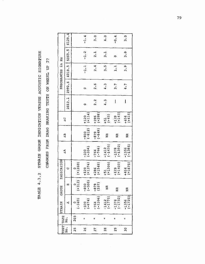
TA
BL
E4
.3.2
ST
RA
ING
AU
GE
IND
ICA
TIO
NV
ER
SUS
AC
OU
STIC
SIG
NA
TU
RE
CH
AN
GES
FRO
MD
RA
GB
RA
KIN
GT
ES
TS
ON
WH
EEL
UP
27
TE
ST
TA
PES
TR
AIN
GA
UG
EIN
DIC
AT
IOR
ESO
NA
NC
ES
inH
z
No
.N
o.
AA
AB
AC
AB
C2
01
2.1
29
90
.64
01
9.5
50
69
.56
12
9.4
25
20
30
00
(-3
40
)(+
31
2)
(+1
26
0)
26"
-33
0-8
00
+1
20
-33
0-8
00
+1
20
00
-1.1
-1.2
-1.
4(-
67
4)
(-5
00
)(+
13
74
)(-
33
4)
(-8
12
)(+
11
4)
27"
-76
4-8
79
+2
86
-76
4-8
79
+2
86
2.2
2.6
2.4
2.1
3.0
.(-1
10
6)
(53
7)
(+1
54
8)
(-7
66
)(-
84
9)
(+2
88
)
28"
-14
12
+5
1-1
41
2+
51
4.3
4.3
3.5
3.1
4.0
(-1
77
5)
NR
(+1
30
5)
(-1
43
5)
NR
(+4
5)
29"
-13
78
+1
29
-13
78
+1
29
-3
.71
.10
-0.4
(-1
73
2)
NR
(+1
40
3)
(-1
39
2)
NR
(+1
43
)
30
"-1
35
6+
40
4-1
35
6+
40
4-
4.7
3.9
3.0
3.0
(-1
72
5)
NR
(+1
67
5)
(-1
38
5)
NR
(+4
15
)
--J '"

80
column 2, the magnetic tape number; in columns 3, 4, 5,
the strain gauge indications from A, Band C gauges; in
columns 6, 7,8, the changes in strain are evaluated from
columns 3, 4 and 5, and the last five columns show the initial
resonant frequency and the frequency shift that occurred
in the subsequent braking stops. Table 4.3.3 is an example
of the machine setup data for narrow band analysis which
includes information about the type of measurement, the
number of averages, the type of signal, the type of trigger,
the center frequency, the bandwidth, and the sampling time
length, from which the frequency error ~F is given,
about 0.4 Hz. The frequency shift shown in the last
columns of Tables 4.3.1 and 4.3.2 was obtained from 54
graphs, such as those shown in Figs. 4.3.4 through 4.3.9.
These figures correspond to the signature of wheel UP 28
at about 3000 Hz, taken before the drag braking test
started (Fig. 4.3.4) and after each successive drag test
(Fig. 4.3.5 through 4.3.9).
The limited results shown in Tables 4.3.1 and 4.3.2
show the interesting feature of a frequency shift almost
independent of the resonant mode. This behavior is con-
sistent with the theory discussed in Section 2. It is
interesting to compare this frequency shift with the
theoretical result given by eqn 2.4.3.
equation one obtains
Rearranging this
FA = a = 21TM
n[EiP] 1/2

TA
BLE
4.3
.3
SET
UP
STA
TE
ON
HP
54
45
REA
LT
IME
AN
ALY
ZER
MEA
SUR
EMEN
T:LI
NE
AR
SPEC
TRUM
AV
ER
AG
E:
SIG
NA
L.
TRIG
GER
:
CENT
FREQ
:
BA
ND
WID
TH.
TIM
ELE
NGTH
•
5
TRAN
SIEN
T
INTE
RN
AL
6.12
500
KHZ
100.
000
HZ
2.56
000
S
•ST
ABLE
•CH
NL1
AF•
390.
625
mHZ
AT
.5.
0000
0m
S
ADC
CHNL
RANG
EA
C/D
CD
ELAY
CA
LCC
l/C2)
*1 2
1V
10V
AC DC50
.000
0m
S0
.0S
1.lill
illill
il01.
lil00
00
co I-'
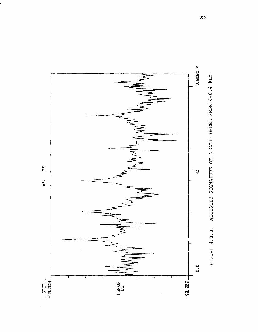
#1"
30L
SPEC
1
-10
.00
0I
1 !~I
\J
\II
Ii~
L':G
illII!
'"il,l
IA~~
1,l
'nI,
.,~.
Jj\I
-9l'
l.0
l'll'l
-)I
II
II
II
l'l.l'
lHZ
6.l'l
l'l0l
'lK
FIG
UR
E4
.3.3
.A
CO
UST
ICSI
GN
AT
UR
EO
FA
CJ3
3W
HEE
LFR
OM
0-6
.4kH
z
(Xl
IV
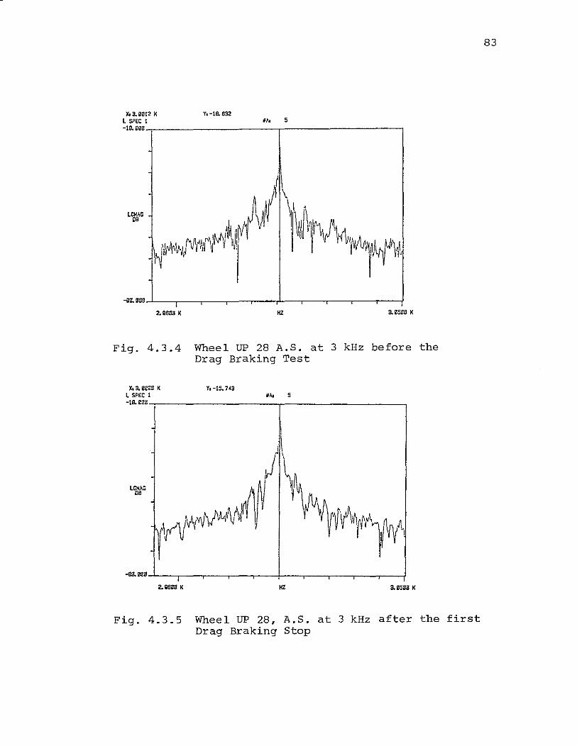
83
." 5
YI-ie. 632X, 3. Bll12 I<L SPEC 1-,0.,,,..,- --, ---,
....."'-'----I,-----.-..,--,---,l-.--r---r--.----t,2. Q500 K HZ a &5Z0 K
Fig. 4.3.4 Wheel UP 28 A.S. at 3 kHz before theDrag Braking Test
." 5
VI-iS. 743XI 3. eea3 KL SPEC t-1<1."',---------,---------,
S.Z5ZiJ KHZ
-so.""-l.....--,I,---,--,--,---+-.--r---r-.-----I2.,gm K
Fig. 4.3.5 Wheel UP 28. A.S. at 3 kHz after the firstDrag Braking Stop
84
fAo 5Xa3.1ir.J18 K
L SPEC 1-......-,--------,------,
3.1I5Illl •HZ
-1.....,...l.--~I.,.-.....-----.----r.L.--.---,--r-----.----,
2. gSDa K
Fig. 4.3.6 Wheel UP 28, A.S. at 3 kHz after theSecond Drag Braking Stop
lAo 5Xt3.2963 .K
L SPEC 1.......-,---------,--------,j
3. esse KHZ
-as. ......l--,.--.--,---,---'-,---L-.---,-_r_____._---!.......
Fig. 4.3.7 Wheel UP 28, A.S. at 3 kHz after theThird Drag Braking Stop
85
LG1<AG06
YI-21. S59IAI 5
3. ZSZ3 r.HZ
-Bll. eOO....L---rj-,-----,--.---• .--.J..,----r----.-----,---,I
2.B6ZB K
Fig. 4.3.8 Wheel UP 28, A.S. at 3kHz after thefourth Drag Braking Stop
'''' 5
YI-2a. t8a>:'3. ewz KL SPEC 1-I0.BB3.- -,-- ---.
LtMAG08
2. g5C0 I( HZ
Fig. 4.3.9 Wheel UP 28, A.S. at 3kHz after thefifth Drag Braking Stop

86
Hence a shift of 6 Hz corresponds to a stress change of
15 Ksi. It should be noted that this value must cor
respond to an average stress change in the rim. Strain
gauge readings at the front and back of the rim were often
of different sign and varied from about 50 Ksi tension to
about 25 Ksi compression with a 6 Hz frequency shift. It
is therefore felt that the theory seems to give a
reasonable indication of average stress.
The correspondence between strain indications and
frequency shift is shown in Fig. 4.3.10 and 4.3.11. These
figures show that stress conditions and frequency shift
were best correlated for the readings from strain gauge A
welded on the plate. This seems quite reasonable because
the changes in the stress at gauge A on the plate are due
to the overall condition of the rim. But there may be
considerable local variations in the rim itself. The
least correlated indications were from strain gauge C on
the back rim. Comparison of the readings from gauge C
from wheels UP 27 and 28 under similar drag braking con
ditions show large differences. Data from gauge B on the
front rim were limited to two values for each wheel
before extreme heat conditions burned them off. As has
been indicated, acoustic signature differences are functions
of the bulk stress, and thus might not be expressed
directly by indications from a single strain gauge. It
is hoped that completing the analyses on wheels UP 27 and
87
UP 272990.6 Hz
Hz
tf),f 2
! ! //
/
I f),e I ;:-
0 500 1000 1500
.. GAUGE A• GAUGE B
-2~ GAUGE C
FIG. 4.3.10 FREQUENCY SHIFT ~f VERSUS STRAIN CHANGE~€ AT 3 kHz FOR WHEELS UP 27 (FIVE DRAGBRAKING STOPS.)
88
/ /1UP 283001.2 Hz II r! I
4 / IHz / I
t/ // /
M / /2
/ /
l,I
0III I ! Ille I~, I
\"-. / 500 / 1000 1500
'}( ,/
!"I -1-/ • GAUGE A
-2• GAUGE B~ GAUGE C
Fig. 4.3.11 Frequency shift Af versus Strainchange ~e at 3 kHz for wheelUP 28 (Pive Drag Braking Stops)
89
28 and also on wheels UP 12,17,18 and 20 will give a
better understanding of the acoustic signature as a function
of the wheel stress conditions.
The changes in frequency are small, of the order of
a few Hz; hence a rather careful error analysis must be
made. Errors in the data collection and data processing
can be divided into error due to the tape transportation
mechanism of the recorder and errors in the signal processing.
The latter error depends on the sampling rate and time
duration of the signal, which for these analyses was
0.4 Hz. Equally or even more important is the error due
to the tape transport speed and fluctuation. Manufacturer's
data for the NAGRA IV at 15 in/sec indicate a maximum
~ 0.05% tape speed error which could give an error of
2.5 Hz at 5 KHz. If tape speed changes occurred during
the recording, the resonances ought to show frequency
shifts proportional to frequency. There are indications,
from comparisons of repeated impacts on the same wheel in
the same conditon, that if such an error occurred it was
much smaller than 0.1 Hz at 1000 Hz or less than 0.01%.
A significant experimental error might be included in
some of the Bessemer results. It is believed now that the
results for CJ36 wheels shown in Fig. 4.2.5 are more accurate
than those for CJ33 wheels shown in Fig. 4.2.6. The
maximum frequency difference should be about 10 Hz instead
of 25 Hz. There is no indication at this point of any
important error in the dynamometer test results.
90
5. SYSTEM COMPONENT DESIGN
5.1 Wheel Exciter
An ideal wheel exciter should:
1. Produce vibrational excitation in the range 0-10 kHz
in all types of railroad wheels. The C-weighted
intensity at 3 feet must equal or exceed 100 dB.
Acoustic signatures resulting from the use of the
exciter must be reproducible independent of train
speed and not contain resonances other than those of
wheels.
2. Induce vibrations in the wheel from a point of contact
low on the wheel's rim or flange. This point of
contact shall be independent of the train velocity.
3. Have an auxiliary power source (electrical or
pneumatic) or be mechanically powered by the train.
In the latter case, the exciter must not cause a
vertical displacement of the wheel.
4. Excite wheels on both rails with train
speeds of up to 45 MPH (for yard operations 10 MPH
should be sufficient).
5. Not present a hazard to the train or to itself for
train speeds up to 80 MPH (30 MPH for yard operations) .
6. Be suitable for use at any railroad track location
outdoors within the continental united States.

91
7. Be designed to comply with requirements for track
side apparatus now imposed by the railroads. This
includes OSHA safety requirements for personnel.
B. Have a Mean Time to Failure such as to allow operation
for 6 months under normal conditions without probable
failure.
These specifications represent an ideal to be aimed
at. The designer is confronted with a large variety of
conceivable devices and many choices. In the feasibility
study [1] a mechanism driven by the wheel itself was used.
In the present work it was decided to explore the
feasibility of some alternative approaches and these are
categorized according to the power source. Since some
field experience had been obtained with the original
hammer mechanism it was decided to pursue this design
concept in parallel with the other studies to ensure that
at least one form of operating exciter would be available
for the field tests.
5.1.1 Mechanically Powered Excitation
The original version of the hammer exciter is shown
in Fig. 1.6.1. The device operates as follows: the
flange of the wheel depresses the plunger, 1, whose travel
is guided by the pin, 2. Thus the link, 3, starts to
rotate around the pivot point, 4. Due to this rotation
point A moves towards point B compressing the hammer
spring,S. At low speeds this spring acts as an energy
92
storage device. When the torque about B due to the hammer
spring exceeds the torque due to the weight of the hammer the
spring starts to expand and drives the hammer up to impact
the wheel flange. At higher speeds (above 2.5 MPH) the
link, 3, actually impacts the roller 6 thus setting the ham
mer into essentially free rotation until it impacts the
wheel. The hammer spring then does not contribute much to
the forward motion of the hammer but acts only to reset the
hammer following wheel impact. The forces of acceleration
and deceleration on the hammer mechanism can be very large
(see Appendix E). The associated stresses in this mechanism
probably were excessive in the device tested in Omaha in
1974, and led to its failure when activated by a fast train
passing over it. A tentative solution to this problem was
to make the entire hammer, and hammer mounting, a one-piece
unit cut from steel plate. In addition, the impacting face
of the hammer was heat treated to harden it against wear.
A view of the modified exciter is shown in Fig. 5.1.1.
This is the version of the hammer exciter used in the
field tests to be described in section 6. It should be
noted that a full dynamic analysis of the hammer mechanism
remains to be completed. However, a simplified model is
discussed in Appendix E. Some snapbuckling mechanisms have
been proposed by Fazekas [41] and these devices were given
some consideration as means of achieving the requirements
of a wheel activated hammer. Although the conceptions are

93
......It)
IIII
==TWW:= I'W,,=_ I
I
" v- .~ :=== :~==~
---~--
/f
/./
/'-~/.
,II
C"'»;cI
I
II
I
I
I
I
IIII0 II
I~---I
0,
I\
If)II
94
elegant, time and resources simply did not permit the
design and construction of a working device.
5.1.2 Electrically Powered Excitation
An electric motor to spin two or more impacters,
preferably 4, 8, etc., for balance reasons, against the rim
of the wheel was also examined (see Fig. 5.1.2). The first
tests were performed using a 1/4 HP 1725 rpm motor; in
later tests a 1/2 HP universal-type AC-DC motor was used
with speed controlled by a VARIAC. The motor exciter
represents two significant departures from the hammer type
exciter concept. It is electrically powered and therefore
the impact is independent of the train speed. However, it
may produce multiple impacts on the same wheel. The attrac
tion of this design is its ability to produce impacts at
train speeds up to 40-45 MPH and to survive at any train
speed. It is a simple design but it must be well guarded
for safety reasons. The electric motor and spinning impacter
combination was tested on good, bad and greasy wheels. The
preliminary conclusions on the feasibility of using this
design were: a) the spectra obtained from the good, bad
and greasy wheel are noticeably different, and b) spectra
from the same wheel were reasonably reproducible.
An impacter to be actuated by a solenoid, such as an
automobile starter, was also given some consideraton.
However, the concept was not pursued since a triggering
pulse would be required and this would involve further

95
FIG. 5.1.2 MOTOR EXCITER, ROTARY
96
complication of the system. The motor exciter could be
left running during the passage of a train.
5.1.3 Pneumatic Powered Excitation
Another concept examined was that of a pneumatic vibrator
impacting a ramp depressed by the wheel flange. The main
attraction of such an exciter is the ruggedness and the
safety. Pneumatic vibrators are also commercially available in a
variety of types, sizes and are low priced. A problem
is the background noise of the hammer itself.
Pneumatic vibrators were obtained for preliminary
testing of the feasibility of this type of wheel excitation.
Included were large and small reciprocating piston types,
and five different sizes of rotary vibrators. Testing
involved holding each vibrator in contact with the wheel,
and obtaining taped wheel signatures associated with
differing points of contact and differing air pressures.
These tapes were then analyzed using both the 1/3 octave
band B & K analyzer and the Spectral Dynamics narrow band
analyzer. The results of this investigation were: a) the
large piston type vibrator was difficult to keep in contact
with the wheel, and therefore no conclusions could be
drawn; b) the small piston type vibrator produced usable
wheel signatures which were reproducible and comparable in
quality to those obtained by rolling ball impact; and c) the
rotary vibrators did not excite a broad spectrum of the
natural modes of vibration in the wheels. An explanation

97
for the failure of the rotary vibrators to excite the
wheels is evident in the fact that an off-center spinning
mass produces a frequency of vibration which is the
inverse of its orbital period. This is not comparable
with the rich spectrum of frequencies associated with
the delta function of an impacting mass. Consequently,
the rotary vibrators will only excite the few natural
wheel frequencies which are close to that of the vibrator's
frequency. The piston vibrator, on the other hand,
induces frequencies of vibration almost uniformly
throughout the 0-10 kHz band of interest.
To test the performance of a pneumatic vibrator
and mounting, aNAVCO model BH 1-1/4 impact type was
installed on a custom made leaf spring (K = 150 lbs/in)
which was mounted on the test track. The leaf spring
parallels the inside of one of the rails, with the
vibrator directly attached to the underside center of
the leaf spring. In use, the vibrator operates con
tinuously. The wheel flange depresses the leaf spring
in passing over it and the impact vibrations are then
transmitted into the wheel. This design is attractive
for its simplicity and suitability for outdoor use.
As it was mentioned earlier the background noise level
produced by the pneumatic vibrator was high but a 6-8 dB reduction
was achieved through the use of an exhaust muffler and
damping compound applied to the vibrator and leaf
spring. Figure 5.1.3 shows the details of this design.
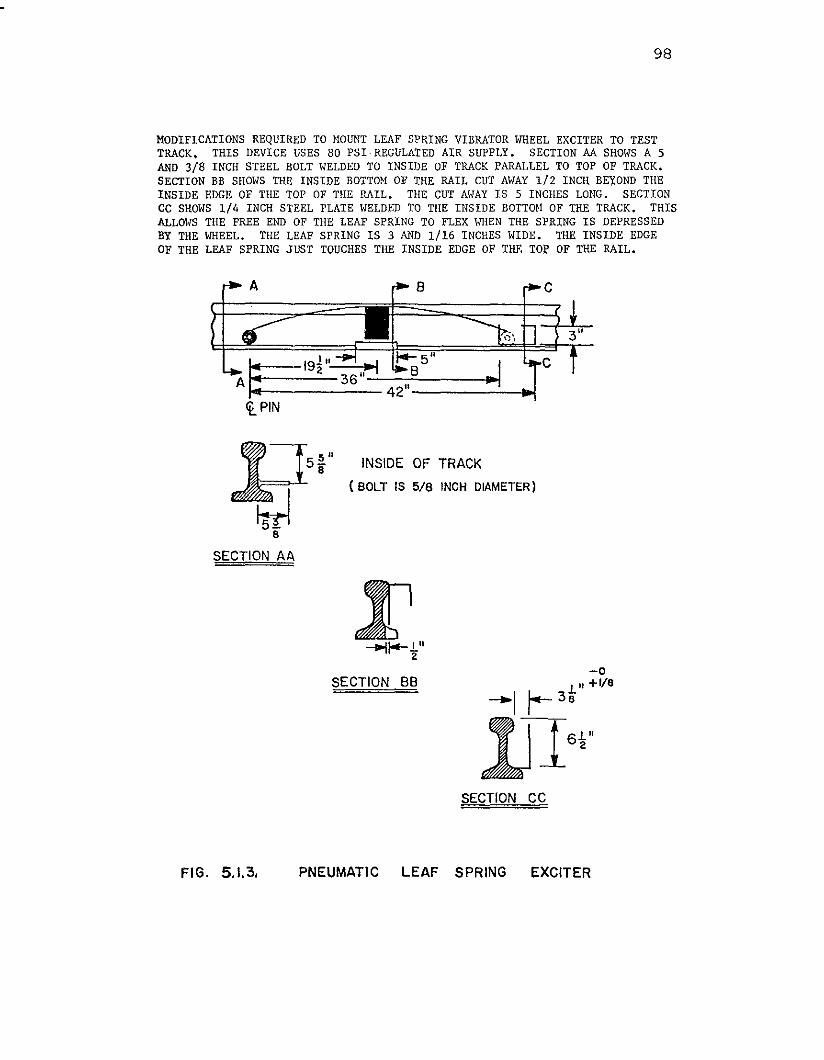
98
MODIFICATIONS REQUIRED TO MOUNT LEAF SPRING VIBRATOR WHEEL EXCITER TO TESTTRACK. THIS DEVICE USES 80 PSI· REGULATED AIR SUPPLY. SECTION AA SHOWS A 5AND 3(8 INCH STEEL BOLT WELDED TO INSIDE OF TRACK PARALLEL TO TOP OF TRACK.SECTION BB SHOWS THE INSIDE BOTTOH OF THE RAIL CUT AWAY 1/2 INCH BEJ:OND TilEINSIDE EDGE OF THE TOP OF THE RAIL. THE CUT AI;AY IS 5 INCHES LONG. SECTIONCC SHOWS 1(4 INCH STEEL PLATE WELDED TO TilE INSIDE BOTTOM OF THE TRACK. TillSALLOWS TilE FREE END OF TilE LEAF SPRING TO FLEX WHEN TilE SPRING IS DEPRESSEDBY THE WHEEL. TilE LEAF SPRING IS 3 AND 1/16 INCHES WIDE. THE INSIDE EDGEOF TilE LEAF SPRING JUST TOUCHES THE INSIDE EDGE OF THE TOp OF THE RAIL.
8A
A~.~-1~92~1"~~_---:=--__•
et. PIN
INSIDE OF TRACK
(BOLT IS 5/8 INCH DIAMETER)
SECTION AA
SECTION SS-0
1." +1/8
-1/- 38
lJ161'SECTION CC
FIG. 5.1.3. PNEUMATIC LEAF SPRING EXCITER

99
The problem with this type of design is that the
amplitude of the sound from a wheel rolling over the
leaf spring is much less than from the directly
impacting devices, such as mechanically and electrically
actuated hammers.
5.1.4 Comparison of Exciter Types
Table 5.1.1 is a summary of ratings of these various
types of exciters assessed according to the specifications
of an ideal exciter. The characteristics of the acoustic signa
ture are given a higher weighting than the other specifica-
tions since if the device does not give a reproducible signature,
it is useless for the present purpose. Overall the
mechanical hammer appeared to be the best device to use
despite its dependence on wheel speed in its present
form. The pneumatic exciter was downgraded because of
the weakness of the signature intensity. The electric
motor driven impacter was downgraded slightly as regards
signature because of the problem of mUltiple impacts
and because of possible safety problems. It would also
present a profile above the top of the rail. As a
result of these considerations it was decided to use
the modified hammer exciter in the field test.
5.2 Wheel Sensor
The search for a device to be used to generate a
trigger pulse was restricted to three possible types:
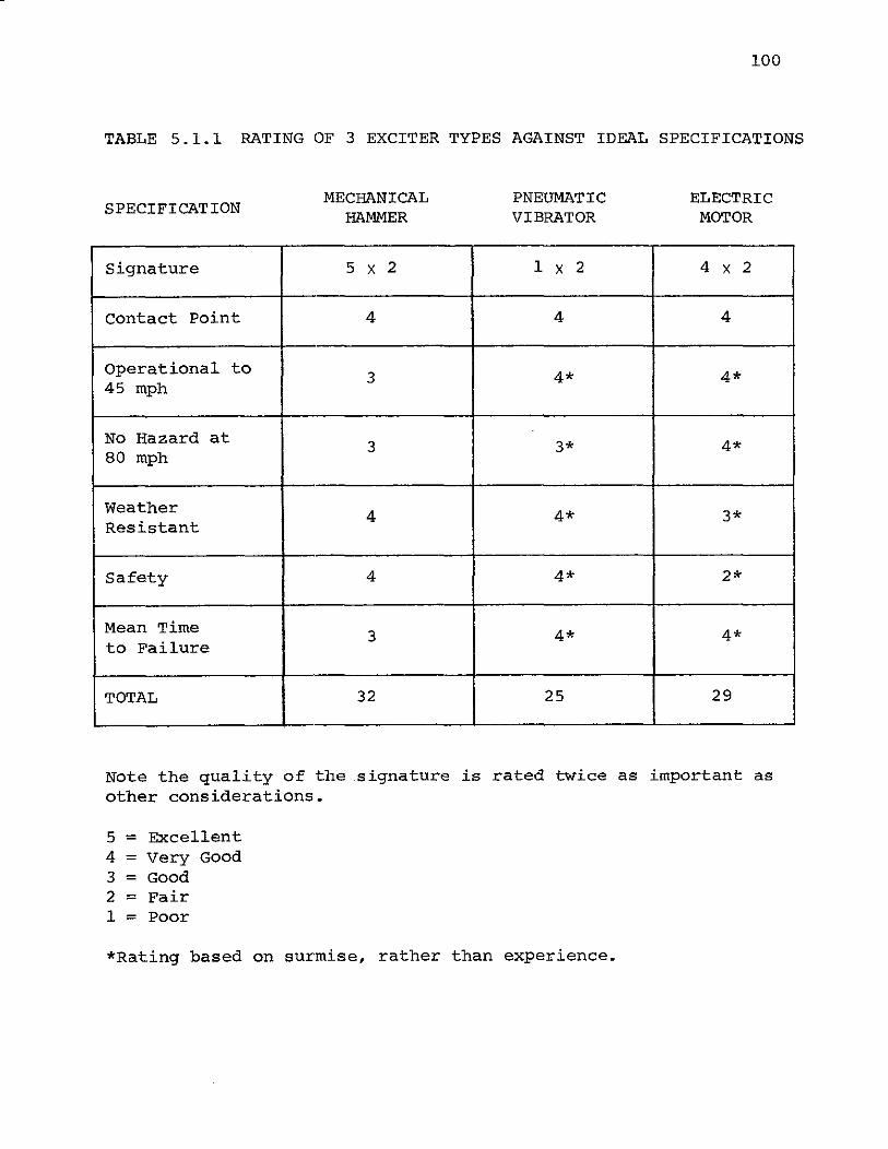
100
TABLE 5.1.1 RATING OF 3 EXCITER TYPES AGAINST IDEAL SPECIFICATIONS
SPECIFICATIONMECHANICAL
HAMMERPNEUMATICVIBRATOR
ELECTRICMOTOR
Signature 5 x 2 1 x 2 4 x 2
contact Point 4 4 4
Operational to 3 4* 4*45 mph
No Hazard at 3 3* 4*80 mph
Weather 4 4* 3*Resistant
Safety 4 4* 2*
Mean Time 3 4* 4*to Failure
TOTAL 32 25 29
Note the quality of the signature is rated twice as important asother considerations.
5 = Excellent4 = Very Good3 = Good2 = Fair1 = Poor
*Rating based on surmise, rather than experience.
101
al microswitches, bl photosensors, and cl commercially
available metal sensors. Microswitches had already
been used in an earlier test. Their performance could
be rated as moderate because they are susceptible to
rough operational conditions. Stable mounting of the
microswitch on the track or exciter was also a problem
due to vibrations induced by the train rolling over it.
Electric contact noise was another problem, although it
could be eliminated with proper electronic filtering.
Photosensors would be an ideal solution if they could
survive the dirt of the yard and severe weather con
ditions. In the third class the best available wheel
sensor system appeared to be the DUAL DIRECTIONAL WHEEL
SENSOR by ACI, since many engineering problems had been
solved in its development. It has solid state circuitry,
which is shock mounted and temperature independent from
_40° to +1400 P. It has a waterproof casing and is easily
installed and adjusted. The wheel speed can range from
o to 80 MPH. The operation of the wheel sensor is based
on the principle of magnetic flux change in a coil to
detect the presence of a wheel. The device has two
sensing units to determine wheel direction. During the
present tests only one unit was used because the
direction of wheel travel was not needed. The basic
elements of each sensor unit are a permanent magnet as
the source of the magnetic flux and a coil whose inductance
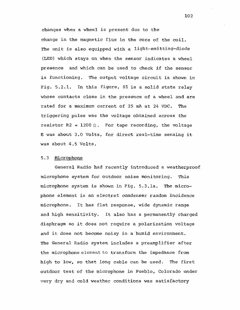
102
changes when a wheel is present due to the
change in the magnetic flux in the core of the coil.
The unit is also equipped with a light-emitting-diode
(LED) which stays on when the sensor indicates a wheel
presence and which can be used to check if the sensor
is functioning. The output voltage circuit is shown in
Fig. 5.2.1. In this figure, 81 is a solid state relay
whose contacts close in the presence of a wheel and are
rated for a maximum current of 25 rnA at 24 VDC. The
triggering pUlse was the voltage obtained across the
resistor R2 = 1200 Q. For tape recording, the voltage
E was about 3.0 Volts, for direct real-time sensing it
was about 4.5 Volts.
5.3 Microphone
General Radio had recently introduced a weatherproof
microphone system for outdoor noise monitoring. This
microphone system is shown in Fig. 5.3.la. The micro
phone element is an electret condenser random incidence
microphone. It has flat response, wide dynamic range
and high sensitivity. It also has a permanently charged
diaphragm so it does not require a polarization voltage
and it does not become noisy in a humid environment.
The General Radio system includes a preamplifier after
the microphone element to transform the impedance from
high to low, so that long cable can be used. The first
outdoor test of the microphone in Pueblo, Colorado under
very dry and cold weather conditions was satisfactory
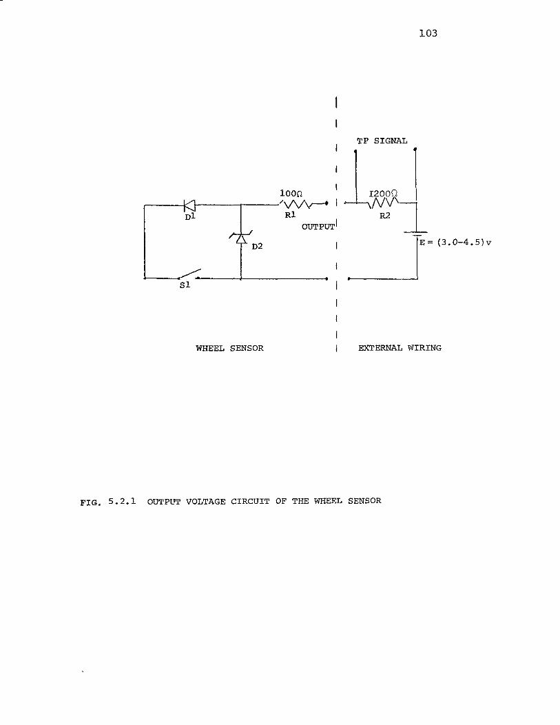
103
TP SIGNAL
lOon,----1'1(' ~---r---_/'I/\/'v--f
~1 Rl
>----~.~~---+------......S1
WHEEL SENSOR
'''ZR 1-----.~2l
E = (3. 0-4.5) v
EXTERNAL WIRING
FIG. 5.2.1 OUTPL~ VOLTAGE CIRCUIT OF THE WHEEL SENSOR
A SPikE
Jl-
"'" """.1(I~I_.b:f.- .:.1 .~~ _. ,111
I' .... ,I
/'MICROPOO"le eX1ENOE ~'""".
r-$HIELO
,"""
a
CLAMP
104
FIG. 5.3.1ab
ASSEMBI,Y OF WEATHERPROOF MICROPHONEDIRECTIONAL RESPONSE PATTERNS FOR THE GR J>, INCHELECTRET-CONDENSER MICROPHONE
105
and encouraged the acceptance of this type of microphone
for the final field test. The only negative aspect
was the need for a power supply for the microphone's
preamplifier. A directional microphone would have been
a better choice than the random incidence type actually
used. The directional response patterns of the present
microphone are shown in Fig. 5.3.lb. The system used in
the final field test included two microphones installed
on either side of the track. The sound signals go into
a microphone mixer whose output goes to a filter
and then to the real-time analyzer.
5.4 spectrum Analyzer, Computer and Diskette Interfacing
The most important parts of the system are the
real-time analyzer (RTA) and the mini-computer. At the
present time there are basically two ways to extract
frequency information from a sound signal: a) using an
analog to digital (A/D) converter and subsequently
analyzing the digitized signal through the use of
computer software or b) using a RTA. The selection of
the proper device is based on the duration, frequency
range, amplitude, type (transient or stationary) of the
signal and the frequency resolution of the analyzed
spectrum. Different commercial devices have similar
specifications and it is hard to select the best. Rapid
improvements and development of these products make the
selection even more complicated.
106
A NOVA 1220 computer interfaced with a 39 channel,
1/3 octave band analyzer had already been used in previous
wheel testing by Nagy [1] and Dousis [4]. Some spectral
analysis had also been done using a Spectral Dynamics
model 330A real-time analyzer on loan from the Company
for a short period of time but without any digital inter
facing. The cost of the SD330A, its fast signal analysis
for the frequency range needed in the tests and the
familiarity of the researchers with it led to the
selection of this device as the spectrum analyzer for
the system. However the use of an A/D converter should
be given serious consideration as a part of a prototype
system. Some advantages and disadvantages of the SD330A
analyzer in respect of transient signal analysis will
be presented in the appropriate chapter.
The computer for the system was a 16K NOVA 1220.
Because of the medium memory size of the computer the
bulk of the software was written in BASIC language.
The digital output of the SD330A analyzer was interfaced
with the NOVA's I/O board according to Table C.l in
Appendix C.
The next major task after the interfacing was the
development of NOVA computer software needed to operate
the analyzer and retrieve data from it. To accomplish
this the following software was written:
107
1. Assembly subroutines for control of the SD330A
analyzer, including the following commands: start,
stop, peak, cursor/plotter, sweep or reset 135),
2. Assembly subroutines for use of the NOVA Real-Time
Clock.
3. Assembly subroutines to read and operate on individual
spectra (250 channels) from the SD330A using the
slow speed plotter output mode.
4. Assembly subroutines to read, print, and operate
on individual spectra in the high speed (53 ms)
output mode, i.e., levels from the 250 channels
are sequentially read in 53 ms directly into core
memory.
5. Assembly subroutines to store complete spectra in
NOVA core memory in sequential order.
6. BASIC language programs to call the above Assembly
subroutines for processing spectra.
The core memory requirement for a single spectrum
is 250, 16 bit, words. After the BASIC interpreter
and the program was stored in the memory, 3K of core
was available for data, whiCh means only 10 spectra
could be stored in the computer. Approximately 5 ms
are required to retrieve one data word for
processing. Retrieval of two complete spectra
for an across-the-axle comparison takes about 2.5
seconds which does not include the analysis program
execution time.

108
Considering this relatively long execution time
for BASIC instructions, it was concluded that the analysis
for wheel fault detection would not be done immediately
following reading the spectra as the train cars pass
over the exciters. (For a car speed of 10 MPH, wheels
on the same side of a truck will pass over the exciter
in approximately 0.4 seconds). Thus it appeared that
the analysis ought to be done in near real-time, i.e.,
immediately after the last wheel spectra is read into
the computer. Furthermore, since core memory was limited
to approximately 1 car, and since additional core memory
boards would not greatly increase this capacity to store
wheel spectra, a peripheral memory device of several
hundred thousand word capacity was needed if long trains
were to be scanned with this apparatus. The speed of
data transfer from the SD330A of 4717 words per sec is
too fast for the NOVA Cassette which writes at 800 words
per second. A Da.ta General Diskette unit, model 6031
was the best technical choice having a transfer rate of
approximately 16,000 words per second and a storage
capacity of 157,596 words. The track to track head
positioning time is 20 ms. Eight spectra may be stored
per track. The assembly routines for data transfer
from the computer to the Data General Diskettes and
retrieval are presented together with the rest of the
software in Appendix C.
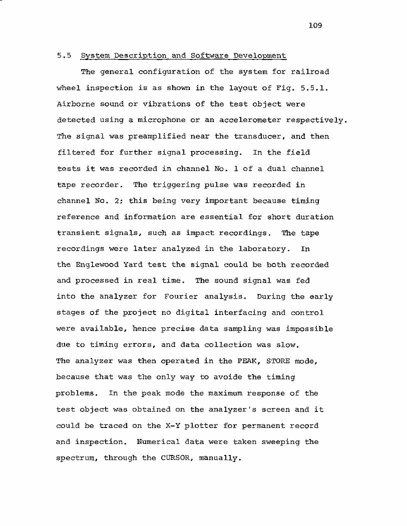
109
5.5 System Description and Software Development
The general configuration of the system for railroad
wheel inspection is as shown in the layout of Fig. 5.5.1.
Airborne sound or vibrations of the test object were
detected using a microphone or an accelerometer respectively.
The signal was preamplified near the transducer, and then
filtered for further signal processing. In the field
tests it was recorded in channel No. 1 of a dual channel
tape recorder. The triggering pulse was recorded in
channel No.2; this being very important because timing
reference and information are essential for short duration
transient signals, such as impact recordings. The tape
recordings were later analyzed in the laboratory. In
the Englewood Yard test the signal could be both recorded
and processed in real time. The sound signal was fed
into the analyzer for Fourier analysis. During the early
stages of the project no digital interfacing and control
were available, hence precise data sampling was impossible
due to timing errors, and data collection was slow.
The analyzer was then operated in the PEAK, STORE mode,
because that was the only way to avoide the timing
problems. In the peak mode the maximum response of the
test object was obtained on the analyzer's screen and it
could be traced on the X-Y plotter for permanent record
and inspection. Numerical data were taken sweeping the
spectrum, through the CURSOR, manually.

110
TRIGGERINGMICROPHONEOR ( PULSE
ACCELEROMETER '., SENSOR
"\
It
STORAGE ~PR1"AMPLIFIER~ DUAL CHANNEL ~TRIGG PULSE
~
OSCILLOSCOPE TAPE RECORDER SHAPING CIRCUIT
~.TER II REAL TIME I x-y
ANALYZER I PLOTTER
TEU~TYPECOMPUTER r
I/O CONTROL
DISKETTE 1
FIG. 5.5.1 SCHEMATIC OF DATA COLLECTION ANDPHOCESSING HARDWARE
III
One disadvantage in the case of impact analysis
using the PEAK mode is the presence of the shock wave
produced during the impact together with the response
of the test object. This means that the spectrum obtained
includes the Fourier components of the shock wave, which
theoretically is a continuous spectrum. In practice though
(narrow band analysis), it does not appear as continuous,
but as a very dense low amplitude line spectrum. When
another mode is used such as EXP. AVG. (exponential
average) or START where the spectrum in the analyzer's
memory is the sum of N successive analyzed spectra
divided by N, the number of averages selected, these
peaks disappear rapidly due to the short duration of
the shock.
One of the recognition and decision schemes used
early in the project was line spectra comparison.
The line spectrum of a signal is a representation of its
spectrum with lines at the resonances whose amplitude is
above a certain level. An example of a line spectrum is
shown in Fig. 1.4.2. From the finite element analysis
studies it was known that a good wheel has fewer resonance
lines compared to the same type of defective Wheel.
Another characteristic is the frequency shift in some
of these resonances in defective wheels of the same
structure and geometry. Therefore, comparison of good
wheels of the same type should give identical or
well matched line spectra, whereas a good to bad wheel
comparison ought to show significant line mismatching.

112
During the first experiments line spectra acquisition
was done manually using the X-Y plots of the acoustic
signatures. An example of these results is shown in
Table 5.5.1. The first column of the table has the
wheel code; the second, the wheel description. The
third column has the total average number of lines based
on three or four signatures from impacts on the same
or different points on the rim of the wheel. The fourth
column has the number of common lines between these
spectra and represents the "average" line spectrum of
the wheel.
As an example, the first axle tested had good 33"
cast, single wear wheels. Three different impacts
(signatures) on the same point showed an average of 38
lines on both wheels. On the east side there were 28
cornmon lines, on the west side, 32. Finally, there were
19 lines common to both sides (fifth column). In the
case of a good 33" wheel compared to a 33" wheel with
a partial crack, the number of matched lines was 11, and
comparison between the partially cracked wheel and the
one with the large crack indicated only 4-7 common lines,
although for some lines it was difficult to see if they
had identical frequencies or if there was a one channel
shift. The line spectra comparison procedure was later
automated using BASIC/ASSEMBLY language software.
Analyzing taped acoustic signatures with the above
software, result:s were obtained as shown in
Table 5.5.2. Important conclusions were obtained from
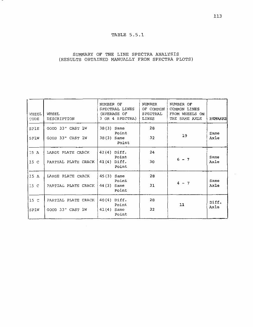
TABLE 5.5.1
SUMMARY OF THE LINE SPECTRA ANALYSIS(RESULTS OBTAINED MANUALLY FROM SPECTRA PLOTS)
113
NUMBER OF NUMBER NUMBER OFSPECTRAL LINES OF COMMON COMMON LINES
'tlHEEL WHEEL (AVERAGE OF SPECTRAL FROM WHEELS ONCODE DESCRIPTION 3 OR 4 SPECTRA) LINES THE SAME AXLE REMl\RKS
SPIE GOOD 33" CAST lW 38(3) Same 28Point
19Same
SPIW GOOD 33" CAST lW 38(3) Same 32 Axlepoint
~_5 A LARGE PLATE CRACK 42(4) Diff. 24Point
6 - 7Same
15 C PARTIAL PLATE CRACK 41 (4) Diff. 30 AxlePoint
15 A LARGE PLATE CRACK 45(3) Same 28Point
4 - 7Same
15 C PARTIAL PLATE CRACK 44 (3) Same 31 AxlePoint
15 C PARTIAL PLATE CRACK 40(4) Diff. 28 Diff.Point 11
AxleSPIW GOOD 33" CAST lW 41(4) Same 32
Point
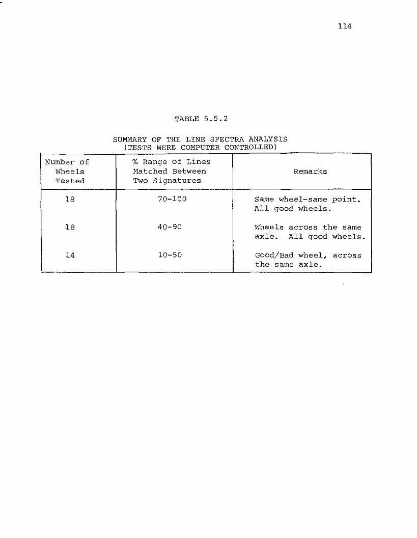
TABLE 5.5.2
SUMMARY OF THE LINE SPECTRA ANALYSIS(TESTS WERE COMPUTER CONTROLLED)
114
Number of % Range of LinesWheels Matched Between RemarksTested Two Signatures
18 70-100 Same wheel-same point.All good wheels.
18 40-90 Wheels across the sameaxle. All good wheels.
14 10-50 Good/Bad wheel. acrossthe same axle.

115
these tests:
a. There is some overlapping in the percentage of
matched lines in good/good and good/bad wheels.
b. Large defects (plate cracks) showed a 10-20% line
matching and therefore should be easily detected
under this scheme.
c. A comparison was made between the spectra of two
good wheels on the same axle, one having a very
worn flange. A low matching percentage of about 30%
was found.
d. A change in the input attenuation by a few dB caused
a different percentage of matching. This was to
be expected, because it changes the discrimination
window.
e. Small defects, such as thermal cracks,had 50% or
higher of matching lines.
f. The Line Spectra comparison scheme could not be
used alone for detection of defective wheels.
Thermal cracks would be difficult to detect and
small changes in the wheel geometry, such as worn
flanges, would appear as defects.
The BASIC software developed for the Englewood Yard
tests is given in Appendix C. A simplified general flow
diagram is shown in Fig. 5.5.2. The most important change
from earlier versions was to base the decision on
consideration of several factors: the number of coincident
resonances, the amplitudes of signals in the same spectral

START
READ, PRINT PROGRAM
PARAMETERS
READ ALL SIGNATURES FROM
RTA TO COMPUTER DISKETTE
r--;;~AD-OUT ACROSS AXLE
~ECTRA
~~TA PROCESSING FOR TWO
~HEELS ON THE SAME AXLE
116
YES NO
FiO.5.5.2 Flow diagram for the Series
of Computer Proorams used in the
SP Enolewood Yard, Houston Tests
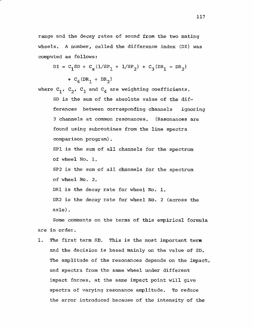
117
range and the decay rates of sound from the two mating
wheels. A number, called the difference index (DI) was
computed as follows:
DI = CISD + Cs(l/SPI + 1/SP 2 ) + C3 (DRI - DR 2 )
+ C4 (DRI
+ DR2 )
where Cl
, C2
, C3 and C4 are weighting coefficients.
SD is the sum of the absolute value of the dif-
ferences between corresponding channels ignoring
3 channels at common resonances. (Resonances are
found using subroutines from the line spectra
comparison program).
SPI is the sum of all channels for the spectrum
of wheel No.1.
SP2 is the sum of all channels for the spectrum
of wheel No.2.
DRI is the decay rate for wheel No.1.
DR2 is the decay rate for wheel No. 2 (across the
axle).
Some comments on the terms of this empirical formula
are in order.
1. The first term SD. This is the most important term
and the decision is based mainly on the value of SD.
The amplitude of the resonances depends on the impact,
and spectra from the same wheel under different
impact forces, at the same impact point will give
spectra of varying resonance amplitude. To reduce
the error introduced because of the intensity of the
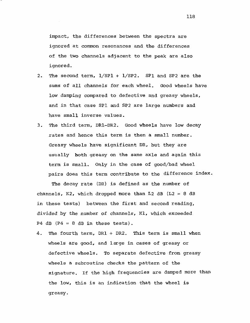
118
impact, the differences between the spectra are
ignored at common resonances and the differences
of the two channels adjacent to the peak are also
ignored.
2. The second term, l/SPI + 1/SP2. SPI and SP2 are the
sums of all channels for each wheel. Good wheels have
low damping compared to defective and greasy wheels,
and in that ca.se SPI and SP2 are large numbers and
have small inverse values.
3. The third term, DRI-DR2. Good whee Is have low decay
rates and hence this term is then a small nUmber.
Greasy wheels have significant DR, but they are
usually both greasy on the same aXle and again this
term is small. Only in the case of good/bad wheel
pairs does this term contribute to the difference index.
The decay rat:e (DR) is defined as the number of
channels, K2, which dropped more than L2 dB (L2 = 8 dB
in these tests) between the first and second reading,
divided by the number of channels, KI, which exceeded
P4 dB (P4 = 8 dB in these tests).
4. The fourth term, DRI + DR2. This term is small when
wheels are good, and large in cases of greasy or
defective wheels. To s.eparate defective from greasy
wheels a subroutine checks the pattern of the
signature. If the high frequencies are damped more than
the low, this is an indication that the wheel is
greasy.
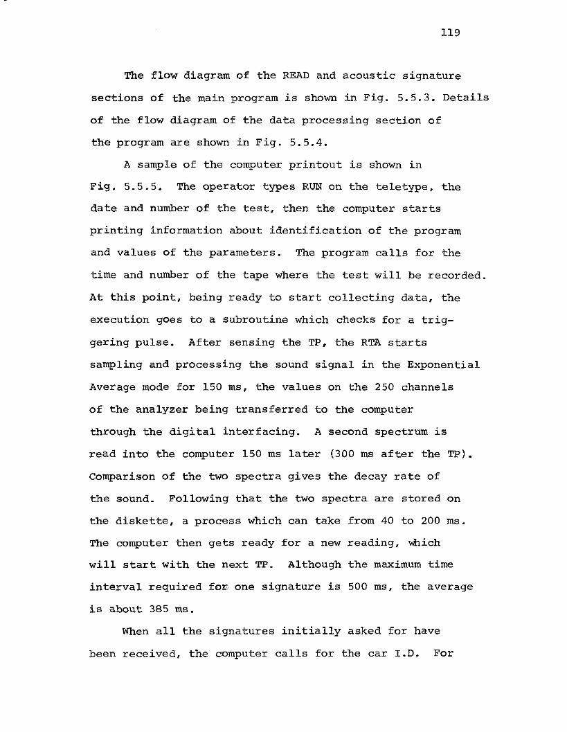
119
The flow diagram of the READ and acoustic signature
sections of the main program is shown in Fig. 5.5.3. Details
of the flow diagram of the data processing section of
the program are shown in Fig. 5.5.4.
A sample of the computer printout is shown in
Fig. 5.5.5. The operator types RUN on the teletype, the
date and number of the test, then the computer starts
printing information about identification of the program
and values of the parameters. The program calls for the
time and number of the tape where the test will be recorded.
At this point, being ready to start collecting data, the
execution goes to a subroutine which checks for a trig
gering pUlse. After sensing the TP, the RTA starts
sampling and processing the sound signal in the Exponential
Average mode for 150 ms, the values on the 250 channels
of the analyzer being transferred to the computer
through the digital interfacing. A second spectrum is
read into the computer 150 ms later (300 ms after the TP).
Comparison of the two spectra gives the decay rate of
the sound. Following that the two spectra are stored on
the diskette, a process which can take from 40 to 200 ms.
The computer then gets ready for a new reading, Which
will start with the next TP. Although the maximum time
interval required for one signature is 500 ms, the average
is about 385 ms.
When all the signatures initially asked for have
been received, the computer calls for the car I.D. For

WAIT FOR 2*l::.T{300ms) AFTER TP
READ MAXN, LET N'I, I, I
THIS IS AXLE NO. "N"
IF I is ODD THIS IS A RIGHT SIDE WHEEL.
IF I IS EVEN THIS IS A LEFT SIDE WHEEL.
[_..,:W..,:A.:.:,IT.:..-F.:.:,O.:.:,R_T_R_'G_G:,:E:.;,.R:.;,.IN_G_P.:.:,U_LS...:E:.;,.{:..:T.:.:,P:....)-----J
[.__W_A_IT_F_O_R_l::._T_{,15_0_m_S_)_A_F_TE_R_T_P----'
[READ FIRST SPECTRUM FROM
, R..,:T..,:A_T_0--...zC..,:O_M_P..,:U_TE_R ----'
[
[READ SECOND SPECTRUM FROM
___..,:R~T:.:::A:.......:T..,:0'---iC.::.OM:;:;..:PU:...:T..,:E;:,:R ---l
[TRANSFER THE TWO SPECTRA
_.:...F:..:.RO:;::M,,--C:;::O::.:M:::.P.;:U...:,T.::.ER:,;..-T:.,:O:.....::D",IS"'Kc::E.:...TT:,.:E=--_--'
120
IS
N'I/2
I , I+ I
YES
GO TO DATA PROCESSiNG
ROUTINE
YES
OF THE READPART OF THE
FIG. 5.5.3 FLOW DIAGRAMACOUSTIC SIGNATURESMAIN PROGRAM.
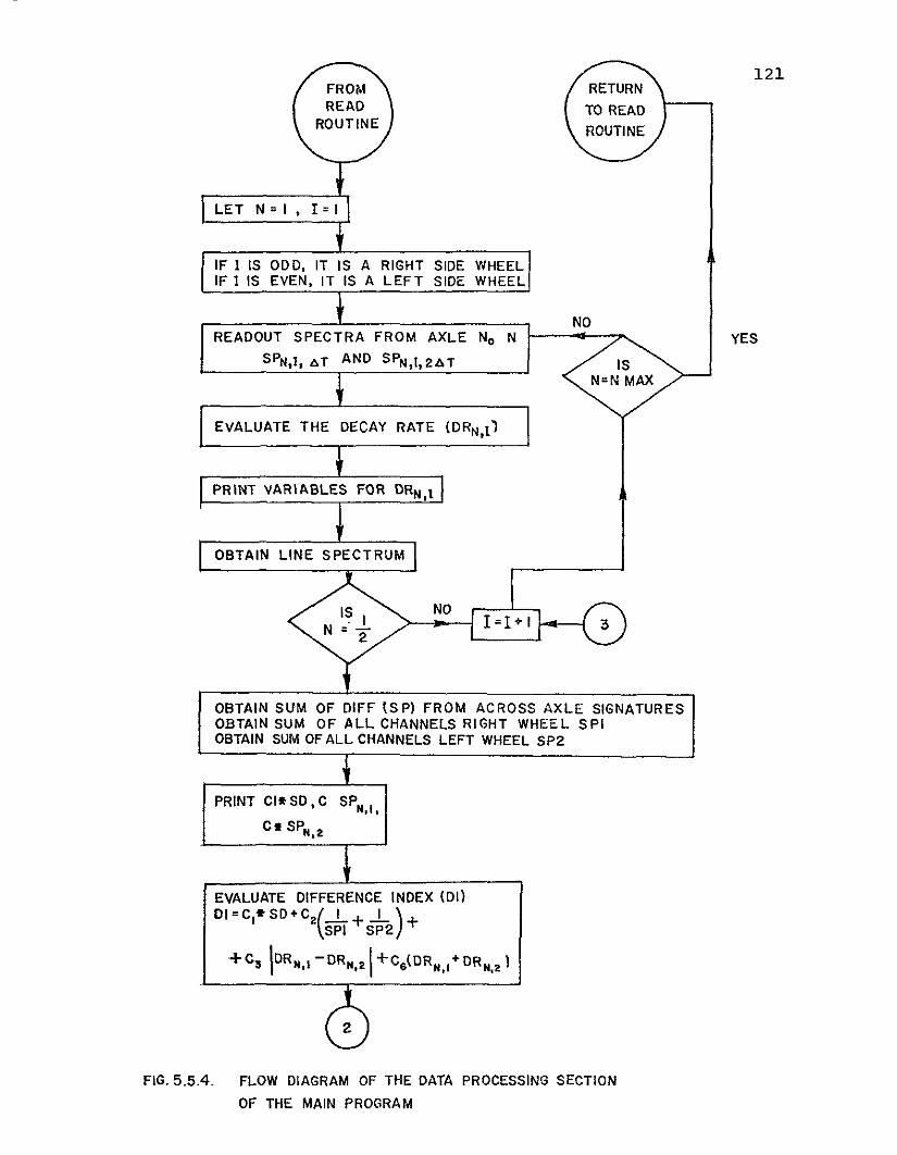
LET N = I , I = I
IF 1 IS ODD, IT IS A RIGHT SIDE WHEELIF 1 IS EVEN, IT IS A LEFT SIDE WHEEL
121
NOREADOUT SPECTRA FROM AXLE No N
SPN,J.6T AND SPN,I,26T
EVALUATE THE DECAY RATE (DRN.t)
PRINT VARIABLES FOR DRN,t
I OBTAIN LINE SPECTRUM
ISN=N MAX
YES
NO>-----1 I =1+ I f-C----l 3
OBTAIN SUM OF DIFF \SP) FROM ACROSS AXLE SIGNATURESOBTAIN SUM OF ALL CHANNELS RI GHT WHEE L S PIOBTAIN SUM OF ALL CHANNELS LEFT WHEEL SP2
PRINT Cllt SO. C SPN,f,
C. SPN,Z
EVALUATE DIFFERENCE INDEX (OilDI=C,ltSD+CZ(_1 + _1_)+
SPI SP2
+ CS\DRN,I -DRN,Z\ +Ce(DRN,,+ DRN,z )
FIG. 5.5.4. FLOW DIAGRAM OF THE DATA PROCESSING SECTION
OF THE MAIN PROGRAM
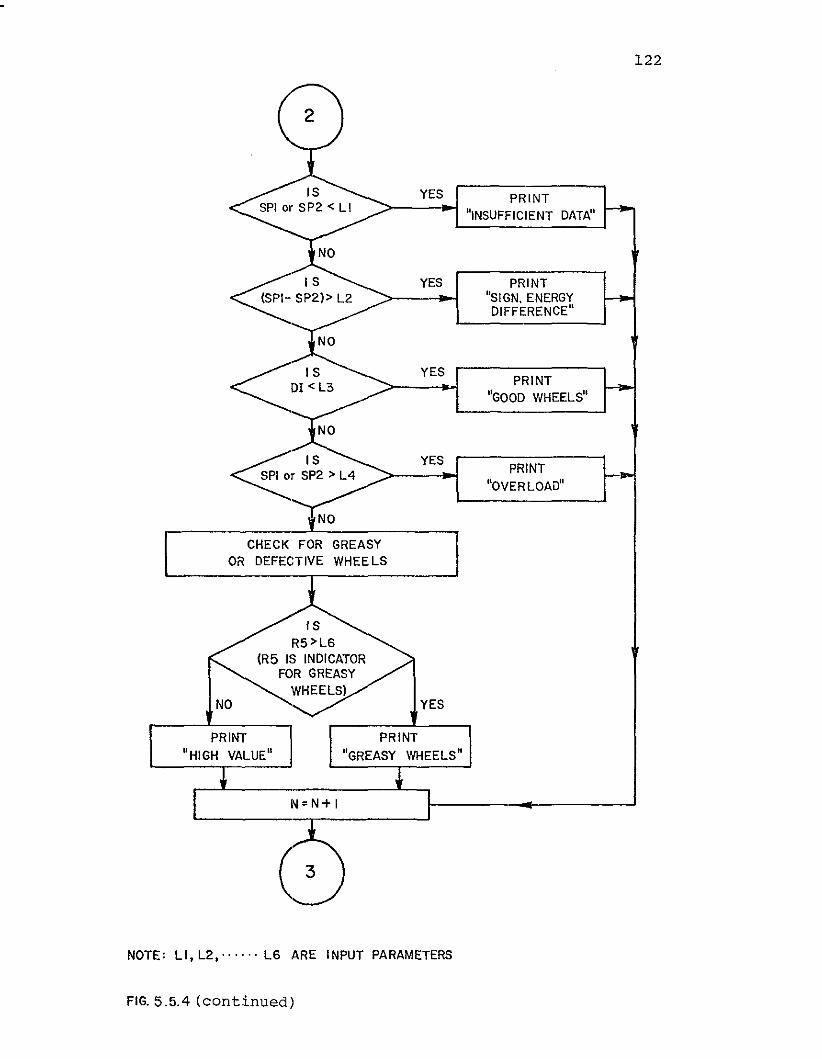
~IS~SP2<L1
YES PRINT>---~ "INSUFFICIENT DATA"
122
YES PRINT"SIGN. ENERGYDIFFERENCE"
~IS~SP2»L2
NO
~IS~rSP2>L4
NO
YES
YES
PRINT"GOOD WHEELS"
PRINT"OVERLOAD"
[-- CHECK FOR GREASYOR DEFECTIVE WHEELS
NO
ISR5>L6
(R5 IS INDICATORFOR GREASY
WHEELS)YES
PRINT"HIGH VALUE"
PRINT"GREASY WHEELS"
N=N+I
NOTE: L1, L2.",,·· L6 ARE INPUT PARAMETERS
FIG. 5.5.4 (continued)

123
RUN 770712-1IJ
----------------------~------T- 562~1Jl I I8~P. AVG.
SPECTRA PROCESSInG ROUTI~JES
TI1GLE.'-rOOD YAED TESTS-JUNE 77+ASSE1DLY A-141O-1X
12 JULY 1977
79457 CL/ATSF 81338 CL\? 173217 CLI SS~']
162 34157 48
57
N1Ji1 BER 0 F CHANtJ ll. S; 250NU1EER OF SPECTRA ; 24FREQUmCY FACTOR D13AN D H~; 410Dl SCprll'Jl\TI ON LEIJEL; 8D.HJDEX DECISI0'1 LE'JEl.; 85DA T E- THI E? I 2 J ULY 7 7 I 5: I 10: IO\? 10TAPE#? 1810CAR I. D.? TPJ 1, !{ 1, J( 2 10JI.!(J,!(2 1
472 39 45
1--------------------------------------------------------------1I TEST I SPI I SP2 I D. INDEX I rUHARJ{S I1------1-------1-------1--------1------------------------------1I I I 138 I I I 1 I 61 I GOOD ~]H EELS IJI.KI.K2 0 140 12Jl.KI.K2 I 180 64
573 47 51 62I 2 I 239 I 182 I 75 I GOOD UHEll.S IJI,KI.J{2 0 I g 7 I 1Jl.!{I,){2 1 173 52
956 79 83 9 1I 3 I 274 I 130 I 103 ISIGNIFF. mERGY VI FF. IJI.KI.K2 0 173 26JI.J{I.j(2 I 168 47
638 53 58 63I II I 176 I 160 I 74 I GOOD ImEELS IJI.I{1.J(2 0 157 23J I. )( I, J( 2 I 145 19
708 59 64 710I 5 I 234 I 137 I 710 I GOOD ~]H EEL S IJ I. i<l. K2 (1) IS5 I IJ I, J( I, )(2 1 193 39316 63 72 73
I 6 I 238 I 157 I 84 I GOOD WHEELS 1
FIG. 5. 5. 5 SAMPLE OUTPUT OF THE MAIN PROGRAM
124
long train cuts the first and last car I.D.s were given,
and thus intermediate cars could be identified by consulting
the consist lists. For short tests, of two to four cars,
all I.D.s were typed. Data processing then begins by
retrieving from the diskette the spectra of wheels across
the axle. The decay rate is evaluated from the two
readings with alSO ms interval.
In order to test the efficiency of the system and
the software, recordings made during the 1975 field test
described in Section 1.8 were analyzed. The distribution
of difference index for 2 runs (Run #21, 23) is shown
in Fig. 5.5.6. The circles indicate a defective wheel.
The distribution of difference index for the same run
(Run #10) for 3 different sampling time intervals is
also shown in Fig. 5.5.7. The analyses indicated better
discrimination and reproducibility compared to analyses
made using the 1/3 octave band RTA.

125
RUN #21 RUN #23
", .. 0
" • · " 0
", · " 0,. , · ,. •.. • .. ,
" • " 0
"0 "
," 0 " 0
01 ", .. 0.. • .. 0.. • " •
" • .... • ".. • .." • .... • .... , .." • ".. • .."
,""
,".. • ..
" • ",. • ,."
,""
, "" • "" • ".. • ".. • .... , "" • "" 0 ".. • .... • ".. • .."
, E> .... • .."
, .... , .... • .... • "" 0 .... 0 .." • ".. • , .... • , .... • , .... 0 , .. ,". 0 ., ". ,... • , '" 0on • , '" ,'" • , '" ,". • 0 ". 0
'" • · ... ,". , · ". 0
'" 0 ,'" 0... • ,'" ,,.. • , '" ,
'" • 0 ". @
'" 0 0 '" '"'" • E> '" 0on 0 , on ,... • · ... •'" • , '" 0
". 0 , '" ,'" 0 0 '"
,'" • , ". ,". 0 , ". 0
". 0 , '" 0
'" • ,'" ,
'" • , ." •". , on •". , '" 0
'", ". ,
'" , '" ,0" ,
'" 0... ,'" ,
'" • I.~? ,... ,'"
,". ,
'",
'",
'" •'"
,'"
,,.. , ". ,". , '" ,'"
, ". ,'" ,
'" ,'" ,
'" ,'"
,'"
,... , ... ,". • ... •,.. , .., ,." , .., ,... ,. ,.. ,... '" ,... ". 0.., ,.. ,... ... 0.., ... 0
"0 ... ,'" '"
,'" '" •'" '" ,". ,,. 0
'" '" •". ". ,'" '"
,'" '" ,.~ ... •
FIG. 5.5.6 DISTRIBUTION OF DIFFERENCE INDEX FOR RUN #21 AND RUN #23FROM THE FIELD TESTS AT ENGLEWOOD YARD, 18 June 1975
~ Indicate Do I. for defective wheel.
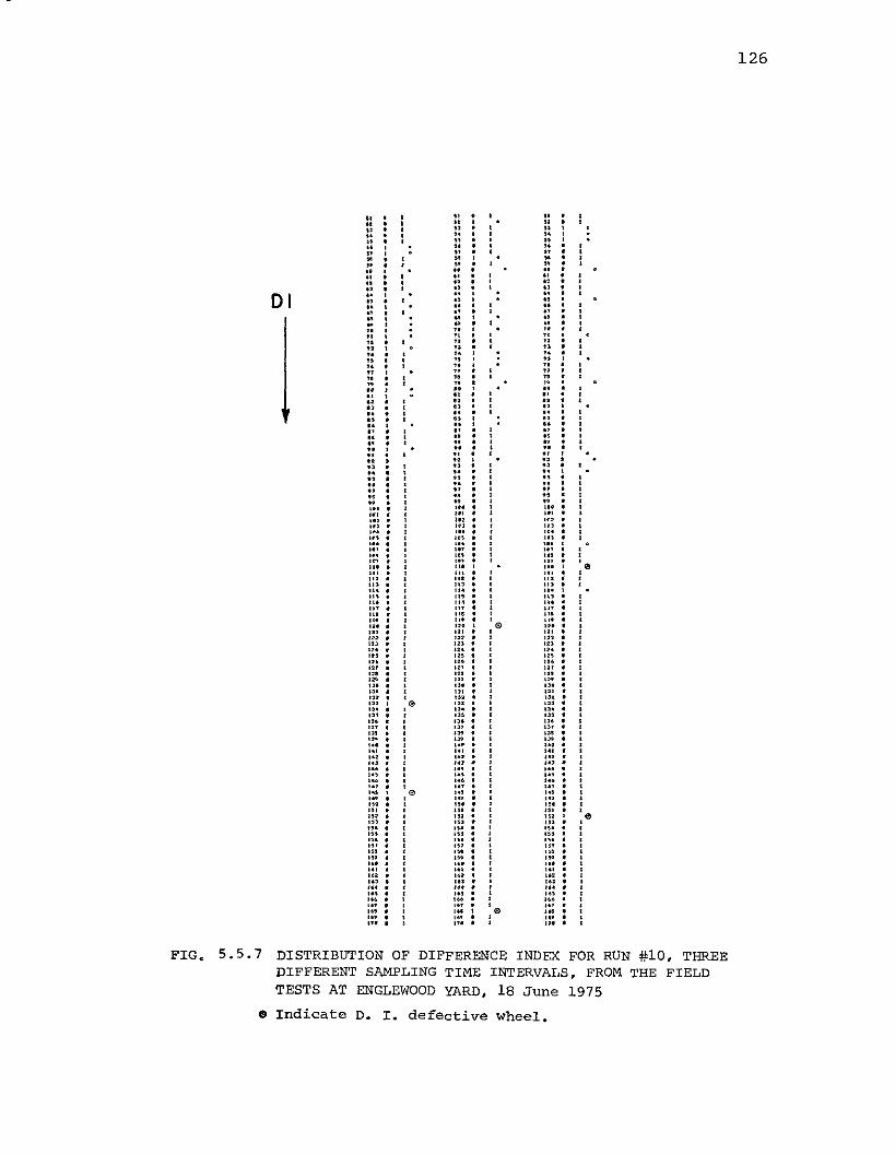
.. , .. .. ,.. .. •.. • " ",
:~ • ,. .. ,,.. • .. ",.. .. ,.. , .. .. ,.. ,
" ",
" • .. .. ·,. • .. .. ,.. , .. .. •.. • .. .. •.. ·.. • ..:~ •
DI .. , .. ,.. • .. .. ,.. , .. .. ,.. , .. .. ·.. , ", .. ·.. , .. • :: •.. , .. , ,.. , .. , .. ,.. • .. • .. •
", " · " ·.. , .. , .. •.. , .. , .. ,.. • .. , .. ·.. , .. • " ,.. , .. ,
~:, · .. ,.. , .. , .. ·.. • .. ·.. : .. , .. •.... · "
,"
,.. · .. · .. ," • "
, " •.. , .. , .. •.. · .. • .. ·.. , .. ," ·.. , .. • :: ·"
, .. · •.. · " · .. ,"
, ", " ,.. · , .. .. •.. · , ,. .. ,
" .. •.. , , .. .. ,.. · ,.. • , .. .. :.. · , .. ".. · , .. .. ·". • , ". ". •,., , : ,.. '" ·,.. · U~ l~' ·::~, '" '" ·· , ". ,.. •,.. • , ,.. '"
,,.. · , ,.. ,.. ,::~ · , '" '"
,· , ". ". •'M · , ". ·'" • , ". '", •'" , ", ,
'" • ,", · , '"
, ", • ,'" · , '"
, ", ,... • , ". , ,..... · , '",
'",
", , , ". , ... ,'" • , '"
,'" ,
'" , , '" , ," ,'" , , '" , ," ,,.. • , '" @ ,.. ,'" · , '"
,'"
,'" · • '"
, ", ,'" • , ,n , ,n ,... · , ". , ". ,,n · , ,n ,
'",
'" , , '", ", ,,,, , , '",
:~~,,,, , , ,n , ,,,, · , ,.. , ,.. ,
". • , '",
'",
'" • ,'"
,'"
,'" · , ", , ,,, ,,n , @ ,n , ," ,". , , ". , ,.. ,". • , ... , ". ,,.. • , ,,, , ,.. ,'" , , '"
,'"
,,,, · , '", 'M ,,,, • , ,,, ,
'",... · , .., ,
'",
'" · , ,.. , .., ,,n · , ..' , ,n ,... , , .., • • '" •... · : ... , , ..' ,... · ". · , ..' •.., • • .., , · ... •... · • ". , , .., ,,n , @ ... · • .., •,.. , ,. · • ... ,". • ,.. • • '.. ·n, , ... · • ,.. •'" , '" · • '" •... • '" • • ,n •n' • n. · , n' •n. • n. · • '" •". • ,.. • , n. •,n • ,.. · • n' ,n. • '" • • '" •'.. • ... • • ,. •". • n. · • ... •.., , ... · , .., ·... , ..' , , ,.. •... • ,.. • , ", •... • ... • • ... •... : ... · • ... •... .., · • ,.. •". , n. · • ... •... , .n , @ .n •,,, , ,m • • ,. •... , ... • • ,.. •
FIG. 5.5.7 DISTRIBUTION OF DIFFERENCE INDEX FOR RUN #10. THREEDIFFERENT SAMPLING TIME INTERVALS. FROM THE FIELDTESTS AT ENGLEWOOD YARD. 18 June 1975
$ Indicate D. I. defective wheel.
126
127
6. WAYSIDE TESTS
6.1 Tests at TTC Pueblo, Colorado
Two field tests were performed in the Transportation
Test Center (TTC) in Pueblo, Colorado, at a three month
interval. The objectives of these tests were:
1. To test certain parts of the system, such as the
microphone, the modified exciter, and the wheel
sensor, in the field.
2. To simulate the operating conditions for the Acoustic
Signature Inspection system under development.
3. To determine the signature change, over a certain
time period, due to wear of the wheels.
6.2 First Pueblo Test
In all 10 tests were done on the bypass of the FAST
track. These are described as follows.
Test
123456789
10
Date
11-16-7811-16-7811-16-7811-16-7811-17-7811-17-7611-17-7611-17-7611-17-7611-17-76
Description(train speed, direction)
5 MPH; counterclockwise5 MPH, counterclockwise8 MPH; counterclockwise8 MPH; counterclockwise5 MPH; clockwise5 MPH; clockwise8 MPH; clockwise8 MPH; clockwise5 MPH; brakes lightly applied12-15 MPH; clockwise
Tape recordings of acoustic signatures were
obtained from each of the project FAST train wheels.
This was done for all wheels on one side of the train

128
on Tuesday evening, 16 November 1976 and for the
wheels on the other side on Wednesday evening. A
consist description was obtained for car identification.
The first four cars in the 70-car consist were replaced
in the Wednesday night test, otherwise the consist
remained the same for both tests.
Wheel excitation in these tests was done with the
improved model of the VH mechanical hammer exciter, as
described in section 5.1.1. A photograph of the installed
exciter is shown in Fig. 6.2.1. This hammer exciter
performed without mishap during the tests, and showed
only minor wear following the 3124 test impacts. At the
time the first series of Pueblo tests were made, it
was believed that the hammer could be activated by impact
from the link, 3, (see Fig. 1.6.1), so the springs,S,
were disconnected from the hammer at point B and instead
connected to the frame. Thus the hammer was allowed to
swing free from the link, 3, on impact and the springs,S,
served to reset the link, 3, rather than the hammer. This
change, although of interest from the design standpoint,
gave rise to some problems, as indicated below.
The wheel impact response was judged to be best for
the 5-8 MPH train speed. The hammer exciter would not
operate effectively for train speeds above 12 MPH and
did not impact at all below 3 MPH. About 1/3 of the
wheels were not struck by the hammer during the 12-15 MPH
test presumably because the hammer could not reset as

129
FIG. 6.2.1 MODIFIED MECHANICAL HAMMER EXCITER USED AT TTC,PUEBLO
130
needed in the time between the passage of wheels on the
same truck. However, the hammer mechanism was not
damaged in this test nor did it appear to present a
hazard to the train or personnel in attendance. The impact
sound levels measured approximately 6 feet from the wheel
usually exceeded 95 dB which was at least 10 dB above the
background train noise.
The performance of the wheel sensor was good. It
was installed and calibrated easily. For calibration
a small vehicle provided by TTC was used. Views of the
system used at TTC Pueblo are shown in Figs. 6.2.2 and
6.2.3.
The acoustic signature of the wheels was recorded
on two different tape recorders simultaneously. One
recorder was a General Radio dual channel. It was used
for simultaneous recording of the sound in channel No. 1
and the triggering pulse in channel No.2. This recorder
operates with a 115 Volt AC, 60 Hz power supply. Unfor
tunately there was no such line available at the test
location and a portable generator was used. That later
proved to be a major obstacle in the analysis, because
the speed of the tape transport mechanism is directly
dependent on the frequency of the power supply. The other
recorder was a NAGRA single channel, battery operated
instrument. This is a very good recorder, but only the
sound could be recorded on the single channel.
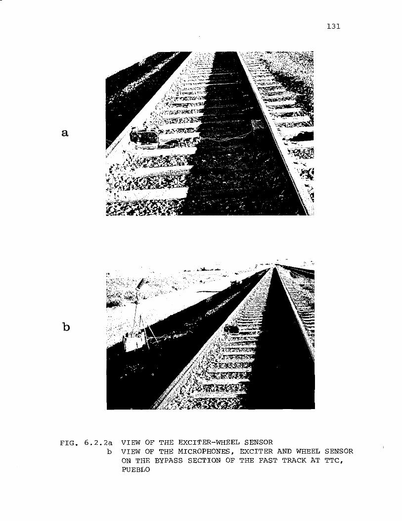
a
b
131
'\.~m'~
':i" ",c.lIiiIIIi..~~ -.,-':f:-«~~
.~~
--- ~.;,...::
'\~
FIG. 6.2.2ab
VIEW OF THE EXCITER-WHEEL SENSORVIEW OF THE MICROPHONES, EXCITER AND WHEEL SENSORON THE BYPASS SECTION OF THE FAST TRACK AT TTC,PUEBLO
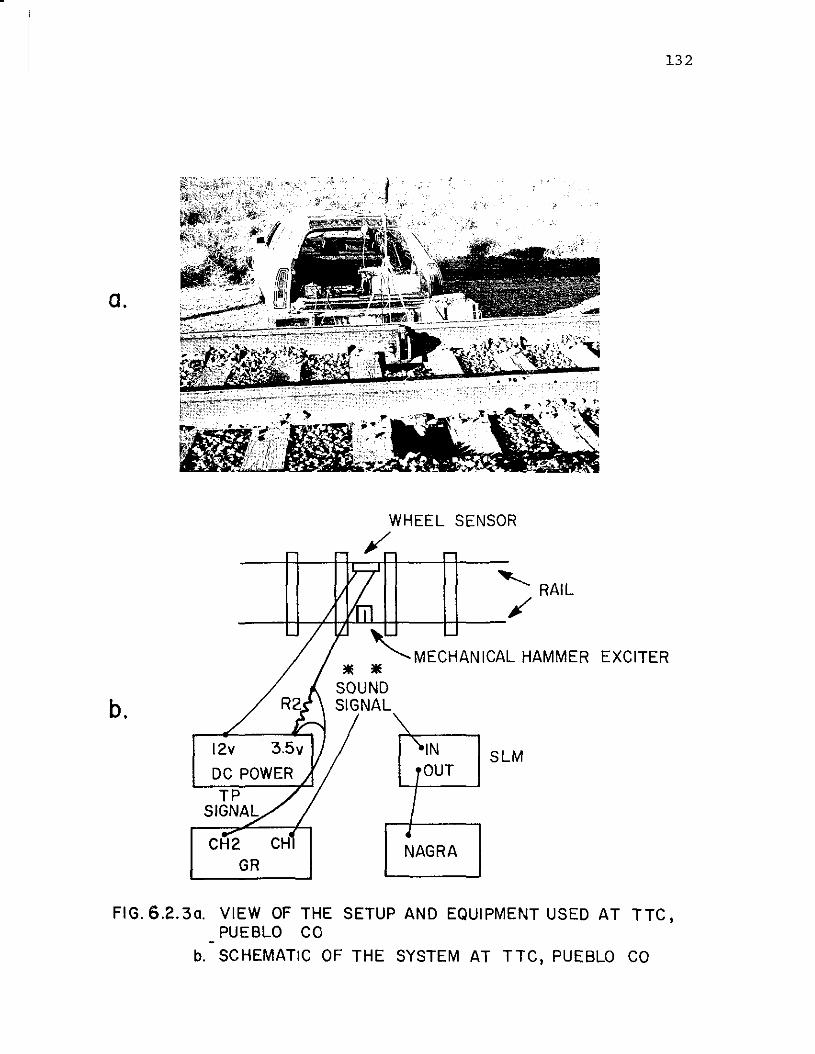
132
a.
WHEEL SENSOR
~
EXCITER
SlM
'\'-IN
'OUT
•NAGRA
, RAil
--t+---+-t"Jf-'-'-'Y+-++--/
~MECHAN ICAl HAMMERlIE lIE
SOUNDSIGNAL
CH2GR
b.
FIG. 6.2.30. VIEW OF THE SETUP AND EQUIPMENT USED AT TTC,PUEBLO CO
b. SCHEMATIC OF THE SYSTEM AT TTC, PUEBLO CO
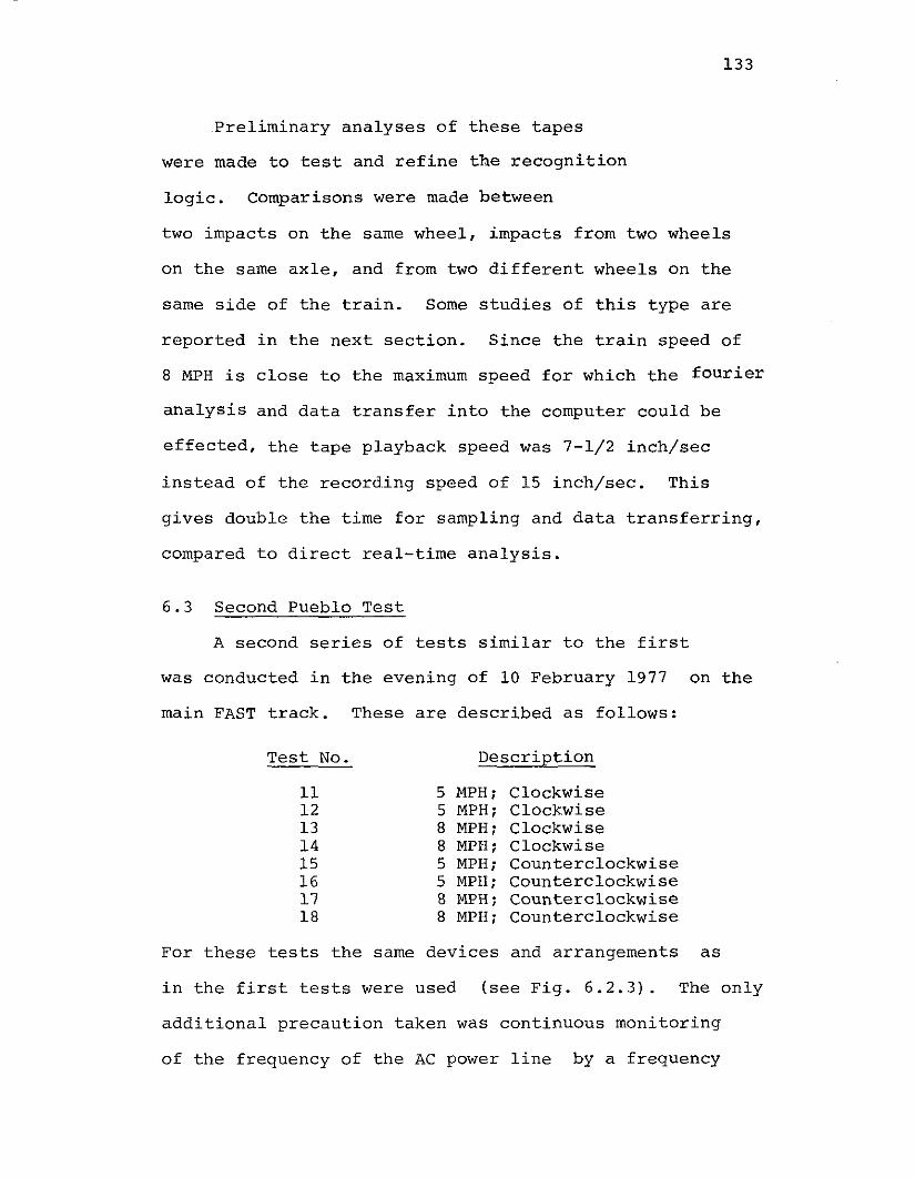
133
Preliminary analyses of these tapes
were made to test and refine the recognition
logic. Comparisons were made between
two impacts on the same wheel, impacts from two wheels
on the same axle, and from two different wheels on the
same side of the train. Some studies of this type are
reported in the next section. Since the train speed of
8 MPH is close to the maximum speed for which the fourier
analysis and data transfer into the computer could be
effected, the tape playback speed was 7-1/2 inch/sec
instead of the recording speed of 15 inch/sec. This
gives double the time for sampling and data transferring,
compared to direct real-time analysis.
6.3 Second Pueblo Test
A second series of tests similar to the first
was conducted in the evening of 10 February 1977 on the
main FAST track. These are described as follows:
Test No. Description
1112131415161718
5 MPH; Clockwise5 MPH; Clockwise8 MPH; Clockwise8 MPH; Clockwise5 MPH; Counterclockwise5 MPH; Counterclockwise8 MPH; Counterclockwise8 MPH; Counterclockwise
For these tests the same devices and arrangements as
in the first tests were used (see Fig. 6.2.3). The only
additional precaution taken was continuous monitoring
of the frequency of the AC power line by a frequency

134
counter. During the second tests a better and bigger
generator was available. The frequency of the generator
was reasonably stable, although it drifted slowly within
the range of 59.0 - 60.2 Hz, during the 5 hour tests.
This introduced a maximum frequency error of 2% in the
acoustic signatures. Errors of this size can be important
in the data analysis, because line spectra comparison
will be impossible. Note that in the line spectra
comparison the tolerable error is 0.4% (a spectrum from
SD330A RTA has 250 channels). During a single test the
frequency of the generator drifted in the range of 0.0
0.3 Hz with an average less than 0.2 Hz. Indications
are that during the first test the phase frequency of
the power supplied was between 52.8 and 54.2 Hz. As a
final note on the error introduced by the change of tape
speed, manufacturers data for the GR data recorder type 1525
indicates that 'flutter and wow' is below 0.2% rms.
According to the Houston Lighting & Power Company, the
maximum average frequency change of the power lines is
0.2% - 0.3%. In unusual cases this may go a little
higher. Therefore there is no error introduced in the
analysis due to the tape transport mechanism due to the
frequency of the laboratory power supply.
Most of the recordings made were good. Comparisons
between wheels on the same side, across the axle and at
different speeds were made. The results are presented
in Fig. 6.3.1, Fig. 6.3.2 and in Fig. 6.3.3. These
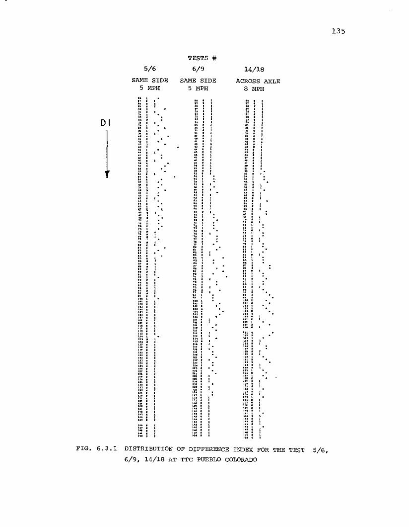
TESTS #
5/6 6/9 14/18
SAME SIDE SAME SIDE ACROSS AXLE5 MPH 5 MPH 8 MPH.. .. • .. ,
".. " • " •.. .. • .. •.. .. • .. ,.. .. · ",
" .. • .. ," " : .. ,
" " ,D I ..
" • .. ,".. " · " ," .. • " ,.. " ·. " ,.. .. " ,.. .. " ,.. .. .. •.. .. .. ," .. .. ,.. , .. .. ,.. , .. .. ,.. • .. .. ," • .. .. •.. .. •=
• ~ .. ,•.. • · ., ," , .. .. ," · " " ," , " ".. • " " , ." • .. .. •" "
,.. • .. • . .. ,.. ,• • " .. •• • •.. , · " •.. , .. .. ·" , .. " •"
,.. • .. " •" " •.. , .. .. ·.. · " .. •.. • .. .. •" t , .. " •.. • .... , .. ..
" • .. .." • " "" • " ".." • " ".. ," ..
" • .. "~: • .. ..• " .." ," ".. • .... • .. ..".. , .. ::.. , .." • " ..
:~ · .. · ..· ", " ·.. • .. • .. ,.. • .. · .. ,.. · .. · .. ,.. • .. • .. •.. • .. • .. ,.. · .. • .. ,.. , .. • .. •.. • .. • .. ,.. • .. · .. ,.. .. • .. ·:: .. l .. ,
" •.. .. i .. ,.." .. ·... ,.. , ,.. •,..'" : '"
,... ... '",... .., ; ,.. ,... ... ... ,.., .., , ... ·... ... ... ·'" .., '" •,.. ,. ,.. ,,.. ,.. ,.. ,". ,.. ... •,..
'"". ... .., ·'" '" '",... • ... '",
'" ... ". ·". ". ... •'" .., ". ·,.. ... ,n •..' ... ,.. ·,,,'" ". •.., .., '"
,'" '" .. ' •'" '" ,. ,". ... .., •::: '" ". ·'"
, ". ,'" '" ". •." ". '" •... ,. '" ·." '"
,. •."'" '" •'" '" ," •'" '" ". :,..'" '"'" '" ". •". '" '"
,'" '" ". •,. ,. '" •,. ,,, '" ·,.. ... ,,, ·.., ,.. ,.. •,.. ,.. ,., ,... ... ... •... ... ..' •... ... ... •... ... ,.. •.., ,.. ,'" ,.. .., •,~ ,.. ,~ •,. ... ,. ·...
'M •
135
FIG. 6.3.1 DISTRIBUTION OF DIFFERENCE INDEX FOR THE TEST
6/9, 14/18 AT TTC PUEBLO COLORADO5/6,

136
TEST #
14/18 6/3 13/13ACROSS AXLE ACROSS AXLE SAME SIDE RANDOM COMPo.. • .... • .. .... • .... • .. ".. · .. n.. • .. .... • .. ..
" • " ".. • .. .." • .. ".. • .. .... • " "0 I .. , .. ..• • l:.. • • • •.. · .. • .... • .. •" • .. • .... , .. , .... • .. , ..:: • .. • ..
• .. • .... , .. • .... , .. ,::.. • .. ,
Il • .. • ..• .. •" • .. • .... ,
", ..
" • .. · "".. " .. , .." • .. , .... • " •.. , .. , .... • .. , ".. • .. , .. •.. • .. , .. •"
, .. , .. ," • "
,.. • ,. · .. ,.. , .. • .. ,.. • .. , .. ,.. • .. , .. ,.. • .. , .. •.. • .. ,:: ,
" \ • .. • •" • · .. , .. •.. • · ", .. ,.. ,
" •.. • .. , .. ·.. , .. , n •.. , .. • .. •" • .. · .. ,.. • n • .. •.. , .. · .. ,.. • .. , .. •:~ : .. · .. :"
, .." • .. , .. ," • ., ,
" •.. • .. · .. ,.. : " • .. ," .. ,
",.. • " • .. •.. , .. ,
" ·.. , .. • .. ,.. , .. • .. ,"
, .. , .. ," • " • .. •.. • " • .. ,.. • .. • .. ,.. · .. • .. •.. , .. · .. •.. • " • .. •.. • .. • "
,... • .. , .. •,.. , ". , ..'"
, ".". • ". , ,..'" • ". , ,..". • ,.. , ,n'"
,'" • ".". · ". • ".'" , ,.. • ".'"
, '" • ".,.. , ,n • ".". • , ,..'"
, no '"'" • '" '"'" '" '"". ". '"'" ". '"". no '"::: '" ".", '"". '" '"". ". "...' ,.. ,..... ,.. ..,,n ," '"". ... III,n ".... ,.. ".,.. ,.. "..., '" '",,, ,.
'",.. ,. ,...., ,.. ...'" on
'"'" '" ,..,.. '" g~'" ...". , on ,n'"
, ,.. ".,.. · '" '",. • ,.. ,..... • ,. ,.,.. • ". ...... ,'" ,..... • ". ".,.. ,..... ". ".,..". ,..". ...,.. ... ,..,.. ... ,..,.. ,.. ,..". ,.. ".".
FIG. 6.3.2 DISTRIBUTION OF DIFFERENCE INDEX FOR TESTS 14/18. 6/3.13/13 AT TTC PUEBLO COLORADO
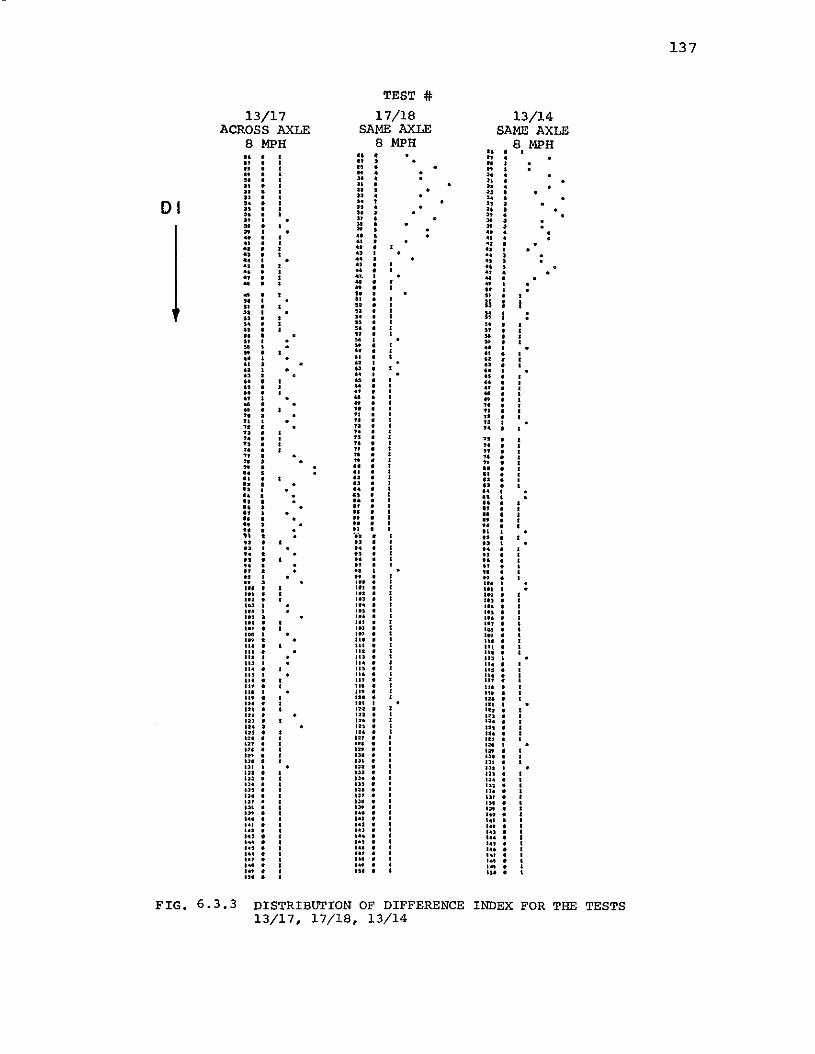
TEST #13/17 17/18 13/14
ACROSS AXLE SAME AXLE SAME AXLE8 MPH 8 MPH 8 MPH.. • .. • •.. .. •.. .. , .. •.. .. • " •.. " • . .. •"
.. • ." •" " • " •.. .. • " •.. .. • " •0 I .. "
,"
,.. .. • " •.. .. ," •
" " • .. ,.. .. • .. ,.. .. • .. •.. .. , .. •.. .. • .. •.. .. • .. ,.. .. , .. ,.. .. , .. ,.. .. .. ,.. .. .... ". MM M .... .... " "" " II"
.... ..".. .. ".. • ..".. • " ..
" • " .."
, .. .... , " .." • .. .... • " .."
, .. .... • .. .... • .. .... • .. .... • .. .... • .. M.. • ..".. • " ..
" • .. .... • " .... • .. .... • .. .... • .... • .. .." • .. .... • " ".. • .. .... , " "" • .. .... • " ".. • .. .... • .. .... , .. .... • : .. .... • .. .... , .. .... • .. .... • .. .... , .. .... : ..
" •.. "·2 .. •.. .. .. •.. .. .. •.. .. .. •.. .. .. •.. " " •.. .. .. •.. .. " •" ... ... •". '" '" •... .., ",... '" '".., ... ...... '" ",... ... ".... '" '"... ,,, ,..." ... ,,,'" ... ...... ... ..,... ,.. ...... '" '".., ... ...... '" '"'" ... ...... '" '"'" ... ...... ... ,..'" ... • ...... ... ..,'" ... '"... '" '"'" ... ... •... ... ...... ... ...In 'n ...'" ... ...'" '" '"'" no ...,.. ..,
'".., no '"... '" '" •'" '" ... •no '" ... ,'" no '" •... '" '" •,.. n. ,,, ,,.. ." '" •'" ... ... •... .., .., ,'" ... ... ,... .., ,.. ,,.. ... ... •... ,.. .., ,,.. ... ... ,... ... ... ,... ,.. 'M •,.. ,.. '" •,.. ". '" •...
137
FIG. 6.3.3 DISTRIBUTION OF DIFFERENCE INDEX FOR THE TESTS13/17, 17/18. 13/14

138
figures show the distribution of the difference index
values for most of the tests. The best results were
obtained comparing the same wheels recorded in successive
tests where the train was moving at the same speed.
Problems related to the tests and subsequent laboratory
analyses are:
1. The train speed varied in most of the tests about
+ 2 MPH from the nominal speed, the reason being the
steep grade existing in the particular section of
the FAST track used.
2. The power frequency was different in tests separated
by long time intervals. This is probably the reason
why across the axle comparison did not show
results as good as expected.
3. Because of the large power frequency difference
between the first and second Pueblo tests (53 and
60 Hz respectively) it was impossible to come to
any reliable conclusions on the effect of wheel
wear.
The following conclusions were arrived at from
the Pueblo tests:
1. The spring assembly of the mechanical exciter was
necessary.
2. Distant mounting of the exciters should be avoided.
A 200 ft separation between exciters was used in
the 1975 Englewood yard tests where the wheels on
one side were inspected first and then those on the other.
139
But the Pueblo tests showed that the greater
the exciter separation the greater is the effect
of varying train speed.
3. The exciter was strong enough to operate and survive
for a large number of impacts.
6.4 Tests at the Southern Pacific Englewood Yard, Houston
The final wayside testing of the Acoustic Signature
wheel inspection system took place in July 1977, in the
Southern Pacific Englewood yard in Houston. Traffic
speed inbound to the yard is sometimes higher than
15 MPH, and hence too fast for the inspection system,
but incoming to the hump the speed is 2-3 MPH. There
are about 3000 cars/day humped in the yard on 3 tracks.
The rail size is 136 lb. (mechanical hammer exciters
were designed for this size of rail). In a previous 2
year period the inspection personnel had discovered 6
broken and 12 overheated wheels.
The objectives for the tests were:
1. To obtain data for a statistically significant
sample of wheels in service. This data sample
could then be used for further studies to find the
optimum Dr equation and to ascertain what wheel
conditions, other than crack~might give rise to
high Dr values.
2. To rate the performance of the hardware to identify
weaknesses and problems.
140
3. Using the best software available at the time to
permit immediate follow-up on some wheels with high
DI values. It was hoped that a cracked wheel might
be found but this was recognized as a somewhat
unlikely occurrence in the time available.
6.5 Englewood Test Site and Equipment
The location for the tests was selected after a
visit to the site and discussions with representatives
of Southern Pacific. A simple chart of the hump is
shown in Fig. 6.5.1. The figure shows the location of
the trailer, where the electronic equipment of the system
was stored, and the mechanical exciter on the north
track. The location for the trailer had to comply
with and fulfill the objectives and requirements set
for the tests. For that reason it was placed at the
bottom of the slope which is about 400 yards from the
top of the hump. It would then take more than two
minutes for a car moving at the regular humping speed
to cover the distance from the trailer to the inspection
pits. An observer sitting in the trailer had an unob
structed view of the inbound or outbound traffic as well as
all train cuts moving over the hump. Electric
power was easily accessible from an electric tower a
few feet away.
Modifications in the hammer exciter and the software
were needed under the new operational conditions and
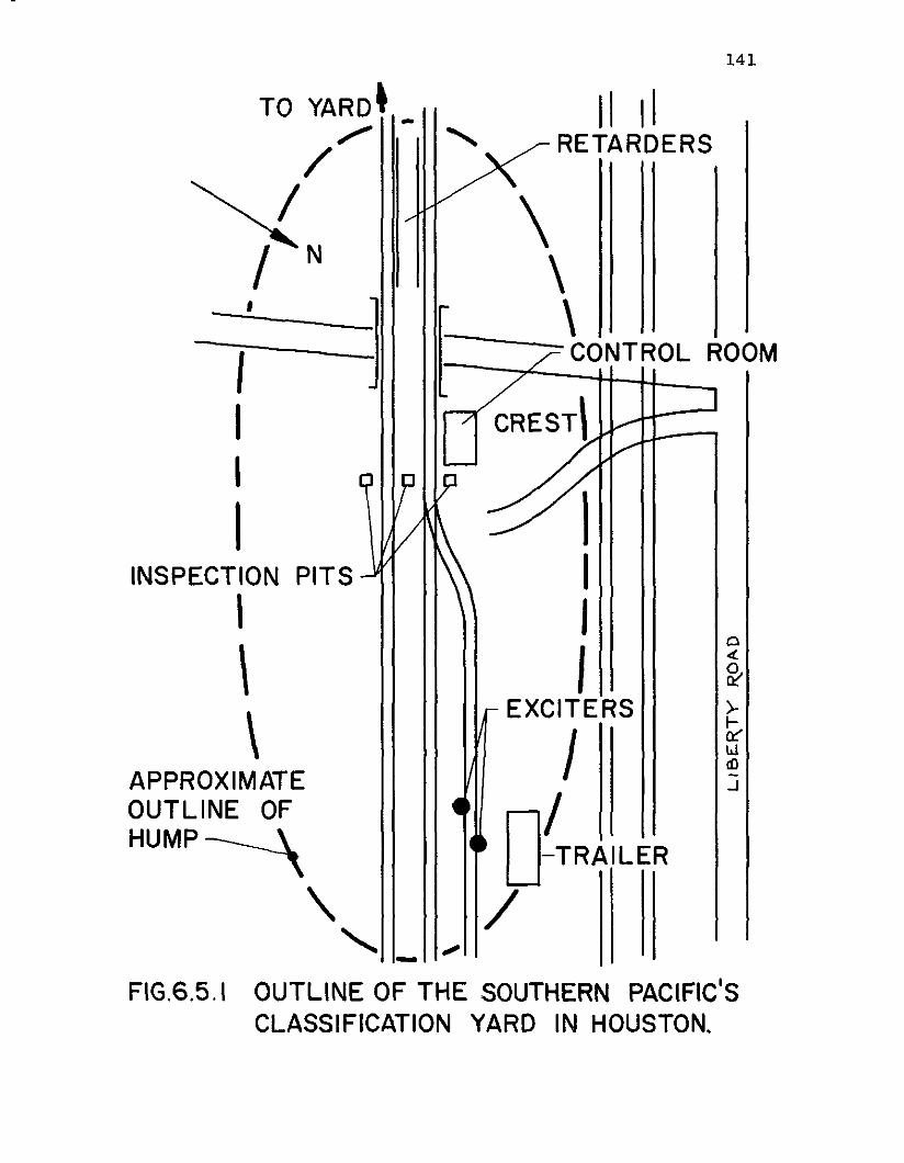
141
\\\
II---CONTROL ROOM
II IIRETARDERS
IIJ,
EXCITERS
I
O/TRAILER
/
CREST'
-
,
III
IINSPECTION PITS,
\\
APPROXIMATEOUTLINE OFHUMP-----\
\
"FIG.6.5.1 OUTLINE OF THE SOUTHERN PACIFIC'SCLASSIFICATION YARD IN HOUSTON.

142
requirements for these tests. The exciter used at
Pueblo did not operate for train speeds below 3 MPH.
Consequently, the spring configuration was returned to
the original design as shown in Fig. 5.1.1. After these
changes the exciter operated best in the range 1.5 to
3.0 MPH. It is obvious that with this design the per
formance of the exciter is speed and flange depth
dependent.
The tests were sCheduled daily between 9:00 a.m.
and 5:00 p.m. An average of 400 cars/day was estimated
to pass through the test location. Only a fraction of
those cars were actually tested, hence the chances of
finding a defective wheel were remote. To define the
discrimination level for good/bad wheels a complete
simulation test was performed in the laboratory. The
discrimination level of 85 was chosen after testing a
selection of wheels, as shown in Table 6.5.1.
An air-conditioned 8' x 21' trailer was installed
in the yard on 15 June 1977. It took about a week to
install, calibrate and make the first complete test
of the system. Two problems arose due to the condition
of the rail. i) Although the size of the rail was
136 Ibs., parts of the exciters had to be machined and
plates of variable thickness were attached to the top
of the plunger because the rail was worn down about
3/8 inch. ii) Calibration of the wheel sensor was

143
TABLE 6.5.1 DIFFERENCE INDEX VALUES FROM WHEELS TESTED IN THELABORATORY, FOR DISCRIMINATION LEVEL SELECTION
AXLE & WHEEL IDENTIFICATIONRUN #, PROGRAM TAPE # GOOD/BAD GOOD/GOOD
15C-15A 8B-8G 4G-4B IG-IB 13A-13C
770701-II T-562-V 175 91 101 142 127 69
770615-IV T-562-I 175 99 93 106 119 71

144
'very difficult for the same reason. No such problem
had been encountered during the test at TTC in Pueblo
or the laboratory simulation. As a result of this
difficulty multiple triggering or missing triggering
pulses were observed. Consequently, the maximum number
of wheel signatures per test had to be reduced to 80,
because faulty triggering invalidates an entire run.
The trailer and the outdoor hardware are shown in
Fig. 6.5.2. Through the window on the left the test
controller could watch the cars moving uphill towards
the crest. The schematic of the inspection system is
shown in Fig. 6.5.2b, distances between different devices
being marked on the drawing. The exciter and the wheel
sensors were mounted between the ties. The clearance
was very small, and therefore inevitably there was some
difference in the time between the triggering pulse and
the impact on the two sides of the track. During the
TTC and simulation tests, the exciter-wheel sensor
alignment was much better. In Fig. 6.5.3, the microphones,
exciters and wheel sensors are shown from the same angle
as seen by the test controller looking through the
window of the trailer. In Fig. 6.5.4a,b the system
and the east part of the hump are shown. The inspection
pits are indicated by arrows (Fig. 6.5.4a).
All testing was performed in real time. During
the last two weeks, when all necessary changes and
corrections had been made the sound and triggering
145
a.
N
/1= ,., =ITRAILER
b. 1 S
28'*Ml
__t--==--=-=--:-- _TO THE CREST W S2 ~3' 2r.
LLJEI DIRECTION OF
.. .....1-----
OF THE HUMP E2 cxr ~ W. SI MOVEMENT OF CARS3'811"""""'
*M2
FIGS 52 a VIEW OF THE INSPECTION SYSTEM
b SCHEMATIC OF THE SYSTEM LAYOUT

146
FIG. 6.5.3 VIEW OF THE MICROPHONES, EXCITERS AND WHEEL SENSORSTHROUGH THE WINDOW OF THE TRAILER

147
a
b
FIG. 6.5.4a VIEW OF THE EAST SIDE OF THE HUMP, INSPECTION PITSARE INDICATED BY ARROW
b VIEW OF THE MICROPHONES, EXCITERS AND WHEEL SENSORS
148
pulse signals were tape-recorded simultaneously with
the real time testing.
6.6 Performance of Hardware during the Englewood Test
The duration of the tests was approximately five
weeks instead of the scheduled four due to the initial
one week delay in the installation of the system.
The components of the system performed as follows
during the tests:
a) Microphones: No problem or failure. Some indications
of excessive attenuation or low gain in the pre
amplifier of one of the microphones during the second
week of the tests were finally attributed to a bad
cable. Rain did not have any adverse effect on the
microphones which survived three heavy rainstorms
during the test period.
b) Wheel Sensors: One of the dual wheel sensing units
failed a couple of days before the end of the tests.
It was easily replaced by the other unit. Some
triggering problems could be attributed to wheel
sensors. In the late afternoon hours, under extreme
heat, the temperature on the cover of the wheel
sensors was estimated to be above 130 o P.
c) Mechanical Hammer Exciters: Most of the parts
operated satisfactorily. Each exciter performed
about 27,000 impacts. One hammer had to be replaced
due to excessive wear, possibly because of improper

149
heat treatment. One pair of springs was also replaced
with new and stiffer springs.
d) SD330A Real Time Analyzer: Some problems developed
when the temperature inside the trailer was above
85°P.
e) NOVA 1220 Minicomputer: Some serious problems
(computer failure) occurred when the temperature
inside the trailer was above 85°P. The temperature
related problems in the RTA and computer were cor
rected by improving the air circulation in the trailer.
f) Diskette System: No problems. Further verification
of proper data transferral from the computer to
diskette and vice-versa was checked with a specially
written test program.
The performance of the exciter is shown in the figures
6.6.1 through 6.6.4. In each figure the top trace is the
triggering pulse signal, and the bottom trace is the sound
signal. These pictures were taken during the tests
using a TEKTRONIX 564 storage oscilloscope and a polaroid
camera.
The events shown in the pictures from left to
right are: The triggering pulse (TP) and the corresponding
impact on the north wheel of the first axle is shown
first, then the TP and the impact on the south wheel
of the same axle, then the TP and impact on the north
wheel of the second axle, etc.
150
Figures 6.6.1.a and b show the typical form of the sig
nals. The top picture which shows normal impact during the
last few days of the test after all possible improvements were
made may be compared to the bottom picture which was taken in the
early experiments. Figures6.6.2a and b show some of
the impact problems. In the top figure double impact
of the hammer on the wheel is shown. This impact is
more prominent on one side. In the bottom figure very
weak impact or no impact occurred at low speed when new
wheels with low flanges were passing over the exciter.
These impacts usually appeared as "insufficient data"
in the printout. Figure 6.6.3a shows, two
impacts on old used wheels with high flanges,
followed by two impacts on rather new
wheels with low flanges. In Figures 6.6.3b are shown
impacts of the type which sometimes gave rise to
the indication Significant Energy Difference. In
Figs. 6.6.1 through 6.6.3 the sweep speed of the
oscilloscope was 500 mS/div., except in Fig. 6.2.3b where
it was 200 ms/div. Figure 6.6.4a shows the signals from
the south exciter, at a sweep speed of 50 ms/div.
Figure 6.6.4b shows the corresponding signals from the
north exciter. On the south side the impact occurred
45-50 ms after the TP, on the north side the impact
occurred 100-105 IDS after the TP, hence there was a
difference of 50-60 ms in the data processing between
151
a
b
FIG. 6.6.1a TYPICAL PERFORMANCE OF THE EXCITERS DURING THE LATETESTS
b TYPICAL PERFORMANCE OF THE EXCITERS DURING THE EARLYTESTS. SWEEP SPEED 500 mS/DIV
152
a
b
FIG. 6.6.2a EXCITER PERFORMANCE, DOUBLE IMPACTb EXCITER PERFORMANCE, NEW WHEELS, LOW OR NO IMPACT;
SWEEP SPEED 500 mS/DIV
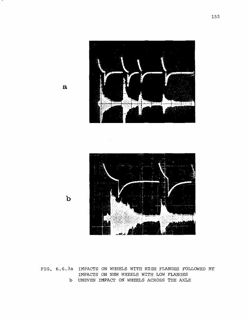
153
a
b
FIG. 6.6.3a IMPACTS ON WHEELS WITH HIGH FLANGES FOLLOWED BYIMPACTS ON NEW WHEELS WITH LOW FLANGES
b UNEVEN IMPACT ON WHEELS ACROSS THE AXLE
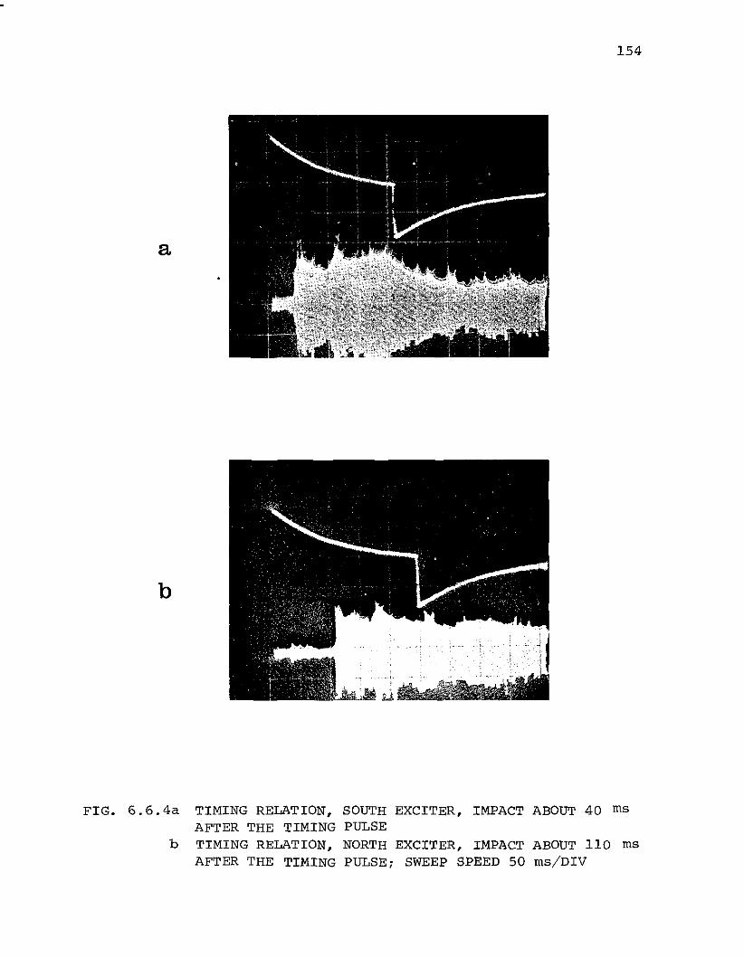
154
a
b
FIG. 6.6.4a TIMING RELATION, SOUTH EXCITER, IMPACT ABOUT 40 rnsAFTER THE TIMING PULSE
b TIMING RELATION, NORTH EXCITER, IMPACT ABOUT 110 rnsAFTER THE TIMING PULSE; SWEEP SPEED 50 rns/DIV
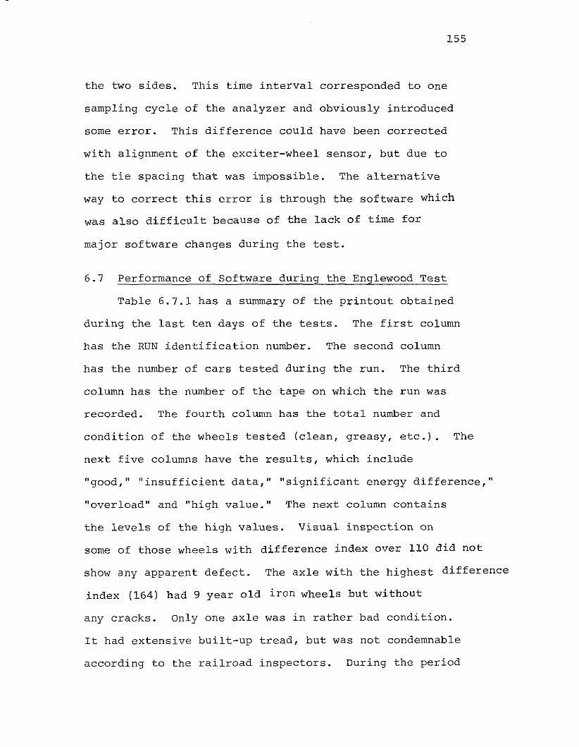
155
the two sides. This time interval corresponded to one
sampling cycle of the analyzer and obviously introduced
some error. This difference could have been corrected
with alignment of the exciter-wheel sensor, but due to
the tie spacing that was impossible. The alternative
way to correct this error is through the software which
was also difficult because of the lack of time for
major software changes during the test.
6.7 Performance of Software during the Englewood Test
Table 6.7.1 has a summary of the printout obtained
during the last ten days of the tests. The first column
has the RUN identification number. The second column
has the number of cars tested during the run. The third
column has the number of the tape on which the run was
recorded. The fourth column has the total number and
condition of the wheels tested (clean, greasy, etc.). The
next five columns have the results, which include
"good," "insufficient data," "significant energy difference,"
"overload" and "high value." The next column contains
the levels of the high values. Visual inspection on
some of those wheels with difference index over 110 did not
show any apparent defect. The axle with the highest difference
index (164) had 9 year old iron wheels but without
any cracks. Only one axle was in rather bad condition.
It had extensive built-up tread, but was not condemnable
according to the railroad inspectors. During the period
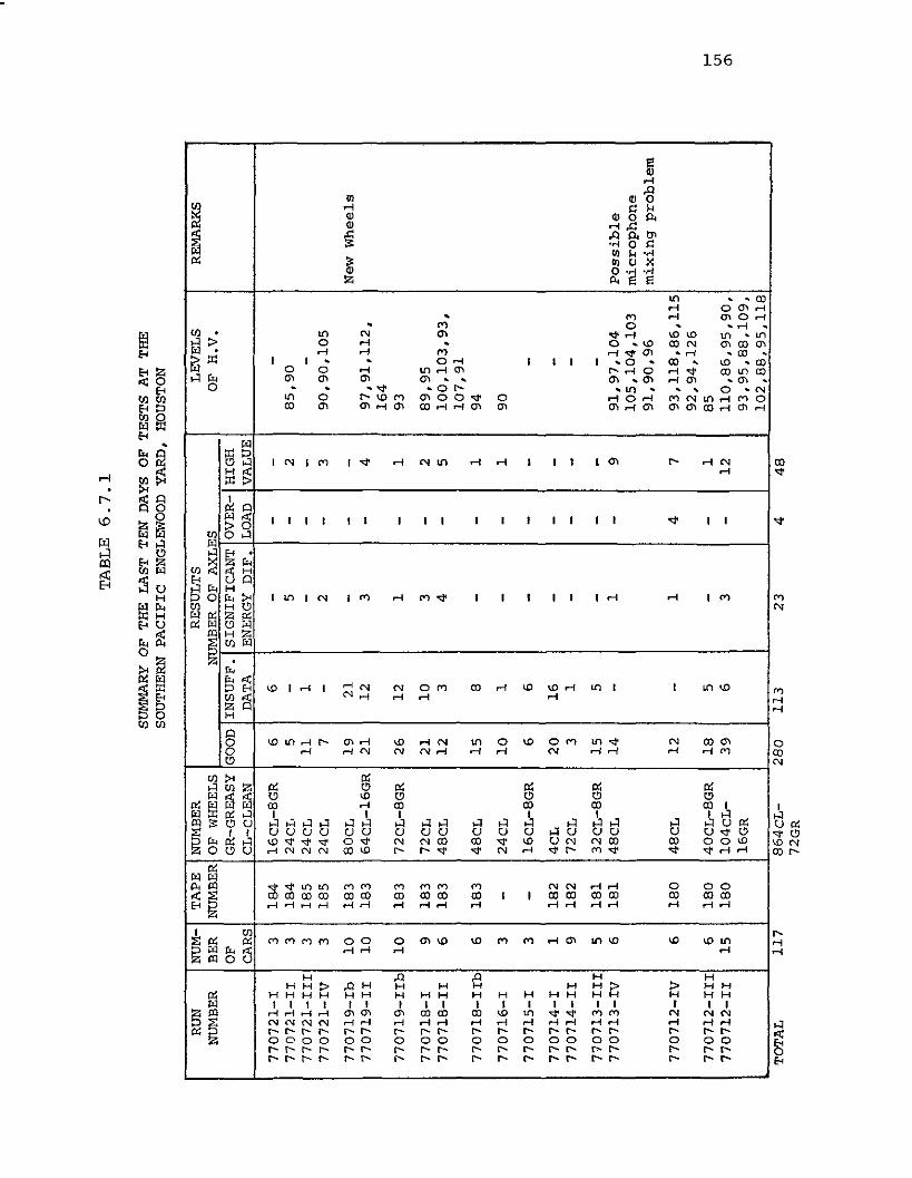
TA
BL
E6
.7.1
SUM
MA
RYO
FT
HE
LA
STT
EN
DA
YS
OF
TE
ST
SA
TT
HE
SOU
TH
ER
NP
AC
IFIC
ENG
LEW
OO
DY
AR
D,
HO
UST
ON
I-'
U1 '"
48
42
31
13
28
08
64
CL
72G
R1
17
TOTA
LRU
NN
UM
-T
APE
NU
MB
ERR
ESU
LT
SL
EV
EL
SR
EMA
RK
SN
UM
BER
BER
NU
MB
ERO
FW
HEE
LSN
UM
BER
OF
AX
LE
SO
FH
.V.
OF
GR
-GR
EA
SYG
OO
DIN
SU
FF
.S
IGN
IFIC
AN
TO
VE
R-
HIG
HC
AR
Scr
,-C
LE
AN
DA
TAEN
ERG
YD
IF.
LOA
DV
ALU
E
77
07
21
-I3
18
41
6C
L-8
GR
66
--
--
77
07
21
-II
31
84
24
cr,
5-
5-
28
5,9
07
70
72
1-I
II3
18
524
CL
11
1-
--
-7
70
72
1-I
V3
18
524
CL
7-
2-
39
0,9
0,1
05
77
07
19
-Ib
10
18
38
0C
L1
921
--
-N
ewW
hee
ls7
70
71
9-I
I1
01
83
64
CL
-16
GR
21
12
3-
49
7,9
1,1
12
,1
64
77
07
19
-IIb
10
18
372
CL
-8G
R2
61
21
-1
93
77
07
18
-I9
18
372
CL
21
10
3-
28
9,9
57
70
71
8-I
I6
18
348
CL
12
34
-5
10
0,1
03
,93
,1
07
,91
77
07
18
-IIb
61
83
48C
L1
58
--
19
4
77
07
16
-I3
-24
CL
10
1-
-1
90
77
07
15
-I3
-16
CL
-8G
R6
6-
--
-7
70
71
4-I
11
82
4CL
20
16
--
--
77
07
14
-II
91
82
72C
L3
1-
--
-7
70
71
3-I
II5
18
132
CL
-8G
R1
55
--
--
77
07
13
-IV
61
81
48C
L1
4-
1-
99
1,9
7,1
04
Po
ssib
le1
05
,10
4,1
03
mic
rop
ho
ne
91
,90
,96
mix
ing
pro
ble
m
77
07
12
-IV
61
80
48C
L1
2-
14
79
3,1
18
,86
,11
59
2,9
4,1
26
77
07
12
-III
61
80
40
CL
-8G
R1
85
--
18
57
70
71
2-I
I1
51
80
10
4C
L-
39
63
-1
21
10
,86
,95
,90
,16
GR
93
,95
,88
,10
9,
10
2,8
8,9
5,1
18
....

157
of the tests the READ assembly subroutine did not have
an error flag for the case of improper reading of the
digital output of the RTA by the computer. When this
error flag was added later it showed on average that 2%
of the indications contained a reading error. It is
not known how much this error might have affected the
results.
In some of the runs with a large number of high
values, certain indications showed improper setting or
calibration in parts of the system. For example in run
7707l3-IV improper microphone mixing was indicated from
the fact that north side readings had a substantially
higher overall sum compared to the south side. In the
case of run 770712-IV the 4 overload indications showed
low input attentuation in the RTA. Indications of
Insufficient Data, Significant Energy Difference, and
Overload are related to the performance of the exciter,
as shown in Fig. 6.6.1 through 6.6.3.
Another point that should be mentioned is the large
number of insufficient data indications. This is mostly
due to greasy wheels. The majority of these wheels are
on cars with plain journal bearings where oil has leaked
from the journal box. For spectral comparisons, the
second reading, 300 ms after the TP, was used. The
signal from greasy wheels in that instance is very low
or completely decayed. This problem could be corrected

158
by checking the first spectrum in cases of fast decay.
Another point of some interest is that wheels with dragging
brake shoes or even squealing under the application of
brake shoe pressure did not appear to generate especially
high Difference Index values.
The distribution of DI values for the last ten
days of field test in SP Englewood yard (July 1977) is
shown in Fig. 6.7.1. In the same figure indications from
defective axles tested in the DR laboratory are marked
with circles.
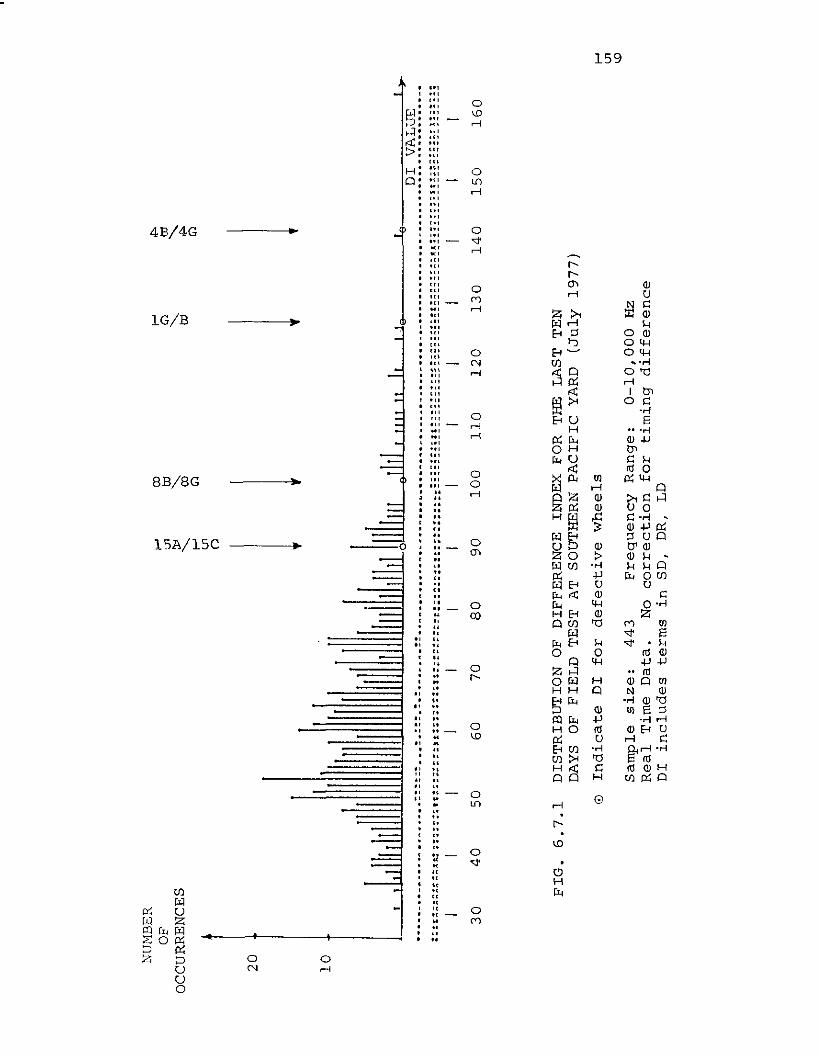
NU
l-lEE
RO
F,...
ex>,...""
~~
0~
OC
CU
RR
EN
CE
S:J>
"-
"-
"-
"-
ex>~""
,...
00
U1
(l
20
,I
Ij
jI
I.I
I..
10
11II
I_J
rI
......
1I
11
1"
",,
11
11
11
11
11
11
11
11
11
"1
11
'"'1
1"
11
11
11
11
11
11
"1
6"
11
11
'e
lill
r11
11e
0D
rV
AL
UE
...
...-..-
~-.~.~..~
:~~::~
~.:::.~.:.-.~.~.::..~
....
•.•.
..•~
~-.-
--_._
_-
-.--.
....
....
••.•
•..•
....
.-.
:::;~~~~~~~~~c;;~:::;.~~=~;::::,~:;:;::::S$:;:::~:::~:
;:::::::::;::::::::;~:~;;;!~~::=:=::==;:~::;::~~~:=::::::~~!::~::~:!!=~::=::::~::::;;
30
40
50
60
70
I
80
I 90
10
01
10
12
01
30
14
01
50
16
0
FIG
.6
.7.1
DIS
TR
IBU
TIO
NO
FD
IFF
ER
EN
CE
IND
EX
FOR
TH
EL
AS
TT
EN
DA
YS
OF
FIE
LD
TE
ST
AT
SOU
TH
ER
NP
AC
IFIC
YA
RD
(Ju
ly1
97
7)
oIn
dic
ate
Dr
for
defe
cti
ve
wh
eels
Sam
ple
siz
e:
44
3F
req
uen
cy
Ran
ge:
0-1
0,0
00
Hz
Real
Tim
eD
ata
.N
oco
rrecti
on
for
tim
ing
dif
fere
nce
Dr
inclu
des
term
sin
SD
,D
R,
LD
,... U1 <.0

160
7. SENSITIVITY ANALYSIS
7.1 Introduction
Figure 6.7.1 is the histogram of DI values obtained
in real time during the tests. It was pointed out in
section 6.7 that a number of system problems occurred
during the tests and that the DI equation used was based
on prior experience with small samples. The idea at the
time of the test was to follow up on a few wheels with
high values. Further study of the analog tape recordings
taken during the test was divided into three parts with
the following objectives:
1) to identify recordings with system problems and to
correct for deficiencies, where possible, in the data
processing software,
2) to use the corrected data to find the optimum DI
equation, and
3) to study the remaining high DI values from the
Englewood data to ascertain what wheel conditions
besides cracks could cause high values.
The maximum sample size (number of axles) used in
this study was 370, a little smaller than the sample
shown in Fig. 6.7.1. The reason for this difference is
that analog tape recordings were not made for a few cars
included in the real-time data. Each time a correction
was introduced into the data processing or a change was
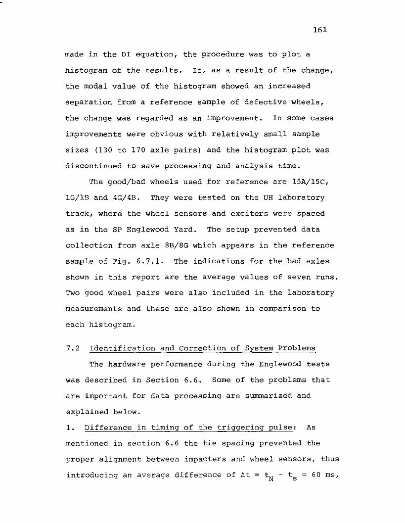
161
made in the DI equation, the procedure was to plot a
histogram of the results. If, as a result of the change,
the modal value of the histogram showed an increased
separation from a reference sample of defective wheels,
the change was regarded as an improvement. In some cases
improvements were obvious with relatively small sample
sizes (130 to 170 axle pairs) and the histogram plot was
discontinued to save processing and analysis time.
The good/bad wheels used for reference are 15A/15C,
IG/IB and 4G/4B. They were tested on the VB laboratory
track, where the wheel sensors and exciters were spaced
as in the SP Englewood Yard. The setup prevented data
collection from axle 8B/8G which appears in the reference
sample of Fig. 6.7.1. The indications for the bad axles
shown in this report are the average values of seven runs.
Two good wheel pairs were also included in the laboratory
measurements and these are also shown in comparison to
each histogram.
7.2 Identification and Correction of System Problems
The hardware performance during the Englewood tests
was described in Section 6.6. Some of the problems that
are important for data processing are summarized and
explained below.
1. Difference in timing of the triggering pulse: As
mentioned in section 6.6 the tie spacing prevented the
proper alignment between impacters and wheel sensors, thus
introducing an average difference of 6t = tN
- t s = 60 ms,
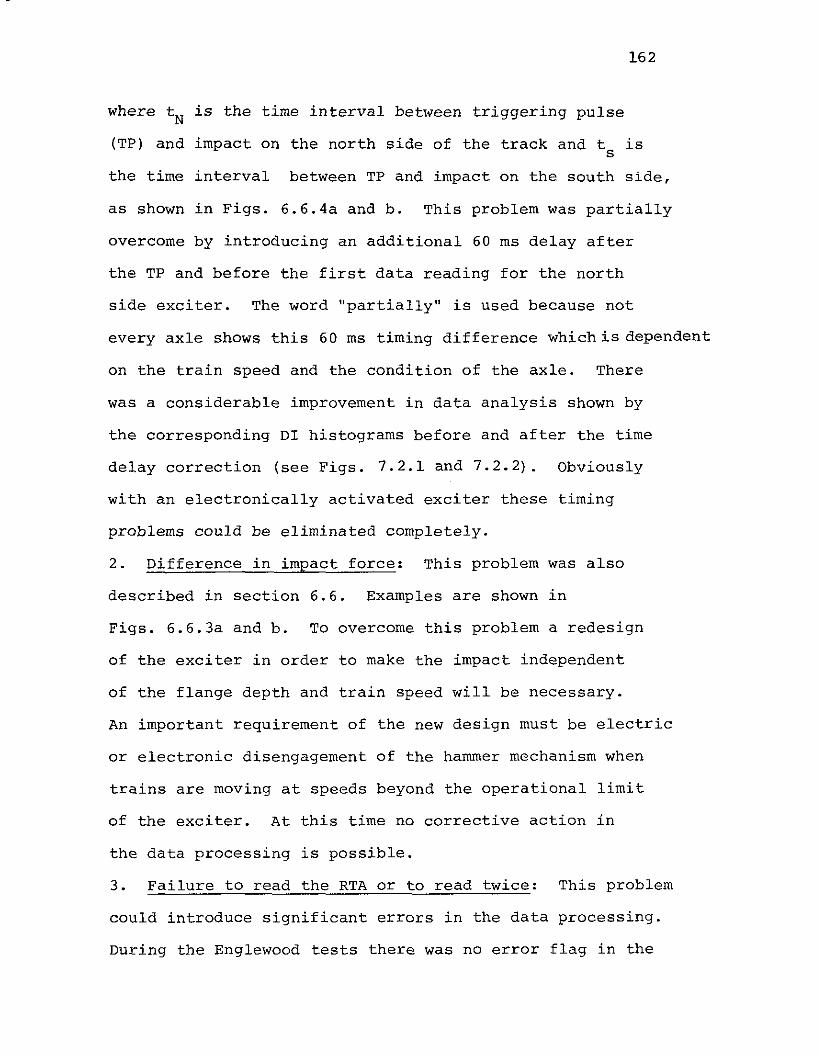
162
where t N is the time interval between triggering pulse
(TP) and impact on the north side of the track and t iss
the time interval between TP and impact on the south side,
as shown in Figs. 6.6.4a and b. This problem was partially
overcome by introducing an additional 60 ms delay after
the TP and before the first data reading for the north
side exciter. The word "partially" is used because not
every axle shows this 60 ms timing difference which is dependent
on the train speed and the condition of the axle. There
was a considerable improvement in data analysis shown by
the corresponding DI histograms before and after the time
delay correction (see Figs. 7.2.1 and 7.2.2). Obviously
with an electronically activated exciter these timing
problems could be eliminated completely.
2. Difference in impact force: This problem was also
described in section 6.6. Examples are shown in
Figs. 6.6.3a and b. To overcome this problem a redesign
of the exciter in order to make the impact independent
of the flange depth and train speed will be necessary.
An important requirement of the new design must be electric
or electronic disengagement of the hammer mechanism when
trains are moving at speeds beyond the operational limit
of the exciter. At this time no corrective action in
the data processing is possible.
3. Failure to read the RTA or to read twice: This problem
could introduce significant errors in the data processing.
During the Englewood tests there was no error flag in the
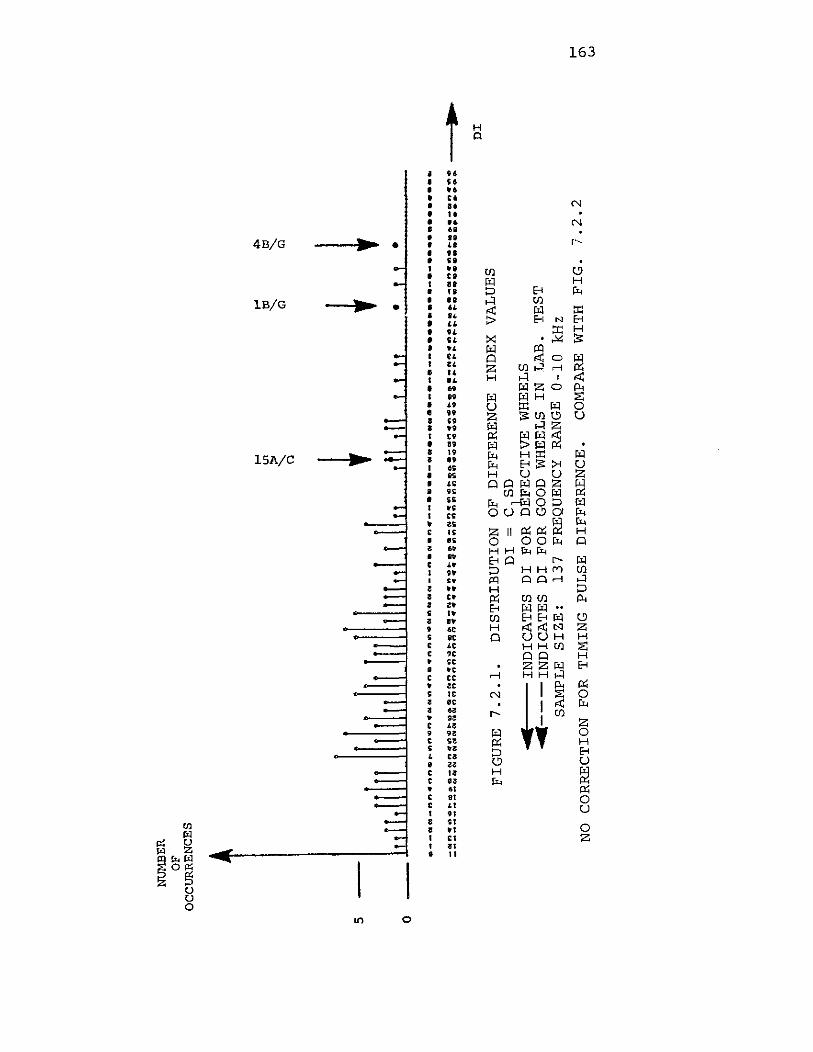
5 o
NU
MB
ERO
FO
CC
UR
RE
NC
ES
.... '" ~ +
.... ~ + •u
"'" ~ ~ ••
__NN_""."".~~"~".NNn."••
""n.
NnN
NN
__".W
."._
_••••
_NN
._••
••_
._._
_••••••••
_._
••••
••••
••••
=~~~~:~~~:;~~:~=~:t~M~~~~~~~~:;~~;;~~,;~~:~~:~~~~:;=~::=~:S~~~~:~:~:~:;::::::::=;:=:::
..D
IF
IGU
RE
7.2
.1.
DIS
TR
IBU
TIO
NO
FD
IFF
ER
EN
CE
IND
EX
VA
LU
ES
DI
=C
SD..
IND
ICA
TE
SD
IFO
RD~FECTIVE
WH
EELS
~---INDICATES
DI
FOR
GO
OD
WH
EELS
INI.
AB
.T
ES
TSA
MPL
ES
IZE
:1
37
FRE
QU
EN
CY
RA
NG
E0
-10
kHz
NO
CO
RR
EC
TIO
NFO
RT
IMIN
GPU
LSE
DIF
FE
RE
NC
E.
CO
MPA
RE
WIT
HF
IG.
7.2
.2I-
'0
' co
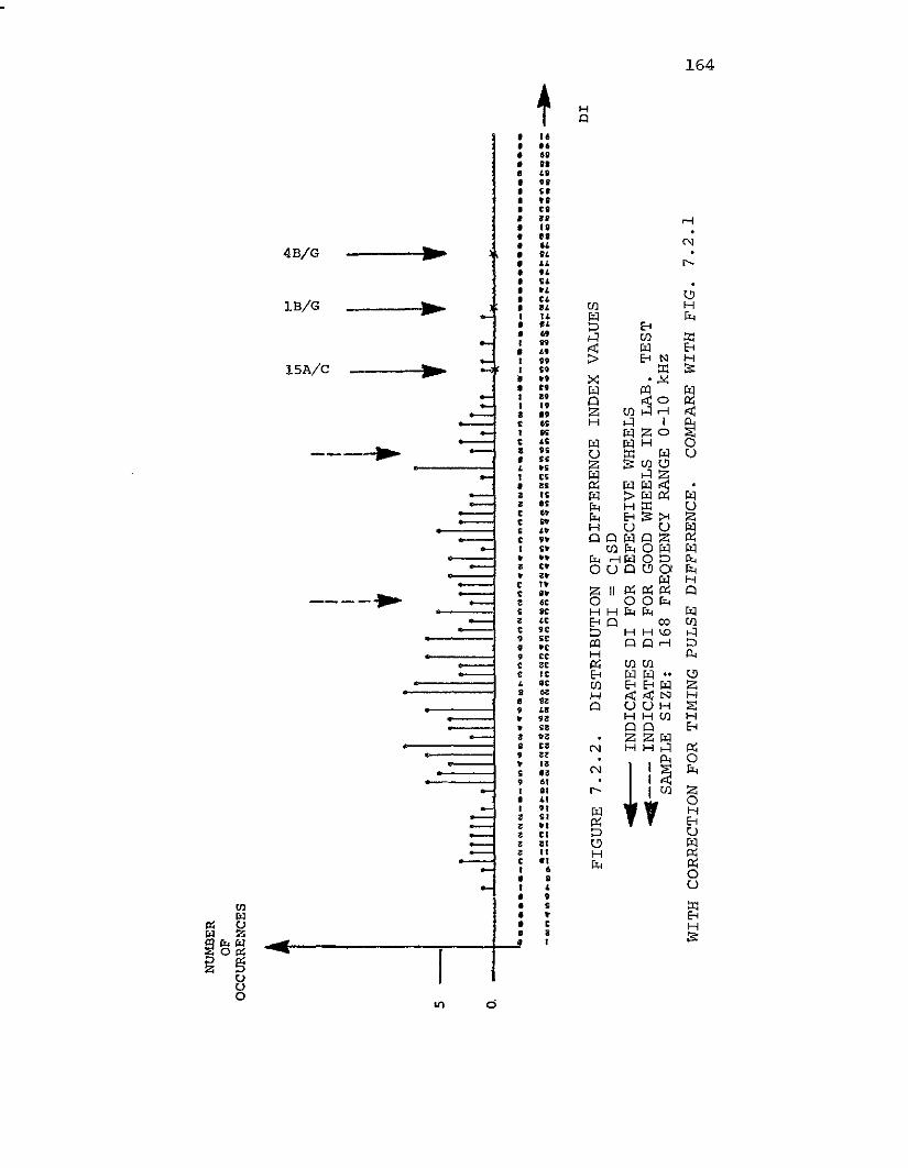
NU
MB
ERO
FO
CC
UR
RE
NC
ES
I I I I •I I +
... tJ1 ~
... ~... ~
5-
o.1••••••_._n~NNN«_._~~••~N••••~~n".G."N~Nn".w._"n""Nw._~••"_
n._
_••
__._
••
_••••••••••••••••••••
-.".~o~c~~:~~:~~~~~:;~~:~:~~&~~~~~~~~~~:;;~:~:~~::~=~~~~~~~:=:::2:~=$:;:~:::~~~:;:::;:::::;~
FIG
UR
E7
.2.2
.D
IST
RIB
UT
ION
OF
DIF
FE
RE
NC
EIN
DE
XV
ALU
ESD
I=
CIS
D4
(IN
DIC
AT
ES
DI
FOR
DE
FEC
TIV
EW
HEE
LS~--_
IND
ICA
TE
SD
IFO
RG
OO
DW
HEE
LSIN
LA
B.
TE
ST
SAM
PLE
SIZ
E:
16
8FR
EQU
ENC
YR
AN
GE
0-1
0kH
z
WIT
HC
OR
RE
CT
ION
FOR
TIM
ING
PUL
SED
IFF
ER
EN
CE
.C
OM
PAR
EW
ITH
FIG
.7
.2.1
Dr
I-'
0' '"
165
software to pinpoint this anomaly. The problem has been
overcome now by making appropriate changes in the assembly
software. The misreadings appear to be related to overload
of the RTA.
4. Missing timing pulse: This is another serious problem,
because the computer starts comparing signatures from
wheels on different axles. The problem is probably due
to the position of the wheel flange in respect to the
sensing element of the proximity detector. The difficulty
was recognized early during the field tests but despite
continuous efforts to make an ideal adjustment of the
sensors, it was not possible to store data from a long
train without missing one or more TP's. This was the main
reason that it was decided to test only a few cars at a
time. Similar problems at other installations using this
type of proximity detector have been reported. The highest
DI indication (164) in Fig. 6.7.1 was due to a missing TP.
For the present the few axles in the Englewood data with
missing TP are not included in the analysis. The recommended
solution is to avoid using this type of sensor, with prefer
ence for strain gauges, or photocells. An alternative
solution is to incorporate circuitry and an error flag in
the software when two successive TP's come from the same
sensor.
5. Missing timing pulse at high train speed: This is due
to the length of sampling time for data collection and
storage. No action has been taken at present. The
166
recommended solution is a hardware-software change to
give an error flag. No recordings at high speed are
included in the present sample.
7.3 Optimizing the DI eguation
There are several features of the acoustic signals
from two wheels which could be used for comparison
purposes:
SD: the sum of the absolute values of the differences
between the sound pressure levels of the two signals
in the same frequency channels.
NC: the number of common resonances, i.e., the number
of resonances occurring in the same frequency channels
in the two signals.
DR: the difference in decay rates of the two signals.
LD: the difference in the overall levels of the two
signals.
NR: the difference in the total numbers of resonances
in each signal.
A variety of experiments were performed to obtain
the optimum DI equation. In each case a histogram of
the results was obtained in the same manner as for Figs.
7.2.1 and 7.2.2 which showed the effects of making a correc
tion for the time delay.
It was decided to take one variable at a time and only
add additional terms to the equation as proven to be
efficacious. The first tests were made using the sum of
the differences, SD. The principal issue here is the
167
most effective frequency range. In order to resolve this
issue, 25 different histograms were plotted dividing the
frequency range between 0 and 10 kHz into 400 Hz bands.
It was clear from these histograms that the separation
between the Englewood sample and the bad wheels was lost
at frequencies above about 7200 Hz. Consequently, in all
subsequent tests the frequency range was restricted to
0-7200 Hz. The improvement resulting from this restriction
of the frequency range can be seen by comparing Figs. 7.3.1
and 7.3.2. Note that in Fig. 7.3.2 only one wheel from
the Englewood sample appears in the range of the bad wheel
reference set. This was the first histogram obtained in
which one of the bad wheel sets showed a DI value higher
than any in the Englewood sample.
This test was followed by several attempts to incor
porate terms involving the differences in decay rates.
Although earlier laboratory tests had shown that the sound
from cracked wheels damps more rapidly than from good wheels
the present set of tests did not lead to an improvement in
separation. It is believed that this disappointing outcome
was because of the uncertainties in the time reference,
and the availability of only two data samples of the sound
from each impact. It is possible that when the TP problems
have been completely eliminated, then terms involving the
difference in decay rate may still lead to improvement
in the DI separation.
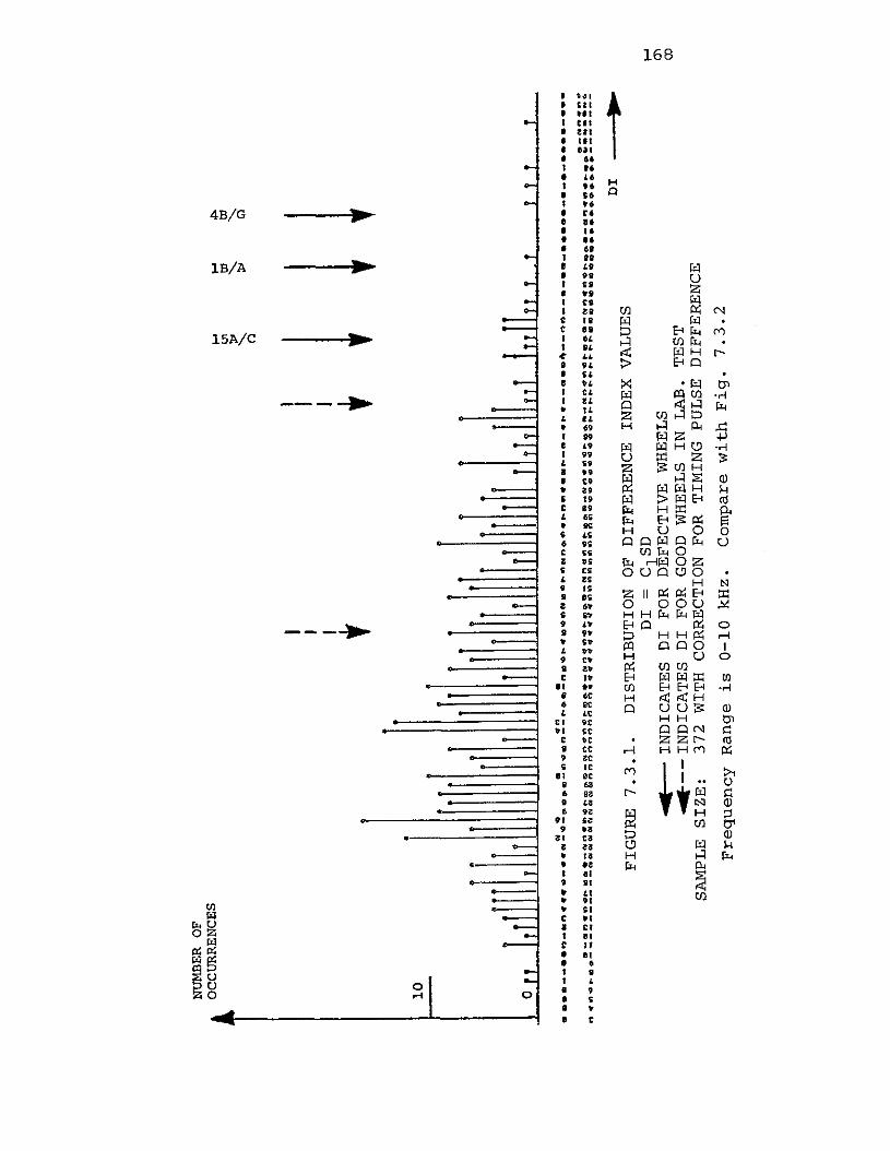
NU
MB
ERO
FI-
'I-
'~
OC
CU
RR
EN
CE
SlJ
lti
lti
l:>-
~"-
"-G'
l(l
II I
IJ
I,
•I
1,•
10
•
o
••••
__••"_
."••••
_••ft~.!~D~D~~.D"~~~•
•!"D.~.D.~ND.~~N".~.~"~•
••~_"_.~.
__a..
~__"
"__._•
•_••.e
._._._
...•_
...e_Nft.~C
".~.~D.!:~~~~~~~~=::~::~~reg~n~~~~~~~~:;~~:;:~,;~~~~~~:~~~:;:::=~~:~~;~~~~~~~~:;:~:::::::;:=::;:::~~::!:~
01
•F
IGU
RE
7.3
.1-
DIS
TR
IBU
TIO
NO
FD
IFF
ER
EN
CE
IND
EX
VA
LU
ES
DI
=C
1SD
........
IND
ICA
TE
SD
IFO
RD
EF
EC
TIV
EW
HEE
LS(J
\
~--INDICATES
DI
FOR
GO
OD
WH
EELS
INL
AB
.T
ES
T00
SAM
PLE
SIZ
E:
37
2W
ITH
CO
RR
EC
TIO
NFO
RT
IMIN
GPU
LSE
DIF
FE
RE
NC
E
Fre
qu
en
cy
Ran
ge
is0
-10
kH
z.C
om
par
ew
ith
Fig
.7
.3.2
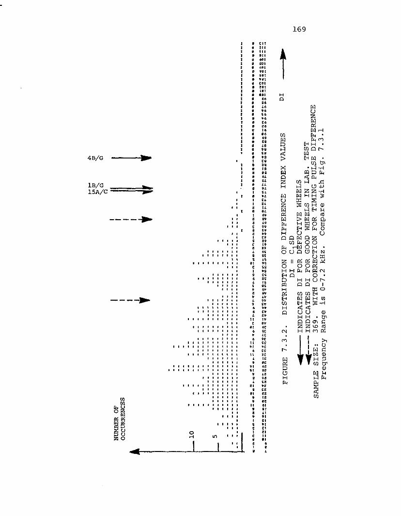
NU
MB
ERO
FO
CC
UR
RE
NC
ES
10 5
I 1 I ,I I I I ,
....
....
>I>ln
tl:t
tl:t
:J>"-
"-
';:)"
"
~-_._----------------------------------------_._--_._-
'....
........
...-..
....
....
....
....
....
....
....
....
...-
......_-
_..._-_
........
.-_...
...
~N
~~
_q
_m
'"m
~-N~n_ft~_•••_4~_.-~.~
__~~_~-_~q~-n-~~~~~.Nq~~~~_n_~D~Nn~_NUnNN_&N
__._
•••••••
-••
m••••
m•••••••••••~••••••
m•••
•_~n.~.~D~._Nn.~.~=~._Nnq~.~=~m_Nnq~.~
~._Nn.~.~.~._Nnq~.~
~m_Nn.~.~m~._N".~.~~~._N".~.~D~:.:~::~~~t!=:~
~D~_-
-N~NNNNNNNN"nnnnnn"nnqq.q.4qq~q~~~~~~~~~~
••••••••2.~~~~~~~~~~••~DD.DmDD~~~~~~~~~~-
_
FIG
UR
E7
.3.2
.D
IST
RIB
UT
ION
OF
DIF
FER
EN
CE
IND
EX
VA
LUES
Dr
DI
=C
SD..
IND
ICA
TE
SD
IFO
RD
tFE
CT
IVE
WH
EELS
~----INDICATES
DI
FOR
GO
OD
WH
EELS
INL
AB
.T
EST
SAM
PLE
SIZ
E:
36
9.
WIT
HC
OR
RE
CT
ION
FOR
TIM
ING
PUL
SED
IFFE
RE
NC
EF
req
uen
cy
Ran
ge
is0
-7.2
kH
z.C
om
par
ew
ith
Fig
.7
.3.1
-t-
'm <.
0
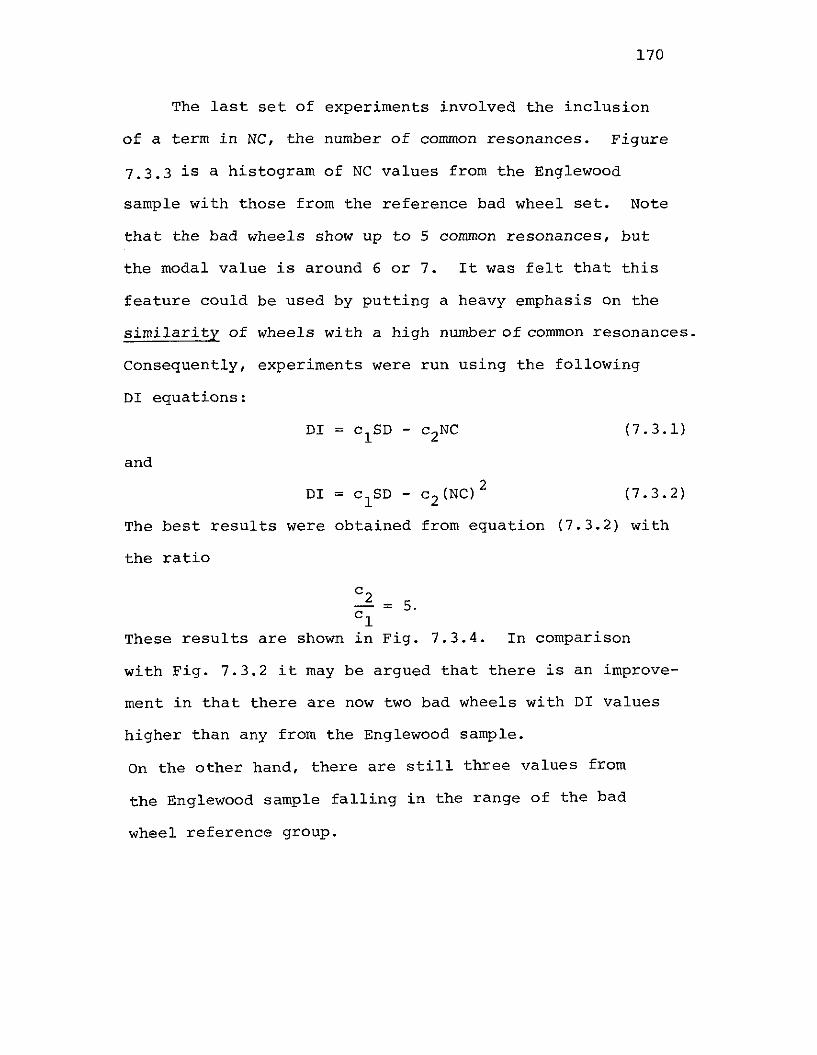
170
The last set of experiments involved the inclusion
of a term in NC, the number of common resonances. Figure
7.3.3 is a histogram of NC values from the Englewood
sample with those from the reference bad wheel set. Note
that the bad wheels show up to 5 common resonances, but
the modal value is around 6 or 7. It was felt that this
feature could be used by putting a heavy emphasis On the
similarity of wheels with a high number of common resonances.
Consequently, experiments were run using the following
DI equations:
(7.3.1)
and
(7.3.2)
The best results were obtained from equation (7.3.2) with
the ratio
= 5.
These results are shown in Fig. 7.3.4. In comparison
with Fig. 7.3.2 it may be argued that there is an improve-
ment in that there are now two bad wheels with DI values
higher than any from the Englewood sample.
On the other hand, there are still three values from
the Englewood sample falling in the range of the bad
wheel reference group.
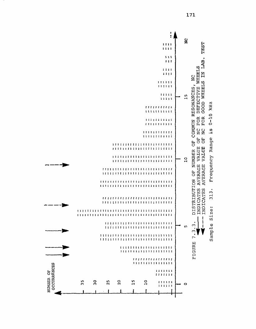
H~
II
NU
MBE
RO
FI
IO
CC
UR
REN
CES
II
•t
,3
5 30
....
....
o•••
o'
'0
....
....
o•••
....
....
eo'0
25..
....
.....
..."
....
o."
....
o'
u...
.o...
.0.,
....
n••
o'
••20
....
....
...,
o•••
.."
....•
0,.
...,
..,.
....
....,
...
..o•
•,
......
....
'0••
o'
••
....
...0
••...
....
....
..."
...,
....1
5.0
_....
...
,-o.
0'n
••
.." .." e
o'0
....
....
....
....n
n••
'0".
'0...
"o
·••
....
o•••
o•••
....1
0'0
••...
.n
••
••
'0-..
....
.."...
.o•••
..-
....
...."
....
n.,
....
••
'0.. '0
'0
....
._'0
••••
eo
.o
....••
•0
'0'0
....
H'
FIG
UR
E7
.3.3
.D
IST
RIB
UT
ION
OF
NU
MB
ERO
FCO
MM
ON
RE
SON
AN
CE
S,N
C..
IND
ICA
TE
SA
VER
AG
EV
ALU
EO
FN
CFO
RD
EFE
CT
IVE
WH
EELS
~---INDICATES
AV
ERA
GE
VA
LUE
OF
NC
FOR
GO
OD
WH
EELS
INL
AB
.
Sam
ple
Siz
e:
31
3.
Fre
qu
en
cy
Ran
ge
is0
-10
kHz
o5
10
15
NC
TE
ST
I-'
-..l
I-'

5
NU
MBE
RO
FO
CC
UR
RE
NC
ES
I f ,I I I •
~~
~
_.a_.
._..
•...
...-
_...
.•..
..._
----
--..
•...
..._
_...
•...
..._
-.
ooJ
-_..
....
....
....
....
....
....
....
....
....
....
....
....
....
....
....
....
....
....
....
....
....
....
...
•••
•__.
~._.
•
•"ft_.
.__
_~...
.•.."
"•.•."
_n••••••~•••••~_~"."•••••
n••"."
•••
"••
_"_
._•••~_N"~"_••
••••
••••
••••
••••
••••
••
'~1;;;1:i:~r;:1~r:;;ff~~~:~~7.-.ft•••~
••~::~~=~~~~:;:::==;Ct~"~~~~~~~s~;~~:~:~,$:;~~~;~~ll:;:~:::~~:=;:~:::;~~:.:::::~:::
DI
~
FIG
UR
E7
.3.4
.D
IST
RIB
UT
ION
OF
DIF
FER
EN
CE
IND
EX
VA
LUES
DI
=C
SD-
C(N
C)2
..
IND
ICA
TE
SD
IIF
OR
DE
§EC
TIV
EW
HEE
LS~--INDICATES
DI
FOR
GO
OD
WH
EELS
INL
AB
.T
ES
T
sam
ple
Siz
e:
37
1.
wit
nco
rrecti
on
for
Tim
ing
Pu
lse
Dif
fere
nce
Fre
qu
en
cy
Ran
ge
is0
-7.2
kH
z.C
om
par
ew
ith
Fig
.7
.3.2
>-'
-.l '"
7.4
7.4.1
173
Several other histograms were made for DI equations
including terms in the difference of total levels LD and
terms in the difference of total numbers of resonances in
each spectrum NR. None of the variations tried led to
any further improvement in the separation.
At this stage therefore there are two variations of
the DI equation which appear to be promising as illustrated
in Figs. 7.3.2 and 7.3.4. The question to be addressed in
the next section is whether or not the high DI values
shown in Figs. 7.3.2 and 7.3.4 are indicative of wheel/axle
conditions, and, if so, what conditions.
The Effect of Wheel Conditions
Introduction
In the previous sections the identification and cor
rection of system problems and the optimization of the DI
equation was presented. As a result of these studies
there was a considerable improvement in the histogram of
DI values in the sense that the DI values for defective
wheels showed the greatest separation yet from the
modal value of the rest of the population. But there is
clearly a wide spread in DI values among the sample. The
purpose of the study reported now was to ascertain, if
possible, what wheel conditions, besides cracks, could give
rise to high DI values. Before starting this phase of
the investigation it was anticipated that a variety of
possible conditions might have caused such high
values:
174
l. skewed axles
2. uneven load
3. uneven wear
4. greasy wheels
5. differences in internal stress
6. cracks.
There is evidence that some skewed axles were
present in the Englewood sample, but these occurrences
did not result in extremely high DI values. Greasy wheels
are highly damped at high frequencies and usually resulted
in an "insufficient data indication." None of the very
high DI values in Fig. 7.3.5 showed very high damping,
and consequently grease is not believed to be the cause
of the high values. Although changes in internal stress
do cause changes in resonant frequencies, such changes are
very small. Even if there were substantial differences
in internal stress between two wheels of a given axle set
(which is hard to believe), the effect in the DI value
should still be very small. The effects of uneven load
should presumably be similarly small since the effect
on the acoustic properties of the wheel does not depend on
whether the stress field is residual or is applied
externally.
Thus, by this process of elimination uneven wear and
cracks were left as potential causes of the high DI values.
However, in a sample of 400 wheel sets, it is very unlikely
that there is a cracked wheel as mentioned previously.
175
One therefore suspects that uneven wear is the most likely
cause of the large number of high DI values.
7.4.2 Data Reduction
In order to investigate this hypothesis it was
decided to make a further study of the data on the ten
wheel sets from the Englewood sample showing the highest
DI values. For these wheel sets the following data was
available:
1) plots of the acoustic spectra from the two wheels
2) oscillograms of the impact and timing pulse
and 3) the car identification number.
In each case the first point of concern was to ascertain
if uneven impact level was a problem. In only two of the
ten cases investigated was there a substantial difference
in impact levels. Figures 7.4.1 and 7.4.2 show the effect
for one of these cases. The impact level was about the
same in the other eight instances. However, all of these
other eight instances showed a common feature in the
spectral comparisons as seen in Figs. 7.4.3 and 7.4.4 for
a typical case.
The feature of importance which distinguishes these
cases is a frequency shift between resonance peaks. Such
shifts are marked in Fig. 7.4.3, The interesting aspect
of this phenomenon is that the amount of the shift appears
to increase proportionally with frequency to a first
approximation. This effect is illustrated in Fig. 7.4.5
where the frequency shifts are plotted as a function of

1 - w u z w a:: w LL W a:: >-3
0a:: ~ f= lD ~20
I-' ...., 0"
1
109
87
6
(kH
z)..
•
,~~l.
'.jV\V
!\..·j
\,""'".J
,..
45
FREQ
UENC
Y3
~! lt w\,;~:f:l~
:}'~i
•:
1"
.:
•.'
:~
".'
,.(!~..
..:'\
f··..':,
.:\
.:..
0••:':
•
2
~
lD ~ ~ w o10
:::> ~ -l
0..
::E ~
FIG
UR
E7
.4.1
SIG
NA
TU
RE
SO
FW
HEE
LSD
UE
TOU
NEV
ENIM
PAC
T

_T.P.
_S.S.\
_S.S.2
177
Fig. 7.4.2 Timing pUlses (T.P.) and sound signals(S.S.) from two unevenly impacted wheels.Sweeping speed 50 ms/div. (The signaturesin Fig. 7.4.1 correspond to the abovesignals. )

10
.- :~.:
,:
9
:"
8
. ;: !:"
:~
;]:
,,
':
.,,
",
"
:.:
7~0',
,}
::
":
:"
:.
"'
.:.
:':,"
:V~.:
x:.....
.
:
" ,:
6
"
5 (kH
z)
:",,
..
, "
"
:....
34
FREQ
UENC
Y
\t
....... w u z w a: w u.. w a: >- ~30
a: I- m a: ~ ai'2
0,
"0
" ;.~
" "
w,
'C
l'
:::::>
',
I- ...J
10a.. ~
IA
II:
~,
•'II
.n.
r.:
\J..l
---,
0I
2
FIG
UR
E7
.4.3
SIG
NA
TU
RE
SO
FW
HEE
LSO
NA
XL
E3
,C
AR
GTA
X1
32
86
I-'
--.J
00

179
_T.P.
_5.5.1
_ 5.5.2
Fig. 7.4.4 Typical timing pulses and sound signalsfrom a pair of wheels tested at theEnglewood yard. Sweeping speed 50 ms/div.(The signatures in Fig. 7.4.3 correspondto the above signals.)
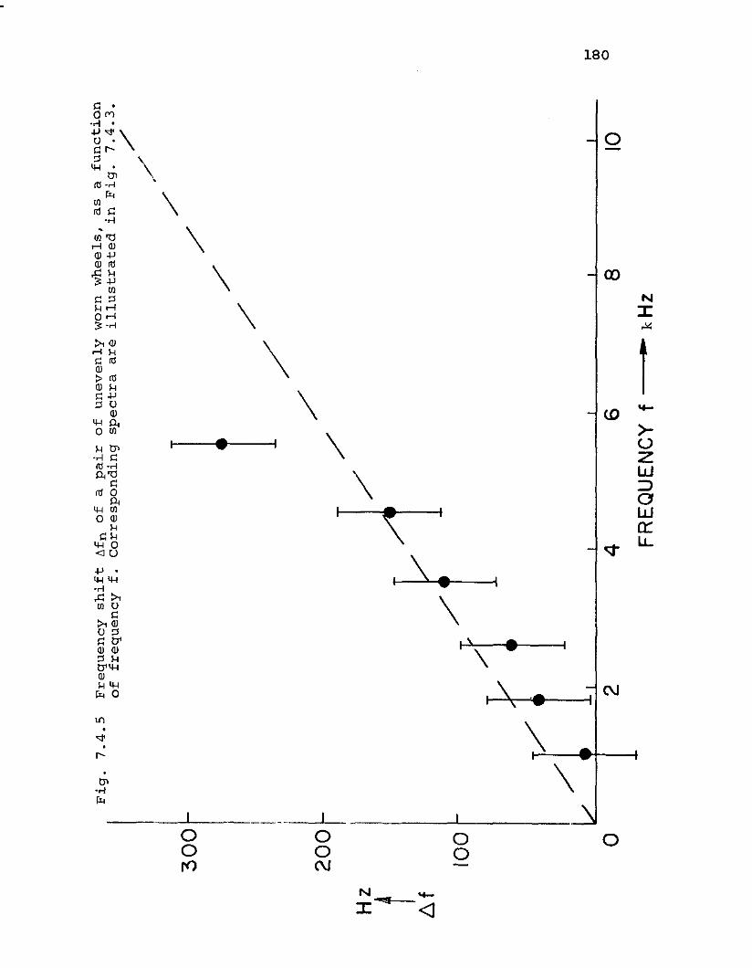
I-'
CD o10
//
8//
//
//
46
FRE
QU
EN
CY
f..
kHz
2
Fig
.7
.4.5
Fre
qu
en
cy
sh
ift
~fn
of
ap
air
of
un
ev
en
lyw
orn
wh
eels
,as
afu
ncti
on
of
freq
uen
cy
f.co
rresp
on
din
gsp
ectr
aare
illu
str
ate
din
Fig
.7
.4.3
./
/
a
300~ I I I ,
200~
Hz
, It bot
10
0I
/
t'~
./
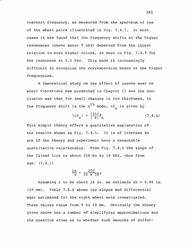
181
resonant frequency, as measured from the spectrum of one
of the wheel pairs illustrated in Fig. 7.4.3. In most
cases it was found that the frequency shifts at the higher
resonances (above about 5 kHz) departed from the linear
relation to even higher values, as seen in Fig. 7.4.5 for
the resonance at 5.5 kHz. This made it increasingly
difficult to recognize the corresponding modes at the higher
frequencies.
A theoretical study on the effect of uneven wear on
wheel vibrations was presented in Chapter II and the con-
elusion was that for small
the frequency shift in the
changes in rim thickness, ~h
thn mode, ~f is given byn
(7.4.1)
This simple theory offers a qualitative explanation of
the results shown in Fig. 7.4.5. It is of interest to
see if the theory and experiment have a reasonable
quantitative relationship. From Fig. 7.4.5 the slope of
the fitted line is about 250 Hz in 10 KHz, thus from
eqn. (7.4.1)
~h 250r = 10 x 10 3
Assuming r to be about 16 in. we estimate ~h = 0.40 in.
(10 rom). Table 7.4.1 shows the slopes and differential
wear estimated for the eight wheel sets investigated.
These values range from 9 to 18 rom. Obviously the theory
given above has a number of simplifying approximations and
the question arose as to whether such amounts of differ-
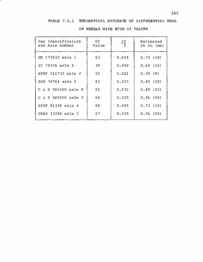
182
TABLE 7.4.1 THEORETICAL ESTIMATE OF DIFFERENTIAL WEAR
ON WHEELS WITH HIGH DI VALUES
Car Identification DI M Estimatedand Axle Number Value f i'lh in (rom)
GN 171932 axle 1 63 0.045 0.72 (18)
IC 75536 axle 4 39 0.040 0.64 (16)
ATSF 521735 axle 2 55 0.021 0.34 (9)
SSW 76704 axle 2 61 0.025 0.40 (10 )
C & S 565500 axle 4 61 0.030 0.48 (12)
C & S 565500 axle 2 66 0.035 0.56 (14)
ATSF 81338 axle 4 68 0.045 0.72 (18)
GTAX 13286 axle 3 67 0.035 0.56 (14 )
183
ential wear are encountered in practice. The expense of
recalling the wheels in question was not felt to be
justifiable, and in any case the wheels would have received
almost a year of additional usage since the Englewood
test. Instead it was decided to make some careful measure
ments on wheels in the laboratory collection at the University.
7.4.3 Laboratory Measurement of Wear
Measurements of the tread and flange thicknesses were
made between the points indicated in Fig. 7.4.6 using a pair
of calipers. Because of difficulty in positioning the
calipers at precisely the same orientation it is estimated
that the accuracy was + 0.5 mm for tread measurements
and + 1.5 mm for flange measurements. The results are
given in Table 7.4.2. Measurements made at different cir
cumferential positions showed no more than + 1 mm variation.
The first observation to be made is that the range
of values of differential tread wear, from 0.0 to 6.9 mm,
while not showing values as high as those hypothesized is,
nevertheless, of the same order of magnitude. It was
decided to study the spectra of the laboratory wheel sets
to ascertain the magnitude of frequency shifts, if any.
Wheels 6B/e, showing the highest differential tread wear,
are 36 in. wheels with thermal cracks and the spectra are
very complex. The next highest values of differential
wear are for wheels lOA/C and llA/C. Both of these sets
also show considerable differential flange wear.
Figures 3.3.1 and 7.4.7 show the spectra for these wheel
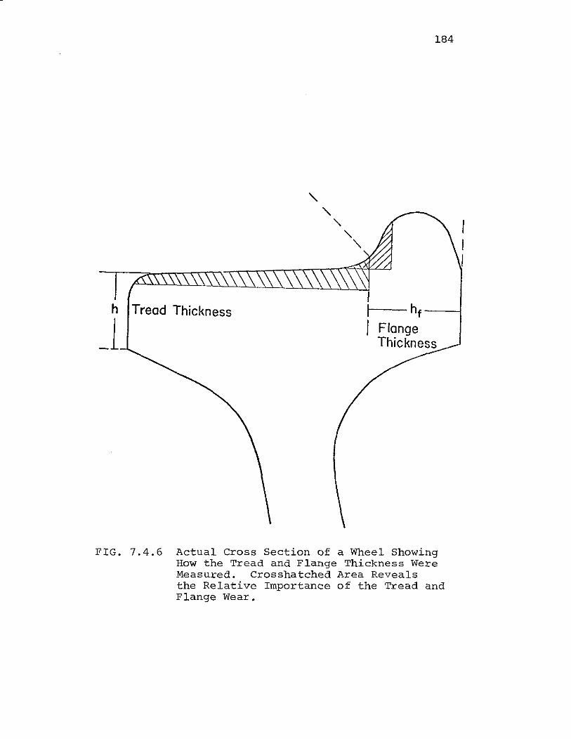
184
f---- hf -----1
FlangeThickness
h Tread Thickness
_1
FIG. 7.4.6 Actual Cross Section of a Wheel ShowingHow the Tread and Flange Thickness WereMeasured. Crosshatched Area Revealsthe Relative Importance of the Tread andFlange Wear.

185
TABLE 7.4.2. TREAD AND FLANGE THICKNESS OF WHEELSAT THE UNIVERSITY OF HOUSTON LABORATORY
UH Wheel IIh forIdentification Flange Tread TreadNumber nun rom rom
9A 32.6 35.5 1.59C 26.2 34.0
lOA 29.5 29.5 3.710C 38.4 25.8
llA 29.3 33.6 3.6llC 39.0 30.0
12A 31.4· 28.2 0.912C 32.4 27.3
l3A 40.0 25.0 0.0l3C 41. 0 25.0
l4A 41.0 31.2 0.0l4C 42.0 31. 2
- - --------- ---------- ---------- --------15A 36.0 35.2 0.215C 34.4 35.0
IB 33.0 34.0 1.8IG 37.3 32.2
2B 29.0 32.2 0.22G 36.2 32.0
4B 41. 0 32.5 0.54G 40.5 32.0
5B 42.5 47.0 1.55G 30.2 48.5
6B 38.3 42.1 6.96G 33.7 49.0
8B 38.8 24.0 0.58G 33.5 24.5

t):::,:u:
.:,'..".
...'
.':::::
:'.
::;:
:
.....:::
···W
::k.
.. ..
__
_II
A
....
....
..11
C
>-'
00 '"
I 10
.' ....
.
I 9I 8
" :'.
I 7I 6
..
I 5(k
Hz)
..
:'1:
-~
Itw
I111
u z W 0::
W lJ..
I1\
'.w
'.
0::
30
-
>-I
II..
0::
<{
0::
I-
20
-1'.
(II
.,I
~••
ft."
0::
<{ ~
(II
"0~
!:'.
W..
::I'
.
a10
...'
::>..
.'.
I-
~•.
...J
'.n.
...
.':E
'.<
{:
'.:\J
II
II
0I
23
4
FREQ
UENC
Y
FIG
UR
E7
.4.7
SIG
NA
TU
RE
OF
WH
EELS
IIA
an
dII
C

187
sets. proportional frequency shifts are more easily seen
in the spectra of llA/C. Plotting ~f versus f forn n
llA/C results in the plot shown in Fig. 7.4.8. From the
slope of the best straight line fit, using eqn (7.4.1) ~h
is estimated to be 8 mrn, about twice the measured value.
A possible explanation for this apparent discrepancy could
be that wear on the inside of the tread is greater than
on the edge, where the measurement was made.
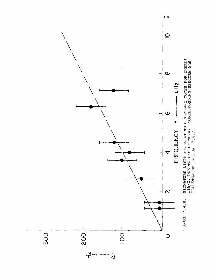
Hz A ! I6
f
30
0
I
20
0r
10
0
/
/
./"
/"
./"
/'"
/
//
//
/'"
o2
46
FRE
QU
EN
CY
f--
kHz
810
I-' co co
FIG
UR
E7
.4.8
.SI
GN
AT
UR
ED
IFF
ER
EN
CE
SA
TT
HE
RES
ON
AN
TM
OD
ESFO
RW
HEE
LSll
A/C
,D
UE
TOU
NV
,lEN
WEA
R.
CO
RR
ESP
ON
DIN
GSP
EC
TR
AA
RE
ILL
UST
RA
TE
DIN
FIG
.7
.4.7
189
8. CONCLUSIONS AND SUGGESTIONS FOR
FURTHER WORK
8.1 Conclusions
In these studies the development of a wayside
system for inspection of railroad wheels in service using
acoustic signature analysis was presented. The basic
claim is that the improvements and modifications of Nagy's
laboratory system have reached the point that the installa
tion of a prototype system can now be contemplated. This
transitional phase included hardware interfacing for
wayside installation, and software development for real
time operation, data acquisition and data analysis.
Experimental studies and theoretical models were used to
obtain more information on the effects on vibrations of
wheels of geometrical variations, wear, internal stress etc.
Finally a field test was performed to elucidate system
problems. Tape recordings were made to permit further
study of these problems, to optimize the software and to
discover other wheel conditions influencing the acoustic
signature. It is appropriate to review these efforts in
more detail.
8.1.1 Advances in Scientific Understanding
A better understanding of wheel vibrations under
various conditions and under varying forcing functions
was needed for the development of the recognition logic.

190
A number of analyses were made using a finite element
program. This is the best theoretical approach because
there is no closed form solution for vibrations of elastic
solids with complex geometries, such as the railroad wheels.
A summary of the work is presented in Appendix F.
Parallel studies were made in the development of
Stappenbeck's simple ring model for comparison and evaluation
of the experimental results. It was successfully used in
the evaluation of the lowest flexural modes of a 33"
wheel, and later in the studies of differential wear on
the tread of two wheels. Finally the effect of residual
stress on wheel vibrations was demonstrated to be plausible
from the theory of the effect of externally applied forces
on beam vibration. In order to verify some of these
theoretical predictions, several laboratory experiments
were conducted. The results reconfirmed earlier
indications that the important modes are those with nodal
diameters.
Further experimental studies on the acoustic signatures
from wheels in manufacture and under drag braking, with
different residual stress, yielded a very important
discovery, namely that there are measurable frequency
shifts which are in agreement with theoretical evaluations.
These shifts are of the order of 0-10 Hz.
8.1.2 System Improvements
The major change and improvement over the earlier
laboratory system was the use of a narrow band instead of
a 1/3 octave band real time analyzer. Most of the fre-
191
quency information of 28" to 40" railroad wheels is
between 400 to 10,000 Hz. For this range a 250 channel
narrow band real time analyzer has a 40 Hz per channel
resolution, compared to several hundred Hz for the cor
responding 1/3 octave band analyzer operating in the same
frequency range. Although this is a significant improve
ment some experiments, such as residual stress evaluation,
required even higher resolution.
A second area of improvement was in the wheel
excitation. Several alternatives were evaluated and
tested. The study led to the selection of a mechanical
hammer, which rated superior to two other possible exciters.
A redesign of the mechanical exciter with the emphasis
on ruggedness produced an exciter which withstood some
27,000 impacts with minimal wear and without breaking.
Despite the improvements impacts were speed dependent.
Commercial all weather microphones were used and performed
without problems despite high temperatures, humidity and
rainstorms. A timing pulse was used in the data processing.
The sound from impact excitation of a moving railroad wheel
is a transient signal of short duration, and the maximum train
speed restricts the sampling time to about 300 ms. Thus
precise sampling becomes an important factor. A reasonable
choice of a timing pulse generator seemed to be a wheel
proximity detector already in use on several railroads.
Field experience indicated that the actual device chosen
sometimes failed to generate the required pulse, and
192
consideration of this must be made in the installation of
a prototype. The addition of two floppy diskettes as
mass memory storage devices was another improvement.
Laboratory tests required a relatively small amount of
memory for data storage. But in actual operation the
fast collection of a large amount of data prevented true
real time analysis. However, near real time operation
was possible in that data processing started after the
transfer of the last wheel signature. The processing time
could and should be reduced in a prototype system.
8.1.3 Software and Signature Recognition Improvements
The field tests at TTC, Pueblo were made as a rehearsal
for the complete test of the system at the Englewood Yard
in Houston. The treatment of the data obtained during
those tests led to the following principal conclusions:
1. Timing differences between the triggering pulse and
impact for the two pairs of wheel sensors and exciters
was found to be an important problem but could be
partially corrected in the data processing.
2. Improper data transfer from the RTA to the computer
can be flagged now, with appropriate changes in the
assembly software.
3. Missing triggering pulses were a problem but could
be accounted for in the data processing.
4. The optimum frequency range to be used in the analysis
has been shown to be 0-7200 Hz.
5. The optimum DI equation has been found to be:
DI = C15D - C2 (NC)2
193
where 3D is the sum of the absolute values of the dif
ferences between the sound pressure levels of the two
signals in the same frequency channel. NC is the number
of common resonances, i.e., the number of the resonances
occurring in the same frequency channels in the two
signals. This simplified DI equation was obtained after
the analysis of the field data, which had shown that
terms such as Decay Rate (DR) or SPI,2 (indicating the
overall sound pressure level) did not improve the separation
between DI values for good and defective wheels.
The criterion for the optimum DI equation was the
achievement of a maximum separation between the modal DI
value in a histogram of results using the sample of
recordings made in the Englewood Yard and some recordings
of bad wheels made in the laboratory. The improvement
in this separation can be related to system reliability
and false alarm rate (see Appendix G). Using such criteria,
two thirds of the defective wheels could be found with
one hundred percent reliability and zero false alarm rate,
based on the small statistical sample presently available.
Uneven or differential wear on wheelsets was established
as the major cause of high DI values. This was concluded
on the following bases:
1) An argument on the basis of prior knowledge
2) A study of the data for the 10 highest DI values
found in the Englewood sample using the optimum DI equation.

194
These instances showed a characteristic shifting of
resonance peaks by amounts approximately proportional to
frequency.
3) A simple theoretical treatment showing that such
an effect is to be expected if there is different wear on
the treads of two wheels.
4) Some measurements of wear differences among wheels
in the collection at the University.
5) A comparison of the frequency shifts in the
spectra of worn wheels in the laboratory, and hence a
demonstration that the wear differential predicted using
the theory mentioned in 3) agrees with the measurement
mentioned in 4) within a factor of two.
Some method of recognition of unevenly worn wheel
sets would probably yield the most significant improvement
over the existing system.
8.2 Suggestions for Further Work
It is advocated that the work on Acoustic Signature
Inspection should be advanced on three fronts:
a) Installation of a prototype system by a railroad.
The Union Pacific Railroad is planning to install a
prototype system. Certain obvious system design improve
ments should be made, as detailed below.
b) Improvement of scientific knowledge. The measure
ment of internal stress in wheels and its effects on
crack growth is probably the most important gap in knowledge
at present. The effect of cyclic loading on crack growth
195
rates is another unknown area. It will be difficult to
improve on wheel removal criteria without such knowledge.
c) System Interaction Studies, Calibrations, etc.
There is a need for a centrally located establishment where
comparisons and interactions of various inspection systems
could be carried out. Suggestions for development of an
ASI system at such a location are also detailed below.
8.2.1 Installation of a Prototype ASI System
Planning for the installation of a prototype ASI
system by the union Pacific Railroad has already reached
an advanced stage. The system will be installed in the
Las Vegas, Nevada yard and the target date for commencement
of operations is January 1979. The hardware will consist
of a Hewlett-Packard computer system interfaced with the
Spectral Dynamics RTA presently on loan to the University
of Houston. A single General Radio all-weather micro-
phone will be used. Two commercialmicroswitch wheel
sensors have been selected. The wheel exciters will be of
the same type used in the 1977 test at the Englewood Yard.
The Union Pacific plans to assemble the system at
Omaha prior to installing it at Las Vegas. Implementation
of the software is considered to be part of the assembly
task. It will be necessary to rewrite the existing pro
grams in FORTRAN in order to reduce the data processing
time.
After installation of the system at a low speed
location it is anticipated that a period of "debugging"

196
will be necessary. The Union Pacific intends to assign
a qualified person to work full time with the system.
It is recommended that additional work to support
the Union Pacific's effort could be directed toward
the detection of uneven wheel wear. Successful identifica
tion of such wheels should further reduce the false alarm
rate. One way to do this would be to incorporate a
subroutine in the computer software to recognize resonant
frequency shifts. Two possible algorithms can be envisaged:
a) mUltiplication of the frequency values of one spectrum
by a variable and use of the minimum DI value obtained,
for decision making; b) elimination from consideration of
wheel sets in which the DI value increases rapidly at high
frequency. Obviously such a subroutine would require
development time and need careful study before incorpora
tion in the program. One problem might be that a wheel
set with a cracked member could also show high differential
wear. Another method to offset the high DI value of sets
with high differential wear would be to include a term
in the DI equation based on input from a system capable
of directly measuring differential wear, such as a flange
height sensor or a rim circumference indicator.
It is also suggested that some effort could be devoted
to exciter design as follows:
a) Improve the present exciter by modifying the impact
delivered so that it shall be independent of train
speed. A solenoid could be used to activate the
impacter. Other changes, not in the exciter alone, are

197
needed to improve the effectiveness of the system at
higher speeds.
bl Instrument the plunger of the present hammer to permit
a reading of flange depth. This reading should be
used to detect uneven wear on wheels of an axle set
and to indicate wear beyond condemnable limits.
cl Instrument the hammer of the present exciter to give
a reading of the impact force. This reading could be
used to indicate a failure of the system or to indicate
the presence of foreign material on the wheel tread.
This could be used to detect wheels liable to slip
through retarders.
d) Reconfigure the mounting of the exciter to permit
speedier attachment to the rail and ready adaptability
to rail of different weights, between 110 Ib/yd and
136 Ib/yd.
el Design an electrical control unit to activate the
hammer and provide the means to program the sequence
of wheels to be struck and to deactivate the exciter
entirely if so required.
Finally it is important that a data bank of tapes
be compiled to permit further sensitivity studies and
improvement of the DI equation. This would also permit
the system reliability and false alarm rate to be monitored.
Causes of high D1 values should be ascertained. In order
to allow such studies to be made the system should include
a 2 or 4 channel analog tape recorder. Tapes should be
catalogued and stored.
198
8.2.2 System Interaction Studies
Beyond the installation of the prototype at Las Vegas,
and benefitting from experience therewith, a second system
should be installed at the Transportation Test Center at
Pueblo, Colorado. In order to permit systems interaction
studies, operation of calibration consists, etc. the
following additional developments should be undertaken:
a) Use of AID Conversion
If the microphone signal were converted directly
into digital form and stored in memory it could then be
processed by a Fast Fourier Transform (FFT) program and
the use of the RTA could be avoided. Hardwired FFT
programs are available. If this task were successfully
accomplished it appears that there would also be an improve
ment in system reliability. However elimination of the
RTA is not recommended until it is demonstrated that the
task can be accomplished without sacrifice in frequency
resolution, and even then the RTA has other desirable
features. The use of a line printer instead of the teletype
will speed up the computer output 10 to 25 times which is
another important factor in the development and use of
the system.
b) Provision of Automatic Turn-on
It would be desirable to provide automatic turn-on
for the system when a train approaches. This will entail
the selection of a train proximity detector and turn-on

199
of the electronics with adequate warm-up time. Equipment
costs are uncertain estimates.
c) Interfacing to a Central Processor
The minicomputer of the ASI system would need to be
interfaced with the Central Processor of the Automated
Wayside Facility. In addition an analog signal from the
microphones should be available to the Central Processor.
8.2.3 Further Research on Residual Stress, Crack Growth
and Wheel Removal Criteria
Further research is necessary in order to develop a better
understanding of crack initiation and growth, the influence of
internal stress, the influence of cyclic loading, etc., with
a view to improving wheel removal criteria.
The Wilmerding data, together with the previous
information on loading and the results of the Bessemer
tests, indicate that changes in resonant frequencies occur
with changes in internal stress. There is a need for
additional data, and there is a need to establish a firm
theoretical explanation of the effect for any complex
residual stress field combined with the rotating stress
field due to the external load. There also arises the
question of the engineering application of the effect.
The major problem in applying the effect is that the
occurrence of a resonance at a certain frequency can only
be used as an indicator of internal stress if the frequency
of resonance in a normally stressed wheel is known.

200
In principle a wayside stress measuring system could
be developed by cataloguing the acoustic signatures of all
the extant wheel types (about 40) under conditions of normal
stress and then comparing the given wheel signature with
this catalog. It would not be possible to use across the
axle comparison since the likelihood is that mating wheels
would have very similar conditions of internal stress.
One difficulty with the wheel recognition scheme is the
problem of recognizing the wheel type. This might be
done by reading the wheel ID lettering or by identifying
the acoustic signature. Another difficulty is that the
acoustic signature is affected by wear, grease, load, etc.
Thus the comparison signature of the wheel type after
identification would need to be corrected according to
these wheel conditions. While these difficulties appear
to be almost insurmountable at present for a wayside
system a program of research might be started with the
aim of developing a machine shop system.
Another method that could be envisaged for shop use
involves a determination of the slope of the ~f - ~a curve
by applying a stress. If an additional load is applied to
a wheel, by means of a hydraulic jack for instance, then
a given resonance line will shift by different amounts in
frequency, depending on its initial internal stress, and
the slope of the curve at the point represented by this
condition. If the curve indeed exhibits a change in slope
from negative to positive for certain resonances as in
201
Fig. 4.3.10 then the resonance line will shift to higher
values for highly stressed wheels or lower values for
normally stressed wheels. The effect of frequency shift
for flexural vibration with circular modal lines may be
different from frequency shifts for vibration with modal
diameters. If this were found to be the case the absolute
stress field might be inferred again by an incremental
loading.
In order to elucidate these questions the following
research tasks are suggested:
a) Development of Research Instrumentation to Measure
Internal Stress
In order to establish the effect of internal stress on
acoustic signatures in various wheel types and under various
conditions it will be necessary to select and procure or
develop instrumentation to make absolute stress measure
ments. The ultrasonic method is favored for this purpose
because it yields bulk values. It will also be necessary
to secure equipment for accurate tread profile measurements.
b) Collection of Data
Data on residual stress, as measured by the ultra
sonic method, together with acoustic signatures needs to
be collected for a variety of wheels and for various
vibrational modes. New wheels as well as wheels in service
need to be evaluated. Accurate wear profiles need to
be measured.
c) Establishment of 6f/0 Curves
Further work needs to be done to establish the nature
of the Lf/o curves. It will be necessary to secure a

202
frequency translator in order to accomplish this. The
first order of business should be to process the remaining
tape recordings from the Wilmerding tests. The apparent
lack of correlation with some strain gauge readings on
the rim needs to be explained. It is desirable to establish
the repeatability of these curves and to correlate
frequencies with absolute stress. Further dynamometer
tests will be necessary although some information may be
forthcoming from the data collection of task b.
d) Theoretical Prediction of Frequency Shifts
If the changes in resonant frequency are indeed due
to changes in internal stress it should be possible to
simulate the changes using one of the standard finite
element programs. NASTRAN, for example, permits such
stress distributions to be imposed. Not only would a
correct prediction of natural frequency shifts enhance
confidence but the study could also be of enormous value
in predicting ~f/G curves because of the difficulties
envisaged in collecting data.
e) Demonstration System for Residual Stress Measurement
After the tasks outlined above have been performed it
should be possible to assemble a laboratory demonstration
system. This should be evaluated by comparing residual
stress measured by ASI with values obtained from ultrasonic
tests.
f) Theoretical Prediction of Crack Growth
While the work of Carter and Caton emphasizes many
important aspects of fracture in wheels, it evidently
203
does not treat fatigue crack growth except in an elementary
manner. Even though the results reported there provide
some idea of crack sizes which ought to result in a wheel
being taken out of service, they do not establish any
basis for estimating the number of cycles to failure for a
crack of subcritical size. It is proposed that this problem
could be tackled on a theoretical basis, using recent
developments in fracture mechanics. There are two possible
avenues of approach. One way would be to use a finite
element technique, modelling the crack tip with a plastic
element and having a moving network of grid points. The
other way would be to use an analytical approach using
path invariant integral. It is not clear at present
which method would be the most satisfactory. The output
of such a study would be predictions of crack growth paths
and crack growth rates under various conditions of cyclic
load and stress.
g) Experimental Study of Crack Growth
Some further experimental studies of crack initiation,
due to braking, cyclic loading, etc. would serve to comple
ment and confirm task f. It is possible that such a study
would best be carried out on model wheels, with accelerated
cycling techniques. The detailed mechanism of crack
initiation needs further study.

204
REFERENCES
1. Nagy, K., "Feasibility Study of Flaw Detection inRailway wheels Using Acoustic Signatures," Ph.D.Thesis, University of Houston, August 1974. Seealso: Report No. FRA/OR & D 76-290, National Technical Information Service, Springfield, Virginia22161.
2. Nagy, K., Dousis, D. A., Finch, R. D., "Detectionof Flaws in Railway Wheels Using Acoustic Signatures,"ASME paper No. 77-WA/RT-l, 1977.
3. Bray, D. E. and Finch, R. D., "Flaw Detection inModel Railway Wheels," Report No. FRA-RT-71-75,National Technical Information Service, Springfield,Virginia 22161, PB-199-956, February 1971. Seealso: Bray, D. E., Dalvi, N. G. and Finch, R. D.,Ultrasonics II, 1973, 66-72.
4. Dousis, D., "Acoustic Signature Processing forRailroad Wheel Flat Spot Detection," M.S. Thesis,University of Houston, December 1975.
5. Bray, P. E., "Pulse Excitation of Railway Wheels,"M.S. Thesis, M-2165, University Microfilms, AnnArbor, Michigan, 48106 III pp. 1969.
6. Leissa, A. W., "Vibration of Plates," NASA SP-160,1969.
7. Leissa, A. w., "Vibration of Wheels," NASA SP-288,1973.
8. Soni, S. R., Amba-Rao, C. L., "AxisymmetricVibrations of Annular Plates of Variable Thickness,"J. Sound Vibr., 38 (4), 465-473,1975.
9. Banerjee, M. M., "On the Non-linear Vibrations ofElastic Circular Plates of Variable Thickness,"J. Sound Vibr. 47 (3), 341-346, 1976.
10. Appl, F. C., Byers, J. R., "Fundamental Frequency ofSimply Supported Rectangular Plates with LinearlyVarying Thickness," J. Appl. Mech., 32, 163-168 (65).
11. Eastep, F. E., "Estimation of the FundamentalFrequency of Beams and Plates with VaryingThickness," AIM, 14 (ll) 1647-1649, 1976.
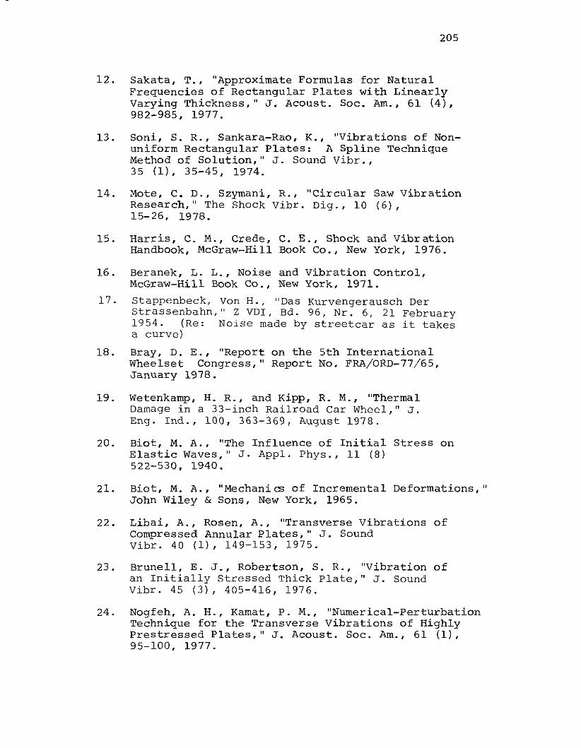
205
12. Sakata, T., "Approximate Formulas for NaturalFrequencies of Rectangular Plates with LinearlyVarying Thickness," J. Acoust. Soc. Am., 61 (4),982-985, 1977.
13. Soni, S. R., Sankara-Rao, K., "Vibrations of Nonuniform Rectangular Plates: A Spline TechniqueMethod of Solution," J. Sound Vibr.,35 (1), 35-45, 1974.
14. Mote, C. D., Szymani, R., "Circular Saw VibrationResearch," The Shock Vibr. Dig., 10 (6),15-26, 1978.
15. Harris, C. M., Crede, C. E., Shock and VibrationHandbook, McGraw-Hill Book Co., New York, 1976.
16. Beranek, L. L., Noise and Vibration Control,McGraw-Hill Book Co., New York, 1971.
17. Stappenbeck, Von H., "Das Kurvengerausch DerStrassenbahn," Z VDI, Bd. 96, Nr. 6, 21 February1954. (Re: Noise made by streetcar as it takesa curve)
18. Bray, D. E., "Report on the 5th InternationalWhee1set Congress," Report No. FRA/ORD-77/65,January 1978.
19. Wetenkamp, H. R., and Kipp, R. M., "ThermalDamage in a 33-inch Railroad Car Wheel," J.Eng. Ind., 100, 363-369, August 1978.
20. Biot, M. A., "The Influence of Initial Stress onElastic Waves," J. Appl. Phys., 11 (8)522-530, 1940.
21. Biot, M. A., "Mechanics of Incremental Deformations,"John Wiley & Sons, New York, 1965.
22. Libai, A., Rosen, A., "Transverse Vibrations ofCompressed Annular Plates," J. SoundVibr. 40 (1), 149-153, 1975.
23. Brunell, E. J., Robertson, S. R., "Vibration ofan Initially Stressed Thick Plate," J. SoundVibr. 45 (3), 405-416, 1976.
24. Nogfeh, A. H., Kamat, P. M., "Numerical-PerturbationTechnique for the Transverse Vibrations of HighlyPrestressed Plates," J. Acoust. Soc. Am., 61 (1),95-100, 1977.
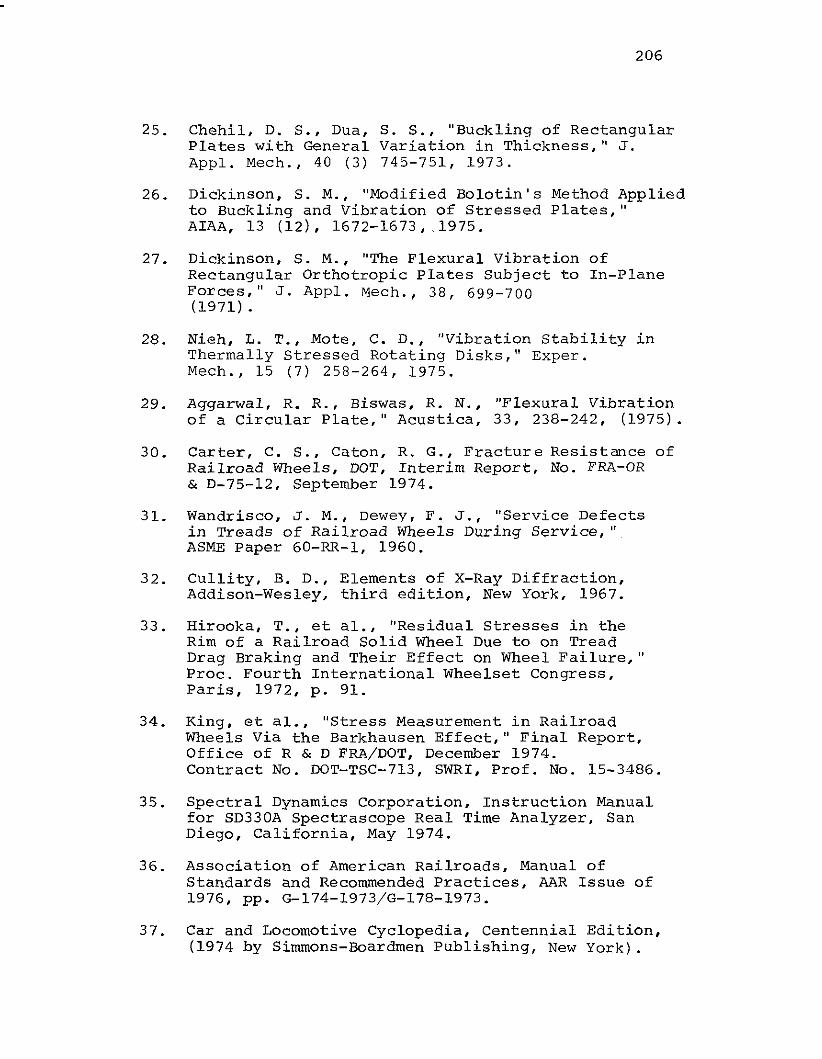
206
25. Chehil, D. S., Dua, S. S., "Buckling of RectangularPlates with General Variation in Thickness," J.App1. Mech., 40 (3) 745-751, 1973.
26. Dickinson, S. M., "Modified Bolotin's Method Appliedto Buckling and Vibration of Stressed Plates,"AIAA, 13 (12), 1672-1673, 1975.
27. Dickinson, S. M., "The Flexural Vibration ofRectangular Orthotropic Plates Subject to In-PlaneForces, II J. Appl. Mech., 38, 699-700(1971) .
28. Nieh, L. T., Mote, C. D., "Vibration Stability inThermally Stressed Rotating Disks," Exper.Mech., 15 (7) 258-264, 1975.
29. Aggarwal, R. R., Biswas, R. N., "Flexural Vibrationof a Circular Plate," Acustica, 33, 238-242, (1975).
30. Carter, C. S., Caton, R. G., Fracture Resistance ofRailroad Wheels, DOT, Interim Report, No. FRA-OR& D-75-l2, September 1974.
31. Wandrisco, J. M., Dewey, F. J., "Service Defectsin Treads of Railroad Wheels During Service, "ASME Paper 60-RR-1, 1960.
32. Cu11ity, B. D., Elements of X-Ray Diffraction,Addison-Wesley, third edition, New York, 1967.
33. Hirooka, T., et a1., "Residual Stresses in theRim of a Railroad Solid Wheel Due to on TreadDrag Braking and Their Effect on Wheel Failure,"Proc. Fourth International Whee1set Congress,Paris, 1972, p. 91.
34. King, et al., "Stress Measurement in RailroadWheels Via the Barkhausen Effect," Final Report,Office of R&D FRA/DOT, December 1974.Contract No. DOT-TSC-713, SWRI, Prof. No. 15-3486.
35. Spectral Dynamics Corporation, Instruction Manualfor SD330A Spectrascope Real Time Analyzer, SanDiego, California, May 1974.
36. Association of American Railroads, Manual ofStandards and Recommended Practices, AAR Issue of1976, pp. G-174-1973/G-178-1973.
37. Car and Locomotive Cyclopedia, Centennial Edition,(1974 by Simmons-Boardmen PUblishing, New York) .
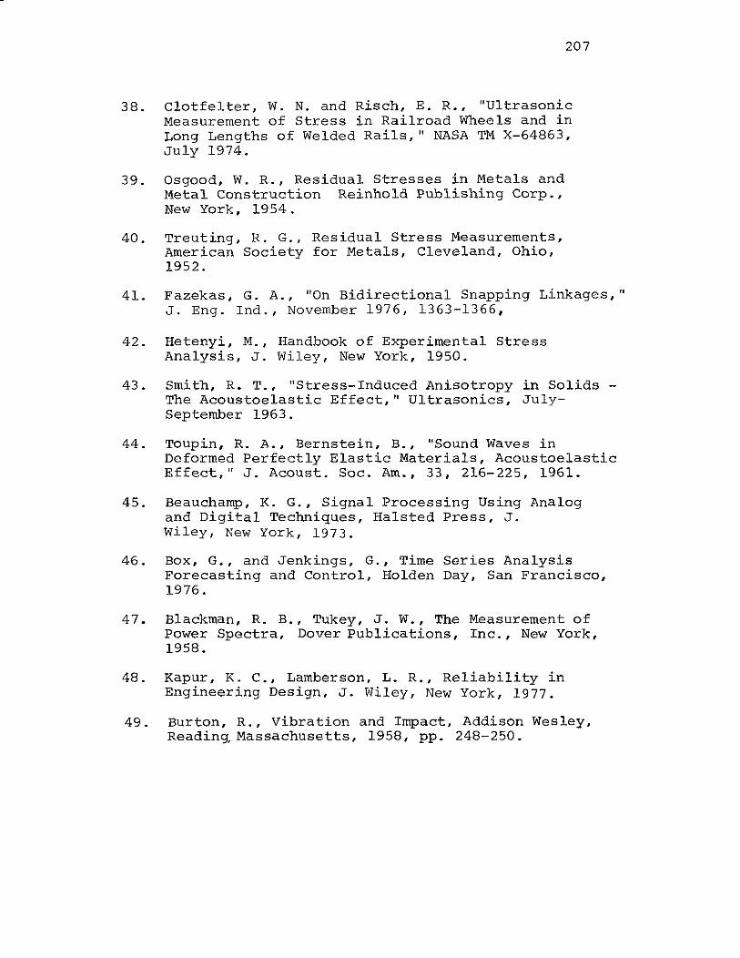
207
38. clotfelter, W. N. and Risch, E. R., "UltrasonicMeasurement of Stress in Railroad Wheels and inLong Lengths of Welded Rails," NASA TM X-64863,July 1974.
39. Osgood, w. R., Residual Stresses in Metals andMetal Construction Reinhold PUblishing Corp.,New York, 1954.
40. Treuting, R. G., Residual Stress Measurements,American Society for Metals, Cleveland, Ohio,1952.
41. Fazekas, G. A., "On Bidirectional Snapping Linkages,"J. Eng. Ind., November 1976, 1363-1366,
42. Hetenyi, M., Handbook of Experimental StressAnalysis, J. Wiley, New York, 1950.
43. Smith, R. T., "Stress-Induced Anisotropy in SolidsThe Acoustoelastic Effect," Ultrasonics, JulySeptember 1963.
44. Toupin, R. A., Bernstein, B., "Sound Waves inDeformed Perfectly Elastic Materials, AcoustoelasticEffect," J. Acoust. Soc. Am., 33, 216-225, 1961.
45. Beauchamp, K. G., Signal Processing Using Analogand Digital Techniques, Halsted Press, J.Wiley, New York, 1973.
46. Box, G., and Jenkings, G., Time Series AnalysisForecasting and Control, Holden Day, San Francisco,1976.
47. Blackman, R. B., Tukey, J. W., The Measurement ofPower Spectra, Dover Publications, Inc., New York,1958.
48. Kapur, K. C., Lamberson, L. R., Reliability inEngineering Design, J. Wiley, New York, 1977.
49. Burton, R., Vibration and Impact, Addison Wesley,Readin~Massachusetts, 1958, pp. 248-250.
208
50. Timoshenko, S., Young, D. H., Weaver, W., VibrationProblems in Engineering, Fourth Edition, JohnWiley & Sons, 1974, pp. 453-455.
51. Carter, C. S., Caton, R. G., Guthrie, J. L., "FractureResistance and Fatigue Crack Growth Characteristicsof Railroad Wheels and Axles," DOT, Final Report,No. FRA/ORD-77/50, November 1977.
52. Michell, J. H., Messenger of Math., Vol. 19 (1890).
53. Yanelak, J. J., Scott, C. N., "Requirements ofResidual Stress Measurements Peculiar to theRail·.ray-Freight Industry," Extendl'd Summaries ofthe Technical Papers Presented at the 1978SESA (Society of Experimental Stress Analysis)Fall Meeting, pp. 17-18.
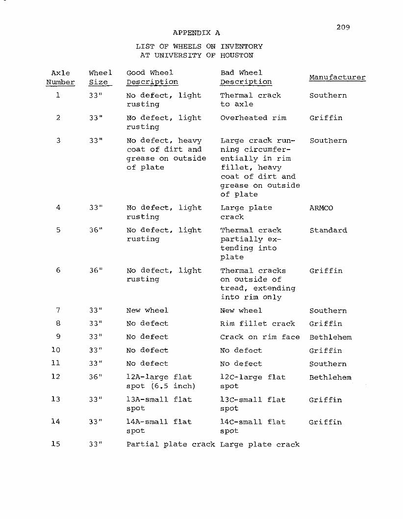
209APPENDIX A
LIST OF WHEELS ON INVENTORYAT UNIVERSITY OF HOUSTON
12C-Iarge flat Bethlehemspot
l3C-small flat Griffinspot
14C-small flat Griffinspot
Thermal crack Standardpartially ex-tending intoplate
Thermal cracks Griffinon outside oftread, extendinginto rim only
New wheel Southern
Rim fillet crack Griffin
Crack on rim face Bethlehem
No defect Griffin
No defect Southern
AxleNumber
1
2
3
4
5
6
7
8
9
10
11
12
13
14
WheelSize
33"
33"
33"
33"
36"
36"
33"
33"
33"
33"
33"
36"
33"
33"
Good WheelDescription
No defect, lightrusting
No defect, lightrusting
No defect, heavycoat of dirt andgrease on outsideof plate
No defect, lightrusting
No defect, lightrusting
No defect, lightrusting
New wheel
No defect
No defect
No defect
No defect
l2A-large flatspot (6.5 inch)
l3A-small flatspot
14A-small flatspot
Bad WheelDescription
Thermal crackto axle
Overheated rim
Large crack running circumferentially in rimfillet, heavycoat of dirt andgrease on outsideof plate
Large platecrack
Manufacturer
Southern
Griffin
Southern
ARMCO
15 33" Partial plate crack Large plate crack

APPENDIX B
EQUIPMENT LIST USED IN THE ENGLEWOOD YARD TESTS
1. SD330A REAL TIME ANALYZER
2. NOVA 1220 MINI-COMPUTER
3. DATA GENERAL DISKETTE SYSTEM
4. DATA GENERAL FAST PAPER TAPE READER
5. (2) BAND-PASS FILTERS
6. TRIGGERING-PULSE CIRCUIT
7. DC POWER SUPPLY FOR ITEM NO.6
8 . HP AMPLIF IER
9. GR TAPE RECORDER
10. (2) GR MICROPHONES
11. (1) OSCILLOSCOPE
12. (10) DISKETTES FOR ITEM NO.3
13. CABLES
14. (2) MECHANICAL EXCITERS
15. SPARE PARTS FOR ITEM NO. 14
16. HAND TOOLS
17. (2) ACI WHEEL DETECTORS
18. (2) WALKY-TALKY'S
210
211
APPENDIX C
SOFTWARE FOR COMPUTER INTERFACINGAND DATA PROCESSING
APPENDIX C.l
PIN ASSIGNMENT
In general loading narrowband spectra into a digital computer
can be done in two ways. First, using the FRAME-SYNC and WORD-SYNC.
pulses to trigger separate computer interrupt lines. These inter-
rupts cause the computer to abandon its current processing task
and jump to an interrupt routine, and service the device which is
requesting the interrupt (in this case the SD330A). The computer
then returns to normal processing. Second, if it is required to
load spectra only at certain defined times, the FRAME-SYNC. and
WORD-SYNC. lines can be connected as data lines to the computer
data register. In this case spectra would be loaded under program
control by testing the individual bits in the data word which
correspond to the FRAME-SYNC. and WORD-SYNC. lines. Under the
present interfacing scheme the WORD-SYNC. line is connected to
the External Interrupt pin and the FRAME-SYNC. to a DATA in pin
(see Table C.I.I).

TABLE c.1.1 COMPl~ER-ANALYZER INTERFACING
PIN ASSIGNMENT
212
REAL TIME ANALYZER COMPUTERSD330A NOVA 1220
SIGNAL NAME PIN PIN SIGNAL NAME
DATA LINES (LSB) (OUTPUT) J-17 28 22 DATA IN 15J-17 27 20 DATA IN 14J-17 26 4 DATA IN 13J-17 25 19 DATA IN 12J-17 24 5 DATA IN 11J-17 23 6 DATA IN 10J-17 22 8 DATA IN 9J-17 21 7 DATA IN 8J-17 19 9 DATA IN 7
(MSB) J-17 18 10 DATA IN 6
~ORD SYNC. (OUTPUT) J-17 29 46 DIO. hXT. INT.SWEEP FRAME SYNC. (OUTPUT) J-17 31 11 DATA IN 4SWEEP (OUTPUT) J-17 16 13 DATA IN 3GROUND J-17 34 1 GROUNDEXT. START (INPUT) J-18 1 21 DATA OUT 1EXT. PEAK HOLD (INPUT) J-18 3 24 DATA OUT 3EXT. STOP (INPUT) J-18 4 27 DATA OUT 4EXT. TR. PULSE (TAPE RECORDER) 16 DATA IN 1EXT. RESET (INPUT) J-18 5 25 DATA OUT 5EXT. SWEEP (INPUT) J-18 6 3 DATA OUT 6EXT. EXP. AVG. J-18 2 23 DATA OUT 0

SW
EE
P(F
RA
ME
)S
YN
C
WO
RO
SY
NC
J-1
7
31 29
AP
PR
OX
.5
3m
s_
Ij.
--(I
NC
LU
DIN
GO
NE
INT
EN
SIF
IED
DO
Ta
RE
TRA
CE
8LK
GT
IME
)---
-,-:1
1:- 10
fLSE
CFR
EE
RU
NN
ING
DU
RIN
GP
LOTT
ER
SW
EE
PrL
__
-.JL
----------V
'.
TT
L
-I~200fLSEC
r-~1
.5mS
.j
-Ij4
-10
fLSE
CI
nl
n2n
3n
24
9n
25
0
__
_._
1U
UI'-
-__
~./'
JU
1'--
TT
L
-.Ik-
20
0fL
SE
C(l
NH
I8IT
ED
DU
RIN
GR
ETR
AC
EB
LKG
aIN
TE
NS
IFIE
DD
OT
) TT
L
TT
L
-.1
10
0m
sf4-
(IN
HIB
ITE
DD
UR
ING
SR
F)
WD
SY
NC
DU
RIN
GP
LOT
SW
EE
PI~READ
DIG
ITA
LD
ATA
WIT
HIN
20
0fL
SE
CL
----.-..-
'-FR
OM
+G
OIN
GE
DG
E.J
I£.
100p
.SE
C_
,~
20
0p
.SE
C-.
,,-
ril
2--
-I3
I.-'
"50
ms
25
0
16P
LOT
TE
RS
WE
EP
OU
TPU
T
DIG
ITA
LO
UT
PU
TS
(BIN
AR
Y)
,D
AT
A
18 19 21 22
23
24
25 26
27
28
MS
B)
BIT
-I -2 -3 -4 -5 -6 -7 -8 -9
LSB
)B
IT-
10
NO
N
AV
ER
AG
ED
8B
ITS
(BIT
PA
RA
LLE
L)T
TL
PO
SIT
IVE
TRU
E
AV
ER
AG
ED
10B
ITS
(BIT
PA
RA
LL
EL
)
TT
LP
OS
ITIV
ETR
UE
'"!-' w
FIG
UR
EC
.l.2
SD33
0AD
IGIT
AL
OU
TPU
TT
IMIN
G
214
APPENDIX c.2
LIST OF THE ASSEMBLER SOFTWARE USED FOR DIGITAL CONTROL OF THEREAL TIME ANALYZER AND DATA TRANSFER TO THE COMPUTER/DISKETTE

;
.LOC 33000
; ---------------------------------------
·~ ----------------------------------~-----------CONTAINS THE FOLLOWING ASSEMBLY SIR
,START SAMPLING: STOP AND STORE'GET PEAK SPECTRU1: RESET CURSOR OR PLOTTER: START SWEEPI NG: START THE CLOCK--CL.FR. 60H~
,READ THE CLOCK: SENSE THE SWEEP FRAME PULSE C53MSEC): READ THE VALUE. OF A CHANNEL:RESET CLOCK: EXTERNAL TRIGGERING:READ-IN SP. IN 53MSEC
USING INTERRUPT:RESET INPUT-OUTPUT POINTER:READ-OUT SPECTRU1: SPECTRUM NUMBER (INPUT-OUTPUT>: EXPONENTIAL AVERAGING,PLOTTER SWEEP OUTPUT:OPEN DISK FOR R/W: WRI TE ON DI SK: READ FROM DI SK: CLOSE A R/W CALL:CLEAR 1/0 TABLES: CHANGE TO FLOAT AN INT. ARRAY
PNTEROUTSPNMREXPAVPLSPOPENWRITEREADCLOSECDISKFLTA
TAPE A-140-XII-N14 SEPT. 1977
DECK STBN. 01
4.RESET30000000
215
·>
2STOP30000000
;
SBRTB: CKINTISTART.RDX 420000000
5.SWEEP20000000
3PEAK20000000
; THI S TAPE; #1 START; #2 STOP; #3 PEAK; #4 RESET; #5 SI"EEP; if6 CLKST; #7 CLOCK; #8 C10) SFRAM E; #9(11) SPEC; 1110(12) RSTCL; #11(13) EXTRG; i'l2( 14) SP250
·>
·>; ---------------------------------------------
·>·>
; #13(15); #14( 16); #16(20); #17(21); 1118(22); 119(23); il'20( 24); 1121 (25); '22C 26); 123( 27); '24( 30)
000002033117140000
000003033137100000
034470000001033107000004100000
000004033147140000
033000
000005033157100000
.MAIN0001
0102030405060708091011121314151617181920212223242526272829303132333435363738 3300039 3300140 330024142 330034344 3300445 3300546 3300647
48 3300749 3301050 330115152 3301253 3301354 330145556 3301557 33016
l 33017I

2160002 .MAIN
01 33020 000Cl06 6.02 33021 033175 CLKST03 33022 100000 200000000405 33023 000007 7.06 33024 033206 CLOCK07 33025 140000 3000000ere0'} 33e26 00001e 8.10 33027 033276 SFRAME11 33030 100000 200000001213 33031 000011 9.14 33032 033304 SPEC15 33033 14ee0e 300000001617 33034 000012 10.18 33035 033222 RSTCL19 33036 100000 200000002021 33037 000013 1 1•22 33040 033261 EXTRG23 33041 100000 200000002425 33042 000014 12.26 33043 033352 SP25027 33044 170000 330000002829 33045 000015 13.30 33046 033417 PNTER31 33047 140000 300000003233 33050 000016 14.34 33051 033424 OUT35 33052 140000 300000003637 33053 000020 16.38 33054 033437 SPNMR39 33055 100000 200000004041 33056 000021 17.42 33057 033127 E.XPA'I43 33060 100000 200000004445 33061 000022 18.46 33062 033267 PLSP47 3312163 140000 300000004849 33064 000023 19.50 33065 033501 OPEN51 33066 125260 222223005253 33067 000024 20.54 33070 033610 1,o1RITE55 33071 136030 2330012112105657 33072 000025 21.
3073 034015 READ3074 136000 23300000
0003 .MAIN217
0102 33075 000026 22.03 33076 034137 CLOSE04 33077 136000 233000000506 33100 000027 23.07 33101 034212 CDISKIil8 33102 100000 200000000910 3311213 000030 24.11 33104 034251 FLTA12 33105 174000 332000001314 000010 .RDX 8 ; RESTORE RADIX 1'0 OC1'AL1516 331136 177777 - 11719 33107 1354544 START: STA 3. SI ; CALL 1. <DUt111Y CHARACTER>20 331113 030535 LOA 2.MASK I21 33111 071042 DOA 2.4222 33112 004455 JSR DfLAY23 33113 030506 LOA 2.~ERO
24 33114 07112142 DOA 2.4225 33115 034536 LOA 3. SI26 33116 13131401 JMP 1. 3 ; RETURN2728 33117 054534 STOP: STA 3. S I ; CALL 2. < DUt1I1Y CHAR.>29 33120 1330530 LDA 2.MASK4313 33121 1371042 DOA 2.4231 33122 13134445 J5R DfLAY32 33123 1330476 LDA 2. i! ERO33 33124 071042 DOA 2.4234 33125 034526 LOA 3.5135 33126 001401 JMP 1.3 ; RETURN3637 33127 054524 EXPAV: STA 3. SI ; CALL 17. <DUMMY CHAR.>33 33130 12130516 LOA 2.MASK239 33131 071042 OOA 2.4240 33132 004435 JSR DELAY41 33133 030466 LDA 2. i! ERO42 33134 1217112142 DOA 2.4243 33135 034516 LDA 3. SI44 33136 001401 JMP 1.3 ; RETURl'J4546 33137 054514 PEAK: STA 3. S 1 ; CALL 3. < DUt1MY CHAR.>47 33140 1213051217 LOA 2.MASK31.6 33141 071042 DOA 2.42IS 33142 004425 JSR DfLAY50 33143 030456 LDA 2. i! ERO51 33144 071042 DOA 2.4252 33145 034506 LDA 3. SI53 33146 001401 JMP 1.3 ; RETURN5455 33147 054504 RESET: STA 3. S 1 ; CALL 4. < OUt1MY CHAR.>56 33150 030501 LOA 2.MASK557 33151 071042 DOA 2.4258 33152 01214415 JSR DELAYQ} 33153 030446 LOA 2. i! ERO0 33154 071042 OOA 2.42

1211211214 .MAIN :218
1211 33155 12134476 I.DA 3. S IrIJ2 33156 12112114131 JMP 1.3 J RETURN0304 33157 1354474 SWEEP: STA 3. S I ; CALI. 5. <:DUMMY CHAR. :>1215 331613 13313472 I.DA 2.MASK6136 33161 13711342 DOA 2.421217 33162 1211344135 JSR DELAY00 33163 13313436 I.DA 2. t! ERO~ 33164 13711342 DOA 2.42113 33165 1334466 I.DA 3. SIII 33166 131314131 JMP 1.3 ; RETURN1213 33167 1354471 DELAY: STA 3. SAVE14 331713 13213465 I.DA 13.NUM15 33171 1214121463 STA 13. CNTf2116 33172 12114462 DSe CNTI2I17 33173 1211210777 JMP • - I16 33174 1302464 JMP II SAVE19213 33175 1354456 CI.KST: STA 3. SI ; CALI. 6. <: INPUT/CI.OCK FREQU.:>21 33176 133141313 I.DA 2.13.3 · A. I F INPUT 13 THEN 60Ht!,22 33177 1212101313 I.DA 0.13.2 · B. I F' INPUT I THEN 10He,23 3321313 1212513131 I.DA I. 1.2 · C. I F INPUT 2 THEN 112I0He,24 3321211 12106130 JSR II.FIX ; D. I F' INPUT 3 THEN 1000He25 33202 044442 STA I.INTVI. ;WARNING:AVOID C OR D26 332133 12165114 DOAS I. RTC27 332134 1334447 I.DA 3. SI28 332135 12113141211 JMP 1.3 ; RETURN293121 332136 12154445 CLOCK: STA 3. S 1 ; CALI. 7. <OUTPUT/CLOCK READING>31 332137 1216121277 INTDS32 3321121 1212121433 I.DA 13. CI.K13233 33211 12124431 I.DA I. CI.Kl2l134 33212 121136132 JSR II.FI.OT35 33213 1213444121 I.DA 3. S I36 33214 121314121121 I.DA 2.121.337 33215 134112112113 STA 0.0.236 33216 13450131 STA I, 1.239 33217 121613177 INTEN413 332213 121014131 JMP 1.3 ; RETURN4142 33221 121131301313 e ERO: 1214344 33222 12154431 RSTCL: STA 3. S I ; CALI. 10.<DUMMY CHAR.>45 33223 020776 I.DA 13. "ERO ; RESET CLOCK TO "ERO46 33224 121413417 STA 13, CLK13247 33225 1214121415 STA 0. CLK0148 33226 12134425 LDA 3. S I49 33227 001401 JMP 1.3 ; RETURN5051 33230 13131211211210 052 33231 12120413 SRTC: LDA ~. INTVI.53 33232 1361 I 14 DOAS 13.RTC54 33233 1211134137 I Sl! CLK13155 33234 1211212404 JMP liE. RET56 33235 01041216 15" CLKI2I257 33236 11311300 MOV 121.0'iF( ~3237 121024131 JMP liE. RET
324121 12134447 E.RET: RET
0005 .MAIN219
01 33241 000400 CMASK: 00040002 33242 000000 CLK01 : 003 33243 000000 CLK02:
'"04 33244 000000 INTVL: 005 33245 040000 MASK I : 04000006 33246 100000 MA5K2: l0000007 33247 010000 MASK3: 01000008 33250 004000 MASK4:00400009 3325l 002000 MASK5:002000l0 33252 001000 MASK6:00100011 33253 000000 S I: 012 33254 000000 CNT0: 013 33255 000002 NtM: 214 33256 000042 FnJO: 4215 33257 00001010 TELOS: 016 33260 0100000 SAVE: 017 000130 .FIX= 130181920 33261 054772 EXTRG: STA 3, S l ; CALL l 1, < D11'I11Y CHAR. >21 33262 020453 LOA 0, NUM 122 33263 064442 DIA 1,4223 33264 107404 AND 0, 1, S~R24 33265 0100776 JMP .-2 ;WAIT FOR TRIG. PULSE25 33266 001401 JMP 1,3 ; RETURN2627 33267 054764 PLSP: STA 3, S I ; CALL 18, < D. CHAR.>28 332710 020447 LDA 0,NUM329 33271 064442 DIA 1,4230 33272 107404 AND 0, 1, s~n31 33273 000776 JMP .-2 ;WAIT WHEN PL. OUTPUT I S HI GH32 33274 034757 LDA 3,5133 33275 001401 JMP 1,3 ; RETURN3435 33276 054755 SFRAME: STA 3, S 1 ; CALL 8, < DUMt1Y CHAR.>36 33277 020441 LOA 0,NUM437 33300 12164442 DIA 1,4238 3331211 107405 AND 0,1, SNR39 3331212 000776 J11P .-2 ; YAI T FOR SWEEP FRAME P.40 33303 001401 JMP 1, 3 ; RETURN41
42 33304 054747 SPEC: STA 3, S 1 ; CALL 9,<OUTPUTI READ VALUE43 33305 020431 LOA 0,NUM2 . OF EACH CHANN EL, SLO W MO DE>•44 33306 064442 DIA 1,4245 33307 107405 AND 0,1,5NR46 33310 0010776 JMP .-247 33311 004403 JSR WAIT48 33312 004410 JSR READ049 33313 001401 Jt1P 1,3 ; RETURN5051 33314 12154432 WAI T: STA 3, SAV652 33315 020421 l.DA 0.NUM253 33316 1064442 DIA 1,4254 33317 107404 AND 0, 1, S~R55 33320 000776 JMP .-256 33321 002425 JMP It SAV657
13322 054417 READ0: STA 3, SAVI13323 020426 l.DA 0,MASK

0006220
.MAIN01 33324 12164442 DIA 1.4202 33325 11217400 AND 121. I03 33326 102400 SUB 0.12104 33327 006132 JSR t. FLOT05 33330 034413 LDA 3. SAV31216 33331 0314121121 LDA 2.121.307 33332 121411211210 STA 0. 'ii. 208 33333 045001 STA I. 1. 2~ 33334 002405 JMP t SAV11011 33335 040000 NU1110400eJI2I12 33336 132130130 NLM21eJ20eJeJeJ13 33337 1311313013 NUM31eJ1eJeJeJeJ14 33340 00413013 NlM41121040121eJ15 33341 000300 SAV11016 33342 1210000121 SAV21017 33343 1301211300 SAV3:018 33344 001211210121 SAV4:019 33345 00012100 SAV51020 33346 1300121130 SAV61021 33347 13130007 CN7: 722 33350 033603 S. PAR: • PAR23 33351 001777 MASK:0017772425 33352 054514 SP250: STA 3. SAV2526 33353 0613277 INTDS27 33354 13214131 LDA 13.1.326 33355 13413516 STA eJ.LINPT29 33356 1320762 SlfFR: LDA eJ.NUM4313 33357 1364442 DIA 1.4231 33360 107405 AND 0.1.SNR32 33361 000776 JMP .-233 33362 020515 LOA 0.NUM2534 33363 040512 STA 0. CNT 135 33364 00041211 WSYNC: JMP • + 136 33365 0613142 NIOS 4237 33366 1320752 LOA I2I.NlJM438 33367 1364442 DIA 1.4239 333713 1074134 AND 13.1. SlR40 33371 1300414 JMP EXODO41 33372 063642 SKPDN 4242 33373 000774 JMP .-443 33374 060242 NIOC 4244 33375 12130476 LDA 2.LINPT45 33376 020753 LDA 0.MASK46 33377 064442 DIA 1.4247 33400 107400 AND 0. 148 3341111 045000 STA 1.0.249 33402 13113471 I Se LINPT50 33403 014472 DSe CNTI51 33404 12100760 JMP WSYNC52 33405 000401 EXODO, JMP .+153 33406 024467 LDA I. CNT 154 33407 102400 SUB 0.055 33410 1306132 JSR @.FLOT56 33411 034455 LOA 3.SAV2557 33412 031400 LOA 2.0.3
33413 041000 STA 0.0.233414 045001 STA 1. 1.2

0007 .t1AIN 221
01 33415 060177 EX 1: INTEI'l02 33416 001402 Jt1P 2.30304 33417 054445 PNTER: STA 3.SAVI205 33420 021400 LOA 0.0.306 33421 040452 STA 0.LINPT07 33422 040440 STA 0.LOUT08 33423 001401 JMP 1. 3 ; RETURN0')
10 33424 054441 OUT: STA 3.SAVI311 33425 030435 LOA 2. LOUT12 33426 010434 I S3 LOUT13 33427 1025000 LOA 1.0.214 33430 102400 SUB 10.015 33431 1006132 JSR @. FLOT16 33432 034433 LOA 3. SAVI317 33433 0314010 LOA 2.10.318 33434 1041100'0 STA 0.10.219 33435 045001 STA I. h22'0 33436 001401 JMP 1.3 ; RETURN2122 33437 054430 SPNMR: STA 3. SAV3123 33440 035400 LOA 3.0.324 33441 021400 LOA 0.10.325 33442 025401 LOA I. I. 326 33443 0106130 JSR @.FIX27 33444 044430 STA I.NSP28 33445 014427 OS!! NSP29 33446 000402 JMP .+230 33447 000411 Jt1P EXO31 33450 020427 LSNP: LOA 0.NUM2532 33451 040424 STA 0. CNT I33 33452 010421 I SI! LINPT34 33453 010407 I SC LOUT35 33454 014421 DS;! eNTl36 33455 000775 J\1P • - 337 33456 014416 OSc NSP38 33457 0010771 JMP LSNP39 334610 1034407 EXO: LOA 3.SAV3140 33461 001401 JMP 1.3 ; RETURN4142 33462 000000 LOUT: 043 33463 000000 cERI: 044 33464 000000 SAVI2: 045 33465 000000 SAVI3: 046 33466 010101000 SAV25: 047 33467 0000100 SAV31: 048 334710 000400 B7: 000400LB 33471 000001 ONE: 150 33472 034000 L34: 341010051 33473 000000 LIN?T: 052 33474 000000 NSP: 053 33475 000000 CNTI: 054 33476 000000 SAVN: 055 33477 0"0373 NU125: 251.57 ;******************************58 ;"0 ; DECK SKI PS. SR.•
0008 .MAIN01 102033 .DALC SLT = ADCi': Ii 0.0. SNC02 102433 .DALC SLE = suai! Ii 0.0. SNC03 102032 .DALC SGE = ADCi! Ii 0.0. Si':C04 102432 .DALC SGT = SUBi': Ii 0.0. Si! C05 .•06 ; ----------
222
;***********************************
223
THRU
ALREADY OPEN
16 APRIL 1977
3,[email protected], ECAOP ;@O. ERT
; CODE FOR ALREADY OPEN
'CODE FOR NO SUCH tlI1 IT
UNIT2, @O.CT0, OUNI T3, O. UT01, UTUN, 3; TABLE NtMBER0, 1, SNR ; OURS?OP4 'YES FOUND IT3,0,33,3, Si'!R 'CHECK FOR MORE.- 51, ECNSU ; * NO SUCH UNI T *@O.ERT
UT330106.
105.CERTNCPREPCONVERT 4 PARAMETERS UtJITRECORD SItE TO INTEGERLDA 0, C4STA 0, CNTLDA 0, .OPPSTA 0, .OPX1St! • PARLDA 3,@.PARLDA 0,0,3LDA 1, 1,3JSR @.IFIXSTA 1,@.OPXlSi'! .OPXDS1! CNTJMP OP2JMP OP3
4oOUNITooooo.CT
6t10VJSRJMPLDAJMP
LOOK FORLDALDALDALDASUBCiJMPLDACO,1/1JMPLDAJMP
DECK OPEN. 01
CALL (OPEN), < CHANN EL=-, <UNI T>, < FI RST SECTOR>,<NUt1BER SECTORS>,<RECORD SIcE>,<ERROR FLAG> **
OP 1:
ECAOP:O. ERT:O. PRE:
OP3:
OPEN :
OP2:
;
·,
·,;
;
;
·,·,
; **
·,
·,
;
C4:CNT:.OPP:.OPX:OUNIT:OFSEC:ONSEC:ORSi'! :O. CT:
000151033770033720
000006171000006406000406024402002402
020/116040416020416040416010466036465021400025401006130046410010407014404000770000412
000004000000033533000000000000000000000000000000033761
032777020772034411025402106475000410035400174014000773024403002735
335063350733510
335003350133502335033350433505
335273353033531335323353333534335353353633537
3351133512335133351433515335163351733520335213352233523335243352533526
3354033541335423354333544335453354633547335503355133552
t 0009 .MAIN02030405060708091011121314151617181920212223242526272829303132333435363738394041424344454647481$
50515253545556575859 33553 035226 O.UT0:
33554 000152 ECNSU:
224
0010 .MAIN01 ; --------02 33555 055002 OP4: STA 3, CT. UT, 2; REM EMBER UNI T03 ; TREAT OTHER PARS04 33556 e21'1756 LDA 0,OrSEC05 33557 024756 LDA I,ONSEC06 33560 107000 ADD 0, I07 33561 034421 LDA 3, D61608 33562 101113 MOVLI e,0,SNCIJ'} 33563 136433 SLE 1, 3Ie 33564 002415 JMP 110. EOr ; EOr ERROR11 33565 04J003 STA 0, CTSST, 212 33566 041005 STA 0, CTSEC, 213 33567 045004 STA I,CTSLM,2;POSITION rILE14 33570 102460 SUBC 0, '"15 33571 041006 STA 0, CTCIJD, 216 33572 020744 LDA 0, ORS~17 33573 101121'1 r10\!~L 0,018 33574 024553 LDA 1, C40019 33575 106433 SLE e, 120 33576 0130407 JMP OP521 33577 04Hl07 STA 0, CTRSl, 222 33600 000567 JMP COKR ; OK RETURN23 ; --------24 33601 034002 O. EO F: CEEOr25 33602 001150 D616: 616.26 33603 000000 • PAR: 027 33604 000153 ECBRS: 107.28 33605 024777 OP5: LDA 1, ECERS29 33606 00121562 Jr·!p CERTN
·,
·,
;** DECK WRITE. 131 **
225
BHNU.33. CT.BH. 213,CT.UT.20, BH. UT, 313, CTSEC, 20.BHSEC.3
INTO BUFFER3.00. BF. 310. CTCWD. 213.3 ;NEXT BUFFER WORD LaC.I.CTRS~.2;NUMBER OF WORDS IN RECORD1.130. CTCWD. 22•• PAR2. 1.2 ;LOC. OF DATA1. 10.0.2el. 13. 32.2 ; THE COPY LOOP3,31,1. St:R.- 52,. CT3, CT.BH, 2EHMOD,3
BUFFER FULLel. CTCWD. 2I, CTRSt:.:2
; PAR' S CHANN., DATA, ERF3,2 ;LOC. RETURNCPREPCENOP ; NOT OPEN3,CT.BH,2;IS A BUFFER ASSIGNED?3,3. StiRWC ;YES10. CTSEC. 2;NO1, CTSLM. 2; CHECK FOR EOF10, 1CEEOF
FREE BUFFER3. W. BHIO0, BHNU. 3; THI S BUFFER IN USE?13,13. S2:RW313, BHQL. 30,0. SNR ; ON AN IO QUEUE?W2 ;NO3, BHCL. 33,3. StiR1~ 1CENBA ;NO BUFFER
I StiSTALOASTALDASTA
COPY DATALOALOAADDLOAADDSTALDALOANEGLOASTAINCINCINCJMPLOALOAI S2:
CHECK FORLOALDA
WCLI
InC:
•,
·,
1~2:
·,
·,
;*********************************
31.JRI TE: t10V
JSRJMPLOACOM"JMPLOALOASLTJMP
; FIND ALOA
IH: LOAMOV#Jt1PLOA110V#JMP
1~3: LOACOM#JMPJMP
;;** CALL CWRITD,<CHANNEL>,<DATA>,<ERROR FLAG> **
t 131311 .t1AIN1020304135060710809 336107 00131313310 336110 17113101311 33611 00450712 33612 10131056613 33613 1035011014 33614 17401415 33615 0101042616 33616 10211010517 33617 10251313418 336210 1106133319 33621 10101356121021 33622 03447222 33623 1021410623 33624 101101424 33625 131013410425 33626 1021410526 33627 1131101527 336310 10131340523 33631 133541313~ 33632 1741314313 33633 131310771331 33634 10101055103233 33635 01140634 33636 055011035 33637 132100236 33640 04140337 33641 021100538 33642 10414043)
40 33643 03540141 33644 0211013642 33645 11700043 33646 0251313744 33647 123100045 33650 1341013646 33651 031373247 33652 103113101LiB 33653 1244131349 33654 02100050 33655 04140051 33656 15140052 33657 175401353 33660 125413454 33661 00077355 33662 031347756 33663 03501057 33664 01140258<=r> 33665 021006
33666 13251307
;IS THERE ROOM FOR ANOTHER REcoa
226
1,0I. C4000. 1COI<R ;YES. SO JUST RETURN
;NO. SO ENQUE FOR WRI TING2.CT.BH.23. BH. UT. 20. W. UQHI. W. BQL ; ENQUEUE BUFFER ON LNI T QUEUE3.02, 1iW.CAL
BHNU.2 ; OECREM EN T USE CO UNT• + 12•• CT0,0 ;CLEAR THE BUFFER0. CT. BH. 2; ASSI GN EM ENT.0.. Ql .;
0. CTCWO. 2CTSEC,2COKR ; RETURN
2•• PAR0. - 3.32.00•• RTEN3. CTMP
STACK0. C. STK0.~C.TP
0. ilC. FP0. C. STL0. ilC.LP3.0.20.0,31. I. 3@. I FIX
; NUMBER OF PARAt1 ETERS3.2 SAVE RETURN FROt1 NE,'{T J SRCPREP
SUPPORT FOR CHANNEL 10 CALLS **
CHAi'lN EL TABL E2,C.CT00. CTNB. 20. I. SNR ; OURS?CP4 ;YES
BH0UTQHBHQLCAL
ADDLOASGTJMP
LOALOALOALOAADOAOOJSRENQUEOSi!JMPLDAAOCSTASUBCSTAlSi!JMP
;
;
CPREP: ¥TA!'.DAADDSTASTASET UPLOASTASTALOASTALOALDALOAJSR
LOCATELOALOASUB#J(1P
;
;
;
;
.,
;
;
;** DECK CPREP.01 **
;************************************
; USAGE:; NP; <ENTRY> :MOV; JSR
; **CPREP
"'.BH0:w.UQH:Iv. BQL:w.CAL:
05066302177 5143000040427054427
030412021001106415000421
031010035003020420024420163000147000006416034321Ql150061001040103045411020000411010102461004100601101050010454
035270000005000005034403
0204320424260424270204300424240350000214000254010061310
33714337153371633717
3372033721337223372333724
3367333674336753367633677337003370133702337033370433705337063370733710337113371233713
337253372633727337303373133732337333373433735
3373633737
'40,41
0012 .MAIN01 33667 12300002 33670 02445703 33671 106Ll3204 33672 000475050607ffier.I10111213141516171819202122232425262728303132333435363738394041424344454647LJ84950515253545556
7g
227
OPEN FLAG
28 APR 77.
2, GTCL, 2; lJO2,2,SlR ; OS TH ERE ANO THER• - 5 ;YES1, ECNSC; NO SUCH CHANNELCERTN ; TO ERROR RETURN
1, 1 ; OK RETURN0,0lI. FLOT3, • RTEN3,-1,3 ;LOC OF <ERROR FLAG>0,0,3.+1 ; **D£G. **1, 1,3lI. RTEN
OPEN2, .CT0, GT. UT, 2; THE0,0,SlRCTMP9GTMP
ERROR RETURNS1, ECNOP ; NOT OPENCERTN1, ECEOF ; END OF FILECERTN1, ECNBA ;NO BUF AVAIL.CERTN1, ECTMO ; TIME OUTCERTN
400CTIil100. ; GODE FOR NO SUCH CHA."J~HL
IiloTPLPFPBUF+1400BUF+1640-LHo
LDACOt11iJt1PLDAJMP
CHECK FORSTALDACO~lU
I SlJMP
C400:C.CTQI:ECNSC:• RTEN:CTMP:C.TP:C.LP:C.FP:C.STK:C. STL:• CT:
COKR: SUBGGERTN: SUBG
JSRLDALDASTAJMPSTAJMP
CP4:
;
; --------ECNOP: 101.ECEOF: 102.ECNBA: 103.ECTMO: 104..IFIX"130.FLOT" 132
;
;
; SPECI ALCENOP: LDA
JMPCEEOF: LDA
JMPCENBA: LDA
JMPCETMO: LDA
JMP
; --------
;
·,
; DECK READ.01
·,
·,;*******************************
;** CALL (READ>,<CHANNEL>,<DATA>.<ERROR FLAG> **
0507770210021000140107660132765
0001450001460001470001500001300013132
000400035331000144000000000000034443034444034442036755037206000000
1324410000767024407000765024406000763024405000761
12646010246000613213347600357770414000004010454010132753
34010340113401234013
337673377033771337723377333774337753377633777
3374733750337513375233753337543375533756337573376033761
3376233763337643376533766
3400034001340023400334004340053400634007
0013 .MAleJ01 33742 03100002 33743 15001403 33744 000773134 33745 02440405 33746 00042206070809101112131415161718192021222324252627
282930313233343536373839404142434445464748495051525455565758
·,341314 0001003 3 ;PAR'S -- CHANN.DATA.ERF

228
WRI TE FLAG
; ENQUE FOR READING
; *NO BUFFER AVAILABLE*
; EOF ERROR
;* TIt1E OUT *
READ2,. CT3, CT.BH, 22,RUAITI, II1I,BHQL,3111,13, StJRR5A1,I,SeR.-42,2, SeRR4CETl10
OUT OF BUFFER2,. CT3~ BH. BF, 313, CTCIJD, 2
BHNU,33, CT.BH, 2111, CT. UT, 2111, BH. UT, 30, CTSEC, 2111, BHSEC, 3
READING111,11113, BHllO D, 3; CL EAR2,BH.UT~3
13, W. UQJiI, W. BQL2,1113, [email protected]
3,2CPREPCENOP ; *NOT OPEN*3~ CT.SH, 23, 3, S~R ; (JUST LI KE WRI TE)R5111, CTSEC, 2I,CTSLM,2111, ICEEOF
FREE BUFFER3,1tl.BHI1I0, BHNU, 3111,0, SeRR3111, BHQL, 3111,0, SNRR23, BHCL, 33,3, SeRRICmBA
-5
COpy DATALDALDALDA
[>lOVJSRJt1PLDACOM#JMPLDALDASLTJMP
FIND ALDALDAMOVIJMPLDAMOV#JMPLDACOt1#JMP..IMP
I S~STALDASTALDASTA
EJI! QUE FORSUBCSTALDALDALDAADDADDJSRENQUE
'''AI T TI LLLDALDALDASUBCLDAMOV#J~1P
INCJl1PINCJMPJMP
R2:
R4:
R I:
R3:
R5A:R5:
;
;
;
·,
;
·,
·,
1113466502141116101111140011141114021411151111111115000405035400174121140121077001110743
1024611111141411121113141113111206421024642143111111111167111011111111166411111134321
030663035/101021006
11111406111551111002100204141113111211110511141404
03111701011135111101113041212646002140510112115011104071254111411111107741514041110077111111113712
3407614107714100
3402734031113403134032341113334111343411135340363403734111411134041
34111511134051340523411153340543411155341115634057341116111
3/~042
3411143340443404534111463411147
34111613411162341116334106434111653411166341116734111711134111713407234107334074
11111114 .MAIN01 3411115 1711110111 READ:1112 341016 1111047021113 34017 0007611114 341112111 111351111005 3411121 174121141116 3411122 11112104551217 34023 1212100503 34024 1112501114129 34025 1060331111 3411126 111111111754II121314151617181920212223242526272829311131323334353637383940414243444546474849511151525354 34075 177773 RWAIT:555657

3CLOSE: MOV 3.2
JSR @C.PRPJMP GENOP; *NOT OPEN*
RETUR1'1 THAT SECTOR NUl1BERLDA 1. CTSEC. 2LDA 111. CTCWO. 2MOV 0.I1I.Si1:RINC 1.1SUBC 111.111JSR @.FLOTLDA 2.IilC.PARLOA 2.1.2STA 0.111.2STA 1.1.2LDA [email protected]
I F A BUFFER I S IN USE. CK FOR WRI TE REQUI REDLOA 3.CT.BH.2COt1# 3.3. SNRJr.1P CL4 ; NO BUFFERLOA 0. EHMOO. 3;YES BUF.
~** CALL (CLOSE>.<CHANNEl.>.<NEXT SEGTOR>.<ERROR FLAG> **
229
;
; --------
·,
·,;******************************
·,; DEC]{ CLO SE. 01
;
ADD 0. 3 ~NEXT BUFFER ~IORO LOC.LOA 1. CTRSe. 2HJUt1BEH OF \JaROS
ADD 1. '"STA 0.CTCUD.2LOA [email protected] 2.1.2 ;LOC. DATANEG 1. 1
RCL: LOA 0.0.3STA 111.0.2HIC 3.3INC 2.2INC 1. 1. SeRJi1P .- 5
; CHECK FOR BUFFER E1PTYLOA 2•• CTLOA 111. CTCWD. 2LOA 1. CTRSc. 2; INCREI-IENT NEXT POINTERADD 1.0LDA 1. C40111 ; I S BUFFER OUT?SGT 111. 1JMP COKR ;OK RETuml
; REMOVE BUFFERI SC CTSEC.2SUBC 13.0STA I1I.CTCWD.2LDA 3.CT.BH.2DSc BHNU.3Jt1P .+1ADC 111.0STA I1I.CT.BH.2JMP COKR
11135111111117401511111104211112141112
13313643132113136132500712313130024625106432000643
111250111502101116111110111412541111111111246111111111613211132436111310111111141111111011145111111111132433
111111111130317111111100111645111111113637
1311131351024613134100613351310015406000401102000041010011113632
3415534156
415741613
34116341173412034121341223412334124
341253412634127341303413134132341333413434135
341363413734141334141
34142341433414434145341463414734151334151341523415334154
0015 .~lAIN
01 341121 117000132 34102 1325007133 341123 1231300134 34104 134100605 341135 032501136 34106 031130107 34107 124401308 34110 02140009 34111 104100010 34112 17540011 34113 1514131312 34114 12540413 34115 1313137731415161718192121212223242526272829313313234353637383941341424344454647484950515253545556
5758
23001316 .MAIN
01 3 /11 61 1131015 MOVI 1'l,1'l,5NR ; WRI TE REQ. ?
02 34162 0130410 JMP CL3 ;NO03 34163 1331403 LDA 2, 13H. UT. 3; YES04 34164 020421 LDA 0, C. UQH135 34165 024417 LDA I, C. BQL06 34166 1431300 ADD 2,007 34167 167000 ADD 3, 108 34170 1306/,13 JSR @C.CAL09 34171 034321 ENQUE10 34172 032415 CL3: LDA 2,ilC.CTII 34173 035010 LDA 3,CT.BH,212 34174 015406 DS~ BHNU, 313 34175 000401 JMP • + 114 34176 102000 ADC 0,015 34177 041010 STA 0. CT.13H, 216 CL4:17 · CLOSE CHANNEL,18 34200 102000 ADC 0,019 34201 041002 STA 0, CT. UT, 220 34202 002406 JMP @C.Olm21 ; -----------22 34203 034403 C.CAL: CAL23 34204 000005 C.BQL: BHQL24 34205 000005 C.UQH: UTQH25 34206 033603 C. PAR: .PAR26 34207 033761 C.CT: .CT27 34210 033767 C.OKR: COKR28 34211 033720 C.PRP: CPREP29 ; --------- ...31 ;***¥**************************32 ;33 · CALL «23) CLR DI SK>,34 ;35 · FOR RESETTING ALL I/O TABLES,36 ;37 34212 060277 CD! Sl(: INTDS38 34213 060233 NIOC D1'039 34214 102400 SUB 0,040 34215 126000 ADC 1, 141 34216 030427 LDA 2,L. DT42 34217 045005 STA 1, DTQH. 243 34220 030426 LDA 2,L.UT44 34221 041010 STA 0, UTQL, 245 34222 045005 STA I, UTQH, 246 34223 031000 LDA 2, UTCL, 247 34224 150014 C0I111 2,2. ScR48 34225 000774 JMP .-44950 34226 030421 LDA 2,L. BH51 34227 041005 STA 0,BHQL.252 34230 041006 STA 0.13HNU.253 34231 045003 STA I,BH.UT,254 34232 031000 LDA 2,BHCL,255 34233 150014 CO:1# 2.2. SeR56 34234 000773 JtlP • - 55758 34235 03121413 LDA 2. L. CT
'''' 34236 045002 STA I, CT·. UT, 234237 045010 STA I,CT.BH,2
23112112117 .'1AIN
1211 3424a 031 121 a 121 LDA 2, CTCL, 21212 34241 15012114 COtH 2,2, SeR03 34242 0121121774 Ji1P • -I!
a405 34243 1216121177 INTE'J1216 34244 l2Ia14a1 J'1P 1, 31217 ; -------00 34245 1035172 L. DT: DT331219 34246 035226 L. UT: UT3301a 34247 a35270 L. BH: BH011 34250 035331 L. CT: CTO12 ; --------t 0018 .'lAIrJ02 ;*************************************03 ; DECK FL T. 0104 ;05 . CALL (NUHBER-24), <ARRAY1>,<ARRAY2>,<NO. OF DATA>,1216 ;07 34251 17541210 FLTA: INC 3,3IiJ8 34252 1754121a WC 3,309 34253 1754a0 INC 3,31121 34254 12154441 STA 3, RTN 1II 34255 a31777 LDA 2, - I, 312 34256 021a0121 l..DA a, a, 213 34257 025001 LDA 1, 1,214 34260 a0613a JSR @. FIXIS 34261 131al2l0 NOV 1,216 34262 12134433 LDA 3, RTN I17 34263 a21775 LDA 0, - 3,318 34264 025776 LDA 1, - 2, 319 34265 01214402 JSR FLX20 34266 12102427 JMP @RTNI2122 34267 143000 FLX: ADD 2,023 34270 14700121 ADD 2, I24 34271 1470121121 ADD 2, I25 34272 1214a42 I STA a, .AI26 34273 a44421 STA I, • A227 34274 050423 STA 2,N328 34275 054421 STA 3, RTfX29 34276 014415 LOOP: DSc .A13121 34277 a26414 LDA I,@.AI31 343aa 125113 t10Vl..# I, I, SNC32 34301 1a2461 SUBC 0, a, SKP33 343a2 102aa0 ADC a,o34 34303 006132 JSR @.FLOT35 343a4 a1441a DSc • A236 34305 044407 STA I, .A237 3431216 a144a6 DSl .A238 343a7 04a4a5 STA 0,. A239 34310 014407 DSc N340 34311 00a765 JMP LOOP41 34312 002404 JtlP @RTFX4243 34313 a00000 • AI: 044 34314 000000 .A2: 045 34315 000000 RTN I: 0
34316 000000 RTFX: 034317 00130130 N3: 0

.MAIN
; -------------
; USAGE:·,
HORD TO 0.
LOC.,ANDLaC.
; REQUIRED FRAt1E SHE (2 WORDS); INTERRUPT ENABLED?; 0 I F ON;-1 IF OFF
; 'JAS THERE AN ERROR?; NO, SO RETUmJ;YES, SO DEQUE
; RECOVER FRAME POHTTER; 15TH E N EH TOP Ei.1PTY?;NO AC2"HEAD AC1=LItJlC
AN ITEM.; WI TH AC0=1I EAD; AC l=LINK
CPU2,2, SKP2,2, SKP
0,0, SNCQRTQD2
CPU2,2, S!{P2,2, S!{P
2, QIF, 32, ACO, 3; AC2"H EAD LO C3,0,2 ;AC3=TOP LINK1,0,3 ;SECOND LINK1,0,2 nlOVE iT TO TOP0,0 ; SET RE:10IJED LINK0,0,33, FP1" 1" S~RQE2
:LENGTH OF FHAME RE.QUIRED;D1SPL. FOR iNTERRUPT ENABLE FLAG.; FOR SERVER ADDRESS
AC0=HEAD
2o1
TO QUEUE UPJ SR C,UENQUE
TO DEQUEUE THE TOP ITEMJSR CI\L ;1NITH ACO=HEAD L0C.DEQUE
QFL =QIF =QSV =
2.32
;
;**ENQUEUE AND DEQUEUE SUBHOUTlNES **
;
; DEQUEUE.QFL
DEQUE: SKPBlSUDCADCINTDSSTA
QD2: LDALDALDASTASUBCSTALDACO'1#J~1P
·,
·,
·,·,
QFLm QUE: SKPBi!
SUBCADCINTDSSTA 2,QIF,3 ;RENE!1BER ENTRY STATEMOV 0,2 ;HEAD LOC.LDA 0,0,2 ;TOP LINKCOM H 0, 0, S;Z R ; I SIT TH E EN DJap .-3 ;NO, SO CHAIN TO NEXTSTA 0,@ACI,3;YES. SET NE1! ITEM'S LIN1{-1STA 1,0,2 ;LINK NE1, ITE!1 INTO CHAINLDA 0,ACI2I,3 ;HEAD LOC.SUB# 0,2, Si"R ; I,AS IT TH E FI RST ENTRY?JM P QRT ; NO, SO RETURN
; NOTE: AC2=HEAD AND AC1=LINKQE2: LDA 0,1,2 ;YES. CALL SERVER BUT FIRST
STA O,QSV,3; MOVE SERVER ADDRESSMOV 2,0 ; AC0=HEADAND ACI=LHJKJSR @Q.CAL ;CALL SERVERQSV['lOV#JMPJMP
·,
·,
·,
; ••**~.***.*~•• ****.***+**~+*1;DEC!C QUEUE.01 31 I'!I\HCH 77
0000020635771524611520010602770514001110000210001001211400077504377304501210021772112414000437
000121£12063577152461152£10106£1217051400031772035000025400045000102460041400034457124014000752
000002000000000001
021001041401141000006436
00121£1£111£11£1130£1£14313000407
t 001902030405060708091011121314151617181920 3432021 3432122 3432223 3432324 3432425 3432526 3432627 343272S 343312129 3433130 3433231 3433332 3433433 3433534 343363536 3433737 3434038 3434139 34342
40 3434341 3434442 3434543 3434644
4546 3434747 3435048 34351L(> 3435250 3435351 3435452 3435553 3435654 3435755 3436056 3436157 3436258 34363
13641365
3441213 175400
; TO CALL A SIR
08 APR 77.
CALRETFP
USAGE:JSR CAL< SBED><RETURN>
A CALL SAVES THE CALLER'S REGISTERS MJD ALLOCATESA FRAt1E ON THE STACK FOR USE BY THE SUBROUTINE.A RETUR."J RELEASES THE FRAt1E AND RETURNSTO THE CALLER. A FRAt1E POINTER.FP.POINTS TO THEBASE OF THE CURRENT FRAt1L A TOP POINTER.TP.POINTSTO THE NEXT AVAILABLE IJORD IN THE FRAt1E. AND ALH1IT POINTER.LP.IS THE HIGHEST VALUE ALLOlo/ED FORFP At-lD SP. LP SHOULD BE 7 LESS THAN THE END OF THESTACK. TH E SBED (SIR ENTRY DESI GNATOR)BELOIO/ '1AY BE EITHER THR ADDRESS OF THEFIRST INSTRUCTION OF A SIR OR (IF BITSo THRU 7 ARE 0) A DISPLACEMENT IN THECALLER'S FRAt1E IJHICH CONTAINS THE ADDRESS OFTHE SIR. THE ENTRY INSTRUCTION OF EACH SIR MUSTBE PRECEDED BY THE NUMBER OF IJORDS REQUI REDIN THE STACK FRAt1 E.
LH = 7 ;LENGTH OF FRAt1E HEADERRTN = -LH ; DI SPLACEM ENT FOR RETURN ADDRESSACI2I = RTN+ 1ACt = RTN+2AC2 = RTN+3OFP = RTN+4 ; FOR OLD FRAt1 E POINTERSBE = RTN+5 ; FOR SIR ENTRYFSt: = RTN+6 , FOR FRAl'1E SIt:E (FSi';=-I); BEGINNING OF CALLCAL: INC 3.3 ; PREPARE RETURN ADDRESS
; JSR RET :'1'0 RETURN TO CALLER; DESIGNED BY J F HERBSTER. 23-27 MAR 77
·,;
Q.CAL:Q. RET:Q. FP:
·,
;;
;
233
LDA 0.2.2 ,I DLER SIR LOC.CO'l# 0.0. StJR ;15 THERE ONE?Jt1P QRTSTA 0. QSV. 3!10 1J 2.0 'LOC. HEADJSR @Q.CALQSV
QRT: I SC QI F. 3 ; TEST ItlTERRUPT ENABLEHlTENJSR @Q.RET ; RETURN
;
·,;
·,
·,
;
·,
; DECK STACK. 01;
;
·,
·,
;;
;
·,
·,
,
;
·,
·,
·,
·,,
,
;********************************
000007177771177772177773177774177775177776177777
0344031534447034442
344003440134402
0020 .llAIN01 34366 0211313202 34367 10001503 343713 001340504 34371 134140105 34372 14113131306 34373 00640507 34374 00000108 34375 1311400Ql9 34376 06017710 3Ll377 0064021112131415171819202122232425262728293631323334353637383940414243444546474849505152535455565758
234
HEADERPOINTERPOINTER
;ADDRESS OF SBED PLUS I.; THE SEE DESI GNATORJMASK IVITH BITS 0-7;IS SBED THE ENTRY ADDRESS?;YES;NO. ITS A DISPL. ON OFP;SO GET ADDRESS FROM OLD FRAl1E; SAVE IN HEADER; REQUI RED FRAM E SI c E; SAVE;NEI" TOP OF STACJ~
;LIM1T Fon TP AND FP;IS LP.GT.TP?;NO; SET N E'.ol PO INTER
3. ilTP ; AND SAVE3.TP ;TOP OF STACK2. AC2+LH. 3I.ACI+LH.30. AC0+LH. 32•• LH ;LENGTH OF2.3 ;NEII FRAMEI. FP ; OL D FRAl1 EI.OFP.3 ; SAVE IT3. FP2. RTN. 32. - 1.20. S13ErM0. 2. S~R.+31.22.0.22. SBE. 32. - 1.22. FS~. 33.20.LP0. 2. S~ CPAN I C2. TP0. AC0. 3I.ACI.3 ;LOAD UP AND ENTER SIR2. AC2. 3@SBE. 3
LH177400
STALDASTASTASTALDAADDLDASTASTALDALDALDAAND#JMPADDLDASTALDASTAADDLDASUB~ 11JSRSTALDALDALDAJMP
;; THE BEGINNIrJG OF THE RETURNRET: LDA 2. FP
LDA 0. RTN. 2STA 0. RTt1PLDA 0•• LH ; PREPARE OLD TOP POI~JTER
SUBC 0.2STA 2. TP ; SET TPLDA 3.0FP+LH. 2; RESTORE OLD FRAi1E POINT.STA 3. FPLDA 0. AC0+LH. 2LDA I.ACI+LH.2;RESTORE REGISTEI1S A'JDLDA 2.AC2+Lil.2; RETUR'J TO CALLERJ,'1P .+ 1 ; ****DEBBUG POHJT*****J:1P @RT:1P
;
.,nTMP: 0F'P: 0TP: 0LP: 0.LH:SBEJ:N:
030773021371040770020773112460050767035004054764021001025002031003000401002756
0000"1000000"1000000000000000007177400
344413444234443344443444534446
344473445034451344523445334454344553/.45634457344603446134462
52 34463
0021 .MAIN01 34404 05643702 34405 03443603 34406 05140304 344"17 "14540205 3441 0 04140106 34411 03043407 34412 15700000 34413 02442709 34414 045775Ie 34415 054425II 34/116 03177112 34417 03137713 34420 02042614 34421 11341415 34422 00040316 34423 133"1"1"117 34424 03100018 34425 05177619 34426 0313772"1 34427 05177721 34430 17300022 34431 02041323 34432 11243224 34433 00443125 34434 05040726 34435 02177227 34436 02577 32B 34437 03177429 34440 00377 63031323334353637383940414243444546474S495051
53 ;54 34464 063077 PA/I I C:
5 34 /.65 0007776 ;
HALTJ:'IP .-1
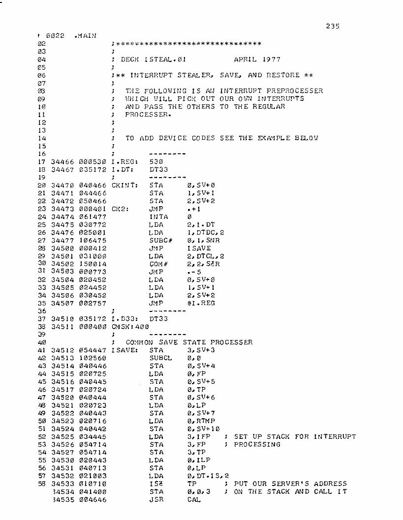
235
;*******************************
; ** INTERHtJPT STEAL ER. SAVE. AND RESTORE **
APRI L 1977
; SET UP STACK FOR INTERRUPT; PROCESSING
INTERRUPT PREPROCESSEROUR OUN IrJTERRUPTSTO THE REGULAR
0, SV+0I. SV+ 12.SV+2• + 1o2. I. DTI. DTDC. 20. I. SNRISAVE2. DTGL. 22.2.StR.- 50. SV+0I. SV+ 12.SV+2@I • REG
STATE PRO CESSER3.SV+30.00.SV+40. FP0.SV+50. TP0. SV+613,LP13. SV+70. RTMP0, SV+103. I FP3. FP3,TP0. I LP0, LP0. DT. IS. 2TP ; PUT OUR SERVER'S ADDRESS0.0.3 ; ON THE STACK AND CALL ITCAL
STASTASTAJ~lP
WTALDALDASUECA'Jt1PLDACOM"Jr-1PLDALDALDAJMP
TO ADD DEVICE CODES SEE THE EXN1PLE BELOW
TH E FOLLOW IrJ GIS AN\·JHICH \JILL PICJ( OUTA"JD PASS THE OTHERSPROCESSER.
CKHJT:
CK2 :
;
·•
;
;
·•
;
;
·•
;
·•
·•
;
;
·•
; DECK ISTEAL.01;
; GOt-lrl0N SAVEI SAVE: STA
SUBCLSTALDAsTALDAsTALDASTALDASTALDASTASTALDASTALDAI S~STAJSR
1354447102560040446020725040445020724040444020723040443020716040442034445054714054714020443040713021003010710041400004646
040466044466050466001340106147703077202500110647513004120310130150131400137730213452024452133134520132757
345123451334514345153451634517345213345213452234523345243452534526345273453133453134532345331453414535
3447133447134472344733447434475344763447734500345013451323450334504345053450634507
t 0022 .MAIN02030485068708091011121314151617 34466 131313530 I.REG: 53018 34467 035172 I. DT: DT3319202122232425262728293031323334353637 34510 035172 I.D33: DT3338 34511 00134130 CMSK: 40039404142434445464748L$
5135152535455565758

ea23 .MAINI'll 34536 000000 002 34537 02a427 01 SM: LOA a. SV+ Ie03 34541/1 04a7e1 STA 0. RTMPe4 34541 a2e424 LOA 0. SV+ 7 ; RESTORE STACK135 34542 04e7a2 STA 0.LP06 34543 e20421 LOA e. SV+607 34544 040677 STA e. TP08 34545 02e416 LOA 0. SV+50) 34546 040674 STA 0. FP10 34547 020413 LOA 0. SV+411 34550 1012e0 MOVR 0.0 . RESTORE REGISTERS•12 34551 034410 LOA 3. SV+313 34552 030406 LOA 2. SV+214 34553 024404 LOA 1. SV+ 115 34554 02e402 LOA 0.SV+016 34555 002711 JMP 81. REG ; ANO RETURN17 ; --------16 34556 000e0e SV: 11119 34557 11101111110111 0
2111 34560 11113111000 021 34561 0e0ee0 022 34562 000000 023 34563 000e00 024 34564 0001110111 11125 34565 000111013 1326 34566 000000 027 34567 0eeel1ll1l 11126 3457111 11111111111100 11129 34571 001300111 030 34572 1337215 1 FPI BUF+ I 6411131 34573 11137346 ILP: BUF+21111110-LH32 . --------•
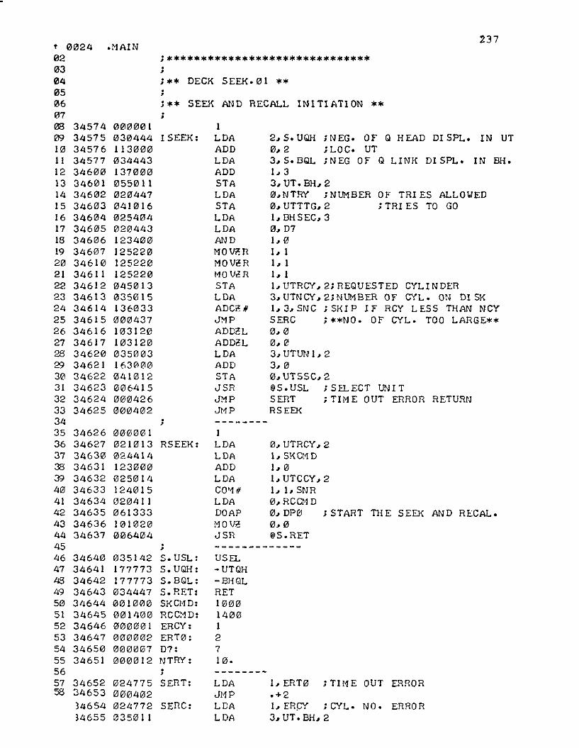
;******************************
;** DECK SEEK.01 **
;** SEEK AND RECALL INITIATION **
:137
;NEG. OF Q HEAD DISPL. IN UT;LOC. UT;NEG OF Q LlNl{ DlSPL. IN BH.
0. UTRCY. 2I.SKCMD1. 0I.UTCCY.21.1, SNR0. RCC11 D0.DPei ; START THE SEEK AND RECAL.0.0li'S.RET
2. S. UQH0.23, S. BQL1. 33. UT. BH. 20.NTRY ;NL~BER OF TRIES ALLOWED0. UTTTG. 2 ; TRI ES TO GO1. DHSEC. 30. D71.01. 11. 11. 1I.UTRCY.2;REQUESTED CYLINDER3. UTNCY.2;NUMBEROF CYL. ON DISK1.3.SNC ;SKIP IF RCY LESS THAN NCYSERC ; **NO. OF CYL. TOO LARGE**0.00. (2J
3. UTUN 1.23.00. UTSSC. [email protected] ;SELECT UNITSERT ; TIM E OUT ERROR RETURIJRSEEK
1. ERT0 ; TIriE OUT ERROR.+2I. FReY ; CYL. NO. ERROR3. UT. BH. 2
USEL-UTQH- BJ-! QLRET1000140012710.
LDAJl1PLDALDA
1RSEEK: LDA
LDAADDLDACO'1 #LDADOAPMOV,oJSR
;1
ISEEK: LDAADDLDAADDSTALDASTALDALDAANDMOW;nMOV~R
MO V,oRSTALDAADC~ II
JMPADD~L
ADD~L
LDAADDSTAJSRJMPJMP
·,
SERT:·,
;
SERC:
·,
·,
S. USL:S. UQH:S. BQL:S.RET:SKCt1D:RCCMD:ERCY:ERT0:D7:NTRY:
t 0024 .~lAIN
02030405060708 34574 00000109 34575 03044410 34576 11300011 34577 03444312 34600 13700013 34601 05501114 34602 02044715 34603 04101616 34604 02540417 34605 02044318 34606 12340019 34607 12522020 34610 125221021 34611 125221022 34612 045101323 34613 '113501524 34614 13603325 3/!615 00043726 34616 10312027 34617 10312028 34620 03500329 34621 163001030 34622 '114101231 34623 00641532 34624 00042633 34625 000/1023435 34626 '110000136 34627 02101337 34630 '112441438 34631 12300039 34632 02501440 34633 12401541 34634 02041 142 34635 06133343 34636 10102044 34637 0064044546 34640 03514247 34641 17777348 34642 17777349 34643 03444750 34644 00100051 34645 00140052 34646 00000153 34647 00000254 34650 00000755 34651 0000125657 34652 02477558 34653 000402
34654 02477234655 035011
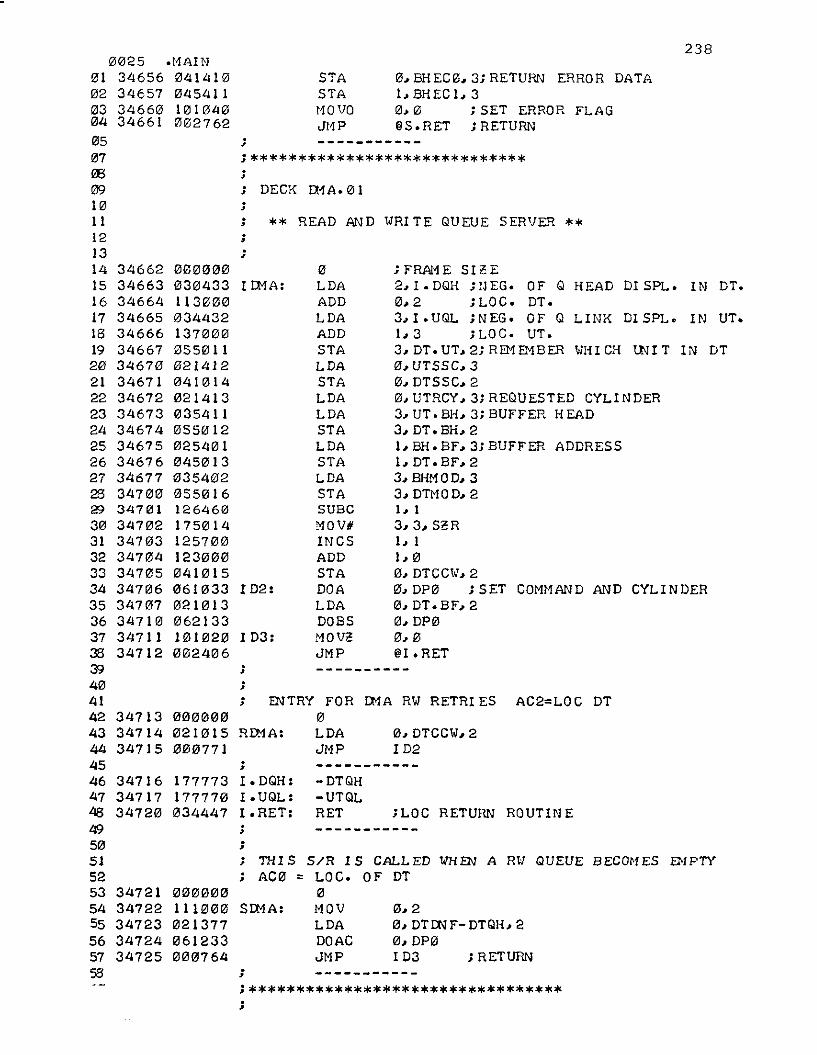
238
AC2=LOC DT
; RETURN
WHEN A RlJ QUEUE BECOMES ENPTY
0. BHEC0. 3; RETURN ERROR DATAI.BHEC1.30.0 ; SET ERROR FLAGliS.RET ;RETURN
; FRl\l1E SIcE2.I.DQH ;lIEG. OF Q HEAD DISPL. IN DT.0.2 ;LOC. DT.3.I.UQL ;NEG. OF Q LINK DISPL. IN UT.1.3 ;LOC. UT.3. DT.UT. 2; Ril1EMBER WHICH UNIT IN DT0. UTSSC. 30. DTSSC. 20,UTRCY.3;REQUESTED CYLINDER3. UT. BH. 3; BUFFER H £AD3. DT.BH. 2I.BH.BF.3;BUFFER ADDRESSI.DT.BF.23.BHMOD.33. DTMOD. 2I. 13.3. ScR1. 11.00. DTCCW. 20. DP0 ; SET COMt1AND AND CYLINDER0. DT.BF. 20. DP00.0liI.RET
0. DTCCW. 2I D2
0.20.DTDNF-DTQH.20. DP0I D3
;LaC RETURN ROUTIN E
O1A RW RETRI ES
STASTAt10VOJt1P
-DTQH-UTQLRET
oLDAADDLDAADDSTALDASTALDALDASTALDASTALOASTASUBCOlaVii'INCSADDSTADOALDADOBSMOveJMP
S/R I 5 CALL EDLaC. OF DToMOVLDADOACJMP
** READ AND WRITE QUEUE SERVER **
ENTRY FORoLDAJMP
; DECK 01A.01
I01A:
;
;
; -----------
I D3:
I D2:
·,
; ----------
S01A:
·,·,
·,
I. DQH:I.UQL:I. RET:
;*****************************
R01A:
·,
·,
; nil S; AC0 =
·,·,
·,;*********************************
000000021015000771
00000003043311300003443213700005501102141204101402141303541105501202541310450130354020550161264601750141257111111123000041015061033021013062133101020002406
177773177770034447
000000111000021377061233000764
34662346633466434665346663466734670346713467234673346743467534676346773470034701347023470334711143471115347136347137347103471134712
347133471434715
3471634717347213
3472134722347233472434725
0025 .11AIN01 34656 04141002 34657 04541103 34660 10104004 34661 0102762
0507Ql3091011121314151617181920212223242526272829303132333435363738394041424344454647481$
505152535455565758
·,
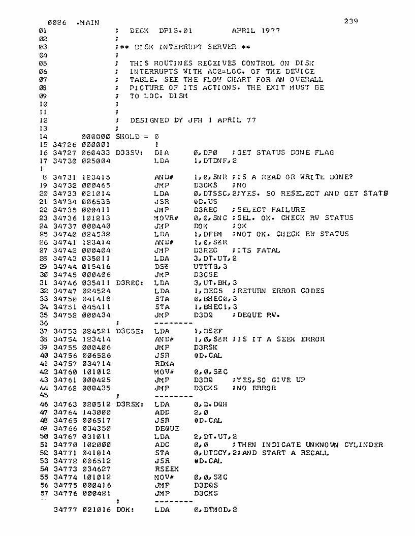
.MAIN
3472634727347313
34753347543475534756347573476133476134762
3476334764347653476634767347713347713477234773347743477534776
APRIL 1977
0. D. DQH2.0ilD.CAL
0, DP0 ; GET STATUS DONE FLAG1. DTDNF. 2
0.13. SeCD3DQ ;YES.SO GIVE UPD3CKS ;NO ERROR
1. DSEF1.0. SeR ; I SIT A SEEK [email protected]
0.0. SeCD3DQSD3CKS
2. DT. UT. 20.0 ;THEN INDICATE UNKNOWN CYLINDER0.UTCCY.2;AND START A RECALLilD.CAL
1.0, SNR ; I S A READ on ~,RI TE DONE?D3CKS ; NO0, DTSSC, 2;YES. SO RESELECT AND GET STATE,0D. USD3REC ; SELECT FAILURE0.0. SNG ; SEL. OK. CHECK RI< STATUSDOK ; OK1. DFEM ;NOT OK. CHECK mJ STATUS1,0, SeRD3REC ;ITS FATAL3. DT.UT. 2UTTTG.3D3CSE3. UT. BH. 31. DEC5 ; RETURN ERROR CODES10. BHEC0. 3I.BHEC1.3D3DQ ; DEQUE RW.
THI S ROUTIN ES REGEl VES CONTROL ON DI Sl,INTERRUPTS WITH AC2=LOC. OF THE DEVICETABLE. SEE THE FLm'l CHART FOR AN OVERALLPICTURE OF ITS ACTIONS. THE EXIT MUST BETO LOC. DI St1
; --------
AND#JMPLDAJSRJMPMOVRIJJ:1PLDAAND#JMPLDADS?:JL'1P
D3REC: LDALDASTASTAJt1P
D3RSK: LDAADDJSRDEQUELDAADCSTAJSRRSEEKMOV#JMPJMP
D3CSE: LDAAND#JMPJSRRIliAMOV#JMPJI'1P
·,
SHOLD = 01
D33SV: DI ALDA
·,
;
; DESIGNED DY JFH 1 APRIL 77
;;;
; DEGK DFIS. 0 1
; ** DI S;{ INTERRUPT SERVER **
·,;
·,
·,
·,
02051214300013136517034350103110111021000041014100651203462711011012100041601313421
02452112341400040601365261334714113113121313042513130435
0013010101310131301061343313250134
123415131313465132113141313653513131341 1113121300134413132453212341413004040350111211541600040613354110245240414101345411000434
347313473234733347343473534736347373474133474134742347433474434745347463474734751213475134752
0132613102133041350613708QI;)
101112131415161718
19202122232425262728~
3133132333435363738394134142434445
4647IcJ3LO5051525354555657
34777 021016 DOK: LDA 0. D1'I10D. 2

2. DT. UTI 20. D. UQH2.0IID.CAL ;DEQUE THE lNIT
240
0.0. SNR.+53. DT. 00. 21. EHMOD. 3 J THE EHMOD COUNTER GETS DECRE0.1 J MENTED DY ITS VALUE DEFORE THE1. BHMOD. 3 J \oIRI TE STARTED. NO CHG ON REAS0. D. DQH2.0'D.CAL ;DEQUE THE READ-WRITE OP.
AN D RECAL DON ES BELOW
0. DP0 ; FETCH STATUS DON E FLAGS.1. D3rM1.0.SNR ;SAVE ONLY lNIT FLAGS.liD. RET2. DTUCH. 2D3CKF
0. SHOLD. 3; CHECK FOR MORE WORK0.0. SNRliD. RET2. UTCL. 2; N EXT UN IT TABL E2. 2. S~R ; I S THERE NORE?.+30. DP0 ; CLEAR THE GHOSTSliD. RET1. UTOOF. 21.0. SNRD3TNX1.00. SHOLD. 3I. DP00. UTOO. 20.0. SNRD3LFMe. UTSSC. [email protected] ;SELECT AND GET STATUSD3TOXI. D3SER ; SEEK ERROR 11AS]{1.0.S~R
D3CFE0. UTCCY. 2; WAS I T A RECAL.0.0. SNR ;D3FRC ;YES0. UTRCY. 2;:10VE REQUESTED CYLItJDER0.UTCCY.2;TO CURRENT CYLINDER0. D. DQH1. D3. UL ; El'l QUQ E A READ 0 R T,m.3.UT.DT.22. [email protected]
LDANOVNJt1PLDACOM'"JI1PooAJMPLDAAND'"JMPSUBSTAooALDACOMiiJI1PLDAJSRJMPLDAAND#JMPLOACOH#JMPLDASTALDALDALDAADDADDJSRill QUE
DIALOAANDJSRLDAJMP
D3TNX:
D3CKF:
D3LFN I
.,
NOV'J~lP
LDALDASUBSTA
D3DQI LDAADDJSRDEQUELDA
D3DQSI LDAADDJSRDEQUE
; PROCESS SEEXD3CKSI
021400101015002456031000150014000403061133300245102500412341500077112240004140006503302100510001500076130211312006422000457024452123414000442021014100015001343013210130410140204140244150350011470001630001306416034321
060433024456123405006463031010000411
3513173502035021350223502335024
35025350263502735030350313503235033351334350353503635037350403504135042350433504435045350463504735050350513505235135335054350553505635057350603506135062350633506435065~ -·066
067
0027 .MAIN01 35000 10101502 35001 011""40503 35002 03501204 35003 02540205 35004 10640006 35005 04540207 35006 020467l!S 35037 14330009 35010 00647410 35011 034350II 35012 03101112 35013 021346513 35014 14300014 35015 00646715 35016 034350161718192021222324252627282930313233343536373839413414243444546474SL$
5051525354555657
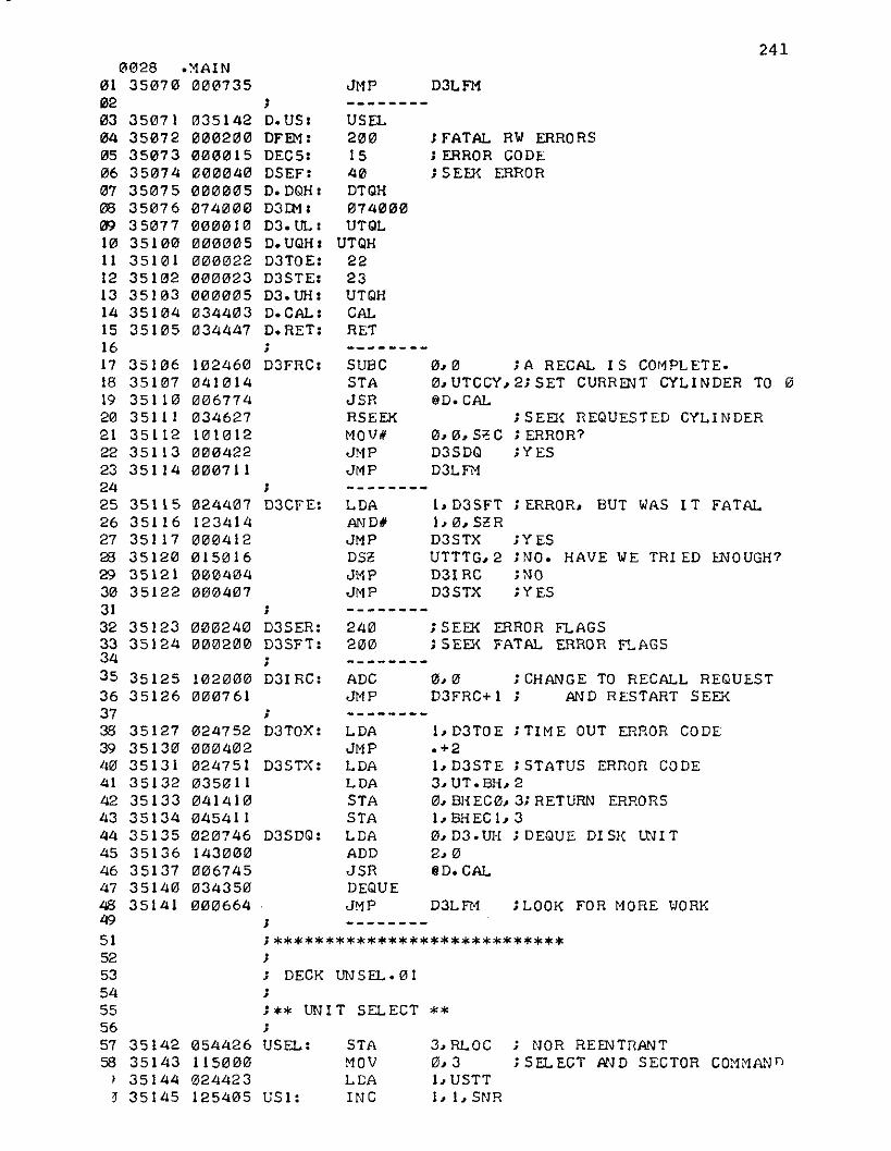
241
;****************************
;** UNIT SELECT **
TO 0
CYLINDER
HAVE WE TR! ED ENOUGH?
; SEEK REQUESTED; ERROR?;YES
; CHANGE TO RECALL REQUEST; AND RESTART SEEK
; ERROR. BUT WAS 1 T FATAL
;YES; NO.;NO;YES
; NOR REENTRANT; SELECT AND SECTOR COMclAl'Jn
; LOOK FOR MORE WORK
D3LFM
0.0. Se CD3SDQD3LFM
1. D3SFT1.0.SlRD3STXUTTTG.2D31RCD3STX
0.0D3FRC+l
0.0 ; A RECAL IS COMPL ETE.0.UTCCY.2;SET CURRENT [email protected]
3. RLOC0.31. USTT1.1. SNR
D3LFM
; FATAL RW ERRORS; ERROR CODE; SEEK ERROR
1. D3TOE ; TIME OUT ERROR CODE.+2I.D3STE ; STATUS ERROR CODE3. UT.BH. 20. BHEC0. 3; RETURN ERRORS1. BHEC 1.30.D3.UH ;DEQUE DIS!{ UNIT2.0liD. CAL
; SEEK ERROR FLAGS; SEEK FATAL ERROR FLAGS
240200
ADCJMP
JMP
SUBCSTAJSRRSEEKMOV",JMPJMP
LDAAND'JMPDSlJt'1 PJMP
STAMOVLeAINC
LDAJMPLDALDASTASTALDAADDJSRDEQUEJMP
USEL2001540DTQH074000UTQL
UTQH2223UTQHCALRET
D3CFE:
D3TOX:
JD.US:DF"EM:DEC5:DSEF:D. DQH:D3[M :D3. UL:D.UQH:D3TOE:D3STE:D3. UH:D.CAL:D.RET:
;
D3SDQ:
D3STX:
;
D3FRC:
;
;
US 1:
;
;
;
USEL:;
;; DECK UN SEL. 01
024752000402024751035011041410045411020746143000006745034350000664
054426115000024423125405
03514200020000001500004000000507400130000100000050001322000023000005034403034447
102460041014006774034627101012000422"'00711
024407123414000412015016"'004040004"'7
3512735130351313513235133351343513535136351373514035141
351153511635117351203512135122
35071350723507335074350753507635077351003510135102351033510435105
35106351073511035111351123511335114
01328 .MAIN01 35070 0007350203040506070812191011121314151617181920212223242526272829303132 35123 000240 D3SER:33 35124 000200 D3SFT:3435 35125 102000 D3IRC:36 35126 0007613738394041424344454647484951525354555657 3514258 35143
, 35144~ 35145

242
; OUTPUT SELECT COMMAND3, DP0
USER0, DP0 ; READ STATUS0,1210,0,SNCUSI
1, USTT1,1, SNRUSER0, DP00.00,0, SNCUS2RLOC0.03, @U.FP@RLOC
; DT. I S;DT~F
; DTQH; SERVER; IDLER; DTUCH; DT. UT; DT. BH; DT.BF; DTSSC; DTCCW
DT1433oD33SV100000- 1Ill1ASOMAUT330oooo121
OOC
-330.121FP
J~lP
DIAMOVSADDeL IiJt1P
LDAINCJt1PDIAMOVSADD2L /IJMPI S2MOVSLDAJMP
;
;
·•
US2:
DT33:
USER:
USTT:RLOC:U. FP:·,
·,
; ** DI SKETTE DEVI CE TABL E **; DISPLACEMENT DEFINITIONS:DTCL = 0 ;DEVICE TBL LINKDTDC = DTCL+ 1 ; DEVI CE CODEDTMSK = DTDC+l ; RESERVEDDT. I S = DTMSK+ 1 ; ADDRESS OF INTERRUPT SERVERDTWF = DToIS+l ; ll1A DONE FLAG POSITIONC 100000)DTQH = DTWF+l ; Il1A QUEUE HEADCINIT. TO -1); DTQH+ 1 ADDRESS OF QUEUE SERVER;DTQH+2 ;ADDRESS OF QUEUE IDLER COR -1.IF NONE)DTUCH = DTQH+3DT. UT = DTUCH+ 1 ; LOC. OF UT BEING SERVEDDT.BH = DT.UT+l ; LOC. OF BH BEING SERVEDDT. BF = DT. BH+ 1 ; LOC. OF BUFFER BEING READ OR IVRI TTENDTSSC = DT.BF+l ; SELECT AND SECTOR COMMANDDTCCIV = DTSSC+ 1 ; CYLINDER AND COMMAND WORDDTMOD = DTCCW+l ;CON OF BHMOD.JUST BEFORE READ OR WRITE
;*************************************; DECK DDTBL. 0
177266000000034442
12124413125405000406060433101300103133000773010405101300036404002402
000010000011000012000013000014000015000016
000000000001000002000003000004000005
0352120000330312103003472711211210121017777703466303472203522600000000000000000000000000001210
3515435155351563515735160351613516235163351643516535166
351673517035171
351723517335174351753517635177352121035212113521212352033520435205
20621217
0029 .MAIN01 35146 1210041602 35147 06043303 35150 10130004 35151 10313305 35152 00077 30607 35153 077033000010111213141516171819202122232426272829303132333435363738394041424344454647484951215152535455565756
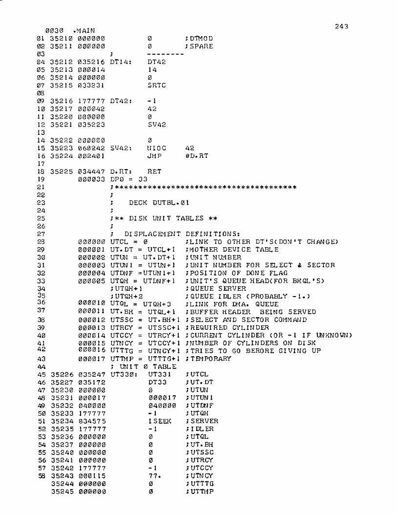
;UTCL; UT. DT;UTUN; UTUN 1; UTDNF;UTQH; SERVER;IDLER;UTQL; UT. BH; UTSSC; UTRCY; UTCCY; UTNCY; UTTTG; UTTI1P
DEfINITIONS:;LINK TO OTHER DT'S(DON'T CHANGE);110THER DEVI CE TABL E;l'NIT NU1BER;UNIT NlJr1BER FOR SELECT 8. SECTOR;POSITION OF DONE FLAG;UNIT'S QUEUE HEAD(FOR BHQL'S); QUEUE SERVER; QUEUE IDLER (PROBABLY -1.);LIlJK FOR D.'1A. QUEUE; BUFFER HEADER BEING SERVED; SELECT AND SECTOR COMMAND; REQUI RED CYL IN DER; CURltElJT CYLINDER (OR -1 IF UNKNOWN)HJUMBER OF CYLINDERS ON DI SK;TRIES TO GO BERORE GIVING UP; TEMPORARY
DT4214121SRTC
- 142'21SV42
'21NlOCJMP
SV42:
243
'21 ; OTMOO'21 ;SPAltE
;; DECK DUTBL.01
;
;
; 01 SPLACEl1 £NTUTCL = '21UT.DT = UTCL+lUTUN = UT. DT+ 1UTlJrJ 1 = UTUN + 1UTDNF =UTUN1+lUTQH = UTDNF+ 1; UTQH+ 1; UTQH+2UTQL = UTQH+ 3UT. BH = UTQL+ 1UTSSC = UT.BH+lUTRCY = UTSSC+ 1UTCCY = UTRCY+ 1UTNCY = UTCCY+ 1UTTTG = UTN CY + 1UTTMP = UTTTG+ 1; UNIT 0 TABLEUT330: UT331
DT3312100'21'2117040'2100- 1I SEEK- 1'21o'21o- 177.o'21
DT42:
DT14:;
;** DISK UNIT TABLES **
D.RT: RETDPO = 33
;***************************************
'2135247035172000000fil0121017'2140'2100177777034575177777000'21000'210'21'210'2100'210'210'210'21121fil1777770001150'210'21'21000'21'210'21
000'21100'210'2111
'2100012'2101210130'210'2114'2100015000'2116
0'210'2117
000'210121121012101211'21'21'21'21'212001210030'2100041211210'2105
17777700004200000'21'2135223
000'2100'21602420'212401
'2135216'21'210'21140'210'2100033231
352263522735230352313523235233352343523535236352373524'213524135242352433524435245
352223522335224
35212352133521435215
35216352173522035221
'21030 .'1AIN'211 3521'21 '21'21'21'21'21'21'212 35211 '21'21'21'21'21'21'213'214'215'2160708091'211112131415161718 35225 '213444719 '2100'21332122232425262723293031323334353637
3839404142
4344454647431$5'215152535455565758
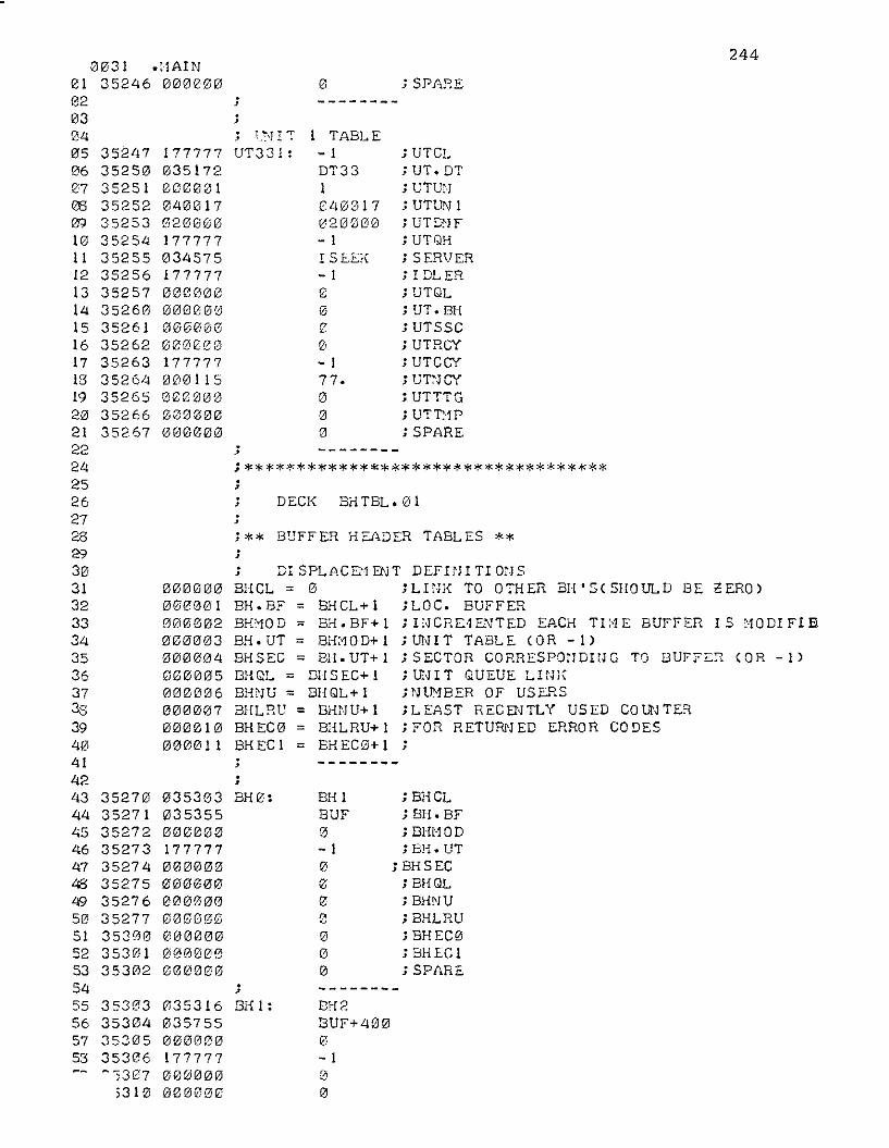
035316035755000000177777000088008000
8080088000131008138288000380000400000500000680088780081080801 I
835303035355808008177777800888000000000000000000e'00008000000000000
177777035172813G00104001702000017777703457517777700000130000001300000000G80177777000115'2lIZG0000000881380080
; UTCL; UT. DT; UTU>J; UTUN I; UT[;~IF
; UTQH;5ERIJER; I DL ER; UTQL; UTe BH; UTSSC; UTRCY; UTCCY; UT~JCY; UTTTG; UTT:-IP; SPARE
; BHCL; SH. SF; BHt10D; BE. Vi
; BHSEC; BHQL; BHNU; BHLRU; BHEC0; BHEC I; SPARE
:3o
- I
BH2BUF+400
8H IBUFo- Iooo\)
ooo
Bli 1:
; DI SPLACE.'!ENl' DEFIflI TI O~JSBHCL = 0 ;UNK TO OTHER BH'S(SHOULD BE eERO)BH.BF = BHCL+l ;LOC. BUFFERBH'10D = BH.BF+l ;r;'ICRE,IENTED EACH TnlE BUFFER IS '·IODIFIEBH. UT = BH:10D+ I ; UNIT TABLE (OR -I)BHSEC = BH. UT+ I ; SECTOR CORRESPOtJDItJ G TO DUFFEe: (OR - J)
BHOL = DHSEC+l ;tNIT QUEUE UNi(BliNU = BHQL+ I HJtNBER OF USERSSHU'll! = BHNU+ I ;LEAST RC:CENTLY USED COUJTERBHEC0 = B;iLRU+ I ; FOR RETURNED ERROR CODESBH EC 1 = BH EC0+ I ;
244
; DECI{ BH TBL. 0 I
BH0:
;
o ; SPARE
; --------
·,
; 1."j 11' 1 TABL EUT331: -I
DT331040017020000- IIS EEt(
- IoooG- 177.ooo
; ** BUFFER HEi\.DER TABLES **
;
; --------
·>
;
·>
·,
;***********************************
0031 .'IAIN101 35246 8880880210304105 35247106 3525807 3525108 352520'J 3525310 3525411 3525512 3525613 3525714 3526015 3526116 3526217 35263IS 3526419 3526520 3526621 35267222425262726293031323334353637383940414243 3527044 3527 I45 3527246 3527347 352744S 3527549 3527650 3527751 3530052 3530153 353025455 3530356 3530457 3530553 35306
-,3875310
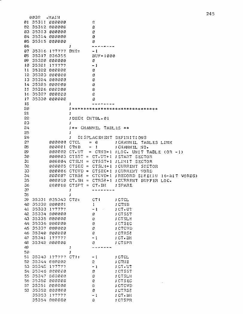
2450032 •~1AI N
01 35311 000000 002 35312 000000 1003 35313 01001000 004 35314 1000000 005 35315 000000 006 ; --------07 35316 177777 BH2: - 108 35317 036355 BUF+100009 35320 100100100 010 35321 177777 - 1II 35322 008800 012 35323 000000 013 35324 000000 014 35325 000000 015 35326 000000 016 35327 000000 017 35330 000000 018 ; --------20 ;******************************21 .,22 ; DEC:{ CHTBL.0123 ;24 ;** CHANNEL TABLES **25 ;26 ; Dl SPLACEMENT DEFINITIONS27 000000 CTCL = 0 ; CHANNEL TABLES LINK28 000001 CTNB = 1 ; CHANNEL NO.2:i 000002 CT.UT = CTNB+ I ; LOC. UNIT TABLE (OR - 1)30 000003 CTSST = CT.UT+l ; STA:1T SECTOR31 000004 CTSUol = CTSST+l ;LHlIT SECTOR32 000005 CTSEC = CTSLN+ 1 ; CURRENT SECTOR33 880086 CTCHD = CTSEC+l ; CURREn ~mRD
34 000087 CTRS1' = CTC'W+ 1 ; RECORD SI l' EC 1 rJ 16- Bl T WORDS)35 800810 CT.BH = CTRS1'+1 ; Cl'RRENT BUFFER LOC.36 000018 CTSPT = CT. Bll ; SPARE37 ; --------3:J ;39 35331 035343 CT0: CTt ; CTCL40 35332 000001 1 ; cnJB41 35333 177777 - 1 ; CT. UT42 35334 000000 0 ; CTSST43 35335 000000 0 ; CTSUI44 35336 000000 0 ;CTSEC45 35337 000000 0 ; CTC~W46 35340 000000 0 ; CTRS1'47 35341 177777 - 1 ; CT. EHLJ8 35342 0000010 0 ; CTSPRLA ; -------50 .,51 353LI3 177777 CT 1: - 1 ; CTCL52 35344 000002 2 ; CnJE53 35345 177777 - 1 ; CT. DT54 35346 020000 0 ; CTSST55 35347 000000 0 ; CTSUI56 35350 000000 0 ; CTSEC57 35351 000000 0 ; CTC;/D53 35352 000000 0 ; CTRS1'
35353 177777 - 1 ; CT. BH3535/1 006000 0 ;CTSPR

246
.ELK 200121
.LO C 10SBRTB• END
BUF:
.,
LOCI0:
.MAIN
.MAIN002001210012101121
130010 033000
003301t 003402030405
247
APPENDIX c.3
LIST OF THE BASIC SOFTWARE USED IN THE ENGLEWOOD YARD FIELD TESTS
50 PRINT ,,-----------------------------"52 PRINT" T- 562- 'll I I "53 PRINT" EXP. AVG."54 PRINT· SPECTRA PROCESSING ROUTINES·55 PRINT· BJGLE',rOOD YAfW TESTS-JUNE 77"S6 PRINT· +ASSE11BLY A-140-IX·Sf) PRINT· 12 JULY 1977"60 PRINT ,,-----------------------------"65 RB1 **REF:T-560-AI40-IX**66 RB1 **REF:T-560-II**67 RE;·! **REF:T-562-I,VII**7S LET K5= 090 DEF FrS E ( X ) = 8 • 63 539 * LOG (X) - f) • 695 CALL 23, D3100 LET tJ=2S011212 LET N3=N/2104 DIi'! Q[ 2]liZ5 DI;1 ACIn, CW]110 DIi1 E[N],t10n, S[IJl,Y[N],~J[IS]114 READ L2,LS,L6,L7,L8116 DATA 3, 44130, 25, 50, 12120 READ T2, T3, T4, T7122 DATA 30, 30, f) 00, 10124 READ f,1I,N2,N3,N4,NS,N6126 DATA 250, 24, 2, 40, 3, °128 READ PI,P2,P3,P4,PS,P6130 DATA 61, 8S, 110,8, .2,8132 READ U, U I, U2, U3, UB, U9134 DATA I, O,-1, 150, 500, 280136 LET N9=N2/2
140 PRINT145 PRINT "NU1BER OF CHANNELS; "HJ1150 PRINT "fJU·1BEn OF SPECTRA; "HJ2160 PRINT "FREQUENCY FACTOR DBAND H'C; "HJ4165 PRINT "DI SCl1EHNATIOfJ LEVEL; ";N5170 PRIr-JT "D. INDEX DECI SIOfJ LEVEL;"; 1'2180 PRWT" DATE- THIE";185 INPUT T1190 PRINT195 PRINT "TAPE#";200 INPUT T0205 PRINT
215 REM -------------------------220 GOSUB 800222 PRINT "CAR I.D.";223 INPUT 1'8224 PRINT225 GOSUB 1100228 PRINT230 GOTO 220
249 RH1 --------------------------------250 RH1 ** START CLOCK **255 CALL 6, B6
780 RH1 ---------------------------------790 RH1 ** READ IN EXP. AVG. **800 CALL 2, B2802 LET U2=- 1806 FOR 1=1 TO N9808 L.ET U2= U2-f.2810 FOR 11= 0 TO 1g I I CALL 22, U. J 6. E820 CALL 19. U. I I. U2, U3, 126. E822 IF E= 0 GOTO 840824 STOP840 CALL 17, D7865 IF I>T4 GOTO '380870 CALL II. D1890 REM ** DELAY LOOP **892 FOR J9= 1 TO 2895 FOR J3= 1 TO 222900 NEXT J3910 IF' J9=2 GOTO 925920 CALL 12. A( 0J921 GOTO 926925 CALL 12. B[ 0J926 NE><T J992'3 CALL 20, V, A( 0J. E929 CALL 20. U. B( 0J. E930 IF E> 0 GOTO 990935 NEXT I I950 NEXT I975 RETURN
248
990109911001110IllS11201122112511301135114011451150115511601165117011751180118511901192119411961200120512101215122012251230124012501260127012801290130014001410142014301450146014701480
STOPR£1 -------------SUB 1100------------REl1 ----*** READ-OUT FROM '1El10RY ***----LET 15=- 1LET 15=15+2FOR J 1= 0 TO 1
FOR 19= 0 TO 1CALL 22, U, J 6, ECALL 19, U, J 1, ( I 5+ 19) , 1, 126, EIF E= 0 GOTO 1145STOPLET AC 0]= 0CALL 21, U, AC 0], ECALL 13, AC 0]
FOR J= 0 TO ~J 1CALL 14, P7IF P7> 4 GOTO 1 lQ 0LET P7=4LET BCJ]= FNE(P7)
NEXT JIF 19=1 GOTO 1200FOR 1=1 TO N
LET ,HI]=BCl]NEXT I
NEXT 19LET K 1= 1LET K2= 0Fon L 1= 1 TO N
IF MCLIJ<P4 GOTO 1260LET Kl=Kl+1LET K4=NCLI]-BCLlJIF K4<L2 GOTO 1260LET ]{2=K2+ I
NEXT L 1PRINT "Jl,l{I,]{2 ";Jl;}(UK2LET QCJl]=K2/KIIF J I = I GOTO 1400GOSUB 7500GOSUB 8000IFJI=I GOTO 1430GOSUB 8500
NEXT J IGOSUB 1500IF 15=(N2-1) GOTO 1480GOTO 1115RETURN
249
1499 Ril1 -------------SUB 1500-----------------1500 Rl:11 SIR TO CQt.1PUTE SP. DI FFERl:1JCE1520 LET R0= 015313 LET RI= a1540 LET R2= (:I
1545 LET ~3= (:I
1550 LET 7.4= a1555 LET 7.5= 01560 LET 7.6= 01760 FOR J=I TO 01-1)17713 LET 7. I=SCJJ17313 LET 7.2=BrJJ1790 IF 1l>P4 GOTO 18101,,013 LET 7. 1= 01810 IF i02>P4 GOTO 18301'320 LET 7. 2= 018313 IF YrJ+ IJ= I GOTO 13521It3LJO GOTO 13301858 LET R3= 81360 IF YrJ+IJ=GrJ+IJ GOTO 18301,,78 GOTO 19:3018313 LET R3=R3+ I1390 IF R3< 3 GOTO 192019013 LET D= ASS (;0 1-7.2)19113 LET :'.0=IHj+D19213 LET RI=R1+c119313 LET :':2=R2+c21931 LET G[JJ= 01932 IF J>N3 GOTD 1940193LJ LET ':3=Rl1936 LET ;;/.=R21940 NEXT J1942 LET ;«5=RI-2'3194/. LET 7.6=R2-7.41946 LET R8= I~JT (Rt'J- ASS «fd-R2) IP6»19LJ9 PRINT 28;1950 LET RO= nJT (ROILS)1951 PRINT RO;1952 LET no= HJT (R0+L5*( 1/21+ I/R2»1953 PRINT RD;195LJ LET no= HIT (R0+L6*(QC IZJ+Qr 1»)1955 PEPJT RO1956 LET RO= INT (RO+L?* ABS (Qr OJ-Qr IJ»19613 LET RI= HJT (RI/HI)1970 LET R2= INT (R2/10)193121 GOTO 21001990 PRI NT
250

2000 FOR 1= 0 TO Nl2002 IF 1>5 GOTO 202020 10 PRJ NT I. B[ IJ • S [ IJ2020 NEXT I2022 GOTO 21002060 FOR J=1 TO N2070 LET ~rJJ=J*N4
2075 LET CrJJ= INT (S[JJ-B[JJ)2080 PRINT M[JJ.B[JJ.S[JJ.C[JJ;20.<35 PRINT2090 NEXT J2095 STOP2100 LET K5=K5+12110 IF P9> 1 GOTO 22002120 LET P9=22130 PRINT2140 PRINT "1----------------------------";2150 PRINT "----------------------------------1"2160 PRINT "I TEST I SP! I SP2 I";2170 PRINT "DoINDEX I RE'1ARKS I"2180 PRINT "1------1-------1-------1";2190 PRINT "--------1------------------------------1"2200 PRINT "I"; TAB (2);'{5; TAB O);"I";Rl;2210 PRINT TAB (15);"1";:12; TAB (23);"I";R0;2220 PRINT TAB (32);"1";2400 IF Rlcpl GOTO 24302410 IF R2cPl GOTO 24502420 GOTO 24702/.30 PRINT" INSUFFICIEnT DATA \VHEEL #1 I"2440 RETURN2450 PRINT" INSUFFICIENT DATA \JHEEL #2 I"2460 RETURN2470 IF ASS (RI-R2)cP3 GOTO 250024.<30 PRINT "SIGNIFF. ENERGY DIFF."; TAE (63);"1"2490 RETURN2500 IF R0cP2 GO TO 26302505 IF (Rl+R2»UB GOTO 26602510 IF Rl>U9 GOTO 26602515 IF R2>U9 GOTO 26602520 REll **CHECK FOR GREASY OR DEFECT! VE W"rlEELS**2555 GOTO 25652560 PRINT "'3."'4.l5.~6
2565 LET R5=;:5n32570 LET R6=l6n42575 IF R5cP5 GOTO 25902580 IF R6cP5 GOTO 25902""5 GOTO 2600
251
259025952600261121262121263121264026502661212670139997001217121107021070257031217040749975007520754075507600762076407660798979908010081010802080308040805081080809081008110812081308140815084998500852085408550
PRINT" GREASY '"rHEELS"; TAB (63); "I"RETURNPRINT" HIGH VALUE";PRINT TAB (63); "I"RETURNPRINT" GOOD 1VHEELS";PRINT TAB (63);"1"RETURNPRINT" OVERLOAD"; TAB (63);"1"RETURNREM ·-----------SUB 7000---------------FOR J J= 1 TO !J 6
CALL II. DIFOR J2= I TO 333NEXT J2
NEXT J IRETURNRB1 -----------SUB 7500---------------FOR 1=1 TO N
LET SCIJ=BCIJNEXT IRETURNFOR 1=1 TO N
LET t1CI ]=BC IJNEXT IRETURNREM ------------SUB 8000--------------
RB1 ** LINE SPECTRA SIR **FOR 1=2 TO (N-2)
IF BCI]<N5 GOTO 8100IF BCIJ>BCI-IJ GOTO 8040GOTO 8090IF BCI+1J<BCIJ GOTO 8130IF Be 1+ I]>BC IJ GOTO 8090IF BCI+2J<BCI+IJ GOTO 8120IF CCIJ=I GOTO 8140LET CC IJ= 0GOTO 81/-1121LET CCI+IJ=ILET CC IJ= I
NEXT IRETURNRDI --------------SUB 8500---------------FOR 1=1 TO N
LET YCIJ=CCIJNEXT IRETURN
252

253
APPENDIX D
RESONANCES OF THE WHEELS TESTED AT THE GRIFFINWHEEL PLANT IN BESSEMER, ALABAMA
(A spectrum translator was used to obtain the recorded resonantfrequencies)
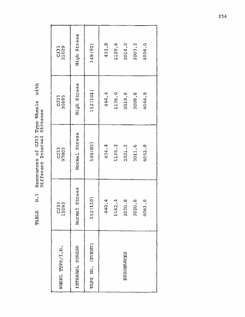
TAB
LED
.lR
eso
nan
ces
of
CJ3
3T
yp
eW
heels
wit
hD
iffe
ren
tIn
tern
al
Str
esses
WH
EEL
TY
PE
/I.D
.C
J33
CJ3
3C
J33
CJ3
31
10
92
97
80
33
06
95
31
02
9
INT
ER
NA
LST
RE
SSN
orm
alS
tress
No
rmal
Str
ess
Hig
hS
tress
Hig
hS
tress
TA
PEN
O.
(EV
EN
T)
15
2(1
10
)1
49
(82
)1
52
(10
1)
14
9(9
2)
44
0.4
43
4.4
44
4.4
43
2.8
11
42
.41
13
5.2
11
36
.01
12
9.6
RES
ON
AN
CES
20
30
.82
02
1.2
20
19
.62
01
4.0
30
20
.83
01
1.6
30
08
.83
00
3.2
40
61
.84
05
2.8
40
44
.84
03
6.0
'" lJ1 >i'o

TAB
LED
.2R
eso
na
nce
so
fC
J36
Ty
pe
Wh
eels
wit
hD
iffe
ren
tIn
tern
al
Str
esses
WH
EEL
TY
FE
/LD
.C
J36
-32
76
9C
J36
-32
78
4C
J36
-23
08
9C
J36
-27
91
0F
J36
-26
42
5C
J36
-26
17
1
INT
ER
NA
LST
RE
SSN
orm
al
Str
ess
No
rma
lS
tress
No
rma
lS
tress
Hig
hS
tress
~igh
Str
ess
Hig
hS
tress
TA
PEN
O.
(EV
EN
T)
15
4(1
28
)1
45
(42
)1
48
(65
)1
48
(56
)1
41
(1)
14
4(2
4
39
0.4
39
0.8
39
2.4
38
6.8
39
5.2
39
5.6
10
40
.01
04
1.2
10
43
.21
03
8.0
10
38
.0--
18
65
.21
86
7.2
18
68
.41
86
6.0
18
62
.01
86
3.6
23
50
.0--
--2
35
0.0
23
41
.62
34
3.2
Wea
kR
eso
na
nce
Wea
kR
eso
na
nce
Wea
kR
eso
na
nce
We
ak
Re
so
na
nc
E
24
68
.82
46
5.6
24
70
.02
47
8.8
24
83
.22
49
3.6
RE
SON
AN
CE
S2
79
4.8
27
98
.82
79
5.6
27
95
.22
78
8.0
27
85
.62
78
9.6
27
87
.2
29
35
.62
94
1.2
29
43
.62
97
3.2
WR
29
94
.02
99
5.6
29
66
.4W
.R.
29
75
.6•
29
98
.4
37
80
.03
78
7.2
37
87
.63
79
0.0
37
80
.43
78
4.0
37
85
.6
48
21
.24
82
0.0
48
18
.04
82
6.4
48
08
.64
80
9.6
58
56
.85
86
4.8
58
64
.85
87
3.6
58
60
.05
86
1.2
58
75
.6
'"V1 V1

256
APPENDIX E
DYNAMICS OF A HAMMER EXCITER
Fig. A.E.l shows a rigid hammer to be used as an exciter, in
a generalized form. The hammer is pivoted at point M and impacts
at point N. The dynamics of the hammer are governed by the rota-
tional form of Newton's 2nd Law:
T = Ie {E. 1)
where T is the applied torque, I the moment of inertia of the
hammer about M and e is the angular acceleration. Let F. be the~
component of a driving force in a transverse (i.e. nonradial)
direction. Then
ZF.t.~ ~
mgkcose = Ie (E.2)
where t. is the moment arm of the driving force F., k is the dis-~ ~
tance from M to the center of mass of the hammer and m is its mass.
In the exciter used in the tests there were two driving forces:
due to the coiled spring and due to impact at the roller (see
Fig. 4.1.1). Both of these forces are time varying, and in the
case of the spring force the moment arm is also time varying.
consequently, a full solution of eqn. (E.2) is complicated and has
yet to be achieved. However, some insight into the problem can be
achieved by solving some simple versions of eqn. (E.2).
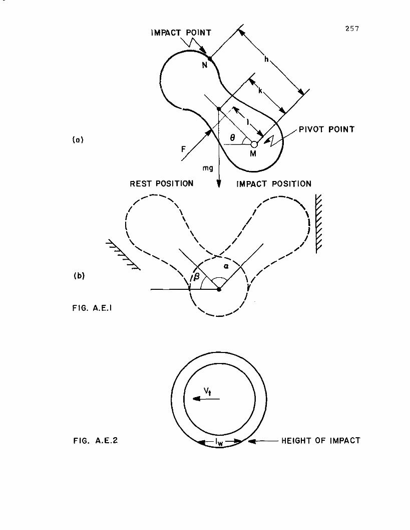
(0)
(b)
FIG. A.E.I
IMPACT POINT
F
mg
REST POSITION
257
h
PIVOT POINT
IMPACT POSITION
FIG. A.E.2 ---alV"4---- HEIGHT OF IMPACT~-::.-
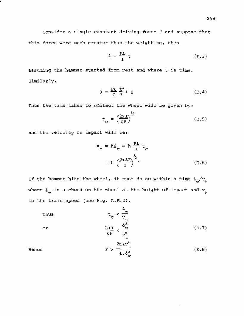
258
Consider a single constant driving force F and suppose that
this force were much greater than the weight mg, then
(E. 3)
assuming the hammer started from rest and where t is time.
Similarly,
F.f., ee=--+sI 2
(E.4)
Thus the time taken to contact the wheel will be given by:
h
t c = (~FI) 2
and the velocity on impact will be:
(E. 5)
v = he = h F.f., tc c I c
~
= h CaI-l.F) • (E.6)
If the hammer hits the wheel, it must do so within a time .f.,~Vt
where .f.,w is a chord on the wheel at the height of impact and vt
is the train speed (see Fig. A.E.2) •
.f.,Thus t
w<-c v
t
1Q","
or< ...3!.
.f.,F~
2QI~Hence F>
.f., • .f.,"w
(E. 7)
(E.8)
259
NOW in the case of a hammer consisting of a heavy ball on a light
shaft,
and from (6) and (8)
and
I = roh2
2aroh2 v 2
F>t
-L-L2W
!<
v = Ca;F) 2
c
(E.9)
(E.IO)
Thus at 20 mph ~ 10 m/sec, with ~ ~ la- 1 m; ~ = la- 2 m; m = 0.5 kg;w
h = la- 1 m and a = rr/2 radians,
F > 15 X 103 n = 3,000 Ib
and v = 30m/secc
This crude calculation shows that at relatively high train
speeds, since the hammer does indeed impact the wheel, that the
driving force must be very large. It is inconceivable that these
forces are generated by compression of the coil spring and can only
be brought about by an impulsive force at impact. On the other
hand, at a low speed, e.g. 2 mph n 1 m/sec
F £; 30 Ib
and v = 3 m/secc
At this end of the speed range the spring force is probably
effective.
260
APPENDIX F
FINITE ELEMENT ANALYSIS
F.l Finite Element Analysis of a Railway Wheel
The finite element method of structural analysis
was used for the mode-frequency analysis of railway wheel
vibrations. The method embodies the concept of representing
the distributed continuum of a physical structure by a
model consisting of a finite number of idealized elements
that are inter-connected at a finite number of points.
The analysis is performed utilizing the ANSYS computer
program developed by Swanson Analysis Systems, Inc.
The ANSYS program employs the matrix displacement
method of finite element analysis. The stiffness matrix
[K] must be generated from a description of the geometrical
and physical properties of the structure. To solve the
resulting system of simultaneous linear equations, ANSYS
uses the wavefront solution method. The "wavefront" is
equal to the number of equations active at any point in
the solution procedure. Each equation is associated with
a particular degree of freedom in the structure. An
active equation is one which has been identified and
previously used in the solution and is required again at
a further point. Equations are activated by the element
to which they are connected as the solution progresses
from element to element.

261
F.2 Mode Frequency Analysis
The equation of motion for a structural system is
[M]{ii.} + [c]{~} + [K]{u} = {F (t)}
where
[M] = Structure Mass Matrix
[c] = Structure Damping Matrix
[K] = Structure Stiffness Matrix
{u} = Vector of Nodal Displacements
{F(t) } = Force at Each Node as a Function of Time.
For an undamped structure with no force applied,
[M] {u} + [K] {u} = 0
there are n values of
If {u} = {un} Cos wnt,
w2 and n eigenvectors which satisfy
the equation above.
The ANSYS program forms the matrices [M] and [K]
by forming the matrices [Me] and [Ke ] for each element.
The eigenvalue problem is solved by a technique called
"Matrix Condensation" (Guyan Reduction). In this process
a set of n "master" degrees of freedom which characterize
the natural frequencies of interest in the system are
specified, and the eigenvalue problem is solved for the
n degrees of freedom.
In the force spectrum option of the ANSYS program,
the input consists of a force distribution on the structure
nodes and a table of force amplitude mUltipliers vs.
frequency. The structural response to force loading is
obtained by superimposing the response of individual

262
vibrational modes and weighting by their "modal participation
factors". The output contains the eigenvalue solution,
the corresponding participation factors, mode coefficients
and equivalent masses, the eigenvector solution, the
expanded mode shapes and the element stress solution.
Natural frequencies and mode shapes are obtained from
([k] - w~[m]){f}. = 0~ ~
where
[k] = the stiffness matrix of the structure
Em] = the mass matrix of the structure
w. = the circular natural frequency of mode i~
{f}. = the mode shape vector of mode~
{f}i is normalized such that
{f}:' Em] {f} = 1~
The equivalent mass for the ith mode
The participation factor is defined as
y. = {f}:'[mJ{p}1. ~
where {p} is the force vector.
The mode coefficient is defined as
P.~
Assumptions
(i) The wheel is rigidly fixed at the hub (UX = UY =
UZ = 0) and constrained in radial and circumferential
directions at a point on the tread just above the
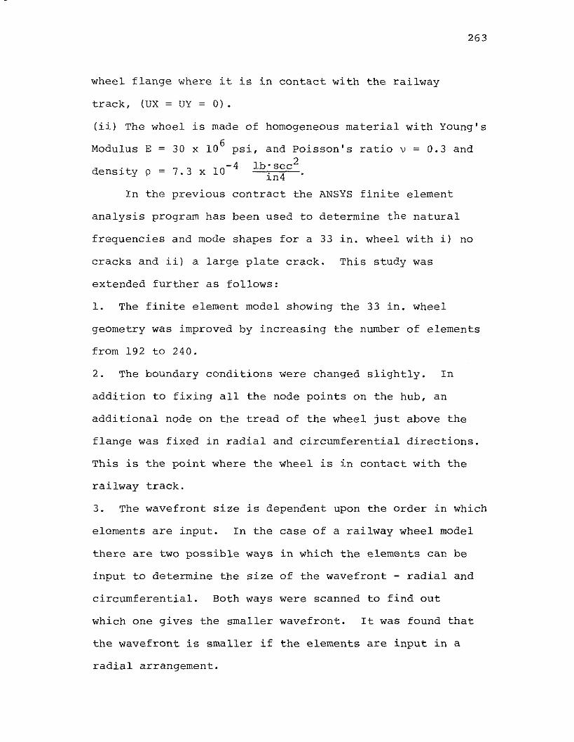
263
wheel flange where it is in contact with the railway
track, (UX = UY = 0).
(ii) The wheel is made of homogeneous material with Young's
Modulus E
density p
= 30 x 10 6 psi, and Poisson's
= 7.3 x 10- 4 Ib:S:C2
1n
ratio v = 0.3 and
In the previous contract the ANSYS finite element
analysis program has been used to determine the natural
frequencies and mode shapes for a 33 in. wheel with i) no
cracks and ii) a large plate crack. This study was
extended further as follows:
1. The finite element model showing the 33 in. wheel
geometry was improved by increasing the number of elements
from 192 to 240.
2. The boundary conditions were changed slightly. In
addition to fixing all the node points on the hub, an
additional node on the tread of the wheel just above the
flange was fixed in radial and circumferential directions.
This is the point where the wheel is in contact with the
railway track.
3. The wavefront size is dependent upon the order in which
elements are input. In the case of a railway wheel model
there are two possible ways in which the elements can be
input to determine the size of the wavefront - radial and
circumferential. Both ways were scanned to find out
which one gives the smaller wavefront. It was found that
the wavefront is smaller if the elements are input in a
radial arrangement.
264
4. A modification of the ANSYS model for the plate portion
of the 33 in. wheel was made to determine if a significant
cost reduction could be achieved in the execution of this
program when the plate geometry was simplified. The
simplification involved modeling the plate portion of the
wheel by 3-D plate elements having 6 degrees-of-freedom
per node instead of the 3-D solid elements having 3
degrees-of-freedom per node. It was hoped that this type
of element simplification would allow more computer runs
for the same cost. However, this attempt was unsuccessful
in achieving a reduction in computer costs. The increase
in the degrees-of-freedom for the four nodes for each
plate element from 3 to 6 (to allow for plate element
rotation) caused the number of simultaneous equations
associated with the computer generated wavefront to
exeeed that of the previous element description.
Various cracks were simulated in the ANSYS model of
the wheel by providing double and disconnected nodes in
the crack area. The following cracks were simulated:
1. One small radial crack, provided by detaching one
boundary on one of the rim elements (Fig. F.2.1).
2. One small radial crack through the rim, but not
extending into the plate (Fig. F.2.2).
3. One large radial crack extending from the rim through
to the axle (Fig. F.2.3).
4. One large plate crack (open on both sides and extending
slightly in the radial direction at both ends
(Fig. F.2.4).
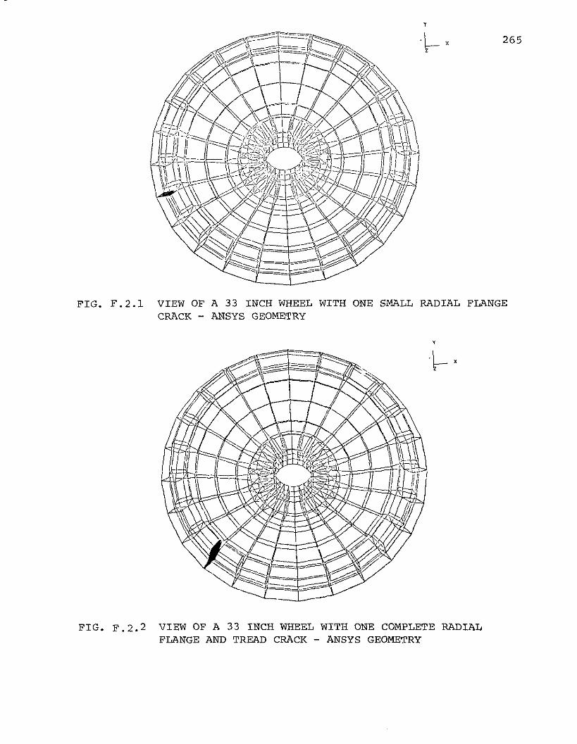
y
·~x 265
FIG. F.2.1 VIEW OF A 33 INCH WHEEL WITH ONE SMALL RADIAL FLANGECRACK - ANSYS GEOMETRY
y
FIG. F.2.2 VIEW OF A 33 INCH WHEEL WITH ONE COMPLETE RADIALFLANGE AND TREAD CRACK - ANSYS GEOMETRY

y
266
FIG. F.2.3 VIEW OF A 33 INCH WHEEL WITH ONE COMPLETE RADIAL CRACK _ANSYS GEOMETRY
FIG. F.2.4 VIEW OF A 33 INCH WHEEL WITH ONE LARGE PLATE CRACK ANSYS GEOMETRY
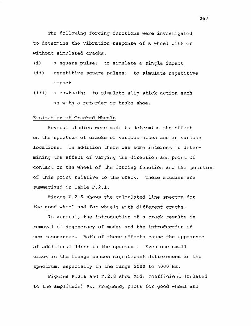
267
The following forcing functions were investigated
to determine the vibration response of a wheel with or
without simulated cracks.
(i) a square pulse: to simulate a single impact
(ii) repetitive square pulses: to simulate repetitive
impact
(iii) a sawtooth: to simulate slip-stick action such
as with a retarder or brake shoe.
Excitation of Cracked Wheels
Several studies were made to determine the effect
on the spectrum of cracks of various sizes and in various
locations. In addition there was some interest in deter
mining the effect of varying the direction and point of
contact on the wheel of the forcing function and the position
of this point relative to the crack. These studies are
summarized in Table F.2.1.
Figure F.2.5 shows the calculated line spectra for
the good wheel and for wheels with different cracks.
In general, the introduction of a crack results in
removal of degeneracy of modes and the introduction of
new resonances. Both of these effects cause the appearnce
of additional lines in the spectrum. Even one small
crack in the flange causes significant differences in the
spectrum, especially in the range 2000 to 4000 Hz.
Figures F.2.6 and F.2.8 show Mode Coefficient (related
to the amplitude) vs. Frequency plots for good wheel and

TA
BL
EF
.2
.1SU
MM
ARY
OF
AN
AL
YS
IS
Dir
ecti
on
an
dL
ocati
on
of
Ex
cit
ati
on
Ax
ial
on
load
lin
ean
d3
0d
eg
ree
fro
mlo
ad
lin
e
Ax
ial
on
load
lin
ean
d3
0,
60
,9
0,
12
0,
15
0an
d1
80
deg
ree
fro
mlo
ad
lin
e
Rad
ial
on
load
lin
ean
d3
0,
60
,9
0,
12
0,
15
0an
d1
80
deg
ree
fro
mlo
ad
lin
e
" "
" "
Stu
dy
Wh
eel
Descri
pti
on
Ty
pe
of
Ex
cit
ati
on
No
.
13
3in
.w
heel
-S
qu
are
pu
lse
no
cra
ck
s
2I
"IS
qu
are
pu
lse
wit
hex
ten
ded
du
rati
on
3I
"I
Tw
osu
ccessiv
esq
uare
pu
lses
4I
33
in.
wh
eel
-o
ne
ISq
uare
pu
lse
sm
all
rad
ial
flan
ge
cra
ck
5I
"IS
qu
are
pu
lse
63
3in
.w
heel
-o
ne
larg
ep
late
cra
ck
Sq
uare
pu
lse
Rad
ial
on
load
lin
e
73
3in
.w
heel
-o
ne
co
mp
lete
rad
ial
cra
ck
83
3in
.w
heel
-o
ne
rad
ial
rim
cra
ck
'"(J'> ro
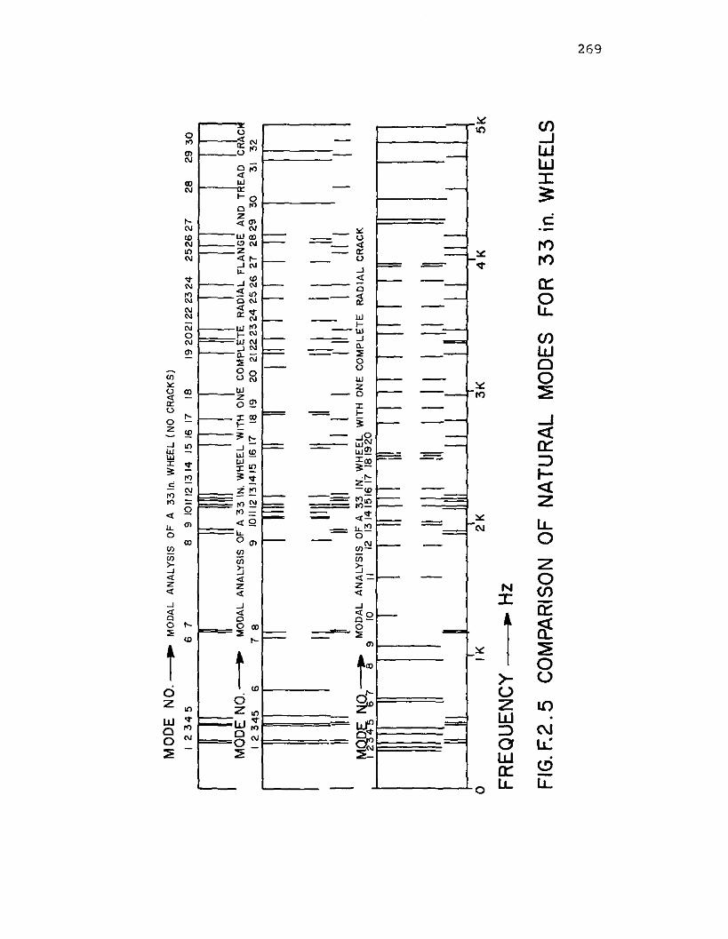
MO
DE
NO
.~M
OD
AL
AN
ALY
SIS
OF
A33
1nW
HE
EL
(NO
CR
AC
KS
)
I2
34
56
78
9/0
1112
1314
1516
1718
19
20
2/2
22
32
42
52
62
72
82
93
0
IM
OD
EN
O.
.-M
OD
AL
AN
ALY
SIS
OF
A3
3IN
.W
HE
EL
WIT
HO
NE
CO
MP
LET
ER
AD
IAL
FL
AN
GE
AN
DT
EA
DC
RA
C1
23
45
67
89
1011
1213
1415
1617
1819
20
21
22
23
24
25
26
27
28
29
30
313
2 II'11
11,
I,II
III
II
IIII
III
1111
I~II
III'
I,'II
Mn
nF
NO-.
MO
DA
LA
NA
LYS
ISO
FA
33
IN.
WH
EE
LW
ITH
ON
EC
OM
PL
ET
ER
AD
IAL
CR
AC
KI
2--:3
""4"1
;•'6
78
9/0
II12
1314
1516
171
81
92
0
oIK
IIIII
!II
2K
4K
5K
FRE
QU
EN
CY
~H
z
FIG
.F.2
.5C
OM
PAR
ISO
NO
FN
ATU
RA
LM
OD
ESFO
R3
3in
.W
HE
ELS
N (J) '"
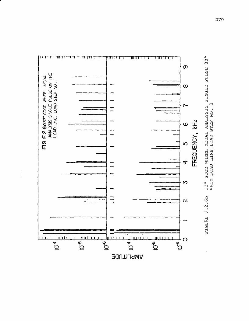
-
104
FIG
.f.2
.603
3''G
OO
DW
HE
EL
MO
DA
LA
NA
LYS
ISS
ING
LEP
ULS
EO
NTH
ELO
AD
LIN
E.
LOA
DS
TEP
NO
I.
-10
-5§ ~ ~ I-
-
10-6
I-I
II
1-
F-
~II
II
JII
III
II
IJ
II
III
II
::
~II'
.=
w o ::::> r- ~lUI
-
98
7
10-5
~ ~ - C_
~-
-I
-1(
)6r
II
01
23
45
6
FREQ
UEN
CY,
kHz
FIG
UR
EF
.2.6
b:;
3"
GO
OD
WH
EEL
MO
DA
LA
NA
LY
SIS
SIN
GL
EPU
LSE
30
°PR
OM
LOA
DL
INE
LOA
DS
TE
PN
O.
2
'" "o
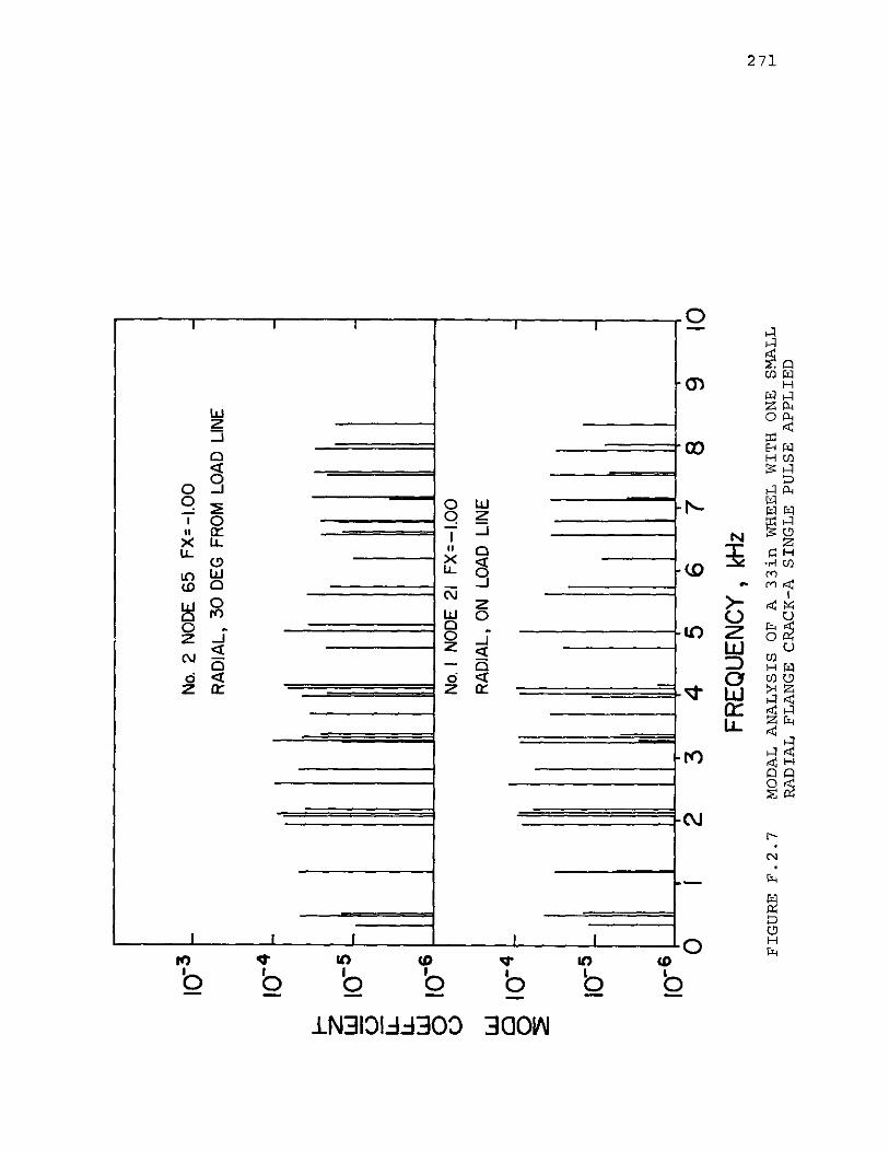
10-3
I-N
o.2
NO
DE
65
FX
=-1
.00
RA
DIA
L,3
0D
EG
FRO
MLO
AD
LIN
E
-
10-4
I-- - -
10-6
II
I!I
II!I
"II!
II!
"I"
III
I!I
I"
III
NO.1
NO
DE
21F
X=
-1.0
0
RA
DIA
L,O
NLO
AD
LIN
Ew 8
10-4
I
~I- ~10
-5I
o I..L.
I..L.
W o o
1()
5I-
-
10-6
II"
I,
IIII
III!
I""
II
,I
1I
II
I!'I
'I
iii
,{iii
oI
23
45
67
89
10
FREQ
UEN
CY
,kH
zF
IGU
RE
F.2
.7M
OD
AL
AN
AL
YSI
SO
FA
33
inW
HEE
LW
ITH
ON
ESM
ALL
RA
DIA
LFL
AN
GE
CR
AC
K-A
SIN
GL
EPU
LSE
AP
PL
IED
'" " .....
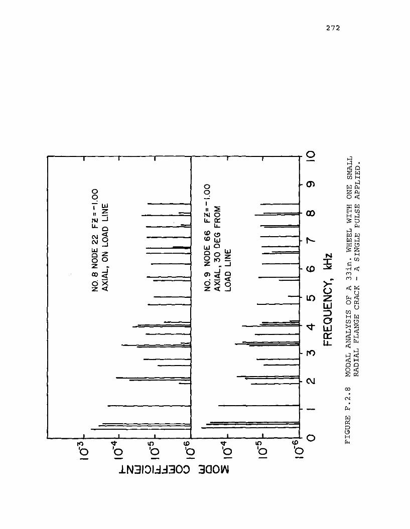
--
NO
.8N
OD
E2
2F
l=-1
.00
AX
IAL,
ON
LOA
DLI
NE
--
--
IIJ
NO
.9N
OD
E66
Fl=
-1.0
0A
XIA
L,3
0D
EG
FRO
M~
LOA
DLI
NE
-
I--
I,
,•
•
10-3
I-10
-4
Z W ~1(
)5lL
.W o u
ler6
w Cl o :E
1()4
1()5
10-6 o
23
45
67
FRE
QU
EN
CY
,kH
z8
910
'"-..J '"FI
GU
RE
F.2
.8M
OD
AL
AN
AL
YSI
SO
FA
33
in.
WH
EEL
WIT
HO
NE
SMA
LLR
AD
IAL
FLA
NG
EC
RA
CK
-A
SIN
GL
EPU
LSE
AP
PL
IED
.
273
wheels with different cracks excited by a square pulse.
For good wheel excitation, it is seen that different modes
are excited depending upon location of the point of excitation
relative to the load line. Also the modal amplitude
varies somewhat. A study of the effect of different impact
points was made for the wheel with the smallest possible
rim crack.
Axial and radial excitation on the flange by a square
pulse was carried out separately at various angular dis
tances (15 degrees apart) from the load line. The purpose
was to determine if the small crack so simulated is evident
in spectral changes, and secondly, to determine if the small
crack may be discovered regardless of the point of wheel
excitation. The results show that the number of resonances
excited between 300 and 10000 Hz in the faulty wheel varied
between 27 and 40 depending upon the nodal location on
which the impulse was applied, and on whether this impulse
was applied axially or radially. However, the amplitude
of the major resonances was not greatly affected and it
was concluded that there was no great advantage to be gained
by impacting the wheel off the load line.
274
APPENDIX G
RELATIONSHIP AMONG OPERATING PARAMETERS
In assessing progress towards the goal of helping
the Railroads find defective wheels it is necessary to have
some "yardsticks" or "figures of merit" by which to measure
the performance of the acoustic signature system in
comparison with current practice and other systems and to
measure the cost/benefit ratio of developing and operating
such systems. Such measures are not easy to come by
partly because some of the information that it is necessary
to have (e.g., the percentage of defective wheels in
service) is not available in a precise form.
It is possible to define two figures of merit which
could be used to assess progress. First, reliability is
defined as:
R = Number of correct decisionsTotal number of decisions
where a decision is a good/bad wheel choice as made by
the system. The false alarm rate is defined as:
F - Number of unconfirmed indications- Total number of bad wheel indications
Let the number of axles passing the inspection point in
a given period be NAo Suppose that ND of these axles
carry a defective wheel and that the fraction of these
identifiable by acoustic signature inspection is g. Then
the number of bad wheels correctly found will be
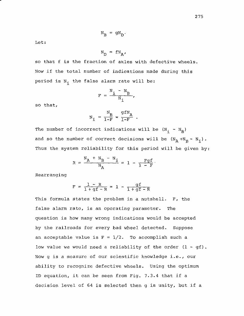
275
Let:
ND = fNA,
so that f is the fraction of axles with defective wheels.
Now if the total number of indications made during this
period is N. the false alarm rate will be:1.
N. - NBF 1.= ,N.
1.
so that,
N.N
BgfN
A= = I-F1. I-F
The number of incorrect indications will be (Ni
- NB)
and so the number of correct decisions will be (NA +NB
- Nil.
Thus the system reliability for this period will be given by:
Rearranging
R ==N
BN.
1. = 1 _ Fgf.1 - F
F = 1 - R = 1 _ gf1 + gf - R 1 + gf - R
This formula states the problem in a nutshell. F, the
false alarm rate, is an operating parameter. The
question is how many wrong indications would be accepted
by the railroads for every bad wheel detected. Suppose
an acceptable value is F = 1/2. To accomplish such a
low value we would need a reliability of the order (1 - gf).
Now g is a measure of our scientific knowledge i.e., our
ability to recognize defective wheels. Using the optimum
ID equation, it can be seen from Fig. 7.3.4 that if a
decision level of 64 is selected then g is unity, but if a
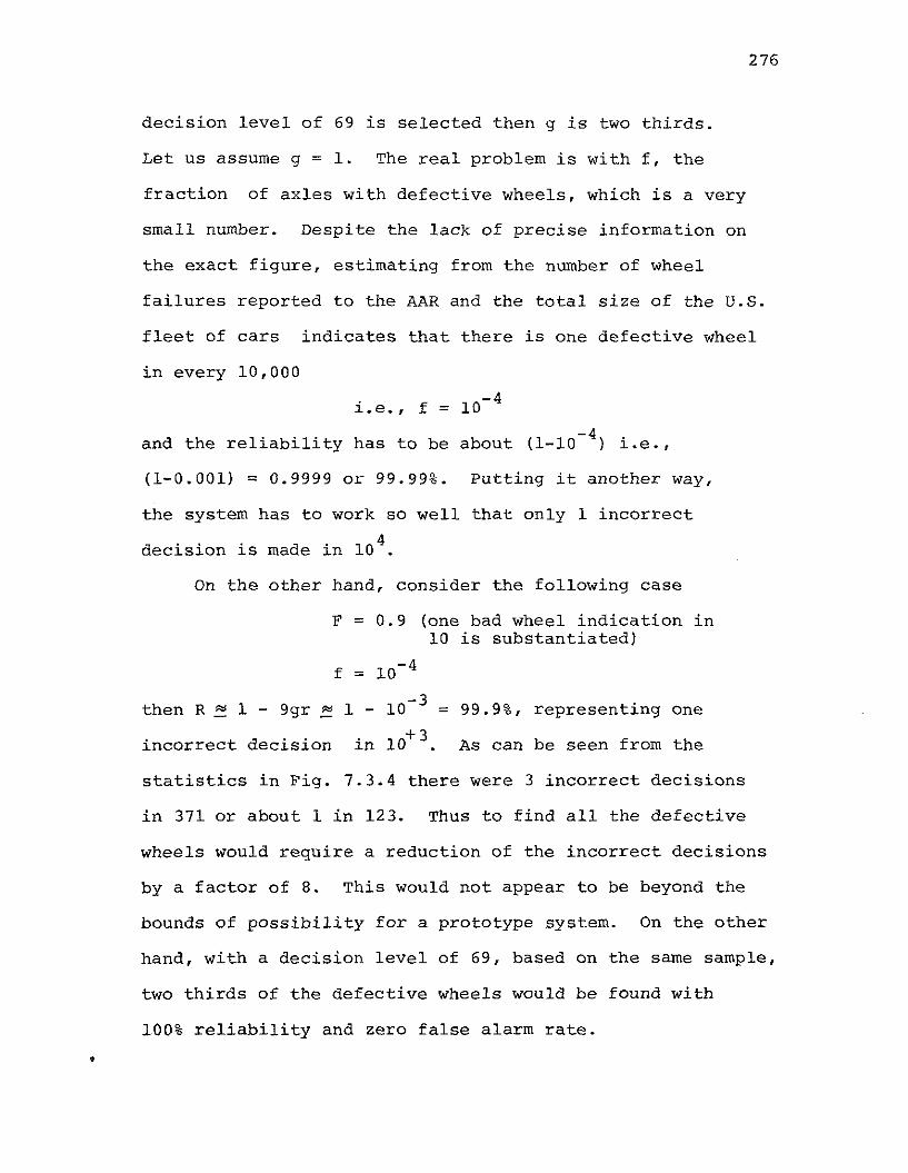
•
276
decision level of 69 is selected then g is two thirds.
Let us assume g = 1. The real problem is with f, the
fraction of axles with defective wheels, which is a very
small number. Despite the lack of precise information on
the exact figure, estimating from the number of wheel
failures reported to the AAR and the total size of the U.S.
fleet of cars indicates that there is one defective wheel
in every 10,000
1" e f = 10-4. .,
and the reliability has to be about (1_10- 4 ) i.e.,
(1-0.001) = 0.9999 or 99.99%. Putting it another way,
the system has to work so well that only 1 incorrect
decision is made in 104
.
On the other hand, consider the following case
F = 0.9 (one bad wheel indication in10 is substantiated)
f = 10-4
then R "" 1 - 9gr "" 1 - 10-3 = 99.9%, representing one
incorrect decision in 10+ 3. As can be seen from the
statistics in Fig. 7.3.4 there were 3 incorrect decisions
in 371 or about 1 in 123. Thus to find all the defective
wheels would require a reduction of the incorrect decisions
by a factor of 8. This would not appear to be beyond the
bounds of possibility for a prototype system. On the other
hand, with a decision level of 69, based on the same sample,
two thirds of the defective wheels would be found with
100% reliability and zero false alarm rate .
277/278
APPENDIX H
REPORT OF NEW TECHNOLOGY
In the earlier report (FRA/OR&D 76-290 or DOT-TSC-FRA-76-6),
three items were listed as possibly patentable. In the present work,
a number of improvements are described and these are now listed under
the same three headings:
1) The system for Acoustic Signature Inspection of Railroad
Wheels is described agaln on page 6-9 and 109-110 with some new
ideas to bypass some problem areas.
2) The mechanical impacter, as actuated by the wheel itself, is
described with improvements on pages 93, 13-14, and 90-94. Additional
ideas for excitation methods are given on pages 94-99.
3) The improved computer programs for analysis of acoustic signa
tures are described on pages 107-122 and printed in full in Appendix C
on pages 211-252.
'* u. S. GOV'. PRINTING OFFICE 1geo 600·768 :I 45

Copyright © 2022 FDOKUMEN

