Modeling the land surface water and energy cycles of a mesoscalewatershed in the central Tibetan Plateau during summerwith a distributed hydrological model

Bao-Lin Xue,1,2 Lei Wang,1 Kun Yang,1 Lide Tian,1 Jun Qin,1 Yingying Chen,1

Long Zhao,1 Yaoming Ma,1 Toshio Koike,3 Zeyong Hu,4 and Xiuping Li1

Received 29 January 2013; revised 29 July 2013; accepted 30 July 2013; published 22 August 2013.

[1] The Tibetan Plateau (TP) is the highest plateau in the world, playing an essential role inAsian monsoon development and concurrent water and energy cycles. In this study, theWater and Energy Budget-based Distributed Hydrological Model (WEB-DHM) wascalibrated and used to simulate water and energy cycles in a central TP watershed during thesummer season. The model was first calibrated at a point scale (BJ site). The simulationresults show that the model can successfully reproduce energy fluxes and soil surfacetemperature with acceptable accuracies. The model was further calibrated at basin scale,using observed discharges in summer 1998 and the entire year of 1999. The modelsuccessfully reproduced discharges near the basin outlet (Nash-Sutcliffe efficiencycoefficients 0.60 and 0.62 in 1998 and 1999, respectively). Finally, the model was validatedusing MODIS land surface temperature (LST) data and measured soil water content (SWC)at 15 points within the watershed in 2010. The simulation results show that the modelsuccessfully reproduced the spatial pattern and LST means in both nighttime and daytime.Furthermore, the model can generally reproduce 15-site averaged SWC in four soil layers,with small bias error and root mean square error. Despite the absence of long-term dischargedata for model verification, we validated it using MODIS LST and measured SWC data.This showed that the WEB-DHM has the potential for use in poorly gauged or ungaugedareas such as the TP. This could improve understanding of water and energy cycles inthese areas.

Citation: Xue, B.-L., et al. (2013), Modeling the land surface water and energy cycles of a mesoscale watershed in thecentral Tibetan Plateau during summer with a distributed hydrological model, J. Geophys. Res. Atmos., 118, 8857–8868,doi:10.1002/jgrd.50696.

1. Introduction

[2] The Tibetan Plateau (TP), sometimes also called the“Third Pole,” covers a large area around 2.5 × 106 km2. It isthe highest plateau in the world, with average elevation 4000m. The TP has been much discussed in previous studies,regarding its essential role in Asian monsoon developmentand concurrent water and energy cycles [Chen et al., 1985;Wu and Zhang, 1998; Tanaka et al., 2003]. Recent research

indicates that the TP has experienced rapid climatic changecompared with surrounding areas, and this in turn has changedthe area hydrologic cycle [Liu and Chen, 2000; Cao et al.,2006; Yang et al., 2011; Gao et al., 2012; Gerken et al.,2012; van der Velde et al., 2012]. For example, decreased dis-charge has been observed because of insignificant increase ofprecipitation yet enhanced evaporation in eastern and southernTP [Yang et al., 2011]. The influence of climate change on thedischarge was more obvious for areas with large permafrostcoverage, where winter discharges increased because of per-mafrost degradation [Niu et al., 2011]. Since the TP is thesource region for most rivers of China and South Asia, it istherefore necessary to investigate how the energy and hydro-logic cycles change on the TP. This will aid clear understandingof future hydrologic responses, especially under the conditionof climate change [Immerzeel et al., 2010].[3] Distributed hydrological models (DHMs) are effective

tools for simulating the water cycle and for predicting futurehydrologic responses [Beven, 2001; Broustert et al., 2002].However, because of harsh meteorological conditions, thehigh elevation, and resulting data sparsity, there have beenfew model applications for the TP on the basin scale, espe-cially for the central plateau with elevations above 5000 m

1Key Laboratory of Tibetan Environmental Changes and Land SurfaceProcesses, Institute of Tibetan Plateau Research, Chinese Academy ofSciences, Beijing, China.

2State Key Laboratory of Vegetation and Environmental Change,Institute of Botany, Chinese Academy of Sciences, Beijing, China.

3Department of Civil Engineering, University of Tokyo, Tokyo, Japan.4Cold and Arid Regions Environmental and Engineering Research

Institute, Chinese Academy of Sciences, Lanzhou, China.

Corresponding author: L.Wang, Key Laboratory of Tibetan EnvironmentalChanges and Land Surface Processes, Institute of Tibetan Plateau Research,Chinese Academy of Sciences, Lincui Road, Chaoyang District, Beijing100101, China. (wanglei@itpcas.ac.cn)

©2013. American Geophysical Union. All Rights Reserved.2169-897X/13/10.1002/jgrd.50696

8857

JOURNAL OF GEOPHYSICAL RESEARCH: ATMOSPHERES, VOL. 118, 8857–8868, doi:10.1002/jgrd.50696, 2013

[Gao et al., 2012]. Prior research has mainly focused on theedge of the plateau, in the source area of the principal riversof China, Nepal, and India [Singh et al., 2006; Fujita et al.,2007; Niu et al., 2011], or on single point simulation ofrunoff response by land surface models [e.g., Yang et al.,2011]. This may be attributed to the fact that traditionalhydrological models generally need relatively long-termdischarge data for their calibration and validation, which isdifficult to obtain on the central TP because of poorly gaugedconditions there. This necessitates the use of a new-generation hydrological model to study the regional hydro-logic processes. Such a model can be calibrated or validatednot only by ground-based discharge measurements, but alsoby other in situ or satellite measurements at various scales.The latter include energy fluxes or soil moisture measuredat a point scale, as well as satellite-derived land surfacetemperature (LST) at basin scale.

[4] Furthermore, accurate estimates of regional- and basin-scale soil moisture are required to understand the hydrologiccycle [Betts et al., 1996; Entekhabi et al., 1996]. Soilmoisture is believed an essential parameter in climate andland surface models [Leese et al., 2001; Kumagai et al.,2009], and can influence runoff/infiltration partitioning,evapotranspiration, and thereby the water and energy cycles[Merz and Blöschl, 2009]. Traditional methods for estimat-ing soil moisture use single point measurements and remotesensing data. However, the former is usually restricted bythe difficulty of maintaining measurements in harsh regionssuch as the TP. Moreover, single point measurements are diffi-cult to conduct at a regional or basin scale, which is essentialfor hydrological models. For the remote sensing method, it isusually restricted by coarse spatial resolution (≈50× 50 km2);a finer resolution is believed to improve its hydrologic simula-tion on a basin scale, given sufficient meteorological observa-tions. In contrast to the above two methods, a fully calibratedland surface or hydrological model can provide continuoussoil moisture data at fine spatial resolution. However, littleresearch has been conducted on simulation of soil watercontent (SWC) on the TP via land surface models or tradi-tional water-balance DHMs, owing to calibration difficulties.As a pioneer study, Lu et al. [2012] calibrated a land dataassimilation system by two station-measured SWC, followedby mapping of SWC across the entire plateau. The studywas a step forward for SWC simulation over the TP, whileit is still incomplete in that the model did not consider theinfluence of topography-driven lateral runoff on SWC, whichcannot be neglected in the area.[5] As tentative research, this study aims to calibrate and

validate the Water and Energy Budget-based DistributedHydrological Model (WEB-DHM) [Wang et al., 2009a,2009b, 2009c] for the central TP in the absence of long-termdischarge data. The WEB-DHM is a coupled biospheremodel of a revised 1-D land surface model (SiB2) [Sellerset al., 1996a, 1996b] and a hillslope-based hydrologicalmodel (GBHM) [Yang et al., 2000, 2002], which can be usedfor simulating water and energy cycles on a basin scale [Wanget al., 2009a]. The model has already been validated in severalwatersheds of Japan and the United States, and showed goodperformance when compared with observations such as runoff[Wang et al., 2011], LST [Wang et al., 2009a, 2009c], andSWC [Wang et al., 2009c]. However, considering the specialconditions of the TP (harsh meteorological conditions, highelevation, unique vegetation, and others), further investigationof the model performance is necessary for application there.We also evaluate model simulation results using remotelysensed LST and observed SWC data. In contrast with earlierresearch [e.g., Lu et al., 2012], systematic SWCmeasurementsare used for model validation. The study contributes to hydro-logical modeling of areas that are poorly gauged or evenungauged, thereby improving understanding of the hydrologiccycle in such areas.[6] The paper is organized as follows. In section 2, we

describe the research area and the data collection in thisstudy. In section 3, we give the calibration results atpoint scale (BJ site) and also at the basin scale using dis-charge data in the summer of 1998 and the whole year of1999. We also show the validation results using MODISLST and multisite SWC measurements for the year of2010. In the last section, we summarize the major results

TP

(a)

(b)

Figure 1. (a) Location of Naqu River watershed; (b) map ofNaqu River watershed, with Naqu gauge, Amdo, and BJ sites(see text).

XUE ET AL.: WATER AND ENERGY CYCLE AT TIBET

8858

of the study and depict the necessities for model improve-ments in future research.

2. Materials and Methods

2.1. Study Area

[7] The study area of the Naqu River watershed is on thecentral TP (Figure 1a). As the headwaters of the Nu Riversystem, the watershed spans longitude 90.94°E to 92.51°Eand latitude 29.99°N to 33.02°N, with a total area of 9247km2. Topography is characterized by gentle hills with eleva-tion range 4494–5737 m a.s.l., and vegetation is classified ashighland meadow. The region is strongly influenced bythe summer Indian monsoon. Precipitation generally fallsbetween June and September and represents around 85%

of the annual total. Mean annual precipitation at BJ station(Figure 1b) was 529 mm during 1952–2006, and the tem-perature range was from �40.94 to 24.14°C, with annualmean �1.25°C.

2.2. Model Description

2.2.1. General Model Structure[8] The WEB-DHM [Wang et al., 2009a, 2009b, 2009c] is

a distributed biosphere hydrological model, which can beused to simulate basin-scale water, energy, and carboncycles. The model is superior to traditional water-balancehydrological models in that it integrates a biosphere scheme(SiB2) [Sellers et al., 1996a] and a hillslope-based hydrolog-ical model (GBHM) [Yang et al., 2000, 2002]. It calculatesevapotranspiration based on both water and energy balance

Datum

Inter flowGroundwater table

Impervious Surface

Hillslope Unit

l

River

Precipitation

Soil surface

CO2H

Rlw

ET

Surface flow

Rsw

Grid size in the model

DEM grid size

(d)(c)

(b)(a)

2

1

3 5

4

7

6

9

8

Outlet

Flow Intervals Subbasin

Groundwater flow

Figure 2. Overall structure of WEB-DHM: (a) division from basin to subbasins; (b) subdivision fromsubbasin to flow intervals comprising several model grids; (c) discretization from a model grid to a numberof geometrically symmetrical hillslopes; and (d) description of water moisture transfer from atmosphere toriver. Here, the land surface submodel is used to describe transfer of turbulent fluxes (energy, water, andCO2) between atmosphere and ground surface for each model grid, where Rsw and Rlw are downward solarand longwave radiation, respectively; H is sensible heat flux; and λ is latent heat of vaporization. GBHMsimulates both surface and subsurface runoff using grid-hillslope discretization and then simulates flowrouting in the river network.

XUE ET AL.: WATER AND ENERGY CYCLE AT TIBET

8859

on each model grid and therefore has a more solid physicalfoundation relative to the traditional models. The model hasbeen validated in several regions, generally showing goodperformance in simulating basin-scale water and energycycles [Wang et al., 2009a, 2009c]. As a test of model perfor-mance, it was first applied to a small watershed of the LittleWashita Basin in the United States, with total area 603 km2

[Wang et al., 2009c]. Since a description of model structurehas been given in Wang et al. [2009c], only a brief reviewis given here.[9] The general model structure is illustrated in Figure 2. A

digital elevation model (DEM) is used to define the targetarea, and then the target basin is divided into a number ofsubbasins using the Pfafstetter system [e.g., Verdin andVerdin, 1999] (Figure 2a). Within each subbasin, a numberof flow intervals are specified to represent the time lag andaccumulating processes in the river network, according tothe distance to the subbasin outlet. Each flow intervalincludes several model grids (Figure 2b). For simplicity, asingle land use type and soil type is assumed in each modelgrid. For each grid within a flow interval, the hydrologicallyimproved land surface model is then used to calculate turbu-lent fluxes (energy, water, and carbon) between the atmo-sphere and land surface [Wang et al., 2009b] (Figure 2d).Each model grid is further divided into a number of geometri-cally symmetric hill slopes, and the hydrological submodelused to simulate lateral water redistribution and calculaterunoff. For simplicity, streams within one flow interval arelumped into a single virtual channel in the shape of a trape-zoid. All flow intervals are linked by the river network gener-ated from the DEM, and all runoff from the model grids in thegiven flow interval is accumulated into the virtual channel

and led to the river basin outlet (Figures 2c and 2d).Simplifications were made to reduce computation costs.First, groundwater interactions between flow intervals arenot considered. Second, within a flow interval, lateral moistureexchanges between model grids were not formulated. Third,all streams (∑L) extracted from the fine DEM within a givenmodel grid (Figure 2c) were simplified as one stream withthe same length (∑L) flowing along the main flow directionof the model grid. Therefore, total runoff generated from agiven model grid can be regarded as being from the newhillslopes along the single stream.[10] In model setup, 9247 grids were generated for the

entire watershed at 1 × 1 km2 resolution, and the watershedwas further divided into nine subbasins (Figure 1). Terrainchanges little across the watershed (Figure 4a), which hasaverage elevation of 4815 m a.s.l. and average slope of 5.68°.2.2.2. Soil Model[11] Within each model grid, the unsaturated zone (Ds;

Figure 3) is defined by the average slope of that grid. Twodifferent soil subdivision schemes are used in describing landsurface and hydrologic processes.[12] In the calculation of land surface processes, the three-

layer soil structure for the unsaturated zone is the same as thatin SiB2. The depth of the first layer (D1) is defined at a fewcentimeters, whereas the root depth (D1+D2) is definedaccording to vegetation type by SiB2 default [Sellers et al.,1996b]. The thickness of the deep soil zone (D3) changes withwater table fluctuation and equals the depth of the groundwa-ter level minus the thickness of the upper two layers.[13] In simulation of soil water flow, a multisublayer soil

structure is used to describe the unsaturated zone. Thenonuniform vertical distribution is represented using an as-sumption of exponentially decreasing hydraulic conductivitywith increasing soil depth, given by kz= ks � exp(�f � z)[Cabral et al., 1992; Robinson and Sivapalan, 1996]. Here,ks and kz are hydraulic conductivities at the soil surface anddepth z, respectively, and f is a decay factor. The surface layerof depth D1 is kept as the first layer. The root zone and deepsoil zone are uniformly subdivided into several sublayers. Asshown in Figure 3, the multisublayer structure is used tocalculate lateral runoff and vertical interlayer flows. Slope-driven lateral water distributions are calculated in three parts:(a) surface flows by Manning’s equation, (b) subsurfaceflows by Darcy’s law, and (c) groundwater exchanges withriver discharge, also by Darcy’s law. Vertical interlayer flowsin the unsaturated zone are described using a one-dimensional Richards equation [Wang et al., 2009a]. In thissoil model, the van Genuchten equation [van Genuchten,1980] is used as the soil hydraulic function.

2.3. Data Sets

2.3.1. Meteorological Forcing Data[14] The meteorological forcing data needed for WEB-

DHM, i.e., near-surface air temperature, specific humidity,downward shortwave and longwave radiation, wind speed,air pressure, and precipitation, are obtained from theChina Meteorological Forcing Dataset (CMFD) [He, 2010;Yang et al., 2010; Chen et al., 2011], which were fromhttp://westdc.westgis.ac.cn/data/7a35329c-c53f-4267-aa07-e0037d913a21. The data set has spatial resolution 0.1° andtemporal resolution 3 h and was developed by thehydrometeorological research group at the Institute of

D3

D2

D1

Ds

Dg

sfc

qgAquifer Model

qsub

Impervious Boundary

q

Figure 3. Soil model of WEB-DHM. Two different soilsubdivision schemes were used to describe land surface andhydrologic processes, respectively. The three-layer soil struc-ture used in SiB2 is retained to represent the unsaturated zonein calculations of land surface processes. The unsaturatedzone is divided into multiple sublayers when simulatingwater flows within it and water exchanges with groundwateraquifer.

XUE ET AL.: WATER AND ENERGY CYCLE AT TIBET

8860

Tibetan Plateau Research, Chinese Academy of Sciences[He, 2010]. The data sets have been used for land surfacemodeling of arid and semiarid regions in China andcompared with in situ observation data [e.g., Chen et al.,2011]. In simulating LST in Chinese dry lands, Chen et al.[2011] found that the newly developed CMFD couldimprove model results by reducing mean bias in MODISdaytime (10:30 local time) LST by more than 2 K, using arevised Noah land surface model [Chen and Dudhia,2001]. With an intercomparison of forcing data with theGlobal Land Data Assimilation System (GLDAS), they alsoshowed that the CMFD was superior to the GLDAS in

model simulation, owing to its integration of informationfrom 740 China Meteorological Administration operationalstations. Despite ongoing updates and evaluation of theCMFD, its data were chosen for forcing in our simulation.We updated the meteorological input data every 3 h exceptfor precipitation, which was disaggregated to hourly values.Since we calibrated the discharge at a daily time step, this“downscaling” method for precipitation affected modeledvalues little.[15] Land surface parameters of WEB-DHM are initially

calibrated on a point scale (BJ site), using in situ observationsfrom the Global Energy and Water Cycle Experiment Asian

(a)

(d)(c)

(b)

Figure 4. (a) DEM; (b) grid slope; (c) spatial distribution of land use; and (d) spatial distribution of soiltype and schematic of soil measurement points of Soil Moisture/Temperature Monitoring Network(SMTMN) within Naqu River watershed.

XUE ET AL.: WATER AND ENERGY CYCLE AT TIBET

8861

Monsoon Experiment-Tibet (GAME-Tibet) [Ishikawa et al.,1999; Koike et al., 1999;Ma et al., 2003]. Here, we focus onsimulating water and energy cycles in summer, since obser-vations of discharges as well as heat and energy fluxes wereavailable from July to September 1998 (except for a largedata gap of sensible and latent heat flux in June 1998).2.3.2. DEM and Remote Sensing Data[16] Digital data of elevation were from the NASA SRTM

(Shuttle Radar Topographic Mission) [Jarvis et al., 2008]with resolution 90 m. We resampled the resolution to 1 kmin model calculation to reduce computation cost. While themodel preprocessed finer DEM (90m grid) to generatesubgrid parameters (such as hillslope angle and length;Figure 2). Grid slope ranges from 0 to 50.68° (Figure 4b).Land use data were obtained from the USGS global landcover data specified for SiB2 classification (http://edc2.usgs.gov/glcc/glcc.ph). Finally, four classes were definedfor the study region: Shrubs with Bare Soil (Class 7),Dwarf Trees and Shrubs (Class 8), Agriculture or C3Grassland (Class 9), and Water body (Class 10). Class 9occupied 95.1% of the total area (Figure 4c). Soil data werefrom the Food and Agriculture Organization global data sets[FAO, 2003]. There are four soil types in the region, with thedominant one lithosols (I-X-2c) (Figure 4d).[17] The dynamic vegetation parameters of leaf area index

(LAI) and fraction of photosynthetically active radiation(FPAR) absorbed by the green vegetation canopy can beobtained from satellite data. LAI in 1998 used for modelcalibration was acquired from NOAA Advanced Very HighResolution Radiometer data sets with spatial resolution 16km [Myneni et al., 1997] (http://eros.usgs.gov/#/Find_Data/Products_and_Data_Available/AVHRR). LAI and FPAR in2010 used for model validation were from MODIS 8 daycomposite products MOD15A2 [Myneni et al., 1997]. LSTdata were also obtained from MODIS product MOD11A2V5 with 1 km and 8 day resolution [Wan, 2008]. These satel-lite-derived data were taken from the NASA Reverbwebsite (http://reverb.echo.nasa.gov/reverb/).2.3.3. In Situ Observation Data Sets (Discharge and SoilWater Content)[18] The basin-scale calibration used observed discharge

data at the Naqu gauge from summer 1998 (1 June to 14

September) and the entire year 1999 (http://monsoon.t.u-to-kyo.ac.jp/tibet/data/iop/runoff/naqu.html). The data werecalibrated at a daily time step.[19] Observed SWC from August and September 2010

used in model validation was from the Tibetan Plateau SoilMoisture/Temperature Monitoring Network (SMTMN). Adetailed description of SMTMN is in Zhao et al. [2012].The SMTMN is on the central TP near the city of Naqu,within an area approximately 100 × 100 km2. Overall, thenetwork was composed of 50 measurement points, amongwhich 15 were within the Naqu watershed and recorded datain 2010 (Figure 4d). All sites were designed to monitor soilmoisture and temperature at 30min intervals in four layers,at 0–5 cm, 10 cm, 20 cm, and 40 cm depths. SWCs for allfour layers were used in model validation. The measuredSWC at a point was assumed equal to an areal mean over1 × 1 km2, which is the model grid size.

3. Results and Discussions

[20] The model was calibrated at two levels: point (BJ site)and basin-scale (with basin-integrated streamflows at Naqugauge). To minimize optimization number in the parameters,most of default values from SiB2 [Sellers et al., 1996b] wereused for the surface and canopy reflection in the simulation.The parameters calibrated for the point level are four landsurface parameters (canopy cover fraction, ground roughnesslength, root depth, and top soil depth; Table 1). For the basinscale, we mainly calibrated five soil hydraulic parameters(Table 1). The model was run continuously from 1998 to1999 for calibration and then run separately for model valida-tion using the year 2010.

3.1. Model Calibration in 1998

3.1.1. Point-Scale Calibration at the BJ Site[21] Figure 5 shows diurnal changes of every 10 consecu-

tive-day averaged observed and simulated net radiation,ground heat flux, and upward shortwave and longwaveradiations from 3 July to 14 September 1998. Net radiationwas calculated from the four components of upward anddownward shortwave and longwave radiation (note: down-ward shortwave and longwave radiations were used as model

Table 1. Basin-Averaged Value of Parameters Used for Naqu Watershed During Calibration Period From 1 June to 14 September 1998and Entire Year 1999a

Symbol Parameters Value Source

Land Surface Parametersz2 (m) Height of canopy top 0.05 Gao et al. [2004]z1 (m) Height of canopy bottom 0.005 Gao et al. [2004]V Canopy cover fraction 0.3 OptimizationZs (m) Ground roughness length 0.001 OptimizationDr (m) Root depth (D1+D2) 0.25 OptimizationDs (m) Top soil depth (D1+D2+D3) 1.4 Optimization

Soil Hydraulic Parametersθs Saturated soil moisture content 0.47 FAO [2003]θr Residual soil moisture content 0.07 FAO [2003]α Van Genuchen’s parameter 0.027 Optimizationn Van Genuchen’s parameter 1.30 OptimizationKs (mm h�1) Saturated hydraulic conductivity for soil surface 112.6 OptimizationKgs (mm h�1) Saturated hydraulic conductivity for unconfined aquifer 6.0 Optimizationanik Hydraulic conductivity anisotropy ratio 150 Optimization

aThe values for the soil hydraulic parameters are basin averages based on areal percentages of each soil class.

XUE ET AL.: WATER AND ENERGY CYCLE AT TIBET

8862

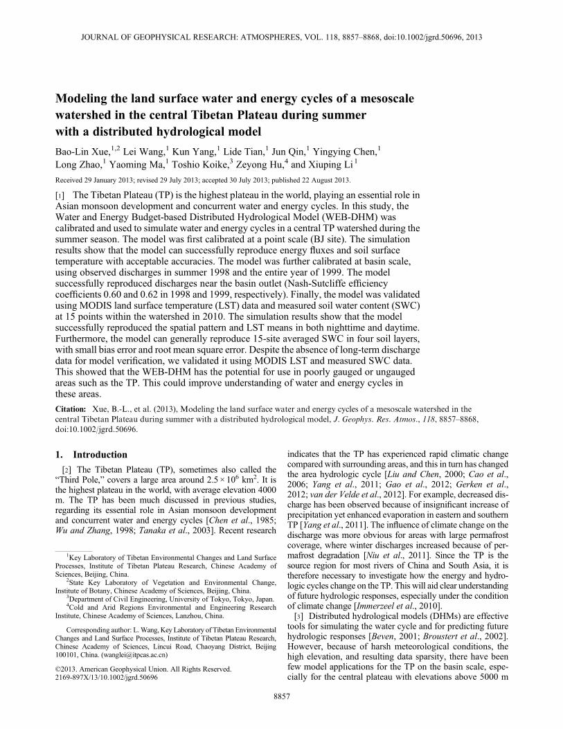
inputs). Bias error (BIAS) and root mean square error(RMSE) were used to evaluate model performance. Resultsshowed that the model generally captured the flux diurnalvariation with small BIAS and RMSE. Overall, the modelshowed good performance in reproducing net radiation(Rn), with slight underestimation (BIAS =�8.84 W m�2).BIAS for ground heat flux (G0) was 0.97 W m�2 andmodeled values closely followed the observed diurnalchange, indicating that the model can generally reproduceobserved values well (Figure 5b). The ground heat flux isan important part of the energy balance in this area [Tanakaet al., 2001; Su et al., 2006]. For instance, the maximum G0

occupies around 30% of the total maximum Rn at our site(Figure 5). Therefore, accurate simulation of G0 is necessaryfor energy flux simulation. The model simulated upwardshortwave radiation well over the period, but there wererelatively large BIAS and RMSE values for upwardlongwave radiation (Figures 5c and 5d).[22] Three output variables, i.e., sensible heat flux (H),

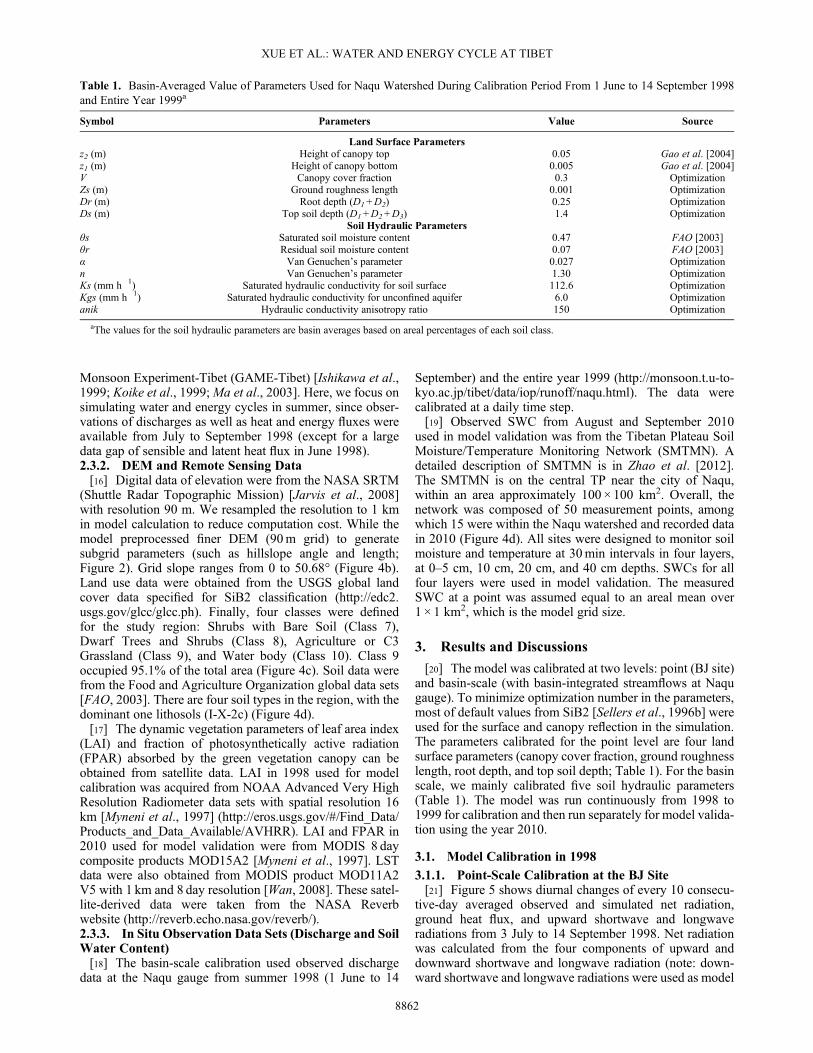
latent heat flux (LE), and ground temperature (Tg) from

WEB-DHM, were used for further calibration. Prior researchhas shown an energy imbalance in the area, despite its homo-geneous vegetation and enough fetch relative to other regions[Kim et al., 2000; Tanaka et al., 2001; Su et al., 2006]. Theaverage closure ratio ((H+ LE)/(Rn�G0)) at the BJ sitewas only 0.65 during the calibration period, similar to thatat Amdo site (within our research region; Figure 1).Research at Amdo site by Su et al. [2006] suggested thatone possible reason for the energy imbalance was underesti-mation of LE. Therefore, we corrected observed H and LEusing the observed Bowen ratio (H/LE) for model calibration[Twine et al., 2000]. Figure 6 shows diurnal changes of every10 consecutive-day average of observed and simulated H,LE, and Tg during the calibration period. The model success-fully reproduced the diurnal variations for all three variables,with small BIAS and RMSE (Figure 6). However, despite thesmall BIAS of Tg, the model overestimated daytime highvalues. The overestimation was more obvious in Septemberwhen soil freezing began (Figure 6c). Similar results werefound by Gao et al. [2004].

0

50

100

150

-200

-100

0

100

200

300

-200

0

200

400

600

800

Rn

(W m

-2)

G0

(W m

-2)

Zsw

up (

W m

-2)

Zlw

up (

W m

-2)

BIAS=-8.84 W m-2 RMSE= 11.55 W m-2

BIAS=0.97 W m-2 RMSE= 18.07 W m-2

BIAS=-6.26 W m-2 RMSE= 7.70 W m-2

BIAS=15.98 W m-2 RMSE= 18.50 W m-2

(a)

(b)

(d)

(c)

300

400

500

0 12 12 12 12 12 12 120 0 0 0 0 0 0 12

Time (Days from 3 July to14 September 1998)

Sim Obs

0

Figure 5. Diurnal changes of every 10 (rightmost day is for 11–14 September 1998) consecutive-dayaverage of observed (Obs) and simulated (Sim): (a) net radiation (Rn, W m�2); (b) ground heat flux(G0, W m�2); (c) upward shortwave radiation (Zswup, W m�2); and (d) upward long wave radiation(Zlwup, W m�2) for 3 July 1998 to 14 September 1998 (74 days) at the BJ site on central TibetanPlateau. Each point stands for the 10 or 4 day average at the time of the 10 or 4 days. BIAS (W m�2) andRMSE (W m�2) are also shown.

XUE ET AL.: WATER AND ENERGY CYCLE AT TIBET

8863

-100

0

100

200

300

400

500

-50

50

150

250

270

295

320

H (

W m

-2)

LE (

W m

-2)

Tg

(K)

BIAS= -10.84 W m-2 RMSE= 28.16 W m-2

BIAS=1.77 K RMSE=2.72 K

BIAS= -2.77 W m-2 RMSE= 15.04 W m-2(a)

(b)

(c)

Sim Obs

0 12 0 12 0 12 0 12 0 12 0 12 0 12 0 12 0

Time (Days from 3 July to14 September 1998)

Figure 6. Similar as Figure 5, but for sensible heat flux (H, W m�2) and latent heat flux (LE, W m�2).Observed H and LE are corrected by the Bowen ratio (H/LE) for model calibration (see the text).

Dis

char

ge (

m3 s

-1)

Date

Prec (m

m day

-1)

BIAS = - 2.77 m3 s-1

RMSE = 19.46 m3 s-1

Nash = 0.60

0

5

10

15

20

25

30

350

50

100

1999

.1.1

1999

.1.1

6

1999

.1.3

1

1999

.2.1

5

1999

.3.2

1999

.3.1

7

1999

.4.1

1999

.4.1

6

1999

.5.1

1999

.5.1

6

1999

.5.3

1

1999

.6.1

5

1999

.6.3

0

1999

.7.1

5

1999

.7.3

0

1999

.8.1

4

1999

.8.2

9

1999

.9.1

3

1999

.9.2

8

1999

.10.

13

1999

.10.

28

1999

.11.

12

1999

.11.

27

1999

.12.

12

1999

.12.

27

BIAS = - 2.41 m3 s-1

RMSE = 9.37 m3 s-1

Nash = 0.62

(a)

(b)

0

5

10

15

20

25

30

350

50

100

150

200

250

1998

.6.1

1998

.6.8

1998

.6.1

5

1998

.6.2

2

1998

.6.2

9

1998

.7.6

1998

.7.1

3

1998

.7.2

0

1998

.7.2

7

1998

.8.3

1998

.8.1

0

1998

.8.1

7

1998

.8.2

4

1998

.8.3

1

1998

.9.7

1998

.9.1

4Prep Observed Simulated

Figure 7. Daily observed (Obs) and simulated (Sim) discharge (m3 s�1) at Naqu gauge during (a) 1 June1998 to 14 September 1998, and (b) entire year 1999. Nash is Nash-Sutcliffe model efficiency coefficient.Daily precipitation (Prec, mm day�1) for same period is also shown (right bar).

XUE ET AL.: WATER AND ENERGY CYCLE AT TIBET

8864

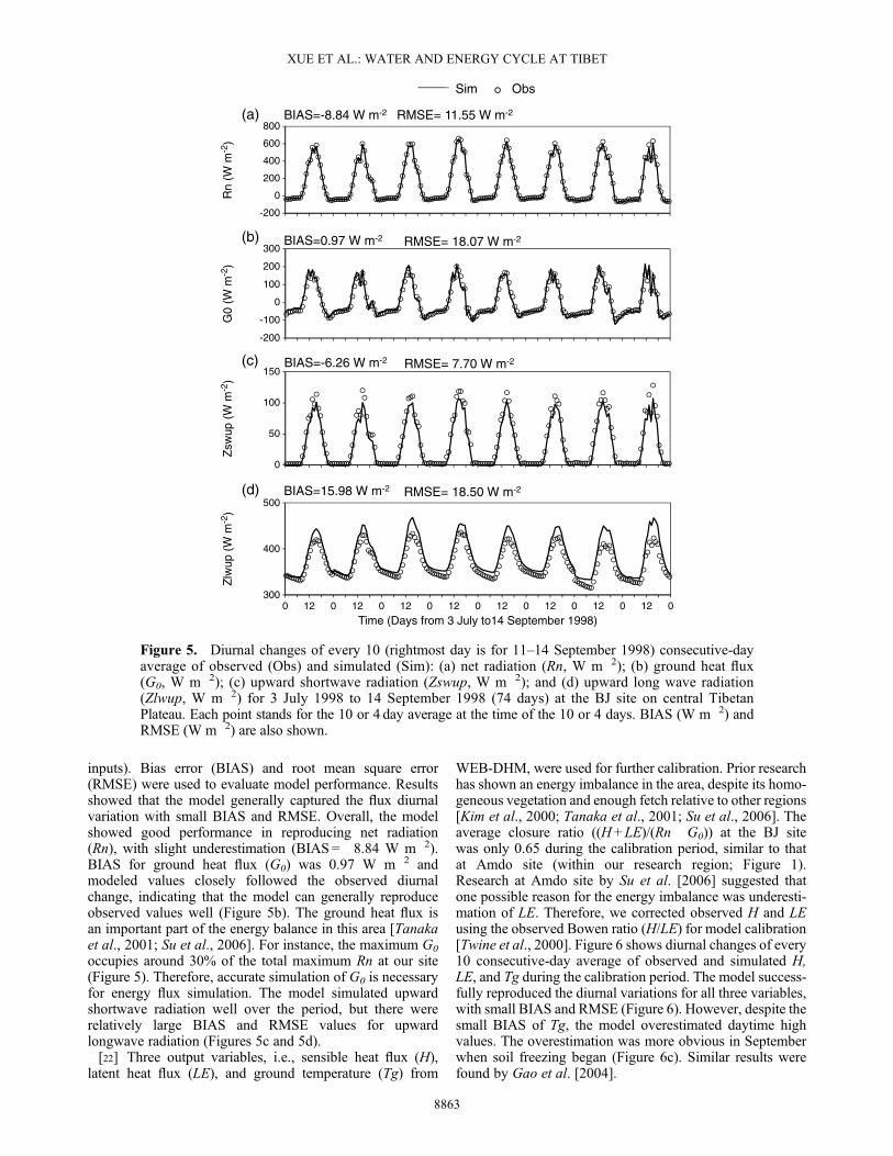
3.1.2. Basin-Scale Calibration Using Discharge Data[23] Model calibration was extended using daily discharge

from the Naqu gauge. The purpose of this calibration was tooptimize the soil hydraulic parameters at basin scale (SeeTable 1). The soil hydraulic parameters were assigned to foursoil classes (Figure 4d) in accordance with the soil spatial pat-tern. Figure 7 shows a comparison of simulated and observeddischarge with corresponding precipitation, from 1 June to 14September 1998 and over all of 1999. The BIAS, RMSE, andNash-Sutcliffe (Nash) model efficiency coefficient [Nash andSutcliffe, 1970] were used to evaluate model performance.[24] Themodel reproduced discharge well during the calibra-

tion period of summer 1998, with BIAS �2.77 m3 s�1 andRMSE 19.46 m3 s�1 (Figure 7). Corresponding values for1999 were �2.41 m3 s�1 and 9.37 m3 s�1. The model slightlyunderestimated the relatively low flows in the summer of bothyears. This may be caused by the underestimated SWC owingto soil vertical heterogeneity [Yang et al., 2005] (see detailsbelow). Overall, Nash reached 0.60 and 0.62 in 1998 summerand 1999, respectively. This verified favorable model perfor-mance in discharge simulation during the calibration period.

3.2. Model Validation for 2010

[25] WEB-DHM was further validated using the data from2010. During calibration and validation (for both point and

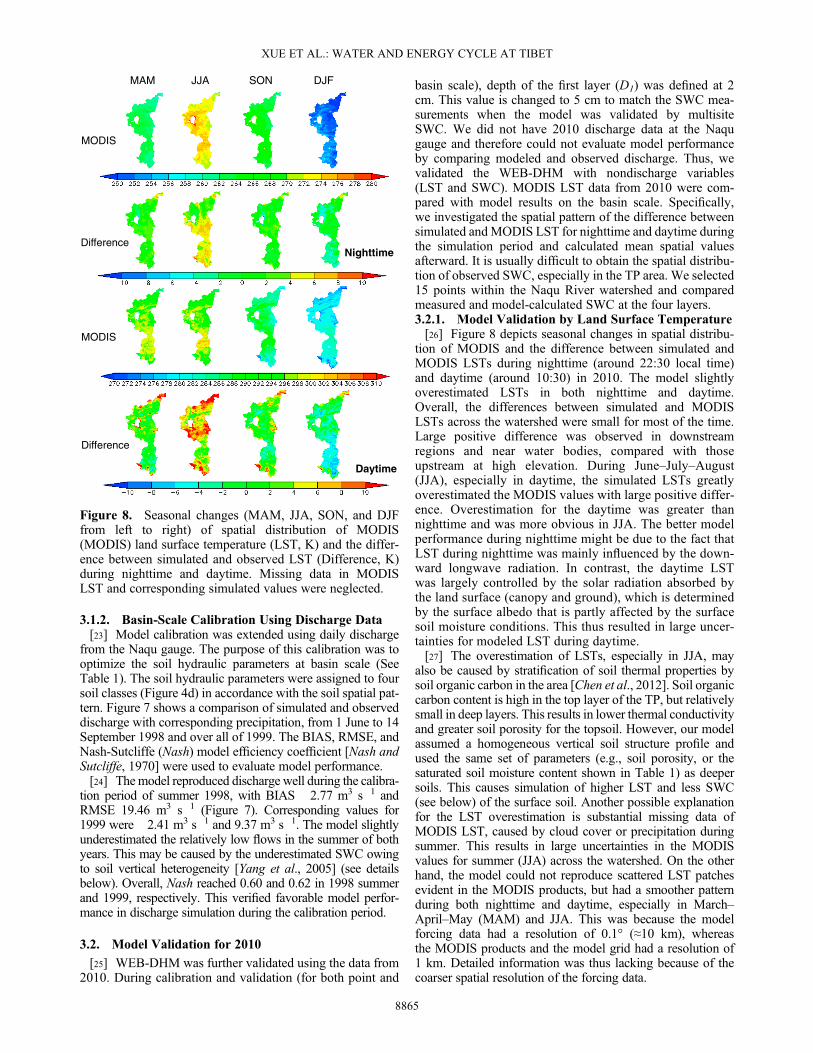
basin scale), depth of the first layer (D1) was defined at 2cm. This value is changed to 5 cm to match the SWC mea-surements when the model was validated by multisiteSWC. We did not have 2010 discharge data at the Naqugauge and therefore could not evaluate model performanceby comparing modeled and observed discharge. Thus, wevalidated the WEB-DHM with nondischarge variables(LST and SWC). MODIS LST data from 2010 were com-pared with model results on the basin scale. Specifically,we investigated the spatial pattern of the difference betweensimulated andMODIS LST for nighttime and daytime duringthe simulation period and calculated mean spatial valuesafterward. It is usually difficult to obtain the spatial distribu-tion of observed SWC, especially in the TP area. We selected15 points within the Naqu River watershed and comparedmeasured and model-calculated SWC at the four layers.3.2.1. Model Validation by Land Surface Temperature[26] Figure 8 depicts seasonal changes in spatial distribu-

tion of MODIS and the difference between simulated andMODIS LSTs during nighttime (around 22:30 local time)and daytime (around 10:30) in 2010. The model slightlyoverestimated LSTs in both nighttime and daytime.Overall, the differences between simulated and MODISLSTs across the watershed were small for most of the time.Large positive difference was observed in downstreamregions and near water bodies, compared with thoseupstream at high elevation. During June–July–August(JJA), especially in daytime, the simulated LSTs greatlyoverestimated the MODIS values with large positive differ-ence. Overestimation for the daytime was greater thannighttime and was more obvious in JJA. The better modelperformance during nighttime might be due to the fact thatLST during nighttime was mainly influenced by the down-ward longwave radiation. In contrast, the daytime LSTwas largely controlled by the solar radiation absorbed bythe land surface (canopy and ground), which is determinedby the surface albedo that is partly affected by the surfacesoil moisture conditions. This thus resulted in large uncer-tainties for modeled LST during daytime.[27] The overestimation of LSTs, especially in JJA, may

also be caused by stratification of soil thermal properties bysoil organic carbon in the area [Chen et al., 2012]. Soil organiccarbon content is high in the top layer of the TP, but relativelysmall in deep layers. This results in lower thermal conductivityand greater soil porosity for the topsoil. However, our modelassumed a homogeneous vertical soil structure profile andused the same set of parameters (e.g., soil porosity, or thesaturated soil moisture content shown in Table 1) as deepersoils. This causes simulation of higher LST and less SWC(see below) of the surface soil. Another possible explanationfor the LST overestimation is substantial missing data ofMODIS LST, caused by cloud cover or precipitation duringsummer. This results in large uncertainties in the MODISvalues for summer (JJA) across the watershed. On the otherhand, the model could not reproduce scattered LST patchesevident in the MODIS products, but had a smoother patternduring both nighttime and daytime, especially in March–April–May (MAM) and JJA. This was because the modelforcing data had a resolution of 0.1° (≈10 km), whereasthe MODIS products and the model grid had a resolution of1 km. Detailed information was thus lacking because of thecoarser spatial resolution of the forcing data.

MAM JJA SON DJF

MODIS

MODIS

DifferenceNighttime

Difference

Daytime

Figure 8. Seasonal changes (MAM, JJA, SON, and DJFfrom left to right) of spatial distribution of MODIS(MODIS) land surface temperature (LST, K) and the differ-ence between simulated and observed LST (Difference, K)during nighttime and daytime. Missing data in MODISLST and corresponding simulated values were neglected.

XUE ET AL.: WATER AND ENERGY CYCLE AT TIBET

8865

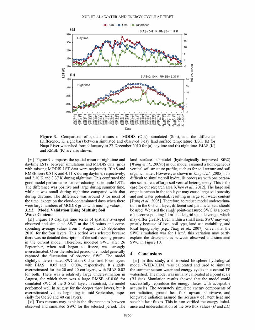
[28] Figure 9 compares the spatial mean of nighttime anddaytime LSTs, between simulations and MODIS data (gridswith missing MODIS LST data were neglected). BIAS andRMSE were 0.81 K and 4.11 K during daytime, respectively,and 2.10 K and 3.37 K during nighttime. This confirmed thegood model performance for reproducing basin-scale LSTs.The difference was positive and large during summer time,while it was small during nighttime compared with thatduring daytime. The difference was around 0 for most ofthe time, except on the cloud-contaminated days when therewere large numbers of MODIS grids with missing values.3.2.2. Model Validation Using Multisite SoilWater Content[29] Figure 10 displays time series of spatially averaged

observed and simulated SWC at the 15 points and corre-sponding average values from 1 August to 26 September2010, for the four layers. This period was selected becausethere was no detailed description of the soil freezing processin the current model. Therefore, modeled SWC after 26September, when soil began to freeze, was stronglyoverestimated. Over the selected period, the model generallycaptured the fluctuation of observed SWC. The modelslightly underestimated SWC at the 0–5 cm and 10 cm layerswith BIAS �0.05 and �0.004, respectively. It slightlyoverestimated for the 20 and 40 cm layers, with BIAS 0.02for both. There was a relatively large underestimation inAugust, for which there was a large RMSE of 0.06 forsimulated SWC of the 0–5 cm layer. In contrast, the modelperformed well in August for the deeper three layers, but itoverestimated values beginning in mid-September, espe-cially for the 20 and 40 cm layers.[30] Two reasons may explain the discrepancies between

observed and simulated SWC for the selected period. The

land surface submodel (hydrologically improved SiB2)[Wang et al., 2009b] in our model assumed a homogeneousvertical soil structure profile, such as for soil texture and soilorganic matter. However, as shown in Yang et al. [2005], it isdifficult to simulate soil hydraulic processes with one param-eter set in areas of large soil vertical heterogeneity. This is thecase for our research area [Chen et al., 2012]. The large soilorganic carbon in the top layer may cause large soil porosityand soil water potential, resulting in large soil water content[Yang et al., 2005]. Therefore, to reduce model underestima-tion in the 0–5 cm layer, different soil parameter sets shouldbe used. We used the single point-measured SWC as a proxyof the corresponding 1 km2 model grid spatial average, whichmay differ greatly. Even within a small area, SWC may varygreatly because of local soil type, land use variability, andlocal topography [e.g., Tang et al., 2007]. Given that theSWC simulation was for 1 km2, this variation may partlyexplain the discrepancies between observed and simulatedSWC in Figure 10.

4. Conclusions

[31] In this study, a distributed biosphere hydrologicalmodel (WEB-DHM) was calibrated and used to simulatethe summer season water and energy cycles in a central TPwatershed. The model was initially calibrated at a point scale(BJ site). Simulation results showed that the model couldsuccessfully reproduce the energy fluxes with acceptableaccuracies. The accurately simulated energy components ofnet radiation, ground heat flux, upward shortwave, andlongwave radiation assured the accuracy of latent heat andsensible heat fluxes. This in turn verified the energy imbal-ance and underestimation of the two flux values (H and LE)

-5

0

5

10

15

20

270

280

290

300

310

Sim Obs Difference

LST

(K

)

BIAS= 0.81 K RMSE= 4.11 K

BIAS=2.10 K RMSE= 3.37 K

Daytime

Nighttime

(a)

(b)

Date

Difference (K

)

-5

0

5

10

15

20

245

255

265

275

285

2010

.1.9

2010

.1.1

720

10.1

.25

2010

.2.2

2010

.2.1

020

10.2

.18

2010

.2.2

620

10.3

.620

10.3

.14

2010

.3.2

220

10.3

.30

2010

.4.7

2010

.4.1

520

10.4

.23

2010

.5.1

2010

.5.9

2010

.5.1

720

10.5

.25

2010

.6.2

2010

.6.1

020

10.6

.18

2010

.6.2

620

10.7

.420

10.7

.12

2010

.7.2

020

10.7

.28

2010

.8.5

2010

.8.1

320

10.8

.21

2010

.8.2

920

10.9

.620

10.9

.14

2010

.9.2

220

10.9

.30

2010

.10.

820

10.1

0.16

2010

.10.

2420

10.1

1.1

2010

.11.

920

10.1

1.17

2010

.11.

2520

10.1

2.3

2010

.12.

1120

10.1

2.19

2010

.12.

27

Figure 9. Comparison of spatial means of MODIS (Obs), simulated (Sim), and the difference(Difference, K; right bar) between simulated and observed 8 day land surface temperature (LST, K) forNaqu River watershed from 9 January to 27 December 2010 for (a) daytime and (b) nighttime. BIAS (K)and RMSE (K) are also shown.

XUE ET AL.: WATER AND ENERGY CYCLE AT TIBET

8866

by the eddy covariance method at the BJ site. The model alsoreproduced soil surface temperature well, despite slightoverestimation (BIAS = 1.77 K and RMSE= 2.72K). Theseresults confirmed model validity at the point scale.[32] Maintaining the WEB-DHM land surface parameters

as above, model soil hydraulic parameters were calibratedat the basin scale using discharge data from the Naqu gaugein summer 1998 and the entire year of 1999. In general, theresults demonstrated good model performance in simulationof discharge across the entire watershed (Nash = 0.60 and0.62 in 1998 and 1999, respectively).[33] Finally, the model was validated using MODIS

LST data and measured SWC at 15 points within the wa-tershed in 2010. The simulation results showed that themodel could successfully reproduce the spatial pattern andmeans of LST during nighttime and daytime. Furthermore,the model generally reproduced SWC in the four layers atthe 15 measurement sites, with small BIAS and RMSE.The model slightly overestimated LST and underestimatedSWC of the surface layer, which may be caused by verticalsoil heterogeneity caused by soil organic carbon content. Infuture simulation of soil thermal and water processes, werecommend different soil parameter data sets for variouslayers on the TP.

[34] Given the absence of long-term discharge data formodel validation, we validated it using MODIS LST andmeasured SWC data. This showed that the WEB-DHM hasthe potential for use in poorly gauged or ungauged areas suchas the TP, which would improve understanding of the hydro-logic cycle there. Model applications for the central TP havebeen rare, and therefore more studies should be undertaken toverify and test our model. Furthermore, since the model wasmainly tested in summer season in this study because of theabsence of a detailed description of the soil freezing process,it should be further improved for the simulation of longertime periods covering soil freezing and thawing. We usedmeasured SWC to validate corresponding modeled valuesin a central TP watershed. As far as we know, this representsthe first hydrological validation with multisite SWC data forthe plateau, mainly because of the difficulties of makingmeasurements in this area. In the validation, we used mea-sured single-point values as a proxy for a model grid average(1 km2), which may have caused a bias relative to the modeledvalues. In the future, further efforts should be made to upscalethe point SWC measurements to the whole watershed. Thiscould produce a direct and more reasonable comparisonbetween observed and modeled spatial SWC patterns.

[35] Acknowledgments. This study was financially supported by the“Strategic Priority Research Program (B)” of the Chinese Academy ofSciences (grant XDB03030302), the National Natural Science Foundationof China (grant 41190083), and Hundred Talents Program of the ChineseAcademy of Sciences (Lei Wang), as well as the National Key Basic ResearchProgram of China (grant 2013CBA01805), and the Key Technologies R&DProgram of China (grant 2013BAB05B03).

ReferencesBetts, A. K., J. H. Ball, A. C. M. Beljaars, M. J. Miller, and P. A. Viterbo(1996), The land surface-atmosphere interaction: A review based on obser-vational and global modeling perspectives, J. Geophys. Res., 101(D3),7,209–7,225, doi:10.1029/95JD02135.

Beven, K. (2001), How far can we go in distributed hydrological modelling?,Hydrol. Earth Syst. Sci., 5(1), 1–12, doi:10.5194/hess-5-1-2001.

Bronstert, A., D. Niehoff, and G. Bürger (2002), Effects of climate and land-use change on storm runoff generation: present knowledge and modellingcapabilities, Hydrol. Processes, 16(2), 509–529, doi:10.1002/hyp.326.

Cabral, M. C., L. Garrote, R. L. Bras, and D. Entekhabi (1992), A kinematicmodel of infiltration and runoff generation in layered and sloped soils, Adv.Water Resour., 15(5), 311–324.

Cao, J., D. Qin, E. Kang, and Y. Li (2006), River discharge changes in theQinghai-Tibet Plateau, Chin. Sci. Bull., 51(5), 594–600, doi:10.1007/s11434-006-0594-6.

Chen, F., and J. Dudhia (2001), Coupling an Advanced Land Surface–Hydrology Model with the Penn State–NCAR MM5 Modeling System.Part I: Model Implementation and Sensitivity, Mon. Weather Rev.,129(4), 569–585.

Chen, L., E. R. Reiter, and Z. Feng (1985), The Atmospheric Heat Source overthe Tibetan Plateau: May–August 1979, Mon. Weather Rev., 113(10),1771–1790, doi:10.1175/1520-0493(1985)113<1771:TAHSOT>2.0.CO;2.

Chen, Y., K. Yang,W. Tang, J. Qin, and L. Zhao (2012), Parameterizing soilorganic carbon’s impacts on soil porosity and thermal parameters forEastern Tibet grasslands, Sci. China Ser. D, 55(6), 1,001–1,011.

Chen, Y., K. Yang, J. He, J. Qin, J. Shi, J. Du, and Q. He (2011), Improvingland surface temperature modeling for dry land of China, J. Geophys. Res.,116, D20104, doi:10.1029/2011JD015921.

Entekhabi, D., I. Rodriguez-Iturbe, and F. Castelli (1996),Mutual interactionof soil moisture state and atmospheric processes, J. Hydrol., 184(1–2),3–17, doi:10.1016/0022-1694(95)02965-6.

Food and Agriculture Organization (FAO) (2003), Digital soil map of theworld and derived soil properties, land and water digital media series[CD-ROM], rev. 1, Rome.

Fujita, K., T. Ohta, and Y. Ageta (2007), Characteristics and climatic sensi-tivities of runoff from a cold-type glacier on the Tibetan Plateau, Hydrol.Processes, 21(21), 2,882–2,891, doi:10.1002/hyp.6505.

Gao, H., X. He, B. Ye, and J. Pu (2012), Modeling the runoff and glaciermass balance in a small watershed on the Central Tibetan Plateau,

0

5

100

0.1

0.2

0.3

0.4

0.5

2010

.8.1

2010

.8.6

2010

.8.1

1

2010

.8.1

6

2010

.8.2

1

2010

.8.2

6

2010

.8.3

1

2010

.9.5

2010

.9.1

0

2010

.9.1

5

2010

.9.2

0

2010

.9.2

5

BIAS= -0.05RMSE= 0.06

Date

SW

C (

m3 m

-3)

Prec (m

m day

-1)

Obs Sim

BIAS= -0.004RMSE= 0.05

BIAS= 0.02

RMSE=0.05

BIAS= 0.02

RMSE=0.02

5 cm

40 cm

20 cm

10 cm

0

5

100

0.1

0.2

0.3

0.4

0.5

0

5

100

0.1

0.2

0.3

0.4

0.5

0

5

100

0.1

0.2

0.3

0.4

0.5

Figure 10. Comparison of observed (Obs) and simulated(Sim) 15-site average volume soil water content (SWC, m3

m�3) in the four layers of 0–5, 10, 20, and 40 cm depths from1 August to 26 September 2010. Corresponding precipitation(mm day�1, right bar) is shown for the same period. Thenumbers (5, 10, 20, and 40 cm) show the different depthsof the soil water content measurements.

XUE ET AL.: WATER AND ENERGY CYCLE AT TIBET

8867

China, from 1955 to 2008, Hydrol. Processes, 26(11), 1,593–1,603,doi:10.1002/hyp.8256.

Gao, Z., N. Chae, J. Kim, J. Hong, T. Choi, and H. Lee (2004), Modeling ofsurface energy partitioning, surface temperature, and soil wetness in theTibetan prairie using the Simple Biosphere Model 2 (SiB2), J. Geophys.Res., 109, D06102, doi:10.1029/2003JD004089.

Gerken, T., W. Babel, A. Hoffmann, T. Biermann, M. Herzog, A. D. Friend,M. Li, Y. Ma, T. Foken, and H.-F. Graf (2012), Turbulent flux modellingwith a simple 2-layer soil model and extrapolated surface temperatureapplied at Nam Co Lake basin on the Tibetan Plateau, Hydrol. EarthSyst. Sci., 16, 1095–1110.

He, J. (2010), Development of surface meteorological dataset of China withhigh temporal and spatial resolution, M.S. thesis, Inst. of Tibetan PlateauRes., Chin. Acad. of Sci., Beijing, China.

Immerzeel, W. W., L. P. H. van Beek, and M. F. P. Bierkens (2010), ClimateChange Will Affect the Asian Water Towers, Science, 328(5984),1382–1385, doi:10.1126/science.1183188.

Ishikawa, H., et al. (1999), Summary of planetary boundary layer observa-tion in GAME-Tibet, in Proc. of the First Int. Workshop on GAME-Tibet, edited by A. Numaguti, L. Liu, L., and Tian, pp. 69–72, ChineseAcademy of Sciences and Japan National Committee for GAME, Xi’an,China, 11 –13 January 1999.

Jarvis A., H. I. Reuter, A. Nelson, and E. Guevara (2008), Hole-filled seam-less SRTM data V4, International Centre for Tropical Agriculture (CIAT),available from http://srtm.csi.cgiar.org.

Kim, J., J. Hong, Z. Gao, and T. Choi (2000), Can we close the energybudget in the Tibetan Plateau?, paper presented at the Second Session ofInternationational Workshop on TIPEX-GAME/Tibet, Joint Coord.Comm., TIPEX-GAME/Tibet, Kunming, China.

Koike, T., T. Yasunari, J. Wang, and T. Yao (1999), GAME-Tibet IOPsummary report, in edited by A. Numaguti, L. Liu, and L. Tian, Proc. ofthe First Int. Workshop on GAME-Tibet, pp. 1–2, Chinese Academy ofSciences and Japan National Committee for GAME, Xi’an, China, 11 –13 January 1999.

Kumagai, T., N. Yoshifuji, N. Tanaka, M. Suzuki, and T. Kume (2009),Comparison of soil moisture dynamics between a tropical rain forest anda tropical seasonal forest in Southeast Asia: Impact of seasonal and year-to-year variations in rainfall, Water Resour. Res., 45, W04413,doi:10.1029/2008WR007307.

Leese, J., T. Jackson, A. Pitman, and P. Dirmeyer (2001), Meeting summary:GEWEX/BAHC International Workshop on Soil Moisture Monitoring,Analysis, and Prediction for Hydrometeorological and HydroclimatologicalApplications, Bull. Am. Meteorol. Soc., 82(7), 1423–1430, doi:10.1175/1520-0477(2001)082<1423:MSGBIW>2.3.CO;2.

Liu, X., and B. Chen (2000), Climatic warming in the Tibetan Plateau duringrecent decades, Int. J. Climatol., 20(14), 1,729–1,742, doi:10.1002/1097-0088(20001130)20:14<1729::AID-JOC556>3.0.CO;2-Y.

Lu, H., T. Koike, K. Yang, Z. Hu, X. Xu, M. Rasmy, D. Kuria, andK. Tamagawa (2012), Improving land surface soil moisture and energyflux simulations over the Tibetan plateau by the assimilation of the micro-wave remote sensing data and the GCMoutput into a land surface model, Int. J.Appl. Earth Obs. Geoinf., 17(0), 43–54, doi:10.1109/IGARSS.2011.6049415.

Ma, Y., Z. Su, T. Koike, T. Yao, H. Ishikawa, K. I. Ueno, and M. Menenti(2003), On measuring and remote sensing surface energy partitioning overthe Tibetan Plateau––from GAME/Tibet to CAMP/Tibet, Phys. Chem.Earth, Parts A/B/C, 28(1–3), 63–74, doi:10.1016/S1474-7065(03)00008-1.

Merz, R., and G. Blöschl (2009), A regional analysis of event runoff coeffi-cients with respect to climate and catchment characteristics in Austria,Water Resour. Res., 45, W01405, doi:10.1029/2008WR007163.

Myneni, R. B., R. R. Nemani, and S. W. Running (1997), Algorithm for theestimation of global land cover, LAI and FPAR based on radiative transfermodels, IEEE T. Geosci. Remote, 35, 1380–1393.

Nash, J. E., and J. V. Sutcliffe (1970), River flow forecasting throughconceptual models part I—A discussion of principles, J. Hydrol., 10,282–290, doi:10.1016/0022-1694(70)90255-6.

Niu, L., B. Ye, J. Li, and Y. Sheng (2011), Effect of permafrost degradationon hydrological processes in typical basins with various permafrost cover-age in Western China, Sci. China Ser. D, 54(4), 615–624, doi:10.1007/s11430-010-4073-1.

Robinson, J. S., and M. Sivapalan (1996), Instantaneous response functionsof overland flow and subsurface stormflow for catchment models, Hydrol.Processes, 10(6), 845–862.

Sellers, P. J., D. A. Randall, G. J. Collatz, J. A. Berry, C. B. Field,D. A. Dazlich, C. Zhang, G. D. Collelo, and L. Bounoua (1996a), ARevised Land Surface Parameterization (SiB2) for Atmospheric GCMS.Part I: Model Formulation, J. Clim., 9(4), 676–705, doi:10.1175/1520-0442(1996)009<0676:ARLSPF>2.0.CO;2.

Sellers, P. J., S. O. Los, C. J. Tucker, C. O. Justice, D. A. Dazlich, G. J. Collatz,and D. A. Randall (1996b), A revised land surface parameterization (SiB2)for atmospheric GCMs, part II: the generation of global fields of terrestrialbiosphysical parameters from satellite data, J. Clim., 9, 706–737.

Singh, P., M. Arora, and N. K. Goel (2006), Effect of climate change onrunoff of a glacierized Himalayan basin, Hydrol. Processes, 20(9),1979–1992, doi:10.1002/hyp.5991.

Su, Z., T. Zhang, Y. Ma, L. Jia, and J. Wen (2006), Energy and water cycleover the Tibetan Plateau: surface energy balance and turbulent heat fluxes,Adv. Earth Sci., 21(21), 1224–1236, doi:10.1002/1001-8166(2006)21:12<1224:EAWCOT>2.0.TX;2-C.

Tanaka, K., H. Ishikawa, T. Hayashi, I. Tamagawa, and Y. Ma (2001), Surfaceenergy budget at Amdo in the TibetanPlateau using GAME/Tibet IOP98data, J. Meteorol. Soc. Jpn., 79, 505–517, doi:10.2151/jmsj.79.505.

Tanaka, K., I. Tamagawa, H. Ishikawa, Y. Ma, and Z. Hu (2003), Surfaceenergy budget and closure of the eastern Tibetan Plateau during theGAME-Tibet IOP 1998, J. Hydrol., 283(1–4), 169–183, doi:10.1016/S0022-1694(03)00243-9.

Tang, Q., T. Oki, S. Kanae, and H. Hu (2007), The Influence of PrecipitationVariability and Partial Irrigation within Grid Cells on a HydrologicalSimulation, J. Hydrometeorol., 8(3), 499–512, doi:10.1175/JHM589.1.

Twine, T. E., W. P. Kustas, J. M. Norman, D. R. Cook, P. R. Houser,T. P. Meyers, J. H. Prueger, P. J. Starks, and M. L. Wesely (2000),Correcting eddy-covariance flux underestimates over a grassland, Agric.For. Meteorol., 103(3), 279–300, doi:10.1016/S0168-1923(00)00123-4.

van der Velde, R., Z. Su, M. Ek, M. Rodell, and Y. Ma (2012), Influence ofthermodynamic soil and vegetation parameterizations on the simulation ofsoil temperature states and surface fluxes by the Noah LSM over a Tibetanplateau site, Hydrol. Earth Syst. Sci., 13, 759–777.

van Genuchten, M. T. (1980), A Closed-form Equation for Predicting theHydraulic Conductivity of Unsaturated Soils1, Soil Sci. Soc. Am. J.,44(5), 892–898.

Verdin, K. L., and J. P. Verdin (1999), A topological system for delineationand codification of the Earth’s river basins, J. Hydrol., 218(1–2), 1–12.

Wan, Z. (2008), New refinements and validation of the MODIS Land-SurfaceTemperature/Emissivity products, Remote Sens. Environ., 112(1), 59–74,doi:10.1016/j.rse.2006.06.026.

Wang, F., L. Wang, T. Koike, H. Zhou, K. Yang, A. Wang, and W. Li(2011), Evaluation and application of a fine-resolution global data set ina semiarid mesoscale river basin with a distributed biosphere hydrologicalmodel, J. Geophys. Res., 116, D21108, doi:10.1029/2011JD015990.

Wang, L., T. Koike, K. Yang, and P. J.-F. Yeh (2009a), Assessment of adistributed biosphere hydrological model against streamflow and MODISland surface temperature in the upper Tone River Basin, J. Hydrol.,377(1–2), 21–34, doi:10.1016/j.jhydrol.2009.08.005.

Wang, L., T. Koike, D. Yang, and K. Yang (2009b), Improving the hydrol-ogy of the Simple Biosphere Model 2 and its evaluation within the frame-work of a distributed hydrological model, Hydrol. Sci. J., 54(6), 989–1006,doi:10.1623/hysj.54.6.989.

Wang, L., T. Koike, K. Yang, T. J. Jackson, R. Bindlish, and D. Yang(2009c), Development of a distributed biosphere hydrological model andits evaluation with the Southern Great Plains Experiments (SGP97 andSGP99), J. Geophys. Res., 114, D08107, doi:10.1029/2008JD010800.

Wu, G., and Y. Zhang (1998), Tibetan Plateau Forcing and the Timing of theMonsoonOnset over SouthAsia and the SouthChina Sea,Mon.Weather Rev.,126(4), 913–927, doi:10.1175/1520-0493(1998)126<0913:TPFATT>2.0.CO;2.

Yang, D., S. Herath, and K. Musiake (2000), Comparison of differentdistributed hydrological models for characterization of catchment spatialvariability, Hydrol. Processes, 14(3), 403–416, doi:10.1002/(SICI)1099-1085(20000228)14:3<403::AID-HYP945>3.0.CO;2–3.

Yang, D., S. Herath, and K. Musiake (2002), A hillslope-based hydrologicalmodel using catchment area and width functions, Hydrol. Sci. J., 47(1),49–65, doi:10.1080/02626660209492907.

Yang, K., Koike, T., Ye, B., and Bastidas, L. (2005), Inverse analysis of therole of soil vertical heterogeneity in controlling surface soil state and energypartition, J. Geophys. Res., 110, D08101, doi:10.1029/2004JD005500.

Yang, K., J. He, W. Tang, J. Qin, and C. C. K. Cheng (2010), On downwardshortwave and longwave radiations over high altitude regions:Observation and modeling in the Tibetan Plateau, Agric. For. Meteorol.,150(1), 38–46, doi:10.1016/j.agrformet.2009.08.004.

Yang, K., B. Ye, D. Zhou, B. Wu, T. Foken, J. Qin, and Z. Zhou (2011),Response of hydrological cycle to recent climate changes in the TibetanPlateau, Clim. Change, 109(3), 517–534, doi:10.1007/s10584-011-0099-4.

Zhao, L., K. Yang, J. Qin, and Y.-Y. Chen (2012), Optimal Exploitation ofAMSR-E Signals for Improving Soil Moisture Estimation Through LandData Assimilation, IEEE T. Geosci. Remote, 51, 399–410, doi:10.1109/TGRS.2012.219.

XUE ET AL.: WATER AND ENERGY CYCLE AT TIBET

8868