

![kkt_6_dan_7_pemupukan_2014 [Compatibility Mode]](https://static.fdokumen.com/doc/165x107/6322b43c28c445989105e2db/kkt6dan7pemupukan2014-compatibility-mode.jpg)


Bahasa
Halaman
Hukum


Mode choice modelling using elementsof MINDSPACE and structural equation
modelling
by
AUGUSTUS ABABIO-DONKOR
B.Sc, M.A, M.Sc
A thesis submitted in partial fulfilment of the requirements
of Edinburgh Napier University, for the award of
Doctor of Philosophy
TRANSPORT RESEARCH INSTITUTE
School of Engineering and the Built Environment
August 2020

Declaration
I hereby declare that the work contained in this thesis is my own work andthat it has not been previously accepted for the award of any degree ordiploma. To the best of my knowledge and belief, it contains no mater-ial previously published or written by another person except where duereference has been made in the text.
.....Augustus Ababio-Donkor
(40178349)
6th October 2020
Professor Wafaa Saleh(DoS)
7th October 2020
i
Abstract
The last two decades have witnessed a rising research interest in integrated choice and
latent variable(ICLV) modelling, in direct response to the inability of the traditional
choice models to adequately explain the over half a century growing trend of vehicular
traffic in cities around the world. With little variations, several researchers in transport
choice behaviour have suggested that the theory behind the traditional choice models
do not sufficiently account for the heterogeneity of human behaviour and observed
choice preferences. Literature is replete with evidence suggesting that attitudes and
perceptions significantly influence decision-making. The challenge for researchers is
understanding the attitude with the most significant impact to include in the hybrid
choice models.
Interestingly, recent literature on consumer behaviour suggests that MINDSPACE have
a significant impact on behaviour. MINDSPACE is the mnemonic for Messenger,
Incentive, Norms, Default, Salience, Priming, Affect, Commitment, and Ego, these
behavioural effects are believed to offer robust way of analysing and influencing beha-
viour. This study, therefore, exploits the potential benefits of these two new research
areas to develop MINDSPACE enriched ICLV model to explain the underlying transport
mode choice behaviour of the population of Edinburgh using five hundred responses
collected in a mail-back revealed preference survey. The proposed model integrates
variables from the MINDSPACE framework as latent variables in the ICLV model. The
study found strong evidence aside the socio-demographic and mode specific variables
that Norm, Salience, and Affect have a significant influence on transport mode choice,
ii

ABSTRACT
among others. Overall, the ICLV model demonstrates considerable improvement over a
reference logit model. The study could prompt policy development toward urban trans-
portation because the findings have broader policy implication for public transport and
travel behaviour change.
Keywords:
Travel mode choice; Behavioural economics; MINDSPACE; Structural equation mod-
elling; Integrated choice and latent variable models; Norms; Affects; Emotions; Ego;
Narcissism; Salience.
iii

Acknowledgements
I am in indebted to many individuals whose contribution made the completion of mystudy possible. My foremost gratitude goes to the Almighty God for his mercy, graceand favour during my study.
I unreservedly thank my Director of Studies, Professor Wafaa Saleh, for the incred-ible support for my PhD, for the patience, encouragement, motivation, the invaluableguidance and direction, which made this dream a reality. I am also thankful for theopportunity to work on the DIAMOND project. I am equally indebted to my supervisorDr Achille Fonzone, for the hours of discussions and guidance. I could not have askedfor a better team and mentors for this study.
My sincere thanks go to Professor Tom Rye and Transport Research Institute (TRI)for offering me a place in the institute and the funding support, I appreciate YvonneLawrie and the entire staff of TRI for their support. I also express my appreciation to myPhD colleges for their support.
My special love goes to my lovely wife and kids; Victoria, Phoebe, Michelle and Yiau fortheir understanding, sacrifice and emotional support. Honey bless you for all the hardwork and prayers.
Lastly, I wish to extend my profound gratitude to my family, Okra Ababio, John Okra,Theresa Obour and friends for their prayer, support and encouragements.
iv

Dedication
I dedicate this thesis to my uncle, Okrah Ababio, not only for raising and nurturing mebut also for unselfishly funding my education since childhood.
I also dedicate this thesis to my lovely wife, Victoria. Her love and months of hard workin providing for me and our children; Phoebe, Michelle and Yiau made the completion
of this work possible.
"... She is far more precious than jewels."Proverbs 31:10
Above all, to the Almighty God for the grace and strength through it all.
v
Tables of contents
Declaration i
Abstract ii
Acknowledgements iv
Dedication v
Tables of contents vi
List of Tables xi
List of Figures xiii
List of Abbreviations xv
I INTRODUCTION AND LITERATURE REVIEW 1
1 Introduction 2
1.1 Background . . . . . . . . . . . . . . . . . . . . . . . . . . . . . . . . . . . . 2
1.2 Research Aim and Methodology . . . . . . . . . . . . . . . . . . . . . . . . 4
1.2.1 Research Aim and objectives . . . . . . . . . . . . . . . . . . . . . 4
1.2.2 Research Methodology . . . . . . . . . . . . . . . . . . . . . . . . . 4
1.3 Research Publications . . . . . . . . . . . . . . . . . . . . . . . . . . . . . . 5
1.4 Structure of the thesis . . . . . . . . . . . . . . . . . . . . . . . . . . . . . . 6
vi

TABLES OF CONTENTS
2 Choice Theories 8
2.1 Introduction . . . . . . . . . . . . . . . . . . . . . . . . . . . . . . . . . . . 8
2.2 Rational Choice Theory . . . . . . . . . . . . . . . . . . . . . . . . . . . . . 9
2.3 Bounded Rationality . . . . . . . . . . . . . . . . . . . . . . . . . . . . . . . 10
2.4 Behavioural Economics . . . . . . . . . . . . . . . . . . . . . . . . . . . . . 11
2.4.1 Mindspace . . . . . . . . . . . . . . . . . . . . . . . . . . . . . . . . 14
2.5 Summary . . . . . . . . . . . . . . . . . . . . . . . . . . . . . . . . . . . . . 24
3 Transport Mode Choice Models 26
3.1 Introduction . . . . . . . . . . . . . . . . . . . . . . . . . . . . . . . . . . . 26
3.2 Transport Demand Management . . . . . . . . . . . . . . . . . . . . . . . 27
3.3 Transport Modelling . . . . . . . . . . . . . . . . . . . . . . . . . . . . . . . 29
3.3.1 Trip-based models . . . . . . . . . . . . . . . . . . . . . . . . . . . 31
3.3.2 Activity-Based Models . . . . . . . . . . . . . . . . . . . . . . . . . 34
3.4 Modal Split Models . . . . . . . . . . . . . . . . . . . . . . . . . . . . . . . 36
3.4.1 Theoretical foundation of choice modelling . . . . . . . . . . . . 37
3.4.2 Factors affecting modal choice . . . . . . . . . . . . . . . . . . . . 37
3.4.3 Discrete choice modelling . . . . . . . . . . . . . . . . . . . . . . . 38
3.4.4 Classes of discrete choice modelling . . . . . . . . . . . . . . . . . 39
3.5 Hybrid /Latent Choice Models . . . . . . . . . . . . . . . . . . . . . . . . . 44
3.5.1 ICLV model framework . . . . . . . . . . . . . . . . . . . . . . . . . 44
3.5.2 Model specification . . . . . . . . . . . . . . . . . . . . . . . . . . 47
3.6 MINDSPACE and ICLV modelling . . . . . . . . . . . . . . . . . . . . . . . 55
3.7 Summary . . . . . . . . . . . . . . . . . . . . . . . . . . . . . . . . . . . . . 56
II RESEARCH METHODOLOGY AND DATA COLLECTION 58
4 Research Methodology 59
4.1 Introduction . . . . . . . . . . . . . . . . . . . . . . . . . . . . . . . . . . . 59
4.2 Research Approach . . . . . . . . . . . . . . . . . . . . . . . . . . . . . . . 59
vii
TABLES OF CONTENTS
4.3 Research Design . . . . . . . . . . . . . . . . . . . . . . . . . . . . . . . . . 60
4.4 Research methods . . . . . . . . . . . . . . . . . . . . . . . . . . . . . . . . 60
4.4.1 Data Collection Methods . . . . . . . . . . . . . . . . . . . . . . . 61
4.4.2 Sampling Methods . . . . . . . . . . . . . . . . . . . . . . . . . . . 64
4.4.3 Sample Size Estimation . . . . . . . . . . . . . . . . . . . . . . . . 71
4.4.4 Sample Generation . . . . . . . . . . . . . . . . . . . . . . . . . . . 74
4.4.5 Questionnaire Design . . . . . . . . . . . . . . . . . . . . . . . . . 80
4.4.6 Pilot Survey . . . . . . . . . . . . . . . . . . . . . . . . . . . . . . . 85
4.5 Method of Data Analysis . . . . . . . . . . . . . . . . . . . . . . . . . . . . 88
4.5.1 Introduction . . . . . . . . . . . . . . . . . . . . . . . . . . . . . . . 88
4.5.2 Kruskal-Wallis Test and Mann Whitney U-test . . . . . . . . . . . 88
4.5.3 Factor Analysis . . . . . . . . . . . . . . . . . . . . . . . . . . . . . 89
4.5.4 Structural Equation Modelling . . . . . . . . . . . . . . . . . . . . 93
4.6 Mode Choice Model Estimation . . . . . . . . . . . . . . . . . . . . . . . . 106
4.6.1 Model specification . . . . . . . . . . . . . . . . . . . . . . . . . . 106
4.7 Summary . . . . . . . . . . . . . . . . . . . . . . . . . . . . . . . . . . . . . 112
5 Case Study 113
5.1 Introduction . . . . . . . . . . . . . . . . . . . . . . . . . . . . . . . . . . . 113
5.2 Profile of the Study Area . . . . . . . . . . . . . . . . . . . . . . . . . . . . . 113
5.3 Transport Characteristics of the Study Area . . . . . . . . . . . . . . . . . 115
5.3.1 Congestion Reduction Measures . . . . . . . . . . . . . . . . . . . 116
5.3.2 Selection of the study Area . . . . . . . . . . . . . . . . . . . . . . 118
5.4 Summary . . . . . . . . . . . . . . . . . . . . . . . . . . . . . . . . . . . . . 118
6 Data collection and Analysis 119
6.1 Introduction . . . . . . . . . . . . . . . . . . . . . . . . . . . . . . . . . . . 119
6.2 Sample generation . . . . . . . . . . . . . . . . . . . . . . . . . . . . . . . . 119
6.2.1 Sample Selection . . . . . . . . . . . . . . . . . . . . . . . . . . . . 120
6.3 Survey Implementation . . . . . . . . . . . . . . . . . . . . . . . . . . . . . 121
6.4 Characteristics of the Sample Data . . . . . . . . . . . . . . . . . . . . . . 124
viii
TABLES OF CONTENTS
6.4.1 Missing data . . . . . . . . . . . . . . . . . . . . . . . . . . . . . . . 126
6.4.2 Data Cleaning . . . . . . . . . . . . . . . . . . . . . . . . . . . . . . 131
6.4.3 Response rate . . . . . . . . . . . . . . . . . . . . . . . . . . . . . . 132
6.4.4 Sample Bias . . . . . . . . . . . . . . . . . . . . . . . . . . . . . . . 133
6.5 Exploratory Data Analysis . . . . . . . . . . . . . . . . . . . . . . . . . . . 140
6.5.1 Modal Split . . . . . . . . . . . . . . . . . . . . . . . . . . . . . . . . 140
6.5.2 MINDSPACE Variables . . . . . . . . . . . . . . . . . . . . . . . . 144
6.6 Summary . . . . . . . . . . . . . . . . . . . . . . . . . . . . . . . . . . . . . 150
III STATISTICAL MODELLING AND CONCLUSIONS 152
7 Statistical Analysis and Model Development 153
7.1 Introduction . . . . . . . . . . . . . . . . . . . . . . . . . . . . . . . . . . . 153
7.2 Construction of latent variables . . . . . . . . . . . . . . . . . . . . . . . . 154
7.2.1 Exploratory factor analysis (EFA) . . . . . . . . . . . . . . . . . . . 155
7.2.2 Confirmatory factor analysis . . . . . . . . . . . . . . . . . . . . . 160
7.3 Mode Choice Modelling . . . . . . . . . . . . . . . . . . . . . . . . . . . . . 166
7.3.1 The Baseline model . . . . . . . . . . . . . . . . . . . . . . . . . . . 167
7.3.2 Integrated Choice and Latent Variable model . . . . . . . . . . . 167
7.4 Results and Discussion . . . . . . . . . . . . . . . . . . . . . . . . . . . . . 168
7.4.1 Results . . . . . . . . . . . . . . . . . . . . . . . . . . . . . . . . . . 168
7.4.2 Discussion . . . . . . . . . . . . . . . . . . . . . . . . . . . . . . . . 170
7.5 Summary of Factors Influencing Mode Choice . . . . . . . . . . . . . . . 176
8 Conclusions and Future Research Direction 179
8.1 Introduction . . . . . . . . . . . . . . . . . . . . . . . . . . . . . . . . . . . 179
8.2 Conclusion . . . . . . . . . . . . . . . . . . . . . . . . . . . . . . . . . . . . 179
8.2.1 Overview of the Research Objectives . . . . . . . . . . . . . . . . . 180
8.3 Contribution and Implication of the Research . . . . . . . . . . . . . . . 188
8.4 Recommendation for Future Research . . . . . . . . . . . . . . . . . . . . 192
ix
TABLES OF CONTENTS
References 195
A Survey Instrument 226
B Ethical Approval 238
C Sample Map 243
D Exploratory and Confirmatory Factor Analysis 245
E Biogeme Script for Model Estimation 250
x

List of Tables
TABLES Page
3.1 Existing Latent/hybrid choice models . . . . . . . . . . . . . . . . . . . . . . 45
4.1 Latent Variables . . . . . . . . . . . . . . . . . . . . . . . . . . . . . . . . . . . 73
4.2 Outward Postcode Addresses . . . . . . . . . . . . . . . . . . . . . . . . . . . . 76
4.3 Sampling frame . . . . . . . . . . . . . . . . . . . . . . . . . . . . . . . . . . . . 78
4.4 reclassified sampling frame . . . . . . . . . . . . . . . . . . . . . . . . . . . . . 79
4.5 Descriptive statistics . . . . . . . . . . . . . . . . . . . . . . . . . . . . . . . . . 87
4.6 Summary of reporting indices and their threshold . . . . . . . . . . . . . . . 105
6.1 Sample by vigintile . . . . . . . . . . . . . . . . . . . . . . . . . . . . . . . . . . 121
6.2 Sample by Outward Postcode . . . . . . . . . . . . . . . . . . . . . . . . . . . 121
6.3 Phases of Survey . . . . . . . . . . . . . . . . . . . . . . . . . . . . . . . . . . . 124
6.4 Received responses . . . . . . . . . . . . . . . . . . . . . . . . . . . . . . . . . 125
6.5 Summary of variables . . . . . . . . . . . . . . . . . . . . . . . . . . . . . . . . 128
6.6 Response rate . . . . . . . . . . . . . . . . . . . . . . . . . . . . . . . . . . . . . 133
6.7 Gender Distribution . . . . . . . . . . . . . . . . . . . . . . . . . . . . . . . . . 135
6.8 Comparison of Respondents by Age . . . . . . . . . . . . . . . . . . . . . . . . 136
6.9 Comparison of Modal Share . . . . . . . . . . . . . . . . . . . . . . . . . . . . 137
6.10 Comparison by Stratum . . . . . . . . . . . . . . . . . . . . . . . . . . . . . . . 138
6.11 Summary Statistics . . . . . . . . . . . . . . . . . . . . . . . . . . . . . . . . . . 139
6.12 Norm differences between NMT, car and PT users . . . . . . . . . . . . . . . 145
xi
LIST OF TABLES
6.13 Difference in Affect between NMT, car and PT users . . . . . . . . . . . . . . 146
6.14 PT Experience between NMT, Car and PT users . . . . . . . . . . . . . . . . . 146
6.15 Narcissism between NMT, Car and PT users . . . . . . . . . . . . . . . . . . . 147
6.16 Narcissistic difference between car users and PT users . . . . . . . . . . . . . 148
6.17 Narcissism and Car Ownership . . . . . . . . . . . . . . . . . . . . . . . . . . 149
6.18 Narcissistic difference between car owners and non car owners . . . . . . . 149
7.1 Exploratory Factor Analysis1 . . . . . . . . . . . . . . . . . . . . . . . . . . . . 157
7.2 Measure of sample Adequacy . . . . . . . . . . . . . . . . . . . . . . . . . . . 158
7.3 CFA model comparison . . . . . . . . . . . . . . . . . . . . . . . . . . . . . . . 161
7.4 Confirmatory Factor Analysis . . . . . . . . . . . . . . . . . . . . . . . . . . . 163
7.5 CFA Validity and Reliability . . . . . . . . . . . . . . . . . . . . . . . . . . . . . 164
7.6 CFA model fitness . . . . . . . . . . . . . . . . . . . . . . . . . . . . . . . . . . 164
7.7 Specification of structural equation for the latent variable model . . . . . . 165
7.8 Regression with CFA factors as dependent variables . . . . . . . . . . . . . . 165
7.9 Modelling Results . . . . . . . . . . . . . . . . . . . . . . . . . . . . . . . . . . 169
7.10 Model fit . . . . . . . . . . . . . . . . . . . . . . . . . . . . . . . . . . . . . . . . 170
7.11 Classification table . . . . . . . . . . . . . . . . . . . . . . . . . . . . . . . . . . 170
7.12 Demand elasticities . . . . . . . . . . . . . . . . . . . . . . . . . . . . . . . . . 170
D.1 List of Variables . . . . . . . . . . . . . . . . . . . . . . . . . . . . . . . . . . . . 245
xii

List of Figures
FIGURES Page
3.1 The four-step model 2 . . . . . . . . . . . . . . . . . . . . . . . . . . . . . . . . 32
3.2 Illustration of deterministic choice models3 . . . . . . . . . . . . . . . . . . . 40
3.3 Framework for integrated latent variable and choice model4 . . . . . . . . . 47
4.1 Multi-stage sampling . . . . . . . . . . . . . . . . . . . . . . . . . . . . . . . . 69
4.2 Integrated choice and latent variable model . . . . . . . . . . . . . . . . . . . 108
5.1 Map of the Study Area5 . . . . . . . . . . . . . . . . . . . . . . . . . . . . . . . 114
5.2 Modal share trend in Edinburgh6 . . . . . . . . . . . . . . . . . . . . . . . . . 116
5.3 Typical weekday PM traffic in Edinburgh 7 . . . . . . . . . . . . . . . . . . . . 116
6.1 Envelope for questionnaire . . . . . . . . . . . . . . . . . . . . . . . . . . . . . 123
6.2 Summary of missing values . . . . . . . . . . . . . . . . . . . . . . . . . . . . . 127
6.3 Original Modal Split . . . . . . . . . . . . . . . . . . . . . . . . . . . . . . . . . 141
6.4 Modified Modal Split . . . . . . . . . . . . . . . . . . . . . . . . . . . . . . . . 141
6.5 Modal Split by Age . . . . . . . . . . . . . . . . . . . . . . . . . . . . . . . . . . 142
6.6 Employment status by age . . . . . . . . . . . . . . . . . . . . . . . . . . . . . 142
6.7 Modal split by Income . . . . . . . . . . . . . . . . . . . . . . . . . . . . . . . . 143
6.8 Modal Share by Quintile (SIMD16) . . . . . . . . . . . . . . . . . . . . . . . . 143
6.9 Car ownership by income . . . . . . . . . . . . . . . . . . . . . . . . . . . . . . 143
6.10 Number of cars by income . . . . . . . . . . . . . . . . . . . . . . . . . . . . . 143
6.11 Mode share by gender . . . . . . . . . . . . . . . . . . . . . . . . . . . . . . . . 144
xiii
LIST OF FIGURES
6.12 Car ownership by gender . . . . . . . . . . . . . . . . . . . . . . . . . . . . . . 144
7.1 Conceptual Diagram for the Analysis . . . . . . . . . . . . . . . . . . . . . . . 154
7.2 Scree plot of EFA and PA . . . . . . . . . . . . . . . . . . . . . . . . . . . . . . 156
7.3 Final CFA Model: Standardised Estimates . . . . . . . . . . . . . . . . . . . . 162
7.4 Modal share by age group . . . . . . . . . . . . . . . . . . . . . . . . . . . . . . 173
C.1 Map of the Study Area by OutCode and Vigintile . . . . . . . . . . . . . . . . 243
C.2 Sample distribution by Outcode and Vigintile . . . . . . . . . . . . . . . . . . 244
D.1 Initial Confirmatory Factor Analysis . . . . . . . . . . . . . . . . . . . . . . . . 248
D.2 Final Confirmatory Factor Analysis . . . . . . . . . . . . . . . . . . . . . . . . 249
xiv

List of Abbreviations
CFA Confirmatory Factor Analysis
CSF Critical Success Factor
EFA Exploratory Factor Analysis
ICLV Integrated Choice and Latent Variable
LV Latent Variable
MINDSPACE Messenger, Incentive, Norms, Default, Salience, Priming, Affect, Commit-ment, Ego
NMT Non-motorised Transport
PT Public Transport
SEM Structural Equation Modelling
SIMD Scottish Index of Multiple Deprivation
TMA Tobacco Manufacturing Association
xv

Part I
INTRODUCTION AND LITERATURE
REVIEW
1

; Chapter One <
Introduction
1.1 Background
The traditional transport mode choice behaviour is a function of individual socio-
economic characteristics, the attributes of the mode and the characteristics of the trips
(Simon, 1955; Ben-Akiva and Lerman, 1985). However, the literature is replete with
evidence suggesting that attitudes, perceptions and situational factors significantly
influence decision-making (Simon, 1955; Ben-akiva and Bierlaire, 1999; Manski, 1973;
Belgiawan et al., 2016; Liu et al., 2017; Samson, 2019; Halonen, 2020). With little vari-
ations, several researchers in transport choice behaviour suggested that the theory
behind the traditional models is not entirely accurate in the prediction of individual
choice preference (Ben-akiva and Bierlaire, 1999; Ben-Akiva and Boccara, 1995; Simon,
1982). The models do not adequately account for the heterogeneity of human behaviour
and observed choice preferences (Manski, 1973). Consequently, choice models that
incorporate attitudinal and behavioural variables as latent factors to account for the
heterogeneity in human behaviour, which hitherto was absent in choice models have
been proposed (Ben-Akiva and Boccara, 1995; Ben-Akiva et al., 2002). Recent studies
incorporating attitudinal variables such as accessibility, reliability and comfort/safety
in the choice models, found that accounting for the individual subjectivity enhanced
the explanatory power of choice models, the resultant models were superior to the
traditional choice models (Johansson and Heldt, 2006; Yáñez et al., 2010; Ardeshiri and
2
CHAPTER 1. INTRODUCTION
Vij, 2019).
However, since attitudes and perceptions are difficult to observe directly, they are
treated as latent variables and observed indirectly with multiple indicator variables.
These latent variables could then be integrated into the choice models utilising struc-
tural equation modelling (SEM), resulting in a hybrid or integrated choice and latent
variable (ICLV) model (Atasoy et al., 2013). SEM provides a powerful tool to analyse and
explain psychometric indicators and latent variables. Literature is replete with numer-
ous studies involving the application of SEM in transportation, including frameworks
for integrating latent variables into choice models in ICLV model (Ben-Akiva et al., 1999;
Ben-Akiva et al., 2002; Yáñez et al., 2010; Vij et al., 2016; Temme et al., 2008a; Bhat and
Dubey, 2014; Chae et al., 2018; Ardeshiri and Vij, 2019).
Numerous studies have developed hybrid choice models with different attitudinal vari-
ables to investigate their impact on individual choice preference. The difficulty for
researchers is understanding the attitude to include in the hybrid choice mode.
Interestingly, recent literature in consumer behaviour have proposed a framework called
MINDSPACE as a possible key for influencing human behaviour(MINDSPACE is a mne-
monic for the following nine contextual effects; Messenger, Incentive, Norms, Default,
Salience, Priming, Affect, Commitment and Ego). It is suggested that MINDSPACE
have a significant impact on behaviour and believed to offer a robust way of analysing
and influencing behaviour, including travel behaviour (Avineri, 2012a; Avineri, 2012b).
Readers are referred to 2.4.1 for detailed review. However, few studies have investigated
the effect of MINDSPACE on travel behaviour and car ownership (Belgiawan et al., 2016).
None of the existing literature in this area have studied the impact of MINDSPACE as
latent variables in ICLV model (Temme et al., 2008b; Zhang et al., 2016; Belgiawan et al.,
2016; Avineri, 2011; Juhász, 2013; Aczél and Markovits-somogyi, 2013).
Temme et al. (2008b) believes that integrating MINDSPACE as latent variables into
the choice model could improve the explanatory power of choice models. Therefore,
building on the hybrid choice models, this research investigates the impact of the
components of MINDSPACE as latent variables in ICLV model on individual choice
preference.
3

CHAPTER 1. INTRODUCTION
MINDSPACE have been applied in explaining, predicting and influencing behaviour in
health and energy consumption (Johnson and Goldstein, 2003; Frederiks et al., 2015).
There are several reported effects and influences of MINDSPACE in literature (Dolan
et al., 2010; Samson, 2017; 2019), however, few of these studies have been in transport.
The impact of MINDSPACE on travel choice decision-making remains to be fully ex-
plored. None of the existing studies considered the incorporation of MINDSPACE as
latent variables to develop ICLV model (Avineri, 2012a). The challenge for transport
planners and policy-makers is how to empirically evaluate the impact of MINDSPACE
on transport schemes, which is the overall aim of this research.
1.2 Research Aim and Methodology
1.2.1 Research Aim and objectives
The overall research aim is to investigate whether the extended ICLV model incor-
porating latent variables from MINDSPACE could enhance the explanatory power of
transport mode choice models and individual choice preference. The following specific
objectives are developed to help achieve the overall aim of the study:
1. To investigate and provide insight into the importance of the components of
MINDSPACE in choice decision-making.
2. Identify potential latent variables from MINDSPACE and develop psychometric
indicators to measure them
3. Investigate the impact of the latent variables on the explanatory power of ICLV
model and individual choice preference.
1.2.2 Research Methodology
The study adopts Revealed Preference(RP) survey methods with stratified random
sampling technique and postal or mail-back survey method to collect data for the study.
The RP approach allows the acquisition of information to understand the respondents’
4
CHAPTER 1. INTRODUCTION
travel behaviour and the relative importance of the psychometric indicators and their
impact on individual choices. EFA and CFA were performed on the psychometric
indicators collected as part of the data. The extracted factors from the CFA together
with the observed socio-demographic and transport characteristics variables were used
to develop ICLV model.
1.3 Research Publications
The Following academic papers have been prepared and published in academic confer-
ences during the course of the study.
Peer Reviewed Paper
• Ababio-Donkor, A., Saleh, W. and Fonzone, A. (2020): The role of Personal Norm
in the Choice of Transport Mode, Research in Transportation Economics
• Ababio-Donkor, A., Saleh, W. and Fonzone, A. (2020):Understanding transport
mode choice for commuting: The Role of Affect, Transportation Planning and
Technology
Conference Paper
• Ababio-Donkor, A., Saleh, W. and Fonzone, A. (2018): The Influence of Narcissism
on Transport Mode Choice, In IATBR2018: 15th International Conference on Travel
Behavior Research. Santa Barbara, CA, United States, 15-20 July 2018.
• Ababio-Donkor, A., Saleh, W. and Fonzone, A. (2019a): Understanding transport
mode choice for commuting: The role of Affect. In UTSG 51st Annual Conference.
Leeds, UK, 8-10 July 2019.
• Ababio-Donkor, A., Saleh, W. and Fonzone, A. (2019b): Augmenting narcissism:
The role of car ownership and commuting mode choices. In 9TH International
Symposium on Travel Demand Management, Edinburgh, UK, 19-21 June 2019.
• Ababio-Donkor, A., Saleh, W. and Fonzone, A. (2019c): The role of personal norms
in the choice of mode for commuting. In 16th International Conference on COLPT.
Singapore, 25-30 August 2019.
5
CHAPTER 1. INTRODUCTION
1.4 Structure of the thesis
This thesis comprises of eight chapters written in four parts. Part one consists of the
introduction of the study and literature review (written in two chapters). Part two
consist of two chapters, involving Research methodology and the study area. Part three
comprise of two chapters, involving the data collection process and statistical analysis of
the sample data. The final part of the thesis titled, "conclusions and recommendations",
covers the research conclusions and recommendations. A brief account of the content
of each chapter is presented in the paragraphs below:
Chapter 1: Introduces the thesis and presents the background and objectives of the
research, the main contribution of the study, and gives a brief outline of the thesis.
Chapters 2 and 3 presents a review of relevant existing literature on choice theories and
transport mode choice modelling, respectively.
Chapter 2: Explains the rational choice theory, the notion of bounded rationality and
choice overload. It argues that these concepts stimulated further research into choice
models and contributed to the development of the recent latent/hybrid choice models.
It further discusses the theory of MINDSPACE in recent behavioural economics research
and how it reinforces the concept of bounded rationality and choice overload. It also ex-
plains the implication of MINDSPACE for transport studies and transport mode choice
modelling based on existing literature. Moreover, the chapter explains how transport
modellers and transport planners could leverage on the potential of MINDSPACE in
understanding travel decision making and influencing travel behaviour change. The
review in chapter two occasioned the need for conducting a further literature review of
transport modelling and latent/hybrid transport mode choice modelling.
Chapter 3: Extends the literature and presents a review of the literature on transport
modelling and provide a brief historical background to it. The main types of transport
models, their characteristics, as well as their strengths and limitations, are similarly
discussed. A brief overview of models developed in an attempt to address the reported
limitations of the earlier models. Therefore, mode choice modelling and modal split
6

CHAPTER 1. INTRODUCTION
models are reviewed and discussed in detail.
Chapter 4: Discusses the research methodology and explains the research instrument
design and, the procedures for data collection and analysis. A critical review of all pos-
sible techniques and procedures are presented with the rationale behind the selection
of any particular method or technique.
Chapter 5: Describes the study area, the demographics, as well as the statistical profiles
of the study population. It further explains the rationale for the choice of the study area
and the study population.
Chapter 6: Extends chapter 4 and further outlines the data collection process, including
sample size estimation and sampling technique. The chapter also reports the descript-
ive statistics and preliminary analysis of the sample data including a brief discussion of
the initial findings of the study.
Chapters 7: Statistical analysis of the sample data is discussed and presented in detail.
The chapter further presents the Exploratory factor analysis and confirmatory factor
analysis conducted in SPSS and AMOS software package, respectively, on the observed
psychometric indicators. Finally, the development of a traditional discrete choice model
and integrated choice and latent variable model using Biogeme are discussed in the
chapter
Chapter 8: The conclusion of the research is summarised and presented in this chapter.
The chapter also shows the link between the research findings and the research ob-
jectives outlined in the introductory chapter. The study’s recommendation and the
researcher’s suggestion for future research direction closes this chapter and the thesis.
7

; Chapter Two <
Choice Theories
"What a piece of work is a man! How noble in reason, how infinite in faculty! In form
and moving, how express and admirable! In action, how like an Angel! In apprehension,
how like a god! The beauty of the world! The paragon of animals!..." (Shakespeare, 1603).
2.1 Introduction
The piece by William Shakespeare above is the view of human nature held mainly by
neoclassical economists. This forms the basis for the neoclassical economic theory
in the 18th and 19th century (Veblen, 1900). Traditional economic theory postulates
a "Rational and economic man", one who is assumed to be rational and perfectly
informed on the relevant aspects of his environment, which if not complete, is at least
impressively clear and quite substantial. He is assumed to also have a well-organised
and consistent system of preferences and computational skills. These qualities enable
him/her to calculate and evaluate alternative courses of action that are available and
consequently, select the option that will provide the highest attainable economic utility
or satisfaction on his preference scale while trading off between costs and benefits(Ben-
Akiva and Boccara, 1995). The following section discusses the rational choice theory and
the limitations of the theory as presented by Simon Herbert. Additionally, the chapter
presents behavioural economic theory, while explaining the MINDSPACE framework
and the meaning and implication of the individual effects for transport. This chapter
forms the basis of this study and the development of the survey instrument.
8

CHAPTER 2. CHOICE THEORIES
2.2 Rational Choice Theory
The rational choice theory suggests that consumer choice decisions result from a careful
weighing of costs and benefits and always lead to optimal decisions making. Becker
(1978) outlined a litany of ideas to buttress the "Rational Choice" theory, ranging from
crime to marriage. The author believes that academic disciplines such as sociology
could learn from the "rational man" assumption of neoclassical economics. This theory
has been the basis for the development of consumer choice models, transport and travel
demand models (such as discrete choice models). It provides the theoretical framework
for the random utility theory (Ben-Akiva and Lerman, 1985; Ortuzar and Willumsen,
2011; Samson and Ariely, 2015).
Notwithstanding, literature suggest that this view is not entirely accurate (Simon, 1955;
1982; Ariely, 2008; Samson and Ariely, 2015). The human race has achieved many great
feats, including building planes for air travel and defence systems, designed and built
sophisticated structures and skyscrapers and most notably has stepped foot on the
moon. However, we have failed from time to time, and the costs of these failures can be
substantial. Think, for example, about smoking, alcohol/drug abuse, using the phone
while driving, and drunk driving. People are very much aware of the devastating effects
these have had on lives and society, including deaths, yet many are found culpable.
These are consumer decisions and choices far from perfect rationality and a deviation
from the rational man paradigm. Several policies and laws including drink driving
laws (UK Government, 2006), the provision of health warning such as "Smoking kills-
quit now" on tobacco products for smokers (UK Goverment, 2016) and the imposition
of high taxes on tobacco products (in the range of 74% and 88% APR of retail price)
(Action on Smoking and Health (ASH), 2015; Tobacco Manufacturing Association (TMA),
2016) are punitive measures to discourage these negative consumer behaviours, yet a
substantial proportion of the population are still complicit. Statistics suggest that the
percentage of UK population smoking has halved since 1974, having said that, 20% of
the UK adult population remain active smokers (Action on Smoking and Health (ASH),
9
CHAPTER 2. CHOICE THEORIES
2016). These are substantial problems facing humanity, the crux of the matter is that
people act in ways that are inconsistent with their long-term interests (Samson and
Ariely, 2015).
Buttressing earlier claims by Kahneman et al. (1990) and Ariely (2008), Acker et al. (2010)
explained that human behaviour is irrational with weakly linkable factors, which makes
it challenging to predict deterministically. Acker et al. (2010) argued that studies like
Gardner and Abraham (2008) explain why the utility maximisation theory does not
entirely explain the motivation of human behaviour and suggest that "unreasoned
behaviour" characterises people’s travel behaviour. The author further suggested that a
perfect predicting model of human behaviour was yet to be developed by researchers.
Therefore, the understanding of people’s travel behaviour and choices would involve
the establishment of a more comprehensive framework, involving the combination and
linkages of theories stemming from not only transport science and microeconomics
but also from transport geography, social psychology and cognitive psychology. The
following sections discuss some of the studies.
2.3 Bounded Rationality
Cognitive bias describes behaviour that reveals inconsistencies in the evaluation of
choices; such as higher implied discount rates on purchase decisions relative to sav-
ings decisions, violation of transitive principles (i.e. rational preference axioms), and
greater aversion to losses than the desire for gains (Ariely, 2008). The term "Bounded
rationality" as coined by Simon Herbert describes decision-making based on imperfect
information, including behaviours such as; procrastination, simplified decision-making
heuristics, disproportionate weight to readily observable factors, and decisions resulting
from incomplete information (Simon, 1955; 1982). This concept, according to Simon,
challenges the notion of perfect human rationality. Humans are rationally bounded
because there are limits to the human information processing capabilities, information
availability and are mostly constraint by time (Kahneman, 2003; Simon, 1955; 1982).
Bounded rationality also explains choice overload (Chernev et al., 2015). The higher
10

CHAPTER 2. CHOICE THEORIES
the number of options presented to the decision-maker and their complexity, the more
difficult decision making becomes for the decision-maker. The resultant effect is de-
cision fatigue, reduction in self-control and eventually to satisficing or choice deferral
(avoiding making a decision) (Simon, 1955; Chernev et al., 2015).
As a heuristic, satisficing result in consumers choosing options that meet their most
basic decision criteria but not necessarily the option with the highest economic utility
(Johnson and Goldstein, 2003; Schwartz, 1977; Baumeister et al., 2008; Samson, 2014).
Similarly, it is suggested that the rationality of consumer decision depends on the struc-
tures found in the environment of the decision-maker (Gigerenzer and Goldstein, 1996;
Simon, 1982). The section below presents a review on human behaviour.
2.4 Behavioural Economics
Behavioural economics is defined by the Oxford Dictionary as "a method of economic
analysis that applies psychological insights into human behaviour to explain economic
decision-making". Thus, behavioural economics involves the use of psychology to
explain economics while maintaining the mathematical structure of economics. More
specifically, this approach draws on psychology and behavioural sciences in assessing
consumer behaviour; how cognitive, social and emotional variables impact choices.
In summary, behavioural economics is essentially a series of observations about how
people behave (The Australian Government, 2013). This field of study has its founda-
tions from the works of Herbert Simon in the mid-1950s (Simon, 1955). Simon (1955)
found that contrary to the classical economic notion of the "rational man", the human
had internal and external limitations that make them psychologically limited in ration-
ality. For instance, Simon argued that limits on the human computational capacity
and predictive ability were a significant constraint, particularly on processing a large
amount of information when making decisions. Simon, therefore, defined human as
a "choosing organism of limited knowledge and ability" (Simon, 1955, p. 114), thus
raising serious doubts about the suitability of the model of economic man paradigm
as the foundation to build the theory of rational consumers behaviour (Simon, 1955).
11

CHAPTER 2. CHOICE THEORIES
A model based on the psychological limitation dubbed "limited" rationality model
commonly referred to as "bounded rationality" was proposed to replace the "global"
rational man model to address the psychological and computational limitations of the
decision-maker (Simon, 1955; 1982; Samson, 2014; 2019).
In the 1970s, two psychologists Daniel Kahneman and Amos Tversky also criticised
the utility theory and demonstrated that people systematically violated the predic-
tions of the expected utility theory (Kahneman and Tversky, 1979). Through a series
of laboratory experiments, the authors proposed and developed an alternative model
by incorporating risk attitudes called the "prospect theory". The foci of the new model
were that people derive utility from "gains" and "losses" measured relative to a reference
point. People were found to be loss averse; losses appear salient than gains of the same
magnitude. It was also noticed that choice making was context dependent, framing of
an offer could significantly influence the outcome of a choice decision (Kahneman and
Tversky, 1979; Camerer, 1999).
Similarly, Becker (1978) argues that the traditional economic theory places so much
emphasis on the monetary value of consumer products than it does for attitudinal
and behavioural factors in decision-making. Becker (1978) argued that the absence of
these subjective factors significantly limited the resultant choice models and further
proposed the formulation of choice theory to include subjective factors absent in the
traditional choice models since decision-makers maximise utility according to their
attitudes (Becker, 1978; 1993; 2013).
Moreover, it is becoming increasingly clear from recent psychological and behavioural
studies that decision-makers do not always seek to maximise their economic utility
neither do consumer choices always satisfy the "rational man" axiom (Ariely, 2008). Ari-
ely (2008) reinforced the findings of Simon (1982) and further suggested that although
people’s decisions are sometimes irrational, they can be predicted, and therefore de-
scribed human behaviour as "predictably irrational" (Ariely, 2008). Halonen (2020)
12
CHAPTER 2. CHOICE THEORIES
indicated that besides the influence of individuals characteristics such as gender, age,
income and social class, every decision is also influenced by situational factors such as
time pressure, cognitive load and social context experienced by the decision-maker
Frederiks et al. (2015) argued that a wide gap exists between consumers values, their
material interests and their observed behaviour. It has thus been established that con-
sumers often act in ways that do not align with their knowledge, values, attitudes and
intentions, which fall short of maximising their economic utility and material interest
(Frederiks et al., 2015). Further to the above, it can be summarised from similar studies
that people are not always self-interested, benefits maximising and costs minimising
individuals with stable preferences. Human decision making is subject to insufficient
knowledge and processing capability. This often involves uncertainty and affected by
the context in which the decision is made. Most choices do not result from careful
deliberation because people are influenced by readily available information in memory
known as the salience effect; salient information in the environment and salient ex-
periences. people also live in the moment; in that they tend to resist change and are
poor predictors of future behaviour. People are subject to distorted memory and are
affected by their physiological and emotional states. Finally, people are social animals
with social preferences, such as those expressed in trust, reciprocity and fairness as
well as susceptible to social norms (Simon, 1955; 1982; Kahneman and Tversky, 1979;
Becker, 1993; Ariely, 2008; Avineri, 2012b; Metcalfe and Dolan, 2012a; Dolan et al., 2012;
Samson, 2014; Aczel and Markovits-somogyi, 2013).
Aczél and Markovits-somogyi (2013) explained that people care about other people
and value the opinion of people important to them; meaning the behaviour of others
shape our norms and decision. Consequently, the attitudes of family members, peers
and colleagues could largely influence one’s travel behaviour. There has been much
research about the cognitive limitation of consumers in the past decades and how
consumers could be nudged to consume a particular goods and services (Avineri, 2009).
The confluence of these behavioural inconsistencies is viewed by some researchers as
the limitation of the existing travel behaviour models and possibly explain the market
failure in the transport sector (Avineri, 2009). The findings of consumers economic
13

CHAPTER 2. CHOICE THEORIES
irrationality in the context above cannot be overlooked when seeking for clues in under-
standing travel behaviour (Frederiks et al., 2015; Beirao and Cabral, 2007).
The observed limitation of behavioural economics is that; there are now literally hun-
dreds of different claimed effects and influences. However, nine of these effects of
behavioural economics referred to as MINDSPACE have been suggested to have a pro-
found effect on consumer behaviour; (Dolan et al., 2012; Metcalfe and Dolan, 2012;
Aczél and Markovits-somogyi, 2013; Liu et al., 2017).
2.4.1 Mindspace
MINDSPACE is the mnemonic for nine contextual effects that can significantly influence
human behaviours: Messengers, Incentives, Norms, Defaults, Salience, Prime, Affect,
Commitment, and Ego (Dolan et al., 2012).
Mindspace framework provides tools to reframe the decision task to engage the system
one thinking processes (Kahneman, 2013) to influence behaviour. The context for
the decision task can be reframed using the Mindspace effects to influence decisions-
making and overcome undesirable bias in behaviour. Several findings in the behavioural
studies have demonstrated the effectiveness of MINDSPACE in public policy contexts
across numerous domains, including health, finance, and climate change (Liu et al.,
2017; Metcalfe and Dolan, 2012).
It has been suggested that Mindspace can be useful in understanding travel and in-
fluencing travel behaviour (Dolan et al., 2010; Metcalfe and Dolan, 2012; Aczél and
Markovits-somogyi, 2013). This study, therefore, employs MINDSPACE to extend travel
mode choice models in an integrated choice and latent variable model. MINDSPACE
could improve the explanatory power of latent/hybrid choice models. These nine effects
(elements) are investigated in the context of transport mode choice in this study. The
study investigates the reasonable way to integrate these effects with the existing trans-
port models, to enhance the understanding of travel behaviour and decision-making
process. The sections below discuss the effects of the various elements of MINDSPACE
in details.
14

CHAPTER 2. CHOICE THEORIES
2.4.1.1 Messenger
Researchers have established that the importance we attach to information depends
to a large extent on the source, the content and most importantly the conveyor of the
information (Dolan et al., 2010; 2012; Metcalfe and Dolan, 2012a; Sy, Horton and Riggio,
2018; Martin and Marks, 2019a; 2019b). Seethaler and Rose (2006) earlier suggested
that people are most likely to follow a request brought forward by someone they ad-
mire. Similarly, Dolan et al. (2012) explained that information carries more weight
when delivered by experts; the authority and respect commanded by the messenger
can produce behaviour compliance. For instance, it was found that nurses complied
bluntly with doctors’ instructions even when the doctors were wrong (Hofling et al.,
1966), the implication is that the messenger holds more influence than the message, in
short, the Messenger rather than the Message holds the greater influence (Martin and
Marks, 2019b; Sy et al., 2018). Similarly, Webb and Sheeran (2006) found that health
interventions delivered by health professionals were more effective in changing beha-
viour compared with interventions delivered by other professionals.
According to Avineri (2012a), people are more likely to change behaviour when influ-
enced by people in their social networks, and geographical and social proximity (such
as neighbours, work colleagues, classmates). Durantini et al. (2006), earlier established
that people from lower socio-economic groups are more sensitive to messengers from
within their group (age, gender, ethnicity, social class/status, culture and profession).
A similar study also indicated that people’s emotional state towards the messenger
because of prior experience or encounter could affect their effectiveness. For instance,
people will mostly discard advice or information from people they dislike or distrust
(Cialdini, 2007; Martin and Marks, 2019a),
The accuracy, reliability and consistency of information from a messenger also play an
essential role in its acceptability and effectiveness. People use cognitive and rational
processes to assess whether the messenger is convincing enough (Kelley, 1967). If
people exhibit consistency and transitivity in their transport choices, then the framing
and presentation of information (alternatives and attributes), the conveyor of that
15
CHAPTER 2. CHOICE THEORIES
information, attitudes and beliefs, social norms and habits should be irrelevant to
decision-making (Ben-Akiva and Lerman, 1985). However, there exist a plethora of
theories in social psychology, suggesting that beliefs and attitudes determine behaviour
rather than economic utilities (Ariely, 2008; Dolan et al., 2010; 2012; Metcalfe and Dolan,
2012a; Avineri, 2012b; The Australian Government, 2013; Liu et al., 2017; Samson, 2017;
Sy, Horton and Riggio, 2018; Martin and Marks, 2019a). Therefore, the effectiveness
of any policy or campaign for transport behaviour change will depend largely on the
integrity of the individual or organisation providing and disseminating the information
about travel behaviour and the benefits of changing our behaviours.
2.4.1.2 Incentives
The economic law of demand suggests that people are perfectly rational and seamlessly
consider options and are sensitive to new information such as changes in prices and
situations (Kreps, 1990; Uri, 2019). It is also suggested that behaviour change can be
induced in people by offering them monetary incentives or disincentives (Marteau
et al., 2009). Incentives can motivate people to create or break habits by negatively or
positively altering the cost or benefit of an activity (Uri, 2019; Liu et al., 2017). Responses
to incentives are shaped by mental shortcuts such as the desire to avoid losses (Ariely,
2008; Liu et al., 2017). Kahneman (2013) proposed that human have two systems of
thinking; the automatic system (fast and shallow thinking mode) and the reflective
system (slow and deep-thinking mode). The author further established that incentives
are effective when people engage the slow and deep thinking process. Meanwhile,
research has shown that many human decisions are made using the automatic system.
People rely mostly on past experiences (salience effects), habits and norms but not on
rationality. Therefore, monetary incentives do not always result in expected changes
in behaviour. It is believed that when considered, these factors can assist researchers
and policymakers to design more effective schemes (Dolan et al., 2012). The following
effects summarise the main effects of incentives on behaviour. People are loss averse,
uses anchors, overweigh small chances, think in discrete bundles, value right now very
highly and inconsistently and care about other people (Dolan et al., 2012).
16
CHAPTER 2. CHOICE THEORIES
2.4.1.3 Norms
Social and cultural norms are the behavioural expectations or rules within a society or
group (Dolan et al., 2012). Alternatively, norm is defined as "a standard, customary or
ideal form of behaviour to which individuals in a social group try to conform" (Burke
and Young, 2011). Norms also signal appropriate behaviour or acceptable actions by
most people. People often take their understanding of social norms from the behaviour
of others, although this may not be maximising their overall utility.
The influence exerted by neighbours on behaviour can be described as normative or
informational (Aronson et al., 2005). Normative influence describes conformity to be
accepted by a social group and informational influence occurs in situations where
people look to others for cues when they are uncertain about the acceptable behaviour
(Schroeder et al., 1983). Sunitiyoso et al. (2011a; 2011b) discovered the existence of stra-
tegic behaviours in social learning models such as confirmation (reinforcing behaviour
if other group members have similar behaviour) and Normative/conformity (following
the majority choice in a group). The author suggested that confirmation and conformity
models may exist in real life whenever individuals have access to social information
about other’s behaviour (Sunitiyoso et al., 2011b; Marek, 2018; Zhang et al., 2019).
Avineri (2012b) believes these social learning models could be relevant in designing
social interventions such as ’social nudges’ to change travel behaviour. Hirshleifer
(1993) observed that the presence of others causes people to change their behaviour
and performed better on simple tasks. Avineri (2009) also demonstrated that people
are motivated to continue in a behaviour if they believe they have the approval of peers
(Liu et al., 2017; Martin and Marks, 2019b).
Some social norms have an automatic effect on behaviour and capable of influencing
actions positively or negatively. The effectiveness of some social norms come from the
social penalties for non-compliance or the social benefit of conformity. Social norms
are also heavily related to herding behaviour and social pressure (DellaVigna, 2009).
Cialdini et al. (1999) noted that giving people information about how others behave in
a task or past behaviour significantly influences their behaviour and leads to greater
17
CHAPTER 2. CHOICE THEORIES
compliance. Similarly, Bamberg et al. (2007) discovered that personal norms, among
others, significantly influence people’s intention to use public transportation.
Additionally, Sunitiyoso et al. (2011a) studied the effect of social information on travel
choices by giving participants two scenarios to choose from; contributing to an employer-
based demand management initiative meant to reduce employees’ car-use or not. Two
schemes of social information about other participants’ behaviour were provided to the
participants. The findings suggest that participants who received information about
the contribution of other participants increase their level of contribution. The more
widely a norm is followed by members of a social group, the more likely that everyone in
the group will adopt it (Burke and Young, 2011). Therefore, presenting a desired social
norm such as the use of greener transport modes to the target population, the more
likely will it be adopted (Dolan et al., 2010; 2012; Metcalfe and Dolan, 2012a).
Norms also could refer to social norms, legal norms and personal norms. Schwartz
(1977) described social norms as expectations, obligations, and sanctions currently
associated with a reference group. Social norms are held in place by the reciprocal
expectation and the fear of social penalties by the reference group (Bamberg et al., 2007;
Mackie et al., 2015). Legal norms are formal rules backed by laws and are enforceable,
while personal norm refers to individual values and principles. Personal norms are
personalised or internalised social norms (Schwartz, 1977). Unlike social norms, per-
sonal norms are internally motivated (Schwartz, 1977; Mackie et al., 2015; Bamberg
et al., 2007). It is argued that activated personal norms prompt behaviour and the
most important moderating factor of pro-environmental behaviour (PEB)(Ferreira and
Wijngaard, 2019).
Therefore, if several people are travelling by unsustainable transport modes within
a population, suggesting to them that they are behaving outside of the norm could
provoke a desirable behaviour change (Dolan et al., 2012). The idea that norms can
influence behaviour is something difficult to explain in terms of ’perfect rationality’
(Schroeder et al., 1983).
18

CHAPTER 2. CHOICE THEORIES
2.4.1.4 Defaults
Defaults are pre-selected options made for individuals when they fail to make an active
choice. Avineri (2009c; 2012b) stated that "people are influenced by ’defaults’ set to them
by choice architects". Most of the routine decisions made by consumers and travellers
have defaults options associated with them (Dolan et al., 2012). Default has a significant
influence on consumer behaviour and can lead to habit formation (Avineri, 2009). It
is argued that a default may be more persuasive in influencing decisions when the
decision-makers care less about a particular choice or do not have a preferred option in
mind (Jachimowicz et al., 2019).
Samson (2014) submitted that the more uncertain consumers are about their decision,
the more likely they are to accept a default option, especially if it is explicitly presented
as a recommended option. Default has been demonstrated to be effective in finan-
cial behaviour, car insurance choice behaviour (Johnson and Goldstein, 2003), car
purchase behaviour, organ donation campaigns (Johnson and Goldstein, 2003) and
pro-environmental behaviour. However, there are no noticeable parallels in travel be-
haviour context (Avineri, 2012b). Avineri (2009a; 2012c) proposed defaulting people
into ’green defaults’ such as clean vehicles and clean mode of travel as a means of
encouraging greener travel. Presenting sustainable modes of transport such as walking,
cycling or public transport as default options in journey planning apps and website
could potentially influence travel behaviour and choices (Avineri, 2009a; 2012c).
2.4.1.5 Salience
Behaviour is greatly influenced by what comes to mind when options are being con-
sidered in choice making. For instance, most popular consumer brands have the
highest probability of being remembered when making product choice (Kahneman,
2013). Therefore, any information that seems relevant to the decision-maker is more
likely to affect his/her thinking and decision (Dolan et al., 2010). Salience is a form
of anchoring, meaning consumers use some initial reference point in estimating the
relative utility or disutility of an option in choice decision making (Ariely, 2008; Stewart,
19

CHAPTER 2. CHOICE THEORIES
2009; Kahneman, 2013). This has been shown to play a very significant role in decision
making and assessing consumer value (Ariely, 2008). The human memory of experi-
ences is said to be governed by most intense moments, as well as the final impression
in a chain of events (Kahneman, 2013). Salience explains why unusual, extreme, or un-
expected experiences loom larger to the consumer and stay in memories for long. The
most prominent (pleasant or unpleasant) experience, such as any incidents of criminal
activity or any undesirable social behaviour experienced by the decision-maker could
have far-reaching consequences on future behaviour. Therefore, addressing customer
complaints to their satisfaction could reverse the salience effect of such experience and
reduce the potential negative impact of the experience on future decisions (Dobbie
et al., 2010). Similarly, delays experienced by passengers which negatively affected them
may have a disproportionate effect on their future travel behaviour. Such experience
could potentially influence their future travel decision. Therefore, salience cost of trans-
port experiences such as traffic delay, passenger annoyance, anti-social behaviour and
criminal behaviours on a travel mode could influence future travel behaviour(Dolan
et al., 2012).
Developing user satisfaction and experience survey for both users and non-users of the
public transport services could unravel the salience effect of such experiences. To this
end, user experience questionnaire is developed and included in the general survey
instrument for measuring any lousy transport experience respondents are likely to
encounter on PT and their impact on travel behaviour.
2.4.1.6 Priming
Research in social and cognitive psychology has proven that when people are exposed
to certain stimuli (such as exposure to certain sights or sensation), memories associated
with the stimuli are activated (Hertel and Fiedler, 1994; Liu et al., 2017). This process is
observed to influence people’s behaviour on subsequent tasks (Tulving et al., 1982). In
other words, people behave differently if they are exposed to certain cues before a related
task. After exposing people to words relating to the elderly stereotype such as wrinkles
and poor vision, Dijksterhuis and Bargh found that the participants subsequently
20
CHAPTER 2. CHOICE THEORIES
behaves as the elderly; they walked more slowly when leaving the room and had a
poorer memory of the room (Dijksterhuis and Bargh, 2001).
There are no empirical studies yet on how priming would work for transport. However,
the Dolan et al. (2012) believes that by priming travellers with images and words about
peak oil, traffic congestion, smarter choices and sustainable transport, policy makers
could influence decision-makers to opt for more sustainable transport mode for their
journeys.
2.4.1.7 Affect
Baumeister and Bushman (2014) defined emotion as a "conscious state that includes
an evaluative reaction to an event and "Affect" as an automatic response to a good
or bad experience. "Affect" could refer to four different states Moods, Affective Styles,
Sentiments, and Emotions (Davidson et al., 2009). All four of these affective constructs
could have a transient or lasting effect on the decision-maker and can consciously or
unconsciously influence decision-making and behaviour. Sentiment is an emotion an
individual attaches to a target because of the subject’s interaction with the target. This
type of "Affect" is categorised either as positive valence (joy, satisfaction, pleasure) or
negative valence (shame, embarrassment, anger, fear, frustration) (Resnick, 2012). If
the sentiments attached to a target is intense, it would usually emerge whenever the
individual is dealing with the target in question.
Similarly, it is believed that any sentiment associated with a travel mode could poten-
tially affect behaviour towards that mode, most importantly, when the emotion pro-
voked is intensely negative (Liz et al., 2016). Sentiments can be remarkably influential;
it can cause overreactions and override rational course of action even in the presence of
evidence suggesting alternative courses of action (Loewenstein, 2000; Loewenstein et
al., 2001; Liu et al., 2017; Samson and Ariely, 2015; Dolan et al., 2012). Rozin et al. (1986)
suggested that once a consumer attaches emotion to a decision targets, it influences the
desirability of the target and become difficult to detach. Consumer’s experiences with a
particular product or service could create temporal or lasting emotional attachment
or detachment towards the products or service, which could influence behaviour (Liz
21
CHAPTER 2. CHOICE THEORIES
et al., 2016). Elster, suggests that aside from economic satisfaction, decision-makers
also evaluate their choice sets emotionally and opt for the product with high perceived
emotional and economic benefits (Elster, 1998).
2.4.1.8 Commitment
It has been established that individuals are susceptible to procrastination and mostly
delay taking decisions that will serve their long-term interests (O’Donoghue and Rabin,
1999). To overcome this innate weakness, people use commitment devices such as
goal setting to achieve behaviour change (Strecher et al., 1995). It has been shown
that people are more likely to make and sustain a change in habitual behaviour if they
make a verbal or written commitment and share this with others (Savage et al., 2011).
This opinion supports an earlier finding by Cialdini (2007) that the act of writing a
commitment down have the tendency to increase the probability of its fulfilment.
Similar to Ego, Cialdini (2008) opines that people like to maintain a positive and con-
sistent self-image of themselves and so are motivated to keep commitments made
publicly. Since breaking them will significantly damage that reputation (Festinger, 1957;
Samson, 2019). There is a large potential to get people to commit to changing their
travel behaviour to cleaner and sustainable mode of transport if these commitments
are done publicly (Liu et al., 2017).
2.4.1.9 Ego
It has been suggested that people behave in ways that tend to support the impression
of a positive and consistent self-image about themselves and are motivated to maintain
that view about themselves to avoid reputational damage. People pat themselves when
things go well with them and blame others or circumstances when things go awry.
This effect is referred to as the "fundamental attribution error" (Miller and Ross, 1975).
Millar and Tesser (1986) explained that people’s desire for positive self-image often
leave them with the tendency to compare themselves with others. This tends to give
them a bias opinion about their performance. It is believed that this self-centred nature
and gratification of one’s own desires guides behaviour (Vazire et al., 2008; Holtzman
22

CHAPTER 2. CHOICE THEORIES
et al., 2010). This tendency to behave in ways that tend to make us feel better about
ourselves, according to (Tajfel and Turner, 1979) is what advertisers take advantage of
when advertising a product. Dolan et al. (2012), therefore believe that the consumer’s
quest for respect, recognition and identity could lead to a change in their preference for
certain goods and services and perhaps their travel behaviour. Therefore, manipulating
people’s Ego using saliency and nudges could result in a change in travel behaviour.
Vazire et al. (2008), suggested that the obsession of narcissist of their reflection was due
in part to their Ego, in other words, narcissism is driven by a strong but fragile ego (Vazire
et al., 2008). Therefore, the terms "narcissism" and "ego" are used interchangeably in
this study. Narcissism describes a person’s obsession with oneself and one’s physical
appearance and/or public perception (Graves, 1968).
Research by social psychologists, behavioural scientists and behavioural economists on
consumer behaviour have suggested a possible relationship between consumer choice
behaviour and level of narcissism. The relationship between narcissism and consumer
behaviour has been widely explored (Tian et al., 2001; Dunning, 2007; Sedikides et al.,
2007; Campbell and Foster, 2007; Vazire et al., 2008; Gao et al., 2009; Horvath and
Morf, 2009; Gregg et al., 2013). Most of these studies present a convincing argument
about the role of narcissism in consumer decision making. Gregg et al. (2013) found
that participants scoring high on the Narcissism Personality Inventory (NPI) scale
were more likely to consume products with the potential of making them socially
unique and distinguishable than those scoring lower. Narcissist deliberately flouts
established norms in pursuit of distinctiveness relative to others. Gregg et al. (2013)
further reinforced the findings of Gao et al. (2009), and Horvath and Morf (2009) on
consumer behaviour and offered a plausible explanation that the narcissist effort to
maintain this perceived positive view and social identity of themselves explains their
consumer behaviour. Actions that threaten to damage this perceived view could trigger a
reaction in the form of attitudinal or behaviour change (Samson, 2014). This attitudinal
weakness gives an insight into human behaviour (Vazire et al., 2008; Holtzman et al.,
2010), and what marketing experts exploit in advertising (Tajfel and Turner, 1979). Very
little is known about the relationship between narcissistic traits and travel behaviour,
23
CHAPTER 2. CHOICE THEORIES
this study, therefore, investigates whether the travel behaviour of narcissists reflect their
personality.
2.5 Summary
This chapter discussed extant literature in behavioural economics relevant to consumer
behaviour. It has been shown that consumer behaviours violate the rational choice
theory. The review also has established the inconsistency in human behaviour and
exposed the limitations that prevent humans from making a perfect rational decision. It
has been established that humans are limited in our computational capabilities. People
resort to mental shortcuts and heuristics in decision making.
The chapter has provided significant insight and implication of MINDSPACE in the
transport sector, particularly, in explanation of consumer behaviour and how that could
be translated into sustainable travel. It was established that people attach substantial
importance to messenger than the message. The study has shown that people do not
always listen to people because of the content or accuracy of their message; rather,
people listen because they feel connected to the messenger. Therefore, the study sub-
mits that using high-status messengers in transport-related campaigns could be an
effective means to achieve behaviour change and promote sustainable travel.
In contrast to the assertion that people are perfectly rational and sensitive to new in-
formation, such as changes in prices and situations, is has been shown that altering the
cost or benefit of an activity through incentives could motivates behavioural change.
The review has established that personal norms also referred to as "own-action" re-
sponsibility are the most relevant moderating factor of pro-environmental behaviour
(PEB), it refers to individual values or internalised social norms. It is found that when
activated, personal norms induce the obligations to act.
It is also shown that the human memory of experience is governed by most intense
moments. The review has explained that dissatisfying experiences loom larger to the
consumer and stay much longer in memory. Lousy and negatively intense experiences
could induce negative valence towards an alternative, this is because such dissatisfying
24

CHAPTER 2. CHOICE THEORIES
incidences could have negative influence on passenger satisfaction and negatively affect
its desirability of PT modes.
It is also demonstrated that people assess both the economic and emotional benefits of
a product when making decision. Emotional associations can negatively or positively
influence decisions and behaviour. Policy making must account for aspect of products
and services because they can override a rational course of action even when altern-
ative course of action is against the decision maker’s economic interest. The study
has demonstrated that individuals are motivated to maintain a consist and positive
self-image of themselves, and less likely break their commitments to maintain a positive
self-image. Hence, encouraging people to develop publish their travel plans could
increase compliance and promote sustainable travel. Additionally. people are said to
behave in ways that tend to make them feel better about themselves. This quest for
approval and recognition leads to changes in preference for consumer goods. They
will deliberately flout established norms to appear unique, this group of people uses
consumer products to maintain a certain their identity.
25

; Chapter Three <
Transport Mode Choice Models
3.1 Introduction
Travelling is a demand derived from the need for activity participation (Ben-Akiva and
Lerman, 1985). Activities that make up human existence such as working, schooling,
shopping and recreation have geographical and time attributes (Pred, 1977; Häger-
straand, 1970). Participation in these activities, therefore, demands travelling from
one geographical location to another through space and at a defined time (Miller,
1991). Once the need for activity participation remains exigent for human existence and
survival, the demand for travel will inevitably remain, and the more so as cities keep
growing spatially and economically. This need for activity participation has over the past
decades resulted in unsustainable levels of demand for travel and the primary cause of
the continuous rise in vehicular population globally (Millard-Ball and Schipper, 2011).
According to Webster and Bly (1981), this increasing demand for activity participation
occasioned by population and economic growth led to the rapid increase in car own-
ership and traffic congestion in the 1960s. Similarly, Millard-Ball and Schipper (2011)
reported a similar trend for the period between the 1970s and early 2000. Net increase
in activity participation and travel demand over the period has resulted in increasing
demand for vehicles and seen the growth in vehicle ownership. This came with lots of
road traffic accidents, traffic congestion, and transport-related externalities including
but not limited to air pollutions, global warming and its attendant health issues as
26
CHAPTER 3. TRANSPORT MODE CHOICE MODELS
well as the fiscal cost of road construction (upgrading and expanding existing roads to
accommodate the vehicular volumes) to the taxpayer in addition to the destruction of
the natural and built environment. While some researchers may want to suggest that
traffic congestion is a result of a failed transportation system, others suggest that it is a
sign of having vibrant and prosperous economies and communities (Webster and Bly,
1982; Pred, 1977; Hägerstraand, 1970).
Moreover, Taylor (2002) argues that the increasing demand for travel reflects the level of
economic and social activities participation of the population. Vibrant cities are those
that promote/support social and economic activity participation amongst its inhab-
itants. Traffic congestion has negative economic consequences on society, however,
redesigning cities and expanding road capacities to ameliorate this effect also have dire
consequences on both the natural and built environment. The relationship between
economic growth, activity participation and traffic congestion are well established in
literature (Ecola and Wachs, 2012).
Notwithstanding, economic prosperity and high level of activity participation have
been the bane of traffic flow. Most of the trips for activity participation are undertaken
by private motorised modes, which has been the principal cause of traffic congestion
in urban centres. It is believed that private motorised modes are largely used because
car travel is hugely under-priced; users are not paying for the external cost of driving
(such as air pollution, global warming, health hazards etc.) on the society and the
environment (Taylor, 2002).
3.2 Transport Demand Management
Evidence suggests that the dramatic increase in car ownership witnessed in the twenti-
eth century necessitated many traffic management and mitigation schemes. Notably,
highway capacity expansion and change in land-use patterns to deal with the challenges
(Buchanan, 1963). However, it was discovered that any added capacity quickly disap-
pears soon after introduction. Meanwhile, the increasing scarcity and cost of space in
27
CHAPTER 3. TRANSPORT MODE CHOICE MODELS
urban centres for road expansion and the burgeoning cost of road expansion schemes
make this demand and supply approach of tackling road congestion unsustainable
(Ettema, 1996; Chien and Ioannou, 1992; Buchanan, 1963).
As discussed in the previous section, travel is a necessity for economic and social activity
participation as well as for human survival and therefore, cannot be entirely substituted.
The scale of which can only be managed and minimised through a combination of soft
and hard measures such as land-use planning, teleworking et cetera. Meanwhile, it
is conventionally accepted that the most efficient and sustainable way of addressing
travel demand for activity participation is through the use of mass public transport
system (Eboli and Mazzulla, 2012) and land-use planning (redesigning our cities into
compact development) (Little and Edition, 2014; Litman, 2013; Taylor, 2002). However,
Litman (2013) argued that land-use planning happens too slowly, and it might take
decades to deliver any significant change capable of altering the dynamics at the trip
nodes. Therefore, mass public transport remains the only option to get around this
conundrum. Public transport is suggested to be of immense benefit to the society, the
natural and the built environment not only in terms of congestion and constructional
cost reduction but in the reduction of air pollution and the preservation of the nat-
ural and the built environment (Teicher et al., 2002; Friman, 2004; Eboli and Mazzulla,
2010; Cipriani et al., 2012). Several schemes have been proposed and implemented to
promote public transport ridership, notably amongst them in the UK are high fuel tax,
congestion and parking charges, park/kiss and ride schemes. After the reported "peak
car" phenomenon in some major cities around the world (Puentes and Tomer, 2008;
Newman and Kenworthy, 2011; Millard-Ball and Schipper, 2011; Goodwin and Dender,
2013), many developed cities around the world including cities in the UK continue
to record rising trend of car traffic and declining public transport ridership numbers
(TomTom International BV, 2016). In this regard, Matas (2004) proposed the use of active
public transport policies based on low transport fares and improved public transport
service quality to reverse the declining trend in public transport ridership. Beirao and
Cabral (2007) also recommended the improvement of public transport service quality
to the satisfaction of customers to attract potential users. There are a plethora of studies
28
CHAPTER 3. TRANSPORT MODE CHOICE MODELS
examining the effect of public transport service quality improvements on customer sat-
isfaction (Friman, 2004; Eboli and Mazzulla, 2010). Startlingly, it has been observed that
public transport service quality improvement has less impact on the level of customer
satisfaction; this provokes calls for further studies to understand where efforts and
resources should be directed to make the necessary impact (Honore et al., 2014). The
main factors influencing travel mode choice decisions remain elusive. Consequently,
attitudinal, social and psychological factors have been proposed by behavioural eco-
nomist as the magic wand needed to unravel the decision-makers’ "black box" (Beirao
and Cabral, 2007; Martin et al., 2012). Martin et al. (2012) further added that improving
the public transport system and level of service might not necessarily induce change
from private car to public transport (Beirao and Cabral, 2007). It is against this backdrop
that this research seeks to explore the effects of behavioural factors on transport mode
choice.
3.3 Transport Modelling
The efficiency of transportation systems is a major driving force in the success of viable
economics in history. To make informed planning decisions on transportation systems,
planners and engineers borrowed from a variety of disciplines including statistics, phys-
ics, geography, economics and engineering in the early 1950s to quantifiably predict
demand for proposed transportation facilities. The primary objective was to under-
stand and predict the response of transportation demand to changes in the attributes
of the transportation system and changes in the characteristics of the people using the
transportation system (Beckmann et al., 1955). The result was the development of travel
demand models that used mathematical relationships to predict travel characteristics
for different socio-economic scenarios and land-use configurations (Beckmann et al.,
1955). The decision on how, where and when to travel is influenced by individual char-
acteristics such as income, gender, number of children, employment status and the
attributes of the travel mode such as travel time and travel cost.
The four-step models (FSM), involving the following four sequence: trip generation,
29
CHAPTER 3. TRANSPORT MODE CHOICE MODELS
trip distribution, modal split and trip assignment was developed to study and predict
demand (McNally, 2007). By the 1960s, the demand models advanced into the Trip-
based models. The four-step model (FSM), is discussed briefly in the following sections.
However, the modal split model; the third component of the four-step model, which
forms the core of this study is discussed in greater details.
The trip-based models have advanced into the recent dynamic traffic assignment (DTA)
models. The demand estimation components of the trip-based models have been
developed into the current advanced form; the "Activity-Based Modelling." Transport
models are essential because their output informs the transport planning process. The
models are used to estimate the number of trips made on transportation systems at
some future date. These estimates form the basis for transport plans and major trans-
port investment analysis. The traditional "predict and provide" demand management
approach has now switched to "predict and manage" (Ben-Akiva and Lerman, 1985;
Ortuzar and Willumsen, 2011; McNally, 2007). As a result, a deeper appreciation of the
triggers of demand is required for the introduction of effective control management
measures. This requires the understanding and application of supply and demand the-
ory of the travel. The traditional approach assumed that travellers would always make
the best decision on their travel choices (McNally, 2007). However, contrarily to earlier
theories, recent findings suggest that travellers do not always maximize their economic
utility neither do they always have complete information about alternatives to make
informed choices. This belies the traditional economic theory of perfect rationality.
Decision-makers are limited in computational abilities (Simon, 1982), hence are not
able to assess the full economic costs of their decisions. The resultant effect is a cost-
benefit decision that is far from ideal economic utility but what could best be described
as the amalgamation of economic, emotional and psychological utility (Simon, 1982).
Therefore, to prevent undesirable outcomes, the transport systems cannot be allowed
to evolve under the free and perfect market assumption; instead, it must be planned
and controlled to produce the maximum overall benefit for society. The need to address
the limitation of the traditional modelling approach and replace them with travel de-
mand models which incorporates behavioural and psychological components is well
30
CHAPTER 3. TRANSPORT MODE CHOICE MODELS
acknowledged in the literature (Kahneman and Tversky, 1979; Simon, 1982; Ben-Akiva
and Boccara, 1995; Ben-akiva and Boersch-supan, 2002; Temme et al., 2008b; Dolan et
al., 2010; 2012; Avineri, 2012a; Metcalfe and Dolan, 2012a). The consequent limitations
of the approach in evaluating demand management policies led to the development
of the activity-based approach to demand analysis. This need is particularly acute
today as the emphasis is shifting from evaluating long-term investment-based capital
improvement strategies to understanding travel behaviour responses to shorter-term
congestion management policies (Bhat and Koppelman, 1999). There has been an
increasing realisation that the traditional statistically oriented trip-based modelling
approach to travel demand analysis need to be replaced with a more behaviourally
oriented activity-based modelling approach (Bhat and Koppelman, 1999).
3.3.1 Trip-based models
Trip-based models are commonly known as four-step models because they primarily
involve four components. Trip-based modelling is the most common approach to
forecasting traffic patterns in the transport planning process. The four-step model has
been broadly applied in transport modelling due to its overarching design framework.
As the name suggests, the model consist of the following four stages trip generation
(how many trips will be made?); this first step involves the estimation of the number
of home-based and non-home-based person-trips produced from or attracted to each
zone in the study area. The second step is trip distribution (where will the trips go?);
this step determines the trip-interchanges (i.e. number of trips from one zone to each
other zone). The third step is the modal split (by what means, or modes will the trips
be carried out?); this step splits the person-trips between each pair of zones by travel
mode. Finally, the trip assignment step (what route or network will be taken?); this last
step assigns the vehicle trips to the road network to determine link volumes and travel
times and the person trips to the transit network. The figure below is the depiction of
the stages
31
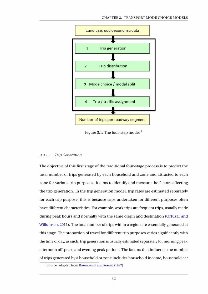
CHAPTER 3. TRANSPORT MODE CHOICE MODELS
Figure 3.1: The four-step model 1
3.3.1.1 Trip Generation
The objective of this first stage of the traditional four-stage process is to predict the
total number of trips generated by each household and zone and attracted to each
zone for various trip purposes. It aims to identify and measure the factors affecting
the trip generation. In the trip generation model, trip rates are estimated separately
for each trip purpose; this is because trips undertaken for different purposes often
have different characteristics. For example, work trips are frequent trips, usually made
during peak hours and normally with the same origin and destination (Ortuzar and
Willumsen, 2011). The total number of trips within a region are essentially generated at
this stage. The proportion of travel for different trip purposes varies significantly with
the time of day, as such, trip generation is usually estimated separately for morning peak,
afternoon off-peak, and evening peak periods. The factors that influence the number
of trips generated by a household or zone includes household income, household car
1Source: adapted from Rosenbaum and Koenig (1997)
32

CHAPTER 3. TRANSPORT MODE CHOICE MODELS
ownership, household size and structure, zonal value of land, zonal residential density
and accessibility. Similarly, zonal trips attraction is influenced by a zone’s roofed space
available for industrial, commercial purposes, zonal employment and accessibility.
3.3.1.2 Trip Distribution
The trip distribution model is a destination choice model that generates the trip matrix
table. It is commonly referred to as the origin-destination matrix (O-D Matrix). In other
words, trip distribution links the trips generated by each zone to the attraction zones.
This stage estimates the number of trips between pairs of zones and within zones in
the study area. There are several methods for distributing trips between origins and
destinations, including the growth factor models and gravity models.
3.3.1.3 Modal split
The purpose of modal split models or modal choice models is to forecast the proportion
of the total number of predicted trips that would use the various transportation modes
available. According to Hensher and Button (2007), Modal split models are mostly
disaggregate models that are often estimated on separate choice-based samples and
reflects the choice probabilities of individual trip makers. The issue of selecting the
most appropriate travelling mode has always been a critical issue in travel behavioural
modelling; it tells an individual about the most efficient travelling mode available. The
quantification of this interaction in terms of mathematical relationships is known as
modal split and travel demand models. Hence, modal split models assist a transport
planner to assess the impact of each urban element on mode choice, and it also allows
the evaluation of various transportation schemes.
3.3.1.4 Trip Assignment
Trip assignment is the last stage of the four-step model. The number of trips is estimated
and loaded onto each link in the network (Ortuzar and Willumsen, 2011). The main
objectives of this stage include: the estimation of traffic flow between zones (origin
zone i to destination zone j); the estimation of travel time and cost between these zones
33
CHAPTER 3. TRANSPORT MODE CHOICE MODELS
and identify congested links while specifying the travel behaviour of the individual,
and determining the preferred routes between any two zones (O-D pairs) (Khan, 2007;
Ortuzar and Willumsen, 2011).
3.3.2 Activity-Based Models
The activity-based models were developed out of the need to address the limitations of
the trip-based models. In an earlier study, Hägerstraand (1970) proposed the incorpora-
tion of a time-space framework in the trip-based models to make them realistic. The
researcher noted that, people live in a time-space continuum and limited by time and
space. People could not be physically present at different locations simultaneously and
therefore, must trade time and cost to move between activity centres (Hägerstraand,
1970; Bowman, 2008). Changes in policy direction from long-term transport investment
policies to short-term strategies in the 70s and the criticism of the traditional four-stage
models (Hagerstraand, 1970; Ettema, 1996; Kitamura, 1996; Bhat and Koppelman, 1999a;
1999b; Castiglione et al., 2015a), led to the development of the activity-based models
(Kitamura et al., 1995). The activity-based models were thus proposed to provide a con-
sistent framework for analysing travel behaviour and transport demand. The theoretical
framework of the activity-based models stems from the appreciation that the need to
pursue activities at a different spatial location (home, work et cetera) generates trips
(Kitamura, 1988; 1996; Kitamura et al., 1995). Activity-based approach views travel as
a derived demand resulting from the need to undertake an activity at different spatial
locations (Axhausen and Gärling, 1992).
3.3.2.1 Historical Perspective
The works of Hägerstraand (1970), Chapin (1974) and Fried et al. (1977), inspired re-
search into activity-based travel analysis. This research area subsequently received
appreciable research coverage and have seen considerable progress after these early
studies. The time-space constraint theorised by Hägerstraand (1970) is one of the
earlier activity-based pioneering studies and provided the foundation for research into
34
CHAPTER 3. TRANSPORT MODE CHOICE MODELS
activity-based modelling (Hägerstraand, 1970). The study theorised that the geograph-
ical distribution of activities (such as work, school, shopping, hospitals et cetera.) poses
a major constraint as well as the "time budget" required for each activity. Hagerstraand’s
study laid the foundation for the emergence of what is generally referred to as the "space-
time prism" (Hägerstraand, 1970).
The space-time or time-geographical framework offers a wide and useful perspective for
analysing human behaviour and daily activity participation. Hägerstraand (1970) opines
that individuals operate within a geographical and time limitations imposed on their
behaviour. The main principle of the space-time framework is the concept that the daily
activities individuals pursue have both spatial and time attributes (Hägerstraand, 1970;
Pred, 1977). An individual can only directly participate in events at a single location in
space at a particular time. For instance, recurring activities like working, schooling and
shopping which an individual of necessity has to participate, all take place at discrete
locations and within a limited time period (Miller, 1991). The need for individuals to
return home daily for rest and personal maintenance after participating in out-of-home
activities is another constraint people must contend with daily (Bowman, 1995).
In a broader view, space-time framework is concerned with the nature of the constraints
limiting the ability to participate in events in space and time (Pred, 1977). Miller (1991)
underscored the importance of the space-time prism and explained that the prism
models the location(s) at which the individual must be at the beginning and end of
any time interval, the time required for activity participation during that time interval
and finally the rates at which the individual can trade time for space in movement (i.e.
travel velocities) through the environment. Miller noted that, the prism models the
accessibility of an individual within a particular geographic and time context and can
offer a valuable measure of accessibility (Miller, 1991). The time-space framework can
also be helpful in planning for the siting of infrastructure for activities (Hägerstraand,
1970; Pred, 1977).
Chapin (1971) argued that human need for activity is provoked by his inherent instinct
35
CHAPTER 3. TRANSPORT MODE CHOICE MODELS
for survival, need for social interactions, health and quest for living a satisfactory life.
The researcher categorised the activities into two main groups namely, obligatory activ-
ities (such as work, sleep, eating et cetera.) and discretional activities (such as visits,
movies). In an effort to understand travel behaviour and why individuals participate
in activities, Fried et al. (1977) noted that, Individuals’ travel behaviour directly relates
to the nature of their participating activities and the spatially distribution of those
activities. They further explained that social role, ethnicity, life cycle status, residential
location, social norms, resource limitations, attitudes and perceptions of opportunities
were major determinants of activity choice and travel patterns. Fried, Havens and Thall,
submitted that the spatial distribution of activity largely relates to the differences in
the urban form; residential densities, socio-demographic distribution and historical
development. These spatial variations, the researchers believe, explains the travel and
activity patterns of various niches of the population.
It is believed that, the consolidation of the works of Hagerstraand and Chapin led to a
surge in research interest on the relationship between human activity and travel beha-
viour (Bowman, 2008). Activity-based models is premised on the often-quoted funda-
mental research finding that, travel is a derived demand, which is derived from people’s
need to participate in activities distributed in space (Hägerstraand, 1970; Jones, 1979;
Jones et al., 1990; Axhausen and Gärling, 1992). Activity-based models are premised
on behavioural theories and therefore, provide forecast for; when and where activities
will take place as well as the length of time and the travel mode required to pursue the
activity. Unlike trip-based models, Activity-based models simulate each individual’s
activities and travel choices across the entire day and assign to each individual traveller
the various activities they participate in (Castiglione et al., 2015).
3.4 Modal Split Models
Modal choice models forecast the transport mode a traveller will select for a trip from
the given choice set available for the same trip. Transport mode choice is argued to
36

CHAPTER 3. TRANSPORT MODE CHOICE MODELS
be the single most important element in transport planning and policy making since
the 1970s (Ettema, 1996). It has overreaching impact on the efficiency of the urban
transportation system and the amount of urban space devoted to transport facilities
(Ortuzar and Willumsen, 2011). The transport mode choice model typically tends to
predict an individual’s travel mode choice when presented with a discrete set of travel
options (alternatives). Models of this type are commonly referred to as "discrete choice
models" (Ettema, 1996; Ben-Akiva and Lerman, 1985).
3.4.1 Theoretical foundation of choice modelling
The theoretical foundation of the choice model has been discussed in the previous
section in details. According to Lancaster (1966), it is assumed that people select travel
mode that maximises their perceived utility (Ben-Akiva and Lerman, 1985; Koppelman
and Bhat, 2006). The utility of travel mode is defined by Khan (2007) as the attraction
associated by an individual to a particular mode. The individual is assumed to select
the mode having the maximum attraction using the attributes of the mode such as;
access time, waiting time, in-vehicle travel time, travel fares, parking availability and
cost of parking et cetera.
3.4.2 Factors affecting modal choice
To develop choice models, it is important to investigate the factors which influence
travellers decisions making. Ortuzar and Willumsen (2011) categorised these factors
into quantitative and qualitative factors. The quantitative factors influencing mode
choice are further classified into three, namely; the characteristics of the decision maker,
attributes of the transport system and attributes of the journey. The qualitative factors,
however, are factors difficult to measure in practice and include; comfort and con-
venience, safety, security et cetera. Guiver (2007) and Beirao and Cabral (2007) found
that travellers also consider comfort, convenience, safety and flexibility when making
decision on travel choice and proposed the incorporation of same in transport mode
choice models. Guiver (2007) suggested that the cost of travel mode was less important
37

CHAPTER 3. TRANSPORT MODE CHOICE MODELS
to bus users.
Similarly, car-users admitted that car travel was comparatively expensive than the bus.
However, it was argued that the cost difference between the two modes was a better
trade-off, when weighed against the level of convenience and flexibility that comes with
a car (Guiver, 2007; Beirao and Cabral, 2007). Therefore, preference for convenience,
safety, comfort, flexibility et cetera are factors that cannot be overlooked when trying to
explain transport mode choice decision and must be incorporated in decision makers’
utility function (Johansson and Heldt, 2006; Guiver, 2007; Temme et al., 2008b; Yáñez
et al., 2010). Recently, behavioural economics have received some research attention
and few researchers have investigated the role of "MINDSPACE" in consumer choice
decision. It is also suggested to have impact on travel choice as well (Avineri, 2012a).
Recent research in cognitive psychology and behavioural economics indicates that
behavioural elements such as the "MINDSPACE" significantly influence consumer
behaviour and might also impact on travel behaviour (Avineri, 2012a). However, none
of the existing studies have incorporated these elements of "MINDSPACE" as latent
factors in modal split models to test their impact on travel behaviour. It is suggested
that extending choice models with these elements of MINDSPACE as latent variables
could improve our understanding of the travel behaviour (Temme et al., 2008b).
3.4.3 Discrete choice modelling
Discrete choice models are mathematical relationship that represent the travel beha-
viour of an individual when provided with distinct set of travel options. Essential to
discrete choice analysis is the random utility model and the concept of generalised
cost. The theory is based on the assumption that travellers when given accurate in-
formation about the available travel alternatives, they will evaluate and always makes
travel choices that will maximise their utilities. Conversely, studies have shown that
decision makers do not always have complete information about all available alternat-
38
CHAPTER 3. TRANSPORT MODE CHOICE MODELS
ives (Simon, 1955). Moreover, decision makers do not possess unlimited information
processing and computational capabilities to enable them to assess all available altern-
atives for perfect decision making (Simon, 1955; 1982; Kahneman and Tversky, 1979;
Ariely, 2008).
3.4.4 Classes of discrete choice modelling
3.4.4.1 Deterministic models
The utility maximization rule suggests that decision makers will rationally allocate
their available resources to different goods such that their utility is maximized. This
implies the decision maker of certainty will choose the highest ranked alternative
under the observed choice conditions (Lancaster, 1966; Koppelman and Bhat, 2006).
Utility models with such level of prediction certainty are called deterministic utility
models. Koppelman and Bhat (2006), provided the following illustration to explain the
application of deterministic utility model.
For instance, Figure 3.2 portrays a utility space in which the utilities of alternatives 1
(Public Transport PT) and 2 (Car) are plotted along the horizontal and vertical axes
respectively, for each individual. The 450 line represents those points for which the
utilities of the two alternatives are equal. Individuals A, D and E (above the equal-utility
line) have higher utility for alternative 2 (Car) than for alternative 1 (PT) and are certain
to choose alternative Car over PT. Similarly, individuals B, C, and F (below the line) have
higher utility for alternative 1 (PT) and are certain to choose alternative PT over Car.
39
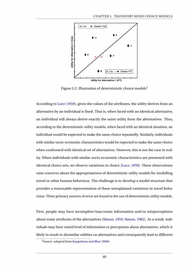
CHAPTER 3. TRANSPORT MODE CHOICE MODELS
Figure 3.2: Illustration of deterministic choice models2
According to Luce (1959), given the values of the attributes, the utility derives from an
alternative by an individual is fixed. That is, when faced with an identical alternative,
an individual will always derive exactly the same utility from the alternatives. Thus,
according to the deterministic utility models, when faced with an identical situation, an
individual would be expected to make the same choice repeatedly. Similarly, individuals
with similar socio-economic characteristics would be expected to make the same choice
when confronted with identical set of alternatives. However, this is not the case in real-
ity. When individuals with similar socio-economic characteristics are presented with
identical choice sets, we observe variations in choice (Luce, 1959). These observations
raise concerns about the appropriateness of deterministic utility models for modelling
travel or other human behaviour. The challenge is to develop a model structure that
provides a reasonable representation of these unexplained variations in travel beha-
viour. Three primary sources of error are found in the use of deterministic utility models.
First, people may have incomplete/inaccurate information and/or misperceptions
about some attributes of the alternatives (Simon, 1955; Simon, 1982). As a result, indi-
viduals may have varied level of information or perceptions about alternatives, which is
likely to result in dissimilar utilities on alternatives and consequently lead to different
2Source: adapted from Koppelman and Bhat (2006)
40
CHAPTER 3. TRANSPORT MODE CHOICE MODELS
choices.
Second, the researcher/analyst may have different or incomplete information about
the attributes relative to the decision maker or inadequate understanding of the utility
function the decision maker uses to evaluate each alternative. For example, the analyst
may not have a good measure of the reliability of a particular alternative. The likelihood
of getting a seat at a specific time of day or the possibility of finding a parking space.
However, regular users are likely to know these things, form opinion about them and
may consider them and other factors oblivious to the analyst.
lastly, the analyst is unlikely to know or account for specific circumstances accounting
for the individual’s travel decision. For example, an individual’s choice of mode for
work trip may depend on whether another family member has a special travel need
on a particular day or not. The failure of these models to account for the analyst lack
of complete information results in the apparent behavioural inconsistencies. While
human behaviour may be argued to be inconsistent (Kahneman and Tversky, 1979;
Ariely, 2008), it can also be argued that the inconsistency can be attributed to the ana-
lyst’s inability to fully appreciate and account for all the factors informing the decision
making process (Koppelman and Bhat, 2006). This concerns led to the development of
Probabilistic choice models (Koppelman and Bhat, 2006).
3.4.4.2 Probabilistic models
The concept of bounded rationality and cognitive bias in human decision making, flaws
the fundamental assumption of the deterministic models. It has been shown that de-
cision makers do lack complete information and understanding necessary for rational
decision making (Kahneman and Tversky, 1979; Ariely, 2008). (Simon (1955; 1982),
challenged the assumption of human perfect rationality and theorised that humans
are rationally bounded and limited in thinking, information processing and compu-
tational capabilities. Therefore, the entire internal decision-making process and how
the decision maker perceives available alternatives is not completely known. In light
41
CHAPTER 3. TRANSPORT MODE CHOICE MODELS
of the above limitations of the deterministic models, it was argued that choice models
need to incorporate an error term to cater for the bias resulting from the incomplete
understanding of the entire choice process.
Luce (1959), found that when decision makers are offered identical alternative, they will
always derive the same utility from the alternative. Luce then proposed that the utility
an individual derives from an alternative given the values of its attributes is fixed. Based
on these utilities, the chance that an alternative is chosen is expressed as a probability
p(i). Subsequently, Luce proposed a probability function in which the choice probabil-
ity of an alternative is proportional to its utility and inversely proportional to the total
utility of all alternatives in the choice set, as shown below:
p(i ) = Ui
Σ jU j(3.1)
Although, the probabilistic model proposed by Luce accounted for the inconsistency
and transitivity of choice behaviour, it was however, based on the assumption of the
deterministic utility function rather than random utility function (Luce, 1959; Ettema,
1996), neither was it based on the actual perception, preferences nor behaviour of the
decision maker (Ettema, 1996).
Random Utility Models
The random utility theory is the theoretical framework for discrete-choice modelling,
this was credited to the works of Thurstone (1927) and latter studies like Luce (1959);
Block and Marschak (1960); Ben-Akiva and Lerman (1985), et cetera. The random utility
theory uses the concept of utility maximization to represent the attractiveness of the
alternatives. It assumes that when decision makers are presented with alternatives,
they will always make choices to maximise their net personal utility. Similar to the
Deterministic theory, random utility theory assumes that the decision maker will always
choose an alternative with the highest utility. It further assumes utilities as random
variables that cannot be precisely measured for the under listed reasons (Manski, 1973;
Ettema, 1996; Walker, 2001; Koppelman and Bhat, 2006);
• measurement errors,
42

CHAPTER 3. TRANSPORT MODE CHOICE MODELS
• instrumental errors,
• lack of complete information about the alternatives and
• the analyst’s lack of complete understanding and information of the individual’s
choice making process.
Avineri (2012a) and Aczél and Markovits-somogyi (2013) also agreed with Manski (1973);
Ettema (1996); Walker (2001); Koppelman and Bhat (2006) on the possible causes of
the observed inconsistencies and violations. Avineri (2012a) and Aczél and Markovits-
somogyi (2013) further suggested that the inconsistencies may be due to absence of the
recently proposed behavioural characteristics in consumer behaviour such as "MIND-
SPACE" and/or the presence of errors in the utility function. Additionally, decision-
makers’ choices pattern is also observed to violate the assumption of transitivity of
preferences (if A is preferred to B and B is preferred to C, then A should be preferred to
C) (Walker, 2001; Ettema, 1996).
It is further suggested that human behaviour may be irrationally probabilistic. Meaning
that even if all the relevant factors are perfectly measured and included, consumer
behaviour cannot still be deterministically predicted. The utility Ui of the decision-
maker is thus expressed in two distinct terms, the known or measurable component
(deterministic term, v) and the unknown component, (random error term, ε), this is
represented mathematically as;
Ui t =Vi t +εi t (3.2)
where
Ui t is the utility of the alternative i to the decision-maker t
Vi t is the deterministic or observable component of the utility estimated
εi t is the unknown component of the random error term of the individual’s utility.
The outputs of the models Ui t represent the probabilities of an individual t select-
ing each alternative i. The utilities are assumed to be a function of the attributes of
the alternatives and the characteristics of the decision-maker. The final component
43
CHAPTER 3. TRANSPORT MODE CHOICE MODELS
of the utility is a random error term. The aggregation of these individual probabilities
produces the forecasts for the study population. The structure of the choice model
depends on the assumptions of the distributions of the random error term and variance-
covariance structure of the error term. Normally distributed error term lead to a probit
model while Gumbel distributed error term results in Logit models (Walker, 2001; Khan,
2007; Ettema, 1996; Koppelman and Bhat, 2006).
3.5 Hybrid /Latent Choice Models
Ben-Akiva and Boccara (1995) proposed the hybrid discrete choice models to address
the limitation and inconsistencies of the traditional travel choice models and the ran-
dom utility models (Manski, 1973; Avineri, 2012a; Aczél and Markovits-somogyi, 2013).
These choice models incorporated behavioural and attitudinal variables such as; hap-
piness, convenience, comfort, flexibility and safety as latent variables in addition to
factors unique to the decision-maker and alternative (Ben-Akiva and Boccara, 1995;
Ben-Akiva et al., 1999; Ben-Akiva et al., 2002; Johansson et al., 2005; Johansson and
Heldt, 2006; Raveau et al., 2012; Yáñez et al., 2010).
Two procedures were developed for the estimation of these models; the first approach
called the sequential approach, construct the latent variables and incorporated them
into the discrete choice model as a regular variable (Johansson et al., 2005; Raveau
et al., 2012). The second method is referred to as the simultaneous approach; with this
approach, the construction of the latent variables and the estimation of the discrete
choice model are done simultaneously (Bolduc et al., 2008; Raveau et al., 2012). The
latter has been argued to result in more efficient estimates of the parameters than the
former (Ben-Akiva et al., 2002). Table 3.1 is a summary of some extant latent/hybrid
choice studies.
3.5.1 ICLV model framework
This section presents the theoretical framework for incorporating the latent variables
into choice models. The integrated choice and latent variable (ICLV) models are a
44

CHAPTER 3. TRANSPORT MODE CHOICE MODELS
Table 3.1: Existing Latent/hybrid choice models
Study Observed variables Unobserved variables Estimation Procedure Software Application
Walker and Ben-Akiva (2002)
Cost
Travel time
No. of Transfers
Gender(Dummy)
Business trip (Dummy)
Ride comfort
ConvenienceSimultaneous Travel mode choice
Morikawa et al. (2002)
Cost
Travel time
Gender
Comfort
ConvenienceSequential Travel mode choice
Ashok et al. (2002)
Satisfaction
Cost of switching
Satisfaction with cost
Satisfaction with coverage
Simultaneous GAUSS
Propensity to switch-
Television provider
Customer satisfaction of-
Health Care provider
Johansson et al. (2006)
Travel Time
Cost
Gender
Age
Kids
Education
Car Ownership/Availability
Flexibility
Convenience
Safety
Comfort
Environment
Sequential Travel mode choice
Temme et al. (2008)
Travel time
Distance to bus stop
Age
Gender
Income
Mode constant
Flexibility
Convenience
Comfort
Safety
Power
Hedonism
Security
CFA and
Discrete choice modelling
M-PlusTravel mode choice
Bolduc et al. (2008)
Age
Income
Gender
Educational level
Transit user
Car pool user
Capital cost
Operational cost
Driving alone
Environmental concerns
Appreciation of new-
car features (ACF)
SEM
M.F. Yanez
Patricio Mansilla and
J. de D. Ortuzar (2009)
Cost
Walking time
waiting time
Travel time
Accessibility
Comfort
Safety
Reliability
Factor analysis Choice
M.F. Yanez
S. Raveau and
J. de D. Ortuzar (2010)
Travel Time
Cost
Waiting time
Number of cars
Transfers
Accessibility
Comfort
Safety
Reliability
Choice
S. Raveau
M.F. Yanez and
J. de D. Ortuzar (2012)
Income
Age
Children
Education Level
Accessibility
Comfort
Safety
Reliability
Choice
Kamargianni m. et al (2015)
Travel time
Income
Age
Gender
Parents’s education status
Travel cost
Walking time to bus stop
Weather
Walking Facility
Safety Consciousness
Physical Propensity
Green Lifestyle
ICLV GAUSSChildren’s travel mode
choice to school
Lavieri P.S. et al (2016)
Income
Age
Gender
Parents’ Education status
Travel cost
Walking time to bus stop
Weather
Walking Facility
Driver’s risky behaviour
Driver distraction/
careless behaviour
Generalized
Heterogeneous
Data Model
Accident severity
45

CHAPTER 3. TRANSPORT MODE CHOICE MODELS
new generation of discrete choice models that expand on standard choice models and
provides improved predictive power. ICLV models provide a mathematical framework
for integrating discrete choice and latent variables models to account for the unob-
served preference heterogeneity in the traditional discrete choice models and to test the
influence of latent variables, such as values, perceptions and attitudes on observable
behaviour (Ben-Akiva and Boccara, 1995; Vij and Walker, 2015; Vij et al., 2016). They
allow the prediction of individual preferences and assess the impact of unobserved
heterogeneity involved in the decision-making process by reflecting the difference
in individual tastes, attitudes, perception and values, which are unaccounted for in
the traditional discrete choice models (Bolduc and Alvarez-daziano, 2010; Mariel and
Meyerhoff, 2016). In the general framework of the ICLV models, there are two separate
sub-models: the discrete choice sub-model and a latent variable sub-model. Each of
these two components consists of both structural and measurement models. The latent
variable component of the ICLV allows a simultaneous relationship between the unob-
served latent variables (psychometric indicators) and the observed exogenous variables
(such as socio-demographics). The discrete component of the ICLV is consistent with
the random utility maximisation theory and consist of the observed variables (charac-
teristics of the decision-maker, attributes of the alternatives and the trip characteristics)
and the unobserved latent variables reflecting the diversity in individual tastes, per-
ception, values, and emotions. The reported gains or enhancement in the explanatory
power of the ICLV models over the traditional discrete choice models is ascribed to
the introduction of the unobserved individual heterogeneity in the specification of the
ICLV models. I refer readers to Ben-Akiva and Boccara (1995); Ben-Akiva et al. (1999);
Bierlaire (2016); Bierlaire (2018b); Bierlaire (2018c); Bolduc et al. (2008); Vij et al. (2016)
for more details. The latent variables are not measured; they are linked with multiple
indicators (questions in a survey) normally measured on a Likert-scale (Bolduc et al.,
2008; Vij et al., 2016).
46
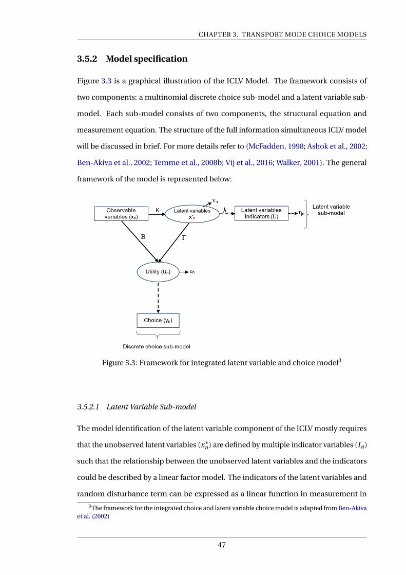
CHAPTER 3. TRANSPORT MODE CHOICE MODELS
3.5.2 Model specification
Figure 3.3 is a graphical illustration of the ICLV Model. The framework consists of
two components: a multinomial discrete choice sub-model and a latent variable sub-
model. Each sub-model consists of two components, the structural equation and
measurement equation. The structure of the full information simultaneous ICLV model
will be discussed in brief. For more details refer to (McFadden, 1998; Ashok et al., 2002;
Ben-Akiva et al., 2002; Temme et al., 2008b; Vij et al., 2016; Walker, 2001). The general
framework of the model is represented below:
Figure 3.3: Framework for integrated latent variable and choice model3
3.5.2.1 Latent Variable Sub-model
The model identification of the latent variable component of the ICLV mostly requires
that the unobserved latent variables (x∗n) are defined by multiple indicator variables (In)
such that the relationship between the unobserved latent variables and the indicators
could be described by a linear factor model. The indicators of the latent variables and
random disturbance term can be expressed as a linear function in measurement in
3The framework for the integrated choice and latent variable choice model is adapted from Ben-Akivaet al. (2002)
47
CHAPTER 3. TRANSPORT MODE CHOICE MODELS
equation. However, since a latent construct typically have more than one indicator, it is
a vector. From Figure 3.3, x∗n represents the vector of latent exogenous variables with
observed indicators In . The measurement model mapping the observed indicators into
the latent variables for the latent variable sub-model is formulated as follows (Ashok
et al., 2002):
In =α+λn x∗n +ηn , ηn ∼ N (0,Σηn ) (3.3)
Where In is a (P x 1) vector of observed scores of the latent variable indicators, αn is the
intercept for indicator n, λn is a (P x M) matrix of factor loading mapping indicator n to
latent variable x∗n . x∗
n is the latent variable or a vector of socio-demographics underlying
the latent factor and ηn , is a vector of errors which are i.i.d. multivariate normally
distributed error term with mean 0. The structural model of the latent variable model is
shown in equation 3.4, the model describes the latent variables in terms of observables
socio-demographic variables and links the latent variable and the indicators (Bolduc
et al., 2008). The framework allows the integration of the latent variable model and the
discrete choice model.
x∗n = K xn +νn , νn ∼ N (0,ψ) (3.4)
Where x∗n is (L x 1) vector of latent variable L is the number of latent variables, xn is (M x
1) vector of the observed socio-demographics underlying the latent factor and K is a
matrix of unknown coefficients mapping the observed socio-demographics variables
xn to the latent factor.
3.5.2.2 Multinomial discrete choice sub-model
The discrete choice component of the ICLV model consists of structural and meas-
urement sub-models which are based on the assumption that when individuals are
presented with a finite set of mutually exclusive alternatives n, they will choose the
alternative that maximises their utility (Ben-Akiva and Lerman, 1985). (Readers are re-
ferred to section 3.4.4 of this thesis for details on discrete choice models). The structural
component (utility function) of the discrete choice sub-model consist of the systematic
48

CHAPTER 3. TRANSPORT MODE CHOICE MODELS
component V(.) and the random error component εn .
Un =V (xn , x∗n ;B ,Γ)+εn or A+B xn +Γx∗
n +εn , εn ∼ N (0,Σεn ) (3.5)
Where Un is the random utility of alternative n, xn is a vector or observed variables, x∗n
is a vector of latent variables, A is an intercept for alternative n, B and Γ are the matrices
of estimates mapping the observed and latent variables respectively to the alternative
n, εn is a vector of random error term associated with the utility terms and Σεn is the
covariance of the random error terms. The measurement equations or the choice model
component of the discrete choice sub-model of the ICLV is denoted as follows:
yi n =
1 if Ui n ≥Ui j , ∀ j ∈Cn , j 6= i ,
0 otherwise.
(3.6)
Where yn is a choice indicator, which takes a value of 1 if alternative n is chosen and 0
otherwise and Cn denotes the choice set of individual i.
3.5.2.3 Integrated model
The integrated model comprises of equations 3.3 to 3.6, equations 3.3 and 3.4 are the
latent variable sub-models and equations 3.5 and 3.6 are the discrete choice sub-model.
Using equations 3.5 and 3.6 and the assumption that all the random error terms are
independent of each other, we can integrate over the joint distribution of the latent
variables, this produces a multidimensional integral because the number of latent
variables defines the dimension of the joint likelihood function of the model (Ben-Akiva
et al., 2002; Temme et al., 2008b; Kamargianni and Amalia, 2014).
3.5.2.4 Likelihood function
To begin with, the likelihood of an individual i observing a choice indicator yn without
latent variable can be expressed as:
P (yi = 1|X ;B) = P (Un ≥U j ); n 6= j , ∀ j ∈C ; where C is the choice set (3.7)
Moreover, because every respondent makes a single choice which is independent of
each other, we can assume that the error terms (η,ν and ε) of equations 3.3 to 3.5 are
49
CHAPTER 3. TRANSPORT MODE CHOICE MODELS
similarly independent of each other. This makes the situation less complicated and we
can include the latent variables to equation 3.7. The likelihood function for observing a
given choice indicator yn , is then given by the joint probability of observing the choice
indicators and the indicators of the latent attitude, this is expressed mathematically as
follows:
f (y , I |X , X ∗;α,λ,K ,B ,Γ;Σε,Ση,Σν) = ∫X ∗ P (y |X , X ∗;B ,Γ,Σε) f3(I |X , X ∗;α,λ,Ση) f1(X |K ,Σν)d X ∗ (3.8)
The first term of the integrand relates to equation 3.5, while the second and third terms
relate to the equations 3.3 and 3.4 respectively.
Assuming a linear function and a normally distributed error term for the choice model.
The choice model component of the likelihood function takes the form of a standard
choice model, with the utility being a function of the latent constructs. Deriving the
probability function from equations 3.5 and 3.6 based on the assumption of i.i.d. error
term ε, standard Gumbel. The probability function takes the form of a logit model as
follows (Ben-Akiva et al., 2002):
Un =Vn +εnor Un =Vn(X , X ∗;B ,Γ), n ∈C , C is the choice set (3.9)
P (yi = 1|X , X ∗;B ,Γ,Σε) =P (Un ≥U j ), n 6= j , ∀ j ∈C
P (Vn +εn ≥V j +ε j ), ∀ j ∈C
P (ε j −εn ≤Vn −V j ), ∀ j ∈C
eVn∑j∈C eV j
(3.10)
Similarly, assuming we have typical uncorrelated latent factors, which are normally
and independently distributed together with the indicators, then using equation (3.4)
we can derive the form of the distribution of the latent variables. While that of the
indicators can be derived from equation (3.3). Again, when we assume that the random
error terms of the structural and measurement equations of the latent variable model
are normally and independently distributed, then the densities can be written as:
f1(X ∗|X , X ∗;K ,σv ) =L∏
l=1
1
σvi
φ
( X ∗l −h(X ;Kl )
σvl
)(3.11)
50
CHAPTER 3. TRANSPORT MODE CHOICE MODELS
f3(I |X , X ∗;α,λ,ση) =Q∏
q=1
1
σvq
φ
(Iq − g (X , X ∗;αq ,λq )
σηq
)(3.12)
Where: συ and ση are the standard deviations of the error terms of υ and η in that order,
φ is the standard normal density function
L is the number of latent variables and
Q is the number of indicators
(readers are referred to Ben-Akiva and Boccara (1995) and Ben-Akiva et al. (2002) for
details).
The independent and identically distributed(iid) error terms assumption simplifies the
model and provides a very convenient form for the choice probability; the normalization
for scale is made simpler if the error terms are assumed to be iid. The popularity of
the logit model is due to this convenience (Train, 2003). However, the drawbacks of
this framework is that the iid assumption is restrictive and fails to take into account
the correlation between alternatives ; the critical part of the iid assumption is that
the unobserved factors are uncorrelated over alternatives, as well as having the same
variance for all alternatives. The assumption of independence can be inappropriate in
some situations. Unobserved factors related to one alternative might be similar to those
related to another alternative. In many instances, it would be expected that unobserved
factors that affect respondents’ choices or scores on different psychological constructs
are related rather than independent. For example, it can be seen from Figure 7.3 that
the latent variables PerNorm and Affect are about 57% correlated; meaning a person
who scores high on PerNorm might also score high on Affect. In such a situation, the
unobserved factors affecting PerNorm and Affect are somehow correlated rather than
independent.
3.5.2.5 Estimation methods
There are three methods for incorporating psychometric factors into discrete choice
models, sequential, simultaneous and simulation approaches; The first approach is
commonly referred to as the sequential approach; the researcher performs a factor
51

CHAPTER 3. TRANSPORT MODE CHOICE MODELS
analysis using the psychometric indicators. The resultant latent variables and their dis-
tributions are then incorporated in the utility function. To obtain consistent estimates,
the researcher must integrate the choice probability over the latent variables. However,
the estimates generated from this technique are not efficient (Ben-Akiva et al., 2002).
The second approach is usually called simultaneous approach, as the name connote,
the researcher jointly estimate the latent variables with their indicators (latent variable
sub-model) and the observed variables of the choice model (Discrete choice sub-model),
using simultaneous maximum likelihood estimation method (Ben-Akiva et al., 2002).
This procedure produces efficient and consistent models estimates. The model estim-
ation requires multidimensional integral over the distribution of the latent variables,
the dimensionality is determined by the number of latent constructs in the model (Kim
et al., 2014).
The limitation of this approach is that, with more than three latent factors, the multidi-
mensional integration of the likelihood function becomes unworkable because of its
complexity (Ben-Akiva et al., 2002). In such circumstances, we use the third approach
known as the simulation technique; this technique estimates the parameters simul-
taneously, however, a smooth simulator (simulated maximum likelihood estimation)
replaces the numerical integration method (Bolduc and Alvarez-daziano, 2010). The
simulated maximum likelihood estimation involves using random draws from the es-
timated distribution of the latent variables to obtain consistent and efficient estimates
(Ashok et al., 2002; Ben-Akiva et al., 2002), the drawback of this approach is the amount
of time required for computing the estimates (Kim et al., 2014).
Moreover, due to the number of latent variables involves in this study, the ML-based
simulation approach with Monte Carlo integration method is deemed appropriate. The
framework of the simultaneous approach and model specification of the integrated
latent variable and discrete choice model are illustrated and discussed in the subsequent
sections of this chapter.
52

CHAPTER 3. TRANSPORT MODE CHOICE MODELS
3.5.2.6 Simulated maximum likelihood solution
The dimension of the integral increases as the number of latent variables increases;
this renders numerical integration practically complex. The numerical integration
method is thus replaced with the simulated methods. This method uses random draws
of the latent variables from their probability distributions. The likelihood function is as
follows:
L(α,B ,Γ,K ,Σ) =N∏
n=1
∏i∈Cn
Pn(i I |XnBΓKΣ) (3.13)
3.5.2.7 Model Application
In the estimation of integrated choice and latent variable model, the function of the
measurement equation is used for the identification of the latent variables and to
enhance the estimates of the structural equations. The focus is on predicting the
probability P (y |X ;α,B ,Γ,Σ) of observing the choice indicator yn when forecasting
rather than the indicators of the latent variables (Kim et al., 2014). Hence, we integrate
the likelihood over the indicators to create a final forecasting model as shown below:
P (y |X ;α,B ,Γ,K ,Σ) =∫
X ∗P (y |X , X ∗;B ,Γ,Σε) f1(X ∗|X ,K ,Ση)d X ∗ (3.14)
Therefore, after the model estimation, we use equation 3.12 for forecasting without the
latent variable and measurement models neither their indicators.
Demand Indicators
Transport demand defines and quantifies the type and amount of travel that people
would choose under particular conditions (Litman, 2019). The factors that influence
transport demand includes the perceived cost of the transport services, which may
include monetary cost, travel time, risk, comfort to mention but a few. Changes in
user attributes such as income, and alternative specific attributes (such as transport
prices, travel time) can affect demand in the form of mode choice, trip frequency,
destination choice, vehicle type and the parking location (Litman, 2019). To understand
the result of the analysis and evaluate the sensitivity of users with respect to important
user and alternatives attributes, the demand elasticities are estimated and reported in
53

CHAPTER 3. TRANSPORT MODE CHOICE MODELS
this thesis. The aggregate direct and cross elasticities for the base model and the ICLV
model are computed for explanatory variables (such as travel times and costs, income,
trip distance, trip frequency, car ownership, Education as well as personal Norms,
Salience and Affect representing the latent variables) for the private motorised modes,
public transport and active mode of transport to assess the impact of a change of the
attribute(variable) of the same or another alternative on the demand of an alternative
(Bierlaire, 2018a; Atasoy et al., 2013; Axhausen et al., 2008).Elasticity measures how
much the amount and type of goods will change when the price of the goods change. In
transportation, It provides a framework for assessing the extent to which consumers will
react to changes in the price or other determinants of demand for transport services,
For detail description of demand elasticities, the reader is referred to (Cowie and Ison.,
2009; Litman, 2019).
Direct elasticity measures the impact of a change of an attribute of alternative i on the
choice probability of the same alternative, whiles cross elasticity measures the effect
of a change in the cost of one alternative on the demand for the services of another
alternative in the choice set.
Given that xi n is a variable associated with individual n and alternative i. If we assume
that xi n is continuous and the relative (infinitesimal) change of the variable x is the
same for every individual n in the population p for alternative i, then;
∂xi n
xi n= ∂xi p
xi p= ∂xi
xiwhere xi = 1
N
N∑n=1
xi n (3.15)
Thus, for individual n, the elasticity E for attribute x of alternative i is given by;
E ixn
= ∂Pn(i )
∂xn
xn
Pn(i )(3.16)
where E ixn
is disaggregate elasticity of alternative i for individual n for variations in
attribute x. Pn(i ) is the probability that individual n chooses alternative i
The aggregate direct elasticity E ix of alternative i with respect to the attribute xi is
defined as;
E ix =
∑Nn=1 WnPn(i )E i
xn∑Nn=1 WnPn(i )
(3.17)
54
CHAPTER 3. TRANSPORT MODE CHOICE MODELS
where Wn is the sample weight for individual n, Readers are referred to Bierlaire (2018a)
for detail description of the mathematical formulations of Elasticities.
3.6 MINDSPACE and ICLV modelling
Transport Mode choice decision has been demonstrated not to only depend on object-
ive criteria such as travel time, cost and income but subjective factors as well. Guiver
(2007) found that while car-users admitted that car travel was comparatively expensive
than a bus, bus users, on the other hand, were less concerned about the cost. Although
car-users were concerned about the cost of driving, the authors argued that the cost
difference between the two modes of transport was a better trade-off when weighed
against the level of convenience and flexibility that comes with a car (Guiver, 2007;
Beirao and Cabral, 2007). Therefore, preference for convenience, safety, comfort, flex-
ibility, emotional satisfaction and similar subjective variables cannot be overlooked
when investigating transport travel behaviour (Johansson and Heldt, 2006; Guiver, 2007;
Temme et al., 2008b; Yáñez et al., 2010).
Researchers investigating consumer choice decision making believe that MINDSPACE
could have a significant impact on travel behaviour (Avineri, 2012a; Avineri, 2012c).
Moreover, few studies have explored the effect of some elements of MINDSPACE on
travel behaviour and car ownership (Belgiawan et al., 2016). However, none of the exist-
ing studies has developed and tested ICLV models incorporating elements of MIND-
SPACE as a latent variables (Temme et al., 2008b; Zhang et al., 2016; Belgiawan et al.,
2016). Temme et al. (2008b) suggested that extending choice models with elements
of MINDSPACE as latent variables could provide higher explanatory power. Therefore
building on the studies of hybrid choice models, this study, incorporates elements of
MINDSPACE as latent variables in modelling an integrated choice and latent variable
model (ICLV) while investigating the impact of MINDSPACE, on travel mode choice
behaviour (Avineri, 2011; Juhász, 2013; Aczél and Markovits-somogyi, 2013).
55

CHAPTER 3. TRANSPORT MODE CHOICE MODELS
3.7 Summary
The chapter reviews the literature on transport models and provides the theoretical
background for the study. It was found that travel is a derived demand out of the need
for activity participation; the level for activity participation rises with economic devel-
opment and growth. Efficient transportation system is a necessity to achieve this end.
Major cities have had to build roads and made changes to land-use patterns to deal with
vehicular traffic for more than half a century. Building more roads to accommodate the
increasing vehicular volumes have only resolved the situation temporarily; volumes
always increase soon after the implementation of such schemes to fill any additional
capacity introduced.
In order to make informed planning decisions, transport demand models (popularly
called four-stage-models) were developed in the 1950s to understand and predict the
response of transportation demand to changes in the attributes of the transportation
system and the characteristics of the users of the transportation system. The results
from these models formed the basis for major long-term transport capital and infra-
structure investment strategies.
It is also shown that the emphasis has shifted from the capital investment strategies to
understanding travel behaviour responses to shorter-term congestion management
schemes. The realisation of the inefficiency of the capital investment strategies and tra-
ditional statistically-oriented modelling approach to travel demand analysis in resolving
the conundrum has shifted the emphasis from the capital investment strategies to a
more behaviourally-oriented modelling approach to understanding travel behaviour
responses to congestion management strategies.
It has been argued from recent literature that travellers do not always maximise their
economic utility neither do they always have complete information about alternatives
to make informed choices as postulated by the economic theory of perfect rational-
ity. The chapter has shown that subjective factors such as attitudes, behaviour and
situational factors affect travel choices; decision-makers do not always assess the full
56

CHAPTER 3. TRANSPORT MODE CHOICE MODELS
economic costs of their decisions. It was further shown that several studies had pro-
posed the inclusion of the subjective factor into the choice models to account for the
heterogeneity in human behaviour. The chapter has also shown the framework for the
development of such models, as well as examples of hybrid choice models developed to
account for these subjective factors in literature.
57

Part II
RESEARCH METHODOLOGY AND DATA
COLLECTION
58

; Chapter Four <
Research Methodology
4.1 Introduction
The theoretical framework for this study has been presented in chapters two and three.
This chapter presents the overall research methodology adopted to address the research
objectives and the overall research aim of empirically evaluating the impact of MIND-
SPACE on transport mode choice or individual choice preference. The existing literature,
as shown in chapters 2 and 3 supports the incorporation of behavioural and attitudinal
variables as latent variables to model and explain travellers’ choice decision (Ben-Akiva
and Lerman, 1985; Ben-akiva, 1997; Ben-Akiva et al., 1999; 2002; Ben-akiva and Boersch-
supan, 2002; Johansson et al., 2005; Johansson and Heldt, 2006; Temme et al., 2008b;
Yanez et al., 2010). Moreover, recent studies in cognitive psychology suggest that the
application of behavioural economics, particularly MINDSPACE in explaining travel
mode choice decision to enhance the understanding of travel mode choice decision
(Avineri, 2012b; Metcalfe and Dolan, 2012; Aczél and Markovits-somogyi, 2013).
4.2 Research Approach
Guba and Lincoln (1994, p.107) defined research paradigm as "the basic belief system or
world-view that guides the investigator ...". Hussey and Hussey (1997, p.47) also defined
research paradigm as "the progress of scientific practice based on peoples’ philosophies
and assumptions about the world and the nature of knowledge". A research paradigm,
59

CHAPTER 4. RESEARCH METHODOLOGY
therefore, is closely related to our belief system of how the real world is constructed
(Ababio-Donkor, 2015). (Hussey and Hussey, 1997) further proposed two main research
paradigms, namely; positivist and phenomenological. Sam (2011) agrees with the
explanation of Hussey and Hussey (1997), which suggests that the type of methodology
selected for a study should be influenced by the research paradigm adopted by the
researcher. Sam (2011) expanded on the above to include time and cost availability
for the research work. However, since the aim of this research is to apply MINDSPACE
as latent variables in calibrating integrated choice and latent variable model (ICLV),
numeric data was be required. Therefore, a questionnaire survey will be deployed for
this purpose, and therefore quantitative approach was adopted for the study.
4.3 Research Design
Research design is defined as "a set of advance decisions that make up the master plan
of the research work, specifying both the methods and procedures for collecting and
analysing the needed information" (Robson, 1993; Burns and Bush, 2002; Yin, 2009).
Yin (2009) expanded on the above definition to include "a logical sequence that links
empirical data collection to research question, data analysis and conclusion". The
author further asserted that the research design must be developed at the inception
stage and kept in mind throughout the research work. The quality of any research work,
therefore, depends on the formulation of the research design. Moreover, the quality
and suitability of research design are essential in procuring information to answer the
research question within resource constraint (Ghauri and Gronhaug, 1995; Sam, 2011).
4.4 Research methods
The methods for achieving the research objectives are discussed in two separate sec-
tions: data collection methods (literature review and revealed preference questionnaire
survey) and data analysis methods (Exploratory and confirmatory factor analysis and
latent variable choice modelling). The following sections discuss these in details.
60

CHAPTER 4. RESEARCH METHODOLOGY
4.4.1 Data Collection Methods
It is suggested that the scope and depth of a research influences to a greater extent
the choice of research method to be adopted (Fellow and Liu, 2005). Richardson et al.
(1995) argued that the choice of a survey method for transport research should be a
trade-off between the objective of the survey and the resource available for the survey.
Since the study involves transport modelling and behavioural economics (cognitive
psychology), a combination of quantitative and qualitative research methods is deemed
appropriate. The data collection involves a comprehensive review of relevant literature
and a revealed preference questionnaire survey.
4.4.1.1 Documentary Survey
A comprehensive review of relevant literature was conducted for consolidating extant
studies and literature by other practitioners and researchers in transport modelling
and behaviour economics; this review is presented in chapters two and three of this
thesis. Relevant studies and works from journal articles, conference papers, textbooks,
research reports, working papers, Doctoral thesis and information from the internet
were reviewed to establish the background of behavioural economics and transport
mode choice modelling. The research framework for the study was developed through
the review of existing literature, the current state of knowledge in transport choice mod-
elling and MINDSPACE were explored to identify the best approach for the integration
of the two areas of knowledge. This process provided a clear understanding of the type
of information required in the survey and was quite helpful in the design of the data
collection instrument (Richardson et al., 1995).
Chapter 2 presents the review of choice theories comprising, rational choice theory,
bounded rationality and behavioural economics. The chapter further explains how
behavioural economics or MINDSPACE could influence transport decision making as
well as its potential application in transport. Materials from journal articles, confer-
ence papers, books, research reports, working papers, government policy document
61
CHAPTER 4. RESEARCH METHODOLOGY
and information from the internet were reviewed for this exercise. Similarly, chapter 3
explored transport demand theories and transport modelling and also looked briefly at
their historical development. The chapter also reviewed the types of choice models as
well as their strengths and limitations. Additionally, published data from the National
Travel Survey (NTS), the Scottish household survey (SHS) and census data provided use-
ful background information on the demographic characteristics and travel behaviour of
the study population.
4.4.1.2 Survey Instrument Design Methodology
Travel demand modelling requires data reflecting the travel behaviour of the targeted
population, which could be acquired through a questionnaire survey. For the developed
model to reflect and predict the travel behaviour accurately, the data must reflect the
characteristics of the study population. Revealed preference survey, generally involves
asking questions to acquire detailed accounts of the population actual travel beha-
viours, such as their previous travel decisions, i.e., frequency of travel, the purpose of
the journey, chosen mode and other relevant attributes of their journeys. This approach
is based basically on the respondents’ past travel behaviour and hence overcomes the
biases of stated preference approach. Stated preference survey, on the other hand,
involves asking the respondents question about their future travel choices based on a
hypothetical travel scenario, in which several travel modes are presented with different
attributes. The respondents’ choice indicates the relative importance of the attributes
associated with their selected mode. Stated preference is superior to the revealed prefer-
ence in terms of the flexibility it offers the researcher to explore the effects of significant
variables efficiently as well as assessing the sensitivity of each variable in the model.
Mode choice data collection method
The previous section discussed the various methods of data collection for choice model-
ling. This section exploits the relative advantages offered by both approaches (Revealed
and Stated preference) to overcome the limitations in using them separately by com-
bining both revealed and stated preference type questionnaire in the data collection
62
CHAPTER 4. RESEARCH METHODOLOGY
instrument. There are several methods for administering a survey questionnaire; this
depends on the methods employed for the data collection and distribution of the ques-
tionnaire (Richardson et al., 1995). These formats include; postal survey (Mail back
survey), computer-assisted survey, paper-and-pencil based, and telephone-based sur-
veys. For this study, a combination of the first two methods was deployed for the data
collection. These methods are described in the next section.
Postal Survey
Postal survey is a method of self-completion survey, which involves mailing the ques-
tionnaire to the respondent and asking them to mail back the completed questionnaire
to the survey administrator. The presence or intervention of the researcher is not neces-
sary in this case. According to Khan (2007), this approach requires less time. However,
the postage fee and the provision of a self-addressed envelope for return postage by the
researcher could make this method expensive (Walonick, 1993). Contrarily, Moser and
Kalton (1979) and Scott (1961) in an earlier report argued that this method could lead
to an increase in response rate since people might feel obliged to complete the survey
because of the guilt of wasting the survey administrator’s resources (the postage stamp)
Notwithstanding, postal survey is argued to be the most economical physical form of
survey administration for population-based survey (Sinclair et al., 2012). The argument
of cost raised by Walonick (1993) and McCrohan and Lowe (1981) was addressed by
using Printed Postage Impressions (PPIs) self-addressed envelopes for return postage.
This arrangement meant that postage fee is paid for only returned questionnaires, thus
reducing the cost of the survey. The survey for the study was carried out between
January 9th 2018 and July, 31st 2018. Four thousand one hundred and fifty-five (4,155)
survey questionnaires and free-post PPIs self-addressed envelopes for return postage
were packaged and distributed to the sampled addresses (in Edinburgh). Additionally,
a web-link to the survey was included in the introductory letter accompanying the
questionnaire for interested participants to complete the survey on-line.
63
CHAPTER 4. RESEARCH METHODOLOGY
Internet Survey
The internet-based survey is an inexpensive computer-assisted survey method for data
collection. It is easier for respondents to answer and environmentally friendly. The
internet-based approach has a quick turn-around time and saves considerable effort
in data input and processing because the data is directly obtained in electronic form.
Question branching is quite straightforward to implement in Internet-based surveys.
Additionally, this method could only be administered to respondents already familiar
with computers or have access to the internet and therefore, could produce a biased
sample. However, to overcome sampling bias in the final dataset, the internet survey
method was used as a supplementary method to the postal survey. A web-link to the
on-line version of the survey was included in the introductory note of the postal survey
questionnaire as an alternative option for respondents who prefer to answer the survey
on-line.
4.4.2 Sampling Methods
This section discusses and compares the most commonly used approaches for selecting
samples, together with their strengths and weaknesses. The sample selection process
must be handled with care to ensure that the resultant sample is representative of the
population. There are two general approaches to sample selection, namely:
1. Probability (Random) Sampling
2. Non-Probability Samples
4.4.2.1 Probability (Random) sampling
This section describes each of the probability sampling methods, indicating their ad-
vantages and disadvantages. In probability sampling, every unit in the target population
has a chance greater than zero of being included in the sample. The probability of se-
lecting any of the units can be mathematical determined (Richardson et al., 1995; Fife
Research Co-ordinating Group, 2005; Chaturvedi, 2015). One advantage of probability
sampling is the ability to calculate the extent to which a sample differs from the tar-
64
CHAPTER 4. RESEARCH METHODOLOGY
get population "sampling error", which is not possible in the case of non-probability
sampling. The commonly known probability sampling methods include the under
listed.
1. Simple random sample
2. Systematic random sample
3. Stratified random sample
4. Cluster sample
5. Multistage sample
Simple Random sampling
Simple random sampling is also known as random sampling without replacement. It
is the simplest of all random sampling techniques and the basis of all other random
sampling techniques. In this method, each unit in the sampling frame is assigned
a unique identifier, and then these identifications are sampled at random to obtain
the sample. Since the selection is made at random, each unit of the frame has an
equal probability of being selected. A table of random numbers is used to determine
which units should be selected. This method is applicable for generating small sample
size from a small or homogeneous population. It is, however, impractical for larger
population and sample sizes. Supposed we need to draw n units from a sampling frame
containing N number of units, given that n ε N. Then the probability N Pn of generating
n samples in n number of draws using simple random sample is given as:
N Pn = n!(N −n)!N !
(4.1)
Where:
N Pn is the probability of selecting n units from a sample frame of N units, such that n εN.
Systematic random sampling
Systematic sampling is sometimes known as interval sampling, it is simpler than the
simple random sampling and one of the widely known sampling techniques among
transport researchers (Khan, 2007). In this method, the sampling frame is arranged
65

CHAPTER 4. RESEARCH METHODOLOGY
in a systematic order. The researcher then draws units at regular intervals from the
ordered frame. The first case is drawn at random, and then all subsequent selections
are made at every kth interval from the first selection onwards. k is the ratio of the
frame size and the sample size (Richardson et al., 1995; Chaturvedi, 2015). It is essential
that the starting point is not automatically the first in the frame, but randomly selected
between the 1st and kth unit in the frame. Although systematic sampling is very useful
and straight forward, it has several limitations. Firstly, the sample may be biased if
there is hidden periodicity in population which coincides with the interval of selection.
Secondly, there is a scenario where the resulting sample may not adequately represent
users of a particular mode in the case of a travel survey. Finally, it is difficult to assess
the precision of the estimate from one survey.
Stratified random sampling
Stratified random sampling is a random sampling technique used for a population
already subdivided into several distinct units such that the units within each subdivision
(Stratum) are homogeneous with respect to the stratifying variable. The frame can be
organised into separate "strata" where each stratum is treated as an independent sub-
frame from which individual units can be randomly selected using the appropriate
weightings. For studies as this, we can organise the strata based on the various transport
modes, (i.e. public transport users and private car users) or based on demographics
such as income-levels, education-level or age. Supposing N is the entire sampling frame
then stratified random sampling can be done by dividing the frame into I number of
distinct units (strata) such that;
N = N 1+N 2+N 3+ . . .+N I (4.2)
Where:
N is the sampling frame
N1,2 . . . I are the number of units in the Ith stratum
This method of sampling has various advantages; firstly, every unit in a stratum has
66
CHAPTER 4. RESEARCH METHODOLOGY
the same chance of being selected. Secondly, using the same sampling fraction for all
strata ensures proportionate representation in the sample. Thirdly. It allows the use of
different survey method for each stratum. Finally, it allows different sampling fractions
to be applied in each stratum, also known as "Variable Fraction Stratified Random
Sampling". Varying the sampling fractions between strata ensures adequate representa-
tion of minority subgroups of interest. Thus, the resulting sample will have the correct
proportion of each stratum within the entire population while reducing the sampling
error. The drawbacks of stratified sampling are that it is more time consuming than
simple random sampling. Sampling frame of the entire population must be prepared
separately for each stratum. Secondly, considerable prior information on the attributes
of the population is required for subdividing the sampling frame into sub-frames.
Cluster sampling
Cluster sampling is a random sampling method where the sampling frame is first di-
vided into clusters of sampling units, based on the characteristics of the population
under investigation. Several clusters are then randomly drawn to represent the target
population. However, depending on the size of the clusters, every unit in the selected
clusters can be included to form the sample or units can be randomly selected from the
selected clusters. This is a simple form of "multi-stage sampling". Cluster sampling is
considerably economical than simple random sampling both in sample selection and in
conducting the survey. However, cluster sampling is less efficient compared to simple
random sampling; sampling error tends to be high for any given sample. Cluster and
Stratified sampling both samples non-overlapping subsets of the population. However,
they differ in several ways. Firstly, only a subset of clusters is in the sample. Conversely,
all strata are represented in the sample. Secondly, with stratified sampling, the best
survey results occur when elements within strata are internally homogeneous. How-
ever, with cluster sampling, the best results occur when elements within clusters are
internally heterogeneous.
Multi-stage sampling
67

CHAPTER 4. RESEARCH METHODOLOGY
Multi-stage sampling is a random sampling technique for a study area with large pop-
ulations. It is a complex form of cluster sampling based on the process of selecting
samples in two or more (multi) stages (Fife Research Co-ordinating Group, 2005). A
multi-stage survey for this study involves the following stages:
• Stage 1: Sub-divide the larger population by country and sample from the total
population of countries.
• Stage 2: Sub-divide the selected country into council areas and sample from these
council areas within each selected country in stage 1
• Stage 3: Sub-divide selected Council area into outward postcode (outcode) and
sample from the outcode within each selected council area in stage 2
• Stage 4: Sub-divide selected outcode into streets or inward postcode (incode) and
sample from the incodes within each selected outcode in stage 3
• Stage 5: Sub-divide selected incode into households and sample from the house-
holds within each selected incode in stage 4 to create the sample for the survey
This method is a multiple randomisations process; it essentially involves taking random
samples of preceding random samples. At the end of this process, the individuals (units)
selected at the final stage are surveyed.
68
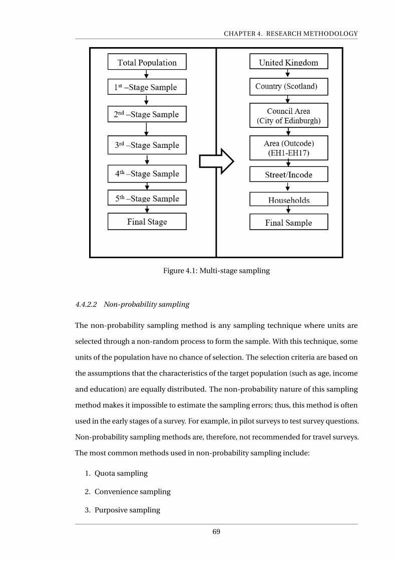
CHAPTER 4. RESEARCH METHODOLOGY
Figure 4.1: Multi-stage sampling
4.4.2.2 Non-probability sampling
The non-probability sampling method is any sampling technique where units are
selected through a non-random process to form the sample. With this technique, some
units of the population have no chance of selection. The selection criteria are based on
the assumptions that the characteristics of the target population (such as age, income
and education) are equally distributed. The non-probability nature of this sampling
method makes it impossible to estimate the sampling errors; thus, this method is often
used in the early stages of a survey. For example, in pilot surveys to test survey questions.
Non-probability sampling methods are, therefore, not recommended for travel surveys.
The most common methods used in non-probability sampling include:
1. Quota sampling
2. Convenience sampling
3. Purposive sampling
69

CHAPTER 4. RESEARCH METHODOLOGY
4. Volunteer sampling and
5. Judgement sampling
4.4.2.3 Summary of Sampling Methods
The generalisability of a study outcome to the larger population is achieved by minim-
ising all potential errors and biases in the survey (Comrey and Lee, 1992; Richardson et
al., 1995; Osborne and Costello, 2010; Field, 2013; Chaturvedi, 2015). Random sampling
is one of such ways to reduce observational errors and biases (Porter, 2011; Richard-
son et al., 1995, p.75, ). It is observed that non-random sampling methods, on the
other hand, often produce biased sample estimates and therefore not recommended
for transport surveys (Richardson et al., 1995; Chaturvedi, 2015). Consequently, all
the non-probability sampling methods, including systematic sampling method, were
deemed inappropriate on the above-stated grounds.
The major limitation of the simple random sampling method is its unsuitability for a
larger population. The study target population is in excess of 507,000, according to The
City of Edinburgh Council (2018). Therefore, considering the large size of the study
population, simple random sampling method is considered unsuitable.
Although multi-stage and cluster sampling methods are suited for a large population,
they tend to have higher sampling error and produce less accurate estimates (Fife Re-
search Co-ordinating Group, 2005). Therefore, given the generalisability requirement of
the study and the above limitations, multi-stage and cluster sampling methods were
considered inappropriate for this research.
Stratified random sampling method is very laborious and time-consuming. Neverthe-
less, it generates a representative sample and consequently, produce better estimates
(Fife Research Co-ordinating Group, 2005). Stratified random sampling also comes
with an added advantage of making it possible to apply weights to each sub-frame or
stratum to generate sample proportional to the size of each sub-frame. This charac-
teristic enhances the representativeness of the sample and the generalizability of the
survey results. Therefore, based on the above strengths, the stratified random sampling
70
CHAPTER 4. RESEARCH METHODOLOGY
method was adopted for this study. This will generate a representative sample from the
sampling frame and improve the generalisability of the study results.
4.4.3 Sample Size Estimation
The reliability of the results of structural equation modelling and factor analysis tech-
niques depends on the sample size used. Larger sample size produces highly reliable
results. However, at a higher cost to the study. On the other hand, too small sample will
lead to large variations in the sample estimates and produce less reliable results. The
adequacy of the sample size for a study is, therefore, a trade-off between the objective of
the study and resource availability (cost and time) (Richardson et al., 1995; Hutcheson
and Sofroniou, 1999). Several rules exist for the determination of sample size, including:
1. Simple rule of thump
2. Sample-to-variable Ratio
3. Central Limit Theorem
4.4.3.1 Simple rule of thump
A useful rule of thumb for estimating sample size adequacy for studies involving SEM
is generally about 200 cases (Kline, 2011), this is more acceptable when using robust
techniques like the Maximum Likelihood Estimator (MLE) (Kline, 2011; Zainudin, 2012;
Bahaman, 2012; Arbuckle, 2017). Others have suggested factors specific to individual
models or complex models sometimes may necessitate a threshold above 200 cases
(Kline, 2011). Consequently, several researchers recommended a minimum of 300 cases
as adequate for obtaining good results (Comrey and Lee, 1992) (Floyd and Widaman
1995; MacCallum, Widaman, Zhang, and Hong 1999). Comrey and Lee (1992), further
suggested that where resources allow, sample size of 1000 cases was ideal for getting
excellent results, while many researchers support this view, others suggest sample size of
500 cases and above is adequate to reduce sampling and inferential errors considerably
and at the same time improves the generalisability of the results (Richardson et al., 1995;
71

CHAPTER 4. RESEARCH METHODOLOGY
Osborne and Costello, 2010; Tabachnick and Fidell, 2012) A threshold of 300 cases is
adopted in this section for the following reasons;
1. 300 cases meet the minimum sample size requirement proposed by the two
groups of researchers.
2. MLE is employed for the CFA and ICLV, 300 cases satisfy the sample requirement
for using MLE (Bahaman, 2012; Arbuckle, 2017)
4.4.3.2 Sample-to-variable ratio
A general rule for estimating minimum sample size requirement for standard ordinary
least squares multiple regression analysis is the Sample-to-variable ratio (N:p) rule,
because of its ability to account for model complexity (Osborne and Costello, 2010;
Kline, 2011; Field, 2013). This method estimates the sample size as a function of the
number of variables. Sample-to-variable ratio (N:p) of 15:1 (15 responses to each
variable) has been recommended for the estimation of sample size (Velicer et al., 1998;
Osborne and Costello, 2010; Field, 2013). However, the sample size requirement for
statistical techniques like the CFA is contestable because it requires large sample (Kline,
2011). Conversely, since SEM is closely related to multiple regression in some respects,
15 cases per measured variable is suggested as reasonable for obtaining reliable results
(Loehlin 1992; Lehmann 1999). Kline (2011) proposed N:p ratio of 20:1 as ideal for
analysis involving SEM.
Osborne and Costello (2010) recommend sample-to-variable ratio (N:p) of 30:1 for
studies that seek to generalise the results to the study population. However, because
the ML estimator is adopted for analysis in this study, sample-to-variable ratio (N:p) of
15:1 is adopted for estimating the minimum sample size requirement. Table 4.1 below
shows the latent variables and the number of indicators developed to measurement
each:
72

CHAPTER 4. RESEARCH METHODOLOGY
Table 4.1: Latent Variables
Variable No. of Constructs
Norm 10
Ego/Narcissism 16
Affect 6
Total 32
From the table above, the highest number of constructs is 32; hence, we adopt 32 as
the number of variables (p) for the estimation of the sample size. Using sample to
variable ratio N:p of 15:1 Number of variables, p = 32 Cases/variable, N = 15 Sample
size (n) = N xp Sample size (n) = 15x32 Sample size (n) = 480
4.4.3.3 Central Limit Theorem
Another technique for determining sample size is the Central Limit Theorem (Richard-
son et al., 1995). According to Richardson et al. (1995), minimum required sample size
is estimated by solving for the standard error equation below:
s.e.(p) =√
((N −n)
N× p(1−p)
n) (4.3)
Solving the equation 4.3 above, the sample size (n’) becomes
n1 = p(1−p)
s.e(p)2(4.4)
The final sample size (n) is estimated by applying equation 4.5, population correction
factor
n = n1
(1+ n1
N )(4.5)
Where,
N = Population size
n1 = unadjusted sample size
n = Final sample size
(N−n)N = Population correction factor
s.e.(p) = Standard error
p = proportion of sample possessing a characteristic
73
CHAPTER 4. RESEARCH METHODOLOGY
The January 2018 edition of the Royal Mail address file contained 242,361 household
addresses in Edinburgh. Additionally, according to National Records of Scotland (2013),
39.9% of households in Edinburgh did not own a car. Therefore, using the central limit
theorem and the information above, the minimum sample size at 95% confidence level
is estimated as follows:
s.e.(µ) = confidence limitz ; s.e.(µ) = 5
1.96 = 2.55
n1 = 39.9(100−39.9)2.552 = 2397.99
6.5025 = 368.78
applying population correction factor;
n = n1
1+ n1N
; = 3691+ 368.78
242.361= 368.22 ≡ 368
Estimated minimum sample requirement according to the central limit theorem is 368.
4.4.3.4 Summary
Since the study seeks to understand the travel behaviour of the study population,
we need sample size sufficient enough to make the results generalisable to the study
population (Comrey and Lee, 1992; Richardson et al., 1995; Osborne and Costello, 2010;
Field, 2013).The highest minimum sample size estimated among the three methods
was 480 from the sample-to-variable ratio technique. This figure almost satisfies the
recommendation of 500 to 1000 for minimising sampling and inferential errors and
obtaining high generalisability (Richardson et al., 1995; Osborne and Costello, 2010;
Field, 2013). Therefore, sample size of 500 is adopted as the minimum requirement for
this study. Moreover, statistical techniques for measuring sample size adequacy such
as Kaiser-Meyer-Olkin (KMO) test and Bartletts test of sphericity will be subsequently
carried out after the survey to confirm the adequacy of the sample.
4.4.4 Sample Generation
Field (2013) defines a sample as "a smaller but hopefully representative collection of
units from a population used to determine truth about that population" (Chaturvedi,
2015; Field, 2013). The purpose of sampling is thus, to select a small group of people
from the population that have similar characteristics as the study population. This
74

CHAPTER 4. RESEARCH METHODOLOGY
makes it possible to draw conclusion or make inference about the population. This is
necessary because of the realisation that we deal with very large population in transport
studies of such nature (Richardson et al., 1995).
Similarly, there were 242,361 households in Edinburgh as at January 2018, according to
the January 2018 release of the Royal Mail PAF address data. Surveying the entire popu-
lation will not only be impossible but very expensive and time consuming (Chaturvedi,
2015). It is essential that the sample generated represent the characteristics of the study
population, Bias sample can lead to biased estimates and skewed modelling results
(Richardson et al., 1995).
4.4.4.1 Sampling units
The population for a survey is made up of several elements which may or may not be
the same as the units of interest (Richardson et al., 1995). The Population of the survey
is composed of residents of the city of Edinburgh above the age of 16. However, the
selection of sample for this study was based on the sample units listed below:
1. EH1-EH17 geographical area of Edinburgh
2. Postcodes and Households
4.4.4.2 Sampling frame
The sampling frame is defined by Richardson et al. (1995) as "a base list or reference
which properly identifies every sampling unit in the survey population". In other words,
it is a universal database from which potential respondents are drawn from. It must be
representative of the population (Chaturvedi, 2015). The sample frame is the universal
set of all the sample units in the survey population. Therefore, having defined the
population for the study and identified the sampling unit, it is necessary to define a
sampling frame from which the sample will be drawn. The sampling frame for the
survey includes:
1. PAF address data, January 2018 release.
2. Datazones - Scottish Index of Multiple Deprivation (SIMD) Postcode lookup table.
75
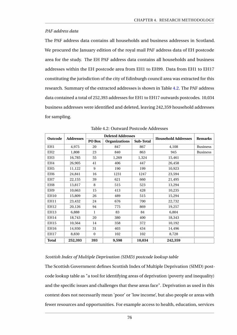
CHAPTER 4. RESEARCH METHODOLOGY
PAF address data
The PAF address data contains all households and business addresses in Scotland.
We procured the January edition of the royal mail PAF address data of EH postcode
area for the study. The EH PAF address data contains all households and business
addresses within the EH postcode area from EH1 to EH99. Data from EH1 to EH17
constituting the jurisdiction of the city of Edinburgh council area was extracted for this
research. Summary of the extracted addresses is shown in Table 4.2. The PAF address
data contained a total of 252,393 addresses for EH1 to EH17 outwards postcodes. 10,034
business addresses were identified and deleted, leaving 242,359 household addresses
for sampling.
Table 4.2: Outward Postcode Addresses
Outcode AddressesDeleted Addresses
Household Addresses RemarksPO Box Organizations Sub-Total
EH1 4,975 20 847 867 4,108 Business
EH2 1,808 23 840 863 945 Business
EH3 16,785 55 1,269 1,324 15,461
EH4 26,905 41 406 447 26,458
EH5 11,122 9 190 199 10,923
EH6 24,841 16 1231 1247 23,594
EH7 22,155 39 621 660 21,495
EH8 13,817 8 515 523 13,294
EH9 10,663 15 413 428 10,235
EH10 15,809 26 489 515 15,294
EH11 23,432 24 676 700 22,732
EH12 20,126 94 775 869 19,257
EH13 6,888 1 83 84 6,804
EH14 18,743 20 380 400 18,343
EH15 10,564 14 358 372 10,192
EH16 14,930 31 403 434 14,496
EH17 8,830 0 102 102 8,728
Total 252,393 393 9,598 10,034 242,359
Scottish Index of Multiple Deprivation (SIMD) postcode lookup table
The Scottish Government defines Scottish Index of Multiple Deprivation (SIMD) post-
code lookup table as "a tool for identifying areas of deprivation (poverty and inequality)
and the specific issues and challenges that these areas face". Deprivation as used in this
context does not necessarily mean ’poor’ or ’low income’, but also people or areas with
fewer resources and opportunities. For example access to health, education, services
76
CHAPTER 4. RESEARCH METHODOLOGY
and transport (Scottish Government, 2016). The SIMD is used as a tool for statistical
classification and as an indicator to target resources and policies to areas that need
them most. The SIMD divide Scotland into 6,976 areas called ’data zones’, using indicat-
ors like pupil performance, travel times to the GP, crime rate, unemployment rate and
many others. Each data zone in the SIMD is ranked from 1 (most deprived) to 6,976
(least deprived). The SIMD further classify the ’data zones’ into Percentile (100 groups),
vigintile (20 groups), decile (10 groups) and Quintile (5 groups) based on the initial
ranking (Scottish Government, 2016).
Using the postcode fields in SIMD postcode lookup table and the dataset extracted from
the PAF address data, the two datasets were merged to create the sampling frame. The
sampling frame was classified based on the definitions of SIMD vigintile (20 groups)
for sampling purposes. Each vigintile contains 5% of the data zones and represents a
stratum in our sampling frame. Table 4.3 shows the household addresses by outward
postcode and vigintile. 2,212 records from the extracted PAF address file could not be
found in the SIMD postcode lookup table and were consequently discarded from the
sampling frame. Table 4.4 presents a summary of the reclassified sampling frame by
strata (vigintile).
77
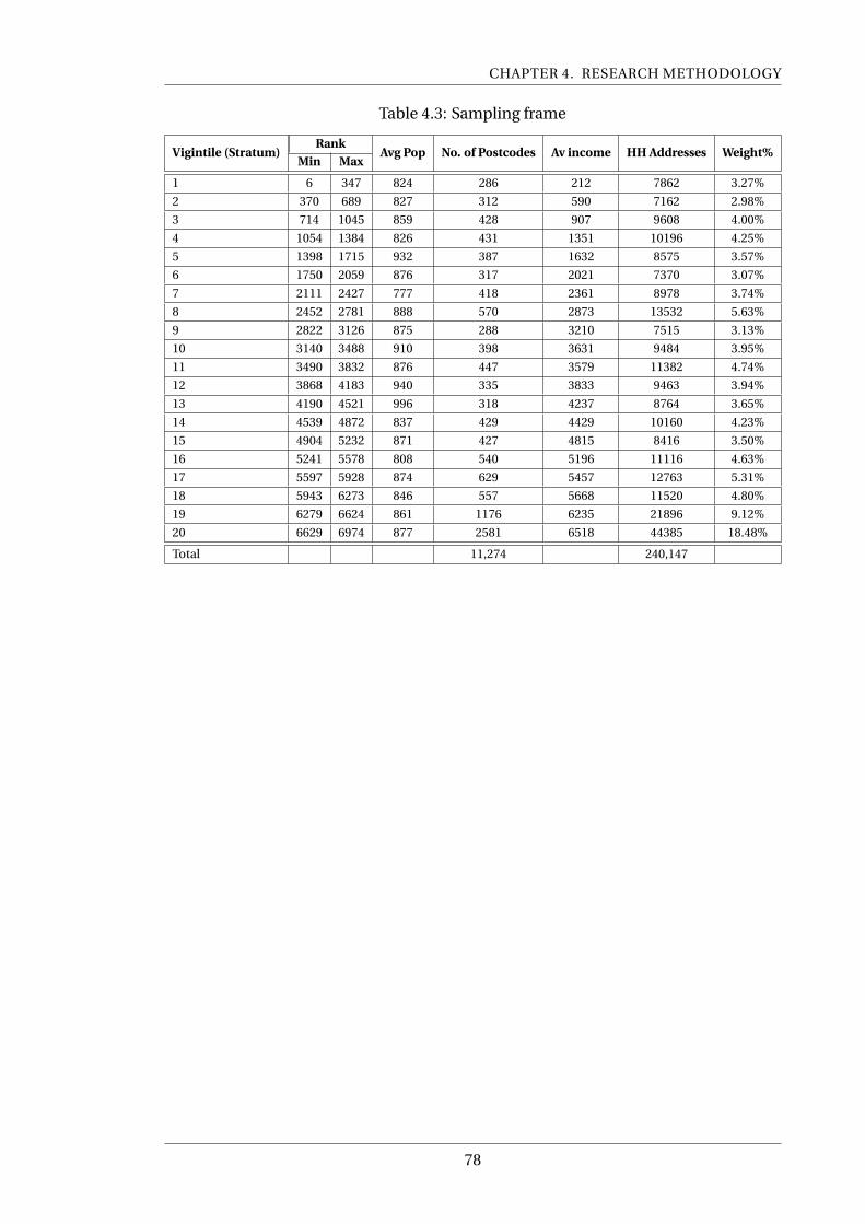
CHAPTER 4. RESEARCH METHODOLOGY
Table 4.3: Sampling frame
Vigintile (Stratum)Rank
Avg Pop No. of Postcodes Av income HH Addresses Weight%Min Max
1 6 347 824 286 212 7862 3.27%
2 370 689 827 312 590 7162 2.98%
3 714 1045 859 428 907 9608 4.00%
4 1054 1384 826 431 1351 10196 4.25%
5 1398 1715 932 387 1632 8575 3.57%
6 1750 2059 876 317 2021 7370 3.07%
7 2111 2427 777 418 2361 8978 3.74%
8 2452 2781 888 570 2873 13532 5.63%
9 2822 3126 875 288 3210 7515 3.13%
10 3140 3488 910 398 3631 9484 3.95%
11 3490 3832 876 447 3579 11382 4.74%
12 3868 4183 940 335 3833 9463 3.94%
13 4190 4521 996 318 4237 8764 3.65%
14 4539 4872 837 429 4429 10160 4.23%
15 4904 5232 871 427 4815 8416 3.50%
16 5241 5578 808 540 5196 11116 4.63%
17 5597 5928 874 629 5457 12763 5.31%
18 5943 6273 846 557 5668 11520 4.80%
19 6279 6624 861 1176 6235 21896 9.12%
20 6629 6974 877 2581 6518 44385 18.48%
Total 11,274 240,147
78

CHAPTER 4. RESEARCH METHODOLOGY
Tab
le4.
4:re
clas
sifi
edsa
mp
lin
gfr
ame
Vig
inti
leE
H1
EH
2E
H3
EH
4E
H5
EH
6E
H7
EH
8E
H9
EH
10E
H11
EH
12E
H13
EH
14E
H15
EH
16E
H17
Tota
l
186
421
214
1954
118
2495
316
2942
078
62
211
6514
9068
079
686
277
135
660
943
371
62
322
3360
410
2142
711
7488
876
231
230
118
8696
08
444
915
6416
6838
912
3114
9039
369
823
122
1019
6
559
096
326
068
089
414
6510
3925
812
9511
3185
75
613
8831
111
4119
8440
732
937
550
992
673
70
714
7128
021
8212
9927
1067
4641
742
914
6429
689
78
810
2320
771
836
135
8737
212
3826
6653
421
893
129
177
061
613
532
998
269
710
7310
0668
712
2111
8846
419
34
7515
1010
7017
442
024
5510
1410
6344
048
110
5196
535
194
84
1153
311
6439
912
8217
0198
037
522
6469
911
8243
230
341
1138
2
1294
2359
427
530
2047
576
440
505
929
841
183
532
9463
1310
2310
4694
814
1950
973
562
214
4335
46
240
6335
687
64
1464
1741
1640
623
118
6511
4830
611
8915
8310
160
1520
151
987
164
54
1588
771
422
5335
982
434
076
929
775
384
16
1621
495
872
332
785
516
3024
434
424
723
2865
911
5231
856
055
711
116
1774
812
0114
1997
662
871
712
0415
4412
0192
712
3696
212
763
1864
119
3186
092
399
195
278
581
711
7920
4839
311
520
1920
919
512
4541
9246
974
212
2811
0021
6316
9812
4213
3496
833
2050
712
3846
2189
6
2017
423
5190
7269
752
368
1715
5286
9540
1786
5284
1774
3365
1288
571
4438
5
No
tfo
un
d1
106
5814
215
045
213
395
138
251
926
912
320
382
2212
Tota
l41
0894
515
461
2645
810
923
2359
421
495
1329
410
235
1529
422
732
1925
768
0418
343
1019
214
496
8728
2423
59
79

CHAPTER 4. RESEARCH METHODOLOGY
4.4.5 Questionnaire Design
One of the main objectives of this study is to analyse travel behaviour of the study
population. The questionnaire consisted of several parts consisting of travel patterns
in terms of past, present as well as their future travel mode choice (next two years).
The latter was measured on a five-point Likert scale (very unlikely-very likely). The
study also seeks to analyse the respondents travel behaviour in the context of behaviour
economics particularly using elements of MINDSPACE as explanatory variables as such
the questionnaire included constructs developed to measure the elements proposed for
this study; norm, Affects, Narcissism, Salience. Additionally, questions on other possible
factors affecting travel mode choice were asked, including socio-demographic charac-
teristics et cetera. Each of which is expanded on below. Detail of the questionnaire is
presented in Appendix A
4.4.5.1 Transport Characteristics
This section of the questionnaire aims to understand respondents’ past and current
mode of travel including walking, cycling, motorcycle car and public transport (bus,
tram and rail) for daily trips such as working trips, shopping trips and leisure trips.
The frequency of the trips as well as travel time, cost, car ownership and accessibility
of public transport were also asked. Questions about respondents’ ability to use PT
for their daily trips and their perception about PT service quality and their overall
satisfaction with the PT service available.
4.4.5.2 MINDSPACE Variables
This section discusses the development of indicators for measuring the individual vari-
ables of MINDSPACE for inclusions as latent variables in a hybrid choice model. Since
the objective is to use the variables of MINDSPACE as latent variables in a hybrid choice
model, it was necessary to consider variables that could be measured with indicators.
The selection of variables to measure for the choice modelling was accordingly based
on: i) the existence of a metric or indicators for measurement. ii) The possibility of
80
CHAPTER 4. RESEARCH METHODOLOGY
measuring the variable with indicators, and iii) whether a variable could be measured in
the context of transport. Four out of the nine variables of MINDSPACE, namely; Norms,
Salience, Affect and Ego or Narcissism, were judged suitable based on the criteria above.
The following sections expatiate on the four selected variables.
Norms
Several studies have indicated that Norms has significant impacts on overt behaviour
(Schwartz, 1977; Cialdini et al., 1991; Bamberg et al., 2007). Cialdini et al. (1991) sugges-
ted that peer influence and approval from social group sustains behaviour and could
lead to behaviour change (Avineri, 2009; Hirshleifer, 1993). Schwartz (1977) found that
personal norms significantly influence behaviour than social norms. It is argued that
people feel morally obligated to act when their personal norms are activated. Therefore
to understand the influence of norms on travel behaviour (in the context of MIND-
SPACE), measurement indicators were developed to assess respondents’ perceived
social and personal norms.
The primary objective is to investigate the impact of norms on travel behaviour and
whether personal norms and social norms are of comparative significance to objective
factors (such as income, age, car ownership, travel time et cetera.) in transport choice
models (Schwartz, 1977; Bamberg et al., 2007; Belgiawan et al., 2016; Cialdini et al.,
1991; Avineri et al., 2009; Avineri, 2009). The questions included statements on the
general perception of cars/PT in society. For example, "Driving is perceived to illustrate
a person’s power, financial status in society and provide the driver/owner with a positive
self-image".
Finally, to measure "personal norms", respondents were asked about their perception
of cars/PT usage and their perceived expectation of others to use car/PT. For example,
"I think people should use public transport more for their work/educational journeys due
to the increasing levels of traffic congestion and air pollution in the urban centres", and
"I feel morally obligated to use more of public transport due to the impact of our travel
behaviour on health and the environment (global warming)". All the statements were
measured on a five-point Likert scale (1= Strongly Disagree; 5= Strongly Agree). Some
81

CHAPTER 4. RESEARCH METHODOLOGY
of the statements used were adapted from Bamberg et al. (2007) and Belgiawan et al.
(2015). Question 23 in Appendix A shows the measurement scale designed to measure
Norms.
Salience (PT User Experience)
The human memory of experiences is found to be governed by the most intense ’peak’
moments and final impressions in a chain of events (Kahneman, 2013). Information
that stands out and seems relevant affect human decision-making (Dolan et al., 2010).
Human behaviour is thus influenced by what comes to mind when evaluating options
in decisions making. The human memory of experiences is found to be governed by the
most intense ’peak’ moments and final impressions in a chain of events (Kahneman,
2013). Information that stands out and seems relevant affect human decision-making
(Dolan et al., 2010). Human behaviour is thus influenced by what comes to mind when
options are being considered for decision making.
Salience explains why unusual, extreme or unexpected experiences appear more signi-
ficant to the consumer. So, the most prominent (desirable or undesirable) experience
with a travel mode can have a disproportionate influence on behaviour.
The most remarkable experience, such as any incidents of passenger annoyance or
anti-social behaviour experienced by a passenger on a bus could have a profound
consequence on their future travel behaviour (Kahneman, 2013). Such undesirable
experiences create negative valence (Resnick, 2012) and negatively reshape future travel
decisions (Dobbie et al., 2010; Metcalfe and Dolan, 2012).
Therefore, this variable seeks to investigate the public transport user experience and
its effects on ridership. A survey instrument is designed based on reported passenger
experiences on public transport (Dobbie et al., 2010; Beirao and Cabral, 2007). The
instrument is in two parts; in the first part, respondents were asked to indicate how
discouraging they will be if they encounter the outlined experiences on public transport.
Indicators for this effect are measured on a five-point Likert scale (1=Not Discouraging,
5=Very Discouraging). Whiles the second part requests respondents to evaluate the
extent to which the experiences could affect or have affected their loyalty to public trans-
82
CHAPTER 4. RESEARCH METHODOLOGY
port. This aspect of the tool is measured on a five-point Likert scale (1=Not at all, 5=Very
much). The experiences investigated includes; "Anti-social behaviour (drunk people
et cetera)", "Poor hygiene (service uncleanliness and smell on the buses)", "Inaccurate
bus and real-time information". Question 20 in Appendix A presents the measurement
instrument for this construct.
Affect
This section seeks to understand the role of Affect on respondents’ travel choices. Affect
is defined as "an automatic response to a good or bad experience". Affect is an omnibus
term and refers to four different states; Sentiments, Moods, Emotions and Affective
Styles (Davidson et al., 2009). These affective states could have a transient or lasting
effect on the subject and can influence behaviour consciously and unconsciously. This
discussion is limited to the affective state of sentiment and its influence on travel beha-
viour for this study.
Sentiment is an emotion an individual attaches to a product as a result of his/her in-
teraction with the product. This could be described either as positive valence (such as
satisfaction or joy) or negative valence (such as embarrassment, anger or frustration)
(Resnick, 2012). Loewenstein (2000) suggest that intensely negative sentiments can be
very influential and can overrule otherwise rational plan of action even in the presence
of cognitive information that would suggest alternative courses of action (Loewenstein
et al., 2001). Sentiment attached to a product becomes difficult to detach and influences
the desirability of the product (Rozin et al., 1986). Elster (1998) found that decision-
makers also evaluate their choice sets emotionally aside economic utility.
The study, therefore, hypotheses that the sentiments associated with public transport
by users could impact its desirability or ridership negatively or positively. To this, the
study developed a measurement scale to investigate public transport user sentiment
and its impact on ridership. Inspired by the findings in Elster (1998) and Han and Lerner
(2012), an instrument was designed to measure respondents sentiments towards PT.
The measurement indicators include; "I feel uncomfortable travelling in the local bus
with strangers", "I am happy using public transport because I can use the travel time for
83
CHAPTER 4. RESEARCH METHODOLOGY
other activities". Participants were requested to indicate the extent to which they agree
or disagree with each of the statements on a five-point Likert scale with endpoints (1 =
Strongly Disagree; 5 = Strongly Agree). Refer to question 21 in Appendix A for the full
measurement tool.
Narcissism or Ego
Narcissism has recently attracted a lot of research attention. Several studies have in-
vestigated the impact of narcissism on consumer behaviour (Cisek et al., 2014; Morf
and Rhodewalt, 2001; Graves, 1968). Literature suggests that the consumer behaviour
of a narcissist is based on the symbolism of consumer products rather than utility
maximisation (Cisek et al., 2014; Gregg et al., 2013; Sedikides et al., 2007). Therefore
the study hypothesis that "narcissist will select transport modes that will enhance their
social identity and sense of uniqueness." Raskin and Terry (1988) developed a 40-item
Narcissism Personality Inventory (NPI-40)for measuring narcissism as a personality
trait. NPI-40 scale consists of forty paired statements for respondents to select the
statement they closely related to their feeling. NPI-40 was subsequently refined to a
16-item scale referred to as NPI-16 by Ames et al. (2006). The author developed the
16-item scale (NPI-16) out the original 40-item measurement scale.
However, very little is known about the relationship between narcissism or ego and
travel behaviour (Metcalfe and Dolan, 2012; Aczél and Markovits-somogyi, 2013). There-
fore, NPI-16 is adapted and included in the survey to measure the narcissism score of
respondents and investigate its relationship with their travel behaviour. The NPI state-
ments adapted include; "I like having authority over people", "I find it easy to manipulate
others" and "I am apt to show off if I get the chance". All the statements were measured
on a five-point Likert scale with the following defined endpoints; 1 = Strongly Disagree
and 5 = Strongly Agree. Refer to question 24 of Appendix A for the NPI measurement
scale.
84

CHAPTER 4. RESEARCH METHODOLOGY
4.4.5.3 Socio-Demographic Characteristics
The survey instrument was concluded with questions on respondent’s demographics.
This section seeks to acquire information necessary to understand respondent’s socio-
economic status. Demographic questions relating to the following information were
posed to participants; gender, age, marital status, highest education level and annual
income (household) as well as employment status and household size. This information
is used in conjunction with other relevant factors to investigate travel mode choices.
4.4.6 Pilot Survey
Pilot surveys were conducted to assess the appropriateness of the survey instrument
concerning clarity, logical sequence, length and to solicit experts’ feedback before doing
the main survey. The pilot survey was in two phases involving:
• Phase one: Solicit expert opinion and feedback on the suitability of the draft
survey instrument discussed in the preceding section.
• Phase two: Collect sample data from a small sample among the study population
after the expert review to assess respondents understanding of the questions,
assess the adequacy, validity, and reliability of the constructs for measuring the
behavioural variables.
4.4.6.1 Expert Interview
Before the pilot data collection, experts opinions were solicited on the suitability of the
data acquisition instrument. One of the major concerns at the stage was the identific-
ation of qualified participants. Hence, a purposive sampling technique was applied
for the selection of participants for this purpose. The main criteria for the selection
were the theoretical perspective of the study and the knowledge and research area of
the participants.
The purpose of the survey was to acquire participants opinion of the survey instrument
and identify potential pitfalls and consequently, improvements in the wording and
presentation of the questionnaire.
Four experts were selected and contacted to participate in the survey and interview,
85
CHAPTER 4. RESEARCH METHODOLOGY
Four experts from the fields of Psychology, transport psychology, transport economics
and transport planning participated in the survey and provided feedback on the various
parts of the survey instrument. One of the expert participants highlighted and discour-
aged the use of double-barrelled questions, most notably among the psychometric
indicators; consequently, some of the psychometric indicators were revised.
4.4.6.2 Pilot Data Collection
A simple pilot survey was conducted to test the survey instrument before the actual
survey. The survey was intended to assess respondents understanding of the questions,
to help improve the questionnaire and assess the validity and reliability of the constructs
for measuring the behavioural variables. The survey was conducted among research
students and staff of the Edinburgh Napier University, and friends in October 2017 using
QuestionPro online survey software. A total of 60 people were selected at random and
invited to take part in the survey.
Again, the purpose of this pilot survey was to acquire respondents’ opinion about the
survey instrument and to identify potential drawbacks in the survey instrument to
improve the questionnaire. Additionally, to assess the validity and reliability of the
survey instrument and to establish the duration for the survey.
4.4.6.3 Results of the Pilot Survey
In general, the pilot survey indicated that the respondents reasonably understood the
questionnaire, the questionnaire was clear, logical, and the presentation was satisfactory.
Out of the 60 invited people to participate in the survey, 45 participants representing
75% of the number contacted completed the survey. The finding of the pilot survey and
the problems noted in the questionnaire are presented below.
86

CHAPTER 4. RESEARCH METHODOLOGY
Table 4.5: Descriptive statistics
Education Employment Status Modal ShareNone 2.2% Students 7% Walking 21%
High School 18.7% Employed (FT) 51% Bicycle 9%
College 15.1% Employed (PT) 15% Car 31%
Bachelors 36% Retired 22% Public Transport 38%
Masters 23.7% Unemployed 5% Other 1%
PhD 3.6%
Table 4.5 shows that 31% and 38% of respondents of the pilot survey were found to be
car and PT users, respectively. The estimates did not deviate from similar statistics from
the Transport Scotland statistics, which reports 29% for car users (Transport Scotland,
2017). Consequently, the Transport Scotland (2017) figures were adopted for estimating
the minimum sample requirement for the study. Some respondents were concern about
the length of some of the questions, the length of the instrument and the duration of
the survey.
4.4.6.4 Final Questionnaire Design
After the pilot survey, it was observed that respondents understood the wording and
layout of most of the questions. However, following the concerns about wordy questions
and overall length of the survey, some of the questions were rephrased and other omitted
to reduce length and time required for the survey. Moreover, respondents were noted be
consistent in their responses to the psychometric indicators for measuring narcissism.
Following this, it was decided to change the layout and format of this part of the survey
instrument to better capture respondents’ responses more accurately, this is presented
the following paragraphs. The final version of the questionnaire is included as Appendix
A.
1. Age: A text box was provided for respondents to supply their age instead of
selecting from a predefined age band.
2. Narcissism: Respondents were presented with a list of 16 pairs of opposite state-
ments, one in Column A and the opposite in Column B. respondents were then
87

CHAPTER 4. RESEARCH METHODOLOGY
asked to select statements from either column that best describe them (Ames
et al., 2006). However, it was observed that almost all respondents selected the
same answer, possibly due to the negative undertone of the statements (Sam,
2011). Consequently, this section of the measurement instrument was revised
for respondents to indicate the extent to which they identify with each of the nar-
cissistic statements on a five-point Likert scale (1= Strongly Disagree, 5= Strongly
Agree).
4.5 Method of Data Analysis
4.5.1 Introduction
Statistical analysis is carried out on the sample data to explore the possible relation-
ships among the variables. Kruskal-Wallis Test and Mann Whitney U-test were used to
investigate the relationship between active travellers, cars users and public transport
users. Exploratory factor analysis (EFA) and confirmatory factor analysis (CFA) were
conducted using SPSS statistical package and AMOS Structural equation modelling
(SEM) software package, respectively. Additionally, Integrated choice and latent variable
model (ICLV) was developed using Pandas Biogeme software (Bierlaire, 2018b; Bierlaire,
2018a). These statistical measures are briefly discussed below.
4.5.2 Kruskal-Wallis Test and Mann Whitney U-test
The Kruskal-Wallis Test and Mann-Whitney U test are non-parametric methods for
comparing independent samples of equal or different sample sizes (McKight and Najab,
2010; Singh et al., 2013). A Mann-Whitney U test (sometimes referred to as Mann-
Whitney-Wilcoxon test or the Wilcoxon rank-sum test) allows analysis to be run on non-
normally distributed data (Singh et al., 2013). A Mann-Whitney U test puts everything in
terms of rank rather than the raw values; this allows analysis to be run on non-normally
distributed data (Chan, 2003). The test ranks everything, sums the ranks and ultimately
produces a statistic which indicates whether the two (or more) sub-populations within
88

CHAPTER 4. RESEARCH METHODOLOGY
the sample likely came from the same underlying population. The major difference
between the Mann-Whitney U and the Kruskal-Wallis H is that the former can handle
only two categories whiles the latter can accommodate more than two groups (Vargha
and Delaney, 1998).
4.5.3 Factor Analysis
Factor analysis (FA) is a statistical technique for transforming a multivariate observation
in a dataset into single or smaller variables or principal factors (latent variables). A
latent variable is an unobserved underlying concept that influences the responses
of two or more of the observed variables (Chong et al., 2014). The latent variables
also account for the correlations between these observed variables (Brown and Moore,
2012). FA therefore assist in establishing the underlying relationship between the latent
constructs and their observed multivariate variables. This produces a more manageable
and understandable variables or factor capable of defining a psychological concept or
behavioural traits (Richardson et al., 1995). Factor analysis provides a useful tool for
investigating the reliability and validity of the measurement constructs used. It is quite
robust in handling very complex sets of data and relationships involving psychological
concepts and unobserved variables. For instance, a person’s level of ’ego’ or ’subjective
norm’ cannot be measured directly by a single indicator question. These concepts
and others of similar nature can only be measured using multiple indicator questions.
Factor analysis is required for confirming the questions measuring the latent constructs
and establish their validity and reliability. There are two forms of factor analysis, namely
Exploratory Factor Analysis (EFA) and Confirmatory Factor Analysis (CFA) (Joreskog,
1969) cited in (Brown and Moore, 2012). It is a very useful tool for consolidating large
number of variables into relatively fewer constructs capable of explaining complex
phenomenon.
89
CHAPTER 4. RESEARCH METHODOLOGY
4.5.3.1 Exploratory Factor Analysis
Exploratory Factor Analysis (EFA) is a descriptive data reduction technique that is used
in the development and validation of assessment instruments (Ruscio and Roche, 2012).
EFA is thus used to explore the data to determine the number of dimensions present in
the dataset and the extent of the relationship between the observed indicator variables
and the unobserved underlying latent construct (Byrne et al., 2012). The main objective
of EFA is to reduce of the number of dimensions in the original data (Baglin, 2014).
However, the decision concerning the number of factors to retain in the factor analysis
is arguably most important than the rotation and extraction method to adopt Zwick
and Velicer, 1986. Evidence indicates that over-extraction or under-extraction can affect
the measurement scale and significantly alter the factor solution and interpretations
of the EFA results (Schönrock-adema et al., 2009; Velicer et al., 2000; Courtney, 2013).
Therefore, the estimation of the number of factors to retain during EFA is of utmost
importance and must be handled with care. There are several methods for estimating
the number of factors to retain, the most popular methods include: eigenvalue greater
than one rule (KI rule), the Scree test, Parallel Analysis, et cetera.
In general, the KI rule theorises that factors with eigenvalue greater than 1 should
be retained and those with eigenvalue below 1 rejected (Kaiser, 1960). The KI rule is
the default procedure for determining the number of factors to retain in EFA in most
statistical softwares, notwithstanding, the approach has been criticised as being too
restrictive for models with many variables. Additionally, the rationale for retaining
a factor with eigenvalue of 1.01 as important and a factor with eigenvalue of 0.99 as
insignificant is questioned (Courtney, 2013; Garrido et al., 2013).
Cattel’s scree plot approach lists all eigenvalues in decreasing order and plot a graph
of the eigenvalues on the y-axis and all the factors on the x-axis (Cattell, 1966). The
rationale is to retain all factors above a point of inflexion or elbow. Since it is believed
that a few major factors will account for the most variance, resulting in a "cliff", followed
by a "scree" of minor factors with relatively small variance. Zwick and Velicer (1986)
90

CHAPTER 4. RESEARCH METHODOLOGY
found that this method performs better than the KI rule, but further alluded that the
selection of the number of factors to retain can be subjective when there is no clearly
defined inflection point especially when there is minimal variation in the estimated
eigenvalues (Garrido et al., 2013; Courtney, 2013).
The Parallel Analysis (PA) method is developed based on the KI rule (Garrido et al., 2013;
Horn, 1965). PA accounts for the proportion of variance resulting from sampling error.
It is one of the highly recommended techniques for estimating the number of factors to
retain in EFA (Horn, 1965; Zwick and Velicer, 1986; Courtney, 2013; Ruscio and Roche,
2012; Garrido et al., 2013). The PA method generates a large number of data matrices
at random. Each matrix is generated with the same number of cases and variables as
the sample data under investigation to estimate eigenvalues. Factors from the EFA with
eigenvalues greater than the eigenvalues of the PA should be retained (Horn, 1965).
Total Variance Extracted is another selection method. The literature varies on how much
variance should be explained before the number of factors is sufficient. While several
researchers recommend factors to account for between 75 - 90% of the variance, others
indicate a minimum of 50% is acceptable. The amount of variance explained by the
extracted factors must adequately represent the data and theory (Beavers et al., 2013;
Schönrock-adema et al., 2009). The following recommendations are adopted for the
EFA:
• Extraction method: ML extraction
• Factor retention method: Combination of KI, PA and Total variance extracted
methods
• Rotation: Oblique rotation (preferably Promax to generate correlated factors)
4.5.3.2 Measures of Sampling Adequacy
Several statistical test are required to establish the suitability and validity of the data for
factor analysis before factor extraction is executed, Kaiser-Meyer-Olkin (KMO) test and
91
CHAPTER 4. RESEARCH METHODOLOGY
Bartletts test of Sphericity are the recommended statistical techniques for the task of
assessing the adequacy and suitability of the data for factor analysis prior to extraction
(Williams et al., 2010).
Kaiser-Meyer-Olkin Test: Kaiser-Meyer-Olkin (KMO) measure of sampling adequacy is
based on the correlation matrix and tests the adequacy of the sample for factor analysis,
it tells whether there are sufficient items for each factor regarding the partial correl-
ations among the variables or distribution of the value for the application of factors
analysis (Kaiser, 1970; Kaiser, 1974; Williams et al., 2010). Kaiser-Meyer-Olkin (KMO)
index of factorial simplicity ranges between 0 and 1 with an index above 0.5 considered
suitable for factor analysis (Kaiser, 1970; Williams et al., 2010). Kaiser (1974) defined
the following levels of evaluation of KMO index of factorial simplicity as follows; index
below 0.5 as unacceptable, index between 0.5-0.7 as mediocre, index between 0.7-0.8
as good, index between 0.8-0.9 as meritorious and index above 0.9 as excellent (Kaiser,
1974; Hutcheson and Sofroniou, 1999; Field, 2013). 0.5 is the boundary line of accept-
ability and so KMO index below 0.5 is unacceptable and suggest that the sum of the
partial correlation among variables is very large relative to the sum of the correlations,
suggesting diffusion in the pattern of the correlation and therefore factor analysis would
not be valid, on the other hand, KMO index above 0.5 and approaching 1 suggests that
the pattern correlation are compact, hence factor analysis would produce unique and
reliable factors (Kaiser, 1974). KMO index of factorial simplicity of 0.7 (good) is adopted
for this study.
Bartletts test of sphericity: The Bartlett’s statistics test the sufficiency of the level of
correlation of the original variables and determine whether the correlation matrix is
significantly different from an identity matrix. Smaller p-value (i.e. p < 0.05) indicates
that the data is adequate for factors analysis; thus, the test establishes the existence
of correlation between the variables (Field, 2013). The success of the Bartlett’s test of
sphericity depends on the sample size.
92
CHAPTER 4. RESEARCH METHODOLOGY
4.5.4 Structural Equation Modelling
Structural equation modelling (SEM) is another name for Latent variable and path
analysis, structural analysis, and causal modelling. SEM is a technique for testing
hypothesis about the relationship between observed multivariate variables and the
unobserved underlying concepts (latent variables) (Maruyama, 1998a; Miles, 2005).
This method of modelling uses statistical techniques for investigating the relationship
between unobserved (latent) variables or construct measured by multiple manifest
(observed) indicators variables (Khine, 2013). SEM combines regression analysis and
factor analysis to offer convenient means of studying complex patterns of relationship
in data and simultaneously estimate both discrete choice and latent variable aspect of a
model. SEM can also model the latent construct separately (Steenkamp and Baumgart-
ner, 2000). The purpose of this modelling approach is to describe the structure of
data and simplify it for easy understanding and interpretation, hence specifying the
relationship between variables in a data (Muthén and Muthén, 2010). In behavioural
science, researchers are often interested in studying hypothetical constructs that cannot
be observed directly. These abstract phenomena are termed latent variables i.e. com-
fort, safety, flexibility, convenience, norms, ego commitment, affects et cetera. Since
these variables cannot be measured directly with a single indicator variable, they are
measured using multiple observable variables that explain them (Byrne et al., 2012).
SEM also offers the researchers the opportunity to assess the validity and reliability of
data under investigation.
4.5.4.1 Confirmatory factor analysis
Confirmatory factor analysis (CFA) is a technique for testing hypotheses based on the
framework of structural equation modelling (SEM) (Bryne, 2012; Miles, 2005; Maruyama,
1998b; Hoyle, 1995). CFA is employed to confirm and validate the latent constructs
specified during the EFA. The main advantage of using CFA is that the factor-solution is
useful for further advanced analysis (Discrete choice modelling, et cetera.). Confirm-
atory factor analysis in AMOS program was used for confirming the latent constructs
93
CHAPTER 4. RESEARCH METHODOLOGY
obtained during the initial EFA analysis. As discussed under section 6.7: Missing Data
Treatment, Maximum Likelihood Estimator (MLE) available in SPSS and AMOS software
packages was adopted for both the EFA, the CFA and the Choice Modelling (Muthén
and Muthén, 2010; Temme et al., 2008b).
Evaluation of CFA and SEM: After the exploratory factor analysis, it is essential to es-
tablish the suitability of every variable and all latent constructs in the measurement
model before undertaking any further analysis. The following assessments are done
prior to the SEM or CFA operation; test of Unidimensionality, test of validity and the
reliability test.
Unidimensionality: Unidimensionality refers to the situation where observed factors
load satisfactorily on their respective latent construct. It is recommended for a newly
developed item to have factor loading of 0.5 or higher and 0.6 or higher for an already
established item. Any observed variable with factor loadings less than the threshold
above must be deleted from the measurement model
Validity: Validity is the ability of an instrument to measure what it is designed to meas-
ure. This is established using CFA (Joreskog, 1969). CFA establishes the uniqueness of
each latent construct and the extent to which each pair of latent constructs share their
variance. Three procedures have been developed for assessing the overall validity of
latent variables; convergent validity, divergent validity and construct validity, (Campbell
and Fiske, 1959; Fornell and Larcker, 1981; Bagozzi, 1988; Shiu et al., 2011; Bahaman,
2012).
Convergent validity assesses the extent to which the indicator variables explain the
variation in their latent construct. According to Fornell and Larcker (1981), convergent
validity can be assessed by computing the Average Variance Extracted (AVE) for each
latent construct. The AVE measures the average amount of variation a latent construct
explains in its observed variables. In other words, AVE is the correlation between a latent
construct and its observed variables. For instance, if a latent variable A is measured
by variables x1, x2 and x3, then A should correlate with x1, x2 and x3. This correlation
94
CHAPTER 4. RESEARCH METHODOLOGY
(Li) between A and its observed variables is the factor loading. The square of each
correlation explains the amount of variation in each observed variable that the latent
construct accounts for. The AVE of the latent construct is thus, the average of all the
sum of the squared correlation/factor loading measuring that construct (Fornell and
Larcker, 1981; Farrell, 2010; Bahaman, 2012). Mathematically, AVE can be expressed as:
AV E = ΣLi 2
n(4.6)
Where;
Li: Factor loading for every indicator variable
n: Number of variables in the latent constructs
Simply stated, variables used for measuring the same construct should strongly con-
verge on the construct. To achieve convergent validity, the value of the AVE computed
for each latent construct must be greater than 0.49 (Fornell and Larcker, 1981) and
the factor loading for each indicator variable for the construct must also be greater
than 0.50. The rationale behind the above condition is that, measurement error should
not be greater than the variance explained by the latent construct (AVE less than 0.50)
(Rourke and Hatcher, 2013).
Discriminant validity is analogous to testing for multicollinearity among independent
variables in a multivariate analysis. It establishes the distinctiveness of each latent
variable from other latent variables within a CFA model (Bahaman, 2012). It meas-
ures the inter-factor correlation in a pooled measurement model. The fundamental
justification for this procedure is that every latent variable should be unique and not
correlated highly with other latent constructs. Theoretically unrelated constructs should
not correlate with each other in the measurement model (Fornell and Larcker, 1981;
Shiu et al., 2011; Bahaman, 2012). A test displays discriminant validity when it can be
demonstrated that it is not measuring a construct that it was not designed to measure.
Indicators designed to assess one latent construct should not be measuring a different
latent construct (Rourke and Hatcher, 2013). Three methods have been proposed and
widely accepted for assessing divergent validity in CFA (Shiu et al., 2011).
95
CHAPTER 4. RESEARCH METHODOLOGY
The first procedure is the average variance extracted (AVE) versus shared variance test.
According to Fornell and Larcker (1981), discriminant validity is assessed by comparing
the average variance extracted (AVE) for every latent construct and its shared variance
with other latent constructs in the measurement model. The AVE of each latent con-
struct should be higher than the value of the squared correlation (shared variance) with
any other latent constructs in the model (Fornell and Larcker, 1981; Shiu et al., 2011).
The fundamental justification for this procedure is that every latent variable should
be unique, having a strong correlation with its indicator variables than with any other
latent variable in the model, also the correlation involving other latent variables should
be smaller than 0.85 (Bahaman, 2012).
The second procedure, the paired constructs test, is attributed to Bagozzi and Phil-
lips (1982) and Anderson and Gerbing (1988). The test compares the chi-square value
between a constrained model (the parameter estimates for two factors is constrained
to 1.0) and an unconstrained model (the parameter estimates are freely estimated) for
each pair of constructs. Discriminant validity is achieved if the difference in chi-square
value is more than 3.84 (Bagozzi and Phillips, 1982; Farrell, 2010; Shiu et al., 2011). The
third procedure also proposed by Bagozzi et al. (1991), estimates the confidence interval
for the correlations between the latent variables. If the 95% confidence interval for
the correlation between a pair of latent variables contains zero but not unity, then the
pair of latent variables are distinct and discriminant validity is achieved. The last two
procedures consider sampling error in determining discriminant validity (Shiu et al.,
2011).
A review by Shiu et al. (2011), on divergent validity found the Fornell-Larcker criterion
for evaluating divergent validity (Fornell and Larcker, 1981) as the widely accepted and
used procedure in literature (Henseler et al., 2014). Consequently, the first method is
adopted for assessing the validity of the latent constructs in this study.
Construct validity is achieved when the Fitness Indexes for a construct achieves the
required level.
96

CHAPTER 4. RESEARCH METHODOLOGY
Reliability: The reliability of an indicator variable is defined by Rourke and Hatcher
(2013) as "the square of the correlation between a latent factor and its indicators or the
percent of variation in the indicators that is explained by the factor it is supposed to
measure". Thus, reliability measures the internal homogeneity of the measurement
instrument (all indicators) used for measuring a construct. It evaluates how much
of the variation in scores is attributable to random error. Similarly, an instrument is
said to be reliable if it produces consistent scores upon repeated administration or by
alternate forms. The following tools are used for assessing the reliability of construct
and their indicator variables; Average Variance Extracted (AVE), Coefficient alpha (α)
and Composite reliability (CR).
Average Variance Extracted: A measurement scale is reliable if the Average Variance
Extracted (AVE) > 0.49. (for details; refer to the section under validity)
Coefficient alpha: The coefficient alpha (α) is the estimation of the internal consist-
ency of a multiple-item scale and a measure of the reliability of the measurement scale
(Cronbach, 1951). For internal reliability, coefficient alpha (α) (Cronbach’s Alpha in
SPSS) of 0.70 is an adequate indication of the internal consistency of the latent variable
(Kline, 2011).
Composite reliability: The composite reliability index (CR) is comparable to the coeffi-
cient alpha and reflects the internal consistency of observed indicators measuring the
latent construct. Composite reliability is achieved if CR ≥ 0.70. Composite reliability is
estimated with the formula below:
C R = (ΣLi )2
[(ΣLi )2 +Σ(1−Li 2)](4.7)
Where;
Li = Standardize Factor loading of every indicator variable
1−Li 2 = error variance of every indicator variable Var(Ei)
Assumptions
The reliability of structural equation modelling like statistical procedures such as gener-
alized least-squares estimation depend on the data satisfying some basic assumptions.
97

CHAPTER 4. RESEARCH METHODOLOGY
First of all, the sample size must be adequate. Secondly, the observations must be
independent and finally, the data must meet multivariate normality assumption (Kline,
2011; Bahaman, 2012; Arbuckle, 2017).
Sample Size Adequacy: (Refer to sub-section 4.4.3 for details)
Multivariate normality: In many statistical procedures, such as linear regression and
generalised least squares, the distribution assumption is that the residuals should be
normally, identically and independently distributed (Kline, 2011; Arbuckle, 2017). This
is necessary to produce valid estimates of the coefficients and p-values for the t-tests.
Violation of this assumption will result in invalid estimates, biased coefficients and mis-
leading results. This assumption also holds for CFA and structural equation modelling.
The normality of the data needs to be evaluated after assessing the fit indexes during
the CFA before conducting any further analysis (Kline, 2011; Arbuckle, 2017; Bahaman,
2012).
Normality is assessed by evaluating the skewness value for each item and the multivari-
ate kurtosis statistic. Normality is achieved when the absolute value of skewness is not
greater than 1.0. However, Maximum Likelihood Estimator (MLE) is robust to skewness
and multivariate kurtosis statistic violation, if the sample size meets the minimum
threshold (Bahaman, 2012). Thus, we could proceed with the CFA when the sample
size is large enough, even when the data fails the normality test (refer to section 4.4.3)
(Bahaman, 2012).
Assessing normality in Amos: One of the techniques useful for identifying outliers when
multivariate normality assumption is violated is the Mahalanobis distance (Mahalan-
obis, 1936). Mahalanobis distance is the estimate of the deviation of each observation
from the centroid of the dataset. The farthest observation from the centroid of the
dataset defines potential outliers. Outliers are observation too far from the centroid
compared to majority of cases in the dataset. We may delete any observation with
Mahalanobis distance having a low p-value (p < .001) (Kline, 2011; Bahaman, 2012).
98

CHAPTER 4. RESEARCH METHODOLOGY
Extreme outliers are called influence because of the impact they have on the model
estimates. Deleting influence in the dataset could substantially change the estimate of
coefficients. Notwithstanding, we can retain outliers and influence and continue with
the CFA if; 1) the method of estimation used is the Maximum Likelihood (ML) and 2)
Bootstrapping is used to confirm and validate the results (Bahaman, 2012). Moreover,
since ML is adopted for the model estimation, this condition is ignored.
Model Fit Statistics
Structural equation modelling and CFA, unlike traditional statistical methods, utilise
several fitness statistics to evaluate how well the hypothetical model explains the data,
known as model fit. These statistics examines whether the covariance matrix of the
hypothetical model of the researcher is close enough to the covariance matrix of the
data under investigation. Reasonable disparities might be attributed to sampling error.
Otherwise, the researcher must explain the differences if they exceed a recommended
threshold or the hypothetical model should be rejected for failing to explain the data
(Kline, 2011).
The knowledge of which model fit indices to report and the thresholds to adopt is
essential in the application of structural equation modelling. Model fit indices and
threshold to report has stimulated debate among researchers in the field of structural
equation modelling (Kenny and McCoach, 2003; Marsh et al, 2004). (Barrett, 2007). Hu
and Bentler (1999) appraised the fit indices with their thresholds and recommended
the following indices RMSEA, CFI, SRMR, NNFI and TLI.
A similar study by McDonald and Ho (2002) supported Hu and Bentler (1999) in part;
the authors found CFI, GFI, NFI and NNFI were widely reported in the literature and
recommended them. A review by Hooper et al. (2008) on fit indices also recommen-
ded the RMSEA, SRMR, CFI, one parsimony index like PNFI and the model chi-square
with its degree of freedom and p-value. Hayduk et al (2007) and Kline (2011) support
the assertion of Hooper et al. (2008) concerning the reporting of the chi-square stat-
99

CHAPTER 4. RESEARCH METHODOLOGY
istics. However, (Kline, 2011) further explained that the chi-square statistics should
only be reported if the Maximum Likelihood (ML) is not the estimation method used.
Several authors, including Arbuckle (2017) recommend reporting the relative/normed
chi-square statistic instead of the chi-square statistic because the latter is sensitive to
sample size. However, Kline (2011) disagrees with Arbuckle (2017) on the reporting of
relative/normed chi-square statistic. According to Kline (2011), chi-square sensitivity to
sample size only applies to incorrect models.
The fit indices can be categorised into three main groups, namely, absolute fit indices,
incremental fit indices and parsimonious fit indices. Hair et al. (2010) recommend
reporting at least one index from each category because each give different inform-
ation about the model. They provide a more reliable evaluation of model fit when
used together (Brown and Moore, 2012). Because it is not practical to report every
index reported by the Amos SEM software, it is reasonable to select indices based on
the recommendations above, while ensuring representation from each of the three
categories. Thus, we limit the scope of this review to the universally recommended
indices for assessing model fit, namely, RMSEA, GFI, CFI, NFI, SRMR, PNFI and the
Relative chi-square. The selected indices are less sensitive to sample size and parameter
estimates. The chi-square statistics is not reported in the document because the estim-
ation method is based on ML (Kline, 2011).
Absolute fit indices: Absolute fit indices measure the degree to which a model fits the
data compared to no model at all (Jöreskog and Sörbom, 1993; Hair et al., 1998)[p.683].
These indices largely provide information on the proportions of the covariance matrix of
the data accounted for by the researcher’s hypothetical model (Kline, 2011). Absolute fit
indices provide a fundamental indication of how well the proposed theory fits the data
and demonstrate which proposed model has the most superior fit. Absolute fit indices
included in this category are presented below. The frequently used and recommended
indices in literature are shown in italics; Chi-square test, RMSEA, PClose GFI, AGFI,
RMR and SRMR.
100

CHAPTER 4. RESEARCH METHODOLOGY
Model chi-square (x2): The chi-square is another name for discrepancy function and
likelihood ratio chi-square. However, it is called the minimum discrepancy (CMIN) in
AMOS with maximum likelihood estimation (MLE). The Chi-Square value measures the
overall model fit; it evaluates the level of discrepancy between the data and the fitted
covariances matrices Hu and Bentler, 1999. A good model fit must be insignificant at
0.05 probability (Barrett, 2007; Rourke and Hatcher, 2013). The model perfectly fits the
data if the chi-square (x2) value equals zero (just-identified model) but this not so for
models with degrees of freedom equals zero (Kline, 2011).
The chi-square test has several limitations, including the assumption of multivariate
normality; the violation of this assumption may lead to model rejections (McIntosh,
2007). Secondly, the chi-square statistics is sensitive to sample size. Bentler (1990);
Jöreskog and Sörbom (1993) found that larger sample size in most cases results in model
rejection. Small sample size is similarly observed to produces unreliable statistics.
Researchers are advised to ignore the chi-Square statistics if the sample size exceeds
200 threshold (Bahaman, 2012). As a rule of thumb, a good fit model should return a
smaller chi-square value and large p-value (p-value >0.05); otherwise, the data does not
support the model, and the null hypothesis of good fit is rejected (Rourke and Hatcher,
2013). Therefore, the chi-square (x2) statistics is regarded unsuitable in this study on
the advice of (Bahaman, 2012) because the sample size exceeds 200.
Root mean square error of approximation (RMSEA): RMSEA is a parsimony adjusted
index with 90% confidence interval. It is one of the most informative and reported
absolute fit indices in literature. RMSEA is related to residual in the model and sensitive
to sample size and degree of freedom (Kline, 2011). RMSEA has an acceptable cut-off
range of 0.0 to 0.06; zero indicates best fit and 0.06 the maximum threshold. RMSEA
values below 0.06 suggestive of a better model fit. (Hu and Bentler, 1999; Kline, 2011).
RMSEA is mathematically expressed as;
RMSE A =√
x2M −d fM
d fM (N −1)(4.8)
101

CHAPTER 4. RESEARCH METHODOLOGY
Where;
x2M is the model chi-square
d fM is the model degree of freedom
N is the sample size
RMSEA = 0, if x2M ≤ d fM . However, this does not always indicate perfect fits (x2
M = 0).
The denominator of the expression indicates that RMSEA decreases with increasing
parsimony (larger degree of freedom) and increasing sample size. The effect of the
parsimony correction factor disappears as the sample size gets larger (Kline, 2011). The
estimation of the confidence interval around the RMSEA values provide an avenue for
testing the null hypothesis more precisely (McQuitty, 2004).
PClose: PClose is based on the RMSEA; it is the calculation of the p-values for testing
the null hypothesis that the population RMSEA ≤ 0.05 (Browne and Cudeck, 1993).
The researchers found that RMSEA of 0.05 or less was suggestive of a good fit. They
further proposed that PClose greater than 0.05 (not significant) indicates that the fit of
the model is "close". Therefore, if PClose is less than 0.05, then the model is poorly fit
(RMSEA > 0.05). Failure to reject the null hypothesis means the proposed model is well
fit. However, like any significance test, the model’s degree of freedom (df) and sample
size are critical factors, the power of the test reduces with lower df Kline, 2011; Arbuckle,
2016.
Root mean square residual: The RMR is the square root of the average of the difference
between the observed covariance matrix and the predicted covariance matrix of the
evaluated model. RMR value of zero is indicative of a perfect fit but unbounded at the
upper limit because RMR computation is based on the scale of each indicator. This
makes it difficult to interpret (Hooper et al., 2008; Kline, 2011). The standardised RMR
(SRMR) account for the limitation above and limit the maximum threshold to 1.0. The
values of SRMR ranges from 0 to 1.0. SRMR should not exceed 0.08 for acceptable fit
(Hu and Bentler, 1999). However, values not greater than 0.05 are preferable (Byrne
et al., 2012).
102
CHAPTER 4. RESEARCH METHODOLOGY
Incremental fit indices: Incremental or Comparative fit indices do not measure model
adequacy in any absolute terms but relatively. They indicate the relative fitness of the
hypothetical model to the data compared with a statistical baseline model. The baseline
model is usually a null model, which assumes that all latent variables are uncorrelated
(McDonald and Ho, 2002; Kline, 2011). In simple words, incremental indices tell the
performance of the proposed model compared with a statistical worst model. Com-
parative fit indices include the following frequently used and recommended indices in
literature are shown in italics; Normed-fit index (NFI), Comparative fit index (CFI) and
Tucker-Lewis Index (TLI).
Normed Fit Index: The Normed Fit Index measures the discrepancy between the model
being evaluated and a baseline model (terribly fitting model). NFI compares the model’s
Chisq (x2) value to the Chisq (x2) value of the null model. The values of NFI ranges
from 0 to 1. (Hu and Bentler, 1999) recommends a minimum threshold of 0.90. NFI is
sensitive to sample size and less reliable when the sample size is less than 200 (Kline,
2011).
Comparative fit index (CFI): The Comparative Fit Index (CFI) is similar to the NFI and
the most reported incremental index in literature. It was proposed by Bentler, 1990 to
cater for the limitation of the NFI. CFI adjust for sample size and degree of freedom
(Byrne et al., 2012). It returns reliable indices even with smaller sample size (Tabachnick
and Fidell, 2007). The CFI, like all incremental indices, compares the sample covariance
matrix with the statistical baseline model and assumes that all latent variables are
uncorrelated (Kline, 2011). CFI ranges between 0.0 and 1.0 with values closer to 1.0,
indicating better fit. CFI value of 0.90 or greater is indicative of a good mode fit. C F I = 1,
if x2M ≤ d fM . However, this does not always mean perfect fits (x2
M = 0)
C F I = 1− (x2M −d fM )
(x2B −d fB )
(4.9)
Where;
103
CHAPTER 4. RESEARCH METHODOLOGY
x2M is the chi-square of the default model
d fM is the degree of freedom of the default model
x2B is the chi-square of the baseline model
d fB is the degree of freedom of the baseline model
Tucker-Lewis Index (TLI): The Tucker-Lewis Index is also known as the Non-Normed
Fit Index (NNFI). The TLI was developed to correct the limitation of the NFI. TLI is
computed as follows:
T LI =x2
d f(Nul l Model )− x2
d f(Pr oposed Model )
x2
d f(Nul l Model )−1
(4.10)
The value of TLI index is set to one if it is greater than one and when x2 = d f , we
assume perfect fit. Similar to the NFI, TLI value of 0.80 is acceptable for a good model
fit. However, TLI value of 0.90 or larger is recommended.
Parsimony fit indices: Comparatively, models having fewer parameters and larger de-
grees of freedom are described as high in parsimony while models with more parameters
and a small degree of freedom are said to be saturated or complex. The parsimony
ratio (PRatio) was proposed to correct for model complexity in the absolute fit indices
and incremental fit indices which failed to account for it (James et al., 1982; Arbuckle,
2017). The indices account for the model degree of freedom (d fM ). Parsimony in-
dices favour simpler models and penalise saturated models. Given two models with an
acceptable model fit to the same data, parsimony fit index would favour the simpler
model with a higher degree of freedom (Kline, 2011; Rourke and Hatcher, 2013). The
parsimonious-adjusted indices include PNFI, PGFI and PCFI. The PRatio was expressed
as;
PRati o = d
db(4.11)
Where;
d is the degrees of freedom of the evaluated model
db is the degrees of freedom of the baseline model
104

CHAPTER 4. RESEARCH METHODOLOGY
Multiplying PRatio with NFI, GFI and CFI discussed above, gives the parsimony-adjusted
indices PNFI, PGFI and PCFI et cetera.
Relative chi-square: The relative chi-square also called the normed chi-square, was
proposed to account for the effect of sample size on the chi-square statistics discussed
above. The relative chi-square statistics is computed by dividing the model chi-square
(x2M ) by its degree of freedom (df) (Wheaton et al., 1977). This makes the index less sens-
itive to sample size. This statistics is estimated by dividing the minimum discrepancy
(CMIN) by the degree of freedom (df) in AMOS software package when using maximum
likelihood estimation (MLE) (Arbuckle, 2017).
Rel ati ve chi sq = x2M
d for
C M I N
d f(4.12)
Wheaton et al. (1977) proposed an upper limit of 5.0 for a reasonable fit model. Re-
searchers are split in opinions on the acceptable ratio for this statistic. While some
researchers share the views of Wheaton et al. (1977), others recommend a ratio of 2.0
(Bryne, 2012). However, the majority seem to favour a ratio in the range of 1 and 3 as
suggestive of acceptable fit between the evaluated model and the sample data (McIver
and Carmines, 1981; Tabachnick and Fidell, 2007; Arbuckle, 2017)
Table 4.6: Summary of reporting indices and their threshold
Category Fitness Index Threshold
Parsimonious Fit IndicesRelative Chisq < 3
PNFI ≥ 0.90
Absolute Fit Indices
Chisq > 0.05
RMSEA < 0.06
PClose ≥ 0.05
Incremental Fit Indices
NFI ≥ 0.90
CFI ≥ 0.90
TLI ≥ 0.90
105
CHAPTER 4. RESEARCH METHODOLOGY
4.6 Mode Choice Model Estimation
The study aims at developing an integrated Choice and latent variable model (ICLV) by
incorporating the measured latent variables (MINDSPACE elements) as latent factors.
This section describes the method for estimating the Choice models. The latent or
hybrid choice model will be developed using the observed variables comprising the trip
characteristics, attributes of the alternatives, characteristics of the decision-maker and
latent variables from the confirmatory factor analysis (CFA). The next sections describe
the specification of the models.
4.6.1 Model specification
This section presents the specification of the proposed model. Two models are de-
veloped and evaluated. Multiple choice model between PT, Car and NMT is developed
and used as a base model to evaluate the ICLV models. The second model is a latent or
hybrid choice model which incorporates the latent variables from the CFA.
4.6.1.1 Base Model
multinomial logistic (MNL) regression model involving three alternatives (PT, Car and
NMT) is estimated without the latent variables and used as a baseline model to evaluate
the ICLV model. The model is based on the logit framework which assumes that the
error terms εPT , εC ar and εN MT are iid Gumbel distributed. The utilities for the three
alternatives (PT, Car and NMT) are shown in Eq. 4.13 to 4.15. The first alternative
(PT) was used as the reference alternative (the Alternative specific constant (ASC) was
normalised to 0) in the estimation. The variables in the model are scaled slightly
different from the scaling in the questionnaire, detailed definitions of the variables are
presented in chapter six. The Public transport (PT) alternative includes bus, tram, and
train, private motorised mode (Car) consist of taxi, car as driver and passenger and the
active modes (NMT), similarly comprises of walking and cycling. The utilities of the
106

CHAPTER 4. RESEARCH METHODOLOGY
alternatives are assumed to be based on utility maximisation and presented below:
UPT = ASCPT +βcost ∗Cost +βT T ∗Tr avelT i me +βIncome ∗ Income +βAg e ∗ Ag e +εPT (4.13)
UC ar =ASCC ar +βT T ∗Tr avelT i me +βNC ar s ∗C ar vai l +βW T i me ∗W alki ng T i me
+βW or k ∗W or kTr i p +βDi st ∗Di st ance +βTr F r eq ∗Tr i pF r eq +βGender ∗Gender +εC ar
(4.14)
UN MT = ASCN MT +βAg e ∗ Ag e +βDi st ∗Di st ance(km)+βE du ∗E ducati on +εN MT (4.15)
4.6.1.2 Integrated Choice and Latent variable model
ICLV models are a new generation of choice models that expand on the standard choice
models. ICLV models provide a mathematical framework for integrating discrete choice
and latent variables models to account for the absent unobserved preference heterogen-
eity in the traditional discrete choice models. They allow the prediction of individual
preferences and assess the impact of the unobserved heterogeneity involved in the
decision-making process which are absent in the traditional discrete choice models
(Bolduc and Alvarez-daziano, 2010; Mariel and Meyerhoff, 2016). The integrated choice
and latent variable model of this thesis is developed by integrating the latent variables
(i.e. Personal Norm, Affect, Salience and Exhibitionism) developed from the CFA into
the discrete choice model discussed in the preceding section. This will accounts for
the unobserved individual heterogeneity in the perception of safety, values, emotions
and taste using the framework in Figure 4.2 and equation 3.9 (Refer to section 3.5 for
details).
107
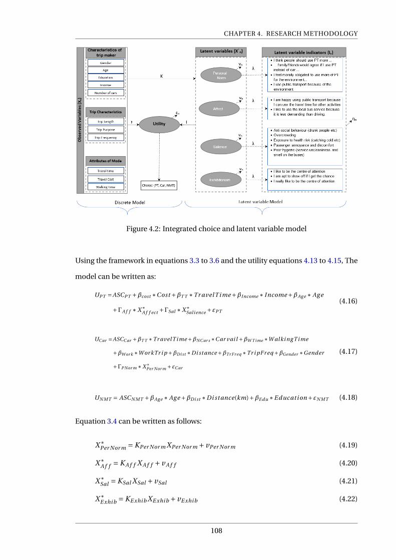
CHAPTER 4. RESEARCH METHODOLOGY
Figure 4.2: Integrated choice and latent variable model
Using the framework in equations 3.3 to 3.6 and the utility equations 4.13 to 4.15, The
model can be written as:
UPT =ASCPT +βcost ∗Cost +βT T ∗Tr avelT i me +βIncome ∗ Income +βAg e ∗ Ag e
+ΓA f f ∗X ∗A f f ect +ΓSal ∗X ∗
Sal i ence +εPT
(4.16)
UC ar =ASCC ar +βT T ∗Tr avelT i me +βNC ar s ∗C ar vai l +βW T i me ∗W alki ng T i me
+βW or k ∗W or kTr i p +βDi st ∗Di st ance +βTr F r eq ∗Tr i pF r eq +βGender ∗Gender
+ΓP Nor m ∗X ∗Per Nor m +εC ar
(4.17)
UN MT = ASCN MT +βAg e ∗ Ag e +βDi st ∗Di st ance(km)+βE du ∗E ducati on +εN MT (4.18)
Equation 3.4 can be written as follows:
X ∗Per Nor m = KPer Nor m XPer Nor m + vPer Nor m (4.19)
X ∗A f f = K A f f X A f f + v A f f (4.20)
X ∗Sal = KSal XSal + vSal (4.21)
X ∗E xhi b = KE xhi b XE xhi b + vE xhi b (4.22)
108
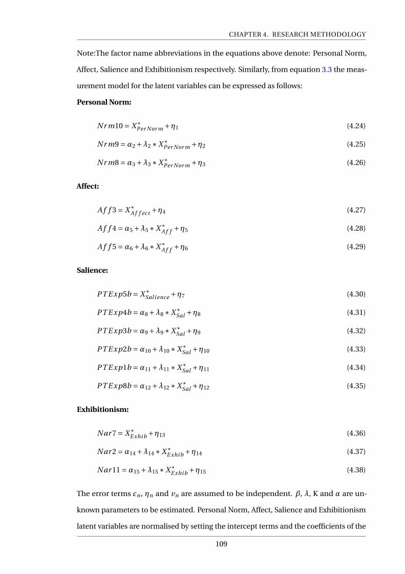
CHAPTER 4. RESEARCH METHODOLOGY
Note:The factor name abbreviations in the equations above denote: Personal Norm,
Affect, Salience and Exhibitionism respectively. Similarly, from equation 3.3 the meas-
urement model for the latent variables can be expressed as follows:
Personal Norm:
N r m10 = X ∗Per Nor m +η1 (4.24)
N r m9 =α2 +λ2 ∗X ∗Per Nor m +η2 (4.25)
N r m8 =α3 +λ3 ∗X ∗Per Nor m +η3 (4.26)
Affect:
A f f 3 = X ∗A f f ect +η4 (4.27)
A f f 4 =α5 +λ5 ∗X ∗A f f +η5 (4.28)
A f f 5 =α6 +λ6 ∗X ∗A f f +η6 (4.29)
Salience:
PT E xp5b = X ∗Sal i ence +η7 (4.30)
PT E xp4b =α8 +λ8 ∗X ∗Sal +η8 (4.31)
PT E xp3b =α9 +λ9 ∗X ∗Sal +η9 (4.32)
PT E xp2b =α10 +λ10 ∗X ∗Sal +η10 (4.33)
PT E xp1b =α11 +λ11 ∗X ∗Sal +η11 (4.34)
PT E xp8b =α12 +λ12 ∗X ∗Sal +η12 (4.35)
Exhibitionism:
N ar 7 = X ∗E xhi b +η13 (4.36)
N ar 2 =α14 +λ14 ∗X ∗E xhi b +η14 (4.37)
N ar 11 =α15 +λ15 ∗X ∗E xhi b +η15 (4.38)
The error terms εn , ηn and vn are assumed to be independent. β, λ, K and α are un-
known parameters to be estimated. Personal Norm, Affect, Salience and Exhibitionism
latent variables are normalised by setting the intercept terms and the coefficients of the
109

CHAPTER 4. RESEARCH METHODOLOGY
latent attitudes to zero(0) and one (1) respectively (see equations 4.24, 4.27, 4.30 and
4.36 in that order).
4.6.1.3 Models Estimation
The base model (equations 4.16 to 4.18) is estimated based on the likelihood function as
equation 3.7. The ICLV model comprising equations 4.19 to 4.38 are estimated simultan-
eously based on the likelihood function in equation 3.8 using Biogeme software package
(Bierlaire, 2018a; 2018b). The python script for the model estimation is presented in
Appendix E.
4.6.1.4 Assessing goodness of fit
The indices for assessing model fit and discriminating between alternative models in
Biogeme include; log-likelihood, the Rho-square (ρ2), the adjusted Rho-square (ρ̄2), the
likelihood ratio test, and the information criteria such as Akaike Information Criterion
(AIC) and the Bayesian Information Criterion (BIC). Biogeme also reports the t-statistics
of all explanatory variables used in the model.
The log-likelihood is the log of the likelihood of observing an alternative given that
individuals make a random selection. Considering that the choice set comprises of three
alternatives (PT, Car and NMT), there is one-third ( 13 ) chance of an individual selecting
either of the alternatives in the null or baseline model. The null log-likelihood (LL(0) is
thus automatically calculated based on the one-third ( 13 )probability of observing each
mode in every observation. Similarly, null log-likelihood of the ICLV model is given
by the joint probability of observing of observing the three alternatives (PT, Car and
NMT) and the indicators of the four latent variables(Personal Norm, Affect, Salience and
Exhibitionism each measured on 5-point Likert scale. Hence, the null log-likelihood and
final log-likelihood values of the ICLV model becomes significantly smaller compared to
log-likelihood estimates of the base model which is estimated from only the alternatives
(PT, Car and NMT). Therefore, the final log-likelihood values are estimated from the
choice probabilities for the ICLV model to be comparable with the discrete model (base
model) (Atasoy et al., 2013).
110
CHAPTER 4. RESEARCH METHODOLOGY
Thus, log-likelihood comparison of the base and ICLV models is not possible using
this approach. However, the final log-likelihood values is estimated the simulated
probabilities.
LL(0) = N ∗ ln(1
c) (4.39)
where: N is the number of observations
C is the number of alternatives in the choice set
The final log-likelihood LL(β) is the simulated log-likelihood values of the final or
unrestricted model.
LL(β) =N∑1
l n(simulated probabilities) (4.40)
where: N is the number of observations
The likelihood ratio test (−2(LL(0)−LL(β))), tests the hypothesis that the null and the
final model are equivalent. The (−2(LL(0)−LL(β))) must be large enough for the final
model to be significantly better than the null model (Antolín, 2016). The statement
above means that the LL(β) should be remarkably different from LL(0) for a good model
fit.
The ρ̄2 is not a statistical test but gives a general overview of model fit when comparing
models. ρ̄2 takes into account the number of explanatory variables used in each model
and normalises for their effect when comparing two or more models, and this makes it
suitable for comparing models with different number of variables.
ρ2 =1− LL(β)
LL(0)(4.41)
and
ρ̄2 =1− LL(β)−p
LL(0)(4.42)
where: p is the number of explanatory parameters in the estimated model
The likelihood of observing an alternative in the ICLV model is given by the joint prob-
ability of observing an alternative and the indicators of the latent variables (Norms,
Salience, Affect and Exhibitionism). The log-likelihood values become significantly
smaller with the incorporation of the latent variables in the ICLV model compared
111
CHAPTER 4. RESEARCH METHODOLOGY
to a discrete choice model of similar specifications. Similarly, the AIC and the BIC
increases substantially with the inclusion of latent variables; this renders these indices
inappropriate for comparing discrete choice models and ICLV models. However, to
discriminate or compare the base model and the ICLV model reported in this document,
the final log-likelihood values are estimated from the simulated choice probabilities for
the unrestricted models (final base model and final ICLV model) based on equations
3.13 and 4.41.
4.7 Summary
The chapter presents detail description of the research methods adopted for this study.
Stratified random sampling method was considered appropriate for the study after a
careful review of the strength and weaknesses of the most popular sampling techniques.
The ability to apply weights to sub-frames when generating the sample is believed to
enhance the representativeness of the sample and the generalisability of the survey
results. A sample size of 500 was found adequate and recommended to ensure the gen-
eralisability of the results. Additionally, postal or mail-back survey method is selected
as the primary mode for administering the survey and supplemented by on-line survey
method. Moreover, the statistical methods for data analysis and choice model estima-
tion methods are discussed and illustrated in detail including the detail specification
for the development of ICLV model. The next chapter presents the study area and the
population of the study.
112
; Chapter Five <
Case Study
5.1 Introduction
Defining the boundary of a study is necessary for contextualising results of a study
and discussing the finding from a specific perspective. It also provides insight into the
demographics and socio-economic characteristics of an area and gives the basis for
comparison. This chapter defines the study area and presents the demographic and
economic characteristics of the area. Additionally, a brief description of the strength
and challenges of the transport system of the study area, as well as some measures
adopted to mitigate the situation.
5.2 Profile of the Study Area
Study Area is a geographic boundary selected to define the geographic space of data
collection and analysis for a study. This section and the next sections describe the
boundaries of the study and the characteristics of the study population. Edinburgh
is the administrative capital city of Scotland, in the United Kingdom (UK). It is UK’s
second-largest financial centre after London and the fastest-growing city (Arcadis, 2017).
Edinburgh is geographically located at the central belt of Scotland, bounded by the
Firth of Forth on the north and the Pentland Hills on the south. The population of
Edinburgh is projected to be 518,100 in 2018 (National Records of Scotland, 2018a).
This population lives on 263 square kilometres of land with a population density of
113
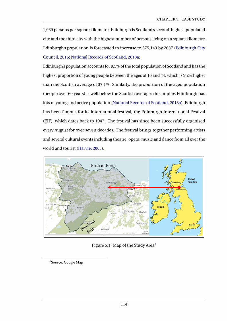
CHAPTER 5. CASE STUDY
1,969 persons per square kilometre. Edinburgh is Scotland’s second-highest populated
city and the third city with the highest number of persons living on a square kilometre.
Edinburgh’s population is forecasted to increase to 575,143 by 2037 (Edinburgh City
Council, 2016; National Records of Scotland, 2018a).
Edinburgh’s population accounts for 9.5% of the total population of Scotland and has the
highest proportion of young people between the ages of 16 and 44, which is 9.2% higher
than the Scottish average of 37.1%. Similarly, the proportion of the aged population
(people over 60 years) is well below the Scottish average: this implies Edinburgh has
lots of young and active population (National Records of Scotland, 2018a). Edinburgh
has been famous for its international festival, the Edinburgh International Festival
(EIF), which dates back to 1947. The festival has since been successfully organised
every August for over seven decades. The festival brings together performing artists
and several cultural events including theatre, opera, music and dance from all over the
world and tourist (Harvie, 2003).
Figure 5.1: Map of the Study Area1
1Source: Google Map
114
CHAPTER 5. CASE STUDY
5.3 Transport Characteristics of the Study Area
In 2014, 160,000 estimated vehicles drove into Edinburgh city centre each morning. This
figure was projected to rise to 180,000 vehicles in 2016. Moreover, 233,370 households
were recorded in 2017; this is forecasted to rise by 39 per cent by 2037 (Edinburgh
City Council, 2016). The factors cited above contribute to the traffic situation in the
city. Edinburgh constitutes a major transport hub in east-central Scotland and at the
centre of a multi-modal transport network comprising road, rail and air. Transport for
Edinburgh is the executive body of the City of Edinburgh Council and responsible for
the development of all transport schemes and policies within the city (Transport for
Edinburgh, 2013). Moreover, Edinburgh is one of the cities with extensive bus services
in the United Kingdom with pervasive and efficient public transport services. The bus
network covers almost all parts of the city (Arcadis, 2017). Nonetheless, according to
Tomtom Traffic Index, Edinburgh is the most congested city in Scotland and performs
better than only Belfast in the United Kingdom (TomTom International BV, 2016). Car
traffic in Edinburgh has been on a rising trajectory since 2009 (TomTom International
BV, 2016; Transport Scotland, 2018b), whereas bus passenger numbers have been
declining since 2008 (Transport Scotland, 2018b). Between 2014 and 2015, the city’s
congestion level rose by eight percentage points to 37%; this means that travel time
in the city has become 37 per cent longer on average than it would have been n free-
flowing traffic. Travel time during the morning peak (7:30 am to 9:30 am) was 64%
longer and that of the evening peak (4:00 pm and 6:00 pm) was 73% more for the same
period (Shan and John, 2015; Edinburgh City Council, 2016; Alastair, 2013; TomTom
International BV, 2016). Moreover, in 2016, the average travel time increased by 43
minutes a day due to congestion (TomTom International BV, 2016).
This is consistent with the findings in Transport Scotland (2015) and Transport Scotland
(2018a). The reports indicate that 9.7%, 11.7% and 12.8% of all car journeys experienced
a delay due to increasing traffic volume in 2015, 2016 and 2017 respectively. Figure 5.2
shows the modal share trend in Edinburgh, while Figure 5.3 shows the congestion level
115
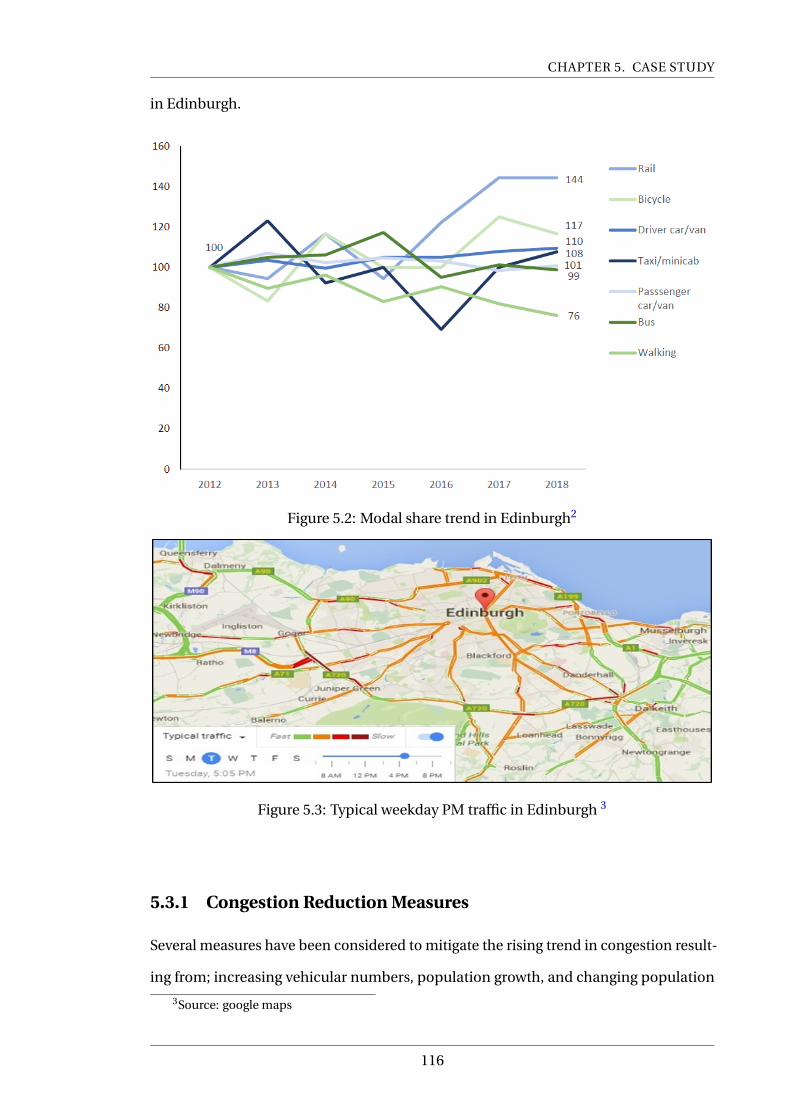
CHAPTER 5. CASE STUDY
in Edinburgh.
Figure 5.2: Modal share trend in Edinburgh2
Figure 5.3: Typical weekday PM traffic in Edinburgh 3
5.3.1 Congestion Reduction Measures
Several measures have been considered to mitigate the rising trend in congestion result-
ing from; increasing vehicular numbers, population growth, and changing population
3Source: google maps
116
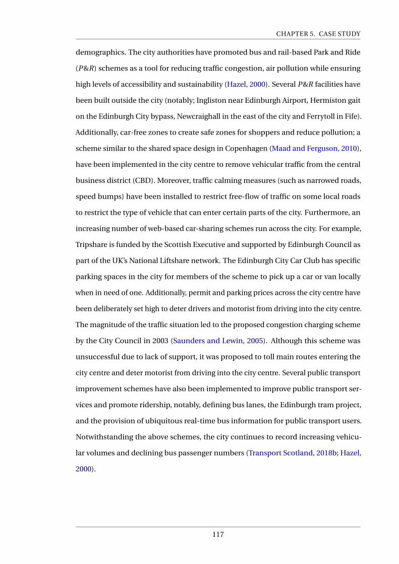
CHAPTER 5. CASE STUDY
demographics. The city authorities have promoted bus and rail-based Park and Ride
(P&R) schemes as a tool for reducing traffic congestion, air pollution while ensuring
high levels of accessibility and sustainability (Hazel, 2000). Several P&R facilities have
been built outside the city (notably; Ingliston near Edinburgh Airport, Hermiston gait
on the Edinburgh City bypass, Newcraighall in the east of the city and Ferrytoll in Fife).
Additionally, car-free zones to create safe zones for shoppers and reduce pollution; a
scheme similar to the shared space design in Copenhagen (Maad and Ferguson, 2010),
have been implemented in the city centre to remove vehicular traffic from the central
business district (CBD). Moreover, traffic calming measures (such as narrowed roads,
speed bumps) have been installed to restrict free-flow of traffic on some local roads
to restrict the type of vehicle that can enter certain parts of the city. Furthermore, an
increasing number of web-based car-sharing schemes run across the city. For example,
Tripshare is funded by the Scottish Executive and supported by Edinburgh Council as
part of the UK’s National Liftshare network. The Edinburgh City Car Club has specific
parking spaces in the city for members of the scheme to pick up a car or van locally
when in need of one. Additionally, permit and parking prices across the city centre have
been deliberately set high to deter drivers and motorist from driving into the city centre.
The magnitude of the traffic situation led to the proposed congestion charging scheme
by the City Council in 2003 (Saunders and Lewin, 2005). Although this scheme was
unsuccessful due to lack of support, it was proposed to toll main routes entering the
city centre and deter motorist from driving into the city centre. Several public transport
improvement schemes have also been implemented to improve public transport ser-
vices and promote ridership, notably, defining bus lanes, the Edinburgh tram project,
and the provision of ubiquitous real-time bus information for public transport users.
Notwithstanding the above schemes, the city continues to record increasing vehicu-
lar volumes and declining bus passenger numbers (Transport Scotland, 2018b; Hazel,
2000).
117
CHAPTER 5. CASE STUDY
5.3.2 Selection of the study Area
The challenges confronting transport planners, city planners and traffic engineers of
the city of Edinburgh going into the next decade include increasing vehicular traffic
and how to stem the tide (TomTom International BV, 2016; Transport Scotland, 2018b;
Hazel, 2000; Saunders and Lewin, 2005). It is in this regard that this study is designed to
investigate the travel behaviour of the population, particularly, the impact of subjective
variables on their travel mode choices.
5.4 Summary
This chapter has described the geographic boundary of the study area and highlight
the characteristics of the study population. It has been argued that given the transport
characteristics of Edinburgh; the rising vehicular congestion in the city; and the travel
behaviour of the study population, MINDSPACE could help explain the travel behavi-
oural of the population. The population of Edinburgh and the proportion of younger
population are projected to increase in the next two decades due to increasing urban-
isation and net immigration. The population increase and the change in demographics
are expected to exert pressure on the transport systems. Therefore, the need to acquire
a clearer understanding of the factors driving the travel behaviour of the population for
developing a workable solution to curb the traffic situation.
118
; Chapter Six <
Data collection and Analysis
6.1 Introduction
This chapter describes that data collection procedure and descriptive analysis of the
sample data. In chapter 4, we discussed the research instrument design and the physical
forms of survey administration adopted for the study. The sample size required for the
study, as well as the various sample generation approaches, were presented. A sample
size of 500 was recommended for the survey, and the sample was to be generated
through a stratified random sampling technique. Additionally, postal and internet-
based forms of survey administering were considered convenient and cost-effective
for the study. Chapter 5 presented the study area selected for this research, along with
household and travel characteristic of the population. Section 6.2 of the is chapter
outlines the sample selection process. The survey administration and implementation
process are covered under section 6.3. Section 6.4 considers the description of the
sample data, while section 6.5 performs exploratory analysis of the sample data and
finally 6.6 summaries the chapter.
6.2 Sample generation
In chapter 4, stratified random sampling technique was recommended for the selec-
tion of the sample. This method was regarded as the most suitable for generating a
representative sample to guarantee the generalisability of the survey results.
119
CHAPTER 6. DATA COLLECTION AND ANALYSIS
6.2.1 Sample Selection
The population of the study comprise residents of Edinburgh living within outward
postcode area EH1 to EH17. The population was divided into 20 strata (vigintile) using
the 2016 Scottish Index of Multiple Deprivation (SIMD 16) datazones classification
tables (see Table 4.2) and the household addresses within the geographical boundary
of the study area (EH1 to EH17) from the royal mail PAF address data file (sampling
frame). (see Table 4.3). Datazones are groups of census areas with average populations
between 500 and 1000 household residents with similar socio-economic characteristics
in Scotland. There are 6505 datazones for covering the entire of Scotland (Scottish
Neighbourhood Statistics, 2003). The SIMD ranks the 6505 datazones most deprived
(datazone 1) to least deprived (datazone 6505). For the purposed of sampling, the 6505
datazones are classified into 20 strata called vigintiles based on the SIMD rankings.
Each vigintile comprises of 5% of the datazones, where vigintile or strata 1 represent
5% of the most deprived household residents while vigintile 20 represents 5% of the
least deprived household residents (Scottish Neighbourhood Statistics, 2003; Scottish
Government, 2016; Scottish Government, 2018). The sample was generated by drawing
households at random from each stratum using the inward postcodes (incodes). The
number of households drawn from each stratum was based on its respective weighting
in the sampling frame. In other to secure the desired 500 responses, a total sample size
of 4,155 household addresses were drawn from a total of 240,147 household addresses
using stratified random sampling technique. A response rate 17% was assumed because
of the low response rate that characterises postal or mail back surveys (Jobber and Reilly,
1998; Greer et al., 2000; David De Vaus, 2002; Sahlqvist et al., 2011; Larson and Poist,
2018). Table 6.1 presents a summary of the sample generated from each stratum. The
sampled addresses were subsequently re-organised into outward postcode (outcode)
areas for easy sorting and distribution, Table 6.2 shows the reclassified data.
120
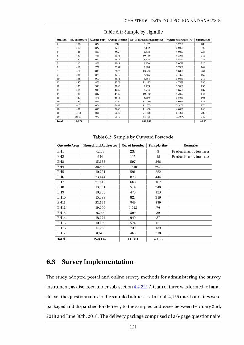
CHAPTER 6. DATA COLLECTION AND ANALYSIS
Table 6.1: Sample by vigintile
Stratum No. of Incodes Average Pop Average Income No. of Household Addresses Weight of Stratum (%) Sample size
1 286 824 212 7,862 3.27% 183
2 312 827 590 7,162 2.98% 88
3 428 859 907 9,608 4.00% 233
4 431 826 1351 10,196 4.25% 212
5 387 932 1632 8,575 3.57% 233
6 317 876 2021 7,370 3.07% 220
7 418 777 2361 8,978 3.74% 142
8 570 888 2873 13,532 5.63% 264
9 288 875 3210 7,515 3.13% 162
10 398 910 3631 9,484 3.95% 219
11 447 876 3579 11,382 4.74% 236
12 335 940 3833 9,463 3.94% 155
13 318 996 4237 8,764 3.65% 137
14 429 837 4429 10,160 4.23% 144
15 427 871 4815 8,416 3.50% 161
16 540 808 5196 11,116 4.63% 122
17 629 874 5457 12,763 5.31% 176
18 557 846 5668 11,520 4.80% 140
19 1,176 861 6235 21,896 9.12% 288
20 2,581 877 6518 44,385 18.48% 640
Total 11,274 240,147 4,155
Table 6.2: Sample by Outward Postcode
Outcode Area Household Addresses No. of Incodes Sample Size Remarks
EH1 4,108 238 3 Predominantly business
EH2 944 115 15 Predominantly business
EH3 15,355 597 366
EH4 26,400 1,539 607
EH5 10,781 591 252
EH6 23,444 873 444
EH7 21,043 660 187
EH8 13,161 514 340
EH9 10,235 475 123
EH10 15,199 823 319
EH11 22,594 849 839
EH12 19,006 1,022 76
EH13 6,795 369 39
EH14 18,074 949 37
EH15 10,069 574 151
EH16 14,293 730 139
EH17 8,646 463 218
Total 240,147 11,381 4,155
6.3 Survey Implementation
The study adopted postal and online survey methods for administering the survey
instrument, as discussed under sub-section 4.4.2.2. A team of three was formed to hand-
deliver the questionnaires to the sampled addresses. In total, 4,155 questionnaires were
packaged and dispatched for delivery to the sampled addresses between February 2nd,
2018 and June 30th, 2018. The delivery package comprised of a 6-page questionnaire
121
CHAPTER 6. DATA COLLECTION AND ANALYSIS
and one PPI self-addressed envelope for return postage. These were enclosed in a C5
envelope and addressed to "the occupier" of the sampled household address (see Figure
6.1). A web-link (https://thissurvey.questionpro.com) to the online version of the survey
was included in the introductory note of the questionnaire. Participants were advised
to complete the survey using their preferred option among the two.
• Complete and return the paper-based questionnaire by post using the PPI self-
addressed envelope enclosed.
• Complete the survey online by following the web-link provided in the introductory
of the questionnaire
Assuming a minimum of 17% response rate and the fact that postage cost of £0.51 is
charged by the postage company for every questionnaire receive through the mail, the
survey was conducted in two phases to ensure the cost of the survey does not exceed the
approved budget in the unlikely event of recording higher responses than anticipated.
In phase one, 2,185 addresses were sampled and sent the survey package. This process
lasted almost two months. At the end of this process, the sample data was analysed
to investigate characteristics of respondents and the distribution of the responses by
vigintile. Considering the results and distribution of the sample for the first phase
of the survey, additional 1,970 addresses were sampled for the second phase of the
survey, which also lasted two months. In total, 4,155 questionnaires were packaged
and dispatched for distribution Table 6.3 shows the number of addresses sampled
during each phase of the survey. However, 3,973 questionnaires were successfully
delivered. One hundred and eighty-two (182) questionnaires representing 4.4% of the
total sampled addresses, returned undelivered (either refused, non-existent address or
vacant address).
122

CHAPTER 6. DATA COLLECTION AND ANALYSIS
Figure 6.1: Envelope for questionnaire
An incentive package of £50 voucher each for four people was offered for participants of
the survey. Participants interested in the voucher were advised to supply their contact
addresses at the end of the survey to register their interest. The four winners were
selected through a random draw at the close of the survey and contacted for their prize.
No personally identifiable information was asked in the survey to ensure respondents
identity was kept anonymous. However, the data provided by participants for the draw
was maintained separately from the survey data and destroyed immediately after the
winners were selected and contacted.
123
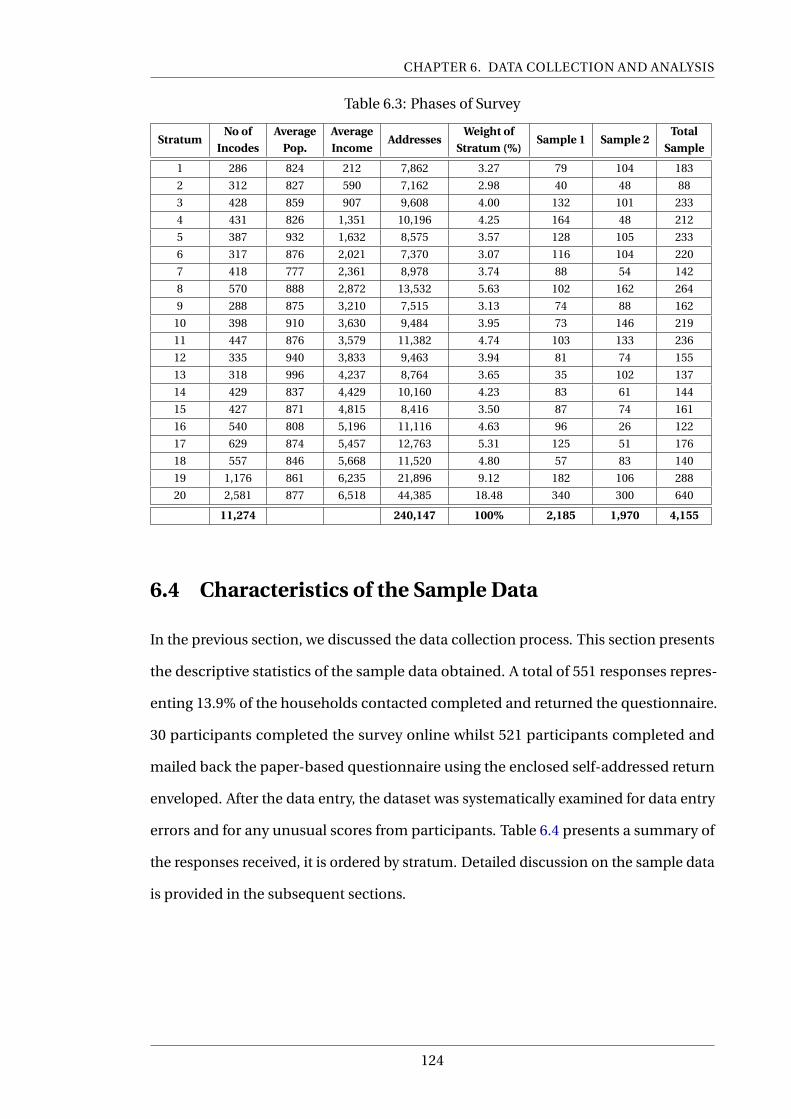
CHAPTER 6. DATA COLLECTION AND ANALYSIS
Table 6.3: Phases of Survey
StratumNo of
IncodesAverage
Pop.AverageIncome
AddressesWeight of
Stratum (%)Sample 1 Sample 2
TotalSample
1 286 824 212 7,862 3.27 79 104 183
2 312 827 590 7,162 2.98 40 48 88
3 428 859 907 9,608 4.00 132 101 233
4 431 826 1,351 10,196 4.25 164 48 212
5 387 932 1,632 8,575 3.57 128 105 233
6 317 876 2,021 7,370 3.07 116 104 220
7 418 777 2,361 8,978 3.74 88 54 142
8 570 888 2,872 13,532 5.63 102 162 264
9 288 875 3,210 7,515 3.13 74 88 162
10 398 910 3,630 9,484 3.95 73 146 219
11 447 876 3,579 11,382 4.74 103 133 236
12 335 940 3,833 9,463 3.94 81 74 155
13 318 996 4,237 8,764 3.65 35 102 137
14 429 837 4,429 10,160 4.23 83 61 144
15 427 871 4,815 8,416 3.50 87 74 161
16 540 808 5,196 11,116 4.63 96 26 122
17 629 874 5,457 12,763 5.31 125 51 176
18 557 846 5,668 11,520 4.80 57 83 140
19 1,176 861 6,235 21,896 9.12 182 106 288
20 2,581 877 6,518 44,385 18.48 340 300 640
11,274 240,147 100% 2,185 1,970 4,155
6.4 Characteristics of the Sample Data
In the previous section, we discussed the data collection process. This section presents
the descriptive statistics of the sample data obtained. A total of 551 responses repres-
enting 13.9% of the households contacted completed and returned the questionnaire.
30 participants completed the survey online whilst 521 participants completed and
mailed back the paper-based questionnaire using the enclosed self-addressed return
enveloped. After the data entry, the dataset was systematically examined for data entry
errors and for any unusual scores from participants. Table 6.4 presents a summary of
the responses received, it is ordered by stratum. Detailed discussion on the sample data
is provided in the subsequent sections.
124
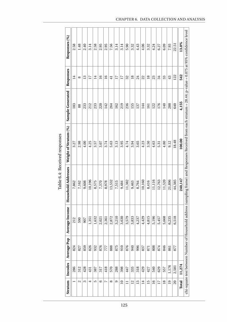
CHAPTER 6. DATA COLLECTION AND ANALYSIS
Tab
le6.
4:R
ecei
ved
resp
on
ses
Stra
tum
Inco
des
Ave
rage
Po
pA
vera
geIn
com
eH
ou
seh
old
Ad
dre
sses
Wei
ghto
fStr
atu
m(%
)Sa
mp
leG
ener
ated
Res
po
nse
sR
esp
on
ses
(%)
128
682
421
27,
862
3.27
183
142.
58
231
282
759
07,
162
2.98
888
1.48
342
885
990
79,
608
4.00
233
132.
40
443
182
61,
351
10,1
964.
2521
217
3.14
538
793
21,
632
8,57
53.
5723
314
2.58
631
787
62,
021
7,37
03.
0722
016
2.95
741
877
72,
361
8,97
83.
7414
216
2.95
857
088
82,
872
13,5
325.
6326
441
7.56
928
887
53,
210
7,51
53.
1316
217
3.14
1039
891
03,
630
9,48
43.
9521
917
3.14
1144
787
63,
579
11,3
824.
7423
632
5.90
1233
594
03,
833
9,46
33.
9415
518
3.32
1331
899
64,
237
8,76
43.
6513
724
4.43
1442
983
74,
429
10,1
604.
2314
422
4.06
1542
787
14,
815
8,41
63.
5016
118
3.32
1654
080
85,
196
11,1
164.
6312
223
4.24
1762
987
45,
457
12,7
635.
3117
634
6.27
1855
784
65,
668
11,5
204.
8014
033
6.09
191,
176
861
6,23
521
,896
9.12
288
437.
93
202,
581
877
6,51
844
,385
18.4
864
012
222
.51
Tota
l11
,274
240,
147
100.
004,
155
542
13.0
%
chi-
squ
are
test
bet
wee
nN
um
ber
ofH
ou
seh
old
add
ress
(sam
pli
ng
fram
e)an
dR
esp
on
ses
Rec
eive
dfr
om
each
stra
tum
=28
.44;
p-v
alu
e=
0.07
5at
95%
con
fid
ence
leve
l
125
CHAPTER 6. DATA COLLECTION AND ANALYSIS
6.4.1 Missing data
Missing data (partial responses) is one of the ubiquitous statistical problems in research
(Baraldi and Enders, 2010). This situation results when participants in a survey fail to
respond to all the questions on the survey. It is caused by several factors such as stress,
fatigue or lack of knowledge about a question and sometimes due to the sensitivity of
the question(s), this is practically inevitable in questionnaire survey (Gyimah, 2001;
Baraldi and Enders, 2010; Little and Edition, 2014; Newman, 2014; Arbuckle, 2017). The
sample data discussed in the preceding section is consistent with the observations in
Newman (2014); the pattern of the missing data observed in the sample data can be
categorised into three levels, namely; item-level missing, construct-level missing and
person-level missing (Newman, 2014). Item-level missing occurs when respondents
fail to answer all the questions in the questionnaire. Construct-level missing occurs
when a respondent answers some questions but skip others on a multi-item scale or
skip an entire measurement scale. In contrast, person-level missing represents non-
respondents (Gyimah, 2001; Newman, 2014). This section will primarily focus on the
first two categories; the latter category is discussed under section 6.4.4 (Sample bias).
As indicated in Figure 6.2, the 500 valid cases comprised of 1,641 missing cells repres-
enting 4.0% of the total number of cells in the entire dataset. Seventy-one (71) cases
representing 14.2% of the total respondents answered every question on the survey (full
respondents). The remaining 85.8% failed to answer at least one question on the survey
(partial respondents).
The high proportion of partial respondents is an indication of the variability of the
response rate across the variables. Five variables out of the 82 variables were answered
by all respondents, and the remaining 77 variables had at least one missing value. Table
6.5 presents a summary of variables with at least 5% missing values.
126
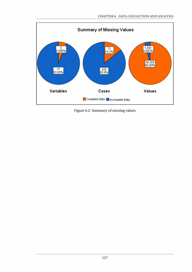
CHAPTER 6. DATA COLLECTION AND ANALYSIS
Figure 6.2: Summary of missing values
127

CHAPTER 6. DATA COLLECTION AND ANALYSIS
Table 6.5: Summary of variables
Item VariableMissing Valid
Mean Std. DeviationCount Percent Count Percent
1 SM_Cost:Alternative travel mode cost 334 60.6% 217 39.4% 51.56 65.821
2 Tr_Cost: Cost of travel mode 258 46.8% 293 53.2% 52.52 60.343
3 PT Usage:Difficulty of using PT 237 43.0% 314 57.0% 2.58 1.477
4 Tr_Time: Travel time of Primary travel mode 121 22.0% 430 78.0% 2.70 1.183
5 Nar13: I am going to be a great person 74 13.4% 477 86.6% 2.32 0.889
6 Nar5: I find it easy to manipulate others 70 12.7% 481 87.3% 2.00 0.725
7 Nar14: I can make anybody believe anything I want them to 69 12.5% 482 87.5% 1.93 0.641
8 Nar11: I really like to be the centre of attention 69 12.5% 482 87.5% 1.90 0.665
9 Nar9: Everybody likes to hear my stories 69 12.5% 482 87.5% 2.34 0.752
10 Nar12: People always seem to recognise my authority 68 12.3% 483 87.7% 2.13 0.81
11 Nar7: I am apt to show off if I get the chance 68 12.3% 483 87.7% 2.07 0.776
12 Nar1: I know that I am good because everybody keep .. 67 12.2% 484 87.8% 2.30 0.812
13 Nar16: I am an extraordinary person 66 12.0% 485 88.0% 2.10 0.785
14 Nar6: I insist upon getting the respect that is due me 66 12.0% 485 88.0% 2.24 0.847
15 Nar2: I like to be the centre of attention 66 12.0% 485 88.0% 2.01 0.67
16 Nar4: I like having authority over people 64 11.6% 487 88.4% 2.01 0.779
17 Nar8: I always know what I am doing 61 11.1% 490 88.9% 2.29 1.071
18 PTM: Travel mode 5 years ago 61 11.1% 490 88.9% 4.50 3.125
19 Nar3: I think I am a special person 60 10.9% 491 89.1% 2.26 0.877
20 Nar15: I am more capable than other people 57 10.3% 494 89.7% 2.18 0.852
21 Nar10: I expect a great deal from other people 56 10.2% 495 89.8% 2.38 0.882
22 R4ChaMode: Reason for changing travel mode 56 10.2% 495 89.8% 3.05 3.142
23 PTExp4b: Passenger annoyance and discomfort 43 7.8% 508 92.2% 2.94 1.193
24 PTExp8b: Safety issues (lack of seatbelt, ... 40 7.3% 511 92.7% 2.36 1.29
25 Nrm9: I believe most of the people important to me 38 6.9% 513 93.1% 3.53 0.986
26 PTExp7b: Long waiting and travel time 38 6.9% 513 93.1% 3.38 1.318
27 PTExp3b: Exposure to health risk (catching a cold etc) 37 6.7% 514 93.3% 2.68 1.325
28 PTExp5b: Poor hygiene (service uncleanliness and ... 35 6.4% 516 93.6% 3.34 1.302
29 PTExp2b: Overcrowding 35 6.4% 516 93.6% 3.13 1.269
30 Nrm7: If my family and friends change their ... 34 6.2% 517 93.8% 1.96 0.872
31 PTExp6b: Inaccurate bus and real-time information 34 6.2% 517 93.8% 3.07 1.25
32 PTExp4a:Passenger annoyance and discomfort 34 6.2% 517 93.8% 3.29 1.106
33 PTExp8a: Safety issues (lack of seatbelt, ... 32 5.8% 519 94.2% 2.61 1.318
34 PTExp1b: Anti-social behaviour (drunk people etc) 31 5.6% 520 94.4% 3.22 1.423
35 PTExp7a:Long waiting and travel time 30 5.4% 521 94.6% 3.66 1.209
36 Income: Household Annual Income 29 5.3% 522 94.7% 4.32 1.869
37 Nrm6: Most of my family and friends use public transport 29 5.3% 522 94.7% 2.91 1.105
38 Aff4: I like to use the local bus service because ... 29 5.3% 522 94.7% 3.45 1.172
39 PTSQl1: I feel personally safe and secure ... 29 5.3% 522 94.7% 3.78 0.92
40 Nrm10: I feel morally obligated to use more of ... 28 5.1% 523 94.9% 3.12 1.188
41 Nrm1: Driving is perceived to illustrate a person’s power ... 28 5.1% 523 94.9% 2.44 1.162
42 PTExp3a:Exposure to health risk (catching a cold etc) 28 5.1% 523 94.9% 3.09 1.297
6.4.1.1 Missing Data Treatment
Several statistical methods are available for dealing with incomplete/partial dataset,
notably, listwise deletion, pairwise deletion, single imputation, multiple and Maximum
likelihood (Kim and Curry, 1977; Baraldi and Enders, 2010; Newman, 2014; Arbuckle,
2017). Listwise and pairwise deletion methods are the most basic techniques of the
missing data treatment methods. Listwise deletion discards any observation with
missing values; the advantage of this technique is that it produces dataset from only
complete cases for analysis. However, handling partial respondents as person-level
128
CHAPTER 6. DATA COLLECTION AND ANALYSIS
missing (non-respondents) and discarding the entire data from a respondent due to
one or two missing values is a major drawback for this technique. This can affect the
estimates and statistical power if the resultant sample size gets too small due to the ex-
clusion of all usable data from partial respondents (Baraldi and Enders, 2010; Newman,
2014). Comparing the two deletion methods, Kim and Curry (1977), pointed out that
the pairwise deletion method performs better than listwise deletion method. Although
both deletion methods are available in most modern statistical software packages, re-
searchers question their suitability; they argue that missing one or two values is not
a reasonable justification for discarding all usable data from a participant. Further-
more, both techniques could lead to a considerable reduction in sample size, thereby
affecting the validity of results. (Gyimah, 2001; Baraldi and Enders, 2010; Newman,
2014) Similarly, single imputation method involves replacing each missing value with
a plausible estimate, such as the mean, median or a predicted value from a multiple
regression equation from the observations. This technique is, however, noted for pro-
ducing bias estimates and inaccurate standard errors (Gyimah, 2001; Newman, 2014).
The advantages of this technique are that it is flexible and retains all usable data for
analysis. However, it is argued that the imputed values may exaggerate the estimates
and lead to type I or type II error. Hence this method is not recommended. (Gyimah,
2001; Baraldi and Enders, 2010; Newman, 2014). Multiple imputation method was de-
veloped to overcome the limitation of the single imputation; several single-imputation
are performed and averaged (Baraldi and Enders, 2010; Newman, 2014). The sample
variation between the different copies of the datasets achieved by allowing different
values of the missing items to be imputed gives this technique advantage over the single
imputation technique (Baraldi and Enders, 2010). This provides unbiased estimates and
more accurate significance test. Multiple imputation procedure involves three stages;
The first stage is the imputation stage, where several different copies of the datasets are
created from the original dataset. A minimum of 40 different imputations is recommen-
ded at this stage for obtaining unbiased estimates (Graham, 2012). The second stage
involves statistical analysis of each of the imputed datasets, and in the final stage, the
researcher combines the estimates and their standard errors (SEs) from the analysis
129
CHAPTER 6. DATA COLLECTION AND ANALYSIS
in the first two stages. This is achieved by simply averaging the estimates from all the
imputed datasets for the final parameter estimates. The second advanced and highly
recommended method for handling incomplete dataset is the Maximum likelihood
estimation method. This technique assumes multivariate normality and scores missing
at random (MAR). Maximum likelihood estimation uses the log-likelihood function and
all the available dataset to estimate the population parameters that have the highest
probability of producing the complete sample data (Baraldi and Enders, 2010; Newman,
2014). Restated, this technique does not impute any missing score; rather, it uses the
available incomplete data to compute the value of the parameter that is most likely to
have resulted in the observed data. The Maximum likelihood estimation technique and
the multiple imputation techniques are the modern techniques for handling missing
data. They are considered superior to the deletion techniques, and the single data
imputation method and provides unbiased estimates than the traditional methods
(Gyimah, 2001; Baraldi and Enders, 2010; Newman, 2014). Although several researchers
favour MI and ML over the deletion and single imputation methods, Binder (1996, p.571)
cited in Gyimah (2001), had this to say.
"none of the approaches is always right or always wrong, and it is important to
understand the conditions under which each approach is preferred"
The crux of the matter is finding the most plausible replacement for any missing value.
According to Newman (2014), maximum likelihood (EM or FIML) or multiple imputa-
tion (MI) techniques with auxiliary interaction variables should be used for treating
missing data when partial respondents exceed 10% of the sample data. Mathematically
expressed, if Par ti al r esponse r ateTot al r esponse r ate > 0.1, then ML or MI should be applied (Newman,
2014). From table 6.5:
Par ti al r esponse r ate
Tot al r esponse r ate= 10.8
12.6= 0.86
As shown above, partial respondents account for 86% of the sample data, more than
the 10% threshold proposed in Newman (2014). For this reason, maximum likelihood is
adopted for missing data handling and for statistical analysis.
130
CHAPTER 6. DATA COLLECTION AND ANALYSIS
6.4.2 Data Cleaning
Descriptive analysis was conducted on the dataset and inspection carried out for data
entry error or entry of unusual scores. Twenty (20) variables were found to contain
unusual and implausible scores and accordingly corrected. Secondly, respondents’
level of engagement when completing the survey was examined. Characteristically of
behavioural survey (Gyimah, 2001), 32 respondents representing 5.8% of respondents
skipped at least one entire behavioural construct. This may be due to the sensitive
nature and/or the unusual wording of the questions for these measurement scales. In
summary, 32 respondents skipped the "narcissism" measurement scale. 17 respondents
skipped all items on "Norm" and "Affects", 16 respondents skipped all items on PT
Experience, and finally, five respondents failed to answer any of the items on public
transport service quality. Although these participants skipped these measurement
scales yet answered the last part of the survey instrument on socio-demographics.
This could be a reflection of the general sense of caginess or political correction when
asked about sensitive social behaviours or attitudes (Gyimah, 2001). Although Gyimah
(2001) believe there is no clear-cut rule for handling all categories of missing data cases,
Newman (2014), suggested that.
"When conducting a construct-level analysis, if a participant responds to any items (even
a single item) from a multi-item scale, then the participants’ average response across the
item(s) answered should be used to represent the participants’ scale/construct score"
Having stated that, because the study seeks to investigate the impact of respondents’
behaviour on their travel choices; it will be deleterious to retain cases with a substantial
amount of behavioural data missing. Moreover, the heterogeneity of human behaviour
makes it injurious to guess values for respondents skipping an entire measurement
scale. Consequently, respondents skipping entire construct and respondents missing
more than 25% of scores across all the behavioural constructs are dropped from the
data. Overall, 51 cases representing 9.3% of the total responses received were discarded
for non-engagement and various infractions; 35 participants representing 6.4% of re-
131
CHAPTER 6. DATA COLLECTION AND ANALYSIS
spondents for failure to answer more than 25% of questions on the survey, at the same
time skipping at least one entire behavioural measurement scale. 14 participants, rep-
resenting 2.5% of respondents for not answering at least 25% of all items on the survey.
Finally, two participants for skipping at least one entire behavioural measurement scale.
This reduced the total valid responses to 500 cases for further analysis.
6.4.3 Response rate
A total of 551 participants making up 13.9% of the sample contacted completed and
returned the survey. Respondents are aged between 18 and 90 (µ= 49.69,σ= 17.45),
Table 6.5 gives a brief overview of the sample data and the response rate. Table 6.4
summaries the responses received by stratum. The youngest respondent is aged 18,
indicating that all respondents were eligible to drive in the study area. 51 partially
completed responses and data from unengaged respondents were deleted from the
dataset. This reduced the total valid responses for the analysis to 500 cases, aged
between 18 and 90 (µ= 48.80,σ= 17.27). Refer to Table 6.11 for the statistical profile of
the respondents. The response rate is mathematically expressed as:
Response r ate = Respondent s
Sample cont acted×100 (6.1)
Full r esponse r ate = Full r espondent s
Sample cont acted×100 (6.2)
Par ti al r esponse r ate = Par ti al r espondent s
Sample cont acted×100 (6.3)
132

CHAPTER 6. DATA COLLECTION AND ANALYSIS
Table 6.6: Response rate
Description Count
Total sample size sampled, (a) 4155
Undelivered questionnaire, (b) 182
Sample Contacted, (c) = (a)-(b) 3973
Total responses received, (d) 551
Invalid responses, (e) 51
Valid responses, (f) = (d)-(e) 500
Full Respondents (g) 71
Partial Respondents (h) 429
Response Rate (%)
Unadjusted response rate = dc 13.9
Total (adjusted) response rate = fc 12.6
Full response rate = gc 1.8
Partial response rate = hc 10.8
6.4.4 Sample Bias
Characteristics of mail-back surveys, despite all the attempts to increase survey re-
sponse rates, a substantial proportion of households contacted did not respond (David
De Vaus, 2002). There exist a plethora of literature suggesting that exciting research
topics (referred to as salience topics) tend to elicit more responses in a survey and vice
versa (Zillmann et al., 2014). Even though transportation may well fall within the cat-
egory of salient topics, the presence of the behavioural and psychological questions in
the survey instrument may have annulled this effects; possibly due to how cagey people
are when it comes to sensitive issues and undesirable social behaviour (Gyimah, 2001).
Consequently, resulting in the observed low response rate, thus increasing the risk of
non-response bias (Olson, 2006). However, this observation is consistent with Olson
(2006) and Zillmann et al. (2014). The authors found an increasing refusal rate and
declining response rate for household population surveys. Although Curtin et al. (2000)
and Groves (2006) did not find any strong association between non-response rates and
non-response bias, Zillmann et al. (2014) suggest it is a major concern when the charac-
teristics of non-respondents systematically deviate from respondents (Richardson et al.,
1995).
Thus, Richardson et al. (1995) and David De Vaus (2002) recommend the use of remind-
133
CHAPTER 6. DATA COLLECTION AND ANALYSIS
ers to increase the response rate and minimise non-response bias in mail-back survey,
unfortunately, the study could not adopt this recommendation due to budgetary con-
straint. Newman (2014) recommend undertaking missing data sensitivity analysis when
response rate fall below 30% and then steps taken to account for the biasing effect of the
non-respondents if established (Zillmann et al., 2014). The conventional method for
assessing post-survey non-response bias is the estimates comparison method (Groves,
2006). This procedure compares the estimates of the sample data with estimates from
a more trusted source (the Scottish Household Survey, SHS data is used in this study).
Transportation Research Record 886 criticises this method of assessing non-response
bias; according to the report, the measurement instrument may differ in both sur-
veys. Besides, differences in measurement errors may influence the outcome of the
comparison (Transportation Research Board, 1982). On the contrary, Groves (2006)
recommends the use of this procedure if the researcher can source credible and inde-
pendent estimates for the comparison and validation. Thus, this method was adopted
to compare the distributions of gender, age (National Records of Scotland, 2018b) and
modal share (Transport Scotland, 2018b) variables with those from the sample data.
This method was adopted due to the quality and credibility of the data from the Scottish
household survey and Transport Scotland. Additionally, the distributions of respond-
ents from each stratum was compared with those from the sampling frame. Discussion
on the comparison method is presented below.
6.4.4.1 Gender
The sample data indicates slightly more females than males; however, this is the charac-
teristics of the study population. The percentage of males and females in the sample
data is compared with similar estimates from the Scottish Household Survey (National
Records of Scotland, 2018a). A chi-square test performed to examine gender represent-
ation between the sample data and the Scottish Household Survey yielded a chi-square
value of (x2) = 0.003, p = 0.955 at 95% confidence level. The test results do not provide
sufficient statistical evidence to reject the null hypothesis that "the gender estimates
of the sample data and that of the Scottish Household Survey data are similar" (refer
134

CHAPTER 6. DATA COLLECTION AND ANALYSIS
to Table 6.7 for details). Hence gender distribution of the sample data is assumed
representative of the study population.
Table 6.7: Gender Distribution
GenderSample Data SHS 2017*
Count Percentage Percentage
Female 259 52.2 51.8
Male 237 47.8 48.2
Total 496
Chi-square 0.003
p-value 0.955
df 1
Confidence level 95%
* Source:(National Records of Scotland, 2018b)
6.4.4.2 Age
The distribution of the sample data by age is compared with similar estimates from
the Scottish Household Survey (National Records of Scotland, 2018a) for ages 18 and
above. In spite of combining mail-back and internet survey method to mitigate the
effect of age-related differences in response (Gigliotti and Dietsch, 2014), the sample
data was found consistent with mail-back surveys (lower response rate of younger (<45)
respondents compared to the older respondents (>45)) (Gigliotti and Dietsch, 2014).
The comparison of the age distribution of the sample data and that of the Scottish
Household Survey data in Table 6.8 indicates that the sample data contains fewer young
respondents and more old respondents compared to the Scottish Household Survey
data. Chi-square test performed to investigate the level of deviations of the sample data,
returned chi-square (x2) value of = 7.09, p-value = 0.313 and df = 6 at 95% confidence
level. The result is not statistically significant enough to justify the rejection of the null
hypothesis (refer to Table 6.8 for details). Hence the distribution of the sample data by
age is assumed representative of the study population.
135

CHAPTER 6. DATA COLLECTION AND ANALYSIS
Table 6.8: Comparison of Respondents by Age
Age BandRepresentation (%)
Sample Data SHS 2017*
18 to 24 yrs 8.3 13.4
25 to 34 yrs 15.4 23.8
35 to 44 yrs 13.4 16.8
45 to 54 yrs 17.4 15.2
55 to 64 yrs 21.1 12.8
65 to 74 yrs 16.0 9.7
>= 75 yrs 8.3 8.4
Chi-square 7.09
p-value 0.313
df 6
Confidence level 95%
* Source:((National Records of Scotland, 2018a)
6.4.4.3 Modal Share
The travel behaviour of respondents was similarly compared with the travel data of
the Scottish Household Survey data (Transport Scotland, 2018b). A chi-square test
performed to compare the modal share distribution of the sample data and that of the
Scottish Household Survey data yielded a chi-square value (x2) of = 2.59, p = 0.858, df =6
at 95% confidence level. the results suggest that the two estimates are not significantly
different (refer to Table 6.9 for details). The test results do not provide enough statistical
evidence to reject the null hypothesis. Hence the distribution of the sample data by
modal share is assumed to characterise the study population, according to Transport
Scotland (2018b)
136
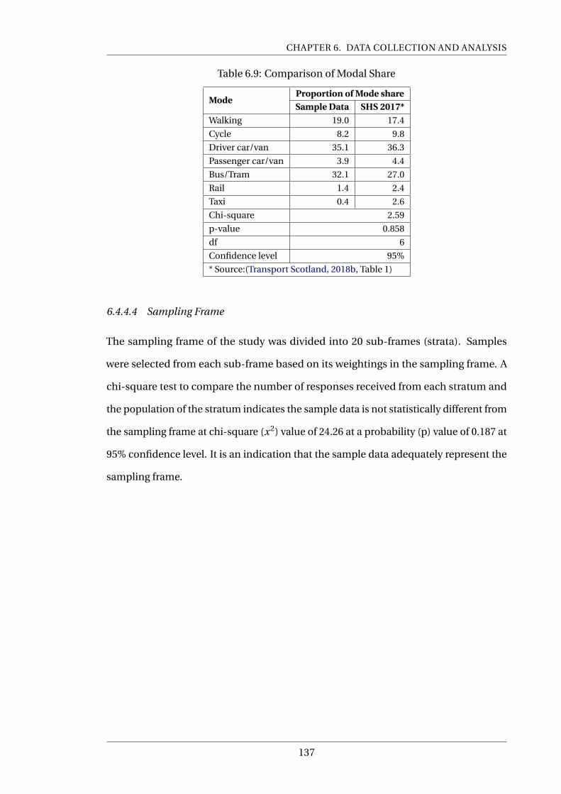
CHAPTER 6. DATA COLLECTION AND ANALYSIS
Table 6.9: Comparison of Modal Share
ModeProportion of Mode shareSample Data SHS 2017*
Walking 19.0 17.4
Cycle 8.2 9.8
Driver car/van 35.1 36.3
Passenger car/van 3.9 4.4
Bus/Tram 32.1 27.0
Rail 1.4 2.4
Taxi 0.4 2.6
Chi-square 2.59
p-value 0.858
df 6
Confidence level 95%
* Source:(Transport Scotland, 2018b, Table 1)
6.4.4.4 Sampling Frame
The sampling frame of the study was divided into 20 sub-frames (strata). Samples
were selected from each sub-frame based on its weightings in the sampling frame. A
chi-square test to compare the number of responses received from each stratum and
the population of the stratum indicates the sample data is not statistically different from
the sampling frame at chi-square (x2) value of 24.26 at a probability (p) value of 0.187 at
95% confidence level. It is an indication that the sample data adequately represent the
sampling frame.
137
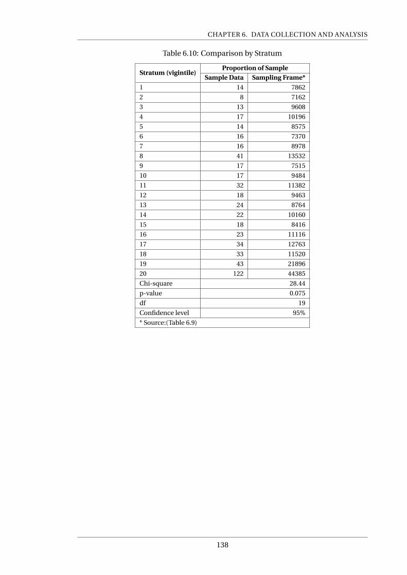
CHAPTER 6. DATA COLLECTION AND ANALYSIS
Table 6.10: Comparison by Stratum
Stratum (vigintile)Proportion of Sample
Sample Data Sampling Frame*
1 14 7862
2 8 7162
3 13 9608
4 17 10196
5 14 8575
6 16 7370
7 16 8978
8 41 13532
9 17 7515
10 17 9484
11 32 11382
12 18 9463
13 24 8764
14 22 10160
15 18 8416
16 23 11116
17 34 12763
18 33 11520
19 43 21896
20 122 44385
Chi-square 28.44
p-value 0.075
df 19
Confidence level 95%
* Source:(Table 6.9)
138

CHAPTER 6. DATA COLLECTION AND ANALYSIS
Table 6.11: Summary Statistics
CharacteristicsSample Estimates Pop. Estimates Chi-square test (95%)Frequency % % x2 p-value
Gender0.003 0.955Female 259 52.2 51.8
Male 237 47.8 48.2
Total 496
Age *
7.090 0.313
18 to 24 years 41 8.3 13.4
25 to 34 years 76 15.4 23.8
35 to 44 years 66 13.4 16.8
45 to 54 years 86 17.4 15.2
55 to 64 years 104 21.1 12.8
65 to 74 years 79 16.0 9.7
75 years or older 41 8.3 8.4
Total 496
Employment status **
1.865 0.761
Employed full-time 216 43.6 45.0
Employed part-time 81 16.3 15.0
Student 40 8.1 13.0
Retired 143 28.8 23.0
Unemployed 16 3.2 3.0
Total 496
Educational LevelNo formal Education 5 1.0
High School 85 17.1
College 98 19.8
Bachelor’s degree 164 33.1
Master’s degree 117 23.6
PhD 27 5.4
Total 496
Car Availability ***
1.644 0.650
0 153 32.09 39.3
1 231 46.58 42.2
2 92 17.39 15.7
3+ 20 3.93 2.9
Total 496
Income **
2.984 0.560
Less than 10000 52 10.5 12.0
10000 to 20000 98 19.8 27.0
20000 to 30000 93 18.8 22.0
30000 to 50000 113 22.8 16.0
50000 + 140 28.2 24.0
Total 496
Households Characteristics **
1.408 0.843
1-Most deprived 48 9.9 15.0
2 75 15.5 14.0
3 75 15.5 13.0
4 78 16.1 17.0
5-Least deprived 207 42.9 41.0
Total 488
* National Records of Scotland (2018), **Scottish Government (2018), *** Transport Scotland (2018b)
139

CHAPTER 6. DATA COLLECTION AND ANALYSIS
6.4.4.5 Summary
Comparison of estimates from the sample data with those from the Scottish Household
Survey data suggests the two sets of estimates are systematically similar. The estimates
of the socio-demographic characteristics of the population such as gender, age, income,
car availability and modal share were compared by t-test with the sample data. The
results show no statistically significant differences between the estimates obtained by
the surveys and the estimates of the population in terms of gender, age, income, car
availability and modal share at 95% confidence level. Similarly, the representation of
each stratum in the sample data was not significantly different from those from the
sampling frame. Therefore, in the absence of enough statistical evidence to suggest
non-response bias, it is concluded that the characteristics of respondents adequately
represent the characteristics of the study population.
The findings did not provide enough statistical evidence to warrant the rejection of the
null hypothesis that "the estimates of the sample data and the population estimates
are similar". As a result, the characteristics of respondents is assumed to represent the
characteristics of the study population, the sample data thus is appropriate to meet the
study objectives.
6.5 Exploratory Data Analysis
6.5.1 Modal Split
The Modal share of the sample is as shown in Figure 6.3. The seven transport modes in
Figure 6.3 are recoded into three transport modes as shown in figure 6.4. All active trans-
port modes like cycling and walking are recoded into new value called "non-motorised
transport mode (NMT)". Similarly, all public transport modes like the Bus/Tram and
Rail are recoded to create a new value termed "public transport PT". Finally, all car
related modes such as car/van either as driver, car sharing, and taxi are recoded into
the value "Car". It is observed that 25% of respondents commute by non-motorised
transport mode such as walking or cycling. 39% commute by car and last 35% commute
140
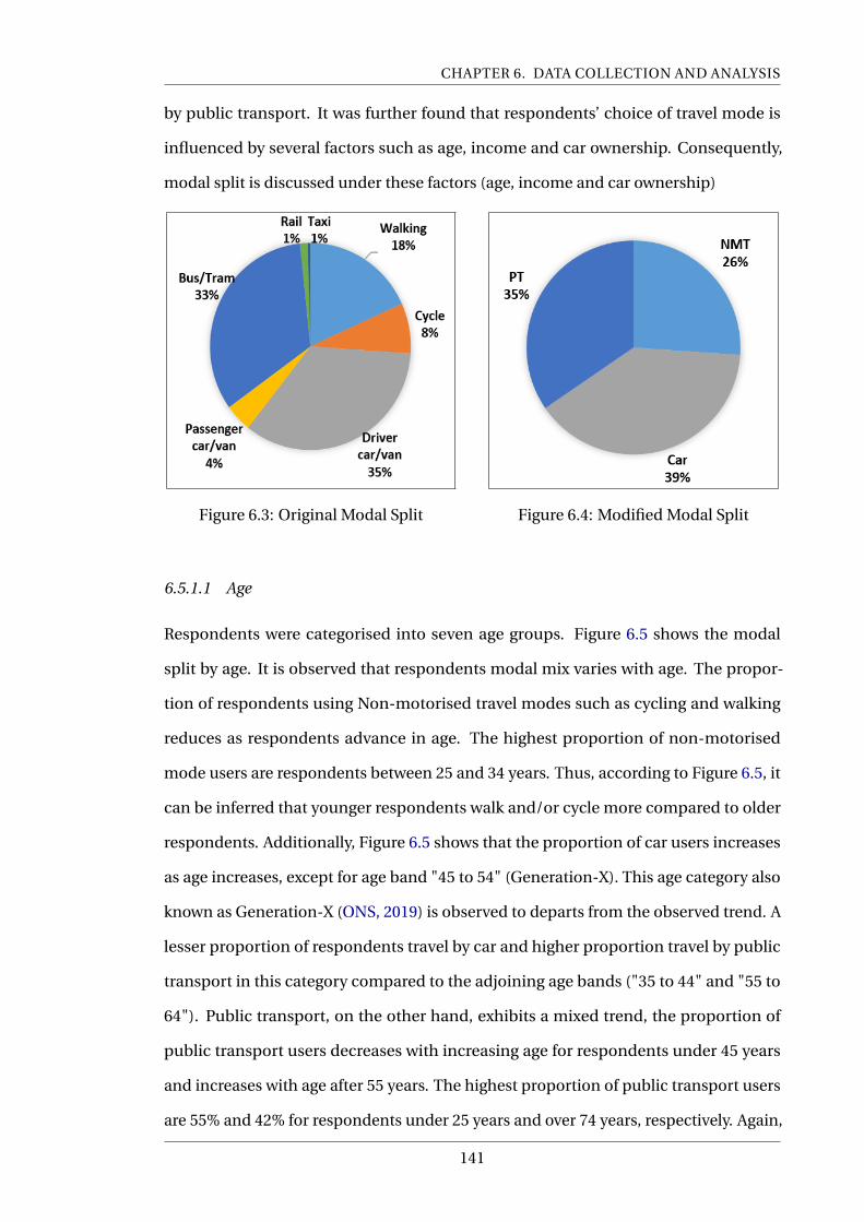
CHAPTER 6. DATA COLLECTION AND ANALYSIS
by public transport. It was further found that respondents’ choice of travel mode is
influenced by several factors such as age, income and car ownership. Consequently,
modal split is discussed under these factors (age, income and car ownership)
Figure 6.3: Original Modal Split Figure 6.4: Modified Modal Split
6.5.1.1 Age
Respondents were categorised into seven age groups. Figure 6.5 shows the modal
split by age. It is observed that respondents modal mix varies with age. The propor-
tion of respondents using Non-motorised travel modes such as cycling and walking
reduces as respondents advance in age. The highest proportion of non-motorised
mode users are respondents between 25 and 34 years. Thus, according to Figure 6.5, it
can be inferred that younger respondents walk and/or cycle more compared to older
respondents. Additionally, Figure 6.5 shows that the proportion of car users increases
as age increases, except for age band "45 to 54" (Generation-X). This age category also
known as Generation-X (ONS, 2019) is observed to departs from the observed trend. A
lesser proportion of respondents travel by car and higher proportion travel by public
transport in this category compared to the adjoining age bands ("35 to 44" and "55 to
64"). Public transport, on the other hand, exhibits a mixed trend, the proportion of
public transport users decreases with increasing age for respondents under 45 years
and increases with age after 55 years. The highest proportion of public transport users
are 55% and 42% for respondents under 25 years and over 74 years, respectively. Again,
141
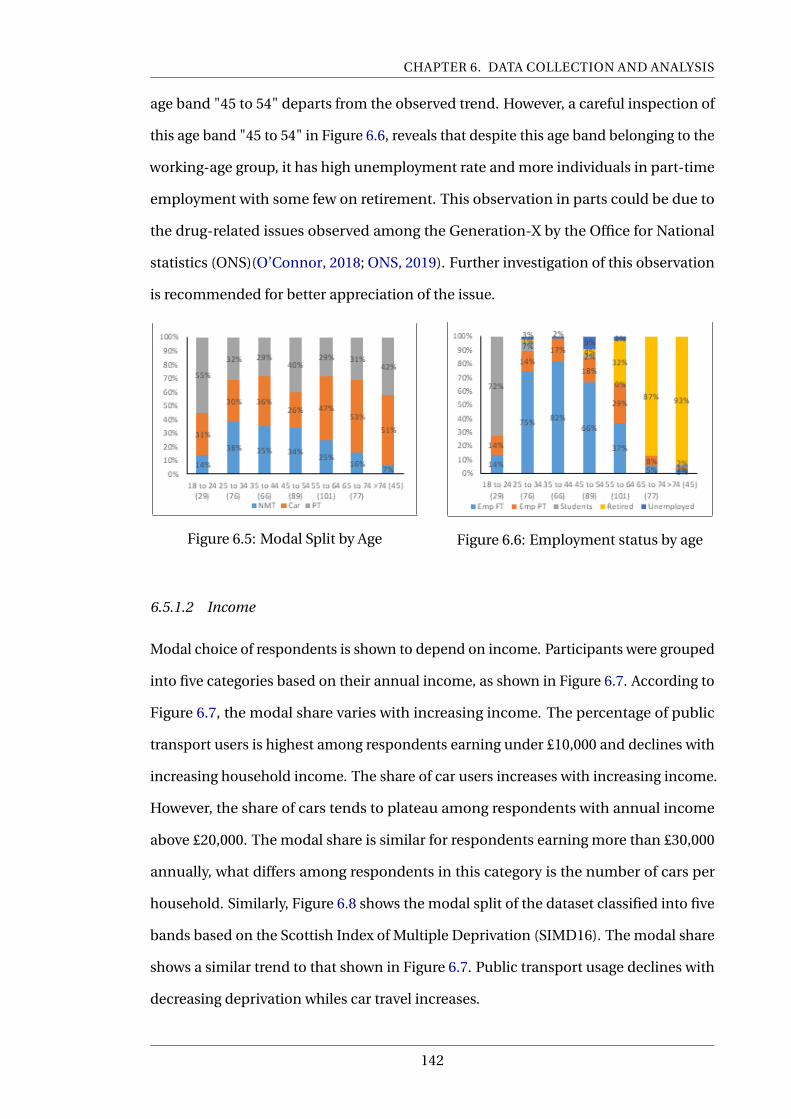
CHAPTER 6. DATA COLLECTION AND ANALYSIS
age band "45 to 54" departs from the observed trend. However, a careful inspection of
this age band "45 to 54" in Figure 6.6, reveals that despite this age band belonging to the
working-age group, it has high unemployment rate and more individuals in part-time
employment with some few on retirement. This observation in parts could be due to
the drug-related issues observed among the Generation-X by the Office for National
statistics (ONS)(O’Connor, 2018; ONS, 2019). Further investigation of this observation
is recommended for better appreciation of the issue.
Figure 6.5: Modal Split by Age Figure 6.6: Employment status by age
6.5.1.2 Income
Modal choice of respondents is shown to depend on income. Participants were grouped
into five categories based on their annual income, as shown in Figure 6.7. According to
Figure 6.7, the modal share varies with increasing income. The percentage of public
transport users is highest among respondents earning under £10,000 and declines with
increasing household income. The share of car users increases with increasing income.
However, the share of cars tends to plateau among respondents with annual income
above £20,000. The modal share is similar for respondents earning more than £30,000
annually, what differs among respondents in this category is the number of cars per
household. Similarly, Figure 6.8 shows the modal split of the dataset classified into five
bands based on the Scottish Index of Multiple Deprivation (SIMD16). The modal share
shows a similar trend to that shown in Figure 6.7. Public transport usage declines with
decreasing deprivation whiles car travel increases.
142
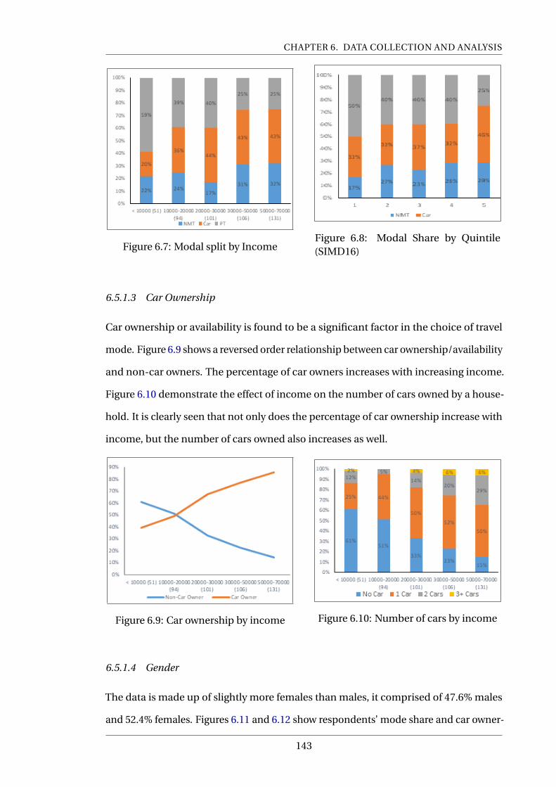
CHAPTER 6. DATA COLLECTION AND ANALYSIS
Figure 6.7: Modal split by IncomeFigure 6.8: Modal Share by Quintile(SIMD16)
6.5.1.3 Car Ownership
Car ownership or availability is found to be a significant factor in the choice of travel
mode. Figure 6.9 shows a reversed order relationship between car ownership/availability
and non-car owners. The percentage of car owners increases with increasing income.
Figure 6.10 demonstrate the effect of income on the number of cars owned by a house-
hold. It is clearly seen that not only does the percentage of car ownership increase with
income, but the number of cars owned also increases as well.
Figure 6.9: Car ownership by income Figure 6.10: Number of cars by income
6.5.1.4 Gender
The data is made up of slightly more females than males, it comprised of 47.6% males
and 52.4% females. Figures 6.11 and 6.12 show respondents’ mode share and car owner-
143
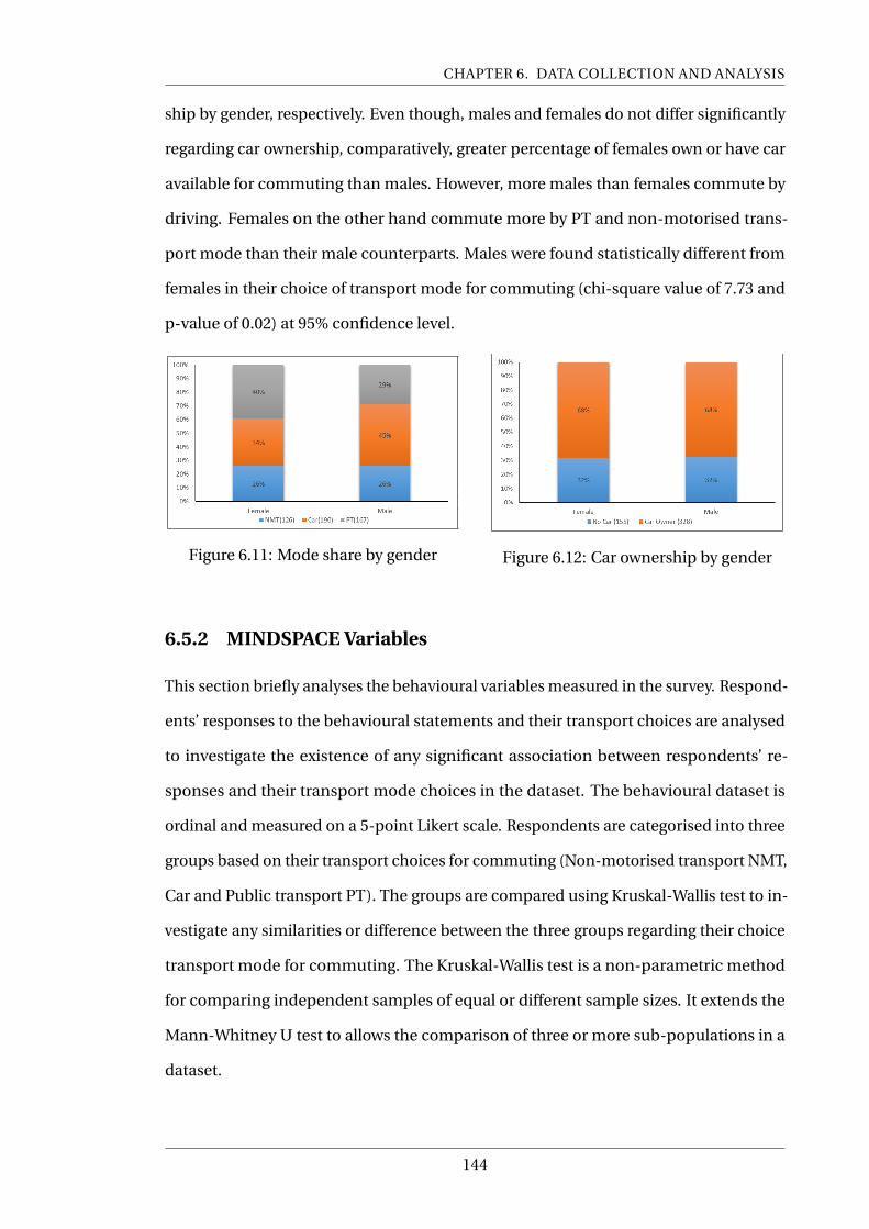
CHAPTER 6. DATA COLLECTION AND ANALYSIS
ship by gender, respectively. Even though, males and females do not differ significantly
regarding car ownership, comparatively, greater percentage of females own or have car
available for commuting than males. However, more males than females commute by
driving. Females on the other hand commute more by PT and non-motorised trans-
port mode than their male counterparts. Males were found statistically different from
females in their choice of transport mode for commuting (chi-square value of 7.73 and
p-value of 0.02) at 95% confidence level.
Figure 6.11: Mode share by gender Figure 6.12: Car ownership by gender
6.5.2 MINDSPACE Variables
This section briefly analyses the behavioural variables measured in the survey. Respond-
ents’ responses to the behavioural statements and their transport choices are analysed
to investigate the existence of any significant association between respondents’ re-
sponses and their transport mode choices in the dataset. The behavioural dataset is
ordinal and measured on a 5-point Likert scale. Respondents are categorised into three
groups based on their transport choices for commuting (Non-motorised transport NMT,
Car and Public transport PT). The groups are compared using Kruskal-Wallis test to in-
vestigate any similarities or difference between the three groups regarding their choice
transport mode for commuting. The Kruskal-Wallis test is a non-parametric method
for comparing independent samples of equal or different sample sizes. It extends the
Mann-Whitney U test to allows the comparison of three or more sub-populations in a
dataset.
144
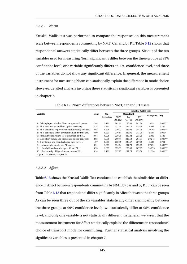
CHAPTER 6. DATA COLLECTION AND ANALYSIS
6.5.2.1 Norm
Kruskal-Wallis test was performed to compare the responses on this measurement
scale between respondents commuting by NMT, Car and by PT. Table 6.12 shows that
respondents’ answers statistically differ between the three groups. Six out of the ten
variables used for measuring Norm significantly differ between the three groups at 99%
confidence level; one variable significantly differs at 90% confidence level, and three
of the variables do not show any significant difference. In general, the measurement
instrument for measuring Norm can statistically explain the difference in mode choice.
However, detailed analysis involving these statistically significant variables is presented
in chapter 7.
Table 6.12: Norm differences between NMT, car and PT users
Variable Mean StdKruskal-Wallis Test
Mean RankChi-Square Sig
Deviation NMT Car PT(N=126) (N=190) (N=167)
1 : Driving is perceived to illustrate a person’s power ... 2.44 1.191 201.69 266.80 241.00 19.991 0.000***
2 : PT is seen as a second best option in society 2.74 1.215 221.34 245.14 235.40 2.692 0.260
3 : PT is perceived to provide environmentally cleaner ... 3.92 0.870 210.72 249.02 244.79 10.702 0.005***
4 : PT is beneficial to the environment and our health. 3.99 0.821 216.84 242.01 243.25 5.637 0.060*
5 : Family/friends believe PT is beneficial to the ... 3.61 0.899 228.75 249.32 223.25 3.338 0.188
6 : Most of my family and friends use public transport 2.93 1.098 200.47 243.58 261.31 20.243 0.000***
7 : If my family and friends change their travel ... 1.97 0.903 232.39 238.57 227.69 0.537 0.764
8 : I think people should use PT more ... 3.91 1.009 194.64 254.78 259.09 27.691 0.000***
9 : ... family/friends would agree if I use PT ... 3.53 1.003 175.99 272.06 267.05 59.275 0.000***
10 : I feel morally obligated to use more of PT ... 3.14 1.199 197.27 257.75 253.56 22.394 0.000***
*: p<0.1, **: p<0.05, ***: p<0.01
6.5.2.2 Affect
Table 6.13 shows the Kruskal-Wallis Test conducted to establish the similarities or differ-
ence in Affect between respondents commuting by NMT, by car and by PT. It can be seen
from Table 6.13 that respondents differ significantly in Affect between the three groups.
As can be seen three out of the six variables statistically differ significantly between
the three groups at 99% confidence level; two statistically differ at 95% confidence
level, and only one variable is not statistically different. In general, we assert that the
measurement instrument for Affect statistically explains the difference in respondents’
choice of transport mode for commuting. Further statistical analysis involving the
significant variables is presented in chapter 7.
145

CHAPTER 6. DATA COLLECTION AND ANALYSIS
Table 6.13: Difference in Affect between NMT, car and PT users
Variable Mean StdKruskal-Wallis Test
Mean RankChi-Square Sig
Deviation NMT Car PT(N=126) (N=190) (N=167)
1 : I enjoy using PT ... I get to meet people 2.12 1.062 225.60 213.75 255.89 8.400 0.015**
2 : Travelling in PT is boring 2.41 0.949 230.65 244.23 225.14 1.729 0.421
3 : I can use travel time for other activities 3.34 1.028 198.25 250.03 258.68 22.316 0.000***
4 : Driving is demanding 3.48 1.166 204.50 235.51 263.11 17.572 0.000***
5 : I use PT for the Environment 3.23 1.179 204.75 257.10 245.27 14.395 0.001***
6 : Uncomfortable travelling with strangers 2.03 1.103 252.94 219.13 219.24 7.951 0.019**
*: p<0.1, **: p<0.050, ***: p<0.01
6.5.2.3 Salience (PT Experience)
Eight variables were used for understanding respondents’ perception and experience
with public transport and the impact that would have on the loyalty to public transport.
Kruskal-Wallis Test conducted on this measurement tool to investigate any difference
in respondents’ responses in the following three categories; commuters by NMT, by car
and by PT is shown in Table 6.14. As can be seen, respondents differ significantly in
response across the three groups. Three variables statistically differ between the three
groups at 99% confidence level; three statistically differ at 95% confidence level, whiles
the remaining two variables were found statistically not different. We can infer from the
results of the Kruskal-Wallis Test that people perception about certain experiences on
public transport can shape their decision and affect their choice of transport for com-
muting. Further statistical analysis and discussion involving the significant variables
are presented in chapters.
Table 6.14: PT Experience between NMT, Car and PT users
Variable Mean StdKruskal-Wallis Test
Mean RankChi-Square Sig
Deviation NMT Car PT(N=126) (N=190) (N=167)
9 : Anti-social behaviour 3.28 1.427 183.00 126.00 155.00 10.972 0.004***
10 : Overcrowding 3.13 1.268 257.46 216.08 216.38 6.401 0.041**
11 : Exposure to health risk 2.68 1.326 248.70 233.44 212.60 6.402 0.041**
12 : Passenger Annoyance and discomfort 2.96 1.208 251.20 216.43 223.48 13.817 0.001***
13 : Poor hygiene (uncleanliness and smell on bus) 3.35 1.291 257.27 230.98 204.49 10.892 0.004***
14 : Inaccurate bus and real-time information 3.07 1.277 254.61 231.06 207.57 4.211 0.122
15 : Long waiting and travel time 3.40 1.346 245.53 233.56 216.26 6.705 0.035**
16 : Safety issues (seatbelts, toilets et cetera.) 2.34 1.302 248.65 234.50 211.81 2.130 0.345
*: p<0.1, **: p<0.05, ***: p<0.01
146

CHAPTER 6. DATA COLLECTION AND ANALYSIS
6.5.2.4 Narcissism
16 variables were used for investigating respondents’ level of narcissism and its impact
on travel behaviour. It is observed that each of the 16 items impacted travel behaviour
differently. Some items have a direct effect on the choice of mode, while others have an
indirect effect.
Narcissism and Mode choice
Kruskal-Wallis Test conducted on the NPI-16 measurement scale to examine respond-
ents’ scores against their regular commuting mode (i.e. NMT, Car and PT) is shown in
Table 6.15. As can be seen, the test shows a statistically significant difference between
three of the narcissism items (2, 7 and 11) and travel mode. These three items define
narcissistic trait of Exhibitionism according to Ames et al. (2006). The remaining 13
variables were found statistically, not different. We may infer from the above that the
narcissistic trait of Exhibitionism could influence travel mode choice, indicating that
exhibitionists are more likely to own and commute by car.
Table 6.15: Narcissism between NMT, Car and PT users
Variable Mean StdKruskal-Wallis Test
Mean RankChi-Square Sig
Deviation NMT Car PT(N=128) (N=188) (N=168)
1 : I know that I am good because everybody ... 2.53 0.998 233.52 237.84 237.33 0.094 0.954
2 : I like to be the centre of attention 2.12 0.906 248.80 246.70 219.9 4.912 0.086*
3 : I think I am a special person 2.47 1.031 251.25 229.81 245.86 2.298 0.317
4 : I like having authority over people 2.34 1.024 235.20 242.13 236.96 0.243 0.886
5 : I find it easy to manipulate others 2.16 1.004 238.52 233.72 236.64 0.108 0.947
6 : I insist upon getting the respect ... 2.32 1.035 240.14 226.72 247.82 2.294 0.318
7 : I am apt to show off if i get the chance 2.21 1.016 247.86 245.79 215.53 6.082 0.048**
8 : I always know what I am doing 2.85 1.157 234.28 246.27 237.34 0.701 0.704
9 : Everybody likes to hear my stories 2.36 0.962 233.66 226.16 250.45 3.119 0.210
10 : I expect a great deal from other ... 2.63 0.999 252.65 236.49 235.72 1.455 0.483
11 : I really like to be the centre of ... 2.06 0.946 249.26 247.98 212.40 8.346 0.015**
12 : People always seem to recognise my ... 2.49 1.022 239.99 230.19 240.95 0.712 0.700
13 : I am going to be a great person 2.50 1.026 236.35 227.45 239.59 0.817 0.665
14 : I can make anybody believe anything ... 2.16 0.953 244.81 244.34 221.13 3.465 0.177
15 : I am more capable than others 2.55 1.039 239.05 247.11 235.76 0.676 0.713
16 : I am an extraordinary person 2.35 0.987 245.30 238.14 230.79 0.888 0.642
*: p<0.1, **: p<0.05, ***: p<0.01
Further to the test above, Mann-Whitney U test conducted to confirm the relation-
ship between car users and PT users. The test found significant difference between
car users and PT users for five of the 16-item NPI scale and confirm that narcissistic
147
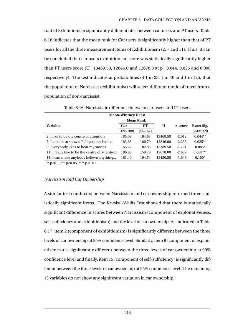
CHAPTER 6. DATA COLLECTION AND ANALYSIS
trait of Exhibitionism significantly differentiates between car users and PT users. Table
6.16 indicates that the mean rank for Car users is significantly higher than that of PT
users for all the three measurement items of Exhibitionism (2, 7 and 11). Thus, it can
be concluded that car users exhibitionism score was statistically significantly higher
than PT users score (U= 13469.50, 12846.0 and 12678.0 at p= 0.044, 0.025 and 0.008
respectively). The test indicates at probabilities of 1 in 23, 1 in 40 and 1 in 125; that
the population of Narcissist (exhibitionist) will select different mode of travel from a
population of non-narcissist.
Table 6.16: Narcissistic difference between car users and PT users
Mann-Whitney U test
Mean RankVariable Car PT U z-score Exact Sig.
(N=188) (N=167) (2-tailed)
2: I like to be the centre of attention 185.08 164.63 13469.50 -2.012 0.044**
7: I am apt to show off if i get the chance 183.68 160.79 12846.00 -2.238 0.025**
9: Everybody likes to hear my stories 165.27 182.85 13389.50 -1.721 0.085*
11: I really like to be the centre of attention 186.60 159.78 12678.00 -2.632 0.008***
14: I can make anybody believe anything... 181.40 164.53 13450.50 -1.646 0.100*
*: p<0.1, **: p<0.05, ***: p<0.01
Narcissism and Car Ownership
A similar test conducted between Narcissism and car ownership returned three stat-
istically significant items. The Kruskal-Wallis Test showed that there is statistically
significant difference in scores between Narcissism (component of exploitativeness,
self-sufficiency and exhibitionism) and the level of car ownership. As indicated in Table
6.17, item 2 (component of exhibitionism) is significantly different between the three
levels of car ownership at 95% confidence level. Similarly, item 9 (component of exploit-
ativeness) is significantly different between the three levels of car ownership at 99%
confidence level and finally, item 15 (component of self-sufficiency) is significantly dif-
ferent between the three levels of car ownership at 95% confidence level. The remaining
13 variables do not show any significant variation in car ownership.
148
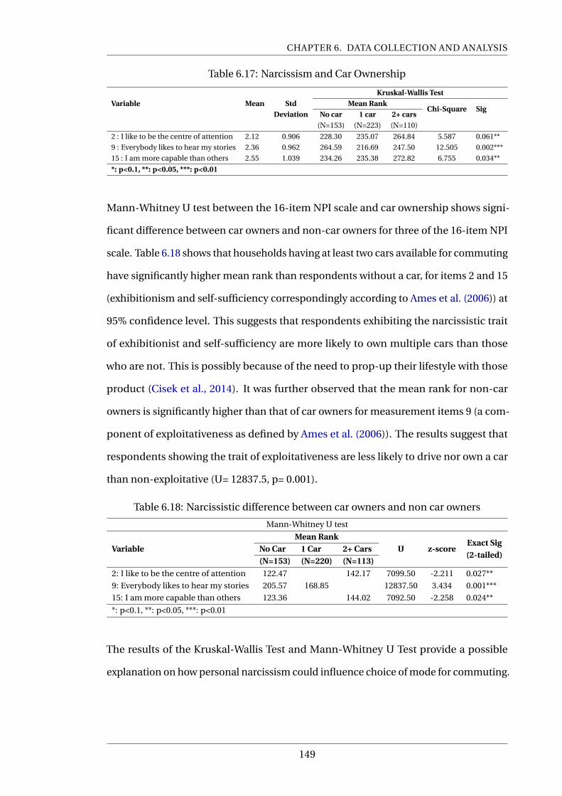
CHAPTER 6. DATA COLLECTION AND ANALYSIS
Table 6.17: Narcissism and Car Ownership
Variable Mean StdKruskal-Wallis Test
Mean RankChi-Square Sig
Deviation No car 1 car 2+ cars(N=153) (N=223) (N=110)
2 : I like to be the centre of attention 2.12 0.906 228.30 235.07 264.84 5.587 0.061**
9 : Everybody likes to hear my stories 2.36 0.962 264.59 216.69 247.50 12.505 0.002***
15 : I am more capable than others 2.55 1.039 234.26 235.38 272.82 6.755 0.034**
*: p<0.1, **: p<0.05, ***: p<0.01
Mann-Whitney U test between the 16-item NPI scale and car ownership shows signi-
ficant difference between car owners and non-car owners for three of the 16-item NPI
scale. Table 6.18 shows that households having at least two cars available for commuting
have significantly higher mean rank than respondents without a car, for items 2 and 15
(exhibitionism and self-sufficiency correspondingly according to Ames et al. (2006)) at
95% confidence level. This suggests that respondents exhibiting the narcissistic trait
of exhibitionist and self-sufficiency are more likely to own multiple cars than those
who are not. This is possibly because of the need to prop-up their lifestyle with those
product (Cisek et al., 2014). It was further observed that the mean rank for non-car
owners is significantly higher than that of car owners for measurement items 9 (a com-
ponent of exploitativeness as defined by Ames et al. (2006)). The results suggest that
respondents showing the trait of exploitativeness are less likely to drive nor own a car
than non-exploitative (U= 12837.5, p= 0.001).
Table 6.18: Narcissistic difference between car owners and non car owners
Mann-Whitney U test
VariableMean Rank
U z-scoreExact Sig(2-tailed)
No Car 1 Car 2+ Cars(N=153) (N=220) (N=113)
2: I like to be the centre of attention 122.47 142.17 7099.50 -2.211 0.027**
9: Everybody likes to hear my stories 205.57 168.85 12837.50 3.434 0.001***
15: I am more capable than others 123.36 144.02 7092.50 -2.258 0.024**
*: p<0.1, **: p<0.05, ***: p<0.01
The results of the Kruskal-Wallis Test and Mann-Whitney U Test provide a possible
explanation on how personal narcissism could influence choice of mode for commuting.
149

CHAPTER 6. DATA COLLECTION AND ANALYSIS
6.6 Summary
This chapter has discussed the data collection procedure and reports the descriptive
statistics of the sample data. Although the response rate is below the expectation of
the researcher, the sample data has been established to be representative of the study
population.
A total number of 3973 households were given the questionnaire package to take part in
the survey. 551 households representing 13.9% completed and returned the question-
naire.
The distribution of the sample data in by age, gender, income, employment, car owner-
ship and modal share was compared with similar estimates from the Scottish Household
Survey data (National Records of Scotland, 2018a) and travel data from the Transport
of Scotland (Transport Scotland, 2018b, Table 1). This was done to investigate the
representativeness of the sample data to the study population. It was necessary to know
whether the study results and analysis could be generalised to the study population or
not. The comparative test suggested that the characteristics of the sample data do not
differ from the Scottish Household Survey data (National Records of Scotland, 2018a)
and the Transport of Scotland travel data. This is an indication that both datasets come
from the same population. Thus, it was found that the sample data was representative
of the study population. Table 6.10 shows a summary of these estimates.
Exploratory analysis of the sample data indicates that participants’ age, income, gender
and car ownership significantly relate to their choice of mode for commuting. It was
found that the proportion of car owners and car usage increases with increasing income
and age. Male and females were found to differ in their choice of mode. While males
predominately drive, females were found to commute more by public transportation
modes. It was further found that the following MINDSPACE elements; Norms, Sali-
ence (experiences on public transport), Affect and Ego/Narcissism could have impact
travel behaviour. The mean ranks of participants’ responses to the indicators designed
for measuring the selected MINDSPACE elements were found to significantly differ
150

CHAPTER 6. DATA COLLECTION AND ANALYSIS
between Car, Public transport and Non-Motorised transport users. The next chapter
presents detailed statistical analysis involving traditional discrete choice model and
ICLV model which incorporates some effects of the MINDSPACE framework as latent
variables.
151

Part III
STATISTICAL MODELLING AND
CONCLUSIONS
152

; Chapter Seven <
Statistical Analysis and Model
Development
7.1 Introduction
The travel behaviour of an individual is explained by modal attributes, trip character-
istics and socio-economic characteristics. However, the literature suggests that these
do not adequately account for the heterogeneity in observed preferences. It is well
established that attitudes and perceptions play a significant role in the decision-making
process (Ben-akiva and Bierlaire, 1999; Ortuzar and Willumsen, 2011; Kamargianni
et al., 2015). Beyond the significance of attitudes and perception in the choice making,
they are difficult to observe directly and are thus considered latent and measured with
psychometric indicators. This chapter extends the analysis from chapter 6 and de-
scribes the systematic process of developing ICLV model by integrating a latent variable
model into a discrete choice model. Section 7.2 of this chapter outlines the processes
for extracting the latent variables from the psychometric indicators for the development
of the latent variable structural model. The development of a traditional discrete choice
model and ICLV model with the integration of the latent variable structural model is
described in 7.3, and section 7.4 presents the results and covers the discussion of the
results.
153
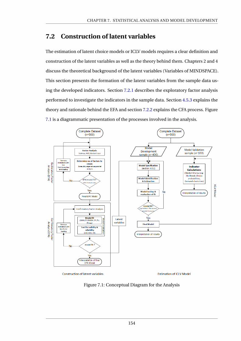
CHAPTER 7. STATISTICAL ANALYSIS AND MODEL DEVELOPMENT
7.2 Construction of latent variables
The estimation of latent choice models or ICLV models requires a clear definition and
construction of the latent variables as well as the theory behind them. Chapters 2 and 4
discuss the theoretical background of the latent variables (Variables of MINDSPACE).
This section presents the formation of the latent variables from the sample data us-
ing the developed indicators. Section 7.2.1 describes the exploratory factor analysis
performed to investigate the indicators in the sample data. Section 4.5.3 explains the
theory and rationale behind the EFA and section 7.2.2 explains the CFA process. Figure
7.1 is a diagrammatic presentation of the processes involved in the analysis.
Figure 7.1: Conceptual Diagram for the Analysis
154
CHAPTER 7. STATISTICAL ANALYSIS AND MODEL DEVELOPMENT
7.2.1 Exploratory factor analysis (EFA)
Since the measurement scale developed for measuring the selected MINDSPACE vari-
ables is being tested for the first time, EFA was performed to explore and reliability of
the underlying dimensionality in the psychometric indicators. The EFA was performed
with the indicators of the proposed MINDSPACE variables in the dataset. The normality
of the indicators was tested using SPSS software package. According to the normality
assumption, data is considered normal if the Skewness and Kurtosis are between ± 3.00
and ± 7.00 Tabachnick and Fidell, 2014. The results of the normality test indicate the
50 indicators had no normality issues (Bryne, 2012; Kline, 2011; Herman, 2016). The
EFA was consequently performed using maximum likelihood (ML) estimation method
in SPSS software package version 23.0 (Field, 2013). The robustness of ML method in
handling normally distributed data, ordinal data, cases with missing data and the fact
that AMOS software package uses ML for the CFA makes it most appropriate for the
factor analysis (Bahaman, 2012; Arbuckle, 2017). Oblimin rotation method was adopted
to allows some level of correlation between the factors.
7.2.1.1 Results and discussion of the EFA
Following the recommendations of Child (2006) and Tabachnick and Fidell (2014), el-
even (11) indicators with communality score less than 0.2 were removed during the
factor analysis. Additionally, items with factors loadings below 0.3 were also suppressed.
Two variables "PTExp6b" and "PTExp7b" were found cross-load above o.40 on two
factors. These two indicators were consequently removed from the analysis and the
EFA reperformed, according to the recommendation in Schönrock-adema et al. (2009)
(to remove variables cross-loading at least 0.40 on more than one construct). Figure
7.2 shows the scree plot of the eigenvalues of the final EFA and the eigenvalues of PA.
According to the PA rule and Figure 7.2, five (5) factors must be retained. However,
the 5-factor solution explains only 49% of the total variance, which is less than the
minimum of 50% recommended by the total of variance extracted technique (Streiner,
1994).
155
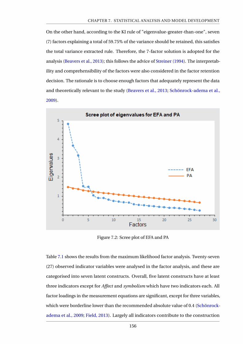
CHAPTER 7. STATISTICAL ANALYSIS AND MODEL DEVELOPMENT
On the other hand, according to the KI rule of "eigenvalue-greater-than-one", seven
(7) factors explaining a total of 59.75% of the variance should be retained, this satisfies
the total variance extracted rule. Therefore, the 7-factor solution is adopted for the
analysis (Beavers et al., 2013); this follows the advice of Streiner (1994). The interpretab-
ility and comprehensibility of the factors were also considered in the factor retention
decision. The rationale is to choose enough factors that adequately represent the data
and theoretically relevant to the study (Beavers et al., 2013; Schönrock-adema et al.,
2009).
Figure 7.2: Scree plot of EFA and PA
Table 7.1 shows the results from the maximum likelihood factor analysis. Twenty-seven
(27) observed indicator variables were analysed in the factor analysis, and these are
categorised into seven latent constructs. Overall, five latent constructs have at least
three indicators except for Affect and symbolism which have two indicators each. All
factor loadings in the measurement equations are significant, except for three variables,
which were borderline lower than the recommended absolute value of 0.4 (Schönrock-
adema et al., 2009; Field, 2013). Largely all indicators contribute to the construction
156

CHAPTER 7. STATISTICAL ANALYSIS AND MODEL DEVELOPMENT
of the latent constructs. Alpha Cronbach’s test has been conducted for the reliability
of latent constructs extracted. Cronbach’s alpha values for six of the seven retained
constructs satisfied the 0.70 minimum requirements for reliability (α≥ 0.70) (Cronbach,
1951). However, Cronbach alpha values for Affect (α = 0.664) is marginally below the
acceptable threshold. Meanwhile, according to Kline (2011), lower values of Cronbach’s
alpha can be tolerated in a latent variable analysis.
Consequently, Affect has been retained for further analysis due to its theoretical relev-
ance to the study.
Additionally, any issue arising from individual heterogeneity could be controlled in
the choice model (Beavers et al., 2013; Schönrock-adema et al., 2009; Streiner, 1994).
Therefore, the extracted latent constructs are assumed to be reliable and acceptable;
the sample size and the indicators are appropriate for testing the CFA.
Table 7.1: Exploratory Factor Analysis1
N = 500 Latent Construct
MINDSPACE Elements Norm Salience Affect Narcissism/Ego
Factor PerNorm SocNorm Symb Sal Aff Nar Exhib
Cronbach’s Alpha 0.785 0.772 0.721 0.859 0.664 0.852 0.762
Nrm10 0.847
Aff5 0.651 0.331
Nrm9 0.452
Nrm8 0.445
Nrm4 0.898
Nrm3 0.763
Nrm5 0.448
Nrm2 0.902
Nrm1 0.629
PTExp4b 0.833
PTExp5b 0.73
PTExp3b 0.722
PTExp1b 0.719
PTExp2b 0.708
PTExp8b 0.572
Aff4 1.017
Aff3 0.441
Nar15 0.67
Nar12 0.493
Nar13 0.475
Nar16 0.461
Nar3 0.441
Nar4 0.441
Nar5 0.418
Nar2 0.68
Nar11 0.534
Nar7 0.398
Nar = Narcissism; SocNorm = Social Norms; Aff = Affect; Exhib = Exhibitionism; PerNorm = Personal Norms
The Kaiser-Meyer-Olkin (KMO) Test verifies the adequacy of the sampling and whether
1For readability, factor loadings upto ± 0.3 has been suppressed, following the advice of Tabachnickand Fidell (2014)
157

CHAPTER 7. STATISTICAL ANALYSIS AND MODEL DEVELOPMENT
the indicators are suitable for factor analysis whiles Bartlett’s test of sphericity test
the significance of the correlation between all the indicators in the EFA (Hair et al.,
1998). Table 7.2 shows the results of the KMO and Bartletts test. From the results, the
KMO value of 0.797 (KMO ≥ 0.70), satisfies the minimum requirement and indicate
an adequate sample size for factor analysis. Similarly, Bartlett’s Test value of 3492.347
is significant (P <0.01), also suggesting that the correlation between the indicators is
adequate for factor analysis.
Table 7.2: Measure of sample Adequacy
Measure of Sample Adequacy
Measure Value
Bartlett’s Test of Sphericity
x2 3492.347
df 351
Sig. 0
Kaiser-Meyer-Olkin Measure
of Sampling Adequacy.0.797
7.2.1.2 Latent Constructs
Seven latent constructs/variables are extracted in the factor analysis, namely: Salience
(Sal: 6 indicators), Social Norms (SocNorms : 3 indicators), Personal Norms (PerNorms:
4 indicators) Symbolism (Symb: 2 indicators), Narcissism (Nar: 6 indicators), Narcissistic
trait of exhibitionism (Exh: 3 indicators) and Affect (Aff: 2 indicators).
Salience describes the participants’ perception of negative experience on public trans-
port (bus and tram services in Edinburgh). This variable reflects the assertion that
negative experiences are exaggerated in human memory and mostly recalled in decision-
making. The investigation seeks to examine the influence of salient PT experiences on
decision making.
Three latent variables were extracted from the instrument designed for measuring
Norms; the results of the factor analysis are consistent with Belgiawan et al. (2016).
The latent variables comprise of Social Norms (SocNorm), Personal Norms (PerNorms)
and social symbolism (Symb).
SocNorm describes the respondents’ perception or understanding of societal beliefs
and perception of cars, public transport and the environment.
158
CHAPTER 7. STATISTICAL ANALYSIS AND MODEL DEVELOPMENT
PerNorm defines the individual views and perception of cars, public transport and
their impact on the environment; this factor describes the internalised norms of the
respondents.
Symb describes the perception of the social-symbolic value of driving and anti-status
value of PT. Symb is constructed with two indicators, one describing the symbolic status
of owning and driving a car and the second indicator depicting PT as anti-status symbol
(Steg, 2005).
Affect could be explained in terms of positive or negative valence. The instrument de-
signed for assessing this concept comprised of statements for measuring both aspects of
Affect. The indicators for negative valence were suppressed and remove for having very
low communalities and factor loadings. Therefore, the variable Affect describes positive
valence and sentiments towards PT modes (Bus/Tram) resulting from the individual’s
experience of PT travel and driving.
Narcissism describes a personality type characterised by a sense of entitlement, special-
ness, a need for admiration and a lack of empathy. Narcissism comprises of seven (7)
first-order subtypes namely, Superiority, Exhibitionism, Exploitativeness, Self-sufficiency,
Authority, entitlement and Vanity (Raskin and Terry, 1988; Ames et al., 2006).
Two latent variables were extracted from the 16-item NPI scale developed for measuring.
Narcissism; 4 indicators with very low communalities and factor loadings were removed
or suppressed from the analysis.
Narcissism is the first factor, this construct was formed with six indicators comprising of
indicators on Superiority, Exploitative, Self-sufficiency, Authority, entitlement (Raskin
and Terry, 1988; Ames et al., 2006).
Exhibitionism; this is Narcissism trait of Exhibitionism (Raskin and Terry, 1988). This
variable is characterised by Grandiosity personality traits and reflect an individual need
for attention and admiration (Levesque, 2011).
159

CHAPTER 7. STATISTICAL ANALYSIS AND MODEL DEVELOPMENT
7.2.2 Confirmatory factor analysis
This section is aimed at assessing the seven factors extracted in the EFA through Con-
firmatory Factor Analysis (CFA). This section tests the seven latent factors extracted
during the EFA for validity and reliability. All the variables (exogenous and endogenous)
are combined in the CFA analysis (pooled CFA) based on the findings in Chong et al.
(2014) and Herman (2016). The threshold for validity, reliability and the goodness of
fit indices are discussed under section 4.5.4.1 and summarised in Table 4.6. The lat-
ent variables are examined in a First Order pooled CFA using AMOS software package
version 26.0.
7.2.2.1 Results and discussion of the CFA
The final CFA model as shown in Figure 7.3 comprise of 20 indicators categorised into
six latent constructs namely; Salience, superiority, social Norms (SocNorms), Affect,
Exhibitionism, Personal Norms (PerNorms). One indicator was dropped from the latent
variable Salience and four indicators from the latent variable Narcissism (Table 7.1).
The latent variable Narcissism (now with three indicators) is redefined as Superiority
narcissism (Superiority) to reflect its indicators (Raskin and Terry, 1988). Superiority
narcissism describes a situational narcissism where an individual believes they are
superior to others and acts in ways that indicate they are not shy about discussing or
flaunting their achievements.
Five of the 27 indicators from the EFA were found to have low loadings and subsequently
dropped from the analysis (refer to Figure D.1 in Appendix D) (Field, 2013). The final
CFA model had 22 indicators classed into seven latent constructs (refer to Figure D.2 in
Appendix D). However, the latent construct, Symbolism was dropped for identification
related issues; the standardised factor loading and squared multiple correlations of
one of its indicators (Nrm1) exceeds unity (1.51 and 2.27 respectively)(Hair et al., 1998,
pg.610), additionally, the critical ratio of Symbolism and Nrm1 of 1.286 and -0.719 are
below the minimum threshold of ≥ 1.96. Researchers differ in opinion on the meaning
and implication of having standardised coefficients greater than one in magnitude
160

CHAPTER 7. STATISTICAL ANALYSIS AND MODEL DEVELOPMENT
(Hair et al., 1998; Jöreskog, 1999, pg.610). While Hair et al. (1998, pg.610) suggest the
elimination of such constructs, Jöreskog (1999) believes this does not mean something is
wrong, but an indication of high degree of multicollinearity (Jöreskog, 1999). Therefore,
two CFA models were performed. The AIC and BIC estimates of the two CFA models
were compared and the best fit CFA model adopted for the ICLV modelling. Table 7.3
below shows the fitness indices of the two measurements models, Model 1 with latent
factor Symbolism and model 2 without Symbolism.
Table 7.3: CFA model comparison
Index Model 1 Model 2
CMIN 357.864 328.809
DF 188 155
CMIN/DF 1.904 2.121
NFI 0.912 0.914
TLI 0.940 0.935
CFI 0.956 0.952
RMSEA 0.042 0.047
PClose 0.978 0.767
AIC 531.864 478.809
BIC 540.048 485.225
∆AIC 53.055 0
∆B IC 54.823 0
The final model satisfied all indices recommended for assessing goodness-of-fit (see Hu
and Bentler, 1999; Kline, 2011), indicating that the measurement model sufficiently fits
the sample data.
The results in Table 7.3 indicate that both models satisfied all indices recommended for
assessing goodness-of-fit (see to 4.6) Hu and Bentler, 1999; Kline, 2011.
A comparison of the AIC and BIC estimates of the two models shows that model 2 has
low AIC and BIC values compared to model 1.
The difference in AIC and BIC values between the two models (∆AIC = 53.055 and
∆B IC =54.823) both provide strong evidence in favour of model 2 (Fabozzi et al., 2014).
Therefore, model 2 is accepted and adopted in the study. Figure 7.3 below shows the
graphical representation of the final CFA model. According to Figure 7.3, the final
pooled first Order CFA has 20 indicators represented by six latent constructs.
161
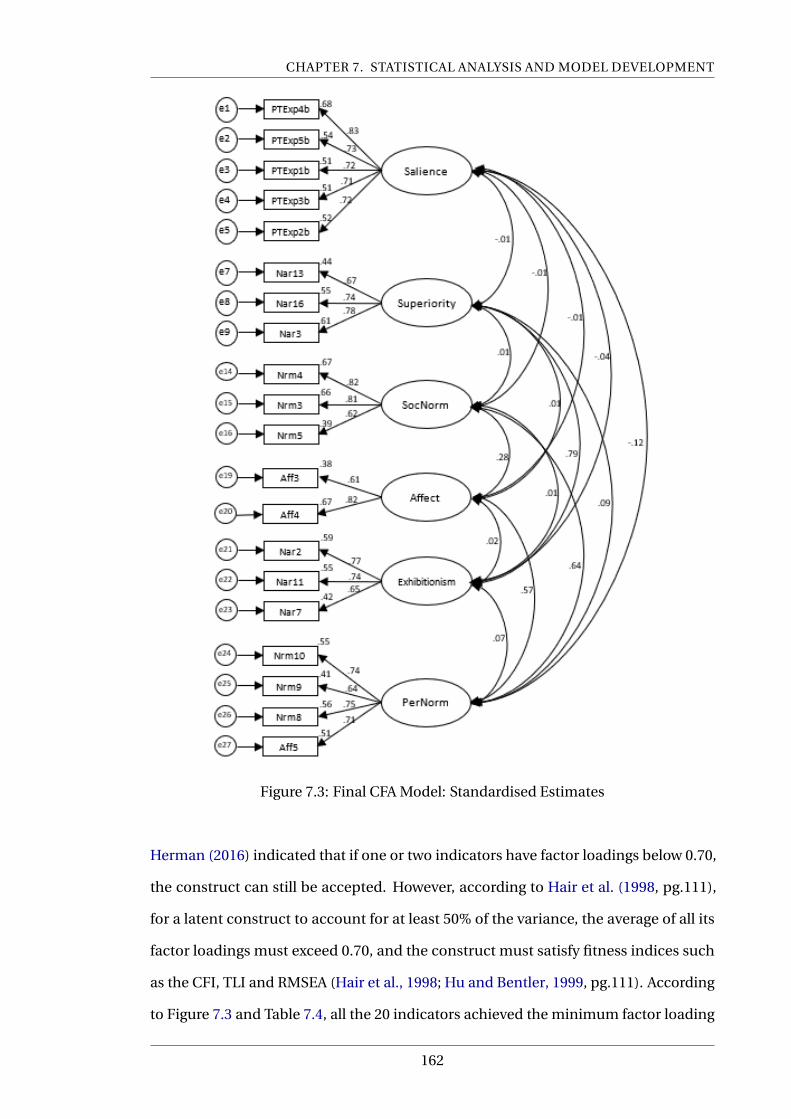
CHAPTER 7. STATISTICAL ANALYSIS AND MODEL DEVELOPMENT
Figure 7.3: Final CFA Model: Standardised Estimates
Herman (2016) indicated that if one or two indicators have factor loadings below 0.70,
the construct can still be accepted. However, according to Hair et al. (1998, pg.111),
for a latent construct to account for at least 50% of the variance, the average of all its
factor loadings must exceed 0.70, and the construct must satisfy fitness indices such
as the CFI, TLI and RMSEA (Hair et al., 1998; Hu and Bentler, 1999, pg.111). According
to Figure 7.3 and Table 7.4, all the 20 indicators achieved the minimum factor loading
162

CHAPTER 7. STATISTICAL ANALYSIS AND MODEL DEVELOPMENT
of 0.50 and the average of the factor loadings of each latent construct above 0.70. The
Measurement model fitness indices presented in Table 7.6 show that there are no issues
with the first order pooled CFA. In addition, Table 7.5 and Table 7.6 indicate that the
CFA model achieved Convergent and Discriminant Validity, and reliability.
Table 7.4: Confirmatory Factor Analysis
N = 500 Latent Construct
MINDSPACE Elements Norm Salience Affect Narcissism/EgoSig
Factor PerNorm SocNorm Sal Aff Sup Exhib
Nrm8 0.748 ***
Nrm9 0.641 ***
Nrm10 0.741 ***
Aff5 0.711 ***
Nrm5 0.623 ***
Nrm3 0.811 ***
Nrm4 0.819 ***
PTExp2b 0.718 ***
PTExp1b 0.712 ***
PTExp3b 0.717 ***
PTExp5b 0.732 ***
PTExp4b 0.825 ***
Aff4 0.818 ***
Aff3 0.613 ***
Nar3 0.778 ***
Nar16 0.739 ***
Nar13 0.666 ***
Nar7 0.648 ***
Nar11 0.744 ***
Nar2 0.765 ***
PerNorm = Personal Norm; SocNorm = Social Norm ; Sup = Superiority Narcissism;
Exhib = Exhibitionism Narcissism; *** = P-value < 0.000
Table 7.5 shows the results of the validity and reliability test performed as part of the
CFA. The CFA findings indicate that The CR values of all the constructs are ≥ 0.70,
except Affect; which has CR value of 0.683. However, Affect is retained, following the
suggestions of Fornell and Larcker (1981); Bagozzi (1988) that CR values greater than
0.60 can be considered adequate. Therefore, all the constructs are considered to have
achieved CR. Moreover, all constructs satisfied the MaxR(H) test of reliability.
Similarly, the results show that there is no issue with convergent validity (AVE ≥ 0.50).
All constructs but Superiority and Exhibitionism achieved Discriminant validity (MSV <
AVE); this suggest a substantial level of correlation among the indicators of Superiority
and Exhibitionism, which raises issues of multicollinearity. Bahaman (2012) recom-
mended cut-off value of 0.85; meanwhile, the correlation between Superiority and
163
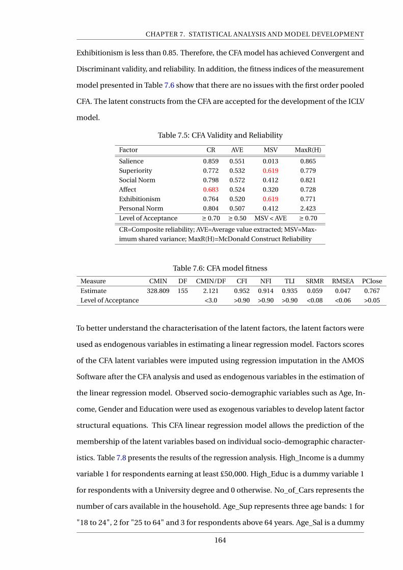
CHAPTER 7. STATISTICAL ANALYSIS AND MODEL DEVELOPMENT
Exhibitionism is less than 0.85. Therefore, the CFA model has achieved Convergent and
Discriminant validity, and reliability. In addition, the fitness indices of the measurement
model presented in Table 7.6 show that there are no issues with the first order pooled
CFA. The latent constructs from the CFA are accepted for the development of the ICLV
model.
Table 7.5: CFA Validity and Reliability
Factor CR AVE MSV MaxR(H)
Salience 0.859 0.551 0.013 0.865
Superiority 0.772 0.532 0.619 0.779
Social Norm 0.798 0.572 0.412 0.821
Affect 0.683 0.524 0.320 0.728
Exhibitionism 0.764 0.520 0.619 0.771
Personal Norm 0.804 0.507 0.412 2.423
Level of Acceptance ≥ 0.70 ≥ 0.50 MSV < AVE ≥ 0.70
CR=Composite reliability; AVE=Average value extracted; MSV=Max-
imum shared variance; MaxR(H)=McDonald Construct Reliability
Table 7.6: CFA model fitness
Measure CMIN DF CMIN/DF CFI NFI TLI SRMR RMSEA PClose
Estimate 328.809 155 2.121 0.952 0.914 0.935 0.059 0.047 0.767
Level of Acceptance <3.0 >0.90 >0.90 >0.90 <0.08 <0.06 >0.05
To better understand the characterisation of the latent factors, the latent factors were
used as endogenous variables in estimating a linear regression model. Factors scores
of the CFA latent variables were imputed using regression imputation in the AMOS
Software after the CFA analysis and used as endogenous variables in the estimation of
the linear regression model. Observed socio-demographic variables such as Age, In-
come, Gender and Education were used as exogenous variables to develop latent factor
structural equations. This CFA linear regression model allows the prediction of the
membership of the latent variables based on individual socio-demographic character-
istics. Table 7.8 presents the results of the regression analysis. High_Income is a dummy
variable 1 for respondents earning at least £50,000. High_Educ is a dummy variable 1
for respondents with a University degree and 0 otherwise. No_of_Cars represents the
number of cars available in the household. Age_Sup represents three age bands: 1 for
"18 to 24", 2 for "25 to 64" and 3 for respondents above 64 years. Age_Sal is a dummy
164
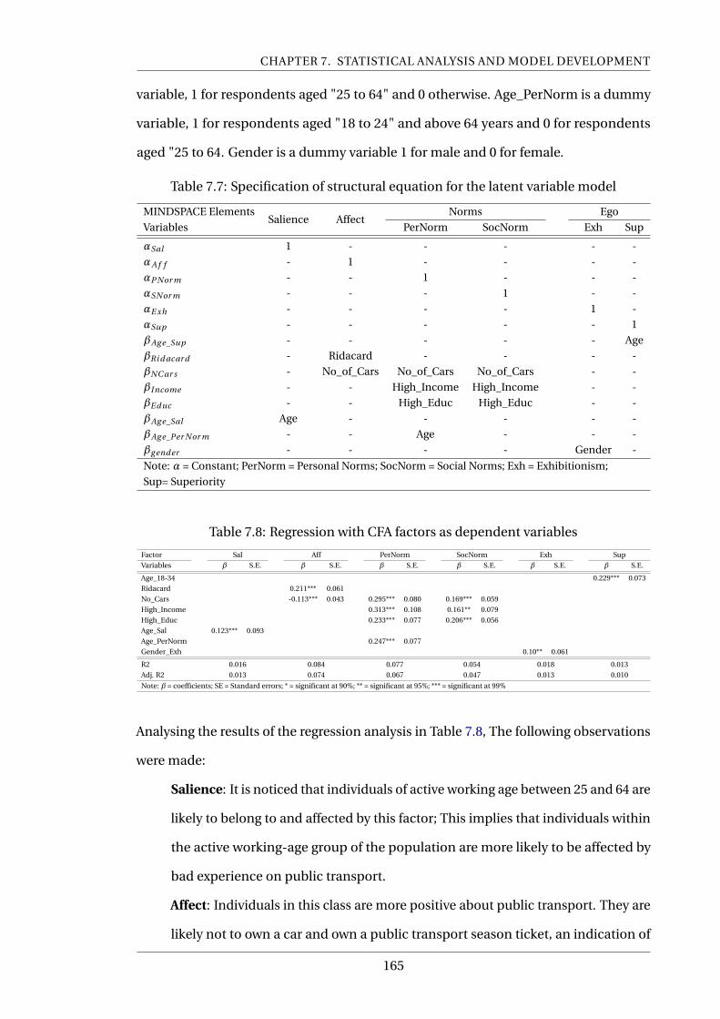
CHAPTER 7. STATISTICAL ANALYSIS AND MODEL DEVELOPMENT
variable, 1 for respondents aged "25 to 64" and 0 otherwise. Age_PerNorm is a dummy
variable, 1 for respondents aged "18 to 24" and above 64 years and 0 for respondents
aged "25 to 64. Gender is a dummy variable 1 for male and 0 for female.
Table 7.7: Specification of structural equation for the latent variable model
MINDSPACE ElementsSalience Affect
Norms Ego
Variables PerNorm SocNorm Exh Sup
αSal 1 - - - - -
αA f f - 1 - - - -
αP Nor m - - 1 - - -
αSNor m - - - 1 - -
αE xh - - - - 1 -
αSup - - - - - 1
βAg e_Sup - - - - - Age
βRi d acar d - Ridacard - - - -
βNC ar s - No_of_Cars No_of_Cars No_of_Cars - -
βIncome - - High_Income High_Income - -
βE duc - - High_Educ High_Educ - -
βAg e_Sal Age - - - - -
βAg e_Per Nor m - - Age - - -
βg ender - - - - Gender -
Note: α = Constant; PerNorm = Personal Norms; SocNorm = Social Norms; Exh = Exhibitionism;
Sup= Superiority
Table 7.8: Regression with CFA factors as dependent variables
Factor Sal Aff PerNorm SocNorm Exh Sup
Variables β S.E. β S.E. β S.E. β S.E. β S.E. β S.E.
Age_18-34 0.229*** 0.073
Ridacard 0.211*** 0.061
No_Cars -0.113*** 0.043 0.295*** 0.080 0.169*** 0.059
High_Income 0.313*** 0.108 0.161** 0.079
High_Educ 0.233*** 0.077 0.206*** 0.056
Age_Sal 0.123*** 0.093
Age_PerNorm 0.247*** 0.077
Gender_Exh 0.10** 0.061
R2 0.016 0.084 0.077 0.054 0.018 0.013
Adj. R2 0.013 0.074 0.067 0.047 0.013 0.010
Note: β = coefficients; SE = Standard errors; * = significant at 90%; ** = significant at 95%; *** = significant at 99%
Analysing the results of the regression analysis in Table 7.8, The following observations
were made:
Salience: It is noticed that individuals of active working age between 25 and 64 are
likely to belong to and affected by this factor; This implies that individuals within
the active working-age group of the population are more likely to be affected by
bad experience on public transport.
Affect: Individuals in this class are more positive about public transport. They are
likely not to own a car and own a public transport season ticket, an indication of
165
CHAPTER 7. STATISTICAL ANALYSIS AND MODEL DEVELOPMENT
loyal riders of public transport and have high utility for PT in-vehicle travel time
and disutility for driving. The likelihood to belong to this group decreases with an
increasing number of household cars.
Norms: Two latent constructs were retained from this MINDSPACE Element in the
CFA analysis named as "personal norm" and "social norms", these two constructs
are discussed below:
Personal Norms: Individuals scoring high on this construct are likely to be either
young or old and aged between 18 and 24 or above 64 years, respectively. The
estimates indicate that members of this class are highly educated and have a
university degree (at least have a first degree). They are likely to have a household
income of at least £50,000 and may not have a car available for the household use.
Social Norms: Individuals scoring high on this latent construct have similar char-
acteristics as those in the Personal norms group. The difference between these
two constructs is that while personal norm is dependent on age, social norm is
less affected by age.
Ego/Narcissism: Similar to Norms, two latent constructs were retained from
Narcissism in the CFA analysis, namely, "Exhibitionism" and "Superiority".
Exhibitionism: This narcissistic trait is associated with the use of material goods
to enhance social status. Members scoring high on this construct are observed to
be single household males of all ages.
Superiority: This trait describes individuals with a delusional sense of superiority
that leads them to believe they are unique from the average person. Respondents
scoring high on this construct are observed to be young individuals aged between
18 and 34.
7.3 Mode Choice Modelling
The choice models were estimated on 80% of the sample data (400 cases randomly
selected from the sample data). The estimated model is then applied to the other 20% of
sample data for validating the developed model. The sections below discuss the model
166
CHAPTER 7. STATISTICAL ANALYSIS AND MODEL DEVELOPMENT
estimation and the model results.
7.3.1 The Baseline model
Multinomial logistic regression model has been estimated as the baseline model using
the maximum likelihood estimator in Biogeme software package (Bierlaire, 2018b)
based on the specification in section 4.6.1.1 and equations 4.13 to 4.15. The choice is
assumed to be between; public transport (PT), which consists of bus, train and tram;
private motorised modes (Car), which include car as a user and a passenger and taxi,
and Non-motorised transport (NMT), representing walking and cycling. Utilities of
the alternatives are presented in section 4.6.1 with explanatory variables of individual
characteristics, modal attributes and trip characteristics.
There are several ways to decide on the variables to include in a model. The selection
of variables allows for the construction of an optimal model. The selection limits the
set of predictor variables to those that are necessary to account for as much of the
variance in the data. The first consideration in the selection of variables included during
the estimation of the base model was their theoretical relevance to the objective of
the study according to the literature. Finally, statistical regression methods such as
forward selection, backward elimination, stepwise selection were used in several trials
to conclude on the final model.
7.3.2 Integrated Choice and Latent Variable model
The final integrated and latent variable (ICLV) model consisting of two components;
the discrete choice model and a latent variable model was estimated using 10,000
Modified Latin Hypercube Sampling (MLHS) draws (Hess et al., 2006). The ICLV model
has the same specification as the Baseline model but with the incorporation of the
latent attitudes or psychometric constructs. The factors extracted during the EFA and
validated in the CFA are used as latent variables in addition to the observed individual
and trip characteristics, and modal attributes. The model estimation is done in the
Biogeme software Bierlaire, 2018b. We estimate an integrated choice and latent variable
167

CHAPTER 7. STATISTICAL ANALYSIS AND MODEL DEVELOPMENT
model. Like the baseline model, the estimated model contains choices between PT,
Car and NMT. The framework and detail specification of the integrated choice model
is illustrated in Figure 4.2. (Readers are referred to the model specification in section
4.6.1) (Ben-Akiva and Boccara, 1995; Ben-akiva and Bierlaire, 1999; Bierlaire, 2018c)
Modified Latin Hypercube Sampling (MLHS).
7.4 Results and Discussion
The results of the base model and the ICLV model are presented and discussed in the
following sections.
7.4.1 Results
Table 7.9 reports the results of the ICLV model. The prediction rate of the ICLV model
with the Base model for the validation sub-sample (20% of data). Overall correct predic-
tion rate of 60% was obtained for the base model and 65% correct prediction rate for the
ICLV model. This suggests that the latent variables succeeded in accounting for some
existent heterogeneity of respondents’ travel choices. In other to assess the validity and
applicability of the estimated model on a similar dataset, the model was validated using
the validation sample; the remaining 20% of the dataset. Table 7.10 presents the good-
ness of fit and the log-likelihood estimates for both models. The log-likelihood values
for the ICLV and the base models are calculated from the simulated choice probabilities
of both models from the validation sample for comparison. The ICLV model is observed
to have the best goodness of fit statistics compared to the base model. Even though the
ICLV model has more predictor variables compared to the base model, a comparison of
the adjusted rho-square (ρ̄2) values indicates that the additional predictor variables in
the ICLV model improved upon the base model more than would be expected by chance.
It can be seen from the results in Table 7.9 that the estimates of all the utility variables,
i.e. travel time, cost, distance, age, education, income, walking time and number of cars
have the expected signs. The estimates and the significance level for both the base and
168
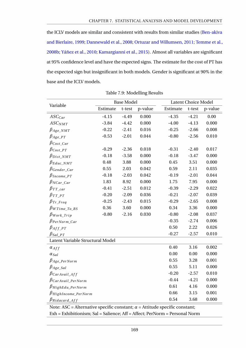
CHAPTER 7. STATISTICAL ANALYSIS AND MODEL DEVELOPMENT
the ICLV models are similar and consistent with results from similar studies (Ben-akiva
and Bierlaire, 1999; Dannewald et al., 2008; Ortuzar and Willumsen, 2011; Temme et al.,
2008b; Yáñez et al., 2010; Kamargianni et al., 2015). Almost all variables are significant
at 95% confidence level and have the expected signs. The estimate for the cost of PT has
the expected sign but insignificant in both models. Gender is significant at 90% in the
base and the ICLV models.
Table 7.9: Modelling Results
VariableBase Model Latent Choice Model
Estimate t-test p-value Estimate t-test p-value
ASCC ar -4.15 -4.49 0.000 -4.35 -4.21 0.00
ASCN MT -3.84 -4.42 0.000 -4.00 -4.13 0.000
βAg e_N MT -0.22 -2.41 0.016 -0.25 -2.66 0.008
βAg e_PT -0.53 -2.01 0.044 -0.80 -2.56 0.010
βCost_C ar
βCost_PT -0.29 -2.36 0.018 -0.31 -2.40 0.017
βDi st_N MT -0.18 -3.58 0.000 -0.18 -3.47 0.000
βE duc_N MT 0.48 3.88 0.000 0.45 3.51 0.000
βGender _C ar 0.55 2.03 0.042 0.59 2.11 0.035
βIncome_PT -0.18 -2.03 0.042 -0.19 -2.01 0.044
βNC ar _C ar 1.83 8.92 0.000 1.75 7.95 0.000
βT T _car -0.41 -2.51 0.012 -0.39 -2.29 0.022
βT T _PT -0.20 -2.09 0.036 -0.21 -2.07 0.039
βTr _F r eq -0.25 -2.43 0.015 -0.29 -2.65 0.008
βW T i me_To_BS 0.36 3.60 0.000 0.34 3.36 0.000
βW or k_Tr i p -0.80 -2.16 0.030 -0.80 -2.08 0.037
βPer Nor m_C ar -0.35 -2.74 0.006
βA f f _PT 0.50 2.22 0.026
βSal _PT -0.27 -2.57 0.010
Latent Variable Structural Model
αA f f 0.40 3.16 0.002
αSal 0.00 0.00 0.000
βAg e_Per Nor m 0.55 3.28 0.001
βAg e_Sal 0.55 5.11 0.000
βC ar Avai l _A f f -0.20 -2.57 0.010
βC ar Avai l _Per Nor m -0.44 -4.21 0.000
βHi g hE du_Per Nor m 0.61 4.16 0.000
βHi g hIncome_Per Nor m 0.66 3.15 0.001
βRi d acar d_A f f 0.54 3.68 0.000
Note: ASC = Alternative specific constant; α = Attitude specific constant;
Exh = Exhibitionism; Sal = Salience; Aff = Affect; PerNorm = Personal Norm
169
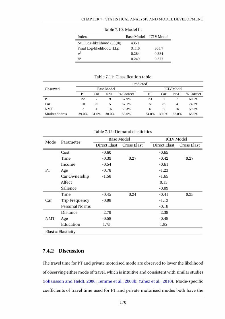
CHAPTER 7. STATISTICAL ANALYSIS AND MODEL DEVELOPMENT
Table 7.10: Model fit
Index Base Model ICLV Model
Null Log-likelihood (LL(0)) 435.1
Final Log-likelihood (LLβ) 311.6 305.7
ρ2 0.284 0.384
ρ̄2 0.249 0.377
Table 7.11: Classification table
Observed
Predicted
Base Model ICLV Model
PT Car NMT % Correct PT Car NMT % Correct
PT 22 7 9 57.9% 23 8 7 60.5%
Car 10 20 5 57.1% 5 26 4 74.3%
NMT 7 4 16 59.3% 6 5 16 59.3%
Market Shares 39.0% 31.0% 30.0% 58.0% 34.0% 39.0% 27.0% 65.0%
Table 7.12: Demand elasticities
Mode ParameterBase Model ICLV Model
Direct Elast Cross Elast Direct Elast Cross Elast
PT
Cost -0.60 -0.65
Time -0.39 0.27 -0.42 0.27
Income -0.54 -0.61
Age -0.78 -1.23
Car Ownership -1.58 -1.65
Affect 0.13
Salience -0.09
Car
Time -0.45 0.24 -0.41 0.25
Trip Frequency -0.98 -1.13
Personal Norms -0.18
NMT
Distance -2.79 -2.39
Age -0.58 -0.48
Education 1.75 1.82
Elast = Elasticity
7.4.2 Discussion
The travel time for PT and private motorised mode are observed to lower the likelihood
of observing either mode of travel, which is intuitive and consistent with similar studies
(Johansson and Heldt, 2006; Temme et al., 2008b; Yáñez et al., 2010). Mode-specific
coefficients of travel time used for PT and private motorised modes both have the
170
CHAPTER 7. STATISTICAL ANALYSIS AND MODEL DEVELOPMENT
expected negative signs and significant at 95% confidence level (Kamargianni et al.,
2015). The direct demand elasticities shown in Table 7.12 highlights this point and
indicate that an increase in the travel time of either PT or Car mode will result in the
reduction of demand of either alternative. Similarly, the positive signs of the cross elasti-
city of demand of both alternatives suggest that Car and PT are substitute goods; hence,
increasing the travel time of either alternative will increases the demand of the other
alternative. However, the disutility of travel time for Private motorised modes is found
higher than that of PT. Thus, Private motorised users are more sensitive to variations in
travel time than PT users; this effect is evident in the variation of the estimates of the
direct elasticities of the two modes.
Mode-specific coefficients for cost were estimated for PT and private motorised modes.
Both have the expected negative signs (Kamargianni et al., 2015). The estimate for PT
cost is significant at 95% confidence level. However, that of the private motorised mode
was insignificant, therefore, it was removed from the final model. It is noted that the
dataset was disproportionally represented by older individuals (aged above 60 years)
most of whom make fewer trips in a month and are entitled to free or subsidised travel
on most public transport services in Scotland (Audit Scotland, 2010). Most respondents
in this category either reported zero or very small figures as monthly travel cost, which
could affect the estimate. The estimates for direct and cross elasticities of travel cost
reveals variations in travel cost sensitivities across the two modes. The cost sensitivity
for the PT is the highest for both the base and ICLV model.
Intuitively, the results also indicate that trip length impact the choice of travel mode.
The average of the approximated walking and cycling distance based on the reported
trip origin and destination postcodes produced walking and cycling distances of 3.4km
and 5.6km respectively and 12.6km and 10.7km for private motorised mode and PT
respectively. The finding reveals that respondents are willing to walk or cycle for shorter
distances; however, active travel becomes less attractive and eventually impossible with
increasing trip distance, in which case either private motorised mode or PT becomes
171
CHAPTER 7. STATISTICAL ANALYSIS AND MODEL DEVELOPMENT
the reasonable option.
Respondents making work-related trips are found to have high disutility for private
motorised modes; the frequent nature of such trips makes this observation intuitive.
The repetitive and routine nature of such trips means they are less likely to vary from
day-to-day, hence reducing the risk of uncertainty. The estimate for the trip character-
istic (trip frequency) support this argument; increasing the frequency of a trip reduces
the utility of private motorised mode. It was further observed that the unemployed and
the retired who make fewer and less frequent trips behave differently, possibly due to
their low level of distant activity participation.
The results also show that the age of an individual has a significant impact on their travel
mode choice. It was observed that younger (25-64) respondents are more likely to walk
or cycle. The proportion of active travellers is highest among individuals of age group
25-34 years. Older respondents (>54 years) have high utility for private motorised mode
and high disutility for active travelling, possibly due to age-related mobility challenges.
Figure 7.4 reports that after age 54, individuals rely more on private motorised mode
and PT to meet their mobility needs, it is seen that the proportion of respondents
travelling by active mode steeply declines after age 64. Private motorised modes have
the highest share of respondents aged above 54 years, even though most individuals in
this category may qualify for subsidised bus fares or free bus travel. The Generation-X
respondents are noticed to have the lowest proportion of private motorised mode users
among all age groups (ONS, 2019; O’Connor, 2018). It is not clear why the Generation-X
respondents differ in travel behaviour, car ownership and employment status from the
other age groups. However, it is strongly believed that the reported drug use among
individuals in this age group account for their low employment and car ownership
rate as reported in section 6.5.1 and Figure 6.5, which consequently affect their travel
behaviour.
172
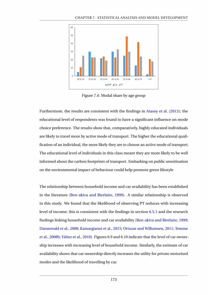
CHAPTER 7. STATISTICAL ANALYSIS AND MODEL DEVELOPMENT
Figure 7.4: Modal share by age group
Furthermore, the results are consistent with the findings in Atasoy et al. (2013); the
educational level of respondents was found to have a significant influence on mode
choice preference. The results show that, comparatively, highly educated individuals
are likely to travel more by active mode of transport. The higher the educational quali-
fication of an individual, the more likely they are to choose an active mode of transport.
The educational level of individuals in this class meant they are more likely to be well
informed about the carbon footprints of transport. Embarking on public sensitisation
on the environmental impact of behaviour could help promote green lifestyle
The relationship between household income and car availability has been established
in the literature (Ben-akiva and Bierlaire, 1999). A similar relationship is observed
in this study. We found that the likelihood of observing PT reduces with increasing
level of income; this is consistent with the findings in section 6.5.1 and the research
findings linking household income and car availability (Ben-akiva and Bierlaire, 1999;
Dannewald et al., 2008; Kamargianni et al., 2015; Ortuzar and Willumsen, 2011; Temme
et al., 2008b; Yáñez et al., 2010). Figures 6.9 and 6.10 indicate that the level of car owner-
ship increases with increasing level of household income. Similarly, the estimate of car
availability shows that car ownership directly increases the utility for private motorised
modes and the likelihood of travelling by car.
173
CHAPTER 7. STATISTICAL ANALYSIS AND MODEL DEVELOPMENT
Longer walking distance for trips involving PT modes is observed to increase the utility
for private motorised mode significantly. The results show that the combined walking
distance for PT trips; comprising the walking distance to the origin bus stop and the
walking distance from the destination bus stop has a significant positive impact on
the likelihood of observing private motorised mode. This effect is significant in both
the base model and the ICLV model and consistent with finding in (Yáñez et al., 2010).
Therefore, locating bus stops closer to trip generation and trip attraction sites could
help reduce the combined walking time for PT trips, which potentially could attract car
users to use PT.
The number of cars available in the household for individual use increases the utility
of private motorised modes. This effect is significant at 99% in both the base and ICLV
models.
Intensely negative sentiments can override otherwise rational course of action even
when cognitive information suggest alternative courses of action (Loewenstein et al.,
2001). The results support the statement above, the negative sign of the estimate of Sali-
ence indicates that such experiences increase the disutility of PT and hurt PT ridership.
Unusual, extreme or unexpected experiences loom more significant to the consumer
and stays in memories much longer. The results reveal that unpleasant experiences
such as anti-social behaviour, passenger annoyance and overcrowding on a bus ap-
pear to evoke negative valence (feeling of anger, embarrassment, fear and frustration).
Such undesirable experiences could have far-reaching consequences on individual
travel behaviour (Kahneman, 2013). This observation is evident in individuals in active
working-age between 25 and 64 years. These results give credence to the findings in the
field of psychology that suggest that human memory of experiences is governed by most
intense moments and the final impressions in a chain of events (Redelmeier et al., 1993).
Preventing or deterring such experiences and addressing similar complaints could
lessen the effects of such experiences and the associated negative valence (Resnick,
2012). That could also reduce the potential negative impact of such experiences on
174
CHAPTER 7. STATISTICAL ANALYSIS AND MODEL DEVELOPMENT
future travel decisions (Dobbie et al., 2010; Metcalfe and Dolan, 2012; Ababio-donkor
et al., 2020)
It is evident from the estimates in Table 7.9 that attitude, Affect or pro-PT attitude
increases the utility of public transport. Individuals in this class have high utility for
the in-vehicle travel time for PT and a positive attitude towards the PT. This attitude
is profound in individuals without a car; it decreases with an increasing number of
cars in the household. Individuals with positive valence towards public transport (high
level of satisfaction for public transport services) have high utility for public transport
in-vehicle travel time (Resnick, 2012). The results buttress the report in Elster (1998) and
indicate that decision-makers evaluate alternatives emotionally alongside economic
utility. The findings further confirm the initial hypotheses and indicate that the sen-
timents associated with public transport by users could influence PT desirability or
ridership. Therefore, user satisfaction and experience with PT services could evoke
positive valence towards PT and influence loyalty (Resnick, 2012).
Individuals with a high level of pro-environmental attitudes (Personal environmental
norms) have high disutility for private motorised modes; this effect is noted to be high
for individuals with high education (university degree) and household income of at
least £50,000. Individuals in this category are between the ages of 18 and 24 or above 64
years. It is also shown that highly educated individuals are likely to be more sensitive
to environmental issues and therefore, mindful of their carbon footprint (Atasoy et al.,
2013), which possible inform the environmentally friendly lifestyle. The results also
confirm the finding of the descriptive analysis reported in section 6.5.2; a significant
difference was found in responses among PT riders, Car users and Active travellers.
Both results demonstrate that individuals holding high pro-environmental attitudes
tend to be decisive and care deeply about their environmental behaviours (Jachimowicz
et al., 2019). The results also corroborate the findings in Belgiawan et al. (2016) and
Ababio-Donkor et al. (2019), it supports the assertion by Schwartz (1977) and suggests
that "in the absence of personal norms, social norms alone did not add to the predictive
175

CHAPTER 7. STATISTICAL ANALYSIS AND MODEL DEVELOPMENT
power already provided in the base model. Neither did social norms add to the predict-
ive power already provided in the model by the personal norm when both variables
were incorporated into the ICLV model" (Cialdini et al., 1991, p. 16).
In conclusion, it can be inferred from the results that personal norms, which describes
individual internalised social norms, have a significant influence on individual beha-
viour. Persons with a high level of pro-environmental attitude are likely to adopt environ-
mentally friendly modes of travel. It is believed that individuals with pro-environmental
attitudes may be more likely to switch to travel options that offset the carbon emis-
sions of their behaviour compared to individuals with anti-environmental attitudes
Jachimowicz et al. (2019). The differences in behaviour observed between individuals
scoring high on personal norms and social norms apparently confirm the suggestions
that activated norms influence overt behaviour by inducing a sense of moral obligations
to act (Schwartz, 1977; Cialdini et al., 1991; Bamberg et al., 2007).
Interesting to note is that the latent factors of Ego or Narcissism are shown to impact
the utility of PT modes negatively. The estimate of Exhibitionism had a negative sign in
the utility equation of PT, confirming the findings of the preliminary analysis; however,
this effect is insignificant in the utility equation for PT. This is believed to result from
the sensitivity of the indicators for measuring narcissism and respondents’ low level of
scores, consequently, this variable was removed from the final model.
7.5 Summary of Factors Influencing Mode Choice
The previous section discusses the estimates of the utility parameters in the models and
highlights the nature of their influence on the decision-making process of the study
population. The variables in the functions of the traditional discrete choice model and
the ICLV model are all significant and have the expected signs. This observation is
consistent with the outcomes of similar studies in the literature. The latent variables
Personal norms, Salience and Affect have plausible estimates and significant. Personal
norms and Salience are significant at 99% level, while Affect is significant at 95% confid-
176

CHAPTER 7. STATISTICAL ANALYSIS AND MODEL DEVELOPMENT
ence level. The magnitude of the standardised coefficients of Salience, Personal norms,
and Affect indicates the level of importance of these variables in their respective utility
functions. This is a clear indication that these MINDSPACE variables play a significant
role in the decision-making process involving transport mode choice. The results loudly
emphasise the significance of the included personality traits and establish their compar-
ative significance to objective variables such as income, age, car ownership and travel
time in the utility functions and by extension, the decision-making process of the study
population. The incorporation of these MINDSPACE variables into the ICLV model
also shows that socio-demographics could be used to define and explain personality
traits or attitudes. For instance, the finding indicates that individuals with a university
degree, aged 18-24 and above 64 are likely to be environmentally friendly and have high
personal environmental norms. Additionally, the ICLV model has shown the effects of
Personal norms, Salience and Affect on the choice of PT and private motorised mode.
The findings of the analysis are summarised below and presented under the following
two categories.
Subjective Factor influencing Mode Choice
• Salient experiences on the PT evokes negative valence and sentiments in indi-
viduals and increases the aversion and disutility of PT modes.
• User satisfaction and positive user experience induce positive valence which in
effect increases the utility of PT modes
• Pro-environmental attitude activates one’s internalised norms and increases the
aversion and disutility of private motorised modes. This effect is high in individu-
als with at least a university degree.
Objective Factors Influencing Mode Choice
• Increasing in travel time and cost increases the disutility of travel mode.
• Active mode users are very sensitive to increase in trip length; trip length is directly
proportional to the utility of active travel mode.
• Frequent and work-related trips increase the disutility of private motorised modes.
• Working aged adults between 25 and 54 are more likely to adopt active modes of
travel than younger (<25) and older (>54) individuals
177

CHAPTER 7. STATISTICAL ANALYSIS AND MODEL DEVELOPMENT
• Longer walking distance in a PT trip increases the utility of private motorised
modes.
• The number of household cars available for individual use significantly increases
the utility of private motorised modes.
178
; Chapter Eight <
Conclusions and Future Research
Direction
8.1 Introduction
This concluding chapter of the thesis presents a summary of the research. Section 8.2
summarises the thesis and highlight the research objectives. Sections 8.3 explains the
contribution of the research and the policy implication of the research findings. Section
8.4 closes the chapter with the research recommendation and give direction for future
research.
8.2 Conclusion
The preceding chapters present the different aspects of the research work. Chapter 1
provides a general overview of the study and introduces the research work. Relevant
literature to the study is reviewed in chapters 2 and 3, while chapter 4 extends the
literature into the general methodology and the various methods and techniques for
sampling, data collection, and the framework for empirical data analysis. Chapter 5
introduces the study population and the study area, and chapter 6 reports the data col-
lection method, the sample data and exploratory analysis of the sample data. Chapter 7
presents the empirical data analysis involving transport choice modelling, presents and
discuss the results of the analysis and the findings. Finally, this chapter concludes the
179

CHAPTER 8. CONCLUSIONS AND FUTURE RESEARCH DIRECTION
study by outlining the findings, contribution and limitations of the study in addition to
the recommendations for future research direction.
Several researchers have studied transport mode choice behaviour and made numer-
ous contributions to the field, including the development of hybrid or ICLV models.
However, very few studies have focused on MINDSPACE and transport mode choice,
particularly, the integration of MINDSPACE in ICLV models.
The overall research aim is "to investigate whether the extended ICLV model incorpor-
ating latent variables from MINDSPACE could enhance the power of transport mode
choice models and individual choice preference". The following specific objectives are
developed to help achieve the overall aim of the study:
1. To investigate and provide insight into the importance of the variables of MIND-
SPACE in choice decision-making.
2. Identify potential latent variables from MINDSPACE and develop psychometric
indicators to measure them
3. Investigate the impact of the latent variables on the explanatory power of ICLV
model and individual choice preference.
8.2.1 Overview of the Research Objectives
This section presents a summary of the methods adopted to achieve each objective and
the outcome of each objectives.
8.2.1.1 Objective 1
To investigate and provide insight into the importance of the variables of MIND-
SPACE in choice decision-making.
Comprehensive literature review of MINDSPACE was conducted in chapter 2. Each
of the nine variables of MINDSPACE has been discussed in detailed citing relevant
180
CHAPTER 8. CONCLUSIONS AND FUTURE RESEARCH DIRECTION
literature and practical application of each variable in literature and industry, including
applications in transport where applicable.
It was demonstrated that the rational choice theory is not entirely accurate in explaining
travel decision task; observed choice preference of individuals violates this fundamental
theory underlying the random utility theory. It has been shown that observed choices
do not only depend on socio-demographic factors such as age, gender and income, but
also on personality traits, attitudes and situational factors. This observation seems to
suggest that people do not always seek to maximise economic benefit but emotional
and psychological benefits as well.
The study has demonstrated that situational factors such as time pressure, cognitive
load and the situational context for the decision task experienced by the decision-maker
at time of decision making could significantly sway a decision. It is indicated that the
limitations of the traditional choice models are the failure to account for these subject-
ive factors.
Recent studies have tried to bridge this knowledge gap by exploring the impact of several
subjective variables on decision-making. However, what matters is the effectiveness of
a subjective variable in explaining behaviour. Review of consumer behaviour literature
revealed nine behavioural effects named MINDSPACE for convenience; these nine
effects are believed to have a significant impact on behaviour and are consequently
explore in the context of travel choice behaviour. The findings in the literature about
the nine MINDSPACE effects are summarised below:
Messenger:
It was established that the importance people attach to information depends to a large
extent on the conveyor of the information rather than the content of the information.
The study has found that people do not always listen to people because of the content
or accuracy of their message; rather, people listen because they feel connected to the
messenger. The study proposed that using high-status messengers in transport-related
campaigns could offer an effective means to achieve behaviour change.
181

CHAPTER 8. CONCLUSIONS AND FUTURE RESEARCH DIRECTION
Incentive:
The economic law of demand suggests that people are perfectly rational and sensitive to
new information, such as changes in prices and situations. The review has shown that
Incentives could have a positive effect on decision-making and can motivates people
to create or break habits by negatively or positively altering the cost or benefit of an
activity. In other words, incentives could cause people to adjust their behaviour
Norms:
Norm describes appropriate behaviour or acceptable behaviour by a majority of people.
It is found that people are motivated to continue in a behaviour if they believe they have
the approval of their reference group. Norm could refer to social norms, legal norms
and personal norms. Social norm describes a subject’s belief about what the society or
reference group accept. Social norms are held in place by the reciprocal expectation
and the fear of social penalties by the reference group. Personal norms or personal
attitude (own-action responsibility) on the other hand, refers to individual values and
principles or internalised social norms. It is found that activated personal norms induce
the obligations to act. The literature also suggests that personal norms are the most
relevant moderating factor of pro-environmental behaviour (PEB).
Defaults:
People will go with the flow when pre-set options are made for them in choice design.
This can have a significant impact on behaviour, even in an unrestricted choice frame-
work. It is found that defaulting to pre-set options could influence decisions when the
decision-makers do not have a preferred option in mind and important for prompt
behaviour change.
Salience:
It is found that the human memory of experience is governed by most intense moments
and the final impression in a chain of events. The review revealed that unusual and
extreme experiences loom larger to the consumer and stay much longer in memory.
182

CHAPTER 8. CONCLUSIONS AND FUTURE RESEARCH DIRECTION
Lousy and negatively intense experiences could induce negative valence towards a
product affect its desirability.
Prime:
The literature demonstrates that subconscious stimuli in the form of words, sounds,
sights, and smells in the environment influence behaviour. Literature suggests that
priming explains some otherwise irrational consumer behaviour. The knowledge and
correct application of priming can help policy-makers influence behaviour.
Affect:
"Affect" is as an automatic response to a good or bad experience. "Affect" could refer
to four different states; Moods, Affective Styles, Sentiments, and Emotions and all the
states could influence behaviour. Emotional associations can remarkably influence
decisions and behaviour. Emotional attachments can lead to overreactions and override
a rational course of action even when alternative course of action is not in one’s own
interest.
Commitment:
It is noted that people lack the inertia and the will power to achieve behaviour change
or break bad behaviour. Individuals seek to be consistent with their public promises;
literature suggests that public commitment reduces procrastination by increasing the
cost of failure. The study argued that individuals are motivated to maintain a consist
and positive self-image of themselves and are more likely to keep commitments to avoid
reputational damage. Therefore, encouraging people to develop and make public their
travel plans could increase compliance.
Ego:
People behave in ways that tend to make them feel better about themselves. This
quest for approval and recognition leads to changes in preference for consumer goods
behaviour. Experts suggest narcissism is due in part high ego; in other words, narcissism
183

CHAPTER 8. CONCLUSIONS AND FUTURE RESEARCH DIRECTION
is driven by ego. Therefore, the study uses narcissism to explain and describe people
with a high ego. Narcissism describes a person’s obsession with oneself and the public
perception of themselves. The study argued that narcissism plays a dominant role
in consumer decision making. The literature demonstrates that individuals scoring
high on the Narcissism Personality Inventory (NPI) scale were more likely to consume
products likely to make them socially unique. They will deliberately flout established
norms in pursuit of distinctiveness. The narcissists use consumer products to maintain
the perceived social identity of themselves. It is also indicated that actions that threaten
to damage this perceived view could trigger behaviour change.
8.2.1.2 Objective 2
Identify potential latent variables from MINDSPACE and develop psychometric in-
dicators to measure them
Section 4.4.5.2 of chapter 4 explains the process of deciding on which MINDSPACE
variable to select as a latent variable and the development of indicators for measuring
the selected variables of MINDSPACE for inclusions as latent variables in the ICLV
model. The decision concerning which variable to include as a latent variable in the
ICLV model was based on:
• the possibility of measuring the variable with psychometric indicators
• the existence of indicators for measurement.
• whether a variable could be measured in the context of transport.
Overall, four of the nine variables of MINDSPACE, namely, Norms, Salience, Affect and
Ego or Narcissism, satisfied the criteria above and were adopted for the study. Refer
section 4.4.5.2 for details on the development of the indicators. The MINDSPACE effects
adopted are discussed below:
Norms:
It is argued that Norms has significant impacts on overt behaviour and people feel
morally obligated to act when their personal norms are activated. Ten measurement
184
CHAPTER 8. CONCLUSIONS AND FUTURE RESEARCH DIRECTION
indicators were developed to assess respondents’ perceived social and personal norms
to investigate the influence of their perceived norms on their behaviour. Question 23 in
Appendix A covers the measurement indicators for this MINDSPACE effect.
Salience:
The study argues that human behaviour is influenced by what comes to mind when
making decisions. It is suggested that the most prominent (desirable or undesirable)
experience with a travel mode can have disproportionate sway on behaviour. The review
of relevant literature reveals that experience, such as any incidents of passenger annoy-
ance or anti-social behaviour experienced by a passenger on public transport could
have a profound consequence on their future travel behaviour. Therefore, measurement
indicators were developed based on passenger experiences reported in the existing
literature to investigate the effect of public transport user experience on ridership.
Affect:
The study hypotheses that the sentiments associated with a transport mode could
impact its desirability. Inspired by the study of Han and Lerner (2012), measurement
indicators were developed to investigate user sentiment and its impact on ridership.
The indicators assess respondents’ perception of cars and PT.
Ego/Narcissism:
The general hypothesis for this MINDSPACE effect is that "narcissist will likely travel by
car to enhance their social identity and sense of uniqueness". This hypothesis is tested
by adapting 16-item Narcissism Personality Inventory (NPI-16) developed by Ames
et al. (2006) from the original 40-item scale to measure the NPI scores of respondents to
investigate the relationship NPI score and travel behaviour.
8.2.1.3 Objective 3
Investigate the impact of the latent variables on the explanatory power of ICLV model
and individual choice preference.
185

CHAPTER 8. CONCLUSIONS AND FUTURE RESEARCH DIRECTION
Chapter 3 presented a comprehensively review of the literature on transport and ICLV
models; the review discussed existing ICLV models. Chapter 4 extended the literature in
chapter 3 and discussed the specifications of the reference and the ICLV models. The
construction of the latent variables from the psychometric indicators and the estima-
tion of the reference and the ICLV model is performed to address objective 3. Sections
7.3 and 7.4 explain the model development process and covers the results of the choice
modelling.
The results indicate that all variables are significant and have the expected signs. The
MINDSPACE effects incorporated as latent variables in the ICLV model all have the
expected signs in their respective utility functions. Personal Norm, Salience and Affect
are significant at 1% level. Narcissistic trait of exhibitionism had the expected sign
but was insignificant. To investigate the impact and significance of the MINDSPACE
variables in the ICLV model, a reference choice model with similar specifications as the
ICLV model but without any of the latent variables was estimated and compared with
the ICLV model. Table 7.10 presents the goodness of fit and the log-likelihood estimates
for both models. The indices show that the ICLV model has the best goodness of fitness
values. The market shares estimates from both models confirm the finding and indicate
that the ICLV model is superior to the reference model.
Based on the results and discussion, it can be concluded that the ICLV model outper-
forms the traditional discrete choice model. The ICLV model provides insight into the
importance of attitudes in transport mode choice. The incorporation of the MIND-
SPACE variables improved the explanatory power of the choice model. Modal travel
time, travel cost, number of cars available, household income and walking time to
bus stop are all significant in the base, and ICLV models, pro-environmental attitudes
(personal environmental norms), pro-PT attitude (Affect) and salience (negative PT
user experience) are equally significant and found to influence travel behaviour.
Individuals with high pro-environmental attitudes show much concern about the envir-
onmental impact of their behaviour and they are likely to travel with modes that offset
their carbon footprint. Individuals with a university degree and aged 18-24 or more
than 64 years are likely to belong to this class.
186
CHAPTER 8. CONCLUSIONS AND FUTURE RESEARCH DIRECTION
Similarly, salient public transport user experiences such as passenger annoyance and
overcrowding are likely to negatively impact the utility of PT modes, individuals in 25-64
age-band are likely to be influenced most by this MINDSPACE effect.
Pro-PT attitudes or positive sentiments increases the utility of PT modes; the study
found that individuals who find in-vehicle travel time of PT useful are more likely to
be loyal riders. The findings imply that Improving the in-vehicle experiences for PT
riders could impact PT loyalty. The results support the assertion about the implica-
tion of MINDSPACE for the transport sector (Aczél and Markovits-somogyi, 2013) and
demonstrate the implications of MINDSPACE for travel behaviour. The incorporation
of MINDSPACE has made it possible to explain the observed heterogeneity in the re-
spondents’ travel choices from several behavioural perspectives. MINDSPACE have
a significant impact on travel decision-making and enhance the explanatory power
of the choice model. A better appreciation of these effects and their influence in the
decision-making process by transportation planners and policy-makers could serve a
useful guide for designing and developing effective transportation policies. The findings
of the study can be group into the following two broad categories;
MINDSPACE Variables
The findings support existing literature in behavioural economics and demonstrate
that people assess both the economic and emotional cost of an alternative when mak-
ing transport mode choice decision. The results of the analysis show that three of
the four MINDSPACE variables investigated in the study have a significant impact on
transport mode choice. The presence of the three MINDSPACE variables (personal
norm, salience and affect) accounts for individual heterogeneity and reflect individual
values, perception of safety and improved the understanding of travel behaviour and en-
hanced predictive power of the final model. The finding addresses the overall research
aim and indicates that the extended ICLV model incorporating latent variables from
MINDSPACE enhances the explanatory power of transport mode choice models and
individual choice preference. The main findings under this category are summarised
below, the following section expatiate and presents the implications of the findings.
187

CHAPTER 8. CONCLUSIONS AND FUTURE RESEARCH DIRECTION
• Salient experiences on PT induces negative valence and sentiments and increases
the disutility of PT modes.
• User satisfaction and positive user experience induce positive valence, which
increases the utility of PT modes
• Pro-environmental attitudes increase the disutility of private motorised modes.
Alternative Specific and Socio-economic Variables
The findings of the study are consistent with results from similar studies and extant
literature. The estimates of all the utility variables are plausible and significant for both
the base and the ICLV models. The key finding from this category are itemised below.
• Increasing in travel time and cost increases the disutility of travel mode.
• Active mode users are susceptible to increases in trip length
• Frequent and work-related trips increase the disutility of private motorised modes.
• Working aged adults between 25 and 54 are more likely to adopt active modes of
travel.
• Longer walking distance for PT trips increases the utility of private motorised
modes.
• The number of household cars available for individual use significantly increases
the utility of private motorised modes.
The findings of the study are relevant and useful for public transport delivery in the
study area (Edinburgh) and could provide useful policy directions for public transport
and travel behaviour change.
8.3 Contribution and Implication of the Research
The study has made a significant contribution to travel behaviour, and choice modelling
literature. The findings have significant implications for transport planning and would
be influential and valuable to transport policymakers and transport planners of the
study area (Edinburgh).
188
CHAPTER 8. CONCLUSIONS AND FUTURE RESEARCH DIRECTION
The novelty of this study is the provision of key indicators, CFS and drivers of indi-
vidual choice preference beyond the traditional objective characteristics and socio-
demographic variables through a systematic process. The study has gone beyond the
existing studies by incorporating and investigating four variables from the MINDSPACE
framework in a single model.
The findings have great implication for transport in the study area; the results explain
the observed rising trend of vehicular traffic and PT ridership decline in Edinburgh.
Salient experiences by PT riders is shown to impact the choice of PT negatively and
explains the observed trend.
The results indicate that pro-environmental attitudes reduce the utility of private mo-
torised modes and can induce behaviour change, thus increasing public education on
environmental issues could help promote these attitudes and consequently affect travel
behaviour of the population. The main findings of the study are summarised below:
The study has also demonstrated that incorporation of personal norms, affect (user
emotional satisfaction) and salient user experience (perception of safety) as latent
variables in the ICLV framework provides comparatively better predictive power than
the traditional discrete choice counterparts. The presence of the three latent variables
accounted for individual heterogeneity and improved the understanding of travel be-
haviour. The model reflects individual values, perception of safety, and emotions. The
framework has indicated that user satisfaction is moderated by the perception of safety
and user perception of service quality. These are influenced by user experience and
objective factors, such as the socio-economic characteristics of the decision-maker.
The framework adopted in this study has shown that transport mode choice depends
on how individuals perceive alternative specific and service attributes. The perception
about alternative attributes is a measure of the individual evaluation of an alternative
and attitudes towards an alternative is a measure of the significance accorded to the
various attributes of alternatives.
The results of the study indicate that individuals with pro-environmental attitudes have
high disutility for private motorised modes. This effect is observed to be high for indi-
189

CHAPTER 8. CONCLUSIONS AND FUTURE RESEARCH DIRECTION
viduals with high education (university degree). This observation has great implication
for public policy. The results have shown that highly educated individuals are well
informed about the environment and mindful of their carbon footprint. Therefore,
developing an educational curriculum on the environmental impact of behaviour and
taught in schools could sensitise more young people about the environment. Bear in
mind that individuals of 18 to 24 age group already belong to this group and represent
the future.
The study has established key attitudinal factors influencing individual transport choice
preference. The results are consistent with findings in similar travel behaviour literature.
This study extends the findings in previous literature and has established that person-
ality trait, perceptions and attitudes significantly inform choices. It is also found that
activated societal beliefs, also referred to as personal norms significantly determine an
individuals choice preference.
In addition, the study has shown that positive user experience and user satisfaction
can create positive valence and sentiments in users towards the target object; this is
revealed to increase the utility of PT modes. The findings have outlined the indicators
underlying this observation and indicate that the perceived utility of public transport
in-vehicle travel-time considerably affect overall user satisfaction, user loyalty and lead
to sustainable travel. The finding has implication for the design and manufacturing of
PT coaches. It is suggested for service operators and planners to design and provides
comfortable and utility coaches and services to improve PT travel experience while
enabling environment for the productive use of the in-vehicle travel time.
Behavioural economics literature suggests that unusual and undesirable experience
stays longer in human memory and looms more significant to the subject. Such ex-
periences create intensely negative sentiments which could override rational choice
preference (Loewenstein et al., 2001; Kahneman, 2013). The study has established that
undesirable user experience on PT appears to induce negative valence in users, which
190
CHAPTER 8. CONCLUSIONS AND FUTURE RESEARCH DIRECTION
is observed to impact the utility of PT modes adversely. The study has defined key
indicators (critical success factors CSF) behinds these attitudinal variables first through
EFA and validated in CFA. The underlying indicators of these attitudes wield significant
influence on individual choice preference and decision-making.
These confirmed and validated CSFs are likely to activate behaviour when triggered.
The following recommendations are suggested to translate the finding contained in this
thesis into a useful application:
• The CSFs of the three latent variables must be critically examined and addressed
through policy to improve PT user experience and loyalty. Facilities and services
necessary to improve the perception of in-vehicle travel time utility for PT riders
should be provided.
• Incidence likely to create intensely negative valence towards PT services must
be severely sanctioned and published to discourage offenders and build public
confidence. Similar reported cases should be addressed satisfactorily to maintain
customer loyalty. For instance: Refusing to admit heavily drunk individuals on
PT carriages, introducing high capacity coaches during peak hours to prevent
overcrowding and keeping the interior of PT coaches clean and tidy at all times
for customers.
The study has provided and demonstrated variables that can influence users’ per-
ceptions, the so-called critical success factors (CFS) defined as encounters that are
particularly satisfying or discouraging for the user. The concept is not limited to rating
the PT service attributes but user perception about on-board safety and negative en-
counters because customers who experience the salience CFS are less likely to forget the
encounter, which in most cases can influence user loyalty (Dolan et al., 2012; Dobbie
et al., 2010). However, since the salience experiences (CFS) are subjective, they may be
beyond the control of the Service providers. It is therefore, suggested that the handling
of the CFS incidences and experiences on PT services through public policy may be a
191
CHAPTER 8. CONCLUSIONS AND FUTURE RESEARCH DIRECTION
critical and logical approach for policy-makers and PT service providers to influence
the overall user satisfaction, the perception of service quality and loyalty of PT users.
Policies and services that eliminates user dissatisfaction, improve user perception of
safety and emotional satisfaction will engender the perception of improved service
quality and ultimately promote and lead to sustainable travel.
Total walking time for a PT journey correlate with the utility of private motorised modes.
However, walking is an inevitable part of every journey but mostly with trips involving
PT modes than private motorised modes, this leg of the journey is even more punit-
ive in inclement weather. The study recommends increasing the density of bus stops
within trip generation and attraction sites to reduce the total walking time for PT trips
to minimise the effects of distance on PT ridership.
8.4 Recommendation for Future Research
The novelty of this study is the provision of key indicators and drivers of individual
choice preference beyond the traditional objective and socio-demographic variables
through a systematic process. The study has gone beyond the existing studies, which
considers one effect/ variable at a time by incorporating and investigating four vari-
ables from the MINDSPACE framework in a single model. Notwithstanding, several
limitations and inconclusive observations were noticed during the study. The following
recommendations for future research could address the observed limitations. Similar
methodology could be applied to build on the useful findings of the investigated MIND-
SPACE variables in addition to those MINDSPACE variables not considered in this study.
The validation of the data shows the sample data is representative of the study popula-
tion; as a result, the finding could be viewed as a reflection of the study population’s
travel behaviour. However, readers should be cognizant of the fact that the study was
carried out in urban travel context in one city in the United Kingdom. The study area has
a very extensive and efficient public transport system which might have influenced the
192

CHAPTER 8. CONCLUSIONS AND FUTURE RESEARCH DIRECTION
results. Literature also suggests that decision-making is influenced by culture (Halonen,
2020). Therefore, it is innocuous to assume that the culture of the study area could
have influenced the outcome of the study. The results, therefore, may not necessarily
apply in different contexts such as cities with less efficient public transport system or
different form of public transport services. It is recommended for future research to
explore the identified CSFs in different cities and context and investigate further the
indicators dropped during the CFA for having low loadings.
This research only explored the MINDSPACE variables in the context of transport mode
choice. A similar study is recommended to explore the impact of the MINDSPACE
variables in other travel behaviour context. For instance, in route choice, departure
time choice, et cetera.
It is also noticed that most of the observed psychometric indicators for the latent vari-
ables had very low factor loadings or did not correlate sufficient enough with other
indicators. For instance, six indicators were developed to measure Affect; however, the
final latent construct had only two indicators with sufficient factor loadings. Although
it is difficult to get the right psychometric indicators for measuring psychological con-
struct, it is recommended for future research to carefully design or adopt indicators
with adequate validity and reliability in capturing their target construct.
The transport characteristics and travel behaviour of individuals of within Generation-X
age band were observed to deviate from any observed trend. Further research is re-
commended to explore the transport characteristics and travel behaviour of individuals
within this age band.
Considerable effort was made to identify and address potential limitations of the survey
instrument. However, the quality of final data collected and the ensuing analysis indic-
ated that the failure to pilot the final survey instrument after revising some aspect of the
instrument after the pilot data collection and before the actual data collection (section
4.4.6.4) had considerable impact on the level of engagement of most respondents on
193

CHAPTER 8. CONCLUSIONS AND FUTURE RESEARCH DIRECTION
the narcissism measurement scale and the related analysis.
194

References
Ababio-Donkor, Augustus, Wafaa Saleh and Achille Fonzone (2019). “The role of per-
sonal norms in the choice of mode for commuting”. In: 16th International Conference
on COLPT. Vol. 16. August 25-30. Singapore, pp. 1–19.
Ababio-donkor, Augustus, Wafaa Saleh and Achille Fonzone (2020). “Understanding
transport mode choice for commuting: The role of Affect”. In: Transportation Planning
and Technology, pp. 1–20.
Acker, Van, van Wee, Veronique Van Acker, Bert Van Wee and Frank Witlox (2010). “When
Transport Geography Meets Social Psychology: Toward a Conceptual Model of Travel
Behaviour”. In: Transport Reviews 30.302, pp. 219–240.
Action on Smoking and Health (ASH) (2015). The economics of tobacco. Tech. rep. Decem-
ber 2015.
Action on Smoking and Health (ASH) (2016). Smoking Statistics. Tech. rep. June, p. 1.
Aczél, Rita Markovits-somogyi Balázs and Rita Markovits-somogyi (2013). “Implications
of Behavioural Economics for the Transport Sector”. In: 1, pp. 65–69.
Alastair, DALTON (Nov. 2013). Edinburgh traffic worse than in London.
Ames, Daniel R., Paul Rose and Cameron P. Anderson (2006). “The NPI-16 as a short
measure of narcissism”. In: Journal of Research in Personality 40.4, pp. 440–450.
195

REFERENCES
Anderson, Jame C. and David W. Gerbing (1988). “Structural Equation Modeling in
Practice: A Review and Recommended Two-Step Approach”. In: Psychological Bulletin.
Antolín, Anna Fernández (2016). Biogeme & Binary Logit Model Estimation.
Arbuckle, J. L. (2017). Amos 25 User ’ S Guide, p. 720.
Arbuckle, James L. (2016). “Ibm Spss Amos 24”. In: Methods, p. 635.
Arcadis (2017). UK Sustainable Cities Mobility Index 2017. Tech. rep.
Ardeshiri, A and A. Vij (2019). “Lifestyles, residential location, and transport mode use:
A hierarchical latent class choice model”. In: Transportation Research Part A: Policy and
Practice 126, pp. 342–359.
Ariely, Dan (2008). Predictably Irrational, p. 294.
Aronson, E., T. Wilson and A. Akert (2005). Social Psychology. 5th. Upper Saddle River,
NJ: Prentice Hall.
Ashok, Kalidas, William R. R. R Dillon, Sophie Yuan, Kalidas Ashok, William R. R. R Dillon
and Sophie Yuan (2002). “Extending Discrete Choice Models to Incorporate Attitudinal
and Other Latent Variables”. In: Journal of Marketing Research 39.1, pp. 31–46.
Atasoy, Bilge, Aurélie Glerum and Michel Bierlaire (2013). “Attitudes towards mode
choice in Switzerland”. In: disP-The planning review 49.2, pp. 101–117.
Audit Scotland (2010). National concessionary travel. Tech. rep. October.
Avineri, Erel (2009). “Nudging Travellers to make Better Choices”. In: The International
Choice Modelling Conference. Leeds, UK, pp. 1–18.
Avineri, Erel (2011). “Applying behavioural economics in the design of travel information
systems”. In: UTSG January, pp. 1–12.
196
REFERENCES
Avineri, Erel (2012a). “On the use and potential of behavioural economics from the
perspective of transport and climate change”. In: Journal of Transport Geography 24,
pp. 512–521.
Avineri, Erel (2012b). Understanding Travel Behaviour : Insight from Behavioural Eco-
nomics and Cognitive Psychology.
Avineri, Erel et al. (2009). “Individual Behaviour Change : Evidence in transport and
public health”. In: November.
Axhausen, Kay W. and Tommy Gärling (1992). “Activity based approaches to travel ana-
lysis: conceptual frameworks, models, and research problems”. In: Transport Reviews
12.4, pp. 323–341.
Axhausen, Kay W., Stephane Hess, Arnd König, Georg Abay, John J. Bates and Michel
Bierlaire (2008). “Income and distance elasticities of values of travel time savings: New
Swiss results”. In: Transport Policy 15.3, pp. 173–185.
Baglin, James (2014). “Improving Your Exploratory Factor Analysis for Ordinal Data : A
Demonstration Using FACTOR”. In: Practical Assessment, Research & Evaluation 19.5,
pp. 1–14.
Bagozzi, Richard P. (1988). “On the Evaluation of Structural Equation Models.pdf”. In:
Academy of Marketing Science 16.1, pp. 74–94.
Bagozzi, Richard P. and Lynn W. Phillips (1982). “Representing and Testing Organiza-
tional Theories: A Holistic Construal”. In: Administrative Science Quarterly.
Bagozzi, Richard P., Youjae Yi and Surrendra Singh (1991). “On the use of structural
equation models in experimental designs: Two extensions”. In: International Journal of
Research in Marketing.
Bahaman, Abu Samah (2012). “Structural Equation Modeling Using AMOS”. In: March.
197

REFERENCES
Bamberg, Sebastian, Marcel Hunecke and Anke Blo (2007). “Social context , personal
norms and the use of public transportation : Two field studies”. In: Environmental
Psychology 27, pp. 190–203.
Baraldi, Amanda N. and Craig K. Enders (2010). “An introduction to modern missing
data analyses”. In: Journal of School Psychology 48.1, pp. 5–37.
Barrett, P. (2007). “"Structural Equation Modelling: Adjudging Model Fit," Personality
and Individual Differences”. In: 42.5, pp. 815–24.
Baumeister, Roy F and B Bushman (2014). Social psychology and human nature, com-
prehensive edition. Belmont, CA.
Baumeister, Roy F., Erin A. Sparks, Tyler F. Stillman and Kathleen D. Vohs (2008). “Free
will in consumer behavior: Self-control, ego depletion, and choice”. In: Journal of
Consumer Psychology 18.1, pp. 4–13.
Beavers, Amy S, John W Lounsbury, Jennifer K Richards, Schuyler W Huck, Gary J Skolits
and Shelley L Esquivel (2013). “Educational Research”. In: Practcial Assessment, Research
& Evalutaion 18.6.
Becker, Gary S. (1978). The Economic Approach to Human Behavior. University of
Chicago Press, p. 314.
Beckmann, Martin J., C. B. McGuire and Christopher B. Winsten (1955). Studies in the
Economics of Transportation.
Beirao, Gabriela and J A Sarsfield Cabral (2007). “Understanding attitudes towards
public transport and private car : A qualitative study”. In: 14, pp. 478–489.
Belgiawan, Prawira F., Jan-Dirk Schmöcker, Maya Abou-Zeid, Joan Walker and Satoshi
Fujii (2015). “The Role of Expectation of Others on Students ’ Likelihood to Buy a Car”.
In: 94th annual meeting of the transportation research board. January. Washington, D.C.
198
REFERENCES
Belgiawan, Prawira F., Jan-dirk Dirk Schmöcker and Satoshi Fujii (2016). “Understanding
car ownership motivations among Indonesian students”. In: International Journal of
Sustainable Transportation 10.4, pp. 295–307.
Ben-akiva, Moshe and Michel Bierlaire (1999). “Discrete Choice Methods and their
Applications to Short Term Travel Decisions”. In: Discrete Choice Methods.
Ben-Akiva, Moshe and Bruno Boccara (1995). “Discrete choice models with latent choice
sets”. In: 12, pp. 9–24.
Ben-Akiva, Moshe, Joan Walker, Adriana T Bernardino, Dinesh A Gopinath, Taka Morikawa
and Amalia Polydoropoulou (1999). “Integration of Choice and Latent Variable Models”.
In: Proceedings of 8th International Conference on Travel Behavior. 1. Austin, USA.
Ben-Akiva, Moshe et al. (2002). “Hybrid Choice Models: Progress and Challenges”. In:
Marketing Letters 13.3, pp. 163–175.
Ben-Akiva, Moshe E. and Steven R. Lerman (1985). Discrete Choice Analysis: Theory and
Application to Travel Demand. Massachusetts: MIT Press, p. 390.
Bentler, P. M. (1990). “Fit Indexes, Lagrange Multipliers, Constraint Changes and Incom-
plete Data in Structural Models”. In: Multivariate Behavioral Research.
Bhat, Chandra R and Subodh K Dubey (2014). “A new estimation approach to integrate
latent psychological constructs in choice modeling”. In: Transportation Research Part B
67, pp. 68–85.
Bhat, Chandra R. and Frank S. Koppelman (1999). “Activity-based modeling of travel
demand”. In: Handbook of Transportation Science. US: Springer. Chap. 3, pp. 35–61.
Bierlaire, Michel (2016). “Estimating Choice Models with Latent Variables with Python-
Biogeme”. In: p. 68.
Bierlaire, Michel (2018a). Calculating indicators with PandasBiogeme. Tech. rep. Trans-
port and Mobility Laboratory, p. 30.
199
REFERENCES
Bierlaire, Michel (2018b). Estimating choice models with latent variables with Pandas-
Biogeme. Tech. rep.
Bierlaire, Michel (2018c). “Mode choice in Switzerland ( Optima )”. In: pp. 1–8.
Block, HD and J Marschak (1960). “Random orderings and stochastic theories of re-
sponses”. In: Contributions to probability and.
Bolduc, Denis and Ricardo Alvarez-daziano (2010). “On estimation of Hybrid Choice
Models”. In: April 2010.
Bolduc, Denis, Nathalie Boucher and Ricardo Alvarez-Daziano (2008). “Hybrid Choice
Modeling of New Technologies for Car Choice in Canada”. In: Transportation Research
Record 2082, pp. 63–71.
Bowman, John L (1995). “Activity Based Travel Demand Model System with Daily Activity
Schedules by”. PhD thesis.
Bowman, John L (2008). “4 . Historical Development of Activity Based Model”. In: April.
Brown, Timothy A. and Michael T. Moore (2012). “Confirmatory Factor Analysis”. In:
July 2012.
Browne, M.W and R. Cudeck (1993). “Alternative ways of assessing model fit”. In: Bollen,
K.A., Long, J.S. (Eds.), Testing Structural Equation Models. Newbury: Sage Publications,
pp. 136–162.
Bryne, Barbara. M. (2012). Structural Equation Modeling with Mplus: Basic Concepts,
Applications and Programming, pp. 1–25.
Buchanan, C (1963). Traffic in Towns.
Burke, M.A. and Peyton H. Young (2011). “Social Norms”. In: Handbook of Social Eco-
nomics. Ed. by In J. Benhabib, A. Bisin and M.O. Jackson. Amsterdam:North-Holland,
pp. 311–338.
200

REFERENCES
Burns, A. C. and R. F. Bush (2002). Marketing research: Online research applications. 4th.
New Jersey: Prentice Hall.
Byrne, Barbara. M., Barbara. M. Bryne and Barbara. M. Byrne (2012). Structural Equation
Modeling with M plus. Basic Concepts, Applications, and Programming, pp. 162–165.
Camerer, Colin F (1999). “Behavioral economics: Reunifying psychology and econom-
ics”. In: Proceedings of the National Academy of Sciences 96.19, pp. 10575–10577.
Campbell, Donald T. and Donald W. Fiske (1959). “Convergent and discriminant valida-
tion by the multitrait-multimethod matrix”. In: Psychological Bulletin.
Campbell, W Keith and D Joshua Foster (2007). “The narcissistic self: Background, an
extended agency model, and ongoing controversies”. In: The Self. Ed. by Constantine
Sedikides and J. Steven Spencer. Hove: Psychology Press. Chap. 6, pp. 115–138.
Castiglione, Joe, Mark Bradley and John Gliebe (2015). Activity-Based Travel Demand
Models: A Primer.
Cattell, R.B. (1966). “The scree test for the number of factors”. In: Multivariate behavioral
research 1.2, pp. 245–276.
Chae, Dasol, Jaeyoung Jung and Keemin Sohn (2018). “Facilitating an expectation-
maximization ( EM ) algorithm to solve an integrated choice and latent variable ( ICLV )
model with fully correlated latent variables”. In: Journal of Choice Modelling 26.August
2017, pp. 64–79.
Chan, Y H (2003). “Biostatistics 102: quantitative data–parametric & non-parametric
tests”. In: Blood Press 140.24.08, p. 79.
Chapin, F (1974). Human activity patterns in the city things people do in time and in
space. New York: Wiley.
Chapin, Stuart F (1971). “Free Time Activities and Quality of Urban Life”. In: J Am I
Planners 37.6, pp. 411–417.
201
REFERENCES
Chaturvedi, Kanupriya (2015). Sampling Methods.
Chernev, Alexander, Ulf Böckenholt and Joseph Goodman (2015). “Choice overload: A
conceptual review and meta-analysis”. In: Journal of Consumer Psychology 25.2, pp. 333–
358.
Chien, C. C. and P. Ioannou (1992). “Automatic Vehicle-Following”. In: 1992 American
Control Conference, pp. 1748–1752.
Child, Dennis (2006). The essentials of factor analysis. 3rd Editio. New York: Continuum
International Publishing Group.
Chong, Eugenie Eugene, Ahmad Nazim and Sabri B Ahmad (2014). “A comparison
between Individual confirmatory factor analysis and pooled confirmatory factor ana-
lysis: An analysis of library service quality, a case study at a public university in Tereng-
ganu”. In: Interational Journal of Engineering Science and Innovative Technology 3.1,
pp. 110–116.
Cialdini, R. B., W. Wosinska, D. W. Barrett, J. Butner and M. Gornik-Durose (1999).
“Compliance with a Request in Two Cultures: The Differential Influence of Social Proof
and Commitment/Consistency on Collectivists and Individualists”. In: Personality and
Social Psychology Bulletin 25.10, pp. 1242–1253.
Cialdini, R.B. (2007). Influence: The Psychology of Persuasion. Revised. New York: Harper-
Business.
Cialdini, R.B. (2008). Influence: Science and Practice. 5th ed. Boston: Pearson.
Cialdini, Robert B, Carl A Kallgren and Raymond R Reno (1991). “A focus theory of
normative conduct. A theoretical refinement and reevaluation of the role of norms in
human behavior”. In: Advances in Experimental Social Psychology 24.20, pp. 201–234.
Cipriani, Ernesto, Stefano Gori and Marco Petrelli (2012). “A bus network design pro-
cedure with elastic demand for large urban areas”. In: Public Transport 4.1, pp. 57–
76.
202

REFERENCES
Cisek, Sylwia Z, Constantine Sedikides, Claire M Hart, Hayward J Godwin and Valerie
Benson (2014). “Narcissism and consumer behavior : a review and preliminary findings”.
In: Frontiers in Psychology 5.March, pp. 1–9.
City of Edinburgh Council (2018). Edinburgh by numbers 2018. Tech. rep. City of Edin-
burgh Council, pp. 1–53.
Comrey, L Andrew and Howard B. Lee (1992). A First Course in Factor Analysis. 2nd ed.
Courtney, Matthew Gordon Ray (2013). “Determining the number of factors to retain in
EFA : Using the SPSS R-Menu v2 . 0 to make more judicious estimations”. In: Practical
Assessment, Research & Evaluation 18.8, pp. 1–14.
Cowie, Jonathan and Stephen Ison. (2009). The Economics of Transport : A Theoretical
and Applied Perspective. Vol. 53. 9. Taylor & Francis Group, p. 384.
Cronbach, Lee J. (1951). “Coefficient alpha and the internal structure of tests”. In:
Psychometrikatrika 16.3.
Curtin, Richard, Stanley Presser and Eleanor Singer (2000). “The Effects of Response
Rate Changes on the Index of Consumer Sentiment”. In: Public Opinion Quarterly.
Dannewald, Till, Marcel Paulssen, Dirk Temme and Joan Walker (2008). “Hybrid choice
models estimation using canned SEM Software”. In: Flexible Marketing in an Unpredict-
able World. Proceedings of the 36th EMAC Conference Sfb 649.
David De Vaus (2002). Surveys in Social Research. 5th Editio. London: Routledge.
Davidson, R.J., K.R. Sherer and H.H. Goldsmith (2009). Handbook of affective sciences.
Oxford: Oxford University Press.
DellaVigna, S. (2009). “Psychology and economics. Evidence from the field”. In: Journal
of Economic Literature 47, pp. 315–372.
203
REFERENCES
Dijksterhuis and J. Bargh (2001). “The perception-behaviour expressway: Automatic
effects of social perception on social behaviour”. In: Advances in Experimental Social
Psychology 33, pp. 1–40.
Dobbie, Fiona, Susan McConvile and Rachel Ormston (2010). Transport Research Series:
Understanding Why Some People Do Not Buses. Tech. rep. Edinburgh: Scottish Govern-
ment Social Research (ScotCen).
Dolan, Paul, M Hallsworth, D Halpern, D King, Robert Metcalfe and I Vlaev (2012).
“Influencing behaviour : The mindspace way”. In: Journal of Economic Psychology 33.1,
pp. 264–277.
Dolan, Paul, Michael Hallsworth, David Halpern, Dominic King and Ivo Vlaev (2010).
MINDSPACE: Influencing behaviour through public policy. Tech. rep. London: The
Institute for Government and Cabinet Office, pp. 1–96.
Dunning, David (2007). “Self-Image Motives and Consumer Behavior : How Sacrosanct
Self-Beliefs Sway Preferences in the Marketplace”. In: Journal of consumer psychology
17.4, pp. 237–249.
Durantini, Marta R, Dolores Albarracin, Amy L Mitchell, Allison N Earl and Jeffrey C
Gillette (2006). “Conceptualizing the influence of social agents of behavior change:
A meta-analysis of the effectiveness of HIV-prevention interventionists for different
groups.” In: Psychological bulletin 132.2, p. 212.
Eboli, Laura and Gabriella Mazzulla (2010). “How to Capture the Passengers ’ Point of
View on a Transit Service through Rating and Choice Options”. In: Transport Reviews
30.July, pp. 435–450.
Eboli, Laura and Gabriella Mazzulla (2012). “Structural Equation Modelling for Analys-
ing Passengers ’ Perceptions about Railway Services”. In: Procedia 54, pp. 96–106.
Ecola, Liisa and Martin Wachs (2012). Exploring the Relationship between Travel De-
mand and Economic Growth. Tech. rep., pp. 1–43.
204
REFERENCES
Edinburgh City Council (2016). Demographic Factsheet. Tech. rep. Edinburgh.
Elster, J O N (1998). “Emotions and Economic Theory”. In: Journal of Economic Literature
36.1, pp. 47–74.
Ettema, Dick (1996). Activity-based travel demand modeling.
Fabozzi, Frank J, Sergio M Focardi, Svetlozar T Rachev and Model Selection (2014).
“Model Selection Criterion : AIC and BIC”. In: The Basics of Financial Econometrics:
Tools, Concepts, and Asset Management Applications. Vol. 41. 1979. John Wiley & Sons,
Inc. Chap. Appendix E, pp. 399–403.
Farrell, Andrew M. (2010). “Insufficient discriminant validity: A comment on Bove,
Pervan, Beatty, and Shiu (2009)”. In: Journal of Business Research 63.3, pp. 324–327.
Fellow, R. and A. Liu (2005). Research methods for Construction research. Oxford: Black-
well.
Ferreira, Maria and Roos van den Wijngaard (2019). “Pro-Environmental Behaviour: We
Care Because Others Do.” In: In A. Samson (Ed.), The Behavioral Economics Guide 2019
(with an Introduction by Uri Gneezy), pp. 122–130.
Festinger, L. (1957). A theory of cognitive dissonance. StanfordX: Stanford: Stanford
University Press.
Field, A. (2013). Discovering Statistics using IBM SPSS Statistics. Sage.
Fife Research Co-ordinating Group (2005). Survey Sampling.
Fornell, Claes and David F. Larcker (1981). Structural Equation Models with Unobserv-
able Variables and Measurement Error: Algebra and Statistics.
Frederiks, Elisha R, Karen Stenner and Elizabeth V Hobman (2015). “Household energy
use : Applying behavioural economics to understand consumer decision-making and
behaviour”. In: Renewable and Sustainable Energy Reviews 41, pp. 1385–1394.
205

REFERENCES
Fried, M, J Havens and M Thall (1977). “Travel Behavior-A Synthesized Theory”. In:
Transportation Research Board.
Friman, Margareta (2004). “Transport Implementing Quality Improvements in Public
Transport”. In: Public Transportation June.
Gao, Leilei, S Christian Wheeler and Baba Shiv (2009). “The " Shaken Self ": Product
Choices as a Means of Restoring Self-View Confidence”. In: Journal of consumer research
36.1, pp. 29–38.
Gardner, Benjamin and Charles Abraham (2008). “Psychological correlates of car use : A
meta-analysis”. In: 11, pp. 300–311.
Garrido, Luis Eduardo, Francisco José Abad and Vicente Ponsoda (2013). “A New Look at
Horn’s Parallel Analysis With Ordinal Variables”. In: Psychological Methods 18.4, pp. 454–
474.
Ghauri, P. and K. Gronhaug (1995). Research Methods in Business Studies; A Practical
Guide. Edinburgh: Pearson Education.
Gigerenzer, G. and D. G. Goldstein (1996). “Reasoning the fast and frugal way: Models of
bounded rationality”. In: Psychological Review 103, pp. 650–669.
Gigliotti, Larry and Alia Dietsch (2014). “Does Age Matter? The Influence of Age on
Response Rates in a Mixed-Mode Survey”. In: Human Dimensions of Wildlife 19.3,
pp. 280–287.
Goodwin, Phil and Kurt Van Dender (2013). “’Peak Car’‚Äî Themes and Issues”. In:
Transport Reviews 33.3, pp. 243–254.
Graham, John W. (2012). “Missing data: Analysis and design”. In: Missing Data: Analysis
and Design. c. Chap. 2, pp. 1–323.
Graves, Robert (1968). The Greek Myths. London: Cassell.
206
REFERENCES
Greer, Thomas V., Nuchai Chuchinprakarn and Sudhindra Seshadri (2000). “Likelihood
of participating in mail survey research: Business respondents’ perspectives”. In: Indus-
trial Marketing Management 29.2, pp. 97–109.
Gregg, Aiden P, Seung Yun Lee and Hoon Seong Park (2013). “The Person in the Purchase
: Narcissistic Consumers Prefer Products That Positively Distinguish Them”. In: Journal
of personality and social psychology 105.2, pp. 335–352.
Groves, Robert M (2006). “Nonresponse Rates and Nonresponse Error in Household Sur-
veys”. In: Annals of the American Academy of Political and Social Science 70.5, pp. 646–
675.
Guba, E. G. and Y. S. Lincoln (1994). “Competing Paradigms in Qualitative Research”. In:
Handbook of qualitative research, pp. 105–117.
Guiver, J. W. (2007). “Modal talk: Discourse analysis of how people talk about bus and
car travel”. In: Transportation Research Part A: Policy and Practice 41.3, pp. 233–248.
Gyimah, S. Obeng-manu (2001). “Missing Data in Quantitative Social Research”. In: PSC
Discussion Papers Series 15.14.
Hägerstraand, Torsten (Jan. 1970). “What about People in Regional Science?” In: Papers
in Regional Science 24.1, pp. 7–24.
Hair, Joseph F. Jr., William. C. Black, Ronald L. Tatham and Rolph E. Anderson (1998).
Multivariate Data Analysis. 5th ed. New Jersey: Prentice Hall.
Halonen, Elina (2020). Does "Irrationality" Travel? Why Applied Behavioural Science
Needs to Consider Cultural Context.
Han, Seunghee and Jennifer S Lerner (2012). “The disgust-promotes-disposal effect”.
In: Business Media, pp. 101–113.
Harvie, Jen (2003). “Cultural effects of the edinburgh international festival: Elitism,
identities, industries”. In: Contemporary Theatre Review 13.4, pp. 12–26.
207
REFERENCES
Hazel, George (2000). “Sustainable transport solutions in Edinburgh”. In: Australian
Civil Engineering Transactions 42.1.
Henseler, Jörg, Christian M. Ringle and Marko Sarstedt (2014). “A new criterion for
assessing discriminant validity in variance-based structural equation modeling”. In:
Journal of the Academy of Marketing Science 43.1, pp. 115–135.
Hensher and Button (2007). “Handbook of Transport Modeling”. In: 2nd. Pergamon.
Chap. 3.
Herman, Doren Ruayah (2016). “CFA First Order and CFA Second Order (Measurement
Model) of the Special Education Teachers’ Readiness on the Implementation of Sexuality
and Health Education for Students with Learning Disabilities in Special Education
(Integration Program) in Sabah, Mala”. In: International Journal of Current Research
8.10.
Hertel, G. and K. Fiedler (1994). “Affective and cognitive influences in a social dilemma
game.” In: European Journal of Social Psychology 24, pp. 131–145.
Hess, Abram S., Kenneth E. Train and John W. Polak (2006). “On the use of a Modified
Latin Hypercube Sampling (MLHS) method in the estimation of a Mixed Logit Model
for vehicle choice”. In: Transportation Research Part B 40.1, pp. 147–163.
Hirshleifer, David (1993). “The Blind leading the blind : social influence, fads, and
informational cascades”. In: The New Economics of Human Behaviour, pp. 188–215.
Hofling, Charles K, Eveline Brotzman, Sarah Dalrymple, Nancy Graves and Chester M
Pierce (1966). “An experimental study in nurse-physician relationships”. In: The Journal
of nervous and mental disease 143.2, pp. 171–180.
Holtzman, Nicholas S, Simine Vazire and Matthias R Mehl (2010). “Sounds like a narciss-
ist : Behavioral manifestations of narcissism in everyday life”. In: Journal of Research in
Personality 44.4, pp. 478–484.
208
REFERENCES
Honore, Luc Yaya Petnji, Mireia Frigola Fortia, Saurina Canals Carme and Frederic
Marimon (2014). “Service quality assessment of public transport and the implication
role of demographic characteristics”. In: Public Transport January 2015.
Hooper, Daire, Joseph Coughlan and Michael R Mullen (2008). “Structural Equation
Modelling: Guidelines for Determining Model Fit”. In: Electronic Journal of Business
Research Methods 6.1, pp. 53–60.
Horn, John L. (1965). “A rationale and test for the number of factors in factor analysis”.
In: Psychometrika 30.2, pp. 179–185.
Horvath, Stephan and Carolyn C Morf (2009). “Narcissistic defensiveness : Hypervigil-
ance and avoidance of worthlessness”. In: Journal of Experimental Social Psychology
45.6, pp. 1252–1258.
Hoyle, R. H. (1995). Structural equation modeling: concepts, issues, and applications.
Thousand Oaks, CA: SAGE PublicationsSage CA: Los Angeles, CA.
Hu, Li Tze L.T. Li-tze and Peter M. P.M Bentler (1999). “Cutoff Criteria for Fit Indexes in
Covariance Structure Analysis: Conventional Criteria Versus New Alternatives, Structural
Equation Modeling”. In: Structural Equation Modeling 6.1, pp. 1–55.
Hussey, Jill and Roger Hussey (1997). Business Research: A Practical Guide for Under-
graduate and Postgraduate Students.
Hutcheson, Graeme and Nick Sofroniou (1999). The multivariate social scientist, pp. 56–
114.
Jachimowicz, J, S Duncan, E Weber and E J Johnson (2019). Defaults are not the same by
default. The Behavioral Scientist. Retrieved from https://behavioralscientist.org/defaultsare-
not-the-same-by-default/.
James, L.R., S.A. Mulaik and J.M. Brett (1982). Causal Analysis: Assumptions, Models and
Data. Thousand Oaks, CA.: Saga Publications.
209

REFERENCES
Jobber, David and Daragh O Reilly (1998). “Industrial Mail Surveys A Methodological
Update”. In: Industrial Marketing Management 27, pp. 95–107.
Johansson, Maria Vredin and Tobias Heldt (2006). “The effects of attitudes and person-
ality traits on mode choice”. In: Transportation Research Part A 40, pp. 507–525.
Johansson, Maria Vredin, Tobias Heldt and Per Johansson (2005). “Latent Variables in
a Travel Mode Choice Model : Attitudinal and Behavioural Indicator Variables Maria
Vredin Johansson , Tobias Heldt”. In:
Johnson, Eric J and Daniel Goldstein (2003). “Do Defaults Save Lives ?” In: pp. 4–5.
Jones, P. (1979). New approaches to understanding travel behaviour: the human activity
approach. Ed. by Hensher and Stopher. Behavioura. Croom Helm.
Jones, P., F. Koppelman and J.P. Orfèuil (1990). “Activity Analysis: State-of-the-Art and
Future Directions”. In: Developments in Dynamic and Activity-Based Approaches to
Travel. Ed. by P. Jones. Avebury, Aldershot, pp. 34–55.
Joreskog, K. G. (1969). “A general approach to confirmatory factor analysis”. In: Psycho-
metrika 34.2, pp. 183–202.
Jöreskog, K. and D. Sörbom (1993). LISREL 8: Structural Equation Modeling with the
SIMPLIS Command Language. Chicago: Scientific Software International Inc.
Jöreskog, Karl G (1999). “How Large Can a Standardized Coefficient be?” In: Unpublished
technical document, pp. 22–24.
Juhász, Mattias (2013). “Travel Demand Management ‚Äì Possibilities of influencing
travel behaviour”. In: 1, pp. 45–50.
Kahneman, Daniel (2013). Thinking, fast and slow (1st pbk. ed.). New York: Farrar, Straus
and Giroux. First edit.
Kahneman, Daniel, Jack L Knetsch and Richard H Thaler (1990). “Experimental Tests of
the Endowment Effect and the Coase Theorem”. In: 98.6, pp. 1325–1348.
210

REFERENCES
Kahneman, Daniel and Amos Tversky (1979). “Prospect Theory: An Analysis of Decision
under Risk”. In: Econometrica 47.2, pp. 263–292.
Kaiser, H.F. (1960). “The application of electronic computers to factor analysis”. In:
Educational and psychological measurement 20.1, pp. 141–151.
Kaiser, Henry F (1974). “An Index of Factorial Simplicity”. In: Psychometrika 39.1, pp. 31–
36.
Kaiser, Henry F. (1970). “A second generation little jiffy”. In: Psychometrika 35.4, pp. 401–
415.
Kamargianni, Maria and Moshe Ben-akiva Amalia (2014). “Incorporating social interac-
tion into hybrid choice models”. In: Transportation 41, pp. 1263–1285.
Kamargianni, Maria, Subodh Dubey, Amalia Polydoropoulou and Chandra Bhat (2015).
“Investigating the subjective and objective factors influencing teenagers’ school travel
mode choice - An integrated choice and latent variable model”. In: Transportation
Research Part A: Policy and Practice.
Kelley, Harold H. (1967). Attribution theory in social psychology. Lincoln: University of
Nebraska Press.
Khan, Omer (2007). “Modelling Passenger Mode Choice Behaviour using Computer
Aided Stated Preference Data.” PhD thesis.
Khine, Myint Swe (2013). Application of Structural Equation Modeling in Educational
Research and Practice, p. 51.
Kim, Jae-On and James Curry (Nov. 1977). “The Treatment of Missing Data in Multivari-
ate Analysis”. In: Sociological Methods & Research 6.2, pp. 215–240.
Kim, Jinhee, Soora Rasouli and Harry Timmermans (2014). “Hybrid Choice Models:
Principles and Recent Progress Incorporating Social Influence and Nonlinear Utility
Functions”. In: Procedia Environmental Sciences 22, pp. 20–34.
211
REFERENCES
Kitamura, Ryuichi, Ram M Pendyala, Eric I Pas and Prasuna D V G Reddy (1995). Ap-
plication of AMOS, an Activity-Based TCM Evaluation Tool to the Washington, D.C.
metropolitan Area.
Kline, Rex B (2011). Principles and practice of structural equation modeling. Vol. 156,
p. 427.
Koppelman, Frank S and Chandra Bhat (2006). “A Self Instructing Course in Mode
Choice Modeling : Multinomial and Nested Logit Models by with technical support from
Table of Contents”. In: Elements 28.3, pp. 501–12.
Kreps, D.M (1990). Corporate Culture and Economic Theory’. In Perspectives on Positive
Political Economy. Ed. by JE Alt Shepsle and KA. Cambridge: Cambridge University
Press., pp. 90–143.
Lancaster, K. J. (1966). “A new approach to consumer theory”. In: Journal of Political
Economy.
Larson, Paul D and Richard F Poist (2018). “Improving Response Rates to Mail Surveys :
A Research Note”. In: 43.4, pp. 67–74.
Levesque, Roger J R (2011). “Exhibitionism”. In: Encyclopedia of Adolescence. Ed. by
Roger J R Levesque. New York, NY: Springer New York, p. 890.
Litman, Todd (2013). “The new transportation paradigm”. In: ITE Journal 83.May, pp. 20–
24, 26, 28.
Litman, Todd (2019). Understanding transport demands and elasticities; How Prices and
Other Factors Affect Travel Behavior. Tech. rep., pp. 1–76.
Little, Arthur D and Second Edition (2014). “Arthur D . Little Urban Mobility Index 2 . 0”.
In: January, pp. 7–8.
212
REFERENCES
Liu, Chengwei, Ivo Vlaev, Christiana Fang, Denrell Jerker and Nick Chater (2017). “Strategiz-
ing with Biases: Making Better Decisions using the MINDSPACE”. In: Special Issue on
Behavioral Strategy Strategizing 59.3, pp. 135–161.
Liz, Bondi, Davidson Joyce and Mick Smith (2016). Emotional Geographies.
Loewenstein, George (2000). “Emotions in Economic Theory and Economic Behavior”.
In: American Economic Review 90.2, pp. 426–432.
Loewenstein, George F., Christopher K. Hsee, Elke U. Weber and Ned Welch (2001). “Risk
as Feelings”. In: Psychological Bulletin 127.2, pp. 267–286.
Luce, RD (1959). “Individual choice behavior: A theoretical analysis”. In: New York.
Maad, Dan Chen and Tutor Evan Ferguson (2010). “History and Theory of Urban Design”.
In:
Mackie, Gerry, Francesca Moneti, Holly Shakya and Elaine Denny (2015). “What are
social norms? How are they measured?” In: ????? July, pp. 1–100.
Mahalanobis, P. C (1936). On the generalized distance in Satistics.
Manski, Frederick Charles (1973). “The analysis of qualitative choice.” PhD thesis. Mas-
sachusetts Institute of Technology, pp. 1–145.
Marek, Ewelina M (2018). “Social learning under the labeling effect : Exploring travellers
’ behavior in social dilemmas”. In: Transportation Research Part F: Psychology and
Behaviour 58, pp. 511–527.
Mariel, Petr and Jürgen Meyerhoff (2016). “Hybrid discrete choice models : Gained
insights versus increasing effort”. In: Science of the Total Environment 568, pp. 433–443.
Marteau, Theresa M, Richard E Ashcroft and Adam Oliver (2009). “Using financial
incentives to achieve healthy behaviour”. In: Bmj 338, b1415.
Martin, Sacristan Mar, Tauler Angeles Alcaraz, Laura Lorenzo Carrascosa, Eduardo
Prieto Escudero, Aida Herranz Cecilia and Sarah Whally (2012). “The attitude of the
213

REFERENCES
Spanish population towards the use of public transport”. In: Proceedings of the 1º
Congreso Internacional de Estudios del Desarrollo, 14-16 November. Santander, Spain.
Martin, Stephen and Joseph Marks (2019a). Messengers: Who we listen to, who we don’t
and why. London. London: Random House.
Martin, Stephen and Joseph Marks (2019b). “Who we listen to, who we don’t and why”.
In: A. Samson (Ed.), The Behavioral Economics Guide 2019 (with an Introduction by Uri
Gneezy), pp. 105–113.
Maruyama, Geoffrey M (1998a). “The Basics of Structural Equation Modeling”. In: Struc-
tural Equation Modeling 18.12, pp. 1–19.
Maruyama, Geoffrey M (1998b). “The Basics of Structural Equation Modeling”. In:
Structural Equation Modeling 18.12, pp. 1–19.
Matas, Anna (2004). “Demand and Revenue Implications of an Integrated Public Trans-
port Policy: The Case of Madrid”. In: Transport Reviews 24.2, pp. 195–217.
McCrohan, K. and L Lowe (1981). “A cost/benefit approach to postage used on mail
questionnaires”. In: Journal of Marketing 45, pp. 130–133.
McDonald, Roderick P. and Moon Ho Ringo Ho (2002). “Principles and practice in
reporting structural equation analyses”. In: Psychological Methods.
McFadden, Daniel (1998). “Measuring willingness to pay for transportation improve-
ments”. In: Theoretical foundations of travel choice modeling, pp. 339–364.
McIntosh, Cameron N. (2007). “Rethinking fit assessment in structural equation model-
ling: A commentary and elaboration on Barrett (2007)”. In: Personality and Individual
Differences.
McIver, J. P. and E. G. Carmines (1981). Unidimensional scaling. Thousand Oaks, CA:
SAGE Publications.
214

REFERENCES
McKight, P.E Patrick E and Julius Najab (2010). “Kruskal-Wallis Test”. In: The Corsini
Encyclopedia of Psychology. Wiley Online Library, p. 1.
McNally, Michael G. (2007). “The Four Step Model”. In: Handbook of Transport Modeling.
Ed. by Hensher and Button. 2nd. Pergamon. Chap. Chapter 3.
McQuitty, S (2004). “Statistical power and structural equation models in business re-
search”. In: Journal of Business Research 57.2, pp. 175–183.
Metcalfe, Robert and Paul Dolan (2012). “Behavioural economics and its implications
for transport”. In: Journal of Transport Geography 24, pp. 503–511.
Miles, Jeremy N V (2005). “Confirmatory factor analysis using Microsoft Excel.” In:
Behavior research methods 37.4, pp. 672–676.
Millar, M. G and A. Tesser (1986). “Effects of affective and cognitive focus on the atti-
tude‚Äìbehavior relation.” In: Journal of Personality and Social Psychology 51.2, pp. 270–
276.
Millard-Ball, Adam and Lee Schipper (2011). “Are we reaching peak travel? trends
in passenger transport in eight industrialized countries”. In: Transport Reviews 31.3,
pp. 357–378.
Miller, Dale T. and Michael Ross (1975). “Self- serving biases in the attribution of causal-
ity: Fact or fiction?” In: Psychological Bulletin 82.2, pp. 213–225.
Miller, Harvey J (1991). “Modelling accessibility using space-time prism concepts within
geographical information systems”. In: Int. J. Geographical Information Systems 5.3,
pp. 287–301.
Morf, Carolyn C. and Frederick Rhodewalt (Oct. 2001). “Unraveling the Paradoxes of
Narcissism: A Dynamic Self-Regulatory Processing Model”. In: Psychological Inquiry
12.4, pp. 177–196.
215
REFERENCES
Moser, C. A. and G Kalton (1979). Methods in Social Investigation. 2nd. London: Heine-
mann Educational Books.
Muthén, Linda K and Bengt O Muthén (2010). Mplus User’s Guide. Ed. by Muthén &
Muthén. Sixth Edit. Los Angeles, CA.
National Records of Scotland (2013). Figure 22: Households with access to one or more
cars or vans by council area, Scotland.
National Records of Scotland (2018a). Population Estimates Time Series Data.
National Records of Scotland (2018b). Population Projections for Scottish Areas (2016-
based).
Newman, Daniel A. (2014). “Missing Data: Five Practical Guidelines”. In: Organizational
Research Methods 17.4, pp. 372–411.
Newman, Peter and Jeff Kenworthy (2011). “’Peak Car Use ’: Understanding the Demise
of Automobile Dependence”. In: World Transport Policy & Practice 17.2, pp. 31–42.
O’Connor, Rosanna (2018). Drug misuse deaths fall but still remain too high.
O’Donoghue, T. and M. Rabin (1999). “Doing it now or later”. In: American Economic
Review 89, pp. 103–124.
Olson, Kristen (2006). “Survey participation, nonresponse bias, measurement error bias,
and total bias”. In: Public Opinion Quarterly 70.5, pp. 737–758.
ONS (2019). Middle-aged generation most likely to die by suicide and drug poisoning.
Ortuzar, Juan de Dios and Luis G. Willumsen (2011). Modelling Transport. Fourth. John
Wiley & Sons, Ltd.
Osborne, Jason W and Anna B Costello (2010). “Sample size and subject to item ratio in
principal components analysis”. In: 9.11, pp. 1–9.
Porter, Bryan E (2011). Handbook of Traffic Psychology. Norfolk, pp. 1–510.
216
REFERENCES
Pred, Allan (1977). “The Choreography of Existence : Comments on Hägerstrand ’ s
Time-Geography and Its Usefulness”. In: Economic Geography 53.2.
Puentes, Robert and Adie Tomer (2008). The road... less traveled: an analysis of vehicle
miles traveled trends in the US. Brookings Institution.
Raskin, Robert and Howard Terry (1988). “A Principal-Components Analysis of the
Narcissistic Personality Inventory and Further Evidence of Its Construct Validity”. In:
Journal of personality and social psychology 54.5, pp. 890–902.
Raveau, Sebastián, María Francisca Yáñez and Juan De Dios Ortúzar (2012). “Prac-
tical and empirical identifiability of hybrid discrete choice models”. In: Transportation
Research Part B Research Part B 46, pp. 1374–1383.
Redelmeier, Donald A, Paul Rozin and Daniel Kahneman (1993). “Understanding pa-
tients’ decisions: cognitive and emotional perspectives”. In: Jama 270.1, pp. 72–76.
Resnick, Marc L. (2012). “The Effect of Affect: Decision Making in the Emotional Con-
text of Health Care”. In: Proceedings of the 2012 Symposium on Human Factors and
Ergonomics in Health Care, pp. 39–44.
Richardson, AJ, ES Ampt and AH Meyburg (1995). Survey methods for transport planning,
p. 475.
Robson, Colin (1993). Real World Research: A Resource for Social Scientist and Practitioner-
Researchers. Oxford: Blackwell.
Rosenbaum, Arlene S. and Brett E. Koenig (1997). Evaluation of Modelling Tools for
Assessing Land Use Policies and Strategies. Tech. rep. August 1997. Rosenbaum1997.
Rourke, Norm O and Larry Hatcher (2013). A Step-by-Step Approach to Using SAS for
Factor Analysis and Structural Equation Modeling. Second Edi.
217
REFERENCES
Rozin, Paul, Linda Millman and Carol Nemeroff (1986). “Operation of the Laws of
Sympathetic Magic in Disgust and Other Domains”. In: Journal of Personality and Social
Psychology 50.4, pp. 703–712.
Ruscio, John and Brendan Roche (2012). “Determining the number of factors to retain
in an exploratory factor analysis using comparison data of known factorial structure.”
In: Psychological Assessment 24.2, pp. 282–292.
Sahlqvist, Shannon, Yena Song, Fiona Bull, Emma Adams, John Preston and David
Ogilvie (2011). “Effect of questionnaire length, personalisation and reminder type on
response rate to a complex postal survey: Randomised controlled trial”. In: BMC Medical
Research Methodology 11.62, pp. 1–8.
Sam, cook (2011). Factors that affect the choice of research methods.
Samson, Alain (2014). The Behavioral Economics Guide 2014 (with a foreword by George
Loewenstein and Rory Sutherland). 2014th ed.
Samson, Alain (2019). The Behavioral Economics Guide 2019 (with an Introduction by
Uri Gneezy). Tech. rep., pp. 1–263.
Samson, Alain and Dan Ariely (2015). The BehavioualEconomics Guide 2015 (with
Introduction by Dan Ariely). 2015th ed.
Saunders, John and Kirsty Lewin (2005). “Congestion charging in Edinburgh-a Gestation
with Complications”. In: PIARC Seminar on Road Pricing with Emphasis on Financing,
Regulation and Equity, pp. 1–15.
Savage, Ben, Tim Knight, Jo Bacon, Anya Millington, Helen Bullock and Jenny Buckland
(2011). Behavioural Insights Toolkit Social Research and Evaluation Division , Depart-
ment for Transport. November.
Schönrock-adema, Johanna, Marjolein Heijne-penninga, Elisabeth A Van Hell and Janke
Cohen-schotanus (2009). “Necessary steps in factor analysis : Enhancing validation
218

REFERENCES
studies of educational instruments . The PHEEM applied to clerks as an example”. In:
Medical Teacher 31.6, pp. 226–232.
Schroeder, David A., Thomas D. Jensen, Andrew J. Reed, Debra K. Sullivan and Mi-
chael Schwab (1983). “The actions of others as determinants of behavior in social trap
situations”. In: Journal of Experimental Social Psychology 19.6, pp. 522–539.
Schwartz, Shalom H (1977). “Normative influences on altruism”. In: Advances in Experi-
mental Social Psychology 10.January 1977, pp. 221–279.
Scott, C (1961). “Research on Mail Surveys”. In: Journal of Royal Statistical Society 124.2,
pp. 149–151.
Scottish Government (2016). “SIMD 16 Methodology”. In: p. 1.
Scottish Government (2018). Scottish Household Survey: Scotland’s People Local Author-
ity Tables - 2017. Tech. rep., pp. 1–161.
Scottish Neighbourhood Statistics (2003). Scottish Neighbourhood Statistics Data Zones
Background Information. Tech. rep.
Sedikides, Constantine, Aiden P Gregg and Claire M Hart (2007). “The I That Buys :
Narcissists as Consumers”. In: Journal of consumer psychology 17.4, pp. 254–257.
Seethaler, K. R and G Rose (2006). “Using the six principles of persuasion to promote
community based travel behavior change”. In: 22p.
Shakespeare, William (1603). The First Edition of the Tragedy of Hamlet. London: reprin-
ted 1825 at the Shakespeare Press, by W. Nicol for Payne and Foss, p. 71.
Shan, Ross and Connell John (Mar. 2015). “Edinburgh third most congested city in UK”.
In: Scotsman, p. 30.
Shiu, Edward, Simon J. Pervan, Liliana L. Bove and Sharon E. Beatty (2011). “Reflections
on discriminant validity: Reexamining the Bove et al. (2009) findings”. In: Journal of
Business Research 64.5, pp. 497–500.
219
REFERENCES
Simon, Herbert A. (1955). “A Behavioral Model of Rational Choice Author ( s ): Herbert A .
Simon Published by : Oxford University Press Stable URL : http://www.jstor.org/stable/1884852”.
In: 69.1, pp. 99–118.
Simon, Herbert A. (1982). Models of bounded rationality (Vol. 2). Cambridge: MA:MIT
Press.
Sinclair, Martha, Joanne O Toole, Manori Malawaraarachchi and Karin Leder (2012).
“Comparison of response rates and cost-effectiveness for a community-based survey
: postal , internet and telephone modes with generic or personalised recruitment ap-
proaches”. In: Medical Research Methodology 12.132, pp. 1–8.
Singh, N Uttam et al. (2013). “Non Parametric Tests: Hands on SPSS”. In: ICAR Research
Complex for NEH Region, Umiam, Meghalaya.
Steenkamp, Jan-benedict E M and Hans Baumgartner (2000). “On the use of structural
equation models for marketing modeling”. In: Research in Marketing 17, pp. 195–202.
Steg, Linda (2005). “Car use : lust and must . Instrumental , symbolic and affective
motives for car use”. In: 39, pp. 147–162.
Stewart, Neil (Jan. 2009). “The cost of anchoring on credit-card minimum repayments.”
In: Psychological science 20.1, pp. 39–41.
Strecher, V. J., G. H. Seijts, G. J. Kok, G. P. Latham, R. Glasgow, B. DeVellis, R. M. Meertens,
D. Bulger and W. (1995). “Goal setting as a strategy for health behavior change”. In:
Health Education Quarterly 22, pp. 190–200.
Streiner, D.L. (1994). “Figuring out factors: the use and misuse of factor analysis”. In:
The Canadian Journal of Psychiatry 39.3, pp. 135–140.
Sunitiyoso, Y., Erel Avineri and K. Chatterjee (2011a). “On the potential of social interac-
tion and social learning in modelling travellers’ change of behaviour under uncertainty.”
In: Transportmetrica 7.1, pp. 5–30.
220
REFERENCES
Sunitiyoso, Y., Erel Avineri and K. Chatterjee (2011b). “The effect of social interactions
on travel behaviour: an exploratory study using a laboratory experiment.” In: Transport-
ation Research Part A 45, pp. 332–344.
Sy, T., C. Horton and R. Riggio (2018). “Charismatic leadership: Eliciting and channeling
follower emotions”. In: The Leadership Quarterly 29.1, pp. 58–69.
Tabachnick, B. G. and L. S. Fidell (2014). Using Multivariate Statistics. 6th ed. Harlown:
Pearson.
Tabachnick, Barbara G and Linda S Fidell (2012). Using Multivariate Statistics.
Tabachnick, Barbara G. and Linda S. Fidell (2007). Experimental designs using ANOVA.
Tajfel, Herny and John C Turner (1979). “An Integrative Theory of Intergroup Conflict”.
In: The social psychology of intergroup relations. January, pp. 33–47.
Taylor, Brian D. (2002). “Rethinking Traffic Congestion”. In: Access Magazine 1(21).
Teicher, Julian, Owen Hughes and Nina Dow (Dec. 2002). “E-government: a new route
to public sector quality”. In: Managing Service Quality: An International Journal 12.6,
pp. 384–393.
Temme, Dirk, Marcel Paulssen and Till Dannewald (2008a). “Incorporating Latent Vari-
ables into Discrete Choice Models -A Simultaneous Estimation Approach Using SEM
Software”. In: 1.2.
Temme, Dirk, Marcel Paulssen, Till Dannewald, Dirk Timme, Paulssen Marcel and
Dannewald (Infas TTR Frankfurt) Till (2008b). “Incorporating Latent Variables into
Discrete Choice Models ‚Äî A Simultaneous Estimation Approach Using SEM Software”.
In: Business Research 1.2, pp. 220–237.
The Australian Government (2013). Influencing Consumer Behaviour: Improving Regu-
latory Design. Tech. rep., pp. 1–73.
Thurstone, LL (1927). “A law of comparative judgment.” In: Psychological review.
221
REFERENCES
Tian, Kelly Tepper, William O Bearden and Gary L Hunter (2001). “Consumers ’ Need
for Uniqueness : Scale Development and Validation”. In: 28.June 2001, pp. 50–66.
Tobacco Manufacturing Association (TMA) (2016). Taxation.
TomTom International BV (2016). TomTom Traffic Index: Measuring Congestion World-
wide.
Train, Kenneth (2003). Discrete choice methods with simulation. Train2003: Cambridge
University Press, pp. 1–334.
Transport for Edinburgh (2013). “Transport for Edinburgh: New body to oversee trams
and buses”. In: BBC News.
Transport Scotland (2015). Transport and Travel in Scotland 2014. Tech. rep. August.
Transport Scotland (2017). A National Statistics Publication for Scotland: Scottish Trans-
port Statistics. Tech. rep. 2017 edition.
Transport Scotland (2018a). Transport and Travel in Scotland 2017. Tech. rep. September.
Edinburgh: Transport Scotland.
Transport Scotland (2018b). Transport and Travel in Scotland 2017 - Scottish Household
Survey Local Authority results. Tech. rep. Edinburgh: Transport Scotland.
Transportation Research Board (1982). New Concepts in Data Analysis. Ed. by Naomi
Kassabian. Washington, D.C.
Tulving, E., D. L. Schacter and H. A. Stark (1982). “Priming effects in word fragment
completion are independent of recognition memory. , 8(4), 336-342.” In: Journal of
Experimental Psychology: Learning, Memory and Cognition 8.4, pp. 336–342.
UK Goverment (2016). “Consumer Protection: The Tobacco and Related Products Regu-
lations 2016”. In:
UK Government (2006). Road Safety Act 2006.
222
REFERENCES
Uri, Gneezy (2019). “Incentives and Behavior Change. In A. Samson (Ed.), The Behavioral
Economics Guide 2019 (with an Introduction by Uri Gneezy)”. In: In A. Samson (Ed.),
The Behavioral Economics Guide 2019 (with an Introduction by Uri Gneezy).
Vargha, András and Harold D Delaney (1998). “The Kruskal-Wallis test and stochastic
homogeneity”. In: Journal of Educational and behavioral Statistics 23.2, pp. 170–192.
Vazire, Simine, Laura P Naumann, Peter J Rentfrow and Samuel D Gosling (2008). “Por-
trait of a narcissist : Manifestations of narcissism in physical appearance”. In: Journal of
Research in Personality 42.6, pp. 1439–1447.
Veblen, Thorstein (1900). “The Preconceptions of Economic Science”. In: The Quarterly
Journal of Economics 14.2, pp. 240–269.
Velicer, W. F., C. A. Eaton and J. L. Fava (2000). “Construct explication through factor or
component analysis: A review and evaluation of alternative procedures for determining
the number of factors or components”. In: Problems and Solutions in Human Assessment.
Ed. by R. D. Goffin and E. Helmes. Boston, MA: Springer, pp. 41–71.
Velicer, Wayne F., Joseph L. Fava, Cancer Prevention, North Ryde and New South Wales
(1998). “Affects of variable and subject sampling on factor pattern recovery.” In: Psycho-
logical Methods 3.2, pp. 231–251.
Vij, Akshay and Joan L Walker (2015). “Statistical properties of Integrated Choice and
Latent Variable models”.
Vij, Akshay, Joan L Walker, Akshay Vij, Joan L Walker, Akshay Vij and Joan L Walker
(2016). “How , when and why integrated choice and latent variable models are latently
useful”. In: Transportation Research Part B 90, pp. 192–217.
Walker, Joan Leslie (2001). “Extended Discrete Choice Models: Integrated Framework,
Flexible Error Structures and Latent Variables (PhD Dissertation)”. In: PhD disser.
Walonick, David S (1993). Everything you wanted to know about questionnaires But were
afraid to ask.
223
REFERENCES
Webb, Thomas L and Paschal Sheeran (2006). “Does changing behavioral intentions
engender behavior change? A meta-analysis of the experimental evidence”. In: Psycho-
logical bulletin 132.2, p. 249.
Webster, F. V and P H Bly (1981). “The demand for public transport, Part I. The changing
environment in which public transport operates”. In: 1.4.
Webster, F. V and P H Bly (1982). “The demand for public transport . part II . supply and
demand factors of public transport”. In: 2.1.
Wheaton, Blair, Bengt Muthén, Duane F . Alwin and Gene F . Summers (1977). “Assessing
Reliability and Stability in Panel Models”. In: sociological Methodology 8, pp. 84–136.
Williams, Brett, Andrys Onsman and Ted Brown (2010). “Exploratory factor analysis: A
five-step guide for novices”. In: Journl of Emergency Primary Health Care 8.3, pp. 1–13.
Yáñez, M. F., S. Raveau and J. De D. Ortúzar (2010). “Inclusion of latent variables in
Mixed Logit models: Modelling and forecasting”. In: Transportation Research Part A:
Policy and Practice 44.9, pp. 744–753.
Yin, R. K (2009). Case Study Research: Design and Methods. London: Saga Publications.
Zainudin, Awang (2012). Structural Equation Modeling Using AMOS.
Zhang, Dong, Jan-Dirk Schmöcker, Satoshi Fujii and Xiaoguang Yang (2016). “Social
norms and public transport usage: empirical study from Shanghai”. In: Transportation
43.5, pp. 869–888.
Zhang, Zhao-ze, Tie-qiao Tang and Hai-jun Huang (2019). “Modeling the social-influence-
based route choice behavior in a two-route network”. In: Physica A 531, p. 121744.
Zillmann, Doreen, Andreas Schmitz, Jan Skopek and Hans Peter Blossfeld (2014). “Survey
topic and unit nonresponse: Evidence from an online survey on mating”. In: Quality
and Quantity 48.4, pp. 2069–2088.
224

REFERENCES
Zwick, W. R. and W. F. Velicer (1986). “Comparison of five rules for determining the
number of components to retain.” In: Psychological Bulletin 99, pp. 432–442.
225
; Appendix A <
Survey Instrument
Introduction
You are kindly invited to participate in our survey on travel behaviour studies by the
Transport Research Institute of Edinburgh Napier University for a PhD Study. The study
seeks to investigate the effects of experiences, perceptions and personality on travel
choices; as such, some questions may appear unrelated to transport. Your kindness in
answering all questions is very important for us. The survey will take approximately 10
minutes to complete. Your participation in this study is completely voluntary. However,
there are no foreseeable risks associated with this project. Your survey responses will
be coded and stored under the University’s Data Protection Policy until PhD project
is finished. The findings will be used for writing a PhD thesis and academic articles.
In order to ensure anonymity, no personally identifiable information will be associ-
ated with your response. We, therefore, entreat you to kindly complete and return the
questionnaire by 20th of June using the enclosed prepaid enveloped. Alternatively, you
may complete the survey online at "https://thissurvey.questionpro.com". Please, you
may contact Augustus at [email protected] if you have any
questions about the survey or the procedures. Thank you very much for your time and
support.
226
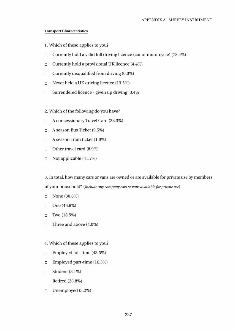
APPENDIX A. SURVEY INSTRUMENT
Transport Characteristics
1. Which of these applies to you?
2 Currently hold a valid full driving licence (car or motorcycle) (78.4%)
2 Currently hold a provisional UK licence (4.4%)
2 Currently disqualified from driving (0.0%)
2 Never held a UK driving licence (13.5%)
2 Surrendered licence - given up driving (3.4%)
2. Which of the following do you have?
2 A concessionary Travel Card (38.3%)
2 A season Bus Ticket (9.5%)
2 A season Train ticket (1.0%)
2 Other travel card (8.9%)
2 Not applicable (41.7%)
3. In total, how many cars or vans are owned or are available for private use by members
of your household? (Include any company cars or vans available for private use)
2 None (30.8%)
2 One (46.6%)
2 Two (18.5%)
2 Three and above (4.0%)
4. Which of these applies to you?
2 Employed full-time (43.5%)
2 Employed part-time (16.3%)
2 Student (8.1%)
2 Retired (28.8%)
2 Unemployed (3.2%)
227

APPENDIX A. SURVEY INSTRUMENT
5. Which of these is the purpose of your most regular journey in a week?
2 Work (54.8%)
2 Education (7.5%)
2 Shopping (23.0%)
2 Other (Leisure, Spots, Tourism) (14.7%)
6. How often do you make this trip in an average week?
2 Once (6.3%)
2 Twice(11.3%)
2 Three times (15.1%)
2 Four time (15.9%)
2 Five times (38.1%)
2 Everyday (13.1%)
7. Please indicate the postcode of the destination of the selected trip above
. . . . . . . . . . . . . . . . . . . . . . . . . . . . . . . . .
8. How do you usually make the journey above?
2 Walking. . . . . . . . . . . . . . . . . . . . . [GOTO QUESTION 12] (18.3%)
2 Bicycle. . . . . . . . . . . . . . . . . . . . . . . . [GOTO QUESTION 12] (7.9%)
2 Motorcycle/moped . . . . . . . . . [GOTO QUESTION 9] (0.0%)
2 Driver car/van . . . . . . . . . . . . . . . [GOTO QUESTION 9] (33.5%)
2 Passenger car/van . . . . . . . . . [GOTO QUESTION 12] (3.4%)
2 Car Sharing . . . . . . . . . . . . . . . . . . [GOTO QUESTION 9] (1.0%)
2 Bus/Tram service . . . . . . . . . . . . [GOTO QUESTION 10] (32.7%)
2 Work/School bus . . . . . . . . . . . . [GOTO QUESTION 12] (0.0%)
2 Rail . . . . . . . . . . . . . . . . . . . . . . . . . . . [GOTO QUESTION 10] (1.8%)
2 Taxi/minicab . . . . . . . . . . . . . . . [GOTO QUESTION 9] (0.2%)
9. How difficult would it be to undertake the journey above using public transport
228
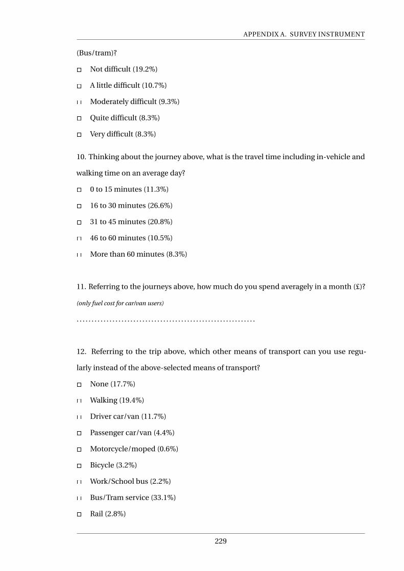
APPENDIX A. SURVEY INSTRUMENT
(Bus/tram)?
2 Not difficult (19.2%)
2 A little difficult (10.7%)
2 Moderately difficult (9.3%)
2 Quite difficult (8.3%)
2 Very difficult (8.3%)
10. Thinking about the journey above, what is the travel time including in-vehicle and
walking time on an average day?
2 0 to 15 minutes (11.3%)
2 16 to 30 minutes (26.6%)
2 31 to 45 minutes (20.8%)
2 46 to 60 minutes (10.5%)
2 More than 60 minutes (8.3%)
11. Referring to the journeys above, how much do you spend averagely in a month (£)?
(only fuel cost for car/van users)
. . . . . . . . . . . . . . . . . . . . . . . . . . . . . . . . . . . . . . . . . . . . . . . . . . . . . . . . . . . .
12. Referring to the trip above, which other means of transport can you use regu-
larly instead of the above-selected means of transport?
2 None (17.7%)
2 Walking (19.4%)
2 Driver car/van (11.7%)
2 Passenger car/van (4.4%)
2 Motorcycle/moped (0.6%)
2 Bicycle (3.2%)
2 Work/School bus (2.2%)
2 Bus/Tram service (33.1%)
2 Rail (2.8%)
229

APPENDIX A. SURVEY INSTRUMENT
2 Taxi/minicab (2.6%)
13. Thinking about the above-selected means of transport, how much would it cost for
your trip in a month, if at all? (only fuel cost for car/van users)
. . . . . . . . . . . . . . . . . . . . . . . . . . . . . . . . . . . . . . . . . . . . . . . . . . . . . . . . . . . .
14. How did you make similar journeys 5 years ago, if different from your current means
of transport?
2 Walking (14.5%)
2 Driver car/van (28.5%)
2 Passenger car/van (5.4%)
2 Motorcycle/moped (0.2%)
2 Bicycle (5.8%)
2 Work/School bus (1.0%)
2 Local Bus service (21.4%)
2 Tram/Rail (1.4%)
2 Taxi/minicab (0.0%)
2 Not Applicable (not in Scotland) (12.1%)
15. Why did you change your means of travel to your current means of travel, if you
have?
2 Not applicable (not changed) (51.4%)
2 I Changed job (8.1%)
2 I live within walking distance (3.6%)
2 I moved home (7.7%)
2 I bought a car / I got a company car (3.6%)
2 I lost my job (1.0%)
2 I lost my licence (0.0%)
2 I drop off/pick up children on the way (1.0%)
2 Health reasons (6.7%)
2 Other (please indicate) . . . . . . (7.7%)
230

APPENDIX A. SURVEY INSTRUMENT
16. How long would it take to walk to the nearest bus-stop from your home?
2 5 minutes walk or less (77.6%)
2 Within 6-10 minutes walk (19.0%)
2 Within 11-20 minutes walk (2.6%)
2 Within 21-30 minutes walk (0.2%)
2 More than 30 minutes walk (0.2%)
2 Don’t know (0.2%)
17. How long would it take to walk to the nearest bus-stop from your trip destina-
tion?
2 5 minutes walk or less (65.9%)
2 Within 6-10 minutes walk (20.2%)
2 Within 11-20 minutes walk (6.9%)
2 Within 21-30 minutes walk (1.6%)
2 More than 30 minutes walk (2.0%)
2 Don’t know (3.2%)
MINDSPACE Variables
18. Please indicate how much you agree with each of the following statements or how
true is it about you?
StatementStronglyDisagree
Disagree Undecided AgreeStrongly
Agree
I feel personally safe and secure on the local bus during the night 2 (2.8%) 2 (6.5%) 2 (16.3%) 2 (54.0%) 2 (17.5%)
The buses and stops are accessible 2 (1.1%) 2 (1.2%) 2 (3.4%) 2 (55.6%) 2 (38.1%)
The cleanliness of the buses interior, seats and bus stops are
acceptable2 (1.4%) 2(6.0%) 2(8.5%) 2(66.9%) 2(16.9%)
The noise level in buses is acceptable 2(2.2%) 2(8.5%) 2(13.1%) 2(61.3%) 2(14.1%)
The buses are comfortable and spacious 2(2.2%) 2(10.3%) 2(14.5%) 2(55.4%) 2(16.9%)
I am satisfied with the bus travel time 2(3.6%) 2(9.1%) 2(13.7%) 2(55.8%) 2(16.7%)
The service is stable and reliable (arrives on time and according
to the scheduled timetable)2(2.2%) 2(9.3%) 2(14.1%) 2(56.0%) 2(18.1%)
The fares are good value 2(3.0%) 2(11.9%) 2(20.8%) 2(44.8%) 2(17.3%)
Real-time travel information (route and timetable) is readily
available and easy to access2(1.4%) 2(7.1%) 2(9.9%) 2(57.5%) 2(23.8%)
Frequency of service is acceptable 2(2.0%) 2(7.3%) 2(8.5%) 2(58.7%) 2(23.4%)
231

APPENDIX A. SURVEY INSTRUMENT
19. Overall how satisfied are you with the bus services in Edinburgh?
2 Very Dissatisfied (4.0%)
2 Not Satisfied (3.4%)
2 Neutral (10.3%)
2 Satisfied (47.2%)
2 Very Satisfied (33.2%)
20. Based on the definition on the left-hand side of the table below;
20a. Please indicate how you would feel about the experiences on a public bus or tram
How discouraging would you
find each of the following
experiences on a bus or tram?
[1=Not Discouraging,
5=Very Discouraging]
1 2 3 4 5
Anti-social behaviour (drunk people etc) 2(3.4%) 2(6.5%) 2(16.1%) 2(28.6%) 2(44.6%)
Overcrowding 2(6.9%) 2(14.1%) 2(29.2%) 2(29.6%) 2(19.4%)
Exposure to health risk (catching a cold etc) 2(15.7%) 2(16.3%) 2(26.4%) 2(24.6%) 2(15.5%)
Passenger annoyance and discomfort 2(6.5%) 2(14.7%) 2(35.1%) 2(26.4%) 2(14.9%)
Poor hygiene (service uncleanliness and smell on the buses) 2(6.5%) 2(8.7%) 2(17.1%) 2(35.3%) 2(31.9%)
Inaccurate bus and real-time information 2(10.5%) 2(15.9%) 2(24.6%) 2(27.8%) 2(20.0%)
Long waiting and travel time 2(7.1%) 2(10.3%) 2(19.8%) 2(32.1%) 2(29.4%)
Safety issues (lack of seatbelt, toilets on board or conductor etc) 2(27.2%) 2(21.4%) 2(25.6%) 2(13.1%) 2(10.5%)
20b. Evaluate the extent to which you think the experiences would affect or have affected
your usage of the public bus or tram services
To what extent would these
experiences affect your regular
usage of the bus or tram?
[1=Not at all, 5=Very much]
1 2 3 4 5
Anti-social behaviour (drunk people etc) 2(15.7%) 2(17.5%) 2(20.6%) 2(19.2%) 2(25.8%)
Overcrowding 2(12.5%) 2(18.5%) 2(26.6%) 2(24.0%) 2(16.3%)
Exposure to health risk (catching a cold etc) 2(25.0%) 2(19.4%) 2(27.4%) 2(13.7%) 2(12.1%)
Passenger annoyance and discomfort 2(14.1%) 2(18.5%) 2(32.9%) 2(20.8%) 2(10.7%)
Poor hygiene (service uncleanliness and smell on the buses) 2(11.1%) 2(14.5%) 2(23.6%) 2(26.4%) 2(22.8%)
Inaccurate bus and real-time information 2(12.9%) 2(19.6%) 2(27.8%) 2(22.6%) 2(%)
Long waiting and travel time 2(11.1%) 2(15.3%) 2(21.0%) 2(24.2%) 2(26.0%)
Safety issues (lack of seatbelt, toilets on board or conductor etc) 2(33.9%) 2(23.8%) 2(21.0%) 2(9.5%) 2(8.9%)
21. Please to what extent do you agree or disagree with each of the following
statements?
232
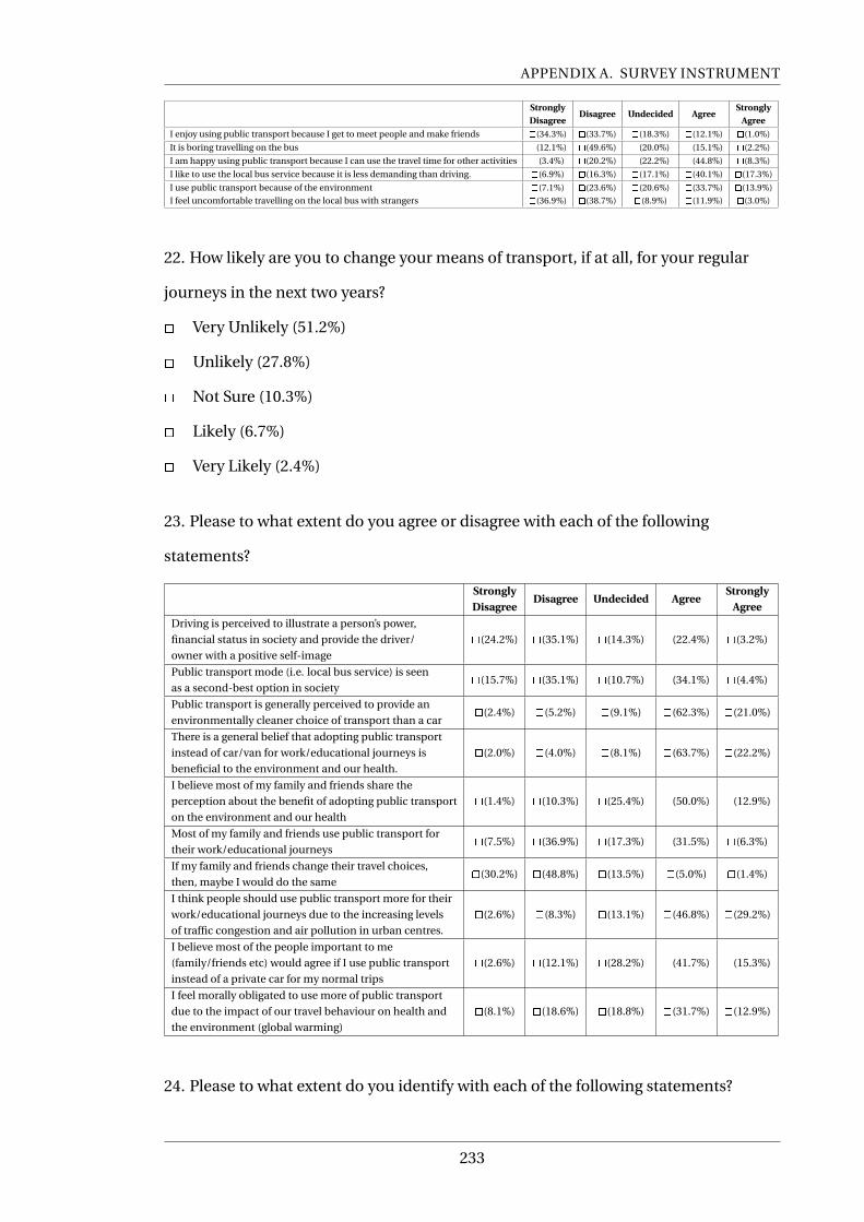
APPENDIX A. SURVEY INSTRUMENT
StronglyDisagree
Disagree Undecided AgreeStrongly
Agree
I enjoy using public transport because I get to meet people and make friends 2(34.3%) 2(33.7%) 2(18.3%) 2(12.1%) 2(1.0%)
It is boring travelling on the bus 2(12.1%) 2(49.6%) 2(20.0%) 2(15.1%) 2(2.2%)
I am happy using public transport because I can use the travel time for other activities 2(3.4%) 2(20.2%) 2(22.2%) 2(44.8%) 2(8.3%)
I like to use the local bus service because it is less demanding than driving. 2(6.9%) 2(16.3%) 2(17.1%) 2(40.1%) 2(17.3%)
I use public transport because of the environment 2(7.1%) 2(23.6%) 2(20.6%) 2(33.7%) 2(13.9%)
I feel uncomfortable travelling on the local bus with strangers 2(36.9%) 2(38.7%) 2(8.9%) 2(11.9%) 2(3.0%)
22. How likely are you to change your means of transport, if at all, for your regular
journeys in the next two years?
2 Very Unlikely (51.2%)
2 Unlikely (27.8%)
2 Not Sure (10.3%)
2 Likely (6.7%)
2 Very Likely (2.4%)
23. Please to what extent do you agree or disagree with each of the following
statements?
StronglyDisagree
Disagree Undecided AgreeStrongly
Agree
Driving is perceived to illustrate a person’s power,
financial status in society and provide the driver/
owner with a positive self-image
2(24.2%) 2(35.1%) 2(14.3%) 2(22.4%) 2(3.2%)
Public transport mode (i.e. local bus service) is seen
as a second-best option in society2(15.7%) 2(35.1%) 2(10.7%) 2(34.1%) 2(4.4%)
Public transport is generally perceived to provide an
environmentally cleaner choice of transport than a car2(2.4%) 2(5.2%) 2(9.1%) 2(62.3%) 2(21.0%)
There is a general belief that adopting public transport
instead of car/van for work/educational journeys is
beneficial to the environment and our health.
2(2.0%) 2(4.0%) 2(8.1%) 2(63.7%) 2(22.2%)
I believe most of my family and friends share the
perception about the benefit of adopting public transport
on the environment and our health
2(1.4%) 2(10.3%) 2(25.4%) 2(50.0%) 2(12.9%)
Most of my family and friends use public transport for
their work/educational journeys2(7.5%) 2(36.9%) 2(17.3%) 2(31.5%) 2(6.3%)
If my family and friends change their travel choices,
then, maybe I would do the same2(30.2%) 2(48.8%) 2(13.5%) 2(5.0%) 2(1.4%)
I think people should use public transport more for their
work/educational journeys due to the increasing levels
of traffic congestion and air pollution in urban centres.
2(2.6%) 2(8.3%) 2(13.1%) 2(46.8%) 2(29.2%)
I believe most of the people important to me
(family/friends etc) would agree if I use public transport
instead of a private car for my normal trips
2(2.6%) 2(12.1%) 2(28.2%) 2(41.7%) 2(15.3%)
I feel morally obligated to use more of public transport
due to the impact of our travel behaviour on health and
the environment (global warming)
2(8.1%) 2(18.6%) 2(18.8%) 2(31.7%) 2(12.9%)
24. Please to what extent do you identify with each of the following statements?
233
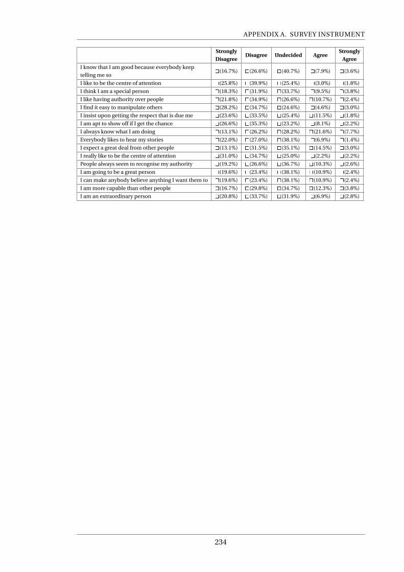
APPENDIX A. SURVEY INSTRUMENT
StronglyDisagree
Disagree Undecided AgreeStrongly
Agree
I know that I am good because everybody keep
telling me so2(16.7%) 2(26.6%) 2(40.7%) 2(7.9%) 2(3.6%)
I like to be the centre of attention 2(25.8%) 2(39.9%) 2(25.4%) 2(3.0%) 2(1.8%)
I think I am a special person 2(18.3%) 2(31.9%) 2(33.7%) 2(9.5%) 2(3.8%)
I like having authority over people 2(21.8%) 2(34.9%) 2(26.6%) 2(10.7%) 2(2.4%)
I find it easy to manipulate others 2(28.2%) 2(34.7%) 2(24.6%) 2(4.6%) 2(3.0%)
I insist upon getting the respect that is due me 2(23.6%) 2(33.5%) 2(25.4%) 2(11.5%) 2(1.8%)
I am apt to show off if I get the chance 2(26.6%) 2(35.3%) 2(23.2%) 2(8.1%) 2(2.2%)
I always know what I am doing 2(13.1%) 2(26.2%) 2(28.2%) 2(21.6%) 2(7.7%)
Everybody likes to hear my stories 2(22.0%) 2(27.0%) 2(38.1%) 2(6.9%) 2(1.4%)
I expect a great deal from other people 2(13.1%) 2(31.5%) 2(35.1%) 2(14.5%) 2(3.0%)
I really like to be the centre of attention 2(31.0%) 2(34.7%) 2(25.0%) 2(2.2%) 2(2.2%)
People always seem to recognise my authority 2(19.2%) 2(26.6%) 2(36.7%) 2(10.3%) 2(2.6%)
I am going to be a great person 2(19.6%) 2(23.4%) 2(38.1%) 2(10.9%) 2(2.4%)
I can make anybody believe anything I want them to 2(19.6%) 2(23.4%) 2(38.1%) 2(10.9%) 2(2.4%)
I am more capable than other people 2(16.7%) 2(29.8%) 2(34.7%) 2(12.3%) 2(3.8%)
I am an extraordinary person 2(20.8%) 2(33.7%) 2(31.9%) 2(6.9%) 2(2.8%)
234

APPENDIX A. SURVEY INSTRUMENT
Demographics
25. What is your gender?
2 Female (52.2%)
2 Male (47.8%)
26. What is your age? . . . . . . . . . . . . . . . . . . . . .
27. What is your Marital Status?
2 Married (including Civil Partnership) (46.8%)
2 Unmarried (46.2%)
2 Divorced/Separated (7.1%)
28. Please, what is the size of your household including yourself and children?
2 1 (32.9%)
2 2 (40.9%)
2 3 (12.1%)
2 More than 3 (14.1%)
29. Please, could you indicate the highest educational qualifications you have?
2 No formal education (1.0%)
2 Primary (0.0%)
2 Secondary (17.1%)
2 College (19.8%)
2 Bachelor’s degree (33.1%)
2 Master’s degree (23.6%)
2 PhD (5.4%)
30. Which of these best represent your household annual income before tax?
2 Less than £10,000 (9.9%)
2 £10,000 to £15,000 (9.7%)
235

APPENDIX A. SURVEY INSTRUMENT
2 £15,000 to £20,000 (10.7%)
2 £20,000 to £30,000 (18.8%)
2 £30,000 to £50,000 (22.8%)
2 £50,000 to £70,000 (13.5%)
2 Over £70,000 (14.7%)
31. Comments/Suggestions about the survey
. . . . . . . . . . . . . . . . . . . . . . . . . . . . . . . . . . . . . . . . . . . . . . . . . . . . . . . . . . . . . . . . . . . . . . . . . . . . . . . . . . . . . . . . . . . . . . . . . . .
. . . . . . . . . . . . . . . . . . . . . . . . . . . . . . . . . . . . . . . . . . . . . . . . . . . . . . . . . . . . . . . . . . . . . . . . . . . . . . . . . . . . . . . . . . . . . . . . . . .
236

; Appendix B <
Ethical Approval
237

APPENDIX B. ETHICAL APPROVAL
238

APPENDIX B. ETHICAL APPROVAL
239

APPENDIX B. ETHICAL APPROVAL
240

APPENDIX B. ETHICAL APPROVAL
241

; Appendix C <
Sample Map
242
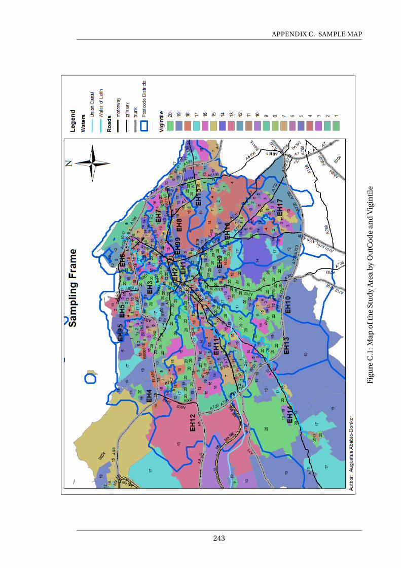
APPENDIX C. SAMPLE MAP
Fig
ure
C.1
:Map
oft
he
Stu
dy
Are
ab
yO
utC
od
ean
dV
igin
tile
243
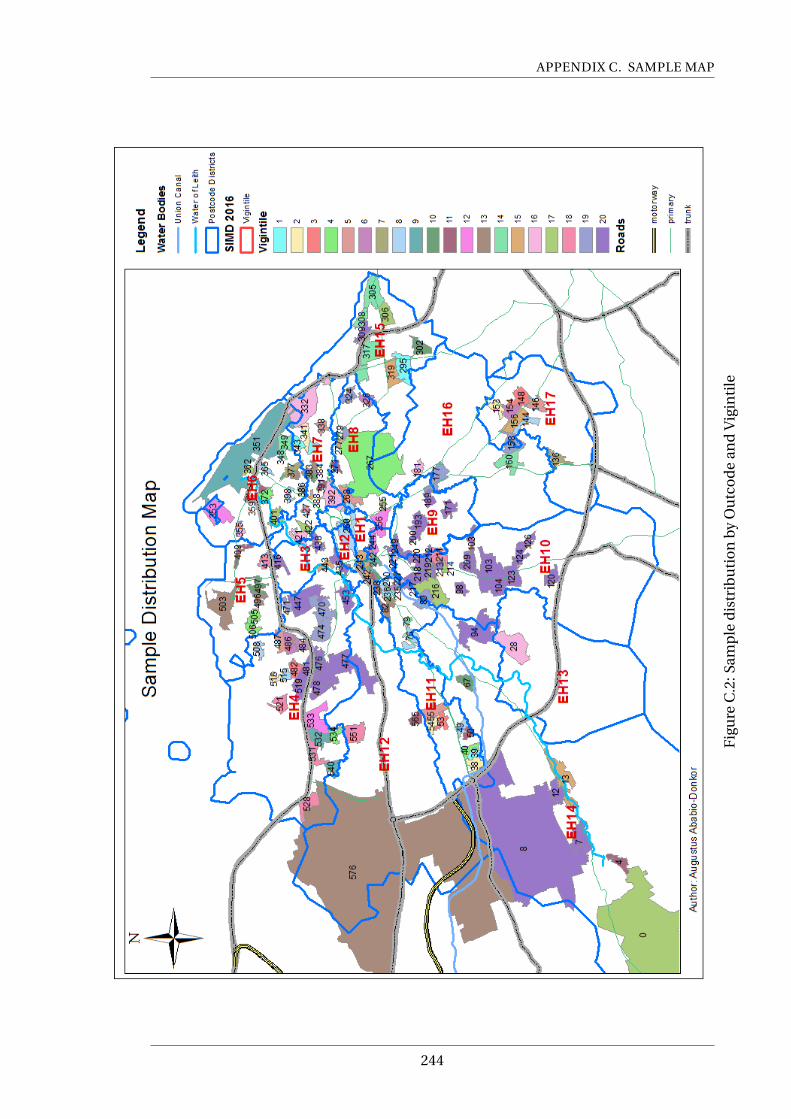
APPENDIX C. SAMPLE MAP
Fig
ure
C.2
:Sam
ple
dis
trib
uti
on
by
Ou
tco
de
and
Vig
inti
le
244
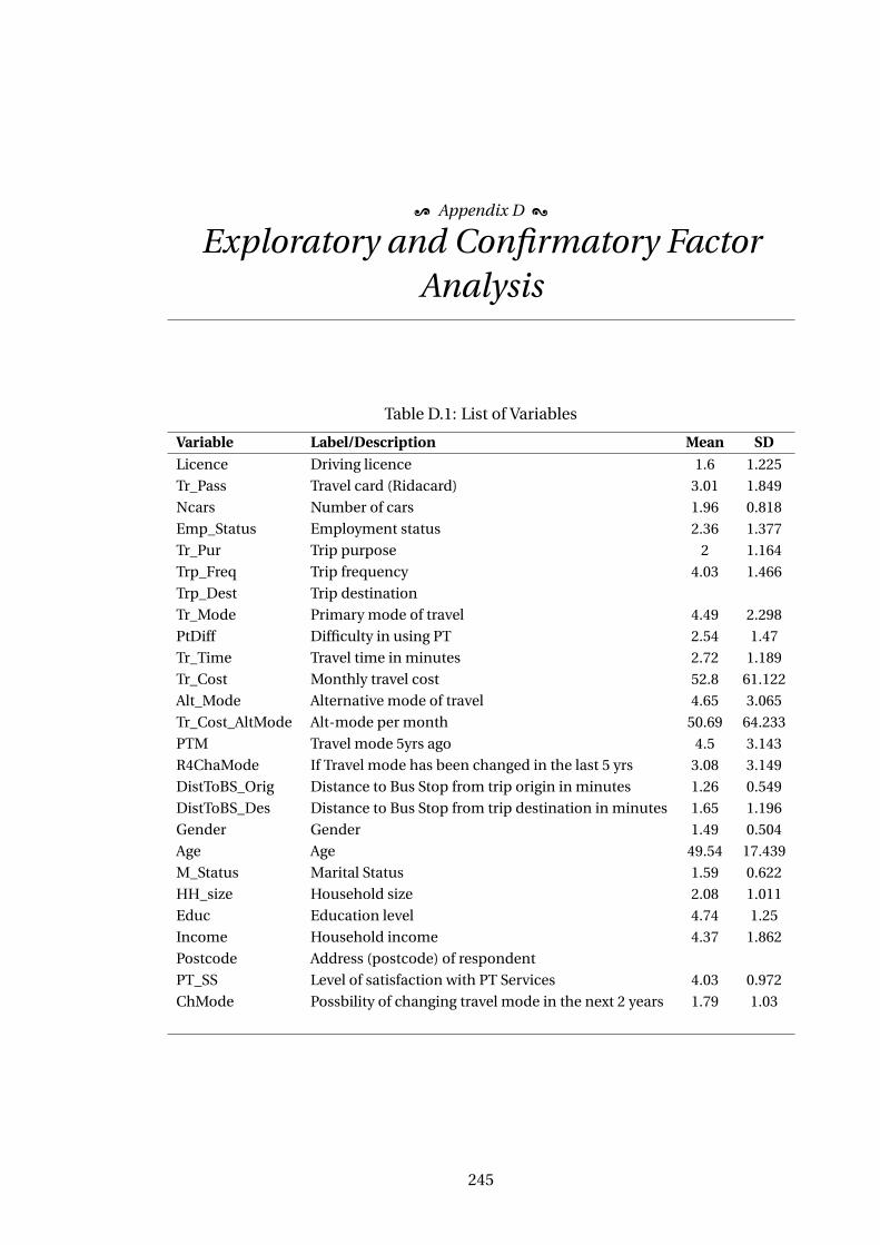
; Appendix D <
Exploratory and Confirmatory FactorAnalysis
Table D.1: List of Variables
Variable Label/Description Mean SD
Licence Driving licence 1.6 1.225
Tr_Pass Travel card (Ridacard) 3.01 1.849
Ncars Number of cars 1.96 0.818
Emp_Status Employment status 2.36 1.377
Tr_Pur Trip purpose 2 1.164
Trp_Freq Trip frequency 4.03 1.466
Trp_Dest Trip destination
Tr_Mode Primary mode of travel 4.49 2.298
PtDiff Difficulty in using PT 2.54 1.47
Tr_Time Travel time in minutes 2.72 1.189
Tr_Cost Monthly travel cost 52.8 61.122
Alt_Mode Alternative mode of travel 4.65 3.065
Tr_Cost_AltMode Alt-mode per month 50.69 64.233
PTM Travel mode 5yrs ago 4.5 3.143
R4ChaMode If Travel mode has been changed in the last 5 yrs 3.08 3.149
DistToBS_Orig Distance to Bus Stop from trip origin in minutes 1.26 0.549
DistToBS_Des Distance to Bus Stop from trip destination in minutes 1.65 1.196
Gender Gender 1.49 0.504
Age Age 49.54 17.439
M_Status Marital Status 1.59 0.622
HH_size Household size 2.08 1.011
Educ Education level 4.74 1.25
Income Household income 4.37 1.862
Postcode Address (postcode) of respondent
PT_SS Level of satisfaction with PT Services 4.03 0.972
ChMode Possbility of changing travel mode in the next 2 years 1.79 1.03
245

APPENDIX D. EXPLORATORY AND CONFIRMATORY FACTOR ANALYSIS
Tab
leC
.1:L
isto
fVar
iab
les
Psy
cho
met
ric
Co
nst
ruct
s
Targ
etC
on
stru
ctIn
dic
ato
rsL
abel
/Des
crip
tio
nM
ean
SD
Ple
ase
tow
hat
exte
ntd
oyo
uag
ree
or
dis
agre
ew
ith
each
oft
he
follo
win
gst
atem
ents
?
Norms
Nrm
1D
rivi
ng
isp
erce
ived
toil
lust
rate
ap
erso
n’s
pow
er,fi
nan
cial
stat
us
inso
ciet
yan
dp
rovi
de
the
dri
ver/
own
erw
ith
ap
osi
tive
self
-im
age
2.45
1.17
7
Nrm
2P
ub
lictr
ansp
ort
mo
de
(i.e
.lo
calb
us
serv
ice)
isse
enas
ase
con
db
esto
pti
on
inso
ciet
y2.
761.
202
Nrm
3P
ub
lictr
ansp
ort
isge
ner
ally
per
ceiv
edto
pro
vid
een
viro
nm
enta
llycl
ean
erch
oic
eo
ftra
nsp
ort
than
aca
r3.
940.
852
Nrm
4T
her
eis
age
ner
alb
elie
fth
atad
op
tin
gp
ub
lic
tran
spo
rtin
stea
do
fcar
/van
for
wo
rk/e
du
cati
on
aljo
urn
eys
is
ben
efici
alto
the
envi
ron
men
tan
do
ur
hea
lth
.4.
000.
804
Nrm
5I
bel
ieve
mo
sto
fmy
fam
ily
and
frie
nd
ssh
are
the
per
cep
tio
nab
ou
tth
eb
enefi
tofa
do
pti
ng
pu
bli
ctr
ansp
ort
on
the
envi
ron
men
tan
do
ur
hea
lth
3.63
0.88
5
Nrm
6M
ost
ofm
yfa
mil
yan
dfr
ien
ds
use
pu
blic
tran
spo
rtfo
rth
eir
wo
rk/e
du
cati
on
aljo
urn
eys
2.92
1.11
2
Nrm
7If
my
fam
ilyan
dfr
ien
ds
chan
geth
eir
trav
elch
oic
es,t
hen
,may
be
Iw
ou
ldd
osa
me
1.98
0.88
Nrm
8I
thin
kp
eop
lesh
ou
ldu
sep
ub
lic
tran
spo
rtm
ore
for
thei
rw
ork
/ed
uca
tio
nal
jou
rney
sd
ue
toth
ein
crea
sin
g
leve
lso
ftra
ffic
con
gest
ion
and
air
po
lluti
on
inth
eu
rban
cen
tres
.3.
920.
993
Nrm
9I
bel
ieve
mo
sto
fth
ep
eop
leim
po
rtan
tto
me
(fam
ily/
frie
nd
set
c)w
ou
ldag
ree
ifI
use
pu
bli
ctr
ansp
ort
inst
ead
ofa
pri
vate
car
for
my
no
rmal
trip
s3.
550.
977
Nrm
10I
feel
mo
rally
ob
liga
ted
tou
sem
ore
ofp
ub
lic
tran
spo
rtd
ue
toth
eim
pac
tofo
ur
trav
elb
ehav
iou
ro
n
hea
lth
and
the
envi
ron
men
t(gl
ob
alw
arm
ing)
3.13
1.19
5
Tow
hat
exte
ntw
ou
ldth
ese
exp
erie
nce
saf
fect
you
rre
gula
ru
sage
oft
he
bu
so
rtr
am?
Salience
PT
Exp
1bA
nti
-so
cial
beh
avio
ur
(dru
nk
peo
ple
etc)
3.13
1.26
4
PT
Exp
2bO
verc
row
din
g2.
951.
195
PT
Exp
3bE
xpo
sure
toh
ealt
hri
sk(c
atch
ing
cold
etc)
3.36
1.29
1
PT
Exp
4bPa
ssen
ger
ann
oyan
cean
dd
isco
mfo
rt3.
081.
255
PT
Exp
5bPo
or
hyg
ien
e(s
ervi
ceu
ncl
ean
lines
san
dsm
ello
nth
eb
use
s)3.
41.
331
PT
Exp
6bIn
accu
rate
bu
san
dre
al-t
ime
info
rmat
ion
2.34
1.29
2
PT
Exp
7bLo
ng
wai
tin
gan
dtr
avel
tim
e3.
221.
417
PT
Exp
8bSa
fety
issu
es(l
ack
ofs
eatb
elt,
toile
tso
nb
oar
do
rco
nd
uct
or
etc)
2.68
1.32
6
Ple
ase
tow
hat
exte
ntd
oyo
uag
ree
or
dis
agre
ew
ith
each
oft
he
follo
win
gst
atem
ents
?
Affect
Aff
1I
enjo
yu
sin
gp
ub
lic
tran
spo
rtb
ecau
seI
gett
om
eetp
eop
lean
dm
ake
frie
nd
s2.
111.
047
Aff
2It
isb
ori
ng
trav
elli
ng
inth
eb
us
2.45
0.96
6
Aff
3I
amh
app
yu
sin
gp
ub
lictr
ansp
ort
bec
ause
Ica
nu
seth
etr
avel
tim
efo
ro
ther
acti
viti
es3.
351.
006
Aff
4I
like
tou
seth
elo
calb
us
serv
ice
bec
ause
itis
less
dem
and
ing
than
dri
vin
g.3.
461.
166
Aff
5I
use
pu
blic
tran
spo
rtb
ecau
seo
fth
een
viro
nm
ent
3.24
1.17
2
Aff
6I
feel
un
com
fort
able
trav
elli
ng
inth
elo
calb
us
wit
hst
ran
gers
2.05
1.10
1
246
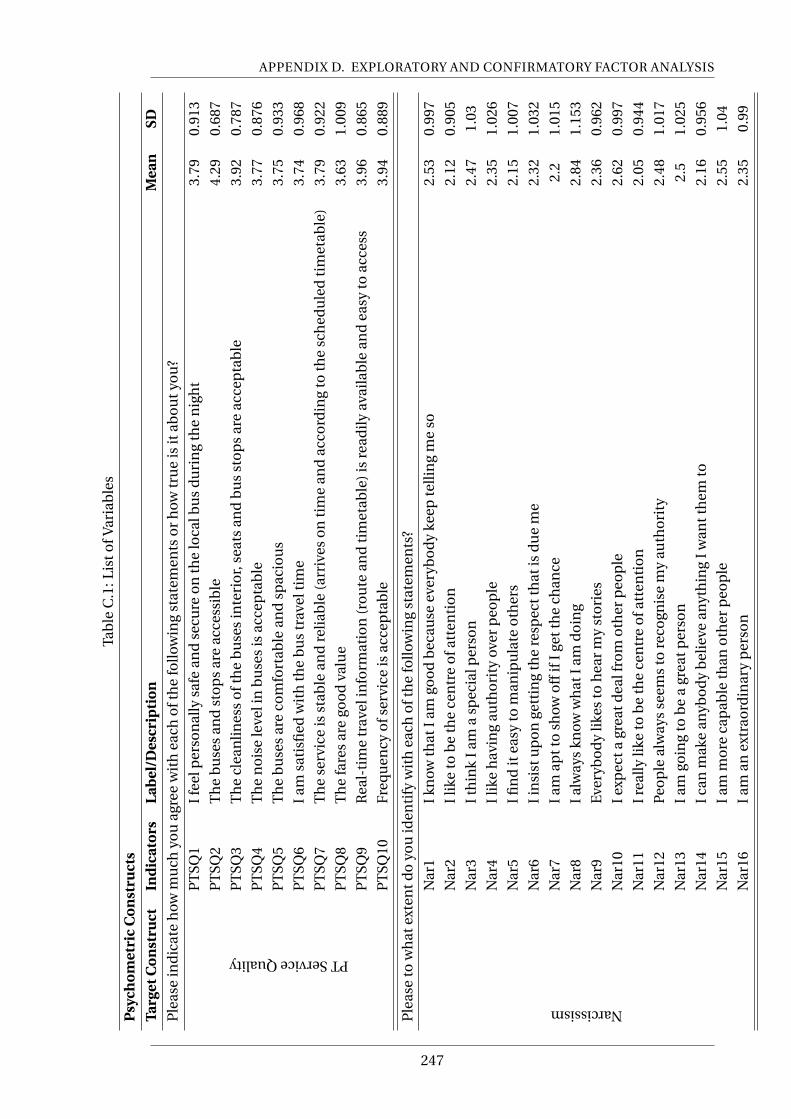
APPENDIX D. EXPLORATORY AND CONFIRMATORY FACTOR ANALYSIS
Tab
leC
.1:L
isto
fVar
iab
les
Psy
cho
met
ric
Co
nst
ruct
s
Targ
etC
on
stru
ctIn
dic
ato
rsL
abel
/Des
crip
tio
nM
ean
SD
Ple
ase
ind
icat
eh
owm
uch
you
agre
ew
ith
each
oft
he
follo
win
gst
atem
ents
or
how
tru
eis
itab
ou
tyo
u?
PTServiceQuality
PT
SQ1
Ife
elp
erso
nal
lysa
fean
dse
cure
on
the
loca
lbu
sd
uri
ng
the
nig
ht
3.79
0.91
3
PT
SQ2
Th
eb
use
san
dst
op
sar
eac
cess
ible
4.29
0.68
7
PT
SQ3
Th
ecl
ean
lin
ess
oft
he
bu
ses
inte
rio
r,se
ats
and
bu
sst
op
sar
eac
cep
tab
le3.
920.
787
PT
SQ4
Th
en
ois
ele
veli
nb
use
sis
acce
pta
ble
3.77
0.87
6
PT
SQ5
Th
eb
use
sar
eco
mfo
rtab
lean
dsp
acio
us
3.75
0.93
3
PT
SQ6
Iam
sati
sfied
wit
hth
eb
us
trav
elti
me
3.74
0.96
8
PT
SQ7
Th
ese
rvic
eis
stab
lean
dre
liab
le(a
rriv
eso
nti
me
and
acco
rdin
gto
the
sch
edu
led
tim
etab
le)
3.79
0.92
2
PT
SQ8
Th
efa
res
are
goo
dva
lue
3.63
1.00
9
PT
SQ9
Rea
l-ti
me
trav
elin
form
atio
n(r
ou
tean
dti
met
able
)is
read
ily
avai
lab
lean
dea
syto
acce
ss3.
960.
865
PT
SQ10
Freq
uen
cyo
fser
vice
isac
cep
tab
le3.
940.
889
Ple
ase
tow
hat
exte
ntd
oyo
uid
enti
fyw
ith
each
oft
he
follo
win
gst
atem
ents
?
Narcissism
Nar
1I
know
that
Iam
goo
db
ecau
seev
eryb
od
yke
epte
llin
gm
eso
2.53
0.99
7
Nar
2I
like
tob
eth
ece
ntr
eo
fatt
enti
on
2.12
0.90
5
Nar
3I
thin
kI
ama
spec
ialp
erso
n2.
471.
03
Nar
4I
like
hav
ing
auth
ori
tyov
erp
eop
le2.
351.
026
Nar
5I
fin
dit
easy
tom
anip
ula
teo
ther
s2.
151.
007
Nar
6I
insi
stu
po
nge
ttin
gth
ere
spec
tth
atis
du
em
e2.
321.
032
Nar
7I
amap
tto
show
off
ifI
gett
he
chan
ce2.
21.
015
Nar
8I
alw
ays
know
wh
atI
amd
oin
g2.
841.
153
Nar
9E
very
bo
dy
likes
toh
ear
my
sto
ries
2.36
0.96
2
Nar
10I
exp
ecta
grea
tdea
lfro
mo
ther
peo
ple
2.62
0.99
7
Nar
11I
real
lyli
keto
be
the
cen
tre
ofa
tten
tio
n2.
050.
944
Nar
12Pe
op
leal
way
sse
ems
tore
cogn
ise
my
auth
ori
ty2.
481.
017
Nar
13I
amgo
ing
tob
ea
grea
tper
son
2.5
1.02
5
Nar
14I
can
mak
ean
ybo
dy
bel
ieve
anyt
hin
gI
wan
tth
emto
2.16
0.95
6
Nar
15I
amm
ore
cap
able
than
oth
erp
eop
le2.
551.
04
Nar
16I
aman
extr
aord
inar
yp
erso
n2.
350.
99
247
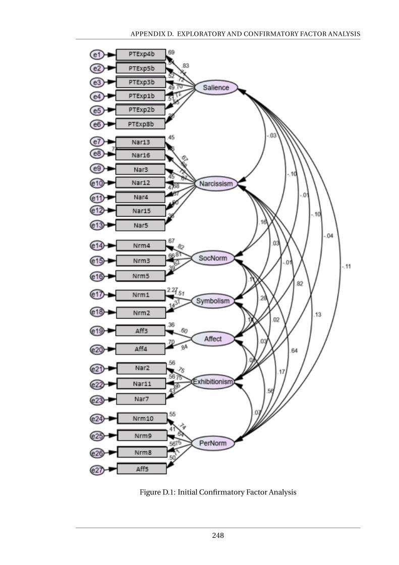
APPENDIX D. EXPLORATORY AND CONFIRMATORY FACTOR ANALYSIS
Figure D.1: Initial Confirmatory Factor Analysis
248

APPENDIX D. EXPLORATORY AND CONFIRMATORY FACTOR ANALYSIS
Figure D.2: Final Confirmatory Factor Analysis
249
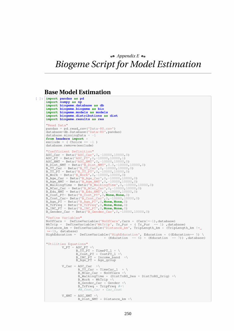
; Appendix E <
Biogeme Script for Model Estimation
Base Model Estimation[ ]: import pandas as pd
import numpy as npimport biogeme.database as dbimport biogeme.biogeme as bioimport biogeme.models as modelsimport biogeme.distributions as distimport biogeme.results as res
"Read Data"pandas = pd.read_csv('Data-80.csv')database=db.Database('Data-80',pandas)database.missingData = -1from headers import *exclude = ( Choice == -1 )database.remove(exclude)
"Coefficient Definition"ASC_Car = Beta('ASC_Car',0,-10000,10000,0)ASC_PT = Beta('ASC_PT',0,-10000,10000,1)ASC_NMT = Beta('ASC_NMT',0,-10000,10000,0)B_Dist_NMT = Beta('B_Dist_NMT',0.0,-10000,10000,0)B_TT_Car = Beta('B_TT_Car',0,-10000,10000,0)B_TT_PT = Beta('B_TT_PT',0,-10000,10000,0)B_Work = Beta('B_Work',0,-10000,10000,0)B_Age_Car = Beta('B_Age_Car',0,-10000,10000,0)B_Age_NMT = Beta('B_Age_NMT',0,-10000,10000,0)B_WalkingTime = Beta('B_WalkingTime',0,-10000,10000,0)B_NCar_Car = Beta('B_NCar_Car',0,-10000,10000,0)B_Edu_NMT = Beta('B_Edu_NMT',0,-10000,10000,0)B_Cost_PT= Beta('B_Cost_PT',0,None,None,0)B_Cost_Car= Beta('B_Cost_Car',0,-10000,10000,0)B_Age_PT = Beta('B_Age_PT',0,None,None,0)B_TrFreq = Beta('B_TrFreq',0,None,None,0)B_INC_PT = Beta('B_INC_PT',0,None,None,0)B_Gender_Car = Beta('B_Gender_Car',0,-10000,10000,0)
"Define Variables"NoOfCars = DefineVariable('NoOfCars',Cars * (Cars!=-1),database)WkTrip = DefineVariable('WkTrip', Tr_Pur * ( Tr_Pur == 1) ,database)Distance_km = DefineVariable('Distance_km', TripLength_km * (TripLength_km !=,→-1), database)HighEducation = DefineVariable('HighEducation', Education * ((Education== 5) \
+ (Education == 6) + (Education == 7)) ,database)
"Utilities Equations"V_PT = ASC_PT +\
B_TT_PT * TimePT_1 + \B_Cost_PT * CostPT_1 +\B_INC_PT * Income_band +\B_Age_PT * Age_group
V_Car = ASC_Car +\B_TT_Car * TimeCar_1 + \B_NCar_Car * NoOfCars +\B_WalkingTime * (DistToBS_Des + DistToBS_Orig) +\B_Work * WkTrip +\B_Gender_Car * Gender +\B_TrFreq * TripFreq #+\#B_Cost_Car * Car_Cost
V_NMT = ASC_NMT +\B_Dist_NMT * Distance_km +\
250
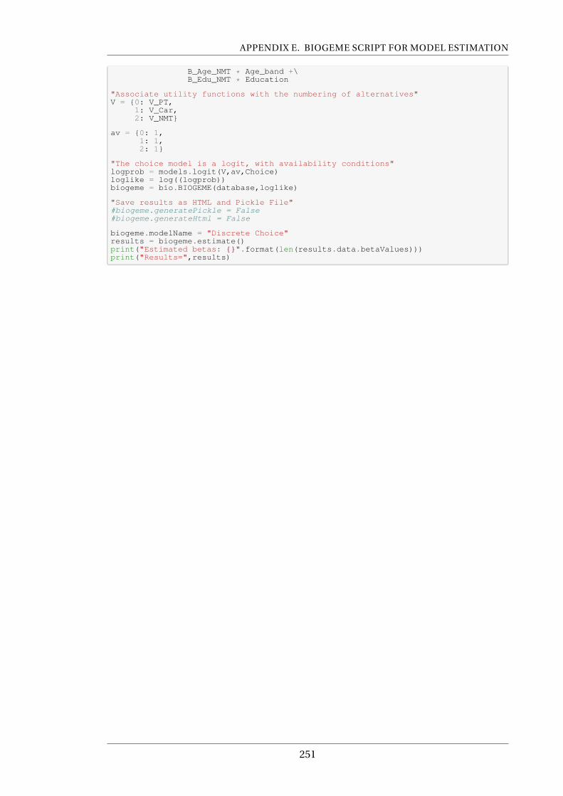
APPENDIX E. BIOGEME SCRIPT FOR MODEL ESTIMATION
B_Age_NMT * Age_band +\B_Edu_NMT * Education
"Associate utility functions with the numbering of alternatives"V = {0: V_PT,
1: V_Car,2: V_NMT}
av = {0: 1,1: 1,2: 1}
"The choice model is a logit, with availability conditions"logprob = models.logit(V,av,Choice)loglike = log((logprob))biogeme = bio.BIOGEME(database,loglike)
"Save results as HTML and Pickle File"#biogeme.generatePickle = False#biogeme.generateHtml = False
biogeme.modelName = "Discrete Choice"results = biogeme.estimate()print("Estimated betas: {}".format(len(results.data.betaValues)))print("Results=",results)
251
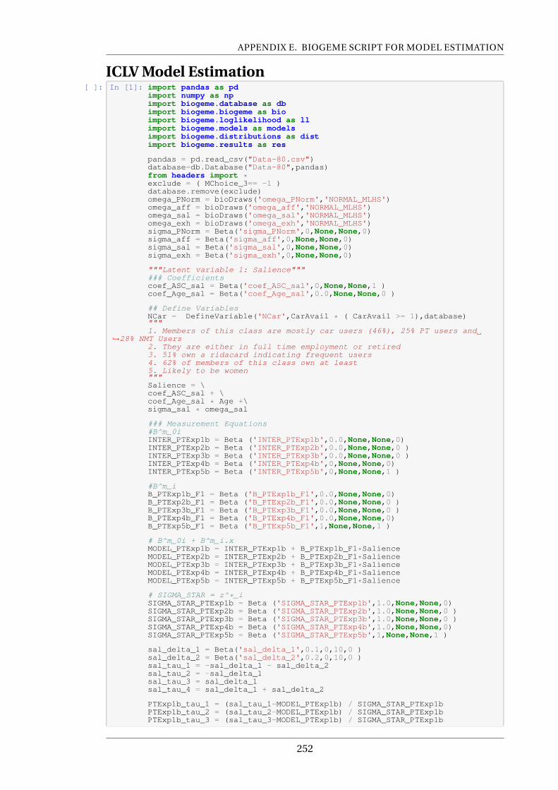
APPENDIX E. BIOGEME SCRIPT FOR MODEL ESTIMATION
ICLV Model Estimation[ ]: In [1]: import pandas as pd
import numpy as npimport biogeme.database as dbimport biogeme.biogeme as bioimport biogeme.loglikelihood as llimport biogeme.models as modelsimport biogeme.distributions as distimport biogeme.results as res
pandas = pd.read_csv("Data-80.csv")database=db.Database("Data-80",pandas)from headers import *exclude = ( MChoice_3== -1 )database.remove(exclude)omega_PNorm = bioDraws('omega_PNorm','NORMAL_MLHS')omega_aff = bioDraws('omega_aff','NORMAL_MLHS')omega_sal = bioDraws('omega_sal','NORMAL_MLHS')omega_exh = bioDraws('omega_exh','NORMAL_MLHS')sigma_PNorm = Beta('sigma_PNorm',0,None,None,0)sigma_aff = Beta('sigma_aff',0,None,None,0)sigma_sal = Beta('sigma_sal',0,None,None,0)sigma_exh = Beta('sigma_exh',0,None,None,0)
"""Latent variable 1: Salience"""### Coefficientscoef_ASC_sal = Beta('coef_ASC_sal',0,None,None,1 )coef_Age_sal = Beta('coef_Age_sal',0.0,None,None,0 )
## Define VariablesNCar = DefineVariable('NCar',CarAvail * ( CarAvail >= 1),database)"""1. Members of this class are mostly car users (46%), 25% PT users and
,→28% NMT Users2. They are either in full time employment or retired3. 51% own a ridacard indicating frequent users4. 62% of members of this class own at least5. Likely to be women"""Salience = \coef_ASC_sal + \coef_Age_sal * Age +\sigma_sal * omega_sal
### Measurement Equations#B^m_0iINTER_PTExp1b = Beta ('INTER_PTExp1b',0.0,None,None,0)INTER_PTExp2b = Beta ('INTER_PTExp2b',0.0,None,None,0 )INTER_PTExp3b = Beta ('INTER_PTExp3b',0.0,None,None,0 )INTER_PTExp4b = Beta ('INTER_PTExp4b',0,None,None,0)INTER_PTExp5b = Beta ('INTER_PTExp5b',0,None,None,1 )
#B^m_iB_PTExp1b_F1 = Beta ('B_PTExp1b_F1',0.0,None,None,0)B_PTExp2b_F1 = Beta ('B_PTExp2b_F1',0.0,None,None,0 )B_PTExp3b_F1 = Beta ('B_PTExp3b_F1',0.0,None,None,0 )B_PTExp4b_F1 = Beta ('B_PTExp4b_F1',0.0,None,None,0)B_PTExp5b_F1 = Beta ('B_PTExp5b_F1',1,None,None,1 )
# B^m_0i + B^m_i.xMODEL_PTExp1b = INTER_PTExp1b + B_PTExp1b_F1*SalienceMODEL_PTExp2b = INTER_PTExp2b + B_PTExp2b_F1*SalienceMODEL_PTExp3b = INTER_PTExp3b + B_PTExp3b_F1*SalienceMODEL_PTExp4b = INTER_PTExp4b + B_PTExp4b_F1*SalienceMODEL_PTExp5b = INTER_PTExp5b + B_PTExp5b_F1*Salience
# SIGMA_STAR = z^*_iSIGMA_STAR_PTExp1b = Beta ('SIGMA_STAR_PTExp1b',1.0,None,None,0)SIGMA_STAR_PTExp2b = Beta ('SIGMA_STAR_PTExp2b',1.0,None,None,0 )SIGMA_STAR_PTExp3b = Beta ('SIGMA_STAR_PTExp3b',1.0,None,None,0 )SIGMA_STAR_PTExp4b = Beta ('SIGMA_STAR_PTExp4b',1.0,None,None,0)SIGMA_STAR_PTExp5b = Beta ('SIGMA_STAR_PTExp5b',1,None,None,1 )
sal_delta_1 = Beta('sal_delta_1',0.1,0,10,0 )sal_delta_2 = Beta('sal_delta_2',0.2,0,10,0 )sal_tau_1 = -sal_delta_1 - sal_delta_2sal_tau_2 = -sal_delta_1sal_tau_3 = sal_delta_1sal_tau_4 = sal_delta_1 + sal_delta_2
PTExp1b_tau_1 = (sal_tau_1-MODEL_PTExp1b) / SIGMA_STAR_PTExp1bPTExp1b_tau_2 = (sal_tau_2-MODEL_PTExp1b) / SIGMA_STAR_PTExp1bPTExp1b_tau_3 = (sal_tau_3-MODEL_PTExp1b) / SIGMA_STAR_PTExp1b
252
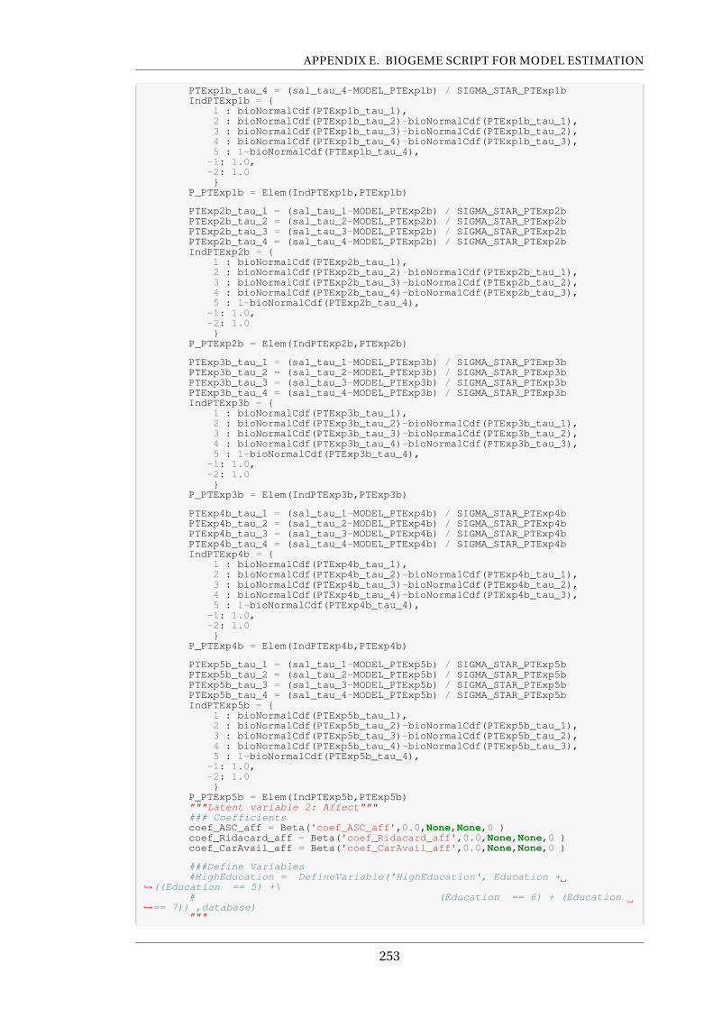
APPENDIX E. BIOGEME SCRIPT FOR MODEL ESTIMATION
PTExp1b_tau_4 = (sal_tau_4-MODEL_PTExp1b) / SIGMA_STAR_PTExp1bIndPTExp1b = {
1 : bioNormalCdf(PTExp1b_tau_1),2 : bioNormalCdf(PTExp1b_tau_2)-bioNormalCdf(PTExp1b_tau_1),3 : bioNormalCdf(PTExp1b_tau_3)-bioNormalCdf(PTExp1b_tau_2),4 : bioNormalCdf(PTExp1b_tau_4)-bioNormalCdf(PTExp1b_tau_3),5 : 1-bioNormalCdf(PTExp1b_tau_4),
-1: 1.0,-2: 1.0}
P_PTExp1b = Elem(IndPTExp1b,PTExp1b)
PTExp2b_tau_1 = (sal_tau_1-MODEL_PTExp2b) / SIGMA_STAR_PTExp2bPTExp2b_tau_2 = (sal_tau_2-MODEL_PTExp2b) / SIGMA_STAR_PTExp2bPTExp2b_tau_3 = (sal_tau_3-MODEL_PTExp2b) / SIGMA_STAR_PTExp2bPTExp2b_tau_4 = (sal_tau_4-MODEL_PTExp2b) / SIGMA_STAR_PTExp2bIndPTExp2b = {
1 : bioNormalCdf(PTExp2b_tau_1),2 : bioNormalCdf(PTExp2b_tau_2)-bioNormalCdf(PTExp2b_tau_1),3 : bioNormalCdf(PTExp2b_tau_3)-bioNormalCdf(PTExp2b_tau_2),4 : bioNormalCdf(PTExp2b_tau_4)-bioNormalCdf(PTExp2b_tau_3),5 : 1-bioNormalCdf(PTExp2b_tau_4),
-1: 1.0,-2: 1.0}
P_PTExp2b = Elem(IndPTExp2b,PTExp2b)
PTExp3b_tau_1 = (sal_tau_1-MODEL_PTExp3b) / SIGMA_STAR_PTExp3bPTExp3b_tau_2 = (sal_tau_2-MODEL_PTExp3b) / SIGMA_STAR_PTExp3bPTExp3b_tau_3 = (sal_tau_3-MODEL_PTExp3b) / SIGMA_STAR_PTExp3bPTExp3b_tau_4 = (sal_tau_4-MODEL_PTExp3b) / SIGMA_STAR_PTExp3bIndPTExp3b = {
1 : bioNormalCdf(PTExp3b_tau_1),2 : bioNormalCdf(PTExp3b_tau_2)-bioNormalCdf(PTExp3b_tau_1),3 : bioNormalCdf(PTExp3b_tau_3)-bioNormalCdf(PTExp3b_tau_2),4 : bioNormalCdf(PTExp3b_tau_4)-bioNormalCdf(PTExp3b_tau_3),5 : 1-bioNormalCdf(PTExp3b_tau_4),
-1: 1.0,-2: 1.0}
P_PTExp3b = Elem(IndPTExp3b,PTExp3b)
PTExp4b_tau_1 = (sal_tau_1-MODEL_PTExp4b) / SIGMA_STAR_PTExp4bPTExp4b_tau_2 = (sal_tau_2-MODEL_PTExp4b) / SIGMA_STAR_PTExp4bPTExp4b_tau_3 = (sal_tau_3-MODEL_PTExp4b) / SIGMA_STAR_PTExp4bPTExp4b_tau_4 = (sal_tau_4-MODEL_PTExp4b) / SIGMA_STAR_PTExp4bIndPTExp4b = {
1 : bioNormalCdf(PTExp4b_tau_1),2 : bioNormalCdf(PTExp4b_tau_2)-bioNormalCdf(PTExp4b_tau_1),3 : bioNormalCdf(PTExp4b_tau_3)-bioNormalCdf(PTExp4b_tau_2),4 : bioNormalCdf(PTExp4b_tau_4)-bioNormalCdf(PTExp4b_tau_3),5 : 1-bioNormalCdf(PTExp4b_tau_4),
-1: 1.0,-2: 1.0}
P_PTExp4b = Elem(IndPTExp4b,PTExp4b)
PTExp5b_tau_1 = (sal_tau_1-MODEL_PTExp5b) / SIGMA_STAR_PTExp5bPTExp5b_tau_2 = (sal_tau_2-MODEL_PTExp5b) / SIGMA_STAR_PTExp5bPTExp5b_tau_3 = (sal_tau_3-MODEL_PTExp5b) / SIGMA_STAR_PTExp5bPTExp5b_tau_4 = (sal_tau_4-MODEL_PTExp5b) / SIGMA_STAR_PTExp5bIndPTExp5b = {
1 : bioNormalCdf(PTExp5b_tau_1),2 : bioNormalCdf(PTExp5b_tau_2)-bioNormalCdf(PTExp5b_tau_1),3 : bioNormalCdf(PTExp5b_tau_3)-bioNormalCdf(PTExp5b_tau_2),4 : bioNormalCdf(PTExp5b_tau_4)-bioNormalCdf(PTExp5b_tau_3),5 : 1-bioNormalCdf(PTExp5b_tau_4),
-1: 1.0,-2: 1.0}
P_PTExp5b = Elem(IndPTExp5b,PTExp5b)"""Latent variable 2: Affect"""### Coefficientscoef_ASC_aff = Beta('coef_ASC_aff',0.0,None,None,0 )coef_Ridacard_aff = Beta('coef_Ridacard_aff',0.0,None,None,0 )coef_CarAvail_aff = Beta('coef_CarAvail_aff',0.0,None,None,0 )
###Define Variables#HighEducation = DefineVariable('HighEducation', Education *
,→((Education == 5) +\# (Education == 6) + (Education
,→== 7)) ,database)"""
253
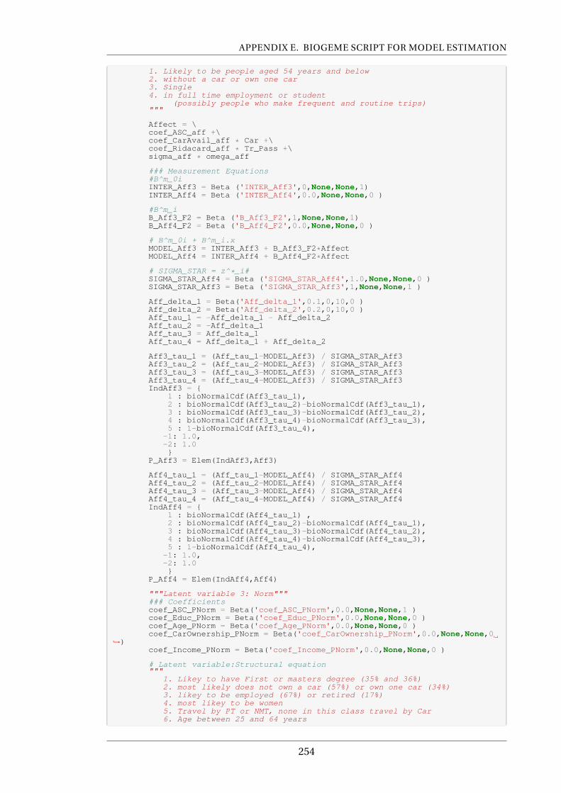
APPENDIX E. BIOGEME SCRIPT FOR MODEL ESTIMATION
1. Likely to be people aged 54 years and below2. without a car or own one car3. Single4. in full time employment or student
(possibly people who make frequent and routine trips)"""
Affect = \coef_ASC_aff +\coef_CarAvail_aff * Car +\coef_Ridacard_aff * Tr_Pass +\sigma_aff * omega_aff
### Measurement Equations#B^m_0iINTER_Aff3 = Beta ('INTER_Aff3',0,None,None,1)INTER_Aff4 = Beta ('INTER_Aff4',0.0,None,None,0 )
#B^m_iB_Aff3_F2 = Beta ('B_Aff3_F2',1,None,None,1)B_Aff4_F2 = Beta ('B_Aff4_F2',0.0,None,None,0 )
# B^m_0i + B^m_i.xMODEL_Aff3 = INTER_Aff3 + B_Aff3_F2*AffectMODEL_Aff4 = INTER_Aff4 + B_Aff4_F2*Affect
# SIGMA_STAR = z^*_i#SIGMA_STAR_Aff4 = Beta ('SIGMA_STAR_Aff4',1.0,None,None,0 )SIGMA_STAR_Aff3 = Beta ('SIGMA_STAR_Aff3',1,None,None,1 )
Aff_delta_1 = Beta('Aff_delta_1',0.1,0,10,0 )Aff_delta_2 = Beta('Aff_delta_2',0.2,0,10,0 )Aff_tau_1 = -Aff_delta_1 - Aff_delta_2Aff_tau_2 = -Aff_delta_1Aff_tau_3 = Aff_delta_1Aff_tau_4 = Aff_delta_1 + Aff_delta_2
Aff3_tau_1 = (Aff_tau_1-MODEL_Aff3) / SIGMA_STAR_Aff3Aff3_tau_2 = (Aff_tau_2-MODEL_Aff3) / SIGMA_STAR_Aff3Aff3_tau_3 = (Aff_tau_3-MODEL_Aff3) / SIGMA_STAR_Aff3Aff3_tau_4 = (Aff_tau_4-MODEL_Aff3) / SIGMA_STAR_Aff3IndAff3 = {
1 : bioNormalCdf(Aff3_tau_1),2 : bioNormalCdf(Aff3_tau_2)-bioNormalCdf(Aff3_tau_1),3 : bioNormalCdf(Aff3_tau_3)-bioNormalCdf(Aff3_tau_2),4 : bioNormalCdf(Aff3_tau_4)-bioNormalCdf(Aff3_tau_3),5 : 1-bioNormalCdf(Aff3_tau_4),
-1: 1.0,-2: 1.0}
P_Aff3 = Elem(IndAff3,Aff3)
Aff4_tau_1 = (Aff_tau_1-MODEL_Aff4) / SIGMA_STAR_Aff4Aff4_tau_2 = (Aff_tau_2-MODEL_Aff4) / SIGMA_STAR_Aff4Aff4_tau_3 = (Aff_tau_3-MODEL_Aff4) / SIGMA_STAR_Aff4Aff4_tau_4 = (Aff_tau_4-MODEL_Aff4) / SIGMA_STAR_Aff4IndAff4 = {
1 : bioNormalCdf(Aff4_tau_1) ,2 : bioNormalCdf(Aff4_tau_2)-bioNormalCdf(Aff4_tau_1),3 : bioNormalCdf(Aff4_tau_3)-bioNormalCdf(Aff4_tau_2),4 : bioNormalCdf(Aff4_tau_4)-bioNormalCdf(Aff4_tau_3),5 : 1-bioNormalCdf(Aff4_tau_4),
-1: 1.0,-2: 1.0}
P_Aff4 = Elem(IndAff4,Aff4)
"""Latent variable 3: Norm"""### Coefficientscoef_ASC_PNorm = Beta('coef_ASC_PNorm',0.0,None,None,1 )coef_Educ_PNorm = Beta('coef_Educ_PNorm',0.0,None,None,0 )coef_Age_PNorm = Beta('coef_Age_PNorm',0.0,None,None,0 )coef_CarOwnership_PNorm = Beta('coef_CarOwnership_PNorm',0.0,None,None,0
,→)coef_Income_PNorm = Beta('coef_Income_PNorm',0.0,None,None,0 )
# Latent variable:Structural equation"""
1. Likey to have First or masters degree (35% and 36%)2. most likely does not own a car (57%) or own one car (34%)3. likey to be employed (67%) or retired (17%)4. most likey to be women5. Travel by PT or NMT, none in this class travel by Car6. Age between 25 and 64 years
254
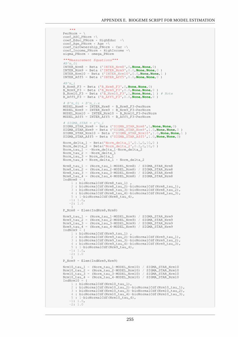
APPENDIX E. BIOGEME SCRIPT FOR MODEL ESTIMATION
"""PerNorm = \coef_ASC_PNorm +\coef_Educ_PNorm * HighEduc +\coef_Age_PNorm * Age +\coef_CarOwnership_PNorm * Car +\coef_Income_PNorm * HighIncome +\sigma_PNorm * omega_PNorm
"""Measurement Equations"""#B^m_0iINTER_Nrm8 = Beta ('INTER_Nrm8',0,None,None,0)INTER_Nrm9 = Beta ('INTER_Nrm9',0.0,None,None,0 )INTER_Nrm10 = Beta ('INTER_Nrm10',0.0,None,None,1 )INTER_Aff5 = Beta ('INTER_Aff5',0.0,None,None,0 )
#B^m_iB_Nrm8_F3 = Beta ('B_Nrm8_F3',0,None,None,0)B_Nrm9_F3 = Beta ('B_Nrm9_F3',0.0,None,None,0 )B_Nrm10_F3 = Beta ('B_Nrm10_F3',1,None,None,1 ) # NoteB_Aff5_F3 = Beta ('B_Aff5_F3',0.0,None,None,0 )
# B^m_0i + B^m_i.xMODEL_Nrm8 = INTER_Nrm8 + B_Nrm8_F3*PerNormMODEL_Nrm9 = INTER_Nrm9 + B_Nrm9_F3*PerNormMODEL_Nrm10 = INTER_Nrm10 + B_Nrm10_F3*PerNormMODEL_Aff5 = INTER_Aff5 + B_Aff5_F3*PerNorm
# SIGMA_STAR = z^*_iSIGMA_STAR_Nrm8 = Beta ('SIGMA_STAR_Nrm8',1,None,None,0)SIGMA_STAR_Nrm9 = Beta ('SIGMA_STAR_Nrm9',1.0,None,None,0 )SIGMA_STAR_Nrm10 = Beta ('SIGMA_STAR_Nrm10',1.0,None,None,1 )SIGMA_STAR_Aff5 = Beta ('SIGMA_STAR_Aff5',1.0,None,None,0)
Norm_delta_1 = Beta('Norm_delta_1',0.1,0,10,0 )Norm_delta_2 = Beta('Norm_delta_2',0.2,0,10,0 )Norm_tau_1 = -Norm_delta_1-Norm_delta_2Norm_tau_2 = -Norm_delta_1Norm_tau_3 = Norm_delta_1Norm_tau_4 = Norm_delta_1 + Norm_delta_2
Nrm8_tau_1 = (Norm_tau_1-MODEL_Nrm8) / SIGMA_STAR_Nrm8Nrm8_tau_2 = (Norm_tau_2-MODEL_Nrm8) / SIGMA_STAR_Nrm8Nrm8_tau_3 = (Norm_tau_3-MODEL_Nrm8) / SIGMA_STAR_Nrm8Nrm8_tau_4 = (Norm_tau_4-MODEL_Nrm8) / SIGMA_STAR_Nrm8IndNrm8 = {
1 : bioNormalCdf(Nrm8_tau_1) ,2 : bioNormalCdf(Nrm8_tau_2)-bioNormalCdf(Nrm8_tau_1),3 : bioNormalCdf(Nrm8_tau_3)-bioNormalCdf(Nrm8_tau_2),4 : bioNormalCdf(Nrm8_tau_4)-bioNormalCdf(Nrm8_tau_3),5 : 1-bioNormalCdf(Nrm8_tau_4),
-1: 1.0,-2: 1.0}
P_Nrm8 = Elem(IndNrm8,Nrm8)
Nrm9_tau_1 = (Norm_tau_1-MODEL_Nrm9) / SIGMA_STAR_Nrm9Nrm9_tau_2 = (Norm_tau_2-MODEL_Nrm9) / SIGMA_STAR_Nrm9Nrm9_tau_3 = (Norm_tau_3-MODEL_Nrm9) / SIGMA_STAR_Nrm9Nrm9_tau_4 = (Norm_tau_4-MODEL_Nrm9) / SIGMA_STAR_Nrm9IndNrm9 = {
1 : bioNormalCdf(Nrm9_tau_1) ,2 : bioNormalCdf(Nrm9_tau_2)-bioNormalCdf(Nrm9_tau_1),3 : bioNormalCdf(Nrm9_tau_3)-bioNormalCdf(Nrm9_tau_2),4 : bioNormalCdf(Nrm9_tau_4)-bioNormalCdf(Nrm9_tau_3),5 : 1-bioNormalCdf(Nrm9_tau_4),
-1: 1.0,-2: 1.0}
P_Nrm9 = Elem(IndNrm9,Nrm9)
Nrm10_tau_1 = (Norm_tau_1-MODEL_Nrm10) / SIGMA_STAR_Nrm10Nrm10_tau_2 = (Norm_tau_2-MODEL_Nrm10) / SIGMA_STAR_Nrm10Nrm10_tau_3 = (Norm_tau_3-MODEL_Nrm10) / SIGMA_STAR_Nrm10Nrm10_tau_4 = (Norm_tau_4-MODEL_Nrm10) / SIGMA_STAR_Nrm10IndNrm10 = {
1 : bioNormalCdf(Nrm10_tau_1),2 : bioNormalCdf(Nrm10_tau_2)-bioNormalCdf(Nrm10_tau_1),3 : bioNormalCdf(Nrm10_tau_3)-bioNormalCdf(Nrm10_tau_2),4 : bioNormalCdf(Nrm10_tau_4)-bioNormalCdf(Nrm10_tau_3),5 : 1-bioNormalCdf(Nrm10_tau_4),
-1: 1.0,-2: 1.0
255

APPENDIX E. BIOGEME SCRIPT FOR MODEL ESTIMATION
}P_Nrm10 = Elem(IndNrm10,Nrm10)
Aff5_tau_1 = (Norm_tau_1-MODEL_Aff5) / SIGMA_STAR_Aff5Aff5_tau_2 = (Norm_tau_2-MODEL_Aff5) / SIGMA_STAR_Aff5Aff5_tau_3 = (Norm_tau_3-MODEL_Aff5) / SIGMA_STAR_Aff5Aff5_tau_4 = (Norm_tau_4-MODEL_Aff5) / SIGMA_STAR_Aff5IndAff5 = {
1 : bioNormalCdf(Aff5_tau_1),2 : bioNormalCdf(Aff5_tau_2)-bioNormalCdf(Aff5_tau_1),3 : bioNormalCdf(Aff5_tau_3)-bioNormalCdf(Aff5_tau_2),4 : bioNormalCdf(Aff5_tau_4)-bioNormalCdf(Aff5_tau_3),5 : 1-bioNormalCdf(Aff5_tau_4),
-1: 1.0,-2: 1.0}
P_Aff5 = Elem(IndAff5,Aff5)
"""Latent variable 4: Narcissism (Exhibitionism)"""## Coefficientscoef_ASC_Exh = Beta('coef_ASC_Exh',0,None,None,0 )coef_Gender_Exh = Beta('coef_Gender_Exh',0.0,None,None,0 )coef_Income_Exh = Beta('coef_Income_Exh',0.0,None,None,0 )
Exh = \coef_ASC_Exh +\coef_Gender_Exh * Gender +\coef_Income_Exh * HighIncome +\omega_exh * sigma_exh
"""Measurement Equations"""#B^m_0iINTER_Nar2 = Beta ('INTER_Nar2',0.0,None,None,0)INTER_Nar7 = Beta ('INTER_Nar7',0,None,None,1 )INTER_Nar11 = Beta ('INTER_Nar11',0.0,None,None,0 )
#B^m_iB_Nar2_F4 = Beta ('B_Nar2_F4',0.0,None,None,0)B_Nar7_F4 = Beta ('B_Nar7_F4',1,None,None,1 )B_Nar11_F4 = Beta ('B_Nar11_F4',0.0,None,None,0 ) # Note
# B^m_0i + B^m_i.xMODEL_Nar2 = INTER_Nar2 + B_Nar2_F4*ExhMODEL_Nar7 = INTER_Nar7 + B_Nar7_F4*ExhMODEL_Nar11 = INTER_Nar11 + B_Nar11_F4*Exh
# SIGMA_STAR = z^*_iSIGMA_STAR_Nar2 = Beta ('SIGMA_STAR_Nar2',1.0,None,None,0)SIGMA_STAR_Nar7 = Beta ('SIGMA_STAR_Nar7',1,None,None,1 )SIGMA_STAR_Nar11 = Beta ('SIGMA_STAR_Nar11',1.0,None,None,0 )
Nar_delta_1 = Beta('Nar_delta_1',0.1,0,10,0 )Nar_delta_2 = Beta('Nar_delta_2',0.2,0,10,0 )Nar_tau_1 = -Nar_delta_1 - Nar_delta_2Nar_tau_2 = -Nar_delta_1Nar_tau_3 = Nar_delta_1Nar_tau_4 = Nar_delta_1 + Nar_delta_2
Nar2_tau_1 = (Nar_tau_1-MODEL_Nar2) / SIGMA_STAR_Nar2Nar2_tau_2 = (Nar_tau_2-MODEL_Nar2) / SIGMA_STAR_Nar2Nar2_tau_3 = (Nar_tau_3-MODEL_Nar2) / SIGMA_STAR_Nar2Nar2_tau_4 = (Nar_tau_4-MODEL_Nar2) / SIGMA_STAR_Nar2IndNar2 = {
1 : bioNormalCdf(Nar2_tau_1) ,2 : bioNormalCdf(Nar2_tau_2)-bioNormalCdf(Nar2_tau_1),3 : bioNormalCdf(Nar2_tau_3)-bioNormalCdf(Nar2_tau_2),4 : bioNormalCdf(Nar2_tau_4)-bioNormalCdf(Nar2_tau_3),5 : 1-bioNormalCdf(Nar2_tau_4),-1: 1.0,-2: 1.0}
P_Nar2 = Elem(IndNar2,Nar2)
Nar7_tau_1 = (Nar_tau_1-MODEL_Nar7) / SIGMA_STAR_Nar7Nar7_tau_2 = (Nar_tau_2-MODEL_Nar7) / SIGMA_STAR_Nar7Nar7_tau_3 = (Nar_tau_3-MODEL_Nar7) / SIGMA_STAR_Nar7Nar7_tau_4 = (Nar_tau_4-MODEL_Nar7) / SIGMA_STAR_Nar7IndNar7 = {
1 : bioNormalCdf(Nar7_tau_1),2 : bioNormalCdf(Nar7_tau_2)-bioNormalCdf(Nar7_tau_1),3 : bioNormalCdf(Nar7_tau_3)-bioNormalCdf(Nar7_tau_2),4 : bioNormalCdf(Nar7_tau_4)-bioNormalCdf(Nar7_tau_3),5 : 1-bioNormalCdf(Nar7_tau_4),-1: 1.0,
256
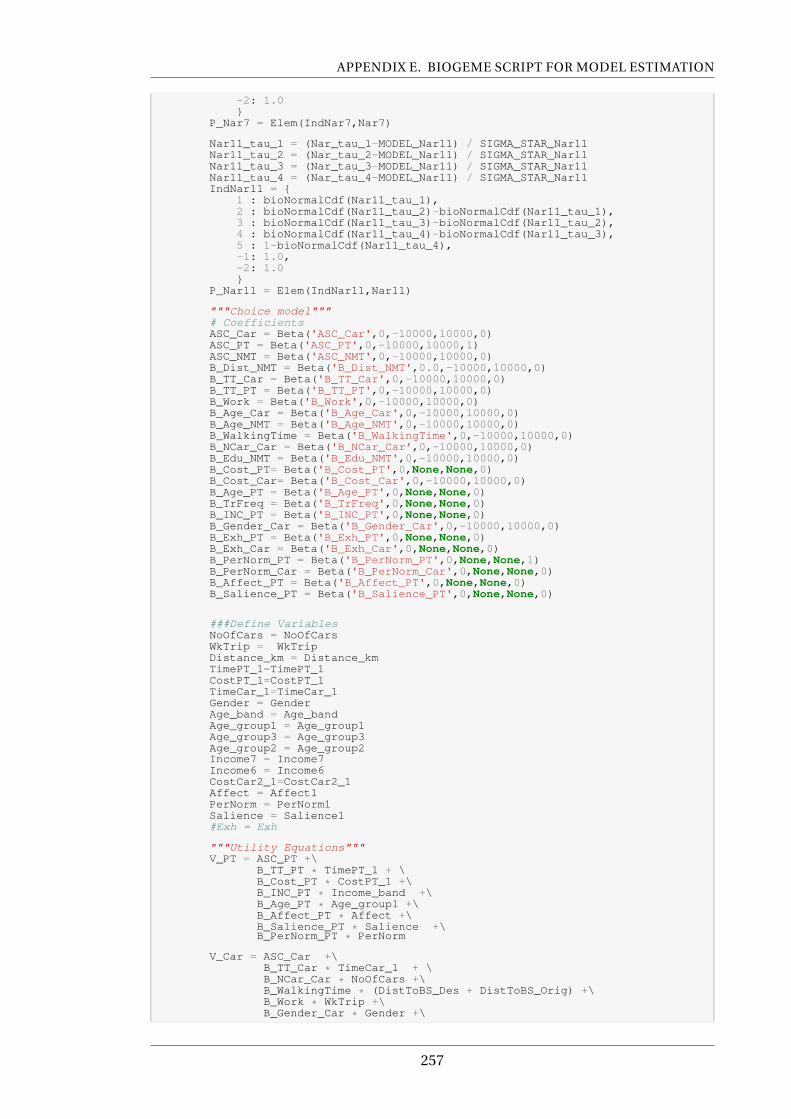
APPENDIX E. BIOGEME SCRIPT FOR MODEL ESTIMATION
-2: 1.0}
P_Nar7 = Elem(IndNar7,Nar7)
Nar11_tau_1 = (Nar_tau_1-MODEL_Nar11) / SIGMA_STAR_Nar11Nar11_tau_2 = (Nar_tau_2-MODEL_Nar11) / SIGMA_STAR_Nar11Nar11_tau_3 = (Nar_tau_3-MODEL_Nar11) / SIGMA_STAR_Nar11Nar11_tau_4 = (Nar_tau_4-MODEL_Nar11) / SIGMA_STAR_Nar11IndNar11 = {
1 : bioNormalCdf(Nar11_tau_1),2 : bioNormalCdf(Nar11_tau_2)-bioNormalCdf(Nar11_tau_1),3 : bioNormalCdf(Nar11_tau_3)-bioNormalCdf(Nar11_tau_2),4 : bioNormalCdf(Nar11_tau_4)-bioNormalCdf(Nar11_tau_3),5 : 1-bioNormalCdf(Nar11_tau_4),-1: 1.0,-2: 1.0}
P_Nar11 = Elem(IndNar11,Nar11)
"""Choice model"""# CoefficientsASC_Car = Beta('ASC_Car',0,-10000,10000,0)ASC_PT = Beta('ASC_PT',0,-10000,10000,1)ASC_NMT = Beta('ASC_NMT',0,-10000,10000,0)B_Dist_NMT = Beta('B_Dist_NMT',0.0,-10000,10000,0)B_TT_Car = Beta('B_TT_Car',0,-10000,10000,0)B_TT_PT = Beta('B_TT_PT',0,-10000,10000,0)B_Work = Beta('B_Work',0,-10000,10000,0)B_Age_Car = Beta('B_Age_Car',0,-10000,10000,0)B_Age_NMT = Beta('B_Age_NMT',0,-10000,10000,0)B_WalkingTime = Beta('B_WalkingTime',0,-10000,10000,0)B_NCar_Car = Beta('B_NCar_Car',0,-10000,10000,0)B_Edu_NMT = Beta('B_Edu_NMT',0,-10000,10000,0)B_Cost_PT= Beta('B_Cost_PT',0,None,None,0)B_Cost_Car= Beta('B_Cost_Car',0,-10000,10000,0)B_Age_PT = Beta('B_Age_PT',0,None,None,0)B_TrFreq = Beta('B_TrFreq',0,None,None,0)B_INC_PT = Beta('B_INC_PT',0,None,None,0)B_Gender_Car = Beta('B_Gender_Car',0,-10000,10000,0)B_Exh_PT = Beta('B_Exh_PT',0,None,None,0)B_Exh_Car = Beta('B_Exh_Car',0,None,None,0)B_PerNorm_PT = Beta('B_PerNorm_PT',0,None,None,1)B_PerNorm_Car = Beta('B_PerNorm_Car',0,None,None,0)B_Affect_PT = Beta('B_Affect_PT',0,None,None,0)B_Salience_PT = Beta('B_Salience_PT',0,None,None,0)
###Define VariablesNoOfCars = NoOfCarsWkTrip = WkTripDistance_km = Distance_kmTimePT_1=TimePT_1CostPT_1=CostPT_1TimeCar_1=TimeCar_1Gender = GenderAge_band = Age_bandAge_group1 = Age_group1Age_group3 = Age_group3Age_group2 = Age_group2Income7 = Income7Income6 = Income6CostCar2_1=CostCar2_1Affect = Affect1PerNorm = PerNorm1Salience = Salience1#Exh = Exh
"""Utility Equations"""V_PT = ASC_PT +\
B_TT_PT * TimePT_1 + \B_Cost_PT * CostPT_1 +\B_INC_PT * Income_band +\B_Age_PT * Age_group1 +\B_Affect_PT * Affect +\B_Salience_PT * Salience +\B_PerNorm_PT * PerNorm
V_Car = ASC_Car +\B_TT_Car * TimeCar_1 + \B_NCar_Car * NoOfCars +\B_WalkingTime * (DistToBS_Des + DistToBS_Orig) +\B_Work * WkTrip +\B_Gender_Car * Gender +\
257
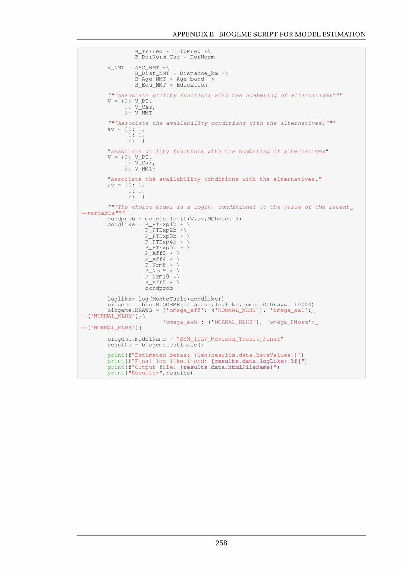
APPENDIX E. BIOGEME SCRIPT FOR MODEL ESTIMATION
B_TrFreq * TripFreq +\B_PerNorm_Car * PerNorm
V_NMT = ASC_NMT +\B_Dist_NMT * Distance_km +\B_Age_NMT * Age_band +\B_Edu_NMT * Education
"""Associate utility functions with the numbering of alternatives"""V = {0: V_PT,
1: V_Car,2: V_NMT}
"""Associate the availability conditions with the alternatives."""av = {0: 1,
1: 1,2: 1}
"Associate utility functions with the numbering of alternatives"V = {0: V_PT,
1: V_Car,2: V_NMT}
"Associate the availability conditions with the alternatives."av = {0: 1,
1: 1,2: 1}
"""The choice model is a logit, conditional to the value of the latent,→variable"""
condprob = models.logit(V,av,MChoice_3)condlike = P_PTExp1b * \
P_PTExp2b *\P_PTExp3b * \P_PTExp4b * \P_PTExp5b * \P_Aff3 * \P_Aff4 * \P_Nrm8 * \P_Nrm9 * \P_Nrm10 *\P_Aff5 * \condprob
loglike= log(MonteCarlo(condlike))biogeme = bio.BIOGEME(database,loglike,numberOfDraws= 10000)biogeme.DRAWS = {'omega_aff': ('NORMAL_MLHS'), 'omega_sal':
,→('NORMAL_MLHS'),\'omega_exh': ('NORMAL_MLHS'), 'omega_PNorm':
,→('NORMAL_MLHS')}
biogeme.modelName = "SEM_ICLV_Revised_Thesis_Final"results = biogeme.estimate()
print(f"Estimated betas: {len(results.data.betaValues)}")print(f"Final log likelihood: {results.data.logLike:.3f}")print(f"Output file: {results.data.htmlFileName}")print("Results=",results)
258
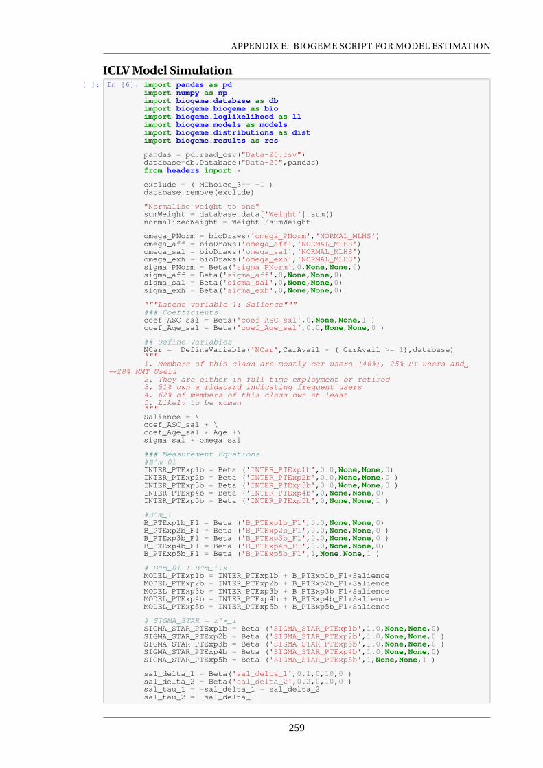
APPENDIX E. BIOGEME SCRIPT FOR MODEL ESTIMATION
ICLV Model Simulation[ ]: In [6]: import pandas as pd
import numpy as npimport biogeme.database as dbimport biogeme.biogeme as bioimport biogeme.loglikelihood as llimport biogeme.models as modelsimport biogeme.distributions as distimport biogeme.results as res
pandas = pd.read_csv("Data-20.csv")database=db.Database("Data-20",pandas)from headers import *
exclude = ( MChoice_3== -1 )database.remove(exclude)
"Normalise weight to one"sumWeight = database.data['Weight'].sum()normalizedWeight = Weight /sumWeight
omega_PNorm = bioDraws('omega_PNorm','NORMAL_MLHS')omega_aff = bioDraws('omega_aff','NORMAL_MLHS')omega_sal = bioDraws('omega_sal','NORMAL_MLHS')omega_exh = bioDraws('omega_exh','NORMAL_MLHS')sigma_PNorm = Beta('sigma_PNorm',0,None,None,0)sigma_aff = Beta('sigma_aff',0,None,None,0)sigma_sal = Beta('sigma_sal',0,None,None,0)sigma_exh = Beta('sigma_exh',0,None,None,0)
"""Latent variable 1: Salience"""### Coefficientscoef_ASC_sal = Beta('coef_ASC_sal',0,None,None,1 )coef_Age_sal = Beta('coef_Age_sal',0.0,None,None,0 )
## Define VariablesNCar = DefineVariable('NCar',CarAvail * ( CarAvail >= 1),database)"""1. Members of this class are mostly car users (46%), 25% PT users and
,→28% NMT Users2. They are either in full time employment or retired3. 51% own a ridacard indicating frequent users4. 62% of members of this class own at least5. Likely to be women"""Salience = \coef_ASC_sal + \coef_Age_sal * Age +\sigma_sal * omega_sal
### Measurement Equations#B^m_0iINTER_PTExp1b = Beta ('INTER_PTExp1b',0.0,None,None,0)INTER_PTExp2b = Beta ('INTER_PTExp2b',0.0,None,None,0 )INTER_PTExp3b = Beta ('INTER_PTExp3b',0.0,None,None,0 )INTER_PTExp4b = Beta ('INTER_PTExp4b',0,None,None,0)INTER_PTExp5b = Beta ('INTER_PTExp5b',0,None,None,1 )
#B^m_iB_PTExp1b_F1 = Beta ('B_PTExp1b_F1',0.0,None,None,0)B_PTExp2b_F1 = Beta ('B_PTExp2b_F1',0.0,None,None,0 )B_PTExp3b_F1 = Beta ('B_PTExp3b_F1',0.0,None,None,0 )B_PTExp4b_F1 = Beta ('B_PTExp4b_F1',0.0,None,None,0)B_PTExp5b_F1 = Beta ('B_PTExp5b_F1',1,None,None,1 )
# B^m_0i + B^m_i.xMODEL_PTExp1b = INTER_PTExp1b + B_PTExp1b_F1*SalienceMODEL_PTExp2b = INTER_PTExp2b + B_PTExp2b_F1*SalienceMODEL_PTExp3b = INTER_PTExp3b + B_PTExp3b_F1*SalienceMODEL_PTExp4b = INTER_PTExp4b + B_PTExp4b_F1*SalienceMODEL_PTExp5b = INTER_PTExp5b + B_PTExp5b_F1*Salience
# SIGMA_STAR = z^*_iSIGMA_STAR_PTExp1b = Beta ('SIGMA_STAR_PTExp1b',1.0,None,None,0)SIGMA_STAR_PTExp2b = Beta ('SIGMA_STAR_PTExp2b',1.0,None,None,0 )SIGMA_STAR_PTExp3b = Beta ('SIGMA_STAR_PTExp3b',1.0,None,None,0 )SIGMA_STAR_PTExp4b = Beta ('SIGMA_STAR_PTExp4b',1.0,None,None,0)SIGMA_STAR_PTExp5b = Beta ('SIGMA_STAR_PTExp5b',1,None,None,1 )
sal_delta_1 = Beta('sal_delta_1',0.1,0,10,0 )sal_delta_2 = Beta('sal_delta_2',0.2,0,10,0 )sal_tau_1 = -sal_delta_1 - sal_delta_2sal_tau_2 = -sal_delta_1
259
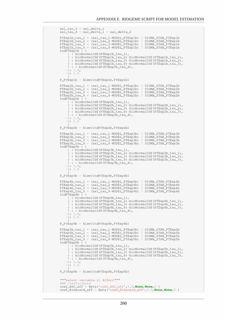
APPENDIX E. BIOGEME SCRIPT FOR MODEL ESTIMATION
sal_tau_3 = sal_delta_1sal_tau_4 = sal_delta_1 + sal_delta_2
PTExp1b_tau_1 = (sal_tau_1-MODEL_PTExp1b) / SIGMA_STAR_PTExp1bPTExp1b_tau_2 = (sal_tau_2-MODEL_PTExp1b) / SIGMA_STAR_PTExp1bPTExp1b_tau_3 = (sal_tau_3-MODEL_PTExp1b) / SIGMA_STAR_PTExp1bPTExp1b_tau_4 = (sal_tau_4-MODEL_PTExp1b) / SIGMA_STAR_PTExp1bIndPTExp1b = {
1 : bioNormalCdf(PTExp1b_tau_1),2 : bioNormalCdf(PTExp1b_tau_2)-bioNormalCdf(PTExp1b_tau_1),3 : bioNormalCdf(PTExp1b_tau_3)-bioNormalCdf(PTExp1b_tau_2),4 : bioNormalCdf(PTExp1b_tau_4)-bioNormalCdf(PTExp1b_tau_3),5 : 1-bioNormalCdf(PTExp1b_tau_4),
-1: 1.0,-2: 1.0}
P_PTExp1b = Elem(IndPTExp1b,PTExp1b)
PTExp2b_tau_1 = (sal_tau_1-MODEL_PTExp2b) / SIGMA_STAR_PTExp2bPTExp2b_tau_2 = (sal_tau_2-MODEL_PTExp2b) / SIGMA_STAR_PTExp2bPTExp2b_tau_3 = (sal_tau_3-MODEL_PTExp2b) / SIGMA_STAR_PTExp2bPTExp2b_tau_4 = (sal_tau_4-MODEL_PTExp2b) / SIGMA_STAR_PTExp2bIndPTExp2b = {
1 : bioNormalCdf(PTExp2b_tau_1),2 : bioNormalCdf(PTExp2b_tau_2)-bioNormalCdf(PTExp2b_tau_1),3 : bioNormalCdf(PTExp2b_tau_3)-bioNormalCdf(PTExp2b_tau_2),4 : bioNormalCdf(PTExp2b_tau_4)-bioNormalCdf(PTExp2b_tau_3),5 : 1-bioNormalCdf(PTExp2b_tau_4),
-1: 1.0,-2: 1.0}
P_PTExp2b = Elem(IndPTExp2b,PTExp2b)
PTExp3b_tau_1 = (sal_tau_1-MODEL_PTExp3b) / SIGMA_STAR_PTExp3bPTExp3b_tau_2 = (sal_tau_2-MODEL_PTExp3b) / SIGMA_STAR_PTExp3bPTExp3b_tau_3 = (sal_tau_3-MODEL_PTExp3b) / SIGMA_STAR_PTExp3bPTExp3b_tau_4 = (sal_tau_4-MODEL_PTExp3b) / SIGMA_STAR_PTExp3bIndPTExp3b = {
1 : bioNormalCdf(PTExp3b_tau_1),2 : bioNormalCdf(PTExp3b_tau_2)-bioNormalCdf(PTExp3b_tau_1),3 : bioNormalCdf(PTExp3b_tau_3)-bioNormalCdf(PTExp3b_tau_2),4 : bioNormalCdf(PTExp3b_tau_4)-bioNormalCdf(PTExp3b_tau_3),5 : 1-bioNormalCdf(PTExp3b_tau_4),
-1: 1.0,-2: 1.0}
P_PTExp3b = Elem(IndPTExp3b,PTExp3b)
PTExp4b_tau_1 = (sal_tau_1-MODEL_PTExp4b) / SIGMA_STAR_PTExp4bPTExp4b_tau_2 = (sal_tau_2-MODEL_PTExp4b) / SIGMA_STAR_PTExp4bPTExp4b_tau_3 = (sal_tau_3-MODEL_PTExp4b) / SIGMA_STAR_PTExp4bPTExp4b_tau_4 = (sal_tau_4-MODEL_PTExp4b) / SIGMA_STAR_PTExp4bIndPTExp4b = {
1 : bioNormalCdf(PTExp4b_tau_1),2 : bioNormalCdf(PTExp4b_tau_2)-bioNormalCdf(PTExp4b_tau_1),3 : bioNormalCdf(PTExp4b_tau_3)-bioNormalCdf(PTExp4b_tau_2),4 : bioNormalCdf(PTExp4b_tau_4)-bioNormalCdf(PTExp4b_tau_3),5 : 1-bioNormalCdf(PTExp4b_tau_4),
-1: 1.0,-2: 1.0}
P_PTExp4b = Elem(IndPTExp4b,PTExp4b)
PTExp5b_tau_1 = (sal_tau_1-MODEL_PTExp5b) / SIGMA_STAR_PTExp5bPTExp5b_tau_2 = (sal_tau_2-MODEL_PTExp5b) / SIGMA_STAR_PTExp5bPTExp5b_tau_3 = (sal_tau_3-MODEL_PTExp5b) / SIGMA_STAR_PTExp5bPTExp5b_tau_4 = (sal_tau_4-MODEL_PTExp5b) / SIGMA_STAR_PTExp5bIndPTExp5b = {
1 : bioNormalCdf(PTExp5b_tau_1),2 : bioNormalCdf(PTExp5b_tau_2)-bioNormalCdf(PTExp5b_tau_1),3 : bioNormalCdf(PTExp5b_tau_3)-bioNormalCdf(PTExp5b_tau_2),4 : bioNormalCdf(PTExp5b_tau_4)-bioNormalCdf(PTExp5b_tau_3),5 : 1-bioNormalCdf(PTExp5b_tau_4),
-1: 1.0,-2: 1.0}
P_PTExp5b = Elem(IndPTExp5b,PTExp5b)
"""Latent variable 2: Affect"""### Coefficientscoef_ASC_aff = Beta('coef_ASC_aff',0.0,None,None,0 )coef_Ridacard_aff = Beta('coef_Ridacard_aff',0.0,None,None,0 )
260
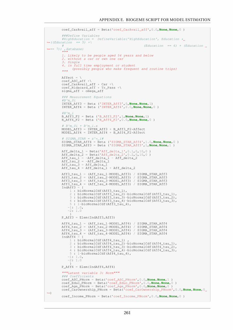
APPENDIX E. BIOGEME SCRIPT FOR MODEL ESTIMATION
coef_CarAvail_aff = Beta('coef_CarAvail_aff',0.0,None,None,0 )
###Define Variables#HighEducation = DefineVariable('HighEducation', Education *
,→((Education == 5) +\# (Education == 6) + (Education
,→== 7)) ,database)"""1. Likely to be people aged 54 years and below2. without a car or own one car3. Single4. in full time employment or student
(possibly people who make frequent and routine trips)"""
Affect = \coef_ASC_aff +\coef_CarAvail_aff * Car +\coef_Ridacard_aff * Tr_Pass +\sigma_aff * omega_aff
### Measurement Equations#B^m_0iINTER_Aff3 = Beta ('INTER_Aff3',0,None,None,1)INTER_Aff4 = Beta ('INTER_Aff4',0.0,None,None,0 )
#B^m_iB_Aff3_F2 = Beta ('B_Aff3_F2',1,None,None,1)B_Aff4_F2 = Beta ('B_Aff4_F2',0.0,None,None,0 )
# B^m_0i + B^m_i.xMODEL_Aff3 = INTER_Aff3 + B_Aff3_F2*AffectMODEL_Aff4 = INTER_Aff4 + B_Aff4_F2*Affect
# SIGMA_STAR = z^*_i#SIGMA_STAR_Aff4 = Beta ('SIGMA_STAR_Aff4',1.0,None,None,0 )SIGMA_STAR_Aff3 = Beta ('SIGMA_STAR_Aff3',1,None,None,1 )
Aff_delta_1 = Beta('Aff_delta_1',0.1,0,10,0 )Aff_delta_2 = Beta('Aff_delta_2',0.2,0,10,0 )Aff_tau_1 = -Aff_delta_1 - Aff_delta_2Aff_tau_2 = -Aff_delta_1Aff_tau_3 = Aff_delta_1Aff_tau_4 = Aff_delta_1 + Aff_delta_2
Aff3_tau_1 = (Aff_tau_1-MODEL_Aff3) / SIGMA_STAR_Aff3Aff3_tau_2 = (Aff_tau_2-MODEL_Aff3) / SIGMA_STAR_Aff3Aff3_tau_3 = (Aff_tau_3-MODEL_Aff3) / SIGMA_STAR_Aff3Aff3_tau_4 = (Aff_tau_4-MODEL_Aff3) / SIGMA_STAR_Aff3IndAff3 = {
1 : bioNormalCdf(Aff3_tau_1),2 : bioNormalCdf(Aff3_tau_2)-bioNormalCdf(Aff3_tau_1),3 : bioNormalCdf(Aff3_tau_3)-bioNormalCdf(Aff3_tau_2),4 : bioNormalCdf(Aff3_tau_4)-bioNormalCdf(Aff3_tau_3),5 : 1-bioNormalCdf(Aff3_tau_4),
-1: 1.0,-2: 1.0}
P_Aff3 = Elem(IndAff3,Aff3)
Aff4_tau_1 = (Aff_tau_1-MODEL_Aff4) / SIGMA_STAR_Aff4Aff4_tau_2 = (Aff_tau_2-MODEL_Aff4) / SIGMA_STAR_Aff4Aff4_tau_3 = (Aff_tau_3-MODEL_Aff4) / SIGMA_STAR_Aff4Aff4_tau_4 = (Aff_tau_4-MODEL_Aff4) / SIGMA_STAR_Aff4IndAff4 = {
1 : bioNormalCdf(Aff4_tau_1) ,2 : bioNormalCdf(Aff4_tau_2)-bioNormalCdf(Aff4_tau_1),3 : bioNormalCdf(Aff4_tau_3)-bioNormalCdf(Aff4_tau_2),4 : bioNormalCdf(Aff4_tau_4)-bioNormalCdf(Aff4_tau_3),5 : 1-bioNormalCdf(Aff4_tau_4),
-1: 1.0,-2: 1.0}
P_Aff4 = Elem(IndAff4,Aff4)
"""Latent variable 3: Norm"""### Coefficientscoef_ASC_PNorm = Beta('coef_ASC_PNorm',0.0,None,None,1 )coef_Educ_PNorm = Beta('coef_Educ_PNorm',0.0,None,None,0 )coef_Age_PNorm = Beta('coef_Age_PNorm',0.0,None,None,0 )coef_CarOwnership_PNorm = Beta('coef_CarOwnership_PNorm',0.0,None,None,0
,→)coef_Income_PNorm = Beta('coef_Income_PNorm',0.0,None,None,0 )
261
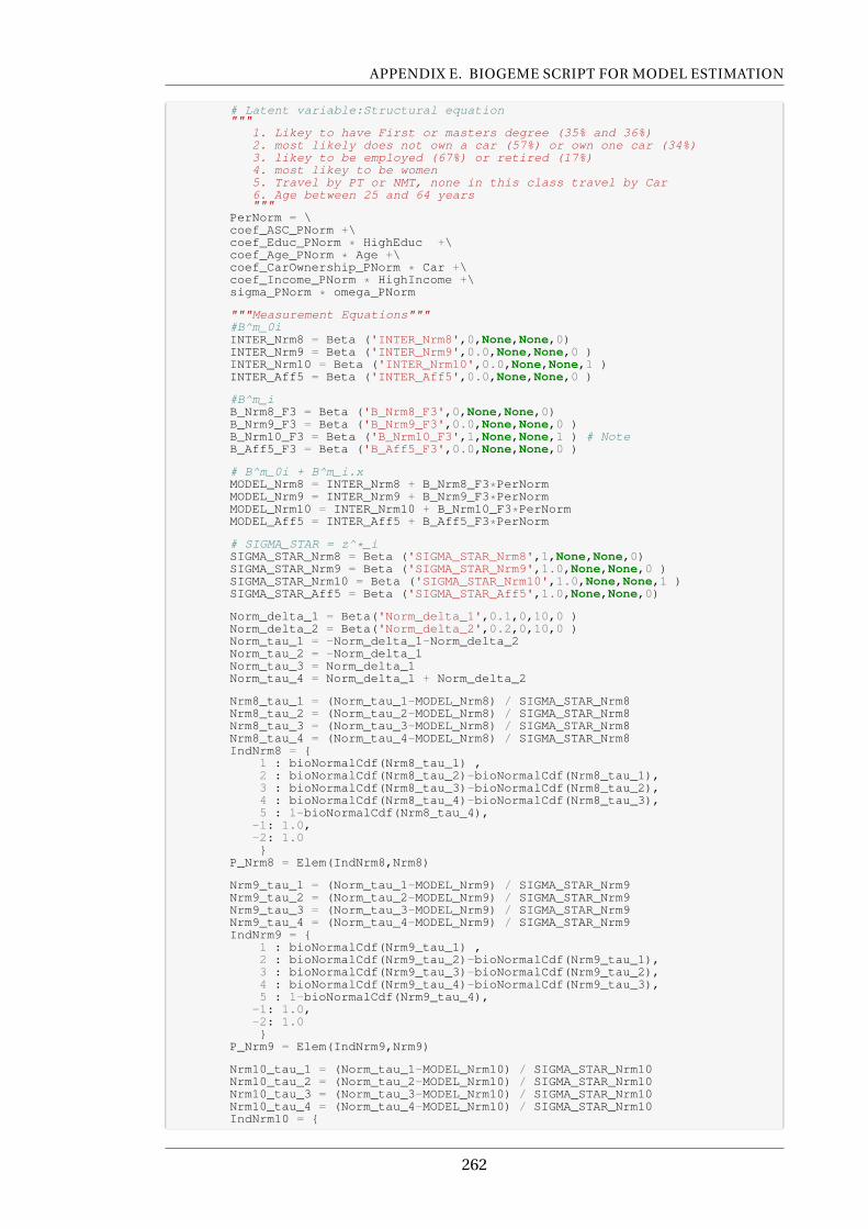
APPENDIX E. BIOGEME SCRIPT FOR MODEL ESTIMATION
# Latent variable:Structural equation"""
1. Likey to have First or masters degree (35% and 36%)2. most likely does not own a car (57%) or own one car (34%)3. likey to be employed (67%) or retired (17%)4. most likey to be women5. Travel by PT or NMT, none in this class travel by Car6. Age between 25 and 64 years"""
PerNorm = \coef_ASC_PNorm +\coef_Educ_PNorm * HighEduc +\coef_Age_PNorm * Age +\coef_CarOwnership_PNorm * Car +\coef_Income_PNorm * HighIncome +\sigma_PNorm * omega_PNorm
"""Measurement Equations"""#B^m_0iINTER_Nrm8 = Beta ('INTER_Nrm8',0,None,None,0)INTER_Nrm9 = Beta ('INTER_Nrm9',0.0,None,None,0 )INTER_Nrm10 = Beta ('INTER_Nrm10',0.0,None,None,1 )INTER_Aff5 = Beta ('INTER_Aff5',0.0,None,None,0 )
#B^m_iB_Nrm8_F3 = Beta ('B_Nrm8_F3',0,None,None,0)B_Nrm9_F3 = Beta ('B_Nrm9_F3',0.0,None,None,0 )B_Nrm10_F3 = Beta ('B_Nrm10_F3',1,None,None,1 ) # NoteB_Aff5_F3 = Beta ('B_Aff5_F3',0.0,None,None,0 )
# B^m_0i + B^m_i.xMODEL_Nrm8 = INTER_Nrm8 + B_Nrm8_F3*PerNormMODEL_Nrm9 = INTER_Nrm9 + B_Nrm9_F3*PerNormMODEL_Nrm10 = INTER_Nrm10 + B_Nrm10_F3*PerNormMODEL_Aff5 = INTER_Aff5 + B_Aff5_F3*PerNorm
# SIGMA_STAR = z^*_iSIGMA_STAR_Nrm8 = Beta ('SIGMA_STAR_Nrm8',1,None,None,0)SIGMA_STAR_Nrm9 = Beta ('SIGMA_STAR_Nrm9',1.0,None,None,0 )SIGMA_STAR_Nrm10 = Beta ('SIGMA_STAR_Nrm10',1.0,None,None,1 )SIGMA_STAR_Aff5 = Beta ('SIGMA_STAR_Aff5',1.0,None,None,0)
Norm_delta_1 = Beta('Norm_delta_1',0.1,0,10,0 )Norm_delta_2 = Beta('Norm_delta_2',0.2,0,10,0 )Norm_tau_1 = -Norm_delta_1-Norm_delta_2Norm_tau_2 = -Norm_delta_1Norm_tau_3 = Norm_delta_1Norm_tau_4 = Norm_delta_1 + Norm_delta_2
Nrm8_tau_1 = (Norm_tau_1-MODEL_Nrm8) / SIGMA_STAR_Nrm8Nrm8_tau_2 = (Norm_tau_2-MODEL_Nrm8) / SIGMA_STAR_Nrm8Nrm8_tau_3 = (Norm_tau_3-MODEL_Nrm8) / SIGMA_STAR_Nrm8Nrm8_tau_4 = (Norm_tau_4-MODEL_Nrm8) / SIGMA_STAR_Nrm8IndNrm8 = {
1 : bioNormalCdf(Nrm8_tau_1) ,2 : bioNormalCdf(Nrm8_tau_2)-bioNormalCdf(Nrm8_tau_1),3 : bioNormalCdf(Nrm8_tau_3)-bioNormalCdf(Nrm8_tau_2),4 : bioNormalCdf(Nrm8_tau_4)-bioNormalCdf(Nrm8_tau_3),5 : 1-bioNormalCdf(Nrm8_tau_4),
-1: 1.0,-2: 1.0}
P_Nrm8 = Elem(IndNrm8,Nrm8)
Nrm9_tau_1 = (Norm_tau_1-MODEL_Nrm9) / SIGMA_STAR_Nrm9Nrm9_tau_2 = (Norm_tau_2-MODEL_Nrm9) / SIGMA_STAR_Nrm9Nrm9_tau_3 = (Norm_tau_3-MODEL_Nrm9) / SIGMA_STAR_Nrm9Nrm9_tau_4 = (Norm_tau_4-MODEL_Nrm9) / SIGMA_STAR_Nrm9IndNrm9 = {
1 : bioNormalCdf(Nrm9_tau_1) ,2 : bioNormalCdf(Nrm9_tau_2)-bioNormalCdf(Nrm9_tau_1),3 : bioNormalCdf(Nrm9_tau_3)-bioNormalCdf(Nrm9_tau_2),4 : bioNormalCdf(Nrm9_tau_4)-bioNormalCdf(Nrm9_tau_3),5 : 1-bioNormalCdf(Nrm9_tau_4),
-1: 1.0,-2: 1.0}
P_Nrm9 = Elem(IndNrm9,Nrm9)
Nrm10_tau_1 = (Norm_tau_1-MODEL_Nrm10) / SIGMA_STAR_Nrm10Nrm10_tau_2 = (Norm_tau_2-MODEL_Nrm10) / SIGMA_STAR_Nrm10Nrm10_tau_3 = (Norm_tau_3-MODEL_Nrm10) / SIGMA_STAR_Nrm10Nrm10_tau_4 = (Norm_tau_4-MODEL_Nrm10) / SIGMA_STAR_Nrm10IndNrm10 = {
262
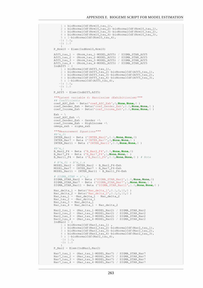
APPENDIX E. BIOGEME SCRIPT FOR MODEL ESTIMATION
1 : bioNormalCdf(Nrm10_tau_1),2 : bioNormalCdf(Nrm10_tau_2)-bioNormalCdf(Nrm10_tau_1),3 : bioNormalCdf(Nrm10_tau_3)-bioNormalCdf(Nrm10_tau_2),4 : bioNormalCdf(Nrm10_tau_4)-bioNormalCdf(Nrm10_tau_3),5 : 1-bioNormalCdf(Nrm10_tau_4),
-1: 1.0,-2: 1.0}
P_Nrm10 = Elem(IndNrm10,Nrm10)
Aff5_tau_1 = (Norm_tau_1-MODEL_Aff5) / SIGMA_STAR_Aff5Aff5_tau_2 = (Norm_tau_2-MODEL_Aff5) / SIGMA_STAR_Aff5Aff5_tau_3 = (Norm_tau_3-MODEL_Aff5) / SIGMA_STAR_Aff5Aff5_tau_4 = (Norm_tau_4-MODEL_Aff5) / SIGMA_STAR_Aff5IndAff5 = {
1 : bioNormalCdf(Aff5_tau_1),2 : bioNormalCdf(Aff5_tau_2)-bioNormalCdf(Aff5_tau_1),3 : bioNormalCdf(Aff5_tau_3)-bioNormalCdf(Aff5_tau_2),4 : bioNormalCdf(Aff5_tau_4)-bioNormalCdf(Aff5_tau_3),5 : 1-bioNormalCdf(Aff5_tau_4),
-1: 1.0,-2: 1.0}
P_Aff5 = Elem(IndAff5,Aff5)
"""Latent variable 4: Narcissism (Exhibitionism)"""## Coefficientscoef_ASC_Exh = Beta('coef_ASC_Exh',0,None,None,0 )coef_Gender_Exh = Beta('coef_Gender_Exh',0.0,None,None,0 )coef_Income_Exh = Beta('coef_Income_Exh',0.0,None,None,0 )
Exh = \coef_ASC_Exh +\coef_Gender_Exh * Gender +\coef_Income_Exh * HighIncome +\omega_exh * sigma_exh
"""Measurement Equations"""#B^m_0iINTER_Nar2 = Beta ('INTER_Nar2',0.0,None,None,0)INTER_Nar7 = Beta ('INTER_Nar7',0,None,None,1 )INTER_Nar11 = Beta ('INTER_Nar11',0.0,None,None,0 )
#B^m_iB_Nar2_F4 = Beta ('B_Nar2_F4',0.0,None,None,0)B_Nar7_F4 = Beta ('B_Nar7_F4',1,None,None,1 )B_Nar11_F4 = Beta ('B_Nar11_F4',0.0,None,None,0 ) # Note
# B^m_0i + B^m_i.xMODEL_Nar2 = INTER_Nar2 + B_Nar2_F4*ExhMODEL_Nar7 = INTER_Nar7 + B_Nar7_F4*ExhMODEL_Nar11 = INTER_Nar11 + B_Nar11_F4*Exh
# SIGMA_STAR = z^*_iSIGMA_STAR_Nar2 = Beta ('SIGMA_STAR_Nar2',1.0,None,None,0)SIGMA_STAR_Nar7 = Beta ('SIGMA_STAR_Nar7',1,None,None,1 )SIGMA_STAR_Nar11 = Beta ('SIGMA_STAR_Nar11',1.0,None,None,0 )
Nar_delta_1 = Beta('Nar_delta_1',0.1,0,10,0 )Nar_delta_2 = Beta('Nar_delta_2',0.2,0,10,0 )Nar_tau_1 = -Nar_delta_1 - Nar_delta_2Nar_tau_2 = -Nar_delta_1Nar_tau_3 = Nar_delta_1Nar_tau_4 = Nar_delta_1 + Nar_delta_2
Nar2_tau_1 = (Nar_tau_1-MODEL_Nar2) / SIGMA_STAR_Nar2Nar2_tau_2 = (Nar_tau_2-MODEL_Nar2) / SIGMA_STAR_Nar2Nar2_tau_3 = (Nar_tau_3-MODEL_Nar2) / SIGMA_STAR_Nar2Nar2_tau_4 = (Nar_tau_4-MODEL_Nar2) / SIGMA_STAR_Nar2IndNar2 = {
1 : bioNormalCdf(Nar2_tau_1) ,2 : bioNormalCdf(Nar2_tau_2)-bioNormalCdf(Nar2_tau_1),3 : bioNormalCdf(Nar2_tau_3)-bioNormalCdf(Nar2_tau_2),4 : bioNormalCdf(Nar2_tau_4)-bioNormalCdf(Nar2_tau_3),5 : 1-bioNormalCdf(Nar2_tau_4),-1: 1.0,-2: 1.0}
P_Nar2 = Elem(IndNar2,Nar2)
Nar7_tau_1 = (Nar_tau_1-MODEL_Nar7) / SIGMA_STAR_Nar7Nar7_tau_2 = (Nar_tau_2-MODEL_Nar7) / SIGMA_STAR_Nar7Nar7_tau_3 = (Nar_tau_3-MODEL_Nar7) / SIGMA_STAR_Nar7Nar7_tau_4 = (Nar_tau_4-MODEL_Nar7) / SIGMA_STAR_Nar7
263
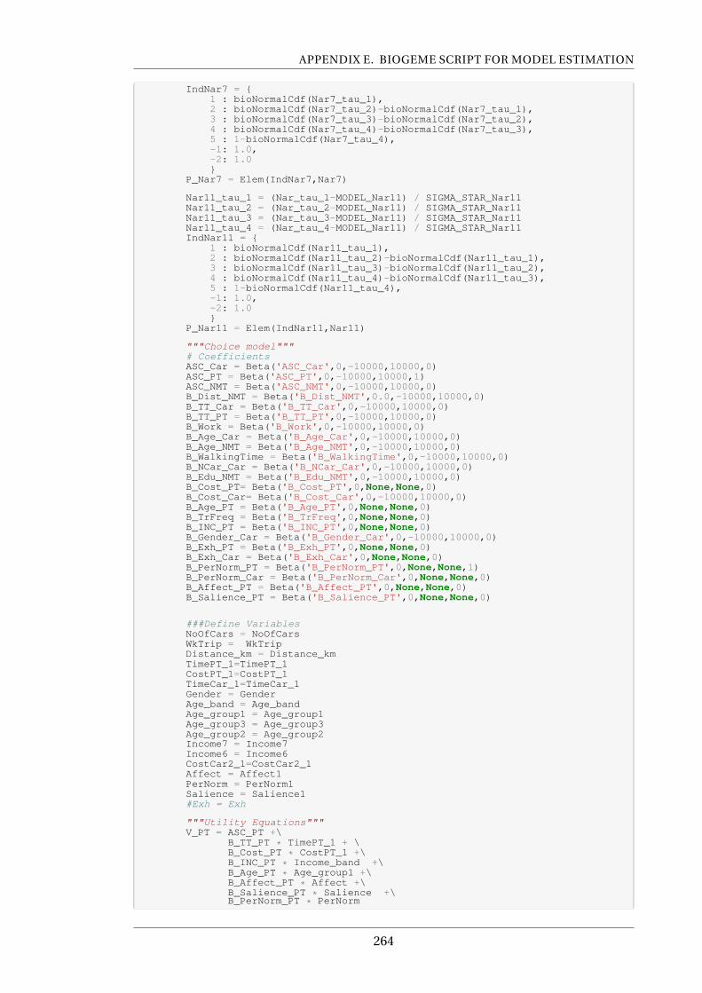
APPENDIX E. BIOGEME SCRIPT FOR MODEL ESTIMATION
IndNar7 = {1 : bioNormalCdf(Nar7_tau_1),2 : bioNormalCdf(Nar7_tau_2)-bioNormalCdf(Nar7_tau_1),3 : bioNormalCdf(Nar7_tau_3)-bioNormalCdf(Nar7_tau_2),4 : bioNormalCdf(Nar7_tau_4)-bioNormalCdf(Nar7_tau_3),5 : 1-bioNormalCdf(Nar7_tau_4),-1: 1.0,-2: 1.0}
P_Nar7 = Elem(IndNar7,Nar7)
Nar11_tau_1 = (Nar_tau_1-MODEL_Nar11) / SIGMA_STAR_Nar11Nar11_tau_2 = (Nar_tau_2-MODEL_Nar11) / SIGMA_STAR_Nar11Nar11_tau_3 = (Nar_tau_3-MODEL_Nar11) / SIGMA_STAR_Nar11Nar11_tau_4 = (Nar_tau_4-MODEL_Nar11) / SIGMA_STAR_Nar11IndNar11 = {
1 : bioNormalCdf(Nar11_tau_1),2 : bioNormalCdf(Nar11_tau_2)-bioNormalCdf(Nar11_tau_1),3 : bioNormalCdf(Nar11_tau_3)-bioNormalCdf(Nar11_tau_2),4 : bioNormalCdf(Nar11_tau_4)-bioNormalCdf(Nar11_tau_3),5 : 1-bioNormalCdf(Nar11_tau_4),-1: 1.0,-2: 1.0}
P_Nar11 = Elem(IndNar11,Nar11)
"""Choice model"""# CoefficientsASC_Car = Beta('ASC_Car',0,-10000,10000,0)ASC_PT = Beta('ASC_PT',0,-10000,10000,1)ASC_NMT = Beta('ASC_NMT',0,-10000,10000,0)B_Dist_NMT = Beta('B_Dist_NMT',0.0,-10000,10000,0)B_TT_Car = Beta('B_TT_Car',0,-10000,10000,0)B_TT_PT = Beta('B_TT_PT',0,-10000,10000,0)B_Work = Beta('B_Work',0,-10000,10000,0)B_Age_Car = Beta('B_Age_Car',0,-10000,10000,0)B_Age_NMT = Beta('B_Age_NMT',0,-10000,10000,0)B_WalkingTime = Beta('B_WalkingTime',0,-10000,10000,0)B_NCar_Car = Beta('B_NCar_Car',0,-10000,10000,0)B_Edu_NMT = Beta('B_Edu_NMT',0,-10000,10000,0)B_Cost_PT= Beta('B_Cost_PT',0,None,None,0)B_Cost_Car= Beta('B_Cost_Car',0,-10000,10000,0)B_Age_PT = Beta('B_Age_PT',0,None,None,0)B_TrFreq = Beta('B_TrFreq',0,None,None,0)B_INC_PT = Beta('B_INC_PT',0,None,None,0)B_Gender_Car = Beta('B_Gender_Car',0,-10000,10000,0)B_Exh_PT = Beta('B_Exh_PT',0,None,None,0)B_Exh_Car = Beta('B_Exh_Car',0,None,None,0)B_PerNorm_PT = Beta('B_PerNorm_PT',0,None,None,1)B_PerNorm_Car = Beta('B_PerNorm_Car',0,None,None,0)B_Affect_PT = Beta('B_Affect_PT',0,None,None,0)B_Salience_PT = Beta('B_Salience_PT',0,None,None,0)
###Define VariablesNoOfCars = NoOfCarsWkTrip = WkTripDistance_km = Distance_kmTimePT_1=TimePT_1CostPT_1=CostPT_1TimeCar_1=TimeCar_1Gender = GenderAge_band = Age_bandAge_group1 = Age_group1Age_group3 = Age_group3Age_group2 = Age_group2Income7 = Income7Income6 = Income6CostCar2_1=CostCar2_1Affect = Affect1PerNorm = PerNorm1Salience = Salience1#Exh = Exh
"""Utility Equations"""V_PT = ASC_PT +\
B_TT_PT * TimePT_1 + \B_Cost_PT * CostPT_1 +\B_INC_PT * Income_band +\B_Age_PT * Age_group1 +\B_Affect_PT * Affect +\B_Salience_PT * Salience +\B_PerNorm_PT * PerNorm
264
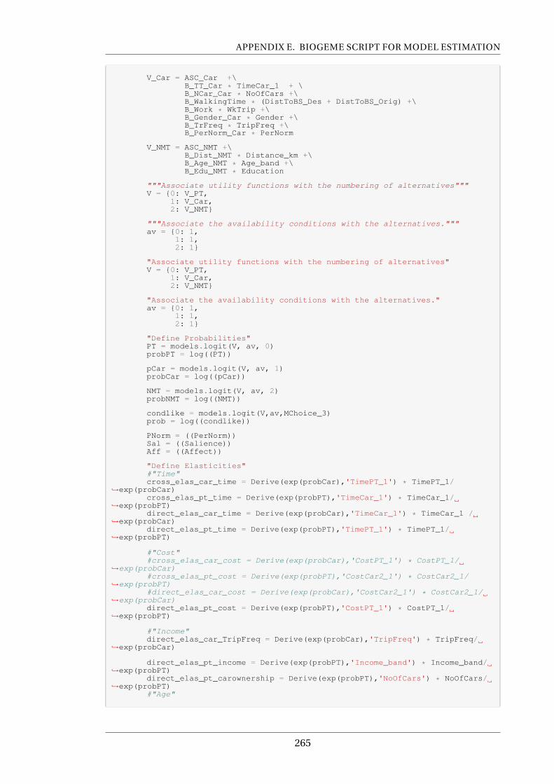
APPENDIX E. BIOGEME SCRIPT FOR MODEL ESTIMATION
V_Car = ASC_Car +\B_TT_Car * TimeCar_1 + \B_NCar_Car * NoOfCars +\B_WalkingTime * (DistToBS_Des + DistToBS_Orig) +\B_Work * WkTrip +\B_Gender_Car * Gender +\B_TrFreq * TripFreq +\B_PerNorm_Car * PerNorm
V_NMT = ASC_NMT +\B_Dist_NMT * Distance_km +\B_Age_NMT * Age_band +\B_Edu_NMT * Education
"""Associate utility functions with the numbering of alternatives"""V = {0: V_PT,
1: V_Car,2: V_NMT}
"""Associate the availability conditions with the alternatives."""av = {0: 1,
1: 1,2: 1}
"Associate utility functions with the numbering of alternatives"V = {0: V_PT,
1: V_Car,2: V_NMT}
"Associate the availability conditions with the alternatives."av = {0: 1,
1: 1,2: 1}
"Define Probabilities"PT = models.logit(V, av, 0)probPT = log((PT))
pCar = models.logit(V, av, 1)probCar = log((pCar))
NMT = models.logit(V, av, 2)probNMT = log((NMT))
condlike = models.logit(V,av,MChoice_3)prob = log((condlike))
PNorm = ((PerNorm))Sal = ((Salience))Aff = ((Affect))
"Define Elasticities"#"Time"cross_elas_car_time = Derive(exp(probCar),'TimePT_1') * TimePT_1/
,→exp(probCar)cross_elas_pt_time = Derive(exp(probPT),'TimeCar_1') * TimeCar_1/
,→exp(probPT)direct_elas_car_time = Derive(exp(probCar),'TimeCar_1') * TimeCar_1 /
,→exp(probCar)direct_elas_pt_time = Derive(exp(probPT),'TimePT_1') * TimePT_1/
,→exp(probPT)
#"Cost"#cross_elas_car_cost = Derive(exp(probCar),'CostPT_1') * CostPT_1/
,→exp(probCar)#cross_elas_pt_cost = Derive(exp(probPT),'CostCar2_1') * CostCar2_1/
,→exp(probPT)#direct_elas_car_cost = Derive(exp(probCar),'CostCar2_1') * CostCar2_1/
,→exp(probCar)direct_elas_pt_cost = Derive(exp(probPT),'CostPT_1') * CostPT_1/
,→exp(probPT)
#"Income"direct_elas_car_TripFreq = Derive(exp(probCar),'TripFreq') * TripFreq/
,→exp(probCar)
direct_elas_pt_income = Derive(exp(probPT),'Income_band') * Income_band/,→exp(probPT)
direct_elas_pt_carownership = Derive(exp(probPT),'NoOfCars') * NoOfCars/,→exp(probPT)
#"Age"
265

APPENDIX E. BIOGEME SCRIPT FOR MODEL ESTIMATION
direct_elas_pt_age = Derive(exp(probPT),'Age_group1') * Age_group1/,→exp(probPT)
direct_elas_NMT_age = Derive(exp(probNMT),'Age_band') * Age_band/,→exp(probNMT)
#"Distance"direct_elas_NMT_dist = Derive(exp(probNMT),'Distance_km') * Distance_km/
,→exp(probNMT)
#"Education"direct_elas_NMT_educ = Derive(exp(probNMT),'Education') * Education/
,→exp(probNMT)
#"PerNorm"direct_elas_car_pernorm = Derive(exp(probCar),'PerNorm1') * PerNorm1/
,→exp(probCar)direct_elas_pt_pernorm = Derive(exp(probPT),'PerNorm1') * PerNorm1/
,→exp(probPT)
#"Affect"direct_elas_car_affect = Derive(exp(probCar),'Affect') * Affect/
,→exp(probCar)direct_elas_pt_affect = Derive(exp(probPT),'Affect1') * Affect1/
,→exp(probPT)
#"Salience"direct_elas_car_salience = Derive(exp(probCar),'Salience') * Salience/
,→exp(probCar)direct_elas_pt_salience = Derive(exp(probPT),'Salience1') * Salience1/
,→exp(probPT)
simulate = {'weight': normalizedWeight,'Prob. PT': probPT,'Prob. car': probCar,'Prob. NMT':probNMT,'Prob':prob,'XE of Car wrt PT time':cross_elas_car_time,'DE of Car wrt time':direct_elas_car_time,'XE of PT wrt car time':cross_elas_pt_time,'DE of PT wrt time': direct_elas_pt_time,'DE of PT wrt cost': direct_elas_pt_cost,'DE of PT wrt Income': direct_elas_pt_income,'DE of NMT wrt Educ':direct_elas_NMT_educ,'DE of NMT wrt Age':direct_elas_NMT_age,'DE of PT wrt Age': direct_elas_pt_age,'DE of PT wrt CarOwnership': direct_elas_pt_carownership,'DE of Car wrt TripFreq': direct_elas_car_TripFreq,'DE of NMT wrt trip length':direct_elas_NMT_dist,'DE of PT wrt PerNorm': direct_elas_pt_pernorm,'DE of Car wrt PerNorm': direct_elas_car_pernorm,'DE of PT wrt Affect': direct_elas_pt_affect,'DE of PT wrt Salience': direct_elas_pt_salience,'Salience':Sal,'Norm':PNorm,'Affec':Aff}
biosim = bio.BIOGEME(database,simulate,numberOfDraws=100000)biosim.DRAWS = {'omega_aff': ('NORMAL_MLHS'), 'omega_sal':
,→('NORMAL_MLHS'),\'omega_exh': ('NORMAL_MLHS'), 'omega_PNorm':
,→('NORMAL_MLHS')}biosim.modelName = "SEM Model_Simul"
""" Retrieve the names of the parameters """betas = biosim.freeBetaNames
""" Read the estimation results from the file """results = res.bioResults(pickleFile='SEM_ICLV_Revised_thesis_final.
,→pickle')
""" Extract the values that are necessary """betaValues = results.getBetaValues(betas)
"""simulatedValues is a Panda dataframe with the same number of rows as thedatabase, and as many columns as formulas to simulate.weighted_simulatedValues has the same structure."""simulatedValues = biosim.simulate(betaValues)
""" Calculate the elasticities """
266
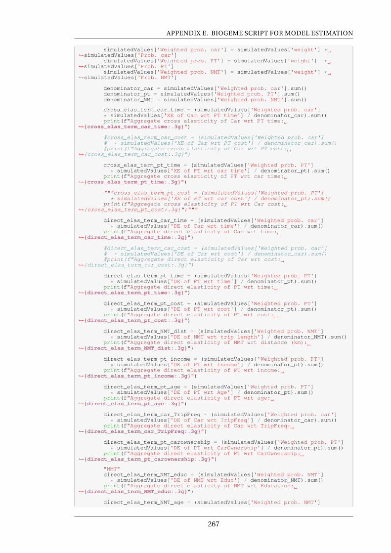
APPENDIX E. BIOGEME SCRIPT FOR MODEL ESTIMATION
simulatedValues['Weighted prob. car'] = simulatedValues['weight'] *,→simulatedValues['Prob. car']
simulatedValues['Weighted prob. PT'] = simulatedValues['weight'] *,→simulatedValues['Prob. PT']
simulatedValues['Weighted prob. NMT'] = simulatedValues['weight'] *,→simulatedValues['Prob. NMT']
denominator_car = simulatedValues['Weighted prob. car'].sum()denominator_pt = simulatedValues['Weighted prob. PT'].sum()denominator_NMT = simulatedValues['Weighted prob. NMT'].sum()
cross_elas_term_car_time = (simulatedValues['Weighted prob. car']* simulatedValues['XE of Car wrt PT time'] / denominator_car).sum()print(f"Aggregate cross elasticity of Car wrt PT time:
,→{cross_elas_term_car_time:.3g}")
#cross_elas_term_car_cost = (simulatedValues['Weighted prob. car']# * simulatedValues['XE of Car wrt PT cost'] / denominator_car).sum()#print(f"Aggregate cross elasticity of Car wrt PT cost:
,→{cross_elas_term_car_cost:.3g}")
cross_elas_term_pt_time = (simulatedValues['Weighted prob. PT']* simulatedValues['XE of PT wrt car time'] / denominator_pt).sum()
print(f"Aggregate cross elasticity of PT wrt car time:,→{cross_elas_term_pt_time:.3g}")
"""cross_elas_term_pt_cost = (simulatedValues['Weighted prob. PT']* simulatedValues['XE of PT wrt car cost'] / denominator_pt).sum()
print(f"Aggregate cross elasticity of PT wrt Car cost:,→{cross_elas_term_pt_cost:.3g}")"""
direct_elas_term_car_time = (simulatedValues['Weighted prob. car']* simulatedValues['DE of Car wrt time'] / denominator_car).sum()
print(f"Aggregate direct elasticity of Car wrt time:,→{direct_elas_term_car_time:.3g}")
#direct_elas_term_car_cost = (simulatedValues['Weighted prob. car']# * simulatedValues['DE of Car wrt cost'] / denominator_car).sum()#print(f"Aggregate direct elasticity of Car wrt cost:
,→{direct_elas_term_car_cost:.3g}")
direct_elas_term_pt_time = (simulatedValues['Weighted prob. PT']* simulatedValues['DE of PT wrt time'] / denominator_pt).sum()
print(f"Aggregate direct elasticity of PT wrt time:,→{direct_elas_term_pt_time:.3g}")
direct_elas_term_pt_cost = (simulatedValues['Weighted prob. PT']* simulatedValues['DE of PT wrt cost'] / denominator_pt).sum()
print(f"Aggregate direct elasticity of PT wrt cost:,→{direct_elas_term_pt_cost:.3g}")
direct_elas_term_NMT_dist = (simulatedValues['Weighted prob. NMT']* simulatedValues['DE of NMT wrt trip length'] / denominator_NMT).sum()
print(f"Aggregate direct elasticity of NMT wrt distance (km):,→{direct_elas_term_NMT_dist:.3g}")
direct_elas_term_pt_income = (simulatedValues['Weighted prob. PT']* simulatedValues['DE of PT wrt Income'] / denominator_pt).sum()
print(f"Aggregate direct elasticity of PT wrt income:,→{direct_elas_term_pt_income:.3g}")
direct_elas_term_pt_age = (simulatedValues['Weighted prob. PT']* simulatedValues['DE of PT wrt Age'] / denominator_pt).sum()
print(f"Aggregate direct elasticity of PT wrt age:,→{direct_elas_term_pt_age:.3g}")
direct_elas_term_car_TripFreq = (simulatedValues['Weighted prob. car']* simulatedValues['DE of Car wrt TripFreq'] / denominator_car).sum()
print(f"Aggregate direct elasticity of Car wrt TripFreq:,→{direct_elas_term_car_TripFreq:.3g}")
direct_elas_term_pt_carownership = (simulatedValues['Weighted prob. PT']* simulatedValues['DE of PT wrt CarOwnership'] / denominator_pt).sum()
print(f"Aggregate direct elasticity of PT wrt CarOwnership:,→{direct_elas_term_pt_carownership:.3g}")
"NMT"direct_elas_term_NMT_educ = (simulatedValues['Weighted prob. NMT']
* simulatedValues['DE of NMT wrt Educ'] / denominator_NMT).sum()print(f"Aggregate direct elasticity of NMT wrt Education:
,→{direct_elas_term_NMT_educ:.3g}")
direct_elas_term_NMT_age = (simulatedValues['Weighted prob. NMT']
267

APPENDIX E. BIOGEME SCRIPT FOR MODEL ESTIMATION
* simulatedValues['DE of NMT wrt Age'] / denominator_NMT).sum()print(f"Aggregate direct elasticity of NMT wrt age:
,→{direct_elas_term_NMT_age:.3g}")
"MINDSPACE"direct_elas_term_pt_pernorm = (simulatedValues['Weighted prob. PT']
* simulatedValues['DE of PT wrt PerNorm'] / denominator_pt).sum()print(f"Aggregate direct elasticity of PT wrt PerNorm:
,→{direct_elas_term_pt_pernorm:.3g}")
direct_elas_term_pt_affect = (simulatedValues['Weighted prob. PT']* simulatedValues['DE of PT wrt Affect'] / denominator_pt).sum()
print(f"Aggregate direct elasticity of PT wrt Affect:,→{direct_elas_term_pt_affect:.3g}")
direct_elas_term_pt_salience = (simulatedValues['Weighted prob. PT']* simulatedValues['DE of PT wrt Salience'] / denominator_pt).sum()
print(f"Aggregate direct elasticity of PT wrt Salience:,→{direct_elas_term_pt_salience:.3g}")
direct_elas_term_car_pernorm = (simulatedValues['Weighted prob. car']* simulatedValues['DE of Car wrt PerNorm'] / denominator_car).sum()
print(f"Aggregate direct elasticity of Car wrt PerNorm:,→{direct_elas_term_car_pernorm:.3g}")
"Append Probabilities to the pandas Dataframe"pandas['prob_PT'] = (simulatedValues['Prob. PT'])pandas['prob_Car'] = (simulatedValues['Prob. car'])pandas['prob_NMT'] = (simulatedValues['Prob. NMT'])pandas['prob'] = (simulatedValues['Prob'])
"""Export dataframe to csv and excel"""pandas.to_csv('Data-20-Simul.csv', index=False)"Print Results"print(sum((simulatedValues['Prob'])))print("Results=",results)
268
Copyright © 2022 FDOKUMEN

