Download - Methods for calculating stress intensity factors in anisotropic materials: Part I—z=0 is a symmetric plane

Engineering Fracture Mechanics 72 (2005) 2328–2358

www.elsevier.com/locate/engfracmech

Methods for calculating stress intensity factors inanisotropic materials: Part I—z = 0 is a symmetric plane

Leslie Banks-Sills a,b,*, Itai Hershkovitz a, Paul A. Wawrzynek b,Rami Eliasi a, Anthony R. Ingraffea b

a The Dreszer Fracture Mechanics Laboratory, Department of Solid Mechanics, Materials and Systems,

The Fleischman Faculty of Engineering, Tel Aviv University, 69978 Ramat Aviv, Israelb School of Civil and Environmental Engineering, Cornell University, Ithaca, NY 14853, United States

Received 10 May 2004; received in revised form 17 December 2004; accepted 27 December 2004

Available online 1 July 2005

Abstract

The problem of a crack in general anisotropic material under LEFM conditions is presented. In Part I, three meth-

ods are presented for calculating stress intensity factors for various anisotropic materials in which z = 0 is a plane of

symmetry. All of the methods employ the displacement field obtained by means of the finite element method. The first

one is known as displacement extrapolation and requires the values of the crack face displacements. The other two are

conservative integrals based upon the J-integral. One employs symmetric and asymmetric fields to separate the mode I

and II stress intensity factors. The second is the M-integral which also allows for calculation of KI and KII separately.

All of these methods were originally presented for isotopic materials. Displacement extrapolation and theM-integral

are extended for orthotropic and monoclinic materials, whereas the JI- and JII-integrals are only extended for ortho-

tropic material in which the crack and material directions coincide. Results are obtained by these methods for several

problems appearing in the literature. Good to excellent agreement is found in comparison to published values. New

results are obtained for several problems.

In Part II, theM-integral is extended for more general anisotropies. In these cases, three-dimensional problems must

be solved, requiring a three-dimensional M-integral.

� 2005 Elsevier Ltd. All rights reserved.

Keywords: Stress intensity factors; Anisotropic material; Finite element method; Conservative integrals

0013-7944/$ - see front matter � 2005 Elsevier Ltd. All rights reserved.

doi:10.1016/j.engfracmech.2004.12.007

* Corresponding author. Address: The Dreszer Fracture Mechanics Laboratory, Department of Solid Mechanics, Materials and

Systems, The Fleischman Faculty of Engineering, Tel Aviv University, 69978 Ramat Aviv, Israel. Tel.: +972 36408132; fax: +972

36407617.

E-mail addresses: [email protected] (L. Banks-Sills), [email protected] (I. Hershkovitz), [email protected] (P.A.

Wawrzynek), [email protected] (R. Eliasi), [email protected] (A.R. Ingraffea).

mailto:[email protected]





L. Banks-Sills et al. / Engineering Fracture Mechanics 72 (2005) 2328–2358 2329

1. Introduction

Anisotropic materials are found in many structures, including jet engine turbine blades, in MEMS and

NEMS. In those cases, they appear as homogeneous materials. Many composite materials are also aniso-

tropic, although they are inhomogeneous. The propagation of cracks is governed by different laws for eachof these material types. But in each case, determination of the stress intensity factors where applicable is

similar.

The first paper to deal with cracks in anisotropic material is that of Sih et al. [13]. In that study, the first

term in the asymptotic expansion of the stress and displacement fields was determined for a crack in a

monoclinic material with z = 0 a plane of symmetry and the crack front perpendicular to this plane. The

energy release rate was also given. The next analytical breakthrough was that of Hoenig [7] in which the

three-dimensional problem of a through crack in a general anisotropic material was treated.

Numerical studies followed. Stress intensity factors for cracks in orthotropic materials in which z = 0 is asymmetry plane were considered by Atluri et al. [1], Boone et al. [5] and Tohgo et al. [17]. In those stud-

ies, the crack may be aligned with the material axes or rotated with respect to them. Atluri et al. [1]

employed hybrid finite elements with a square root singularity surrounding the crack tip and regular ele-

ments in the rest of the domain to determine stress intensity factors. Boone et al. [5] used quarter point,

triangular, singular elements surrounding the crack tip. Displacement correlation was employed to deter-

mine stress intensity factors. Several crack propagation theories were described with one used to predict

propagation in orthotropic materials. In testing cracked composite specimens, Tohgo et al. [17] obtained

stress intensity factors in two ways. Firstly, they used the separated J-integral method of Ishikawa et al.[8] to obtain the stress intensity factors KI and KII. In their study, the crack and fiber directions coincided.

For particular cases, it is shown in our investigation that the separation method is, in fact, valid. Most likely

it is valid for the cases they studied. In addition, they calculated the J-integral and found the ratio of the

normal to shear stress ahead of the crack tip by extrapolation. These two conditions are sufficient to pro-

duce the two stress intensity factors. It may be noted that differences of 5% were found between the two

methods.

In the first part of this investigation, the two-dimensional problem of a crack in monoclinic, orthotropic

and cubic materials is considered. The crack is assumed to be along the x-axis as shown in Fig. 1. In thesecond part of this study, the more general anisotropic three-dimensional problem of a through crack is

examined. Here we begin with the general solution and then specialize it for the case of interest.

The asymptotic stress and displacement fields in the vicinity of the crack tip in a general anisotropic

material are presented. These were derived by Hoenig [7] based on the Lekhnitskii [9] formalism. They

are given by

rxx ¼1ffiffiffiffiffiffiffi2pr

p RX3i¼1

p2i N�1ij Kj

Qi

" #; ð1Þ

Fig. 1. Path of J-integral and crack tip coordinates.

https://www.researchgate.net/publication/245197957_Near-tip_behavior_of_a_crack_in_a_plane_anisotropic_elastic_body?el=1_x_8&enrichId=rgreq-376c7eb1-92a3-4a70-921e-7ea5fa45a6a0&enrichSource=Y292ZXJQYWdlOzIwMDA5MjgxOTtBUzoxOTUzMjAxMTkwNzQ4MTZAMTQyMzU3OTM1MzEwMQ==


https://www.researchgate.net/publication/222789998_Finite_Element_Modelling_of_Fracture_Propagation_in_Orthotropic_Materials?el=1_x_8&enrichId=rgreq-376c7eb1-92a3-4a70-921e-7ea5fa45a6a0&enrichSource=Y292ZXJQYWdlOzIwMDA5MjgxOTtBUzoxOTUzMjAxMTkwNzQ4MTZAMTQyMzU3OTM1MzEwMQ==

https://www.researchgate.net/publication/222789998_Finite_Element_Modelling_of_Fracture_Propagation_in_Orthotropic_Materials?el=1_x_8&enrichId=rgreq-376c7eb1-92a3-4a70-921e-7ea5fa45a6a0&enrichSource=Y292ZXJQYWdlOzIwMDA5MjgxOTtBUzoxOTUzMjAxMTkwNzQ4MTZAMTQyMzU3OTM1MzEwMQ==

https://www.researchgate.net/publication/200093216_On_Cracks_in_Rectilinear_Anisotropic_Bodies?el=1_x_8&enrichId=rgreq-376c7eb1-92a3-4a70-921e-7ea5fa45a6a0&enrichSource=Y292ZXJQYWdlOzIwMDA5MjgxOTtBUzoxOTUzMjAxMTkwNzQ4MTZAMTQyMzU3OTM1MzEwMQ==

2330 L. Banks-Sills et al. / Engineering Fracture Mechanics 72 (2005) 2328–2358

ryy ¼1ffiffiffiffiffiffiffi2pr

p RX3i¼1

N�1ij Kj

Qi

" #; ð2Þ

rxy ¼ � 1ffiffiffiffiffiffiffi2pr

p RX3i¼1

piN�1ij Kj

Qi

" #; ð3Þ

rzx ¼1ffiffiffiffiffiffiffi2pr

p RX3i¼1

pikiN�1ij Kj

Qi

" #; ð4Þ

rzy ¼ � 1ffiffiffiffiffiffiffi2pr

p RX3i¼1

kiN�1ij Kj

Qi

" #; ð5Þ

ui ¼ffiffiffiffiffi2rp

rRX3j¼1

mijN�1jl KlQj

" #; ð6Þ

where R represents the real part of the quantity in brackets, two repeated indices in (1)–(6) obey the sum-

mation convention from 1 to 3, the coordinates x, y, z, r and h refer to the crack coordinates in Fig. 1, Kj are

the stress intensity factors KI, KII and KIII. It is assumed that the stresses and displacements are functions

only of the in-plane coordinates. Before defining pi, ki, mij, Nij, and Qi, the compliance matrix sij must be

rotated to the crack tip coordinates. In order that the notation will be clear, the rotated matrix is defined as

Sij where i and j take on values 1 through 6; these refer to the crack tip or problem coordinates and not the

material coordinates. Note that the compliance matrix is given in contracted notation as Sij; the indices are

taken such that 23! 4, 13! 5 and 12! 6. The material coordinates are taken as x1, x2 and x3 and are indirections arbitrary to the problem or crack coordinates.

For plane stress conditions, the full matrix is employed. For a plane strain problem, the reduced com-

pliance matrix is obtained from

S0ij ¼ Sij �Si3S3jS33

; ð7Þ

where i, j = 1, 2, 4, 5, 6, S0ij is symmetric and

S0i3 ¼ S03i ¼ 0. ð8Þ

The parameters pi, i = 1, 2, 3, are the eigenvalues of the compatibility equations with positive imaginary

part. These are found, in general, from the characteristic sixth order polynomial equation

l4ðpÞl2ðpÞ � l23ðpÞ ¼ 0; ð9Þ

where

l2ðpÞ ¼ S055p2 � 2S045p þ S044; ð10Þ

l3ðpÞ ¼ S015p3 � ðS014 þ S056Þp2 þ ðS025 þ S046Þp � S024; ð11Þ

l4ðpÞ ¼ S011p4 � 2S016p

3 þ ð2S012 þ S066Þp2 � 2S026p þ S022. ð12Þ

Solution of (9) leads to three pairs of complex conjugate roots. As mentioned previously, the three with

positive imaginary part are chosen in Eqs. (1)–(6). The reduced compliance coefficients in (10)–(12) may

be replaced by the ordinary compliances for plane stress. The parameters ki are given by

ki ¼ � l3ðpiÞl2ðpiÞ

; ð13Þ


where i = 1, 2, 3. The parameters mij are given by

m1i ¼ S011p2i � S016pi þ S012 þ kiðS015pi � S014Þ; ð14Þ

m2i ¼ S021pi � S026 þ S022=pi þ kiðS025 � S024=piÞ; ð15Þm3i ¼ S041pi � S046 þ S042=pi þ kiðS045 � S044=piÞ. ð16Þ

The expressions in (13)–(16) appear to rely on the Lekhnitskii formalism [9], although there are differences

with Lekhnitskii for k3 and m3i. The expressions developed by Hoenig [7] are correct.

The matrix

Nij ¼1 1 1

�p1 �p2 �p3�k1 �k2 �k3

0B@1CA; ð17Þ

its inverse is given by

N�1ij ¼ 1

jN j

p2k3 � p3k2 k3 � k2 p2 � p3p3k1 � p1k3 k1 � k3 p3 � p1p1k2 � p2k1 k2 � k1 p1 � p2

0B@1CA ð18Þ

and jNj is the determinant of the matrix Nij. Finally,

Qi ¼ffiffiffiffiffiffiffiffiffiffiffiffiffiffiffiffiffiffiffiffiffiffiffiffiffiffiffiffifficos h þ pi sin h

p. ð19Þ

There are special anisotropies for which the above development is mathematically degenerate. These in-

clude monoclinic materials with x3 = z = 0 being a symmetry plane, as well as orthotropic and cubic mate-

rials for which all three material axes are perpendicular to symmetry planes and x3 = z = 0 is a symmetry

plane. The stress and displacement fields for the degenerate cases are given in [7,13]. The forms of theexpressions presented in these two papers differ, but they agree.

If the material is monoclinic with x3 = z = 0 a plane of symmetry, then

S014 ¼ S024 ¼ S015 ¼ S025 ¼ S046 ¼ S056 ¼ 0. ð20Þ
This implies that l3 = 0 in (11) and ki = 0 in Eq. (13). The values of mij in (14)–(16) become
m1i ¼ S011p2i � S016pi þ S012; ð21Þ

m2i ¼ S021pi � S026 þ S022=pi; ð22Þm3i ¼ 0 ð23Þ

for i = 1, 2 and

m13 ¼ m23 ¼ 0; ð24Þm33 ¼ S045 � S044=p3. ð25Þ

Following Hoenig [7], the stress and displacement fields in the neighborhood of the crack tip are given by

rxx ¼1ffiffiffiffiffiffiffi2pr

p RX2i¼1

p2i BiQi

" #; ð26Þ

ryy ¼1ffiffiffiffiffiffiffi2pr

p RX2i¼1

BiQi

" #; ð27Þ



rxy ¼ � 1ffiffiffiffiffiffiffi2pr

p RX2i¼1

piBiQi

" #; ð28Þ

rzx ¼1ffiffiffiffiffiffiffi2pr

p Rp3B3

Q3

�; ð29Þ

rzy ¼ � 1ffiffiffiffiffiffiffi2pr

p RB3

Q3

�; ð30Þ

ui ¼ffiffiffiffiffi2rp

rRX3j¼1

mijBjQj

" #; ð31Þ

where

B1

B2

B3

0B@1CA ¼ 1

p2 � p1

p2 1 0

�p1 �1 0

0 0 p1 � p2

0B@1CA KI

KII

KIII

0B@1CA. ð32Þ

It may be noted that most expressions for mode III deformation are presented in this part of the investi-

gation, although no numerical results are obtained.

For an orthotropic material with symmetry planes xi = 0 (i = 1, 2, 3) and with coincident material and

crack coordinates, one finds, in addition to (20),

S016 ¼ S026 ¼ S045 ¼ 0. ð33Þ

As with the monoclinic material, l3 = 0 in Eq. (11) and thus ki = 0 in Eq. (13). The values of mij in (14)–(16)

are now given by

m1i ¼ S011p2i þ S012 ð34Þ

m2i ¼ S021pi þ S022=pi ð35Þm3i ¼ 0 ð36Þ

for i = 1, 2 and

m13 ¼ m23 ¼ 0 ð37Þm33 ¼ �S044=p3. ð38Þ

The asymptotic stress and displacement fields presented above were employed by Hoenig [7] to obtain

relationships between the J-integral and stress intensity factors. These are described in Section 2. In Section

3, three methods for calculating stress intensity factors are discussed for the special case of a monoclinic

material with x3 = z = 0 a plane of symmetry. These methods are employed for several problems in the lite-

rature and presented in Section 4. Solutions to several new problems are also described. In Part II of this

study, a through crack in which the material and crack coordinates do not coincide is treated.

2. Relationship between the J-integral and the stress intensity factors

The J-integral developed by Rice [12] is given by

J ¼Z

CWnx � T i

ouiox

� �ds; ð39Þ


where the integration path C is illustrated in Fig. 1, the strain energy density

W ¼ 1

2rij�ij; ð40Þ

the outer normal to C is ni, the traction vector is Ti = rijnj, ui is the displacement vector and ds is differentialarc length along C. Note that the J-integral is written in terms of crack tip coordinates.

By means of the crack closure integral, Hoenig [7] developed the relationship between the J-integral and

the stress intensity factors as

J ¼ � 1

2KIIðm2iN�1

ij KjÞ þ KIIIðm1iN�1ij KjÞ þ KIIIIðm3iN�1

ij KjÞn o

; ð41Þ

where I represents the imaginary part of the expression in parentheses and summation should be applied torepeated indices.

For monoclinic materials in which x3 = z = 0 is a symmetry plane, Eq. (41) reduces to

J ¼ 1

2I � p1 þ p2

p1p2

� �S022K

2I þ S011p1p2 �

S022p1p2

�KIKII þ ðp1 þ p2ÞS011K2

II

� �þ 1

2

ffiffiffiffiffiffiffiffiffiffiffiffiffiffiffiffiffiffiffiffiffiffiffiffiS044S

055 � S0245

qK2

III. ð42Þ

The in-plane terms in (42) agree with those presented in [13]; the mode III term may be shown to agree with

that given in a later study of Sih and Liebowitz [14].

If the material is orthotropic with material and crack coordinates coinciding, the expression in Eq. (42)

reduces to

J ¼ Do

2

ffiffiffiffiffiffiffiS022

qK2

I þffiffiffiffiffiffiffiS011

qK2

II

�þ 1

2


055 � S0245

qK2

III; ð43Þ

where

Do ¼ 2

ffiffiffiffiffiffiffiffiffiffiffiffiffiS011S

022

qþ 2S012 þ S066

�1=2. ð44Þ

3. Methods for calculating stress intensity factors

In this section, several methods are presented for calculating stress intensity factors when x3 = z = 0 is a

symmetry plane. First, the M-integral is presented for monoclinic and orthotropic material. The conserva-

tive M-integral was first presented by Yau et al. [20] for mixed mode problems in isotropic material and

then by Wang et al. [18] for monoclinic and orthotropic material. Next, the displacement extrapolation

method is extended for these cases. Finally, the J-integral is separated into components JI and JII for ortho-

tropic material when the material and crack coordinates coincide. This follows closely the derivation of

Ishikawa et al. [8] for isotropic material. In Part II of this study, the M-integral is extended to three dimen-

sions and general anisotropic material is treated.

3.1. The M-integral

In this section, the conservative M-integral is extended for monoclinic and orthotropic material when

x3 = z = 0 is a symmetry plane. With the J-integral in Eq. (39) and the relation in Eq. (42), the combination

of the stress intensity factors may be calculated for monoclinic materials. The M-integral may be employed

to determine the individual stress intensity factors. To obtain the M-integral from (42), two solutions are

assumed and superposed; this is possible since the material is linearly elastic. Thus, define


rij ¼ rð1Þij þ rð2Þ

ij ; ð45Þ�ij ¼ �

ð1Þij þ �

ð2Þij ; ð46Þ

ui ¼ uð1Þi þ uð2Þi . ð47Þ

The stress intensity factors associated with the superposed solutions are

KI ¼ Kð1ÞI þ Kð2Þ

I ; ð48ÞKII ¼ Kð1Þ

II þ Kð2ÞII ; ð49Þ

KIII ¼ Kð1ÞIII þ Kð2Þ

III . ð50Þ

On the one hand, the stress, strain and displacement fields are substituted into the expression for the J-inte-

gral in (39). This leads to

J ¼ J ð1Þ þ J ð2Þ þM ð1;2Þ; ð51Þ
where
J ð1Þ ¼Z

CW ð1Þn1 � T ð1Þ

iouð1Þi

ox1

!ds; ð52Þ

J ð2Þ ¼Z

CW ð2Þn1 � T ð2Þ

iouð2Þi

ox1

!ds; ð53Þ

M ð1;2Þ ¼Z

CW ð1;2Þn1 � T ð1Þ

iouð2Þiox1

� T ð2Þi

ouð1Þi

ox1

!ds. ð54Þ

The superscripts (1) and (2) in (52)–(54) refer to solutions (1) and (2), respectively. The interaction strain

energy density is given by

W ð1;2Þ ¼ rð1Þij �

ð2Þij ¼ rð2Þ

ij �ð1Þij ð55Þ

and M(1,2) is the M-integral.

On the other hand, the superposed stress intensity factors in (48)–(50) are substituted into (42) to yield

J ¼ J ð1Þ þ J ð2Þ � Ip1 þ p2p1p2

� �S022K

ð1ÞI Kð2Þ

I þ 1

2I p1p2S

011 �

S022p1p2

� �Kð1Þ

I Kð2ÞII þ Kð2Þ

I Kð1ÞII

h iþ Iðp1 þ p2ÞS011K

ð1ÞII K

ð2ÞII þ


055 � S0245

qKð1Þ

IIIKð2ÞIII ; ð56Þ

where

J ð1Þ ¼ 1

2I � p1 þ p2

p1p2

� �S022K

ð1Þ2I þ S011p1p2 �

S022p1p2

�Kð1Þ

I Kð1ÞII þ ðp1 þ p2ÞS011K

ð1Þ2II

� �þ 1

2


055 � S0245

qKð1Þ2

III ð57Þ

and

J ð2Þ ¼ 1

2I � p1 þ p2

p1p2

� �S022K

ð2Þ2I þ S011p1p2 �

S022p1p2

�Kð2Þ

I Kð2ÞII þ ðp1 þ p2ÞS011K

ð2Þ2II

� �þ 1

2


055 � S0245

qKð2Þ2

III . ð58Þ


Equating (51) and (56), leads to the definition of the M-integral as

M ð1;2Þ ¼ �Ip1 þ p2p1p2

� �S022K

ð1ÞI Kð2Þ

I þ 1

2I p1p2S

011 �

S022p1p2

� �Kð1Þ

I Kð2ÞII þ Kð2Þ

I Kð1ÞII

h iþ Iðp1 þ p2ÞS011K

ð1ÞII K

ð2ÞII þ


055 � S0245

qKð1Þ

IIIKð2ÞIII . ð59Þ

Before considering implementation of the M-integral, its expression in (54) which is a line integral is con-

verted into an area integral following Li et al. [10]. It is well known that area integrals lead to more accu-

rate, stable results than line integrals (see [3]). By defining a function q1 which is zero on C2, unity on C1 and

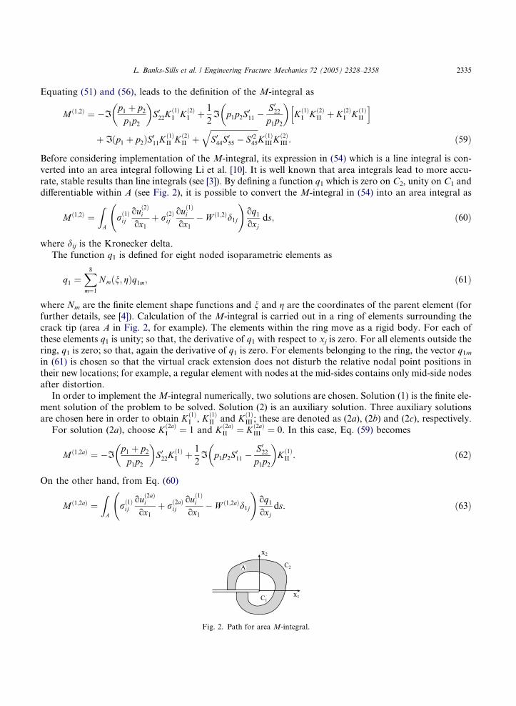
differentiable within A (see Fig. 2), it is possible to convert the M-integral in (54) into an area integral as

M ð1;2Þ ¼ZA

rð1Þij

ouð2Þiox1

þ rð2Þij

ouð1Þiox1

� W ð1;2Þd1j

!oq1oxj

ds; ð60Þ

where dij is the Kronecker delta.The function q1 is defined for eight noded isoparametric elements as

q1 ¼X8m¼1

Nmðn; gÞq1m; ð61Þ

where Nm are the finite element shape functions and n and g are the coordinates of the parent element (for

further details, see [4]). Calculation of the M-integral is carried out in a ring of elements surrounding the

crack tip (area A in Fig. 2, for example). The elements within the ring move as a rigid body. For each of

these elements q1 is unity; so that, the derivative of q1 with respect to xj is zero. For all elements outside thering, q1 is zero; so that, again the derivative of q1 is zero. For elements belonging to the ring, the vector q1min (61) is chosen so that the virtual crack extension does not disturb the relative nodal point positions in

their new locations; for example, a regular element with nodes at the mid-sides contains only mid-side nodes

after distortion.

In order to implement the M-integral numerically, two solutions are chosen. Solution (1) is the finite ele-

ment solution of the problem to be solved. Solution (2) is an auxiliary solution. Three auxiliary solutions

are chosen here in order to obtain Kð1ÞI , Kð1Þ

II and Kð1ÞIII ; these are denoted as (2a), (2b) and (2c), respectively.

For solution (2a), choose Kð2aÞI ¼ 1 and Kð2aÞ

II ¼ Kð2aÞIII ¼ 0. In this case, Eq. (59) becomes

M ð1;2aÞ ¼ �Ip1 þ p2p1p2

� �S022K

ð1ÞI þ 1

2I p1p2S

011 �

S022p1p2

� �Kð1Þ

II . ð62Þ

On the other hand, from Eq. (60)

M ð1;2aÞ ¼ZA

rð1Þij

ouð2aÞi

ox1þ rð2aÞ

ijouð1Þi

ox1� W ð1;2aÞd1j

!oq1oxj

ds. ð63Þ

Fig. 2. Path for area M-integral.


The displacements required for solution (1) are taken from a finite element analysis of the problem to be

solved; the stresses and strains are calculated from these. Asymptotic expressions for the stresses, strains

and displacements for solution (2a) are given by Eqs. (26)–(28) and (31) with the appropriated stress inten-

sity factor values.

For solution (2b), choose Kð2bÞII ¼ 1 and Kð2bÞ

I ¼ Kð2bÞIII ¼ 0. In this case, Eq. (59) becomes

M ð1;2bÞ ¼ 1

2I p1p2S

011 �

S022p1p2

� �Kð1Þ

I þ Iðp1 þ p2ÞS011Kð1ÞII . ð64Þ


M ð1;2bÞ ¼ZA

rð1Þij

ouð2bÞi

ox1þ rð2bÞ

ijouð1Þiox1

� W ð1;2bÞd1j

!oq1oxj

ds. ð65Þ

Again, the displacements required for solution (1) are taken from a finite element analysis of the problem to

be solved; the stresses and strains are calculated from these. Asymptotic expressions for the stresses, strains

and displacements for solution (2b) are given by Eqs. (26)–(28) and (31) with the appropriated stress inten-

sity factor values.

Finally, for solution (2c), choose Kð2cÞIII ¼ 1 and Kð2cÞ

I ¼ Kð2cÞII ¼ 0. In this case, Eq. (59) becomes

M ð1;2cÞ ¼ffiffiffiffiffiffiffiffiffiffiffiffiffiffiffiffiffiffiffiffiffiffiffiffiS044S

055 � S0245

qKð1Þ

III . ð66Þ


M ð1;2cÞ ¼ZA

rð1Þij

ouð2cÞi

ox1þ rð2cÞ

ijouð1Þi

ox1� W ð1;2cÞd1j

!oq1oxj

ds. ð67Þ

Again, the displacements required for solution (1) are taken from a finite element analysis of the problem to

be solved; the stresses and strains are calculated from these. Asymptotic expressions for the stresses, strainsand displacements for solution (2c) are given by Eqs. (29)–(31) with the appropriated stress intensity factor

values.

Since there is a separation between the in-plane and out-of-plane problem, there are two simultaneous

linear equations (62) and (64) which may be solved for the unknowns Kð1ÞI and Kð1Þ

II as

Kð1ÞI ¼ 2

D�2Iðp1 þ p2ÞS011M ð1;2aÞ þ I p1p2S

011 �

S022p1p2

� �M ð1;2bÞ

�; ð68Þ

Kð1ÞII ¼ 2

DI p1p2S

011 �

S022p1p2

� �M ð1;2aÞ þ 2I

p1 þ p2p1p2

� �S022M

ð1;2bÞ �

; ð69Þ

where

D ¼ 4Iðp1 þ p2ÞIp1 þ p2p1p2

� �S011S

022 þ I p1p2S

011 �

S022p1p2

� � �2. ð70Þ

The values of M(1,2a) and M(1,2b) in (68) and (69) are obtained by evaluating the integrals in (63) and (65).

Solving for Kð1ÞIII from Eq. (66) is straightforward.

The M-integral is considered next, for the case of orthotropic material when the material and problem

coordinates coincide. Here, the relation between J and the stress intensity factors is given in (43). This leads

to an expression for M(1,2) as

M ð1;2Þ ¼ Do


qKð1Þ

I Kð2ÞI þ


qKð1Þ

II Kð2ÞII

� �þ


055 � S0245

qKð1Þ

IIIKð2ÞIII ; ð71Þ

where Do is given in (44).


In this case, there is a separate equation for each stress intensity factor; that is

Kð1ÞI ¼ 1

Do


p M ð1;2aÞ; ð72Þ

Kð1ÞII ¼ 1

Do


p M ð1;2bÞ; ð73Þ

Kð1ÞIII ¼

1ffiffiffiffiffiffiffiffiffiffiffiffiffiffiffiffiffiffiffiffiffiffiffiffiS044S

055 � S0245

q M ð1;2cÞ. ð74Þ

Of course, the appropriate asymptotic expressions for solutions (2a), (2b) and (2c) must be employed.

3.2. Displacement extrapolation method

Displacement extrapolation is the simplest method to implement; but it is the least accurate. In this

study, it is employed as a check on the energy based methods. This method has been presented and imple-

mented in many papers for isotropic materials.For monoclinic materials, the displacement jump along the crack faces in the neighborhood of the crack

tip is given by

Du1 ¼ 2S011

ffiffiffiffiffi2rp

r½KIIðp1p2Þ þ KIIIðp1 þ p2Þ�; ð75Þ

Du2 ¼ �2S022

ffiffiffiffiffi2rp

rKII

p1 þ p2p1p2

� �þ KIII

1

p1p2

� � �; ð76Þ

Du3 ¼ 2KIII

ffiffiffiffiffi2rp

r ffiffiffiffiffiffiffiffiffiffiffiffiffiffiffiffiffiffiffiffiffiffiffiffiS044S

055 � S0245

q. ð77Þ

It may be noted that, similar to isotropic materials, Dui=ffiffir

palong the crack faces is linear in r near the

crack tip. Hence, the justification for linear displacement extrapolation (see [3] for details on isotropic

materials).

With the displacement extrapolation method, the stress intensity factors are solved for in Eqs. (75)–(77).

This leads to values of K which differ for each point along the crack faces. This variation of K is defined asK* leading to

K�I ¼

1

4S011S022Dm

ffiffiffiffiffiffi2pr

rDu1S

022I

1

p1p2

� �þ Du2S

011Iðp1 þ p2Þ

�; ð78Þ

K�II ¼ � 1

4S011S022Dm

ffiffiffiffiffiffi2pr

rDu1S

022I

p1 þ p2p1p2

� �þ Du2S

011Iðp1p2Þ

�; ð79Þ

K�III ¼

1

4ffiffiffiffiffiffiffiffiffiffiffiffiffiffiffiffiffiffiffiffiffiffiffiffiS044S

055 � S0245

q ffiffiffiffiffiffi2pr

rDu3; ð80Þ

where

Dm ¼ Iðp1p2ÞI1

p1p2

� �� Iðp1 þ p2ÞI

p1 þ p2p1p2

� �. ð81Þ

As will be described in the section on results, values of K�j are plotted for points along the crack faces and fit

with a �best� line.


For orthotropic materials in which the material and crack coordinates coincide, the expressions in (78)

and (79) become

K�I ¼

ffiffiffiffiffiffi2p

p

4

1ffiffiffiffiffiffiffiS022

pDo

Du2ffiffir

p ; ð82Þ

K�II ¼

ffiffiffiffiffiffi2p

p

4

1ffiffiffiffiffiffiffiS011

pDo

Du1ffiffir

p ; ð83Þ

where Do is given in (44) and K�III is given in (80).

3.3. Separated J-integrals

For mixed modes I and II in isotropic materials, the J-integral was separated into components JI and JIIeach of which corresponds to KI and KII, respectively, by Ishikawa et al. [8]. Details of their proof and addi-tions made here for orthotropic material are presented in Appendix A.

Until now in this study, no distinction has been made between the energy release rate and the J-integral.

The J-integral is given precisely by Eq. (39), whereas it is equal to the energy release rate G. The latter maybe obtained from the crack closure integral. It may be noted that if the crack closure integral is employed to

determine GI and GII for orthotropic material in which the material and problem coordinates coincide,

there is a separation of the energy into modes I and II, namely, Eq. (43) may be written as

GI ¼Do

2


qK2

I ; ð84Þ

GII ¼Do

2


qK2

II. ð85Þ

Note that mode III is not discussed here.Moreover, the J-integrals, written as area integrals, are given by

J I ¼Z

ArIij

ouI

ox1� W Id1j

� �oq1oxj

dA; ð86Þ

J II ¼Z

ArIIij

ouII

ox1� W IId1j

� �oq1oxj

dA; ð87Þ

where A is the area shown in Fig. 2, the superscript I and II represent, respectively, symmetric and asym-

metric fields found in Eqs. (A.4), (A.5), (A.8) and (A.9), and

W I ¼1

2rIij�

Iij; ð88Þ

W II ¼1

2rIIij �

IIij . ð89Þ

Substituting the asymptotic symmetric and asymmetric fields into (86) and (87) or their equivalents before

being converted to area integrals leads to

J I ¼ CðIÞ1 K

2I þ CðIÞ

2 KIKII þ CðIÞ3 K

2II; ð90Þ

J II ¼ CðIIÞ1 K2

I þ CðIIÞ2 KIKII þ CðIIÞ

3 K2II; ð91Þ

where the coefficients CðjÞi are sums of integrals given in (A.23) and (A.24), as well as some of the compli-

ance coefficients. It has not been possible to show analytically that CðIÞ2 , CðIÞ

3 , CðIIÞ1 and CðIIÞ

2 are zero. All

numerical examples showed them to be at least nine orders of magnitude smaller than CðIÞ1 and CðIIÞ

3 . The


latter two were seen to be equal to the coefficients in Eqs. (84) and (85), respectively, or to validate, at least

numerically, Eqs. (A.27) and (A.28).

Because of the mixed term in Eq. (42) for monoclinic material, the separation obtained for the orthotro-

pic material is not possible. But this direction was considered in detail. The symmetry and asymmetry con-

ditions implicit in Eqs. (A.4) and (A.5), for example, where the symmetric field is denoted by mode I and theasymmetric field is denoted by mode II, are not correct for monoclinic material. If one denotes the I field by

A and the II field by B, Eqs. (A.1)–(A.11) may be written by replacing the appropriate superscripts. These

are no longer symmetric and asymmetric fields; each is mixed. Because of the interaction between normal

and shear, stresses and strains for monoclinic materials

�Aij 6¼ SijklrAkl; ð92Þ

�Bij 6¼ SijklrBkl. ð93Þ

Equalities in (92) and (93) are required in the proof of path independence. Without path independence, it is

still possible to obtain additional integrals and continue development of this method. This direction was not

pursued here.

4. Numerical results for material with x3 = z = 0 a symmetry plane

In this section, the three methods described in Section 3 are applied to materials for which the symmetry

plane is x3 = z = 0. Recall that the x-, y- and z-axes refer to the crack and the xi-axes refer to the material.

Solutions are sought for examples found in the literature, as well as new solutions. The finite element pro-

gram ADINA [2] is employed. Eight noded isoparametric elements are used with square, quarter-point sin-

gular elements about the crack tip.In order to examine path independence of the M-integral and the separated J-integrals, the paths used

for the examples are shown in Fig. 3. Path 1 is found to produce less accurate results. Sometimes, path 2

also does not produce accurate results. Thus, the averages indicated in the tables are for paths 3, 4 and 5.

Most of the results are presented in normalized form as

eKj ¼Kj

rffiffiffiffiffiffipa

p ; ð94Þ

where j = I, II, r is the applied stress and a is crack length for an edge crack or half crack length for a cen-

tral crack. Mode III is not considered in the calculations.

Fig. 3. Mesh and integration regions about the crack tip.


In Section 4.1, problems with solutions in the literature are examined for which the material is orthotro-

pic such that material and crack coordinates coincide. In Section 4.2, similar problems are considered in

which the material and crack coordinates are rotated with respect to each other. In this way, as a result

of a transformation of the material compliance matrix from material coordinates to crack coordinates,

the material appears monoclinic with respect to the crack. In Section 4.3, several new problems are solved.

4.1. Linearly elastic, homogeneous, orthotropic material: comparison to solutions in the literature

Orthotropic material is defined by means of Young�s moduli, Poisson�s ratios and shear moduli. These

parameters are related to the compliance coefficients as

S11 ¼1

E11

; S22 ¼1

E22

; S33 ¼1

E33

; S44 ¼1

l23

; S55 ¼1

l13

; S66 ¼1

l12

;

S12 ¼ � m12E11

¼ � m21E22

; S13 ¼ � m13E11

¼ � m31E33

; S23 ¼ � m23E22

¼ � m32E33

.

ð95Þ

It should be noted that mij = ��j/�i when ri is the only applied stress.

4.1.1. An infinite orthotropic body subjected to tension containing an angled crack

The first problem considered is an angled crack in an infinite orthotropic body subjected to tension as

illustrated in Fig. 4. The material and problem coordinates coincide. This problem has an analytic solution

which was obtained by Sih et al. [13] and is given by

KI ¼ rffiffiffiffiffiffipa

psin2a; ð96Þ

KII ¼ rffiffiffiffiffiffipa

psin a cos a; ð97Þ

where r is the applied far field stress, a is the half crack length and a is the angle between the vertical and thecrack.

In order to examine the three methods for calculating stress intensity factors, the crack angle a = p/6 ischosen. The normalized stress intensity factors from Eqs. (94), (96) and (97) are eK I ¼ 0.2500 andeK II ¼ 0.4330. So that the body will be sufficiently large to simulate infinite conditions, the ratio 1:18.7 is

chosen between the crack length 2a and the height and width of the body. The material properties employedhere are presented in Table 1 as Case 1. Both plane stress and plane strain conditions were assumed.

Three finite element meshes were constructed with different levels of refinement. These are exhibited in

Fig. 5. Mesh 1 contains 552 elements and 1672 nodal points; mesh 2 contains 3324 elements and 10,061

nodal points; mesh 3 contains 13,156 elements and 39,564 nodal points. Only paths 1 and 2 in Fig. 3 exist

Fig. 4. Angled crack in an infinite orthotropic body.

Table 1

Orthotropic mechanical properties employed for the geometry in Fig. 4

Case 1 Case 2

E11 = 10 E22 = 8 E33 = 6 E11 = 100 E22 = 2 E33 = 1

m12 = 0.1 m23 = 0.2 m13 = 0.3 m12 = 0.1 m23 = 0.2 m13 = 0.3

l12 = 4 l23 = 5 l13 = 6 l12 = 4 l23 = 5 l13 = 6

Fig. 5. Meshes constructed for the geometry in Fig. 4. (a) Mesh 1 contains 552 elements and 1672 nodal points (the crack is denoted as

the solid line), (b) mesh 2 contains 3324 elements and 10,061 nodal points and (c) mesh 3 contains 13,156 elements and 39,564 nodal

points.


for mesh 1. For meshes 1 and 2, the distance in the x-direction between the crack tip and the furthest path is

the half crack length a; for mesh 3 it is a/2.

Before employing the separated J-integrals in (86) and (87), calculations are made to obtain the coeffi-

cients CðjÞi in (90) and (91). These cannot be computed once and for all, since they depend upon the eigen-

values pi. They are obtained here by means of MAPLE [11]. The values which are expected to be zero,namely, CðIÞ

2 , CðIÞ3 , CðIIÞ

1 and CðIIÞ2 are found to be smaller than 10�9. The values of CðIÞ

1 and CðIIÞ3 agree with

the coefficients in (84) and (85) to 10 significant figures and were O(10�1). Calculations are carried out for

both plane strain and plane stress conditions.

Both the separated J-integrals and the M-integral are employed along possible paths about the crack tip

as shown in Fig. 3. For mesh 2 in Fig. 5, the stress intensity factors calculated along these paths are exhib-

ited in Table 2. Except for the path within the quarter-point elements, the other paths yield the same values

(except for path 2, KII from the JMN-integral). For this fine mesh, the lack of accuracy in the first path may

be observed particularly for the M-integral.

Table 2

Normalized stress intensity factors for the angled crack problem in Fig. 4 for crack angle a = p/6 and with material properties in Table1 for Case 1

Path M-integral JMN-integralseK IeK II

eK IeK II

1 0.2516 0.4343 0.2503 0.4320

2 0.2503 0.4334 0.2501 0.4330

3 0.2503 0.4334 0.2501 0.4331

4 0.2503 0.4334 0.2501 0.4331

5 0.2503 0.4334 0.2501 0.4331

Mesh 2 is used in the calculations.

Table 3

Normalized stress intensity factors for the angled crack problem in Fig. 4 with the crack angle a = p/6 and with material properties in

Table 1 for Case 1

Mesh eK IeK II

JMN M DE JMN M DE

1 0.2497 0.2502 0.2510 0.4327 0.4334 0.4506

2 0.2501 0.2503 0.2525 0.4331 0.4334 0.4389

3 0.2502 0.2503 0.2506 0.4333 0.4334 0.4334


Averages from paths 3 through 5 are exhibited in Table 3 for meshes 2 and 3. For mesh 1, path 2 is em-

ployed. In the table, JMN refers to the values calculated with the separated J-integrals, M refers to the M-integral and DE specifies the displacement extrapolation method. It should be noted that the finite element

results are obtained for plane strain conditions. Except for the first path in the elements adjacent to the

crack tip, the results were nearly path independent. For JMN the results from the first path differed by only

0.1% from the average results; for M the difference is 0.5%. Comparing to the exact solution, the energy

based methods produce results which are in error of 0.1% or less.

The displacement extrapolation method is implemented, as well. This is not a particularly accurate

method, but it produces results which may be employed as a check on the more exact results obtained

by energy methods. In this study, the displacement jump across the crack faces is taken from the finite ele-ment results and substituted into Eqs. (82) and (83) to obtain K�

I and K�II. These are plotted in a graph such

as that in Fig. 6. Excluding the quarter point, a straight line is fit through three consecutive points near the

crack tip and the correlation function R2 is calculated. The line with R2 closest to unity is chosen provided it

is sufficiently near the crack tip. The intercept of this line with the ordinate provides the value of K which is

exhibited in Table 3. The maximum difference between the stress intensity factors calculated by this method

and the analytic solution is 4.1%.

In addition, for generalized plane stress conditions, the results were nearly the same and hence not

exhibited.It may be noted that the analytic results are for an infinite body. Thus, part of the slight difference be-

tween the values obtained here and the analytic values are a result of analysis of a large, but finite body. A

larger body was analyzed with the crack length remaining the same. The results were closer to the analytic

solution. If it is assumed that the results obtained for the finest mesh are the �best� results for this size body,one may conclude that the M-integral converges even for the coarsest mesh as compared to the JMN-

integrals.

Fig. 6. The parameter eK �I as a function of the distance from the crack tip along the crack faces for mesh 2 in Fig. 5b. The line shown is

the one which produces the �best� straight line.

Table 4


Table 1 for Case 2


eK IeK II

1 0.2548 0.4117 0.2520 0.4152

2 0.2494 0.4377 0.2499 0.4317

3 0.2501 0.4334 0.2499 0.4317

4 0.2501 0.4329 0.2499 0.4317

5 0.2501 0.4328 0.2499 0.4316



For the mechanical properties shown in Table 1, the ratio E11/E22 = 1.25, which is not very anisotropic.

In order to examine the effect of a higher ratio, E11/E22 = 50 is chosen. The mechanical properties are pre-sented in Table 1 as Case 2. The finest mesh in Fig. 5c is employed in the computations for JMN andM. The

displacement extrapolation method was not employed in this case.

Results for the stress intensity factors obtained by means of the two integral methods are presented in

Table 4 for the five integration paths in Fig. 3. In reviewing the results, it is immediately apparent that the

results obtained by JMN are more stable than those obtained by M, in particular, for KII. The average re-

sults for paths 3 through 5 is eK I ¼ 0.2501 and eK II ¼ 0.4330 for the M calculation; for JMN, this average

yields eK I ¼ 0.2499 and eK II ¼ 0.4317. The greatest difference with the exact result is 0.3% for the latter value

of eK II. This is in comparison to Case 1 in which the difference was �0.07%. These differences together withthe lack of path stability with the M-integral points to the difficulty in obtaining exact results when there is

a high degree of anisotropy.

Thus, results from a still finer mesh are determined. This mesh, denoted as mesh 4, contains 24,516 ele-

ments and 73,524 nodal points. The region in which meshes 3 and 4 differ is exhibited in Fig. 7; this is the

region surrounding the crack. For each element in the square surrounding the crack in Fig. 7a, there are

four elements for mesh 4.

The results obtained for each of the meshes by means of the two energy based methods are presented in

Table 5. In addition, to paths 1 through 5 defined in Fig. 3 there are two new paths: 6 and 7. In mesh 4,these paths are at a similar distance from the crack tip as paths 4 and 5 for mesh 3. The average values from

paths 3 through 7 is eK I ¼ 0.2501 and eK II ¼ 0.4333 for the M calculation; for JMN, this average yieldseK I ¼ 0.2500 and eK II ¼ 0.4325. It may be observed when considering four significant figures that identical

Fig. 7. Detail of meshes constructed for the geometry in Fig. 4. (a) Mesh 3 containing 13,156 elements and 39,564 nodal points for the

entire mesh and (b) mesh 4 containing 24,516 elements and 73,524 nodal points.

Table 5


Table 1 for Case 2


eK IeK II

1 0.2547 0.4111 0.2520 0.4147

2 0.2495 0.4381 0.2501 0.4328

3 0.2500 0.4337 0.2500 0.4327

4 0.2502 0.4330 0.2501 0.4323

5 0.2501 0.4334 0.2500 0.4326

6 0.2502 0.4331 0.2501 0.4325

7 0.2501 0.4331 0.2500 0.4325



results are not achieved for all paths especially for eK II. One might think that this lack of path independence

reduces the reliability of the results. It may be pointed out, that path independence was achieved for the eK II

values computed by means of the separated J-integrals with mesh 3 (see Table 3). But the solution did not

converge to the correct value. Therefore, path independent results do not guarantee exactness. The mesh

refinement carried out in mesh 4 did not improve significantly path stability; but the average results are

closer to that of the infinite solution than the previous results for mesh 3.

It may be noted from the two material cases studied that there is an effect of the size of Young�s moduliratio on accuracy. The greater the deviation of this ratio from unity, the more difficult it is to attain accu-rate results.

4.1.2. Finite orthotropic body containing a central crack subjected to tension

The next problem considered is shown in Fig. 8. It consists of a finite orthotropic body containing a cen-

tral crack and subjected to tension. The material and crack axes coincide. This problem was solved by Bo-

wie and Freese [6] by the boundary collocation method for a variety of material properties and geometric

ratios. Conditions of plane stress were assumed. Bowie and Freese [6] defined the material properties

through the eigenvalues of the compatibility equations p1 and p2. They restricted their study to eigenvalueswhich are purely imaginary.

The geometric parameters are chosen here to be a/b = 1/2 and h/b = 1. Two sets of material parameters

are considered based upon given values of p1 and p2; these are presented in Table 6 as materials A and B. It

may be noted that for problems in homogeneous anisotropic bodies, the stresses, as well as the stress inten-

sity factors are functions of p1 and p2. One can deduce this from expressions given in [16, pp. 129 and 420].

Fig. 8. Finite orthotropic body containing a central crack.

Table 6

Orthotropic mechanical properties employed for the geometry in Fig. 8

Material Iðp1Þ ½Iðp2Þ�2

E11 E22 m12 l12

A 1 0.5 5 10 0.1 2.941

B 1 0.1 1 10 0.1 0.769


Determination of the mechanical properties yields an over-determined system of equations; so that two of

the four material properties may be chosen arbitrarily. This leads to the mechanical properties shown in

Table 6. These two sets of parameters are chosen to examine the effect of the ratio E11/E22 on solution accu-

racy, path stability and convergence.

Beginning with material A, the solution presented by Bowie and Freese [6] is eK I ¼ 1.46. Because of geo-

metric, loading and material symmetry, it is possible to construct a mesh of one-quarter of the body. Since

the post-processors developed here to calculate the stress intensity factors are for more general situations,

meshes of one-half the body are constructed. To examine convergence, four meshes are employed. Theseare shown in Fig. 9. The integrals could be calculated on only two paths with mesh 1 which is rather coarse.

For meshes 1 and 2 the distance between the crack tip and the furthest path along the x-axis is a; whereas

for meshes 3 and 4, this distance is respectively, a/5 and a/10.

For the two integrals, near path independence is found for meshes 2 through 4, similar to that seen in

Table 2 for the angle crack in an infinite body. There is a slight difference in the results obtained on a path

within the quarter-point elements. In Table 7 results are presented which are obtained by means of the three

methods. The paths chosen for presentation are path 2 for mesh 1 and the average of paths 3 through 5 for

the other meshes. It may be noted that the results for these three paths yield identical results for each mesh.For the two energy methods, the result for the stress intensity factor converges to eK I ¼ 1.455 which when

rounded to three significant figures agrees with the result of Bowie and Freese [6]. The boundary collocation

method employed by Bowie and Freese [6] is known to yield rather accurate results. It may be noted that

the convergence of the M-integral is slightly faster than the separated J-integrals. The results for meshes 3

Fig. 9. Meshes constructed for the geometry in Fig. 8 with a/b = 1/2 and h/b = 1. (a) Mesh 1 contains 32 elements and 125 nodal points,

(b) mesh 2 contains 200 elements and 601 nodal points, (c) mesh 3 contains 520 elements and 1647 nodal points and (d) mesh 4 contains

2400 elements and 7381 nodal points.

Table 7

Normalized stress intensity factors for the problem in Fig. 8 with mechanical properties in Table 6 for materials A and B

Mesh eK I-case A eK I-case B

JMN M DE JMN M DE

1 1.448 1.447 1.420 1.834 1.831 –

2 1.452 1.452 1.480 1.839 1.838 1.897

3 1.454 1.455 1.452 1.844 1.844 1.838

4 1.455 1.455 1.453 1.845 1.845 1.843


and 4 obtained by means of the displacement extrapolation method differ by less than about 1% from those

of Bowie and Freese [6]. Those found with the coarser meshes are not as good.

For case B with the material parameters presented in Table 6 the result obtained by Bowie and Freese [6]

is eK I ¼ 1.85. Here the ratio E11/E22 = 0.1. Path stability is slightly disturbed as compared to case A, more so

for the J-integral. Results obtained for the same paths as in case A appear in Table 7 together with those

obtained by means of the displacement extrapolation method. Values of eK from the quarter-point element

diverge from the average results. For mesh 4, for example, there is a difference of 0.9% for J and 1.4% forM

with the solution of Bowie and Freese [6]. With the coarsest mesh, a result could not be obtained with thedisplacement extrapolation method for this material combination.

It may be concluded that it is more difficult to obtain path stability for E11/E22 differing from unity.

However, it is possible to obtain accurate results with sufficient mesh refinement. The first path through

the quarter-point elements provides less accurate results, especially with the M-integral. Finally, it may

be noted that displacement extrapolation produces KII = 0 exactly. For both materials, the conservative

integrals provided values O(10�6) through O(10�15) for these values.

4.2. Orthotropic material rotated with respect to crack axes: comparison to solutions in the literature

In Section 4.1, two geometries were considered for orthotropic material in which the material and crack

axes coincided. In this section, two further problems are examined in which there is a difference between the

material and crack axes. In the crack axes, the material appears monoclinic. In this case, the JMN-integrals

are not path independent. Hence, only the M-integral and displacement extrapolation method are em-

ployed. Here, the compliance coefficients in Eqs. (95) are calculated and then rotated to the crack

coordinates.

The first problem considered is that of a crack rotated by an angle of p/4 with respect to the horizontalaxis. The body which is subjected to tension is sufficiently large compared to the crack length so that the

results may be compared to an analytic solution for the infinite body. The second problem consists of a

double edge cracked rectangular body subjected to tension. The material is orthotropic but rotated by

an angle of p/4 with respect to the crack axis.

4.2.1. Orthotropic body subjected to tension containing a diagonal crack

An orthotropic rectangular plated subject to tension containing an angled crack is shown in Fig. 10. The

material axes are in the x1-, x2-directions so that the crack axes are rotated by an angle of a = p/4 with re-spect to them. Atluri et al. [1] solved this problem employing the material properties presented in Table 8.

Recall that in that study, a hybrid finite element approach was used with special singular elements at the

crack tip and quadratic elements in the remainder of the body. The mesh included 96 elements and 260 no-

dal points. The geometric parameters used were b = 10 in., h = 20 in., a ¼ffiffiffi2

pin. and r = 1 psi. The results

obtained by Atluri et al. [1] were KI = 1.0195 psiffiffiffiffiffiffiin.

pand KII = 1.0759 psi

ffiffiffiffiffiffiin.

p

2h

2b

σ

2a

y x

x2

x1

α

Fig. 10. Angled crack in a rectangular orthotropic body.

Table 8

Orthotropic mechanical properties with respect to the x1-, x2-axes, employed for the geometry in Fig. 10

E11 (psi) E22 (psi) l12 (psi) m12

3.5 · 10�6 12.0 · 10�6 3.0 · 10�6 0.7


In order to examine convergence of the results, five finite element meshes are constructed which are illus-

trated in Fig. 11. Meshes 1 and 2 have the same refinement in the vicinity of the crack tip with a different

total number of elements. Mesh 3 is further refined. Meshes 4 and 5 have the same refinement in the vicinity

of the crack tip with mesh 5 containing substantially more elements. For the M-integral with meshes 1through 3, the furthest path is a distance a from the crack tip along the x-axis. For meshes 4 and 5 this

distance is reduced to a/2.

Fig. 11. Meshes constructed for the geometry in Fig. 10 with b=a ¼ 5ffiffiffi2

pand h/b = 2. (a) Mesh 1 contains 84 elements and 248 nodal

points, (b) mesh 2 contains 188 elements and 584 nodal points, (c) mesh 3 contains 1092 elements and 3220 nodal points, (d) mesh 4

contains 4336 elements and 13,096 nodal points and (e) mesh 5 contains 5986 elements and 17,914 nodal points.

Table 9

The stress intensity factors KI and KII for the angled crack problem in Fig. 10 with material properties in Table 8

Mesh 1 2 3 4 5

KI (psiffiffiffiffiffiffiin.

p)

M 1.0492 1.0665 1.0678 1.0682 1.0682

DE 1.0368 1.0536 1.0761 1.0705 1.0653

KII (psiffiffiffiffiffiffiin.

p)

M 1.0420 1.0607 1.0620 1.0623 1.0623

DE 1.0651 1.0767 1.0709 1.0597 1.0596


With meshes 3 through 5, there is essentially path independence for paths 2 through 5 shown in Fig. 3 for

both KI and KII. There are discrepancies within the quarter-point elements (path 1); for example, for KII thedifference is about 1% for meshes 3, 4 and 5 and the rest of the paths. In Table 9, the KI and KII values

obtained by means of the M-integral as an average from paths 3 through 5 for meshes 3 through 5 are pre-

sented. For meshes 1 and 2, the values from path 2 are presented. In addition, results are obtained by means

of displacement extrapolation.

Although there is a great difference between the total number of elements in meshes 4 and 5, the same

results are obtained by means of the M-integral. Recall that the meshes surrounding the crack tip are the

same. With meshes 1 and 2, however, the results obtained by this method are different even though the

meshes surrounding the crack are the same. It appears that with sufficiently fine meshes, the elements awayfrom the crack region are less important. For meshes 4 and 5, the results obtained by means of the displace-

ment extrapolation method differ by less than 0.3% with those obtained with the M-integral. However,

there are multiple answers that may be chosen. In addition, results obtained with the path independent inte-

gral and mesh 2 are quite good.

The differences between the results found by Atluri et al. [1] and the converged results of meshes 4 and 5

obtained with the M-integral are �4.8% for KI and 1.3% for KII. Atluri et al. [1] compared their results to

an angled crack in an infinite body shown in Fig. 4. Substituting a = p/4 into Eqs. (96) and (97), one obtainsKI = KII = 1.0539 psi


p

To address these discrepancies, a square body with b = h = 20 in and a ¼ffiffiffi2

pin (refer to Fig. 10) is con-

sidered. A larger body would be required to more accurately model an infinite body; note that b/a = 7.1. A

mesh based on that in Fig. 11d with 5136 elements and 15,536 nodal points is constructed. The stress inten-

sity factors obtained by means of the M-integral are KI = 1.0628 psiffiffiffiffiffiffiin.

pand KII = 1.0603 psi


pThese

results are essentially identical on paths 2 through 5. The difference between these results and the infinite

solution are �0.8% and �0.6% for KI and KII, respectively. If the geometric parameters of the body were

made larger with respect to crack length, the K values should approach the exact solution as was found in

Section 4.1.1. Hence, the results found with the finer meshes appear to be more reliable than those found byAtluri et al. [1].

4.2.2. Double edge cracked rectangular orthotropic body: material and crack axes differ by 45�The next problem considered was examined first by Atluri et al. [1] and then by Boone et al. [5]. It is a

double edge cracked rectangular orthotropic body subjected to tension as shown in Fig. 12. The dimensions

of the body are h/b = 4. The material axes are rotated by an angle of a = p/4 with respect to the crack axes.

The material properties employed are presented in Table 10. Note that E11/E22 = 14.3. The material is

orthotropic in the x1, x2 frame. Plane stress conditions are enforced.In both investigations, only graphical results were presented. Two crack lengths are studied here:

a/b = 0.4 and a/b = 0.8. Results obtained by the two references from the literature are presented in Table

11; the numerical values were obtained by inspection from the graphs. These two crack lengths are chosen

Fig. 12. Double edge cracked rectangular orthotropic body.

Table 10

Orthotropic mechanical properties with respect to the x1-, x2-axes, employed for the geometry in Fig. 12

E11 (psi) E22 (psi) l12 (psi) m12

25 · 106 1.75 · 106 0.77 · 106 0.27

Table 11

Results obtained from graphs presented by Atluri et al. [1] and Boone et al. [5] for the double edge cracked problem in Fig. 12 with

material properties in Table 10

a/b Atluri et al. [1] Boone et al. [5]eK I KII/KIeK I KII/KI

0.4 1.42 0.24 1.41 0.25

0.8 1.59 0.09 1.60 0.09


because of the excellent agreement between the two studies. Other results presented in those investigations

did not agree as well. The method used by Atluri et al. [1] was described in the previous section. In that

study, a mesh was constructed with 80 elements and 130 nodal points. Boone et al. [5] employed triangular

quarter-point elements surrounding the crack tip and eight noded isoparametric elements elsewhere with an

estimated total of 172 elements. The stress intensity factors were extracted by a displacement correlation

method along the sides of the triangular elements on the crack faces.

Three meshes are employed here to determine the K values for a/b = 0.4. The finest contains 6400 ele-

ments and 19,561 nodal points. The mesh surrounding the crack tips for this mesh is similar to that exhib-ited in Fig. 13a for a/b = 0.8. Results calculated by means of theM-integral from this mesh are presented in

Table 12. It may be noted that path independence is not quite as good as in previous examples. In addition,

there is a difference for results obtained with this mesh and the path passing through the quarter-point ele-

ments of about �12% for eK I and �36% for KII/KI. For this problem, reliable results are not obtained from

this path. Results from the displacement extrapolation method are not presented. Coarser meshes may be

employed for this problem with similar results obtained. The ratio of E11/E22 is the dominant factor influ-

encing the quality of these results.

In the next geometry considered, a/b = 0.8. The mesh employed for this crack length contains 6800 ele-ments and 20,781 nodal points; that portion surrounding the crack tips is illustrated in Fig. 13a. Near path

independence is achieved for paths 3 through 5. Results obtained from path 1 (through the quarter-point

Fig. 13. Detail of meshes constructed for the geometry in Fig. 12. For a/b = 0.8, total mesh contains for (a) 6800 and (b) 16,160

elements.

Table 12

Comparison of results obtained for the double edge cracked problem in Fig. 12 with material properties in Table 10

a/b eK I % diff. A % diff. B KII/KI % diff. A % diff. B

0.4 1.410 0.7 0 0.239 0.4 4.4

0.8 (mesh, Fig. 13a) 1.678 �5.5 �4.9 0.0662 26.4 26.4

0.8 (mesh, Fig. 13b) 1.679 �5.6 �4.9 0.0667 25.9 25.9

0.8 (coarse mesh) 1.665 �4.7 �4.1 0.0923 2.6 2.6

A and B correspond respectively to results of Atluri et al. [1] and Boone et al. [5].


elements) differs by �10% and �137% for eK I and KII/KI, respectively, when compared to the average for

paths 3 through 5. These differences appear to be caused by the large ratio of E11/E22, the proximity of the

crack tips to one another and relative rotation of the crack plane to the orthotropic material directions. In

spite of this, near path independence is achieved.It may be noted that there are large differences between the results obtained in this study and those ob-

tained by Atluri et al. [1] and Boone et al. [5] which nearly agree with each other. As a result of this poor

agreement, a finer mesh is constructed containing 16,160 elements and 48,845 nodal points. The region sur-

rounding the crack tips is exhibited in Fig. 13b. It may be noted that in this region, each element in the mesh

in Fig. 13a has been divided into four elements. It is interesting to point out that the results from path 1 are

essentially the same for both meshes. Those from path three for the finer mesh are in rather good agreement

with those from the coarse mesh even though path 3 for the fine mesh is located in path 2 for the coarse

mesh. It appears that most of the numerical noise caused by the singular stresses dies out by the third ringof elements regardless of element size. Two additional paths are added for the fine mesh and produce the

same results as paths 3 through 5. The results for both meshes are quite similar.

The differences of the results with those of the two references is unsatisfactory. Hence, a mesh containing

690 elements with some refinement near the crack tips was constructed. These results are also presented in

Table 12 as �coarse mesh�. The result for KII/KI is much closer to that of the two references. Thus, a coarser

mesh provides closer agreement with the results presented in the literature. The results obtained here with

the very fine meshes and the M-integral are more accurate. It should be pointed out that at the time those

studies were carried out, computers were much less capable.

4.3. New solutions

In this section, problems involving actual materials are considered. One case is that of a cubic material

characteristic of single crystal turbine blades used in some aircraft engines. The crack axis does not neces-


sarily coincide with the material axis. For most cases S016 6¼ S026. This problem is presented in Section 4.3.1.

In Section 4.3.2, the problem of a through crack in the cortical bone of a femur is described. For both cases,

the geometry and loading illustrated in Fig. 10 are studied with b/h = 1 and a/h = 0.5. The x1, x2 axes which

relate to the material direction is constant as shown. The crack rotates with respect to the material

direction.To study convergence, four meshes are constructed for a = p/12 (see Fig. 10) which are shown in Fig. 14.

As in the previous section, mesh 4 is obtained from mesh 3 with each element about the crack tips divided

into four elements. Five other angles are also considered: a = 0, p/6, p/4, p/3 and 5p/12. Convergence is notexamined for the other angles and meshes with the same refinement in Fig. 14d are used. These meshes are

illustrated in Fig. 15. For a = 0, the same mesh shown in Fig. 9d is used. In this case, the material and crack

axes coincide so that symmetry may be employed with a model of half the body. This mesh and the one in

Fig. 14d have the same refinement about the crack tip.

4.3.1. Cubic material: a single crystal superalloy

The material chosen here for study is used in jet engine turbine blades. It is a single crystal, nickel-based

superalloy (PWA 1480/1493) described in a NASA report by Swanson and Arakere [15]. Its mechanical

properties are given in Table 13. Plane strain conditions are enforced in the solution.

When the crack angle a = 0, the crack and material axes coincide and it is possible to analyze the prob-

lem with all three methods (M-integral, separated J-integrals and the displacement extrapolation method).

For a = p/4, S016 ¼ S026 ¼ 0 so that again it is possible to use all three methods. For all other angles, the

Fig. 14. Meshes constructed for the geometry in Fig. 10 for b/h = 1, a/h = 0.5 and a = p/12. (a) Mesh 1 contains 142 elements and 454

nodal points, (b) mesh 2 contains 814 elements and 2498 nodal points, (c) mesh 3 contains 1374 elements and 4206 nodal points and (d)

mesh 4 contains 5064 elements and 15,352 nodal points.

Fig. 15. Meshes constructed for the geometry in Fig. 10 for b/h = 1 and a/h = 0.5. (a) For a = p/6, the mesh contains 6070 elements and18,290 nodal points; (b) for a = p/4, the mesh contains 5804 elements and 17,456 nodal points; (c) for a = p/3, the mesh contains 6070

elements and 18,290 nodal points; (d) for a = 5p/12, the mesh contains 5064 elements and 15,352 nodal points.

Table 13

Cubic mechanical properties for PWA 1480/1493 employed for the geometry in Fig. 10 with b/h = 1 and a/h = 0.5

E11 = E22 = E33 = 15.4 · 106 (psi)l12 = l23 = l13 = 15.7 · 106 (psi)m12 = m23 = m13 = 0.4009


material appears to be monoclinic in the crack axes. In that case, only the M-integral and displacement

extrapolation method may be used to calculate the stress intensity factors.

For both a = 0 and p/4, the constants in Eqs. (90) and (91) are sought. It is seen that CðIÞ1 and CðIIÞ

3 agree

with the coefficients in Eqs. (84) and (85) to 10 and 9 significant figures for a = 0 and p/4, respectively. In thefirst case, CðIÞ

2 , CðIÞ3 , CðIIÞ

1 and CðIIÞ2 are 10 orders of magnitude smaller than the other coefficients. In the sec-

ond case, it is reduced to eight orders of magnitude. Hence, the expressions in Eqs. (A.27) and (A.28) maybe employed to calculate the stress intensity factors.

As mentioned, a convergence study for a = p/12 is carried out. Near path independence was observed forthe M-integral along paths 2 through 5 (see Fig. 3) for both eK I and eK II for meshes 2 through 4. Mesh 1

provides only two integration paths. As usual, there are differences observed in the stress intensity factors

along path 1 for each mesh. Results obtained by this method, as well as displacement extrapolation are pre-

sented in Table 14. Both methods appear to converge, although not to the same result. The difference for

the finest mesh between results obtained by the two methods is 0.4% and 1.0% for eK I and eK II, respectively.

With the coarsest mesh, these differences increase to �3.5% and �1.1%.For other angles a, the meshes in Figs. 9d and 15 have the same degree of refinement about the crack tips

as that of mesh 4 in Fig. 14. For all angles, near path independence is achieved for theM-integral in paths 2

through 5. The largest difference between the value from the first path is �2.7% for a = 0 and eK I. This dif-

ference examined with a finer mesh does not lead to any change of the results along the first path. For other

angles, this difference was always less than 1%.

Boone et al. [5] showed that great errors may occur when calculating stress intensity factors for ortho-

tropic materials in cases where the same geometry and mesh yield much more accurate results for isotropic

material. For this cubic material, the relation between the shear modulus relative to the crack axes and thatwhich would be calculated for an isotropic material are compared. To this end, in the crack axes, define

E � E011 ¼ E0

22 ¼ E033, l � l0

12 ¼ l023 ¼ l0

13 and m � m012 ¼ m023 ¼ m013. Let

Table

Norm

Mesh

M

DE

X ¼ E2ð1þ mÞ ð98Þ

which represents the shear modulus for an isotropic material. Comparison between l and X for the various

crack angles is shown in Table 15. It may be observed that for the two values of l/X furthest from unity (2.9

and 0.35), the greatest errors in path 1 are obtained. Note that 1/2.9 = 0.35. Thus, at the angles of a = 0 and

p/4 the worst results are obtained within the quarter-point elements. For all other cases, the same difference

is obtained; 0.62 is the inverse of 1.6.

14

alized stress intensity factors eK I and eK II for the angled crack problem in Fig. 10 with a = p/12 and material properties in Table 13eK IeK II

1 2 3 4 1 2 3 4

1.2607 1.2667 1.2687 1.2692 0.2900 0.2908 0.2911 0.2912

1.3053 1.2724 1.2645 1.2644 0.2932 0.2882 0.2883 0.2884

Table 15

Mechanical properties in the crack coordinates for the geometry in Fig. 10 for various values of aa

a E ( · 106 psi) m l ( · 106 psi) X ( · 106 psi) l/X % diff.

0 15.4 0.40 15.7 5.5 2.9 �2.7p/12 21.2 0.62 10.7 6.6 1.6 �0.3p/6 30.9 0.44 6.6 10.7 0.62 0.3

p/4 40.1 0.28 5.5 15.7 0.35 0.6

p/3 30.9 0.44 6.6 10.7 0.62 0.3

5p/12 21.2 0.62 10.7 6.6 1.6 �0.3a The mechanical properties in the x1-, x2-axes are given in Table 13. The percent difference for eK I is between path 1 and the averaged

values from paths 3 through 5.


For both a = 0 and p/4, the JMN-integrals are employed. Again, calculations are carried out along paths

1 through 5. Nearly identical results are obtained on paths 3 through 5. Differences between values from

path 1 are less than 1%. In particular for a = 0, the difference for eK I is �0.5%. Again it is observed that

the JMN-integrals produce better results in the singular elements.

A summary of results is presented in Table 16. These include averages of paths 3 through 5 for the M-

integral and the JMN-integrals (the latter for a = 0 and p/4). It is possible to observe the excellent agreementbetween K values obtained by means of these two methods. This was also seen for results in Section 4.1 in

which the material and crack coordinates coincided. For a = 0, eK II is shown as zero. For displacementextrapolation it is exactly zero. For the other two methods it is O(10�7) to O(10�8) along various paths.

The results obtained by the displacement extrapolation method differ from those obtained by means of

the M-integral by between 0.1% and 9%.

4.3.2. Orthotropic material-cortical bone from the proximal femur

Cortical bone from the proximal femur is studied. It is known that bone is inhomogeneous and visco-

elastic. These two aspects of its material behavior are neglected and it is treated as an orthotropic, linearly

elastic, homogeneous material. Wirtz et al. [19] surveyed 300 experimental studies measuring material prop-erties of this bone. Some typical properties are taken to be used in the analyses here. These are presented in

Table 17. With these properties, only plane stress conditions may be imposed.

The same geometry studied in the previous section is considered with these material properties. It is clear

that the proximal femur is a three-dimensional body including underlying cancellous bone in certain re-

gions. This is a simplified model. As opposed to the cubic material studied, only when a = 0 can the sep-

arated J-integrals be employed. For all other angles, only the M-integral and displacement extrapolation

method are used.

Table 16

Normalized stress intensity factors eK I and eK II for the angled crack problem in Fig. 10 for various values of a and material properties inTable 13

a 0 p/12 p/6 p/4 p/3 5p/12eK I

M 1.3577 1.2692 1.0268 0.6952 0.3579 0.1095

JMN 1.3576 – – 0.6951 – –

DE 1.3507 1.2644 1.0239 0.6926 0.3575 0.0994eK II

M 0 0.2912 0.5092 0.5807 0.5248 0.3108

JMN 0 – – 0.5806 – –

DE 0 0.2884 0.5073 0.5935 0.5270 0.3105

Table 17

Orthotropic mechanical properties with respect to the x1-, x2-axes, employed for the geometry in Fig. 10 (see [19])

E11 (MPa) E22 (MPa) l12 (MPa) m12

3.5 12.0 3.0 0.7

Table 18

Normalized stress intensity factors eK I and eK II for the angled crack problem in Fig. 10 for various values of a and material properties inTable 17

a 0 p/12 p/6 p/4 p/3 5p/12eK I

M 1.4349 1.3336 1.0577 0.6926 0.3434 0.0922

DE 1.4326 1.3335 1.0559 0.6913 0.3427 0.0920eK II

M 0 0.3310 0.5634 0.6306 0.5318 0.3036

DE 0 0.3302 0.5623 0.6300 0.5313 0.3030


Calculations are made for a = p/12 first to examine convergence. With meshes 1 through 4 in which cal-

culations may be made along paths 1 through 5 with the M-integral, there is essentially path independence

for both eK I and eK II except along the path through the quarter point elements. The maximum differencesobtained between path 1 and the other paths is �0.2% for eK I and �2% for eK II for all the meshes. The val-

ues converge to eK I ¼ 1.3336 and eK II ¼ 0.3310 with mesh 4. The difference between the values obtained with

this mesh and mesh 1 is 0.4% for both eK I and eK II. For mesh 4, results obtained with the displacement

extrapolation method differed by at most 0.2% for both eK I and eK II. This should not mislead the reader

to view the displacement extrapolation method as being of equal accuracy as that of the M-integral. There

are many ways to choose the points for carrying out the linear regression. In addition, the mesh used here is

overly fine. For this material, it is not difficult to obtain accurate results.

Results obtained by means of the M-integral and the meshes in Figs. 9d, 14d and 15 for a = 0, p/12, p/6,p/4, p/3 and 5p/12, respectively, are exhibited in Table 18. These values are the same along paths 3 through5. If there are differences along path 2, they are in the fifth significant figure. As previously, there are some

differences in path 1. It may be noted that in contrast to the results obtained for the cubic material pre-

sented in the previous section, the difference between the result obtained along path 1 and that in Table

18 for a = 0 is �0.03%. For eK I, the error in the results of path 1 increases for increasing a with the greatest

difference being �1.5% for a = 5p/12. The opposite behavior is observed for eK II with the difference �2% for

a = p/6 and decreasing to �0.2% for a = 5p/12. When a = 0, eK II is O(10�12) when calculated by the M-inte-

gral and O(10�10) with the JII-integral.In using the separated J-integrals the coefficients CðIÞ

1 and CðIIÞ3 in Eqs. (90) and (91) agree to 9 significant

figures with the coefficients in Eqs. (A.27) and (A.28). These coefficients are O(10�10) whereas the others are

negligible and of O(10�19). Results obtained by this method are identical to those obtained by means of the

M-integral and shown in Table 18; note that this method is only employed for a = 0.

5. Summary and conclusions

In this study, the stress and displacement fields determined by Hoenig [7] for a crack in a general aniso-

tropic material are reviewed. Special anisotropies in which x3 = z = 0 is a symmetry plane are also consid-

ered. Recall that x, y and z are crack coordinates and x1, x2 and x3 are material coordinates. For all cases,


the relationship between the J-integral and stress intensity factors was presented. Three methods were

derived for calculating stress intensity factors for the special anisotropies. These include the M-integral,

displacement extrapolation and the separated J-integrals. The first two are general and may be applied

for all anisotropies. The latter may be applied for special symmetries, for example, when the material

and crack coordinates coincide.Four problems with solutions in the literature were studied. In the first two cases, the material and crack

axes coincided. The greater the difference between the ratio E11/E22 from unity, the more difficult it was

to obtain accurate results. The best results were obtained with the M-integral. It is not necessary to use

the finest meshes with this method to obtain accurate results, although sufficient mesh refinement about

the crack tips is required. For a sufficiently refined mesh, the third ring about the crack tip, irrespective

of element size, leads to accurate results. It appears that the major inaccuracies are within the ring contain-

ing the quarter point elements. The displacement extrapolation method produces results which differ by at

most 5% for these problems from the comparative results. The J-integrals are limited to certain symmetriesand are therefore less useful than the M-integral.

In Part II, a through crack at an arbitrary angle to the material coordinates in three dimensions will be

studied. The M-integral will be extended to three dimensions for this situation. A cubic material will be

studied in depth.

Appendix A. On the separated J-integrals

For isotropic and orthotropic materials with certain symmetries, the J-integral may be separated into

two integrals, one consisting of symmetric quantities and the other of asymmetric quantities. This method

was first described by Ishikawa et al. [8] for isotropic materials.

For the coordinate system shown in Fig. 1, the field quantities are separated into symmetric and asym-

metric parts, namely

rij ¼ rðIÞij þ rðIIÞ

ij ; ðA:1Þ�ij ¼ �

ðIÞij þ �

ðIIÞij ; ðA:2Þ

ui ¼ uðIÞi þ uðIIÞi . ðA:3Þ

The stresses are defined as

rðIÞ11 ðx1; x2Þ

rðIÞ22 ðx1; x2Þ

rðIÞ12 ðx1; x2Þ

8>><>>:9>>=>>; ¼ 1

2

r11ðx1; x2Þ þ r11ðx1;�x2Þr22ðx1; x2Þ þ r22ðx1;�x2Þr12ðx1; x2Þ � r12ðx1;�x2Þ

8><>:9>=>;; ðA:4Þ

rðIIÞ11 ðx1; x2Þ



8>><>>:9>>=>>; ¼ 1

2

r11ðx1; x2Þ � r11ðx1;�x2Þr22ðx1; x2Þ � r22ðx1;�x2Þr12ðx1; x2Þ þ r12ðx1;�x2Þ

8><>:9>=>;; ðA:5Þ

so that

rðIÞ11 ðx1;�x2Þ



8>><>>:9>>=>>; ¼

rðIÞ11 ðx1; x2Þ

rðIÞ22 ðx1; x2Þ

�rðIÞ12 ðx1; x2Þ

8>><>>:9>>=>>; ðA:6Þ


and

rðIIÞ11 ðx1;�x2Þ



8>><>>:9>>=>>; ¼

�rðIIÞ11 ðx1; x2Þ

�rðIIÞ22 ðx1; x2Þ


8>><>>:9>>=>>;. ðA:7Þ

The strains are defined similarly. The displacements are given by

uðIÞ1 ðx1; x2Þ

uðIÞ2 ðx1; x2Þ

( )¼ 1

2

u1ðx1; x2Þ þ u1ðx1;�x2Þu2ðx1; x2Þ � u2ðx1;�x2Þ

( ); ðA:8Þ

uðIIÞ1 ðx1; x2Þ

uðIIÞ2 ðx1; x2Þ

( )¼ 1

2

u1ðx1; x2Þ � u1ðx1;�x2Þu2ðx1; x2Þ þ u2ðx1;�x2Þ

( ); ðA:9Þ

so that

uðIÞ1 ðx1;�x2Þ

uðIÞ2 ðx1;�x2Þ

( )¼

uðIÞ1 ðx1; x2Þ

�uðIÞ2 ðx1; x2Þ

( ); ðA:10Þ

uðIIÞ1 ðx1;�x2Þ

uðIIÞ2 ðx1;�x2Þ

( )¼

�uðIIÞ1 ðx1; x2Þ

uðIIÞ2 ðx1; x2Þ

( ). ðA:11Þ

Substitution of (A.1)–(A.3) into the J-integral in (39) leads to

J ¼ J I I þ J I II þ J II I þ J II II; ðA:12Þ

where

JMN ¼Z

CW MNn1 � T ðMÞ

iouðNÞi

ox1

!ds ðM ;N ¼ I; IIÞ ðA:13Þ

and the strain energy density is given by

W MN ¼ 1

2rðMÞij �

ðNÞij . ðA:14Þ

One may show that

oW MN

o�Nij¼ rMij if M ¼ N ; ðA:15Þ

oW MN

o�Nij¼ 1

2rMij if M 6¼ N . ðA:16Þ

With (A.15), it is possible to show that JMN is independent of path when M = N. But because of (A.16),

JMN is not path independent for M 5 N. This was not noticed by Ishikawa et al. [8].

However, if a path symmetric with respect to the x1-axis is taken, it is possible to show that

JMN ¼ 0 if M 6¼ N . ðA:17Þ


In addition, it is possible to show for both isotropic and orthotropic materials in which the material and

crack axes coincide, that JI I and JII II are independent of path. Redefining these as JI � JI I and JII � JII II.

Under these conditions,

J ¼ J I þ J II ðA:18Þ
and JI and JII may be calculated along any path, as long as mirror points about the crack occur in the body
being analyzed.

Substituting the asymptotic stress, strain and displacement fields into (A.13) for isotropic material and

M = N leads to

J I ¼ GI ¼K2

I

H; ðA:19Þ

J II ¼ GII ¼K2

II

H; ðA:20Þ

where H = E for generalized plane stress conditions and H = E/(1 � m2) for plane strain. For orthotropicmaterial the situation is more complicated. By substituting the asymptotic relations into (A.13) it is found

that

J I ¼ CðIÞ1 K

2I þ CðIÞ

2 KIKI þ CðIÞ3 K

2II; ðA:21Þ

J II ¼ CðIIÞ1 K2

I þ CðIIÞ2 KIKI þ CðIIÞ

3 K2II; ðA:22Þ

where CðIÞl and CðIIÞ

l (l = 1, 2, 3) are combinations of integrals of the sought
Z p
�p

ffiffiffiffiffiffiffiffiffiffiffiffiffiffiffiffiffiffiffiffiffiffiffiffiffiffiffiffiffifficos h � pi sin hcos h � pj sin h

sF ð1Þk dh; k ¼ 1; 2; ðA:23ÞZ p

�p

� sin h � pi cos hffiffiffiffiffiffiffiffiffiffiffiffiffiffiffiffiffiffiffiffiffiffiffiffiffiffiffiffiffiffiffiffiffiffiffiffiffiffiffiffiffiffiffiffiffiffiffiffiffiffiffiffiffiffiffiffiffiffiffiffiffiffiffiffiffiffifficos h � pi sin hð Þ cos h � pj sin h

& 'q F ð2Þk dh; k ¼ 1; 2; 3; ðA:24Þ

and i, j = 1, 2, 4, 5. In the integrals in (A.23) and (A.24),

F ð1Þk ¼ cos2h; k ¼ 1;

sin h cos h; k ¼ 2;

�ðA:25Þ

and

F ð2Þk ¼

1; k ¼ 1;

sin2h; k ¼ 2;

sin h cos h; k ¼ 3.

8><>: ðA:26Þ

In (A.23) and (A.24), p4 ¼ �p1 and p5 ¼ �p2. It was not possible to analytically evaluate the integrals in (A.23)and (A.24) with the program MAPLE [11]. Hence for each material set, these integrals are obtained numer-

ically. In all materials considered in this study, it was found that CðIÞ2 , CðIÞ

3 , CðIIÞ1 and CðIIÞ

2 are at least nine

orders of magnitude smaller than CðIÞ1 and CðIIÞ

3 so that they may be neglected and to very high accuracy it

was found that

J I ¼ GI ¼Do

2


qK2

I ; ðA:27Þ

J II ¼ GII ¼Do

2


qK2

II; ðA:28Þ

where Do is given in (44).


References

[1] Atluri SN, Kobayashi AS, Nakagaki M. A finite-element program for fracture mechanics analysis of composite material. In:

Sendeckyj GP, editor. Fracture mechanics of composites, ASTM-STP 593. American Society for Testing and Materials; 1975.

p. 86–98.

[2] Bathe KJ. ADINA-automatic dynamic incremental nonlinear anaylsis. Version 7.5.0. Adina, R&D, Inc., Watertown, 2001.

[3] Banks-Sills L. Application of the finite element method to linear elastic fracture mechanics. Appl Mech Rev 1991;44:447–61.

[4] Banks-Sills L, Sherman D. On the computation of stress intensity factors for three-dimensional geometries by means of the

stiffness derivative and J-integral methods. Int J Fract 1992;53:1–20.

[5] Boone TJ, Wawrzynek PA, Ingraffea AR. Finite element modeling of fracture propagation in orthotropic materials. Engng Fract

Mech 1987;26:185–201.

[6] Bowie OL, Freese CD. Central crack in plane orthotropic rectangular sheet. Int J Fract 1972;8:49–58.

[7] Hoenig A. Near-tip behavior of a crack in a plane anisotropic elastic body. Engng Fract Mech 1982;16:393–403.

[8] Ishikawa H, Kitagawa H, Okamura H. J-integral of a mixed mode crack and its application. In: Mechanical behavior of

materials, ICM 3, Cambridge, England, 1979. p. 447–55.

[9] Lekhnitskii SG. Theory of elasticity of an anisotropic body. San Francisco: Holden-Day; 1950 [in Russian, 1963, in English,

translated by Fern P].

[10] Li FZ, Shih CF, Needleman A. A comparison of methods for calculating energy release rates. Engng Fract Mech 1985;21:405–21.

[11] MAPLE 7, Release 7, Version 7, Maple, Inc., Waterloo, 2001.

[12] Rice JR. A path independent integral and the approximate analysis of strain concentration by notches and cracks. J Appl Mech

1968;35:379–86.

[13] Sih GC, Paris PC, Irwin GR. On cracks in rectilinearly anisotropic bodies. Int J Fract Mech 1965;1:189–302.

[14] Sih GC, Liebowitz H. Mathematical theories of brittle fracture. In: Liebowitz H, editor. Fracture, An Advanced Treatise, vol.

II. New York: Academic Press; 1968. p. 68–188.

[15] Swanson G, Arakere NK. Effect of crystal orientation on the analysis of single-crystal, nickel-based turbine blade superalloys.

NASA Technical Report, NASA/TP-2000-210074, 2000.

[16] Ting TCT. Anisotropic elasticity—theory and applications. Oxford: Oxford University Press; 1996.

[17] Tohgo K, Wang ASD, Chou T. A criterion for splitting crack initiation in unidirectional fiber-reinforced composites. J Compos

Mater 1993;27:1054–76.

[18] Wang SS, Yau JF, Corten HT. A mixed-mode crack analysis of rectilinear anisotropic solids using conservation laws of elasticity.

Int J Fract 1980;16:247–59.

[19] Wirtz DC, Schiffers N, Pandorf T, Radermacher K, Weichert D, Forst R. Critical evaluation of known bone material properties

to realize anisotropic FE-simulation of proximal femur. J Biomechan 2000;33:1325–30.

[20] Yau JF, Wang SS, Corten HT. A mixed-mode crack analysis of isotropic solids using conservation laws of elasticity. J Appl Mech

1980;47:335–41.