


Bahasa
Halaman
Hukum

American Institute of Aeronautics and Astronautics
1
Massively Parallel Optimal Solution to the Nationwide
Traffic Flow Management Problem
Monish D. Tandale*, Sandy Wiraatmadja
† and V. V. S. Sai Vaddi
‡
Optimal Synthesis Inc., Los Altos, CA, 94022-2777
and
Joseph L. Rios§
NASA Ames Research Center, Moffett Field, CA, 94035-1000
NASA is developing algorithms and methodologies for efficient air-traffic management.
Several researchers have adopted an optimization framework for solving problems such as
flight scheduling, route assignment, flight rerouting, nationwide traffic flow management
and dynamic airspace configuration. Computational complexity of these problems have led
investigators to conclude that in many instances, real-time solutions are computationally
infeasible, forcing the use of relaxed versions of the problem to manage computational
complexity. The primary objective of this research is to accelerate optimization algorithms
that play central roles in NASA’s ATM research, by parallel implementation on Graphics
Processing Units (GPUs). This paper focuses on one of the optimization problems viz. the
nationwide Traffic Flow Management Problem (TFMP) formulated by as a Binary Integer
program. The Binary Integer program has a primal block angular structure that renders it
amenable to the Dantzig-Wolfe decomposition algorithm. This research effort implemented
a Simplex-based Dantzig-Wolfe (DW) decomposition solver on GPUs that exploits both
coarse-grain and fine-grain parallelism. The implementation also exploits the sparsity in the
problems, to manage both memory requirements and run-times for large-scale optimization
problems. The GPU implementation was used to solve a TFM problem with 17,000 aircraft
(linear program with 7 million constraints), in 15 seconds. The GPU implementation is 30
times faster than the exact same code running on the CPU. It is also 16 times faster than the
NASA’s current solution that implements parallel DW decomposition using the GNU Linear
Programming Kit (GLPK) on an 8-core computer with hyper-threading.
Nomenclature
ATM Air Traffic Management
BSP Bertsimas and Stock-Patterson
CPU Central Processing Unit
CUDA Compute Unified Device Architecture
DW Dantzig-Wolfe
GLPK GNU Linear Programming Kit
GPU Graphics Processing Unit
LP
MAP
Linear Programming
Monitor Alert Parameter
NAS National Airspace System
RAM Random Access Memory
* Senior Research Scientist, 95 First Street, [email protected], Senior Member AIAA
† Research Engineer, 95 First Street, [email protected]
‡ Senior Research Scientist, 95 First Street, [email protected], Senior Member AIAA
§ Aerospace Engineer, Mail Stop 210-15, [email protected], Senior Member AIAA

American Institute of Aeronautics and Astronautics
2
TFMP Traffic Flow Management Problem
I. Introduction
ASA has been developing algorithms for efficient air-traffic management for the past several years.
Researchers1-18
from different research focus areas have adopted an optimization framework for solving
problems such as flight scheduling, route assignment, flight rerouting, nationwide traffic flow management and
dynamic airspace configuration. The resulting optimization problems involve allocation of National Airspace
System (NAS) resources such as gates, taxiways, runways, fixes, and en route sectors as well as scheduling the
times at which these resources would be used. The optimization framework is particularly attractive for extracting
the most available performance out of the resource constrained NAS. It offers a formal methodology for explicitly
modeling the constraints in the system. The optimization framework also serves well to create flight-specific
solutions as opposed to aggregate solutions. On the other hand, solving large scale optimization problems can be a
very computationally challenging proposition. Researchers have often struggled with this computational complexity
and have either concluded that a real-time solution is computationally infeasible or have been forced to use relaxed
versions of the problem purely to keep the computational complexity in check.
While the ATM researchers are faced with the daunting task of taming the computational complexity of
optimization problems, there is a revolution unfolding in the area of parallel computing due to the introduction of
programmable Graphics Processing Units (GPUs). The highly parallel GPU is rapidly gaining maturity as a
powerful engine for computationally demanding applications. Over the past few years, there has been a marked
increase in the performance and capabilities of the GPU. It has evolved from a fixed-function processor built around
the graphics pipeline into a full-featured parallel programmable processor. Recently, NVIDIA released Compute
Unified Device Architecture (CUDA)19-23
, which is a set of software tools for managing computations on the GPU
as a data-parallel computing device without the need of mapping them to a graphics language such as OpenGL.
GPU’s rapid growth in both programmability and capability has spawned a research community that has
successfully mapped a broad range of computationally demanding, complex problems to the GPU. One of the
attractive features of the GPU-enabled workstation is that it provides performance that rivals traditional
supercomputing clusters at desktop prices.
The central idea of this research is to leverage the emerging computational power of GPUs for accelerating
ATM optimization algorithms. This paper focuses on accelerating the solution of the nationwide Traffic Flow
Management Problem (TFMP) posed as a Binary Integer Programming problem.
The remainder of the paper is organized as follows. Section II describes the TFMP, the Bertsimas Stock
Patterson (BSP) formulation of the TFMP as a Binary Integer Program and the applicability of the Dantzig-Wolfe
Decomposition Algorithm to the BSP formulation. Section III describes Dantzig-Wolfe (DW) Decomposition in
detail and discusses its parallelization potential. Section III also describes the features of the GPU implementation of
the DW algorithm. Section III describes the evaluation of the developed DW decomposition solver on a real-life
TFMP. This section also compares performance with a benchmark parallel multi-core solver developed at NASA
Ames Research Center and analyzes the scalability of the developed implementation. Finally, summary and
concluding remarks are presented in Section V.
II. The Nationwide Traffic Flow Management Problem
A. Traffic Flow Management Problem Definition
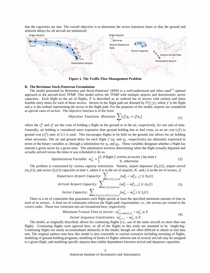
The aircraft-level Traffic Flow Management Problem (TFMP) is concerned with the strategic scheduling of
flights from the arrival airport to the destination airport, while passing through various sectors along the way as
shown in Figure 1. Each flight has a planned flight plan route, which also specifies the sequence of sectors that the
flight must fly through. Depending on the planned cruise speed and prevalent wind field, each flight has a transit
time through each of the sectors along its planned route. The National Airspace System (NAS) resources such as
arrival/departure airports and sectors have a limited capacity. This limited capacity of the airports is specified by the
maximum arrival and departure rates. This research effort uses the Monitor Alert Parameter (MAP) as a measure of
the sector capacity. Note that an accurate definition of sector capacity is still an active area of research and the
approach developed in this paper can readily use any other measure that restricts the total number of aircraft in every
sector. Every aircraft aims to execute its planned flight while respecting the airport and sector capacity constraints.
The sector transition times for every sector for every flight are the control variables that can be modulated to ensure
N
American Institute of Aeronautics and Astronautics
3
that the capacities are met. The overall objective is to determine the sector transition times so that the ground and
airborne delays for all aircraft are minimized.
Figure 1. The Traffic Flow Management Problem
B. The Bertsimas Stock-Patterson Formulation
The model presented by Bertsimas and Stock-Patterson1 (BSP) is a well-understood and often used
2-5 optimal
approach to the aircraft-level TFMP. This model solves the TFMP with multiple airports and deterministic sector
capacities. Each flight in the set of flights, is described as an ordered list of sectors with earliest and latest
feasible entry times for each of those sectors. Sectors in the flight path are denoted by , where is the flight
and is the ordinal representing the sector in the flight path. For the purposes of the model, airports are considered
as special cases of sectors. The objective function is of the form:
(1)
where the
and are the costs of holding a flight on the ground or in the air, respectively, for one unit of time.
Generally, air holding is considered more expensive than ground holding due to fuel costs, so an air cost ( ) to
ground cost (
) ratio of 2:1 is used. This encourages flights to be held on the ground, but allows for air holding
when necessary. The air and ground delay for each flight ( and , respectively) are ultimately expressed in
terms of the binary variables , through a substitution for and . These variables designate whether a flight has
entered a given sector by a given time. The substitution involves determining when the flight actually departed and
actually arrived versus the times it was scheduled to do so.
(2)
The problem is constrained by various capacity restrictions. Namely, airport departure ( ), airport arrival
( ), and sector ( ) capacities at time , where is in the set of airports, , and is in the set of sectors, :
(3)
There is a set of constraints that guarantees each flight spends at least the specified minimum amount of time in
each of its sectors. A final set of constraints enforces the flight path requirements, i.e., the sectors are visited in the
correct order. These two constraint sets are formalized here, respectively:
(4)
The model, as originally described, allows for continuing flights (i.e., use of the same aircraft on more than one
flight). Continuing flights were ignored here, so all of the flights in this study are assumed to be `single-leg.'
Continuing flights are easily accommodated abstractly in the model, though are often difficult to obtain in real data
sets. The original authors note how this model is also extensible to various scenarios including rerouting of flights,
modeling of ground-holding programs, modeling of banks of flights wherein one of several aircraft may be assigned
to a given flight, and modeling specific airports that exhibit dependence between arrival and departure capacities.
ttakeoff
tland
t12 t34t23
t45
t56
t78
t67
Origin Airport
Destination Airport
Airport Departure Rate
Airport Arrival Rate
Sector Capacity
Destination Airport
Origin Airport
American Institute of Aeronautics and Astronautics
4
C. Dantzig-Wolfe Decomposition Applied to the BSP Problem
The constraint matrix for the BSP model is in the primal block angular form. Rios and Ross5 applied Dantzig-
Wolfe decomposition for solving the BSP TFMP. The sub-problems for this decomposition were solved in parallel
via independent computational threads on an 8-core computer. Experiments conducted by Rios and Ross showed
that as the number of sub-problems/threads increases (and their sizes decrease), for a given problem, the solution
quality, convergence and runtime improve. A demonstration of this was provided by using the finest possible
decomposition: one flight per sub-problem. This massively parallel decomposition showed the best performance in
terms of solution integrality, accuracy and runtime. The runtime performance was projected to decrease further with
the availability of additional cores on the computer. Currently available GPUs have about 440 cores as opposed to
the 8-core CPU used by Rios and Ross. Also additional GPU cards can be added to the computer to increase the
number of cores available. This provides the motivation for implementing Dantzig-Wolfe decomposition on the
GPU, to solve the BSP TFMP, in order to achieve a significant decrease in run time.
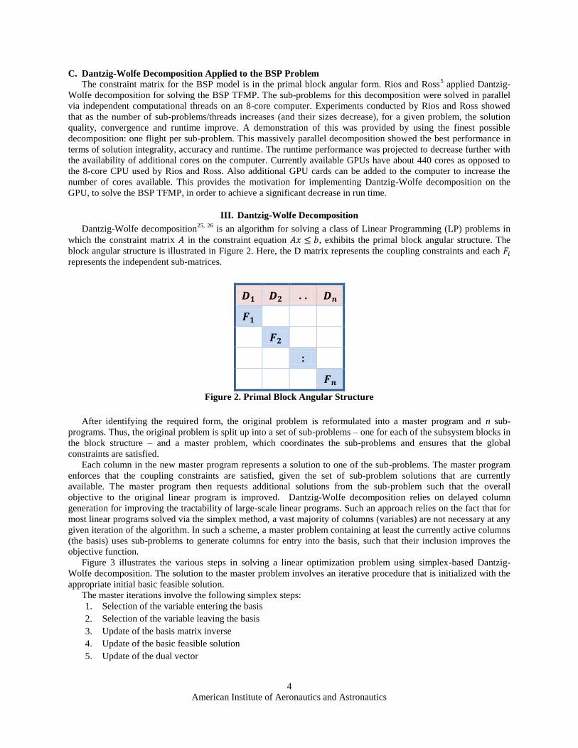
III. Dantzig-Wolfe Decomposition
Dantzig-Wolfe decomposition25, 26
is an algorithm for solving a class of Linear Programming (LP) problems in
which the constraint matrix in the constraint equation , exhibits the primal block angular structure. The
block angular structure is illustrated in Figure 2. Here, the D matrix represents the coupling constraints and each
represents the independent sub-matrices.
. .
:
Figure 2. Primal Block Angular Structure
After identifying the required form, the original problem is reformulated into a master program and n sub-
programs. Thus, the original problem is split up into a set of sub-problems – one for each of the subsystem blocks in
the block structure – and a master problem, which coordinates the sub-problems and ensures that the global
constraints are satisfied.
Each column in the new master program represents a solution to one of the sub-problems. The master program
enforces that the coupling constraints are satisfied, given the set of sub-problem solutions that are currently
available. The master program then requests additional solutions from the sub-problem such that the overall
objective to the original linear program is improved. Dantzig-Wolfe decomposition relies on delayed column
generation for improving the tractability of large-scale linear programs. Such an approach relies on the fact that for
most linear programs solved via the simplex method, a vast majority of columns (variables) are not necessary at any
given iteration of the algorithm. In such a scheme, a master problem containing at least the currently active columns
(the basis) uses sub-problems to generate columns for entry into the basis, such that their inclusion improves the
objective function.
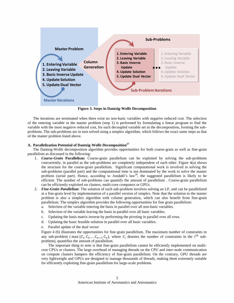
Figure 3 illustrates the various steps in solving a linear optimization problem using simplex-based Dantzig-
Wolfe decomposition. The solution to the master problem involves an iterative procedure that is initialized with the
appropriate initial basic feasible solution.
The master iterations involve the following simplex steps:
1. Selection of the variable entering the basis
2. Selection of the variable leaving the basis
3. Update of the basis matrix inverse
4. Update of the basic feasible solution
5. Update of the dual vector
American Institute of Aeronautics and Astronautics
5
Figure 3. Steps in Dantzig-Wolfe Decomposition
The iterations are terminated when there exist no non-basic variables with negative reduced cost. The selection
of the entering variable in the master problem (step 1) is performed by formulating a linear program to find the
variable with the most negative reduced cost, for each decoupled variable set in the decomposition, forming the sub-
problems. The sub-problems are in turn solved using a simplex algorithm, which follows the exact same steps as that
of the master problem listed above.
A. Parallelization Potential of Dantzig-Wolfe Decomposition27
The Dantzig-Wolfe decomposition algorithm provides opportunities for both coarse-grain as well as fine-grain
parallelism as discussed in the following:
1. Coarse-Grain Parallelism: Coarse-grain parallelism can be exploited by solving the sub-problems
concurrently, in parallel as the sub-problems are completely independent of each other. Figure 4(a) shows
the structure for the coarse-grain parallelism. Significant computational work is involved in solving the
sub-problems (parallel part) and the computational time is not dominated by the work to solve the master
problem (serial part). Hence, according to Amdahl’s law28
, the suggested parallelism is likely to be
efficient. The number of sub-problems can quantify the amount of parallelism . Coarse-grain parallelism
can be efficiently exploited on clusters, multi-core computers or GPUs.
2. Fine-Grain Parallelism: The solution of each sub-problem involves solving an LP, and can be parallelized
at a fine-grain level by implementation of a parallel version of simplex. Note that the solution to the master
problem is also a simplex algorithm with column generation, which can also benefit from fine-grain
parallelism. The simplex algorithm provides the following opportunities for fine grain parallelism:
a. Selection of the variable entering the basis in parallel over all non-basic variables.
b. Selection of the variable leaving the basis in parallel over all basic variables.
c. Updating the basis matrix inverse by performing the pivoting in parallel over all rows.
d. Updating the basic feasible solution in parallel over all basic variables.
e. Parallel update of the dual vector
Figure 4 (b) illustrates the opportunities for fine-grain parallelism. The maximum number of constraints in
any sub-problem ( , where denotes the number of constraints in the sub-
problem), quantifies the amount of parallelism.
The important thing to note is that fine-grain parallelism cannot be efficiently implemented on multi-
core CPUs or clusters. The large overhead of managing threads on the CPU and inter-node communication
on compute clusters hampers the efficiency of fine-grain parallelism. On the contrary, GPU threads are
very lightweight and GPUs are designed to manage thousands of threads, making them extremely suitable
for efficiently exploiting fine-grain parallelism for large-scale problems.
Master Problem
1. Entering Variable2. Leaving Variable3. Basis Inverse Update4. Update Solution5. Update Dual Vector
Master Iterations
1. Entering Variable2. Leaving Variable3. Basis Inverse
Update4. Update Solution5. Update Dual Vector
ColumnGeneration
Sub-Problems
1. Entering Variable2. Leaving Variable3. Basis Inverse
Update4. Update Solution5. Update Dual Vector
Sub-Problem Iterations

American Institute of Aeronautics and Astronautics
6
(a) Coarse-Grain Parallelism
(b) Fine Grain Parallelism
Figure 4. Coarse and Fine-Grain Parallelism Opportunities in Dantzig-Wolfe Decomposition
Thus, DW decomposition offers opportunities for parallelizing at different levels with one level nested within the
other; however implementation of nested parallelism on the GPU is not possible. The functions that implement
parallel code in CUDA are called kernels. CUDA cannot call a kernel within a kernel**
. Thus, either the sub-
problems can be solved in parallel or a parallel version of simplex can be implemented to solve each sub-problem.
Figure 5. Refined Fine-Gain Implementation that Exploits both Coarse and Fine-Grain Parallelism
Opportunities in Dantzig-Wolfe Decomposition
This research effort implemented an innovative fine-grain parallel implementation that exploits both the coarse
and fine-grain parallelism opportunities in a composite manner. This parallel version (shown in Figure 5)
implements fine-grain parallelism for the solution to each sub-problem. Instead of looping serially over all sub-
problems as in Figure 4 (b), all the sub-problems are grouped in to a single massive CUDA kernel that implements
the simplex algorithm over all sub-problems concurrently. The CUDA kernel ensures that data from the appropriate
sub-problem is passed to each thread. The main advantage of this formulation is that the amount of parallelism is
equal to the sum of the number of constraints over all sub-problems , which is much larger than
the amount of parallelism in the coarse and fine-grain implementation illustrated in Figure 4. This massive amount
of parallelism makes this formulation extremely suitable for GPU implementation, where the execution performance
(amount of speedup achieved) increases with the number of parallel threads.
**
Note that at the time this code was developed Dynamic Parallelism –the ability to call a kernel within a kernel–
was not available. Dynamic parallelism is available in CUDA 5.0 for GPUs with compute capability 3.5.
Master
Sub 1 Sub 2 Sub n-1 Sub n
Solve Sub-Problems in Parallel
Master
Sub 1 Sub 2 Sub n-1 Sub n
Parallel Simplex for eachSub-Problem
Parallel Simplex for Master
Loop Serially over all Sub-Problems
Master
Sub 1 Sub 2 Sub n-1 Sub n
Assign Data from the Correct Sub-Problem for Each Thread
Parallel Simplex over All Sub-Problems
Parallel Simplex for Master
American Institute of Aeronautics and Astronautics
7
B. GPU Implementation of the Dantzig-Wolfe Decomposition Algorithm
The target audience for this paper is researchers in the air traffic management domain and not CUDA
programmers. Hence this section provides an overview of the features of the GPU implementation rather than
delving to the details of the CUDA code. The features of the GPU implementation of DW decomposition solver are
as follows:
1. Code development from scratch: The entire code was developed from scratch without the use of any pre-
compiled third-party libraries or linear algebra packages. This was done to ensure that the code could be
tailored to exploit features of the GPU architecture to the fullest, for optimum performance.
2. Phase-I Simplex: The sample TFMP solved under this research effort did not have any negative values in
the right hand side of the constraint equation ( , for all elements of vector in . In this case,
the trivial solution – a vector of zeros – is a valid initial basic feasible solution. Hence the algorithm for
determination of the initial basic feasible solution (commonly referred to as Phase-I Simplex) was not
implemented.
3. Sparse Implementation: The GPU implementation exploits general, unstructured sparsity by storing the
location and value for each non-zero element in various vectors and matrices. The sparse implementation
results in reduced memory requirement and faster execution times. Note that a sparse implementation is
necessary for large-scale problems as a dense storage scheme can easily exceed the available RAM even on
high performance computers.
4. Warm Starts: As described earlier, the DW decomposition algorithm involves sub-problem iterations
nested within master iterations. In the current implementation, optimal sub-problem solutions at previous
master iteration were used to warm-start the sub-problems at the subsequent master iteration. This results in
considerable reduction in execution time over the strategy of starting the sub-problem iteration from the
trivial initial basic feasible solution.
5. Short Int: The BSP formulation results in a ‘0-1’ Binary Integer Program which has a strong LP relaxation.
The formulation uses the binary decision variables given by Eq. (2). The developed code uses the
variable type short int for decision variables and other related intermediate variables. The use of
short int (2 bytes) as opposed to double (8 bytes) results in reduced memory requirement and faster
execution times, without compromising on solution accuracy.
6. Parallel Master: The code developed in this paper exploits both coarse and fine-grain parallelism
opportunities in DW decomposition solution for both master and sub-problems. Note that efficient
implementation of fine-grain parallelism is not possible on clusters or multi-core CPUs. Thus, the GPU
implementation can exploit parallelism in the master, whereas master problem solution can only be
implemented serially on clusters or multi-core CPUs.
7. Multi-GPU: This implementation takes advantage of multiple GPUs available in a computer for solving the
sub-problems in parallel over multiple GPUs.
IV. Solver Evaluation
This section presents the results of the solver evaluation performed under this research effort. Section A
describes the 3 solvers that were evaluated as a part of this research. The hardware test-bed is described in Section
B. Section C describes the 1000 flight TFMP and the experimental plan. Finally the run times and the achieved
speed up are presented in Section D.
A. Description of the 3 Solvers
The following solvers were evaluated for comparing the run times:
1. dwsolver: The dwsolver5,29,30
was developed at NASA Ames Research Center. The dwsolver solves
TFMPs formulated as a BSP Binary Integer Program. It is a parallel implementation of the Dantzig-Wolfe
decomposition that exploits coarse-grain parallelism by solving the sub-problems in parallel on a multi-core
computer. The underlying LP solver is the GNU Linear Programming Kit (GLPK), which employs a sparse
implementation of primal simplex algorithm. This formulation does not exploit parallelism in the master
problem.
2. CPU: CPU refers to the serial version of the DW solver developed in ‘C’ under this research effort, running
on a single core of the CPU.
3. GPU: The GPU version refers to the fine-grain parallel version of the DW solver on GPUs developed using
CUDA.
American Institute of Aeronautics and Astronautics
8
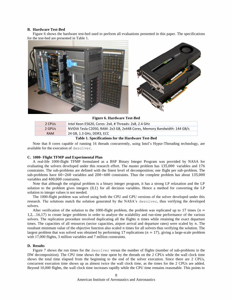
B. Hardware Test-Bed
Figure 6 shows the hardware test-bed used to perform all evaluations presented in this paper. The specifications
for the test-bed are presented in Table 1.
Figure 6. Hardware Test-Bed
2 CPUs Intel Xeon E5620, Cores: 2x4, # Threads: 2x8, 2.4 GHz
2 GPUs NVIDIA Tesla C2050, RAM: 2x3 GB, 2x448 Cores, Memory Bandwidth: 144 GB/s
RAM 24 GB, 1.3 GHz, DDR3, ECC
Table 1. Specifications for the Hardware Test-Bed
Note that 8 cores capable of running 16 threads concurrently, using Intel’s Hyper-Threading technology, are
available for the execution of dwsolver.
C. 1000- Flight TFMP and Experimental Plan
A real-life 1000-flight TFMP formulated as a BSP Binary Integer Program was provided by NASA for
evaluating the solvers developed under this research effort. The master problem has variables and
constraints. The sub-problems are defined with the finest level of decomposition; one flight per sub-problem. The
sub-problems have variables and constraints. Thus the complete problem has about
variables and constraints.
Note that although the original problem is a binary integer program, it has a strong LP relaxation and the LP
solution to the problem gives integers for all decision variables. Hence a method for converting the LP
solution to integer values is not needed.
The 1000-flight problem was solved using both the CPU and GPU versions of the solver developed under this
research. The solutions match the solution generated by the NASA’s dwsolver, thus verifying the developed
solvers.
After verification of the solution to the 1000-flight problem, the problem was replicated up to times to create larger problems in order to analyze the scalability and run-time performance of the various
solvers. The replication procedure involved duplicating all the flights times while retaining the exact departure
times. The capacities of all resources (sector capacities, airport arrival and departure rates) were scaled by . The
resultant minimum value of the objective function also scaled times for all solvers thus verifying the solution. The
largest problem that was solved was obtained by performing replications ( , giving a large-scale problem
with 17,000 flights, 3 million variables and 7 million constraints.
D. Results
Figure 7 shows the run times for the dwsolver versus the number of flights (number of sub-problems in the
DW decomposition). The CPU time shows the time spent by the threads on the 2 CPUs while the wall clock time
shows the total time elapsed from the beginning to the end of the solver execution. Since there are 2 CPUs,
concurrent execution time shows up as almost twice the wall clock time, as the times for the 2 CPUs are added.
Beyond 10,000 flights, the wall clock time increases rapidly while the CPU time remains reasonable. This points to

American Institute of Aeronautics and Astronautics
9
the fact that the wall clock time includes the overhead for thread creation and management, and thread overhead
prevents scaling of the dwsolver beyond 10,000 flights. Note that the scalability conclusion holds when the level
of DW decomposition is one flight per sub-problem. Larger problems can be solved by grouping more flights per
sub-problem. However, the desirable properties of using one flight per sub-problem, such as the solution quality,
convergence characteristics and run-time performance are lost. Figure 8 shows a zoomed in version of Figure 7 for
problem sizes up to 10,000 aircraft (10 replications).
Figure 7. Run Times for the dwsolver
Figure 8. Run Times for the dwsolver
(Problem Size up to 10 Replications)
The run times for the CPU implementation of the solver developed under this research effort are shown in Figure
9. This figure shows that a major fraction of the computational effort is spent in solving the sub-problems relative to
the master problem. Although insignificant for small problems, the computational effort for the master problem can
become substantial for large-scale problems. This shows that a parallel implementation of the master in addition to
sub-problem parallelization can lead to performance benefits.
Figure 9. Run Times on the CPU
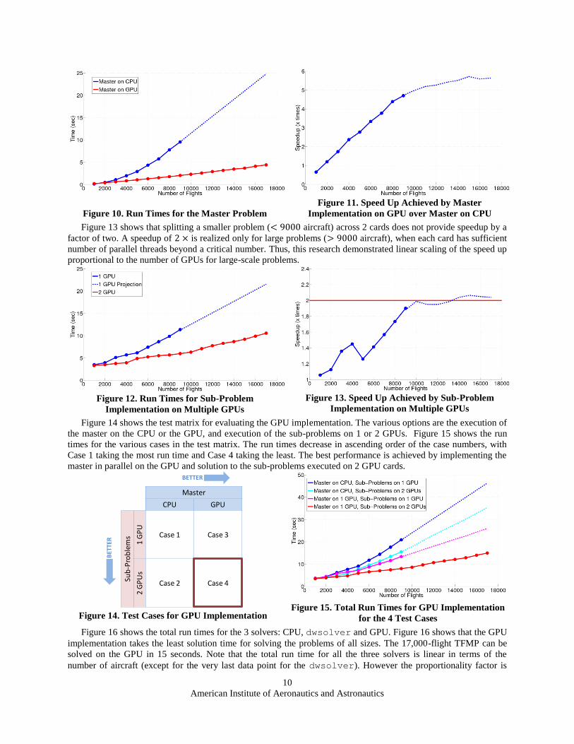
Figure 10 shows the comparison between the run times for serial master implementation on the CPU and parallel
master implementation on the GPU. Note that in all the figures presented in this section, solid lines indicate
observed trends, where the dots are the actual observed values and dotted lines represent projections. Also linear
projections are used to predict run times, which give conservative estimates. Note that the projections are only used
to predict baseline data for comparisons, and a conservative estimate on the baseline gives a conservative estimate of
the achieved performance improvement. All values reported for the final GPU implementation are observed values.
Figure 11 shows that by implementing the master problem on the GPU, a speedup of 5 to 6 times can be achieved
for the master problem execution.
Figure 12 shows the comparison between the run times for the sub-problem when executed on a single GPU as
opposed to a multi-GPU solution with 2 GPUs. Note that with the 3GB of RAM available on the Tesla C2050 GPU
cards, the maximum number of sub-problems that could be accommodated on a single C2050 is 9000. Larger
problems could be solved on a single card if the Tesla C2070 cards with 6GB RAM are used. The dotted line shows
the projection of the run times on a C2070 card. The maximum number of sub-problems that were solved on the
current two-C2050 GPU configuration is 17,000.
American Institute of Aeronautics and Astronautics
10
Figure 10. Run Times for the Master Problem
Figure 11. Speed Up Achieved by Master
Implementation on GPU over Master on CPU
Figure 13 shows that splitting a smaller problem ( aircraft) across 2 cards does not provide speedup by a
factor of two. A speedup of is realized only for large problems ( aircraft), when each card has sufficient
number of parallel threads beyond a critical number. Thus, this research demonstrated linear scaling of the speed up
proportional to the number of GPUs for large-scale problems.
Figure 12. Run Times for Sub-Problem
Implementation on Multiple GPUs
Figure 13. Speed Up Achieved by Sub-Problem
Implementation on Multiple GPUs
Figure 14 shows the test matrix for evaluating the GPU implementation. The various options are the execution of
the master on the CPU or the GPU, and execution of the sub-problems on 1 or 2 GPUs. Figure 15 shows the run
times for the various cases in the test matrix. The run times decrease in ascending order of the case numbers, with
Case 1 taking the most run time and Case 4 taking the least. The best performance is achieved by implementing the
master in parallel on the GPU and solution to the sub-problems executed on 2 GPU cards.
Figure 14. Test Cases for GPU Implementation
Figure 15. Total Run Times for GPU Implementation
for the 4 Test Cases
Figure 16 shows the total run times for the 3 solvers: CPU, dwsolver and GPU. Figure 16 shows that the GPU
implementation takes the least solution time for solving the problems of all sizes. The 17,000-flight TFMP can be
solved on the GPU in 15 seconds. Note that the total run time for all the three solvers is linear in terms of the
number of aircraft (except for the very last data point for the dwsolver). However the proportionality factor is
Master
CPU GPU
Sub
-Pro
ble
ms
1 G
PU
Case 1 Case 3
2 G
PU
s
Case 2 Case 4
BETTER
BET
TER

American Institute of Aeronautics and Astronautics
11
much smaller for the GPU when compared with the CPU or dwsolver. Note that the sparse implementations in all
the three solvers play an important role in maintaining the linear scalability.
Figure 17 shows that the GPU implementation is faster than the exact same code running on the CPU and
faster than dwsolver. Note that the speedup factor with respect to the CPU increases rapidly with the
number of aircraft when the number of aircraft is below 9000. For larger problem sizes ( aircraft), the
speedup saturates at . The speedup with respect the dwsolver increases for problem sizes up to 10,000
aircraft, beyond which it becomes impractical to run larger problems using dwsolver (using the 1-flight-per sub-
problem decomposition).
Figure 16. Total Run Times for the 3 Solvers: CPU,
dwsolver and GPU
Figure 17. Speed Achieved by the GPU Version over
CPU and dwsolver
E. Projected Scalability of the Developed Solver
This paper demonstrated the solution to a 17,000-aircraft TFMP in less than 15 seconds. This result was
demonstrated on a hardware configuration with 2 GPUs. This paper also demonstrated linear scaling in the speedup
with the number of GPUs, for a problem involving large numbers of aircraft. Hardware configurations with 8 GPUs
in a single workstation/server (Figure 18) are currently available in the market, which can potentially provide a
factor of over the current implementation.
Figure 18. COTS Workstation/Server with 8 GPUs
Based on the above discussion, it can be projected that a 68,000-aircraft TFMP can be solved in 15 seconds, by
running the solver developed in this research effort on an 8-GPU workstation. Note that the alternate hypothesis that
the 17,000-aircraft TFMPs can be solved in seconds, is erroneous. This is because, if the same
problem is split across a larger number of cards, each card may not have sufficient number of threads to realize the
full performance benefit of each GPU.
V. Summary and Concluding Remarks
Significant accomplishments of this research effort are as follows:
American Institute of Aeronautics and Astronautics
12
1. This research effort developed a GPU implementation of a linear optimization solver that exploits the
Dantzig-Wolfe (DW) decomposition framework based on the primal simplex algorithm.
a. Coded from scratch to exploit GPU architecture to the fullest
b. Developed an innovative fine-grain implementation that exploits both coarse and fine-grain parallelism
opportunities in DW decomposition
c. Sparse implementation suitable for large-scale problems
d. Exploits parallelism in the solution of both the master and the sub-problems
2. Demonstrated solution to large-scale TFM problems formulated as Bertsimas Stock-Patterson (BSP) ‘0-1’
Binary Integer Programs
3. Demonstrated that a BSP TFM Problem with 17,000 aircraft (7 million constraints) can be solved in less
than 15 seconds.
4. GPU implementation is 30× faster than the exact same code running serially (single-threaded) on the CPU.
5. The GPU implementation is 16× faster than the NASA’s current solution: dwsolver, that implements
coarse-grain parallel DW decomposition using the GNU Linear Programming Kit (GLPK) on an 8-core
computer with hyper-threading (16 threads).
6. Demonstrated that the solution time is linear in the number of sub-problems (number of aircraft). Hence
larger problems can be solved with only a linear increase in run time
7. Demonstrated linear scalability in the speedup with the number of GPUs. Thus times speedup can be
achieved by using GPUs in a single computer.
This paper demonstrated that fast-time solutions to large-scale aircraft-level optimal traffic flow management
problems are made feasible by a massively parallel implementation on Graphics Processing Units. Using this
approach, traffic flow management problems with aircraft over 3 hours can now be solved in under
seconds, whereas previous approaches might take over minutes for a serial implementation on a desktop
computer or minutes for a multi-threaded implementation on an 8-core desktop workstation. Thus, this paper takes
the first step in removing the computational time hurdle in the use of numerical optimization techniques for strategic
control of NAS operations.
Acknowledgments
This research was supported under NASA Phase I SBIR Contract No. NNX11CD10P monitored out of the
NASA Ames Research Center.
References 1Bertsimas D., and Patterson S. S., “The Air Traffic Flow Management Problem with Enroute Capacities,” Operations
Research, Vol. 46, No. 3, May-June 1998. 2Rios, J. and Ross, K., “Delay Optimization for Airspace Capacity Management with Runtime and Equity Considerations,”
AIAA Guidance, Navigation, and Control Conference and Exhibit, Hilton Head, South Carolina, August 2007. 3Grabbe, S., Sridhar, B., and Mukherjee, A., “Central East Pacific Flight Scheduling,” AIAA Guidance, Navigation, and
Control Conference and Exhibit, Hilton Head, South Carolina, August 2007. 4Rios J., and Ross K., “Parallelization of the Traffic Flow Management Problem,” AIAA Guidance, Navigation and Control
Conference and Exhibit, Honolulu, Hawaii, Aug. 18-21, 2008. 5Rios J., and Ross K., “Massively Parallel Dantzig-Wolfe Decomposition Applied to Traffic Flow Scheduling,” Journal of
Aerospace Computing, Information, and Communication, Vol.7, No.1, pp 32-45, Jan 2010. 6Mukherjee, A., Hansen, M., and Grabbe, S., “Ground Delay Program Planning Under Uncertainty in Airport Capacity,”
Proceedings of the AIAA Guidance, Navigation, and Control Conference and Exhibit, August 2009, Chicago, Illinois. 7Malik, W., Gupta, G., and Jung, Y. C., “Managing Departure Airport Release for Efficient Airport Surface Operations,”
Proceedings of the AIAA Guidance, Navigation, Control Conference and Exhibit, August 2010, Toronto, Canada. 8Rathinam, S., Montoya, J., and Jung, Y. C., “An Optimization Model for Reducing Aircraft Taxi Times at the Dallas Fort
Worth International Airport,” Proceedings of the 26th International Congress of the Aeronautical Sciences, September 2008. 9Gupta, G., Malik, W., and Jung, Y. C., “Incorporating Active Runway Crossings in Departure Scheduling,” Proceedings of
the AIAA Guidance, Navigation, Control Conference and Exhibit, August 2010, Toronto, Canada. 10Capozzi, B. J., Atkins, S., and Choi, S., “Towards Optimal Routing and Scheduling of Metroplex Operations,” Proceedings
of the 9th AIAA Aviation Technology, Integration, and Operation Conference, September 2009, Hilton Head, South Carolina. 11Mukherjee, A., Grabbe, S., and Sridhar, B., “Alleviating Airspace Restrictions through Strategic Control,” Proceedings of
the AIAA Guidance, Navigation, and Control Conference and Exhibit, Honolulu, Hawaii, August 2008. 12Grabbe, S., Mukherjee, A., and Sridhar, B., “Sequential Traffic Flow Optimization with Tactical Flight Control Heuristics,”
Journal of Guidance, Control, and Dynamics, Vol. 32, No. 3, May-June, 2009. 13Yousefi, A., Khorrami, B., Hoffman, R., and Hackney, B., “Enhanced Dynamic Airspace Configuration Algorithms and
Concepts, Metron Aviation Inc., Tech. Rep. Report No. 34N1207-001-R0, December 2007.
American Institute of Aeronautics and Astronautics
13
14Balakrishnan H., Chandran, B., “Scheduling Aircraft Landings under Constrained Position Shifting,” AIAA Guidance
Navigation and Control Conference and Exhibit, Aug 21-24, 2006, Keystone, CO. AIAA 2006-6320. 15Grabbe, S., Sridhar, B., and Mukherjee, A., “Central East Pacific Flight Scheduling,” Proceedings of the AIAA Guidance,
Navigation, and Control Conference and Exhibit, August 2007, Hilton Head, South Carolina. 16Hok, Ng., Grabbe, S, and Mukherjee, A., “Design and Evaluation of a Dynamic Programming Flight Routing Algorithm
Using the Convective Weather Avoidance Model,” Proceedings of the AIAA Guidance, Navigation, and Control Conference and
Exhibit, August 2009, Chicago, Illinois. 17Rios J., and Lohn J., “A Comparison of Optimization Approaches for Nationwide Traffic Flow Management,” AIAA
Guidance Navigation and Control Conference and Exhibit, Aug 10-13, 2009. Chicago, IL. AIAA 2009-6010 18Xue, M. “Airspace Sector Redesign Based on Voronoi Diagrams,” AIAA Guidance, Navigation and Control Conference
and Exhibit, Honolulu, Hawaii, August 2008. AIAA-2008-7223. 19NVIDIA CUDA (Compute Unified Device Architecture) http://www.NVIDIA.com/object/cuda_what_is.html 20NVIDIA: CUDA http://www.NVIDIA.com/object/cuda_home.html# 21Kirk D. B., and Hwu W. W., “Programming Massively Parallel Processors: A Hands-on Approach,” Morgan Kaufmann,
Burlington MA, Feb 5, 2010. 22Sanders J., and Kandrot E., “CUDA by Example: An Introduction to General Purpose GPU Programming,” Addison-Wesley
Professional, Reading, MA, Jul 29, 2010. 23NVIDIA CUDA, Compute Unified Device Architecture, Programming Manual 24NVIDIA Tesla S1070: http://www.nvidia.com/object/preconfigured-clusters.html 25Bertsimas D., Tsitsiklis J. N., “Introduction to Linear Optimization,” Athena Scientific, Nashua NH, Feb 1, 1997. 26Dantzig G B., and Wolfe P., “Decomposition Principle for Linear Programs,” Operations Research, Vol. 8, No. 1, pp. 101-
111, Jan-Feb 1960. 27Tebboth J. R., “A Computational Study of Dantzig-Wolfe Decomposition,” Ph.D. Dissertation, University of Buckingham,
December 2001. 28Amdahl’s Law: http://en.wikipedia.org/wiki/Amdahl%27s_law 29SourceForge.net Homepage for dwsolver http://sourceforge.net/apps/wordpress/dwsolver/ 30Rios J., “Algorithm 928: A General, Parallel Implementation of Dantzig-Wolfe Decomposition,” ACM Transactions on
Mathematical Software, Vol. 39, No. 3, April 2013
Top Related
Copyright © 2022 FDOKUMEN

