Journal of Geochemical Exploration 124 (2013) 79–91

Contents lists available at SciVerse ScienceDirect

Journal of Geochemical Exploration

j ourna l homepage: www.e lsev ie r .com/ locate / jgeoexp

Mapping geochemical patterns at regional to continental scales using compositesamples to reduce the analytical costs

D. Cicchella a,⁎, A. Lima b, M. Birke c, A. Demetriades d, X. Wang e, B. De Vivo b

a Department of Biological, Geological and Environmental Science, University of Sannio, Via dei Mulini 59/A, 82100 Benevento, Italyb Department of Earth Science, University of Napoli “Federico II”, Via Mezzocannone 8, 80138 Napoli, Italyc Federal Institute for Geosciences and Natural Resources, Stilleweg 2, 30655 Hannover, Germanyd Institute of Geology and Mineral Exploration (IGME), 1 Spirou Louis Street, 13677 Acharnae, Athens, Greecee Institute of Geophysical and Geochemical Exploration, CAGS, 84 Jinguang Road, Langfang, Hebei 065000, China

⁎ Corresponding author. Tel.: +39 0824 323642; fax:E-mail address: cidom@unisannio.it (D. Cicchella).

0375-6742/$ – see front matter © 2012 Elsevier B.V. Allhttp://dx.doi.org/10.1016/j.gexplo.2012.08.012

a b s t r a c t

a r t i c l e i n f o

Article history:Received 9 July 2011Accepted 11 August 2012Available online 23 August 2012

Keywords:Composite samplesGeochemical mappingElementsEuropean soilFOREGS

The use of composite samples to reduce the time and cost of chemical analysis is discussed. It is shown whencomposite samples can be used without affecting predefined project objectives. Furthermore, it is also dem-onstrated when they should not be used, and also how much information is lost due to their use.The study presents a comparison of data concentrations of some major (Al2O3, CaO, Fe2O3, K2O, P2O5, TiO2)and trace elements (Cd, Co, Cr, La, Rb, Sr, Th, Tl, U, Zn) in European topsoil and subsoil produced byFOREGS (Forum of European Geological Surveys) and two other data sets derived by compositing the five in-dividual samples in each 160×160 km cell of the Global Terrestrial Network (GTN); the first by physicallycompositing the samples, and analysing the composites, and the second by artificially compositing the sam-ples in each GTN cell.The three soil databases were compared statistically and spatially to quantify the significance of the differ-ences. The results of this study clearly demonstrate that composite samples can be used effectively toshow broad continental-scale element distribution patterns; their use may not be effective if the goal is tohighlight local geochemical anomalies. It is concluded that compositing samples for continental-scale surveysis a time- and cost-effective procedure, especially for reducing the costs for chemical analysis.

© 2012 Elsevier B.V. All rights reserved.

1. Introduction

Composite sampling is a technique whereby multiple temporally orspatially discretemedia samples are combined, thoroughly homogenised,and treated as a single sample (Correll, 2001; El Baz and Nayak, 2004;Splitstone, 2001). Composite sampling can improve spatial or temporalrepresentations of the data by reducing considerably the number ofanalysed samples and the local, in space or time, variability. Suitabilityof composite sampling is dependent, however, upon project objectivesand site characteristics.

The high costs of laboratory analytical procedures frequentlyincrease to a prohibitive level the budget of geochemical explorationand mapping projects. Composite samples can, therefore, substantiallyreduce analytical costs due to the reduction of the total number of sam-ples to be analysed. It can be very cost-effective to analyse the first set ofcomposite samples and then decide, based on the first results, in whicharea to analyse all the single samples.

+39 0824 323623.

rights reserved.

Obviously, there are a number of immediate questions to be an-swered regarding the use of composite samples: (a) Is it correct to usecomposite samples in small scale geochemical mapping? (b) How muchsignificant information is lost due to compositing samples? (c) When cancomposite samples be used without seriously affecting project objectives?and (d) When should composite samples avoided? This work attemptsto give justifiable answers to these questions, using the data generatedin the FOREGS (Forum of European Geological Surveys) continental-scale project.

The FOREGS Geochemical Baseline Mapping Programme's mainaim was to provide high quality, multi-purpose geochemical base-line data for Europe (Salminen et al., 1998). The generated geo-chemical data are based on the analysis of samples of streamwater, stream sediment, floodplain sediment (or alluvial soil), resid-ual soil (top and bottom), and humus collected from 26 Europeancountries. High quality and consistency of the data were ensuredby using standardised sampling methods (Salminen et al., 1998),and by applying rigorous, harmonised quality control and assuranceprocedures during chemical analysis and subsequent data handlingstages.

The results of this programme are reported in the two volume setof the ‘Geochemical Atlas of Europe’ (De Vos et al., 2006; Salminen et

80 D. Cicchella et al. / Journal of Geochemical Exploration 124 (2013) 79–91

al., 2005), which represents the first multi-purpose, multi-media,and multi-determinant geochemical atlas at the European scale,published as a contribution of the FOREGS Geochemistry Group tothe Global Geochemical Baselines project, which is being carriedout under the auspices of the International Union of GeologicalSciences (IUGS) and International Association of GeoChemistry(IAGC).

In this paper, the original FOREGS data of some major and traceelements in topsoil and subsoil are compared to the concentrationdata of the same elements resulting from compositing samples ofeach FOREGS GTN cell (Darnley et al., 1995; Salminen et al., 2005)either physically or artificially.

2. Methods

2.1. Sampling

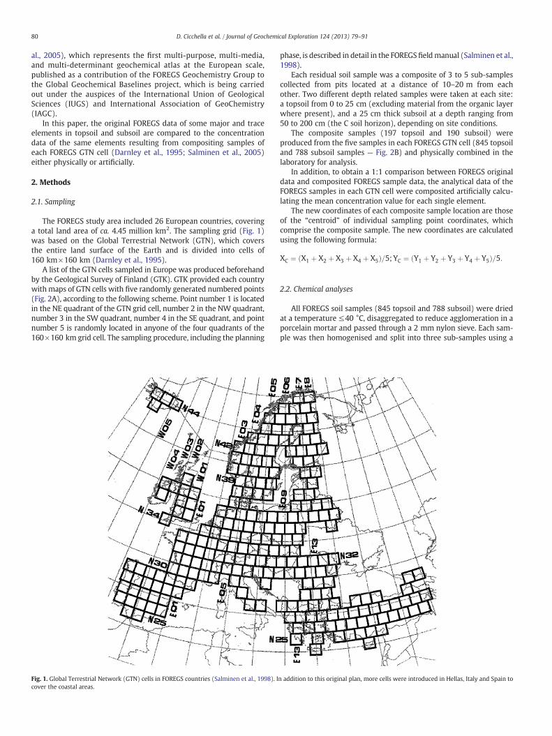
The FOREGS study area included 26 European countries, coveringa total land area of ca. 4.45 million km2. The sampling grid (Fig. 1)was based on the Global Terrestrial Network (GTN), which coversthe entire land surface of the Earth and is divided into cells of160 km×160 km (Darnley et al., 1995).

A list of the GTN cells sampled in Europe was produced beforehandby the Geological Survey of Finland (GTK). GTK provided each countrywithmaps of GTN cells with five randomly generated numbered points(Fig. 2A), according to the following scheme. Point number 1 is locatedin the NE quadrant of the GTN grid cell, number 2 in the NW quadrant,number 3 in the SW quadrant, number 4 in the SE quadrant, and pointnumber 5 is randomly located in anyone of the four quadrants of the160×160 km grid cell. The sampling procedure, including the planning

Fig. 1. Global Terrestrial Network (GTN) cells in FOREGS countries (Salminen et al., 1998). Icover the coastal areas.

phase, is described in detail in the FOREGS fieldmanual (Salminen et al.,1998).

Each residual soil sample was a composite of 3 to 5 sub-samplescollected from pits located at a distance of 10–20 m from eachother. Two different depth related samples were taken at each site:a topsoil from 0 to 25 cm (excluding material from the organic layerwhere present), and a 25 cm thick subsoil at a depth ranging from50 to 200 cm (the C soil horizon), depending on site conditions.

The composite samples (197 topsoil and 190 subsoil) wereproduced from the five samples in each FOREGS GTN cell (845 topsoiland 788 subsoil samples — Fig. 2B) and physically combined in thelaboratory for analysis.

In addition, to obtain a 1:1 comparison between FOREGS originaldata and composited FOREGS sample data, the analytical data of theFOREGS samples in each GTN cell were composited artificially calcu-lating the mean concentration value for each single element.

The new coordinates of each composite sample location are thoseof the “centroid” of individual sampling point coordinates, whichcomprise the composite sample. The new coordinates are calculatedusing the following formula:

XC ¼ X1 þ X2 þ X3 þ X4 þ X5ð Þ=5; YC ¼ Y1 þ Y2 þ Y3 þ Y4 þ Y5ð Þ=5:

2.2. Chemical analyses

All FOREGS soil samples (845 topsoil and 788 subsoil) were driedat a temperature ≤40 °C, disaggregated to reduce agglomeration in aporcelain mortar and passed through a 2 mm nylon sieve. Each sam-ple was then homogenised and split into three sub-samples using a

n addition to this original plan, more cells were introduced in Hellas, Italy and Spain to

Table 1Instrumental methods, detection limit, precisiona and accuracya of analytical results for197 topsoil and 190 subsoil samples.

Parameter Method Detection limit Precision % Accuracy %

Al2O3 (%) XRF 0.1 3.35 2.35CaO (%) XRF 0.05 4.2 3.4Fe2O3 (%) XRF 0.1 1.29 5.08K2O (%) XRF 0.05 2.15 5.14P2O5 (%) XRF 0.001 5.45 4.13TiO2 (%) XRF 0.001 2.38 3.17Cd (mg/kg) ICP-MS 0.03 12.62 5.63Co (mg/kg) ICP-MS 1 7.34 4.82Cr (mg/kg) XRF 5 5.56 3.35La (mg/kg) ICP-MS 1 4.71 3.19Rb (mg/kg) XRF 5 5.35 2.43Sr (mg/kg) XRF 5 5.19 4Th (mg/kg) ICP-MS 1 9.47 5.75Tl (mg/kg) ICP-MS 0.1 7.19 5.9U (mg/kg) ICP-MS 0.2 8.08 5.6Zn (mg/kg) XRF 2 5.59 4.74

a The laboratory accuracy error is calculated on ten analyses of the standard samples bythe following formula:

Accuracyerror ¼ abs X–TVð Þ=TV½ � � 100

where

X laboratory's analysis result for the performance sample (standard sample)TV true value of the performance sample (standard sample).

The precision is calculated as Relative Per cent Difference (%RPD) by the followingformula:

%RPD ¼ abs SV–DVð Þ=0:5 � SVþ DVÞ� � 100ð½

where

SV the original sample valueDV the duplicate sample value.

20

10

30

40

50

60

70

80

90

100

110

120

130

140

150

14010 30 40 50 60 70 80 90 130120 150 km100110

N25W04T1

N25W04T2

N25W04T4

N25W04T3

FOREGS CELL N25W04

20

10

30

40

50

60

70

80

90

100

110

120

130

140

150

10 20 30 40 50 60 70 80 90 130120 150 km100 110 140

N25W04T1N25W04T2

N25W04T4

N25W04T5

N25W04T3

Composite sample N25W04

FOREGS CELL N25W04

A B

N25W04T5

NW NE

SW SE

20

Fig. 2. FOREGS GTN cell with five randomly generated sample sites (A), and new coordinates calculated for the composite sample location (B).

81D. Cicchella et al. / Journal of Geochemical Exploration 124 (2013) 79–91

rotary divider; one sub-sample for storage, and three sub-samples forlaboratory analysis, which were sieved to b0.063 mm (Salminen etal., 1998).

All FOREGS soil samples were analysed for the same suite of ele-ments by the same laboratory using the same analytical method;some elements were determined in different laboratories using adifferent leach and instrumental method (ICP-MS, ICP-AES, XRF).A full description of the analytical and quality control methods isavailable in the FOREGS Geochemical Atlas of Europe (Sandströmet al., 2005).

All the new composite b0.063 mm samples (197 topsoil and 190subsoil) after being mixed andhomogenised were analysed in thelaboratories of the Institute of Geophysical and GeochemicalExploration in Langfang (China). A more detailed description of theanalytical methods used at the Chinese laboratory is given byZheng Kangle et al. (2005). Here only the minor differences in theanalytical methods are mentioned. In China, pressed powder pelletswere used for the XRFmeasurements, whereas in the FOREGS projectfused beads were used. This difference in the sample preparationprocedure should not influence the comparability of two sets ofXRF results significantly. With respect to ICP-MS determinations,the same reagents were used (nitric acid, hydrofluoric acid andperchloric acid) for the preparation of sample solutions. TheFOREGS and Chinese procedures are, however, not 100% identical.Nevertheless, the ICP-MS determinations can be assumed to be com-parable between the two laboratories. In facts, Yao et al., 2011,comparing geochemical data obtained from China and European lab-oratories, demonstrated that the results of two datasets (IGGE's anal-ysis data for composited samples, and the FOREGS average data ofsamples in each GNT cell) agree extremely well for about 23elements (SiO2, Sr, Al2O3, Zr, Ba, Fe2O3, Ti, Rb, Mn, Gd, CaO, Ga,MgO, P, Pb, Na2O, Y, Th, As, U Sc, Cr, and Co). There are slight differ-ences between-laboratory biases shown as proportional errorsbetween the datasets for Ni, K2O, Tb, Tl, Cu, S, Sm, La, Ce, Pr, Nd, Eu,Ho, Er, Tm, Yb, Lu, Ta, Nb, Hf, and Dy. For Cd, Cs, Be, Sb, In, Mo, I, Sn,and Te, the correlation of the two datasets and the similarity of thegeochemical maps are fairly good, but obvious biases exist betweenthe two datasets at values near detection limits.

In this paper we discuss only those elements analysed by both lab-oratories, FOREGS and Chinese, with the same analytical methods:XRF for Al2O3, CaO, Fe2O3, K2O, P2O5, TiO2, Cr, Rb, Sr and Zn andICP-MS for Cd, Co, La, Th, Tl and U.

Precision of the composite sample analyses was calculated onthirty-three laboratory replicates of the composite samples, and accura-cy estimated on standard reference materials, GSD-1a, GSD-9, GSD-10,and GSS-1. Table 1 lists the analytical methods, the instrumental

82 D. Cicchella et al. / Journal of Geochemical Exploration 124 (2013) 79–91

detection limits, accuracy and precision of the geochemical data for theelements analysed in the Chinese laboratories.

2.3. Data treatment

In order to compare effectively the original FOREGS data with thoseof the corresponding Chinese composite samples, the FOREGS concen-tration data for each European GTN grid cell were artificially composit-ed by calculating the mean concentration value of each investigatedelement. Thus, three data sets were generated: (i) FOREGS SamplesData (FSD), (ii) Artificially Composited FOREGS Data (ACFD), and(iii) Composited FOREGS Samples Data (CFSD). In this paper we discussonly those elements analysed by both laboratories, FOREGS andChinese, with the same analytical methods: XRF for Al2O3, CaO, Fe2O3,K2O, P2O5, TiO2, Cr, Rb, Sr and Zn and ICP-MS for Cd, Co, La, Th, Tl and U.

Basic descriptive statistics of top-soil and sub-soil were calculated inorder to study the overall structure of the raw data (Tables 2 and 3). Forstatistical computation, the data below the instrumental detection limit(DL) have been assigned a value corresponding to 50% of the detectionlimit.

Cumulative frequency curves (Figs. 3, 4 and 5) of the three topsoildata sets (FSD (N=845), ACFD and CFSD (N=197)) and the threesubsoil data sets (FSD (N=788) and ACFD and CFSD (N=190)) were

Table 2Summary statistics of major elements in European topsoil and subsoil.

Parameter Number of samples DL Min Median

TopsoilAl2O3

a 845 0.05 0.37 11Al2O3

b 197 0.05 2.45 11.3Al2O3

c 197 0.1 2.61 11.1CaOa 845 0.01 0.03 0.9CaOb 197 0.01 0.15 1.5CaOc 197 0.05 0.17 1.5Fe2O3

a 845 0.01 0.16 3.5Fe2O3

b 197 0.01 0.54 3.9Fe2O3

c 197 0.1 0.56 4.4K2Oa 845 0.01 0.026 1.92K2Ob 197 0.01 0.69 2.01K2Oc 197 0.05 0.75 2.31P2O5

a 845 0.001 0.011 0.13P2O5

b 197 0.001 0.037 0.13P2O5

c 197 0.001 0.06 0.16TiO2

a 845 0.001 0.021 0.57TiO2

b 197 0.001 0.132 0.60TiO2

c 197 0.001 0.128 0.61

SubsoilAl2O3

a 788 0.05 0.21 11.7Al2O3

b 190 0.05 0.78 11.8Al2O3

c 190 0.1 1.01 11.6CaOa 788 0.01 0.02 1.1CaOb 190 0.01 0.04 2CaOc 190 0.05 0.09 2Fe2O3

a 788 0.01 0.11 3.8Fe2O3

b 190 0.01 0.11 4.2Fe2O3

c 190 0.1 b 0.1 4.3K2Oa 788 0.01 b0.01 2.02K2Ob 190 0.01 0.307 2.1K2Oc 190 0.05 0.339 2.3P2O5

a 788 0.001 0.007 0.10P2O5

b 190 0.001 0.007 0.11P2O5

c 190 0.001 0.027 0.12TiO2

a 788 0.001 0.012 0.57TiO2

b 190 0.001 0.036 0.58TiO2

c 190 0.001 0.019 0.57

Unit: %.a FOREGS Samples Data (FSD).b Artificially Composited FOREGS Data (ACFD).c Composited FOREGS Samples Data (CFSD).

used to show and to compare the data distribution. Statistical hypo-thesis tests were applied to quantify the significance levels of thedifferences.

Geographical Information System (GIS) mapping techniques wereused to plot the spatial patterns of the differences, specifically the gridvalues of element distribution maps were compared by linear regres-sion using an ArcView extension “Grid and Theme Regression” ofJenness Enterprises (Jenness, 2006). The raw and log-transformeddata were interpolated to generate a regular grid with a 6 km×6 kmoutput cell size, using the Multifractal Inverse Distance Weighted(MIDW) interpolation method (Cheng, 1999; Cicchella et al., 2005;Lima et al., 2003) with a search radius of 150 km and a minimumnumber of 4 neighbouring points.

The SPSS® software was used for statistical analyses, and ArcView®3.2 GIS software for plotting geochemical maps.

3. Results and discussion

3.1. Comparison between the three data sets with descriptive statistics

The differences in maximum values for all elements between theoriginal FOREGS (FSD) and composited sample data sets (ACFD andCFSD) are quite large. These differences are certainly due to the

Mean SD MAD 25% 75% 90% Max

10.5 4.46 4.61 7.03 13.54 16 26.6710.7 3.50 3.18 8.64 12.98 15 18.3510.7 3.42 3.11 8.51 12.75 14.8 19.93.5 7.26 0.95 0.39 2.13 10.6 47.73.7 5.78 1.41 0.73 3.15 12.5 35.264 6.31 1.32 0.8 3.18 12.5 36.33.8 2.34 2.3 2.1 5.27 6.7 22.33.9 1.62 1.62 2.81 5.02 5.96 10.14.3 1.77 1.79 2.96 5.38 6.35 122.02 0.95 0.92 1.33 2.57 3.25 6.132.05 0.71 0.75 1.51 2.54 3.03 4.962.3 0.75 0.8 1.77 2.82 3.24 4.590.15 0.12 0.07 0.08 0.18 0.25 1.320.15 0.08 0.05 0.1 0.18 0.23 0.540.17 0.09 0.06 0.11 0.21 0.25 0.590.61 0.37 0.29 0.38 0.78 0.97 5.450.61 0.24 0.2 0.45 0.73 0.87 2.050.62 0.24 0.2 0.46 0.74 0.86 2.32

11.2 4.82 4.83 7.68 14.5 17.1 27.111.3 3.81 2.97 8.63 13.56 16 21.911.2 3.56 2.76 8.93 13.2 15.6 21.64.4 8.62 1.34 0.38 2.97 13.5 51.65.1 7.05 2.09 0.96 6.53 14.9 38.65.2 7.3 2 0.97 6.87 15.6 38.64.1 2.32 2.24 2.4 5.44 7.06 15.64.1 1.65 1.77 2.82 5.21 6.4 8.84.3 1.69 1.76 2.98 5.44 6.6 9.22.13 1.02 1 1.4 2.78 3.43 6.052.13 0.75 0.82 1.55 2.7 3.12 4.342.32 0.74 0.77 1.79 2.85 3.28 4.410.12 0.11 0.05 0.07 0.14 0.19 1.660.12 0.07 0.04 0.08 0.15 0.18 0.660.13 0.08 0.04 0.09 0.15 0.18 0.760.59 0.32 0.3 0.36 0.78 0.94 3.140.59 0.23 0.23 0.41 0.73 0.87 1.330.58 0.22 0.21 0.43 0.71 0.85 1.35

Table 3Summary statistics of trace elements in European topsoil and subsoil.

Parameter Number of samples DL Min Median Mean SD MAD 25% 75% 90% Max

TopsoilCda 840 0.01 b0.01 0.145 0.28 0.71 0.11 0.08 0.26 0.48 14.1Cdb 197 0.01 0.026 0.17 0.29 0.49 0.13 0.096 0.31 0.53 5.28Cdc 197 0.03 0.03 0.176 0.29 0.50 0.14 0.09 0.29 0.57 5.06Coa 843 3 b3 7.78 10.4 13.3 6.51 4.02 13.2 19.7 249Cob 197 3 1.5 9.27 10.6 8.3 5.61 5.4 13 19.6 74.9Coc 197 1 1.1 9.31 10.9 7.9 5.86 5.61 13.4 20.7 49Cra 845 3 b3 60 94.8 285 41.51 32.5 88 122 6230Crb 197 3 15.3 65 96.3 170 35.6 39.5 85.3 135 1718Crc 197 5 11.6 63.9 90.3 149 36.9 36.7 84.1 129 1490Laa 843 0.1 1.10 23.5 25.9 15.8 14.68 14.1 34.2 43.7 143Lab 197 0.1 6.36 25.7 25.9 11.2 10.9 17.7 32.2 39.5 74.7Lac 197 1 6.79 29.3 29.2 12.4 12.3 19.7 36.6 44.8 82.5Rba 845 2 b2 80 86.8 47 38.55 55.5 108 140 390Rbb 197 2 27 83.4 87.9 34.7 29.9 64.6 105 136.7 210Rbc 197 5 24.3 83.8 89.2 37.1 33.8 63.4 108 139.4 224Sra 845 2 8 89 130 153 59.3 59 159 246 3120Srb 197 2 28 108 138.4 112 62.3 74.6 166.8 242 817Src 197 5 34.4 109 138.8 108 59.3 74.9 170 247 841Tha 843 0.1 0.3 7.24 8.24 6.15 4.39 4.36 10.4 14.2 75.9Thb 197 0.1 1.79 7.51 8.31 4.38 3.2 5.34 9.78 13.9 31.7Thc 197 1 1.23 8.39 9.12 4.68 3.87 5.79 11.05 15.6 31.7Tla 840 0.01 0.05 0.66 0.82 1.02 0.37 0.43 0.94 1.38 24.0Tlb 197 0.01 0.15 0.71 0.82 0.56 0.31 0.52 0.94 1.4 5.65Tlc 197 0.1 0.16 0.58 0.69 0.47 0.23 0.44 0.74 1.03 5.13Ua 843 0.1 0.21 2 2.36 2.35 1.13 1.31 2.82 3.76 53.2Ub 197 0.1 0.53 2.21 2.38 1.34 0.9 1.57 2.79 3.92 11.8Uc 197 0.2 0.59 2.19 2.49 1.54 0.9 1.61 2.81 4.09 13.6Zna 845 3 b3 52 68.1 141 40 27 83 111 2900Znb 197 3 7.9 59.6 68.2 75.9 32.5 38.25 81.8 95.6 815Znc 197 2 14.1 63.1 73.7 77.7 30.8 42.2 84.05 97.6 805

SubsoilCda 783 0.01 b0.01 0.09 0.19 0.62 0.07 0.05 0.15 0.31 14.2Cdb 190 0.01 0.01 0.1 0.2 0.5 0.07 0.06 0.18 0.34 5.24Cdc 190 0.03 0.03 0.11 0.2 0.45 0.08 0.06 0.18 0.31 5.31Coa 788 3 b3 8.97 11.1 10.5 6.92 4.9 14.4 20.3 170Cob 190 3 1.5 10.4 11.2 6.9 5.97 6.17 14.2 19.7 54.2Coc 190 1 b1 11.15 11.8 7.3 6.26 6.74 14.6 20 58.2Cra 787 3 3 62 86.7 151 44.5 34 95 129 2137Crb 190 3 15 67.7 85.6 97 35.4 42.2 87.8 137.4 789.2Crc 190 5 b5 63.5 80.3 91.5 36.6 38.9 88.7 121 729Laa 788 0.1 0.78 25.6 27.7 16.1 13.94 16.8 36.1 46.7 155Lab 190 0.1 2.17 26.8 27.6 11.4 10.9 19.5 34.4 41.8 77.7Lac 190 1 2.54 30.4 30.5 12.3 12.1 21.5 37.8 43.8 96.4Rba 788 2 5 82.5 89.2 50.7 40.8 56 111 144 378Rbb 190 2 11 86.7 88.9 36.6 32.4 62.1 106.5 141.8 258Rbc 190 5 10.4 89.5 93 39.3 35.6 64.3 111 147.6 272Sra 788 2 6.00 95 143 150 66.7 63 177.7 270 2010Srb 191 2 6 118.2 153.6 120.8 72.9 77 193.5 299.7 1087Src 190 5 15.7 122 156.4 120 71.2 82 198.2 299.6 1100Tha 788 0.1 0.16 7.63 8.7 6.29 4.51 4.97 10.97 14.4 71.7Thb 190 0.1 0.64 8.11 8.7 4.45 3.28 5.69 10.19 13.55 30.69Thc 190 1 b1 8.49 9 4.6 3.41 6.05 10.6 14 36.9Tla 783 0.01 0.01 0.67 0.83 0.98 0.37 0.44 0.97 1.37 21.3Tlb 190 0.01 0.1 0.7 0.83 0.56 0.3 0.51 0.93 1.44 5.03Tlc 190 0.1 b0.1 0.57 0.65 0.45 0.23 0.42 0.73 1.09 4.75Ua 788 0.1 b0.1 2.03 2.45 2.34 1.09 1.36 2.89 3.94 30.3Ub 190 0.1 0.19 2.16 2.42 1.54 0.92 1.52 2.78 3.88 15Uc 190 0.2 0.22 2.09 2.41 1.48 0.89 1.55 2.77 3.97 11.5Zna 788 3 b3 47 61.1 122 34.1 26 75.7 107 3060Znb 190 3 1.5 52.1 60.1 65.2 28.7 34.7 73.2 92.3 848Znc 190 2 3.2 58.3 66 65.4 29.4 40.3 79.7 97.3 861

Unit: mg/kg.DL: detection limit; SD: standard deviation; MAD: median absolute deviation.

a FOREGS Samples Data (FSD).b Artificially Composited FOREGS Data (ACFD).c Composited FOREGS Samples Data (CFSD).

83D. Cicchella et al. / Journal of Geochemical Exploration 124 (2013) 79–91

smoothing effect on the concentration values caused by artificially(ACFD) or physically (CFSD) compositing samples of each individualGTN cell. In fact, the composite sample average of an anomalous con-centration value of an element at a specific sample site of the GTN cellin comparison with other concentration values of the same element,

measured at the other sample sites of the cell, results in a lower con-centration value of the composite sample.

The differences between the data sets are reduced, if the averageconcentration values (mean and median) are considered, while, asexpected, the standard deviation of the original FOREGS data is

Fig. 3. Cumulative frequency curves for major elements in subsoil and topsoil. Each graph shows the element distribution in the three data sets (black-FSD, blue-ACFD andred-CFSD).

84 D. Cicchella et al. / Journal of Geochemical Exploration 124 (2013) 79–91

always greater than those of the other two data sets (ACFD andCFSD), except for Ca. This means that composite samples are effective,in terms of cost reduction, for estimating mean and median concen-tration values, but there is, however, loss of information for varianceevaluation.

Large differences between three datasets are not observed in thedistribution range between 25th and 90th percentile (Tables 2 and 3).

Figs. 3, 4 and 5 shows the cumulative frequency curves for all theanalysed elements in topsoils and subsoils. From the curves, it isevident that there are no differences in the data distribution between

Fig. 4. Cumulative frequency curves for trace elements in topsoil.

85D. Cicchella et al. / Journal of Geochemical Exploration 124 (2013) 79–91

Fig. 5. Cumulative frequency curves for trace elements in subsoil.

86 D. Cicchella et al. / Journal of Geochemical Exploration 124 (2013) 79–91

Table 4Results of the Wilcoxon signed rank tests; bold numbers denote that the null hypoth-esis is accepted for p lower than 0.001.

Parameter Topsoil Subsoil

p p_log p p_log

Al2O3 0.994 0.659 0.002 0.153CaO 0.000 0.000 0.000 0.000Fe2O3 0.000 0.000 0.000 0.000K2O 0.000 0.000 0.000 0.000P2O5 0.000 0.000 0.000 0.000TiO2 0.004 0.000 0.401 0.987Cd 0.034 0.004 0.643 0.563Co 0.000 0.001 0.000 0.000Cr 0.000 0.000 0.000 0.000La 0.000 0.000 0.000 0.000Rb 0.069 0.426 0.000 0.000Sr 0.000 0.000 0.000 0.000Th 0.000 0.000 0.000 0.000Tl 0.000 0.000 0.000 0.000U 0.000 0.001 0.440 0.576Zn 0.000 0.000 0.000 0.000

87D. Cicchella et al. / Journal of Geochemical Exploration 124 (2013) 79–91

ACFD and CFSD both in subsoil and topsoil. On the other hand,significant differences are observed with a distribution of FSD in par-ticular below 20th and above the 95th percentile (lower and upperoutliers).

3.2. Comparison between ACFD and CFSD with statistical tests

Typically, geochemical data, but especially trace elements, arenot distributed normally and exhibit strong skewness. Logarithmictransformation of element concentrations converts the data, insome cases, into an approximately symmetrical distribution, ifthe data are unimodal (Filzmoser et al., 2009; Reimann et al.,2008).

In most cases, however, the data may appear to be neithernormally or log-normally distributed, and in these cases a non-parametric test must be performed to evaluate if the differencesbetween the two geochemical data sets are significant or not.

The non-parametric Wilcoxon signed rank test was performed toevaluate if the differences between the artificially compositedFOREGS (ACFD) and composited FOREGS (CFSD) samples data weresignificant or not. The null hypothesis tested in this case, is that tworelated medians are the same. When the probability calculated byWilcoxon signed rank test is lower than 0.001, it is inferred that thenull hypothesis is accepted. The results are displayed in Table 4;bold-numbers denote that there is virtually no difference betweenthe two distributions.

It is quite apparent that half of the investigated elements (Fe2O3,K2O, P2O5, Cr, La, Th, Tl and Zn) show that differences between thetwo data sets (ACFD and CFSD) are statistically significant.

3.3. Comparison between GIS mapping

Spatial patterns may provide evidence of systematic errorsbetween data sets. In this study, CaO distribution in subsoil, andTh and U distribution in topsoil were selected to show differencesbetween results of the two methods at each sampling location.The geochemical distribution maps of FSD, ACFD and CFSD datasets were compared using a linear regression function on calculat-ed grid values (Jenness, 2006). This function analyses the linearrelationship between one or more independent predictor gridsand a dependent response grid (the FSD grid which has maximuminformation and provides the best available representation of the

spatial reality). The analysis returns a scatter plot illustrating thelinear regression relationship and R-squared (coefficient of deter-mination) (Fig. 6 and Table 5).

R-squared is a measure of how much of the variability in thedependent variable (Y-axis) can be explained by the variability inthe independent variable (X-axis). It is, in fact, a measure ofhow well the two variables are linearly correlated, and can beinterpreted as the proportion of variation in the dependent vari-able that can be explained by that in the independent variable.The analysis of variance gives several details about the regressionrelationship, including the probability that a true linear relation-ship exists. The standardised residuals map shows the residualvalues transformed into Z-scores, with mean=0 and standarddeviation=1 (Fig. 6). Standardising the residuals, makes it easierto identify the outlying values, and with a good approxima-tion these residual values, as estimates of the true errors, can beconsidered.

Table 5 shows the coefficients of determination of interpo-lated raw data and interpolated log-transformed data obtainedfrom linear regression carried out on grids by means of ArcViewextension.

When comparing the results for the FSD (a) with those for theCFSD (c), the coefficients of determination are almost always higherin subsoil than in topsoil, except ions being Co, La, Th and U(Table 5). This is caused by the higher variance of the data for thetopsoils.

From this comparison, it is evident that some elements, such asCaO, K2O, Rb and Sr show a good linear correlation between subsoilFSD (a) and CFSD (c) maps, while there is a lower correlation be-tween topsoil FSD and CFSD maps. There is no great difference inthe topsoil and subsoil determination coefficients of elements, suchas Co, La, Th and U. This feature is probably related to the differentmobility of elements.

The interpolated spatial distribution maps do not show large dif-ferences between FSD and CFSD, if the interest is focussed in delineat-ing regional geochemical patterns. Comparing the maps of CaO insubsoil and those of Th and U in topsoil (Figs. 6 and 7), the lack of sig-nificant differences between the two spatial distributions (FSD, CFSD)is apparent. Obviously, the maps plotted using the FSD data give morespecific information (clearer positive and negative local anomalies)that is lost by the smoothing effect, when the composited data areused. These differences are well illustrated by the standardised resid-uals map (Fig. 6).

The median CaO content in FSD subsoil is 1.1% and in CFSD subsoil2%, with a range varying from 0.02 to 51.6% in FSD subsoils and 0.05to 38.6% in CFSD subsoil (Table 2).

Low CaO values in FSD subsoil (b0.5%) occur in the easternIberian peninsula, the Armorican Massif and the Central Massifin France (all Variscan areas), over most of England, Wales andIreland, and in the glacial drift area of Denmark, northernGermany and Poland. The CFSD subsoil pattern is very similar(Fig. 6).

In both FSD and CFSD subsoil maps (Fig. 6), high CaO values(>7.1%) are found in the calcareous regions of southern Spain(Triassic limestone in the Baetic Cordillera) in the Cordillera Ibéricain eastern Spain (Jurassic and Cretaceous limestone), in Cantabriain northern Spain (Carboniferous and Cretaceous limestone) inthe Pyrenees (Cretaceous and Palaeogene limestone and marl), insouthern Italy, Greece, France and the western Alps, the easternpart of the Paris Basin and the Charente, in western Slovakia(calcareous loess).

As well illustrated by the standardised residuals map (Fig. 6),some differences between FSD and CFSD subsoil maps are foundin France, Spain, South Italy, western Ireland and the Balticstates (Estonia, Latvia, Lithuania) where the smoothing effect ofcompositing on CFSD subsoil maps reduces local anomalies.

Fig. 6. Interpolated concentration maps of CaO in European subsoil. The figure shows also the standardised residuals map and a scatter plot illustrating the regression relationship.

88 D. Cicchella et al. / Journal of Geochemical Exploration 124 (2013) 79–91

As a further example, it is possible to observe in Fig. 7 how Thand U anomalies, related to the recent alkaline volcanism alongthe Tyrrhenian coast from Central to Southern Italy, are well de-fined and more realistic on the interpolated FSD maps, while thesame anomalies extend unrealistically to the east coast on the in-terpolated CFSD maps. The use of composite samples, in some

cases, has the effect of enlarging the areal extent of anomalies(see U maps, Fig. 7C and D), and in other cases, it has the effect ofsmoothing, or eliminating completely, the anomalous areas (seeTh maps, Fig. 7A and B).

The same happens in the granitic Vosges on the border betweenFrance, Switzerland and Germany and in the Variscan Ardennes–

Table 5Coefficients of determination of interpolated raw data and interpolated log-transformeddata.

Parameter Subsoil Topsoil Parameter Subsoil Topsoil

Rawdata

Logdata

Rawdata

Logdata

Rawdata

Logdata

Rawdata

Logdata

Al2O3a–

Al2O3b

0.80 0.74 0.43 0.48 Cra–Crb 0.67 0.67 0.30 0.48

Al2O3a–

Al2O3c

0.78 0.72 0.43 0.47 Cra–Crc 0.67 0.62 0.28 0.46

Al2O3b–

Al2O3c

0.98 0.98 0.95 0.96 Crb–Crc 0.99 0.93 0.97 0.93

CaOa–CaOb 0.82 0.68 0.34 0.39 Laa–Lab 0.72 0.69 0.78 0.77CaOa–CaOc 0.81 0.65 0.35 0.36 Laa–Lac 0.69 0.65 0.74 0.73CaOb–CaOc 0.98 0.93 0.99 0.97 Lab–Lac 0.96 0.96 0.95 0.95Fe2O3

a–

Fe2O3b

0.72 0.69 0.42 0.54 Rba–Rbb 0.74 0.69 0.32 0.34

Fe2O3a–

Fe2O3c

0.70 0.62 0.40 0.50 Rba–Rbc 0.73 0.65 0.33 0.35

Fe2O3b–

Fe2O3c

0.98 0.96 0.94 0.95 Rbb–Rbc 0.98 0.96 0.95 0.95

K2Oa–K2Ob 0.71 0.61 0.37 0.39 Sra–Srb 0.75 0.75 0.28 0.45K2Oa–K2Oc 0.69 0.58 0.33 0.30 Sra–Src 0.73 0.73 0.28 0.41K2Ob–K2Oc 0.98 0.98 0.89 0.88 Srb–Src 0.98 0.94 0.98 0.93P2O5

a–

P2O5b

0.62 0.64 0.44 0.64 Tha–Thb 0.75 0.68 0.78 0.68

P2O5a–

P2O5c

0.57 0.59 0.44 0.59 Tha–Thc 0.66 0.60 0.73 0.60

P2O5b–

P2O5c

0.96 0.92 0.87 0.92 Thb–Thc 0.90 0.90 0.94 0.90

TiO2a–

TiO2b

0.73 0.68 0.45 0.47 Tla–Tlb 0.65 0.71 0.16 0.42

TiO2a–

TiO2c

0.71 0.61 0.44 0.45 Tla–Tlc 0.57 0.58 0.13 0.38

TiO2b–

TiO2c

0.97 0.95 0.94 0.94 Tlb–Tlc 0.89 0.86 0.89 0.84

Cda–Cdb 0.70 0.74 0.57 0.44 Ua–Ub 0.69 0.71 0.64 0.77Cda–Cdc 0.74 0.64 0.45 0.40 Ua–Uc 0.61 0.63 0.37 0.69Cdb–Cdc 0.94 0.90 0.84 0.90 Ub–Uc 0.90 0.90 0.64 0.85Coa–Cob 0.67 0.74 0.67 0.78 Zna–Znb 0.53 0.69 0.29 0.49Coa–Coc 0.63 0.65 0.62 0.76 Zna–Znc 0.53 0.65 0.21 0.39Cob–Coc 0.96 0.91 0.91 0.95 Znb–Znc 0.99 0.94 0.82 0.88

a FOREGS Samples Data (FSD).b Artificially Composited FOREGS Data (ACFD).c Composited FOREGS Samples Data (CFSD).

89D. Cicchella et al. / Journal of Geochemical Exploration 124 (2013) 79–91

Rhenish Massif straddling the Belgian–German border, where thereare abundant shale lithologies and also in north-eastern Greece,where the high uranium and thorium values are related to graniticintrusions of the Rhodope Massif of Late Cretaceous to Palaeogeneage which are known to host uranium mineralization.

On the other hand, the uranium CFSD topsoil map (Fig. 7D)shows better the anomalous areas (>2.9 mg/kg) of the north-eastern Ireland and of the Highlands of Scotland (Caledoniangranites).

4. Conclusions

The goal of this work was to answer the following simple ques-tions: (a) is it correct to use composite samples in small scale re-gional or continental geochemical mapping? (b) How muchinformation is lost due to compositing? (c) When can compositesamples be used without jeopardising the project objectives?and (d) When should compositing soil samples not be used?

The answer is that the benefits of the reduction in analyticalcosts through compositing depend clearly on the spatial scale of in-terest. This study has shown that it is appropriate to use compositesamples in small scale geochemical mapping to delineate regional

or continental patterns. The dimensions of these patterns are inthe order of several tens to hundreds of km2 and highlight, howev-er, the regional or continental-scale features. In environmentalgeochemistry, the regional to continental scale geochemicalmapping, using composite samples may be extremely useful indefining the regional or continental baseline values of differentelements at considerably reduced cost.

Although the cost of estimating the overall baseline values canbe reduced by using composite samples, one has to be aware thatthe ability to estimate total variance (in terms of upper andlower outliers) is lost and therefore, most of the informationabout local anomalies is lost. If the goal of a project is to identifycontamination caused by a point source, composite samples can-not be used.

It is clear that what is lost by compositing is the resolution but notthe overall patterns at the regional or continental scale. It can be verycost-effective to analyse the first set of composite samples and thendecide, based on the first results, in which area to analyse all the sin-gle samples.

The most expensive part of any such project at the continentalscale is probably the sampling and we need all the samples to preparecomposite samples, but we demonstrate that the analytical cost canbe reduced by almost 80% in a first step without a very serious lossin information if the aim is to depict the continental scale patternsand the processes driving them. In a first phase, that would allowusing money to analyse much more parameters than otherwise possi-ble and to then choose areas where more detailed work appearsjustified.

This work also prove a lot about the robustness of geochemicalpatterns produced from low density surveys as has already beenamply demonstrated by Smith and Reimann, 2008 who summariseseveral examples of existing low-density geochemical mappingprojects that illustrate the robustness of the map patterns andthe relationship of those patterns to processes acting at theselarge scales. Smith and Reimann, 2008 demonstrate that low-density geochemical mapping provides a viable means of deter-mining the abundance and spatial distribution of elements in thenear-surface environment of the Earth at continental and globalscales. Such maps are needed to better understand processes de-termining the spatial distribution of chemical elements in thenear-surface environment.

The analytical data for topsoil and subsoil samples, have also dem-onstrated that the use of composite samples provides overall betterresults for the subsoil than topsoil, due to the lower variability ofthe former.

In conclusion, the results of this study clearly demonstrate thatthe use of composite samples is possible and appropriate to dis-play the distribution of regional or continental-scale trends andpatterns, but are of reduced value if local anomalies need to beemphasised. This has a significant financial impact, because itmakes possible the reduction of analytical costs. An important fac-tor, especially for the Third World Countries, where the financialconsiderations play an important role in deciding whether or notprojects can be carried out to obtain the necessary geochemicaldata for preliminary resource assessment through the recognitionof geochemical and metallogenic provinces and to establish envi-ronmental baselines.

Acknowledgements

The authors gratefully acknowledge all the staff of the laboratoriesof the Institute for Geophysical and Geochemical Exploration inLangfang (China) who carried out the analytical work. A specialthanks goes to the whole EuroGeoSurveys Geochemistry ExpertGroup.

1

A

C D

B

Fig. 7. Interpolated concentration maps of Th and U in European topsoil.

90 D. Cicchella et al. / Journal of Geochemical Exploration 124 (2013) 79–91

References

Cheng, Q., 1999. Spatial and scaling modeling for geochemical anomaly separation.Journal of Geochemical Exploration 65, 175–194.

Cicchella, D., De Vivo, B., Lima, A., 2005. Background and baseline concentration valuesof elements harmful to human health in the volcanic soils of the metropolitan andprovincial area of Napoli (Italy). Geochemistry: Exploration, Environment, Analysis5, 29–40.

Correll, R.L., 2001. The use of composite sampling in contaminated sites — a case study.Environmental and Ecological Statistics 8, 185–200.

Darnley, A.G., Björklund, A., Bölviken, B., Gustavsson, N., Koval, P.V., Plant, J.A., Steenfelt,A., Tauchid, M., Xuejing, Xie, Garrett, R.G., Hall, G.E.M., 1995. A Global geochemicaldatabase for environmental and resource management. Final report of IGCP Project259: Earth Sciences, 19. UNESCO Publishing, Paris. 122pp.

De Vos,W., Tarvainen, T. (Chief Editors), Salminen, R., Reeder, S., De Vivo, B., Demetriades,A., Pirc, S., Batista, M.J., Marsina, K., Ottesen, R.T., O'Connor, P.J., Bidovec, M., Lima, A.,

91D. Cicchella et al. / Journal of Geochemical Exploration 124 (2013) 79–91

Siewers, U., Smith, B., Taylor, H., Shaw, R., Salpeteur, I., Gregorauskiene, V., Halamic, J.,Slaninka, I., Lax, K., Gravesen, P., Birke,M., Breward, N., Ander, E.L., Jordan, G., Duris,M.,Klein, P., Locutura, J., Bel-lan, A., Pasieczna, A., Lis, J., Mazreku, A., Gilucis, A.,Heitzmann, P., Klaver, G., Petersell, V., 2006. Geochemical Atlas of Europe. Part 2 – In-terpretation of Geochemical Maps, Additional Tables, Figures, Maps, and Related Pub-lications. Geological Survey of Finland, Espoo, 692 pp. Available online at: http://www.gtk.fi/publ/foregsatlas/ - Last accessed on 14th May 2012.

El Baz, A., Nayak, T.K., 2004. Efficiency of composite sampling for estimating a lognor-mal distribution. Environmental and Ecological Statistics 11, 283–294.

Filzmoser, P., Hron, K., Reimann, C., 2009. Univariate statistical analysis of environmen-tal (compositional) data— problems and possibilities. Science of the Total Environ-ment 407, 6100–6108.

Jenness, J., 2006. Grid and Theme Regression 3.1e (grid_regression.avx) extension forArcView 3.x. Jenness Enterprises. Available online at http://www.jennessent.com/arcview/regression.htmLast accessed on 14th May 2012.

Kangle, Zheng, Jiayu, Ye, Baolin, Jiang (Eds.), 2005. Selected Analytical Methods of 57Elements for Multi-Purpose Geochemical Survey. Geological Publishing House, Bei-jing, China. 401pp.

Lima, A., De Vivo, B., Cicchella, D., Cortini, M., Albanese, S., 2003. Multifractal IDW inter-polation and fractal filtering method in environmental studies: an application onregional stream sediments of Campania Region (Italy). Applied Geochemistry 18,1853–1865.

Reimann, C., Filzmoser, P., Garrett, R.G., Dutter, R., 2008. Statistical data analysisexplained. Applied Environmental Statistics. R. Wiley, Chichester, UK. 343pp.

Salminen, R., Tarvainen, T., Demetriades, A., Duris, M., Fordyce, F.M., Gregorauskiene,V., Kahelin, H., Kivisilla, J., Klaver, G., Klein, P., Larson, J.O., Lis, J., Locutura, J.,Marsina, K., Mjartanova, H., Mouvet, C., O'Connor, P., Odor, L., Ottonello, G.,Paukola, T., Plant, J.A., Reimann, C., Schermann, O., Siewers, U., Steenfelt, A.,Vander Sluys, J., DeVivo, B., 1998. FOREGS Geochemical Mapping Field Manual.

Geological Survey of Finland, Espoo. Guide 47 36pp. Available online at: http://www.gtk.fi/foregs/geochem/fieldman.pdf - Last accessed on 14th May 2012.

Salminen, R. (Chief Editor), Batista, M.J., Bidovec, M., Demetriades, A., De Vivo, B., DeVos, W., Duris, M., Gilucis, A., Gregorauskiene, V., Halamic, J., Heitzmann, P., Lima,A., Jordan, G., Klaver, G., Klein, P., Lis, J., Locutura, J., Marsina, K., Mazreku, A.,O'Connor, P.J., Olsson, S.Å., Ottesen, R.T., Petersell, V., Plant, J.A., Reeder, S.,Salpeteur, I., Sandström, H., Siewers, U., Steenfelt, A., Tarvainen, T., 2005. Geochem-ical Atlas of Europe, Part 1 – Background Information, Methodology and Maps.Geological Survey of Finland, Espoo, 526 pp. Available online at: http//www.gtk.fi/publ/foregsatlas - Last accessed on 14th May 2012.

Sandström, H., Reeder, S, Bartha, A., Birke, M., Berge, F., Davidsen, B., Grimstvedt, A.,Hagel-Brunnström, M-L. Kantor, W., Kallio, E., Klaver, G., Lucivjansky, P.,Mackovych, D., Mjartanova, H., van Os, B., Paslawski, P., Popiolek, E., Siewers, U.,Varga-Barna, Z., van Vilsteren, E., Ødegård, M., 2005. Sample preparation and anal-ysis. In: R. Salminen (Chief Editor) et al., Geochemical Atlas of Europe, Part 1 –

Background Information, Methodology and Maps. Geological Survey of Finland,Espoo, 526 pp. Available online at: http//www.gtk.fi/publ/foregsatlas - Lastaccessed on 14th May 2012.

Smith, D.B., Reimann, C., 2008. Low-density geochemical mapping and the robustnessof geochemical patterns. Geochemistry: Exploration, Environment, Analysis 8,219–227.

Splitstone, D.E., 2001. Sample support and related scale issues in composite sampling.Environmental and Ecological Statistics 8, 137–149.

Yao, W., Xie, X., Wang, X., 2011. Comparison of results analyzed by Chinese and Europeanlaboratories for FOREGS geochemical baselines mapping samples. GeoscienceFrontiers 2, 247–259.