arX

iv:0

805.

3865

v1 [

hep-

ph]

26

May

200

8

Relativistic corrections to the Zeeman splitting

of hyperfine structure levels

in two-fermion bound-state systems

Andrei G. Terekidia, Jurij W. Darewychb, Marko Horbatschc

Department of Physics and Astronomy, York University, Toronto, Ontario, M3J 1P3, Canadaaterekidi@yorku.ca, bdarewych@yorku.ca,cmarko@yorku.ca

Abstract

A relativistic theory of the Zeeman splitting of hyperfine levels in two-fermion systemsis presented. The approach is based on the variational equation for bound states derivedfrom quantum electrodynamics [1]. Relativistic corrections to the g-factor are obtained upto O

((α)2). Calculations are provided for all quantum states and for arbitrary fermionic

mass ratio. In the one-body limit our calculations reproduce the formula for the g-factor(to O

((Zα)2)) obtained from the Dirac equation. The results will be useful for comparison

with high-precision measurements.

1. Introduction

In a recent paper [2] we have presented a self-consistent variational method for calculatingthe non-relativistic Lande g factor of the two-fermion bound-state system. In the lowest-order approximation the linearly dependent part of the energy splitting for a two-fermionsystem placed in a weak static magnetic field B can be written as [2-6]

∆EextJ,mJ ,S,ℓ,s1,s2

= (µB1g1 + µB2g2)BmJ , (1)

where J , mJ , S, ℓ, s1, s2 are quantum numbers, which characterize the system: s1 and s2 arethe spins of the first and second particle respectively, S = s1 + s2, s1 + s2 − 1, ..., |s1 − s2|is the total spin of the particles, ℓ and J represent the orbital and total angular momentumquantum numbers, where J = ℓ+S, ℓ+S−1, ..., |ℓ− S|. The projection of the total angularmomentum on the B field direction is labeled by mJ = −J, −J+1, ..., J−1, J . The “Bohrmagnetons” for the two particles are defined as µB1 = Q1~/2m1c, and µB2 = −Q2~/2m2c,where Q1 and Q2 represent the magnitude of the charges. In our notation, m1 and m2

correspond to the masses of the light and heavy particle respectively. The description of theinteracting system by the set of quantum numbers J , mJ , S, ℓ, s1, s2 corresponds to the

1

LS coupling representation. This representation is used in contrast to the customary j1-j2coupling scheme (for the case m2 >> m1), where the states are taken to be the eigenstates

of the operators j21 =(L + s1

)2

, j22 = s22. As discussed previously [7], for the general

case of arbitrary mass ratio, the j1 value is not a good quantum number. Even in the LSrepresentation, for spin-mixed states the orbital angular momentum L, and total spin S ofthe system are not conserved. In this case we designate the states by an additional quantumnumber s, which takes on the values of 0 or 1 for quasisinglet (sgq) and quasitriplet (trq)states respectively.

In our calculations we assume that the energy-level splitting (1) is smaller than thehyperfine structure (HFS) splitting, ∆Eext << ∆EHFS, i.e., we treat the interaction withan external magnetic field as a perturbation.

The non-relativistic Lande factors g1 and g2 obtained in [2] can be summarized as follows:

for ℓ = J − 1:

gi = 1 − µiJ − 1

J+

(gsi

2− 1

)1

J, (2)

for ℓ = J + 1:

gi = 1 − µiJ + 2

J + 1−(gsi

2− 1

)1

J + 1, (3)

for spin–mixed states ℓ = J 6= 0

gi =

(1 − 1 ∓ ξ

2J (J + 1)

)µj +

gsi

2

(1 ∓ ξ

2J (J + 1)∓ (−1)i 2 |µi − µj| ξ

), (4)

where i = 1, 2 is the index designating the particle. The index j is defined as j = 1 wheni = 2, and j = 2 when i = 1. The quantities µi represent the mass factors:

µi =mi

m1 +m2

, (5)

and ξ is given as

ξ =(4 (µ1 − µ2)

2 J (J + J) + 1)−1/2

. (6)

The upper and the lower signs in (4) correspond to the quasisinglet sgq and quasitriplet trq

states respectively. Note that gsiare the intrinsic spin magnetic moments of the constituent

particles. According to the Dirac theory a free particle at rest has gsi= 2. In QED gsi

is modified by the “anomaly”, which to lowest order is given by the Schwinger correctiongsi

= 2 + α/π [7], where α is the fine-structure constant.In the case when m2 >> m1 our general result reduces to the previously known result

[3-6], in which the orbital motion of the heavy particle is ignored, namely

g1 = gj1

F (F + 1) + j1 (j1 + 1) − I (I + 1)

2F (F + 1), (7)

2

where

gj1 = 1 + (gs1− 1)

j1 (j1 + 1) + s1 (s1 + 1) − ℓ (ℓ+ 1)

2j1 (j1 + 1), (8)

and

g2 = gs2

F (F + 1) − j1 (j1 + 1) + I (I + 1)

2F (F + 1). (9)

Here I is the spin of the second particle, and F is the total angular momentum of the system.To facilitate the comparison of (4) with (7)-(9) we need to make the following replacementof quantum numbers: F → J , J → j1, ℓ1 = ℓ, S → s1, I → s2.

In this paper we present results for the relativistic case beyond the formulae (2)-(4).Thus, the g-factors in (1) are written more generally as

gi = gNRi + gREL

i , (10)

where gNRi are the nonrelativistic Lande factors defined by (2)-(4), and gREL

i is the rela-tivistic correction. In the next section we calculate gREL

i to order O((α′)2) for all quan-

tum states and arbitrary masses of particles. In most expressions we use natural units, i.e.,~ = c = 1, α = e2/4π. The coupling constant is defined as α′ = Q1Q2/4π.

2. Variational wave equation and relativistic corrections to g-factors of two-fermion systems

The relativistic wave equations for two-fermion systems in the absence of external fieldswere derived in [1] and [8] on the basis of a modified QED Lagrangian [9]-[10]. In thisapproach a simple Fock-space trial state of the form

|ψtrial〉 =∑

s1s2

∫d3p1d

3p2Fs1s2(p1,p2)b

†p1s1

D†p2s2

|0〉 , (11)

is sufficient to obtain the HFS levels correct to fourth order in the coupling constant α′. Hereb†q1s1

and D†q2s2

are creation operators for a free fermion of mass m1 and an (anti) fermionof mass m2 respectively, and |0〉 is the trial vacuum state such that bq1s1

|0〉 = Dq2s2|0〉 = 0.

The Fs1s2are four-component adjustable functions.

The variational principle δ⟨ψtrial

∣∣∣H − E∣∣∣ψtrial

⟩= 0, where H is the QED Hamiltonian

is invoked to obtain a momentum-space wave equation for the amplitudes Fs1s2[1]:

0 =∑

s1s2

∫d3p1d

3p2 (ωp1+ Ωp2

− E)Fs1s2(p1,p2)δF

∗s1s2

(p1,p2) (12)

− m1m2

(2π)3

∑

σ1σ2s1s2

∫d3p1d

3p2d3q1d

3q2√ωp1

ωq1Ωp2

Ωq2

× Fσ1σ2(q1,q2) (−i)Ms1s2σ1σ2

(p1,p2,q1,q2) δF∗s1s2

(p1,p2),

3

where ω2p1

= p21 + m2

1 and Ω2p1

= p21 + m2

2. The inter-particle interaction is represented bythe generalized invariant M-matrix,

Ms1s2σ1σ2(p1,p2,q1,q2) = M(1)

s1s2σ1σ2(p1,p2,q1,q2) + M(2)

s1s2σ1σ2(p1,p2,q1,q2) + .., (13)

obtained as part of the derivation. It includes reducible and irreducible effects in all orders ofthe coupling constant α′, and the sum contains all relevant Feynman diagrams. A discussionof the derivation and structure of the M-matrix to one-loop level is provided in [1]. Thisequation allows one to obtain, in principle, all relativistic and QED corrections to the g-factor.

The lowest-order QED corrections appear within the term M(2) and can be formallyincluded in the intrinsic factor gsi

, however we shall not do so in this work. In this paper werestrict our consideration to the first term M(1) of the expansion (13), i.e., only tree leveldiagrams are included. The term M(1) contains only relativistic corrections and it can bebroken into two parts, namely

M(1)s1s2σ1σ2

(p1,p2,q1,q2) = Mopes1s2σ1σ2

(p1,p2,q1,q2) + Mexts1s2σ1σ2

(p1,p2,q1,q2) , (14)

where Mopes1s2σ1σ2

(p1,p2,q1,q2) is the usual invariant matrix element, corresponding to theone-photon exchange Feynman diagram [1]. The element Mext

s1s2σ1σ2represents the interaction

with a given external classical field Aextµ ,

Mexts1s2σ1σ2

(p1,p2,q1,q2) (15)

= i (2π)3/2

( √Ωp2

Ωq2

m2

Aextµ (p1 − q1)u (p1, s1) (−iQ1) γ

µu (q1, σ1) δs2σ2

+√

ωp1ωq1

m1

Aextµ (q2 − p2)V (p2, σ2) (−iQ2) γ

µV (q2, s2) δs1σ1

).

Using the semi-relativistic expansion of the expression u (p1, s1) γu (q1, σ1) up to order 1/c3

we obtain for the M−matrix

Mexts1s2σ1σ2

(p1,p2,q1,q2) = M(1)exts1s2σ1σ2

(p1,p2,q1,q2) + M(2)exts1s2σ1σ2

(p1,p2,q1,q2) , (16)

where

M(1)exts1s2σ1σ2

(p1,p2,q1,q2) (17)

=(2π)3/2

2c

(Q1

m1

Aextj (p1 − q1)ϕ

†s1

(i (σ1 × (p1 − q1)) + q1 + p1)j ϕσ1δs2σ2

δ3 (p2 − q2)

+Q2

m2

Aextj (q2 − p2)χ

†σ2

(i (σ2 × (p2 − q2)) + q2 + p2)j χs2δs1σ1

δ3 (p1 − q1)

),

is the non-relativistic contribution, and

M(2)exts1s2σ1σ2

(p1,p2,q1,q2) (18)

=(2π)3/2

2c

Q1

8m3

1c2Aext

j (p1 − q1)ϕ†s1

((p2

1 − q21) (q1 − i (σ1 × q1))

− (p21 − q2

1) (p1 + i (σ1 × p1))

)

j

ϕσ1δs2σ2

δ3 (p2 − q2)

+ Q2

8m3

2c2Aext

j (q2 − p2)χ†σ2

((p2

2 − q22) (q2 − i (σ2 × q2))

− (p22 − q2

2) (p2 + i (σ2 × p2))

)

j

χs2δs1σ1

δ3 (p1 − q1)

,

4

(with ϕ†1 = [1 0], ϕ†

2 = [0 1], χ†1 = [0 1], χ†

2 = −[1 0], and j = 1, 2) is the lowest-orderrelativistic correction to the non-relativistic term M(1)ext.

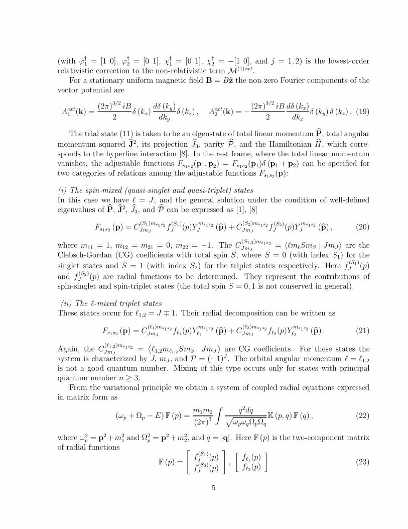
For a stationary uniform magnetic field B = Bz the non-zero Fourier components of thevector potential are

Aext1 (k) =

(2π)3/2 iB

2δ (kx)

dδ (ky)

dky

δ (kz) , Aext2 (k) = −(2π)3/2 iB

2

dδ (kx)

dkx

δ (ky) δ (kz) . (19)

The trial state (11) is taken to be an eigenstate of total linear momentum P, total angular

momentum squared J2, its projection J3, parity P, and the Hamiltonian H , which corre-sponds to the hyperfine interaction [8]. In the rest frame, where the total linear momentumvanishes, the adjustable functions Fs1s2

(p1,p2) = Fs1s2(p1)δ (p1 + p2) can be specified for

two categories of relations among the adjustable functions Fs1s2(p):

(i) The spin-mixed (quasi-singlet and quasi-triplet) statesIn this case we have ℓ = J , and the general solution under the condition of well-definedeigenvalues of P, J2, J3, and P can be expressed as [1], [8]

Fs1s2(p) = C

(S1)ms1s2

JmJf

(S1)J (p)Y

ms1s2

J (p) + C(S2)ms1s2

JmJf

(S2)J (p)Y

ms1s2

J (p) , (20)

where m11 = 1, m12 = m21 = 0, m22 = −1. The C(S1,2)ms1s2

JmJ= 〈ℓmℓSmS | JmJ〉 are the

Clebsch-Gordan (CG) coefficients with total spin S, where S = 0 (with index S1) for the

singlet states and S = 1 (with index S2) for the triplet states respectively. Here f(S1)J (p)

and f(S2)J (p) are radial functions to be determined. They represent the contributions of

spin-singlet and spin-triplet states (the total spin S = 0, 1 is not conserved in general).

(ii) The ℓ-mixed triplet statesThese states occur for ℓ1,2 = J ∓ 1. Their radial decomposition can be written as

Fs1s2(p) = C

(ℓ1)ms1s2

JmJfℓ1(p)Y

ms1s2

ℓ1(p) + C

(ℓ2)ms1s2

JmJfℓ2(p)Y

ms1s2

ℓ2(p) . (21)

Again, the C(ℓ1,2)ms1s2

JmJ=⟨ℓ1,2mℓ1,2

SmS | JmJ

⟩are CG coefficients. For these states the

system is characterized by J, mJ , and P = (−1)J . The orbital angular momentum ℓ = ℓ1,2

is not a good quantum number. Mixing of this type occurs only for states with principalquantum number n ≥ 3.

From the variational principle we obtain a system of coupled radial equations expressedin matrix form as

(ωp + Ωp − E) F (p) =m1m2

(2π)3

∫q2dq√

ωpωqΩpΩq

K (p, q) F (q) , (22)

where ω2p = p2 +m2

1 and Ω2p = p2 +m2

2, and q = |q|. Here F (p) is the two-component matrixof radial functions

F (p) =

[f

(S1)J (p)

f(S2)J (p)

],

[fℓ1(p)fℓ2(p)

](23)

5

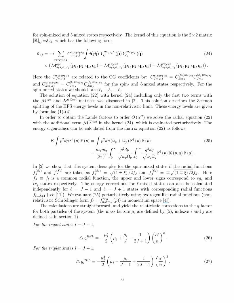
for spin-mixed and ℓ-mixed states respectively. The kernel of this equation is the 2×2 matrix[K]ij =Kij, which has the following form

Kij = −i∑

s1s2σ1σ2

Cs1s2σ1σ2

JmJ ij

∫dqdp Y

ms1s2∗

ℓi(p) Y

mσ1σ2

ℓj(q) (24)

×(Mope

s1s2σ1σ2(p1,p2,q1,q2) + M(1)ext

s1s2σ1σ2(p1,p2,q1,q2) + M(2)ext

s1s2σ1σ2(p1,p2,q1,q2)

).

Here the Cs1s2σ1σ2

JmJ ij are related to the CG coefficients by: Cs1s2σ1σ2

JmJ ij = C(Si)ms1s2

JmJC

(Sj)ms1s2

JmJ

and Cs1s2σ1σ2

JmJ ij = C(ℓi)ms1s2

JmJC

(ℓj)mσ1σ2

JmJfor the spin- and ℓ-mixed states respectively. For the

spin-mixed states we should take ℓi ≡ ℓj ≡ ℓ.The solution of equation (22) with kernel (24) including only the first two terms with

the Mope and M(1)ext matrices was discussed in [2]. This solution describes the Zeemansplitting of the HFS energy levels in the non-relativistic limit. These energy levels are givenby formulae (1)-(4).

In order to obtain the Lande factors to order O (α′2) we solve the radial equation (22)with the additional term M(2)ext in the kernel (24), which is evaluated perturbatively. Theenergy eigenvalues can be calculated from the matrix equation (22) as follows:

E

∫p2dpF† (p) F (p) =

∫p2dp (ωp + Ωp) F

† (p) F (p) (25)

− m1m2

(2π)3

∫ ∞

0

p2dp√ωpΩp

∫ ∞

0

q2dq√ωqΩq

F† (p) K (p, q) F (q) .

In [2] we show that this system decouples for the spin-mixed states if the radial functions

f(S1)J and f

(S1)J are taken as f

(S1)J =

√(1 ± ξ) /2fJ and f

(S1)J = ∓

√(1 ∓ ξ) /2fJ . Here

fJ ≡ fℓ is a common radial function, the upper and lower signs correspond to sgq andtrq states respectively. The energy corrections for ℓ-mixed states can also be calculatedindependently for ℓ = J − 1 and ℓ = J + 1 states with corresponding radial functionsfℓ=J∓1 (see [11]). We evaluate (25) perturbatively using hydrogen-like radial functions (non-relativistic Schrodinger form fℓ = fSch

n,J,mJ(p)) in momentum space [4]).

The calculations are straightforward, and yield the relativistic corrections to the g-factorfor both particles of the system (the mass factors µi are defined by (5), indexes i and j aredefined as in section 1).

For the triplet states l = J − 1,

gRELi = −

µ2j

2

(µj +

µi

J− 1

2J + 1

)(α′

n

)2

. (26)

For the triplet states l = J + 1,

gRELi = −

µ2j

2

(µj −

µi

J + 1+

1

2J + 1

)(α′

n

)2

. (27)

6

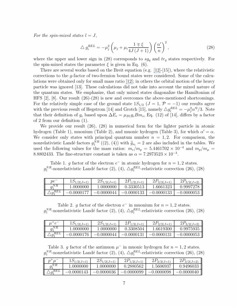
For the spin-mixed states l = J ,

gRELi = −µ2

j

(µj + µi

1 ∓ ξ

4J (J + 1)

)(α′

n

)2

, (28)

where the upper and lower sign in (28) corresponds to sgq and trq states respectively. Forthe spin-mixed states the parameter ξ is given in Eq. (6).

There are several works based on the Breit equation (e.g. [12]-[15]), where the relativisticcorrections to the g-factor of two-fermion bound states were considered. Some of the calcu-lations were obtained only for small mass ratio [12]; in others the orbital motion of the heavyparticle was ignored [13]. These calculations did not take into account the mixed nature ofthe quantum states. We emphasize, that only mixed states diagonalize the Hamiltonian ofHFS [2], [8]. Our result (26)-(28) is new and overcomes the above-mentioned shortcomings.For the relatively simple case of the ground state 1S1/2 (J = 1, P = −1) our results agreewith the previous result of Hegstrom [14] and Grotch [15], namely gREL

i = −µ2jα

′2/3. Notethat their definition of ge based upon ∆Ee = µB1geBms, Eq. (12) of [14], differs by a factorof 2 from our definition (1).

We provide our result (26), (28) in numerical form for the lighter particle in atomichydrogen (Table 1), muonium (Table 2), and muonic hydrogen (Table 3), for which α′ = α.We consider only states with principal quantum number n = 1, 2. For comparison, thenonrelativistic Lande factors gNR

1 ((2), (4)) with gs1= 2 are also included in the tables. We

used the following values for the mass ratios: me/mp = 5.4461702 × 10−4 and mp/mµ =8.8802433. The fine-structure constant is taken as α = 7.2973523 × 10−3.

Table 1. g factor of the electron e− in atomic hydrogen for n = 1, 2 states.gNR1 -nonrelativistic Lande factor (2), (4), gREL

1 -relativistic correction (26), (28)

pe− 1S1/2(J=1) 2S1/2(J=1) 2P1/2(J=1) 2P3/2(J=1) 2P3/2(J=2)

gNR1 1.0000000 1.0000000 0.3330513 1.6661323 0.9997278

gREL1 −0.0000177 −0.0000044 −0.0000133 −0.0000133 −0.0000053

Table 2. g factor of the electron e− in muonium for n = 1, 2 states.gNR1 -nonrelativistic Lande factor (2), (4), gREL

1 -relativistic correction (26), (28)

µ+e− 1S1/2(J=1) 2S1/2(J=1) 2P1/2(J=1) 2P3/2(J=1) 2P3/2(J=2)

gNR1 1.0000000 1.0000000 0.3308504 1.6619300 0.9975935

gREL1 −0.0000176 −0.0000044 −0.0000131 −0.0000131 −0.0000053

Table 3. g factor of the antimuon µ− in muonic hydrogen for n = 1, 2 states.gNR1 -nonrelativistic Lande factor (2), (4), gREL

1 -relativistic correction (26), (28)

p+µ− 1S1/2(J=1) 2S1/2(J=1) 2P1/2(J=1) 2P3/2(J=1) 2P3/2(J=2)

gNR1 1.0000000 1.0000000 0.2880562 1.5606937 0.9496033

gREL1 −0.0000143 −0.0000036 −0.0000099 −0.0000098 −0.0000040

7

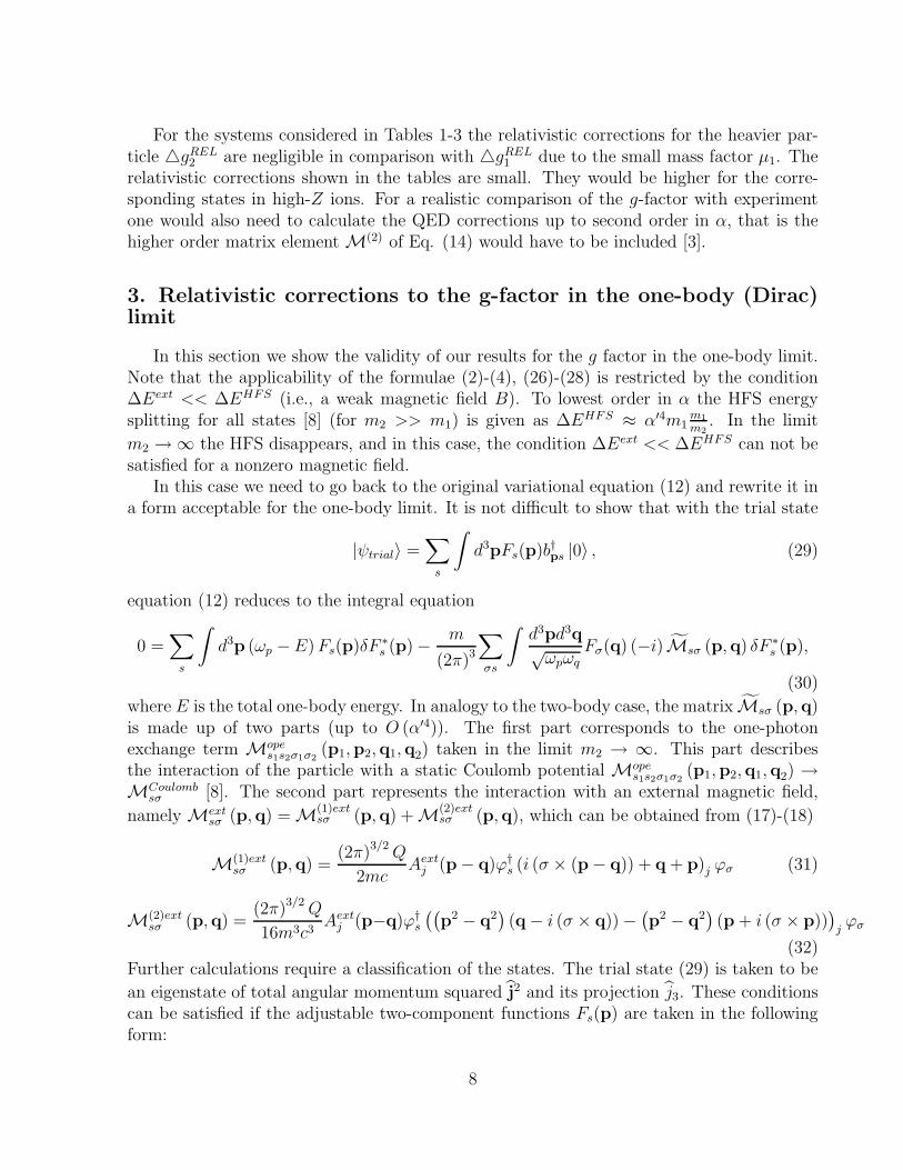
For the systems considered in Tables 1-3 the relativistic corrections for the heavier par-ticle gREL

2 are negligible in comparison with gREL1 due to the small mass factor µ1. The

relativistic corrections shown in the tables are small. They would be higher for the corre-sponding states in high-Z ions. For a realistic comparison of the g-factor with experimentone would also need to calculate the QED corrections up to second order in α, that is thehigher order matrix element M(2) of Eq. (14) would have to be included [3].

3. Relativistic corrections to the g-factor in the one-body (Dirac)limit

In this section we show the validity of our results for the g factor in the one-body limit.Note that the applicability of the formulae (2)-(4), (26)-(28) is restricted by the condition∆Eext << ∆EHFS (i.e., a weak magnetic field B). To lowest order in α the HFS energysplitting for all states [8] (for m2 >> m1) is given as ∆EHFS ≈ α′4m1

m1

m2

. In the limit

m2 → ∞ the HFS disappears, and in this case, the condition ∆Eext << ∆EHFS can not besatisfied for a nonzero magnetic field.

In this case we need to go back to the original variational equation (12) and rewrite it ina form acceptable for the one-body limit. It is not difficult to show that with the trial state

|ψtrial〉 =∑

s

∫d3pFs(p)b†

ps |0〉 , (29)

equation (12) reduces to the integral equation

0 =∑

s

∫d3p (ωp −E)Fs(p)δF ∗

s (p) − m

(2π)3

∑

σs

∫d3pd3q√ωpωq

Fσ(q) (−i)Msσ (p,q) δF ∗s (p),

(30)

where E is the total one-body energy. In analogy to the two-body case, the matrix Msσ (p,q)is made up of two parts (up to O (α′4)). The first part corresponds to the one-photonexchange term Mope

s1s2σ1σ2(p1,p2,q1,q2) taken in the limit m2 → ∞. This part describes

the interaction of the particle with a static Coulomb potential Mopes1s2σ1σ2

(p1,p2,q1,q2) →MCoulomb

sσ [8]. The second part represents the interaction with an external magnetic field,

namely Mextsσ (p,q) = M(1)ext

sσ (p,q) + M(2)extsσ (p,q), which can be obtained from (17)-(18)

M(1)extsσ (p,q) =

(2π)3/2Q

2mcAext

j (p− q)ϕ†s (i (σ × (p− q)) + q + p)j ϕσ (31)

M(2)extsσ (p,q) =

(2π)3/2 Q

16m3c3Aext

j (p−q)ϕ†s

((p2 − q2

)(q − i (σ × q)) −

(p2 − q2

)(p + i (σ × p))

)jϕσ

(32)Further calculations require a classification of the states. The trial state (29) is taken to be

an eigenstate of total angular momentum squared j2 and its projection j3. These conditionscan be satisfied if the adjustable two-component functions Fs(p) are taken in the followingform:

8

For states ℓ = j − 1/2

F1 (p) = fj− 1

2

(p)Cℓmℓ

1

2

1

2

jmjY

mj−1/2

j−1/2 (p) , F2 (p) = fj− 1

2

(p)Cℓmℓ

1

2− 1

2

jmjY

mj+1/2

j−1/2 (p) (33)

For states ℓ = j + 1/2

F1 (p) = fj+ 1

2

(p)Cℓmℓ

1

2

1

2

jmjY

mj−1/2

j+1/2 (p) , F2 (p) = fj+ 1

2

(p)Cℓmℓ

1

2− 1

2

jmjY

mj+1/2

j+1/2 (p) , (34)

where Cℓmℓsms

jmj= 〈ℓmℓsms | jmj〉 are the CG coefficients for s = 1/2, ms = ±1/2.

After substitution of these formulae into (30) and completion of the variational procedurewe obtain the radial equation

(ωp −E) fℓ (p) =m

(2π)3

∫q2dq

√ωpωq

Kℓ (p, q) fℓ (p) , (35)

where the kernel Kℓ (p, q) is expressed through the matrix M and coefficients Cσ′σjmj

=

Cℓmℓsmσ′

jmjCℓmℓsmσ

jmj, namely

Kℓ (p, q) = −i∑

σ′σ

Cσ′σjmj

∫dqdp

(MCoulomb

σ′σ + M(1)extσ′σ (p,q) + M(2)ext

σ′σ (p,q))Y

mσ′∗ℓ (p) Y mσ

ℓ (q) ,

(36)with σ′ = 1, 2, σ = 1, 2, and m1,2 = mj ∓ 1/2.

In the absence of an external magnetic field, equation (35) represents the relativisticradial equation in momentum space for a bound one-body system. As was shown in [8],the solution of the two-body equation (22) reduces to the solution of the one-body equation(35).

We now evaluate the contribution of the next two terms M(1)extσ′σ (p,q) and M(2)ext

σ′σ (p,q)of equations (31) and (32). The relevant energy ∆Eext

j,mj ,ℓ can be calculated perturbatively

like in the two-body case (cf. Eq. (25)). We obtain

∆Eextj,mj ,ℓ = µBgDBmj , (37)

wheregD = gL (ℓ, j) + gREL

D (n, j) . (38)

Here gL (ℓ) is the usual result for the anomalous Zeeman effect, being the Lande g factor,whose value is ([4]):

gL (ℓ, j) =2j + 1

2ℓ+ 1. (39)

The second term is the relativistic correction to the gD factor

gRELD (n, j) = − (2j + 1)2

8j (j + 1)

(α′

n

)2

. (40)

Formulae (39) and (40) coincide with the result of the expansion (up to O (α′2)) of the generalformula for the g-factor obtained by Margenau [16] on the basis of the Dirac equation withα′ = Zα.

9

4. Concluding remarks

We considered the relativistic theory of the Zeeman splitting and the g-factor of thehyperfine structure in the two-fermion system on the basis of variational relativistic equationsderived from quantum electrodynamics [1]. Relativistic corrections to the g-factor beyondthe non-relativistic formulae (2)-(4) (from Ref. [2]) were calculated up to order O (α′2) for allquantum states, and are given in Eqs. (26)-(28). The g-factor corrections take into accountthe mixed nature of the states (spin-mixing and ℓ-mixing), and the orbital motion of theheavy particle. They are obtained for arbitrary mass ratio and are symmetrical with respectto the masses of the constituent particles. For the ground state our result reduces to thewell-known formula obtained some time ago by Hegstrom [14] and Grotch [15]. We showthat in the one-body case the solution of the variational relativistic equation reproduces theresult for the g-factor obtained from the Dirac equation.

In our calculations we assumed that the trial state (11) is an eigenstate of the total

linear momentum operator P . However this is only an approximation, because one can showthat the operator P does not commute with the HFS Hamiltonian. To fix this problem weneed to modify the trial state, or use an appropriate unitary transformation for the HFSHamiltonian. The latter approach was discussed in the literature [12], [13], [17]. An analysisshows, that in our case the unitary transformation leads to the appearance of additionalterms in the invariant M-matrix. This is a technically difficult problem which we postponefor the future.

We note that, in contrast to the Breit approach, the anomalous magnetic moment is notintroduced from another calculation. As discussed in section 2 (below equation (13)) allQED effects are contained in the M-matrix. The anomalous magnetic moment will appearnaturally in our calculations if we include the next term M(2) of the expansion of M- matrixin (13).

Concerning comparison with experiment we note that measurements so far appear to berestricted to states where the spin structure of the heavier particle can be ignored. Thisincludes data for the 1S1/2 state in ions [18], [19]. The present work will be of practicalimportance when these measurements will be extended to all n = 2 (or higher-n) levels.

Acknowledgment

AGT and MH acknowledge the financial support of the Natural Sciences and EngineeringResearch Council of Canada for this work.

10

References

1. A. G. Terekidi, J. W. Darewych, M. Horbatsch, Can. J. Phys. 85, 813-836.(2007).2. A. G. Terekidi, J. W. Darewych, M. Horbatsch, Phys. Rev. A 75, 043401 (2007).3. V. W. Hughes and G. zu Putlitz, in Quantum Electrodynamics, edited by T. Kinoshita

(World Scientific, Singapore, 1990), p. 822.4. H. A. Bethe and E. E. Salpeter, Quantum Mechanics of One- and Two-Electron Atoms

(Springer, 1957).5. M. Mizushima, Quantum Mechanics of Atomic Spectra and Atomic Structure (W. A.

Benjamin, 1970). p.331.6. G. K. Woodgate, Elementary atomic structure (Clarendon Press, Oxford, 1980).7. J. Schwinger, Phys. Rev. 73, 416 (1948).8. A. G. Terekidi, J. W. Darewych, Journal of Mathematical Physics 46, 032302 (2005).9. J. W. Darewych, Annales Fond. L. de Broglie (Paris) 23, 15 (1998).10. J. W. Darewych, in Causality and Locality in Modern Physics, G Hunter et al. (eds.),

p. 333, (Kluwer, 1998).11. A. G. Terekidi, J. W. Darewych, Journal of Mathematical Physics 45, 1474 (2004).12. H. Grotch, R. Kashuba, Phys. Rev. A, 7, 78-84 (1973)13. J. M. Anthony, K. J. Sebastian, Phys. Rev. A, 49, 192-206 (1994)14. R. A. Hegstrom, Phys. Rev. 184, 1, p. 17-22 (1969).15. H. Grotch, Phys. Rev. Let. 24, 2, p.39-42 (1970).16. H. Margenau, Phys. Rev. 57, p. 387-386 (1940).17. H Grotch, Roger A. Hegstrom, Phys. Rev. A, 4, 59-69 (1971).18. J. L. Verdu, S. Djekic, S. Stahl, T. Valenzuela, M. Vogel, G. Werth, T. Beier, H. -J.

Kluge, and W. Quint, Phys. Rev. Lett. 92, 093002 (2004).19. D. L. Moskovkin, V. M. Shabaev, Phys. Rev. A, 73,.052506 (2006).

11