CERN-TH/99-282McGill/99-29

hep-ph/9909495

Details on the O(meα6) Positronium Hyperfine Splitting

due to Single Photon Annihilation

A.H. Hoanga, P. Labelleb and S.M. Zebarjadc

a Theory Division, CERN,CH-1211 Geneva 23, Switzerland

b Department of Physics, McGill University,Montreal, Quebec, Canada H3A 2T8

c Physics Department and Biruni Observatory,Shiraz University, Shiraz 71454, Iran

Abstract

A detailed presentation is given of the analytic calculation of the single-photon annihila-tion contributions for the positronium ground state hyperfine splitting, to order meα

6 inthe framework of non-relativistic effective theories. The current status of the theoreticaldescription of the positronium ground state hyperfine splitting is reviewed.

PACS numbers: 12.20.Ds, 31.30.Jv, 31.15.Md.

CERN-TH/99-282September 1999

1 Introduction

Quantum electrodynamics is the prototype of a quantum field theory, and it is fair to say that no onein the physics community has any doubt about its validity in describing the interactions of leptonsand photons. Nevertheless, continuous quantitative tests of QED, particularly at the level of highprecision, are important. The positronium system, a two-body bound state consisting of an electronand a positron, provides a clean testing ground of QED because the effects of the strong and theelectroweak interactions are negligible, even at the present accuracy of experimental measurements.The existence of positronium was predicted in 1934 [1] based on the relativistic quantum theorydeveloped by Dirac and experimentally verified at the beginning of the 1950s [2]. For the groundstate hyperfine splitting, the mass difference between the 13S1 (ortho) and 11S0 (para) states, the mostrecent experimental values read [3]

W ≡ Me+e−(13S1)−Me+e−(11S0) = 203 389.10(74) MHz (1)

and [4, 5]W = 203 387.5(1.6) MHz . (2)

They represent a precision of 3.6 and 7.9 ppm, respectively, which makes the calculation of all O(α2)(NNLO) corrections to the leading and next-to-leading order expression mandatory. Since the dom-inant contribution to the hyperfine splitting is of order meα

4, NNLO corrections correspond to thecontributions of order meα

6. Including also the known order meα7 ln2 α−1 contributions [6, 7] the

theoretical expression for the hyperfine splitting reads1

W = me α4[

712− α

π

(89

+12

ln 2)

+ α2(

524

lnα−1 +K

)− 7

8πα3 ln2 α−1

], (3)

where α is the fine-structure constant. At order meα6 it is convenient to distinguish between four

different sorts of corrections: non-annihilation, single-, two- and three-photon annihilation corrections.The two- and three-photon annihilation contributions have been calculated analytically in Refs. [9]and [10], respectively. The single-photon annihilation contributions have recently been determined inRefs. [11, 12]. In Ref. [12] an analytic result has been presented and in Ref. [11] a numerical one; thetwo results are in agreement. For the non-annihilation contributions, three different results exist inthe literature [13, 14, 15, 16], where Refs. [13, 14, 15] have presented numerical results and Ref. [16]analytical ones. The results of Refs. [14] and [16] are in agreement.

A modern and very economical method to calculate non-relativistic bound state problemsis based on the concept of effective field theories. This approach was first proposed in Ref. [13].The effective field theoretical approach to the positronium bound state problem is based on theexistence of widely separated scales in the positronium system. The physical effects associated to thesescales are separated by reformulating QED in terms of an effective non-relativistic, non-renormalizableLagrangian, where the low scale effects correspond to an infinite set of operators and the high scaleeffects are encoded in the coefficients of the operators. It is the characteristic feature of the effectivefield theoretical approach that it provides a set of systematic scaling (or power counting) rules thatallow for an easy identification of all terms that contribute to a certain order in the bound statecalculation. The results presented in Refs. [12, 13, 14, 16] have been obtained within an effective field

1We use natural units, in which h = c = 1. The term ∝ meα6 lnα−1 has been determined in Ref. [8].

2

theory approach. It is the purpose of this paper to present details of the analytical calculation ofthe order meα

6 single-photon annihilation contribution to the hyperfine splitting presented recentlyin Ref. [12].

The program of this paper is as follows: in Sec. 2 we give an overview of the effective field theoryapproach to the positronium bound state problem, and we explain the various steps in the calculation ofthe single-photon annihilation contributions to the hyperfine splitting. Section 3 contains a discussionof the subtleties of the cutoff regularization prescription that we use in our calculation. In Sec. 4 wedescribe in detail the calculation of the two-loop short-distance coefficient that is needed to determinethe single-photon annihilation contributions to the hyperfine splitting at order meα

6, and in Sec. 5 wepresent the bound state calculation, which leads to the final result. A generalization of the result forthe single-photon annihilation contributions to the hyperfine splitting to general radial excitations isgiven in Sec. 6. Section 7 outlines the status of the theoretical calculations of the hyperfine splitting,and Sec. 8 contains a summary. At the end of this work we have attached an appendix where we givea collection of integrals that is useful for the matching calculation.

2 The Conceptual Framework

The dynamics of a non-relativistic e+e− pair bound together in the positronium is governed by threewidely separated scales: me, meα and meα

2. Because we are dealing with a Coulombic system,where the electron/positron velocity v is of order α (v ∼ α), we could equally well talk about thescales mev and mev

2 instead of meα and meα2. These three scales govern different kinds of physical

processes of the positronium dynamics. The hard scale me is associated with e+e− annihilation andproduction processes, the dynamics of the small component and photons with virtuality of the orderof the electron mass. The soft scale mev governs the binding of the e+e− pair into a bound stateand directly sets the scale of the size of the bound state wave function, the inverse Bohr radius. Theultrasoft scale mev

2 is of the order of the binding energy and governs low virtuality photon radiationprocesses. These processes are associated with higher Fock states, where one has to consider theextended system e+e−γ rather than only an electron–positron pair. Because the interactions betweenthe e+e− pair associated with a low virtuality photon can arise with a temporal retardation, the effectscaused by these higher Fock states are called “retardation effects”. The Lamb shift in hydrogen is themost famous effect of this sort. The effective field theoretical approach uses the hierarchy of thesescales (me � meα � meα

2) to successively integrate out momenta of the order of the hard and thesoft scale, and, by the same means, to separate the effects associated with them. In this section wegive a brief overview onto the conceptual issues involved in this method following Refs. [13, 17, 18, 19].It is the strength of the effective field theoretical approach that it provides systematical momentumscaling rules (also called power counting rules) which allow an easy identification of all effects thathave to be taken into account for a calculation at a specific order. We apply these scaling rules toshow that retardation effects do not contribute to the hyperfine splitting at order meα

6.NRQED is the effective field theory, which is obtained from QED after all hard elec-

tron/positron and photon momenta, and the respective antiparticle poles associated with the small

3

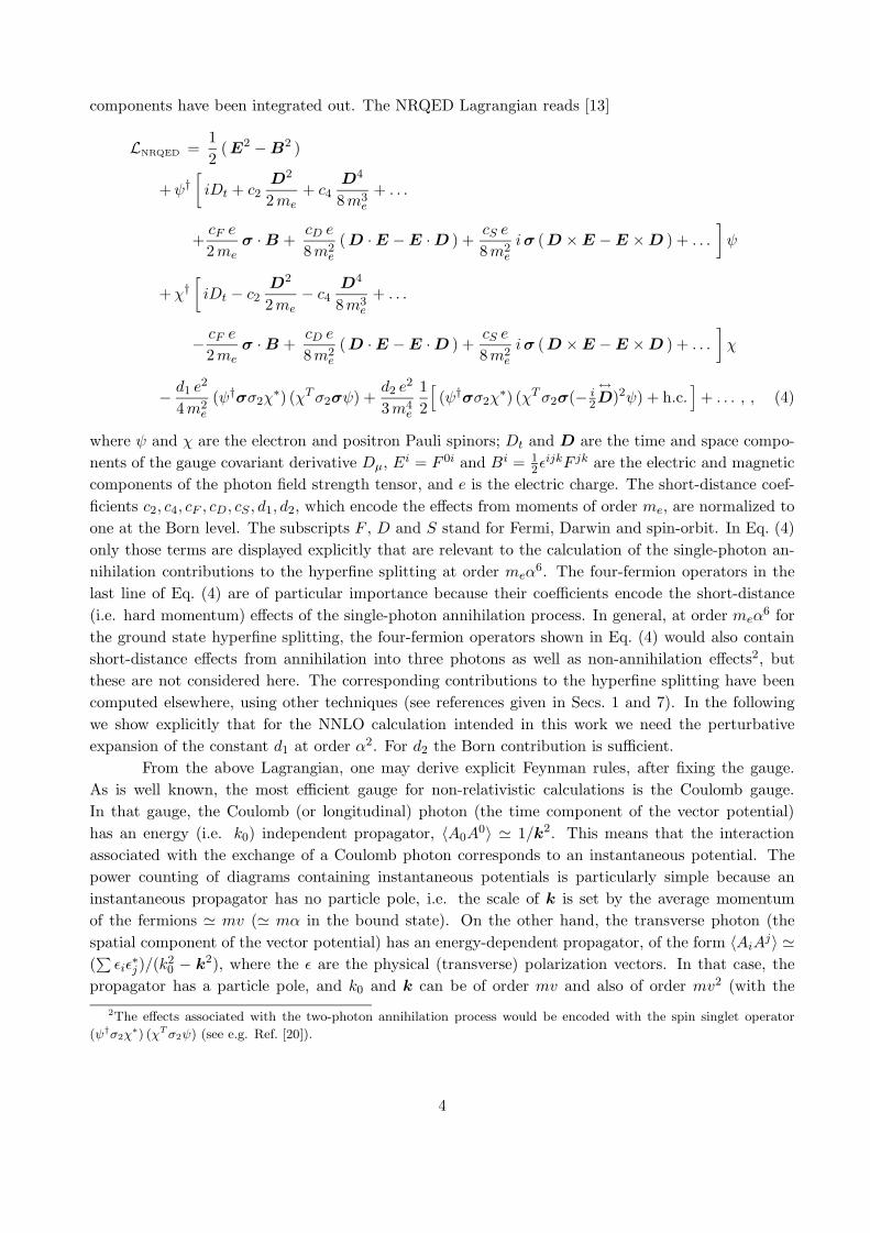
components have been integrated out. The NRQED Lagrangian reads [13]

LNRQED =12

(E2 −B2 )

+ψ†[iDt + c2

D2

2me+ c4

D4

8m3e

+ . . .

+cF e

2meσ ·B +

cD e

8m2e

(D ·E −E ·D ) +cS e

8m2e

iσ (D ×E −E ×D ) + . . .

]ψ

+χ†[iDt − c2

D2

2me− c4

D4

8m3e

+ . . .

− cF e

2meσ ·B +

cD e

8m2e

(D ·E −E ·D ) +cS e

8m2e

iσ (D ×E −E ×D ) + . . .

]χ

− d1 e2

4m2e

(ψ†σσ2χ∗) (χTσ2σψ) +

d2 e2

3m4e

12

[(ψ†σσ2χ

∗) (χTσ2σ(− i2

↔D)2ψ) + h.c.

]+ . . . , , (4)

where ψ and χ are the electron and positron Pauli spinors; Dt and D are the time and space compo-nents of the gauge covariant derivative Dµ, Ei = F 0i and Bi = 1

2εijkF jk are the electric and magnetic

components of the photon field strength tensor, and e is the electric charge. The short-distance coef-ficients c2, c4, cF , cD, cS , d1, d2, which encode the effects from moments of order me, are normalized toone at the Born level. The subscripts F , D and S stand for Fermi, Darwin and spin-orbit. In Eq. (4)only those terms are displayed explicitly that are relevant to the calculation of the single-photon an-nihilation contributions to the hyperfine splitting at order meα

6. The four-fermion operators in thelast line of Eq. (4) are of particular importance because their coefficients encode the short-distance(i.e. hard momentum) effects of the single-photon annihilation process. In general, at order meα

6 forthe ground state hyperfine splitting, the four-fermion operators shown in Eq. (4) would also containshort-distance effects from annihilation into three photons as well as non-annihilation effects2, butthese are not considered here. The corresponding contributions to the hyperfine splitting have beencomputed elsewhere, using other techniques (see references given in Secs. 1 and 7). In the followingwe show explicitly that for the NNLO calculation intended in this work we need the perturbativeexpansion of the constant d1 at order α2. For d2 the Born contribution is sufficient.

From the above Lagrangian, one may derive explicit Feynman rules, after fixing the gauge.As is well known, the most efficient gauge for non-relativistic calculations is the Coulomb gauge.In that gauge, the Coulomb (or longitudinal) photon (the time component of the vector potential)has an energy (i.e. k0) independent propagator, 〈A0A

0〉 ' 1/k2. This means that the interactionassociated with the exchange of a Coulomb photon corresponds to an instantaneous potential. Thepower counting of diagrams containing instantaneous potentials is particularly simple because aninstantaneous propagator has no particle pole, i.e. the scale of k is set by the average momentumof the fermions ' mv (' mα in the bound state). On the other hand, the transverse photon (thespatial component of the vector potential) has an energy-dependent propagator, of the form 〈AiA

j〉 '(∑εiε

∗j)/(k

20 − k2), where the ε are the physical (transverse) polarization vectors. In that case, the

propagator has a particle pole, and k0 and k can be of order mv and also of order mv2 (with the2The effects associated with the two-photon annihilation process would be encoded with the spin singlet operator

(ψ†σ2χ∗) (χTσ2ψ) (see e.g. Ref. [20]).

4

condition that k0 ≤ |k| ([19, 21])). This has the consequence that NRQED diagrams containingtransverse photons involve contributions from these two scales and, therefore, do not contribute toa unique order in v (or α in a bound state). This fact can be easily illustrated in the contextof old-fashioned (or “time-ordered”) perturbation theory in which the integration over the energymomentum components (via the residues) is done from the very beginning, and one only has tointegrate over the spatial momentum components. Usually, the covariant approach is preferred overthe old-fashioned perturbation theory because a single covariant diagram contains several time-orderedconfigurations (which are recovered by performing the contour integration over the energy momentumcomponents). However, the advantage is lost in a non-relativistic application since the different time-ordered diagrams generally scale differently and it is in fact a disadvantage to combine them together.In old-fashioned perturbation theory, one finds that a diagram containing an electron–positron pairand a transverse photon will contain a propagator of the form (see [17] for more details)

1|k|

1p2

ext/me − p2/me − (p− k)2/2me − |k| , (5)

where pext ' p ' mev are the external and loop momenta of the fermions (we are working in thecentre-of-mass frame). From this, one can see that different contributions arise depending on whetherthe scale of |k| is set by p ' mev or by p2/me ' mev

2. The effects associated with the latter scaleare the retardation effects. The contributions from both momentum regions will not contribute to thesame order in v. It is, however, possible to generalize NRQED is such a way that the contributionsassociated to the different scales are coming from separate diagrams. This is achieved by simplyTaylor-expanding the NRQED diagrams containing Eq. (5) around k ' mev and around k ' mev

2

(the latter expansion is equivalent to a multipole expansion of the vertices) [17]. One finds that thelowest order term of the expansion around k ' mev gives a contribution of order∫

d3k1|k|

−1|k| '

(mev)3

(mev)2' mev , (6)

whereas the lowest order term of the expansion around k ' mev2 gives∫

d3k1|k|

1p2

ext/me − p2/me + k' (mev

2)3

(mev2)2' mev

2. (7)

This shows that the dominant contribution from the transverse photon exchange comes from the scalek ' mev and that, to leading order, the transverse photon propagator reduces to −1/k2 (which corre-sponds to simply approximating the transverse photon propagator 1/(k2

0 −k2) by −1/k2). To leadingorder, the diagrams containing transverse photons are therefore also instantaneous and one recoversthe simple power counting rules valid for the exchange of a Coulomb photon. At sub-leading order,things are more complicated, because both expansions must be taken into account but, fortunately,the instantaneous approximation will be sufficient for the present calculation, as will be shown below.

Because the dominant contribution from the exchange of a transverse photon between anelectron-positron pair is suppressed by v2 compared to the dominant contribution from a Coulombphoton exchange (see the electron/positron–photon couplings involving the B field in Eq. (4)) allinteractions at NNLO (i.e. up to order v2 with respect to the Coulomb exchange) can be written asa set of simple instantaneous potentials. In momentum space representation they are given by

VCoul(p, q) = − 4π α|p− q|2 + λ2

, (8)

5

VBF(p, q) = − 4π αm2

e

[ |p× q|2(|p− q|2 + λ2)2

− (p− q)× S− · (p− q)× S+

|p − q|2 + λ2

+ i32

(p× q) · (S− + S+)|p− q|2 + λ2

− 14

|p− q|2|p− q|2 + λ2

], (9)

V4(p, q) =2π α2m2

e

d1

[34

+ S− · S+

], (10)

V4der(p, q) = − 4π α3m4

e

(p2 + q2)[

34

+ S− · S+

], (11)

δHkin(p, q) = −(2π)3δ(3)(p− q)q4

4m3e

. (12)

Here, λ is a small fictitious photon mass introduced to regularize infrared divergences, S∓ are theelectron/positron spin operators, and α is the fine structure constant; VBF is the Breit–Fermi potentialin the Coulomb gauge, which includes the NNLO relativistic corrections to the Coulomb potentialfrom the longitudinal and transverse photon exchange. The potentials V4 and V4der come from thefour-fermion operators in Eq. (4) and account for the single-photon annihilation process at leadingorder and NNLO in the non-relativistic expansion. For convenience we will also count the NNLOkinetic energy correction in Eq. (12) as a potential.

Using the potentials given above, it is straightforward to derive the momentum space equationof motion for an off-shell, time-independent e+e−e+e− four-point function in the centre-of-mass frame,valid up to NNLO:[

p2

me− E

]G(p, q; s) +

∫d3q′

(2π)3V (p, q′) G(q, q′; s) = (2π)3 δ(3)(p − q) , (13)

whereE ≡ √

s− 2me (14)

is the centre-of-mass energy relative to the electron–positron threshold and

V (p, q) = VCoul(p, q) + VBF(p, q) + V4(p, q) + V4 der(p, q) + δHkin(p, q) . (15)

The equation of motion (13) is a relativistic extension of the non-relativistic Schrodinger equation ofthe Coulomb problem. Because the potentials VBF, V4, V4der and δHkin lead to ultra-violet divergences,it is important to consider Eq. (13) in the framework of a consistent regularization scheme. The formof the short-distance coefficient d1 depends on the choice of the regularization scheme. We will comeback to this issue in Sec. 3.

One can easily establish simple power counting rules showing that the potentials given aboveare all what is needed for our calculation 3: after factoring out the factors of 1/me that appearsexplicitly in the potentials, the only scale left in diagrams containing the potentials above is theinverse Bohr radius 〈p〉 ' meα. In order for the final result to have the dimensions of energy adiagram containing any of the potentials shown above will generate one more factor of 〈p〉 than thereare factors of inverse electron mass. If there are n factors of 1/me, the diagram will therefore generatea factor 〈p〉n+1/mn

e ' meαn+1. This is one source of powers of α. In addition, there are sums over

3We set aside subtleties arising in a cutoff regularization scheme. Those are discussed in Sec. 3.

6

intermediate states. Those contain a factor 1/(Eext − Eint), which scales like 1/(meα2). In order to

cancel this factor of 1/me, the diagram will also generate a factor of 〈p〉, which means that each sumover intermediate state brings in another factor of 1/α. Finally, one must multiply by the explicitfactors of α contained in the NRQED vertices and in the short distance coefficients. As a simpleillustration of the counting rules, we may consider the Coulomb interaction. The potential containsno inverse power of mass (so n = 0) and one explicit factor of α. In first order of perturbation theoryit therefore contributes to order meα

2, which is the same order as the contribution coming from theleading order kinetic energy. Adding one more Coulomb potential brings in an extra factor of α fromthe vertices, but this is cancelled by the inverse power of α generated by the sum over intermediatestates. The Coulomb interaction must therefore be summed up to all orders, as is well known. Thisargument also shows that the Coulomb potential is the only interaction that must be treated exactly,as all the other potentials contain at least two powers of inverse mass so that adding one of thosepotentials leads to a contribution of order mα4 (or higher).

From Eq. (13) we can now derive directly the formula for the single-photon annihilation contri-bution to the hyperfine splitting at order meα

6, W 1-γ annNNLO . Because the para-positronium state does not

contribute, owing to C invariance, one starts with the well-known n = 1, 3S1 e+e− bound state wave

function of the non-relativistic Coulomb problem and determines W 1-γ annNNLO via Rayleigh–Schrodinger

time-independent perturbation theory. Because we are interested in the single-photon annihilationcontributions only corrections with at least one insertion of V4 or V4der have to be taken into account.The formula for W 1-γ ann at order meα

6 then reads

W 1-γ ann = 〈 13S1 |V4 | 13S1 〉+ 〈 13S1 |V4 der | 13S1 〉

+〈 13S1 |V4

∑∫l 6=13S1

| l 〉 〈 l |E0 − El

V4 | 13S1 〉

+[〈 13S1 |V4

∑∫l 6=13S1

| l 〉 〈 l |E0 − El

(VBF + δHkin) | 13S1 〉+ h.c.]

+ . . . , (16)

where | l 〉 represent normalized (bound state and continuum) eigenstates to the Coulomb Schrodingerequation with the eigenvalues El; | 13S1 〉 and E0 = −meα

2/4 denote the state and binding energy ofthe n = 1, 3S1 Coulomb bound state. Using the counting rules developed above it is easy to showthat Eq. (16) is all we need to determine the ground state hyperfine splitting to order meα

6: thefour-fermion operator V4 contains two powers of inverse mass and one explicit factor of α (with theBorn level value for the coefficient d1, see Eq. (10)). The contribution of this interaction is thereforeof order meα

4. In order to obtain the O(meα6) contribution that we are looking for, we therefore

need to match the coefficient d1 to two loops, as mentioned above. The operator V4der, on the otherhand, contains four powers of inverse mass and therefore contributes already to order meα

6 with theBorn level coefficient given in Eq. (11). It is easy to verify that the terms evaluated in second orderof perturbation theory also contribute to this order if one uses the Born level coefficients in all thepotentials. Consider for example the term with two insertions of the potential V4. Since there arefour explicit powers of inverse mass, two explicit factors of α (with d1 set to 1), and one sum overintermediate states, the final contribution is of order meα

5+2−1 = meα6. The Breit potential obviously

contributes to the same order. The operator δHkin does not contain any factor of α, but it contains onemore power of inverse mass and therefore also contributes to order meα

6. All other potentials built

7

from the NRQED Feynman rules have higher powers of inverse mass and will therefore be suppressed.We note again that the Breit–Fermi potential VBF contains contributions arising from the exchange ofCoulomb photons and of transverse photons in the instantaneous approximation (i.e. without any k0-dependence in the propagator). Since, as we have shown before, the latter contribute already to ordermeα

6, we do not need to consider any sub-leading terms coming from the expansions around k ' mev.Terms from the expansion around k ' mev

2 do not need to be considered at all. The instantaneousapproximation for the transverse photons is therefore sufficient for the present calculation.

From the above discussion, it is clear that the calculation of W 1-γ annNNLO proceeds in two basic

steps.

1. Matching calculation – Calculation of the O(α) and O(α2) contributions to the constant d1 bymatching the QED amplitudes for the elastic s-channel scattering of free and on-shell electronsand positrons via a single photon, e+e− → γ → e+e−, close to threshold up to two loops and toNNLO in the velocity of the electrons and positrons in the centre-of-mass frame. This is possiblebecause the short-distance effects encoded in d1 do not depend on the kinematic situation towhich the NRQED Lagrangian is applied.

2. Bound state calculation – Calculation of formula on the RHS of Eq. (16).

The details of the calculations involved in steps 1 and 2 are presented in Secs. 4 and 5, respectively.To conclude this section we would also like to briefly mention a formal way to establish the

multipole expansion and the counting rules presented above. This is achieved by integrating outNRQED electron/positron and photon momenta of order meα. The resulting effective theory hasbeen called “potential NRQED” (PNRQED) [18]. The basic ingredient to construct PNRQED is toidentify the relevant momentum regions of the electron/positron and photon field in the NRQEDLagrangian (4). These momentum regions have been found in Ref. [19]. Because NRQED is notLorentz-covariant, the time and spatial components of the momenta are independent, which meansthat the time and spatial components can have a different scaling behaviour. The relevant momentumregions are “soft”4 (k0 ∼ mev, k ∼ mev), “potential” (k0 ∼ mev

2, k ∼ mev) and “ultrasoft” (k0 ∼mev

2, k ∼ mev2). It can be shown that electron, positrons and photons can have soft and potential

momenta, but that only photons can have ultrasoft momenta. A momentum region with k0 ∼ mev,k ∼ mev

2 does not exist. PNRQED is constructed by integrating out “soft” electrons/positrons andphotons and “potential” photons. In addition, the “potential” photon momenta have to be expandedin terms of their time component, because the latter scales with an additional power of α with respectto the spatial components. The exchange of “potential” photons between the electron and the positronthen leads to spatially non-local, but temporally instantaneous, four-fermion operators that representan instantaneous coupling of an electron–positron pair separated by a distance of order the inverseBohr radius ∼ meα. The coefficients of these operators are a generalization of the notion of aninstantaneous potential. Generically the PNRQED Lagrangian has the form

LPNRQED = LNRQED +∫d3r

(ψ†ψ

)(r)V (r)

(χ†χ

)(0) + . . . , (17)

where the tilde above LNRQED on the RHS of Eq. (17) indicates that the corresponding operatorsonly describe potential electrons/positrons and ultrasoft photonic degrees of freedom and that an

4The soft momentum regime has not been taken into account in the arguments employed in Ref. [17]. However, this

does not affect any conclusions concerning the ground state hyperfine splitting at order meα6.

8

expansion in momentum components ∼ meα2 is understood. To NNLO, the contributions to V are

just given in Eqs. (8) to (11). Using the scaling of “potential” electron/positron momenta, we see thatthe Coulomb potential scales like meα

2, i.e. it is of the same order as the electron/positron kineticenergy. Thus, the Coulomb potential has to be treated exactly rather than perturbatively. From thePNRQED Lagrangian it is straightforward to derive the momentum space equation of motion of anoff-shell, time-independent (e+e−)(e+e−) four-point function in the centre-of-mass frame valid up toorder α4, Eq. (13). Using the momentum scaling rules of PNRQED one can show that retardationeffects cannot contribute to W 1-γ ann at order meα

6. Retardation effects are caused by the ultrasoftphotons, because their low virtuality propagation can develop a pole for the momenta available inthe positronium system. Choosing again the Coulomb gauge for our argumentation, where the timecomponent of the Coulomb photon vanishes, only the transverse photon needs to be considered asultrasoft5. Thus the emission and subsequent absorption of an ultrasoft photon between the electron–positron pair are already suppressed by v2 ∼ α2 with respect to the Coulomb interaction owing to thecoupling of transverse photon to electrons/positrons. To see that an additional power of α arises fromthe corresponding loop integration over the ultrasoft photon momentum, let us compare the scaling ofthe product of the integration measure and the photon propagator in the potential and the ultrasoftmomentum regime. In the ultrasoft case the product of the integration measure d4k and the photonpropagator 1/k2 counts as α8×α−4 = α4, whereas in the potential case the result reads α5×α−2 = α3.Thus the exchange of an ultrasoft photon is suppressed by an addition power of α with respect tothe effects of the Breit–Fermi potential (9). In other words, retardation effects cannot contribute toW 1-γ ann at order meα

6. We would like to note that PNRQED is designed as a complete field theorycapable of describing the dynamics of a bound electron–positron pair and ultrasoft photons. Althoughuseful for establishing consistent counting rules, its full strength only develops if one explicitly considersthe dynamics of ultrasoft photons. For cases where the instantaneous approximation is sufficient –such as the ground state hyperfine splitting at order meα

6 – the introduction of PNRQED is notessential.

3 The Regularization Scheme

All equations in the previous section have to be considered within the framework of a consistent UVregularization scheme. In general, the form of the short-distance coefficients of the NRQED6 operatorsdepends on the choice of the regularization scheme. In this work we use a cutoff prescription toregularize the UV divergences, where the cutoff Λ is considered much larger than meα. The infrareddivergences, which arise in the intermediate steps of the matching calculation to determine the higherorder contributions to d1, are regularized by a small fictitious photon mass λ, see Eqs. (8) and (9).The use of a cutoff regularization involves a number of subtleties that shall be briefly discussed in thissection.

5The argument is true in any gauge after gauge cancellations. The argumentation is, however, most transparent in

the Coulomb gauge.6In what follows, when using the notion “NRQED”, we actually mean the generalized NRQED or PNRQED, as

discussed in Sec. 2.

9

kn-1 kn kn+1

Figure 1: Routing convention for loop momenta in ladder diagrams. Half of the external centre-of-massenergy is flowing through each of the electron and positron lines.

It is well known that the use of a cutoff regularization scheme leads to terms that violate gaugeinvariance and Ward identities. These effects, however, are generated at the cutoff and are, therefore,cancelled by corresponding terms with a different sign in the short-distance coefficients of the NRQEDoperators. Thus, gauge invariance and Ward identities are restored to the order at which the matchingcalculation has been carried out. Another subtlety is that a cutoff scheme is only well defined after aspecific momentum routing convention is adopted for loop diagrams in the effective field theory. It isnatural to choose the routing convention employed in the equation of motion (13). For clarity we haveillustrated this convention in Fig. 1. Because we only need to consider interactions in our calculationthat are instantaneous in time, only ladder-type diagrams have to be taken into account.

A very important feature of a cutoff regularization scheme is that it inevitably leads to power-counting-breaking effects. This means that NRQED operators can lead to effects that are belowthe order indicated by the momentum scaling rules described in the previous section. Examplesof this feature will be visible in the matching, and the bound state calculations presented in thenext two sections. These power-counting-breaking effects are a consequence of the fact that a cutoffregularization does not suppress divergences of scaleless integrals (as do analytic regularization schemeslike MS). To illustrate the problem let us consider the third term on the RHS of Eq. (16). This termcontains the contribution to W 1-γ ann coming from two insertions of the four-fermion operator V4.According to the momentum scaling rules described in the previous section, it can only contribute atorder meα

6. However, the bound state diagram with two V4 operators is linearly divergent and, usingthe momentum cutoff Λ, the result has, for dimensional reasons, the form Ameα

6 + BΛα5 where Aand B are finite constants (modulo logarithmic terms). If one counts the cutoff to be of the orderof me, then the diagram would contribute to both orders meα

5 and meα6. Even worse, by including

sufficiently high order operators (in the p/me expansion), one can easily convince oneself that aninfinite number of operators, having much higher dimension than indicated by the counting rules,would contribute to any given order in α, starting at order meα

5. However, contributions comingfrom those higher-dimension operators can only arise in the form of explicit cutoff-dependent termsand not as constants. As for the effects that violate gauge invariance and Ward identities, all termsdepending on the cutoff are cancelled in the combination of the bound state integrations and theshort-distance coefficient. In our perturbative calculation we can therefore simply ignore that thescaling violating terms coming from operators with dimensions higher than indicated by the counting

10

1 2

Figure 2: Graphical representation of the NRQED single-photon annihilation scattering diagrams atthe Born level and at NNLO in the non-relativistic expansion.

rules exist. For our calculation this means that we only have to calculate the terms presented on theRHS of Eq. (16), excluding the higher order corrections of d1 in the third and fourth terms.

Finally, we would like to mention that we implement our cutoff regularization scheme in sucha way that only divergent integrations are actually cut off. This choice simplifies the calculations,because we can use the known analytic solutions of the non-relativistic Coulomb problem for the 13S1

wave function and the Green function in our perturbative calculation. The fact that we use a specificrouting convention ensures that this does not lead to inconsistencies. In addition, we impose the cutoffonly on the spatial components of the loop momenta.

4 The Matching Calculation

The single-photon annihilation contributions of the short-distance coefficient of the operator(ψ†σσ2χ

∗) (χTσ2σψ) are obtained by matching the amplitude for elastic s-channel scattering of ane+e− pair via a virtual photon in full QED in the kinematical regime close to threshold to the sameamplitude determined in the non-relativistic effective theory NRQED. To determine the short-distancecoefficient d1 to order α2 we have to carry out the matching at the two-loop level, including all effectsup to NNLO in the non-relativistic expansion. Because we regulate infrared divergences in the effectivetheory using a small fictitious photon mass, we have to do the same in the full QED calculation.

To obtain the single-photon scattering amplitude in NRQED we have to calculate the Feyn-man diagrams depicted in Figs. 2, 3 and 4, where the various symbols are defined in Fig. 5. TheFeynman diagrams for the single-photon annihilation contributions of the NRQED scattering ampli-tude contain, as the formula for W 1-γ ann in Eq. (16), at least one insertion of V4 or V4der. As shownin the wave equation (13), we can use time-independent electron–positron propagators also for theNRQED scattering amplitude. This is possible because all interactions are instantaneous in time, i.e.the loop integration over the energy components of the NRQED electron and positron propagators istrivial by residue (see Eq. (26)). Because the single-photon annihilation process is only possible forthe electron–positron pair in a 3S1 spin triplet state, we only need to consider a spin and angularaverage of the Breit–Fermi potential:

V sBF(p, q) =

113π α

m2e

− 2π α

M2t

p2 + q2

(p− q)2 + λ2, (18)

11

1 2 3

4 5

Figure 3: Graphical representation of the NRQED single-photon annihilation scattering diagrams atthe one-loop level and at NNLO in the non-relativistic expansion.

where the angular integration it carried out over the angle between p and q. We have eliminatedthe photon mass in the first term on the RHS of Eq. (18) because it does not lead to any infrareddivergences. An additional simplification for the NRQED calculation is obtained by replacing thecentre-of-mass energy relative to the e+e− threshold, E =

√s − 2me, by the new energy parameter

p0, which is defined asp20 ≡

s

4−m2

e . (19)

The parameter p0 is equal to the relativistic centre-of-mass three-momentum of the electron/positronin the scattering process. At NNLO in the non-relativistic expansion we have the relation

E =p20

me− p4

0

4m3e

+ . . . , (20)

where we keep the term p20/me in the LO non-relativistic electron–positron propagator. In this con-

vention, the NNLO kinetic energy correction reads

δH∗kin(p, q) = −(2π)3 δ(3)(p− q)

q4 − p40

4m3e

(21)

and simplifies the form of an insertion of the kinetic energy correction∫d3q

(2π)3me

p2 − p20 − i ε

(− δH∗

kin(p, q)) me

q2 − p20 − i ε

=me

p2 − p20 − i ε

(p2 + p2

0

4m3e

). (22)

We emphasize that the introduction of the parameter p0 is just a technical trick for the matchingcalculation, which does not affect the form of d1. Using the 3S1 spin average

13

∑J=1,0,−1

[(ψ†σσ2χ

∗) (χTσ2σψ)]

= 2 (23)

for the four-fermion operators V4 and V4der in Eq. (4), we arrive at the following results for the diagramsdisplayed in Figs. 2, 3 and 4 (D(k) ≡ me/(k2 − p2

0 − iε)):

I(0)1 =

[1 +

(απ

)d(1)1 +

(απ

)2d(2)1

]2π αm2

e

, (24)

12

1 2 3

4 5 6

7 8 9

10 11 12

Figure 4: Graphical representation of the NRQED single-photon annihilation scattering diagrams atthe two-loop level and at NNLO in the non-relativistic expansion.

I(0)2 = − 8π α

3m2e

p20

m2e

, (25)

I(1)1 = 2 i

[1 +

(απ

)d(1)1

] (2π αm2

e

) ∫d4k

(2π)41

k0 + p20

2me− k2

2me

1

k0 − p20

2me+ k2

2me

4π α(k − p0)2 + λ2

= 2[1 +

(απ

)d(1)1

] (2π αm2

e

) ∫d3k

(2π)3D(k)

4π α(k − p0)2 + λ2

=[1 +

(απ

)d(1)1

]2α2

me p0

[π2

2+ i π ln

(2 p0

λ

) ], (26)

I(1)2 = −2

(4π α3m2

e

) ∫d3k

(2π)3

(k2 + p2

0

m2e

)D(k)

4π α(k − p0)2 + λ2

= − 4α2

3m2e

[4Λme

+p0 π

2

me+ 2 i π

p0

meln

(2 p0

λ

) ], (27)

I(1)3 = 2

(2π αm2

e

) ∫d3k

(2π)3D(k)

(k2 + p2

0

4m2e

)4π α

(k − p0)2 + λ2

13

V4 V4 der δHkin

VCoul VBF

Figure 5: Symbols describing the NRQED potentials that have to be taken into account for thematching calculation at NNLO in the non-relativistic expansion.

=α2

2m2e

[4Λme

+p0 π

2

me+ 2 i π

p0

meln

(2 p0

λ

) ], (28)

I(1)4 = 2

(2π αm2

e

) ∫d3k

(2π)3D(k)

(2π α

m2e

k2 + p20

(k − p0)2 + λ2− 11

3π α

m2e

)

=α2

m2e

[− 10Λ

3me+p0 π

2

me+ 2 i π

p0

me

(− 4

3+ ln

(2 p0

λ

) ) ], (29)

I(1)5 =

(2π αm2

e

)2 ∫d3k

(2π)3D(k) = − α2

m2e

[2Λme

+ i πp0

me

], (30)

I(2)1 =

(m2

e

8π α

) [I(1)1

]2, (31)

I(2)2 = 2

(2π αm2

e

) ∫d3k1

(2π)3

∫d3k2

(2π)3D(k1)

4π α(k1 − k2)2 + λ2

D(k2)4π α

(k2 − p0)2 + λ2

=π α3

2 p20

[π2

12− ln2

(2 p0

λ

)+ i π ln

(2 p0

λ

) ], (32)

I(2)3 = −

(4π α3m2

e

) ∫d3k1

(2π)3

∫d3k2

(2π)34π α

(p0 − k1)2 + λ2D(k1)

(k1

2 + k22

m2e

)D(k2)

4π α(k2 − p0)2 + λ2

= − 2α3

3πme p0

[π2

2+ i π ln

(2 p0

λ

) ] [4Λme

+p0 π

2

2me+ i π

p0

meln

(2 p0

λ

) ], (33)

14

I(2)4 = −2

(4π α3m2

e

) ∫d3k1

(2π)3

∫d3k2

(2π)3D(k1)

(p0

2 + k12

m2e

)4π α

(k1 − k2)2 + λ2D(k2)

4π α(k2 − p0)2 + λ2

= − 2α3

3me p0

[2Λme

(π + 2 i ln

(2 p0

λ

))− 2 p0 π

me

(1− π2

24+

12

ln2(2 p0

λ

)− i

π

2ln

(2 p0

λ

)) ], (34)

I(2)5 =

(m2

e

4π α

) [I(1)1

] [I(1)3

], (35)

I(2)6 = 2

(2π αm2

e

) ∫d3k1

(2π)3

∫d3k2

(2π)3D(k1)

(k1

2 + p20

4m2e

)4π α

(k1 − k2)2 + λ2D(k2)

4π α(k2 − p0)2 + λ2

=α3

4me p0

[2Λme

(π + 2 i ln

(2 p0

λ

))− 2 p0 π

me

(1− π2

24+

12

ln2(2 p0

λ

)− i

π

2ln

(2 p0

λ

)) ], (36)

I(2)7 = 2

(2π αm2

e

) ∫d3k1

(2π)3

∫d3k2

(2π)3D(k1)

4π α(k1 − k2)2 + λ2

D(k2)(

k22 + p2

0

4m2e

)4π α

(k2 − p0)2 + λ2

=π α3

m2e

[π2

48+ 1− ln

(2 p0

Λ

)− 1

4ln2

(2 p0

λ

)+ i

π

2

(1 +

12

ln(2 p0

λ

)) ], (37)

I(2)8 =

(m2

e

4π α

) [I(1)1

] [I(1)4

], (38)

I(2)9 = 2

(2π αm2

e

) ∫d3k1

(2π)3

∫d3k2

(2π)3D(k1)

(2π α

m2e

k12 + k2

2

(k1 − k2)2 + λ2− 11

3π α

m2e

)

×D(k2)(

k22 + p2

0

4m2e

)4π α

(k2 − p0)2 + λ2

=α3

me p0

[π p0

me

(π2

24+ 1− 1

2ln 2− 2 ln

(2 p0

Λ

)+

116

ln(2 p0

λ

)− 1

2ln2

(2 p0

λ

))

− 5Λ6me

(π + 2 i ln

(2 p0

λ

))+ i

π2 p0

2me

(16

+ ln(2 p0

λ

)) ], (39)

I(2)10 = 2

(2π αm2

e

) ∫d3k1

(2π)3

∫d3k2

(2π)3D(k1)

4π α(k1 − k2)2 + λ2

D(k2)

×(

2π α

m2e

k22 + p2

0

(k2 − p0)2 + λ2− 11

3π α

m2e

)

=π α3

2m2e

[π2

12+ 4 + ln 2 +

103

ln(2 p0

Λ

)− ln

(2 p0

λ

)− ln2

(2 p0

λ

)+ i π

(− 7

6+ ln

(2 p0

λ

)) ],(40)

I(2)11 =

(m2

e

2π α

) [I(1)1

] [I(1)5

], (41)

I(2)12 =

(2π αm2

e

)2 ∫d3k1

(2π)3

∫d3k2

(2π)3D(k1)

4π α(k1 − k2)2 + λ2

D(k2) =π α3

m2e

[ln

(2 p0

Λ

)− i

π

2

]. (42)

The upper index of the functions I(i)j corresponds to the power of the fine structure constant of the

diagrams and the lower index to the numeration given in Figs. 2, 3 and 4. Combinatorial factors are

15

taken into account. We note that all the above results have been given in the limit λ � p0 � me

and that only the powers of p0 relevant at NNLO have been kept. A collection of integrals that havebeen useful in determining the results given above is presented in Appendix. A. The full NRQEDamplitude reads

A1-γ annNRQED =

2∑i=1

I(0)i +

5∑i=1

I(1)i +

12∑i=1

I(2)i . (43)

The elastic single-photon annihilation amplitude in full QED can be obtained from the elec-tromagnetic form factors, which parametrize the radiative corrections to the electromagnetic vertex,and the photon vacuum polarization function. The electromagnetic form factors F1 (Dirac) and F2

(Pauli) are defined through

u(p′)Λemµ v(p) = i e u(p′)

[γµ F1(q2) +

i

2Mσµν q

ν F2(q2)]v(p) , (44)

for the e+e− production vertex, where q = p + p′ and σµν = i2 [ γµ, γν ]. We need the form factors

in the limit λ � p0 � me. The one-loop contributions have been known for a long time for allmomenta [22, 23], whereas the two-loop contributions have been calculated in the desired limit inRef. [24]. Parametrizing the loop corrections to the form factors as

F1(q2) = 1 +(απ

)F

(1)1 (q2) +

(απ

)2F

(2)1 (q2) + · · · ,

F2(q2) =(απ

)F

(1)2 (q2) +

(απ

)2F

(2)2 (q2) + · · · , (45)

and using the energy parameter p0 (Eq. (19)) the results for the form factors in the threshold regionat NNLO in the non-relativistic expansion read (λ� p0 � me):

F(1)1 (q2) = i

π me

2 p0

[`− 1

2

]− 3

2+ i

3π p0

4me

[`− 5

6

]+O

( p20

m2e

), (46)

F(2)1 (q2) =

π2m2e

8 p20

[− `2 + `− π2

6− 1

3

]− i πme

4 p0

[3 `− 1

]

−[π4

16+

3π2

8

(`2 − 4

3`+

4645

ln(− i

p0

me

)+

715

ln 2 +27291350

)

+980

(9 ζ3 − 43

) ]+O

( p0

me

), (47)

F(1)2 (q2) = i

π me

4 p0− 1

2− i

π p0

8me+O

( p20

m2e

), (48)

F(2)2 (q2) =

π2m2e

8 p20

[− `+

13

]− i πme

4 p0

[`+ 1

]

+[π2

8

(− `+

25

ln(− i

p0

me

)+

10115

ln 2− 1621450

)

+180

(41 ζ3 +

3479

) ]+O

( p0

me

), (49)

(50)

16

where` ≡ ln

(− 2 i p0

λ

). (51)

The photon vacuum polarization function Π is defined as

(q2 gµν − qµ qν)Π(q2) ≡ i

∫d4x eiqx 〈 0 |T jµ(x) jν(0) | 0 〉 , (52)

where jν is the electromagnetic current. The one- and two-loop contributions to Π are also known fromRefs. [22, 23] for all values of q2 and read, expanded up to NNLO in the non-relativistic expansion,

Π(q2) =(απ

)Π(1)(q2) +

(απ

)2Π(2)(q2) + · · · , (53)

with

Π(1)(q2)p0�me=

89

+ iπ p0

2me+O

( p20

m2e

), (54)

Π(2)(q2) p0�me= −π2

2

(ln

(− i

p0

me

)− 11

16+

32

ln 2)− 21

8ζ3 +

34

+O( p0

me

). (55)

Including all effects up to NNLO in p0/me and taking the 3S1 spin average, the QED amplitude reads

A1-γ annQED =

(2απm2

e

) (1− p2

0

m2e

)1

1 + Π(q2)

[ (1− p2

0

6m2e

)F1(q2) +

(1 +

p20

6m2e

)F2(q2)

]2

. (56)

The short-distance coefficient d1 is determined by requiring equality of all the terms up to order α3

and NNLO in p0/me in the QED and the NRQED amplitudes in Eqs. (56) and (43). The result ford1 reads

d1 = 1 +(απ

)d(1)1 +

(απ

)2d(2)1 + · · · , (57)

where

d(1)1 =

133

Λme

− 449, (58)

d(2)1 = −π

2

6ln

( Λme

)+

138ζ3 − 1483π2

288+

9π2

4ln 2 +

147781

. (59)

5 The Bound State Calculation

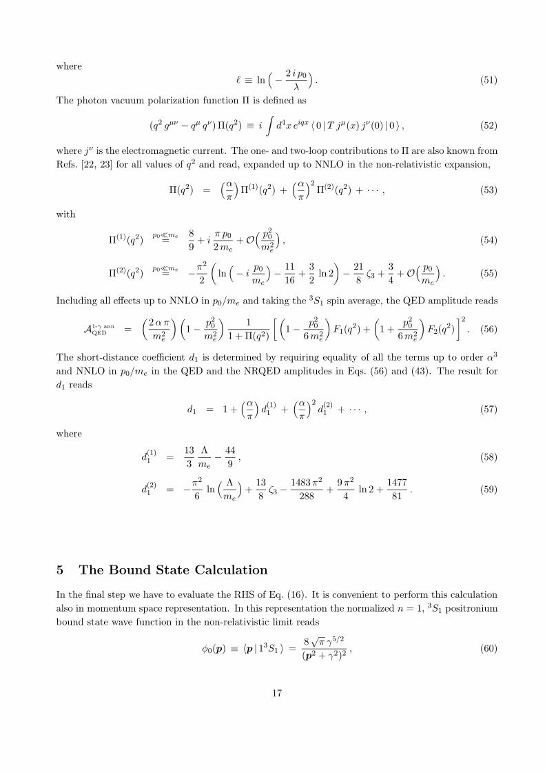
In the final step we have to evaluate the RHS of Eq. (16). It is convenient to perform this calculationalso in momentum space representation. In this representation the normalized n = 1, 3S1 positroniumbound state wave function in the non-relativistic limit reads

φ0(p) ≡ 〈p | 13S1 〉 =8√π γ5/2

(p2 + γ2)2, (60)

17

whereγ ≡ me α

2. (61)

We also need a momentum space expression for the sum over intermediate Coulomb states in thethird and fourth terms on the RHS of Eq. (16). This sum is just the Green function of the non-relativistic Coulomb problem, where the n = 1, 3S1 ground state pole is subtracted and E = E0 =−meα

2/4. A compact momentum space integral representation for the Coulomb Green function hasbeen determined by Schwinger [25]:

〈p |∑∫l

| l 〉 〈 l |El − E − i ε

| q 〉 =(2π)3 δ(3)(p − q)me

p2 −meE − i ε+

me

p2 −mE − i ε

4π α(p − q)2

me

q2 −mE − i ε(62)

− 4π αme

p2 −mE − i ε

1∫0

dxi η x−i η

(p − q)2 x− 14 me E (p2 −meE − i ε) (q2 −meE − i ε) (1 − x)2

me

q2,

where

i η =α

2

√me

−E − i ε. (63)

Taking the limit E → E0 the third term on the RHS of Eq. (62) develops the n = 1, 3S1 pole,|φ0(p)|2/(E0 −E). After subtraction of this pole, one finds that the momentum space representationof the sum over intermediate states in Eq. (16) can be written as:

〈p |∑∫

l 6=13S1

| l 〉 〈 l |E0 − El + i ε

| q 〉 = −(2π)3 δ(3)(p− q)me

p2 −meE0 − i ε

− me

p2 −mE0 − i ε

4π α(p− q)2

me

q2 −mE0 − i ε−R(p, q) , (64)

where

R(p, q) =64π γ4

α (p2 + γ2)2 (q2 + γ2)2

[52− 4 γ2

p2 + γ2− 4 γ2

q2 + γ2+

12

lnA

+2A− 1√4A− 1

arctan(√

4A− 1) ]

, (65)

A ≡ (p2 + γ2) (q2 + γ2)4 γ2 (p− q)2

. (66)

Details of the derivation of expression (65) can be found in Ref. [26]. In Eq. (64), the three termscorrespond to no Coulomb, one Coulomb, and two and more Coulomb potentials in the intermediatestate. In the bound state calculation of Eq.(16), the no-Coulomb contributions are linearly divergent,the one-Coulomb contributions are logarithmically divergent and the R-term contributions are finite.In the case of the bound state contributions involving the R terms, the following relation is quiteuseful (q ≡ |q|) [26]:∫

d3p

(2π)3R(p, q) =

8 γ3

α (q2 + γ2)2

(52− ln 2− γ

qarctan

( qγ

)+

12

ln(1 +

q2

γ2

)− 4

γ2

q2 + γ2

).(67)

18

The results for the individual contributions of the RHS of Eq. (16) read

〈 13S1 |V4 | 13S1 〉 =∫

d3k1

(2π)3

∫d3k2

(2π)3φ0(k1)

[2παm2

e

d1

]φ0(k2) =

me α4

4d1 , (68)

〈 13S1 |V4 der | 13S1 〉 =∫

d3k1

(2π)3

∫d3k2

(2π)3φ0(k1)

[− 4πα

3m2e

k12 + k2

2

m2e

]φ0(k2)

= −2me α5

3πΛme

+me α

6

4, (69)

〈 13S1 |V4

∑∫l 6=13S1

| l 〉 〈 l |E0 − El

V4 | 13S1 〉

=[− meα

5

4πΛme

+meα

6

16

]−

[meα

6

8ln

( Λ2 γ

) ]−

[3meα

6

16

], (70)

[〈 13S1 |V4

∑∫l 6=13S1

| l 〉 〈 l |E0 − El

VBF | 13S1 〉+ h.c.]

= −[

5meα5

12πΛme

+meα

6

4

(112− ln

( Λ2 γ

)) ]+

[meα

6

8

(− 1 +

π2

3− 5

3ln

( Λ2 γ

)) ]

+[meα

6

4

(1− π2

6

) ], (71)

[〈 13S1 |V4

∑∫l 6=13S1

| l 〉 〈 l |E0 − El

δHkin | 13S1 〉+ H.c.]

=[meα

5

4πΛme

− 15meα6

128

]+

[meα

6

8

(− 13

32+ ln

( Λ2 γ

)) ]+

[51meα

6

256

], (72)

where, in the last three terms, the results from the no-Coulomb, one-Coulomb and R-terms have beenpresented in separate brackets. We note that for the bound state calculation we have adopted theusual energy definition as given in Eq. (13). A collection of integrals, which were useful to obtain theresults given above, can be found in Ref. [7].

Adding all terms together and taking into account the corrections to d1 shown in Eq. (57), wearrive at the final result for the single photon annihilation contributions to the hyperfine splitting atNNLO [12]

W 1-γ ann =meα

4

4− 11meα

5

9π+meα

6

4

[1π2

(147781

+138ζ3

)− 1183

288+

94

ln 2 +16

lnα−1]. (73)

The lnα−1 term in Eq. (73) was already known and is included in the lnα−1 contribution quoted inEq. (3). The single photon annihilation contribution to the constant K defined in Eq. (3) correspondsto a contribution of −2.34 MHz to the theoretical prediction of the hyperfine splitting. The sameresult has been obtained in Ref. [11] using the Bethe–Salpeter formalism and numerical methods.

19

6 Radial Excitations

From the results presented in the previous sections it would be straightforward to determine thesingle photon annihilation contributions to the hyperfine splitting for arbitrary radial excitations n:we “only” have to redo the bound state calculation shown in the previous section using the generaln3S1 wave functions and the momentum space Coulomb Green function, Eq. (62), where the n3S1

pole is subtracted. The matching calculation (i.e. the form of the short-distance coefficient d1), whichdoes not depend on the non-relativistic dynamics, would remain unchanged. Although such a strategywould be perfectly suited to the general spirit of this work, it would be quite a cumbersome task towork our all the formulae for arbitrary integer values of n. (Unlike the contributions to the hyperfinesplitting from the annihilation into two [9] and three photons [10], which are pure short-distancecorrections and therefore have a trivial dependence on the value of n (∝ |φn(0)|2 ∼ 1/n3), the singlephoton annihilation contributions have a more complicated dependence on the value of n because theyinvolve a non-trivial mixing of bound state and short-distance dynamics.) Thus for the calculationof the single photon annihilation contributions to the hyperfine splitting for arbitrary values of n weuse a much simpler method, which one might almost call a “back of the envelope” calculation [12].However, we emphasize that this method relies more on physical intuition and a careful inspectionof the ingredients needed for this specific calculation than on a systematic approach that could begenerally used for other problems as well. Nevertheless, this method leads to the correct result, andwe therefore present it here as well, following Ref. [12].

We start from the formula for the single photon annihilation contributions to the hyperfinesplitting, Eq. (16), generalized to arbitrary values of n. (This amounts to replacing “13S1” by “n3S1”everywhere in Eq. (16). In the following we simply refer to this generalized equation as “Eq. (16)”.)Because we use Eq. (16) only to identify two physical quantities from which the single photon con-tributions to the hyperfine splitting can be derived, we can consider the operators as unrenormalizedobjects. The relevant physical quantities are easily found if one considers Eq. (16) in configurationspace representation, where the operator V4 corresponds to a δ-function. From this we see that Eq. (16)depends entirely on the zero-distance Coulomb Green function An ≡ 〈0 |

∑l 6=n

∫ | l 〉 〈 l |El−En

|0 〉 (where then3S1 bound state pole is subtracted) and on the rate for the annihilation of an n3S1 bound stateinto a single photon, Pn ≡ 〈n |V4 |n 〉 + [〈n |V4

∑l 6=n

∫ | l 〉 〈 l |En−El

(VBF + δHkin) |n 〉 + h.c.] + 〈n |V4der |n 〉(where the effects from VBF and δHkin are included in the form of corrections to the wave function).Because we have only considered unrenormalized operators, An and Pn are still UV-divergent fromthe integration over the high energy modes. In the NRQED approach worked out in the previoussections the renormalization was achieved at the level of the operators. Now, the renormalizationwill be carried out by relating An and Pn to physical (and finite) quantities, which incorporate theproper short-distance physics from the one photon annihilation process. For An this physical quantityis just the QED vacuum polarization function in the non-relativistic limit and for Pn the Abeliancontribution of the NNLO expression for the leptonic decay width of a super-heavy quark–antiquarkn3S1 bound state [27]. Both quantities have been determined in Refs. [28, 29]. From the results givenin Refs. [28, 29] it is straightforward to derive the renormalized versions of An and Pn,

Aphysn =

m2e

2π

{8

9π− α

2

[C1 +

(ln

( α

2n

)− 1n

+ γ + Ψ(n)) ] }

, (74)

20

P physn =

2απm2

e

(m3

e α3

8π n3

) {1− 4

α

π+ α2

[C2 − 37

24n2− 2

3

(ln

( α

2n

)− 1n

+ γ + Ψ(n)) ] }

, (75)

where C1 = 12π2 (−3 + 21

2 ζ3) − 1116 + 3

2 ln 2 and C2 = 1π2 (527

36 − ζ3) + 43 ln 2 − 43

18 . Here, γ is the Eulerconstant and Ψ the digamma function. Inserting now Aphys

n and P physn back into expression (16) we

arrive at

W 1-γ annn = P phys

n

[1− 2απ

m2e

Aphysn +

(2απm2

e

Aphysn

)2 ]. (76)

which leads to [12]

W 1-γ annn =

meα4

4n3− 11meα

5

9π n3

+meα

6

4n3

{12C1 + C2 +

35281π2

− 3724n2

+16

[1n

+ ln(2nα

)− γ −Ψ(n)

] }. (77)

For the ground state n = 1 Eq. (77) reduces to the result shown in Eq. (73). Equation (77) has alsobeen confirmed by an independent calculation in Ref. [30].

7 Discussion

In Table 1 we have summarized the status of the theoretical calculations to the positronium groundstate hyperfine splitting, including our own result. To order meα

6 the contribution that it logarithmicin α and the constant one are given separately. The constant terms are further subdivided into non-recoil, recoil, and one-, two- and three-photon annihilation contributions. The non-recoil correctionscorrespond to diagrams in which one or two photons are emitted and absorbed by the same lepton.(One example is the two-loop contribution to the anomalous magnetic moment.) They are pure short-distance corrections and arise from loop momenta of order me and above. In the effective field theoryapproach they are included as a finite renormalization of the coefficients of the NRQED operators.These non-recoil corrections were first evaluated numerically a certain time ago [34]. More recently,they were calculated analytically by two independent groups [30, 16] who agreed with each other butdisagreed slightly with the numerical result (by about 0.10 Mhz). The number we quote in the tableis based on the analytical expression. The error of the result at order meα

4 in row 1 comes from theuncertainties in the input parameters α, h and me given in Ref. [31]. The errors given in rows 5 and7 are of numerical origin. For all other contributions the errors are negligible. The uncertainties dueto the ignorance of the remaining meα

7 lnα−1 and meα7 contributions are not taken into account in

the summed results.Except for the recoil corrections, all the quoted results are by now well established. There is

still some controversy concerning the recoil corrections for which three different results can be foundin the literature. The first calculation was performed by Caswell and Lepage in their seminal paperon NRQED [13]. Recently, new calculations were performed by three different groups, using differenttechniques. First, Pachucki [14], using an effective field theory approach in coordinate space and adifferent regularization scheme, obtained a result differing significantly from the one of Caswell and

21

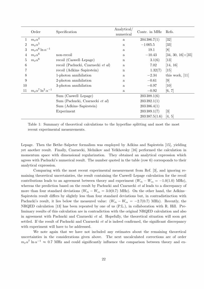
Analytical/Order Specification

numericalContr. in MHz Refs.

1 meα4 a 204 386.7(1) [32]

2 meα5 a −1 005.5 [33]

3 meα6 lnα−1 a 19.1 [8]

4 meα6 non-recoil a −10.43 [34, 30, 16]+[35]

5 meα6 recoil (Caswell–Lepage) n 3.1(6) [13]

6 recoil (Pachucki, Czarnecki et al) a 7.02 [14, 16]7 recoil (Adkins–Sapirstein) n 1.32(7) [15]8 1-photon annihilation a −2.34 this work, [11]9 2-photon annihilation a −0.61 [9]

10 3-photon annihilation a −0.97 [10]11 meα

7 ln2 α−1 a −0.92 [6, 7]Sum (Caswell–Lepage) 203 388.1(6)Sum (Pachucki, Czarnecki et al) 203 392.1(1)Sum (Adkins–Sapirstein) 203 386.4(1)Experiment 203 389.1(7) [3]

203 387.5(1.6) [4, 5]

Table 1: Summary of theoretical calculations to the hyperfine splitting and most the mostrecent experimental measurements.

Lepage. Then the Bethe–Salpeter formalism was employed by Adkins and Sapirstein [15], yieldingyet another result. Finally, Czarnecki, Melnikov and Yelkhovsky [16] performed the calculation inmomentum space with dimensional regularization. They obtained an analytical expression whichagrees with Pachucki’s numerical result. The number quoted in the table (row 6) corresponds to theiranalytical expression.

Comparing with the most recent experimental measurement from Ref. [3], and ignoring re-maining theoretical uncertainties, the result containing the Caswell–Lepage calculation for the recoilcontributions leads to an agreement between theory and experiment (Wth −Wex = −1.0(1.0) MHz),whereas the prediction based on the result by Pachucki and Czarnecki et al leads to a discrepancy ofmore than four standard deviations (Wth −Wex = 3.0(0.7) MHz). On the other hand, the Adkins–Sapirstein result differs by slightly less than four standard deviations but, in contradistinction withPachucki’s result, it lies below the measured value: (Wth − Wex = −2.7(0.7) MHz). Recently, theNRQED calculation [13] has been repeated by one of us (P.L.), in collaboration with R. Hill. Pre-liminary results of this calculation are in contradiction with the original NRQED calculation and alsoin agreement with Pachucki and Czarnecki et al. Hopefully, the theoretical situation will soon getsettled. If the result of Pachucki and Czarnecki et al is indeed confirmed, the significant discrepancywith experiment will have to be addressed.

We note again that we have not included any estimates about the remaining theoreticaluncertainties in the considerations given above. The next uncalculated corrections are of ordermeα

7 lnα−1 ≈ 0.7 MHz and could significantly influence the comparison between theory and ex-

22

periment. However, the coefficient of the log corrections are usually much smaller than 1, and wetherefore believe that a contribution of 1 MHz from the higher order corrections is probably a conser-vative estimate. In this case, the discrepancy between theory and experiment remains unexplained.Clearly, further work on positronium calculations is necessary.

8 Summary

We have provided the details of the NRQED calculation of the O(meα6) contribution to the positro-

nium ground state hyperfine splitting due to single photon annihilation reported in an earlier paper.The counting rules needed to this order have been explained in detail and a discussion on some of theissues related to the use of an explicit cutoff on the momentum integrals has been given. We haveprovided a list of integrals useful for the evaluation of non-relativistic scattering diagrams. Our resultcompletes the O(meα

6) calculation of the ground state hyperfine splitting and permits a comparisonbetween theory and experiment at the level of 1 MHz. A comparison with the most recent exper-imental measurement underlines the need for more theoretical work concerning the O(meα

6) recoilcorrections and higher order contributions.

Acknowledgements

We are grateful to A. Czarnecki, P. Lepage, A. V. Manohar and K. Melnikov for useful discussionsand G. Buchalla for reading the manuscript. One of us (P.L.) has benefited from the hospitality of theLaboratory of Nuclear Studies, Cornell University, where a part of this work has been accomplished.We thank T. Teubner for providing us with Fig. 1.

A Useful Integrals for the Matching Calculation

In this appendix we present a set of integrals that has been useful for the matching calculations carriedout in Sec. 4. All integrals containing ultraviolet divergences are regulated by the cutoff Λ, where therelation Λ � p0 is implied. Terms of order 1/Λk, k > 0 are discarded. As explained in Sec. 2 wehave regulated all infrared divergences by using a small fictitious photon mass λ. In the following wegive the results for arbitrary values of λ, and in an expansion for λ � p0 discarding terms of orderλk, k > 0. For the matching calculations presented in this work only the fully expanded results are

23

relevant:

A1 =Λ�p0∫0

dpp2

p2 − p20 − iε

= Λ + i πp0

2, (78)

A2 =Λ�p0∫0

dpp2 (p2 − p2

0)(p2 + p2

0 + λ2)2 − 4 p2 p20

= Λ− 34λπ

λ→0−→ Λ , (79)

A3 =∞∫0

dpp

p2 − p20 − iε

ln(

(p+ p0)2 + λ2

(p− p0)2 + λ2

)= π arctan

(2 p0

λ

)+ i

π

2ln

(1 +

4 p20

λ2

)

λ→0−→ π2

2+ i π ln

(2 p0

λ

), (80)

A4 =Λ�p0∫0

dpp3

p2 − p20 − iε

ln(

(p+ p0)2 + λ2

(p− p0)2 + λ2

)

= p20 π arctan

(2 p0

λ

)+ p0 (4Λ− 2π λ) + i

π p20

2ln

(1 +

4 p20

λ2

)λ→0−→ π2

2p20 + 4 p0 Λ + i π p2

0 ln(2 p0

λ

), (81)

A5 =∞∫0

dpp

(p2 + p20 + λ2)2 − 4 p2 p2

0

ln(

(p+ p0)2 + λ2

(p− p0)2 + λ2

)

=π

4λ p0ln

(1 +

p20

λ2

)λ→0−→ π

2λ p0ln

(p0

λ

), (82)

A6 =∞∫0

dpp3

(p2 + p20 + λ2)2 − 4 p2 p2

0

ln(

(p+ p0)2 + λ2

(p− p0)2 + λ2

)

= π arctan(p0

λ

)+ π

p20 − λ2

4λ p0ln

(1 +

p20

λ2

)λ→0−→ π2

2+π p0

2λln

(p0

λ

), (83)

A7 =∞∫0

dpp

p2 − p20 − i ε

1(p2 + p2

0 + λ2)2 − 4 p2 p20

ln(

(p+ p0)2 + λ2

(p− p0)2 + λ2

)

=π

4λ2 p0 (λ2 + 4 p20)

[4 p0

(arctan

(2 p0

λ

)− arctan

(p0

λ

) )− λ ln

(1 +

p20

λ2

) ]

+iπ

2λ2 (λ2 + 4 p20)

ln(1 +

4 p20

λ2

)λ→0−→ π

[4 p0 + i λ

32λ p40

− 18λ p3

0

ln(p0

λ

)− i

λ2 − 4 p20

16λ2 p40

ln(2 p0

λ

) ], (84)

24

A8 =∞∫0

dp1

Λ�p0∫0

dp2p1 p2

(p21 − p2

0 − iε) (p22 − p2

0 − iε)ln

((p1 + p2)2 + λ2

(p1 − p2)2 + λ2

)

= π2[

ln(Λλ

)− 1

2ln

(1 +

4 p20

λ2

)+ i arctan

(2 p0

λ

) ]λ→0−→ π2

[− ln

(2 p0

Λ

)+ i

π

2

], (85)

A9 =∞∫0

dp1

Λ�p0∫0

dp2p1

p21 − p2

0 − iε

p2 (p22 − p2

0)(p2

2 + p20 + λ2)2 − 4 p2

2 p20

ln(

(p1 + p2)2 + λ2

(p1 − p2)2 + λ2

)

= −π2[λ

4 p0arctan

(p0

λ

)+ ln 2 +

14

ln(1 +

p20

λ2

)− ln

(Λλ

) ]+

i π2[

12

arctan(p0

λ

)− λ

8 p0ln

(1 +

p20

λ2

) ]λ→0−→ π2

(ln

(Λλ

)− 1

2ln

(p0

λ

)− ln 2

)+ i

π3

4, (86)

A10 =∞∫0

dp1

∞∫0

dp2p1

(p21 − p2

0 − iε) (p22 − p2

0 − iε)ln

((p1 + p2)2 + λ2

(p1 − p2)2 + λ2

)ln

((p2 + p0)2 + λ2

(p2 − p0)2 + λ2

)

=π2

p0

[− π2

6+

12

arctan2(2 p0

λ

)− 3

8ln2

(1 +

4 p20

λ2

)− Li2

(− 1− 2 i p0

λ

)−Li2

(− 1 +

2 i p0

λ

) ]

+iπ2

p0

[arctan

(2 p0

λ

) (ln 2 + ln

(1 +

4 p20

λ2

))

+i(

Li2(− 1 +

2 i p0

λ

)− Li2

(− 1− 2 i p0

λ

)+

12

Li2(12− i p0

λ

)− 1

2Li2

(12

+i p0

λ

)) ]λ→0−→ π2

2 p0

[π2

12− ln2

(2 p0

λ

)+ i π ln

(2 p0

λ

) ], (87)

A11 =Λ�p0∫0

dp1

∞∫0

dp2p1

p22 − p2

0 − iεln

((p1 + p2)2 + λ2

(p1 − p2)2 + λ2

)ln

((p2 + p0)2 + λ2

(p2 − p0)2 + λ2

)

= 4π Λ[

arctan(2 p0

λ

)+i

2ln

(1 +

4 p20

λ2

) ]− 2π2 p0 − 2λπ2 arctan

(2 p0

λ

)

−i λ π2 ln(1 +

4 p20

λ2

)λ→0−→ 2Λπ2 − 2 p0 π

2 + 4 iΛπ ln(2 p0

λ

), (88)

25

A12 =∞∫0

dp1

Λ�p0∫0

dp2p1

p21 − p2

0 − iεln

((p1 + p2)2 + λ2

(p1 − p2)2 + λ2

)ln

((p2 + p0)2 + λ2

(p2 − p0)2 + λ2

)

= π2[− 4λ arctan

(p0

λ

)+ 2 p0

(2− 2 ln 2− ln

(λ2 + p20

Λ2

) ) ]

i π2[4 p0 arctan

(p0

λ

)− 2λ ln

(1 +

p20

λ2

) ]λ→0−→ 4 p0 π

2[1− ln

(2 p0

Λ

)+ i

π

2

]. (89)

References

[1] S. Mohorovicic, Astron. Nachr. 253 (1934), 94.

[2] M. Deutsch, Phys. Rev. 82 (1951) 455;M. Deutsch and E. Dulit, Phys. Rev. 84 (1951) 601.

[3] M. W. Ritter, P.O. Egan, V.W. Hughes and K.A. Woodle, Phys. Rev. A 30 (1984) 1331.

[4] A. P. Mills, Jr., Phys. Rev. A 27 (1983) 262.

[5] A. P. Mills, Jr. and G. H. Bearman, Phys. Rev. Lett. 34 (1975) 246.

[6] S.G. Karshenboım, JETP 76 (1993) 41.

[7] P. Labelle, Ph.D. thesis Cornell University, UMI-94-16736-mc (microfiche), Jan. 1994.

[8] G.T. Bodwin and D.R. Yennie, Phys. Reports 43 (1978) 267;W.E. Caswell and G.P. Lepage, Phys. Rev. A 20 (1979) 36.

[9] G.S. Adkins, Y.M. Aksu and M.H.T. Bui, Phys. Rev. A 47 (1993) 2640.

[10] G.S. Adkins, M.H.T. Bui and D. Zhu, Phys. Rev. A 37 (1988) 4071.

[11] G. S. Adkins, R. N. Fell and P. M. Mitrikov, Phys. Rev. Lett. 79 (1997) 3383.

[12] A. H. Hoang, P. Labelle and S. M. Zebarjad, Phys. Rev. Lett. 79 (1997) 3387.

[13] W.E. Caswell and G.E. Lepage, Phys. Lett. B 167 (1986) 437.

[14] K. Pachucki, Phys. Rev. A 56 (1997) 297.

[15] G. S. Adkins and J. Sapirstein, Phys. Rev. A 58 (1998) 3552.

[16] A. Czarnecki, K. Melnikov and A. Yelkhovsky, Phys. Rev. Lett. 82 (1999) 311; Phys. Rev. A 59(1999) 4316.

26

[17] P. Labelle, Phys. Rev. D 58 (1998) 093013.

[18] N. Brambilla, A. Pineda, J. Soto and A. Vairo, hep-ph/9903355.

[19] M. Beneke and V. A. Smirnov, Nucl. Phys. B 522 (1998) 321.

[20] P. Labelle, S. M. Zebarjad and C. P. Burgess, Phys. Rev. D 56 (1997) 8053.

[21] H. W. Griesshammer, Phys. Rev. D 58 (1998) 094027.

[22] G. Kallen and A. Sabry, K. Dan. Vidensk. Selsk. Mat.-Fys. Medd. 29 (1955) No. 17.

[23] J. Schwinger, Particles, Sources and Fields, Vol II (Addison-Wesley, New York, 1973).

[24] A. H. Hoang, Phys. Rev. D 56 (1997) 7276.

[25] J. Schwinger, J. Math. Phys. 5 (1964) 1606.

[26] W. E. Caswell and G. P. Lepage, Phys. Rev. A 18 (1978) 810.

[27] G.T. Bodwin, E. Braaten and G.P. Lepage, Phys. Rev. D 51 (1995) 1125.

[28] A.H. Hoang, Phys. Rev. D 57 (1998) 1615.

[29] A.H. Hoang, Phys. Rev. D 56 (1997) 5851.

[30] K. Pachucki and S. G. Karshenboım, Phys. Rev. Lett. 80 (1998) 2101.

[31] Particle Data Group, C. Caso et al., Eur. Phys. J. C 3 (1998) 1.

[32] J. Pirenne, Arch. Sci. Phys. Nat. 28 (1946) 233.

[33] R. Karplus and A. Klein, Phys. Rev. 87 (1952) 848.

[34] J.R. Sapirstein, E.A. Terray and D.R. Yennie, Phys. Rev. D 29 (1984) 2290.

[35] A trivial correction to order meα6 is obtained by including the anomalous magnetic moment to

two loops in the lowest order Fermi correction, meα4/3 → meα

4(1 + ae)2/3 which leads to anO(meα

6) contribution equal to meα6[ 1

2π2 (215108 + ζ3) + 1

18 − 13 ln 2] ≈ −0.26 MHz. We are grateful

to G. Adkins for bringing to our attention that this correction was not included in some of theearlier references.

27