


Bahasa
Halaman
Hukum


Université Libre de BruxellesFaculté des SciencesDépartement de Biologie MoléculaireService de Bioinformatique des Génomes et des Reséaux
Development, assessment and application ofbioinformatics tools for the extraction of pathways
from metabolic networks
Karoline Faust
Thèse présentée en vue de l’obtention du grade de Docteur en Sciences
JuryPrésident: Prof. Etienne PaysVice-président: Prof. Oberdan LeoSecrétaire: Prof. Anna Maria MariniDirecteur de thèse: Prof. Jacques van HeldenRapporteur: Prof. Bruno AndréRapporteur: Prof. Tom LenaertsExpert extérieur: Prof. Pierre DupontExpert extérieur: Prof. Claudine Médigue
Février 2010

AcknowledgementFirst of all I would like to thank my supervisor Jacques van Helden, who gave me this challengingtopic, who encouraged and supported me throughout this work and who always managed to find timefor explanations, discussions and corrections despite of his overfull timetable. Discussions with him,on whatever topic, were always stimulating and always gave new insights. I also appreciate his way ofguiding me through the PhD. He left me the independence I need, but at the same time made sure thatmy research did not go astray.
A big thanks also to Didier Croes, who worked before me on metabolic pathway prediction and onwhose work this PhD is based. Although he had left the lab when I started, he took the time to meetme and gave me many explanations and ideas.
I am indebted to all members of the aMAZE team for explaining me their work, answering myquestions and giving me access to their code. In particular, I would like to thank Fabian Couche andFrédéric Fays, who introduced me to Eclipse and Java. Christian Lemer gave me several lessons ongood programming practice and got me started with ANT. Olivier Hubaut made the useful suggestionof representing seed node groups by pseudo nodes.
I would like to thank all the current and former BiGre members for their kindness. I was warmlywelcomed and enjoyed a lot the lab’s social activities, such as the Christmas parties and the girls’evenings with Morgane, Gipsi and Alejandra. In particular I would like to thank Raphaël, whom Ibothered regularly with computer problems and whose ongoing efforts simply keep the computers ofthe lab running. A big thanks also to Morgane, the good fairy of the lab. She helped me an uncountednumber of times with various issues. Sylvain was a great colleague whose cheerful personality andreliability made it a pleasure to work with him. Thanks to Gipsi for numerous scientific discussionsand relaxing chats and to Alejandra for introducing me to Mexican drinking and eating habits. It wasgreat to embark on the adventure of parenthood together with so many colleagues in the same year,among them Jean-Valery, Rekin’s, Sylvain, Matthieu and Gipsi. My thanks also goes to Myriam, Marc,Olivier, Ariane and Fernanda for their support and help with different problems and questions. Aspecial thanks to Raul, with whom I had many interesting discussions on various topics.
I am grateful to Bruno André, the president of my PhD commission, and the other commission mem-bers, Marcelline Kaufmann and Gianluca Bontempi, who gave useful advice, support and suggestionsthroughout my thesis. Thanks as well to Patrice Godard, who gave me access to his microarray data.
Pierre Dupont patiently explained me the kWalks algorithm and made numerous contributions to thiswork. I am grateful for his ideas, his exceptional communication skills and his friendliness.
I would like to acknowledge Pierre Schaus, Jean-Noël Monette and their supervisor Yves Deville,who helped me during the initial stages of my PhD. Thanks as well to Grégoire Dooms, who introducedme to (CP)Graph.
I also wish to thank the members of my jury and especially Claudine Médigue, who accepted to takethe trouble to come from Paris to Brussels.
A big thanks to Didier Gonze and my family for their unfailing support and love. Thanks also toDidier’s family and Didier for several babysitting sessions, without which I could not have finished thisthesis. Last but not least I would like to thank Sophie for her smiles, for her sweetness, for her presencein my life.
ii

AbstractGenes can be associated in numerous ways, e.g. by co-expression in micro-arrays, co-regulation inoperons and regulons or co-localization on the genome. Association of genes often indicates that theycontribute to a common biological function, such as a pathway. The aim of this thesis is to predictmetabolic pathways from associated enzyme-coding genes. The prediction approach developed in thiswork consists of two steps: First, the reactions are obtained that are carried out by the enzymes codedby the genes. Second, the gaps between these seed reactions are filled with intermediate compoundsand reactions. In order to select these intermediates, metabolic data is needed. This work made use ofmetabolic data collected from the two major metabolic databases, KEGG and MetaCyc. The metabolicdata is represented as a network (or graph) consisting of reaction nodes and compound nodes. Interme-diate compounds and reactions are then predicted by connecting the seed reactions obtained from thequery genes in this metabolic network using a graph algorithm.
In large metabolic networks, there are numerous ways to connect the seed reactions. The mainproblem of the graph-based prediction approach is to differentiate biochemically valid connectionsfrom others. Metabolic networks contain hub compounds, which are involved in a large number ofreactions, such as ATP, NADPH, H2O or CO2. When a graph algorithm traverses the metabolic networkvia these hub compounds, the resulting metabolic pathway is often biochemically invalid.
In the first step of the thesis, an already existing approach to predict pathways from two seeds wasimproved. In the previous approach, the metabolic network was weighted to penalize hub compoundsand an extensive evaluation was performed, which showed that the weighted network yielded higherprediction accuracies than either a raw or filtered network (where hub compounds are removed). Inthe improved approach, hub compounds are avoided using reaction-specific side/main compound an-notations from KEGG RPAIR. As an evaluation showed, this approach in combination with weightsincreases prediction accuracy with respect to the weighted, filtered and raw network.
In the second step of the thesis, path finding between two seeds was extended to pathway predictiongiven multiple seeds. Several multiple-seed pathay prediction approaches were evaluated, namely threeSteiner tree solving heuristics and a random-walk based algorithm called kWalks. The evaluationshowed that a combination of kWalks with a Steiner tree heuristic applied to a weighted graph yieldedthe highest prediction accuracy.
Finally, the best perfoming algorithm was applied to a microarray data set, which measured geneexpression in S. cerevisiae cells growing on 21 different compounds as sole nitrogen source. For 20nitrogen sources, gene groups were obtained that were significantly over-expressed or suppressed withrespect to urea as reference nitrogen source. For each of these 40 gene groups, a metabolic pathwaywas predicted that represents the part of metabolism up- or down-regulated in the presence of theinvestigated nitrogen source.
The graph-based prediction of pathways is not restricted to metabolic networks. It may be applied toany biological network and to any data set yielding groups of associated genes, enzymes or compounds.Thus, multiple-end pathway prediction can serve to interpret various high-throughput data sets.
iii

AbbreviationsAL Average path length
ADP Adenosine Diphosphate
ATP Adenosine Triphosphate
EC Enzyme Commission
E. coli Escherichia coli
EM Elementary Mode
FN False Negative
FP False Positive
GABA Gamma-aminobutyric acid
GML Graph Modelling Language
HQL Hibernate Query Language
IQR Interquartile Range
KEGG Kyoto Encyclopedia of Genes and Genomes
NAD Nicotinamide Adenine Dinucleotide
NADP Nicotinamide Adenine Dinucleotide Phosphate
NCR Nitrogen Catabolite Repression
NeAT Network Analysis Tools
ORF Open Reading Frame
OWL Web Ontology Language
PPV Positive Predictive Value
REA Recursive Enumeration Algorithm
S. cerevisiae Saccharomyces cerevisiae
SGD Saccharomyces Genome Database
SMILES Simplified Molecular Input Line Entry System
TCA cycle Tricarboxylic Acid cycle, also known as Krebs or citric acid cycle
TP True Positive
iv

Publication list
K. Faust and J. van HeldenPredicting metabolic pathways by subnetwork extractionMethods in Molecular Biology - Bacterial Molecular Networks, Submitted.
K. Faust, P. Dupont, J. Callut and J. van HeldenPathway discovery in metabolic networks by subgraph extractionSubmitted.
K. Faust, D. Croes and J. van HeldenIn response to "Can sugars be produced from fatty acids? A test case for pathwayanalysis tools"Bioinformatics, vol. 25, pp. 3202-3205, 2009.
K. Faust, D. Croes and J. van HeldenMetabolic Pathfinding Using RPAIR AnnotationJournal of Molecular Biology, vol. 388, pp. 390-414, 2009.
K. Faust, J. Callut, P. Dupont and J. van HeldenInference of pathways from metabolic networks by subgraph extractionProceedings of the second International Workshop on Machine Learning in Systems Biology2008.
S. Brohée, K. Faust, G. Lima-Mendez, O. Sand, R. Janky, G. Vanderstocken, Y. Deville andJ. van HeldenNeAT: a toolbox for the analysis of biological networks, clusters, classes and pathwaysNucleic Acids Research, vol. 36, pp. W444-W451, 2008.
K. Faust1, S. Brohee, Gipsi Lima-Mendez, G. Vanderstocken and J. van HeldenNetwork Analysis Tools: from biological networks to clusters and pathwaysNature Protocols, vol. 3, pp. 1616-1629, 2008.
1K. Faust and S. Brohée contributed equally to this publication.
v
Contents
1 Introduction 11.1 Motivation . . . . . . . . . . . . . . . . . . . . . . . . . . . . . . . . . . . . 11.2 Goal of the thesis . . . . . . . . . . . . . . . . . . . . . . . . . . . . . . . . 11.3 Biological background: Metabolism . . . . . . . . . . . . . . . . . . . . . . 3
1.3.1 Compounds . . . . . . . . . . . . . . . . . . . . . . . . . . . . . . . 31.3.2 Reactions . . . . . . . . . . . . . . . . . . . . . . . . . . . . . . . . 61.3.3 Enzymes . . . . . . . . . . . . . . . . . . . . . . . . . . . . . . . . 7
1.4 Metabolic databases . . . . . . . . . . . . . . . . . . . . . . . . . . . . . . . 111.5 Mapping of metabolism onto a network . . . . . . . . . . . . . . . . . . . . 131.6 Properties of metabolic networks . . . . . . . . . . . . . . . . . . . . . . . . 17
1.6.1 Power law and small world property . . . . . . . . . . . . . . . . . . 171.6.2 Modularity and hierarchical organization . . . . . . . . . . . . . . . 201.6.3 Bow-tie shape . . . . . . . . . . . . . . . . . . . . . . . . . . . . . . 211.6.4 Core and periphery . . . . . . . . . . . . . . . . . . . . . . . . . . . 21
1.7 Metabolic pathway definition . . . . . . . . . . . . . . . . . . . . . . . . . . 221.7.1 Classical definition of metabolic pathways . . . . . . . . . . . . . . . 231.7.2 Atom-flow based definitions of metabolic pathways . . . . . . . . . . 251.7.3 Feasibility-based definition of metabolic pathways . . . . . . . . . . 271.7.4 Functional definition of metabolic pathways . . . . . . . . . . . . . . 281.7.5 Stoichiometry-based definitions of metabolic pathways . . . . . . . . 281.7.6 Metabolic pathway definition based on chemical organization theory . 28
1.8 Which definition is most appropriate for pathway prediction? . . . . . . . . . 291.9 Experimental validation of metabolic pathways . . . . . . . . . . . . . . . . 29
1.9.1 Mutagenesis . . . . . . . . . . . . . . . . . . . . . . . . . . . . . . 301.9.2 Atom tracing . . . . . . . . . . . . . . . . . . . . . . . . . . . . . . 301.9.3 In vitro reconstitution . . . . . . . . . . . . . . . . . . . . . . . . . . 30
1.10 Review on the computational prediction of metabolic pathways . . . . . . . . 311.10.1 Pathway prediction and metabolic reconstruction . . . . . . . . . . . 311.10.2 Prediction of metabolic pathways - the challenge . . . . . . . . . . . 311.10.3 Two-end metabolic pathway prediction . . . . . . . . . . . . . . . . 341.10.4 Multiple-end metabolic pathway prediction . . . . . . . . . . . . . . 49
2 Two-end metabolic pathway prediction 552.1 Introduction . . . . . . . . . . . . . . . . . . . . . . . . . . . . . . . . . . . 552.2 Contribution . . . . . . . . . . . . . . . . . . . . . . . . . . . . . . . . . . . 552.3 Methods . . . . . . . . . . . . . . . . . . . . . . . . . . . . . . . . . . . . . 55
vi

2.4 Results . . . . . . . . . . . . . . . . . . . . . . . . . . . . . . . . . . . . . . 572.5 Conclusion . . . . . . . . . . . . . . . . . . . . . . . . . . . . . . . . . . . 57
3 Multiple-end metabolic pathway prediction 83
3.1 Introduction . . . . . . . . . . . . . . . . . . . . . . . . . . . . . . . . . . . 833.2 Contribution . . . . . . . . . . . . . . . . . . . . . . . . . . . . . . . . . . . 833.3 Methods . . . . . . . . . . . . . . . . . . . . . . . . . . . . . . . . . . . . . 833.4 Results . . . . . . . . . . . . . . . . . . . . . . . . . . . . . . . . . . . . . . 843.5 Conclusion . . . . . . . . . . . . . . . . . . . . . . . . . . . . . . . . . . . 84
4 Application of pathway discovery to a gene expression data set from S.
cerevisiae 92
4.1 Biological background . . . . . . . . . . . . . . . . . . . . . . . . . . . . . 924.2 Gene expression data set . . . . . . . . . . . . . . . . . . . . . . . . . . . . 924.3 Data processing . . . . . . . . . . . . . . . . . . . . . . . . . . . . . . . . . 954.4 Gene-to-reaction mapping . . . . . . . . . . . . . . . . . . . . . . . . . . . 984.5 Multiple-end pathway prediction parameters . . . . . . . . . . . . . . . . . . 102
4.5.1 Metabolic network . . . . . . . . . . . . . . . . . . . . . . . . . . . 1024.5.2 Seed nodes . . . . . . . . . . . . . . . . . . . . . . . . . . . . . . . 1024.5.3 Algorithm . . . . . . . . . . . . . . . . . . . . . . . . . . . . . . . . 102
4.6 Pathway predicted to be up-regulated in the presence of aspartate . . . . . . . 1034.6.1 Up-regulated genes . . . . . . . . . . . . . . . . . . . . . . . . . . . 1034.6.2 Predicted pathway . . . . . . . . . . . . . . . . . . . . . . . . . . . 104
4.7 Pathway predicted to be down-regulated in the presence of aspartate . . . . . 1044.7.1 Down-regulated genes . . . . . . . . . . . . . . . . . . . . . . . . . 1044.7.2 Predicted pathway . . . . . . . . . . . . . . . . . . . . . . . . . . . 106
4.8 Pathway predicted to be up-regulated in the presence of phenylalanine . . . . 1094.8.1 Up-regulated genes . . . . . . . . . . . . . . . . . . . . . . . . . . . 1094.8.2 Predicted pathway . . . . . . . . . . . . . . . . . . . . . . . . . . . 110
4.9 Pathway predicted to be down-regulated in the presence of phenylalanine . . 1104.9.1 Down-regulated genes . . . . . . . . . . . . . . . . . . . . . . . . . 1104.9.2 Predicted pathway . . . . . . . . . . . . . . . . . . . . . . . . . . . 112
4.10 Pathway predicted to be up-regulated in the presence of leucine . . . . . . . . 1124.10.1 Up-regulated genes . . . . . . . . . . . . . . . . . . . . . . . . . . . 1124.10.2 Predicted pathway . . . . . . . . . . . . . . . . . . . . . . . . . . . 114
4.11 Pathway predicted to be down-regulated in the presence of leucine . . . . . . 1154.11.1 Down-regulated genes . . . . . . . . . . . . . . . . . . . . . . . . . 1154.11.2 Predicted pathway . . . . . . . . . . . . . . . . . . . . . . . . . . . 116
4.12 Comparison of nitrogen sources based on predicted pathways . . . . . . . . . 1164.13 Discussion and conclusion . . . . . . . . . . . . . . . . . . . . . . . . . . . 118
vii

5 Stoichiometric versus non-stoichiometric pathway prediction 1215.1 Introduction . . . . . . . . . . . . . . . . . . . . . . . . . . . . . . . . . . . 1215.2 Treatment of the fatty-acid-to-sugar study case without stoichiometric balance 124
5.2.1 Atom tracing . . . . . . . . . . . . . . . . . . . . . . . . . . . . . . 1245.2.2 Cycle treatment . . . . . . . . . . . . . . . . . . . . . . . . . . . . . 124
5.3 Assumptions of stoichiometrically balanced and unbalanced pathways . . . . 1245.4 Stoichiometry and incomplete metabolic networks . . . . . . . . . . . . . . . 1255.5 EM analysis versus path finding . . . . . . . . . . . . . . . . . . . . . . . . 1255.6 Alternative stoichiometric approaches . . . . . . . . . . . . . . . . . . . . . 1265.7 Stoichiometric balance and feasibility of metabolic pathways . . . . . . . . . 1265.8 Conclusion . . . . . . . . . . . . . . . . . . . . . . . . . . . . . . . . . . . 126
6 Contributions to NeAT 1326.1 Presentation of NeAT . . . . . . . . . . . . . . . . . . . . . . . . . . . . . . 1326.2 Tools contributed to NeAT . . . . . . . . . . . . . . . . . . . . . . . . . . . 1326.3 On the use of NeAT tools . . . . . . . . . . . . . . . . . . . . . . . . . . . . 135
6.3.1 Data input . . . . . . . . . . . . . . . . . . . . . . . . . . . . . . . . 1356.3.2 Data output and interpretation . . . . . . . . . . . . . . . . . . . . . 135
7 Discussion 1597.1 Summary . . . . . . . . . . . . . . . . . . . . . . . . . . . . . . . . . . . . 159
7.1.1 Path finding in RPAIR networks . . . . . . . . . . . . . . . . . . . . 1597.1.2 Multiple-end pathway prediction by subgraph extraction . . . . . . . 1597.1.3 Application to microarray data set . . . . . . . . . . . . . . . . . . . 1597.1.4 Stoichiometric versus non-stoichiometric pathway prediction . . . . . 160
7.2 Strengths of pathway prediction . . . . . . . . . . . . . . . . . . . . . . . . 1607.3 Limitations of pathway prediction . . . . . . . . . . . . . . . . . . . . . . . 1617.4 Alternative prediction approaches . . . . . . . . . . . . . . . . . . . . . . . 163
7.4.1 Enzyme kinetics . . . . . . . . . . . . . . . . . . . . . . . . . . . . 1647.4.2 Atom tracing . . . . . . . . . . . . . . . . . . . . . . . . . . . . . . 1647.4.3 Stoichiometry . . . . . . . . . . . . . . . . . . . . . . . . . . . . . . 164
7.5 Top-down versus bottom-up pathway prediction . . . . . . . . . . . . . . . . 1657.6 Tuning pathway prediction . . . . . . . . . . . . . . . . . . . . . . . . . . . 1667.7 Condition-specificity of metabolic pathways . . . . . . . . . . . . . . . . . . 1667.8 Functional association of genes . . . . . . . . . . . . . . . . . . . . . . . . . 167
7.8.1 Co-regulation of genes . . . . . . . . . . . . . . . . . . . . . . . . . 1677.8.2 Other types of gene association . . . . . . . . . . . . . . . . . . . . 167
8 Perspectives 1688.1 Increase of pathway prediction accuracy . . . . . . . . . . . . . . . . . . . . 1688.2 Improvement of pathway prediction . . . . . . . . . . . . . . . . . . . . . . 1688.3 Evaluation of pathway prediction applied to biological data . . . . . . . . . . 1708.4 Applications of pathway prediction . . . . . . . . . . . . . . . . . . . . . . . 170
viii
9 Materials and methods 1729.1 Graph algorithms . . . . . . . . . . . . . . . . . . . . . . . . . . . . . . . . 172
9.1.1 Enumeration of the K-shortest paths . . . . . . . . . . . . . . . . . . 1729.1.2 Subgraph extraction from multiple seeds . . . . . . . . . . . . . . . 173
9.2 Networks and reference pathways . . . . . . . . . . . . . . . . . . . . . . . 1839.2.1 Metabolic networks . . . . . . . . . . . . . . . . . . . . . . . . . . . 1839.2.2 Metabolic reference pathways . . . . . . . . . . . . . . . . . . . . . 1839.2.3 Comparison of a predicted to a reference pathway . . . . . . . . . . . 1889.2.4 Evaluation procedure . . . . . . . . . . . . . . . . . . . . . . . . . . 190
9.3 Metabolic database . . . . . . . . . . . . . . . . . . . . . . . . . . . . . . . 1919.3.1 Data model . . . . . . . . . . . . . . . . . . . . . . . . . . . . . . . 1919.3.2 Implementation . . . . . . . . . . . . . . . . . . . . . . . . . . . . . 1939.3.3 Contents of the metabolic database . . . . . . . . . . . . . . . . . . . 193
A Introduction to graph theory 195
Bibliography 213
ix

1 Introduction
1.1 Motivation
High-throughput experiments such as microarrays allow to measure gene expression in differ-ent conditions at a genomic scale. Interpretation of these data is however a challenging task.One approach commonly applied to the interpretation of microarray data has been termed"Guilt by association" [137]. It states that co-expressed genes (genes whose expression valuesare either increased simultaneously or decreased simultaneously with respect to a reference)are likely to contribute to a common biological function such as a pathway.Genes may not only be "guilty of association" by co-expression, but also by co-regulation inoperons and regulons, co-occurrence in phylogeny, co-localization in the genome or in otherways. In all these cases, it is of interest to identify the biological module or pathway in whichthe "guilty" genes are involved.
In order to identify pathways from associated genes, many software tools simply map thegenes on a set of pre-defined pathways [34, 159, 123, 84, 64, 1]. An example for pathwaymapping is given in Figure 1.1.
This mapping approach has several shortcomings:
• It is only applicable to organisms with correspondences to known pathways.
• It does not deal well with genes mapping to several pathways.
• It fails to find variants of pre-defined pathways.
• It is unable to uncover novel pathways from known components (e.g. known reactions,compounds or protein interactions).
A major reason for these drawbacks is the inability of the mapping approaches to take theinterconnection of biological pathways into account. The accumulation of more and morebiological data triggered recently a shift in data representation from modules and pathwaystowards whole networks. Networks have the advantage to account for the interconnection ofpathways and to enable a series of interesting analyses. However, predicting relevant biologi-cal pathways from networks instead of pre-defined pathways poses a challenge.
1.2 Goal of the thesis
The goal of this thesis is to predict biochemically relevant metabolic pathways from metabolicnetworks and groups of associated enzyme-coding genes. The metabolic network is assembled
1
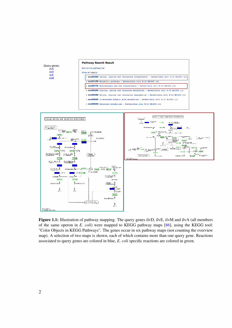
Query genes:ilvAilvDilvEilvM
Figure 1.1: Illustration of pathway mapping. The query genes ilvD, ilvE, ilvM and ilvA (all membersof the same operon in E. coli) were mapped to KEGG pathway maps [86], using the KEGG tool:"Color Objects in KEGG Pathways". The genes occur in six pathway maps (not counting the overviewmap). A selection of two maps is shown, each of which contains more than one query gene. Reactionsassociated to query genes are colored in blue, E. coli specific reactions are colored in green.
2

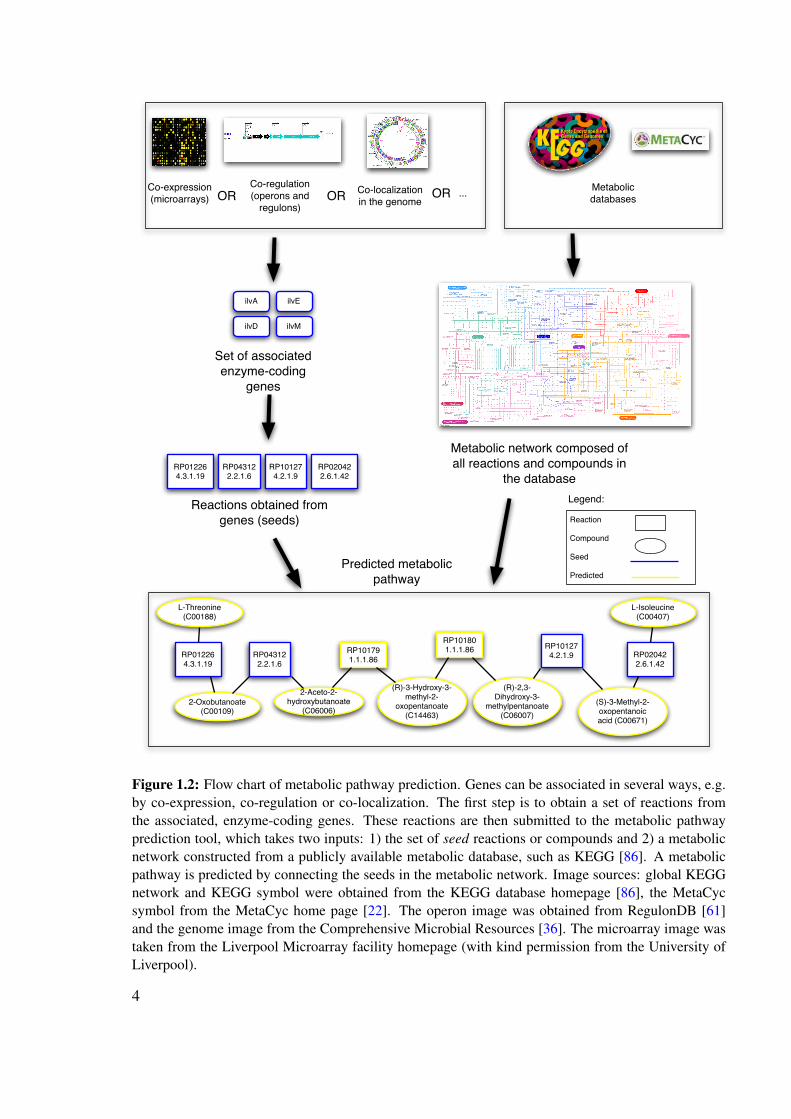
from a metabolic database, whereas the genes can come from a variety of data sources (co-expression, co-regulation, co-occurrence in phylogenetic profiles etc.). From the enzyme-coding genes, reactions are obtained, which serve as seeds for pathway prediction. Figure 1.2depicts a flow chart of metabolic pathway prediction.
The first step to reach this goal consisted in the development of a new algorithm and theadaptation of existing algorithms to the prediction of pathways from metabolic networks. Ina second step, the prediction accuracy of these algorithms was evaluated on a large set of an-notated metabolic pathways. During this evaluation, the impact of various parameters (suchas network properties or the integration of main/side compound annotations from the RPAIRdatabase [96]) on the accuracy was assessed. Finally, the best-performing algorithm was ap-plied to extract pathways from co-expressed gene groups obtained from a microarray dataset.
1.3 Biological background: Metabolism
The classical biochemistry textbook [13] defines metabolism as follows: "Metabolism is es-sentially a linked series of chemical reactions that begins with a particular molecule and con-verts it into some other molecule or molecules in a carefully defined fashion."
Chemical reactions involved in metabolism will from now on be termed metabolic reactionsor reactions. They act on molecules, which will be termed compounds throughout this work.
Metabolic reactions can be subdivided into two basic categories: Anabolic reactions syn-thesize molecules from smaller building blocks whilst consuming energy, whereas catabolicreactions break down large molecules to generate energy and building blocks required byanabolic reactions.
Another classification of metabolism is based on the importance of compounds for the sur-vival of an organism. Primary compounds, such as glucose 6-phosphate or ATP, are involvedin the maintenance of the basic functions of life (growth, development, reproduction). Sec-ondary compounds are not required for these basic tasks, but are needed in specific conditions,such as defense against parasites (e.g. antibiotics produced by fungi).
As will be discussed in detail in section 1.5, metabolism can be represented as a net-work. This representation allows to define core and peripheral metabolism. This classificationloosely corresponds to the traditional classification into primary and secondary compoundsand will be presented in section 1.6.4.
A typical cell is composed of thousands of compounds and reactions. For instance EcoCyc(version 13.1) [90] lists 1,415 enzymes, 1,784 reactions and 1,753 compounds for Escherichiacoli.
In the following, the major concepts of metabolism will be discussed in more detail.
1.3.1 Compounds
The chemical structure of a compound can be represented in a variety of ways. Most importantare the sum formula, which lists the numbers of different atoms contained in the compoundand the structural formula, which shows how the atoms are arranged. For bioinformatics, the
3
Set of associated enzyme-coding
genes
Co-expression (microarrays)
Co-regulation (operons and
regulons)Co-localization in the genome
Metabolic network composed of all reactions and compounds in
the database
OR ORMetabolic databases
ilvD
ilvEilvA
ilvM
Reactions obtained from genes (seeds)
RP012264.3.1.19
RP043122.2.1.6
RP101274.2.1.9
RP020422.6.1.42
RP012264.3.1.19
2-Oxobutanoate (C00109)
RP043122.2.1.6
2-Aceto-2-hydroxybutanoate
(C06006)
RP101791.1.1.86
(R)-3-Hydroxy-3-methyl-2-
oxopentanoate (C14463)
L-Threonine (C00188)
L-Isoleucine (C00407)
RP101801.1.1.86
(R)-2,3-Dihydroxy-3-
methylpentanoate (C06007)
RP101274.2.1.9
(S)-3-Methyl-2-oxopentanoic acid (C00671)
RP020422.6.1.42
Reaction
Compound
Seed
Predicted
Legend:
OR ...
Predicted metabolic pathway
Figure 1.2: Flow chart of metabolic pathway prediction. Genes can be associated in several ways, e.g.by co-expression, co-regulation or co-localization. The first step is to obtain a set of reactions fromthe associated, enzyme-coding genes. These reactions are then submitted to the metabolic pathwayprediction tool, which takes two inputs: 1) the set of seed reactions or compounds and 2) a metabolicnetwork constructed from a publicly available metabolic database, such as KEGG [86]. A metabolicpathway is predicted by connecting the seeds in the metabolic network. Image sources: global KEGGnetwork and KEGG symbol were obtained from the KEGG database homepage [86], the MetaCycsymbol from the MetaCyc home page [22]. The operon image was obtained from RegulonDB [61]and the genome image from the Comprehensive Microbial Resources [36]. The microarray image wastaken from the Liverpool Microarray facility homepage (with kind permission from the University ofLiverpool).
4

representation of a compound by a string of characters is also relevant. One such string rep-resentation is the SMILES notation [168]. Figure 1.3 illustrates these different representationson the example of D-glucose.
Different representations of compound structure
Structural formula:
D-glucose
Sum formula: C6H12O6
SMILES: C(C1C(C(C(C(O1)O)O)O)O)O
Figure 1.3: The chemical structure, the sum formula and the SMILES representation of the compoundD-glucose are shown. The structure image was taken from KEGG [86].
Compounds take on different roles in metabolism. For instance, many authors distinguishbetween main and side compounds of a pathway. Main compounds "carry" a major part of thecarbon atoms through the reactions of the pathway. They form the "backbone" of pathways,as Karp put it [88] and are also called intermediate compounds. Typical side compounds actas donors/acceptors of energy or electrons, such as ATP/ADP and NAD(P)+/NAD(P)H or asdonors/acceptors of functional groups such as tetrahydrofolic acid. The distinction betweenmain and side compounds poses problems discussed in section 1.7.2. In addition, other atomtypes than carbon may be relevant in a pathway, e.g. the sulfur incorporation pathway containsintermediates such as sulfide that do not contain carbon.
Side compounds such as ATP/ADP or NAD(P)+/NAD(P)H and small inorganic compoundssuch as H2O or CO2 are involved in many reactions and are therefore called ubiquitous or hubcompounds. As will be discussed in section 1.10.3, appropriate treatment of hub compoundsis necessary to predict metabolic pathways accurately.
In this thesis, only small molecules and their reactions are taken into account. Polymerssuch as DNA, proteins or RNA and their reactions are neglected.
5

1.3.2 Reactions
Reactions convert a set of input compounds called substrates into a set of products. Substratesand products together are also named reactants. Figure 1.4 depicts an example reaction withtwo substrates and two products.
glucokinase (2.7.1.2)
ATP ADP
D-glucoseD-glucose-6-phosphate
Figure 1.4: Example of a metabolic reaction (KEGG identifier R00299). The substrates D-glucose andATP are converted into the products D-glucose-6-phosphate and ADP. The reaction is catalyzed by theenzyme glucokinase, which has the EC number 2.7.1.2 assigned to it. The direction of this reactionis not specified by this illustration. However, in physiological conditions, this reaction is irreversible,since it consumes energy by hydrolyzing ATP. The compound structure images were taken from KEGG[86].
A reaction can proceed in two directions. Consider for example reaction A + B ↔ C. Itcan proceed from A and B towards C (forward direction) or from C towards A and B (reversedirection). In this thesis, the following notation is adobted: If the arrow in a reaction equationpoints from left to right, compounds on the left-hand side are considered as substrates andcompounds on the right-hand side as products. If it points from right to left, right-hand sidecompounds are substrates and left-hand side compounds are products.
The direction of a reaction depends on its change in Gibbs free energy ∆G. If ∆G = 0,the reaction is at equilibrium and neither the forward nor the reverse direction is preferred.If ∆G > 0, the forward direction is unfavorable and the reaction cannot occur spontaneously(endergonic reactions). If ∆G < 0, the forward direction is preferred and the reaction mayoccur spontaneously (exergonic reactions).
∆G is a function of the concentrations of the reactants, the temperature and the standardfree energy change ∆G0 of the reaction: ∆G = ∆G0 + RT lnQ, with the reaction quotientQ = [product1]c...[productd
n ][substratea
1]...[substratebm] , where n is the number of products and m the number of substrates
of the reaction and a,b, c and d are stoichiometric coefficients of the substrates and products.The standard free energy change is defined as ∆G0 =−RT lnKeq, with the equilibrium constantKeq = Qequilibrium. Qequilibrium refers to the reactant concentrations in equilibrium. The stan-dard conditions are defined as follows: one molar concentration of reactants, one atmosphere
6

pressure and for metabolic reactions pH 7.0.Reactions that are far from equilibrium ( ∆G 6= 0) are also termed irreversible reactions,
because the preference for one reaction direction is so great that the other one can be ne-glected. Since ∆G depends on reactant concentrations and the temperature, a reaction thatis physiological irreversible in one organism may be reversible in another one. For instance,the temperature in thermophilic organisms is different from the temperature in mesophilicorganisms, thus their ∆G values also differ, even if reactant concentrations are the same.
These considerations affect the representation of reactions in metabolic networks compris-ing several organisms.
1.3.3 Enzymes
Enzymes are biomolecules that catalyze reactions. Most enzymes are proteins, but RNA mayalso act as an enzyme (ribozyme). Importantly, an enzyme does not change the equilibriumconstant of a reaction; it only accelerates its rate. Not all reactions are catalyzed by enzymes:Some occur spontaneously, e.g. the conversion from L-glutamate gamma-semialdehyde intowater and (S)-1-pyrroline-5-carboxylate (MetaCyc identifier: SPONTPRO-RXN).
Enzymes are hierarchically classified based on the reactions they catalyze [121]. The clas-sification scheme consists of four levels, each represented by a separate digit and ordered frommost generic to most specific. The first level comprises the following 6 categories:
1. Oxidoreductases catalyze oxidation/reduction reactions.
2. Transferases catalyze the transfer of functional groups.
3. Hydrolases catalyze the hydrolyzation of a substrate into two products.
4. Lyases catalyze the non-hydrolytic addition or removal of atom groups from substrates.
5. Isomerases catalyze isomeric changes within a single compound.
6. Ligases join together two molecules under ATP consumption.
Figures 1.5 and 1.6 give an example for each category of the first level.For instance, an enzyme with the EC number 5.3.1.9 belongs to the isomerases (category
5). More specifically, it is an intramolecular oxidoreductase (5.3), which interconverts aldosesand ketoses (5.3.1). The fourth digit is an index to distinguish enzymes acting on differentreactants (glucose-6-phosphate and fructose-6-phosphate in this case).
Relating enzymes to reactions
A many-to-many relationship exists between enzymes and reactions, meaning that one enzymemay catalyze several reactions and that one reaction may be catalyzed by several enzymes.
Multifunctional enzymes such as Aro1p in Saccharomyces cerevisiae may carry out severalsubsequent reactions (5 in the case of Aro1p). A multifunctional enzyme possesses multiplefunctional sites, which enable compound channeling.
7

1. Oxidoreductases
Example: 1.2.1.41 Name: L-Glutamate-5-semialdehyde: NADP+ 5-oxidoreductaseKEGG identifier: R03313
L-Glutamate 5-semialdehyde
(reduced)
OrtophosphateNADP+
(oxidized)
L-Glutamyl 5-phosphate (oxidized)
NADPH (reduced)
H+
2. Transferases
Example: 2.1.3.3Name: Carbamoyl-phosphate: L-ornithine carbamoyltransferaseKEGG identifier: R01398
Carbamoyl phosphate L-Ornithine
Orthophosphate L-Citrulline
3. Hydrolases
Example: 3.5.3.9Name: Allantoate amidinohydrolaseKEGG identifier: R02423
AllantoateWater
NH3
Ureidoglycine
CO2
Transferred atom groups are encircled in corresponding colors.
Transferred atom groups are encircled in corresponding colors.
Figure 1.5: Examples for the first, second and third category of the first level of the enzyme classifi-cation scheme. The compound structure images were taken from KEGG [86].
8

4. Lyases
Example: 4.2.1.10 Name: 3-Dehydroquinate hydro-lyaseKEGG identifier: R03084
Water
3-Dehydroshikimate
3-Dehydroquinate
Hydroxylgroup is highlighted in blue.
5. Isomerases
6. Ligases
Example: 5.4.2.2 Name: alpha-D-glucose 1,6-phosphomutaseKEGG identifier: R08639
D-glucose 6-phosphate
D-glucose 1-phosphate
Example: 6.2.1.1 Name: Acetate:CoA ligaseKEGG identifier: R00235
ATP AMP
Acetyl-CoA
Diphosphate
Acetate
CoA
Transferred atom groups are encircled in corresponding colors.
Different position of phosphate group is highlighted in blue.
Figure 1.6: Examples for the fourth, fifth and sixth category of the first level of the enzyme classifica-tion scheme. The compound structure images were taken from KEGG [86].
9

pentafunctional Aro1p protein in S. cerevisiae
3-dehydroquinate synthase (4.2.3.4)
3-dehydroquinate dehydratase (4.2.1.10)
shikimate dehydrogenase (1.1.1.25)
shikimate kinase (2.7.1.71)
3-phosphoshikimate 1-carboxyvinyltransferase (2.5.1.19)
N:N
N:N
Enzyme
EC number
ReactionR02413shikimate + NADP+ = 3-dehydroshikimate + NADPH + H+
R02414Shikimate + NADP+ = 5-Dehydroshikimate + NADPH
Gene
N:N
ARO1 gene in S. cerevisiae
Figure 1.7: This Figure illustrates the many-to-many relationships between genes and reactions withthe pentafunctional ARO1 gene from S. cerevisiae as an example. Altogether, this gene is associatedto six reactions. Only the reactions associated to shikimate dehydrogenase are shown. Image sources:The image of the ORF is taken from SGD [74], the image of the protein structure from PDB [14].
10

When compounds are channeled, they are not released from the enzymes but passed fromone enzyme to another one or, as in the case of Aro1p, from one catalytic site to another one,thus increasing the efficiency of metabolism.
Isoenzymes catalyze the same reaction, e.g. in Escherichia coli three different aspartatekinases catalyze the conversion from L-aspartate to L-aspartate-4-phosphate. Each is regulatedin another way, thus isoenzymes allow the cell to fine-tune metabolic reactions.
Furthermore, a many-to-many relationship exists between EC numbers and reactions, be-cause reactions with the same EC number may differ by their substrates and one reaction maybe catalyzed by various catalytic mechanisms (corresponding to different EC numbers). Forinstance, homoserine dehydrogenase with EC number 1.1.1.3 converts L-homoserine into L-aspartate 4-semialdehyde. There are two reactions associated to this EC number, having eitherNAD+ or NADP+ as a co-substrate. Another example is EC number 1.1.1.23, which is asso-ciated to two reactions: The first converts histidinol to histidinal and the second histidinal tohistidine.
Finally, a many-to-many relationship exists between genes and enzymes. Several genes maycode for different sub-units of one enzyme and several enzymes may be synthesized from onegene via alternative splicing. Figure 1.7 illustrates the many-to-many relationships betweenan enzyme-coding gene and its associated reactions.
Regulation of enzyme-coding genes
The activity of enzymes may be regulated on several levels, including the transcriptional level(regulation of the enzyme-coding gene’s expression) and the post-transcriptional level (in-hibitors and activators binding to the enzyme). As this thesis deals with the interpretation ofa set of associated genes, the focus here is on the transcriptional level. Enzyme-coding genesinvolved in a common pathway are frequently grouped in operons and regulons. An operonis a part of the genome that contains a set of genes that are controlled by common regulatoryelements, and that are transcribed together from a common promoter (the binding site of theRNA polymerase). Figure 1.8 shows an example of an operon. A regulon is defined as "a setof genes subject to regulation of one and only one regulator." (RegulonDB, [61]). In contrastto an operon, the genes of a regulon are not necessarily under the control of a single promoter.A classical example of a regulon is the arginine repressor of E. coli [108].
Operons and regulons allow the cell to switch on or off an entire pathway in response toenvironmental signals.
1.4 Metabolic databases
Metabolic information is available in the classical metabolic textbooks, in the biochemicalliterature and more recently in metabolic databases.
The two most important generic metabolic databases are KEGG [86] and BioCyc [22].Other metabolic databases, such as Reactome [165] (human metabolism) and UM-BBD [50](microbial degradation pathways) are also relevant, but more specialized.
11

L-threonine (THR)
2-oxobutanoate(OXOBUTANOATE)
2-aceto-2-hydroxy-butyrate(2-ACETO-2-HYDROXY-BUTYRATE)
2,3-dihydroxy-3-methylvalerate(1-KETO-2-METHYLVALERATE)
2-keto-3-methyl-valerate(2-KETO-3-METHYL-VALERATE)
L-isoleucine (ILE)
THREDEHYD-RXN 4.3.1.19
ACETOOHBUTSYN-RXN 2.2.1.6
ACETOOHBUTREDUCTOISOM-RXN 1.1.1.86
DIHYDROXYMETVALDEHYDRAT-RXN 4.2.1.9
BRANCHED-CHAINAMINOTRANSFERILEU-RXN 2.6.1.42
pyruvate(PYRUVATE)
2-acetolactate(2-ACETO-LACTATE)
2,3-dihydroxy-isovalerate(DIOH-ISOVALERATE)
2-keto-isovalerate(2-KETO-ISOVALERATE)
L-valine (VAL)
ACETOLACTSYN-RXN 2.2.1.6
ACETOLACTREDUCTOISOM-RXN 1.1.1.86
DIHYDROXYISOVALDEHYDRAT-RXN 4.2.1.9
BRANCHED-CHAINAMINOTRANSFERVAL-RXN 2.6.1.42
2-ISOPROPYLMALATESYN-RXN 2.3.3.13
(2S)-2-isopropylmalate (3-CARBOXY-3-HYDROXY-ISOCAPROATE)
ilvE
ilvD
ilvM
ilvA
isoleucine and valine biosynthesis pathway
ilvLG
_1_G
_2M
EDA
op
ero
n
Figure 1.8: The ilvLG_1G_2MEDA operon of E. coli contains eight genes, four of which are involvedin the synthesis of valine and isoleucine. Each of the enzyme-coding genes is associated to metabolicreactions (the color code allows to match each gene to its respective reactions). Compounds and reac-tions not associated to the ilvLG_1G_2MEDA operon are colored in yellow.
12
KEGG and BioCyc cover many organisms and store pathways that are either collected fromthe literature or predicted with automated or semi-automated metabolic reconstruction proce-dures [87, 114]. Both consist of a collection of databases (KEGG: KEGG LIGAND, KEGGRPAIRS, KEGG GLYCAN . . . ), (BioCyc: MetaCyc, EcoCyc, HumanCyc, . . . ).
KEGG and BioCyc differ in the way they organize the metabolic data. In BioCyc, organism-specific metabolic pathways are dynamically drawn, whereas KEGG shows static maps thatunite all known reactions involved in a common “theme” as defined by the KEGG team, suchas purine metabolism. Organism-specific reactions in these maps can be highlighted uponmouse-click.
KEGG and BioCyc have different strengths and weaknesses [169, 103]. The advantage ofKEGG for metabolic pathway prediction is the manual annotation of the reactant pairs of areaction and their roles, which are provided by the RPAIR database [96]. Its disadvantage isthe absence of organism-specific pathways. Because a KEGG map is not conceived as a path-way, but rather as a union of all known reactions belonging to a common “metabolic theme”, itcannot serve as reference for the evaluation of pathway prediction. BioCyc documents betterthan KEGG its sources (literature, experimental evidence) and separates clearer between pre-dicted and annotated pathways. Instead of "a union of reactions" it displays organism-specificpathways at different levels of detail, which in contrast to KEGG include the side compounds.The relationship between EC numbers and reactions is also less ambiguous than in KEGG.However, reactant pair annotation as in KEGG RPAIR is absent from BioCyc. Table 1.1 sum-marizes the differences between KEGG and BioCyc that are relevant for pathway prediction,whereas Figure 1.9 shows an example that illustrates the different pathway concept of KEGGand BioCyc.
The differences between KEGG maps and BioCyc pathways illustrate that it is not alwaysclear where to draw the border between metabolic pathways. This touches upon the problemof metabolic pathway definition, which will be discussed in detail in section 1.7.
1.5 Mapping of metabolism onto a network
In order to predict metabolic pathways, metabolic data has to be represented in a structuredfashion that makes the application of prediction algorithms possible.
Metabolism has been represented using stoichiometric matrices, graphs, rule sets, first-orderlogic and other formalisms (see section 1.10.3). Since the pathway prediction techniques pre-sented in this work are based on the extraction of relevant parts from graphs, the representationof metabolism as a graph will be discussed in more detail.
A graph is a mathematical abstraction of connected objects and consists of nodes (alsocalled vertices) and edges, which connect the nodes (See appendix A for a brief introductionto graph theory). In this thesis, the terms “network” and “graph” are more or less used assynonyms. Network refers to a set of interconnected biological objects (e.g. compounds andreactions in a metabolic network), whereas graph refers to the formal representation of anetwork.
It is not trivial to map metabolism onto a graph in a meaningful way. Some network repre-sentations suffer from important drawbacks, and are therefore less suited for the prediction of
13

Table 1.1: Differences between KEGG and BioCyc that are relevant for metabolic pathway prediction
Property KEGG BioCycPathway Clickable, Dynamically drawn,display static maps clickable pathwaysPathway Maps merge Each variantvariants all known variants is a separate
of a pathway pathwayOrganism Organism-specific Pathway variantsspecificity parts of maps are organism-
can be highlighted specificSide Maps do not Pathways includecompounds include side side compounds,
compounds which are markedas such
EC number- EC number EC numberreaction- reaction relationships reaction relationshipsmapping are sometimes ambiguous are rarely ambiguousDirect gene- Stored in KGML Stored in biopax filesreaction- files, but not and accessiblerelation- accessible via web inter- via web interfaceships face or APIReactant pair KEGG RPAIR AbsentannotationPredicted versus Status not Predicted pathwaysannotated clearly indicated well separated frompathways annotated pathways
(Tier 1, 2 and 3)Documentation Links to Literature sourcesof data literature are well referencedsources sparse
14

A
B
Figure 1.9: Representation of lysine biosynthesis in S. cerevisiae in KEGG (A) and MetaCyc (B).In KEGG, the lysine biosynthesis pathway map contains all reactions known to be involved in lysinebiosynthesis. Thus, not a species-specific pathway is displayed, but species-specific parts of the map arehighlighted (in green). In MetaCyc, six variants of lysine biosynthesis are stored as separate pathways,each of which is specific to a set of organisms. The pathway shown in B is the lysine biosynthesispathway IV (MetaCyc identifier LYSINE-AMINOAD-PWY).
15
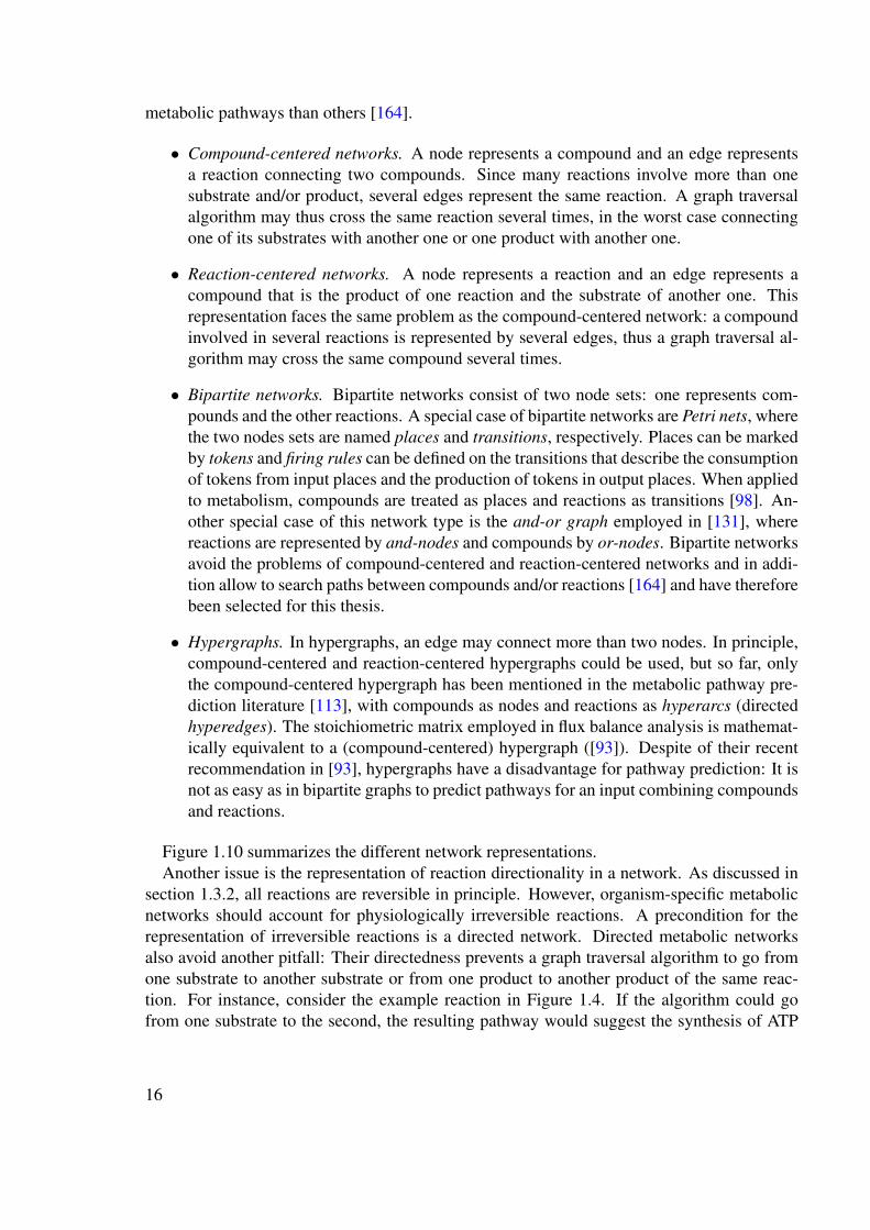
metabolic pathways than others [164].
• Compound-centered networks. A node represents a compound and an edge representsa reaction connecting two compounds. Since many reactions involve more than onesubstrate and/or product, several edges represent the same reaction. A graph traversalalgorithm may thus cross the same reaction several times, in the worst case connectingone of its substrates with another one or one product with another one.
• Reaction-centered networks. A node represents a reaction and an edge represents acompound that is the product of one reaction and the substrate of another one. Thisrepresentation faces the same problem as the compound-centered network: a compoundinvolved in several reactions is represented by several edges, thus a graph traversal al-gorithm may cross the same compound several times.
• Bipartite networks. Bipartite networks consist of two node sets: one represents com-pounds and the other reactions. A special case of bipartite networks are Petri nets, wherethe two nodes sets are named places and transitions, respectively. Places can be markedby tokens and firing rules can be defined on the transitions that describe the consumptionof tokens from input places and the production of tokens in output places. When appliedto metabolism, compounds are treated as places and reactions as transitions [98]. An-other special case of this network type is the and-or graph employed in [131], wherereactions are represented by and-nodes and compounds by or-nodes. Bipartite networksavoid the problems of compound-centered and reaction-centered networks and in addi-tion allow to search paths between compounds and/or reactions [164] and have thereforebeen selected for this thesis.
• Hypergraphs. In hypergraphs, an edge may connect more than two nodes. In principle,compound-centered and reaction-centered hypergraphs could be used, but so far, onlythe compound-centered hypergraph has been mentioned in the metabolic pathway pre-diction literature [113], with compounds as nodes and reactions as hyperarcs (directedhyperedges). The stoichiometric matrix employed in flux balance analysis is mathemat-ically equivalent to a (compound-centered) hypergraph ([93]). Despite of their recentrecommendation in [93], hypergraphs have a disadvantage for pathway prediction: It isnot as easy as in bipartite graphs to predict pathways for an input combining compoundsand reactions.
Figure 1.10 summarizes the different network representations.Another issue is the representation of reaction directionality in a network. As discussed in
section 1.3.2, all reactions are reversible in principle. However, organism-specific metabolicnetworks should account for physiologically irreversible reactions. A precondition for therepresentation of irreversible reactions is a directed network. Directed metabolic networksalso avoid another pitfall: Their directedness prevents a graph traversal algorithm to go fromone substrate to another substrate or from one product to another product of the same reac-tion. For instance, consider the example reaction in Figure 1.4. If the algorithm could gofrom one substrate to the second, the resulting pathway would suggest the synthesis of ATP
16

from D-glucose within one step, which is biochemically impossible. In a directed bipartitemetabolic network, reversible reactions can be represented by including two nodes; one foreach reaction direction (see Figure 1.10 F). Irreversible reactions can then be represented byincluding only one direction node. To prevent a graph traversal algorithm to go twice throughthe same reaction, forward and reverse direction node have to exclude each other mutually,i.e. they cannot both appear in the same path [31, 32]. Thus, a XOR (exclusive OR) rela-tionship exists between the forward and reverse direction of a reaction. If the direction nodeswould not be mutually exclusive, the following pathway could be predicted from the reactionshown in Figure 1.4: D-glucose → 2.7.1.2_forward → D-glucose 6-phosphate →2.7.1.2_reverse → ATP. This pathway falsely suggests that ATP can be synthesized fromD-glucose within two reaction steps.
In this thesis, metabolic networks were constructed from all reactions and compoundspresent in a metabolic database and are thus not organism-specific. In these generic networks,all irreversible reactions were represented as reversible for two reasons: (1) to avoid conflict-ing reaction directions in case a reaction proceeds in one direction in one organism and in theother direction in another organism and (2) to take into account the fact that all reactions arepotentially reversible (see section 1.3.2). However, the tools developed during this thesis canas well deal with networks containing irreversible reactions.
To summarize: Metabolic networks in this thesis are, if not stated otherwise, directed bipar-tite networks in which each reaction is represented by two mutually exclusive nodes: one forits forward and one for its reverse direction.
1.6 Properties of metabolic networks
The representation of metabolism as a network allows to quantify a number of topologicalproperties.
1.6.1 Power law and small world property
In [82] topological properties of metabolic networks from 43 different species have been mea-sured. First, the authors plotted the distribution of compound node degree frequencies on alogarithmic scale, where the degree of a compound is the number of reactions it is involved in.They found that this distribution follows a power-law P(k) ≈ k−γ, where k is the compoundnode degree and P(k) is the probability of degree k in the network. Figure 1.11 shows a com-pound node degree distribution for KEGG data. The power-law is indicative of a scale-freeproperty of the network, i.e. "any part of the scale-free network is stochastically similar to thewhole network, and parameters are assumed to be independent of the system size" [91]. Thisparticular topology is not displayed by random networks.
Second, Jeong et al. measured the network diameter, which they define as "the shortestbiochemical pathway averaged over all pairs of substrates" [82] and which is around three forthe investigated metabolic networks. From the small network diameter, Jeong and coworkersdeduce a small world property of the metabolic network, which states that each node can bereached from each other node within a few steps.
17

D-glucose-6-phosphate
2.7.1.2
D-glucose
ADP
ATP
D-glucose-6-phosphate
2.7.1.2
D-glucose
ADP
ATP
D-glucose-6-phosphate
2.7.1.2
ADP
2.7.1.2D-glucose-6-phosphate
2.7.1.2
D-glucose
ADP
ATP
2.7.1.2
ATP
2.7.1.2
D-glucose
5.3.1.9
2.7.1.40
5.1.3.3A B
C D
2.7.1.41
D-glucose
D-glucose-6-phosphate
2.7.1.2
D-glucose
ADP
ATP
D-glucose-6-phosphate
2.7.1.2 reverse
D-glucose
ADP
ATP
2.7.1.2 forward
E F
Figure 1.10: Figure A gives an example for the compound-centered network, Figure B for the reaction-centered network, Figure C for a bipartite network and Figure D for a hypergraph. Note that all net-works are directed. Figure E illustrates the problem of undirected networks: a graph traversal algorithmcan easily go from one substrate to another one (in this case from D-glucose to ATP) or from one prod-uct to another one. Figure F illustrates how each reaction direction is represented by its own node in thedirected bipartite network. The two nodes 2.7.1.2_forward and 2.7.1.2_reverse are mutually exclusive,i.e. they cannot both appear in the same path.
18

++
+
+
+
+ ++ +
+
++
++++
++++
++
+
+
++++
+
+
+++
+
++
++
++
++++
+ +
+ +++ ++ ++++ ++ + ++ +++ ++ ++ ++++ + + +
1e−04 5e−04 1e−03 5e−03 1e−02 5e−02 1e−01
15
1050
500
degree distribution of small molecule compounds in KEGG LIGAND version 41
log(k)
log(
P(k
))
Figure 1.11: An example of the kind of plot introduced by [82]. The distribution of compound nodedegree probabilities P(k) in a small molecule network constructed from KEGG LIGAND version 41.0is plotted on a logarithmic scale. The probability of a degree is estimated by its frequency, i.e. the ratiobetween the number of nodes having this degree and the total number of nodes in the network. Thisplot differs from the one shown in [82] inasmuch as the degree is not separated into in-degree (numberof incoming arcs) and out-degree (number of outgoing arcs), the node degrees are not binned and themetabolic data comes from another source. It can be seen that a linear function (that is a power law inlogarithmic scale) does not describe well the two tails of this distribution.
19

It should be noted that some authors employ a different definition of network diameter,which is: "... the path length of the longest pathway among all the shortest pathways [107]".The network diameter definition of Jeong and coworkers corresponds rather to the averagepath length (abbreviated AL, also called characteristic path length), which is defined by Wattsand Strogatz as the "number of edges in the shortest path between two nodes, averaged overall pairs of nodes" [41].
Jeong et al. postulated that the small world property of metabolic networks is due to thepresence of hub compounds, i.e. compounds involved in a large number of reactions. Togive an example of hub compounds, Table 1.2 lists the top ten hub compounds for the smallmolecule metabolic networks used in this thesis, namely the KEGG LIGAND network, KEGGRPAIR network (both version 41.0) and MetaCyc network (version 11). It is of note that theKEGG LIGAND and MetaCyc lists are similar, but differ from the KEGG RPAIR list. Thereason for this difference will be explained in section 1.10.3.
Table 1.2: Top ten hub compounds of the three networks used in this thesis.
KEGG LIGAND KEGG RPAIR MetaCycversion 41.0 version 41.0 version 11.0
H2O H2O H2OH+ ATP O2O2 NH3 NADPH
NADP S-Adenosylmethionine NADPNADPH CO2 NAD
NAD pyruvate NADHNADH glutamate ATP
ATP acetyl-CoA CO2CO2 O2 phosphate
phosphate oxoglutarate diphosphate
The two properties claimed by Jeong and coworkers (power-law degree distribution andsmall world) have been questioned by a number of authors. The small world property will becriticized in section 1.10.3. Khanin and Wit computed the degree distributions of several bio-logical networks and measured the goodness of fit of different functions to those distributions.Their results demonstrated that these biological networks do not follow a power law distribu-tion [91]. In a recent review, the power law and the small world property were declared tobe "myths of network biology" [104], because they are not statistically valid (power law) oreven due to the computation of shortest paths that are biochemically invalid (small world, seesection 1.10.3).
1.6.2 Modularity and hierarchical organization
Several authors point out the modularity of metabolic networks [140, 128] or describe algo-rithms to partition a metabolic network into smaller units [144, 68].
20
In [140], the modularity of the Escherichia coli metabolic network is measured with thecluster coefficient. The node-specific cluster coefficient Ci is a function of the fraction of real-ized connections among all possible connections between a node and its group of neighbors.It is defined as
Ci =2n
ki(ki−1)(1.1)
where i is a node index, n is the number of direct links between the k nearest neighbours ofnode i and N is the number of nodes in the network. The cluster coefficient C is then obtainedas the average over all node-specific cluster coefficients. The cluster coefficient indicates thatthe metabolic network of E. coli is highly modular.
Ravasz et al. [140] pointed out a contradiction between the high modularity of metabolicnetworks on the one hand and the presence of hub compounds connecting all nodes on theother hand. To resolve this contradiction, they suggest that metabolic networks are hierar-chically structured. In a hierarchically structured network, several small modules form largermodules, thus creating a hierarchy of nested modules. The modules have many intra-moduleconnections, but only few inter-module connections, which explains how a modular networkcan give rise to a power law distribution of node degrees. To check this hypothesis, Ravasz andcolleagues defined a topological overlap matrix, where a value of 1 indicates that two com-pounds are connected to the same neighbors and a value of 0 indicates that two compoundsdo not share neighbors. Then, they applied a hierarchical clustering algorithm to this topolog-ical overlap matrix and identified modules at various levels of distance. In many cases, thesemodules corresponded well to biochemical units (e.g. purine metabolism).
1.6.3 Bow-tie shape
Several authors have commented on the bow-tie shape of metabolism [33, 175]. This specialshape arises because hundreds of nutrients (the left fan of the bow-tie) are catabolized into asmall set of precursors (the knot of the bow-tie), from which the hundreds of building blocksneeded by the cell are synthesized (the right fan of the bow-tie).
It has been stated that this particular structure has evolved to allow rapid adaptation, totolerate perturbations and to ease regulation [33].
1.6.4 Core and periphery
In section 1.3, the classification of metabolism into core and peripheral has been mentioned.In [2], this classification receives a graph-theoretical basis. Core reactions are defined as con-nected sets of reactions that are active in all tested environments, whereas peripheral reactionsare only activated in specific environments. The effect of different environments on reactionactivity is simulated with flux balance analysis, which calculates flux distributions throughmetabolic networks given an objective function. The core, which corresponds to the "knot" ofthe bow-tie, was found to be conserved across different organisms, whereas the periphery (thetwo fans of the bow-tie) alters considerably, reflecting adaptation to different environments[128].
21

In [126] the idea of a conserved core is extended to find the minimal set of essential yeastgenes, that is the minimal number of genes required by the cell to survive in a nutrient-richmedium. The authors conclude that the major part of dispensable genes are important inspecific environments and only 20% of yeast genes are essential. In a nutrient-rich medium,yeast cells survive with a minimal core metabolic network, but as soon as nutrients are lacking,"peripheral" pathways need to be activated.
1.7 Metabolic pathway de�nition
A precise definition of metabolic pathways eases their accurate prediction. However, it is notas easy as one might think to precisely define what is meant by "metabolic pathway", a factthat is also underlined by the large number of existing definitions.
In the following, different definitions are listed, approximately sorted from more general tomore specific. A definition is more general than another one if it covers more pathways thanthe other one.
The definitions have been conceived with different questions in mind and it is thereforedifficult to find criteria to compare them.
A number of metabolic pathways are described in the literature, which are confirmed byvarious experiments. Since these pathways represent biochemical knowledge, they shouldbe covered by a good pathway definition. It should also be possible to experimentally vali-date pathways satisfying the definition in question. Finally, a good definition should prohibitpathways that violate basic principles of biochemistry.
Many of the pathway definitions listed below are tailored to specific pathway validationexperiments (discussed in section 1.9) and linked to a particular metabolic pathway predictionapproach (see section 1.10.3). Table 1.3 compares different definitions according to thesecritera.
Table 1.3: Summary of metabolic pathway definitions.
Metabolic Coverage of Consideration of Selected experimental Problems of definitionpathway known metabolic hub compounds validation techniques for metabolicdefinition pathways pathway prediction
Classical/ Yes, all No Atom tracing, This definition providestopological in vitro reconstitution, no distinction between bio-
mutant construction, ... chemically irrelevant andrelevant pathways.
Atom-flow If carbon only is considered, Hub compounds Atom tracing Atom mappings are requiredbased sulfur incorporation and are avoided experiments. to apply this definition in
similar pathways are not by atom tracing. practice. They may becovered, but definition obtained computationallymay be extended to or manually.other atom types.
Feasibility- Yes, with appropriate Yes, with auxiliary In vitro In vivo experimentalbased contents of substrate compound set. reconstitution. validation may be difficult,
compound set A and because compounds notauxiliary compound set S. specified as
substrates or auxiliarycompounds should notinterfere. Assignmentof compounds to sets Aand S may require prior
22

knowledge of the pathwaysto be predicted.
Functional Not all reference Yes, Manipulation of activators Does not cover allpathways are defined implicitly. or inhibitors affecting the reference pathways.on the basis of the expression of genes in Requires knowledge oftheir regulation. the pathway, measurements of regulation.
gene co-expression in a varietyof conditions.
Stoichio- Some reference pathways Yes, by treating Measurement of fluxes Does not cover allmetric contain unbalanced internal hub compunds as with atom tracing the reference pathways.
compounds, e.g. TCA external compounds. techniques. External compounds have tocycle [132]. Measurement of concentrations be assigned manually.
of selected compounds and EM analysis assumesof growth rate for wild type additionally that metabolismversus knock-out mutants. is in steady state (e.g. compound
concentrations remain constant ata relevant time scale)
Chemical With appropriate Yes, hub compounds can In vitro External compounds have toorgani- choices for in- and be treated as external reconstitution. be assigned manually.zation outflows, most by adding in- and In vivo experimental validationtheory reference pathways outflows. may be difficult.
should be covered.
At this point, the difference between "path" and "pathway" should be clarified. A path is agraph-theoretical concept that refers to a linear sequence of nodes (see Appendix A for details),whereas the term (metabolic) pathway refers to a set of interconnected reactions involved incommon biological function. In contrast to paths, pathways may be branched.
1.7.1 Classical de�nition of metabolic pathways
In the words of the classical biochemistry textbook Nelson and Cox [117], a metabolic path-way is a “sequence of enzyme-catalysed reactions by which a living organism transforms aninitial source compound into a final target compound.”
This definition has to be extended to cover branched and cyclic pathways (such as aromaticamino acid biosynthesis and TCA cycle, see Figure 1.12) and to take into account spontaneousreactions. It may be reformulated thus:
“A metabolic pathway is a sequence of enzyme-catalyzed or spontaneous reactions by whicha living organism transforms an initial set of source compounds into a final set of target com-pounds, where source and target compound sets may overlap.”
As discussed in section 1.5, metabolism may be represented as a graph. A graph-theoreticalformulation of the classical definition is for example:
“A metabolic network is a directed reaction graph with substrates as vertices and directed,labeled edges denoting reactions between substrates catalyzed by enzymes. A metabolic path-way is a special case of a metabolic network with distinct start and end points, initial andterminal vertices, respectively, and a unique path between them” [59]. Note that this defini-tion implies that metabolism is represented by a directed compound-centered network. It ishowever easy to adapt to bipartite networks. In addition, this definition needs the same mod-ifications as Nelson and Cox’s definition in order to account for spontaneous reactions andcyclic pathways.
More generally, a graph-theoretical formulation of the classical pathway definition couldbe:
23

A
B
Figure 1.12: Examples for a cyclic pathway (TCA cycle, Figure A) and a branched pathway (aromaticamino acid biosynthesis, Figure B). The pathway images were taken from MetaCyc [22].
24

“A metabolic pathway is a connected subgraph of the metabolic graph.”Since the classical definition can be expressed entirely in a graph theoretical form, without
the need of additional concepts, it could be also called the topological definition of metabolicpathways.
Küffner et al. applied the topological definition consequently and enumerated paths betweenglucose and pyruvate in a network constructed from KEGG, Brenda [26] and ENZYME [9].They found no less than 500,000 paths [98]! This illustrates well the problem of combinatorialexplosion that a pathway prediction algorithm is faced with.
Not all of these paths are relevant biochemically. Consider for example the path D-glucose→ 2.7.1.2 → ADP → 2.7.1.40 → pyruvate shown in Figure 1.13. This path suggests thatpyruvate can be synthesized from D-glucose in two steps with ADP as an intermediate com-pound. Such a pathway is biochemically impossible, because the structures of D-glucose andADP and the structures of ADP and pyruvate are so different that no enzyme can carry out allthe required atomic re-arrangements, additions and removals in one reaction.
Figure 1.13: Pathway illustrating the problem of the classical metabolic pathway definition, namelythat not all sequences of reactions represent biochemically acceptable pathways. In this example path-way, the two reactions are connected via ADP, which is a side compound that does not carry atomsfrom glucose to pyruvate.
Thus, the classical definition needs refinement to exclude irrelevant pathways.The rule-based and weighted network pathway prediction approaches (see 1.10.3) make use
of the classical definition with some restrictions, thereby manually or automatically excludingirrelevant pathways.
1.7.2 Atom-�ow based de�nitions of metabolic pathways
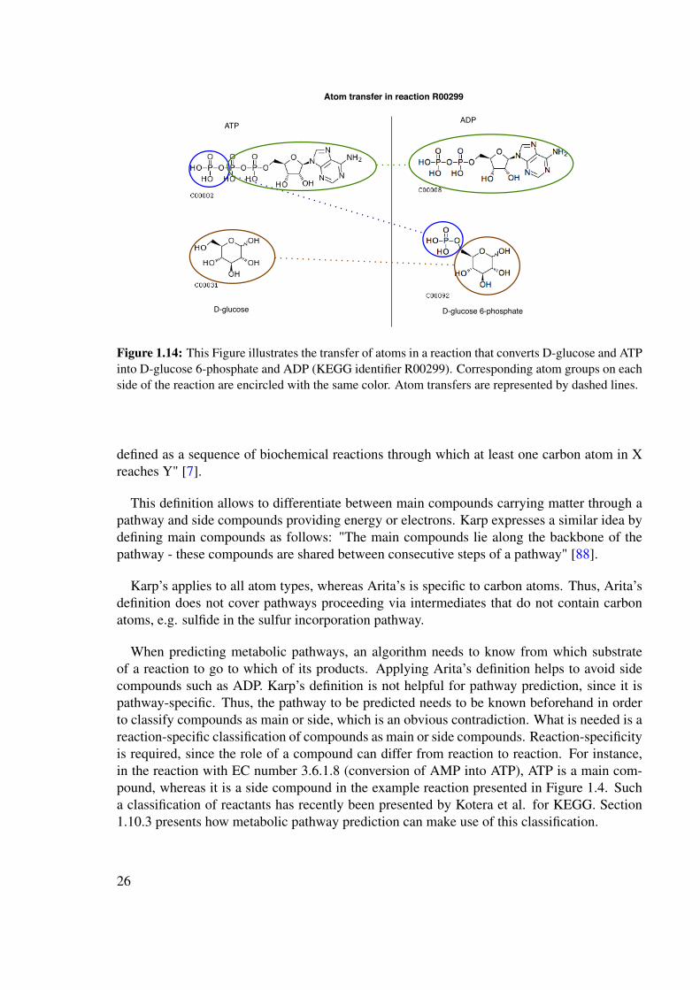
Atom-flow based pathway definitions take into account that a metabolic pathway transfersatom groups from a source compound to a target compound. Figure 1.14 illustrates the transferof atom groups in the example reaction shown in Figure 1.4.
Arita is credited with the invention of the atom-flow based pathway definition, which hephrases as follows: "A metabolic pathway (pathway for short) from metabolite X to Y is
25
ATP
D-glucose D-glucose 6-phosphate
ADP
Atom transfer in reaction R00299
Figure 1.14: This Figure illustrates the transfer of atoms in a reaction that converts D-glucose and ATPinto D-glucose 6-phosphate and ADP (KEGG identifier R00299). Corresponding atom groups on eachside of the reaction are encircled with the same color. Atom transfers are represented by dashed lines.
defined as a sequence of biochemical reactions through which at least one carbon atom in Xreaches Y" [7].
This definition allows to differentiate between main compounds carrying matter through apathway and side compounds providing energy or electrons. Karp expresses a similar idea bydefining main compounds as follows: "The main compounds lie along the backbone of thepathway - these compounds are shared between consecutive steps of a pathway" [88].
Karp’s applies to all atom types, whereas Arita’s is specific to carbon atoms. Thus, Arita’sdefinition does not cover pathways proceeding via intermediates that do not contain carbonatoms, e.g. sulfide in the sulfur incorporation pathway.
When predicting metabolic pathways, an algorithm needs to know from which substrateof a reaction to go to which of its products. Applying Arita’s definition helps to avoid sidecompounds such as ADP. Karp’s definition is not helpful for pathway prediction, since it ispathway-specific. Thus, the pathway to be predicted needs to be known beforehand in orderto classify compounds as main or side, which is an obvious contradiction. What is needed is areaction-specific classification of compounds as main or side compounds. Reaction-specificityis required, since the role of a compound can differ from reaction to reaction. For instance,in the reaction with EC number 3.6.1.8 (conversion of AMP into ATP), ATP is a main com-pound, whereas it is a side compound in the example reaction presented in Figure 1.4. Sucha classification of reactants has recently been presented by Kotera et al. for KEGG. Section1.10.3 presents how metabolic pathway prediction can make use of this classification.
26
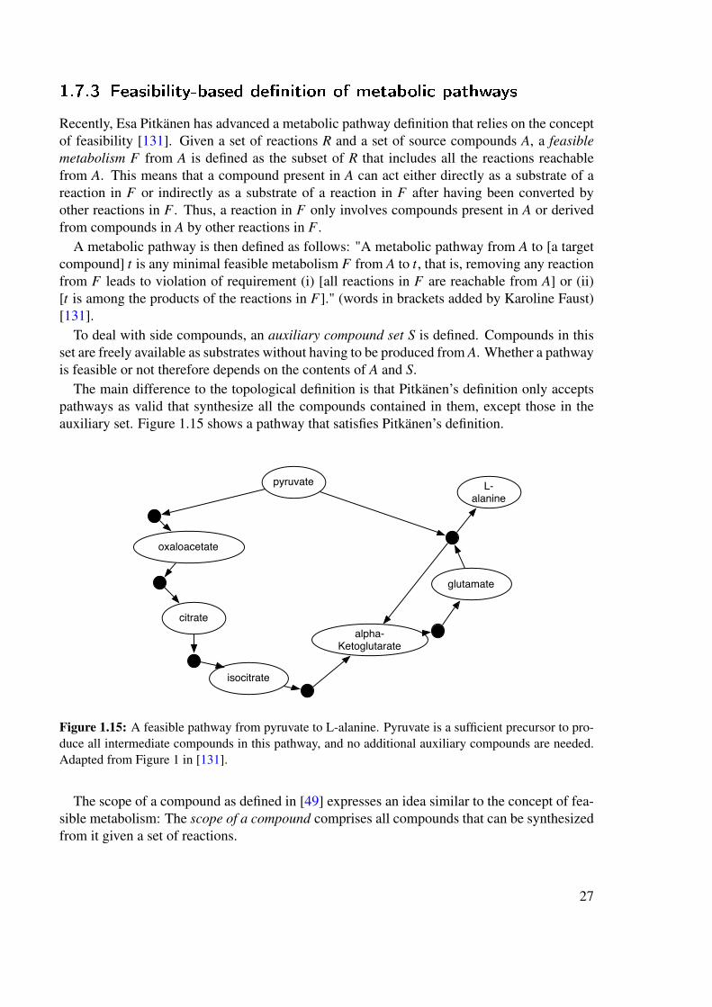
1.7.3 Feasibility-based de�nition of metabolic pathways
Recently, Esa Pitkänen has advanced a metabolic pathway definition that relies on the conceptof feasibility [131]. Given a set of reactions R and a set of source compounds A, a feasiblemetabolism F from A is defined as the subset of R that includes all the reactions reachablefrom A. This means that a compound present in A can act either directly as a substrate of areaction in F or indirectly as a substrate of a reaction in F after having been converted byother reactions in F . Thus, a reaction in F only involves compounds present in A or derivedfrom compounds in A by other reactions in F .
A metabolic pathway is then defined as follows: "A metabolic pathway from A to [a targetcompound] t is any minimal feasible metabolism F from A to t, that is, removing any reactionfrom F leads to violation of requirement (i) [all reactions in F are reachable from A] or (ii)[t is among the products of the reactions in F]." (words in brackets added by Karoline Faust)[131].
To deal with side compounds, an auxiliary compound set S is defined. Compounds in thisset are freely available as substrates without having to be produced from A. Whether a pathwayis feasible or not therefore depends on the contents of A and S.
The main difference to the topological definition is that Pitkänen’s definition only acceptspathways as valid that synthesize all the compounds contained in them, except those in theauxiliary set. Figure 1.15 shows a pathway that satisfies Pitkänen’s definition.
pyruvate
oxaloacetate
citrate
isocitrate
alpha-Ketoglutarate
glutamate
L-alanine
Figure 1.15: A feasible pathway from pyruvate to L-alanine. Pyruvate is a sufficient precursor to pro-duce all intermediate compounds in this pathway, and no additional auxiliary compounds are needed.Adapted from Figure 1 in [131].
The scope of a compound as defined in [49] expresses an idea similar to the concept of fea-sible metabolism: The scope of a compound comprises all compounds that can be synthesizedfrom it given a set of reactions.
27

1.7.4 Functional de�nition of metabolic pathways
In a personal communication, Jacques van Helden suggested a definition that emphasizes reg-ulatory and functional aspects of metabolic pathways. He phrased it as follows: “Geneswhose products are involved in a same metabolic pathways are generally (but not always)co-regulated. This regulation may differ from organism to organism. Different organismsmay respond to the same metabolic requirement by expressing different sets of enzymes andtransporters. The “boundaries” of a metabolic pathway should thus not be defined in termsof absolute rules, such as key compounds or stoichiometry, but be considered as organism-and even context-dependent. Other criteria can be used in addition to co-regulation, such asoperons, synteny, horizontal gene transfer (e.g. in plasmids) or any other criterion revealingsome functional association between sets of genes.”
1.7.5 Stoichiometry-based de�nitions of metabolic pathways
Stoichiometry-based definitions demand that a valid metabolic pathway stoichiometricallybalances all its internal compounds. Compounds classified as external do not need to bebalanced. The classification of compounds into internal and external is pathway-specific.
A famous stoichiometry-based definition of a metabolic pathway is the elementary mode(EM), defined as the "minimal set of enzymes that could operate at steady state with all ir-reversible reactions proceeding in the appropriate direction" [143]. Extreme pathways aresimilarly defined, but differ from elementary modes by their treatment of irreversible and re-versible reactions. For the calculation of extreme pathways, each reversible reaction is splitinto two separate reactions for the forward and reverse directions, whereas in EM analysis, anumber of constraints is placed on reaction directionality [125].
A special case of a stoichiometry-based definition is the enzyme-subset introduced in [129].It defines metabolic pathways as enzyme subsets which are: "groups of enzymes that, inall steady states of the system, operate together in fixed flux proportions" [129]. These en-zymes are considered to form linear metabolic pathways with the same steady-state flux andto be co-expressed simultaneously. This definition forms a link between the functional andstoichiometry-based definitions.
1.7.6 Metabolic pathway de�nition based on chemical
organization theory
Chemical organization theory is a general concept that can be applied to any kind of networkand which has applications in virus infection modeling [109], atmospheric photochemistry[24] and metabolism [23]. According to chemical organization theory, a metabolic pathwayis considered as an organization if it is self-maintaining (all compounds can be re-generatedby the pathway) and closed (all compounds that can be generated given the reactions of thepathway are part of the pathway).
The self-maintainance property combines stoichiometric balance with the idea of feasibilityproposed in [131]. Both, self-maintainance and feasibility, require that all compounds in a
28
pathway can be synthesized by the pathway. The self-maintainance property requires in addi-tion that each pathway synthesizing a compound within the organization is stoichiometricallybalanced.
Compounds that are not self-maintained can flow in or out of the organization. Importantly,compound concentrations can either remain constant or increase, which is an important differ-ence to EM analysis and related methods (see section 1.10.3), which assume approximatelyconstant compound concentrations.
Organizations can be ranked according to the number of different compounds they contain.A changing metabolic network may move up- or downward this hierarchy. Thus, chemicalorganization theory may be applied to describe the evolution of metabolic networks.
1.8 Which de�nition is most appropriate for pathway
prediction?
Most of these pathway definitions have been conceived with specific applications in mind.For example, atom tracing experiments make use of the atom-flow based pathway definition.Thus, in my opinion, the appropriateness of a definition depends on the use one makes of path-way prediction. The functional definition for instance is most appropriate for the predictionof pathways from functionally associated genes, because it defines a pathway through geneassociation. When predicting pathways from sets of reactions or compounds, for instance tomeasure metabolic distances between enzymes [30], the classical definition (with some con-straints to avoid biochemically meaningless pathways), might be more appropriate than thefunctional one.
1.9 Experimental validation of metabolic pathways
Different definitions emphasize different properties of metabolic pathways. Likewise, differ-ent experiments validate different aspects of metabolic pathways, such as the inability of anorganism to synthesize a certain compound if the pathway is disrupted (validation of function)or the flow of atoms through the pathway (validation of flux).
Experiments can be performed at different levels, i.e. at the level of the pathway compo-nents (validation of interaction between enzymes and substrates, measurements of enzymeactivity etc.), at the level of the pathway in vitro (in vitro reconstitution) or in vivo (mutagen-esis, 13C tracing, ...). For the reference pathways listed in the literature, the accumulation ofevidence from different experiments over the years led to their widespread acceptance. Whenpredicting metabolic pathways, it is important to be aware of the experimental techniques fortheir validation. Therefore, three selected whole-pathway validation techniques are brieflypresented.
29

1.9.1 Mutagenesis
A mutant lacking an enzyme of the pathway may not be able to produce the end product of thatpathway. If this disruption of the pathway renders the mutant unable to synthesize essentialcompounds, the mutant is said to be auxotrophic for these compounds, i.e. it can only growwhen these compounds are supplied to it. Absence of the end product or accumulation of oneof its predecessors supports the hypothesis that the enzyme is indeed involved in the pathway.A series of mutants, each lacking another enzyme of the pathway and accumulating anotherintermediate compound, form a strong evidence for the pathway in question.
This classical strategy of elucidating a metabolic pathway has been developed by the fathersof the one-gene-one-enzyme hypothesis, Beadle and Tatum. They identified two Neurosporacrassa mutants, which were unable to produce tryptophan. The first mutant (strain 10575)could only grow in the presence of indole and accumulated anthranilic acid, which could beutilized for growth by the second mutant (strain 4008) [156]. From this and similar findings(e.g. [155]), it could be established that both anthranilic acid and indole are precursors of tryp-tophan and that indole is first synthesized from anthranilate and then converted into tryptophan(see also Figure 1.16).
A problem of mutant construction is the possible presence of isoenzymes or alternativepathways consuming the predecessor or producing the end product. In addition, a many-to-many relationship exists between genes and reactions (see section 1.3.3). Thus, a geneknock-out may not always produce a phenotype that can elucidate a pathway.
anthranilic acid indole tryptophanserine
synthesis blocked in
mutant 10575
synthesis blocked in
mutant 4008
Figure 1.16: The steps of the tryptophan pathway that were elucidated by generating different Neu-rospora crassa mutants [156, 155].
1.9.2 Atom tracing
Atom tracing techniques (isotope labeling in combination with mass spectrometry or othertechniques to identify labeled compounds) confirm that atoms flow indeed through the path-way in question (e.g. in [120, 172]).
1.9.3 In vitro reconstitution
Enzymes of a putative pathway are assembled together with the initial substrate and requiredcofactors in vitro. The formation of the end product is then confirmed with mass spectrometryor another compound identification technique (e.g. [173]).
30

1.10 Review on the computational prediction of
metabolic pathways
In general, metabolic pathway prediction is the task of predicting biochemically validmetabolic pathways given a set of compounds or reactions of interest (referred to as the seedset) and metabolic data. More specifically, when given a group of associated enzyme-codinggenes from an organism of interest, the task is to predict the specific metabolic pathway inwhich the gene products are involved. In addition to the metabolic network and the seeds,most pathway prediction approaches take further information into account (e.g. compoundstructures) in order to increase their prediction accuracy.
1.10.1 Pathway prediction and metabolic reconstruction
This thesis deals with de novo metabolic pathway prediction. In contrast, metabolic recon-struction relies in most cases on known pathways. Metabolic reconstruction aims at recon-structing the entire metabolism of an organism given its genome and additional informationavailable in the literature or from databases. The reconstruction process can be carried outmanually (e.g. [46]), automatically (e.g. [87, 114]) or semi-automatically (automated predic-tion combined with manual curation as in the second tier of BioCyc [22]). During automaticreconstruction, the enzymes of the organism of interest are mapped on a set of known path-ways. This may result in gaps, if enzymes catalyzing reactions of the pathway are absent fromthe organism. Absence of enzymes may have the following reasons:
• The pathway is not present in the organism of interest. [124]
• A variant of the pathway is present in the organism of interest. [124]
• The missing enzymes have not yet been identified in the genome. [124]
• The reaction is spontaneous.
Sophisticated procedures have been developed to fill these gaps [92, 65], but they do notaddress the existence of alternative pathways.
However, an automated metabolic reconstruction procedure was published recently, whichdoes not rely on pre-defined pathways and can therefore detect alternative pathways [28].
1.10.2 Prediction of metabolic pathways - the challenge
Metabolic pathways are highly interconnected, forming large complex networks as shown inFigure 1.17. Extracting relevant pathways from this "hairball" is a challenging task.
Pathway prediction algorithms have to deal with the exponential explosion of the numberof possible pathways [111], because of the many reactions that form more than one product.As explained in section 1.7.1, not all topologically possible pathways are biochemically rele-vant. Thus, an algorithm has to sieve a large set of pathways to arrive at a subset of relevantpathways.
31
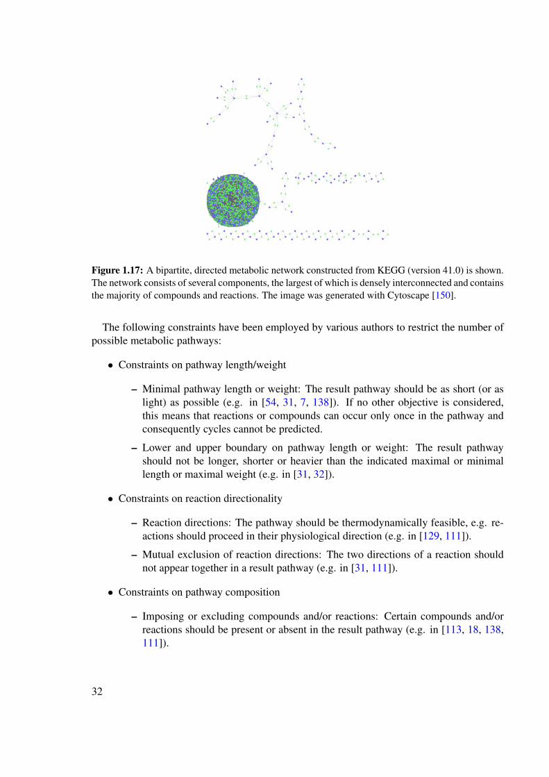
Figure 1.17: A bipartite, directed metabolic network constructed from KEGG (version 41.0) is shown.The network consists of several components, the largest of which is densely interconnected and containsthe majority of compounds and reactions. The image was generated with Cytoscape [150].
The following constraints have been employed by various authors to restrict the number ofpossible metabolic pathways:
• Constraints on pathway length/weight
– Minimal pathway length or weight: The result pathway should be as short (or aslight) as possible (e.g. in [54, 31, 7, 138]). If no other objective is considered,this means that reactions or compounds can occur only once in the pathway andconsequently cycles cannot be predicted.
– Lower and upper boundary on pathway length or weight: The result pathwayshould not be longer, shorter or heavier than the indicated maximal or minimallength or maximal weight (e.g. in [31, 32]).
• Constraints on reaction directionality
– Reaction directions: The pathway should be thermodynamically feasible, e.g. re-actions should proceed in their physiological direction (e.g. in [129, 111]).
– Mutual exclusion of reaction directions: The two directions of a reaction shouldnot appear together in a result pathway (e.g. in [31, 111]).
• Constraints on pathway composition
– Imposing or excluding compounds and/or reactions: Certain compounds and/orreactions should be present or absent in the result pathway (e.g. in [113, 18, 138,111]).
32
• Constraints on compound production
– Maximization of yields: The molar yield of a desired compound should be as highas possible [161].
– Maximization of ATP production: The result pathway should produce a maximumof ATP [11].
• Constraints on compound stoichiometry
– Stoichiometric balance: Internal compounds have to be stoichiometrically bal-anced (e.g. in [11, 129, 111]).
– Minimal number of unbalanced intermediate compounds: The result pathwayshould minimize the number of unbalanced intermediate compounds [133].
• Constraint on pathway specificity
– Optimization of pathway specificity: A compound is the more specific, the fewerthe number of reactions is in which it acts as a substrate or product. The path-way specificity is the sum of the compound specificities in the result pathway andshould be minimal [133]. The specificity concept was inspired by the observationthat penalizing highly connected (i.e. unspecific) compounds improves pathwayprediction [31, 32].
Metabolic pathway prediction approaches, as different as they may be, have twometabolism-specific problems to deal with:
• They have to treat hub compounds (also termed highly connected compounds or high-presence compounds by different authors). An algorithm that accepts hub compoundssuch as water, ADP or ATP as intermediates in a pathway will in most cases predicta biochemically wrong pathway (such as the one shown in Figure 1.13). However,hub compounds may be valid intermediates in some pathways (e.g. ATP in purinemetabolism, see Figure 1.18).
• They have to deal with reaction directions. This problem is often solved by an appro-priate graph representation (as discussed in 1.5). Alternatively, it can be tackled byintroducing constraints on the reaction directions as in EM analysis.
If metabolic pathways are predicted from a set of query genes, genes have to be mapped toreactions, which is complicated by the many-to-many relationship between them. If the querygenes are derived from a genome-scale experiment, scores associated to the genes have to betaken into account as well.
Metabolic pathway prediction from multiple seeds faces in addition the following chal-lenges:
• The result pathway should not depend on the order in which seeds are provided.
33

Figure 1.18: Zoom into the purine metabolism KEGG map. This Figure illustrates that the hub com-pound ATP is a valid intermediate in several pathways. ATP is encircled in maroon.
• It should be possible to provide groups of seed nodes. As mentioned in section 1.3.3,EC numbers are ambiguous and may comprise several reactions. A prediction approachthat can handle seed node groups can treat all reactions of an EC number as belonging tothe same group. As soon as one of the group members occurs in the predicted pathway,the seed node group is considered to be included in the pathway.
• It should be possible to integrate scores derived from high-througput experiments intothe prediction approach in order to preferentially include reactions that are up- or down-regulated according to these data.
1.10.3 Two-end metabolic pathway prediction
Two-end metabolic pathway prediction is a special case of metabolic pathway prediction thatpredicts pathways from two seeds or seed sets. In case pathways are predicted from two seedsets, two-end pathway prediction is also called multiple-to-multiple end pathway prediction.
A remark on notation is needed here. Pathway prediction approaches are classified ac-cording to the number of seed nodes they take into one-seed, two-seed and multiple-seedapproaches (synonymously called one-end, two-end and multiple-end). This thesis focusseson the two-seed and multiple-seed approaches.
Two-end metabolic pathway prediction has several applications, for instance:
• Metabolic reconstruction. Two-end pathway prediction can suggest organism-specificvariants of metabolic pathways.
34

• Measurement of the metabolic distance between enzymes. Didier Croes measured thedistance between enzymes that were associated in various ways (e.g. by protein-protein-interactions, fusion of their genes or grouping of their genes in operons) [30].
• Calculation of metabolic network properties. For example, Jeong et al. searched pathsbetween all compound pairs in a metabolic network to measure its diameter [82] (seesection 1.6).
The tables 1.4 and 1.5 summarize the major two-end metabolic pathway prediction ap-proaches.
35

Tabl
e1.
4:Tw
o-en
dm
etab
olic
path
way
pred
ictio
nst
rate
gies
-Fir
stpa
rt.
Path
findi
ngR
epre
sent
atio
nof
Trea
tmen
tof
Trea
tmen
tof
Num
bero
frea
ctio
n/Im
plem
enta
tion
stra
tegy
met
abol
ickn
owle
dge
hub
com
poun
dsir
reve
rsib
lere
actio
nstr
ansf
orm
atio
nru
les
curr
ently
trea
ted
byth
eap
proa
ch
Path
Met
abol
ickn
owle
dge
isre
pres
ente
dE
xclu
sion
ofa
pre-
defin
edG
raph
stru
ctur
ela
rge
(gra
phs
may
Gra
phtr
aver
sal
findi
ngas
adi
rect
edgr
aph,
listo
fhig
hly
conn
ecte
dco
mpo
unds
(pre
senc
eof
dire
ctan
dco
ntai
nov
er6,
000
(sho
rtes
tpat
hsor
ofte
nw
ithco
mpo
unds
asno
des
[56,
152,
164,
27].
abse
nce
ofre
vers
ear
cre
actio
ns)
k-sh
orte
stpa
ths
algo
rith
ms)
and
reac
tions
asar
csC
onsi
dera
tion
ofco
mpo
und
stru
ctur
ein
adi
rect
edgr
aph)
.(o
ther
vari
ants
,suc
has
bipa
rtite
grap
hsor
atom
trac
ing
[6,1
9,11
2,7,
138,
113]
.or
reac
tion-
cent
ered
grap
hs,e
xist
).W
eigh
ted
grap
hs[3
1,32
].W
eigh
ted
grap
hsco
mbi
ned
with
com
poun
dst
ruct
ure
[18,
54].
Stoi
chio
met
ric
Met
abol
ickn
owle
dge
Man
uala
ssig
nmen
tSp
ecifi
cco
nstr
aint
ssm
all(
<10
0re
actio
ns)t
oE
num
erat
ion
ofso
lutio
nsis
repr
esen
ted
asa
[148
,111
,129
,11]
.(e
.g.E
Man
alys
is)o
rin
term
edia
te(1
00-1
,000
reac
tions
)th
atsa
tisfy
the
set
seto
flin
eare
quat
ions
(EM
)or
Aut
omat
icas
sign
men
t[13
3].
grap
hst
ruct
ure
ofco
nstr
aint
sor
solv
eth
ese
ta
seto
fcon
stra
ints
actin
gon
Com
poun
dsas
sign
edas
exte
rnal
(e.g
.ext
rem
epa
thw
ays
oflin
eare
quat
ions
.se
tsof
com
poun
dsan
dre
actio
ns.
are
notc
onst
rain
edan
alys
is)
Inea
rly
stoi
chio
met
ric
appr
oach
es,
tobe
bala
nced
.L
ISP
isus
edto
find
solu
tions
satis
fyin
gth
egi
ven
cons
trai
nts
[148
,111
].So
met
imes
,an
obje
ctiv
efu
nctio
nis
form
ulat
edan
da
linea
rpro
gram
min
gap
proa
chis
adob
ted
toso
lve
the
seto
flin
eare
quat
ions
with
resp
ectt
oth
eob
ject
ive
func
tion
usin
gav
aila
ble
linea
rpro
gram
min
gso
lver
ssu
chas
CPL
EX
[11,
133]
.R
ule-
base
dM
etab
olic
know
ledg
eR
ules
acto
nSp
ecifi
ctr
ansf
orm
atio
nin
term
edia
tePa
thw
ays
are
gene
rate
dis
repr
esen
ted
asa
seto
fsu
b-st
ruct
ures
(i.e
.fun
ctio
nalg
roup
s)ru
les.
(100
-1,0
00tr
ansf
orm
atio
nru
les)
byite
rativ
ely
appl
ying
auto
mat
ical
lyde
rived
orex
pert
-ass
igne
dof
com
poun
ds.
the
rule
seto
nth
etr
ansf
orm
atio
nru
les
actin
gqu
ery
com
poun
ds(a
tthe
first
step
)on
ase
tofc
ompo
unds
.or
the
tran
sfor
med
com
poun
dsof
the
nth
gene
ratio
n(a
tthe
nth
step
).C
ombi
nato
rial
expl
osio
nis
tack
led
byra
nkin
gru
les
oras
sign
ing
alik
elih
ood
toth
emw
ithth
ehe
lpof
expe
rts
orm
achi
nele
arni
ngap
proa
ches
[80,
50].
Rel
ativ
ere
ason
ing
may
furt
her
redu
ceth
eru
lenu
mbe
r[57
].R
ule
appl
icat
ion
isof
ten
carr
ied
outb
ya
reas
onin
gen
gine
such
asPr
olog
(Met
abol
Exp
ert)
.
36

Tabl
e1.
5:Tw
o-en
dm
etab
olic
path
way
pred
ictio
nst
rate
gies
-Sec
ond
part
.
Poss
ible
cons
trai
nts
Sele
cted
exam
ples
ofSe
lect
edex
ampl
esof
Ava
ilabi
lity
Pote
ntia
lU
nder
lyin
gon
path
way
sco
mpu
tatio
nalv
alid
atio
nex
peri
men
talv
alid
atio
nof
tool
sap
plic
atio
nspa
thw
ayde
finiti
on
Path
leng
th,p
ath
scor
eA
ccur
acy
ofpr
edic
tion
mea
sure
dfo
r:13
Ctr
acin
gin
vivo
Seve
ralo
nlin
eto
ols
Pred
ictio
nof
drug
bios
ynth
esis
[172
]To
polo
gica
l(w
eigh
t,co
mpo
und
148
refe
renc
epa
thw
ays
from
[172
]to
valid
ate
avai
labl
e,se
eTa
ble
1.6.
and
was
teco
mpo
und
defin
ition
.si
mila
rity
,etc
.),ab
senc
e/aM
AZ
Ean
dE
coC
yc[3
2],
path
way
pred
icte
dby
biod
egra
datio
npa
thw
ays
[127
].pr
esen
ceof
com
poun
ds/
92re
fere
nce
path
way
sfr
omE
coC
yc[1
8],
byA
RM
[6]
Rec
onst
ruct
ion
ofm
etab
olic
path
way
sre
actio
ns,r
eact
ion
55re
fere
nce
path
way
sfr
omaM
AZ
E[5
4]fr
omth
ege
nom
e[9
2].
dire
ctio
nalit
yA
llto
polo
gica
lcon
stra
ints
Acc
urac
yof
pred
ictio
nm
easu
red
for:
Des
ign
ofm
utan
tE.c
oli
Seve
ralt
ools
for
Pred
ictio
nof
EM
sSt
oich
iom
etri
can
dad
ditio
nal
10re
fere
nce
path
way
sfr
omE
.col
i[11
]st
rain
sto
optim
ize
biom
ass
EM
anal
ysis
are
avai
labl
e,fo
rthe
desi
gnof
knoc
k-ou
t/in
stra
ins
defin
ition
.st
oich
iom
etri
cco
nstr
aint
40re
fere
nce
path
way
sfr
omE
.col
i[13
3]pr
oduc
tion,
EM
pred
icte
dco
rrec
tlye.
g.YA
NA
[146
],w
ithhi
ghyi
elds
fora
com
poun
dof
inte
rest
.on
inte
rnal
com
poun
ds.
prod
uctio
nof
biom
ass
[161
]M
ETA
TOO
L5.
0[1
66]a
ndA
naly
sis
ofro
bust
ness
ofm
etab
olic
Cel
lNet
Ana
lyze
r[94
]ne
twor
ks.A
naly
sis
ofm
etab
olic
capa
bilit
ies
ofan
orga
nism
[162
].T
hres
hold
son
Bio
degr
adab
ility
pred
ictio
nof
Pred
ictio
nsof
the
met
abol
ism
UM
-PPS
pred
ictio
nsy
stem
Pred
ictio
nof
biod
egra
datio
nTo
polo
gica
lru
lepr
obab
ilitie
s.pe
rfluo
rina
ted
com
poun
ds(C
ATA
BO
L),
ofth
ree
orga
noni
trog
enco
mpo
unds
[75,
50]i
spu
blic
lyof
toxi
cco
mpo
unds
(UM
-PPS
,CA
TAB
OL
),de
finiti
on.
drug
met
abol
ism
pred
ictio
nsfo
rby
UM
-PPS
wer
eco
nsis
tent
avai
labl
e,ot
herp
athw
aypr
edic
tion
ofdr
ugm
etab
olis
m10
subs
trat
es(M
ET
EO
R)[
158]
,w
ithen
rich
men
tcul
ture
sof
pred
ictio
nto
ols
are
avai
labl
e(M
ET
EO
R,M
etab
olE
xper
t).
com
pari
son
ofpr
edic
tions
for
mic
robe
sgr
own
onth
ese
asco
mm
erci
also
ftw
are
six
unkn
own
com
poun
dsby
hum
anco
mpo
unds
asso
leni
trog
en(e
.g.M
ET
EO
R,C
ATA
BO
L,
expe
rts
and
bypr
edic
tion
syst
emso
urce
[75]
.M
etab
olE
xper
t).
(UM
-PPS
).
37

Path �nding approaches
In this section, prediction approaches are presented that do not balance compounds and cantherefore not predict stoichiometry. These approaches are also referred to as path findingapproaches.
Path finding approaches rely in most cases on a graph traversal algorithm in order to enu-merate paths between two compounds or reactions of interest. An exception is the path find-ing approach described in [42, 43], which relies on constraint programming. Path findingapproaches are classified according to their treatment of highly connected compounds.
Tables 1.6 and 1.7 compare a number of path finding tools available on-line (i.e. withweb interfaces). When compiling these tables, MetaRouter [127] and PathMiner [112] werenot available at their published URLs (http://pdg.cnb.uam.es/MetaRouter/ and http:
//pathminer.uchsc.edu, respectively), therefore they are not included.
38

Tabl
e1.
6:Pa
thfin
ding
on-l
ine
tool
s-F
irst
part
.In
puto
ptio
nsO
utpu
topt
ions
Acc
epte
dM
ultip
le-t
o-O
rgan
ism
-spe
cific
Obl
igat
ory
abse
nce
Path
sfil
teri
ngPa
ths
rank
ing
Dis
play
optio
nsTo
olna
me
seed
sm
ultip
lese
edne
twor
kor
pres
ence
ofus
er-p
rovi
ded
optio
nscr
iteri
onM
etab
olic
(ref
eren
ce)
path
findi
ngco
nstr
uctio
nfr
omco
mpo
unds
and/
orre
actio
nsso
urce
data
base
sK
EG
GPA
TH
WA
Yin
pred
icte
dpa
ths
FMM
Com
poun
dsN
oN
oN
oN
one
No
crite
rion
defin
edN
one
KE
GG
[27]
PAT
HW
AY
/L
IGA
ND
,U
niPr
otK
B/
Swis
s-Pr
ot,
dbPT
MR
ahnu
ma
Com
poun
dsY
esY
es,v
ario
usA
user
-pro
vide
dPa
thle
ngth
Path
leng
thH
TM
Lor
sim
ple
text
KE
GG
[113
]op
tions
toco
nstr
uct
ora
pre-
defin
edlis
tof
and
conn
ectiv
itysc
ore
PAT
HW
AY
/ne
twor
kssp
ecifi
cco
mpo
unds
can
beex
clud
ed.
(all
path
ofth
esa
me
leng
thar
eR
PAIR
toa
seto
fA
listo
fele
men
tsth
atha
veto
rank
edac
cord
ing
toth
issc
ore)
and
man
ually
com
pile
dor
gani
sms
orbe
pres
enti
nth
epa
ths
atom
map
ping
sfo
ra
give
nph
ylog
eny
can
begi
ven.
carb
onan
dni
trog
enin
som
eK
EG
Gm
aps.
Met
abol
icC
ompo
unds
,Y
esY
es,v
iaY
esM
axim
alra
nkPa
thw
eigh
tO
utpu
tfor
mat
KE
GG
LIG
AN
D/
Path
finde
rR
eact
ions
,K
EG
Gne
twor
kin
dex
ofpa
ths,
(res
ultt
able
can
beso
rted
(tab
leor
sepa
rate
RPA
IRor
[54]
Rea
ctan
tpai
rs,
prov
ider
.Net
wor
ksm
axim
alpa
thw
eigh
t,ac
cord
ing
topa
thra
nk,
path
sgr
aphs
orpa
ths
optio
nally
KE
GG
EC
num
bers
.ca
nbe
RPA
IRm
inim
alpa
thle
ngth
,pa
thw
eigh
torp
ath
leng
th)
unifi
edin
toon
egr
aph)
.PA
TH
WA
Yne
twor
ks.
max
imal
path
leng
th.
Gra
phfo
rmat
(dot
,gm
l,vi
sml,
tab-
delim
ited)
.R
esul
tsse
ntby
emai
lor
disp
laye
din
brow
ser.
Met
aRou
teC
ompo
unds
No,
but
Yes
Yes
,M
axim
alpa
ths
num
ber
Com
poun
dor
reac
tion
Non
eK
EG
GPA
TH
WA
Y/
[18]
one-
to-a
ll(i
nsu
bseq
uent
step
s).
wei
ght,
path
leng
thL
IGA
ND
,pa
thfin
ding
atom
map
ping
rule
ssu
ppor
ted.
com
pute
dfr
omK
EG
Gan
dE
coC
ycda
ta.
Path
Find
erC
ompo
unds
,N
oN
oN
oN
umbe
rofr
anks
,Pa
thw
eigh
tIm
age
form
atK
EG
GL
IGA
ND
[31,
32]
Rea
ctio
ns,
max
imal
path
leng
th,
(svg
,png
)E
Cnu
mbe
rs.
max
imal
path
wei
ght.
PHT
Com
poun
dsN
oY
esC
ompo
unds
tobe
pres
ent
Min
imal
path
leng
thPa
thle
ngth
and
Non
eK
EG
G(P
athw
ayas
wel
las
EC
num
bers
com
poun
dsi
mila
rity
PAT
HW
AY,
Hun
terT
ool)
tobe
excl
uded
BR
EN
DA
,[1
38]
can
besp
ecifi
ed.
PRO
SIT
EA
RM
Com
poun
dsN
oN
oY
es(e
xclu
sion
only
).N
one
Path
leng
thA
tom
trac
ing
vers
usK
EG
GL
IGA
ND
,(A
tom
icR
eact
ions
can
besp
ecifi
eddr
awin
gm
ode
Eco
Cyc
and
reco
nstr
uctio
nby
thei
rnam
eor
EC
Roc
hePa
thw
aych
art,
ofM
etab
olis
m)
num
ber,
com
poun
dsby
thei
rda
tacu
rate
dan
d[6
,7]
KE
GG
iden
tifier
orna
me.
atom
map
ping
sco
mpu
ted
byth
eau
thor
.
39
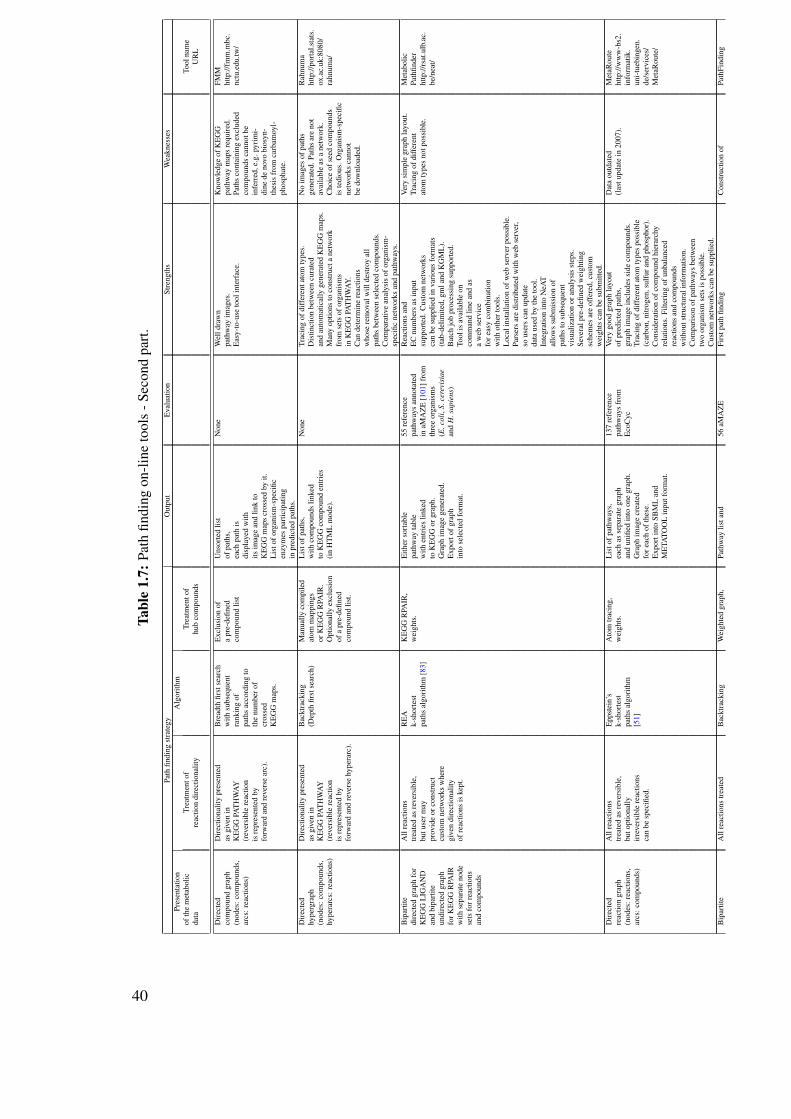
Tabl
e1.
7:Pa
thfin
ding
on-l
ine
tool
s-S
econ
dpa
rt.
Path
findi
ngst
rate
gyO
utpu
tE
valu
atio
nSt
reng
ths
Wea
knes
ses
Pres
enta
tion
Alg
orith
mof
the
met
abol
icTr
eatm
ento
fTr
eatm
ento
fTo
olna
me
data
reac
tion
dire
ctio
nalit
yhu
bco
mpo
unds
UR
L
Dir
ecte
dD
irec
tiona
lity
pres
ente
dB
read
thfir
stse
arch
Exc
lusi
onof
Uns
orte
dlis
tN
one
Wel
ldra
wn
Kno
wle
dge
ofK
EG
GFM
Mco
mpo
und
grap
has
give
nin
with
subs
eque
nta
pre-
defin
edof
path
s,pa
thw
ayim
ages
.pa
thw
aym
aps
requ
ired
.ht
tp://
fmm
.mbc
.(n
odes
:com
poun
ds,
KE
GG
PAT
HW
AY
rank
ing
ofco
mpo
und
list
each
path
isE
asy-
to-u
seto
olin
terf
ace.
Path
sco
ntai
ning
excl
uded
nctu
.edu
.tw/
arcs
:rea
ctio
ns)
(rev
ersi
ble
reac
tion
path
sac
cord
ing
todi
spla
yed
with
com
poun
dsca
nnot
beis
repr
esen
ted
byth
enu
mbe
rof
itsim
age
and
link
toin
ferr
ed,e
.g.p
yrim
i-fo
rwar
dan
dre
vers
ear
c).
cros
sed
KE
GG
map
scr
osse
dby
it.di
nede
novo
bios
yn-
KE
GG
map
s.L
isto
forg
anis
m-s
peci
ficth
esis
from
carb
amoy
l-en
zym
espa
rtic
ipat
ing
phos
phat
e.in
pred
icte
dpa
ths.
Dir
ecte
dD
irec
tiona
lity
pres
ente
dB
ackt
rack
ing
Man
ually
com
pile
dL
isto
fpat
hs,
Non
eTr
acin
gof
diff
eren
tato
mty
pes.
No
imag
esof
path
sR
ahnu
ma
hype
rgra
phas
give
nin
(Dep
thfir
stse
arch
)at
omm
appi
ngs
with
com
poun
dslin
ked
Dis
tinct
ion
betw
een
cura
ted
gene
rate
d.Pa
ths
are
not
http
://po
rtal
.sta
ts.
(nod
es:c
ompo
unds
,K
EG
GPA
TH
WA
Yor
KE
GG
RPA
IR.
toK
EG
Gco
mpo
und
entr
ies
and
auto
mat
ical
lyge
nera
ted
KE
GG
map
s.av
aila
ble
asa
netw
ork.
ox.a
c.uk
:808
0/hy
pera
rcs:
reac
tions
)(r
ever
sibl
ere
actio
nO
ptio
nally
excl
usio
n(i
nH
TM
Lm
ode)
.M
any
optio
nsto
cons
truc
tane
twor
kC
hoic
eof
seed
com
poun
dsra
hnum
a/is
repr
esen
ted
byof
apr
e-de
fined
from
sets
ofor
gani
sms
iste
diou
s.O
rgan
ism
-spe
cific
forw
ard
and
reve
rse
hype
rarc
).co
mpo
und
list.
inK
EG
GPA
TH
WA
Y.ne
twor
ksca
nnot
Can
dete
rmin
ere
actio
nsbe
dow
nloa
ded.
who
sere
mov
alw
illde
stro
yal
lpa
ths
betw
een
sele
cted
com
poun
ds.
Com
para
tive
anal
ysis
ofor
gani
sm-
spec
ific
netw
orks
and
path
way
s.B
ipar
tite
All
reac
tions
RE
AK
EG
GR
PAIR
,E
ither
sort
able
55re
fere
nce
Rea
ctio
nsan
dV
ery
sim
ple
grap
hla
yout
.M
etab
olic
dire
cted
grap
hfo
rtr
eate
das
reve
rsib
le,
k-sh
orte
stw
eigh
ts.
path
way
tabl
epa
thw
ays
anno
tate
dE
Cnu
mbe
rsas
inpu
tTr
acin
gof
diff
eren
tPa
thfin
der
KE
GG
LIG
AN
Dbu
tuse
rmay
path
sal
gori
thm
[83]
with
entr
ies
linke
din
aMA
ZE
[101
]fro
msu
ppor
ted.
Cus
tom
netw
orks
atom
type
sno
tpos
sibl
e.ht
tp://
rsat
.ulb
.ac.
and
bipa
rtite
prov
ide
orco
nstr
uct
toK
EG
Gor
grap
h.th
ree
orga
nism
sca
nbe
supp
lied
inva
riou
sfo
rmat
sbe
/nea
t/un
dire
cted
grap
hcu
stom
netw
orks
whe
reG
raph
imag
ege
nera
ted.
(E.c
oli,
S.ce
revi
siae
(tab
-del
imite
d,gm
land
KG
ML
).fo
rKE
GG
RPA
IRgi
ven
dire
ctio
nalit
yE
xpor
tofg
raph
and
H.s
apie
ns)
Bat
chjo
bpr
oces
sing
supp
orte
d.w
ithse
para
teno
deof
reac
tions
iske
pt.
into
sele
cted
form
at.
Tool
isav
aila
ble
onse
tsfo
rrea
ctio
nsco
mm
and
line
and
asan
dco
mpo
unds
aw
ebse
rvic
efo
reas
yco
mbi
natio
nw
ithot
hert
ools
.L
ocal
inst
alla
tion
ofw
ebse
rver
poss
ible
.Pa
rser
sar
edi
stri
bute
dw
ithw
ebse
rver
,so
user
sca
nup
date
data
used
byth
eto
ol.
Inte
grat
ion
into
NeA
Tal
low
ssu
bmis
sion
ofpa
ths
tosu
bseq
uent
visu
aliz
atio
nor
anal
ysis
step
s.Se
vera
lpre
-defi
ned
wei
ghtin
gsc
hem
esar
eof
fere
d,cu
stom
wei
ghts
can
besu
bmitt
ed.
Dir
ecte
dA
llre
actio
nsE
ppst
ein’
sA
tom
trac
ing,
Lis
tofp
athw
ays,
137
refe
renc
eV
ery
good
grap
hla
yout
Dat
aou
tdat
edM
etaR
oute
reac
tion
grap
htr
eate
das
reve
rsib
le,
k-sh
orte
stw
eigh
ts.
each
asse
para
tegr
aph
path
way
sfr
omof
pred
icte
dpa
ths,
(las
tupd
ate
in20
07).
http
://w
ww
-bs2
.(n
odes
:rea
ctio
ns,
buto
ptio
nally
path
sal
gori
thm
and
unifi
edin
toon
egr
aph.
Eco
Cyc
grap
him
age
incl
udes
side
com
poun
ds.
info
rmat
ik.
arcs
:com
poun
ds)
irre
vers
ible
reac
tions
[51]
Gra
phim
age
crea
ted
Trac
ing
ofdi
ffer
enta
tom
type
spo
ssib
leun
i-tu
ebin
gen.
can
besp
ecifi
ed.
fore
ach
ofth
ese.
(car
bon,
nitr
ogen
,sul
fura
ndph
osph
or).
de/s
ervi
ces/
Exp
orti
nto
SBM
Lan
dC
onsi
dera
tion
ofco
mpo
und
hier
arch
yM
etaR
oute
/M
ETA
TOO
Lin
putf
orm
at.
rela
tions
.Filt
erin
gof
unba
lanc
edre
actio
nsan
dco
mpo
unds
with
outs
truc
tura
linf
orm
atio
n.C
ompa
riso
nof
path
way
sbe
twee
ntw
oor
gani
smse
tsis
poss
ible
.C
usto
mne
twor
ksca
nbe
supp
lied.
Bip
artit
eA
llre
actio
nstr
eate
dB
ackt
rack
ing
Wei
ghte
dgr
aph,
Path
way
lista
nd56
aMA
ZE
Firs
tpat
hfin
ding
Con
stru
ctio
nof
Path
Find
ing
40

dire
cted
grap
has
reve
rsib
le.
(Dep
thfir
stse
arch
)op
tiona
llyim
age
isse
ntby
emai
l.pa
thw
ays
from
tool
that
has
been
care
fully
eval
uate
d.or
gani
sm-s
peci
ficht
tp://
ww
w.
with
sepa
rate
node
anun
wei
ghte
dor
E.c
olia
ndC
ompo
und
stru
ctur
esor
KE
GG
PAT
HW
AY
netw
orks
scm
bb.u
lb.a
c.be
/se
tsfo
rcom
poun
dsfil
tere
dgr
aph
S.ce
revi
siae
,at
omm
appi
ngs
notr
equi
red.
orsu
bmis
sion
ofcu
stom
Use
rs/d
idie
r/an
dre
actio
ns(p
re-d
efine
d92
path
way
sE
asy-
to-u
seto
olin
terf
ace.
netw
orks
isno
tpos
sibl
e.pa
thfin
ding
/co
mpo
unds
from
Eco
Cyc
met
abpa
thfin
ding
.ex
clud
ed)c
anph
pbe
sele
cted
.D
irec
ted
Dir
ectio
nalit
ypr
esen
ted
Bre
adth
Firs
tSea
rch
Glo
bala
ndL
isto
fpat
hs,
2pa
thw
ays
Alis
tofE
Cnu
mbe
rsR
esul
tpag
eis
PHT
com
poun
dgr
aph
asgi
ven
inw
ithco
nstr
aint
slo
calc
ompo
und
each
with
com
poun
dst
ruct
ure
can
bepr
ovid
edto
cons
truc
tdi
fficu
ltto
read
.ht
tp://
pht.t
u-bs
.(n
odes
:com
poun
ds,
KE
GG
PAT
HW
AY
(che
mic
alsi
mila
rity
sim
ilari
tyan
dlin
ksto
KE
GG
entr
ies.
acu
stom
netw
ork.
Dat
ais
outd
ated
de/P
HT
/ar
cs:r
eact
ions
)(r
ever
sibl
ere
actio
nbe
twee
nco
mpo
unds
)Pa
ths
can
bePa
thw
ayou
tput
incl
udes
(las
tupd
ate
in20
06)
isre
pres
ente
ddo
wnl
oade
din
gml
ata
ble
disp
layi
ngby
forw
ard
and
orst
oich
iom
etri
cm
atri
xfo
rmat
.w
hich
reac
tions
occu
rre
vers
ear
c).
Org
anis
min
form
atio
ndi
spla
yed.
inw
hich
ofth
ese
lect
edor
gani
sms.
Mat
rice
sw
ithre
actio
n/en
zym
eA
naly
sis
and
dow
nloa
dof
occu
rren
ces
inse
lect
edor
gani
sm-s
peci
ficne
twor
ksis
poss
ible
.or
gani
sms
avai
labl
e.H
ubco
mpo
unds
and
reac
tions
asw
ella
slo
adan
dch
oke
poin
tsar
elis
ted.
Dir
ecte
dD
irec
tiona
lity
pres
ente
dE
ppst
ein’
sA
tom
trac
ing
Lis
tofp
aths
,C
orre
cttr
acin
gW
elld
raw
npa
thw
ayU
seri
nter
face
isA
RM
com
poun
dgr
aph
asgi
ven
ink-
shor
test
each
path
asso
ciat
edw
ithof
atom
sha
sbe
enim
ages
incl
udin
gco
mpo
und
stru
ctur
es.
noti
ntui
tive.
Java
appl
etis
http
://w
ww
.(n
odes
:com
poun
ds,
KE
GG
LIG
AN
D.
path
sal
gori
thm
anim
age
show
ing
syst
emat
ical
lyTr
acin
gof
diff
eren
tato
mty
pes:
inco
nven
ient
tocl
ose
met
abol
ome.
jp/
arcs
:rea
ctio
ns)
Dir
ectio
nalit
yof
the
com
poun
dst
ruct
ures
.va
lidat
ed,b
utac
cura
cyca
rbon
,nitr
ogen
and
sulf
urar
esu
ppor
ted.
(bro
wse
rhas
tobe
clos
ed).
soft
war
e/re
actio
nsca
nbe
Mor
epa
ths
can
beof
reco
very
ofV
isua
lizat
ion
ofat
omtr
acin
g:E
xpor
tofp
aths
notp
ossi
ble.
plon
ejav
aapp
let.
mod
ified
.ad
ded
toth
elis
tkn
own
path
way
sPo
sitio
nsof
sele
cted
atom
2006
-06-
29.
with
am
ouse
clic
k.w
asno
tmea
sure
d.in
path
com
poun
dsis
9364
6046
35/
high
light
edon
mou
secl
ick.
Path
way
sca
nbe
mod
ified
byth
eus
erw
itha
chem
ical
stru
ctur
edr
awin
gto
ol.
App
letv
isua
lizes
stru
ctur
esof
subs
trat
esan
dpr
oduc
ts,
whi
chca
nbe
sear
ched
byen
teri
ngco
mpo
und
orre
actio
nK
EG
Gid
entifi
ers
orna
mes
,re
actio
neq
uatio
nsor
EC
num
bers
,m
anua
llydr
awn
com
poun
dst
ruct
ures
orco
mpo
und
form
ulas
.
41
A. Path �nding without hub compound treatment
As mentioned in 1.6, a "small world" property of metabolic networks is postulated in [82], i.e.in most metabolic networks, any two compounds can be connected by a short path (of lengtharound three). However, these authors failed to treat highly connected compounds and there-fore based their analysis on biochemically invalid pathways. Several authors have repeatedthis analysis and have demonstrated that the average shortest path length is much higher ifhub compounds are treated appropriately. For instance, the average shortest path length be-tween compounds in the Escherichia coli network was measured independently in [107] and[7] to be around eight, where the former authors treated hub compounds by excluding themand the latter avoided them by atom tracing. The distribution of average path lengths betweenreactions in the complete KEGG network peaked between five and eight reaction steps [32].
Currently, no path finding tool exists that does not treat hub compounds.
B. Path �nding with exclusion of highly connected compounds
Many authors treat highly connected compounds by excluding them from the network [56,164, 152, 107, 27]. This strategy has the drawback that pathways containing those compoundsas intermediates cannot be predicted. For instance, ADP and ATP are often excluded as typicalhub compounds, but are valid intermediates in the purine biosynthesis pathway. In addition,the distinction of a non-hub from a hub node requires additional parameters (e.g. a thresholdon the node degree).
FMM [27] is an example for a path finding tool that treats hub compounds by excludingthem. Consequently, it fails to find a path between carbamoyl-phosphate and CTP (the startand end point of pyrimidine ribonucleotides de novo biosynthesis). Remarkably, this pathfinding tool is the only one in the tables 1.6 and 1.7 that predicts the glycolysis pathwaycorrectly from glucose and pyruvate. The reason is that pathways are post-filtered with KEGGpathway maps. Strictly speaking, because of its use of KEGG maps, FMM is not a de novopathway prediction tool as the others discussed in this section. It has been included in tables1.6 and 1.7 because it shares many properties with other path finding tools.
C. Path �nding in weighted networks
In [31, 32], Didier Croes presented a path finding approach that avoids highly connected com-pounds by assigning weights to the nodes of the metabolic network. The weights are assignedsuch that sparsely connected compounds are preferentially traversed by the path finding algo-rithm. More precisely, each compound receives a weight equivalent to its degree, that is to itsnumber of incoming and outgoing arcs. Reactions receive a weight of one. The backtrack-ing algorithm developed by Fabian Couche [29] enumerates the lightest paths in the weightednetwork. Path finding in weighted networks can identify relevant metabolic pathways withoutthe need of compound exclusion or compound structures.
In addition, Didier Croes compared the performance of the weighted network to a filterednetwork (where 36 highly connected compounds were removed) and to an untreated "raw"network. The evaluation was carried out on metabolic networks constructed from KEGG andEcoCyc [90] (which is a part of BioCyc) and proceeded as follows: First, a pathway waspredicted given the start and end reaction of a linearized reference pathway. Then, the pathfinding accuracy was computed by comparing the node sets of the predicted and the reference
42

pathway. This procedure was repeated on 56 pathways from aMAZE [101] and 104 pathwaysfrom EcoCyc. For both, KEGG and EcoCyc, the weighted network clearly outperformed thefiltered and the raw network.
A path finding tool accompanied the evaluation (PathFinding, [31]). This tool is no longeravailable, but is listed in tables 1.6 and 1.7 because it is the predecessor of the MetabolicPathfinder tool developed during this thesis.
Didier Croes’ work was the starting point for this thesis, which owes not only the use ofa weight policy to him but also ideas on path finding accuracy measurement and metabolicnetwork construction. In addition, Didier Croes inspired the improved path finding approachpresented in [54].
D. Path �nding considering compound structure
Faced with the hub compound problem, many authors developed different solutions that allrelied on the idea of taking the structure of compounds into account.
As mentioned in 1.7.2, Arita introduced the idea to trace atoms through metabolic networksin silico [5] and developed a path finding tool (ARM, atomic reconstruction of metabolism)based on this idea [6, 7]. Atom tracing proceeds as follows: For each reaction in the metabolicnetwork, each of its substrates is paired with each of its products. For each substrate-productpair, the structures are mapped such that corresponding atom positions can be identified. Todo so computationally means to solve the maximum common subgraph problem, which isNP-hard. Arita developed an efficient heuristic, which minimizes breakage and formation ofchemical bonds [5, 6]. In [19], this heuristic is combined with maximal partial injections,which allow to find reactions that transfer a maximal number of atoms. Other authors do nottrace atoms, but instead compute overall compound similarities. The compound structure isfirst reduced to a descriptor, which is either a vector in a chemical state space [112] or a stringgenerated with dedicated software [138]. In a second step, a distance measure between thesedescriptors is introduced, which allows to search for paths that maximize compound similarity.
Atom tracing considers the two-dimensional structure of compounds, whereas compoundstructure descriptors simplify compound structure further to one dimension, allowing forquicker search and comparison. In the absence of a comparative evaluation of tools basedon two-dimensional compound structure (such as ARM) or one-dimensional compound struc-ture description (such as Pathway Hunter Tool [138]), it is not clear whether a simplificationfrom two to one dimension means a loss of path finding accuracy.
With the RPAIR database, manually compiled reactant pair mappings became available[97, 96]. Each of these reactant pairs has a role assigned to it, such as main ("main changeson substrates" [96]) or trans ("focused on transferred groups for transferases" [96]). Table 1.8lists all such roles as defined in [96].
With these reactant pairs at hand, it is possible to identify the main and side compounds ofa reaction. For instance, a naive algorithm could cross the reaction shown in Figure 1.4 fromD-glucose to ADP or from ATP to D-glucose-6-phosphate. An informed algorithm takinginto account the RPAIR annotation will avoid these irrelevant paths, because the pair ATP/D-glucose-6-phosphate has the role trans instead of main and the pair D-glucose/ADP does noteven exist (since no atoms are transfered between these two compounds). Figure 1.19 givesan illustration of this example.
43

RP00003 (main)
RP00060 (main)
RP08556 (trans)
ATP (C00002)
D-Glucose (C00031)
ADP (C00008)
D-Glucose 6-phosphate (C00092)
R00299
A
B
Figure 1.19: Figure A shows the reactant pair decomposition of KEGG reaction R00299, whereasFigure B depicts more clearly the relationships between the reactant pairs and their substrates andproducts. The reaction can be decomposed into three reaction pairs, two main reactant pairs reflectingthe transfer of large atom groups (ATP/ADP and D-glucose/D-glucose 6-phosphate) and one transreactant pair (ATP/D-glucose 6-phosphate), which describes the transfer of the phosphate group. Thesethree reactant pairs correspond to the three atom groups shown in Figure 1.14 for the same reaction.Importantly, there is no reactant pair between D-glucose and ADP, since no atoms are transferredbetween these two compounds. Note also that each reactant pair has only one substrate and one product.
44
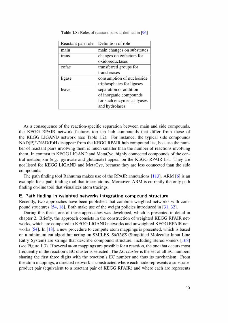
Table 1.8: Roles of reactant pairs as defined in [96]
Reactant pair role Definition of rolemain main changes on substratestrans changes on cofactors for
oxidoreductasescofac transferred groups for
transferasesligase consumption of nucleoside
triphosphates for ligasesleave separation or addition
of inorganic compoundsfor such enzymes as lyasesand hydrolases
As a consequence of the reaction-specific separation between main and side compounds,the KEGG RPAIR network features top ten hub compounds that differ from those ofthe KEGG LIGAND network (see Table 1.2). For instance, the typical side compoundsNAD(P)+/NAD(P)H disappear from the KEGG RPAIR hub compound list, because the num-ber of reactant pairs involving them is much smaller than the number of reactions involvingthem. In contrast to KEGG LIGAND and MetaCyc, highly connected compounds of the cen-tral metabolism (e.g. pyruvate and glutamate) appear on the KEGG RPAIR list. They arenot listed for KEGG LIGAND and MetaCyc, because they are less connected than the sidecompounds.
The path finding tool Rahnuma makes use of the RPAIR annotations [113]. ARM [6] is anexample for a path finding tool that traces atoms. Moreover, ARM is currently the only pathfinding on-line tool that visualizes atom tracings.
E. Path �nding in weighted networks integrating compound structureRecently, two approaches have been published that combine weighted networks with com-pound structures [54, 18]. Both make use of the weight policies introduced in [31, 32].
During this thesis one of these approaches was developed, which is presented in detail inchapter 2. Briefly, the approach consists in the construction of weighted KEGG RPAIR net-works, which are compared to KEGG LIGAND networks and unweighted KEGG RPAIR net-works [54]. In [18], a new procedure to compute atom mappings is presented, which is basedon a minimum cut algorithm acting on SMILES. SMILES (Simplified Molecular Input LineEntry System) are strings that describe compound structure, including stereoisomers [168](see Figure 1.3). If several atom mappings are possible for a reaction, the one that occurs mostfrequently in the reaction’s EC cluster is selected. The EC cluster is the set of all EC numberssharing the first three digits with the reaction’s EC number and thus its mechanism. Fromthe atom mappings, a directed network is constructed where each node represents a substrate-product pair (equivalent to a reactant pair of KEGG RPAIR) and where each arc represents
45

a compound shared by two substrate-product pairs. The performance of this network undervarious weight policies was assessed.
For both approaches, thorough evaluation showed that a weighted network penalizing hubcompounds and integrating compound structure reached the highest path finding accuracy.
Both approaches are available as on-line tools: Metabolic Pathfinder [54](http://rsat.ulb.ac.be/neat/) and MetaRoute [17] (http://www-bs2.informatik.uni-tuebingen.de/services/MetaRoute/). Metabolic Pathfinder is currently the onlypath finding on-line tool that accepts reactions as source and target, whereas MetaRoute is theonly path finding on-line tool that offers tracing of four atom types.
Stoichiometric pathway prediction
Stoichiometric pathway prediction constraints the solution space further than path finding byonly accepting stoichiometrically balanced paths. Thus, in contrast to path finding, this path-way prediction approach can also predict stoichiometric coefficients.
A. Early contributions
In one of the first articles on computational metabolic pathway prediction, a search algorithmwritten in LISP acts on a database including 100 compounds and 70 enzymes [148]. For eachcompound, the elements it carries are listed (e.g. carbon, nitrogen, . . . ), which facilitate bal-ances on carbon, phosphorus, sulfur, and nitrogen. Energy carriers such as ATP and electrondonors such as NADPH are freely available, all other compounds involved in a pathway haveto be synthesized by it. A pathway can be predicted by defining an "initial state" (equivalent toa source compound) and by applying enzyme "operators" on it until a a "target state" (a targetcompound) has been reached. An enzyme and its reaction are represented as a single entity,which is annotated with the EC number, the physiological reaction direction, the reactantswith their stoichiometric coefficients, the enzyme activators, inhibitors and known pathways.The system was tested by providing glucose-6-phosphate and pyruvate as seeds, which yieldedthe Embden-Meyerhof-Parnas (that is glycolysis), Entner-Doudoroff, and pentose phosphatepathways.
Some years later, Mavrovouniotis [111] extended this work by introducing new constraintsto the system, which still consists of a metabolic database (with 250 reactions and 400 com-pounds) and a search algorithm written in LISP. The constraints include those on the ther-modynamic feasibility of a reaction, i.e. only reactions are allowed that can proceed in thepredicted direction under physiological conditions. As described in section 1.3.2, the direc-tion of a reaction depends on its Gibbs free energy change. Mavrovouniotis developed a groupcontribution method to calculate this quantity. Other constraints forbid or require selectedcompounds and reactions to occur in predicted pathways and limit the pathway size. Hubcompounds are treated as in [148] as freely available compounds, which do not need to bebalanced or synthesized. Mavrovouniotis analyzed the production of lysine from glucose andammonia as a case study. He identified kinetic bottlenecks given reactant concentrations andenzyme rates and suggested alternative pathways to circumvent these bottlenecks. He alsointroduced the lumping of a linear sequence of reactions into one reaction and the ranking ofpathways by yield.
46
B. Elementary mode analysis
ELementary mode analysis does not take two seed nodes and can therefore not be consideredas a two-end pathway prediction technique. But since it has been compared with path finding[38, 132], it will be treated here.
The definition of elementary modes (EM) is given in section 1.7.5. In the following, thecomputation of EMs is summarized (see e.g. [129, 162]).
The development of compound concentrations over time can be described by a set of lineardifferential equations involving the reaction rates and the stoichiometry of compounds partic-ipating in a reaction. These equations can be written in a compact form using matrices andvectors:
dCdt
= S∗ v (1.2)
where v is the vector of reaction rates (also called fluxes), S the stoichiometric matrix and Cthe vector of compound concentrations. Each row of the stoichiometric matrix represents acompound and each column a reaction, whereas each entry is the stoichiometric coefficient ofthe ith compound in the jth reaction.
The basic assumption of EM analysis (as well as flux balance analysis and metabolic fluxanalysis) is that due to the fast turn-over of compounds, metabolism can be considered to beat steady state (chemostat) or at pseudo steady state (batch culture) at relevant time scales.Thus, compound concentrations do not change over time and consequently the left-hand sideof equation 1.2 can be set to zero:
S∗ v = 0 (1.3)
With this simplification it is possible to compute the solutions that satisfy equation 1.3 andsome additional constraints concerning reaction directionality. Geometrically, the solutionspace forms a convex polyhedral cone. Each solution is a vector of fluxes. EMs are specialsolution vectors satisfying an additional non-decomposability constraint, which roughly statesthat no reaction can be removed from an EM without disturbing it as a functional unit [125].EMs can be computed with tools such as METATOOL [166] or efmtool [157].
In EM analysis, compounds are classified into internal compounds, which need to be bal-anced and external compounds, which are assumed to be freely available and are therefore notbalanced. Likewise, reactions are classified into internal reactions, which take place insidethe system and exchange reactions, which cross system borders (e.g. transport). Metabolicnetworks need to meet certain requirements in order to apply EM analysis on them: for eachreaction, all concerned elements (i.e. atoms and ions) and their charges need to be balanced.Parallel pathways, null cycles, dead ends or erroneous exchange reactions need to be identi-fied and removed. In order to simplify the metabolic network, linear sequences of reactionsare lumped into one reaction, e.g. the last four steps of glycolysis in [38]. Metabolic net-works are usually small and carefully constructed by hand. However, recent advances in EMcomputation allow their application to genome-scale metabolic networks [85, 37, 157].
De Figueiredo et al. compared EM analysis to path finding tools (namely PathFinder andPathway Hunter Tool) [38]. In [53], we pointed out weaknesses of this comparison and in ad-dition enumerate advantages and disadvantages of EM analysis and path finding for metabolic
47
pathway prediction. This discussion can be found in chapter 5. A comparison of both ap-proaches has also been published in [132].
The solution space of equation 1.3 is spanned by flux vectors called extreme pathways (e.g.[125]). Since the extreme pathways were apparently not yet employed for metabolic pathwayprediction, they will not be further discussed here.
C. Other stoichiometric approachesIn [11], a stoichiometric approach is presented that combines constraints with an objectivefunction. Thus, in contrast to EM analysis, the solution space is narrowed to one solution,which optimizes the objective function. The objective function is a mixture of two objectives:(1) minimize the number of reactions in a pathway and (2) maximize the ATP production.
Compounds are classified as low presence and high presence compounds depending on thenumber of reactions they are involved in. As the external compounds in EM analysis, "highpresence" compounds do not need to be balanced.
Constraints include those for low presence compound balancing and for mutual exclusionof the two directions of one reaction. In particular, a number of constraints concerns cycles;e.g. cycles involving more than one high presence compound are forbidden.
With these objective function and constraints, a number of known pathways could be recov-ered from the Escherichia coli metabolic network, among others glycolysis.
In a second article [133], this constraint-based pathway prediction is further refined:
• Prediction of more than one paths (K paths) between a source and a sink allows to dealwith branched pathways.
• "Low presence" and "high presence" compounds are no longer manually assigned be-forehand, but automatically during pathway prediction.
• Another optimization function is introduced, which minimizes the number of unbal-anced main compounds and maximizes the specificity of the pathway. The pathwayspecificity depends on its number of specific compounds. A compound is the morespecific the less it is involved in other reactions.
• Additional constraints for the treatment of highly connected compounds are introduced,e.g. inorganic compounds or high presence compounds are not allowed to occur in apath if source and sink can be connected by other compounds.
Pathway prediction has been evaluated on 40 reference pathways from Escherichia coli, 36of which were exactly recovered [133].
Rule-based pathway prediction
Rule-based pathway prediction consists in the iterative application of transition rules on a setof compounds. It may proceed as one-end prediction (e.g. to propose a number of differentdegradation pathways for one query compound) or two-end prediction (after a desired targetcompound was obtained, the iterative application of rules is stopped). The rules are definedsuch that hub compounds are avoided.
48
Rules describe generalized reactions, which cover a set of specific reactions. Usually, arule applies to a certain sub-structure (e.g. functional group) of a compound class, e.g. therule "primary Alcohol converted to Aldehyde" (rule identifier bt0001 in UM-BBD [50]) isapplicable to all compounds with an alcoholic group.
Rules are often manually annotated by experts (e.g. in UM-PPS [50], METEOR [66] orMetabolExpert [35]) or automatically derived by generalizing reactions (e.g. [80, 69]).
In order to deal with combinatorial explosion, rules are ranked with the help of expertknowledge (e.g. [50]) or by machine learning approaches (e.g. [57]).
A number of rule-based tools is available, which are specialized on different metabolicnetworks. For example, METEOR and MetabolExpert are commercial expert systems tailoredto drug metabolism, whereas CATABOL (commercial) and UM-PPS (freely available) aredesigned to predict biodegradation pathways.
In contrast to the path finding and stoichiometric approaches, the metabolic fate of com-pounds not yet present in a database can be predicted, since rules apply to compound sub-structures and not to the whole compound. Most rule-based pathway prediction tools are com-mercialized, probably because carefully designed rules allow them to reach a high positivepredictive value. However, without a systematic evaluation, it is unclear whether these toolsalso reach a high accuracy, because overly restrictive rules might decrease their sensitivity.
1.10.4 Multiple-end metabolic pathway prediction
In the previous section, metabolic pathway discovery with two seeds or seed sets was pre-sented, where seeds act as source and target compound(s) and/or reaction(s) respectively. Amore ambitious goal is the prediction of a metabolic pathway from a seed group (or severalseed groups). For this, an algorithm is needed that extracts a relevant sub-network from theinput network given the seed nodes. Metabolic pathway prediction from several seeds has re-ceived much less attention than prediction given two seeds. Therefore, sub-network extractiontechniques applied to other biological networks will be discussed here as well.
There is a clear distinction between the inference of a network from microarray or other datasets (as in [171]) and the extraction of a sub-network from a network. The goal of the formerapproach is to predict (at least partially) a network from high-throughput data (e.g. regulatorynetworks from gene expression profiles), whereas the goal of the latter approach is to predict apathway from a network that is already known. In sub-network extraction, the network can beweighted with high-througput data, but these weights do not affect the topology of the networkitself.
The development of multiple-seed pathway extraction techniques has been driven by theneed to interpret high-troughput data sets. Zien et al. [177] were among the first to advance atechnique that instead of mapping genes on pre-defined pathways enumerated possible path-ways in a metabolic network and selected the pathway that fitted best the given gene expressiondata. However, their work was restricted to two-end pathway prediction.
Tables 1.9 and 1.10 summarize a selection of different multiple-seed sub-network extractionapproaches developed during the last years. These approaches may be classified into globaland local approaches according to seed node treatment. Global approaches ([77, 139, 119])
49

select nodes in the network during execution of the algorithm such that the resulting sub-network optimizes a criterium (usually sub-network weight) whereas local approaches receivea set of seed nodes beforehand which are then connected ([147, 40, 3, 4]). However, seed-nodespecific sub-networks can also be extracted with global approaches, by assigning appropriateweights to the network nodes (low weights to the seeds, high weights to all other nodes).
Sub-network extraction has been applied to protein-protein and protein-DNA interactionnetworks [77, 147, 40], metabolic networks [119, 3, 4] and networks integrating both of theformer [139].
Usually, sub-networks are extracted from weighted networks. Often, the weights representscores derived from one or several high-throughput experiments (microarray data in [77, 40]or enzyme levels in [119]). This thesis focusses on sub-network extraction and does not makeuse of high-throughput data to weight the networks. However, since the weight assignmentstep is clearly separated from the sub-network extraction step, the procedures applied in thisthesis can be easily combined with more sophisticated weight policies.
Many authors developed their own heuristics to solve the sub-network extraction problem[77, 139, 119, 3, 4]. Others extract sub-networks with Steiner tree algorithms [147, 40]. Asdescribed in section 9.1, a Steiner tree algorithm searches for the sub-network that connectsthe given seed nodes in the given network with minimal weight. This problem is knownto be NP-hard, which means, roughly stated, that it cannot be solved in polynomial time.Nevertheless, some Steiner tree algorithms have been published that solve the problem exactly(though not in polynomial time). For instance, the Dreyfus-Wagner algorithm [45] is appliedwith modifications in [147] and Ljubic’s exact solution [105] is applied in [40].
Most sub-network extraction techniques are not accompanied by web servers or ready-to-use applications, with the exception of [77] (Cytoscape plugin) and [3] (two web servers).In addition, only few approaches have been evaluated ([139, 40]). Thus, the evaluation pre-sented in [55] and the pathway prediction web server developed during this thesis are usefulcontributions to the prediction of metabolic pathways from multiple seeds.
50

Tabl
e1.
9:M
ultip
le-e
ndpa
thw
aypr
edic
tion
stra
tegi
es-F
irst
part
.Su
bgra
phex
trac
tion
stra
tegy
Bio
logi
caln
etw
ork
Om
ics
data
map
ped
Net
wor
kw
eigh
tTr
eatm
ento
fM
etab
olic
netw
orks
only
:(r
efer
ence
)on
netw
ork
assi
gnm
ent
hub
node
str
eatm
ento
frea
ctio
ndi
rect
iona
lity
Heu
rist
icba
sed
onU
ndir
ecte
dpr
otei
n-pr
otei
nG
ene
expr
essi
onin
Eac
hno
deis
assi
gned
Ifno
dede
gree
isgr
eate
r_
sim
ulat
edan
neal
ing
and
prot
ein-
DN
Ain
tera
ctio
nne
twor
kse
vera
lcon
ditio
ns[7
8].
anag
greg
ated
z-sc
ore
than
aus
er-d
efine
dpa
ram
eter
d min
,(I
deke
reta
l.[7
7])
(sm
alln
etw
ork:
362
edge
s,ob
tain
edfr
omca
lcul
ated
over
seve
ralc
ondi
tions
.al
lnei
ghbo
urs
ofth
eno
deG
AL
path
way
pert
urba
tion
stud
yth
atar
eno
tin
the
top-
scor
ing
inye
ast[
78],
larg
ene
twor
k:co
mpo
nent
are
rem
oved
.7,
462
edge
sfr
omB
IND
[8]
and
TR
AN
SFA
C[1
10])
Heu
rist
icba
sed
onU
ndir
ecte
dne
twor
kin
tegr
atin
gN
one
Low
wei
ghts
for
Exc
lusi
on(c
omm
onco
fact
ors,
AT
P,et
c.)
Und
irec
ted
netw
ork:
brea
dth
and
dept
hfir
stse
arch
data
from
Inge
nuity
Path
way
sge
neno
des
ofin
tere
stan
dpe
nalty
scor
efo
rhub
node
s.re
actio
ndi
rect
iona
lity
cann
ot(R
ajag
opal
anan
dA
garw
al[1
39])
Kno
wle
dge
Bas
e,T
RA
NSF
AC
and
(ran
dom
lydi
stri
bute
dbe
twee
n0
and
Pena
ltyde
pend
son
betr
eate
d.H
uman
Cyc
,thu
sco
veri
ngm
etab
olis
m,
10−
3to
sim
ulat
elo
wp-
valu
es).
aus
er-p
rovi
ded
para
met
erβ
,si
gnal
tran
sduc
tion
and
gene
regu
latio
nA
llot
herg
ene
node
sre
ceiv
edw
hich
cont
rols
the
size
of(9
,300
node
san
d30
,000
edge
s).
aw
eigh
tran
dom
lydi
stri
bute
dth
esu
b-ne
twor
k.be
twee
n0
and
1(t
osi
mul
ate
rand
omp-
valu
es).
Heu
rist
ican
dex
act
Und
irec
ted
prot
ein-
prot
ein
Gen
eex
pres
sion
P-va
lue
p uof
diff
eren
tially
Non
e_
Stei
nert
ree
algo
rith
ms
and
prot
ein-
DN
Ain
tera
ctio
nin
seve
ralc
ondi
tions
expr
esse
dge
neu
isas
sum
ed(S
cott
etal
.[14
7])
netw
ork
inte
grat
ing
data
from
[78]
.to
begi
ven.
P uis
then
BIN
D,T
RA
NSF
AC
,SC
PD[1
76]a
ndco
nver
ted
into
aw
eigh
tby
yeas
tChI
P-C
hip
expe
rim
ents
the
wei
ghtf
unct
ion
wd(
u)=−
log(
1−
p u).
(5,4
58no
des
and
23,6
42ed
ges)
.A
nal
tern
ativ
ew
eigh
tfun
ctio
nw
1as
sign
sw
eigh
tofo
neto
each
node
.H
euri
stic
base
don
Und
irec
ted
enzy
me
netw
ork
Rat
ioof
prot
ein
quan
titie
sW
eigh
tofa
ned
geW
eigh
ts(h
ubco
mpo
unds
Und
irec
ted
netw
ork:
mer
ging
filte
red
path
sob
tain
edfr
omK
EG
G(n
etw
ork
mea
sure
dfo
rtw
oco
nditi
ons
betw
een
two
rece
ive
ape
nalty
)re
actio
ndi
rect
iona
lity
(Noi
rele
tal.
[119
])si
zeno
tind
icat
ed).
[153
]en
zym
esis
the
cann
otbe
trea
ted.
num
bero
focc
urre
nces
ofco
nnec
ting
com
poun
d(f
orse
vera
lcom
poun
ds,l
east
com
mon
one
isus
ed).
Exa
ctSt
eine
rU
ndir
ecte
dpr
otei
n-pr
otei
nG
ene
expr
essi
onP-
valu
esde
rived
from
Non
e_
tree
algo
rith
min
tera
ctio
nne
twor
kob
tain
edfr
om(B
-cel
llym
phom
as,[
142]
)di
ffer
ents
ourc
esar
eag
greg
ated
(Ditt
rich
etal
.[40
])H
PRD
[136
](9,
392
node
san
dan
dpa
tient
surv
ival
data
usin
gith
orde
rsta
tistic
.36
,504
edge
sfo
rful
lnet
wor
k,(1
90pa
tient
s,[1
42])
The
p-va
lue
dist
ribu
tion
isas
sum
edin
ters
ectio
nne
twor
kw
ithto
bea
mix
ture
ofsi
gnal
and
nois
e.ge
ne-e
xpre
ssio
nst
udy:
2,56
1no
des
The
nois
edi
stri
butio
nis
assu
med
and
8,53
8ed
ges)
tobe
unif
orm
,whe
reas
the
sign
aldi
stri
butio
nis
mod
eled
asa
βdi
stri
butio
n.T
hem
ixed
dist
ribu
tion
depe
nds
onon
esh
ape
para
met
er(f
rom
the
βdi
stri
butio
n)an
da
mix
ture
para
met
er.
Bot
hpa
ram
eter
sar
eob
tain
edfr
omth
ep-
valu
esby
num
eric
alop
timiz
atio
n.T
hesc
ore
ofa
p-va
lue
isth
elo
gra
tiobe
twee
nits
valu
eun
dert
hesi
gnal
and
the
nois
edi
stri
butio
n.Fo
ragi
ven
fals
e-di
scov
ery
rate
,ath
resh
old
p-va
lue
isco
mpu
ted.
The
scor
eis
then
adju
sted
with
this
thre
shol
dp-
valu
e.T
hefa
lse-
disc
over
yra
teis
aus
er-p
rovi
ded
para
met
erw
hich
cont
rols
the
size
ofth
esu
b-ne
twor
k.
51
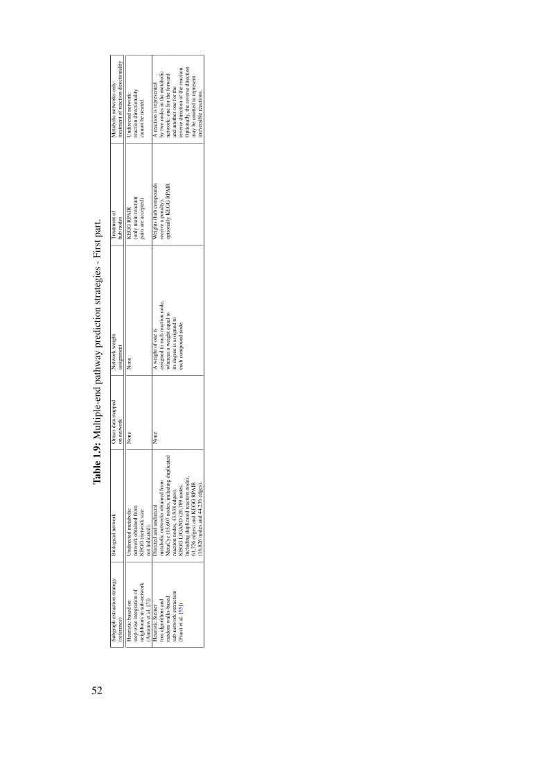
Tabl
e1.
9:M
ultip
le-e
ndpa
thw
aypr
edic
tion
stra
tegi
es-F
irst
part
.Su
bgra
phex
trac
tion
stra
tegy
Bio
logi
caln
etw
ork
Om
ics
data
map
ped
Net
wor
kw
eigh
tTr
eatm
ento
fM
etab
olic
netw
orks
only
:(r
efer
ence
)on
netw
ork
assi
gnm
ent
hub
node
str
eatm
ento
frea
ctio
ndi
rect
iona
lity
Heu
rist
icba
sed
onU
ndir
ecte
dm
etab
olic
Non
eN
one
KE
GG
RPA
IRU
ndir
ecte
dne
twor
k:st
ep-w
ise
inte
grat
ion
ofne
twor
kob
tain
edfr
om(o
nly
mai
nre
acta
ntre
actio
ndi
rect
iona
lity
neig
hbou
rsin
sub-
netw
ork
KE
GG
(net
wor
ksi
zepa
irs
are
acce
pted
)ca
nnot
betr
eate
d.(A
nton
ovet
al.[
3])
noti
ndic
ated
).H
euri
stic
Stei
ner
Dir
ecte
dan
dun
dire
ced
Non
eA
wei
ghto
fone
isW
eigh
ts(h
ubco
mpo
unds
Are
actio
nis
repr
esen
ted
tree
algo
rith
ms
and
met
abol
icne
twor
ksob
tain
edfr
omas
sign
edto
each
reac
tion
node
,re
ceiv
ea
pena
lty),
bytw
ono
des
inth
em
etab
olic
rand
omw
alks
-bas
edM
etaC
yc(1
5,60
7no
des,
incl
udin
gdu
plic
ated
whe
reas
aw
eigh
tequ
alto
optio
nally
KE
GG
RPA
IRne
twor
k:on
efo
rthe
forw
ard
sub-
netw
ork
extr
actio
nre
actio
nno
des,
43,9
38ed
ges)
,its
degr
eeis
assi
gned
toan
dan
othe
rone
fort
he(F
aust
etal
.[55
])K
EG
GL
IGA
ND
(20,
789
node
s,ea
chco
mpo
und
node
.re
vers
edi
rect
ion
ofth
ere
actio
n.in
clud
ing
dupl
icat
edre
actio
nno
des,
Opt
iona
lly,t
here
vers
edi
rect
ion
61,7
26ed
ges)
and
KE
GG
RPA
IRm
aybe
omitt
edto
repr
esen
t(1
6,82
6no
des
and
44,2
36ed
ges)
.ir
reve
rsib
lere
actio
ns.
52
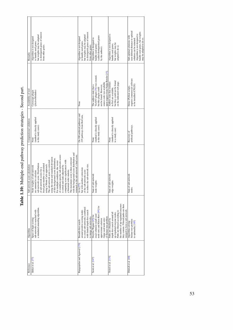
Tabl
e1.
10:M
ultip
le-e
ndpa
thw
aypr
edic
tion
stra
tegi
es-S
econ
dpa
rt.
Ref
eren
ceA
lgor
ithm
Sub-
netw
ork
scor
eca
lcul
atio
nC
ompu
tatio
nalv
alid
atio
nA
vaila
bilit
yof
tool
Rem
arks
Idek
eret
al.[
77]
Spac
eof
high
-sco
ring
Nod
ew
eigh
tsof
sub-
netw
ork
Non
eC
ytos
cape
plug
inA
lgor
ithm
isno
tdes
igne
dsu
b-ne
twor
ksis
sear
ched
with
are
sum
med
toca
lcul
ate
(met
hod
isdi
rect
lyap
plie
d(j
Act
iveM
odul
es)
toha
ndle
seed
gene
s,a
sim
ulat
edan
neal
ing
algo
rith
m.
sub-
netw
ork
scor
e.D
istr
ibut
ion
toth
est
udy
case
s).
butw
eigh
tsm
aybe
adap
ted
ofsu
b-ne
twor
ksc
ores
fora
todi
stin
guis
hge
nes
ofin
tere
stfix
edge
nenu
mbe
ris
calc
ulat
edfr
omot
herg
enes
.us
ing
aM
onte
Car
loap
proa
ch.
The
sub-
netw
ork
scor
eis
corr
ecte
dus
ing
the
mea
nan
dst
anda
rdde
viat
ion
ofth
isba
ckgr
ound
scor
edi
stri
butio
n.Fo
rmul
tiple
cond
ition
s,th
eve
ctor
ofco
nditi
on-s
peci
ficsu
b-ne
twor
ksc
ores
isso
rted
and
rank
-adj
uste
dby
com
putin
gsc
ore
sign
ifica
nces
with
abi
nom
ialo
rder
stat
istic
.T
hem
axim
umsc
ore
isth
enco
rrec
ted
with
the
back
grou
ndsc
ore
dist
ribu
tion
and
retu
rned
asth
esu
b-ne
twor
k’s
final
scor
e.R
ajag
opal
anan
dA
garw
al[1
39]
Bre
adth
-firs
tsea
rch
As
in[7
7],
On
100
artifi
cial
path
way
san
dN
one
Alg
orith
mis
notd
esig
ned
arou
ndpo
sitiv
e-sc
orin
gno
des
butw
ithan
othe
rcor
rect
ion
219
path
way
sfr
omB
ioC
arta
.to
hand
lese
edge
nes,
tocr
eate
sub-
netw
orks
com
bine
dof
the
sub-
netw
ork
scor
ebu
twei
ghts
may
bead
apte
dw
ithlim
ited
dept
h-fir
stse
arch
tore
duce
the
sub-
netw
ork
size
.to
dist
ingu
ish
gene
sof
inte
rest
tom
erge
sub-
netw
orks
.fr
omot
herg
enes
.Sc
otte
tal.
[147
]D
reyf
us-W
agne
r[45
]for
Sum
ofsu
b-ne
twor
kN
one
The
auth
ors
stat
eth
ata
Alg
orith
mis
desi
gned
toex
acts
olut
ion
(sm
alls
eed
node
wei
ghts
.(m
etho
dis
dire
ctly
appl
ied
Vis
AN
Tpl
ugin
[76]
was
crea
ted,
hand
lese
edge
nes
node
sets
)and
Kle
in-R
avi[
95]f
orto
the
stud
yca
ses)
.bu
tthi
spl
ugin
coul
d(c
alle
ddi
stin
guis
hed
gene
sap
prox
imat
eso
lutio
nno
tbe
foun
d.H
owev
er,
byth
eau
thor
s).
(lar
gese
edno
dese
ts)
sour
ceco
dew
asav
aila
ble
ofSt
eine
rtre
epr
oble
mup
onre
ques
tfro
mN
adja
Bet
zler
[15]
.N
oire
leta
l.[1
19]
Path
sar
eob
tain
edby
Sum
ofsu
b-ne
twor
kN
one
Aut
hors
stat
eth
atro
utin
esA
lgor
ithm
isno
tdes
igne
dto
dept
h-fir
stse
arch
arou
ndal
led
gew
eigh
ts.
(met
hod
isdi
rect
lyap
plie
din
Perl
are
avai
labl
e,ha
ndle
seed
gene
s,up
-reg
ulat
eden
zym
eno
des.
toa
stud
yca
se)
butt
hey
coul
dno
tbe
foun
dbu
twei
ghts
may
bePa
ths
are
filte
red
acco
rdin
gto
onth
ein
dica
ted
web
page
.ad
apte
dto
doso
.th
enu
mbe
rofu
p-re
gula
ted
enzy
mes
they
cont
ain.
Filte
red
path
sar
eth
enm
erge
dto
form
asu
b-ne
twor
k.D
ittri
chet
al.[
40]
Alg
orith
mso
lvin
gSu
mof
sub-
netw
ork
Rec
over
yof
Hei
nz(P
ytho
nsc
ript
),Su
b-op
timal
solu
tions
with
Stei
nert
ree
prob
lem
node
s.ar
tifici
alpa
thw
ays.
requ
ires
com
mer
cial
soft
war
eus
er-d
efine
ddi
stan
ceto
optim
alto
optim
ality
[105
]to
bein
stal
led
(CPL
EX
)so
lutio
nca
nbe
retu
rned
.A
lgor
ithm
isno
tdes
igne
dto
hand
lese
edge
nes,
butw
eigh
tsm
aybe
adap
ted
todo
so.
53

Tabl
e1.
10:M
ultip
le-e
ndpa
thw
aypr
edic
tion
stra
tegi
es-S
econ
dpa
rt.
Ref
eren
ceA
lgor
ithm
Sub-
netw
ork
scor
eca
lcul
atio
nC
ompu
tatio
nalv
alid
atio
nA
vaila
bilit
yof
tool
Rem
arks
Ant
onov
etal
.[3]
Seed
sar
eco
nnec
ted
with
The
scor
eof
asu
b-ne
twor
kis
Ahu
genu
mbe
rof
web
serv
erA
lgor
ithm
isde
sign
edto
thei
rfirs
t-de
gree
neig
hbou
rsan
dth
enu
mbe
rofs
eeds
conn
ecte
dby
it.st
udy
case
s(2
72)
(http
://m
ips.
helm
holtz
-mue
nche
n.de
/ha
ndle
seed
gene
sor
com
poun
ds.
the
larg
esta
mon
gth
ere
sulti
ngA
back
grou
nddi
stri
butio
nof
scor
esis
com
pute
dis
pres
ente
d,pr
oj/k
eggs
pide
r/an
dht
tp://
mip
s.he
lmho
ltz-
Sepa
rate
web
serv
ers
for
netw
ork
com
pone
nts
isre
turn
edas
ktim
esfo
rafix
edse
ednu
mbe
r.bu
tno
real
valid
atio
nm
uenc
hen.
de/p
roj/c
mp/
)ge
nes
(KE
GG
Spid
er[3
])di
stan
ce1
sub-
netw
ork.
Thi
spr
oced
ure
isT
hep-
valu
eis
then
calc
ulat
edas
:is
perf
orm
ed(w
hich
wou
ldal
low
and
com
poun
ds(T
ICL
[4])
repe
ated
ford
ista
nce
2,3,
...so
that
p=
(n+
1)/k
,whe
ren
isth
eto
mea
sure
the
accu
racy
inm
etab
olic
netw
orks
.a
seri
esof
dist
ance
-spe
cific
num
bero
fsco
res
inth
eof
the
proc
edur
e).
sub-
netw
orks
iscr
eate
d.ba
ckgr
ound
dist
ribu
tion
equa
lorg
reat
erth
anth
esu
b-ne
twor
ksc
ore.
Faus
teta
l.[5
5]A
ppro
xim
ativ
eSt
eine
rtre
eSu
mof
sub-
netw
ork
on71
S.ce
revi
siae
web
serv
erA
lgor
ithm
isde
sign
edal
gori
thm
s:Ta
kaha
shi-
Mat
suya
ma
[154
],ar
cw
eigh
ts.
path
way
sfr
omM
etaC
yc(h
ttp://
rsat
.ulb
.ac.
be/n
eat/)
toha
ndle
seed
s.K
lein
-Rav
i,re
petit
ive
RE
AW
ebse
rver
allo
ws
tosu
bmit
(com
bina
tion
ofk
shor
test
path
s).
cust
omne
twor
ksw
ithcu
stom
wei
ghts
,R
ando
mw
alk-
base
dal
gori
thm
:th
usal
gori
thm
sca
nbe
com
bine
dkW
alks
[48,
21].
Inad
ditio
n,co
mbi
natio
nsw
ithm
ore
soph
istic
ated
wei
ghtp
olic
ies.
ofth
ese
algo
rith
ms
wer
ete
sted
.Fo
rthe
pre-
load
edm
etab
olic
netw
orks
,ge
nes,
EC
num
bers
,rea
ctio
nsor
com
poun
dsar
eac
cept
edas
seed
s.
54
2 Two-end metabolic pathway
prediction
Presented article:K. Faust, D. Croes and J. van HeldenMetabolic Pathfinding Using RPAIR AnnotationJournal of Molecular Biology, vol. 388, pp. 390-414, 2009.
2.1 Introduction
The first step towards the prediction of metabolic pathways from multiple seeds is the increaseof two-end path finding accuracy. As discussed in section 1.10.3, appropriate treatment of hubcompounds (i.e. compounds involved in a large number of reactions) is crucial to reach highprediction accuracies. The key idea of the article presented here is to use pre-defined substrate-product pairs from the RPAIR database [97] in order to avoid side compounds.
Reactant pairs (RPAIRs) are manually annotated substrate-product pairs that map each sub-strate of a reaction onto its structurally most similar product (see Figure 1.19). RPAIRs areclassified into main, trans, cofac, ligase or leave RPAIRs according to their role in the reaction(see Table 1.8).
There are different ways in which reactant pairs can be integrated into path finding. Wetherefore assessed the impact of a number of different parameters on path finding accuracy,namely network type, network directionality, RPAIR role filtering, compound filtering anddifferent weight policies. Table 2.1 describes each of these parameters.
2.2 Contribution
D. Croes conceived the idea of integrating RPAIRS to improve path finding. I performed theevaluation, analyzed the study cases and wrote the article. J. van Helden supervised the workand substantially revised the article.
2.3 Methods
Three networks were constructed: one from KEGG LIGAND (termed reaction network) andtwo from KEGG RPAIR (termed RPAIR and reaction-specific RPAIR network). The referencepathways were taken from aMAZE [101]. Of these, 25 are branched and seven contain cycles.
55

Table 2.1: Table of parameters that were assessed during the evaluation of path finding
Parameter DescriptionNetwork Network consisting of all reactionstype and compounds in KEGG LIGAND versus
network consisting of all reactant pairsand compounds in KEGG RPAIR
Network Network is directed (where eachdirectionality reaction is represented by two
direction nodes) or undirectedRPAIR role RPAIRS of a specific rolefiltering (such as cofac, ligase or leave) are
removed from the RPAIR networkCompound Highly connected compoundsfiltering (such as ATP or H2O) are
removed from the networkWeight policy Four weight policies were tested:
1) unit (all nodes receive a weight of one)2) degree (all compound nodesreceive a weight equal to their degree)3) RPAIR weight (all reactant pairsreceive a role-specific weight)4) RPAIR weight and degree (combination ofweight policies 2 and 3)
56

Path finding cannot predict pathways having more than two terminal nodes (i.e. nodes withoutincoming or outgoing arcs), because it accepts only two seed nodes. It was therefore necessaryto linearize the reference pathways, i.e. to extract their linear parts. Details on the referencepathways and their treatment are listed in section 9.2.
To evaluate the accuracy of two-end pathway prediction, the start and end reaction of areference pathway are given to the path finding algorithm, which is based on REA [83]. Allfirst-ranked paths (i.e. paths of equal weight) are merged to form the predicted pathway. Thepath finding accuracy is then calculated on the basis of non-seed node overlap between thepredicted and the reference pathway (see section 9.2).
Path finding was carried out under various conditions for a set of 55 reference pathwaysfrom three organisms.
2.4 Results
With the best-performing parameter combination, an overall accuracy of 83% was reached forthe 55 reference pathways (93% for 32 E. coli pathways, 66% for 11 S. cerevsiae pathwaysand 70% for H. sapiens pathways).
The assessment of parameter impact revealed that:
• In agreement with [31, 32], a weighted metabolic network performs better than an un-weighted or filtered network (where hub compounds are removed).
• The RPAIR network outperforms the reaction network.
• Directed reaction networks perform better than undirected ones, because they preventthe path finding algorithm to go from substrate to substrate or from product to product.In contrast, for RPAIR networks, there is no difference between directed and undirectednetworks, since each reactant pair has only one substrate and one product.
• Filtering of RPAIR classes does not increase the path finding accuracy, because somereference pathways contain other than main RPAIRs.
• Weighting of RPAIRs only increases path finding accuracy in the absence of compoundweights.
2.5 Conclusion
Our evaluation has shown that the combination of reactant pairs with a weight policy penal-izing hub compounds yielded the highest path finding accuracy. Thus, metabolic pathwayprediction accuracy can be increased by taking into account RPAIR annotations.
57

Author's personal copy
Metabolic Pathfinding Using RPAIR Annotation
Karoline Faust⁎, Didier Croes and Jacques van Helden
Laboratoire de Bioinformatiquedes Génomes et des Réseaux(BiGRe), Université Libre deBruxelles, Campus Plaine,CP 263, Bld du Triomphe,B-1050 Bruxelles, Belgium
Received 9 November 2008;received in revised form25 February 2009;accepted 3 March 2009Available online10 March 2009
Metabolic databases contain information about thousands of smallmolecules and reactions, which can be represented as networks. In thecontext of metabolic reconstruction, pathways can be inferred by searchingoptimal paths in such networks. A recurrent problem is the presence of poolmetabolites (e.g., water, energy carriers, and cofactors), which are connectedto hundreds of reactions, thus establishing irrelevant shortcuts betweennodes of the network. One solution to this problem relies on weightednetworks to penalize highly connected compounds. Amore refined solutiontakes the chemical structure of reactants into account in order todifferentiate between side and main compounds of a reaction. Thanks toan intensive annotation effort at KEGG, decompositions of reactions intoreactant pairs (RPAIR) categorized by their role (main, trans, cofac, ligase,and leave) are now available.The goal of this article is to evaluate the impact of RPAIR data on
pathfinding in metabolic networks. To this end, we measure the impact ofdifferent parameters concerning the construction of the metabolic network:mapping of reactions and reactant pairs onto a graph, use of selectedcategories of reactant pairs, weighting schemes for compounds andreactions, removal of highly connected metabolites, and reaction direction-ality. In total, we tested 104 combinations of parameters and identified theiroptimal values for pathfinding on the basis of 55 reference pathways fromthree organisms.The best-performing metabolic network combines the biochemical
knowledge encoded by KEGG RPAIR with a weighting scheme penalizinghighly connected compounds. With this network, we could recoverreference pathways from Escherichia coli with an average accuracy of 93%(32 pathways), from Saccharomyces cerevisiae with an average accuracy of66% (11 pathways), and from humans with an average accuracy of 70%(12 pathways). Our pathfinding approach is available as part of theNetwork Analysis Tools.
© 2009 Elsevier Ltd. All rights reserved.
Edited by M. SternbergKeywords: pathfinding; KEGG RPAIR; metabolic network; pathfindingevaluation; metabolic pathways
Introduction
In biochemical textbooks1 and in databases suchas KEGG2,3 or BioCyc,4,5 metabolic information isrepresented in the form of generic or organism-specific metabolic maps or pathways. Historically,the characterization of metabolic pathways relied ona very few model organisms (Escherichia coli,Salmonella, Saccharomyces cerevisiae, mouse, human,
and so on). Enzyme grouping into pathways wasdefined on the basis of mutant phenotypes (e.g.,methionine auxotrophy) and, with progress in bio-chemistry, detailed successions of reactions could beestablished. Such biochemical analyses revealed thatdifferent organisms can use alternative pathways toproduce or utilize the same molecules. For example,in E. coli, L-lysine is produced in nine reactions fromL-aspartate, whereas in S. cerevisiae, it is produced ineight reactions from 2-oxoglutarate. The documen-ted examples of alternative pathways probablyreflect a tiny part of the huge diversity of bioche-mical pathways.The large size of the biochemical pathway space is
also apparent from calculations performed by
⁎Corresponding author. E-mail address: [email protected] used: Sn, sensitivity; PPV, positive
predictive value; Acc, geometric accuracy.
doi:10.1016/j.jmb.2009.03.006 J. Mol. Biol. (2009) 388, 390–414
Available online at www.sciencedirect.com
0022-2836/$ - see front matter © 2009 Elsevier Ltd. All rights reserved.
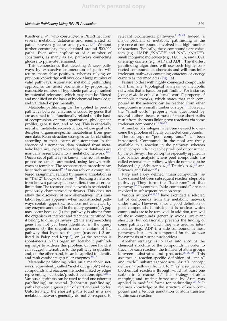
Author's personal copy
Kueffner et al., who constructed a PETRI net fromseveral metabolic databases and enumerated allpaths between glucose and pyruvate.6 Withoutfurther constraints, they obtained around 500,000paths. Even after application of a number ofconstraints, as many as 170 pathways connectingglucose to pyruvate remained.This demonstrates that detecting de novo path-
ways by exhaustive enumeration of paths willreturn many false positives, whereas relying onprevious knowledge will overlook a large number ofvalid pathways. Automated metabolic pathfindingapproaches can assist biochemists by proposing areasonable number of hypothetic pathways rankedby potential relevance, which may then be filteredandmodified on the basis of biochemical knowledgeand validated experimentally.Metabolic pathfinding can be applied to predict
pathways between enzymes encoded by genes thatare assumed to be functionally related (on the basisof coexpression, operon organization, phylogeneticprofiles, gene fusion, and so on). This is especiallyuseful in metabolic reconstruction, whose goal is todecipher organism-specific metabolism from gen-ome data. Reconstruction strategies can be classifiedaccording to their extent of automation: In theabsence of automation, data obtained from meta-bolic literature, expert knowledge, or databases aremanually assembled into a metabolic network.4,7,8
Once a set of pathways is known, the reconstructionprocedure can be automated, using known path-ways as template. The reconstruction procedure canbe entirely automated9–14 or can rely on a computer-based assignment refined by manual annotation asin “Tier 2” BioCyc databases.12 Building a networkfrom known pathways alone suffers from a seriouslimitation: The reconstructed network is restricted topreviously characterized pathways. This does notallow the discovery of new alternatives. This limi-tation becomes apparent when reconstructed path-ways contain gaps (i.e., reactions not catalyzed byany enzyme annotated in the query genome). A gapmay occur because (1) the pathway is absent fromthe organism of interest and reactions identified forit belong to other pathways; (2) the enzyme-codinggene has not yet been identified in the querygenome; (3) the organism uses a variant of thepathway that bypasses the gap (reasons 1–3 arelisted in Paley and Karp15); or (4) the reaction isspontaneous in this organism. Metabolic pathfind-ing helps to address this problem: On one hand, itcan suggest alternatives to the pathway in questionand, on the other hand, it can be applied to identifyand rank candidate gap filler enzymes.16,17
Metabolic pathfinding relies on a metabolic net-work (equivalently called “metabolic graph”) wherecompounds and reactions are nodes linked by edgesrepresenting substrate/product relationships.6,18,19Various algorithms can be used to find one (shortestpathfinding) or several (k-shortest pathfinding)paths between a given pair of start and end nodes.Unfortunately, the shortest paths found in a rawmetabolic network generally do not correspond to
relevant biochemical pathways.11,20,21 Indeed, amajor problem of metabolic pathfinding is thepresence of compounds involved in a high numberof reactions. Typically, these compounds are cofac-tors (e.g., NADP+/NADPH and NAD+/NADH),small inorganic molecules (e.g., H2O, O2, and CO2),or energy carriers (e.g., ATP and ADP). The shortestpathfinding algorithms will use such highly con-nected compounds as shortcuts and will thus inferirrelevant pathways containing cofactors or energycarriers as intermediates (Fig. 1a).Failure to deal with highly connected compounds
will bias any topological analysis of metabolicnetworks that is based on pathfinding. For instance,Jeong et al. described a “small-world” property ofmetabolic networks, which states that each com-pound in the network can be reached from othercompounds in a small number of steps.18 However,the “small-world” property was questioned byseveral authors because most of these short pathsresult from shortcuts linking two reactions via someirrelevant compounds.11,20–22A number of strategies have been devised to over-
come the problem of highly connected compounds.The concept of “pool compounds” has been
introduced. Compounds in the pool are freelyavailable to a reaction in the pathway, whereasother compounds have to be produced or consumedby the pathway. This concept is especially applied influx balance analysis where pool compounds arecalled external metabolites, which do not need to bebalanced (e.g., Schuster et al.,23 Teusink et al.,24 andEdwards and Palsson25).Karp and Paley defined “main compounds” as
those shared between subsequent reaction steps of apathway: They form the “backbone” of thatpathway.26 In contrast, “side compounds” are notinvolved in subsequent reaction steps.Various authors16,19,22 have excluded a selected
list of compounds from the metabolic networkunder study. However, since a good definition ofpool compounds is missing, it is unclear whichcompounds are to be removed. In addition, removalof those compounds generally avoids irrelevantshortcuts, but occasionally prevents the finding ofsome pathways in which they are used as inter-mediates (e.g., ADP is a side compound in mostpathways, but a main compound for the de novobiosynthesis of purine nucleotides).Another strategy is to take into account the
chemical structure of the compounds in order totrace, for each reaction, the transfer of atom groupsbetween substrates and products.20,27,28 Thisassumes a reaction-specific definition of “main”and “side” substrates/products. Arita's conceptdefines “a pathway from X to Y [as] a sequence ofbiochemical reactions through which at least onecarbon in X reaches Y.” This strategy of atommapping and tracing introduced by Arita wasapplied in modified forms for pathfinding.29–32 Itrequires knowledge of the structure of each com-pound and a tedious annotation of atom transferswithin each reaction.
391Metabolic Pathfinding Using RPAIR Annotation

Author's personal copy
Fig. 1. Illustration of the relevance of RPAIR annotations. (a) Example showing that paths traversing pool metabolites often result in biochemically invalid pathways. Theshortest path found in the unweighted reaction graph erroneously suggests that L-methionine can be produced from L-aspartate in three reaction steps via ADP andtetrahydrofolate (rectangles representing seed nodes have a border in boldface). (b) RPAIR composition of selected reactions used in the path of (a). Reaction R00480 is divided intothree reactant pairs: The two reactant pairs labeled as “main” go from ATP to ADP, or from L-aspartate to 4-phospho-L-aspartate. In reaction R00943, the main reactant pairsconnect tetrahydrofolate, formate, and 10-formyltetrahydrofolate. Note that there are no reactant pairs from L-aspartate to ADP or fromADP to tetrahydrofolate in these reactions,so that path (a) cannot be formed. (c) The shortest path between L-aspartate and L-methionine found in the unweighted RPAIR graph. (d) The shortest path between L-aspartateand L-methionine found in the weighted RPAIR graph.
392Metabolic
Pathfinding
Using
RPAIR
Annotation

Author's personal copy
Pool compounds can also be avoided by defininga set of rules,33 assigned by experts on the basis ofcompound structure and biochemical literature, inorder to enumerate all conversions allowed for eachcompound. The drawback of this approach is thatthe rule set might be incomplete or too restrictive toallow discovery of new pathways.Kotera et al. introduced the concept of reactant
pairs (RPAIRs), defined as “pairs of compounds thathave atoms or atom groups in common on two sidesof a reaction.”34,35 RPAIR thus establishes pairwiserelationships between one substrate and one pro-duct, taking into account the respective roles of thesecompounds in the reaction. Accordingly, reactantpairs are grouped into the following classes: main,trans, cofac, ligase, and leave. For instance, a cofacreactant pair couples a substrate cofactor with aproduct cofactor (i.e., A00002 pairs NADH withNAD+). Figure 1 shows typical examples of decom-position of reactions (Fig. 1a) into reactant pairs(Fig. 1b). This figure also demonstrates that bio-chemically irrelevant connections betweenATP/ADPand other compounds are avoided in the RPAIRgraph (Fig. 1c and d) simply because correspondingreactant pairs are absent in the RPAIR database. Notethat the same reactant pair may take on different rolesin different reactions (i.e., the ATP/orthophosphatereactant pair belonging to all five classes).Oh et al. combined RPAIRs and structural com-
parisons to predict biodegradation pathways byiteratively matching a compound with its mostsimilar partner in a library of reactant pairs.36
In a previous article, we introduced a strategy forpredicting metabolic pathways based on k-shortestpathfinding in a weighted graph.37 By default, eachcompound is assigned a weight equal to its degree(“connectivity”) in themetabolic graph. Theweight isthen used as a penalty for pathfinding, leading to theconcept of lightestpathfinding (as opposed to shortest).Thus, the more highly connected is a compound, theless likely it is to appear in an inferred pathway.An important issue is the protocol used to assess
the reliability of a pathway discovery method.Indeed, several approaches were tested on only afew study cases (e.g., McShan et al.,29 Rahman et al.,31
and de Figueiredo et al.38), or conclusions weredrawn from global topological parameters withoutany attempt to compare discovered paths to anno-tated pathways (e.g., Jeong et al.18). In contrast, ourstrategy to penalize compounds according to theirdegree was supported by an evaluation on severaltens of pathways.21
With the availability of the KEGG RPAIR data-base, we can now integrate manually compiledknowledge on atom flow as stored in the reactantpairs into pathfinding. In this article, we quantifythe impact of KEGG RPAIR on pathfinding accuracyby carrying out a careful validation of knownpathways from three organisms (E. coli, S. cerevisiae,and Homo sapiens). In addition, we evaluate theeffects of parameters linked to the RPAIR database[e.g., the filtering and weighting of reactant pairsaccording to their class (main, trans, cofac, ligase, or
leave)]. In order to compare results obtained withKEGG RPAIR to those obtained from our previousmethod, we also measure the impact of differentweighting schemes and the filtering of pool meta-bolites on pathfinding accuracy.We added the new version of the metabolic
pathfinding tool and the best-performing metabolicnetworks to the Network Analysis ToolsWeb server.39
Results and Discussion
Graph construction and evaluation
We summarize here the main features of themetabolic graphs and pathways used for evaluation.The detailed description can be found in Materialsand Methods.We constructed three bipartite metabolic graphs
from KEGG/LIGAND. The first one, called reactiongraph, is built from all compounds and reactions, inthe same way as in our previous work.21 The secondgraph, named RPAIR graph, consists of all reactantpairs listed in KEGG RPAIR and their associatedcompounds. The third graph, called reaction-specificRPAIR graph, is a variant of the RPAIR graph, whereeach reactant pair instantiates one separate node foreach reaction in which it is involved. Reactant pairsassociated with the same reaction are mutuallyexclusive.The performance of these graphs was evaluated
on a set of 55 known reference pathways from threeorganisms (E. coli, S. cerevisiae, and H. sapiens). Foreach of the reference pathways, we measured howwell it could be recovered from the metabolic graphgiven its start and end reactions alone.This evaluation was repeated for each of the three
graphs and for a variety of parameter values. Thetested parameters included compound weightingscheme, reactant pair weighting scheme, graphdirectionality, compound filtering, and reactant pairfiltering.
Study cases
In the following, we discuss three examples thatillustrate the benefits of RPAIR annotations.Two additional examples (lysine biosynthesis and
proline degradation) demonstrate how pathfindingcan uncover pathways in organism-specific net-works and suggest alternatives to known metabolicpathways.For each graph mentioned in these examples, we
used parameter values yielding the highest path-finding accuracies in our evaluation.
Aldosterone biosynthesis in humans
Aldosterone biosynthesis (Fig. 2a) in humans pro-duces the hormone aldosterone from cholesterol.Aldosterone regulates the absorption of ions in thekidney.
393Metabolic Pathfinding Using RPAIR Annotation

Author's personal copy
Fig. 2. Inference of the aldosterone biosynthesis pathway in the reaction graph and RPAIR graph. (a) Human aldosterone pathway as annotated in the aMAZE data set. (b) Thelightest path found in the compound-weighted reaction graph. (c) The lightest path found in the compound-weighted RPAIR graph. (d) Reactant pair composition of the firstreaction in the annotated pathway. Note the absence of any reactant pair connecting cholesterol to reduced adrenal ferredoxin. The compound pairs oxygen/water and reducedadrenal ferredoxin/oxidized adrenal ferredoxin differ by hydrogen atoms and electrons, respectively, which are not covered by KEGG RPAIR. Green, true positives; orange, falsepositives; blue, seed nodes.
394Metabolic
Pathfinding
Using
RPAIR
Annotation
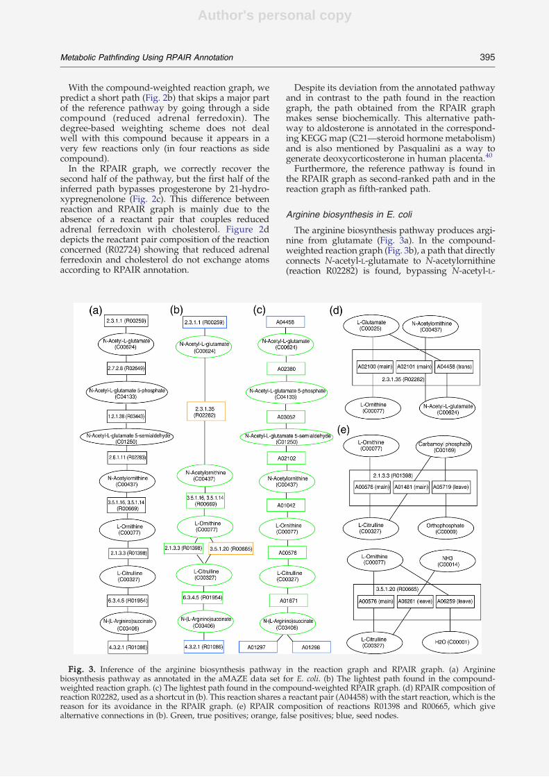
Author's personal copy
With the compound-weighted reaction graph, wepredict a short path (Fig. 2b) that skips a major partof the reference pathway by going through a sidecompound (reduced adrenal ferredoxin). Thedegree-based weighting scheme does not dealwell with this compound because it appears in avery few reactions only (in four reactions as sidecompound).In the RPAIR graph, we correctly recover the
second half of the pathway, but the first half of theinferred path bypasses progesterone by 21-hydro-xypregnenolone (Fig. 2c). This difference betweenreaction and RPAIR graph is mainly due to theabsence of a reactant pair that couples reducedadrenal ferredoxin with cholesterol. Figure 2ddepicts the reactant pair composition of the reactionconcerned (R02724) showing that reduced adrenalferredoxin and cholesterol do not exchange atomsaccording to RPAIR annotation.
Despite its deviation from the annotated pathwayand in contrast to the path found in the reactiongraph, the path obtained from the RPAIR graphmakes sense biochemically. This alternative path-way to aldosterone is annotated in the correspond-ing KEGGmap (C21—steroid hormone metabolism)and is also mentioned by Pasqualini as a way togenerate deoxycorticosterone in human placenta.40
Furthermore, the reference pathway is found inthe RPAIR graph as second-ranked path and in thereaction graph as fifth-ranked path.
Arginine biosynthesis in E. coli
The arginine biosynthesis pathway produces argi-nine from glutamate (Fig. 3a). In the compound-weighted reaction graph (Fig. 3b), a path that directlyconnects N-acetyl-L-glutamate to N-acetylornithine(reaction R02282) is found, bypassing N-acetyl-L-
Fig. 3. Inference of the arginine biosynthesis pathway in the reaction graph and RPAIR graph. (a) Argininebiosynthesis pathway as annotated in the aMAZE data set for E. coli. (b) The lightest path found in the compound-weighted reaction graph. (c) The lightest path found in the compound-weighted RPAIR graph. (d) RPAIR composition ofreaction R02282, used as a shortcut in (b). This reaction shares a reactant pair (A04458) with the start reaction, which is thereason for its avoidance in the RPAIR graph. (e) RPAIR composition of reactions R01398 and R00665, which givealternative connections in (b). Green, true positives; orange, false positives; blue, seed nodes.
395Metabolic Pathfinding Using RPAIR Annotation

Author's personal copy
glutamate 5-phosphate and N-acetyl-L-glutamate5-semialdehyde.This shortcut is avoided in the RPAIR graph
(Fig. 3c) because the starting reactant pair A04458excludes all reactant pairs (A02100, A0201, andA04458) associated with the bypass reaction(R02282) of Fig. 3b. In Fig. 3d, the reactant paircomposition of the bypass reaction is shown.In addition, the pathway inferred in the reaction
graph consists of two alternative paths: one con-necting L-ornithine to L-citrulline via reaction R01398and another via reaction R00665. Both reactionsdiffer by their side compounds: In the annotatedreaction R01398, carbamoyl phosphate is added to L-ornithine by the enzyme carbamoyl transferase. Thealternative reaction R00665 is catalyzed by theenzyme citrullinase, which hydrolyzes citrulline toform ornithine, ammoniac, and water. Citrullinase
favors the formation of ornithine from citrullinemore strongly than the reverse. The reactant paircomposition of both reactions is depicted in Fig. 3e.By default, alternative reactions in inferred path-
ways are counted as false positives. However, in theRPAIR graph, we can no longer differentiatebetween the two reactions. Both share a commonmain reactant pair, namely, A00576, which connectsL-ornithine and L-citrulline. This loss of one falsepositive in the inferred path contributes to thehigher accuracy reached with the RPAIR graph.
Pyruvate oxidation pathway in E. coli
The first reaction (R03145) of the pyruvate oxida-tion pathway in E. coli converts pyruvate intoacetate (Fig. 4a) and can be divided into fourreactant pairs (A00473, A02797, A05678, and
Fig. 4. Inference of the pyruvateoxidation pathway in the reactiongraph and RPAIR graph. (a) Pyru-vate oxidation pathway as anno-tated in the aMAZE data set for E.coli. (b) The lightest path found inthe compound-weighted reactiongraph. (c) The lightest path foundin the compound-weighted RPAIRgraph. Green, true positives; orange,false positives; blue, seed nodes.
396 Metabolic Pathfinding Using RPAIR Annotation

Author's personal copy
A05698). In the reaction graph, the correct path ismissed because instead of following the mainreactant pair A02797, the cofac reactant pairconnecting ferrocytochrome b1 to ferricytochromeb1 is chosen (Fig. 4b). In the RPAIR graph, thispathway is inferred correctly (Fig. 4c).
Lysine biosynthesis
Metabolic pathfinding can suggest alternativepathways either by finding multiple paths in ageneric metabolic network (the k-lightest paths) orby considering the top-ranking paths in differentorganism-specific networks. In Croes et al., weshowed that the top-ranking paths connecting L-aspartate and L-lysine obtained from the genericcompound-weighted reaction network correspond
to alternative pathways that are valid in differentorganisms.21 However, without further information,it is unclear which path might be active in whichorganism. Here, we repeated the search inorganism-specific RPAIR networks constructedfrom KEGG PATHWAY 46.0 for the three yeastspecies S. cerevisiae, Saccharomyces bayanus, andSchizosaccharomyces pombe, and for the prokaryotesE. coli, Salmonella typhimurium, and Bacillus subtilis.For each of the organism-specific networks, weperformed a search between L-aspartate and L-lysine, as well as a search between acetyl-CoA andL-lysine (L-aspartate and acetyl-CoA are bothknown start compounds for lysine biosynthesis).Figure 5 displays the paths of first rank obtained foreach organism, grouping together organisms withidentical paths. For E. coli, Sal. typhimurium, and B.
Fig. 5. Pathfinding results for lysine biosynthesis in organism-specific compound-weighted RPAIR networks.Organisms for which identical paths were found are grouped together. The search was conducted between L-aspartateand L-lysine and between acetyl-CoA and L-lysine; the first-ranking paths obtained were then merged. For B. subtilis andE. coli/Sal. typhimurium, the complete annotated lysine biosynthesis pathways are covered; for the yeast species, a largepart of the known pathway is found. Green, RPAIR/compound is a part of the lysine biosynthesis KEGGmap; blue, seednodes.
397Metabolic Pathfinding Using RPAIR Annotation

Author's personal copy
subtilis, the lysine biosynthesis pathways startingfrom L-aspartate are fully covered. For each yeastspecies, a large part of the known pathway startingfrom acetyl-CoA is found. Note that the Gram-negative bacteria E. coli and Sal. typhimurium, theGram-positive bacterium B. subtilis, and the eukar-yotes S. cerevisiae, S. bayanus, and Sc. pombe eachemploy a different lysine biosynthesis pathway.
Proline degradation
The following study case illustrates how alternativesto known pathways can be found by enumeration ofpaths in a generic metabolic network. The amino acidL-proline is degraded to L-glutamate. MetaCyc5 liststwo known pathways for proline degradation. Thearginine and proline metabolism KEGG map alsosuggests two proline degradation pathways: oneconnecting L-1-pyrroline-5-carboxylate directly to L-glutamate and the other going through L-glutamate5-semialdehyde before reaching L-glutamate. If we
enumerate paths between L-proline and L-glutamatein the compound-weighted KEGG RPAIR network,we obtain these pathways as the first-ranked andsecond-ranked paths (Fig. 6, paths 1 and 2.1). Inaddition, several paths contained neither in MetaCycnor in KEGG are returned (Fig. 6, other paths),suggesting the degradation of proline via D-prolineand aminopentanoate (paths 2.2 and 3.1), via trans-4-hydroxy-L-proline (path 3.2), and via L-ornithine(paths 5.1 and 5.2).
Impact of parameter values
So far, we discussed the behavior of pathfinding ina few illustrative study cases. In order to assess thegenerality of our observations, we extend thisanalysis to a benchmark collection of 55 pathwaysfrom three model organisms: the bacterium E. coli(32 pathways), the yeast S. cerevisiae (11 pathways),and humans (12 pathways). We systematicallytested the impact of six different parameters on
Fig. 6. Enumeration of proline degradation pathways in the compound-weighted RPAIR network. The top-rankingpaths correspond to the annotated pathways for proline degradation, as listed in MetaCyc (path 1 highlighted with thickedges) and as visible from the arginine and proline metabolism KEGG map (paths 1 and 2.1). The paths of higher rankpropose alternative pathways for the degradation of L-proline that are not apparent from the corresponding KEGG map.Green, RPAIR/compound is part of the arginine and proline metabolism KEGGmap; blue, seed nodes. Edge labels: Rankindex of the path(s) to which edge belongs. Paths of equal weights have the same rank index (first digit). The second digitdistinguishes between paths of equal rank (e.g., paths 2.1 and 2.2 both have a weight of 130).
398 Metabolic Pathfinding Using RPAIR Annotation

Author's personal copy
pathfinding accuracy (see Table 1 for a descriptionof the parameters). Taking into account someinterdependencies between parameters (e.g., reac-tion weights only apply to RPAIRs and reaction-specific RPAIRs), the total number of possibleparameter combinations is 104. For each combina-tion of parameters, we ran the k-shortest pathfindingalgorithm on each test pathway and measuredsensitivity (Sn), positive predictive value (PPV),and geometric accuracy (Acc) as described inMaterials andMethods. The analysis of all pathwayswith one specific combination of parameters isreferred to as “an experiment.” We thus performed104 distinct experiments.
Optimal combinations of parameters
Table 2 lists, for some selected experiments, theAcc averaged over all reference pathways in E. coli,S. cerevisiae, and H. sapiens, respectively (the com-plete results of the 104 experiments are available inTables S1–S4). For all three species tested, the RPAIRgraph, in combination with compound degreeweights, yielded the highest Acc. The average Accvalues reached for the top-ranking parameter com-bination were 93% for E. coli, 66% for S. cerevisiae,and 70% for human pathways, and 83% for all the
pathways merged. There are three explanations forthese organism-specific differences in accuracy. First,there is a selection bias due to the availableannotations. Secondly, the pathway sets have differ-ent length distributions. For instance, the 12 humanpathways analyzed here have an average length of14 nodes, whereas the 32 E. coli pathways consist, onaverage, of only eight nodes. Thirdly, pathways areeasier to infer if they are less interconnected with themetabolic network. In our selection, the humanpathways happen to be more specialized (e.g.,hormone metabolism) than the ones from E. coliand S. cerevisiae. This might be the reason that wereach a higher average accuracy for the humanpathways compared to the yeast pathways, althoughthe human pathways are, on average, longer thanthe yeast pathways. Despite these organism-specificdifferences, the following general trends appear inthe ranking of experiments: Firstly, the 16 top-ranking combinations of parameters (Table S4) arealways based on pathfinding in the RPAIR graph,with compound weighting. Among those, unitRPAIR weights always give better results thanclass-specific RPAIR weights. RPAIR class filteringdoes not appear to improve the results (thedifference between “all RPAIRs” and “main+transRPAIRs” is not significant; Table 3).
Table 1. Description of the parameters needed to construct the metabolic graphs
Parameter name Values Description
Graph type Reaction Bipartite graph with one node per compound and one nodeper reaction
RPAIR Bipartite graph with one node per compound and one nodeper reactant pair
Reaction-specific RPAIR Same as RPAIR, but a separate node is created for each combinationof RPAIR/reaction
Graph directionality Directed Reaction and RPAIR nodes are duplicated in order to represent hetwo possible directions (forward and reverse); edges are directed
Undirected One node per reaction; undirected edges
Compound filtering Filtered 36 highly connected compounds removed from the graph21,26
Unfiltered All compounds present in the graph
Compound weight Unit Each compound has the same weight (w=1)
Degree Each compound node has a weight equal to its degree(incoming+outgoing edges)
RPAIR class filtering All All LIGAND reactant pairs are present in the graph
Main The graph only contains reactant pairs classified as“main”+their substrates/products
Main+trans The graph only contains reactant pairs classified as “main”or “trans”+their substrates/products
RPAIR weight Unit weight Each RPAIR node has the same weight (w=1)
Class-specific weight(only applies to RPAIRand reaction-specificRPAIR graphs)
Weights are assigned to reactant pairs according to their class asfollows: main=1; trans=5; cofac=10; ligase=15; and leave=20;if an RPAIR is found with several classifications in differentreactions, we always choose the highest weight(the least favorable classification)
399Metabolic Pathfinding Using RPAIR Annotation

Author's personal copy
Statistical significance of parameter impact
In order to quantify the impact of each parameter,we performed a systematic comparison between eachpair of alternativeparameter values (e.g., degree versusunit compound weight), with all other parametersbeing equivalent (“experimentwise” comparison;Table 3). For a given pair of parameter values, wecounted the number of experiments where theaccuracy is better, worse, or identical, respectively.The significance of the differences was estimated bycomputing theP-valuewithapairedWilcoxon signed-rank test. This systematic comparison shows that themost significant parameters are compound weight(degree weight is better than unit weight), graph type(RPAIR is better than reaction-specific RPAIR, andboth are better than reaction graph), and compoundfiltering (filtered is better than nonfiltered).It should be noted that, for each pair of parameter
values, this comparison includes all the possiblecombinations of the five other parameters. However,because of interdependencies between some para-meters, a given choice might return better or worseresults, depending on the values chosen for the otherparameters. In order to estimate the best possibleperformances for each parametric choice, we per-formed a second comparison, where each parametervalue is coupled to its “best-friend” parameters (i.e.,the combination of values for the five other para-meters that returns the highest average accuracy forthe reference pathways) (“best-combination-wise”comparison; Table 4). Interestingly, this analysisindicates a significant impact for one parameteronly, the graph type: RPAIR outperforms bothreaction graph (P=2.4E−5 for all pathways merged)and reaction-specific RPAIR graph (P=4.7E−5). Atfirst sight, it might seem surprising that, in this best-combination-wise analysis (Table 4), the compoundweighting (degree or unit) had no significant effect(P=0.15), whereas it appeared as the most significantparameter in the systematic comparison discussedabove (Table 3). This is explained by the fact that thedisadvantage of the unit weight can be compensatedfor by a specific combination of companion para-meters, including the filtering of 36 highly connectedcompounds and the class-specific weighting ofreactant pairs. It should also be noted that, for almostall pairs of parameters, the common best-friendparameter values include compound degree weight,thereby confirming the importance of this parameterfor obtaining optimal accuracy.In the following sections, we will try to under-
stand the reason why these parameters affect therelevance of the inferred pathways.
Graph type
RPAIR graph versus reaction graph. We noticed thefollowing reasons for accuracy differences betweenthe RPAIR graph and the reaction graph:
1. Using the RPAIR graph eliminates false posi-tives introduced by alternative reactions linkingthe same pair of compounds (e.g., R01398 and
R00665; Fig. 3b). They are represented as asingle reactant pair in theRPAIRgraph (A00576;Fig. 3c).
2. Amain compound and a side compound can beconnected by a reaction in the reaction graph,without forming a reactant pair in the RPAIRgraph, because the side compound onlyexchanges electrons, protons, or energy withthe considered main compound (e.g., reducedadrenal ferredoxin and pregnenolone in reac-tion R02724 of aldosterone biosynthesis inhumans; Fig. 2d).
3. A wrong path can be avoided in the RPAIRgraph, thanks to themutual exclusion of RPAIRs(e.g., reactant pair A04458 is associatedwith startreaction R00259 and reaction R02282, whichprevents the traversal of reactant pairs belongingto R02282 in the RPAIR graph, as shown in Fig. 3for arginine biosynthesis in E. coli).
4. In the RPAIR graph, start and end nodes areselected by identifying the main reactant pairof the initial and terminal reactions (e.g., RPAIRA02797 in the start reaction R03145 of pyruvateoxidation in E. coli; Fig. 4), thereby restrictingthe initial and final possibilities for searchinginappropriate paths.
5. The RPAIR and reaction graphs differ incompound node degrees and, consequently, incompound weights.
Point 1 can be considered as a side effect of thescoring scheme. When calculating the accuracy ofpathfinding with a scoring scheme that does notcount as false positive the alternative reactionslinking the same pair of compounds, the accuracydifference between the reaction graph and theRPAIR graph is reduced, but remains significant(Tables S5 and S6). Thus, the superior performanceof the RPAIR graph cannot be explained solely by aside effect of the scoring scheme, but reflects thebenefits of RPAIR annotation discussed in points 2,3, and 4, and illustrated by the study cases.Concerning point 5, we found examples for path-ways correctly recovered in the RPAIR graph, butnot in the reaction graph, because of compoundweight differences (i.e., arginine utilization in E.coli). Other paths are recovered in the reactiongraph, but not in the RPAIR graph, for the samereason (i.e., aromatic amino acid biosynthesis in S.cerevisiae). We may assume that differences incompound weights favor neither the reactiongraph nor the RPAIR graph.
RPAIR graph versus reaction-specific RPAIRgraph. The mutual exclusion of reactant pairs isless strict in the reaction-specific RPAIR graph thanin the RPAIR graph. To clarify this, consider thefollowing example: The cofac RPAIR A00002, con-verting NAD+ into NADH+H+, occurs in 810 reac-tions. In the RPAIR graph, as soon as any of thesereactions has been traversed through the mainreaction, the associated cofac RPAIR is marked asforbidden in the next pathfinding steps. In contrast,
400 Metabolic Pathfinding Using RPAIR Annotation

Author's personal copy
in the reaction-specific RPAIR graph, the RPAIRA00002 is represented as 810 independent nodes. Letus assume that we traverse the main RPAIR of somereaction involving A00002 as cofac RPAIR. In thereaction-specific RPAIR graph, other instances ofA00002 can still occur among the next path steps aspart of another reaction. In the RPAIR graph, thecofac reactant pair A00002 is excluded from the path.Under the default scoring scheme, the RPAIR
graph performs significantly better than the reac-tion-specific RPAIR graph. However, this superiorperformance of the RPAIR graph comes at a cost:When inferring a path, we do not know which ofseveral reactions sharing the same reactant pair hasbeen predicted. The reaction-specific RPAIR graphgives a more precise answer, returning for eachreactant pair its associated reaction. However, thisapparent precision might be misleading becausepathfinding may arbitrarily choose one among thepossible reactions associated with a given RPAIR.The difference in performance between RPAIR
graph and reaction-specific RPAIR graph is lesssignificant when applying the alternative scoringscheme (in which alternative reactions betweencompound pairs are not counted as false positives;see Tables S5 and S6).
Directionality
We do not observe a significant differencebetween directed and undirected graphs in any ofthe Wilcoxon tests.When considering the reaction-specific RPAIR
graph or the RPAIR graph, we realize that eachreactant pair has, by definition, only one substrateand one product. This prevents traversion of areaction from substrate to substrate or from productto product in these graphs. In contrast, for theweighted reaction graph, the directed graph per-forms better than the undirected one (Table 2).
Compound filtering and weighting
Consistent with our previous study,21,37 the presentevaluation shows that a compound-weighted graphyields higher accuracies compared to a compound-filtered graph and that the latter increases accuracycompared to the raw graph (Table 2). In theexperimentwise Wilcoxon test, the impact of bothfiltering and weighting is highly significant (Table 3).As discussed above, this significance does not appearin the best-combination-wise Wilcoxon test (Table 4)because the “best-friend” parameters of the unfil-tered or unweighted graph compensate for theabsence of compound filtering or weighting. How-ever, in this table, the compound degree weightingscheme is always among the best friends of all otherparameter values.
Reaction filtering and weighting
The existence of annotated pathways containingtrans reactant pairs shows that, analogous to the
removal of highly connected compounds, the exclu-sion of non-main reactant pairs might cause the lossof valid pathways. Indeed, RPAIR graphs consistingof main reactant pairs perform worse than thoseincluding reactant pairs of classes main and trans orof all classes. The performance decreases not onlybecause pathways with trans reactant pairs aremissed but also because the weight of highlyconnected compounds is reduced by this strictfiltering policy, thereby decreasing the efficiency ofthe compound degree weighting scheme.To avoid the drastic effect of filtering, we tested a
weighting scheme that maintains all RPAIR classeswhile favoring main reactant pairs over other reac-tant pairs (RPAIR class-specific weighting scheme).The difference in accuracy caused by this weightingscheme is not significant for any of the testedorganisms in the best-combination-wise Wilcoxontest. In the experimentwise Wilcoxon test, a sig-nificant impact of reactant pair class-specific weightsis only observed for E. coli.Overall, neither filtering nor weighting of reactant
pairs contributes significantly to pathfinding accu-racy. It is possible that reactant pair class-specificweights can still be optimized, but such an optimi-zation would require intensive testing.
Conclusion
In previous studies,21,37 we evaluated the infer-ence of metabolic pathways by pathfinding in threealternative graph types (raw, compound-filtered,and compound-weighted) and showed that path-finding accuracy is strongly improved by weightingcompounds according to their degree in the meta-bolic graph. We now extended this analysis bycomparing 104 combinations of parameters and byquantifying the impact of each parameter on theaccuracy of the inferred pathways. In particular, weassessed the benefit of a new level of annotationavailable in KEGG in the form of reactant pairs(RPAIRs). The main conclusion of our evaluation isthat RPAIR annotation, when combined withcompound weighting, significantly improves thequality of pathfinding. Our findings are consistentwith a recent study that combines weighted meta-bolic graphs with atom mappings determinedcomputationally.32 In contrast, the present analysisrelies on manual annotations by the KEGG/LIGAND team. From both studies, we may con-clude that the highest accuracies are achieved whencombining knowledge on atom flow in reactions (asprovided by RPAIR) and a weighting schemepenalizing highly connected compounds.
Limitations of pathfinding
The k-shortest pathfinding relies on the assump-tions that (1) the number of enzymes required tosynthesize or degrade a compound has beenminimized during evolution and that (2) eachcompound and each reaction appear only once in
401Metabolic Pathfinding Using RPAIR Annotation

Author's personal copy
Table 2. Impact of input parameters on the accuracy of pathway inference
Graph typeRPAIR classfiltering
RPAIRweights
Compoundweights Directed Filtered Sn (%) PPV (%)
Acc (%)Geometricaccuracy
Organisms mergedRPAIR graph Main–trans Unit Degree True False 81.3 85.0 82.6RPAIR graph Main–trans Unit Degree False False 81.3 85.0 82.6Reaction-specific RPAIR graph All Unit Degree True False 79.6 75.3 76.7Reaction-specific RPAIR graph All Unit Degree False False 79.6 75.3 76.7Reaction-specific RPAIR graph All Unit Degree True True 79.2 75.6 76.7Reaction-specific RPAIR graph All Unit Degree False True 79.2 75.6 76.7Reaction graph All Unit Degree True False 74.6 72.2 72.5Reaction graph All Unit Degree True True 74.6 72.2 72.5Reaction graph All Unit Degree False False 71.2 69.9 69.5Reaction graph All Unit Degree False True 71.2 69.9 69.5Reaction graph All Unit Unit True True 61.4 55.6 56.9Reaction graph All Unit Unit False True 59.9 51.8 54.0Reaction graph All Unit Unit True False 43.5 8.6 15.7Reaction graph All Unit Unit False False 45.1 8.0 15.3
E. coliRPAIR graph Main–trans Unit Degree True False 92.3 93.7 93.0RPAIR graph All RPAIR class-specific Degree True False 92.3 93.7 93.0RPAIR graph All RPAIR class-specific Degree False False 92.3 93.7 93.0RPAIR graph Main–trans RPAIR class-specific Degree True False 92.3 93.7 93.0RPAIR graph Main–trans Unit Degree False False 92.3 93.7 93.0RPAIR graph Main–trans RPAIR class-specific Degree False False 92.3 93.7 93.0Reaction-specific RPAIR graph Main–trans RPAIR class-specific Degree False True 92.0 83.0 87.0Reaction graph All Unit Degree True False 85.7 78.0 81.3Reaction graph All Unit Degree True True 85.7 78.0 81.3Reaction graph All Unit Degree False False 82.6 76.8 78.8Reaction graph All Unit Degree False True 82.6 76.8 78.8Reaction graph All Unit Unit True True 73.9 66.1 69.2Reaction graph All Unit Unit False True 73.0 63.1 66.5Reaction graph All Unit Unit True False 51.8 9.5 18.6Reaction graph All Unit Unit False False 53.1 8.3 17.7
S. cerevisiaeRPAIR graph All Unit Degree False True 59.5 76.4 65.5RPAIR graph All Unit Degree False False 59.5 76.4 65.5RPAIR graph All Unit Degree True False 59.5 76.4 65.5RPAIR graph All Unit Degree True True 59.5 76.4 65.5Reaction-specific RPAIR graph All RPAIR class-specific Degree True True 59.5 69.5 62.4Reaction-specific RPAIR graph All RPAIR class-specific Degree True False 59.5 69.5 62.4Reaction-specific RPAIR graph All RPAIR class-specific Degree False False 59.5 69.5 62.4Reaction-specific RPAIR graph All Unit Degree False True 59.5 69.5 62.4Reaction-specific RPAIR graph All Unit Degree False False 59.5 69.5 62.4Reaction-specific RPAIR graph All RPAIR class-specific Degree False True 59.5 69.5 62.4Reaction-specific RPAIR graph All Unit Degree True False 59.5 69.5 62.4Reaction-specific RPAIR graph All Unit Degree True True 59.5 69.5 62.4Reaction graph All Unit Degree True True 55.6 67.5 59.5Reaction graph All Unit Degree True False 55.6 67.5 59.5Reaction graph All Unit Degree False True 54.6 66.4 58.4Reaction graph All Unit Degree False False 54.6 66.4 58.4Reaction graph All Unit Unit True True 45.5 52.5 46.7Reaction graph All Unit Unit False True 40.3 46.8 42.6Reaction graph All Unit Unit False False 29.7 12.6 15.1Reaction graph All Unit Unit True False 29.0 12.1 14.6
H. sapiensRPAIR graph Main–trans Unit Degree True True 70.0 71.4 70.2RPAIR graph All Unit Degree False True 70.0 71.4 70.2RPAIR graph All RPAIR class-specific Degree False False 70.0 71.4 70.2RPAIR graph Main–trans RPAIR class-specific Degree False True 70.0 71.4 70.2RPAIR graph All RPAIR class-specific Degree True True 70.0 71.4 70.2RPAIR graph All Unit Degree False False 70.0 71.4 70.2RPAIR graph Main–trans Unit Degree False False 70.0 71.4 70.2RPAIR graph Main–trans RPAIR class-specific Degree False False 70.0 71.4 70.2RPAIR graph All Unit Degree True False 70.0 71.4 70.2RPAIR graph Main–trans Unit Degree True False 70.0 71.4 70.2RPAIR graph All RPAIR class-specific Degree True False 70.0 71.4 70.2RPAIR graph Main–trans Unit Degree False True 70.0 71.4 70.2RPAIR graph All RPAIR class-specific Degree False True 70.0 71.4 70.2RPAIR graph Main–trans RPAIR class-specific Degree True True 70.0 71.4 70.2
402 Metabolic Pathfinding Using RPAIR Annotation
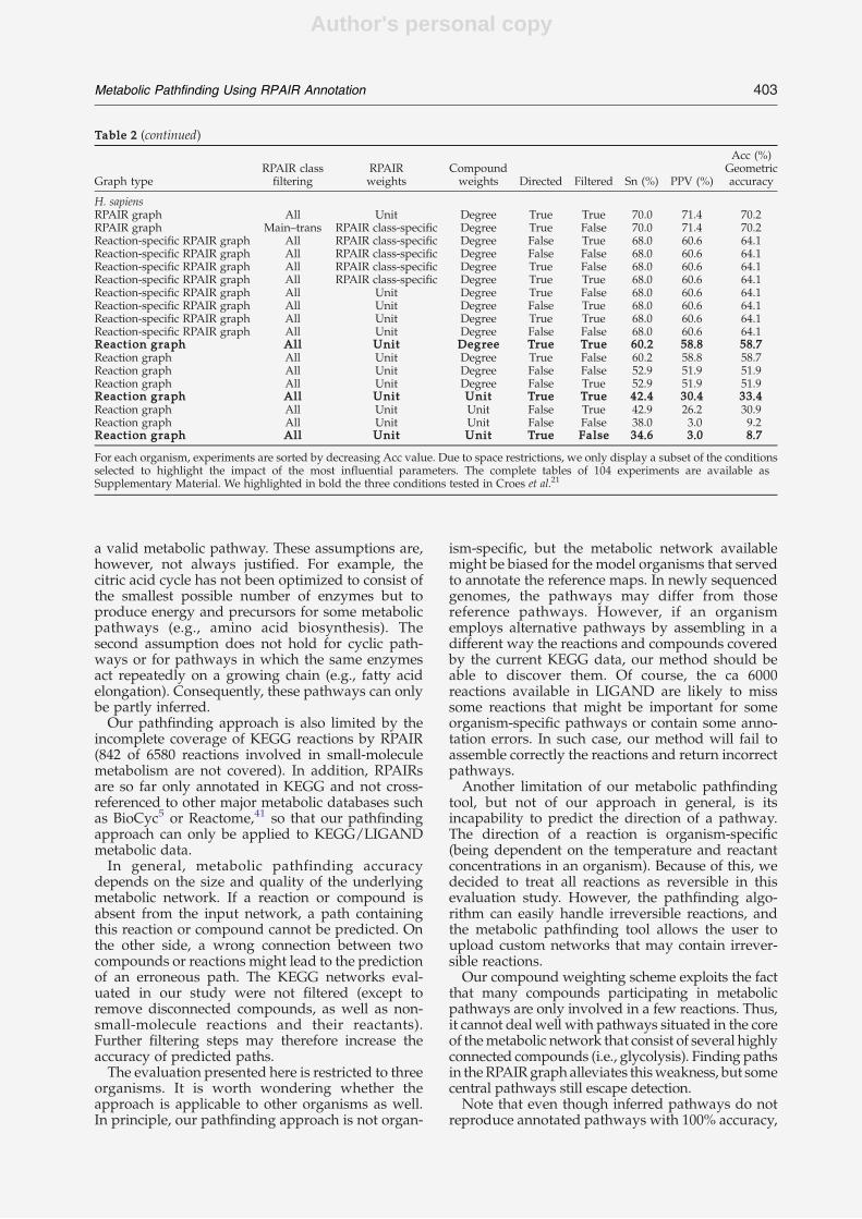
Author's personal copy
a valid metabolic pathway. These assumptions are,however, not always justified. For example, thecitric acid cycle has not been optimized to consist ofthe smallest possible number of enzymes but toproduce energy and precursors for some metabolicpathways (e.g., amino acid biosynthesis). Thesecond assumption does not hold for cyclic path-ways or for pathways in which the same enzymesact repeatedly on a growing chain (e.g., fatty acidelongation). Consequently, these pathways can onlybe partly inferred.Our pathfinding approach is also limited by the
incomplete coverage of KEGG reactions by RPAIR(842 of 6580 reactions involved in small-moleculemetabolism are not covered). In addition, RPAIRsare so far only annotated in KEGG and not cross-referenced to other major metabolic databases suchas BioCyc5 or Reactome,41 so that our pathfindingapproach can only be applied to KEGG/LIGANDmetabolic data.In general, metabolic pathfinding accuracy
depends on the size and quality of the underlyingmetabolic network. If a reaction or compound isabsent from the input network, a path containingthis reaction or compound cannot be predicted. Onthe other side, a wrong connection between twocompounds or reactions might lead to the predictionof an erroneous path. The KEGG networks eval-uated in our study were not filtered (except toremove disconnected compounds, as well as non-small-molecule reactions and their reactants).Further filtering steps may therefore increase theaccuracy of predicted paths.The evaluation presented here is restricted to three
organisms. It is worth wondering whether theapproach is applicable to other organisms as well.In principle, our pathfinding approach is not organ-
ism-specific, but the metabolic network availablemight be biased for the model organisms that servedto annotate the reference maps. In newly sequencedgenomes, the pathways may differ from thosereference pathways. However, if an organismemploys alternative pathways by assembling in adifferent way the reactions and compounds coveredby the current KEGG data, our method should beable to discover them. Of course, the ca 6000reactions available in LIGAND are likely to misssome reactions that might be important for someorganism-specific pathways or contain some anno-tation errors. In such case, our method will fail toassemble correctly the reactions and return incorrectpathways.Another limitation of our metabolic pathfinding
tool, but not of our approach in general, is itsincapability to predict the direction of a pathway.The direction of a reaction is organism-specific(being dependent on the temperature and reactantconcentrations in an organism). Because of this, wedecided to treat all reactions as reversible in thisevaluation study. However, the pathfinding algo-rithm can easily handle irreversible reactions, andthe metabolic pathfinding tool allows the user toupload custom networks that may contain irrever-sible reactions.Our compound weighting scheme exploits the fact
that many compounds participating in metabolicpathways are only involved in a few reactions. Thus,it cannot deal well with pathways situated in the coreof themetabolic network that consist of several highlyconnected compounds (i.e., glycolysis). Finding pathsin theRPAIRgraph alleviates thisweakness, but somecentral pathways still escape detection.Note that even though inferred pathways do not
reproduce annotated pathways with 100% accuracy,
Table 2 (continued)
Graph typeRPAIR classfiltering
RPAIRweights
Compoundweights Directed Filtered Sn (%) PPV (%)
Acc (%)Geometricaccuracy
H. sapiensRPAIR graph All Unit Degree True True 70.0 71.4 70.2RPAIR graph Main–trans RPAIR class-specific Degree True False 70.0 71.4 70.2Reaction-specific RPAIR graph All RPAIR class-specific Degree False True 68.0 60.6 64.1Reaction-specific RPAIR graph All RPAIR class-specific Degree False False 68.0 60.6 64.1Reaction-specific RPAIR graph All RPAIR class-specific Degree True False 68.0 60.6 64.1Reaction-specific RPAIR graph All RPAIR class-specific Degree True True 68.0 60.6 64.1Reaction-specific RPAIR graph All Unit Degree True False 68.0 60.6 64.1Reaction-specific RPAIR graph All Unit Degree False True 68.0 60.6 64.1Reaction-specific RPAIR graph All Unit Degree True True 68.0 60.6 64.1Reaction-specific RPAIR graph All Unit Degree False False 68.0 60.6 64.1Reaction graph All Unit Degree True True 60.2 58.8 58.7Reaction graph All Unit Degree True False 60.2 58.8 58.7Reaction graph All Unit Degree False False 52.9 51.9 51.9Reaction graph All Unit Degree False True 52.9 51.9 51.9Reaction graph All Unit Unit True True 42.4 30.4 33.4Reaction graph All Unit Unit False True 42.9 26.2 30.9Reaction graph All Unit Unit False False 38.0 3.0 9.2Reaction graph All Unit Unit True False 34.6 3.0 8.7
For each organism, experiments are sorted by decreasing Acc value. Due to space restrictions, we only display a subset of the conditionsselected to highlight the impact of the most influential parameters. The complete tables of 104 experiments are available asSupplementary Material. We highlighted in bold the three conditions tested in Croes et al.21
403Metabolic Pathfinding Using RPAIR Annotation
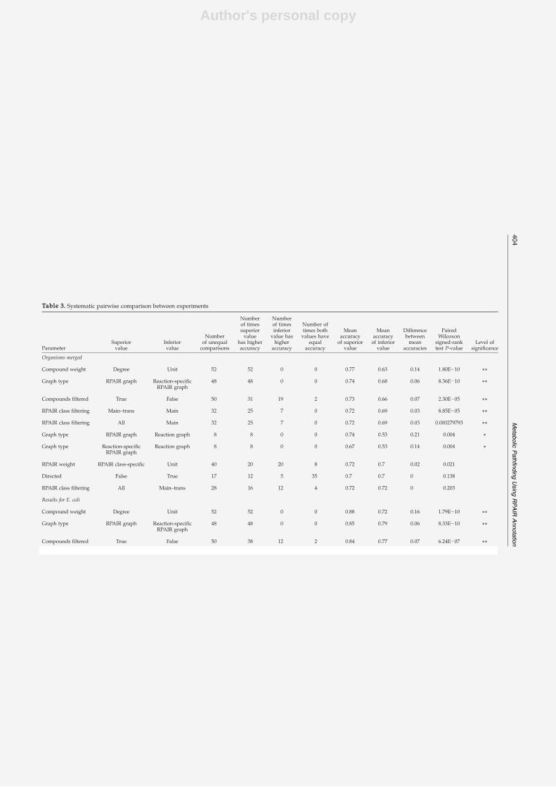
Author's personal copy
Table 3. Systematic pairwise comparison between experiments
ParameterSuperiorvalue
Inferiorvalue
Numberof unequalcomparisons
Numberof timessuperiorvalue
has higheraccuracy
Numberof timesinferiorvalue hashigher
accuracy
Number oftimes bothvalues have
equalaccuracy
Meanaccuracy
of superiorvalue
Meanaccuracyof inferior
value
Differencebetweenmean
accuracies
PairedWilcoxon
signed-ranktest P-value
Level ofsignificance
Organisms merged
Compound weight Degree Unit 52 52 0 0 0.77 0.63 0.14 1.80E−10 ⁎⁎
Graph type RPAIR graph Reaction-specificRPAIR graph
48 48 0 0 0.74 0.68 0.06 8.36E−10 ⁎⁎
Compounds filtered True False 50 31 19 2 0.73 0.66 0.07 2.30E−05 ⁎⁎
RPAIR class filtering Main–trans Main 32 25 7 0 0.72 0.69 0.03 8.85E−05 ⁎⁎
RPAIR class filtering All Main 32 25 7 0 0.72 0.69 0.03 0.000279793 ⁎⁎
Graph type RPAIR graph Reaction graph 8 8 0 0 0.74 0.53 0.21 0.004 ⁎
Graph type Reaction-specificRPAIR graph
Reaction graph 8 8 0 0 0.67 0.53 0.14 0.004 ⁎
RPAIR weight RPAIR class-specific Unit 40 20 20 8 0.72 0.7 0.02 0.021
Directed False True 17 12 5 35 0.7 0.7 0 0.138
RPAIR class filtering All Main–trans 28 16 12 4 0.72 0.72 0 0.203
Results for E. coli
Compound weight Degree Unit 52 52 0 0 0.88 0.72 0.16 1.79E−10 ⁎⁎
Graph type RPAIR graph Reaction-specificRPAIR graph
48 48 0 0 0.85 0.79 0.06 8.33E−10 ⁎⁎
Compounds filtered True False 50 38 12 2 0.84 0.77 0.07 6.24E−07 ⁎⁎
404Metabolic
Pathfinding
Using
RPAIR
Annotation

Author's personal copy
RPAIR weight RPAIR class-specific Unit 33 24 9 15 0.83 0.81 0.02 0.000827796 ⁎⁎
Graph type RPAIR graph Reaction graph 8 8 0 0 0.83 0.62 0.21 0.004 ⁎
Graph type Reaction-specificRPAIR graph
Reaction graph 8 8 0 0 0.76 0.62 0.14 0.004 ⁎
RPAIR class filtering Main All 32 23 9 0 0.83 0.81 0.02 0.025
RPAIR class filtering Main–trans All 23 13 10 9 0.82 0.81 0.01 0.046
RPAIR class filtering Main Main–trans 32 16 16 0 0.83 0.82 0.01 0.168
Directed False True 11 6 5 41 0.8 0.8 0 0.518
Results for S. cerevisiae
Compound weight Degree Unit 52 48 4 0 0.6 0.47 0.13 3.19E−10 ⁎⁎
Compounds filtered True False 28 27 1 24 0.58 0.49 0.09 2.18E−06 ⁎⁎
Graph type RPAIR graph Reaction-specificRPAIR graph
48 40 8 0 0.55 0.53 0.02 8.05E−05 ⁎⁎
Graph type RPAIR graph Reaction graph 8 8 0 0 0.57 0.44 0.13 0.007
Graph type Reaction-specificRPAIR graph
Reaction graph 8 8 0 0 0.54 0.44 0.1 0.007
RPAIR class filtering Main–trans Main 28 16 12 4 0.55 0.53 0.02 0.022
RPAIR class filtering All Main–trans 28 18 10 4 0.55 0.55 0 0.023
RPAIR weight RPAIR class-specific Unit 26 17 9 22 0.54 0.54 0 0.419
Directed False True 6 3 3 46 0.53 0.53 0 0.663
RPAIR class filtering Main All 30 16 14 2 0.53 0.55 0.02 0.967
(continued on next page)
405Metabolic
Pathfinding
Using
RPAIR
Annotation

Author's personal copy
Table 3 (continued)
ParameterSuperiorvalue
Inferiorvalue
Numberof unequalcomparisons
Numberof timessuperiorvalue
has higheraccuracy
Numberof timesinferiorvalue hashigher
accuracy
Number oftimes bothvalues have
equalaccuracy
Meanaccuracy
of superiorvalue
Meanaccuracyof inferior
value
Differencebetweenmean
accuracies
PairedWilcoxon
signed-ranktest P-value
Level ofsignificance
Results for H. sapiensGraph type RPAIR graph Reaction-specific
RPAIR graph48 45 3 0 0.62 0.54 0.08 1.41E−09 ⁎⁎
Compound weight Degree Unit 52 50 2 0 0.61 0.52 0.09 1.63E−09 ⁎⁎
RPAIR class filtering Main–trans Main 32 30 2 0 0.6 0.52 0.08 1.66E−06 ⁎⁎
Compounds filtered True False 30 28 2 22 0.58 0.54 0.04 1.75E−06 ⁎⁎
RPAIR class filtering All Main 32 30 2 0 0.61 0.52 0.09 2.39E−06 ⁎⁎
Graph type RPAIR graph Reaction graph 8 8 0 0 0.63 0.38 0.25 0.007
Graph type Reaction-specificRPAIR graph
Reaction graph 8 8 0 0 0.54 0.38 0.16 0.007
RPAIR weight RPAIR class-specific Unit 20 12 8 28 0.58 0.57 0.01 0.017
Directed FALSE True 10 7 3 42 0.56 0.56 0 0.154
RPAIR class filtering All Main–trans 12 8 4 20 0.61 0.6 0.01 0.155
AWilcoxon paired signed-rank test was applied to all pairs of parameter values, with all other parameters having the same value. This test computes Acc differences for combinations that differ by onlyone parameter value. P-value indicates the first error risk (i.e., the probability to consider a difference as significant when it is not). The table is sorted by ascending P-values, so the most significantparameter value differences appear on top.* P-value below 0.005.** P-value below 0.001.
406Metabolic
Pathfinding
Using
RPAIR
Annotation

Author's personal copy
they may be biochemically valid alternatives (e.g.,aldosterone biosynthesis in humans). Our evalua-tion may thus underestimate the accuracy of ourpathfinding approach.
Pathfinding and constraints
In the Introduction, we have discussed pathfind-ing approaches under the aspect of treatment ofhighly connected compounds. Another way toclassify these approaches might rely on the con-straints used to narrow down the huge number ofpossible solution pathways.We can list the followingbiologically or biochemically motivated constraints:
1. Pathway length/weight: The solution path-way should be as short (light) as possible (i.e.,Croes et al.,21 Arita,28 Rahman et al.,31 Sirava etal.,42 and Beasley and Planes43).
2. Imposing or excluding nodes: Certain com-pounds or reactions should appear or should notappear in the solution pathway (e.g. Rahmanet al.,31 Sirava et al.,42 and Mavrovouniotis44).
3. Mutual exclusion of reaction directions: Thedirect and reverse directions of a reaction shouldnot appear together in a solution pathway.21,44
4. Maximal pathway length: The length (numberof reactions) of the solution pathway shouldneither exceed a maximum nor fall below aminimum.6,21
5. Stoichiometric constraint: Stoichiometric bal-ance should be respected between some or allof the compounds of the solution pathway (e.g.Beasley and Planes,43 Mavrovouniotis,44 andSeressiotis and Bailey45).
The first constraint is the most widely applied: Allapproaches based on the shortest pathfinding makeuse of it implicitly. Beasley and Planes employpathway length as an objective function to beoptimized (alternatively to ATP production max-imization). Constraints 2–4 are already integrated inour pathfinding approach, except for imposingselected nodes, which we hope to deal with in thefuture by using multiseed pathfinding.To our knowledge, Beasley and Planes presented
the most recent approach capable of computingpathway stoichiometry. They used a strategy remi-niscent of flux balance analysis that is based on theoptimization of an objective function while satisfy-ing a number of constraints. They evaluated thisapproach on a network reconstructed for E. coliconsisting of 880 reactions and recovered, amongothers, the glycolysis pathway correctly. However,in a recent review, Planes and Beasley pointedout some disadvantages of the stoichiometricconstraint.46 First of all, it is unclear which com-pounds should be stoichiometrically balanced(internal compounds) and which can be left uncon-strained (external compounds). Furthermore, theylisted metabolic pathways in which compoundsannotated to be internal are not balanced. In
conclusion, they state that pathfinding withoutstoichiometric constraints is more suited for path-way analysis in genome-scale metabolic networks.
Perspectives
In the future, we hope to extend our method tomore than two sets of input reactions or compounds.This will enable the inference of branched pathwaysand might allow for an increase in predictionaccuracy when more input reactions or compoundsare available. A complementary refinement of ourmethod might be to select metabolic networksrepresenting the metabolism of only one or severalrelated organisms.The compound weighting applied in this evalua-
tion is based on a relatively simple rule (a compoundweight is set equal to its degree in the metabolicnetwork). In the future, alternative weightingschemes will be considered in order to achievecontext-specific pathfinding. For instance, organism-specific pathfinding might be refined by applyingweights to reactions according to their likelihood tobe catalyzed in the organism of interest, rather thanby selecting the subnetwork on the basis of genomeannotations. Indeed, some enzyme-coding genesmay have been missed in the annotation but play anessential role in some pathways. Another possibilityis to weight reactions according to the level ofexpression of the corresponding enzymes, as mea-sured by microarray experiments. A similarapproach has been applied earlier by scoring pathsaccording to the average correlation between theexpression profiles of the corresponding genes.47
Instead of scoring the paths a posteriori, weightedpathfinding would allow application of an a prioribias on pathfinding in order to favor reactionscatalyzed by the products of up-regulated genes.Pathfinding could thus be tuned according to thephysiological state of the cell under particularculture conditions.Another perspective is to generalize the concept of
pathfinding by applying constraint programmingmethods to the problem of metabolic pathwayinference. In this context, Dooms et al. designed ageneral framework for constrained pathfinding inbiochemical networks, named CP(BioNet).48 At thetime of writing, CP(BioNet) was restricted to net-works consisting of, at most, 500 nodes, and wecould thus not evaluate it on our metabolic net-works, but its performance might be improved inthe near future. The combination of this frameworkwith the optimal conditions that we identified in thepresent study might result in a powerful and flexiblemetabolic pathfinding tool.It would be of great interest to carry out a
comparative evaluation of the different metabolicpathfinding approaches available. Although somecomparative studies have been published,38,46 athorough evaluation either based on a community-based CASP-like blind protocol or performed byindependent users is still missing.
407Metabolic Pathfinding Using RPAIR Annotation

Author's personal copy
Table 4. Pairwise comparison between parameter values, with each parameter being associated with its “best friends” (conditionally optimal combinations)
ParameterSuperiorvalue
Inferiorvalue
Numberof unequalcomparisons
Numberof timessuperiorvalue hashigher
accuracy
Numberof timesinferiorvalue hashigher
accuracy
Numberof timesbothvalues
have equalaccuracies
Meanaccuracy
ofsuperiorvalue
Meanaccuracy
ofinferiorvalue
Differencebetweenmean
accuracies
PairedWilcoxon
signed-ranktest P-value
Unique best friendsof superior value
Unique best friendsof inferior value Common best friends
Level ofsignificance
Organisms mergedGraph type RPAIRs Reaction
graph25 23 2 24 0.83 0.73 0.1 2.4E−05 RPAIRs; main–trans;
Cpd unfilteredRct graph; all; directed Rct unit weight;
Cpd degree weight⁎⁎
Graph type RPAIRs Reaction-specificRPAIRs
24 23 1 25 0.83 0.77 0.06 4.7E−05 RPAIRs; main–trans Rct-specific RPAIRs;all
Rct unit weight;Cpd degree weight;
Cpd unfiltered
⁎⁎
Graph type Reaction-specificRPAIRs
Reactiongraph
9 7 2 40 0.77 0.73 0.04 0.012 Rct-specific RPAIRs;Cpd unfiltered
Rct graph; directed All; Rct unit weight;Cpd degree weight
RPAIR classfiltering
All Main 10 9 1 39 0.83 0.79 0.04 0.033 All; Cpd unfiltered Main; undirected;Cpd filtered
RPAIRs; Rct unitweight; Cpd degree
weight
RPAIR classfiltering
Main–trans Main 8 7 1 41 0.83 0.79 0.04 0.070 Main–trans; Cpdunfiltered
Main; undirected;Cpd filtered
RPAIRs; Rct unitweight; Cpd degree
weight
Compoundweight
Degree Unit 18 11 7 31 0.83 0.79 0.04 0.148 Main–trans; Rct unitweight; Cpd degree
weight; Cpdunfiltered
All; RPAIRclass-specific weight;Cpd unit weight;
Cpd filtered
RPAIRs
RPAIRweight
RPAIRclass-specific
Unit weight 3 2 1 46 0.82 0.83 0.01 0.605 All; RPAIRclass-specific
weight
Main–trans; Rct unitweight
RPAIRs; Cpd degreeweight; Cpd unfiltered
RPAIR classfiltering
All Main–trans 4 2 2 45 0.83 0.83 0 0.821 All Main–trans RPAIRs; Rct unit weight;Cpd degree weight;
Cpd unfiltered
Directed True False 0 0 0 49 0.83 0.83 0 1 Directed Undirected RPAIRs; main–trans;Rct unit weight;
Cpd degree weight;Cpd unfiltered
Compoundsfiltered
True False 0 0 0 49 0.83 0.83 0 1 Cpd filtered Cpd unfiltered RPAIRs; main–trans;Rct unit weight;
Cpd degree weight
Results for E. coliGraph type RPAIRs Reaction-
specificRPAIRs
14 14 0 14 0.95 0.88 0.07 5.3E−04 RPAIRs; Cpdunfiltered
Rct-specific RPAIRs;main–trans; RPAIRclass-specific weight;
Undirected; Cpd filtered
Cpd degree weight ⁎⁎
Graph type RPAIRs Reactiongraph
14 14 0 14 0.95 0.84 0.11 5.3E−04 RPAIRs; Cpdunfiltered
Rct graph; all; Rct unitweight; directed
Cpd degree weight ⁎⁎
408Metabolic
Pathfinding
Using
RPAIR
Annotation
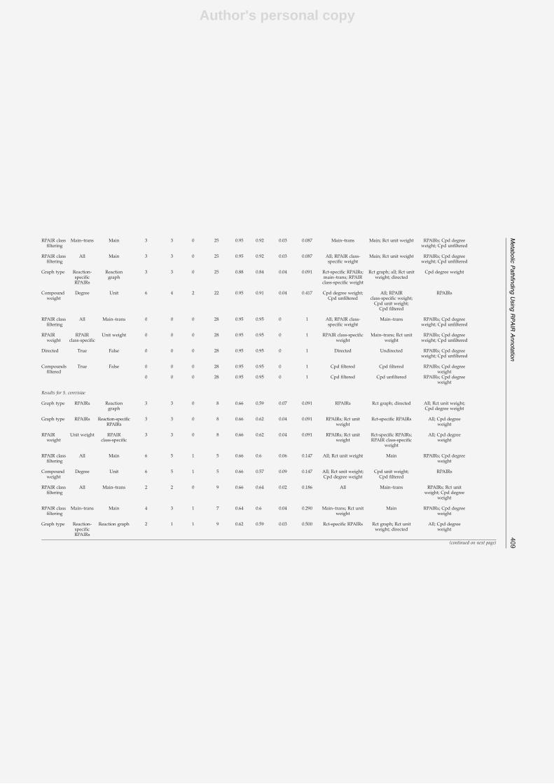
Author's personal copy
RPAIR classfiltering
Main–trans Main 3 3 0 25 0.95 0.92 0.03 0.087 Main–trans Main; Rct unit weight RPAIRs; Cpd degreeweight; Cpd unfiltered
RPAIR classfiltering
All Main 3 3 0 25 0.95 0.92 0.03 0.087 All; RPAIR class-specific weight
Main; Rct unit weight RPAIRs; Cpd degreeweight; Cpd unfiltered
Graph type Reaction-specificRPAIRs
Reactiongraph
3 3 0 25 0.88 0.84 0.04 0.091 Rct-specific RPAIRs;main–trans; RPAIRclass-specific weight
Rct graph; all; Rct unitweight; directed
Cpd degree weight
Compoundweight
Degree Unit 6 4 2 22 0.95 0.91 0.04 0.417 Cpd degree weight;Cpd unfiltered
All; RPAIRclass-specific weight;Cpd unit weight;
Cpd filtered
RPAIRs
RPAIR classfiltering
All Main–trans 0 0 0 28 0.95 0.95 0 1 All; RPAIR class-specific weight
Main–trans RPAIRs; Cpd degreeweight; Cpd unfiltered
RPAIRweight
RPAIRclass-specific
Unit weight 0 0 0 28 0.95 0.95 0 1 RPAIR class-specificweight
Main–trans; Rct unitweight
RPAIRs; Cpd degreeweight; Cpd unfiltered
Directed True False 0 0 0 28 0.95 0.95 0 1 Directed Undirected RPAIRs; Cpd degreeweight; Cpd unfiltered
Compoundsfiltered
True False 0 0 0 28 0.95 0.95 0 1 Cpd filtered Cpd filtered RPAIRs; Cpd degreeweight
0 0 0 28 0.95 0.95 0 1 Cpd filtered Cpd unfiltered RPAIRs; Cpd degreeweight
Results for S. cerevisiae
Graph type RPAIRs Reactiongraph
3 3 0 8 0.66 0.59 0.07 0.091 RPAIRs Rct graph; directed All; Rct unit weight;Cpd degree weight
Graph type RPAIRs Reaction-specificRPAIRs
3 3 0 8 0.66 0.62 0.04 0.091 RPAIRs; Rct unitweight
Rct-specific RPAIRs All; Cpd degreeweight
RPAIRweight
Unit weight RPAIRclass-specific
3 3 0 8 0.66 0.62 0.04 0.091 RPAIRs; Rct unitweight
Rct-specific RPAIRs;RPAIR class-specific
weight
All; Cpd degreeweight
RPAIR classfiltering
All Main 6 5 1 5 0.66 0.6 0.06 0.147 All; Rct unit weight Main RPAIRs; Cpd degreeweight
Compoundweight
Degree Unit 6 5 1 5 0.66 0.57 0.09 0.147 All; Rct unit weight;Cpd degree weight
Cpd unit weight;Cpd filtered
RPAIRs
RPAIR classfiltering
All Main–trans 2 2 0 9 0.66 0.64 0.02 0.186 All Main–trans RPAIRs; Rct unitweight; Cpd degree
weight
RPAIR classfiltering
Main–trans Main 4 3 1 7 0.64 0.6 0.04 0.290 Main–trans; Rct unitweight
Main RPAIRs; Cpd degreeweight
Graph type Reaction-specificRPAIRs
Reaction graph 2 1 1 9 0.62 0.59 0.03 0.500 Rct-specific RPAIRs Rct graph; Rct unitweight; directed
All; Cpd degreeweight
(continued on next page)
409Metabolic
Pathfinding
Using
RPAIR
Annotation

Author's personal copy
Table 4 (continued)
ParameterSuperiorvalue
Inferiorvalue
Numberof unequalcomparisons
Numberof timessuperiorvalue hashigher
accuracy
Numberof timesinferiorvalue hashigher
accuracy
Numberof timesbothvalues
have equalaccuracies
Meanaccuracy
ofsuperiorvalue
Meanaccuracy
ofinferiorvalue
Differencebetweenmean
accuracies
PairedWilcoxon
signed-ranktest P-value
Unique best friendsof superior value
Unique best friendsof inferior value Common best friends
Level ofsignificance
Directed True False 0 0 0 11 0.66 0.66 0 1 Directed Undirected RPAIRs; all; Rct unitweight; Cpd degree
weight
Compoundsfiltered
True False 0 0 0 11 0.66 0.66 0 1 Cpd filtered Cpd unfiltered RPAIRs; all; Rct unitweight; Cpd degree
weightResults for H. sapiensGraph type RPAIRs Reaction
graph8 7 1 2 0.7 0.59 0.11 0.021 RPAIRs Rct graph; all; Rct
unit weight; directedCpd degree weight
Graph type RPAIRs Reaction-specificRPAIRs
8 7 1 2 0.7 0.64 0.06 0.040 RPAIRs Rct-specific RPAIRs;all
Cpd degree weight
RPAIR classfiltering
Main–trans Main 8 7 1 2 0.7 0.6 0.1 0.040 RPAIRs; main–trans Rct-specific RPAIRs;main; Rct unit weight
Cpd degree weight
RPAIR classfiltering All Main 8 7 1 2 0.7 0.6 0.1 0.040 RPAIRs; all Rct-specific RPAIRs;
main; Rct unit weightCpd degree weight
Graph type Reaction-specificRPAIRs
Reactiongraph
4 3 1 6 0.64 0.59 0.05 0.101 Rct-specific RPAIRs Rct graph; Rct unitweight; directed
All; Cpd degreeweight
Compoundweight
Degree Unit 6 3 3 4 0.7 0.67 0.03 0.500 Cpd degree weight RPAIR class-specificweight; Cpd unit
RPAIRs
RPAIR classfiltering
All Main–trans 0 0 0 10 0.7 0.7 0 1 All Weight; Cpd RPAIRs; Cpd degreeweight
RPAIRweight
RPAIRclass-specific
Unit weight 0 0 0 10 0.7 0.7 0 1 RPAIR class-specificweight
Rct unit weight RPAIRs; Cpd degreeweight
Directed True False 0 0 0 10 0.7 0.7 0 1 Directed Undirected RPAIRs; Cpd degreeweight
Compoundsfiltered
True False 0 0 0 10 0.7 0.7 0 1 Cpd filtered Cpd unfiltered RPAIRs; Cpd degreeweight
For each parameter, we selected the combination of other parameters giving the best accuracy. Wilcoxon test was then performed by counting the number of pathways for each alternative value, giving a better, worse, or equalaccuracy, respectively.Cpd: compound; Rct: reaction.* P-value below 0.005.** P-value below 0.001.
(continued)
410Metabolic
Pathfinding
Using
RPAIR
Annotation
Author's personal copy
Materials and Methods
Network construction
We constructed three different networks from KEGG/LIGAND (release 41.0).The first graph, named reaction graph, was built from
all reactions and compounds present in KEGG/LIGAND. The resulting graph is composed of 6359reactions and 5312 compounds, which are connected by26,786 edges.The second graph, termed RPAIR graph, was con-
structed from all reactant pairs (7058) in KEGG RPAIR(release 41.0) and all compounds involved in at least oneof these reactant pairs (4297). It has fewer compounds thanthe reaction graph because RPAIR does not cover all thereactions and compounds listed in LIGAND.Finally, we constructed a reaction-specific RPAIR graph,
where each reaction is divided into its reactant pairs. Inthis graph, the same RPAIR can correspond to distinctnodes if it is part of multiple reactions. This graph contains12,828 reaction-specific reactant pairs and as manycompounds as the RPAIR graph (4297).All three networks (or graphs, to use the mathematical
term) are bipartite and not organism-specific. We excludedglycans and orphan nodes (nodes not connected to anyother node), as well as reactions having a substrate and aproduct with an identical identifier in KEGG (thesecorrespond to polymerization reactions). The reaction/RPAIR and compound node numbers given above refer tothese filtered networks. The KEGG/LIGAND databasecontains a number of problematic entries (see Poolmanet al.,49 Félix and Valiente,50 and Ott and Vriend51; e.g.,generic compounds, duplicated reactions, and unbalancedreactions). However, further filtering steps are beyond thescope of this evaluation.
Mutual exclusion between reaction nodes
As discussed in Croes et al.,37 the direction of a reaction(or a reaction pair) depends on physiological conditions inan organism (substrate concentration, product concentra-tions, and temperature). In our previous work, we thusconsidered that each reaction can be traversed either inforward direction or in reverse direction. Each reactionwas therefore represented as a pair of nodes for theforward direction and the reverse direction, respectively.To prevent the pathfinding algorithm from traversing thesame reaction/reactant pair twice, the forward andreverse directions exclude each other mutually. In theRPAIR and reaction-specific RPAIR graphs, we ensure, inaddition, that reactant pairs belonging to the samereaction exclude each other.
Parameters
Table 1 summarizes the different parameters used forgraph construction. In total, the values of the parameterslisted (graph construction, graph structure, compoundand reaction weights, and compound and reactionfiltering) can be combined in 104 possible ways.
Reference pathways
In order to measure the accuracy of pathfinding inmetabolic graphs, a set of reference pathways is needed.
We chose the metabolic pathways stored in the aMAZEdatabase52 (version 2006) because they have been care-fully annotated and provide side/main compoundclassification and cross-reference reactions and com-pounds to KEGG/LIGAND. Since pathfinding cannotdeal with branched pathways, we selected the linearsegments as in our previous work37 and removed sidecompounds. Pathways composed of less than threereactions were discarded, since finding them would betrivial. For the two RPAIR graphs, reactions of thereference pathways had to be mapped to their corre-sponding reactant pairs. Each reaction was replaced byits main reactant pair. When a reaction was associatedwith several main reactant pairs, we selected only thosewhose substrate and product were part of the linearizedpathway. For three of the E. coli pathways (alaninebiosynthesis and the two branches of methioninebiosynthesis), mapping to main reactant pairs was notsufficient to obtain the fully connected pathway, and wehad to use trans reactant pairs.The aMAZE database contained 116 pathways: 55
from E. coli, 29 from S. cerevisiae, and 32 from H. sapiens.Of these, 7 were cyclic (E. coli, 2; S. cerevisiae, 4; H.sapiens, 1), 25 were branched (E. coli, 13; S. cerevisiae, 5;H. sapiens, 7), and 46 contained less than three reactions(E. coli, 20; S. cerevisiae, 14; H. sapiens, 12). After filteringand linearization, 69 pathways remained (E. coli, 37; S.cerevisiae, 14; H. sapiens, 18). After mapping of reactionsto main/trans RPAIRs, we ended up with the 55pathways used for evaluation (E. coli, 32; S. cerevisiae,11; H. sapiens, 12).
Metabolic pathfinding algorithm
We find paths in weighted graphs using the k-shortestpaths algorithm developed and implemented by Jimenezand Marzal.53 By introducing pseudo nodes (a graphtransformation described in Duin et al.54), we enable thesearch between a set of start nodes and a set of end nodes.Starts and ends can be compounds, reactions, or both. Forgiven sets of start and end nodes, we regard as an inferredpathway the union of all paths of first rank (having equalweights) between them. Thus, inferred pathways cancontain alternative branches.
Evaluation procedure
The evaluation procedure consists in finding the k-shortest (or lightest) paths between the start and the endreactions of a reference pathway and comparing theintermediate nodes of the inferred path with those of theannotated pathway. The motivation for searching pathsfrom reaction to reaction (rather than from compound tocompound) is that this is more relevant to metabolicreconstruction, where one starts from sets of enzyme-coding genes.To compute the accuracy of an inferred pathway, we
consider the intersection of node sets of the inferred andreference pathways. Nodes appearing in both pathwayscount as true positives, whereas nodes absent in theinferred pathway but present in the reference pathwayare false negatives. Nodes found in the inferred path-way but not in the reference pathway are falsepositives. Since start and end nodes are known before-hand, they are not considered for those matchingstatistics.Note that, in our previous publication,21 alternative
reactions linking a pair of compounds were not counted as
411Metabolic Pathfinding Using RPAIR Annotation

Author's personal copy
false positives. In the present study, we applied morestringent criteria in order to precisely quantify theimpact of the RPAIR annotations. For the sake ofcomparison, we also applied all the tests with theprevious scoring scheme, and the results are available asTables S5 and S6.Sn is the fraction of annotated nodes that are found in
the inferred pathway:
Sn ¼ TP=ðTPþ FPÞPPV is defined as the fraction of inferred nodes that belongto the annotated pathway:
PPV ¼ TP=ðTPþ FPÞGiven both Sn and PPV, we calculate the accuracy of aninferred pathway as their geometric mean:
Acc ¼ sqrtðSN� PPVÞThe evaluation of a specific parameter combinationproceeds as follows: First, we identify the start and endreactions (or main reactant pairs) of one reference path-way. Metabolic pathfinding is run on these input reactionsin one of the three metabolic graphs and returns apathway. By comparing the predicted pathway with thereference pathway, the accuracy of pathway prediction iscalculated. These steps are performed for each pathway inthe reference set and for each possible combination of theparameters described above. Since we deal with 104parameter combinations, 104 such evaluations have beenperformed.
Wilcoxon paired signed-rank test
Since we perform a number of experiments withdifferent parameter values, we need a statistical test tomeasure the significance of accuracy differences that resultfrom having used two different values for the sameparameter. We have chosen the Wilcoxon paired signed-rank test for this task because it makes no assumptions onsample distribution.Let us consider one group of pathfinding experiments
performed with one value and another group of experi-ments performed with another value for the sameparameter. The null hypothesis states that there is noaccuracy difference between the two experiment groups.The alternative hypothesis says that one of the twoexperiment groups yields pathfinding accuracies thatbelong to another (right-shifted) distribution comparedto those obtained for the other experiment group, and that,consequently, one parameter value improves pathfindingaccuracy as compared to the other to a certain level ofsignificance.For the experimentwise Wilcoxon test, we paired all
experiments that differed only by the parameter inquestion. We thus obtained two vectors, where eachentry represents the pathfinding accuracy averaged overall paths of an experiment. The significance of pathfindingaccuracy difference is then computed on these pairedvectors.In contrast, for the best-combination-wiseWilcoxon test,
we paired only those experiments that yielded the highestaccuracies for the two values of a parameter in question.We then calculated the significance of the accuracydifference by comparing the pathfinding accuracies ofthese experiments pathwaywise.For both Wilcoxon tests, we used the function wilcox.
test in R to compute P-values.
Implementation and availability
The metabolic pathfinding tool† is available as part ofNetwork Analysis Tools.39 It allows the enumeration ofthe shortest paths in the three graph types and lets theuser choose between different combinations of com-pound and reaction weights. The optimal parametervalues obtained by our evaluation are set as default.KEGG identifiers of compounds, reactions and reactantpairs, EC numbers, and compound names can be givento specify start and end nodes. In addition, multiple startand end nodes can be provided. It is also possible tofind paths in organism-specific metabolic networksextracted from KEGG.The complete results of our evaluation (104 experiments
for E. coli, S. cerevisiae, and H. sapiens) can be found at theRSAT Web site‡.
Acknowledgements
We would like to thank Jean-Noël Monette andPierre Schaus for making available useful modifica-tions to the REA algorithm. They also implementeda Python wrapper around REA that inspired theJava wrapper employed for pathfinding evaluation.We acknowledge the aMAZE team for their
support during the initial stages of this work. Weused their Java graph library and, in addition, one ofthem (Olivier Hubaut) suggested the graph trans-formation that extended pathfinding with twonodes to pathfinding with two sets of nodes. Thanksas well to Pierre Dupont and Grégoire Dooms forhelpful discussions.K.F. was supported by Actions de Recherches
Concertées de la Communauté Française de Belgi-que (ARC grant no. 04/09-307). The laboratory is amember of the BioSapiens Network of Excellencefunded under the Sixth Framework Program of theEuropean Communities (LSHG-CT-2003-503265).The work was also supported by the BelgianProgram on Interuniversity Attraction Poles,initiated by the Belgian Federal Science PolicyOffice, under project P6/25 (BioMaGNet).
Supplementary Data
Supplementary data associated with this articlecan be found, in the online version, at doi:10.1016/j.jmb.2009.03.006
References1. Berg, J. M., Tymoczko, J. L. & Stryer, L. (2002). In
Biochemistry, 5th edit. (Stryer, L., ed.), W. H. Freemanand Company, New York.
†http://rsat.ulb.ac.be/neat/‡http://rsat.ulb.ac.be/pathfindingsupplementref/
index.html
412 Metabolic Pathfinding Using RPAIR Annotation
Author's personal copy
2. Goto, S., Bono, H., Ogata, H., Fujibuchi, W., Nishioka,T., Sato, K. & Kanehisa, M. (1997). Organizing andcomputing metabolic pathway data in terms of binaryrelations. Pac. Symp. Biocomput. 175–186.
3. Kanehisa, M., Araki, M., Goto, S., Hattori, M.,Hirakawa, M., Itoh, M. et al. (2008). KEGG for linkinggenomes to life and the environment. Nucleic AcidsRes. 36, D480–D484.
4. Karp, P. D., Riley, M., Paley, S. & Pellegrini-Toole, A.(1996). EcoCyc: an encyclopedia of Escherichia coligenes and metabolism. Nucleic Acids Res. 24, 32–39.
5. Caspi, R., Foerster, H., Fulcher, C. A., Kaipa, P.,Krummenacker, M., Latendresse, M. et al. (2008). TheMetaCyc database of metabolic pathways andenzymes and the BioCyc collection of pathway/genome databases. Nucleic Acids Res. 36, D623–D631.
6. Kueffner, R., Zimmer, R. & Lengauer, T. (2000).Pathway analysis in metabolic databases via diffe-rential metabolic display. Bioinformatics, 16, 825–836.
7. Förster, J., Famili, I., Fu, P., Palsson, B.Ø. & Nielsen, J.(2003). Genome-scale reconstruction of the Sacchar-omyces cerevisiae metabolic network. Genome Res. 13,244–253.
8. Duarte, N. C., Becker, S. A., Jamshidi, N., Thiele, I.,Mo, M. L., Vo, T. D. et al. (2007). Global reconstruc-tion of the human metabolic network based ongenomic and bibliomic data. Proc. Natl Aced. Sci.104, 1777–1782.
9. Gaasterland, T. & Selkov, E. (1995). Reconstruction ofmetabolic networks using incomplete information.Proc. Int. Conf. Intell. Syst. Mol. Biol. 3, 127.
10. Arita, M. (2000). Metabolic reconstruction usingshortest paths. Simul. Pract. Theory, 8, 109–125.
11. Ma, H. & Zeng, A. -P. (2003). Reconstruction of meta-bolic networks from genome data and analysis of theirglobal structure for various organisms. Bioinformatics,19, 270–277.
12. Karp, P. D., Ouzounis, C. A., Moore-Kochlacs, C.,Goldovsky, L., Kaipa, P., Ahrén, D. et al. (2005).Expansion of the BioCyc collection of pathway/genome databases to 160 genomes. Nucleic Acids Res.33, 6083–6089.
13. Moriya, Y., Itoh, M., Okuda, S., Yoshizawa, A. C. &Kanehisa, M. (2007). KAAS: an automatic genomeannotation and pathway reconstruction server.Nucleic Acids Res. 35, W182–W185.
14. DeJongh, M., Formsma, K., Boillot, P., Gould, J.,Rycenga, M. & Best, A. (2007). Toward the automatedgeneration of genome-scale metabolic networks in theSEED. BMC Bioinf. 8, 139.
15. Paley, S. M. & Karp, P. D. (2002). Evaluation ofcomputational metabolic-pathway predictions forHelicobacter pylori. Bioinformatics, 18, 705–714.
16. Kharchenko, P., Vitkup, D. & Church, G. M. (2004).Filling gaps in a metabolic network using expressioninformation. Bioinformatics, 20, i178–i185.
17. Kharchenko, P., Chen, L., Freund, Y., Vitkup, D. &Church, G. M. (2006). Identifying metabolic enzymeswith multiple types of association evidence. BMCBioinf. 7, 177.
18. Jeong, H., Tombor, B., Albert, R., Oltvai, Z. N. &Barabási, A. -L. (2000). The large-scale organization ofmetabolic networks. Nature, 407, 651–654.
19. Fell, D. A. & Wagner, A. (2000). The small worldof metabolism. Metab. Eng. 18, 1121–1122; NatureAmerica, Inc.
20. Arita, M. (2004). The metabolic world of Escherichiacoli is not small. Proc. Natl Acad. Sci. 101, 1543–1547.
21. Croes, D., Couche, F., Wodak, S. & van Helden, J.
(2006). Inferring meaningful pathways in weightedmetabolic networks. J. Mol. Biol. 356, 222–236.
22. van Helden, J., Wernisch, L., Gilbert, D. & Wodak, S.(2002). Graph-based analysis of metabolic networks.Ernst Schering Res. Found. Workshop, 38, 245–274.
23. Schuster, S., Dandekar, T. & Fell, D. A. (1999).Detection of elementary flux modes in biochemicalnetworks: a promising tool for pathway analysis andmetabolic engineering. TIBTECH, 17, 53–60.
24. Teusink, B., Wiersma, A., Molenaar, D., Francke, C., deVos, W. M., Siezen, R. J. & Smid, E. J. (2006). Analysisof growth of Lactobacillus plantarum WCFS1 on acomplex medium using a genome-scale metabolicmodel. J. Biol. Chem. 281, 40041–40048.
25. Edwards, J. S. & Palsson, B.Ø. (2001). Metabolic fluxbalance analysis and the in silico analysis of Escherichiacoli K-12 gene deletions. BMC Bioinf. 1, 1.
26. Karp, P. D. & Paley, S. M. (1994). Representations ofmetabolic knowledge: pathways. Proc. 2nd Int. Conf.Intell. Syst. Mol. Biol. 203–211.
27. Arita, M., Asai, K. & Nishioka, T. (2000). Graphmodeling of metabolism. J. Jpn. Soc. Artif. Intell. 15,703–710.
28. Arita, M. (2003). In silico atomic tracing by substrate–product relationships in Escherichia coli intermediarymetabolism. Genome Res. 13, 2455–2466.
29. McShan, D. C., Rao, S. & Shah, I. (2003). PathMiner:predicting metabolic pathways by heuristic search.Bioinformatics, 19, 1692–1698.
30. Boyer, F. & Viari, A. (2003). Ab initio reconstruction ofmetabolic pathways. Bioinformatics, 19, ii26–ii34.
31. Rahman, S. A., Advani, P., Schunk, R., Schrader, R. &Schomburg, D. (2004). Metabolic pathway analysisweb service (Pathway Hunter Tool at CUBIC).Bioinformatics, 21, 1189–1193.
32. Blum, T. & Kolhbalcher, O. (2008). Using atommapping rules for an improved detection of relevantroutes in weighted metabolic networks. J. Comput.Biol. 15, 565–576.
33. Hou, B. K., Ellis, L. B. M. & Wackett, L. P. (2004).Encoding microbial metabolic logic: predicting biode-gradation. J. Ind. Microbiol. Biotechnol. 31, 261–272.
34. Kotera, M., Hattori, M., Oh, M. -A., Yamamoto, R.,Komeno, T., Yabuzaki, J. et al. (2004). RPAIR: areactant-pair database representing chemical changesin enzymatic reactions. Genome Inf. 15, P062.
35. Kotera, M., Okuno, Y., Hattori, M., Goto, S. &Kanehisa, M. (2004). Computational assignment ofthe EC numbers for genomic-scale analysis of enzy-matic reactions. J. Am. Chem. Soc. 126, 16487–16498.
36. Oh, M., Yamada, T., Hattori, M., Goto, S. &Kanehisa, M. (2007). Systematic analysis ofenzyme-catalyzed reaction patterns and predictionof microbial biodegradation pathways. J. Chem. Inf.Model, 47, 1702–1712.
37. Croes, D., Couche, F., Wodak, S. & van Helden, J.(2005). Metabolic PathFinding: inferring relevant path-ways in biochemical networks. Nucleic Acids Res. 33,W326–W330.
38. de Figueiredo, L. F., Schuster, S., Kaleta, C. & Fell, D. A.(2008). Can sugars be produced from fatty acids?A testcase for pathway analysis tools. Bioinformatics, 24,2615–2621.
39. Brohee, S., Faust, K., Lima-Mendez, G., Sand, O.,Janky, R., Vanderstocken, G. et al. (2008). NeAT: atoolbox for the analysis of biological networks,clusters, classes and pathways. Nucleic Acids Res. 36.
40. Pasqualini, J. R. (2005). Enzymes involved in theformation and transformation of steroid hormones in
413Metabolic Pathfinding Using RPAIR Annotation

Author's personal copy
the fetal and placental compartments. J. SteroidBiochem. Mol. Biol. 97, 401–415.
41. Vastrik, I., D'Eustachio, P., Schmidt, E., Joshi-Tope, G.,Gopinath, G., Croft, D. et al. (2007). Reactome: aknowledge base of biologic pathways and processes.Genome Biol. 8, R39.
42. Sirava, M., Schaefer, T., Eiglsperger, M., Kaufmann,M., Kohlbacher, O., Bornberg-Bauer, E. & Lenhof,H. P. (2002). BioMiners—modeling, analyzing, andvisualizing biochemical pathways and networks.Bioinformatics, 18, S219–S230.
43. Beasley, J. E. & Planes, F. J. (2007). Recoveringmetabolicpathways via optimization. Bioinformatics, 23, 92–98.
44. Mavrovouniotis, M. L. (1993). Identification of qualita-tively feasible metabolic pathways. In Artificial Intelli-gence and Molecular Biology, pp. 325–364, AmericanAssociation for Artificial Intelligence, Menlo Park, CA.
45. Seressiotis, A. & Bailey, J. E. (1986). MPS: an algorithmand data base for metabolic pathway synthesis.Biotechnol. Lett. 8, 837–842.
46. Planes, F. J. & Beasley, J. E. (2008). A critical examinationof stoichiometric and path-finding approaches tometabolic pathways. Brief. Bioinf. 9, 422–436.
47. Zien, A., Kuffner, R., Zimmer, R. & Lengauer, T. (2000).Analysis of gene expression data with pathway scores.ISMB, 8, 407–417.
48. Dooms, G., Deville, Y. & Dupont, P. (2004). Con-strained path finding in biochemical networks. In5èmes Journées Ouvertes Biologie Informatique Mathéma-tiques, JOBIM 2004.
49. Poolman, M. G., Bonde, B. K., Gevorgyan, A., Patel,H. H. & Fell, D. A. (2006). Challenges to be faced inthe reconstruction of metabolic networks from publicdatabases. IEE Proc. Syst. Biol. 153, 379–384.
50. Félix, L. & Valiente, G. (2007). Validation of metabolicpathway databases based on chemical substructuresearch. Biomol. Eng. 24, 327–335.
51. Ott, M. A. & Vriend, G. (2006). Correcting ligands,metabolites, and pathways. BMC Bioinf. 7, 517.
52. Lemer, C., Antezana, E., Couche, F., Fays, F., Santolaria,X., Janky, R. et al. (2004). The aMAZE LightBench: aweb interface to a relational database of cellularprocesses. Nucleic Acids Res. 32, D443–D448.
53. Jimenez, V. M. & Marzal, A. (1999). Computing theK Shortest Paths: A New Algorithm and anExperimental Comparison. Proc. 3rd Int. WorkshopAlgorithm Eng. (WAE 1999), Lecture Notes in ComputerScience, vol. 1668, pp. 15–29 Springer-Verlag,London.
54. Duin, C. W., Volgenant, A. & Vo, S. (2004). Solvinggroup Steiner problems as Steiner problems. Eur. J.Oper. Res. 154, 323–329.
414 Metabolic Pathfinding Using RPAIR Annotation
3 Multiple-end metabolic pathway
prediction
Presented article:K. Faust, P. Dupont, J. Callut and J. van HeldenPathway discovery in metabolic networks by subgraph extractionSubmitted.
3.1 Introduction
After having established a strategy to increase the accuracy of two-end path finding, the nextstep of the thesis was to develop, evaluate and apply multiple-end pathway prediction ap-proaches. In contrast to path finding, multiple-seed pathway prediction can predict pathwaysstarting from or ending in several compounds or reactions. In addition, the ability to treat morethan two seeds allows to predict metabolic pathways from groups of enzyme-coding genes, en-zymes, reactions or compounds. This in turn can serve the interpretation of high-throughputdata sets featuring these seed groups.
This chapter presents the development and evaluation of multiple-end pathway predictionapproaches, whereas the next chapter ( 4 ) presents their application to a microarray data set.
Seven algorithms were evaluated, one of them based on random walks (kWalks [48]), andthree others on shortest paths. The other three algorithms are combinations of the shortest-paths based algorithms with kWalks. The algorithms are presented in section 9.1. All al-gorithms rely on the extraction of a subgraph from the input network, which represents thepredicted pathway.
3.2 Contribution
P. Dupont and J. Callut developed and implemented the kWalks algorithm. K. Faust imple-mented the other algorithms (except for Klein-Ravi), carried out the evaluation and wrote thearticle. P. Dupont and J. van Helden revised the article.
3.3 Methods
The evaluation of the algorithms was carried out on a network constructed from MetaCyc,with 71 reference pathways taken from S. cerevisiae (see section 9.2 for the pathway list). In
83

contrast to the evaluation of path finding presented in chapter 2, a linearization of the referencepathways was unnecessary, since the evaluation of multiple-end pathway prediction shouldalso quantify the prediction accuracy for branched pathways.
Each of the seven algorithms was launched several times on each of the 71 pathways, topredict pathways for increasing number of seed reactions.
In addition, the performance of the algorithms was evaluated for various parameters, e.g.network directionality, different weight policies, kWalks iteration number and others. KWalksoutputs node and edge relevances, which can serve as new node or edge weights. Theseweights can be refined by calling kWalks iteratively on the input network, whose weightsare up-dated in each round with the node/edge relevances computed by kWalks. The kWalksiteration number refers to the number of times kWalks is repeated.
3.4 Results
The algorithm reaching highest accuracy (∼77%) was a hybrid of kWalks and Takahashi-Matsuyama [154]. The hybrid algorithm takes advantage of the complementary strengths ofkWalks (high sensitivity, low computational complexity) and shortest-paths based approaches(high PPV).
The evaluation also yielded the following insights:
• KWalks can be used to discover weights in case a good weight policy is not at hand.
• Combining a shortest-paths based algorithm with kWalks increases its speed.
• Iterations of more than three do not increase the accuracy of kWalks any further.
• Reduction of the intermediate network size (i.e. its node number) in the hybrid approachdown to a certain percentage (0.5% in this evaluation) increases the prediction accuracy.
3.5 Conclusion
A combination of a random walk-based (kWalks) with a shortest-paths based (Takahashi-Matsuyama) approach yields a pathway prediction accuracy of ∼77% in the weighted Meta-Cyc network, which was the highest achieved for any algorithm or parameter combination.
84

BIOINFORMATICS Vol. 00 no. 00 2009Pages 1–7
Pathway discovery in metabolic networks by subgraphextractionKaroline Faust 1,∗, Pierre Dupont 2,∗, Jerome Callut 2 and Jacques vanHelden 1,∗
1Laboratoire de Bioinformatique des Genomes et des Reseaux (BiGRe), Universite Libre deBruxelles, Campus Plaine - CP263, Boulevard du Triomphe, 1050 Bruxelles, Belgium.2 UCL Machine Learning Group, Computing Science and Engineering Department, Universitecatholique de Louvain, B-1348 Louvain-la-Neuve, Belgium.Received on XXXXX; revised on XXXXX; accepted on XXXXX
Associate Editor: XXXXXXX
ABSTRACTMotivation: Subgraph extraction is a powerful technique to predictpathways from biological networks and a set of query items (e.g.genes, proteins, compounds...). It can be applied to a variety of diffe-rent data types, such as gene expression, protein levels, operons orphylogenetic profiles. In this article, we investigate different approa-ches to extract relevant pathways from metabolic networks. Althoughthese approaches have been adapted to metabolic networks, they aregeneric enough to be adjusted to other biological networks as well.Results: We comparatively evaluated seven sub-network extractionapproaches on 71 known metabolic pathways from S. cerevisiae anda metabolic network obtained from MetaCyc. The best performingapproach is a novel hybrid strategy, which combines a random walk-based reduction of the graph with a shortest-paths based algorithm,and which recovers the reference pathways with an accuracy of ∼77%.Availability: Most of the presented algorithms are available as part ofthe network analysis tool set (NeAT). The kWalks method is releasedunder the GPL3 license.Contact: kfaustulb.ac.be
1 INTRODUCTIONPathway inference aims to extract a meaningful pathway given abiological network (e.g. protein-protein interaction or metabolicnetwork) and a set of query items (e.g. genes, proteins, compounds).This methodology may serve to predict pathways from a variety ofdata types, such as gene expression, operons, phylogenetic profilesor protein levels.
To our knowledge, Zien et al. (2000) were the first to inferpathways from a biological network. They construct a bipartitemetabolic network consisting of compound and reaction nodes,where enzyme-coding genes are linked to reactions via their ECnumbers, and subsequently enumerate all possible paths betweena source node (D-glucose) and a target node (pyruvate) under cer-tain constraints. The score of each path is computed on the basisof expression values of the genes involved in this path as measured
∗to whom correspondence should be addressed
with microarrays. This method ranks predicted paths according totheir degree of up- or down-regulation.
Ideker et al. (2002) extended this idea to the extraction of morecomplex, non-linear sub-networks in protein-protein and protein-DNA networks given yeast gene expression data. Sub-networks areconsidered active whenever they involve highly expressed genes.Such sub-networks can be identified by sampling the space ofpossible sub-networks with simulated annealing. The authors alsomention several strengths of the sub-network extraction approach ascompared to traditional gene clustering, for instance the considera-tion of genes that are only weakly differentially expressed.
Scott et al. (2005) also search for sub-networks in protein-proteinand protein-DNA interaction networks given gene expression data.To our knowledge, their algorithm is the first to tackle the Steinertree problem (Hwang et al. (1992)) on biological networks in orderto connect nodes of interest (i.e. differentially expressed genes).
Rajagopalan and Agarwal (2005) integrate various data sources(TransFac, HumanCyc and Ingenuity Pathways Knowledge Base)into a network of gene-metabolite relationships. Query nodes inthis network are connected by an algorithm based on breadth-firstsearch. A key contribution of these authors is the systematic evalua-tion of their subgraph extraction approach on both simulated dataand known pathways taken from BioCarta.
Noirel et al. (2008) apply sub-network extraction to proteomicsdata (that is enzyme level ratios, measured by mass spectrometry)from the cyanobacterium Nostoc. A sub-network is extracted froma weighted KEGG metabolic network by generating paths aroundeach up-regulated enzyme node up to a given maximal weightand subsequently filtering these paths according to the number ofup-regulated enzymes contained in them. The filtered paths arethen merged to form a network whose connected components areconsidered as the extracted sub-networks.
Dittrich et al. (2008) identify high-scoring sub-networks inprotein-protein interaction networks with a strategy similar to Scottet al. (2005), by applying an algorithm that solves the Steinertree problem exactly. Interestingly, their method allows to reportsub-optimal solutions with a user-specified distance to previouslylisted solutions. The pathway prediction approach is validated onsimulated data.
c© Oxford University Press 2009. 1

Faust et al
Antonov and co-workers predict metabolic pathways from KEGGdata and from input genes mapped to reactions (Antonov et al.(2008)) or input compounds (Antonov et al. (2009)). Seed nodesseparated by one edge are added to a growing sub-network, whichmay consist of several components. The component covering mostseeds is considered as the inferred pathway. The procedure is repea-ted for distances of 2,3... edges, resulting in a set of distance-specificpredictions. This sub-network extraction procedure is available viatwo web tools specific to metabolic data.
In this article, we present a systematic assessment of sub-networkextraction accuracy given a metabolic network. We evaluate the per-formance of four different algorithms (combined in seven approa-ches) on the basis of 71 pathways obtained from MetaCyc. Oneof these algorithms (pair-wise K-shortest paths) has been develo-ped for this study and two other algorithms (Takahashi-Matsuyama,kWalks) have apparently not yet been applied to sub-network extrac-tion in biological networks. The extraction techniques consideredhere are not specific to metabolic networks or gene expression data.They can be applied to any biological network and to any data setgenerating specific nodes of interest (e.g. functionally related groupsof genes/enzymes as derived from phylogenetic co-occurrence,operons, gene fusion events etc.).
2 METHODS
2.1 Metabolic network constructionIn order to predict metabolic pathways, we need to represent metabolic dataas a network (or a graph, to use the mathematical term). We selected Meta-Cyc (Krieger et al. (2004)), the well-curated tier of BioCyc (Caspi et al.(2008)), as our data source, and constructed a bipartite, directed graph fromall small molecule entries and their associated reactions contained in theOWL file of MetaCyc (Release 11.0). The resulting graph consists of 4,891compound nodes and 5,358 reaction nodes. As discussed in Croes et al.(2005), reactions that are annotated as irreversible can be reversed dependingon physiological conditions (substrate and product concentrations, tempera-ture). Consequently, we represent each reaction as a pair of nodes, for theforward and the reverse directions, respectively. To prevent the paths-basedalgorithms to cross the same reaction twice, forward and reverse directionare mutually exclusive. After this duplication of reaction nodes, we obtain adirected network with 15,607 nodes and 43,938 edges, referred hereafter asthe MetaCyc network.
We constructed two variants of the MetaCyc network: the directed onedescribed above and an undirected network, in which reaction nodes arenot duplicated. In both cases however, the weight matrix is designed to besymmetric.
2.2 Weight policiesMetabolic networks contain hub compounds such as H2O, NADP and ATP,which are involved in a large number of reactions. A straightforward graphtraversal algorithm would preferentially cross these compounds, resultingin biochemically invalid paths that connect for instance D-glucose withpyruvate in one reaction step via ADP. Available path finding tools (whichextract a sub-network from a single source and target node) try to solvethis problem by considering compound structure (e.g. Arita (2000); McShanet al. (2003); Rahman et al. (2004); Blum and Kohlbacher (2008)), networkweights (Croes et al. (2005, 2006); Blum and Kohlbacher (2008)), anno-tated reactant pairs (Faust et al. (2009)) or rules (Ellis et al. (2008)). Weadopted the weighting approach and tested three different weight policies.The simplest one (“unit weight”) sets all node weights to one. The secondpolicy (“compound degree weight”) penalizes highly connected compoundsby assigning to each compound a weight equal to its degree, whilst setting to
each reaction a weight of one. The third weight policy (“inflated compounddegree weight”) takes to the power of two the node weights defined by thesecond weight policy. The purpose is to enlarge weight differences betweenhighly and weakly connected compound nodes. For most algorithms, thenode-weighted network had to be converted to an edge/arc-weighted net-work, by taking for each edge/arc the mean of weights of its two adjacentnodes.
2.3 Reference pathwaysWe obtained a selected set of 71 known S. cerevisiae pathways from Meta-Cyc (Release 11.0). All pathways in this reference set consist of at least5 nodes and are included in the largest connected component of the Meta-Cyc network. On average, the pathways are composed of 13 nodes and inaddition, more than half of them are branched and/or cyclic.
2.4 AlgorithmsWe measured the sub-network extraction accuracy of four different algo-rithms: three are based on shortest paths (Takahashi and Matsuyama (1980);Klein and Ravi (1995), pair-wise K-shortest paths) and one is based on ran-dom walks (Dupont et al. (2006); Callut (2007)). In addition, we combinedthe random walks-based approach with each of the three shortest paths-basedapproaches, thus testing altogether seven approaches.
2.4.1 Common features of the extraction algorithms All algo-rithms extract sub-networks by connecting a set of selected nodes (the seednodes) in the input network. The problem of connecting seed nodes ina weighted network such that the weight of the resulting sub-network isminimized is an instance of the Steiner tree problem which is known tobe NP-complete (Karp (1972)). The Takahashi-Matsuyama, the Klein-Raviand pair-wise K-shortest paths algorithms tackle the Steiner tree problemapproximately using different heuristics.
The kWalks approach takes a qualitatively different approach to subgraphextraction by efficiently computing the set of edges most likely to be usedwhile walking from a seed node to any other one. The weights in the networkobviously influence the random walks together with the network topology.
2.4.2 Challenges faced by metabolic pathway inference algo-rithms The metabolic pathway inference algorithms face the followingchallenges.
(1) Be able to cope with weighted networks.(2) Allow the input graph to be directed. In undirected graphs the paths-
based approaches would not make the difference between reaction productsand substrates, and would thus establish artefactual links from substrate tosubstrate, or from product to product. This requirement is not met by theimplementation of Klein-Ravi used for evaluation.
(3) Treat forward and reverse direction of reactions as mutually exclusive.Without mutual exclusion of forward and reverse reaction direction nodes,the same reaction may appear twice in a shortest path. The kWalks methoddoes not distinguish between forward and reverse reactions because it is notbased on the explicit computation of paths.
(4) Be able to process seed node groups instead of seed nodes. The reac-tion mechanism(s) of an enzyme is (are) usually described by its EC num-ber(s). But this annotation is ambiguous, because reactions with the sameEC number may differ by their co-factor or by their substrate. For instance,homoserine dehydrogenase with EC number 1.1.1.3 converts L-homoserineinto L-aspartate 4-semialdehyde. There are two reactions associated to thisEC number (having either NAD+ or NADP+ as a co-factor), but only oneof these may actually occur in the pathway to be inferred. An algorithmhandling seed node groups can treat all reactions of EC number 1.1.1.3as belonging to the same group. As soon as one of the group membersis connected to the sub-network, the seed node group is considered to beconnected as well. To address this last requirement, we applied the graphtransformation suggested by Duin et al. (2004). The idea is to introducepseudo nodes, which connect all members of a seed node group in the inputgraph. Thus, when we mention seed nodes, these nodes may be artificial
2
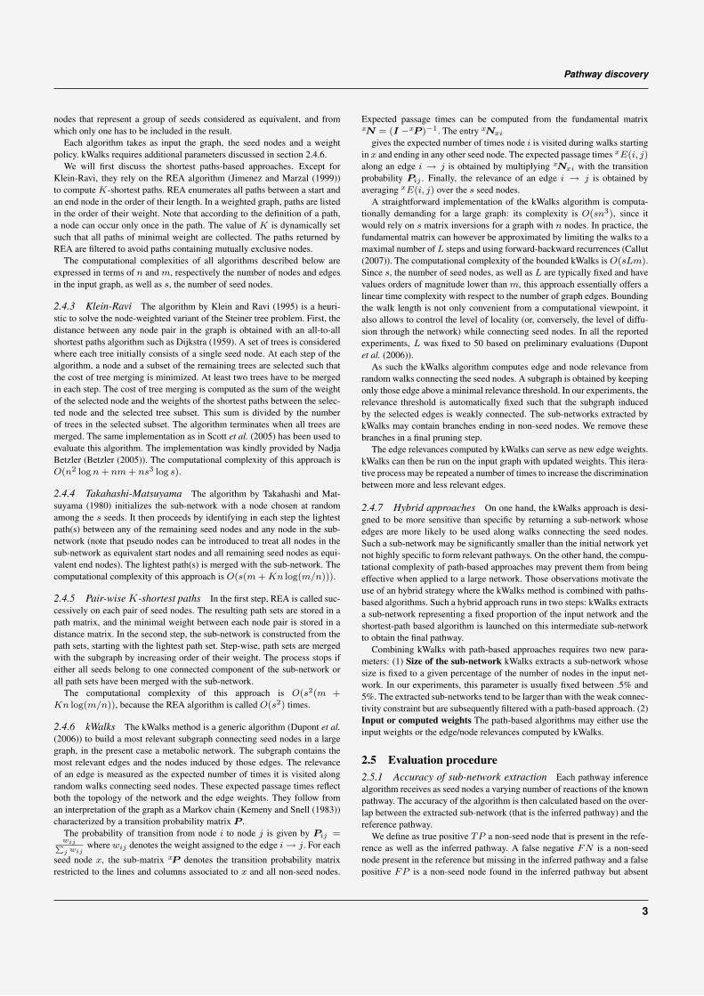
Pathway discovery
nodes that represent a group of seeds considered as equivalent, and fromwhich only one has to be included in the result.
Each algorithm takes as input the graph, the seed nodes and a weightpolicy. kWalks requires additional parameters discussed in section 2.4.6.
We will first discuss the shortest paths-based approaches. Except forKlein-Ravi, they rely on the REA algorithm (Jimenez and Marzal (1999))to compute K-shortest paths. REA enumerates all paths between a start andan end node in the order of their length. In a weighted graph, paths are listedin the order of their weight. Note that according to the definition of a path,a node can occur only once in the path. The value of K is dynamically setsuch that all paths of minimal weight are collected. The paths returned byREA are filtered to avoid paths containing mutually exclusive nodes.
The computational complexities of all algorithms described below areexpressed in terms of n and m, respectively the number of nodes and edgesin the input graph, as well as s, the number of seed nodes.
2.4.3 Klein-Ravi The algorithm by Klein and Ravi (1995) is a heuri-stic to solve the node-weighted variant of the Steiner tree problem. First, thedistance between any node pair in the graph is obtained with an all-to-allshortest paths algorithm such as Dijkstra (1959). A set of trees is consideredwhere each tree initially consists of a single seed node. At each step of thealgorithm, a node and a subset of the remaining trees are selected such thatthe cost of tree merging is minimized. At least two trees have to be mergedin each step. The cost of tree merging is computed as the sum of the weightof the selected node and the weights of the shortest paths between the selec-ted node and the selected tree subset. This sum is divided by the numberof trees in the selected subset. The algorithm terminates when all trees aremerged. The same implementation as in Scott et al. (2005) has been used toevaluate this algorithm. The implementation was kindly provided by NadjaBetzler (Betzler (2005)). The computational complexity of this approach isO(n2 log n + nm + ns3 log s).
2.4.4 Takahashi-Matsuyama The algorithm by Takahashi and Mat-suyama (1980) initializes the sub-network with a node chosen at randomamong the s seeds. It then proceeds by identifying in each step the lightestpath(s) between any of the remaining seed nodes and any node in the sub-network (note that pseudo nodes can be introduced to treat all nodes in thesub-network as equivalent start nodes and all remaining seed nodes as equi-valent end nodes). The lightest path(s) is merged with the sub-network. Thecomputational complexity of this approach is O(s(m + Kn log(m/n))).
2.4.5 Pair-wise K-shortest paths In the first step, REA is called suc-cessively on each pair of seed nodes. The resulting path sets are stored in apath matrix, and the minimal weight between each node pair is stored in adistance matrix. In the second step, the sub-network is constructed from thepath sets, starting with the lightest path set. Step-wise, path sets are mergedwith the subgraph by increasing order of their weight. The process stops ifeither all seeds belong to one connected component of the sub-network orall path sets have been merged with the sub-network.
The computational complexity of this approach is O(s2(m +
Kn log(m/n)), because the REA algorithm is called O(s2) times.
2.4.6 kWalks The kWalks method is a generic algorithm (Dupont et al.(2006)) to build a most relevant subgraph connecting seed nodes in a largegraph, in the present case a metabolic network. The subgraph contains themost relevant edges and the nodes induced by those edges. The relevanceof an edge is measured as the expected number of times it is visited alongrandom walks connecting seed nodes. These expected passage times reflectboth the topology of the network and the edge weights. They follow froman interpretation of the graph as a Markov chain (Kemeny and Snell (1983))characterized by a transition probability matrix P .
The probability of transition from node i to node j is given by Pij =wijPj wij
where wij denotes the weight assigned to the edge i → j. For each
seed node x, the sub-matrix xP denotes the transition probability matrixrestricted to the lines and columns associated to x and all non-seed nodes.
Expected passage times can be computed from the fundamental matrixxN = (I −xP )−1. The entry xNxi
gives the expected number of times node i is visited during walks startingin x and ending in any other seed node. The expected passage times xE(i, j)
along an edge i → j is obtained by multiplying xNxi with the transitionprobability Pij . Finally, the relevance of an edge i → j is obtained byaveraging xE(i, j) over the s seed nodes.
A straightforward implementation of the kWalks algorithm is computa-tionally demanding for a large graph: its complexity is O(sn3), since itwould rely on s matrix inversions for a graph with n nodes. In practice, thefundamental matrix can however be approximated by limiting the walks to amaximal number of L steps and using forward-backward recurrences (Callut(2007)). The computational complexity of the bounded kWalks is O(sLm).Since s, the number of seed nodes, as well as L are typically fixed and havevalues orders of magnitude lower than m, this approach essentially offers alinear time complexity with respect to the number of graph edges. Boundingthe walk length is not only convenient from a computational viewpoint, italso allows to control the level of locality (or, conversely, the level of diffu-sion through the network) while connecting seed nodes. In all the reportedexperiments, L was fixed to 50 based on preliminary evaluations (Dupontet al. (2006)).
As such the kWalks algorithm computes edge and node relevance fromrandom walks connecting the seed nodes. A subgraph is obtained by keepingonly those edge above a minimal relevance threshold. In our experiments, therelevance threshold is automatically fixed such that the subgraph inducedby the selected edges is weakly connected. The sub-networks extracted bykWalks may contain branches ending in non-seed nodes. We remove thesebranches in a final pruning step.
The edge relevances computed by kWalks can serve as new edge weights.kWalks can then be run on the input graph with updated weights. This itera-tive process may be repeated a number of times to increase the discriminationbetween more and less relevant edges.
2.4.7 Hybrid approaches On one hand, the kWalks approach is desi-gned to be more sensitive than specific by returning a sub-network whoseedges are more likely to be used along walks connecting the seed nodes.Such a sub-network may be significantly smaller than the initial network yetnot highly specific to form relevant pathways. On the other hand, the compu-tational complexity of path-based approaches may prevent them from beingeffective when applied to a large network. Those observations motivate theuse of an hybrid strategy where the kWalks method is combined with paths-based algorithms. Such a hybrid approach runs in two steps: kWalks extractsa sub-network representing a fixed proportion of the input network and theshortest-path based algorithm is launched on this intermediate sub-networkto obtain the final pathway.
Combining kWalks with path-based approaches requires two new para-meters: (1) Size of the sub-network kWalks extracts a sub-network whosesize is fixed to a given percentage of the number of nodes in the input net-work. In our experiments, this parameter is usually fixed between .5% and5%. The extracted sub-networks tend to be larger than with the weak connec-tivity constraint but are subsequently filtered with a path-based approach. (2)Input or computed weights The path-based algorithms may either use theinput weights or the edge/node relevances computed by kWalks.
2.5 Evaluation procedure2.5.1 Accuracy of sub-network extraction Each pathway inferencealgorithm receives as seed nodes a varying number of reactions of the knownpathway. The accuracy of the algorithm is then calculated based on the over-lap between the extracted sub-network (that is the inferred pathway) and thereference pathway.
We define as true positive TP a non-seed node that is present in the refe-rence as well as the inferred pathway. A false negative FN is a non-seednode present in the reference but missing in the inferred pathway and a falsepositive FP is a non-seed node found in the inferred pathway but absent
3

Faust et al
from the reference. The sensitivity Sn is defined as the ratio of correctlyinferred nodes versus all reference nodes:
Sn = TP(TP+FN)
, whereas the positive predictive value PPV givesthe ratio of correctly inferred nodes versus all inferred nodes: PPV =
TP(TP+FP )
. We calculate the accuracy as the geometric mean between
sensitivity and positive predictive value (Accg =√
Sn ∗ PPV ).
2.5.2 Experiments For each reference pathway, several inferences (i.e.sub-network extractions) are performed, with increasing seed node number,in order to test the impact of the seed node number on the accuracy of theresult. For each of the 71 reference pathways, we first select the terminalreactions as seeds, we infer a pathway that interconnects them, and we com-pare the nodes of the inferred pathways with those of the annotated pathway.Then, we progressively increase the number of seeds by adding reactionsrandomly selected from the reference pathway, and re-do the inference andevaluation, until all reactions of the pathway are selected as seeds. We defineas one experiment the set of all the pathway inferences performed for a givenparameter value combination (e.g. pair-wise K-shortest paths on directedMetaCyc network with compound degree weight). In total, we carried out108 such experiments.
3 RESULTS3.1 Global performance of pathway inference
algorithms3.1.1 Comparison of algorithms The average geometric accu-racy of a selected number of experiments is listed in Table 1. Thefull experiment table is available as supplementary Table ST1. Thestrategy resulting in the highest accuracy combines the Takahashi-Matsuyama algorithm with kWalks. The top experiments all involvea compound-weighted, directed MetaCyc network and, in case ofthe kWalks algorithm, an iteration number larger than one.
The performance of paths-based algorithms in the unweighted(unit weight), directed MetaCyc network is at most 53% whereaskWalks (without iteration) reaches an average accuracy of 62% inthe same conditions. Hence kWalks is able to assign edge rele-vances even without a dedicated weight policy for the problem athand, such as the compound degree weighting scheme for metabo-lic networks. All approaches however benefit from such a dedicatedweight policy.
In the pair-wise K-shortest paths/kWalks hybrid approach,kWalks is configured to extract 5% of the input network. If thispercentage is reduced to 0.5% (the optimum among 22 differentsub-network sizes tested), the average accuracy increases by 3%.Obviously, the size of the intermediate sub-network should not gobelow a certain limit as it should be large enough to contain ametabolic pathway.
Combining a paths-based algorithm with kWalks tends to reduceits runtime. Supplementary Figure SF1 compares run-times for all 7pathway inference algorithms.
3.1.2 Influence of parameter setting We measured the impactof alternative parameter values over a subset of the experimentsas measured by a paired signed Wilcoxon rank test (Supplemen-tary Table ST2). The parameter values having highest impacton the pathway inference accuracy are in this order: compounddegree weight and inflated compound degree weight outperform unitweight, directed network outperforms undirected network, kWalkssupersedes hybrid approaches and three kWalk iterations are betterthan a single run.
CARBPSYN-RXN (6.3.5.5)
Carbamoyl phosphate (CARBAMOYL-P)
ASPCARBTRANS-RXN (2.1.3.2)
N-Carbamoyl-L- aspartate (CARBAMYUL-L-ASPARTATE)
DIHYDROOROT-RXN (3.5.2.3)
(S)-Dihydroorotate (DI-H-OROTATE)
DIHYDROOROTOX-RXN (1.3.3.1)
Orotate (OROTATE)
OROPRIBTRANS-RXN (2.4.2.10)
Orotidine 5'-phosphate (OROTIDINE-5-PHOSPHATE)
OROTPDECARB-RXN (4.1.1.23)
UMP (UMP)
UMPKI-RXN (2.7.4.4)
UDP (UDP)
UDPKIN-RXN(not assigned)
CTPSYN-RXN (6.3.4.2)
UTP (UTP)
Carbamoyl phosphate (CARBAMOYL-P)
ASPCARBTRANS-RXN (2.1.3.2)
N-Carbamoyl-L- aspartate (CARBAMYUL-L-ASPARTATE)
DIHYDROOROT-RXN (3.5.2.3)
DIHYDROOROTOX-RXN (1.3.3.1)
OROPRIBTRANS-RXN (2.4.2.10)
Orotidine 5'-phosphate (OROTIDINE-5-PHOSPHATE)
OROTPDECARB-RXN (4.1.1.23)
UMP (UMP)
UMPKI-RXN (2.7.4.4)
CARBPSYN-RXN (6.3.5.5)
CTP (CTP)
CDPKIN-RXN (2.7.4.6)
CDPKIN-RXN (2.7.4.6)
CARBPSYN-RXN (6.3.5.5)
L-glutamine (GLN)
CTPSYN-RXN (6.3.4.2)
CDPKIN-RXN (2.7.4.6)
CTP (CTP)
dolichyl-phosphate (DOLICHOLP)
DOLICHYL-PHOSPHATASE-RXN (not assigned)
dolichol(DOLICHOL)
DOLICHOL-KINASE-RXN (2.7.1.108)
CDP (CDP)
2.7.8.15-RXN (2.7.8.15)
OROTATE-REDUCTASE-(NADH)-RXN (1.3.1.14)
OROTATE-REDUCTASE-(NADPH)-RXN (1.3.1.15)
DIHYDROOROTATE-DEHYDROGENASE-RXN (1.3.5.2)
(S)-Dihydroorotate (DI-H-OROTATE)
Orotate (OROTATE)
CDP (CDP)
bicarbonate (HCO3)A B C
Fig. 1. Pathway inference results for the pyrimidine ribonucleotides denovo biosynthesis pathway (MetaCyc identifier: PWY0-162) in E. coli. (A)Reference pathway. (B) Pathway inferred with two seeds in the compound-weighted, directed MetaCyc network. (C) Pathway inferred with four seedsin the same network. Ellipses represent compounds, rectangles reactions.Compounds and reactions are labeled with their MetaCyc identifiers in capi-tal letters, compounds in addition with their name and reactions with theirassociated EC number. Seed nodes have a blue border, true positive nodes agreen and false positives an orange border.
The superiority of the other two weighting schemes over unitweights is in agreement with previous results (Croes et al. (2005,2006)), which show that weighting the metabolic network avoidsirrelevant hub compounds. It is also no surprise that the directedMetaCyc network yields higher accuracies than the undirected one,because the directed network prevents the traversal from substrateto substrate or from product to product.
It might seem surprizing that when all experiments are takentogether, kWalks alone outperforms the pair-wise K-shortest pathshybrid, whereas the 5 top-raking approaches rely either on hybridapproach or path finding alone. The reason is that kWalks, as explai-ned above, deals well with the unit weight policy, whereas thehybrid only performs well if it can either use weights generatedby kWalks or by a weight policy that penalizes hub compounds.However, if run with optimal parameter values, both algorithms areamong the top experiments (see Table 1). Iterating kWalks impro-ves the accuracy, as it increases the difference between relevant andirrelevant edges.
3.2 Study casesAll study cases were inferred with the hybrid algorithm combi-ning Takahashi-Matsuyama and kWalks in the directed, compound-weighted MetaCyc network.
Since we cannot infer reaction directions due to the way weconstructed the MetaCyc network, inferred pathways are displayed
4

Pathway discovery
oxaloacetate(OXALACETIC_ACID)
ASPAMINOTRANS-RXN (2.6.1.1)
L-aspartate (L-ASPARTATE)
ASPARTATEKIN-RXN (2.7.2.4)
L-aspartyl-4-phosphate (L-BETA-ASPARTYL-P)
L-aspartate-semialdehyde (L-BETA-ASPARTYL-P)
ASPARTATE-SEMIALDEHYDE-DEHYDROGENASE-RXN (1.2.1.11)
homoserine (HOMO-SER)
HOMOSERDEHYDROG-RXN (1.1.1.3)
HOMOSERKIN-RXN (2.7.1.39)
O-phospho-L-homoserine (O-PHOSPHO-L-HOMOSERINE)
THRESYN-RXN (4.2.3.1)
L-threonine (THR)
HOMSUCTRAN-RXN (2.3.1.46)
O-succinyl-L-homoserine (O-SUCCINYL-L-HOMOSERINE)
O-SUCCHOMOSERLYASE-RXN (2.5.1.48)
L-cystathionine (L-CYSTATHIONINE)
CYSTATHIONINE-BETA-LYASE-RXN (4.4.1.8)
L-homocysteine (HOMO-CYS)
L-methionine (MET)
HOMOCYSMETB12-RXN (2.1.1.13)
HOMOCYSMET-RXN (2.1.1.14)
DIHYDRODIPICSYN-RXN (4.2.1.52)
L-2,3-dihydrodipicolinate (2-3-DIHYDRODIPICOLINATE)
DIHYDROPICRED-RXN (1.3.1.26)
tetrahydrodipicolinate (DELTA1-PIPERIDEINE-2-6-DICARBOXYLATE)
TETHYDPICSUCC-RXN (2.3.1.117)
N-succinyl-2-amino-6-ketopimelate (N-SUCCINYL-2-AMINO-6-KETOPIMELATE)
SUCCINYLDIAMINOPIMTRANS-RXN (2.6.1.17)
N-succinyl-L,L-2,6-diaminopimelate(N-SUCCINYLLL-2-6-DIAMINOPIMELATE)
SUCCDIAMINOPIMDESUCC-RXN (3.5.1.18)
L,L-diaminopimelate (LL-DIAMINOPIMELATE)
DIAMINOPIMEPIM-RXN (5.1.1.7)
meso-diaminopimelate(MESO-DIAMINOPIMELATE)
DIAMINOPIMDECARB-RXN (4.1.1.20)
L-lysine (LYS)
ASPAMINOTRANS-RXN (2.6.1.1)
L-aspartate (L-ASPARTATE)
ASPARTATEKIN-RXN (2.7.2.4)
L-aspartyl-4-phosphate (L-BETA-ASPARTYL-P)
L-aspartate-semialdehyde (L-BETA-ASPARTYL-P)
ASPARTATE-SEMIALDEHYDE-DEHYDROGENASE-RXN (1.2.1.11)
homoserine (HOMO-SER)
HOMOSERDEHYDROG-RXN (1.1.1.3)
HOMOSERKIN-RXN (2.7.1.39)
O-phospho-L-homoserine (O-PHOSPHO-L-HOMOSERINE)
THRESYN-RXN (4.2.3.1)
Cystathionine (L-CYSTATHIONINE)
CYSTATHIONINE-BETA-LYASE-RXN (4.4.1.8)
L-homocysteine (HOMO-CYS)
HOMOCYSMETB12-RXN (2.1.1.13)
HOMOCYSMET-RXN (2.1.1.14)
DIHYDRODIPICSYN-RXN (4.2.1.52)
L-2,3-dihydrodipicolinate (2-3-DIHYDRODIPICOLINATE)
DIHYDROPICRED-RXN (1.3.1.26)
tetrahydrodipicolinate (DELTA1-PIPERIDEINE-2-6-DICARBOXYLATE)
RXN-4821 (3.5.99.-)
L-2-Amino-6-oxoheptanedioate (L-ALPHA-AMINO-EPSILON-KETO-PIMELATE)
DIAMINOPIMELATE-DEHYDROGENASE-RXN (1.4.1.16)
meso-2,6-Diaminoheptanedioate (MESO-DIAMINOPIMELATE)
DIAMINOPIMDECARB-RXN (4.1.1.20)
CYSPH-RXN (2.5.1.-)
A B
CYSTATHIONINE-BETA-SYNTHASE-RXN (4.2.1.22)
ASPAMINOTRANS-RXN (2.6.1.1)
L-aspartate (L-ASPARTATE)
ASPARTATEKIN-RXN (2.7.2.4)
L-aspartyl-4-phosphate (L-BETA-ASPARTYL-P)
L-aspartate-semialdehyde (L-BETA-ASPARTYL-P)
ASPARTATE-SEMIALDEHYDE-DEHYDROGENASE-RXN (1.2.1.11)
HOMOSERDEHYDROG-RXN (1.1.1.3)
DIHYDRODIPICSYN-RXN (4.2.1.52)
L-2,3-dihydrodipicolinate (2-3-DIHYDRODIPICOLINATE)
DIHYDROPICRED-RXN (1.3.1.26)
tetrahydrodipicolinate (DELTA1-PIPERIDEINE-2-6-DICARBOXYLATE)
TETHYDPICSUCC-RXN (2.3.1.117)
N-succinyl-2-amino-6-ketopimelate (N-SUCCINYL-2-AMINO-6-KETOPIMELATE)
SUCCINYLDIAMINOPIMTRANS-RXN (2.6.1.17)
N-succinyl-L,L-2,6-diaminopimelate(N-SUCCINYLLL-2-6-DIAMINOPIMELATE)
SUCCDIAMINOPIMDESUCC-RXN (3.5.1.18)
L,L-diaminopimelate (LL-DIAMINOPIMELATE)
DIAMINOPIMEPIM-RXN (5.1.1.7)
meso-2,6-Diaminopimelate (MESO-DIAMINOPIMELATE)
DIAMINOPIMDECARB-RXN (4.1.1.20)
C
O-Acetyl-L-homoserine (CPD-667)
ACETYLHOMOSER-CYS-RXN (2.5.1.49)
HOMOSERINE-O-ACETYLTRANSFERASE-RXN (2.3.1.31)
homoserine (HOMO-SER)
HOMOSERKIN-RXN (2.7.1.39)
O-phospho-L-homoserine (O-PHOSPHO-L-HOMOSERINE)
THRESYN-RXN (4.2.3.1)
Cystathionine (L-CYSTATHIONINE)
CYSTATHIONINE-BETA-LYASE-RXN (4.4.1.8)
L-homocysteine (HOMO-CYS)
HOMOCYSMETB12-RXN (2.1.1.13)
HOMOCYSMET-RXN (2.1.1.14)
CYSPH-RXN (2.5.1.-)
CYSTATHIONINE-BETA-SYNTHASE-RXN (4.2.1.22)
ACETYLHOMOSER-CYS-RXN (2.5.1.49)
HOMOSERINE-O-ACETYLTRANSFERASE-RXN (2.3.1.31)
O-Acetyl-L-homoserine (CPD-667)
Fig. 2. Pathway inference results for the superpathway of lysine, threonine and methionine biosynthesis I (MetaCyc identifier: P4-PWY) in E. coli. (A) Refe-rence pathway. (B) Pathway inferred with the five terminal reactions as seeds in the compound-weighted, directed MetaCyc network and Figure. (C) Pathwayinferred with the terminal and two additional intermediate reactions in the same network. Ellipses represent compounds, rectangles reactions. Compounds andreactions are labeled with their MetaCyc identifiers in capital letters, compounds in addition with their name and reactions with their associated EC number.Seed nodes have a blue border, true positive nodes a green and false positives an orange border.
Table 1. Selected set of experiments, their conditions and results. Each table row represents one experiment. Each experiment was performed on71 reference pathways with varying seed reaction number, comprising 406 launches of the tested pathway inference algorithm for the indicatedconditions. Abbreviations: PPV = positive predictive value, acc.g = geometric accuracy
Algorithm kWalks Size of Weighting Directed kWalks Mean Sn Mean PPV Meaniteration sub-network scheme graph weights in % in % acc.gnumber extracted by re-used in %
kWalks in %
Takahashi-Matusyama/kWalks 1 5 Compound degree TRUE FALSE 77.13 77.97 76.81Takahashi-Matsuyama 0 - Compound degree TRUE - 75.90 77.25 75.83
pair-wise K-shortest paths/kWalks 1 0.5 Compound degree TRUE FALSE 68.89 78.90 71.79pair-wise K-shortest paths/kWalks 6 5 Compound degree TRUE FALSE 70.20 69.10 68.22
pair-wise K-shortest paths 0 - Compound degree TRUE - 69.95 68.73 68.03kWalks 3 - Compound degree TRUE - 71.49 68.54 67.96kWalks 6 - Inflated compound TRUE - 71.06 68.62 67.90
degreepair-wise K-shortest paths/kWalks 3 5 Compound degree TRUE FALSE 69.19 69.37 67.86
Klein-Ravi/kWalks 1 5 Compound degree FALSE FALSE 63.21 68.03 64.10kWalks 3 - Unit TRUE - 61.40 71.33 64.30kWalks 6 - Unit TRUE - 60.00 71.75 63.53
Klein-Ravi 0 - Compound degree FALSE - 62.55 66.27 63.05kWalks 1 - Unit TRUE - 62.13 65.93 61.83
pair-wise K-shortest paths/kWalks 1 5 Unit TRUE TRUE 46.91 69.38 55.32Takahashi-Matsuyama 0 - Unit TRUE - 60.02 53.83 52.74
pair-wise K-shortest paths 0 - Unit TRUE - 71.37 35.87 42.86
as undirected graphs. The annotated pathways have been obtainedfrom EcoCyc version 13.1 (Keseler et al. (2009)).
3.2.1 De novo synthesis of pyrimidine ribonucleotides in Esche-richia coli The de novo synthesis of pyrimidine ribonucleotides
pathway in E. coli produces CDP from L-glutamine in a series of 10subsequent reaction steps (Figure 1A).
Two-end path finding results in a metabolic pathway that bypassesa large segment of the annotated pathway by taking a shortcut viaL-glutamine (Figure 1B). Consequently, the geometric accuracy islow (28%).
5
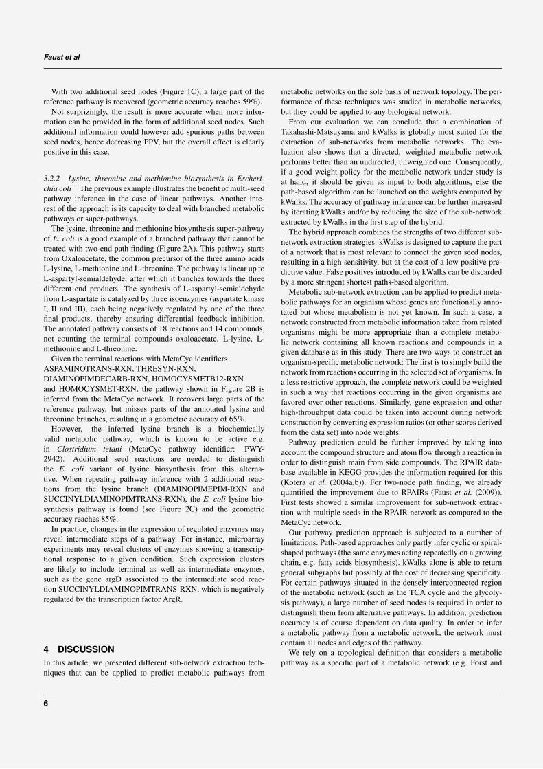
Faust et al
With two additional seed nodes (Figure 1C), a large part of thereference pathway is recovered (geometric accuracy reaches 59%).
Not surprizingly, the result is more accurate when more infor-mation can be provided in the form of additional seed nodes. Suchadditional information could however add spurious paths betweenseed nodes, hence decreasing PPV, but the overall effect is clearlypositive in this case.
3.2.2 Lysine, threonine and methionine biosynthesis in Escheri-chia coli The previous example illustrates the benefit of multi-seedpathway inference in the case of linear pathways. Another inte-rest of the approach is its capacity to deal with branched metabolicpathways or super-pathways.
The lysine, threonine and methionine biosynthesis super-pathwayof E. coli is a good example of a branched pathway that cannot betreated with two-end path finding (Figure 2A). This pathway startsfrom Oxaloacetate, the common precursor of the three amino acidsL-lysine, L-methionine and L-threonine. The pathway is linear up toL-aspartyl-semialdehyde, after which it banches towards the threedifferent end products. The synthesis of L-aspartyl-semialdehydefrom L-aspartate is catalyzed by three isoenzymes (aspartate kinaseI, II and III), each being negatively regulated by one of the threefinal products, thereby ensuring differential feedback inhibition.The annotated pathway consists of 18 reactions and 14 compounds,not counting the terminal compounds oxaloacetate, L-lysine, L-methionine and L-threonine.
Given the terminal reactions with MetaCyc identifiersASPAMINOTRANS-RXN, THRESYN-RXN,DIAMINOPIMDECARB-RXN, HOMOCYSMETB12-RXNand HOMOCYSMET-RXN, the pathway shown in Figure 2B isinferred from the MetaCyc network. It recovers large parts of thereference pathway, but misses parts of the annotated lysine andthreonine branches, resulting in a geometric accuracy of 65%.
However, the inferred lysine branch is a biochemicallyvalid metabolic pathway, which is known to be active e.g.in Clostridium tetani (MetaCyc pathway identifier: PWY-2942). Additional seed reactions are needed to distinguishthe E. coli variant of lysine biosynthesis from this alterna-tive. When repeating pathway inference with 2 additional reac-tions from the lysine branch (DIAMINOPIMEPIM-RXN andSUCCINYLDIAMINOPIMTRANS-RXN), the E. coli lysine bio-synthesis pathway is found (see Figure 2C) and the geometricaccuracy reaches 85%.
In practice, changes in the expression of regulated enzymes mayreveal intermediate steps of a pathway. For instance, microarrayexperiments may reveal clusters of enzymes showing a transcrip-tional response to a given condition. Such expression clustersare likely to include terminal as well as intermediate enzymes,such as the gene argD associated to the intermediate seed reac-tion SUCCINYLDIAMINOPIMTRANS-RXN, which is negativelyregulated by the transcription factor ArgR.
4 DISCUSSIONIn this article, we presented different sub-network extraction tech-niques that can be applied to predict metabolic pathways from
metabolic networks on the sole basis of network topology. The per-formance of these techniques was studied in metabolic networks,but they could be applied to any biological network.
From our evaluation we can conclude that a combination ofTakahashi-Matsuyama and kWalks is globally most suited for theextraction of sub-networks from metabolic networks. The eva-luation also shows that a directed, weighted metabolic networkperforms better than an undirected, unweighted one. Consequently,if a good weight policy for the metabolic network under study isat hand, it should be given as input to both algorithms, else thepath-based algorithm can be launched on the weights computed bykWalks. The accuracy of pathway inference can be further increasedby iterating kWalks and/or by reducing the size of the sub-networkextracted by kWalks in the first step of the hybrid.
The hybrid approach combines the strengths of two different sub-network extraction strategies: kWalks is designed to capture the partof a network that is most relevant to connect the given seed nodes,resulting in a high sensitivity, but at the cost of a low positive pre-dictive value. False positives introduced by kWalks can be discardedby a more stringent shortest paths-based algorithm.
Metabolic sub-network extraction can be applied to predict meta-bolic pathways for an organism whose genes are functionally anno-tated but whose metabolism is not yet known. In such a case, anetwork constructed from metabolic information taken from relatedorganisms might be more appropriate than a complete metabo-lic network containing all known reactions and compounds in agiven database as in this study. There are two ways to construct anorganism-specific metabolic network: The first is to simply build thenetwork from reactions occurring in the selected set of organisms. Ina less restrictive approach, the complete network could be weightedin such a way that reactions occurring in the given organisms arefavored over other reactions. Similarly, gene expression and otherhigh-throughput data could be taken into account during networkconstruction by converting expression ratios (or other scores derivedfrom the data set) into node weights.
Pathway prediction could be further improved by taking intoaccount the compound structure and atom flow through a reaction inorder to distinguish main from side compounds. The RPAIR data-base available in KEGG provides the information required for this(Kotera et al. (2004a,b)). For two-node path finding, we alreadyquantified the improvement due to RPAIRs (Faust et al. (2009)).First tests showed a similar improvement for sub-network extrac-tion with multiple seeds in the RPAIR network as compared to theMetaCyc network.
Our pathway prediction approach is subjected to a number oflimitations. Path-based approaches only partly infer cyclic or spiral-shaped pathways (the same enzymes acting repeatedly on a growingchain, e.g. fatty acids biosynthesis). kWalks alone is able to returngeneral subgraphs but possibly at the cost of decreasing specificity.For certain pathways situated in the densely interconnected regionof the metabolic network (such as the TCA cycle and the glycoly-sis pathway), a large number of seed nodes is required in order todistinguish them from alternative pathways. In addition, predictionaccuracy is of course dependent on data quality. In order to infera metabolic pathway from a metabolic network, the network mustcontain all nodes and edges of the pathway.
We rely on a topological definition that considers a metabolicpathway as a specific part of a metabolic network (e.g. Forst and
6
Pathway discovery
Schulten (1999)). This definition covers all classical pathways des-cribed in the literature, but also includes pathways that are notbiochemically valid in contrast to stoichiometry-centered definiti-ons (e.g. elementary modes, extreme pathways, see Schilling et al.(2000)). A revised definition of metabolic pathway could influenceand possibly improve pathway prediction tools, but this objective isbeyond the scope of the present article.
In a future application, we will apply the techniques evaluatedin this article to gene expression data as well as operons, fusiongenes and other data sets featuring genes assumed to be functionallyrelated. This requires testing different scoring schemes in order tomeasure the quality of the predicted pathway.
The pathway inference algorithms were added to NeAT (Broheeet al. (2008)) at http://rsat.ulb.ac.be/neat/. A generickWalks implementation is freely available atwww.ucl.ac.be/mlg/index.php?page=Softwares.
ACKNOWLEDGEMENTWe would like to thank the former aMAZE team for their graphlibrary and Nadja Betzler for providing us with her implementationof the Klein-Ravi algorithm. We acknowledge Jean-Noel Monetteand Pierre Schaus from the INGI team at UCL for making publiclyavailable their improvement of the REA code.
Funding: KF is supported by Actions de Recherches Concerteesde la Communaute Francaise de Belgique (ARC grant number04/09-307). The BiGRe laboratory is a member of the BioSapiensNetwork of Excellence funded under the sixth Framework programof the European Communities (LSHG-CT-2003-503265). The workwas supported by the Belgian Program on Interuniversity AttractionPoles, initiated by the Belgian Federal Science Policy Office, projectP6/25 (BioMaGNet).
REFERENCESAntonov, A., Dietmann, S., and Mewes, H. W. (2008). KEGG spider: interpretation
of genomics data in the context of the global gene metabolic network. GenomeBiology, 9.
Antonov, A., Dietmann, S., Wong, P., and Mewes, H. W. (2009). TICL - a webtool for network-based interpretation of compound lists inferred by high-throughputmetabolomics. FEBS Journal, 276, 2084–2094.
Arita, M. (2000). Metabolic reconstruction using shortest paths. Simulation Practiceand Theory, 8, 109–125.
Betzler, N. (2005). Steiner Tree Problems in the Analysis of Biological Networks.Master’s thesis, Wilhelm-Schickard-Institut fur Informatik, Universitat Tubingen,Germany.
Blum, T. and Kohlbacher, O. (2008). MetaRoute: fast search for relevant metabo-lic routes for interactive network navigation and visualization. Bioinformatics, 24,2108–2109.
Brohee, S., Faust, K., Lima-Mendez, G., Sand, O., Janky, R., Vanderstocken, G.,Deville, Y., and van Helden, J. (2008). NeAT: a toolbox for the analysis of biologicalnetworks, clusters, classes and pathways. Nucleic Acids Research, 36, W444–W451.
Callut, J. (2007). First Passage Times Dynamics in Markov Models with Applicati-ons to HMM Induction, Sequence Classication, and Graph Mining. Ph.D. thesis,Universite catholique de Louvain.
Caspi, R., Foerster, H., Fulcher, C. A., Kaipa, P., Krummenacker, M., Latendresse,M., Paley, S., Rhee, S. Y., Shearer, A. G., Tissier, C., Walk, T. C., Zhang, P., andKarp, P. D. (2008). The MetaCyc Database of metabolic pathways and enzymesand the BioCyc collection of Pathway/Genome Databases. Nucleic Acids Res, 36,D623–D631.
Croes, D., Couche, F., Wodak, S., and van Helden, J. (2005). Metabolic PathFinding:inferring relevant pathways in biochemical networks. Nucleic Acids Research, 33,W326–W330.
Croes, D., Couche, F., Wodak, S., and van Helden, J. (2006). Inferring meaningfulpathways in weighted metabolic networks. J. Mol. Biol., 356, 222–236.
Dijkstra, E. W. (1959). A note on two problems in connexion with graphs. NumerischeMathematik, 1, 269–271.
Dittrich, M. T., Klau, G. W., Rosenwald, A., Dandekar, T., and Muller, T. (2008).Identifying functional modules in protein-protein interaction networks: an integratedexact approach. Bioinformatics, 24, i223–i231.
Duin, C. W., Volgenant, A., and Voß, S. (2004). Solving group Steiner problems asSteiner problems. European Journal of Operational Research, 154, 323–329.
Dupont, P., Callut, J., Dooms, G., Monette, J.-N., and Deville, Y. (2006). Relevantsubgraph extraction from random walks in a graph. Research Report UCL/FSA/INGIRR 2006-07.
Ellis, L., Gao, J., Fenner, K., and Wackett, L. (2008). The University of Minnesotapathway prediction system: predicting metabolic logic. Nucleic Acids Research, 36,W427–W432.
Faust, K., Croes, D., and van Helden, J. (2009). Metabolic path finding using RPAIRannotation. Journal of Molecular Biology, 388, 390–414.
Forst, C. and Schulten, K. (1999). Evolution of metabolisms: A new method forthe comparison of metabolic pathways using genomics information. Journal ofComputational Biology, 6, 343–360.
Hwang, F., Richards, D., and Winter, P. (1992). The Steiner Tree Problem, volume 53of Annals of Discrete Mathematics. North-Holland, Amsterdam, Netherlands.
Ideker, T., Ozier, O., Schwikowski, B., and Siegel, A. F. (2002). Discovering regulatoryand signalling circuits in molecular interaction networks. Bioinformatics, 18, S233–S240.
Jimenez, V. and Marzal, A. (1999). Computing the k shortest paths: a new algorithmand an experimental comparison. Proc. 3rd Int. Worksh. Algorithm Engineering(WAE 1999), 1668, 15–29.
Karp, R. (1972). Reducibility among combinatorial problems, pages 85–103. Com-plexity of Computer Computations. R. E. Miller and J. W. Thatcher, PlenumPress.
Kemeny, J. G. and Snell, J. L. (1983). Finite Markov Chains. Springer-Verlag.Keseler, I. M., Bonavides-Martınez, C., Collado-Vides, J., Gama-Castro, S., Gunsa-
lus, R. P., Johnson, D. A., Krummenacker, M., Nolan, L. M., Paley, S., Paulsen,I. T., Peralta-Gil, M., Santos-Zavaleta, A., Shearer, A. G., and Karp, P. D. (2009).EcoCyc: a comprehensive view of escherichia coli biology. Nucleic Acids Res, 37,D464–D470.
Klein, P. and Ravi, R. (1995). A nearly best-possible approximation algorithm fornode-weighted Steiner trees. Journal of Algorithms, 19, 104–115.
Kotera, M., Okuno, Y., Hattori, M., Goto, S., and Kanehisa, M. (2004a). Computationalassignment of the EC numbers for genomic-scale analysis of enzymatic reactions. JAm Chem Soc., 126, 16487–16498.
Kotera, M., Hattori, M., Oh, M.-A., Yamamoto, R., Komeno, T., Yabuzaki, J., Tono-mura, K., Goto, S., and Kanehisa, M. (2004b). RPAIR: a reactant-pair databaserepresenting chemical changes in enzymatic reactions. Genome Informatics, 15,P062.
Krieger, C. J., Zhang, P., Mueller, L. A., Wang, A., Paley, S., Arnaud, M., Pick, J.,Rhee, S. Y., and Palsson, B. Ø. (2004). MetaCyc: a multiorganism database ofmetabolic pathways and enzymes. Nucleic Acids Res, 32, D438–D442.
McShan, D., Rao, S., and Shah, I. (2003). PathMiner: predicting metabolic pathwaysby heuristic search. Bioinformatics, 19, 1692–1698.
Noirel, J., Ow, S. Y., Sanguinetti, G., Jaramillo, A., and Wright, P. C. (2008). Automa-ted extraction of meaningful pathways from quantitative proteomics data. Briefingsin Functional Genomics and Proteomics, 7, 136–146.
Rahman, S., Advani, P., Schunk, R., Schrader, R., and Schomburg, D. (2004). Metabo-lic pathway analysis web service (Pathway Hunter Tool at CUBIC). Bioinformatics,21, 1189–1193.
Rajagopalan, D. and Agarwal, P. (2005). Inferring pathways from gene lists using aliterature-derived network of biological relationships. Bioinformatics, 21(5), 788–793.
Schilling, C., Letscher, D., and Palsson, B. (2000). Theory for the systemic definition ofmetabolic pathways and their use in interpreting metabolic function from a pathway-oriented perspective. Journal of Theoretical Biology, 203, 229–248.
Scott, M. S., Perkins, T., Bunnell, S., Pepin, F., Thomas, D. Y., and Hallett, M. (2005).Identifying regulatory subnetworks for a set of genes. Mol Cell Proteomics, 4(5),683–692.
Takahashi, H. and Matsuyama, A. (1980). An approximate solution for the Steinerproblem in graphs. Math. Japonica, 24, 573–577.
Zien, A., Kuffner, R., Zimmer, R., and Lengauer, T. (2000). Analysis of gene expres-sion data with pathway scores. In Proceedings of the International Conference ofIntelligent Systems Molecular Biology, pages 407–417.
7

4 Application of pathway discovery
to a gene expression data set
from S. cerevisiae
The previous chapters (2 and 3) presented the development and evaluation of two-end andmultiple-end pathway prediction approaches. In this chapter, multiple-end pathway predictionis applied to a microarray study conducted on S. cerevisiae.
4.1 Biological background
S. cerevisiae is capable to grow on a variety of nitrogenous compounds as sole nitrogen source,among others ammonium and urea. The nitrogen required in anabolic reactions is providedby glutamine and glutamate, the major nitrogen donors in yeast, which are either importedfrom the environment or derived from catabolic reactions of other nitrogenous compounds.Thus, yeast cells can survive on a single nitrogen source by metabolizing it directly and/or bydegrading it to ammonium, glutamate or both. From ammonium and glutamate, glutamine canbe synthesized, which can then serve together with glutamate as nitrogen donor for anabolicreactions.
4.2 Gene expression data set
In order to elucidate the response of yeast cells to the presence of alternative nitrogen sources,Godard et al. performed a gene expression study, which measured the effects of 21 differentnitrogen sources on the gene expression in S. cerevisiae [63].
In the original article, the experiment was conducted and the resulting data processed in thefollowing way:
1. Yeast cells were grown on each of the 21 compounds as sole nitrogen source and theexpression of all 5,690 yeast genes was quantified.
2. Gene expression ratios were calculated for each of the 20 nitrogen sources as the log-ratio between gene expression given the nitrogen source and gene expression given ureaas nitrogen source (considered as reference).
3. Genes with a P-value of differential expression below 1/5,690 were discarded to correctfor multiple testing. The P-value was calculated with the SAM method [160].
92

4. A matrix of expression ratios was obtained consisting of 20 columns (for the 20 nitrogensources) and 390 rows (all genes significantly differentially expressed for at least onenitrogen source and with expression ratios obtained for at least 13 nitrogen sources).
5. Hierarchical clustering of this matrix (see Figure 4.1) revealed two main groups, wheregroup A contains good nitrogen sources (which allow generation times ∼2h) and groupB bad nitrogen sources (which support only slow growth). The 20 sources and theirgroups are listed in Table 4.1, where group C refers to all nitrogen sources that neitherclustered with group A nor with group B nitrogen sources.
Figure 4.1: Gene expression ratio matrix re-arranged according to the outcome of the "completelinkage" cluster algorithm. The distances were calculated as the average dot product between geneexpression profiles. Reproduction of Figure 2A from Godard et al., [63].
93

Table 4.1: Groups of nitrogen sources: A = good sources, B = bad sources, C = all other sources.Nitrogen source Group(Abbreviation)asparagine (asn) Aglutamine (gln) Aserine (ser) Aammonium (amm) Aaspartate (asp) Aalanine (ala) Aarginine (arg) Aglutamate (glt) Avaline (val) Cphenylalanine (phe) Cornithine (orn) Cproline (pro) CGABA (gab) Ccitrulline (cit) Cleucine (leu) Bisoleucine (ile) Bmethionine (met) Bthreonine (thr) Btryptophan (trp) Btyrosine (tyr) BThe reference nitrogen source urea is statedin [63] to belong to the poor nitrogen sources.
94

4.3 Data processing
Given the results of Godard’s experiments, I did the following analysis steps for each nitrogensource separately:
1. The distribution of gene expression ratios (i.e. the ratio between the gene expressionvalue in the presence of the investigated nitrogen source with respect to urea) was plottedto check whether it approximates a Gauss distribution (see Figure 4.2). This was the casefor all nitrogen sources.
2. Mean and standard deviation of the gene expression ratio distribution were robustlyestimated with the median and interquartile range (IQR) using an R script written byJacques van Helden.
3. The gene expression ratios were standardized as follows: zi, j = Mi, j−median(M j)iqr(M j)/k , where
Mi, j is the expression ratio of gene i for nitrogen source j; M j denotes the vector of allexpression ratios obtained for nitrogen source j (with 5,690 entries); k is a normalizingconstant to estimate the standard deviation from the iqr 1. The effect of the standard-ization is to convert a normal distribution N (µ,σ) into a standard normal distributionN (0,1), i.e. a distribution centered on 0 and with a unit standard deviation. The stan-dardized expression ratios are referred to as z-scores.
4. Each z-score zi, j is then converted into a nominal P-value by calculating the right tailof a normal distribution. The P-value Pvali, j is an estimation of the probability for agiven gene (i) to reach by chance a given z-score (zi, j) in a given microarray experiment( j). It is interpreted as the risk of false positive, i.e. the fact to erroneously consider assignificant the expression ratio of a given gene i on a given microarray j.
5. For a large number of statistical tests (5,690 in this case), it is very likely that a testrejects the null hypothesis (i.e. no differential expression of a gene) by chance. Forthis reason, P-values are corrected for multiple testing using the Bonferroni correction,which converts P-values into E-values by multiplying each P-value with the number oftests performed, i.e. with the number of genes (g = 5,690):
Eval = Pval ·g
6. Finally, groups of up- and down-regulated genes are obtained by setting a thresholdon the E-value. This is done separately for genes with positive z-scores (up-regulated)and negative z-scores (down-regulated), so that two gene groups are obtained for eachnitrogen source. The E-value threshold was set to one, to restrict the number of genesfalsely regarded as differentially expressed to one by nitrogen source. Since only asub-set of all genes (namely the enzyme-coding genes) is considered for analysis, thisthreshold is sufficiently stringent to avoid false positives in most cases while preventinga loss of relevant enzymes.
1k = qnorm(0.75)−qnorm(0.25) = 1.349
95

After these processing steps, 20 up- and 20 down-regulated genes groups were obtained.Table 4.2 summarizes the number of enzymes and their associated reactions and main reac-
tant pairs for each gene group.
Table 4.2: Numbers of genes, enzymes and reactions associated to each gene group for an E-valuethreshold set to one
Gene Number of Number of Number of EC Number of Number of maincluster genes of enzymes numbers reactions reactant pairsala_up 82 26 24 121 116
ala_down 84 24 25 88 71amm_up 54 19 17 86 75
amm_down 66 21 22 88 78arg_up 37 16 14 86 76
arg_down 66 19 21 53 56asn_up 50 19 17 97 101
asn_down 95 33 34 106 92asp_up 69 25 23 160 145
asp_down 48 12 14 28 24cit_up 61 25 23 92 90
cit_down 27 6 6 31 25gab_up 40 19 16 71 57
gab_down 71 19 22 79 58gln_up 57 15 14 65 72
gln_down 69 26 28 80 78glt_up 56 18 15 58 49
glt_down 64 24 25 109 94ile_up 69 21 20 79 85
ile_down 23 6 6 34 24leu_up 103 39 34 106 104
leu_down 26 9 8 17 16met_up 119 49 45 179 200
met_down 33 9 10 41 33orn_up 66 22 20 116 126
orn_down 39 14 14 57 52phe_up 103 29 27 166 173
phe_down 24 4 4 10 13pro_up 71 20 18 106 106
pro_down 32 9 11 18 17ser_up 47 17 16 69 70
ser_down 59 17 18 65 73thr_up 98 27 27 50 62
thr_down 16 2 2 2 3
96

Table 4.2: Numbers of genes, enzymes and reactions associated to each gene group for an E-valuethreshold set to one
Gene Number of Number of Number of EC Number of Number of maincluster genes of enzymes numbers reactions reactant pairstrp_up 121 47 38 136 138
trp_down 21 3 3 21 20tyr_up 96 35 31 138 136
tyr_down 14 4 4 24 24val_up 73 24 22 88 89
val_down 27 9 9 46 51
−2 0 2 4
0001
002003
00 4
Distribution of expression ratios for GABA versus urea, fitted by Gauss distribution
gene expression ratios
ycneuqerf
observedfitted
Figure 4.2: Distribution of gene expression ratios for GABA as sole nitrogen source with respect tourea. The blue line represents the Gauss distribution whose mean is estimated by the median of the geneexpression ratios and whose standard deviation is estimated by their interquartile range. The estimatedGauss distribution describes well the gene expression ratio distribution. The Figure was generated withan R script written by Jacques van Helden.
97
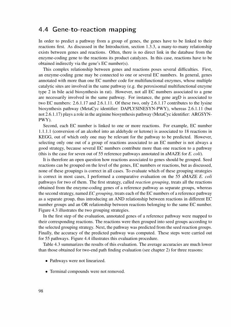
4.4 Gene-to-reaction mapping
In order to predict a pathway from a group of genes, the genes have to be linked to theirreactions first. As discussed in the Introduction, section 1.3.3, a many-to-many relationshipexists between genes and reactions. Often, there is no direct link in the database from theenzyme-coding gene to the reactions its product catalyzes. In this case, reactions have to beobtained indirectly via the gene’s EC number(s).
This complex relationship between genes and reactions poses several difficulties. First,an enzyme-coding gene may be connected to one or several EC numbers. In general, genesannotated with more than one EC number code for multifunctional enzymes, whose multiplecatalytic sites are involved in the same pathway (e.g. the peroxisomal multifunctional enzymetype 2 in bile acid biosynthesis in rat). However, not all EC numbers associated to a geneare necessarily involved in the same pathway. For instance, the gene argD is associated totwo EC numbers: 2.6.1.17 and 2.6.1.11. Of these two, only 2.6.1.17 contributes to the lysinebiosynthesis pathway (MetaCyc identifier: DAPLYSINESYN-PWY), whereas 2.6.1.11 (butnot 2.6.1.17) plays a role in the arginine biosynthesis pathway (MetaCyc identifier: ARGSYN-PWY).
Second, each EC number is linked to one or more reactions. For example, EC number1.1.1.1 (conversion of an alcohol into an aldehyde or ketone) is associated to 18 reactions inKEGG, out of which only one may be relevant for the pathway to be predicted. However,selecting only one out of a group of reactions associated to an EC number is not always agood strategy, because several EC numbers contribute more than one reaction to a pathway(this is the case for seven out of 55 reference pathways annotated in aMAZE for E. coli).
It is therefore an open question how reactions associated to genes should be grouped. Seedreactions can be grouped on the level of the genes, EC numbers or reactions, but as discussed,none of these groupings is correct in all cases. To evaluate which of these grouping strategiesis correct in most cases, I performed a comparative evaluation on the 55 aMAZE E. colipathways for two of them. The first strategy, called reaction grouping, treats all the reactionsobtained from the enzyme-coding genes of a reference pathway as separate groups, whereasthe second strategy, named EC grouping, treats each of the EC numbers of a reference pathwayas a separate group, thus introducing an AND relationship between reactions in different ECnumber groups and an OR relationship between reactions belonging to the same EC number.Figure 4.3 illustrates the two grouping strategies.
In the first step of the evaluation, annotated genes of a reference pathway were mapped totheir corresponding reactions. The reactions were then grouped into seed groups according tothe selected grouping strategy. Next, the pathway was predicted from the seed reaction groups.Finally, the accuracy of the predicted pathway was computed. These steps were carried outfor 55 pathways. Figure 4.4 illustrates this evaluation procedure.
Table 4.3 summarizes the results of this evaluation. The average accuracies are much lowerthan those obtained for two-end path finding evaluation (see chapter 2) for three reasons:
• Pathways were not linearized.
• Terminal compounds were not removed.
98
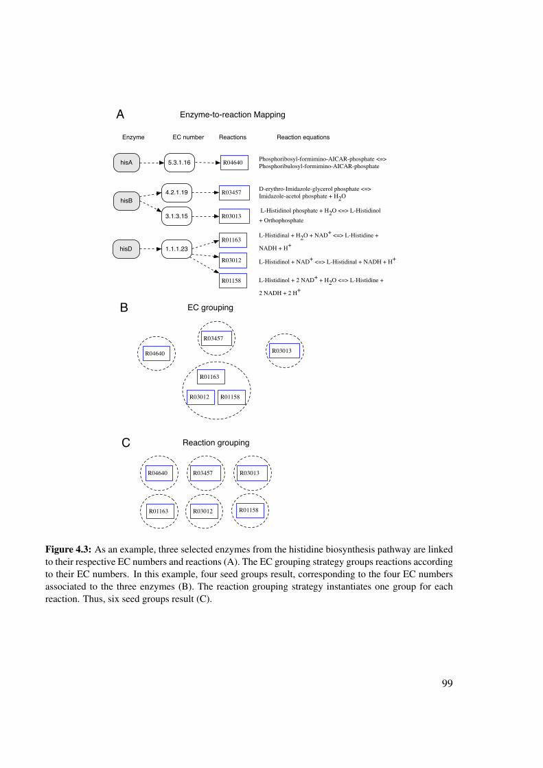
A
EC grouping
Reaction grouping
B
R04640
R03457
R03013
R03012
R01163
R01158
hisA
hisB
R046405.3.1.16
4.2.1.19
3.1.3.15 R03013
R03457
Enzyme EC number Reactions
hisD 1.1.1.23R01163
R01158
R03012
Enzyme-to-reaction Mapping
C
R04640 R03457 R03013
R01163 R01158R03012
Phosphoribosyl-formimino-AICAR-phosphate <=>Phosphoribulosyl-formimino-AICAR-phosphate
D-erythro-Imidazole-glycerol phosphate <=>Imidazole-acetol phosphate + H2O
Reaction equations
L-Histidinol phosphate + H2O <=> L-Histidinol + Orthophosphate
L-Histidinal + H2O + NAD+ <=> L-Histidine +
NADH + H+
L-Histidinol + NAD+ <=> L-Histidinal + NADH + H+
L-Histidinol + 2 NAD+ + H2O <=> L-Histidine +
2 NADH + 2 H+
Figure 4.3: As an example, three selected enzymes from the histidine biosynthesis pathway are linkedto their respective EC numbers and reactions (A). The EC grouping strategy groups reactions accordingto their EC numbers. In this example, four seed groups result, corresponding to the four EC numbersassociated to the three enzymes (B). The reaction grouping strategy instantiates one group for eachreaction. Thus, six seed groups result (C).
99

CL-Glutamate
R01214ilvE
L-Valine
R01215avtA
L-Alanine
R00401dadX
alr
D-Alanine
Reference pathway (Alanine biosynthesis)
ilvE avtA dadX alr
2.6.1.42
R01090
R02199
R01214
2.6.1.66
R01215
5.1.1.1
R00401
5.1.1.1
R00401
A
B Gene-to-reaction mapping
Predicted pathway
Genes
EC numbers
Reactions
Figure 4.4: Procedure for the evaluation of reaction grouping strategies. The evaluation starts witha reference pathway (A). The genes of the reference pathway are mapped to reactions (B), which aregrouped according to the strategy to be evaluated. In the example shown, reactions are grouped ECnumber-wise. From the seed reaction groups, a pathway is predicted (C), which is then compared tothe reference pathway.
100
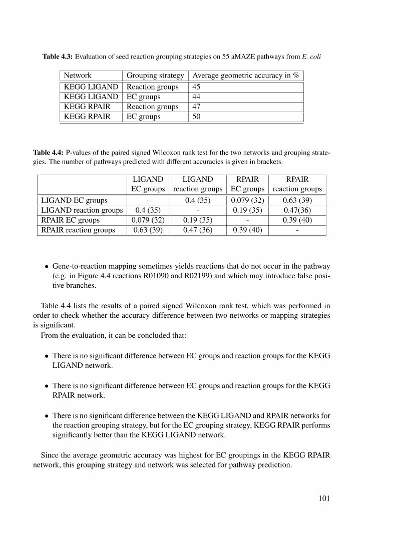
Table 4.3: Evaluation of seed reaction grouping strategies on 55 aMAZE pathways from E. coli
Network Grouping strategy Average geometric accuracy in %KEGG LIGAND Reaction groups 45KEGG LIGAND EC groups 44KEGG RPAIR Reaction groups 47KEGG RPAIR EC groups 50
Table 4.4: P-values of the paired signed Wilcoxon rank test for the two networks and grouping strate-gies. The number of pathways predicted with different accuracies is given in brackets.
LIGAND LIGAND RPAIR RPAIREC groups reaction groups EC groups reaction groups
LIGAND EC groups - 0.4 (35) 0.079 (32) 0.63 (39)LIGAND reaction groups 0.4 (35) - 0.19 (35) 0.47(36)RPAIR EC groups 0.079 (32) 0.19 (35) - 0.39 (40)RPAIR reaction groups 0.63 (39) 0.47 (36) 0.39 (40) -
• Gene-to-reaction mapping sometimes yields reactions that do not occur in the pathway(e.g. in Figure 4.4 reactions R01090 and R02199) and which may introduce false posi-tive branches.
Table 4.4 lists the results of a paired signed Wilcoxon rank test, which was performed inorder to check whether the accuracy difference between two networks or mapping strategiesis significant.
From the evaluation, it can be concluded that:
• There is no significant difference between EC groups and reaction groups for the KEGGLIGAND network.
• There is no significant difference between EC groups and reaction groups for the KEGGRPAIR network.
• There is no significant difference between the KEGG LIGAND and RPAIR networks forthe reaction grouping strategy, but for the EC grouping strategy, KEGG RPAIR performssignificantly better than the KEGG LIGAND network.
Since the average geometric accuracy was highest for EC groupings in the KEGG RPAIRnetwork, this grouping strategy and network was selected for pathway prediction.
101

4.5 Multiple-end pathway prediction parameters
4.5.1 Metabolic network
From the evaluation of gene-to-reaction mapping strategies, it emerged that the EC groupingin the KEGG RPAIR network performed best. Thus, the KEGG RPAIR network (KEGGRPAIR vs 49.0) was selected as input network for pathway prediction. It consists of 11,066reactant pairs and 5,760 compounds, connected by 44,236 edges.
The MetaCyc network, which offers a more precise gene-to-reaction mapping (becausegenes can be directly linked to reactions), could not be employed, because MetaCyc does notcontain many yeast genes.
4.5.2 Seed nodes
Two pathway predictions were performed for each nitrogen source: one for the up-regulatedgenes and the second for the down-regulated genes.
The gene groups were filtered such that for each group only the 5 enzyme-coding geneswith the lowest E-value were retained. Previous experiments with unfiltered gene groups gavecomplex results that were hard to interpret. The aim of the reduction of the input gene numberis to keep only the part of the pathway that is most affected by the nitrogen source in question.
For each of the reduced gene groups, reactant pairs were obtained in three steps using KEGGdata:
1. For each enzyme-coding gene, EC numbers were obtained by querying the KEGGdatabase on-the-fly.
2. Each EC number was associated to its reactions using the custom metabolic databasedescribed in section 9.3.
3. Each reaction in turn was associated to its main reactant pairs using the custommetabolic database.
4. The previous steps yield for each gene cluster a set of EC number groups, where each ECnumber group consists of a set of main reactant pairs. EC number groups with mutuallyexclusive reactant pairs (i.e. reactant pairs belonging to the same reaction) were mergedinto one group, to prevent that the same reaction appears twice in the predicted pathway.
5. Finally, overlapping groups (i.e. groups containing the same reactant pair) were mergedas well.
4.5.3 Algorithm
Pathways were predicted with the hybrid of kWalks and Takahashi-Matsuyama, which was thebest-performing algorithm in the evaluation presented in chapter 3. The intermediate networksize extracted by kWalks in the first step of the hybrid was set to 5% of the input network
102

size (i.e. the input network node number). KWalks was not iterated and its relevances notused as weights. Preprocessing was enabled (see section 9.1 for details on these parameters).Compounds adjacent to seed reactant pairs were included in the predictions.
After execution of the algorithm on the 40 gene clusters, 39 pathways could be predicted (forthr_down, which is associated to only three main reactant pairs, pathway prediction failed).
4.6 Pathway predicted to be up-regulated in the
presence of aspartate
4.6.1 Up-regulated genes
In the presence of aspartate, 69 genes are up-regulated, 25 of them enzyme-coding. Table 4.5displays the EC numbers and reactions associated to the five top enzyme-coding genes (i.e.those with lowest E-values). One of the genes, ADH4, codes for a broad-specificity enzymethat is associated to no less than 17 main reactant pairs. Seed reaction grouping allows to treatcases like this one, where only a subset of the reactions associated to a gene is likely to berelevant for the pathway.
Table 4.5: Gene-to-reactant pair mappings for the top five enzyme-coding genes up-regulated withaspartate as sole nitrogen source
Gene Gene Gene EC numbers Reactions and mainidentifier name description of gene reactant pairs
of EC number
YCR012W PGK1 3-phosphoglycerate kinase, 2.7.2.3 R01512 [RP00003, RP00113]catalyzes transfer ofhigh-energy phosphorylgroups from the acylphosphate of 1,3-bisphosphoglycerateto ADP to produce ATP
YER062C HOR2 One of two redundant 3.1.3.21 R00841 [RP00194]DL-glycerol-3-phosphatases R07298 [RP01251](RHR2/GPP1 encodes theother) involved in glycerolbiosynthesis
YHR044C DOG1 2-deoxyglucose-6-phosphate 3.1.3.68 R08548 [RP00680]phosphatase, similar R02587 [RP02325]to Dog2p, member of afamily of low molecularweight phosphatases
YBR067C TIP1 Major cell wall 3.1.1.- R07680 [RP11273]mannoprotein with R07677 [RP11937]possible lipase R06729 [RP09164, RP09420]activity R05420 [RP05028]
YGL256W ADH4 Alcohol dehydrogenase 1.1.1.1 R05234 [RP11679]isoenzyme type IV, dimeric R00623 [RP00139]enzyme demonstrated to R07327 []be zinc-dependent despite R05233 [RP04835]sequence similarity to R08558 [RP00236]iron-activated alcohol R00624 [RP00542]dehydrogenases R06917 [RP09622]
R07326 []R08306 [RP13225]R08310 [RP13235]R06927 [RP09285]
103
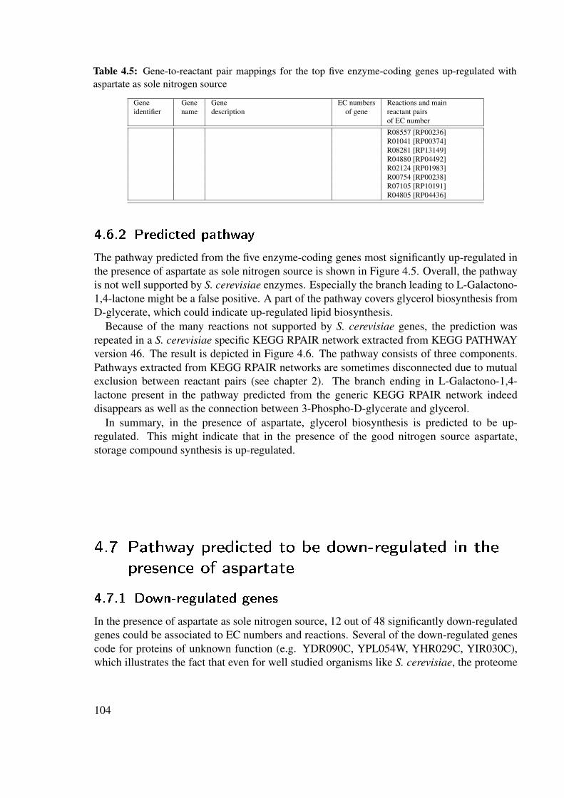
Table 4.5: Gene-to-reactant pair mappings for the top five enzyme-coding genes up-regulated withaspartate as sole nitrogen source
Gene Gene Gene EC numbers Reactions and mainidentifier name description of gene reactant pairs
of EC number
R08557 [RP00236]R01041 [RP00374]R08281 [RP13149]R04880 [RP04492]R02124 [RP01983]R00754 [RP00238]R07105 [RP10191]R04805 [RP04436]
4.6.2 Predicted pathway
The pathway predicted from the five enzyme-coding genes most significantly up-regulated inthe presence of aspartate as sole nitrogen source is shown in Figure 4.5. Overall, the pathwayis not well supported by S. cerevisiae enzymes. Especially the branch leading to L-Galactono-1,4-lactone might be a false positive. A part of the pathway covers glycerol biosynthesis fromD-glycerate, which could indicate up-regulated lipid biosynthesis.
Because of the many reactions not supported by S. cerevisiae genes, the prediction wasrepeated in a S. cerevisiae specific KEGG RPAIR network extracted from KEGG PATHWAYversion 46. The result is depicted in Figure 4.6. The pathway consists of three components.Pathways extracted from KEGG RPAIR networks are sometimes disconnected due to mutualexclusion between reactant pairs (see chapter 2). The branch ending in L-Galactono-1,4-lactone present in the pathway predicted from the generic KEGG RPAIR network indeeddisappears as well as the connection between 3-Phospho-D-glycerate and glycerol.
In summary, in the presence of aspartate, glycerol biosynthesis is predicted to be up-regulated. This might indicate that in the presence of the good nitrogen source aspartate,storage compound synthesis is up-regulated.
4.7 Pathway predicted to be down-regulated in the
presence of aspartate
4.7.1 Down-regulated genes
In the presence of aspartate as sole nitrogen source, 12 out of 48 significantly down-regulatedgenes could be associated to EC numbers and reactions. Several of the down-regulated genescode for proteins of unknown function (e.g. YDR090C, YPL054W, YHR029C, YIR030C),which illustrates the fact that even for well studied organisms like S. cerevisiae, the proteome
104
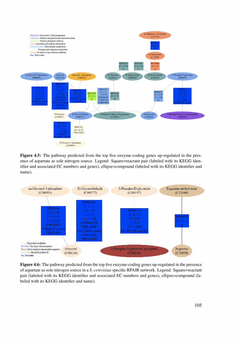
Figure 4.5: The pathway predicted from the top five enzyme-coding genes up-regulated in the pres-ence of aspartate as sole nitrogen source. Legend: Square=reactant pair (labeled with its KEGG iden-tifier and associated EC numbers and genes), ellipse=compound (labeled with its KEGG identifier andname).
Figure 4.6: The pathway predicted from the top five enzyme-coding genes up-regulated in the presenceof aspartate as sole nitrogen source in a S. cerevisiae specific RPAIR network. Legend: Square=reactantpair (labeled with its KEGG identifier and associated EC numbers and genes), ellipse=compound (la-beled with its KEGG identifier and name).
105

is not completely elucidated. Table 4.6 lists the associated EC numbers and reactions of thetop five enzyme-coding genes.
Another annotation problem is apparent for gene YNL141W (AAH1): In KEGG, it is an-notated with EC number 3.5.4.2 (gene definition field), but in fact is associated to EC number3.5.4.4 according to both KEGG and SGD [74].
YCL064C (CHA1) is known to accept both serine (EC number: 4.3.1.17) and threonine(EC number: 4.3.1.19) as substrates and thus furnishes an example for a gene associated tomore than one EC number.
There are also two genes associated to the same EC number, namely YNL117W (MLS1)and YIR031C (DAL7). Both code for a malate synthase and are thus an example for isoen-zymes.
Table 4.6: Gene-to-reactant pair mappings for for the top five enzyme-coding genes down-regulatedwith aspartate as sole nitrogen source
Gene Gene Gene EC numbers Reactions and mainidentifier name description of gene reactant pairs
of EC numberYIR029W DAL2 Allantoicase, converts 3.5.3.4 R02422 [RP02197, RP02198]
allantoate to urea andureidoglycolate in thesecond step of allantoindegradation
YCL064C CHA1 Catabolic L-serine (L-threonine) 4.3.1.19 R00220 [RP04290]deaminase, catalyzes R00996 [RP01226]the degradation of both R06131 [RP00068]L-serine and L-threonine 4.3.1.17 R00220 [RP04290]
R00590 [RP00998]R06131 [RP00068]
YNL141W AAH1 Adenine deaminase (adenine 3.5.4.4 R01560 [RP01594]aminohydrolase), converts R06137 []adenine to hypoxanthine R02556 [RP02305]
YNL117W MLS1 Malate synthase, enzyme 2.3.3.9 R00472 [RP00921, RP00007]of the glyoxylate cycle,involved in utilizationof non-fermentable carbonsources
YIR031C DAL7 Malate synthase, role 2.3.3.9 R00472 [RP00921, RP00007]in allantoin degradationunknown
4.7.2 Predicted pathway
The reactions associated to the 5 enzyme-coding genes are contained in 6 KEGG maps (seeFigure 4.7), which underlines the difficulty of interpreting a differentially expressed gene
106

group by pathway mapping alone.
Figure 4.7: The list of pathways obtained from KEGG for the top five enzyme-coding genes down-regulated in the presence of aspartate as sole nitrogen source. Metabolic pathways is a global map,comprising all other KEGG maps.
The predicted pathway, shown in Figure 4.8, consists of three components: two of them areorphan seed reactant pairs with their adjacent compounds (RP00998 and RP04290).
The prediction suggests a degradation pathway for purines, which converts deoxyadenosineto deoxyinosine, hypoxanthine and xanthine, which is finally degraded to urate. This purinedegradation pathway corresponds well to the known purine degradation pathway I in MetaCyc(identifier: PWY-5044). The purine degradation pathway is connected via 5-hydroxyisourateto the allantoin degradation pathway (MetaCyc identifier: PWY-5697), which yields urea. Inaddition, there are dubious connections to steps of the TCA cycle (fumarate, malate) and to areaction converting the generic compound 2-oxo acid into the generic compound alpha-aminoacid.
The prediction suggests that in the presence of the good nitrogen source aspartate, the degra-dation of purines and allantoin is suppressed.
The nitrogen catabolite repression (NCR) is known to suppress a number of nitrogen degra-dation pathways in the presence of good nitrogen sources in S. cerevisiae and other fungi (e.g.[170]). One may hypothesize that the aforementioned degradation pathways are also undercontrol of the NCR.
107
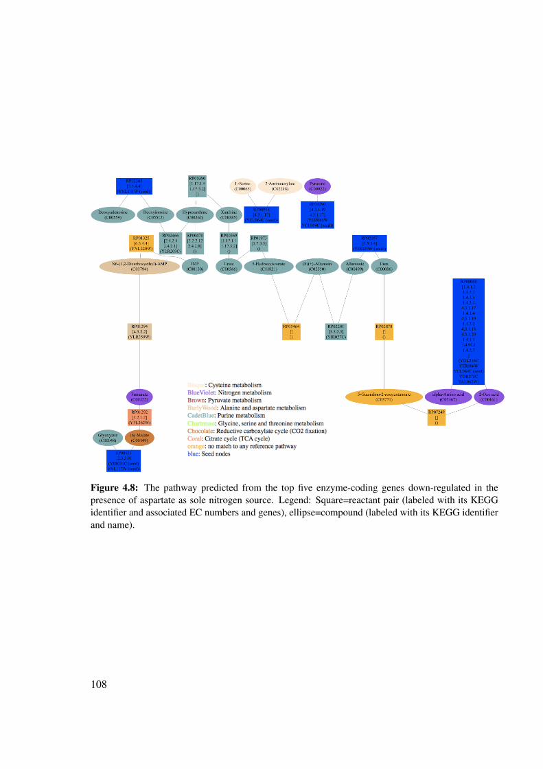
Figure 4.8: The pathway predicted from the top five enzyme-coding genes down-regulated in thepresence of aspartate as sole nitrogen source. Legend: Square=reactant pair (labeled with its KEGGidentifier and associated EC numbers and genes), ellipse=compound (labeled with its KEGG identifierand name).
108

4.8 Pathway predicted to be up-regulated in the
presence of phenylalanine
4.8.1 Up-regulated genes
From the 103 genes up-regulated in the presence of phenylalanine, 29 are enzyme-coding.Table 4.7 lists the five most significantly up-regulated enzyme-coding genes with their ECnumbers and reactions. ARO10 exemplifies well the difference in gene-reaction mappingbetween KEGG and MetaCyc: Whereas ARO10 is associated to no less than 19 reactions inKEGG (via its EC number), it is directly linked to only 4 reactions in MetaCyc.
Table 4.7: Gene-to-reactant pair mappings for genes up-regulated with phenylalanine as sole nitrogensource
Gene Gene Gene EC numbers Reactions and mainidentifier name description of gene reactant pairs
of EC numberQ0045 COX1 Subunit I of cytochrome 1.9.3.1 R00081 [RP00038]
c oxidase, which is theterminal member of themitochondrial inner membraneelectron transport chain
YKL165C MCD4 Protein involved in 2.7.-.- R07678 [RP11388]glycosylphosphatidylinositol(GPI) anchor synthesis
YDR380W ARO10 Phenylpyruvate decarboxylase, 4.1.1.- R02518 []catalyzes decarboxylation R06925 [RP09207]of phenylpyruvate to R00219 [RP04275]phenylacetaldehyde, which R04008 [RP03629]is the first specific R05376 [RP04982]step in the Ehrlich pathway R04986 [RP04595]
R03341 [RP02956]R04885 [RP04496]R03674 [RP03301]R05087 [RP04692]R03367 [RP02986]R05377 [RP04983]R04223 [RP03854]R02669 [RP02396]R06973 [RP10307]R04732 [RP04373]R04515 [RP04156]R02952 [RP02631]R04172 [RP03805]
YGR088W CTT1 Cytosolic catalase T, 1.11.1.6 R02670 [RP02397, RP12780]has a role in protection R00602 [RP00094]from oxidative damage R00009 [RP02902]by hydrogen peroxide
YHR137W ARO9 Aromatic aminotransferase 2.6.1.57 R07396 [RP00014, RP00558]II, catalyzes the first R01731 [RP01721, RP00059]
109

Table 4.7: Gene-to-reactant pair mappings for genes up-regulated with phenylalanine as sole nitrogensource
Gene Gene Gene EC numbers Reactions and mainidentifier name description of gene reactant pairs
of EC numberstep of tryptophan, phenylalanine, R00734 [RP00621, RP00014]and tyrosine catabolism R00694 [RP00014, RP00057]
R03120 [RP00550, RP00014]
4.8.2 Predicted pathway
The predicted pathway (see Figure 4.9) consists of three components. One of them is anorphan reactant pair with its adjacent compounds (RP00038). The second component containscompounds and reactant pairs associated to tryptophan metabolism. The third componentfinally postulates a connection between galactose and tyrosine metabolism. This connection isvery likely a false positive, as there is a lack of intermediate seeds. The tyrosine-metabolism-mapping part of the prediction contains the first steps of the tyrosine degradation pathway.Interestingly, the EC numbers of these steps (2.6.1.5 and 4.1.1.-/4.1.1.80) are the same asthe EC numbers of the first steps of phenylalanine degradation as annotated in KEGG (withphenylpyruvate and phenylacetaldehyde as intermediates).
The pathway is not well supported by yeast-specific enzymes, except for its parts mappingtryptophan and tyrosine metabolism, respectively. One might assume that both are involvedin the degradation of phenylalanine, which explains their up-regulation in the presence of thisnitrogen source.
In the yeast-specific network, the selected genes could not be connected, because most oftheir associated reactant pairs were not present in this network. This discrepancy may be eitherdue to an incomplete yeast-specific network and/or to imprecise gene-reaction mappings.
4.9 Pathway predicted to be down-regulated in the
presence of phenylalanine
4.9.1 Down-regulated genes
In the presence of phenylalanine as sole nitrogen source, 24 genes are down-regulated, amongthem four enzymes. Table 4.8 lists the EC numbers, reactions and main reactant pairs obtainedfor each enzyme.
110
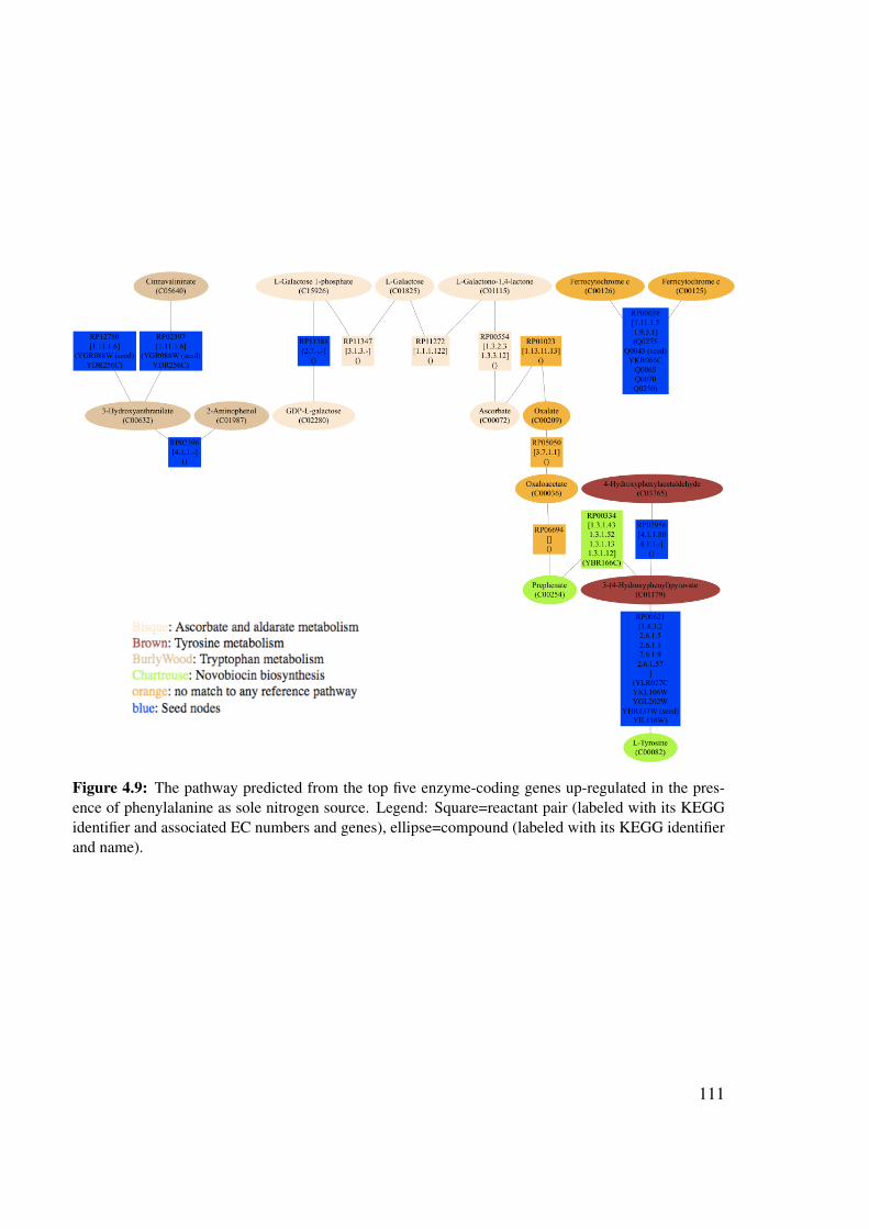
Figure 4.9: The pathway predicted from the top five enzyme-coding genes up-regulated in the pres-ence of phenylalanine as sole nitrogen source. Legend: Square=reactant pair (labeled with its KEGGidentifier and associated EC numbers and genes), ellipse=compound (labeled with its KEGG identifierand name).
111

Table 4.8: Gene-to-reactant pair mappings for genes down-regulated with phenylalanine as sole nitro-gen source
Gene Gene Gene EC numbers Reactions and mainidentifier name description of gene reactant pairs
of EC numberYIR029W DAL2 Allantoicase, converts 3.5.3.4 R02422 [RP02197, RP02198]
allantoate to urea andureidoglycolate in thesecond step of allantoindegradation
YNL141W AAH1 Adenine deaminase (adenine 3.5.4.4 R01560 [RP01594]aminohydrolase), converts R06137 []adenine to hypoxanthine R02556 [RP02305]
YIR031C DAL7 Malate synthase, role 2.3.3.9 R00472 [RP00921, RP00007]in allantoin degradationunknown
YGL202W ARO8 Aromatic aminotransferase 2.6.1.57 R07396 [RP00014, RP00558]I, expression is regulated R01731 [RP01721, RP00059]by general control of R00734 [RP00621, RP00014]amino acid biosynthesis R00694 [RP00014, RP00057]
R03120 [RP00550, RP00014]
4.9.2 Predicted pathway
The predicted pathway (see Figure 4.10) contains a purine degradation pathway that was alsopredicted for the genes down-regulated in the presence of aspartate. The purine degradationpathway ends in urate, which is predicted to be degraded to ureidoglycolate via the allantoindegradation pathway (MetaCyc identifier PWY-5697). Finally, ureidoglycolate is linked viaglyoxylate, malate and oxaloacetate to aspartate.
As in the case of aspartate, one may assume that the purine degradation pathway, which isactive in the presence of the bad nitrogen source urea, is not needed in the presence of theintermediate nitrogen source phenylalanine.
4.10 Pathway predicted to be up-regulated in the
presence of leucine
4.10.1 Up-regulated genes
The top five genes up-regulated in the presence of leucine are mostly associated to incompleteEC numbers. Incomplete EC numbers indicate that the knowledge of the reaction mechanismis not yet elucidated. These EC numbers are problematic, because they cannot be precisely
112

Figure 4.10: The pathway predicted from four enzyme-coding genes down-regulated in the presenceof phenylalanine as sole nitrogen source. Legend: Square=reactant pair (labeled with its KEGG iden-tifier and associated EC numbers and genes), ellipse=compound (labeled with its KEGG identifier andname).
mapped to reactions. KEGG nevertheless associates reactions to incomplete EC numbers.These associations will be used here, except for EC numbers where only the first level isknown (e.g. 4.-.-.-). Table 4.9 lists the genes with their EC numbers and associated reactions.A special case is YIR019C (MUC1), which is associated to a complete EC number (3.2.1.3),but not to any main reactant pair. The reason is that the reactions associated to this EC numberare polymeric (e.g. R01791 equation is: Dextrin + H2O ↔ alpha-D-Glucose + Dextrin) andthe metabolic networks constructed during this work do not include polymeric reactions.
Table 4.9: Gene-to-reactant pair mappings for the top five enzyme-coding genes up-regulated withleucine as sole nitrogen source
Gene Gene Gene EC numbers Reactions and mainidentifier name description of gene reactant pairs
of EC numberYMR095C SNO1 Protein of unconfirmed 2.6.-.- R07386 [RP10955, RP11005]
function, involved inpyridoxine metabolism
YDR380W ARO10 Phenylpyruvate decarboxylase, 4.1.1.- R02518 []catalyzes decarboxylation R06925 [RP09207]of phenylpyruvate to R00219 [RP04275]phenylacetaldehyde, which R04008 [RP03629]is the first specific R05376 [RP04982]step in the Ehrlich pathway R04986 [RP04595]
R03341 [RP02956]R04885 [RP04496]R03674 [RP03301]R05087 [RP04692]R03367 [RP02986]
113

Table 4.9: Gene-to-reactant pair mappings for the top five enzyme-coding genes up-regulated withleucine as sole nitrogen source
Gene Gene Gene EC numbers Reactions and mainidentifier name description of gene reactant pairs
of EC numberR05377 [RP04983]R04223 [RP03854]R02669 [RP02396]R06973 [RP10307]R04732 [RP04373]R04515 [RP04156]R02952 [RP02631]R04172 [RP03805]
YMR096W SNZ1 Protein involved in vitamin 4.-.-.- -B6 biosynthesis
YIR019C MUC1 GPI-anchored cell surface 3.2.1.3 -glycoprotein (flocculin)required for pseudohyphalformation, invasive growth,flocculation, and biofilms
YHR137W ARO9 Aromatic aminotransferase 2.6.1.57 R07396 [RP00014, RP00558]II, catalyzes the first R01731 [RP01721, RP00059]step of tryptophan, phenylalanine, R00734 [RP00621, RP00014]and tyrosine catabolism R00694 [RP00014, RP00057]
R03120 [RP00550, RP00014]
4.10.2 Predicted pathway
The pathway predicted for four genes most significantly up-regulated in the presence ofleucine as sole nitrogen source is shown in Figure 4.11. It consists of one component, a partof which maps to tyrosine metabolism and contains the first steps of the tyrosine degradationpathway. 4-Hydroxyphenylacetate is connected to choline via Penicillin G, which very likelyrepresents a false positive.
The predicted pathway suggests an up-regulation of tyrosine degradation in the presence ofleucine as sole nitrogen source.
Unfortunately, the prediction could not be repeated in the yeast-specific network, because itdid not contain enough seed reactant pairs.
114

Figure 4.11: The pathway predicted from the top five enzyme-coding genes up-regulated in the pres-ence of leucine as sole nitrogen source. Legend: Square=reactant pair (labeled with its KEGG identi-fier and associated EC numbers and genes), ellipse=compound (labeled with its KEGG identifier andname).
4.11 Pathway predicted to be down-regulated in the
presence of leucine
4.11.1 Down-regulated genes
26 out of 5,690 S. cerevisiae genes were identified to be significantly down-regulated in thepresence of leucine, nine of them enzyme-coding. Table 4.10 lists the top five enzyme-codinggenes together with their EC numbers and reactions. As for aspartate as sole nitrogen source,two malate synthases are down-regulated.
Table 4.10: Gene-to-reactant pair mappings for the top five enzyme-coding genes down-regulated withleucine as sole nitrogen source
Gene Gene Gene EC numbers Reactions and mainidentifier name description of gene reactant pairs
of EC numberYIR029W DAL2 Allantoicase, converts 3.5.3.4 R02422 [RP02197, RP02198]
allantoate to urea andureidoglycolate in thesecond step of allantoindegradation
YNL141W AAH1 Adenine deaminase (adenine 3.5.4.4 R01560 [RP01594]aminohydrolase), converts R06137 []
115
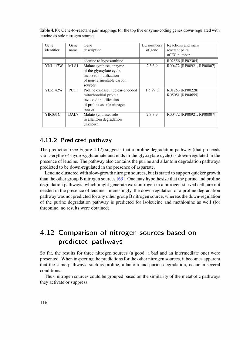
Table 4.10: Gene-to-reactant pair mappings for the top five enzyme-coding genes down-regulated withleucine as sole nitrogen source
Gene Gene Gene EC numbers Reactions and mainidentifier name description of gene reactant pairs
of EC numberadenine to hypoxanthine R02556 [RP02305]
YNL117W MLS1 Malate synthase, enzyme 2.3.3.9 R00472 [RP00921, RP00007]of the glyoxylate cycle,involved in utilizationof non-fermentable carbonsources
YLR142W PUT1 Proline oxidase, nuclear-encoded 1.5.99.8 R01253 [RP00228]mitochondrial protein R05051 [RP04655]involved in utilizationof proline as sole nitrogensource
YIR031C DAL7 Malate synthase, role 2.3.3.9 R00472 [RP00921, RP00007]in allantoin degradationunknown
4.11.2 Predicted pathway
The prediction (see Figure 4.12) suggests that a proline degradation pathway (that proceedsvia L-erythro-4-hydroxyglutamate and ends in the glyoxylate cycle) is down-regulated in thepresence of leucine. The pathway also contains the purine and allantoin degradation pathwayspredicted to be down-regulated in the presence of aspartate.
Leucine clustered with slow-growth nitrogen sources, but is stated to support quicker growththan the other group B nitrogen sources [63]. One may hypothesize that the purine and prolinedegradation pathways, which might generate extra nitrogen in a nitrogen-starved cell, are notneeded in the presence of leucine. Interestingly, the down-regulation of a proline degradationpathway was not predicted for any other group B nitrogen source, whereas the down-regulationof the purine degradation pathway is predicted for isoleucine and methionine as well (forthreonine, no results were obtained).
4.12 Comparison of nitrogen sources based on
predicted pathways
So far, the results for three nitrogen sources (a good, a bad and an intermediate one) werepresented. When inspecting the predictions for the other nitrogen sources, it becomes apparentthat the same pathways, such as proline, allantoin and purine degradation, occur in severalconditions.
Thus, nitrogen sources could be grouped based on the similarity of the metabolic pathwaysthey activate or suppress.
116

Figure 4.12: The pathway predicted from the top five enzyme-coding genes down-regulated in thepresence of leucine as sole nitrogen source. Legend: Square=reactant pair (labeled with its KEGGidentifier and associated EC numbers and genes), ellipse=compound (labeled with its KEGG identifierand name).
More precisely, the distance between two nitrogen sources i and j can be defined as
disti, j = 1− Jaccard(i, j) (4.1)
Given node set A from the pathway predicted for nitrogen source i and node set B from thepathway predicted for nitrogen source j, the Jaccard coefficient is defined as:
Jaccard =A∩BA∪B
(4.2)
Orphan reactant pairs (and their adjacent compounds) are not taken into account, to avoid abias due to many shared nodes for a broad-specificity enzyme.
Once the distance between two nitrogen sources is defined, the nitrogen sources can be clus-tered as shown in Figure 4.13. Clusters were obtained using function "heatmap" with method"ward" in R, other cluster algorithms yield similar results. For comparison, the clustering ofnitrogen sources based on gene expression ratios is shown in Figure 4.1.
When analyzing the pathway-based clustering, the following can be noted:
• In general, pathways are very dissimilar.
• Pathways are roughly divided into up- and down-regulated.
• Notable clusters (with distances below 0.6) are formed by: (1) pathways up-regulated inthe presence of aspartate, glutamate and proline, (2) pathways up-regulated in the pres-ence of alanine and ammonium, (3) pathways up-regulated in the presence of glutamine
117

and valine, (4) pathways down-regulated in the presence of aspartate, serine, isoleucine,arginine, leucine and phenylalanine, (5) pathways down-regulated in the presence ofammonium and asparagine and (6) pathways down-regulated in the presence of trypto-phan and tyrosine.
• The clustering is different to the one obtained from the gene expression ratio matrix.This may be due to the separation into up- and down-regulated pathways and the ne-glect of non-enzyme-coding genes. Notably, good and bad nitrogen sources were notseparated as clearly as in Figure 4.1.
• Nitrogen sources with intersecting up-regulated pathways do not necessarily have inter-secting down-regulated pathways.
4.13 Discussion and conclusion
The evaluation of two seed reaction grouping strategies showed that EC groups performslightly better than reaction groups. Grouping seed reactions on the gene level was not tested,but might be useful to predict pathways from genes that can be directly linked to reactions.
Interestingly, some good and bad nitrogen sources cluster together, mainly because of theallantoin and purine degradation pathways down-regulated in their presence (e.g. for aspartate,phenylalanine and leucine). The pathways are down-regulated with respect to urea as solenitrogen source and may therefore be specific to this reference nitrogen source rather than thetested nitrogen sources.
The up-regulated pathways are more variable and may be specific to the investigated nitro-gen sources. In a few cases, a part of the up-regulated pathway corresponds to a referencepathway degrading the given nitrogen source (phenylalanine, GABA). In other cases (aspar-tate, asparagine, ammonium) storage compound formation is up-regulated.
During prediction of pathways from up- and down-regulated gene groups, several difficul-ties were encountered: First, it is not obvious how many of the differentially expressed genesin each group should serve as input to pathway prediction. A conservative threshold (E valueset to one) resulted in quite large gene groups and pathways predicted for them were hard tovisualize and to interpret. One could either divide those pathways in smaller units using agraph cluster algorithm or, as done in this chapter, keep only the genes with lowest E values.In the latter case, a threshold is required, which was set arbitrarily to five. Second, gene-to-reaction mapping is ambiguous in KEGG. Genes are not directly linked to reactions (apartfrom the links hidden in the KGML files that are not accessible via the KEGG API or webinterface), thus genes have to be linked to reactions via EC numbers, which introduces falsepositive reactions. EC numbers are sometimes incomplete (e.g. YMR095C with EC number2.6.-.-), or describe broad-specificity enzymes associated to a large number of reactions (e.g.YGL256W alias ADH4). Third, there is a tradeoff in network choice. On the one hand, aspecies-specific metabolic network cannot discover varieties of pathways yet unknown in thisspecies. On the other hand, a network that is too generic introduces many false positives.Fourth, KEGG contains generic compounds such as alpha-amino acid, whose treatment is not
118

nwo d_psanwo d_ resn wod _el inwo d_granwod _ue lnw od _e hppu_ nlgpu_ lavpu _g rapu_ ns apu _r espu _al apu_
mm a
pu_ tlgpu _ps apu _orpn wo d_t icnw od _b agpu _e hppu _ uelpu _ prtpu _ te
mpu _rytnw o d_t e
mpu _ ticpu_e lip u_ nropu _r htpu _b agn wo d_l avnw od_p rtnwo d_ry tnwo d_tl gnw od _or pnw o d_a lanw od _n l gnw od_nr onw od_
mm a
nwod_ nsa
asn_downamm_downorn_downgln_downala_downpro_downglt_downtyr_downtrp_downval_downgab_upthr_uporn_upile_upcit_upmet_downtyr_upmet_uptrp_upleu_upphe_upgab_downcit_downpro_upasp_upglt_upamm_upala_upser_upasn_uparg_upval_upgln_upphe_downleu_downarg_downile_downser_downasp_down
0.0
0.2
0.4
0.6
0.8
1.0
Figure 4.13: Heat map of nitrogen source distances. The columns of the matrix are re-arrangedaccording to the outcome of the "ward" cluster algorithm. The distance ranges between zero (identicalpathways) and one (intersection of pathways is zero).
119

obvious. They are useful to describe broad-specificity reactions, but may introduce dubiousconnections.
Thus, errors are introduced on several levels: during the identification of significantly over-expressed genes, during the mapping of genes to reactions and finally during pathway predic-tion. To reduce errors in future applications of pathway prediction, one may consider otherdatabases than KEGG to map genes to reactions. For instance, MetaCyc offers more precisegene-to-reaction mappings and in addition cross-references its reactions to KEGG. Severaltaxonomic levels could be tested to construct a metabolic network with sufficient sensitivity(new pathways can be detected) and specificity (most reactions are supported by species-specific enzymes). In general, species-specific KEGG metabolic networks are of low quality.One might therefore consider the high-quality metabolic reconstruction of yeast metabolismrecently described in [141].
Overall, this chapter highlights the many problems encountered when interpreting microar-ray data on the pathway level and the presented results should be considered as preliminary.
120

5 Stoichiometric versus
non-stoichiometric pathway
prediction
Presented letter to the editor:K. Faust, D. Croes and J. van HeldenIn response to "Can sugars be produced from fatty acids? A test case for pathway anal-ysis tools"Bioinformatics, vol. 25, pp. 3202-3205, 2009.
5.1 Introduction
The question can be raised whether the stoichiometry of compounds should be taken intoaccount during pathway prediction. This chapter deals with this question.
First, taking into account the stoichiometry of pathways means to stoichiometrically balancethe metabolic pathway. Merely labeling the reactions of a pathway with their stoichiometriescan easily be done by querying a metabolic database and is not a point of discussion.
In a stoichiometrically balanced pathway, as many compounds are produced as consumedand reactions can only occur if their substrates are present in sufficient numbers.
The prediction approaches presented in chapter 2 and 3 do not stoichiometrically balancethe predicted pathway. However, several prediction approaches presented in the Introduction(such as elementary mode analysis and the constraint-based approaches by Planes & Beasley,see section 1.10.3) are designed to predict balanced pathways only. Figure 5.1 shows the bal-anced and non-balanced part of a reference pathway. In the reference pathways listed in Meta-Cyc and aMAZE, side compounds are usually not balanced. A pathway prediction approachthat predicts balanced pathways is thus not capable to predict these reference pathways, exceptif it excludes certain compounds from the balancing condition (called external compounds inEM analysis). Thus, side compounds need to be defined before pathway prediction, whichposes the difficulties mentioned in the Introduction: (1) It is not clear beforehand which com-pounds are side compounds (2) Pathways synthesizing or degrading the side compounds areexcluded together with the side compounds.
On the other hand, if stoichiometry is neglected in pathway prediction, biochemically ir-relevant pathways may result. A study case illustrating this was recently presented by deFigueiredo et al. [38] and concerns the synthesis of sugars from fatty acids. Fatty acidsare essentially broken down to acetyl-CoA molecules. Several organisms (e.g. E. coli and
121

3-phospho-D-glycerate
3-phospho-hydroxypyruvate
3-phospho-L-serine
L-serine
1.1.1.95
1
1
1
2.6.1.52
1
1
1NAD+
NADH1
H+
3.1.3.3
1
1
1L-glutamate
2-oxoglutarate
1
H2O
phosphate
1
1
Figure 5.1: The serine biosynthesis pathway as annotated in MetaCyc (identifier: SERSYN-PWY) isshown. Each reaction is displayed with all its substrates and products. Each arc connecting a compoundand a reaction is labeled with the stoichiometric coefficient, i.e. the number of units of the compoundconsumed or produced by the reaction. In this pathway, only the white compounds are balanced, thatis they are produced and consumed in equal numbers. The blue compounds (start and end compoundof the pathway) as well as the grey compounds (side compounds) are not balanced. An approach thatstoichiometrically balances pathways can predict the serine biosynthesis pathway only if it excludescertain compounds from the balancing condition. In EM analysis, such non-balanced compounds arecalled external compounds.
122

plants) can synthesize sugars (such as glucose) from acetyl-CoA. In the TCA cycle, acetyl-CoA is converted into oxaloacetate, which can enter the glucose-yielding gluconeogenesispathway. However, in the TCA cycle, acetyl-CoA is entirely degraded to CO2. Without sto-ichiometrically balancing the pathway, a prediction method could falsely predict that sugarsare synthesized from fatty acids via the TCA cycle. Figure 5.2 illustrates this study case.
glucose
glyoxylate bypass
fatty acid degradationgluconeogenesis
glyoxylate
CO2
CO2
(containing two carbon atoms)
Figure 5.2: Illustration of the study case presented by de Figueiredo et al. [38]. Acetyl-CoA is con-verted into oxaloacetate via the TCA cycle. Oxaloacetate in turn can enter the gluconeogenesis path-way, which yields glucose. However, the TCA cycle degrades acetyl-CoA entirely to carbon dioxide.It is therefore not possible to synthesize glucose from acetyl-CoA via this cycle. Since path findingdoes not balance the pathway, it could nevertheless predict a pathway that falsely converts the startcompound acetyl-CoA into the end compound glucose via this cycle. A bypass such as the glyoxylatecycle is needed to enable the net synthesis of glucose from acetyl-CoA. Image sources: The pathwayimage was taken from MetaCyc. Text and arrows in black as well as blue ellipses were added by theauthor.
123
5.2 Treatment of the fatty-acid-to-sugar study case
without stoichiometric balance
It is worthwhile exploring whether the fatty-acid-to-sugar study case and similar cases can betreated correctly without stoichiometrically balancing the predicted pathway.
5.2.1 Atom tracing
First, one may ask whether the study case can be treated correctly by atom tracing. In orderto check whether a net production via the TCA cycle is possible, atom tracing methods haveto trace not only the fatty acid atoms to the desired target compound (the sugar), but alsothrough the TCA cycle. Thus, the atom tracing method needs to follow all the atoms of aninput compound through the network and in addition to keep track of cycling atoms (such asthose in the TCA cycle) by counting atoms. This amounts to stoichiometrically balancing thecompounds of a pathway.
5.2.2 Cycle treatment
If one assumes that all problematic cases are caused by a special kind of metabolic cycle,one can attempt to identify all such cycles in the metabolic network. If all cycles without netproduction of compounds could be identified prior to pathway prediction, path finding couldbe forbidden to reach a target compound via such a cycle. Whether simple assumptions likethis one are sufficient to remedy path finding is an open question.
5.3 Assumptions of stoichiometrically balanced and
unbalanced pathways
From what has been said so far, we may conclude that pathway prediction methods shouldalways stoichiometrically balance a predicted pathway. There is however another turn to thestory.
When stoichiometrically balancing a pathway, it is assumed that the metabolic network iscompletely known, otherwise compounds cannot be balanced correctly (as unknown reactionsmay consume or produce them). For stoichiometrically unbalanced pathways, this assumptionis not made, but it is assumed that compounds are always available in sufficient numbers forthe pathway to proceed.
Concerning the study case, non-stoichiometric pathway prediction assumes that another partof the network will generate oxaloacetate from the source compound by other routes than theTCA cycle (which may or may not be the case), whereas stoichiometric pathway predictionassumes that the network (where oxaloacetate is generated from the source compound onlyvia the TCA cycle) is complete (which may or may not be the case).
Thus, stoichiometric pathway prediction is the method of choice in case a well curated,complete metabolic network is available. For incomplete metabolic networks, pathway pre-
124

diction with stoichiometry is not superior to pathway prediction without stoichiometry, as bothmake (possibly unjustified) assumptions in this case.
5.4 Stoichiometry and incomplete metabolic
networks
The less is known about the metabolism of an organism, the less accurate will be predic-tions from both stoichiometric and non-stoichiometric approaches. However, stoichiometricapproaches are more strongly affected by incomplete networks.
In contrast to non-stoichiometric approaches, stoichiometric approaches may predict theabsence of a number of pathways, because balancing reactions for certain compounds areabsent from the network. These pathways will be false negatives in case balancing reactionsare present in the organism, but have been missed during construction of the network.
For instance, consider the fatty-acid-to-sugar study case and assume that the organism inquestion possesses the glyoxylate cycle. In this case, a stoichiometric approach, based on theincomplete metabolic network, would wrongly predict that fatty acids cannot be convertedinto sugars, whereas a non-stoichiometric approach (which assumes that oxaloacetate is re-plenished by some other part of metabolism) would probably predict a pathway close to thetrue pathway (where the true pathway is determined by experimentally tracing carbon atomsfrom fatty acids to sugar).
5.5 EM analysis versus path �nding
There are different ways of stoichiometrically balancing a pathway, one of which is EM anal-ysis (see Introduction, section 1.10.3).
In the same article that presented the fatty-acid-to-sugar study case, de Figueiredo and co-authors also compared EM analysis with path finding (for path finding, see section 1.10.3).This comparison had several weaknesses, which prompted us to respond in a comment. In thiscomment, we not only point out the weaknesses of the comparison of EM analysis and pathfinding, we also discuss strengths and weaknesses of both approaches.
Some of the weaknesses of EM analysis listed in our comment have meanwhile been ad-dressed. This concerns the following weaknesses:
• EM analysis can only be applied to small networks: Recently, methods have beenpublished which allow the application of EM analysis to genome-scale networks[157, 85, 37].
• In large networks, EM analysis enumerates millions of EMs: A strategy to restrict thenumber of EMs has been published recently, which consist in ranking EMs accordingto their length [37].
Apart from the weaknesses of EM analysis mentioned in the comment, there are additionalweaknesses listed below:
125

• EM analysis cannot deal with parallel pathways or isoenzymes, which have to be re-moved from the metabolic network.
• EM analysis assumes that the compound concentrations remain approximately constantat an appropriate time scale. This is motivated by stating that compound pools rapidlyreach a steady state (within seconds). However, recent measurements in S. cerevisiaehave shown that there are slow compound pools [118]. Thus, the steady state assumptionis not valid for all compounds to the same extend. Slow compounds could be consideredas external compounds, but without measurements, it is not clear which are the slowcompounds.
5.6 Alternative stoichiometric approaches
The stoichiometric pathway prediction approach by Planes and Beasley [133] (see Introduc-tion, section 1.10.3) does not suffer from many of the drawbacks of EM analysis (e.g. steadystate assumption, assignment of external compounds, millions of EMs) and copes with largenetworks. In contrast to many path finding approaches, it also deals well with cycles. More-over, this approach has been systematically evaluated on reference pathways from E. coli.Thus, for the prediction of stoichiometrically balanced pathways given two seed nodes, thisapproach may be more appropriate than EM analysis.
5.7 Stoichiometric balance and feasibility of
metabolic pathways
One may ask whether metabolic pathways should not only be balanced, but also be feasible.In other words, should a pathway produce and consume all its compounds in equal numbersand generate all its compounds from the given seed nodes? The difference becomes clearwhen we consider the pair NADPH/NADP. In a balanced pathway, as many units of NADPHand NADP are produced as consumed. In a feasible pathway, NADPH and NADP have tobe synthesized by the pathway (or to be excluded from the feasibility condition). Chemicalorganizations (see Introduction, section 1.7.6) are an example for systems that generate alltheir compounds via stoichiometrically balanced pathways. Whether or not pathways shouldbe balanced and feasible largely depends on the application in mind. One such applicationmay be the construction of in vitro pathways that synthesize a desired compound [73].
5.8 Conclusion
From the comparison of stoichiometric versus non-stoichiometric prediction approaches, onecan conclude that each is appropriate in a different situation. Non-stoichiometric approachesshould be applied when predicting pathways from a large, possibly incomplete network, whichmay or may not be organism-specific. In contrast, stoichiometric approaches should be applied
126

when predicting pathways from a well-curated, organism-specific network. Of course, one ofthe goals of pathway prediction, namely the discovery of new pathways, is less interesting ina well-known network.
127

1
LETTER TO THE EDITOR
In response to “Can sugars be produced from fatty acids? A test case for pathway analysis tools” Karoline Faust*, Didier Croes and Jacques van Helden Laboratoire de Bioinformatique des Génomes et des Réseaux (BiGRe). Université Libre de Bruxelles, Campus Plaine, CP 263. Bld du Triomphe. B-1050 Bruxelles, Belgium. Associate Editor: Prof. Alfonso Valencia
ABSTRACT Motivation: In their article entitled “Can sugars be produced from fatty acids? A test case for pathway analysis tools” de Figueiredo and co-authors assess the performance of three pathway prediction tools (METATOOL, PathFinding and Pathway Hunter Tool) using the synthesis of glucose-6-phosphate (G6P) from acetyl-CoA in humans as a test case (de Figueiredo, et al., 2008). We think that this article is biased for three reasons: (1) The metabolic networks used as input for the respective tools were of very different sizes; (2) the “assessment” is restricted to two study cases; (3) developers are inherently more skilled to use their own tools than those developed by other people. We extended the analyses led by de Figueiredo and clearly show that the apparent superior performance of their tool (METATOOL) is partly due to the differences in input network sizes. We also see a conceptual problem in the comparison of tools that serve different purposes. In our opinion, metabolic path finding and elementary mode analysis are answering different biological questions, and should be considered as complementary rather than competitive approaches.
1 INTRODUCTION The CO2-releasing reactions of the Krebs cycle need to be bypassed in
order to synthesize G6P (a sugar) from acetyl-CoA via this cycle. Such a bypass is the glyoxylate cycle, which is active in many organisms capable of growing on fatty acids (such as certain plants and bacteria), but absent in humans (Berg, et al., 2002). Based on this study case, de Figueiredo and colleagues compare the following tools:
(1) METATOOL 5.0 (von Kamp and Schuster, 2006), which computes the elementary modes (EM) of a metabolic network. An elementary mode is defined as the “minimal set of enzymes that could operate at steady state” (Pfeiffer, et al., 1999). The steady state condition requires the stoichiometric balance (production and consumption in equal numbers) of all compounds that are not external to the metabolic network.
(2) PathFinding (Croes, et al., 2005; Croes, et al., 2006) is based on a k-shortest paths algorithm (depth-first search). It circumvents the problem of highly connected compounds (van Helden, et al., 2002) by assigning weights to compounds according to their degree in the metabolic network.
(3) Pathway Hunter Tool (PHT) (Rahman, et al., 2004) is also based on a k-shortest paths algorithm (depth-first search). It relies on the chemical similarity of substrate-product pairs to avoid side compounds.
*To whom correspondence should be addressed.
We will refer to pathway prediction tools relying mainly on network topology and ignoring stoichiometry (such as PathFinding and PHT) as path finding tools.
In this letter, we do not contest the main conclusion of the authors that only METATOOL deals correctly with the selected test case. Indeed, this test case illustrates well some problems that can arise when the stoichiometry is ignored in pathway prediction. However, we question the evaluation procedure, and therefore the generality of their conclusion. We also give a different view on the respective strengths and weaknesses of EM-based versus path finding approaches.
2 BIASES IN THE EVALUATION PROCEDURE
2.1 Tools should be fed with the same input network Instead of supplying all three tools with the same metabolic network, each of them was tested with a different input metabolic network. METATOOL was fed with a network consisting of 29 carefully selected reactions involved in central metabolism. PHT was launched on a human-specific network obtained from KEGG (Kanehisa, et al., 2008) (v.39.0) containing 1,492 reactions and 1,490 compounds. PathFinding was tested with the complete KEGG small molecule metabolic network, which comprised 5,985 reactions and 5,082 compounds (Croes, et al., 2005), and its results were a posteriori filtered to keep only paths present in the human-specific KEGG network. Considering this difference in input network size, it is not surprising that METATOOL comes closest to the expected result.
To demonstrate that network size does matter in such a comparison, we ran PathFinding on the same input network as given to METATOOL. For this, we constructed two bipartite networks from the 29 reactions (including the glyoxylate cycle) used by de Figueiredo, one taking into account reaction directionality and another one treating all reactions as reversible. Compounds were assigned a weight equal to their degree in the complete small molecule metabolic network (KEGG LIGAND version 44.0), as done in (Croes, et al., 2006). Given these small networks, PathFinding returned the glyoxylate cycle and gluconeogenesis pathway as top-ranking paths (supplementary material), which is not the case if it is run on the full KEGG network as done by de Figueiredo.
2.2 Tools should be assessed on a representative number of study cases
The comparison presented by de Figueiredo et al. is also questionable because of its restriction to two carefully selected study cases. This results in a biased view on the quality of the compared tools. Path finding tools are particularly weak in discovering paths situated in the highly connected core of large metabolic networks (e.g. glycolysis, TCA cycle, etc.). In contrast, these pathways have been studied with EM analysis before, e.g. (Carlson, et al., 2004; Schwartz and Kanehisa, 2006), which shows that the study case was not selected at random. A fair comparison should be based either
© The Author (2009). Published by Oxford University Press. All rights reserved. For Permissions, please email: [email protected]
Bioinformatics Advance Access published September 23, 2009

In response to “Can sugars be produced from fatty acids? A test case for pathway analysis tools”
2
on the analysis of all available pathways, or on a representative and unbiased selection of them.
2.3 Tool comparisons should be carried out by neutral assessors
Lastly, we would like to point out that the comparison of the three pathway prediction tools has been carried out by authors involved in the development of one of these tools (namely METATOOL). This induces an inherent bias in the comparison, as a developer is more skilled in the use of his/her own tools than in those developed by other people. A fairer procedure would be to follow a CASP-like protocol (Moult, et al., 2007), where developers would use their own tools on a set of test cases, and the evaluation of the results would be carried out by an independent committee. However, in our opinion it is not meaningful to compare pathway prediction performance of EM analysis and path finding approaches, since they differ in their definition of a metabolic pathway and have been designed for different tasks.
3 DISCUSSION The main difference between EM analysis and path finding approaches lies in their definition of a metabolic pathway. Whereas EM analysis considers as valid pathways only those metabolic sub-networks where all internal compounds are stoichiometrically balanced, path finding approaches do not impose any stoichiometric constraints. In our opinion, this fundamental distinction in the definition of a metabolic pathway leads to different advantages and disadvantages of both types of tools for pathway prediction, which are summarized below.
Advantages of EM-based tools: (1) They predict pathways whose internal compounds are balanced; (2) consequently, they also predict the pathway stoichiometry; (3) they can treat cyclic pathways.
Disadvantages of EM-based tools: (1) They require the user to decide for each compound of a given metabolic network whether it is internal or external to the system. In case the assignment of a compound as internal is faulty, EM analysis might fail to detect biochemically valid pathways; (2) EM-based tools cannot predict pathways that do not fit into their definition of a pathway. Planes and Beasley (Planes and Beasley, 2008) listed a number of classical pathways that are missed by EM-based tools for this reason (among them arginine biosynthesis and pentose phosphate salvage pathway); (3) combinatorial explosion limits the size of the input network that EM-based tools can treat. For instance, METATOOL 5.0 computed 2,450,787 EMs for a metabolic network of E. coli consisting of 112 reactions and 89 internal compounds within 87 minutes (von Kamp and Schuster, 2006); (4) predicted EMs are not ranked, which makes it hard to inspect EM analysis results for large metabolic networks (e.g. networks with more than 100 nodes). However, they may be ranked according to molar yield of a compound of interest (Trinh, et al., 2009) or on the basis of experimentally measured fluxes (Schwartz and Kanehisa, 2006); (5) the steady state constraint might not be appropriate for the metabolic network under study. Indeed, an organism may live in a rapidly changing environment, where the utilization of some substrates will modify their external concentration, which will be compensated by the activation or repression of other pathways. The steady-state constraint on the models seems essentially valid when experiments are performed in perfectly controlled conditions such as a chemostat, so that the system is really in steady state. In such conditions, it is crucial to carefully choose the set of reactions included in the network in order to ensure that the derived mathematical model can reach a steady state. For example, Teusink et al. modified their model of glycolysis because numerical simulations performed with experimentally measured metabolite concentrations had shown that this model failed to reach a steady state (Teusink, et al., 2000).
Path finding tools have the following advantages: (1) They can deal with large input networks (e.g. all currently known compounds and reactions); (2) they do not require the partition of compounds into internal and external (though some path finding tools need additional knowledge such as the
compound structure); (3) they allow the integration of contextual information. For instance, weights can express the probability of a reaction to occur in the organism under study; (4) they rank predicted paths according to a certain criterion such as path weight or degree of similarity between compounds in subsequent steps.
Disadvantages of path finding tools: (1) They do not take into account stoichiometry and therefore do not guarantee that predicted paths allow the net synthesis of a given end compound; (2) consequently, they cannot predict the stoichiometry of paths; (3) they cannot find cyclic pathways (trivial cycles excepted) or pathways in which the same enzymes act repeatedly on a growing chain (e.g. in fatty acid elongation). However, they can predict parts of these pathways; (4) path finding tools have difficulties to correctly predict pathways located in the densely connected central metabolism, such as glycolysis. In this region, currently employed criteria such as weight or compound similarity are not sufficient to identify relevant pathways in large networks; (5) most path finding tools require parameter tuning with respect to the given input network (node weights, cut-off on the number of paths requested).
For a more in-depth discussion of different pathway prediction approaches we recommend (Planes and Beasley, 2008).
Not only do EM-based and path finding tools differ in their strengths and weaknesses, they also answer different questions about metabolism. EM analysis is applied to study well-known, often manually compiled, small metabolic networks (less than hundred reactions) in order to gain insight into the physiology of particular organisms (Poolman, et al., 2003; Van Dien and Lidstrom, 2002) or to find elementary modes that have high molar yields for a compound of interest (Carlson, et al., 2004; Liao, et al., 1996). Knowledge of such elementary modes helps to produce desired compounds more efficiently (Trinh, et al., 2009), e.g. by modifying the compound-producing organism (Trinh, et al., 2006).
Path finding tools are obviously not suited for this kind of detailed analysis. In contrast to EM analysis, they are applied to large metabolic networks (up to several thousands of reactions), with the purpose of predicting biosynthesis and/or biodegradation pathways in organisms or sets of organisms (such as microbial communities) (e.g. (Dimitrov, et al., 2004; Pazos, et al., 2005; Yamazaki, et al., 2004)) or to fill gaps in genome-wide metabolic pathway reconstruction (Kharchenko, et al., 2006; Kharchenko, et al., 2004). Future application of path finding in metabolic reconstruction may go beyond gap filling. Current automated metabolic reconstruction tools (e.g. (Karp, et al., 2002; Moriya, et al., 2007)) are based on the mapping of enzymes onto pre-defined pathways, which prevents the detection of variants of known pathways and novel pathways. The more flexible path finding approach may help to solve these problems. Currently, only MaGe (microbial genome annotation system (Vallenet, et al., 2006)) integrates a path finding tool (PHT). Another interesting application of path finding could be to predict pathways from gene expression data, more specifically from sets of activated/repressed enzymes (van Helden, et al., 2001).
To summarize: EM analysis is suitable for detailed analysis of small-scale, high-quality metabolic networks, whereas path finding is designed to predict pathways in large-scale, possibly low-quality metabolic networks.
In our opinion, EM and path finding should be perceived as complementary tools that can be combined to explore metabolic diversity. For example, path finding might be used as a first step to discover novel pathways from various data sources (operons, synteny, gene expression), which might then be submitted to EM analysis in order to extract consistent modules of reactions. More generally, each approach is designed to answer different questions, and cannot be compared to methods conceived for other purposes. For example, Panke and co-workers analyze the dynacmis of in vitro enzymatic systems using a formalism that relies on the precise measurement of each enzyme’s condition (Hold and Panke, 2009; Makart, et al., 2007). Palsson’s group applies flux balance analysis to model genome-scale metabolic networks, in order to predict mutant phenotypes under controlled conditions, and design mutants with improved

In response to “Can sugars be produced from fatty acids? A test case for pathway analysis tools”
3
biosynthetic efficiency (Edwards and Palsson, 2000; Herrgård, et al., 2006; Portnoy, et al., 2008). Yet other methods have been developed to address different metabolism-related problems, whose enumeration is out of scope for this comment.
Rather than comparing EM-based tools to path finding tools, it would be much more interesting to compare path finding tools among themselves, or, even better, to evaluate the best ways to combine these tools. Indeed, many path finding approaches have been published that address the same question, but rely on different strategies (compound similarity, node or edge weights, rules) (Arita, 2003; Blum and Kohlbacher, 2008; Croes, et al., 2005; Croes, et al., 2006; Ellis, et al., 2008; Faust, et al., 2009; McShan, et al., 2003; Pazos, et al., 2005; Rahman, et al., 2004).
Currently, no approach is able to predict biochemically valid pathways in a genome-scale metabolic network with 100% accuracy, leaving a challenge for future research. Yet a greater challenge will be to perform experimental validations of the predictions, which, so far, has been done only in a very restricted number of cases (Table 1).
ACKNOWLEDGEMENTS Funding: KF is supported by Actions de Recherches Concertées de la Communauté Française de Belgique (ARC grant number 04/09-307). The laboratory is a member of the BioSapiens Network of Excellence funded under the sixth Framework program of the European Communities (LSHG-CT-2003-503265). The work was also supported by the Belgian Program on Interuniversity Attraction Poles, initiated by the Belgian Federal Science Policy Office, project P6/25 (BioMaGNet). We would like to thank the referees for their helpful comments.
REFERENCES Arita, M. (2003) In Silico Atomic Tracing by Substrate-Product Relationships in
Escherichia coli Intermediary Metabolism, Genome Research, 13, 2455-2466. Berg, J.M., Tymoczko, J.L. and Stryer, L. (2002) Biochemistry. W.H. Freeman and
Company, New York. Blum, T. and Kohlbacher, O. (2008) MetaRoute: fast search for relevant metabolic
routes for interactive network navigation and visualization Bioinformatics, 24, 2108-2109.
Carlson, R., Wlaschin, A. and Srienc, F. (2004) Kinetic Studies and Biochemical Pathway Analysis of Anaerobic Poly-(R)-3-Hydroxybutyric Acid Synthesis in Escherichia coli Applied and Environmental Microbiology, 71, 713-720.
Croes, D., Couche, F., Wodak, S. and van Helden, J. (2005) Metabolic PathFinding: inferring relevant pathways in biochemical networks, Nucleic Acids Res, 33, W326-W330.
Croes, D., Couche, F., Wodak, S. and van Helden, J. (2006) Inferring Meaningful Pathways in Weighted Metabolic Networks, J. Mol. Biol., 356, 222-236.
de Figueiredo, L.F., Schuster, S., Kaleta, C. and Fell, D.A. (2008) Can sugars be produced from fatty acids? A test case for pathway analysis tools Bioinformatics, 24, 2615-2621.
Dimitrov, S., Kamenska, V., Walker, J.D., Windle, W., Purdy, R., Lewis, M. and Mekenyan, O. (2004) Predicting the biodegradation products of perfluorinated chemicals using CATABOL, SAK and QSAR in Environmental Research, 15, 69-82.
Edwards, J.S. and Palsson, B.O. (2000) Metabolic flux balance analysis and the in silico analysis of Escherichia coli K-12 gene deletions, BMC Bioinformatics, 1:1.
Ellis, L., Gao, J., Fenner, K. and Wackett, L. (2008) The University of Minnesota pathway prediction system: predicting metabolic logic, Nucleic Acids Res, 36, W427-W432.
Faust, K., Croes, D. and van Helden, J. (2009) Metabolic pathfinding using RPAIR annotation., J. Mol. Biol., 388, 390-414.
Herrgård, M.J., Fong, S.S. and Palsson, B.Ø. (2006) Identification of Genome-Scale Metabolic Network Models Using Experimentally Measured Flux Profiles 2:e72.
Hold, C. and Panke, S. (2009) Towards the engineering of in vitro systems, Journal of the Royal Society Interface, 6, S507-S521.
Kanehisa, M., Araki, M., Goto, S., Hattori, M., Hirakawa, M., Itoh, M., Katayama, T., Kawashima, S., Okuda, S., Tokimatsu, T. and Yamanishi (2008) KEGG for
linking genomes to life and the environment, Nucleic Acids Research, 36, D480-484.
Karp, P.D., Paley, S. and Romero, P. (2002) The Pathway Tools software, Bioinformatics, 18, S225-S232.
Kharchenko, P., Chen, L., Freund, Y., Vitkup, D. and Church, G.M. (2006) Identifying metabolic enzymes with multiple types of association evidence BMC Bioinformatics, 7:177.
Kharchenko, P., Vitkup, D. and Church, G.M. (2004) Filling gaps in a metabolic network using expression information Bioinformatics, 20, i178-i185.
Liao, J.C., Hou, S.-Y. and Chao, Y.-P. (1996) Pathway Analysis, Engineering, and Physiological Considerations for Redirecting Central Metabolism Biotechnology and Bioengineering, 52, 129-140.
Makart, S., Bechtold, M. and Panke, S. (2007) Towards preparative asymmetric synthesis of β-hydroxy-α-amino acids: L-allo-Threonine formation from glycine and acetaldehyde using recombinant GlyA, Journal of Biotechnology, 130, 402-410.
McShan, D.C., Rao, S. and Shah, I. (2003) PathMiner: predicting metabolic pathways by heuristic search, Bioinformatics, 19, 1692-1698.
Moriya, Y., Itoh, M., Okuda, S., Yoshizawa, A.C. and Kanehisa, M. (2007) KAAS: anautomatic genome annotation and pathway reconstruction server, Nucleic Acids Res, 35, W182–W185.
Moult, J., Fidelis, K., Kryshtafovych, A., Rost, B., Hubbard, T. and Tramontano, A. (2007) Critical assessment of methods of protein structure prediction—Round VII Proteins, 69, 3-9.
Pazos, F., Guijas, D., Valencia, A. and De Lorenzo, V. (2005) MetaRouter: bioinformatics for bioremediation, Nucleic Acids Res, 33, D588-D592.
Pfeiffer, T., Sanchez-Valdenebro, I., Nuno, J.C., Montero, F. and Schuster, S. (1999) METATOOL: for studying metabolic networks., Bioinformatics, 15, 251-257.
Planes, F.J. and Beasley, J.E. (2008) A critical examination of stoichiometric and path-finding approaches to metabolic pathways, Brief Bioinformatics, 9, 422-436.
Poolman, M.G., Fell, D.A. and Raines, C.A. (2003) Elementary modes analysis of photosynthate metabolism in the chloroplast stroma Eur. J. Biochem., 270, 430-439.
Portnoy, V.A., Herrgård, M.J. and Palsson, B.Ø. (2008) Aerobic Fermentation of D-Glucose by an Evolved Cytochrome Oxidase-Deficient Escherichia coli Strain, Applied and Environmental Microbiology, 74, 7561-7569.
Rahman, S.A., Advani, P., Schunk, R., Schrader, R. and Schomburg, D. (2004) Metabolic pathway analysis web service (Pathway Hunter Tool at CUBIC), Bioinformatics, 21, 1189-1193.
Remde, A. and Debus, R. (1996) BIODEGRADABILITY OF FLUORINATED SURFACTANTS UNDER AEROBIC AND ANAEROBIC CONDITIONS Chemosphere, 32, 1563-1574.
Schwartz, J.M. and Kanehisa, M. (2006) Quantitative elementary mode analysis of metabolic pathways: the example of yeast glycolysis BMC Bioinformatics, 7:186.
Teusink, B., Passarge, J., Reijenga, C.A., Esgalhado, E., van der Weijden, C.C., Schepper, M., Walsh, M.C., Bakker, B.M., van Dam, K., Westerhoff, H.V. and Snoep, J.L. (2000) Can yeast glycolysis be understood in terms of in vitro kinetics of the constituent enzymes? Testing biochemistry Eur. J. Biochem., 267, 5313-5329.
Trinh, C.T., Carlson, R., Wlaschin, A. and Srienc, F. (2006) Design, construction and performance of the most efficient biomass producing E. coli bacterium METABOLIC ENGINEERING, 8, 628-638.
Trinh, C.T., Wlaschin, A. and Srienc, F. (2009) Elementary mode analysis: a useful metabolic pathway analysis tool for characterizing cellular metabolism, Appl Microbiol Biotechnol 81, 813-826.
Vallenet, D., Labarre, L., Rouy, Z., Barbe, V., Bocs, S., Cruveiller, S., Lajus, A., Pascal, G., Scarpelli, C. and Medigue, C. (2006) MaGe: a microbial genome annotation system supported by synteny results Nucleic Acids Research, 34, 53-65.
Van Dien, S.J. and Lidstrom, M.E. (2002) Stoichiometric Model for Evaluating the Metabolic Capabilities of the Facultative Methylotroph Methylobacterium extorquens AM1, with Application to Reconstruction of C3 and C4 Metabolism, Biotechnology and Bioengineering, 78, 296-312.
van Helden, J., Gilbert, D., Wernisch, L., Schroeder, M. and Wodak, S. (2001) Application of Regulatory Sequence Analysis and Metabolic Network Analysis to the Interpretation of Gene Expression Data Lecture Notes in Computer Science, 2066, 147-165.
van Helden, J., Wernisch, L., Gilbert, D. and Wodak, S. (2002) Graph-based analysis of metabolic networks. In Mewes, H.-W., Weiss, B. and Seidel, H. (eds), Ernst Schering Res. Found. Workshop. Springer-Verlag, Heidelberg, 245-274.
von Kamp, A. and Schuster, S. (2006) Metatool 5.0: fast and flexible elementary modes analysis, Bioinformatics, 22, 1930-1931.

In response to “Can sugars be produced from fatty acids? A test case for pathway analysis tools”
4
Yamazaki, Y., Kitajima, M., Arita, M., Takayama, H., Sudo, H., Yamazaki, M., Aimi, N. and Saito, K. (2004) Biosynthesis of Camptothecin. In Silico and in Vivo Tracer Study from [1-13C]Glucose1 Plant Physiology, 134, 161-170.
Table 1. Selected examples of application cases of metabolic predictions that have been confirmed experimentally. Reference Question Approach Tool Network size Experimental
confirmation method
Yamazaki et al. (2004)
Enumeration of possible pathways to produce a compound of interest (Campto-thecin).
Path finding (k-shortest paths)
ARM (Atomic Reconstruc-tion of Metabolism)
131 reactions, 280 atom mappings
13C tracing in vivo
Trinh et al. (2008)
Design of mutant Escherichia coli strains to optimize biomass production
EM METATOOL 44 reactions, 47 metabolites
Gene knock-outs in combination with biomass yield measure-ments
Carlson et al. (2005)
Enumeration of possible pathways to produce a compound of interest (poly- -hydroxybutyrate (PHB)).
EM METATOOL 44 reactions 47 metabolites
Measure-ment of PHB, glucose and other compound concentra-tions at different time points
Dimitrov et al. (2004)
Prediction of compound biodegrada-bility (perfluori-nated chemi-cals).
Rule-based pathway prediction
CATABOL 24 transfor-mations derived from > 150 compounds participating in bio-degradation pathways
Biodegrada-bility tests (Remde and Debus, 1996)
6 Contributions to NeAT
Presented articles:S. Brohée, K. Faust, G. Lima-Mendez, O. Sand, R. Janky, G. Vanderstocken, Y. Deville andJ. van HeldenNeAT: a toolbox for the analysis of biological networks, clusters, classes and pathwaysNucleic Acids Research, vol. 36, pp. W444-W451, 2008.
K. Faust1, S. Brohee, Gipsi Lima-Mendez, G. Vanderstocken and J. van HeldenNetwork Analysis Tools: from biological networks to clusters and pathwaysNature Protocols, vol. 3, pp. 1616-1629, 2008.
6.1 Presentation of NeAT
NeAT is a publicly available set of tools dedicated to the analysis of biological networks[20, 52]. Most NeAT tools can handle large input networks and finish jobs within one minute.NeAT can be accessed via a web server (http://rsat.ulb.ac.be/neat/), a collection of web ser-vices (SOAP/WSDL interface) as well as on command line. The web server, web servicesand the command line version are distributed on request and can be installed locally. NeAT isdesigned to be modular, to allow for easy combination of tools and implementation of work-flows. Tools can be combined programmatically via command line pipes and web servicesor via mouse clicks on the web server. Each web server tool provides a number of buttonsthat appear after completion of a job and which allow to send the results as input to anotherNeAT tool without having to copy-paste. In addition, NeAT is documented on several levels:Each tool comes with its command line and WSDL documentation. On the web server level,a manual, a tutorial and at least one demo accompany most tools.
6.2 Tools contributed to NeAT
Table 6.1 lists the tools that I contributed to NeAT during my thesis. The tools make use ofa database containing metabolic data from KEGG and BioCyc. This database is described insection 9.3.
1K. Faust and S. Brohée contributed equally to this publication.
132

Tabl
e6.
1:To
ols
cont
ribu
ted
toN
eAT
Tool
Purp
ose
Dat
aIn
put
Out
put
Opt
ions
Impl
emen
tatio
nR
emar
ksna
me
sour
ces
Path
finde
rE
num
erat
ion
ofN
one
Net
wor
k,Pa
ths
tabl
eIn
putn
etw
ork
form
atJa
vaw
rapp
erca
lling
Sets
ofst
arta
ndk-
shor
test
path
sst
artn
ode
set,
orne
twor
k(g
ml[
72]o
rtab
-del
imite
d),
RE
Aro
utin
e[8
3]en
dno
des
are
inw
eigh
ted
netw
orks
end
node
set.
com
bini
ngpa
ths
max
imal
path
wei
ght,
and
usin
gth
eaM
AZ
Esu
ppor
ted
usin
ga
max
imal
path
leng
th,
grap
hlib
rary
.gr
aph
tran
sfor
mat
ion
min
imal
path
leng
th,
Web
inte
rfac
ede
scri
bed
in[4
7].
path
rank
inde
x,w
ritte
nin
PHP.
node
sto
beab
sent
from
path
s,no
des
tobe
pres
enti
npa
ths,
wei
ghtp
olic
y(d
egre
e,un
itor
cust
om),
outp
utty
pe(t
able
orne
twor
k),
outp
utne
twor
kfo
rmat
(gm
lort
ab),
resu
ltsse
ntby
emai
lor
disp
laye
din
brow
ser.
Adv
ance
dop
tions
:Fl
agne
twor
kas
met
abol
ic(w
illaf
fect
wei
ghtp
olic
yan
dre
actio
ndi
rect
iona
lity
trea
tmen
t),
excl
usio
nat
trib
ute,
alte
rnat
ive
path
findi
ngal
gori
thm
[31,
32].
Met
abol
icE
num
erat
ion
ofK
EG
GL
IGA
ND
,E
Cnu
mbe
rs,
Path
sta
ble
Net
wor
k(K
EG
GSe
tofJ
ava
serv
lets
and
jsp
page
s.T
his
tool
does
note
xist
onpa
thfin
der
met
abol
icpa
ths
inK
EG
GR
PAIR
reac
tions
,rea
ctan
tpai
rs,
linke
dto
KE
GG
entr
ies
orL
IGA
ND
,KE
GG
Cal
lsth
ePa
thfin
derw
ebse
rvic
eco
mm
and
line
oras
wei
ghte
dK
EG
Gco
mpo
unds
netw
ork
com
bini
ngpa
ths,
RPA
IRor
aan
dqu
erie
sth
em
etab
olic
data
base
aw
ebse
rvic
e,ne
twor
ksw
ithne
twor
kim
age.
mix
ture
ofbo
th),
usin
gth
eH
iber
nate
quer
ysi
nce
itis
acl
ient
ofw
eigh
tpol
icy,
path
rank
inde
x,la
ngua
ge(H
QL
,[71
])to
anno
tate
path
s.th
ePa
thfin
derw
ebse
rvic
e.m
inim
alpa
thle
ngth
,m
axim
alpa
thle
ngth
,m
axim
alpa
thw
eigh
t,no
des
tobe
abse
ntfr
ompa
ths,
node
sto
bepr
esen
tin
path
s,ou
tput
type
(tab
leor
netw
ork)
,ou
tput
netw
ork
form
at(g
ml,
Vis
ML
[76]
,dot
[44]
orta
b),
resu
ltsse
ntby
emai
lor
disp
laye
din
brow
ser.
Adv
ance
dop
tions
:cu
stom
KE
GG
netw
ork
(in
tab,
gmlo
rKG
ML
form
at),
cust
omw
eigh
ts.
KE
GG
Con
stru
ctio
nof
KE
GG
PAT
HW
AY
KE
GG
orga
nism
s,N
etw
ork
Net
wor
kfil
tere
dfo
rIm
plem
ente
din
Java
,C
onve
rsio
nto
netw
ork
netw
orks
spec
ific
KE
GG
reac
tions
com
poun
ds,r
eact
ions
orR
PAIR
clas
ses.
met
abol
icda
taba
seK
EG
GR
PAIR
isof
fere
d,pr
ovid
erto
ase
tof
Con
stru
ctio
nof
RPA
IRne
twor
ks,
isqu
erie
dw
ithH
QL
whi
chis
anop
tion
orga
nism
s.di
rect
edne
twor
ksan
dne
twor
ksto
setn
ode
notp
rese
ntin
resp
ectin
gir
reve
rsib
lere
actio
ns.
attr
ibut
es.N
etw
orks
are
othe
rKE
GG
PAT
HW
AY
Nod
eat
trib
utes
(EC
num
bers
,co
nstr
ucte
dfr
omlo
cally
stor
edpa
rser
s[1
45,1
74,1
16].
reac
tion
equa
tions
,com
poun
dla
bels
KG
ML
files
and
save
d,an
dco
mpo
und
form
ulas
),so
that
they
need
tobe
Net
wor
kfo
rmat
cons
truc
ted
only
once
.(t
ab,g
ml,
doto
rVis
ML
).W
ebin
terf
ace
isR
esul
tsse
ntby
emai
lw
ritte
nin
PHP.
ordi
spla
yed
inbr
owse
r.
133

Tabl
e6.
1:To
ols
cont
ribu
ted
toN
eAT
Tool
Purp
ose
Dat
aIn
put
Out
put
Opt
ions
Impl
emen
tatio
nR
emar
ksna
me
sour
ces
Net
wor
kC
onve
rsio
nof
netw
orks
Non
eN
etw
ork
inta
b-N
etw
ork
inta
b-N
one
Impl
emen
ted
inJa
va.
Thi
sto
olha
sno
conv
erte
rin
toan
othe
rfor
mat
delim
ited,
gml,
GD
L,
delim
ited,
gml,
dot,
GD
Lis
anX
ML
-bas
edgr
aph
web
inte
rfac
e(b
ecau
seN
eAT
tool
KG
ML
orbi
opax
[16]
form
atPa
jek
[10]
,Vis
ML
form
atde
velo
ped
byth
eaM
AZ
Ete
am.
conv
ert-
grap
hfu
lfills
asi
mila
ror
GD
Lfo
rmat
.pu
rpos
e),b
utit
isav
aila
ble
asa
web
serv
ice
and
onco
mm
and
line.
Itis
used
with
inN
eAT
toco
nver
tgra
phs
into
Vis
ML
form
at.
Path
way
Ext
ract
ion
ofa
KE
GG
LIG
AN
D,
Net
wor
k,se
edno
des.
Sub-
netw
ork
(file
Pre-
load
edne
twor
k(M
etaC
yc,
Impl
emen
ted
inJa
vaex
trac
tion
sub-
netw
ork
KE
GG
RPA
IR,
Forp
re-l
oade
dne
twor
ks,
and
imag
e)w
itha
tabl
elis
ting
som
eK
EG
GR
PAIR
,KE
GG
LIG
AN
D)
with
calls
tofr
oma
wei
ghte
dne
twor
kM
etaC
ycse
eds
can
bege
nena
mes
,of
itsto
polo
gica
lpro
pert
ies.
orcu
stom
netw
ork
(in
tab,
exte
rnal
rout
ines
give
na
seto
rset
sof
Uni
Prot
iden
tifier
s,Fo
rpre
-loa
ded
netw
orks
,gm
lorK
GM
Lfo
rmat
),w
eigh
tpol
icy
wri
tten
inC
forR
EA
and
kWal
ks.
seed
node
s.R
efSe
qid
entifi
ers,
enzy
me
refe
renc
epa
thw
ays
are
orcu
stom
wei
ghts
,T
hem
etab
olic
data
base
isna
mes
,com
poun
ds,
map
ped
onto
the
sub-
netw
ork.
extr
actio
nal
gori
thm
(rep
etiti
veR
EA
,qu
erie
dvi
aH
QL
reac
tions
,EC
num
bers
Taka
hash
i-M
atsu
yam
a[1
54],
toan
nota
tem
etab
olic
orre
acta
ntpa
irs.
kWal
ks[4
8,21
]or
sub-
netw
orks
and
tom
apSe
eds
can
beco
mbi
natio
nsth
ereo
f),
refe
renc
epa
thw
ays.
grou
ped
inse
ts.
prep
roce
ss,p
ostp
roce
ss,
Web
inte
rfac
eis
itera
tion
num
ber,
perc
enta
geim
plem
ente
dw
ithJS
Pan
dof
inpu
tnet
wor
kto
beex
trac
ted
Java
serv
lets
.in
ahy
brid
appr
oach
,co
mpu
tatio
nof
wei
ghts
with
kWal
ks,s
ub-n
etw
ork
form
at(t
ab-d
elim
ited,
Vis
ML
,gm
l,do
t),
seed
grou
ptr
eatm
ent.
134

6.3 On the use of NeAT tools
6.3.1 Data input
Users can up-load their data to NeAT in two main formats: as a network (graph) or as a tab-delimited table (note that tables can be interpreted as networks as well). NeAT supports avariety of graph formats: tab-delimited (table with two selected columns), DOT [44], GML[72] and some specialized tools also KGML, the XML format of KEGG. In addition, userscan retrieve networks from the two database interfaces offered by NeAT: one for STRING[81] and the second for KEGG PATHWAY, which store data on protein-protein interactionsand metabolism respectively.
Usually, network nodes represent biological objects whose interactions have been deter-mined by a variety of methods. For instance, a user interested in the analysis of proteininteractions might up-load a protein-protein interaction network having proteins as nodes andtheir interactions as edges. In practice, this could be a tab-delimited file with two protein namecolumns, where each row describes the interaction between two proteins. The user could thenup-load a second protein-protein interaction network and measure the overlap between the twonetworks (see details in the Nature Protocol attached to this chapter) or compare the networkwith experimentally obtained protein-protein interactions stored in STRING (experimentaldata channel). With the path finder tool, the user could in addition enumerate paths between apair of proteins of interest.
6.3.2 Data output and interpretation
The main outputs of NeAT are tab-delimited tables displaying statistics or networks. Networkscan be returned in several formats: GML, DOT, VisML [76], tab-delimited and as adjacencymatrix.
For the path finding and pathway extraction tools in NeAT, it is often not easy to interpretthe output. For instance, the pathfinder tool lists paths in the order of their length (unweightednetworks) or their weight (weighted networks). In order to filter out irrelevant paths, usershave several possibilities: First and foremost, they can assign network weights that favorcertain nodes and penalize others. In addition, they can indicate nodes that have to appear inpaths or that should be avoided. Moreover, they can restrict the path length. For example, ifa user would like to predict a signal transduction pathway from a protein-protein interactionnetwork and has an idea about the minimal length (say 8 steps) of this pathway and some ofits participating proteins (e.g. STE20 and STE7), he or she can set these constraints in the webform as minimal length and nodes to be included parameter values.
The pathway extraction tool outputs only one solution, namely the predicted pathway. How-ever, the interpretation of a predicted pathway, especially if large, is not straightforward. Cri-teria that could be taken into account for interpretation are:
• Seed node coverage. A high percentage of seed nodes among all pathway nodes indi-cates that the predicted pathway is strongly supported by the seed nodes.
135

• Distance between seed nodes. The reliability of the predicted pathway decreases withthe distance between seeds. For instance, a long branch not supported by any seed nodeexcept the terminal one very likely represents a false positive.
• Presence of enyzmes catalyzing predicted reactions in the query organism. The pre-dicted pathway consists of seed nodes and predicted nodes connecting the seeds. Apathway is more reliable if all its predicted reactions are likely to be catalyzed in the or-ganism of interest. However, reactions not associated to any gene in the query organismmight also be spontaneous. Also, some enzymes may be missing due to errors in thegenome annotation process.
• Presence of predicted nodes in the source data set. Closer inspection of the source dataset may indicate that seed nodes and some predicted nodes belong to the same group.For instance, in a microarray data set, genes may have been removed from a clusterbecause their expression ratios were below the given threshold. However, these genesmay be part of the pathway connecting the seed genes.
• Reproducibility. If several data sources exist for the same kind of data, pathway predic-tion can be repeated in a network constructed from an alternative source. For example,the pathway extraction tool offers metabolic networks from databases assembled bytwo independent groups, namely the KEGG and MetaCyc teams. The reproduction of apathway discovered in the KEGG network with the MetaCyc network may increase theconfidence in this pathway.
• Known pathways. Known pathways overlapping with the extracted pathway may helpto interpret the latter one. For instance, the extracted pathway may be a combination ofknown pathways or may combine a known pathway with a novel one. To ease interpre-tation, the pathway extraction tool displays links to the overlapping pathways annotatedin KEGG or MetaCyc (depending on the network used) and computes the significanceof their overlap using various metrics (e.g. Jaccard similarity).
136

W444–W451 Nucleic Acids Research, 2008, Vol. 36, Web Server issue Published online 4 June 2008doi:10.1093/nar/gkn336
NeAT: a toolbox for the analysis of biologicalnetworks, clusters, classes and pathwaysSylvain Brohee1,*, Karoline Faust1, Gipsi Lima-Mendez1, Olivier Sand1, Rekin’s Janky1,
Gilles Vanderstocken1, Yves Deville2 and Jacques van Helden1
1Laboratoire de Bioinformatique des Genomes et Reseaux (BiGRE), Universite Libre de Bruxelles (ULB), Boulevarddu Triomphe, CP263, B-1050 Bruxelles and 2Department of Computing Science and Engineering, Universitecatholique de Louvain (UCL), Place Sainte Barbe, 2. B-1348 Louvain-la-Neuve, Belgium
Received January 31, 2008; Revised April 24, 2008; Accepted May 10, 2008
ABSTRACT
The network analysis tools (NeAT) (http://rsat.ulb.ac.be/neat/) provide a user-friendly web access to acollection of modular tools for the analysis ofnetworks (graphs) and clusters (e.g. microarrayclusters, functional classes, etc.). A first set of toolssupports basic operations on graphs (comparisonbetween two graphs, neighborhood of a set of inputnodes, path finding and graph randomization).Another set of programs makes the connectionbetween networks and clusters (graph-based clus-tering, cliques discovery and mapping of clustersonto a network). The toolbox also includes programsfor detecting significant intersections between clus-ters/classes (e.g. clusters of co-expression versusfunctional classes of genes). NeAT are designed tocope with large datasets and provide a flexibletoolbox for analyzing biological networks stored invarious databases (protein interactions, regulationand metabolism) or obtained from high-throughputexperiments (two-hybrid, mass-spectrometry andmicroarrays). The web interface interconnects theprograms in predefined analysis flows, enabling toaddress a series of questions about networks ofinterest. Each tool can also be used separately byentering custom data for a specific analysis. NeATcan also be used as web services (SOAP/WSDLinterface), in order to design programmatic work-flows and integrate them with other availableresources.
INTRODUCTION
During the last decade, large-scale biological studiesproduced huge amounts of data that reveal variouslayers of molecular interaction networks: protein
interactions, transcriptional regulation, metabolic reac-tions, signal transduction, etc.
Graphs (in the mathematical sense) have been used torepresent, study and integrate such biological networks.By definition, a mathematical graph is a set of nodes(generally represented as dots) that are connected by edges(lines between dots). Edges may be enriched by severalfeatures, e.g. a direction (an edge from node A to node Bis distinct from an edge from B to A), a color, a type anda weight (a value is associated to the edges).
Such edges and nodes provide convenient ways torepresent biological features. For example, in a protein–protein interaction network, a node represents a polypep-tide and an edge indicates the existence of a physicalinteraction between two polypeptides (1). A weight canoptionally be put on edges to reflect the strength ofinteractions. In ‘compound-centric’ metabolic networks,nodes represent metabolites and the directed edgesrepresent the enzymes used to convert a metabolite intoanother one (2). The metabolic networks may also berepresented as bipartite graphs, i.e. a network with twodistinct types of nodes (one for compounds and one forreactions), where edges must always link a node of one typeto a node of the other type (3,4). Similarly, graphs can beused to represent regulatory relationships (5,6) andtransduction pathways (7). Network biology is emergingas a very fertile field, as reflected by the rapidly increasingpace of relevant publications (8,9).
Despite the ever-increasing availability of data that maybe represented as networks, large-scale analyses should beconsidered with caution, for several reasons. Firstly, high-throughput data are notoriously noisy (presence of falsepositives) and incomplete (10,11). In addition, someinteraction networks have been characterized by severalindependent studies, which are providing complementarysubsets of the data. Important efforts will thus be requiredto extract reliable information from the ever-increasingamount of data.
Specialized tools are required to extract and compareinformation obtained from multiple data sources, and
*To whom correspondence should be addressed. Tel: +32 02 6505434; Fax: +32 02 6505425; Email: [email protected]
� 2008 The Author(s)
This is an Open Access article distributed under the terms of the Creative Commons Attribution Non-Commercial License (http://creativecommons.org/licenses/
by-nc/2.0/uk/) which permits unrestricted non-commercial use, distribution, and reproduction in any medium, provided the original work is properly cited.

apply various statistical parameters treatments to describeand understand networks properties. For this purpose, wedeveloped the Network Analysis Tools (NeAT), a set ofmodular software tools supporting a large variety ofoperations on networks and clusters. The web interfaceprovides a convenient and intuitive access to the tools andallows to thread user-provided data sets through typicalanalysis work flows, in order to interpret their networks.The NeAT programs may be grouped in three categories:tools formanipulating graphs (graph comparison, random-ization, alteration, visualization, etc.), tools for analyzingclusters (or, equivalently, classes) (cluster comparison, etc.)and tools that establish the link between networks andclusters (graph clustering, graph–cluster mapping, etc.).
NeAT DESCRIPTION
Figure 1 and Table 1 present the collection of toolsavailable in NeAT as well as their input and output types.On the website, each tool is accessible via the menu on theleft panel of the web page (Figure 3, inset).
As shown in Table 1, NeAT tools can be broadlygrouped in three categories: network tools perform various
operations on one or several graphs, cluster tools aremainly dedicated to comparisons between clusters andnetwork–clusters tools make the connection betweennetworks and clusters.We will briefly describe the function of each tool
together and discuss some typical application. Furtherinformation and examples of utilization can be found inthe cited literature.
NETWORK TOOLS
Network topology
Several statistics have been defined to characterize globaltopological properties of a network. It has been shownthat these topological properties distinguish biologicalnetworks from random networks. Noticeably, it is oftenstated that the distribution of degree (the number of edgesconnected per nodes) follows a power-law distribution(12). The program graph-topology computes the degree ofeach node of a graph, which can then be analyzed either asa full result table or visualized as a XY plot (Figure 2).Graph-topology also computes the betweenness (i.e. theproportion of shortest going through a node) and the
Figure 1. Flow chart of the tools and data types supported on NeAT. Trapezoidal boxes represent user-provided input, rounded boxes programs andrectangles results.
Nucleic Acids Research, 2008, Vol. 36,Web Server issue W445

Table
1.Descriptionoftheprogramsavailable
inNeA
T
Program
Description
Input
Output
Network
tools
convert-graph
Converts
agraphfrom
aform
atto
another
one,
positionthenodes
andchanges
theedge
colors
andwidth
accordingto
itsweight
Anetwork
inagiven
form
at
Anetwork
intherequestedform
at
display-graph
Drawsanetwork
graphicalrepresentation
Anetwork
Afigure
intherequestedform
at
compare-graphs
Computestheintersection,theunionorthe
difference
oftw
onetworks
Twonetworksto
becompared
Anetwork
(intersection,union,difference)
random-graph
Generatesrandom
graphseither
from
an
existinggraphorfrom
scratchaccordingto
differentrandomizationprocedure.
Agraphoralist
ofnodenames
ornothing
Arandomized
network
graph-topology
Calculatesthedegree,
betweennessandclose-
nessofeach
nodeandspecifies
ifthisnodeisa
sourceoratarget
node
Anetwork,(listofnodes
forwhichthedegree
hasto
becomputed)
Atable
therequestedcentrality
statisticsof
each
requestednode
alter-graph
Altersagrapheither
byaddingorremoving
edges
ornodes
(targeted
removalornot)
Anetwork
Analtered
network
Pathfinder
Findsthek-shortestpath
betweenasetof
sourcenodes
andasetoftarget
nodes
Anetwork
andthelist
ofsourceandtarget
nodes
Atable
ofpathwayoranetwork
composedof
thesetofpathways
Stringdatasetdownload
Downloadsasubsetofthenetwork
ofthe
Stringdatabase
(40)
Alist
ofnodes
forwhichyouwantto
know
theneighbors
inString
Theneighbors
ofthenodes
yourenteredin
andtheedges
betweenthem
.
Network
clusterstools
MCL
(34,36)andRNSC
(37)
Findsthedensely
connectedsubsets
ofthe
graph
Anetwork
Alist
ofclusters
graph-cligue
Extract
alcliques
from
agraph
Anetwork
Alist
ofcliques
graph-neighbours
Extractsfrom
agraphtheneighborhoodofa
setofseed
nodes
Anetwork,(a
list
ofseed
nodes)
Clustersofneighbor-sourcenodepairs
graph-cluster-m
embership
Mapsaclusteringresult
onto
agraphand
compute
themem
bership
degreebetweeneach
nodeandeach
cluster,onthebasisofedges
linkingthis
nodeto
thecluster
Anetwork,clusteringresults
Atab-delim
ited
mem
bership
table,whereeach
row
represents
anodeandeach
columna
cluster.Entriesare
themem
bership
degreeof
thenode.
graph-get-clusters
Comparesagraphswithclusters.
Extractsthe
intra-clustersedges
ormaptheclustersonthe
network
Anetwork
Anedge-labeled
network
Clusterstools
compare-classes
Comparestw
oclass
files(thequeryfile
and
thereference
file).
Each
class
ofthequeryfile
iscomparedto
each
class
ofthereference
file.
Oneortw
ocluster
files
Foreach
comparison,thenumber
ofcommon
elem
ents
andcomparisonstatisticsoracon-
tingency
table
contingency-stats
Studyofacontingency
table
Acontingency
table
Statisticsaccordingto
ref.(26)
Otherstools
roc-stats
CalculatesanddrawsROC
curve
Scoredresultsassociatedwithvalidationlabels
Foreach
score
value,
thederived
statistics(Sn,
PPV,FPR),whichcanbefurther
usedto
draw
aROC
curve.
InputParametersbetweenbracketsare
optional.
W446 Nucleic Acids Research, 2008, Vol. 36,Web Server issue

closeness (i.e. the mean shortest distance of a node to allothers) of each node in the network.
Node neighborhood
Starting from one or several nodes of interest, theprogram graph-neighbours collects neighbor nodes up toa user-specified distance. Neighborhood analysis can befor example applied to predict the function of an unknownpolypeptide by collecting its neighbors with knownfunction in a protein interaction network (‘guilty byassociation’) (13).
Network comparison
The program compare-graphs computes the intersection,the union and/or the difference between two inputnetworks and estimates the statistical significance of theoverlap (Figure 3, inset).
These basic operations between graphs can serve formany other tasks: the union can be used to integratenetworks at different layers (e.g. metabolism, transductionsignal and transcriptional regulation), the intersection toselect interactions with evidences in two distinct experi-ments, the differences to select interactions detected byone method and missed by another one. A typical exampleof application is to estimate the relevance of a protein–protein interaction network obtained by some high-throughput experiment, by comparing it with a manuallycurated network [e.g. BioGrid or MIPS databases data(14,15)].
Evaluation of predicted networks using receiver operatingcharacteristic (ROC) curves
The program roc-stats is typically used as a postanalysisprogram after a network comparison between predictedand annotated networks. It takes as input a set of scoredresults associated with validation status (positives ornegatives) and computes, for each threshold on thescore, the derived statistics: true positive rate (TPR, alsocalled sensitivity), positive predictive value (PPV), falsepositive rate (FPR) and accuracy.Those statistics are also further used to draw different
graphical plots showing the performance as a function ofthe score threshold or allowing performance comparisons(precision recall and ROC curves).ROC curves show the fraction of the true positives
(TPR) versus the fraction of the (FPR) and are often usedto compare the predictive performance of differentprograms (16).
Path finding in a network
Biochemical interactions form intricate networks, where amultitude of pathways can be used to join two nodes ofinterest. The search of optimal paths (minimizing thenumber of steps, or the distance, or some weight) has along tradition in graph theory. Path finding algorithmshave been applied to uncover signal transduction path-ways from protein–protein interaction networks (17–19)or metabolic pathways in metabolic networks, respectively(20–22). Recently, we evaluated the performance of ak-shortest path finding algorithm for metabolic pathwayinference and found that the correspondence betweeninferred and annotated pathways can be cruciallyimproved by setting an appropriate weighting on thenodes of the metabolic network, in order to penalizehighly connected compounds (4).The NeAT interface includes a general k-shortest path
finding algorithm, that supports searches from a set of(one or several) source nodes to a set of target nodes (23).Node weights can either be specified in the input graph orcomputed automatically according to node degree (4).
Network randomization and alteration
Random graphs are extremely useful to analyze statisticalproperties of graphs and to validate theoretical models(24–27). The significance of some properties observed in abiological network (e.g. node degree, clustering coefficient,network diameter, etc.) can be estimated by measuring thedistribution of probability of the same property in a largeset of random networks. Random networks can also beused to observe the behavior of a given algorithm (e.g.clustering) in absence of biological information.The program random-graph supports different proce-
dures to randomize a network, which can then besubmitted to the same workflows in the same way as areal biological network. Random graphs can be generatedfrom the scratch, according to an Erdos-Renyi model.Alternatively, random graphs can be generated bypermuting the edges between the nodes of a given inputgraph. This randomization preserves the degree of each
Figure 2. Node degree distribution of a yeast protein interactionnetwork obtained from two-hybrid data. The distribution wascomputed with the program graph-topology and plotted on log scalesfor both the abscissa and ordinates. The linear shape of the curve onthe log–log graph suggests that this network follows a power-lawdistribution of degree. Color code : blue, absolute frequency; green,reverse cumulative frequency.
Nucleic Acids Research, 2008, Vol. 36,Web Server issue W447

node. A third mode of randomization preserves the degreedistribution of the input graph, without preserving thedegree of individual nodes.Another tool, alter-graph, performs a partial randomi-
zation of a given input graph, by combining twooperations: random addition and/or deletion of nodesand/or edges. Altered graphs are particularly useful tostudy the robustness of procedures to the presence of noise(node/edge additions) or to missing information (node/edge deletions). This tool was used in our comparativeassessment of four graph-based clustering algorithms (26).
Network display
NeAT includes a tool called display-graph, which generatesstatic images of an input network. Such drawings areconvenient for a quick inspection of the results from theweb browser, especially when dealing with large graphs.However, the cost of this speed is that the layout is ratherrudimentary and the resulting image is static.For more sophisticated layouts and for a dynamical
manipulation of the drawing, NeAT is also able to load anetwork directly into the VisANT graph editor via JavaWeb Start (28).For more advanced visualization facilities, we recom-
mend specialized graph editors like yED Graph Editor
(http://www.yworks.com/en/products_yed_about.html)and Cytoscape [(29), http://www.cytoscape.org]. To thispurpose, the tool convert-graph permits to export anynetwork resulting from NeAT to the GML format (http://www.infosun.fim.uni-passau.de/Graphlet/GML/gml-tr.html) which is supported by both editors.
CLUSTER TOOLS
NeAT also presents a series of tools allowing to studyclusters or classification (functional classes) (Table 1,clusters tools). For example, the program compare-classescan study if among the clusters of highly connected nodesextracted from a graph via some clustering algorithm,some overlap with biological relevant classes [e.g. geneontology classes (30)] exists. This program also allows tocreate a contingency table that can be further analyzed viathe contingency-stats application.
NETWORK–CLUSTER TOOLS
Network clustering
Various algorithms have been implemented to extractclusters (i.e. groups of densely connected nodes) frombiological networks. Clustering algorithms are often used
Figure 3. The compare-graphs result. Main figure: result of the comparison between two large-scale yeast protein interaction networks obtained bythe two-hybrid method (41,42). The networks were compared using compare-graphs and displayed with yED. Edge color code: green, edges present inboth networks (intersection); red, edges present in Ito’s data set only; violet, edges present in Uetz’ dataset only. Inset: comparison statistics,including an estimation of the significance of the intersection between the network comparison, based on the hypergeometric distribution.
W448 Nucleic Acids Research, 2008, Vol. 36,Web Server issue

in biology in order to extract coherent groups of nodesfrom networks : detection of protein complexes (26,31–33), of protein families (24), extraction of co-expressedclusters from in co-expression networks (35), etc.
The graph-based clustering algorithms MCL (34,36)and RNSC (37) have been shown to obtain goodperformances for extracting protein complexes fromprotein interaction networks (26). These algorithms candeal with large graphs and are very efficient in time. Forthese reasons, we included them in the NeAT tool suite.
Moreover, NeAT also includes a tool that discoverscliques (fully connected set of nodes) in networks.
From partitions to fuzzy clusters
As many clustering algorithms, MCL or RNSC partitionthe graphs into nonoverlapping clusters: each node isassigned to one and only one cluster. However, in sometypes of biological data, a single assignment may fail torepresent multiple relationships between a node andvarious types of neighbors (for example, a protein maybe part of different complexes).
Some graph-based clustering algorithms support multi-ple assignment and nonassigned nodes (i.e. fuzzy cluster-ing), but the tuning of their parameters is sometimesdelicate and the results can sometimes be weaker thanthose of a partitioning algorithm.
To keep the best of both worlds, an approach is to firstrun a partitioning algorithm and to postprocess its resultby measuring a posteriori the membership between eachnode and each cluster of the partition. The membership of
a node to a cluster is the proportion of edges from thisnode that reach that cluster. If the graph is weighted, themembership can take edge weights into account.This two-step approach has been used to perform a
reticulate classification of phages and detect mosaicphages resulting from fusions between other phagegenomes (38). The program graph-cluster-membershiptakes as input a graph and a clustering result, and returnsa node/cluster table indicating the degree of membershipof each node to each cluster.On the NeAT site, clustering results can automatically
be launched to the graph-cluster-membership form. graph-cluster-membership can easily be adapted to be combinedwith other graph-based clustering algorithms.
Mapping of classes onto network
NeAT program graph-get-clusters then allows to extract orto map node clusters onto the network. A first function ofsuch a mapping is to visualize the coherence of proteinclusters or functional classes in the context of the network.Figure 4 displays a typical example of graph-get-clustersresults, where known protein complexes (15) have beenmapped onto a yeast protein interaction network obtainedby high-throughput co-immunoprecipitation experiments(39). Edges between proteins belonging to annotatedstructural complexes have been colored according to theircluster (complex) membership. This helps the user tovisualize the position of complexes in the interactionnetwork.
Figure 4. Comparison between a network and a set of classes. Mapping of the yeast protein complexes stored in MIPS database (15) on a large-scaleinteraction data set obtained by coimmunoprecipitation followed by mass spectrometry experiments (39). The mapping and coloring was performedwith graph-get-clusters, and the image generated with the graphical editor yED. Intercluster edges (edges between nodes that do not belong to thesame complex) are displayed in gray. Intracluster edges (edges between nodes belonging to the same complex) are colored with cluster-specific colors(one color for each protein complex).
Nucleic Acids Research, 2008, Vol. 36,Web Server issue W449
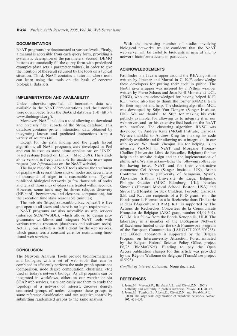
DOCUMENTATION
NeAT programs are documented at various levels. Firstly,a manual is accessible from each query form, providing asystematic description of the parameters. Second, DEMObuttons automatically fill the query form with predefinedexamples (data sets+parameter values), in order to givethe intuition of the result returned by the tools on a typicalsituation. Third, NeAT contains a tutorial, where userscan learn using the tools on the basis of concretebiological data sets.
IMPLEMENTATION AND AVAILABILITY
Unless otherwise specified, all interaction data setsavailable in the NeAT demonstrations and the tutorialswere downloaded from the BioGrid database (14) (http://www.thebiogrid.org/).Moreover, NeAT includes a tool allowing to download
and precisely filter subsets of the String database. Thisdatabase contains protein interaction data obtained byintegrating known and predicted interactions from avariety of sources (40).Except for the path finding and the graph layout
algorithms, all NeAT programs were developed in Perland can be used as stand-alone applications on UNIX-based systems (tested on Linux+Mac OSX). The stand-alone version is freely available for academic users uponrequest (see Informations on the NeAT website).The large majority of NeAT tools allows the treatment
of graphs with several thousands of nodes and several tensof thousands of edges in a reasonable time. Typicalpublished biological networks (a few thousands of nodesand tens of thousands of edges) are treated within seconds.However, some tools may be slower (cliques discovery(NP-hard), betweenness and closeness computation), butthe execution time stays reasonable (minutes).The web site (http://rsat.scmbb.ulb.ac.be/neat/) is free
and open to all users and there is no login requirement.NeAT programs are also accessible as web services
(interface SOAP/WSDL), which allows to design pro-grammatic workflows and integrate NeAT tools withvarious remote resources (databases and software tools).Actually, our website is itself a client for the web services,which guarantees a constant care for maintaining func-tional web services.
CONCLUSION
The Network Analysis Tools provide bioinformaticiansand biologists with a set of web tools that can becombined to efficiently perform the main graph operations(comparison, node degree computation, clustering, etc.)used in today’s network biology. As all programs can beintegrated in workflows, either on our website or viaSOAP web services, users can easily use them to study thetopology of a network of interest, discover denselyconnected groups of nodes, compare these groups tosome reference classification and run negative control bysubmitting randomized graphs to the same analysis.
With the increasing number of studies involvingbiological networks, we are confident that the NeATweb server will be useful to biologists in general and tonetwork bioinformaticians in particular.
ACKNOWLEDGEMENTS
Pathfinder is a Java wrapper around the REA algorithmwritten by Jimenez and Marzal in C. K.F. acknowledgethese developers for putting their code in public. TheNeAT java wrapper was inspired by a Python wrapperwritten by Pierre Schaus and Jean-Noel Monette at UCL(INGI), who are acknowledged for having helped K.F.K.F. would also like to thank the former aMAZE teamfor their support and help. The clustering algorithm MCLwas developed by Stijn Van Dongen (Sanger Institute,UK). We are thankful to Stijn for making his codepublicly available, for allowing us to integrate it in ourweb server, and for his extensive feed-back on the NeATweb interface. The clustering algorithm RNSC wasdeveloped by Andrew King (McGill Institute, Canada).We are thankful to Andrew King for making his codepublicly available and for allowing us to integrate it in ourweb server. We thank Zhenjun Hu for helping us tointegrate VisANT in NeAT and Morgane Thomas-Chollier (Universite Libre de Bruxelles, Belgium) for herhelp in the website design and in the implementation ofphp scripts. We also acknowledge the following colleaguesfor having tested NeAT and for their constructivecomments: Cei Abreu (Sanger Institute, UK), BrunoContreras Moreira (University of Saragossa, Spain),Alexandre Irrthum (Universite de Liege, Belgium),Philippe Gautier (MRC Edimburg, UK), NicolasSimonis (Harvard Medical School, Boston, USA) andShuye Pu (Hospital for Sick Children, Toronto, Canada).S.B. and R.J. are recipients of a PhD grant from theFonds pour la Formation a la Recherche dans l’Industrieet dans l’Agriculture (FRIA). K.F. is supported by TheActions de Recherches Concertees de la CommunauteFrancaise de Belgique (ARC grant number 04/09-307).G.L.M. is a fellow from the Fonds Xenophilia, ULB. Thelaboratory is a member of the BioSapiens Networkof Excellence funded under the sixth Framework programof the European Communities (LSHG-CT-2003-503265).The BiGRe laboratory is supported by the BelgianProgram on Interuniversity Attraction Poles, initiatedby the Belgian Federal Science Policy Office, projectP6/25 (BioMaGNet). Funding to pay the OpenAccess publication charges for this article was providedby the Region Wallonne de Belgique (TransMaze project415925).
Conflict of interest statement. None declared.
REFERENCES
1. Jeong,H., Mason,S.P., Barabasi,A.L. and Oltvai,Z.N. (2001)Lethality and centrality in protein networks. Nature, 411, 41–42.
2. Jeong,H., Tombor,B., Albert,R., Oltvai,Z.N. and Barabasi,A.L.(2000) The large-scale organization of metabolic networks. Nature,407, 651–654.
W450 Nucleic Acids Research, 2008, Vol. 36,Web Server issue

3. Gagneur,J., Jackson,D.B. and Casari,G. (2003) Hierarchical analy-sis of dependency in metabolic networks. Bioinformatics, 19,1027–1034.
4. Croes,D., Couche,F., Wodak,S.J. and van Helden,J. (2006)Inferring meaningful pathways in weighted metabolic networks.J. Mol. Biol., 356, 222–236.
5. Luscombe,N.M., Babu,M.M., Yu,H., Snyder,M., Teichmann,S.A.and Gerstein,M. (2004) Genomic analysis of regulatory networkdynamics reveals large topological changes. Nature, 431, 308–312.
6. Babu,M.M., Luscombe,N.M., Aravind,L., Gerstein,M. andTeichmann,S.A. (2004) Structure and evolution of transcriptionalregulatory networks. Curr. Opin. Struct. Biol., 14, 283–291.
7. Fukuda,K. and Takagi,T. (2001) Knowledge representation ofsignal transduction pathways. Bioinformatics, 17, 829–837.
8. Deville,Y., Gilbert,D., van Helden,J. and Wodak,S.J. (2003) Anoverview of data models for the analysis of biochemical pathways.Brief Bioinform., 4, 246–259.
9. Huber,W., Carey,V.J., Long,L., Falcon,S. and Gentleman,R. (2007)Graphs in molecular biology. BMC Bioinform., 8 (Suppl 6), S8.
10. von Mering,C., Krause,R., Snel,B., Cornell,M., Oliver,S.G.,Fields,S. and Bork,P. (2002) Comparative assessment of large-scaledata sets of protein-protein interactions. Nature, 417, 399–403.
11. Sprinzak,E., Sattath,S. and Margalit,H. (2003) How reliable areexperimental protein-protein interaction data? J. Mol. Biol., 327,919–923.
12. Yook,S.-H., Oltvai,Z.N. and Barabasi,A.-L. (2004) Functional andtopological characterization of protein interaction networks.Proteomics, 4, 928–942.
13. Letovsky,S. and Kasif,S. (2003) Predicting protein function fromprotein/protein interaction data: a probabilistic approach.Bioinformatics, 19 (Suppl 1), i197–i204.
14. Breitkreutz,B.-J., Stark,C., Reguly,T., Boucher,L., Breitkreutz,A.,Livstone,M., Oughtred,R., Lackner,D.H., Bahler,J., Wood,V. et al.(2008) The biogrid interaction database: 2008 update. Nucleic AcidsRes., 36 (Database issue), D637–D640.
15. Mewes,H.W., Amid,C., Arnold,R., Frishman,D., Guldener,U.,Mannhaupt,G., Munsterkotter,M., Pagel,P., Strack,N.,Stumpflen,V. et al. (2004) MIPS: analysis and annotation ofproteins from whole genomes. Nucleic Acids Res., 32 (Database
issue), D41–D44.16. Janky,R. and van Helden,J. (2008) Evaluation of phylogenetic
footprint discovery for predicting bacterial cis-regulatory elementsand revealing their evolution. BMC Bioinform., 9, 37.
17. Scott,J., Ideker,T., Karp,R.M. and Sharan,R. (2006) Efficientalgorithms for detecting signaling pathways in protein interactionnetworks. J. Comput. Biol., 13, 133–144.
18. Bebek,G. and Yang,J. (2007) Pathfinder: mining signal transductionpathway segments from protein-protein interaction networks. BMCBioinform., 8, 335.
19. Rahman,S.A., Advani,P., Schunk,R., Schrader,R. andSchomburg,D. (2005) Metabolic pathway analysis web service(pathway hunter tool at cubic). Bioinformatics, 21, 1189–1193.
20. van Helden,J., Gilbert,D., Wernisch,L., Schroeder,M. andWodak,S. (2001) Applications of regulatory sequence analysis andmetabolic network analysis to the interpretation of gene expressiondata. In O.Gascuel and M.-F.Sagot (eds), Computational Biology :First International Conference on Biology, Informatics, andMathematics, JOBIM 2000. LNCS Vol. 2066, Springer, Montpellier,pp. 155–172.
21. van Helden,J., Wernisch,L., Gilbert,D. and Wodak,S.J. (2002)Graph-based analysis of metabolic networks. Ernst Schering Res.Found.Workshop, 38, 245–274.
22. Croes,D., Couche,F., Wodak,S.J. and van Helden,J. (2005)Metabolic pathfinding: inferring relevant pathways in
biochemical networks. Nucleic Acids Res., 33 (Web Server issue),W326–W330.
23. Jimenez,V. and Marzal,A. (1999) Computing the k shortest paths: anew algorithm and an experimental comparison. Proc. 3rd Int.Worksh. Algorithm Engineering (WAE 1999), 1668, 15–29.
24. Spirin,V. and Mirny,L.A. (2003) Protein complexes and functionalmodules in molecular networks. Proc. Natl Acad. Sci. USA, 100,12123–12128.
25. Han,J.-D.J., Dupuy,D., Bertin,N., Cusick,M.E. and Vidal,M. (2005)Effect of sampling on topology predictions of protein-proteininteraction networks. Nat. Biotechnol., 23, 839–844.
26. Brohee,S. and van Helden,J. (2006) Evaluation of clusteringalgorithms for protein-protein interaction networks. BMCBioinform., 7, 488.
27. Milenkovic,T., Lai,J. and Przulj,N. (2008) Graphcrunch: a tool forlarge network analyses. BMC Bioinform., 9, 70.
28. Hu,Z., Ng,D.M., Yamada,T., Chen,C., Kawashima,S., Mellor,J.,Linghu,B., Kanehisa,M., Stuart,J.M. and DeLisi,C. (2007) Visant3.0: new modules for pathway visualization, editing, prediction andconstruction. Nucleic Acids Res., 35 (Web Server issue),W625–W632.
29. Shannon,P., Markiel,A., Ozier,O., Baliga,N.S., Wang,J.T.,Ramage,D., Amin,N., Schwikowski,B. and Ideker,T. (2003)Cytoscape: a software environment for integrated models ofbiomolecular interaction networks. Genome Res., 13, 2498–2504.
30. Gene Ontology Consortium. (2008) The Gene Ontology project in2008. Nucleic Acids Res., 36 (Database issue), D440–D444.
31. Sharan,R., Ulitsky,I. and Shamir,R. (2007) Network-based predic-tion of protein function. Mol. Syst. Biol., 3, 88.
32. Krogan,N.J., Cagney,G., Yu,H., Zhong,G., Guo,X.,Ignatchenko,A., Li,J., Pu,S., Datta,N., Tikuisis,A.P. et al. (2006)Global landscape of protein complexes in the yeast Saccharomycescerevisiae. Nature, 440, 637–643.
33. Pereira-Leal,J.B., Enright,A.J. and Ouzounis,C.A. (2004) Detectionof functional modules from protein interaction networks. Proteins,54, 49–57.
34. Enright,A.J., Dongen,S.V. and Ouzounis,C.A. (2002) An efficientalgorithm for large-scale detection of protein families. Nucleic AcidsRes., 30, 1575–1584.
35. Lattimore,B.S., van Dongen,S. and Crabbe,M.J.C. (2005) Genemclin microarray analysis. Comput. Biol. Chem., 29, 354–359.
36. Van Dongen,S. (2000) Graph clustering by flow simulation. Ph.D.Thesis. Centers for Mathematics and Computer science (CWI),University of Utrecht.
37. King,A.D., Przulj,N. and Jurisica,I. (2004) Protein complexprediction via cost-based clustering. Bioinformatics, 20, 3013–3020.
38. Lima-Mendez,G., van Helden,J., Toussaint,A. and Leplae,R. (2008)Reticulate representation of evolutionary and functional relation-ships between phage genomes. Mol. Biol. Evol., 25, 762–777.
39. Gavin,A.-C., Aloy,P., Grandi,P., Krause,R., Boesche,M.,Marzioch,M., Rau,C., Jensen,L.J., Bastuck,S., Dumpelfeld,B. et al.(2006) Proteome survey reveals modularity of the yeast cellmachinery. Nature, 440, 631–636.
40. von Mering,C., Jensen,L.J., Kuhn,M., Chaffron,S., Doerks,T.,Kruger,B., Snel,B. and Bork,P. (2007) String 7-recent developmentsin the integration and prediction of protein interactions. NucleicAcids Res., 35 (Database issue), D358–D362.
41. Uetz,P., Giot,L., Cagney,G., Mansfield,T.A., Judson,R.S.,Knight,J.R., Lockshon,D., Narayan,V., Srinivasan,M., Pochart,P.et al. (2000) A comprehensive analysis of protein-protein interac-tions in Saccharomyces cerevisiae. Nature, 403, 623–627.
42. Ito,T., Chiba,T., Ozawa,R., Yoshida,M., Hattori,M. and Sakaki,Y.(2001) A comprehensive two-hybrid analysis to explore the yeastprotein interactome. Proc. Natl Acad. Sci. USA, 98, 4569–4574.
Nucleic Acids Research, 2008, Vol. 36,Web Server issue W451

Network Analysis Tools: from biological networks toclusters and pathwaysSylvain Brohee, Karoline Faust, Gipsi Lima-Mendez, Gilles Vanderstocken & Jacques van Helden
Laboratoire de Bioinformatique des Genomes et des Reseaux (BiGRe), Universite Libre de Bruxelles, Campus Plaine, CP 263, Boulevard du Triomphe, B-1050 Bruxelles,Belgium. Correspondence should be addressed to J.v.H. ([email protected]).
Published online 18 September 2008; doi:10.1038/nprot.2008.100
Network Analysis Tools (NeAT) is a suite of computer tools that integrate various algorithms for the analysis of biological networks:
comparison between graphs, between clusters, or between graphs and clusters; network randomization; analysis of degree
distribution; network-based clustering and path finding. The tools are interconnected to enable a stepwise analysis of the network
through a complete analytical workflow. In this protocol, we present a typical case of utilization, where the tasks above are combined
to decipher a protein–protein interaction network retrieved from the STRING database. The results returned by NeAT are typically
subnetworks, networks enriched with additional information (i.e., clusters or paths) or tables displaying statistics. Typical networks
comprising several thousands of nodes and arcs can be analyzed within a few minutes. The complete protocol can be read and
executed in B1 h.
INTRODUCTIONThis is the last article in a series of four protocols for the analysis ofregulatory sequences with the Regulatory Sequence Analysis Tools1
(http://rsat.ulb.ac.be/rsat/) and biological networks with theNetwork Analysis Tools (NeAT)2 (http://rsat.ulb.ac.be/neat/). Thefirst article3 presents a protocol to predict the location of bindingsites for transcription factors whose specificity is already known(pattern matching). In the second article4, we describe a protocolfor the ab initio discovery of biological signals in biologicalsequences (pattern discovery). The third article5 shows how towrite scripts to automate the analysis on multiple clusters of genesusing Web services. In this article, we describe a workflow fordeciphering biological networks by combining network compar-ison, module identification and path finding. This protocol can beexecuted independently of the three other ones.
Network biology is emerging as a new field in biology, due to theincreasing availability of genome-scale data sets of molecularinteractions, such as those resulting from high-throughputtechnologies (e.g., protein interactions, regulatory networks andmetabolome). Extracting relevant information from this hugeamount of data requires dedicated tools. These data sets arecommonly represented as graphs (or networks), where nodesrepresent molecules, and arcs their interactions. This representationeases data integration and makes it possible to apply well-knownnetwork algorithms to analyze the data.
In this protocol, we show how large biological networks can beexplored by combining a set of modular tools accessible via a Webinterface named NeAT. We describe hereafter the typical questionsthat can be addressed.Network topology. It has been observed that some topological
properties distinguish biological networks from randomnetworks6,7. Noticeably, the distribution of degree (the number ofarcs connected per nodes) is often claimed to follow a power-lawdistribution6,8. The tool graph-topology can be used to analyze thedegree distribution of any kind of network.Network comparison. Given two networks (i.e., protein–proteininteraction networks from two different experiments), one wouldlike to analyze their degree of overlap. This question is answered by
the tool compare-graphs, which computes the intersection, unionand difference between two networks and estimates the statisticalsignificance of the overlap.Node neighborhood. Given a protein, gene or another node in a
biological network, it is of interest to identify its direct orindirect neighbors in this network. This is the task of the toolgraph-neighbours, which returns the neighbors of a query node ina network up to a certain distance. This tool can be applied forinstance on protein–protein interaction networks to retrieve theinteraction partners of a given protein.Cluster analysis. Various algorithms have been implemented to
extract clusters (i.e., groups of densely connected nodes) frombiological networks9–13. Among those, MCL14 algorithm has beenshown to obtain good performances for extracting proteincomplexes from protein interaction networks15–17. In addition,this algorithm can deal with large graphs and is very efficient intime. For these reasons, we included MCL in the NeAT suite. Theclusters resulting from MCL or other methods can be compared tosome reference groups (e.g., functional classes) with the programcompare-classes and mapped onto networks with graph-get-clusters. Upon partitioning with MCL, each node belongs to onlyone cluster. However, sometimes the assignment of a node to asingle cluster is an over-simplification of the biological data, forexample, a protein may be part of different protein complexes. Inthose cases, it would be better to describe how much each node isrelated to the different clusters. The program graph-cluster-membership postprocesses a clustering result and calculates themembership as the proportion of edges (or weight) linking eachnode to each cluster. The node–cluster relationships are describedas a membership matrix, where each row represents a node andeach column a cluster.Path finding. Given a biological network and two nodes of interest,
a common task is to find a biological meaningful path connectingthose nodes in the network. For instance, path-finding algorithmsare applied to uncover signal transduction or metabolic pathwaysin protein–protein interaction or metabolic networks, respec-tively18–21. Recently, we evaluated the performance of a k-shortest
p
uor
G g
n ih si l
bu
P eru ta
N 800 2©
nat
ure
pro
toco
ls/
moc.er
ut an.
ww
w//:ptt
h
1616 | VOL.3 NO.10 | 2008 | NATURE PROTOCOLS
PROTOCOL

path-finding algorithm for metabolic pathway inference and foundhigh accuracies if appropriate weights are set on the network22.Network randomization. Negative controls are essential to esti-
mate the relevance of the results. The tool random-graph proposesdifferent procedures to randomize a network, which can then besubmitted to the same workflows as the original network.Network alteration. To test the robustness of analytic methods to
the presence of noise, or to the incompleteness of information, thetool alter-graph allows to modify an existing network by randomaddition or deletion of nodes and/or edges.Network display. NeAT includes a tool called display-graph,
which generates static images of the input networks. Such drawingsare convenient for a quick inspection of the results from the Webbrowser. For more sophisticated layouts and for a dynamicalmanipulation of the drawing, we recommend graph editors suchas yEd (http://www.yworks.com/en/products_yed_about.html) orCytoscape23. The tool convert-graph permits to export any networkanalyzed with NeAT into Graph Modeling Language (GML)(http://www.infosun.fim.uni-passau.de/Graphlet/GML/gml-tr.html),a file format supported by both editors.Figure 1 depicts the way in which the NeAT can be connected.
We suggest the reader to follow this flow chart progressively duringthe execution of the protocol.
Comparison to other graph analysis tool suitesA large variety of graph analysis tools exist. We may classify them inthree categories: (i) libraries that can only be used programmati-cally, for example, Boost (http://www.boost.org/), igraph (http://cneurocvs.rmki.kfki.hu/igraph/index.html) or JUNG (http://jung.sourceforge.net/); (ii) stand-alone tools with graphical userinterface (GUI) (Pajek24, Network Workbench (http://nwb.slis.indiana.edu), BiologicalNetworks25, VisANT26, yEd, Cytoscape,etc.) and (iii) tools with GUI available via the Web such as tYNA(http://tyna.gersteinlab.org/tyna/) or CABiNeT (http://mips.gsf.de/genre/proj/CABiNet/).
Usually, the libraries offer generic graph algorithms, whereasstand-alone or Web-based tool suites are often specialized. Forinstance, VisANT, Cytoscape (with its plugins) and BiologicalNet-works focus on the analysis and display of biological networks,whereas yEd offers a flexible interface for the display, layout andedition of general-purpose graphs, but is equipped with limitedanalysis functions. Pajek and Network Workbench are stand-alonetools for generic graph analysis. Cytoscape (with plugins) andBiologicalNetworks allow in addition retrieval and integration ofbiological networks.
We describe hereafter some of the advantages and currentlimitations of NeAT.Main advantages. The main advantages of NeAT are
(1) NeAT supports a variety of modular tools, which can either beused separately, or combined in a workflow. These toolsinclude a number of unique features (fuzzy clustering, Webaccess to MCL and RNSC, k-shortest paths with multiple startand end nodes, statistical comparison of classes and clusters,etc.) that are currently not available in other packages.
(2) The programs are designed to enable treating very large graphs(several thousands of nodes) without excessive cost in memoryor time.
(3) Although most of the analyses can also be performed inspecialized software packages such as R, the NeAT Web site
offers a user-friendly access for biologists who are not familiarwith programming languages.
(4) NeAT can be run on command line, either by installing it locallyor by calling Web services. This is not the case of the other stand-alone and Web-based tools (a notable exception is Pajek). Theprogrammatic access (either as stand-alone application or asWeb services) allows one to automate the executions of work-flows for multiple data sets, which would require hundreds orthousands of manual operations with conventional GUIs or on aWeb site. To our knowledge, there is only one other networktools suite enabling workflows, namely tYNA. NeAT and tYNAare complementary: NeAT supports path-finding, graph-basedclustering (MCL, RNSC and fuzzy clustering), network rando-mization and cluster comparisons, whereas tYNA includes toolsto find motifs in networks. Because both tools support Webservices, they can be easily combined in workflows, either byprogramming client scripts or using GUIs such as Taverna27.
(5) NeAT may be used for any kind of network, but it wasdeveloped with biological networks in mind. The tools havebeen extensively tested on a variety of biological networks(protein–protein interaction networks17, evolutionary net-works28 and metabolic networks21,22). Extensive evaluation israrely reported for other biological network tools suites.
Main limitations. NeAT essentially provides facilities for theanalysis of networks, clusters and pathways, but is not focused on
pu
orG
gn i
h si lb
uP er
u taN 800 2
©n
atu
rep
roto
cols
/m
oc.erut a
n.w
ww//:
ptth
Flow chart of NeAT demo workflow
MIPScomplexes
Steps 4–10Steps 27–36
Steps 11–15
Steps 20 and 21Steps 22–26
Steps 37–39 Steps 40–46
PathfinderRandom-graph
Compare- graphs
Network intersection
Randomizednetwork
Convert-graph
Compare-classes
MCL
Node clustermemberships
Graph-get-clusters
Display-graph
Graph-cluster-
member-ship
Clustered graph
Steps 16 and 17
Netwokimage
Fuzzy clustermembership
matrix
Sortablecomparison
table
Interactivenetwok
display in yEdor Cytoscape
Networkof paths
Sortablepathstable
Input/outputToolUser date
Legend
Yeast STRINGnetwork
Yeast syntheticlethality BioGRID
network
Figure 1 | Flow chart of the data, tools and results described in this protocol.
Yellow represents the data set, orange the tool and light brown the results.
NATURE PROTOCOLS | VOL.3 NO.10 | 2008 | 1617
PROTOCOL

the problem of network visualization. This limitation, however, iseasily circumvented by installing some specialized visualizationsoftware: all graphs generated by NeAT can be exported to severalformats, including GML, which can be loaded with Cytoscape, yEdand VisANT, and DOT, which can be loaded with Graphviz.
To summarize, NeAT addresses the needs of researchersinterested in the analysis of biological networks. Some tools mayrequire background knowledge (e.g., MCL, fuzzy clustering),whereas others are intuitive and easy to use (e.g., graph conversionand comparison).
For the user with experience in programming, NeAT can be runon command line or within workflow management environmentssuch as Taverna. Otherwise, the user may access NeAT via its Webinterface, guided by tutorials and demos. To our knowledge,
no other biological network tools suite exists that combines allthe features of NeAT.
Other applications of this protocolFor the sake of consistency, the cases treated in this protocol arerestricted to protein interaction networks. The tools available inNeAT can also be used to analyze other types of biological networksrepresenting other types of interactions, for example, regulation,signal transduction, metabolic reactions, and ecology. The fuzzyclustering approach was initially conceived to address the problemof classifying phage genomes while taking into account the frequentexchanges of genetic material between them28. The k-shortest path-finding algorithm has previously been applied to infer relevantpathways in metabolic networks29,30.
MATERIALSEQUIPMENT.This protocol describes an online tool. The only requirement is a computer
with Internet connection. Optionally, you can install yEd (http://www.yworks.com/) or Cytoscape23 for visualization
.Sample interaction networks, which can be obtained from various biologicaldatabases. As examples, we cite the following:.STRING31 (http://string.embl.de/), a database integrating seven different
types of evidences for physical and/or functional interactions betweenproteins: experimental evidences, phylogenetic profiles (‘co-occurrence’),gene fusion/fission, synteny (‘neighborhood’), coexpression, text miningand a data set called ‘database’, regrouping several criterion selected by theSTRING annotation team
.BioGRID32 (http://www.thebiogrid.org/), a database of protein and geneticinteractions including 4116,000 curated interactions from yeast,Caenorhabditis elegans, drosophila and human
.BioCyc33 (http://www.biocyc.org/) or KEGG34 (www.genome.jp/kegg/), thetwo main metabolic pathway databases
.The data required for the study cases treated in this protocol is available inthe data repository site: http://rsat.ulb.ac.be/nedt/. All the networks used toillustrate this protocol were taken from the yeast Saccharomyces cerevisiae.We selected various networks representing diverse types of interactionsbetween biological molecules (protein interactions, metabolism, proteincomplexes, genetic interactions, etc.).Protein–protein interactions (physical and functional). From the STRING
database31, we extracted a subset labeled as ‘database’ by the STRING team.Under this label, they regrouped different types of protein–protein interactions
and metabolic relationships (Jensen L., personal communication). Thisnetwork contains 1,237 nodes representing proteins, and 11,027 edgesrepresenting a mixture of physical and functional protein–protein interactions.The interactions between two proteins are considered symmetrical; it is anundirected graph. The network is stored in data repository, a tab-delimitedtext file named yeast_string_database_graph_names_undirected.tab
.The synthetic lethality network was extracted from the BioGRIDdatabase32. It represents genes (2,353 nodes) whose individual deletion isviable, but whose paired deletions (12,419 edges) are lethal
.Protein complexes. The file mips_complexes_names.tab describes thecollection of protein complexes annotated in the MIPS database35.Complexes detected only by high-throughput experiments were discardedfrom the data set. The first column of the file gives the gene name, thesecond column the complex name and the third column the gene identifier.In total, the file contains 1,121 distinct proteins forming 243 distinctcomplexes. Note that a protein can belong to several complexes
.Signal transduction pathway. As study case for the path finding, we take ayeast signal transduction pathway mentioned by Scott and colleagues18.This pathway, known to regulate filamentous growth in yeast, starts withRAS2 and ends with TEC1. The authors attempt to recover this pathwaywith a path-finding algorithm based on color coding18. We will try torecover it using Pathfinder
. Incompatibility between file formats is a constant problem in bioinformatics.To facilitate the use of the Web site, most tools support several among themost popular formats used to describe networks. A description of thesupported format is given in Box 1
p
uor
G g
n ih si l
bu
P eru ta
N 800 2©
nat
ure
pro
toco
ls/
moc.er
ut an.
ww
w//:ptt
h
BOX 1 | MAIN GRAPH FORMATS
The tab-delimited format is a convenient and intuitive way to encode a graph. Each row represents an edge and each column an attribute ofthis edge. The two column fields are the source and target nodes. If the graph is directed, the source node is the node from which the arc leavesand the target node is the node to which the arc arrives. Logically, in undirected graph, the columns containing the source and the target nodesmay be swapped. Orphan nodes can be included by specifying a source node without target. Some additional edge attributes (weight, label,color) can be placed in additional columns. The tool Pathfinder extends this format by supporting any number of attributes on nodes or edges.Check the Pathfinder help page for more details.The GML format allows for the specification of additional layout and display attribute, such as node position, as well as the color, the label andthe width of nodes and edges. A Graph Modeling Language (GML) file is made up of nested key-value pairs. The most popular graph editors(such as Cytoscape and yEd) support GML as input format.The DOT format is a plain text graph description language. DOT files can be loaded in the programs of the suite Graphviz (http://www.graphviz.org/). It is a simple way of describing graphs in a human- and computer-readable format. Similar to GML, DOT supportsvarious attributes on nodes (i.e., color, width, label).Several tools also accept adjacency matrices as input. An adjacency matrix is an N � N table (with N the number of nodes), where a cell A[i,j]indicates the weight of the edge between nodes i and j (or 1 if the graph is unweighted).The Network Analysis Tools program convert-graph facilitates the handling of these formats by supporting interconversions between variousinput (tab, gml, adjacency) and output formats (tab, dot, gml, adjacency).
1618 | VOL.3 NO.10 | 2008 | NATURE PROTOCOLS
PROTOCOL

PROCEDUREDownloading a sample network1| We will show on an example workflow how the different tools of NeAT can be combined to analyze a network taken fromthe STRING database. Open a connection to the data repository for this protocol (see EQUIPMENT).
2| Download the network file yeast_string_database_graph_names_undirected.tab on your computer. It is described in atab-delimited file that contains five columns. Each row represents one interaction between two genes or between their products.As described in Box 1, the two first columns indicate the name of the Source and Target genes/proteins of the source and targetnodes. The third column contains a score ranging from 0 to 900, which reflects the reliability of the indications available forthis interaction. Higher scores represent more reliable interactions. In this case, the score is higher if an interaction is foundseveral times in different data set. The columns 4 and 5 contain the gene identifiers corresponding to the gene names incolumns 1 and 2.
3| Open a connection to the NeAT Web server: http://rsat.ulb.ac.be/neat/.
Cluster analysis4| Extracting clusters from the network with MCL (Steps 4–10). We will first apply graph-based clustering to detect groups ofhighly interconnected nodes in the sample network. For this, we will use the MCL algorithm, a fast unsupervised clusteringalgorithm based on simulation of flows in graphs14. In the menu from the left panel, click on the link MCL clustering to openthe MCL query form.
5| Click on the Browse . . . button, and choose the file containing the network (e.g., yeast_string_database_graph_names_undirected.tab for the study case discussed here).
6| Specify the columns containing the source, target and (optionally) weight attributes of the tab-delimited file. In ourexample file, the source and target columns are by default 1 and 2 so we only have to add the weight column:Weight column ¼ 3. Note that if you want to work with the gene identifiers instead of the gene names, you could have usedvalue 4 and 5 in the source and target column fields. However, this is not recommended in this protocol as in the following wewill only work with gene names.m CRITICAL STEP The weighting of edges strongly affects the MCL result, because the principle of the algorithm is to iterativelyenforce the weight of the most ‘important’ edges in the network. The ‘importance’ of an edge is determined by both its initial weightand its place in the network.
7| Choose an inflation value (between 1.2 and 5). For the study case, select 1.8.m CRITICAL STEP This parameter acts on the granularity of the clustering procedure, that is, the number of clusters (andconsequently the number of elements per cluster). The number of clusters increases with the inflation value. This parameter mustthus be fine-tuned according to the structure of the network. In a recent evaluation, we found that an inflation value of 1.8 wasoptimal for protein–protein interaction networks17.
8| Click on the GO button. The processing should take a bit less than one 1 min.? TROUBLESHOOTING
9| The result page displays a figure showing the cluster size distribution, that is, the number of clusters (ordinate) of eachsize (abscissa). The page also contains a link to the clustering result. This file can be saved by right-clicking on the URL linkand selecting Save link as . . ., and save it on your computer under the name yeast_string_MCL_clusters.tab.
10| To inspect the result file, you can either use a text editor to open the file yeast_string_MCL_clusters.tab stored onyour computer, or click on the URL on the result page. The MCL result is a simple two-column table, where the first columnindicates the node names (gene names in our case), and the second column the cluster names. A quick inspection of this tablefrom top to bottom shows that the first clusters contain more nodes than the last ones. MCL sorts the clusters by decreasingorder of size.
11| Extracting the subnetwork defined by the clusters (Steps 11–17). We will now map the clusters resulting from MCL onto theiroriginal network. For this, there are two alternative ways to proceed: directly load the files stored on the server (option A) ortransfer the network and cluster files from your computer (option B).(A) Directly load the files stored on the server
(i) The MCL result page displays a ‘Next step’ box, allowing you to send the MCL output to several alternative tools. Click thebutton Map those cluster on the network. This will call a form graph-get-clusters, with prefilled values for the parametersGraph and Clusters.
p
uor
G g
n ih si l
bu
P eru ta
N 800 2©
nat
ure
pro
toco
ls/
moc.er
ut an.
ww
w//:ptt
h
NATURE PROTOCOLS | VOL.3 NO.10 | 2008 | 1619
PROTOCOL

(B) Transfer the network and cluster files from your computer(i) An alternative way to enter data in the tool graph-get-clusters is to click on the link ‘Map clusters onto network’ in the
left menu. This will open an empty form, in which you will have to enter the data (for our study case, the graph is inthe file yeast_string_database_graph_names_undirected.tab and the clusters in the file yeast_string_MCL_clusters.tab).However, this would require to transfer those two files to the server, albeit it already contains a copy of both in thetemporary directory. Whenever possible, you should thus use the ‘Next step’ buttons rather than transferring the files backand forth between your computer and the server.
12| The main choice for the tool graph-get-clusters is the output type. The program supports two types of operations betweenthe network and the clusters. (i) The option annotated graph labels each edge according to its intracluster or interclusternature. (ii) intracluster edges selects a subnetwork restricted to the intracluster edges (intercluster edges are simply deletedfrom the network). You can experiment the three options. In this section of the protocol, we will extract the subnetworkdefined by the MCL clusters. For this, select the option intracluster edges.
13| Several output formats are proposed, but for the visualization purpose, select the intracluster edges output in theGML format.
14| Click on the button GO.
15| The result page should appear after o1 min, displaying a set of buttons for postprocessing the graph-get-cluster result,and a link toward the result file. You can store the resulting GML graph on your computer for later use by right-clicking on theURL in the graph-get-clusters result page. Save the result in afile named yeast_string_MCL_intra_cluster.gml.
16| A quick way to visualize the result is to fetch it to theNeAT visualization tool. However, beware that this tool offerslimited functionalities: it returns a static image, with a sim-plistic layout. The main function of this tool is to provide aquick view of the result, before visualizing it with specializedtools. To visualize the result network with NeAT, click on thebutton Display the graph. A new form will then be displayed.Select the desired output format. If the network is weighted(e.g., our study case), you can activate the option Edge widthproportional to the weight. To obtain the figure, click on thebutton GO. This process may be slow (41 min) depending onthe size of the graph.
17| For a better visualization of the network, open the GMLformatted file obtained in Step 15 with Cytoscape, yEd or anyother visualization program of your choice. After havingopened the GML file, you need to apply some layout to displaynodes and edges harmoniously. For yEd and Cytoscape werecommend the option Organic layout. After this, you shouldsee a set of well-separated components, each corresponding toa MCL cluster. Each cluster is displayed with a specific color forthe edges (Fig. 2a).? TROUBLESHOOTING
18| Mapping the clusters onto the network (Steps 18 and 19).In the previous section, we used graph-get-clusters to sepa-rate the MCL clusters by deleting intercluster edges from theoriginal network. Alternatively, the same tool can be used tolabel all the edges according to the cluster composition.Come back to Step 12, but this time, select ‘annotated graph(all edges)’ as output type.
19| Repeat Steps 13–17, and compare visually the result withthat obtained in the previous section (Fig. 2b).
p
uor
G g
n ih si l
bu
P eru ta
N 800 2©
nat
ure
pro
toco
ls/
moc.er
ut an.
ww
w//:ptt
h
a
b
Figure 2 | Mapping of the clusters obtained with the MCL algorithm on the
STRING database data set. (a) Only the intracluster edges were conserved and
each cluster is highlighted with a different color. (b) Intercluster (black) and
intracluster (colored) edges are both displayed. The layout and display were
obtained with yEd.
1620 | VOL.3 NO.10 | 2008 | NATURE PROTOCOLS
PROTOCOL

Fuzzy clustering20| We will now use the tool graph-cluster-membership to compute the degree of membership of each node to each of thecluster obtained from MCL. This can be done in either of two ways. (i) Come back to the page with the MCL output and click on‘Cluster membership’ to open graph-cluster-membership. (ii) Alternatively, you can click on the link Cluster membership inthe left panel, and specify the graph parameters as in Steps 5 and 6. To upload the MCL output, click on the button besides‘Upload clusters from file’: and specify the location of the file yeast_string_MCL_clusters.tab on your disk.
21| Search for the membership matrix and select weight as stat.m CRITICAL STEP For weighted graphs, weight or relative weight may be chosen. Otherwise, the strength of the links is notconsidered for calculating the membership of a node to a cluster. When relative weight or relative edge is selected, the weights ornumber of edges of a node to a cluster are divided by the number of nodes of that cluster.
22| Click on the GO button. After a minute, a page appears with links to three files: a tab-delimited text file, and two imagefiles providing, respectively, low- and high-resolution heatmaps. In all cases, the output displays the membership matrix,where entries correspond to the membership degree of the node given by the row to the cluster given by the column. Thetext-formatted table contains the numeric values of the memberships coefficient associating each node (row) to each cluster(column). This is a tab-delimited file that can be loaded in various programs (e.g., Excel, R) for further processing. The heatmapis a graphical representation of the same data, where the gray level is proportional to the degree of membership (Fig. 3).? TROUBLESHOOTING
23| Comparing the clusters with reference classes (Steps 23–27). To evaluate the biological relevance of the clusters discoveredwith MCL, we can compare them with some reference classification, for example the Gene Ontology36 or the collection of proteincomplexes from the MIPS database. To illustrate this, we will compare the MCL clusters obtained above with the complexesstored in the MIPS database. Each MCL cluster will be compared to each complex of the database. Cluster/complex comparisonswill then be scored with different statistics described in the manual page of the tool and in Box 2. Come back to the page withthe MCL result (Step 9). On in the Next step box, click on the button ‘Compare these clusters with other clusters’. Alternatively,in case you saved the MCL result in a file, you can directly click on the link Compare clusters/classes in the left panel andupload the MCL result file with the Browse button under query class.
24| As reference classes, we will use the collection of MIPS complexes. For this, first download the file mips_complexes_names.tab from the data repository (see EQUIPMENT).
25| We will now specify the reference classes in the compare-classes form. To indicate that MIPS complexes will serve asreference classes, click on the Browse . . . button below Reference classes, and select the file mips_complexes_names.tab thatyou downloaded on your computer at Step 24. In NeAT, classes are described with the same tab-delimited format as clusters:each row describes the membership ofone element (first column) to a class(second column). Optionally, an addi-tional column can be specified with theoption ‘Score column’, to indicate ascore that will be used to compute somesimilarity metrics (e.g., dot product).For this study case, the MIPS complexesare described in a three-column fileindicating the protein name (first col-umn), the complex (second column) andthe gene ID (third column). There is noscore associated to the protein-complexmembership, and we will thus leaveempty the option score column.
26| The options Thresholds on returnfields (see Box 2) allow one to combinevarious constraints to select the mostsignificant intersections between queryand reference clusters/classes. Thedefault threshold on significance(sig Z 0) usually gives satisfactoryresults. For our study case, the otherthresholds do not need to be changed.
p
uor
G g
n ih si l
bu
P eru ta
N 800 2©
nat
ure
pro
toco
ls/
moc.er
ut an.
ww
w//:ptt
h
EFB1 1.00
cl_1
cl_2
cl_3
cl_4
cl_5
cl_6
cl_7
cl_8
cl_9
cl_1
0
cl_1
1
cl_1
2
cl_1
3
cl_1
4
cl_1
5
cl_1
6
cl_1
7
cl_1
81.00
0.00 0.83 0.05
0.05
0.00
0.00
0.00
0.00
0.00
0.00
0.00
0.00
0.00
0.00
0.00
0.00
0.00
0.00
0.00
0.10
0.00
0.00
0.00 0.43
0.00
0.00 0.00
0.00
0.00
0.00
0.00
0.00
0.00
0.00
0.00
0.00
0.00
0.00
0.43
0.00
0.00
0.00
0.00
0.00
0.00
0.00
0.00
0.00
0.00
0.00
0.00
0.00
0.00
0.00
0.00 0.00
0.00
0.00
0.00
0.00
0.00 0.00 0.00
0.00 0.05
0.00 0.00
0.00 0.05
0.00
0.00
0.00
0.00
0.00
0.00
0.00
0.00
0.00
0.00
0.00
0.00
0.00
0.00
0.00
0.00
0.00
0.00
0.00
0.00
0.00
0.00
0.00
0.00
0.00
0.00
0.00
0.00
0.00
0.00
0.00
0.00
0.00
0.00
0.00
0.00
0.00
0.00
0.00 0.04
0.00
0.00
0.00
0.00
0.00
0.00
0.00
0.00
0.00
0.00
0.00 0.33
0.00 0.00
0.00 0.04 0.04
0.00
0.00
0.00
0.00
0.00 0.02 0.02
0.00
0.00
0.00
0.00
0.00
0.00
0.00
0.00
0.00 0.00
0.00
0.00
0.00
0.00
0.00
0.00
0.00
0.00
0.00
0.00
0.00
0.00
0.00
0.00
0.00
0.00
0.00
0.00
0.00
0.00
0.02 0.01
0.02
0.00
0.00
0.00
0.00
0.00
0.00
0.00
0.00
0.00
0.00
0.00
0.00
0.00
0.00
0.00
0.00
0.00
0.00
0.00
0.00
0.00
0.00
0.00
0.00
0.00
0.00
0.00
0.00
0.00
0.00
0.00
0.00
0.00
0.00
0.00
0.00
0.00
0.00
0.00
0.00
0.00
0.00
0.00
0.00
0.00
0.00
0.00
0.00
0.00
0.00
0.00
0.00
0.00
0.00
0.00
0.00
0.00
0.00
0.00
0.00
0.00
0.00
0.00
0.00
0.00
0.00
0.00
0.00
0.00
0.00
0.00
0.00
0.00
0.00
0.00
0.00
0.00
0.00
0.00
0.00
0.00
0.00
0.00
0.00
0.00
0.00
0.00
0.00 0.00
0.00 0.08
0.08
0.08
0.00
0.00
0.00
0.00
0.00
0.00
0.00
0.00
0.00
0.00
0.00
0.00
0.00
0.00
0.00
0.00
0.00
0.00
0.00
0.00
0.00
0.00
0.00
0.00
0.00
0.00
0.00
0.00
0.00
0.00
0.10
0.74
1.00
0.77
0.92
1.00
0.57
0.95
1.00
0.57
0.96
1.00
1.00
1.00
1.00
1.00
0.67
1.00
0.00 0.00 0.00 0.00 0.00 0.00 0.00 0.00 0.00 0.00 0.00 0.00 0.00 0.00 0.00 0.00
0.000.000.000.000.000.000.000.000.000.000.000.000.000.000.000.000.00
0.00
0.00
0.00
0.00
0.00
0.00
0.00
0.00
0.00
0.00
0.00
0.00
0.00
0.00
0.00
0.00
0.00
0.00
RPL19B...
PDA1
LPD1
LEU1
PYC1
RPB9
RNR4
ENO1
FOL2
RPC10
EN02
RPB3
RNR3
CYR1
RNR2
RPB4
RPB34
HYS2
POL32
...
Figure 3 | Fuzzy-clusters obtained by combining MCL and the graph-cluster-membership tools. The
section of the heatmap shows that several proteins have cluster membership percentages larger than zero
for several clusters; for example, ENO1 belongs to both clusters cl_2 (57%) and cl_5 (43%).
NATURE PROTOCOLS | VOL.3 NO.10 | 2008 | 1621
PROTOCOL
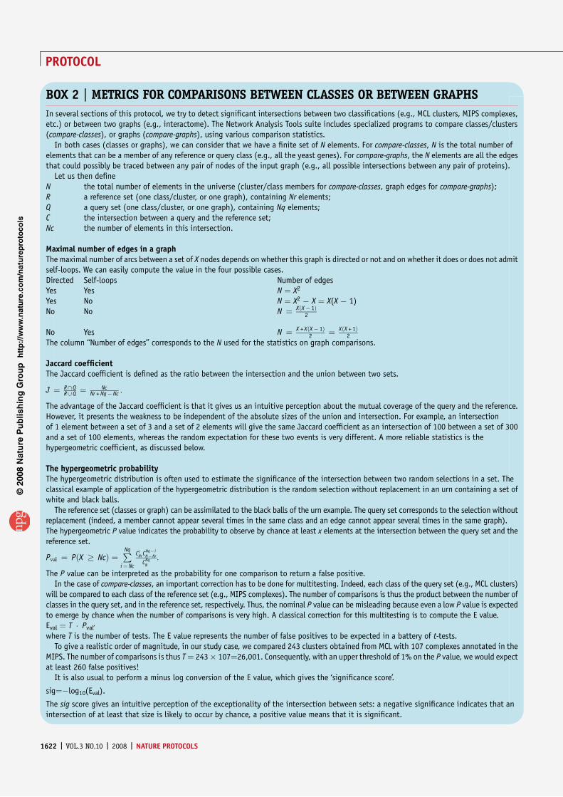
p
uor
G g
n ih si l
bu
P eru ta
N 800 2©
nat
ure
pro
toco
ls/
moc.er
ut an.
ww
w//:ptt
h
BOX 2 | METRICS FOR COMPARISONS BETWEEN CLASSES OR BETWEEN GRAPHS
In several sections of this protocol, we try to detect significant intersections between two classifications (e.g., MCL clusters, MIPS complexes,etc.) or between two graphs (e.g., interactome). The Network Analysis Tools suite includes specialized programs to compare classes/clusters(compare-classes), or graphs (compare-graphs), using various comparison statistics.
In both cases (classes or graphs), we can consider that we have a finite set of N elements. For compare-classes, N is the total number ofelements that can be a member of any reference or query class (e.g., all the yeast genes). For compare-graphs, the N elements are all the edgesthat could possibly be traced between any pair of nodes of the input graph (e.g., all possible intersections between any pair of proteins).
Let us then defineN the total number of elements in the universe (cluster/class members for compare-classes, graph edges for compare-graphs);R a reference set (one class/cluster, or one graph), containing Nr elements;Q a query set (one class/cluster, or one graph), containing Nq elements;C the intersection between a query and the reference set;Nc the number of elements in this intersection.
Maximal number of edges in a graphThe maximal number of arcs between a set of X nodes depends on whether this graph is directed or not and on whether it does or does not admitself-loops. We can easily compute the value in the four possible cases.Directed Self-loops Number of edgesYes Yes N ¼ X2
Yes No N ¼ X2 � X ¼ X(X � 1)No No N ¼ XðX � 1Þ
2
No Yes N ¼ X + XðX � 1Þ2 ¼ XðX + 1Þ
2
The column ‘‘Number of edges’’ corresponds to the N used for the statistics on graph comparisons.
Jaccard coefficientThe Jaccard coefficient is defined as the ratio between the intersection and the union between two sets.
J ¼ R\ QR[ Q ¼ Nc
Nr + Nq� Nc :
The advantage of the Jaccard coefficient is that it gives us an intuitive perception about the mutual coverage of the query and the reference.However, it presents the weakness to be independent of the absolute sizes of the union and intersection. For example, an intersectionof 1 element between a set of 3 and a set of 2 elements will give the same Jaccard coefficient as an intersection of 100 between a set of 300and a set of 100 elements, whereas the random expectation for these two events is very different. A more reliable statistics is thehypergeometric coefficient, as discussed below.
The hypergeometric probabilityThe hypergeometric distribution is often used to estimate the significance of the intersection between two random selections in a set. Theclassical example of application of the hypergeometric distribution is the random selection without replacement in an urn containing a set ofwhite and black balls.
The reference set (classes or graph) can be assimilated to the black balls of the urn example. The query set corresponds to the selection withoutreplacement (indeed, a member cannot appear several times in the same class and an edge cannot appear several times in the same graph).The hypergeometric P value indicates the probability to observe by chance at least x elements at the intersection between the query set and thereference set.
Pval ¼ PðX � NcÞ ¼PNq
i¼ Nc
CiNr C
Nq� iN� Nr
CNqN
:
The P value can be interpreted as the probability for one comparison to return a false positive.In the case of compare-classes, an important correction has to be done for multitesting. Indeed, each class of the query set (e.g., MCL clusters)
will be compared to each class of the reference set (e.g., MIPS complexes). The number of comparisons is thus the product between the number ofclasses in the query set, and in the reference set, respectively. Thus, the nominal P value can be misleading because even a low P value is expectedto emerge by chance when the number of comparisons is very high. A classical correction for this multitesting is to compute the E value.Eval ¼ T � Pval’
where T is the number of tests. The E value represents the number of false positives to be expected in a battery of t-tests.To give a realistic order of magnitude, in our study case, we compared 243 clusters obtained from MCL with 107 complexes annotated in the
MIPS. The number of comparisons is thus T ¼ 243� 107¼26,001. Consequently, with an upper threshold of 1% on the P value, we would expectat least 260 false positives!
It is also usual to perform a minus log conversion of the E value, which gives the ‘significance score’.
sig¼�log10(Eval).
The sig score gives an intuitive perception of the exceptionality of the intersection between sets: a negative significance indicates that anintersection of at least that size is likely to occur by chance, a positive value means that it is significant.
1622 | VOL.3 NO.10 | 2008 | NATURE PROTOCOLS
PROTOCOL

27| Click on the GO button. After a few seconds, a result page appears with links pointing toward two alternative outputformats: tab-delimited text file or hypertext markup language (HTML) page (Fig. 4). The tab-delimited text file can bedownloaded to your computer and then imported to various applications for further analysis. The HTML format is useful forinspecting and handling the result on the Web browser. The NeAT HTML tables support dynamic reordering of the rows accordingto the values of any column, by clicking on the header of this column. The first line of the result file indicates the parametersused for the analysis and documents the content of the columns. This is followed by a result table, where each line reports thecomparison between one MCL cluster and one complex.
Network comparison28| In this section, we will use the tool compare-graphs to compare the interactions annotated for the yeast Saccharomycescerevisiae in the STRING database with the synthetic lethality relationships obtained from the BioGRID database. Downloadon your computer the file Saccharomyces_cerevisiae_biogrid_synthetic_lethality_names.tab from the data repository(see EQUIPMENT).
29| In the NeAT menu of the left panel, click on the link Network comparison. For our study case, select as Query graph thepreviously downloaded file yeast_string_database_graph_names_undirected.tab, and as Reference graph the file Saccharomyces_cerevisiae_biogrid_synthetic_lethality_names.tab, by clicking on the corresponding Browse . . . buttons. For each file, you need tospecify the columns containing source and target nodes, respectively. In both files, the first column contains the source andsecond column the target. We thus just have to fill the weight column for the query graph (weight ¼ 3) as done previously. Thereference network (synthetic lethality) does not contain edge weights.
30| Since in our example, only the edges of the STRING network are weighted, select weight/label of the query for the optionWeight/label on the edges of the output graph.
p
uor
G g
n ih si l
bu
P eru ta
N 800 2©
nat
ure
pro
toco
ls/
moc.er
ut an.
ww
w//:ptt
h
; compare-classes -v 1 -r /home/rsat/rsa-tools/public_html/tmp/compare-ref-classes.4BlvXAMVHb -q /home/rsat/rsa-tools/public_hocc,proba -lth Q 1 -lth R 1 -lth QR 1 -lth sig 0 -sort sig
tml/tmp/compare-query-classes.rw4INKwoRT -return rank,
; Input files; query_classes /home/rsat/rsa-tools/public_html/tmp/compare-query-classes.rw4INKwoRT; ref_classes /home/rsat/rsa-tools/public_html/tmp/compare-ref-classes.4BlvXAMVHb; Query classes (nq) 106; Reference classes (nr) 243; Elements in ref classes (nr) 1121; Elements in query classes (nq) 1240; Elements in query+ref classes 1861; Population size 1861; Comparisons (rn*nq) 25758; Multi-testing correction (nc) 25758; Sort key sig; Thresholds lower upper; 1 NA; 1 NA; 1 NA; sig 0 NA; Column contents; 1 rank Rank of the comparison; 2 ref Name of the first class (called class Q hereafter); 3 query Name of the second class (called class R hereafter); 4 R Number of elements in class R; 5 Q Number of elements in class Q; 6 QR Number of elements found in the intersecion between classes R and Q; 7 QvR Number of elements found in the union of classes R and Q. This is R or Q.; 8 R!Q Number of elements found in class R but not class Q; 9 Q!R Number of elements found in the class Q but not in class R; 10 !Q!R Number of elements of the population (P) found neither in class Q nor in the class R; 11 P_val P-value of the intersection, calculated witht he hypergeometric function. Pval = P(X >= QR). ; 12 E_val E-value of the intersection. E_val = P_val * nb_tests; 13 sig Significance of the intersection. sig = –log10(E_val)
#rank ref query R Q QR QvR R!Q Q!R !Q!R P_val E_val sig1 Cytoplasmic-ribosomes cl_1 138 151 123 166 15 28 1695 4.00E-146 1.00E-141 140.992 cytoplasmic-ribosomal-large-scl_1 81 151 74 158 7 77 1703 7.30E-81 1.90E-76 75.733 26S-proteasome cl_8 36 36 32 40 4 4 1821 2.80E-60 7.10E-56 55.154 cytoplasmic-ribosomal-small-scl_1 57 151 49 159 8 102 1702 1.10E-48 2.80E-44 43.565 19-22S-regulator cl_8 18 36 18 36 0 18 1825 8.80E-34 2.30E-29 28.646 Pre-replication-complex cl_17 14 16 14 16 0 2 1845 1.80E-33 4.70E-29 28.327 Replication-complexes cl_17 49 16 16 49 33 0 1812 3.60E-27 9.30E-23 22.038 Replication-complex cl_17 19 16 13 22 6 3 1839 3.00E-26 7.80E-22 21.119 H+-transporting-ATPase-vacuolcl_9 15 34 14 35 1 20 1826 3.20E-25 8.20E-21 20.0910 20S-proteasome cl_8 15 36 14 37 1 22 1824 8.60E-25 2.20E-20 19.6511 F0-F1-ATP-synthase cl_9 15 34 13 36 2 21 1825 1.90E-22 5.00E-18 17.312 Cytochrome-bc1-complex cl_38 9 7 7 9 2 0 1852 2.40E-18 6.10E-14 13.2113 Oligosaccharyltransferase cl_21 9 13 8 14 1 5 1847 3.30E-18 8.50E-14 13.0714 Replication-initiation-complecl_17 8 16 8 16 0 8 1845 3.70E-18 9.40E-14 13.0315 Replication-fork-complexes cl_10 30 27 13 44 17 14 1817 4.30E-18 1.10E-13 12.9516 Anaphase-promoting-complex cl_4 11 58 11 58 0 47 1803 1.00E-17 2.60E-13 12.5817 Cytochrome-c-oxidase cl_27 8 10 7 11 1 3 1850 6.30E-17 1.60E-12 11.7918 RNA-polymerase-I cl_2 14 149 14 149 0 135 1712 2.50E-16 6.40E-12 11.1919 Cdc28p-complexes cl_4 10 58 10 58 0 48 1803 3.90E-16 1.00E-11 11
QQRR
Figure 4 | Most significant associations between MCL clusters versus MIPS complexes. This figure shows only the top of the table returned by the program
compare-classes. Each row represents the comparison between one complex (reference) and one MCL cluster (query).
NATURE PROTOCOLS | VOL.3 NO.10 | 2008 | 1623
PROTOCOL

31| Several alternatives are possible for the option Output type, corresponding to various combinations of the query and refer-ence graphs (union and difference). The arcs of the resulting graph will be labeled and colored differently depending on whetherthey belong to the query graph only, the reference graph only or to their intersection. For the study case, to only return thearcs that are in common to both graphs, select Intersection as Output type.
32| If you want to visualize the resulting network with yEd or Cytoscape, select GML format as Output format.
33| In case your graph is directed, check the option Graphs must be considered as directed, so that an edge from node A tonode B is considered as distinct from an edge from B to A. In our study case, protein interactions are undirected, so this optionmust remain unchecked.
34| Finally, you can indicate whether or not your graph may admit self-loops (edges having the same node as source andtarget). In our study case (synthetic lethality versus STRING interactions), the graph is undirected and has no self-loop.m CRITICAL STEP The intersection statistics will be strongly affected by the nature of the graph (directed or not, with or withoutself-loops), as described in Box 2.
35| When this form is filled, click on the GO button. The computation of the comparison may take some time (between 10 sand a few minutes) depending on the size of the input networks.
36| The result page (Fig. 5a) shows statistics about the sizes of the input graphs, their union, intersection and differences(see Box 2) and a link pointing to a separate file corresponding to the comparison network. To save this network on your com-puter, right click on its URL and select Save link asy. The resulting network can be visualized as described above (Fig. 5b).
37| The ‘Next step’ box permits to use the network resulting from compare-graphs as input for some other NeAT programs(clustering, display, randomization, etc.).
Negative controls38| To check that the results described previously were not obtained by chance only, we can run random negative controls byapplying the processes described previously to random graphs. The program random-graph can be used to generate randomgraphs according to various random models. Click on the link Network randomization in the left menu. Upload a graph (e.g.,yeast_string_database_graph_names_undirected.tab) and select the output format of your choice.m CRITICAL STEP The most important parameter is the choice of the type of randomization. In general, we would recommend toselect the option node degree conservation that consists in shuffling the edges, each node keeping the same number of neighborsas in the original graph. This procedure is specially designed to avoid duplicating edges, unless you check the option ‘Allowduplicated edges’ (this should usually not be done). Another randomization type is the node degree distribution conservationwhere the global distribution of the node degree is conserved but each node presents a different degree than in the originalgraph. Finally, the program also supports Erdos-Renyi randomization, where edges are distributed between pairs of nodes withequal probability.
39| To obtain the randomized network, click on the GO button.
40| You can now apply to this randomized network all the steps described in the previous paragraphs (clustering, subnetworkextraction, comparison with reference graph, etc.). In principle, the results obtained with the randomized graph should beclearly less convincing than those obtained with the real STRING interaction network.
Path finding41| Given an interaction network (e.g., the STRING database network) and two query proteins, we can ask which intermediateproteins connect them. This question can be answered using Pathfinder, a tool that retrieves the k-shortest paths in a networkfor given source and target nodes (see Box 3 for more information on k-shortest paths finding). The STRING network withconverted weights is available in the data repository (see EQUIPMENT), in the file string_database_graph_converted_weights.tab.Download this file to your computer.
42| In the NeAT main menu, click on the menu Path finding, then on k shortest path finding to open the Pathfinder queryform. Upload your network by clicking on the Browse . . . button in the section Network. Alternatively, you can copy–pastethe network into the text field. For the case you would like to store this network on the server for later use, click the
p
uor
G g
n ih si l
bu
P eru ta
N 800 2©
nat
ure
pro
toco
ls/
moc.er
ut an.
ww
w//:ptt
h
1624 | VOL.3 NO.10 | 2008 | NATURE PROTOCOLS
PROTOCOL

p
uor
G g
n ih si l
bu
P eru ta
N 800 2©
nat
ure
pro
toco
ls/
moc.er
ut an.
ww
w//:ptt
h
a
b
Figure 5 | Result of the fusion between the BioGRID synthetic lethality data set (reference graph) and the yeast–protein interaction data set annotated in the
STRING database (query graph). (a) Comparison statistics (see Box 2). (b) Drawing of the union graph (with yEd). Color code: red edges, false positives (edges
found in the query graph but not in the reference graph); blue edges, false negatives (edges found in the reference graph but not in the query); green edges,
true positives (edges present in both networks, in this case, only 138 among the B20,000).
NATURE PROTOCOLS | VOL.3 NO.10 | 2008 | 1625
PROTOCOL
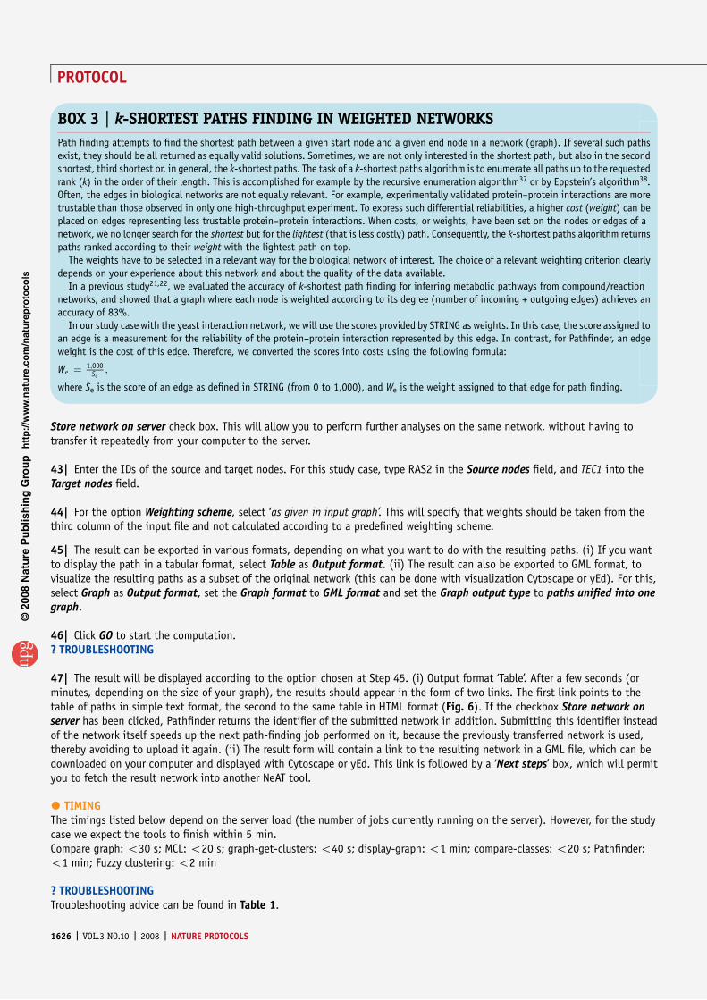
Store network on server check box. This will allow you to perform further analyses on the same network, without having totransfer it repeatedly from your computer to the server.
43| Enter the IDs of the source and target nodes. For this study case, type RAS2 in the Source nodes field, and TEC1 into theTarget nodes field.
44| For the option Weighting scheme, select ‘as given in input graph’. This will specify that weights should be taken from thethird column of the input file and not calculated according to a predefined weighting scheme.
45| The result can be exported in various formats, depending on what you want to do with the resulting paths. (i) If you wantto display the path in a tabular format, select Table as Output format. (ii) The result can also be exported to GML format, tovisualize the resulting paths as a subset of the original network (this can be done with visualization Cytoscape or yEd). For this,select Graph as Output format, set the Graph format to GML format and set the Graph output type to paths unified into onegraph.
46| Click GO to start the computation.? TROUBLESHOOTING
47| The result will be displayed according to the option chosen at Step 45. (i) Output format ‘Table’. After a few seconds (orminutes, depending on the size of your graph), the results should appear in the form of two links. The first link points to thetable of paths in simple text format, the second to the same table in HTML format (Fig. 6). If the checkbox Store network onserver has been clicked, Pathfinder returns the identifier of the submitted network in addition. Submitting this identifier insteadof the network itself speeds up the next path-finding job performed on it, because the previously transferred network is used,thereby avoiding to upload it again. (ii) The result form will contain a link to the resulting network in a GML file, which can bedownloaded on your computer and displayed with Cytoscape or yEd. This link is followed by a ‘Next steps’ box, which will permityou to fetch the result network into another NeAT tool.
� TIMINGThe timings listed below depend on the server load (the number of jobs currently running on the server). However, for the studycase we expect the tools to finish within 5 min.Compare graph: o30 s; MCL: o20 s; graph-get-clusters: o40 s; display-graph: o1 min; compare-classes: o20 s; Pathfinder:o1 min; Fuzzy clustering: o2 min
? TROUBLESHOOTINGTroubleshooting advice can be found in Table 1.
p
uor
G g
n ih si l
bu
P eru ta
N 800 2©
nat
ure
pro
toco
ls/
moc.er
ut an.
ww
w//:ptt
h
BOX 3 | k-SHORTEST PATHS FINDING IN WEIGHTED NETWORKS
Path finding attempts to find the shortest path between a given start node and a given end node in a network (graph). If several such pathsexist, they should be all returned as equally valid solutions. Sometimes, we are not only interested in the shortest path, but also in the secondshortest, third shortest or, in general, the k-shortest paths. The task of a k-shortest paths algorithm is to enumerate all paths up to the requestedrank (k) in the order of their length. This is accomplished for example by the recursive enumeration algorithm37 or by Eppstein’s algorithm38.Often, the edges in biological networks are not equally relevant. For example, experimentally validated protein–protein interactions are moretrustable than those observed in only one high-throughput experiment. To express such differential reliabilities, a higher cost (weight) can beplaced on edges representing less trustable protein–protein interactions. When costs, or weights, have been set on the nodes or edges of anetwork, we no longer search for the shortest but for the lightest (that is less costly) path. Consequently, the k-shortest paths algorithm returnspaths ranked according to their weight with the lightest path on top.
The weights have to be selected in a relevant way for the biological network of interest. The choice of a relevant weighting criterion clearlydepends on your experience about this network and about the quality of the data available.
In a previous study21,22, we evaluated the accuracy of k-shortest path finding for inferring metabolic pathways from compound/reactionnetworks, and showed that a graph where each node is weighted according to its degree (number of incoming + outgoing edges) achieves anaccuracy of 83%.
In our study case with the yeast interaction network, we will use the scores provided by STRING as weights. In this case, the score assigned toan edge is a measurement for the reliability of the protein–protein interaction represented by this edge. In contrast, for Pathfinder, an edgeweight is the cost of this edge. Therefore, we converted the scores into costs using the following formula:
We ¼ 1;000Se
;
where Se is the score of an edge as defined in STRING (from 0 to 1,000), and We is the weight assigned to that edge for path finding.
1626 | VOL.3 NO.10 | 2008 | NATURE PROTOCOLS
PROTOCOL

p
uor
G g
n ih si l
bu
P eru ta
N 800 2©
nat
ure
pro
toco
ls/
moc.er
ut an.
ww
w//:ptt
h
; Experiment exp_0
; Pathfinding results
; Date=Thu Jun 26 16:03:53 CEST 2008
; ===============================
; INPUT
; Source=RAS2
; Target=TEC1
; Graph=Pathfinder_tmpGraph_d597cd86-3095-475f-99e7-d70a542d072a.tab
; Undirected=true
; Metabolic standard format=false
; REA format=false
; Temporary directory=Temp
; CONFIGURATION
; Algorithm=rea
; Weight Policy=
; Weights given on arcs=true
; Maximal weight=1000000
; Maximal length=1000000
; Minimal length=0
; Exclusion attribute=ReferencedObject.PublicId
; Rank=5
; REA timeout=10
; EXPLANATION OF COLUMNS
; Start node=given start node identifier
; End node=given end node identifier
; K=path index
; Rank=rank of path (paths having same distance have the same rank, though their step number might differ)
; Distance=weight of path (sum of edge weights)
; Steps=number of nodes in path
; Path=sequence of nodes from start to end node that forms the path
; ===============================
#start node end node path index rank distance steps path
RAS2 TEC1 1 1 6.25 6 RAS2->CDC42->STE20->FUS3->STE12->TEC1
RAS2 TEC1 2 2 7.5 7 RAS2->CDC42->STE20->STE11->FUS3->STE12->TEC1
RAS2 TEC1 3 2 7.5 7 RAS2->CDC42->SHO1->STE20->FUS3->STE12->TEC1
RAS2 TEC1 4 2 7.5 7 RAS2->CDC42->STE20->FUS3->DIG1->STE12->TEC1
RAS2 TEC1 5 2 7.5 7 RAS2->CDC42->BEM1->STE20->FUS3->STE12->TEC1
RAS2 TEC1 6 2 7.5 7 RAS2->CDC42->STE20->STE5->FUS3->STE12->TEC1
RAS2 TEC1 7 2 7.5 7 RAS2->CDC42->STE20->FUS3->DIG2->STE12->TEC1
RAS2 TEC1 8 2 7.5 7 RAS2->CDC42->STE20->STE7->FUS3->STE12->TEC1
RAS2 TEC1 9 9 8.75 8 RAS2->CDC42->STE20->STE5->STE7->FUS3->STE12->TEC1
RAS2 TEC1 10 9 8.75 8 RAS2->CDC42->BEM1->STE20->STE11->FUS3->STE12->TEC1
RAS2 TEC1 11 9 8.75 8 RAS2->CDC42->STE20->STE7->STE11->FUS3->STE12->TEC1
RAS2 TEC1 12 9 8.75 8 RAS2->CDC42->STE20->STE5->STE11->FUS3->STE12->TEC1
RAS2 TEC1 13 9 8.75 8 RAS2->CDC42->SHO1->STE20->FUS3->DIG1->STE12->TEC1
RAS2 TEC1 14 9 8.75 8 RAS2->CDC42->BEM1->STE20->STE7->FUS3->STE12->TEC1
RAS2 TEC1 15 9 8.75 8 RAS2->CDC42->STE20->STE5->FUS3->DIG1->STE12->TEC1
RAS2 TEC1 16 9 8.75 8 RAS2->CDC42->STE20->STE7->FUS3->DIG1->STE12->TEC1
RAS2 TEC1 17 9 8.75 8 RAS2->CDC42->STE20->STE11->STE7->FUS3->STE12->TEC1
RAS2 TEC1 18 9 8.75 8 RAS2->CDC42->STE20->STE11->STE5->FUS3->STE12->TEC1
RAS2 TEC1 19 9 8.75 8 RAS2->CDC42->STE20->STE7->KSS1->DIG1->STE12->TEC1
RAS2 TEC1 20 9 8.75 8 RAS2->CDC42->SHO1->STE20->STE5->FUS3->STE12->TEC1
RAS2 TEC1 21 9 8.75 8 RAS2->CDC42->BEM1->STE20->FUS3->DIG1->STE12->TEC1
RAS2 TEC1 22 9 8.75 8 RAS2->CDC42->STE20->STE11->FUS3->DIG2->STE12->TEC1
RAS2 TEC1 23 9 8.75 8 RAS2->CDC42->STE20->STE7->FUS3->DIG2->STE12->TEC1
RAS2 TEC1 24 9 8.75 8 RAS2->CDC42->BEM1->STE20->FUS3->DIG2->STE12->TEC1
RAS2 TEC1 25 9 8.75 8 RAS2->CDC42->STE20->FUS3->DIG1->DIG2->STE12->TEC1
RAS2 TEC1 26 9 8.75 8 RAS2->CDC42->STE20->FUS3->DIG2->DIG1->STE12->TEC1
RAS2 TEC1 27 9 8.75 8 RAS2->CDC42->SHO1->STE20->STE11->FUS3->STE12->TEC1
RAS2 TEC1 28 9 8.75 8 RAS2->CDC42->STE20->STE7->KSS1->DIG2->STE12->TEC1
RAS2 TEC1 29 9 8.75 8 RAS2->CDC42->STE20->STE7->STE5->FUS3->STE12->TEC1
RAS2 TEC1 30 9 8.75 8 RAS2->CDC42->STE20->STE5->FUS3->DIG2->STE12->TEC1
RAS2 TEC1 31 9 8.75 8 RAS2->CDC42->SHO1->STE20->STE7->FUS3->STE12->TEC1
RAS2 TEC1 32 9 8.75 8 RAS2->CDC42->STE20->STE11->FUS3->DIG1->STE12->TEC1
RAS2 TEC1 33 9 8.75 8 RAS2->CDC42->BEM1->STE20->STE5->FUS3->STE12->TEC1
RAS2 TEC1 34 9 8.75 8 RAS2->CDC42->SHO1->STE20->FUS3->DIG2->STE12->TEC1
Figure 6 | Result obtained with Pathfinder upon execution of protocol with the study case. The table lists the paths found between RAS2 (source node) and
TEC1 (target node), ranked by increasing value of weight (distance). RAS2 and TEC1 are the start and end node of the filamentous growth pathway in yeast.
(continued)
TABLE 1 | Troubleshooting table.
Step Problem Possible reason Solution
8 After a few minutes, I still do nothave any answer and the browser displays‘‘Server is not responding’’
If you submitted a heavy task, theprocessing may exceed 5 min. Afterthat delay, Internet browser programsstop waiting for the server and displaythe error message
For heavy tasks, it is preferable either to install thestand-alone version of the command-line tools onyour machine or to write a client script for the RSATWeb services
Another possibility (if the task yousubmitted is not heavy) is that there is aproblem with your Internet connection
17 No graph layout after having loaded aGML file into yEd or Cytoscape
When a graph is loaded in yEd orCytoScape, it is initially displayed witha trivial layout (all nodes on a diagonal)
In yEd: select Layout from the menu, then selectthe submenu Organic and choose the optionClassic, then click OK
In Cytoscape: select Layout from the menu, thenselect the submenu yFiles and choose Organic
Both editors offer other layouts that you may try
NATURE PROTOCOLS | VOL.3 NO.10 | 2008 | 1627
PROTOCOL

ANTICIPATED RESULTSClusteringFigure 2 shows the results that should be obtained by applying the MCL graph clustering algorithm on the STRING databaseinteraction network. Each cluster is highlighted with a specific color. Figure 2a only displays intracluster edges, so that eachcluster appears as a separate component. This representation highlights the intracluster structure and edge density, and couldgive indication about possible improvement of the clusters by further subdivision. For example, the top-left cluster seems tobe composed of several various connected regions, which could be explored in more detail, taking into account some biologicalknowledge. On Figure 2b, both intra- and interclusters are displayed. Intracluster edges are highlighted by cluster-specificcolors, whereas intercluster edges are displayed in black, thereby revealing the interactions that were discarded duringthe clustering procedure. These two representations thus provide complementary indication for the interpretation of theclustering result.
The heatmap in Figure 3 represents a section of the node–cluster membership matrix, with cells colored according to themembership degree (the darker the cell, the higher the membership value). Within each cell, the membership degree values aredisplayed, indicating how strongly each node (row) is connected to each cluster (column). This strength (node–clustermembership) is defined as the sum of weights of the edges connecting the considered node to the considered cluster, divided bythe sum of weights of all edges starting from this node. The figure shows only a fragment of the table, but it already appearsthat some genes have similar membership profiles, thereby suggesting their involvement in common functions. This is the caseof the genes LPD1, PDA1 and PYC1, which are involved in pyruvate metabolism.
Figure 4 shows the results of the comparison between the dense clusters of the STRING graph and the complexes annotatedin the MIPS database. The header gives a short explanation for the content of each column of the result table. In this case,results are sorted by decreasing values of the hypergeometric significance (last column) calculated as described in Box 2. Eachrow describes the comparison between one MCL cluster and one MIPS complex. For example, the first row compares the MCL clus-ter ‘cl_2 ’, which contains 151 proteins, with a set of 138 proteins involved in cytoplasmic ribosomes. The intersection contains123 proteins, which represents a very high fraction of both the MCL cluster, and the annotated complex. The probability toobserve such an intersection by chance is 4E–146. The E value, obtained with the correction for multitesting, indicates that thenumber of false positives expected with such a P value would be 1E–141. In other terms, the correspondence between this MCLcluster and the cytoplasmic ribosome is too high to be explained by chance.
Network comparisonFigure 5a shows the statistics of comparison between the STRING ‘database’ network and the BioGRID synthetic lethality data set.The ‘synthetic lethality’ network used as reference contains 2,352 proteins linked by 9,413 edges, and the query graph contained1,240 nodes and 11,027 edges. The intersection between those graphs is apparently weak: 138 edges only. The Jaccard coefficientindicates that this intersection represents no 40.68% of the union. However, the number of edges expected by chance at theintersection is even smaller: E(Q^R) ¼ 23.24. The hypergeometric P value (Box 2) indicates the probability to observe at least138 edges at the intersection when 23.24 are expected by chance. In this study case, we observe that even with no 40.68% ofedges at the intersection, the P value is very low (1.4E�59). In other terms, the number of edges at the intersection is too muchhigh to be explained by chance, and is more likely to result from the biological relevance of both datasets.
PathfinderThe known signal transduction path connecting RAS2 and TEC1 consists of the following steps18:RAS2 - CDC42 - STE20 - STE11 - STE7 - KSS1 - DIG1/2 - TEC1
p
uor
G g
n ih si l
bu
P eru ta
N 800 2©
nat
ure
pro
toco
ls/
moc.er
ut an.
ww
w//:ptt
h
TABLE 1 | Troubleshooting table (continued).
Step Problem Possible reason Solution
22 You obtain the message: ‘‘ErrorIncongruence between graph andcluster files’’
Cluster and graph files do not correspondto the same network, or the specifiedformat of the graph is not correct
Check that the clusters correspond to the graph. Ifso, check the format of your graph file is the oneyou entered in the relevant field
The low-resolution heatmap does notdisplay properly
The image is scaled so it fits on thewindow
Click on the image to zoom. You may inspect thewhole map by using the scrolling bar
46 You obtain the message: ‘‘PATHFINDERERROR: One of your seed nodes is notpart of the input graph’’
You provided seed node identifiers thatdo not match any of the node identifiersof the input graph
Check the spelling of your seed node identifiers
In general, all tools require an exact match betweeninput node identifiers and those of nodes in thenetwork
1628 | VOL.3 NO.10 | 2008 | NATURE PROTOCOLS
PROTOCOL

Pathfinder reports the following path of first rank (the matching parts are underlined, and the nonseed matching part are high-lighted in bold):
RAS2 - CDC42 - STE20 - FUS3 - STE12 - TEC1This path connects STE20 to TEC1 via FUS3 and STE12, bypassing STE11, STE7, KSS1 and DIG1/2.Among the paths of length 8 (third rank paths), we find paths closer to the annotated pathway, such asRAS2 - CDC42 - STE20 - STE11 - FUS3 - DIG1 - STE12 - TEC1Scott and colleagues applied their path-finding algorithm to another yeast protein–protein interaction network of similar size
(4,500 nodes and 14,500 edges) taken from MIPS. For RAS2 and TEC1, they obtain the following as best path of length 8:RAS2 - CDC25 - HSP82 - STE11 - STE5 - STE7 - KSS1 - TEC1
Although Pathfinder has not been designed in particular for protein interaction networks, it can be used to predict signaltransduction pathways if appropriate weights have been set on the network under investigation. The accuracy of the predictiondepends also on the data quality. For example, the STRING interaction network does not contain any edge between DIG2/DIG1and TEC1, making it impossible to reach a prediction accuracy of 100%. When predicting pathways from real-world interactionnetworks, one must always keep in mind that these data might be incomplete or contain false positive interactions.
ACKNOWLEDGMENTS S.B. is the recipient of a PhD grant from the Fonds pour laFormation a la Recherche dans l’Industrie et dans l’Agriculture (FRIA). K.F. issupported by the Actions de Recherches Concertees de la Communaute Francaisede Belgique (ARC grant number 04/09-307). G.L.-M. was funded by a PhD grantfrom the Fonds Xenophilia [Universite Libre de Bruxelles (ULB)] and by apostdoctoral fellowship from the Region Wallonne de Belgique (TransMaze project415925). The BiGRe laboratory is supported by the BioSapiens Network ofExcellence funded under the sixth Framework program of the EuropeanCommunities (LSHG-CT-2003-503265) and by the Belgian Program onInteruniversity Attraction Poles, initiated by the Belgian Federal Science PolicyOffice, project P6/25 (BioMaGNet). We acknowledge the students of the Master inBioinformatics and Modeling (ULB, Belgium) for their useful corrections andsuggestions. S.B. and K.E. equally contributed to this article.
Published online at http://www.natureprotocols.com/Reprints and permissions information is available online at http://npg.nature.com/reprintsandpermissions/
1. Thomas-Chollier, M. et al. RSAT: regulatory sequence analysis tools. Nucleic AcidsRes. 36, W119–W127 (2008).
2. Brohee, S. et al. NeAT: a toolbox for the analysis of biological networks, clusters,classes and pathways. Nucleic Acids Res. 36, W444–W451 (2008).
3. Turatsinze, J.-V., Thomas-Chollier, M., Defrance, M. & van Helden, J. Using RSAT toscan genome sequences for transcription factor binding sites and cis-regulatorymodules. Nat. Protoc. doi:10.1038/nprot.2008.97 (2008).
4. Defrance, M., Janky, R., Sand, O. & van Helden, J. Using RSAT oligo-analysisand dyad-analysis tools to discover regulatory signals in nucleic sequences.Nat. Protoc. doi:10.1038/nprot.2008.98 (2008).
5. Sand, O., Thomas-Chollier, M., Vervisch, E. & van Helden, J. Analyzing multipledata sets by interconnecting RSAT programs via SOAP Web services–an examplewith ChIP-chip data. Nat. Protoc. doi:10.1038/nprot.2008.99 (2008).
6. Jeong, H., Tombor, B., Albert, R., Oltvai, Z.N. & Barabasi, A.L The large-scaleorganization of metabolic networks. Nature 407, 651–654 (2000).
7. Jeong, H., Mason, S.P., Barabasi, A.L. & Oltvai, Z.N. Lethality and centrality inprotein networks. Nature 411, 41–42 (2001).
8. Fell, D.A. & Wagner, A. The small world of metabolism. Nat. Biotechnol. 18,1121–1122 (2000).
9. Blatt, M., Wiseman, S. & Domany, E. Superparamagnetic clustering of data.Phys. Rev. Lett. 76, 3251–3254 (1996).
10. Bader, G.D. & Hogue, C.W.V. An automated method for finding molecularcomplexes in large protein interaction networks. BMC Bioinformatics 4, 2(2003).
11. Gagneur, J., Jackson, D.B. & Casari, G. Hierarchical analysis of dependency inmetabolic networks. Bioinformatics 19, 1027–1034 (2003).
12. Spirin, V. & Mirny, L.A. Protein complexes and functional modules in molecularnetworks. Proc. Natl. Acad. Sci. USA 100, 12123–12128 (2003).
13. King, A.D., Przulj, N. & Jurisica, I. Protein complex prediction via cost-basedclustering. Bioinformatics 20, 3013–3020 (2004).
14. Van Dongen, S. Graph Clustering by Flow Simulation. PhD Thesis (Centers forMathematics and Computer Science (CWI), University of Utrecht, 2000).
15. Pereira-Leal, J.B., Enright, A.J. & Ouzounis, C.A. Detection of functional modulesfrom protein interaction networks. Proteins 54, 49–57 (2004).
16. Enright, A.J., Van Dongen, S. & Ouzounis, C.A. An efficient algorithm for large-scale detection of protein families. Nucleic Acids Res. 30, 1575–1584 (2002).
17. Brohee, S. & van Helden, J. Evaluation of clustering algorithms for protein-protein interaction networks. BMC Bioinformatics 7, 488 (2006).
18. Scott, J., Ideker, T., Karp, R.M. & Sharan, R. Efficient algorithms for detectingsignaling pathways in protein interaction networks. J. Comput. Biol. 13, 133–144(2005).
19. Bebek, G. & Yang, J. PathFinder: mining signal transduction pathwaysegments from protein-protein interaction networks. BMC Bioinformatics 8, 335(2007).
20. Rahman, S.A., Advani, P., Schunk, R., Schrader, R. & Schomburg, D Metabolicpathway analysis web service (Pathway Hunter Tool at CUBIC). Bioinformatics 21,1189–1193 (2004).
21. Croes, D., Couche, F., Wodak, S. & van Helden, J. Metabolic PathFinding: inferringrelevant pathways in biochemical networks. Nucleic Acids Res. 33, W326–W330(2005).
22. Croes, D., Couche, F., Wodak, S. & van Helden, J. Inferring meaningful pathways inweighted metabolic networks. J. Mol. Biol. 356, 222–236 (2006).
23. Shannon, P. et al. Cytoscape: a software environment for integrated models ofbiomolecular interaction networks. Genome Res. 13, 2498–2504 (2003).
24. de Nooy, W., Mrvar, A. & Batagelj, V. Exploratory Social Network Analysis with PajekSeries: Structural Analysis in the Social Sciences (No. 27) (Cambridge UniversityPress, Cambridge, 2005).
25. Baitaluk, M., Sedova, M., Ray, A. & Gupta, A. BiologicalNetworks: visualizationand analysis tool for systems biology. Nucleic Acids Res. 34, W466–W471(2006).
26. Hu, Z. et al. VisANT 3.0: new modules for pathway visualization, editing,prediction and construction. Nucleic Acids Res. 35, W625–W632 (2007).
27. Hull, D. et al. Taverna: a tool for building and running workflows of services.Nucleic Acids Res. 34, W729–W732 (2006).
28. Lima-Mendez, G., van Helden, J., Toussaint, A. & Leplae, R. Reticulaterepresentation of evolutionary and functional relationships between phagegenomes. Mol. Biol. Evol. 25, 762–777 (2008).
29. Croes, D., Couche, F., Wodak, S.J. & van Helden, J. Inferring meaningful pathwaysin weighted metabolic networks. J. Mol. Biol. 356, 222–236 (2006).
30. Croes, D., Couche, F., Wodak, S.J. & van Helden, J. Metabolic PathFinding:inferring relevant pathways in biochemical networks. Nucleic Acids Res. 33,W326–W330 (2005).
31. von Mering, C. et al. STRING 7-recent developments in the integration andprediction of protein interactions. Nucleic Acids Res. 35, D358–D362 (2007).
32. Breitkreutz, B.J. et al. The BioGRID Interaction Database: 2008 update.Nucleic Acids Res. 36, D637–D640 (2008).
33. Keseler, I.M. et al. EcoCyc: a comprehensive database resource for Escherichia coli.Nucleic Acids Res. 33, D334–D337 (2005).
34. Kanehisa, M., Goto, S., Kawashima, S. & Nakaya, A. The KEGG databases atGenomeNet. Nucleic Acids Res. 30, 42–46 (2002).
35. Mewes, H.W. et al. MIPS: analysis and annotation of proteins from wholegenomes. Nucleic Acids Res. 32, D41–D44 (2004).
36. Ashburner, M. et al. Gene ontology: tool for the unification of biology. The GeneOntology Consortium. Nat. Genet. 25, 25–29 (2000).
37. Jimenez, V.M. & Marzal, A. Computing the K shortest paths: a new algorithm andan experimental comparison. In Proceeding of the 3rd International Workshop onAlgorithm Engineering (WAE 1999) Vol. 1668, 15–29 (Springer-Verlag, London,1999).
38. Eppstein, D. Finding the k shortest paths. SIAM J. Comput. 28, 652–673 (1998).
p
uor
G g
n ih si l
bu
P eru ta
N 800 2©
nat
ure
pro
toco
ls/
moc.er
ut an.
ww
w//:ptt
h
NATURE PROTOCOLS | VOL.3 NO.10 | 2008 | 1629
PROTOCOL

7 Discussion
7.1 Summary
7.1.1 Path �nding in RPAIR networks
A path finding tool was developed, which predicts metabolic pathways in KEGG LIGANDand KEGG RPAIR networks and which is integrated into NeAT.
The evaluation of path finding in RPAIR networks showed that RPAIR annotation, com-bined with a weight policy that penalizes hub compounds, yields a higher accuracy than eitherRPAIR annotation or weight policy alone. This is a step forward with respect to the previousresults by Didier Croes, whose work was the starting point for this thesis.
7.1.2 Multiple-end pathway prediction by subgraph extraction
The evaluation of several multiple-end pathway prediction approaches showed that a combi-nation of a random walk-based (kWalks) with a shortest-paths based (Takahashi-Matsuyama)approach reaches the highest overall accuracy. In addition, kWalks can discover weights. Inthe absence of a good weight policy, these weights increase pathway prediction accuracy con-siderably. This can be helpful when pathway prediction is applied to biological networks otherthan metabolic networks, for which a good weight policy is not yet known.
The subgraph extraction approaches are publicly available within the NeAT tool "Pathwayextraction". This tool accepts compounds as well as reactions, reactant pairs, EC numbers,enzymes or genes as seeds. The user can submit custom groups of seeds or select a pre-defined seed node grouping strategy (for instance, if enzymes are provided as seeds, theirassociated reactions can be grouped according to their EC numbers). In addition, the tooloffers networks from the major metabolic databases KEGG and MetaCyc and maps referencemaps or pathways from these databases onto the predicted pathway. Last but not least, the toolcan take custom networks and custom weights as input.
7.1.3 Application to microarray data set
Multiple-end pathway prediction was applied to a microarray data set that measured differ-ential gene expression in the presence of each of 20 different compounds as sole nitrogensource with respect to urea as reference nitrogen source. Given the top five differentially ex-pressed enzyme-coding genes for each condition, multiple-end pathway prediction suggestedpathways that are up- or down-regulated in the presence of a specific nitrogen source.
159
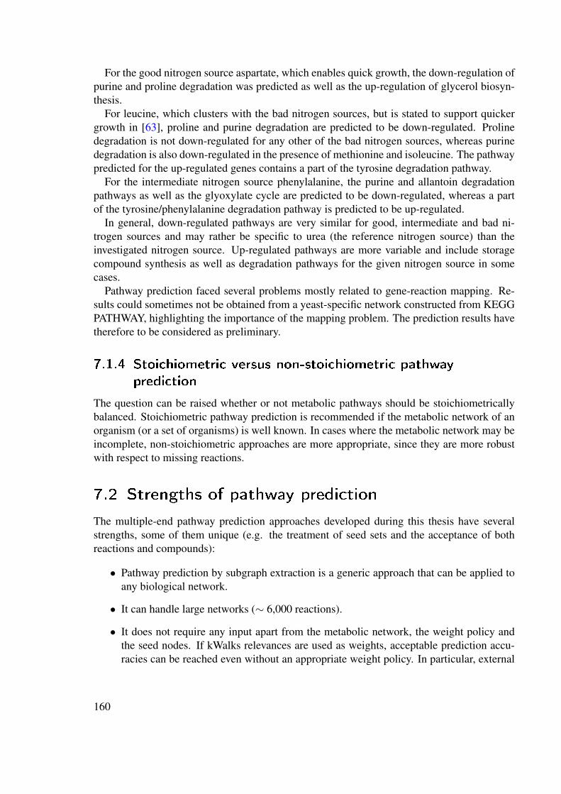
For the good nitrogen source aspartate, which enables quick growth, the down-regulation ofpurine and proline degradation was predicted as well as the up-regulation of glycerol biosyn-thesis.
For leucine, which clusters with the bad nitrogen sources, but is stated to support quickergrowth in [63], proline and purine degradation are predicted to be down-regulated. Prolinedegradation is not down-regulated for any other of the bad nitrogen sources, whereas purinedegradation is also down-regulated in the presence of methionine and isoleucine. The pathwaypredicted for the up-regulated genes contains a part of the tyrosine degradation pathway.
For the intermediate nitrogen source phenylalanine, the purine and allantoin degradationpathways as well as the glyoxylate cycle are predicted to be down-regulated, whereas a partof the tyrosine/phenylalanine degradation pathway is predicted to be up-regulated.
In general, down-regulated pathways are very similar for good, intermediate and bad ni-trogen sources and may rather be specific to urea (the reference nitrogen source) than theinvestigated nitrogen source. Up-regulated pathways are more variable and include storagecompound synthesis as well as degradation pathways for the given nitrogen source in somecases.
Pathway prediction faced several problems mostly related to gene-reaction mapping. Re-sults could sometimes not be obtained from a yeast-specific network constructed from KEGGPATHWAY, highlighting the importance of the mapping problem. The prediction results havetherefore to be considered as preliminary.
7.1.4 Stoichiometric versus non-stoichiometric pathway
prediction
The question can be raised whether or not metabolic pathways should be stoichiometricallybalanced. Stoichiometric pathway prediction is recommended if the metabolic network of anorganism (or a set of organisms) is well known. In cases where the metabolic network may beincomplete, non-stoichiometric approaches are more appropriate, since they are more robustwith respect to missing reactions.
7.2 Strengths of pathway prediction
The multiple-end pathway prediction approaches developed during this thesis have severalstrengths, some of them unique (e.g. the treatment of seed sets and the acceptance of bothreactions and compounds):
• Pathway prediction by subgraph extraction is a generic approach that can be applied toany biological network.
• It can handle large networks (∼ 6,000 reactions).
• It does not require any input apart from the metabolic network, the weight policy andthe seed nodes. If kWalks relevances are used as weights, acceptable prediction accu-racies can be reached even without an appropriate weight policy. In particular, external
160

compounds do not need to be specified and it is not assumed that metabolism is at steadystate.
• The prediction approach can discover unknown pathways consisting of known compo-nents.
• Pathway prediction can be fine-tuned to favor certain nodes. For instance, in a genericmetabolic network, i.e. a network consisting of all reactions and compounds presentin a metabolic database, reactions known to occur in certain organisms might receivea weight much lower than other reactions, to favor the extraction of organism-specificsubgraphs. Similarly, results from a high-throughput experiment can be incorporatedby assigning a node weight that represents a score obtained from the experiment (e.g. afunction of the p-value of differential expression of the gene associated to the node).
• Sets of seed nodes can be specified to reflect AND/OR relationships between seed nodes.An AND relationship holds between seed node sets, whereas an inclusive OR relation-ship exists between the members of a seed node set.
• The web application allows to predict pathways from networks constructed from thetwo major metabolic databases KEGG and MetaCyc.
• Both, compounds and reactions can be provided as seeds. Thus, the web applicationsupports compounds, reactions, reactant pairs, EC numbers or genes/enzymes as seednodes and handles the required association of these seeds to reactions, reactant pairs andcompounds.
• For metabolic networks from MetaCyc or KEGG, the web application maps the pre-dicted pathway to known pathways from MetaCyc or KEGG respectively.
7.3 Limitations of pathway prediction
When using the pathway prediction approaches presented in this thesis, one should be awareof their limitations:
• Data quality.As for any other prediction method, prediction accuracy depends on the quality of thedata. If reactions or compounds are absent in the source database, pathways contain-ing them cannot be predicted. If associations of genes to reactions are imprecise, thepredicted pathway will be inaccurate.
• Cycles and spirals.Cyclic and spiral-shaped pathways such as TCA cycle and fatty acid biosynthesis canonly be partly predicted in most cases. Two-end path finding relies on the enumerationof the K-shortest paths. Paths by definition do not contain cycles, and closed pathsare not enumerated. Pathways composed of several paths of equal weight may containcycles, however.
161

Likewise, most multiple-end pathway prediction algorithms tested in this thesis searchfor the minimum weight tree connecting the seed nodes. The minimum weight treewould no longer be of minimal weight if it contained an additional edge to close acycle. As in two-end path finding, a pathway may be cyclic if it contains several pathshaving the same weight between two seed nodes.
KWalks is a special case, because in contrast to the shortest-paths based algorithms,it does not seek to minimize the weight of a subgraph, but instead to maximize itsrelevance. With the kWalks algorithm, a subgraph is built by adding the most relevantof the remaining edges at each step and checking whether the pathway is connected.Thus, cycles may be obtained in some cases.
• Most parsimonious pathway assumption.Path finding makes the assumption that pathways are as short (parsimonious) as bio-chemically possible. It may be argued that this makes sense for the cell, since the syn-thesis of an enzyme is costly. In many cases, this assumption indeed results in accuratepredictions. However, not all pathways are designed to synthesize a product or degradea compound with the minimal number of enzymatic steps. For example, the TCA cyclehas not been optimized to consist of the smallest possible number of enzymes but toproduce energy and precursors for some metabolic pathways (e.g. amino acid biosyn-thesis). Pathway prediction with multiple seeds alleviates this problem, as it can takeintermediate reaction steps into account.
• Central metabolism.From the evaluations performed during this thesis, it emerged that pathway predictionis particularly weak for central pathways such as glycolysis, which are highly intercon-nected and where many different alternatives exist. The criteria employed by the pathfinding approach presented in this work and by other non-stoichiometric approaches(e.g. [138, 18]) are currently not sufficient to distinguish between valid and invalid cen-tral pathways. Multiple-seed pathway prediction alleviates the problem by allowing theincorporation of more information. Still, a high proportion of a central pathway needsto be provided (as seed nodes) in order to correctly predict it.
• Generic compounds and stereoisomersKEGG and MetaCyc contain generic compounds, e.g. compounds such as "alcohol" or"an amino acid". Generic compounds serve as substrates and products of generic reac-tions (i.e. reactions carried out by broad-specificity enzymes) and organize compoundsin a hierarchy. In this tree-shaped hierarchy, compounds with specific structures formleaves at the bottom, which are merged into generic parent compound classes with in-creasing broadness. For instance, tryptophan (leave) is an aromatic amino acid (genericcompound), which is an amino acid (higher level generic compound). Stereoisomers in-troduce a new level of detail at the bottom of this compound hierarchy. For instance, D-and L-tryptophan, two leaves in the compound tree, are the children of the tryptophancompound class. Ideally, pathway prediction should navigate the compound hierarchyfor each compound to find its most specific representative in the hierarchy, but this hasnot been implemented for the present prediction approach.
162

• Polymeric reactions and compoundsThe networks constructed during this work do not contain polymeric reactions, becausethey need an annotation effort to distinguish between substrate and product (which areoften identical as in the case of KEGG reaction R01790 involving starch). Polymericcompounds such as DNA or RNA are also excluded to simplify the prediction task.Therefore, pathways containing polymeric reactions or compounds cannot be predicted.
• Stoichiometries.Pathways are not stoichiometrically balanced. The implications of this have been dis-cussed in detail in chapter 5.
• Irreversible reactions.In general, the direction of a pathway can only be predicted if irreversible reactions arepreserved during the construction of the metabolic graph. The generic metabolic net-works offered by NeAT pathway prediction tools do not contain irreversible reactions.However, custom graphs containing irreversible reactions can be uploaded by the user.However, for multiple-seed pathway prediction, it is possible that a predicted pathwaycontains irreversible reactions of opposite directions.
• Reaction group treatment.If genes or EC numbers are associated to several reactions, it is not clear how many ofthem are contributed to the pathway. As explained in the Introduction (section 1.3.3),this ambiguity is due mainly to two reasons: On the one hand, enzymes may containseveral catalytic sites and thus be associated to several EC numbers. On the other hand,one EC number may comprise several reactions. Such EC numbers are often assignedto broad-specificity enzymes, which are enzymes that are not specific to one substrate.For instance, EC number 1.1.1.1 describes the conversion of an alcohol to a ketoneand is associated to the broad-specificity enzyme alcohol dehydrogenase. From themany reactions associated to this EC number, only a sub-set may be relevant for thepathway to be predicted. To deal with these ambiguities, the pathway prediction webtool allows to group reactions associated to a gene according to their EC numbers. Thus,an AND relationship exists between the reactions in different EC number groups and anOR relationship exists between the reactions within one EC number group. However,this grouping does not solve the problem entirely, as there are some cases where oneEC number contributes more than one of its reactions to the pathway (e.g. histidinebiosynthesis) or where only one of two EC numbers of an enzyme participates in thepathway (lysine biosynthesis). In section 9.1, postprocessing is discussed as a strategyto deal with this problem.
7.4 Alternative prediction approaches
As seen in the introduction, many different metabolic pathway prediction approaches exist.The multiple-end pathway prediction approach presented in this thesis is a large-scale ap-
proach, which is not overly sensitive to noisy data (evaluation was performed in low-quality
163

networks), which does not require any input other than the metabolic network, a weight policyand seed nodes, which is flexible (accepts compounds and reactions as seeds, can be applied toany network), but which on average does not reach high prediction accuracies (i.e. accuraciesabove 90%).
A few steps can be taken to increase the accuracy of multiple-end pathway prediction (seesection 7.6), but it has inherent limitations: It does not take into account enzyme kinetics, doesnot explicitly trace atoms and does not consider stoichiometry.
In the following, each of these shortcomings is discussed in more detail.
7.4.1 Enzyme kinetics
Detailed models of metabolism (e.g. [118]) explicitly take into account the (often non-linear)kinetics of enzymes using various approximation techniques ([70]). Currently, kinetic data ona large number of enzymes are gathered for model organisms such as S. cerevisiae, which willallow to extend these models to the genome scale (personal communication J.J. Heijnen). Atthis level of description, the metabolic network of the organism needs to be well known, andthe purpose of the model is the accurate prediction of the (wild type or mutant) organism’sbehavior in given conditions instead of the reconstruction of a metabolic network, the discov-ery of novel pathways or the interpretation of omics data. Thus, detailed models integratingenzyme kinetics answer different questions about metabolism than pathway prediction does.
7.4.2 Atom tracing
Path finding in the RPAIR graph considers atom flow indirectly, but does not explicitly traceatoms. Other tools (e.g. [6, 18, 130]) do trace atoms through the compounds of a pathway.This may result in higher prediction accuracies, as it ensures that atoms from the source indeedreach the target(s). There is however a drawback to it: It is not straightforward to search pathsbetween reactions. Indeed, none of the tools relying on atom tracing accepts reactions asinput (see tables 1.6 and 1.7). Given a reaction, it is not clear which of its products is ofinterest. The selection of a substrate-product pair with maximal structural similarity (or withmaximal carbon atom transfer) does not help, because often a pair of hub compounds suchas NADP/NADPH displays the highest structural similarity and transfers the largest numberof carbon atoms. What is needed is information on the role of compound pairs in a reaction,which is provided by the RPAIR database. For instance, the pair NADP/NADPH is classifiedas "cofac". It is an open question whether carbon atom transfer rules (a maximal number ofcarbon atoms from the source should arrive at the target) can be combined with reactant pairroles and whether this would indeed increase the accuracy of path finding between reactions.
7.4.3 Stoichiometry
Stoichiometric versus non-stoichiometric pathway prediction was already discussed in chapter5. It is conceivable to combine both approaches. For instance, first all EMs could be enumer-ated that contain one of the seeds of interest. Selected EMs could then form the input network
164

to pathway prediction, which could extract a sub-network containing other compounds of in-terest. In this case, pathway prediction would act as a zoom to inspect a complex EM solution.Another way to combine both approaches would be to check whether a pathway predicted bysubgraph extraction is a subgraph of an EM. In this case, EMs would serve as a filter to discardpredicted pathways that do not ensure the net production of a compound of interest.
7.5 Top-down versus bottom-up pathway prediction
In the introduction, pathway prediction was defined as the enumeration of biochemically fea-sible pathways that connect a set of seeds. This may be referred to as a bottom-up approach:Given the seed set, a part of the metabolic network is extracted which represents the predictedpathway.
Another approach, which was mentioned in the introduction (section 1.6.2) starts from thewhole metabolic network and divides it in smaller units that correspond to metabolic mod-ules (or pathways). For pathway prediction, this top-down approach is less interesting, sincereactions or compounds of interest are not taken into account. However, it allows to definepathways by defining the partition procedure. For instance, in [68], the network is partitionedby maximizing the number of intra-module links and minimizing the number of inter-modulelinks. Many of the modules thus obtained were close to the reference maps listed in KEGG.Others (especially those from central metabolism) corresponded to a mixture of KEGG refer-ence maps.
The decomposition algorithm introduced by [60] groups compounds in the order of theirspecificity (i.e. number of reactions they are involved in), starting from the most specificcompounds that are linked to the lowest number of reactions and ending with the least specificcompounds such as ATP and ADP. It outputs a tree consisting of a hierarchy of clusters thatreflects the hierarchical organization of metabolic networks as suggested by Ravasz et al.(see Introduction, section 1.6.2). The least specific compounds (corresponding to the hubcompounds) form clusters at the root of the tree, whereas the most specific compound clustersform its leaves. When applied to the metabolic network of E. coli, the computed clusterscorrespond well to the metabolic pathways as defined by the operons annotated in RegulonDB[61].
In [62] the metabolic network of E. coli is pruned iteratively by removing highly connectedcompounds. Parts of the pruned network corresponded to pathways annotated in EcoCyc.
In the context of metabolic pathway prediction, there are two interesting applications ofnetwork partitioning and pruning.
First, if the modules obtained from the partitioning are close enough to reference metabolicpathways, then network partitioning would be an interesting way to generate a set of(organism-specific) reference pathways from metabolic databases where reference pathwaysare not available.
Second, a pruned network can speed up pathway prediction, but with the important draw-back that pathways containing the pruned compounds cannot be predicted, thus predictionaccuracy will be lost.
165

7.6 Tuning pathway prediction
Several strategies can be adopted to increase the accuracy of pathway prediction without mod-ifying the approach itself:
• Weight. A more sophisticated weight policy can be used, which integrates scores fromomics data.
• Network quality. Pathways can be predicted from a higher-quality network, which doesnot contain imbalanced reactions or redundant compound entries (such as C06623 andC11915 in previous versions of KEGG, [134]). One such network can be obtained fromBioMeta [122].
• Network size. Pathways can be predicted from a smaller network, possibly one that isspecific to a set of organisms.
• Seed node number. The better the pathway of interest is covered by the seed nodes,the higher will be the prediction accuracy (see section 7.8 on the extend of pathwaycoverage by associated enzyme-coding genes).
However, as the evaluations presented in chapter 2 and 3 have shown, reasonable predictionaccuracies can be achieved for huge low-quality networks, a simple weight policy and a smallseed nod number.
In general, the prediction accuracy is highly dependent on the pathway shape and the cover-age of the pathway by the seed nodes. Thus, the accuracy is pathway-specific, not organism-specific. In general, pathways are predicted with higher accuracy, if they are
• linear or branched instead of cyclic or spiral-shaped and
• located in the periphery of the metabolic network (i.e. not well interconnected withother pathways) rather than at its center (where pathways are highly interconnected).
7.7 Condition-speci�city of metabolic pathways
Many pathways are only activated in certain conditions. Thus, if one wants to predict a path-way that is active in an organism in the given conditions, one needs either to integrate gene ex-pression or similar data into the prediction approach or one needs to work with the condition-specific metabolic network (which is in turn obtained from gene expression or similar data).
One of the strengths of multiple-end pathway prediction is that it can easily integrate geneexpression data, thus allowing to predict condition-specific pathways.
In a recent article, Shlomi et al. attempt the reconstruction of tissue-specific metabolismfrom the human metabolic network by combining flux balance analysis with gene expressiondata [151]. Multiple-end pathway prediction from seed genes offers an alternative to the re-construction of tissue-specific metabolism from gene expression data.
166
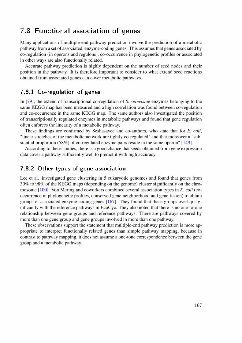
7.8 Functional association of genes
Many applications of multiple-end pathway prediction involve the prediction of a metabolicpathway from a set of associated, enzyme-coding genes. This assumes that genes associated byco-regulation (in operons and regulons), co-occurrence in phylogenetic profiles or associatedin other ways are also functionally related.
Accurate pathway prediction is highly dependent on the number of seed nodes and theirposition in the pathway. It is therefore important to consider to what extend seed reactionsobtained from associated genes can cover metabolic pathways.
7.8.1 Co-regulation of genes
In [79], the extend of transcriptional co-regulation of S. cerevisiae enzymes belonging to thesame KEGG map has been measured and a high correlation was found between co-regulationand co-occurrence in the same KEGG map. The same authors also investigated the positionof transcriptionally regulated enzymes in metabolic pathways and found that gene regulationoften enforces the linearity of a metabolic pathway.
These findings are confirmed by Seshasayee and co-authors, who state that for E. coli,"linear stretches of the metabolic network are tightly co-regulated" and that moreover a "sub-stantial proportion (58%) of co-regulated enzyme pairs reside in the same operon" [149].
According to these studies, there is a good chance that seeds obtained from gene expressiondata cover a pathway sufficiently well to predict it with high accuracy.
7.8.2 Other types of gene association
Lee et al. investigated gene clustering in 5 eukaryotic genomes and found that genes from30% to 98% of the KEGG maps (depending on the genome) cluster significantly on the chro-mosome [100]. Von Mering and coworkers combined several association types in E. coli (co-occurrence in phylogenetic profiles, conserved gene neighborhood and gene fusion) to obtaingroups of associated enzyme-coding genes [167]. They found that these groups overlap sig-nificantly with the reference pathways in EcoCyc. They also noted that there is no one-to-onerelationship between gene groups and reference pathways: There are pathways covered bymore than one gene group and gene groups involved in more than one pathway.
These observations support the statement that multiple-end pathway prediction is more ap-propriate to interpret functionally related genes than simple pathway mapping, because incontrast to pathway mapping, it does not assume a one-tone correspondence between the genegroup and a metabolic pathway.
167

8 Perspectives
8.1 Increase of pathway prediction accuracy
Several suggestions that might increase the prediction accuracy and which were not exploredin this thesis are listed below.
• Thermodynamical constraints. Thermodynamical constraints on reaction directions fil-ter out thermodynamically infeasible pathways. As explained in section 1.3.2, the di-rection of a reaction depends on its change in Gibbs free energy. Mavrovouniotis [111]developed a group contribution method to estimate the standard Gibbs free energy ofthe formation of a compound from its structure. He proposed to apply these estimatedstandard Gibbs free energies as constraints on reactions for which no information onreversibility was available from databases. However, the direction of a reaction in phys-iological conditions is not only dependent on the standard Gibbs free energy change,but also on compound concentrations and the temperature (see Introduction, section1.3.2). Thus, thermodynamical constraints may be difficult to compute from compoundstructure alone.
• Combination with EMs. As described in the discussion (section 7.4), a network consist-ing of selected elementary modes may serve to filter out pathways that do not allow thenet production of a compound of interest.
• Improved weight policy. Node weights could be obtained by a machine learning tech-nique from the reference pathways. However, the risk of over-fitting is high in this case,since the number of reference pathways is far below the number of possible weightpolicies.
• Explicit tracing of atoms. In this thesis, reactant pair mappings from the RPAIR databasewere employed, but atoms were not explicitly traced. As mentioned in the discussion(section 7.4), relying only on atom tracing makes it hard to predict pathways from seedreactions. However, a mixed approach that combines atom tracing (as many substrateatoms as possible should reach the product) with RPAIR roles could improve the pre-diction accuracy for seed compounds as well as reactions.
8.2 Improvement of pathway prediction
In this section, improvements are suggested that do not affect the accuracy, but ease the inter-pretation of results or extend the applicability of the approach.
168

First, improvements concerning the subgraph extraction are listed.
• Subgraph enumeration. To allow the inspection of alternatives, not only the lightestsubgraph should be returned, but subgraphs up to a requested number ordered accordingto their weight.
• Subgraph p-value. It is of interest to know how likely it is to obtain a particular subgraphscore for a given seed node number. To answer this question, several authors computethe p-value of a subgraph ([77, 3]). These authors repetitively extract subgraphs fora given number of randomly selected seeds to obtain a distribution of subgraph scores.The p-value of an extracted subgraph given a certain seed node number is then computedfrom the seed number-specific distribution. Since the subgraph extraction approachesdeveloped in this thesis are computationally expensive, it could be envisaged to pre-compute these distributions for several seed node numbers.
• Subgraph filtering. In two-end path finding, a number of filter options exist. Some ofthese filter options (no paths above a certain length or weight, absence of specific nodes)could be implemented for multiple-end pathway prediction as well. For instance, thepredicted pathway could be filtered to remove all inter-seed paths above a certain lengthor weight.
• Subgraph layout. An improved graph layout would improve the "readability" of thepredicted pathway. Currently, a general-purpose graph software [44] is used to layoutpredicted pathways. This software could be replaced by tools specialized on the layoutof biological pathways (e.g. [102]).
Another series of improvements concerns the data sets.
• More metabolic databases. The pathway extraction tool currently offers networks fromKEGG and MetaCyc. Integration of other metabolic databases, e.g. Reactome and UM-BBD would allow the prediction of pathways in more specialized metabolic networks.
• Transporters and compartments. Another extension would be the prediction ofmetabolic pathways from metabolic networks that integrate data on transporters. Forinstance, the transport of glucose across the cell membrane could be described by thereaction: glucose_extern → glucose_cytoplasm. Ideally, the different cell com-partments should also be described by these extended metabolic networks. A metabolicnetwork consisting of several modules would result, where each module describes themetabolism in one compartment and where the same compound may occur more thanonce in different modules (e.g. glucose_extern, glucose_cytoplasm). Modules are con-nected by transport reactions. For such networks, an additional constraint may be nec-essary to minimize the number of transport reactions in a predicted pathway.
• Integration of other biological networks. Networks could not only integrate data ontransporters and compartments, but also on enzyme regulation and signal transduction.Such integrated networks are already available for some organisms (e.g. [46, 165]).
169
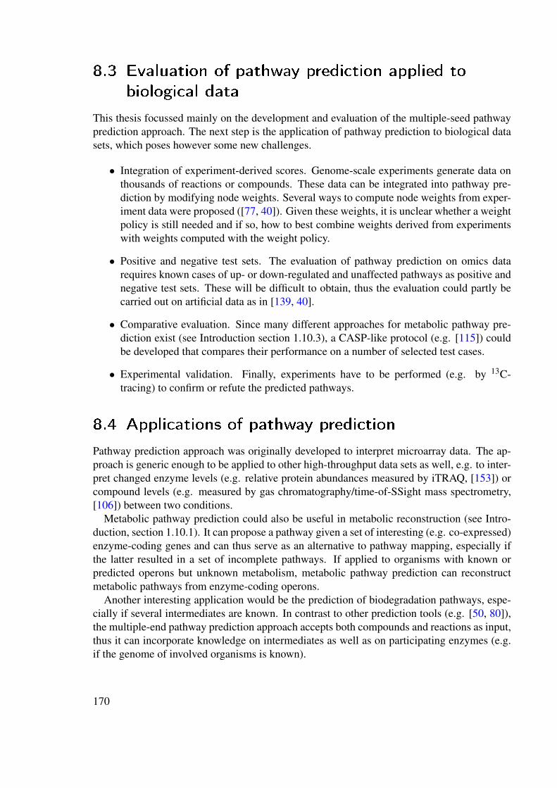
8.3 Evaluation of pathway prediction applied to
biological data
This thesis focussed mainly on the development and evaluation of the multiple-seed pathwayprediction approach. The next step is the application of pathway prediction to biological datasets, which poses however some new challenges.
• Integration of experiment-derived scores. Genome-scale experiments generate data onthousands of reactions or compounds. These data can be integrated into pathway pre-diction by modifying node weights. Several ways to compute node weights from exper-iment data were proposed ([77, 40]). Given these weights, it is unclear whether a weightpolicy is still needed and if so, how to best combine weights derived from experimentswith weights computed with the weight policy.
• Positive and negative test sets. The evaluation of pathway prediction on omics datarequires known cases of up- or down-regulated and unaffected pathways as positive andnegative test sets. These will be difficult to obtain, thus the evaluation could partly becarried out on artificial data as in [139, 40].
• Comparative evaluation. Since many different approaches for metabolic pathway pre-diction exist (see Introduction section 1.10.3), a CASP-like protocol (e.g. [115]) couldbe developed that compares their performance on a number of selected test cases.
• Experimental validation. Finally, experiments have to be performed (e.g. by 13C-tracing) to confirm or refute the predicted pathways.
8.4 Applications of pathway prediction
Pathway prediction approach was originally developed to interpret microarray data. The ap-proach is generic enough to be applied to other high-throughput data sets as well, e.g. to inter-pret changed enzyme levels (e.g. relative protein abundances measured by iTRAQ, [153]) orcompound levels (e.g. measured by gas chromatography/time-of-SSight mass spectrometry,[106]) between two conditions.
Metabolic pathway prediction could also be useful in metabolic reconstruction (see Intro-duction, section 1.10.1). It can propose a pathway given a set of interesting (e.g. co-expressed)enzyme-coding genes and can thus serve as an alternative to pathway mapping, especially ifthe latter resulted in a set of incomplete pathways. If applied to organisms with known orpredicted operons but unknown metabolism, metabolic pathway prediction can reconstructmetabolic pathways from enzyme-coding operons.
Another interesting application would be the prediction of biodegradation pathways, espe-cially if several intermediates are known. In contrast to other prediction tools (e.g. [50, 80]),the multiple-end pathway prediction approach accepts both compounds and reactions as input,thus it can incorporate knowledge on intermediates as well as on participating enzymes (e.g.if the genome of involved organisms is known).
170

An example for a possible application of pathway prediction is the following case: In [12], anovel experimental technique is presented that determines the presence/absence of thousandsof annotated reactions in an organism of interest. This technique, termed reactome array,was applied to two organisms (Pseudomonas putida and Streptomyces coelicolor) and threemicrobial communities (geothermal pool on a volcanic island, surface seawater and deep-seahypersaline anoxic lake). Pathway prediction could elucidate which metabolic pathways aredifferentially active in these organisms and communities.
171

9 Materials and methods
9.1 Graph algorithms
This section summarizes the graph algorithms that were applied in this thesis.The computational complexity of the algorithms is given using the following notation: n is
the number of nodes of the input network, m is the number of edges/arcs in the input network,s is the number of seeds 1 or seed node groups and K is the number of requested paths.
9.1.1 Enumeration of the K-shortest paths
The K-shortest paths problem is the problem of enumerating, in increasing length, the K-shortest paths between a source and a target node in a graph or digraph. In a weighted graphor digraph, the K lightest paths should be enumerated.
REA
In this thesis, the recursive enumeration algorithm (REA) developed by Jimenez and Marzal[83] has been selected as K-shortest paths algorithm. Other algorithms for this problem exist(e.g. [51]). REA has a computational complexity of O(m + Kn log(m/n)) and outputs onepath at a time in order of increasing weight. The original REA source code written in C (withmodifications by Pierre Schaus and Jean-Noël Monette) is called within a Java wrapper.
REA does not return paths, but walks (i.e. nodes may be repeated). However, in practiceREA is sufficiently quick that non-simple paths can be filtered out. Other constraints appliedon the paths (e.g. maximal path length and weight, mutual exclusion of reaction directions,mutual exclusion of node sets in general, absence/presence of user-provided nodes) are like-wise implemented by filtering the REA output.
Filtering REA output is effective and convenient, but poses a problem. Since REA listswalks instead of paths, it can enumerate an infinite number of walks in case the input graphcontains a cycle. Thus, a time limit is required to stop REA in case the requested paths do notexist or do not pass the filter criteria. In addition, an upper limit on the output walk numberprevents out-of-memory errors. Both limits may prevent the complete enumeration of correctpaths. In practice, this problem is only relevant in large, unweighted networks. The userreceives a warning when REA was stopped due to these limits.
1The set of seed nodes is a sub-set of the nodes in the network.
172

Source and target node sets
By default, K-shortest paths algorithms enumerate paths between one source and one tar-get. Using a graph transformation suggested by Olivier Hubaut and described in [47], pathsbetween a set of sources and a set of targets can be enumerated. The idea is to introducepseudo-nodes, each of which is connected to one seed node set. Then, paths can be enumer-ated between the pseudo-nodes, which are afterwards removed from the output paths. Figure9.1 illustrates this concept.
start pseudo node
start node 1
start node 3
start node 2 ...
end pseudo node
end node 1
end node 2
network
Figure 9.1: Pseudo-nodes are artificial nodes that are added to the input network to enable searchesbetween seed node sets. For instance in K-shortest path finding, all start nodes are connected to a startpseudo-node and all end nodes to an end pseudo-node. Paths are enumerated between the start and theend pseudo-node, which are afterwards removed from the paths.
Paths and pathways
In the path finding approach presented in chapter 2, a pathway is considered to be the unionof all first-ranked paths, i.e. all paths having the same weight. Thus, a pathway predicted bypath finding may contain branches.
Directionality and symmetry
In a symmetric graph, the weight of the shortest path between any two nodes A, Bw(shortest_path(A,B)) equals w(shortest_path(B,A)). Undirected graphs are obviouslysymmetric, since their adjacency matrix is symmetric. Importantly, the directed graphs eval-uated in this thesis are also symmetric, because each reaction is represented by two reactiondirections. This is exemplified in Figure 9.2. Thus, shortest paths between a node pair needto be computed in only one direction, either from A to B or from B to A. This symmetry nolonger holds for graphs containing irreversible reactions. In these graphs, shortest_path(A,B)and shortest_path(B,A) both need to be computed to find the shortest paths between a nodepair A and B.
9.1.2 Subgraph extraction from multiple seeds
Computationally, it is much more challenging to predict pathways from a seed set instead oftwo seeds. The enumeration of the lightest paths between two seeds or two seed sets is a
173

R1forward
TA
R2forward
B
R1reverse
R2reverse
R1forward
TA
R2forward
B
R2reverse
A
B
Figure 9.2: In a symmetric graph, the weight of the shortest path between nodes A and B is the sameas the weight of the shortest path between B and A. This property holds also for directed metabolicgraphs that include for each reaction both directions (Figure A). In this case, the shortest path betweenA and B (colored in violet) can be "mirrored" to obtain the shortest path between B and A (coloredin cyan). Reactions R1 and R2 are reversible. However, if the metabolic graph contains irreversiblereactions (e.g. R1 in B), this symmetry no longer holds (Figure B).
174
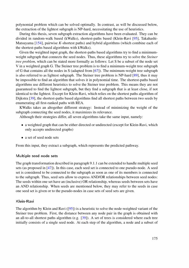
polynomial problem which can be solved optimally. In contrast, as will be discussed below,the extraction of the lightest subgraph is NP-hard, necessitating the use of heuristics.
During this thesis, seven subgraph extraction algorithms have been evaluated. They can bedivided in random-walk based (kWalks), shortest-paths based (Klein-Ravi [95], Takahashi-Matsuyama [154], pairwise K-shortest paths) and hybrid algorithms (which combine each ofthe shortest-paths based algorithms with kWalks).
Given the weighted input graph, the shortest-paths based algorithms try to find a minimum-weight subgraph that connects the seed nodes. Thus, these algorithms try to solve the Steinertree problem, which can be stated more formally as follows: Let S be a subset of the node setV in a weighted graph G. The Steiner tree problem is to find a minimum-weight tree subgraphof G that contains all the nodes in S (adapted from [67]). The minimum-weight tree subgraphis also referred to as lightest subgraph. The Steiner tree problem is NP-hard [89], thus it maybe impossible to find an algorithm that solves it in polynomial time. The shortest-paths basedalgorithms use different heuristics to solve the Steiner tree problem. This means they are notguaranteed to find the lightest subgraph, but they find a subgraph that is at least close, if notidentical to the lightest. Except for Klein-Ravi, which relies on the shortest paths algorithm ofDijkstra [39], the shortest-paths based algorithms find all shortest paths between two seeds byenumerating all first-ranked paths with REA.
KWalks takes an altogether different strategy: Instead of minimizing the weight of thesubgraph connecting the seed nodes, it maximizes its relevance.
Although their strategies differ, all seven algorithms take the same input, namely:
• a weighted graph that can be either directed or undirected (except for Klein-Ravi, whichonly accepts undirected graphs)
• a set of seed node sets
From this input, they extract a subgraph, which represents the predicted pathway.
Multiple seed node sets
The graph transformation described in paragraph 9.1.1 can be extended to handle multiple seedsets (as proposed in [47]). In this case, each seed set is connected to one pseudo-node. A seedset is considered to be connected to the subgraph as soon as one of its members is connectedto the subgraph. Thus, seed sets allow to express AND/OR relationships between seed nodes:The seeds within one set have an (inclusive) OR relationship, whereas seeds between sets havean AND relationship. When seeds are mentioned below, they may refer to the seeds in caseone seed set is given or to the pseudo-nodes in case sets of seed sets are given.
Klein-Ravi
The algorithm by Klein and Ravi ([95]) is a heuristic to solve the node-weighted variant of theSteiner tree problem. First, the distance between any node pair in the graph is obtained withan all-to-all shortest paths algorithm (e.g. [39]). A set of trees is considered where each treeinitially consists of a single seed node. At each step of the algorithm, a node and a subset of
175

the remaining trees are selected such that the cost of tree merging is minimized. At least twotrees have to be merged in each step. The cost of tree merging is computed as the sum of theweight of the selected node and the weights of the shortest paths between the selected nodeand the selected tree subset. This sum is divided by the number of trees in the selected subset.The algorithm terminates when all trees are merged. The computational complexity of thisapproach is O(n2 logn+nm+ns3 logs).
The same implementation as in [147] was used, which was kindly provided by Nadja Betzler[15].
Takahashi-Matsuyama
The algorithm by Takahashi and Matsuyama ([154]) initializes the sub-network with a nodechosen at random among the s seeds. It then proceeds by identifying in each step the lightestpath(s) between any of the remaining seed nodes and any node in the sub-network. The lightestpath(s) is merged with the sub-network. The computational complexity of this approach isO(s(m+Kn log(m/n))).
This algorithm has been implemented in Java, with the following modifications:
• Not the shortest, but the K-shortest paths are searched to ensure that all paths of thesame weight are included in the solution subgraph. Thus, the subgraph extracted by thisalgorithm is not necessarily a tree.
• Instead of pre-computing the shortest paths between all node pairs as proposed by Taka-hashi and Matsuyama, only needed (K-shortest) paths are computed. This is doneefficiently by introducing at each step a pair of pseudo-nodes, one of which is con-nected to all nodes in the current subgraph and the other is connected to all remainingseed nodes. This reduces the run-time from O(s(n2)) as indicated by the authors toO(s(m+Kn log(m/n))), where O(m+Kn log(m/n))) is the run-time of REA.
• If no paths can be found between the initial single-node subgraph and the remainingseeds, the subgraph is initialized with another seed. This is repeated until either all seedshave served to initialize the subgraph or a single-node subgraph has been initialized thatcan be connected to one of the remaining seeds. This alleviates Takahashi-Matsuyama’sweakness with respect to orphan seed treatment. Why this is important will be discussedin paragraph 9.1.2.
Pair-wise K-shortest paths
Pair-wise K-shortest paths has been developed during the initial stages of this thesis and canbe considered as a heuristic to solve the Steiner tree problem. In the first step, REA is calledsuccessively on each pair of seed nodes. The resulting path sets are stored in a path matrix, andthe minimal weight between each node pair is stored in a distance matrix. In the second step,the sub-network is constructed from the path sets, starting with the lightest path set. Step-wise,path sets are merged with the subgraph by increasing order of their weight. The process stops
176

Table 9.1: KWalks parameters.
Parameter Default Explanation Modified invalue the evaluation
Limited true Random walks are not infinite, nobut of limited length.
L 50 Maximal length of a random walk. noUp to true Random walks of less than no
the maximal step numberare allowed.
Initial seed node uniform Distribution of seed node noprobabilities distribution probabilities.Iteration number 1 The number of times kWalks yes
is executed on a graph.
if either all seeds belong to one connected component of the sub-network or all path sets havebeen merged with the sub-network.
The computational complexity of this approach is O(s2(m + Kn log(m/n)), because theREA algorithm is called s2 times.
kWalks
The kWalks method is a generic algorithm ([48, 21]) to build a most relevant subgraph con-necting seed nodes in a large graph. The relevance of an edge is measured as the expectednumber of times it is visited by random walks connecting seed nodes. These expected passagetimes reflect both the topology of the network and the edge weights.
A subgraph is obtained from the edge relevances by keeping only those edges above a min-imal relevance threshold. This threshold is automatically fixed such that the subgraph inducedby the selected edges is weakly connected. The sub-networks extracted by kWalks may con-tain branches ending in non-seed nodes. These branches are removed in a final pruning step.
KWalks takes some additional parameters not shared with the other subgraph extractionalgorithms. An important one is the iteration number. The edge relevances computed bykWalks can serve as new edge weights. kWalks can then be run on the input graph withupdated weights. This iterative process may be repeated a number of times to increase thedifference between more and less relevant edges.
Table 9.1 lists the kWalks-specific parameters. The unlimited kWalks computes the edgeand node relevances as the expected number of times edges and nodes are visited by walksof unlimited length. The limited kWalks is a computationally more efficient approximationof the unlimited case, where walk length is limited. Most of the parameters were not variedduring evaluation, because they have reasonable default values. For instance, the parameter L(maximal length of random walks) is set to 50, because measurements on artificial networkshave shown that very good precision/recall curves are obtained for this length [48].
177
In this thesis, the implementation of kWalks by Jerôme Callut was used, which was kindlyprovided by Pierre Dupont. The computational complexity of the unlimited kWalks is O(sn3)and of the limited kWalks is O(sLm), where L is the maximal allowed length of the randomwalks. Since L is typically a small constant, kWalk’s runtime increases linearly with the seednode number for a given input graph.
Hybrid subgraph extraction algorithms
As discussed in chapter 3, kWalks is more sensitive whereas the shortest-paths based algo-rithms are more specific with respect to pathway prediction accuracy. Therefore, they werecombined in a hybrid approach.
Such a hybrid approach runs in two steps: kWalks extracts a sub-network representing afixed proportion of the input network and the shortest-path based algorithm is launched onthis intermediate sub-network to obtain the final pathway.
Combining kWalks with path-based approaches gives two new parameters:
• Size of the sub-network kWalks extracts a sub-network whose size is fixed to a givenpercentage of the number of nodes in the input network.
• Input or computed weights The path-based algorithms may either use the input weightsor the edge/node relevances computed by kWalks.
The di�culties of assembling a metabolic pathway from multiple paths
The shortest-paths based algorithms construct a pathway from several paths. For metabolicgraphs, this creates several problems, which have not yet been solved satisfactorily.
• Treatment of irreversible reactions. In graphs containing irreversible reactions, it is notensured that the irreversible reactions in the subgraph operate in the same direction.
• Mutual exclusion of reactant pairs across paths. This is currently only implementedfor Takahashi-Matsuyama, at the cost of rendering the resulting subgraph seed-node-order dependent. Thus, this algorithm could return different subgraphs when repetitivelyexecuted on the same seeds and input RPAIR graph. However, such behavior is rarelyobserved in practice.
Orphan seed nodes and disconnected components
A predicted metabolic pathway may contain orphan seeds or may consist of several compo-nents.
Orphan seeds are seed nodes or seed node sets that could not be connected to the subgraph.Orphan seeds can occur for the following reasons:
• No path exists between the orphan and the subgraph in the input graph, either becausethe input graph consists of several components or contains irreversible reactions.
178

• A path exists, but does not pass the filter criteria (e.g. it contains nodes already excluded,or does not contain nodes required to be present).
A pathway may connect all seeds and seed node groups, but may not be a connected graph.This can occur when several seed node sets have been given as input, as depicted in Figure9.3A.
group A
seed A1
seed A2
seed A3
group Bseed B1
seed B2
group C
seed C1
re-arranged group A
seed A1
re-arranged group B
seed B1
seed B2
seed C1
A
B
Figure 9.3: A subgraph is extracted for the three seed node sets group A, group B and group C. GroupA is connected to group B via seed B1, but group C is connected to group B via seed B2. Thus, twocomponents are formed, one containing seed A1 and B1 and the other containing seed C1 and B2(Figure A). After re-grouping of the seed sets, it is possible that the two components are connected (inthis case by an intra-group connection with respect to the original seed groups) (Figure B).
179

Preprocessing and postprocessing
PreprocessingPreprocessing eases the task of subgraph extraction by connecting seeds that can be treatedwithout heavy computation. For instance, neighboring seed nodes such as a reaction and itssubstrate can be directly connected. The treatment of indirect neighbors (those that are sep-arated by one node, e.g. substrate and product of a reaction) is less obvious. In a weightedgraph, a path with many intermediate nodes may be lighter than a path with only one interme-diate node. However, in the RPAIR network, additional information on the intermediate nodebecomes available. Consider for instance two seed reactant pairs that share a main compound.It makes sense biochemically to link them via this compound. It is still possible that a lighterpath exist, but it is less likely that this path is biochemically more relevant. A small-scale eval-uation on four branched pathways manually mapped from MetaCyc onto KEGG showed thatpreprocessing enhances both accuracy and speed of computation. In the absence of a thoroughevaluation, the decision on whether or not this option should be enabled is left to the user.
PostprocessingAs discussed in section 9.1.2, the extracted subgraph may consist of several components. Insome situations, it may make sense to repeat pathway prediction with re-grouped seed sets.
Consider for instance an enzyme B that contributes two reactions B1 and B2 to a path-way. This enzyme will be treated as a seed node group consisting of two seeds. Duringconventional pathway prediction, at least one of these seed reactions will be connected to thesubgraph (assuming the seeds are not orphans), but the second reaction is not necessarily con-nected. If pathway prediction is repeated with seed sets re-arranged such that the seed nodesof each component form a new seed set (see Figure 9.3B), the second reaction of the enzymemay be connected to the pathway. However, the solution obtained after postprocessing is notnecessarily identical to the solution that would have been obtained had the seeds been givenseparately.
Treating all reactions associated to an enzyme as separate seeds is not a satisfying solutioneither, because due to the imprecise enzyme-reaction mappings not all of them may be rele-vant for the pathway. Thus, seed sets in combination with postprocessing might be a way todeal with these imprecise mappings. However, without an evaluation, it is not clear whetherpostprocessing is really helpful in these cases and is therefore left as an option to the user.
Comparison of the subgraph extraction algorithms
Di�erential prediction accuracy of subgraph extraction algorithmsChapter 3 presented a comparison of the subgraph extraction algorithms with respect to theirpathway prediction accuracy. This section discusses likely reasons for the different accuraciesreached by the subgraph extraction algorithms. The performance of the algorithms might dif-fer for other networks, for instance the KEGG RPAIR network. Unfortunately, the accuracy ofthe algorithms could not be evaluated for the KEGG RPAIR network, because of the absenceof a sufficient number of branched reference pathways with KEGG identifiers. KEGG mapsare not suitable for reasons discussed in the introduction, section 1.4. The aMAZE pathways
180

are not an appropriate reference pathway set either, because of their small number of branchedpathways. Careful mapping of four selected MetaCyc pathways onto KEGG showed that auto-matic mapping without curation would be inaccurate and it was beyond the scope of this thesisto manually map all the MetaCyc pathways onto KEGG. However, it would be highly inter-esting to compile such a reference pathway set in the future in order to evaluate systematicallythe performance of the subgraph extraction algorithms for KEGG RPAIR networks.
In the compound-weighted MetaCyc network, kWalks, even if iterated, does not reach theaccuracy of shortest-paths based approaches. One possible reason may be that the currentversion of kWalks does not handle mutual exclusion between forward and reverse directionof reactions. Thus walks can cross reactions from substrate to product to another substrate,which results in an irrelevant pathway.
Klein-Ravi has the lowest prediction accuracy of the three shortest-paths based algorithms,very likely because in its current implementation it does not accept directed networks. Itsaccuracy may be higher for the RPAIR network, which can be undirected for reasons discussedin chapter 2. Takahashi-Matsuyama outperforms pairwise K-shortest paths by 8%. The reasonis that pairwise K-shortest paths only searches shortest paths between seed nodes, whereasTakahashi-Matsuyama also takes into account shortest paths between seed nodes and othersubgraph nodes. Thus, K-shortest paths can miss a path between a seed node and a subgraphnode that is lighter than any path to another seed node, which would be detected by Takahashi-Matsuyama.
All three shortest-paths based approaches yield a small yet significant increase in accuracywhen combined with kWalks (as measured with a paired signed Wilcoxon rank test). Ap-parently, kWalks discards nodes that would otherwise be predicted as false positives in thepathway. However, kWalks’ main role is to increase the computational speed of pathwayprediction.
Strengths and weaknesses of subgraph algorithms
Apart from their prediction accuracy, the algorithms have other strengths and weaknesses thatare discussed here.
To summarize: There is no single subgraph extraction algorithm that can be recommendedfor all situations. In most situations however, the winner of the evaluation described in chapter3, namely the hybrid of Takahashi-Matsuyama and kWalks, should be used.
In general, hybrids are quicker and more accurate than their shortest-paths based pendants,but they have a shortcoming: Whereas the repetition of the shortest-paths based algorithmsdoes not change the solution (except for Takahashi-Matsuyama as discussed in 9.1.2), it wasobserved that different solutions were returned when executing one of the random-walk basedalgorithms repetitively on the same seeds. This behavior may probably be due to ties in theedges relevances. From two edges of equal relevance, one is selected at random and addedto the growing subgraph. When the selected edge is the last needed to meet the thresholdcriterion, the algorithm stops. Which of the two edges is incorporated into the subgraph cantherefore differ upon repetition of the subgraph extraction. However, in most cases only oneor a very small set of solutions is returned for repetitive executions.
KWalks is the quickest of all the tested subgraph extraction algorithms and in addition candiscover weights. In the absence of a weight policy, extracting a subgraph with the edge rel-
181

evances returned by kWalks instead of unit weights increases the accuracy of the pairwiseK-shortest paths algorithm by more than 10%. Moreover, kWalks allows to refine the rela-tionship between seed nodes by assigning probabilities to them. It is also the only one of thetested algorithms that can extract other than trivial cyclic pathways.
However, kWalks has to be iterated to reach a high accuracy, which decreases its speed con-siderably. Even iterated kWalks was not among the top five algorithms with highest accuracy,for reasons discussed in section 9.1.2.
Klein-Ravi is by far the quickest among the three shortest-paths based algorithms, but nei-ther does it take into account several paths of equal weight nor is it applicable to directednetworks.
Pairwise K-shortest paths is the slowest of the three shortest-paths based algorithms, be-cause it computes the K-shortest paths between each pair of seed nodes, thus its runtimeincreases quadratically with the seed node number instead of linearly as for Takahashi-Matsuyama.
However, pairwise K-shortest paths is robust with respect to orphan seed nodes, whereasTakahashi-Matsuyama is not. At each step, Takahashi-Matusyama computes the K-shortestpaths between all remaining seed nodes and the subgraph. As soon as Takahashi-Matsuyamacannot connect any of the remaining seed nodes to the subgraph, it stops and returns an un-connected subgraph. However, even though it is not possible to connect the seed nodes to thesubgraph, it may be possible to connect them among each other, thus obtaining a subgraphwith several components. In order to connect non-orphan seeds among each other, Takahashi-Matsuyama would have to test all s× (s− 1) seed node combinations and thus would reachthe runtime of pairwise K-shortest paths.
Simply using the largest connected component of a network does not avoid orphans, sincein RPAIR networks, reactant pairs exclude each other mutually. Thus, whether a seed nodeis an orphan or not depends on the other seed nodes. Even worse, the order of seed nodes inRPAIR networks matters, because the nodes that are forbidden (by mutual exclusion) dependon which seed node is selected first. As mentioned in 9.1.2 reactant pair exclusion across pathsis only implemented for the Takahashi-Matsuyama algorithm.
Apart from the better treatment of orphans, another advantage of pairwise K-shortest pathsis that it outputs a distance matrix for the seeds, which allows to group them by standardcluster algorithms. Pairwise K-shortest paths comes with an option to generate a dendrogramof the seed nodes. Such a dendrogram cannot be obtained from Takahashi-Matsuyama.
By default, Takahashi-Matsuyama should be favored over pairwise K-shortest paths, be-cause it is quicker, more accurate and takes mutual exclusion of reactant pairs across pathsinto account. In special situations and if the graph is not an RPAIR graph, pairwise K-shortestpaths can be run to connect orphans among each other or to group seeds using the seed distancematrix.
Exact solution of the Steiner tree problem
In [105], an algorithm solving the Steiner tree problem exactly is described. This algorithm hasnot been used because it requires commercial software to be installed (CPLEX) and becauseit is unclear whether it could be customized to treat mutual exclusion of nodes (required for
182

Table 9.2: Composition of selected metabolic networks that were employed for the evaluation of path-way prediction.
Network Database Di- Compound Reaction Arc/edge Evalu-(version) rected* number number number ation
reaction KEGG true 5,312 6,359 × 2 53,572 pathgraph LIGAND (41.0) findingRPAIR KEGG false 4,297 7,058 28,232 pathgraph RPAIR (41.0) findingreaction- KEGG false 4,297 12,828 51,312 pathspecific LIGAND/ findingRPAIR RPAIRgraph (41.0)MetaCyc MetaCyc true 4,891 5,358 × 2 43,938 pathwaygraph (11.0) prediction
with mul-tiple seeds
* In a directed graph, reactions are duplicated to represent both directions. Consequently,the arc number between a reaction and a compound is also duplicated.
treatment of reaction directions and reactant pairs). If these obstacles could be overcome, itwould be worth evaluating this algorithm.
9.2 Networks and reference pathways
9.2.1 Metabolic networks
During this thesis, pathway prediction was evaluated with networks constructed from bothKEGG and MetaCyc. KEGG networks were built in a variety of ways: with selectedcompounds or reactant pair classes removed and as directed or undirected graphs. An ex-haustive list of all KEGG networks constructed is available at http://rsat.ulb.ac.be/pathfindingsupplementref/MetabolicGraphs.html. Likewise, several versions of theMetaCyc network were built (details can be found in chapter 3).
Table 9.2 lists properties for a selection of these networks, namely all those that are sup-ported by NeAT (of course, since the networks in NeAT are updated, their version and conse-quently their node and edge numbers may be different from those indicated in the table).
9.2.2 Metabolic reference pathways
In general, reference pathways were modified as follows: Terminal compound nodes were re-moved from all reference pathways, because the evaluation took place between seed reactions.
183

Table 9.3: Filtering steps applied to the aMAZE reference pathways.All organisms E. coli S. cerevisiae H.sapiens
Pathways before filteringPathways (116) 55 29 32Cyclic* pathways (7) 2 4 1Branched* pathways (25) 13 5 7Pathways with less than 3 reactions (46) 20 14 12
Pathways after filtering and linearizationPathways (69) 37 14 18
Pathways after mapping of reactions to reactant pairsPathways (55) 32 11 12* BioPool compounds not counted
After removal of terminal compounds, only reference pathways with at least five nodes werekept, to avoid trivial predictions. A number of more specific filter steps and modifications wasapplied to each reference pathway set separately.
Reference pathways for path �nding
Path finding was evaluated with reference pathways from three organisms taken from aMAZE.Table 9.3 summarizes the filtering steps, which reduced the 116 aMAZE pathways to the 55linearized reference pathways used for evaluation. Figure 9.4 displays a histogram of the nodenumbers for the final pathway set. Since the pathways are linearized, the node number of apathway indicate its length.
The linearized aMAZE pathways can be obtained in various formats from http://
rsat.ulb.ac.be/pathfindingsupplementref/ReferencePathways.html. The unmod-ified aMAZE pathways are available as part of the metabolic database described in section9.3.
Reference pathways for multiple seed pathway prediction
As can be seen from Table 9.3, only 25 of the aMAZE pathways are branched. To eval-uate pathway prediction with multiple seeds on a larger set of branched pathways, the 171reference pathways annotated for S. cerevisiae in MetaCyc (version 11.0) were parsed fromthe organism-specific biopax.owl and pathways.dat files. The latter file contains the pathway-specific classification of compounds into side and main, which is not included in the OWL file.From these reference pathways, a large number had to be removed for the following reasons:
• They involved non-small molecules.
• They consisted of several components.
184
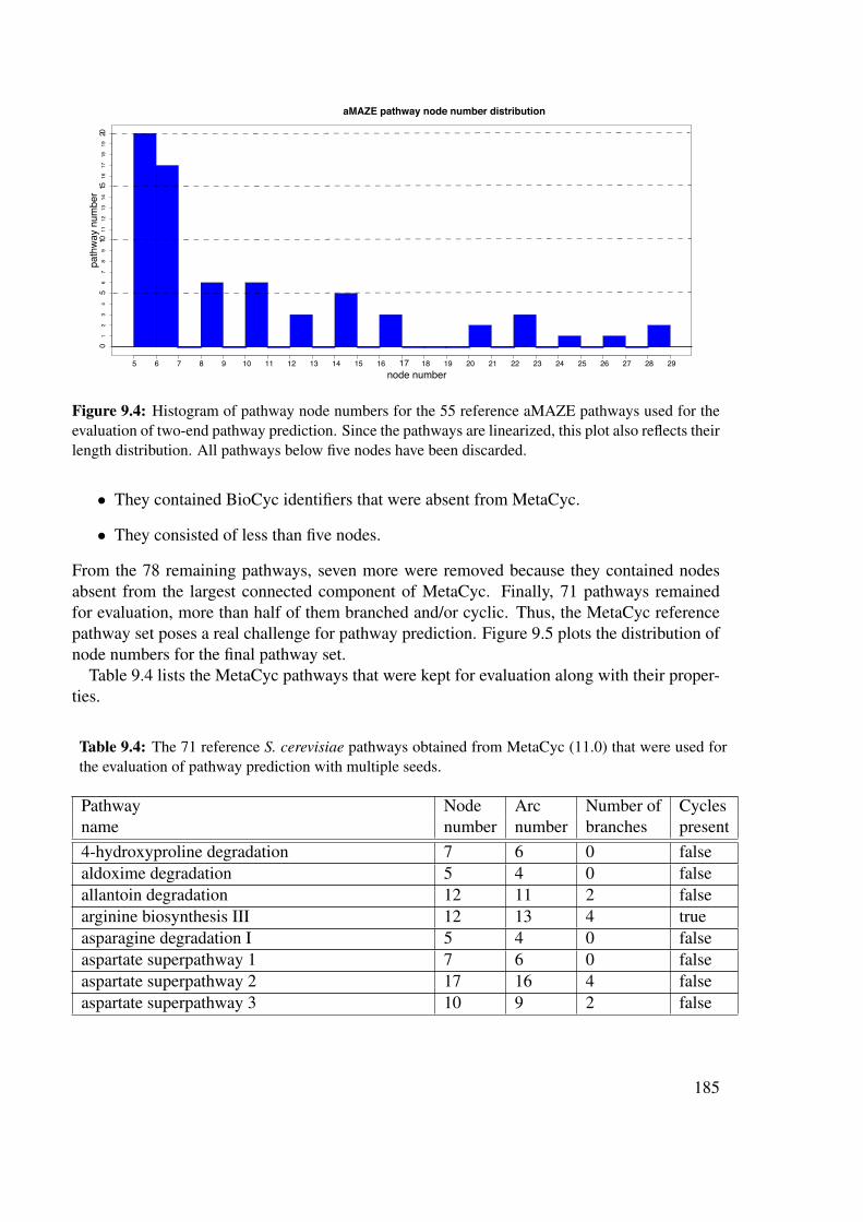
aMAZE pathway node number distribution
node number5 6 7 8 9 10 11 12 13 14 15 16 17 18 19 20 21 22 23 24 25 26 27 28 29
01
23
45
67
89
0111
213 1
4151
617 1
8191
0 2pa
thw
ay n
umbe
r
Figure 9.4: Histogram of pathway node numbers for the 55 reference aMAZE pathways used for theevaluation of two-end pathway prediction. Since the pathways are linearized, this plot also reflects theirlength distribution. All pathways below five nodes have been discarded.
• They contained BioCyc identifiers that were absent from MetaCyc.
• They consisted of less than five nodes.
From the 78 remaining pathways, seven more were removed because they contained nodesabsent from the largest connected component of MetaCyc. Finally, 71 pathways remainedfor evaluation, more than half of them branched and/or cyclic. Thus, the MetaCyc referencepathway set poses a real challenge for pathway prediction. Figure 9.5 plots the distribution ofnode numbers for the final pathway set.
Table 9.4 lists the MetaCyc pathways that were kept for evaluation along with their proper-ties.
Table 9.4: The 71 reference S. cerevisiae pathways obtained from MetaCyc (11.0) that were used forthe evaluation of pathway prediction with multiple seeds.
Pathway Node Arc Number of Cyclesname number number branches present4-hydroxyproline degradation 7 6 0 falsealdoxime degradation 5 4 0 falseallantoin degradation 12 11 2 falsearginine biosynthesis III 12 13 4 trueasparagine degradation I 5 4 0 falseaspartate superpathway 1 7 6 0 falseaspartate superpathway 2 17 16 4 falseaspartate superpathway 3 10 9 2 false
185

bifidum pathway 29 33 12 truebutanediol fermentation 36 47 18 truechorismate biosynthesis 13 12 0 falsecysteine biosynthesis II 9 8 0 falsede novo biosynthesis of pyrimidineribonucleotides 19 18 0 falsefatty acid oxidation pathway 11 10 0 falsegluconeogenesis 22 22 2 falseglutamate degradation I 6 6 2 trueglutamate fermentation I-thehydroxyglutarate pathway 9 8 0 falseglycerol degradation II 16 16 2 falseglycolysis I 17 17 2 falseheme biosynthesis II 15 14 0 falsehistidine biosynthesis I 19 18 0 falsehomocysteine and cysteine interconversion 7 8 2 truehomoserine and methionine biosynthesis 14 13 2 falsehomoserine biosynthesis 5 4 0 falseisoleucine biosynthesis I 9 8 0 falseisoleucine degradation III 17 16 0 falseleucine biosynthesis 7 6 0 falselipoxygenase pathway 13 12 6 falsemannosyl-chito-dolichol biosynthesis 5 4 0 falsemethionine biosynthesis I 8 7 2 falsemethionine biosynthesis III 5 4 0 falsenon-oxidative branch of thepentose phosphate pathway 10 12 4 truepolyamine biosynthesis I 8 7 0 falsepolyamine biosynthesis III 8 7 0 falsepyridine nucleotide biosynthesis 10 9 2 falsepyridine nucleotide cycling 15 18 6 truepyruvate oxidation pathway 6 5 2 falseriboflavin and FMN and FAD biosynthesis 17 17 2 truesalvage pathways of purineand pyrimidine nucleotides 29 35 13 truesalvage pathways of purine nucleosides 16 17 4 truesalvage pathways of pyrimidine ribonucleotides 1 5 4 0 falsesalvage pathways of pyrimidine ribonucleotides 2 7 6 2 falseserine biosynthesis 5 4 0 falseserine-isocitrate lyase pathway 28 29 4 truespermine biosynthesis 7 6 0 false
186

sucrose biosynthesis 8 7 2 falsesucrose degradation I 5 4 0 falsesucrose degradation III 12 12 4 falsesuperpathway of fatty acid oxidationand glyoxylate cycle 1 7 6 0 falsesuperpathway of fatty acid oxidationand glyoxylate cycle 2 11 10 0 falsesuperpathway of glycolysis andTCA variant VIII 46 55 16 truesuperpathway of glycolysis, pyruvatedehydrogenase, TCA, and glyoxylate bypass 39 41 4 truesuperpathway of isoleucine andvaline biosynthesis 1 7 6 0 falsesuperpathway of isoleucine andvaline biosynthesis 2 9 8 0 falsesuperpathway of leucine, valine,and isoleucine biosynthesis 1 14 13 2 falsesuperpathway of lysine, threonine andmethionine biosynthesis 9 8 0 falsesuperpathway of phenylalanine, tyrosineand tryptophan biosynthesis 25 24 0 falsesuperpathway of ribose and deoxyribosephosphate degradation 1 9 8 2 falsesuperpathway of ribose and deoxyribosephosphate degradation 2 8 7 0 falsesuperpathway of serine and glycine biosynthesis 7 6 0 falsesuperpathway of sulfur amino acid biosynthesis 19 20 4 trueTCA cycle – aerobic respiration 19 20 2 trueTCA cycle variation VIII 28 32 8 truethreonine biosynthesis 9 8 0 falsetrehalose biosynthesis III 7 6 0 falsetryptophan biosynthesis 11 10 0 falseUDP-N-acetylgalactosamine biosynthesis 9 8 0 falseurate degradation 12 11 2 falseureide degradation 9 9 6 falsevaline biosynthesis 7 6 0 falsexylulose-monophosphate cycle 10 10 0 true
187

S. cerevisiae (MetaCyc) pathway node number distribution
node number5 6 7 8 9 10 11 12 13 14 15 16 17 18 19 20 21 22 23 24 25 26 27 28 29 30 31 32 33 34 35 36 37 38 39 40 41 42 43 44 45 46
01
23
45
67
89
011 1
path
way
num
ber
Figure 9.5: Histogram of pathway node numbers for the 71 reference MetaCyc pathways used for theevaluation of multiple-end pathway prediction. All pathways below five nodes have been discarded.
9.2.3 Comparison of a predicted to a reference pathway
In order to quantify the accuracy of the metabolic pathway prediction algorithms, predictedpathways have to be compared with annotated ones.
Accuracy calculation
In this thesis, accuracies are calculated as in [31, 32] based on the overlap of nodes in thepredicted and annotated pathway.
A true positive (TP) node is a node that is present in both the reference and the predictedpathway. A false positive (FP) node is a node that is present in the predicted but absent in thereference pathway. Finally, a false negative (FN) node is a node that is absent in the predictedbut present in the reference pathway.
Importantly, seed nodes are not counted as true positives.Figure 9.6 illustrates these definitions.The sensitivity of pathway prediction is then defined as:
Sn =T P
T P+FN(9.1)
The positive predictive value is defined as:
PPV =T P
T P+FP(9.2)
The PPV instead of the specificity is used for accuracy calculation, because the formula for
188
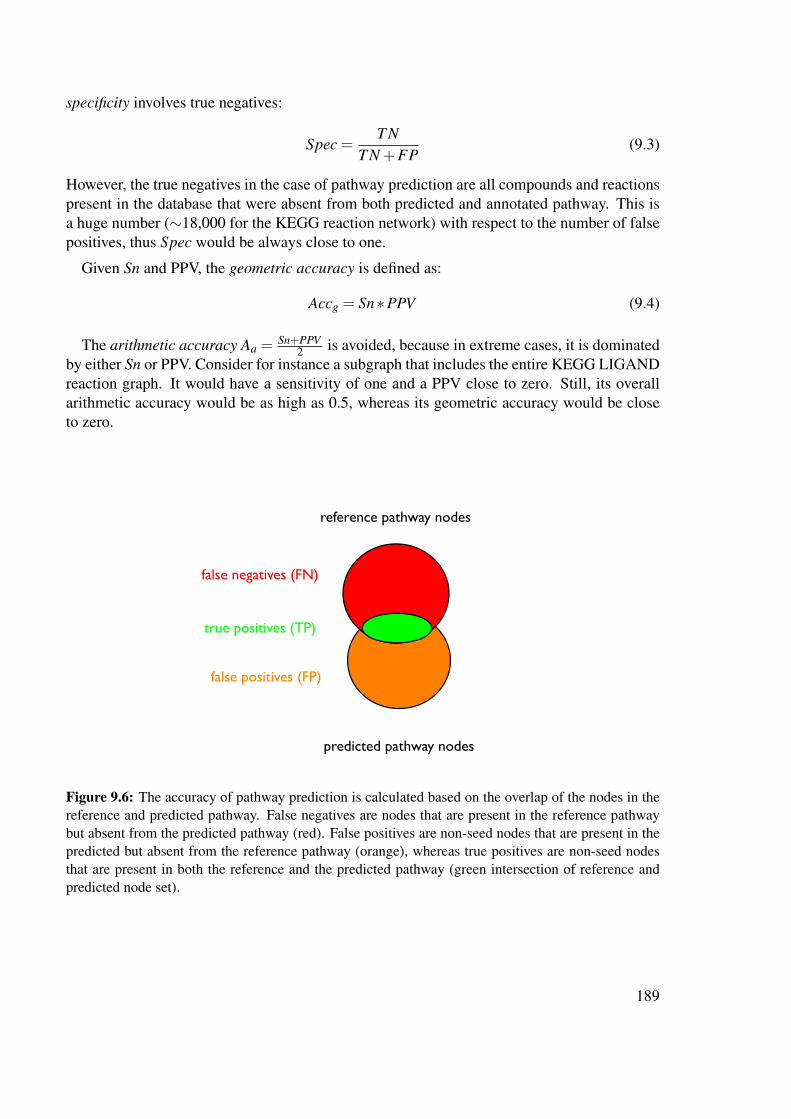
specificity involves true negatives:
Spec =T N
T N +FP(9.3)
However, the true negatives in the case of pathway prediction are all compounds and reactionspresent in the database that were absent from both predicted and annotated pathway. This isa huge number (∼18,000 for the KEGG reaction network) with respect to the number of falsepositives, thus Spec would be always close to one.
Given Sn and PPV, the geometric accuracy is defined as:
Accg = Sn∗PPV (9.4)
The arithmetic accuracy Aa = Sn+PPV2 is avoided, because in extreme cases, it is dominated
by either Sn or PPV. Consider for instance a subgraph that includes the entire KEGG LIGANDreaction graph. It would have a sensitivity of one and a PPV close to zero. Still, its overallarithmetic accuracy would be as high as 0.5, whereas its geometric accuracy would be closeto zero.
reference pathway nodes
true positives (TP)
false negatives (FN)
false positives (FP)
predicted pathway nodes
Figure 9.6: The accuracy of pathway prediction is calculated based on the overlap of the nodes in thereference and predicted pathway. False negatives are nodes that are present in the reference pathwaybut absent from the predicted pathway (red). False positives are non-seed nodes that are present in thepredicted but absent from the reference pathway (orange), whereas true positives are non-seed nodesthat are present in both the reference and the predicted pathway (green intersection of reference andpredicted node set).
189

Node set overlap versus pathway alignment
An alternative to the node set comparison would be a pathway alignment. However, path-way alignment algorithms would have comparatively long runtimes, as they have to cope withbranched pathways. Thus, their use is infeasible in a large-scale evaluation such as the onepresented in chapter 3. The main advantage of pathway alignment algorithms is their consid-eration of node arrangement. However, because of the structure of metabolic pathways, thenodes composing them cannot be arranged in any number of ways. Thus, node set intersec-tions reflect well the degree of similarity between two metabolic pathways.
Overall, the accuracy measurement is quite conservative. Since terminal compounds wereremoved from the reference pathways, they are counted as false positives. Likewise, alterna-tive reactions between two compounds are counted as false positives, even though they sharea reactant pair with the correct reaction.
9.2.4 Evaluation procedure
Before starting the evaluation, the reference pathway set, the metabolic graph, the pathwayprediction algorithm to be evaluated and its parameters are selected. Then, the evaluationiterates over the set of reference pathways. The final accuracy is the average of all individualaccuracies.
The results of the evaluations are stored in a database. For two-end pathway prediction, aweb interface has been written, so that the results can be browsed on the internet at: http:
//rsat.ulb.ac.be/pathfindingsupplementref/index.html.
Evaluation of path �nding
For each reference pathway, the following steps are performed:
1. The terminal reactions of the reference pathway are selected as seed nodes.
2. The metabolic graph and the seeds are given to the pathway prediction algorithm, whichreturns a pathway.
3. The accuracy of the predicted pathway is computed as described above.
Evaluation of multiple-end pathway prediction
For each reference pathway, the following steps are performed:
1. All terminal reactions of the reference pathway are selected as seed nodes. Pathwayprediction and accuracy computation are carried out for these seeds.
2. One additional intermediate reaction is selected at random from the reference pathway.Pathway prediction and accuracy computation are repeated with the terminal and inter-mediate reactions as seed nodes.
190
3. Step 2 is repeated as many times as reactions exist in the reference pathway. Reactionsalready in the seed node set are not selected again from the reference pathway.
4. The evaluation of the reference pathway terminates if all its reactions have been addedto the seed node set.
Figure 9.7 shows the result of the evaluation for the Takahashi-Matsuyama algorithm in thedirected, degree-weighted MetaCyc graph.
9.3 Metabolic database
In order to store, manage and access metabolic data from different sources, a database isneeded.
In particular, the database has to meet the three following requirements:
• Storage and retrieval of metabolic networks obtained from different source databases.
• Storage and retrieval of metabolic pathways obtained from different source databases.
• Mapping of genes to reactions and reactant pairs.
The aMAZE database [101] would have been the database of choice, but it is no longermaintained. Other generic biological or metabolic databases or parsers [99, 25, 58] were notavailable at the time or did not offer needed functionality (such as coverage of KEGG RPAIR).
Therefore, it became necessary to design and implement a metabolic database that performsthe tasks listed above.
9.3.1 Data model
The data model of the metabolic database was inspired by the aMAZE data model [163, 101],but is much simpler, since its goals are much less ambitious than those of the aMAZEdatabase. The aMAZE database was designed to accommodate biological data in general(metabolism, regulation, signal transduction, etc.), whereas the database presented here isspecific to metabolic data and does not cover regulation or signal transduction. Furthermore,it does not model explicitly the stoichiometry of reactions, because this was not needed forthe pathway prediction approach adopted in this thesis. Polypeptides that are themselves re-actants of reactions cannot be modeled, because the database is restricted to small moleculemetabolism. Care has been taken to ensure that organism-specific features of pathways suchas reaction directions are modeled at the level of pathway steps and not at the level of reac-tions, compounds and enzymes. The pathwayStep class roughly corresponds to the catalysisclass in biopax, with the difference that pathwayStep objects can be associated to main com-pounds. Proteins consisting of several polypeptides or operons comprising several genes canbe modeled with the help of the bioentity child and parent classes.
Figure 9.8 depicts the data model of the metabolic database.
191

Figure 9.7: This heat map summarizes the evaluation performed for the algorithm Takahashi-Matsuyama in the directed, degree-weighted MetaCyc graph. The x-axis lists the number of reactionnodes that still have to be predicted. Thus, for x equals 1, all except one reaction were given as seednodes to the algorithm. For x equals 2, all but two reactions were given as seeds to the algorithm, andso forth. The y-axis enumerates all 71 reference pathways in alphabetical order. The colors of the heatmap reflect the geometric accuracy, with red for an accuracy of 0, orange for an accuracy of 0.5 andgreen for an accuracy of 1. Overall, 406 predictions were carried out.
192

Table 9.5: Content of the metabolic database as of October 2009.Database version Number of Number of Number of Number of
reactions/ compounds pathways organismsreactant pairs
KEGG 49.0 7,432 6,078 0 0LIGAND
KEGG 49.0 10,913 5,661 0 0RPAIRKEGG 50.0 5,301 4,233 145 1 (refe-
PATHWAY rence)MetaCyc 13.0 4,116 3,412 1347 391aMAZE 2006 392 443 116 3
(no longermaintained)
9.3.2 Implementation
The metabolic database is object oriented. The underlying relational database is hosted bypostgres [135] and the object-relational mapping was implemented in Java with Hibernate[71]. These technologies have the advantage to be open source (postgres: BSD license, Hiber-nate: GNU Lesser General Public License) and can therefore be freely distributed.
9.3.3 Contents of the metabolic database
Since most metabolic databases provide their data in biopax format [16], a parser was writtento load data in this format into the metabolic database. In addition, a parser for KGML fileswas written, because at the time these files were not available in biopax format (they havebeen converted recently to biopax). These parsers do not modify or filter the data, except forremoving orphan compounds, non-small molecule compounds (such as polymers and glycans)and reactions having identical substrates and products or involving non-small molecules. Toimplement more sophisticated quality checks was out of the scope of this thesis.
Currently, the metabolic database contains KEGG LIGAND, KEGG RPAIR, the referencemaps of KEGG PATHWAY, MetaCyc and aMAZE pathways.
Since the parsers are included in the NeAT command line tool set, users can update thedata or add more data, e.g. organism-specific KEGG PATHWAY maps or PGDBs (path-way/genome databases) from BioCyc (such as HumanCyc).
193

unidnamesynonymsversionurl
DatabaseunidnamesynonymstaxonomicClassification
Organism
0:N 1:N
unidnamesynonyms
Pathway
unidbioentityTypenamesynonyms
Bioentity
ncbiGeneIdorganismSpecificDbId
Gene
uniprotIdsequence
Polypeptide
0:N0:N
keggIdbiocycUniqueIdcasIdpubchemIdformula
Compound
unidtransformationTypenamesynonymsequation
Transformation
keggIdbiocycUniqueId
Reaction
keggIdSubreaction
directionlocationspontaneous
PathwayStep
0:N0:N
1:N
0:N
1:N
1:N
0:N
0:N
1:N0:N
0:N
0:N
0:N
0:N
2:N
0:N
unidside
1:N
0:N
1:N 0:N
0:N
1
unidrpairClass
1:N
0:N
1:N 0:N
0:N
0:N
0:N
1:N
0:N
unidecNumber
ECnumber
0:N
0:N
1:N
Figure 9.8: Data model of the metabolic database, showing the classes with their attributes and therelations between them.
194

A Introduction to graph theory
In this section, a number of concepts and definitions from graph theory that are important forthis thesis are explained. Alternative names for the defined terms are given in brackets. Mostof the definitions have been adapted from [67]. Figure A.2 visualizes some of these concepts.
Graph
A graph is a structure consisting of a set of nodes (also called vertices) and a set of edges. Anedge is defined as an unordered pair of nodes (the nodes of a pair do not need to be distinct incase of a self-loop). The unordered node pair represents the end points of the edge.
Directed graph (digraph)
The definition of a directed graph is the same as of a graph, except that the node pair thatrepresents the end points of an edge is now ordered. The first node of the ordered pair is alsocalled tail node, the second head node. Thus, an edge points from the tail node to the headnode. An edge in a directed graph is also called an arc. From this definition follows that anarc has always one of two possible directions. For instance, given the nodes u and v, an arcmay point from u to v or from v to u.
Simple graph
A simple graph contains no self-loops or multiple edges (arcs) between a node pair. All graphsused in this thesis are simple.
Bipartite graph
A bipartite graph (digraph) consists of two node sets A and B and one edge (arc) set. Eachedge (arc) has one end point belonging to A and the other end point belonging to B. Thus,there is no edge (arc) between any two nodes of the same node set.
Hypergraph
A hypergraph is a graph where each edge is an unordered node set. A graph is a special caseof a hypergraph where each edge is a node set with only two (possibly identical) nodes. Adirected hypergraph is a directed graph where each arc is an ordered pair of (possibly empty)disjoint node sets A and B, where A is the tail of the arc and B the head. Thus, the hypergraphis a generalized graph where an edge (arc) may connect more than two nodes. Figure A.1shows an example of a hypergraph.
Weighted graph
A weighted graph (digraph) is a (directed) graph where each edge (arc) is assigned a realnumber, called its weight or cost. A variant is the node-weighted graph (digraph), where eachnode instead of each edge (arc) receives a weight.
195

Figure A.1: The three node sets C1, C2 and C3 define three hyperedges in a hypergraph. The Figurewas taken from Figure 1 in [93].
Table A.1: Adjacency matrix of graph shown in Figure A.2.1a 1b 1c 1d 1e 2a 2b 2c 2d
1a 0 0 0 0 0 3 2 0 01b 0 0 0 0 0 0 0 0 01c 0 0 0 0 0 0 0 3 01d 0 0 0 0 0 0 0 0 41e 0 0 0 0 0 0 0 0 02a 0 2 0 6 0 0 0 0 02b 0 0 0 66 0 0 0 0 02c 0 0 0 0 0 0 0 0 02d 0 0 0 0 0 0 0 0 0
SubgraphA subgraph of a graph (digraph) G is a graph H whose nodes and edges (arcs) are in G. Theweight of a subgraph is the sum of its edge (arc) weights. In a node-weighted graph, it is thesum of its node weights.
Adjacency matrixThe adjacency matrix uniquely describes a graph or digraph. Given a graph G with n nodes,its adjacency matrix A is a n× n square matrix, where each entry Ai j may be either 0 (thereis no edge between node i and j) or 1 (there is an edge between node i and j). In a weightedgraph, entry Ai j may be a real number, which represents the weight of the edge between nodei and j. The adjacency matrix of a graph is always symmetric, but it may be asymmetric incase of a digraph.
As an example, the adjacency matrix of the directed, weighted, bipartite graph depicted inFigure A.2 is given in Table A.1.
In-degreeIn a directed graph D, the in-degree of a node v is the number of arcs in D of which it is a headnode.
Out-degreeIn a directed graph D, the out-degree of a node v is the number of arcs in D of which it is atail node.
196

Degree (connectivity)
The degree of a node v in a graph is the number of edges of which it is an end point plus twicethe number of self loops. In a directed graph, the degree of a node v is the sum of its in- andout-degree.
Neighbor nodes (neighbors)
A neighbor of a node A is an end point of an edge, of which node A is the other end point.
Walk
In a graph, a walk from node v0 to node vn is an alternating sequence W =<v0,e1,v1,e2, ...,vn−1,en,vn > of nodes and edges such that the endpoints of edge ei is thenode pair vi−1,vi for i = 1, ...,n. In a directed graph, W is a walk if each arc ei is directed fromnode vi−1 to node vi, that is vi−1 is the tail of arc ei and vi is the head of arc ei for all i = 1, ...,n.Importantly, a node v or an edge (arc) e may appear more than once in a walk. A trivial walkconsists of only one node and no edges (arcs). A closed walk is a non-trivial walk that beginsand ends with the same node. An open walk begins and ends with different nodes.
Path (Simple path)
A path is a walk with no repeated edges (arcs) and no repeated nodes (except the start andend node in a closed path). The weight of a path is the sum of its edge (arc) weights. In anode-weighted graph, it is the sum of its node weights. The length of a path is the number ofits edges (arcs).
Cycle
A non-trivial closed path is called a cycle.
Terminal nodes
In this thesis, terminal nodes are nodes in a directed graph that have either an in-degree of zeroor an out-degree of zero.
Node distance
In [31, 32], the distance between two nodes u and v in a node-weighted graph is definedas: dist(u,v) = w(shortest_path(u,v))− w(u)+w(v)
2 , where w denotes the path weight or nodeweight.
Connected graph
A node v is reachable from a node u if there is a walk from u to v. A graph is connected if forevery pair of nodes u and v, there is a walk from u to v.
Weakly connected digraph (Connected digraph)
A digraph is weakly connected if for every pair of nodes u and v, there is a walk from u to vand/or a walk from v to u.
Strongly connected digraph
Two nodes u and v are mutually reachable in a digraph D, if D contains both a directed u-vwalk and a directed v-u walk. A digraph is strongly connected if every two of its nodes aremutually reachable. A strongly connected digraph is also weakly connected.
197

ComponentsA graph G that is not connected is made up of components, each of which is a connectedsubgraph of G.
Orphan node (orphan)In this thesis, a trivial walk is called orphan node. An orphan node has a degree of zero.
TreeA tree is a connected graph (or weakly connected digraph) that has no cycles.
1a
2a
1b
1c
2c
2b
1d
2d
2
66
4
3
6 2
3
1e
Figure A.2: A directed, weighted, bipartite graph D is depicted. It has two node sets, namely setsquare = {1a,1b,1c,1d,1e} and set ellipse = {2a,2b,2c,2d}. Each arc has one end point belongingto square and the other end point belonging to ellipse. Each arc is in addition labeled with an integer,its weight. Graph D consists of three weakly connected components H1, H2 and H3, where H1 containsthe nodes 1a, 2a, 2b, 1b, 1d and 2d, H2 the nodes 1c and 2c and H3 the node 1e. Node 1e is an orphannode. Node 2a has an in-degree of one, an out-degree of two and therefore a degree of three. Thickarcs depict a possible path from start node 1a to end node 2d. The weight of this path is the sum of itsarc weights, namely 72. Subgraph H1, H2 and H3 form each a tree, but graph D is not a tree, since it isnot connected.
198
Bibliography
[1] P. Adler, J. Reimand, J. Jänes, R. Kolde, H. Peterson, and J. Vilo. KEGGanim: pathwayanimations for high-throughput data. Bioinformatics, 24:588–590, 2008. 1
[2] E. Almaas, Z.N. Oltvai, and A-L. Barabási. The activity reaction core and plasticity ofmetabolic networks. PLoS Computational Biology, 1:e68, 2005. 21
[3] A. Antonov, S. Dietmann, and H.W. Mewes. KEGG spider: interpretation of genomicsdata in the context of the global gene metabolic network. Genome Biology, 9, 2008. 50,52, 54, 169
[4] A. Antonov, S. Dietmann, P. Wong, and H.W. Mewes. TICL - a web tool for network-based interpretation of compound lists inferred by high-throughput metabolomics.FEBS Journal, 276:2084–2094, 2009. 50, 54
[5] M. Arita. Metabolic reconstruction using shortest paths. Simulation Practice and The-ory, 8:109–125, 2000. 43
[6] M. Arita. In Silico Atomic Tracing by Substrate-Product Relationships in Escherichiacoli Intermediary Metabolism. Genome Research, 13:2455–2466, 2003. 36, 37, 39, 43,45, 164
[7] M. Arita. The metabolic world of Escherichia coli is not small. PNAS, 101:1543–1547,2004. 26, 32, 36, 39, 42, 43
[8] G.D. Bader, D. Betel, and C.W.V. Hogue. BIND: the Biomolecular Interaction NetworkDatabase. Nucleic Acids Research, 31:248–250, 2003. 51
[9] A. Bairoch. The ENZYME data bank. Nucleic Acids Research, 22:3626–3627, 1994.25
[10] V. Batagelj and A. Mrvar. Graph Drawing Software, chapter Pajek - Analysis and Visu-alization of Large Networks, pages 77–103. Mathematics and Visualization. Springer,Berlin, 2004. 134
[11] J.E. Beasley and F.J. Planes. Recovering metabolic pathways via optimization. Bioin-formatics, 23:92–98, 2007. 33, 36, 37, 48
[12] A. Beloqui, M.-E. Guazzaroni, F. Pazos, J.M. Vieites, M. Godoy, O.V. Golyshina, T.N.Chernikova, A. Waliczek, R. Silva-Rocha, Y. Al-ramahi, V. La Cono, C. Mendez, J.A.
199
Salas, R. Solano, M.M. Yakimov, K.N. Timmis, P.N. Golyshin, and M. Ferrer. Reac-tome array: Forging a link between metabolome and genome. Science, 326:252–257,2009. 171
[13] J.M. Berg, J.L. Tymoczko, and L. Stryer. Biochemistry, fifth edition. W.H. Freeman andCompany, 2002. 3
[14] H.M. Berman, J. Westbrook, Z. Feng, G. Gilliland, T.N. Bhat, H. Weissig, I.N.Shindyalov, and P.E. Bourne. The Protein Data Bank. Nucleic Acids Research, 28:235–242, 2000. 10
[15] N. Betzler. Steiner Tree Problems in the Analysis of Biological Networks. Master’sthesis, Universität Tübingen, 2006. 53, 176
[16] BioPAX: Biological Pathways Exchange. http://www.biopax.org/. 134, 193
[17] T. Blum and O. Kohlbacher. MetaRoute: fast search for relevant metabolic routes forinteractive network navigation and visualization. Bioinformatics, 24:2108–2109, 2008.46
[18] T. Blum and O. Kohlbacher. Using atom mapping rules for an improved detection ofrelevant routes in weighted metabolic networks. Journal of Computational Biology,15:565–576, 2008. 32, 36, 37, 39, 45, 162, 164
[19] F. Boyer and A. Viari. Ab initio reconstruction of metabolic pathways. Bioinformatics,19:ii26–ii34, 2003. 36, 43
[20] S. Brohée, K. Faust, G. Lima-Mendez, O. Sand, R. Janky, G. Vanderstocken, Y. Deville,and J. van Helden. NeAT: a toolbox for the analysis of biological networks, clusters,classes and pathways. Nucleic Acids Research, 36:W444–W451, 2008. 132
[21] J. Callut. First Passage Times Dynamics in Markov Models with Applications toHMM Induction, Sequence Classification, and Graph Mining. PhD thesis, Universitécatholique de Louvain, 2007. 54, 134, 177
[22] R. Caspi, H. Foerster, C.A. Fulcher, P. Kaipa, M. Krummenacker, M. Latendresse,S. Paley, S.Y. Rhee, A.G. Shearer, C. Tissier, T.C. Walk, P. Zhang, and P.D. Karp.The MetaCyc Database of metabolic pathways and enzymes and the BioCyc collectionof Pathway/Genome Databases. Nucleic Acids Research, 36:D623–D631, 2008. 4, 11,24, 31
[23] F. Centler, P. Speroni di Fenizio, N. Matsumaru, and P. Dittrich. Chemical Organiza-tions in the central sugar metabolism of Escherichia coli. Modeling and Simulation inScience Engineering and Technology, Post-proceedings of ECMTB 2005, 2005. 28
[24] F. Centler and P. Dittrich. Chemical organizations in atmospheric photochemistries: anew method to analyze chemical reaction networks. Planet Space Science, 2006. 28
200
[25] E.G. Cerami, G.D. Bader, B.E. Gross, and C. Sander. cPath: open source softwarefor collecting, storing, and querying biological pathways. BMC Bioinformatics, 7:497,2006. 191
[26] A. Chang, M. Scheer, A. Grote, I. Schomburg, and D. Schomburg. Brenda, amenda andfrenda the enzyme information system: new content and tools in 2009. Nucleic AcidsResearch, 37:D588–D592, 2009. 25
[27] C.-H. Chou, W.-C. Chang, C.-M. Chiu, C.-C. Huang, and H.-D. Huang. FMM: a webserver for metabolic pathway reconstruction and comparative analysis. Nucleic AcidsResearch, 37:W129–W134, 2009. 36, 39, 42
[28] N. Christian, P. May, S. Kempa, T. Handorf, and O. Ebenhöh. An integrative approachtowards completing genome-scale metabolic networks. Mol. Biosyst., Advance Access,2009. 31
[29] F. Couche. Recherche de chemins sur les voies métaboliques. Technical report, Uni-versité Libre de Bruxelles, 2002. 42
[30] D. Croes. Recherches de chemins dans le réseau métabolique et mesure de la distancemétabolique entre enzymes. PhD thesis, Université Libre de Bruxelles, 2005. 29, 35
[31] D. Croes, F. Couche, S. Wodak, and J. van Helden. Metabolic pathfinding: inferringrelevant pathways in biochemical networks. Nucleic Acids Research, 33:W326–W330,2005. 17, 32, 33, 36, 39, 42, 43, 45, 57, 133, 188, 197
[32] D. Croes, F. Couche, S. Wodak, and J. van Helden. Inferring meaningful pathways inweighted metabolic networks. J. Mol. Biol., 356:222–236, 2006. 17, 32, 33, 36, 37, 39,42, 45, 57, 133, 188, 197
[33] M. Csete and J. Doyle. Bow ties, metabolism and disease. TRENDS in Biotechnology,22, 2004. 21
[34] K. D. Dahlquist, N. Salomonis, K. Vranizan, S.C. Lawlor, and B.R. Conklin. Gen-MAPP, a new tool for viewing and analyzing microarray data on biological pathways.Nature Genetics, 31:19–20, 2002. 1
[35] F. Darvas. MetabolExpert, an expert system for predicting updated version of the com-pact procedure for the evaluation metabolism of substances. QSAR in EnvironmentalToxicology, 81:709–737, 1987. 49
[36] T. Davidsen, E. Beck, A. Ganapathy, R. Montgomery, N. Zafar, Q. Yang, R. Madupu,P. Goetz, K. Galinsky, O. White, and G. Sutton. The comprehensive microbial resource.Nucleic Acids Research, page Advance Access, 2009. 4
[37] L.F. de Figueiredo, A. Podhorski, A. Rubio, C. Kaleta, J.E. Beasley, S. Schuster, andF.J. Planes. Computing the shortest elementary flux modes in genome-scale metabolicnetworks. Bioinformatics, page Advanced access, 2009. 47, 125
201

[38] L.F. de Figueiredo, S. Schuster, C. Kaleta, and D.A. Fell. Can sugars be produced fromfatty acids? A test case for pathway analysis tools. Bioinformatics, 24:2615–2621,2008. 47, 121, 123
[39] E.W. Dijkstra. A note on two problems in connexion with graphs. Numerische Mathe-matik, 1:269–271, 1959. 175
[40] M.T. Dittrich, G.W. Klau, A. Rosenwald, T. Dandekar, and T. Müller. Identifying func-tional modules in protein-protein interaction networks: an integrated exact approach.Bioinformatics, 24:i223–i231, 2008. 50, 51, 53, 170
[41] D.J.Watts and S.H. Strogatz. Collective dynamics of ’small-world’ networks. Nature,393:440–442, 1998. 20
[42] G. Dooms, Y. Deville, and P. Dupont. Constrained path finding in biochemical net-works. In In 5émes Journées Ouvertes Biologie Informatique Mathématiques, 2004.38
[43] G. Dooms, Y. Deville, and P. Dupont. Constrained metabolic network analysis: Dis-covering pathways using cp(graph), 2005. 38
[44] The DOT Language. http://www.graphviz.org/doc/info/lang.html. 133, 135,169
[45] S.E. Dreyfus and R.A. Wagner. The steiner tree problem in graphs. Networks, 1:195–207, 1971. 50, 53
[46] N.C. Duarte, S.A. Becker, N. Jamshidi, I. Thiele, M.L. Mo, T.D. Vo, and R. Srivasad B.Ø. Palsson. Global reconstruction of the human metabolic network based on ge-nomic and bibliomic data. PNAS, 104:1777–1782, 2007. 31, 169
[47] C.W. Duin, A. Volgenant, and S. Voß. Solving group steiner problems as steiner prob-lems. European Journal of Operational Research, 154:323–329, 2004. 133, 173, 175
[48] P. Dupont, J. Callut, G. Dooms, J.-N. Monette, and Y. Deville. Relevant subgraphextraction from random walks in a graph. Research Report (Scientifique - portée inter-nationale), 2006-2007. 54, 83, 134, 177
[49] O. Ebenhöh, T. Handorf, and R. Heinrich. Structural analysis of expanding metabolicnetworks. Genome Informatics, 15:35–45, 2004. 27
[50] L. Ellis, J. Gao, K. Fenner, and L.P. Wackett. The University of Minnesota pathway pre-diction system: predicting metabolic logic. Nucleic Acids Research, 36:W427–W432,2008. 11, 36, 37, 49, 170
[51] D. Eppstein. Finding the k shortest paths. SIAM Journal on Computing, 28:652–673,1999. 40, 172
202

[52] K. Faust, S. Brohée, G. Lima-Mendez, G. Vanderstocken, and J. van Helden. NetworkAnalysis Tools: from biological networks to clusters and pathways. Nature Protocols,3:1616–1629, 2009. 132
[53] K. Faust, D. Croes, and J. van Helden. In response to "Can sugars be produced fromfatty acids? A test case for pathway analysis tools". Bioinformatics, Advanced Access,2009. 47
[54] K. Faust, D. Croes, and J. van Helden. Metabolic pathfinding using RPAIR annotation.J. Mol. Biol., 388:390–414, 2009. 32, 36, 37, 39, 43, 45, 46
[55] K. Faust, P. Dupont, J. Callut, and J. van Helden. Pathway discovery in metabolicnetworks by subgraph extraction. Submitted, 2009. 50, 52, 54
[56] D.A. Fell and A. Wagner. The small world of metabolism. Nature Metabolic Engineer-ing, 18:1121–1122, 2000. 36, 42
[57] K. Fenner, J. Gao, S. Kramer, L. Ellis, and L. Wackett. Data-driven extraction of relativereasoning rules to limit combinatorial explosion in biodegradation pathway prediction.Bioinformatics, 24:2079–2085, 2008. 36, 49
[58] F. Le Fèvre, S. Smidtas, and V. Schächter. Cyclone: java-based querying and computingwith pathway/genome databases. Bioinformatics, 23:1299–1300, 2007. 191
[59] C.V. Forst and K. Schulten. Evolution of metabolisms: A new method for the com-parison of metabolic pathways using genomics information. Journal of ComputationalBiology, 6:343–360, 1999. 23
[60] J. Gagneur, D.B. Jackson, and G. Casari. Hierarchical analysis of dependency inmetabolic networks. Bioinformatics, 19:1027–1034, 2003. 165
[61] S. Gama-Castro, V. Jiménez-Jacinto, M. Peralta-Gil, A. Santos-Zavaleta, M.I. Pe nalozaSpinola, B. Contreras-Moreira, J. Segura-Salazar, L. Mu niz Rascado, I. Martínez-Flores, H. Salgado, C. Bonavides-Martínez, C. Abreu-Goodger, C. Rodríguez-Penagos,J. Miranda-Ríos, E. Morett, E. Merino, A.M. Huerta, L. Trevi no Quintanilla, andJ. Collado-Vides. RegulonDB (version 6.0): gene regulation model of Escherichia coliK-12 beyond transcription, active (experimental) annotated promoters and Textpressonavigation. Nucleic acids research, 36, 2008. 4, 11, 165
[62] P. Gerlee, L. Lizana, and K. Sneppen. Pathway identification by network pruning in themetabolic network of E. coli. Bioinformatics, page Advance Access, 2009. 165
[63] P. Godard, A. Urrestarazu, S. Vissers, K. Kontos, G. Bontempi, J. van Helden, andB. Andre. Effect of 21 Different Nitrogen Sources on Global Gene Expression inthe Yeast Saccharomyces cerevisiae. Molecular and Cellular Biology, 27:3065–3086,2007. 92, 93, 94, 116, 160
203

[64] N. Goffard and G. Weiller. PathExpress: a web-based tool to identify relevant pathwaysin gene expression data. Nucleic Acids Research, 35:W176–W181, 2007. 1
[65] M.L Green and P.D. Karp. A Bayesian method for identifying missing enzymes inpredicted metabolic pathway databases. BMC Bioinformatics, 5:76, 2004. 31
[66] N. Greene, P.N. Judson, J.J. Langowski, and C.A. Marchant. Knowledge-based ExpertSystems for Toxicity and Metabolism Prediction: DEREK, StAR, and METEOR. SARand QSAR in Environmental Research, 10:299–313, 1999. 49
[67] J.L. Gross and J. Yellen. Graph theory and its applications, second edition. Discretemathematics and its applications. Chapman and Hall, CRC, 2 edition, 2006. 175, 195
[68] R. Guimerà and L.A.N. Amaral. Functional cartography of complex metabolic net-works. Nature, 433:895–900, 2005. 20, 165
[69] V. Hatzimanikatis, C. Li, J.A. Ionita, C.S. Henry, M.D. Jankowski, and L.J. Broadbelt.Exploring the diversity of complex metabolic networks. Bioinformatics, 21:1603–1609,2005. 49
[70] J.J. Heijnen. Approximative kinetic formats used in metabolic network modeling.Biotechnology and Bioengineering, 91:534–545, 2005. 164
[71] HIBERNATE. Relational Persistence for Java and .NET. https://www.hibernate.
org/. 133, 193
[72] M. Himsolt. GML: A portable Graph File Format. http://www.infosun.fim.
uni-passau.de/Graphlet/GML/gml-tr.html. 133, 135
[73] C. Hold and S. Panke. Towards the engineering of in vitro systems. Journal of theRoyal Society Interface, 6:S507–S521, 2009. 126
[74] E.L. Hong, R. Balakrishnan, Q. Dong, K.R. Christie, J. Park, G. Binkley, M.C.Costanzo, S.S. Dwight, S.R. Engel, D.G. Fisk, J.E. Hirschman, B.C. Hitz, C.J. Krieger,M.S. Livstone, S.R. Miyasato, R.S. Nash, R. Oughtred, M.S. Skrzypek, S. Weng, E.D.Wong, K.K. Zhu, K. Dolinski, D. Botstein, and J.M. Cherry. Gene Ontology anno-tations at SGD: new data sources and annotation methods. Nucleic Acids Research,36:D577–D581, 2008. 10, 106
[75] B.K. Hou, L.B.M. Ellis, and L.P. Wackett. Encoding microbial metabolic logic: pre-dicting biodegradation. J. Ind. Microbiol. Biotechnol., 31:261–272, 2004. 37
[76] Z. Hu, D.M. Ng, T. Yamada, C. Chen, S. Kawashima, J. Mellor, B. Linghu, M. Kane-hisa, J.M. Stuart, and C. DeLisi. VisANT 3.0: new modules for pathway visualization,editing, prediction and construction. Nucleic Acids Research, 35:W625–W32, 2007.53, 133, 135
204

[77] T. Ideker, O. Ozier, B. Schwikowski, and A.F. Siegel. Discovering regulatory andsignalling circuits in molecular interaction networks. Bioinformatics, 18:S233–S240,2002. 49, 50, 51, 53, 169, 170
[78] T. Ideker, V. Thorsson, J.A. Ranish, R. Christmas, J. Buhler, J.K. Eng, R. Bumgarner,D.R. Goodlett, R. Aebersold, and L. Hood. Integrated Genomic and Proteomic Anal-yses of a Systematically Perturbed Metabolic Network. Science, 292:929–934, 2001.51
[79] J. Ihmels, R. Levy, and N. Barkai. Principles of transcriptional control in the metabolicnetwork of Saccharomyces cerevisiae. Nature biotechnology, 22:86–92, 2004. 167
[80] J. Jaworska, S. Dimitrov, N. Nikolova, and O. Mekenyan. Probabilistic assessment ofbiodegradatability based on metabolic pathways: CATABOL system. SAR and QSARin Environmental Research, 13:307–323, 2002. 36, 49, 170
[81] L.J. Jensen, M. Kuhn, M. Stark, S. Chaffron, C. Creevey, J. Muller, T. Doerks, P. Julien,A. Roth, M. Simonovic, P. Bork, and C. von Mering. STRING 8 - a global view onproteins and their functional interactions in 630 organisms. Nucleic Acids Research,37:D412–D416, 2009. 135
[82] H. Jeong, B. Tombor, R. Albert, Z.N. Oltvai, and A.-L. Barabási. The large-scaleorganization of metabolic networks. Nature, 407:651–654, 2000. 17, 19, 35, 42
[83] V.M. Jimenez and A. Marzal. Computing the k shortest paths: a new algorithm andan experimental comparison. Lecture Notes in Computer Science - Proceedings of the3rd International Workshop on Algorithm Engineering, 1668:15–29, 1999. 40, 57, 133,172
[84] B. H. Junker, C. Klukas, and F. Schreiber. VANTED: A system for advanced dataanalysis and visualization in the context of biological networks. BMC Bioinformatics,7, 2006. 1
[85] C. Kaleta, L.F. de Figueiredo, and S. Schuster. Can the whole be less than the sum ofits parts? Pathway analysis in genome-scale metabolic networks using elementary fluxpatterns. Genome Research, 19:1872–1883, 2009. 47, 125
[86] M. Kanehisa, M. Araki, S. Goto, M. Hattori, M. Hirakawa, M. Itoh, T. Katayama,S. Kawashima, S. Okuda, T. Tokimatsu, and Y. Yamanishi. KEGG for linking genomesto life and the environment. Nucleic Acids Research, 36:D480–D484, 2008. 2, 4, 5, 6,8, 9, 11
[87] P.D. Karp, S. Paley, and P. Romero. The pathway tools software. Bioinformatics,18:S225–S232, 2002. 13, 31
[88] P.D. Karp and S.M. Paley. Representations of metabolic knowledge: Pathways. In ProcInt Conf Intell Syst Mol Biol, volume 2, pages 203–211, 1994. 5, 26
205

[89] R.M. Karp. Reducibility among combinatorial problems, pages 85–103. Complexityof Computer Computations. R. E. Miller and J. W. Thatcher, Plenum Press, 1972. 175
[90] I.M. Keseler, C. Bonavides-Martínez, J. Collado-Vides, S. Gama-Castro, R.P. Gunsalus,D.A. Johnson, M. Krummenacker, L.M. Nolan, S. Paley, I.T. Paulsen, M. Peralta-Gil,A. Santos-Zavaleta, A.G. Shearer, and P.D. Karp. EcoCyc: a comprehensive view ofEscherichia coli biology. Nucleic Acids Research, 37:D464–D470, 2009. 3, 42
[91] R. Khanin and E. Wit. How scale-free are biological networks. Journal of Computa-tional Biology, 13:810–818, 2006. 17, 20
[92] P. Kharchenko, D. Vitkup, and G.M. Church. Filling gaps in a metabolic network usingexpression information. Bioinformatics, 20:i178–i185, 2004. 31, 37
[93] S. Klamt, U.-U. Haus, and F. Theis. Hypergraphs and cellular networks. PLoS Compu-tational Biology, 5:5, 2009. 16, 196
[94] S. Klamt, J. Saez-Rodriguez, and E.D. Gilles. Structural and functional analysis ofcellular networks with CellNetAnalyzer. BMC Systems Biology, 1:2, 2007. 37
[95] P. Klein and R. Ravi. A nearly best-possible approximation algorithm for node-weighted steiner trees, 1993. 53, 175
[96] M. Kotera, M. Hattori, M.-A. Oh, R. Yamamoto, T. Komeno, J. Yabuzaki, K. Tonomura,S. Goto, and M. Kanehisa. RPAIR: a reactant-pair database representing chemicalchanges in enzymatic reactions. Genome Informatics, 15:P062, 2004. 3, 13, 43, 45
[97] M. Kotera, Y. Okuno, M. Hattori, S. Goto, and M. Kanehisa. Computational Assign-ment of the EC Numbers for Genomic-Scale Analysis of Enzymatic Reactions. Journalof the American Chemical Society, 126:16487–16498, 2004. 43, 55
[98] R. Küffner, R. Zimmer, and T. Lengauer. Pathway analysis in metabolic databases viadifferential metabolic display. Bioinformatics, 16:825–836, 2000. 16, 25
[99] J. Küntzer, C. Backes, T. Blum, A. Gerasch, M. Kaufmann, O. Kohlbacher, and H.-P.Lenhof. BNDB - The Biochemical Network Database. BMC Bioinformatics, 8:367,2007. 191
[100] I. Lee, S.V. Date, A.T. Adai, and E.M. Marcotte. A probabilistic functional network ofyeast genes. Science, 306:1555–1558, 2004. 167
[101] C. Lemer, E. Antezana, F. Couche, F. Fays, X. Santolaria, R. Janky, Y. Deville,J. Richelle, and S. Wodak. The aMAZE LightBench: a web interface to a relationaldatabase of cellular processes. Nucleic Acids Research, 32:D444–D448, 2004. 40, 43,55, 191
[102] W. Li and H. Kurata. A grid layout algorithm for automatic drawing of biochemicalnetworks. Bioinformatics, 21:2036–2042, 2005. 169
206
[103] V.A. Likic. Databases of metabolic pathways. BIOCHEMISTRY AND MOLECULARBIOLOGY EDUCATION, 34:408–412, 2006. 13
[104] G. Lima-Mendez and J. van Helden. The powerful law of the power law and othermyths in network biology. Molecular BioSystems, Advance access, 2009. 20
[105] I. Ljubic, R. Weiskircher, U. Pferschy, G. W. Klau, P. Mutzel, and M. Fischetti. An al-gorithmic framework for the exact solution of the prize-collecting steiner tree problem.Math. Program. Ser. B, 105:427–449, 2006. 50, 53, 182
[106] Y. Lu, J. A, G. Wang, H. Hao, Q. Huang, B. Yan, W. Zha, S. Gu, H. Ren, Y. Zhang,X. Fan, M. Zhang, and K. Hao. Gas chromatography/time-of-flight mass spectrom-etry based metabonomic approach to differentiating hypertension- and age-relatedmetabolic variation in spontaneously hypertensive rats. Rapid Commun Mass Spec-trom, 22:2882–2888, 2008. 170
[107] H. Ma and A.-P. Zeng. Reconstruction of metabolic networks from genome data andanalysis of their global structure for various organisms. Bioinformatics, 19:270–277,2003. 20, 42
[108] W.K. Maas. The Arginine Repressor of Escherichia coli. MICROBIOLOGICAL RE-VIEWS, 58:631–640, 1994. 11
[109] N. Matsumaru, F. Centler, P. Speroni di Fenizio, and P. Dittrich. Chemical organizationtheory applied to virus dynamics. Information Technology, 48:154–160, 2006. 28
[110] V. Matys, O.V. Kel-Margoulis, E. Fricke, I. Liebich, S. Land, A. Barre-Dirrie, I. Reuter,D. Chekmenev, M. Krull, K. Hornischer, N. Voss, P. Stegmaier, B. Lewicki-Potapov,H. Saxel, A.E. Kel, and E. Wingender. TRANSFAC and its module TRANSCompel:transcriptional gene regulation in eukaryotes. Nucleic Acids Research, 34:D108–D110,2006. 51
[111] M. L. Mavrovouniotis. Identification of qualitatively feasible metabolic pathways. Ar-tificial intelligence and molecular biology, pages 325–364, 1993. 31, 32, 33, 36, 46,168
[112] D.C. McShan, S. Rao, and I. Shah. PathMiner: predicting metabolic pathways byheuristic search. Bioinformatics, 19(13):1692–1698, 2003. 36, 38, 43
[113] A. Mithani, G. M. Preston, and J. Hein. Hypergraph based tool for metabolic pathwayprediction and network comparison. Bioinformatics, 25:1831–1832, 2009. 16, 32, 36,39, 45
[114] Y. Moriya, M. Itoh, S. Okuda, A.C. Yoshizawa, and M. Kanehisa. KAAS: an auto-matic genome annotation and pathway reconstruction server. Nucleic Acids Research,35:W182–W185, 2007. 13, 31
207
[115] J. Moult, K. Fidelis, A. Kryshtafovych, B. Rost, T. Hubbard, and A. Tramontano. Crit-ical assessment of methods of protein structure prediction-round vii. Proteins, 69:3–9,2007. 170
[116] K. Moutselos, I. Kanaris, A. Chatziioannou, I. Maglogiannis, and F.N. Kolisis. KEG-Gconverter: a tool for the in-silico modelling of metabolic networks of the KEGGpathways database. BMC Bioinformatics, 10:324, 2009. 133
[117] D.L. Nelson and M.M. Cox. Lehninger Principles Of Biochemistry, fourth edition.Worth Publishers, 2005. 23
[118] I.E. Nikerel, W.A. van Winden, P.J.T. Verheijen, and J.J. Heijnen. Model reductionand a priori kinetic parameter identifiability analysis using metabolome time series formetabolic reaction networks with linlog kinetics. Metabolic Engineering, 11:20–30,2009. 126, 164
[119] J. Noirel, S. Y. Ow, G. Sanguinetti, A. Jaramillo, and P. C. Wright. Automated extrac-tion of meaningful pathways from quantitative proteomics data. Briefings in FunctionalGenomics and Proteomics, 7:136–146, 2008. 49, 50, 51, 53
[120] J.F. Nyc, H.K. Mitchell, E. Leifer, and W.H. Langham. The use of isotopic carbon ina study of the metabolsim of anthranilic acid in neurospora. The Journal of BiologicalChemistry, 179:783–787, 1949. 30
[121] International Union of Biochemistry and Molecular Biology Nomenclature Committee.Enzyme Nomenclature 1992: IUB Recommendations of the Nomenclature Committeeof the International Union of Biochemistry and Molecular Biology on the Nomenclatureand Classification of Enzymes, 1992. 7
[122] M.A. Ott and G. Vriend. Correcting ligands, metabolites, and pathways. BMC Bioin-formatics, 7:517, 2006. 166
[123] S. M. Paley and P. D. Karp. The Pathway Tools cellular overview diagram and OmicsViewer. Nucleic Acids Research, 34:3771–3778, 2006. 1
[124] S.M. Paley and P.D. Karp. Evaluation of Computational Metabolic-Pathway Predictionsfor Helicobacter pylori. Bioinformatics, 18:715–724, 2002. 31
[125] J.A. Papin, J. Stelling, N.D. Price, S. Klamt, S. Schuster, and B.Ø. Palsson. Comparisonof network-based pathway analysis methods. TRENDS in Biotechnology, 22:400–405,2004. 28, 47, 48
[126] B. Papp, C. Pal, and L.D. Hurst. Metabolic network analysis of the causes and evolutionof enzyme dispensability in yeast. PLoS Computational Biology, 429:661–664, 2004.22
[127] F. Pazos, D. Guijas, A. Valencia, and V. De Lorenzo. Metarouter: bioinformatics forbioremediation. Nucleic Acids Research, 35:D588–D592, 2005. 37, 38
208

[128] J.M. Peregrín-Alvarez, C. Sanford, and J. Parkinson. The conservation and evolutionarymodularity of metabolism. Genome Biology, 10:R63, 2009. 20, 21
[129] T. Pfeiffer, I. Sanchez-Valdenebro, J.C. Nuno, F. Montero, and S. Schuster. META-TOOL: for studying metabolic networks. Bioinformatics, 15:251–257, 1999. 28, 32,33, 36, 47
[130] E. Pitkänen, P. Jouhten, and J. Rouso. Inferring branching pathways in genome-scalemetabolic networks. BMC Systems Biology, 3:103, 2009. 164
[131] E. Pitkänen, A. Rantanen, J. Rousu, and E. Ukkonen. Finding feasible pathways inmetabolic networks. In In Proceedings of the 10th Panhellenic Conference on In-formatics (PCI’2005), Lecture Notes in Computer Science, pages 123–133. Springer,2005. 16, 27, 28
[132] F.J. Planes and J. Beasley. A critical examination of stoichiometric and path-findingapproaches to metabolic pathways. Briefings in Bioinformatics, 9:422–436, 2008. 23,47, 48
[133] F.J. Planes and J.E. Beasley. An optimisation model for metabolic pathways. Bioinfor-matics, 25:2723–2729, 2009. 33, 36, 37, 48, 126
[134] M.G. Poolman, B.K. Bonde, A. Gevorgyan, H.H. Patel, and D.A. Fell. Challengesto be faced in the reconstruction of metabolic networks from public databases. IEEProc.-Syst. Biol., 153:379–384, 2006. 166
[135] PostgreSQL. The world’s most advanced open source database. http://www.
postgresql.org/. 193
[136] T.S.K. Prasad, R. Goel, K. Kandasamy, S. Keerthikumar, S. Kumar, S. Mathivanan,D. Telikicherla, R. Raju, B. Shafreen, A. Venugopal, L. Balakrishnan, A. Marimuthu,S. Banerjee, D.S. Somanathan, A. Sebastian, S. Rani, S. Ray, C.J.H. Kishore, S. Kanth,M. Ahmed, M.K. Kashyap, R. Mohmood, Y.L. Ramachandra, V. Krishna, B.A. Rahi-man, S. Mohan, P. Ranganathan, S. Ramabadran, R. Chaerkady, and A. Pandey. HumanProtein Reference DatabaseÑ2009 update. Nucleic Acids Research, 37:D767–D772,2009. 51
[137] J. Quackenbush. Microarrays - Guilt by Association. Science, 302:240–241, 2003. 1
[138] S.A. Rahman, P. Advani, R. Schunk, R. Schrader, and D. Schomburg. Metabolic path-way analysis web service (pathway hunter tool at cubic). Bioinformatics, 2004. 32, 36,39, 43, 162
[139] D. Rajagopalan and P. Agarwal. Inferring pathways from gene lists using a literature-derived network of biological relationships. Bioinformatics, 21(5):788–793, 2005. 49,50, 51, 53, 170
209

[140] E. Ravasz, A.L. Somera, D.A. Mongru, and Z.N. Oltvai, A.-L. Barabási. Hierarchicalorganization of modularity in metabolic networks. Science, 297:1551–1555, 2002. 20,21
[141] M.J. Herrgård, N. Swainston, P. Dobson, W.B. Dunn, K.Y. Arga, M. Arvas, N. Blüth-gen, S. Borger, R. Costenoble, M. Heinemann, M. Hucka, N. Le Novère, P. Li,W. Liebermeister, M.L. Mo, A.P. Oliveira, D. Petranovic, S. Pettifer, E. Simeonidis,K. Smallbone, I. Spasié, D. Weichart, R. Brent, D.S. Broomhead, H.V. Westerhoff,B. Kürdar, M. Penttilä, E. Klipp, B.Ø. Palsson, U. Sauer, S.G. Oliver, P. Mendes,J. Nielsen, and D.B. Kell. A consensus yeast metabolic network reconstruction obtainedfrom a community approach to systems biology. Nature Biotechnology, 26:1155–1160,2008. 120
[142] A. Rosenwald, G. Wright, W.C. Chan, J.M. Connors, E. Campo, and et al. The useof molecular profiling to predict survival after chemotherapy for diffuse large-B-celllymphoma. N. Engl. J. Med., 346:1937–1947, 2002. 51
[143] S. Schuster, T. Dandekar, and D.A. Fell. Detection of elementary flux modes in bio-chemical networks: a promising tool for pathway analysis and metabolic engineering.TIBTECH, 17:53–60, 1999. 28
[144] S. Schuster, T. Pfeiffer, F. Moldenhauer, I. Koch, and T. Dandekar. Exploring the path-way structure of metabolism: decomposition into subnetworks and application. Bioin-formatics, 18:351–361, 2002. 20
[145] R. Schwarz, C. Liang, C. Kaleta, M. Kühnel, E. Hoffmann, S. Kuznetsov, M. Hecker,G. Griffiths, S. Schuster, and T. Dandekar. Integrated network reconstruction, visual-ization and analysis using YANAsquare. BMC Bioinformatics, 8:313, 2007. 133
[146] R. Schwarz, P. Musch, A. von Kamp, B. Engels, H. Schirmer, S. Schuster, and T. Dan-dekar. YANA - a software tool for analyzing flux modes, gene-expression and enzymeactivities. BMC Bioinformatics, 6:135, 2005. 37
[147] M.S Scott, T. Perkins, S. Bunnell, F. Pepin, D.Y. Thomas, and M. Hallett. Identifyingregulatory subnetworks for a set of genes. Mol Cell Proteomics, 4(5):683–692, 2005.50, 51, 53, 176
[148] A. Seressiotis and J.E. Bailey. Mps : An algorithm and data base for metabolic pathwaysynthesis. Biotechnology Letters, 8:837–842, 1986. 36, 46
[149] A.S.N Seshasayee, G.M. Fraser, M.M. Babu, and N.M. Luscombe. Principles of tran-scriptional regulation and evolution of the metabolic system in E. coli. Genome Re-search, 19:79–91, 2008. 167
[150] P. Shannon, A. Markiel, O. Ozier, N.S. Baliga, J.T. Wang, D. Ramage, N. Amin,B. Schwikowski, and T. Ideker. Cytoscape: A software environment for integratedmodels of biomolecular interaction networks. Genome Research, 13:2498–2504, 2003.32
210
[151] T. Shlomi, M.N. Cabili, M.J. Herrgård, B.Ø. Palsson, and E. Ruppin. Network-basedprediction of human tissue-speciÞc metabolism. Nature Biotechnology, 26:1003–1010,2008. 166
[152] M. Sirava, T. Schaefer, M. Eiglsperger, M. Kaufmann, O. Kohlbacher, E. Bornberg-Bauer, and H.P. Lenhof. BioMiner - modeling, analyzing, and visualizing biochemicalpathways and networks. Bioinformatics, 18(2):S219–S230, 2002. 36, 42
[153] K. Stensjö, S.Y. Ow, M.E. Barrios-Llerena, P. Lindblad, and P.C. Wright. An iTRAQ-based quantitative analysis to elaborate the proteomic response of Nostoc sp. PCC 7120under N2 fixing conditions. J. Proteome Research, 6:621–635, 2001. 51, 170
[154] H. Takahashi and A. Matsuyama. An approximate solution for the Steiner problem ingraphs. Math. Japonica, 24:573–577, 1980. 54, 84, 134, 175, 176
[155] E.L. Tatum and D. Bonner. Indole and serine in the biosynthesis and breakdown oftryptophane. PNAS, 30:30–37, 1944. 30
[156] E.L. Tatum, D. Bonner, and G.W. Beadle. Anthranilic acid and the biosynthesis ofindole and tryptophan by Neurospora. Arch. Biochem., 3:477, 1944. 30
[157] M. Terzer and J. Stelling. Large-scale computation of elementary flux modes with bitpattern trees. Bioinformatics, 24:2229–2235, 2008. 47, 125
[158] B. Testa, A.-L. Balmat, and A. Long. Predicting drug metabolism: Concepts and chal-lenges. Pure Appl. Chem., 76:907–914, 2004. 37
[159] O. Thimm, O. Bläsing, Y. Gibon, A. Nagel, S. Meyer, P. Krüger, J. Selbig, L. A. Müller,S. Y. Rhee, and M. Stitt. MAPMAN: a user-driven tool to display genomics data setsonto diagrams of metabolic pathways and other biological processes. The Plant Jour-nal, 37:914–939, 2004. 1
[160] R. Tibshirani. A simple method for assessing sample sizes in microarray experiments.BMC Bioinformatics, 7:106, 2006. 92
[161] C.T. Trinh, P. Unrean, and F. Srienc. Minimal Escherichia coli Cell for the Most Ef-ficient Production of Ethanol from Hexoses and Pentoses. Applied and EnvironmentalMicrobiology, 74:3634–3643, 2008. 33, 37
[162] C.T. Trinh, A. Wlaschin, and F. Srienc. Elementary mode analysis: a useful metabolicpathway analysis tool for characterizing cellular metabolism. Appl. Microbiol. Biotech-nol., 81:813–826, 2009. 37, 47
[163] J. van Helden, A. Naim, R. Mancuso, M. Eldridge, L. Wernisch, D. Gilbert, andS. Wodak. Representing and analysing molecular and cellular function in the computer.Biol Chem, 381:921–935, 2000. 191
211
[164] J. van Helden, L. Wernisch, D. Gilbert, and S. Wodak. Graph-based analysis ofmetabolic networks. In Ernst Schering Research Foundation Workshop., volume 38,pages 245–274. Springer-Verlag, 2002. 16, 36, 42
[165] I. Vastrik, P. D’Eustachio, E. Schmidt, G. Joshi-Tope, G. Gopinath, D. Croft,B. de Bono, M. Gillespie, B. Jassal, S. Lewis, L. Matthews, G. Wu, E. Birney, andL. Stein. Reactome: a knowledge base of biologic pathways and processes. GenomeBiology, 8:R39, 2007. 11, 169
[166] A. von Kamp and S. Schuster. Metatool 5.0: fast and flexible elementary modes analy-sis. Bioinformatics, 22:1930–1931, 2006. 37, 47
[167] C. von Mering, E.M. Zdobnov, S. Tsoka, F.D. Ciccarelli, J.B. Pereira-Leal, C.A. Ouzou-nis, and P. Bork. Genome evolution reveals biochemical networks and functional mod-ules. PNAS, 100:15428–15433, 2003. 167
[168] D. Weininger. SMILES, a chemical language and information system. 1. introductionto methodology and encoding rules. J. Chem. Inf. Comput. Sci., 28:31–36, 1988. 5, 45
[169] U. Wittig and A. De Beuckelaer. Analysis and comparison of metabolic pathwaydatabases. Briefings in Bioinformatics, 2:126–142, 2001. 13
[170] K.H. Wong, M.J. Hynes, and M.A. Davis. Recent advances in nitrogen regulation: acomparison between yeast and filamentous fungi. Eukaryotic cell, 7:917–925, 2008.107
[171] Y. Yamanishi. Supervised enzyme network inference from the integration of genomicdata and chemical information. Bioinformatics, 21:i468–i477, 2005. 49
[172] Y. Yamazaki, M. Kitajima, M. Arita, H. Takayama, H. Sudo, M. Yamazaki, N. Aimi,and K. Saito. Biosynthesis of Camptothecin. In Silico and in Vivo Tracer Study from[1-13C]Glucose. PLANT PHYSIOLOGY, 134:161–170, 2004. 30, 37
[173] Ch. Yang, D.A. Rodionov, X. Li, O.N. Laikova, M.S. Gelfand, O.P. Zagnitko, M.F.Romine, A.Y. Obraztsova, K.H. Nealson, and A.L. Osterman. Comparative Genomicsand Experimental Characterization of N-Acetylglucosamine Utilization Pathway ofShewanella oneidensis. The Journal of Biological Chemistry, 281:29872–29885, 2006.30
[174] J.D. Zhang and S. Wiemann. KEGGgraph: a graph approach to KEGG PATHWAY inR and Bioconductor. Bioinformatics, 25:1470–1471, 2009. 133
[175] J. Zhao, H. Yu, J.-H. Luo, Z.-W. Cao, and Y.-X. Li. Hierarchical modularity of nestedbow-ties in metabolic networks. BMC Bioinformatics, 7:386, 2006. 21
[176] J. Zhu and M.Q. Zhang. SCPD: a promoter database of the yeast Saccharomyces cere-visiae. Bioinformatics, 15:607–611, 1999. 51
212

[177] A. Zien, R. Küffner, R. Zimmer, and T. Lengauer. Analysis of gene expression data withpathway scores. In Proceedings of the International Conference of Intelligent SystemsMolecular Biology, pages 407–417, 2000. 49
213
Top Related

Copyright © 2022 FDOKUMEN

