ISSN 0976-0806

Journal of Soil Salinity and Water Quality

Volume 7 2015 Number 1

CONTENTS

1. Assessing the Hazards of High SAR and Alkali Water: A Critical Review … 1-11SK Gupta

2. Unlocking Production Potential of Degraded Coastal Land through Innovative … 12-18Land Management Practices: A SynthesisD Burman, Subhasis Mandal, BK Bandopadhyay, B Maji, DK Sharma, KK Mahanta,SK Sarangi, UK Mandal, S Patra, S De, S Patra, B Mandal, NJ Maitra, TK Ghoshaland A Velmurugan

3. Geo-electrical Investigations to Characterize Subsurface Lithology and Groundwater … 19-28Quality in Assandh Block of Karnal District, HaryanaS K Lunkad, Vikas Tomar and S K Kamra

4. Impact of Eucalyptus Plantations on Soil Aggregates and Organic Carbon in Sodic-Saline … 29-34Waterlogged SoilsSharif Ahamad and JC Dagar

5. Effect of Sodic Water Irrigation with Application of Sulphur as Single Super Phosphate … 35-39on Yield, Mineral Composition and Soil Properties in Rice-Wheat SystemNPS Yaduvanshi, K Lal and A Swarup

6. Salinity Induced Changes in Chlorophyll Pigments and Ionic Relations in Bael … 40-44(Aegle marmelos Correa) CultivarsAnshuman Singh, PC Sharma, A Kumar, MD Meena and DK Sharma

7. Screening of Chilli (Capsicum annuum L.) Genotypes under Saline Environment of … 45-53Sundarbans in West Bengal, IndiaChandan Kumar Mondal, Ashim Datta, Prabir Kumar Garain, Pinaki Acharyya andPranab Hazra

8. Consumptive Use, Water Use Efficiency, Soil Moisture Use and Productivity of … 54-57Fenugreek (Trigonella foenum-graecum L.) under Varying IW-CPE Ratios andFertilizer Levels on Calcareous Alkali Soils of South West RajasthanRC Dhaker, RK Dubey, RC Tiwari and SK Dubey

9. Study of Different Genotypes of Groundnut (Arachis hypogaea L.) and their Relative … 58-60Salt Tolerance Under Simulated Saline Soil ConditionShalini Kumari, Pamu Swetha and MS Solanki

10. Impact of Organic Mulch, Soil Configuration and Soil Amendments on Yield … 61-63of Onion and Soil Properties under Coastal Saline ConditionShalini Kumari, Pamu Swetha and MS Solanki

11. Comparative Efficacy of Different Crop Residues, Green Manures and Gypsum in … 64-67Improving Biological Properties of Sodic VertisolsAO Shirale, VK Kharche, RN Katkar, RS Zadode and AB Aage

12. Reducing Farm Income Losses through Land Reclamation: A Case Study from … 68-76Indo-Gangetic PlainsK Thimmappa, Yashpal Singh, R Raju, Sandeep Kumar, RS Tripathi, Govind Pal andA Amarender Reddy

Short Note

13. Assessment of Nutrient Status of Soil from Cashew Orchard of Coastal Lateritic … 77-78Soil of KonkanJJ Palkar, NB Gokhale, KD Patil, MC Kasture, PR Parte and VD Cheke

Assessing the Hazards of High SAR and AlkaliWater: A Critical Review

SK Gupta

ICAR-Central Soil Salinity Research Institute, Karnal -132001, Haryana

Abstract

Based on the chemical composition, waters have been classified as saline, high SAR saline, alkali and toxic.While diagnosis and assessment of hazards of saline water are quite well understood, high sodium adsorptionratio (SAR), alkali and toxic water pose several problems either in diagnostics or in assessing the hazards ofsuch waters on soils and crops. This paper deals with the assessment of the hazards of high SAR and alkaliwaters on physico-chemical properties of soils. A critical review of various parameters such as SAR, adjustedSAR (Adj. SAR) and adjusted sodium hazard (adj. RNa) has been made as these are commonly used to assessthe soil ESP irrigated with high SAR or alkali waters. It emerged that there is need to modify the SAR equationto take care of role of magnesium alone or high Mg/Ca ratios commonly encountered in water from arid andsemiarid zones. Modifications proposed in the paper needs to be tested and evaluated under varying agro-climatic conditions. While use of adj. SAR may be dispensed with, adj. RNa seems to be the most promisingparameter. This parameter may even make the use of RSC as redundant, which itself requires modificationbecause soil conditions usually encountered in agriculture may not cause Mg to precipitate. Two parametersnamely permeability index (PI) and soil structure stability have been considered in assessing the adverse impacton infiltration rate and soil structure. It has emerged that these parameters may prove superior over the qualitativedata from FAO and Rhodes diagram commonly used for assessment purposes. It has been shown that even agood quality water having low EC and medium carbonate (CO3 + HCO3) content can reduce the permeabilityby about 25% and impact the soil structure. Finally, a stepwise procedure to assess the hazards and role ofmanagement options in getting the targeted yields is described. As we make advancements in diagnostics andassessment procedures, such management tools can be used to assess the potential of poor quality waters inagriculture.

Key words: Adj. SAR, Adj. RNa, Alkali water, Permeability index, Saline water, Structural stability

Introduction

The aims underlying the application of poor qualitywater for irrigation are to maximize the use of thewater resource, to maximise production, to minimizeon-site and off-site adverse impacts especially onreceiving soil and vegetation and to return thenutrients to the soil vegetation system. The use ofpoor quality waters may prove to be counter-productive if adverse impacts/hazards eventuallyresult in land degradation and/or loss ofproductivity. The key issues concerning irrigationwater quality effects on soil, plants and water; andrelevant parameters/indices for various hazards areas follows:

• Salinity hazard- total dissolved salts (TDS), totalsoluble salt content (Electrical Conductivity, EC)

• pH

• Sodium hazard- soluble sodium percent, SSP,SSP (possible), relative proportion of sodium

(Na+) to calcium (Ca2+) and magnesium (Mg2+)ions (Sodium Adsorption Ratio, SAR)

• Alkalinity hazard- carbonate and bicarbonate(Residual Sodium Carbonate, RSC; AdjustedSodium Adsorption ratio, Adj. SAR andAdjusted RNa and others)

• Permeability hazard- permeability index

• Specific ions- chloride (Cl), sulphate (SO42-),

boron (B), and nitrate-nitrogen (NO3-N) andheavy metals; their build-up in soils and crops

• Other potential contaminants- BOD, COD, andpathogenic contaminants.

Although assessment of each kind of hazard hasits own procedural problems, assessment of sodiumand alkali hazards has been the most misunderstoodand has remained quite controversial. Therefore, itis proposed to critically look at various indices relatedto this hazard to understand their effect on diagnostic

Journal of Soil Salinity and Water Quality 7(1), 1-11, 2015

2 Gupta

capability and soil infiltration rate in order toassemble reasonable guidelines. It is not claimed thatthis paper provides the solutions to this problem, yetan earnest attempt is made to address various issuesthat should enable the users to arrive atknowledgeable decisions based on the sodium andalkali hazards of irrigation water.

Materials and Methods

A critical review of commonly used indices/parameters to assess sodium and associatedpermeability hazard has been made for their relativeapplication potential. The indices/parametersincluded are: SSP, SSP (possible), Mg/Ca ratio, SAR,Adj. SAR with or without Mg, Adj. RNa, RSC withor without Mg together with few combinations ofthese parameters. For permeability hazard, Rhoadesdiagram, FAO table, soil structure stability diagramand permeability index have been used. Based onthe critical analysis, some modifications in severalindices/parameters are suggested.

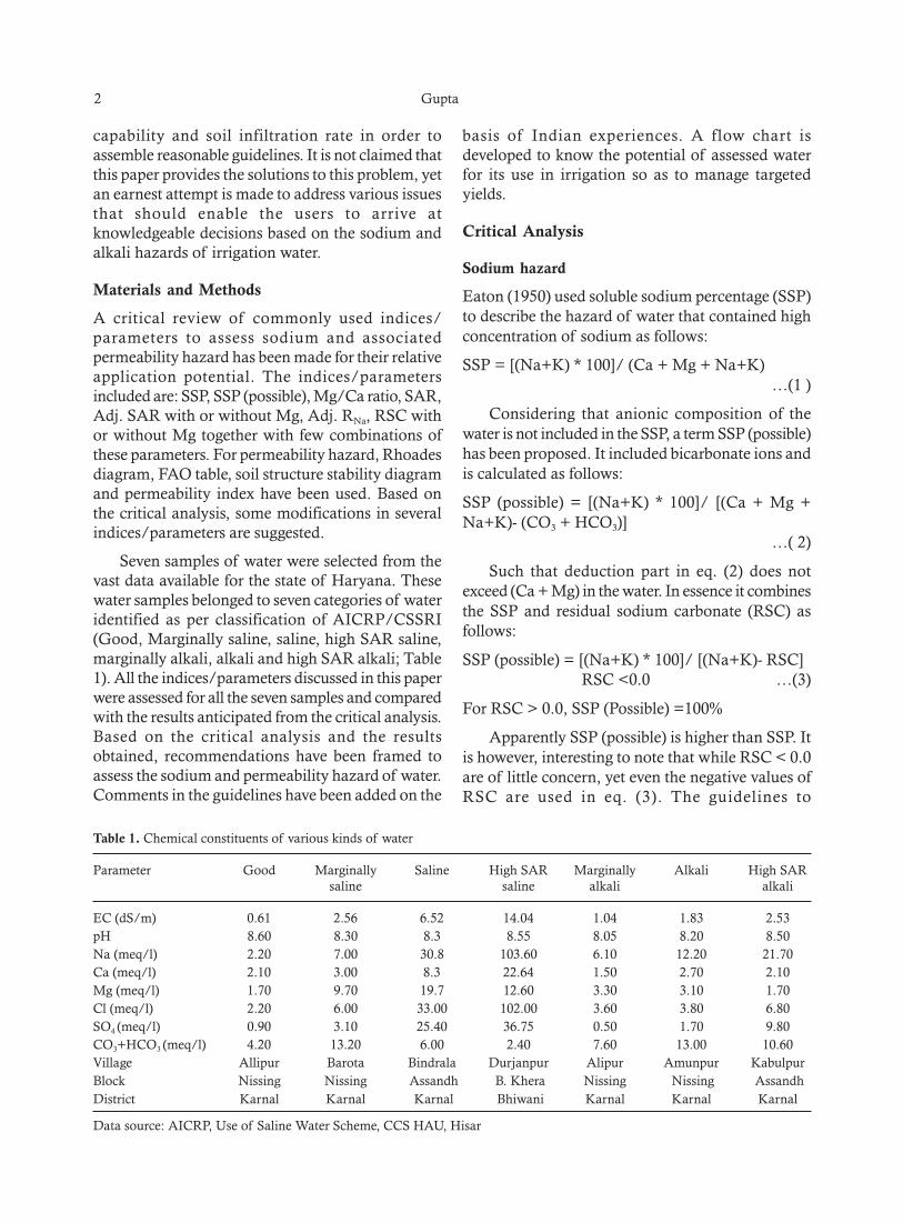
Seven samples of water were selected from thevast data available for the state of Haryana. Thesewater samples belonged to seven categories of wateridentified as per classification of AICRP/CSSRI(Good, Marginally saline, saline, high SAR saline,marginally alkali, alkali and high SAR alkali; Table1). All the indices/parameters discussed in this paperwere assessed for all the seven samples and comparedwith the results anticipated from the critical analysis.Based on the critical analysis and the resultsobtained, recommendations have been framed toassess the sodium and permeability hazard of water.Comments in the guidelines have been added on the

basis of Indian experiences. A flow chart isdeveloped to know the potential of assessed waterfor its use in irrigation so as to manage targetedyields.

Critical Analysis

Sodium hazard

Eaton (1950) used soluble sodium percentage (SSP)to describe the hazard of water that contained highconcentration of sodium as follows:

SSP = [(Na+K) * 100]/ (Ca + Mg + Na+K)…(1 )

Considering that anionic composition of thewater is not included in the SSP, a term SSP (possible)has been proposed. It included bicarbonate ions andis calculated as follows:

SSP (possible) = [(Na+K) * 100]/ [(Ca + Mg +Na+K)- (CO3 + HCO3)]

…( 2)

Such that deduction part in eq. (2) does notexceed (Ca + Mg) in the water. In essence it combinesthe SSP and residual sodium carbonate (RSC) asfollows:

SSP (possible) = [(Na+K) * 100]/ [(Na+K)- RSC] RSC <0.0 …(3)

For RSC > 0.0, SSP (Possible) =100%

Apparently SSP (possible) is higher than SSP. Itis however, interesting to note that while RSC < 0.0are of little concern, yet even the negative values ofRSC are used in eq. (3). The guidelines to

Table 1. Chemical constituents of various kinds of water

Parameter Good Marginally Saline High SAR Marginally Alkali High SARsaline saline alkali alkali

EC (dS/m) 0.61 2.56 6.52 14.04 1.04 1.83 2.53pH 8.60 8.30 8.3 8.55 8.05 8.20 8.50Na (meq/l) 2.20 7.00 30.8 103.60 6.10 12.20 21.70Ca (meq/l) 2.10 3.00 8.3 22.64 1.50 2.70 2.10Mg (meq/l) 1.70 9.70 19.7 12.60 3.30 3.10 1.70Cl (meq/l) 2.20 6.00 33.00 102.00 3.60 3.80 6.80SO4 (meq/l) 0.90 3.10 25.40 36.75 0.50 1.70 9.80CO3+HCO3 (meq/l) 4.20 13.20 6.00 2.40 7.60 13.00 10.60Village Allipur Barota Bindrala Durjanpur Alipur Amunpur KabulpurBlock Nissing Nissing Assandh B. Khera Nissing Nissing AssandhDistrict Karnal Karnal Karnal Bhiwani Karnal Karnal Karnal

Data source: AICRP, Use of Saline Water Scheme, CCS HAU, Hisar

Assessing the Hazards of High SAR and Alkali Water 3

characterize the water on the basis of SSP are givenin Table 2. Wilcox (1955) proposed a diagramrelating SSP and EC and rated the water quality asexcellent to good, permissible to doubtful, doubtfulto unsuitable and unsuitable (Table 2). Since thereare no guidelines on SSP (possible), the guidelinesfor SSP can be used for SSP (possible) as well. Thevalues of SSP or SSP (possible) are rarely used inIndia to assess the water quality although it mayprovide valuable information on the water quality.

Sodium Adsorption Ratio

Most widely used parameter to assess the sodiumhazard of water is sodium adsorption ratio (SAR)expressed as:

NaSAR = ——————— (meq/L)1/2 …(4)

[(Ca + Mg) /2]½

Here concentration of the ions is expressed inmeq/L.

An unusual aspect of the SAR is that Ca andMg have been lumped together making itcontroversial. Considering various opposingarguments, scientists are veering around the view thatMg does not affect the soil as adversely as Na but isnot as beneficial as Ca. Being intermediate of Naand Ca, its clubbing with Ca is questionableespecially for Indian conditions where Mg/Ca ratiosof 2-4 are commonly encountered and even can goas high as 16 (Gupta and Gupta, 1987). AICRPguidelines stipulate that if Mg/Ca ratio is more than3, some chemical amendments are needed to managesuch kind of water (Minhas and Gupta, 1992). Thus,under Indian conditions where Mg/Ca ratios tendto increase with salinity of water, SAR may

underestimate the sodium hazard of irrigation water.The only justification to club calcium withmagnesium appears to be that in the past Ca andMg were reported together and since the calciumplus magnesium is divided by 2, one need not worrymuch about the Mg until the Mg/Ca ratio remainsaround 1.0. With slight manipulation, eq. (4) can bewritten as:

NaSAR = —————————— (meq/L)1/2 …(5)

√Ca [(1 + Mg/Ca) /2]½

Apparently, SAR is underestimated withincreasing Mg/Ca ratios, even though high Mg/Caratios are known to cause dispersion and build-upof higher ESP in soils than waters with low Mg/Caratios (Yadav and Girdhar, 1981). For the sameamount of Na and Ca in waters, SAR will be 0.63times the SAR of the water for Mg/Ca ratio of 4compared to Mg/Ca ratio of 1.0. Therefore, to avoidsuch underestimation, eq. (4) should be used withthe following stipulations:

For non-calcareous soils, actual value of Mg/Ca may be taken in eq. (5) if it is less than 1. If it ismore than 1, Mg/Ca in the water may be taken as1.0 irrespective of its value such that:

NaSAR = —— (meq/L)1/2 …(6)

√Ca

For calcareous soils, limit of Mg/Ca ratio maybe increased to 2.0 such that actual values below 2are used in eq. (5). For Mg/Ca greater than 2.0, eq.(5) is given as:

0.82 NaSAR = ———— (meq/L)1/2 …(7)

√Ca

Table 2. Some parameter/indices for rating ground water quality for irrigation (Ayers and Westcot, 1985, Eaton, 1950 and Wilcox,1948)

Class SSP (%) SAR (meq/L)1/2 Sustainability for irrigationValues Comment

I <20 Excellent < 10 Use on sodium sensitive crops such as avocados andon heavy textured soils* needs caution

II 20-40 Good 10-18 Amendments (such as gypsum, sulphitation pressmud*, distillery spent wash*) and leaching needed

III 40-80 (40-60)* Fair (Permissible) 18-26 Generally unsuitable for continuous useIV >80 (60-80) Poor (Doubtful) > 26 Generally unsuitable for useV (>80) Unsuitable

*Classification in Parenthesis by Wilcox (1955); *added by the author based on Indian experience

4 Gupta

It may be noted that contrary to theirappearances, eq. (6) or eq. (7) do not neglect Mg buttakes it equal to Ca or twice the Ca respectively. Eq.(6) has earlier been proposed by Gupta and Gupta(2002) albeit without this justification. Data in Table3 reveal that SAR calculated with eq. (6) is moreclosely related to ESP of the soil than conventionalSAR.

General guidelines on the use of SAR tocharacterize irrigation waters are given in Table 2along with some comments on the managementoptions. Several other Tables have also appeared inthe literature making the issue quite complex becauseof wide differences in the guidelines. For example;tolerance of crops to SAR of the irrigation water fornon-saline conditions given in Table 4 are quite highespecially for moderately tolerant and tolerant crops.Since SAR in general is high in high EC waters, tohave a non-saline environment with such high SARvalues may not be possible. Clearly, such Tables mayhave limited applications under Indian conditions.Until guidelines conforming to Indian conditions areavailable, guidelines given in Table 2 can be safelyused.

USSL Diagram for Water Quality Characterization

High SAR adversely affects the crop yield but not inisolation from EC of water. Thus, Richards (1954)

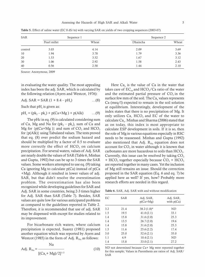
combined the effect of EC and SAR in a USSLdiagram which is frequently used and quoted tocategorize irrigation waters. Some confusion hasemerged on the use of this diagram. In this diagram,for a better quality rating of the water, water havinghigh EC needs to have low SAR. Some userscompare it with Rhoades diagram or FAO data setwherein high SAR water should have high EC tomaintain the infiltration rate. These opposingcontentions cause confusion. It should be noted thatboth these classifications are complementary and notcontrary to each other. While the former is relatedto crop performance, later is to maintain the soil’sinfiltration rate. Studies have proved that for the sameEC of water, high SAR water will produce lesseryields than a low SAR water (Table 5). Similar resultshave also been reported by Minhas and Gupta(1992). Notwithstanding other limitations, if any,USSL diagram can be safely used to have a first guessof EC and SAR hazard of poor quality irrigationwaters.

Adj. SAR and Adj. RNa

To overcome the limitations of SAR and consideringthat anions especially carbonates and bicarbonatesaffect the quality of irrigation water, attempts havebeen made to include the relevant anions and cations

Table 3. Comparison of SAR (Eq. 4) and SAR (Eq. 6) values of irrigation waters in relation to observed ESP of soils

Location Irrigation water Irrigated soils

EC Mg/Ca SAR (eq. 4) SAR (eq. 6) SARe ESP(dS/m) ratio (meq/l)1/2 (meq/l)1/2 (meq/l)1/2

Kaparda 10.8 4.4 28 59 31 60Jelwa 5.9 8.1 23 36 28 38Shikarpura 4.5 16.0 8 26 32 35

Table 4. Tolerance of crops to SAR under non-saline environment

Tolerance SAR of Crop Conditionirrigation water

Very sensitive 2-8 Deciduous fruits, nuts, citrus, avocado Leaf tip burn, leaf scorchSensitive 8-18 Beans Stunted, soil structure favourableModerately tolerant 18-46 Clover, oats, rice, tall fescue Stunted due to nutrition and soil

structureTolerant 46-102 Wheat, barley, tomatoes, beets, tall Stunted due to poor soil structure

wheat grass, crested grass, lucerne

Source: Extracted from the Australian Water Quality Guidelines for Fresh & Marine Waters (ANZECC) http://www.mfe.govt.nz/publications/water/anzecc-water-quality-guide-02/revision-water-quality.html. Adopted from Pearson (1960)

Assessing the Hazards of High SAR and Alkali Water 5

in evaluating the water quality. The most appealingindex has been the adj. SAR, which is calculated bythe following relation (Ayers and Westcot, 1976):

Adj. SAR = SAR (1 + 8.4 – pHc) …(8)

Such that pHc is given as:

pHc = (pk2 – pkc) + p(Ca+Mg ) + p(Alk) …(9)

The pHc in eq. (9) is calculated considering sumof Ca, Mg and Na for (pk2 – pkc), sum of Ca andMg for {p(Ca+Mg )} and sum of CO3 and HCO3

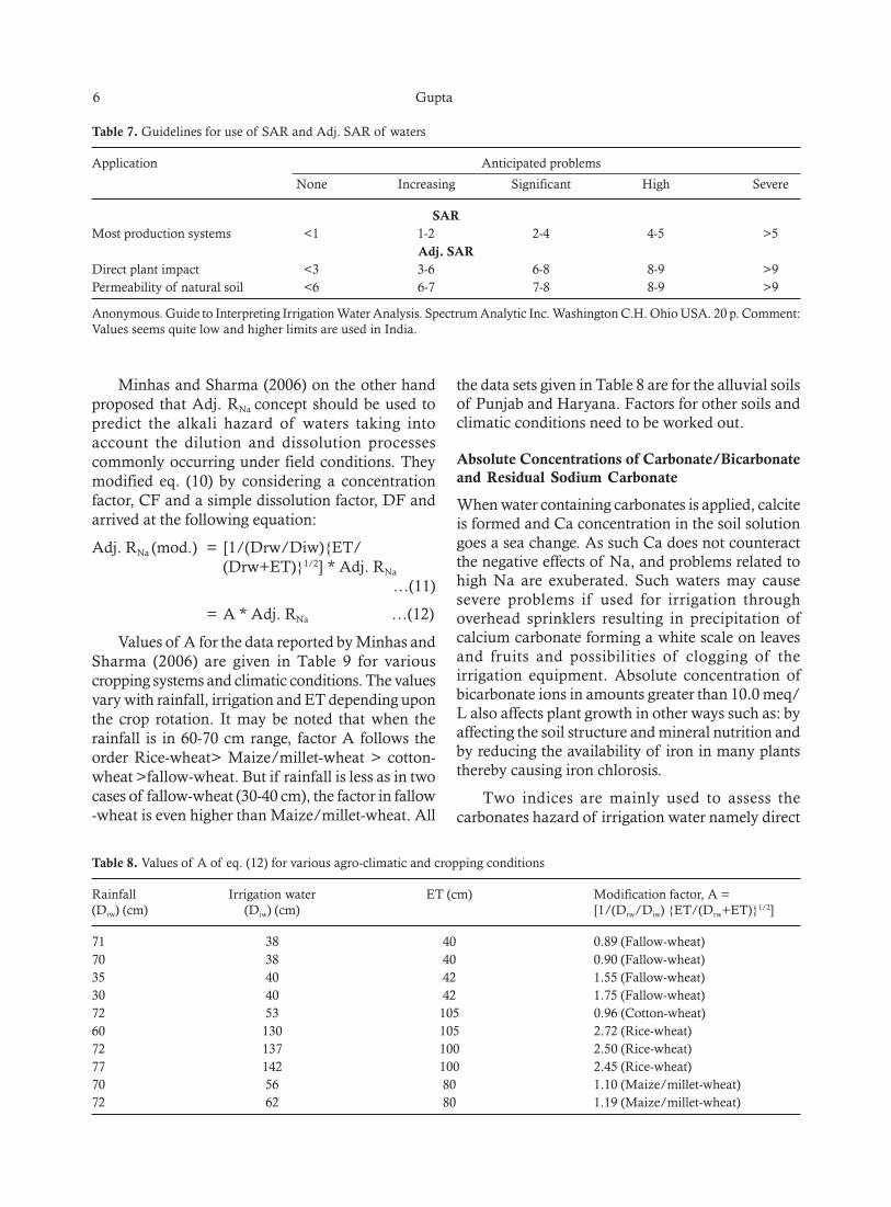
for {p(Alk)} using Tabulated values. The tests provedthat eq. (8) over predict the sodium hazard andshould be multiplied by a factor of 0.5 to evaluatemore correctly the effect of HCO3 on calciumprecipitation. For several waters, values of Adj. SARare nearly double the values of SAR (Table 6, Minhasand Gupta, 1992) but can be up to 3 times the SARvalues. Some workers attempted to use eq. (9) takingCa ignoring Mg to calculate p(Ca) instead of p(Ca+Mg). Although it resulted in lower values of adj.SAR, but that didn’t resolve the overestimationproblem. The overestimation has also beenrecognized while developing guidelines for SAR andAdj. SAR in some countries, being 2-3 times higherfor Adj. SAR than SAR (Table 7). Besides, SARvalues are quite low for various anticipated problemsas compared to the guidelines reported in Table 2.Therefore, it is recommended that use of adj. SARmay be dispensed with except for studies related toits improvement.

For bicarbonate rich waters, where calciumprecipitation is expected, Suarez (1981) proposedanother equation which was reported by Ayers andWestcot (1985) in the form of Adj. RNa as follows:

NaAdj. RNa = ——————— (10)

[(Cax+ Mg)/2]1/2

Here Cax is the value of Ca in the water thattakes care of ECiw and HCO3/Ca ratio of the waterand the estimated partial pressure of CO2 in thesurface few mm of the soil. The Cax values representsCa (meq/l) expected to remain in the soil solutionat equilibrium. Interestingly, development of theindex states that there is no precipitation of Mg. Itonly utilizes Ca, HCO3 and EC of the water tocalculate Cax. Minhas and Sharma (2006) stated thatas on today, this index is most appropriate tocalculate ESP development in soils. If it is so, thenthe role of Mg in various equations especially in RSCneeds to be reassessed. Minhas and Gupta (1992)also mentioned that Adj. RNa equation does notaccount for CO3 in water although it is known thatcarbonates are more hazardous to soils than HCO3.Currently, this issue can be resolved by taking CO3

+ HCO3 together especially because CO3 + HCO3

are reported together in many cases. Yet the inclusionof Mg still remains an issue. Should the correctionproposed in the SAR equation (Eq. 6 and eq. 7) beapplied here as well? If yes, how? Probably moreresearch efforts are needed in this regard.

Table 5. Effect of saline water (EC 8 dS/m) with varying SAR on yields of two cropping sequences (2003-07)

SAR Sequence 1 Sequence 2

Pearl millet Wheat Dhaincha Wheat

control 3.03 4.14 2.09 3.6910 1.94 3.78 1.79 3.3620 1.53 3.52 1.67 3.1230 1.06 2.92 1.58 2.4340 0.56 2.58 1.44 2.10

Source: Anonymous, 2009

Table 6. SAR, Adj. SAR with and without modification

EC SAR Adj. SAR, Adj. SAR,p(Ca+Mg) with p(Ca)

3.2 21.4 38.2 (1.8)* ND1.5 19.5 41.0 (2.1) 33.11.4 15.8 31.6 (2.0) 25.31.4 13.5 26.7 (2.0) 19.61.4 15.8 31.6 (2.0) 25.31.5 11.6 25.6 (2.2) 17.43.0 25.0 52.6 (2.1) 35.01.1 4.9 10.4 (2.1) ND1.4 15.8 33.0 (2.1) 27.2

ND not determined because Ca+ Mg were reported togetherfor this sample; Values in Parenthesis are ratios of Adj. SAR/SAR

6 Gupta

Table 7. Guidelines for use of SAR and Adj. SAR of waters

Application Anticipated problems

None Increasing Significant High Severe

SARMost production systems <1 1-2 2-4 4-5 >5

Adj. SARDirect plant impact <3 3-6 6-8 8-9 >9Permeability of natural soil <6 6-7 7-8 8-9 >9

Anonymous. Guide to Interpreting Irrigation Water Analysis. Spectrum Analytic Inc. Washington C.H. Ohio USA. 20 p. Comment:Values seems quite low and higher limits are used in India.

Minhas and Sharma (2006) on the other handproposed that Adj. RNa concept should be used topredict the alkali hazard of waters taking intoaccount the dilution and dissolution processescommonly occurring under field conditions. Theymodified eq. (10) by considering a concentrationfactor, CF and a simple dissolution factor, DF andarrived at the following equation:

Adj. RNa (mod.) = [1/(Drw/Diw){ET/(Drw+ET)}1/2] * Adj. RNa

…(11)

= A * Adj. RNa …(12)

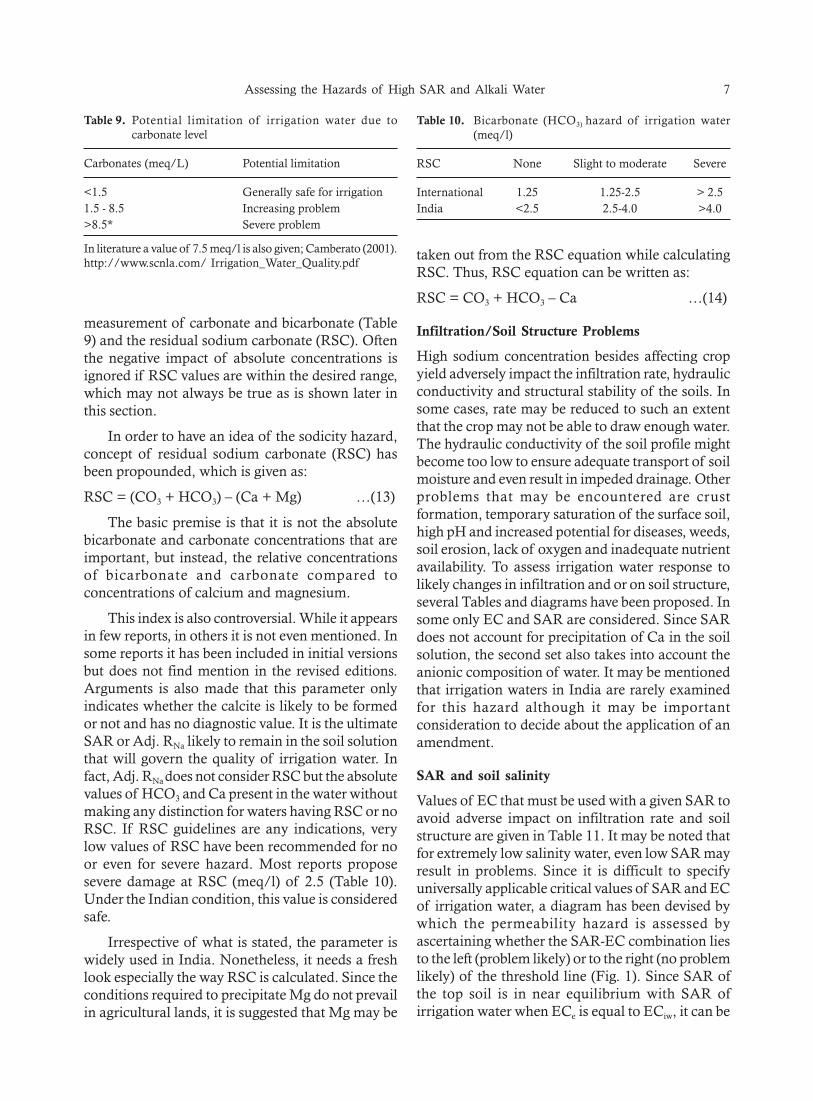
Values of A for the data reported by Minhas andSharma (2006) are given in Table 9 for variouscropping systems and climatic conditions. The valuesvary with rainfall, irrigation and ET depending uponthe crop rotation. It may be noted that when therainfall is in 60-70 cm range, factor A follows theorder Rice-wheat> Maize/millet-wheat > cotton-wheat >fallow-wheat. But if rainfall is less as in twocases of fallow-wheat (30-40 cm), the factor in fallow-wheat is even higher than Maize/millet-wheat. All

Table 8. Values of A of eq. (12) for various agro-climatic and cropping conditions

Rainfall Irrigation water ET (cm) Modification factor, A =(Drw) (cm) (Diw) (cm) [1/(Drw/Diw) {ET/(Drw+ET)}1/2]

71 38 40 0.89 (Fallow-wheat)70 38 40 0.90 (Fallow-wheat)35 40 42 1.55 (Fallow-wheat)30 40 42 1.75 (Fallow-wheat)72 53 105 0.96 (Cotton-wheat)60 130 105 2.72 (Rice-wheat)72 137 100 2.50 (Rice-wheat)77 142 100 2.45 (Rice-wheat)70 56 80 1.10 (Maize/millet-wheat)72 62 80 1.19 (Maize/millet-wheat)

the data sets given in Table 8 are for the alluvial soilsof Punjab and Haryana. Factors for other soils andclimatic conditions need to be worked out.

Absolute Concentrations of Carbonate/Bicarbonateand Residual Sodium Carbonate

When water containing carbonates is applied, calciteis formed and Ca concentration in the soil solutiongoes a sea change. As such Ca does not counteractthe negative effects of Na, and problems related tohigh Na are exuberated. Such waters may causesevere problems if used for irrigation throughoverhead sprinklers resulting in precipitation ofcalcium carbonate forming a white scale on leavesand fruits and possibilities of clogging of theirrigation equipment. Absolute concentration ofbicarbonate ions in amounts greater than 10.0 meq/L also affects plant growth in other ways such as: byaffecting the soil structure and mineral nutrition andby reducing the availability of iron in many plantsthereby causing iron chlorosis.

Two indices are mainly used to assess thecarbonates hazard of irrigation water namely direct

Assessing the Hazards of High SAR and Alkali Water 7

measurement of carbonate and bicarbonate (Table9) and the residual sodium carbonate (RSC). Oftenthe negative impact of absolute concentrations isignored if RSC values are within the desired range,which may not always be true as is shown later inthis section.

In order to have an idea of the sodicity hazard,concept of residual sodium carbonate (RSC) hasbeen propounded, which is given as:

RSC = (CO3 + HCO3) – (Ca + Mg) …(13)

The basic premise is that it is not the absolutebicarbonate and carbonate concentrations that areimportant, but instead, the relative concentrationsof bicarbonate and carbonate compared toconcentrations of calcium and magnesium.

This index is also controversial. While it appearsin few reports, in others it is not even mentioned. Insome reports it has been included in initial versionsbut does not find mention in the revised editions.Arguments is also made that this parameter onlyindicates whether the calcite is likely to be formedor not and has no diagnostic value. It is the ultimateSAR or Adj. RNa likely to remain in the soil solutionthat will govern the quality of irrigation water. Infact, Adj. RNa does not consider RSC but the absolutevalues of HCO3 and Ca present in the water withoutmaking any distinction for waters having RSC or noRSC. If RSC guidelines are any indications, verylow values of RSC have been recommended for noor even for severe hazard. Most reports proposesevere damage at RSC (meq/l) of 2.5 (Table 10).Under the Indian condition, this value is consideredsafe.

Irrespective of what is stated, the parameter iswidely used in India. Nonetheless, it needs a freshlook especially the way RSC is calculated. Since theconditions required to precipitate Mg do not prevailin agricultural lands, it is suggested that Mg may be

taken out from the RSC equation while calculatingRSC. Thus, RSC equation can be written as:

RSC = CO3 + HCO3 – Ca …(14)

Infiltration/Soil Structure Problems

High sodium concentration besides affecting cropyield adversely impact the infiltration rate, hydraulicconductivity and structural stability of the soils. Insome cases, rate may be reduced to such an extentthat the crop may not be able to draw enough water.The hydraulic conductivity of the soil profile mightbecome too low to ensure adequate transport of soilmoisture and even result in impeded drainage. Otherproblems that may be encountered are crustformation, temporary saturation of the surface soil,high pH and increased potential for diseases, weeds,soil erosion, lack of oxygen and inadequate nutrientavailability. To assess irrigation water response tolikely changes in infiltration and or on soil structure,several Tables and diagrams have been proposed. Insome only EC and SAR are considered. Since SARdoes not account for precipitation of Ca in the soilsolution, the second set also takes into account theanionic composition of water. It may be mentionedthat irrigation waters in India are rarely examinedfor this hazard although it may be importantconsideration to decide about the application of anamendment.

SAR and soil salinity

Values of EC that must be used with a given SAR toavoid adverse impact on infiltration rate and soilstructure are given in Table 11. It may be noted thatfor extremely low salinity water, even low SAR mayresult in problems. Since it is difficult to specifyuniversally applicable critical values of SAR and ECof irrigation water, a diagram has been devised bywhich the permeability hazard is assessed byascertaining whether the SAR-EC combination liesto the left (problem likely) or to the right (no problemlikely) of the threshold line (Fig. 1). Since SAR ofthe top soil is in near equilibrium with SAR ofirrigation water when ECe is equal to ECiw, it can be

Table 9. Potential limitation of irrigation water due tocarbonate level

Carbonates (meq/L) Potential limitation

<1.5 Generally safe for irrigation1.5 - 8.5 Increasing problem>8.5* Severe problem

In literature a value of 7.5 meq/l is also given; Camberato (2001).http://www.scnla.com/ Irrigation_Water_Quality.pdf

Table 10. Bicarbonate (HCO3) hazard of irrigation water(meq/l)

RSC None Slight to moderate Severe

International 1.25 1.25-2.5 > 2.5India <2.5 2.5-4.0 >4.0

8 Gupta

concluded that the irrigation waters having SAR, 10,20 and 30 should not have EC of water less than 1, 2and 3 dS/m, respectively. The tabulated valuesreported by Ayers and Westcot (1985) are generallyhigher than these values (Table 11).

PI = 100 *(Na + “HCO3)/ (Na + Ca + Mg + K)…(15)

It may be noted that unlike other equation/diagrams, it takes into account bicarbonate contentof the water, although does not account forcarbonates. Nonetheless, it may be possible to modifythe equation by adding K and CO3 in the numerator.The classification of the water is then made in thethree groups shown in Fig. 3. Class 1 shows noproblem while class II and Class III mean 25 and75% reduction in permeability.

Applications and Discussions

Calculated water quality parameters for the sevensamples reported in Table 1 are given in Table 12.SSP varies from a low value of 35.5 for themarginally saline water to 85.1 for high SAR saline

Table 11. Irrigation water quality criteria (EC, dS/m) forvarious SAR values of water

SAR EC for various degrees of restriction on use

No Slight to Severemoderate

< 3 <0.7 0.7—0.2 >33-6 >1.2 1.2-0.2 <0.26-12 >1.9 1.9-0.5 <0.512-20 >2.9 2.9- 0.5 <0.520-40 >5 5 - 2.9 <2.9

Source: Ayers and Westcot (1985)

Fig. 1. Relative rate of water infiltration as affected by salinityand SAR (Rhoades, 1977)

To predict soil structural stability, a diagramshowing relationship between SAR and EC has beenproposed (Fig. 2). Water quality that falls to the rightof the dashed line is unlikely to cause soil structuralproblems. Water quality that falls to the left of thesolid line is likely to induce degradation of soilstructure calling for corrective management (e.g.application of gypsum or some suitableamendment). Water that falls between the lines is ofmarginal quality and should be treated with cautiondepending upon the soil properties and rainfall.

Permeability Index

According to Doneen (1964), the permeability Index(PI) is calculated by using the following equation:

Fig. 2. Relationship between SAR and EC of irrigation waterfor predicting soil structural stability (Source: ANZECC, 2000)

Fig. 3. Classification of irrigation water on the basis ofpermeability index

Assessing the Hazards of High SAR and Alkali Water 9

water. SSP (Possible) varied from 58.3% for salinewater to 100% for all waters having positive RSCirrespective of the RSC values. Even the watercategorized as good had SSP (possible) as 100%.Although it may appear contrary to expectation, itis shown that because of low salinity and mediumCO3+HCO3, this water may cause permeabilityproblems. The values of Adj. SAR are the highestfor all the waters and lowest with SAR equation givenas eq. (4). The SAR values with modified equationssuggested are equal to or higher than the values ofSAR calculated with the help of eq. (4). Thedifference varied from as low as 3% to as high as40% for water having Mg/Ca ratio of 3.23. For avery high Mg/Ca ratio of 16, SAR (eq. 6) was 3.25times the SAR given by eq. (4) (Table 3). The valuesof Adj. RNa are in between the values of SAR andAdj. SAR (Table 12). Irrespective of the RSC,precipitation of Ca resulted in higher values of Adj.RNa than SAR (Eq. 4). Based on the critical reviewalong with the analysis of permeability hazard andresults presented in Table 12, it emerges that a singleparameter Adj. RNa may be sufficient to assess theNa hazard of irrigation water. Adj. RNa of the top30 cm of the soil can be calculated by the procedureoutlined by Minhas and Sharma (2006) and shownthrough eq. 12 and Table 8. It has been proved thatAdj. RNa (modified) has one to one relationship withESP of the 30 cm profile (Minhas and Sharma,2006).

Based on PI, out of seven samples, 3 falls in classI (one sample plot not shown because it was out ofscale of the Figure), 3 in class II and 1 in class III.While alkali waters falling in class II and III is

understandable, good quality water falling in classII was critically examined and seems to be in linewith the current assessment procedures often ignoredby the researchers and planners. The water inquestion has low EC and medium carbonates content(Table 9). Thus, the water quality of this nature callsfor precautions as permeability loss may be around25%. It seems that all waters assessed for Adj. RNa

may also be examined for its impact on infiltration/permeability using the PI index and Fig. 3. Thisanalysis in association with Adj. RNa would revealwhether carbonates in water irrespective of RSC willor will not be hazardous to soil permeability. Tounderstand the adverse effect on soil structure, allwater samples from Table 12 are plotted on Fig. 2.While all alkali water may cause soil structuralproblem, even the good quality water may result insoil structure problems as emerged from PI analysisas well. High SAR saline and other waters fall onthe boundary. Clearly caution is needed even in theuse of these waters. The tabulated data of Table 11however reveal slight to moderate problems for highSAR alkali water and no problem with high SARsaline water calling for the use of Fig. 2 and Fig. 3in the hazard analysis of waters.

From the critical analysis and assessment ofwater quality of selected samples, it emerges that:

• The sodium hazard can be best estimated byAdj. RNa making use of SAR/RSC redundant.The next best option is to use a combination ofeqs. (5) and (6) for non-calcareous and eqs. (5)and (7) for calcareous soils. In any case, use ofAdj. SAR should be avoided as it may causeunnecessary confusion.

Table 12. Chemical constituents of various kinds on water

Parameter Good Marginally Saline High SAR Marginally Alkali High SARsaline saline alkali alkali

SAR (Eq. 4) (meq/L) 1/2 1.6 2.9 8.2 24.8 3.9 7.2 15.7SAR (Eq. 6) (meq/L)1/2 1.6 4.0 10.7 24.8 5.0 7.4 15.7% change in SAR - 39.8 29.7 - 27.6 3.1 -Adj. SAR (meq/L)1/2 3.2 8.1 19.0 62.7 7.2 18.2 33.5Adj. RNa (meq/L)1/2 1.8 3.1 9.1 29.4 4.3 8.8 19.5RSC (meq/L) 0.4 1.5 Nil Nil 2.8 7.2 6.8RSC (meq/L) 2.1 10.2 Nil Nil 6.1 10.3 8.5Mg/Ca ratio 0.8 3.2 2.4 0.6 2.2 1.15 0.8Cl/SO4 ratio 2.4 1.9 1.3 2.8 7.2 2.2 0.7SSP 36.6 35.5 52.3 74.6 56.0 67.8 85.1SSP possible 100 100 58.3 75.9 100 100 100PI (%) 33 (II) 54 (I) 57 (I) 76 (I) 81 (II) 88 (II) 98 (III)

10 Gupta

• Existing equations developed using Adj. SARcan be used by replacing Adj. SAR with Adj.RNa.

• In all equations, HCO3 alone should be replacedwith CO3 + HCO3.

• Permeability index appears to be the best wayto assess permeability hazard of waters.

Water quality and management options for use

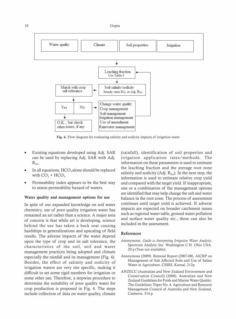
In spite of our expanded knowledge on soil waterchemistry, use of poor quality irrigation water hasremained an art rather than a science. A major areaof concern is that while art is developing, sciencebehind the use has taken a back seat causinghardships in generalizations and upscaling of fieldresults. The adverse impacts of the water dependupon the type of crop and its salt tolerance, thecharacteristics of the soil, soil and watermanagement practices being adopted and climateespecially the rainfall and its management (Fig. 4).Besides, the effect of salinity and sodicity ofirrigation waters are very site specific, making itdifficult to set some rigid numbers for irrigation orsome other use. Therefore, a stepwise procedure todetermine the suitability of poor quality water forcrop production is proposed in Fig. 4. The stepsinclude collection of data on water quality, climate

(rainfall), identification of soil properties andirrigation application rates/methods. Theinformation on these parameters is used to estimatethe leaching fraction and the average root zonesalinity and sodicity (Adj. RNa). In the next step, theinformation is used to estimate relative crop yieldand compared with the target yield. If inappropriate,one or a combination of the management optionsare identified that may help change the salt and waterbalance in the root zone. The process of assessmentcontinues until target yield is achieved. If adverseimpacts are expected on broader catchment issuessuch as regional water table, ground water pollutionand surface water quality etc., these can also beincluded in the assessment.

References

Anonymous. Guide to Interpreting Irrigation Water Analysis.Spectrum Analytic Inc. Washington C.H. Ohio USA.20 p (Year not available).

Anonymous (2009). Biennial Report (2007-08). AICRP onManagement of Salt Affected Soils and Use of SalineWater in Agriculture. CSSRI, Karnal. 212p.

ANZECC (Australian and New Zealand Environment andConservation Council) (2000). Australian and NewZealand Guidelines for Fresh and Marine Water Quality:The Guidelines. Paper No. 4. Agriculture and ResourceManagement Council of Australia and New Zealand,Canberra. 314 p.

Fig. 4. Flow diagram for evaluating salinity and sodicity impacts of irrigation water

Assessing the Hazards of High SAR and Alkali Water 11

Ayers RS and Westcot DW (1976). Water Quality forAgriculture. Irrigation and Drainage Paper, 29. FAO,Rome.

Ayers RS and Westcot DW (1985).Water quality foragriculture FAO irrigation and drain. Paper No 29(1):1-109.

Camberato (2001). http://www.scnla.com/Irrigation_Water_ Quality.pdf

Doneen LD (1964). Notes on water quality in agriculture.Published as a water science and engineering paper 4001,Department of Water Science and Engineering,University of California.

Eaton FM (1950). Significance of carbonate in Irrigationwaters. Soil Sci., 67: 128-133.

Gupta IC and Gupta SK (2003). Use of Saline Water inAgriculture: A Study of Arid and Semi-arid Zones of India.Scientific Publishers (India), Jodhpur. 302p.

Gupta SK and Gupta IC (1987). Management of Saline Soilsand Water. Oxford and IBH Publication Co., New Delhi,India. 399 p.

Minhas PS and Gupta RK (1992). Quality of Irrigation Water– Assessment and Management. Indian Council ofAgricultural Research, New Delhi, 123p.

Minhas PS and Sharma DR (2006). Predicability of existingindices and an alternative coefficient for estimating

sodicity build-up using adj RNa and permissible limitsfor crops grown on soils irrigated with waters havingresidual alkalinity. J. Ind. Soc. Soil Sci. 54 : 331-338.

Pearson GA (1960). Tolerance of Crops to ExchangeableSodium. Agricultural Information Bulletin 206,Agricultural Research Service, US Department ofAgriculture, Washington DC.

Rhoades JD (1977). Potential for using saline drainage watersfor irrigation. Proc. Water Management for Irrigationand Drainage. ASCE, Reno, Nevada. 85-116.

Richards LA (Ed.) (1954). Diagnosis and Improvement of Salineand Alkali Soils. USDA Handbook No. 60. U.S. SalinityLaboratory, Riverside, California. 160p.

Suarez DL (1981). Relationship between pHc and SAR andan alternate method for estimating SAR of soil ordrainage water. Soil Sci. Soc. Am. J. 45: 469-475.

Wilcox LV (1955). Classification and Use of Irrigation Waters,USDA, circular 969, Washington DC, USA.

Wilcox LV (1948). The Quality of Water for Irrigation Use. Vol40. US Department of Agriculture Technology Bulletin962, Washington DC.

Yadav JSP and Girdhar IK (1981). Effect of differentmagnesium: calcium ratios and sodium adsorption ratiovalues of leaching water and properties of calcareousversus non-calcareous soil. Soil Science 131: 194-198.

Received: December, 2014; Accepted January, 2015

Unlocking Production Potential of Degraded CoastalLand through Innovative Land Management Practices:

A Synthesis*

D Burman*, Subhasis Mandal, BK Bandopadhyay, B Maji, DK Sharma1,KK Mahanta, SK Sarangi, UK Mandal, S Patra, S De, S Patra, B Mandal2,

NJ Maitra3, TK Ghoshal4 and A Velmurugan5

ICAR-Central Central Soil Salinity Research Institute, Regional Research Station,Canning Town – 743329, West Bengal

1ICAR-Central Central Soil Salinity Research Institute, Karnal- 132 001, Haryanal2Bidhan Chandra Krishi Viswavidyalaya, Mohanpur- 741 252, West Bengall

3Ramkrishna Ashram Krishi Vigyan Kendra, Nimpith- 743 338, West Bengall4ICAR-Central Institute of Brackishwater Aquaculture, Kakdwip Research Centre, Kakdwip- 743 347, West Bengal

5ICAR-Central Island Agricultural Research Institute, Port Blair, Andaman & Nicobar Islands-744101*Corresponding author: burman.d@gmail.com

Abstract

Coastal land resources are vulnerable to various processes of land degradation like salinization, waterlogging,drainage congestion, etc. Unlocking the production potential of degraded land in coastal region is the biggestchallenge towards achieving regional food security as well as contributing to national food basket. Implementinginnovative land management practices like land shaping technique (LST) in combination with productiveutilization opportunities of the coastal areas are major concerns. Different land shaping techniques like farmpond; deep furrow and high ridge; shallow furrow and medium ridge; paddy-cum-fish cultivation; broad bedand furrow; three tier-pair beds and brackish water aquaculture pond techniques for improving drainage facility;rain water harvesting; salinity reduction; and cultivation of crops and fish (freshwater and brackish water fish)for livelihood and environmental security were tested on about 400 ha salt-affected land in Sundarbans regionof Ganges delta (West Bengal) and Tsunami affected areas in Andaman & Nicobar Islands. The results havebeen summarized. Raising of land and creating water harvesting structures reduced the problem of drainagecongestion during kharif season and this provided the scope for growing high value crops like vegetables duringthis season and it also facilitated early sowing of rabi crops. Salinity building up in the soil of different landsituations especially medium land and highland/ridges/ dikes in land shaped area was reduced and, fertilitystatus and biological activities in soil were increased under land shaping techniques. The cropping intensityincreased up to 240 % from a base level value of 100%. Land shaping techniques have increased the employmentand income of the households by many times. Net income per ha of farm land increased from Rs 22000 to Rs1,23,000 in Sundarbans and Rs 22400 to Rs 1,90,000 in Andaman & Nicobar Islands. Brackishwater aquaculturewas demonstrated through shaping of land into more than 110 shallow depth ponds in Sundarbans particularlynear the brackish water rivers. Farmers were benefitted from this technique with a net income of about Rs1,43,000 ha-1 of pond area. Land shaping techniques were financially viable and attractive proposition for thecoastal region. However, major constraints for adoption of land-shaping techniques were marginal land holdingsthat too divided into several parcels, high initial investment, presence of acid sulphate soils near surface or atshallow depth at places, and distance from residential village.

Key words: Land degradation, Coastal salinity, Land management, Land- shaping, Water harvesting structures

issue because of its adverse impact on food security,livelihood and environment. It refers to a temporaryor permanent decline in the productive capacity of

Journal of Soil Salinity and Water Quality 7(1), 12-18, 2015

*The paper was presented in The National Seminar “Innovative Saline Agriculture in Changing Environment” held by IndianSociety of Soil Salinity & Water Quality at Rajmata Vijayaraje Scindia Krishi Vishwa Vidayalaya, Gwalior (12-14 December, 2014).

IntroductionLand resource has become scarce and is under threatof degradation. Land degradation is a major global

Unlocking Production Potential of Degraded Coastal Land 13

the land or its potential for environmentalmanagement (Scherr and Yadav, 1996). Landdegradation is intrinsically linked with thedegradation of other natural resources like, soil,water, forests and biodiversity. Land degradation isincreasing in severity and extent in many parts ofthe world. About 24% of land in the world has beenaffected by various forms of land degradation(Nkonya et al., 2011). This degraded area isequivalent to the annual loss of about 1 % of globalland area, which could produce 20 million Mg ofgrain each year, or 1 % of global annual grainproduction. About 1.5 billion people and 42 % ofthe very poor people live on the degraded land. InIndia about 114.01 m ha out of total geographicalarea of 328.84 m ha is under degraded andwastelands (Maji et al., 2010).

The coastal region plays a vital role in the globaleconomy due to its rich natural resources, productivehabitats and biodiversity. Total coastline of the worldis 3,56,000 km and the coastal area covers more than10% of the earth surface (SAC, 2012). India has acoastline of 7517 km (SAC, 2012), its peninsularregion bounded by the Arabian Sea on the west, theBay of Bengal on the east and the Indian Ocean toits south. According to Velayutham et al. (1999)Indian coastal agro-eco system occupies 10.78 m haand extends over the states/ union territories of WestBengal, Odisha, Andhra Pradesh and Pondicherryon the Bay of Bengal in the East, and Tamilnadu,Kerala, Karnataka, Goa, Maharashtra and Gujaraton the Arabian sea in the West besides, the two islandgroups viz. the Andaman & Nicobar andLakshadwip. Land resource in the coastal region isvulnerable to degradation due to combinations ofnatural, hydrological and anthropogenic factors. InIndia, the major features for the degradation of landin the coastal region are salinization/ sodificationdue to the presence of brackish groundwater tablenear the soil surface or sea water intrusion,acidification, reduced organic matter content andmicrobial activities, poor vegetation/ forest cover,waterlogging with fresh/ brackish water, drainagecongestion, desertification/ lack of fresh water,erosion, etc. Out of these, salinization, waterloggingand drainage congestion besides the climaticconstraints are the major processes of landdegradation in the coastal region. Salinity build-upin coastal land takes place mainly due to salinityingress of ground water aquifers, for which the mainfactors responsible are presence of saline ground

water near land surface, excessive and heavywithdrawals of ground water from coastal plainaquifers, seawater ingress, tidal water ingress,relatively less recharge, and poor land and watermanagement (Bandyapadhyay et al., 1987; Yadav etal., 2009). Most of the lands in the coastal area arelow-lying and flat in topography resulted in deepwaterlogging and drainage congestion especiallyduring kharif season following heavy monsoonshower.

Yet, agriculture, which is one of majoroccupations of the rural people in the coastal regionsof India, is less productive and productivity in thisecosystem is generally lower than the country’saverage. Enhancing agricultural productivity ofdegraded coastal land for improving food securityand livelihood of poverty stricken rural men andwomen in the face of the increasing demand for foodfor country’s burgeoning population, changingclimatic scenario and degradation of the finite landand water resources is the biggest challenge. In spiteof several constraints, there are tremendousopportunities to attain the production potential ofthe degraded land and water in the coastal region.The land management practices which address keychallenges like land and water degradation (salinity),drainage congestion and scarcity of fresh water forirrigation could enhance agriculture production andlivelihood security of people in coastal region. Thispaper deals with innovative land managementpractices, termed as land shaping techniques whichprovide the scope for enhancing the productivity ofdegraded land and water and livelihood security ofthe farming communities, experiences learned fromon-farm implementation and limitation in adoption.

Innovative Degraded Land Management Practices

Land shaping techniques

Unlocking the production potential of degraded landin coastal region is the biggest challenge towardsachieving food security of the country. Implementinginnovative land management practices incombination with productive utilization ofopportunities of the coastal areas like excessrainwater and vast brackish water resources couldbe a best approach to meet the challenge. Landshaping is the innovative land management practicein which the surface of the land has been altered tomeet the requirements of the users. In land shaping,the surface of the land is modified primarily for

14 Burman et al.

creating source for irrigation especially for dry seasonby harvesting excess rain water which is otherwisegoes waste as run-off water, lowering degrading ofland by reducing salinity build up primarily from sub-surface saline groundwater, reducing drainagecongestion by creating raised land and harvestingexcess rain water, growing multiple and diversifiedcrops, integrated cultivation of crop and freshwaterfish and also cultivation of fish with brackish waterresources which is available in plenty in the coastalregion. Different innovative land shaping techniquesthat suit to different land situations, farm size andfarmers’ requirements under coastal agro-ecosystemare described below (CSSRI-NAIP, 2014, Burmanet al., 2013):-

(i) Farm pond: About 20% of the farm area isconverted into on-farm pond of about 3m depth toharvest excess rainwater. The dug-out soil is used toraise the land to form high land/dike and mediumland. Raised land and original low land are used forgrowing multiple and diversified crops throughoutthe year. High land/dike is used for growing highvalue vegetables and fruit crops round the year.During kharif season high yielding variety of riceare grown in medium land and low land is used forpaddy + fish cultivation. The low water requiringcrops like sunflower, groundnut, and cotton aregrown on the medium land and rice is grown onlowland during rabi/summer season. The pond isused for harvesting of about 5000 m3ha-1 rainwaterfor irrigation and poly-culture of fish.

(ii) Deep furrow and high ridge: About 50 % of thefarm land is shaped into alternate ridges (1.5 m topwidth and1.0 m height) and furrows (3m top widthand 1.0 m depth). Dug out soil from furrows is usedfor making ridges. About 1875 m3ha-1 of rainwateris harvested of in the deep furrows and is used forfish cultivation and irrigation during rabi. The ridgesare used for cultivation of vegetables and otherhorticultural crops/ multi-purpose tree species(MPTs) round the year. Remaining portion of thefarmland including the furrows is used for growingmore profitable paddy + fish cultivation in kharif.During rabi/ summer season farm land (non-furrowand non-ridge area) is used for low water requiringcrops.

(iii) Shallow furrow and medium ridge: About 40 %of the farm land is shaped into shallow furrow of0.50-0.75m deep at a distance of about 4-5m andmedium ridges of 0.80- 1.00m high along the

furrows. The furrows are used for rainwaterharvesting of about 1200 m3ha-1 and paddy + fishcultivation during kharif. The cropping schedule issimilar to that followed in deep furrow & high ridgeexcept rice can be grown in furrows in rabi/summerwith lesser supplementary irrigation.

(iv) Paddy-cum-fish cultivation: Deep trenches (3-5mwidth and 1.5 m depth) are dug around the peripheryof the farm land and the dugout soil is used formaking dikes (1.5 - 4 m width and 1.5 m height) toprotect free flow of water from the field andharvesting more rain water in the field and trench.A small ditch is dug out at one corner of the field asshelter for fishes when water will dry out in trenches.The dikes are used for growing vegetables and/orgreen manuring crops/fruit crops/multi-purpose treespecies (MPTs) round the year. Remaining portionof the farm land including the trenches is used formore profitable paddy + fish cultivation in kharif.The farm land (non-trench and non-dike area) is usedfor growing low water requiring crops during dry(rabi/summer) season with the harvested rainwaterof about 1400 - 3500 m3ha-1 in the trenches.

(v) Broad bed & furrow: This involves shaping of landfor broad beds (4-5 m width and 1 m height) andfurrows (5-6 m width and 1m deep) with a provisionof (2 m x 4 m x 1 m) fish shelter at the end of thefurrow alternatively in low-lying lands. Raised bedsare used for cultivation of vegetables round the yearand fish is cultivated in the furrows. This systemprovided the scope for in-situ rainwater harvestingof about 3800 m3ha-1 and which is used to cultivatesecond crop during dry seasons.

(vi) Three tier land configuration: In this techniqueof land shaping degraded low-lying land is shapedinto three equal portions as raised land, medium ororiginal land and pond with a depth of 2.5-3 m anddikes of 5 m wide and 1.5 m height. Pond at thelower part of the land is used for harvesting of rainwater of about 4500 m3 ha-1 and poly-culture of fish.Paddy in medium (original) land along withvegetables on raised land and dikes are cultivated.

(vii) Paired bed technique: In paired bed techniquedegraded low lying land is shaped into broad furrowof 9 m width x 2 m depth and two beds of 6 m width.In this technique a nursery pond of 5 m x 9 m size isalso created at one end of the furrow for raising fingerlings while broad furrow is used for brooders. Twodikes are created of 2-3 m width at both ends. Broadfurrow is used for harvesting of rain water of about

Unlocking Production Potential of Degraded Coastal Land 15

3750 m3ha-1. Vegetables are grown round the year inthe raised beds and dikes.

(viii) Brackish water aquaculture pond: There aremany areas in the coastal areas particularly near thebrackish water river or sea coast remain highly salinethroughout the year and not suitable for cropcultivation. These lands are shaped into shallowdepth brackish water pond. The pond size variesfrom 0.13 - 0.4 ha with a depth of 1.0 -1.5 m. Theheight of the embankment of the pond is determinedby the tidal height occurring in the area, generallyabout 30 cm above the maximum flood level. Ingeneral about 1.2 m hight and 1.6 m wideembankment is made on the periphery of the pond.Polyculture system of brackishwater fish farmingwith tiger shrimp (Penaeus monodon) along withbrackishwater fish like golbhangon/bhangon (Lizatade) and aansbhangon (Mugil cephalus) is practicedin the pond with brackishwater from the nearest river.

Lessen Learned from Implementation of Land-shaping Techniques

Different land-shaping techniques for improvingdrainage facility, rain water harvesting, salinityreduction and cultivation of crops and fish (freshwater and brackish water fish) for livelihood andenvironmental security were tested on about 400 hadegraded and low-productive land in disadvantagedareas in Sundarbans region of Ganges delta (WestBengal) and Tsunami affected areas in Andaman andNicobar Islands covering 32 villages in 4 districts(South 24 Parganas and North 24 Parganas districtsin West Bengal and South Andaman and North andMiddle Andaman districts in Andaman and NicobarIslands) during 2010-2014. In the pilot area it wasobserved from base line survey that the land holdingwas very low and fragmented in Sundarbans regionwith dominance of marginal farmers (about 90%)with average land holding ranged between 0.19-0.56ha (Mandal et al., 2011). The land holding size washigher in the study area in Andaman and NicobarIslands and the average holding size was 1.80 - 2.80ha. The land topography was dominated by low land(80%) in Sundarban region and the same was 10-23% in case of villages in Andaman and NicobarIslands. In Andaman and Nicobar Islands substantialarea was under hilly and undulated topography andnot suitable for agricultural crop cultivation. Due tolow-lying nature of the land, waterloging coupledwith severe drainage congestion was prevalent in the

study area during monsoon months. In contrastduring non-monsoon months due to non-availabilityof good quality water, salinity builds up graduallyand make the crop cultivation challenging. InSundarbans, agriculture was the primary occupationof the majority of the households (39-56%) followedby daily labourers, migration to distance places foralternative livelihoods, fisheries and others. Averagefamily income in Sundarbans was calculated to beRs 22000-25000 per family per year during 2011-12.In Andaman and Nicobar Islands, services were themajor occupation and agriculture as primaryoccupation was practiced by very few households(< 5 %). Overall the cropping intensity in the studyregion was low (114-127%) in the Sundarbans regionwith low level of crop diversification. The croppingintensities in Andaman and Nicobar Islands wererelatively higher (137-188%) primarily due topresence of perennial crops. The soil in the studyarea was affected by high level of soil salinity (ECeupto 18 dS m-1) and water salinity (EC upto 22 dSm-1) that limits the choice and options of growingcrops in the area.

With land-shaping techniques, different landsituations like, high land, medium land and low land(original) apart from rainwater harvesting structureslike farm pond/furrows/trenches were created inlow-lying and degraded farmers’ fields. Raising ofland and creating water harvesting structures reducedthe problem of drainage congestion during kharifseason (Table 1) and this provided the scope forgrowing high value crops like vegetables during thisseason. It also facilitated early sowing of rabi cropsso that the farmers could get better return. It wasobserved that the salinity build up in the soil ofdifferent land situations especially medium land andhighland/ridges/ dikes in land shaped area wasrelatively less compared to original salt-affectedcoastal low land (without land shaping) (Table 1).Lower soil salinity build up in the raised soil mightbe due to : i) increased distance between the salinegroundwater table and the surface soil resulting indecreased accumulation of salt through upwardcapillary flow and/or ii) due to the presence of freshwater (harvested rain water) in the furrows/trenches,the soil at the bottom region of ridges/dikes/raisedbed, remains almost saturated with fresh water inthe initial months after the kharif season (or as longas there was fresh water available in the furrows)thereby, decreasing the soil water potential at thebottom region of ridges, which resulted in less

16 Burman et al.

upward capillary movement of saline groundwater.Due to creation of different land situations andfollowing cultivation of crops round the year organicC, available N, P and K and biological activities(microbial biomass C) in surface soil have beenincreased under land shaping techniques comparedto land without land shaping (Table 1).

About 1950 water storage structures were createdunder different land-shaping techniques and13,05,000 m3 rainwater has been harvested annuallyin these structures in the study area and with thisharvested rain water, about 260 ha areas which wereearlier under mono-cropping with rice due toshortage of irrigation water have been brought underirrigation for growing multiple crops round the year.The cropping intensity has been increased up to 240% from a base level value of 100% due toimplementing the land-shaping techniques (Table 2).These land shaping techniques are very popular

among the farmers of both Sundarbans andAndaman & Nicobar Islands as these technologieshave increased the employment and income of thefarm family by manifolds compared to base linevalue (Table 2). Average net income per ha of farmland has been increased from Rs 22000 to Rs1,23,000 in Sundarbans and Rs 22400 to Rs 1,90,000in Andaman and Nicobar Islands.

Brackishwater aquaculture was demonstratedthrough shaping of land into more than 110 shallowdepth ponds in the coastal areas of Sundarbansparticularly near the brackishwater rivers which wasremain almost fallow and not being utilized for anyagricultural activity on account of high soil salinity.Farmers were benefitted from this brackishwateraquaculture with a net income of about Rs1,46,000ha-1 of pond area. Farming activities under landshaping techniques have enhanced the employmentopportunities for the farm families in the study areas.

Table 1. Average depth of standing water and soil properties under different land situations created through land shaping techniques

Land situations Depth of ECe pH Organic C MBC Available N Available P Available Kstanding (dSm-1) (%) (µg g-1 (kg ha-1) (kg ha-1) (kg ha-1)

water (cm) dry soil)in kharif

Low land (without LS) 40-50 15.5 7.2 0.61 187.7 195.8 15.4 673.8Low land (LS) 30-40 13.2 7.5 0.80 244.0 234.0 17.1 628.4Medium land (LS) 15-20 7.3 7.4 1.10 279.0 238.1 18.9 480.3High land (LS) 0 6.6 7.3 1.20 280.5 251.7 22.4 430.5

LS= land shaping technique

Table 2. Enhancement in cropping intensity, employment generation and net income under different land shaping techniques inSundarbans and Andaman and Nicobar Islands

Land shaping Cropping intensity Employment generation Net return(%) (man-days hh-1* yr-1) (Rs ha-1 yr-1)

technologies Before land After land Before land After land Before land After landshaping shaping shaping shaping shaping shaping

Farm pond 114a, 100b 193a, 200b 87a, 8b 227a, 22b 22000a, 140000a,10000b 148000b

Deep furrow & high ridge 114a 186 87 218 22000a 102000a

Paddy-cum-fish 114a, 100b 166a, 200b 87a, 8b 223a, 35b 22000a, 127000a,24000b 148000b

Broad bed & furrow 100b 240b 9b 48b 24000b 212000b

Three tier 100b 220b 10b 42b 30000b 221000b

Paired bed 100b 240b 9b 54b 24000b 216000b

Brackishwater aquaculture 0/100 - 25a 100a - 146000a

pond

Note: Costs and returns at current price of 2012-13 *hh-1: per household (av. holding was 0.35 ha in Sundarbans a, av. holding ofimplementation was 0.20 ha in Andaman & Nicobar Islands b)

Unlocking Production Potential of Degraded Coastal Land 17

Table 3. Factors affecting adoption of land shaping techniques

Factors Name Co-efficient SE

Constant 1.3471*** 0.0214X1 Farm size (in ha) 0.435*** 0.0473X2 No of parcels in farm holdings (no) -0.0187*** 0.0045X3 % of lowland area 0.0952*** 0.0388X4 Distance of land from residential area (binary var, 1=within 1km, 0 otherwise) -0.2110* 0.012X5 Aggregate family income (Rs/year) 0.0871*** 0.0126X6 % of off-farm income (Rs/year) -1.1543*** 0.0.4422X7 Family size (no) 0.0675*** 0.0548X8 Availability of irrigation water (binary var. 1= available for at least 4 months, -0.4871*** 0.1789

0 otherwise)X9 Education level (no of years of education of key respondents) 0.1510*** 0.0984X10 Rental value of land (Rs/year/ha) 0.0511NS 0.0432

-2 Log Likelihood 149.52Correct Prediction (%) 68.93No of observation 180

***p ≤ 0.01, * p ≤ 0.05, NS - not significant

As the farmers could get employment in their ownfarm land throughout the year, this has also checkedthe seasonal migration rate of the farm family insearch of their livelihood. Social security is alsoestablished through this technology by ensuringincome security. Consumption of vegetables and fishfrom won farm land has improved their nutritionalsecurity.

Financial analysis of land shaping techniquesindicated, these were financially viable and attractiveproposition for the coastal region (Mandal et al.,2013). Different factors that influence the farmers’behaviour towards adoption of land shapingtechniques and also probability of adoption wereanalyzed in the study areas. It was noticed that asthe farm size, % of lowland area, aggregate familyincome, family size and educational level increased,the probability of adoption of these techniques alsoincreased (Table 3). Whereas as the no. of parcels infarm holdings, distance of farm land from residentialarea, % of off-farm income and availability ofirrigation water from sources (e.g. canals, creeks,reserviours, etc.) decreased the probability ofadoption of these techniques. The rental value ofland was not a significant factor to influenceadoption behaviour of these techniques.

Conclusions and Recommendations

In coastal area the land shaping is an innovativetechnology for addressing the key challenges likeland degradation (salinity), drainage congestion andscarcity of fresh water for irrigation and in turn have

the potential to enhancing production, productivity,income and employment. This is one of the mostimportant strategies not only to control run-off inthe region and soil loss but also contribute to climatechange mitigation as well as increased ecologicalresilience due to improvement of degraded land andwater quality and more carbon sequestration due tomore plant cover. These techniques are financiallyviable and attractive proposition for the coastalregion. However, major constraints for adoption ofland-shaping techniques are marginal land holdingsthat too divided into several parcels, high initialinvestment, presence of acid sulphate soils nearsurface or at shallow depth at places, distance fromresidential village etc. Though the technology havebeen well adopted at farm level, there is lack ofinformation on larger watershed or basin levelhydrological impacts such as availability of rainwaterfor downstream flow and groundwater recharge.There is a need to understand and resolve issues onlarge scale dissemination of land-shaping technologycovering the areas of input-supplies andmanagement, market and marketing environment –the driver of change in cropping pattern andproduction, credit needs and absorption of thefarmers, and the role financial institutions therein.More intensive study, particularly the long termimplications of these techniques should beundertaken to address those issues so that the land-shaping will be adopted in a large scale for thesustainable agricultural development in the salt-affected coastal region.

18 Burman et al.

References

Bandyopadhyay BK, Bandyopadhyay AK and Sen HS(1987). Physico-chemical characteristics of coastal salinesoils of India. Journal of Indian Society of CoastalAgricultural Research 5: 1-14.

Burman D, Bandyopadhyay BK, Mandal, Subhasis, MandalUK, Mahanta KK, Sarangi SK, Maji B, Rout S, Bal AR,Gupta SK and Sharma DK (2013). Land shaping – Aunique technology for improving productivity of coastalland, Bulletin No. CSSRI/Canning Town/Bulletin/2013/02. Central Soil Salinity Research Institute,Regional Research Station, Canning Town, West Bengal,India. p. 38.

CSSRI-NAIP (2014). Final Report of NAIP sub-project on:Strategies for Sustainable Management of DegradedCoastal Land and Water for Enhancing LivelihoodSecurity of Farming Communities (Component 3, GEFfunded) (eds. D. Burman, S. Mandal & K. K. Mahanta).Central Soil Salinity Research Institute, RegionalResearch Station, (CSSRI, RRS), Canning Town - 743329, South 24 Parganas, West Bengal. p. 104

Maji AK, Reddy GP, Obi and Sarkar D (2010). Degradedand Wastelands of India: Status and SpatialDistribution. Indian Council of Agricultural Research,New Delhi, India. p. 159.

Mandal S, Bandyapadhyay BK, Burman D, Sarangi SK,Mahanta KK, De S, Patra P (2011). Baseline Report.Central Soil Salinity Research Institute, RegionalResearch Station, Canning Town, West Bengal. p. 47.

Mandal Subhasis, Sarangi SK, Burman D, andBandyopadhyay BK, Maji B, Mandal UK and SharmaDK (2013). Land shaping models for enhancingagricultural productivity in salt affected coastal areas ofWest Bengal – An economic analysis. Indian Journal ofAgricultural Economics 3: 389-401.

Nkonya E, Koo J, Marenya P and Licker R (2011). LandDegradation: Land under Pressure. In Global foodpolicy report. International Food Policy ResearchInstitute, Washington, DC , USA. pp. 63-67.

SAC (2012). Coastal Zones of India. Space ApplicationsCentre, ISRO, Ahmedabad, Gujarat. p. 597.

Scherr, S.J. and Yadav, Satya (1996). Land degradation inthe developing world: Implications for food, agricultureand the environement to 2020. Food, Agricultutre andthe Environment Discusssin Papers 14, Internation FoodPolicy Research Instittue, Washington, DC, USA. p. 36.

Velayutham M, Sarkar D, Reddy R S, Natarajan A, KrishanP, Shiva Prasad CR, Challa O, Harindranath CS,Shyampura RL, Sharma JP and Bhattacharyya T (1999).Soil resosurce and their potentialities in coastal areas ofIndia. J. Indian Society of Coastal Agricultural Research 17:29-47.

Yadav JSP, Sen HS and Bandyopadhyay BK (2009). CoastalSoils —Management for higher agricultural productivityand livelihood security with special reference to India.Journal of Soil Salinity & Water Quality 1(1-2): 1-13.

Received: December, 2014; Accepted: December, 2014

Geo-electrical Investigations to Characterize SubsurfaceLithology and Groundwater Quality in Assandh Block

of Karnal District, Haryana

S K Lunkad1, Vikas Tomar2* and S K Kamra2

1Department of Geology, Kurukshetra University, Kurukshetra, Haryana2ICAR-Central Soil Salinity Research Institute, Karnal-132001, Haryana

*Corresponding Author: vikasgeologist@gmail.com

Abstract

Direct current resistivity surveys were conducted to characterize the subsurface lithology and groundwaterconditions upto 50 m depth at 4 locations in Assandh block of Karnal district in Haryana (India). Thegroundwater level in the study sites ranged from 4- 12 m and its TDS varied between 371 to 2080 ppm (0.6 to 3.3dS/m). Vertical Electrical Soundings (VES) based on Schlumberger configuration were carried out at theselocations using Aquameter CRM-AT resistivity meter. The curve matching and computer software approacheswere employed to estimate the thickness and resistivity of subsurface horizons with support of field observationson subsurface lithology and groundwater salinity. The 3 layer curve matching approach indicated a combinationof A and K type curves suggestive of either fresh to marginal groundwater salinity or dominance of finermaterial layers in a thick alluvial zone in the study area. Computer software based inversion methodologyhighlighted the presence of fine to medium sand of 10 to 27 ohm m resistivity in 10- 35 m depth aquifer zone.At 3 sites (Yatriwala, Bindrala and Kala Singh), low resistivity values of 8- 17 ohm m in saturated layers belowwatertable represent fine to medium sand of marginally saline groundwater. At fourth site, Balpabana, higherresistivity of 57- 69 ohm m in 10 to 20 m layers represents a mixture of loam and fine sand of relatively goodquality water while a lower resistivity of 27 ohm m beyond 35 m represents coarser sand though of marginallyhigher water salinity. Based on analysis of Dar Zarrouk parameters of Longitudinal Unit Conductance (S) andTransverse Unit Resistance (T), and supporting field evidence, it can be concluded that Balpabana and KalaSingh, amongst 4 study sites, have respectively the best and the worst quantitative and qualitative aquifer potentialupto 50 m depth; the remaining 2 sites of Bindrala and Yatriwala falling in between. For long term protection,the farmers in the area may be advised to explore better aquifer below 50 m depth with the help of VES surveysand competent professional interpretation.

Key words: Resistivity; VES; Lithology; Groundwater quality; Type curves

Introduction

The monitoring of the groundwater levels over past3 to 4 decades exhibits a declining trend of waterlevel in 12 districts of Haryana (Malik et al., 2013).The main reason for this decline is that pumping ofgroundwater has exceeded its natural recharge(Lunkad, 2006). It is important to make anassessment of the hydro-geological conditions indifferent regions for optimal planning, developmentand management of groundwater resources. Oftensuch investigations are carried out using conventionaland costly geotechnical methods which provideinformation at discrete selected points only. Surfacegeophysical surveys, a veritable tool in groundwaterexploration, have the basic advantage of saving costof borehole construction by locating target aquifer

before drilling is embarked upon (Obiora andOwnuka, 2005).

Vertical electrical sounding (VES) is a commonand useful method employed for measuring verticaldistribution of electrical resistivity (Heilan, 1940),more successfully when a good resistivity contrastexists between the water bearing aquifer formationsand the underlying rocky zone (Zohdy et al., 1974).Of different electrode configurations, Schlumbergerarray has been reported to be more suitable andcommon in both alluvial and weathered hard rockterrains (Vivekanath et al., 2014). A large number ofresistivity surveys have been undertaken in India withthe basic aim to provide information on sub-surfacelithology. Singh and Yadav (1984) and Yadav andSingh (1987) conducted these for delineation of fresh

Journal of Soil Salinity and Water Quality 7(1), 19-28, 2015

20 Lunkad et al.

and saline water zones in the alluvial Ganga plainsin eastern Uttar Pradesh. In the same region, Bajpaiand Kumar (1988) and Bajpai (1989) used resistivitydata to characterize the lateral and longitudinalextent of deeper aquifers based on the stratigraphicinterpretation. In India, there are limited applicationsof VES surveys for alluvial regions despite its hugescope to map the extensive plains without the needto drill bores.

This paper aims to provide a practicalmethodology on the application of resistivity surveysto characterize sub-surface lithology and the extentand quality of groundwater

Material and Methods

Study area

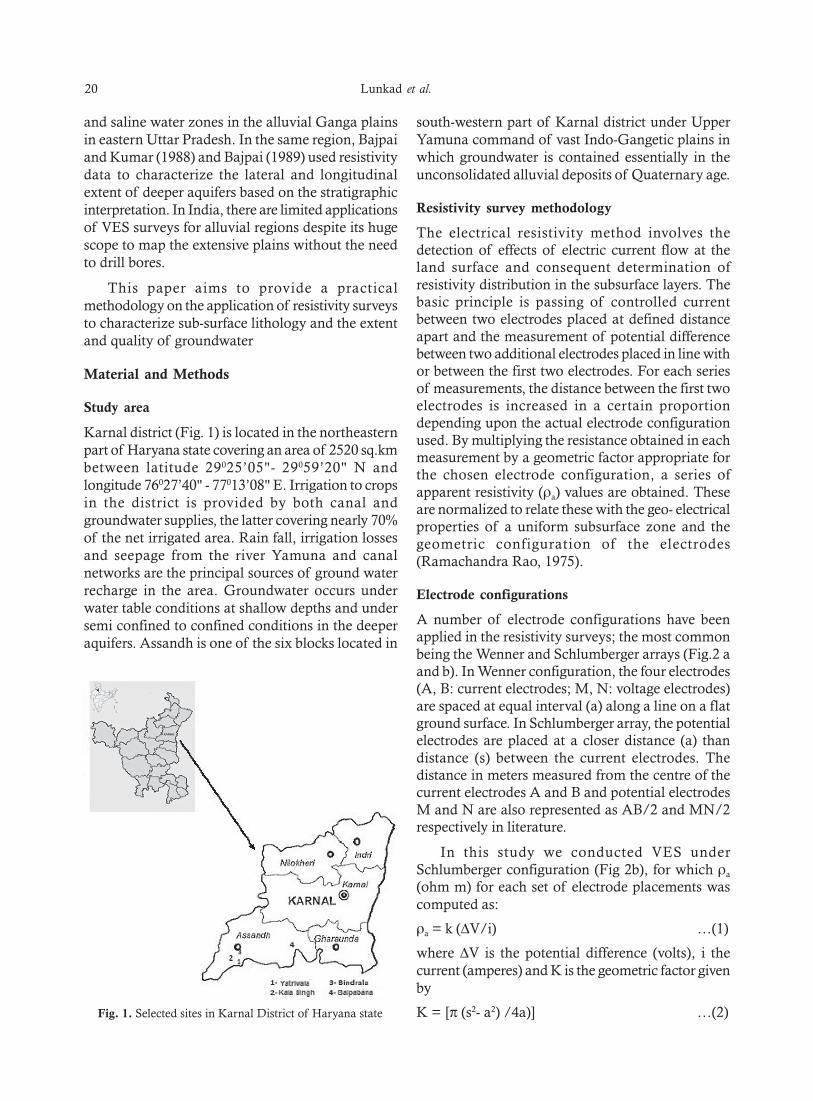
Karnal district (Fig. 1) is located in the northeasternpart of Haryana state covering an area of 2520 sq.kmbetween latitude 29025’05"- 29059’20" N andlongitude 76027’40" - 77013’08" E. Irrigation to cropsin the district is provided by both canal andgroundwater supplies, the latter covering nearly 70%of the net irrigated area. Rain fall, irrigation lossesand seepage from the river Yamuna and canalnetworks are the principal sources of ground waterrecharge in the area. Groundwater occurs underwater table conditions at shallow depths and undersemi confined to confined conditions in the deeperaquifers. Assandh is one of the six blocks located in

south-western part of Karnal district under UpperYamuna command of vast Indo-Gangetic plains inwhich groundwater is contained essentially in theunconsolidated alluvial deposits of Quaternary age.

Resistivity survey methodology

The electrical resistivity method involves thedetection of effects of electric current flow at theland surface and consequent determination ofresistivity distribution in the subsurface layers. Thebasic principle is passing of controlled currentbetween two electrodes placed at defined distanceapart and the measurement of potential differencebetween two additional electrodes placed in line withor between the first two electrodes. For each seriesof measurements, the distance between the first twoelectrodes is increased in a certain proportiondepending upon the actual electrode configurationused. By multiplying the resistance obtained in eachmeasurement by a geometric factor appropriate forthe chosen electrode configuration, a series ofapparent resistivity (ρa) values are obtained. Theseare normalized to relate these with the geo- electricalproperties of a uniform subsurface zone and thegeometric configuration of the electrodes(Ramachandra Rao, 1975).

Electrode configurations

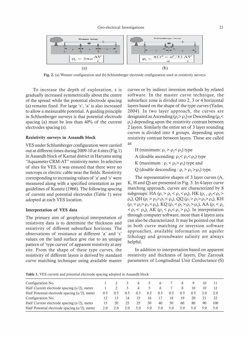
A number of electrode configurations have beenapplied in the resistivity surveys; the most commonbeing the Wenner and Schlumberger arrays (Fig.2 aand b). In Wenner configuration, the four electrodes(A, B: current electrodes; M, N: voltage electrodes)are spaced at equal interval (a) along a line on a flatground surface. In Schlumberger array, the potentialelectrodes are placed at a closer distance (a) thandistance (s) between the current electrodes. Thedistance in meters measured from the centre of thecurrent electrodes A and B and potential electrodesM and N are also represented as AB/2 and MN/2respectively in literature.

In this study we conducted VES underSchlumberger configuration (Fig 2b), for which ρa

(ohm m) for each set of electrode placements wascomputed as:

ρa = k (∆V/i) …(1)

where ∆V is the potential difference (volts), i thecurrent (amperes) and K is the geometric factor givenby

K = [π (s2- a2) /4a)] …(2)Fig. 1. Selected sites in Karnal District of Haryana state

Geo-electrical Investigations 21

To increase the depth of exploration, s isgradually increased symmetrically about the centreof the spread while the potential electrode spacing(a) remains fixed. For large ‘s’, ‘a’ is also increasedto allow a measurable potential. A guiding principlein Schlumberger surveys is that potential electrodespacing (a) must be less than 40% of the currentelectrodes spacing (s).

Resistivity surveys in Assandh block

VES under Schlumberger configuration were carriedout at different times during 2009-10 at 4 sites (Fig.1)in Assandh block of Karnal district in Haryana using“Aquameter CRM-AT” resistivity meter. In selectionof sites for VES, it was ensured that there were nooutcrops or electric cable near the fields. Resistivitycorresponding to increasing values of ‘a’ and ‘s’ weremeasured along with a specified orientation as perguidelines of Kunetz (1966). The following spacingof current and potential electrodes (Table 1) wereadopted at each VES location.

Interpretation of VES data

The primary aim of geophysical interpretation ofresistivity data is to determine the thickness andresistivity of different subsurface horizons. Theobservations of resistance at different ‘a’ and ‘s’values on the land surface give rise to an uniquepattern of ‘type curves’ of apparent resistivity at anysite. From the shape of these type curves, theresistivity of different layers is derived by standardcurve matching technique using available master

curves or by indirect inversion methods by relatedsoftware. In the master curve technique, thesubsurface zone is divided into 2, 3 or 4 horizontallayers based on the shape of the type curves (Yadav,2004). In two layer approach, the curves aredesignated as Ascending (ρ2> ρ1) or Descending (ρ2<ρ1) depending upon the resistivity contrast between2 layers. Similarly the entire set of 3 layer soundingcurves is divided into 4 groups, depending uponresistivity contrast between layers. These are calledas

H (minimum: ρ1 > ρ2< ρ3) type

A (double ascending: ρ1< ρ2< ρ3) type

K (maximum : ρ1 < ρ2> ρ3) type and

Q (double descending : ρ1 > ρ2 > ρ3) type.

The representative shapes of 3 layer curves (A,K, H and Q) are presented in Fig. 3. In 4-layer curvematching approach, curves are characterized by 8subgroups: HA (ρ1 > ρ2 < ρ3 < ρ4), HK (ρ1 > ρ2< ρ3 >ρ4), QH (ρ1 > ρ2> ρ3 < ρ4), QQ (ρ1 > ρ2> ρ3> ρ4), KH(ρ1 < ρ2> ρ3 < ρ4), KQ (ρ1 < ρ2 > ρ3 > ρ4), AA (ρ1 < ρ2

< ρ3 < ρ4), AK (ρ1 < ρ2< ρ3 > ρ4). In interpretationthrough computer software, more than 4 layers areacan also be characterized. It may be pointed out thatin both curve matching or inversion softwareapproaches, available information on aquiferlithology and groundwater salinity are alwayshelpful.

In addition to interpretation based on apparentresistivity and thickness of layers, Dar Zarroukparameters of Longitudinal Unit Conductance (S)

Fig. 2. (a) Wenner configuration and (b) Schlumberger electrode configuration used in resistivity surveys

Table 1. VES current and potential electrode spacing adopted in Assandh block

Configuration No. 1 2 3 4 5 6 7 8 9 10 11Half Current electrode spacing (s/2), meter 1 2 3 4 5 6 7 8 10 10 12Half Potential electrode spacing (a/2), meter 0.5 0.5 0.5 0.5 0.5 0.5 0.5 0.5 0.5 2.0 2.0Configuration No. 12 13 14 15 16 17 18 19 20 21 22Half Current electrode spacing (s/2), meter 15 20 25 25 30 40 50 60 80 90 100Half Potential electrode spacing (a/2), meter 2.0 2.0 2.0 5.0 5.0 5.0 5.0 5.0 5.0 5.0 5.0

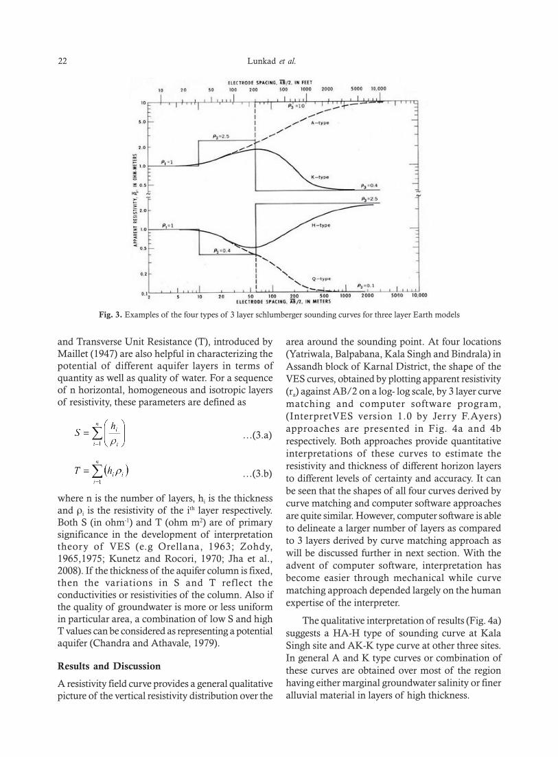
22 Lunkad et al.

and Transverse Unit Resistance (T), introduced byMaillet (1947) are also helpful in characterizing thepotential of different aquifer layers in terms ofquantity as well as quality of water. For a sequenceof n horizontal, homogeneous and isotropic layersof resistivity, these parameters are defined as

…(3.a)

…(3.b)

where n is the number of layers, hi is the thicknessand ρi is the resistivity of the ith layer respectively.Both S (in ohm-1) and T (ohm m2) are of primarysignificance in the development of interpretationtheory of VES (e.g Orellana, 1963; Zohdy,1965,1975; Kunetz and Rocori, 1970; Jha et al.,2008). If the thickness of the aquifer column is fixed,then the variations in S and T reflect theconductivities or resistivities of the column. Also ifthe quality of groundwater is more or less uniformin particular area, a combination of low S and highT values can be considered as representing a potentialaquifer (Chandra and Athavale, 1979).

Results and Discussion

A resistivity field curve provides a general qualitativepicture of the vertical resistivity distribution over the

area around the sounding point. At four locations(Yatriwala, Balpabana, Kala Singh and Bindrala) inAssandh block of Karnal District, the shape of theVES curves, obtained by plotting apparent resistivity(ra) against AB/2 on a log- log scale, by 3 layer curvematching and computer software program,(InterpretVES version 1.0 by Jerry F.Ayers)approaches are presented in Fig. 4a and 4brespectively. Both approaches provide quantitativeinterpretations of these curves to estimate theresistivity and thickness of different horizon layersto different levels of certainty and accuracy. It canbe seen that the shapes of all four curves derived bycurve matching and computer software approachesare quite similar. However, computer software is ableto delineate a larger number of layers as comparedto 3 layers derived by curve matching approach aswill be discussed further in next section. With theadvent of computer software, interpretation hasbecome easier through mechanical while curvematching approach depended largely on the humanexpertise of the interpreter.

The qualitative interpretation of results (Fig. 4a)suggests a HA-H type of sounding curve at KalaSingh site and AK-K type curve at other three sites.In general A and K type curves or combination ofthese curves are obtained over most of the regionhaving either marginal groundwater salinity or fineralluvial material in layers of high thickness.

Fig. 3. Examples of the four types of 3 layer schlumberger sounding curves for three layer Earth models

Geo-electrical Investigations 23

Fig. 4. Types of sounding curves at different sites

Subsurface geo-electric layers

From quantitative point of view, the interpretationof VES data suggests that there were 5 to 6 geo-electric layers (Table 2) in this region. The outputsof the software include the depth, resistivity andexpected lithology classification of geo- electricallayers in the study area. This information along withestimated Dar Zarrouk parameters, S and T, providegood diagnostic guidelines on the groundwaterpotential of different horizons in terms of quantityand quality. However, for further strengthening ofinterpretation, the VES survey results weresupplemented with actual texture of different layers

and groundwater quality (total dissolved solids, ppm)determined from bore hole sampling near to the VESlocations.

The combined results of estimated thickness andresistivity of different layers and observed texturefor 4 sites are presented in Figure 5. These, alongwith expected lithology classification provided bycomputer software and observed groundwaterquality, are summarized for individual study sites inTable 3-6. The combined results presented in Table2 and 6 have been utilized for interpreting the aquiferpotential of individual sites in the subsequentsections.

24 Lunkad et al.

Balpabana

The water level in Balpabana was 12 m below groundsurface at the time of investigation. Theinterpretation of VES data suggests that there werefive geo-electric subsurface layers in the study area.These consisted of surface layer (top soil), clay mixwith loam, fine sand with loam and successivesaturated mixture of fine and medium sand layers(Fig 5; Table 3). The topmost layer of 9.1 ohm-mresistivity and 1.5 m thickness represents dry top soilwith appreciable clay content. The second layer withhigher resistivity of 36.3 ohm-m and 1 m thicknessindicates the unsaturated mixture of clay and loam.The third layer of 68.5 ohm-m resistivity and 12 mthickness represents finer material, i.e loam with veryfine sand.

The fourth layer having resistivity of 57 ohm-mand 10 m thickness indicates coarser material thanabove layer i.e. fine to medium sand. The resistivityin the fifth layer extending to a good undefined depthdecreases from 57ohm m in upper layer to 26.5 ohm-m representing fine sand conditions.

The horizon resistivity values represent theintegrated effect of texture and groundwater qualityand it requires good professional expertise and priorknowledge about the hydro geological conditions toseparate out these effects. It can be seen thatgroundwater quality in terms of TDS, though notacceptable from drinking water criteria, is stillsuitable for irrigation till 24 m depth of the 4th layerand to some additional depth below in 5th layer

considering the permissible threshold level being1300 ppm. The fourth layer of about 10 m thicknessof medium to fine sand and 800- 900 ppm qualityoffers the best possibilities of groundwater withinthe investigated depth in Balpabana. Relativelydeeper water level (12 m) at this site vis-a – vis atother sites is also indicative to reflect suchpossibilities.

The integrated effect of whole aquifer column,represented through Dar Zarrouk parameters,indicates that relatively low (0.6 ohm-1) value of Sand high value (1452 ohm m2) of T point to potentialexistence of a good aquifer in the 4th layer. Basedonly on the comparative values of S and T, it can bestated with certainty that Balpabana has the bestquantitative and qualitative aquifer potentialamongst 4 sites reported in this paper. The increasingtrend of TDS of groundwater with depth beyond 24m recommends either restriction of aquifer to within4th and part of 5th layer or explore for still better stratain deeper layers.

Yatriwala

The water level in Yatriwala was very shallow at 4m below ground surface at the time of investigation.The interpretation of VES data suggests existenceof 5-6 geo- electric sub-surface layers in the studyarea. These consisted of surface layer (top soil), finesand with marginally saline groundwater at shallowdepth and successive saturated mixture of fine andmedium sand layers (Fig 5; Table 4).

Table 2: Geoelectrical parameters* of different site

VES LayersPoints I II III IV V VI Entire Aquifer

Column

Balpabana ρ/h 9/2 36/1 69/12 57/10 27/∞S 0.22 0.03 0.17 0.18 0.60T 18 36 828 570 1452

Yatriwala ρ/h 8/2 18/4 8/6 10/13 14/25 3/∞S 0.25 0.22 0.33 1.30 1.78 3.88T 16 72 48 130 350 616

Kala singh ρ/h 2/2 8/11 9/15 7/20 55/”S 1.00 1.38 1.60 2.86 6.84T 4 88 135 140 367

Bindrala ρ/h 13/2 71/2 17/5 20/15 14/16 7/∞S 0.15 0.03 0.29 0.75 1.14 2.36T 26 142 85 300 224 777

*Horizon thickness (h) in m, apparent resistivity (ρ) in ohm-m, longitudinal unit conductance (S) in ohm-1 and transverse unitresistance (T) in ohm m2

Geo-electrical Investigations 25

Fig. 5. Observed lithology and resistivity of the corresponding layers at different sites

Table 3. Resistivity survey and field observation results at Balpabana

Computer software output Bore hole observations

Depth Resistivity Lithology classification Texture Groundwater quality(m) (ohm-m) (TDS in ppm)

0-1.5 9.1 Top dry soil Clay1.5-2.5 36.3 A mixture of clay and loam Clay2.5-15 68.5 A mixture of loam and fine sand Loam/Loamy sand 84515-24 57 A mixture of fine to Medium sand Loamy sand/sandy loam 91524-∞ 26.5 Mixture of very fine to fine sand Sandy loam /sand 1375

The topmost layer of 7.7 ohm-m resistivity and1.5 m thickness represents loamy saline soil whilethe second 4 m thick layer of 18.3 ohm m resistivityindicates the saturated fine sand zone resulting fromshallow groundwater of 1152 ppm salinity. The third

layer of 8.1 ohm-m resistivity and 6 m thicknessdepicts finer aquifer material like a mixture of loamand fine sand. Low resistivity of this layer can bedue to combined effect of fine aquifer material andmarginally higher (1408 ppm) salinity of

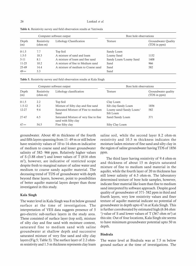
26 Lunkad et al.

Table 4. Resistivity survey and field observation results at Yatriwala

Computer software output Bore hole observations

Depth Resistivity Lithology Classification Texture Groundwater Quality(m) (ohm-m) (TDS in ppm)

0-1.5 7.7 Top Soil Sandy Loam1.5-5 18.3 A mixture of sand and loam Loamy Sand 11525-11 8.1 A mixture of loam and fine sand Sandy Loam/Loamy Sand 140811-25 10.2 A mixture of fine to Medium sand Sand 96625-49 14.4 A mixture of medium to Coarse sand Sand 58249-∞ 3.3 Sand

Table 5. Resistivity survey and field observation results at Kala Singh

Computer software output Bore hole observations

Depth Resistivity Lithology classification Texture Groundwater quality(m) (ohm-m) (TDS in ppm)

0-1.5 2.2 Top Soil Clay Loam1.5-12 8.2 Mixture of Silty clay and fine sand Silt clay-Sandy Loam 185612-27 9.4 Saturated Mixture of Fine to medium Loamy sand/Sandy Loam/ 582

Sand Silt Loam27-47 6.5 Saturated Mixture of very fine to fine Sand/Sandy Loam 371

sand with Silty clay47-∞ 54.5 Fine Silty clay Silty Clay Loam

groundwater. About 40 m thickness of the fourthand fifth layers spanning from 11- 49 m or still belowhave resistivity values of 10 to 14 ohm-m indicativeof medium to coarse sand and lesser groundwatersalinity of 582- 966 ppm. Relatively higher valuesof S (3.88 ohm-1) and lower values of T (616 ohmm2), however, are indicative of restricted scopedespite fresh to marginal nature of saline water andmedium to coarse sandy aquifer material. Thedeceasing trend of TDS of groundwater with depthbeyond these layers, however, point to possibilitiesof better aquifer material layers deeper than thoseinvestigated in this study.

Kala Singh

The water level in Kala Singh was 8 m below groundsurface at the time of investigation. Theinterpretation of VES data suggests presence of 5geo-electric sub-surface layers in the study area.These consisted of surface layer (top soil), mixtureof silty clay and fine sand with moisture content,saturated fine to medium sand with salinegroundwater at shallow depth and successivesaturated mixture of very fine sand and silty claylayers (Fig 5; Table 5). The surface layer of 2.2 ohm-m resistivity and 1.5 m thickness represents clay loam

saline soil, while the second layer 8.2 ohm-mresistivity and 10.5 m thickness indicates themoisture laden mixture of fine sand and silty clay inthe region of saline groundwater having TDS of 1856ppm.

The third layer having resistivity of 9.4 ohm-mand thickness of about 15 m depicts saturatedmixture of fine to medium sand material in theaquifer, while the fourth layer of 20 m thickness hasstill lower salinity of 6.5 ohm-m. The laboratorydetermined texture of bore hole samples, however,indicate finer material like loam than fine to mediumsand interpreted by software approach. Despite goodquality of groundwater of 371- 582 ppm in third andfourth layers, very low resistivity values and finertexture of aquifer material indicate no potential ofgroundwater in depth upto 47 m at Kala Singh. Thisis further corroborated by estimated high (6.84 ohm-

1) value of S and lower values of T (367 ohm m2) atthis site. Out of four locations, Kala Singh site seemsto have minimum groundwater potential upto 50 mdepth.

Bindrala

The water level at Bindrala was at 7.5 m belowground surface at the time of investigations. The

Geo-electrical Investigations 27

interpretation of VES data suggests presence of sixgeo- electric sub-surface layers in the study area.These consisted of surface layer (top soil), mixtureof silty clay and fine sand, saturated sand with siltand clay mixture, medium to coarse saturated sandand fine silty material at bottom layers (Fig 5; Table6).

The topmost layer of 12.9 ohm-m resistivity and2 m thickness represents dry top soil which may besilt loam. The second layer with higher resistivity of71.1 ohm-m and about 2 m thickness indicates amixture of silty clay and fine sand .In the third layerof about 5 m thickness resistivity drops to 17.2 ohm-m having thickness of about 5 m depicts the saturatedcondition of the aquifer having fine mixture of siltyclay and fine sand with TDS content of 2067 ppm.The fourth layer having resistivity value of 19.3 ohm-m and thickness of about 15 m indicated the mediumsand with few lenses of clay in the aquifer withdecrease in TDS to 1400 ppm ,the fifth layer havingresistivity value of 13.2 ohm-m and thickness ofabout 16 m consist of coarser aquifer material i.e.medium to coarse sand and increase in TDS ofaquifer to 2080.

From Geophysical resistivity surveys employingSchlumberger (Sounding) method, it is concludedthat the specific conductance of groundwater islimited to 1400 to 2080 ppm making groundwatermoderately saline while the aquifer material variesfrom silty clay, fine sand to medium sand.

Summary and Conclusions

Four alluvial aquifer sites in Assandh block of Karnaldistrict in Haryana were investigated usingSchlumberger VES surveys to characterize sub-surface hydro-geological conditions up to 50 mdepth. The groundwater level in the study sites

ranged from 4- 12 m and its salinity (TDS) variedbetween 371 to 2080 ppm (0.6 to 3.3 dS/m). Theconventional 3 layer curve matching and computersoftware approaches were employed to estimate thethickness and resistivity of different subsurfacehorizons and related Dar Zarrouk parameters ofLongitudinal Unit Conductance (S) and TransverseUnit Resistance (T). These were furthersupplemented with bore- hole field data onsubsurface lithology and groundwater salinity formaking reliable interpretation of VES surveys results.Following salient observations and conclusions canbe made based on results of this study:

1. Vertical electrical sounding (VES) is a cost-effective approach to characterize subsurfacelithology and groundwater salinity in an area,but need good expertise on proper interpretationof results.

2. Qualitative interpretation of the data throughcurve matching approach indicated acombination of A and K type curves for thestudy area suggesting either fresh to marginalgroundwater salinity or dominance of layers offiner material in thick alluvial zone.

3. Computer software approach to delineate thethickness and provide resistivity estimates ofdifferent geo- electric layers has distinctadvantages over conventional curve matchingapproaches. Interpretation of the VES resultsthrough this approach highlighted the presenceof fine to medium sand aquifers, characterizedby resistivity values of 10 to 27 ohm m in varyingthick layers at 10- 35 m below ground level.

4. At 3 sites (Yatriwala, Bindrala and Kala Singh),low resistivity values of 8- 17 ohm m in saturatedlayers below water level represent fine tomedium sand of marginally saline groundwater.

Table 6. Resistivity survey and field observation results at Bindrala

Computer software output Bore hole observations

Depth Resistivity Lithology classification Texture Groundwater quality(m) (ohm-m) (TDS in ppm)

0-2 12.9 Top Soil Silt Loam2-4 71.1 Mixture of Silty clay and fine sand Sandy Loam4-9 17.2 Saturated sand with fine mixture of Silty clay-Sandy Loam 2067

silt and clay9-24 19.3 Saturated Medium sand mix with clay Sandy-Silt-Sandy Loam 140024-40 13.2 Medium to coarse saturated sand Loamy Sand-Sand 208040-∞ 6.4 Fine Silty material Silty Loam

28 Lunkad et al.

At Balpabana, the fourth site, higher resistivityvalues of 57- 69 ohm m in 10 to 20m layersrepresent a mixture of loam and fine sand ofrelatively good quality groundwater. The lowerresistivity of 27 ohm m beyond 35 m at this siterepresents better aquifer lithology though ofmarginally higher groundwater salinity.

5. Based on analysis of S and T values andsupporting evidence, it can be safely stated thatBalpabana, amongst 4 study sites, has the bestquantitative and qualitative aquifer potential.Kala Singh site has the most unfavorable hydro-geological conditions upto 50 m depth whileremaining 2 sites of Bindrala and Yatriwala fallin between these extremes.

6. Though the expected TDS of groundwater inthe study site area upto 50 m depth is likely tobe within 500-2000 mg/l (fresh to marginallysaline) range, quite suitable for irrigation,excessive withdrawal of groundwater in theseareas may lead to deterioration in pumped waterquality. For long term protection, the farmersmay be advised to explore better aquifer below50 m depth with the help of VES surveys.

References

Bajpai VN (1989). Surface and subsurface evidence ofneotectonics and the aquifer disposition in CentralGangetic Alluvial terrain of Kanpur-Unnao region inUttar Pradesh, India. Photonirvachak. Journal of theIndian Society of Remote Sensing 17 (2): 47-53.

Bajpai VN and Kumar H (1988). Aquifer disposition andpalaeochannel morphology in Kanpur-Unnao region ofCentral Ganga Plain, India. In: Singh S, Tiwari RC(eds.),Geomorphology and Environment. AllahabadGeographical Society,Allahabad, pp. 142-152.

Chandra PC and Athavale RN (1979). Close grid resistivitysurvey for demarcating the aquifer encountered in borewell at Koyyur in lower Maner basin. Technical ReportNo. GH-11-GP-7,Hyderabad.

Heilan C A (1940). Geophysical Exploration. Prentice Hall,NewYork, N.Y., 240 pp.

Jha MK, Kumar S and Chowdhury A (2008). Verticalelectrical sounding survey and resistivity inversion usingGenetic Algorithm optimization technique. J. Hydrology359(1-2): 71-87.

Kunetz G (1966). Principles of Direct Current ResistivitySurveying. Gebrüder Borntraeger, Berlin pp103.

Kunetz G and Rocori JP (1970). Traitment automatique dessondages electriques. Geophysical prospecting 18, 157-198pp.

Lunkad SK (2006). The present and the future ofgroundwater resources of Haryana, India, In:Venketaswara Rao B. et al. (eds) Proceedings ofInternational Conference on Hydrology and WatershedManagement (ICHWAM-2006), Dec. 5-8, Jawahar LalNehru Technical University, Hyderabad, India, 1, pp165-181.

Maillet R (1947). The fundamental equations of electricalprospecting: Geophysics 12, 529- 556 pp.

Malik A, Setia B and Kamra SK (2013). A GIS based quantityand quality analysis of groundwater in alluvial regionsof Haryana. In: Sundar V, Srinivasan K and Murali, K(eds) Proceedings of the Hydro 2013 International XVIIIConference on Hydraulics, Water Resources, Coastaland Environmental Engineering, Chennai (India),December 4- 6, 2013, pp 1019- 1028.

Obiora DN and Onwuka OS (2005). Groundwaterexploration in Ikorodu, Lagos-Nigeria: a surfacegeophysical survey contribution. The Pacific Journal ofScience and Technology 6(1): 86-93.

Orellana E (1963). Properties and drawing of the so-calledDar Zarrouk curves. Geophysics 28: 99-110

Ramachandra Rao MB (1975). Outlines of GeophysicalProspecting: A Manual for Geologists. 38pp.

Singh CL and Yadav GS (1984). Geoelectrical soundingsfor ground water investigations of Kushmi area ofGhazipur district, U.P. The Journal of Scientific Research34 (I): 197- 205.

Vivekananth A, Gowtham B and Hussain SM (2014).Identification of groundwater potential zones inKadayanallur watershed,Tirunelveli district, TamilNadu, using remote sensing and geophysical data.Gondwana Geological Magazine. Special Vol. No. 14, pp.41-48.

Yadav GS and Singh CL (1987). Groundwater investigationsusing Schlumberger sounding in the Vindhyan Fringebelt of Ahraura region, Mirzapur, U.P. Journal ofGeophysics 8: 237-245.

Yadav GS (2004). Parameter identification- Electricalmethods. In: Rai, SN (ed) Role of Mathematical Modelingin Groundwater Resource Management, NationalGeophysical Research Institute, Hyderabad- 500007,India, pp 177- 216

Zohdy AAR (1965). Geoelctrical and Seismic refractioninvestigations near San jose, California. Groundwater,3(3): 41-48.

Zohdy AAR (1974). Use of Dar Zarrouk Curves in theInterpretation of Vertical ElectricalSounding Data. UnitedStates Geological Survey Bulletin, 1313-D: 41 p.

Zohdy AAR (1975). Automatic interpretation ofSchlumberger sounding curves using modified Dar-Zarrouk functions. United States Geological Survey Bulletin,1313-E: 39 p.

Received: January, 2015; Accepted March, 2015

Impact of Eucalyptus Plantations on Soil Aggregates andOrganic Carbon in Sodic-Saline Waterlogged Soils

Sharif Ahamad and JC Dagar

ICAR-Central Soil Salinity Research Institute, Karnal-132001, Haryana

Abstract

The total water stable aggregates were compared in sodic-saline waterlogged soil under cloned Eucalyptustereticornis plantations with non-planted conditions. These were influenced due to variation in pH of soil andwaterlogging. Average total water stable aggregates and their indices were significantly (p≤0.05) higher (38.24%) in 0-30 cm soil layer and decreased with increase in soil depth. Average macro-aggregates were also decreasedwith increase in soil depth. The average soil organic carbon (SOC) after seven years of plantation was recordedto be 0.35 % in soil profile (0-120 cm) compared to unplanted area (0.11 %). The SOC was higher (0.83 %) inupper (0-15 cm) soil layer followed by 0.41 % in 15-30 cm soil depth under plantations. The higher SOC in thesurface layer was due to the fact that the litter fall and its decomposition mainly took place on surface andinfluenced mainly upper soil layers. There was significant (p≤0.05) correlation between macro-aggregates andsoil organic carbon, which were maximum in upper soil layers under cloned Eucalyptus tereticornis (C-7)plantations.

Key words: Aggregates, Sodic-saline soils, Eucalyptus tereticornis plantations, Soil organic carbon, Canal commandarea, Waterlogging, Soil physical properties, Water stable aggregates (WSA)

Introduction

Canal command areas are facing a major challengedue to rise in groundwater table followed bywaterlogging and secondary soil salinization in aridand semi-arid regions. It is estimated that in India,about 6.41 m ha land in considered waterlogged, outof which 4.75 m ha is due to sub-surfacewaterlogging and 1.66 mha due to surface ponding(Maji et al., 2010). For rehabilitation and reclamationof such soils the plantation of Eucalyptus has beenpromoted and successfully grown as ridge plantation(Jeet-Ram et al., 2011). Trees plantation has a greatpotential in carbon sequestering in above-ground andbelow-ground soil and helps in mitigating thegreenhouse effect by reducing carbon emissions(Albrecht and Kandji, 2003). Tree plantation is thusthe most viable option to tackle land degradationand to bring about eco-restoration and sustenanceof soil resources (Dhyani and Chauhan, 1995). Soilshave the capacity to store carbon, accounting formore carbon than is found in the atmosphere andliving plant biomass combined (Jobbagy andJackson, 2000). Soil aggregates, a group of primarysoil particles,which by soil physical, chemical andbiological influences, helps in sequestering carbon

and protecting against microbial decomposition (Sixet al., 2000). Some of the most important factorsinfluencing the aggregation include surface tension,intermolecular attractive forces between water andsolids, precipitated solutes, roots and fungal hyphaeand various chemical phenomena.The complexdynamics of aggregation are the results of theinteraction of many factors, including theenvironment, soil management factors, plantinfluences and soil properties such as mineralcomposition, texture, soil organic carbon (SOC)concentration, pedogenic processes, microbialactivities, exchangeable ions, nutrient reserves, andmoisture availability (Kay, 1990). These soilaggregations are the basic index for appraisal of soilphysical properties, especially structure, and that isimportant to sustain soil fertility by reducing soilerosion and mediates air permeability, waterinfiltration and nutrient cycling (Spohn and Giani,2011; Zhang et al., 2012). Soil aggregate stability hasalso been shown to provide a good index of soilerodibility (Kay, 2000; Diaz-Zorita et al., 2002). Thesoil aggregate stability may be affected by soil texture,organic matter, soil and moisture content(Mostaghimi et al., 1988; Oztas and Fayetorbay,2003). The abundant water stable aggregates (WSA)

Journal of Soil Salinity and Water Quality 7(1), 29-34, 2015

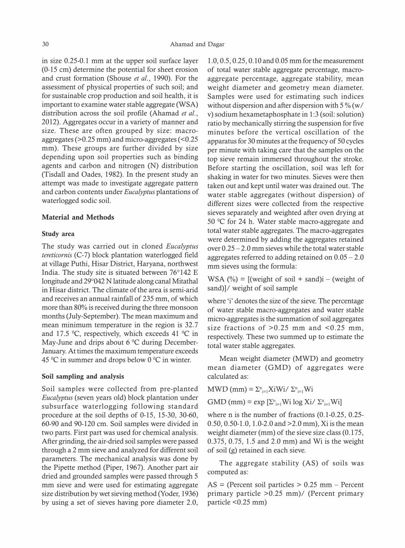
30 Ahamad and Dagar

in size 0.25-0.1 mm at the upper soil surface layer(0-15 cm) determine the potential for sheet erosionand crust formation (Shouse et al., 1990). For theassessment of physical properties of such soil; andfor sustainable crop production and soil health, it isimportant to examine water stable aggregate (WSA)distribution across the soil profile (Ahamad et al.,2012). Aggregates occur in a variety of manner andsize. These are often grouped by size: macro-aggregates (>0.25 mm) and micro-aggregates (<0.25mm). These groups are further divided by sizedepending upon soil properties such as bindingagents and carbon and nitrogen (N) distribution(Tisdall and Oades, 1982). In the present study anattempt was made to investigate aggregate patternand carbon contents under Eucalyptus plantations ofwaterlogged sodic soil.

Material and Methods

Study area

The study was carried out in cloned Eucalyptustereticornis (C-7) block plantation waterlogged fieldat village Puthi, Hisar District, Haryana, northwestIndia. The study site is situated between 76°142 Elongitude and 29°042 N latitude along canal Mitathalin Hisar district. The climate of the area is semi-aridand receives an annual rainfall of 235 mm, of whichmore than 80% is received during the three monsoonmonths (July-September). The mean maximum andmean minimum temperature in the region is 32.7and 17.5 0C, respectively, which exceeds 41 0C inMay-June and drips about 6 0C during December-January. At times the maximum temperature exceeds45 0C in summer and drops below 0 0C in winter.

Soil sampling and analysis

Soil samples were collected from pre-plantedEucalyptus (seven years old) block plantation undersubsurface waterlogging following standardprocedure at the soil depths of 0-15, 15-30, 30-60,60-90 and 90-120 cm. Soil samples were divided intwo parts. First part was used for chemical analysis.After grinding, the air-dried soil samples were passedthrough a 2 mm sieve and analyzed for different soilparameters. The mechanical analysis was done bythe Pipette method (Piper, 1967). Another part airdried and grounded samples were passed through 5mm sieve and were used for estimating aggregatesize distribution by wet sieving method (Yoder, 1936)by using a set of sieves having pore diameter 2.0,

1.0, 0.5, 0.25, 0.10 and 0.05 mm for the measurementof total water stable aggregate percentage, macro-aggregate percentage, aggregate stability, meanweight diameter and geometry mean diameter.Samples were used for estimating such indiceswithout dispersion and after dispersion with 5 % (w/v) sodium hexametaphosphate in 1:3 (soil: solution)ratio by mechanically stirring the suspension for fiveminutes before the vertical oscillation of theapparatus for 30 minutes at the frequency of 50 cyclesper minute with taking care that the samples on thetop sieve remain immersed throughout the stroke.Before starting the oscillation, soil was left forshaking in water for two minutes. Sieves were thentaken out and kept until water was drained out. Thewater stable aggregates (without dispersion) ofdifferent sizes were collected from the respectivesieves separately and weighted after oven drying at50 0C for 24 h. Water stable macro-aggregate andtotal water stable aggregates. The macro-aggregateswere determined by adding the aggregates retainedover 0.25 – 2.0 mm sieves while the total water stableaggregates referred to adding retained on 0.05 – 2.0mm sieves using the formula:

WSA (%) = [(weight of soil + sand)i – (weight ofsand)]/ weight of soil sample

where ‘i’ denotes the size of the sieve. The percentageof water stable macro-aggregates and water stablemicro-aggregates is the summation of soil aggregatessize fractions of >0.25 mm and <0.25 mm,respectively. These two summed up to estimate thetotal water stable aggregates.

Mean weight diameter (MWD) and geometrymean diameter (GMD) of aggregates werecalculated as:

MWD (mm) = Σni=1XiWi/ Σn

i=1Wi

GMD (mm) = exp [Σni=1Wi log Xi/ Σn

i=1Wi]

where n is the number of fractions (0.1-0.25, 0.25-0.50, 0.50-1.0, 1.0-2.0 and >2.0 mm), Xi is the meanweight diameter (mm) of the sieve size class (0.175,0.375, 0.75, 1.5 and 2.0 mm) and Wi is the weightof soil (g) retained in each sieve.

The aggregate stability (AS) of soils wascomputed as:

AS = (Percent soil particles > 0.25 mm – Percentprimary particle >0.25 mm)/ (Percent primaryparticle <0.25 mm)

Impact of Eucalyptus Plantations on Soil Aggregates 31

The aggregate ratio (AR) of soils was computedas:

AR=[Percent of water stable macro-aggregates]/[Percent of water stable micro-aggregates]

Statistical analysis

Statistical analysis was performed using SPSSprogramme to determine the statistical significanceof soil condition effect. Duncan’s Multiple RangeTest (DMRT) was used to compare mean throughleast significant difference. The 5 % probability levelis regarded as statistically significant.

Results and Discussion

Results showed that the pH2 and ECe weresignificantly (p≤0.05) lower under the planation in0-15 cm soil depth than unplanted land left nearby

plantations (Fig.1 and Table 1). Kumar et al. (2014)also observed the pH, EC and physical properties ofsodic soil improved under the Eucalyptus plantation.The litter fall of trees release acidity during theirdecomposition (Noureen et al., 2008), cause reducepH, EC and improved soil physical properties.

Soil organic carbon (SOC)

In present study the distribution of soil organiccarbon (SOC) among the soil profile are stronglyinfluenced (p≤0.05) by the plantation of Eucalyptusunder waterlogging (Fig. 2). The average SOC afterseven years of plantation was recorded to be 0.35 %in soil profile (0-120 cm) compared (0.11 %) tounplanted area. The SOC was higher (0.83 %)inupper (0-15 cm) soil layer followed by 0.41 % in 15-30 cm soil depth. The higher SOC in the surface layeris due to fact that the litter fall takes place mainly onthe surface layers (Kumar et al., 2014; Mongia et al.,1998).

Soil aggregation

The results from the wet sieving method for waterstable aggregates and its indices of Eucalyptusplantation area are shown for soil depths (Table 2).The results showed that average total water stableaggregates were found highest (33 %) in 15-30 cmlayer followed by 30 % and 28 % in lower 0-15 and30-60 cm depth, respectively. Das et al. (2014) alsoreported that the soil aggregates decreased withincreasing the soil depth. Chaudhury et al. (2014)expressed in a study that soil aggregation increasedby improving of organic matter in soil, which canmanage through conservational tillage and residuemanagement, in tropical soils. However, in presentstudy the maximum (38.24 %) total water stableaggregates were found in waterlogged soil conditionin 0-35 cm soil depth followed by 33.81 % in 15-30

Table 1. Soil condition under Eucalyptus plantated on sodic-saline waterlogged condition

Soil Depth Na (me/l) Na (me/l) Ca (me/l) Mg (me/l)

Initial Ecalyptus Initia Ecalyptus Initial Ecalyptus Initial Ecalyptusplantation plantation plantation plantation

0-15 6.17 1.51 0.01 0.02 5.00 9.25 2.50 5.315-30 1.81 0.96 0.04 0.04 0.50 6.25 1.00 3.530-60 0.85 1.13 0.04 0.04 0.50 7.85 0.50 4.960-90 0.80 0.56 0.04 0.03 0.40 7.85 0.40 4.990-120 0.73 0.47 0.03 0.04 0.30 7.50 0.40 5.0Mean 2.07 0.93 0.03 0.04 1.34 7.74 0.96 3.92SD 2.34 0.45 0.01 0.01 2.05 1.12 0.90 1.29

Fig. 1. Soil pH and electrical conductivity (ECe) before andafter Eucalyptus plantation

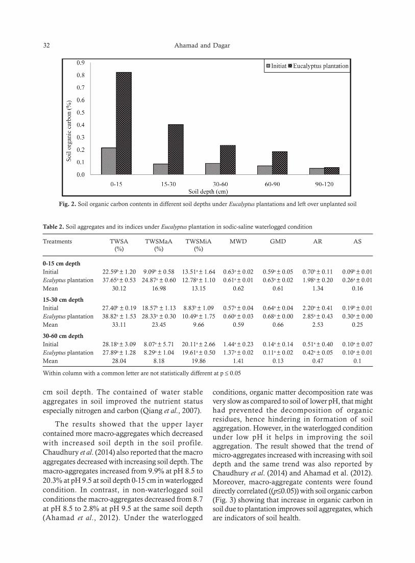
32 Ahamad and Dagar

Table 2. Soil aggregates and its indices under Eucalyptus plantation in sodic-saline waterlogged condition

Treatments TWSA TWSMaA TWSMiA MWD GMD AR AS(%) (%) (%)

0-15 cm depthInitial 22.59b ± 1.20 9.09b ± 0.58 13.51a ± 1.64 0.63a ± 0.02 0.59a ± 0.05 0.70b ± 0.11 0.09b ± 0.01Ecalyptus plantation 37.65a ± 0.53 24.87a ± 0.60 12.78a ± 1.10 0.61a ± 0.01 0.63a ± 0.02 1.98a ± 0.20 0.26a ± 0.01Mean 30.12 16.98 13.15 0.62 0.61 1.34 0.16

15-30 cm depthInitial 27.40b ± 0.19 18.57b ± 1.13 8.83b ± 1.09 0.57a ± 0.04 0.64a ± 0.04 2.20a ± 0.41 0.19b ± 0.01Ecalyptus plantation 38.82a ± 1.53 28.33a ± 0.30 10.49a ± 1.75 0.60a ± 0.03 0.68a ± 0.00 2.85a ± 0.43 0.30a ± 0.00Mean 33.11 23.45 9.66 0.59 0.66 2.53 0.25

30-60 cm depthInitial 28.18a ± 3.09 8.07a ± 5.71 20.11a ± 2.66 1.44a ± 0.23 0.14a ± 0.14 0.51a ± 0.40 0.10a ± 0.07Ecalyptus plantation 27.89a ± 1.28 8.29a ± 1.04 19.61a ± 0.50 1.37a ± 0.02 0.11a ± 0.02 0.42a ± 0.05 0.10a ± 0.01Mean 28.04 8.18 19.86 1.41 0.13 0.47 0.1

Within column with a common letter are not statistically different at p ≤ 0.05

Fig. 2. Soil organic carbon contents in different soil depths under Eucalyptus plantations and left over unplanted soil

cm soil depth. The contained of water stableaggregates in soil improved the nutrient statusespecially nitrogen and carbon (Qiang et al., 2007).

The results showed that the upper layercontained more macro-aggregates which decreasedwith increased soil depth in the soil profile.Chaudhury et al. (2014) also reported that the macroaggregates decreased with increasing soil depth. Themacro-aggregates increased from 9.9% at pH 8.5 to20.3% at pH 9.5 at soil depth 0-15 cm in waterloggedcondition. In contrast, in non-waterlogged soilconditions the macro-aggregates decreased from 8.7at pH 8.5 to 2.8% at pH 9.5 at the same soil depth(Ahamad et al., 2012). Under the waterlogged

conditions, organic matter decomposition rate wasvery slow as compared to soil of lower pH, that mighthad prevented the decomposition of organicresidues, hence hindering in formation of soilaggregation. However, in the waterlogged conditionunder low pH it helps in improving the soilaggregation. The result showed that the trend ofmicro-aggregates increased with increasing with soildepth and the same trend was also reported byChaudhury et al. (2014) and Ahamad et al. (2012).Moreover, macro-aggregate contents were founddirectly correlated ((p≤0.05)) with soil organic carbon(Fig. 3) showing that increase in organic carbon insoil due to plantation improves soil aggregates, whichare indicators of soil health.

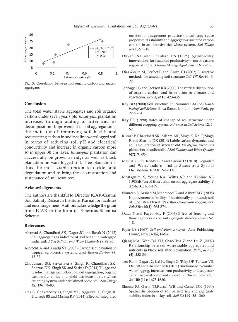
Impact of Eucalyptus Plantations on Soil Aggregates 33

Conclusion

The total water stable aggregates and soil organiccarbon under seven years old Eucalyptus plantationincreases through adding of litter and itsdecomposition. Improvement in soil aggregation isthe indicator of improving soil health andsequestering carbon in sodic-saline waterlogged soilin terms of reducing soil pH and electricalconductivity and increase in organic carbon moreso in upper 30 cm layer. Eucalyptus plantation cansuccessfully be grown as ridge as well as blockplantation on waterlogged soil. Tree plantation isthus the most viable option to tackle landdegradation and to bring the eco-restoration andsustenance of soil resources.

Acknowledgements

The authors are thankful to Director ICAR-CentralSoil Salinity Research Institute, Karnal for facilitiesand encouragement. Authors acknowledge the grantfrom ICAR in the form of Emeritus ScientistScheme.

References

Ahamad S, Chaudhari SK, Dagar JC and Basak N (2012)Soil aggregates as indicator of soil health in waterggedsodic soil. J Soil Salinity and Water Quality 4(2): 92-96.

Albrecht A and Kandji ST (2003) Carbon sequestration intropical agroforestry systems. Agric Ecosyst Environ 99:15-27.

Choudhury SG, Srivastava S, Singh R, Chaudhari SK,Sharma DK, Singh SK and Sarkar D (2014) Tillage andresidue management effect on soil aggregation, organiccarbon dynamics and yield attribute in rice-wheatcropping system under reclaimed sodic soil. Soil TillageRes 136: 76-83.

Das B, Chakraborty D, Singh VK, Aggarwal P, Singh R,Dwivedi BS and Mishra RP (2014) Effect of integrated

nutrient management practice on soil aggregateproperties, its stability and aggregate-associated carboncontent in an intensive rice-wheat system. Soil TillageRes 136: 9-18.

Dhyani SK and Chauhan DS (1995) Agroforestryinterventions for sustained productivity in north-easternregion of India. J Range Manage Agroforestry 16: 79-85.

Diaz-Zorita M, Perfect E and Grove JH (2002) Disruptivemethods for assessing soil structure.Soil Till Res 64: 3-22.

Jobbagy EG and Jackson RB (2000) The vertical distributionof organic carbon and its relation to climate andvegetation. Ecol Appl 10: 423-436.

Kay BD (2000) Soil structure. In: Summer EM (ed) Hand-book of Soil Science. Boca Raton, London, New York, pp229- 264.

Kay BD (1990) Rates of change of soil structure underdifferent cropping system. Advances in Soil Science 12: 1-52.

Kumar P, Chaudhari SK, Mishra AK, Singh K, Rai P, SinghR and Sharma DK (2014) Labile carbon dynamics andsoil amelioration in six-year old Eucalyptus tereticornisplantation in sodic soils. J Soil Salinity and Water Quality6(2): 91-95.

Maji AK, Obi Reddy GP and Sarkar D (2010) Degradedand Wastelands of India: Status and SpecialDistribution. ICAR, New Delhi.

Mostaghimi S, Young RA, Wiltts AR and Kenime AL(1988)Effect of frost action on soil aggregate stability. TASAE 31: 435-439.

Noureen S, Arshad M,Mahmood K and Ashraf MY (2008)Improvement in fertility of nutritionally poor sandy soilof Cholistan Desert, Pakistan Calligonum polygonoides.Pak J Bot 40(1): 265-274.

Oztas T and Fayetorbay F (2003) Effect of freezing andthawing processes on soil aggregate stability. Catena 52:1-8.

Piper CS (1967) Soil and Plant Analysis. Asia PublishingHouse, New Delhi, India.

Qiang MA, Wan-Tai YU, Shao-Hua Z and Lu Z (2007)Relationship between water-stable aggregates andnutrients in black soil after reclamation. Pedosphere 17(4): 538-544.

Jeet-Ram, Dagar JC, Lal K, Singh G, Toky OP, Tanwar VS,Dar SR and Chauhan MK (2011) Biodrainage to combatwaterlogging, increase from productivity and sequestercarbon in canal command areas of northwest India. CurrSci 100 (11): 1673-1680.

Shouse PJ, Gerik TJ,Russel WB and Cassel DK (1990)Spatial distribution of soil particle size and aggregatestability index in a clay soil. Soil Sci 149: 351-360.

Fig. 3. Correlation between soil organic carbon and macro-aggregates

34 Ahamad and Dagar

Six J, Elliott ET and Paustian K (2000) Soil macroaggregateturnover and microaggregate formation: a mechanismfor C sequestration under no-tillage agriculture. Soil BiolBiochem 32: 2099-2103

Spohn M and Giani L (2011)Impact of land use change onsoil aggregation and aggregate stabilizing compound asdependent on time. Soil Biol Biochem 43: 1081-1088.

Tisdall JM and OadesJM (1982) Organic matter and water-stable aggregates in soils. J Soil Sci 62: 141-163.

Yoder RE (1936) A direct method of aggregate analysis ofsoil and the study of the physical nature of erosion losses.J Am Soc Agron 28: 337-351

Young A (1989) Agroforestry for Soil Conservation. CABInternational ICRAF, pp 276

Zhang S, Li Q, Zhang X, Wei K, Chen L and Liang W(2012)Effect of conservation tillage on soil aggregation andaggregate binding agents in black soil of NortheastChina. Soil Tillage Res 124: 196-202.

Received: January, 2015; Accepted March, 2015

Effect of Sodic Water Irrigation with Application of Sulphuras Single Super Phosphate on Yield, Mineral Composition

and Soil Properties in Rice-Wheat System

NPS Yaduvanshi*, K Lal* and A Swarup*

Division of Soil and Crop Management, ICAR-Central Soil Salinity Research Institute, Karnal-132001, Haryana

Abstract

The effects of sulphur as single super phosphate with different levels of sulphur (0, 30 and 45 kg ha-1) werestudied in rice- wheat crops on clay loam soil at Farmers’ field, Dera Bhaini Majra, Kaithal. The grain yield ofwheat increased significantly with the application of 45 kg S ha-1 through single super phosphate withrecommended doses of NPK fertilizer over control. The N-S composition of plant and their uptake wereconsiderably higher with 45 kg S ha-1 with recommended doses of NPK fertilizer at all growth stages. The Nand S composition of plant and their uptake were considerably higher with 45 kg S ha-1 at all growth stages. Useof sodic water with 100% NP during two years slightly decreased the soil pH and SAR from the initial value of8.6 and 16.2, respectively. However, treatments involving the use of 45 kg S ha-1 significantly decreased the soilpH and SAR over 100% NP treatments. The results suggest that 45 kg S ha-1 through single super phosphatewith recommended doses of NP fertilizer must be used to sustain the productivity of rice – wheat system inareas having sodic ground water for irrigation.

Key words: Sodic water, single superphosphate, rice –wheat sequence, Sulphur content

Introduction

In many arid and semiarid regions of the world,sodic groundwater is the main source of irrigationand its use poses a threat to improved rice and wheatproduction. Moreover, a large number of farmershave discontinued their source of underground waterfor irrigation on account of soil deterioration leadingto drastic reduction in the yield of crops. In spite ofpoor quality, the water is being used for irrigation asthere are no alternatives. Application of gypsum asa soil or water amendment is commonlyrecommended to offset the deteriorating effects ofthese types of water (Yaduvanshi and Swarup, 2005).In view of non-availability of gypsum, there is strongneed to alternative sources of gypsum, especially Scontent fertilizer, in order to supplement the S supplythrough chemical fertilizers as single super phosphateare multi-nutrients compound. Thus, there is anurgent need to work out sulphur fertilizer usestrategies to enhance and sustain higher level of cropand soil productivity of rice - wheat system inreclaimed alkali soils under sodic water irrigation

conditions. These poor quality waters constituteabout 47% in Punjab (Bajwa et al., 1974; Sehgal etal., 1985), 62% in Haryana 84% in Rajasthan, 38%in Karnataka, 32% in Andhra Pradesh, 30% inGujarat and 50% in Agra, Aligarh, Etah, Mainpuriand Mathura districts of UP (Dixit, 1974 ). Sincerice-wheat is the most commonly practiced croprotation system in the Indo-Genetic plains,improving its productivity, particularly in areas withpoor-quality groundwater, is a major challenge.Keeping in the view the above problems, the workwas undertaken to find out the ways for managingsuch hazardous waters by sulphur applicationthrough single super phosphate for sustainable cropproduction in the area.

Material and Methods

A field experiment was conducted during 2004-05and 2005-06 on a gypsum amended sodic soil toevaluate the use of sulphur fertilizer (single superphosphate) in rice-wheat cropping system under highRSC irrigation water at Farmers’ field Dera, BhainiMajra, Kaithal. The experimental soil (0-15cm) hadpH 9.0, EC2 0.79 dS m-1, SAR 16.2 (m mol l-1)1/2 ;organic carbon 0.44%, available P 14.8 kg ha-1,available and K 275 kg ha-1. The treatment consisted

Journal of Soil Salinity and Water Quality 7(1), 35-39, 2015

Correspondence e-mail: npsyaduvanshi@gmail.com*Present addressed. Indian Agricultural Research institute, NewDelhi.

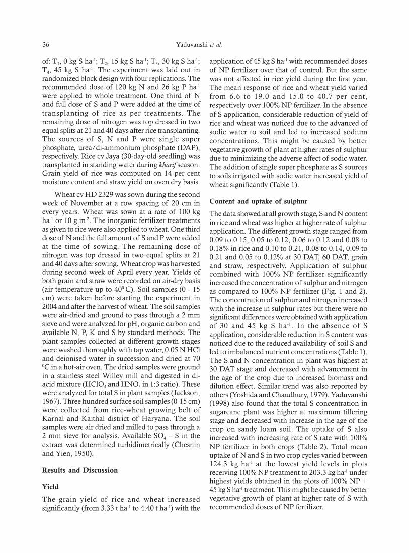
36 Yaduvanshi et al.

of: T1, 0 kg S ha-1; T2, 15 kg S ha-1; T3, 30 kg S ha-1;T4, 45 kg S ha-1. The experiment was laid out inrandomized block design with four replications. Therecommended dose of 120 kg N and 26 kg P ha-1

were applied to whole treatment. One third of Nand full dose of S and P were added at the time oftransplanting of rice as per treatments. Theremaining dose of nitrogen was top dressed in twoequal splits at 21 and 40 days after rice transplanting.The sources of S, N and P were single superphosphate, urea/di-ammonium phosphate (DAP),respectively. Rice cv Jaya (30-day-old seedling) wastransplanted in standing water during kharif season.Grain yield of rice was computed on 14 per centmoisture content and straw yield on oven dry basis.

Wheat cv HD 2329 was sown during the secondweek of November at a row spacing of 20 cm inevery years. Wheat was sown at a rate of 100 kgha-1 or 10 g m-2. The inorganic fertilizer treatmentsas given to rice were also applied to wheat. One thirddose of N and the full amount of S and P were addedat the time of sowing. The remaining dose ofnitrogen was top dressed in two equal splits at 21and 40 days after sowing. Wheat crop was harvestedduring second week of April every year. Yields ofboth grain and straw were recorded on air-dry basis(air temperature up to 400 C). Soil samples (0 - 15cm) were taken before starting the experiment in2004 and after the harvest of wheat. The soil sampleswere air-dried and ground to pass through a 2 mmsieve and were analyzed for pH, organic carbon andavailable N, P, K and S by standard methods. Theplant samples collected at different growth stageswere washed thoroughly with tap water, 0.05 N HCland deionised water in succession and dried at 700C in a hot-air oven. The dried samples were groundin a stainless steel Willey mill and digested in di-acid mixture (HClO4 and HNO3 in 1:3 ratio). Thesewere analyzed for total S in plant samples (Jackson,1967). Three hundred surface soil samples (0-15 cm)were collected from rice-wheat growing belt ofKarnal and Kaithal district of Haryana. The soilsamples were air dried and milled to pass through a2 mm sieve for analysis. Available SO4 – S in theextract was determined turbidimetrically (Chesninand Yien, 1950).

Results and Discussion

Yield

The grain yield of rice and wheat increasedsignificantly (from 3.33 t ha-1 to 4.40 t ha-1) with the

application of 45 kg S ha-1 with recommended dosesof NP fertilizer over that of control. But the samewas not affected in rice yield during the first year.The mean response of rice and wheat yield variedfrom 6.6 to 19.0 and 15.0 to 40.7 per cent,respectively over 100% NP fertilizer. In the absenceof S application, considerable reduction of yield ofrice and wheat was noticed due to the advanced ofsodic water to soil and led to increased sodiumconcentrations. This might be caused by bettervegetative growth of plant at higher rates of sulphurdue to minimizing the adverse affect of sodic water.The addition of single super phosphate as S sourcesto soils irrigated with sodic water increased yield ofwheat significantly (Table 1).

Content and uptake of sulphur

The data showed at all growth stage, S and N contentin rice and wheat was higher at higher rate of sulphurapplication. The different growth stage ranged from0.09 to 0.15, 0.05 to 0.12, 0.06 to 0.12 and 0.08 to0.18% in rice and 0.10 to 0.21, 0.08 to 0.14, 0.09 to0.21 and 0.05 to 0.12% at 30 DAT, 60 DAT, grainand straw, respectively. Application of sulphurcombined with 100% NP fertilizer significantlyincreased the concentration of sulphur and nitrogenas compared to 100% NP fertilizer (Fig. 1 and 2).The concentration of sulphur and nitrogen increasedwith the increase in sulphur rates but there were nosignificant differences were obtained with applicationof 30 and 45 kg S ha-1. In the absence of Sapplication, considerable reduction in S content wasnoticed due to the reduced availability of soil S andled to imbalanced nutrient concentrations (Table 1).The S and N concentration in plant was highest at30 DAT stage and decreased with advancement inthe age of the crop due to increased biomass anddilution effect. Similar trend was also reported byothers (Yoshida and Chaudhury, 1979). Yaduvanshi(1998) also found that the total S concentration insugarcane plant was higher at maximum tilleringstage and decreased with increase in the age of thecrop on sandy loam soil. The uptake of S alsoincreased with increasing rate of S rate with 100%NP fertilizer in both crops (Table 2). Total meanuptake of N and S in two crop cycles varied between124.3 kg ha-1 at the lowest yield levels in plotsreceiving 100% NP treatment to 203.3 kg ha-1 underhighest yields obtained in the plots of 100% NP +45 kg S ha-1 treatment. This might be caused by bettervegetative growth of plant at higher rate of S withrecommended doses of NP fertilizer.

Effect of Sodic Water Irrigation with Application of Sulphur 37

Fig. 1. Nitrogen and sulphur contents of rice under different treatments

Fig. 2. Nitrogen and sulphur contents of wheat under different treatments

Table 1. Effect of sulphur fertilizer on yield of rice and wheat

Sulphur Rice yield (t ha-1) Wheat yield (t ha-1)

(kg ha-1) Grain Straw Grain Straw

2004 2005 2004 2005 2004-05 2005-06 2004-05 2005-06

0 3.30 3.33 5.17 5.03 2.61 2.30 3.10 3.2515 3.43 3.65 5.36 5.46 2.73 2.92 3.32 3.4130 3.45 3.97 5.40 5.66 2.87 3.14 3.84 3.7245 3.49 4.40 5.54 5.84 3.25 3.66 3.98 4.05LSD(p=0.05) NS 0.78 NS 0.81 0.54 0.27 0.24 0.21

Soil properties

The soil pH, after two cycles of rice-wheat rotation,slightly declined over initial status in all thetreatments (Table 3). The magnitude of decreased,however was greater in plots receiving sulphur with100% NP fertilizer compared to 100% NP fertilizer.Application of sulphur with 100% NP fertilizersignificantly decreased the sodium absorption ratio(SAR) of surface soil (0-15cm) in two year of riceand wheat crop harvest over that of 100% NPfertilizer under use of sodic water irrigation (Table

3). The beneficial effect of gypsum (20% S) towardsreducing SAR or ESP of sodic water irrigated soilhas also been reported earlier by Sharma et al. (2001)and Sharma and Minhas (2004). The buildup of lowSAR in the surface 15 cm soil layer despite itsreceiving large number of irrigations with sodic waterduring growth of rice – wheat crops has beenattributed to the greater dissolution of calcium fromCaCO3 owing to high leaching fraction and highpCO2 attained during rice growth under submergedconditions (Sharma et al., 2001).

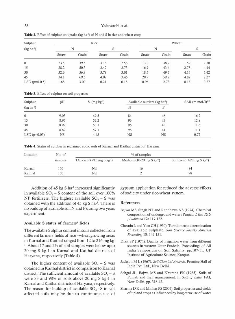
38 Yaduvanshi et al.

Table 2. Effect of sulphur on uptake (kg ha-1) of N and S in rice and wheat crop

Sulphur Rice Wheat

(kg ha-1) N S N S

Straw Grain Straw Grain Straw Grain Straw Grain

0 23.5 39.5 3.18 2.56 13.0 38.7 1.59 2.3015 28.2 50.3 3.47 2.73 16.9 43.4 2.78 4.4430 32.6 56.8 3.78 3.01 18.5 49.7 4.16 5.4245 34.1 69.5 4.02 3.46 20.9 59.2 4.82 7.27LSD (p=0.0 5) 1.68 3.00 0.21 0.18 0.96 2.73 0.18 0.27

Table 3. Effect of sulphur on soil properties

Sulphur pH S (mg kg-1) Available nutrient (kg ha-1) SAR (m mol/l)1/2

(kg ha-1) N P

0 9.03 49.5 84 46 16.215 8.95 52.2 96 45 12.830 8.92 53.1 96 45 11.645 8.89 57.1 98 44 11.1LSD (p=0.05) NS 4.45 NS NS 0.72

Table 4. Status of sulphur in reclaimed sodic soils of Karnal and Kaithal district of Haryana

Location No. of % of samples

samples Deficient (<10 mg S kg-1) Medium (10-20 mg S kg-1) Sufficient (>20 mg S kg-1)

Karnal 150 Nil 16 84Kaithal 150 Nil 2 98

Addition of 45 kg S ha-1 increased significantlyin available SO4 – S content of the soil over 100%NP fertilizers. The highest available SO4 – S wasobtained with the addition of 45 kg S ha-1. There isno buildup of available soil N and P during two yearsexperiment.

Available S status of farmers’ fields

The available Sulphur content in soils collected fromdifferent farmers’fields of rice –wheat growing areasin Karnal and Kaithal ranged from 12 to 216 mg kg-

1. About 17 and 2% of soil samples were below upto20 mg S kg-1 in Karnal and Kaithal districts ofHaryana, respectively (Table 4).

The higher content of available SO4 – S wasobtained in Kaithal district in comparison to Karnaldistrict. The sufficient amount of available SO4 – Swere 83 and 98% of soils above 20 mg S kg-1 inKarnal and Kaithal districts of Haryana, respectively.The reason for buildup of available SO4 –S in saltaffected soils may be due to continuous use of

gypsum application for reduced the adverse effectsof sodicity under rice-wheat system.

References

Bajwa MS, Singh NT and Randhawa NS (1974). Chemicalcomposition of underground waters Punjab. J. Res. PAU, Ludhiana 12: 117-122.

Chesnin L and Yien CH (1950). Turbidimetric determinationof available sulphate. Soil Science Society AmericaProceeding 15: 149-151.

Dixit SP (1974). Quality of irrigation water from differentsources in western Uttar Pradesh. Proceedings of AllIndia Symposium on Soil Salinity, pp.107-11, UPInstitute of Agriculture Science, Kanpur.

Jackson M L (1967). Soil Chemical Analysis. Prentice Hall ofIndia Pvt. Ltd., New Delhi.

Sehgal JL, Bajwa MS and Khurana PK (1985). Soils ofPunjab and their management. In Soils of India. FAI,New Delhi. pp. 316-42.

Sharma D R and Minhas PS (2004). Soil properties and yieldsof upland crops as influenced by long-term use of water

Effect of Sodic Water Irrigation with Application of Sulphur 39

having variable residual alkalinity, salinity and sodicity.Journal of the Indian Society of Soil Science 1: 100-104.

Sharma DR, Minhas PS and Sharma D K (2001). Responseof wheat to sodic water irrigation and gypsumapplication. Journal of the Indian Society of Soil Science49: 324-327.

Yaduvanshi NPS (1998). Sulphur fertilization in sugarcane.Sugar Cane 6: 6-8.

Yaduvanshi NPS and Swarup A (2005). Effect of continuoususe of sodic irrigation water with and without gypsum,farm yard manure, pressmud and fertilizer on soilproperties and yields of rice and wheat in a long termexperiment. Nutrient Cyclic in Agroecosystems. 73: 111-118.

Yoshida S and Chaudhury MR (1979). Sulphur nutrition ofrice. Soil Science Plant Nutrition. 25:121.

Received: February, 2015; Accepted April, 2015

Salinity Induced Changes in Chlorophyll Pigments and IonicRelations in Bael (Aegle marmelos Correa) Cultivars

Anshuman Singh*, PC Sharma, A Kumar, MD Meena and DK Sharma

ICAR-Central Soil Salinity Research Institute, Karnal-132001, Haryana*Email- anshumaniari@gmail.com

Abstract

Bael (Aegle marmelos) cultivars NB-5, NB-9, CB-1 and CB-2 were grown in normal (ECe 1.3 dS m-1), moderate(6.5 dS m-1) and high (10.7 dS m-1) saline soils. The cultivars, evaluated for changes in appearance, leaf chlorophyllpigments and ionic relations, exhibited salt stress symptoms as yellowing, scorching and chlorosis of the leaves.Majority of the affected leaves subsequently abscised from the plants. Salinity significantly increased membraneinjury and caused reduction in relative water content in all the cultivars. Accumulation of total soluble sugarsin salt treated plants showed genotypic differences with NB-5 plants recording their maximum accumulation.Leaf chlorophyll (a, b and total) values showed a consistent decrease with increase in salinity except for NB-5plants which exhibited slightly higher chlorophyll contents at moderate salinity. All the cultivars except NB-5exhibited significantly higher leaf Na+ concentrations with increasing salinity while the plants of cultivar NB-5 maintained a favourable ionic balance in terms of low Na+/K+ ratio resulting in good plant performanceunder salinity. The plants of NB-9 and CB-2 varieties did not survive at high salinity. Based on overall performance,NB-5 exhibited tolerance to moderately saline soils (ECe ~6.5dS m-1) and was successfully established whenirrigated with normal water.

Key words: Aegle marmelos, Cultivars, Mineral nutrition, Salinity tolerance, Salt-affected soils

Introduction

A sustainable approach for the productive utilizationof salt-affected soils (SAS), which coverapproximately 6.73 m ha area in India, relates tothe use of salt tolerant crop genotypes (Singh et al.,2010). Many plants of economic importance exhibitsalt tolerance and are adapted to grow in salt-affectedenvironments. Similarly, many improved cropgenotypes have been developed and/or identified forcommercial cultivation in SAS (Flowers, 2004). Anumber of fruit crops perform well under salinitystress and may be commercially grown in saline andsodic soils (Dagar, 2009). Bael (Aegle marmelosCorrea) is an indigenous underutilized fruit cropvalued for its medicinal and processing values andtolerance to different biotic and abiotic stresses. Inspite of these strengths, there is no organizedcultivation of this fruit in India. Bael cultivation inSAS could be a good option for alternate land useand crop diversification (Dagar, 2009). Salt stressedbael plants suffer from nutrient deficiencies (N, P, Kand Ca) which may account for poor plantestablishment and growth under salt stress (Shuklaand Singh, 1996). The available reports on salinity

tolerance in bael provide least information onimportant physiological and biochemical parametersof the tolerant and susceptible accessions which mayexplain plant behaviour in relation to salinity andmay be correlated with salinity tolerance mechanismin certain cultivar(s). In this backdrop, one-year oldplants of four improved bael genotypes wereevaluated in saline soils for assessing their salttolerance so as to appraise their suitability forcultivation in SAS.

Material and Methods

The present experiment was carried out during 2013-2014 at the experimental facility of ICAR-CentralSoil Salinity Research Institute (CSSRI), Karnal,India. One-year-old, grafted plants of four baelcultivars, namely, Narendra Bael-5 (NB-5), NarendraBael-9 (NB-9), CISH Bael-1 (CB-1) and CISH Bael-2 (CB-2) procured from the ICAR-Central Instituteof Subtropical Horticulture, Lucknow, India wereused. The saline soils used in this experiment wereobtained from the CSSRI-Nain Experimental Farm,Panipat, India; while control soil was obtained fromthe crop fields. The soil was filled in large, metallic

Journal of Soil Salinity and Water Quality 7(1), 40-44, 2015

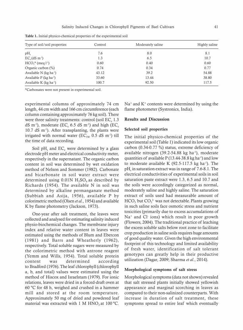
Salinity Induced Changes in Chlorophyll Pigments of Bael Cultivars 41

experimental columns of approximately 74 cmlength, 44 cm width and 166 cm circumference (eachcolumn containing approximately 76 kg soil). Therewere three salinity treatments: control (soil ECe 1.3dS m-1), moderate (ECe 6.5 dS m-1) and high (ECe

10.7 dS m-1). After transplanting, the plants wereirrigated with normal water (ECIW 0.5 dS m-1) tillthe time of data recording.

Soil pHs and ECe were determined by a glasselectrode pH meter and electrical conductivity meter,respectively in the supernatant. The organic carboncontent in soil was determined by wet oxidationmethod of Nelson and Sommer (1982). Carbonateand bicarbonate in soil water extract weredetermined using 0.01N H2SO4 as described byRichards (1954). The available N in soil wasdetermined by alkaline permanganate method(Subbiah and Asija, 1956), available P bycolorimetric method (Olsen et al., 1954) and availableK by flame photometry (Jackson, 1973).

One-year after salt treatment, the leaves werecollected and analysed for estimating salinity inducedphysio-biochemical changes. The membrane injuryindex and relative water content in leaves wereestimated using the methods of Blum and Ebercon(1981) and Barrs and Wheatherly (1962),respectively. Total soluble sugars were measured bythe colorimetric method with antrone reagent(Yemm and Wills, 1954). Total soluble proteincontent was determined accordingto Bradford (1976). The leaf chlorophyll (chlorophylla, b, and total) values were estimated using themethod of Hiscox and Israelstam (1979). For ionicrelations, leaves were dried in a forced-draft oven at60 ºC for 48 h, weighed and crushed in a hammermill and stored at the room temperature.Approximately 50 mg of dried and powdered leafmaterial was extracted with 1 M HNO3 at 100 ºC.

Na+ and K+ contents were determined by using theflame photometer (Systronics, India).

Results and Discussion

Selected soil properties

The initial physico-chemical properties of theexperimental soil (Table 1) indicated its low organiccarbon (0.34-0.77 %) status, extreme deficiency ofavailable nitrogen (39.2-54.88 kg ha-1), moderatequantities of available P (13.44-38.8 kg ha-1) and lowto moderate available K (92.5-117.5 kg ha-1). ThepHs in saturation extract was in range of 7.6-8.1. Theelectrical conductivities of experimental soils in soilsaturation paste extract were 1.3, 6.5 and 10.7 andthe soils were accordingly categorized as normal,moderately saline and highly saline. The saturationextract of soils used had measurable amount ofHCO3

- but CO32- was not detectable. Plants growing

in such saline soils face osmotic stress and nutrienttoxicities (primarily due to excess accumulations ofNa+ and Cl- ions) which result in poor growth(Flowers, 2004). The traditional practice of leachingthe excess soluble salts below root zone to facilitatecrop production in saline soils requires huge amountsof good quality water. Given the high environmentalfootprint of this technology and limited availabilityof fresh water, identification of salt tolerantgenotypes can greatly help in their productiveutilization (Dagar, 2009; Sharma et al., 2014).

Morphological symptoms of salt stress

Morphological symptoms (data not shown) revealedthat salt stressed plants initially showed yellowishappearance and marginal scorching in leaves ascompared to their non-salinized counterparts. Withincrease in duration of salt treatment, thesesymptoms spread to entire leaf which eventually

Table 1. Initial physico-chemical properties of the experimental soil

Type of soil/soil properties Control Moderately saline Highly saline

pHs 7.6 8.0 8.1ECe (dS m-1) 1.3 6.5 10.7HCO3* (meq l-1) 0.60 0.40 0.60Organic carbon (%) 0.74 0.34 0.77Available N (kg ha-1) 43.12 39.2 54.88Available P (kg ha-1) 33.60 13.44 38.80Available K (kg ha-1) 100.7 92.50 117.5

*Carbonates were not present in experimental soil.

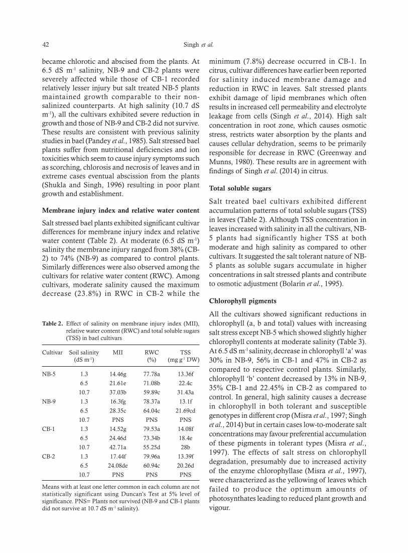
42 Singh et al.

became chlorotic and abscised from the plants. At6.5 dS m-1 salinity, NB-9 and CB-2 plants wereseverely affected while those of CB-1 recordedrelatively lesser injury but salt treated NB-5 plantsmaintained growth comparable to their non-salinized counterparts. At high salinity (10.7 dSm-1), all the cultivars exhibited severe reduction ingrowth and those of NB-9 and CB-2 did not survive.These results are consistent with previous salinitystudies in bael (Pandey et al., 1985). Salt stressed baelplants suffer from nutritional deficiencies and iontoxicities which seem to cause injury symptoms suchas scorching, chlorosis and necrosis of leaves and inextreme cases eventual abscission from the plants(Shukla and Singh, 1996) resulting in poor plantgrowth and establishment.

Membrane injury index and relative water content

Salt stressed bael plants exhibited significant cultivardifferences for membrane injury index and relativewater content (Table 2). At moderate (6.5 dS m-1)salinity the membrane injury ranged from 38% (CB-2) to 74% (NB-9) as compared to control plants.Similarly differences were also observed among thecultivars for relative water content (RWC). Amongcultivars, moderate salinity caused the maximumdecrease (23.8%) in RWC in CB-2 while the

minimum (7.8%) decrease occurred in CB-1. Incitrus, cultivar differences have earlier been reportedfor salinity induced membrane damage andreduction in RWC in leaves. Salt stressed plantsexhibit damage of lipid membranes which oftenresults in increased cell permeability and electrolyteleakage from cells (Singh et al., 2014). High saltconcentration in root zone, which causes osmoticstress, restricts water absorption by the plants andcauses cellular dehydration, seems to be primarilyresponsible for decrease in RWC (Greenway andMunns, 1980). These results are in agreement withfindings of Singh et al. (2014) in citrus.

Total soluble sugars

Salt treated bael cultivars exhibited differentaccumulation patterns of total soluble sugars (TSS)in leaves (Table 2). Although TSS concentration inleaves increased with salinity in all the cultivars, NB-5 plants had significantly higher TSS at bothmoderate and high salinity as compared to othercultivars. It suggested the salt tolerant nature of NB-5 plants as soluble sugars accumulate in higherconcentrations in salt stressed plants and contributeto osmotic adjustment (Bolarín et al., 1995).

Chlorophyll pigments

All the cultivars showed significant reductions inchlorophyll (a, b and total) values with increasingsalt stress except NB-5 which showed slightly higherchlorophyll contents at moderate salinity (Table 3).At 6.5 dS m-1 salinity, decrease in chlorophyll ‘a’ was30% in NB-9, 56% in CB-1 and 47% in CB-2 ascompared to respective control plants. Similarly,chlorophyll ‘b’ content decreased by 13% in NB-9,35% CB-1 and 22.45% in CB-2 as compared tocontrol. In general, high salinity causes a decreasein chlorophyll in both tolerant and susceptiblegenotypes in different crop (Misra et al., 1997; Singhet al., 2014) but in certain cases low-to-moderate saltconcentrations may favour preferential accumulationof these pigments in tolerant types (Misra et al.,1997). The effects of salt stress on chlorophylldegradation, presumably due to increased activityof the enzyme chlorophyllase (Misra et al., 1997),were characterized as the yellowing of leaves whichfailed to produce the optimum amounts ofphotosynthates leading to reduced plant growth andvigour.

Table 2. Effect of salinity on membrane injury index (MII),relative water content (RWC) and total soluble sugars(TSS) in bael cultivars

Cultivar Soil salinity MII RWC TSS(dS m-1) (%) (mg g-1 DW)

NB-5 1.3 14.46g 77.78a 13.36f

6.5 21.61e 71.08b 22.4c

10.7 37.03b 59.89c 31.43a

NB-9 1.3 16.3fg 78.37a 13.1f

6.5 28.35c 64.04c 21.69cd

10.7 PNS PNS PNS

CB-1 1.3 14.52g 79.53a 14.08f

6.5 24.46d 73.34b 18.4e

10.7 42.71a 55.25d 28b

CB-2 1.3 17.44f 79.96a 13.39f

6.5 24.08de 60.94c 20.26d

10.7 PNS PNS PNS

Means with at least one letter common in each column are notstatistically significant using Duncan’s Test at 5% level ofsignificance. PNS= Plants not survived (NB-9 and CB-1 plantsdid not survive at 10.7 dS m-1 salinity).

Salinity Induced Changes in Chlorophyll Pigments of Bael Cultivars 43

Sodium, potassium and sodium: potassium ratio

At both salinity levels, there was a significant increasein leaf Na+ accumulation irrespective of the cultivar(Table 4). At moderate salinity, there was a three-fold increase in Na+ concentration in leaves of NB-5 relative to control while the corresponding increasewas five-times in NB-9 and four-times in both CB-1and CB-2 cultivars. Cultivar NB-5 not only preventedthe accumulation of Na+ to toxic levels but alsoexhibited higher K+ concentrations and thusmaintained a favourable ionic balance in terms of

low Na+/K+ ratio resulting in good plantperformance.

The plants of NB-9 and CB-2 varieties, due toNa+ toxicity, did not survive at high salinity. Mostof the fruit crops are sensitive to excessiveconcentrations of Na+ ions in the growing medium.Excessive Na+ concentration reduces the uptake ofK+ and Ca2+ by plants. Available reports in citruspoint to genotypic differences which may explainbetter performance by some scions and/or rootstocksas compared to others (Levy and Syvertsen, 2004;Murkute et al., 2005).

Conclusions

The bael cultivars tested in this experiment exhibitedtolerance to low and moderate salinity. Cultivar NB-5 exhibited relatively higher salinity tolerance andshowed better performance as compared to othercultivars. Although salinity adversely affected someof the physiological traits in NB-5 plants, theyshowed better salt tolerance owing to favourablechlorophyll concentration, restricted uptake of Na+

ions and higher K+ accumulation in leaves. Inconcluding remarks, the commercial cultivation ofNB-5 is feasible in moderately saline soils (ECe ~6.5).

References

Barrs HD and Weatherley PE (1962). A re-examination ofthe relative turgidity technique for estimating waterdeficits in leaves. Australian Journal of Biological Science15: 413-28.

Table 3. Effect of salinity on chlorophyll pigments in bael cultivars

Cultivar Soil salinity Chlorophyll ‘a’ Chlorophyll ‘b’ Total chlorophyll(dS m-1) (mg g-1 FW) (mg g-1 FW) (mg g-1 FW)

NB-5 1.3 2.02d 1.38b 3.41b6.5 2.4bc 1.59a 4a10.7 0.85g 1.12d 1.97d

NB-9 1.3 2.32c 1.56ab 3.87a6.5 1.63e 1.36bc 2.99c10.7 PNS PNS PNS

CB-1 1.3 2.69a 1.17cd 3.86a6.5 1.17f 0.76e 1.93d10.7 0.68h 0.49f 1.17e

CB-2 1.3 2.46b 0.98d 3.44b6.5 1.3f 0.76e 2.06d10.7 PNS PNS PNS

Means with at least one letter common in each column are not statistically significant using Duncan’s Test at 5% level of significance.PNS= Plants not survived (NB-9 and CB-1 plants did not survive at 10.7 dS m-1 salinity).

Table 4. Ionic relations in bael cultivars under salinity stress

Cultivar Soil salinity Na+ K+ Na+/ K+

(dS m-1) (% DW) (% DW) ratio

NB-5 1.3 0.06e 0.27g 0.22a6.5 0.18d 1e 0.18cd10.7 0.29b 1.46b 0.2bc

NB-9 1.3 0.06e 0.45f 0.13e6.5 0.3b 1.35c 0.22a10.7 PNS PNS PNS

CB-1 1.3 0.06e 0.42f 0.14e6.5 0.24c 1.07d 0.23a10.7 0.35a 1.65a 0.21ab

CB-2 1.3 0.06e 0.46f 0.12e6.5 0.24c 1.41bc 0.17d10.7 PNS PNS PNS

Means with at least one letter common in each column are notstatistically significant using Duncan’s Test at 5% level ofsignificance. PNS= Plants not survived (NB-9 and CB-1 plantsdid not survive at 10.7 dS m-1 salinity).

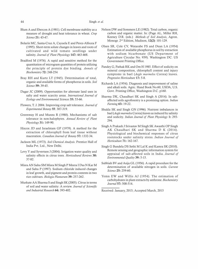
44 Singh et al.

Blum A and Ebercon A (1981). Cell membrane stability as ameasure of drought and heat tolerance in wheat. CropScience 21: 43-47.

Bolarín MC, Santa-Cruz A, Cayuela E and Perez-Alfocea F(1995). Short-term solute changes in leaves and roots ofcultivated and wild tomato seedlings undersalinity. Journal of Plant Physiology 147: 463-468.

Bradford M (1976). A rapid and sensitive method for thequantitation of microgram quantities of protein utilizingthe principle of protein dye binding. Annals ofBiochemistry 72: 248-254

Bray RH and Kurtz LT (1945). Determination of total,organic and available forms of phosphorus in soils. SoilScience 59: 39-45.

Dagar JC (2009). Opportunities for alternate land uses insalty and water scarcity areas. International Journal ofEcology and Environmental Sciences 35: 53-66.

Flowers, T. J. 2004. Improving crop salt tolerance. Journal ofExperimental Botany 55: 307-319.

Greenway H and Munns R (1980). Mechanisms of salttolerance in non-halophytes. Annual Review of PlantPhysiology 31: 149-90.

Hiscox JD and Israelstam GF (1979). A method for theextraction of chlorophyll from leaf tissue withoutmaceration. Canadian Journal of Botany 57: 1332-34.

Jackson ML (1973). Soil Chemical Analysis. Prentice Hall ofIndia Pvt. Ltd., New Delhi.

Levy Y and Syvertsen J (2004). Irrigation water quality andsalinity effects in citrus trees. Horticultural Reviews 30:37-82.

Misra AN Sahu SM Misra M Singh P Meera I Das N Kar Mand Sahu P (1997). Sodium chloride induced changesin leaf growth, and pigment and protein contents in tworice cultivars. Biologia Plantarum 39: 257-262.

Murkute AA Sharma S and Singh SK (2005). Citrus in termsof soil and water salinity: A review. Journal of Scientificand Industrial Research 64: 393-402.

Nelson DW and Sommers LE (1982). Total carbon, organiccarbon and organic matter. In: (Page AL, Miller RH,Keeney D.R. (eds.) Methods of Soil Analysis, Agron.Monogr. 2nd Edition, Madison, 12(2): 101-129.

Olsen SR, Cole CV, Watarabe FS and Dean LA (1954)Estimation of available phosphorus in soil by extractionwith sodium bicarbonate (US Department ofAgriculture Circular No. 939). Washington DC. USGovernment Printing Office.

Pandey G, Pathak RK and Om H 1985. Effect of sodicity onmineral composition, chlorophyll content and injurysymptoms in bael (Aegle marmelos Correa) leaves.Progressive Horticulture 17: 5-8.

Richards LA (1954). Diagnosis and improvement of salineand alkali soils. Agric. Hand Book No.60, USDA, U.S.Govt. Printing Office, Washington D.C. p160.

Sharma DK, Chaudhari SK and Singh A (2014). In salt-affected soils agroforestry is a promising option. IndianFarming 63: 19-22.

Shukla SK and Singh GN (1996). Nutrient imbalances inbael (Aegle marmelos Correa) leaves as induced by salinityand sodicity. Indian Journal of Plant Physiology 1: 293-294.

Singh A Prakash J Srivastav M Singh SK Awasthi OP SinghAK Chaudhari SK and Sharma D K (2014).Physiological and biochemical responses of citrusrootstocks under salinity stress. Indian Journal ofHorticulture 71: 162-167.

Singh G Bundela DS Sethi M Lal K and Kamra SK (2010).Remote sensing and geographic information system forappraisal of salt-affected soils in India. Journal ofEnvironmental Quality 39: 5-15.

Subbiah BV and Asija GL (1956). A rapid procedure for thedetermination of available nitrogen in soils. CurrentScience 25: 259-60.

Yemn EW and Willis AJ (1954). The estimation ofcarbohydrates in plant extracts by anthrone. BiochemistryJournal 57: 508-514.

Received: January, 2015; Accepted March, 2015

Screening of Chilli (Capsicum annuum L.) Genotypes underSaline Environment of Sundarbans in West Bengal, India

Chandan Kumar Mondal1*, Ashim Datta2#, Prabir Kumar Garain1,Pinaki Acharyya3 and Pranab Hazra4

1Ramkrishna Ashram Krishi Vigyan Kendra, Nimpith Ashram, South 24 Parganas-743338, West Bengal2Division of Soil and Crop Management, Central Soil Salinity Research Institute, Karnal-132 001, Haryana

3Department of Horticulture, Institute of Agricultural Science, University of Calcutta, 51/2, Hazra Road, Kolkata-7000194Department of Vegetable Crops, Faculty of Horticulture, BCKV, Mohanpur, Nadia-741252, West Bengal

*Author for Correspondence: drchandanmondal@gmail.com

Abstract

Agriculture in the Sundarban region is literally backward due to the problems of soil salinity, poor drainagethere by late release of land for rabi crop and poor irrigation facility for rabi crop because of ground watersalinity. Here, farmers have a very limited crop choice option. Chilli (Capsicum annuum L.) is an importantcommercial crop of this region as it can tolerate higher levels of salinity and have good storability of theharvested dry produce. But the productivity of the crop is declining now-a-days due to use of local undescribedland races for a long period. Chilli leaf curl complex is another major problem whose prevalence is quite high.In this backdrop a study was made to find out genotypes having tolerance to both salinity and leaf curl complex.Twelve genotypes were collected and evaluated at three locations having salinity gradients (ECe) of 6.68 dS m-

1, 10.46 dS m-1 and 15.25 dS m-1, respectively in three Sundarban Blocks. Seven genotypes (CUCH-1, CUCH-4,CUCH-6, CUCH-29, CUCH-31, CUCH-34 and CUCH-35) performed satisfactorily in all the three situationswith good stability parameters coupled with higher leaf curl tolerance. Among these, best two performers wereCUCH-31 and CUCH-34 recording a fresh yield of 218.17 and 190.54 g/plant; 175.56 and 159.77 g/plant;139.68 and 148.19 g/plant, respectively at low, medium and high salinity levels.These genotypes can be promotedfor commercial cultivation at varied salinity environments. Yield reduction at higher salinity level was lowestfor CUCH-34 (22.23%), so this genotype will be a better choice over CUCH-31.

Key words: Chilli, Soil Salinity, Leaf Curl, Stability, Sundarban

Introduction

Soil salinity is a major factor limiting plantproductivity affecting about 323 million haworldwide (Brinkman, 1980). One of such saltaffected area is Sundarbans of great Gangetic Delta.High soil salinity is of great concern in this area.According to agro-ecosystem analysis, Sundarbansbelongs to CDR System which implies Critical,Diversified and Risk prone area. The agrarian systemin Sundarbans faces the problems of salinity in bothsoil and water, poor drainage system during rainyseason and poor irrigation opportunity. Here, chilli(Capsicum annuum L.) proved to be a good choice bythe farmers over the decades. Chilli can be grown insaline soils because they can accumulate the salt

which can be useful for osmotic adjustment againstwater stress due to salinity (Kaliappan andRajagopal, 1970); although the germination andearly vigour of the plants are affected by the salinityin the soil. Most of the regions where cultivation ofchilli was predominant are characterized by thepresence of moderately high level of salts and highwater table (Kameswari and Prasad, 2005). Inspiteof soil and climatic problems, chilli still now, is thefirst choice of the Sundarban farmers. There aremany genotypes of chilli normally grown by thefarmers. However, introduction of chilli genotypestolerant to both soil salinity and leaf curl complexwill be a boon for the farming community ofSundarbans. Therefore, an attempt has been madeto screen suitable chilli genotypes resistant to bothsoil salinity and leaf curl complex disease under theSundarban region of West Bengal.

Journal of Soil Salinity and Water Quality 7(1), 45-53, 2015

#presently at the Department of Agricultural Chemistry andSoil Science, BCKV, Mohanpur, Nadia-741252, West Bengal

46 Mondal et al.

Twelve elite chilli genotypes (CUCH-1, CUCH-4, CUCH-5, CUCH-6, CUCH-11, CUCH-7,CUCH-16, CUCH-15, CUCH-29, CUCH-31,CUCH-34 and CUCH-35) were grown in naturalsaline soil condition having three levels of soil salinity(ECe) of 6.68 dS m-1, 10.46 dS m-1and 15.25 dS m-1

to identify promising genotypes for salinityconditions of Sundarbans.

Material and Methods

Multi-location trials of the selected genotypes werecarried out at the farmers plot in three coastal blocksof South 24 Parganas falling under Sundarban regionof West Bengal, namely Kultali (Kaikhali village),Kakdwip (Kamarhat village) and Pathar Pratima(Kamdebpur village). Agro-climatic situation of theexperimental site comes under coastal saline zoneof West Bengal. Soil is clay-loam and almost neutralin reaction. Physico-chemical properties of the soilof experimental sites are presented in Table 1.

Agro-climatic condition

The experimental site falls under subtropical region,the average temperature of which ranged from23.190C – 37.580C during summer months andbetween 10.780C – 27.740C during winter months,

with a relative humidity range of 32.54% – 97.48%.The average rainfall is in between 1600 to 1800 mmwith the maximum precipitation occurring from Juneto October.

Assemblage of plant materials for the study

Twelve chilli genotypes including many local typesof 24 Parganas (South) were collected from differentsources (Regional Institutes, Government agencies,Universities, authorized seed vendors etc. of WestBengal as well as from neighbouring states)comprised the plant material for the present study.Name and source of the germplasm have beenpresented in Table 2.

Crop husbandry

Pre-soaked seeds of all the genotypes were sown inseedbed in the first week of November each year.Seedlingsof 45 days old were transplanted in themain field in the individual plots with a spacing of45cm × 45cm between row-to-row and plant-to-plant, respectively ensuring 40 plants in each plot.Transplanting was done by second fortnight ofDecember each year. Chemical fertilizer was applied@ 72:58:46 kg NPK/ha. Essential interculturaloperations (weeding, staking, time bound irrigationetc.) were carried out as and when required.

Table 2. Name and source of chilli germplasm under study

Accession No. Name at source Source/Place of collection

CUCH-1 BCC–12 (sel) AICRP-Vegetable Crops, Directorate of Research, B.C.K.V., Kalyani, WBCUCH-4 BCC–28 (18) -do-CUCH-5 BCC–28 (int) -do-CUCH-6 BCC–30 -do-CUCH-7 BCC–49(var) -do-CUCH-11 Guntur-002 Horticultural Research Station, Lam, Guntur, A.P.- 522034CUCH-15 PusaJwala IARI, Pusa, New Delhi - 110012CUCH-16 Pant-C-1 G. B. Pant University Of Agriculture & Technology, Pantnagar, Udham Singh Nagar,

Uttarakhand - 263145CUCH-29 Ankur-228 Amtala Seed Stores, Amtala, South 24 PGS, W.B.CUCH-31 Roshni Amtala Seed Stores, Amtala, South 24 PGS, W.B.CUCH-34 Canning Bullet Local collection from Canning, 24 Pgs.(S) W.B.CUCH-35 Damkal Local collection from Damkal island, South 24 PGS

Table 1. Physico-chemical characteristics of soil of the experimental field

Experimental area pH ECedS/m OC (%) N (kg/ha) P2O5 (kg/ha) K2O (kg/ha)

Farmers’ plot (Kaikhali) 6.94 4.08 0.61 171.94 81.37 987.4Farmers’ plot (Kakdwip) 6.88 6.38 0.38 185.22 76.22 962.3Farmers’ plot (PatharPratima) 7.25 9.30 0.53 176.38 73.13 1054.8

Screening of Chilli Genotypes 47

Observations recorded

Five random plants per replication (plot) weresampled for recording data on different quantitativecharacters viz. plant height (cm), number. of primarybranches/plant, days to 50 % flowering, fruit length(cm), fruit girth (mm), number of fruits per plant,fresh and dry fruit weight (g), and fruit yield per plant(g).

Evaluation of the collected genotypes against leafcurl complex

The assessment of chilli leaf curl complex was doneas per Banerjee and Kaloo (1987). Individual plantswere evaluated for leaf curl disease reaction. Fortyplants of each genotype were grown in everyreplication. No insecticide or acaricide was appliedin these plots. Disease reaction data was recordedduring the peak period of fruiting which was usuallyat 60 – 70 days after transplanting. The percentdisease severity and disease intensity grade wascalculated by using the following formula:

Percent Disease Intensity (PDI) =

Number of diseased plant(s)–––––––––––––––––––––––––––– × 100Total number of plants observed

The coefficient of infection was calculated bymultiplying the PDI with the Response valueassigned to each severity grade. The overall diseasereaction was assigned to the coefficient of infectionrange as given in the Table 3.

Statistical analysis

Plot Means were used for standard analysis.Statistical analysis for various parameters wasexecuted using the statistical package SPSS 16.0.Analysis of variance was calculated as per Gomezand Gomez (1984).

Results and Discussion

Mean performance

Mean values for nine growth and yield relatedcharacters viz., plant height, number of primarybranches per plant, days to 50% flowering, fruitlength, fruit girth, fruits per plant, fresh fruit weight,dry fruit weight and fresh fruit yield per plant wererecorded in all the genotypes (Table 4). All the ninequantitative characters varied considerably with thesalinity level. High salinity level drastically reducedthe manifestation of all the characters including fruityield in all the genotypes compared to low andmedium salinity level. However, such reduction wasmore conspicuous for plant height, number of fruitsper plants and fruit yield per plant. Average plantheight in all the 12 genotypes reduced by 15.9 to36.8% when they were grown in the higher salinityconditions compared to low salinity condition (Table5). Similarly, number of fruits per plant and averagefruit yield per plant also declined by 13.1 to 45.2%and 22.2 to 52.5%,respectively under similarsituation. Extent of fruit yield loss in all thegenotypes with rising salinity levels in the presentinvestigation agreed well to the earlier work ofGoldberg (2004) who advocated that rising electricalconductivity having an ECe value of 5+dS/m lead to50% yield loss with an additional 10-12% reductionin yield for every additional unit increase in ECe.However, such reduction in different set of charactersin the present investigation varied with the genotypes.

Variance

Mean sum of squares presented in Table 6 clearlysuggested significant difference of the genotypes forall the characters even at 1% level of significancewhich clearly depicted the justification of studyinggenetic variability employing these genotypes andcharacters for these three locations. This finding

Table 3. Scale of classifying disease reaction of Chilli to leaf curl complex

Symptom Symptom Response Coefficient Reaction*severity grade value of infestation

Symptom absent 0 0.00 0-4 HRVery mild curling upto 25% leaves 1 0.25 5-9 RCurling and puckering of 26-50% leaves 2 0.50 10-19 MRCurling and puckering of 51-75% leaves 3 0.75 20-39 MSSevere curling and puckering of >75% leaves 4 1.00 40-69 S

70-100 HS

* R = resistant, HR - highly resistant, MR - moderate resistant, MS - moderate susceptible, S - susceptible, HS - highly susceptible

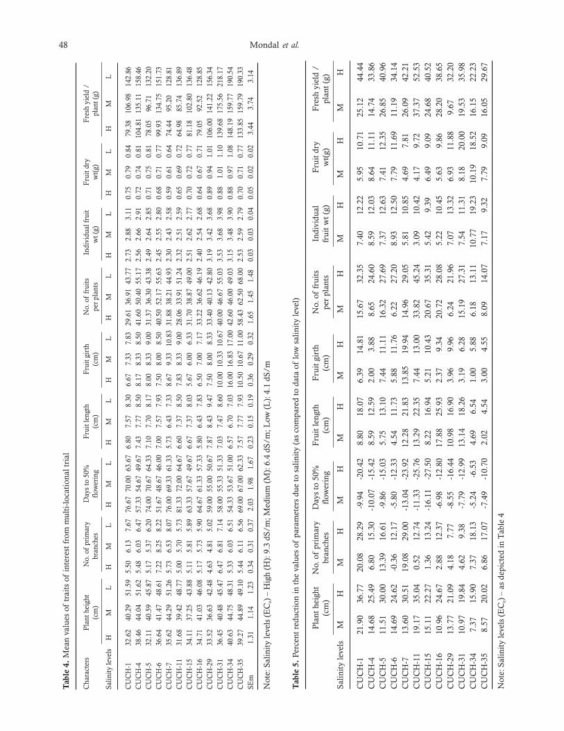
48 Mondal et al.

Tab

le 4

. M

ean

valu

es o

f tr

aits

of

inte

rest

from

mul

ti-lo

cati

onal

tria

l

Cha

ract

ers

Pla

nt h

eigh

tN

o. o

f pr

imar

yD

ays

to 5

0%F

ruit

leng

thF

ruit

girt

hN

o. o

f fr

uits

Indi

vidu

al fr

uit

Fru

it dr

yF

resh

yie

ld /

(cm

)br

anch

esflo

wer

ing

(cm

)(c

m)

per p

lant

sw

t (g)

wt(

g)pl

ant (

g)

Salin

ity le

vels

HM

LH

ML

HM

LH

ML

HM

LH

ML

HM

LH

ML

HM

L

CU

CH

-132

.62

40.2

951

.59

5.50

6.13

7.67

76.6

770

.00

63.6

76.

807.

578.

306.

677.

337.

8329

.61

36.9

143

.77

2.73

2.88

3.11

0.75

0.79

0.84

79.3

810

6.98

142.

86C

UC

H-4

38.4

644

.04

51.6

25.

486.

036.

4757

.33

54.6

749

.67

7.43

7.77

8.50

8.17

8.33

8.50

41.6

050

.40

55.1

72.

562.

662.

910.

720.

740.

8110

4.81

135.

1115

8.46

CU

CH

-532

.11

40.5

945

.87

5.17

5.37

6.20

74.0

070

.67

64.3

37.

107.

708.

178.

008.

339.

0031

.37

36.3

043

.38

2.49

2.64

2.85

0.71

0.75

0.81

78.0

596

.71

132.

20C

UC

H-6

36.6

441

.47

48.6

17.

228.

258.

2251

.67

48.6

746

.00

7.00

7.57

7.93

7.50

8.00

8.50

40.5

052

.17

55.6

32.

452.

552.

800.

680.

710.

7799

.93

134.

7515

1.73

CU

CH

-735

.62

44.2

951

.26

5.73

6.53

8.07

76.0

069

.33

61.3

35.

736.

437.

338.

679.

3310

.83

31.8

838

.21

44.9

32.

302.

432.

580.

590.

610.

6474

.44

95.2

012

8.81

CU

CH

-11

31.6

839

.42

48.7

75.

005.

705.

7381

.33

72.0

064

.67

6.60

7.37

8.50

7.83

8.33

9.00

28.0

633

.91

51.2

42.

322.

512.

590.

650.

690.

7264

.98

85.7

413

6.89

CU

CH

-15

34.1

137

.25

43.8

85.

115.

815.

8963

.33

57.6

749

.67

6.67

7.37

8.03

5.67

6.00

6.33

31.7

038

.87

49.0

02.

512.

622.

770.

700.

720.

7781

.18

102.

8013

6.48

CU

CH

-16

34.7

141

.03

46.0

85.

175.

735.

9064

.67

61.3

357

.33

5.80

6.43

7.83

6.50

7.00

7.17

33.2

236

.62

46.1

92.

402.

542.

680.

640.

670.

7179

.05

92.5

212

8.85

CU

CH

-29

33.5

236

.63

42.4

84.

634.

815.

0259

.00

55.0

050

.67

7.87

8.43

9.47

7.50

8.00

8.33

33.4

040

.13

42.8

03.

193.

423.

680.

890.

941.

0110

6.00

141.

2215

6.34

CU

CH

-31

36.4

540

.48

45.4

76.

476.

817.

1458

.00

55.3

351

.33

7.03

7.47

8.60

10.0

010

.33

10.6

740

.00

46.6

755

.03

3.53

3.68

3.98

0.88

1.01

1.10

139.

6817

5.56

218.

17C

UC

H-3

440

.63

44.7

548

.31

5.33

6.03

6.51

54.3

353

.67

51.0

06.

576.

707.

0316

.00

16.8

317

.00

42.6

046

.00

49.0

33.

153.

483.

900.

880.

971.

0814

8.19

159.

7719

0.54

CU

CH

-35

39.2

744

.89

49.1

05.

446.

116.

5669

.00

67.0

062

.33

7.57

7.77

7.93

10.5

010

.67

11.0

058

.43

62.5

068

.00

2.53

2.59

2.79

0.70

0.71

0.77

133.

8515

9.79

190.

33SE

m1.

311.

141.

230.

340.

310.

372.

031.

981.

670.

230.

150.

190.

360.

290.

321.

651.

451.

480.

030.

030.

040.

050.

020.

023.

443.

743.

14

Not

e: S

alin

ity

leve

ls (

EC

e) –

Hig

h (H

): 9

.3 d

S/m

; Med

ium

(M

): 6

.4 d

S/m

; Low

(L

): 4

.1 d

S/m

Tab

le 5

. P

erce

nt r

educ

tion

in th

e va

lues

of

para

met

ers

due

to s

alin

ity

(as

com

pare

d to

dat

a of

low

sal

init

y le

vel)

Pla

nt h

eigh

tN

o. o

f pr

imar

yD

ays

to 5

0%F

ruit

leng

thF

ruit

gir

thN

o. o

f fr

uits

Indi

vidu

alF

ruit

dry

Fre

sh y

ield

/(c

m)

bran

ches

flow

erin

g(c

m)

(cm

)pe

r pl

ants

frui

t wt (

g)w

t(g)

plan

t (g

)

Salin

ity

leve

lsM

HM

HM

HM

HM

HM

HM

HM

HM

H

CU

CH

-121

.90

36.7

720

.08

28.2

9-9

.94

-20.

428.

8018

.07

6.39

14.8

115

.67

32.3

57.

4012

.22

5.95

10.7

125

.12

44.4

4C

UC

H-4

14.6

825

.49

6.80

15.3

0-1

0.07

-15.

428.

5912

.59

2.00

3.88

8.65

24.6

08.

5912

.03

8.64

11.1

114

.74

33.8

6C

UC

H-5

11.5

130

.00

13.3

916

.61

-9.8

6-1

5.03

5.75

13.1

07.

4411

.11

16.3

227

.69

7.37

12.6

37.

4112

.35

26.8

540

.96

CU

CH

-614

.69

24.6

2-0

.36

12.1

7-5

.80

-12.

334.

5411

.73

5.88

11.7

66.

2227

.20

8.93

12.5

07.

7911

.69

11.1

934

.14

CU

CH

-713

.60

30.5

119

.08

29.0

0-1

3.04

-23.

9212

.28

21.8

313

.85

19.9

414

.96

29.0

55.

8110

.85

4.69

7.81

26.0

942

.21

CU

CH

-11

19.1

735

.04

0.52

12.7

4-1

1.33

-25.

7613

.29

22.3

57.

4413

.00

33.8

245

.24

3.09

10.4

24.

179.

7237

.37

52.5

3C

UC

H-1

515

.11

22.2

71.

3613

.24

-16.

11-2

7.50

8.22

16.9

45.

2110

.43

20.6

735

.31

5.42

9.39

6.49

9.09

24.6

840

.52

CU

CH

-16

10.9

624

.67

2.88

12.3

7-6

.98

-12.

8017

.88

25.9

32.

379.

3420

.72

28.0

85.

2210

.45

5.63

9.86

28.2

038

.65

CU

CH

-29

13.7

721

.09

4.18

7.77

-8.5

5-1

6.44

10.9

816

.90

3.96

9.96

6.24

21.9

67.

0713

.32

6.93

11.8

89.

6732

.20

CU

CH

-31

10.9

719

.84

4.62

9.38

-7.7

9-1

2.99

13.1

418

.26

3.19

6.28

15.1

927

.31

7.54

11.3

18.

1820

.00

19.5

335

.98

CU

CH

-34

7.37

15.9

07.

3718

.13

-5.2

4-6

.53

4.69

6.54

1.00

5.88

6.18

13.1

110

.77

19.2

310

.19

18.5

216

.15

22.2

3C

UC

H-3

58.

5720

.02

6.86

17.0

7-7

.49

-10.

702.

024.

543.

004.

558.

0914

.07

7.17

9.32

7.79

9.09

16.0

529

.67

Not

e: S

alin

ity

leve

ls (

EC

e) –

as

depi

cted

in T

able

4

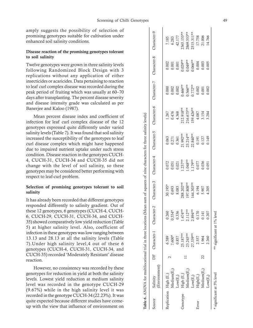
Screening of Chilli Genotypes 49

amply suggests the possibility of selection ofpromising genotypes suitable for cultivation underenhanced soil salinity conditions.

Disease reaction of the promising genotypes tolerantto soil salinity

Twelve genotypes were grown in three salinity levelsfollowing Randomized Block Design with 3replications without any application of eitherinsecticides or acaricides. Data pertaining to reactionto leaf curl complex disease was recorded during thepeak period of fruiting which was usually at 60–70days after transplanting. The percent disease severityand disease intensity grade was calculated as perBanerjee and Kaloo (1987).

Mean percent disease index and coefficient ofinfection for leaf curl complex disease of the 12genotypes expressed quite differently under variedsalinity levels (Table 7). It was found that soil salinityincreased the susceptibility of the genotypes to leafcurl disease complex which might have happeneddue to impaired nutrient uptake under such stresscondition. Disease reaction in the genotypes CUCH-4, CUCH-31, CUCH-34 and CUCH-35 did notchange with the level of soil salinity, so thesegenotypes may be considered better performing withrespect to leaf-curl problem.

Selection of promising genotypes tolerant to soilsalinity

It has already been recorded that different genotypesresponded differently to salinity gradient. Out ofthese 12 genotypes, 6 genotypes (CUCH-4, CUCH-6, CUCH-29, CUCH-31, CUCH-34, and CUCH-35) showed comparatively low yield reduction (Table5) at higher salinity level. Also, coefficient ofinfection in these genotypes was low ranging between13.13 and 28.13 at all the salinity levels (Table7).Under high salinity level,4 out of these 6genotypes (CUCH-4, CUCH-31, CUCH-34, andCUCH-35) recorded ‘Moderately Resistant’ diseasereaction.

However, no consistency was recorded by thesegenotypes for reduction in yield at both the salinitylevels. Lowest yield reduction at medium salinitylevel was recorded in the genotype CUCH-29(9.67%) while in the high salinity level it wasrecorded in the genotype CUCH-34 (22.23%). It wasquite expected because different studies have come-up with the view that influence of environment on T

able

6.

AN

OV

A fo

r m

ulti

loca

tion

al tr

ial i

n th

ree

loca

tion

s (M

ean

sum

of

squa

res

of n

ine

char

acte

rs fo

r th

ree

salin

ity

leve

ls)

Sour

ceSa

linit

yD

FC

hara

cter

-1C

hara

cter

-2C

hara

cter

-3C

hara

cter

-4C

hara

cter

-5C

hara

cter

-6C

hara

cter

-7C

hara

cter

-8C

hara

cter

-9(E

nvir

onm

ent)

Rep

licat

ion

Hig

h (E

1)2

6.58

90.

260

30.1

95*

0.07

20.

063

1.26

70.

000

0.00

27.

185

Med

ium

(E2)

7.60

0*0.

554*

0.69

30.

051

0.27

10.

476

0.00

20.

001

6.28

3L

ow(E

3)0.

857

0.33

68.

083

0.02

10.

361

4.36

80.

002

0.00

142

.177

Gen

otyp

eH

igh

(E1)

1125

.187

**1.

474*

*28

8.20

2**

1.23

7**

21.9

92**

212.

918*

*0.

466*

*0.

029*

*23

65.1

55**

Med

ium

(E2)

23.2

45**

2.11

2**

197.

808*

*1.

048*

*23

.214

**21

6.67

5**

0.56

6**

0.04

9**

2869

.553

**L

ow(E

3)27

.339

**2.

894*

*14

4.30

3**

1.17

9**

22.8

40**

159.

426*

*0.

772*

*0.

066*

*25

15.3

11**

Err

orH

igh(

E1)

2.55

70.

170

6.19

40.

077

0.19

14.

087

0.00

20.

004

17.7

58M

ediu

m(E

2)22

1.96

40.

141

5.90

70.

036

0.12

73.

154

0.00

10.

003

21.0

06L

ow(E

3)2.

260

0.20

74.

205

0.05

10.

149

3.28

40.

002

0.00

514

.766

* si

gnif

ican

t at 5

% le

vel

** s

igni

fica

nt a

t 1%

leve

l

50 Mondal et al.

Tab

le 7

. E

valu

atio

n of

gen

otyp

es a

gain

st le

af c

url c

ompl

ex u

nder

var

ied

salin

ity

leve

ls

Gen

otyp

es*

Seve

rity

Gra

de ‘0

’Se

veri

ty G

rade

‘1’

Seve

rity

Gra

de ‘2

’Se

veri

ty G

rade

‘3’

Seve

rity

Gra

de ‘4

’

Dis

ease

Rea

ctio

n

RV

No.

of

PD

IR

VN

o. o

fP

DI

RV

No.

of

PD

IR

VN

o. o

fP

DI

RV

No.

of

PD

IC

IR

eac-

plan

tspl

ants

plan

tspl

ants

plan

tsti

on

Loc

atio

n: L

ow s

alin

ity

(EC

- 4.0

8 dS

/m)

CU

CH

-10

1025

0.25

2255

0.5

820

0.75

00

10

023

.75

MS

CU

CH

-40

2357

.50.

2513

32.5

0.5

410

0.75

00

10

013

.13

MR

CU

CH

-50

922

.50.

2521

52.5

0.5

922

.50.

751

2.5

10

026

.25

MS

CU

CH

-60

1742

.50.

2516

400.

57

17.5

0.75

00

10

018

.75

MR

CU

CH

-70

615

0.25

2767

.50.

57

17.5

0.75

00

10

025

.625

MS

CU

CH

-11

00

00.

2528

700.

59

22.5

0.75

37.

51

00

34.3

8M

SC

UC

H-1

50

615

0.25

2767

.50.

57

17.5

0.75

00

10

025

.63

MS

CU

CH

-16

06

150.

2528

700.

56

150.

750

01

00

25M

SC

UC

H-2

90

1537

.50.

2520

500.

55

12.5

0.75

00

10

018

.75

MR

CU

CH

-31

013

32.5

0.25

2767

.50.

50

00.

750

01

00

16.8

8M

RC

UC

H-3

40

1742

.50.

2523

57.5

0.5

00

0.75

00

10

014

.38

MR

CU

CH

-35

019

47.5

0.25

2152

.50.

50

00.

750

01

00

13.1

3M

RL

ocat

ion:

Mod

erat

e sa

linit

y (E

C- 6

.38

dS/m

)C

UC

H-1

06

150.

2525

62.5

0.5

922

.50.

750

01

00

26.8

8M

SC

UC

H-4

016

400.

2519

47.5

0.5

512

.50.

750

01

00

18.1

3M

RC

UC

H-5

01

2.5

0.25

2870

0.5

1127

.50.

750

01

00

31.2

5M

SC

UC

H-6

011

27.5

0.25

2255

0.5

717

.50.

750

01

00

22.5

MS

CU

CH

-70

12.

50.

2527

67.5

0.5

1025

0.75

25

10

033

.13

MS

CU

CH

-11

02

50.

2527

67.5

0.5

615

0.75

512

.51

25

38.7

5M

SC

UC

H-1

50

37.

50.

2528

700.

59

22.5

0.75

00

10

028

.75

MS

CU

CH

-16

00

00.

2531

77.5

0.5

717

.50.

752

51

00

31.8

8M

SC

UC

H-2

90

820

0.25

2665

0.5

615

0.75

00

10

023

.75

MS

CU

CH

-31

014

350.

2523

57.5

0.5

37.

50.

750

01

00

18.1

3M

RC

UC

H-3

40

1742

.50.

2522

550.

51

2.5

0.75

00

10

015

MR

CU

CH

-35

016

400.

2524

600.

50

00.

750

01

00

15M

RL

ocat

ion:

Hig

h sa

linit

y (E

C- 9

.30

dS/m

)C

UC

H-1

00

00.

2531

77.5

0.5

717

.50.

752

51

00

31.8

8M

SC

UC

H-4

017

42.5

0.25

1640

0.5

717

.50.

750

01

00

18.7

5M

RC

UC

H-5

00

00.

2528

700.

59

22.5

0.75

37.

51

12.

536

.88

MS

CU

CH

-60

410

0.25

2767

.50.

59

22.5

0.75

00

10

028

.13

MS

CU

CH

-70

00

0.25

3075

0.5

820

0.75

25

10

032

.5M

SC

UC

H-1

10

00

0.25

2767

.50.

59

22.5

0.75

410

14

1045

.63

SC

UC

H-1

50

00

0.25

2767

.50.

511

27.5

0.75

25

12

539

.38

MS

CU

CH

-16

00

00.

2530

750.

58

200.

752

51

00

32.5

MS

CU

CH

-29

06

150.

2526

650.

58

200.

750

01

00

26.2

5M

SC

UC

H-3

10

1127

.50.

2528

700.

51

2.5

0.75

00

10

018

.75

MR

CU

CH

-34

011

27.5

0.25

2972

.50.

50

00.

750

01

00

18.1

3M

RC

UC

H-3

50

1435

0.25

2665

0.5

00

0.75

00

10

016

.25

MR

*Tot

al n

umbe

r of

pla

nts

per

plot

in e

ach

geno

type

= 4

0, R

V =

Res

pons

e va

lue,

PD

I =

(N

o. o

f di

seas

ed p

lant

/ t

otal

no

of p

l(40

))*1

00, C

I (C

oeff

icie

nt o

f In

fect

ion)

= Σ

[(R

espo

nse

Val

ue 0.

00 –

1.0

0) ×

Res

pect

ive

PD

I; R

= R

esis

tant

, MR

= M

oder

atel

y R

esis

tant

, MS

= M

oder

atel

y Su

scep

tibl

e, S

= S

usce

ptib

le, H

S =

Hig

hly

Susc

eptib

le

Screening of Chilli Genotypes 51

the genotypes for the expression of quantitativecharacters is neither uniform nor consistent.

Analysis of adaptability under differential soilsalinity conditions

Primary objective of applied biological research isthe improvement of plant adaptation. The termadaptation has been applied to both process andcondition. On one hand, it is used to refer to theaction or process of becoming modified to suit newcircumstances and on the other hand, it may be usedto refer to the state or condition of adaptation.Whatever may be the outcome of the term, it clearlyimplies the genetic change as the basic principle andenvironmental pressure as the driving force of suchchange.

The importance of ‘Genotype x Environment’interactions in most investigations of quantitativegenetics has been widely discussed (Comstock andMoll, 1963). The significance of linear regressionanalysis of ‘Genotype x Environment’ interactionsin crop breeding programme has been understoodmuch later (Wright, 1976). In the presentinvestigation, an attempt was made to examine theadaptability of 12 genotypes under three distinct soilsalinity levels through the analysis of ‘Genotype xEnvironment’ interactions by adapting the approachof regression analysis of Eberhart and Russell (1966).The analysis of variance indicated that differencesbetween the genotypes and environments werehighly significant for all the 9 characters includingfruit yield (Table 8). The ‘Genotype x Environment’interaction was found highly significant for thecharacters namely number of fruits per plant, freshfruit weight and fruit yield per plant indicating thatthe genotypes showed differential response indifferent salinity levels with respect to thesecharacters. However, the magnitude of ‘Genotype xEnvironment’ variance was smaller as compared togenotype and environmental variances for thesecharacters. Both the environment (linear) and‘Genotype x Environment’ (linear) components ofvariance were highly significant for all the ninecharacters which indicated that the genotypesresponded differently in varying environments.Deviation from regression i.e. pooled deviation wassignificant for number of fruits per plant and fruityield per plant. However, linear component wasrelatively greater than non-linear component for allthe characters indicating that the performance of thegenotypes could be predicted. T

able

8.

AN

OV

A fo

r pa

ram

eter

s of

sta

bilit

y an

alys

is

Sour

ceD

FP

lant

hei

ght

No.

of

prim

ary

Day

s to

50%

Fru

it le

ngth

Fru

it g

irth

No.

of

frui

tsF

resh

fru

itD

ry fr

uit

Fre

sh y

ield

/(c

m)

bran

ches

flow

erin

g(c

m)

(cm

)pe

r pl

ants

wei

ght

(g)

wei

ght

(g)

plan

t (g

)

Gen

otyp

es (

G)

1118

.126

**1.

933*

*20

1.28

9**

1.00

1**

22.5

50**

183.

042*

*0.

591*

*0.

046*

*24

93.4

34**

Env

iron

men

t (E

)3

452.

043*

*3.

619*

*26

8.84

9**

5.03

3**

2.59

8**

545.

984*

*0.

421*

*0.

033*

*97

48.8

77**

G X

E22

3.56

60.

114

4.40

80.

077

0.06

66.

648*

0.00

5**

0.00

144

.948

**E

nvir

onm

ent

(Lin

ear)

190

4.09

3**

7.23

8**

537.

655*

*10

.066

**5.

196*

*10

91.9

74**

0.84

3**

0.06

6**

1949

7.63

3**

G X

E (

Lin

ear)

116.

286*

*0.

163*

*8.

323*

*0.

141*

*0.

110*

*9.

224*

0.01

0**

0.00

1**

51.0

67P

oole

d de

viat

ion

120.

775

0.05

90.

455

0.01

20.

020

3.73

2**

0.00

10.

000

35.6

03**

Poo

led

erro

r66

2.26

00.

173

5.43

50.

055

0.15

63.

509

0.00

20.

002

17.8

43

* si

gnif

ican

t at 5

% le

vel

** s

igni

fica

nt a

t 1%

leve

l

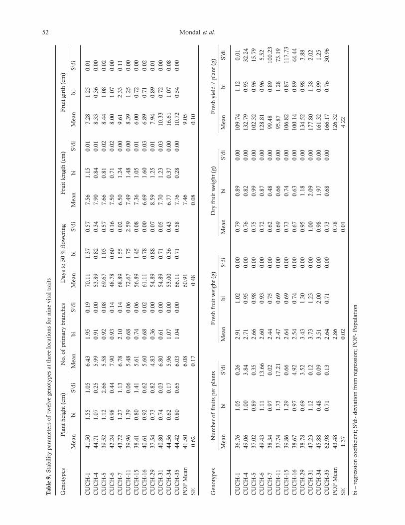
52 Mondal et al.

Tab

le 9

. St

abili

ty p

aram

eter

s of

twel

ve g

enot

ypes

at t

hree

loca

tion

s fo

r ni

ne v

ital

trai

ts

Gen

otyp

esP

lant

hei

ght (

cm)

No.

of

prim

ary

bran

ches

Day

s to

50

% f

low

erin

gF

ruit

leng

th (

cm)

Fru

it g

irth

(cm

)

Mea

nbi

S2 di

Mea

nbi

S2 di

Mea

nbi

S2 di

Mea

nbi

S2 di

Mea

nbi

S2 di

CU

CH

-141

.50

1.55

1.05

6.43

1.95

0.19

70.1

11.

370.

577.

561.

150.

017.

281.

250.

01C

UC

H-4

44.7

11.

070.

255.

990.

910.

0053

.89

0.82

0.34

7.90

0.84

0.01

8.33

0.36

0.00

CU

CH

-539

.52

1.12

2.66

5.58

0.92

0.08

69.6

71.

030.

577.

660.

810.

028.

441.

080.

02C

UC

H-6

42.2

40.

980.

447.

900.

930.

1448

.78

0.60

0.16

7.50

0.71

0.02

8.00

1.07

0.00

CU

CH

-743

.72

1.27

1.13

6.78

2.10

0.14

68.8

91.

550.

026.

501.

240.

009.

612.

330.

11C

UC

H-1

139

.96

1.39

0.06

5.48

0.68

0.06

72.6

71.

752.

597.

491.

480.

008.

391.

250.

00C

UC

H-1

538

.41

0.80

1.41

5.61

0.74

0.06

56.8

91.

450.

087.

361.

050.

016.

000.

720.

00C

UC

H-1

640

.61

0.92

0.62

5.60

0.68

0.02

61.1

10.

780.

006.

691.

600.

036.

890.

710.

02C

UC

H-2

937

.54

0.73

0.82

4.83

0.36

0.00

54.8

90.

880.

078.

591.

250.

017.

940.

890.

01C

UC

H-3

140

.80

0.74

0.03

6.80

0.61

0.00

54.8

90.

710.

057.

701.

230.

0310

.33

0.72

0.00

CU

CH

-34

44.5

60.

620.

175.

961.

070.

0053

.00

0.36

0.43

6.77

0.37

0.00

16.6

11.

070.

08C

UC

H-3

544

.42

0.80

0.65

6.03

1.04

0.00

66.1

10.

710.

587.

760.

280.

0010

.72

0.54

0.00

PO

P M

ean

41.5

06.

0860

.91

7.46

9.05

SE0.

620.

170.

480.

080.

10

Gen

otyp

esN

umbe

r of

frui

ts p

er p

lant

sF

resh

frui

t wei

ght (

g)D

ry fr

uit w

eigh

t (g)

Fre

sh y

ield

/ p

lant

(g)

Mea

nbi

S2 di

Mea

nbi

S2 di

Mea

nbi

S2 di

Mea

nbi

S2 di

CU

CH

-136

.76

1.05

0.26

2.91

1.02

0.00

0.79

0.89

0.00

109.

741.

120.

01C

UC

H-4

49.0

61.

003.

842.

710.

950.

000.

760.

820.

0013

2.79

0.93

32.2

4C

UC

H-5

37.0

20.

890.

352.

660.

980.

000.

750.

990.

0010

2.32

0.96

15.7

9C

UC

H-6

49.4

31.

1113

.66

2.60

0.93

0.00

0.72

0.87

0.00

128.

810.

965.

52C

UC

H-7

38.3

40.

970.

022.

440.

750.

000.

620.

480.

0099

.48

0.89

100.

23C

UC

H-1

137

.74

1.73

17.2

12.

470.

690.

000.

690.

660.

0095

.87

1.28

73.1

9C

UC

H-1

539

.86

1.29

0.66

2.64

0.69

0.00

0.73

0.74

0.00

106.

820.

8711

7.73

CU

CH

-16

38.6

70.

974.

922.

540.

740.

000.

670.

630.

0010

0.14

0.89

44.4

4C

UC

H-2

938

.78

0.69

3.52

3.43

1.30

0.00

0.95

1.18

0.00

134.

520.

983.

88C

UC

H-3

147

.23

1.12

0.12

3.73

1.23

0.00

1.00

2.09

0.00

177.

801.

382.

02C

UC

H-3

445

.88

0.48

0.09

3.51

2.00

0.00

0.98

1.97

0.00

161.

320.

991.

25C

UC

H-3

562

.98

0.71

0.13

2.64

0.71

0.00

0.73

0.68

0.00

166.

170.

7630

.96

PO

P M

ean

43.4

82.

860.

7812

6.32

SE1.

370.

020.

014.

22

bi –

reg

ress

ion

coef

fici

ent;

S2 d

i- d

evia

tion

from

reg

ress

ion;

PO

P- P

opul

atio

n

Screening of Chilli Genotypes 53

Out of 12 genotypes, CUCH-6, CUCH-29,CUCH-31 and CUCH-34 exhibited bi value close to1.00 with very low S2di value (Table 9) for most ofthe characters particularly fruit yield per plant.

Eberhart and Russell (1966) classified a varietyto be stable which showed high mean, unit regressioncoefficient (bi = 1) and the deviation from regressionas small as possible (S2di= 0). In the present study,the genotypes CUCH-29, CUCH-31 and CUCH-34could therefore, be considered as stable since thesegenotypes registered high mean fruit yield with unitregression coefficient close to 1.00 and very low S2divalues. Two genotypes viz., CUCH-4 and CUCH-35 showed high mean values for fruit yield with bi

values nearer to 1.00 but S2di values were high, thussuggesting that these two genotypes are fit to beadapted only under specific favourable environment(below average stability).

Conclusion

Twelve better performing genotypes were put inmultilocational salinity stress trial and only threegenotypes viz. CUCH-29, CUCH-31 and CUCH-34expressed stability under varying stress levels. Thegenotypes CUCH-4 and CUCH-35 showed highmean values for fruit yield but their S2di values werehigh suggesting that these genotypes are suited forspecific favourable environment. With respect to dualstress tolerance for salinity and leaf curl complex,only the genotypesCUCH-31 and CUCH-34performed better as their ranking for disease reactiondid not change with the level of soil salinity. So, thesegenotypes can be promoted for commercialcultivation at varied salinity environments. Yield

reduction at higher salinity level was lowest forCUCH-34 (22.23%)among all the twelve genotypes,so this genotype will be a better option over CUCH31.

References

Banerjee MK and Kalloo G (1987). A scale for classifyingdisease reaction of Lycopersicon species to tomato leafcurl virus. Theor. Appl. Genet.73: 707-710.

Brinkman R (1980). Saline and sodic soils. In: LandReclamation and Water Management. InternationalInstitute for Land Reclamation and Improvement(ILRI), Wageningen, The Netherlands. pp. 62-68.

Comstock RE and Moll RH (1963). Genotype-environmentInteractions in Statistical Genetics and Plant Breeding. NAS-NRC Publ. USA 982: 164-196.

Eberhart SA and Russell WA (1966). Stability parametersfor comparing varieties.Crop Sci. 6: 36-40.

Goldberg NP (2004). Chile Pepper Disorders Caused byEnvironmental Stress. New Mexico State UniversityCollege of Agriculture and Home Economics, H-249.

Gomez KA and Gomez AA (1984).Statistical Procedures inAgricultural Research, Wiley, New York, Chichester, etc.,2nd edition, pp. 680.

Kaliappan R and Rajagopal A (1970). Effect of salinity onthe south Indian field crops: germination and earlyvigour of chillies (Capsicum annuum, Linn.). MadrasAgric. J. 57(4): 231-233.

Kameswari PL and Prasad DM (2005). Evaluation of chilligenotypes for salt tolerance. Indian J. Hort. 62(1): 46-48.

Wright AJ (1976). The significance for breeding of linearregression analysis of genotype-environmentinteractions. Heredity.37: 83-93.

Received: January, 2015; Accepted March, 2015

Consumptive Use, Water Use Efficiency, Soil Moisture Useand Productivity of Fenugreek (Trigonella foenum-graecum L.)

under Varying IW-CPE Ratios and Fertilizer Levels onCalcareous Alkali Soils of South West Rajasthan

RC Dhaker*, RK Dubey2, RC Tiwari3 and SK Dubey4

Department of Agronomy, Rajasthan College of Agriculture, Maharana Pratap University of Agriculture andTechnology, Udaipur-313 001, Rajasthan

*Corresponding author E-mail: rameshagro2011@gmail.com

Abstract

Field experiment was conducted at Udaipur (rabi seasons of 2011-12 and 2012-13) with objective to optimizethe productivity and water use in fenugreek through use of appropriate IW-CPE ratio and fertility level. Itrevealed that IW-CPE ratio of 1.0 registered significantly higher of pooled yield and an enhancement of 45.48,27.50 and 11.90% in seed yield and 41.42, 23.72 and 10.26% in haulm yield at IW-CPE ratio of 1.0 over IW-CPE ratios of 0.4, 0.6 and 0.8, respectively. The IW-CPE ratio of 1.0 also recorded significantly higher residualsoil moisture at 0-15 cm (36.41%) and 15-30 cm (23.94%) soil depths after 40 days of sowing over differentlower IW-CPE ratios. However, WUE at IW-CPE ratio of 1.0 (11.58 kg mm ha-1) was significantly lower thanlower IW-CPE ratios of 0.8 (9.34 kg mm ha-1), 0.6 (8.63 kg mm ha-1) and 0.4 (8.61 kg mm ha-1). Results furthershowed that 40 kg N + 40 kg P2O5 ha-1 recorded significantly higher pooled seed yield (8.38 and 20.69% higher),haulm yield (5.57 and 17.60% higher) and biological yield (6.30 and 18.39% higher) under 40 kg N + 40 kg P2O5

ha-1 over 20 kg N + 20 kg P2O5 ha-1 and control, respectively. Application of 40 kg N + 40 kg P2O5 ha-1 recordedsignificantly higher consumptive use over different lower fertility levels but WUE under each lower fertilitylevels up to 40 kg N + 40 kg P2O5 ha-1 recorded significantly higher WUE over it higher fertility level.

Key words: Consumptive use, Fenugreek, Residual soil moisture, Water use efficiency, Seed yield

Introduction

Fenugreek (Trigonella foenum-graecum L.) is animportant multipurpose rabi season seed spice cropmainly grown in Rajasthan, Gujarat, MadhyaPradesh, Maharashtra, Haryana, Punjab, Bihar andAndhra Pradesh. The seeds of fenugreek are usedas a condiment and seasoning agent for garnishingand flavoring dishes. Being a leguminous crop, theroot nodules enrich the soil with atmosphericnitrogen. Intensive agriculture involving use of highinput for increasing production resulted heavyremoval of nutrients from the soil. Thus, there is widegap between nutrients removed from soil and nutrientsupplied. This gap can be bridged with use ofchemical fertilizers along with application of low-cost inputs like bio-fertilizers. Water is scarcecommodity, which if judiciously used along withsuitable agro-techniques, would substantiallyincrease yield, consumptive use and water useefficiency. With the introduction of high yielding

varieties coupled with increased use of fertilizers andirrigation, weed problem has increased manifolds.Recently irrigation is being scheduled on the basisof climatologically-approach which is nowconsidered as most scientific, since it integrate allweather parameters giving them natural weightagein a given climate-plant continuum (Datta andChatarjee, 2006). The highest seed yield of fenugreekwas obtained with irrigation at IW-CPE ratio of 1.0at Nadia, West Bengal as compared to other lowerratios tested. Phosphorus (P) is an important elementthat significantly affects plant growth andmetabolism. P is a component of DNA and RNA,involved in cell division and is important for plantgrowth (Brady and Weil, 2004). Expansion of leavesunder P stress becomes limited by the number ofcell divisions, which implies control of cell divisionby a common regulatory factor; symbiotic N2

fixation has a higher P requirement for maximumactivity than growth supported by nitrate

Journal of Soil Salinity and Water Quality 7(1), 54-57, 2015

Consumptive Use, Water Use Efficiency, Soil Moisture Use and Productivity of Fenugreek 55

assimilation because of high energy requirementsin the reduction of atmospheric N2 by the nitrogenasesystem and P deficiency conditions also result inreduced nodule number and mass (Rotaru andSinclair, 2009).

Material and Methods

Twenty treatments comprising of five IW-CPE(Irrigation water-cumulative pan evaporation) ratiosi.e. (0.4, 0.6, 0.8, 1.0 and 1.2) (in main plots) andfour fertility levels i.e. control; 20 kg N + 20 kg P2O5

ha-1; 40 kg N + 40 kg P2O5 ha-1; and 60 kg N + 60 kgP2O5 ha-1 (in sub-plots) were evaluated in the splitplot design having three replications during rabi 2011and 2012 at the Instructional Farm of RajasthanCollege of Agriculture, Udaipur (altitude: 582.17 mabove mean sea level; location 23035’ N and 72042’E). The mechanical analysis of soil and bulk densitywere done as described by Piper (1967); pH by usingpH meter; EC as described by Richards (1968);organic carbon by rapid titration method (Walkleyand Black, 1934); available nitrogen by alkalineKMnO4 method (Subbiah and Asija, 1956); availableP by Olsen’s method (Olsen et al., 1954); and availableK by using Flame Photometer (Richards, 1968). Soilof the study site at 0-15 cm depth was slightly alkaline(pH: 8.1); clay loam in texture (sand: 38.5 %, silt:26.0 % and clay: 35.5 % ) having bulk density of1.38 mg cm-3 and 5.6 g kg-1 organic carbon. The soilwas medium in state of N and P2O5 (283 and 20 kg

ha-1, respectively). Full dose of phosphorus and halfdose of nitrogen were applied as basal dressing atsowing through DAP and urea, respectively(adjusting N from DAP).

Results and Discussion

Results (Table 1) showed that consumptive useof fenugreek crop significantly improved atincreasing levels of IW-CPE ratios up to 1.0 but IW-CPE ratios of 1.0 and 1.2 were indifferent duringboth the years and on pooled basis. Consumptiveuse almost linearly increased up to IW-CPE ratio of1.0 as variations recorded between IW-CPE ratiosof 0.4; 0.6 and 0.6; 0.8 corresponded to pool valuesof 27.55 and 49.16 ha mm-1 respectively. BetweenIW-CPE ratio of 0.8 and 1.0, consumptive use valuesdepicted a curvilinear trend as pooled differencecorresponded to only 36.71 ha mm-1. However,consumptive use declined between IW-CPE ratiosof 1.0 and 1.2 as pooled variation corresponded justto 5.22 ha mm-1. As such, IW-CPE ratio of 1.0 wasalso most effective from consumptive use point ofview since it avoided soil moisture deficit as well asexcessive soil moisture regimes to a legume cropfenugreek. This is also well supported by data ongrowth and yield performance. Significantenhancement in consumptive use at each higher IW-CPE ratio up to 1.0 clearly reveals that water uptakeby fenugreek profoundly depended on soil moistureavailability. Higher root biomasses of fenugreek at

Table 1. Effect of IW-CPE ratios and fertility levels on consumptive use, water use efficiency and moisture content of fenugreek

Treatment Consumptive use Water use efficiency Moisture (%) at 40 DAS

(mm ha -1) (kg grain mm ha-1) 0-15 cm depth 15-30 cm depth

2011 2012 Pooled 2011 2012 Pooled 2011 2012 Pooled 2011 2012 Pooled

IW-CPE ratiosI0 (0.4) 97.85 100.20 99.03 11.18 14.33 12.75 34.49 35.10 34.79 22.39 23.09 22.74I1 (0.6) 123.79 129.36 126.58 10.62 12.54 11.58 35.97 36.85 36.41 23.54 24.33 23.94I2 (0.8) 173.93 177.55 175.74 8.55 10.13 9.34 37.29 38.69 37.99 24.57 25.95 25.26I3 (1.0) 208.59 215.22 211.91 7.84 9.43 8.63 39.63 41.10 40.37 25.63 27.39 26.51I4 (1.2) 214.21 220.06 217.13 7.82 9.39 8.61 39.69 41.23 40.46 26.10 27.82 26.96SEm.± 1.86 3.00 1.76 0.15 0.18 0.11 0.36 0.48 0.30 0.29 0.33 0.22LSD (p= 0.05) 6.07 9.77 5.29 0.47 0.57 0.34 1.18 1.57 0.90 0.96 1.07 0.66Fertility levels (N : P2O5 kg ha-1)F0 (0:0) 151.52 153.62 152.57 8.80 10.82 9.81 36.93 38.26 37.59 24.43 25.36 24.90F1 (20 : 20) 161.45 163.80 162.62 9.12 11.31 10.22 37.34 38.30 37.82 24.24 25.76 25.00F2 (40 : 40) 170.00 177.17 173.59 9.46 11.34 10.40 37.67 38.90 38.28 24.54 25.87 25.20F3 (60 : 60) 171.73 179.32 175.52 9.43 11.18 10.31 37.72 38.92 38.32 24.57 25.86 25.22SEm.± 1.30 1.56 1.02 0.06 0.08 0.05 0.31 0.26 0.20 0.20 0.14 0.12LSD (p= 0.05) 3.75 4.51 2.88 0.18 0.22 0.14 NS NS NS NS NS NS

56 Dhaker et al.

IW-CPE ratio of 1.0 over lower IW-CPE ratios havealso been reported by Mehta et al. (2010), Datta andChatarjee (2006) and Lakpale et al. (2004).

Data (Table 1) clearly showed that consumptiveuse of fenugreek crop significantly enhanced on eachincrement in higher fertility level up to 40 kg N + 40kg P2O5 ha-1 during both the years and on pooledbasis but variations between 40 kg N + 40 kg P2O5

ha-1 and 60 kg N + 60 kg P2O5 ha-1 were indifferent.Use of 40 kg N + 40 kg P2O5 ha-1 recorded 6.74 and13.78% higher consumptive use over fertility levelsof 20 kg N + 20 kg P2O5 ha-1 and control, respectively.Increase in consumptive use at each higher fertilitylevel can again be attributed to significantly highergrowth and resultant higher plant transpiring surfaceand transpiration losses by fenugreek crop. Theincrease in consumptive use at higher fertility levelscan also be attributed due to increase in rootbiomass/ length/ ramification and to higher turgidityof plant which is well supported by findings ofLakpale et al. (2004).

Water use efficiency was also significantlyinfluenced under different fertility levels during boththe years and on pooled basis. The fertility level of40 kg N + 40 kg P2O5 ha-1 recorded maximum wateruse efficiency (at par with 60 kg N + 60 kg P2O5

ha-1) which was significantly higher than pooledwater use efficiency under 20 kg N + 20 kg P2O5

ha-1 and control that corresponded to 1.76 and 6.01%,respectively. This can be ascribed to fact that addition

of nutrients/ fertilizer normally improve cropnutrition, growth and productivity and thereby wateruse efficiency at a given soil moisture level whichcritically controls nutrient uptake. Nutrientsfavorably influence different physiological andmetabolic processes of plants on account of varietyof cellular, structural and other roles. This is clearlyevidenced and each higher fertility level up to 40 kgN + 40 kg P2O5 ha-1 recorded significantly higherwater use efficiency over the immediately lowerfertility level while pooled variations in water useefficiency corresponded to 4.18% between controland 20 kg N + 20 kg P2O5 ha-1 and 1.76% between20 kg N + 20 kg P2O5 ha-1 and 40 kg N + 40 kg P2O5

ha-1. Increase in consumptive use and decrease inwater use efficiency of fenugreek at each higherfertility level up to 40 kg N + 40 kg P2O5 ha-1 havealso been reported by Kumar et al. (2009).

Results appended in Table 2 reveal thatstatistically identical IW-CPE ratios of 1.0 and 1.2recorded significantly higher performance of seed,haulm and biological yield over lower IW-CPE ratiosof 0.8, 0.6 and 0.4 during 2011, 2012 and on pooledbasis. This shows the sufficiency of soil moisture tofenugreek crop at IW-CPE ratio of 1.0 over all lowerIW-CPE ratios. The data on performance of variousgrowth parameters also recorded significantly highervalues up to IW-CPE ratio of 1.0 (Datta andChatarjee, 2006). This reveals that IW-CPE ratio of1.0 maintained sufficient soil moisture during entire

Table 2. Effect of IW-CPE ratios and fertility levels on seed, haulm yields, net return and B-C ratio of fenugreek

Treatment Seed yield (kg ha-1) Haulm yield (kg ha-1) Biological yield (kg ha-1)

2011 2012 Pooled 2011 2012 Pooled 2011 2012 Pooled

IW-CPE ratiosI0 (0.4) 1095 1425 1260 3223 4005 3614 4318 5430 4874I1 (0.6) 1316 1622 1469 3782 4480 4131 5098 6102 5600I2 (0.8) 1484 1792 1638 4254 5015 4635 5738 6807 6272I3 (1.0) 1638 2028 1833 4653 5569 5111 6291 7597 6944I4 (1.2) 1678 2069 1873 4751 5681 5216 6429 7750 7089SEm.± 31 48 28 93 133 81 106 169 100LSD (p= 0.05) 100 157 85 303 434 243 347 551 299

Fertility levels (N : P2O5 kg ha-1)F0 (0:0) 1270 1582 1426 3746 4378 4062 5016 5960 5488F1 (20 : 20) 1406 1769 1588 4088 4962 4525 5494 6731 6112F2 (40 : 40) 1545 1896 1721 4346 5207 4777 5892 7103 6497F3 (60 : 60) 1547 1902 1725 4351 5253 4802 5898 7155 6526SEm.± 17 21 14 34 45 28 35 48 30LSD(p= 0.05) 48 62 38 99 131 80 100 138 84

Consumptive Use, Water Use Efficiency, Soil Moisture Use and Productivity of Fenugreek 57

crop period particularly during critical stages(flowering and pod formation) that resulted insignificantly higher performance of growth, yieldattributes and yield components. Datta andChatarjee, (2006) reported at Nadia, West Bengalthe highest seed yield of fenugreek at IW-CPE ratioof 1.0. Irrigation scheduling on basis ofclimatological approach like IW-CPE ratio isconsidered to be most scientific since it integratesall weather parameters giving them naturalweightage in a given climate-plant continuum.

Results clearly indicate that each higher fertilitylevel from control to 40 kg N + 40 kg P2O5 ha-1

recorded significantly higher seed, haulm andbiological yield over its immediately lower level. Useof 20 kg N + 20 kg P2O5 ha-1 recorded 162 and 463kg ha-1 higher pooled seed and haulm yield overcontrol. However, variations in pooled seed, haulmand biological yields between 60 kg N + 60 kg P2O5

ha-1 and 40 kg N + 40 kg P2O5 ha-1 was just marginallyhigher (not significant) and corresponded to only 4,25 and 29 kg ha-1, respectively. The result wellcorroborate with findings of Kumar et al. (2009).

References

Brady NC and Weil RR (2004). The Nature and Properties ofSoils. 13th Ed. Pearson Educ. Inc. pp.580.

Datta S and Chatarjee R (2006). Effect of irrigation regimeson moisture extraction pattern, evaporation and yieldof fenugreek (Trigonella foenum-graecum L). Journal ofSpices and Aromatic Crops 15 (2):125-129.

Kumar S, Singh D and Nepalia V (2009). Performance offenugreek (Trigonella foenum-graecum) varieties at variousfertilizer levels and bio-fertilizer inoculations. IndianJournal of Agricultural Sciences 79 (1): 80-83.

Lakpale R, Shrivastava GK and Tripathi RS (2007). Effectof irrigation schedule on growth, yield and economicsof spice crops. Indian Journal of Agricultural Sciences 77(3):170-173.

Mehta RS, Meena SS and Lal G (2010). Effect of irrigationlevels and weed control methods on dry matteraccumulation, growth dynamics and yield of fenugreek.Indian Journal of Horticulture 67 (2): 219-224.

Olsen SR, Cole CV, Watarabe FS and Dean LA (1954)Estimation of available phosphorus in soil by extractionwith sodium bicarbonate (US Department ofAgriculture Circular No. 939). Washington DC. USGovernment Printing Office.

Piper CS (1967) Soil and Plant Analysis. Asia PublishingHouse, New Delhi, India.

Richards LA (1954). Diagnosis and improvement of salineand alkali soils. Agric. Hand Book No.60, USDA, U.S.Govt. Printing Office, Washington D.C. p160.

Rotaru V and Sinclair TR (2009). Interactive influence ofphosphorus and iron on nitrogen fixation by soybean.Environmental Experimental Biotechnology 66: 94-99.

Subbiah BV and Asija GL (1956). A rapid procedure for thedetermination of available nitrogen in soils. CurrentScience 25: 259-60.

Walkley A and Black IA (1934) An examination of theDigital method for determining soil organic matter anda proposed modification of the chromic acid titrationmethod. Soil Science 37: 29-38.

Received: December, 2014; Accepted March, 2015

Study of Different Genotypes of Groundnut(Arachis hypogaea L.) and their Relative Salt Tolerance

Under Simulated Saline Soil Condition

Shalini Kumari*, Pamu Swetha and MS Solanki

Department of Soil Science and Agriculture Chemistry , College of Agriculture,Junagadh Agricultural University, Junagadh-362001, Gujarat

Email:-shalinikumari136@gmail.com

Abstract

A greenhouse experiment was conducted at Junagadh during 2012-2013 in galvanized pots (75 x 60 x 30 cm)containing 120 kg soil to evaluate the salt tolerance of three spreading (GG-12,GG-13 and JSP-11391), threesemi-spreading (GG-20,TG-26 and JSSP-22302) and four bunch (GG-6,GG-7,GG-5 and J-33533) genotypesof groundnut (Arachis hypogaea L.) using four levels of salinity (control,4,8 and 12 EC dS m-1) using RBD withthree replications. The results showed that as the salinity levels increased the germination count, plant heightand pod and haulm yield decreased significantly but reverse was true in case of Na/K ratio. The varieties GG-12 (spreading), GG-20 (semi-spreading) and J-33533 (bunch) showed better performance at all the salinitylevels than the other varieties tested in their respective groups.

Key words: Groundnut genotypes, Salt tolerance, Galvanized pots, Simulated salinity

Introduction

Groundnut is the most important oil seed crop inGujarat in general, and in Saurashtra regionparticular with 66 per cent of salt-affected soil ofthe State (Patel et al., 1992). Groundnut crop hasbeen reported to be salt sensitive, however, the limitof salt tolerance would depend on nature of ionicspecies, crop species, stage of growth, environmentalfactors and physico-chemical properties of soil.Some farmers in the region of groundnut are alsogrowing in the salt-affected soils. Information onrelative performance of commonly cultivatedvarieties of groundnut in respect to their salttolerance is lacking. Therefore, the presentinvestigation was undertaken to investigate therelative salt tolerance of different groundnutgenotypes under simulated saline soil condition.

Material and Methods

Development of salt-tolerant plant materials willrequire selection at several stages of plant growth.Selection for salt tolerance of different genotype inthe field has proven to be very difficult and often noteffective, because of lack of uniformity of most saltaffected fields. In order to develop simple screening

methodology for salt tolerance, initially, threegenotypes of spreading, three semi-spreading andfour bunch genotypes of groundnut using four levelsof salinity in a completely randomized block designwith three replications was taken under study in agreenhouse at Junagadh.

Experimental site

A greenhouse study in big galvanized iron pots (75× 60 × 30 cm) containing 120 kg medium blackcalcareous clay soil (Typic Ustochrepts) wasconducted during kharif-2012 -2013 at junagadh toevaluate the salt tolerance of three spreading (GG-12, GG-13 and JSP-11391), three semi-spreading(GG-20, TG-26 and JSSP-22302) and four bunch(GG-6, GG-7, GG-5 and J-33533) genotypes ofgroundnut using four levels of salinity (control, 4, 8and 12 EC dS m-1) in a completely randomized blockdesign (RBD) with three replications.

Treatments

Salinity levels: S0: control, S1: 4 ECe, S2:8 ECe, S3: 12ECe

Varieties: V1:GG-12(S),V2:GG-13(s), V3:JSP-11391(S),V4:GG-20(SS),V5:TG-26(SS),V6:JSSP-

Journal of Soil Salinity and Water Quality 7(1), 58-60, 2015

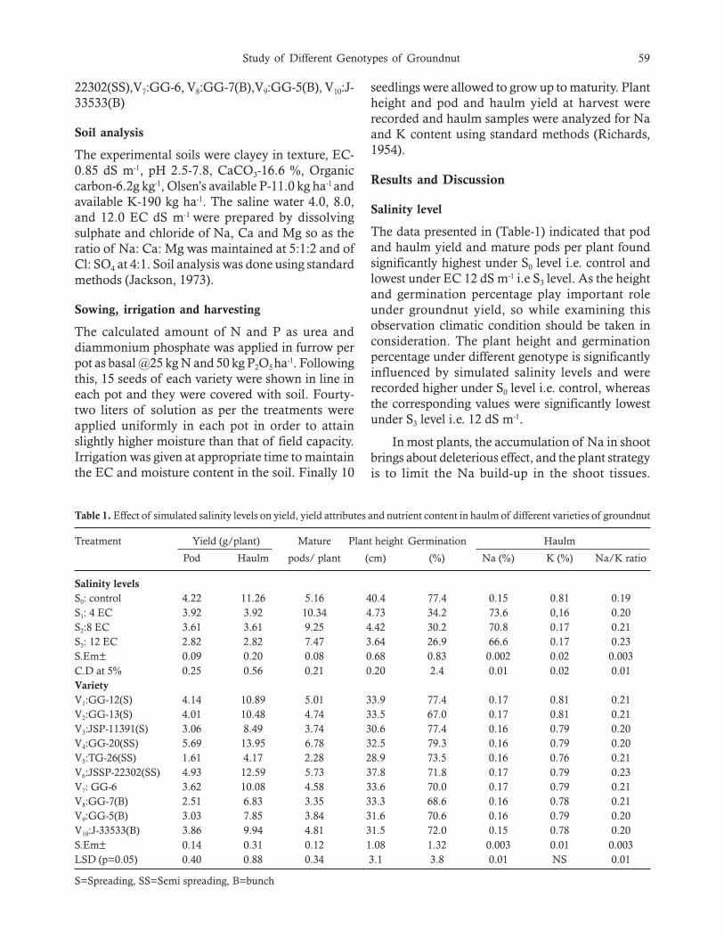
Study of Different Genotypes of Groundnut 59

22302(SS),V7:GG-6, V8:GG-7(B),V9:GG-5(B), V10:J-33533(B)

Soil analysis

The experimental soils were clayey in texture, EC-0.85 dS m-1, pH 2.5-7.8, CaCO3-16.6 %, Organiccarbon-6.2g kg-1, Olsen’s available P-11.0 kg ha-1 andavailable K-190 kg ha-1. The saline water 4.0, 8.0,and 12.0 EC dS m-1 were prepared by dissolvingsulphate and chloride of Na, Ca and Mg so as theratio of Na: Ca: Mg was maintained at 5:1:2 and ofCl: SO4 at 4:1. Soil analysis was done using standardmethods (Jackson, 1973).

Sowing, irrigation and harvesting

The calculated amount of N and P as urea anddiammonium phosphate was applied in furrow perpot as basal @25 kg N and 50 kg P2O5 ha-1. Followingthis, 15 seeds of each variety were shown in line ineach pot and they were covered with soil. Fourty-two liters of solution as per the treatments wereapplied uniformly in each pot in order to attainslightly higher moisture than that of field capacity.Irrigation was given at appropriate time to maintainthe EC and moisture content in the soil. Finally 10

seedlings were allowed to grow up to maturity. Plantheight and pod and haulm yield at harvest wererecorded and haulm samples were analyzed for Naand K content using standard methods (Richards,1954).

Results and Discussion

Salinity level

The data presented in (Table-1) indicated that podand haulm yield and mature pods per plant foundsignificantly highest under S0 level i.e. control andlowest under EC 12 dS m-1 i.e S3 level. As the heightand germination percentage play important roleunder groundnut yield, so while examining thisobservation climatic condition should be taken inconsideration. The plant height and germinationpercentage under different genotype is significantlyinfluenced by simulated salinity levels and wererecorded higher under S0 level i.e. control, whereasthe corresponding values were significantly lowestunder S3 level i.e. 12 dS m-1.

In most plants, the accumulation of Na in shootbrings about deleterious effect, and the plant strategyis to limit the Na build-up in the shoot tissues.

Table 1. Effect of simulated salinity levels on yield, yield attributes and nutrient content in haulm of different varieties of groundnut

Treatment Yield (g/plant) Mature Plant height Germination Haulm

Pod Haulm pods/ plant (cm) (%) Na (%) K (%) Na/K ratio

Salinity levelsS0: control 4.22 11.26 5.16 40.4 77.4 0.15 0.81 0.19S1: 4 EC 3.92 3.92 10.34 4.73 34.2 73.6 0,16 0.20S2:8 EC 3.61 3.61 9.25 4.42 30.2 70.8 0.17 0.21S3: 12 EC 2.82 2.82 7.47 3.64 26.9 66.6 0.17 0.23S.Em± 0.09 0.20 0.08 0.68 0.83 0.002 0.02 0.003C.D at 5% 0.25 0.56 0.21 0.20 2.4 0.01 0.02 0.01VarietyV1:GG-12(S) 4.14 10.89 5.01 33.9 77.4 0.17 0.81 0.21V2:GG-13(S) 4.01 10.48 4.74 33.5 67.0 0.17 0.81 0.21V3:JSP-11391(S) 3.06 8.49 3.74 30.6 77.4 0.16 0.79 0.20V4:GG-20(SS) 5.69 13.95 6.78 32.5 79.3 0.16 0.79 0.20V5:TG-26(SS) 1.61 4.17 2.28 28.9 73.5 0.16 0.76 0.21V6:JSSP-22302(SS) 4.93 12.59 5.73 37.8 71.8 0.17 0.79 0.23V7: GG-6 3.62 10.08 4.58 33.6 70.0 0.17 0.79 0.21V8:GG-7(B) 2.51 6.83 3.35 33.3 68.6 0.16 0.78 0.21V9:GG-5(B) 3.03 7.85 3.84 31.6 70.6 0.16 0.79 0.20V10:J-33533(B) 3.86 9.94 4.81 31.5 72.0 0.15 0.78 0.20S.Em± 0.14 0.31 0.12 1.08 1.32 0.003 0.01 0.003LSD (p=0.05) 0.40 0.88 0.34 3.1 3.8 0.01 NS 0.01

S=Spreading, SS=Semi spreading, B=bunch

60 Shalini Kumari et al.

Although it was found that the Na concentration inshoot increased with the salt treatment. It was alsofound in sorghum (Sorghum bicolor) that plants undersalinity store a large amount of Na in the stem, ascompared to leaves and young leaves (Netondo etal., 2004). It was found in sorghum that there was ahighly significant correlation between the salinitytolerance and the stem/leaves ratio (our on-goingunpublished work in sorghum). The same turned outto be true in groundnut, where stems could be usedas Na storage. Nautiyal et al. (1989, 2000) andMensah et al. (2006) also observed salinity tolerancein genotypes of groundnut. Further investigation isneeded to dissect the precise localization of Na inthe shoot parts of tolerant and sensitive groundnutgenotypes. Thus, the result showed that the Nacontent and Na/K ratio in haulm were foundsignificantly lowest and K content significantlyhighest under S0 level and were remains at par withsimulated salinity level S1.

Varieties

Among the spreading varieties, variety V1 (GG-12)produced significantly highest pod (4.14g) and haulmyield (10.89 g) mature pods per plant (5.01) and plantheight (33.88cm) but was at par with variety V2 (GG-13), while germination percentage was recordedsignificantly higher under variety V1 (GG-12) and V3

(Sp-11391). All the three varieties of spreadinggroundnut had almost similar Na and K content andNa/K ratio. In case of semi spreading varieties, pod(5.69 g) and haulm (13.45 g) yield per plant, maturepods per plant (6.78) and germination percentage(79.25) found significantly higher under variety V4

(GG-20) of groundnut, while plant height and Na/K ratio under variety V6 (JSSP-22302). Significantlyhighest pod yield (3.86 g), mature pods per plant(4.81) and germination percentage (72.0) wasrecorded under variety V10 (J-33533) of bunchgroundnut, which was at par with variety V7 (GG-

6), but reverse was true in case of haulm yield perplant. The significantly highest Na content wasrecorded under variety V7 (GG-6), while all the fourvarieties of bunch groundnut were similar withrespect to plant height, K content and Na/K ratio.

Conclusions

The foregoing discussion revealed that as the salinitylevels increased the germination count, plant heightand pod and haulm yield decreased significantly butreverse was true in case of Na/K ratio. The varietiesGG-12 (spreading) GG-20 (semi- spreading) and J-33533 (bunch) were found salt tolerance at all thesalinity levels.

References

Jackson ML (1973) Soil Chemical Analysis. Prentice Hall ofIndia Pvt. Ltd., New Delhi.

Mensah JK, Akomeah PA, Ikhajiagbe B and EkpekuredeEO (2006) Effect of salinity on germination, growth andyield of five groundnut genotypes. African Journal ofBiotechnology 5: 1973-1979.

Nautiyal PC, Ravindra V and Joshi YC (1989) Germinationand early seedling growth of some groundnut (Arachishypogaea L.) cultivars under salt stress. Indian Journal ofPlant Physiology 32: 251-253.

Nautiyal PC, Bandyopadhyay A, Koradia VG and MakadM (2000) Performance of groundnut germplasm andcultivars under saline water irrigation in the soils ofMundra in Gujarat, India. International Arachis Newsletter20: 80-82.

Netondo GW, Onyango JC and Beck E. (2004). Sorghumand salinity: I. Response of growth, water relations, andion accumulation to NaCl salinity. Crop Science 44:797–805.

Patel MS, Gundalia JD and Polara KB (1992) Evaluation ofsalt tolerance of different groundnut (Arachis hypogaeaL.) genotypes. Gujarat Agricultural University Res J 18:17-23.

Received: December, 2014; Accepted April, 2015

Impact of Organic Mulch, Soil Configuration and SoilAmendments on Yield of Onion and Soil Properties under

Coastal Saline Condition

Shalini Kumari*, Pamu Swetha and MS Solanki

Department of Soil Science and Agriculture Chemistry, College of Agriculture,Junagadh Agricultural University, Junagadh -362001, Gujarat

Email: shalinikumari136@gmail.com

Abstract

A field experiment was conducted in a coastal saline region of Saurashtra of Gujarat state at Junagadh districtduring 2010-2013 designed in a RBD with four replication on the impact of surface organic mulch, soilconfiguration and soil amendment on yield of onion crop. Pearl millet husk was applied as surface organicmulch at 3 t ha-1. Gypsum was broadcast at 5 t ha-1and incorporated before sowing. The result revealed that thetreatment of flat bed with surface organic mulch gave significantly higher onion bulb yield. The effect of thegypsum and soil configuration were found non-significant on the yield of onion bulb in the pooled data. At theend of the experiment soil analysis data indicated that significantly lower EC and ESP was recorded withmulch treatment in flat bed or ridge and furrow method. The mulch treatment was effective for reducing soilsalinity. The maximum net return of Rs 22220 per ha with net CB ratio 1: 22 was also noted with flat bed withmulch treatment.

Key words: Onion bulb, Flat bed, Ridge furrow, mulch, ESP

Introduction

Onion (Allium cepa L.) is one of the major cash cropsgrown in Mahuva and Talaja under Shentrujicommand area. During last decade there was nofacility of canal water, therefore, farmers are usingground water, which is over exploited in this area.Hence the quality of ground water is deterioratingrapidly. Under such condition the soil properties andthereby crop yields are adversely affected. With aproper management practices it could be possible tobetter harvest of crops under such condition. Thereis no any information available on this aspect in thisarea; therefore, a field experiment was planned onfarmers’ fields of Mahuvataluka to study the effectof soil configuration, organic mulch and soilsamendments on yield of onion and soil propertiesunder saline condition.

Material and Methods

Experimental site

A field experiment was conducted on coastal salinesoil of Saurashtra for the three years during Rabiseason from the year 2010 to 2013 in a RBD with

four replications at the farmers’ field (Village: Vadli,Taluka: Mahuva, Dist: Bhavnagar, State: Gujarat)cultivating onion, Cv, Talaja red (Local variety). Theobservations on growth and yield attributes wererecorded from 5 randomly selected plants from eachplot. The data were recorded for bulb yield on netplot basis and then converted on hectare basis andsubjected to statistical analysis.

Treatments

The treatments were T1: Flat bed (Fb, Control), T2:Fb+ Mulch (3 t ha-1), T3: Fb + Gypsum (5 t ha-1), T4:Fb + Mulch (3 t ha-1) + Gypsum (5 t ha-1), T5: Ridgeand furrow (R&F), T6: R&F + Mulch (3 tha-1), T7: R&F +Gypsum (5 t ha-1), T8: R&F +Mulch(3 t ha-1) + Gypsum (5 t ha-1).

Soil and plant analysis

Soil samples were analyzed following methodsdescribed by Jackson (1973). Potassium contentswere determined according to the method mentionedby Jackson (1973). After drying, a sample of bulbsand leaves from onion plants from each plot wereused to measure potassium levels (%) using flamphotometer.

Journal of Soil Salinity and Water Quality 7(1), 61-63, 2015

62 Shalini Kumari et al.

The experiment soil had texture silty loam, EC(dS m-1) 1.3, pH 8.2, CaCO3 28 g kg-1, ESP 8.5, OC4.3 g kg-1, available P2O5 35.4 kg ha-1 and availableK20 510 kg ha-1.

Fertilizer doses

The half N and full P2O5 and K2O of RD-recommended dose (75.0:60.0:50.0 N + P2O5 +K2Okg ha-1) were applied as basal and remaining halfdose of N of RD as split at 30 days after planting ofonion seedling.

Spacing

The plant spacing of 15 cm by 10 cm adopted foronion seedling.

Irrigation

The mean annual rainfall of the area is about 400mm of an erratic distribution. The slope of the studyarea was less than 2 per cent, with little variation inphysiography. The onion crop grown in plots wassubjected to irrigation by flood system. Irrigationapplication was scheduled to ensure that the cropsmoisture sensitive periods were covered andsufficient water supplied. The value of EC (dS m-1)and pH of the irrigation water were 2.3 and 7.9,respectively.

Results and Discussion

Effect on crop yield

The onion bulb yields were significantly affected dueto different treatments and mentioned in Table 1.

The pooled results revealed that the treatment of flatbed with surface organic mulch gave significantlyhigher onion bulb yield and was at par with thetreatment of ridge and furrow with mulch. Thesurface organic mulch under irrigated conditionsresulted in higher initial infiltration rates (Singh andSachhan, 1998; Arika and Lenga, 2000). Such animproved trend in the onion bulb yield, fallowingmulching, could be attributed to moderated soilhydrothermal regime (Sharma and Parmar, 1998)which resulted in an enhanced growth and activityof roots and shoots. The effects of the gypsum andsoil configuration were found non-significant on theyield of onion bulb in the pooled data. Wong andHo (1991) also observed encouraging results due togypsum application.

Table 1. Effect of different treatment on bulb yield of onion (t ha-1)

Sr. no. Treatment Bulb yield (t ha-1) Pooled

2010-11 2011-12 2012-13

T1 Fb (Control) 42.73 63.20 47.69 51.21T2 Fb+Mulch (M) 46.09 76.63 65.75 62.82T3 Fb +Gypsum (G) 44.89 66.44 56.02 55.78T4 Fb+M+G 48.99 64.59 53.71 55.76T5 R & F 43.92 55.79 50.47 50.06T6 R & F+ Mulch 51.07 68.76 50.93 56.92T7 R & F +Gypsum 44.26 61.81 49.08 51.72T8 R & F +M+ G 49.80 63.20 51.16 54.72

S.Em± 1.69 1.64 2.04 2.20LSD (p=0.05) 4.94 4.81 6.01 6.66C.V.% 7.23 5.03 7.69 6.54

Depictions: Fb-flat bed, M-mulch, G- gypsum, R & F- ridge and furrow

Table 2. Effect of different treatment on soil properties

Sr. Treatment Soil analysis (last year)

no. EC2.5 dS/m pH (1:2.5) ESP

T1 Fb (Control) 0.53 7.95 17.38T2 Fb+Mulch (M) 0.50 7.95 16.88T3 Fb +Gypsum (G) 0.88 7.78 16.43T4 Fb+M+G 0.78 7.68 16.30T5 R & F 0.56 8.00 19.03T6 R & F+ Mulch 0.55 7.98 18.75T7 R & F +Gypsum 1.58 7.63 15.23T8 R & F +M+ G 1.03 7.80 15.10

S.Em± 0.072 0.079 0.689LSD (p=0.05) 0.213 0.232 2.026C.V.% 18.11 2.01 8.16

Depictions as in Table 1

Impact of Organic Mulch, Soil Configuration and Soil Amendments on Onion Yield 63

Table 3. Economic of treatments for rabi onion crop.

Sr. Treatment Bulb Additional Additional Total additional Total additional NETno. yield bulb yield bulb yield income expenditure income over CBR

(t ha-1) over control over control over control control(t ha-1) (Rs. ha-1) (Rs ha-1) (Rs ha-1)

T1 Fb (Control) 51.21 - - - - -T2 Fb+Mulch (M) 62.82 11.61 23220 1000 22220 1:22.22T3 Fb+Gypsum (G) 55.78 4.57 9140 1250 7890 1:6.31T4 Fb+M+G 55.76 4.55 9100 2250 6850 1:3.04T5 R & F 50.06 -1.15 -2300 1000 -3300 -T6 R & F+ Mulch 56.92 5.71 11420 2000 9420 1:4.71T7 R & F +Gypsum 51.72 0.51 1020 2250 -1230 -T8 R & F +M+ G 54.72 3.51 7020 3250 3770 1:1.16

Depictions as in Table 1Price of the materials considered and application chargeOnion bulb: 2.00 Rs kg-1 Husk of pearl millet (mulch): 1000 Rs t-1

Gypsum: 250 Rs t-1 Cost of ridge and furrow : 1000 Rs ha-1

Yield and bulb quality

After harvesting and curing of onion bulbs, anothersample were taken to measure bulb physicalcharacteristics such as bulb weight (g), diameter (cm),and length (cm). In the same above sample bulbquality were evaluated by measuring total solublesolids (TSS %) which determined using a hand-heldrefractometer.

Effect on soil properties

At the end of the experiment soil analysis data (Table2) indicated that significantly lower EC was recordedwith mulch treatment in flat bed or/and in ridge andfurrow method. Whereas, significantly lower ESPwas recorded under the treatment of ridge andfurrow + mulch + gypsum. Thus the mulchtreatment was effective for reducing soil salinity.

Economy

The perusal of data presented (Table-3) revealed thatthe treatment of f lat bed with mulch gavesignificantly higher bulb yield of onion. Similarly,the maximum net return of Rs 22220 per ha withnet CBR 1: 22 was also noted with flat bed withmulch treatment.

Conclusion

The study revealed that addition of gypsum andorganic amendments acted as ameliorant to coastalsaline soils. In this study, individual or combined

effect of gypsum and organic mulch was moreeffective in changing EC and ESP. Gypsumapplication in combination with organicamendments improved the soil chemical propertiesby reducing the EC, ESP and pH, than the applyinggypsum alone.It is therefore, inferred from theexperiment that by the application of surface organicmulching, the onion bulb yield can be increased by22.69 per cent over traditional cultivation practicesof the coastal saline area of Saurashtra.

References

Arika CN and Lenga FK (2000). Effect of mulch applicationmethod on soil moisture characteristics and maize yieldin a semiarid region of Kenya Journal of Indian SocietySoil Science 48: 9-15.

Jackson ML (1973). Soil Chemical Analysis. Prentice Hall ofIndia Pvt. Ltd. New Delhi.

Singh SR and Sacchan BA (1998). Response of different bulbsize and spacing combinations on seed yield and yieldattributing traits on onion (Allium cepa L) Haryana Journalof Horticultural Science. 21(1): 56-58.

Sharma PK and Parmer DK (1998). Effect of phosphorusand mulching on the uptake of secondary nutrients andproductivity of wheat at different growth stages onAlfisol from Western Himalayas. Journal of Indian Societyof Soil Science. 46: 67-70.

Wong JWC and Ho GH. (1991). Effect of gypsum andsewage sludge amendment on physical properties of finebauxite refining residue. Soil Science 152: 326-332.

Received: December, 2014; Accepted April, 2015

Comparative Efficacy of Different Crop Residues, Green Manuresand Gypsum in Improving Biological Properties of Sodic Vertisols

AO Shirale1*, VK Kharche1, RN Katkar, RS Zadode and AB Aage1Department of Soil Science and Agril. Chemistry, 2 Department of Agronomy

Dr. Panjabrao Deshmukh Krishi Vidyapeeth, Akola, Maharashtra*E-mail: abhayshirale@gmail.com

Abstract

The field experiments on cotton followed by green gram in kharif (2011) and chickpea in rabi season (2012)were conducted on farmers’ fields in Kutasa village of Purna valley of Vidarbha region of Maharashtra. Thetreatments comprised of five different green manures (sunhemp, dhaincha, cowpea, green gram and leucaenaloppings), two crop residues (cotton stalk and farm waste as bio-mulch), gypsum and control. There were ninetreatments replicated on three farmers’ fields on Vertisols treating each farmer as one replication. Applicationof crop residues and green manures significantly enhanced the CO2 evolution, soil microbial biomass carbon,permanganate oxidizable carbon and dehydrogenase activity over the application of gypsum and control. Theapplication of dhaincha and sunhemp in situ green manuring showed highest potential to improve biologicalproperties of soils. The different treatments of organic amendments followed the sequence dhaincha > sunhemp> cowpea > leucaena loppings > green gram > cotton stalk > bio-mulch for improving biological properties.The results thus suggest the potential of different crop residues and green manures of improving biologicalproperties in sodic Vertisols.

Key words: Biological properties, Crop residues, Green manures, Microbial biomass carbon, Reclamation, SodicVertisols.

Introduction

Salt- affected soils are an important ecological entityin the landscape of semi-arid and arid regions ofthe world. The soil degradation due to salinity andsodicity has affected larger areas of fertile tracts,particularly in arid and semi-arid regions of thecountry and caused significant losses to cropproductivity. In sodic soils there is low biologicalactivity including enzyme activity, nitrogenmineralization and microbial biomass carbon, dueto high pH, exchangeable Na+, excessive CO3

2- andHCO3

- and low organic matter and N status (Raoand Pathak, 1996). The Application of green manureenhances the reclamation action of organic manuresby improving physical and chemical properties ofsoil and by markedly decreasing soil pH. Plant litterincorporation improves aggregation and lead tobetter aeration and water relationship, creatingfavorable environment for better establishment ofmicrobial activities. Purna valley in Vidarbha regionof Maharashtra is such an area having majorproblems like native salinity/sodicity, poor hydraulicconductivity, high degree of swell shrink potential,

compact and dense sub-soil, incomplete leaching ofsalts from soil due to severe drainage impairmentsand low biological activities. It is therefore necessaryto identify cost effective and site specific managementoptions for improvement of these soils. In thiscontext the present study was carried out inrepresentative village Kutasa District Akola in Purnavalley and the field experiments were conducted fortwo years on farmers fields in order to ascertain thecomparative efficacy of different crop residues, greenmanures and gypsum in improving biologicalproperties of sodic Vertisols.

Material and Methods

The field experiments on cotton (2011) followed bygreen gram and chickpea (2012) were conducted onselected farmers’fields in Purna valley. Thetreatments comprised of five different green manures(sunhemp-Crotalaria juncea, dhaincha-Sesbaniaaculeata, cowpea - Cajanus cajan, green gram -Vignaradiata and leucaena-Leucaena leucocephala, greenleaf), two kinds of mulch (composted cotton stalkresidue and bio-mulch (mulching with farm waste)),

Journal of Soil Salinity and Water Quality 7(1), 64-67, 2015

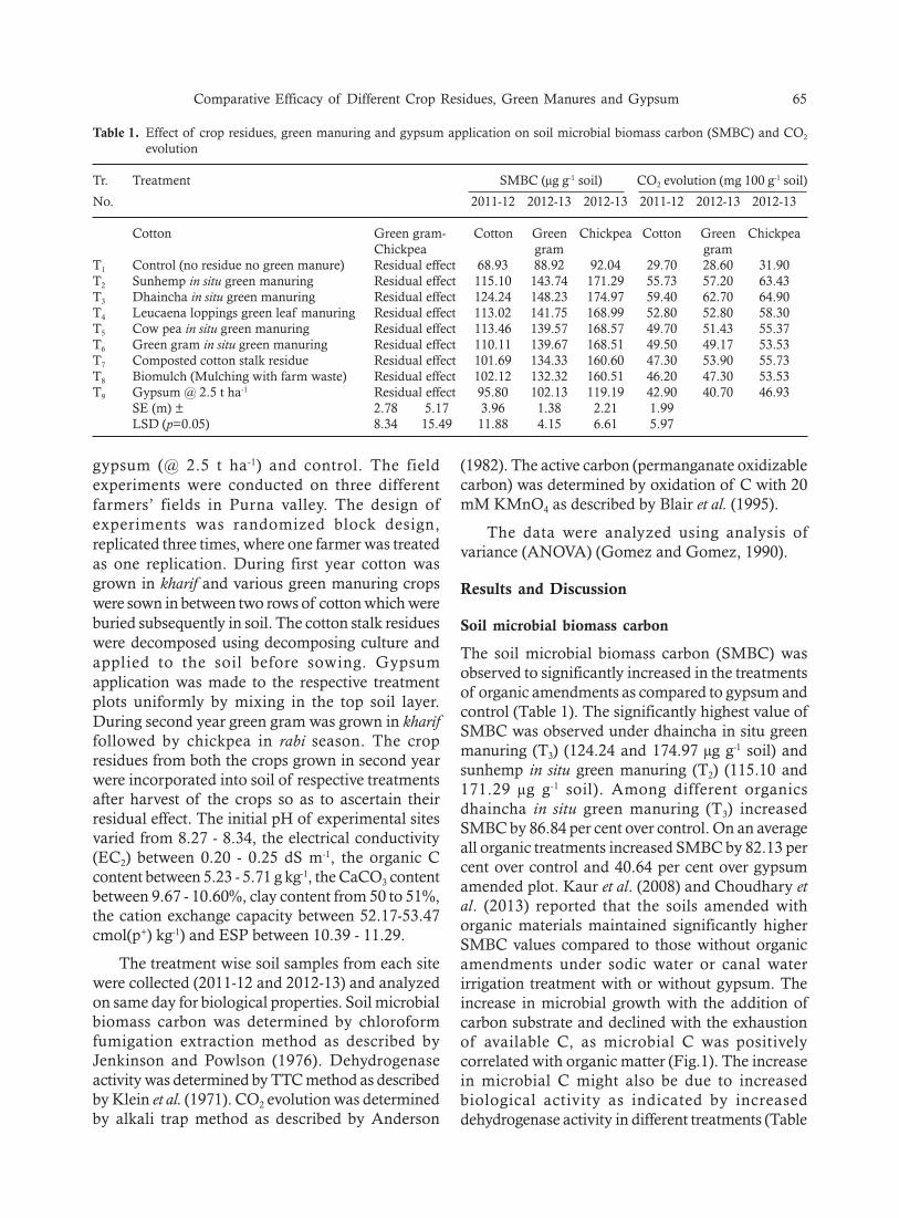
Comparative Efficacy of Different Crop Residues, Green Manures and Gypsum 65

gypsum (@ 2.5 t ha-1) and control. The fieldexperiments were conducted on three differentfarmers’ fields in Purna valley. The design ofexperiments was randomized block design,replicated three times, where one farmer was treatedas one replication. During first year cotton wasgrown in kharif and various green manuring cropswere sown in between two rows of cotton which wereburied subsequently in soil. The cotton stalk residueswere decomposed using decomposing culture andapplied to the soil before sowing. Gypsumapplication was made to the respective treatmentplots uniformly by mixing in the top soil layer.During second year green gram was grown in khariffollowed by chickpea in rabi season. The cropresidues from both the crops grown in second yearwere incorporated into soil of respective treatmentsafter harvest of the crops so as to ascertain theirresidual effect. The initial pH of experimental sitesvaried from 8.27 - 8.34, the electrical conductivity(EC2) between 0.20 - 0.25 dS m-1, the organic Ccontent between 5.23 - 5.71 g kg-1, the CaCO3 contentbetween 9.67 - 10.60%, clay content from 50 to 51%,the cation exchange capacity between 52.17-53.47cmol(p+) kg-1) and ESP between 10.39 - 11.29.

The treatment wise soil samples from each sitewere collected (2011-12 and 2012-13) and analyzedon same day for biological properties. Soil microbialbiomass carbon was determined by chloroformfumigation extraction method as described byJenkinson and Powlson (1976). Dehydrogenaseactivity was determined by TTC method as describedby Klein et al. (1971). CO2 evolution was determinedby alkali trap method as described by Anderson

(1982). The active carbon (permanganate oxidizablecarbon) was determined by oxidation of C with 20mM KMnO4 as described by Blair et al. (1995).

The data were analyzed using analysis ofvariance (ANOVA) (Gomez and Gomez, 1990).

Results and Discussion

Soil microbial biomass carbon

The soil microbial biomass carbon (SMBC) wasobserved to significantly increased in the treatmentsof organic amendments as compared to gypsum andcontrol (Table 1). The significantly highest value ofSMBC was observed under dhaincha in situ greenmanuring (T3) (124.24 and 174.97 µg g-1 soil) andsunhemp in situ green manuring (T2) (115.10 and171.29 µg g-1 soil). Among different organicsdhaincha in situ green manuring (T3) increasedSMBC by 86.84 per cent over control. On an averageall organic treatments increased SMBC by 82.13 percent over control and 40.64 per cent over gypsumamended plot. Kaur et al. (2008) and Choudhary etal. (2013) reported that the soils amended withorganic materials maintained significantly higherSMBC values compared to those without organicamendments under sodic water or canal waterirrigation treatment with or without gypsum. Theincrease in microbial growth with the addition ofcarbon substrate and declined with the exhaustionof available C, as microbial C was positivelycorrelated with organic matter (Fig.1). The increasein microbial C might also be due to increasedbiological activity as indicated by increaseddehydrogenase activity in different treatments (Table

Table 1. Effect of crop residues, green manuring and gypsum application on soil microbial biomass carbon (SMBC) and CO2

evolution

Tr. Treatment SMBC (µg g-1 soil) CO2 evolution (mg 100 g-1 soil)

No. 2011-12 2012-13 2012-13 2011-12 2012-13 2012-13

Cotton Green gram- Cotton Green Chickpea Cotton Green ChickpeaChickpea gram gram

T1 Control (no residue no green manure) Residual effect 68.93 88.92 92.04 29.70 28.60 31.90T2 Sunhemp in situ green manuring Residual effect 115.10 143.74 171.29 55.73 57.20 63.43T3 Dhaincha in situ green manuring Residual effect 124.24 148.23 174.97 59.40 62.70 64.90T4 Leucaena loppings green leaf manuring Residual effect 113.02 141.75 168.99 52.80 52.80 58.30T5 Cow pea in situ green manuring Residual effect 113.46 139.57 168.57 49.70 51.43 55.37T6 Green gram in situ green manuring Residual effect 110.11 139.67 168.51 49.50 49.17 53.53T7 Composted cotton stalk residue Residual effect 101.69 134.33 160.60 47.30 53.90 55.73T8 Biomulch (Mulching with farm waste) Residual effect 102.12 132.32 160.51 46.20 47.30 53.53T9 Gypsum @ 2.5 t ha-1 Residual effect 95.80 102.13 119.19 42.90 40.70 46.93

SE (m) ± 2.78 5.17 3.96 1.38 2.21 1.99LSD (p=0.05) 8.34 15.49 11.88 4.15 6.61 5.97

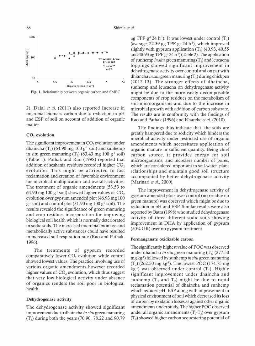
66 Shirale et al.

2). Dalal et al. (2011) also reported Increase inmicrobial biomass carbon due to reduction in pHand ESP of soil on account of addition of organicmatter.

CO2 evolution

The significant improvement in CO2 evolution underdhaincha (T3) (64.90 mg 100 g-1 soil) and sunhempin situ green manuring (T2) (63.43 mg 100 g-1 soil)(Table 1). Pathak and Rao (1998) reported thataddition of sesbania residues recorded higher CO2

evolution. This might be attributed to fastreclamation and creation of favorable environmentfor microbial multiplication and overall activities.The treatment of organic amendments (53.53 to64.90 mg 100 g-1 soil) showed higher values of CO2

evolution over gypsum amended plot (46.93 mg 100g-1 soil) and control plot (31.90 mg 100 g-1 soil). Theresults revealed the significance of green manuringand crop residues incorporation for improvingbiological soil health which is normally deterioratedin sodic soils. The increased microbial biomass andmetabolically active substances could have resultedin increased soil respiration rate (Rao and Pathak.1996).

The treatments of gypsum recordedcomparatively lower CO2 evolution while controlshowed lowest values. The practice involving use ofvarious organic amendments however recordedhigher values of CO2 evolution, which thus suggestthat very low biological activity under absenceof organics renders the soil poor in biologicalhealth.

Dehydrogenase activity

The dehydrogenase activity showed significantimprovement due to dhaincha in-situ green manuring(T3) during both the years (70.90, 78.22 and 90.79

µg TPF g-1 24 h-1). It was lowest under control (T1)(average, 22.39 µg TPF g-1 24 h-1), which improvedslightly with gypsum application (T9) (40.93, 40.55and 48.93 µg TPF g-1 24 h-1) (Table 2). The applicationof sunhemp in situ green manuring (T2) and leucaenaloppings showed significant improvement indehydrogenase activity over control and on par withdhiancha in situ green manuring (T3) during chickpea(2012-13). The stronger effects of dhaincha,sunhemp and leucaena on dehydrogenase activitymight be due to the more easily decomposablecomponents of crop residues on the metabolism ofsoil microorganisms and due to the increase inmicrobial growth with addition of carbon substrate.The results are in conformity with the findings ofRao and Pathak (1996) and Kharche et al. (2010).

The findings thus indicate that, the soils aregreatly hampered due to sodicity which hinders themicrobial activity under restricted use of organicamendments which necessitates application oforganic manure in sufficient quantity. Being chiefcarbon source, it provides energy for soilmicroorganisms, and increases number of pores,which are considered important in soil-water–plantrelationships and maintain good soil structureaccompanied by better dehydrogenase activity(Marinari et al., 2000).

The improvement in dehydrogenase activity ofgypsum amended plots over control (no residue nogreen manure) was observed which might be due toreduction in pH and ESP. Similar results were alsoreported by Batra (1998) who studied dehydrogenaseactivity of three different sodic soils showingimprovement in DHA by application of gypsum(50% GR) over no gypsum treatment.

Permanganate oxidizable carbon

The significantly highest value of POC was observedunder dhaincha in situ green manuring (T3) (277.50mg kg-1) followed by sunhemp in situ green manuring(T2) (262.50 mg kg-1). The lowest POC (174.75 mgkg-1) was observed under control (T1). Highlysignificant improvement under dhaincha andsunhemp (T3 and T2) might be due to rapidreclamation potential of dhaincha and sunhempwhich reduces pH, ESP along with improvement inphysical environment of soil which decreased its lossof carbon by oxidation losses as against other organicamendments under study. The higher POC observedunder all organic amendments (T2-T8) over gypsum(T9) showed higher carbon sequestering potential of

Fig. 1. Relationship between organic carbon and SMBC

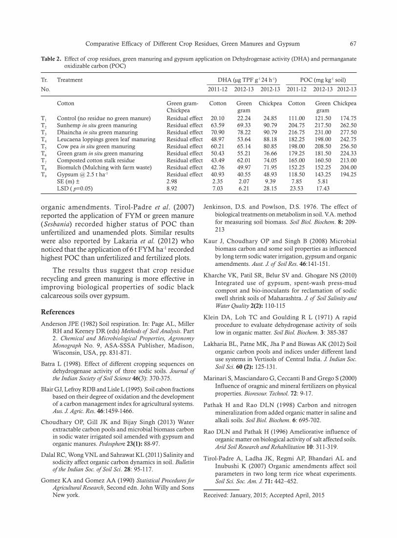
Comparative Efficacy of Different Crop Residues, Green Manures and Gypsum 67

organic amendments. Tirol-Padre et al. (2007)reported the application of FYM or green manure(Sesbania) recorded higher status of POC thanunfertilized and unamended plots. Similar resultswere also reported by Lakaria et al. (2012) whonoticed that the application of 6 t FYM ha-1 recordedhighest POC than unfertilized and fertilized plots.

The results thus suggest that crop residuerecycling and green manuring is more effective inimproving biological properties of sodic blackcalcareous soils over gypsum.

References

Anderson JPE (1982) Soil respiration. In: Page AL, MillerRH and Keeney DR (eds) Methods of Soil Analysis. Part2. Chemical and Microbiological Properties, AgronomyMonograph No. 9, ASA-SSSA Publisher, Madison,Wisconsin, USA, pp. 831-871.

Batra L (1998). Effect of different cropping sequences ondehydrogenase activity of three sodic soils. Journal ofthe Indian Society of Soil Science 46(3): 370-375.

Blair GJ, Lefroy RDB and Lisle L (1995). Soil cabon fractionsbased on their degree of oxidation and the developmentof a carbon management index for agricultural systems.Aus. J. Agric. Res. 46:1459-1466.

Choudhary OP, Gill JK and Bijay Singh (2013) Waterextractable carbon pools and microbial biomass carbonin sodic water irrigated soil amended with gypsum andorganic manures. Pedosphere 23(1): 88-97.

Dalal RC, Wong VNL and Sahrawat KL (2011) Salinity andsodicity affect organic carbon dynamics in soil. Bulletinof the Indian Soc. of Soil Sci. 28: 95-117.

Gomez KA and Gomez AA (1990) Statistical Procedures forAgricultural Research, Second edn. John Willy and SonsNew york.

Table 2. Effect of crop residues, green manuring and gypsum application on Dehydrogenase activity (DHA) and permanganateoxidizable carbon (POC)

Tr. Treatment DHA (µg TPF g-1 24 h-1) POC (mg kg-1 soil)

No. 2011-12 2012-13 2012-13 2011-12 2012-13 2012-13

Cotton Green gram- Cotton Green Chickpea Cotton Green ChickpeaChickpea gram gram

T1 Control (no residue no green manure) Residual effect 20.10 22.24 24.85 111.00 121.50 174.75T2 Sunhemp in situ green manuring Residual effect 63.59 69.33 90.79 204.75 217.50 262.50T3 Dhaincha in situ green manuring Residual effect 70.90 78.22 90.79 216.75 231.00 277.50T4 Leucaena loppings green leaf manuring Residual effect 48.97 53.64 88.18 182.25 198.00 242.75T5 Cow pea in situ green manuring Residual effect 60.21 65.14 80.85 198.00 208.50 256.50T6 Green gram in situ green manuring Residual effect 50.43 55.21 76.66 179.25 181.50 224.33T7 Composted cotton stalk residue Residual effect 43.49 62.01 74.05 165.00 160.50 213.00T8 Biomulch (Mulching with farm waste) Residual effect 42.76 49.97 71.95 152.25 152.25 204.00T9 Gypsum @ 2.5 t ha-1 Residual effect 40.93 40.55 48.93 118.50 143.25 194.25

SE (m) ± 2.98 2.35 2.07 9.39 7.85 5.81LSD ( p=0.05) 8.92 7.03 6.21 28.15 23.53 17.43

Jenkinson, D.S. and Powlson, D.S. 1976. The effect ofbiological treatments on metabolism in soil. V.A. methodfor measuring soil biomass. Soil Biol. Biochem. 8: 209-213

Kaur J, Choudhary OP and Singh B (2008) Microbialbiomass carbon and some soil properties as influencedby long term sodic water irrigation, gypsum and organicamendments. Aust. J. of Soil Res. 46:141-151.

Kharche VK, Patil SR, Belur SV and. Ghogare NS (2010)Integrated use of gypsum, spent-wash press-mudcompost and bio-inoculants for reclamation of sodicswell shrink soils of Maharashtra. J. of Soil Salinity andWater Quality 2(2): 110-115

Klein DA, Loh TC and Goulding R L (1971) A rapidprocedure to evaluate dehydrogenase activity of soilslow in organic matter. Soil Biol. Biochem. 3: 385-387

Lakharia BL, Patne MK, Jha P and Biswas AK (2012) Soilorganic carbon pools and indices under different landuse systems in Vertisols of Central India. J. Indian Soc.Soil Sci. 60 (2): 125-131.

Marinari S, Masciandaro G, Ceccanti B and Grego S (2000)Influence of oragnic and mineral fertilizers on physicalproperties. Bioresour. Technol. 72: 9-17.

Pathak H and Rao DLN (1998) Carbon and nitrogenmineralization from added organic matter in saline andalkali soils. Soil Biol. Biochem. 6: 695-702.

Rao DLN and Pathak H (1996) Ameliorative influence oforganic matter on biological activity of salt affected soils.Arid Soil Research and Rehabilitation 10: 311-319.

Tirol-Padre A, Ladha JK, Regmi AP, Bhandari AL andInubushi K (2007) Organic amendments affect soilparameters in two long term rice wheat experiments.Soil Sci. Soc. Am. J. 71: 442–452.

Received: January, 2015; Accepted April, 2015

Reducing Farm Income Losses through Land Reclamation:A Case Study from Indo-Gangetic Plains

K Thimmappa*1, Yashpal Singh1, R Raju1, Sandeep Kumar2, RS Tripathi1,Govind Pal3 and A Amarender Reddy4

1ICAR-Central Soil Salinity Research Institute, Zarifa Farm, Kachhwa Road, Karnal-132 001, Haryana2Uttar Pradesh Land Development Corporation, Lucknow-226 001, Uttar Pradesh

3Directorate of Seed Research, Mau-275 101, Uttar Pradesh4ICAR-Indian Agricultural Research Institute, New Delhi-110 012

*E-mail:thimpu@rediffmail.com

Abstract

Soil sodicity is a major problem in arid and semi-arid regions of Indo-Gangetic plains in India. A large proportionof sodicity-affected soils in Indo-Gangetic areas occur on land inhibited by resource poor farmers. Severalefforts have been made by the Central and State governments to check soil degradation and increase agriculturalproductivity through land reclamation programmes in salt-affected regions of India. The present study is anattempt to measure the impact of land reclamation on reduction in farm income losses. The study sourced datafrom published records and survey from farm households in Uttar Pradesh, India. Analysis revealed that landreclamation has contributed substantially to improve the soil health, crop productivity and farm income. Alluncultivated degraded lands in pre-reclamation period have been put under cultivation in post-reclamationperiod and cropping intensity has significantly increased. The farm income losses were reduced substantially inpost-reclamation period. The study has concluded that sodic land reclamation technology has made a significantcontribution to livelihood security of resource-poor farmers in salt-affected regions. The study has suggestedthat a large part of agricultural land is being abandoned in India due to severe sodicity related problems andneed to be reclaimed on priority basis to improve land productivity and farm income of resource poor farmers.

Key words: Gypsum, Farm income, Land degradation, Sodic soil, Land reclamation

Introduction

Land degradation due to sodicity is a major threatto agriculture in Indo-Gangetic plains. The sodic soilsare widely distributed across the globe and occupynearly 357.2 million hectares (Pessarakli andSzabolcs, 1999). India has 6.73 Mha of salt-affectedsoils, of which 3.72 Mha is sodic soils predominantlypresent in Indo-Gangetic plains (Mandal et al., 2010).Sodic soils are characterized by the occurrence ofexcess Na+ that adversely affects soil structure andcrop growth (Qadir and Schubert, 2002). Theweathering of alumino-silicate minerals produces acontinuous supply of sodium, potassium, calciumand magnesium salts in the catchment area. Due toarid and semi-arid climate, the water evaporates inpost-rainy months leave sodium carbonates(Na2CO3) and bi-carbonates (NaHCO3) on soilsurface, which contribute to the formation of sodicsoils in Indo-Gangetic plains (Chhabra, 1996). Indo-Gangetic plain lies between 210 55’ to 320 39’ N and

730 45’ to 880 25’ E comprising of the states ofPunjab, Haryana, Uttar Pradesh and part of Bihar(North), West Bengal (South) and Rajsthan (North)is having about 2.7 Mha salt affected soils (NRSA,1996).

Soil sodicity creates an inordinately high soil pHranging from 8.5 to 11 in addition to the ion toxicityand high osmotic pressure (Bing-Sheng et al., 2013).A high pH condition causes deficiencies of severalimportant minerals which in turn inhibits the plantgrowth (Guan et al., 2009) and adversely affects thegrowth of early seedlings, grain yield (Chhabra,1996; Sharma et al., 2010) and grain quality (Rao etal., 2013).

India’s foodgrain demand projections(Radhakrishna and Ravi, 1990; Kumar, 1998; Kumaret al., 2009) suggest that the need to produce morefood to an expanding human population, which willresult in an increase in the use of poor-quality waters

Journal of Soil Salinity and Water Quality 7(1), 68-76, 2015

Reducing Farm Income Losses through Land Reclamation 69

and soils for foodgrain production (Yadav, 1981;Oster and Jayawardane, 1998; Qadir et al., 2001).Plant growth in sodic soils is affected by high osmoticstress, ion toxicity and nutritional disorders whichultimately reduces crop yield (Qadir and Schubert,2002).

A significant advancement in sodic landreclamation technology has been made at CentralSoil Salinity Research Institute (CSSRI), Karnal(India) to use the degraded sodic soils with theaddition of soil amendments to meet the food grainsdemand for growing population. The successfulapplication of sodic soil reclamation technology atthe farmers’ fields has encouraged many states tolaunch ambitious programmes of land reclamationthrough Land Reclamation and DevelopmentCorporations by providing necessary inputs toaugment the food and livelihood security of resourcepoor farmers.

However, studies on yield and income of majorcrops in sodic soils before and after soil reclamationhas been very limited which is most important todetermine measures for improving crop productionpractices and for long term sustainability ofagriculture. Hence, this study was focused onassessing the impact of land reclamation on cropproductivity improvement and reduction in farmincome losses in sodicity affected regions of Indo-Gangetic plains.

Material and Methods

Study site

An intensive study was conducted in Santarahavillage in Hardoi district of Uttar Pradesh, India. Itis located at an elevation of 139 meters above meansea level. Temperature in summer goes as high as 44°C and in winter comes down to as low as 4°C. Therainy season prevails from mid-June to mid-September and annual rainfall varies from 629 to818 mm.

The average size of land holding was 0.62 haand the majority of the farmers were marginalcategory (Table 1). The crop production was animportant activity contributing 68 per cent to the totalhousehold income. Many farmers (27%)supplemented their household income by engagingthemselves or their family members as farm laborers.Farmers grew crops in kharif season (June–October)and rabi seasons (November–March). Transplanted

rice (Oryza sativa) crop was most popular in kharifseason. Wheat (Triticum aestivum) was grown afterrice in rabi season. In ‘moderate’ soil sodicity (ESP15–40), rice was grown in kharif season and landremained barren in rabi season. There was no cropcultivation in the severe soil sodicity condition dueto extreme sodicity (ESP >40).Table 1. Socio-economic profile of sample farmers

Particulars Percentage / value

(I) General information(a) Family size (No.) 7(b) Literacy level (%) 40(c) Age (years) 48(d) Average farm size (ha) 0.62(e) Annual rainfall (mm) 629 - 818(f) Temperature (°C) 4 - 44(II) Classification of farm holdings (%)(a) Marginal (<1 ha) 84(b) Small (1 to 2 ha) 16(c) Medium (>2 to 10 ha) 0(d) Large (> 10 ha) 0(III) Sources of family income (%)(a) Crop production 68(b) Livestock 2(c) Service 1(d) Business 2(e) Others 27

Source: Survey data.

Field survey

The village has total agricultural land of 123 haowned by approximately 197 farmers. The degradedland constituted 39 per cent of the total land holdingsand has varying levels of soil sodicity. The landholdings have been classified into ‘normal’, ‘slightlyaffected’, ‘moderately affected’ and ‘severely affected’by sodicity based on the extent of sodicity hazard(Table 2). Soil sodicity is usually quantified by theexchangeable sodium percentage (Van der Zee et al.,2010). It also can be quantified by soil pH. Sodicsoils have pH greater than 8.5. Several studies haveshown that there is an intimate relationship betweenESP and pH of the saturation paste (Kanwar et al.,1963; Kolarkar and Singh, 1970; Abrol et al., 1980).Since pH of the saturation paste can be easilydetermined in laboratory, this property can be usedas an approximate measure of ESP, which isotherwise a cumbersome determination (Chhabra,1996). The sodicity hazards were low in ‘slight’sodicity soil category. Farmers grew both rice and

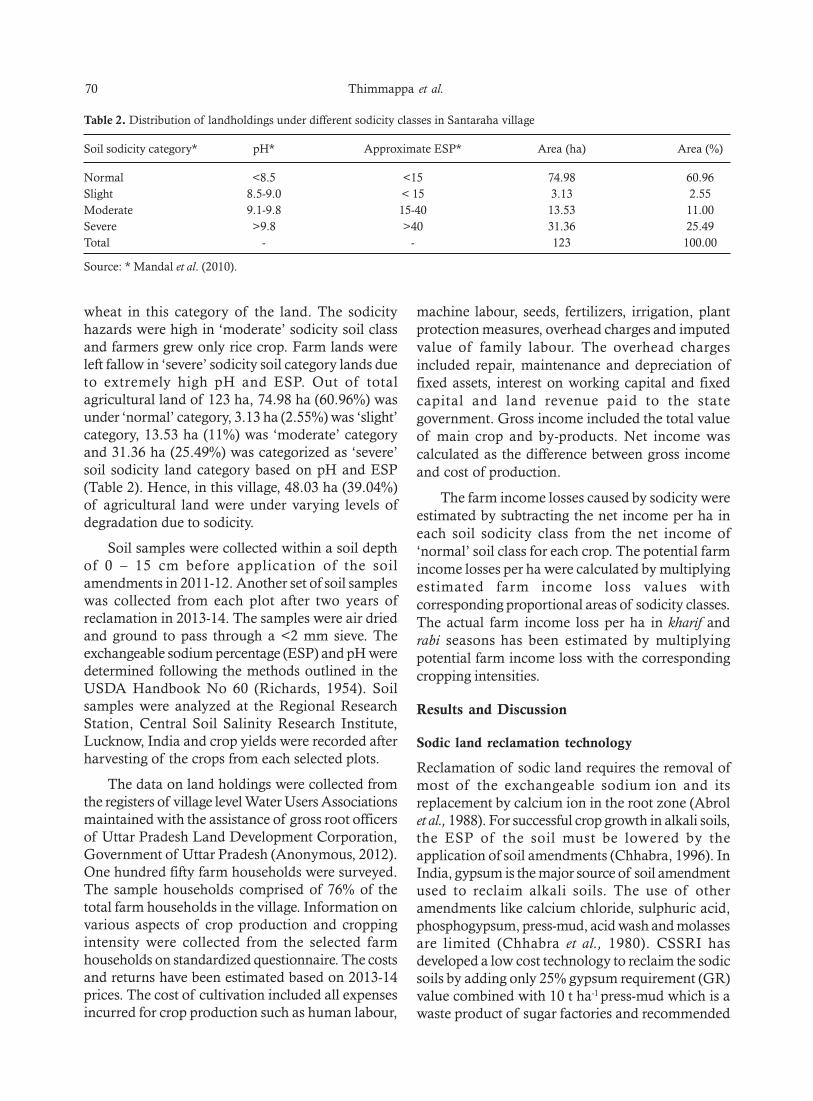
70 Thimmappa et al.

wheat in this category of the land. The sodicityhazards were high in ‘moderate’ sodicity soil classand farmers grew only rice crop. Farm lands wereleft fallow in ‘severe’ sodicity soil category lands dueto extremely high pH and ESP. Out of totalagricultural land of 123 ha, 74.98 ha (60.96%) wasunder ‘normal’ category, 3.13 ha (2.55%) was ‘slight’category, 13.53 ha (11%) was ‘moderate’ categoryand 31.36 ha (25.49%) was categorized as ‘severe’soil sodicity land category based on pH and ESP(Table 2). Hence, in this village, 48.03 ha (39.04%)of agricultural land were under varying levels ofdegradation due to sodicity.

Soil samples were collected within a soil depthof 0 – 15 cm before application of the soilamendments in 2011-12. Another set of soil sampleswas collected from each plot after two years ofreclamation in 2013-14. The samples were air driedand ground to pass through a <2 mm sieve. Theexchangeable sodium percentage (ESP) and pH weredetermined following the methods outlined in theUSDA Handbook No 60 (Richards, 1954). Soilsamples were analyzed at the Regional ResearchStation, Central Soil Salinity Research Institute,Lucknow, India and crop yields were recorded afterharvesting of the crops from each selected plots.

The data on land holdings were collected fromthe registers of village level Water Users Associationsmaintained with the assistance of gross root officersof Uttar Pradesh Land Development Corporation,Government of Uttar Pradesh (Anonymous, 2012).One hundred fifty farm households were surveyed.The sample households comprised of 76% of thetotal farm households in the village. Information onvarious aspects of crop production and croppingintensity were collected from the selected farmhouseholds on standardized questionnaire. The costsand returns have been estimated based on 2013-14prices. The cost of cultivation included all expensesincurred for crop production such as human labour,

machine labour, seeds, fertilizers, irrigation, plantprotection measures, overhead charges and imputedvalue of family labour. The overhead chargesincluded repair, maintenance and depreciation offixed assets, interest on working capital and fixedcapital and land revenue paid to the stategovernment. Gross income included the total valueof main crop and by-products. Net income wascalculated as the difference between gross incomeand cost of production.

The farm income losses caused by sodicity wereestimated by subtracting the net income per ha ineach soil sodicity class from the net income of‘normal’ soil class for each crop. The potential farmincome losses per ha were calculated by multiplyingestimated farm income loss values withcorresponding proportional areas of sodicity classes.The actual farm income loss per ha in kharif andrabi seasons has been estimated by multiplyingpotential farm income loss with the correspondingcropping intensities.

Results and Discussion

Sodic land reclamation technology

Reclamation of sodic land requires the removal ofmost of the exchangeable sodium ion and itsreplacement by calcium ion in the root zone (Abrolet al., 1988). For successful crop growth in alkali soils,the ESP of the soil must be lowered by theapplication of soil amendments (Chhabra, 1996). InIndia, gypsum is the major source of soil amendmentused to reclaim alkali soils. The use of otheramendments like calcium chloride, sulphuric acid,phosphogypsum, press-mud, acid wash and molassesare limited (Chhabra et al., 1980). CSSRI hasdeveloped a low cost technology to reclaim the sodicsoils by adding only 25% gypsum requirement (GR)value combined with 10 t ha-1 press-mud which is awaste product of sugar factories and recommended

Table 2. Distribution of landholdings under different sodicity classes in Santaraha village

Soil sodicity category* pH* Approximate ESP* Area (ha) Area (%)

Normal <8.5 <15 74.98 60.96Slight 8.5-9.0 < 15 3.13 2.55Moderate 9.1-9.8 15-40 13.53 11.00Severe >9.8 >40 31.36 25.49Total - - 123 100.00

Source: * Mandal et al. (2010).

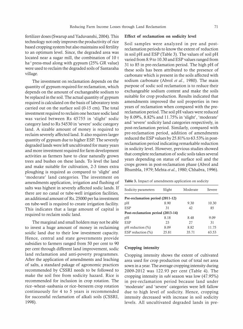
Reducing Farm Income Losses through Land Reclamation 71

fertilizer doses (Swarup and Yaduvanshi, 2004). Thistechnology not only improves the productivity of ricebased cropping system but also maintains soil fertilityto an optimum level. Since, the degraded area waslocated near a sugar mill, the combination of 10 tha-1 press-mud along with gypsum (25% GR value)were used to reclaim the degraded soils of Santarahavillage.

The investment on reclamation depends on thequantity of gypsum required for reclamation, whichdepends on the amount of exchangeable sodium tobe replaced in the soil. The actual quantity of gypsumrequired is calculated on the basis of laboratory testscarried out on the surface soil (0-15 cm). The totalinvestment required to reclaim one hectare sodic landwas varied between Rs 45755 in ‘slight’ sodiccategory land to Rs 54530 in ‘severe’ sodic categoryland. A sizable amount of money is required toreclaim severely affected land. It also requires largerquantity of gypsum due to higher ESP. The severelydegraded lands were left uncultivated for many yearsand more investment required for farm developmentactivities as farmers have to clear naturally growntrees and bushes on these lands. To level the landand make suitable for cultivation, 2-3 times extraploughing is required as compared to ‘slight’ and‘moderate’ land categories. The investment onamendments application, irrigation and flushing ofsalts was highest in severely affected sodic lands. Ifthere are no canal or tube-well irrigation facilities,an additional amount of Rs. 25000 per ha investmenton tube-well is required to create irrigation facility.This indicates that a large amount of capital isrequired to reclaim sodic land.

The marginal and small holders may not be ableto invest a huge amount of money in reclaimingsoidic land due to their low investment capacity.Hence, central and state governments providesubsidies to farmers ranged from 50 per cent to 90per cent through different land improvement, sodicland reclamation and anti-poverty programmes.After the application of amendments and leachingof salts, a standard pakage of agronomic practicesrecommended by CSSRI needs to be followed tomake the soil free from sodicity hazard. Rice isrecommended for inclusion in crop rotation. Therice–wheat–sasbania or rice–berseem crop rotationcontinuously for 4 to 5 years is recommendedfor successful reclamation of alkali soils (CSSRI,1998).

Effect of reclamation on sodicity level

Soil samples were analyzed in pre and post-reclamation periods to know the extent of reductionin soil pH and ESP (Table 3). The values of soil pHvaried from 8.9 to 10.30 and ESP values ranged from31 to 85 in pre-reclamation period. The high pH ofthese soils has been attributed to the presence ofcarbonate which is present in the soils affected withsodium carbonate (Abrol et al., 1980). The mainpurpose of sodic soil reclamation is to reduce theirexchangeable sodium content and make the soilssuitable for crop production. Results indicated thatamendments improved the soil properties in twoyears of reclamation when compared with the pre-reclamation period. The soil pH values were reducedby 8.09%, 8.82% and 11.75% in ‘slight’, ‘moderate’and ‘severe’ sodicity land categories respectively, inpost-reclamation period. Similarly, compared withpre-reclamation period, addition of amendmentsreduced the ESP values by 25.81% to 63.53% in post-reclamation period indicating remarkable reductionin sodicity level. However, previous studies showedthat complete reclamation of sodic soils takes severalyears depending on status of surface soil and thecrops grown in post-reclamation phase (Abrol andBhumbla, 1979; Mehta et al., 1980; Chhabra, 1996).

Table 3. Impact of amendments application on sodicity

Sodicity parameters Slight Moderate Severe

Pre-reclamation period (2011-12)pH 8.90 9.30 10.30ESP 31 42 85Post-reclamation period (2013-14)pH 8.18 8.48 9.09ESP 23 27 31pH reduction (%) 8.09 8.82 11.75ESP reduction (%) 25.81 35.71 63.53

Cropping intensity

Cropping intensity shows the extent of cultivatedarea used for crop production out of total net areasown in a year. The average cropping intensity during2009-2012 was 122.93 per cent (Table 4). Thecropping intensity in rabi season was low (47.95%)in pre-reclamation period because land under‘moderate’ and ‘severe’ categories were left fallowdue to high level of sodicity. Hence, croppingintensity decreased with increase in soil sodicitylevels. All uncultivated degraded lands in pre-

72 Thimmappa et al.

reclamation period have been put under cultivationin post-reclamation period. Hence, the croppingintensity was 199.54 per cent and increased by62.32%. The increased cropping intensitycontributed to higher total farm production andincome.

Crop yield

Yield loss is detrimental at a local scale because salt-affected soils are not uniformly distributed. Thedegree of sodicity varied across the farms with inthe village. It was observed that the salt concentrationin soil has steeply reduced the crop yield (Table 5).The rice yield decreased from 4.87 t/ha in ‘normal’soils to 2.95 t/ha in ‘slight’ soil sodicity class,indicating 39.43 per cent decline. Several studies haveshown that crop yield decreases with increase in thelevel of sodicity (Abrol and Bhumbla, 1979;Chhabra, 2002; Dwivedi and Qadar, 2011). The yieldreduction was drastic (74.95%) in ‘moderate’ soilsodicity class. A large number of studies indicatedthat the sodicity inhibits shoot and root growth ofrice seedlings and had less biomass when grownunder sodic conditions (Chhabra, 1996; Van Aste etal., 2003; Wang et al., 2011).

Wheat yield decreased from 3.65 t ha-1 in‘normal’ soil to 2.82 t/ha in ‘slight’ land class,depicting 22.74 per cent yield loss (Table 5). The yieldloss of wheat was greater at the higher sodicity levels(Sharma et al., 2010). Yield of wheat is highlydependent on the number of spikes produced by eachplant. Sodic conditions negatively affect number ofspikes produced per plant (Maas and Grieve, 1990)and the fertility of the spikelets (Seifert et al., 2011;Fatemeh et al., 2013). Sodic soils usually have pooravailability of most micronutrients, which isgenerally attributed to high soil pH (Naidu andRengasamy, 1993). In addition, poor physical

properties of sodic soils, which directly limit cropgrowth through poor seedling emergence and rootgrowth, also exhibit indirect effects on plant nutritionby restricting water and nutrient uptake and gaseousexchange (Curtin and Naidu, 1998) which ultimatelyresult in reduced crop yield and quality (Grattan andGrieve, 1999).

There was no wheat production in ‘moderate’and ‘severe’ soil sodicity classes. A high pH conditiondamages plants directly and causes deficiencies ofnutritional minerals such as iron and phosphorus(Guan et al., 2009). The ‘severe’ category of soilsodicity class remained barren in both the seasonsdue to high sodicity as ESP ranged from 65 to 90and pH varied from 9.5 to 11. Heavy salt stressgenerally leads to reduced growth and even plantdeath (Qadar, 1998; Parida and Das, 2005).

The rice-wheat rotation is most common in Indo-Gangetic plains. It was noticed that land reclamationhad a profound impact on productivity of rice andwheat. Before reclamation, the productivity of ricewas 2.95 t ha-1 in ‘slight’ and 1.22 ha-1 in ‘moderate’land categories. The productivity of rice increasedto 4.71 t ha-1 in ‘slight’ soil sodicity category,depicting a gain of 60%. In ‘moderate’ soil sodicitycategory, rice productivity increased to 4.40 t ha-1,indicating a remarkable increase of 261%. Hence, asignificant yield gain was observed in rice after landreclamation. In the ‘severe’ soil sodicity category,rice production was 3.90 t ha-1, which was barren inpre-reclamation period.

Before reclamation, wheat production was 2.82t ha-1 in ‘slight’ land category and increased to 3.49 tha-1 in post-reclamation period. The wheat yield was3.17 t ha-1 in ‘moderate’ and 2.75 t ha-1 in ‘severe’land sodicity categories in post-reclamation periodwhich were uncultivated in pre-reclamation period.It suggested that a significant yield gain was observed

Table 4. Cropping intensity (%) by soil sodicity classes

Soil sodicity class Pre-reclamation period Post-reclamation period

2009-10 2010-11 2011-12 Average 2012-13 2013-14 Average

Normal 198.57 198.47 198.47 198.50 198.47 198.47 198.47Slight 196.86 191.44 191.44 193.25 199.73 199.73 199.73Moderate 99.96 99.96 99.96 99.96 199.93 199.93 199.93Severe 0.00 0.00 0.00 0.00 200.00 200.00 200.00Average in kharif 74.47 73.73 73.73 73.98 99.77 99.77 99.77Average in rabi 49.38 48.74 48.74 48.95 99.77 99.77 99.77Annual average 123.85 122.47 122.47 122.93 199.54 199.54 199.54

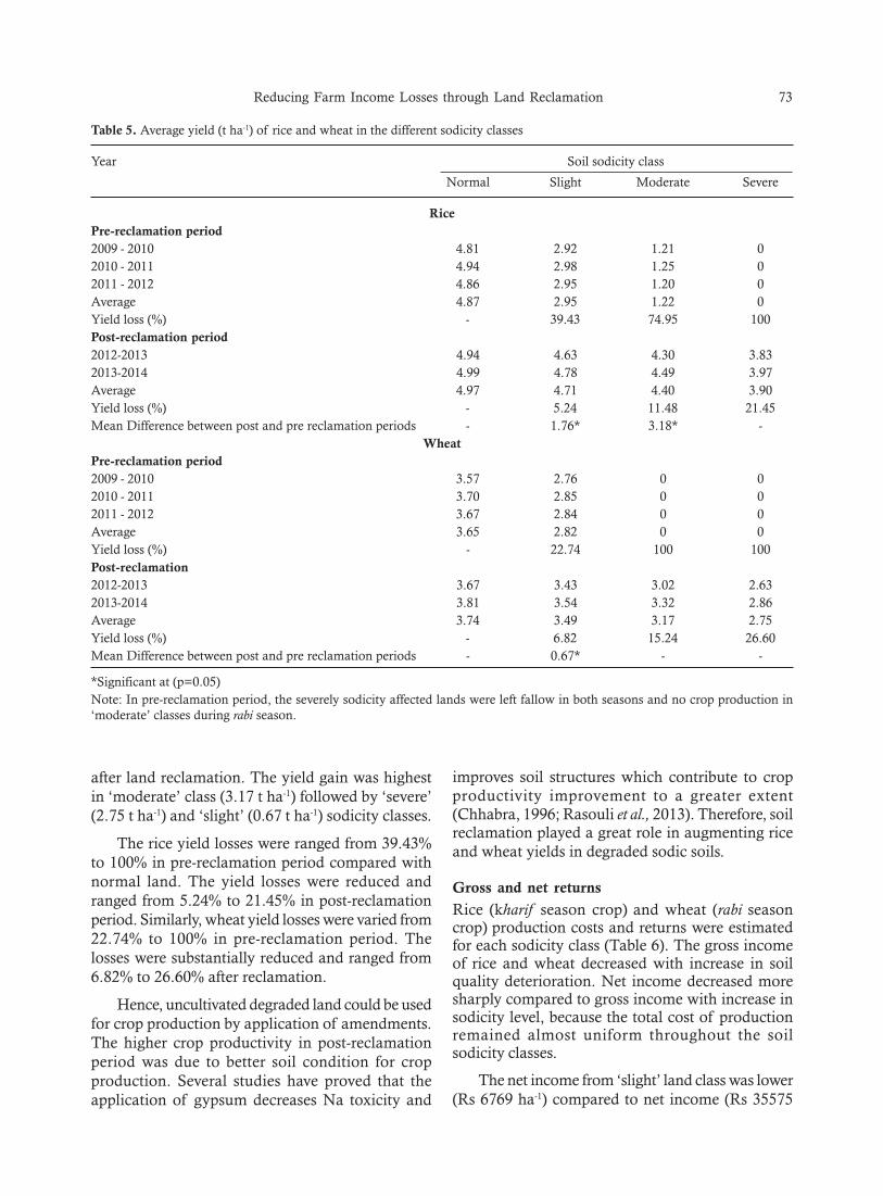
Reducing Farm Income Losses through Land Reclamation 73

Table 5. Average yield (t ha-1) of rice and wheat in the different sodicity classes

Year Soil sodicity class

Normal Slight Moderate Severe

RicePre-reclamation period2009 - 2010 4.81 2.92 1.21 02010 - 2011 4.94 2.98 1.25 02011 - 2012 4.86 2.95 1.20 0Average 4.87 2.95 1.22 0Yield loss (%) - 39.43 74.95 100Post-reclamation period2012-2013 4.94 4.63 4.30 3.832013-2014 4.99 4.78 4.49 3.97Average 4.97 4.71 4.40 3.90Yield loss (%) - 5.24 11.48 21.45Mean Difference between post and pre reclamation periods - 1.76* 3.18* -

WheatPre-reclamation period2009 - 2010 3.57 2.76 0 02010 - 2011 3.70 2.85 0 02011 - 2012 3.67 2.84 0 0Average 3.65 2.82 0 0Yield loss (%) - 22.74 100 100Post-reclamation2012-2013 3.67 3.43 3.02 2.632013-2014 3.81 3.54 3.32 2.86Average 3.74 3.49 3.17 2.75Yield loss (%) - 6.82 15.24 26.60Mean Difference between post and pre reclamation periods - 0.67* - -

*Significant at (p=0.05)Note: In pre-reclamation period, the severely sodicity affected lands were left fallow in both seasons and no crop production in‘moderate’ classes during rabi season.

after land reclamation. The yield gain was highestin ‘moderate’ class (3.17 t ha-1) followed by ‘severe’(2.75 t ha-1) and ‘slight’ (0.67 t ha-1) sodicity classes.

The rice yield losses were ranged from 39.43%to 100% in pre-reclamation period compared withnormal land. The yield losses were reduced andranged from 5.24% to 21.45% in post-reclamationperiod. Similarly, wheat yield losses were varied from22.74% to 100% in pre-reclamation period. Thelosses were substantially reduced and ranged from6.82% to 26.60% after reclamation.

Hence, uncultivated degraded land could be usedfor crop production by application of amendments.The higher crop productivity in post-reclamationperiod was due to better soil condition for cropproduction. Several studies have proved that theapplication of gypsum decreases Na toxicity and

improves soil structures which contribute to cropproductivity improvement to a greater extent(Chhabra, 1996; Rasouli et al., 2013). Therefore, soilreclamation played a great role in augmenting riceand wheat yields in degraded sodic soils.

Gross and net returns

Rice (kharif season crop) and wheat (rabi seasoncrop) production costs and returns were estimatedfor each sodicity class (Table 6). The gross incomeof rice and wheat decreased with increase in soilquality deterioration. Net income decreased moresharply compared to gross income with increase insodicity level, because the total cost of productionremained almost uniform throughout the soilsodicity classes.

The net income from ‘slight’ land class was lower(Rs 6769 ha-1) compared to net income (Rs 35575

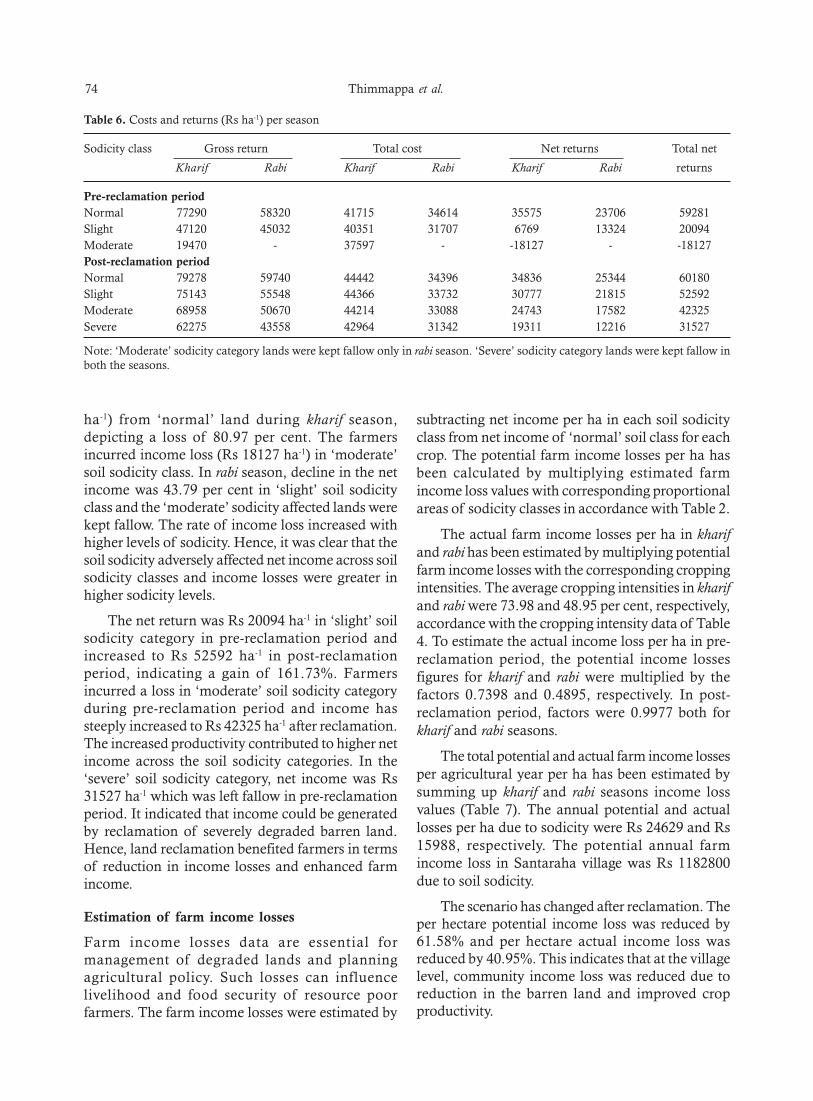
74 Thimmappa et al.

ha-1) from ‘normal’ land during kharif season,depicting a loss of 80.97 per cent. The farmersincurred income loss (Rs 18127 ha-1) in ‘moderate’soil sodicity class. In rabi season, decline in the netincome was 43.79 per cent in ‘slight’ soil sodicityclass and the ‘moderate’ sodicity affected lands werekept fallow. The rate of income loss increased withhigher levels of sodicity. Hence, it was clear that thesoil sodicity adversely affected net income across soilsodicity classes and income losses were greater inhigher sodicity levels.

The net return was Rs 20094 ha-1 in ‘slight’ soilsodicity category in pre-reclamation period andincreased to Rs 52592 ha-1 in post-reclamationperiod, indicating a gain of 161.73%. Farmersincurred a loss in ‘moderate’ soil sodicity categoryduring pre-reclamation period and income hassteeply increased to Rs 42325 ha-1 after reclamation.The increased productivity contributed to higher netincome across the soil sodicity categories. In the‘severe’ soil sodicity category, net income was Rs31527 ha-1 which was left fallow in pre-reclamationperiod. It indicated that income could be generatedby reclamation of severely degraded barren land.Hence, land reclamation benefited farmers in termsof reduction in income losses and enhanced farmincome.

Estimation of farm income losses

Farm income losses data are essential formanagement of degraded lands and planningagricultural policy. Such losses can influencelivelihood and food security of resource poorfarmers. The farm income losses were estimated by

subtracting net income per ha in each soil sodicityclass from net income of ‘normal’ soil class for eachcrop. The potential farm income losses per ha hasbeen calculated by multiplying estimated farmincome loss values with corresponding proportionalareas of sodicity classes in accordance with Table 2.

The actual farm income losses per ha in kharifand rabi has been estimated by multiplying potentialfarm income losses with the corresponding croppingintensities. The average cropping intensities in kharifand rabi were 73.98 and 48.95 per cent, respectively,accordance with the cropping intensity data of Table4. To estimate the actual income loss per ha in pre-reclamation period, the potential income lossesfigures for kharif and rabi were multiplied by thefactors 0.7398 and 0.4895, respectively. In post-reclamation period, factors were 0.9977 both forkharif and rabi seasons.

The total potential and actual farm income lossesper agricultural year per ha has been estimated bysumming up kharif and rabi seasons income lossvalues (Table 7). The annual potential and actuallosses per ha due to sodicity were Rs 24629 and Rs15988, respectively. The potential annual farmincome loss in Santaraha village was Rs 1182800due to soil sodicity.

The scenario has changed after reclamation. Theper hectare potential income loss was reduced by61.58% and per hectare actual income loss wasreduced by 40.95%. This indicates that at the villagelevel, community income loss was reduced due toreduction in the barren land and improved cropproductivity.

Table 6. Costs and returns (Rs ha-1) per season

Sodicity class Gross return Total cost Net returns Total net

Kharif Rabi Kharif Rabi Kharif Rabi returns

Pre-reclamation periodNormal 77290 58320 41715 34614 35575 23706 59281Slight 47120 45032 40351 31707 6769 13324 20094Moderate 19470 - 37597 - -18127 - -18127Post-reclamation periodNormal 79278 59740 44442 34396 34836 25344 60180Slight 75143 55548 44366 33732 30777 21815 52592Moderate 68958 50670 44214 33088 24743 17582 42325Severe 62275 43558 42964 31342 19311 12216 31527

Note: ‘Moderate’ sodicity category lands were kept fallow only in rabi season. ‘Severe’ sodicity category lands were kept fallow inboth the seasons.

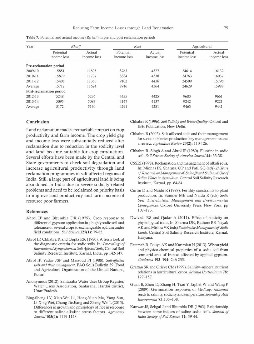
Reducing Farm Income Losses through Land Reclamation 75

Table 7. Potential and actual income (Rs ha-1) in pre and post reclamation periods

Year Kharif Rabi Agricultural

Potential Actual Potential Actual Potential Actualincome loss income loss income loss income loss income loss income loss

Pre-reclamation period2009-10 15851 11805 8763 4327 24614 161322010-11 15879 11707 8884 4330 24763 160372011-12 15408 11360 9102 4436 24509 15796Average 15712 11624 8916 4364 24629 15988Post-reclamation period2012-13 5248 5236 4435 4425 9683 96612013-14 5095 5083 4147 4137 9242 9221Average 5172 5160 4291 4281 9463 9441

Conclusion

Land reclamation made a remarkable impact on cropproductivity and farm income. The crop yield gapand income loss were substantially reduced afterreclamation due to reduction in the sodicity leveland land became suitable for crop production.Several efforts have been made by the Central andState governments to check soil degradation andincrease agricultural productivity through landreclamation programmes in salt-affected regions ofIndia. Still, a large part of agricultural land is beingabandoned in India due to severe sodicity relatedproblems and need to be reclaimed on priority basisto improve land productivity and farm income ofresource poor farmers.

ReferencesAbrol IP and Bhumbla DR (1979). Crop response to

differential gypsum application in a highly sodic soil andtolerance of several crops to exchangeable sodium underfield conditions. Soil Science 127(1): 79-85.

Abrol IP, Chhabra R and Gupta RK (1980). A fresh look atthe diagnostic criteria for sodic soils. In: Proceedings ofInternational Symposium on Salt Affected Soils, Central SoilSalinity Research Institute, Karnal, India, pp 142-147.

Abrol IP, Yadav JSP and Massoud FI (1988). Salt-affectedsoils and their management. FAO Soils Bulletin 39. Foodand Agriculture Organization of the United Nations,Rome.

Anonymous (2012). Santaraha Water User Group Register,Water Users Association, Santaraha, Hardoi district,Uttar Pradesh.

Bing-Sheng LV, Xiao-Wei Li, Hong-Yuan Ma, Yang Sun,Li-Xing Wei, Chang-Jie Jiang and Zheng-Wei L (2013).Differences in growth and physiology of rice in responseto different saline-alkaline stress factors. AgronomyJournal 105(4): 1119-1128.

Chhabra R (1996). Soil Salinity and Water Quality. Oxford andIBH Publication, New Delhi.

Chhabra R (2002). Salt-affected soils and their managementfor sustainable rice production-key management issues:a review. Agriculture Review 23(2): 110-126.

Chhabra R, Singh A and Abrol IP (1980). Fluorine in sodicsoil. Soil Science Society of America Journal 44: 33-38.

CSSRI (1998). Reclamation and management of alkali soils,In: Minhas PS, Sharma, OP and Patil SG (eds) 25 Yearsof Research on Management of Salt-affected Soils and Use ofSaline Water in Agriculture. Central Soil Salinity ResearchInstitute, Karnal. pp. 64-84.

Curtin D and Naidu R (1998). Fertility constraints to plantproduction. In: Sumner ME and Naidu R (eds) SodicSoil: Distribution, Management and EnvironmentalConsequences. Oxford University Press, New York, pp107–123.

Dwivedi RS and Qadar A (2011). Effect of sodicity onphysiological traits. In: Sharma DK, Rathore RS, NayakAK and Mishra VK (eds) Sustainable Management of SodicLands. Central Soil Salinity Research Institute, Karnal,Haryana.

Fatemeh R, Pouya AK and Karimian N (2013). Wheat yieldand physico-chemical properties of a sodic soil fromsemi-arid area of Iran as affected by applied gypsum.Geoderma 193–194: 246-255.

Grattan SR and Grieve CM (1999). Salinity–mineral nutrientrelations in horticultural crops. Scientia Horticulturae 78:127–157.

Guan B, Zhou D, Zhang H, Tian Y, Japhet W and Wang P(2009). Germination responses of Medicago ruthenicaseeds to salinity, sodicity and temperature. Journal of AridEnvironment 73:135–138.

Kanwar JS, Sehgal J and Bhumbla DR (1963). Relationshipbetween some indices of saline sodic soils. Journal ofIndia Society of Soil Science 11: 39-44.

76 Thimmappa et al.

Kolarkar AS and Singh N (1970). Diagnosis of sodicconditions in saline alkali soils of Western Rajastan.Annals of Arid Zone 9(1): 31-35.

Kumar P (1998). Food Demand and Supply Projections for India.Agricultural Economics Policy Paper 98-01, IndianAgricultural Research Institute, New Delhi.

Kumar P, Joshi PK and Pratap SB (2009). Demandprojections for food grains in India. Agricultural EconomicsResearch Review 22 (2): 237-243.

Maas EV and Grieve CM (1990). Spike and leaf developmentin salt-stressed wheat. Crop Science 30: 1309–1313.

Mandal AK, Sharma RC, Singh G and Dagar JC (2010).Computerized Database on Salt Affected Soils in India.Technical bulletin 2/2010, Central Soil Salinity ResearchInstitute, Karnal, 28p.

Mehta KK, Yadav JSP and Sharma DP (1980). Effect ofgypsum on the reclamation of alkali soils and cropgrowth in the farmers’ fields in Karnal District ofHaryana. In: International Symposium on Salt Affected Soils,February 18-21. Central Soil Salinity Research Institute.pp. 525-531.

Naidu R and Rengasamy P (1993). Ion interactions andconstraints to plant nutrition in Australian sodic soils.Australian Journal of Soil Research 31: 801–819.

NRSA (1996). Mapping salt-affected soils of India on1:250,000. National Remote Sensing Agency,Hyderabad, India.

Oster JD and Jayawardane NS (1998). Agriculturalmanagement of sodic soils. In: Sumner ME and NaiduR (eds) Sodic Soil: Distribution, Management andEnvironmental Consequences. Oxford University Press,New York, pp 126–147.

Parida AK and Das AB (2005). Salt tolerance and salinityeffects on plants: A review. Ecotoxicology EnvironmentalSafety 60: 324–349.

Pessarakli M and Szabolcs I (1999). Soil salinity and sodicityas particular plant stress factors. In: Pessarakli M andMarcell Dekker (eds) Handbook of Plant and Crop Stress.New York, pp 3-11.

Qadar A (1998). Alleviation of sodicity stress on ricegenotypes by phosphorus fertilization. Plant and Soil 203:269–277.

Qadir M and Schubert S (2002). Degradation processes andnutrient constraints in sodic soils. Land Degradation andDevelopment 13: 275–294.

Qadir M, Schubert S, Ghafoor A and Murtaza G (2001).Amelioration strategies for sodic soils: a review. LandDegradation & Development 12: 357–386.

Radhakrishna R and Ravi C (1990). Food Demand Projectionsfor India. Centre for Economic and Social Studies,Hyderabad, India.

Rao PS, Mishra B and Gupta SR (2013). Effects of soilsalinity and sodicity on grain quality of tolerant, semi-tolerant and sensitive rice genotypes. Rice Science 20(4):284-291.

Rasouli F, Ali KP and Karimian N (2013). Wheat yield andphysico-chemical properties of a sodic soil from semi-arid area of Iran as affected by applied gypsum.Geoderma 193–194: 246–255.

Richards LA (1954). Determination of the properties of salineand alkali soils. Agriculture Handbook No 60, USDA,Washington D.C: 7-40.

Seifert C, Ivan Ortiz-Monasterio and David BL (2011).Satellite based detection of salinity and sodicity impactson wheat production in the Mexicali Valley. Soil ScienceSociety of America Journal 75(2): 699-707.

Sharma PK, Sharma SK and Choi IY (2010). Individual andcombined effects of waterlogging and sodicity on yieldof wheat (Triticum aestivum L.) imposed at three criticalstages. Physiology and Molecular Biology of Plants 16(3):317–320.

Swarup A and Yaduvanshi NPS (2004). Response of riceand wheat to organic and inorganic fertilizers and soilamendment under sodic water irrigated conditions.International Rice Research Notes 29.1: 49-51.

Van Aste PJA, Wopereisl MCS, Haefelel S, Quid Isselmou,M and Kropff MJ (2003). Explaining yield gaps onfarmer-identified degraded and non-degraded soils in aSahelian irrigated rice scheme. Net Journal of AgriculturalSciences 50(3/4): 277-296.

Van der Zee SEATM, Shah SHH, Van Uffelen CGR, RaatsPAC and Dal Ferro N (2010). Soil sodicity as a result ofperiodical drought. Agricultural Water Management 97:41-49.

Wang H, Wu Z, Chen Y, Yang C and Shi D (2011). Effectsof salt and alkali stresses on growth and ion balance inrice (Oryza sativa L.). Plant Soil and Environment 57: 286-294.

Yadav, JSP (1981). Reclamation and crop production in alkalisoils. Current Science 50(9): 387-393.

Received: February, 2015; Accepted May, 2015

Short Note

Assessment of Nutrient Status of Soil from CashewOrchard of Coastal Lateritic Soil of Konkan

JJ Palkar, NB Gokhale, KD Patil, MC Kasture, PR Parte and VD Cheke

Department of Soil Science and Agricultural ChemistryDr. B.S. Konkan Krishi Vidyapeeth, Dapoli, Dist. Ratnagiri-415712, Maharashtra

Email: jjpalkar@gmail.com; kashinath_111@yahoo.com

Cashew is one of the most important commercialcrops among the horticultural and plantation cropsin the country. It requires minimum rainfall of 50cm per annum but can withstand it up to 300-400cm. It is cultivated on wide variety of soils in India,including, soils of marginal lands of coastal belts ofthe poor and sandy soils, fairly steep sloped lateriticand red soils. It is also found growing in saline coastalareas. In spite of the high yielding varieties of cashewthe yield levels are quite low and are stagnatedaround 1-1.2 tones ha-1. Introduction of newpotential high yielding varieties have forced to havea relook at the nutrient levels in soils of the existingold orchards. Therefore, to get the status of soils ofcashew orchard, the present experiment was carriedout in coastal areas of Konkan region.

Representative surface soil samples (0-15 cm soildepth) were collected at three stages (viz. beforefertilizer application, after fertilizer application andat harvest) for analyzing their nutrient status incashew orchard. The soil pH and EC (in watersuspension soil: water ratio 1:2) were determinedusing digital pH and EC meters, respectively. Theorganic carbon was determined by Walkley andBlack (1934) method. Soil physic-chemical propertieswere analysed following standard methods (Jackson,1967). The DTPA extractable micro-nutrients weredetermined (Lindsay and Norvell, 1978) usingAtomic Absorption Spectrophotometer. The initialsoil properties are shown in Table 1.

The soil was slightly acidic in reaction. Theelectrical conductivity showed variation at all stages,it increases after fertilizer application and declinesat harvest stages. Similar results are reported byPalsande et al., (2013). Organic carbon content of

soil at different stages showed a slight increase up tofertilizer application stage, but it decreased at harveststage. The N, P2O5, and K2O content in casheworchard after fertilizer application stage was foundto significantly increase. The highest average meanN content i.e. 828 kg ha-1 observed after fertilizerapplication stage. Thereafter, decreasing trend ofavailable N at harvest stage was observed in all thesamples. The average P2O5 content i.e. 32 kg ha-1 wasrecorded after fertilizer application and decreasegradually 25 kg ha-1 at harvest. This can be ascribedto solubilization of soil P by organic acids producedduring decomposition of FYM and due to releaseof P contained in it. Similar trend were observed inavailable K2O content in soil and showed highestavailability content after fertilizer application. Ghoshet al. (1986) and Aikpokpodion et al. (2009) alsoemphasized the importance of nutrients in cashewplantations. The DTPA extractable (Fe, Mn, Zn andCu) micronutrient status of the soil at different stagesshowed similar maximum availability after fertilizerapplication and thereafter it decreases at harvest stage

Journal of Soil Salinity and Water Quality 7(1), 77-78, 2015

Table 1. Chemical properties of the experimental field

Chemical properties Contents

pH (1 : 2.5) 5.64Electrical conductivity (dS m-1) 1.0Organic Carbon (g kg-1) 19.34Available N (kg ha-1) 248Available P2O5 (kg ha-1) 7Available K2O (kg ha-1) 125DTPA extractable Fe (mg kg-1) 36DTPA extractable Mn (mg kg-1) 45DTPA extractable Zn (mg kg-1) 0.5DTPA extractable Cu (mg kg-1) 3.4

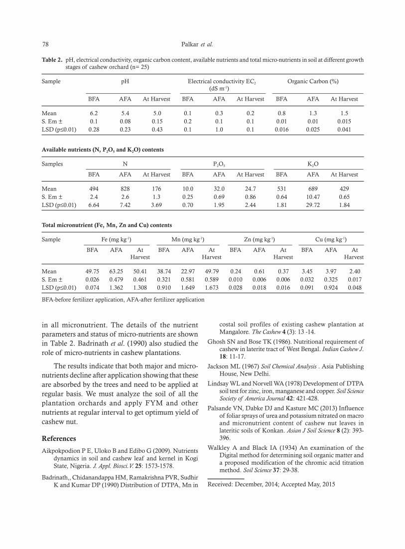
78 Palkar et al.

in all micronutrient. The details of the nutrientparameters and status of micro-nutrients are shownin Table 2. Badrinath et al. (1990) also studied therole of micro-nutrients in cashew plantations.

The results indicate that both major and micro-nutrients decline after application showing that theseare absorbed by the trees and need to be applied atregular basis. We must analyze the soil of all theplantation orchards and apply FYM and othernutrients at regular interval to get optimum yield ofcashew nut.

References

Aikpokpodion P E, Uloko B and Edibo G (2009). Nutrientsdynamics in soil and cashew leaf and kernel in KogiState, Nigeria. J. Appl. Biosci.V. 25: 1573-1578.

Badrinath,, Chidanandappa HM, Ramakrishna PVR, SudhirK and Kumar DP (1990) Distribution of DTPA, Mn in

Table 2. pH, electrical conductivity, organic carbon content, available nutrients and total micro-nutrients in soil at different growthstages of cashew orchard (n= 25)

Sample pH Electrical conductivity EC2 Organic Carbon (%)(dS m-1)

BFA AFA At Harvest BFA AFA At Harvest BFA AFA At Harvest

Mean 6.2 5.4 5.0 0.1 0.3 0.2 0.8 1.3 1.5S. Em ± 0.1 0.08 0.15 0.2 0.1 0.1 0.01 0.01 0.015LSD (p≤0.01) 0.28 0.23 0.43 0.1 1.0 0.1 0.016 0.025 0.041

Available nutrients (N, P2O5 and K2O) contents

Samples N P2O5 K2O

BFA AFA At Harvest BFA AFA At Harvest BFA AFA At Harvest

Mean 494 828 176 10.0 32.0 24.7 531 689 429S. Em ± 2.4 2.6 1.3 0.25 0.69 0.86 0.64 10.47 0.65LSD (p≤0.01) 6.64 7.42 3.69 0.70 1.95 2.44 1.81 29.72 1.84

Total micronutrient (Fe, Mn, Zn and Cu) contents

Sample Fe (mg kg-1) Mn (mg kg-1) Zn (mg kg-1) Cu (mg kg-1)

BFA AFA At BFA AFA At BFA AFA At BFA AFA AtHarvest Harvest Harvest Harvest

Mean 49.75 63.25 50.41 38.74 22.97 49.79 0.24 0.61 0.37 3.45 3.97 2.40S. Em ± 0.026 0.479 0.461 0.321 0.581 0.589 0.010 0.006 0.006 0.032 0.325 0.017LSD (p≤0.01) 0.074 1.362 1.308 0.910 1.649 1.673 0.028 0.018 0.016 0.091 0.924 0.048

BFA-before fertilizer application, AFA-after fertilizer application

costal soil profiles of existing cashew plantation atMangalore. The Cashew 4 (3): 13 -14.

Ghosh SN and Bose TK (1986). Nutritional requirement ofcashew in laterite tract of West Bengal. Indian Cashew J.18: 11-17.

Jackson ML (1967) Soil Chemical Analysis . Asia PublishingHouse, New Delhi.

Lindsay WL and Norvell WA (1978) Development of DTPAsoil test for zinc, iron, manganese and copper. Soil ScienceSociety of America Journal 42: 421-428.

Palsande VN, Dabke DJ and Kasture MC (2013) Influenceof foliar sprays of urea and potassium nitrated on macroand micronutrient content of cashew nut leaves inlateritic soils of Konkan. Asian J Soil Science 8 (2): 393-396.

Walkley A and Black IA (1934) An examination of theDigital method for determining soil organic matter anda proposed modification of the chromic acid titrationmethod. Soil Science 37: 29-38.

Received: December, 2014; Accepted May, 2015

Guidelines for authors for submitting manuscript for publication in the“Journal of Soil Salinity and Water Quality”

The authors are advised to follow the guidelines given in latest issue of journal for preparation of manuscript.The authors are required to submit one electronic copy in the form of CD or email (salinitysocietykarnal@gmail.com;pcsharma.knl@gmail.com) and one hard copy completed in all respects to General Secretary, Journal of Soil Salinityand Water Quality, Central Soil Salinity Research Institute, Kachhwa Road, Karnal-132001, Haryana, India. Thereceipt of manuscript as well as subsequent correspondences regarding the manuscript will be done electronicallyonly.

Manuscript

• The article should be as concise as possible. All the full length papers should comprise of Short title, Title,Author(s)’ name(s), Affiliations, email ID of corresponding author, Abstract, Key words, Introduction, Materialand Methods, Results and Discussion, Conclusions, Acknowledgement (if any), References, Tables and Figures(if any). The text under each section should throughout have 12 fonts in MSW, Times New Roman, justifiedwith 1.5 line spacing. However in the Abstract part, text should be 11 font with 1.5 line spacing and should notexceeds 250 words.

• The total length of article should not exceed 15 typed pages (2.5 cm. margin on each side of A4 paper) includingTables and Figures.

• All headings should be bold in capital letters with 12 fonts except Title which should be in Title Case and have 14fonts. However, the subheadings within each section wherever necessary should be in title case bold in 14 font,further headings should be in Sentence case and bold; whereas further sub-sub titles should be bold italic. Allmain and subheadings should be aligned left.

Title Page

It should be a separate page and comprise of following:

Short Title : It should have a short title (not exceeding five words in italics) on the top of right hand corner.

Title : It should not exceed 15 words and should reflect the contents of paper. It should be in title case like“Alleviation of Sodicity Stress on Rice Genotypes by Phosphorous Fertilization”.

Author(s) : Name of author(s) should be 12 font bold (without their official designations), aligned in center and inthe title case like “AK Aggarwal and MK Tiwari”.

Address : Each author’s name should have number as superscript to indicate the address. The correspondingauthor’s name should have number as superscript to indicate more than one address. The correspondingauthor’s name should have asterisk (*) mark as superscript e.g. AK Aggarwal*1 and MK Tiwari2. Theaddress should be written in italics as shown below:

*1 Central Soil Salinity Research Institute, Zarifa Farm, Kachhwa Road, Karnal-132001, Haryana, India

2 Indian Institute of Soil Science, Nabibagh,, Berasia Road, Bhopal-462038, Madhya Pradesh, India.

All addresses should be complete indicating state/ province, PIN/ postal code and country etc. Theemail ID of corresponding author should be given after the address. The total number of pages, tablesand figures of the manuscript should also be mentioned on title page.

First Page

Actual paging (on right lower corner) of the manuscript should start from this page. It should have full title ofpaper followed by Abstract, Keywords and Introduction, etc. To ensure anonymity of the author(s), author’s namesand addresses should not be indicated on this page.

Abstract : Its contents should be in 11 font, single space and single paragraph with justified alignment.

Key words : Key words should appear just after the abstract and to be written as key words (11 fonts). These may beup to 7 in alphabetic order each separated by a comma. The scientific names (if any) should be italicized.e.g.

Key words : Agroforestry model, Biodrainage, Gypsum, Oryza sativa L., Salt tolerance

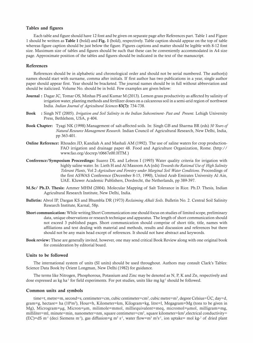
Tables and figures

Each table and figure should have 12 font and be given on separate page after References part. Table 1 and Figure1 should be written as Table 1 (bold) and Fig. 1 (bold), respectively. Table caption should appear on the top of tablewhereas figure caption should be just below the figure. Figures captions and matter should be legible with 8-12 fontsize. Maximum size of tables and figures should be such that these can be conveniently accommodated in A4 sizepage. Approximate position of the tables and figures should be indicated in the text of the manuscript.

References

References should be in alphabetic and chronological order and should not be serial numbered. The author(s)names should start with surname, comma after initials. If first author has two publications in a year, single authorpaper should appear first. Year should be bracketed. The journal names should be in full without abbreviation andshould be italicized. Volume No. should be in bold. Few examples are given below:

Journal : Dagar JC, Tomar OS, Minhas PS and Kumar M (2013). Lemon grass productivity as affected by salinity ofirrigation water, planting methods and fertilizer doses on a calcareous soil in a semi-arid region of northwestIndia. Indian Journal of Agricultural Sciences 83(7): 734-738.

Book : Singh NT (2005). Irrigation and Soil Salinity in the Indian Subcontinent- Past and Present. Lehigh UniversityPress, Bethlehem, USA, p 404.

Book Chapter: Tyagi NK (1998) Management of salt-affected soils. In: Singh GB and Sharma BR (eds) 50 Years ofNatural Resource Management Research. Indian Council of Agricultural Research, New Delhi, India,pp 363-401.

Online Reference: Rhoades JD, Kandiah A and Mashali AM (1992). The use of saline waters for crop production-FAO irrigation and drainage paper 48. Food and Agriculture Organization, Rome. (http://www.fao.org/docrep/t0667e00.HTM.)

Conference/Symposium Proceedings: Suarez DL and Lebron I (1993) Water quality criteria for irrigation withhighly saline water. In: Lieth H and Al Masoom AA (eds) Towards the Rational Use of High SalinityTolerant Plants, Vol 2-Agriculture and Forestry under Marginal Soil Water Conditions. Proceedings ofthe first ASWAS Conference (December 8-15, 1990), United Arab Emirates University Al Ain,UAE. Kluwer Academic Publishers, Dordrecht, the Netherlands, pp 389-397.

M.Sc/ Ph.D. Thesis: Ammer MHM (2004). Molecular Mapping of Salt Tolerance in Rice. Ph.D. Thesis, IndianAgricultural Research Institute, New Delhi, India.

Bulletin: Abrol IP, Dargan KS and Bhumbla DR (1973) Reclaiming Alkali Soils. Bulletin No. 2. Central Soil SalinityResearch Institute, Karnal, 58p.

Short communication: While writing Short Communication one should focus on studies of limited scope, preliminarydata, unique observations or research technique and apparatus. The length of short communication shouldnot exceed 3 published pages. Short communication should comprise of short title, title, names withaffiliations and text dealing with material and methods, results and discussion and references but thereshould not be any main head except of references. It should not have abstract and keywords.

Book review: These are generally invited, however, one may send critical Book Review along with one original bookfor consideration by editorial board.

Units to be followed

The international system of units (SI units) should be used throughout. Authors may consult Clark’s Tables:Science Data Book by Orient Longman, New Delhi (1982) for guidance.

The terms like Nitrogen, Phosphorous, Potassium and Zinc may be denoted as N, P, K and Zn, respectively anddose expressed as kg ha-1 for field experiments. For pot studies, units like mg kg-1 should be followed.

Common units and symbols

time=t, metre=m, second=s, centimeter=cm, cubic centimeter=cm3, cubic metre=m3, degree Celsius=ÚC, day=d,gram=g, hectare= ha (104m2), Hour=h, Kilometer=km, Kilogram=kg, litre=l, Megagram=Mg (tons to be given inMg), Microgram=µg, Micron=µm, milimole=mmol, milliequivalent=meq, micromol=µmol, milligram=mg,milliliter=ml, minute=min, nanometer=nm, square centimeter=cm2, square kilometer=km2,electrical conductivity=(EC)=dS m-1 (deci Siemens m-1), gas diffusion=g m2 s-1, water flow=m3 m2s-1, ion uptake= mol kg-1 of dried plant

material, leaf area=m2kg-1, nutrient content in plants= mg g-1 (dry matter basis), root density or root length density=m m-3, soil bulk density= g cm-3, transpiration rate=mg m2 s-1, water content of soil=kg kg-1, water tension=kPa, yield(grain or forage)= Mg ha-1, organic carbon content of soil= percent (%), cation exchange capacity of soil= cmol (p+)kg-1

Style Guidelines

All soils discussed in the manuscript should be identified according to the U.S Soil Taxonomic System at firstmention. The Latin binomial or trinomial and authority must be must be shown for all plants, insects, pathogens,microorganisms and animals when first mentioned. Both the accepted common name and the chemical name of anychemicals mentioned (including pesticides) must be provided. SI units must be used throughout the manuscript.Corresponding metric or English units may be added in parentheses at the discretion of the author. For spelling,Webster’s New Collegiate Dictionary should be used as reference. If a commonly available product is mentioned, thename and the location of manufacturer should be included in parentheses after first mention. Responsibility of thefacts and opinions expressed in the articles rests entirely with the author(s) and not with the journal.

Form IV

1 Place of Publication Karnal

2 Periodicity of its Publication Twice in a year

3 Printer’s Name M/s Cambridge Printing Works

Nationality Indian

Address B-85, Phase - IINaraina Industrial AreaNew Delhi - 110 028

4 Publisher’s Name Dr PC Sharma

Nationality Indian

Address ICAR-Central Soil Salinity Research InstituteZarif Farm, Kachhwa RoadKarnal – 132 001 (Haryana), India

5 Chief Editor’s Name Dr JC Dagar

Nationality Indian

Address ICAR-Central Soil Salinity Research InstituteZarif Farm, Kachhwa Road, Karnal – 132 001(Haryana), India

6 Name and Address of Individuals, General Secretarywho own the Journal and Partners or Indian Society of Soil Salinity and Water Qualityshare holders holding more than onepercent of the total Registered Office:

ICAR-Central Soil Salinity Research InstituteZarif Farm, Kachhwa Road, Karnal – 132 001(Haryana), India

I, Dr PC Sharma, hereby declare that the particulars given above are true to the best of my knowledgeand belief.

Sd/-PC SHARMA

General SecretaryIndian Society of Soil Salinity and Water Quality