


Bahasa
Halaman
Hukum


12TH INTERNATIONAL SYMPOSIUM ON FLOW VISUALIZATIONSeptember 10-14 2006 German Aerospace Center (DLR) Goumlttingen Germany
INVESTIGATIONS OF TURBULENCE STATISTICS IN THE LABORATORY MODEL OF AN ATMOSPHERIC
CLOUD
P M KorczykT A Kowalewski S P Malinowski IPPT PAN Department of Mechanics amp Physics of Fluids Warszawa Poland
Warsaw University Institute of Geophysics Warszawa Poland
Keywords PIV warm rain droplets coalescence particle-turbulence interactions
ABSTRACT
Mixing of air containing small water droplets is investigated in the laboratory model to elucidate smallest scales of air entrainment and mixing in real clouds Particle Image Velocimetry (PIV) is applied to evaluate turbulent characteristics of the flow field generated in the cloud chamber by buoyancy of the introduced mist It permits to investigate dynamics of the process for scales from 007 mm to few centimeters characteristic for a real cloud microphysics Three velocity components retrieved in the vertical cross-section through the chamber interior indicate anisotropy of small-scale turbulent motions with the preferred vertical direction This result confirms earlier numerical studies indicating that evaporation of cloud droplets at the cloud-clear air interface may substantially influence the small-scale turbulence in clouds
1 INTRODUCTIONThe so called ldquowarm rain initiation problemrdquo attracts attention of cloud physicists turbulence researchers engineers and meteorologists It is still uncertain which mechanism is responsible for the formation of drizzle and rain (precipitation) drops Papers concerning the impact of high-Reynolds-number turbulence on spatial distribution of cloud droplets their diffusional growth collisions and coalescence are published at high rate Our understanding of particle motion in turbulent flows is based on both theoretical and experimental studies [1] [2] [3] In particular these works show that small-scale turbulence ie with spatial scales comparable with the Kolmogorov length scale may influence the spatial distribution of droplets and yield non-Poisson statistics Due to the inertia the relative velocity between falling droplets depends not only on their terminal velocity and collision efficiency increases As a consequence particles tend to diverge out of regions of high vorticity nad converge preferentially in regions of low vorticity Regions of much higher and lower concentration than predicted from Poisson spatial distribution can develop Direct visual evidence of preferential concentration has been obtained in several laboratory experiments even for very slow convective flow of viscous liquid in a cube-shaped cavity [4] On the other hand droplets can mechanically and thermodynamically (latent heat release) influence the small-scale flow in a complex manner The flow in regions of mixing may not be isotropic because of the negative buoyancy produced by droplet evaporation Hence it is expected that the -53 power law observed in cumulus clouds at scales between 15 and 200 m also extends down to the smaller scales in the cloud core [5]
Unfortunately due to the experimental constrains properties of the cloud turbulence at scales relevant for the interactions between droplets and the air flow have never been documented Recently Siebert et al [6] were able to study turbulent velocities at scales down to 20 cm Such a scale is still
1
P M Korczyk T A Kowalewski S P Malinowski
about two orders of magnitude larger than a typical distance between cloud droplets which coincidentally is also the Kolmogorov microscale for typical levels of cloud turbulence It follows that far-reaching assumptions have to be made in order to study interaction between cloud dynamics thermodynamics and microphysics Usually it is assumed that cloud turbulence is generated at large scales (100m or more) and it cascades through the inertial range of turbulent eddies down to the Kolmogorov microscale where it is dissipated At the smallest scales turbulent velocities are usually assumed to be isotropic and they are described by statistical distributions based on laboratorywind tunnelatmospheric boundary layer measurements or direct numerical simulation (DNS) It is also assumed that temperature and humidity are passive scalars ie they do not influence small-scale dynamics through the buoyancy effects [7] [8] [9] In the following we show that these assumptions are not always fulfilled We present laboratory cloud chamber experiments with turbulent mixing between cloudy air and unsaturated clear air at scales down to a fraction of a centimeter It appears that at these scales turbulence is substantially anisotropic due to the action of buoyancy forces resulting from evaporation of cloud droplets Recently several attempts to simulate directly the interface microscale mixing are reported [10] [11] [12] DNS simulations performed to mimic laboratory experiment reported by Malinowski et al [13] evidently confirm that buoyancy forces resulting from evaporation may substantially modify smallest scale of turbulence
2 EXPERIMENT
21 Experimental setup
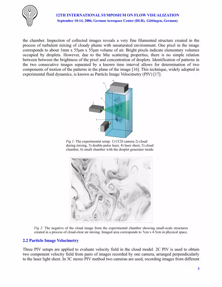
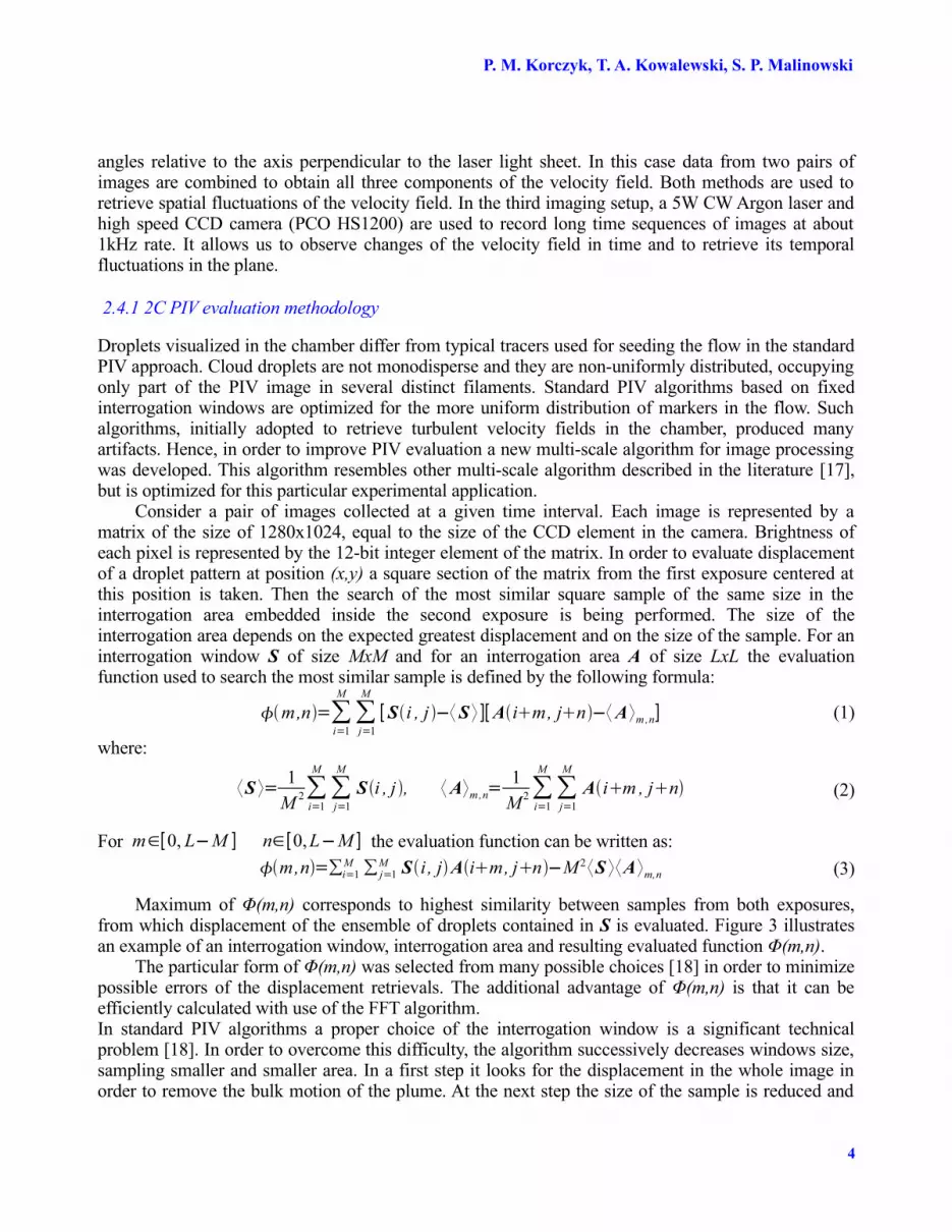
In the following experiment we adopt cloud chamber previously constructed to analyze spatial distribution of droplets [14] [15] The flow of water mist is generated in a glass-walled chamber of size 1x1x18m3 (Fig 1) On the top of this chamber a smaller box is located This box is filled with the water mist using standard ultrasound humidifier Liquid water content increases density of the mixture collected in the upper box Once the box is completely saturated with the mixture a circular opening of 10cm diameter connecting it with the cloud chamber is abruptly unblocked The cloudy plume of the small negative buoyancy smoothly enters the chamber with the velocity of approximately 10 cm s-1 The plum interacts with a quiescent air stimulating turbulent mixing of cloud droplets with the unsaturated air It descends slowly when mixing with the environment forming turbulent filaments of dry and cloudy air This process is visualized in the planar cross-section of the chamber using the laser light sheet technique (comp Fig 2) For this purpose tandem of two pulsed lasers (NdYag wavelength 532nm) is used It permits to illuminate interior of the chamber with pairs of 5ns light pulses of 36mJ energy and repetition rate of 12Hz An optical system with cylindrical lenses provides 1-mm thick light sheet of about 15cm width Images of the cloud are observed from the perpendicular direction For the recording one or two high resolution CCD cameras (PCO Sensi-Cam) are used in conjunction with a PC Pentium 4HT computer and a frame grabber The system allows for storing up to 200 pairs of 1280x1024pixels 12bit images in the computer RAM at a rate of 45Hz The time interval between two laser pulses can be adjusted from minimum delay of 200ns in order to select the appropriate delay between the images Usually for typical experiments it is of order of 1ms During experimental runs separate equipment is used to continuously monitor temperature in the filling box and in the cloud chamber (4 measuring points) Atmospheric air pressure temperature and humidity are monitored as well Liquid water content and droplets size distribution is estimated by taking samples of the mixture during separate control experiments A typical image (negative) of the cloud observed in the chamber is presented in Fig 2 The image area covers about 7x45cm2 in the center of
2
12TH INTERNATIONAL SYMPOSIUM ON FLOW VISUALIZATIONSeptember 10-14 2006 German Aerospace Center (DLR) Goumlttingen Germany
the chamber Inspection of collected images reveals a very fine filamented structure created in the process of turbulent mixing of cloudy plume with unsaturated environment One pixel in the image corresponds to about 1mm x 55μm x 55μm volume of air Bright pixels indicate elementary volumes occupied by droplets However due to the Mie scattering properties there is no simple relation between between the brightness of the pixel and concentration of droplets Identification of patterns in the two consecutive images separated by a known time interval allows for determination of two components of motion of the patterns in the plane of the image [16] This technique widely adopted in experimental fluid dynamics is known as Particle Image Velocimetry (PIV) [17]
Fig 1 The experimental setup 1) CCD camera 2) cloud during mixing 3) double-pulse laser 4) laser sheet 5) cloud chamber 6) small chamber with the droplet generator inside
Fig 2 The negative of the cloud image from the experimental chamber showing small-scale structures created in a process of cloud-clear air mixing Imaged area corresponds to 7cm x 45cm in physical space
22 Particle Image Velocimetry
Three PIV setups are applied to evaluate velocity field in the cloud model 2C PIV is used to obtain two component velocity field from pairs of images recorded by one camera arranged perpendicularly to the laser light sheet In 3C stereo PIV method two cameras are used recording images from different
3
P M Korczyk T A Kowalewski S P Malinowski
angles relative to the axis perpendicular to the laser light sheet In this case data from two pairs of images are combined to obtain all three components of the velocity field Both methods are used to retrieve spatial fluctuations of the velocity field In the third imaging setup a 5W CW Argon laser and high speed CCD camera (PCO HS1200) are used to record long time sequences of images at about 1kHz rate It allows us to observe changes of the velocity field in time and to retrieve its temporal fluctuations in the plane
241 2C PIV evaluation methodology
Droplets visualized in the chamber differ from typical tracers used for seeding the flow in the standard PIV approach Cloud droplets are not monodisperse and they are non-uniformly distributed occupying only part of the PIV image in several distinct filaments Standard PIV algorithms based on fixed interrogation windows are optimized for the more uniform distribution of markers in the flow Such algorithms initially adopted to retrieve turbulent velocity fields in the chamber produced many artifacts Hence in order to improve PIV evaluation a new multi-scale algorithm for image processing was developed This algorithm resembles other multi-scale algorithm described in the literature [17] but is optimized for this particular experimental application
Consider a pair of images collected at a given time interval Each image is represented by a matrix of the size of 1280x1024 equal to the size of the CCD element in the camera Brightness of each pixel is represented by the 12-bit integer element of the matrix In order to evaluate displacement of a droplet pattern at position (xy) a square section of the matrix from the first exposure centered at this position is taken Then the search of the most similar square sample of the same size in the interrogation area embedded inside the second exposure is being performed The size of the interrogation area depends on the expected greatest displacement and on the size of the sample For an interrogation window S of size MxM and for an interrogation area A of size LxL the evaluation function used to search the most similar sample is defined by the following formula
mn=sumi=1
M
sumj=1
M
[ Si j minuslang S rang ][Aim jnminuslangArangmn] (1)
where
langS rang= 1
M 2sumi=1
M
sumj=1
M
Si j
langArangmn=1
M 2sumi=1
M
sumj=1
M
Aim jn (2)
For misin[0 LminusM ] nisin[0 LminusM ] the evaluation function can be written as
mn=sumi=1M sum j=1
M Si jAim jnminusM 2langS ranglangArangmn (3)
Maximum of Φ(mn) corresponds to highest similarity between samples from both exposures from which displacement of the ensemble of droplets contained in S is evaluated Figure 3 illustrates an example of an interrogation window interrogation area and resulting evaluated function Φ(mn)
The particular form of Φ(mn) was selected from many possible choices [18] in order to minimize possible errors of the displacement retrievals The additional advantage of Φ(mn) is that it can be efficiently calculated with use of the FFT algorithmIn standard PIV algorithms a proper choice of the interrogation window is a significant technical problem [18] In order to overcome this difficulty the algorithm successively decreases windows size sampling smaller and smaller area In a first step it looks for the displacement in the whole image in order to remove the bulk motion of the plume At the next step the size of the sample is reduced and
4
12TH INTERNATIONAL SYMPOSIUM ON FLOW VISUALIZATIONSeptember 10-14 2006 German Aerospace Center (DLR) Goumlttingen Germany
the displacement vector evaluated earlier determines the position of the interrogation area In this way the displacement is corrected This algorithm is repeated few times with the decreasing size of the sample giving successive corrections for the velocity in smaller and smaller scales After such sequence of operations two components of turbulent velocity are evaluated for small patterns In addition to improve accuracy in presence of high gradients of velocities and pixels brightness variations at each iteration image deformations algorithm is applied This technique is widely used for adopting interrogation widows to local velocity gradients [19] Here calculated velocity field is used to deform the whole first image from the pair After that it becomes more similar to the second image and in the next step the field of displacement is evaluated for a pair consisting of the first deformed image and the second original one In such a way the correction of the field of displacement from the previous step can be evaluated This procedure is repeated several times until the subsequent corrections are efficiently small
(a) (b)
Fig 3 (a) - An example of image section S (40times40 pixels) for the first exposure and the corresponding interrogation area A (100times100 pixels) of the second exposure extracted from the pair of images The most similar part is highlighted (b) - an example of the evaluation function Φ(mn) obtained for the experimental data presented in (a)
The obvious limitation of the method is that the retrieved velocity field is limited to the cloudy part of the imaged flow In the regions with the clear air we do not have information of the turbulent motion A suitable mask has been created for each scene to depict areas without droplets This mask has been applied to further statistical analysis of the data It should be remembered that results given below represent only those parts of the volume where concentration of droplets is sufficient to perform our PIV analysis It must be underlined that application of the PIV technique to the cloud droplets which due to inertia and gravity may move with respect to the airflow causes problem in the interpretation With the presented approach we do not detect the velocity of the air but velocity of droplet patterns conveyed by the flow
241 Stereo PIV evaluation
The stereo PIV system applied consists of two cameras observing the same area of the flow simultaneously Each camera view the object from different angle hence stereoscopic conditions are obtained Stereo PIV is applied to retrieve all three velocity components for the plane defined by the laser light sheet In our case two different 3C-PIV evaluation software were used The first one is
5
S
A
P M Korczyk T A Kowalewski S P Malinowski
commercial package VidPIV developed by GmbH ILA (Germany httpwwwilade) For the stereo system calibration it uses a special target consisting of several rows of precise markers placed on two parallel plates The perspective properties of stereoscopic projection of images is reconstructed using known information about positions of markers in real 3D space and positions of the same markers on 2D plane of image The second 3C-PIV system applied is based on the Optical Flow methodology [20] extended to stereo images The new 3C software developed by George Quenote uses only one calibration target and known geometry of the optical system It automatically finds the target markers and evaluates calibration matrix necessary for further reconstruction of tracers displacement
23 Droplets spectrum and liquid water content
In additional experimental runs droplets in the cloud plume are collected on the oil film covering microscopic glass sheet and immediately thereafter photographed with a CCD camera under the microscope In order to estimate the droplets spectrum the software recognizing droplets in images and calculating their radius is applied Fig 4 shows result of the droplets size evaluation obtained from about 20 measurements It clearly indicates non-uniformity of the cloud droplets size with a characteristic double-peak shape Accuracy of droplet diameter measurements is quite good (3 error) However it must be mentioned that despite short time (~10s) of a single measurement we cannot exclude possible bias in droplets size due to the evaporation of the droplets on the microscope slit
Fig 4 Spectrum of droplets
Initial liquid water content (the ratio of mass of liquid water containing certain portion of air to the mass of this portion) of cloudy air is estimated in additional experiment Well defined 10 liter sample of saturated cloudy air entering main chamber is gravitationally sucked into a container During this operation sucked air-water mixture passes through a cotton wool filter were droplets are trapped Weight of the filter before and after the experiment allows us to evaluate mass of water droplets being sucked with the given portion of air It was found that liquid water content in our experiments is typically about 20gkg
3 RESULTS
31 Energy dissipation rate and Kolmogorov length
The Kolmogorov phenomenological theory [21] formulated for fully developed homogeneous turbulence appeared in several experimental studied to work well for small scales typical for laboratory models The two dimensional velocity fields obtained from the PIV measurements in the
6
12TH INTERNATIONAL SYMPOSIUM ON FLOW VISUALIZATIONSeptember 10-14 2006 German Aerospace Center (DLR) Goumlttingen Germany
cloud chamber give us possibility to estimate the Kolmogorov length (4) It is found that it varies in the narrow range form about 72 10-4 m to 78 10-4 m The mean value of the Kolmogorov length obtained during our laboratory experiments is 7610-4m It is typical for cumulus clouds in presence of weak convection [22] It is interesting to note that the Kolmogorov length appears to depend on the relative humidity of air ie initial humidity measured in the chamber before the plum with droplets is introduced
Kolmogorov length = 3
1 4
- where ν is viscosity and ε is energy dissipation rate (4)
Fig 5 Experimental value of Kolmogorov length as a function of relative humidity Each of charts corresponds to another experimental runFigure 5 presents variation of the evaluated Kolmogorov length in time for three different independent experimental runs During each of these runs initial relative humidity inside the main chamber is increased It becomes evident that the Kolmogorov length is systematically decreasing with the relative humidity indicating that properties of the small scale turbulence may depend on efficiency of the droplets evaporation
32 Statistics of velocity field
Three series of experiments with slightly varying thermodynamical conditions inside the chamber are performed In each series at least 500 pairs of frames (tens of thousands of vectors in each frame) are evaluated in order to retrieve properties of turbulent velocity fluctuations Our analysis of stereo PIV data indicates that in horizontal plane velocity fluctuations are isotropic Hence in the following one horizontal component is presented Combined statistics of turbulent velocity fluctuations in horizontal
7
P M Korczyk T A Kowalewski S P Malinowski
(u) and vertical (w) directions are displayed in Fig 6 and summarized in Table 1 Here customary definition of standard deviation skewness and kurtosis are used
u=langu 2rang Su=langu 3rang u
3 K u=
langu 4rangu
4 (5)
Fig 6 Distribution of horizontal (red) and vertical (blue) turbulent velocity fluctuations from three series of measurements
TABLE 1 Distribution of horizontal (u) and vertical (w) turbulent velocity fluctuations for the experimental data shown in Fig 6
Standard deviation [cms] Skewness Kurtosis
u 54 -001 32
w 80 -02 31
It is evident that the distribution of the vertical velocity fluctuations characterizes larger dispersion and it has longer tails than the distribution of horizontal velocity fluctuations Calculated skewness and kurtosis indicate that both distributions are close to the Gaussian (normal) These results has been used to validate recent direct numerical simulations performed for similar conditions by Malinowski et al [13] It confirms strong influence of the buoyancy forces on the developed of turbulent fluctuations
33 Structure functions
In order to evaluate the persistence of the turbulence the second order structure function was calculated for the velocity flow in the small section of the cloud chamber evaluating solely area covered by the imaging system (7cm x 45cm) The second order structure function appears useful to discriminate viscous and inertial range of the turbulent flow [23] [24] The second order longitudinal structure function is a mean velocity increment between two points separated by l projected onto the line of separation Hence we can introduce structure function for both x and z direction and obtain its variation for horizontal and vertical velocity components u w
8
12TH INTERNATIONAL SYMPOSIUM ON FLOW VISUALIZATIONSeptember 10-14 2006 German Aerospace Center (DLR) Goumlttingen Germany
S u⋳ l =lang[u xl z minusu x z]2rang
Sw⋳ l =lang[w x zl minusw x z ]2rang
(6)
Fig 7 Second order longitudinal structure functions shown in log-log scale Red solid line ndash vertical components Blue dashed line ndash horizontal component Straight lines indicate initial slope exponent (l2) and asymptotic slope exponent (l23)
Figure 7 clearly shows different behavior of the structure function for vertical and horizontal velocity components Whereas initially both structure functions follow l2 slope characteristic for the dissipation range at larger separations the inertial range l23 behavior can be observed for the vertical velocity only It indicates already mentioned anisotropy of the velocity field structures present for all scales observed in the laboratory experiments
CONCLUSIONSSmall scale mixing of cloud with unsaturated environment is investigated in laboratory cloud chamber by means of Particle Image Velocimetry (PIV) The high spatial resolution of the experimental setup (007mm) allowed us to evaluate statistics of the turbulent flow field down to the Kolmogorov length The results indicate that small-scale turbulence in such conditions is highly anisotropic with the preferred vertical direction The present investigation indicates also that properties of turbulence in small scales is sensitive to the initial air humidity Hence obviously buoyancy forces resulting from evaporation of cloud droplets substantially influence smallest scales of turbulence Typically lt(u)2gt is about two times smaller than lt(w)2gt The probability distribution functions of w are broader than those of u These results have been successfully used to validate numerical simulations (DNS) performed for a similar experimental configuration [13] However it is still uncertain to what extent infromation gained in the laboratory cloud can be applied to atmospheric systems Hence in situ measurements of turbulent velocity fluctuations from various types of clouds are necessary to validate common assumptions on small-scale cloud isotropy
9
P M Korczyk T A Kowalewski S P Malinowski
ACKNOWLEDGMENTSThis research was supported by the Polish Committee for Scientific Research and PIVNET2 Thematic Network
REFERENCES
1 Falkovich G Gawedzki K and Vergassola M Particles and fields in fluid turbulence Rev Modern Phys Vol 73 pp 913-975 2001
2 Shaw RA Particle-turbulence interactions in atmospheric clouds Annual Review of Fluid Mechanics Vol 35 pp 183-227 2003
3 Ghosh S Davila J Hunt JCR Srdic A Fernando HJS Jonas PR How turbulence enhances coalescence of settling particles with applications to rain in clouds Proc R Soc A Vol 461 pp 3059-3088 2005
4 Yarin A Kowalewski T A Hiller WJ Koch S Distribution of particles suspended in 3D laminar convection flow Physics of Fluids Vol 8 pp 1130-1140 1996
5 Vaillancourt PA Yau MK Review of particle-turbulence interactions and consequences for cloud physics Bull Am Meteorol Soc Vol 81 pp 285ndash98 2000
6 Siebert H Lehmann K and Wendish M Observations of small-scale turbulence and energy dissipation rates in the cloud boundary layer J Atmos Sci Vol 63 pp 1451-1466 2006
7 Pinsky M and Khain AP Turbulence effects on the collision kernel Part 1 Formation of velocity deviations of drops falling within a turbulent three-dimensional flow Quart J Roy Meteor Soc Vol 123 pp 1517-1542 1997
8 Shaw RA Walter CR Lance RC and Johannes V Preferential concentration of cloud droplets by turbulence Effects on the early evolution of cumulus cloud droplet spectra J Atmos Sci Vol 55 pp 1965-1976 1998
9 Shaw RA and Oncley S P Acceleration intermittency and enhanced collision kernels in turbulent clouds Atmos Res Vol 59-60 pp 77-87 2001
10 Vaillancourt PA Yau MK and Bartello P Grabowski WW Microscopic Approach to Cloud Droplet Growth by Condensation Part II Turbulence Clustering and Condensational Growth J Atmos Sc Vol 59 pp 3421ndash3435 2002
11 Grabowski WW MJO-like coherent structures Sensitivity simulations using theCloud-Resolving Convection Parameterization (CRCP) J Atmos Sci Vol 60 pp 847ndash864 2003
12 Andrejczuk M Grabowski W Malinowski SP and Smolarkiewicz PK Numerical Simulation of Cloud-Clear Air Interfacial Mixing J Atmos Sci Vol 61 pp 1726ndash1739 2004
13 Malinowski SP and Andrejczuk M Grabowski WW Korczyk P Kowalewski TA and Smolarkiewicz PK Cloud-clear air interfacial mixing anisotropy of turbulence generated by evaporation of liquid water Laboratory observations and numerical modeling 12th Conference on Cloud Physics Madison (WI USA) 2006
14 Malinowski SP Zawadzki I and Banat P Laboratory observations of cloud-clear air mixing in small scales J Atmos Oceanic Technol Vol 15 pp 1060-1065 1998
15 Jaczewski A Malinowski SP Spatial distribution of cloud droplets in a turbulent cloud-chamber flow Quart J Roy Meteor Soc Vol 131 pp 2047-2062 2005
16 Korczyk P Malinowski SP Kowalewski TA Mixing of cloud and clear air in centimeter scales observed in laboratory by means of particle image velocimetry Atmos Res (in press) 2006
17 Raffel M Willert ChE and Kompenhans J Particle image velocimetry a practical guide 3rd edition Springer 1998
18 Gui L W Merzkirch Generating arbitrarily sized interrogation windows for correlation-based analysis of particle image velocimetry recordings Exp Fluids Vol 24 pp 66-69 1998
19 Scarano F Iterative image deformation methods in PIV Meas Sci Technol Vol 13 pp R1-R19 2002
20 Quenote G Pakleza J Kowalewski TA Particle Image Velocimetry with Optical Flow Experiments in Fluids Vol 25 pp 177-189 1998
21 Kolmogorow AN Dissipation of energy under locally isotropic turbulence CR Acad Sci USSR Vol 32 pp 16-18 1941
22 Pruppacher HR Klett JD Microphysics of clouds and precipitation 1st edition Kluwer 1997
23 Frish U Turbulence - The legacy of A N Kolmogorov 1st edition Cambridge University Press 1995
24 Batchelor GK Pressure fluctuations in isotropic turbulence Proc Cambridge Phil Soc Vol 47 pp 533-559 1951
10

P M Korczyk T A Kowalewski S P Malinowski
about two orders of magnitude larger than a typical distance between cloud droplets which coincidentally is also the Kolmogorov microscale for typical levels of cloud turbulence It follows that far-reaching assumptions have to be made in order to study interaction between cloud dynamics thermodynamics and microphysics Usually it is assumed that cloud turbulence is generated at large scales (100m or more) and it cascades through the inertial range of turbulent eddies down to the Kolmogorov microscale where it is dissipated At the smallest scales turbulent velocities are usually assumed to be isotropic and they are described by statistical distributions based on laboratorywind tunnelatmospheric boundary layer measurements or direct numerical simulation (DNS) It is also assumed that temperature and humidity are passive scalars ie they do not influence small-scale dynamics through the buoyancy effects [7] [8] [9] In the following we show that these assumptions are not always fulfilled We present laboratory cloud chamber experiments with turbulent mixing between cloudy air and unsaturated clear air at scales down to a fraction of a centimeter It appears that at these scales turbulence is substantially anisotropic due to the action of buoyancy forces resulting from evaporation of cloud droplets Recently several attempts to simulate directly the interface microscale mixing are reported [10] [11] [12] DNS simulations performed to mimic laboratory experiment reported by Malinowski et al [13] evidently confirm that buoyancy forces resulting from evaporation may substantially modify smallest scale of turbulence
2 EXPERIMENT
21 Experimental setup
In the following experiment we adopt cloud chamber previously constructed to analyze spatial distribution of droplets [14] [15] The flow of water mist is generated in a glass-walled chamber of size 1x1x18m3 (Fig 1) On the top of this chamber a smaller box is located This box is filled with the water mist using standard ultrasound humidifier Liquid water content increases density of the mixture collected in the upper box Once the box is completely saturated with the mixture a circular opening of 10cm diameter connecting it with the cloud chamber is abruptly unblocked The cloudy plume of the small negative buoyancy smoothly enters the chamber with the velocity of approximately 10 cm s-1 The plum interacts with a quiescent air stimulating turbulent mixing of cloud droplets with the unsaturated air It descends slowly when mixing with the environment forming turbulent filaments of dry and cloudy air This process is visualized in the planar cross-section of the chamber using the laser light sheet technique (comp Fig 2) For this purpose tandem of two pulsed lasers (NdYag wavelength 532nm) is used It permits to illuminate interior of the chamber with pairs of 5ns light pulses of 36mJ energy and repetition rate of 12Hz An optical system with cylindrical lenses provides 1-mm thick light sheet of about 15cm width Images of the cloud are observed from the perpendicular direction For the recording one or two high resolution CCD cameras (PCO Sensi-Cam) are used in conjunction with a PC Pentium 4HT computer and a frame grabber The system allows for storing up to 200 pairs of 1280x1024pixels 12bit images in the computer RAM at a rate of 45Hz The time interval between two laser pulses can be adjusted from minimum delay of 200ns in order to select the appropriate delay between the images Usually for typical experiments it is of order of 1ms During experimental runs separate equipment is used to continuously monitor temperature in the filling box and in the cloud chamber (4 measuring points) Atmospheric air pressure temperature and humidity are monitored as well Liquid water content and droplets size distribution is estimated by taking samples of the mixture during separate control experiments A typical image (negative) of the cloud observed in the chamber is presented in Fig 2 The image area covers about 7x45cm2 in the center of
2
12TH INTERNATIONAL SYMPOSIUM ON FLOW VISUALIZATIONSeptember 10-14 2006 German Aerospace Center (DLR) Goumlttingen Germany
the chamber Inspection of collected images reveals a very fine filamented structure created in the process of turbulent mixing of cloudy plume with unsaturated environment One pixel in the image corresponds to about 1mm x 55μm x 55μm volume of air Bright pixels indicate elementary volumes occupied by droplets However due to the Mie scattering properties there is no simple relation between between the brightness of the pixel and concentration of droplets Identification of patterns in the two consecutive images separated by a known time interval allows for determination of two components of motion of the patterns in the plane of the image [16] This technique widely adopted in experimental fluid dynamics is known as Particle Image Velocimetry (PIV) [17]
Fig 1 The experimental setup 1) CCD camera 2) cloud during mixing 3) double-pulse laser 4) laser sheet 5) cloud chamber 6) small chamber with the droplet generator inside
Fig 2 The negative of the cloud image from the experimental chamber showing small-scale structures created in a process of cloud-clear air mixing Imaged area corresponds to 7cm x 45cm in physical space
22 Particle Image Velocimetry
Three PIV setups are applied to evaluate velocity field in the cloud model 2C PIV is used to obtain two component velocity field from pairs of images recorded by one camera arranged perpendicularly to the laser light sheet In 3C stereo PIV method two cameras are used recording images from different
3
P M Korczyk T A Kowalewski S P Malinowski
angles relative to the axis perpendicular to the laser light sheet In this case data from two pairs of images are combined to obtain all three components of the velocity field Both methods are used to retrieve spatial fluctuations of the velocity field In the third imaging setup a 5W CW Argon laser and high speed CCD camera (PCO HS1200) are used to record long time sequences of images at about 1kHz rate It allows us to observe changes of the velocity field in time and to retrieve its temporal fluctuations in the plane
241 2C PIV evaluation methodology
Droplets visualized in the chamber differ from typical tracers used for seeding the flow in the standard PIV approach Cloud droplets are not monodisperse and they are non-uniformly distributed occupying only part of the PIV image in several distinct filaments Standard PIV algorithms based on fixed interrogation windows are optimized for the more uniform distribution of markers in the flow Such algorithms initially adopted to retrieve turbulent velocity fields in the chamber produced many artifacts Hence in order to improve PIV evaluation a new multi-scale algorithm for image processing was developed This algorithm resembles other multi-scale algorithm described in the literature [17] but is optimized for this particular experimental application
Consider a pair of images collected at a given time interval Each image is represented by a matrix of the size of 1280x1024 equal to the size of the CCD element in the camera Brightness of each pixel is represented by the 12-bit integer element of the matrix In order to evaluate displacement of a droplet pattern at position (xy) a square section of the matrix from the first exposure centered at this position is taken Then the search of the most similar square sample of the same size in the interrogation area embedded inside the second exposure is being performed The size of the interrogation area depends on the expected greatest displacement and on the size of the sample For an interrogation window S of size MxM and for an interrogation area A of size LxL the evaluation function used to search the most similar sample is defined by the following formula
mn=sumi=1
M
sumj=1
M
[ Si j minuslang S rang ][Aim jnminuslangArangmn] (1)
where
langS rang= 1
M 2sumi=1
M
sumj=1
M
Si j
langArangmn=1
M 2sumi=1
M
sumj=1
M
Aim jn (2)
For misin[0 LminusM ] nisin[0 LminusM ] the evaluation function can be written as
mn=sumi=1M sum j=1
M Si jAim jnminusM 2langS ranglangArangmn (3)
Maximum of Φ(mn) corresponds to highest similarity between samples from both exposures from which displacement of the ensemble of droplets contained in S is evaluated Figure 3 illustrates an example of an interrogation window interrogation area and resulting evaluated function Φ(mn)
The particular form of Φ(mn) was selected from many possible choices [18] in order to minimize possible errors of the displacement retrievals The additional advantage of Φ(mn) is that it can be efficiently calculated with use of the FFT algorithmIn standard PIV algorithms a proper choice of the interrogation window is a significant technical problem [18] In order to overcome this difficulty the algorithm successively decreases windows size sampling smaller and smaller area In a first step it looks for the displacement in the whole image in order to remove the bulk motion of the plume At the next step the size of the sample is reduced and
4
12TH INTERNATIONAL SYMPOSIUM ON FLOW VISUALIZATIONSeptember 10-14 2006 German Aerospace Center (DLR) Goumlttingen Germany
the displacement vector evaluated earlier determines the position of the interrogation area In this way the displacement is corrected This algorithm is repeated few times with the decreasing size of the sample giving successive corrections for the velocity in smaller and smaller scales After such sequence of operations two components of turbulent velocity are evaluated for small patterns In addition to improve accuracy in presence of high gradients of velocities and pixels brightness variations at each iteration image deformations algorithm is applied This technique is widely used for adopting interrogation widows to local velocity gradients [19] Here calculated velocity field is used to deform the whole first image from the pair After that it becomes more similar to the second image and in the next step the field of displacement is evaluated for a pair consisting of the first deformed image and the second original one In such a way the correction of the field of displacement from the previous step can be evaluated This procedure is repeated several times until the subsequent corrections are efficiently small
(a) (b)
Fig 3 (a) - An example of image section S (40times40 pixels) for the first exposure and the corresponding interrogation area A (100times100 pixels) of the second exposure extracted from the pair of images The most similar part is highlighted (b) - an example of the evaluation function Φ(mn) obtained for the experimental data presented in (a)
The obvious limitation of the method is that the retrieved velocity field is limited to the cloudy part of the imaged flow In the regions with the clear air we do not have information of the turbulent motion A suitable mask has been created for each scene to depict areas without droplets This mask has been applied to further statistical analysis of the data It should be remembered that results given below represent only those parts of the volume where concentration of droplets is sufficient to perform our PIV analysis It must be underlined that application of the PIV technique to the cloud droplets which due to inertia and gravity may move with respect to the airflow causes problem in the interpretation With the presented approach we do not detect the velocity of the air but velocity of droplet patterns conveyed by the flow
241 Stereo PIV evaluation
The stereo PIV system applied consists of two cameras observing the same area of the flow simultaneously Each camera view the object from different angle hence stereoscopic conditions are obtained Stereo PIV is applied to retrieve all three velocity components for the plane defined by the laser light sheet In our case two different 3C-PIV evaluation software were used The first one is
5
S
A
P M Korczyk T A Kowalewski S P Malinowski
commercial package VidPIV developed by GmbH ILA (Germany httpwwwilade) For the stereo system calibration it uses a special target consisting of several rows of precise markers placed on two parallel plates The perspective properties of stereoscopic projection of images is reconstructed using known information about positions of markers in real 3D space and positions of the same markers on 2D plane of image The second 3C-PIV system applied is based on the Optical Flow methodology [20] extended to stereo images The new 3C software developed by George Quenote uses only one calibration target and known geometry of the optical system It automatically finds the target markers and evaluates calibration matrix necessary for further reconstruction of tracers displacement
23 Droplets spectrum and liquid water content
In additional experimental runs droplets in the cloud plume are collected on the oil film covering microscopic glass sheet and immediately thereafter photographed with a CCD camera under the microscope In order to estimate the droplets spectrum the software recognizing droplets in images and calculating their radius is applied Fig 4 shows result of the droplets size evaluation obtained from about 20 measurements It clearly indicates non-uniformity of the cloud droplets size with a characteristic double-peak shape Accuracy of droplet diameter measurements is quite good (3 error) However it must be mentioned that despite short time (~10s) of a single measurement we cannot exclude possible bias in droplets size due to the evaporation of the droplets on the microscope slit
Fig 4 Spectrum of droplets
Initial liquid water content (the ratio of mass of liquid water containing certain portion of air to the mass of this portion) of cloudy air is estimated in additional experiment Well defined 10 liter sample of saturated cloudy air entering main chamber is gravitationally sucked into a container During this operation sucked air-water mixture passes through a cotton wool filter were droplets are trapped Weight of the filter before and after the experiment allows us to evaluate mass of water droplets being sucked with the given portion of air It was found that liquid water content in our experiments is typically about 20gkg
3 RESULTS
31 Energy dissipation rate and Kolmogorov length
The Kolmogorov phenomenological theory [21] formulated for fully developed homogeneous turbulence appeared in several experimental studied to work well for small scales typical for laboratory models The two dimensional velocity fields obtained from the PIV measurements in the
6
12TH INTERNATIONAL SYMPOSIUM ON FLOW VISUALIZATIONSeptember 10-14 2006 German Aerospace Center (DLR) Goumlttingen Germany
cloud chamber give us possibility to estimate the Kolmogorov length (4) It is found that it varies in the narrow range form about 72 10-4 m to 78 10-4 m The mean value of the Kolmogorov length obtained during our laboratory experiments is 7610-4m It is typical for cumulus clouds in presence of weak convection [22] It is interesting to note that the Kolmogorov length appears to depend on the relative humidity of air ie initial humidity measured in the chamber before the plum with droplets is introduced
Kolmogorov length = 3
1 4
- where ν is viscosity and ε is energy dissipation rate (4)
Fig 5 Experimental value of Kolmogorov length as a function of relative humidity Each of charts corresponds to another experimental runFigure 5 presents variation of the evaluated Kolmogorov length in time for three different independent experimental runs During each of these runs initial relative humidity inside the main chamber is increased It becomes evident that the Kolmogorov length is systematically decreasing with the relative humidity indicating that properties of the small scale turbulence may depend on efficiency of the droplets evaporation
32 Statistics of velocity field
Three series of experiments with slightly varying thermodynamical conditions inside the chamber are performed In each series at least 500 pairs of frames (tens of thousands of vectors in each frame) are evaluated in order to retrieve properties of turbulent velocity fluctuations Our analysis of stereo PIV data indicates that in horizontal plane velocity fluctuations are isotropic Hence in the following one horizontal component is presented Combined statistics of turbulent velocity fluctuations in horizontal
7
P M Korczyk T A Kowalewski S P Malinowski
(u) and vertical (w) directions are displayed in Fig 6 and summarized in Table 1 Here customary definition of standard deviation skewness and kurtosis are used
u=langu 2rang Su=langu 3rang u
3 K u=
langu 4rangu
4 (5)
Fig 6 Distribution of horizontal (red) and vertical (blue) turbulent velocity fluctuations from three series of measurements
TABLE 1 Distribution of horizontal (u) and vertical (w) turbulent velocity fluctuations for the experimental data shown in Fig 6
Standard deviation [cms] Skewness Kurtosis
u 54 -001 32
w 80 -02 31
It is evident that the distribution of the vertical velocity fluctuations characterizes larger dispersion and it has longer tails than the distribution of horizontal velocity fluctuations Calculated skewness and kurtosis indicate that both distributions are close to the Gaussian (normal) These results has been used to validate recent direct numerical simulations performed for similar conditions by Malinowski et al [13] It confirms strong influence of the buoyancy forces on the developed of turbulent fluctuations
33 Structure functions
In order to evaluate the persistence of the turbulence the second order structure function was calculated for the velocity flow in the small section of the cloud chamber evaluating solely area covered by the imaging system (7cm x 45cm) The second order structure function appears useful to discriminate viscous and inertial range of the turbulent flow [23] [24] The second order longitudinal structure function is a mean velocity increment between two points separated by l projected onto the line of separation Hence we can introduce structure function for both x and z direction and obtain its variation for horizontal and vertical velocity components u w
8
12TH INTERNATIONAL SYMPOSIUM ON FLOW VISUALIZATIONSeptember 10-14 2006 German Aerospace Center (DLR) Goumlttingen Germany
S u⋳ l =lang[u xl z minusu x z]2rang
Sw⋳ l =lang[w x zl minusw x z ]2rang
(6)
Fig 7 Second order longitudinal structure functions shown in log-log scale Red solid line ndash vertical components Blue dashed line ndash horizontal component Straight lines indicate initial slope exponent (l2) and asymptotic slope exponent (l23)
Figure 7 clearly shows different behavior of the structure function for vertical and horizontal velocity components Whereas initially both structure functions follow l2 slope characteristic for the dissipation range at larger separations the inertial range l23 behavior can be observed for the vertical velocity only It indicates already mentioned anisotropy of the velocity field structures present for all scales observed in the laboratory experiments
CONCLUSIONSSmall scale mixing of cloud with unsaturated environment is investigated in laboratory cloud chamber by means of Particle Image Velocimetry (PIV) The high spatial resolution of the experimental setup (007mm) allowed us to evaluate statistics of the turbulent flow field down to the Kolmogorov length The results indicate that small-scale turbulence in such conditions is highly anisotropic with the preferred vertical direction The present investigation indicates also that properties of turbulence in small scales is sensitive to the initial air humidity Hence obviously buoyancy forces resulting from evaporation of cloud droplets substantially influence smallest scales of turbulence Typically lt(u)2gt is about two times smaller than lt(w)2gt The probability distribution functions of w are broader than those of u These results have been successfully used to validate numerical simulations (DNS) performed for a similar experimental configuration [13] However it is still uncertain to what extent infromation gained in the laboratory cloud can be applied to atmospheric systems Hence in situ measurements of turbulent velocity fluctuations from various types of clouds are necessary to validate common assumptions on small-scale cloud isotropy
9
P M Korczyk T A Kowalewski S P Malinowski
ACKNOWLEDGMENTSThis research was supported by the Polish Committee for Scientific Research and PIVNET2 Thematic Network
REFERENCES
1 Falkovich G Gawedzki K and Vergassola M Particles and fields in fluid turbulence Rev Modern Phys Vol 73 pp 913-975 2001
2 Shaw RA Particle-turbulence interactions in atmospheric clouds Annual Review of Fluid Mechanics Vol 35 pp 183-227 2003
3 Ghosh S Davila J Hunt JCR Srdic A Fernando HJS Jonas PR How turbulence enhances coalescence of settling particles with applications to rain in clouds Proc R Soc A Vol 461 pp 3059-3088 2005
4 Yarin A Kowalewski T A Hiller WJ Koch S Distribution of particles suspended in 3D laminar convection flow Physics of Fluids Vol 8 pp 1130-1140 1996
5 Vaillancourt PA Yau MK Review of particle-turbulence interactions and consequences for cloud physics Bull Am Meteorol Soc Vol 81 pp 285ndash98 2000
6 Siebert H Lehmann K and Wendish M Observations of small-scale turbulence and energy dissipation rates in the cloud boundary layer J Atmos Sci Vol 63 pp 1451-1466 2006
7 Pinsky M and Khain AP Turbulence effects on the collision kernel Part 1 Formation of velocity deviations of drops falling within a turbulent three-dimensional flow Quart J Roy Meteor Soc Vol 123 pp 1517-1542 1997
8 Shaw RA Walter CR Lance RC and Johannes V Preferential concentration of cloud droplets by turbulence Effects on the early evolution of cumulus cloud droplet spectra J Atmos Sci Vol 55 pp 1965-1976 1998
9 Shaw RA and Oncley S P Acceleration intermittency and enhanced collision kernels in turbulent clouds Atmos Res Vol 59-60 pp 77-87 2001
10 Vaillancourt PA Yau MK and Bartello P Grabowski WW Microscopic Approach to Cloud Droplet Growth by Condensation Part II Turbulence Clustering and Condensational Growth J Atmos Sc Vol 59 pp 3421ndash3435 2002
11 Grabowski WW MJO-like coherent structures Sensitivity simulations using theCloud-Resolving Convection Parameterization (CRCP) J Atmos Sci Vol 60 pp 847ndash864 2003
12 Andrejczuk M Grabowski W Malinowski SP and Smolarkiewicz PK Numerical Simulation of Cloud-Clear Air Interfacial Mixing J Atmos Sci Vol 61 pp 1726ndash1739 2004
13 Malinowski SP and Andrejczuk M Grabowski WW Korczyk P Kowalewski TA and Smolarkiewicz PK Cloud-clear air interfacial mixing anisotropy of turbulence generated by evaporation of liquid water Laboratory observations and numerical modeling 12th Conference on Cloud Physics Madison (WI USA) 2006
14 Malinowski SP Zawadzki I and Banat P Laboratory observations of cloud-clear air mixing in small scales J Atmos Oceanic Technol Vol 15 pp 1060-1065 1998
15 Jaczewski A Malinowski SP Spatial distribution of cloud droplets in a turbulent cloud-chamber flow Quart J Roy Meteor Soc Vol 131 pp 2047-2062 2005
16 Korczyk P Malinowski SP Kowalewski TA Mixing of cloud and clear air in centimeter scales observed in laboratory by means of particle image velocimetry Atmos Res (in press) 2006
17 Raffel M Willert ChE and Kompenhans J Particle image velocimetry a practical guide 3rd edition Springer 1998
18 Gui L W Merzkirch Generating arbitrarily sized interrogation windows for correlation-based analysis of particle image velocimetry recordings Exp Fluids Vol 24 pp 66-69 1998
19 Scarano F Iterative image deformation methods in PIV Meas Sci Technol Vol 13 pp R1-R19 2002
20 Quenote G Pakleza J Kowalewski TA Particle Image Velocimetry with Optical Flow Experiments in Fluids Vol 25 pp 177-189 1998
21 Kolmogorow AN Dissipation of energy under locally isotropic turbulence CR Acad Sci USSR Vol 32 pp 16-18 1941
22 Pruppacher HR Klett JD Microphysics of clouds and precipitation 1st edition Kluwer 1997
23 Frish U Turbulence - The legacy of A N Kolmogorov 1st edition Cambridge University Press 1995
24 Batchelor GK Pressure fluctuations in isotropic turbulence Proc Cambridge Phil Soc Vol 47 pp 533-559 1951
10
12TH INTERNATIONAL SYMPOSIUM ON FLOW VISUALIZATIONSeptember 10-14 2006 German Aerospace Center (DLR) Goumlttingen Germany
the chamber Inspection of collected images reveals a very fine filamented structure created in the process of turbulent mixing of cloudy plume with unsaturated environment One pixel in the image corresponds to about 1mm x 55μm x 55μm volume of air Bright pixels indicate elementary volumes occupied by droplets However due to the Mie scattering properties there is no simple relation between between the brightness of the pixel and concentration of droplets Identification of patterns in the two consecutive images separated by a known time interval allows for determination of two components of motion of the patterns in the plane of the image [16] This technique widely adopted in experimental fluid dynamics is known as Particle Image Velocimetry (PIV) [17]
Fig 1 The experimental setup 1) CCD camera 2) cloud during mixing 3) double-pulse laser 4) laser sheet 5) cloud chamber 6) small chamber with the droplet generator inside
Fig 2 The negative of the cloud image from the experimental chamber showing small-scale structures created in a process of cloud-clear air mixing Imaged area corresponds to 7cm x 45cm in physical space
22 Particle Image Velocimetry
Three PIV setups are applied to evaluate velocity field in the cloud model 2C PIV is used to obtain two component velocity field from pairs of images recorded by one camera arranged perpendicularly to the laser light sheet In 3C stereo PIV method two cameras are used recording images from different
3
P M Korczyk T A Kowalewski S P Malinowski
angles relative to the axis perpendicular to the laser light sheet In this case data from two pairs of images are combined to obtain all three components of the velocity field Both methods are used to retrieve spatial fluctuations of the velocity field In the third imaging setup a 5W CW Argon laser and high speed CCD camera (PCO HS1200) are used to record long time sequences of images at about 1kHz rate It allows us to observe changes of the velocity field in time and to retrieve its temporal fluctuations in the plane
241 2C PIV evaluation methodology
Droplets visualized in the chamber differ from typical tracers used for seeding the flow in the standard PIV approach Cloud droplets are not monodisperse and they are non-uniformly distributed occupying only part of the PIV image in several distinct filaments Standard PIV algorithms based on fixed interrogation windows are optimized for the more uniform distribution of markers in the flow Such algorithms initially adopted to retrieve turbulent velocity fields in the chamber produced many artifacts Hence in order to improve PIV evaluation a new multi-scale algorithm for image processing was developed This algorithm resembles other multi-scale algorithm described in the literature [17] but is optimized for this particular experimental application
Consider a pair of images collected at a given time interval Each image is represented by a matrix of the size of 1280x1024 equal to the size of the CCD element in the camera Brightness of each pixel is represented by the 12-bit integer element of the matrix In order to evaluate displacement of a droplet pattern at position (xy) a square section of the matrix from the first exposure centered at this position is taken Then the search of the most similar square sample of the same size in the interrogation area embedded inside the second exposure is being performed The size of the interrogation area depends on the expected greatest displacement and on the size of the sample For an interrogation window S of size MxM and for an interrogation area A of size LxL the evaluation function used to search the most similar sample is defined by the following formula
mn=sumi=1
M
sumj=1
M
[ Si j minuslang S rang ][Aim jnminuslangArangmn] (1)
where
langS rang= 1
M 2sumi=1
M
sumj=1
M
Si j
langArangmn=1
M 2sumi=1
M
sumj=1
M
Aim jn (2)
For misin[0 LminusM ] nisin[0 LminusM ] the evaluation function can be written as
mn=sumi=1M sum j=1
M Si jAim jnminusM 2langS ranglangArangmn (3)
Maximum of Φ(mn) corresponds to highest similarity between samples from both exposures from which displacement of the ensemble of droplets contained in S is evaluated Figure 3 illustrates an example of an interrogation window interrogation area and resulting evaluated function Φ(mn)
The particular form of Φ(mn) was selected from many possible choices [18] in order to minimize possible errors of the displacement retrievals The additional advantage of Φ(mn) is that it can be efficiently calculated with use of the FFT algorithmIn standard PIV algorithms a proper choice of the interrogation window is a significant technical problem [18] In order to overcome this difficulty the algorithm successively decreases windows size sampling smaller and smaller area In a first step it looks for the displacement in the whole image in order to remove the bulk motion of the plume At the next step the size of the sample is reduced and
4
12TH INTERNATIONAL SYMPOSIUM ON FLOW VISUALIZATIONSeptember 10-14 2006 German Aerospace Center (DLR) Goumlttingen Germany
the displacement vector evaluated earlier determines the position of the interrogation area In this way the displacement is corrected This algorithm is repeated few times with the decreasing size of the sample giving successive corrections for the velocity in smaller and smaller scales After such sequence of operations two components of turbulent velocity are evaluated for small patterns In addition to improve accuracy in presence of high gradients of velocities and pixels brightness variations at each iteration image deformations algorithm is applied This technique is widely used for adopting interrogation widows to local velocity gradients [19] Here calculated velocity field is used to deform the whole first image from the pair After that it becomes more similar to the second image and in the next step the field of displacement is evaluated for a pair consisting of the first deformed image and the second original one In such a way the correction of the field of displacement from the previous step can be evaluated This procedure is repeated several times until the subsequent corrections are efficiently small
(a) (b)
Fig 3 (a) - An example of image section S (40times40 pixels) for the first exposure and the corresponding interrogation area A (100times100 pixels) of the second exposure extracted from the pair of images The most similar part is highlighted (b) - an example of the evaluation function Φ(mn) obtained for the experimental data presented in (a)
The obvious limitation of the method is that the retrieved velocity field is limited to the cloudy part of the imaged flow In the regions with the clear air we do not have information of the turbulent motion A suitable mask has been created for each scene to depict areas without droplets This mask has been applied to further statistical analysis of the data It should be remembered that results given below represent only those parts of the volume where concentration of droplets is sufficient to perform our PIV analysis It must be underlined that application of the PIV technique to the cloud droplets which due to inertia and gravity may move with respect to the airflow causes problem in the interpretation With the presented approach we do not detect the velocity of the air but velocity of droplet patterns conveyed by the flow
241 Stereo PIV evaluation
The stereo PIV system applied consists of two cameras observing the same area of the flow simultaneously Each camera view the object from different angle hence stereoscopic conditions are obtained Stereo PIV is applied to retrieve all three velocity components for the plane defined by the laser light sheet In our case two different 3C-PIV evaluation software were used The first one is
5
S
A
P M Korczyk T A Kowalewski S P Malinowski
commercial package VidPIV developed by GmbH ILA (Germany httpwwwilade) For the stereo system calibration it uses a special target consisting of several rows of precise markers placed on two parallel plates The perspective properties of stereoscopic projection of images is reconstructed using known information about positions of markers in real 3D space and positions of the same markers on 2D plane of image The second 3C-PIV system applied is based on the Optical Flow methodology [20] extended to stereo images The new 3C software developed by George Quenote uses only one calibration target and known geometry of the optical system It automatically finds the target markers and evaluates calibration matrix necessary for further reconstruction of tracers displacement
23 Droplets spectrum and liquid water content
In additional experimental runs droplets in the cloud plume are collected on the oil film covering microscopic glass sheet and immediately thereafter photographed with a CCD camera under the microscope In order to estimate the droplets spectrum the software recognizing droplets in images and calculating their radius is applied Fig 4 shows result of the droplets size evaluation obtained from about 20 measurements It clearly indicates non-uniformity of the cloud droplets size with a characteristic double-peak shape Accuracy of droplet diameter measurements is quite good (3 error) However it must be mentioned that despite short time (~10s) of a single measurement we cannot exclude possible bias in droplets size due to the evaporation of the droplets on the microscope slit
Fig 4 Spectrum of droplets
Initial liquid water content (the ratio of mass of liquid water containing certain portion of air to the mass of this portion) of cloudy air is estimated in additional experiment Well defined 10 liter sample of saturated cloudy air entering main chamber is gravitationally sucked into a container During this operation sucked air-water mixture passes through a cotton wool filter were droplets are trapped Weight of the filter before and after the experiment allows us to evaluate mass of water droplets being sucked with the given portion of air It was found that liquid water content in our experiments is typically about 20gkg
3 RESULTS
31 Energy dissipation rate and Kolmogorov length
The Kolmogorov phenomenological theory [21] formulated for fully developed homogeneous turbulence appeared in several experimental studied to work well for small scales typical for laboratory models The two dimensional velocity fields obtained from the PIV measurements in the
6
12TH INTERNATIONAL SYMPOSIUM ON FLOW VISUALIZATIONSeptember 10-14 2006 German Aerospace Center (DLR) Goumlttingen Germany
cloud chamber give us possibility to estimate the Kolmogorov length (4) It is found that it varies in the narrow range form about 72 10-4 m to 78 10-4 m The mean value of the Kolmogorov length obtained during our laboratory experiments is 7610-4m It is typical for cumulus clouds in presence of weak convection [22] It is interesting to note that the Kolmogorov length appears to depend on the relative humidity of air ie initial humidity measured in the chamber before the plum with droplets is introduced
Kolmogorov length = 3
1 4
- where ν is viscosity and ε is energy dissipation rate (4)
Fig 5 Experimental value of Kolmogorov length as a function of relative humidity Each of charts corresponds to another experimental runFigure 5 presents variation of the evaluated Kolmogorov length in time for three different independent experimental runs During each of these runs initial relative humidity inside the main chamber is increased It becomes evident that the Kolmogorov length is systematically decreasing with the relative humidity indicating that properties of the small scale turbulence may depend on efficiency of the droplets evaporation
32 Statistics of velocity field
Three series of experiments with slightly varying thermodynamical conditions inside the chamber are performed In each series at least 500 pairs of frames (tens of thousands of vectors in each frame) are evaluated in order to retrieve properties of turbulent velocity fluctuations Our analysis of stereo PIV data indicates that in horizontal plane velocity fluctuations are isotropic Hence in the following one horizontal component is presented Combined statistics of turbulent velocity fluctuations in horizontal
7
P M Korczyk T A Kowalewski S P Malinowski
(u) and vertical (w) directions are displayed in Fig 6 and summarized in Table 1 Here customary definition of standard deviation skewness and kurtosis are used
u=langu 2rang Su=langu 3rang u
3 K u=
langu 4rangu
4 (5)
Fig 6 Distribution of horizontal (red) and vertical (blue) turbulent velocity fluctuations from three series of measurements
TABLE 1 Distribution of horizontal (u) and vertical (w) turbulent velocity fluctuations for the experimental data shown in Fig 6
Standard deviation [cms] Skewness Kurtosis
u 54 -001 32
w 80 -02 31
It is evident that the distribution of the vertical velocity fluctuations characterizes larger dispersion and it has longer tails than the distribution of horizontal velocity fluctuations Calculated skewness and kurtosis indicate that both distributions are close to the Gaussian (normal) These results has been used to validate recent direct numerical simulations performed for similar conditions by Malinowski et al [13] It confirms strong influence of the buoyancy forces on the developed of turbulent fluctuations
33 Structure functions
In order to evaluate the persistence of the turbulence the second order structure function was calculated for the velocity flow in the small section of the cloud chamber evaluating solely area covered by the imaging system (7cm x 45cm) The second order structure function appears useful to discriminate viscous and inertial range of the turbulent flow [23] [24] The second order longitudinal structure function is a mean velocity increment between two points separated by l projected onto the line of separation Hence we can introduce structure function for both x and z direction and obtain its variation for horizontal and vertical velocity components u w
8
12TH INTERNATIONAL SYMPOSIUM ON FLOW VISUALIZATIONSeptember 10-14 2006 German Aerospace Center (DLR) Goumlttingen Germany
S u⋳ l =lang[u xl z minusu x z]2rang
Sw⋳ l =lang[w x zl minusw x z ]2rang
(6)
Fig 7 Second order longitudinal structure functions shown in log-log scale Red solid line ndash vertical components Blue dashed line ndash horizontal component Straight lines indicate initial slope exponent (l2) and asymptotic slope exponent (l23)
Figure 7 clearly shows different behavior of the structure function for vertical and horizontal velocity components Whereas initially both structure functions follow l2 slope characteristic for the dissipation range at larger separations the inertial range l23 behavior can be observed for the vertical velocity only It indicates already mentioned anisotropy of the velocity field structures present for all scales observed in the laboratory experiments
CONCLUSIONSSmall scale mixing of cloud with unsaturated environment is investigated in laboratory cloud chamber by means of Particle Image Velocimetry (PIV) The high spatial resolution of the experimental setup (007mm) allowed us to evaluate statistics of the turbulent flow field down to the Kolmogorov length The results indicate that small-scale turbulence in such conditions is highly anisotropic with the preferred vertical direction The present investigation indicates also that properties of turbulence in small scales is sensitive to the initial air humidity Hence obviously buoyancy forces resulting from evaporation of cloud droplets substantially influence smallest scales of turbulence Typically lt(u)2gt is about two times smaller than lt(w)2gt The probability distribution functions of w are broader than those of u These results have been successfully used to validate numerical simulations (DNS) performed for a similar experimental configuration [13] However it is still uncertain to what extent infromation gained in the laboratory cloud can be applied to atmospheric systems Hence in situ measurements of turbulent velocity fluctuations from various types of clouds are necessary to validate common assumptions on small-scale cloud isotropy
9
P M Korczyk T A Kowalewski S P Malinowski
ACKNOWLEDGMENTSThis research was supported by the Polish Committee for Scientific Research and PIVNET2 Thematic Network
REFERENCES
1 Falkovich G Gawedzki K and Vergassola M Particles and fields in fluid turbulence Rev Modern Phys Vol 73 pp 913-975 2001
2 Shaw RA Particle-turbulence interactions in atmospheric clouds Annual Review of Fluid Mechanics Vol 35 pp 183-227 2003
3 Ghosh S Davila J Hunt JCR Srdic A Fernando HJS Jonas PR How turbulence enhances coalescence of settling particles with applications to rain in clouds Proc R Soc A Vol 461 pp 3059-3088 2005
4 Yarin A Kowalewski T A Hiller WJ Koch S Distribution of particles suspended in 3D laminar convection flow Physics of Fluids Vol 8 pp 1130-1140 1996
5 Vaillancourt PA Yau MK Review of particle-turbulence interactions and consequences for cloud physics Bull Am Meteorol Soc Vol 81 pp 285ndash98 2000
6 Siebert H Lehmann K and Wendish M Observations of small-scale turbulence and energy dissipation rates in the cloud boundary layer J Atmos Sci Vol 63 pp 1451-1466 2006
7 Pinsky M and Khain AP Turbulence effects on the collision kernel Part 1 Formation of velocity deviations of drops falling within a turbulent three-dimensional flow Quart J Roy Meteor Soc Vol 123 pp 1517-1542 1997
8 Shaw RA Walter CR Lance RC and Johannes V Preferential concentration of cloud droplets by turbulence Effects on the early evolution of cumulus cloud droplet spectra J Atmos Sci Vol 55 pp 1965-1976 1998
9 Shaw RA and Oncley S P Acceleration intermittency and enhanced collision kernels in turbulent clouds Atmos Res Vol 59-60 pp 77-87 2001
10 Vaillancourt PA Yau MK and Bartello P Grabowski WW Microscopic Approach to Cloud Droplet Growth by Condensation Part II Turbulence Clustering and Condensational Growth J Atmos Sc Vol 59 pp 3421ndash3435 2002
11 Grabowski WW MJO-like coherent structures Sensitivity simulations using theCloud-Resolving Convection Parameterization (CRCP) J Atmos Sci Vol 60 pp 847ndash864 2003
12 Andrejczuk M Grabowski W Malinowski SP and Smolarkiewicz PK Numerical Simulation of Cloud-Clear Air Interfacial Mixing J Atmos Sci Vol 61 pp 1726ndash1739 2004
13 Malinowski SP and Andrejczuk M Grabowski WW Korczyk P Kowalewski TA and Smolarkiewicz PK Cloud-clear air interfacial mixing anisotropy of turbulence generated by evaporation of liquid water Laboratory observations and numerical modeling 12th Conference on Cloud Physics Madison (WI USA) 2006
14 Malinowski SP Zawadzki I and Banat P Laboratory observations of cloud-clear air mixing in small scales J Atmos Oceanic Technol Vol 15 pp 1060-1065 1998
15 Jaczewski A Malinowski SP Spatial distribution of cloud droplets in a turbulent cloud-chamber flow Quart J Roy Meteor Soc Vol 131 pp 2047-2062 2005
16 Korczyk P Malinowski SP Kowalewski TA Mixing of cloud and clear air in centimeter scales observed in laboratory by means of particle image velocimetry Atmos Res (in press) 2006
17 Raffel M Willert ChE and Kompenhans J Particle image velocimetry a practical guide 3rd edition Springer 1998
18 Gui L W Merzkirch Generating arbitrarily sized interrogation windows for correlation-based analysis of particle image velocimetry recordings Exp Fluids Vol 24 pp 66-69 1998
19 Scarano F Iterative image deformation methods in PIV Meas Sci Technol Vol 13 pp R1-R19 2002
20 Quenote G Pakleza J Kowalewski TA Particle Image Velocimetry with Optical Flow Experiments in Fluids Vol 25 pp 177-189 1998
21 Kolmogorow AN Dissipation of energy under locally isotropic turbulence CR Acad Sci USSR Vol 32 pp 16-18 1941
22 Pruppacher HR Klett JD Microphysics of clouds and precipitation 1st edition Kluwer 1997
23 Frish U Turbulence - The legacy of A N Kolmogorov 1st edition Cambridge University Press 1995
24 Batchelor GK Pressure fluctuations in isotropic turbulence Proc Cambridge Phil Soc Vol 47 pp 533-559 1951
10
P M Korczyk T A Kowalewski S P Malinowski
angles relative to the axis perpendicular to the laser light sheet In this case data from two pairs of images are combined to obtain all three components of the velocity field Both methods are used to retrieve spatial fluctuations of the velocity field In the third imaging setup a 5W CW Argon laser and high speed CCD camera (PCO HS1200) are used to record long time sequences of images at about 1kHz rate It allows us to observe changes of the velocity field in time and to retrieve its temporal fluctuations in the plane
241 2C PIV evaluation methodology
Droplets visualized in the chamber differ from typical tracers used for seeding the flow in the standard PIV approach Cloud droplets are not monodisperse and they are non-uniformly distributed occupying only part of the PIV image in several distinct filaments Standard PIV algorithms based on fixed interrogation windows are optimized for the more uniform distribution of markers in the flow Such algorithms initially adopted to retrieve turbulent velocity fields in the chamber produced many artifacts Hence in order to improve PIV evaluation a new multi-scale algorithm for image processing was developed This algorithm resembles other multi-scale algorithm described in the literature [17] but is optimized for this particular experimental application
Consider a pair of images collected at a given time interval Each image is represented by a matrix of the size of 1280x1024 equal to the size of the CCD element in the camera Brightness of each pixel is represented by the 12-bit integer element of the matrix In order to evaluate displacement of a droplet pattern at position (xy) a square section of the matrix from the first exposure centered at this position is taken Then the search of the most similar square sample of the same size in the interrogation area embedded inside the second exposure is being performed The size of the interrogation area depends on the expected greatest displacement and on the size of the sample For an interrogation window S of size MxM and for an interrogation area A of size LxL the evaluation function used to search the most similar sample is defined by the following formula
mn=sumi=1
M
sumj=1
M
[ Si j minuslang S rang ][Aim jnminuslangArangmn] (1)
where
langS rang= 1
M 2sumi=1
M
sumj=1
M
Si j
langArangmn=1
M 2sumi=1
M
sumj=1
M
Aim jn (2)
For misin[0 LminusM ] nisin[0 LminusM ] the evaluation function can be written as
mn=sumi=1M sum j=1
M Si jAim jnminusM 2langS ranglangArangmn (3)
Maximum of Φ(mn) corresponds to highest similarity between samples from both exposures from which displacement of the ensemble of droplets contained in S is evaluated Figure 3 illustrates an example of an interrogation window interrogation area and resulting evaluated function Φ(mn)
The particular form of Φ(mn) was selected from many possible choices [18] in order to minimize possible errors of the displacement retrievals The additional advantage of Φ(mn) is that it can be efficiently calculated with use of the FFT algorithmIn standard PIV algorithms a proper choice of the interrogation window is a significant technical problem [18] In order to overcome this difficulty the algorithm successively decreases windows size sampling smaller and smaller area In a first step it looks for the displacement in the whole image in order to remove the bulk motion of the plume At the next step the size of the sample is reduced and
4
12TH INTERNATIONAL SYMPOSIUM ON FLOW VISUALIZATIONSeptember 10-14 2006 German Aerospace Center (DLR) Goumlttingen Germany
the displacement vector evaluated earlier determines the position of the interrogation area In this way the displacement is corrected This algorithm is repeated few times with the decreasing size of the sample giving successive corrections for the velocity in smaller and smaller scales After such sequence of operations two components of turbulent velocity are evaluated for small patterns In addition to improve accuracy in presence of high gradients of velocities and pixels brightness variations at each iteration image deformations algorithm is applied This technique is widely used for adopting interrogation widows to local velocity gradients [19] Here calculated velocity field is used to deform the whole first image from the pair After that it becomes more similar to the second image and in the next step the field of displacement is evaluated for a pair consisting of the first deformed image and the second original one In such a way the correction of the field of displacement from the previous step can be evaluated This procedure is repeated several times until the subsequent corrections are efficiently small
(a) (b)
Fig 3 (a) - An example of image section S (40times40 pixels) for the first exposure and the corresponding interrogation area A (100times100 pixels) of the second exposure extracted from the pair of images The most similar part is highlighted (b) - an example of the evaluation function Φ(mn) obtained for the experimental data presented in (a)
The obvious limitation of the method is that the retrieved velocity field is limited to the cloudy part of the imaged flow In the regions with the clear air we do not have information of the turbulent motion A suitable mask has been created for each scene to depict areas without droplets This mask has been applied to further statistical analysis of the data It should be remembered that results given below represent only those parts of the volume where concentration of droplets is sufficient to perform our PIV analysis It must be underlined that application of the PIV technique to the cloud droplets which due to inertia and gravity may move with respect to the airflow causes problem in the interpretation With the presented approach we do not detect the velocity of the air but velocity of droplet patterns conveyed by the flow
241 Stereo PIV evaluation
The stereo PIV system applied consists of two cameras observing the same area of the flow simultaneously Each camera view the object from different angle hence stereoscopic conditions are obtained Stereo PIV is applied to retrieve all three velocity components for the plane defined by the laser light sheet In our case two different 3C-PIV evaluation software were used The first one is
5
S
A
P M Korczyk T A Kowalewski S P Malinowski
commercial package VidPIV developed by GmbH ILA (Germany httpwwwilade) For the stereo system calibration it uses a special target consisting of several rows of precise markers placed on two parallel plates The perspective properties of stereoscopic projection of images is reconstructed using known information about positions of markers in real 3D space and positions of the same markers on 2D plane of image The second 3C-PIV system applied is based on the Optical Flow methodology [20] extended to stereo images The new 3C software developed by George Quenote uses only one calibration target and known geometry of the optical system It automatically finds the target markers and evaluates calibration matrix necessary for further reconstruction of tracers displacement
23 Droplets spectrum and liquid water content
In additional experimental runs droplets in the cloud plume are collected on the oil film covering microscopic glass sheet and immediately thereafter photographed with a CCD camera under the microscope In order to estimate the droplets spectrum the software recognizing droplets in images and calculating their radius is applied Fig 4 shows result of the droplets size evaluation obtained from about 20 measurements It clearly indicates non-uniformity of the cloud droplets size with a characteristic double-peak shape Accuracy of droplet diameter measurements is quite good (3 error) However it must be mentioned that despite short time (~10s) of a single measurement we cannot exclude possible bias in droplets size due to the evaporation of the droplets on the microscope slit
Fig 4 Spectrum of droplets
Initial liquid water content (the ratio of mass of liquid water containing certain portion of air to the mass of this portion) of cloudy air is estimated in additional experiment Well defined 10 liter sample of saturated cloudy air entering main chamber is gravitationally sucked into a container During this operation sucked air-water mixture passes through a cotton wool filter were droplets are trapped Weight of the filter before and after the experiment allows us to evaluate mass of water droplets being sucked with the given portion of air It was found that liquid water content in our experiments is typically about 20gkg
3 RESULTS
31 Energy dissipation rate and Kolmogorov length
The Kolmogorov phenomenological theory [21] formulated for fully developed homogeneous turbulence appeared in several experimental studied to work well for small scales typical for laboratory models The two dimensional velocity fields obtained from the PIV measurements in the
6
12TH INTERNATIONAL SYMPOSIUM ON FLOW VISUALIZATIONSeptember 10-14 2006 German Aerospace Center (DLR) Goumlttingen Germany
cloud chamber give us possibility to estimate the Kolmogorov length (4) It is found that it varies in the narrow range form about 72 10-4 m to 78 10-4 m The mean value of the Kolmogorov length obtained during our laboratory experiments is 7610-4m It is typical for cumulus clouds in presence of weak convection [22] It is interesting to note that the Kolmogorov length appears to depend on the relative humidity of air ie initial humidity measured in the chamber before the plum with droplets is introduced
Kolmogorov length = 3
1 4
- where ν is viscosity and ε is energy dissipation rate (4)
Fig 5 Experimental value of Kolmogorov length as a function of relative humidity Each of charts corresponds to another experimental runFigure 5 presents variation of the evaluated Kolmogorov length in time for three different independent experimental runs During each of these runs initial relative humidity inside the main chamber is increased It becomes evident that the Kolmogorov length is systematically decreasing with the relative humidity indicating that properties of the small scale turbulence may depend on efficiency of the droplets evaporation
32 Statistics of velocity field
Three series of experiments with slightly varying thermodynamical conditions inside the chamber are performed In each series at least 500 pairs of frames (tens of thousands of vectors in each frame) are evaluated in order to retrieve properties of turbulent velocity fluctuations Our analysis of stereo PIV data indicates that in horizontal plane velocity fluctuations are isotropic Hence in the following one horizontal component is presented Combined statistics of turbulent velocity fluctuations in horizontal
7
P M Korczyk T A Kowalewski S P Malinowski
(u) and vertical (w) directions are displayed in Fig 6 and summarized in Table 1 Here customary definition of standard deviation skewness and kurtosis are used
u=langu 2rang Su=langu 3rang u
3 K u=
langu 4rangu
4 (5)
Fig 6 Distribution of horizontal (red) and vertical (blue) turbulent velocity fluctuations from three series of measurements
TABLE 1 Distribution of horizontal (u) and vertical (w) turbulent velocity fluctuations for the experimental data shown in Fig 6
Standard deviation [cms] Skewness Kurtosis
u 54 -001 32
w 80 -02 31
It is evident that the distribution of the vertical velocity fluctuations characterizes larger dispersion and it has longer tails than the distribution of horizontal velocity fluctuations Calculated skewness and kurtosis indicate that both distributions are close to the Gaussian (normal) These results has been used to validate recent direct numerical simulations performed for similar conditions by Malinowski et al [13] It confirms strong influence of the buoyancy forces on the developed of turbulent fluctuations
33 Structure functions
In order to evaluate the persistence of the turbulence the second order structure function was calculated for the velocity flow in the small section of the cloud chamber evaluating solely area covered by the imaging system (7cm x 45cm) The second order structure function appears useful to discriminate viscous and inertial range of the turbulent flow [23] [24] The second order longitudinal structure function is a mean velocity increment between two points separated by l projected onto the line of separation Hence we can introduce structure function for both x and z direction and obtain its variation for horizontal and vertical velocity components u w
8
12TH INTERNATIONAL SYMPOSIUM ON FLOW VISUALIZATIONSeptember 10-14 2006 German Aerospace Center (DLR) Goumlttingen Germany
S u⋳ l =lang[u xl z minusu x z]2rang
Sw⋳ l =lang[w x zl minusw x z ]2rang
(6)
Fig 7 Second order longitudinal structure functions shown in log-log scale Red solid line ndash vertical components Blue dashed line ndash horizontal component Straight lines indicate initial slope exponent (l2) and asymptotic slope exponent (l23)
Figure 7 clearly shows different behavior of the structure function for vertical and horizontal velocity components Whereas initially both structure functions follow l2 slope characteristic for the dissipation range at larger separations the inertial range l23 behavior can be observed for the vertical velocity only It indicates already mentioned anisotropy of the velocity field structures present for all scales observed in the laboratory experiments
CONCLUSIONSSmall scale mixing of cloud with unsaturated environment is investigated in laboratory cloud chamber by means of Particle Image Velocimetry (PIV) The high spatial resolution of the experimental setup (007mm) allowed us to evaluate statistics of the turbulent flow field down to the Kolmogorov length The results indicate that small-scale turbulence in such conditions is highly anisotropic with the preferred vertical direction The present investigation indicates also that properties of turbulence in small scales is sensitive to the initial air humidity Hence obviously buoyancy forces resulting from evaporation of cloud droplets substantially influence smallest scales of turbulence Typically lt(u)2gt is about two times smaller than lt(w)2gt The probability distribution functions of w are broader than those of u These results have been successfully used to validate numerical simulations (DNS) performed for a similar experimental configuration [13] However it is still uncertain to what extent infromation gained in the laboratory cloud can be applied to atmospheric systems Hence in situ measurements of turbulent velocity fluctuations from various types of clouds are necessary to validate common assumptions on small-scale cloud isotropy
9
P M Korczyk T A Kowalewski S P Malinowski
ACKNOWLEDGMENTSThis research was supported by the Polish Committee for Scientific Research and PIVNET2 Thematic Network
REFERENCES
1 Falkovich G Gawedzki K and Vergassola M Particles and fields in fluid turbulence Rev Modern Phys Vol 73 pp 913-975 2001
2 Shaw RA Particle-turbulence interactions in atmospheric clouds Annual Review of Fluid Mechanics Vol 35 pp 183-227 2003
3 Ghosh S Davila J Hunt JCR Srdic A Fernando HJS Jonas PR How turbulence enhances coalescence of settling particles with applications to rain in clouds Proc R Soc A Vol 461 pp 3059-3088 2005
4 Yarin A Kowalewski T A Hiller WJ Koch S Distribution of particles suspended in 3D laminar convection flow Physics of Fluids Vol 8 pp 1130-1140 1996
5 Vaillancourt PA Yau MK Review of particle-turbulence interactions and consequences for cloud physics Bull Am Meteorol Soc Vol 81 pp 285ndash98 2000
6 Siebert H Lehmann K and Wendish M Observations of small-scale turbulence and energy dissipation rates in the cloud boundary layer J Atmos Sci Vol 63 pp 1451-1466 2006
7 Pinsky M and Khain AP Turbulence effects on the collision kernel Part 1 Formation of velocity deviations of drops falling within a turbulent three-dimensional flow Quart J Roy Meteor Soc Vol 123 pp 1517-1542 1997
8 Shaw RA Walter CR Lance RC and Johannes V Preferential concentration of cloud droplets by turbulence Effects on the early evolution of cumulus cloud droplet spectra J Atmos Sci Vol 55 pp 1965-1976 1998
9 Shaw RA and Oncley S P Acceleration intermittency and enhanced collision kernels in turbulent clouds Atmos Res Vol 59-60 pp 77-87 2001
10 Vaillancourt PA Yau MK and Bartello P Grabowski WW Microscopic Approach to Cloud Droplet Growth by Condensation Part II Turbulence Clustering and Condensational Growth J Atmos Sc Vol 59 pp 3421ndash3435 2002
11 Grabowski WW MJO-like coherent structures Sensitivity simulations using theCloud-Resolving Convection Parameterization (CRCP) J Atmos Sci Vol 60 pp 847ndash864 2003
12 Andrejczuk M Grabowski W Malinowski SP and Smolarkiewicz PK Numerical Simulation of Cloud-Clear Air Interfacial Mixing J Atmos Sci Vol 61 pp 1726ndash1739 2004
13 Malinowski SP and Andrejczuk M Grabowski WW Korczyk P Kowalewski TA and Smolarkiewicz PK Cloud-clear air interfacial mixing anisotropy of turbulence generated by evaporation of liquid water Laboratory observations and numerical modeling 12th Conference on Cloud Physics Madison (WI USA) 2006
14 Malinowski SP Zawadzki I and Banat P Laboratory observations of cloud-clear air mixing in small scales J Atmos Oceanic Technol Vol 15 pp 1060-1065 1998
15 Jaczewski A Malinowski SP Spatial distribution of cloud droplets in a turbulent cloud-chamber flow Quart J Roy Meteor Soc Vol 131 pp 2047-2062 2005
16 Korczyk P Malinowski SP Kowalewski TA Mixing of cloud and clear air in centimeter scales observed in laboratory by means of particle image velocimetry Atmos Res (in press) 2006
17 Raffel M Willert ChE and Kompenhans J Particle image velocimetry a practical guide 3rd edition Springer 1998
18 Gui L W Merzkirch Generating arbitrarily sized interrogation windows for correlation-based analysis of particle image velocimetry recordings Exp Fluids Vol 24 pp 66-69 1998
19 Scarano F Iterative image deformation methods in PIV Meas Sci Technol Vol 13 pp R1-R19 2002
20 Quenote G Pakleza J Kowalewski TA Particle Image Velocimetry with Optical Flow Experiments in Fluids Vol 25 pp 177-189 1998
21 Kolmogorow AN Dissipation of energy under locally isotropic turbulence CR Acad Sci USSR Vol 32 pp 16-18 1941
22 Pruppacher HR Klett JD Microphysics of clouds and precipitation 1st edition Kluwer 1997
23 Frish U Turbulence - The legacy of A N Kolmogorov 1st edition Cambridge University Press 1995
24 Batchelor GK Pressure fluctuations in isotropic turbulence Proc Cambridge Phil Soc Vol 47 pp 533-559 1951
10

12TH INTERNATIONAL SYMPOSIUM ON FLOW VISUALIZATIONSeptember 10-14 2006 German Aerospace Center (DLR) Goumlttingen Germany
the displacement vector evaluated earlier determines the position of the interrogation area In this way the displacement is corrected This algorithm is repeated few times with the decreasing size of the sample giving successive corrections for the velocity in smaller and smaller scales After such sequence of operations two components of turbulent velocity are evaluated for small patterns In addition to improve accuracy in presence of high gradients of velocities and pixels brightness variations at each iteration image deformations algorithm is applied This technique is widely used for adopting interrogation widows to local velocity gradients [19] Here calculated velocity field is used to deform the whole first image from the pair After that it becomes more similar to the second image and in the next step the field of displacement is evaluated for a pair consisting of the first deformed image and the second original one In such a way the correction of the field of displacement from the previous step can be evaluated This procedure is repeated several times until the subsequent corrections are efficiently small
(a) (b)
Fig 3 (a) - An example of image section S (40times40 pixels) for the first exposure and the corresponding interrogation area A (100times100 pixels) of the second exposure extracted from the pair of images The most similar part is highlighted (b) - an example of the evaluation function Φ(mn) obtained for the experimental data presented in (a)
The obvious limitation of the method is that the retrieved velocity field is limited to the cloudy part of the imaged flow In the regions with the clear air we do not have information of the turbulent motion A suitable mask has been created for each scene to depict areas without droplets This mask has been applied to further statistical analysis of the data It should be remembered that results given below represent only those parts of the volume where concentration of droplets is sufficient to perform our PIV analysis It must be underlined that application of the PIV technique to the cloud droplets which due to inertia and gravity may move with respect to the airflow causes problem in the interpretation With the presented approach we do not detect the velocity of the air but velocity of droplet patterns conveyed by the flow
241 Stereo PIV evaluation
The stereo PIV system applied consists of two cameras observing the same area of the flow simultaneously Each camera view the object from different angle hence stereoscopic conditions are obtained Stereo PIV is applied to retrieve all three velocity components for the plane defined by the laser light sheet In our case two different 3C-PIV evaluation software were used The first one is
5
S
A
P M Korczyk T A Kowalewski S P Malinowski
commercial package VidPIV developed by GmbH ILA (Germany httpwwwilade) For the stereo system calibration it uses a special target consisting of several rows of precise markers placed on two parallel plates The perspective properties of stereoscopic projection of images is reconstructed using known information about positions of markers in real 3D space and positions of the same markers on 2D plane of image The second 3C-PIV system applied is based on the Optical Flow methodology [20] extended to stereo images The new 3C software developed by George Quenote uses only one calibration target and known geometry of the optical system It automatically finds the target markers and evaluates calibration matrix necessary for further reconstruction of tracers displacement
23 Droplets spectrum and liquid water content
In additional experimental runs droplets in the cloud plume are collected on the oil film covering microscopic glass sheet and immediately thereafter photographed with a CCD camera under the microscope In order to estimate the droplets spectrum the software recognizing droplets in images and calculating their radius is applied Fig 4 shows result of the droplets size evaluation obtained from about 20 measurements It clearly indicates non-uniformity of the cloud droplets size with a characteristic double-peak shape Accuracy of droplet diameter measurements is quite good (3 error) However it must be mentioned that despite short time (~10s) of a single measurement we cannot exclude possible bias in droplets size due to the evaporation of the droplets on the microscope slit
Fig 4 Spectrum of droplets
Initial liquid water content (the ratio of mass of liquid water containing certain portion of air to the mass of this portion) of cloudy air is estimated in additional experiment Well defined 10 liter sample of saturated cloudy air entering main chamber is gravitationally sucked into a container During this operation sucked air-water mixture passes through a cotton wool filter were droplets are trapped Weight of the filter before and after the experiment allows us to evaluate mass of water droplets being sucked with the given portion of air It was found that liquid water content in our experiments is typically about 20gkg
3 RESULTS
31 Energy dissipation rate and Kolmogorov length
The Kolmogorov phenomenological theory [21] formulated for fully developed homogeneous turbulence appeared in several experimental studied to work well for small scales typical for laboratory models The two dimensional velocity fields obtained from the PIV measurements in the
6
12TH INTERNATIONAL SYMPOSIUM ON FLOW VISUALIZATIONSeptember 10-14 2006 German Aerospace Center (DLR) Goumlttingen Germany
cloud chamber give us possibility to estimate the Kolmogorov length (4) It is found that it varies in the narrow range form about 72 10-4 m to 78 10-4 m The mean value of the Kolmogorov length obtained during our laboratory experiments is 7610-4m It is typical for cumulus clouds in presence of weak convection [22] It is interesting to note that the Kolmogorov length appears to depend on the relative humidity of air ie initial humidity measured in the chamber before the plum with droplets is introduced
Kolmogorov length = 3
1 4
- where ν is viscosity and ε is energy dissipation rate (4)
Fig 5 Experimental value of Kolmogorov length as a function of relative humidity Each of charts corresponds to another experimental runFigure 5 presents variation of the evaluated Kolmogorov length in time for three different independent experimental runs During each of these runs initial relative humidity inside the main chamber is increased It becomes evident that the Kolmogorov length is systematically decreasing with the relative humidity indicating that properties of the small scale turbulence may depend on efficiency of the droplets evaporation
32 Statistics of velocity field
Three series of experiments with slightly varying thermodynamical conditions inside the chamber are performed In each series at least 500 pairs of frames (tens of thousands of vectors in each frame) are evaluated in order to retrieve properties of turbulent velocity fluctuations Our analysis of stereo PIV data indicates that in horizontal plane velocity fluctuations are isotropic Hence in the following one horizontal component is presented Combined statistics of turbulent velocity fluctuations in horizontal
7
P M Korczyk T A Kowalewski S P Malinowski
(u) and vertical (w) directions are displayed in Fig 6 and summarized in Table 1 Here customary definition of standard deviation skewness and kurtosis are used
u=langu 2rang Su=langu 3rang u
3 K u=
langu 4rangu
4 (5)
Fig 6 Distribution of horizontal (red) and vertical (blue) turbulent velocity fluctuations from three series of measurements
TABLE 1 Distribution of horizontal (u) and vertical (w) turbulent velocity fluctuations for the experimental data shown in Fig 6
Standard deviation [cms] Skewness Kurtosis
u 54 -001 32
w 80 -02 31
It is evident that the distribution of the vertical velocity fluctuations characterizes larger dispersion and it has longer tails than the distribution of horizontal velocity fluctuations Calculated skewness and kurtosis indicate that both distributions are close to the Gaussian (normal) These results has been used to validate recent direct numerical simulations performed for similar conditions by Malinowski et al [13] It confirms strong influence of the buoyancy forces on the developed of turbulent fluctuations
33 Structure functions
In order to evaluate the persistence of the turbulence the second order structure function was calculated for the velocity flow in the small section of the cloud chamber evaluating solely area covered by the imaging system (7cm x 45cm) The second order structure function appears useful to discriminate viscous and inertial range of the turbulent flow [23] [24] The second order longitudinal structure function is a mean velocity increment between two points separated by l projected onto the line of separation Hence we can introduce structure function for both x and z direction and obtain its variation for horizontal and vertical velocity components u w
8
12TH INTERNATIONAL SYMPOSIUM ON FLOW VISUALIZATIONSeptember 10-14 2006 German Aerospace Center (DLR) Goumlttingen Germany
S u⋳ l =lang[u xl z minusu x z]2rang
Sw⋳ l =lang[w x zl minusw x z ]2rang
(6)
Fig 7 Second order longitudinal structure functions shown in log-log scale Red solid line ndash vertical components Blue dashed line ndash horizontal component Straight lines indicate initial slope exponent (l2) and asymptotic slope exponent (l23)
Figure 7 clearly shows different behavior of the structure function for vertical and horizontal velocity components Whereas initially both structure functions follow l2 slope characteristic for the dissipation range at larger separations the inertial range l23 behavior can be observed for the vertical velocity only It indicates already mentioned anisotropy of the velocity field structures present for all scales observed in the laboratory experiments
CONCLUSIONSSmall scale mixing of cloud with unsaturated environment is investigated in laboratory cloud chamber by means of Particle Image Velocimetry (PIV) The high spatial resolution of the experimental setup (007mm) allowed us to evaluate statistics of the turbulent flow field down to the Kolmogorov length The results indicate that small-scale turbulence in such conditions is highly anisotropic with the preferred vertical direction The present investigation indicates also that properties of turbulence in small scales is sensitive to the initial air humidity Hence obviously buoyancy forces resulting from evaporation of cloud droplets substantially influence smallest scales of turbulence Typically lt(u)2gt is about two times smaller than lt(w)2gt The probability distribution functions of w are broader than those of u These results have been successfully used to validate numerical simulations (DNS) performed for a similar experimental configuration [13] However it is still uncertain to what extent infromation gained in the laboratory cloud can be applied to atmospheric systems Hence in situ measurements of turbulent velocity fluctuations from various types of clouds are necessary to validate common assumptions on small-scale cloud isotropy
9
P M Korczyk T A Kowalewski S P Malinowski
ACKNOWLEDGMENTSThis research was supported by the Polish Committee for Scientific Research and PIVNET2 Thematic Network
REFERENCES
1 Falkovich G Gawedzki K and Vergassola M Particles and fields in fluid turbulence Rev Modern Phys Vol 73 pp 913-975 2001
2 Shaw RA Particle-turbulence interactions in atmospheric clouds Annual Review of Fluid Mechanics Vol 35 pp 183-227 2003
3 Ghosh S Davila J Hunt JCR Srdic A Fernando HJS Jonas PR How turbulence enhances coalescence of settling particles with applications to rain in clouds Proc R Soc A Vol 461 pp 3059-3088 2005
4 Yarin A Kowalewski T A Hiller WJ Koch S Distribution of particles suspended in 3D laminar convection flow Physics of Fluids Vol 8 pp 1130-1140 1996
5 Vaillancourt PA Yau MK Review of particle-turbulence interactions and consequences for cloud physics Bull Am Meteorol Soc Vol 81 pp 285ndash98 2000
6 Siebert H Lehmann K and Wendish M Observations of small-scale turbulence and energy dissipation rates in the cloud boundary layer J Atmos Sci Vol 63 pp 1451-1466 2006
7 Pinsky M and Khain AP Turbulence effects on the collision kernel Part 1 Formation of velocity deviations of drops falling within a turbulent three-dimensional flow Quart J Roy Meteor Soc Vol 123 pp 1517-1542 1997
8 Shaw RA Walter CR Lance RC and Johannes V Preferential concentration of cloud droplets by turbulence Effects on the early evolution of cumulus cloud droplet spectra J Atmos Sci Vol 55 pp 1965-1976 1998
9 Shaw RA and Oncley S P Acceleration intermittency and enhanced collision kernels in turbulent clouds Atmos Res Vol 59-60 pp 77-87 2001
10 Vaillancourt PA Yau MK and Bartello P Grabowski WW Microscopic Approach to Cloud Droplet Growth by Condensation Part II Turbulence Clustering and Condensational Growth J Atmos Sc Vol 59 pp 3421ndash3435 2002
11 Grabowski WW MJO-like coherent structures Sensitivity simulations using theCloud-Resolving Convection Parameterization (CRCP) J Atmos Sci Vol 60 pp 847ndash864 2003
12 Andrejczuk M Grabowski W Malinowski SP and Smolarkiewicz PK Numerical Simulation of Cloud-Clear Air Interfacial Mixing J Atmos Sci Vol 61 pp 1726ndash1739 2004
13 Malinowski SP and Andrejczuk M Grabowski WW Korczyk P Kowalewski TA and Smolarkiewicz PK Cloud-clear air interfacial mixing anisotropy of turbulence generated by evaporation of liquid water Laboratory observations and numerical modeling 12th Conference on Cloud Physics Madison (WI USA) 2006
14 Malinowski SP Zawadzki I and Banat P Laboratory observations of cloud-clear air mixing in small scales J Atmos Oceanic Technol Vol 15 pp 1060-1065 1998
15 Jaczewski A Malinowski SP Spatial distribution of cloud droplets in a turbulent cloud-chamber flow Quart J Roy Meteor Soc Vol 131 pp 2047-2062 2005
16 Korczyk P Malinowski SP Kowalewski TA Mixing of cloud and clear air in centimeter scales observed in laboratory by means of particle image velocimetry Atmos Res (in press) 2006
17 Raffel M Willert ChE and Kompenhans J Particle image velocimetry a practical guide 3rd edition Springer 1998
18 Gui L W Merzkirch Generating arbitrarily sized interrogation windows for correlation-based analysis of particle image velocimetry recordings Exp Fluids Vol 24 pp 66-69 1998
19 Scarano F Iterative image deformation methods in PIV Meas Sci Technol Vol 13 pp R1-R19 2002
20 Quenote G Pakleza J Kowalewski TA Particle Image Velocimetry with Optical Flow Experiments in Fluids Vol 25 pp 177-189 1998
21 Kolmogorow AN Dissipation of energy under locally isotropic turbulence CR Acad Sci USSR Vol 32 pp 16-18 1941
22 Pruppacher HR Klett JD Microphysics of clouds and precipitation 1st edition Kluwer 1997
23 Frish U Turbulence - The legacy of A N Kolmogorov 1st edition Cambridge University Press 1995
24 Batchelor GK Pressure fluctuations in isotropic turbulence Proc Cambridge Phil Soc Vol 47 pp 533-559 1951
10
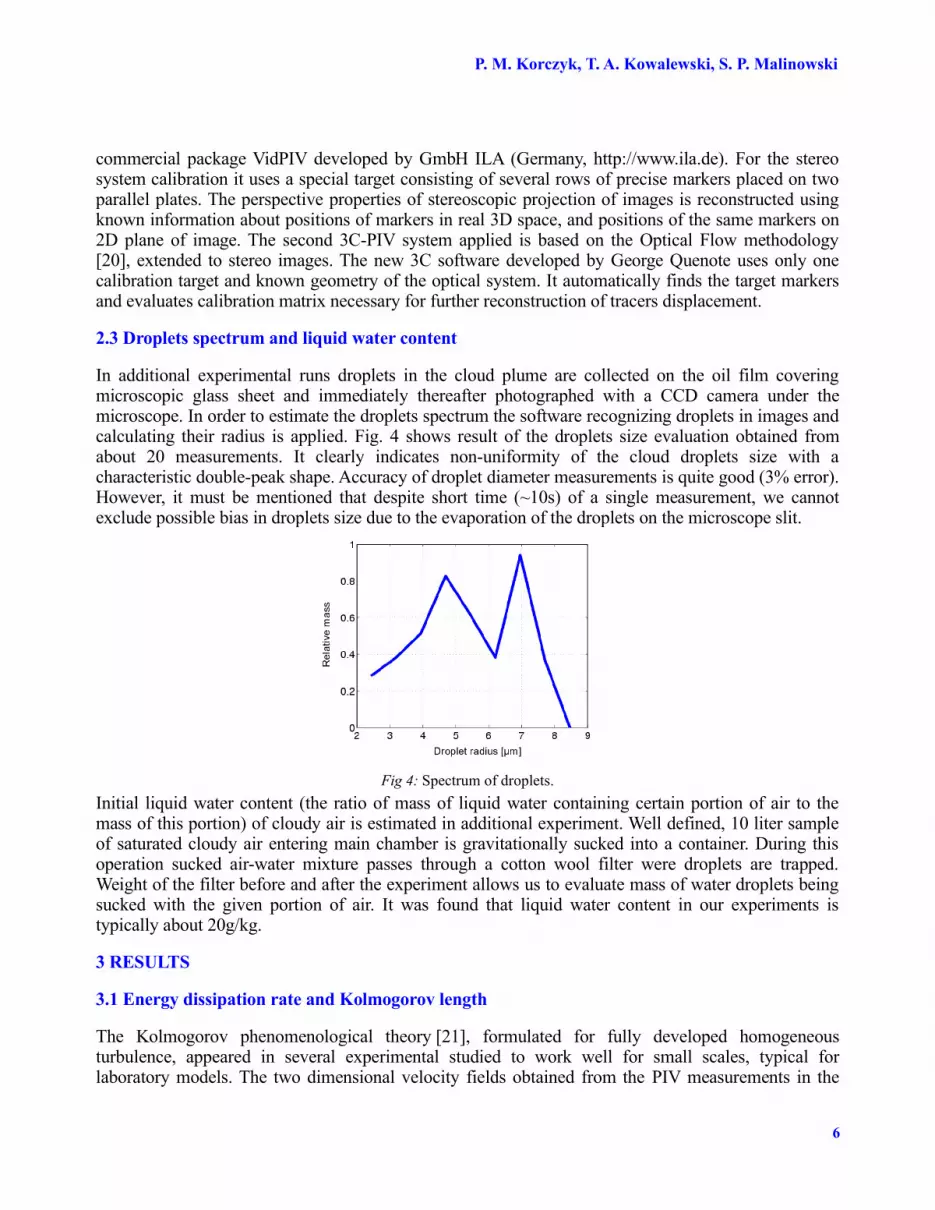
P M Korczyk T A Kowalewski S P Malinowski
commercial package VidPIV developed by GmbH ILA (Germany httpwwwilade) For the stereo system calibration it uses a special target consisting of several rows of precise markers placed on two parallel plates The perspective properties of stereoscopic projection of images is reconstructed using known information about positions of markers in real 3D space and positions of the same markers on 2D plane of image The second 3C-PIV system applied is based on the Optical Flow methodology [20] extended to stereo images The new 3C software developed by George Quenote uses only one calibration target and known geometry of the optical system It automatically finds the target markers and evaluates calibration matrix necessary for further reconstruction of tracers displacement
23 Droplets spectrum and liquid water content
In additional experimental runs droplets in the cloud plume are collected on the oil film covering microscopic glass sheet and immediately thereafter photographed with a CCD camera under the microscope In order to estimate the droplets spectrum the software recognizing droplets in images and calculating their radius is applied Fig 4 shows result of the droplets size evaluation obtained from about 20 measurements It clearly indicates non-uniformity of the cloud droplets size with a characteristic double-peak shape Accuracy of droplet diameter measurements is quite good (3 error) However it must be mentioned that despite short time (~10s) of a single measurement we cannot exclude possible bias in droplets size due to the evaporation of the droplets on the microscope slit
Fig 4 Spectrum of droplets
Initial liquid water content (the ratio of mass of liquid water containing certain portion of air to the mass of this portion) of cloudy air is estimated in additional experiment Well defined 10 liter sample of saturated cloudy air entering main chamber is gravitationally sucked into a container During this operation sucked air-water mixture passes through a cotton wool filter were droplets are trapped Weight of the filter before and after the experiment allows us to evaluate mass of water droplets being sucked with the given portion of air It was found that liquid water content in our experiments is typically about 20gkg
3 RESULTS
31 Energy dissipation rate and Kolmogorov length
The Kolmogorov phenomenological theory [21] formulated for fully developed homogeneous turbulence appeared in several experimental studied to work well for small scales typical for laboratory models The two dimensional velocity fields obtained from the PIV measurements in the
6
12TH INTERNATIONAL SYMPOSIUM ON FLOW VISUALIZATIONSeptember 10-14 2006 German Aerospace Center (DLR) Goumlttingen Germany
cloud chamber give us possibility to estimate the Kolmogorov length (4) It is found that it varies in the narrow range form about 72 10-4 m to 78 10-4 m The mean value of the Kolmogorov length obtained during our laboratory experiments is 7610-4m It is typical for cumulus clouds in presence of weak convection [22] It is interesting to note that the Kolmogorov length appears to depend on the relative humidity of air ie initial humidity measured in the chamber before the plum with droplets is introduced
Kolmogorov length = 3
1 4
- where ν is viscosity and ε is energy dissipation rate (4)
Fig 5 Experimental value of Kolmogorov length as a function of relative humidity Each of charts corresponds to another experimental runFigure 5 presents variation of the evaluated Kolmogorov length in time for three different independent experimental runs During each of these runs initial relative humidity inside the main chamber is increased It becomes evident that the Kolmogorov length is systematically decreasing with the relative humidity indicating that properties of the small scale turbulence may depend on efficiency of the droplets evaporation
32 Statistics of velocity field
Three series of experiments with slightly varying thermodynamical conditions inside the chamber are performed In each series at least 500 pairs of frames (tens of thousands of vectors in each frame) are evaluated in order to retrieve properties of turbulent velocity fluctuations Our analysis of stereo PIV data indicates that in horizontal plane velocity fluctuations are isotropic Hence in the following one horizontal component is presented Combined statistics of turbulent velocity fluctuations in horizontal
7
P M Korczyk T A Kowalewski S P Malinowski
(u) and vertical (w) directions are displayed in Fig 6 and summarized in Table 1 Here customary definition of standard deviation skewness and kurtosis are used
u=langu 2rang Su=langu 3rang u
3 K u=
langu 4rangu
4 (5)
Fig 6 Distribution of horizontal (red) and vertical (blue) turbulent velocity fluctuations from three series of measurements
TABLE 1 Distribution of horizontal (u) and vertical (w) turbulent velocity fluctuations for the experimental data shown in Fig 6
Standard deviation [cms] Skewness Kurtosis
u 54 -001 32
w 80 -02 31
It is evident that the distribution of the vertical velocity fluctuations characterizes larger dispersion and it has longer tails than the distribution of horizontal velocity fluctuations Calculated skewness and kurtosis indicate that both distributions are close to the Gaussian (normal) These results has been used to validate recent direct numerical simulations performed for similar conditions by Malinowski et al [13] It confirms strong influence of the buoyancy forces on the developed of turbulent fluctuations
33 Structure functions
In order to evaluate the persistence of the turbulence the second order structure function was calculated for the velocity flow in the small section of the cloud chamber evaluating solely area covered by the imaging system (7cm x 45cm) The second order structure function appears useful to discriminate viscous and inertial range of the turbulent flow [23] [24] The second order longitudinal structure function is a mean velocity increment between two points separated by l projected onto the line of separation Hence we can introduce structure function for both x and z direction and obtain its variation for horizontal and vertical velocity components u w
8
12TH INTERNATIONAL SYMPOSIUM ON FLOW VISUALIZATIONSeptember 10-14 2006 German Aerospace Center (DLR) Goumlttingen Germany
S u⋳ l =lang[u xl z minusu x z]2rang
Sw⋳ l =lang[w x zl minusw x z ]2rang
(6)
Fig 7 Second order longitudinal structure functions shown in log-log scale Red solid line ndash vertical components Blue dashed line ndash horizontal component Straight lines indicate initial slope exponent (l2) and asymptotic slope exponent (l23)
Figure 7 clearly shows different behavior of the structure function for vertical and horizontal velocity components Whereas initially both structure functions follow l2 slope characteristic for the dissipation range at larger separations the inertial range l23 behavior can be observed for the vertical velocity only It indicates already mentioned anisotropy of the velocity field structures present for all scales observed in the laboratory experiments
CONCLUSIONSSmall scale mixing of cloud with unsaturated environment is investigated in laboratory cloud chamber by means of Particle Image Velocimetry (PIV) The high spatial resolution of the experimental setup (007mm) allowed us to evaluate statistics of the turbulent flow field down to the Kolmogorov length The results indicate that small-scale turbulence in such conditions is highly anisotropic with the preferred vertical direction The present investigation indicates also that properties of turbulence in small scales is sensitive to the initial air humidity Hence obviously buoyancy forces resulting from evaporation of cloud droplets substantially influence smallest scales of turbulence Typically lt(u)2gt is about two times smaller than lt(w)2gt The probability distribution functions of w are broader than those of u These results have been successfully used to validate numerical simulations (DNS) performed for a similar experimental configuration [13] However it is still uncertain to what extent infromation gained in the laboratory cloud can be applied to atmospheric systems Hence in situ measurements of turbulent velocity fluctuations from various types of clouds are necessary to validate common assumptions on small-scale cloud isotropy
9
P M Korczyk T A Kowalewski S P Malinowski
ACKNOWLEDGMENTSThis research was supported by the Polish Committee for Scientific Research and PIVNET2 Thematic Network
REFERENCES
1 Falkovich G Gawedzki K and Vergassola M Particles and fields in fluid turbulence Rev Modern Phys Vol 73 pp 913-975 2001
2 Shaw RA Particle-turbulence interactions in atmospheric clouds Annual Review of Fluid Mechanics Vol 35 pp 183-227 2003
3 Ghosh S Davila J Hunt JCR Srdic A Fernando HJS Jonas PR How turbulence enhances coalescence of settling particles with applications to rain in clouds Proc R Soc A Vol 461 pp 3059-3088 2005
4 Yarin A Kowalewski T A Hiller WJ Koch S Distribution of particles suspended in 3D laminar convection flow Physics of Fluids Vol 8 pp 1130-1140 1996
5 Vaillancourt PA Yau MK Review of particle-turbulence interactions and consequences for cloud physics Bull Am Meteorol Soc Vol 81 pp 285ndash98 2000
6 Siebert H Lehmann K and Wendish M Observations of small-scale turbulence and energy dissipation rates in the cloud boundary layer J Atmos Sci Vol 63 pp 1451-1466 2006
7 Pinsky M and Khain AP Turbulence effects on the collision kernel Part 1 Formation of velocity deviations of drops falling within a turbulent three-dimensional flow Quart J Roy Meteor Soc Vol 123 pp 1517-1542 1997
8 Shaw RA Walter CR Lance RC and Johannes V Preferential concentration of cloud droplets by turbulence Effects on the early evolution of cumulus cloud droplet spectra J Atmos Sci Vol 55 pp 1965-1976 1998
9 Shaw RA and Oncley S P Acceleration intermittency and enhanced collision kernels in turbulent clouds Atmos Res Vol 59-60 pp 77-87 2001
10 Vaillancourt PA Yau MK and Bartello P Grabowski WW Microscopic Approach to Cloud Droplet Growth by Condensation Part II Turbulence Clustering and Condensational Growth J Atmos Sc Vol 59 pp 3421ndash3435 2002
11 Grabowski WW MJO-like coherent structures Sensitivity simulations using theCloud-Resolving Convection Parameterization (CRCP) J Atmos Sci Vol 60 pp 847ndash864 2003
12 Andrejczuk M Grabowski W Malinowski SP and Smolarkiewicz PK Numerical Simulation of Cloud-Clear Air Interfacial Mixing J Atmos Sci Vol 61 pp 1726ndash1739 2004
13 Malinowski SP and Andrejczuk M Grabowski WW Korczyk P Kowalewski TA and Smolarkiewicz PK Cloud-clear air interfacial mixing anisotropy of turbulence generated by evaporation of liquid water Laboratory observations and numerical modeling 12th Conference on Cloud Physics Madison (WI USA) 2006
14 Malinowski SP Zawadzki I and Banat P Laboratory observations of cloud-clear air mixing in small scales J Atmos Oceanic Technol Vol 15 pp 1060-1065 1998
15 Jaczewski A Malinowski SP Spatial distribution of cloud droplets in a turbulent cloud-chamber flow Quart J Roy Meteor Soc Vol 131 pp 2047-2062 2005
16 Korczyk P Malinowski SP Kowalewski TA Mixing of cloud and clear air in centimeter scales observed in laboratory by means of particle image velocimetry Atmos Res (in press) 2006
17 Raffel M Willert ChE and Kompenhans J Particle image velocimetry a practical guide 3rd edition Springer 1998
18 Gui L W Merzkirch Generating arbitrarily sized interrogation windows for correlation-based analysis of particle image velocimetry recordings Exp Fluids Vol 24 pp 66-69 1998
19 Scarano F Iterative image deformation methods in PIV Meas Sci Technol Vol 13 pp R1-R19 2002
20 Quenote G Pakleza J Kowalewski TA Particle Image Velocimetry with Optical Flow Experiments in Fluids Vol 25 pp 177-189 1998
21 Kolmogorow AN Dissipation of energy under locally isotropic turbulence CR Acad Sci USSR Vol 32 pp 16-18 1941
22 Pruppacher HR Klett JD Microphysics of clouds and precipitation 1st edition Kluwer 1997
23 Frish U Turbulence - The legacy of A N Kolmogorov 1st edition Cambridge University Press 1995
24 Batchelor GK Pressure fluctuations in isotropic turbulence Proc Cambridge Phil Soc Vol 47 pp 533-559 1951
10

12TH INTERNATIONAL SYMPOSIUM ON FLOW VISUALIZATIONSeptember 10-14 2006 German Aerospace Center (DLR) Goumlttingen Germany
cloud chamber give us possibility to estimate the Kolmogorov length (4) It is found that it varies in the narrow range form about 72 10-4 m to 78 10-4 m The mean value of the Kolmogorov length obtained during our laboratory experiments is 7610-4m It is typical for cumulus clouds in presence of weak convection [22] It is interesting to note that the Kolmogorov length appears to depend on the relative humidity of air ie initial humidity measured in the chamber before the plum with droplets is introduced
Kolmogorov length = 3
1 4
- where ν is viscosity and ε is energy dissipation rate (4)
Fig 5 Experimental value of Kolmogorov length as a function of relative humidity Each of charts corresponds to another experimental runFigure 5 presents variation of the evaluated Kolmogorov length in time for three different independent experimental runs During each of these runs initial relative humidity inside the main chamber is increased It becomes evident that the Kolmogorov length is systematically decreasing with the relative humidity indicating that properties of the small scale turbulence may depend on efficiency of the droplets evaporation
32 Statistics of velocity field
Three series of experiments with slightly varying thermodynamical conditions inside the chamber are performed In each series at least 500 pairs of frames (tens of thousands of vectors in each frame) are evaluated in order to retrieve properties of turbulent velocity fluctuations Our analysis of stereo PIV data indicates that in horizontal plane velocity fluctuations are isotropic Hence in the following one horizontal component is presented Combined statistics of turbulent velocity fluctuations in horizontal
7
P M Korczyk T A Kowalewski S P Malinowski
(u) and vertical (w) directions are displayed in Fig 6 and summarized in Table 1 Here customary definition of standard deviation skewness and kurtosis are used
u=langu 2rang Su=langu 3rang u
3 K u=
langu 4rangu
4 (5)
Fig 6 Distribution of horizontal (red) and vertical (blue) turbulent velocity fluctuations from three series of measurements
TABLE 1 Distribution of horizontal (u) and vertical (w) turbulent velocity fluctuations for the experimental data shown in Fig 6
Standard deviation [cms] Skewness Kurtosis
u 54 -001 32
w 80 -02 31
It is evident that the distribution of the vertical velocity fluctuations characterizes larger dispersion and it has longer tails than the distribution of horizontal velocity fluctuations Calculated skewness and kurtosis indicate that both distributions are close to the Gaussian (normal) These results has been used to validate recent direct numerical simulations performed for similar conditions by Malinowski et al [13] It confirms strong influence of the buoyancy forces on the developed of turbulent fluctuations
33 Structure functions
In order to evaluate the persistence of the turbulence the second order structure function was calculated for the velocity flow in the small section of the cloud chamber evaluating solely area covered by the imaging system (7cm x 45cm) The second order structure function appears useful to discriminate viscous and inertial range of the turbulent flow [23] [24] The second order longitudinal structure function is a mean velocity increment between two points separated by l projected onto the line of separation Hence we can introduce structure function for both x and z direction and obtain its variation for horizontal and vertical velocity components u w
8
12TH INTERNATIONAL SYMPOSIUM ON FLOW VISUALIZATIONSeptember 10-14 2006 German Aerospace Center (DLR) Goumlttingen Germany
S u⋳ l =lang[u xl z minusu x z]2rang
Sw⋳ l =lang[w x zl minusw x z ]2rang
(6)
Fig 7 Second order longitudinal structure functions shown in log-log scale Red solid line ndash vertical components Blue dashed line ndash horizontal component Straight lines indicate initial slope exponent (l2) and asymptotic slope exponent (l23)
Figure 7 clearly shows different behavior of the structure function for vertical and horizontal velocity components Whereas initially both structure functions follow l2 slope characteristic for the dissipation range at larger separations the inertial range l23 behavior can be observed for the vertical velocity only It indicates already mentioned anisotropy of the velocity field structures present for all scales observed in the laboratory experiments
CONCLUSIONSSmall scale mixing of cloud with unsaturated environment is investigated in laboratory cloud chamber by means of Particle Image Velocimetry (PIV) The high spatial resolution of the experimental setup (007mm) allowed us to evaluate statistics of the turbulent flow field down to the Kolmogorov length The results indicate that small-scale turbulence in such conditions is highly anisotropic with the preferred vertical direction The present investigation indicates also that properties of turbulence in small scales is sensitive to the initial air humidity Hence obviously buoyancy forces resulting from evaporation of cloud droplets substantially influence smallest scales of turbulence Typically lt(u)2gt is about two times smaller than lt(w)2gt The probability distribution functions of w are broader than those of u These results have been successfully used to validate numerical simulations (DNS) performed for a similar experimental configuration [13] However it is still uncertain to what extent infromation gained in the laboratory cloud can be applied to atmospheric systems Hence in situ measurements of turbulent velocity fluctuations from various types of clouds are necessary to validate common assumptions on small-scale cloud isotropy
9
P M Korczyk T A Kowalewski S P Malinowski
ACKNOWLEDGMENTSThis research was supported by the Polish Committee for Scientific Research and PIVNET2 Thematic Network
REFERENCES
1 Falkovich G Gawedzki K and Vergassola M Particles and fields in fluid turbulence Rev Modern Phys Vol 73 pp 913-975 2001
2 Shaw RA Particle-turbulence interactions in atmospheric clouds Annual Review of Fluid Mechanics Vol 35 pp 183-227 2003
3 Ghosh S Davila J Hunt JCR Srdic A Fernando HJS Jonas PR How turbulence enhances coalescence of settling particles with applications to rain in clouds Proc R Soc A Vol 461 pp 3059-3088 2005
4 Yarin A Kowalewski T A Hiller WJ Koch S Distribution of particles suspended in 3D laminar convection flow Physics of Fluids Vol 8 pp 1130-1140 1996
5 Vaillancourt PA Yau MK Review of particle-turbulence interactions and consequences for cloud physics Bull Am Meteorol Soc Vol 81 pp 285ndash98 2000
6 Siebert H Lehmann K and Wendish M Observations of small-scale turbulence and energy dissipation rates in the cloud boundary layer J Atmos Sci Vol 63 pp 1451-1466 2006
7 Pinsky M and Khain AP Turbulence effects on the collision kernel Part 1 Formation of velocity deviations of drops falling within a turbulent three-dimensional flow Quart J Roy Meteor Soc Vol 123 pp 1517-1542 1997
8 Shaw RA Walter CR Lance RC and Johannes V Preferential concentration of cloud droplets by turbulence Effects on the early evolution of cumulus cloud droplet spectra J Atmos Sci Vol 55 pp 1965-1976 1998
9 Shaw RA and Oncley S P Acceleration intermittency and enhanced collision kernels in turbulent clouds Atmos Res Vol 59-60 pp 77-87 2001
10 Vaillancourt PA Yau MK and Bartello P Grabowski WW Microscopic Approach to Cloud Droplet Growth by Condensation Part II Turbulence Clustering and Condensational Growth J Atmos Sc Vol 59 pp 3421ndash3435 2002
11 Grabowski WW MJO-like coherent structures Sensitivity simulations using theCloud-Resolving Convection Parameterization (CRCP) J Atmos Sci Vol 60 pp 847ndash864 2003
12 Andrejczuk M Grabowski W Malinowski SP and Smolarkiewicz PK Numerical Simulation of Cloud-Clear Air Interfacial Mixing J Atmos Sci Vol 61 pp 1726ndash1739 2004
13 Malinowski SP and Andrejczuk M Grabowski WW Korczyk P Kowalewski TA and Smolarkiewicz PK Cloud-clear air interfacial mixing anisotropy of turbulence generated by evaporation of liquid water Laboratory observations and numerical modeling 12th Conference on Cloud Physics Madison (WI USA) 2006
14 Malinowski SP Zawadzki I and Banat P Laboratory observations of cloud-clear air mixing in small scales J Atmos Oceanic Technol Vol 15 pp 1060-1065 1998
15 Jaczewski A Malinowski SP Spatial distribution of cloud droplets in a turbulent cloud-chamber flow Quart J Roy Meteor Soc Vol 131 pp 2047-2062 2005
16 Korczyk P Malinowski SP Kowalewski TA Mixing of cloud and clear air in centimeter scales observed in laboratory by means of particle image velocimetry Atmos Res (in press) 2006
17 Raffel M Willert ChE and Kompenhans J Particle image velocimetry a practical guide 3rd edition Springer 1998
18 Gui L W Merzkirch Generating arbitrarily sized interrogation windows for correlation-based analysis of particle image velocimetry recordings Exp Fluids Vol 24 pp 66-69 1998
19 Scarano F Iterative image deformation methods in PIV Meas Sci Technol Vol 13 pp R1-R19 2002
20 Quenote G Pakleza J Kowalewski TA Particle Image Velocimetry with Optical Flow Experiments in Fluids Vol 25 pp 177-189 1998
21 Kolmogorow AN Dissipation of energy under locally isotropic turbulence CR Acad Sci USSR Vol 32 pp 16-18 1941
22 Pruppacher HR Klett JD Microphysics of clouds and precipitation 1st edition Kluwer 1997
23 Frish U Turbulence - The legacy of A N Kolmogorov 1st edition Cambridge University Press 1995
24 Batchelor GK Pressure fluctuations in isotropic turbulence Proc Cambridge Phil Soc Vol 47 pp 533-559 1951
10

P M Korczyk T A Kowalewski S P Malinowski
(u) and vertical (w) directions are displayed in Fig 6 and summarized in Table 1 Here customary definition of standard deviation skewness and kurtosis are used
u=langu 2rang Su=langu 3rang u
3 K u=
langu 4rangu
4 (5)
Fig 6 Distribution of horizontal (red) and vertical (blue) turbulent velocity fluctuations from three series of measurements
TABLE 1 Distribution of horizontal (u) and vertical (w) turbulent velocity fluctuations for the experimental data shown in Fig 6
Standard deviation [cms] Skewness Kurtosis
u 54 -001 32
w 80 -02 31
It is evident that the distribution of the vertical velocity fluctuations characterizes larger dispersion and it has longer tails than the distribution of horizontal velocity fluctuations Calculated skewness and kurtosis indicate that both distributions are close to the Gaussian (normal) These results has been used to validate recent direct numerical simulations performed for similar conditions by Malinowski et al [13] It confirms strong influence of the buoyancy forces on the developed of turbulent fluctuations
33 Structure functions
In order to evaluate the persistence of the turbulence the second order structure function was calculated for the velocity flow in the small section of the cloud chamber evaluating solely area covered by the imaging system (7cm x 45cm) The second order structure function appears useful to discriminate viscous and inertial range of the turbulent flow [23] [24] The second order longitudinal structure function is a mean velocity increment between two points separated by l projected onto the line of separation Hence we can introduce structure function for both x and z direction and obtain its variation for horizontal and vertical velocity components u w
8
12TH INTERNATIONAL SYMPOSIUM ON FLOW VISUALIZATIONSeptember 10-14 2006 German Aerospace Center (DLR) Goumlttingen Germany
S u⋳ l =lang[u xl z minusu x z]2rang
Sw⋳ l =lang[w x zl minusw x z ]2rang
(6)
Fig 7 Second order longitudinal structure functions shown in log-log scale Red solid line ndash vertical components Blue dashed line ndash horizontal component Straight lines indicate initial slope exponent (l2) and asymptotic slope exponent (l23)
Figure 7 clearly shows different behavior of the structure function for vertical and horizontal velocity components Whereas initially both structure functions follow l2 slope characteristic for the dissipation range at larger separations the inertial range l23 behavior can be observed for the vertical velocity only It indicates already mentioned anisotropy of the velocity field structures present for all scales observed in the laboratory experiments
CONCLUSIONSSmall scale mixing of cloud with unsaturated environment is investigated in laboratory cloud chamber by means of Particle Image Velocimetry (PIV) The high spatial resolution of the experimental setup (007mm) allowed us to evaluate statistics of the turbulent flow field down to the Kolmogorov length The results indicate that small-scale turbulence in such conditions is highly anisotropic with the preferred vertical direction The present investigation indicates also that properties of turbulence in small scales is sensitive to the initial air humidity Hence obviously buoyancy forces resulting from evaporation of cloud droplets substantially influence smallest scales of turbulence Typically lt(u)2gt is about two times smaller than lt(w)2gt The probability distribution functions of w are broader than those of u These results have been successfully used to validate numerical simulations (DNS) performed for a similar experimental configuration [13] However it is still uncertain to what extent infromation gained in the laboratory cloud can be applied to atmospheric systems Hence in situ measurements of turbulent velocity fluctuations from various types of clouds are necessary to validate common assumptions on small-scale cloud isotropy
9
P M Korczyk T A Kowalewski S P Malinowski
ACKNOWLEDGMENTSThis research was supported by the Polish Committee for Scientific Research and PIVNET2 Thematic Network
REFERENCES
1 Falkovich G Gawedzki K and Vergassola M Particles and fields in fluid turbulence Rev Modern Phys Vol 73 pp 913-975 2001
2 Shaw RA Particle-turbulence interactions in atmospheric clouds Annual Review of Fluid Mechanics Vol 35 pp 183-227 2003
3 Ghosh S Davila J Hunt JCR Srdic A Fernando HJS Jonas PR How turbulence enhances coalescence of settling particles with applications to rain in clouds Proc R Soc A Vol 461 pp 3059-3088 2005
4 Yarin A Kowalewski T A Hiller WJ Koch S Distribution of particles suspended in 3D laminar convection flow Physics of Fluids Vol 8 pp 1130-1140 1996
5 Vaillancourt PA Yau MK Review of particle-turbulence interactions and consequences for cloud physics Bull Am Meteorol Soc Vol 81 pp 285ndash98 2000
6 Siebert H Lehmann K and Wendish M Observations of small-scale turbulence and energy dissipation rates in the cloud boundary layer J Atmos Sci Vol 63 pp 1451-1466 2006
7 Pinsky M and Khain AP Turbulence effects on the collision kernel Part 1 Formation of velocity deviations of drops falling within a turbulent three-dimensional flow Quart J Roy Meteor Soc Vol 123 pp 1517-1542 1997
8 Shaw RA Walter CR Lance RC and Johannes V Preferential concentration of cloud droplets by turbulence Effects on the early evolution of cumulus cloud droplet spectra J Atmos Sci Vol 55 pp 1965-1976 1998
9 Shaw RA and Oncley S P Acceleration intermittency and enhanced collision kernels in turbulent clouds Atmos Res Vol 59-60 pp 77-87 2001
10 Vaillancourt PA Yau MK and Bartello P Grabowski WW Microscopic Approach to Cloud Droplet Growth by Condensation Part II Turbulence Clustering and Condensational Growth J Atmos Sc Vol 59 pp 3421ndash3435 2002
11 Grabowski WW MJO-like coherent structures Sensitivity simulations using theCloud-Resolving Convection Parameterization (CRCP) J Atmos Sci Vol 60 pp 847ndash864 2003
12 Andrejczuk M Grabowski W Malinowski SP and Smolarkiewicz PK Numerical Simulation of Cloud-Clear Air Interfacial Mixing J Atmos Sci Vol 61 pp 1726ndash1739 2004
13 Malinowski SP and Andrejczuk M Grabowski WW Korczyk P Kowalewski TA and Smolarkiewicz PK Cloud-clear air interfacial mixing anisotropy of turbulence generated by evaporation of liquid water Laboratory observations and numerical modeling 12th Conference on Cloud Physics Madison (WI USA) 2006
14 Malinowski SP Zawadzki I and Banat P Laboratory observations of cloud-clear air mixing in small scales J Atmos Oceanic Technol Vol 15 pp 1060-1065 1998
15 Jaczewski A Malinowski SP Spatial distribution of cloud droplets in a turbulent cloud-chamber flow Quart J Roy Meteor Soc Vol 131 pp 2047-2062 2005
16 Korczyk P Malinowski SP Kowalewski TA Mixing of cloud and clear air in centimeter scales observed in laboratory by means of particle image velocimetry Atmos Res (in press) 2006
17 Raffel M Willert ChE and Kompenhans J Particle image velocimetry a practical guide 3rd edition Springer 1998
18 Gui L W Merzkirch Generating arbitrarily sized interrogation windows for correlation-based analysis of particle image velocimetry recordings Exp Fluids Vol 24 pp 66-69 1998
19 Scarano F Iterative image deformation methods in PIV Meas Sci Technol Vol 13 pp R1-R19 2002
20 Quenote G Pakleza J Kowalewski TA Particle Image Velocimetry with Optical Flow Experiments in Fluids Vol 25 pp 177-189 1998
21 Kolmogorow AN Dissipation of energy under locally isotropic turbulence CR Acad Sci USSR Vol 32 pp 16-18 1941
22 Pruppacher HR Klett JD Microphysics of clouds and precipitation 1st edition Kluwer 1997
23 Frish U Turbulence - The legacy of A N Kolmogorov 1st edition Cambridge University Press 1995
24 Batchelor GK Pressure fluctuations in isotropic turbulence Proc Cambridge Phil Soc Vol 47 pp 533-559 1951
10
Top Related
Copyright © 2022 FDOKUMEN

