Investigating the Impact of Selection Bias in Dose-ResponseAnalyses of Preventive Interventions

Herle M. McGowan,North Carolina State University

Robert L. Nix,Pennsylvania State University

Susan A. Murphy,University of Michigan

Karen L. Bierman, andPennsylvania State University

Conduct Problems Prevention Research Group*

AbstractThis paper focuses on the impact of selection bias in the context of extended, community-basedprevention trials that attempt to “unpack” intervention effects and analyze mechanisms of change.Relying on dose-response analyses as the most general form of such efforts, this study providestwo examples of how selection bias can affect the estimation of treatment effects. In Example 1,we describe an actual intervention in which selection bias was believed to influence the dose-response relation of an adaptive component in a preventive intervention for young children withsevere behavior problems. In Example 2, we conduct a series of Monte Carlo simulations toillustrate just how severely selection bias can affect estimates in a dose-response analysis when thefactors that affect dose are not recorded. We also assess the extent to which selection bias isameliorated by the use of pretreatment covariates. We examine the implications of these examplesand review trial design, data collection, and data analysis factors that can reduce selection bias inefforts to understand how preventive interventions have the effects they do.

KeywordsSelection bias; preventive interventions; dose-response; simulations

As preventive interventions become larger and more complex, researchers are increasinglylikely to examine the outcomes of randomized control designs as well as investigate possiblemechanisms of change. These implementation studies focus on how differences in factorssuch as intervention dose, therapeutic process, or fidelity might account for differences inparticipant outcomes. However, these efforts to “unpack” intervention effects are vulnerableto selection biases (Winship & Mare, 1992), which occur when either known or unknowncompositional differences among subgroups of participants – rather than factors related to

Correspondence regarding this study should be addressed to Herle McGowan, NCSU Department of Statistics, 2311 Stinson Drive,Campus Box 8203, Raleigh, NC 27695-8203; phone: 919-915-0634; mcgowan@stat.ncsu.edu.*Members of the Conduct Problems Prevention Research Group are, in alphabetical order, Karen L. Bierman, Pennsylvania StateUniversity; John D. Coie, Duke University; Kenneth A. Dodge, Duke University; Mark T. Greenberg, Pennsylvania State University;John E. Lochman, University of Alabama; Robert J. McMahon, University of Washington; and Ellen E. Pinderhughes, TuftsUniversity.

NIH Public AccessAuthor ManuscriptPrev Sci. Author manuscript; available in PMC 2011 February 24.

Published in final edited form as:Prev Sci. 2010 September ; 11(3): 239–251. doi:10.1007/s11121-010-0169-2.

NIH

-PA Author Manuscript

NIH

-PA Author Manuscript

NIH

-PA Author Manuscript

the intervention itself – account for final observed differences (Rosenbaum, 2002). Forexample, the conscientiousness and competence that compel a teacher to administer anintervention as intended might affect other ways in which she or he teaches, so that childrenin that classroom would do well, almost regardless of the study condition to which they wereassigned. Unfortunately, such selection biases are rarely acknowledged and adequatelyaddressed (see studies included in the review of implementation research by Durlak &DuPre, 2008).

Selection Bias and Dose-Response AnalysesProblems with selection bias are not new and apply to most studies of interventionimplementation. The threat selection bias poses to internal validity as well as to externalvalidity has been discussed at length elsewhere (e.g., Shadish et al., 2002). The key featureof selection bias is that there is some systematic difference between those participants whopartake in some aspect of treatment and those participants who do not. Researcherscommonly think of selection bias that results from pretreatment differences, but selectionbias also can result from known or unknown differences that arise during the study period asthe result of variation in treatment adherence, quality of implementation, and attrition. Thisthreat to validity is known as unreliability of treatment implementation or selection bytreatment interactions (Shadish et al., 2002); it can be especially problematic wheneverinvestigators seek to understand what happened within the treatment condition of apreventive intervention trial.

In those cases when selection bias occurs after the start of an intervention, features of studydesign, like random assignment, will be insufficient to control the bias. Likewise, unless theconfounder is a stable trait that is known and measureable and exerts all its influence prior tothe beginning of the intervention, the use of pretreatment covariates will be insufficient tocontrol the bias. In those cases when the confounder varies over time, only moresophisticated statistical analyses can be used to reduce its influence (e.g., Rosenbaum,1984a, 1984b; Rosenbaum & Rubin, 1983; Winship & Mare, 1992).

Although problems with selection bias apply to most studies of intervention processes, theseproblems are most apparent in dose-response analyses. Such analyses examine thefundamental logic model underlying preventive interventions – that participants mustreceive services to improve (Cicchetti & Hinshaw, 2002; Domitrovich & Greenberg, 2000).In such analyses, dose does not represent the hypothesized mechanisms of change, like thefactors studied in mediation analyses; rather dose is a coarse indicator of how muchtreatment was received in which to acquire those mechanisms of change.

The strongest design for a planned dose-response analysis would be to randomize differentlevels of dose among participants, as randomization limits the possibility that there arecompositional differences between the subgroups assigned to different doses. Wheneverdose is not randomized, or when the randomized dose is not adhered to, variables that affectselection of the dose received produce compositional differences between the subgroups. Ifthese variables also affect the outcome, the observed dose-response relation confounds theeffects of these compositional differences with the true dose-response relation. For example,motivation is a confounder if more motivated participants adhere more closely to therecommended dose and exhibit better outcomes than less motivated participants, or familydisorganization is a confounder if children who are frequently absent receive fewer sessionsof a school-based curriculum and exhibit worse outcomes than children who attendregularly. In both cases, better outcomes are associated with higher dose; the selection biasis positive and the observed dose-response relation appears stronger than the true relation.However, if a counselor decides to schedule an extra session of treatment for a family incrisis or extra tutoring is provided to those children who are failing a class, then worse

McGowan et al. Page 2

Prev Sci. Author manuscript; available in PMC 2011 February 24.

NIH

-PA Author Manuscript

NIH

-PA Author Manuscript

NIH

-PA Author Manuscript

outcomes would be associated with a higher dose; the selection bias would be negative andthe observed dose-response relation would appear weaker than the true relation.

The Present ResearchThis paper focuses on the impact of selection bias in the context of extended, community-based preventive intervention trials. It demonstrates how selection bias can affect estimationof treatment effects when confounders are unknown or incompletely recorded and thereforecannot be controlled via analysis. In particular, this paper offers two detailed examples inwhich confounding makes treatment appear less effective than it might be or eveniatrogenic. In Example 1, we describe an actual intervention in which selection bias wasbelieved to play havoc in estimates of the dose-response analysis of a preventiveintervention for young children with severe behavior problems. In Example 2, a series ofMonte Carlo simulations illustrate how severely selection bias can affect estimates in a dose-response analysis when dose is tailored to participants’ need but when the reasons fortailoring dose are unrecorded. In the final section of the paper, we examine the implicationsof these examples and review trial design, data collection, and data analysis factors that canreduce selection bias in implementation studies, such as dose-response analyses, ofpreventive interventions.

Example 1The purpose of Example 1 is to illustrate with real data how purported selection bias canmake it very difficult to interpret dose-response relations in an adaptive intervention.Increasingly, preventive interventions are using adaptive designs, in which the amount ortype of an intervention component is adapted to participant need (Collins et al., 2004). Therationale is that researchers can achieve more efficient and cost-effective interventions thanstandard one-size-fits-all programs by providing more intensive treatment only when it iswarranted (Jacobson et al., 1989; Kreuter et al., 2000; Lavori et al., 2000). In the presentexample, however, on-going decisions regarding the need for additional treatment mostlikely results in selection bias as well. Depending on how we attempt to control for thisselection bias, we come to dramatically different conclusions about dose-response relations.

This example relies on data from Fast Track (Conduct Problems Prevention Research Group[CPPRG], 1992), a multi-site, multi-year, randomized trial evaluating a six-componentintervention designed to prevent the development of severe conduct problems amongchildren exhibiting high rates of aggression at school entry. Evaluations of Fast Trackintervention effects have been published elsewhere (CPPRG, 1999; 2002). Intent-to-treatanalyses, comparing the randomized intervention and control groups, revealed a pattern ofpositive intervention effects on various measures of social competence at the end of firstgrade (CPPRG, 1999).

Because many treatment effects were small in magnitude and because some components ofthe intervention required more resources to deliver, we were interested in conducting dose-Selection response analyses to determine how well the various intervention componentswere working. The peer pairing component was of particular interest for this study. Peerpairing sought to enhance the impact of the social-skills training children received in theuniversal classroom curriculum and small therapeutic groups by helping them generalize theuse of those new skills to individual peer interactions (Bierman et al., l996). Peer pairingconsisted of structured dyadic play sessions involving the intervention child and a rotating,same-sex classmate who did not have behavior problems. In first grade, all children in theintervention condition were offered one session of peer pairing per week for a total of 22sessions. After one year of intervention, some children were exhibiting normal levels of

McGowan et al. Page 3

Prev Sci. Author manuscript; available in PMC 2011 February 24.

NIH

-PA Author Manuscript

NIH

-PA Author Manuscript

NIH

-PA Author Manuscript

social competence and aggression and were not experiencing peer rejection. Therefore, insecond grade, peer pairing was offered only to those children who still appeared to need it.

Continued need for peer pairing was based on objective criteria, measured at the end of firstgrade. If children received a t-score of 65 or higher on the aggressive behavior or attentionproblems syndrome of the Teacher’s Report Form (Achenbach, 1991), they were consideredto have clinically significant behavior problems that could undermine peer relations and thuswere supposed to receive peer pairing throughout second grade. T-scores between 60 and 65were considered borderline. If children received patterns of sociometric nominations for“like most” and “like least” indicating they were rejected by their classmates (Coie &Dodge, 1988), they also were considered in need of an additional year of peer pairing.Children whose sociometric nominations suggested they were controversial or neglectedwere considered borderline. If children were “borderline” in terms of teacher ratings orsociometric nominations, Fast Track allowed staff members to use their best clinicaljudgment, based on their own observations and discussions with teachers, to decide whetherthe child should receive peer pairing in second grade. When project guidelines specifiedpeer pairing or staff members determined that a child should receive peer pairing, that childwas supposed to receive peer pairing throughout the fall and spring of second grade.However, Fast Track also allowed staff members to initiate peer pairing sessions at anypoint during second grade if they noticed worrisome declines in children’s socialfunctioning. In addition, staff members could deliver extra peer pairing sessions if theybelieved the sessions would be helpful. The number of peer pairing sessions childrenreceived ranged from 0 to 43.

MeasuresFor this study, dose is the total number of peer pairing sessions that each child receivedduring second grade, based on weekly records kept by clinical staff members. Response isthe child’s social competence, as rated by teachers at the end of second grade. Socialcompetence was measured using the Social Health Profile, a questionnaire developed forFast Track, which consisted of nine items, such as “Friendly” and “Controls temper whenthere is a disagreement.” Each item was rated on a 6-point Likert scale, with responseoptions ranging from “almost never” to “almost always” (Cronbach a > .80). Pre-secondgrade covariates included social competence (using the Social Health Profile) measured atthe end of first grade, as well as study cohort, study site, child race, and child sex.

AnalysesRegression analyses of intervention-control group differences among children who werepromoted to second grade and entered the adaptive phase of peer pairing intervention (n =410 and 403 in the intervention and control groups, respectively) revealed a small andmarginally significant effect of being in Fast Track on growth in social competence duringsecond grade, after controlling for end-of-first-grade social competence scores, cohort, site,race, and sex: Standardized β (for treatment) = 0.06, p = 0.06 (unstandardized parameterestimate = 0.12, F [n = 745, df = 9 and 735] = 15.07, p < 0.001, R2 = 0.16).1 Relations likethis – suggesting that children in the intervention condition were doing better than childrenin the control condition but that the adjusted mean difference was less than one-tenth of onestandard deviation – often motivate efforts to examine intervention effects in greater depthto understand exactly what might be happening.

1Although necessary to examine what happened in second grade, it should be noted that biases might be introduced by stratifying on apost-randomization variable, such as promotion to second grade. The children in the intervention group who were promoted afterreceiving a year of intensive Fast Track services might be quite different than the children in the control group who were promotedwithout such services.

McGowan et al. Page 4

Prev Sci. Author manuscript; available in PMC 2011 February 24.

NIH

-PA Author Manuscript

NIH

-PA Author Manuscript

NIH

-PA Author Manuscript

Dose-response analysis 1: All intervention children who were promoted tosecond grade—Our first implementation analyses relied on data from the children in theintervention group only to examine whether the dose of peer pairing in second gradeaffected their growth in social competence. Controlling for end-of-first-grade socialcompetence scores, cohort, site, race, and sex, a linear regression equation revealed amarginally significant negative association between the peer pairing dose and the socialcompetence outcome: β (for dose of peer pairing) = −0.09, p = 0.07 (unstandardizedparameter estimate = −0.01, F [n = 383, df = 9 and 373] = 8.94, p < 0.001, R2 = 0.18).

In hindsight, the emergence of this negative effect is not surprising: By design, the childrenwho were displaying the most problems and the least social competence were provided thehighest doses of peer pairing. From a theoretical and clinical standpoint, it seems highlyunlikely that peer pairing actually had a negative effect on children’s growth in socialcompetence. The overall positive effect of the Fast Track intervention on social competencealso argues against this interpretation. Thus, it is plausible that the negative estimated effectof peer pairing is being driven by systematic differences between those children receivingmore peer pairing and those receiving less – in other words, by selection bias.

There are many analytic methods available for dealing with such bias, and we employedseveral as a follow-up to the above dose-response analysis. When pretreatmentcharacteristics affect the quantity of dose (i.e., when selection bias is the result ofpretreatment differences between those children receiving different doses), it is common toadjust for the relevant pretreatment covariates in the regression model. Indeed, weconducted additional analyses adjusting for up to 15 relevant covariates assessed at thebeginning and end of first grade, and a negative association between peer paring dose andthe social competence response still emerged. This suggests that controlling for both distalpre-first grade covariates and more proximal end-of-first grade covariates was not enough toameliorate the confounding.

Again, in hindsight this is not surprising: The dose of peer pairing was adapted to each childnot only at the beginning of second grade but also during second grade, based on the child’sfunctioning. Unfortunately, variables that may have factored into the use of clinicaljudgment to adapt and re-adapt the dose of peer pairing during second grade were notrecorded. Because these time-varying confounders were not recorded, the use of methods fordealing with them was precluded.

Dose-response analysis 2: Intervention children who were promoted tosecond grade, were determined to need peer pairing, and actually received it—Another way of controlling for confounding is to focus only on the dose-response relationwithin a subgroup of participants who are subject to a reduced level of selection bias. Forexample, in the Fast Track intervention, one potential source of selection bias was theaforementioned use of clinical judgment which was used to supplement and modifyassessments of child functioning to determine a child’s need for peer pairing. According toFast Track guidelines regarding teacher behavior ratings and sociometric nominations at theend of first grade, 240 children were supposed to receive peer pairing throughout secondgrade. Of these children, however, only 159 actually received peer pairing in both spring andfall; the other 81 did not, primarily because of moves out of core schools, feasibility issues,or staff members’ idiosyncratic decisions that peer pairing was no longer needed. Becausewe believed that selection bias due to clinical judgment would be least at work among thissubsample of 159 children for whom staff members’ judgment did not override projectguidelines, we conducted a second dose-response analysis which focused only on them.

McGowan et al. Page 5

Prev Sci. Author manuscript; available in PMC 2011 February 24.

NIH

-PA Author Manuscript

NIH

-PA Author Manuscript

NIH

-PA Author Manuscript

In this regression equation we again controlled for end-of-first-grade social competencescores, cohort, site, race, and sex. Interestingly, the dose-response relation within thissubsample of children – for whom we expected selection bias due to clinical judgment tohave the least impact – was positive: β (for dose of peer pairing) = 0.18, p = 0.02(unstandardized parameter estimate = 0.03, F [n = 157, df = 9 and 147] = 2.93, p < 0.003, R2

= 0.15). In this subsample only, children who received more peer pairing appeared to showgreater gains in social competence during second grade.

Discussion of Example 1Did peer pairing in second grade reduce or improve children’s social competence in FastTrack? In the end, this question really cannot be addressed by our analyses. Individualresearchers might put different emphasis on the credibility of the two dose-responseanalyses and come to different conclusions. The first dose-response analysis suggests thatthe gains in social competence that emerged when comparing the randomized interventionand control groups might have been the result of some other components of the Fast Trackintervention, not peer Selection Bias in Dose-Response Analyses 12 pairing. In fact, peerpairing might have even worked against those broad gains that resulted from the othercomponents of the intervention. The second dose-response analysis, however, suggests thatpeer pairing might have improved social competence, at least for those children who were inneed of the intervention component and actually received it as planned. It is important toremember, however, that in each analysis we cannot be sure of our ability to control for theselection bias that exists or to avoid introducing new bias by stratifying on post-randomization variables to choose a sub-group for analysis.

Selection bias in dose-response analyses exists for a variety of reasons. Recall that selectionbias occurs when there are common factors for why a child received treatment and thechild’s outcome, and these factors are unknown, improperly measured, or not controlled inthe analysis. In Fast Track these factors are likely due to both the use of clinical judgment inthe adaptation and re-adaptation of peer pairing, and to feasibility issues in the delivery ofservices.

Clinical judgment, presumably based on more proximal, but unrecorded, assessments ofchild functioning, contributed to selection bias in Fast Track because it affected whetherchildren did or did not receive peer pairing in a large proportion of cases. Clinical judgmentwas supposed to be used in recommending whether those children who were “borderline” interms of objective indicators of need received peer pairing in second grade. However, staffmembers also were allowed to initiate peer pairing during second grade if they observednew problems. Some staff members also provided extra peer pairing (up to 43 sessions)when they thought it was especially helpful for a particular child. And, in some instancesstaff members made the unsanctioned decision to withhold peer pairing when they thought itwas unnecessary or might be stigmatizing for a particular child.

Feasibility issues also might have contributed to selection bias in Fast Track. Like manycommunity-based preventive interventions targeting early-starting conduct problems (e.g.,Rohrbach et al., l993), we encountered real-world obstacles in implementation. Over 29% ofintervention children transferred schools by the end of second grade, and many childrenwere absent on the days they were supposed to receive peer pairing.2 In our case, feasibilityissues could have resulted in positive selection bias if unknown factors positively related tochildren’s social competence, such as child cooperativeness, affected the ease with which

2Additional analyses that excluded the large percentage of children who transferred schools revealed the same pattern of findings asthe analyses presented here; therefore it is unlikely that compositional differences between children receiving different doses of peerpairing were related to residential mobility only.

McGowan et al. Page 6

Prev Sci. Author manuscript; available in PMC 2011 February 24.

NIH

-PA Author Manuscript

NIH

-PA Author Manuscript

NIH

-PA Author Manuscript

staff members could deliver peer pairing. On the other hand, feasibility issues could haveresulted in negative selection bias if staff members strove harder to overcome logisticalbarriers when they were especially concerned about a particular child or when they believedthat peer pairing was an especially important component of intervention for a particularchild.

Thus, Example 1 highlights, with real-world data, how selection bias affects our ability tounpack intervention effects in prevention programs. Depending on our success in reducingselection bias – and our success in not introducing additional bias in the process, a feat werarely can be certain of – our conclusions about dose effectiveness can change dramatically.

Example 2In Example 2, a series of Monte Carlo simulations illustrate the degree to whichconfounding can impair the interpretation of intervention effects when conductingimplementation studies of preventive interventions. We wanted to determine whether wecould reproduce a similar pattern of results to what we observed in Example 1. Because realdata were used in Example 1, we could not know with certainty what the true effect of peerpairing dose was. Through simulations, however, we could generate data with specific dose-response relations and assess our ability to detect them. In Example 2, we demonstrate thefrequency with which confounding might contribute to an incorrect assessment of the dose-response relation, illustrate the extent to which the duration of the preventive interventionaffects the degree of selection bias, and examine the conditions under which includingpretreatment covariate controls might attenuate selection bias.

The simulated data mimic aspects of the Fast Track example. The maximal dose was set atone session per week for 22 weeks, but the receipt of treatment was variable from week toweek, thereby modeling actual variation in child attendance and participation. We simulatedata with a time-varying confounder that positively affects the received dose and negativelyaffects child outcome. This variable represents factors such as time-varying clinicaljudgment that might operate to increase the participation of higher risk children in theintervention and decrease the participation of lower risk children. To mimic that aspect ofFast Track in which the time-varying confounder was unrecorded, we used a time-varyingconfounder to generate our simulated datasets, and then we deleted that variable beforeconducting any analyses.

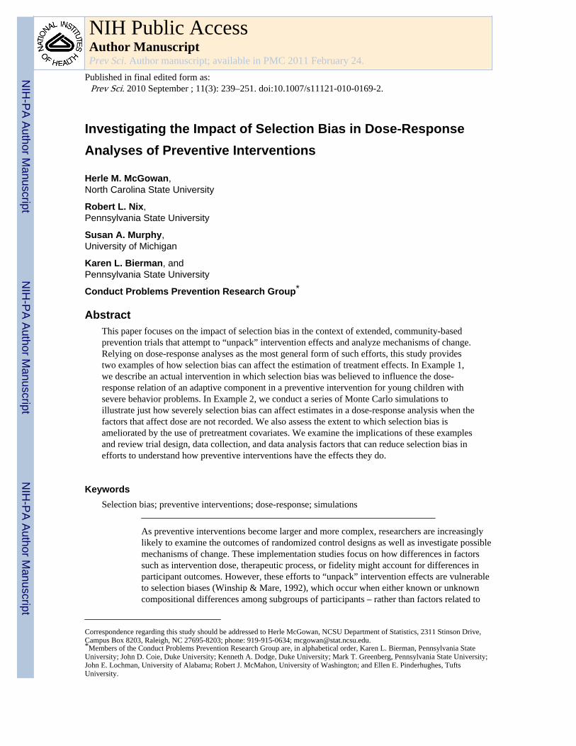
Data GenerationFigure 1 provides a pictorial representation as well as the generative models used to createeach of the variables for these simulations. (Programming code for these simulations isavailable at http://www.stat.lsa.umich.edu/~samurphy/papers/McGowanSimCode.txt.) Wegenerated each participant’s data by first drawing a variable (X) that represents a recordedpretreatment variable. Next, we drew an indicator of receipt of the first intervention dose(D1), which could be affected by this pretreatment variable. For each of the remaining timepoints (t = 2,…,22), we drew a time-varying confounder (Ct) prior to each interventionsession, which represents an unrecorded covariate that affects both the dose and theoutcome. An indicator that dose was either received at session t (Dt = 1) or not (Dt = 0) wasthen generated. Finally, after 22 sessions the outcome (Y) was generated. The continuousvariables (X, Ct, and Y) were standardized to have a mean of 0 and a standard deviation of 1.

As seen in Figure 1, the effect of cumulative dose ( ) on the outcome (Y) is given by β.Also seen in Figure 1, the strength of the confounding was represented by the product of therelation between the confounder and dose (γt) and the relation between the confounder and

McGowan et al. Page 7

Prev Sci. Author manuscript; available in PMC 2011 February 24.

NIH

-PA Author Manuscript

NIH

-PA Author Manuscript

NIH

-PA Author Manuscript

the response (ϕ). The direction of these relations was set so that the selection bias wasnegative: Those participants with higher values of Ct received a higher dose of treatment (γt> 0) but had worse outcomes (ϕ< 0). In an adaptive intervention, negative selection bias likethis occurs when higher doses are provided for participants with more serious problems, aswas the case with Fast Track in Example 1. The magnitude of the relation between theconfounder and dose (γt) was set to .14 or .39, and the magnitude of the relation between theconfounder and the outcome (ϕ) was set to −.14 or −.39, so that the product of standardizedversions of these two parameters (γt * ϕ) was equal to one of two negative values, −0.02 or−0.15 (i.e., .14 * −.14 = −.02 and .39 * −.39 = −.15). These values indicate that theconfounding would account for less than one-half of 1% of the variance in the outcome orfor about 2% of the variance in the outcome, respectively.3 According to Cohen (1988),even our larger value would only correspond to a conventional small effect, for theconversion of an R2 statistic in a multiple regression equation. We purposefully chose levelsof confounding that most prevention researchers would consider negligible to illustrate thedegree of selection bias that can affect the dose-response relation.

Simulation DesignThree simulations, A, B, and C, each of 1,000 data sets with 400 participants, weregenerated. The sample size for each simulated data set was selected to be similar to the sizeof the intervention group from Fast Track.

For simplicity, in Simulations A and B, data were generated so that all participants werehomogenous prior to treatment (e.g., there was no effect of the pretreatment covariate X, γ0= d0 = 0). Simulation A was designed so there was no effect of cumulative dose (β = 0) todetermine whether a null treatment effect could be overpowered by selection bias, resultingin a negative estimated treatment coefficient. In Simulation B there was a true positive effectof cumulative dose (β > 0). The purpose was to examine whether even a true positive effectcould be overpowered by selection bias, resulting in an estimated negative effect ofcumulative dose, as we suspected was happening in Fast Track. In both simulations, we

analyzed the data by a simple linear regression of Y on the cumulative treatment dose .The slope in this regression equation will be our estimator of β. (Recall that Ct has beendiscarded from the analyzed data so as to mimic Example 1, and that we did not need toinclude the pretreatment covariate [X] in these analyses because the data were generated sothat X had no effect on Y.)

In Simulation C, data were generated so that a pretreatment covariate (X) explains some ofthe confounding (γ0 > 0, d0 > 0), and there was no effect of treatment (β = 0). Thissimulation was designed to assess the extent to which adjusting for pretreatment covariatesin the estimated regression model can reduce selection bias. To analyze the data inSimulation C, we again used linear regression, but this time we regressed Y on both the

cumulative treatment dose ( ) and the pretreatment covariate X. In this model, theregression coefficient of cumulative treatment dose represents the effect of cumulative dosecontrolling for X.4

3As a frame of reference to help understand the magnitude of the confounding on the response, consider the case of the linearregression of a standardized response (Ystd = [Y − Ȳ] / sY) on a single standardized predictor (Xstd = [X − X̄] / sX. The regressionmodel for standardized variables is intercept free: Ystd = βstd * Xstd + ε, where ε~N(0,1). For this model, the standardized coefficient(βstd)2 is equal to R2 (Neter, et. al., 1996). Under this frame of reference, a standardized coefficient of −0.02 corresponds to an R2value of (−0.02)2 = 0.0004, and a standardized coefficient of −0.15 corresponds to an R2 value of (−0.15)2 = 0.0225.

McGowan et al. Page 8

Prev Sci. Author manuscript; available in PMC 2011 February 24.

NIH

-PA Author Manuscript

NIH

-PA Author Manuscript

NIH

-PA Author Manuscript

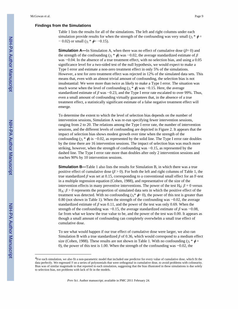
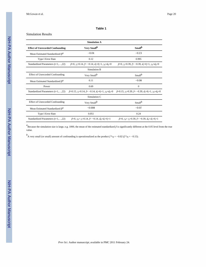
Findings from the SimulationsTable 1 lists the results for all of the simulations. The left and right columns under eachsimulation provide results for when the strength of the confounding was very small (γt * ϕ =− 0.02) or small (γt * ϕ= −0.15).

Simulation A—In Simulation A, when there was no effect of cumulative dose (β= 0) andthe strength of the confounding (γt * ϕ) was −0.02, the average standardized estimate of βwas −0.04. In the absence of a true treatment effect, with no selection bias, and using a 0.05significance level for a two-sided test of the null hypothesis, we would expect to make aType I error and estimate a non-zero treatment effect in only 5% of the simulations.However, a test for zero treatment effect was rejected in 12% of the simulated data sets. Thismeans that, even with an almost trivial amount of confounding, the selection bias is notinsubstantial: We were more than twice as likely to make a Type I error. The situation wasmuch worse when the level of confounding (γt * ϕ) was −0.15. Here, the averagestandardized estimate of β was −0.23, and the Type I error rate escalated to over 99%. Thus,even a small amount of confounding virtually guarantees that, in the absence of a truetreatment effect, a statistically significant estimate of a false negative treatment effect willemerge.

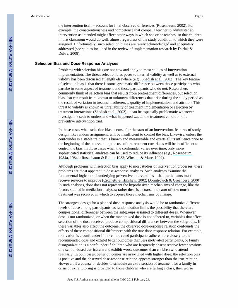
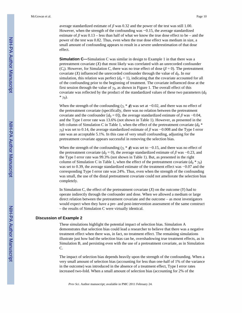
To determine the extent to which the level of selection bias depends on the number ofintervention sessions, Simulation A was re-run specifying fewer intervention sessions,ranging from 2 to 20. The relations among the Type I error rate, the number of interventionsessions, and the different levels of confounding are depicted in Figure 2. It appears that theimpact of selection bias shows modest growth over time when the strength of theconfounding (γt * ϕ) is −0.02, as represented by the solid line. The Type I error rate doublesby the time there are 16 intervention sessions. The impact of selection bias was much morestriking, however, when the strength of confounding was −0.15, as represented by thedashed line. The Type I error rate more than doubles after only 2 intervention sessions andreaches 90% by 10 intervention sessions.

Simulation B—Table 1 also lists the results for Simulation B, in which there was a truepositive effect of cumulative dose (β > 0). For both the left and right columns of Table 1, thetrue standardized β was set at 0.15, corresponding to a conventional small effect for an F-testin a multiple regression equation (Cohen, 1988), and representative of the size of theintervention effects in many preventive interventions. The power of the test H0: β = 0 versusHA: β > 0 represents the proportion of simulated data sets in which the positive effect of thetreatment was detected. With no confounding (γt* ϕ= 0), the power of this test is greater than0.80 (not shown in Table 1). When the strength of the confounding was −0.02, the averagestandardized estimate of β was 0.11, and the power of the test was only 0.69. When thestrength of the confounding was −0.15, the average standardized estimate of β was −0.08,far from what we knew the true value to be, and the power of the test was 0.00. It appears asthough a small amount of confounding can completely overwhelm a small true effect ofcumulative dose.

To see what would happen if our true effect of cumulative dose were larger, we also ranSimulation B with a true standardized β of 0.36, which would correspond to a medium effectsize (Cohen, 1988). These results are not shown in Table 1. With no confounding (γt * ϕ =0), the power of this test is 1.00. When the strength of the confounding was −0.02, the

4For each simulation, we also fit a non-parametric model that included one predictor for every value of cumulative dose, which fit thedata perfectly. We regressed Y on a series of polynomials that were orthogonal in cumulative dose, to avoid problems with colinearity.Bias was of similar magnitude to that reported in each simulation, suggesting that the bias illustrated in these simulations is due solelyto selection bias, not problems with lack of fit in the models.

McGowan et al. Page 9

Prev Sci. Author manuscript; available in PMC 2011 February 24.

NIH

-PA Author Manuscript

NIH

-PA Author Manuscript

NIH

-PA Author Manuscript

average standardized estimate of β was 0.32 and the power of the test was still 1.00.However, when the strength of the confounding was −0.15, the average standardizedestimate of β was 0.13 – less than half of what we know the true dose effect to be – and thepower of the test was 0.82. Thus, even when the true dose effect was medium in size, asmall amount of confounding appears to result in a severe underestimation of that doseeffect.

Simulation C—Simulation C was similar in design to Example 1 in that there was apretreatment covariate (X) that most likely was correlated with an unrecorded confounder(Ct). However, for Simulation C, there was no true effect of dose (β = 0). The pretreatmentcovariate (X) influenced the unrecorded confounder through the value of d0. In oursimulation, this relation was perfect (d0 = 1), indicating that the covariate accounted for allof the confounding prior to the beginning of treatment. The covariate influenced dose at thefirst session through the value of γ0, as shown in Figure 1. The overall effect of thiscovariate was reflected by the product of the standardized values of these two parameters (d0* γ0).

When the strength of the confounding (γt * ϕ) was set at −0.02, and there was no effect ofthe pretreatment covariate (specifically, there was no relation between the pretreatmentcovariate and the confounder [d0 = 0]), the average standardized estimate of β was −0.04,and the Type I error rate was 13.6% (not shown in Table 1). However, as presented in theleft column of Simulation C in Table 1, when the effect of the pretreatment covariate (d0 *γ0) was set to 0.14, the average standardized estimate of β was −0.008 and the Type I errorrate was an acceptable 5.1%. In this case of very small confounding, adjusting for thepretreatment covariate appears successful in removing the selection bias.

When the strength of the confounding (γt * ϕ) was set to −0.15, and there was no effect ofthe pretreatment covariate (d0 = 0), the average standardized estimate of β was −0.23, andthe Type I error rate was 99.3% (not shown in Table 1). But, as presented in the rightcolumn of Simulation C in Table 1, when the effect of the pretreatment covariate (d0 * γ0)was set to 0.39, the average standardized estimate of the treatment effect was −0.07 and thecorresponding Type I error rate was 24%. Thus, even when the strength of the confoundingwas small, the use of the distal pretreatment covariate could not ameliorate the selection biascompletely.

In Simulation C, the effect of the pretreatment covariate (X) on the outcome (Y) had tooperate indirectly through the confounder and dose. When we allowed a medium or largedirect relation between the pretreatment covariate and the outcome – as most investigatorswould expect when they have a pre- and post-intervention assessment of the same construct– the results of Simulation C were virtually identical.

Discussion of Example 2These simulations highlight the potential impact of selection bias. Simulation Ademonstrates that selection bias could lead a researcher to believe that there was a negativetreatment effect when there was, in fact, no treatment effect. The remaining simulationsillustrate just how bad the selection bias can be, overshadowing true treatment effects, as inSimulation B, and persisting even with the use of a pretreatment covariate, as in SimulationC.

The impact of selection bias depends heavily upon the strength of the confounding. When avery small amount of selection bias (accounting for less than one-half of 1% of the variancein the outcome) was introduced in the absence of a treatment effect, Type I error ratesincreased two-fold. When a small amount of selection bias (accounting for 2% of the

McGowan et al. Page 10

Prev Sci. Author manuscript; available in PMC 2011 February 24.

NIH

-PA Author Manuscript

NIH

-PA Author Manuscript

NIH

-PA Author Manuscript

variance in the outcome) was introduced in the absence of a treatment effect, false positivetreatment effects were almost certain, occurring in over 99% of the simulations.

Somewhat surprisingly, a small amount of confounding can cause bias in the estimateddose-response relation, even in the presence of a true positive effect of dose. (This mighthave been what we observed with Fast Track in Example 1.) With a true small treatmenteffect, a small amount of confounding can lead to a severe underestimation of the treatmenteffect and a reduction in power. With a true medium treatment effect, a small amount ofconfounding still can lead to severe underestimation of the treatment effect.

The length of the intervention program also affects the impact of confounding onconclusions. When the confounding is very small and there is no true treatment effect, theType I error rate climbs in a linear fashion with each successive intervention session. With asmall amount of confounding and no true treatment effect, the Type I error rate doubledafter only two intervention sessions and reached 90% by 10 sessions.

In some cases, pretreatment covariates may successfully reduce the effects of selection bias.In our simulation, this occurred when the effect of the confounder was very small and thepretreatment covariate was related to the confounder. When the confounding was stronger,or when there was no relation between the pretreatment covariate and the unrecordedconfounder, the use of the pretreatment covariate did not offer this protection.

Thus, the results of Example 2 illustrate how studies seeking to unpack intervention effectsusing a dose-response analysis are highly susceptible to inaccurate interpretations when thereasons for assigning dose at each time point are unrecorded (i.e., when selection bias existsdue to unmeasured time-varying confounders). Even when the strength of the confounding isvery small, the impact of selection bias is such that researchers cannot have confidence inestimates of significant relations – or lack thereof – in most dose-response analyses.

Summary and RecommendationsTo make optimal progress in the prevention and treatment of mental health or behaviorproblems, we must determine not only which intervention programs are effective but alsohow they work (Silverman, 2006). Implementation studies, such as dose-response analysesand examinations of fidelity, are invaluable in this regard. They have been used to assess thetheory of change and determine whether exposure to the experimental manipulation of theintervention is related to degree of improvement (Hill et al., 2003; Lyons-Ruth & Melnick,2004). In addition, they have been recommended when investigators are trying to determinewhether null or weak treatment effects reflect implementation difficulties, such that fewparticipants got the intervention as intended (Rohrbach et al., l993). As with otherdescriptive or correlational studies, however, efforts to peer inside the “black box” ofpreventive interventions can be susceptible to selection biases (Shadish et al., 2002). Even ifthe preventive intervention itself is experimental, implementation studies, such as dose-response analyses, typically are not.

This paper highlights the significant risk of confounding when conducting dose-responseanalyses, particularly when the reasons why dose is adapted – or why assigned dose is notadhered to – are unrecorded. The “real-life” example of the Fast Track peer pairingcomponent, along with the simulation studies, demonstrate that even minimal confoundingcannot be ignored, as it increases the chance of falsely detecting a treatment effect whenthere is none or failing to detect a treatment effect when one exists. Fortunately, theseexamples suggest a number of methodological features that might guard againstconfounding and foster the capacity to use implementation studies to learn more aboutmechanisms of change.

McGowan et al. Page 11

Prev Sci. Author manuscript; available in PMC 2011 February 24.

NIH

-PA Author Manuscript

NIH

-PA Author Manuscript

NIH

-PA Author Manuscript

Controlling Selection Bias Through DesignObviously, the best solution to the threat of confounding is through experimental design.This is the only certain means to address problems associated with unknown andunmeasured confounders. If researchers are specifically interested in using dose-responserelations to discern potential thresholds of participation necessary to achieve specificoutcomes, an ideal study design would involve the random assignment of dose, and theanalysis of “assigned dose” levels, rather than dose levels actually received (Feinstein,1991).

The relation between dose and response also can be assessed through some naturalexperiments. For example, in a study of the effects of a special program for adolescentmothers (Seitz et al., 1991), dose was determined by the month of delivery, a factor that,although not random, was unlikely to be related to pertinent confounders.

If researchers are interested in the impact of one part of a multi-component intervention –like peer pairing within the larger Fast Track project – they might consider factorial designs,which can be more powerful and more efficient than typical two-group designs (Shadish etal., 2002; Trochim, 2006; Box et. al., 1978). Similarly, there are dismantling studies inwhich a specific component is isolated and tested against the effects of a morecomprehensive intervention (e.g., Dimidjian et al., 2006; Dobson et al., 2008). TheMultiphase Optimization Strategy (Collins et al., 2005; Collins et al., 2007) provides explicitinstruction on how to use experimental design to systematically investigate whichcombinations of intervention components might be most effective in bringing about change.

Controlling Selection Bias Through the Use of CovariatesMost implementation studies are undertaken in a post-hoc fashion to examine mechanismsof change operating within a randomized control trial. It is rarely adequate, however, tosimply assess dose or some other aspect of implementation quality and examine relations tooutcomes (Pocock & Abdalla, 1998). Instead, researchers must rely on the careful selection,collection, and use of relevant covariates to control for selection biases.

Careful selection of relevant covariates at the point of program design might allowresearchers to identify and determine appropriate measures of potentially important time-varying confounding variables so they may be utilized during analysis. Researchers shouldpay special attention to those variables that have been related to motivation, participation inintervention, or adherence to intervention protocols in previous studies, as well as variablesthat were predictive of response to treatment. In the case of adaptive interventions,researchers also should consider those variables that would be expected to influence staffmembers’ clinical judgment regarding need for services (Collins et al., 2004), such as aglobal assessment of functioning (Hall, 1995) or some indicator of a primary outcome, likesocial competence and aggression in Fast Track. To assist in the identification of importantpotential confounding variables, it would be beneficial for prevention researchers to reportthe strongest predictors of dose received, project guidelines regarding how and when dosewas adjusted, and characteristics of those participants most likely to respond to services.

Just as with any construct, it is critical to assess covariates with psychometrically-soundmeasures. Ideally, these would rely on objective informants or methods that are independentof participants’ or staff members’ decisions to adjust dose.

Careful collection of relevant covariates requires assessment each time a decision to changedose is made. When participants in the intervention make those decisions on their own – bychoosing to attend or miss an intervention session – it will be difficult to conduct perfectly-timed assessments. In that case, it might make sense to conduct brief, frequent assessments

McGowan et al. Page 12

Prev Sci. Author manuscript; available in PMC 2011 February 24.

NIH

-PA Author Manuscript

NIH

-PA Author Manuscript

NIH

-PA Author Manuscript

throughout the intervention. In adaptive interventions, it is best to time assessments so theycoincide with staff members’ decisions to alter dose. In Fast Track, it was not useful to havecovariates at the end of kindergarten or even first grade because decisions to adjust the doseof peer pairing were made throughout second grade. It would have been preferable if staffmembers had completed brief ratings of social competence and aggression on every child intheir caseload at the end of each week in second grade; staff members also could havechecked in with teachers more systematically and recorded their impressions. Regardless ofwho makes the decision to change dose, it is critical to conduct assessments on allparticipants in the intervention, regardless of whether a particular participant’s dose waschanged or not.

When investigators collect measures prior to the start and throughout the duration of theintervention, they will be in a much better position to evaluate and control for the impact ofselection bias (Wilkinson & the Task Force on Statistical Inference, 1999). There exist anumber of well-documented analytic techniques that can reduce the effects of selection biasdue to pretreatment confounders, such as inclusion of pretreatment covariates in theregression model, use of propensity scores techniques (e.g., Rosenbaum & Rubin, 1983;Rubin, 1997), or use of the Heckman estimator (Heckman, 1976). The goal of any of theseanalytic techniques is the same: To compare subjects with similar characteristics across therange of covariates who differ only with respect to dose received. It has been shown that, iftreatment assignment is independent of the response after accounting for the covariates (i.e.,if treatment assignment is strongly ignorable, in the language of causal inference), thenunbiased estimates of the treatment effect can be found (Rosenbaum & Rubin, 1983). Likeany analytic technique, however, each of these statistical models depends on certainassumptions and will only be successful in controlling selection bias to the extent that theassumptions are satisfied.

When dose is adapted and readapted at multiple time points, either informally as indicatedby participants’ variable attendance or by formal design according to participants’ assessedneed, pretreatment covariates are unlikely to be sufficient predictors of dose. Additionalmid-intervention assessments of outcomes and individual characteristics that function astime-varying confounders are required to adequately predict which participants will receivemore intervention services.

In the epidemiology literature, the propensity score method has been adapted for use withtime-varying confounders and is known as the marginal structural model (e.g., Robins et al.,2000; Hernán et al., 2000; Bodnar et al., 2004). In the first step of such analyses a regressionequation, referred to as the treatment model, is estimated to predict the receipt ofintervention at time point t. The independent variables in this logistic regression equationwould include indicators of the receipt of intervention for every session prior to time point tand measures of time-varying confounders, such as child behavior problems, assessed atregular intervals throughout the intervention. The results of this logistic regression equationyield a predicted probability of the receipt of intervention for each participant at time point tconditioned on the confounders and treatment history up to that time. For example,participants who had attended all prior sessions of the intervention would have a highpredicted probability of the receipt of that final session, whether they actually attended thatfinal session or not. (A modeling note: When dose at each time point is recorded as a binary[1/0] variable according to whether a participant did or did not receive treatment at that time,care must be taken to model the receipt of intervention [1] rather than its absence [0]. Forexample, in SAS proc logistic, it is necessary to specify the ‘descending’ option in the modelstatement.)

McGowan et al. Page 13

Prev Sci. Author manuscript; available in PMC 2011 February 24.

NIH

-PA Author Manuscript

NIH

-PA Author Manuscript

NIH

-PA Author Manuscript

The predicted probabilities from the treatment model are then used to calculate sampleweights (for details on how to construct these weights, see Barber et al., 2004; Cole &Hernán, 2008; Mortimer et al., 2005). The weights are based on the inverse of the predictedprobabilities so that more weight is given to participants who are less represented in theobserved data than they would have been if assignment to intervention had been randomized(Mortimer et al., 2005). This serves to decouple the relation between the history ofattendance and the history of time-varying confounders from the receipt of intervention attime point t. In other words, the weights can mimic what would have happened ifparticipants with similar histories of attendance and similar histories of time-varyingconfounders had been randomly assigned to receive intervention at time point t, balancingparticipants with different histories of attendance and different histories of the time-varyingconfounders across different doses of intervention.

In the final step of a marginal structural model, the weighted data are used in a typicalregression equation to assess the dose-response relation. The most important assumptionguaranteeing that the coefficient for dose provides an unbiased estimate of the treatmenteffect is that there is no unmeasured confounding; this is sometimes referred to as thesequential randomization assumption and implies that all important time-varyingconfounders have been accounted for in the treatment model (Cole & Hernán, 2008;Mortimer et al., 2005). Research has shown, however, that with a marginal structural modelselection bias is reduced, though not eliminated, even if every important time-varyingconfounder is not included (Barber et al., 2004; Bray et al., 2006).

In applying a marginal structural model, it is critical to remember that bias is only reduced tothe extent that the treatment model is correctly specified. It is usually unwise to simply“dump” all measured time-varying confounders into the treatment model; careful fitting isnecessary to determine the best form and complexity (Cole & Hernán, 2008; Mortimer et al.,2005; for examples of how to determine the most appropriate treatment model and calculateprobability weights, see Barber et al., 2004; Cole & Hernán, 2008; Mortimer et al., 2005). Italso is critical to remember that all time-varying confounders must be assessed for allchildren and families assigned to the intervention at every time point the decision to changedose for any individual is considered. Otherwise, it will be impossible to compareparticipants with similar characteristics who differ with respect to dose received.

Final ThoughtsIt is important to remember that the validity of a dose-response analysis hinges on variationin dose that is unrelated to participants’ need or to reasons why they might respond to aparticular intervention. Otherwise, dose-response analyses are likely affected by selectionbias, as illustrated in this paper.

Randomization of dose is the optimal strategy for assessing dose effects, as it avoidsselection bias, and can be extended to studies in which treatment is time-varying (Murphy etal., 2006). Without randomization of dose, researchers can never be certain of their ability tocompletely remove confounding; they can only use sensitivity analysis and boundingmethods to assess the likely magnitude of any residual bias (Robins, 1999). As with anyanalysis of observational data, causal claims of treatment effectiveness must be temperedwith appropriate caution about the possibility of residual confounding.

When randomization is not possible, or when adherence to randomized dose is low,prevention researchers can control for systematic differences between those participantsreceiving different doses through the careful selection, measurement, collection, and use ofboth pretreatment and time-varying confounding variables. In these post-hoc analyses, it isonly by removing systematic differences through the proper use of relevant covariates – for

McGowan et al. Page 14

Prev Sci. Author manuscript; available in PMC 2011 February 24.

NIH

-PA Author Manuscript

NIH

-PA Author Manuscript

NIH

-PA Author Manuscript

example, by using a marginal structural model – that investigators can hope to gain a lessbiased understanding of what is happening inside the “black box” of preventiveinterventions.

ReferencesAchenbach, TM. Manual for the Teacher’s Report Form and 1991 Profile. Burlington, VT: University

of Vermont Department of Psychiatry; 1991.Barber JS, Murphy SA, Verbitsky N. Adjusting for time-varying confounding in survival analysis.

Sociological Methodology 2004;34:163–192.Bierman, KL.; Greenberg, MT. Conduct Problems Prevention Research Group. Social skills training in

the Fast Track Program. In: Peters, RD.; McMahon, RJ., editors. Preventing childhood disorders,substance abuse, and delinquency. Thousand Oaks, CA: Sage; 1996. p. 65-89.

Bierman KL, Nix RL, Maples JJ, Murphy SA. Conduct Problems Prevention Research Group.Examining clinical judgment in an adaptive intervention design: The Fast Track program. Journal ofConsulting and Clinical Psychology 2006;74:468–481. [PubMed: 16822104]

Bodnar LM, Davidian M, Siega-Riz AM, Tsiatis AA. Marginal structural models for analyzing causaleffects of time-dependent treatments: An application in perinatal epidemiology. American Journalof Epidemiology 2004;159:926–934. [PubMed: 15128604]

Box, GEP.; Hunter, WG.; Hunter, JS. An Introduction to Design. Data Analysis, and Model Building.New York: John Wiley and Sons; 1978. Statistics for Experimenters.

Bray B, Almirall D, Zimmerman R, Lynam D, Murphy SA. Assessing the total effect of time-varyingpredictors in prevention research. Prevention Science 2006;7:1–17. [PubMed: 16489417]

Cicchetti D, Hinshaw SP. Prevention and intervention science: Contributions to developmental theory.Development and Psychopathology 2002;14:667–671. [PubMed: 12549698]

Cochran WG, Rubin DR. Controlling bias in observational studies: A review. Sankhya: The IndianJournal of Statistics, Series A 1973;35:417–446.

Cohen, J. Statistical power analysis for the behavioral sciences. 2. Hillsdale, NJ: Lawrence EarlbaumAssociates; 1988.

Coie JD, Dodge KA. Multiple sources of data on social behavior and social status in the school: Across-age comparison. Child Development 1988;59:815–829. [PubMed: 3383681]

Cole SR, Hernán MA. Constructing Inverse Probability Weights for Marginal Structural Models.American Journal of Epidemiology 2008;168:656–664. [PubMed: 18682488]

Collins LM, Murphy SA, Bierman KA. A conceptual framework for adaptive preventive interventions.Prevention Science 2004;5:185–196. [PubMed: 15470938]

Collins LM, Murphy SA, Nair VN, Strecher V. A strategy for optimizing and evaluating behavioralinterventions. Annals of Behavioral Medicine 2005;30:65–73. [PubMed: 16097907]

Collins LM, Murphy SA, Strecher V. The Multiphase Optimization Strategy (MOST) and theSequential Multiple Assignment Randomized Trial (SMART): New methods for more potentehealth interventions. American Journal of Preventive Medicine 2007;32:S112–S118. [PubMed:17466815]

Conduct Problems Prevention Research Group. A developmental and clinical model for the preventionof conduct disorders: The Fast Track program. Development and Psychopathology 1992;4:509–527.

Conduct Problems Prevention Research Group. Initial impact of the Fast Track prevention trial forconduct problems: I. The high-risk sample. Journal of Consulting and Clinical Psychology1999;67:631–647. [PubMed: 10535230]

Conduct Problems Prevention Research Group. Evaluation of the first 3 years of the Fast Trackprevention trial with children at high risk for adolescent conduct problems. Journal of AbnormalChild Psychology 2002;30:19–35. [PubMed: 11930969]

Dimidjian S, Hollon SD, Dobson KS, Schmaling KB, Kohlenberg RJ, Addis ME, Gallop R,McGlinchey JB, Markley DK, Gollan JK, Atkins DC, Dunner DL, Jacobson NS. Randomized trialof behavioral activation, cognitive therapy, and antidepressant medication in the acute treatment of

McGowan et al. Page 15

Prev Sci. Author manuscript; available in PMC 2011 February 24.

NIH

-PA Author Manuscript

NIH

-PA Author Manuscript

NIH

-PA Author Manuscript

adults with major depression. Journal of Consulting and Clinical Psychology 2006;74:658–670.[PubMed: 16881773]

Domitrovich CE, Greenberg MT. The study of implementation: Current findings from effectiveprograms that prevent mental disorders in school-aged children. Journal of Educational andPsychological Consultation 2000;11:193–221.

Durlak JA, DuPre EP. Implementation matters: A review of research on the influence ofimplementation on program outcomes and the factors affecting implementation. American Journalof Community Psychology 2008;41:327–350. [PubMed: 18322790]

Feinstein, AL. Intention to treat policy for analyzing randomized trials: statistical distortions andneglected clinical challenges. In: Cramer, J.; Spilker, B., editors. Patient compliance in medicalpractice and clinical trials. New York: Raven Press; 1991.

Hall RCW. Global Assessment of Functioning: A modified scale. Psychosomatics: Journal ofConsultation Liaison Psychiatry 1995;36:267–275.

Heckman J. The common structure of statistical models of truncation, sample selection, and limiteddependent variables and a simple estimator for such models. Annals of Economic and SocialMeasurement 1976;5:475–492.

Hernán MA, Brumback B, Robins JM. Estimating the causal effect of zidovudine on CD4 count with amarginal structural model for repeated measures. Statistics in Medicine 2000;21:1689–1709.

Hill JL, Brooks-Gunn J, Waldfogel J. Sustained effects of high participation in an early interventionfor low birth-weight premature infants. Developmental Psychology 2003;39:730–744. [PubMed:12859126]

Jacobson NS, Schmaling KB, Holtzworth-Munroe A, Katt JL, Wood LF, Follette VM. Research-structured vs. clinically flexible versions of social learning-based marital therapy. BehaviourResearch and Therapy 1989;27:173–180. [PubMed: 2930443]

Kreuter, M.; Farrell, D.; Olevitch, L.; Brennan, L. Tailoring health messages: Customizingcommunication with computer technology. Malway, NJ: Erlbaum; 2000.

Lavori PW, Dawon R, Roth AJ. Flexible treatment strategies in chronic disease: Clinical and researchimplications. Biological Psychiatry 2000;48:605–614. [PubMed: 11018231]

Lyons-Ruth K, Melnick S. Dose-response effect of mother-infant clinical home visiting on aggressivebehavior problems in kindergarten. Journal of the American Academy of Child and AdolescentPsychiatry 2004;43:699–707. [PubMed: 15167086]

Mortimer KM, Neugebauer R, van der Laan M, Tager IB. An Application of Model-fitting Proceduresfor Marginal Structural Models. American Journal of Epidemiology 162:382–388. [PubMed:16014771]

Murphy SA, Oslin D, Rush AJ, Zhu J. for MCATS. Methodological challenges in constructingeffective treatment sequences for chronic disorders. Neuropsychopharmacology 2006;32:257–262.[PubMed: 17091129]

Neter, J.; Kutner, MH.; Nachtsheim, CJ.; Wasserman, W. Applied linear statistical models. 4. NewYork: McGraw-Hill; 1996.

Pocock SJ, Abdalla M. The hope and hazards of using compliance data in randomized controlled trials.Statistics in Medicine 1998;17:303–317. [PubMed: 9493256]

Robins JM. Association, causation, and marginal structural models. Synthese 1999;121:151–179.Robins JM, Hernán MA, Brumback B. Marginal structural models and causal inference in

epidemiology. Epidemiology 2000;11:550–560. [PubMed: 10955408]Rohrbach LA, Graham JW, Hansen WB. Diffusion of school-based substance abuse prevention

program: Predictors of program implementation. Preventive Medicine 1993;22:237–260.[PubMed: 8483862]

Rosenbaum, PR. Observational studies. 2. New York: Springer; 2002.Rosenbaum PR. The consequences of adjustment for a concomitant variable that has been affected by

the treatment. Journal of the Royal Statistical Society, Series A 1984a;147:656–666.Rosenbaum PR. From association to causation in observational studies: the role of tests of strongly

ignorable treatment assignment. Journal of the American Statistical Association 1984b;79:41–48.

McGowan et al. Page 16

Prev Sci. Author manuscript; available in PMC 2011 February 24.

NIH

-PA Author Manuscript

NIH

-PA Author Manuscript

NIH

-PA Author Manuscript

Rosenbaum PR, Rubin DB. The central role of the propensity score in observational studies for causaleffects. Biometrika 1983;70:41–55.

Rubin DB. Estimating causal effects from large data sets using propensity scores. Annals of InternalMedicine 1997;127:757–763. [PubMed: 9382394]

Trochim, William M. The Research Methods Knowledge Base. 22006. Retrieved November 10, 2009,from http://www.socialresearchmethods.net/kb/expfact.php

Seitz V, Apfel NH, Rosenbaum LK. Effects of an intervention program for pregnant adolescents:Educational outcomes at two years postpartum. American Journal of Community Psychology1991;19:911–930. [PubMed: 1793098]

Shadish, WR.; Cook, TD.; Campbell, DT. Experimental and quasi-experimental designs forgeneralized causal inference. New York: Houghton Mifflin; 2002.

Silverman WK. Shifting our thinking and training from evidence-based treatments to evidence-basedexplanations of treatments. In Balance: Society of Clinical Child and Adolescent PsychologyNewsletter 2006:21.

Wilkinson L. The Task Force on Statistical Inference. Statistical methods in psychology journals:Guidelines and explanations. American Psychologist 1999;54:594–604.

Winship C, Mare RD. Models for sample selection bias. Annual Review of Sociology 1992;18:327–350.

McGowan et al. Page 17

Prev Sci. Author manuscript; available in PMC 2011 February 24.

NIH

-PA Author Manuscript

NIH

-PA Author Manuscript

NIH

-PA Author Manuscript

Figure 1.Relations Modeled in Simulations

Note: Note: ε1, …, εT−1, ε are independent Normally distributed random

variables each with mean 0 and variance 1, and is aNormally distributed random variable with mean zero and variance:

McGowan et al. Page 18

Prev Sci. Author manuscript; available in PMC 2011 February 24.

NIH

-PA Author Manuscript

NIH

-PA Author Manuscript

NIH

-PA Author Manuscript

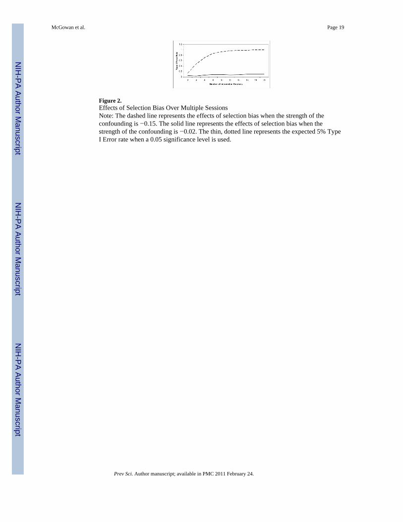
Figure 2.Effects of Selection Bias Over Multiple SessionsNote: The dashed line represents the effects of selection bias when the strength of theconfounding is −0.15. The solid line represents the effects of selection bias when thestrength of the confounding is −0.02. The thin, dotted line represents the expected 5% TypeI Error rate when a 0.05 significance level is used.

McGowan et al. Page 19

Prev Sci. Author manuscript; available in PMC 2011 February 24.

NIH

-PA Author Manuscript

NIH

-PA Author Manuscript

NIH

-PA Author Manuscript

NIH

-PA Author Manuscript

NIH

-PA Author Manuscript

NIH

-PA Author Manuscript

McGowan et al. Page 20

Table 1

Simulation Results

Simulation A

Effect of Unrecorded Confounding Very Smallb Smallb

Mean Estimated Standardized βa −0.04 −0.23

Type I Error Rate 0.12 0.995

Standardized Parameters (t=1,…,22) β=0, γt=0.14, f= −0.14, dt=θt=1, γ0=d0=0 β=0, γt=0.39, f= −0.39, dt=θt=1, γ0=d0=0

Simulation B

Effect of Unrecorded Confounding Very Smallb Smallb

Mean Estimated Standardized βa 0.11 −0.08

Power 0.69 0

Standardized Parameters (t=1,…,22) β=0.15, γt=0.14, f= −0.14, dt=θt=1, γ0=d0=0 β=0.15, γt=0.39, f= −0.39, dt=θt=1, γ0=d0=0

Simulation C

Effect of Unrecorded Confounding Very Smallb Smallb

Mean Estimated Standardized βa −0.008 −0.07

Type I Error Rate 0.051 0.24

Standardized Parameters (t=1,…,22) β=0, γ0= γt=0.14, f= −0.14, d0=dt=θt=1 β=0, γ0= γt=0.39, f= −0.39, d0=dt=θt=1

aBecause the simulation size is large, e.g. 1000, the mean of the estimated standardized β is significantly different at the 0.05 level from the true

value.

bA very small (or small) amount of confounding is operationalized as the product f *γt = −0.02 (f *γt = −0.15).

Prev Sci. Author manuscript; available in PMC 2011 February 24.