Download - Improving intelligent dasymetric mapping population density ...

1

Improving intelligent dasymetric mapping population density

estimates at 30-meter resolution for the conterminous United States

by excluding uninhabited areas

Jeremy Baynes1, Anne Neale1, Torrin Hultgren2

1. Center for Public Health and Environmental Assessment, US Environmental Protection Agency, Research Triangle Park, 5

NC 27711, USA

2. EPA National Geospatial Support Team, ITS-EPA III Infrastructure Support and Application Hosting Contract, Research

Triangle Park, NC 27711, USA

Correspondence: Jeremy Baynes ([email protected])

Abstract. Population change impacts almost every aspect of global change from land use, to greenhouse gas emissions, to 10

biodiversity conservation, to the spread of disease. Data on spatial patterns of population density help us understand patterns

and drivers of human settlement and can help us quantify the exposure we face to natural disasters, pollution, and infectious

disease. Human populations are typically recorded by national or regional units that can vary in shape and size. Using these

irregularly sized units and ancillary data related to population dynamics, we can produce high resolution, gridded estimates of

population density through intelligent dasymetric mapping (IDM). The gridded population density provides a more detailed 15

estimate of how the population is distributed within larger units. Furthermore, we can refine our estimates of population density

by specifying uninhabited areas which have impacts on the analysis of population density such as our estimates of human

exposure. In this study, we used various geospatial datasets to expand the existing specification of uninhabited areas within

EPA’s EnviroAtlas Dasymetric Population Map for conterminous United States (CONUS). When compared to the existing

definition of uninhabited areas for the EnviroAtlas Dasymetric Population Map, we found that IDM’s population estimates for 20

U.S Census Bureau blocks improved across all states in CONUS. We also found that IDM performed better in states with

larger urban areas than in states that are sparsely populated. Future updates of the Dasymetric Population Map might benefit

from stratified (e.g., urban/exurban/rural) multi-state sampling of population density rather than state-specific sampling. We

also updated the existing EnviroAtlas Intelligent Dasymetric Mapping toolbox and expanded its capabilities to accept

uninhabited areas. 25

1. Introduction

Population density is a critical variable for understanding human-environment relationships. It has been recognized as an

essential societal variable for studying human interactions with the environment and it is crucial for quantifying human

exposure to natural hazards. Data on population density have facilitated global mapping of the changing human footprint on

Earth’s terrestrial surface(Venter et al., 2016). The drivers and patterns of human settlement and population growth are a key 30

part of understanding this expanding human footprint. Population density data allow researchers to investigate the spatio-

https://doi.org/10.5194/essd-2021-277

Ope

n A

cces

s Earth System

Science

DataD

iscussio

ns

Preprint. Discussion started: 15 February 2022c© Author(s) 2022. CC BY 4.0 License.

2

temporal patterns of human settlement, monitor changes in those patterns, and investigate how urban areas expand (Yu Fang

et al., 2018; Y. Fang & Jawitz, 2019; Taubenböck et al., 2019; Wei, Taubenböck, & Blaschke, 2017). Furthermore, population

density maps have allowed researchers to identify natural drivers of population density such as elevation, temperature, and

precipitation (Liu, Wang, & Xu, 2019; Samson, Berteaux, McGill, & Humphries, 2011). Population density data offer insights 35

about the impact of human settlement and the risks and exposure people face from the environment. Population density has

been used to assess the impacts of human activity on coral reefs (Bellwood, Hoey, & Hughes, 2012; Cinner, Graham, Huchery,

& Macneil, 2013; Morais, Connolly, & Bellwood, 2019). Considerable work has used population density data to quantify

human exposure and vulnerability to natural disasters and pollution (Carroll et al., 1997; Nahayo et al., 2019; Nasiri, Yusof,

Ali, & Hussein, 2018; Nicholls & Small, 2002; Samoli et al., 2019; Smith et al., 2019; Yuan, Gao, & Qi, 2019). For example, 40

population data has been used to quantify U.S population exposure to fine particles as a part of reporting the costs and benefits

of the Clean Air Act Amendments of 1990 (U.S. Environmental Protection Agency, 2011). In Vietnam, researchers identified

critical values of population density where the risk of dengue fever is high (Schmidt et al., 2011). Globally, population density

was found to be a significant driver of the origins of emerging infectious diseases from 1940 – 2004 (Jones et al., 2008).

In the United States (US), estimating population density usually involves distributing population counts collected within source 45

units such as blocks, or block groups delineated by the U.S. Census Bureau. The Census Bureau, like many other organizations,

relies on censuses and surveys to allocate people to source units. Population density is often simply estimated as the population

count divided by the area for each source unit. However, the population recorded in these units can be disaggregated to provide

estimates of how the population within source units is distributed. This disaggregation is important when source units are large,

varying in shapes and sizes, or the population within the source units is not evenly distributed (Leyk et al., 2019). Various 50

techniques have been used to allocate population counts from source units to estimate population density. Pycnophylactic

interpolation estimates population density within source units using a grid of equal-sized cells (Tobler, 1979). The

pycnophylactic property of this method ensures that the counts from each source unit are maintained in the process and that

population is not lost nor displaced beyond the source unit within which it was recorded (Tobler, 1979). Source units can be

divided up into smaller target units of homogenous population density. For example, target units can be determined by the 55

spatial intersection between census blocks and land cover classes. In this example, a target unit consists of the area of a land

cover class inside a census block. Areal weighting distributes the population of source units to target units by the proportion

of the area of the target unit inside the source unit (Goodchild & Lam, 1980). This method maintains the counts of the source

units as suggested by Tobler (1979). However, the only determinant of population density is the area of a target unit inside a

source unit. This is problematic where area might not be the best indicator of population dynamics. For example, in a source 60

unit that is largely covered by a wildlife refuge and minimally covered by urban land use, the proportion of the source unit’s

population that resides in urban land use should, in reality, be greater than that in the wildlife refuge.


Ope

n A

cces

s Earth System

Science

DataD

iscussio

ns


3

Dasymetric allocation of population can incorporate the population dynamics that are to be expected within source units in

order to estimate population density. Dobson et al. (2000) used coefficients calculated by weighted combinations of factors

that influence human populations to estimate population density from aggregate population counts. Other methods have used 65

the Random Forest algorithm to predict population density at fine scales using aggregate population counts and aggregated

fine-scale covariates that are related to population density (Sorichetta et al., 2015; Stevens, Gaughan, Linard, & Tatem, 2015).

Researchers have modeled gridded population density from small area sampling of population counts rather than using a

national census (Weber et al., 2018). To improve estimates, various dasymetric population mapping methods have used land

use/land cover, climatic and topographic variables such as temperature, precipitation, elevation, and slope, and socio-economic 70

variables such as nighttime lights, roads, and points of interest related to human activity (Karunarathne & Lee, 2019; Lloyd et

al., 2019; Ye et al., 2019).

Mennis and Hultgren (2006) developed an Intelligent Dasymetric Mapping (IDM) technique that estimates population density

by determining class-specific representative population densities from an ancillary raster containing classes that are indicative

of population dynamics. In 2016, IDM was used to develop a dasymetric population map of the conterminous US by the 75

Environmental Protection Agency’s (EPA) Office of Research and Development. The map was developed for EnviroAtlas, an

online collection of interactive tools and resources that provides data, research, and analysis on the relationships between

nature, people, health, and the economy (Pickard, Daniel, Mehaffey, Jackson, & Neale, 2015). Census block counts for 2010

were disaggregated to 30 m grid cells using the 2011 National Land Cover Database (NLCD) as the ancillary raster. The

identification of uninhabited areas and not allocating people to those areas can further refine population density to areas where 80

humans are more likely to settle. This refinement has a marked impact on the accuracy of estimates of population density (Y.

Fang & Jawitz, 2018; Leyk et al., 2019; Smith et al., 2019).

Uninhabited areas in the 2016 EnviroAtlas dasymetric population map effort were identified as the open water, perennial

ice/snow, and emergent herbaceous wetlands land cover classes along with areas that have a slope greater than 25%. In this

study, we updated the pre-existing EnviroAtlas dasymetric population map for the conterminous United States (CONUS) by 85

incorporating additional geospatial data sets to expand areas identified as uninhabited. We then conducted an assessment to

test the validity of our methods and measure any improvement in population density mapping associated with our effort. While

updating the EnviroAtlas dasymetric population map, we also updated the EnviroAtlas IDM toolbox, a toolbox originally

developed for ESRI ArcMap 10.3 that allows users to create dasymetric population maps of their own study areas. The updated

methodology has been implemented as a toolbox for ArcGIS Pro and a standalone Python tool that relies on open source 90

libraries. We expanded the IDM toolbox’s capabilities to accept additional uninhabited areas from users.


Ope

n A

cces

s Earth System

Science

DataD

iscussio

ns


4

2. Data

We updated the existing population density map for CONUS using data that were nationally consistent and complete, fit for

purpose, freely available or available under existing license, and relevant to human land use. Table 1 presents the data sets and

layers that were used to update the dasymetric population map. 95

Table 1. Datasets used for updating the EnviroAtlas dasymetric population map. IDM uses in bold were used in the 2016 EnviroAtlas

dasymetric population map.

Source Dataset / Version /

Format Name IDM use

U.S. Census Bureau

Census blocks

Vintage, 2010

TIGER/Line ESRI

Shapefile

Census blocks with population and

housing counts Source units

Multi-Resolution

Land Characteristics

Consortium/ National

Land Cover Database

2011 Land Cover

Version 2 (2016)

ERDAS Imagine

Developed, Open Space Inhabited ancillary class

Developed, Low Intensity Inhabited ancillary class

Developed, Medium Intensity Inhabited ancillary class

Developed, High Intensity Inhabited ancillary class

Barren Land (Rock/Sand/Clay) Inhabited ancillary class

Evergreen Forest Inhabited ancillary class

Mixed Forest Inhabited ancillary class

Shrub/Scrub Inhabited ancillary class

Grassland/Herbaceous Inhabited ancillary class

Pasture/Hay Inhabited ancillary class

Cultivated Crops Inhabited ancillary class

Woody Wetlands Inhabited ancillary class

Emergent Herbaceous Wetlands Uninhabited ancillary class

Perennial Ice/Snow Uninhabited ancillary class

Open Water Uninhabited ancillary class

Developed

Imperviousness

Descriptor

2016 Edition, 2011

ERDAS Imagine

Primary road in urban area Uninhabited ancillary class

Primary road outside urban area Uninhabited ancillary class

Energy production site in urban area Uninhabited ancillary class

Energy production site outside urban

area Uninhabited ancillary class

HERE/

NAVSTREETS

Land Use A

9.0, 2017

ESRI Geodatabase

Shopping center Uninhabited ancillary class

Industrial complex Uninhabited ancillary class

Cemetery Uninhabited ancillary class

Land Use B

9.0, 2017

ESRI Geodatabase

Aircraft roads Uninhabited ancillary class

OpenStreetMap

Foundation (OSMF)

& Contributors

Land use

2019

ESRI Shapefile

Retail Uninhabited ancillary class

Commercial Uninhabited ancillary class

Mall Uninhabited ancillary class

Industrial Uninhabited ancillary class

Places of interest

2019

ESRI Shapefile

Supermarket Uninhabited ancillary class

School Uninhabited ancillary class


Ope

n A

cces

s Earth System

Science

DataD

iscussio

ns


5

North American Rail

Network

Rail network

2019

ESRI Shapefile

Rail network Uninhabited ancillary class

CoreLogic

Residential parcels

2018

ESRI Geodatabase

Residential parcels Inhabited ancillary class

U.S. Geological

Survey Gap Analysis

Project/ Protected

Areas Database of the

U.S.

Combined Protected

Areas: Proclamation,

marine, fee, designation,

easement

2.0, 2018

ESRI Geodatabase

Local park Uninhabited ancillary class

State park Uninhabited ancillary class

State forest Uninhabited ancillary class

National wildlife refuge Uninhabited ancillary class

National forest Uninhabited ancillary class

National park Uninhabited ancillary class

National lakeshore/seashore Uninhabited ancillary class

National grassland Uninhabited ancillary class

U.S. Geological

Survey 2012 (30m) National Elevation Dataset Uninhabited ancillary class

2.1 Boundaries 100

The TIGER/Line shapefiles from the United States Census Bureau provided state boundaries along with their Federal

Information Processing Series (FIPS) codes (U.S. Census Bureau, 2012). The boundaries for statistical entities from the U.S.

Census Bureau are organized hierarchically from census blocks within block groups which are contained within census tracts

within the counties of a state (U.S. Census Bureau, 2012). We used a special release shapefile of the 2010 TIGER/Line census

blocks that included the population and housing counts from the 2010 decennial census carried out by the U. S. Census Bureau 105

(U.S. Census Bureau, 2012). The shapefile also includes the state FIPS code, county FIPS code, the census tract code, and the

census tabulation block number for each block (U.S. Census Bureau, 2012).

2.2 Land Cover

The 30 m, 2011 land cover classification from the 2016 NLCD (i.e., NLCD2016 2011) was used as the ancillary raster (Homer

et al., 2020; Yang et al., 2018). Yang et al. used a leaf-on Landsat image as the base image for the 2011 NLCD classification. 110

Pixels with cloud, shade, and other anomalies in the base Landsat image were filled using leaf-on or leaf-off Landsat images

within two years of the base image (Yang et al., 2018). The NLCD classification was carried out using a decision-tree classifier

with the Landsat image and ancillary data (Yang et al., 2018). The overall users accuracy for NLCD2016 2011 is 86.8%

(Wickham, Stehman, Sorenson, Gass, & Dewitz, 2021)

2.3 Land Use 115

In order to identify uninhabited areas, we used several publicly available and proprietary datasets from the OpenStreetMap

Foundation & Contributors (OSM), NAVSTREETS, CoreLogic, the Protected Areas Database of the U.S. (PAD-US), the

North American Rail Network (NARN), NLCD, and the National Elevation Dataset (NED)(CoreLogic, 2018; HERE, 2017;

OpenStreetMap contributors, 2019; U.S. Geological Survey, EROS Data Center, 1999; U.S. Geological Survey, Gap Analysis


Ope

n A

cces

s Earth System

Science

DataD

iscussio

ns


6

Program; Yang et al., 2018). From these data, we used several vector features and rasters related to built structures, zoning, 120

topography, and protected areas. Volunteers contribute and maintain geospatial data about roads, rail roads, built structures,

land use, parks, and various other categories for OSM (OpenStreetMap contributors, 2019). NAVSTREETS provides

boundaries for built structures and land use and CoreLogic provides boundaries for residential and non-residential parcels

(CoreLogic, 2018; HERE, 2017). PAD-US is produced by the United States Geological Survey (USGS) Gap Analysis Program

and provides nation-wide spatial data outlining the boundaries of protected open space held by national, state, and 125

regional/local governments, and non-profit conservation organizations (Gergely & McKerrow, 2016; U.S. Geological Survey,

Gap Analysis Program, 2018). NARN is managed by the Federal Railroad Administration and is a comprehensive database of

the US railway system (Federal Railroad Administration, 2019). NLCD includes a Developed Impervious Descriptor product

that classifies the NLCD’s percent impervious product into types of roads and energy production (Yang et al., 2018). The

impervious product was developed by MRLC using regression tree models with Landsat imagery and training datasets 130

generated from nighttime lights imagery (Yang et al., 2018).

3 Methods

3.1 Uninhabited areas

Uninhabited areas were identified and prepared for each CONUS state and Washington D.C. using both vector features and

raster layers. The goal of this step was to produce a raster layer of uninhabited areas for each state that would be used to 135

reclassify NLCD pixels to a new uninhabited land cover class. From NAVSTREETS, we identified shopping centers, industrial

complexes, cemeteries, aircraft roads, and rail roads as uninhabited. A 30 m buffer was created around aircraft road centerlines

and a 15 m buffer was created around railroad centerlines to ensure that all line features were converted to raster. Because we

could find no existing railyard polygon data, railyard polygons were derived from railroad lines in NARN. We approximated

railyard extents by applying a 500 m buffer around all rail line features with “YARDS’ in the name field and then dissolving 140

the resulting polygons into one feature. We then applied a negative 480 m buffer to the results of the 500 m buffer to ensure

we were not capturing areas outside the extent of the rail lines. These areas were identified as uninhabited. From OSM we

identified retail, commercial land use, malls, industrial complexes, supermarkets, and schools as uninhabited (Table 1).

Additionally, we designated local parks, state parks, state forests, national wildlife refuges, national forests, national parks,

national lake shore or seashore, and national grasslands from PAD-US as uninhabited (Table 1). Finally, we used the 145

Developed Imperviousness Descriptor raster from NLCD2016 2011to designate primary roads and energy production classes

as uninhabited.

The possibility of housing within the areas we identified as uninhabited warranted additional attention before marking the

entire area as uninhabited. For example, national forests have experienced an estimated housing growth of about 940,000 units

between 1940 and 2000 within their boundaries (Radeloff et al., 2010). In order to allocate potential population within areas 150

identified as uninhabited, we removed (i.e., spatially clipped) areas covered by residential parcels within all uninhabited


Ope

n A

cces

s Earth System

Science

DataD

iscussio

ns


7

features listed in Table 1. We used the residential parcels from the area parcel feature class from CoreLogic (2018). Residential

parcels in this dataset included typical single-family residences; however, multi-family dwellings including apartment

complexes, urban mixed-use, and retirement communities were often considered commercial properties. We found no

consistent method to isolate these multi-family inhabited land-use parcels from other uninhabited commercial parcels; 155

therefore, we could not identify all commercial parcels as uninhabited.

Mixed-use zones may contain census blocks with a mix of retail, commercial, civic, business, industrial, and residential land

uses (Moos, Vinodrai, Revington, & Seasons, 2018; Song & Knaap, 2004). Several of the land use types we identified as

uninhabited can exist in mixed use zoning and thus potentially be inhabited. From OSM and NAVSTREETS, we labeled

shopping centers, industrial complexes, malls, and supermarkets along with retail and commercial land uses as areas we 160

initially identified as uninhabited that can be found in mixed-use zoning (Table 1). If the combined area of these features

covered greater than 90% of the entire census block area, that block was labeled as mixed-use and those features within that

block were excluded from our uninhabited features.

Furthermore, if the combined area of features we identified as uninhabited covered more than 99% of a census block, all

features within that block were excluded from our uninhabited features. This way, if a census block was covered almost entirely 165

by uninhabited features, any population recorded in that block would not be lost. Uninhabited vector features remaining after

excluding residential parcels, mixed-use features, and features that covered more than 99% of a block were projected to Albers

Conical Equal Area projection and converted to a binary 30 m raster to match the resolution and extent of the NLCD.

Finally, we retained the only non-land cover attribute for identifying uninhabited areas from the 2016 EnviroAtlas dasymetric

population map; areas with a slope of greater than 25 % were considered uninhabited. The percent slope was calculated from 170

the National Elevation Dataset using GDAL (GDAL/OGR contributors, 2019). NLCD pixels that coincided with either pixels

in the uninhabited raster, primary roads and energy production classes from the Developed Imperviousness Descriptor, or a

slope of greater than 25% were reclassified to a new uninhabited land cover class. This reclassified NLCD classification was

used as the ancillary raster for IDM.

3.2 Source Units 175

The U.S. Census Bureau blocks with associated population counts from the 2010 decennial census were used as source units

for IDM. IDM converts source units into a raster that matches the spatial resolution and extent of the input ancillary dataset.

Small or irregularly shaped source units that do not coincide with the center of a pixel at the ancillary dataset resolution will

not be represented in the derived raster and the population in that unit will not be included in the estimate of population density.

In order to account for the population in these blocks, we identified any populated census block that would not be represented 180

in a 30 x 30 m pixel. These blocks were spatially merged and had their population added to the neighboring block that met all

the following criteria:


Ope

n A

cces

s Earth System

Science

DataD

iscussio

ns


8

1. had the longest shared border.

2. was in the same census tract.

3. had a population greater than zero. 185

If no neighboring block in the same census tract had population then criteria 3 was dropped. This allowed us to account for

population in these small blocks while not displacing the population outside of the census tract and limiting displacing

population into unpopulated blocks. Census blocks were projected to Albers Conical Equal Area projection to match the

NLCD. This modification of the 2010 census blocks was used as the source units for IDM.

3.3 Intelligent Dasymetric Mapping 190

The IDM method from Mennis and Hultgren (2006) was used to estimate the population density (people per pixel). The

modified 2010 U.S. Census Bureau blocks with associated population were used as source units and the NLCD reclassified to

incorporate uninhabited areas was used as the ancillary raster. The target units were created by the spatial intersection between

NLCD classes and U.S. Census Bureau blocks. Therefore, each target unit consists of the area of an NLCD class inside a block.

A homogenous gridded population density (30 x 30 m) was estimated for each target unit inside the census blocks. 195

In order to estimate the population density for the target units, a representative population density was estimated for each land

cover class from NLCD for each state. The representative population density of a land cover class is the number of people per

pixel that were expected to reside in that land cover class throughout the state. IDM offers three ways to estimate the

representative population density for an ancillary class. First, a representative population density can be set for an ancillary

class from expert or domain knowledge or previous research. In line with the 2016 specification of uninhabited areas, the 200

representative population density for the following land cover classes from NLCD was preset to zero people/pixel: open water,

perennial ice/snow, and emergent herbaceous wetlands. Since we added an additional “uninhabited” class to the NLCD

classification, we also set the preset density for this class to zero people/pixel. Second, the representative population density

for an ancillary class can be sampled from source units that are considered representative of that ancillary class. The IDM

toolboxes we developed allow users to set sampling eligibility thresholds. For this effort we determined that a representative 205

block, b, for a sampled land cover class, s, met the following criteria:

1. Ninety five percent of the area of the source unit b was covered by land cover class s.

2. The area of source unit b was greater than 900 m2 (1 pixel).

At least three representative census blocks were required for a land cover class to be considered sampled. After collecting all

the representative blocks for a sampled land cover class, the representative population density for the class was estimated as 210

(Mennis & Hultgren, 2006):


Ope

n A

cces

s Earth System

Science

DataD

iscussio

ns


9

𝐷�̂� =∑𝑦𝑏/∑𝐴𝑏

𝑚

𝑏=1

𝑚

𝑏=1

(1)

where:

𝐷�̂� = the representative population density of sampled land cover class s

𝑦𝑏 = the population count of census block b

𝐴𝑏 = the area of census block b 215

𝑚 = the number of representative blocks for class s

Since the entire area of the block is used to distribute population counts in Eq. (1), only using blocks where 95% of the area is

covered by the sampled land cover class ensures that the representative population density estimated for the class is based on

homogenous blocks. Lastly, intelligent areal weighting (IAW) was used to calculate the representative population density for

all land cover classes within each state where insufficient representative blocks were found and no representative population 220

density was preset. By this point, a representative population density had been determined by either a sampled or preset

representative population density for land cover class k (i.e., {𝑘 ∈ 𝐶 | 𝑘 ∈ (𝑃 ∪ 𝑆)} where C is the set of all ancillary classes,

P is the set of all preset ancillary classes, and S is the set of all sampled ancillary classes). IAW calculates the remaining

population counts for each source unit after sampled and preset representative population densities have determined a

population estimate for target units in the source unit when possible (Mennis & Hultgren, 2006): 225

𝐺𝑏 = 𝑦𝑏 − ∑ 𝐷�̂�𝑡(𝑘)∈𝑏

𝐴𝑡(𝑘) (2)

where:

𝐺𝑏 = the remaining census population count for block b

𝐷�̂� = the representative population density of land cover class k

𝐴𝑡(𝑘) = the area of the target unit associated with land cover class k in census block b

After calculating the remaining population for each block, an initial population was allocated to a given block’s target units 230

associated with land cover class i that had not been determined by either a sampled or preset representative population density


Ope

n A

cces

s Earth System

Science

DataD

iscussio

ns


10

(i.e., { 𝑖 ∈ 𝐶 | 𝑖 ∉ (𝑃 ∪ 𝑆)}). IAW uses areal weighting to distribute the remaining census counts to the remaining target units

(Mennis & Hultgren, 2006):

�̂�𝑡(𝑖) = {

0, 𝑖𝑓 𝐺𝑏 < 0

𝐺𝑏(𝐴𝑡(𝑖)/ ∑ 𝐴𝑡(𝑖))

𝑡(𝑖)∈𝑏

, 𝑖𝑓 𝐺𝑏 ≥ 0 (3)

where:

�̂�𝑡(𝑖) = the initial estimated population count for the target unit associated with land cover class i in block b 235

𝐴𝑡(𝑖) = the area of the target unit associated with land cover class i in block b

Equation (3) differs slightly from the methods of Mennis and Hultgren in that here an initial population of zero was allocated

to unsampled land cover classes if the total population estimated for sampled or preset classes in the block exceeded the census

count for the block. Although not explicitly stated in Mennis and Hultgren, this was implied as it avoids negative population

estimates attributed to target units. After the initial population counts were estimated for each target unit associated with land 240

cover class i, the representative population density of land cover class i was determined as (Mennis & Hultgren, 2006):

𝐷�̂� = ∑ �̂�𝑡(𝑖)

𝑝

𝑡(𝑖)=1

/ ∑ 𝐴𝑡(𝑖)

𝑝

𝑡(𝑖)=1

(4)

where:

𝐷�̂� = the representative population density of land cover class i

𝑝 = the number of target units in the study area that are associated with land cover class i

After the representative population density for each land cover class was determined using either a preset density, sampling 245

(Eq. (1)), or IAW (Eq. (4)), the final population estimate for target unit t which consists of the area of a land cover class c (i.e.,

{ 𝑐 ∈ 𝐶 }) inside block b was calculated as (Mennis & Hultgren, 2006):

�̂�𝑡 =

{

𝑦𝑏 (𝐴𝑡/∑𝐴𝑡

𝑛

𝑡=1

) , 𝑖𝑓 ∑𝐷𝑐(𝑡)̂

𝑛

𝑡=1

= 0

𝑦𝑏 (𝐴𝑡𝐷𝑐(𝑡)̂/∑𝐴𝑡

𝑛

𝑡=1

𝐷𝑐(𝑡)̂) , 𝑖𝑓 ∑𝐷𝑐(𝑡)̂

𝑛

𝑡=1

> 0

(5)


Ope

n A

cces

s Earth System

Science

DataD

iscussio

ns


11

where:

�̂�𝑡 = the population estimated for target unit t associated with land cover class c in block b

𝑛 = the number of target units in block b 250

𝐴𝑡 = the area of target unit t

𝐷𝑐(𝑡)̂ = the representative population density of land cover class c associated with target unit t

Equation (5) ensured that the population was not displaced beyond the block (Mennis & Hultgren, 2006). Equation (5) is also

a slight deviation from Mennis and Hultgren in that area weighting would be used for population within a block made up

entirely of land cover classes with representative population densities estimated at or preset to zero. Although rare, there were 255

instances of populated Census blocks composed entirely of these land cover classes. This modification ensured any population

within these blocks were not lost without giving weight to any specific land cover class. The final population density for a

target unit t that is associated with ancillary class c and source unit b can be calculated as (Mennis & Hultgren, 2006):

𝑑�̂� = 𝑦�̂�/𝐴𝑡 (6)

where:

𝑑�̂� = the population density (people / pixel) estimated for target unit t 260

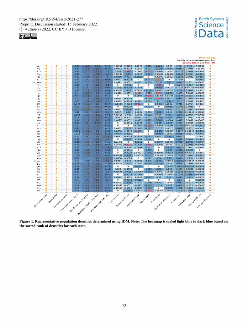
The input blocks, uninhabited features, and land cover rasters were prepared for each CONUS state and Washington D.C. In

order to increase the number of representative blocks, all data for Rhode Island were combined with neighboring

Massachusetts. Likewise, data for Washington D.C. were combined with Maryland. Representative population densities were

determined for 17 land cover classes in 47 ‘states’ in the US for a total of 799 estimated densities (Fig. 1). Four land cover

types were preset at zero for every state. Of the 611 unique land cover type / state combinations that were not initially preset 265

at zero, 596 were determined with sampling, 14 were determined using IAW, and one was preset (Fig. 1). In Connecticut, the

representative population density for scrub/shrub was estimated at 3.4 using IAW. This would have resulted in shrub/scrub

having the highest representative population density for any land cover type in the state and the estimate was over six standard

deviations above the mean for that land cover type in all states. We chose to rerun IDM for Connecticut using the average

representative density for scrub/shrub from all other states as a preset density. Population density was determined for each 270

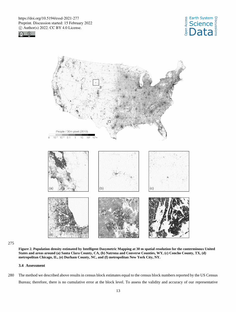
NLCD pixel within each state then joined to create a seamless 30 m population density estimate for the CONUS (Fig. 2).


Ope

n A

cces

s Earth System

Science

DataD

iscussio

ns


12

Figure 1. Representative population densities determined using IDM. Note: The heatmap is scaled light blue to dark blue based on

the sorted rank of densities for each state.


Ope

n A

cces

s Earth System

Science

DataD

iscussio

ns


13

275

Figure 2. Population density estimated by Intelligent Dasymetric Mapping at 30 m spatial resolution for the conterminous United

States and areas around (a) Santa Clara County, CA, (b) Natrona and Converse Counties, WY, (c) Concho County, TX, (d)

metropolitan Chicago, IL, (e) Durham County, NC, and (f) metropolitan New York City, NY.

3.4 Assessment

The method we described above results in census block estimates equal to the census block numbers reported by the US Census 280

Bureau; therefore, there is no cumulative error at the block level. To assess the validity and accuracy of our representative


Ope

n A

cces

s Earth System

Science

DataD

iscussio

ns


14

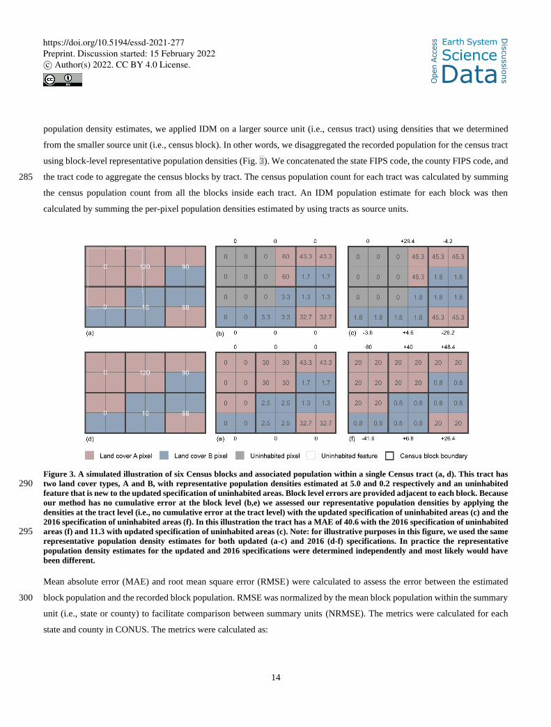
population density estimates, we applied IDM on a larger source unit (i.e., census tract) using densities that we determined

from the smaller source unit (i.e., census block). In other words, we disaggregated the recorded population for the census tract

using block-level representative population densities (Fig. 3). We concatenated the state FIPS code, the county FIPS code, and

the tract code to aggregate the census blocks by tract. The census population count for each tract was calculated by summing 285

the census population count from all the blocks inside each tract. An IDM population estimate for each block was then

calculated by summing the per-pixel population densities estimated by using tracts as source units.

Figure 3. A simulated illustration of six Census blocks and associated population within a single Census tract (a, d). This tract has

two land cover types, A and B, with representative population densities estimated at 5.0 and 0.2 respectively and an uninhabited 290 feature that is new to the updated specification of uninhabited areas. Block level errors are provided adjacent to each block. Because

our method has no cumulative error at the block level (b,e) we assessed our representative population densities by applying the

densities at the tract level (i.e., no cumulative error at the tract level) with the updated specification of uninhabited areas (c) and the

2016 specification of uninhabited areas (f). In this illustration the tract has a MAE of 40.6 with the 2016 specification of uninhabited

areas (f) and 11.3 with updated specification of uninhabited areas (c). Note: for illustrative purposes in this figure, we used the same 295 representative population density estimates for both updated (a-c) and 2016 (d-f) specifications. In practice the representative

population density estimates for the updated and 2016 specifications were determined independently and most likely would have

been different.

Mean absolute error (MAE) and root mean square error (RMSE) were calculated to assess the error between the estimated

block population and the recorded block population. RMSE was normalized by the mean block population within the summary 300

unit (i.e., state or county) to facilitate comparison between summary units (NRMSE). The metrics were calculated for each

state and county in CONUS. The metrics were calculated as:


Ope

n A

cces

s Earth System

Science

DataD

iscussio

ns


15

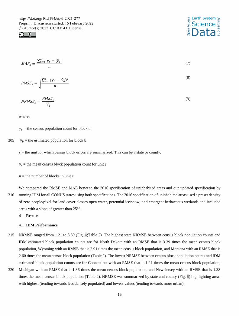
𝑀𝐴𝐸𝑠 = ∑ |𝑦𝑏 − �̂�𝑏|𝑛𝑏=1

𝑛 (7)

𝑅𝑀𝑆𝐸𝑠 = √∑ (𝑦𝑏 − �̂�𝑏)

2𝑛𝑏=1

𝑛

(8)

𝑁𝑅𝑀𝑆𝐸𝑠 = 𝑅𝑀𝑆𝐸𝑠𝑦𝑠

(9)

where:

𝑦𝑏 = the census population count for block b

�̂�𝑏 = the estimated population for block b 305

𝑠 = the unit for which census block errors are summarized. This can be a state or county.

�̅�𝑠 = the mean census block population count for unit s

𝑛 = the number of blocks in unit s

We compared the RMSE and MAE between the 2016 specification of uninhabited areas and our updated specification by

running IDM for all CONUS states using both specifications. The 2016 specification of uninhabited areas used a preset density 310

of zero people/pixel for land cover classes open water, perennial ice/snow, and emergent herbaceous wetlands and included

areas with a slope of greater than 25%.

4 Results

4.1 IDM Performance

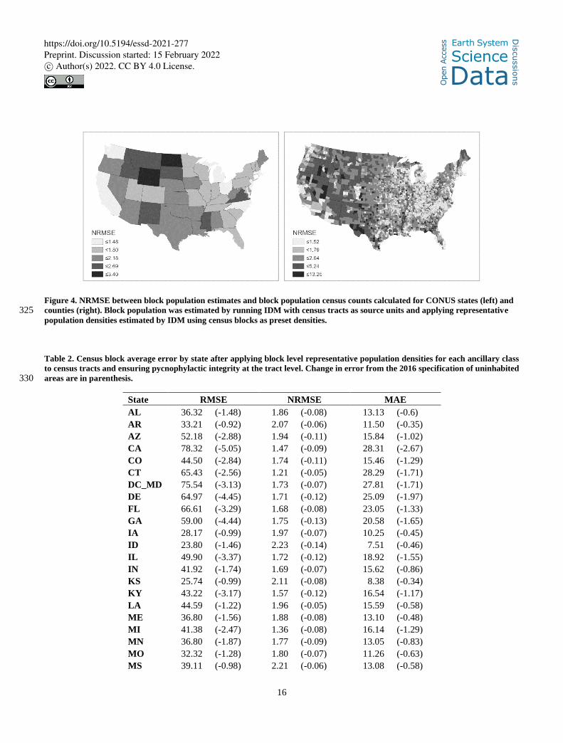
NRMSE ranged from 1.21 to 3.39 (Fig. 4;Table 2). The highest state NRMSE between census block population counts and 315

IDM estimated block population counts are for North Dakota with an RMSE that is 3.39 times the mean census block

population, Wyoming with an RMSE that is 2.91 times the mean census block population, and Montana with an RMSE that is

2.60 times the mean census block population (Table 2). The lowest NRMSE between census block population counts and IDM

estimated block population counts are for Connecticut with an RMSE that is 1.21 times the mean census block population,

Michigan with an RMSE that is 1.36 times the mean census block population, and New Jersey with an RMSE that is 1.38 320

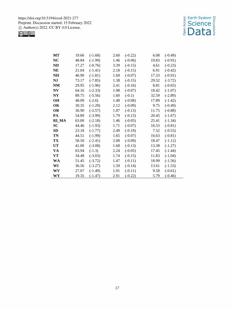
times the mean census block population (Table 2). NRMSE was summarized by state and county (Fig. 5) highlighting areas

with highest (tending towards less densely populated) and lowest values (tending towards more urban).


Ope

n A

cces

s Earth System

Science

DataD

iscussio

ns


16

Figure 4. NRMSE between block population estimates and block population census counts calculated for CONUS states (left) and

counties (right). Block population was estimated by running IDM with census tracts as source units and applying representative 325 population densities estimated by IDM using census blocks as preset densities.

Table 2. Census block average error by state after applying block level representative population densities for each ancillary class

to census tracts and ensuring pycnophylactic integrity at the tract level. Change in error from the 2016 specification of uninhabited

areas are in parenthesis. 330

State RMSE NRMSE MAE

AL 36.32 (-1.48) 1.86 (-0.08) 13.13 (-0.6)

AR 33.21 (-0.92) 2.07 (-0.06) 11.50 (-0.35)

AZ 52.18 (-2.88) 1.94 (-0.11) 15.84 (-1.02)

CA 78.32 (-5.05) 1.47 (-0.09) 28.31 (-2.67)

CO 44.50 (-2.84) 1.74 (-0.11) 15.46 (-1.29)

CT 65.43 (-2.56) 1.21 (-0.05) 28.29 (-1.71)

DC_MD 75.54 (-3.13) 1.73 (-0.07) 27.81 (-1.71)

DE 64.97 (-4.45) 1.71 (-0.12) 25.09 (-1.97)

FL 66.61 (-3.29) 1.68 (-0.08) 23.05 (-1.33)

GA 59.00 (-4.44) 1.75 (-0.13) 20.58 (-1.65)

IA 28.17 (-0.99) 1.97 (-0.07) 10.25 (-0.45)

ID 23.80 (-1.46) 2.23 (-0.14) 7.51 (-0.46)

IL 49.90 (-3.37) 1.72 (-0.12) 18.92 (-1.55)

IN 41.92 (-1.74) 1.69 (-0.07) 15.62 (-0.86)

KS 25.74 (-0.99) 2.11 (-0.08) 8.38 (-0.34)

KY 43.22 (-3.17) 1.57 (-0.12) 16.54 (-1.17)

LA 44.59 (-1.22) 1.96 (-0.05) 15.59 (-0.58)

ME 36.80 (-1.56) 1.88 (-0.08) 13.10 (-0.48)

MI 41.38 (-2.47) 1.36 (-0.08) 16.14 (-1.29)

MN 36.80 (-1.87) 1.77 (-0.09) 13.05 (-0.83)

MO 32.32 (-1.28) 1.80 (-0.07) 11.26 (-0.63)

MS 39.11 (-0.98) 2.21 (-0.06) 13.08 (-0.58)


Ope

n A

cces

s Earth System

Science

DataD

iscussio

ns


17

MT 19.66 (-1.68) 2.60 (-0.22) 6.08 (-0.49)

NC 48.84 (-1.99) 1.46 (-0.06) 19.83 (-0.91)

ND 17.27 (-0.76) 3.39 (-0.15) 4.61 (-0.23)

NE 21.04 (-1.41) 2.18 (-0.15) 6.91 (-0.42)

NH 46.90 (-1.81) 1.69 (-0.07) 17.33 (-0.91)

NJ 73.17 (-7.85) 1.38 (-0.15) 29.52 (-3.72)

NM 29.95 (-1.96) 2.41 (-0.16) 8.81 (-0.65)

NV 64.16 (-2.33) 1.98 (-0.07) 18.42 (-1.07)

NY 89.75 (-5.56) 1.60 (-0.1) 32.59 (-2.89)

OH 48.09 (-2.6) 1.48 (-0.08) 17.89 (-1.42)

OK 30.35 (-1.29) 2.12 (-0.09) 9.75 (-0.49)

OR 36.90 (-2.57) 1.87 (-0.13) 11.75 (-0.88)

PA 54.89 (-3.99) 1.79 (-0.13) 20.45 (-1.67)

RI_MA 63.00 (-2.18) 1.46 (-0.05) 25.41 (-1.34)

SC 44.46 (-1.93) 1.71 (-0.07) 16.53 (-0.81)

SD 23.18 (-1.77) 2.49 (-0.19) 7.52 (-0.55)

TN 44.51 (-1.99) 1.65 (-0.07) 16.63 (-0.81)

TX 58.50 (-2.41) 2.08 (-0.09) 18.47 (-1.12)

UT 41.00 (-3.08) 1.68 (-0.13) 13.38 (-1.27)

VA 63.94 (-1.3) 2.24 (-0.05) 17.45 (-1.44)

VT 34.48 (-3.03) 1.74 (-0.15) 11.83 (-1.04)

WA 51.45 (-3.72) 1.47 (-0.11) 18.99 (-1.56)

WI 36.56 (-3.27) 1.59 (-0.14) 13.61 (-1.53)

WV 27.07 (-1.49) 1.91 (-0.11) 9.58 (-0.61)

WY 19.35 (-1.47) 2.91 (-0.22) 5.79 (-0.46)


Ope

n A

cces

s Earth System

Science

DataD

iscussio

ns


18

Figure 5. Census urban areas and county NRMSE between census block population count and the estimated block population

count from IDM for some of the states with the lowest NRMSE: (a) Connecticut, (b) Michigan, and (c) New Jersey and highest

NRMSE: (d) Montana, (e) Wyoming, and (f) North Dakota. 335

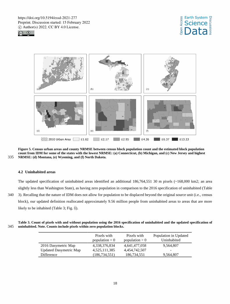
4.2 Uninhabited areas

The updated specification of uninhabited areas identified an additional 186,764,551 30 m pixels (~168,000 km2; an area

slightly less than Washington State), as having zero population in comparison to the 2016 specification of uninhabited (Table

3). Recalling that the nature of IDM does not allow for population to be displaced beyond the original source unit (i.e., census 340

block), our updated definition reallocated approximately 9.56 million people from uninhabited areas to areas that are more

likely to be inhabited (Table 3; Fig. 6).

Table 3. Count of pixels with and without population using the 2016 specification of uninhabited and the updated specification of

uninhabited. Note. Counts include pixels within zero population blocks. 345

Pixels with

population = 0

Pixels with

population > 0

Population in Updated

Uninhabited

2016 Dasymetric Map 4,338,376,834 4,641,477,058 9,564,807

Updated Dasymetric Map 4,525,111,385 4,454,742,507 -

Difference (186,734,551) 186,734,551 9,564,807


Ope

n A

cces

s Earth System

Science

DataD

iscussio

ns


19

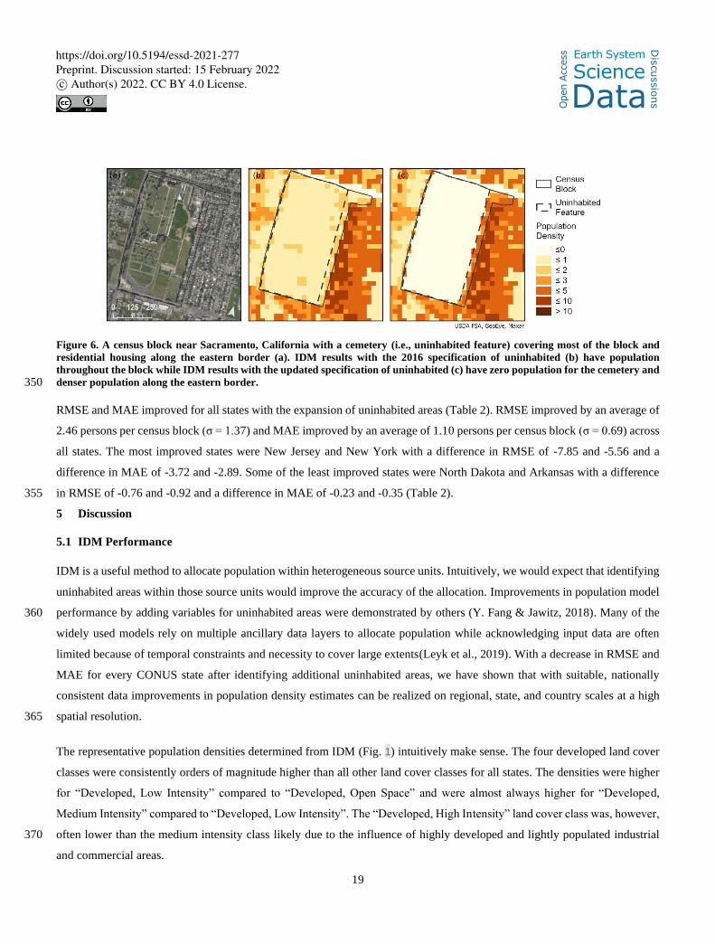
Figure 6. A census block near Sacramento, California with a cemetery (i.e., uninhabited feature) covering most of the block and

residential housing along the eastern border (a). IDM results with the 2016 specification of uninhabited (b) have population

throughout the block while IDM results with the updated specification of uninhabited (c) have zero population for the cemetery and

denser population along the eastern border. 350

RMSE and MAE improved for all states with the expansion of uninhabited areas (Table 2). RMSE improved by an average of

2.46 persons per census block (σ = 1.37) and MAE improved by an average of 1.10 persons per census block (σ = 0.69) across

all states. The most improved states were New Jersey and New York with a difference in RMSE of -7.85 and -5.56 and a

difference in MAE of -3.72 and -2.89. Some of the least improved states were North Dakota and Arkansas with a difference

in RMSE of -0.76 and -0.92 and a difference in MAE of -0.23 and -0.35 (Table 2). 355

5 Discussion

5.1 IDM Performance

IDM is a useful method to allocate population within heterogeneous source units. Intuitively, we would expect that identifying

uninhabited areas within those source units would improve the accuracy of the allocation. Improvements in population model

performance by adding variables for uninhabited areas were demonstrated by others (Y. Fang & Jawitz, 2018). Many of the 360

widely used models rely on multiple ancillary data layers to allocate population while acknowledging input data are often

limited because of temporal constraints and necessity to cover large extents(Leyk et al., 2019). With a decrease in RMSE and

MAE for every CONUS state after identifying additional uninhabited areas, we have shown that with suitable, nationally

consistent data improvements in population density estimates can be realized on regional, state, and country scales at a high

spatial resolution. 365

The representative population densities determined from IDM (Fig. 1) intuitively make sense. The four developed land cover

classes were consistently orders of magnitude higher than all other land cover classes for all states. The densities were higher

for “Developed, Low Intensity” compared to “Developed, Open Space” and were almost always higher for “Developed,

Medium Intensity” compared to “Developed, Low Intensity”. The “Developed, High Intensity” land cover class was, however,

often lower than the medium intensity class likely due to the influence of highly developed and lightly populated industrial 370

and commercial areas.


Ope

n A

cces

s Earth System

Science

DataD

iscussio

ns


20

IDM’s accuracy seems to be dependent on the spatial distribution of the population. States with the lowest NRMSE such as

Connecticut and New Jersey tend to have larger urban areas with higher population counts well distributed throughout the

state. This trend is likely from these states having a higher number of homogenous blocks from across the state identified as

representative blocks. Conversely, states with the highest NRMSE such as North Dakota and Wyoming tend to be characterized 375

by small population centers surrounded by large sparsely populated lands (Fig. 5). These states tend to have fewer, less evenly

distributed blocks eligible to be representative blocks. The same pattern seems to be repeated for counties. A given state’s

IDM representative population densities perform better in counties with a dispersed distribution of high population throughout

the county rather than a stark difference between high population centers and surrounding sparsely populated areas. For

example, some of the counties with the highest NRMSE in central and western Montana are characterized by low population 380

blocks throughout the county with small concentrations of higher population blocks (Fig. 5). Furthermore, the counties in

Michigan’s upper peninsula with fewer urban areas tend to have higher NRMSE than the counties in the south with more

distributed urban areas (Fig. 5).

5.2 Uncertainty and Limitations

The decision to substitute the representative population density of shrub/scrub in Connecticut with a national average illustrates 385

the importance of reviewing the output of IDM. Indeed, we would not expect shrub/scrub to be the most densely populated

land cover class within Connecticut, and the estimated density is clearly an outlier when compared to other state’s values for

that same land cover class. While there are other values in our final estimates (Fig. 1) that may warrant additional attention,

we believed this particular representative population density was so far outside the range of the other states we needed to

consider an alternative value. It is imperative to review the results for logical consistency and consider modifications based on 390

local knowledge before accepting the results.

Data for our uninhabited areas have a wide temporal range due to the varying frequency at which they are updated. For

example, OSM data reflect the most recent edits made by contributers while the NLCD roads and energy development are

from 2011. Although our population estimates are from the 2010 decennial census, the uninhabited areas are not restricted to

2010. There might be additional uninhabited areas since 2010. Furthermore, the rules applied to filter and refine uninhabited 395

areas were determined for a national allocation of population. The EnviroAtlas IDM toolbox for ArcGIS Pro

(https://github.com/USEPA/Dasymetric-Toolbox-ArcGISPro) or open source GIS (https://github.com/USEPA/Dasymetric-

Toolbox-OpenSource) can be used to refine population estimates if more detailed local or regional data for uninhabited areas

are available. It is important to note that the accuracy of the population estimates is dependent on the accuracy of the input

data. Some sources of uncertainty are the accuracy of the NLCD classification, the census block boundaries, and the boundaries 400

and labels of various OSM, PAD-US, and NAVSTREETS layers.


Ope

n A

cces

s Earth System

Science

DataD

iscussio

ns


21

5.3 Conclusion

In this study, we updated the existing dasymetric population map by EPA’s EnviroAtlas by using additional geospatial datasets

to expand the coverage of uninhabited areas. We used IDM developed by Mennis and Hultgren (2006) to estimate gridded 30

m population density for CONUS. The improved identification and masking of uninhabited areas improved the accuracy of 405

population estimates for all CONUS states. Our accuracy assessment method showed that the IDM method was better at

mirroring the Census block population counts of states with larger urban areas and smaller areas of sparsely populated land.

Future development of the dasymetric population map might benefit from stratified sampling for urban and non-urban areas

conducted on a regional basis rather than by state. The state-level and county-level error maps from this study can serve as

guidance on potential regions with similar population dynamics. The datasets and methods described here will be used to 410

update the dasymetric population estimates for the CONUS once 2020 land cover and census data are available. Furthermore,

the updated IDM toolbox will be used to specify uninhabited areas and to produce gridded population estimates for Alaska,

Hawaii, Puerto Rico, and the Virgin Islands. The dasymetric population map and the IDM toolbox will be available in

EnviroAtlas.

6 Code and Data Availability 415

The Dasymetric Toolbox for ArcGIS Pro (https://github.com/USEPA/Dasymetric-Toolbox-ArcGISPro) and Dasymetric

Toolbox for Open Source GIS (https://github.com/USEPA/Dasymetric-Toolbox-OpenSource) are available on US EPA’s

GitHub page. The updated EnviroAtlas dasymetric population map at 30 m resolution for the CONUS is available via EPA’s

Environmental Dataset Gateway (Baynes et al., 2021; https://doi.org/10.23719/1522948). Data can also be accessed or viewed

from EPA’s EnviroAtlas (https://www.epa.gov/enviroatlas). Dasymetric population estimates for US States and Territories 420

outside CONUS are in progress. Updates for all US States and Territories for the 2020 US Census are planned and will be

available on EPA’s EnviroAtlas.

7 Author contributions

JB and AN designed the study with input from TH. JB performed the analysis. All authors contributed to and approved the

final manuscript. 425

8 Competing interests

The authors declare that they have no conflict of interest.

9 Acknowledgements

This paper has been reviewed in accordance with the U.S. Environmental Protection Agency's Center for Public Health and

Environmental Assessment peer-review policies and approved for publication. Mention of trade names or commercial products 430

does not constitute endorsement or recommendation for use. Statements in this publication reflect the authors' personal views

and opinions and should not be construed to represent any determination of policy of the U.S. Environmental Protection

Agency.


Ope

n A

cces

s Earth System

Science

DataD

iscussio

ns


22

Maps throughout this article were created using ArcGIS® software by Esri. ArcGIS® and ArcMap™ are the intellectual

property of Esri and are used herein under license. Copyright © Esri. All rights reserved. For more information about Esri® 435

software, please visit www.esri.com. Use of OpenStreetMap data requires the following acknowledgment: “Map data

copyrighted OpenStreetMap contributors and available from https://www.openstreetmap.org.”

We acknowledge Anam Khan for her expertise in developing the new IDM toolboxes and contributions to the manuscript

including her invaluable data analysis efforts. We acknowledge colleague Daniel Rosenbaum for providing the rail yards

dataset along with James Wickham and Justin Bousquin for their comments on the manuscript. T. Hultgren’s participation was 440

underwritten by contract GS00Q09BGD0055 Task Order GSQ0017AJ0037 Mod 24 between US EPA and General Dynamics

Information Technology, Inc.

References

Baynes, J., Neale, A., Hultgren, T. (2021). 2010 Dasymetric Population for the Conterminous United States v3[data set].

doi:10.23719/1522948 445

Bellwood, D. R., Hoey, A. S., & Hughes, T. P. (2012). Human activity selectively impacts the ecosystem roles of parrotfishes

on coral reefs. Proc Biol Sci, 279(1733), 1621-1629. doi:10.1098/rspb.2011.1906

Carroll, R. J., Chen, R., George, E. I., Li, T. H., Newton, H. J., Schmiediche, H., & Wang, N. (1997). Ozone Exposure and

Population Density in Harris County, Texas. Journal of the American Statistical Association, 92(438), 392-404.

doi:10.1080/01621459.1997.10473988 450

Cinner, J. E., Graham, N. A., Huchery, C., & Macneil, M. A. (2013). Global effects of local human population density and

distance to markets on the condition of coral reef fisheries. Conserv Biol, 27(3), 453-458. doi:10.1111/j.1523-

1739.2012.01933.x

CoreLogic. (2018). CoreLogic Parcel.

Dobson, J. E., Bright, E. A., Coleman, P. R., Durfee, R. C., & Worley, B. A. (2000). LandScan: A Global Population Database 455

for Estimating Populations at Risk. Photogrammetric Engineering & Remote Sensing, 66(7), 9. Retrieved from <Go

to ISI>://WOS:000087824000005

Fang, Y., Ceola, S., Paik, K., McGrath, G., Rao, P. S. C., Montanari, A., & Jawitz, J. W. (2018). Globally Universal Fractal

Pattern of Human Settlements in River Networks. Earth's Future, 6(8), 1134-1145. doi:10.1029/2017ef000746

Fang, Y., & Jawitz, J. W. (2018). High-resolution reconstruction of the United States human population distribution, 1790 to 460

2010. Sci Data, 5, 180067. doi:10.1038/sdata.2018.67

Fang, Y., & Jawitz, J. W. (2019). The evolution of human population distance to water in the USA from 1790 to 2010. Nat

Commun, 10(1), 430. doi:10.1038/s41467-019-08366-z

Federal Railroad Administration. (2019). North American Rail Lines. Retrieved from: https://data-

usdot.opendata.arcgis.com/datasets/north-american-rail-lines 465

GDAL/OGR contributors. (2019). GDAL/OGR Geospatial Data Abstraction Software Library: Open Source Geospatial

Foundation.

Gergely, K. J., & McKerrow, A. (2016). PAD-US—National inventory of protected areas (ver. 1.1, August 2016): U.S.

Geological Survey Fact Sheet 2013–3086. 2. doi:10.3133/fs20133086

Goodchild, M. F., & Lam, N. S.-N. (1980). Areal interpolation: A variant of the traditional spatial problem. Geo-Processing, 470

1(3), 15. Retrieved from <Go to ISI>://WOS:A1980KY00200007

HERE. (2017). NAVSTREETS Street Data Reference Manual v9.0.

Homer, C., Dewitz, J., Jin, S., Xian, G., Costello, C., Danielson, P., . . . Riitters, K. (2020). Conterminous United States land

cover change patterns 2001–2016 from the 2016 National Land Cover Database. ISPRS Journal of Photogrammetry

and Remote Sensing, 162, 184-199. doi:https://doi.org/10.1016/j.isprsjprs.2020.02.019 475


Ope

n A

cces

s Earth System

Science

DataD

iscussio

ns


23

Jones, K. E., Patel, N. G., Levy, M. A., Storeygard, A., Balk, D., Gittleman, J. L., & Daszak, P. (2008). Global trends in

emerging infectious diseases. Nature, 451(7181), 990-993. doi:10.1038/nature06536

Karunarathne, A., & Lee, G. (2019). Estimating Hilly Areas Population Using a Dasymetric Mapping Approach: A Case of

Sri Lanka’s Highest Mountain Range. ISPRS International Journal of Geo-Information, 8(4), 166.

doi:10.3390/ijgi8040166 480

Leyk, S., Gaughan, A. E., Adamo, S. B., de Sherbinin, A., Balk, D., Freire, S., . . . Pesaresi, M. (2019). The spatial allocation

of population: a review of large-scale gridded population data products and their fitness for use. Earth System Science

Data, 11(3), 1385-1409. doi:10.5194/essd-11-1385-2019

Liu, C., Wang, F., & Xu, Y. (2019). Habitation environment suitability and population density patterns in China: A

regionalization approach. Growth and Change, 50(1), 184-200. doi:10.1111/grow.12283 485

Lloyd, C. T., Chamberlain, H., Kerr, D., Yetman, G., Pistolesi, L., Stevens, F. R., . . . Tatem, A. J. (2019). Global spatio-

temporally harmonised datasets for producing high-resolution gridded population distribution datasets. Big Earth

Data, 3(2), 108-139. doi:10.1080/20964471.2019.1625151

Mennis, J., & Hultgren, T. (2006). Intelligent Dasymetric Mapping and Its Application to Areal Interpolation. Cartography

and Geographic Information Science, 33(3), 179-194. doi:10.1559/152304006779077309 490

Moos, M., Vinodrai, T., Revington, N., & Seasons, M. (2018). Planning for Mixed Use: Affordable for Whom? Journal of the

American Planning Association, 84(1), 7-20. doi:10.1080/01944363.2017.1406315

Morais, R. A., Connolly, S. R., & Bellwood, D. R. (2019). Human exploitation shapes productivity-biomass relationships on

coral reefs. Glob Chang Biol. doi:10.1111/gcb.14941

Nahayo, L., Ndayisaba, F., Karamage, F., Nsengiyumva, J. B., Kalisa, E., Mind'je, R., . . . Li, L. (2019). Estimating landslides 495

vulnerability in Rwanda using analytic hierarchy process and geographic information system. Integr Environ Assess

Manag, 15(3), 364-373. doi:10.1002/ieam.4132

Nasiri, H., Yusof, M. J. M., Ali, T. A. M., & Hussein, M. K. B. (2018). District flood vulnerability index: urban decision-

making tool. International Journal of Environmental Science and Technology, 16(5), 2249-2258.

doi:10.1007/s13762-018-1797-5 500

Nicholls, R. J., & Small, C. (2002). Improved Estimates of Coastal Population and Exposure to Hazards Released. EOS, 83(28),

301 - 305.

OpenStreetMap contributors. (2019). Planet dump retrieved from https://planet.osm.org. Retrieved from:

https://download.geofabrik.de/

Pickard, B. R., Daniel, J., Mehaffey, M., Jackson, L. E., & Neale, A. (2015). EnviroAtlas: A new geospatial tool to foster 505

ecosystem services science and resource management. Ecosystem Services, 14, 45-55.

doi:10.1016/j.ecoser.2015.04.005

Radeloff, V. C., Stewart, S. I., Hawbaker, T. J., Gimmi, U., Pidgeon, A. M., Flather, C. H., . . . Helmers, D. P. (2010). Housing

growth in and near United States protected areas limits their conservation value. Proc Natl Acad Sci U S A, 107(2),

940-945. doi:10.1073/pnas.0911131107 510

Samoli, E., Stergiopoulou, A., Santana, P., Rodopoulou, S., Mitsakou, C., Dimitroulopoulou, C., . . . Consortium, E.-H. (2019).

Spatial variability in air pollution exposure in relation to socioeconomic indicators in nine European metropolitan

areas: A study on environmental inequality. Environ Pollut, 249, 345-353. doi:10.1016/j.envpol.2019.03.050

Samson, J., Berteaux, D., McGill, B. J., & Humphries, M. M. (2011). Geographic disparities and moral hazards in the predicted

impacts of climate change on human populations. Global Ecology and Biogeography, 20(4), 532-544. 515

doi:10.1111/j.1466-8238.2010.00632.x

Schmidt, W. P., Suzuki, M., Thiem, V. D., White, R. G., Tsuzuki, A., Yoshida, L. M., . . . Ariyoshi, K. (2011). Population

density, water supply, and the risk of dengue fever in Vietnam: cohort study and spatial analysis. PLoS Med, 8(8),

e1001082. doi:10.1371/journal.pmed.1001082

Smith, A., Bates, P. D., Wing, O., Sampson, C., Quinn, N., & Neal, J. (2019). New estimates of flood exposure in developing 520

countries using high-resolution population data. Nat Commun, 10(1), 1814. doi:10.1038/s41467-019-09282-y

Song, Y., & Knaap, G.-J. (2004). Measuring Urban Form: Is Portland Winning the War on Sprawl? Jounral of the American

Planning Association, 70(2), 16.


Ope

n A

cces

s Earth System

Science

DataD

iscussio

ns


24

Sorichetta, A., Hornby, G. M., Stevens, F. R., Gaughan, A. E., Linard, C., & Tatem, A. J. (2015). High-resolution gridded

population datasets for Latin America and the Caribbean in 2010, 2015, and 2020. Sci Data, 2, 150045. 525

doi:10.1038/sdata.2015.45

Stevens, F. R., Gaughan, A. E., Linard, C., & Tatem, A. J. (2015). Disaggregating census data for population mapping using

random forests with remotely-sensed and ancillary data. PLoS One, 10(2), e0107042.

doi:10.1371/journal.pone.0107042

Taubenböck, H., Weigand, M., Esch, T., Staab, J., Wurm, M., Mast, J., & Dech, S. (2019). A new ranking of the world's largest 530

cities—Do administrative units obscure morphological realities? Remote Sensing of Environment, 232, 111353.

doi:10.1016/j.rse.2019.111353

Tobler, W. R. (1979). Smooth Pycnophylactic Interpolation for Geographical Regions. Journal of the American Statistical

Association, 74(367), 519-530. doi:10.1080/01621459.1979.10481647

U.S. Census Bureau. TIGER/Line Shapefiles. Retrieved from: https://www.census.gov/geographies/mapping-files/time-535

series/geo/tiger-line-file.2010.html

U.S. Census Bureau. (2012). 2010 TIGER/Line Shapefiles Technical Documentation.

U.S. Environmental Protection Agency. (2011). The Benefits and Costs of the Clean Air Act from 1990 to 2020. Retrieved

from https://www.epa.gov/sites/production/files/2015-07/documents/fullreport_rev_a.pdf

U.S. Geological Survey, EROS Data Center. (1999). USGS 30 Meter Resolution, One-Sixtieth Degree National Elevation 540

Dataset for CONUS, Alaska, Hawaii, Puerto Rico, and the U. S. Virgin Islands.

U.S. Geological Survey, Gap Analysis Program. (2018). Protected Areas Database of the United States (PAD-US). Retrieved

from: https://doi.org/10.5066/F7G73BSZ

Venter, O., Sanderson, E. W., Magrach, A., Allan, J. R., Beher, J., Jones, K. R., . . . Watson, J. E. (2016). Sixteen years of

change in the global terrestrial human footprint and implications for biodiversity conservation. Nat Commun, 7, 545

12558. doi:10.1038/ncomms12558

Weber, E. M., Seaman, V. Y., Stewart, R. N., Bird, T. J., Tatem, A. J., McKee, J. J., . . . Reith, A. E. (2018). Census-independent

population mapping in northern Nigeria. Remote Sens Environ, 204, 786-798. doi:10.1016/j.rse.2017.09.024

Wei, C., Taubenböck, H., & Blaschke, T. (2017). Measuring urban agglomeration using a city-scale dasymetric population

map: A study in the Pearl River Delta, China. Habitat International, 59, 32-43. doi:10.1016/j.habitatint.2016.11.007 550

Wickham, J., Stehman, S. V., Sorenson, D. G., Gass, L., & Dewitz, J. A. (2021). Thematic accuracy assessment of the NLCD

2016 land cover for the conterminous United States. Remote Sensing of Environment, 257, 112357.

doi:https://doi.org/10.1016/j.rse.2021.112357

Yang, L., Jin, S., Danielson, P., Homer, C., Gass, L., Bender, S. M., . . . Xian, G. (2018). A new generation of the United States

National Land Cover Database: Requirements, research priorities, design, and implementation strategies. ISPRS 555

Journal of Photogrammetry and Remote Sensing, 146, 108-123. doi:10.1016/j.isprsjprs.2018.09.006

Ye, T., Zhao, N., Yang, X., Ouyang, Z., Liu, X., Chen, Q., . . . Jia, P. (2019). Improved population mapping for China using

remotely sensed and points-of-interest data within a random forests model. Sci Total Environ, 658, 936-946.

doi:10.1016/j.scitotenv.2018.12.276

Yuan, H., Gao, X., & Qi, W. (2019). Fine-Scale Spatiotemporal Analysis of Population Vulnerability to Earthquake Disasters: 560

Theoretical Models and Application to Cities. Sustainability, 11(7), 2149. doi:10.3390/su11072149


Ope

n A

cces

s Earth System

Science

DataD

iscussio

ns
