


Bahasa
Halaman
Hukum


Addis Ababa University
Addis Ababa Institute of Technology School of
Electrical and Computer Engineering
Hybrid Approach to Detect Fault Caused KPIs
Anomaly in UMTS Cells
by : yared hawulte
adviser : surafel lemma (phd)
THESIS
Submitted in partial fulfillment of the requirements for the degree of Master of
Science in Telecommunication Engineering.
Addis Ababa, Ethiopia
February 24, 2020

Declaration
I, the undersigned, declare that the thesis comprises my own work in compliance
with internationally accepted practices; I have fully acknowledged and referred all
materials used in this thesis work.
Yared Hawulte
NameSignature

Addis Ababa University
Addis Ababa Institute of Technology
School of Electrical and Computer Engineering
This is to certify that the thesis prepared by Yared Hawulte, entitled Hybrid Approach to
Detect Fault Caused KPIs Anomaly in UMTS Cells and submitted in partial fulfillment of
the requirements for the degree of Master of Science Telecommunication Engineering
complies with the regulations of the University and meets the accepted standards
with respect to originality and quality.
Signed by the Examining Committee:
Internal Examiner Signature Date
External Examiner Signature Date
Adviser Surafel Lemma (PhD) Signature Date
Co-Adviser Signature Date
Dean, School of Electrical and Computer
Engineering

D E D I C AT I O N
This research work is dedicated to my families ( Ato Hawulte Kebede, Wro.
Agegnehu Kebede, Woineshet, Solomon, Samuel, and Rahel) and my friends
(Hayalu Fekadu, Bizuayehu and Tsedey Dimiru).
iv

A B S T R A C T
Cellular networks usually suffer from failures or performance degradations due
to several reasons, such as external interference, hardware/software bugs on net-
work elements, power outages, or cable disconnections. Therefore, to avoid cus-
tomer dissatisfaction and loss of revenue due to failures telecom operators need
to detect and respond to performance anomalies of cellular networks instantly.
However, the state of art performance anomaly detection framework (CELLPAD),
which uses a correlation between two Key Performance Indicators (KPI)s as a
means to detect anomaly is not capable of detecting anomalies happing during the
off-pick hour, and; could not differentiate the causes of the anomalies. In this the-
sis, we propose a system model, which is capable of detecting anomalies happing
at any traffic load and could differentiate the two causes of a correlational change
anomaly. The proposed system model uses a newly added parameter called mean
Received Total Wideband Power (RTWP) and filtering rules. To assess the perfor-
mance of the proposed system model, we conducted an experiment using four-
month performance counter data collected from 20 selected sites. The result shows
that the proposed approach improves the detection of sudden drop anomaly by
10% when compared to the state of the art statistical model, Weighted Moving Av-
erage (WMA). Besides, we can differentiate the two causes of correlational change
anomaly with an F1-score above 75%.
K E Y W O R D S
Anomaly detection, correlational change anomaly, KPI, sudden drop anomaly, RTWP,
Universal Mobile Telecommunications System (UMTS),
v

A C K N O W L E D G M E N T S
Glory and praise to the Most High God, the Son of the Virgin Mary, who has done
everything for me and has brought me here. In addition to this, I would like to
express my gratitude to my mentor, Dr. Surafel Lemma for his advice and support
during the whole session. I also want to extend my appreciation for my company
ethio telecom and Addis Ababa Institute of Technology (AAiT) for opening such
a program and allow me to study.
vi

C O N T E N T S
1 introduction 1
1.1 Problem Statement . . . . . . . . . . . . . . . . . . . . . . . . . . . . . . . 4
1.2 Objective . . . . . . . . . . . . . . . . . . . . . . . . . . . . . . . . . . . . . 5
1.2.1 General Objective . . . . . . . . . . . . . . . . . . . . . . . . . . . . . . . 5
1.2.2 Specific Objectives . . . . . . . . . . . . . . . . . . . . . . . . . . . . . . 5
1.3 Scope . . . . . . . . . . . . . . . . . . . . . . . . . . . . . . . . . . . . . . . 6
1.4 Contributions of the research . . . . . . . . . . . . . . . . . . . . . . . . . 6
1.5 Methodology . . . . . . . . . . . . . . . . . . . . . . . . . . . . . . . . . . . 7
1.6 Thesis Organization . . . . . . . . . . . . . . . . . . . . . . . . . . . . . . . 7
2 literature review 9
2.1 UMTS architecture . . . . . . . . . . . . . . . . . . . . . . . . . . . . . . . 9
2.2 Call setup flow . . . . . . . . . . . . . . . . . . . . . . . . . . . . . . . . . 10
2.3 Related works . . . . . . . . . . . . . . . . . . . . . . . . . . . . . . . . . . 11
2.3.1 Statistical based approaches . . . . . . . . . . . . . . . . . . . . . . . . . 12
2.3.2 AI based approaches . . . . . . . . . . . . . . . . . . . . . . . . . . . . . 12
2.3.3 Hybrid approaches . . . . . . . . . . . . . . . . . . . . . . . . . . . . . . 15
2.3.4 Summary . . . . . . . . . . . . . . . . . . . . . . . . . . . . . . . . . . . . 16
3 system model 17
3.1 Proposed system model . . . . . . . . . . . . . . . . . . . . . . . . . . . . 17
3.1.1 Preprocessing . . . . . . . . . . . . . . . . . . . . . . . . . . . . . . . . . 20
3.1.2 Feature extraction . . . . . . . . . . . . . . . . . . . . . . . . . . . . . . . 21
3.1.3 Building reference model . . . . . . . . . . . . . . . . . . . . . . . . . . 21
3.1.4 Detection phase . . . . . . . . . . . . . . . . . . . . . . . . . . . . . . . 28
3.1.5 Retraining . . . . . . . . . . . . . . . . . . . . . . . . . . . . . . . . . . . 32
4 experimental setup 33
4.1 Dataset . . . . . . . . . . . . . . . . . . . . . . . . . . . . . . . . . . . . . . 33
vii

contents
4.1.1 Site selection . . . . . . . . . . . . . . . . . . . . . . . . . . . . . . . . . . 33
4.1.2 Description of the data . . . . . . . . . . . . . . . . . . . . . . . . . . . . 34
4.2 Parameter selection . . . . . . . . . . . . . . . . . . . . . . . . . . . . . . . 42
4.3 Anomaly detection scenarios . . . . . . . . . . . . . . . . . . . . . . . . . 43
4.4 Evaluation metrics . . . . . . . . . . . . . . . . . . . . . . . . . . . . . . . 43
4.5 Results and discussion . . . . . . . . . . . . . . . . . . . . . . . . . . . . . 45
4.6 Observation . . . . . . . . . . . . . . . . . . . . . . . . . . . . . . . . . . . 50
4.7 Threats to validity . . . . . . . . . . . . . . . . . . . . . . . . . . . . . . . . 51
5 conclusion and future work 52
5.1 Conclusion . . . . . . . . . . . . . . . . . . . . . . . . . . . . . . . . . . . . 52
reference 54
viii

L I S T O F F I G U R E S
Figure 2.1.1 UMTS network architecture . . . . . . . . . . . . . . . . . . . 10
Figure 2.2.1 Brief call setup flow in UMTS network . . . . . . . . . . . . . 11
Figure 2.3.1 CELLPAD architecture . . . . . . . . . . . . . . . . . . . . . . 16
Figure 3.1.1 Proposed system model to detect anomaly . . . . . . . . . . 18
Figure 3.1.2 Typical values of RTWP . . . . . . . . . . . . . . . . . . . . . . 20
Figure 3.1.3 N-sigma rule and data distribution . . . . . . . . . . . . . . . 30
Figure 4.1.1 Alarm distribution of AA UMTS sites . . . . . . . . . . . . . 33
Figure 4.1.2 One week’s total RRC request for each hour . . . . . . . . . . 35
Figure 4.1.3 One week’s average number of active users . . . . . . . . . . 35
Figure 4.1.4 One week’s total traffic (kbps) . . . . . . . . . . . . . . . . . . 36
Figure 4.1.5 Additive decomposition of two weeks RRC data . . . . . . . 37
Figure 4.1.6 Multiplicative decomposition of two weeks RRC data . . . . 38
Figure 4.1.7 RRC value before and after data transformation . . . . . . . 41
Figure 4.5.1 Boxplot (whisker plot) . . . . . . . . . . . . . . . . . . . . . . 46
Figure 4.5.2 F1-score for fault caused sudden drop anomaly detection . . 47
Figure 4.5.3 F1-score for fault caused correlational change anomaly de-
tection . . . . . . . . . . . . . . . . . . . . . . . . . . . . . . . . 49
Figure 4.5.4 F1-score for a correlational change anomaly detection clas-
sification . . . . . . . . . . . . . . . . . . . . . . . . . . . . . . 50
Figure 4.6.1 UE distribution of selected sites and its neighbors during
normal and anomaly condition . . . . . . . . . . . . . . . . . 51
ix

L I S T O F TA B L E S
Table 3.1.1 List of performance counters and their brief description . . . 19
Table 4.1.1 Sample raw KPIs and derived KPIs . . . . . . . . . . . . . . . 34
Table 4.1.2 Pearson Correlation Coefficient (PCC) of the KPIs under nor-
mal condition . . . . . . . . . . . . . . . . . . . . . . . . . . . 39
Table 4.2.1 Different window size and their corresponding Mean Squared
Error (MSE) . . . . . . . . . . . . . . . . . . . . . . . . . . . . . 42
Table 4.4.1 Confusion matrix for anomaly detection . . . . . . . . . . . . 44
Table 4.5.1 Confusion matrix for sudden drop anomaly detection . . . . 47
Table 4.5.2 Confusion matrix for correlational change anomaly detection 49
x

A C R O N Y M S
Ack Acknowledgment
ADF Augmented Dickey Fuller
AI Artificial Intelligence
AIC Akaike Information Criterion
APN Access Point Name
AR Auto-regression
ARIMA Autoregressive Integrated Moving Average
AuC Authentication Center
BS Base Stations
CFSFDP Clustering by Fast Search and Find of Density Peaks
CN Core Network
CS Circuit Switched
DNS Domain Name System
EIR Equipment Identity Register
EWMA Exponentially Weighted Moving Average
FEC Foreword Error Correction
FN False Negative
FP False Positive
GGSN Gateway GPRS Support Node
GMSC Gateway MSC
xi

list of tables
HetNets Heterogeneous network
HLR Home Location Register
HMM Hidden Markov Model
HR Huber Regression
HSDPA High-Speed Downlink Packet Access
HSPA High Speed Packet Access
HSUPA High Speed Uplink Packet Access
IMSI International Mobile Subscriber Identity
InHO Incoming Hanadover
KPI Key Performance Indicators
K-NN K-Nearest Neighbors algorithm
LSH Local-Sensitive Hashing
LTE Long-Term Evolution
MA Moving Average
MDT Minimization of Drive Test
MSE Mean Squared Error
MSC Mobile Switching Center
MT Mobile Terminal
NMS Network Management System
OSS Operating Support System
PAD Probabilistic Anomaly Detection
PC Packet Switched
PCC Pearson Correlation Coefficient
PRS Performance Report System
xii

list of tables
PS Packet Switched
RACH Random Access Channel
RAB Radio Access Bearers
RNC Radio Network Controller
RNN Recurrent Neural Network
RNS Radio Network Subsystem
ROC Receiver Operating Characteristic
RRC Radio Resource Controller
RSRP Reference Signal Received Power
RSRQ Reference Signal Received Quality
RTWP Received Total Wideband Power
R99 Release 99
SARIMA Seasonal Auto Regressive Integrated Moving Average
SGSN Serving GPRS Support Node
SMA Simple Moving Average
SOM Self Organizing Map
SRB Signaling Radio Bearer
SVM Support Vector Machines
THR Throughput
TN True Negative
TP True Positive
QoS Quality of Service
UE User Equipment
UMTS Universal Mobile Telecommunications System
xiii

list of tables
UTRAN UMTS Terrestrial Radio Access Network
WMA Weighted Moving Average
xiv

1I N T R O D U C T I O N
The telecom services have been recognized as a crucial factor to realize the so-
cioeconomic objectives of a country [1]. For the realization of these objectives,
the service provided should satisfy the need and requirements of its customers.
Telecom operators provide their key services using various wired and wireless
technologies. UMTS is one of these technologies and its network architecture con-
sists of three fundamental components, which are the User Equipment (UE), Radio
Network Subsystem (RNS) and Core Network (CN) [2]. The detail description of
each component of UMTS and a call setup flow in UMTS is found in chapter two
literature review section of this document.
To assure Quality of Service (QoS) and to enhance the user experience, telecom
operators must have the right network performance monitoring solution. The op-
erator’s network needs to be at its best all the time not only to keep the subscribers
happy but also to retain them and attract new ones. This can happen with proper
monitoring and maintenance of the network itself with the help of a Network
Management System (NMS). "NMS is an application or set of applications that lets
network administrators manage a network independent component’s inside a big-
ger network management framework that performs several key functions [3]. An
NMS identifies, configures, monitors, updates and troubleshoots both wired and
wireless network devices in an enterprise network. A system management con-
trol application then displays the performance data collected from each network
component, which in turn allows network engineers to make changes as needed.
The network management system architecture consists of a centralized network
manager along with many agents. The agents reside in various network nodes
to collect data. They communicate with the central network manager through a
network management protocol. NMS consists of five key components: fault man-
1

introduction
agement, configuration and name management, performance management, and
accounting management.
Performance management is one of the components of a network management
system concerned with performance monitoring and reporting based on perfor-
mance counters collected from NEs and the operations performed on the Operating
Support System (OSS) [4] [5]. Cellular network performance degradation or fail-
ures occur due to several reasons, such as hardware and/or software malfunctions,
power outages, faulty links, background interference or multi-vendor incompati-
bility and misconfiguration of parameters during network operation [6]. The rate
of performance degradation due to failures is proportional to network equipment
density, and complexity of software and hardware that constitute the network.
Performance management helps administrators to check whether the network el-
ement provide the intended service effectively or not, detect their performance
degradation, troubleshoot faults to give suggestions and provide detailed infor-
mation which can be input for optimization and planning [4].Therefore, it is crit-
ical for cellular network administrators to detect and respond to such anomalies
instantly, so as to maintain network reliability and improve subscriber quality of
experience.
Performance anomaly detection refers to the identification of unusual performance
counter data which raises doubts by differing significantly from the expected be-
havior or majority of the data. Such unusual data are commonly referred to as
anomalies or outliers [7][8]. Detecting and handling performance anomaly in the
UMTS network in advance will avoid the catastrophic failures that may cause net-
work blackouts [9]. Current literature categorizes cell with performance anomaly
into three main classes such as a degraded cell, crippled cell and catatonic cell [10].
A degraded cell is a cell that carries traffic but a bit less than the expected one,
whereas a crippled cell is a cell that still serves some users, but its expected traffic
severely decreases, and this may be due to a critical failure of a NodeB. A catatonic
cell is a cell that does not serve any users at all. The users that were supposed to
be handled by the catatonic cell are handed over to the neighboring cells. Accord-
ing to literature the approaches used to detect performance anomaly usually use
2

introduction
predefined thresholds, statistical, artificial intelligence method or combining the
best of two or more methods [11].
Traditional anomaly detection relay on predefined thresholds. Since the thresh-
olds are hard set network wide, they would not be able to consider the state of
individual network elements. The traditional approach needs a careful setup of
baseline values. The approach also does not consider a cyclic rhythm in the per-
formance counter’s behavior originated from human interaction [12]. Due to these,
such method either detects only the most severe once or causes high false positive
detection. Hence, the traditional approach is usually the last choice followed in
practice. Therefore, the necessity of human like skills for information analyzing
and reasoning pushed researchers towards artificial intelligence or statistics-based
approaches.
Statistical methods are easy to implement but severely depend on parameter set-
ting, and such approaches use either instantaneous or average values over a time
period, so it has a limitation of not sensing local degradation [13]. Locally de-
graded value can fall in the normal range if the whole period is considered hence
the metric could not violate the baseline thresholds (i.e. the metric would be lo-
cally degraded but not globally). Another issue with such approach is that if an
insufficient number of samples are collected over a period, this will have an in-
fluence on the variance of a metric[14]. As a result, the samples collected at a
given period in the observed and the baseline may be very unlike due to a lack of
statistical significance.
The Artificial Intelligence (AI) based approach first profiles the normal (faultless)
behavior of the network and uses such profile as a reference to detect significant
deviation from the normal behavior [11]. However, the performance of such ap-
proach can be adversely affected by the inconsistency of behavior of the metric
over the time domain. To overcome the dependence on time, multiple profiles for
each KPIs with a recognized context need be created. This, however, will increase
the complexity of the system. In addition to these, distinguishing between the
normal instance and abnormalities is challenging and it often requires domain
knowledge, and since outliers occur much more infrequently than normal data,
3

1.1 problem statement
and this imbalanced nature can reduce learning accuracy [15][16]. In general AI
based detection requires an extreme understanding of the structure of the data, the
algorithms that are going to be used and the underlying computing environment.
1.1 problem statement
Due to the anticipated growth in the number of devices, expansion in network
coverage and technology advancement such as virtualization, future cellular net-
works will be exposed to a higher number of network faults. Cellular networks
usually suffer from performance degradation due to external interference, hard-
ware/software bugs on network elements, power outage, or cable disconnection
[6]. These failures would lead to poor QoS that brings customer dissatisfaction and
loss of revenue. To address customer dissatisfaction and loss of revenue, telecom
operators need to detect and respond to performance anomalies of cellular net-
works instantly.
Performance anomaly detection refers to the way of finding patterns in KPIs
data that do not conform to expected behavior. Such unusual patterns are com-
monly referred to as anomalies or outliers [7]. The common approaches used
to detect performance anomaly are based on statistical methods, artificial intelli-
gence, predefined thresholds or their combinations. The state of art performance
anomaly detection framework combines the best of both statistical and AI based
approaches[13]. It used a correlation between two KPIs as a means to detect
anomaly. In their approach, J. Wu,et al. , detected anomaly when there is a sudden
drop on any performance counter or inconsistency between the current and his-
torical correlations of two correlated KPIs. The categories of the KPIs used for their
study are active number of users, resource usage and transmission load. These
KPIs, however, miss counters which indicate the quality of the service; and hence,
could not detect anomalies that are happening during off-pick hour. A correla-
tional change anomaly may also happen due to hardware/software failure on
the access or core network of the UMTS, congestion due to neighbor cell failure,
or special events (e.g., festivals and road traffic jam). Therefore, their proposed
approach could not differentiate the possible cause of the correlational change
4

1.2 objective
anomalies which will possibly confuse the system administrators and making it
difficult to take immediate action.
This thesis investigates parameters and approaches that are capable of detecting
anomalies happening at any traffic load and; helps to differentiate the causes of a
correlational change anomaly.
1.2 objective
1.2.1 General Objective
The main goal of this thesis is to analyze UMTS network performance counter data
to detect cell-level fault caused anomaly such as a sudden drop on performance
counters data and a correlational change between performance counters caused
by congestion or software/hardware malfunctioning happening at any traffic load
using a hybrid technique.
1.2.2 Specific Objectives
The specific objectives of this thesis are:
• Collect a performance counter data from the selected sites
• Study how the collected performance counter data behaves
• Identify the degree of correlation between performance counter within a cell
• Label the data-set using event logs collected from the network management
system
• Build a faultless reference model of each performance counter
• Detect fault caused sudden drop and correlational change KPI’s anomaly
5

1.3 scope
1.3 scope
As described above performance management system helps administrators to
check whether the network element provides the intended service effectively or
not, detect their performance degradation, troubleshoot faults to give suggestions
and provide detailed information that can be input for optimization and planning.
But, this thesis categorizing the unusual behavior on UMTS performance counter
data into two different anomalies: sudden drop and correlation change. Further-
more, the detected correlational change anomalies are classified into two possible
causes of anomalies such as congestion and software/hardware malfunctioning.
The anomaly detection is only done at the cell-level. Identifying the root cause
of the unusual behavior and end to end anomaly detection such as anomaly at
the Radio Network Controller (RNC) or core level is not considered in this study.
Out of 741 UMTS sites in Addis Ababa, Ethiopia only twenty sites are selected to
conduct the study.
1.4 contributions of the research
Various researches were done on cellular network anomaly detection, and as of
our knowledge, only the referenced work study the correlation of each KPIs and
used a deviation on this correlation as a means to detect the cellular anomaly.
However, the referenced work also showed some limitations like the technique
followed by the researchers could not detect anomalies happening during off-pick
hours, and on the correlation change anomaly detection again the researcher’s
approach could not differentiate the two causes of correlational change anomaly.
Therefore, this paper proposed a new approach which is capable of detecting
fault caused anomalies happening at any traffic load and differentiate the detected
correlational anomaly into its two possible causes, doing so can help the network
administrator to take the right action. Finally this paper insight possible future
research directions.
6

1.5 methodology
1.5 methodology
The methodologies followed to achieve the general and specific objective of this
thesis are:
1. Related literatures are reviewed to understand the available cellular anomaly
detection techniques.
2. ethio telecom’s UMTS network architecture and performance management
system are review.
3. An informal meeting was conducted with ethio telecom’s (domain) experts
regarding the common behavior of cellular network anomaly, and the limi-
tation of the existing performance management system.
4. The input datasets were collected from ethio telecom’s UMTS network through
Performance Report System (PRS) server in .xlsx format. Data were collected
into two periods, the first period was from June 1st till the end of July and
the second period was from September 15 to December 15, 2019.
5. Python programming language was chosen to analyze the collected data
and to implement the proposed algorithm, as it has clear syntax, easy to
code, and it has plenty of analytical libraries and supporting materials at
zero cost.
1.6 thesis organization
The rest of the paper’s content is organized as follows: In Chapter Two,UMTS
network architecture, call setup flow, and related works that are written on cel-
lular network anomaly detection is being presented. On related works review
the strength and limitations of the techniques followed by the researches are
briefly discussed. Chapter Three describes the proposed system model for cel-
lular anomaly detection and summarizes the input data-sets and mathematical
background of a statistical-models used in the rest of the paper. Chapter Four dis-
7

1.6 thesis organization
cusses the obtained results, considering the techniques followed by the referenced
work and the proposed system model. Finally, Chapter Five concluded this paper
and highlights the possible future works.
8

2L I T E R AT U R E R E V I E W
2.1 umts architecture
Telecom operators provide their key services using various wired and wireless
technologies. Universal Mobile Telecommunications System (UMTS) is one of these
technologies and its network architecture consists of three fundamental compo-
nents, which are the User Equipment (UE), Radio Network Subsystem (RNS) and
Core Network (CN) as shown in Figure 2.1.1 [2]. UE is a device that forms the final
interface with the user. RNS also called the UMTS Radio Access Network or UMTS
Terrestrial Radio Access Network (UTRAN) provides and manages the air interface
for the overall network. It has two components NodeB and Radio Network Con-
troller (RNC). NodeB is a radio transmission and reception unit. It is responsible
for conversion of data to and from the Uu interface, including rate adaptation,
Foreword Error Correction (FEC), spreading and dispreading. RNC holds and con-
trols the radio resources in its domain.
UMTS-CN offers all the central processing and management for the system. It
consists of Circuit Switched (CS) network,Packet Switched (PS) network and other
network entities shared by both CS and Packet Switched (PC) networks. The CS
contains network entities such as Mobile Switching Center (MSC) managing cir-
cuit switched calls underway, and Gateway MSC (GMSC) an interface to the ex-
ternal networks. The PS contains network entities such as, Serving GPRS Support
Node (SGSN), which provides a number of functionalities such as mobility man-
agement, session management, billing, and interaction with other areas of the
network. Gateway GPRS Support Node (GGSN) has a similar role as GMSC for the PS
network. Network entities shared by both CS and PC network includes Home Loca-
tion Register (HLR). HLR is a database that contains subscriber’s information along
9

2.2 call setup flow
with their last known location. Equipment Identity Register (EIR) is an optional com-
ponent that authenticates UE equipment. Authentication Center (AuC) is a protected
database that stores data for each mobile subscriber. It contains International Mo-
bile Subscriber Identity (IMSI) for authentication and secret key for ciphering the
communication over the radio path.
Figure 2.1.1: UMTS network architecture.
2.2 call setup flow
In UMTS network connection setup procedure involves complex signaling to setup
and release the connection. Figure 2.2.1 below shows a brief call setup flow in
UMTS network. When UE needs to establish a call, it sends an Radio Resource
Controller (RRC) connection request to the RNC which contains information like
UE identity, UE capabilities, establishment cause, and others. The RNC accepts the
request and assigns a traffic channel. The message also creates a Signaling Radio
Bearer (SRB). The UE replied to indicate the completion of the RRC connection
setup. After the authentication/ciphering phase finished the core network initiates
a Radio Access Bearers (RAB) assignment request with a message that specifies
the QoS parameters. RNC replies to the core network by sending RAB assignment
response Acknowledgment (Ack), after finishing RAB setup with the UE.
10

2.3 related works
Figure 2.2.1: Brief call setup flow in UMTS network.
2.3 related works
Based on the anomaly detection approach, literature written on cellular network
performance anomaly detection is organized into predefined thresholds, statis-
tical approaches, artificial intelligence method, and hybrid methods. Predefined
thresholds are hard set network wide and if a certain KPI value is below or above
the seated threshold the measurement is going to be labeled as anomaly [12]. A
statistical approach takes statistical based decisions, if a certain KPI value signifi-
11

2.3 related works
cantly deviates from a statistical parameter (e.g., mean) over a certain period, the
measurement is going to be labeled as anomaly. In artificial intelligence based
approaches, data-driven decisions are taken rather than the statistics. Artificial in-
telligence profiles the normal (faultless) behavior of the network and uses it as a
reference to detect significant deviation from the normal behavior [11].
2.3.1 Statistical based approaches
L. Bodrog, et.al, [12]. Used a simple and effective statistical method to detect cel-
lular network anomaly such as cell outages at the individual cell level, by process-
ing each KPIs individually and then aggregates the result for the network element.
The researcher’s assumed that all KPIs equally contribute to anomaly detection.
However, such approach increase the false positive detection rate. Therefore, there
should be a way that assigns a weight to each KPI according to their impact on
anomaly detection. In addition to this, the authors do not look for the correlation
between each KPIs and a deviation on the correlation as a means to detect anomaly.
Another literature that followed such approach is conducted by R. Barco, et.al, [17].
Tried to detect cell outage based on Incoming Hanadover (InHO) statistics. When
an InHO statistics is reported as zero, the algorithm checks whether the cell is
switched off for maintenance or energy saving before detecting cell outage. How-
ever, if the performance indicator is not reported at all, the algorithm will label
the cell as an outage cell. The limitation of such approach is that if there is con-
nectivity problem between the site and the OSS server the KPI will not be available,
even if the site is active, it will consider it as an outage.
2.3.2 AI based approaches
X.Guo, et.al., [18].tried to figure out the linear relationship between a time serious
performance indicator data of a cellular network using a Clustering by Fast Search
and Find of Density Peaks (CFSFDP) algorithm. The clusters reflect the linear rela-
tionship and these implicit associations used to locate the root cause of network
12

2.3 related works
degradation. Hence, it is possible to adopt the technique for silent failure detection.
The limitation of this research is that the authors only consider the linear relation-
ship. Another literature that followed such approach is P. Munoz. et.al, [14]. Most
of the previous papers used performance metric’s instance or average values over
a time period as an input to the algorithms, and compare these values to normal
instance (expected values) of the metric. However, in this paper, the authors used
time-series values of the metrics and compared it with a generated hypothetical
abnormal (degraded) pattern. On this correlation-based approach, cell degrada-
tion is detected if there is a sufficient correlation between the observed sequence
and degraded pattern. The limitation of such approach is that coming up with the
degraded or abnormal pattern is a bit difficult, and unusual user’s movement due
to some special events like festivals, holiday or event traffic jam will result in false
positive. M.Alias et.al.,[19]. categorize the 5G Heterogeneous network (HetNets)
Base Stations (BS)s into four different states such as Healthy (S1), Degraded (S2),
Crippled (S3) and Catatonic (S4). Hidden Markov Model (HMM) is used to auto
capture current states of the BSs and probabilistically predict a cell outage. Cell
performance info such as Reference Signal Received Power (RSRP),Reference Sig-
nal Received Quality (RSRQ) of a serving cell’s and the best neighbor cells reported
by UE are used as an observation to inferred current state of the BS. The authors
evaluated the proposed algorithm on ns3 LENA1 simulation platform, and capa-
ble of guessing the state of a BS at an average of 80% accuracy.
Another literature that followed AI based approach is by P.Casas et.al.,[20]. The
authors, addressed the problem of automatic network traffic anomaly detection
and classification using a semi-synthetic data drawn from real cellular network
traffic, based on a popular simple C4.5 decision tree algorithm. Domain Name
System (DNS) queries count and additional information about end-device, access
network, Access Point Name (APN), and the requested service are used as in-
put datasets. The authors compared the performance of their approach against
other popular anomaly detection and classification algorithms in the literature
(e.g., distribution based, entropy-based), however, C4.5 decision tree approach out-
performs the rest. One of the limitations of this study is that the authors detect
only a particular type of anomaly (application-specific anomalies).
13

2.3 related works
S. Chernov,et.al,.[21].detect cell degradation (sleeping cell) problem only caused
by Random Access Channel (RACH) failure in Long-Term Evolution (LTE) net-
works. Such failure may happen due to excessive load, misconfiguration, a soft-
ware bug or hardware problems. The malfunctioning cell will not accept a new
connection or handover request,however, it keeps serving perilously connected
Mobile Terminal (MT). To detect such cell degradation, the authors’ analysis se-
quences of events reported by UE to a serving BS instead of using radio envi-
ronment measurements. The detection framework, first profile "normal" network
behavior such as signal strength and Minimization of Drive Test (MDT) logs in-
formation of the network without cell outage problem then compares the current
network state against the trained model to predict a cell outage. For binary classifi-
cation, the authors used different algorithms such as centroid distance based Self
Organizing Map (SOM), distance based K-Nearest Neighbors algorithm (K-NN),
and probabilistic data structures based such as Local-Sensitive Hashing (LSH) and
Probabilistic Anomaly Detection (PAD), and compare their detection capability us-
ing Receiver Operating Characteristic (ROC) curves. Their experiment result shows
that a PAD method outperforms the others, however it is computationally expen-
sive to train as compared with others. One of the limitations of the study is that
the input dataset (sequences of events reported by UE to a serving BS) has high
computational overhead for a large network that serves too many subscribes.
I. de-la-Bandera, et.al,[22], used a correlational study to analyze the impact of a
cell outage on its neighboring cells. Cell outage is a special anomaly in which KPIs
from the affected cells are lost, and, hence, the analysis of KPIs should necessar-
ily be done in neighboring cells. Cell outage is detected by identifying a degraded
KPIs in neighboring cells. The authors calculated the traffic lost due to a cell outage
to determine the degree of compensation actions to be taken. Limitation of such
approach is that on densely deployed cells the impact of cell outage on its neigh-
bors may not show a significant deviation on its neighbor’s cells KPIs and similarly,
rear events also have the potential to trigger KPI degradation on its neighbor cells.
14

2.3 related works
2.3.3 Hybrid approaches
S.M. Abdullah, et al.[11], combined range and profile based anomaly detection
methods to detect silent hardware faults and software bugs. In their study, a sin-
gle class Support Vector Machines (SVM) algorithm is used to identify outliers in
range based KPI values, and LSTM Recurrent Neural Network (RNN) is used for
profile based anomaly detection. Any silent hardware faults or software bugs is
detected when both methods flag the incident, otherwise, it will be ignored. The
author’s approach missed to handle seasonal conditions (the authors only con-
sider the weekdays). Another literature that used a combination of two or more
methods is conducted by; J. Wu,et.al,[13]. The authors came up with a unified
framework called CELLPAD which detects performance anomalies in cellular net-
works using the system model shown in Figure 2.3.1. The platform target to detect
two types of anomaly, namely sudden drop, and correlation change, by using a
different type of statistical modeling and machine learning-based regression. The
detection process were based on a per-cell inspection of the time-series value of
multiple KPIs, which are collected from an active LTE network. The authors take
into account both trend and seasonality components in the dataset, and provides
a feedback loop for retraining the models in order to improve detection accuracy.
However, they could not detect anomalies happing during off-pick hour, because
most of the KPIs are close to zero during this period. In addition to this, when cor-
relational change anomaly is detected, the detected outliers may be cause by faults
on the cell itself, neighbor cell, capacity issues (poor planning), or rare events like
festivals or road traffic jam. Normally such factors mislead the operation and
maintenance team to take wrong actions. The authors could not differentiate be-
tween the causes of the anomaly.
15

2.3 related works
Figure 2.3.1: CELLPAD architecture.
2.3.4 Summary
As a summary, literatures that detect cell outage or sleeping cell can only detect a
specific type of cellular performance anomaly and missed other types of anoma-
lies which can affect the service or the end users. Moreover, studies conducted
on a controlled environment missed the heterogeneity and complexity of the real
traffic.
16

3S Y S T E M M O D E L
3.1 proposed system model
The proposed system model is used to detect sudden drop and correlational
change anomalies. The model has the capability to detect anomalies during off-
pick hour, and further, classify the detected correlational anomalies into conges-
tion caused and fault caused. Figure 3.1.1 shows the general structure of the pro-
posed approach. To do so new parameter introduced in state of art solution, which
is RTWP and filtering rules are incorporated. The proposed model has two basic
phases: learning and detection phases. The basic activities under learning phases
are preprocessing, feature extraction, building reference model and remodeling;
while feature extraction, anomaly detection, and classification are the basic activ-
ities in the detection phases. Activates under each phase are described in detail
below.
17

3.1 proposed system model
Figure 3.1.1: Proposed system model to detect anomaly (Adopted from [13]).
The system model takes a time-series value of selected performance counter data
of UMTS cells as input. The dataset is collected from the PRS solution of ethio
telecom. Each raw data are collected on an hourly basis, which shows the per-
formance of a cell in the latest hour. Table 3.1.1 shows the summary of list of
performance counter with their description. The selected KPIs address the cellular
network performance in four aspects, such as accessibility, retain-ability, traffic vol-
ume and network quality of service. Accessibility refers to how successfully users can
access the services (i.e. how easily the call is established). Retain-ability is defined
as the ability to retain the requested service for the required duration once con-
nected. QoS performance counters monitor the achieved level of performance the
network provides to the end users.
18

3.1 proposed system model
Table 3.1.1: List of performance counters and their brief description
Name Category Description Justification Unit
UE Accessibility Number of active users To capture the number of
UE actively served by the
cell
Number
RRC Accessibility Total number of radio
resource connection re-
quest between a UE and
NodeB
To capture the number of
UE tried to get the ser-
vice
Number
RAB Accessibility Total number of radio
access bearer request
between a UE and
HLR/HSS
To know for which re-
quest the core network al-
located a resource
Number
RAB_NR Retainabiltiy Total number of as-
signed RAB released
normally
To know the requested
services provided suc-
cessful (without interrup-
tion)
Number
THR
(UL/DL)
Traffic vol-
ume
Data transmission
throughput in DL/UL
direction
Shows overall current
serving capacity of a cell
Kb/sec
RTWP Qos indicates the level of in-
terference in UMTS net-
work
To detect anomalies oc-
curring on off-pick hour
(traffic load is very low)
dBm
RTWP is a new parameter introduced in the proposed system model. RTWP mea-
sures the total level of noise within the frequency band of any cell or the uplink
interference. In short, it represents the interference level on a cell. The uplink in-
terference is caused by a number of reasons. Some of the reasons are the number
of active users, radio condition of a connection type, the commonest reason is the
number of users in that cell. Uplink interference due to an increased number of
active users is considered as normal, whereas if it is due to hardware issues or
19

3.1 proposed system model
external interference it is considered as abnormal. Typical values of mean RTWP
are shown in Figure 3.1.2 [23]. Under a normal condition, the acceptable mean
value of RTWP ranges between −104.5dBm and −105.5dBm. If the value is below
−85dBm, the network is considered to be in a bad condition, with strong uplink
interference. Consequently, by simultaneously monitoring mean RTWP and the to-
tal number of active users, it is possible to classify a detected correlational change
anomaly into congestion caused or hardware and external interference caused
anomaly. Likewise, using the two KPIs it possible to filter out detected sudden
drop anomalies that are not caused by faults.
Figure 3.1.2: Typical values of RTWP adopted from [23]
.
3.1.1 Preprocessing
The raw performance counter data could be noisy or incomplete, hence the data
must go through the preprocessing step. In this step redundant and error data are
removed from the dataset.
20
3.1 proposed system model
3.1.2 Feature extraction
Feature extraction is conducted by selecting the only features that are relevant for
performance counter anomaly detection. In this phase, a set of features, whose
values are derived from the collected performance counters data are computed by
applying numerical operations. A time index of each KPI instance is used as an
indexical feature. To uniquely identify and quickly retrieve a certain performance
counter record, the hour indexed from 0to23. To capture the daily seasonality
KPI instances are grouped by the same hour of a day. These indexical features are
going to be used by both statistical and AI based algorithms to predict the expected
normal value of the KPI and to calculate the mean and standard deviation of a
performance count at that specific hour.
3.1.3 Building reference model
In this step, a fault free behavior of each cell is modeled using a statistical or AI
based model. To detect abnormal behavior on the performance counter data, one
first needs to establish a fault free behavior of the network (i.e. normal behavior
of the network), as a baseline. For such purpose historical data is vital to realize
how the network behaves under normal or faulty situations. Therefore, a faultless
value of each KPI instance is used to build a baseline model and this model is used
to predict the expected values of KPI instances at each hour in normal conditions
(i.e., without outliers). For fault caused sudden drop type anomaly detection re-
moval of the trend component gives the best detection accuracy [13]. Hence, in
this research, the same approach is followed for each KPI.
Before diving into a deep analysis, and build the reference fault free model, it is
better to understand how a cellular network performance counter data behaves,
by studying its statistical properties such as stationarity, trend, seasonality and
residual of the collected performance counter data. A time serious data is said
to be stationary, if it has a certain statistical behavior over time, and there is a
very high possibility that it will follow the same trend in the future. Some of the
21

3.1 proposed system model
strict criteria for a serious to be stationary is that it must have constant statistical
properties such as constant mean, constant variance and time independent auto-
covariance over a time. One of the statistical approaches to check stationarity is
Dickey-Fuller Test [24]. In this test, the null hypothesis is a "time serious is non-
stationary". After the test is conducted, its result contains a test statistic and some
critical values for different confidence levels. Thus, if the ’Test Statistic’ is less than
the ’Critical Value’, the time serious data is said to be stationary by rejecting the
null hypothesis.
Time series data shows a variety of patterns, and it is often helpful to split a time
series into a number of components, each representing an underlying pattern cat-
egory. In general a time serious data have three main components namely trend,
seasonality, and residue [25]. The trend component of time serious data reflects
the long-term overall increasing or decreasing tendency of the serious. It is obvi-
ous that the tendencies may increase, decrease or be stable in different sections
of time. But the overall trend must be upward, downward or stable over a given
period of time. The trend component can be linear or non-linear. Seasonality is an-
other component of a time series in which the data shows regular and predictable
changes that repeat over a fixed known period. Seasonal variation exists when a
serious is affected by seasonal factors such as days, weeks, months, seasons, etc.
The third component of a time serious data are residuals. It clearly describes the
random or irregular variations of the data which are less likely to be repeated. It
represents the remainder of the time series after the other components have been
removed.
To decompose a time serious data, two alternatives are available multiplicative
and additive decomposition. For multiplicative decomposition, it is assumed that
Yt = Tt × St × Rt, where Yt is the data, Tt is the trend, St is the seasonal, and Rt
is the remainder component, both at period t. Whereas, In additive decomposi-
tion, Yt = Tt + St + Rt,. Multiplicative decomposition is more appropriate when
the variation in the seasonal pattern, or trend, appears to be proportional to the
level of the time series, otherwise additive decomposition is more appropriate
[26]. A multiplicative decomposition is also used to transform a non-stationary
time serious data into a stationary one. When a log transformation has been used
22

3.1 proposed system model
to stabilize the variation of time serious data over time, this is equivalent to us-
ing a multiplicative decomposition because Yt = Tt × St × Rt, is equivalent to
logYt = logTt + logSt + logRt. Then after decomposing the time serious data and
having a clear understanding on how the datasets behaving, the next activity is
identify which KPIs in a cell are correlated. To identify the correlation between
KPIs a PCC is computed for every pair of time-series data by assuming they have
a linear correlation. In statistics, correlation coefficients are used to measure the
degree of relationship between two variables. PCC is a commonly used correlation
coefficient to measure a linear correlation [27]. It is the covariance of the two vari-
ables divided by the product of their standard deviations as shown in Equation 3.1
below, and its value is in the range of +1 and 1, where 1 means that the two vari-
ables have a strong positive linear correlation. Zero indicates no linear correlation
while a negative one indicates a strong negative linear correlation between the
two variables. After getting the average PCC value across all cells,KPI pairs which
show strong correlation are identified.
ρX,Y =cov(X, Y)σXσY
(3.1)
covx,y =
∑Ni=1(xi − x)(yi − y)
N− 1(3.2)
Where:
• cov is the covariance
• σX is the standard deviation of X
• σY is the standard deviation of Y
• x is the mean of X
• y is the mean of Y
• N is the number of data points
23

3.1 proposed system model
To build the faultless baseline model for each KPIs, a statistical modeling algorithm
WMA, Exponentially Weighted Moving Average (EWMA), Seasonal Auto Regressive
Integrated Moving Average (SARIMA) and a regression model, Huber Regression
(HR) are selected because they showed a better performance when compared to
other algorithms[13].
In statistics moving average routines are intended to get rid of the cyclic and ar-
bitrary noise deviation within a time series[28]. A Simple Moving Average (SMA)
is simply calculated by adding the previous values in the sampling window and
then dividing the sum by the size of the window. When the following values are
calculated, a new value comes into the sum, and the oldest value drops out. SMA
gives equal weight for all values on the time period, so it depends too heavily on
outdated data since it treats the oldest value impact just as equal as the newest.
However, WMA gives a higher weighting to recent values, because the new value
will better reflect all available information. WMA is an average that has multiplying
factors to give different weights to data at different positions in the sample win-
dow. The weights decrease in arithmetical progression. EWMA is similar to WMA,
but its weighting factors decrease exponentially. The weighting for each older da-
tum decreases exponentially, never reaching zero. The mathematical formula for
a weighted moving average and exponential moving average are shown below.
WMA (M) =nPM+ (n− 1)PM− 1+ · · ·+ 2P (M−n+ 2) + P (M−n+ 1)
n+ (n− 1) + · · ·+ 2+ 1(3.3)
The denominator is the sum of the individual weights and it is equal ton(n+ 1)
2EWMA of a series Y may calculate recursively:
St =
Y1, t = 1
α ∗ Yt+ (1−α) ∗ St− 1, t > 1
(3.4)
24

3.1 proposed system model
and α is related to N approximately via α =2
N+ 1
Where:
• α isthedegreeofweightingdecreaseandintherangeof0to1Ytisthevalueatatimeperiodt
•• St is the value of the EWMA at any time period t
• N is the window size
S1 may be initialized in a number of different ways, most commonly by setting S1
to Y1 or an average of the first 4 or 5 observations. Smaller values make the choice
of S1 relatively more significant than larger values, since a higher discounts older
observations faster.
One of the challenges in using a moving average to forecast the upcoming value
is to decide on the correct moving window to use. The moving window is a key
parameter and highly subjective. Someone may use a window size of 3, another
one may use 12 and so on. Smaller window size will not let one see major trends
whereas a large size will hide details you might be interested on. To decide on best
window size, MSE is used as a criterion. As shown in Equation 3.5, MSE is the aver-
age squared of the difference between the actual values and the forecasted. Each
difference is squared so that positive and negative values do not cancel each other
out. The smaller the value, the closer to finding the best fitting moving window.
Depending on the data, it may be difficult to get a very small value. By calculating
the forecast (expected) value for different window sizes and then by computing
a MSE between the forecast (expected) value and the actual value, it is possible to
choose the best window size that is going to be used.
MSE =1
n
∑n0 (yi−αi)2 (3.5)
Where, yi is the actual value and α i the forecasted value.
Regression analysis is a dominant statistical method for examining the relation-
ships between a dependent variable (outcome variable) and one or more indepen-
dent variables (features). It is mainly used either for prediction or to infer causal
25

3.1 proposed system model
relationships between the dependent and independent variables. In order to real-
ize regression analysis completely, it is vital to understand the following terms:
• The independent variables, a variable that has an impact on the dependent
variable.
• The dependent variable, a variable trying to be predicted or understand.
• The unknown parameters, coefficient determines the degree of relationship
between independent and dependent variables.
• The error terms represent the un-modeled elements or random statistical
noise.
In this thesis, HR and SARIMA are used to build a fault free reference model. Re-
gression analysis commonly used ordinary least squares method of regressions
and it has favorable properties if their principal assumptions are true, thus they
are not robust to outliers [29]. HR aimed to overcome some the limitations of tra-
ditional approach, by using a different loss function instead of the least-squares
as in Equation 3.6 and Equation 3.7.
Rn =
m∑i=1
(Yi −XTi ) (3.6)
for variable Rn, where the loss is the Huber function with threshold M>0,
φ(u) =
u2 if |u| 6M
2Mu−M2 if |u| > M
. (3.7)
Where: M Huber threshold
This function is identical to the least squares penalty for small residuals, but on
large residuals, its penalty is lower and increases linearly rather than quadratically.
It is thus more forgiving of outlier [30].
26

3.1 proposed system model
Another regression based model is Auto-regression (AR) model as its name indi-
cates it is a regression of its variables against itself and a variable of interest is
predicated using a linear combination of previous values of the variable. Thus,
AR model of order p can be written as in Equation 3.8
Yt = c+φ1Yt−1 +φ2Yt−2 + · · ·+φpYt−p + εt (3.8)
,where εt is white noise. Whereas a Moving Average (MA) model uses previous
forecast errors instead of previous values of a variable in a regression-like model,
as a result each value of Yt can be thought of as a weighted moving average of the
previous few forecast errors. A moving average model of order q MA (q) model
can be written as in Equation 3.9
Yt = c+ εt + θ1εt−1 + θ2εt−2 + · · ·+ θqεt−q (3.9)
Moving average model is different from the moving average smoothing model. A
MA model is used for predicting future values while moving average smoothing is
used for guessing the trend-cycle of past values. It is possible to write any station-
ary AR (p) model as an MA (∞) model. For example, using repeated substitution,
we can demonstrate this for an AR (1) model.
Yt = φ1Yt−1 + εt (3.10)
. = φ1(φ1Yt−2 + εt−1) + εt
. = φ21Yt2 +φ1εt1 + εt
. = φ31εt3 +φ21εt2 +φ1εt1 + εt
Provided 1 < φ1 < 1, the value of φk1willgetsmalleraskgetslarger.SoeventuallyweobtainYt =
εt +φ1εt1 +φ21εt2 +φ31εt3 + ..., an MA (∞)process.
The reverse result holds if we impose some constraints on the MA parameters.
Then the MA model is called invertible. That is, we can write any invertible MA
(q) process as an AR (∞) process. ARMA model without "I" is used only for sta-
tionary series, if the serious is non-stationary ARIMA model needs to be used. In
the ARIMA model, "I" stands for "Integrated" and it is a differentiation step (i.e.
data values have been replaced with the difference between their values and the
previous values). This step may be performed multiple times and used to remove
27

3.1 proposed system model
non-stationarity. ARIMA support time series with trend, but still does not recog-
nize seasonality. Hence, SARIMA comes to play, which can recognize the season-
ality of the time series. Seasonal ARIMA model integrates both non-seasonal and
seasonal aspects in a multiplicative model, and usually represented by ARIMA
(p, d, q) X (P, D, Q) m, where the lowercase p, d, q refers the non-seasonal part,
whereas the uppercase P, D, Q refers to the seasonal part autoregressive, differ-
encing, and moving average terms of the model respectively, and m refers to the
number of periods in each season. SARIMA model is used for non-stationary se-
ries and it can recognize trend and seasonality, which makes it so essential. To
determine the seven parameters of SARIM the Akaike Information Criterion (Akaike
Information Criterion (AIC)) is used.
3.1.4 Detection phase
The second phase of the system model is a detection phase. In this phase, the
proposed system model returns one expected (predicted) KPI value for each KPI
instance being considered. Then, for sudden drop fault caused anomaly detection
a deviation ratio is calculated using Equation 9.
DR =(KPIxa −KPIxe)
KPIxe(3.11)
Where,
• DR: deviation ratio
• KPIxa is actual KPI value of x and
• KPIxe is expected KPI value of x
For correlational anomaly detection, different techniques are being used for differ-
ent statistical models; for a time serious models such as WMA, EWMA, and SARIMA,
the difference between two correlated KPIs is calculated as D = KPIX−KPIY. The
expected difference (De) between two KPIs are predicted using the system model
28

3.1 proposed system model
and the actual difference (Da). Then the deviation between the actual difference
(Da) and the expected difference (De) are going to be used to decide whether
there is a correlational anomaly or not. Whereas, for regression models such as
linear regression and Huber regression, to detect correlational change anomaly,
one KPI is considered as an independent variable and the other as a dependent
variable or vis versa. Then using a fault free reference model, the expected value
of the KPI (the one considered as dependent variable) is calculated and the abso-
lute value of the deviation between this value and the actual KPI value is calculated
as in case of sudden drop anomaly detection. To detect the fault caused anomaly,
the N-sigma rule is used, the rule is shown in Figure 3.1.3. N-sigma are used to
decide whether a specific KPI instance of each hour is anomaly or not. The detail
mathematical analysis for N-sigma rule and a brief description of the pseudo codes
used for filtering false positives are presented below.
N-sigma rule it is a parametric outlier detection method, and it labels a data point
in terms of its correlation to the mean and standard deviation of a dataset as
a whole with the assumption of Gaussian distribution. Outliers are data points
that are far from the mean, and the distance depends on a set of N values. Com-
monly used N values are 2.5, 3.0 and 3.5. For an approximately normal data set,
the values within one standard deviation of the mean account for about 68% of
the set; whereas, two standard deviations account for about 95%; and for three
standard deviations account for about 99.7%. These values are wished-for only to
approximate the empirical data derived from a normal population. In mathemati-
cal notation, these facts can be expressed as follows, where is an observation from
a normally distributed random variable, µ is the mean of the distribution, and σ
is its standard deviation:
Pr (µ− 1σXµ+ 1σ) ≈ 0.6827
Pr (µ− 2σXµ+ 2σ) ≈ 0.9545
Pr (µ− 3σXµ+ 3σ) ≈ 0.9973
29

3.1 proposed system model
Figure 3.1.3: N-sigma rule and data distribution[31].
For fault caused sudden drop anomaly detection the pseudo code number one
uses a performance counter data of each KPI instance as input. First, it will check
the absolute value of mean RTWP is less than 96 or not. If it is less than 96 indicates
there is strong uplink interferers or the network is in serious condition and needs
some action to be taken. Such condition is considered as anomaly (fault caused
anomaly). If absolute value of mean RTWP is not < 96, the next thing to check
is whether there is a KPI drop or not. For example, when RRC drop is detected
before deciding it is anomaly or not the algorithm will check rule in the pseudo
code. Normally RRC at a given hour will drop due to two conditions: if the cell
(network) only serve a few active numbers of customer and due to a fault. If RRC
drop is detected and the number of active users at a given hour is below the
expected value, it will further check the mean RTWP. At normal condition when
the number of active users is very few absolute value of mean RTWP value is
expected to be > 105. If the absolute value of mean RTWP is above 106 it indicates
30

3.1 proposed system model
the network status is normal otherwise there is a fault caused anomaly, which
requires an administrator’s intervention.
For a correlational change anomaly detection, the algorithm will use performance
counter data of each KPI instance as input. To further classify the detected correla-
tional anomaly the algorithm will check the total number of active users that were
served by the cell (network) during that particular hour. If the total number of
active users is above the expected value it will further check the mean RTWP value
at that given hour. At normal conditions, if the number of active users is higher,
the absolute value of mean RTWP value is expected to be less than 104. This is
because when the number of active users increase the guard band between con-
secutive channel are getting narrow and narrow, this will increase the interference
( i.e. mean RTWP value will be affected). If absolute value of mean RTWP value is
< 102 the algorithm will decide the detected correlational anomaly was caused by
congestion otherwise the correlational anomaly is caused by other causes (faults)
and it requires administrator’s intervention.
31

3.1 proposed system model
3.1.5 Retraining
Finally, after the anomaly detection step is performed the system model will use
KPI instances which are labeled as normal for retraining (incrementally update)
the reference model to improve the detection accuracy.
32

4E X P E R I M E N TA L S E T U P
4.1 dataset
This subsection discusses how the study area (site) is selected, how the data is
collected from a production UMTS network, what the characteristics of the data
are, and transformation techniques used to transform the data.
4.1.1 Site selection
Before the raw data is collected a site selection was done. To select the study area
(sites) two month alarm logs were collected from ethio telecom 3G sites in Addis
Ababa. There are 741 3G sites and 34, 050 log records are collected. Figure 4.1.1
shows the alarm distribution data. Most of the alarms are reported from sites
around North West region of the city. Of this region, 20 sites with the highest
alarm record and all possible configuration are selected.
Figure 4.1.1: Alarm distribution of AA UMTS sites.
33

4.1 dataset
4.1.2 Description of the data
The input datasets are collected from ethio telecom UMTS network through PRS
server in .xlsx format. The data was collected from June 1st to July 31 and Septem-
ber 15 to December 15, 2019. Sometimes, KPI data can miss values which implies
the data was not captured or was not available for those periods. The values could
be missing due to a service outage or connectivity problems between the sites and
OSS that demanded filling up the null values (/0) with zero (0) for completeness
of the data. On a feature extraction phase, there are some derived features that are
going to be used by the system model. For example, RTWP_N is a derived feature
resulted from an absolute value of the original RTWP value collected from each
cell. In a correlational anomaly detection for a time serious models such as WMA,
EWMA and SARIMA the difference between two correlated KPIs are calculated. As
an example shown in Table 4.1.1 derived KPIs such as RRC_RAB = RRC− RAB.
Table 4.1.1: Sample raw KPIs and derived KPIs
RRC RAB RAB_NR UE THR RTWP RRC-
RAB
RAB-
NRAB
RTWP
_N
4 3 3 2.0 50052.0 -107.0 1 0 107
6 6 6 2.3 54255.3 -106.9 0 0 107
10 9 9 1.1 7469.3 -107.0 1 0 107
32 32 32 1.9 16483.7 -106.9 0 0 107
7 7 7 1.4 5030.6 -106.8 0 0 107
3 3 3 1.0 1889.3 -107.1 0 0 107
To understand how the performance counter data behaves and to choose the most
appropriate time serious model, it is better to study its statistical properties like
stationarity and decompose it into its individual building components: trend, sea-
34

4.1 dataset
sonality and residual. There are many approaches to check whether a time series
data is stationary or non-stationary. One may choose to decide stationarity by just
looking at the plot and visually checking out evident trends. Figure 4.1.2 to Fig-
ure 4.1.4 shows that all KPIs have a distinctive self-repeating pattern every other
day, this implies that the time serious data has a high seasonality component. Re-
garding their trend and residual components, it is difficult to tell by observing
Figure 4.1.2 to Figure 4.1.4, so it requires further time serious decomposition.
Figure 4.1.2: One week’s total RRC request for each hour.
Figure 4.1.3: One week’s average number of active users.
35

4.1 dataset
Figure 4.1.4: One week’s total traffic (kbps).
A time series decomposition procedure could be used to visualize and understand
the time serious data. The decomposition helps to decide whether a time serious
is stationary or not and to choose the right statistical model. In a statistical time
serious model, some of the models consider either a trend or seasonality compo-
nent, others consider both trend and seasonality, while the rest may not consider
both. In reality, it is very difficult to specify a time series data is an additive or
multiplicative combination of its components. There exists a combination of the
two and it does not go according to rules. Therefore, a classical decomposition
is done for both additive and multiplicative model as shown in Figure 4.1.5 and
Figure 4.1.6. When one looks at the additive decomposition, its residual compo-
nents show some leftover patterns, however, the multiplicative residual compo-
nent looks quite random. Thus, ideally, multiplicative decomposition should be
preferred over the additive decomposition for this specific series. In Figure 4.1.5
the decomposition clearly shows that the KPIs data have strong trends and sea-
sonal components, so it is non-stationary.
36

4.1 dataset
Figure 4.1.5: Additive decomposition of two weeks RRC data .
37

4.1 dataset
Figure 4.1.6: Multiplicative decomposition of two weeks RRC data .
A quantitative approach to decide the stationarity of a given serious is done by
using statistical tests called ’Unit Root Tests’. ’Unit Root Tests’ have several vari-
ations, and the Augmented Dickey Fuller (ADF) Test being the most regularly used.
To interpret the test result, if the ’Test Statistic’ is less than the ’Critical Value’, the
time serious data is said to be stationary rejecting the null hypothesis, else the null
hypothesis failed to be rejected and the time serious is non-stationary. The result
of the Augmented Dickey-Fuller test of each KPIs is shown below, and based on
the test result RRC, UE, and Throughput (THR) are non-stationary, because their
’Test Statistic’ is less than the ’Critical Value’.
Results of Dickey-Fuller Test for test for RRC
ADFStatistic : −5.183185946032712
p− value : 9.514276415991044e− 06
CritialValues : 1%,−3.435163869552687
38

4.1 dataset
CritialValues : 5%,−2.863665960737661
CritialValues : 10%,−2.567901861810129
Results of Dickey-Fuller Test for test for UE
ADFStatistic : −4.6002266882131115
p− value : 0.00012904542607881632
CritialValues : 1%,−3.435163869552687
CritialValues : 5%,−2.863665960737661
CritialValues : 10%,−2.567901861810129
Results of Dickey-Fuller Test for test for THR
ADFStatistic : −4.651099336706762
p− value : 0.0001038748350116103
CritialValues : 1%,−3.435170967430817
CritialValues : 5%,−2.8636690928667523
CritialValues : 10%,−2.5679035297726274
After understanding how each KPI data behaves, the next step is to study the re-
lation between them. PCC is one of the techniques which helps to figure out such
a relationship. In Table 4.1.2, the KPIs show a strong positive linear correlation
under normal faultless network (cell) conditions. When there is an abnormal con-
dition on the network this correlation will be affected in some fashion. Hence, it
is possible to easily detect anomaly if there is a change in such correlation.
Table 4.1.2: PCC of the KPIs under normal condition
RRC RAB RAB_NR UE THR
RRC 1 0.99983 0.999558 0.88269 0.94501
RAB - 1 0.999785 0.88161 0.94439
RAB_NR - - 1 0.87781 0.94178
UE - - - 1 0.89333
THR - - - - 1
39

4.1 dataset
Most statistical predicting approaches are designed to work on a stationary time
series. Stationary series are relatively easier and their predictions are more reli-
able. Therefore, it is recommended to apply a suitable transformation technique
to convert non-stationary time serious into stationary. On the referenced literature
the trend component removed from each KPIs, to transform the data to a station-
ary [13]. Such transformation helps to improve the detection capability of sud-
den drop anomaly. However, such action has a negative impact on correlational
change anomaly detection, because removing a trend component from the time
serious, will also remove any determined autocorrelation [32]. In python scipy.stats
library provides an implementation of the Box-Cox transform, which selects the
best fit power transform option for a given time serious. Lambda is one of boxcox()
function argument and it controls the type of transform to be performed. Some
common values of lambda are:-
• lambda = -1 is a reciprocal transform.
• lambda = -0.5 is a reciprocal square root transform.
• lambda = 0.0 is a log transform.
• lambda = 0.5 is a square root transform.
• lambda = 1.0 is no transform.
If the lambda parameter of boxcox() function is set to none(default), the function
will automatically select the best fitting value.Boxcox() function assumes all values
are positive and non-zero. To satisfy this requirement fixed constant value, in this
case one (1) is added all input values. Boxcox() result gives Lambda: 0.111982, this
value is very close to 0.0 than 0.5 this implies log transform is a better fit for
this data than the square root transform. Therefore, the log transform will remove
exponential variance from the time serious. Figure 4.1.7 shows two month RRC
value before and after the log transformation.
40

4.1 dataset
Figure 4.1.7: RRC value before and after data transformation.
After the log transformation, ADF tests are conducted to verify the stationarity of a
time serious. As shown on the test result below ’Test Statistic’ (1.299605) is greater
than the ’Critical Value’. Hence, the transformed data is stationary.
Results of Dickey-Fuller Test for RRC:
Test Statistic 1.299605
p-value 0.996607
Lags Used 5.000000
Number of Observations Used 1458.000000
Critical Value (1%) -3.434843
Critical Value (5%) -2.863524
Critical Value (10%) -2.567826
dtype: float64
41
4.2 parameter selection
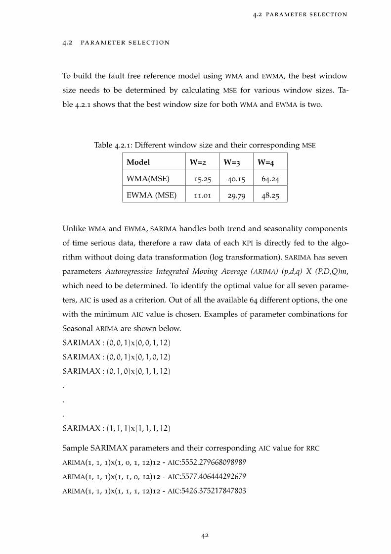
4.2 parameter selection
To build the fault free reference model using WMA and EWMA, the best window
size needs to be determined by calculating MSE for various window sizes. Ta-
ble 4.2.1 shows that the best window size for both WMA and EWMA is two.
Table 4.2.1: Different window size and their corresponding MSE
Model W=2 W=3 W=4
WMA(MSE) 15.25 40.15 64.24
EWMA (MSE) 11.01 29.79 48.25
Unlike WMA and EWMA, SARIMA handles both trend and seasonality components
of time serious data, therefore a raw data of each KPI is directly fed to the algo-
rithm without doing data transformation (log transformation). SARIMA has seven
parameters Autoregressive Integrated Moving Average (ARIMA) (p,d,q) X (P,D,Q)m,
which need to be determined. To identify the optimal value for all seven parame-
ters, AIC is used as a criterion. Out of all the available 64 different options, the one
with the minimum AIC value is chosen. Examples of parameter combinations for
Seasonal ARIMA are shown below.
SARIMAX : (0, 0, 1)x(0, 0, 1, 12)
SARIMAX : (0, 0, 1)x(0, 1, 0, 12)
SARIMAX : (0, 1, 0)x(0, 1, 1, 12)
.
.
.
SARIMAX : (1, 1, 1)x(1, 1, 1, 12)
Sample SARIMAX parameters and their corresponding AIC value for RRC
ARIMA(1, 1, 1)x(1, 0, 1, 12)12 - AIC:5552.279668098989
ARIMA(1, 1, 1)x(1, 1, 0, 12)12 - AIC:5577.406444292679
ARIMA(1, 1, 1)x(1, 1, 1, 12)12 - AIC:5426.375217847803
42

4.3 anomaly detection scenarios
Sample SARIMAX parameters and their corresponding value for UE
ARIMA(1, 0, 1)x(1, 1, 0, 12)12 - AIC:2349.9388424371646
ARIMA(1, 0, 1)x(1, 1, 1, 12)12 - AIC:2207.521912431226
ARIMA(1, 1, 0)x(0, 0, 0, 12)12 - AIC:2425.7679056047964
4.3 anomaly detection scenarios
The aim of this research is to detect a sudden drop and correlation change anomaly
from UMTS network KPI data. The first scenario is to detect a fault caused sudden
drop anomaly, on this scenario two cases are considered. The first case uses tech-
niques with RTWP KPI and additional filtering rules. Whereas, the second case uses
techniques without RTWP KPI and additional filtering rule. The statistical models
such as WMA, EWMA and SARIMA are used to detect the sudden drop anomaly.
The second scenario is to detect a correlational change anomaly, which refers a
large deviation between two correlated KPI instances.
To statistically determine such correlation change anomaly, statistical models such
as WMA, EWMA, SARIMA, and HR are used. Furthermore, when a correlational
anomaly is detected, the experimental setup further classifies the detected anomaly
into two root causes (i.e. fault or external interference caused correlational change
anomaly and congestion caused correlational change anomaly). In all detection
algorithms, remodeling was considered and it only uses instances labeled as nor-
mal to update the reference model. For a correlational change anomaly detection
removal of the trend component has a negative impact on the detection capability
because removing a trend component from the time serious is one of the actions
to make a time serious stationary and such action will remove any determined
autocorrelation[13][32].
4.4 evaluation metrics
Using the pre-determined parameters of each statistical model, a faultless normal
condition of the network is modeled. This model helps to detect the anomaly
43

4.4 evaluation metrics
whenever it is happening. To evaluate anomaly detection capability of different
statistical models, a confusion matrix is used. The matrix contains four classes:
True Negative (TN), True Positive (TP), False Negative (FN), and False Positive (FP).
Table 4.4.1: Confusion matrix for anomaly detection
Observed state
TRUE FALSE
TRUE TP FP
(Anomaly states that
were correctly detected)
( Normal states that
were incorrectly marked
as anomaly)
Detected state FALSE FN TN
(Anomaly states that
were incorrectly labeled
as normal)
( Normal states that
were correctly classi-
fied)
Anomaly detection accuracy, precision, recall, and F-score were then calculated
using Equation 4.1, Equation 4.2 and Equation 4.3. Precision states how the model
is precise/accurate, i.e. how many of the detected anomalies are real anomalies.
Precision is a worthy metric to select the best model when false detection or false
positive costs are high. Recall determines how many of the real anomalies in the
input data can the model capture and label them as anomalies (True Positive).
Similar to precision, a recall is a commendable metric to select the best model,
when false negative is high. F1-score is the harmonic mean of precision and recall,
and it is a better metric to choose if a balance between precision and recall is
needed[33][34]. Its values vary from zero to one, having one as the best and zero
the worst result.
44

4.5 results and discussion
Accuracy =(TP+ TN)
(TP+ FP+ TN+ FN)(4.1)
Precision =(TP)
(TP+ FP)(4.2)
F1 = 2 ∗ (P ∗ R)(P+ R)
(4.3)
4.5 results and discussion
The result is presented using a boxplot. To briefly describe what a boxplot (whisker
plot) is. It is a way to show the range and centers of a data set. As shown in Fig-
ure 4.5.1 the plot has five points: minimum, Q1, Q3, median and maximum[35]. The
main part of the chart is the interquartile range (the "box") shows where the middle
portion of the data is. At the ends of the box, Q1, the first quartile (the 25% mark)
and Q3, the third quartile (the 75% mark) are found. The tip of the up "whiskers" is
the maximum (the largest number in the set) and the tip of the lower whisker is the
minimum (the smallest number in the set). Finally, the median is represented by a
vertical bar in the center of the box. Hence, F1-score value is in the range of 0 and
1 with ’0’ the minimum value and ’1’ the maximum value. The bar in the middle of
the box (median) shows the F1-score for a particular statistical model.
45

4.5 results and discussion
Figure 4.5.1: Boxplot (whisker plot).
The results of the first scenario are shown in Figure 4.5.2. The first scenario is
setup to detect sudden drop anomaly caused due faults for two cases: with and
without RTWP. For all statistical models without RTWP, the mean F1 score is lower
than the models with RTWP. Details of the results are shown in Table 4.5.1 and
Figure 4.5.2.
46

4.5 results and discussion
Table 4.5.1: Confusion matrix for sudden drop anomaly detection
Observed state
TRUE FALSE
WMA TRUE 3080 60
FALSE 1200 24940
WMA(RTWP) TRUE 3840 100
FALSE 440 24900
EWMA TRUE 3640 600
Detected state FALSE 640 24400
EWMA(RTWP) TRUE 3860 320
FALSE 420 24680
SARIMA TRUE 1100 40
FALSE 3180 24960
SARIMA(RTWP) TRUE 3880 100
FALSE 400 24900
Figure 4.5.2: F1-score for fault caused sudden drop anomaly detection.
47

4.5 results and discussion
Because on the second case all statistical models could not detect anomalies hap-
ping during off-pick hour especially after midnight. Since most KPIs are closer to
zero during this period, there is no significant deviation between the expected
and the observed value. Hence, the models cannot detect such anomalies even if
the networks were in an abnormal condition. In the first case, an additional fea-
ture mean RTWP is used, which helps to detect anomalies happing during off-pick
hours. The first case also has an additional rule which helps to filter a false posi-
tive happening in the first setting. A KPI at a given hour might significantly drop
from what is expected, and this could happen due to a fault on the network or
a few numbers of active users served by the network. The statistical models on
the second case cannot differentiate these two conditions. In the first case, when
a sudden drop is detected before deciding the network status, the system model
further checks additional rules. If the total number of active users served by the
network is below the baseline and the RTWP value is better (>-105dBm), the system
model label such conditions as normal otherwise the network status is labeled as
anomaly. Therefore, system models in the first case avoid false positive using such
filtering rule and, hence, gives a better F1-score as compared to system models
without filtering rule.
The second scenario is setup to detect correlational change anomalies. A correla-
tion change anomaly can be caused by congestion or fault. Figure 4.5.3 shows the
detection capability without using RTWP parameter and a filtering rule. Details
of the results are shown in Table 4.5.2 and Figure 4.5.3. As shown in Figure 4.5.3
WMA has a better detection capability with F1-score of above 0.8 as compared
to others. However, such a detection approach has its own limitations. In our
proposed model by using RTWP parameter and a filtering rule we classified the
detected correlational change anomaly into congestion caused and fault caused
anomaly. Because, some operators did not respond to congestion caused anomaly
which happens for hours due to rare events like festivals, holidays or road traf-
fic jam. For such operators, the correlation change anomaly due to congestion is
considered as false positive. Whereas some operators may respond to congestion
caused correlational change anomaly, in such cases, it considers as true positive.
48

4.5 results and discussion
Since it depends on the operator’s preference, we want to classify it into two
groups.
Table 4.5.2: Confusion matrix for correlational change anomaly detection
Observed state
TRUE FALSE
WMA TRUE 1480 640
FALSE 40 27120
EWMA TRUE 1520 920
Detected state FALSE 0 26840
HR TRUE 1340 840
FALSE 180 26920
SARIMA TRUE 1500 740
FALSE 20 27020
Figure 4.5.3: F1-score for fault caused correlational change anomaly detection.
49

4.6 observation
On the proposed approach after the correlational change anomaly is detected, the
detected anomalies further classified using the rules specified in the system model.
F1-score on the Figure 4.5.4 shows the classification capability of the configured
rule. For all statistical models, the classification rule has F1-score above 0.75.
Figure 4.5.4: F1-score for a correlational change anomaly detection classification.
4.6 observation
To observe the effect of anomaly on cell and its neighbors, we collected the number
of active users every 270 meters, when a cell is in normal condition and in abnor-
mal condition for the same hour of a day. Based on our observation when there
is anomaly like transmission link failure, all cells in a site and its most neighbors
are affected. User distribution of a cell and its neighbors are affected as shown in
Figure 4.6.1. The left side of the figure shows, user distribution of a cell and its
neighbors at normal conditions without anomaly, whereas the right side shows
user distribution of a cell and one or more of its neighbors are in abnormal condi-
tion ( i.e. when anomaly detected ).
50

4.7 threats to validity
Figure 4.6.1: UE distribution of selected sites and its neighbors during normal and
anomaly condition.
4.7 threats to validity
The performance counter data of each cell are not directly collected from each site,
instead, it is collected from the third party server called PRS. One of the reasons for
such setup is that the operator is not willing to do any new configuration setup
on a live operational network to collect data directly from each site. As a result,
the integrity and trustworthiness of the collected data relay on PRS services as a
whole. Out of 741 UMTS sites in Addis Ababa, Ethiopia only twenty sites are se-
lected to conduct the study, and it is difficult to take general assumption by taking
20 sites only. However, during site selection, we tried to incorporate all possible
site configuration and sites which report the highest number of alarm (relatively
highly exposed to faults).
51

5C O N C L U S I O N A N D F U T U R E W O R K
5.1 conclusion
Cellular networks usually suffer from failures or performance degradation. To
avoid high customer dissatisfaction and loss of revenue due to poor service qual-
ity, telecom operators need to detect and respond to performance anomalies of
cellular networks instantly. Properly implemented, network performance manage-
ment system can keep connectivity, applications and services running at an opti-
mum level, provide fault tolerance and minimize downtime. Since a performance
management system knows about critical situations in advance, it can avoid catas-
trophic failures that may cause network blackouts, and this will increase the avail-
ability of services, customer satisfaction and revenues of the telecom providers.
The state of art performance anomaly detection framework combines the best of
both statistical and AI based approaches[13]. It used a correlation between two
KPIs as a means to detect anomaly. In their approach, J. Wu,et.al. [13], detected
anomaly when there is a sudden drop on any performance counter or inconsis-
tency between the current and historical correlations of two correlated KPIs. How-
ever, could not detect anomalies which are happing during off-pick hour. Because
most of the KPIs are close to zero during this period. In addition to this, a corre-
lational change anomaly may also happen due to hardware/software failure on
the access or core network of the UMTS, congestion due to neighbor cell failure,
or special events (e.g., festivals and road traffic jam). Therefore, their proposed
approach could not differentiate the possible cause of the correlational change
anomalies which will possibly confuse the system administrators and making it
difficult to take immediate action.
52

5.1 conclusion
The proposed system model aims to detect two types of anomalies which are
known to be sudden drop and correlation change anomalies, which are happing
at any network traffic load. In addition to this, it can differentiate the two causes of
a correlational change anomaly with the help of a newly added parameter called
mean RTWP and filtering rules. The proposed approach improves the detection of
sudden drop anomaly by 10% when compared to the state of the art statistical
model, WMA. Beside, we are able to differentiate the two causes of correlational
change anomaly with an F1-score above 75%.
In our system model, the KPI data is collected on an hourly basis. By using such
data it is difficult to detect anomalies lasting for less than half an hour. If the
data is collected within less than half an hour, it may be possible to detect such
anomalies. For a correlational change anomaly detection, our system model clas-
sifies the detected anomalies into two classes. Such classification includes, the
false positive alarms. If there is a mechanism to differentiate such false positives
and only the true positive classified into two causes of the anomaly is better. Fi-
nally, UMTS network has a number of releases such as High Speed Packet Ac-
cess (HSPA), High-Speed Downlink Packet Access (HSDPA), High Speed Uplink
Packet Access (HSUPA) and Release 99 (R99), even if these releases are independent
they share a physical resources on one site, and a fault may affect a specific release.
As future work, we suggested to study each release independently.
53

R E F E R E N C E
[1] M. P. Kumar, “Telecom services: Emerging trends, opportunities and risk,”
International Journal of Business and Administration Research Review, vol. 1,
no. 5, pp. 34–41, 2014.
[2] H. Kaaranen, A. Ahtiainen, L. Laitinen, S. Naghian, and V. Niemi, UMTS
networks: architecture, mobility and services. John Wiley & Sons, 2005.
[3] techtarget.com. (Oct. 2, 2018). “what is network management system? - def-
inition from whatis.com.”, [Online]. Available: https://searchnetworking.
techtarget.com/definition/network-management-system..
[4] R. Kangas and E. M. Metsälä, “Network management,” in LTE Backhaul,
Wiley Online Library, 2015.
[5] techopedia.com. (Nov. 27, 2019). What is network performance manage-
ment? [Online]. Available: https : / / www . techopedia . com / definition /
29972/network-performance-management.
[6] Y. Kumar, H. Farooq, and A. Imran, “Fault prediction and reliability analysis
in a real cellular network,” in 2017 13th International Wireless Communications
and Mobile Computing Conference (IWCMC), IEEE, 2017, pp. 1090–1095.
[7] V. Chandola, A. Banerjee, and V. Kumar, “Anomaly detection: A survey,”
ACM computing surveys (CSUR), vol. 41, no. 3, p. 15, 2009.
[8] A. Zimek and E. Schubert, “Outlier detection,” Encyclopedia of Database Sys-
tems, pp. 1–5, 2017.
[9] A. Imran, A. Zoha, and A. Abu-Dayya, “Challenges in 5g: How to empower
son with big data for enabling 5g,” IEEE network, vol. 28, no. 6, pp. 27–33,
2014.
54

reference
[10] M. G.N.K.M.S.A.R.H. P. Benjamin Cheung Lake Hiawatha; Stacy Gail Fishkin,
“Method of monitoring wireless network performance,” pat. US 2006/0063521
A1, Feb. 23, 2006.
[11] S. A. Al Mamun and J. Valimaki, “Anomaly detection and classification in
cellular networks using automatic labeling technique for applying super-
vised learning,” Procedia Computer Science, vol. 140, pp. 186–195, 2018.
[12] L. Bodrog, M. Kajó, S. Kocsis, and B. Schultz, “A robust algorithm for
anomaly detection in mobile networks,” in 2016 IEEE 27th Annual Interna-
tional Symposium on Personal, Indoor, and Mobile Radio Communications (PIMRC),
IEEE, 2016, pp. 1–6.
[13] J. Wu, P. P. Lee, Q. Li, L. Pan, and J. Zhang, “Cellpad: Detecting perfor-
mance anomalies in cellular networks via regression analysis,” in 2018 IFIP
Networking Conference (IFIP Networking) and Workshops, IEEE, 2018, pp. 1–9.
[14] P. Muñoz, R. Barco, I. Serrano, and A. Gómez-Andrades, “Correlation-based
time-series analysis for cell degradation detection in son,” IEEE Communica-
tions Letters, vol. 20, no. 2, pp. 396–399, 2016.
[15] H. He and E. A. Garcia, “Learning from imbalanced data,” IEEE Transactions
on knowledge and data engineering, vol. 21, no. 9, pp. 1263–1284, 2009.
[16] D. Liu, Y. Zhao, H. Xu, Y. Sun, D. Pei, J. Luo, X. Jing, and M. Feng, “Oppren-
tice: Towards practical and automatic anomaly detection through machine
learning,” in Proceedings of the 2015 Internet Measurement Conference, ACM,
2015, pp. 211–224.
[17] I. de-la Bandera, R. Barco, P Munoz, and I. Serrano, “Cell outage detection
based on handover statistics,” IEEE Communications Letters, vol. 19, no. 7,
pp. 1189–1192, 2015.
[18] X. Guo, P. Yu, W. Li, and X. Qiu, “Clustering-based kpi data association
analysis method in cellular networks,” in NOMS 2016-2016 IEEE/IFIP Net-
work Operations and Management Symposium, IEEE, 2016, pp. 1101–1104.
[19] M. Alias, N. Saxena, and A. Roy, “Efficient cell outage detection in 5g het-
nets using hidden markov model,” IEEE Communications Letters, vol. 20,
no. 3, pp. 562–565, 2016.
55

reference
[20] P. Casas, P. Fiadino, and A. D’Alconzo, “Machine-learning based approaches
for anomaly detection and classification in cellular networks.,” in TMA,
2016.
[21] S. Chernov, M. Cochez, and T. Ristaniemi, “Anomaly detection algorithms
for the sleeping cell detection in lte networks,” in 2015 IEEE 81st Vehicular
Technology Conference (VTC Spring), IEEE, 2015, pp. 1–5.
[22] I. de la Bandera, P. Munoz, I. Serrano, and R. Barco, “Improving cell outage
management through data analysis,” IEEE Wireless Communications, vol. 24,
no. 4, pp. 113–119, 2017.
[23] telecomhall. (Nov. 27, 2019). What is rtwp? [Online]. Available: http://www.
telecomhall.net/t/what-is-rtwp/6393.
[24] D. Kwiatkowski, P. C. Phillips, P. Schmidt, and Y. Shin, “Testing the null
hypothesis of stationarity against the alternative of a unit root: How sure
are we that economic time series have a unit root?” Journal of econometrics,
vol. 54, no. 1-3, pp. 159–178, 1992.
[25] R. J. Hyndman and G. Athanasopoulos, Forecasting: principles and practice.
OTexts, 2018.
[26] R. Hyndman. (Dec. 18, 2019). 6 -time series decomposition., [Online]. Avail-
able: http://course1.winona.edu/bdeppa/FIN335/Handouts/Time_Series_
Decomposition.html..
[27] K Yeager, Libguides: Spss tutorials: Pearson correlation [internet].[citado 18 de
diciembre de 2018].
[28] J. Brownlee. (Dec. 18, 2019). Moving average smoothing for data prepa-
ration and time series forecasting in python., [Online]. Available: https :
//machinelearningmastery.com/moving-average-smoothing-for-time-
series-forecasting-python.
[29] P. J. Huber, Robust statistics. Springer, 2011.
[30] T. Hastie, R. Tibshirani, and J. Friedman, The elements of statistical learning:
data mining, inference, and prediction. Springer Science & Business Media,
2009.
56

reference
[31] F. Pukelsheim, “The three sigma rule,” The American Statistician, vol. 48, no. 2,
pp. 88–91, 1994.
[32] K. H. Chan, J. C. Hayya, and J. K. Ord, “A note on trend removal methods:
The case of polynomial regression versus variate differencing,” Econometrica
(pre-1986), vol. 45, no. 3, p. 737, 1977.
[33] Y. Sasaki et al., “The truth of the f-measure,” Teach Tutor mater, vol. 1, no. 5,
pp. 1–5, 2007.
[34] D. Hand and P. Christen, “A note on using the f-measure for evaluating
record linkage algorithms,” Statistics and Computing, vol. 28, no. 3, pp. 539–
547, 2018.
[35] datasciencecentral.com. (Dec. 16, 2019). Box plot (box and whiskers): How
to read one & how to make one in excel, ti-83, spss - statistics how to.,
[Online]. Available: https://www.statisticshowto.datasciencecentral.
com/probability-and-statistics/descriptive-statistics/box-plot/.
57
Top Related
Copyright © 2022 FDOKUMEN

