Gene networks reconstruction and time-seriesprediction from microarray data usingrecurrent neural fuzzy networks

I.A. Maraziotis, A. Dragomir and A. Bezerianos

Abstract: Reverse engineering problems concerning the reconstruction and identification of generegulatory networks through gene expression data are central issues in computational molecularbiology and have become the focus of much research in the last few years. An approach hasbeen proposed for inferring the complex causal relationships among genes from microarrayexperimental data, which is based on a novel neural fuzzy recurrent network. The methodderives information on the gene interactions in a highly interpretable form (fuzzy rules) andtakes into account the dynamical aspects of gene regulation through its recurrent structure. Todetermine the efficiency of the proposed approach, microarray data from two experiments relatingto Saccharomyces cerevisiae and Escherichia coli have been used and experiments concerninggene expression time course prediction have been conducted. The interactions that have beenretrieved among a set of genes known to be highly regulated during the yeast cell-cycle arevalidated by previous biological studies. The method surpasses other computational techniques,which have attempted genetic network reconstruction, by being able to recover significantlymore biologically valid relationships among genes.

1 Introduction

The investigation of complex biological processes at themolecular level is now possible by monitoring the geneexpression activity at the whole genome level [1]. Theamount and the complexity of information that gene expres-sion data contains, together with the inherent large dimen-sionality of available data sets, poses new challenges tothe data analysis research community and thus requiresnovel data analysis and modelling techniques. Theavailability of expression data initially made possible theinference of functional information for genes of unknownfunctionality in several partially mapped genomes bymeans of co-expression clustering [2, 3]. Other approachesbased on supervised learning techniques have resulted inthe development of novel diagnosis tools that discriminatebetween different sample classes (e.g. healthy againstdiseased tissue diagnosis) [4]. However, as the ultimategoal of molecular biologists is to uncover the complexregulatory mechanisms controlling cells and organisms,the reconstruction and modelling of gene networks remainsone of the central problems in functional genomics.

Proteins and metabolites, which are produced by proteins,regulate the activity of genes. Proteins, however, are alsogene products and thus genes can influence each other(induce or repress) through a chain of proteins and meta-bolites. At the genetic level, it is thus legitimate, andindeed common, to consider gene–gene interactions, andthese lead to the concept of gene networks. Gene networks

# The Institution of Engineering and Technology 2007

doi:10.1049/iet-syb:20050107

Paper first received 21st December 2005 and in revised form 9th April 2006

The authors are with the Department of Medical Physics, Medical School,University of Patras, Rio 26500, Greece

E-mail: imarazi@heart.med.upatras.gr

IET Syst. Biol., 2007, 1, (1), pp. 41–50

ultimately attempt to describe how genes or groups of genesinteract with each other and identify the complex regulatorymechanisms that control the activity of genes in living cells.The reconstructed gene interaction models should be able toprovide biologists with a range of hypotheses explaining theresults of experiments and suggesting optimal designs forfurther experiments.

The reconstruction of gene networks based on expressiondata is hampered by peculiarities specific to this kind ofdata; therefore the methods employed should be able tohandle underconstrained data, should be robust to noise(as experimental data obtained from microarrays aremeasurement noise-prone), and should be able to provideinterpretable results. Recently, there have been severalattempts to describe models for gene networks. Booleannetworks have been used due to their computationalsimplicity and their ability to deal with noisy experimentaldata [5]. However, the Boolean network’s formalismassumes that a gene is either on or off (no intermediateexpression levels allowed) and the models derived haveinadequate dynamic resolution. Other approaches,reconstructing models using differential equations, haveproved to be computationally expensive and very sensitiveto imprecise data [6]. Models based on Bayesian networks,although attractive due to their ability to deal with stochasticaspects of gene expression and noisy measurements, havethe disadvantage of minimising the dynamical aspects ofgene regulation [7].

Our approach uses a novel recurrent neural fuzzy networkto extract information from time-series gene expression datafrom microarray experiments. It is known that both fuzzylogic systems and neural networks aim at exploiting a human-like knowledge processing capability. Artificial neural net-works are well-known universal function approximators, interms that they can approximate any continuous functionrepresented by data subject to having an appropriate neural

41

network model. A recurrent neural network naturally involvesdynamic elements in the form of feedback connectionsused as internal memories. Unlike the feedforward neuralnetwork whose output is a function of its current input onlyand is limited to static mapping, recurrent neural networksperform dynamic mapping. In contrast, fuzzy logic is anatural language for linguistic modelling; as a consequence,it is consistent with the qualitative linguistic–graphicalmethods used to describe biological systems. Neuro-fuzzysystems combine the advantages of computational powerand low-level learning common to neural networks, andthe high-level human-like reasoning of fuzzy systems. Thedynamic aspects of gene regulatory interactions are con-sidered by the recurrent structure of the neuro-fuzzy architec-ture we propose, while the online learning algorithmdrastically reduces the computational time.

The method was experimentally validated by applying itto two real biological data sets from Saccharomyces cerevi-siae (yeast) and Escherichia coli, from where we proveexperimentally the neural fuzzy recurrent network (NFRN)ability for gene time-series prediction. Interactions amonga set of target genes found to be highly involved in theyeast cell-cycle regulation from previous biological studies[8] are studied and knowledge in the form of IF–THENrules is inferred. The algorithm is trained on a subset ofexperimental samples and the inferred relations are testedfor consistency on the remaining samples. We demonstratethat the proposed approach manages to single out the pre-sence of gene regulatory relations, which is not apparentwhen other methods are applied.

2 Materials and methods

The computational approach described in this paper isthat of a multilayer NFRN. In the literature, there existseveral recurrent neural fuzzy network models such asD-FUNCOM [9], TRFN [10] and RSONFIN [11]. Being ahybrid neuro-fuzzy architecture, it is able to overcome thedrawbacks specific to pure neural networks, which functionas black boxes. By incorporating elements specific to fuzzyreasoning processes, we are able to give to each node andweight their meaning and function as part of a fuzzy rule,instead of just being abstract numbers.

In addition, its recurrent structure manages to possess thesame advantages of a pure recurrent neural network (interms of computational power and time prediction), whilesucceeding in extending the application of the classic neuro-fuzzy networks to temporal problems. In the following, weillustrate our technique for using a number of NFRN modelsto extract relations in the form of fuzzy IF–THEN rules thatdescribe a gene network.

2.1 Neural fuzzy recurrent network

NFRN adopts the Zadeh–Mamdani’s fuzzy model [12] torealise fuzzy inference and each one of the rules for thecase of multi-input multi-output has the following form

Ri: If x1 is A1i and x2 is A2i and � � � and xn is Ani

Then y1 is B1i and � � � and ym is Bmi ð1Þ

where A1i, A2i, . . . , Ani and B1i, B2i, . . . , Bmi are fuzzy setsthat are used from the NR (i ¼ 1, 2, . . . , NR) fuzzy IF–THEN rules to perform a map from the input space,which has the form of a vector X ¼ [x1, x2, . . . , xn]TMPn

to the output space vector Y ¼ [y1, y2, . . . , ym]TMPm.In contrast to other neuro-fuzzy network architectures,

where the network structure is fixed and the rules should

42

be assigned in advance, there are no rules initially in thearchitecture we are presenting; all of them are constructedduring online learning. Two learning phases, the structureas well as parameter learning phases, are used to accomplishthis task. The structure learning phase is responsible for thegeneration of fuzzy IF–THEN rules as well as the judge-ment of the feedback configuration, and the parameterlearning phase for tuning the free parameters of eachdynamic rule (such as the shapes and positions of member-ship functions), which is accomplished through repeatedtraining on the input–output patterns.

The way the input space is partitioned determines thenumber of rules. Given the scale and complexity of thedata, the number of possible rules describing the causalrelationships is kept under constraint by employing analigned clustering-based partition method for the inputspace, meaning that both input and output variables mayhave a different number of fuzzy sets describing them,and by allowing a scene in which rules with different pre-conditions may have the same consequent part [11]. Byincorporating the above clustering scheme, we are able totackle the problem of rule set combinatorial explosion thatappears when using other neuro-fuzzy approaches likeANFIS. One of the main issues this paper attempts toaddress is the extraction of gene networks in the explanatoryform of IF–THEN rules. In order for this to be feasible, therules must be both meaningful and easily interpretable; thuswe have to restrict the number of fuzzy sets on everyvariable to a maximum of seven, even though this mightlead to slightly less accurate results. From our empiricalobservations, further increasing the number of fuzzy setsdoes not provide additional insightful information butunnecessarily increases the complexity. In contrast, experi-mentation has proved that an attempt to keep the number offuzzy sets less than three fails to give adequate resolution.

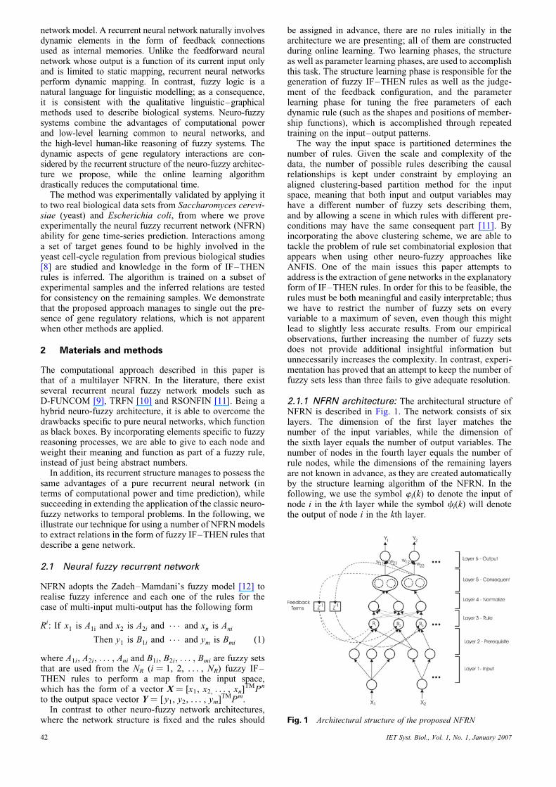
2.1.1 NFRN architecture: The architectural structure ofNFRN is described in Fig. 1. The network consists of sixlayers. The dimension of the first layer matches thenumber of the input variables, while the dimension ofthe sixth layer equals the number of output variables. Thenumber of nodes in the fourth layer equals the number ofrule nodes, while the dimensions of the remaining layersare not known in advance, as they are created automaticallyby the structure learning algorithm of the NFRN. In thefollowing, we use the symbol wi(k) to denote the input ofnode i in the k th layer while the symbol ci(k) will denotethe output of node i in the kth layer.

Fig. 1 Architectural structure of the proposed NFRN

IET Syst. Biol., Vol. 1, No. 1, January 2007

The nodes in the first layer represent an input variable.There is no computation in the first layer and the valuesare transmitted directly to the next layer

cð1Þi ¼ w

ð1Þi ¼ xi ð2Þ

Each node in the second layer corresponds to a linguisticlabel (e.g. low-expressed, average-expressed highly-expressed etc.) and is represented by a membership functionof the Gaussian form

cð2Þij ¼ exp �

ðxi � cijÞ2

s2ij

( )ð3Þ

where i runs through all the input variables and j runsthrough the number of fuzzy sets of each one of the iinput variables, cij is the jth membership function ofthe ith input variable, cij and sij are the centre and widthof the cij membership function, while xi is the value ofthe ith input variable. The linguistic labels result fromthe fuzzification of the expression data, which translatescontinuous attributes into fuzzy ones, efficiently managingthe uncertainty and the vagueness of the expression levels.Qualitative descriptors such as ‘highly-expressed’,‘average-expressed’, ‘low-expressed’ and so on areemployed to denote values of expression data. Each nodein this layer calculates the membership value specifyingthe degree to which an input value belongs to a linguisticlabel. This is accomplished by comparing the input valuewith the centre c and width s of the corresponding fuzzysets for every linguistic label. Other types of membershipfunctions like trapezoidal or triangular could be used.

The nodes of the third layer are called rule nodes. Everyrule node represents a fuzzy logic rule and performs pre-condition matching for the rule. The following fuzzyAND operation is performed by all nodes in this layer

cð3Þi ðtÞ ¼ bi � c

ð5Þj ðt � 1Þ �

Yk

fð3Þi ðtÞ ð4Þ

while we have thatYk

fð3Þi ¼ exp �½Dkðxk � ckÞ�

T½Dkðxk � ckÞ�

� �ð5Þ

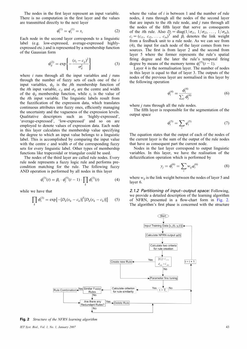
Fig. 2 Structure of the NFRN learning algorithm

IET Syst. Biol., Vol. 1, No. 1, January 2007

where the value of i is between 1 and the number of rulenodes, k runs through all the nodes of the second layerthat are inputs to the ith rule node, and j runs through allthe nodes of the fifth layer that serve as consequentsof the ith rule. Also Di ¼ diag(1/si1, 1/si2, . . . , 1/sin),ci ¼ (ci1, ci2, . . . , cin)T and bi denotes the link weightfrom a feedback unit to a rule node. As we can see from(4), the input for each node of the layer comes from twosources. The first is from layer 2 and the second fromlayer 5 where the former represents the rule’s spatialfiring degree and the later the rule’s temporal firingdegree by means of the memory terms cj

(5)(t 2 1).Layer 4 is the normalisation layer. The number of nodes

in this layer is equal to that of layer 3. The outputs of thenodes of the previous layer are normalised in this layer bythe following operation

cð4Þi ¼

fð4ÞiP

j fð4Þj

ð6Þ

where j runs through all the rule nodes.The fifth layer is responsible for the segmentation of the

output space

cð5Þi ¼

Xi

wð5Þi ð7Þ

The equation states that the output of each of the nodes ofthe current layer is the sum of the output of the rule nodesthat have as consequent part the current node.

Nodes in the last layer correspond to output linguisticvariables. In this layer, we have the realisation of thedefuzzification operation which is performed by

yj ¼ cð6Þi ¼

Xi

wijwð6Þi ð8Þ

where wij is the link weight between the nodes of layer 5 andlayer 6.

2.1.2 Partitioning of input–output space: Following,we provide a detailed description of the learning algorithmof NFRN, presented in a flow-chart form in Fig. 2.The algorithm’s first phase is concerned with the structure

43

learning of the network, which is directly connected with thepartitioning of the input and output space. The creation of anew rule corresponds to the creation of a new cluster in theinput space. Therefore the way the input space is parti-tioned–clustered determines the number of fuzzy rulescreated. This fact lead us to the conclusion that the numberof rules created by NFRN is problem dependent, that is themore complex a problem is, the greater the number of rulesbecomes. A similar scheme stands for the output space, asthe number of generated clusters in the consequent spaceis also problem dependent. The number of output clusters islarge for complex problems and small for simple ones. Inorder for the NFRN to decide whether a new rule must begenerated for the description of an incoming pattern (x, y), atwo criteria scheme is adopted. The first one computes theoverall error Ek, which is defined as the difference betweenthe actual and the desired output and is given by

kEkk ¼ kydk � ykk ð9Þ

where yk is the value computed by the model based on thecurrent input pattern Xk while yk

d is the desired output forthe same pattern.

The second criterion is based on the calculation of thedistance di between the newly arrived observation Xk andall of the rules that have been created up to time step k

dkð jÞ ¼ kX k � Rjk; j ¼ 1; 2; . . . ;Nr ð10Þ

where Nr is the number of the rules, each one of the dk iscomputed by using equation (5). Then we find

dmin ¼ minjðdkð jÞÞ ð11Þ

Now, if both the criteria below are true, we create anew rule

kEkk . lerror

dmin . ldist

ð12Þ

The first criterion checks whether the error of the model isgreater than a specific value, which shows that in the currentstate of the network we cannot deal with the new patternwithout a large value of the error. The second checks tosee whether the pattern is ‘close’ enough to an existingcluster, so that it can become a member of it, or if a newcluster has to be created for it.

If the procedure described leads to the creation of a rule,the next step is the assignment of initial centres and widthsof the corresponding membership functions. Given the factthat the centres and widths will be refined later in theparameter learning scheme, we simply set

ciðt þ 1Þ ¼ xi ð13Þ

siðt þ 1Þ ¼ �1

d

1

lnðdminÞð14Þ

where i runs through all the input variables, d is a constantdeciding the overlap of the clusters, dmin is the distance tothe closest cluster (from the current pattern) and ci, si arethe centre and width for the membership function of eachinput variable, respectively.

A similar method, where width s is accounted for in thedegree measure for the creation of a new radial basis unit,has been used before [9, 11]. This method ensures that forthe description of a cluster with larger width (whichmeans a larger covering region), fewer rules will be gener-ated. To reduce the number of fuzzy sets of each input vari-able and to avoid the existence of redundant fuzzy sets, we

44

check the similarities between them in each input dimension.For the similarity measure of two fuzzy sets, we use theformula previously derived in the work of Lin and Lee[13], which concerns bell-shaped membership functions.

Finally, NFRN has to determine if a new output clustermust be created. A cluster in the output space is the conse-quent of a rule. We have already seen that one of the charac-teristics of NFRN is that more than one rule can beconnected to the same consequent. As a result, the creationof a cluster in the input space does not necessarily mean asubsequent creation of a cluster in the output space; itdepends on the incoming pattern because the newlycreated cluster in the input space could be connected to analready existing cluster of the output space.

The model decides whether or not to create a new outputcluster based on the two criteria described earlier (12).

2.1.3 Merging and deletion of rules: As a concludingstep in the structure learning process of NFRN, we havedeveloped a scheme for deleting redundant rules andcombining similar fuzzy rules into an equivalent new one.This process has the dual goal of both decreasing the redun-dancy of the model as well as increasing the model’ssimplicity.

If a fuzzy set is near zero over its own universe ofdiscourse for a certain number of time steps, then the rulewith the specific fuzzy set as a precondition should beremoved, as this fact indicates that the output of the ruleis also near zero.

When two fuzzy rules have different consequents but verysimilar antecedents, we have a case of conflict among thoserules. The solution to this conflict problem is either to deleteone of the rules, or combine them into a new one. Thereforewe decide whether we can combine two rules by evaluatingthe similarity of their antecedent part. Given, for example,two rules Ri and Rj, their antecedent parts are Ai1, Ai2, . . . ,Ain1 and Aj1, Aj2, . . . , Ajn1, respectively, where Akl is thekth fuzzy set of the lth fuzzy rule and the similarity for theantecedents can be computed as

SðAi;AjÞ ¼ minlfSðAil;AjlÞg; l ¼ 1; 2; . . . ; n1 ð15Þ

if S(Ai, Aj) exceed a value ls then those fuzzy sets are con-sidered to be similar and thus the rules that they constitutecan be combined towards the creation of a new rule Rc.For the evaluation of the centre and width of the joinedfuzzy sets Acl, we use the average of the fuzzy sets Ail, Ajl,ccl ¼ (cilþ cjl)/2, wcl ¼ (wilþ wjl)/2. The same technique isused for the two consequents, meaning zc ¼ (ziþ zj)/2. Hereagain, we follow the same methodology used by Lin andLee [13] for checking the similarity among two fuzzy sets.

Usually the main reason for a case where we have tocombine rules is the inherent noise in the microarray inputdata. Another reason though for such a scenario is thatthere might be a gap in the experimental knowledge andthat triggers us to mark those genes in order for futureexperiments to specify this behaviour. A measure for dis-tinguishing among those two grounds is the value of ls.

It should be pointed out that the value of ls has an initialvalue that decays through time so that higher similaritybetween two fuzzy sets is allowed in the initial stage oflearning.

2.1.4 Parameter learning scheme: After the structureof the network is completed according to the current train-ing pattern, the NFRN enters the parameter learningscheme to adjust the parameters of the network (e.g.widths and centres of the fuzzy sets) based on the same

IET Syst. Biol., Vol. 1, No. 1, January 2007

training pattern. At this point, we should state that, as can benoted, the parameter learning process is performed concur-rently with the structure learning. For the parameter identi-fication of the NFRN, we have used an algorithm based onthe method of gradient descent. The backpropagation learn-ing algorithm is a widely used algorithm for training neuralnetworks or fuzzy networks by means of error propagationvia variation calculus. Owing to the simplicity of the back-propagation through time (BPTT) learning algorithm, weadopt this method to tune free parameters of the NFRNmodel. This study attempts to emphasise the methodologyand dynamic mapping abilities of the NFRN model in thesubject of gene network reconstruction based on micro-arrays time series expression data. Lee and Teng [14] alsoadapted BPTT to successfully train the recurrent fuzzystructure they proposed. Of course, there are many existinglearning algorithms in the literature like the real-time recur-rent learning algorithm [15] or the order-derivative algor-ithm [16] for training recurrent neural networks that canalso be adapted for the fine tuning of the NFRN model.

2.2 NFRN models for the description ofgene networks

A method for depicting gene regulatory networks is nowdescribed, through fuzzy IF–THEN rules, with the help ofthe NFRN model described in the preceding section.

In order to recover functional relationships among genesand to build models describing their interactions, weemploy transcriptional data from microarray experiments.A simple representation of the data would be that of amatrix with rows containing gene expression measurementsover several experimental conditions/samples. Geneexpression patterns give an indication of the levels ofactivity of genes in the tissues under study. A number ofnetwork models that match the number of genes are con-structed, each model having as an output node one selectedgene and as input nodes the remaining genes from the dataset. Models attempt to describe the behaviour of the geneselected as output based on possible interactions from theinput genes and stores the knowledge on the derivedgene–gene interactions in a pool of fuzzy rules.

For each model, we use an error criterion, in order to testthe accuracy on a given data set, by using an overall errormeasure based on the difference between the predictionsof the model for the output variable (i.e. gene). Several cri-teria exist to fulfil this purpose; two of the most common aremean square error and mean error, described by the follow-ing equations

Ei ¼1

N

XN

i¼1

ypredictedi � ymeasured

i

� �2

ð16Þ

Ei ¼1

N

XN

i¼1

ymeasuredi � y

predictedi

��� ���ymeasured

i

ð17Þ

where N is the number of samples in the data set.The number of rules governs the expressive power of the

network. Intuitively, an increase in the number of rulesdescribing the gene interactions in a certain model resultsin a decrease in the error measure of (16) accounted forby the respective model. However, pursuing a low errormeasure may result in the network becoming tuned to theparticular training data set and exhibiting low performanceon the test sets (the well-known overfitting problem).Therefore the problem becomes one of combinationaloptimisation: minimise the number of rules while

IET Syst. Biol., Vol. 1, No. 1, January 2007

preserving the error measure at an adequate level by choos-ing an optimal set of values for the model parameters(overlap degree between partition clusters, learning rates,rule creation criteria).

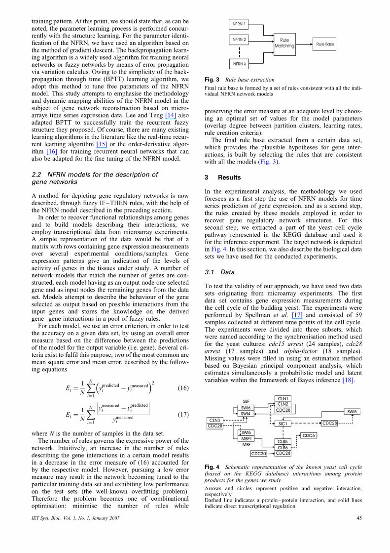
The final rule base extracted from a certain data set,which provides the plausible hypotheses for gene inter-actions, is built by selecting the rules that are consistentwith all the models (Fig. 3).

3 Results

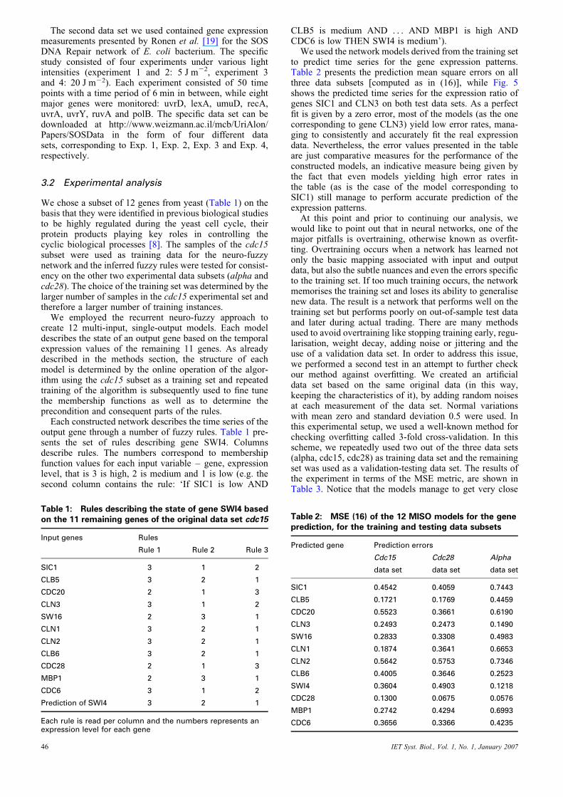
In the experimental analysis, the methodology we usedforesees as a first step the use of NFRN models for timeseries prediction of gene expression, and as a second step,the rules created by these models employed in order torecover gene regulatory network structures. For thissecond step, we extracted a part of the yeast cell cyclepathway represented in the KEGG database and used itfor the inference experiment. The target network is depictedin Fig. 4. In this section, we also describe the biological datasets we have used for the conducted experiments.

3.1 Data

To test the validity of our approach, we have used two datasets originating from microarray experiments. The firstdata set contains gene expression measurements duringthe cell cycle of the budding yeast. The experiments wereperformed by Spellman et al. [17] and consisted of 59samples collected at different time points of the cell cycle.The experiments were divided into three subsets, whichwere named according to the synchronisation method usedfor the yeast cultures: cdc15 arrest (24 samples), cdc28arrest (17 samples) and alpha-factor (18 samples).Missing values were filled in using an estimation methodbased on Bayesian principal component analysis, whichestimates simultaneously a probabilistic model and latentvariables within the framework of Bayes inference [18].

Fig. 3 Rule base extraction

Final rule base is formed by a set of rules consistent with all the indi-vidual NFRN network models

Fig. 4 Schematic representation of the known yeast cell cycle(based on the KEGG database) interactions among proteinproducts for the genes we study

Arrows and circles represent positive and negative interaction,respectivelyDashed line indicates a protein–protein interaction, and solid linesindicate direct transcriptional regulation

45

The second data set we used contained gene expressionmeasurements presented by Ronen et al. [19] for the SOSDNA Repair network of E. coli bacterium. The specificstudy consisted of four experiments under various lightintensities (experiment 1 and 2: 5 J m22, experiment 3and 4: 20 J m22). Each experiment consisted of 50 timepoints with a time period of 6 min in between, while eightmajor genes were monitored: uvrD, lexA, umuD, recA,uvrA, uvrY, ruvA and polB. The specific data set can bedownloaded at http://www.weizmann.ac.il/mcb/UriAlon/Papers/SOSData in the form of four different datasets, corresponding to Exp. 1, Exp. 2, Exp. 3 and Exp. 4,respectively.

3.2 Experimental analysis

We chose a subset of 12 genes from yeast (Table 1) on thebasis that they were identified in previous biological studiesto be highly regulated during the yeast cell cycle, theirprotein products playing key roles in controlling thecyclic biological processes [8]. The samples of the cdc15subset were used as training data for the neuro-fuzzynetwork and the inferred fuzzy rules were tested for consist-ency on the other two experimental data subsets (alpha andcdc28). The choice of the training set was determined by thelarger number of samples in the cdc15 experimental set andtherefore a larger number of training instances.

We employed the recurrent neuro-fuzzy approach tocreate 12 multi-input, single-output models. Each modeldescribes the state of an output gene based on the temporalexpression values of the remaining 11 genes. As alreadydescribed in the methods section, the structure of eachmodel is determined by the online operation of the algor-ithm using the cdc15 subset as a training set and repeatedtraining of the algorithm is subsequently used to fine tunethe membership functions as well as to determine theprecondition and consequent parts of the rules.

Each constructed network describes the time series of theoutput gene through a number of fuzzy rules. Table 1 pre-sents the set of rules describing gene SWI4. Columnsdescribe rules. The numbers correspond to membershipfunction values for each input variable – gene, expressionlevel, that is 3 is high, 2 is medium and 1 is low (e.g. thesecond column contains the rule: ‘If SIC1 is low AND

Table 1: Rules describing the state of gene SWI4 basedon the 11 remaining genes of the original data set cdc15

Input genes Rules

Rule 1 Rule 2 Rule 3

SIC1 3 1 2

CLB5 3 2 1

CDC20 2 1 3

CLN3 3 1 2

SW16 2 3 1

CLN1 3 2 1

CLN2 3 2 1

CLB6 3 2 1

CDC28 2 1 3

MBP1 2 3 1

CDC6 3 1 2

Prediction of SWI4 3 2 1

Each rule is read per column and the numbers represents anexpression level for each gene

46

CLB5 is medium AND . . . AND MBP1 is high ANDCDC6 is low THEN SWI4 is medium’).

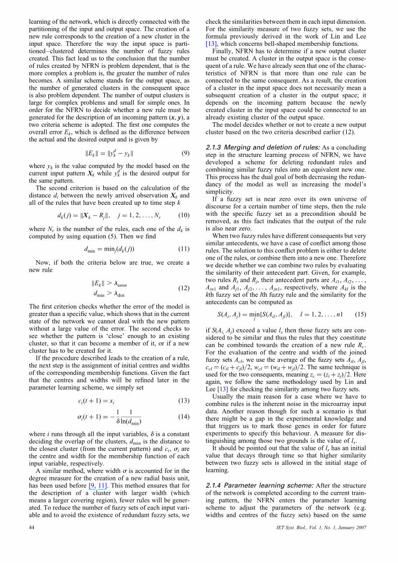
We used the network models derived from the training setto predict time series for the gene expression patterns.Table 2 presents the prediction mean square errors on allthree data subsets [computed as in (16)], while Fig. 5shows the predicted time series for the expression ratio ofgenes SIC1 and CLN3 on both test data sets. As a perfectfit is given by a zero error, most of the models (as the onecorresponding to gene CLN3) yield low error rates, mana-ging to consistently and accurately fit the real expressiondata. Nevertheless, the error values presented in the tableare just comparative measures for the performance of theconstructed models, an indicative measure being given bythe fact that even models yielding high error rates inthe table (as is the case of the model corresponding toSIC1) still manage to perform accurate prediction of theexpression patterns.

At this point and prior to continuing our analysis, wewould like to point out that in neural networks, one of themajor pitfalls is overtraining, otherwise known as overfit-ting. Overtraining occurs when a network has learned notonly the basic mapping associated with input and outputdata, but also the subtle nuances and even the errors specificto the training set. If too much training occurs, the networkmemorises the training set and loses its ability to generalisenew data. The result is a network that performs well on thetraining set but performs poorly on out-of-sample test dataand later during actual trading. There are many methodsused to avoid overtraining like stopping training early, regu-larisation, weight decay, adding noise or jittering and theuse of a validation data set. In order to address this issue,we performed a second test in an attempt to further checkour method against overfitting. We created an artificialdata set based on the same original data (in this way,keeping the characteristics of it), by adding random noisesat each measurement of the data set. Normal variationswith mean zero and standard deviation 0.5 were used. Inthis experimental setup, we used a well-known method forchecking overfitting called 3-fold cross-validation. In thisscheme, we repeatedly used two out of the three data sets(alpha, cdc15, cdc28) as training data set and the remainingset was used as a validation-testing data set. The results ofthe experiment in terms of the MSE metric, are shown inTable 3. Notice that the models manage to get very close

Table 2: MSE (16) of the 12 MISO models for the geneprediction, for the training and testing data subsets

Predicted gene Prediction errors

Cdc15

data set

Cdc28

data set

Alpha

data set

SIC1 0.4542 0.4059 0.7443

CLB5 0.1721 0.1769 0.4459

CDC20 0.5523 0.3661 0.6190

CLN3 0.2493 0.2473 0.1490

SW16 0.2833 0.3308 0.4983

CLN1 0.1874 0.3641 0.6653

CLN2 0.5642 0.5753 0.7346

CLB6 0.4005 0.3646 0.2523

SWI4 0.3604 0.4903 0.1218

CDC28 0.1300 0.0675 0.0576

MBP1 0.2742 0.4294 0.6993

CDC6 0.3656 0.3366 0.4235

IET Syst. Biol., Vol. 1, No. 1, January 2007

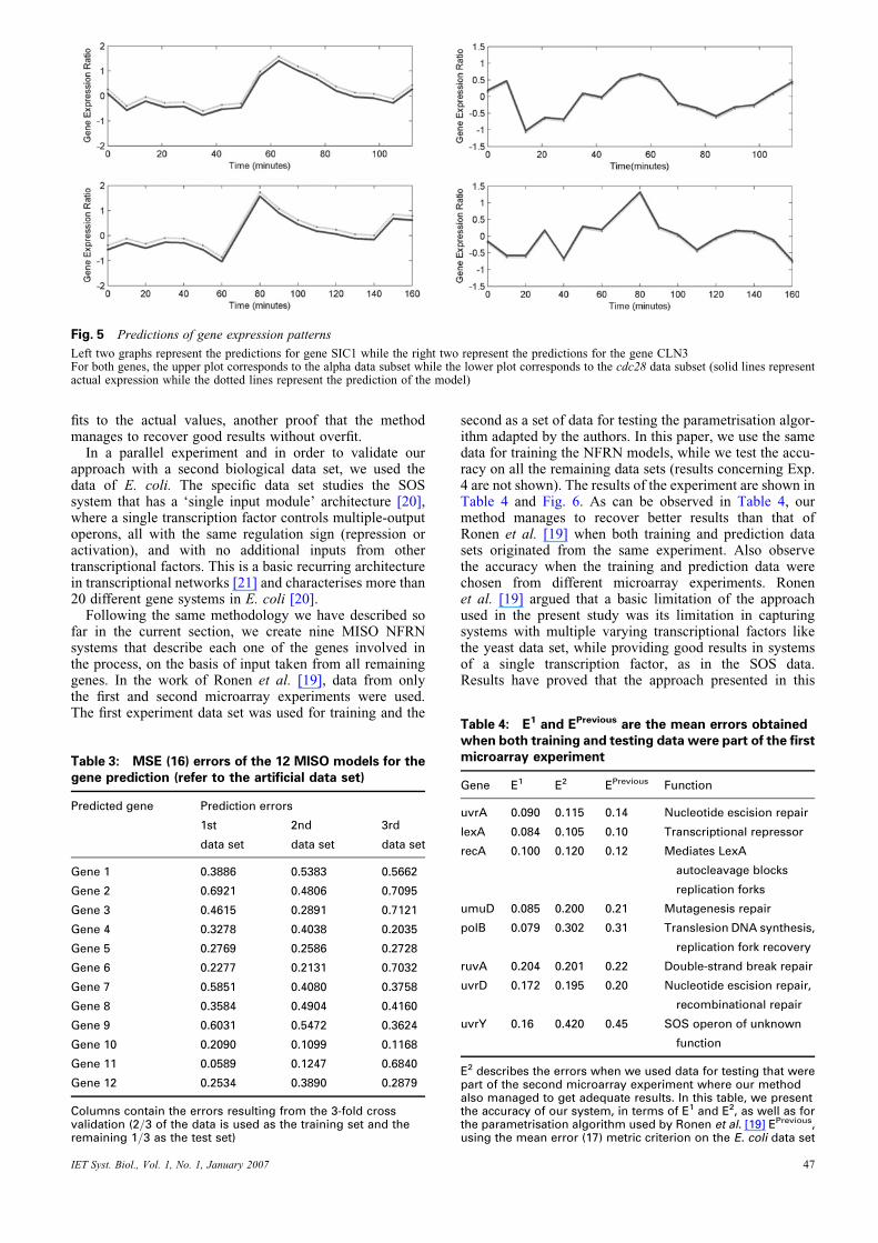
Fig. 5 Predictions of gene expression patterns

Left two graphs represent the predictions for gene SIC1 while the right two represent the predictions for the gene CLN3For both genes, the upper plot corresponds to the alpha data subset while the lower plot corresponds to the cdc28 data subset (solid lines representactual expression while the dotted lines represent the prediction of the model)

fits to the actual values, another proof that the methodmanages to recover good results without overfit.

In a parallel experiment and in order to validate ourapproach with a second biological data set, we used thedata of E. coli. The specific data set studies the SOSsystem that has a ‘single input module’ architecture [20],where a single transcription factor controls multiple-outputoperons, all with the same regulation sign (repression oractivation), and with no additional inputs from othertranscriptional factors. This is a basic recurring architecturein transcriptional networks [21] and characterises more than20 different gene systems in E. coli [20].

Following the same methodology we have described sofar in the current section, we create nine MISO NFRNsystems that describe each one of the genes involved inthe process, on the basis of input taken from all remaininggenes. In the work of Ronen et al. [19], data from onlythe first and second microarray experiments were used.The first experiment data set was used for training and the

Table 3: MSE (16) errors of the 12 MISO models for thegene prediction (refer to the artificial data set)

Predicted gene Prediction errors

1st

data set

2nd

data set

3rd

data set

Gene 1 0.3886 0.5383 0.5662

Gene 2 0.6921 0.4806 0.7095

Gene 3 0.4615 0.2891 0.7121

Gene 4 0.3278 0.4038 0.2035

Gene 5 0.2769 0.2586 0.2728

Gene 6 0.2277 0.2131 0.7032

Gene 7 0.5851 0.4080 0.3758

Gene 8 0.3584 0.4904 0.4160

Gene 9 0.6031 0.5472 0.3624

Gene 10 0.2090 0.1099 0.1168

Gene 11 0.0589 0.1247 0.6840

Gene 12 0.2534 0.3890 0.2879

Columns contain the errors resulting from the 3-fold crossvalidation (2/3 of the data is used as the training set and theremaining 1/3 as the test set)

IET Syst. Biol., Vol. 1, No. 1, January 2007

second as a set of data for testing the parametrisation algor-ithm adapted by the authors. In this paper, we use the samedata for training the NFRN models, while we test the accu-racy on all the remaining data sets (results concerning Exp.4 are not shown). The results of the experiment are shown inTable 4 and Fig. 6. As can be observed in Table 4, ourmethod manages to recover better results than that ofRonen et al. [19] when both training and prediction datasets originated from the same experiment. Also observethe accuracy when the training and prediction data werechosen from different microarray experiments. Ronenet al. [19] argued that a basic limitation of the approachused in the present study was its limitation in capturingsystems with multiple varying transcriptional factors likethe yeast data set, while providing good results in systemsof a single transcription factor, as in the SOS data.Results have proved that the approach presented in this

Table 4: E1 and EPrevious are the mean errors obtainedwhen both training and testing data were part of the firstmicroarray experiment

Gene E1 E2 EPrevious Function

uvrA 0.090 0.115 0.14 Nucleotide escision repair

lexA 0.084 0.105 0.10 Transcriptional repressor

recA 0.100 0.120 0.12 Mediates LexA

autocleavage blocks

replication forks

umuD 0.085 0.200 0.21 Mutagenesis repair

polB 0.079 0.302 0.31 Translesion DNA synthesis,

replication fork recovery

ruvA 0.204 0.201 0.22 Double-strand break repair

uvrD 0.172 0.195 0.20 Nucleotide escision repair,

recombinational repair

uvrY 0.16 0.420 0.45 SOS operon of unknown

function

E2 describes the errors when we used data for testing that werepart of the second microarray experiment where our methodalso managed to get adequate results. In this table, we presentthe accuracy of our system, in terms of E1 and E2, as well as forthe parametrisation algorithm used by Ronen et al. [19] EPrevious,using the mean error (17) metric criterion on the E. coli data set

47

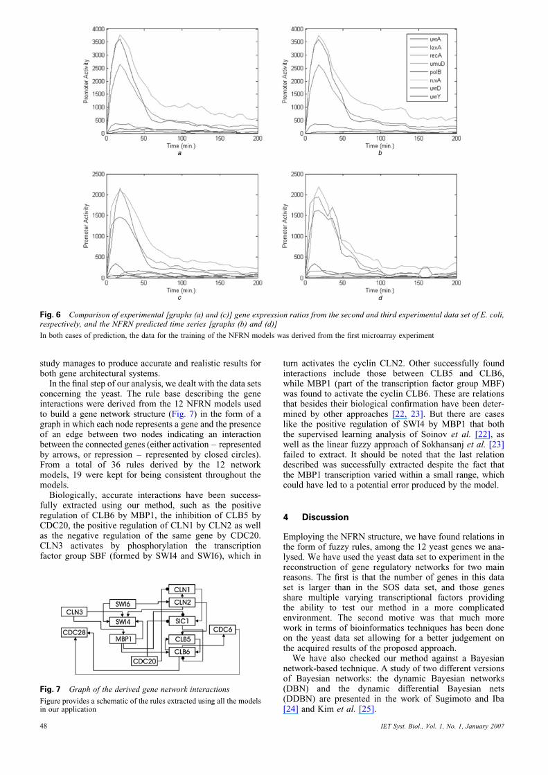
Fig. 6 Comparison of experimental [graphs (a) and (c)] gene expression ratios from the second and third experimental data set of E. coli,respectively, and the NFRN predicted time series [graphs (b) and (d)]

In both cases of prediction, the data for the training of the NFRN models was derived from the first microarray experiment

study manages to produce accurate and realistic results forboth gene architectural systems.

In the final step of our analysis, we dealt with the data setsconcerning the yeast. The rule base describing the geneinteractions were derived from the 12 NFRN models usedto build a gene network structure (Fig. 7) in the form of agraph in which each node represents a gene and the presenceof an edge between two nodes indicating an interactionbetween the connected genes (either activation – representedby arrows, or repression – represented by closed circles).From a total of 36 rules derived by the 12 networkmodels, 19 were kept for being consistent throughout themodels.

Biologically, accurate interactions have been success-fully extracted using our method, such as the positiveregulation of CLB6 by MBP1, the inhibition of CLB5 byCDC20, the positive regulation of CLN1 by CLN2 as wellas the negative regulation of the same gene by CDC20.CLN3 activates by phosphorylation the transcriptionfactor group SBF (formed by SWI4 and SWI6), which in

Fig. 7 Graph of the derived gene network interactions

Figure provides a schematic of the rules extracted using all the modelsin our application

48

turn activates the cyclin CLN2. Other successfully foundinteractions include those between CLB5 and CLB6,while MBP1 (part of the transcription factor group MBF)was found to activate the cyclin CLB6. These are relationsthat besides their biological confirmation have been deter-mined by other approaches [22, 23]. But there are caseslike the positive regulation of SWI4 by MBP1 that boththe supervised learning analysis of Soinov et al. [22], aswell as the linear fuzzy approach of Sokhansanj et al. [23]failed to extract. It should be noted that the last relationdescribed was successfully extracted despite the fact thatthe MBP1 transcription varied within a small range, whichcould have led to a potential error produced by the model.

4 Discussion

Employing the NFRN structure, we have found relations inthe form of fuzzy rules, among the 12 yeast genes we ana-lysed. We have used the yeast data set to experiment in thereconstruction of gene regulatory networks for two mainreasons. The first is that the number of genes in this dataset is larger than in the SOS data set, and those genesshare multiple varying transcriptional factors providingthe ability to test our method in a more complicatedenvironment. The second motive was that much morework in terms of bioinformatics techniques has been doneon the yeast data set allowing for a better judgement onthe acquired results of the proposed approach.

We have also checked our method against a Bayesiannetwork-based technique. A study of two different versionsof Bayesian networks: the dynamic Bayesian networks(DBN) and the dynamic differential Bayesian nets(DDBN) are presented in the work of Sugimoto and Iba[24] and Kim et al. [25].

IET Syst. Biol., Vol. 1, No. 1, January 2007

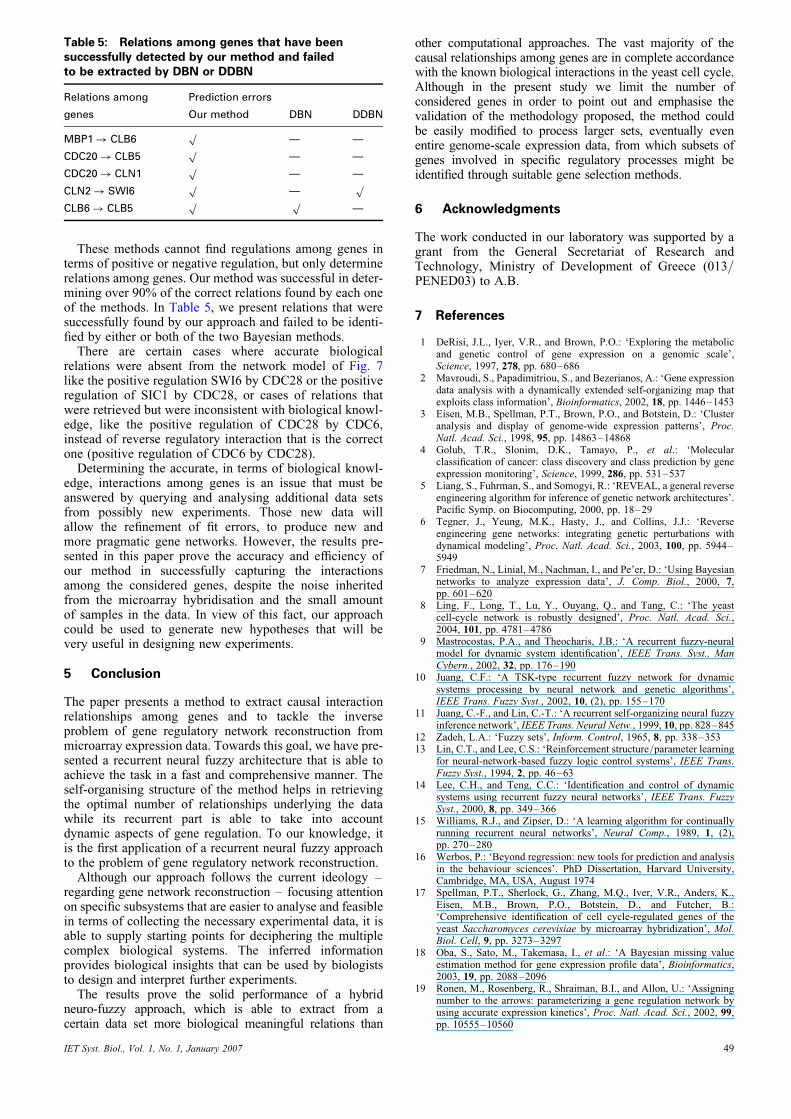
These methods cannot find regulations among genes interms of positive or negative regulation, but only determinerelations among genes. Our method was successful in deter-mining over 90% of the correct relations found by each oneof the methods. In Table 5, we present relations that weresuccessfully found by our approach and failed to be identi-fied by either or both of the two Bayesian methods.

There are certain cases where accurate biologicalrelations were absent from the network model of Fig. 7like the positive regulation SWI6 by CDC28 or the positiveregulation of SIC1 by CDC28, or cases of relations thatwere retrieved but were inconsistent with biological knowl-edge, like the positive regulation of CDC28 by CDC6,instead of reverse regulatory interaction that is the correctone (positive regulation of CDC6 by CDC28).

Determining the accurate, in terms of biological knowl-edge, interactions among genes is an issue that must beanswered by querying and analysing additional data setsfrom possibly new experiments. Those new data willallow the refinement of fit errors, to produce new andmore pragmatic gene networks. However, the results pre-sented in this paper prove the accuracy and efficiency ofour method in successfully capturing the interactionsamong the considered genes, despite the noise inheritedfrom the microarray hybridisation and the small amountof samples in the data. In view of this fact, our approachcould be used to generate new hypotheses that will bevery useful in designing new experiments.

5 Conclusion

The paper presents a method to extract causal interactionrelationships among genes and to tackle the inverseproblem of gene regulatory network reconstruction frommicroarray expression data. Towards this goal, we have pre-sented a recurrent neural fuzzy architecture that is able toachieve the task in a fast and comprehensive manner. Theself-organising structure of the method helps in retrievingthe optimal number of relationships underlying the datawhile its recurrent part is able to take into accountdynamic aspects of gene regulation. To our knowledge, itis the first application of a recurrent neural fuzzy approachto the problem of gene regulatory network reconstruction.

Although our approach follows the current ideology –regarding gene network reconstruction – focusing attentionon specific subsystems that are easier to analyse and feasiblein terms of collecting the necessary experimental data, it isable to supply starting points for deciphering the multiplecomplex biological systems. The inferred informationprovides biological insights that can be used by biologiststo design and interpret further experiments.

The results prove the solid performance of a hybridneuro-fuzzy approach, which is able to extract from acertain data set more biological meaningful relations than

Table 5: Relations among genes that have beensuccessfully detected by our method and failedto be extracted by DBN or DDBN

Relations among

genes

Prediction errors

Our method DBN DDBN

MBP1! CLB6p

— —

CDC20! CLB5p

— —

CDC20! CLN1p

— —

CLN2! SWI6p

—p

CLB6! CLB5p p

—

IET Syst. Biol., Vol. 1, No. 1, January 2007

other computational approaches. The vast majority of thecausal relationships among genes are in complete accordancewith the known biological interactions in the yeast cell cycle.Although in the present study we limit the number ofconsidered genes in order to point out and emphasise thevalidation of the methodology proposed, the method couldbe easily modified to process larger sets, eventually evenentire genome-scale expression data, from which subsets ofgenes involved in specific regulatory processes might beidentified through suitable gene selection methods.

6 Acknowledgments

The work conducted in our laboratory was supported by agrant from the General Secretariat of Research andTechnology, Ministry of Development of Greece (013/PENED03) to A.B.

7 References

1 DeRisi, J.L., Iyer, V.R., and Brown, P.O.: ‘Exploring the metabolicand genetic control of gene expression on a genomic scale’,Science, 1997, 278, pp. 680–686

2 Mavroudi, S., Papadimitriou, S., and Bezerianos, A.: ‘Gene expressiondata analysis with a dynamically extended self-organizing map thatexploits class information’, Bioinformatics, 2002, 18, pp. 1446–1453

3 Eisen, M.B., Spellman, P.T., Brown, P.O., and Botstein, D.: ‘Clusteranalysis and display of genome-wide expression patterns’, Proc.Natl. Acad. Sci., 1998, 95, pp. 14863–14868

4 Golub, T.R., Slonim, D.K., Tamayo, P., et al.: ‘Molecularclassification of cancer: class discovery and class prediction by geneexpression monitoring’, Science, 1999, 286, pp. 531–537

5 Liang, S., Fuhrman, S., and Somogyi, R.: ‘REVEAL, a general reverseengineering algorithm for inference of genetic network architectures’.Pacific Symp. on Biocomputing, 2000, pp. 18–29

6 Tegner, J., Yeung, M.K., Hasty, J., and Collins, J.J.: ‘Reverseengineering gene networks: integrating genetic perturbations withdynamical modeling’, Proc. Natl. Acad. Sci., 2003, 100, pp. 5944–5949

7 Friedman, N., Linial, M., Nachman, I., and Pe’er, D.: ‘Using Bayesiannetworks to analyze expression data’, J. Comp. Biol., 2000, 7,pp. 601–620

8 Ling, F., Long, T., Lu, Y., Ouyang, Q., and Tang, C.: ‘The yeastcell-cycle network is robustly designed’, Proc. Natl. Acad. Sci.,2004, 101, pp. 4781–4786

9 Mastrocostas, P.A., and Theocharis, J.B.: ‘A recurrent fuzzy-neuralmodel for dynamic system identification’, IEEE Trans. Syst., ManCybern., 2002, 32, pp. 176–190

10 Juang, C.F.: ‘A TSK-type recurrent fuzzy network for dynamicsystems processing by neural network and genetic algorithms’,IEEE Trans. Fuzzy Syst., 2002, 10, (2), pp. 155–170

11 Juang, C.-F., and Lin, C.-T.: ‘A recurrent self-organizing neural fuzzyinference network’, IEEE Trans. Neural Netw., 1999, 10, pp. 828–845

12 Zadeh, L.A.: ‘Fuzzy sets’, Inform. Control, 1965, 8, pp. 338–35313 Lin, C.T., and Lee, C.S.: ‘Reinforcement structure/parameter learning

for neural-network-based fuzzy logic control systems’, IEEE Trans.Fuzzy Syst., 1994, 2, pp. 46–63

14 Lee, C.H., and Teng, C.C.: ‘Identification and control of dynamicsystems using recurrent fuzzy neural networks’, IEEE Trans. FuzzySyst., 2000, 8, pp. 349–366

15 Williams, R.J., and Zipser, D.: ‘A learning algorithm for continuallyrunning recurrent neural networks’, Neural Comp., 1989, 1, (2),pp. 270–280

16 Werbos, P.: ‘Beyond regression: new tools for prediction and analysisin the behaviour sciences’. PhD Dissertation, Harvard University,Cambridge, MA, USA, August 1974

17 Spellman, P.T., Sherlock, G., Zhang, M.Q., Iver, V.R., Anders, K.,Eisen, M.B., Brown, P.O., Botstein, D., and Futcher, B.:‘Comprehensive identification of cell cycle-regulated genes of theyeast Saccharomyces cerevisiae by microarray hybridization’, Mol.Biol. Cell, 9, pp. 3273–3297

18 Oba, S., Sato, M., Takemasa, I., et al.: ‘A Bayesian missing valueestimation method for gene expression profile data’, Bioinformatics,2003, 19, pp. 2088–2096

19 Ronen, M., Rosenberg, R., Shraiman, B.I., and Allon, U.: ‘Assigningnumber to the arrows: parameterizing a gene regulation network byusing accurate expression kinetics’, Proc. Natl. Acad. Sci., 2002, 99,pp. 10555–10560

49

20 Shen-Orr, S.S., Milo, R., Mangan, S., and Alon, U.: ‘Network motifsin the transcriptional regulation network of Escherichia coli’, Nat.Genet., 2002, 31, pp. 64–68

21 Neidhardt, F.C., and Savageau, M.A.: ‘Regulation beyond the operon’in Neidhardt, F.C. (Ed.): ‘Escherichia coli and Salmonella: cellularand molecular biology’ (American Society of Microbiology,Washington DC, 1996, 2nd edn), pp. 1310–1324

22 Soinov, L., Krestyaninova, M., and Brazma, A.: ‘Towardsreconstruction of gene networks from expression data by supervisedlearning’, Genome Biol., 2003, 4, pp. R6.1–R6.10

50

23 Sokhansanj, B., Fitch, P., Quong, J., and Quong, A.: ‘Linear fuzzygene network models obtained from microarray data by exhaustivesearch’, BMC Bioinform., 2004, 5, pp. 1–12

24 Sugimoto, N., and Iba, H.: ‘Inference of gene regulatory networks bymeans of dynamic differential Bayesian networks and nonparametricregression’, Genome Inform., 2004, 15, (2), pp. 121–130

25 Kim, S., Imoto, S., and Miyano, S.: ‘Dynamic Bayesian network andnonparametric regression for nonlinear modelling of gene networksfrom time series gene expression data’, Biosystems, 2004, 75,pp. 57–65

IET Syst. Biol., Vol. 1, No. 1, January 2007