


Bahasa
Halaman
Hukum


© D.J.DUNN 1
TUTORIAL No. 1
FLUID FLOW THEORY In order to complete this tutorial you should already have completed level 1 or have a good basic knowledge of fluid mechanics equivalent to the Engineering Council part 1 examination 103. When you have completed this tutorial, you should be able to do the following.
Explain the meaning of viscosity.
Define the units of viscosity.
Describe the basic principles of viscometers.
Describe non-Newtonian flow
Explain and solve problems involving laminar flow though pipes and between parallel surfaces.
Explain and solve problems involving drag force on spheres.
Explain and solve problems involving turbulent flow.
Explain and solve problems involving friction coefficient.
Throughout there are worked examples, assignments and typical exam questions. You should complete each assignment in order so that you progress from one level of knowledge to another. Let us start by examining the meaning of viscosity and how it is measured.

1. VISCOSITY1.1 BASIC THEORY Molecules of fluids exert forces of attraction on each other. In liquids this is strong enough to keep the mass together but not strong enough to keep it rigid. In gases these forces are very weak and cannot hold the mass together. When a fluid flows over a surface, the layer next to the surface may become attached to it (it wets the surface). The layers of fluid above the surface are moving so there must be shearing taking place between the layers of the fluid.
Fig.1.1 Let us suppose that the fluid is flowing over a flat surface in laminated layers from left to right as shown in figure 1.1. y is the distance above the solid surface (no slip surface) L is an arbitrary distance from a point upstream. dy is the thickness of each layer. dL is the length of the layer. dx is the distance moved by each layer relative to the one below in a corresponding time dt. u is the velocity of any layer. du is the increase in velocity between two adjacent layers. Each layer moves a distance dx in time dt relative to the layer below it. The ratio dx/dt must be the change in velocity between layers so du = dx/dt. When any material is deformed sideways by a (shear) force acting in the same direction, a shear stress τ is produced between the layers and a corresponding shear strain γ is produced. Shear strain is defined as follows.
dydx
deformed beinglayer theofheight ndeformatio sideways
==γ
The rate of shear strain is defined as follows.
dydu
dy dtdx
dt takentimestrainshear
==γ
==γ&
It is found that fluids such as water, oil and air, behave in such a manner that the shear stress between layers is directly proportional to the rate of shear strain.
γ=τ & constant x Fluids that obey this law are called NEWTONIAN FLUIDS.
© D.J.DUNN 2
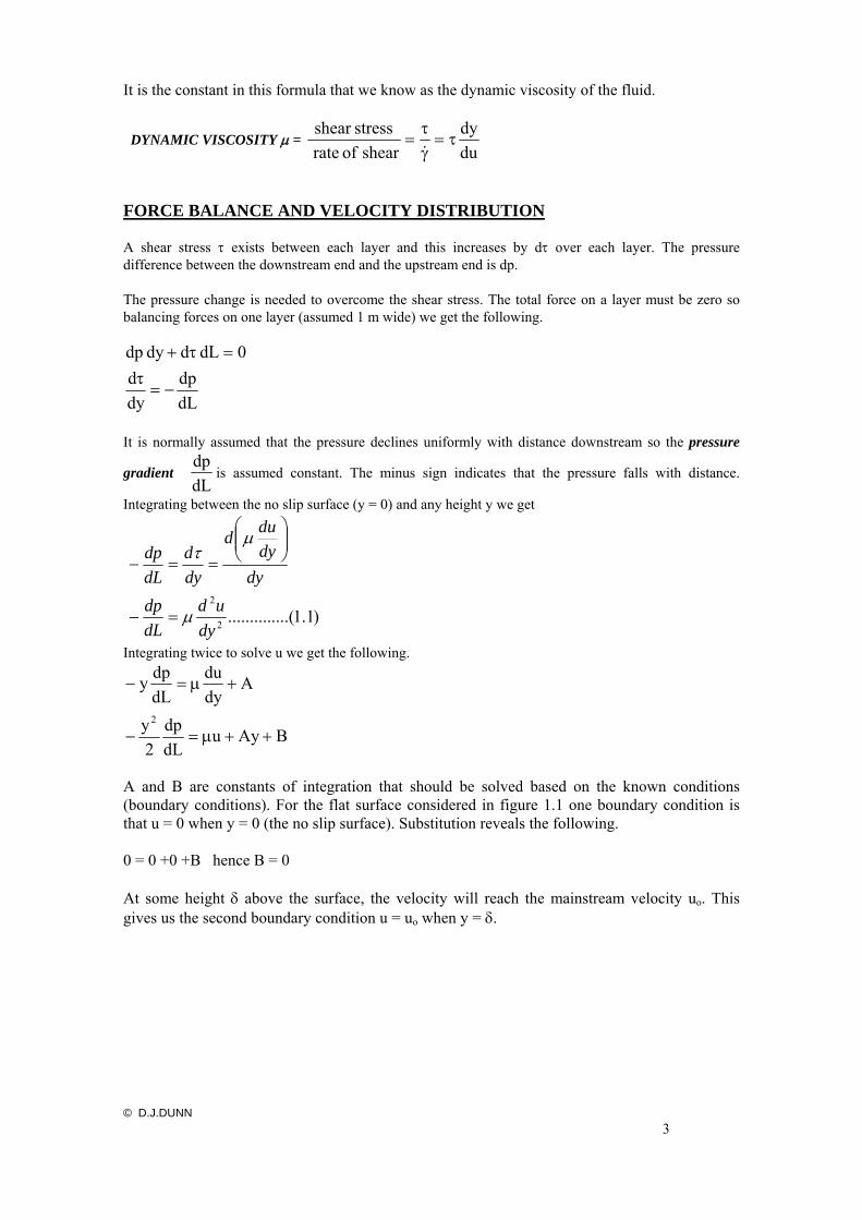
It is the constant in this formula that we know as the dynamic viscosity of the fluid.
DYNAMIC VISCOSITY µ = dudy
shear of rate stressshear
τ=γτ
=&
FORCE BALANCE AND VELOCITY DISTRIBUTION A shear stress τ exists between each layer and this increases by dτ over each layer. The pressure difference between the downstream end and the upstream end is dp. The pressure change is needed to overcome the shear stress. The total force on a layer must be zero so balancing forces on one layer (assumed 1 m wide) we get the following.
dLdp
dyd
0dL d dy dp
−=τ
=τ+
It is normally assumed that the pressure declines uniformly with distance downstream so the pressure
gradient dLdp
is assumed constant. The minus sign indicates that the pressure falls with distance.
Integrating between the no slip surface (y = 0) and any height y we get
)1.1....(..........2
2
dyud
dLdp
dydydud
dyd
dLdp
µ
µτ
=−
⎟⎟⎠
⎞⎜⎜⎝
⎛
==−
Integrating twice to solve u we get the following.
BAyudLdp
2y
Adydu
dLdpy
2
++µ=−
+µ=−
A and B are constants of integration that should be solved based on the known conditions (boundary conditions). For the flat surface considered in figure 1.1 one boundary condition is that u = 0 when y = 0 (the no slip surface). Substitution reveals the following. 0 = 0 +0 +B hence B = 0 At some height δ above the surface, the velocity will reach the mainstream velocity uo. This gives us the second boundary condition u = uo when y = δ.
© D.J.DUNN 3

Substituting we find the following.
⎟⎟⎠
⎞⎜⎜⎝
⎛δ
+µδ
=
⎟⎠⎞
⎜⎝⎛
δµ
−δ
−+µ=−
δµ
−δ
−=
δ+µ=δ
−
o
o2
o
o
2
udLdp
2yu
yu
dLdp
2u
dLdp
2y
hence u
dLdp
2A
AudLdp
2
Plotting u against y gives figure 1.2. BOUNDARY LAYER. The velocity grows from zero at the surface to a maximum at height δ. In theory, the value of δ is infinity but in practice it is taken as the height needed to obtain 99% of the mainstream velocity. This layer is called the boundary layer and δ is the boundary layer thickness. It is a very important concept and is discussed more fully in later work. The inverse gradient of the boundary layer is du/dy and this is the rate of shear strain γ.
Fig.1.2
© D.J.DUNN 4

© D.J.DUNN 5
1.2. UNITS of VISCOSITY 1.2.1 DYNAMIC VISCOSITY µ The units of dynamic viscosity µ are N s/m2. It is normal in the international system (SI) to give a name to a compound unit. The old metric unit was a dyne.s/cm2 and this was called a POISE after Poiseuille. The SI unit is related to the Poise as follows. 10 Poise = 1 Ns/m2 which is not an acceptable multiple. Since, however, 1 Centi Poise (1cP) is 0.001 N s/m2 then the cP is the accepted SI unit.
1cP = 0.001 N s/m2.
The symbol η is also commonly used for dynamic viscosity. There are other ways of expressing viscosity and this is covered next. 1.2.2 KINEMATIC VISCOSITY ν This is defined as : ν = dynamic viscosity /density
ν = µ/ρ
The basic units are m2/s. The old metric unit was the cm2/s and this was called the STOKE after the British scientist. The SI unit is related to the Stoke as follows. 1 Stoke (St) = 0.0001 m2/s and is not an acceptable SI multiple. The centi Stoke (cSt),however, is 0.000001 m2/s and this is an acceptable multiple.
1cSt = 0.000001 m2/s = 1 mm2/s
1.2.3 OTHER UNITS Other units of viscosity have come about because of the way viscosity is measured. For example REDWOOD SECONDS comes from the name of the Redwood viscometer. Other units are Engler Degrees, SAE numbers and so on. Conversion charts and formulae are available to convert them into useable engineering or SI units. 1.2.4 VISCOMETERS The measurement of viscosity is a large and complicated subject. The principles rely on the resistance to flow or the resistance to motion through a fluid. Many of these are covered in British Standards 188. The following is a brief description of some types.

U TUBE VISCOMETER
The fluid is drawn up into a reservoir and allowed to run through a capillary tube to another reservoir in the other limb of the U tube.
© D.J.DUNN 6
The time taken for the level to fall between the marks is converted into cSt by multiplying the time by the viscometer constant.
ν = ct The constant c should be accurately obtained by calibrating the viscometer against a master viscometer from a standards laboratory.
Fig.1.3 REDWOOD VISCOMETER
This works on the principle of allowing the fluid to run through an orifice of very accurate size in an agate block. 50 ml of fluid are allowed to fall from the level indicator into a measuring flask. The time taken is the viscosity in Redwood seconds. There are two sizes giving Redwood No.1 or No.2 seconds. These units are converted into engineering units with tables.
Fig.1.4

FALLING SPHERE VISCOMETER
This viscometer is covered in BS188 and is based on measuring the time for a small sphere to fall in a viscous fluid from one level to another. The buoyant weight of the sphere is balanced by the fluid resistance and the sphere falls with a constant velocity. The theory is based on Stokes’ Law and is only valid for very slow velocities. The theory is covered later in the section on laminar flow where it is shown that the terminal velocity (u) of the sphere is related to the dynamic viscosity (µ) and the density of the fluid and sphere (ρf and ρs) by the formula
µ = F gd2(ρs -ρf)/18u Fig.1.5 F is a correction factor called the Faxen correction factor, which takes into account a reduction in the velocity due to the effect of the fluid being constrained to flow between the wall of the tube and the sphere. ROTATIONAL TYPES There are many types of viscometers, which use the principle that it requires a torque to rotate or oscillate a disc or cylinder in a fluid. The torque is related to the viscosity. Modern instruments consist of a small electric motor, which spins a disc or cylinder in the fluid. The torsion of the connecting shaft is measured and processed into a digital readout of the viscosity in engineering units. You should now find out more details about viscometers by reading BS188, suitable textbooks or literature from oil companies.
ASSIGNMENT No. 1 1. Describe the principle of operation of the following types of viscometers. a. Redwood Viscometers. b. British Standard 188 glass U tube viscometer. c. British Standard 188 Falling Sphere Viscometer. d. Any form of Rotational Viscometer Note that this covers the E.C. exam question 6a from the 1987 paper.
© D.J.DUNN 7

2. LAMINAR FLOW THEORY The following work only applies to Newtonian fluids. 2.1 LAMINAR FLOW A stream line is an imaginary line with no flow normal to it, only along it. When the flow is laminar, the streamlines are parallel and for flow between two parallel surfaces we may consider the flow as made up of parallel laminar layers. In a pipe these laminar layers are cylindrical and may be called stream tubes. In laminar flow, no mixing occurs between adjacent layers and it occurs at low average velocities. 2.2 TURBULENT FLOW The shearing process causes energy loss and heating of the fluid. This increases with mean velocity. When a certain critical velocity is exceeded, the streamlines break up and mixing of the fluid occurs. The diagram illustrates Reynolds coloured ribbon experiment. Coloured dye is injected into a horizontal flow. When the flow is laminar the dye passes along without mixing with the water. When the speed of the flow is increased turbulence sets in and the dye mixes with the surrounding water. One explanation of this transition is that it is necessary to change the pressure loss into other forms of energy such as angular kinetic energy as indicated by small eddies in the flow.
Fig.2.1 2.3 LAMINAR AND TURBULENT BOUNDARY LAYERS In chapter 2 it was explained that a boundary layer is the layer in which the velocity grows from zero at the wall (no slip surface) to 99% of the maximum and the thickness of the layer is denoted δ. When the flow within the boundary layer becomes turbulent, the shape of the boundary layers waivers and when diagrams are drawn of turbulent boundary layers, the mean shape is usually shown. Comparing a laminar and turbulent boundary layer reveals that the turbulent layer is thinner than the laminar layer.
Fig.2.2 © D.J.DUNN
8

2.4 CRITICAL VELOCITY - REYNOLDS NUMBER When a fluid flows in a pipe at a volumetric flow rate Q m3/s the average velocity is defined
AQu m = A is the cross sectional area.
The Reynolds number is defined as ν
=µ
ρ=
DuDuR mme
If you check the units of Re you will see that there are none and that it is a dimensionless number. You will learn more about such numbers in a later section. Reynolds discovered that it was possible to predict the velocity or flow rate at which the transition from laminar to turbulent flow occurred for any Newtonian fluid in any pipe. He also discovered that the critical velocity at which it changed back again was different. He found that when the flow was gradually increased, the change from laminar to turbulent always occurred at a Reynolds number of 2500 and when the flow was gradually reduced it changed back again at a Reynolds number of 2000. Normally, 2000 is taken as the critical value. WORKED EXAMPLE 2.1 Oil of density 860 kg/m3 has a kinematic viscosity of 40 cSt. Calculate the critical velocity when it flows in a pipe 50 mm bore diameter. SOLUTION
m/s 1.60.05
2000x40x10DνR
u
νDuR
6e
m
me
===
=
−
© D.J.DUNN 9

2.5 DERIVATION OF POISEUILLE'S EQUATION for LAMINAR FLOW Poiseuille did the original derivation shown below which relates pressure loss in a pipe to the velocity and viscosity for LAMINAR FLOW. His equation is the basis for measurement of viscosity hence his name has been used for the unit of viscosity. Consider a pipe with laminar flow in it. Consider a stream tube of length ∆L at radius r and thickness dr.
Fig.2.3
y is the distance from the pipe wall. drdu
−=−=−=dydudr dyr Ry
The shear stress on the outside of the stream tube is τ. The force (Fs) acting from right to left is due to the shear stress and is found by multiplying τ by the surface area. Fs = τ x 2πr ∆L
For a Newtonian fluid ,drdu
dydu
µ−=µ=τ . Substituting for τ we get the following.
drduLr2- Fs µ∆π=
The pressure difference between the left end and the right end of the section is ∆p. The force due to this (Fp) is ∆p x circular area of radius r. Fp = ∆p x πr2
rdrL2
pdu
rpdrduL2- have weforces Equating 2
∆∆
−=
∆=∆
µ
πµπr
In order to obtain the velocity of the streamline at any radius r we must integrate between the limits u = 0 when r = R and u = u when r = r.
( )
( )22
22
0
L4p4
L2p-du
rRu
RrL
pu
rdrr
R
u
−∆
=
−∆∆
−=
∆∆
= ∫∫
µ
µ
µ
© D.J.DUNN 10

This is the equation of a Parabola so if the equation is plotted to show the boundary layer, it is seen to extend from zero at the edge to a maximum at the middle.
Fig.2.4
For maximum velocity put r = 0 and we get L
pR∆
∆=
µ4u
2
1
The average height of a parabola is half the maximum value so the average velocity is
L
pR∆
∆=
µ8u
2
m
Often we wish to calculate the pressure drop in terms of diameter D. Substitute R=D/2 and rearrange.
2
32D
Lup m∆=∆
µ
The volume flow rate is average velocity x cross sectional area.
LpD
LpR
LpRRQ
∆∆
=∆∆
=∆∆
=µ
πµ
πµ
π12888
4422
This is often changed to give the pressure drop as a friction head. The friction head for a length L is found from hf =∆p/ρg
2
32gD
Luh m
f ρµ
=
This is Poiseuille's equation that applies only to laminar flow.
© D.J.DUNN 11

WORKED EXAMPLE 2.2 A capillary tube is 30 mm long and 1 mm bore. The head required to produce a
flow rate of 8 mm3/s is 30 mm. The fluid density is 800 kg/m3. Calculate the dynamic and kinematic viscosity of the oil. SOLUTION Rearranging Poiseuille's equation we get
cSt 30.11or s/m10 x 11.308000241.0
cP 24.1or s/m N 0241.00.01018 x 0.03 x 32
0.001 x 9.81 x 800 x 0.03
mm/s 18.10785.08
AQu
mm 785.041 x
4dA
Lu32gDh
26-
2
m
222
m
2f
==ρµ
=ν
==µ
===
=π
=π
=
ρ=µ
WORKED EXAMPLE No.2.3 Oil flows in a pipe 100 mm bore with a Reynolds number of 250. The dynamic
viscosity is 0.018 Ns/m2. The density is 900 kg/m3. Determine the pressure drop per metre length, the average velocity and the radius at
which it occurs. SOLUTION Re=ρum D/µ. Hence um = Re µ/ ρD um = (250 x 0.018)/(900 x 0.1) = 0.05 m/s ∆p = 32µL um /D2 ∆p = 32 x 0.018 x 1 x 0.05/0.12 ∆p= 2.88 Pascals. u = {∆p/4Lµ}(R2 - r2) which is made equal to the average velocity 0.05 m/s 0.05 = (2.88/4 x 1 x 0.018)(0.052 - r2) r = 0.035 m or 35.3 mm.
© D.J.DUNN 12

2.6. FLOW BETWEEN FLAT PLATES Consider a small element of fluid moving at velocity u with a length dx and height dy at
distance y above a flat surface. The shear stress acting on the element increases by dτ in the y direction and the pressure decreases by dp in the x
direction. It was shown earlier that 2
2
dyud
dxdp µ=−
It is assumed that dp/dx does not vary with y so it may be regarded as a fixed value in the following work.
Fig.2.5
)6.2..(..........2
y- again gIntegratin
dxdp - once gIntegratin
2
ABAyudxdp
Adyduy
++=
+=
µ
µ
A and B are constants of integration. The solution of the equation now depends upon the boundary conditions that will yield A and B.
WORKED EXAMPLE No.2.4 Derive the equation linking velocity u and height y at a given point in the x direction when the flow is laminar between two stationary flat parallel plates distance h apart. Go on to derive the volume flow rate and mean velocity. SOLUTION When a fluid touches a surface, it sticks to it and moves with it. The velocity at the flat plates is the same as the plates and in this case is zero. The boundary conditions are hence u = 0 when y = 0 Substituting into equation 2.6A yields that B = 0 u=0 when y=h Substituting into equation 2.6A yields that A = (dp/dx)h/2 Putting this into equation 2.6A yields u = (dp/dx)(1/2µ){y2 - hy} (The student should do the algebra for this). The result is a parabolic distribution similar that given by Poiseuille's equation earlier only this time it is between two flat parallel surfaces.
© D.J.DUNN 13

FLOW RATE To find the flow rate we consider flow through a small rectangular slit of width B and height dy at height y.
Fig.2.6
The flow through the slit is dQ = u Bdy =(dp/dx)(1/2µ){y2 - hy} Bdy Integrating between y = 0 and y = h to find Q yields Q = -B(dp/dx)(h3/12µ) The mean velocity is um = Q/Area = Q/Bh
hence um = -(dp/dx)(h2/12µ) (The student should do the algebra)
2.7 CONCENTRIC CYLINDERS This could be a shaft rotating in a bush filled with oil or a rotational viscometer. Consider a shaft rotating in a cylinder with the gap between filled with a Newtonian liquid. There is no overall flow rate so equation 2.A does not apply.
Due to the stickiness of the fluid, the liquid sticks to both surfaces and has a velocity u = ωRi at the inner layer and zero at the outer layer.
Fig 2.7
© D.J.DUNN 14

If the gap is small, it may be assumed that the change in the velocity across the gap changes from u to zero linearly with radius r. τ = µ du/dy But since the change is linear du/dy = u/(Ro-Ri) = ω Ri /(Ro-Ri) τ = µ ω Ri /(Ro-Ri)
io
i
io
ii
RRhR
FrT
RRhR
hRF
−==
=−
==
=
µωπ
µωπτπ
3i
2
2
R x F Torque
22
areasurfacex stressshear Fcylinder on forceShear
In the case of a rotational viscometer we rearrange so that ( )
ωπµ
hRRRT
i
o32−
=
In reality, it is unlikely that the velocity varies linearly with radius and the bottom of the cylinder would have an affect on the torque. 2.8 FALLING SPHERES This theory may be applied to particle separation in tanks and to a falling sphere viscometer. When a sphere falls, it initially accelerates under the action of gravity. The resistance to motion is due to the shearing of the liquid passing around it. At some point, the resistance balances the force of gravity and the sphere falls at a constant velocity. This is the terminal velocity. For a body immersed in a liquid, the buoyant weight is W and this is equal to the viscous resistance R when the terminal velocity is reached. R = W = volume x density difference x gravity
( )6
3fsgd
WRρρπ −
==
ρs = density of the sphere material ρf = density of fluid d = sphere diameter The viscous resistance is much harder to derive from first principles and this will not be attempted here. In general, we use the concept of DRAG and define the DRAG COEFFICIENT as
Area projected x pressure Dynamicforce Resistance
=DC
© D.J.DUNN 15

22
2
2
d8
4d is sphere a of area projected The
2 is stream flow a of pressure dynamic The
πρ
π
ρ
uRC
u
D =
Research shows the following relationship between CD and Re for a sphere.
Fig. 2.8
For Re<0.2 the flow is called Stokes flow and Stokes showed that R = 3πdµu hence CD=24µ/ρfud = 24/Re For 0.2 < Re < 500 the flow is called Allen flow and CD=18.5Re
-0.6
For 500 < Re < 105 CD is constant CD = 0.44 An empirical formula that covers the range 0.2 < Re < 105 is as follows.
4.01
624+
++=
eeD RR
C
For a falling sphere viscometer, Stokes flow applies. Equating the drag force and the buoyant weight we get 3πdµu = (πd3/6)(ρs - ρf) g µ = gd2(ρs - ρf)/18u for a falling sphere vicometer The terminal velocity for Stokes flow is u = d2g(ρs - ρf)18µ This formula assumes a fluid of infinite width but in a falling sphere viscometer, the liquid is squeezed between the sphere and the tube walls and additional viscous resistance is produced. The Faxen correction factor F is used to correct the result.
© D.J.DUNN 16

2.9 THRUST BEARINGS Consider a round flat disc of radius R rotating at angular velocity ω rad/s on top of a flat surface and separated from it by an oil film of thickness t.
Fig.2.9 Assume the velocity gradient is linear in which case du/dy = u/t = ωr/t at any radius r.
32t is thisDdiameter of In terms
22
r. respect to with gintegratinby found is torque totalThe
2 is torqueThe
2 is forceshear The
is ring on the stressshear The
4
4R
0
3
3
2
DT
tR
tdrrT
tdrrrdFdT
tdrrdF
tr
dydu
µπω
ωµπωµπ
ωµπ
ωµπ
ωµµτ
=
==
==
=
==
∫
There are many variations on this theme that you should be prepared to handle.
© D.J.DUNN 17

2.10 MORE ON FLOW THROUGH PIPES Consider an elementary thin cylindrical layer that makes an element of flow within a pipe. The length is δx , the inside radius is r and the radial thickness is dr. The pressure difference between the ends is δp and the shear stress on the surface increases by dτ from the inner to the outer surface. The velocity at any point is u and the dynamic viscosity is µ.
Fig.2.10
The pressure force acting in the direction of flow is {π(r+dr)2-πr2}δp The shear force opposing is {(τ+δτ)(2π)(r+dr) - τ2πr}δx Equating, simplifying and ignoring the product of two small quantities we have the following result.
n.integratio ofconstant a isA where
.(A).......... 2
drdu
2
drdurget wegIntegratin
dr
drdurd
hence
result theyields dr
drdurd
atedifferenti ation todifferenti partial Using
11
sodr - dy and-y r then pipe theof inside thefrom measured isy If
fluids.Newtonian for
2
2
2
2
2
2
2
2
2
rA
xpr
Axpr
xpr
drurd
drdu
xpr
drurd
drdu
xp
drud
drdu
r
drud
drdu
rxp
drdu
dydu
drd
rxp
+−=
+−=
−=⎟⎠⎞
⎜⎝⎛
+⎟⎠⎞
⎜⎝⎛
−=+
−=+
−−=
−===
=+=
δδ
µ
δδ
µ
δδ
µ
δδ
µ
δδ
µ
µµδδ
µτ
µτττδδ
© D.J.DUNN 18

n.integratio ofconstant another is B where
)......(..........ln4
get again we gIntegratin2
BBrAxpru ++−=δδ
µ
Equations (A) and (B) may be used to derive Poiseuille's equation or it may be used to solve flow through an annular passage. 2.10.1 PIPE At the middle r=0 so from equation (A) it follows that A=0 At the wall, u=0 and r=R. Putting this into equation B yields
{ } again.equation s'Poiseuilleis thisand 41
44
4
0A whereln4
0
2222
2
2
rRxp
xpR
xpru
xpRB
BRAxpR
−=+−=
=
=++−=
δδ
µδδ
µδδ
µ
δδ
µ
δδ
µ
2.10.2 ANNULUS
Fig.2.11
{ } { }
{ }⎭⎬⎫
⎩⎨⎧
+−=
−++−=
++−=
++−=
===
++−=
i
oi
ioio
ii
oo
RR
ARRxp
RRARRxp
BRAxpR
CBRAxpR
BrAxpru
ln410
lnln410
C from Dsubtract
.....(D).................... ln4
0
).......(....................ln4
0
.Rr and R rat 0 u are conditionsboundary The
ln4
20
2
22
2
2oi
2
δδ
µ
δδ
µ
δδ
µ
δδ
µ
δδ
µ
© D.J.DUNN 19

{ }
{ }
{ }
{ } { }
{ } { }
{ }
⎥⎥⎥⎥⎥
⎦
⎤
⎢⎢⎢⎢⎢
⎣
⎡
−+
⎭⎬⎫
⎩⎨⎧−
=
⎥⎥⎥⎥⎥
⎦
⎤
⎢⎢⎢⎢⎢
⎣
⎡
⎭⎬⎫
⎩⎨⎧−
−+
⎭⎬⎫
⎩⎨⎧−
+−=
⎥⎥⎥⎥⎥
⎦
⎤
⎢⎢⎢⎢⎢
⎣
⎡
⎪⎪⎭
⎪⎪⎬
⎫
⎪⎪⎩
⎪⎪⎨
⎧
⎭⎬⎫
⎩⎨⎧−
−+
⎭⎬⎫
⎩⎨⎧−
+=
⎥⎥⎥⎥⎥
⎦
⎤
⎢⎢⎢⎢⎢
⎣
⎡
⎪⎪⎭
⎪⎪⎬
⎫
⎪⎪⎩
⎪⎪⎨
⎧
⎭⎬⎫
⎩⎨⎧−
−=
+
⎭⎬⎫
⎩⎨⎧−
+−=
⎭⎬⎫
⎩⎨⎧−
=
2222
222
222
222
222
222
222
22
lnln
41
lnln
lnln
41u
lnln
41ln
ln41
4r-
Bequation intoput is This lnln
41
lnln
41
40
C. from obtained be lresult wil same The D.equation intoback dsubstitute bemay This
ln41A
rRRr
RR
RRxpu
R
RR
RRRr
RR
RRr
xp
R
RR
RRR
xpr
RR
RRxp
xpu
R
RR
RRR
xpB
BR
RR
RRxp
xpR
RR
RRxp
ii
i
o
io
i
i
o
ioi
i
o
io
i
i
o
ioi
i
o
io
i
i
o
ioi
i
i
o
ioi
i
o
io
δδ
µ
δδ
µ
δδ
µδδ
µδδ
µ
δδ
µ
δδ
µδδ
µ
δδ
µ
For given values the velocity distribution is similar to this.
Fig. 2.12 © D.J.DUNN
20

ASSIGNMENT 2 1. Oil flows in a pipe 80 mm bore diameter with a mean velocity of 0.4 m/s. The
density is 890 kg/m3 and the viscosity is 0.075 Ns/m2. Show that the flow is laminar and hence deduce the pressure loss per metre length.
(150 Pa per metre). 2. Oil flows in a pipe 100 mm bore diameter with a Reynolds’ Number of 500. The
density is 800 kg/m3. Calculate the velocity of a streamline at a radius of 40 mm. The viscosity µ = 0.08 Ns/m2. (0.36 m/s)
3. A liquid of dynamic viscosity 5 x 10⁻³ Ns/m2 flows through a capillary of
diameter 3.0 mm under a pressure gradient of 1800 N/m3. Evaluate the volumetric flow rate, the mean velocity, the centre line velocity and the radial position at which the velocity is equal to the mean velocity.
(uav = 0.101 m/s, umax = 0.202 m/s r = 1.06 mm) 4. Similar to Q6 1998 a. Explain the term Stokes flow and terminal velocity. b. Show that a spherical particle with Stokes flow has a terminal velocity given by
u = d2g(ρs - ρf)/18µ Go on to show that CD=24/Re
c. For spherical particles, a useful empirical formula relating the drag coefficient
and the Reynold’s number is
4.01
624+
++=
eeD RR
C
Given ρf = 1000 kg/m3, µ= 1 cP and ρs= 2630 kg/m3 determine the maximum size of spherical particles that will be lifted upwards by a vertical stream of water moving at 1 m/s.
d. If the water velocity is reduced to 0.5 m/s, show that particles with a diameter of
less than 5.95 mm will fall downwards.
© D.J.DUNN 21

5. Similar to Q5 1998 A simple fluid coupling consists of two parallel round discs of radius R separated
by a a gap h. One disc is connected to the input shaft and rotates at ω1 rad/s. The other disc is connected to the output shaft and rotates at ω2 rad/s. The discs are separated by oil of dynamic viscosity µ and it may be assumed that the velocity gradient is linear at all radii.
Show that the Torque at the input shaft is given by ( )
hDT
3221
4 ωωµπ −=
The input shaft rotates at 900 rev/min and transmits 500W of power. Calculate the output speed, torque and power. (747 rev/min, 5.3 Nm and 414 W)
Show by application of max/min theory that the output speed is half the input speed when maximum output power is obtained.
6. Show that for fully developed laminar flow of a fluid of viscosity µ between
horizontal parallel plates a distance h apart, the mean velocity um is related to the pressure gradient dp/dx by um = - (h2/12µ)(dp/dx)
Fig.2.11 shows a flanged pipe joint of internal diameter di containing viscous
fluid of viscosity µ at gauge pressure p. The flange has an outer diameter do and is imperfectly tightened so that there is a narrow gap of thickness h. Obtain an expression for the leakage rate of the fluid through the flange.
Fig.2.13
Note that this is a radial flow problem and B in the notes becomes 2πr and dp/dx
becomes -dp/dr. An integration between inner and outer radii will be required to give flow rate Q in terms of pressure drop p.
The answer is Q = (2πh3p/12µ)/{ln(do/di)}
© D.J.DUNN 22

3. TURBULENT FLOW
3.1 FRICTION COEFFICIENT The friction coefficient is a convenient idea that can be used to calculate the pressure drop in a pipe. It is defined as follows.
Pressure Dynamic
StressShear WallCf =
3.1.1 DYNAMIC PRESSURE Consider a fluid flowing with mean velocity um. If the kinetic energy of the fluid is converted into flow or fluid energy, the pressure would increase. The pressure rise due to this conversion is called the dynamic pressure. KE = ½ mum
2
Flow Energy = p Q Q is the volume flow rate and ρ = m/Q Equating ½ mum
2 = p Q p = mu2/2Q = ½ ρ um2
3.1.2 WALL SHEAR STRESS τo The wall shear stress is the shear stress in the layer of fluid next to the wall of the pipe.
Fig.3.1
The shear stress in the layer next to the wall is wall
o dydu
⎟⎟⎠
⎞⎜⎜⎝
⎛= µτ
The shear force resisting flow is LDF os πτ=
The resulting pressure drop produces a force of 4
2DpFpπ∆
=
Equating forces gives LpD
o 4∆
=τ
© D.J.DUNN 23

3.1.3 FRICTION COEFFICIENT for LAMINAR FLOW
2m
f uL4pD2
Pressure DynamicStressShear WallC
ρ∆
==
From Poiseuille’s equation 2m
DLu32p µ
=∆ Hence e
2m
22m
f R16
Du16
DLu32
uL4D2C =
ρµ
=⎟⎠⎞
⎜⎝⎛ µ⎟⎟⎠
⎞⎜⎜⎝
⎛ρ
=
3.1.4 DARCY FORMULA This formula is mainly used for calculating the pressure loss in a pipe due to turbulent flow but it can be used for laminar flow also. Turbulent flow in pipes occurs when the Reynolds Number exceeds 2500 but this is not a clear point so 3000 is used to be sure. In order to calculate the frictional losses we use the concept of friction coefficient symbol Cf. This was defined as follows.
2m
f uL4pD2
Pressure DynamicStressShear WallC
ρ∆
==
Rearranging equation to make ∆p the subject
D2
uLC4p2mf ρ
=∆
This is often expressed as a friction head hf
gD2LuC4
gph
2mf
f =ρ∆
=
This is the Darcy formula. In the case of laminar flow, Darcy's and Poiseuille's equations must give the same result so equating them gives
emf
2m
2mf
R16
Du16C
gDLu32
gD2LuC4
=ρ
µ=
ρµ
=
This is the same result as before for laminar flow. Turbulent flow may be safely assumed in pipes when the Reynolds’ Number exceeds 3000. In order to calculate the frictional losses we use the concept of friction coefficient symbol Cf. Note that in older textbooks Cf was written as f but now the symbol f represents 4Cf.
3.1.5 FLUID RESISTANCE Fluid resistance is an alternative approach to solving problems involving losses. The above equations may be expressed in terms of flow rate Q by substituting u = Q/A
2
2f
2mf
f gDA2LQC4
gD2LuC4h == Substituting A =πD2/4 we get the following.
252
2f
f RQDgLQC32h =
π= R is the fluid resistance or restriction. 52
32Dg
LCR f
π=
© D.J.DUNN 24

If we want pressure loss instead of head loss the equations are as follows.
252
2f
ff RQDLQC32ghp =
πρ
=ρ= R is the fluid resistance or restriction. 52
32D
LCR f
πρ
=
It should be noted that R contains the friction coefficient and this is a variable with velocity and surface roughness so R should be used with care. 3.2 MOODY DIAGRAM AND RELATIVE SURFACE ROUGHNESS In general the friction head is some function of um such that hf = φumn. Clearly for laminar flow, n =1 but for turbulent flow n is between 1 and 2 and its precise value depends upon the roughness of the pipe surface. Surface roughness promotes turbulence and the effect is shown in the following work. Relative surface roughness is defined as ε = k/D where k is the mean surface roughness and D the bore diameter. An American Engineer called Moody conducted exhaustive experiments and came up with the Moody Chart. The chart is a plot of Cf vertically against Re horizontally for various values of ε. In order to use this chart you must know two of the three co-ordinates in order to pick out the point on the chart and hence pick out the unknown third co-ordinate. For smooth pipes, (the bottom curve on the diagram), various formulae have been derived such as those by Blasius and Lee. BLASIUS Cf = 0.0791 Re
0.25
LEE Cf = 0.0018 + 0.152 Re
0.35. The Moody diagram shows that the friction coefficient reduces with Reynolds number but at a certain point, it becomes constant. When this point is reached, the flow is said to be fully developed turbulent flow. This point occurs at lower Reynolds numbers for rough pipes. A formula that gives an approximate answer for any surface roughness is that given by Haaland.
⎪⎭
⎪⎬⎫
⎪⎩
⎪⎨⎧
⎟⎠⎞
⎜⎝⎛ ε
+−=11.1
e10
f 71.3R9.6log6.3
C1
© D.J.DUNN 25

© D.J.DUNN 26
Fig. 3.2 CHART

WORKED EXAMPLE 3.1 Determine the friction coefficient for a pipe 100 mm bore with a mean surface roughness of
0.06 mm when a fluid flows through it with a Reynolds number of 20 000. SOLUTION The mean surface roughness ε = k/d = 0.06/100 = 0.0006 Locate the line for ε = k/d = 0.0006. Trace the line until it meets the vertical line at Re = 20 000. Read of the value of Cf
horizontally on the left. Answer Cf = 0.0067.Check using the formula from Haaland.
0067.0C
206.12C1
71.30006.0
200009.6log6.3
C1
71.30006.0
200009.6log6.3
C1
71.3R9.6log6.3
C1
f
f
11.1
10f
11.1
10f
11.1
e10
f
=
=
⎪⎭
⎪⎬⎫
⎪⎩
⎪⎨⎧
⎟⎠⎞
⎜⎝⎛+−=
⎪⎭
⎪⎬⎫
⎪⎩
⎪⎨⎧
⎟⎠⎞
⎜⎝⎛+−=
⎪⎭
⎪⎬⎫
⎪⎩
⎪⎨⎧
⎟⎠⎞
⎜⎝⎛ ε
+−=
WORKED EXAMPLE 3.2 Oil flows in a pipe 80 mm bore with a mean velocity of 4 m/s. The mean surface roughness
is 0.02 mm and the length is 60 m. The dynamic viscosity is 0.005 N s/m2 and the density is 900 kg/m3. Determine the pressure loss.
SOLUTION Re = ρud/µ = (900 x 4 x 0.08)/0.005 = 57600 ε= k/d = 0.02/80 = 0.00025 From the chart Cf = 0.0052 hf = 4CfLu2/2dg = (4 x 0.0052 x 60 x 42)/(2 x 9.81 x 0.08) = 12.72 m ∆p = ρghf = 900 x 9.81 x 12.72 = 112.32 kPa.
© D.J.DUNN 27

© D.J.DUNN 28
ASSIGNMENT 3 1. A pipe is 25 km long and 80 mm bore diameter. The mean surface roughness is
0.03 mm. It carries oil of density 825 kg/m3 at a rate of 10 kg/s. The dynamic viscosity is 0.025 N s/m2.
Determine the friction coefficient using the Moody Chart and calculate the
friction head. (Ans. 3075 m.) 2. Water flows in a pipe at 0.015 m3/s. The pipe is 50 mm bore diameter. The
pressure drop is 13 420 Pa per metre length. The density is 1000 kg/m3 and the dynamic viscosity is 0.001 N s/m2.
Determine i. the wall shear stress (167.75 Pa) ii. the dynamic pressure (29180 Pa). iii. the friction coefficient (0.00575) iv. the mean surface roughness (0.0875 mm) 3. Explain briefly what is meant by fully developed laminar flow. The velocity u at any
radius r in fully developed laminar flow through a straight horizontal pipe of internal radius ro is given by
u = (1/4µ)(ro2 - r2)dp/dx
dp/dx is the pressure gradient in the direction of flow and µ is the dynamic viscosity. Show that the pressure drop over a length L is given by the following formula.
∆p = 32µLum/D2
The wall skin friction coefficient is defined as Cf = 2τo/( ρum2). Show that Cf = 16/Re where Re = ρumD/µ and ρ is the density, um is the mean velocity
and τo is the wall shear stress. 4. Oil with viscosity 2 x 10⁻² Ns/m2 and density 850 kg/m3 is pumped along a straight
horizontal pipe with a flow rate of 5 dm3/s. The static pressure difference between two tapping points 10 m apart is 80 N/m2. Assuming laminar flow determine the following.
i. The pipe diameter. ii. The Reynolds number. Comment on the validity of the assumption that the flow is laminar
4. NON-NEWTONIAN FLUIDS

A Newtonian fluid as discussed so far in this tutorial is a fluid that obeys the law γµµτ &==dydu
A Non – Newtonian fluid is generally described by the non-linear law ny kγττ &+=
τy is known as the yield shear stress and γ& is the rate of shear strain. Figure 4.1 shows the principle forms of this equation. Graph A shows an ideal fluid that has no viscosity and hence has no shear stress at any point. This is often used in theoretical models of fluid flow. Graph B shows a Newtonian Fluid. This is the type of fluid with which this book is mostly concerned, fluids such as water and oil. The graph is hence a straight line and the gradient is the viscosity µ. There is a range of other liquid or semi-liquid materials that do not obey this law and produce strange flow characteristics. Such materials include various foodstuffs, paints, cements and so on. Many of these are in fact solid particles suspended in a liquid with various concentrations. Graph C shows the relationship for a Dilatent fluid. The gradient and hence viscosity increases with γ& and such fluids are also called shear-thickening. This phenomenon occurs with some solutions of sugar and starches. Graph D shows the relationship for a Pseudo-plastic. The gradient and hence viscosity reduces with γ& and they are called shear-thinning. Most foodstuffs are like this as well as clay and liquid cement.. Other fluids behave like a plastic and require a minimum stress before it shears τy. This is plastic behaviour but unlike plastics, there may be no elasticity prior to shearing. Graph E shows the relationship for a Bingham plastic. This is the special case where the behaviour is the same as a Newtonian fluid except for the existence of the yield stress. Foodstuffs containing high level of fats approximate to this model (butter, margarine, chocolate and Mayonnaise). Graph F shows the relationship for a plastic fluid that exhibits shear thickening characteristics. Graph G shows the relationship for a Casson fluid. This is a plastic fluid that exhibits shear-thinning characteristics. This model was developed for fluids containing rod like solids and is often applied to molten chocolate and blood.
Fig.4.1
© D.J.DUNN 29

MATHEMATICAL MODELS The graphs that relate shear stress τ and rate of shear strain γ are based on models or equations. Most are mathematical equations created to represent empirical data. Hirschel and Bulkeley developed the power law for non-Newtonian equations. This is as follows.
ny Kγ+τ=τ & K is called the consistency coefficient and n is a power.
In the case of a Newtonian fluid n = 1 and τy = 0 and K = µ (the dynamic viscosity) γµ=τ & For a Bingham plastic, n = 1 and K is also called the plastic viscosity µp. The relationship reduces to γµ+τ=τ &py
For a dilatent fluid, τy = 0 and n>1 For a pseudo-plastic, τy = 0 and n<1 The model for both is nKγ=τ &
The Herchel-Bulkeley model is as follows. n
y Kγ+τ=τ &
This may be developed as follows.
1y
1
app1
1
pp
so 0 eshear valu yield no with Fluid aFor
so 1 n plastic Bingham aFor
iscosity apparent v thecalled is ratio The
by dividing
. viscosityplastic thecalled is where as written sometimes
−
−
−
−
==
+==
+==
+=
==−
=−=−
+=
napp
yapp
nyapp
ny
nn
y
ny
ny
ny
K
K
K
K
KK
K
K
γµτγτ
µ
γγτ
γτµ
µγγτ
γτ
γγγ
γτ
γτ
γ
µγµττγττ
γττ
&
&
&&&
&&&
&&
&
&&
&
&&
&
The Casson fluid model is quite different in form from the others and is as follows.
21
21
y21
Kγ+τ=τ &
© D.J.DUNN 30

THE FLOW OF A PLASTIC FLUID
© D.J.DUNN 31
Note that fluids with a shear yield stress will flow in a pipe as a plug. Within a certain radius, the shear stress will be insufficient to produce shearing so inside that radius the fluid flows as a solid plug. Fig. 4.2 shows a typical situation for a Bingham Plastic.
Fig.4.2
MINIMUM PRESSURE The shear stress acting on the surface of the plug is the yield value. Let the plug be diameter d. The pressure force acting on the plug is ∆p x πd2/4 The shear force acting on the surface of the plug is τy x π d L Equating we find ∆p x πd2/4 = τy x π d L
d = τy x 4 L/∆p or ∆p = τy x 4 L/d The minimum pressure required to produce flow must occur when d is largest and equal to the bore of the pipe. ∆p (minimum) = τy x 4 L/D The diameter of the plug at any greater pressure must be given by d = τy x 4 L/∆p For a Bingham Plastic, the boundary layer between the plug and the wall must be laminar and the velocity must be related to radius by the formula derived earlier.
( ) ( )2222
L16p
L4p dDrRu −
∆=−
∆=
µµ
FLOW RATE The flow rate should be calculated in two stages. The plug moves at a constant velocity so the flow rate for the plug is simply Qp = u x cross sectional area = u x πd2/4 The flow within the boundary layer is found in the usual way as follows. Consider an elementary ring radius r and width dr.
( )
( )
⎥⎦
⎤⎢⎣
⎡+−⎟⎟
⎠
⎞⎜⎜⎝
⎛∆=
⎥⎦
⎤⎢⎣
⎡⎟⎟⎠
⎞⎜⎜⎝
⎛−−⎟⎟
⎠
⎞⎜⎜⎝
⎛−
∆=⎥
⎦
⎤⎢⎣
⎡−
∆=
−∆
=
−∆
==
∫
424L2p Q
4242L2p
42L2p Q
dr L2
p Q
drr 2 x L4p dr r 2u x dQ
4224
42244422
r
R
32
22
rRrR
rRrRRrRr
rrR
rR
R
r
µπ
µπ
µπ
µπ
πµ
π
The mean velocity as always is defined as um = Q/Cross sectional area.

WORKED EXAMPLE 4.1 The Herchel-Bulkeley model for a non-Newtonian fluid is as follows. . n
y Kγ+τ=τ &
Derive an equation for the minimum pressure required drop per metre length in a straight
horizontal pipe that will produce flow. Given that the pressure drop per metre length in the pipe is 60 Pa/m and the yield shear
stress is 0.2 Pa, calculate the radius of the slug sliding through the middle. SOLUTION
© D.J.DUNN 32
Fig. 3.3
The pressure difference p acting on the cross sectional area must produce sufficient force to
overcome the shear stress τ acting on the surface area of the cylindrical slug. For the slug to move, the shear stress must be at least equal to the yield value τy. Balancing the forces gives the following.
p x πr2 = τy x 2πrL p/L = 2τy /r 60 = 2 x 0.2/r r = 0.4/60 = 0.0066 m or 6.6 mm

WORKED EXAMPLE 4.2 A Bingham plastic flows in a pipe and it is observed that the central plug is 30 mm
diameter when the pressure drop is 100 Pa/m. Calculate the yield shear stress. Given that at a larger radius the rate of shear strain is 20 s-1 and the consistency coefficient
is 0.6 Pa s, calculate the shear stress. SOLUTION For a Bingham plastic, the same theory as in the last example applies. p/L = 2τy /r 100 = 2 τy/0.015 τy = 100 x 0.015/2 = 0.75 Pa A mathematical model for a Bingham plastic is γ+τ=τ &Ky = 0.75 + 0.6 x 20 = 12.75 Pa
© D.J.DUNN 33
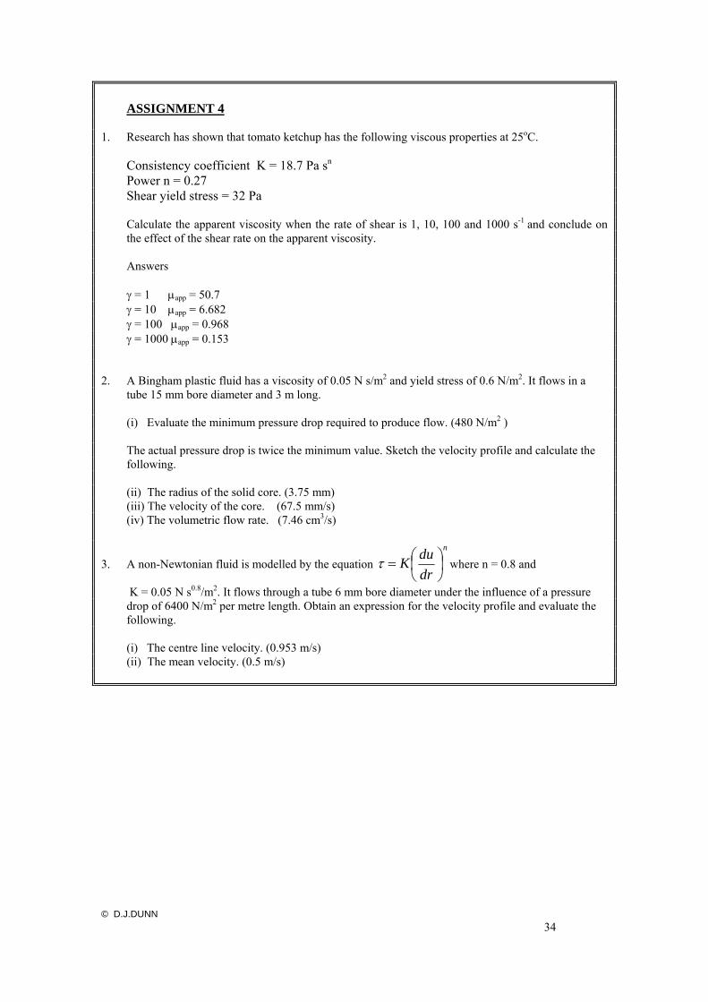
ASSIGNMENT 4 1. Research has shown that tomato ketchup has the following viscous properties at 25oC. Consistency coefficient K = 18.7 Pa sn
Power n = 0.27 Shear yield stress = 32 Pa Calculate the apparent viscosity when the rate of shear is 1, 10, 100 and 1000 s-1 and conclude on
the effect of the shear rate on the apparent viscosity. Answers γ = 1 µapp = 50.7 γ = 10 µapp = 6.682 γ = 100 µapp = 0.968 γ = 1000 µapp = 0.153 2. A Bingham plastic fluid has a viscosity of 0.05 N s/m2 and yield stress of 0.6 N/m2. It flows in a
tube 15 mm bore diameter and 3 m long. (i) Evaluate the minimum pressure drop required to produce flow. (480 N/m2 ) The actual pressure drop is twice the minimum value. Sketch the velocity profile and calculate the
following. (ii) The radius of the solid core. (3.75 mm) (iii) The velocity of the core. (67.5 mm/s) (iv) The volumetric flow rate. (7.46 cm3/s)
3. A non-Newtonian fluid is modelled by the equation n
drduK ⎟
⎠⎞
⎜⎝⎛=τ where n = 0.8 and
K = 0.05 N s0.8/m2. It flows through a tube 6 mm bore diameter under the influence of a pressure drop of 6400 N/m2 per metre length. Obtain an expression for the velocity profile and evaluate the following.
(i) The centre line velocity. (0.953 m/s) (ii) The mean velocity. (0.5 m/s)
© D.J.DUNN 34

© D.J.DUNN www.freestudy.co.uk 1
FLUID MECHANICS 203 TUTORIAL No.2
APPLICATIONS OF BERNOULLI
On completion of this tutorial you should be able to
derive Bernoulli's equation for liquids.
find the pressure losses in piped systems due to fluid friction.
find the minor frictional losses in piped systems.
match pumps of known characteristics to a given system.
derive the basic relationship between pressure, velocity and force..
solve problems involving flow through orifices.
solve problems involving flow through Venturi meters.
understand orifice meters.
understand nozzle meters.
understand the principles of jet pumps
solve problems from past papers. Let's start by revising basics. The flow of a fluid in a pipe depends upon two fundamental laws, the conservation of mass and energy.

© D.J.DUNN www.freestudy.co.uk 2
1. PIPE FLOW The solution of pipe flow problems requires the applications of two principles, the law of conservation of mass (continuity equation) and the law of conservation of energy (Bernoulli’s equation) 1.1 CONSERVATION OF MASS When a fluid flows at a constant rate in a pipe or duct, the mass flow rate must be the same at all points along the length. Consider a liquid being pumped into a tank as shown (fig.1). The mass flow rate at any section is m = ρAum ρ = density (kg/m3) um = mean velocity (m/s) A = Cross Sectional Area (m2)
Fig.1.1
For the system shown the mass flow rate at (1), (2) and (3) must be the same so
ρ1A1u1 = ρ2A2u2 = ρ3A3u3
In the case of liquids the density is equal and cancels so
A1u1 = A2u2 = A3u3 = Q

© D.J.DUNN www.freestudy.co.uk 3
1.2 CONSERVATION OF ENERGY ENERGY FORMS FLOW ENERGY This is the energy a fluid possesses by virtue of its pressure. The formula is F.E. = pQ Joules p is the pressure (Pascals) Q is volume rate (m3) POTENTIAL OR GRAVITATIONAL ENERGY This is the energy a fluid possesses by virtue of its altitude relative to a datum level. The formula is P.E. = mgz Joules m is mass (kg) z is altitude (m) KINETIC ENERGY This is the energy a fluid possesses by virtue of its velocity. The formula is K.E. = ½ mum
2 Joules um is mean velocity (m/s) INTERNAL ENERGY This is the energy a fluid possesses by virtue of its temperature. It is usually expressed relative to 0oC. The formula is U = mcθ c is the specific heat capacity (J/kg oC) θ is the temperature in oC In the following work, internal energy is not considered in the energy balance. SPECIFIC ENERGY Specific energy is the energy per kg so the three energy forms as specific energy are as follows. F.E./m = pQ/m = p/ρ Joules/kg P.E/m. = gz Joules/kg K.E./m = ½ u2 Joules/kg ENERGY HEAD If the energy terms are divided by the weight mg, the result is energy per Newton. Examining the units closely we have J/N = N m/N = metres. It is normal to refer to the energy in this form as the energy head. The three energy terms expressed this way are as follows. F.E./mg = p/ρg = h P.E./mg = z K.E./mg = u2 /2g The flow energy term is called the pressure head and this follows since earlier it was shown that p/ρg = h. This is the height that the liquid would rise to in a vertical pipe connected to the system. The potential energy term is the actual altitude relative to a datum. The term u2/2g is called the kinetic head and this is the pressure head that would result if the velocity is converted into pressure.

© D.J.DUNN www.freestudy.co.uk 4
1.3 BERNOULLI’S EQUATION Bernoulli’s equation is based on the conservation of energy. If no energy is added to the system as work or heat then the total energy of the fluid is conserved. Remember that internal (thermal energy) has not been included. The total energy ET at (1) and (2) on the diagram (fig.3.1) must be equal so :
2ummgzQp
2ummgzQpE
22
222
21
111T ++=++=
Dividing by mass gives the specific energy form
2ugzp
2ugzp
mE 2
22
2
221
11
1T ++ρ
=++ρ
=
Dividing by g gives the energy terms per unit weight
g2uz
gp
g2uz
gp
mgE 2
22
2
221
11
1T ++ρ
=++ρ
=
Since p/ρg = pressure head h then the total head is given by the following.
g2uzh
g2uzhh
22
22
21
11T ++=++=
This is the head form of the equation in which each term is an energy head in metres. z is the potential or gravitational head and u2/2g is the kinetic or velocity head. For liquids the density is the same at both points so multiplying by ρg gives the pressure form. The total pressure is as follows.
2ugzp
2ugzpp
22
22
21
11Tρ
+ρ+=ρ
+ρ+=
In real systems there is friction in the pipe and elsewhere. This produces heat that is absorbed by the liquid causing a rise in the internal energy and hence the temperature. In fact the temperature rise will be very small except in extreme cases because it takes a lot of energy to raise the temperature. If the pipe is long, the energy might be lost as heat transfer to the surroundings. Since the equations did not include internal energy, the balance is lost and we need to add an extra term to the right side of the equation to maintain the balance. This term is either the head lost to friction hL or the pressure loss pL.
L
22
22
21
11 hg2
uzhg2
uzh +++=++
The pressure form of the equation is as follows.
L
22
22
21
11 p2ugzp
2ugzp +
ρ+ρ+=
ρ+ρ+
The total energy of the fluid (excluding internal energy) is no longer constant. Note that if a point is a free surface the pressure is normally atmospheric but if gauge pressures are used, the pressure and pressure head becomes zero. Also, if the surface area is large (say a large tank), the velocity of the surface is small and when squared becomes negligible so the kinetic energy term is neglected (made zero).

© D.J.DUNN www.freestudy.co.uk 5
WORKED EXAMPLE No. 1 The diagram shows a pump delivering water through as pipe 30 mm bore to a tank. Find
the pressure at point (1) when the flow rate is 1.4 dm3/s. The density of water is 1000 kg/m3. The loss of pressure due to friction is 50 kPa.
Fig.1.2
SOLUTION Area of bore A = π x 0.032/4 = 706.8 x 10⁻⁶ m2. Flow rate Q = 1.4 dm3/s = 0.0014 m3/s Mean velocity in pipe = Q/A = 1.98 m/s Apply Bernoulli between point (1) and the surface of the tank.
Lpugzpugzp +++=++22
22
22
21
11ρ
ρρ
ρ
Make the low level the datum level and z1 = 0 and z2 = 25. The pressure on the surface is zero gauge pressure. PL = 50 000 Pa The velocity at (1) is 1.98 m/s and at the surface it is zero.
pressure gauge 29.293
5000009125.9100002
98.110000
1
2
1
kPap
xxp
=
+++=++

© D.J.DUNN www.freestudy.co.uk 6
WORKED EXAMPLE 2 The diagram shows a tank that is drained by a horizontal pipe. Calculate the pressure head
at point (2) when the valve is partly closed so that the flow rate is reduced to 20 dm3/s. The pressure loss is equal to 2 m head.
Fig.1.3
SOLUTION Since point (1) is a free surface, h1 = 0 and u1 is assumed negligible. The datum level is point (2) so z1 = 15 and z2 = 0. Q = 0.02 m3/s A2 = πd2/4 = π x (0.052)/4 = 1.963 x 10⁻³ m2. u2 = Q/A = 0.02/1.963 x 10-3 = 10.18 m/s Bernoulli’s equation in head form is as follows.
m72.7h
29.81 x 2
10.180h0510
hg2
uzhg2
uzh
2
2
2
L
22
22
21
11
=
+++=++
+++=++

© D.J.DUNN www.freestudy.co.uk 7
WORKED EXAMPLE 3 The diagram shows a horizontal nozzle discharging into the atmosphere. The inlet has a
bore area of 600 mm2 and the exit has a bore area of 200 mm2. Calculate the flow rate when the inlet pressure is 400 Pa. Assume there is no energy loss.
Fig. 1.4
SOLUTION Apply Bernoulli between (1) and (2)
L
22
22
21
11 p2ρuρgzp
2ρuρgzp +++=++
Using gauge pressure, p2 = 0 and being horizontal the potential terms cancel. The loss term is zero so the equation simplifies to the following.
2ρu
2ρup
22
21
1 =+
From the continuity equation we have
Q 000 5
10 x 200Q
AQu
666.7Q 110 x 600
QAQu
6-2
2
6-1
1
===
===
Putting this into Bernoulli’s equation we have the following.
( ) ( )
/scm 189.7or /sm 10 x 7.189Q
x1036 x1011.11
400Q
Q x10.1111400
Q10 x 52.1Q x10389.14002
5000Q x10002
1666.7Q x1000400
336-
99
2
29
2929
22
=
==
=
=+
=+
−
© D.J.DUNN www.freestudy.co.uk 8
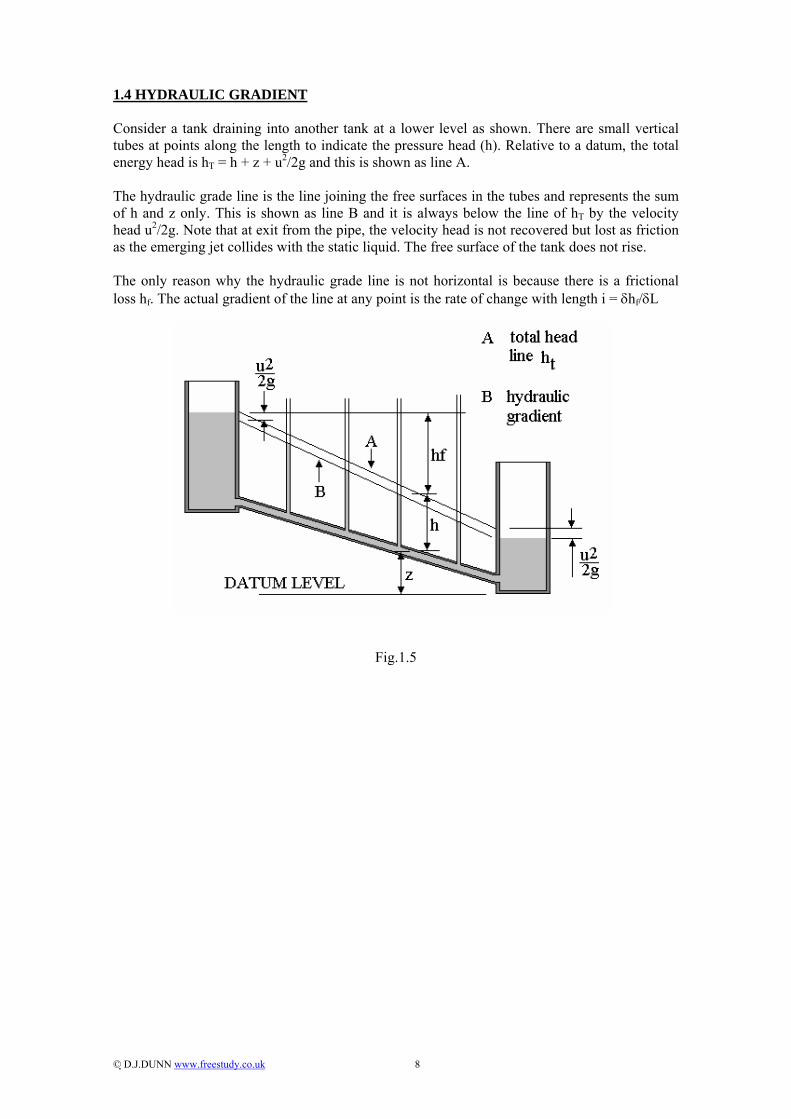
1.4 HYDRAULIC GRADIENT Consider a tank draining into another tank at a lower level as shown. There are small vertical tubes at points along the length to indicate the pressure head (h). Relative to a datum, the total energy head is hT = h + z + u2/2g and this is shown as line A. The hydraulic grade line is the line joining the free surfaces in the tubes and represents the sum of h and z only. This is shown as line B and it is always below the line of hT by the velocity head u2/2g. Note that at exit from the pipe, the velocity head is not recovered but lost as friction as the emerging jet collides with the static liquid. The free surface of the tank does not rise. The only reason why the hydraulic grade line is not horizontal is because there is a frictional loss hf. The actual gradient of the line at any point is the rate of change with length i = δhf/δL
Fig.1.5

© D.J.DUNN www.freestudy.co.uk 9
SELF ASSESSMENT EXERCISE 1 1. A pipe 100 mm bore diameter carries oil of density 900 kg/m3 at a rate of 4 kg/s. The pipe
reduces to 60 mm bore diameter and rises 120 m in altitude. The pressure at this point is atmospheric (zero gauge). Assuming no frictional losses, determine:
i. The volume/s (4.44 dm3/s) ii. The velocity at each section (0.566 m/s and 1.57 m/s) iii. The pressure at the lower end. (1.06 MPa) 2. A pipe 120 mm bore diameter carries water with a head of 3 m. The pipe descends 12 m in
altitude and reduces to 80 mm bore diameter. The pressure head at this point is 13 m. The density is 1000 kg/m3. Assuming no losses, determine
i. The velocity in the small pipe (7 m/s) ii. The volume flow rate. (35 dm3/s) 3. A horizontal nozzle reduces from 100 mm bore diameter at inlet to 50 mm at exit. It carries
liquid of density 1000 kg/m3 at a rate of 0.05 m3/s. The pressure at the wide end is 500 kPa (gauge). Calculate the pressure at the narrow end neglecting friction. (196 kPa)
4. A pipe carries oil of density 800 kg/m3. At a given point (1) the pipe has a bore area of
0.005 m2 and the oil flows with a mean velocity of 4 m/s with a gauge pressure of 800 kPa. Point (2) is further along the pipe and there the bore area is 0.002 m2 and the level is 50 m above point (1). Calculate the pressure at this point (2). Neglect friction. (374 kPa)
5. A horizontal nozzle has an inlet velocity u1 and an outlet velocity u2 and discharges into the
atmosphere. Show that the velocity at exit is given by the following formulae. u2 ={2∆p/ρ + u1
2}½ and u2 ={2g∆h + u1
2}½
© D.J.DUNN www.freestudy.co.uk 10
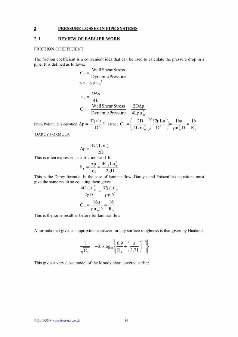
2 PRESSURE LOSSES IN PIPE SYSTEMS 2 .1 REVIEW OF EARLIER WORK FRICTION COEFFICIENT The friction coefficient is a convenient idea that can be used to calculate the pressure drop in a pipe. It is defined as follows.
Pressure Dynamic
StressShear WallCf =
p = ½ ρ um2
LpD
o 4∆
=τ
2m
f uL4pD2
Pressure DynamicStressShear WallC
ρ∆
==
From Poiseuille’s equation 2m
DLu32p µ
=∆ Hence e
2m
22m
f R16
Du16
DLu32
uL4D2C =
ρµ
=⎟⎠⎞
⎜⎝⎛ µ⎟⎟⎠
⎞⎜⎜⎝
⎛ρ
=
DARCY FORMULA
D2
uLC4p2mf ρ
=∆
This is often expressed as a friction head hf
gD2LuC4
gph
2mf
f =ρ∆
=
This is the Darcy formula. In the case of laminar flow, Darcy's and Poiseuille's equations must give the same result so equating them gives
emf
2m
2mf
R16
Du16C
gDLu32
gD2LuC4
=ρ
µ=
ρµ
=
This is the same result as before for laminar flow.
A formula that gives an approximate answer for any surface roughness is that given by Haaland.
⎪⎭
⎪⎬⎫
⎪⎩
⎪⎨⎧
⎟⎠⎞
⎜⎝⎛ ε
+−=11.1
e10
f 71.3R9.6log6.3
C1
This gives a very close model of the Moody chart covered earlier.

© D.J.DUNN www.freestudy.co.uk 11
WORKED EXAMPLE 4 Determine the friction coefficient for a pipe 100 mm bore with a mean surface roughness of
0.06 mm when a fluid flows through it with a Reynolds number of 20 000. SOLUTION The mean surface roughness ε = k/d = 0.06/100 = 0.0006 Locate the line for ε = k/d = 0.0006. Trace the line until it meets the vertical line at Re = 20 000. Read of the value of Cf
horizontally on the left. Answer Cf = 0.0067 Check using the formula from Haaland.
0067.0C
206.12C1
71.30006.0
200009.6log6.3
C1
71.30006.0
200009.6log6.3
C1
71.3R9.6log6.3
C1
f
f
11.1
10f
11.1
10f
11.1
e10
f
=
=
⎪⎭
⎪⎬⎫
⎪⎩
⎪⎨⎧
⎟⎠⎞
⎜⎝⎛+−=
⎪⎭
⎪⎬⎫
⎪⎩
⎪⎨⎧
⎟⎠⎞
⎜⎝⎛+−=
⎪⎭
⎪⎬⎫
⎪⎩
⎪⎨⎧
⎟⎠⎞
⎜⎝⎛ ε
+−=

© D.J.DUNN www.freestudy.co.uk 12
WORKED EXAMPLE 5 Oil flows in a pipe 80 mm bore with a mean velocity of 4 m/s. The mean surface roughness
is 0.02 mm and the length is 60 m. The dynamic viscosity is 0.005 N s/m2 and the density is 900 kg/m3. Determine the pressure loss.
SOLUTION Re = ρud/µ = (900 x 4 x 0.08)/0.005 = 57600 ε= k/d = 0.02/80 = 0.00025 From the chart Cf = 0.0052 hf = 4CfLu2/2dg = (4 x 0.0052 x 60 x 42)/(2 x 9.81 x 0.08) = 12.72 m ∆p = ρghf = 900 x 9.81 x 12.72 = 112.32 kPa.

© D.J.DUNN www.freestudy.co.uk 13
2.2 MINOR LOSSES Minor losses occur in the following circumstances.
i. Exit from a pipe into a tank. ii. Entry to a pipe from a tank. iii. Sudden enlargement in a pipe. iv. Sudden contraction in a pipe. v. Bends in a pipe. vi. Any other source of restriction such as pipe fittings and valves.
Fig.2.1 In general, minor losses are neglected when the pipe friction is large in comparison but for short pipe systems with bends, fittings and changes in section, the minor losses are the dominant factor. In general, the minor losses are expressed as a fraction of the kinetic head or dynamic pressure in the smaller pipe. Minor head loss = k u2/2g Minor pressure loss = ½ kρu2 Values of k can be derived for standard cases but for items like elbows and valves in a pipeline, it is determined by experimental methods. Minor losses can also be expressed in terms of fluid resistance R as follows.
242
2
2
22
L RQD
Q8kA2
Qk2
ukh =π
=== Hence 42Dk8R
π=
242
2
L RQD
gQ8kp =πρ
= hence 42Dgk8R
πρ
=
Before you go on to look at the derivations, you must first learn about the coefficients of contraction and velocity.
© D.J.DUNN www.freestudy.co.uk 14
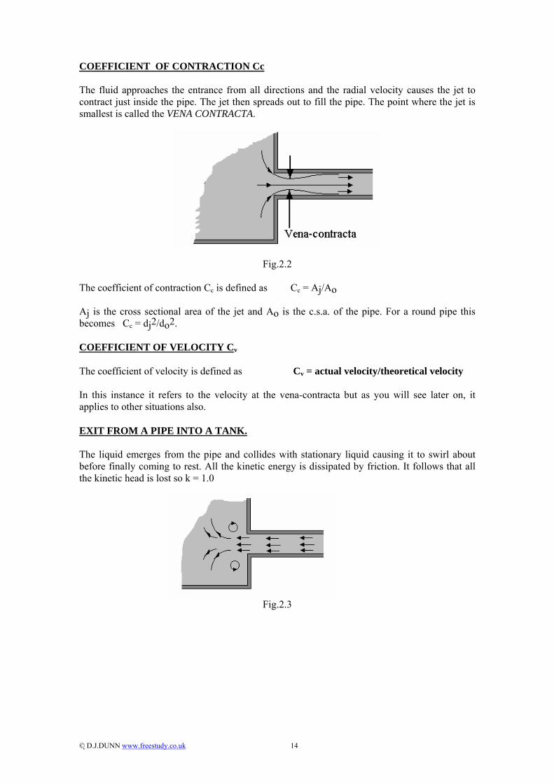
COEFFICIENT OF CONTRACTION Cc The fluid approaches the entrance from all directions and the radial velocity causes the jet to contract just inside the pipe. The jet then spreads out to fill the pipe. The point where the jet is smallest is called the VENA CONTRACTA.
Fig.2.2
The coefficient of contraction Cc is defined as Cc = Aj/Ao Aj is the cross sectional area of the jet and Ao is the c.s.a. of the pipe. For a round pipe this becomes Cc = dj2/do2.
COEFFICIENT OF VELOCITY Cv The coefficient of velocity is defined as Cv = actual velocity/theoretical velocity In this instance it refers to the velocity at the vena-contracta but as you will see later on, it applies to other situations also. EXIT FROM A PIPE INTO A TANK. The liquid emerges from the pipe and collides with stationary liquid causing it to swirl about before finally coming to rest. All the kinetic energy is dissipated by friction. It follows that all the kinetic head is lost so k = 1.0
Fig.2.3

© D.J.DUNN www.freestudy.co.uk 15
ENTRY TO A PIPE FROM A TANK The value of k varies from 0.78 to 0.04 depending on the shape of the inlet. A good rounded inlet has a low value but the case shown is the worst.
Fig.2.4
SUDDEN ENLARGEMENT This is similar to a pipe discharging into a tank but this time it does not collide with static fluid but with slower moving fluid in the large pipe. The resulting loss coefficient is given by the following expression.
22
2
11⎪⎭
⎪⎬⎫
⎪⎩
⎪⎨⎧
⎟⎟⎠
⎞⎜⎜⎝
⎛−=
ddk
Fig.2.5 SUDDEN CONTRACTION This is similar to the entry to a pipe from a tank. The best case gives k = 0 and the worse case is for a sharp corner which gives k = 0.5.
Fig.2.6
BENDS AND FITTINGS The k value for bends depends upon the radius of the bend and the diameter of the pipe. The k value for bends and the other cases is on various data sheets. For fittings, the manufacturer usually gives the k value. Often instead of a k value, the loss is expressed as an equivalent length of straight pipe that is to be added to L in the Darcy formula.

© D.J.DUNN www.freestudy.co.uk 16
WORKED EXAMPLE 6 A tank of water empties by gravity through a horizontal pipe into another tank. There is a sudden enlargement in the pipe as shown. At a certain time, the difference in levels is 3 m. Each pipe is 2 m long and has a friction coefficient Cf = 0.005. The inlet loss constant is K = 0.3. Calculate the volume flow rate at this point.
Fig.2.7

© D.J.DUNN www.freestudy.co.uk 17
SOLUTION There are five different sources of pressure loss in the system and these may be expressed in terms of the fluid resistance as follows. The head loss is made up of five different parts. It is usual to express each as a fraction of the kinetic head as follows.
Resistance pipe A 5262525
A
f1 ms10 x 0328.1
0.02 x g 2 x 0.005 x 32
gDLC32R −=
π=
π=
Resistance in pipe B 5232525
B
f2 ms10x250.4
0.06 x g 2 x 0.005 x 32
gDLC32R −=
π=
π=
Loss at entry K=0.3 52424
A23 ms 158
0.02x πg0.3 x 8
DgK8R −==
π=
Loss at sudden enlargement. 79.060201
dd
1k22
22
B
A =⎪⎭
⎪⎬⎫
⎪⎩
⎪⎨⎧
⎟⎠⎞
⎜⎝⎛−=
⎪⎭
⎪⎬⎫
⎪⎩
⎪⎨⎧
⎟⎟⎠
⎞⎜⎜⎝
⎛−=
52424
A24 ms 407.7
0.02x gπ8x0.79
Dgπ8KR −===
Loss at exit K=1 52424
B25 ms 63710
0.06x gπ8x1
Dgπ8KR −===
Total losses. 26
L
254221L
25
24
23
22
21L
Q10 x 1.101h
)QRRRR(Rh
QRQRQRQRQRh
=
++++=
++++=
BERNOULLI’S EQUATION Apply Bernoulli between the free surfaces (1) and (2)
L
22
22
21
11 hg2
uzhg2
uzh +++=++
On the free surface the velocities are small and about equal and the pressures are both atmospheric so the equation reduces to the following. z1 - z2 = hL = 3 3 = 1.101 x 10⁶ Q2 Q2 = 2.724 x 10⁻⁶ Q = 1.65 x 10⁻³ m3/s

© D.J.DUNN www.freestudy.co.uk 18
2.3 SIPHONS Liquid will siphon from a tank to a lower level even if the pipe connecting them rises above the level of both tanks as shown in the diagram. Calculation will reveal that the pressure at point (2) is lower than atmospheric pressure (a vacuum) and there is a limit to this pressure when the liquid starts to turn into vapour. For water about 8 metres is the practical limit that it can be sucked (8 m water head of vacuum).
Fig.2.8
WORKED EXAMPLE 7 A tank of water empties by gravity through a siphon. The difference in levels is 3 m and the highest point of the siphon is 2 m above the top surface level and the length of pipe from inlet to the highest point is 2.5 m. The pipe has a bore of 25 mm and length 6 m. The friction coefficient for the pipe is 0.007.The inlet loss coefficient K is 0.7. Calculate the volume flow rate and the pressure at the highest point in the pipe. SOLUTION There are three different sources of pressure loss in the system and these may be expressed in terms of the fluid resistance as follows.
Pipe Resistance 5262525
f1 ms 10 x 1.422
π0.025 x g 6 x 0.007 x 32
πgDL32C
R −===
Entry Loss Resistance 52342422 ms 10 x 1.15
0.025x gπ0.7 x 8
DgK8R −==
π=
Exit loss Resistance 52342423 ms 10 x 57.21
0.025x g8x1
DgK8R −=
π=
π=
Total Resistance RT = R1 + R2 + R3 = 1.458 x 10⁶ s2 m-5

© D.J.DUNN www.freestudy.co.uk 19
Apply Bernoulli between the free surfaces (1) and (3)
3hzzh0z00z0
hg2
uzh
g2uzh
L31
L311
L
23
33
21
11
==−+++=++
+++=++
Flow rate s/m10x434.110 x 458.1
3R
zzQ 33
6T
31 −==−
=
Bore Area A=πD2/4 = π x 0.0252/4 = 490.87 x 10⁻⁶ m2 Velocity in Pipe u = Q/A = 1.434 x 10⁻³/490.87 x 10-6 = 2.922 m/s Apply Bernoulli between the free surfaces (1) and (2)
LL2
L
2
L2
L
2
2
L
22
22
21
11
h435.2h0.4352h
h2g
2.922h2h
h2g
2.9222h000
h2guzh
2guzh
−−=−+−=
−−−=
+++=++
+++=++
Calculate the losses between (1) and (2) Pipe friction Resistance is proportionally smaller by the length ratio. R1 = (2.5/6) x1.422 x 106 = 0.593 x 10⁶ Entry Resistance R2 = 15.1 x 10³ as before Total resistance RT = 608.1 x 10³ Head loss hL = RT Q2 = 1.245m The pressure head at point (2) is hence h2 = -2.435 -1.245 = -3.68 m head
© D.J.DUNN www.freestudy.co.uk 20
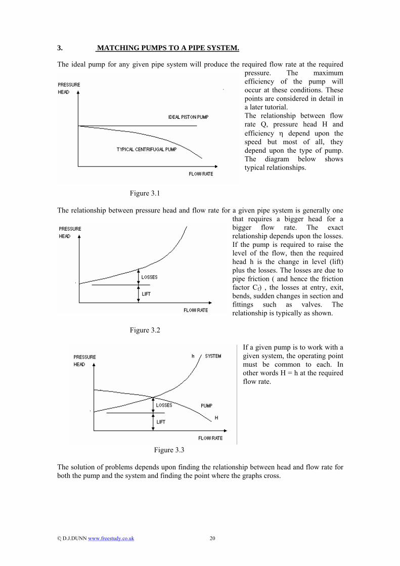
3. MATCHING PUMPS TO A PIPE SYSTEM. The ideal pump for any given pipe system will produce the required flow rate at the required
pressure. The maximum efficiency of the pump will occur at these conditions. These points are considered in detail in a later tutorial. The relationship between flow rate Q, pressure head H and efficiency η depend upon the speed but most of all, they depend upon the type of pump. The diagram below shows typical relationships.
Figure 3.1
The relationship between pressure head and flow rate for a given pipe system is generally one that requires a bigger head for a bigger flow rate. The exact relationship depends upon the losses. If the pump is required to raise the level of the flow, then the required head h is the change in level (lift) plus the losses. The losses are due to pipe friction ( and hence the friction factor Cf) , the losses at entry, exit, bends, sudden changes in section and fittings such as valves. The relationship is typically as shown.
Figure 3.2
If a given pump is to work with a given system, the operating point must be common to each. In other words H = h at the required flow rate.
Figure 3.3
The solution of problems depends upon finding the relationship between head and flow rate for both the pump and the system and finding the point where the graphs cross.
© D.J.DUNN www.freestudy.co.uk 21
SELF ASSESSMENT EXERCISE 2 1. A pipe carries oil at a mean velocity of 6 m/s. The pipe is 5 km long and 1.5 m diameter.
The surface roughness is 0.8 mm. The density is 890 kg/m3 and the dynamic viscosity is 0.014 N s/m2. Determine the friction coefficient from the Moody chart and go on to calculate the friction head hf.
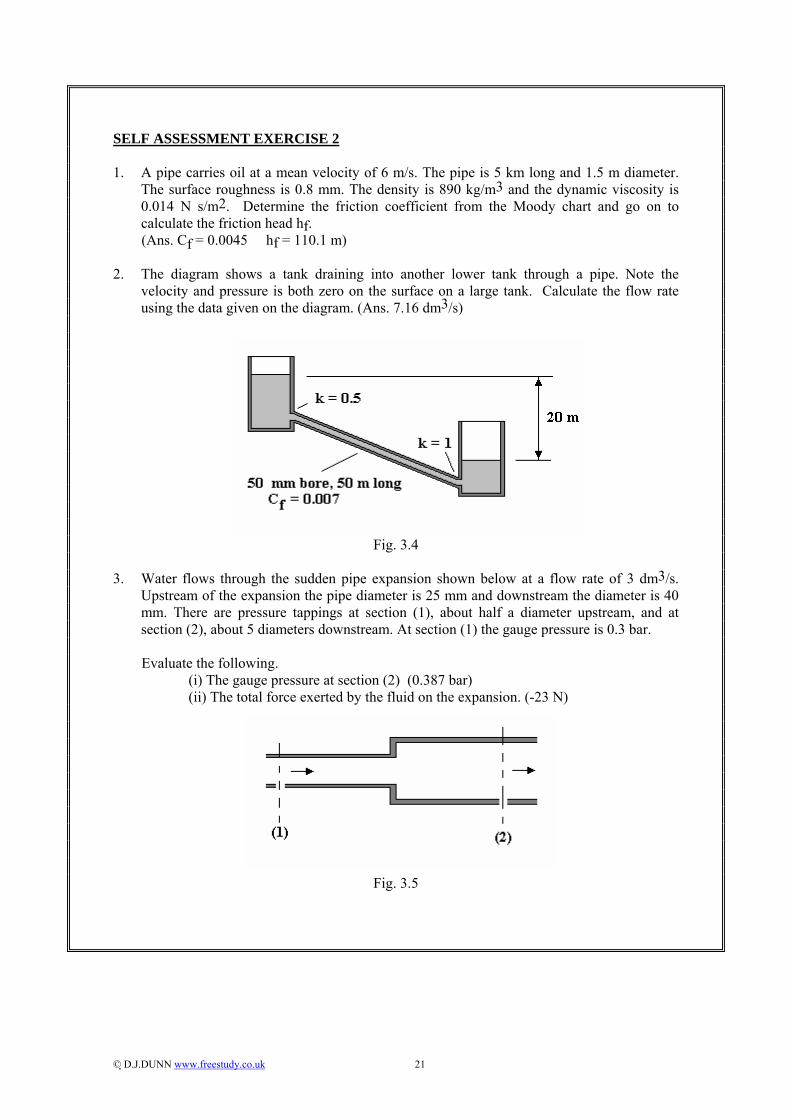
(Ans. Cf = 0.0045 hf = 110.1 m) 2. The diagram shows a tank draining into another lower tank through a pipe. Note the
velocity and pressure is both zero on the surface on a large tank. Calculate the flow rate using the data given on the diagram. (Ans. 7.16 dm3/s)
Fig. 3.4
3. Water flows through the sudden pipe expansion shown below at a flow rate of 3 dm3/s. Upstream of the expansion the pipe diameter is 25 mm and downstream the diameter is 40 mm. There are pressure tappings at section (1), about half a diameter upstream, and at section (2), about 5 diameters downstream. At section (1) the gauge pressure is 0.3 bar.
Evaluate the following. (i) The gauge pressure at section (2) (0.387 bar) (ii) The total force exerted by the fluid on the expansion. (-23 N)
Fig. 3.5

© D.J.DUNN www.freestudy.co.uk 22
4. A tank of water empties by gravity through a siphon into a lower tank. The difference in
levels is 6 m and the highest point of the siphon is 2 m above the top surface level. The length of pipe from the inlet to the highest point is 3 m. The pipe has a bore of 30 mm and length 11 m. The friction coefficient for the pipe is 0.006.The inlet loss coefficient K is 0.6.
Calculate the volume flow rate and the pressure at the highest point in the pipe. (Answers 2.378 dm3/s and –4.31 m) 5. A domestic water supply consists of a large tank with a loss free-inlet to a 10 mm diameter
pipe of length 20 m, that contains 9 right angles bends. The pipe discharges to atmosphere 8.0 m below the free surface level of the water in the tank.
Evaluate the flow rate of water assuming that there is a loss of 0.75 velocity heads in each
bend and that friction in the pipe is given by the Blasius equation Cf=0.079(Re)-0.25 The dynamic viscosity is 0.89 x 10⁻³ and the density is 997 kg/m3. (0.118 dm3/s). 6. A pump A whose characteristics are given in table 1, is used to pump water from
an open tank through 40 m of 70 mm diameter pipe of friction factor Cf=0.005 to another open tank in which the surface level of the water is 5.0 m above that in the supply tank.
Determine the flow rate when the pump is operated at 1450 rev/min. (7.8 dm3/s) It is desired to increase the flow rate and 3 possibilities are under investigation. (i) To install a second identical pump in series with pump A. (ii) To install a second identical pump in parallel with pump A. (iii) To increase the speed of the pump by 10%. Predict the flow rate that would occur in each of these situations.
Head-Flow Characteristics of pump A when operating at 1450 rev/min
Head/m 9.75 8.83 7.73 6.90 5.50 3.83 Flow Rate/(l/s) 4.73 6.22 7.57 8.36 9.55 10.75
Table 1

© D.J.DUNN www.freestudy.co.uk 23
7. A steel pipe of 0.075 m inside diameter and length 120 m is connected to a large
reservoir. Water is discharged to atmosphere through a gate valve at the free end, which is 6 m below the surface level in the reservoir. There are four right angle bends in the pipe line. Find the rate of discharge when the valve is fully open. (ans. 8.3 dm3/s).The kinematic viscosity of the water may be taken to be 1.14 x 10⁻⁶ m2/s. Use a value of the friction factor Cf taken from table 2 which gives Cf as a function of the Reynolds number Re and allow for other losses as follows.
at entry to the pipe 0.5 velocity heads. at each right angle bend 0.9 velocity heads. for a fully open gate valve 0.2 velocity heads. Re x 105 0.987 1.184 1.382 Cf 0.00448 0.00432 0.00419
Table 2
8. (i) Sketch diagrams showing the relationship between Reynolds number, Re, and
friction factor, Cf , for the head lost when oil flows through pipes of varying degrees of roughness. Discuss the importance of the information given in the diagrams when specifying the pipework for a particular system.
(ii) The connection between the supply tank and the suction side of a pump consists
of 0.4 m of horizontal pipe , a gate valve one elbow of equivalent pipe length 0.7 m and a vertical pipe down to the tank.
If the diameter of the pipes is 25 mm and the flow rate is 30 l/min, estimate the
maximum distance at which the supply tank may be placed below the pump inlet in order that the pressure there is no less than 0.8 bar absolute. (Ans. 1.78 m)
The fluid has kinematic viscosity 40x10-6 m2/s and density 870 kg/m3. Assume (a) for laminar flow Cf =16/(Re) and for turbulent flow Cf = 0.08/(Re)0.25. (b) head loss due to friction is 4Cf V2L/2gD and due to fittings is KV2/2g. where K=0.72 for an elbow and K=0.25 for a gate valve. What would be a suitable diameter for the delivery pipe ?

© D.J.DUNN www.freestudy.co.uk 24
4. DIFFERENTIAL PRESSURE DEVICES
Differential pressure devices produce differential pressure as a result of changes in fluid velocity. They have many uses but mainly they are used for flow measurement. In this section you will apply Bernoulli's equation to such devices. You will also briefly examine forces produced by momentum changes. 4.1 GENERAL RELATIONSHIP Many devices make use of the transition of flow energy into kinetic energy. Consider a flow of liquid which is constrained to flow from one sectional area into a smaller sectional area as shown below.
Fig.4.1
The velocity in the smaller bore u2 is given by the continuity equation as u2 = u1A1/A2 Let A1/A2 = r u2 = ru1 In BS1042 the symbol used is m but r is used here to avoid confusion with mass. If we apply Bernoulli (head form) between (1) and (2) and ignoring energy losses we have
g
uzh
gu
zh22
22
22
21
11 ++=++
For a horizontal system z1=z2 so
( ) ( ) ( )( )( )
( )( )1
2/
12
1222
221
111
221
1
221
21
2221
22
2
21
1
−−
===
−−
=
−=−=−
+=+
rhhgAuAQsVol
rhhg
u
ruuuhhgg
uhg
uh
In terms of pressure rather than head we get, by substituting p= ρgh
To find the mass flow remember m = ρAu = ρQ
( )12
21 −∆
=r
pAQρ
© D.J.DUNN www.freestudy.co.uk 25
Because we did not allow for energy loss, we introduce a coefficient of discharge Cd to correct the answer resulting in
( )12
21 −∆
=r
pACQ d ρ
The value of Cd depends upon many factors and is not constant over a wide range of flows. BS1042 should be used to determine suitable values. It will be shown later that if there is a contraction of the jet, the formula needs further modification. For a given device, if we regard Cd as constant then the equation may be reduced to :
Q = K(∆p)0.5 where K is the meter constant. 4.2 MOMENTUM and PRESSURE FORCES Changes in velocities mean changes in momentum and Newton's second law tells us that this is accompanied by a force such that Force = rate of change of momentum. Pressure changes in the fluid must also be considered as these also produce a force. Translated into a form that helps us solve the force produced on devices such as those considered here, we use the equation F = ∆(pA) + m ∆u. When dealing with devices that produce a change in direction, such as pipe bends, this has to be considered more carefully and this is covered in chapter 4. In the case of sudden changes in section, we may apply the formula F = (p1A1 + mu1)- (p2 A2 + mu2) point 1 is upstream and point 2 is downstream.
© D.J.DUNN www.freestudy.co.uk 26
WORKED EXAMPLE 8
A pipe carrying water experiences a sudden reduction in area as shown. The area at point (1) is 0.002 m2 and at point (2) it is 0.001 m2. The pressure at point (2) is 500 kPa and the velocity is 8 m/s. The loss coefficient K is 0.4. The density of water is 1000 kg/m3. Calculate the following. i. The mass flow rate. ii. The pressure at point (1) iii. The force acting on the section.
Fig.4.2
SOLUTION u1 = u2A2/A1 = (8 x 0.001)/0.002 = 4 m/s m = ρA1u1 = 1000 x 0.002 x 4 = 8 kg/s. Q = A1u1 = 0.002 x 4 = 0.008 m3/s Pressure loss at contraction = ½ ρku1
2 = ½ x 1000 x 0.4 x 42 = 3200 Pa Apply Bernoulli between (1) and (2)
kPa 527.2 p
32002
8 x 100010 x 5002
4 x 1000 p
p2up
2up
1
23
2
1
L
22
2
21
1
=
++=+
+ρ
+=ρ
+
F = (p1A1 + mu1)- (p2 A2 + mu2) F = [(527.2 x 103 x 0.002) + (8 x 4)] – [500 x 103 x 0.001) + (8 x 8)] F = 1054.4 +32 – 500 – 64 F = 522.4 N
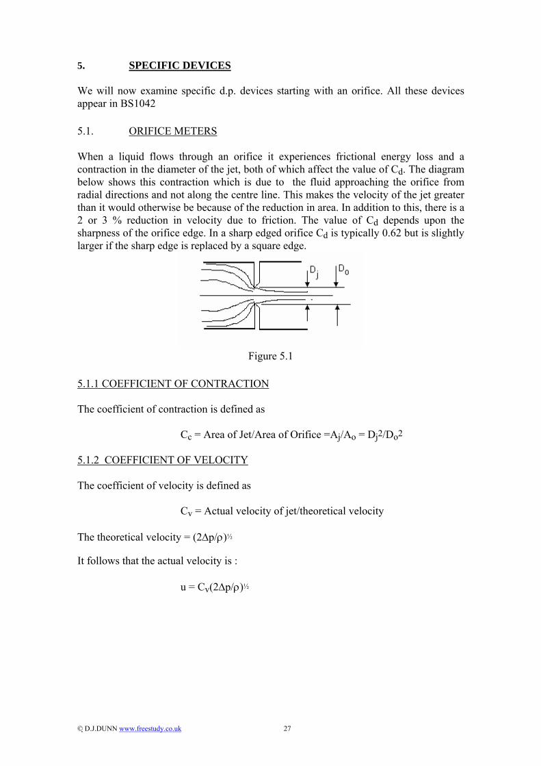
© D.J.DUNN www.freestudy.co.uk 27
5. SPECIFIC DEVICES We will now examine specific d.p. devices starting with an orifice. All these devices appear in BS1042 5.1. ORIFICE METERS When a liquid flows through an orifice it experiences frictional energy loss and a contraction in the diameter of the jet, both of which affect the value of Cd. The diagram below shows this contraction which is due to the fluid approaching the orifice from radial directions and not along the centre line. This makes the velocity of the jet greater than it would otherwise be because of the reduction in area. In addition to this, there is a 2 or 3 % reduction in velocity due to friction. The value of Cd depends upon the sharpness of the orifice edge. In a sharp edged orifice Cd is typically 0.62 but is slightly larger if the sharp edge is replaced by a square edge.
Figure 5.1
5.1.1 COEFFICIENT OF CONTRACTION The coefficient of contraction is defined as Cc = Area of Jet/Area of Orifice =Aj/Ao = Dj2/Do2 5.1.2 COEFFICIENT OF VELOCITY The coefficient of velocity is defined as Cv = Actual velocity of jet/theoretical velocity The theoretical velocity = (2∆p/ρ)½
It follows that the actual velocity is : u = Cv(2∆p/ρ)½
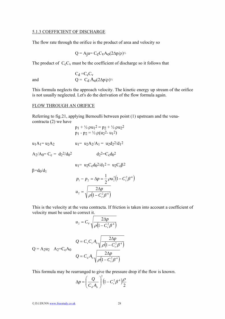
© D.J.DUNN www.freestudy.co.uk 28
5.1.3 COEFFICIENT OF DISCHARGE The flow rate through the orifice is the product of area and velocity so Q = Aju= CcCvAo(2∆p/ρ)½ The product of CcCv must be the coefficient of discharge so it follows that Cd =CcCv and Q = Cd Ao(2∆p/ρ)½
This formula neglects the approach velocity. The kinetic energy up stream of the orifice is not usually neglected. Let's do the derivation of the flow formula again. FLOW THROUGH AN ORIFICE Referring to fig.21, applying Bernoulli between point (1) upstream and the vena-contracta (2) we have p1 + ½ ρu12 = p2 + ½ ρu22 p1 - p2 = ½ ρ( u22- u12) u1A1= u2A2 u1= u2A2/A1 = u2d22/d12 A2/A0= Cc = d22/d02 d22=Ccd02 u1= u2Ccd02/d12 = u2Ccβ2 β=d0/d1
( )422221 1
21 βρ cCuppp −=∆=−
( )422 12
βρ cCpu
−∆
=
This is the velocity at the vena contracta. If friction is taken into account a coefficient of velocity must be used to correct it.
( )422 12
βρ cV C
pCu−∆
=
Q = A2u2 A2=CcA0 ( )
( )42
42
12
12
βρ
βρ
cod
cocv
CpACQ
CpACCQ
−∆
=
−∆
=
This formula may be rearranged to give the pressure drop if the flow is known.
( )2
1 422
ρβcod
CAC
Qp −⎟⎟⎠
⎞⎜⎜⎝
⎛=∆

© D.J.DUNN www.freestudy.co.uk 29
The pressure tapping points are normally placed at one pipe diameter upstream and one half pipe diameter downstream in order to get the maximum d.p. However if the maximum value is not important, the d.p. is more easily obtained by the use of corner or flange tappings. The results are still valid but less d.p. is obtained.
Fig.5.2 showing tapping positions
Figure 5.2 shows how the flow after the orifice must expand to the full bore of the pipe. The velocity in the full bore is less than the jet so the jet must be slowed down. It can only do this by colliding with the slower moving fluid downstream and consequently there is a lot of friction and energy loss in the turbulent mixing taking place. The result is that only a small amount of kinetic energy is reconverted into pressure downstream and the overall pressure loss for the system is high. The loss from the vena contracta (2) to the point downstream where the flow has settled (3) is the loss due to sudden expansion covered earlier and is given by pressure loss due to expansion = ½ ρ(u2 -u3)2 Further pressure losses are produced by skin friction and could be estimated. The problem is that the mean velocity is uncertain in the areas near the orifice so it is difficult to apply Darcy's formula. Figure 5.3 shows the way that pressure changes on approach to and departure from the orifice.
Figure 5.3

© D.J.DUNN www.freestudy.co.uk 30
WORKED EXAMPLE No.9 The figure shows a sharp edged orifice plate of diameter 20 mm in a horizontal pipe of diameter 25 mm. There are three pressure tappings as follows. (1) at about 3 pipe diameters upstream of the orifice plate. (2) at half a pipe diameter downstream of the orifice plate and (3) at about 5 pipe diameters downstream of the orifice plate. The tappings read pressures p1, p2 and p3 respectively. If there is a flow rate of 0.8 x 10⁻³ m3/s of water at 25oC, evaluate the pressure differences p1-p2 and p1-p3. Calculate the % of pressure recovered downstream of the orifice. It may be assumed that the discharge coefficient is 0.64 and the contraction coefficient is 0.74. The density and viscosity for water are usually given on the front of the exam paper. The density is 998 kg/m3.
Fig.5.4
SOLUTION First the pressure drop from 1 to 2. There is friction in the jet so the formula to be used is ∆p = (Q/CdA0)2(1 - Cc2β4)ρ/2 A0= p x 0.022/4 = 0.0003142 m2 b = 20/25=0.8 ∆p = {0.0008/(0.64x 0.0003142)2}(1 - 0.742x0.84)998/2 ∆p =p1-p2 = 6.126 kPa This includes the pressure loss due to friction in the jet as well as due to the change in velocity. u1 = u3 = 0.0008/(px0.0252/4 ) =1.63 m/s A2=Cc x p x 0.022/4 =0.000232 m2 u2 = 0.0008/0.000232 = 3.44 m/s loss due to sudden expansion = ρ(u2 -u3)2/2 = 998(3.44 - 1.63)2/2 = 1.63 kPa Now we must find the pressure loss due to friction in the jet. Ideal jet velocity = u2/Cv Cv= Cd/Cc = 0.64/0.74 = 0.865

© D.J.DUNN www.freestudy.co.uk 31
Ideal jet velocity = 3.44/0.865 = 3.98 m/s Loss of kinetic energy as pressure = (ρ/2)(3.982 -3.442) = 1.99 kPa p1 + ρu12/2 = p3 + ρu32/2 p1 - p3 = (ρ/2)(u32-u12) + losses u3 = u3 p1 - p3 = losses = 1.63 kPa + 1.99 kPa = 3.62 kPa The pressure regained downstream = 6.126 - 3.62 = 2.5 kPa The diffuser efficiency = 2.5/6.126 = 41% 5.2. VENTURI METERS The Venturi Meter is designed to taper down to the throat gradually and then taper out again. No contraction occurs in the flow so Cc = 1. The outlet (diffuser) is designed to expand the flow gradually so that the kinetic energy at the throat is reconverted into pressure with little friction. Consequently the coefficient of discharge is much better than for an orifice meter. The overall pressure loss is much better than for an orifice meter.
Fig.5.5 showing pressure distribution
If there is no vena-contracta then the flow rate is given by the formula
( )12
21 −∆
=r
pACQ d ρ
and Cd = Cv and is about 0.97 for a good meter. The draw back of the Venturi is the expense involved in the design. The pressure tappings have special inserts in the bore to gather the pressure from around the circumference.

© D.J.DUNN www.freestudy.co.uk 32
5.3 NOZZLE METER The nozzle meter is a compromise between the orifice and the venturi. It may be easily fitted in a pipe between flanges with flange or corner tappings. There is no contraction of the jet but there is little pressure recovery downstream. The loss due to sudden expansion occurs down stream. The flow formula is the same as before.
Fig.5.6 Nozzle Meter
WORKED EXAMPLE No.10 A nozzle is 100 mm diameter at inlet and 20 mm diameter at outlet. The coefficient
of velocity is 0.97 and there is no contraction of the jet. The jet discharges into the atmosphere. The static pressure at inlet is 300 kPa gauge. The density is 1000 kg/m3.
Calculate: a. the velocity at exit. b. the flow rate. c. the pressure loss due to friction expressed as a fraction of the dynamic pressure at
outlet. d. the force on the nozzle.

© D.J.DUNN www.freestudy.co.uk 33
SOLUTION The velocity at exit when the inlet velocity is not negligible is Q = A1Cd[(2∆p/ρ)/(r2 - 1)]0.5 r = A1/A2 = d12/d22 = (100/20)2 = 25 Cd = Cv Cc = 0.97 x 1 = 0.97 A1 = (p x 0.12)/4 = 0.00785 m2 hence Q = 0.97x 0.00785 [(2 x 300 x 103/1000)/(252 - 1)]0.5 Q = 0.00747 m3/s The velocity at inlet = Q/A1 = 0.00747/0.00785 = 0.951 m/s The velocity at outlet = Q/A2 = 0.00747 x 4/(p x 0.022)= 23.8 m/s The dynamic pressure of the jet is ρu22/2 = 1000 x 23.8 2/2 = 282.7 kPa. Applying Bernoulli between the inlet (1) and outlet (2) using the pressure form we
have p1 - p2 = ρu22/2 - ρu12/2 + pressure loss to friction 3 x 105 = (1000/2)(23.82 - 0.9512) + pressure loss 3 x 105 = 2.827 x 10⁵ + pressure loss pressure loss = 17.3 kPa Expressed as a fraction of the dynamic pressure of the jet this is 17.3/ 282.7 or
6.1%. The force exerted on the water is given by F = p1A1 + - p2 A2 + mu1 - mu2 We must use gauge pressures to solve this problem because the atmosphere acts on
the outer surface of the nozzle. The mass flow is 7.47 kg/s. F = 300 x 103 x 0.00785 - 0 + 7.47(0.951 - 23.8) = 2.18 kN The figure is positive which indicates the force is accelerating the water out of the
nozzle. The force on the nozzle is the reaction to this and is opposite in direction. Think of a fireman's hose. The force on the nozzle pushes it away from the water like a rocket. The force to accelerate the water must be supplied by those holding it.
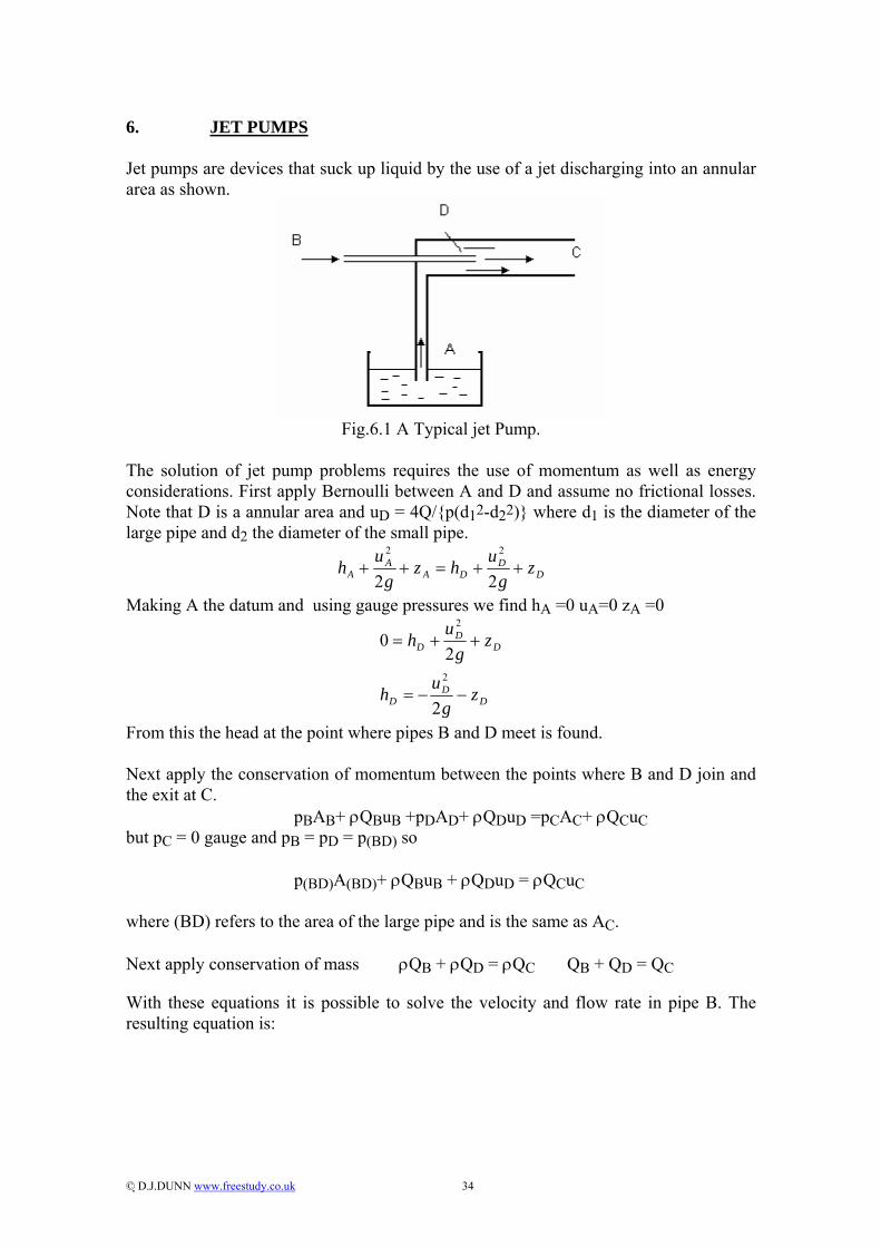
© D.J.DUNN www.freestudy.co.uk 34
6. JET PUMPS Jet pumps are devices that suck up liquid by the use of a jet discharging into an annular area as shown.
Fig.6.1 A Typical jet Pump.
The solution of jet pump problems requires the use of momentum as well as energy considerations. First apply Bernoulli between A and D and assume no frictional losses. Note that D is a annular area and uD = 4Q/{p(d12-d22)} where d1 is the diameter of the large pipe and d2 the diameter of the small pipe.
DD
DAA
A zg
uhzg
uh ++=++22
22
Making A the datum and using gauge pressures we find hA =0 uA=0 zA =0
DD
D
DD
D
zg
uh
zg
uh
−−=
++=
2
20
2
2
From this the head at the point where pipes B and D meet is found. Next apply the conservation of momentum between the points where B and D join and the exit at C. pBAB+ ρQBuB +pDAD+ ρQDuD =pCAC+ ρQCuC but pC = 0 gauge and pB = pD = p(BD) so p(BD)A(BD)+ ρQBuB + ρQDuD = ρQCuC where (BD) refers to the area of the large pipe and is the same as AC. Next apply conservation of mass ρQB + ρQD = ρQC QB + QD = QC With these equations it is possible to solve the velocity and flow rate in pipe B. The resulting equation is:

© D.J.DUNN www.freestudy.co.uk 35
2a4acbbQ
henceequation w quadratic a is This 0cbQaQ
0A1
A1Q
ρAp
AQ2Q
A1
A1Q
2
B
B2B
CD
2D
CB
C
DB
CB
2B
−±−=
=++
=⎭⎬⎫
⎩⎨⎧
−++−⎭⎬⎫
⎩⎨⎧
−

© D.J.DUNN www.freestudy.co.uk 36
SELF ASSESSMENT EXERCISE 3 Take the density of water to be 997 kg/m3 throughout unless otherwise stated. 1. A Venturi meter is 50 mm bore diameter at inlet and 10 mm bore diameter at the
throat. Oil of density 900 kg/m3 flows through it and a differential pressure head of 80 mm is produced. Given Cd = 0.92, determine the flow rate in kg/s.
(ans. 0.0815 kg/s). 2. A Venturi meter is 60 mm bore diameter at inlet and 20 mm bore diameter at the
throat. Water of density 1000 kg/m3 flows through it and a differential pressure head of 150 mm is produced. Given Cd = 0.95, determine the flow rate in dm3/s.
(ans. 0.515 dm3/s). 3. Calculate the differential pressure expected from a Venturi meter when the flow
rate is 2 dm3/s of water. The area ratio is 4 and Cd is 0.94. The inlet c.s.a. is 900 mm2. (ans. 41.916 kPa).
4. Calculate the mass flow rate of water through a Venturi meter when the differential
pressure is 980 Pa given Cd = 0.93, the area ratio is 5 and the inlet c.s.a. is 1000 mm2. (ans. 0.266 kg/s).
5. Calculate the flow rate of water through an orifice meter with an area ratio of 4
given Cd is 0.62, the pipe area is 900 mm2 and the d.p. is 586 Pa. (ans. 0.156 dm3/3).
6. Water flows at a mass flow rate 0f 0.8 kg/s through a pipe of diameter 30 mm fitted
with a 15 mm diameter .sharp edged orifice. There are pressure tappings (a) 60 mm upstream of the orifice, (b) 15 mm
downstream of the orifice and (c) 150 mm downstream of the orifice, recording pressure pa, pb and pc respectively. Assuming a contraction coefficient 0f 0.68, evaluate
(i) the pressure difference (pa - pb) and hence the discharge coefficient. (21.6 kPa, 0.67) (ii)the pressure difference (pb - pc) and hence the diffuser efficiency. (-6.4 kPa, 29.5%) (iii) the net force on the orifice plate. (10.8 N) State any assumption made in your analysis.

© D.J.DUNN www.freestudy.co.uk 37
7. The figure shows an ejector (or jet pump) which extracts 2 x 10⁻³ m3/s of water from tank A which is situated 2.0 m below the centre-line of the ejector. The diameter of the outer pipe of the ejector is 40 mm and water is supplied from a reservoir to the thin-walled inner pipe which is of diameter 20 mm. The ejector discharges to atmosphere at section C.
Evaluate the pressure p at section D, just downstream of the end of pipe B, the
velocity in pipe B and the required height of the free water level in the reservoir supplying pipe B. (-21.8 kPa gauge, 12.922 m/s, 6.28 m).
It may be assumed that both supply pipes are loss free.
Figure 6.2
8. Discuss the use of orifice plates and venturi-meters for the measurement of flow
rates in pipes. Water flows with a mean velocity of 0.6 m/s in a 50 mm diameter pipe fitted with a
sharp edged orifice of diameter 30 mm. Assuming the contraction coefficient is 0.64, find the pressure difference between tappings at the vena contracta and a few diameters upstream of the orifice, and hence evaluate the discharge coefficient.
Estimate also the overall pressure loss caused by the orifice plate. It may be assumed that there is no loss of energy upstream of the vena contracta. 9. Fig.28 shows an ejector pump BDC designed to lift 2 x 10⁻³ m3/s of water from an
open tank A, 3.0 m below the level of the centre-line of the pump. The pump discharges to atmosphere at C.
The diameter of thin-walled inner pipe 12 mm and the internal diameter of the outer
pipe of the is 25 mm. Assuming that there is no energy loss in pipe AD and there is no shear stress on the wall of pipe DC, calculate the pressure at point D and the required velocity of the water in pipe BD.
(-43.3 kPa and 20.947 m/s) Derive all the equations used and state your assumptions.

1
FLUID MECHANICS
TUTORIAL No. 3
BOUNDARY LAYER THEORY In order to complete this tutorial you should already have completed tutorial 1 and 2 in this series. This tutorial examines boundary layer theory in some depth. When you have completed this tutorial, you should be able to do the following.
Discuss the drag on bluff objects including long cylinders and spheres.
Explain skin drag and form drag.
Discuss the formation of wakes.
Explain the concept of momentum thickness and displacement thickness.
Solve problems involving laminar and turbulent boundary layers.
Throughout there are worked examples, assignments and typical exam questions. You should complete each assignment in order so that you progress from one level of knowledge to another. Let us start by examining how drag is created on objects.

2
1. DRAG When a fluid flows around the outside of a body, it produces a force that tends to drag the body in the direction of the flow. The drag acting on a moving object such as a ship or an aeroplane must be overcome by the propulsion system. Drag takes two forms, skin friction drag and form drag. 1.1 SKIN FRICTION DRAG
Skin friction drag is due to the viscous shearing that takes place between the surface and the layer of fluid immediately above it. This occurs on surfaces of objects that are long in the direction of flow compared to their height. Such bodies are called STREAMLINED. When a fluid flows over a solid surface, the layer next to the surface may become attached to it (it wets the surface). This is called the ‘no slip condition’. The layers of fluid above the surface are moving so there must be shearing taking place between the layers of the fluid. The shear stress acting between the wall and the first moving layer next to it is called the wall shear stress and denoted τw.
The result is that the velocity of the fluid u increases with height y. The boundary layer thickness δ is taken as the distance required for the velocity to reach 99% of uo. This layer is called the BOUNDARY LAYER and δ is the boundary layer thickness. Fig. 1.1 Shows how the velocity "u" varies with height "y" for a typical boundary layer.
Fig.1.1
In a pipe, this is the only form of drag and it results in a pressure and energy lost along the length. A thin flat plate is an example of a streamlined object. Consider a stream of fluid flowing with a uniform velocity uo. When the stream is interrupted by the plate (fig. 1.2), the boundary layer forms on both sides. The diagram shows what happens on one side only.
Fig. 1.2
The boundary layer thickness δ grows with distance from the leading edge. At some distance from the leading edge, it reaches a constant thickness. It is then called a FULLY DEVELOPED BOUNDARY LAYER.

3
The Reynolds number for these cases is defined as: µ
ρ=
xu)R( o
xe
x is the distance from the leading edge. At low Reynolds numbers, the boundary layer may be laminar throughout the entire thickness. At higher Reynolds numbers, it is turbulent. This means that at some distance from the leading edge the flow within the boundary layer becomes turbulent. A turbulent boundary layer is very unsteady and the streamlines do not remain parallel. The boundary layer shape represents an average of the velocity at any height. There is a region between the laminar and turbulent section where transition takes place The turbulent boundary layer exists on top of a thin laminar layer called the LAMINAR SUB LAYER. The velocity gradient within this layer is linear as shown. A deeper analysis would reveal that for long surfaces, the boundary layer is turbulent over most of the length. Many equations have been developed to describe the shape of the laminar and turbulent boundary layers and these may be used to estimate the skin friction drag. Note that for this ideal example, it is assumed that the velocity is the undisturbed velocity uo everywhere outside the boundary layer and that there is no acceleration and hence no change in the static pressure acting on the surface. There is hence no drag force due to pressure changes. CALCULATING SKIN DRAG The skin drag is due to the wall shear stress τw and this acts on the surface area (wetted area). The drag force is hence: R = τw x wetted area. The dynamic pressure is the pressure resulting from the conversion of the kinetic energy of the stream into pressure and is defined by the
expression 2u 2
oρ.The drag coefficient is defined as
u2
area x wetteduR2C
area d x wettepressure dynamicforce DragC
20
w20
Df
Df
ρ
τ=
ρ=
=
Note that this is the same definition for the pipe friction coefficient Cf and it is in fact the same thing. It is used in the Darcy formula to calculate the pressure lost in pipes due to friction. For a smooth surface, it can be shown that CDf = 0.074 (Re)x
-1/5
(Re)x is the Reynolds number based on the length. µ
ρ=
Lu)R( o
xe

4
WORKED EXAMPLE 1.1 Calculate the drag force on each side of a thin smooth plate 2 m long and 1 m wide with the length parallel to a flow of fluid moving at 30 m/s. The density of the fluid is 800 kg/m3 and the dynamic viscosity is 8 cP. SOLUTION
N 2347.2 1 x 2 x 1173.6 Area x Wetted RPa 1173.6 10 x 360 x 0.00326 pressure dynamic x C
kPa 360 2
30 x 800 2u
pressure Dynamic
0.00326 ) x10(6 x 0.074 C
10 x 6 0.008
2 x 30 x 800 Lu
)R(
w
3Dfw
220
51
6Df
6oxe
==τ====τ
==ρ
=
==
==µ
ρ=
−
On a small area the drag is dR = τw dA. If the body is not a thin plate and has an area inclined at an angle θ to the flow direction, the drag force in the direction of flow is τw dA cosθ.
Fig.1.3 The drag force acting on the entire surface area is found by integrating over the entire area.
∫ θτ= dA cosR w
Solving this equation requires more advanced studies concerning the boundary layer and students should refer to the classic textbooks on this subject.
SELF ASSESSMENT EXERCISE No. 1
1. A smooth thin plate 5 m long and 1 m wide is placed in an air stream moving at 3 m/s with its length parallel with the flow. Calculate the drag force on each side of the plate. The density of the air is 1.2 kg/m3 and the kinematic viscosity is 1.6 x 10⁻⁵ m2/s.
(0.128 N)
2. A pipe bore diameter D and length L has fully developed laminar flow throughout the entire length with a centre line velocity uo. Given that the drag coefficient is given as
CDf = 16/Re where µ
ρ=
DuRe o , show that the drag force on the inside of the pipe is
given as R=8πµuoL and hence the pressure loss in the pipe due to skin friction is pL = 32µuoL/D2

5
1.2 FORM DRAG and WAKES Form or pressure drag applies to bodies that are tall in comparison to the length in the direction of flow. Such bodies are called BLUFF BODIES. Consider the case below that could for example, be the pier of a bridge in a river. The water speeds up around the leading edges and the boundary layer quickly breaks away from the surface. Water is sucked in from behind the pier in the opposite direction. The total effect is to produce eddy currents or whirl pools that are shed in the wake. There is a build up of positive pressure on the front and a negative pressure at the back. The pressure force resulting is the form drag. When the breakaway or separation point is at the front corner, the drag is almost entirely due to this effect but if the separation point moves along the side towards the back, then a boundary layer forms and skin friction drag is also produced. In reality, the drag is always a combination of skin friction and form drag. The degree of each depends upon the shape of the body.
Fig.1.4 The next diagram typifies what happens when fluid flows around a bluff object. The fluid speeds up around the front edge. Remember that the closer the streamlines, the faster the velocity. The line representing the maximum velocity is shown but also remember that this is the maximum at any point and this maximum value also increases as the stream lines get closer together.
Fig.1.5

6
Two important effects affect the drag. Outside the boundary layer, the velocity increases up to point 2 so the pressure acting on the surface goes down. The boundary layer thickness δ gets smaller until at point S it is reduced to zero and the flow separates from the surface. At point 3, the pressure is negative. This change in pressure is responsible for the form drag. Inside the boundary layer, the velocity is reduced from umax to zero and skin friction drag results.
Fig.1.6
In problems involving liquids with a free surface, a negative pressure shows up as a drop in level and the pressure build up on the front shows as a rise in level. If the object is totally immersed, the pressure on the front rises and a vacuum is formed at the back. This results in a pressure force opposing movement (form drag). The swirling flow forms vortices and the wake is an area of great turbulence behind the object that takes some distance to settle down and revert to the normal flow condition. Here is an outline of the mathematical approach needed to solve the form drag. Form drag is due to pressure changes only. The drag coefficient due to pressure only is denoted CDp and defined as
area projected x uR2C
area projected x pressure dynamicforce DragC
20
Dp
Dp
ρ=
=
The projected area is the area of the outline of the shape projected at right angles to the flow. The pressure acting at any point on the surface is p. The force exerted by the pressure on a small surface area is p dA. If the surface is inclined at an angle θ to the general direction of flow, the force is p cosθ dA. The total force is found by integrating all over the surface.
∫ θ= dA cospR
The pressure distribution over the surface is often expressed in the form of a pressure coefficient defined as follows.
2o
op u
)p - p(2C
ρ=
po is the static pressure of the undisturbed fluid, uo is the velocity of the undisturbed fluid and
2u 2
oρis the dynamic pressure of the stream.

7
Consider any streamline that is affected by the surface. Applying Bernoulli between an undisturbed point and another point on the surface, we have the following.
2o
2
2o
22o
2o
22o
2o
op
22oo
22o
0
uu1
u)u - (u
ρu
)u - (u2ρ2
ρu)p - 2(p
C
)u - (u2ρ p - p
2ρu
p 2ρu
p
−==
==
=
+=+
In order to calculate the drag force, further knowledge about the velocity distribution over the object would be needed and students are again recommended to study the classic textbooks on this subject. The equation shows that if u<uo then the pressure is positive and if u>uo the pressure is negative. 1.3 TOTAL DRAG It has been explained that a body usually experiences both skin friction drag and form drag. The total drag is the sum of both. This applies to aeroplanes and ships as well as bluff objects such as cylinders and spheres. The drag force on a body is very hard to predict by purely theoretical methods. Much of the data about drag forces is based on experimental data and the concept of a drag coefficient is widely used. The DRAG COEFFICIENT is denoted CD and is defined by the following expression.
Area projected x pressure Dynamicforce ResistanceCD =
Area projected x ρu2RC 2
oD =

8
WORKED EXAMPLE 1.2 A cylinder 80 mm diameter and 200 mm long is placed in a stream of fluid flowing at
0.5 m/s. The axis of the cylinder is normal to the direction of flow. The density of the fluid is 800 kg/m3. The drag force is measured and found to be 30 N.
Calculate the drag coefficient. At a point on the surface the pressure is measured as 96 Pa above the ambient level. Calculate the velocity at this point. SOLUTION Projected area = 0.08 x 0.2 =0.016 m2 R = 30 N uo = 0.5 m/s ρ = 800 kg/m3 dynamic pressure = ρuo
2/2 = 800 x 0.52/2 = 100 Pa
75.18
0.016 x 10030
Area projected x pressure Dynamicforce ResistanceCD ===
m/s 1.0u0.01u
u - 0.25 0.24
)u (0.5 800
2 x 96
)u (0.52
800 96
)u - (u2ρ p - p
2
2
22
22
22oo
==
=
−=
−=
=

9
1.4 APPLICATION TO A CYLINDER
The drag coefficient is defined as : Area projected x ρu
2RC 2o
D = The projected Area is LD
where L is the length and D the diameter. The drag around long cylinders is more predictable than for short cylinders and the following applies to long cylinders. Much research has been
carried out into the relationship between drag and Reynolds number. µ
ρ=
duRe o and d is the
diameter of the cylinder. At very small velocities, (Re <0.5) the fluid sticks to the cylinder all the way round and never separates from the cylinder. This produces a streamline pattern similar to that of an ideal fluid. The drag coefficient is at its highest and is mainly due to skin friction. The pressure distribution shows that the dynamic pressure is achieved at the front stagnation point and vacuum equal to three dynamic pressures exists at the top and bottom where the velocity is at its greatest.
Fig.1.7
As the velocity increases the boundary layer breaks away and eddies are formed behind. The drag becomes increasingly due to the pressure build up at the front and pressure drop at the back.
Fig.1.8

10
Further increases in the velocity cause the eddies to elongate and the drag coefficient becomes nearly constant. The pressure distribution shows that ambient pressure exists at the rear of the cylinder.
Fig.1.9
At a Reynolds number of around 90 the vortices break away alternatively from the top and bottom of the cylinder producing a vortex street in the wake. The pressure distribution shows a vacuum at the rear.
Fig.1.10
Up to a Reynolds number of about 2 x 10⁵, the drag coefficient is constant with a value of approximately 1. The drag is now almost entirely due to pressure. Up to this velocity, the boundary layer has remained laminar but at higher velocities, flow within the boundary layer becomes turbulent. The point of separation moves back producing a narrow wake and a pronounced drop in the drag coefficient. When the wake contains vortices shed alternately from the top and bottom, they produce alternating forces on the structure. If the structure resonates with the frequency of the vortex shedding, it may oscillate and produce catastrophic damage. This is a problem with tall chimneys and suspension bridges. The vortex shedding may produce audible sound. Fig. 1.12 shows an approximate relationship between CD and Re for a cylinder and a sphere.

11
SELF ASSESSMENT EXERCISE No. 2 1. Calculate the drag force for a cylindrical chimney 0.9 m diameter and 50 m tall in a wind
blowing at 30 m/s given that the drag coefficient is 0.8. The density of the air is 1.2 kg/m3. (19.44 N) 2 Using the graph (fig.1.12) to find the drag coefficient, determine the drag force per metre
length acting on an overhead power line 30 mm diameter when the wind blows at 8 m/s. The density of air may be taken as 1.25 kg/m3 and the kinematic viscosity as 1.5 x 10⁻⁵ m2/s. (1.8 N).
1.5 APPLICATION TO SPHERES The relationship between drag and Reynolds number is roughly the same as for a cylinder but
it is more predictable. The Reynolds number is µ
ρ=
duRe o where d is the diameter of the
sphere. The projected area of a sphere of diameter d is ¼ πd2. In this case, the expression for
the drag coefficient is as follows. 22D d x ρu8RCπ
=.
At very small Reynolds numbers (less than 0.2) the flow stays attached to the sphere all the way around and this is called Stokes flow. The drag is at its highest in this region. As the velocity increases, the boundary layer separates at the rear stagnation point and moves forward. A toroidal vortex is formed. For 0.2<Re<500 the flow is called Allen flow.
Fig.1.11
The breakaway or separation point reaches a stable position approximately 80o from the front stagnation point and this happens when Re is about 1000. For 500<Re the flow is called Newton flow. The drag coefficient remains constant at about 0.4. Depending on various factors, when Re reaches 105 or larger, the boundary layer becomes totally turbulent and the separation point moves back again forming a smaller wake and a sudden drop in the drag coefficient to about 0.3. There are two empirical formulae in common use.
For 0.2 < Re < 105 4.0R1
6R24C
eeD +
++=

12
For Re <1000 [ ]687.0Re15.0124+=
eD R
C
Fig. 1.12 shows this approximate relationship between CD and Re.
Fig.1.12
WORKED EXAMPLE 1.3
A sphere diameter 40 mm moves through a fluid of density 750 kg/m3 and dynamic
viscosity 50 cP with a velocity of 0.6 m/s. Note 1 cP = 0.001 Ns/m2.
Calculate the drag on the sphere.
Use the graph to obtain the drag coefficient.
SOLUTION
N 0.136 2
10 x 1.2566 x0.6 x 750 x 0.8 2
A ρuC R
m10 x 1.2566 4
0.04 4
d area Projected Area projected x ρu
2RC
0.8Cgraph thefrom
360 0.05
0.04 x 0.6 x 750µρudRe
3-22D
23-22
2D
D
===
=π=π==
=
===

13
1.6 TERMINAL VELOCITY When a body falls under the action of gravity, a point is reached, where the drag force is equal and opposite to the force of gravity. When this condition is reached, the body stops accelerating and the terminal velocity reached. Small particles settling in a liquid are usually modelled as small spheres and the preceding work may be used to calculate the terminal velocity of small bodies settling in a liquid. A good application of this is the falling sphere viscometer described in earlier work. For a body immersed in a liquid, the buoyant weight is W and this is equal to the viscous resistance R when the terminal velocity is reached.
R = W = volume x gravity x density difference ( )
6gd fs
3 ρ−ρπ=
ρs = density of the sphere material ρf = density of fluid d = sphere diameter STOKES’ FLOW For Re<0.2 the flow is called Stokes flow and Stokes showed that R = 3πdµut For a falling sphere viscometer, Stokes flow applies. Equating the drag force and the buoyant weight we get
( )
( )t
fs2
fs3
t
u18gd
6gd
ud3
ρ−ρ=µ
ρ−ρπ=µπ
The terminal velocity for Stokes flow is ( )
µρ−ρ
=18
gdu fs
2
t
This formula assumes a fluid of infinite width but in a falling sphere viscometer, the liquid is squeezed between the sphere and the tube walls and additional viscous resistance is produced. The Faxen correction factor F is used to correct the result. WORKED EXAMPLE 1.4 The terminal velocity of a steel sphere falling in a liquid is 0.03 m/s. The sphere is 1 mm
diameter and the density of the steel is 7830 kg/m3. The density of the liquid is 800 kg/m3. Calculate the dynamic and kinematic viscosity of the liquid.
SOLUTION Assuming Stokes’ flow the viscosity is found from the following equation.
( )
cSt 159.6 s/m 0001596.08001277.0
cP 7.127Ns/m 0.1277 0.03 x 18
800) - (7830 x 9.81 x 001.0u18
gd
2
s
22
t
fs2
===ρµ
=ν
===ρ−ρ
=µ
Check the Reynolds number. 0.188 0.0547
0.001 x 0.03 x 800udR f
e ==µ
ρ=
As this is smaller than 0.2 the assumption of Stokes’ flow is correct.
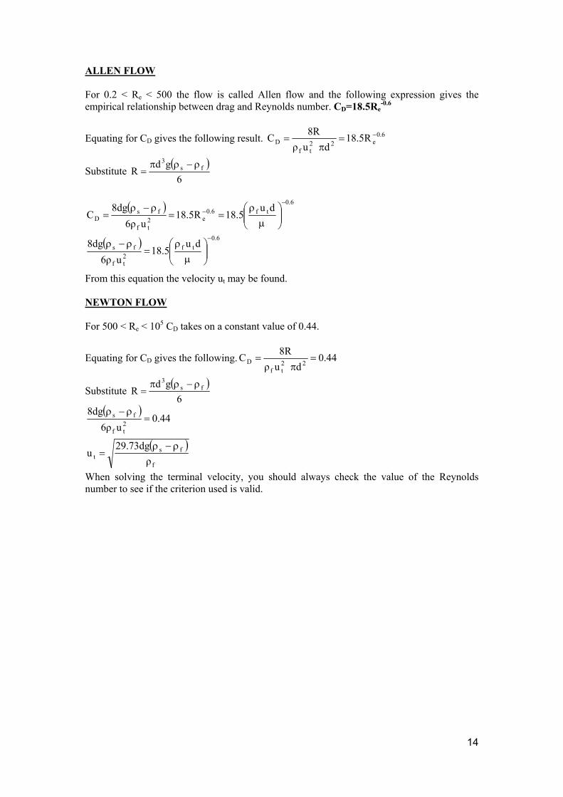
14
ALLEN FLOW
For 0.2 < Re < 500 the flow is called Allen flow and the following expression gives the empirical relationship between drag and Reynolds number. CD=18.5Re
-0.6
Equating for CD gives the following result. 6.0e22
tfD R5.18
d uρ8RC −=π
=
Substitute ( )
6gd
R fs3 ρ−ρπ
=
( )
( ) 6.0tf
2tf
fs
6.0tf6.0
e2tf
fsD
du5.18
u6ρ8dg
du5.18R5.18
u6ρ8dg
C
−
−−
µ
ρ=
ρ−ρ
µ
ρ==
ρ−ρ=
From this equation the velocity ut may be found. NEWTON FLOW For 500 < Re < 105 CD takes on a constant value of 0.44.
Equating for CD gives the following. 44.0d uρ
8RC 22tf
D =π
=
Substitute ( )
6gd
R fs3 ρ−ρπ
=
( )
( )f
fst
2tf
fs
ρ29.73dg
u
44.0u6ρ
8dg
ρ−ρ=
=ρ−ρ
When solving the terminal velocity, you should always check the value of the Reynolds number to see if the criterion used is valid.

15
WORKED EXAMPLE 1.5 Small glass spheres are suspended in an up wards flow of water moving with a mean
velocity of 1 m/s. Calculate the diameter of the spheres. The density of glass is 2630 kg/m3. The density of water is 1000 kg/m3 and the dynamic viscosity is 1 cP.
SOLUTION First, try the Newton flow equation. This is the easiest.
( )
( ) ( ) mm 2.1or m 0.0021 1000 - 2630 x 9.81 x 29.73
1000 x 1ρρg 29.73
ρud
ρρρg 29.73d
u
2
fs
f2t
f
fst
==−
=
−=
Check the Reynolds number.
2103 0.001
0.0021 x 1 x 1000duR tf
e ==µ
ρ=
The assumption of Newton flow was correct so the answer is valid. WORKED EXAMPLE 1.6 Repeat the last question but this time with a velocity of 0.05 m/s. Determine the type of
flow that exists. SOLUTION If no assumptions are made, we should use the general
formula 4.0R1
6R24C
eeD +
++=
0.4223.6d1
60.00048dC
0.450000d16
50000d24C
0.4R1
6R24C
000d 50 0.001
d x 0.05 x 1000µ
duρR
0.51
D
D
eeD
tfe
++
+=
++
+=
++
+=
===
−
( )
0.4223.6d1
60.00048d 8528.16d
8528.16d 0.05 x 1000 x 6
1000)- (2630 x 9.81 x 8du6ρρρ8dg
C
0.51
22f
fsD
++
+=
==−
=
−

16
This should be solved by any method known to you such as plotting two functions and
finding the point of interception.
4.0d6.2231
6d00048.0 f2(d)
8528.16d f1(d)
5.01 +
++=
=
−
The graph below gives an answer of d = 0.35 mm.
Fig. 1.13
Checking the Reynolds’ number 17.5 0.001
0.00035 x 0.05 x 1000duR tf
e ==µ
ρ=
This puts the flow in the Allen's flow section.
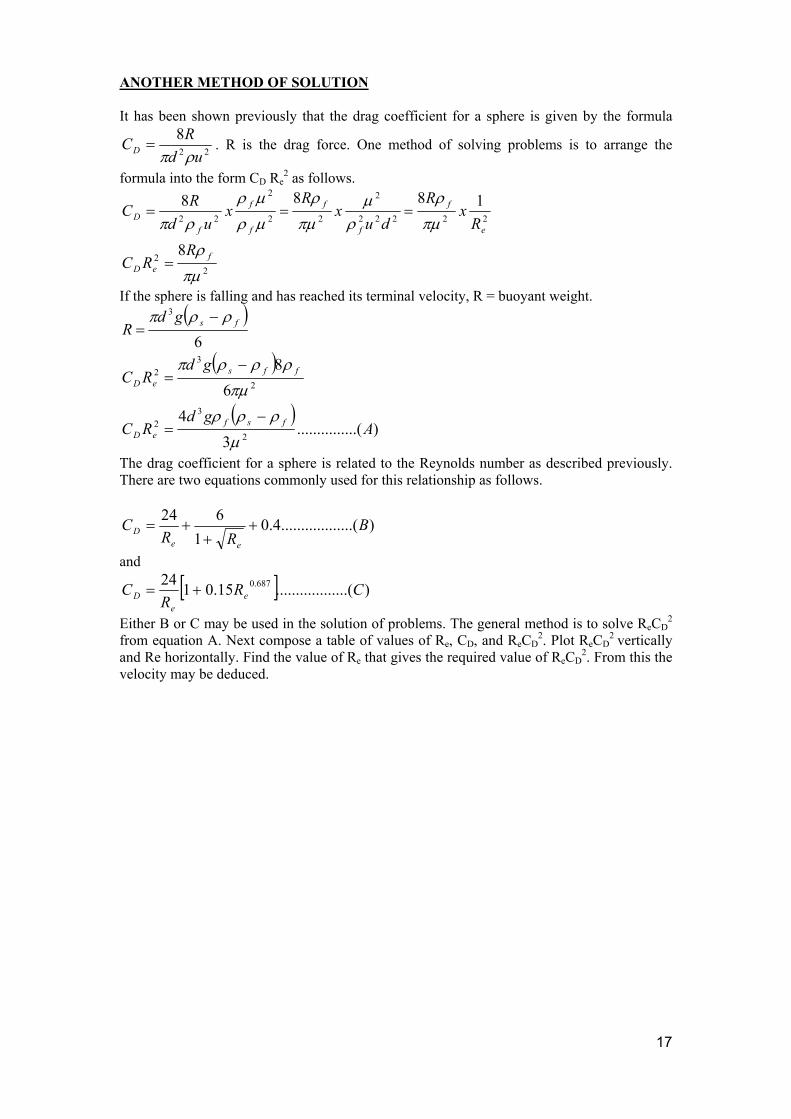
17
ANOTHER METHOD OF SOLUTION It has been shown previously that the drag coefficient for a sphere is given by the formula
22
8ud
RCD ρπ= . R is the drag force. One method of solving problems is to arrange the
formula into the form CD Re2 as follows.
22
22222
2
22
2
22
8
1888
πµ
ρ
πµ
ρ
ρµ
πµ
ρ
µρ
µρ
ρπ
feD
e
f
f
f
f
f
fD
RRC
Rx
Rdu
xR
xud
RC
=
===
If the sphere is falling and has reached its terminal velocity, R = buoyant weight. ( )
( )
( )).....(..........
34
68
6
2
32
2
32
3
Agd
RC
gdRC
gdR
fsfeD
ffseD
fs
µ
ρρρπµ
ρρρπ
ρρπ
−=
−=
−=
The drag coefficient for a sphere is related to the Reynolds number as described previously. There are two equations commonly used for this relationship as follows.
)........(..........4.01
624 BRR
Cee
D ++
+=
and
[ ] )........(..........15.0124 687.0 CRR
C ee
D +=
Either B or C may be used in the solution of problems. The general method is to solve ReCD2
from equation A. Next compose a table of values of Re, CD, and ReCD2. Plot ReCD
2 vertically and Re horizontally. Find the value of Re that gives the required value of ReCD
2. From this the velocity may be deduced.

18
WORKED EXAMPLE 1.7 A sphere 1.5 mm diameter falls in water. The density of the sphere is 2500 kg/m3. The density and dynamic viscosity of water is 997 kg/m3 and 0.89 x 10⁻³ Ns/m2 respectively. The drag
coefficient is given by the formula [ ]687.015.0124e
eD R
RC += . Determine the terminal
velocity. SOLUTION
( ) ( ) 83513)1089.0(3
997250099781.9)0015.0(43
423
3
2
32 =
−=
−=
−xxxgd
RC fsfeD µ
ρρρ
Next compile a table using the formula [ ]687.0Re15.0124+=
eD R
C .
Re 0.1 1 10 100 1000 CD 24.7 27.6 4.15 1.09 0.44 CDRe
2 2.47 27.6 415 109 438288 We are looking for a value of CDRe
2 = 83513 and it is apparent that this occurs when Re is between 100 and 1000. By plotting or by narrowing down the figure by trial and error we find that the correct value of Re is 356. Re = 356 = ρfud/µ 356 = 997 x u x 0.0015/0.89 x 10-3
u = 0.212 m/s and this is the terminal velocity.

19
SELF ASSESSMENT EXERCISE No. 3 1. a. Explain the term Stokes flow and terminal velocity. b. Show that the terminal velocity of a spherical particle with Stokes flow is given by the
formula u = d2g(ρs - ρf)/18µ Go on to show that CD=24/Re 2. Calculate the largest diameter sphere that can be lifted upwards by a vertical flow of
water moving at 1 m/s. The sphere is made of glass with a density of 2630 kg/m3. The water has a density of 998 kg/m3 and a dynamic viscosity of 1 cP. (20.7 mm)
3. Using the same data for the sphere and water as in Q2, calculate the diameter of the
largest sphere that can be lifted upwards by a vertical flow of water moving at 0.5 m/s. (5.95 mm).
4. Using the graph (fig. 1.12) to obtain the drag coefficient of a sphere, determine the drag
on a totally immersed sphere 0.2 m diameter moving at 0.3 m/s in sea water. The density of the water is 1025 kg/m3 and the dynamic viscosity is 1.05 x 10⁻³ Ns/m2. (0.639 N).
5. A glass sphere of diameter 1.5 mm and density 2 500 kg/m3 is allowed to fall through
water under the action of gravity. The density of the water is 1000 kg/m3 and the dynamic viscosity is 1 cP.
Calculate the terminal velocity assuming the drag coefficient is CD = 24 Re -1 (1+ 0.15Re 0.687) (Ans. 0.215 m/s 6. Similar to part of Q1 1990 A glass sphere of density 2 690 kg/m3 falls freely through water. Find the terminal
velocity for a 4 mm diameter sphere and a 0.4 mm diameter sphere. The drag coefficient is CD = 8F/{πd2ρu2} This coefficient is related to the Reynolds number as shown. Re 15 20 25 30 35 CD 3.14 2.61 2.33 2.04 1.87 The density and viscosity of the water is 997 kg/m3 and 0.89 x 10⁻³ N s/m2. Answer 0.45 m/s and 0.06625 m/s. 7. Similar to part of Q4 1988. A glass sphere of diameter 1.5 mm and density 2 500 kg/m3 is allowed to fall through
water under the action of gravity. Find the terminal velocity assuming the drag coefficient is CD = 24 Re-1(1+ 0.15Re0.687) (Ans. 0.215 m/s)

20
8. Similar to Q1 1986 The force F on a sphere of diameter d moving at velocity um in a fluid is given by F = CD {πd2ρum2}/8 For Reynolds numbers less than 1 000, CD is given by CD= 24 Re-1(1+ 0.15Re0.687) Estimate the terminal velocity of a glass sphere 1 mm diameter and density 2 650 kg/m3
in water of density 997 kg/m3 and viscosity 0.89 x 10⁻³ N s/m2. Answer 0.15 m/s

21
2. BOUNDARY LAYERS In this tutorial we will look at the shape of various types of boundary layers. We will look at the mathematical equations for the shape of the boundary layer and use them to solve problems. You may recall that the definition of a BL is the thickness of that layer next to a surface in which the velocity grows from zero to a maximum value (or so close to a maximum as to be of no practical difference). This thickness is usually given the symbol δ (small delta). The boundary layer, once established may have a constant thickness but, for example, when a flow meets the leading edge of a surface, the boundary layer will grow as shown (fig.2.1).
Fig.2.1
When the flow enters a pipe the BL builds up from all around the entrance and a cross section shows the layer meets at the centre (fig.2.2)
Fig.2.2
The symbol u1 is used to designate the maximum velocity in the fully developed layer. The fully developed layer may be laminar or turbulent depending on the Reynolds’ Number.

22
The velocity profile for a typical case is shown on fig.2.3.
Fig.2.3
The shear stress between any two horizontal layers is τ. For a Newtonian Fluid the relationship between shear stress, dynamic viscosity (µ) and rate of shear strain (du/dy) is
τ = µ du/dy
At the wall the shear stress is called the WALL SHEAR STRESS, τo and occurs at y = 0. Note that the gradient du/dy is the rate of shear strain and it is steeper for turbulent flow than for laminar flow giving a greater shear resistance. The solution of problems is simplified by the concepts of DISPLACEMENT THICKNESS AND MOMENTUM THICKNESS which we will now examine. 2.1. DISPLACEMENT THICKNESS δ* The flow rate within a boundary layer is less than that for a uniform flow of velocity u1. The reduction in flow is equal to the area under the curve in fig.2.3. If we had a uniform flow equal to that in the boundary layer, the surface would have to be displaced a distance δ* in order to produce the reduction. This distance is called the displacement thickness and it is given by :
[ ] ∗=−= ∫ δδ
10
1u redution flow udyu
If this is equivalent to a flow of velocity u1 in a layer δ* thick then :
dyuu
∫
−=∗
δ
δ0 1
1
2.2. MOMENTUM THICKNESS θ The momentum in a flow with a BL present is less than that in a uniform flow of the same thickness. The momentum in a uniform layer at velocity u1 and height h is ρhu12. When a BL exists this is reduced by ρu12θ. Where θ is the thickness of the uniform layer that contains the equivalent to the reduction. Using the same reasoning as before we get :
dyuu
uu
−
= ∫
10 1
1δ
θ

23
2.3. BOUNDARY LAYER LAWS The velocity at any distance y above a surface is a function of the wall shear stress, the dynamic viscosity and the density.
u =φ(y, τo, ρ ,µ) If you are familiar with the method of dimensional analysis you may wish to show for yourself that :
u(ρ/τo)½ = φ{y(τo)½}
Generally the law governing the growth of a BL is of the form u = φ(y) and the limits must be that u = 0 at the wall and u = u1 in the fully developed flow. There are many ways in which this is expressed according to the Reynolds’ Number for the flow. The important boundary conditions that are used in the formulation of boundary layer laws are: 1. The velocity is zero at the wall ( u = 0 @ y = 0). 2. The velocity is a maximum at the top of the layer ( u = u1 @ y = δ). 3. The gradient of the b.l. is zero at the top of the layer (du/dy = 0 @ y = δ). 4. The gradient is constant at the wall (du/dy = C @ y = 0). 5. Following from (4) d2u/dy2 = 0 @ y = 0). Let us start by considering LAMINAR BOUNDARY LAYERS.

24
2.3.1 LAMINAR BOUNDARY LAYERS One of the laws which seem to work for laminar flow is u = u1 sin(π y/2δ)
WORKED EXAMPLE No.2.1 Find the displacement thickness δ* for a Laminar BL modelled by the equation u = u1 sin(π y/2δ)
{ } δπδδ
δπ
πδδ
δπδ
δ
δδ
364.02002
cos2
2sin11
0
00 1
=
+−+=
+=
−=
−=
∗
∗ ∫∫
yy
ydyuu
Another way of expressing the shape of the laminar BL is with a power law. The next example is typical of that used in the examination.
WORKED EXAMPLE No.2.2 The velocity distribution inside a laminar BL over a flat plate is described by the cubic law :
u/u1 = a0 + a1y + a2y2 + a3y3
Show that the momentum thickness is 39δ/280 SOLUTION At y = 0, u = 0 so it follows that a0 = 0 d2u/dy2 = 0 @ y = 0 so a2= 0. Show for yourself that this is so. The law is reduced to u/u1 = a1y + a3y3
at y = δ, u = u1 so 1 = a1δ + 3a3δ2
hence a1 =(1-a3δ3)/δ
Now differentiate and du/dy = u1(a1+3a3y2) at y = δ, du/dy is zero so 0 =a1+ 3a3δ2 so a1= -3a3δ2
Hence by equating a1= 3/2δ and a3 = -1/2δ3 Now we can write the velocity distribution as u/u1=3y/2δ -(y/δ)3/2 and du/dy = u1{3/2δ + 3y2/2δ3}

25
If we give the term y/δ the symbol η we may rewrite the equation as: u/u1=3η/2 - η3/2 The momentum thickness θ is given by :
ηηηηηθ
ηδθδ
d
dyuu
uu
−−
−=
=
−
=
∫
∫
2231
223
d dybut 1
31
0
3
10 1
Integrating gives :
+−−−=
103
28129
843 57342 ηηηηηδθ
between the limits η=0 and η=1 this evaluates to
θ = 39δ/280

26
WORKED EXAMPLE No.2.3 Show that δ/x=4.64Re-0.5 for the same case as before. SOLUTION We must first go back to the basic relationship. From the previous page du/dy = u1{3/2δ + 3y2/2δ3} At the wall where y=0 the shear stress is τo=µdu/dy = µu1{3/2δ + 3y2/2δ3} =(µu1/δ) δ [(3/2δ) +3y2/2δ3] Putting y/δ= η we get : τo = (µu1/δ) δ [(3/2δ) +3δ2/2δ] τo = (µu1/δ) [(3/2) +3δ2/2] at the wall η=0 τo = (µu1/δ) (3/2)………........(2.1) The friction coefficient Cf is always defined as Cf = τo/(ρ u1
2/2).............(2.2) It has been shown elsewhere that Cf = 2dθ/dx. The student should search out this information from test books. Putting θ = 39δ/280 (from the last example) then Cf = 2dθ/dx = (2x39/280) dδ/dx ..............(2.3) equating (2.2) and (2.3) gives τo=( ρu1
2)(39/280)dδ/dx .............(2.4) equating (2.1) and (2.4) gives (ρu1
2)(39/280)dδ/dx = (µu/δ)(3/2) hence (3 x 280)/(2 x 39)(µdx)/ρu) = δdδ Integrating 10.77(µx/ ρu1) = δ2/2 + C Since δ = 0 at x = 0 (the leading edge of the plate) then C=0 hence δ= {21.54µx/ρu1}½ dividing both sides by x gives δ/x = 4.64(µ/ρu1x)-½ = 4.64Re-½ NB Rex= ρu1x/µ and is based on length from the leading edge.

27
SELF ASSESSMENT EXERCISE No. 4 1. The BL over a plate is described by u/u1=sin(πy/2δ). Show that the momentum thickness
is 0.137δ. 2. The velocity profile in a laminar boundary layer on a flat plate is to be modelled by the
cubic expression u/u1=a0+a1y + a2y2+a3y3 where u is the velocity a distance y from the wall and u1 is the main stream velocity. Explain why a0 and a2 are zero and evaluate the constants a1 and a3 in terms of the
boundary layer thickness δ. Define the momentum thickness θ and show that it equals 39δ/280 Hence evaluate the constant A in the expression δ/x = A (Rex)-0.5
where x is the distance from the leading edge of the plate. It may be assumed without proof that the friction factor Cf = 2 dθ/dx
3. (a) The velocity profile in a laminar boundary layer is sometimes expressed in the form
u/u1=a0+a1(y/δ)+a2(y/δ)2+a3 (y/δ)3+a4(y/δ)4 where u1 is the velocity outside the boundary layer and δ is the boundary layer
thickness. Evaluate the coefficients a0 to a4 for the case when the pressure gradient along the surface is zero.
(b) Assuming a velocity profile u/u1=2(y/δ) - (y/δ)2 obtain an expression for the
mass and momentum fluxes within the boundary layer and hence determine the displacement and momentum thickness.
4. When a fluid flows over a flat surface and the flow is laminar, the boundary layer
profile may be represented by the equation
u/u1= 2(η) - (η)2 where η = y/δ y is the height within the layer and δ is the thickness of the layer. u is the velocity
within the layer and u1 is the velocity of the main stream. Show that this distribution satisfies the boundary conditions for the layer. Show that the thickness of the layer varies with distance (x) from the leading edge by
the equation δ=5.48x(Rex)-0.5
It may be assumed that τo = ρu12 dθ/dx

28
5. Define the terms displacement thickness δ * and momentum thickness θ. Find the ratio of these quantities to the boundary layer thickness δ if the velocity profile
within the boundary layer is given by u/u1=sin(πy/2δ) Show, by means of a momentum balance, that the variation of the boundary layer
thickness δ with distance (x) from the leading edge is given by δ = 4.8(Rex)-0.5
It may be assumed that τo = ρu12 dθ/dx Estimate the boundary layer thickness at the trailing edge of a plane surface of length
0.1 m when air at STP is flowing parallel to it with a free stream velocity u1 of 0.8 m/s. It may be assumed without proof that the friction factor Cf is given by
Cf = 2 dθ/dx N.B. standard data µ = 1.71 x 10⁻⁵ N s/m2. ρ = 1.29 kg/m3. 6. In a laminar flow of a fluid over a flat plate with zero pressure gradient an
approximation to the velocity profile is u/u1=(3/2)(η) - (1/2)(η)3
η = y/δand u is the velocity at a distance y from the plate and u1 is the mainstream
velocity. δ is the boundary layer thickness. Discuss whether this profile satisfies appropriate boundary conditions. Show that the local skin-friction coefficient Cf is related to the Reynolds’ number
(Rex) based on distance x from the leading edge by the expression Cf =A (Rex)-0.5
and evaluate the constant A. It may be assumed without proof that Cf = 2 dθ/dx and that θ is the integral of (u/u1)(1 - u/u1)dy between the limits 0 and δ
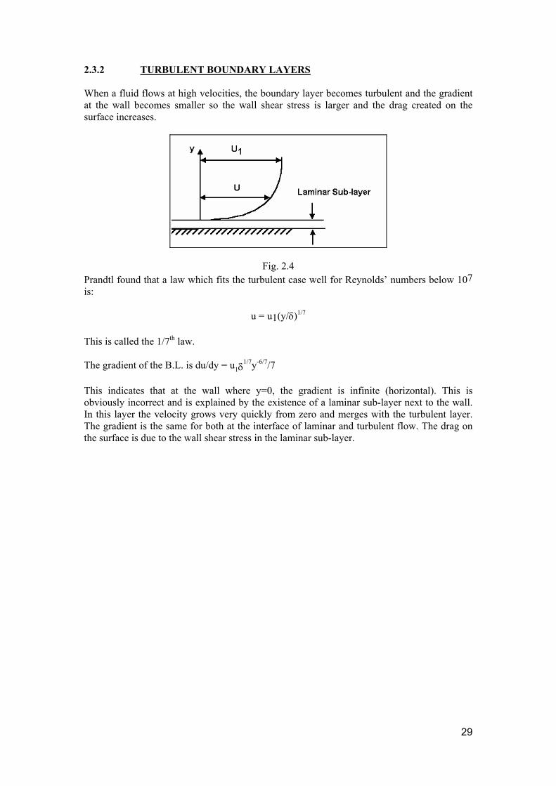
29
2.3.2 TURBULENT BOUNDARY LAYERS When a fluid flows at high velocities, the boundary layer becomes turbulent and the gradient at the wall becomes smaller so the wall shear stress is larger and the drag created on the surface increases.
Fig. 2.4 Prandtl found that a law which fits the turbulent case well for Reynolds’ numbers below 107 is:
u = u1(y/δ)1/7 This is called the 1/7th law. The gradient of the B.L. is du/dy = u1δ
1/7y-6/7/7 This indicates that at the wall where y=0, the gradient is infinite (horizontal). This is obviously incorrect and is explained by the existence of a laminar sub-layer next to the wall. In this layer the velocity grows very quickly from zero and merges with the turbulent layer. The gradient is the same for both at the interface of laminar and turbulent flow. The drag on the surface is due to the wall shear stress in the laminar sub-layer.

30
WORKED EXAMPLE No.2.4 Show that the mean velocity in a pipe with fully developed turbulent flow is 49/60 of the maximum velocity. Assume the 1/7th law. For a pipe, the B.L. extends to the centre so δ = radius = R. Consider an elementary ring of flow.
Fig.2.5 The velocity through the ring is u. The volume flow rate through the ring is 2πrudr The volume flow rate in the pipe is Q = 2π∫rudr
Since δ = R then u = u1(y/R)1/7
also r = R-y
Q = 2π∫ (R-y)udr = 2π∫u1R-1/7 (R-y)y
1/7dy
Q =2πu1R-1/7
[Ry1/7
-y8/7
]
Q =2πu1R-1/7
[(7/8)Ry8/7
- (7/15)y15/7
]
Q =(49/60)πR2
u1.
The mean velocity is defined by um=Q/πR2
hence um=(49/60)u1

31
2.4 FRICTION COEFFICIENT AND BOUNDARY LAYERS Earlier it was explained that the friction coefficient Cf is the ratio of the wall shear stress to the dynamic pressure so : Cf = 2τo/(ρum
2) ..........................(2.4.1) For smooth walled pipes, Blazius determined that Cf = 0.079Re-0.25 ........................(2.4.2) Equating (2.4.1) and (2.4.2) gives : 2τo/(ρum
2) = 0.079Re-0.25
Note that um is the mean velocity and u1 is the maximum velocity. Research shows that um=0.8u1 Also Note that Re=ρu1D/µ and D = 2δ. Hence τo=0.02125ρu1
2(µ/ρδu1) 0.25.............(2.4.3) 2.5 FORCE BALANCE IN THE BOUNDARY LAYER The student should refer to textbooks for finer details of the following work. Consider again the growth of the B.L. as the fluid comes onto a flat surface. A stream line for the flow is not parallel to the B.L. Now consider a control volume A, B, C, D.
Fig.2.6
Balancing pressure force and shear force at the surface with momentum changes gives :
[ ] [ ]∫∫ −
+−
=
δδ
δδρ
δδρτ
01
01 )4.4.2.(..........udyuu
xuudyuu
xo
Using equations (2.4.2), (2.4.3) and (2.4.4) gives (4/5)δ5/4= 0.231{µ/ρu}1/5x = Re-1/5
The shear force on the surface is Fs= τo x surface area The surface skin friction coefficient is Cf=2Fs/(ρu12) = 0.072Re-1/5 Experiments have shown that a more accurate figure is : Cf= 0.074Re-1/5

32
SELF ASSESSMENT EXERCISE No. 5 1. Under what circumstances is the velocity profile in a pipe adequately represented by
the 1/7 th power law u/u1=(y/R)1/7
where u is the velocity at distance y from the wall, R is the pipe radius and u1 is the centre-line velocity ?
The table shows the measured velocity profile in a pipe radius 30 mm. Show that these
data satisfy the 1/7 th power law and hence evaluate (i) the centre-line velocity (ii) the mean velocity um (iii) the distance from the wall at which the velocity equals um. 1.0 2.0 5.0 10.0 15.0 20.0 y (mm) 1.54 1.70 1.94 2.14 2.26 2.36 u (m/s)
2. (a) Discuss the limitations of the 1/7th power law u/u1=(y/R)1/7
for the velocity profile in a circular pipe of radius R, indicating the range of Reynolds numbers for which this law is applicable.
(b) Show that the mean velocity is given by 49u1/60. (c) Water flows at a volumetric flow rate of 1.1 x 10⁻³ m3/s in a tube of diameter
25 mm. Calculate the centre-line velocity and the distance from the wall at which the velocity is equal to the mean velocity.
(d) Assuming that Cf=0.079(Re)-0.25
evaluate the wall shear stress and hence estimate the laminar sub-layer thickness.
µ = 0.89 x 10⁻³ N s/m2. ρ=998 kg/m3.

FLUID MECHANICS
TUTORIAL No.4
FLOW THROUGH POROUS PASSAGES
In this tutorial you will continue the work on laminar flow and develop Poiseuille's equation to the form known as the Carman - Kozeny equation. This equation is used to predict the flow rate through porous passages such as filter, filter beds and fluidised beds in combustion chambers. On completion of this tutorial you should be able to do the following.
Derive the Carman - Kozeny equation.
Solve problems involving the flow of fluids through a porous material.
In order to do this tutorial you must be familiar with Poiseuille's equation for laminar flow and this is covered in tutorial 1.

FLOW THROUGH POROUS PASSAGES The following are examples where porous flow occurs.
A filter element made of thick sintered particles. This might be a cylinder with radial flow.
A sand bed filter for cleaning water. The water percolates down through the filter though long tortuous passages. The depth of water on top of the filter governs the rate at which the water is forced through.
A layer of rock through which water, gas or oil might seep. This is similar to a radial flow filter but on a much larger scale.

When a fluid passes through a porous material, it flows through long thin tortuous passages of varying cross section. The problem is how to calculate the flow rate based on nominal thickness of the layer. This was tackled by Kozeny and later by Carman. The result is a formula, which gives a mean velocity of flow in the direction at right angles to the layer plane in terms of its thickness and other parameters. The passage between the particles is so small that the velocity in them is small and the flow is well and truly laminar. Poiseuille's Equation for laminar flow states ∆p/l = -32 µu'/D2.
Kozeny modelled the layer as many small capillary tubes of diameter D making up a layer of cross sectional area A. The actual cross sectional area for the flow path is A'. The difference is the area of the solid material. The ratio is ε = A'/A and this is known as the porosity of the material. The volume flow rate through the layer is Q. Kozeny used the notion that Q = Au where u is the mean velocity at right angles to the layer.
Figure 1 The volume flow rate is also Q= A'u' where u' is the mean velocity in the tube. Equating u' = uA/A' ε = void fraction = A'/A. u'= u/ε. Carman modified this formula when he realised that the actual velocity inside the tubes must be proportionally larger because the actual length is greater than the layer
thickness. It follows that lluuε′
=′
where l is the layer thickness and l' the mean length of the passages. Substituting this in Poiseuille's Equation gives :
2
32lDlu
lp
εµ ′
−=∆
rearranging 2
32Dllu
lp
εµ ′
−=∆
This is usually expressed as a pressure gradient in the direction of the mean flow (say x) and it becomes :
2
32Dllu
dxdp
εµ ′
−= .......................(1)

As= csa of the solid A'= csa of the tubes A = csa of the layer = A' + As.
sAA
AAA
+′′
=′
=ε
Multiply top and bottom by thye length l and the areas become volumes so
sQQ
Q+′′
=ε
where Q' is the volume of the tubes and Qs is the volume of the solid.
( )
( )
( )
( )
( )εεε
ε
εε
ε
−=′
+′=−
=
−=
−=−=′
−==′−
+′=′
1
1
1
1
s
ss
s
s
s
QQQQ
QQQQQQQQQQ
QQQ
S = Surface Area of the tubes . Divide both sides by S ( )εε−
=′
1SQ
SQ s
Q' is made up of tubes diameter D and length l' so 4
2lDnQ′
=′π
and S = nπDl' where n is the number of tubes which cancels when these are
substituted into the formula. This results in : ( )εε−
=1
4SQD s
Next we consider the solid as made up of spherical particles of mean diameter ds. S = surface area of tubes but also the surface area of the solid particles.
Hence 6S
Q and and
6s2
3s
ss
sddSdQ === π
π
It follows that ( )εε−
=132 sdD
Substitute this into equation (1) and : ( )32
2172ε
εµ
sldlu
dxdp −′
−=
Research has shown that (l'/l) is about 2.5 hence : ( )32
21180ε
εµ
sdu
dxdp −
−=
This is the Carman- Kozeny.

WORKED EXAMPLE No.1 Water is filtered through a sand bed 150 mm thick. The depth of water on top of the bed is 120 mm. The porosity ε is 0.4 and the mean particle diameter is 0.25 mm. The dynamic viscosity is 0.89 cP and the density is 998 kg/m3. Calculate the flow rate per square metre of area. SOLUTION The pressure difference across the sand bed is assumed to be the head of water since atmospheric pressure acts on top of the water and at the bottom of the bed.
First convert the head into pressure difference. ∆p = ρg(h2 – h1) = {0 – (998 x 9.81 x 0.12)} = -1174.8 Pa. The length of the bed (L) is 120 mm. Assume that dp/dx = ∆p/L The dynamic viscosity is 0.89 x 10⁻³ Ns/m2. Using the Carman- Kozeny equation where the pressure gradient is assumed to be linear.
( )
area. ofmeter squareper s/m10x543.0Qs/m10x543.0uu144180003.7832
0.4 x0.25x10 0.4) - (1u 10 x 0.89 x 180
12.08.1174
dxdp
d1u180
dxdp
33
3
33-
23-
32s
2
−
−
=
=
=
−=−=
εε−µ
−=

WORKED EXAMPLE No.2 Calculate the flow rate through a filter 70 mm outside diameter and 40 mm inside
diameter and 100 mm long given that the pressure on the outside is 20 kPa greater than on the inside. The mean particle diameter d is 0.04 mm and the void fraction is 0.3. The dynamic viscosity is 0.06 N s/m2.
SOLUTION The flow is radial so -dp/dx = dp/dr since radius increases in the opposite sense
to x in the derivation. The equation may be written as :
( )32
21180ε
εµ
sdu
dxdp −
−=
r is the radius. Putting in values:
( ) uxx
uxdrdp 9
32
2
105.1223.000004.0
3.0106.0180=
−=
Consider an elementary cylinder through which the oil flows. The velocity
normal to the surface is
1591.11.022
−=== Qrxrx
QLrQu
ππ
hence: dp =122.5 x 109 x 1.591Q r -1 dr = 194.8975 Q r -1 dr
Integrating between the outside and inside radius yields:
smmsmxQ
Qp
RRQpi
o
/3.183/103.1832035ln89.19420000
ln89.194
339 ==
==
=

SELF ASSESSMENT EXCERCISE No.1 Q.1 Outline briefly the derivation of the Carman-Kozeny equation.
( )32
21180ε
εµ
sdu
dldp −
−=
dp/dl is the pressure gradient, µ is the fluid viscosity, u is the superficial velocity, ds is the particle diameter and ε is the void fraction.
A cartridge filter consists of an annular piece of material of length 150 mm and
internal diameter and external diameters 10 mm and 20 mm. Water at 25oC flows radially inwards under the influence of a pressure difference of 0.1 bar. Determine the volumetric flow rate. (21.53 cm3/s)
For the filter material take d = 0.05 mm and ε = 0.35. µ=0.89 x 10⁻³ N s/m2 and ρ= 997 kg/m3. Q.2 (a) Discuss the assumptions leading to the equation of horizontal viscous flow
through a packed bed ( )32
21180ε
εµ
sdu
dLdp −
−=
where ∆p is the pressure drop across a bed of depth L, void fraction ε and effective particle diameter d. u is the approach velocity and µ is the viscosity of the fluid.
(b) Water percolates downwards through a sand filter of thickness 15 mm,
consisting of sand grains of effective diameter 0.3 mm and void fraction 0.45. The depth of the effectively stagnant clear water above the filter is 20 mm and the pressure at the base of the filter is atmospheric. Calculate the volumetric flow rate per m2 of filter. (2.2 dm3/s)
(Note the density and viscosity of water are given in the instructions on all exams
papers) µ=0.89 x 10⁻³ N s/m2 and ρ= 997 kg/m3

Q3. Oil is extracted from a horizontal oil-bearing stratum of thickness 15 m into a
vertical bore hole of radius 0.18 m. Find the rate of extraction of the oil if the pressure in the bore-hole is 250 bar and the pressure 300 m from the bore hole is 350 bar.
Take d= 0.05 mm, ε= 0.30 and µ = 5.0 x 10⁻³ N s/m2.

D.J.DUNN 1
FLUID MECHANICS
TUTORIAL No.5
POTENTIAL FLOW
In this tutorial you will study the flow of ideal fluids. On completion you should be able to do the following.
§ Define the stream function.
§ Define the velocity potential.
§ Understand the flow of an ideal fluid around a long cylinder.
§ Understand the main points concerning vortices. An ideal fluid has no viscosity (inviscid) and is incompressible. No such fluid exists but these assumptions make it possible to produce models for the flow of fluids in and around solid boundaries such as long cylinders. In particular, the concepts of POTENTIAL FLOW and STREAM FUNCTION give us useful mathematical models to study these phenomena.

D.J.DUNN 2
1 STREAM FUNCTION Consider the streamlines representing a 2 dimensional flow of a perfect fluid.
Figure 1
Flux is defined as the volume flow rate per metre depth normal to the page. The stream function is defined as the flux across the line O -P. The symbol used is ψ (psi). Since there is no flow rate normal to a stream line, then it follows that the stream function is the same between O and any point P, P' or P'' on the same stream line. In other words, the stream line represents a constant value of the stream function. It is easier to understand ψ in terms of small changes. Consider a short line of length ds perpendicular to a stream line. Let the velocity across this line have a mean value of v'. The flux crossing this line is hence v'ds and this is the small change in the stream function dψ. It follows that dψ = v'ds
Figure 2
In this analysis, the stream function is positive when it crosses the line in an anti-clockwise direction (right to left on the diagram). This is quite arbitrary with some publications using clockwise as positive, others using anti-clockwise.
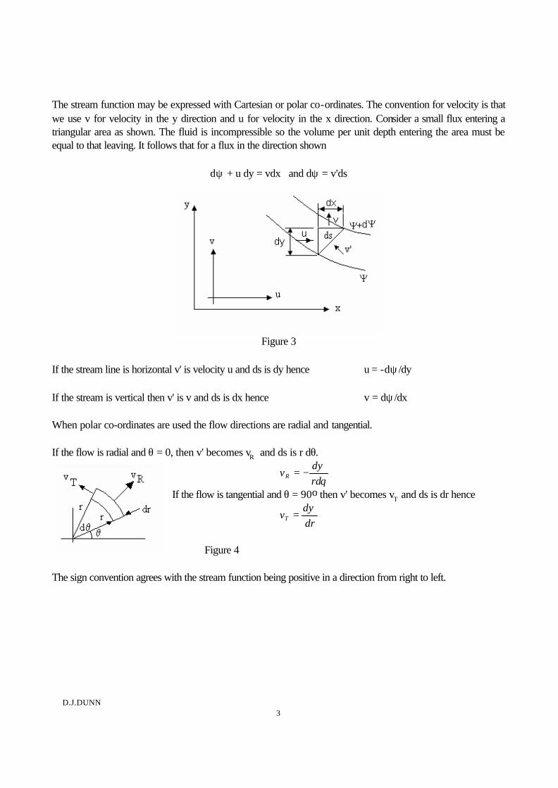
D.J.DUNN 3
The stream function may be expressed with Cartesian or polar co-ordinates. The convention for velocity is that we use v for velocity in the y direction and u for velocity in the x direction. Consider a small flux entering a triangular area as shown. The fluid is incompressible so the volume per unit depth entering the area must be equal to that leaving. It follows that for a flux in the direction shown
dψ + u dy = vdx and dψ = v'ds
Figure 3
If the stream line is horizontal v' is velocity u and ds is dy hence u = -dψ /dy If the stream is vertical then v' is v and ds is dx hence v = dψ /dx When polar co-ordinates are used the flow directions are radial and tangential.
If the flow is radial and θ = 0, then v' becomes vR and ds is r dθ.
θ
ψrdd
vR −=
If the flow is tangential and θ = 90o then v' becomes vT and ds is dr hence
drd
vTψ
=
Figure 4
The sign convention agrees with the stream function being positive in a direction from right to left.

D.J.DUNN 4
2 VELOCITY POTENTIAL The velocity potential has a symbol φ. It is best explained as follows. Consider a line along which the velocity v' varies. Over a short length ds the velocity potential varies by dφ. Hence dφ = v'ds or v' = dφ/ds. The velocity potential may be thought of as the product of velocity and length in the same direction. It follows that φ = ∫v' ds Some text books use a sign convention opposite to this and again this is arbitrary.
If the line is horizontal v' is velocity u and ds is dx hence dxd
uφ
=
If the line is vertical then v' is v and ds is dy hence dyd
vφ
=
If the flow is radial then v' is vR and ds is dr hence drd
vR
φ=
If the flow is tangential then v' is vT and ds is r dθ hence θφ
rdd
vT =
The sign convention is positive for increasing radius and positive for anti- clockwise rotation. Since v' is zero perpendicular to a stream line it follows that lines of constant φ run perpendicular to the stream lines. If these lines are superimposed on a flow we have a flow net. Consider a flow with lines of constant ψ and φ as shown.
Figure 5
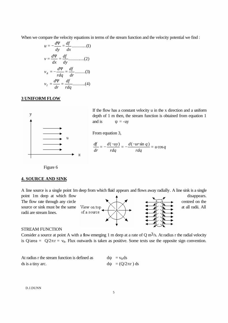
D.J.DUNN 5
When we compare the velocity equations in terms of the stream function and the velocity potential we find :
)4.(..........
)3.........(
)2....(..........
)1...(..........
θφ
φθ
φ
φ
rdd
drd
v
drd
rdd
v
dyd
dxdv
dxd
dydu
T
R
=Ψ
=
=Ψ
−=
=Ψ=
=Ψ−=
3 UNIFORM FLOW
If the flow has a constant velocity u in the x direction and a uniform depth of 1 m then, the stream function is obtained from equation 1 and is ψ = -uy From equation 3,
θθ
θθ
φcos
)sin()(u
rdurd
rduyd
drd
=−
−=−
−=
Figure 6 4. SOURCE AND SINK A line source is a single point 1m deep from which fluid appears and flows away radially. A line sink is a single point 1m deep at which flow disappears. The flow rate through any circle centred on the source or sink must be the same at all radii. All radii are stream lines. Figure 7 STREAM FUNCTION Consider a source at point A with a flow emerging 1 m deep at a rate of Q m3/s. At radius r the radial velocity is Q/area = Q/2πr = vR. Flux outwards is taken as positive. Some texts use the opposite sign convention.
At radius r the stream function is defined as dψ = vRds ds is a tiny arc. dψ = (Q/2πr ) ds
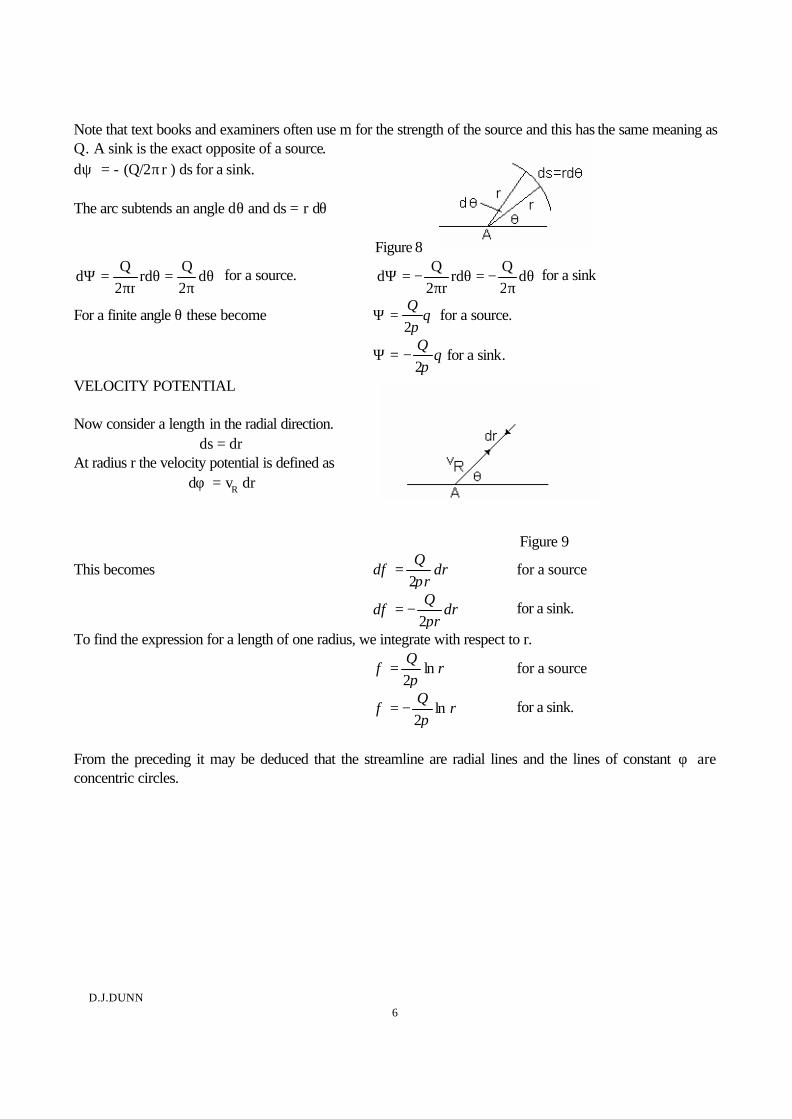
D.J.DUNN 6
Note that text books and examiners often use m for the strength of the source and this has the same meaning as Q. A sink is the exact opposite of a source. dψ = - (Q/2πr ) ds for a sink. The arc subtends an angle dθ and ds = r dθ
Figure 8
θπ
=θπ
=Ψ d2Q
rdr2
Qd for a source. θ
π−=θ
π−=Ψ d
2Q
rdr2
Qd for a sink
For a finite angle θ these become θπ2
Q=Ψ for a source.
θπ2
Q−=Ψ for a sink.
VELOCITY POTENTIAL
Now consider a length in the radial direction. ds = dr
At radius r the velocity potential is defined as dφ = vR dr
Figure 9
This becomes drr
Qd
πφ
2= for a source
drr
Qd
πφ
2−= for a sink.
To find the expression for a length of one radius, we integrate with respect to r.
rQ
ln2π
φ = for a source
rQ
ln2π
φ −= for a sink.
From the preceding it may be deduced that the streamline are radial lines and the lines of constant φ are concentric circles.

D.J.DUNN 7
5 DOUBLET A doublet is formed when an equal source and a sink are brought close together. Consider a source and sink of equal strength placed at A and B respectively. The stream function for point P relative to A and B are respectively
22θ
πQ
B =Ψ for the source
12θ
πQ
A −=Ψ for the sink
( )122θθ
π−=Ψ+Ψ=Ψ
QABP
Figure 10
Referring to the diagram
( )
( ) ( ) ( )
( )
( ) 2212
2
22212
22
212
12
1212
21
yxby2
radians.in itself angle he as same thebecomes angle theof tan theand 0b 0,b As
ybxby2
tan
bxy
1
bxybxytan
tantan1tantan
tan
bxy
tan,bx
ytan
+=θ−θ
→→
+−=θ−θ
−+
+−−=θ−θ
θθ+θ−θ
=θ−θ
−=θ
+=θ
+π
=Ψ22p y x
by22Q
When the source and sink are brought close together we have DOUBLET but b remains finite.
Let B = (Qb/π) 22 yxBy+
=Ψ
Since y = r sinθ and x2 + y2 = r2 then
rB
rBr θθ sinsin
2 ==Ψ
ψ = 0 is the streamline across which there is no flux and this is a circle so it can be used to represent a cylinder. Figure 11

D.J.DUNN 8
6. COMBINATION OF UNIFORM FLOW AND SOURCE OR SINK For this development, consider the case for the source at the origin of the x – y co-ordinates with a uniform flow of velocity u from left to right. The development for a sink in a uniform flow follows the same principles. The uniform flow encounters the flux from the source producing a pattern as shown. At large values of x the flow has become uniform again with velocity u. The flux from the source is Q. this divides equally to the top and bottom. At point s there is a stagnation point where the radial velocity from the source is equal and opposite of the uniform velocity u. The radial velocity is Q/2πr. Equating to u we have r = Q/2πu and this is the distance from the origin to the stagnation point. For uniform flow Ψ1 = -uy For the source Ψ2 = Qθ/2π . The combined value is Ψ = -uy + Qθ/2π The flux between the origin and the stagnation point S is half the flow from the source. Hence, the flux is Q/2 and the angle θ is π radian (180o). The dividing streamline emanating from S is the zero streamline Ψ = 0. Since no flux crosses this streamline, the dividing streamline could be a solid boundary. When the flow is uniform, we have: Ψ = 0 = -uy + Qθ/2π = -uy + Qπ /2π y = -uy + Q/2 y = Q/2u y is the distance from the x axis to the zero stream line where the flow is uniform (at large values of x). The thickness of the uniform stream emerging from the source is t = 2y. Hence t =Q/u.
Figure 12 PRESSURE Consider points S and A. At S there is a pressure ps and no velocity. At point A there is a velocity vA and pressure pA. Applying Bernoulli between these points, we have: ps = pA + ρ vA
2/2 ps - pA = ρ vA
2/2

D.J.DUNN 9
To solve the pressure difference we need to know the velocity. At point A we can solve this as follows. The velocity is the resultant velocity of the uniform flow u and the radial velocity from the source vR.
Figure 13
vA2 = u2 + vR
2 The stream line at point A is Ψ = 0 hence 0 = -uy + Qθ/2π hence y = Qθ/2πu At this point θ = π /2 (90o) so y = Q/4u This is the distance to point A along the y axis. vR = Q/2πr. The radius at point A is Q/4u hence vR = 2u/π vA
2 = u2 + (2u/π)2 = u2 {1 +4/π2} ps - pA = ρ vA
2/2 = (ρu2/2) {1 +4/π 2} WORKED EXAMPLE No.1 A uniform flow of fluid with a density of 800 kg/m3 is from left to right with a velocity u = 2 m/s. It is
combined with a source of strength Q = 8 m2/s at the origin. Calculate: 1. The distance to the stagnation point. 2. The width of the flow stream emanating from the source when it has reached a uniform state. 3. The pressure difference between the stagnation point and the point where the zero streamline crosses the y
axis. SOLUTION From the preceding work Distance to stagnation point = Q/2πu = 8/(2π x 2) = 2/π metres t = Q/u = 8/2 = 4 m ps - pA = (ρu2/2) {1 +4/π 2} ps - pA = (800 x 22/2){1 + 4/π 2} ps - pA = 1600(1.405) = 2248 N/m2

D.J.DUNN 10
If a sink is placed at the origin, the flow pattern is like this.
Figure 14
The analysis is similar and yields the same result. 7. FLOW AROUND A LONG CYLINDER When an ideal fluid flows around a long cylinder, the stream lines and velocity potentials form the same pattern as a doublet placed in a constant uniform flow. It follows that we may use a doublet to study the flow pattern around a cylinder. The result of combining a doublet with a uniform flow at velocity u is shown below.
Figure 15

D.J.DUNN 11
Consider a doublet at the origin with a uniform flow from left to right. The stream function for point p is obtained by adding the functions for a doublet and a uniform flow.
For a doublet is ψ = Bsinθ/r For a uniform flow ψ = -uy. For the combined flow is ψ = Bsinθ/r- uy
Figure 16 Where B = (Qb/π) From the diagram we have y = r sinθ ?and substituting this into the stream function gives
θθθ
sinsinsin
−=−=Ψ ur
rB
urr
B
θsin2
−
−=
Ψu
rB
drd (5)
θcos
−=Ψ ur
rB (6)
The equation is usually given in the form θ
−=Ψ cosAr
rB where A = u
The stream functions may be converted into velocity potentials by use of equations 3 and 5 or 4 and 6 as follows. Equation 4 Equation 3
φθ
θφ
θ
θφ
θ
θφ
θφ
θφ
=
+
=
−−
=
−−
=Ψ
=Ψ
=Ψ
=
cos
sin
sin2
ArrB
dd
ArrB
dd
ArB
r
dd
drd
r
rdd
drd
rdd
drd
vT
φθ
φθ
φθ
φθ
φθ
=
+
=
+−
=
−−
=Ψ
−
=Ψ
−=
cos
cos
cos
2
ArrB
ddrArB
drd
rdrArrB
drd
rdd
drd
rdd
vR

D.J.DUNN 12
At any given point in the flow with co-ordinates r,θ the velocity has a radial and tangential component. The true velocity vθ is the vector sum of both which, being at a right angle to each other, is found from Pythagoras as 2
T2R vvv +=θ
From equation 3 and 4 we can show that
)8...(..........sin1
)7..(..........cos1
2
2
2
2
θ
θ
+−=
−−=
rR
uv
rR
uv
T
R
R is the radius of the cylinder. From these equations we may find the true velocity at any point in the flow. WORKED EXAMPLE No. 2 The velocity potential for an ideal fluid flowing around a long cylinder is given by
φθ =
+ cosAr
rB
The cylinder has a radius R and is placed in a uniform flow of velocity u, which affects the velocity near to the cylinder. Determine the constants A and B and determine where the maximum velocity occurs.
SOLUTION The values of the constants depend upon the quadrant selected to solve the boundary conditions. This is
because the sign of the tangential velocity and radial velocity are different in each quadrant. Which ever one is used, the final result is the same. Let us select the quadrant from 90o to 180o.
At a large distance from the cylinder and at the 90o position the velocity is from left to right so at this point
vT = -u. From equation 4 we have
θ
+−=
θ
+−=
θ
+=φ
θφ
=
sinArB
v
sinArrB
r1
v
cosArrBrdd
v
2T
T
T
D.J.DUNN 13
Putting r = infinity and θ = 90o and remembering that +vT is anticlockwise +u is left to right, we have
{ } 1xA0sinArB
uv 2T +−=θ
+−=−=
Hence vT = -A = -u so A = u as expected from earlier work.
At angle 180o with r = R, the velocity is only radial in directions and is zero because it is arrested.
From equation 3 we have θφ
cos2
+−== A
rB
drd
vR
Putting r = R and vR = 0 and θ = 180 we have
−=
−
+−=
AR
B0
)1(ARB
0
2
2
Put A = u 22 0 uRBu
RB
=−=
Substituting for B = uR2 and A = u we have
θθφ coscos2
+=
+= ur
ruR
ArrB
At the surface of the cylinder r = R the velocity potential is { } θθφ cos2cos uRuRuR =+= The tangential velocity on the surface of the cylinder is then
θ
θ
θθφ
sin2
sin
sin
2
2
2
uv
ur
uRv
ArB
rdd
v
T
T
T
−=
+−=
+−==
This is a maximum at θ ?= 90o where the streamlines are closest together so the maximum velocity is 2u on the top and bottom of the cylinder.

D.J.DUNN 14
WORKED EXAMPLE No.3 The potential for flow around a cylinder of radius a is given by
+
+=22
2
1yx
auxφ
where x and y are the Cartesian co-ordinates with the origin at the middle. Derive an expression for the stream function ψ.
SOLUTION First convert from Cartesian to polar co-ordinates. x2 + y2 = r2 x = r cosθ
θ
θ
θ
θθφ
θφ
θφ
sin1
sin
sin1
sin
1cos
2
2
2
2
2
2
2
2
−=Ψ
−−=Ψ
+−=
Ψ
+−==
Ψ
=Ψ
=
+=
ra
ur
ra
ru
ra
udrd
ra
rudd
drd
r
rdd
drd
v
ra
ur
T
Now change back to Cartesian co-ordinates
−
+=
−
+=Ψ 1sin1
22
2
22
2
yxauy
yxaur θ

D.J.DUNN 15
8. PRESSURE DISTRIBUTION AROUND The velocity of the main stream flow is u and the pressure is p'. When it flows over the surface of the cylinder the pressure is p because of the change in velocity. The pressure change is p - p'. The dynamic pressure for a stream is defined as ρu2/2 The pressure distribution is usually shown in the dimensionless form 2(p - p' )/(ρu2) For an infinitely long cylinder placed in a stream of mean velocity u we apply Bernoulli's equation between a point well away from the stream and a point on the surface. At the surface the velocity is entirely tangential so : p' + ρu2/ 2 = p + ρvT
2/2 From the work previous this becomes p' + ρu2/2 = p + ρ(2u sinθ)2/2 p - p' = ρu2/2 - (ρ/2)(4u2sin2θ) = (ρu2/2)(1 - 4sin2θ) (p - p')/(ρu2/2) = 1 - 4 sin2θ If this function is plotted against angle we find that the distributio n has a maximum value of 1.0 at the front and back, and a minimum value of -3 at the sides.
Figure 17

D.J.DUNN 16
9. THE FLOW OF REAL INCOMPRESSIBLE FLUIDS AROUND A CYLINDER This is covered in detail in tutorial 3. When the fluid is real, it has viscosity and where it flows over a surface a boundary layer is formed. Remember a boundary layer is the thickness of the layer in which the velocity grows from zero at the surface to a maximum in the main stream. When the fluid flows around a cylinder, the tangential velocity reaches a theoretical maximum on the top edge. This means the velocity increases around the leading edge. The flow may be laminar or turbulent depending on conditions. If it remains laminar, then the boundary layer gets thinner as shown below. A point may be reached where the layer thickness is reduced to zero and then it actually becomes reversed with eddies forming as shown. At this point the boundary layer separates from the surface and a wake is formed.
Figure 18
Research shows that the drag coefficient reduces with increased stream velocity and then remains constant when the boundary layer achieves separation. If the mainstream velocity is further increased, turbulent flow sets in around the cylinder and this produces a marked drop in the drag. This is shown below on the graph of CD against Reynolds’s number. The point where the sudden drop occurs is at a critical value of Reynolds’s number of 5 x10⁵.
Figure 19
The drag coefficient is defined as : CD = Drag Force/ρA(u2/2) where A is the area normal to the flow in cases such as this. The student should read up details of boundary layer formation, wakes and separation as this work is only a brief description of what occurs.

D.J.DUNN 17
WORKED EXAMPLE No.4 Water flows around a cylinder 80 mm radius. At large distances from the cylinder, the velocity is 7.5 m/s
in the x direction and the pressure is 1 bar. Find the velocity and pressure at the point x = -90 mm and y = 20 mm. The velocity and stream functions are as given in the last example.
SOLUTION vR = u[R2/r2 - 1 ] cosθ vT = u[1 + R2/r2] sin θ changing the co-ordinates into angle we have θ = tan-1(y/x) = 167.5o R = 0.08 m u = 7.5 m/s r = (x2 + y2)1/2 = 92.19 mm vR = 7.5[0.082/0.0922 - 1 ] cos167.5o vR = 1.785 m/s vT = 7.5[1 + 0.082/0.0922 ] sin167.5o vT = 2.85 m/s The true velocity is the vector sum of these two so v = (1.7852 + 2.852)1/2 = 3.363 m/s Applying Bernoulli between the mainstream flow and this point we have 1 x 10⁵/ρg + 7.52/2g = p/ρg + 3.3632/2g p = 122.47 kPa
D.J.DUNN 18
SELF ASSESSMENT EXCERCISE No.1 1.a. Show that the potential function φ = A(r + B/r)cosθ represents the flow of an ideal fluid around a long
cylinder. Evaluate the constants A and B if the cylinder is 40 mm radius and the velocity of the main flow is 3 m/s. (A = 3 m/s and B = 0.0016)
b. Obtain expressions for the tangential and radial velocities and hence the stream function ψ. c. Evaluate the largest velocity in the directions parallel and perpendicular to the flow direction. (6 m/s for
tangential velocity) d. A small neutrally buoyant particle is released into the stream at r = 100 mm and θ = 150o. Determine
the distance at the closest approach to the cylinder. (66.18 mm) 2.a. Show that the potential function φ = (Ar + B/r)cosθ gives the flow of an ideal fluid around a cylinder.
Determine the constants A and B if the velocity of the main stream is u and the cylinder is radius R. b. Find the pressure distribution around the cylinder expressed in the form (p - p')/(ρu2/2) as a function of angle. c. Sketch the relationship derived above and compare it with the actual pressure profiles that occur up to
a Reynolds number of 5 x 10⁵. 3. Show that in the region y>0 the potential function φ = a ln[x2 + (y-c)2 ] + a ln [x2 + (y+c)2 ] gives the 2 dimensional flow pattern associated with a
source distance c above a solid flat plane at y=0. b. Obtain expressions for the velocity adjacent to the plane at y = 0. Find the pressure distribution along
this plane. c. Derive an expression for the stream function φ. 4. A uniform flow has a sink placed in it at the origin of the Cartesian co-ordinates. The stream function of
the uniform flow and sink are ψ1= Uy and ψ2= Bθ Write out the combined stream function in Cartesian co-ordinates. Given U=0.001 m/s and B= -0.04 m3/3 per m thickness, derive the velocity potential. Determine the width of the flux into the sink at a large distance upstream. (Ans. 80π m)

D.J.DUNN 19
10. VORTICES 10.1 CIRCULATION Consider a stream line that forms a closed loop. The velocity of the streamline at any point is tangential to the radius of curvature R. the radius is rotating at angular velocity ω. Now consider a small length of that streamline ds.
Figure 20
The circulation is defined as K = ∫v
T ds and the integration is around the entire loop.
Substituting v
T = ωR ds = R dθ
K = ∫ωR2 dθ The limits are 0 and 2π K = 2πωR2 In terms of v
T K = 2πv
TR
10.2 VORTICITY Vorticity is defined as G = ∫vT ds/A where A is the area of the rotating element. The area of the element shown in the diagram is a small sector of arc ds and angle dθ.
point.any at 2
2
2
22
2
2
2
22
ωθ
θω
θ
θππθ
==
=
==
∫∫∫
dR
dRG
dRA
dRRddA
It should be remembered in this simplistic approach that ω may vary with angle.

D.J.DUNN 20
10.3 VORTICES Consider a cylindrical mass rotating about a vertical axis. The streamlines form concentric circles. The angular velocity of the streamlines are the same at all radii for a forced vortex , but varies with radius for a free vortex. Consider a small annular element between two streamlines. The streamlines are so close that the circumference of each is the same and length 2πr. Let the depth be dh, a small part of the actual depth.
Figure 21
The velocity of the outer streamline is u + du and the inner streamline is u. The pressure at the inner streamline is p and at the outer streamline is p + dp. The mass of the element is ρ2πr dh dr The centrifugal force acting on the mass is ρ2πr dh dr u2/r It must be the centrifugal force acting on the element that gives rise to the change in pressure dp. It follows that dp 2πr dh = ρ2πr dh dr u2/r and dp/ρ = u2 dr/r Changing pressure into head dp = ρg dh so dh/dr = u2/gr The kinetic head at the inner streamline is u2/2g Differentiating w.r.t. radius we get u du/(g dr) The total energy may be represented as a Head H where H = Total Energy/mg The rate of change of energy head with radius is dH/dr. It follows that this must be the sum of the rate of change of pressure and kinetic heads so dH/dr = u2/gr + u du/(g dr)

D.J.DUNN 21
10.3.1 FREE VORTEX A free vortex is one with no energy added nor removed so dH/dr = 0. It is also irrotational which means that although the streamlines are circle and the individual molecules orbit the axis of the vortex, they do not spin. This may be demonstrated practically with a vorticity meter that is a float with a cross on it. The cross can be seen to orbit the axis but not spin as shown.
Figure 22
Since the total head H is the same at all radii it follows the dH/dr = 0. The equation reduces to u/r + du/dr = 0 dr/r + du/v = 0 Integrating ln u + ln r = Constant ln (ur) = constant ur = C Note that a vortex is positive for anti-clockwise rotation. C is the strength of the free vortex with units of m2/s 10.3.2 STREAM FUNCTION FOR A FREE VORTEX The tangential velocity was shown to be linked to the stream function by dΨ = vT dr Substituting v
T = C/r
dΨ = C dr /r Suppose the vortex has an inner radius of a and an outer radius of R. Ψ= C ∫dr/r = C ln (R/a) 10.3.3 VELOCITY POTENTIAL FOR A FREE VORTEX The velocity potential was defined in the equation dφ = v
T r dθ Substituting v
T = C/r and integrating.
φ = ∫ (C/r)r dθ Over the limits 0 to θ we have φ = Cθ

D.J.DUNN 22
10.3.4 SURFACE PROFILE OF A FREE VORTEX It was shown earlier that dh/dr = u2/gr where h is the depth. Substituting u=C/r we get
dh/dr = C2/gr3 dh = C 2gr-3 dr/g
Integrating between a small radius r and large radius R we get
h2 – h1 = (C2/2g)(1/R2 – 1/r2)
Plotting h against r produces a shape like this.
Figure 23 10.3.5 FORCED VORTEX A forced vortex is one in which the whole cylindrical mass rotates at one angular velocity ω. It was shown earlier that dH/dr = u2/gr + u du/(g dr) where h is the depth. Substituting u = ωr and noting du/dr =ω we have dH/dr = (ωr)2/gr + ω2r /g dH/dr = 2ω2r/g Integrating without limits yields
H = ω2r2/g + A H was also given by H = h + u2/2g = h + ω2r2/2g Equating we have h = ω2r2/2g + A At radius r h1 =ω2r2/2g + A At radius R h2 =ω2R2/2g + A
h2 - h1 =(ω2/2g)( R2 - r2)

D.J.DUNN 23
This produces a parabolic surface profile like this.
Figure 24
WORKED EXAMPLE No.5 A free vortex of strength C is placed in a uniform flow of velocity u. Derive the stream function and
velocity potential for the combined flow. SOLUTION The derivation of the stream function and velocity potential for a free vortex is given previously as
Ψ = C ln (r/a) and φ= Cθ The corresponding functions for a uniform flow are Ψ = -uy = -ur sinθ and φ = ur cosθ Combining the functions we get Ψ = C ln (r/a) - ur sinθ φ = Cθ + ur cosθ

D.J.DUNN 24
WORKED EXAMPLE No.6 The strength of a free vortex is 2 m2/s and it is placed in a uniform flow of 3 m/s in the x direction. Calculate the pressure difference between the main stream and a point at x= 0.5 and y=0.5. The density of the fluid is 997 kg/m3. SOLUTION The velocity of the combined flow at this point is vθ. This the vector sum of the radial and tangential velocities so vθ = {v
T
2 + v
R
2}1/2
C = 2 u = 3 v
R = dφ /dr = u cosθ
vT = dΨ /dr = C/r - u sinθ
At point A θ = 90o R = 0.5 vR = 0 hence v
T = 7 m/s and vθA
= 7m/s At point B θ = 0o R = 0.5 vR = 3 m/s hence vT = 4 m/s and vθB = 5 m/s The mainstream pressure is p and the velocity is u. Apply Bernoulli between the main stream and point A . p + ρu2/2 = pA + ρvθA
2/2 Apply Bernoulli between the main stream and point B . p + ρu2/2 = p
B + ρvθB
2/2 The pressure difference is then p
A - p
B = (ρ/2){vθB
2 - vθA2} = -11 964 Pascal

D.J.DUNN 25
WORKED EXAMPLE 7 A rectangular channel 1 m deep carries 2 m3/s of water around a 90o bend with an inner radius of 2 m and outer radius of 4 m. Treating the around the bend as part of a free vortex, determine the difference in levels between the inner and outer edge. SOLUTION Free vortex ur = C m2/s ψ = C ln (R/r) ψ = Flux = Flow/depth = 2 m2/s and this must be the same across any radial line on the bend. Putting r = 2 m and R = 4 m C ln (4/2) = 2 hence C = 2.885 ψ = 2.885 ln (R/r) The surface profile of a free vortex is h2 – h1 = (C2/2g)(1/r12 – 1/r2
2) Let the inside level of the bend be 0 so h2 is the change in level over the bend. h2 = {(2.885)2/2g)}(1/22 – 1/42) = 0.08 m

D.J.DUNN 26
SELF ASSESSMENT EXERCISE No.2
1. Define the following terms. Stream function. Velocity potential function. Streamline Stream tube Circulation Vorticity.
2. A free vortex of with circulation K = 2πvTR is placed in a uniform flow of velocity u.
Derive the stream function and velocity potential for the combined flow. The circulation is 7 m2/s and it is placed in a uniform flow of 3 m/s in the x direction. Calculate the
pressure difference between a point at x= 0.5 and y=0.5. The density of the fluid is 1000 kg/m3. (Ans. 6695 Pascal)

D. J. Dunn 1
APPLIED FLUID MECHANICS
TUTORIAL No.6
DIMENSIONAL ANALYSIS When you have completed this tutorial you should be able to do the following.
Explain the basic system of dimensions. Find the relationship between variables affecting a phenomenon.
Define and use dimensionless numbers.
Solve problems by the use of model tests.
Solve typical exam questions.

D. J. Dunn 2
1. BASIC DIMENSIONS All quantities used in engineering can be reduced to six basic dimensions. These are the dimensions of Mass M Length L Time T Temperature θ Electric Current I Luminous Intensity J The last two are not used in fluid mechanics and temperature is only used sometimes. All engineering quantities can be defined in terms of the four basic dimensions M,L,T and θ. We could use the S.I. units of kilogrammes, metres, seconds and Kelvins, or any other system of units, but if we stick to M,L,T and θ we free ourselves of any constraints to a particular system of measurements. Let's now explain the above with an example. Consider the quantity density. The S.I. units are kg/m3 and the imperial units are lb/in3. In our system the units would be Mass/Length3 or M/L3. It will be easier in the work ahead if we revert to the inverse indice notation and write it as ML-3. Other engineering quantities need a little more thought when writing out the basic MLTθ dimensions. The most important of these is the unit of force or the Newton in the S.I. system. Engineers have opted to define force as that which is needed to accelerate a mass such that 1 N is needed to accelerate 1 kg at 1 m/s2. From this we find that the Newton is a derived unit equal to 1 kg m/s2. In our system the dimensions of force become MLT-2. This must be considered when writing down the dimensions of anything containing force. Another unit that produces problems is that of angle. Angle is a ratio of two sides of a triangle and so has no units nor dimensions at all. This also applies to revolutions which are angular measurements. Strain is also a ratio and has no units nor dimensions. Angle and strain are in fact examples of dimensionless quantities that will be considered in detail later.

D. J. Dunn 3
WORKED EXAMPLE No. 1 Write down the basic dimensions of pressure p. SOLUTION Pressure is defined as p = Force/Area The S.I. unit of pressure is the Pascal which is the name for 1N/m2. Since force is MLT-2 and area is L2 then the basic dimensions of pressure are ML-1T-2 When solving problems it is useful to use a notation to indicate the MLT dimensions of a quantity and in this case we would write [p] = ML-1T-2 WORKED EXAMPLE No.2 Deduce the basic dimensions of dynamic viscosity. SOLUTION Dynamic viscosity was defined in an earlier tutorial from the formula τ = µdu/dy τ is the shear stress, du/dy is the velocity gradient and µ is the dynamic viscosity. From this we have µ = τ dy/du Shear stress is force/area. The basic dimensions of force are MLT-2 The basic dimensions of area are L2. The basic dimensions of shear stress are ML-1T-2. The basic dimensions of distance y are L. The basic dimensions of velocity v are LT-1. It follows that the basic dimension of dy/du (a differential coefficient) is T. The basic dimensions of dynamic viscosity are hence ( ML-1 T-2)(T) = ML-1T-1. [µ] = ML-1 T-1.
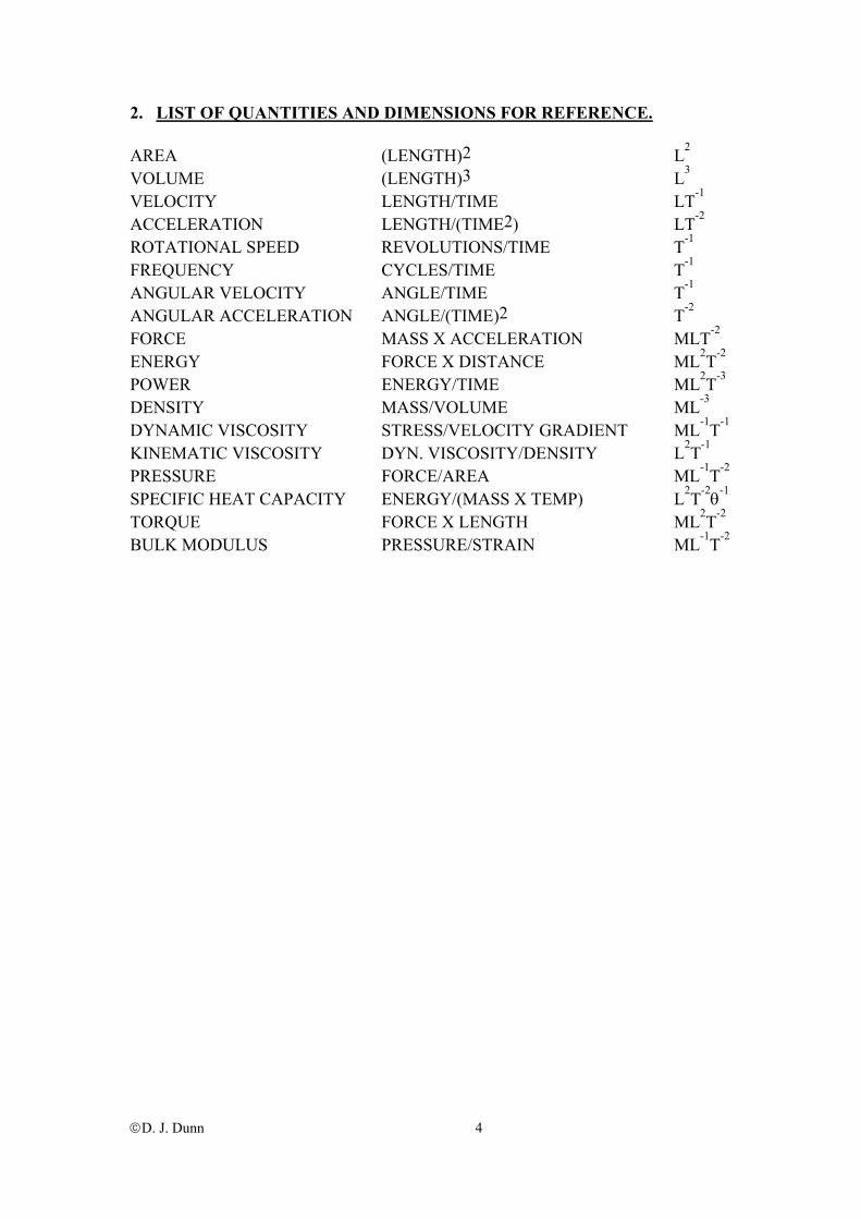
D. J. Dunn 4
2. LIST OF QUANTITIES AND DIMENSIONS FOR REFERENCE. AREA (LENGTH)2 L2 VOLUME (LENGTH)3 L3 VELOCITY LENGTH/TIME LT-1 ACCELERATION LENGTH/(TIME2) LT-2 ROTATIONAL SPEED REVOLUTIONS/TIME T-1 FREQUENCY CYCLES/TIME T-1
ANGULAR VELOCITY ANGLE/TIME T-1 ANGULAR ACCELERATION ANGLE/(TIME)2 T-2 FORCE MASS X ACCELERATION MLT-2 ENERGY FORCE X DISTANCE ML2T-2 POWER ENERGY/TIME ML2T-3 DENSITY MASS/VOLUME ML-3 DYNAMIC VISCOSITY STRESS/VELOCITY GRADIENT ML-1T-1 KINEMATIC VISCOSITY DYN. VISCOSITY/DENSITY L2T-1 PRESSURE FORCE/AREA ML-1T-2 SPECIFIC HEAT CAPACITY ENERGY/(MASS X TEMP) L2T-2
θ-1
TORQUE FORCE X LENGTH ML2T-2 BULK MODULUS PRESSURE/STRAIN ML-1T-2

D. J. Dunn 5
3. HOMOGENEOUS EQUATIONS All equations must be homogeneous. Consider the equation F = 3 + T/R F is force, T is torque and R is radius. Rearranging we have 3 = F - T/R Examine the units. F is Newton. T is Newton metre and R is metre. hence 3 = F (N) - T/R (N m)/m) 3 = F(N) - T/R (N) It follows that the number 3 must represent 3 Newton. It also follows that the unit of F and T/R must both be Newton. If this was not so, the equation would be nonsense. In other words all the components of an equation that add together must have the same units. You cannot add dissimilar quantities. For example you cannot say that 5 apples + 6 pears = 11 plums. This is clearly nonsense. When all parts of an equation that add together have the same dimensions, then the equation is homogeneous. WORKED EXAMPLE No.3 Show that the equation Power = Force x velocity is homogeneous in both S.I. units and basic dimensions. SOLUTION The equation to be checked is P = F v The S.I. Unit of power (P) is the Watt. The Watt is a Joule per second. A Joule is a Newton metre of energy. Hence a Watt is 1 N m/s. The S.I. unit of force (F) is the Newton and of velocity (v) is the metre/second. The units of F v are hence N m/s. It follows that both sides of the equation have S.I. units of N m/s so the equation is homogeneous. Writing out the MLT dimensions of each term we have [P] = ML2T-3
[v] = LT-1 [F] = MLT-2
Substituting into the equation we have ML2T-3 = MLT-2 LT-1= ML2T-3 Hence the equation is homogeneous.
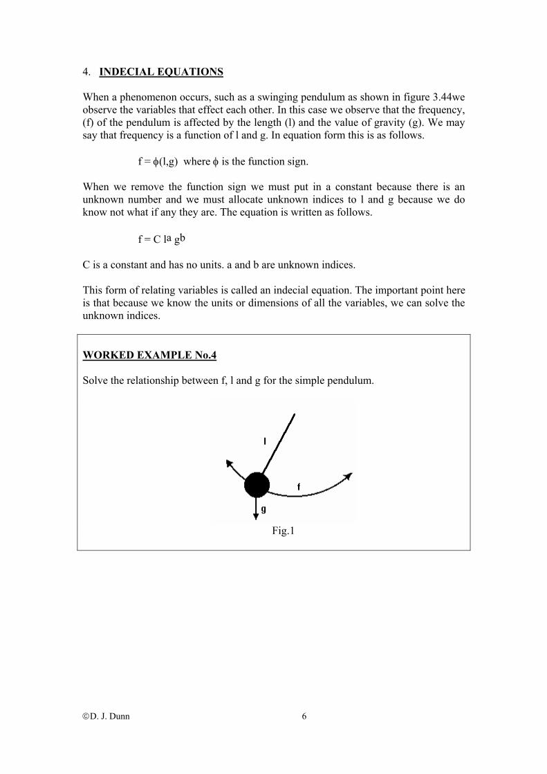
D. J. Dunn 6
4. INDECIAL EQUATIONS
When a phenomenon occurs, such as a swinging pendulum as shown in figure 3.44we observe the variables that effect each other. In this case we observe that the frequency, (f) of the pendulum is affected by the length (l) and the value of gravity (g). We may say that frequency is a function of l and g. In equation form this is as follows. f = φ(l,g) where φ is the function sign. When we remove the function sign we must put in a constant because there is an unknown number and we must allocate unknown indices to l and g because we do know not what if any they are. The equation is written as follows. f = C la gb C is a constant and has no units. a and b are unknown indices. This form of relating variables is called an indecial equation. The important point here is that because we know the units or dimensions of all the variables, we can solve the unknown indices. WORKED EXAMPLE No.4 Solve the relationship between f, l and g for the simple pendulum.
Fig.1

D. J. Dunn 7
SOLUTION
First write down the indecial form of the equation (covered overleaf).
f = C la gb Next write down the basic dimensions of all the variables. [f] = T-1 [l] = L1 [g] = LT-2 Next substitute the dimensions in place of the variables.
T-1= (L1)a (LT-2)b Next tidy up the equation. T-1= L1a LbT-2b Since the equation must be homogeneous then the power of each dimension must
be the same on the left and right side of the equation. If a dimension does not appear at all then it is implied that it exists to the power of zero. We may write them in until we get use to it. The equation is written as follows.
M0L0T-1= L1a LT-2bM0 Next we equate powers of each dimension. First equate powers of Time. T-1 = T-2b -1 = -2b b = 1/2 Next equate powers of Length. L0 = L1a Lb 0 = 1a + b hence a = -b = -1/2 M0 = M0 yields nothing in this case. Now substitute the values of a and b back into the original equation and we have
the following. f = C l-½ g½ f = C (g/l) ½ The frequency of a pendulum may be derived from basic mechanics and shown to
be f = (1/2π)(g/l) ½
D. J. Dunn 8
If we did not know how to find C = (½ π) from basic mechanics, then we know
that if we conducted an experiment and measured the values f for various values of l and g, we could find C by plotting a graph of f against (g/l) ½. This is the importance of dimensional analysis to fluid mechanics. We are able to determine the basic relationships and then conduct experiments and determine the remaining unknown constants. We are able to plot graphs because we know what to plot against what.
SELF ASSESSMENT EXERCISE No.1 1. It is observed that the velocity 'v' of a liquid leaving a nozzle depends upon the
pressure drop 'p' and the density 'ρ'. Show that the relationship between them is of the form
21
=
ρpCv
2. It is observed that the speed of a sound in 'a' in a liquid depends upon the density
'ρ' and the bulk modulus 'K'. Show that the relationship between them is
21
=
ρKCa
3. It is observed that the frequency of oscillation of a guitar string 'f' depends upon
the mass 'm', the length 'l' and tension 'F'. Show that the relationship between them is
21
=mlFCf

D. J. Dunn 9
5. DIMENSIONLESS NUMBERS We will now consider cases where the number of unknown indices to be solved, exceed the number of equations to solve them. This leads into the use of dimensionless numbers. Consider that typically a problem uses only the three dimensions M, L and T. This will yield 3 simultaneous equations in the solution. If the number of variables in the equation gives 4 indices say a, b, c and d, then one of them cannot be resolved and the others may only be found in terms of it. In general there are n unknown indices and m variables. There will be m-n unknown indices. This is best shown through a worked example. WORKED EXAMPLE No. 5 The pressure drop per unit length 'p' due to friction in a pipe depends upon the diameter 'D' , the mean velocity 'v' , the density 'ρ' and the dynamic viscosity 'µ'. Find the relationship between these variables. SOLUTION p = function (D v ρ µ) = K Da vb ρc µd p is pressure per metre [p] = ML-2T-2 [D] = L [v] = LT-1 [ρ] = ML-3 [µ] = ML-1T-1 ML-2T-2 = La (LT-1) b (ML-3) c(ML-1T-1) d ML-2T-2 =La+b-3c-d Mc+d T-b-d The problem is now deciding which index not to solve. The best way is to use experience gained from doing problems. Viscosity is the quantity that causes viscous friction so the index associated with it (d) is the one to identify. We will resolve a, b and c in terms of d. TIME -2 = -b - d hence b = 2 - d is as far as we can resolve MASS 1 = c + d hence c = 1 -d LENGTH -2 = a + b - 3c - d -2 = a +(2 -d) -3(1-d) – d hence a = -1 - d

D. J. Dunn 10
Next put these back into the original formula. p = K D-1-d v 2-d ρ1-d µd Next group the quantities with same power together as follows : p = K{ ρv2D-1} {µ ρ -1v-1D-1}d
Remember that p was pressure drop per unit length so the pressure loss over a length L is P = K L{ρ v2D-1} {µ ρ -1v-1D-1}d We have two unknown constants K and d. The usefulness of dimensional analysis is that it tells us the form of the equation so we can deduce how to present experimental data. With suitable experiments we could now find K and d. Note that this equation matches up with Poiseuille's equation which gives the relationship as : p = 32 µ L v D-2 It may be deduced that K = 32 and d = 1 (laminar flow only) The term {ρvDµ-1} has no units. If you check it out all the units will cancel. This is a DIMENSIONLESS NUMBER, and it is named after Reynolds. Reynolds Number is denoted Re.The whole equation can be put into a dimensionless form as follows. {p ρ-1 L-1 v-2D1} = K {µ ρ-1v-1D-1}d {p ρ-1 L-1 v-2D1} = function ( Re ) This is a dimensionless equation. The term {pρ-1 L -1v-2D1} is also a dimensionless number. Let us now examine another similar problem.

D. J. Dunn 11
WORKED EXAMPLE No.6 Consider a sphere moving through an viscous fluid completely submerged. The resistance to motion R depends upon the diameter D, the velocity v, the density ρ and the dynamic viscosity µ. Find the equation that relates the variables.
Figure 3.45
Fig.2 SOLUTION
R = function (D v ρ µ) = K Da vb ρc µd First write out the MLT dimensions. [R] = ML1T-2 [D] = L ML1T-2 = La (LT-1)b (ML-3) c(ML-1T-1)d [v] = LT-1 ML1T-2 =L a+b-3c-d M c+d T -b-d [ρ] = ML-3 [µ] = ML-1T-1 Viscosity is the quantity which causes viscous friction so the index associated
with it ( d) is the one to identify. We will resolve a,b and c in terms of d as before.
TIME -2 = -b - d hence b = 2 - d is as far as we can resolve b MASS 1 = c + d hence c = 1 - d LENGTH 1= a + b - 3c - d 1 = a +(2 -d) -3(1-d) - d hence a = 2-d Next put these back into the original formula.
R = K D2-d v2-d ρ1-d µd
D. J. Dunn 12
Next group the quantities with same power together as follows : R= K{ρv2D2} {µ ρ-1v-1D-1}d R{ρv2D2}-1 = K {µ ρ-1v-1D-1}d
The term {ρvDµ-1} is the Reynolds Number Re and the term R{ρv2D2}-1 is
called the Newton Number Ne. Hence the relationship between the variables may be written as follows.
R{ρv2D2}-1 = function {ρvD µ-1} Ne = function (Re) Once the basic relationship between the variables has been determined, experiments can be conducted to find the parameters in the equation. For the case of the sphere in an incompressible fluid we have shown that Ne = function (Re) Or put another way Ne = K (Re)n where K is a constant of proportionality and n is an unknown index (equivalent to -d in the earlier lines). In logarithmic form the equation is log(Ne ) = log (K) + n log(Re) This is a straight line graph from which log K and n are taken. Without dimensional analysis we would not have known how to present the information and plot it. The procedure now would be to conduct an experiment and plot log(Ne) against log(Re). From the graph we would then determine K and n.

D. J. Dunn 13
6. BUCKINGHAM'S Π (Pi) THEORY Many people prefer to find the dimensionless numbers by intuitive methods. Buckingham's theory is based on the knowledge that if there are m basic dimensions and n variables, then there are m - n dimensionless numbers. Consider worked example No.6 again. We had the basic equation R = function (D v ρ µ) There are 5 quantities and there will be 3 basic dimensions ML and T. This means that there will be 2 dimensionless numbers Π1 and Π2. These numbers are found by choosing two prime quantities (R and µ). Π1 is the group formed between µ and D v ρ Π2 is the group formed between R and D v ρ First taking µ. Experience tells us that this will be the Reynolds number but suppose we don't know this. The dimensions of µ are ML-1T-1 The dimensions of D v ρ must be arranged to be the same. µ = Π1 Da vb ρ c M1L-1T-1 = Π1 (L)a (LT-1)b (ML-3)c Time -1 = -b b = 1 Mass c = 1 Length -1 = a + b -3c -1 = a + 1 – 3 a=1
µ = Π1 D1 v1 ρ 1 ρ
µ=Π
Dv1
The second number must be formed by combining R with ρ,v and D R = Π2 Da vb ρ c MLT-2 =Π2 (L)a (LT-1)b(ML-3)c Time -2 = -b b = 2 Mass c = 1 Length 1 = a + b -3c 1 = a + 2 – 3 a = 2
R = Π2 D2 v2 ρ 1 222 Dv
Rρ
=Π
The dimensionless equation is Π2 = f(Π1)

D. J. Dunn 14
WORKED EXAMPLE No.7 The resistance to motion 'R' for a sphere of diameter 'D' moving at constant
velocity 'v' through a compressible fluid is dependant upon the density 'ρ' and the bulk modulus 'K'. The resistance is primarily due to the compression of the fluid in front of the sphere. Show that the dimensionless relationship between these quantities is Ne = function (Ma)
SOLUTION R = function (D v ρ K) = C Da vb ρc Kd There are 3 dimensions and 5 quantities so there will be 5 –3 = 2 dimensionless
numbers. Identify that the one dimensionless group will be formed with R and the other with K.
Π1 is the group formed between K and D v ρ Π2 is the group formed between R and D v ρ K = Π2 Da vb ρc R = Π1 Da vb ρc [K] = ML-1 T-2 [R] = MLT-2 [D] = L [D] = L [v] = LT-1 [v] = LT-1 [ρ] = ML-3 [ρ] = ML-3 ML-1T-2 = La (LT-1)b (ML-3)c MLT-2 = La (LT-1)b (ML-3)c ML-1T-2 =La+b-3c Mc T-b ML1T-2 =La+b-3c Mc T-b Time -2 = -b b = 2 Time -2 = -b b = 2 Mass c = 1 Mass c = 1 Length -1 = a + b -3c Length 1 = a + b -3c -1 = a + 2 – 3 a = 0 1 = a + 2 – 3 a = 2 K = Π2 Do v2 ρ 1 R = Π1 D2 v2 ρ 1
22 vKρ
=Π 221 DvR
ρ=Π
It was shown earlier that the speed of sound in an elastic medium is given by the
following formula. a = (k/ρ)½ It follows that (k/ρ) = a2 and so Π2 = (a/v)2 The ratio v/a is called the Mach number (Ma) so (Ma)-2 Π1 is the Newton Number Ne. The equation may be written as Π1 = φΠ2 Ne or Ne = φ(Ma)
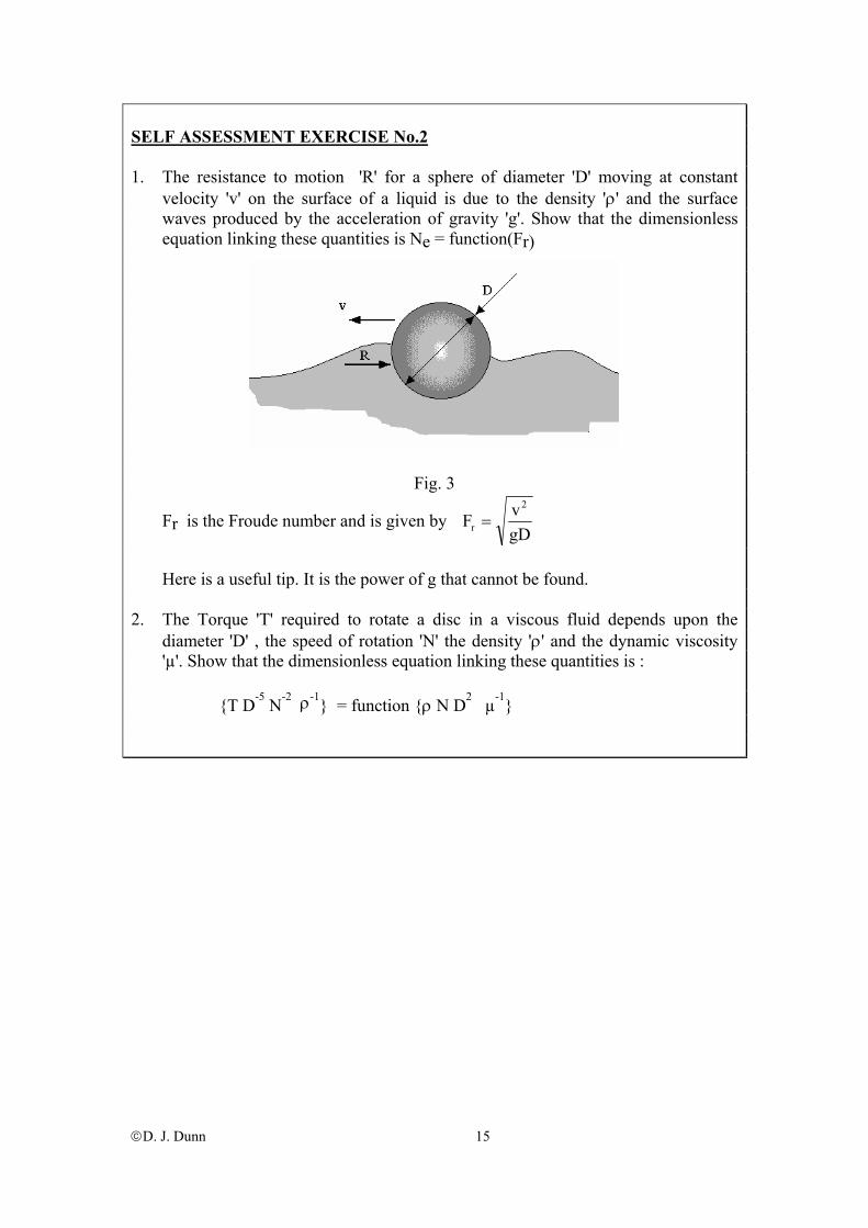
D. J. Dunn 15
SELF ASSESSMENT EXERCISE No.2 1. The resistance to motion 'R' for a sphere of diameter 'D' moving at constant
velocity 'v' on the surface of a liquid is due to the density 'ρ' and the surface waves produced by the acceleration of gravity 'g'. Show that the dimensionless equation linking these quantities is Ne = function(Fr)
Fig. 3
Fr is the Froude number and is given by gDvF
2
r =
Here is a useful tip. It is the power of g that cannot be found. 2. The Torque 'T' required to rotate a disc in a viscous fluid depends upon the
diameter 'D' , the speed of rotation 'N' the density 'ρ' and the dynamic viscosity 'µ'. Show that the dimensionless equation linking these quantities is :
{T D-5 N-2 ρ-1} = function {ρ N D2 µ-1}
D. J. Dunn 16
MORE DIFFICULT PROBLEMS The problems so far seen have one unknown index in the solution. When there are two (or more) unknown indexes, the procedure is the same as before. A group of quantities must be formed for each unknown index left in the penultimate part of the solution. SELF ASSESSMENT EXERCISE No.3 1. The resistance to motion 'R' of a sphere travelling through a fluid which is both
viscous and compressible, depends upon the diameter 'D' , the velocity 'v' , the density 'ρ' , the dynamic viscosity 'µ' and the bulk modulus 'K'. Show that the complete relationship between these quantities is :
Ne = function{Re } {Ma} where Ne = R ρ-1 v -2 D -2 Re = ρ v D µ-1 Ma = v/a and a = (k/ρ)0.5

D. J. Dunn 17
7 MODEL TESTING
When we test a model in order to predict the performance of the real thing, the results are only valid when the forces acting on the model are in the same ratio to each other as they are on the real thing. When this occurs we have DYNAMIC SIMILARITY. It will be shown that in order to have dynamic similarity, the model must also be a true scale model, in other words we must have GEOMETRIC SIMILARITY. 7.1 DYNAMIC SIMILARITY We have already seen that certain dimensionless numbers occur in problems of fluid mechanics. Each of these is associated with a particular kind of force. The Newton Number Ne is associated with total resistance. The Reynolds Number Re is associated with viscous resistance. The Mach Number Ma is associated with compression wave resistance. The Froude Number Fr is associated with surface wave resistance. There are others and all dimensionless numbers can take various forms. In order to obtain dynamic similarity, these dimensionless numbers must have the same values on the model and the real thing. Consider for example the resistance to motion of a sphere due to viscosity and compressibility of the fluid. The dimensionless equation is: Ne = φ(Re)(Ma) To ensure that the viscous, compression and resistance forces are in the same ratio to each other on the model and on the object, then the three numbers must be the same on both. This is often difficult or impossible to obtain when there are more than three numbers for reasons which will become apparent. 7.2 GEOMETRIC SIMILARITY In much of the forgoing work, the work has been about a sphere of diameter D so that only one actual length dimension was needed to define both the shape and size of the object. If we tried the same analysis for a submarine or an aeroplane, we should include all the linear dimensions necessary to define the shape and this would be enormous. Consider the following problem that needs two linear dimensions and it is the one we looked at previously in a slightly different way. The pressure drop p in a pipe depends upon the diameter D, the length l, the density ρ and the viscosity µ. Dimensional analysis shows that :
=
µρφ
ρvD
Dl
vp
2

D. J. Dunn 18
p/(ρv2) is a form of the Newton number and (ρvD/µ) is a form of the Reynolds number. It could have been arranged for Reynolds number to include l instead of D. Because we needed two linear dimensions D and l, we now have another dimensionless number (l/D) that is the ratio of the two. In a model test this must be made the same as for the object and if the ratio is the same then geometric similarity exists. If many such linear dimensions exist in a problem, then many dimensionless numbers will be created which are all the possible ratios of any one with all the others. To avoid all this work, we usually just assume a characteristic length. This is valid when geometric similarity exists as will become apparent. We may express our equation as :
( )Re
=dlNe φ
Removing the function sign gives :
( )ndlKNe Re
= where K is the constant of proportionality.
If we make the value of Re the same on the model and the real object and if we have geometric similarity , then since the function is the same for both (K and n) then it follows that the Newton number must be the same also. In other words since
( ) ( ) eln
elobjectn
object dlKNe
dlKNe modmod ReRe
==
=
Then {Ne}object ={Ne}model From this the resisting force may be predicted. Note that if we had many linear dimensions and many ratios like l/D, then they would also cancel so it is not necessary to include them, just a characteristic length. Let us finish this problem now as a worked example.

D. J. Dunn 19
WORKED EXAMPLE No.8 The pipe in the previous analysis is 200 m long and 0.5 m diameter and must
carry water with a mean velocity of 0.2 m/s. In order to predict the pressure drop, a model is made to a scale of 1/10. Calculate the velocity at which water must flow in the model in order to obtain dynamic similarity.
SOLUTION For this section we must obtain dynamic similarity by equating the Reynolds
numbers. Hence : (ρvD/µ)model = (ρvD/µ)object The density and viscosity will be the same in both since the same water is used so (vD)model = (vD)object v model x D/10 = 2 x D hence vmodel = 2 m/s When the model is tested at the velocity, the pressure drop is found to be 100kPa.
Predict the pressure drop in the real pipe. Since Re is now the same and l/D is the same for both cases then the Newton
number is the same so p/(ρv2)model =p/(ρv2)pipe Again density and viscosity cancel so we have 100/22 = p/0.22 p = 1 kPa on the full size pipe.

D. J. Dunn 20
WORKED EXAMPLE No.9a The resistance to motion R of a hydrofoil depends upon the characteristic length
l, the velocity v, the density ρ and the acceleration of gravity g. It may be shown that Ne= f(Fr) where Ne = R/(ρv2l2) and Fr = v/(gl)1/2 In order to predict the resistance of a hydrofoil, a model is made to a scale of
1/20. The actual hydrofoil must move at 0.8 m/s over water. Calculate the velocity of the model that gives dynamic similarity on the same water.
SOLUTION For dynamic similarity the Froude numbers must be made the same. v/(gl)1/2 model = v/(gl)1/2(hydrofoil) v/(l)1/2 model = v/(l)1/2(hydrofoil) vmodel x (20/l)1/2 =0.8 /l1/2 vmodel =0.8 /201/2 vmodel = 0.179 m/s

D. J. Dunn 21
WORKED EXAMPLE No.9b The model is tested at 0.179 m/s and the resistance to motion was found to be
2.2N. Predict the resistance of the hydrofoil at 0.8 m/s. SOLUTION Since the Froude number is the same and the function is the same then the
Newton number must be the same for both. R/(ρv2l2)model=R/(ρv2l2)hydrofoil Since the density is the same then {2.2 x 202/(0.179 l)2}= {R/(vl)2 R = 17 570 N

D. J. Dunn 22
SELF ASSESSMENT EXERCISE No.4 1. (a) The viscous torque produced on a disc rotating in a liquid depends upon the
characteristic dimension D, the speed of rotation N, the density ρ and the dynamic viscosity µ. Show that :
{T/(ρN2D5)} =f(ρND2/µ) (b) In order to predict the torque on a disc 0.5 m diameter which rotates in oil at
200 rev/min, a model is made to a scale of 1/5. The model is rotated in water. Calculate the speed of rotation for the model which produces dynamic similarity.
For the oil the density is 750 kg/m3 and the dynamic viscosity is 0.2 Ns/m2. For water the density is 1000 kg/m3 and the dynamic viscosity is 0.001 Ns/m2. (The answer is 18.75 rev/min) (c) When the model is tested at 18.75 rev/min the torque was 0.02 Nm. Predict
the torque on the full size disc at 200 rev/min. (Ans 5 333 N) 2. The resistance to motion of a submarine due to viscous resistance is given by : {R/(ρv2D2)} =f(ρvD/µ) where D is the characteristic dimension. The submarine moves at 8 m/s through sea water. In order to predict its
resistance, a model is made to a scale of 1/100 and tested in fresh water. Determine the velocity at which the model should be tested. (690.7 m/s)
The density of sea water is 1036 kg/m3 The density of fresh water is 1000 kg/m3 The viscosity of sea water is 0.0012 N s/m2. The viscosity of fresh water is 0.001 N s/m2. When run at the calculated speed, the model resistance was 200 N. Predict the
resistance of the submarine. (278 N).

D. J. Dunn 23
3. The resistance of an aeroplane is due to, viscosity and compressibility of the
fluid. Show that: {R/(ρv2D2)} =f(Ma) (Re) An aeroplane is to fly at an altitude of 30 km at Mach 2.0. A model is to be made
to a suitable scale and tested at a suitable velocity at ground level. Determine the velocity of the model that gives dynamic similarity for the Mach number and then using this velocity determine the scale which makes dynamic similarity in the Reynolds number. (680.6 m/s and 1/61.86)
The properties of air are sea level a= 340.3 m/s µ= 1.7897 x 10⁻⁵ ρ = 1.225 kg/m3 30 km a= 301.7 m/s µ= 1.4745 x 10⁻⁵ ρ = 0.0184 kg/m3 When built and tested at the correct speed, the resistance of the model was 50 N.
Predict the resistance of the aeroplane. (2 259 N). 4. The force on a body of length 3 m placed in an air stream at 1 bar and moving at
60 m/s is to be found by testing a scale model. The model is 0.3 m long and placed in high pressure air moving at 30 m/s. Assuming the same temperature and viscosity, determine the air pressure which produced dynamic similarity.
The force on the model is found to be 500 N. Predict the force on the actual body. (Ans. 20 bar and 10 kN). 5. Show by dimensional analysis that the velocity profile near the wall of a pipe
containing turbulent flow is of the form u+ = f(y+) where u+ = u(ρ/τo)1/2 and y+ = y(ρτo)1/2/µ When water flows through a smooth walled pipe 60 mm bore diameter at 0.8 m/s,
the velocity profile is u+ = 2.5ln(y+) + 5.5 Find the velocity 10 mm from the wall. The friction coefficient is Cf = 0.079 Re
-0.25. Answer 0.85 m/s

©D.J.Dunn freestudy.co.uk 1
FLUID MECHANICS
TUTORIAL No.7
FLUID FORCES When you have completed this tutorial you should be able to
• Solve forces due to pressure difference. • Solve problems due to momentum changes. • Solve problems involving pressure and momentum changes. • Solve forces on pipe bends. • Solve problems on stationary vanes. • Construct blade vector diagrams for moving vanes. • Calculate the momentum changes over a moving vane.
Let's start by examining forces due to pressure changes.

1. PRESSURE FORCES Consider a duct as shown in fig.1. First identify the control volume on which to conduct a force balance. The inner passage is filled with fluid with pressure p1 at inlet and p2 at outlet. There will be forces on the outer surface of the volume due to atmospheric pressure. If the pressures of the fluid are measured relative to atmosphere (i.e. use gauge pressures) then these forces need not be calculated and the resultant force on the volume is due to that of the fluid only. The approach to be used here is to find the forces in both the x and y directions and then combine them to find the resultant force.
Fig. 1
The force normal to the plane of the bore is pA. At the inlet (1) the force is Fp1= p1A1 At the outlet (2) the force is Fp2 = p2A2 These forces must be resolved vertically and horizontally to give the following. Fpx1 = Fp1 cos θ1 (to the right) Fpx2 = Fp1 cos θ2 (to the left) The total horizontal force FH = Fpx1 - Fpx2 Fpy1 = Fp1 sin θ1 (up) Fpy2 = Fp2 sin θ2 (down) The total vertical force FV = Fpy1 - Fpy2
©D.J.Dunn freestudy.co.uk 2

WORKED EXAMPLE No. 1 A nozzle has an inlet area of 0.005 m2 and it discharges into the atmosphere. The inlet gauge pressure is 3 bar. Calculate the resultant force on the nozzle.
Fig.2 SOLUTION Since the areas are only in the vertical plane, there is no vertical force. FV = 0 Using gauge pressures, the pressure force at exit is zero. Fpx2 = 0 Fpx1 = 3 x 105 x 0.005 = 1500 N FH = 1500 – 0 = 1500 N to the right. WORKED EXAMPLE No.2 The nozzle shown has an inlet area of 0.002 m2
and an outlet area of 0.0005 m2. The inlet gauge pressure is 300 kPa and the outlet gauge pressure is 200 kPa. Calculate the horizontal and vertical forces on the nozzle.
Fig.3
SOLUTION Fp1= 300 x 103 x 0.002 = 600 N Fpx1= 600 N Fpy1=0 N since the plane is vertical. Fp2 = 200 x 103 x 0.0005 = 100 N Fpx2 = 100 x cos 60o = 50 N Fpy2 = 100 x sin 60o = 86.67 N Total Horizontal force FH = 600 - 50 = 550 N Total vertical force FV = 0 - 86.67 N = - 86.67 N
©D.J.Dunn freestudy.co.uk 3
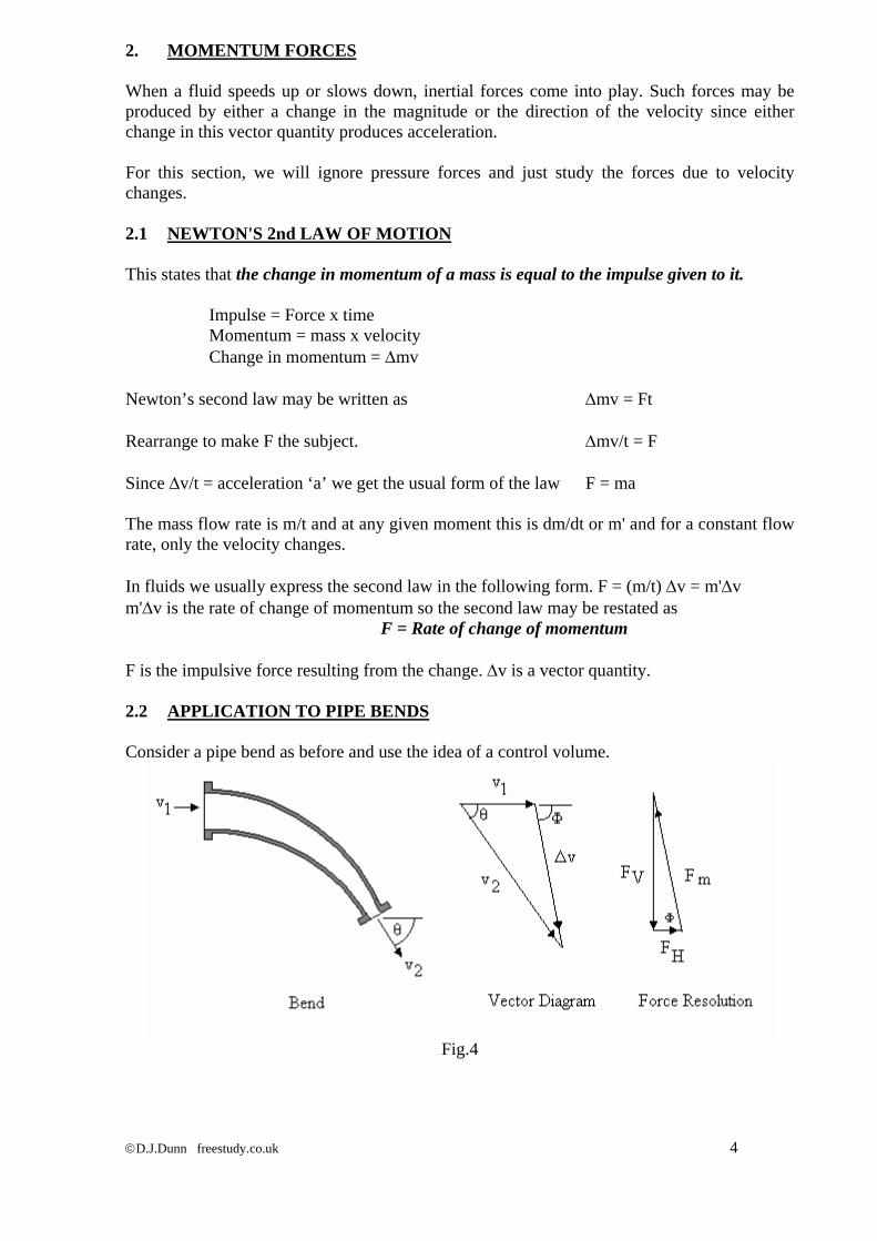
2. MOMENTUM FORCES When a fluid speeds up or slows down, inertial forces come into play. Such forces may be produced by either a change in the magnitude or the direction of the velocity since either change in this vector quantity produces acceleration. For this section, we will ignore pressure forces and just study the forces due to velocity changes. 2.1 NEWTON'S 2nd LAW OF MOTION This states that the change in momentum of a mass is equal to the impulse given to it. Impulse = Force x time Momentum = mass x velocity Change in momentum = ∆mv Newton’s second law may be written as ∆mv = Ft Rearrange to make F the subject. ∆mv/t = F Since ∆v/t = acceleration ‘a’ we get the usual form of the law F = ma The mass flow rate is m/t and at any given moment this is dm/dt or m' and for a constant flow rate, only the velocity changes. In fluids we usually express the second law in the following form. F = (m/t) ∆v = m'∆v m'∆v is the rate of change of momentum so the second law may be restated as F = Rate of change of momentum F is the impulsive force resulting from the change. ∆v is a vector quantity. 2.2 APPLICATION TO PIPE BENDS Consider a pipe bend as before and use the idea of a control volume.
Fig.4
©D.J.Dunn freestudy.co.uk 4

First find the vector change in velocity using trigonometry.
( ) ( ){ }21
212
22
12
2 vcosθvsinθv∆v vcosθv
sinθvtanΦ −+=−
=
Alternatively ∆v could be found by drawing the diagram to scale and measuring it. If we had no change in magnitude then v1 = v2 = v then ∆v= v {2(1 - cosθ)}½
The momentum force acting on the fluid is Fm = m'∆v The force is a vector quantity which must be in the direction of ∆v. Every force has an equal and opposite reaction so there must be a force on the bend equal and opposite to the force on the fluid. This force could be resolved vertically and horizontally such that FH = FmcosΦ and FV = FmsinΦ This theory may be applied to turbines and pump blade theory as well as to pipe bends. SELF ASSESSMENT EXERCISE No.1 1. A pipe bends through an angle of 90o in the vertical plane. At the inlet it has a cross
sectional area of 0.003 m2 and a gauge pressure of 500 kPa. At exit it has an area of 0.001 m2 and a gauge pressure of 200 kPa.
Calculate the vertical and horizontal forces due to the pressure only. (Answers 200 N and 1500 N). 2. A pipe bends through an angle of 45o in the vertical plane. At the inlet it has a cross
sectional area of 0.002 m2 and a gauge pressure of 800 kPa. At exit it has an area of 0.0008 m2 and a gauge pressure of 300 kPa.
Calculate the vertical and horizontal forces due to the pressure only. (Answers 169.7 N and 1430 N). 3. Calculate the momentum force acting on a bend of 130o that carries 2 kg/s of water at
16m/s velocity. Determine the vertical and horizontal components. (Answers 24.5 N and 52.6 N) 4. Calculate the momentum force on a 180o bend that carries 5 kg/s of water. The pipe is 50
mm bore diameter throughout. The density is 1000 kg/m3. (Answer 25.46 N) 5. A horizontal pipe bend reduces from 300 mm bore diameter at inlet to 150 mm diameter
at outlet. The bend is swept through 50o from its initial direction. The flow rate is 0.05 m3/s and the density is 1000 kg/m3. Calculate the momentum force
on the bend and resolve it into two perpendicular directions relative to the initial direction.
(Answers 108.1 N and 55.46 N).
©D.J.Dunn freestudy.co.uk 5
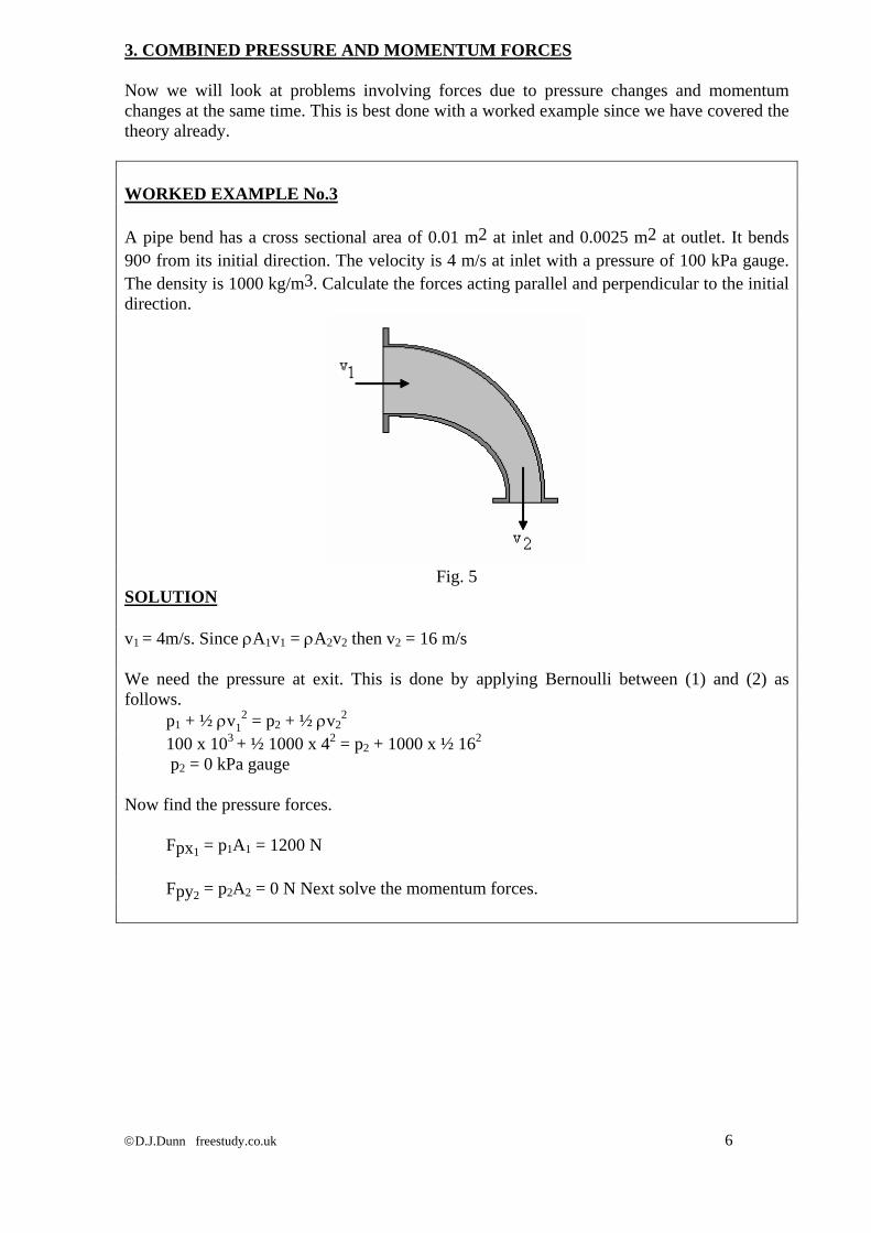
3. COMBINED PRESSURE AND MOMENTUM FORCES Now we will look at problems involving forces due to pressure changes and momentum changes at the same time. This is best done with a worked example since we have covered the theory already. WORKED EXAMPLE No.3 A pipe bend has a cross sectional area of 0.01 m2 at inlet and 0.0025 m2 at outlet. It bends 90o from its initial direction. The velocity is 4 m/s at inlet with a pressure of 100 kPa gauge. The density is 1000 kg/m3. Calculate the forces acting parallel and perpendicular to the initial direction.
Fig. 5
SOLUTION v1 = 4m/s. Since ρA1v1 = ρA2v2 then v2 = 16 m/s We need the pressure at exit. This is done by applying Bernoulli between (1) and (2) as follows. p1 + ½ ρv1
2 = p2 + ½ ρv22
100 x 103 + ½ 1000 x 42 = p2 + 1000 x ½ 162
p2 = 0 kPa gauge Now find the pressure forces. Fpx1 = p1A1 = 1200 N Fpy2 = p2A2 = 0 N Next solve the momentum forces.
©D.J.Dunn freestudy.co.uk 6

Fig.6
m' = ρAv = 40 kg/s ∆v = (42 + 162)½ = 16.49 m/s Fm = m'∆v = 659.7 N φ = tan-1(16/4) = 75.96o RESOLVE Fmy = 659.7 sin 75.96 = 640 N Fmx = 659.7 cos 75.96 = 160 N Total forces in x direction = 1200 + 160 = 1360 N Total forces in y direction = 0 + 640 = 640 N ALTERNATIVE SOLUTION Many people prefer to solve the complete problems by solving pressure and momentum forces in the x or y directions as follows. x direction m'v1 + p1A1 = FX = 1200 N y direction m'v2 + p2A2 = FY = 640 N When the bend is other than 90o this has to be used more carefully because there is an x component at exit also.
©D.J.Dunn freestudy.co.uk 7

4. APPLICATIONS TO STATIONARY VANES When a jet of fluid strikes a stationary vane, the vane decelerates the fluid in a given direction. Even if the speed of the fluid is unchanged, a change in direction produces changes in the velocity vectors and hence momentum forces are produced. The resulting force on the vane being struck by the fluid is an impulsive force. Since the fluid is at atmospheric pressure at all times after leaving the nozzle, there are no forces due to pressure change. 4.1 FLAT PLATE NORMAL TO JET Consider first a jet of liquid from a nozzle striking a flat plate as shown in figure 7.
Fig.7
The velocity of the jet leaving the nozzle is v1. The jet is decelerated to zero velocity in the original direction. Usually the liquid flows off sideways with equal velocity in all radial directions with no splashing occurring. The fluid is accelerated from zero in the radial directions but since the flow is equally divided no resultant force is produced in the radial directions. This means the only force on the plate is the one produced normal to the plate. This is found as follows. m' = mass flow rate. Initial velocity = v1. Final velocity in the original direction = v2 = 0. Change in velocity =∆v = v2 – v1= - v1
Force = m'∆v = -mv1 This is the force required to produce the momentum changes in the fluid. The force on the plate must be equal and opposite so F = m'v1 = ρA v1
©D.J.Dunn freestudy.co.uk 8

WORKED EXAMPLE No.4 A nozzle has an exit diameter of 15 mm and discharges water into the atmosphere. The gauge pressure behind the nozzle is 400 kPa. The coefficient of velocity is 0.98 and there is no contraction of the jet. The jet hits a stationary flat plate normal to its direction. Determine the force on the plate. The density of the water is 1000 kg/m3. Assume the velocity of approach into the nozzle is negligible. SOLUTION The velocity of the jet is v1 = Cv(2∆p/ρ)½
v1 = 0.98 (2x 400 000/1000) ½ = 27.72 m/s The nozzle exit area A = π x 0.0152/4 = 176.7 x 10⁻⁶ m2. The mass flow rate is ρAv1 = 1000 x 176.7 x 10-6 x 27.72 = 4.898 kg/s. The force on the vane = 4.898 x 27.72 = 135.8 N 4.2 FLAT PLATE AT ANGLE TO JET If the plate is at an angle as shown in fig. 8 then the fluid is not completely decelerated in the original direction but the radial flow is still equal in all radial directions. All the momentum normal to the plate is destroyed. It is easier to consider the momentum changes normal to the plate rather than normal to the jet.
Fig.8
Initial velocity normal to plate = v1 cosθ. Final velocity normal to plate = 0. Force normal to plate = m'∆v =0 - ρA v1 cosθ. This is the force acting on the fluid so the force on the plate is m' v1 cosθ or ρA v1
2 cosθ. If the horizontal and vertical components of this force are required then the force must be resolved.
©D.J.Dunn freestudy.co.uk 9

WORKED EXAMPLE No. 5 A jet of water has a velocity of 20 m/s and flows at 2 kg/s. The jet strikes a stationary flat plate. The normal direction to the plate is inclined at 30o to the jet. Determine the force on the plate in the direction of the jet. SOLUTION
Fig.9
The force normal to the plate is mv1 cosθ = 2 x 20cos 30o = 34.64 N. The force in the direction of the jet is found by resolving. FH = F/cos30o = 34.64/cos 30o = 40 N
©D.J.Dunn freestudy.co.uk 10

4.3 CURVED VANES When a jet hits a curved vane, it is usual to arrange for it to arrive on the vane at the same angle as the vane. The jet is then diverted from with no splashing by the curve of the vane. If there is no friction present, then only the direction of the jet is changed, not its speed.
Fig.10
This is the same problem as a pipe bend with uniform size. v1 is numerically equal to v2.
Fig.11
If the deflection angle is θ as shown in figs.10 and 11 then the impulsive force is F = m'∆v = m' v1{2(1 - cosθ)}1/2
The direction of the force on the fluid is in the direction of ∆v and the direction of the force on the vane is opposite. The force may be resolved to find the forces acting horizontally and/or vertically. It is often necessary to solve the horizontal force and this is done as follows.
Fig.12
Initial horizontal velocity = vH1 = v1
Final horizontal velocity = vH2 = -v2 cos (180 - θ) = v2 cos θ Change in horizontal velocity = ∆vH1 Since v2 = v1 this becomes ∆vh= {v2 cosθ - v1 } = v1{cosθ - 1} Horizontal force on fluid = m'v1{cosθ - 1} The horizontal force on the vane is opposite so Horizontal force = m'∆vH = m'v1{1 - cosθ}
©D.J.Dunn freestudy.co.uk 11

WORKED EXAMPLE No.6 A jet of water travels horizontally at 16 m/s with a flow rate of 2 kg/s. It is deflected 130o by a curved vane. Calculate resulting force on the vane in the horizontal direction. SOLUTION The resulting force on the vane is F = m' v1{2(1 - cosθ)½
F = 2 x 16 {2(1 -cos 130o)} ½ = 58 N The horizontal force is FH = m' v1{cosθ - 1} FH = 2 x 16 x (1 - cos130) FH = 52.6 N SELF ASSESSMENT EXERCISE No. 2 Assume the density of water is 1000 kg/m3 throughout. 1. A pipe bends through 90o from its initial direction as shown in fig.13. The pipe reduces
in diameter such that the velocity at point (2) is 1.5 times the velocity at point (1). The pipe is 200 mm diameter at point (1) and the static pressure is 100 kPa. The volume flow rate is 0.2 m3/s. Assume there is no friction. Calculate the following.
a) The static pressure at (2). b) The velocity at (2). c) The horizontal and vertical forces on the bend FH and FV. d) The total resultant force on the bend.
Fig.13
©D.J.Dunn freestudy.co.uk 12

©D.J.Dunn freestudy.co.uk 13
2. A nozzle produces a jet of water. The gauge pressure behind the nozzle is 2 MPa. The
exit diameter is 100 mm. The coefficient of velocity is 0.97 and there is no contraction of the jet. The approach velocity is negligible. The jet of water is deflected 165o from its initial direction by a stationary vane. Calculate the resultant force on the nozzle and on the vane due to momentum changes only.
(Answers 29.5 kN and 58.5 kN). 3. A stationary vane deflects 5 kg/s of water 50o from its initial direction. The jet velocity is
13 m/s. Draw the vector diagram to scale showing the velocity change. Deduce by either scaling or calculation the change in velocity and go on to calculate the force on the vane in the original direction of the jet.
(Answer 49.8 N). 4. A jet of water travelling with a velocity of 25 m/s and flow rate 0.4 kg/s is deflected 150o
from its initial direction by a stationary vane. Calculate the force on the vane acting parallel to and perpendicular to the initial direction.
(Answers 18.66 N and 5 N) 5. A jet of water discharges from a nozzle 30 mm diameter with a flow rate of 15 dm3/s into
the atmosphere. The inlet to the nozzle is 100 mm diameter. There is no friction nor contraction of the jet. Calculate the following.
i. The jet velocity.(21.22 m/s) ii. The gauge pressure at inlet. (223.2 kPa) iii. The force on the nozzle. (2039 N) The jet strikes a flat stationary plate normal to it. Determine the force on the plate. (312 N)

5. MOVING VANES When a vane moves away from the jet as shown on fig.14, the mass flow arriving on the vane is reduced because some of the mass leaving the nozzle is producing a growing column of fluid between the jet and the nozzle. This is what happens in turbines where the vanes are part of a revolving wheel. We need only consider the simplest case of movement in a straight line in the direction of the jet. 5.1 MOVING FLAT PLATE
Fig.14
The velocity of the jet is v and the velocity of the vane is u. If you were on the plate, the velocity of the fluid arriving would be v - u. This is the relative velocity, that is, relative to the plate. The mass flow rate arriving on the plate is then m' = ρA(v-u) The initial direction of the fluid is the direction of the jet. However, due to movement of the plate, the velocity of the fluid as it leaves the edge is not at 90o to the initial direction. In order to understand this we must consider the fluid as it flows off the plate. Just before it leaves the plate it is still travelling forward with the plate at velocity u. When it leaves the plate it will have a true velocity that is a combination of its radial velocity and u. The result is that it appears to come off the plate at a forward angle as shown. We are only likely to be interested in the force in the direction of movement so we only require the change in velocity of the fluid in this direction. The initial forward velocity of the fluid = v The final forward velocity of the fluid = u The change in forward velocity = v-u The force on the plate = m'ρv = m' (v-u) Since m' = ρA(v-u) then the force on the plate is F = ρA(v-u)2
©D.J.Dunn freestudy.co.uk 14

5.2 MOVING CURVED VANE Turbine vanes are normally curved and the fluid joins it at the same angle as the vane as shown in fig.15.
Fig.15
The velocity of the fluid leaving the nozzle is v1. This is a true or absolute velocity as observed by anyone standing still on the ground. The fluid arrives on the vane with relative velocity v1-u as before. This is a relative velocity as observed by someone moving with the vane. If there is no friction then the velocity of the fluid over the surface of the vane will be v1-u at all points. At the tip where the fluid leaves the vane, it will have two velocities. The fluid will be flowing at v1-u over the vane but also at velocity u in the forward direction. The true velocity v2 at exit must be the vector sum of these two.
Fig.16 If we only require the force acting on the vane in the direction of movement then we must find the horizontal component of v2. Because this direction is the direction in which the vane is whirling about the centre of the wheel, it is called the velocity of whirl vw2. The velocity v1 is also in the direction of whirling so it follows that v1 = vw1. Vw2 may be found by drawing the vector diagram (fig.16) to scale or by using trigonometry. In this case you may care to show for yourself that vw2 = u + (v1-u)(cosθ) The horizontal force on the vane becomes FH = m' (vw1-vw2) = m' (v1-vw2) You may care to show for yourself that this simplifies down to Fh = m'(v1-u)(1-cosθ) This force moves at the same velocity as the vane. The power developed by a force is the product of force and velocity. This is called the Diagram Power (D.P.) and the diagram power developed by a simple turbine blade is D.P. = m'u(v1-u)(1-cosθ) This work involving the force on a moving vane is the basis of turbine problems and the geometry of the case considered is that of a simple water turbine known as a Pelton Wheel. You are not required to do this in the exam. It is unlikely that the examination will require you to calculate the force on the moving plate but the question in self assessment exercise 5 does require you to calculate the exit velocity v2.
©D.J.Dunn freestudy.co.uk 15
©D.J.Dunn freestudy.co.uk 16
WORKED EXAMPLE No.7 A simple turbine vane as shown in fig.15 moves at 40 m/s and has a deflection angle of
150o. The jet velocity from the nozzle is 70 m/s and flows at 1.7 kg/s. Calculate the absolute velocity of the water leaving the vane and the diagram power. SOLUTION Drawing the vector diagram (fig.16) to scale, you may show that v2 = 20.5 m/s. This may
also be deduced by trigonometry. The angle at which the water leaves the vane may be measured from the diagram or deduced by trigonometry and is 46.9o to the original jet direction.
D.P. = m'u(v1-u)(1+cosθ) = 1.7 x 40(70-40)(1 - cos 150) = 3807 Watts SELF ASSESSMENT EXERCISE No.3 1. A vane moving at 30 m/s has a deflection angle of 90o. The water jet moves at 50 m/s
with a flow of 2.5 kg/s. Calculate the diagram power assuming that all the mass strikes the vane.
(Answer 1.5 kW). 2. Figure 10 shows a jet of water 40 mm diameter flowing at 45 m/s onto a curved fixed
vane. The deflection angle is 150o. There is no friction. Determine the magnitude and direction of the resultant force on the vane. (4916 N)
The vane is allowed to move away from the nozzle in the same direction as the jet at a
velocity of 18 m/s. Draw the vector diagram for the velocity at exit from the vane and determine the magnitude and direction of the velocity at exit from the vane. (14.53 m/s)

©D.J.Dunn freestudy.co.uk 1
FLUID MECHANICS
TUTORIAL No.8A
WATER TURBINES When you have completed this tutorial you should be able to
• Explain the significance of specific speed to turbine selection. • Explain the general principles of
Pelton Wheels Kaplan Turbines Francis Turbine
• Construct blade vector diagrams for moving vanes for a Pelton Wheels and a Francis Turbine
• Deduce formulae for power and efficiency for turbines. • Solve numerical problems for a Pelton Wheels and a Francis
Turbine

1. INTRODUCTION A water turbine is a device for converting water (fluid) power into shaft (mechanical) power. A pump is a device for converting shaft power into water power. Two basic categories of machines are the rotary type and the reciprocating type. Reciprocating motors are quite common in power hydraulics but the rotary principle is universally used for large power devices such as on hydroelectric systems. Large pumps are usually of the rotary type but reciprocating pumps are used for smaller applications. 1.1 THE SPECIFIC SPEED FOR VARIOUS TYPES OF TURBINES The power 'P' of any rotary hydraulic machine (pump or motor) depends upon the density 'ρ' , the speed 'N', the characteristic diameter 'D', the head change '∆H', the volume flow rate 'Q' and the gravitational constant 'g'. The general equation is: P = f(ρ, N, D, ∆H, Q, g) It is normal to consider g∆H as one quantity. P = f{ρ, N, D, (g∆H),Q} There are 6 quantities and 3 dimensions so there are three dimensionless groups Π1, Π2and Π3. First form a group with P and ρND.
( )( ) ( ) ( )
tCoefficienPower DNρ
PΠ DNρΠP
5c c 3- c-3a2Length 3b b3 Time a1 MassDTMLTLM
DNρΠρNDφP
531531
1
c1b1a3321
cba1
===
=+=+==−=−==
==−−−
Next repeat the process between Q and ρND ( )
( ) ( ) ( )
tCoefficien Flow ND
QΠ DNρΠQ
3c c-3a3Length a0 Mass 1b b1- TimeDTMLTM
DNρΠρNDφQ
32310
2
c1b1a313
cba2
===
=+===−==
==−−−
Next repeat the process between g∆H and ρND ( )( ) ( ) ( )
tCoefficien Head DN
QΠ DNρΠQ
2c c-3a2Length 2b b2- Time a0 MassDTMLTLM
DNρΠρNDφ∆H) (g
223220
3
c1b1a3220
cba3
===
=+==−===
==−−−
Finally the complete equation is ⎟⎠⎞
⎜⎝⎛⎟⎠⎞
⎜⎝⎛= 22253 DN
∆H gND
QφDρN
P
©D.J.Dunn freestudy.co.uk 2

SPECIFIC SPEED Ns The specific speed is a parameter used for pumps and turbines to determine the best design to match a given pumped system. The formula may be derived from consideration of the pump geometry or by dimensional analysis. The latter will be used here.
⎟⎠⎞
⎜⎝⎛⎟⎠⎞
⎜⎝⎛= 22253 DN
∆H gND
QφDρN
P
The three dimensionless numbers represent the Power coefficient, the flow coefficient and the Head coefficient respectively. Now consider a family of geometrically similar machines operating at dynamically similar conditions. For this to be the case the coefficients must have the same values for each size. Let the 3 coefficients be Π1, Π2 and Π3 such that
43
21
s21
43
21
21
21
432
3
31
21
32
31
21
21
31
2
21
3
32
31
21
31
31
2
31
21
3
21
32
31
2
21
32223
31
232531
∆H) (
NQN constant K
∆H) (
NQ
QK
∆H) (N
KQ
∆H) (
N
KQ
∆H) ( constant
gΠ
Π
NQ
∆H) (
NΠ
QΠ∆H g
N1
ΠN∆H g
NΠQ Equating
ΠN∆H gD
DN∆H gΠ
NΠQ D
NDQΠ
DρNPΠ
=====⎥⎥⎥
⎦
⎤
⎢⎢⎢
⎣
⎡
===
=⎟⎟⎠
⎞⎜⎜⎝
⎛⎟⎟⎠
⎞⎜⎜⎝
⎛=⎟⎟
⎠
⎞⎜⎜⎝
⎛
⎟⎟⎠
⎞⎜⎜⎝
⎛==⎟⎟
⎠
⎞⎜⎜⎝
⎛===
−
Ns is a dimensionless parameter that and the units used are normally rev/min for speed, m3/s for flow rate and metres for head. Other units are often used and care should be taken when quoting Ns values. It follows that for a given speed, the specific speed is large for large flows and low heads and small for small flows and large heads. The important value is the one that corresponds to the conditions that produce the greatest efficiency. The diagram illustrates how the design affects the specific speed.
Figure 1
©D.J.Dunn freestudy.co.uk 3

©D.J.Dunn freestudy.co.uk 4
2. GENERAL PRINCIPLES OF TURBINES. WATER POWER This is the fluid power supplied to the machine in the form of pressure and volume. Expressed in terms of pressure head the formula is W.P. = mg∆H M is the mass flow rate in kg/s and ∆H is the pressure head difference over the turbine in metres. Remember that ∆p = ρg∆H Expressed in terms of pressure the formula is W.P. = Q∆p Q is the volume flow rate in m3/s. ∆p is the pressure drop over the turbine in N/m2 or Pascals. SHAFT POWER This is the mechanical, power output of the turbine shaft. The well known formula is
S.P. = 2πNT Where T is the torque in Nm and N is the speed of rotation in rev/s DIAGRAM POWER This is the power produced by the force of the water acting on the rotor. It is reduced by losses before appearing as shaft power. The formula for D.P. depends upon the design of the turbine and involves analysis of the velocity vector diagrams. HYDRAULIC EFFICIENCY This is the efficiency with which water power is converted into diagram power and is given by ηhyd= D.P./W.P. MECHANICAL EFFICIENCY This is the efficiency with which the diagram power is converted into shaft power. The difference is the mechanical power loss. ηmech= S.P./D.P. OVERALL EFFICIENCY This is the efficiency relating fluid power input to shaft power output. ηo/a= S.P./W.P. It is worth noting at this point that when we come to examine pumps, all the above expressions are inverted because the energy flow is reversed in direction. The water power is converted into shaft power by the force produced when the vanes deflect the direction of the water. There are two basic principles in the process, IMPULSE and REACTION.

IMPULSE occurs when the direction of the fluid is changed with no pressure change. It follows that the magnitude of the velocity remains unchanged. REACTION occurs when the water is accelerated or decelerated over the vanes. A force is needed to do this and the reaction to this force acts on the vanes. Impulsive and reaction forces are determined by examining the changes in velocity (magnitude and direction) when the water flows over the vane. The following is a typical analysis. The vane is part of a rotor and rotates about some centre point. Depending on the geometrical layout, the inlet and outlet may or may not be moving at the same velocity and on the same circle. In order to do a general study, consider the case where the inlet and outlet rotate on two different diameters and hence have different velocities.
Fig.2
u1 is the velocity of the blade at inlet and u2 is the velocity of the blade at outlet. Both have tangential directions.ω1 is the relative velocity at inlet and ω2 is the relative velocity at outlet. The water on the blade has two velocity components. It is moving tangentially at velocity u and over the surface at velocity ω. The absolute velocity of the water is the vector sum of these two and is denoted v. At any point on the vane v = ω + u At inlet, this rule does not apply unless the direction of v1 is made such that the vector addition is true. At any other angle, the velocities will not add up and the result is chaos with energy being lost as the water finds its way onto the vane surface. The perfect entry is called "SHOCKLESS ENTRY" and the entry angle β1 must be correct. This angle is only correct for a given value of v1.
Fig.3
INLET DIAGRAM For a given or fixed value of u1 and v1, shockless entry will occur only if the vane angle α1 is correct or the delivery angle β1 is correct. In order to solve momentum forces on the vane and deduce the flow rates, we are interested in two components of v1. These are the components in the direction of the vane movement denoted vw (meaning velocity of whirl) and the direction at right angles to it vR (meaning radial velocity but it is not always radial in direction depending on the wheel design). The suffix (1) indicates the entry point. A typical vector triangle is shown.
Fig.4
©D.J.Dunn freestudy.co.uk 5

OUTLET DIAGRAM At outlet, the absolute velocity of the water has to be the vector resultant of u and ω and the direction is unconstrained so it must come off the wheel at the angle resulting. Suffix (2) refers to the outlet point. A typical vector triangle is shown.
Fig. 5
DIAGRAM POWER Diagram power is the theoretical power of the wheel based on momentum changes in the fluid. The force on the vane due to the change in velocity of the fluid is F = m∆v and these forces are vector quantities. m is the mass flow rate. The force that propels the wheel is the force developed in the direction of movement (whirl direction). In order to deduce this force, we should only consider the velocity changes in the whirl direction (direction of rotation) ∆vw. The power of the force is always the product of force and velocity. The velocity of the force is the velocity of the vane (u). If this velocity is different at inlet and outlet it can be shown that the resulting power is given by
D.P. = m ∆vw = m (u1vw1 – u2 vw2)
©D.J.Dunn freestudy.co.uk 6

3. PELTON WHEEL
Fig. 6 Pelton Wheel With Case Removed
Pelton wheels are mainly used with high pressure heads such as in mountain hydroelectric schemes. The diagram shows a layout for a Pelton wheel with two nozzles.
Fig.7 Schematic Diagram Of Pelton Wheel With Two Nozzles
©D.J.Dunn freestudy.co.uk 7

3.1 GENERAL THEORY The Pelton Wheel is an impulse turbine. The fluid power is converted into kinetic energy in the nozzles. The total pressure drop occurs in the nozzle. The resulting jet of water is directed tangentially at buckets on the wheel producing impulsive force on them. The buckets are small compared to the wheel and so they have a single velocity u = πND D is the mean diameter of rotation for the buckets. The theoretical velocity issuing from the nozzle is given by v1= (2gH)1/2 or v1= (2p/ρ)1/2
Allowing for friction in the nozzle this becomes v1= Cv(2gH)1/2 or v1= Cv(2p/ρ)1/2
H is the gauge pressure head behind the nozzle, p the gauge pressure and cv the coefficient of velocity and this is usually close to unity. The mass flow rate from the nozzle is m = Cc ρAv1 = CcρACv(2gH)1/2 = Cd ρA(2gH)1/2 Cc is the coefficient of contraction (normally unity because the nozzles are designed not to have a contraction). Cd is the coefficient of discharge and Cd = CcCv In order to produce no axial force on the wheel, the flow is divided equally by the shape of the bucket. This produces a zero net change in momentum in the axial direction.
Fig.8 Fig. 9
Layout of Pelton Wheel with One Nozzle Cross Section Through Bucket
The water is deflected over each half of the bucket by an angle of θ degrees. Since the change in momentum is the same for both halves of the flow, we need only consider the vector diagram for one half. The initial velocity is v1 and the bucket velocity u1 is in the same direction. The relative velocity of the water at inlet (in the middle) is ω1 and is also in the same direction so the vector diagram is a straight line.
Fig. 10
©D.J.Dunn freestudy.co.uk 8

If the water is not slowed down as it passes over the bucket surface, the relative velocity ω2 will be the same as ω1. In reality friction slows it down slightly and we define a blade friction coefficient as k = ω2/ω1The exact angle at which the water leaves the sides of the bucket depends upon the other velocities but as always the vectors must add up so that v2= u + ω2Note that u2 = u1 = u since the bucket has a uniform velocity everywhere. The vector diagram at exit is as shown. Fig. 11 It is normal to use ω1 and u as common to both diagrams and combine them as shown.
©D.J.Dunn freestudy.co.uk 9
Since u2 = u1 = u the diagram power becomes D.P. = mu∆vw Examining the combined vector diagram shows that ∆vw = ω1- ω2cosθ
Fig. 12 Hence D.P.= mu(ω1 - ω2cosθ) but ω2 = kω1 D.P.= muω1(1 - kcosθ) but ω1 = v1-u D.P.= mu(v1-u)( 1- kcosθ) WORKED EXAMPLE No. 1 A Pelton wheel is supplied with 1.2 kg/s of water at 20 m/s. The buckets rotate on a mean
diameter of 250 mm at 800 rev/min. The deflection angle is 165o and friction is negligible. Determine the diagram power. Draw the vector diagram to scale and determine ∆vw.
SOLUTION u = πND/60 = π x 800 x 0.25/60 = 10.47 m/s D.P = mu(v1-u)( 1- kcosθ) D.P = 1.2 x 10.47 x (20 - 10.47)(1 - cos 165) = 235 Watts You should now draw the vector diagram to scale and show that ∆vw= 18.5 m/s
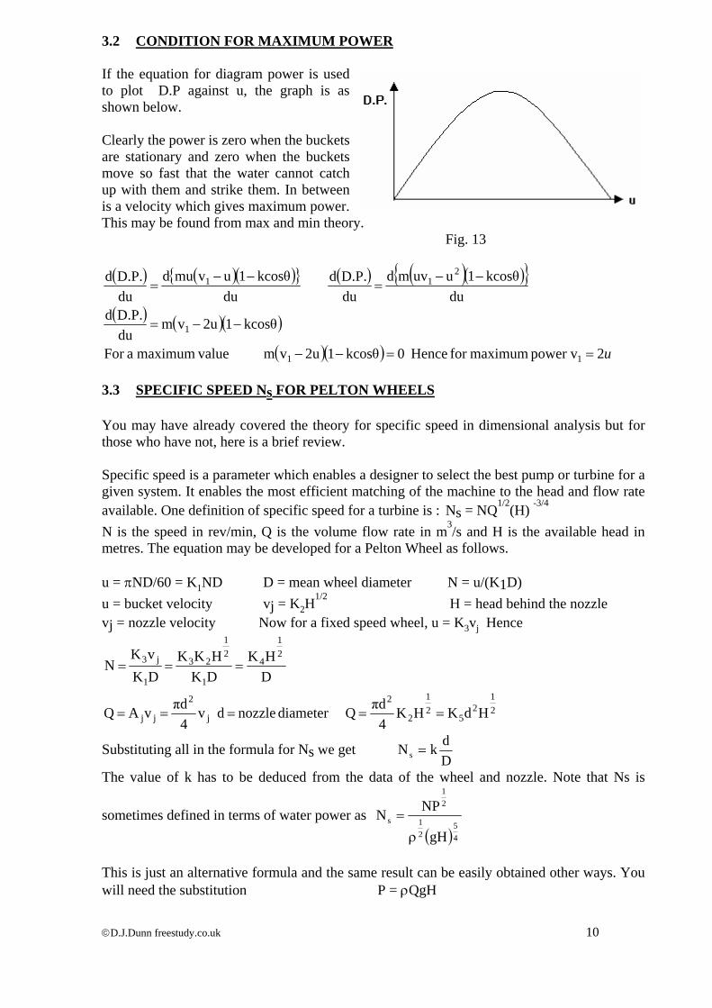
3.2 CONDITION FOR MAXIMUM POWER If the equation for diagram power is used to plot D.P against u, the graph is as shown below.
©D.J.Dunn freestudy.co.uk 10
Clearly the power is zero when the buckets are stationary and zero when the buckets move so fast that the water cannot catch up with them and strike them. In between is a velocity which gives maximum power. This may be found from max and min theory. Fig. 13 ( ) ( )( ){ } ( ) ( )( ){ }
( ) ( )( )
( )( ) u2power v maximumfor Hence 0kcosθ12uvm valuemaximum aFor
kcosθ12uvmduD.P.d
dukcosθ1uuvmd
duD.P.d
dukcosθ1uvmud
duD.P.d
11
1
211
==−−
−−=
−−=
−−=
3.3 SPECIFIC SPEED Ns FOR PELTON WHEELS You may have already covered the theory for specific speed in dimensional analysis but for those who have not, here is a brief review. Specific speed is a parameter which enables a designer to select the best pump or turbine for a given system. It enables the most efficient matching of the machine to the head and flow rate available. One definition of specific speed for a turbine is : Ns = NQ1/2(H) -3/4
N is the speed in rev/min, Q is the volume flow rate in m3/s and H is the available head in metres. The equation may be developed for a Pelton Wheel as follows. u = πND/60 = K1ND D = mean wheel diameter N = u/(K1D) u = bucket velocity vj = K2H
1/2 H = head behind the nozzle vj = nozzle velocity Now for a fixed speed wheel, u = K3vj Hence
21
25
21
2
2
j
2
jj
21
4
1
21
23
1
j3
HdKHK4πdQ diameter nozzle d v
4πdvAQ
DHK
DKHKK
DKvK
N
=====
===
Substituting all in the formula for Ns we get DdkNs =
The value of k has to be deduced from the data of the wheel and nozzle. Note that Ns is
sometimes defined in terms of water power as ( )4
521
21
s
gH
NPNρ
=
This is just an alternative formula and the same result can be easily obtained other ways. You will need the substitution P = ρQgH

©D.J.Dunn freestudy.co.uk 11
SELF ASSESSMENT EXERCISE No. 1 1. The buckets of a Pelton wheel revolve on a mean diameter of 1.5 m at 1500 rev/min. The
jet velocity is 1.8 times the bucket velocity. Calculate the water flow rate required to produce a power output of 2MW. The mechanical efficiency is 80% and the blade friction coefficient is 0.97. The deflection angle is 165o.
(Ans. 116.3 kg/s) 2. Calculate the diagram power for a Pelton Wheel 2m mean diameter revolving at 3000
rev/min with a deflection angle of 170o under the action of two nozzles , each supplying 10 kg/s of water with a velocity twice the bucket velocity. The blade friction coefficient is 0.98.
(Ans. 3.88 MW) If the coefficient of velocity is 0.97, calculate the pressure behind the nozzles. (Ans 209.8 MPa) 3. A Pelton Wheel is 1.7 m mean diameter and runs at maximum power. It is supplied from
two nozzles. The gauge pressure head behind each nozzle is 180 metres of water. Other data for the wheel is :
Coefficient of Discharge Cd = 0.99 Coefficient of velocity Cv = 0.995 Deflection angle = 165o. Blade friction coefficient = 0.98 Mechanical efficiency = 87% Nozzle diameters = 30 mm Calculate the following. i. The jet velocity (59.13 m/s) ii. The mass flow rate (41.586 kg/s) iii The water power ( 73.432 kW) iv. The diagram power ( 70.759 kW) v. The diagram efficiency (96.36%) vi. The overall efficiency (83.8%) vii. The wheel speed in rev/min (332 rev/min)

©D.J.Dunn freestudy.co.uk 12
4. Explain the significance and use of 'specific speed' Ns = NP1/2/{ρ1/2(gH)5/4} Explain why in the case of a Pelton wheel with several nozzles, P is the power per nozzle. Explain why a Francis Wheel is likely to be preferred to a Pelton wheel when site
conditions suggest that either could be used. Calculate the specific speed of a Pelton Wheel given the following. d = nozzle diameter. D = Wheel diameter. u = optimum blade speed = 0.46 v1 v1= jet speed. η = 88% Cv = coefficient of velocity = 0.98 Answer Ns = 11.9 d/D 5. Explain the usefulness of specific speed in the selection of pumps and turbines. A turbine is to run at 150 rev/min under a head difference of 22 m and an expected flow
rate of 85 m3/s. A scale model is made and tested with a flow rate of 0.1 m3/s and a head difference of 5
m. Determine the scale and speed of the model in order to obtain valid results. When tested at the speed calculated, the power was 4.5 kW. Predict the power and
efficiency of the full size turbine. Answers 0.05 scale 16.17 MW and 88%.

4. KAPLAN TURBINE The Kaplan turbine is a pure reaction turbine. The main point concerning this is that all the flow energy and pressure is expended over the rotor and not in the supply nozzles. The picture shows the rotor of a large Kaplan turbine. They are most suited to low pressure heads and large flow rates such as on dams and tidal barrage schemes. The diagram below shows the layout of a large hydroelectric generator in a dam.
Fig.14 Picture and schematic of a Kaplan Turbine
©D.J.Dunn freestudy.co.uk 13

5. FRANCIS WHEEL The Francis wheel is an example of a mixed impulse and reaction turbine. They are adaptable to varying heads and flows and may be run in reverse as a pump such as on a pumped storage scheme. The diagram shows the layout of a vertical axis Francis wheel.
Fig.15
The Francis Wheel is an inward flow device with the water entering around the periphery and moving to the centre before exhausting. The rotor is contained in a casing that spreads the flow and pressure evenly around the periphery.
The impulse part comes about because guide vanes are used to produce an initial velocity v1 that is directed at the rotor. Pressure drop occurs in the guide vanes and the velocity is v1 = k (∆H)½ where ∆H is the head drop in the guide vanes.
Fig.16 The angle of the guide vanes is adjustable so that the inlet angle β1 is correct for shockless entry. The shape of the rotor is such that the vanes are taller at the centre than at the ends. This gives control over the radial velocity component and usually this is constant from inlet to outlet. The volume flow rate is usually expressed in terms of radial velocity and circumferential area. Fig.17 vR = radial velocity A = circumferential area = πD h k Q = vR πD h k h = height of the vane. k is a factor which allows for the area taken up by the thickness of the vanes on the circumference. If vR is constant then since Q is the same at all circumferences,
D1h1=D2h2.
©D.J.Dunn freestudy.co.uk 14

VECTOR DIAGRAMS
Fig. 18
The diagram shows how the vector diagrams are constructed for the inlet and outlet. Remember the rule is that the vectors add up so that u + v = ω If u is drawn horizontal as shown, then Vw is the horizontal component of v and vR is the radial component (vertical). MORE DETAILED EXAMINATION OF VECTOR DIAGRAM Applying the sine rule to the inlet triangle we find
( ){ }
( )( )
( )
( )( )
( ) ( )( ) ( )( )
( ) ( )( ) ...(5)..........
tanββαsinβsinαsinu v(4) and (3) equate .(4)..........
βαsinβsinαsinuv
βsinv
βαsinαsinu (2) and (1) equate
......(3)..........tanβv v ..(2)..........βsin
v vAlso
.......(1)..........βαsinαsinu v
βαsinu
)sin(αv
α180β180sinu
)αsin(180v
111
111w1
11
111r1
1
r1
11
11
1w1r11
r11
11
111
11
1
1
1
11
1
1
1
−=
−=
=−
==
−=
−=
−−−=
−
If all the angles are known, then vw1 may be found as a fraction of u1. DIAGRAM POWER Because u is different at inlet and outlet we express the diagram power as : D.P. = m ∆(uvw)= m (u1vw1 – u2vw2) The kinetic energy represented by v2 is energy lost in the exhausted water. For maximum efficiency, this should be reduced to a minimum and this occurs when the water leaves radially with no whirl so that vw2 = 0. This is produced by designing the exit angle to suit the speed of the wheel. The water would leave down the centre hole with some swirl in it. The direction of the swirl depends upon the direction of v2 but if the flow leaves radially, there is no swirl and less kinetic energy. Ideally then, D.P. = m u1 vw1
©D.J.Dunn freestudy.co.uk 15

WATER POWER The water power supplied to the wheel is mg∆H where ∆H is the head difference between inlet and outlet. HYDRAULIC EFFICIENCY The maximum value with no swirl at exit is ηhyd = D.P./W.P. = u1v w1/gρH OVERALL EFFICIENCY ηo/a= Shaft Power/Water Power ηo/a = 2πNT/mg∆H LOSSES The hydraulic losses are the difference between the water power and diagram power. Loss = mg∆H - mu1vw1= mghL hL = ∆H – u1vw1/g ∆H - hL = u1vw1/g WORKED EXAMPLE No. 2 The following data is for a Francis Wheel. Radial velocity is constant No whirl at exit. Flow rate 0.189 m3/s D1= 0.6 m D2=0.4 m k =0.85 h1=50 mm α1=110o N=562 rev/min Head difference from inlet to outlet is 32 m. Entry is shockless. Calculate i. the guide vane angle ii. the diagram power iii. the hydraulic efficiency iv. the outlet vane angle v. the blade height at outlet. SOLUTION u1= πND1 = 17.655 m/s vr1= Q/(πD1h1k)= 0.189/(π x 0.6 x 0.05 x 0.85) = 2.35 m/s
Fig. 19
vw1 and β1 may be found by scaling or by trigonometry. vw1=16.47m/s β1=8.12o u2= πND2 = 11.77 m/s α2= tan-1 (2.35/11.77) = 11.29o D.P. = m u1vw1=189 (17.655 x 16.47) = 54 957 Watts W.P.= mg∆H = 189 x 9.81 x 32 = 59 331 Watts ηhyd = 54 957/59 331 = 92.6% since vr1 = vr2 then D1h1 = D2 h2 h2 = 0.6 x 0.05/0.4 = 0.075 m
©D.J.Dunn freestudy.co.uk 16

WORKED EXAMPLE No. 3 The runner (rotor) of a Francis turbine has a blade configuration as shown. The outer diameter is 0.4 m and the inner diameter is 0.25 m. The vanes are 65 mm high at inlet and 100 mm at outlet. The supply head is 20 m and the losses in the guide vanes and runner are equivalent to 0.4 m. The water exhausts from the middle at atmospheric pressure. Entry is shockless and there is no whirl at exit. Neglecting the blade thickness, determine : i. the speed of rotation. ii. the flow rate. iii. the output power given a mecanical efficiency of 88%. iv. the overall efficiency. v. The outlet vane angle.
Fig.20 SOLUTION
©D.J.Dunn freestudy.co.uk 17
( ) ( )( )
11
w1
111
111w1
8260.n(20)sin(100)tan(20)sin(120)siuv
tanββαsinβsinαsinuv
u==
−=
Fig.21 The inlet vector diagram is as shown. Values can be found by drawing to scale. Since all angles are known but no flow rate, find vw1 in terms of u1
∆H - hL = u1vw1/g 20 - 0.4 = 19.6 = u1vw1/g 19.6 = 0.826 u1
2/g u1 =15.26 m/s u1 = πND1/60 N = 15.26 x 60/(πx0.4) = 728.5 rev/min
( ) ( )( )
( ) ( )( ) m/s589.4100sin
20sin120sin26.15sin
sinsin
111
1111 ==
−=
βαβαuvr
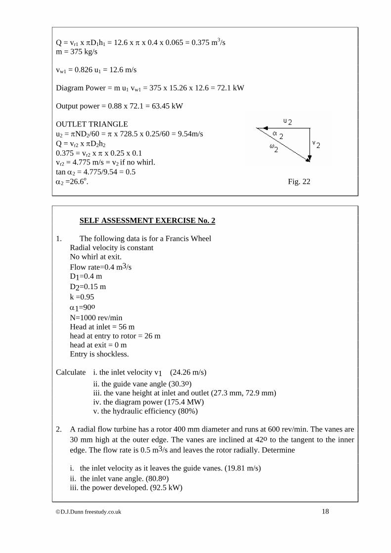
Q = vr1 x πD1h1 = 12.6 x π x 0.4 x 0.065 = 0.375 m3/s m = 375 kg/s vw1 = 0.826 u1 = 12.6 m/s Diagram Power = m u1 vw1 = 375 x 15.26 x 12.6 = 72.1 kW Output power = 0.88 x 72.1 = 63.45 kW
©D.J.Dunn freestudy.co.uk 18
OUTLET TRIANGLE u2 = πND2/60 = π x 728.5 x 0.25/60 = 9.54m/s Q = vr2 x πD2h2
0.375 = vr2 x π x 0.25 x 0.1 vr2 = 4.775 m/s = v2 if no whirl. tan α2 = 4.775/9.54 = 0.5 α2 =26.6o. Fig. 22 SELF ASSESSMENT EXERCISE No. 2 1. The following data is for a Francis Wheel Radial velocity is constant No whirl at exit. Flow rate=0.4 m3/s D1=0.4 m D2=0.15 m k =0.95 α1=90o N=1000 rev/min Head at inlet = 56 m head at entry to rotor = 26 m head at exit = 0 m Entry is shockless. Calculate i. the inlet velocity v1 (24.26 m/s) ii. the guide vane angle (30.3o) iii. the vane height at inlet and outlet (27.3 mm, 72.9 mm) iv. the diagram power (175.4 MW) v. the hydraulic efficiency (80%) 2. A radial flow turbine has a rotor 400 mm diameter and runs at 600 rev/min. The vanes are
30 mm high at the outer edge. The vanes are inclined at 42o to the tangent to the inner edge. The flow rate is 0.5 m3/s and leaves the rotor radially. Determine
i. the inlet velocity as it leaves the guide vanes. (19.81 m/s) ii. the inlet vane angle. (80.8o) iii. the power developed. (92.5 kW)

3. The runner (rotor) of a Francis turbine has a blade configuration as shown. The outer
diameter is 0.45 m and the inner diameter is 0.3 m. The vanes are 62.5 mm high at inlet and 100 mm at outlet. The supply head is 18 m and the losses in the guide vanes and runner are equivalent to 0.36 m. The water exhausts from the middle at atmospheric pressure. Entry is shockless and there is no whirl at exit. Neglecting the blade thickness, determine :
i. The speed of rotation. (1691 rev/min) ii. The flow rate. (1.056 m3/s) iii. The output power given a mechanical efficiency of 90%. (182.2 MW) iv. The overall efficiency. (88.2%) v. The outlet vane angle. (22.97o)
Fig. 23
©D.J.Dunn freestudy.co.uk 19

©D.J.Dunn freestudy.co.uk 1
FLUID MECHANICS
TUTORIAL No.8B
CENTRIFUGAL PUMPS When you have completed this tutorial you should be able to
• Derive the dimensionless parameters of a pump
• Flow Coefficient • Head Coefficient • Power Coefficient • Specific Speed.
• Explain how to match a pump to system requirements. • Explain the general principles of Centrifugal Pumps.
• Construct blade vector diagrams for Centrifugal Pumps. • Deduce formulae for power and efficiency and Head. • Solve numerical problems for Centrifugal Pumps.

1. DIMENSIONAL ANALYSIS The power 'P' of any rotary hydraulic pump depends upon the density 'ρ' , the speed 'N', the characteristic diameter 'D', the head change '∆H', the volume flow rate 'Q' and the gravitational constant 'g'. The general equation is: P = f(ρ, N, D, ∆H, Q, g) It is normal to consider g∆H as one quantity. P = f{ρ, N, D, (g∆H),Q} There are 6 quantities and 3 dimensions so there are three dimensionless groups Π1, Π2and Π3. First form a group with P and ρND.
( )( ) ( ) ( )
tCoefficienPower DNρ
PΠ DNρΠP
5c c 3- c-3a2Length 3b b3 Time
a1 MassDTMLTLM
DNρΠρNDφP
531531
1
c1b1a3321
cba1
===
=+=+==−=−
==
==−−−
Next repeat the process between Q and ρND ( )
( ) ( ) ( )
tCoefficien Flow ND
QΠ DNρΠQ
3c c-3a3Length a0 Mass
1b b1- TimeDTMLTM
DNρΠρNDφQ
32310
2
c1b1a313
cba2
===
=+==
=−==
==−−−
Next repeat the process between g∆H and ρND ( )( ) ( ) ( )
tCoefficien Head DN
QΠ DNρΠQ
2c c-3a2Length 2b b2- Time a0 MassDTMLTLM
DNρΠρNDφ∆H) (g
223220
3
c1b1a3220
cba3
===
=+==−===
==−−−
Finally the complete equation is ⎟⎠⎞
⎜⎝⎛⎟⎠⎞
⎜⎝⎛=
22353 DN∆H g
NDQφ
DρNP
©D.J.Dunn freestudy.co.uk 2

SPECIFIC SPEED Ns The specific speed is a parameter used for pumps and turbines to determine the best design to match a given pumped system. The formula may be derived from consideration of the pump geometry or
by dimensional analysis. The latter will be used here. ⎟⎠⎞
⎜⎝⎛⎟⎠⎞
⎜⎝⎛= 22253 DN
∆H gND
QφDρN
P
The three dimensionless numbers represent the power coefficient, the flow coefficient and the head coefficient respectively. Now consider a family of geometrically similar machines operating at dynamically similar conditions. For this to be the case the coefficients must have the same values for each size. Let the 3 coefficients be Π1, Π2 and Π3 such that
constant K
∆H) (
NQ
QK
∆H) (N
KQ
∆H) (
N
KQ
∆H) (
constant
gΠ
Π
NQ
∆H) (
NΠ
QΠ∆H g
N1
ΠN∆H g
NΠQ Equating
ΠN∆H gD
DN∆H gΠ
NΠQ D
NDQΠ
DρNPΠ
21
43
21
21
21
432
3
31
21
32
31
21
21
31
2
21
3
32
31
21
31
31
2
31
21
3
21
32
31
2
21
32223
31
232531
====⎥⎥⎥
⎦
⎤
⎢⎢⎢
⎣
⎡
=
==
=⎟⎟⎠
⎞⎜⎜⎝
⎛
⎟⎟⎠
⎞⎜⎜⎝
⎛=⎟⎟
⎠
⎞⎜⎜⎝
⎛
⎟⎟⎠
⎞⎜⎜⎝
⎛==⎟⎟
⎠
⎞⎜⎜⎝
⎛===
−
This constant is called the Specific Speed 43
21
∆H) (
NQNs =
Ns is a dimensionless parameter that and the units used are normally rev/min for speed, m3/s for flow rate and metres for head. Other units are often used and care should be taken when quoting Ns values. It follows that for a given speed, the specific speed is large for large flows and low heads and small for small flows and large heads. The important value is the one that corresponds to the conditions that produce the greatest efficiency.
©D.J.Dunn freestudy.co.uk 3

2. MATCHING PUMPS TO SYSTEM REQUIREMENTS The diagram shows a typical relationship between the head and flow of a given CF pump at a given speed.
Figure 1
The Ns value may be calculated using the flow and head corresponding to the maximum efficiency at point A. SELECTING PUMP SIZE The problem is that the optimal point of any given pump is unlikely to correspond to the system requirements for example at point B. What we should do ideally is find a geometrically similar pump that will produce the required head and flow at the optimal point. The geometrically similar pump will run under dynamically similar conditions so it follows that the specific speed Ns is the same for both pumps at the optimal point. The procedure is to first calculate the specific speed of the pump using the flow and head at the optimal conditions.
43
A
21
AAs
H
QNN =
Suppose point B is the required operating point defined by the system.
43
B
21
BBs
H
QNN = Equating, we can calculate NB, the speed of the geometrically similar pump.
We still don’t know the size of the pump that will produce the head and flow at B. Since the head and flow coefficients are the same then:-
Equating Flow Coefficients we get 1/3
BA
ABAB NQ
NQDD ⎟⎟⎠
⎞⎜⎜⎝
⎛=
Equating head coefficients we get we get A
B
B
AB H
H NND =
If the forgoing is correct then both will give the same answer.
©D.J.Dunn freestudy.co.uk 4

WORKED EXAMPLE No. 1 A centrifugal pump is required to produce a flow of water at a rate of 0.0160 m3/s against a
total head of 30.5 m. The operating characteristic of a pump at a speed of 1430 rev/min and a rotor diameter of 125 mm is as follows.
Efficiency 0 48 66 66 45 % QA 0 0.0148 0.0295 0.0441 0.059 m3/s HA 68.6 72 68.6 53.4 22.8 m Determine the correct size of pump and its speed to produce the required head and flow. SOLUTION Plot the data for the pump and determine that the optimal head and flow are 65 m and
0.036m3/s
Calculate Ns at point A 85.1165
0.036 x 1430
H
QNN 3/4
1/2
43
A
21
AAs ===
Calculate the Speed for a geometrically similar pump at the required conditions.
rev/min 12160.016
30.5 x 11.85
Q
HNsN 1/2
3/4
21
B
43
BB ===
Next calculate the diameter of this pump.
mm 1011216 x 0.0361430 x 0.016125
NQNQDD
1/31/3
BA
ABAB =⎟
⎠⎞
⎜⎝⎛=⎟⎟
⎠
⎞⎜⎜⎝
⎛=
or mm 10165
30.5 12161430 x 251
HH
NNDD
A
B
B
AAB ===
Answer:- we need a pump 101 mm diameter running at 1216 rev/min.
©D.J.Dunn freestudy.co.uk 5

RUNNING WITH THE WRONG SIZE In reality we are unlikely to find a pump exactly the right size so we are forced to use the nearest we can get and adjust the speed to obtain the required flow and head. Let B be the required operating point and A the optimal point for the wrong size pump. We make the flow and head coefficients the same for B and some other point C on the operating curve. The diameters cancel because they are the same.
3CC
C3
BB
B
DNQ
DNQ
= C
BCB N
NQQ = 2C
2C
A2
C2
C
C
DNH g
DNH g
= 2C
2B
CB N NHH =
Substitute A
B
A
B
NN
= to eliminate the speed
©D.J.Dunn freestudy.co.uk 6
2
B
CBC Q
QHH ⎟⎟⎠
⎞⎜⎜⎝
⎛=
This is a family of parabolic curves starting at the origin. If we take the operating point B we can determine point C as the point where it intersects the operating curve at speed A. The important point is that the efficiency curve is unaffected so at point B the efficiency is not optimal. Figure 2 WORKED EXAMPLE No. 2 If only the 125 mm pump in WE 1 is available, what speed must it be run at to obtain the
required head and flow? What is the efficiency and input power to the pump? SOLUTION B is the operating point so we must calculate HC and QC
2C
2C
2
B
CBC 119141Q
0.016Q5.30
QQHH =⎟
⎠⎞
⎜⎝⎛=⎟⎟
⎠
⎞⎜⎜⎝
⎛=
This must be plotted to determine QC
From the plot HC = 74 m QC = 0.025 m3/s Equate flow coefficients to find the speed at B
3CC
C3
BB
B
DNQ
DNQ
= 14300.025
N0.016
B=
NB = 915 rev/min Check by repeating the process with the head coefficient.
2A
2A
A2
B2
B
B
DNH g
DNH g
= rev/min 91874
30.51430HHNN
A
BAB ===
The efficiency at this point is 63% Water Power = mgH = 16 x 9.81 x 30.5 = 4787 W Power Input = WP/η = 4787/0.63 =7598 W

©D.J.Dunn freestudy.co.uk 7
WORKED EXAMPLE No.3 A pump draws water from a tank and delivers it to another with the surface 8 m above that of
the lower tank. The delivery pipe is 30 m long, 100 bore diameter and has a friction coefficient of 0.003. The pump impeller is 500 mm diameter and revolves at 600 rev/min. The pump is geometrically similar to another pump with an impeller 550 mm diameter which gave the data below when running at 900 rev/min.
∆H (m) 37 41 44 45 42 36 28 Q(m3/s) 0 0.016 0.32 0.048 0.064 0.08 0.096 Determine the flow rate and developed head for the pump used. SOLUTION First determine the head flow characteristic for the system. ∆H = developed head of the pump = 8 + 4fLu2/2gd + minor losses No details are provided about minor losses so only the loss at exit may be found. hL = 4fLu2/2gd + u2/2g ∆H = = 8 + 4fLu2/2gd + u2/2g u = 4Q/πd2 = 127.3 Q ∆H = 8 + 4x 0.003 x 30 000(127.3Q)2/(2g x 0.1) + (127.3Q)2/2g ∆H = 8 + 3800Q2 Produce a table and plot ∆H against Q for the system. ∆H (m) 8 8.38 14.08 32.3 46 Q(m3/s) 0 0.01 0.04 0.08 0.1 Plot the system head and pump head against flow and find the matching point. This is at H = 34.5 and Q = 0.084 m3/s Next determine the head - flow characteristic for the pump actually used by assuming dynamic
and geometric similarity. Flow Coefficient Q/ND3 = constant Q2 =Q2 (N1/N2)(D13/D23) Q2 =(600/900) (500/550)3= 0.5 Q1 ∆H/(ND)2 = constant ∆H2 = ∆H1(N2D2/N1D1)2 ∆H2= ∆H1{600 x 500/900 x 550}2 = 0.367 ∆H1 Produce a table for the pump using the coefficients and data for the first pump. ∆H2 (m) 13.58 15.05 16.15 16.51 15.41 13.21 10.28 Q2(m3/s) 0 0.08 0.016 0.024 0.032 0.04 0.048 Plot this graph along with the system graph and pick off the matching point.

Figure 3
Ans. 13.5 m head and 38 dm3/s flow rate.
©D.J.Dunn freestudy.co.uk 8
©D.J.Dunn freestudy.co.uk 9
SELF ASSESSMENT EXERCISE No.1 1. A centrifugal pump must produce a head of 15 m with a flow rate of 40 dm3/s and shaft speed
of 725 rev/min. The pump must be geometrically similar to either pump A or pump B whose characteristics are shown in the table below.
Which of the two designs will give the highest efficiency and what impeller diameter should be
used ? Pump A D = 0.25 m N = 1 000 rev/min Q (dm3/s) 8 11 15 19 H (m) 8.1 7.9 7.3 6.1 η % 48 55 62 56 Pump B D = 0.55 m N = 900 rev/min Q (dm3/s) 6 8 9 11 H (m) 42 36 33 27 η % 55 65 66 58 Answer Pump B with D= 0.455 m 2. Define the Head and flow Coefficients for a pump. Oil is pumped through a pipe 750 m long and 0.15 bore diameter. The outlet is 4 m below the
oil level in the supply tank. The pump has an impeller diameter of 508 mm which runs at 600 rev/min. Calculate the flow rate of oil and the power consumed by the pump. It may be assumed Cf=0.079(Re)-0.25. The density of the oil is 950 kg/m3 and the dynamic viscosity is 5 x 10⁻³ N s/m2.
The data for a geometrically similar pump is shown below. D = 0.552 m N = 900 rev/min Q (m3/min) 0 1.14 2.27 3.41 4.55 5.68 6.86 H (m) 34.1 37.2 39.9 40.5 38.1 32.9 25.9 η % 0 22 41 56 67 72 65 Answer 2 m3/min and 7.89 kWatts

3. GENERAL THEORY A Centrifugal pump is a Francis turbine running backwards. The water between the rotor vanes experiences centrifugal force and flows radially outwards from the middle to the outside. As it flows, it gains kinetic energy and when thrown off the outer edge of the rotor, the kinetic energy must be converted into flow energy. The use of vanes similar to those in the Francis wheel helps. The correct design of the casing is also vital to ensure efficient low friction conversion from velocity to pressure. The water enters the middle of the rotor without swirling so we know vw1 is always zero for a c.f. pump. Note that in all the following work, the inlet is suffix 1 and is at the inside of the rotor. The outlet is suffix 2 and is the outer edge he rotor.
of t
va
vane the
Fig. v
Fig. 1 Basic Design
The increase in momentum through the rotor is found as always by drawing the vector diagrams. At inlet v1 is radial and equal to vr1 and so vw1 is zero. This is so regardless of the vane angle but there is only one angle which produces shockless entry and this must be used at the design speed.
©D.J.Dunn freestudy.co.uk 10
At outlet, the shape of the vector diagram is greatly affected by the ane angle. The diagram below shows typical vector diagram when the is swept backwards (referred to vane velocity u).
2 w2 may be found by scaling
from the diagram. We can also apply trigonometry to the diagram as follows.
( ) ( ). thicknessblade for thefactor correction theisk and vane theofheight theist
πNDu αtantπkD
QuαtanA
Qutanα
vuv = 22222
222
22
r22w2 =−=−=−

3.1. DIAGRAM POWER D.P.= m∆uvw since usually vw1 is zero this becomes D.P.= mu2vw2 3.2. WATER POWER W.P. = mg∆h ∆h is the pressure head rise over the pump. 3.3. MANOMETRIC HEAD ∆hm This is the head that would result if all the energy given to the water is converted into pressure head. It is found by equating the diagram power and water power.
( )⎭⎬⎫
⎩⎨⎧
−===22
22w22
mmw22 αtanAQu
gu
gvu∆h mg∆gvmu
3.4. MANOMETRIC EFFICIENCY ηm
mmw22
m ∆h∆h
∆h mg∆h mg
vmu∆h mg
Power DiagramPowerWater η ====
3.5. SHAFT POWER S.P. = 2πNT
3.6. OVERALL EFFICIENCY PowerShaft PowerWater
/ =aoη
3.7. KINETIC ENERGY AT ROTOR OUTLET 2
mvK.E.22=
Note the energy lost is mainly in the casing and is usually expressed as a fraction of the K.E. at exit. 3.8. NO FLOW CONDITION There are two cases where you might want to calculate the head produced under no flow condition. One is when the outlet is blocked say by closing a valve, and the other is when the speed is just sufficient for flow to commence. Under normal operating conditions the developed head is given by the following equation.
( )⎭⎬⎫
⎩⎨⎧
−==22
22w22
αtanAQu
gu
gvu∆h
When the outlet valve is closed the flow is zero. The developed head is given by the following
equation. { }g
u0ug
u∆h22
22 =−=
When the speed is reduced until the head is just sufficient to produce flow and overcome the static head, the radial velocity vr2 is zero and the fluid has a velocity u2 as it is carried around with the
rotor. The kinetic energy of the fluid is 2
mu22 and this is converted into head equal to the static head.
It follows that 2guh
22
s = . Substituting 60
πNDu 22 = we find that
Dh
83.5N s= .
©D.J.Dunn freestudy.co.uk 11

WORKED EXAMPLE No.4 A centrifugal pump has the following data : Rotor inlet diameter D1 = 40 mm Rotor outlet diameter D2 = 100 mm Inlet vane height h1 = 60 mm Outlet vane height h2 = 20 mm Speed N =1420 rev/min Flow rate Q = 0.0022 m3/s Blade thickness coefficient k = 0.95 The flow enters radially without shock. The blades are swept forward at 30o at exit. The developed head is 5 m and the power input to the shaft is 170 Watts. Determine the following. i. The inlet vane angle ii. The diagram power iii. The manometric head iv. The manometric efficiency v. The overall efficiency. vi. The head produced when the outlet valve is shut. vii. The speed at which pumping commences for a static head of 5 m. SOLUTION u1= πND1 = 2.97 m/s u2= πND2 = 7.435 m/s vr1=Q/kπD1h1= 0.307 m/s vr2=Q/kπD2h2= 0.368 m/s Since the flow enters radially v1 = vr1= 0.307 m/s and vw1 = 0 From the inlet vector diagram the angle of the vane that produces no shock is found as follows: tanα1 = 0.307/2.97 hence α1 = 5.9o.
Fig. 41
Inlet vector diagram
©D.J.Dunn freestudy.co.uk 12

From the outlet vector diagram we find :
Fig. 42
Outlet vector diagram
vw2 = 7.435 + 0.368/tan 30o = 8.07 m/s D.P.= mu2vw2 D.P.= 2.2 x 7.435 x 8.07 = 132 Watts W.P. = mg∆h = 2.2 x 9.81 x 5 = 107.9 Watts ∆hm = W.P./D.P.= 107.9/132 = 81.7% ∆hm = u2vw2/g = 7.435 x 8.07/9.81 =6.12 m ∆m = ∆h/∆hm = 5/6.12 = 81.7% ηo/a = W.P./S.P. = 107.9/170 = 63.5%
When the outlet valve is closed the static head is m 5.639.81
7.435g
u∆h22
2 ===
The speed at which flow commences is rev/min 18670.1
583.5Dh
83.5N s ===
©D.J.Dunn freestudy.co.uk 13

©D.J.Dunn freestudy.co.uk 14
SELF ASSESSMENT EXERCISE No. 2 1. The rotor of a centrifugal pump is 100 mm diameter and runs at 1 450 rev/min. It is 10 mm
deep at the outer edge and swept back at 30o. The inlet flow is radial. the vanes take up 10% of the outlet area. 25% of the outlet velocity head is lost in the volute chamber. Estimate the shut off head and developed head when 8 dm3/s is pumped. (5.87 m and 1.89 m)
2. The rotor of a centrifugal pump is 170 mm diameter and runs at 1 450 rev/min. It is 15 mm
deep at the outer edge and swept back at 30o. The inlet flow is radial. the vanes take up 10% of the outlet area. 65% of the outlet velocity head is lost in the volute chamber. The pump delivers 15 dm3/s of water.
Calculate i. The head produced. (9.23 m) ii. The efficiency. (75.4%) iii. The power consumed. (1.8 kW)

FLUID MECHANICS
TUTORIAL 8C
PUMPED PIPED SYSTEMS On completion of this tutorial you should be able to do the following.
Examine the conditions that produce cavitation.
Calculate pressure surges due to flow changes.
Calculate the stress in pipes due to pressure changes.
Describe how pressure surges are damped.
Describe how pressure oscillations occur in pipes.
Let's start by examining the meaning of specific speed of pumps.
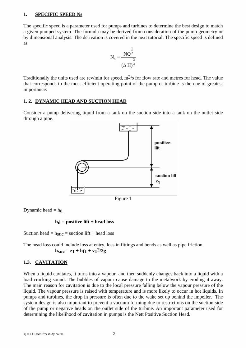
1. SPECIFIC SPEED Ns The specific speed is a parameter used for pumps and turbines to determine the best design to match a given pumped system. The formula may be derived from consideration of the pump geometry or by dimensional analysis. The derivation is covered in the next tutorial. The specific speed is defined as
43
21
s
H) (∆
NQN =
Traditionally the units used are rev/min for speed, m3/s for flow rate and metres for head. The value that corresponds to the most efficient operating point of the pump or turbine is the one of greatest importance. 1. 2. DYNAMIC HEAD AND SUCTION HEAD Consider a pump delivering liquid from a tank on the suction side into a tank on the outlet side through a pipe.
Figure 1
Dynamic head = hd hd = positive lift + head loss Suction head = hsuc = suction lift + head loss The head loss could include loss at entry, loss in fittings and bends as well as pipe friction. hsuc = z1 + hf1 + v12/2g 1.3. CAVITATION When a liquid cavitates, it turns into a vapour and then suddenly changes back into a liquid with a load cracking sound. The bubbles of vapour cause damage to the metalwork by eroding it away. The main reason for cavitation is due to the local pressure falling below the vapour pressure of the liquid. The vapour pressure is raised with temperature and is more likely to occur in hot liquids. In pumps and turbines, the drop in pressure is often due to the wake set up behind the impeller. The system design is also important to prevent a vacuum forming due to restrictions on the suction side of the pump or negative heads on the outlet side of the turbine. An important parameter used for determining the likelihood of cavitation in pumps is the Nett Positive Suction Head.
© D.J.DUNN freestudy.co.uk 2

1.4. NET POSITIVE SUCTION HEAD (N.P.S.H.) The Net Positive Suction Head is the amount by which the absolute pressure on the suction side is larger than the vapour pressure (saturation pressure) of the liquid. NPSH = absolute inlet head - vapour pressure head Absolute inlet head = pa/ρg - hs where pa= atmospheric pressure and hs= ps/ρg The vapour pressure varies with temperature and for water is found in thermodynamic temperatures under the heading ps. (for saturation pressure). Vapour pressure as a head is ps/ρg NPSH = (pa/ρg - hsuc ) - ps/ρg NPSH = (pa - ps )/ρg - hsuc WORKED EXAMPLE No.1 A water pump has a suction lift of 5 m. The friction head in the suction pipe is 0.3m. The
kinetic head is negligible. The water temperature is 16oC. Atmospheric pressure is 1.011 bar (10.31 m water). Determine the NPSH .
SOLUTION hsuc = 5 + 0.3 = 5.3 m ps = 0.01817 bar (from tables) NPSH = (1.011 - 0.01817) x 105/(1000 x 9.81) - 5.3 NPSH = 4.821 metres of water
Figure 2
© D.J.DUNN freestudy.co.uk 3
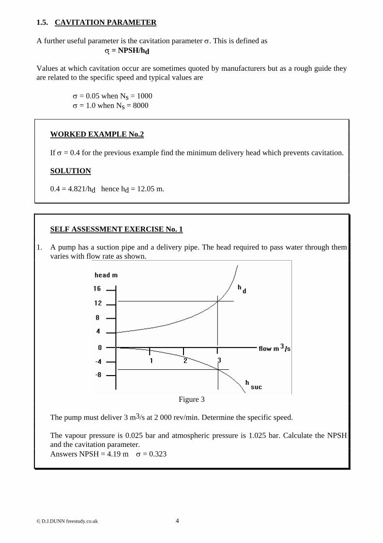
1.5. CAVITATION PARAMETER A further useful parameter is the cavitation parameter σ. This is defined as σ = NPSH/hd Values at which cavitation occur are sometimes quoted by manufacturers but as a rough guide they are related to the specific speed and typical values are σ = 0.05 when Ns = 1000 σ = 1.0 when Ns = 8000 WORKED EXAMPLE No.2 If σ = 0.4 for the previous example find the minimum delivery head which prevents cavitation. SOLUTION 0.4 = 4.821/hd hence hd = 12.05 m. SELF ASSESSMENT EXERCISE No. 1 1. A pump has a suction pipe and a delivery pipe. The head required to pass water through them
varies with flow rate as shown.
Figure 3
The pump must deliver 3 m3/s at 2 000 rev/min. Determine the specific speed. The vapour pressure is 0.025 bar and atmospheric pressure is 1.025 bar. Calculate the NPSH
and the cavitation parameter. Answers NPSH = 4.19 m σ = 0.323
© D.J.DUNN freestudy.co.uk 4

© D.J.DUNN freestudy.co.uk 5
2. Define the term "Nett Positive Suction Head" and explain its significance in pump operation. 1.2 kg/s of acetone is to be pumped from a tank at 1 bar pressure. The acetone is at 40oC and
the pump is 1.5 m below the surface. The suction pipe is 25 mm bore diameter. Calculate the NPSH at the pump inlet.
Losses in the suction pipe are equal to three velocity heads. The vapour pressure of acetone is 55 kPa. The density is 780 kg/m3. Answer 5.37 m 3. A centrifugal pump delivers fluid from one vessel to another distant vessel. The flow is
controlled with a valve. Sketch and justify appropriate positions for the pump and valve when the fluid is a) a liquid and b) a gas.
Let's move on to examine the transient pressure changes in pipes when the fluid is accelerated
or decelerated.

2. WATER HAMMER In this section, we will examine the causes of water hammer. The sudden acceleration or deceleration of fluids in pipes is accompanied by corresponding changes in pressure that can be extremely large. In the extreme, the pressure surge can split the pipe. The phenomenon is often accompanied by load hammer noises, hence the name. First, we must examine the Bulk Modulus (K) and the derivation of the acoustic velocity in an elastic fluid. 2.1 BULK MODULUS ( K) Bulk modulus was discussed in Chapter 1 and defined as follows.
VpV
VpV
strain Volumetricpressurein ChangeK
δδ
=∆∆
==
V is volume and p is pressure. The following work shows how this may be changed to the form K = ρdp/dρ
Consider a volume V1 that is compressed to volume V2 by a small increase in pressure δp. The reduction in volume is δV. The initial density is ρ and this increases by δρ
Figure 4 The mass of δV is δm = ρ δV .....................(2.1) The initial mass of V2 is m1 = ρ V2 .....................(2.2) The final mass of V2 is m2 = (ρ + δρ) V2..............(2.3) The increase in mass is due to the mass of δV being compressed into the volume V2. Hence (2.1) = (2.3) - (2.2) ρ δV = (ρ + δρ) V2 - ρV2 = ρ V2+ δρ V2 - ρV2
ρ δV = δρ V2
ρ δV = δρ (V1- δV) ρ δV = V1δρ - δρ δV The product of two small quantities (δρ δV) is infinitesimally small so it may be ignored.
δρρδ
=δδ
=
δρρ
=δ
ρδρ
=δ
δρ=ρδ
pVpVK
Kfor formula theinto thissubstitute V
VVV
VV
1
1
1
In the limit as δV → 0, we may revert to calculus notation. Hence K = ρdp/dρ
© D.J.DUNN freestudy.co.uk 6

2.2 SPEED OF SOUND IN AN ELASTIC MEDIUM Most students don’t need to know the derivation of the formula for the speed of sound but for those who are interested, here it is. Consider a pipe of cross sectional area A full of fluid. Suppose a piston is pushed into the end with a velocity u m/s. Due to the compressibility of the fluid, further along the pipe at distance L, the fluid is still stationary. It has taken t seconds to achieve this position. The velocity of the interface is hence a = L/t m/s. In the same time the piston has moved x metres so u = x/t.
Figure 5
The moving fluid has been accelerated from rest to velocity a. The inertia force needed to do this is in the form of pressure so the moving fluid is at a higher pressure than the static fluid and the interface is hence a pressure wave travelling along the pipe at velocity a. The volume Ax has been compacted into the length L. The initial density of the fluid is ρ. The mass compacted into length L is dm = ρAx. substitute x = ut dm = ρ A u t .........(2.4) The density of the compacted fluid has increased by dρ so the mass in the length L has increased by dm = A L dρ Substitute L = at dm = A a t dρ......(2.5) Equate (3.10. 4) and (3.10.5) ρ A u t= A a t dρ a = u ρ/dρ............(2.6) The force to accelerate the fluid from rest to a m/s is given by Newton's 2nd law F = mass x acceleration = A dp mass = ρAL acceleration = u/t A dp = ρ A L u/t dp = ρ L u/t Substitute L = at then dp = ρ a u a = (dp/uρ) ...................(2.7) The velocity of the pressure wave a is by definition the acoustic velocity. Multiplying (2.8) by (2.7) gives a2. Hence a2=(uρ/dρ)(dp/uρ) a = (dp/dρ)½ ............(2.9) Previously it was shown that K =ρ dp/dρ a =(K/ρ)½
© D.J.DUNN freestudy.co.uk 7

Students who have studied fundamental thermodynamics will understand the following extension of the theory to gases. The following section is not needed by those following the basic module. Two important gas constants are the adiabatic index γ and the characteristic gas constant R. For a gas, the pressure change is adiabatic and if dp is small then the adiabatic law applies. pVγ = Constant Dividing through by mγ we get p(V/m)γ = constant/mγ = constant p/ργ = C Differentiating we get dp/dρ = C (γργ-1) dp/dρ = (p/ργ)(γργ-1) dp/dρ = pγ/ρ From (2.8) it follows that a =(pγ/ρ)½ From the gas law we have pV = mRT p = (m/V)RT p = ρRT The velocity of a sound wave is that of a weak pressure wave. If the pressure change is large then dp/dρ is not a constant and the velocity would be that of a shock wave which is larger than the acoustic velocity. For air γ = 1.4 and R = 287 J/kg K. Hence at 20oC (293 K) the acoustic velocity in air is as follows. a = (γRT)1/2 = (1.4 x 287 x 293)½ = 343 m/s 2.3 PRESSURE SURGES DUE TO GRADUAL VALVE CLOSURE Consider a pipe line with a fluid flowing at a steady velocity of u m/s. A stop valve is gradually closed thus decelerating the fluid uniformly from u to zero in t seconds.
Figure 6
Volume of fluid = AL Mass of fluid = ρAL Deceleration = u/t Inertia force required F = mass x deceleration = ρAL u/t To provide this force the pressure of the fluid rises by ∆p and the force is A ∆p. Equating forces we have A ∆p = ρAL u/t ∆p = ρL u/t
© D.J.DUNN freestudy.co.uk 8

2.4 PRESSURE SURGES DUE TO SUDDEN VALVE CLOSURE If the valve is closed suddenly then as t is very small the pressure rise is very large. In reality, a valve cannot close instantly but very rapid closure produces very large pressures. When this occurs, the compressibility of the fluid and the elasticity of the pipe is an important factor in reducing the rise in pressure. First, we will consider the pipe as rigid.
Figure 7
When the fluid stops suddenly at the valve, the fluid further up the pipe is still moving and compacting into the static fluid. An interface between moving and static fluid (a shock wave) travels up the pipe at the acoustic velocity. This is given by the equation: a= (K/ρ)½ K = Vdp/dV If we assume that the change in volume is directly proportional to the change in pressure then we may change this to finite changes such that K = V δp/δV δV= Vδp/K The mean pressure rise is δp/2 The strain energy stored by the compression = δp δV/2 The change in kinetic energy = ½ mu2 Equating for energy conservation we get mu2/2 = δp δV/2= (δp)V(δp)/2K mu2 = V(δp) 2/K mKu2/V = (δp) 2
(δp) 2 = (m/V)K u2 = ρ K u2
δp = u(Kρ)½ Since a2 = K/ρ then K = a2ρ δp = u(a2ρ2)½ Then δp = u a ρ For a large finite change, this becomes ∆p = a u ρ
SELF ASSESSMENT EXERCISE No. 2 The density of water is 1000 kg/m3 and the bulk modulus is 4 GPa throughout. 1. A pipe 50 m long carries water at 1.5 m/s. Calculate the pressure rise produced when a) the valve is closed uniformly in 3 seconds. (25 kPa) b) when it is shut suddenly. (3 MPa) 2. A pipe 2000 m long carries water at 0.8 m/s. A valve is closed. Calculate the pressure rise
when a) it is closed uniformly in 10 seconds. (160 kPa) b) it is suddenly closed. (1.6 MPa)
© D.J.DUNN freestudy.co.uk 9
© D.J.DUNN freestudy.co.uk 10

2.5 THE EFFECT OF ELASTICITY IN THE PIPE A pressure surge in an elastic pipe will cause the pipe to swell and some of the energy will be absorbed by straining the pipe wall. This reduces the rise in pressure. The more elastic the wall is, the less the pressure rise will be. Consider the case shown.
Figure 8
Kinetic Energy lost by fluid = ½ mu2 The mass of fluid is ρAL so substituting K.E. = ½ ρALu2
Strain Energy of fluid = ∆p2AL/2K (from last section)
© D.J.DUNN freestudy.co.uk 11
Now consider the strain energy of the pipe wall. The strain energy of an elastic material with a direct stress σ is given by S.E. = (σ2/2E) x volume of material The pipe may be regarded as a thin cylinder and suitable references will show that stress stretching it around the circumference is given by the following formula. Figure 9 σ = ∆pD/2t Volume of metal = πDtL
Hence ( )2tE
DAL∆p 2EπDtLx
2tD ∆p S.E.
22
=⎟⎠⎞
⎜⎝⎛=
Equating KE lost to the total S.E. gained yields
( ) ( )
( ) ( ) ( )
⎭⎬⎫
⎩⎨⎧ +
=
⎭⎬⎫
⎩⎨⎧ +=+=
+=
K1
2tEDρu∆p
K1
tED∆p
K∆p
tED∆pρu
2KAL∆p
2tEDAL∆p
2ρALu
222
2
222
The solution is usually given in terms of the effective bulk modulus K' which is defined as follows.
1
K1
tEDK
−
⎭⎬⎫
⎩⎨⎧ +=′
The pressure rise is then given by ∆p = u[ρ/K']½ The acoustic velocity in an elastic pipe becomes a' and is given as a' = (K'/ρ)½ Hence ∆p = ρ u a'

WORKED EXAMPLE No.3 The density of water is 1000 kg/m3 and the bulk modulus is 4 GPa. The modulus of elasticity
for steel E is 200 Gpa. A steel pipe carries water at 2 m/s. The pipe is 0.8 m bore diameter and has a wall 5 mm thick.
Calculate the pressure rise produced when the flow is suddenly interrupted. SOLUTION
MPa 952.4 10 x 41
10 x 200 x 0.0050.8
K1
tEDK
1
99
1
=⎭⎬⎫
⎩⎨⎧ +=
⎭⎬⎫
⎩⎨⎧ +=′
−−
Sudden closure a' = (K'/ρ) ½ = (952.4 x 10⁶/1000) ½ = 976 m/s ∆p = a' u ρ = 976 x 2 x 1000 = 1.95 MPa 2.6 DAMPING OUT PRESSURE SURGES Pressure surges or water hammer occurs whenever there is a change in flow rate. There are many causes for this besides the opening and closing of valves. Changes in pump speeds may cause the same effect. Piston pumps in particular cause rapid acceleration and deceleration of the fluid. In power hydraulics, changes in the velocity of the ram cause the same effect. The problem occurs both on large scale plant such as hydroelectric pipelines and on small plant such as power hydraulic systems. The principles behind reduction of the pressure surges are the same for each, only the scale of the equipment is different. For example, on power hydraulic systems, accumulators are used. These are vessels filled with both liquid and gas. On piston pumps, air vessels attached to the pipe are used. In both cases, a sudden rise in pressure produces compression of the gas that absorbs the strain energy and then releases it as the pressure passes.
Figure 10
© D.J.DUNN freestudy.co.uk 12

On hydroelectric schemes or large pumped systems, a surge tank is used. This is an elevated reservoir attached as close to the equipment needing protection as possible. When the valve is closed, the large quantity of water in the main system is diverted upwards into the surge tank. The pressure surge is converted into a raised level and hence potential energy. The level drops again as the surge passes and an oscillatory trend sets in with the water level rising and falling. A damping orifice in the pipe to the surge tank will help to dissipate the energy as friction and the oscillation dies away quickly.
Figure 11
2.7 ANALYSIS OF SURGE TANK Let the area of the surge tank be AT and the area of the main pipe be Ap. The length of the pipe is L. Let the volume flow rate during normal operation of the turbines be Q. In the simplest analysis we will consider that there is no friction anywhere and that when an emergency stop is made, all the water is diverted into the surge tank.
.(1).......... AA
dtdzu Qfor Substitute
AQu pipe in theity Mean veloc
dtdzA Q
AQ
dtdz u tank surgein ity Mean veloc
p
Tp
pp
TT
T
=
=
===
The diversion of the flow into the surge tank raises the level by z. This produces an increased pressure at the junction point of ∆p = ρgz The pressure force produced F= Ap∆p= Ap∆gz The inertia force required to decelerate the water in the pipe is F = mass x deceleration = - mass x acceleration = - ρApL du/dt Equating forces we have the following.
)........(2..........dtdu
gL- z
dtduL- gz
dtduLρA- ρgzA pp ===
Putting (1) into (2) we get
..(3).................... zLAgA
dtzd
dtzd
AA
gL- z
T
p2
2
2
2
p
T −==
© D.J.DUNN freestudy.co.uk 13

By definition this is simple harmonic motion since the displacement z is directly proportional to the acceleration and opposite in sense. It follows that the frequency of the resulting oscillation is
T
p
AA
Lg
21fπ
=
The periodic time will be T=1/f The amplitude and periodic time are referred to as the APO (amplitude and period of oscillation). A good mathematician would solve the 2nd order differential equation to produce both the frequency and amplitude. Equation (3) maybe re-written as follows.
0zdt
zdω1 zωz
LAgA
dtzd
2
2
22
T
p2
2=+−=−=
This is a special case of the standard 2nd order differential equation with no friction.
0zdtdz2
dtzd12
22
=+⎟⎠⎞
⎜⎝⎛
ωδ
+⎟⎟⎠
⎞⎜⎜⎝
⎛⎟⎠⎞
⎜⎝⎛ω
δ is called the damping ratio and this appears when frictional damping is considered. ω is the angular frequency (ω=2πf). This equation appears in many forms including the following.
0zωdt
zd
friction nofor and
0zωdtdz2δδ
dtzd
22
2
22
2
=+
=+⎟⎠⎞
⎜⎝⎛+
The standard solution to this equation is )tsin(zz o ω= zo is the amplitude, that is, the amount by which the height in the tank will move up and down from the mean level. The following is a direct way of finding the amplitude.
T
poo
2o
T
2
p
2
p
2
2o
To
oT
oT
o
gALA
uz
2z
gA2
uLA energies. theEquate
2uLA
2u x Mass lost energy kinetic The
2z
gA2z
zgA tankin the storedenergy potential The
zgA tank surge theentering water of weight The2z
height in changemean The
=
ρ=ρ
ρ==
ρ=ρ=
ρ=
=
The equation for the motion in full is
t)sin(ωgALA
uzT
po=
The peak of the surge occurs at T/4 seconds from the disturbance.
Figure 12
© D.J.DUNN freestudy.co.uk 14

2.8 THE EFFECT OF PIPE FRICTION If pipe friction is taken into account, then the normal level of the surge tank will not be the same as the level of the storage lake but will be less by an amount equal to the frictional loss in the system. This is given by D'Arcys equation as hf = 4fLu2/2g If f is regarded as a constant then we may say hf = Cu2 This must be now included into equation (3) so that z (plus or minus hf)= - (L/g)(AT/Ap)(d2z/dt2) The solution of this may be done by step by step integration and it would show that the amplitude of the oscillation dies down (as for any damped oscillation in mechanical systems). In reality the problem is more complicated because f is not constant and varies from 0 at zero flow conditions to a maximum at maximum flow conditions. Reflected waves also complicate the story.
Figure 13
2.9 OSCILLATIONS The pressure surge travel along the pipe lines at the local acoustic velocity. They can be reflected so that they travel back again to where they started. Reflections may occur from a dead end (such as a valve, a ram or a pump) , or from an open end (such as a free surface). When they are reflected from an open end, they are reversed into a rarefaction (negative pressure with respect to the normal level). When a valve is suddenly closed at the turbine of a hydro-electric plant, a pressure surge is set up which travels to the lake and is reflected back as a rarefaction to the valve where it is again reflected as pressure. The pressure waves will pass back and forth in the pipe gradually dying away as the energy is dissipated. The use of a surge tank with a damping orifice reduces the effect to two or three oscillations. The same thing may occur when a large pump is suddenly switched off only in this case the fluid on the suction side will cause a pressure wave and on the delivery side will cause a rarefaction because the fluid is travelling away from the pump. In some systems such as power hydraulics, the time taken for the pressure surge to travel away from the disturbance and to be reflected back again may coincide with the natural frequency of the item causing the disturbance. This may be a spring loaded valve for example. The result is a unstable oscillation with interaction between the dynamics of the valve and the dynamics of the system causing positive feedback and sustaining the oscillation. This results in valve squeal. This is a complex area of study and the student should consult advanced text for full details. Attenuation due to friction is also involved. The theory is similar to that of A.C. electric power transmission. The student would also need to study the dynamics of mechanisms, especially forced and natural oscillations. © D.J.DUNN freestudy.co.uk 15

SELF ASSESSMENT EXERCISE No. 3 1. Derive the water hammer equation for a long elastic pipe carrying water from a large upstream
reservoir with a constant water level to a lower downstream reservoir. Flow is controlled by a valve at the downstream end.
Sketch the variation in pressure with time for both ends and the middle of the pipe. following
sudden closure of the valve. Sketch these variations for when friction is negligible and for when both friction and cavitation occur.
Assuming the effective bulk modulus is given by K' = {(D/tE) + 1/K}-1 and that the maximum stress in the pipe is σ, derive a formula for the maximum allowable
discharge. 2a. Explain the purpose and features of a surge tank used to protect hydroelectric installations. b. Derive an expression for the amplitude of oscillation of the water surface in a surge tank of
cross sectional area AT connected to a pipe of cross sectional area Ap and length L following a complete stoppage of the flow. The normal mean velocity in the pipe is uo and friction may be ignored.
The general solution to the standard second order differential equation
222
2cm
dtzd
=+ z
is 2
2
mcFcos(mt)Esin(mt)z ++=
3.a. A hydroelectric turbine is supplied with 0.76 m3/s of water from a dam with the level 51 m
above the inlet valve. The pipe is 0.5 m bore diameter and 650 m long. Calculate the pressure at inlet to the turbine given that the head loss in the pipe is 8.1 m. (0.41
MPa). Calculate the maximum pressure on the inlet valve if it is closed suddenly. The speed of sound
in the pipe is 1200 m/s. (5.05 MPa) b. The pipe is protected by a surge tank positioned close to the inlet valve. Calculate the maximum change in level in the surge tank when the valve is closed suddenly
(ignore friction). (3.97 m) Calculate the periodic time of the resulting oscillation.
© D.J.DUNN freestudy.co.uk 16

© D.J.DUNN freestudy.co.uk 17
4. A pipe 2 m bore diameter and 420 m long supplies water from a dam to a turbine. The turbine
is located 80 m below the dam level. The pipe friction coefficient f is 0.01 (f = 4Cf). Calculate the pressure at inlet to the turbine when 10 m3/s of water is supplied. (0.772 MPa) Calculate the pressure that would result on the inlet valve if it was closed suddenly. The speed
of sound in the pipe is 1432 m/s. (4.55 MPa) Calculate the fastest time the valve could be closed unormly if the pressure rise must not
exceed 0.772 MPa). (1.72 s) 5. a) Sketch the main features of a high-head hydro-electric scheme. b) Deduce from Newton's laws the amplitude and period of oscillation (APO) in a cylindrical
surge tank after a sudden stoppage of flow to the turbine. Assume there is no friction. c) State the approximate effect of friction on the oscillation. d) An orifice of one half the tunnel diameter is added in the surge pipe near to the junction with
the tunnel. What effect does this have on the APO ?

FLUID MECHANICS
TUTORIAL 9
COMPRESSIBLE FLOW
On completion of this tutorial you should be able to
• define entropy
• derive expressions for entropy changes in fluids
• derive Bernoulli's equation for gas
• derive equations for compressible ISENTROPIC flow
• derive equations for compressible ISOTHERMAL flow
• solve problems involving compressible flow
• derive equations for shock waves
• solve problems involving shock waves
Let's start by revising entropy.

2 D.J.Dunn
1. ENTROPY 1.1 DEFINITION You should already be familiar with the theory of work laws in closed systems. You should know that the area under a pressure-volume diagram for a reversible expansion or compression gives the work done during the process. In thermodynamics there are two forms of energy transfer, work (W) and heat (Q). By analogy to work, there should be a property which if plotted against temperature, then the area under the graph would give the heat transfer. This property is entropy and it is given the symbol S. Consider a p-V and T-s graph for a reversible expansion.
Figure 1
From the p-V graph we have W = ∫pdV
From the T-S graph we have Q = ∫TdS This is the way entropy was developed for thermodynamics and from the above we get the definition dS = dQ/T The units of entropy are hence J/K. Specific entropy has a symbol s and the units are J/kg K It should be pointed out that there are other definitions of entropy but this one is the most meaningful for thermodynamics. A suitable integration will enable you to solve the entropy change for a fluid process.

3 D.J.Dunn
2. ISENTROPIC PROCESSES The word Isentropic means constant entropy and this is a very important thermodynamic process. It occurs in particular when a process is reversible and adiabatic. This means that there is no heat transfer to or from the fluid and no internal heat generation due to friction. In such a process it follows that if dQ is zero then dS must be zero. Since there is no area under the T-S graph, then the graph must be a vertical line as shown.
Figure 2
There are other cases where the entropy is constant. For example, if there is friction in the process generating heat but this is lost through cooling, then the nett result is zero heat transfer and constant entropy. You do not need to be concerned about this at this stage. Entropy is used in the solution of gas and vapour problems. We should now look at practical applications of this property and study the entropy changes which occur in closed and steady flow systems for perfect gases and vapours. These derivations should be learned for the examination.

4 D.J.Dunn
3. ENTROPY CHANGES FOR A PERFECT GAS IN A CLOSED SYSTEMS Consider a closed system expansion of a fluid against a piston with heat and work transfer taking place.
Figure 3 Applying the non-flow energy equation we have Q + W = ∆U Differentiating we have dQ + dW = dU Since dQ = TdS and dW = -pdV then TdS - pdV = dU TdS = dU + pdV This expression is the starting point for all derivations of entropy changes for any fluid (gas or vapour) in closed systems. It is normal to use specific properties so the equation becomes Tds = du + pdv but from the gas law pv = RT we may substitute for p and the equation becomes Tds = du + RTdv/v rearranging and substituting du = cv dT we have ds = cv dT/T + Rdv/v...............(1) s is specific entropy v is specific volume. u is specific internal energy and later on is also used for velocity.

5 D.J.Dunn
3.1 ISOTHERMAL PROCESS
Figure 4
In this case temperature is constant. Starting with equation (1) ds = cv dT/T + Rdv/v. since dT = 0 then s2 - s1 = ∆s = R ln(v2/v1) A quicker alternative derivation for those familiar with the work laws is:
2
1
2
1
1
2
1
2
1
2
1
2
1
2
ln
since and ln
ln
lnS
constant. is Tbut
ln WandW - Q then 0Ubut
ppRs
pp
vv
vvRs
VVmRS
VV
mRTW
TQ
STTdsQ
VV -mRT UWQ
=∆
==∆
=∆
=−==∆
∆==
===∆∆=+
∫

6 D.J.Dunn
3.2 CONSTANT VOLUME PROCESS
Figure 5
Starting again with equation (1) we have ds = cvdT/T + Rdv/v In this case dv=0 so ds = cvdT/T Integrating between limits (1) and (2) ∆s= cv ln(T2/T1) 3.3 CONSTANT PRESSURE PROCESS
Figure 6
Starting again with equation (1) we have
vdvR
TdTCds v += In this case we integrate and obtain
1
2
1
2 lnlnvvR
TTCs v=∆ For a constant pressure process, v/T = constant
11
22
TT
vv
= so the expression becomes ( )11
22
1
2 lnlnlnTT
RCTT
RTT
Cs vv +=+=∆
It was shown in an earlier tutorial that R = cp - cv hence
1
2lnTTCs p=∆

7 D.J.Dunn
3.4 POLYTROPIC PROCESS This is the most difficult of all the derivations here. Since all the forgoing are particular examples of the polytropic process then the resulting formula should apply to them also.
Figure 7
The polytropic expansion is from (1) to (2) on the T-s diagram with different pressures, volumes and temperatures at the two points. The derivation is done in two stages by supposing the change takes place first at constant temperature from (1) to (A) and then at constant pressure from (A) to (2). You could use a constant volume process instead of constant pressure if you wish. s2-s1 = (sA-s1) - (sA-s2) s2-s1 = (sA-s1) + (s2-sA) For the constant temperature process (sA-s1) = R ln(p1/pA) For the constant pressure process (s2-sA) = (cp) ln(T2/TA) Hence
++=∆A
pA T
TC
pp
Rs 21 lnln s2-s1 Since pA = p2 and TA= T1
Then
∆s = s2-s1 = 1
2
2
1 lnlnTT
Cpp
R p+ Divide through by R
1
2
2
1 lnlnTT
RC
pp
Rs p+=
∆
From the relationship between cp, cv, R and γ we have cp/R =γ /(γ-1)
Hence 1
2
2
1 ln1
lnTT
pp
Rs
−+=
∆γγ
1
1
2
2
1ln−
=
∆ γγ
TT
pp
Rs
This formula is for a polytropic process and should work for isothermal, constant pressure, constant volume and adiabatic processes also. In other words, it must be the derivation for the entropy change of a perfect gas for any closed system process. This derivation is often requested in the exam.

8 D.J.Dunn
WORKED EXAMPLE No. 1 A perfect gas is expanded from 5 bar to 1 bar by the law pV1.2 = C. The initial
temperature is 200oC. Calculate the change in specific entropy. R = 287 J/kg K γ =1.4. SOLUTION
J/kgK 192.5287 x 0.671∆s
671.0472
7.361)5(lnRs
TT
ppln
Rs
K7.36151473T
5.3
1
1
2
2
1
2.111
2
==
=
=
∆
=
∆
=
=
−γγ
−
SELF ASSESSMENT EXERCISE No. 1 1. Calculate the specific entropy change when a perfect gas undergoes a reversible
isothermal expansion from 500 kPa to 100 kPa. R = 287 J/kg K. (Answer +461.9 J/kg K). 2. Calculate the total entropy change when 2 kg of perfect gas is compressed
reversibly and isothermally from 9 dm3 to 1 dm3. R=300 J/kg K. (Answer -1.32 kJ/k)
3. Calculate the change in entropy when 2.5 kg of perfect gas is heated from 20oC to
100oC at constant volume. Take cv= 780 J/kg K (Answer 470 J/K) 4. Calculate the total entropy change when 5 kg of gas is expanded at constant
pressure from 30oC to 200oC. R = 300 J/kg K cv= 800 J/kg K (Answer 2.45 kJ/K) 5. Derive the formula for the specific change in entropy during a polytropic process
using a constant volume process from (A) to (2). 6. A perfect gas is expanded from 5 bar to 1 bar by the law pV 1.6 = C. The initial
temperature is 200oC. Calculate the change in specific entropy. R = 287 J/kg K γ =1.4. (Answer -144 J/kg K) 7. A perfect gas is expanded reversibly and adiabatically from 5 bar to 1 bar by the
law pVγ = C. The initial temperature is 200oC. Calculate the change in specific entropy using the formula for a polytropic process. R = 287 J/kg K γ =1.4. (The answer should be zero since the process is constant entropy).

9 D.J.Dunn
Let's go on to apply the knowledge of entropy to the flow of compressible fluids starting with isentropic flow. 4. ISENTROPIC FLOW Isentropic means constant entropy. In this case we will consider the flow to be ADIABATIC also, that is, with no heat transfer. Consider gas flowing in a duct which varies in size. The pressure and temperature of the gas may change.
Figure 8
Applying the steady flow energy equation between (1) and (2) we have : Φ - P = ∆U + ∆F.E. + ∆K.E. + ∆P.E. For Adiabatic Flow, Φ = 0 and if no work is done then P = 0 ∆U + ∆F.E. = ∆H hence : 0 = ∆H + ∆K.E.+ ∆P.E. In specific energy terms this becomes : 0 = ∆h + ∆k.e. + ∆p.e. rewriting we get: h1 + u1
2/2 + g z1 = h2 + u22/2 + g z2
For a gas, h = Cp T so we get Bernoulli's equation for gas which is : CpT1 + u1
2/2 + g z1 = C pT2 + u22/2 + g z2
Note that T is absolute temperature in Kelvins T = oC + 273

10 D.J.Dunn
4.1 STAGNATION CONDITIONS If a stream of gas is brought to rest, it is said to STAGNATE. This occurs on leading edges of any obstacle placed in the flow and in instruments such as a Pitot Tube. Consider such a case for horizontal flow in which P.E. may be neglected.
Figure 9
u2 = 0 and z1 = z2 so CpT1 + u12/2 = C pT2 + 0 T2 = u12/2Cp + T1 T2 is the stagnation temperature for this case. Let T2 - T1 = ∆T = u12/2Cp ∆T = u12/2Cp Now Cp - Cv = R and Cp / Cv = γ γ is the adiabatic index . hence Cp = R / (γ - 1) and so : ∆T = u12 (γ - 1) / (2γ R) It can be shown elsewhere that the speed of sound a is given by :
a 2 = γ RT hence at point 1:
∆T / T1 = u12 (γ - 1) / (2γ RT1) = u12 (γ - 1 ) /2a12
The ratio u/a is the Mach Number Ma so this may be written as :
∆T / T1 = Ma2 (γ - 1 ) /2 If Ma is less than 0.2 then Ma2 is less than 0.04 and so ∆T/T1 is less than 0.008. It follows that for low velocities, the rise in temperature is negligible under stagnation conditions.
11 D.J.Dunn
The equation may be written as :
( )
( )1
21
21
2
1
2
2
1
12
+
−
=
−=
−
γ
γ
a
a
MTT
MT
TT
Since pV/T = constant and p Vγ = constant then :
γγ 1
1
2
1
2
−
=
pp
TT
Hence :
( )
( ) 12a
1
2
2a
1
1
2
12
1Mpp
12
1Mpp
−γγ
γ−γ
+
−γ=
+−γ
=
p2 is the stagnation pressure. If we now expand the equation using the binomial theorem we get :
+++γ
+= ..........8
Ma4
Ma12
Ma1pp 422
1
2
If Ma is less than 0.4 then : 2
Ma1pp 2
1
2 γ+=
Now compare the equations for gas and liquids : LIQUIDS u = ( 2∆p/ρ)0.5
GAS 2
Ma1pp 2
1
2 γ+=
Put p2 = p1 + ∆p so : 2u
RT2pvp
2Map
2111
21
1
2 ρ=
γγ
=γ
=∆
where ρ1= p1/ RT and Ma2 = u12/ (γ RT) hence u = ( 2∆p /ρ1)0.5 which is the same as for liquids.
12 D.J.Dunn
SELF ASSESSMENT EXERCISE No. 2 Take γ = 1.4 and R = 283 J/kg K in all the following questions. 1. An aeroplane flies at Mach 0.8 in air at 15o C and 100 kPa pressure. Calculate the
stagnation pressure and temperature. (Answers 324.9 K and 152.4 kPa) 2. Repeat problem 1 if the aeroplane flies at Mach 2. (Answers 518.4 K and 782.4
kPa) 3. The pressure on the leading edges of an aircraft is 4.52 kPa more than the
surrounding atmosphere. The aeroplane flies at an altitude of 5 000 metres. Calculate the speed of the aeroplane.( Answer 109.186 m/s)
Note from fluids tables, find that a = 320.5 m/s p1 = 54.05 kPa γ = 1.4 4. An air compressor delivers air with a stagnation temperature 5 K above the
ambient temperature. Determine the velocity of the air. (Answer 100.2 m/s) Let's now extend the work to pitot tubes.

13 D.J.Dunn
5. PITOT STATIC TUBE
A Pitot Static Tube is used to measure the velocity of a fluid. It is pointed into the stream and the differential pressure obtained gives the stagnation pressure.
Figure 10
p2 = p1 + ∆p Using the formula in the last section, the velocity v may be found. WORKED EXAMPLE No.2 A pitot tube is pointed into an air stream which has a pressure of 105 kPa. The
differential pressure is 20 kPa and the air temperature is 20oC. Calculate the air speed.
SOLUTION p2 = p1 + ∆p = 105 + 20 = 125 kPa
( )
( ) 0.634Ma hence 12
1Ma105125
12
1Mapp
2
12
1
2
=
+
−γ
=
+
−γ
=−γγ
a = (γRT)0.5 = (1.4 x 287 x 293 )0.5 = 343 m/s Ma = u/a hence u = 217.7 m/s Let's further extend the work now to venturi meters and nozzles.

14 D.J.Dunn
6. VENTURI METERS AND NOZZLES Consider the diagrams below and apply Isentropic theory between the inlet and the throat.
Figure 11
u22 - u12 = h1 - h2 If the Kinetic energy at inlet is ignored this gives us u22 = h1 - h2 For a gas h = CpT so: [ ]21
22 TTCu P −=
Using Cp = γR/(γ-1) we get [ ]2122 1
2 TTRu −−
=γγ
RT = pV/m = p/ρ so
−
−=
2
2
1
122 1
2ρργ
γ ppu
−
−
=
==
21
12
1
122
2
2
1
12211
11
2
that followsit so
ρρ
ργγ
ρρ γγγγ
pppu
ppVpVp
−
−
=−γ
ργγ
11
1
2
1
122 1
12
pppu
The mass flow rate m =ρ2 A2 u2 Cd where Cd is the coefficient of discharge which for a well designed nozzle or Venturi is the same as the coefficient of velocity since there is no contraction and only friction reduces the velocity.
γρρ
1
1
212
=
pp hence [ ]
−
−
=+γγ
ργγ
11
1
2
2
1
2112 1
2pp
pppACm d
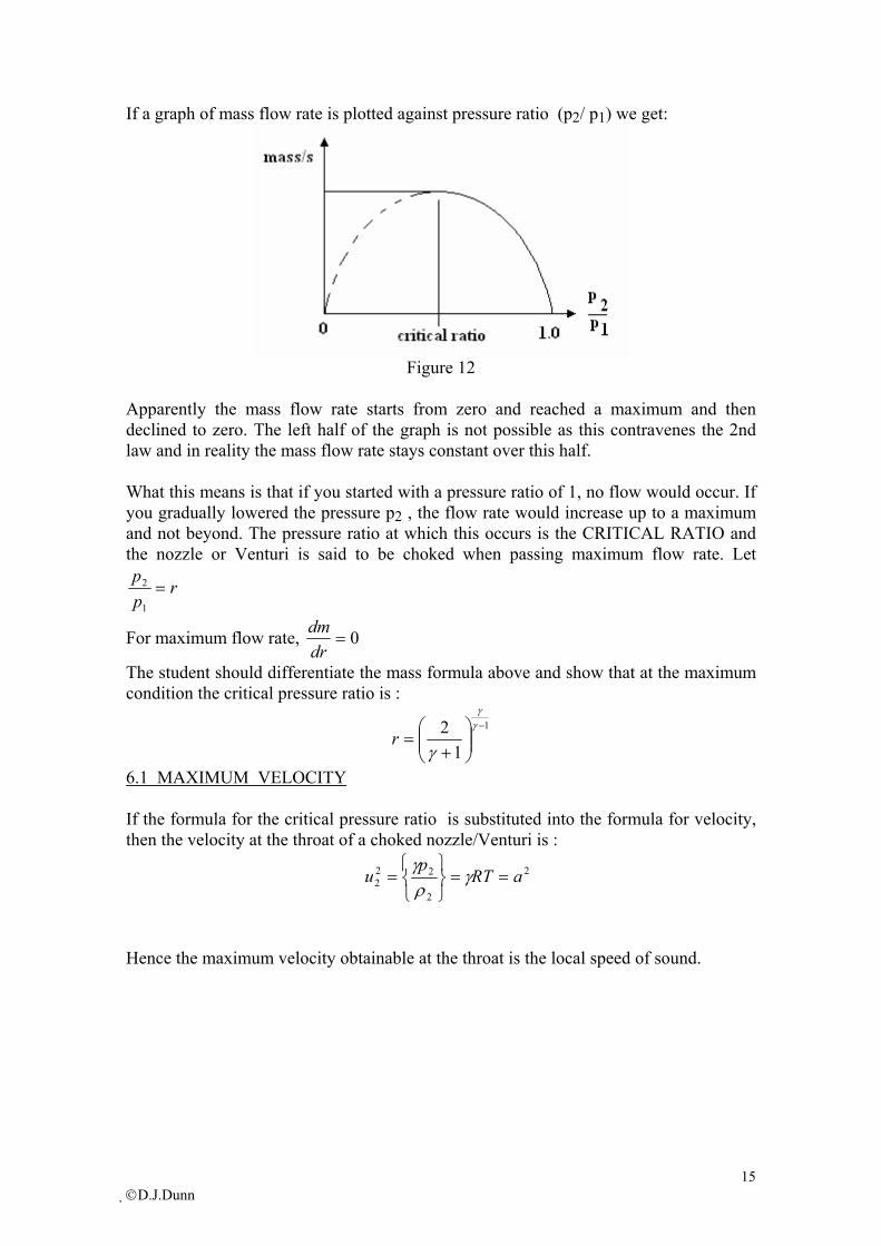
15 D.J.Dunn
If a graph of mass flow rate is plotted against pressure ratio (p2/ p1) we get:
Figure 12
Apparently the mass flow rate starts from zero and reached a maximum and then declined to zero. The left half of the graph is not possible as this contravenes the 2nd law and in reality the mass flow rate stays constant over this half. What this means is that if you started with a pressure ratio of 1, no flow would occur. If you gradually lowered the pressure p2 , the flow rate would increase up to a maximum and not beyond. The pressure ratio at which this occurs is the CRITICAL RATIO and the nozzle or Venturi is said to be choked when passing maximum flow rate. Let
rpp
=1
2
For maximum flow rate, 0=drdm
The student should differentiate the mass formula above and show that at the maximum condition the critical pressure ratio is :
1
12 −
+
=γγ
γr
6.1 MAXIMUM VELOCITY If the formula for the critical pressure ratio is substituted into the formula for velocity, then the velocity at the throat of a choked nozzle/Venturi is :
2
2
222 aRT
pu ==
= γργ
Hence the maximum velocity obtainable at the throat is the local speed of sound.

16 D.J.Dunn
6.2 CORRECTION FOR INLET VELOCITY In the preceding derivations, the inlet velocity was assumed negligible. This is not always the case and especially in Venturi Meters, the inlet and throat diameters are not very different and the inlet velocity should not be neglected. The student should go through the derivation again from the beginning but this time keep v1 in the formula and show that the mass flow rate is
γ
γγ
γγρ
2
1
2
2
1
2
11
1
2
2
1
2112
1
12
−
−
−
=
+
pp
AA
pp
pppAC
m
d
The critical pressure ratio can be shown to be the same as before. 6.3 MORE ON ISENTROPIC FLOW When flow is isentropic it can be shown that all the stagnation properties are constant. Consider the conservation of energy for a horizontal duct :
h + u2/2 = constant h = specific enthalpy
If the fluid is brought to rest the total energy must stay the same so the stagnation enthalpy ho is given by : ho = h + u2/2 and will have the same value at any point in the duct. since ho = Cp To then To (the stagnation temperature) must be the same at all points. It follows that the stagnation pressure po is the same at all points also. This knowledge is very useful in solving questions.

17 D.J.Dunn
6.4 ISENTROPIC EFFICIENCY (NOZZLE EFFICIENCY) If there is friction present but the flow remains adiabatic, then the entropy is not constant and the nozzle efficiency is defined as :
η= actual enthalpy drop/ideal enthalpy drop For a gas this becomes : (T1 - T2)/(T1 - T2' ) T2' is the ideal temperature following expansion. Now apply the conservation of energy between the two points for isentropic and non isentropic flow :
Cp T1 + u12/2 =Cp T2 + u22/2 ....... for isentropic flow
Cp T1 + u12/2 =Cp T2' + u2' 2/2 .........for non isentropic Hence
η= (T1 - T2)/(T1 - T2' ) = (u22 - u12)/(u2' 2 - u12)
If v1 is zero (for example Rockets) then this becomes : η= u22 /u2' 2

18 D.J.Dunn
SELF ASSESSMENT EXERCISE No. 3 1. A Venturi Meter must pass 300g/s of air. The inlet pressure is 2 bar and the inlet
temperature is 120oC. Ignoring the inlet velocity, determine the throat area. Take Cd as 0.97. Take γ =1.4 and R = 287 J/kg K (assume choked flow)
(Answer 0.000758 m2) 2. Repeat problem 1 given that the inlet is 60 mm diameter and the inlet velocity
must not be neglected. (Answer 0.000747 m2) 3. A nozzle must pass 0.5 kg/s of steam with inlet conditions of 10 bar and 400oC.
Calculate the throat diameter that causes choking at this condition. The density of the steam at inlet is 3.263 kg/m3. Take γ for steam as 1.3 and Cd as 0.98.
(Answer 23.2 mm) 4. A Venturi Meter has a throat area of 500 mm2. Steam flows through it, and the inlet
pressure is 7 bar and the throat pressure is 5 bar. The inlet temperature is 400oC. Calculate the flow rate. The density of the steam at inlet is 2.274 kg/m3.
Take γ= 1.3. R = 462 J/kg K. Cd=0.97. (Answer 383 g/s) 5. A pitot tube is pointed into an air stream which has an ambient pressure of 100 kPa
and temperature of 20oC. The pressure rise measured is 23 kPa. Calculate the air velocity. Take γ = 1.4 and R = 287 J/kg K. (Answer 189.4 m/s)
6. A fast moving stream of gas has a temperature of 25oC. A thermometer is placed
into it in front of a small barrier to record the stagnation temperature. The stagnation temperature is 28oC. Calculate the velocity of the gas. Take γ= 1.5 and R = 300 J/kg K. (Answer 73.5 m/s)
Let's do some further study of nozzles of venturi shapes now.

19 D.J.Dunn
7. CONVERGENT - DIVERGENT NOZZLES A nozzle fitted with a divergent section is in effect a Venturi shape. The divergent section is known as a diffuser.
Figure 13
If p1 is constant and p3 is reduced in stages, at some point p2 will reach the critical value which causes the nozzle to choke. At this point the velocity in the throat is sonic. If p3 is further reduced, p2 will remain at the choked value but there will be a further pressure drop from the throat to the outlet. The pressure drop will cause the volume of the gas to expand. The increase in area will tend to slow down the velocity but the decrease in volume will tend to increase the velocity. If the nozzle is so designed, the velocity may increase and become supersonic at exit. In rocket and jet designs, the diffuser is important to make the exit velocity supersonic and so increase the thrust of the engine. 7.1 NOZZLE AREAS When the nozzle is choked, the velocity at the throat is the sonic velocity and the Mach number is 1. If the Mach number at exit is Me then the ratio of the throat and exit area may be found easily as follows. ut= (γRTt)0.5 ue= Me(γRTe)0.5 mass/s = ρtAtvt = ρeAeve.
( )( )
γγ+
γ−
γ
γ−
γ
γ
=
=
=
γ
γ
=
=
ρρ
ρρ
=
21
t
ee
e
t
5.011
t
ee
1
t
e
e
t
11
t
e
t
e5.0
t
5.0ee
1
t
e
e
t
1
t
e
t
e
tt
ee
e
t
pp
MAA
pp
Mpp
AA
pp
TT
at earlier thshown also wasIt RT
RTMpp
AA
pp
shown that it wasearlier but uu
AA
There is much more which can be said about nozzle design for gas and steam with implications to turbine designs. This should be studied in advanced text books.

20 D.J.Dunn
WORKED EXAMPLE No.3 Solve the exit velocity for the nozzle shown assuming isentropic flow:
Figure 14
T1 = 350 K P1 = 1 MPa p2 = 100 kPa The nozzle is fully expanded (choked). Hence Mt = 1 (the Mach No.) The adiabatic index γ = 1.4 SOLUTION The critical pressure pt = p1 {2/(γ - 1)} γ/(γ-1) = 0.528 MPa Tt/T1 = (pt/p1)( γ-1)/ γ hence Tt = 291.7 K To/Tt = {1 + M2(γ -1)/2 } hence To = 350 K It makes sense that the initial pressure and temperature are the stagnation values
since the initial velocity is zero. T2=Tt (p2/pt)
( γ-1)/ γ = 181.3 K a2 = (γRT2)0.5 = 270 m/s po/p2 = {1 + M22(γ - 1)/2 } γ/(γ-1) Hence M2 = 2.157 and u2 = 2.157 x 270 = 582.4 m/s

21 D.J.Dunn
SELF ASSESSMENT EXERCISE No. 4 1. Air discharges from a pipe into the atmosphere through an orifice. The stagnation
pressure and temperature immediately upstream of the orifice is 10 bar and 287 K at all times.
Determine the diameter of the orifice which regulates the flow rate to 0.03 kg/s. (Answer 4 mm) Determine the diameter of the orifice which regulates the flow rate to 0.0675 kg/s. (Answer 6 mm) Atmospheric pressure is 1 bar, the flow is isentropic and the air should be treated as
a perfect gas. The following formulae are given to you. To = T{1 + M2(γ-1)/2 } p1/p2 = (T1/T2) γ/(γ-1)
The relationship between areas for the flow of air through a convergent- divergent
nozzle is given by A/A* = (1/M){(M2 + 5)/6}3 where A and A* are cross sectional areas at which the Mach Numbers are M and
1.0 respectively. Determine the ratio of exit to throat areas of the nozzle when the Mach number is
2.44 at exit. (Answer 2.49/1) Confirm that an exit Mach number of 0.24 also gives the same area ratio. 2. Air discharges from a vessel in which the stagnation temperature and pressure are
350 K and 1.3 bar into the atmosphere through a convergent-divergent nozzle. The throat area is 1 x 10⁻³ m2. The exit area is 1.2 x 10⁻³ m2. Assuming isentropic flow and no friction and starting with the equations
a = (γRT)1/2 Cp To= CpT + v2/2 pρ-γ = constant Determine the mass flow rate through the nozzle , the pressure at the throat and the
exit velocity. (Answers 0.28 kg/s, 0.686 bar, 215.4 m/s)

22 D.J.Dunn
3. Show that the velocity of sound in a perfect gas is given by a = (γRT)½ Show that the relationship between stagnation pressure, pressure and Mach number
for the isentropic flow of a perfect gas is po/p = {1 + (γ-1)M2/2}γ/(γ-1) It may be assumed that ds = Cp d(lnv) + Cv d(lnp) where v is the specific volume. A convergent - divergent nozzle is to be designed to produce a Mach number of 3
when the absolute pressure is 1 bar. Calculate the required supply pressure and the ratio of the throat and exit areas.
(Answers 36.73 bar 0.236/1) Let's now examine the flow of gases in long pipes and ducts in which the temperature stays constant.

23 D.J.Dunn
8. ISOTHERMAL FLOW Isothermal flow normally occurs in long pipes in which the temperature of the gas has time to normalise with the surroundings. Consider a section of such a pipe :
Figure 15
The friction coefficient is Cf as defined by D'Arcy's formula. p2 - p1 = dp Pressure force = A(p1 - p2) = -A dp Resisting shear force = τwπDdL where τw is the wall shear stress and D is the diameter. Since the pressure drops along the length, the volume expands and so the velocity increases since the area is constant du = increase in velocity. If the velocity increases, then the mass must be accelerated. the inertia force required to this is equal to the change in momentum per second m(u2 – u1) Balancing forces produces this equation :
( )
( ) ( )
( )duuD
dL 4dp
duuu that so small very bey in velocit change let the uuuD
dL D4dp
4DA put andA by divide Auuum dL D πdpA
22w
1212222w
2
2212w
ρ+τ
=−
=−−ρ+π
τπ=−
π=ρ=−=τ−−
The friction coefficient Cf is defined as : Cf = Wall shear Stress/dynamic pressure = 2 τw / ρ u2
( )
udu
DCdL 2
u dp
u by through divide duu2D
Cu dL 4dp
f222
22222
f222
+=ρ−
ρρ+ρ
=−
We may drop the suffix so that for any given point in the pipe
udu
DCdL 2
u dp f
2 +=ρ−
-dp / (ρu2 ) = (2 Cf dL / D )+ (du / u) Usually the change in velocity is negligible and dv is approximately zero. This reduces the equation to :

24 D.J.Dunn
-dp / (ρu2 ) = (2 Cf dL / D ) Hence -dp /dL = (ρ u2 )(2 Cf / D ) Since V = mRT/p = Av then v = mRT/pA = 4mRT/pπD2 where m is the mass flow rate and so u2 =16m2R2T2/p2π2D4 and ρu2=16 ρm2R2T2/p2π2D4

25 D.J.Dunn
but ρ=p/RT so ρ u2=16 ρm2RT/pπ2D4 so -dp /dL = (32 Cf m2RT)/(pπ2D5) -pdp = (32 Cf m2RT)(dL)/ π2D5) Integrating with corresponding limits of L=0 when p = p1 and L=L when p = p2 Then (1-p22/p12)= (64 m2RT Cf L)/( π2 D5 p12)
SELF ASSESSMENT EXERCISE No. 5 1. An air storage vessel contains air at 6.5 bar and 15oC. Air is supplied from the
vessel to a machine through a pipe 90 m long and 50 mm diameter. The flow rate is 2.25 m3/min at the pipe inlet. The friction coefficient Cf is 0.005. Neglecting kinetic energy, calculate the pressure at the machine assuming isothermal flow.
(Answer 5.98 bar) 8.1 FRICTION COEFFICIENT The friction coefficient Cf has been comprehensively explained in other tutorials for non - compressible flow. For smooth bore pipes the following is found to be accurate. BLAZIUS found Cf = 0.079 Re -0.25 LEE found that Cf = 0.0018 + Re-0.35 Otherwise use the Moody chart to find f in which case you need to remember that Re = ρu D/ µ but since u = V/A and ρ=m/V then Re = 4m/ρu D

26 D.J.Dunn
ASSIGNMENT 6 1. A natural gas pipeline is 1000 m long and 100 mm bore diameter. It carries 0.7
kg/s of gas at a constant temperature of 0o C. The viscosity is 10.3 x 10⁻⁶ N s/m2 and the gas constant R = 519.6 J/kg K. The outlet pressure is 105 kPa. Calculate the inlet pressure. using the Blazius formula to find f. (Answer 357 kPa.)
2. A pipeline is 20 km long and 500 mm bore diameter. 3 kg/s of natural gas must be
pumped through it at a constant temperature of 20oC. The outlet pressure is 200 kPa. Calculate the inlet pressure using the same gas constants as Q.1.
(Answer 235 kPa) 3. Air flows at a mass flow rate of 9.0 kg/s isothermally at 300 K through a straight
rough duct of constant cross sectional area of 1.5 x 10⁻³ m2. At end A the pressure is 6.5 bar and at end B it is 8.5 bar. Determine
a. the velocities at each end. (Answers 794.8m/s and 607.7 m/s) b. the force on the duct. (Answer 1 380 N) c. the rate of heat transfer through the walls. (Answer 1.18 MJ) d. the entropy change due to heat transfer. (Answer 3.935 KJ/k) e. the total entropy change. (Answer 0.693 kJ/K) It may be assumed that ds = Cp dT/T + R dp/p

27 D.J.Dunn
4. A gas flows along a pipe of diameter D at a rate of m kg/s. Show that the pressure
gradient is -dp /dL = (32 fm2RT)/(pπ2D5) Methane gas is passed through a pipe 500 mm diameter and 40 km long at 13 kg/s.
The supply pressure is 11 bar. The flow is isothermal at 15oC. Given that the molecular mass is 16 kg/kmol and the friction coefficient Cf is 0.005 determine
a. the exit pressure. (Answer 3.99 bar) b. the inlet and exit velocities. (Answers 9.014 m/s and 24.85 m/s) c. the rate of heat transfer to the gas. (Answer 3.48 kW) d. the entropy change resulting from the heat transfer. (Answer 12.09 kJ/K) e. the total entropy change calculated from the formula ds = Cp ln(T2/T1) - R ln(p2/p1) (Answer 1.054 kJ/K) Let's now go on to look at shock waves that occur in compressible flow when it goes supersonic.

28 D.J.Dunn
9. NORMAL SHOCK WAVES
Shock waves occur in compressible fluids and are due to a sudden rise in pressure from p1 to p2 for example resulting from an explosion or from a sudden change in flow. Consider a sudden rise in pressure travelling through a stream tube of fluid of constant cross sectional area A. The conditions before the change are denoted by suffix (1) and after the change by suffix (2). In particular the Mach Numbers are M1 and M2. We will look at the laws governing the changes one at a time starting with momentum.
Figure 16 9.1 MOMENTUM CHANGE From the fundamental law Force = rate of change in momentum we get (p1 - p2) A = m (u2 - u1) Substitute mass flow rate = m = ρA u and divide both sides by A (p1 - p2) = (ρ2v22 - ρ1v12) Substitute the sonic velocity a = √γRT and RT = p/ρ It follows that a2 = γp/ρ Mach Number is defined as M = u/a so u2= γpM2/ρ Hence (p1 - p2) = ( p2γM22 - p1γ M12)
)i....(....................M1M1
pp
22
21
1
2
γ+γ+
=
9.2 ENERGY CONSERVATION The change in pressure is so rapid that there is no time for heat to transfer out of the gas so the pressure rise is adiabatic. In this case we may use Bernoulli.
( )
( )
( ))ii.(....................
2M
11
2M11
TT
simplify and 1c
R iprelationsh thesubstitute
2RMc
2RMc
TT
2MRTTc
2MRTTc
RTMu substitute andconstant is c assume 2
uTc2
uTc
22
21
1
2
p22
p
21
p
1
2
222
2p
211
1p
22p
22
2p
21
1p
−γ+
−γ+=
γ
−γ=
γ+
γ+
=
γ+=
γ+
γ=+=+
9.3 CONSERVATION OF MASS

29 D.J.Dunn
m = ρ1 Au1 = ρ2 Au2 so ρ1/ρ2= u2/u1 but u = a M
so
( )
( ))iii.......(..........
MM x
2M
11
2M11
(ii)equation substitute MM
x TT
MM
x RTRT
RT a whereMaMa
1
222
21
2
1
1
2
1
2
1
2
1
2
2
1
11
22
2
1
−γ+
−γ+=
ρρ
=
γ
γ=
ρρ
γ==ρρ
9.4 GAS LAWS
11
22
1
2
VpVp
TT
= so dividing top and bottom by m
21
12
1
2
pp
TT
ρρ
= and substituting equation (iii) gives :
( )
( ))iv..(....................
pp
MM x
2M11
2M11
TT
1
2
1
222
21
1
2
−γ+
−γ+=
9.4 OVERALL RESULT By combining the previous work the following equation can be obtained.
)v....(....................1
1M2
M1
2
M 21
21
22
−−γγ
+−γ=
This equation can now be used to solve problems where the Mach number before the change is known. Note if M1 = 1 then M2 = 1 and if M1 > 1 then M2 <1

30 D.J.Dunn
WORKED EXAMPLE No. 4 A gas has a temperature of 300 K, pressure of 1.5 bar and velocity of 450 m/s.
Calculate the velocity, pressure and temperature after a shock wave passes into it. Take γ = 1.3 and the mean molar mass is 44.
SOLUTION First calculate the gas constant R R = Ro/molar mass = 8314/44 = 188.95 J/kg K Note the universal gas constant Ro is on the back page of the fluids tables or should
be remembered as 8314 J/kmol K Next calculate a1 = √(γ RT) = √ (1.3 x 188.95 x 300) = 271.46 m/s Hence the initial velocity is supersonic with a Mach No. M1 = 450/271.46 = 1.6577 Now calculate M2 from equation (v) Show for yourself that M2 = 0.642
Now use equation (i) to find p2 22
21
1
2
M1M1
pp
γ+γ+
=
Show for yourself that p2 = 4.47 bar Next use equation (ii) to find T2
( )
( )2
M11
2M11
TT
22
21
1
2
−γ+
−γ+
=
Show for yourself that T2 = 399 K Now find the sonic velocity after compression a2 = √(γ RT) = 313 m/s Hence u2 = a2M2 = 201 m/s

31 D.J.Dunn
SELF ASSESSMENT EXERCISE No. 7 1. Write down the equations representing the conservation of mass, energy and
momentum across a normal shock wave. Carbon dioxide gas enters a normal shock wave at 300 K and 1.5 bar with a
velocity of 450 m/s. Calculate the pressure, temperature and velocity after the shock wave. The molecular mass is 44 kg/kmol and the adiabatic index is 1.3.
(Answers 446 kPa, 399 K and 201 m/s) 2. Air discharges from a large container through a convergent - divergent nozzle into
another large container at 1 bar. the exit mach number is 2.0. Determine the pressure in the container and at the throat. (Answers 7.82 bar and 4.13 bar).
When the pressure is increased in the outlet container to 6 bar, a normal shock
wave occurs in the divergent section of the nozzle. Sketch the variation of pressure, stagnation pressure, stagnation temperature and Mach number through the nozzle.
Assume isentropic flow except through the shock. The following equations may be
used.
1
2
1
2
1
2
TT
pp
RTMau
constant2
u1
RT
−γγ
=
γ=
=+−γ
γ

HYDROLOGY - TUTORIAL 1
UNIFORM FLOW IN CHANNELS In this tutorial you will
• Derive formula for flow through notches. • Solve problems involving flow through notches.
• Define uniform channel flow.
• Derive formulae relating channel dimensions and flow rate.
• Define the Froude Number.
• Define sub-critical and super critical flow.
The student is advised to study Tutorial 1 from the Fluid mechanics D203 section before starting this tutorial.
© D.J.DUNN www.freestudy.co.uk 1
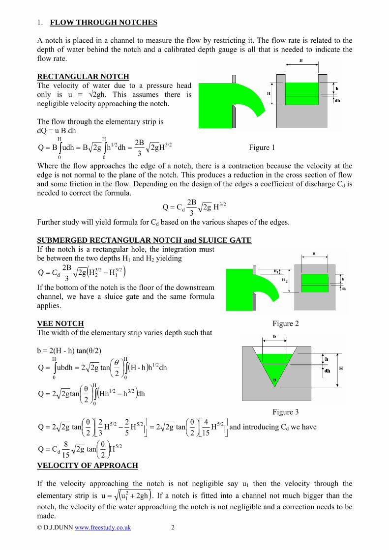
1. FLOW THROUGH NOTCHES A notch is placed in a channel to measure the flow by restricting it. The flow rate is related to the depth of water behind the notch and a calibrated depth gauge is all that is needed to indicate the flow rate.
© D.J.DUNN www.freestudy.co.uk 2
RECTANGULAR NOTCH The velocity of water due to a pressure head only is u = √2gh. This assumes there is negligible velocity approaching the notch. The flow through the elementary strip is dQ = u B dh
3/2H
0
1/2H
0
H2g3
2Bdhh2gBudhBQ === ∫∫ Figure 1
Where the flow approaches the edge of a notch, there is a contraction because the velocity at the edge is not normal to the plane of the notch. This produces a reduction in the cross section of flow and some friction in the flow. Depending on the design of the edges a coefficient of discharge Cd is needed to correct the formula.
3/2d H 2g
32BCQ =
Further study will yield formula for Cd based on the various shapes of the edges. SUBMERGED RECTANGULAR NOTCH and SLUICE GATE If the notch is a rectangular hole, the integration must be between the two depths H1 and H2 yielding
( )3/21
3/22d HH2g
32BQ −= C
If the bottom of the notch is the floor of the downstream channel, we have a sluice gate and the same formula applies. VEE NOTCH Figure 2 The width of the elementary strip varies depth such that b = 2(H - h) tan(θ/2)
( )∫∫ ⎟⎠⎞
⎜⎝⎛==
H
0
1/2H
0
dhhh-H2
tan2g2ubdhQ θ
( )∫ −⎟⎠⎞
⎜⎝⎛=
H
0
3/21/2 dhhHh2θtan2g2Q
Figure 3
⎥⎦⎤
⎢⎣⎡ −⎟⎠⎞
⎜⎝⎛= 5/25/2 H
52H
32
2θ tan2g2Q ⎥⎦
⎤⎢⎣⎡⎟⎠⎞
⎜⎝⎛= 5/2H
154
2θ tan2g2 and introducing Cd we have
5/2d H
2θ tan2g
158CQ ⎟
⎠⎞
⎜⎝⎛=
VELOCITY OF APPROACH If the velocity approaching the notch is not negligible say u1 then the velocity through the elementary strip is ( )2ghuu 2
1 += . If a notch is fitted into a channel not much bigger than the notch, the velocity of the water approaching the notch is not negligible and a correction needs to be made.

WORKED EXAMPLE No.1 The depth of water above the sill of a rectangular notch is 0.23 m and the notch is 0.5 m wide.
The coefficient of discharge is 0.6. Calculate the flow rate of water. SOLUTION
/sm 0.11070.25 2g30.5 x 20.6H2g
32BCQ 33/23/2
d =⎟⎠⎞
⎜⎝⎛==
WORKED EXAMPLE No.2 The depth of water above the sill of a vee notch is 0.4 m and has an included angle of 90o. The
coefficient of discharge is 0.65. Calculate the flow rate of water. SOLUTION
/sm 0.1550.4x tan452g158 x0.65H
2θ tan2g
158CQ 35/2o5/2
d ==⎟⎠⎞
⎜⎝⎛=
WORKED EXAMPLE No.3 The depth of water behind a sluice gate in a horizontal rectangular channel is 3 m and the sluice
is 0.8 m high. The coefficient of discharge is 0.75. Calculate the flow rate of water in the channel downstream.
SOLUTION
( )3/22
3/22d HH2g
32BQ −= C = ( ) 33/23/2 m 84.122.232g
33 x 275.0 =−
SELF ASSESSMENT EXERCISE No.1 1 The depth of water above the sill of a rectangular notch is 0.4 m and the notch is 0.75 m wide.
The coefficient of discharge is 0.62. Calculate the flow rate of water. (0.347 m3/s) 2 The depth of water above the sill of a Vee notch is 0.2 m and has an included angle of 60o. The
coefficient of discharge is 0.6. Calculate the flow rate of water. (0.228 m3/s) 3. A sluice controls the flow in a rectangular channel 2.5 m wide. The depth behind the sluice is
2 m and the sluice is 0.5 m high. What is the discharge? Take Cd =0.8. (5.85 m3/s)
© D.J.DUNN www.freestudy.co.uk 3

2. UNIFORM FLOW IN CHANNEL Channel flow is characterised by constant pressure (usually atmosphere) at all points on the surface. This means that flow can only be induced by gravity so the bed of the channel must slope downwards. There is no pressure gradient in the fluid pushing it along. If the cross section is uniform and the depth is uniform then the flow rate is uniform at all points along the length. This can only occur if the change of potential height is balanced by the friction losses. This is UNIFORM FLOW. DEFINITIONS Flow rate= Q (m3/s) Flow rate per unit width q m2/s Cross sectional area = A (m2) Wetted perimeter = P (m) Mean velocity = uo = Q/A (m/s) Slope of bed = S which is otherwise called the energy gradient. The hydraulic gradient is i and this is the friction head loss per unit length of the bed. The hydraulic gradient is the same as the slope if the flow has a constant depth (uniform flow). The hydraulic radius is defined as Rh = A/P and this is also often called the hydraulic mean depth with symbol m. The wetted area is Aw = PL τw is the wall shear stress. This is the force per unit surface area resisting flow at the surface of contact between the fluid and the wall. CHEZY FORMULA Consider part of a flow of regular cross section A and length L.
Figure 4
If the slope is small the weight of the section considered is W = ρgAL Resolving the weight parallel to the bed the force causing flow is F = W sin(S) If S is small sin S = S radians so F = W S = ρgALS If the flow is steady there is no inertia involved so the force resisting motion must be equal to this force. The resisting force per unit surface area = F/Aw = τw = F/PL = ρgALS /PL= ρgAS /P = ρg Rh S Chezy thought that τw ∝ uo
2 and so τw = C1 uo2 Hence C1 uo
2 = ρg Rh S The Chezy formula is uo = C (RhS) ½ C = (ρg/C1) ½ and C is the Chezy constant. © D.J.DUNN www.freestudy.co.uk 4

WORKED EXAMPLE No. 4 An open channel has a rectangular section 2 m wide. The flow rate is 0.05 m3/s and the depth is
0.4 m. Calculate the slope of the channel using the Chezy formula for steady flow. Take the constant C = 50 m½ /s
SOLUTION
A = 2 x 0.4 = 0.8 m2
P = 2 + 0.4 + 0.4 = 2.8 m Rh = A/P = 0.2857 m uo = Q/A = 0.05/0.8 = 0.0625 m/s uo = 0.0625 = C (Rh S) ½ uo = 0.0625 = 50 (0.2857 S) ½ S = 5.469 x 10⁻⁶
SELF ASSESSMENT EXERCISE No.2 1. An open channel has a triangular section with sides at 45o to the vertical. The flow rate is
0.0425 m3/s and the depth is 0.225 m. Calculate the slope of the channel using the Chezy formula for steady flow. Take the constant C = 49 m½ /s
(Answer 0.00369) 2. A channel with a section as shown carries 1.1 m3/s of water with the depth as shown. The slope
of the bed is 1/2000. Calculate the constant C in the Chezy formula.
Figure 5
(Answer 51.44)
© D.J.DUNN www.freestudy.co.uk 5
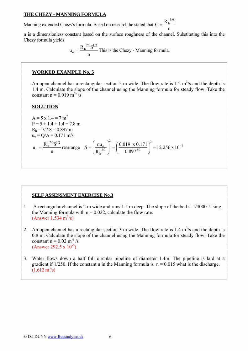
THE CHEZY - MANNING FORMULA
Manning extended Chezy's formula. Based on research he stated that n
RC1/6
h=
n is a dimensionless constant based on the surface roughness of the channel. Substituting this into the Chezy formula yields
n
SRu1/22/3
ho = This is the Chezy - Manning formula.
WORKED EXAMPLE No. 5 An open channel has a rectangular section 5 m wide. The flow rate is 1.2 m3/s and the depth is
1.4 m. Calculate the slope of the channel using the Manning formula for steady flow. Take the constant n = 0.019 m½ /s
SOLUTION
A = 5 x 1.4 = 7 m2
P = 5 + 1.4 + 1.4 = 7.8 m Rh = 7/7.8 = 0.897 m uo = Q/A = 0.171 m/s
n
SRu1/22/3
ho = rearrange
2
2/3h
o
Rnu
⎟⎟⎠
⎞⎜⎜⎝
⎛=S 6
2
2/3 10 x 12.2560.897
0.171 x 0.019 −=⎟⎠⎞
⎜⎝⎛=
SELF ASSESSMENT EXERCISE No.3 1. A rectangular channel is 2 m wide and runs 1.5 m deep. The slope of the bed is 1/4000. Using
the Manning formula with n = 0.022, calculate the flow rate. (Answer 1.534 m3/s) 2. An open channel has a rectangular section 3 m wide. The flow rate is 1.4 m3/s and the depth is
0.8 m. Calculate the slope of the channel using the Manning formula for steady flow. Take the constant n = 0.02 m½ /s
(Answer 292.5 x 10⁻⁶) 3. Water flows down a half full circular pipeline of diameter 1.4m. The pipeline is laid at a
gradient if 1/250. If the constant n in the Manning formula is n = 0.015 what is the discharge. (1.612 m3/s)
© D.J.DUNN www.freestudy.co.uk 6
DARCY FORMULA APPLIED TO CHANNELS The Chezy formula may be related to the Darcy formula for flow in round pipes.
The Darcy formula (not derived here) is 2gd
Lu4Ch2
off =
Sometimes this is stated as 2gdLu fh
2o
f = where 4Cf = f
hf is the friction head and Cf is the friction coefficient which is related to the Reynolds's number and the relative surface roughness. If a round pipe runs full but with constant pressure along the length, then the Chezy and Darcy formulae may be equated.
From the Darcy formula we have L4C
2gdhuf
f2o =
For constant pressure, hf/L = S f
2o 4C
2gdSu =
From the Chezy formula we have uo2 = C2RhS
For a round pipe diameter d running full Rh = d/4 uo
2 = C2Sd/4
Equating we have f
2
4C2gdS
4SdC
=
2f C2gC =
From the Chezy equation we have LRhCu f
22
o =
h
2of
h2
2o
f 2gRLuC
RCLuh ==
This version of the Darcy formula may be used for pipes and channels of any shape with no pressure gradient. Discussion of the Darcy formula show that Cf is related to the surface roughness and this compares with Manning's work. In the case of LAMINAR FLOW Poiseuille's equation is also relevant and this gives the friction head as
2o
f ρgdu Lµ 32h =
Equating this to the Darcy formula gives:
2gdLu4C
ρgdu Lµ 32 2
of2
o = hence eo
f R16
dρu16µC ==
The complete relationship between the Reynolds' number Re and the relative surface roughness is given on the Moody Chart. The chart has several regions, laminar flow, turbulent flow and a region between where it is in transition. The turbulent flow varies between smooth surfaces and fully rough surfaces that produce fully developed turbulent flow. Relative surface roughness is defined as ε = k/D where k is the mean surface roughness and D the bore diameter. The chart is a plot of Cf vertically against Re horizontally for various values of ε. In order to use this chart you must know two of the three co-ordinates in order to pick out the point on the chart and hence pick out the unknown third co-ordinate.
© D.J.DUNN www.freestudy.co.uk 7

For the laminar region e
f R16C =
For smooth pipes, (the bottom curve on the diagram), various formulae have been derived such as those by Blasius and Lee. BLASIUS Cf = 0.0791 Re
0.25
LEE Cf = 0.0018 + 0.152 Re0.35.
The Moody diagram shows that the friction coefficient reduces with Reynolds number but at a certain point, it becomes constant. When this point is reached, the flow is said to be fully developed turbulent flow. This point occurs at lower Reynolds numbers for rough pipes. A formula that gives an approximate answer for any surface roughness is that given by Haaland.
⎪⎭
⎪⎬⎫
⎪⎩
⎪⎨⎧
⎟⎠⎞
⎜⎝⎛ ε
+−=11.1
e10
f 71.3R9.6log6.3
C1
Figure 6 SELF ASSESSMENT EXERCISE No. 4 1. The Darcy - Weisbach formula for a round pipe running full states that hf = 4 Cf Lu2/2gd where L is
the length, d the diameter and u the mean velocity. a. Show that for laminar flow Cf = 16/Re b. Relate the Chezy formula u = C (RS)1/2 and the Manning formula u = (R2/3 S1/2)/n to the Darcy -
Weisbach formula and list the ranges of applicability of all three formula. c. Sketch the relationship between Cf and Re for the range Re = 100 to Re = 106 in a pipe of circular cross
section for typical values of surface roughness k. d. If ageing causes the surface roughness of a pipe to increase, what affect would this have on the flow
carrying capacity of the pipe?
© D.J.DUNN www.freestudy.co.uk 8

3. CRITICAL FLOW SPECIFIC ENERGY HEAD - hs At any point in the length of the channel the fluid has three forms of energy relative to the bed, kinetic, gravitational (potential) and flow (pressure) energy. Figure 7 Strictly, all energy terms should be the mean values. The mean depth is h and the mean gravitational (potential) head is y (the distance to the centroid). The depth at the bottom is hb = h + y and the mean velocity is uo
From the Bernoulli Equation 2guh
2guyhh
2o
b
2o
s +=++=
Text books jump straight to this formula wrongly giving hb as the pressure head. Rearrange the formula and ( ){ }1/2
bso hh2gu −=Consider a channel with an unspecified cross section of area A. Q = Auo ( ){ }1/2
bs hh2gAQ −= CRITICAL DEPTH – hC It will be shown that for a given value of hs there is a depth hc that produces maximum flow rate but the value of hc depends on the shape of the channel since the width is a function of depth and hence the area is a function of depth. Let's examine a rectangular cross section. RECTANGULAR SECTION
( ){ } ({ }1/2bsb
1/2bs hh2gBhhh2gAQ −=−= )
( ){ }1/23bs
2b hhh2gBQ −=
Figure 8 If we plot h – Q for a given value of B and hs we get figure 9a and if we plot h – hs for a given value of B and Q we get figure 9b.
Figures 9a Figure 9 b
The plots reveal some interesting things. Point C is called the critical point and this gives the minimum energy head for a given flow rate or a maximum flow rate for a given energy head. For a flow rate other than the critical value, there are two possible depths of flow. This is logical since for a given amount of energy the flow can be slow and deep or fast and shallow. Flow at the shallow depth is super-critical and flow at the larger depth is sub-critical. The critical depth is denoted hc.
© D.J.DUNN www.freestudy.co.uk 9

To find the critical depth we use max and min theory. At point C dQ/dhb = 0 Differentiate and we get:
( )( )1/2
bs
1/2b
s1/2
b hhB
23hh2g
dhdQ
−⎭⎬⎫
⎩⎨⎧
⎟⎠⎞
⎜⎝⎛ −= h
32h h
23hh0 c
sb
bs ==⎟
⎠⎞
⎜⎝⎛ −=
Since then substituting for h( ){ 1/2bso hh2gu −= } s will produce the critical velocity.
gh 2h2g h
23h2gu c
cc
cc =⎟
⎠⎞
⎜⎝⎛=⎟
⎠⎞
⎜⎝⎛ −=
It follows that the critical flow rate is h gBAuQ 3/2ccc ==
Here is an alternative derivation for the rectangular channel. A = B hb uo = Q/(A) = Q/(B hb)
( )2b
2
2
bs hB2gQhh += For a given flow rate the minimum value of hs is found by differentiating.
( ) ( )3b
2
2
3b
2
2
b
s
hBgQ1
hB2g2Q1
hdh
−=−= For a minimum value equate to zero.
( ) ( )3/1
2
2
b3b
23b
2
2
gBQhor hBgQ
hBgQ10 ⎟⎟
⎠
⎞⎜⎜⎝
⎛==−=
These are the critical values so it follows that 1/3
2
2c
c3/2cc gB
Qhor h gBQ ⎟⎟⎠
⎞⎜⎜⎝
⎛==
guhor gh
BhhgB
BhQu
2c
ccc
3/2c
c
cc ====
2u3
2guu
2guh
2guhh
2c
2c
22c
c
2o
bs =+=+=+=gc
cc
c
2c
cs h23
2gghh
2guhh =+=+= sc h
32h =
The critical flow in terms of hs is 3/2s
3/2
s3/2cc h
278 gBh
32 gB h gBQ ⎟
⎠⎞
⎜⎝⎛=⎟
⎠⎞
⎜⎝⎛==
The critical velocity in terms of hs is 32gh ghu s
cc ==
FROUDE NUMBER You may have studied this in dimensional analysis. The Froude Number is a dimensionless number important to channel flow as well as to surface waves. It is defined as :
ghuFr = For critical flow
c
cr gh
uF = Substitute ghu cc = into this and 1ghgh
Fc
cr ==
The Froude number is always 1 when the flow is critical in a RECTANGULAR CHANNEL but not for other shapes. Another name for super-critical flow is SHOOTING or RAPID FLOW and sub–critical is called TRANQUIL FLOW. Summary for a rectangular channel
The critical depth is sc h32h = The critical velocity is ghu cc = =
32ghs
The critical flow is h gBQ 3/2cc = 3/2
sh 278 gB ⎟⎠⎞
⎜⎝⎛= Froude Number Fr = 1
© D.J.DUNN www.freestudy.co.uk 10

WORKED EXAMPLE No. 6 A rectangular channel 1.6 m wide must carry water at depth of 1 m. What would be the maximum
possible flow rate and what would be the mean velocity? SOLUTION For maximum flow rate the depth must be the critical depth so hc = 1m. The critical velocity is uc = (g hc)½ = (9.81 x 1) ½ = 3.132 m/s The critical flow is Qc = A uc = 1.6 x 1 x 3.132 = 5.01 m3/s
Check the Froude number 11 x g
3.132ghuF
c
cr ===
If the constant n in the Manning formula is 0.019 m½ /s what must the slope of the bed be for
constant depth at maximum flow rate? A = 1.6 x 1 = 1.6 m2 P = 1.6 + 1 + 1 = 3.6 m Rh = 1.6/3.6 = 0.444 m uo = uc = 3.132 m/s
n
SRu1/22/3
ho = rearrange
2
2/3h
o
Rnu
⎟⎟⎠
⎞⎜⎜⎝
⎛=S 0104.0
444.03.132 x 0.019 2
2/3 =⎟⎠⎞
⎜⎝⎛=
WORKED EXAMPLE No. 7 Water flows in a rectangular channel 3 m wide with a mean velocity of 1.5 m/s and a depth of
1.2 m. Determine whether the flow is tranquil or shooting. Calculate the following. The actual flow rate The specific energy head The critical depth The maximum flow possible SOLUTION
437.01.2 x g
1.5gh
uF or === It follows that the flow is tranquil.
Actual flow rate = A uo = (3 x 1.2) x 1.5 = 5.5 m3/s Energy Head hs = h + uo
2/2g = 1.2 + 1.52/2g = 1.315 m hc = 2hs/3 = 2 x 1.315/3 = 0.876 m For maximum flow rate Fr = 1
c
cr gh
u1F == m/s 2.9310.876 x 9.81ghu cc ===
A = 3 x 0.876 = 2.629 m2
Qc = Auc = 2.629 x 2.931 = 7.71 m3/s If the depth changed to the critical depth, the flow rate would increase.
© D.J.DUNN www.freestudy.co.uk 11

SELF ASSESSMENT EXERCISE No.5 1. A rectangular channel is 3.2 m wide and must carry 5 m3/s of water with the minimum specific head.
What would the depth and mean velocity be? (1.563 m and 3.915 m/s) 2. If the channel in question 1 must carry flow at a constant depth and n in the manning formula is 0.022,
what is the slope of the bed? (0.013) 3. The flow in a horizontal, rectangular channel, 6m wide is controlled by a sluice gate. The
depths of flow upstream and downstream of the gate are 1.5m and 0.300 m respectively. Determine:
(a) the discharge (b) the specific energy of the flow (c) the critical depth. VEE OR TRIANGULAR SECTION
© D.J.DUNN www.freestudy.co.uk 12
( ){ }1/2
bs hh2gAQ −= A = ½ hb x 2 hb tan(θ/2)
( ) ( ){ }1/2bs
2b hh2gθ/2tanhQ −=
( ) ({ 1/25bs
4b hhh2gθ/2tanQ −= )}
( )( ) ( 1/24bs
3b
1/2
b5hh4h2gθ/2tan
dhdQ
−= ) Figure 10
For maximum ( )4bs
3b 5hh4h = ( )bs 5h4h =
54hh s
c =
Since then substituting for h( ){ 1/2bso hh2gu −= } s will produce the critical velocity.
( )1/2
c1/2
c1/21/2
cco 2gh
4h2ghh
452gu ⎟
⎠⎞
⎜⎝⎛=⎟
⎠⎞
⎜⎝⎛=
⎭⎬⎫
⎩⎨⎧
⎟⎠⎞
⎜⎝⎛ −=
1/2c
c 2ghu ⎟
⎠⎞
⎜⎝⎛=
( ) ( ) 5/2c
2/1
c
1/2c2
ccc hθ/2tan2
Q 2
ghθ/2tanhAuQ ⎟⎠⎞
⎜⎝⎛=⎟
⎠⎞
⎜⎝⎛==
g
FROUDE NUMBER
For critical flow c
cr gh
uF = Substitute for uc 707.02
1gh2
gh
Fc
c
r === ghuFr =
In terms of hs
( ) ( ) ( )θ/2tan5
4h25
4hθ/2tan2
hθ/2tan2
Q 2/5
s2/5
s2/1
5/2c
2/1
c ⎟⎠⎞
⎜⎝⎛⎟⎠⎞
⎜⎝⎛=⎟
⎠⎞
⎜⎝⎛
⎟⎠⎞
⎜⎝⎛=⎟
⎠⎞
⎜⎝⎛=
ggg
s
1/2
s
1/2c
c h5
2gh54x
2g
2ghu =⎟
⎠⎞
⎜⎝⎛=⎟
⎠⎞
⎜⎝⎛=
Summary for triangular section
The critical depth is 5
4hh sc =
The critical velocity is 2
ghu cc = = sh
52g
The critical flow is ( ) 5/2c
2/1
c hθ/2tan2
Q ⎟⎠⎞
⎜⎝⎛=
g ( )θ/2tan5
4h2
2/5s ⎟⎠⎞
⎜⎝⎛⎟⎠⎞
⎜⎝⎛=
g
Froude Number 707.02
1Fr ==
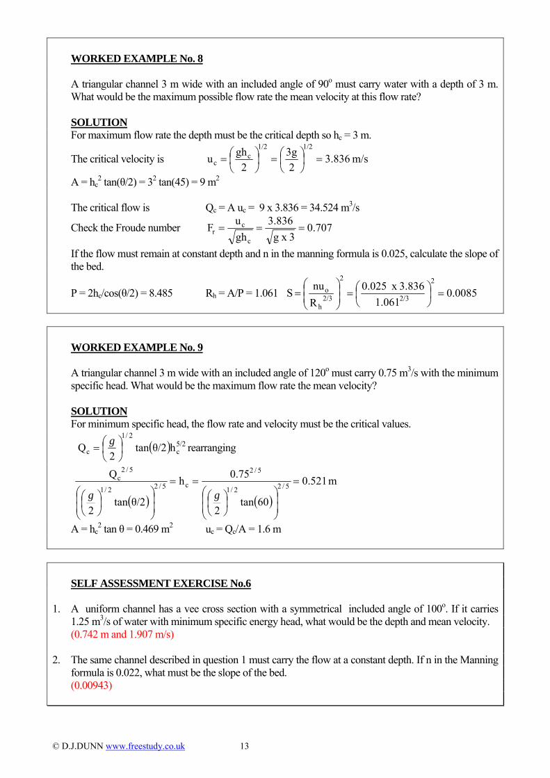
WORKED EXAMPLE No. 8 A triangular channel 3 m wide with an included angle of 90o must carry water with a depth of 3 m.
What would be the maximum possible flow rate the mean velocity at this flow rate? SOLUTION For maximum flow rate the depth must be the critical depth so hc = 3 m.
The critical velocity is m/s 3.8362
3g2
ghu1/21/2
cc =⎟
⎠⎞
⎜⎝⎛=⎟
⎠⎞
⎜⎝⎛=
A = hc2 tan(θ/2) = 32 tan(45) = 9 m2
The critical flow is Qc = A uc = 9 x 3.836 = 34.524 m3/s
Check the Froude number 707.03 x g
3.836ghuF
c
cr ===
If the flow must remain at constant depth and n in the manning formula is 0.025, calculate the slope of the bed.
P = 2hc/cos(θ/2) = 8.485 Rh = A/P = 1.061 2
2/3h
o
RnuS ⎟
⎟⎠
⎞⎜⎜⎝
⎛= 0085.0
061.13.836 x 0.025 2
2/3 =⎟⎠⎞
⎜⎝⎛=
WORKED EXAMPLE No. 9 A triangular channel 3 m wide with an included angle of 120o must carry 0.75 m3/s with the minimum
specific head. What would be the maximum flow rate the mean velocity? SOLUTION For minimum specific head, the flow rate and velocity must be the critical values.
( ) 5/2c
2/1
c hθ/2tan2
Q ⎟⎠⎞
⎜⎝⎛=
g rearranging
( ) ( )m 0.521
60tan2
75.0h
θ/2tan2
Q 5/22/1
5/2
c5/22/1
5/2c =
⎟⎟⎠
⎞⎜⎜⎝
⎛⎟⎠⎞
⎜⎝⎛
==
⎟⎟⎠
⎞⎜⎜⎝
⎛⎟⎠⎞
⎜⎝⎛ gg
A = hc2 tan θ = 0.469 m2 uc = Qc/A = 1.6 m
SELF ASSESSMENT EXERCISE No.6 1. A uniform channel has a vee cross section with a symmetrical included angle of 100o. If it carries
1.25 m3/s of water with minimum specific energy head, what would be the depth and mean velocity. (0.742 m and 1.907 m/s) 2. The same channel described in question 1 must carry the flow at a constant depth. If n in the Manning
formula is 0.022, what must be the slope of the bed. (0.00943)
© D.J.DUNN www.freestudy.co.uk 13

HYDROLOGY - TUTORIAL 2
TRAPEZOIDAL CHANNELS
In this tutorial you will
• Derive equations associated with flow in a trapezoidal channel. • Derive equations for optimal dimensions. • Solve slope of bed using Chezy and manning formulae.
• Solve questions from past papers.
This tutorial is a continuation of tutorial 1 which should be studied first.
© D.J.DUNN www.freestudy.co.uk 1

TRAPEZOIDAL SECTION This topic occurs regularly in the Engineering Council Exam. The trapezoidal section is widely used in canals to accommodate the shape of boats and reduce the erosion of the sides. BEST DIMENSION Figure 1 The channel dimensions that give the maximum flow rate for a fixed cross sectional area is the one with the least amount of friction. This means that it must have the minimum wetted surface area and hence the minimum wetted perimeter P. If this value is then used in any formulae for the flow rate, we will have the maximum discharge possible. Using the notation shown on the diagram we proceed as follows. Area A = (B + b) hb from which B = (A/ hb) – b = (A/ hb) – hb/tanθ Wetted Perimeter P = B + 2hb /sinθ
Substitute for B ⎟⎠⎞
⎜⎝⎛ −+=+−=
tanθ1
sinθ2h
hA
sinθ2h
tanθh
hAP b
b
bb
b
For a given cross sectional area the minimum value of P occurs when dp/dhb = 0
⎟⎠⎞
⎜⎝⎛ −+−=
tanθ1
sinθ2
hA
dhdP
2bb
Equate to zero and ⎟⎠⎞
⎜⎝⎛ −=
tanθ1
sinθ2hA 2
b and substitute for A
⎟⎠⎞
⎜⎝⎛ −=⎟
⎠⎞
⎜⎝⎛ +
tanθ1
sinθ2hh
tanhB 2
bbb
θ ⎟
⎠⎞
⎜⎝⎛ −=⎟
⎠⎞
⎜⎝⎛ +
tanθ1
sinθ2h
tanhB b
b
θ
⎟⎠⎞
⎜⎝⎛ −=
tanθ1
sinθ1h2B b or whereKh2B b= ⎟
⎠⎞
⎜⎝⎛ −=
tanθ1
sinθ1K
It can be shown that when this is the case, the bottom and sides are both tangents to a circle of radius hb. When θ = 90o K = 1 and when θ = 45o K = √2 -1 = 0.414 and in fact K is almost a linear function such that K ≈ θ/90 WORKED EXAMPLE No.1 Calculate the dimensions of a trapezoidal channel with sides at 45o if it must carry 2.5 m3/s of water
with minimum friction given that C = 50 in the Chezy formula and the bed has a gradient of 1 in 1000 SOLUTION The Chezy formula is uo = C (RhS) ½ or Q = A C (RhS) ½
bb 0.828htan45
1sin45
1h2B =⎟⎠⎞
⎜⎝⎛ −= b = hb/tan 45o = hb
A = (B + b) hb = (0.828 hb + hb) hb = 1.828 hb2
bbbb 3.656h2.828h0.828hsin45
1h2BP =+=⎟⎠⎞
⎜⎝⎛+=
Rh = A/P = 0.5 hb Q = 2.5 = 1.828 hb
2 x 50(0.5 hb/1000)1/2 0.000748 = hb
4 (0.5 hb/1000) 0.748 = 0.5 hb
5 hb = 1.084 m B = 0.828 hb = 0.897 m
© D.J.DUNN www.freestudy.co.uk 2

SELF ASSESSMENT EXERCISE No.1 1. Calculate the dimensions of a trapezoidal channel with sides at 60o to the horizontal if it must carry
4 m3/s of water with minimum friction given that C = 55 in the Chezy formula and the bed has a gradient of 1 in 1200.
(hb = 1.334 m B = 1.541 m) 2. Calculate the dimensions of a trapezoidal channel with sides at 30o to the horizontal if it must carry
2 m3/s of water with minimum friction given that C = 49 in the Chezy formula and the bed has a gradient of 1 in 2000.
(hb = 1.053 m B = 0.564 m) CRITICAL DEPTH It requires a lot of Algebra to get to the critical values. Start as before hs = hb + uo
2/2g Rearrange to make u the subject ( ){ }bs
2o hh2gu −=
Q = Auo Q2 = A2uo2
A = (B + b)hb Q2 = (B + b)2hb
2 uo2
Substitute for uo ( )( ) 2b
2bs
2hbBhh
2Q
+−=g
We cannot differentiate this expression because b is a function of h so we make a substitution first. b = hb/tan θ
( ) 2b
2b
bs
2h
tanθhBhh
2Q
⎟⎠⎞
⎜⎝⎛ +−=
g( )
22b
bbs tanθhBhhh ⎟⎟
⎠
⎞⎜⎜⎝
⎛+−= Now we need to multiply out.
( ) ⎟⎟⎠
⎞⎜⎜⎝
⎛++−⎟⎟
⎠
⎞⎜⎜⎝
⎛++=⎟⎟
⎠
⎞⎜⎜⎝
⎛++−=
tanθ2Bh
θtanhhB
tanθh2Bh
θtanhhhhB
tanθ2Bh
θtanhhBhh
2Q 4
b2
5b3
b2s
3b
2s
4b
s2b
23b
2
4b2
b2
bs
2
g
Now differentiate with respect to hb to find the maximum flow rate for a given specific energy head.
tanθ8Bh
θtan5hh3B
tanθh6Bh
θtanh4hhh2B
2gdh2QdQ 3
b2
4b2
b2s
2b
2s
3b
sb2
b−−−++=
For maximum Flow rate equate dQ/dhb to zero.
tanθ8Bh
θtan5hh3B
tanθh6Bh
θtanh4hhh2B0
3b
2
4b2
b2s
2b
2s
3b
sb2 −−−++=
We can simplify by substituting back hb/tan θ = b 2b
2b
22b
2sbsb
2sb
2 8Bbhh5bh3Bh6Bbhhh4bhh2B0 −−−++=
( ) ( )8Bb5b3Bh6Bbhhh4bh2Bh0 222bss
2s
2b ++−++=
( ) ( )8Bb5b3Bh6Bbhhh4bh2B0 22bss
2s
2 ++−++=
Rearrange to get the critical depth ( )( ) ss22
22
cb Chh8Bb5b3B6Bb4b2Bhh =
++++
==
( )( )
( )( )( )
( )( )5b3B
4b2Bb)(B5b3BbB4b2B
8Bb5b3B6Bb4b2BC 22
22
++
=++++
=++++
=
© D.J.DUNN www.freestudy.co.uk 3

( )( ) sc h
5b3B4b2Bh
++
= or ( )( ) cs h
4b2B5b3Bh
++
=
If B = 0 we have a Vee section 5
4hhh scb == as before.
If b = 0 we have a rectangular section 3
2hhh scb == as before.
There are computer programs for making the calculations such as the one at http://www.lmnoeng.com/Channels/trapezoid.htm
To find the critical velocity flow rate substitute ( )( ) cs h
4b2B5b3Bh
++
= into ( ){ }cs2c
2o hh2guu −==
( )( )
( )( ) ⎭
⎬⎫
⎩⎨⎧
⎟⎟⎠
⎞⎜⎜⎝
⎛−
++
=⎭⎬⎫
⎩⎨⎧
⎟⎟⎠
⎞⎜⎜⎝
⎛−
++
== 14b2B5b3B2ghhh
4b2B5b3B2guu ccc
2c
2o
( )( )
( ) ( )( ) ⎭
⎬⎫
⎩⎨⎧
⎟⎟⎠
⎞⎜⎜⎝
⎛+
+−+=
⎭⎬⎫
⎩⎨⎧
⎟⎟⎠
⎞⎜⎜⎝
⎛−
++
=4b2B
4b2B5b3B2gh14b2B5b3B2ghu ccc
( ) ⎭⎬⎫
⎩⎨⎧
⎟⎟⎠
⎞⎜⎜⎝
⎛++
=4b2BbB2ghu cc
If B = 0 we have a Vee section ⎭⎬⎫
⎩⎨⎧=
2ghu c
c as before.
If b = 0 we have a rectangular section we have { }cc ghu = as before. To find the critical flow rate substitute use Qc = A uc A = (B + b)hc
( ) ⎭⎬⎫
⎩⎨⎧
⎟⎟⎠
⎞⎜⎜⎝
⎛++
+=4b2BbB2ghb)h(BQ ccc ( ) ⎭
⎬⎫
⎩⎨⎧
⎟⎟⎠
⎞⎜⎜⎝
⎛++
+=4b2BbB2gb)h(BQ 3/2
cc
If B = 0 we have a Vee section ⎭⎬⎫
⎩⎨⎧=
2gbhQ 3/2
cc as before in a slightly different form
If b = 0 we have a rectangular section we have gBhQ 3/2cc = as before.
Summary for trapezoidal section
The critical depth is ( )( ) sc h
5b3B4b2Bh
++
=
The critical velocity is ( ) ⎭⎬⎫
⎩⎨⎧
⎟⎟⎠
⎞⎜⎜⎝
⎛++
=4b2BbB2ghu cc
The critical flow is ( ) ⎭⎬⎫
⎩⎨⎧
⎟⎟⎠
⎞⎜⎜⎝
⎛++
+=4b2BbB2gb)h(BQ 3/2
cc
The major problem exists that solving with these formulae requires a value for b and this depends on the answer itself.
© D.J.DUNN www.freestudy.co.uk 4
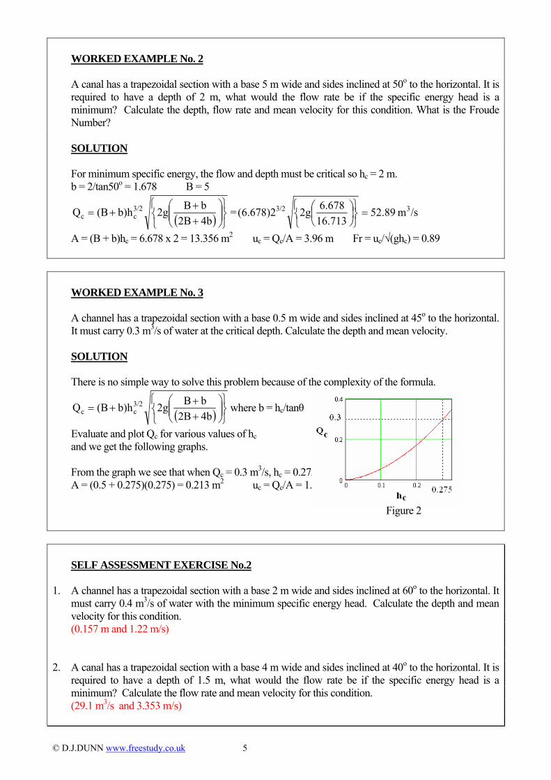
WORKED EXAMPLE No. 2 A canal has a trapezoidal section with a base 5 m wide and sides inclined at 50o to the horizontal. It is
required to have a depth of 2 m, what would the flow rate be if the specific energy head is a minimum? Calculate the depth, flow rate and mean velocity for this condition. What is the Froude Number?
SOLUTION For minimum specific energy, the flow and depth must be critical so hc = 2 m. b = 2/tan50o = 1.678 B = 5
( ) ⎭⎬⎫
⎩⎨⎧
⎟⎟⎠
⎞⎜⎜⎝
⎛++
+=4b2BbB2gb)h(BQ 3/2
cc = /sm 52.89713.16678.62g.678)26( 33/2 =
⎭⎬⎫
⎩⎨⎧
⎟⎠⎞
⎜⎝⎛
A = (B + b)hc = 6.678 x 2 = 13.356 m2 uc = Qc/A = 3.96 m Fr = uc/√(ghc) = 0.89 WORKED EXAMPLE No. 3 A channel has a trapezoidal section with a base 0.5 m wide and sides inclined at 45o to the horizontal.
It must carry 0.3 m3/s of water at the critical depth. Calculate the depth and mean velocity. SOLUTION There is no simple way to solve this problem because of the complexity of the formula.
( ) ⎭⎬⎫
⎩⎨⎧
⎟⎟⎠
⎞⎜⎜⎝
⎛++
+=4b2BbB2gb)h(BQ 3/2
cc where b = hc/tanθ
© D.J.DUNN www.freestudy.co.uk 5
Evaluate and plot Qc for various values of hc and we get the following graphs.
From the graph we see that when Qc = 0.3 m3/s, hc = 0.275 m A = (0.5 + 0.275)(0.275) = 0.213 m2 uc = Qc/A = 1.41 m/s Figure 2 SELF ASSESSMENT EXERCISE No.2 1. A channel has a trapezoidal section with a base 2 m wide and sides inclined at 60o to the horizontal. It
must carry 0.4 m3/s of water with the minimum specific energy head. Calculate the depth and mean velocity for this condition.
(0.157 m and 1.22 m/s) 2. A canal has a trapezoidal section with a base 4 m wide and sides inclined at 40o to the horizontal. It is
required to have a depth of 1.5 m, what would the flow rate be if the specific energy head is a minimum? Calculate the flow rate and mean velocity for this condition.
(29.1 m3/s and 3.353 m/s)

WORKED EXAMPLE No. 4 An open channel has a trapezoidal cross section with sides inclined at 45o to the vertical. The
channel must carry 21 m3/s with a velocity of 3 m/s with minimum friction. Determine the smallest slope of the bed for these conditions and the corresponding depth and dimensions of the channel. The constant n in the Manning formula is 0.012. Show that this is a sub critical flow.
Figure 3
SOLUTION Q = 21 m3/s uo = 3 m/s A = Q/u = 7 m2
For minimum friction the optimal value of B is ⎟⎠⎞
⎜⎝⎛ −=
tanθ1
sinθ1h2B b
bb h8284.0tan45
1sin45
1h2B =⎟⎠⎞
⎜⎝⎛ −= b = hb
A = (B + b)hb 7 = (0.8284hb + hb)hb = 1. 8284hb
2 hb = √(7/1. 8284) = 1.957 m B = 1.621 m b = 1.957 m P = B + 2b/sin 45 = 1.621 + 2 x 1.957/sin 45 = 7.155 A = 7 Rh = 7/7.155 = 0.978 m (Note that for 45o Rh = 0.5 hb)
Manning formula nSRu
1/22/3=
0.012S978.03
1/22/3=
S = 0.001333 The specific energy head is hs = 1.957 + 32/2g = 2.416 m
The critical depth is ( )( ) m 0.756
14.64811.07
1.957 x 51.621 x 31.957 x 41.621 x 2h
5b3B4b2Bh sc ==
++
=++
=
Since the actual depth is larger the flow is sub critical.
© D.J.DUNN www.freestudy.co.uk 6

SELF ASSESSMENT EXERCISE No. 3 These are exam standard questions. 1. An open channel has a trapezoidal section with sides inclined at 45o to the vertical. The channel must
carry 20 m3/s of water with a mean velocity of 2.5 m/s. Determine the smallest slope of the bed possible and the corresponding depth and dimensions of the channel. The constant n in the Manning formula is 0.012. Show that this is a sub critical flow.
u = (R2/3S1/2)/n (Answer S = 0.000845, h = 2.1, B = 2.1 m and b = 2.1 m.) 2. A channel has a trapezoidal section 5 m wide at the bottom. The sides slope at 1 metre up for each 2
horizontal. The bed has a slope of 1/3600 and n in the manning formula is 0.024. Calculate the flow rates corresponding to mean velocities of 0.3 and 0.6 m/s. (Ans. 0.549 m3/s and 4.81 m3/s)
© D.J.DUNN www.freestudy.co.uk 7

HYDROLOGY - TUTORIAL 4
UNSTEADY FLOW IN CHANNELS In this tutorial you will
• Derive equations associated with a rise in the level of the bed.
• Define a hydraulic jump and derive the equations for it.
• Define a narrow weir and derive equations for it. • Define a broad weir and derive equations for it. • Derive equations for the flow rate through a Venturi Flume.
• Solve questions from past papers.
This tutorial is a continuation of tutorial 1 and 2 and these should be studied first.
© D.J.DUNN www.freestudy.co.uk 1

UNSTEADY FLOW
If the depth of the water is not constant, we have unsteady flow. This might occur when the frictional losses do not match the change in potential energy. In this case the hydraulic gradient 'i' is not the same as the slope 'S'. The height of the bed relative to the datum level is z.
Figure 1
The total head is defined as hs plus the additional potential head z hT = hS + z = h + z + u2/2g Start with hS = hT - z Differentiate with respect to x (the distance along the channel from a given datum point). dhS /dx = dhT/dx - dz/dx dz/dx is the gradient of the bed and this is clearly negative so dz/dx = - S dhS /dx = dhT/dx + S The change in the total head can only be due to frictional losses and this will be a reduction so we can define this as the hydraulic gradient i = dhf/dx = - dhT/dx dhS /dx = S - i We had hS = h + u2/2g Differentiate this with respect to h dhS/dh =1 + (u/g)du/dh u = Q/A. Differentiate with respect to A du/dA = -Q/A2
If A is a function of depth, then this is difficult. For a rectangular channel A = B h Differentiate with respect to h dA/dh = B Substitute du/dh = (-Q/A2) B Substitute into dhS/dh =1 + (u/g)du/dh dhS/dh = 1 - (u/g) (Q/A2) B dhS/dh = 1 - (u/g) (Q/A2) B Substitute Q/A = u dhS/dh = 1 - (u2/g) B/A Substitute B/A = 1/h dhS/dh = 1 - (u2/gh) = 1 – Fr
2
For maximum or minimum specific head dhS/dh = 0 and this can only occur if Fr = 1 Flow is at the critical depth when Fr = 1 The velocity that produces the critical depth is uc = √(g h) Note that it has been assumed that h is constant at all widths so the Froude number is only 1 when the channel is rectangular in section. © D.J.DUNN www.freestudy.co.uk 2

HYDRAULIC JUMP It has already been shown that for a given flow rate in an open channel, there are two possible depths. One is when the flow is slow and deep called TRANQUIL FLOW and the other when it is shallow and fast called RAPID FLOW or SHOOTING FLOW. It is possible rapid flow to change to tranquil flow quite suddenly and spontaneously and when it does we get a phenomenon called a hydraulic jump. It is not possible for the reverse to happen. For a hydraulic jump to occur, the Fr > 1, i.e. the flow must be supercritical. The jump might occur because the slope of the bed is insufficient for friction to balance the loss of potential energy. Since the losses are smaller for the tranquil flow, the balance can be restored.
© D.J.DUNN www.freestudy.co.uk 3
A jump can be made to occur if there is an obstacle on the bed higher than the critical depth. Figure 2
When the change occurs there is a reduction in momentum and an increase in the hydrostatic force. The solution is based on equating them. uo = mean velocity. The mean depth is h/2 Pressure force on a cross section is Fp = ρgAh/2 Momentum force at a section =Fm = ρAu2
The cross sectional area is A = B h where B is the width.
Change in pressure force = 2
hρgB2
ρgBh2
hρgA2
hρgA 222
212211 −=−
Change in pressure force = ( ) ( )( 212122
21 hhhh
2ρgBhh
2ρgB
+−=− ) Change in momentum force = ρBh1u1
2 - ρBh2u22 = ρB(h1u1
2- h2u22)
For continuity of flow u22 = ( u1 h1/ h2)2
Change in momentum force = ( )122
121
212
2
2122
11 hhhhρBuu
hhhuhρB −=⎟⎟
⎠
⎞⎜⎜⎝
⎛−
The change in pressure and momentum forces may be equated.
( )( ) ( )122
1212121 hh
hhρBuhhhh
2ρgB
−=+−
( )2
12121 h
huhh2g
=+
( )2g
hhhhu
1
221
21 ⎟⎟
⎠
⎞⎜⎜⎝
⎛+= ................(1)
In terms of the flow rate
( ) ( )2ghhhhB
2g
hhhhhBQ 2121
2
1
221
21
22 +=⎟⎟⎠
⎞⎜⎜⎝
⎛+=
The flow per unit width is usually given as ( )2
hhhghq 2121
2 += ....................(2)

From (1) ( )2221
211 hhhu2h
+=g
02uhhhh21
12122 =−+
g
h2 may be solved with the quadratic equation giving:
⎭⎬⎫
⎩⎨⎧+±−=
1
21
112 gh8u1hh2h and since h2 cannot be negative
⎭⎬⎫
⎩⎨⎧++−=
1
21
112 gh8u1hh2h
Substitute the Froude Number 1
212
r ghuF = { }2
r112 8F1hh2h ++−=
{ }[ ]18F12hh 2
r1
2 −+=
Next consider the energy balance before and after the jump. Energy Head before the jump = h1 + u1
2/2g Energy Head after the jump = h2 + u22/2g
Head loss = hL = h1 + u1
2/2g - h2 - u22/2g hL = h1 - h2 + (u1
2 - u22)/2g
Continuity of flow Q = u1 B h1 = u2 B h2 2
112 h
huu =
Hence ⎪⎭
⎪⎬⎫
⎪⎩
⎪⎨⎧
⎟⎟⎠
⎞⎜⎜⎝
⎛−=⎟⎟
⎠
⎞⎜⎜⎝
⎛=−
2
2
121
2
2
121
21
22
21 h
h1uhhu-uuu
We already found equation (1) was ( )2g
hhhhu
1
221
21 ⎟⎟
⎠
⎞⎜⎜⎝
⎛+=
Substitute
( )
( )
( ) ( )( ){ }21
21
22212
221
22
21
22
1
221
22
21
2
2
1
1
221
22
21
h2hhhhhuu
hhh
hhhh
2guu
hh1
2g
hhhhuu
−+=−
⎭⎬⎫
⎩⎨⎧ −⎟⎟⎠
⎞⎜⎜⎝
⎛+=−
⎪⎭
⎪⎬⎫
⎪⎩
⎪⎨⎧
⎟⎟⎠
⎞⎜⎜⎝
⎛−⎟⎟
⎠
⎞⎜⎜⎝
⎛+=−
g
Substitute into the formula for hL hL = h1 - h2 + (u1
2 - u22)/2g
( ) ( )( ) ( ) ( )( )
( ) ( )( ){ }
21
221
221
31
32
2212
21
L
21
21
22212121
L
21
21
2221
2121
21
2221
21L
h4hhhhhhhh4hh4hh
h4hhhhhhhh4hh
h4hhhhhhh
h2gh x 2hhhhghhh
−+−+−=
−++−=
−++−=
−++−=
( )21
312
L
21
31
32
2212
21
L
h4hh-hh
h4hhhh3hh3hh
=
−+−=
Useful website http://www.lmnoeng.com/Channels/HydraulicJump.htm
© D.J.DUNN www.freestudy.co.uk 4

WORKED EXAMPLE No.1 50 m3/s of water flows in a rectangular channel 8 m wide with a depth of 0.5 m. Show that a
hydraulic jump is likely to occur. Calculate the depth after the jump and the energy loss per second. SOLUTION A1 = 8 x 0.5 = 4 m2 u1 = Q/A1 = 50/4 = 12.5 m/s Froude Number Fr1 = u/√gh = = 12.5/√(9.81 x 0.5) = 31.855 This is supercritical so a jump is
possible.
{ }[ ] m 3.74831.855 x 812
0.518F12hh 22
r1
2 =+=−+=
A2 = 8 x 3.748 = 30 m2 u2 = Q/A2 = 50/30 = 1.667 m/s
( ) ( ) m 4.5733.748 x 0.5 x 40.5-3.748
h4hh-hh
3
21
312
L ===
Energy loss = mghL = 50 000 x 9.81 x 4.573 = 2.243 MJ/s m = 50 000 kg/s SELF ASSESSMENT EXERCISE No. 1 1. Show by applying Newton's Laws that when a hydraulic jump occurs in a rectangular channel
the depth after the jump is
{ }[ ]18F12hh 2
r1
2 −+=
Go on to show that the head loss is ( )21
312
L h4hh-hh =
2. 40 m3/s of water flows in a rectangular channel 10 m wide with a depth of 1.0 m. Show that a hydraulic jump is likely to occur. Calculate the depth after the jump and the energy loss per second.
(Answers 1.374 m and 3.735 kJ/s) 3. Water has a depth H = 1.5 m behind a sluice gate and emerges from the gate with a depth of
0.4 m. Downstream a hydraulic jump occurs. Calculate depth after the jump and the mean velocity before and after the jump. (Note use Bernoulli to find u1)
Figure 3
(Answers 1.416 and 1.627 m/s)
© D.J.DUNN www.freestudy.co.uk 5

RISE IN LEVEL OF BED In this section we will examine what happens to the level of water flowing in a channel when there is a sudden ride in the level of the bed.
Figure 4
First apply Bernoulli between points (1) and (2)
z2guh
2guh
22
2
21
1 ++=+
From the continuity equation substitute 2
112 h
huu =
z2ghhu
h2guh
2
2
11
2
21
1 +⎟⎟⎠
⎞⎜⎜⎝
⎛
+=+
Rearrange 0z2gh
huh2guh 2
2
21
21
2
21
1 =−−−+
02ghuhzh
2guh
21
212
22
21
1 =−⎟⎟⎠
⎞⎜⎜⎝
⎛−−+
Substitute h2 = x + h1 – z
( ) ( ) ( ){ } 02g
z-hxuz-hxzz-hx2guh
21
212
11
21
1 =+
−+⎭⎬⎫
⎩⎨⎧
−+−+
( ) ( ){ } 02g
z-hxuz-hxx2gu 2
1212
1
21 =
+−+
⎭⎬⎫
⎩⎨⎧
−
{ }( ) ( ) 0z-hxuz-hx2gxu 21
21
21
21 =+−+−
{ }( ) ( ) 0z-hxuz-hx2gxu 21
21
21
21 =+−+−
There follows a long bout of more algebra to produce a cubic equation for x :
( ) ( ) 0z2h2guz
guzhzhx
4guzh2xx 1
21
21
11
21
123 =−+⎟⎟
⎠
⎞⎜⎜⎝
⎛−−−+⎟⎟
⎠
⎞⎜⎜⎝
⎛−−+
This equation may be used to solve the change in height of the water. If the values of x and z are small, we may neglect products and higher powers of small numbers so the equation simplifies to:
0g
zuguhx
21
21
1 =+⎟⎟⎠
⎞⎜⎜⎝
⎛−
0ghzu
ghu1x
1
21
1
21 =+⎟⎟⎠
⎞⎜⎜⎝
⎛−
© D.J.DUNN www.freestudy.co.uk 6

The Froude number approaching the change is 1
1r1 gh
uF = hence
( ) 0zFF1x 21
21 =+− rr
( )121
21
hFzF
x−
=r
r
The equation indicates that if flow is supercritical (Fr1>1) then x is positive and the surface rises. If the flow is sub critical (tranquil Fr1<1) then x is negative and the surface is depressed. WORKED EXAMPLE No. 2 Water flows in a rectangular channel with a depth of 0.55 m and a mean velocity of 4.5 m/s.
Downstream there is a rise in the level of the bed of 0.075 m. Determine the depth and mean velocity after the rise. Is Bernoulli's equation is satisfied?
SOLUTION
z = 0.075 m h1 = 0.55 m u1 = 4.5 m/s 1.9379.81x0.55
4.5ghuF
1
1r1 ===
The flow is supercritical (Rapid) ( ) 0.102m0.551.937
(1.937) 0.075 x 2
2=
−=
Depth = 0.55 + 0.102 = 0.577 m
4.289m/s0.577
0.55 x 4.5hhuu2
112 ===
Energy head before rise is 2guh
21
1 + 582.12g
4.555.02=+=
Energy Head after the rise is z2guh
22
2 ++ 616.1102.02g
4.289577.02
=++=
There is a small discrepancy. SELF ASSESSMENT EXERCISE No. 2 1. Water flows in a rectangular channel with a depth of 1.0 m. Downstream there is a rise in the
level of the bed of 0.1 m. Determine the mean velocity after the rise and the critical depth upstream if the depth after the rise is :
(a) 1.1 m (Answers 3.13 and 1 m) (b) 0.8 m (Answer 2.215 m/s and 0.833 m)
© D.J.DUNN www.freestudy.co.uk 7

WEIRS We shall consider two forms of weirs, a narrow one with a sharp edge and a broad one with a rounded edge. NARROW WEIRS The flow over a sharp edge weir is in essence the same as flow through a rectangular notch. Consider the flow from section (1) to section (2).
Figure 5
We shall only consider the depth upstream relative to the top of the weir. The mean velocity at a given point is u. The pressure head at (2) is atmospheric Applying Bernoulli between (1) and (2) we have:
2guh
2guh
22
2
21
1 +=+
The velocity upstream is usually small so we can neglect u1 and if we use gauge pressure then h2 = 0
2guh
22
1 = and 12 2ghu =
Next consider a thin horizontal strip at distance h from the bottom of the weir and height dh. The volume flow through it is dQ = u2 Bdh
Bdh2ghdQ 1=
∫=H
0
1/21 dhh B2gQ
2/3BH2g32Q =
It is normal to introduce a coefficient of discharge to correct for losses. 2/3
d BH2gC32Q =
© D.J.DUNN www.freestudy.co.uk 8
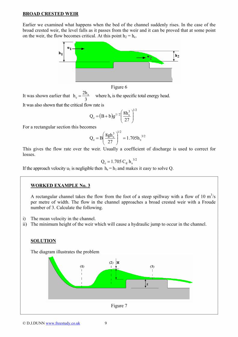
BROAD CRESTED WEIR Earlier we examined what happens when the bed of the channel suddenly rises. In the case of the broad crested weir, the level falls as it passes from the weir and it can be proved that at some point on the weir, the flow becomes critical. At this point h2 = hc.
Figure 6
It was shown earlier that 3
2h h sc = where hs is the specific total energy head.
It was also shown that the critical flow rate is
( )1/23
s2/1c 27
8hbB Q ⎟⎟⎠
⎞⎜⎜⎝
⎛+= g
For a rectangular section this becomes
3/2s
1/23s
c 1.705h27
8ghB Q =⎟⎟⎠
⎞⎜⎜⎝
⎛=
This gives the flow rate over the weir. Usually a coefficient of discharge is used to correct for losses.
3/2sdc h C 1.705 Q =
If the approach velocity u1 is negligible then hs = h1 and makes it easy to solve Q. WORKED EXAMPLE No. 3 A rectangular channel takes the flow from the foot of a steep spillway with a flow of 10 m3/s
per metre of width. The flow in the channel approaches a broad crested weir with a Froude number of 3. Calculate the following.
i) The mean velocity in the channel. ii) The minimum height of the weir which will cause a hydraulic jump to occur in the channel. SOLUTION The diagram illustrates the problem
Figure 7
© D.J.DUNN www.freestudy.co.uk 9
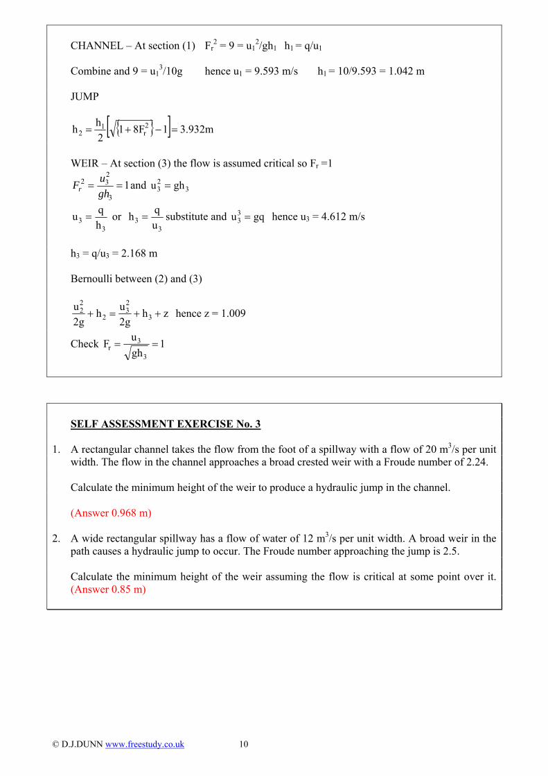
CHANNEL – At section (1) Fr
2 = 9 = u12/gh1 h1 = q/u1
Combine and 9 = u1
3/10g hence u1 = 9.593 m/s h1 = 10/9.593 = 1.042 m JUMP
{ }[ ] 3.932m18F12hh 2
r1
2 =−+=
WEIR – At section (3) the flow is assumed critical so Fr =1
13
232 ==
ghuFr and 3
23 ghu =
3
3 hqu = or
33 u
qh = substitute and hence ugqu33 = 3 = 4.612 m/s
h3 = q/u3 = 2.168 m Bernoulli between (2) and (3)
zh2guh
2gu
3
23
2
22 ++=+ hence z = 1.009
Check 1ghuF
3
3r ==
SELF ASSESSMENT EXERCISE No. 3 1. A rectangular channel takes the flow from the foot of a spillway with a flow of 20 m3/s per unit
width. The flow in the channel approaches a broad crested weir with a Froude number of 2.24. Calculate the minimum height of the weir to produce a hydraulic jump in the channel. (Answer 0.968 m) 2. A wide rectangular spillway has a flow of water of 12 m3/s per unit width. A broad weir in the
path causes a hydraulic jump to occur. The Froude number approaching the jump is 2.5. Calculate the minimum height of the weir assuming the flow is critical at some point over it.
(Answer 0.85 m)
© D.J.DUNN www.freestudy.co.uk 10

2. VENTURI FLUME A venturi flume is a flume that narrows to the throat and then widens back out again. The reduction in width causes a change in velocity and hence height. In a Venturi meter the change is reflected as a change in static pressure but in a flume it is height. If energy is conserved the total energy head at inlet and at the throat are the same so from Bernoulli we have:
2guH
2guH
22
2
21
1 +=+
The flow rate is Q = Au = B1 H1 u1 = B2 H2 u2 Hence 11
2221 HB
HBuu =
2guH
2g1
HBHBuH
22
2
2
11
2221 +=⎟⎟
⎠
⎞⎜⎜⎝
⎛+
⎪⎭
⎪⎬⎫
⎪⎩
⎪⎨⎧
⎟⎟⎠
⎞⎜⎜⎝
⎛−+=−
2
11
2222
21 HBHB1
2guHH ( )
2
11
22
212
HBHB1
HH2gu
⎟⎟⎠
⎞⎜⎜⎝
⎛−
−=
( )
⎥⎦
⎤⎢⎣
⎡−
−=
21
2
22
221
22
H BH b1
HH2gH BQ Allowing for energy losses ( )
⎥⎦
⎤⎢⎣
⎡−
−=
21
2
22
221
22d
H BH b1
HH2gH BCQ
If the flow rate is a maximum, the depth at the throat will be the critical depth and a hydraulic jump will form downstream of the throat. In this case
s2 h32H = and
2gu
32h
2guHh
22s
22
2s +=+= Hence 3h2u s
2g
=
32gh
3hs2B
32ghHBuHBQ s2s
22222 ===
Introducing the coefficient of discharge 2/3sd h 1.705CQ =
This is the same as for Broad Crested weir. Solving Q with this formula is not straight forward because hs contains the velocity term. The examination often asks for the derivation of this formula. WORKED EXAMPLE No.4 A rectangular channel is 1.2 m wide and narrows to 0.6 m wide in a venturi flume. The depth at
the entrance and throat are 0.6 m and 0.55 m respectively. Calculate the flow rate given Cd = 0.88.
SOLUTION
( ) ( ) /3m 0.324
0.6 x 1.20.55 x 6.01
05.02g0.55 x 0.6 x 88.0
H BH B1
HH2gH BCQ 32
21
21
22
22
2122d =
⎥⎦⎤
⎢⎣⎡ −
=
⎥⎦
⎤⎢⎣
⎡−
−=
© D.J.DUNN www.freestudy.co.uk 11

SELF ASSESSMENT EXERCISE No.4 Show that for critical flow with a Froude Number of 1 in a rectangular channel, the depth of
flow yc is related to the specific energy head H by the expression H = 3yc/2 Describe with sketches a broad crested weir and a venturi flume. Show that for both structures the flow rate is related to the critical depth by the relationship
3/2d H 1.705CQ =
Note the symbols are not the same as in the notes and are the ones used typically in the EC
exam.
© D.J.DUNN www.freestudy.co.uk 12

ENGINEERING COUNCIL EXAM
HYDROLOGY D204
TUTORIAL 13 - PIPE NETWORKS
In this tutorial you will
• Revise pipe friction equations. • Derive iterative balance equations for nodes and loops. • Solve problems about networks with a common junction. • Solve problems about networks with connected loops.
Students are advised to complete tutorial 1 and study the flow in pipes before doing this tutorial.
© D.J.DUNN www.freestudy.co.uk 1

BRIEF REVISION OF PIPE FLOW PIPE FRICTION
When a fluid flows in a pipe the friction head is defined by the Darcy equation 2gD
Lu4Ch2mf
f =
hf = friction head um = mean velocity = Q/A D = pipe bore L = pipe length Re = Reynolds number = ρumD/µ R = Hydraulic resistance The friction coefficient Cf is dependent on the surface roughness and degree of turbulence and there are many theories about its relationship. The most common method for finding Cf is from the Moody Chart or from one of many developed formulae such as : BLASIUS Cf = 0.0791 Re
0.25
LEE Cf = 0.0018 + 0.152 Re
0.35.
HAALAND ⎪⎭
⎪⎬⎫
⎪⎩
⎪⎨⎧
⎟⎠⎞
⎜⎝⎛ ε
+−=11.1
e10
f 71.3R9.6log6.3
C1
For laminar flow n = 1 and Cf = 16/Re
Basically we are saying hf ∝ um
n and n is only 2 for complete turbulent flow. We must remember that Cf depends on the Reynolds number. In this case we would need to think about recalculating Cf every time we change the flow. In terms of flow rate Q hf = R Qn
R (or often K) is the fluid resistance. When n = 2 52f
DgπL32CR = and when n is not 2, Cf and hence
R changes with the flow rate. The units of R are s2/m5. MINOR LOSSES Minor losses occur at Entry and exit from a reservoir, at sudden changes in sections and sharp bends. In general these are small compared to pipe friction when the pipes are long and are neglected for short connections they are important. In terms of pressure head the losses are usually formulated as:
2L RQh = where the resistance is given by 42D
k8Rπ
= where k is a factor that depends on the pipe
sizes and can be found in literature. The Moody chart and other details concerning pipe losses can be found in tutorial 1.
© D.J.DUNN www.freestudy.co.uk 2

GUESSING and CORRECTING
Starting with hf = R Qn differentiate to get Q
dQnRQdQnRQdhn
1-nf == and since R Qn = hf
QdQnhdh f
f = or f
f
nhQdhdQ =
If this relationship holds approximately true for finite changes then QδQnhδh f
f = or f
f
nhδh QδQ =
These equations are used to make corrections in the guessing game that follows. NETWORKS WITH A COMMON JUNCTION The diagram shows a typical example with four reservoirs A, B, C and D connected to a common junction J. The problem is to find the pressure head h at the junction.
For a system such as that illustrated, suppose that we need to find the flow in each pipe but we don't know the pressure at the junction. We could do four simultaneous equations in order to find the flow in each pipe but these days with fast computational methods it is relatively easier to guess at values and make corrections. Applying Bernoulli between the free surface of any reservoir and the junction gives:
h + z + u2/2g = hJ + zJ + uJ2/2g + hf
At the free surface h = 0 and u = 0 (This is an assumption normally made).
z = hJ + zj + uJ2/2g + hf hf = z - hJ - zj - uJ
2/2g Many sources of information ignore the velocity term and state hf = z - zj - hJ and this will be so here. For a given pipe we calculate the hydraulic resistance R (or K) and get the form hf = R Qn Hence for any pipe hf = R Qn = z – zJ – hJ Q = {( z – zJ – hJ)1/n/R} Suppose we guess at the value of hJ (or more likely hJ + zJ). With a suitable programme such as Excel™ it is easy to guess the head and keep changing it until ΣQ = 0. The point is that at the junction the total or net flow rate must be zero so each time we guess we add up the total flow until ΣQ = 0. If it is not very close to zero then we guess again. A more systematic method of arriving at the correct answer is to make a correction after each guess based on the error formula derived previously. Using the guessed value of head we work out Q for each pipe. Any error in the guess will produce
an error in the flow of f
f
nhδh QδQ = and the correction to the head must be
QδQnhδh f
f = for each
pipe. © D.J.DUNN www.freestudy.co.uk 3

For four pipes A, B, C and D the total error is:
D
f
C
f
B
f
A
ff Q
δQ nhQδQ nh
QδQ nh
QδQ nhδh ⎟
⎠
⎞⎜⎝
⎛+⎟
⎠
⎞⎜⎝
⎛+⎟
⎠
⎞⎜⎝
⎛+⎟
⎠
⎞⎜⎝
⎛=∑
∑∑ =f
f Q/hδQn δh
This method is called the nodal balance method. WORKED EXAMPLE No.1 Based on the diagram previous, the following data applies. zA = 143 m zB = 134 m zC = 120 m zD = 100 m zJ = 80 DA = 0.4 m DB = 0.3 m DC = 0.5 m DD = 0.4 m LA = 4200 m LB = 1200 m LC = 1250 m LD = 1200 m Cf = 0.005 for all pipes. The constant n is 2. Find the pressure head at the junction by guessing and hence the flow rate in or out of each
reservoir. SOLUTION
Calculate R for each pipe. 552f
DL0.001653
DgπL32CR ==
RA = 677.8 RB = 816 RC = 66.1 RD = 193.7 The following solution was done on a spread sheet. Remember that on the spread sheet the
values in the table will automatically change when you change hJ in the programme. Adjusting hJ until ΣQ ≈ 0 gives the following.
PIPE R z - zJ hf = z - zJ - hJ Q=√hf/R ∆Q/∆hf Guess hJ = 39.998 A 677.8 63 23.002 0.18422 0.00801 B 816 54 14.002 0.13099 0.00936 C 66.1 40 0.002 0.0055 2.75033 D 193.7 20 -19.998 -0.3213 0.01607 ΣQ =-0.0006 Σ =2.78376 Note that if Q is minus it is implied that hf is minus but this will cause a problem in the
calculations so use Q = √Modulus(hf/R) In Excel the formula would be entered =SQRT(ABS(cell1/cell2))*(cell3/ABS(cell3)) where cell 1
and cell2 are the cells containing hf and R and cell3 contains hf. The final values of flow rate are QA = 0.18422 m3/s QB = 0.13099 m3/s QC = 0.13099 m3/s QD = -0.3213 m3/s
© D.J.DUNN www.freestudy.co.uk 4

In an examination you may not have access to a suitable programmable calculator so you would have to keep repeating all the calculations with an adjustment to the value of hJ each time. WORKED EXAMPLE No.2 Repeat the last worked example but use iteration to arrive at the answer.
The correction to be made after each iteration is ∑∑ =
ff Q/h
δQn h
With this formula you can calculate the adjustment each time. With no other data, a good idea for the starting value is the mean height of the reservoirs. Also note that the height of the junction is not normally given but if we guess at hJ + zJ we get the same result but do not know the static head at J. Also note that K is commonly used instead of R. A good starting guess might be hJ = (63 + 54 + 40 + 20)/4 = 44 m
PIPE R z - zJ hf Q Q/hf A 677.8 63 19 0.16743 0.00881 B 816 54 10 0.1107 0.01107 C 66.1 40 -4 -0.246 0.0615 D 193.7 20 -24 -0.352 0.01467 Σ=-0.3199 Σ=0.09605 Now find the correction
66.60.09605(-0.3199) x 2
Q/hδQ 2δh
ff −===∑∑ Change the values of hJ to 37.34 and repeat.
PIPE R z - zJ hf Q Q/hf A 677.8 63 25.66 0.19457 0.00758 B 816 54 16.66 0.14289 0.00858 C 66.1 40 2.66 0.2006 0.07542 D 193.7 20 -17.34 -0.2992 0.01725 Σ=0.23886 Σ=0.10883 Now find the correction
39.40.10883(0.23886) x 2
Q/hδQ 2δh
ff ===∑∑ Change the values of hJ to 41.73 and repeat.
PIPE R z - zJ hf Q Q/hf A 677.8 63 21.27 0.17715 0.00833 B 816 54 12.27 0.12262 0.00999 C 66.1 40 -1.73 -0.1618 0.09351 D 193.7 20 -21.73 -0.3349 0.01541 Σ=-0.1969 Σ=0.12725 Now find the correction
09.30.1273(-0.1969) x 2
Q/hδQ 2δh
ff −===∑∑ Change the values of hJ to 38.6 and repeat.
PIPE R z - zJ hf Q Q/hf A 677.8 63 24.64 0.19066 0.00774 B 816 54 15.64 0.13844 0.00885 C 66.1 40 1.64 0.15751 0.09605 D 193.7 20 -18.36 -0.3079 0.01677 Σ=0.17875 Σ=0.1294
76.20.1294(0.17875) x 2
Q/hδQ 2δh
ff ===∑∑ Change the values of hJ to 41.4 and repeat.
The number of iterations depends on how accurate you want the answer to be but you can see the answer is converging on 40 m.
© D.J.DUNN www.freestudy.co.uk 5

WORKED EXAMPLE No.3 (EC Exam Standard) The table shows the data for the network of pipes shown connecting four reservoirs to a
common junction.
© D.J.DUNN www.freestudy.co.uk 6
Reservoir Water Level K for Pipe (m) above a connecting datum to J (s2/m5) A 50 4.0 B 45 3.0 C 40 2.0 D 30 2.0 Calculate the flow in each pipe using iteration until the final head correction at the junction is
less than 0.1 m. SOLUTION The height of the datum is not given so we can only calculate the combined head and height.
The best guess is usually the mean height of the reservoirs which is (50 + 45 + 40 + 30)/4 = 41.25
1st ITERATION PIPE K z ∆hf Q Q/hf Guess hJ+zJ A 4 50 8.75 1.47902 0.16903 41.25 B 3 45 3.75 1.11803 0.29814 C 2 40 -1.25 -0.7906 0.63246 D 2 30 -11.25 -2.3717 0.21082 -0.5652 1.31045
863.01.310(-0.5652) x 2
Q/hδQ 2δh
ff −===∑∑ =Correct hJ + zJ = 40.4
2nd ITERATION PIPE R z ∆hf Q Q/hf Guess hJ+zJ A 4 50 9.6 1.54919 0.16137 41.25 B 3 45 4.6 1.23828 0.26919 C 2 40 -0.4 -0.4472 1.11803 D 2 30 -10.4 -2.2804 0.21926 0.05991 1.76786
0678.01.76786
(0.5991) x 2Q/hδQ 2δh
ff ===∑∑ This is less than 0.1 so meets the answer
QA = 1.55 m3/s QB = 1.24 m3/s QC = -0.45 m3/s QD = -2.28 m3/s
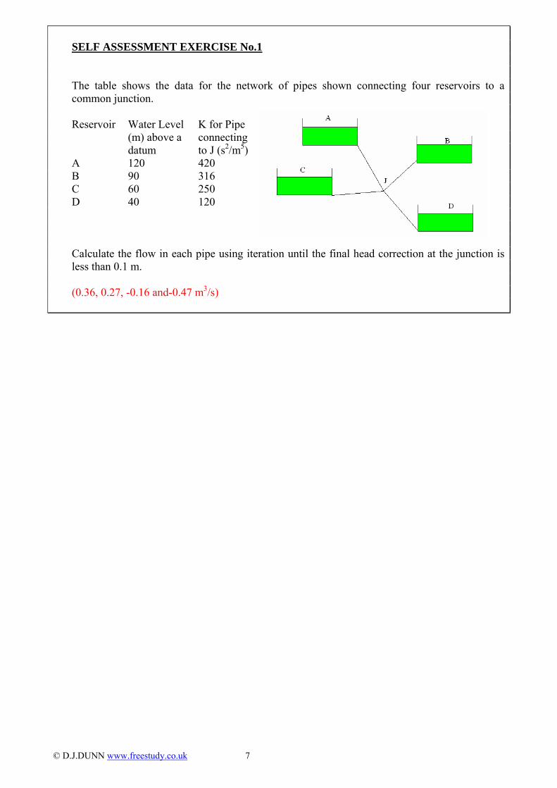
SELF ASSESSMENT EXERCISE No.1 The table shows the data for the network of pipes shown connecting four reservoirs to a
common junction.
© D.J.DUNN www.freestudy.co.uk 7
Reservoir Water Level K for Pipe (m) above a connecting datum to J (s2/m5) A 120 420 B 90 316 C 60 250 D 40 120
Calculate the flow in each pipe using iteration until the final head correction at the junction is
less than 0.1 m. (0.36, 0.27, -0.16 and-0.47 m3/s)

NETWORKS Consider a small network laying in the horizontal plane as shown in the diagram. There are three nodes A, B and C and three pipes AB, BC and AC. The purpose is to find the flow in each pipe. Suppose the pressure head at node A is hA. Assume the flow is clockwise around the loop. The pressure head at node B must be hA + hf (AB). The pressure head at node C must be hA + hf (AB) + hf (BC). The pressure head at node A must be hA + hf (AB) + hf (BC) + hf (CB). We are back to where we started so hA = hA + hf (AB) + hf (BC) + hf (CB). It follows that hf (AB) + hf (BC) + hf (CB) = 0 If the flow in any pipe is the opposite way, then hf will be negative and all is taken care of. If we went anti-clockwise around the loop, the same would be true. Notation is clockwise is positive (opposite to maths convention, typical engineering) Anti- clockwise is negative. The solution is based on calculating the total hf for either the clockwise or anti-clockwise flow and adjusting the Q values until Σhf is zero.
The correction to the flow in each pipe is ∑∑=
/Qnhh
δQf1
f1
We start by guessing the flow in each pipe (ensuring balance at each node) and calculating the friction head for each. We add up the friction heads and if it is not close to zero we correct our guess and do it again. The method is known as the Hardy Cross method or Loop Balance. IMPORTANT NOTE – the correction must be SUBTRACTED
© D.J.DUNN www.freestudy.co.uk 8

WORKED EXAMPLE No.4
© D.J.DUNN www.freestudy.co.uk 9
In the simple network shown Q1 = 0.8 m3/s, Q2 = -1.2 m3/s. The resistance of each pipe is as follows. Pipe AB R = 50 s2/m5
Pipe BC R = 30 s2/m5
Pipe AC R = 60 s2/m5
Determine the flow in the three pipes. Take n = 2 SOLUTION By conservation of flow, Q3 = 0.4 m3/s Guess the flow in each pipe bearing in mind the total flow at a node is zero. Clockwise is
positive. The starting guess is: Q (AB) = 0.6 Q (BC) = -0.6 Q (BC) = -0.4 First iteration PIPE R Q hf hf/Q AB 50 0.6 18 30 BC 30 -0.6 -10.8 18 AC 60 -0.2 -2.4 12 -0.2 4.8 60
04.060 x 2
4.8/Qh2
hδQ
f1
f1 ===∑∑ Correct the Q values by subtracting
Second iteration PIPE R Q hf hf/Q AB 50 0.56 15.68 28 BC 30 -0.64 -12.288 19.2 AC 60 -0.24 -3.456 14.4 -0.32 -0.064 61.6
000524.061.6 x 2
0.32-/Qh2
hδQ
f1
f1 −===∑∑ Correct the Q values by subtracting
Third iteration PIPE R Q hf hf/Q AB 50 0.56052 15.708 28.025 BC 30 -0.6395 -12.2688 19.185 AC 60 -0.2395 -3.44162 14.37 -0.3185 -0.00005 61.58 This is one iteration more than we need. The head loss is so close to zero that this is the correct
answer. Q (AB) = 0.56052 m3/s, Q (BC) = -0.6395 m3/s and Q (AC) = -0.2395 m3/s If we check the flow into each node we will see that the original figures have been maintained.

MULTIPLE LOOPS When a network contains multiple loops, there will be pipes common to adjoining loops with a clockwise flow in one loop appearing as anti-clockwise in the other. Each loop must be identified and the corrections made systematically to each loop in turn. The correction to the flows must be made each time before moving on to the next loop. For more than two loops in a network, the process becomes very elaborate and computer methods need to be used. WORKED EXAMPLE No. 5
© D.J.DUNN www.freestudy.co.uk 10
The diagram shows a water supply network with the demands indicated at the nodes. The value of K for each pipe is 1000 s2/m5 except for BE which is 7500 s2/m5. The supply pressure head at A is 50 m above the ground elevation for the area served which is flat and level. Calculate the pressure head at each node.
SOLUTION The problem must be solved as two loops with a common pipe BE. First make a guess at the flow rates. The supply must be 0.02 + 0.05 + 0.03 + 0.03 + 0.05 + 0.02 = 0.2 m3/s. Bear in mind that the net flow is zero at all nodes.
Data shown for initial guess Start with loop ABEFA PIPE R Q hf hf/Q AB 1000 0.08 6.4 80
BE 7500 0.01 0.75 75 EF 1000 -0.08 -6.4 80
01386.0335 x 2
9.25-/Qh2
hδQ
f1
f1 −===∑∑
FA 1000 -0.1 -10 100 -9.25 335 Correct all flows in this loop by adding 0.01386.
Data after first correction to left loop

Now do loop BCDEB PIPE R Q hf hf/Q
© D.J.DUNN www.freestudy.co.uk 11
BC 1000 0.02 0.4 20 CD 1000 -0.01 -0.1 10
01117.0248.5 x 25.55-
/Qh2h
δQf1
f1 −===∑∑
DE 1000 -0.04 -1.6 40 BE 7500 -0.02381 -4.2504 178.5 -5.550 248.5 Correct all flows in this loop by adding 0.01117.
Data after first correction to the right loop
This completes the first iteration so now do loop ABEFA again. PIPE R Q hf hf/Q AB 1000 0.09381 8.79956 93.80597 BE 7500 0.01264 1.19829 94.80084
00266.0341 x 2
1.8132-/Qh2
hδQ
f1
f1 −===∑∑
EF 1000 -0.0662 -4.38165 66.19403 FA 1000 -0.0862 -7.42941 86.19403 -1.81321 340.9949 Correct all flows by adding 0.00266
Data after second correction to the left loop
Now do loop BCDEB again. PIPE R Q hf hf/Q BC 1000 0.03117 0.971311 31.16586 CD 1000 0.00117 0.001359 1.165859
00459.0175.9 x 2
1.6141/Qh2
hδQ
f1
f1 −===∑∑
DE 1000 -0.0288 -0.83141 28.83414 BE 7500 -0.0153 -1.7554 114.7411 -1.61414 175.907 Correct all flows by adding 0.00459
Data after second correction to right loop
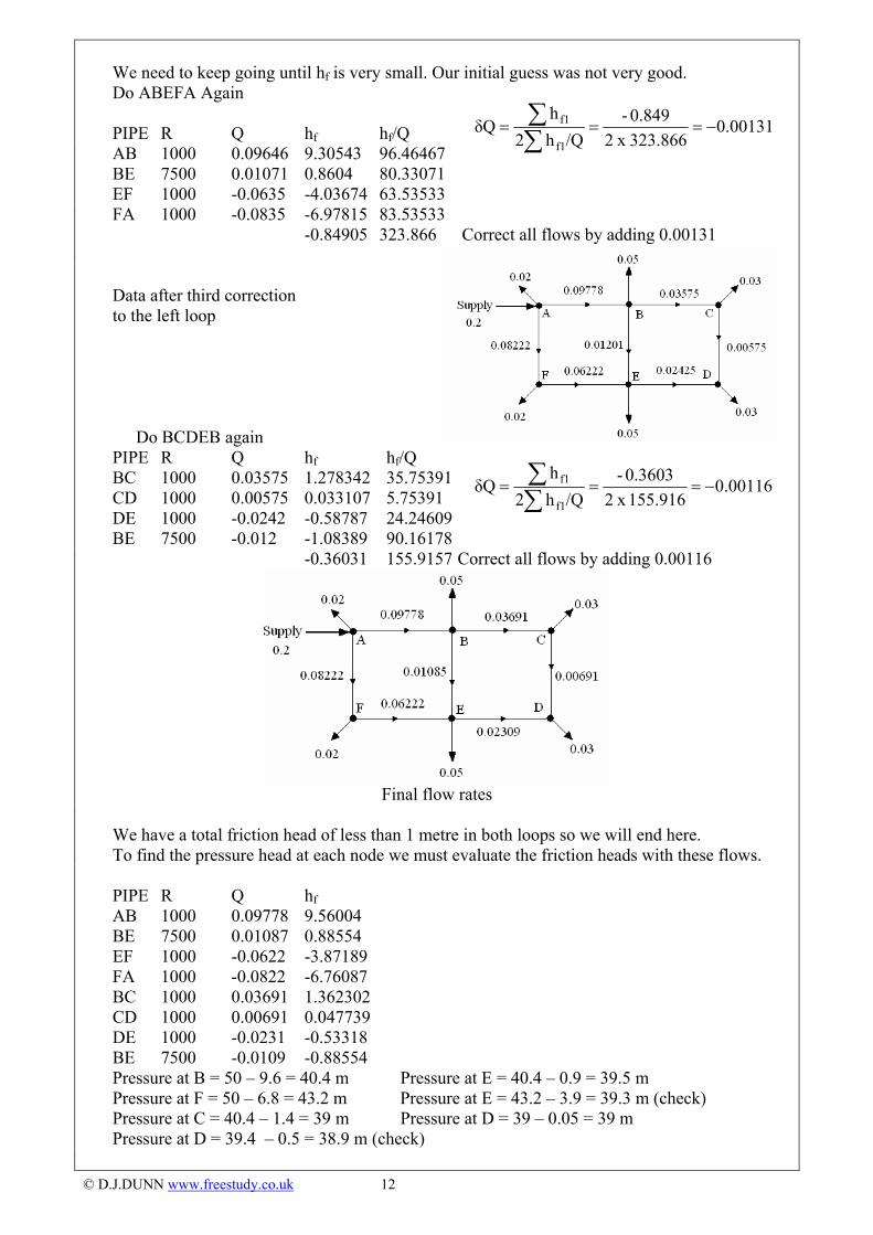
We need to keep going until hf is very small. Our initial guess was not very good. Do ABEFA Again
© D.J.DUNN www.freestudy.co.uk 12
PIPE R Q hf hf/Q AB 1000 0.09646 9.30543 96.46467
00131.0323.866 x 20.849-
/Qh2h
δQf1
f1 −===∑∑
BE 7500 0.01071 0.8604 80.33071 EF 1000 -0.0635 -4.03674 63.53533 FA 1000 -0.0835 -6.97815 83.53533 -0.84905 323.866 Correct all flows by adding 0.00131
Data after third correction to the left loop Do BCDEB again PIPE R Q hf hf/Q BC 1000 0.03575 1.278342 35.75391 CD 1000 0.00575 0.033107 5.75391 DE 1000 -0.0242 -0.58787 24.24609
00116.0155.916 x 20.3603-
/Qh2h
δQf1
f1 −===∑∑
BE 7500 -0.012 -1.08389 90.16178 -0.36031 155.9157 Correct all flows by adding 0.00116
Final flow rates
We have a total friction head of less than 1 metre in both loops so we will end here. To find the pressure head at each node we must evaluate the friction heads with these flows. PIPE R Q hf AB 1000 0.09778 9.56004 BE 7500 0.01087 0.88554 EF 1000 -0.0622 -3.87189 FA 1000 -0.0822 -6.76087 BC 1000 0.03691 1.362302 CD 1000 0.00691 0.047739 DE 1000 -0.0231 -0.53318 BE 7500 -0.0109 -0.88554 Pressure at B = 50 – 9.6 = 40.4 m Pressure at E = 40.4 – 0.9 = 39.5 m Pressure at F = 50 – 6.8 = 43.2 m Pressure at E = 43.2 – 3.9 = 39.3 m (check) Pressure at C = 40.4 – 1.4 = 39 m Pressure at D = 39 – 0.05 = 39 m Pressure at D = 39.4 – 0.5 = 38.9 m (check)

SELF ASSESSMENT EXERCISE No.2 1. The diagram shows a simple pipe network in the horizontal plane with nodes at A, B, C and D
with flow rates as indicated. The hydraulic resistance of each pipe is as follows: AB 500 s2/m5
© D.J.DUNN www.freestudy.co.uk 13
BC 500 s2/m5
CD 1200 s2/m5
DA 1200 s2/m5
BD 600 s2/m5
Determine the flow in each pipe The answers are shown next.
2. The diagram shows a water supply network with the demands indicated at the nodes. The value of K for each pipe is 500 s2/m5 except for BE which is 600 s2/m5. The supply pressure head at A is 120 m above the ground elevation for the area served which is
flat and level. Calculate the flow rate in each pipe and the pressure head at each node.
ANSWERS Q m3/s hf m Node h m AB 0.373 69.6 A 120 BE 0.126 9.6 B 50.4 EF -0.227 -25.7 C 35.4 FA -0.327 -53.4 D 32.7 BC 0.173 15.0 E 40.7 CD 0.0732 2.7 F 66.6 DE -0.127 -8.0 BE -0.126 -9.6
Top Related
Copyright © 2022 FDOKUMEN

