Topics in fluid mechanics

A.C. FowlerMathematical Institute, Oxford University

October 30, 2018

Contents

Preface . . . . . . . . . . . . . . . . . . . . . . . . . . . . . . . . . . . iv

1 Thin film flows 1

1.1 Lubrication theory . . . . . . . . . . . . . . . . . . . . . . . . . . . . 11.2 Droplet dynamics . . . . . . . . . . . . . . . . . . . . . . . . . . . . . 3

1.2.1 Gravity . . . . . . . . . . . . . . . . . . . . . . . . . . . . . . 51.2.2 Surface tension . . . . . . . . . . . . . . . . . . . . . . . . . . 51.2.3 The capillary droplet . . . . . . . . . . . . . . . . . . . . . . . 81.2.4 Advance and retreat . . . . . . . . . . . . . . . . . . . . . . . 10

1.3 Elongational flows . . . . . . . . . . . . . . . . . . . . . . . . . . . . . 111.3.1 Steady flow . . . . . . . . . . . . . . . . . . . . . . . . . . . . 121.3.2 Capillary effects . . . . . . . . . . . . . . . . . . . . . . . . . . 14

1.4 Foam drainage . . . . . . . . . . . . . . . . . . . . . . . . . . . . . . 16Exercises . . . . . . . . . . . . . . . . . . . . . . . . . . . . . . . . . . 16

2 Porous media 19

2.1 Darcy’s law . . . . . . . . . . . . . . . . . . . . . . . . . . . . . . . . 202.1.1 Homogenisation . . . . . . . . . . . . . . . . . . . . . . . . . . 222.1.2 Empirical measures . . . . . . . . . . . . . . . . . . . . . . . . 24

2.2 Basic groundwater flow . . . . . . . . . . . . . . . . . . . . . . . . . . 252.2.1 Boundary conditions . . . . . . . . . . . . . . . . . . . . . . . 262.2.2 Dupuit approximation . . . . . . . . . . . . . . . . . . . . . . 26

2.3 Unsaturated soils . . . . . . . . . . . . . . . . . . . . . . . . . . . . . 302.3.1 The Richards equation . . . . . . . . . . . . . . . . . . . . . . 312.3.2 Non-dimensionalisation . . . . . . . . . . . . . . . . . . . . . . 322.3.3 Snow melting . . . . . . . . . . . . . . . . . . . . . . . . . . . 332.3.4 Similarity solutions . . . . . . . . . . . . . . . . . . . . . . . . 36

2.4 Immiscible two-phase flows: the Buckley-Leverett equation . . . . . . 372.5 Consolidation . . . . . . . . . . . . . . . . . . . . . . . . . . . . . . . 412.6 Compaction . . . . . . . . . . . . . . . . . . . . . . . . . . . . . . . . 442.7 Notes and references . . . . . . . . . . . . . . . . . . . . . . . . . . . 50

Exercises . . . . . . . . . . . . . . . . . . . . . . . . . . . . . . . . . . 53

i

3 Convection 62

3.1 Mantle convection . . . . . . . . . . . . . . . . . . . . . . . . . . . . . 623.2 The Earth’s core . . . . . . . . . . . . . . . . . . . . . . . . . . . . . 643.3 Magma chambers . . . . . . . . . . . . . . . . . . . . . . . . . . . . . 663.4 Rayleigh–Benard convection . . . . . . . . . . . . . . . . . . . . . . . 68

3.4.1 Linear stability . . . . . . . . . . . . . . . . . . . . . . . . . . 703.5 Double-diffusive convection . . . . . . . . . . . . . . . . . . . . . . . . 72

3.5.1 Linear stability . . . . . . . . . . . . . . . . . . . . . . . . . . 733.5.2 Layered convection . . . . . . . . . . . . . . . . . . . . . . . . 76

3.6 High Rayleigh number convection . . . . . . . . . . . . . . . . . . . . 773.6.1 Boundary layer theory . . . . . . . . . . . . . . . . . . . . . . 78

3.7 Parameterised convection . . . . . . . . . . . . . . . . . . . . . . . . . 833.8 Plumes . . . . . . . . . . . . . . . . . . . . . . . . . . . . . . . . . . . 843.9 Turbulent convection . . . . . . . . . . . . . . . . . . . . . . . . . . . 873.10 The filling box . . . . . . . . . . . . . . . . . . . . . . . . . . . . . . . 893.11 Double-diffusive layering . . . . . . . . . . . . . . . . . . . . . . . . . 893.12 Notes and references . . . . . . . . . . . . . . . . . . . . . . . . . . . 89

Exercises . . . . . . . . . . . . . . . . . . . . . . . . . . . . . . . . . . 90

4 Atmospheric and oceanic circulation 97

4.1 Basic equations . . . . . . . . . . . . . . . . . . . . . . . . . . . . . . 994.1.1 Eddy viscosity . . . . . . . . . . . . . . . . . . . . . . . . . . . 100

4.2 Geostrophic flow . . . . . . . . . . . . . . . . . . . . . . . . . . . . . 1004.3 The quasi-geostrophic potential vorticity equation . . . . . . . . . . . 1014.4 Non-dimensionalisation . . . . . . . . . . . . . . . . . . . . . . . . . . 1034.5 Parameter estimates . . . . . . . . . . . . . . . . . . . . . . . . . . . 106

4.5.1 Basic reference state . . . . . . . . . . . . . . . . . . . . . . . 1074.5.2 A reduced model . . . . . . . . . . . . . . . . . . . . . . . . . 1084.5.3 Geostrophic balance . . . . . . . . . . . . . . . . . . . . . . . 110

4.6 The quasi-geostrophic approximation . . . . . . . . . . . . . . . . . . 1114.7 Poincare, Kelvin and Rossby waves . . . . . . . . . . . . . . . . . . . 1154.8 Gravity waves . . . . . . . . . . . . . . . . . . . . . . . . . . . . . . . 1154.9 Rossby waves . . . . . . . . . . . . . . . . . . . . . . . . . . . . . . . 1184.10 Baroclinic instability . . . . . . . . . . . . . . . . . . . . . . . . . . . 1194.11 The Eady model . . . . . . . . . . . . . . . . . . . . . . . . . . . . . 1204.12 Frontogenesis . . . . . . . . . . . . . . . . . . . . . . . . . . . . . . . 1234.13 Depressions and hurricanes . . . . . . . . . . . . . . . . . . . . . . . . 124

Notes and references . . . . . . . . . . . . . . . . . . . . . . . . . . . 126Exercises . . . . . . . . . . . . . . . . . . . . . . . . . . . . . . . . . . 126

5 Two-phase flows 129

5.1 Flow regimes . . . . . . . . . . . . . . . . . . . . . . . . . . . . . . . 1295.2 A simple two-fluid model . . . . . . . . . . . . . . . . . . . . . . . . . 1315.3 Other models . . . . . . . . . . . . . . . . . . . . . . . . . . . . . . . 131

ii

5.4 Characteristics . . . . . . . . . . . . . . . . . . . . . . . . . . . . . . 1325.5 More on averaging . . . . . . . . . . . . . . . . . . . . . . . . . . . . 1335.6 A simple model for annular flow . . . . . . . . . . . . . . . . . . . . . 1375.7 Density wave oscillations . . . . . . . . . . . . . . . . . . . . . . . . . 141

Notes and references . . . . . . . . . . . . . . . . . . . . . . . . . . . 151Exercises . . . . . . . . . . . . . . . . . . . . . . . . . . . . . . . . . . 151

References 152

iii

Preface

These notes have been produced to accompany the section C course ‘Topics in fluidmechanics’, introduced into the Oxford curriculum for the first time in MichaelmasTerm 2007. The aim of the course is to show how fluid mechanics is used in realapplications. The notes describe five topics of current interest, and the course treatseach of these in turn. The separate chapters of the notes follow the scheme of thelectures. The present edition of these notes should be treated as a draft; they havebeen cobbled together from other sources (of mine), and are not yet fully edited orindeed finished.

A.C. Fowler

Oxford, October 30, 2018

iv

Chapter 1

Thin film flows

1.1 Lubrication theory

Lubrication theory refers to a class of approximations of the Navier–Stokes equationswhich are based on a large aspect ratio of the flow. The aspect ratio is the ratio of twodifferent directional length scales of the flow, as for example the depth and the width.Typical examples of flows where the aspect ratio is large (or small, depending on whichlength is in the numerator) are lakes, rivers, atmospheric winds, waterfalls, lava flows,and in an industrial setting, oil flows in bearings (whence the term lubrication theory).Lubrication theory forms a basic constituent of a viscous flow course and will not bedwelt on here.

In brief the Navier–Stokes equations for an incompressible take the form

∇.u = 0,

ρ[ut + (u.∇)u] = −∇p+ µ∇2u, (1.1)

at least in Cartesian coordinates. It should be recalled that the actual definition of∇2 ≡ ∇∇. −∇×∇×, and the components of ∇2u = ∇2uiei (we use the summationconvention) is only applicable in Cartesian coordinates. For other systems, one canfor example consult the appendix in Batchelor (1967).

We begin by non-dimensionalising the equations by choosing scales

x ∼ l, t ∼ l

U, u ∼ U, p− pa ∼

µU

l; (1.2)

this is the usual way to scale the equations, except that we have chosen to balance thepressure with the viscous terms. The pressure pa is an ambient pressure, commonlyatmospheric pressure. The resulting dimensionless equations are

∇.u = 0,

Re u ≡ Re [ut + (u.∇)u] = −∇p+∇2u, (1.3)

where

Re =ρUl

µ(1.4)

1

U

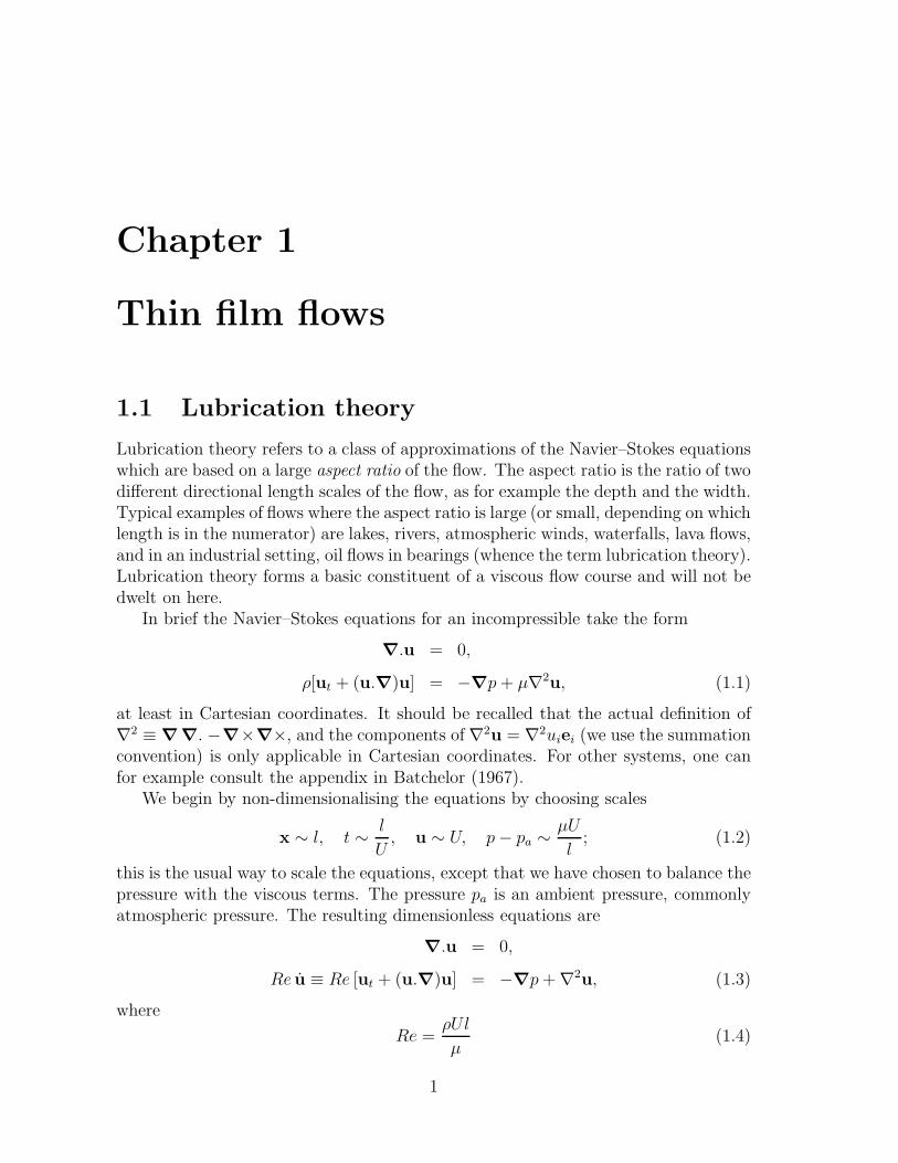
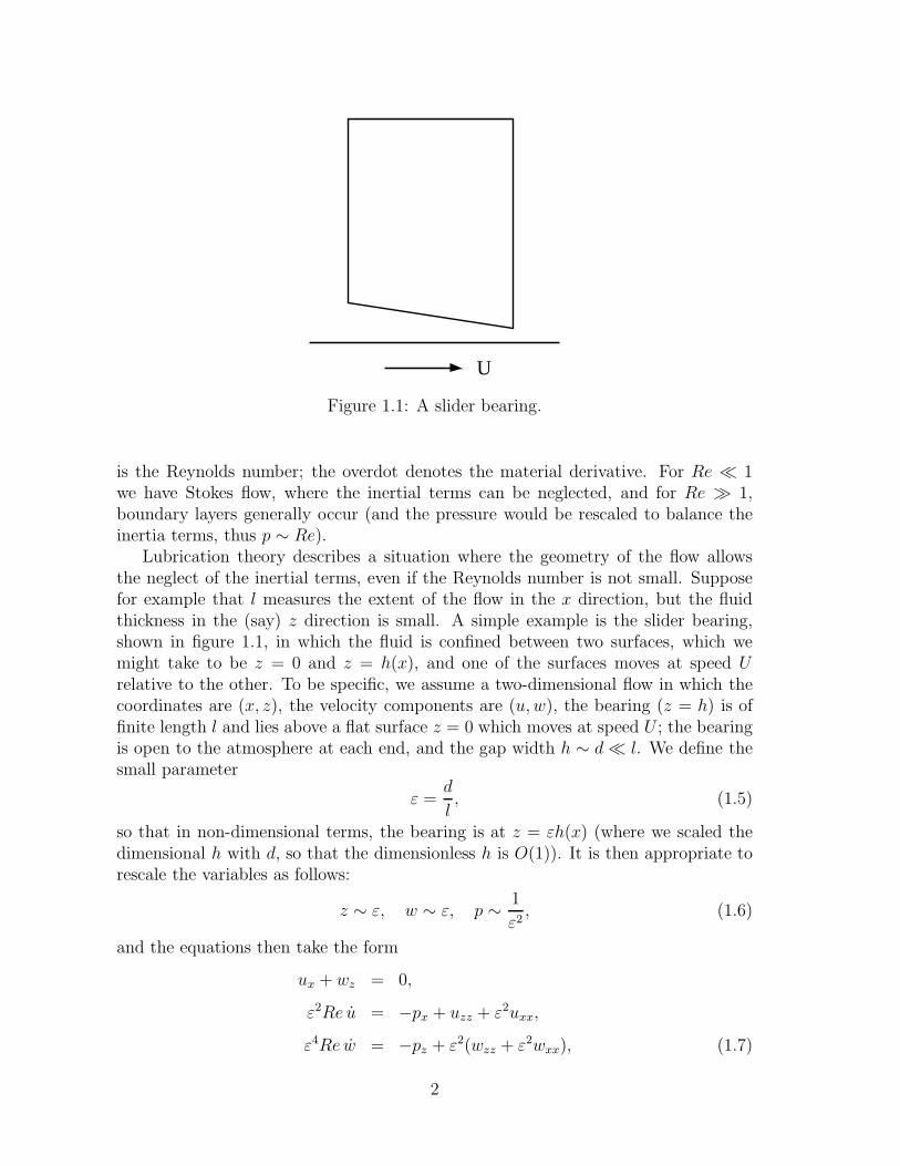
Figure 1.1: A slider bearing.

is the Reynolds number; the overdot denotes the material derivative. For Re ≪ 1we have Stokes flow, where the inertial terms can be neglected, and for Re ≫ 1,boundary layers generally occur (and the pressure would be rescaled to balance theinertia terms, thus p ∼ Re).

Lubrication theory describes a situation where the geometry of the flow allowsthe neglect of the inertial terms, even if the Reynolds number is not small. Supposefor example that l measures the extent of the flow in the x direction, but the fluidthickness in the (say) z direction is small. A simple example is the slider bearing,shown in figure 1.1, in which the fluid is confined between two surfaces, which wemight take to be z = 0 and z = h(x), and one of the surfaces moves at speed Urelative to the other. To be specific, we assume a two-dimensional flow in which thecoordinates are (x, z), the velocity components are (u, w), the bearing (z = h) is offinite length l and lies above a flat surface z = 0 which moves at speed U ; the bearingis open to the atmosphere at each end, and the gap width h ∼ d≪ l. We define thesmall parameter

ε =d

l, (1.5)

so that in non-dimensional terms, the bearing is at z = εh(x) (where we scaled thedimensional h with d, so that the dimensionless h is O(1)). It is then appropriate torescale the variables as follows:

z ∼ ε, w ∼ ε, p ∼ 1

ε2, (1.6)

and the equations then take the form

ux + wz = 0,

ε2Re u = −px + uzz + ε2uxx,

ε4Re w = −pz + ε2(wzz + ε2wxx), (1.7)

2

with boundary conditions

u = 1, w = 0 at z = 0,

u = w = 0 at z = h,

p = 0 at x = 0, 1. (1.8)

At leading order we then have p = p(x, t), and thus, integrating, we obtain

u = 1− z

h− 1

2px(hz − z2). (1.9)

The final part of the solution comes from integrating the mass conservation equa-tion from z = 0 to z = h. This gives

0 = −[w]h0 = −∫ h

0

wz dz =

∫ h

0

ux dz =∂

∂x

∫ h

0

u dz, (1.10)

where we can take the differentiation outside the integral because u is zero at z = h.In fact we can write down (1.10) directly since it is an expression of conservation ofmass across the layer; and this applies more generally, even if the base is not flat, andindeed even if both surfaces depend on time, and the result can be extended to threedimensions; see question 1.2. Calculating the flux from (1.9), we obtain

∫ s

b

u dz = 12h− 1

12h3px = K (1.11)

is constant. Given h, the solution for p can be found as a quadrature, and is

p = 6

[f2(x)−

f2(1)f3(x)

f3(1)

], fn(x) =

∫ x

0

dx

hn. (1.12)

In three dimensions, exactly the same procedure leads to the equation

112∇H .(h

3∇Hp) =

12hx, (1.13)

where the plate flow direction is taken along the x axis; derivation of this is left asan exercise.

1.2 Droplet dynamics

When one of the surfaces is a free surface (meaning it is free to deform), such as adroplet of liquid resting on a surface, or a rivulet flowing down a window pane, thereare two differences which must be accounted for in formulating the problem. One isthat the free surface is usually a material surface, so that a kinematic condition isappropriate. In three dimensions, this takes the form

w = st + usx + vsy − a. (1.14)

3

Here, z = s is the free surface, and (u, v, w) is the velocity; the term a is normallyabsent, but a non-zero value describes surface accumulation (which might for examplebe due to condensation); if a < 0 it describes ablation due for example to evaporation.

The other difference is that the boundary conditions at the free surface are gen-erally not ones of prescribed velocity but of prescribed stress. In the common case ofa droplet of liquid with air above, these conditions take the form

σnn = −pa, σnt = 0, (1.15)

representing the fact that the atmosphere exerts a constant pressure on the surface,and no shear stress. To unravel these conditions, we will consider the case of a two-dimensional incompressible flow. In this case, the components of the stress tensorare

σ11 = −p+ τ1, σ13 = σ31 = τ3, σ33 = −p− τ1, (1.16)

whereτ1 = 2µux, τ3 = µ(uz + wx), (1.17)

and then with

n =(−sx, 1)

(1 + s2x)1/2, t =

(1, sx)

(1 + s2x)1/2, (1.18)

we have

σnn = σijninj = −p− [τ1(1− s2x) + 2τ3sx]

1 + s2x,

σnt = σijnitj =[τ3(1− s2x)− 2τ1sx]

1 + s2x. (1.19)

The dimensionless equations are virtually the same, as we initially scale p−pa, τ1 andτ3 with µU/l, and then when the rescaling in (1.6) is done (note that consequentlywe rescale τ3 ∼ 1/ε), the surface boundary conditions become

p+ε2[τ1(1− ε2s2x) + 2τ3sx]

1 + ε2s2x= 0,

τ3(1− ε2s2x)− 2ε2τ1sx = 0, (1.20)

whereτ1 = 2ux, τ3 = uz + ε2wx. (1.21)

Putting ε = 0, we thus obtain the leading order conditions

p = τ3 = 0 on z = s. (1.22)

We can then integrate uzz = px, assuming also a no slip base at z = b, to obtain anexpression for the flux ∫ s

b

u dz = −13h3px, (1.23)

and the conservation of mass equation then integrates (see question 1.2) to give theevolution equation for h = s− b in the form

ht =13

∂

∂x[h3px]. (1.24)

4

1.2.1 Gravity

The astute reader will notice that something is missing. Unlike the slider bearing,nothing is driving the flow! Indeed, since p = p(x, t) and p = 0 at z = s, p = 0everywhere. Related to this is the fact that there is nothing to determine the velocityscale U . Commonly such droplet flows are driven by gravity. If we include gravityin the z momentum equation, then it takes the dimensional form . . . = −pz − ρg . . .,and since in the rescaled model all the other terms are negligible, the pressure will behydrostatic, p ≈ pa + ρg(s− z), and this gives a natural scale for p− pa ∼ ρgd, andequating this with the eventual pressure scale µUl/d2 determines the velocity scaleas

U =ρgd3

µl. (1.25)

The dimensionless pressure then becomes p = s− z, so that px = sx, and (1.24) nowtakes the form of a nonlinear diffusion equation,

ht =13

∂

∂x[h3sx]. (1.26)

One might wonder how the length scales l and d should be chosen; the answer tothis, at least if the base is flat, is that it can be taken from the initial condition for s.The reason for this is that, since (1.26) is a diffusion equation, the drop will simplycontinue to spread out: there is no natural length scale in the model. Associated withthis is the consequent fact that for an initial concentration of liquid at the origin (againon a flat base), the solution takes the form of a similarity solution (see question 1.5).On the other hand, if b is variable, then it provides a natural length scale. Indeed,for a basin shaped b (for example x2, dimensionlessly), the initial volume (or cross-sectional area) determines the eventual steady state as a lake with s constant, andboth d and l prescribed.

1.2.2 Surface tension

Another way in which a natural length scale can occur in the model is through theintroduction of surface tension at the interface. Let us digress for a moment to con-sider how surface tension arises. Surface tension is a property of interfaces, wherebythey have an apparent strength. This is most simply manifested by the ability ofsmall objects which are themselves heavier than water to float on the interface. Theexperiment is relatively easily done using a paper clip, and certain insects (waterstriders) have the ability to stay on the surface of a pond.

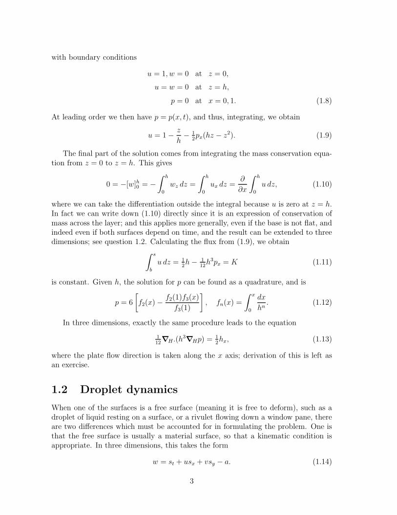
The simplest way to think about surface tension is mechanically. The interfacebetween two fluids has an associated tension, such that if one draws a line in theinterface of length l, then there is a force of magnitude γl which acts along this line:γ is the surface tension, and is a force per unit length. The presence of a surfacetension causes an imbalance in the normal stress across the interface, as is indicatedin figure 1.2, which also provides a means of calculating it. Taking ds as a short

5

dθ

dθ dθ

R

/2 /2

γ γ

ds

p

p

+

_

Figure 1.2: The simple mechanical interpretation of surface tension.

line segment in an interface subtending an angle dθ at its centre of curvature, a forcebalance normal to the interface leads to the condition

p+ − p− =γ

R, (1.27)

where

R =ds

dθ(1.28)

is the radius of curvature, and its inverse 1/R is the curvature.For a two-dimensional surface, the curvature is described by two principal radii of

curvature R1 and R2, the mean curvature is defined by

κ = 12

(1

R1+

1

R2

), (1.29)

and the pressure jump condition is

p+ − p− = 2γκ = γ

(1

R1+

1

R2

), (1.30)

although this is not much use to us unless we have a way of calculating the curvatureof a surface. This leads us off into the subject of differential geometry, and we do notwant to go there. A better way lies along the following path.

The sceptical reader will in any case wonder what this surface tension actuallyis. It manifests itself as a force, but along a line? And what is its physical origin?The answer to this question veers towards the philosophical. We think we understandforce, after all it pops up in Newton’s second law, but how do we measure it? Pressure,for example, we conceive of as being due to the collision of molecules with a surface,

6

dV

p

p_

+

VA

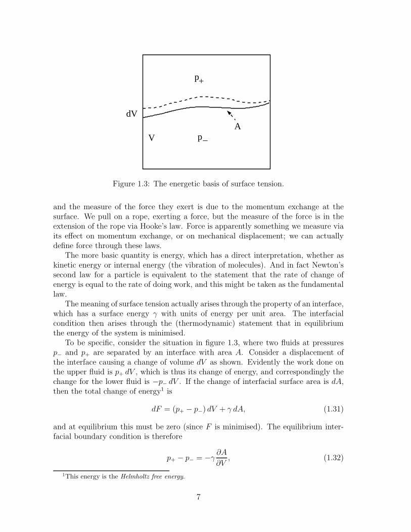
Figure 1.3: The energetic basis of surface tension.

and the measure of the force they exert is due to the momentum exchange at thesurface. We pull on a rope, exerting a force, but the measure of the force is in theextension of the rope via Hooke’s law. Force is apparently something we measure viaits effect on momentum exchange, or on mechanical displacement; we can actuallydefine force through these laws.

The more basic quantity is energy, which has a direct interpretation, whether askinetic energy or internal energy (the vibration of molecules). And in fact Newton’ssecond law for a particle is equivalent to the statement that the rate of change ofenergy is equal to the rate of doing work, and this might be taken as the fundamentallaw.

The meaning of surface tension actually arises through the property of an interface,which has a surface energy γ with units of energy per unit area. The interfacialcondition then arises through the (thermodynamic) statement that in equilibriumthe energy of the system is minimised.

To be specific, consider the situation in figure 1.3, where two fluids at pressuresp− and p+ are separated by an interface with area A. Consider a displacement ofthe interface causing a change of volume dV as shown. Evidently the work done onthe upper fluid is p+ dV , which is thus its change of energy, and correspondingly thechange for the lower fluid is −p− dV . If the change of interfacial surface area is dA,then the total change of energy1 is

dF = (p+ − p−) dV + γ dA, (1.31)

and at equilibrium this must be zero (since F is minimised). The equilibrium inter-facial boundary condition is therefore

p+ − p− = −γ ∂A∂V

, (1.32)

1This energy is the Helmholtz free energy.

7

nn

A + dA

dV

A

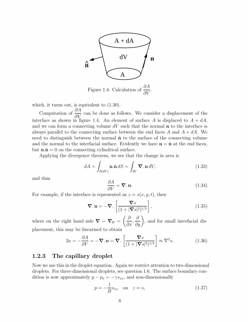
Figure 1.4: Calculation of∂A

∂V.

which, it turns out, is equivalent to (1.30).

Computation of∂A

∂Vcan be done as follows. We consider a displacement of the

interface as shown in figure 1.4. An element of surface A is displaced to A + dA,and we can form a connecting volume dV such that the normal n to the interface isalways parallel to the connecting surface between the end faces A and A + dA. Weneed to distinguish between the normal n to the surface of the connecting volumeand the normal to the interfacial surface. Evidently we have n = n at the end faces,but n.n = 0 on the connecting cylindrical surface.

Applying the divergence theorem, we see that the change in area is

dA =

∫

∂(dV )

n.n dS =

∫

dV

∇.n dV, (1.33)

and thus∂A

∂V= ∇.n. (1.34)

For example, if the interface is represented as z = s(x, y, t), then

∇.n = −∇.

[∇s

(1 + |∇s|2)1/2], (1.35)

where on the right hand side ∇ = ∇H =

(∂

∂x,∂

∂y

), and for small interfacial dis-

placement, this may be linearised to obtain

2κ = −∂A∂V

= −∇.n = ∇.

[∇s

(1 + |∇s|2)1/2]≈ ∇2s. (1.36)

1.2.3 The capillary droplet

Now we use this in the droplet equation. Again we restrict attention to two-dimensionaldroplets. For three-dimensional droplets, see question 1.6. The surface boundary con-dition is now approximately p− pa = −γsxx, and non-dimensionally

p = − 1

Bsxx on z = s, (1.37)

8

where B (commonly also written Bo) is the Bond number, given by

B =ρgl2

γ. (1.38)

This gives a natural length scale for the droplet, by choosing B = 1, thus

l =

(γ

ρg

)1/2

; (1.39)

in this case the dimensionless pressure is p = s− z− sxx, and thus mass conservationleads to

ht =13

∂

∂x

[h3(sx − sxxx)

], (1.40)

and the surface tension term acts as a further stabilising term.2

Surface tension acts to limit the spread of a droplet. Indeed there is a steady stateof (1.40) which is easily found. Suppose the base is flat, so s = h. We prescribe thecross-sectional area of the drop, A. In dimensionless terms, we thus require

∫h dx = 2α =

(ρg

γ

)1/2A

d. (1.41)

Let us choose d so that the maximum depth is one (note that the value of d remainsto be determined). We can suppose that the drop is symmetric about the origin, andthat its dimensionless half-width is λ, also to be determined. Thus

h(±λ) = 0, h(0) = 1, (1.42)

as well as (1.41), and both α and λ are to be determined.A further condition is necessary at the margins. This is the prescription of a

contact angle, which can be construed as arising through a balance of the surfacetension forces at the three interfaces at the contact line: gas/liquid, liquid/solid, andsolid/gas. All three interfaces have a surface energy, and minimisation of this corre-sponds to prescription of a contact angle. Specifically, if θ is the angle between thegas/liquid and liquid/solid interfaces, then resolution of the surface tension tangentialto the wall leads to

γSL + γ cos θ = γSG, (1.43)

where γSL is the solid/liquid surface energy, and γSG is the solid/gas surface energy.Defining S = l tan θ/d, this implies that

hx = ∓S at x = ±λ. (1.44)

2This can be seen by considering small perturbations about a uniform solution h = s = 1 (witha flat base), for which the linearised equation has normal mode solutions ∝ exp(σt + ikx), withσ = − 1

3(k2 + k4).

9

The steady state of (1.40) is easily found. The flux is zero, so hx − hxxx is zero,and integration of this leads to

h = 1−(cosh x− 1

coshλ− 1

), (1.45)

and then (1.41) and (1.44) yield

α =λ coshλ− sinhλ

cosh λ− 1,

sinh λ

cosh λ− 1= S. (1.46)

S(λ) is a monotonically decreasing function of λ (why?), and tends to one as λ→ ∞,and therefore the second relation determines λ providing S > 1. It seems there is aproblem if S < 1, but this is illusory since both α and S depend on the unknown d,so it is best to solve

α

S=

A

2l2 tan θ=λ coshλ− sinh λ

sinhλ; (1.47)

the right hand side increases monotonically from 0 to ∞ as λ increases, and thereforeprovides a unique solution for λ for any values of A and θ; d is then determined byeither expression in (1.46).

It is of interest to see when the assumption d≪ l is then valid. From (1.46),

ε = tan θ

(cosh λ− 1

sinh λ

). (1.48)

The expression in λ increases monotonically from 0 to 1 as λ increases. Thus ε ≪ 1if either θ ≪ 1, or (if tan θ ∼ O(1)) λ ≪ 1. From (1.47), this is the case provided

A≪ l2, i. e.,ρgA

γ≪ 1. For air and water, this implies A≪ 7 mm2.

1.2.4 Advance and retreat

When a droplet is of finite extent, it is possible to describe the behaviour near themargins by a local expansion. Typically the surface approaches the base with localpower law behaviour, and this depends on whether the droplet is advancing or re-treating. Consider, for example, the gravity-driven droplet with an accumulation orablation term:

ht =13

(h3hx

)x+ a, (1.49)

where a > 0 for accumulation, and a < 0 for ablation. (1.49) represents a simplemodel for the motion of an ice sheet such as Antarctica, where a > 0 representsaccumulation due to snowfall. If we suppose that near the margin x = xs in a two-dimensional motion, h ∼ C(xs−x)ν , then a local expansion shows that if the front isadvancing, xs > 0, then ν = 1

3and xs ∼ 1

9C3; in advance the front is therefore steep.

On the other hand, if the front is retreating, then this can only occur if a < 0 (as is infact obvious), and in that case ν = 1 and xs ∼ −|a|/C. The fact that the front slopeis infinite in advance and finite in retreat is associated with ‘waiting time’ behaviour,which occurs when the front has to ‘fatten up’ before it can advance.

10

T

x

z

z = sz = b

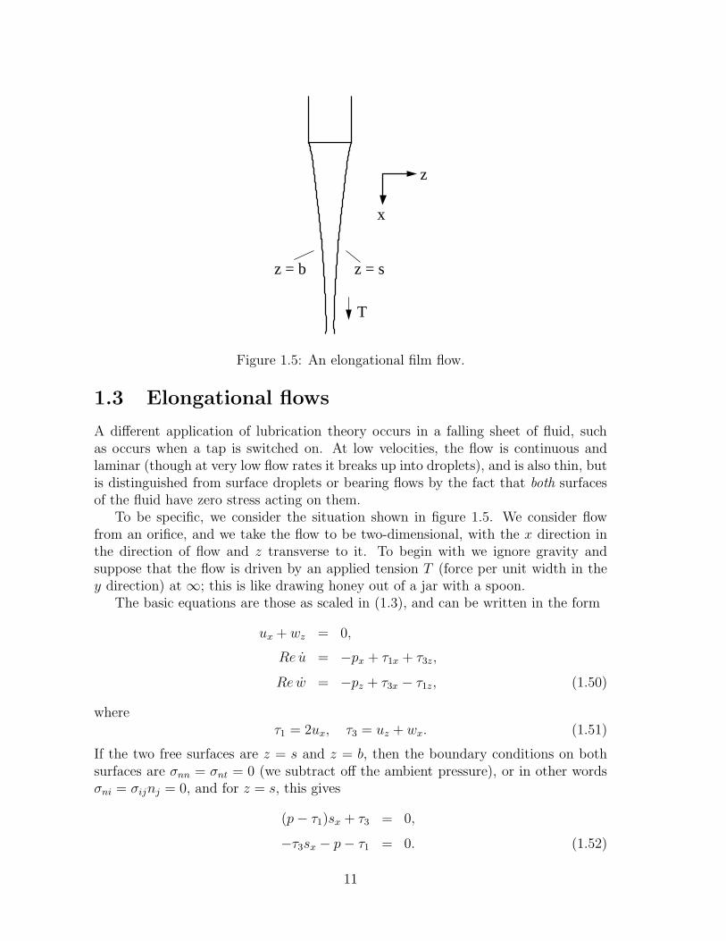
Figure 1.5: An elongational film flow.

1.3 Elongational flows

A different application of lubrication theory occurs in a falling sheet of fluid, suchas occurs when a tap is switched on. At low velocities, the flow is continuous andlaminar (though at very low flow rates it breaks up into droplets), and is also thin, butis distinguished from surface droplets or bearing flows by the fact that both surfacesof the fluid have zero stress acting on them.

To be specific, we consider the situation shown in figure 1.5. We consider flowfrom an orifice, and we take the flow to be two-dimensional, with the x direction inthe direction of flow and z transverse to it. To begin with we ignore gravity andsuppose that the flow is driven by an applied tension T (force per unit width in they direction) at ∞; this is like drawing honey out of a jar with a spoon.

The basic equations are those as scaled in (1.3), and can be written in the form

ux + wz = 0,

Re u = −px + τ1x + τ3z,

Re w = −pz + τ3x − τ1z, (1.50)

whereτ1 = 2ux, τ3 = uz + wx. (1.51)

If the two free surfaces are z = s and z = b, then the boundary conditions on bothsurfaces are σnn = σnt = 0 (we subtract off the ambient pressure), or in other wordsσni = σijnj = 0, and for z = s, this gives

(p− τ1)sx + τ3 = 0,

−τ3sx − p− τ1 = 0. (1.52)

11

(These are actually equivalent to (1.19).)Now we rescale the variables to account for the large aspect ratio. The difference

with the earlier approach is that shear stresses are uniformly small, and so we alsorescale τ3 to be small. Thus we rescale the variables as

z ∼ ε, w ∼ ε, τ3 ∼ ε, (1.53)

and this leads to the rescaled equations

ux + wz = 0,

Re u = −px + τ1x + τ3z,

ε2Re w = −pz + ε2τ3x − τ1z, (1.54)

whereτ1 = 2ux, ε2τ3 = uz + ε2wx, (1.55)

and on the free surfaces (e. g., z = s)

(p− τ1)sx + τ3 = 0,

−ε2τ3sx − p− τ1 = 0. (1.56)

At leading order, we have u = u(x, t), p+ τ1 = 0, p = −2ux, whence we find

τ3z = Re u− 4uxx, (1.57)

withτ3 = 4uxsx on z = s, τ3 = 4uxbx on z = b,

and from these we deduce

Reh(ut + uux) = 4(hux)x,

ht + (hu)x = 0, (1.58)

where the second equation is derived as usual to represent conservation of mass. Notein this derivation that the inertial terms are not necessarily small; nevertheless theasymptotic procedure works in the usual way.

1.3.1 Steady flow

For a long filament such as that shown in figure 1.5, it is appropriate to prescribeinlet conditions, and these can be taken to be

h = u = 1 at x = 0, (1.59)

by appropriate choice of U and d. In addition, we prescribe the force (per unit widthin the third dimension) to be T , and this leads to

hux → 1 as x→ ∞, (1.60)

12

t

x

h = 1

x = 0t =

x = t = 0ξh = h 0(ξ )

τ

u = 1

Figure 1.6: Characteristics for (1.58). The dividing characteristic from the origin isshown in red.

where the constant is set to one by choice of the length scale as

l =2µdU

T; (1.61)

thus the aspect ratio is small (d ≪ l) if T ≪ µU .If we consider a slow, steady flow in which the inertial terms can be ignored

(Re→ 0), it is easy to solve the equations. We have hu = 1 and hux = 1, and thus

u = ex, h = e−x. (1.62)

As a matter of curiosity, one can actually solve the time-dependent problem (1.58),at least when Re = 0. We write the equations in the form

ht + uhx = −1,

hux = 1, (1.63)

with the boundary and initial conditions as shown in figure 1.6. The characteristicform of the first equation is

xt = u[x(ξ, t), t], ht = −1, (1.64)

where the partial derivatives are holding ξ fixed, i. e., we consider x = x(ξ, t), h =h(ξ, t). The dividing characteristic from the origin (which we define to be t = td(x))divides the quadrant into two regions, in which the initial data is parameteriseddifferently. For the lower region t < td(x), we have

h = h0(ξ)− t. (1.65)

13

We take the first equation in (1.64), and differentiate with respect to ξ. Using thedefinition of ux from (1.63), we find

xξt =xξ

h0(ξ)− t. (1.66)

We can integrate this with respect to t, holding ξ constant, that is, the integral withrespect to t is along a characteristic. It follows that

xξ =h0(ξ)

h0(ξ)− t, (1.67)

in which we have applied the initial condition xξ = 1 at t = 0.Next we integrate with respect to ξ holding t constant; since (1.67) only holds for

t < td(x), we integrate back to this, but note that this corresponds to the value ξ = 0;we then have

x = xd(t) +

∫ ξ

0

h0(s) ds

h0(s)− t, (1.68)

where xd is the inverse of td(x): to calculate this we need to solve for the upper regiont > td.

To do this, we can proceed as above, but it is quicker to note that since theboundary conditions on x = 0 are constant, the solution is just the steady statesolution (1.62). In particular, the characteristics are e−x = 1 − (t − τ), and thedividing characteristic is that with τ = 0, thus

td = 1− e−x, xd = − ln(1− t). (1.69)

The solution in t < td is thus

x = − ln(1− t) +

∫ ξ

0

h0(s) ds

h0(s)− t, (1.70)

but the transient is of little interest since it disappears after finite time, t = 1. As acheck, notice that if h0 = e−ξ, the steady state solution is regained everywhere.

The steady solution can be extended to positive Reynolds number. In steady flowwe then find

ux = Ku+ 14Reu2 (1.71)

for some constant K, and we see that there is no solution in which the filament canbe drawn to ∞, as pinch-off always occurs. This is in keeping with experience.

1.3.2 Capillary effects

As for the shear-driven droplet flows, one can add gravity to the model, and this isdone in question 1.3. In this section we consider the modification to the equations

14

which occurs when capillary effects are included. The normal stress conditions aremodified to

−σnn = − γsxx(1 + s2x)

3/2on z = s,

σnn = − γbxx(1 + b2x)

3/2on z = b. (1.72)

The definition of σnn is in (1.19), and with the basic scaling (all lengths scaled withl, etc.) this leads to

−p− 2τ3sx1 + s2x

− τ1(1− s2x)

1 + s2x=

1

Ca

γsxx(1 + s2x)

3/2on z = s, (1.73)

where

Ca =µU

γ(1.74)

is the capillary number; a similar expression applies on z = b, with the opposite signon the right hand side. When the equations are re-scaled (z ∼ ε, etc.), then thesetake the approximate form

p+ τ1 ≈ − 1

Csxx on z = s,

p+ τ1 ≈ 1

Cbxx on z = b, (1.75)

where we writeCa = εC. (1.76)

Now the normal stress is constant across the filament, thus

p+ τ1 ≈ − 1

Csxx (1.77)

everywhere, and this forces symmetry of the filament, sxx = −bxx. The rest of thederivation proceeds as before, except that (1.57) gains an extra term −sxxx/C on theright hand side; integrating this and applying the boundary conditions leads to themodification of (1.58) as (bearing in mind that h = s− b and thus hxx = 2sxx)

ht + (hu)x = 0,

Re h(ut + uux) =1

2Chhxxx + 4(hux)x. (1.78)

Steady flow

The extra derivatives for h require, apparently, two extra boundary conditions. If wesuppose the pressure becomes atmospheric at ∞, then we might apply

hxx → 0 as x→ ∞. (1.79)

15

Since this also implies hx → 0, it may be sufficient. On the other hand, if h → 0 at∞, the multiplication of the third derivative term by h may render an extra boundarycondition unnecessary.

Again we can consider the steady state. Then hu = 1, and (1.78) has a firstintegral

K +Re

h=

1

2C

[hhxx − 1

2h2x]− 4hx

h, (1.80)

where K is constant. Evidently there is no solution if Re > 0, as pinch-off must againoccur. For the case of slow flow, taking Re = 0, we have K = 4 due to the far fieldstress condition, and

h2hxx − 12hh2x − 8C(hx + h) = 0. (1.81)

We seek a solution of this with h(0) = 1 and h(∞) = 0. Phase plane analysis showsthat there is a unique such solution: see question 1.7.

1.4 Foam drainage

Exercises

1.1 A thin incompressible liquid film flows in two dimensions (x, z) between a solidbase z = 0 where the horizontal (x) component of the velocity is U(t), and maydepend on time, and a stationary upper solid surface z = h(x), where a no slipcondition applies. The upper surface is of horizontal length l, and is open to theatmosphere at the ends. Write down the equations and boundary conditionsdescribing the flow, and non-dimensionalise them assuming that U(t) ∼ U0.(You may neglect gravity.)

Assuming ε = d/l is sufficiently small, where d is a measure of the gap width,rescale the variables suitably, and derive an approximate equation for the pres-sure p. Hence derive a formal solution if the block is of finite length l, andthe pressure is atmospheric at each end, and obtain an expression involvingintegrals of powers of h for the horizontal fluid flux, q(t) =

∫ h0u dz.

1.2 A two-dimensional incompressible fluid flow is contained between two surfacesz = b(x, t) and z = s(x, t), on which kinematic conditions hold:

w = st + usx at z = s,

w = bt + ubx at z = b.

By integrating the equation of conservation of mass, show that the fluid thick-ness h = s− b satisfies the conservation law

∂h

∂t+

∂

∂x

∫ s

b

u dx = 0.

16

Extend the result to three dimensions to show that

ht +∇H .

[∫ s

b

uH dz

]= 0,

where uH = (u, v) is the horizontal velocity, and ∇H =

(∂

∂x,∂

∂y

)is the hori-

zontal gradient operator.

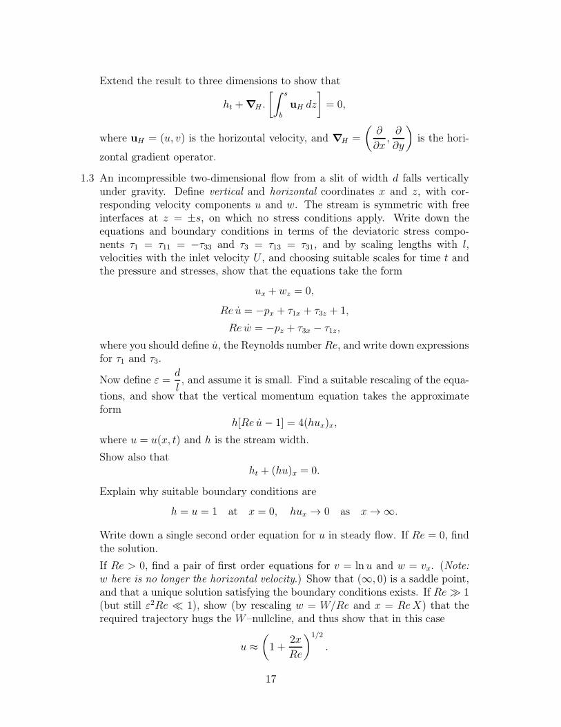
1.3 An incompressible two-dimensional flow from a slit of width d falls verticallyunder gravity. Define vertical and horizontal coordinates x and z, with cor-responding velocity components u and w. The stream is symmetric with freeinterfaces at z = ±s, on which no stress conditions apply. Write down theequations and boundary conditions in terms of the deviatoric stress compo-nents τ1 = τ11 = −τ33 and τ3 = τ13 = τ31, and by scaling lengths with l,velocities with the inlet velocity U , and choosing suitable scales for time t andthe pressure and stresses, show that the equations take the form

ux + wz = 0,

Re u = −px + τ1x + τ3z + 1,

Re w = −pz + τ3x − τ1z,

where you should define u, the Reynolds number Re, and write down expressionsfor τ1 and τ3.

Now define ε =d

l, and assume it is small. Find a suitable rescaling of the equa-

tions, and show that the vertical momentum equation takes the approximateform

h[Re u− 1] = 4(hux)x,

where u = u(x, t) and h is the stream width.

Show also thatht + (hu)x = 0.

Explain why suitable boundary conditions are

h = u = 1 at x = 0, hux → 0 as x→ ∞.

Write down a single second order equation for u in steady flow. If Re = 0, findthe solution.

If Re > 0, find a pair of first order equations for v = ln u and w = vx. (Note:w here is no longer the horizontal velocity.) Show that (∞, 0) is a saddle point,and that a unique solution satisfying the boundary conditions exists. If Re≫ 1(but still ε2Re ≪ 1), show (by rescaling w = W/Re and x = ReX) that therequired trajectory hugs the W–nullcline, and thus show that in this case

u ≈(1 +

2x

Re

)1/2

.

17

1.4 A (two-dimensional) droplet rests on a rough surface z = b and is subjectto gravity g and surface tension γ. Write down the equations and boundaryconditions which govern its motion, non-dimensionalise them, and assuming thedepth at the summit d is much less than the half-width l, derive an approximateequation for the evolution in time of the depth h. Show that the horizontalvelocity scale is

U =ρgd3

µl,

and derive an approximate set of equations assuming

ε =d

l≪ 1, F =

U√gd

≪ 1.

Hence show that

ht =∂

∂x

[13h3(sx −

1

Bsxxx

)],

where you should define the Bond number B.

Find a steady state solution of this equation for the case of a flat base, assum-ing that the droplet area A and a contact angle θ = εφ are prescribed, withφ ∼ O(1), and show that it is unique. Explain how the solution chooses theunknowns d and l.

1.5 A droplet of thickness h satisfies the equation

ht =∂

∂x

[13h3hx

].

Find a similarity solution of this equation which describes the spread of a dropof area one which is initially concentrated at the origin (i. e., h(x, 0) = δ(x)).

1.6 Three-dimensional droplet

1.7 A film of fluid is drawn downwards under the action of a tensile force. A modelfor the dimensionless thickness h and dimensionless downwards velocity u ofthe film is

ht + (hu)x = 0,

Re h(ut + uux) =1

2Chhxxx + 4(hux)x,

withh = u = 1 on x = 0, hux → 1 as x→ ∞.

Show that a steady state solution in which h → 0 as x → ∞ can only occur ifRe = 0. In that case, determine a second order differential equation satisfiedby h, and by writing h = 1

2U2 and V = U ′ = Ux, write the equation as a pair

of first order equations for U and V . Show that the origin is a (degenerate)saddle, and therefore show that a solution exists which satisfies the boundaryconditions.

18

Chapter 2

Porous media

Groundwater is water which is stored in the soil and rock beneath the surface ofthe Earth. It forms a fundamental constituent reservoir of the hydrological system,and it is important because of its massive and long lived storage capacity. It is theresource which provides drinking and irrigation water for crops, and increasingly inrecent decades it has become an unwilling recipient of toxic industrial and agriculturalwaste. For all these reasons, the movement of groundwater is an important subjectof study.

Soil consists of very small grains of organic and inorganic matter, ranging insize from millimetres to microns. Differently sized particles have different names.Particularly, we distinguish clay particles (size < 2 microns) from silt particles (2–60microns) and sand (60 microns to 1 mm). Coarser particles still are termed gravel.

Viewed at the large scale, soil thus forms a continuum which is granular at thesmall scale, and which contains a certain fraction of pore space, as shown in figure2.1. The volume fraction of the soil (or sediment, or rock) which is occupied by thepore space (or void space, or voidage) is called the porosity, and is commonly denotedby the symbol φ; sometimes other symbols are used, for example n, as in chapter ??.

As we described in chapter ??, soils are formed by the weathering of rocks, andare specifically referred to as soils when they contain organic matter formed by therotting of plants and animals. There are two main types of rock: igneous, formedby the crystallisation of molten lava, and sedimentary, formed by the cementation ofsediments under conditions of great temperature and pressure as they are buried atdepth.1 Sedimentary rocks, such as sandstone, chalk, shale, thus have their porositybuilt in, because of the pre-existing granular structure. With increasing pressure,the grains are compacted, thus reducing their porosity, and eventually intergranularcements bond the grains into a rock. Sediment compaction is described in section2.6.

Igneous rock tends to be porous also, for a different reason. It is typically thecase for any rock that it is fractured. Most simply, rock at the surface of the Earth is

1There are also metamorphic rocks, which form from pre-existing rocks through chemical changesinduced by burial at high temperatures and pressures; for example, marble is a metamorphic formof limestone.

19

Figure 2.1: A granular porous medium.

subjected to enormous tectonic stresses, which cause folding and fracturing of rock.Thus, even if the rock matrix itself is not porous, there are commonly faults andfractures within the rock which act as channels through which fluids may flow, andwhich act on the large scale as an effective porosity. If the matrix is porous atthe grain scale also, then one refers to the rock as having a dual porosity, and thecorresponding flow models are called double porosity models.

In the subsurface, whether it be soil, underlying regolith, a sedimentary basin,or oceanic lithosphere, the pore space contains liquid. At sufficient depth, the porespace will be saturated with fluid, normally water. At greater depths, other fluidsmay be present. For example, oil may be found in the pore space of the rocks ofsedimentary basins. In the near surface, both air and water will be present in thepore space, and this (unsaturated) region is called the unsaturated zone, or the vadosezone. The surface separating the two is called the piezometric surface, the phreaticsurface, or more simply the water table. Commonly it lies tens of metres below theground surface.

2.1 Darcy’s law

Groundwater is fed by surface rainfall, and as with surface water it moves under apressure gradient driven by the slope of the piezometric surface. In order to char-acterise the flow of a liquid in a porous medium, we must therefore relate the flowrate to the pressure gradient. An idealised case is to consider that the pores consistof uniform cylindrical tubes of radius a; initially we will suppose that these are allaligned in one direction. If a is small enough that the flow in the tubes is laminar(this will be the case if the associated Reynolds number is <∼ 1000), then Poiseuille

20

flow in each tube leads to a volume flux in each tube of q =πa4

8µ|∇p|, where µ is

the liquid viscosity, and ∇p is the pressure gradient along the tube. A more realisticporous medium is isotropic, which is to say that if the pores have this tubular shape,the tubules will be arranged randomly, and form an interconnected network. How-ever, between nodes of this network, Poiseuille flow will still be appropriate, and anappropriate generalisation is to suppose that the volume flux vector is given by

q ≈ − a4

µX∇p, (2.1)

where the approximation takes account of small interactions at the nodes; the numer-ical tortuosity factor X >∼ 1 takes some account of the arrangement of the pipes.

To relate this to macroscopic variables, and in particular the porosity φ, we observethat φ ∼ a2/d2p, where dp is a representative particle or grain size so that q/d2p ∼

−(φ2d2pµX

)∇p. We define the volume flux per unit area (having units of velocity) as

the discharge u. Darcy’s law then relates this to an applied pressure gradient by therelation

u = −kµ∇p, (2.2)

where k is an empirically determined parameter called the permeability, having unitsof length squared. The discussion above suggests that we can write

k =d2pφ

2

X; (2.3)

the numerical factor X may typically be of the order of 103.To check whether the pore flow is indeed laminar, we calculate the (particle)

Reynolds number for the porous flow. If v is the (average) fluid velocity in the porespace, then

v =u

φ; (2.4)

If a is the pore radius, then we define a particle Reynolds number based on grain sizeas

Rep =2ρva

µ∼ ρ|u|dp

µ√φ, (2.5)

since φ ∼ a/dp. Suppose (2.3) gives the permeability, and we use the gravitationalpressure gradient ρg to define (via Darcy’s law) a velocity scale2; then

Rep ∼φ3/2

X

(ρ√gdp dp

µ

)2

∼ 10[dp]3, (2.6)

2This scale is thus the hydraulic conductivity, defined below in (2.9).

21

where dp = [dp] mm, and using φ3/2/X = 10−3, g = 10 m s−2, µ/ρ = 10−6 m2 s−2.Thus the flow is laminar for d < 5 mm, corresponding to a gravel. Only for free flowthrough very coarse gravel could the flow become turbulent, but for water percolationin rocks and soils, we invariably have slow, laminar flow.

In other situations, and notably for forced gas stream flow in fluidised beds or inpacked catalyst reactor beds, the flow can be rapid and turbulent. In this case, thePoiseuille flow balance −∇p = µu/k can be replaced by the Ergun equation

−∇p =ρ|u|uk′

; (2.7)

more generally, the right hand side will a sum of the two (laminar and turbulent)interfacial resistances. The Ergun equation reflects the fact that turbulent flow in apipe is resisted by Reynolds stresses, which are generated by the fluctuation of theinertial terms in the momentum equation. Just as for the laminar case, the parameterk′, having units of length, depends both on the grain size dp and on φ. Evidently, wewill have

k′ = dpE(φ), (2.8)

with the numerical factor E → 0 as φ → 0.

Hydraulic conductivity

Another measure of flow rate in porous soil or rock relates specifically to the passageof water through a porous medium under gravity. For free flow, the pressure gradientdownwards due to gravity is just ρg, where ρ is the density of water and g is thegravitational acceleration; thus the water flux per unit area in this case is just

K =kρg

µ, (2.9)

and this quantity is called the hydraulic conductivity. It has units of velocity. Ahydraulic conductivity of K = 10−5 m s−1 (about 300 m y−1) corresponds to apermeability of k = 10−12 m2, this latter unit also being called the darcy.

2.1.1 Homogenisation

The ‘derivation’ of Darcy’s law can be carried out in a more formal way using themethod of homogenisation. This is essentially an application of the method of multiple(space) scales to problems with microstructure. Usually (for analytic reasons) oneassumes that the microstructure is periodic, although this is probably not strictlynecessary (so long as local averages can be defined).

Consider the Stokes flow equations for a viscous fluid in a medium of macroscopiclength l, subject to a pressure gradient of order ∆p/l. If the microscopic (e. g.,grain size) length scale is dp, and ε = dp/l, then if we scale velocity with d2p∆p/lµ

22

(appropriate for local Poiseuille-type flow), length with l, and pressure with ∆p, theNavier-Stokes equations can be written in the dimensionless form

∇.u = 0,

0 = −∇p+ ε2∇2u, (2.10)

together with the no-slip boundary condition,

u = 0 on S : f(x/ε) = 0, (2.11)

where S is the interfacial surface. We put x = εξ and seek solutions in the form

u = u(0)(x, ξ) + εu(1)(x, ξ) . . .

p = p(0)(x, ξ) + εp(1)(x, ξ) . . . . (2.12)

Expanding the equations in powers of ε and equating terms leads to p(0) = p(0)(x),and u(0) satisfies

∇ξ.u(0) = 0,

0 = −∇ξp(1) +∇2

ξu(0) −∇xp

(0), (2.13)

equivalent to Stokes’ equations for u(0) with a forcing term −∇xp(0). If wj is the

velocity field which (uniquely) solves

∇ξ.wj = 0,

0 = −∇ξP +∇2ξw

j + ej, (2.14)

with periodic (in ξ) boundary conditions and u = 0 on f(ξ) = 0, where ej is theunit-vector in the ξj direction, then (since the equation is linear) we have (summingover j)3

u(0) = −∂p(0)

∂xjwj. (2.15)

We define the average flux

〈u〉 = 1

V

∫

V

u(0)dV, (2.16)

where V is the volume over which S is periodic.4 Averaging (2.15) then gives

〈u〉 = −k∗.∇p, (2.17)

where the (dimensionless) permeability tensor is defined by

k∗ij = 〈wji 〉. (2.18)

3In other words, we employ the summation convention which states that summation is impliedover repeated suffixes, see for example Jeffreys and Jeffreys (1953).

4Specifically, we take V to be the soil volume, but the integral is only over the pore space volume,where u is defined. In that case, the average 〈u〉 is in fact the Darcy flux (i. e., volume fluid flux perunit area).

23

k (m2) material10−8 gravel10−10 sand10−12 fractured igneous rock10−13 sandstone10−14 silt10−18 clay10−20 granite

Table 2.1: Different grain size materials and their typical permeabilities.

Recollecting the scales for velocity, length and pressure, we find that the dimensionalversion of (2.17) is

〈u〉 = −k

µ.∇p, (2.19)

wherek = k∗d2p, (2.20)

so that k∗ is the equivalent in homogenisation theory of the quantity φ2/X in (2.3).

2.1.2 Empirical measures

While the validity of Darcy’s law can be motivated theoretically, it ultimately relieson experimental measurements for its accuracy. The permeability k has dimensionsof (length)2, which as we have seen is related to the mean ‘grain size’. If we writek = d2pC, then the number C depends on the pore configuration. For a tubularnetwork (in three dimensions), one finds C ≈ φ2/72π (as long as φ is relativelysmall). A different and often used relation is that of Carman and Kozeny, whichapplies to pseudo-spherical grains (for example sand grains); this is

C ≈ φ3

180(1− φ)2. (2.21)

The factor (1−φ)2 takes some account of the fact that as φ increases towards one, theresistance to motion becomes negligible. In fact, for media consisting of uncemented(i. e., separate) grains, there is a critical value of φ beyond which the medium as awhole will deform like a fluid. Depending on the grain size distribution, this valueis about 0.5 to 0.6. When the medium deforms in this way, the description of theintergranular fluid flow can still be taken to be given by Darcy’s law, but this nowconstitutes a particular choice of the interactive drag term in a two-phase flow model.At lower porosities, deformation can still occur, but it is elastic not viscous (on shorttime scales), and given by the theory of consolidation or compaction, which we discusslater.

24

In the case of soils or sediments, empirical power laws of the form

C ∼ φm (2.22)

are often used, with much higher values of the exponent (e.g. m = 8). Such behaviourreflects the (chemically-derived) ability of clay-rich soils to retain a high fraction ofwater, thus making flow difficult. Table 2.1 gives typical values of the permeabilityof several common rock and soil types, ranging from coarse gravel and sand to finersilt and clay.

An explicit formula of Carman-Kozeny type for the turbulent Ergun equationexpresses the ‘turbulent’ permeability k′, defined in (2.7), as

k′ =φ3dp

175(1− φ). (2.23)

2.2 Basic groundwater flow

Darcy’s equation is supplemented by an equation for the conservation of the fluidphase (or phases, for example in oil recovery, where these may be oil and water). Fora single phase, this equation is of the simple conservation form

∂

∂t(ρφ) +∇.(ρu) = 0, (2.24)

supposing there are no sources or sinks within the medium. In this equation, ρ is thematerial density, that is, mass per unit volume of the fluid. A term φ is not presentin the divergence term, since u has already been written as a volume flux (i.e., the φhas already been included in it: cf. (2.4)).

Eliminating u, we have the parabolic equation

∂

∂t(ρφ) = ∇.

[k

µρ∇p

], (2.25)

and we need a further equation of state (or two) to complete the model. The simplestassumption corresponds to incompressible groundwater flowing through a rigid porousmedium. In this case, ρ and φ are constant, and the governing equation reduces (ifalso k is constant) to Laplace’s equation

∇2p = 0. (2.26)

This simple equation forms the basis for the following development. Before pur-suing this, we briefly mention one variant, and that is when there is a compressiblepore fluid (e. g., a gas) in a non-deformable medium. Then φ is constant (so k isconstant), but ρ is determined by pressure and temperature. If we can ignore theeffects of temperature, then we can assume p = p(ρ) with p′(ρ) > 0, and

ρt =k

µφ∇.[ρp′(ρ)∇ρ], (2.27)

25

which is a nonlinear diffusion equation for ρ, sometimes called the porous medium

equation. If p ∝ ργ , γ > 0, this is degenerate when ρ = 0, and the solutions displaythe typical feature of finite spreading rate of compactly supported initial data.

2.2.1 Boundary conditions

The Laplace equation (2.26) in a domain D requires boundary data to be prescribedon the boundary ∂D of the spatial domain. Typical conditions which apply are a noflow through condition at an impermeable boundary, u.n = 0, whence

∂p

∂n= 0 on ∂D, (2.28)

or a permeable surface condition

p = pa on ∂D, (2.29)

where for example pa would be atmospheric pressure at the ground surface. Anotherexample of such a condition would be the prescription of oceanic pressure at theinterface with the oceanic crust.

A more common application of the condition (2.29) is in the consideration of flowin the saturated zone below the water table (which demarcates the upper limit ofthe saturated zone). At the water table, the pressure is in equilibrium with the airin the unsaturated zone, and (2.29) applies. The water table is a free surface, andan extra kinematic condition is prescribed to locate it. This condition says that thephreatic surface is also a material surface for the underlying groundwater flow, sothat its velocity is equal to the average fluid velocity (not the flux): bearing in mind(2.4), we have

∂F

∂t+

u

φ.∇F = 0 on ∂D, (2.30)

if the free surface ∂D is defined by F (x, t) = 0.

2.2.2 Dupuit approximation

One of the principally obvious features of mature topography is that it is relativelyflat. A slope of 0.1 is very steep, for example. As a consequence of this, it is typicallyalso the case that gradients of the free groundwater (phreatic) surface are also small,and a consequence of this is that we can make an approximation to the equations ofgroundwater flow which is analogous to that used in shallow water theory or the lubri-cation approximation, i. e., we can take advantage of the large aspect ratio of the flow.This approximation is called the Dupuit, or Dupuit–Forchheimer, approximation.

To be specific, suppose that we have to solve

∇2p = 0 in 0 < z < h(x, y, t), (2.31)

26

where z is the vertical coordinate, z = h is the phreatic surface, and z = 0 is an im-permeable basement. We let u denote the horizontal (vector) component of the Darcy

flux, and w the vertical component. In addition, we now denote by ∇ =

(∂

∂x,∂

∂y

)

the horizontal component of the gradient vector. The boundary conditions are then

p = 0, φht + u .∇h = w on z = h,

∂p

∂z+ ρg = 0 on z = 0; (2.32)

here we take (gauge) pressure measured relative to atmospheric pressure. The condi-tion at z = 0 is that of no normal flux, allowing for gravity.

Let us suppose that a horizontal length scale of relevance is l, and that the corre-sponding variation in h is of order d, thus

ε =d

l(2.33)

is the size of the phreatic gradient, and is small. We non-dimensionalise the variablesby scaling as follows:

x, y ∼ l, z ∼ d, p ∼ ρgd,

u ∼ kρgd

µl, w ∼ kρgd2

µl2, t ∼ φµl2

kρgd. (2.34)

The choice of scales is motivated by the same ideas as lubrication theory. The pressureis nearly hydrostatic, and the flow is nearly horizontal.

The dimensionless equations are

u = −∇p, ε2w = −(pz + 1),

∇.u+ wz = 0, (2.35)

withpz = −1 on z = 0,

p = 0, ht = w +∇p.∇h on z = h. (2.36)

At leading order as ε→ 0, the pressure is hydrostatic:

p = h− z +O(ε2). (2.37)

More precisely, if we putp = h− z + ε2p1 + . . . , (2.38)

then (2.35) impliesp1zz = −∇2h, (2.39)

27

with boundary conditions, from (2.36),

p1z = 0 on z = 0,

p1z = −ht + |∇h|2 on z = h. (2.40)

Integrating (2.39) from z = 0 to z = h thus yields the evolution equation for h in theform

ht = ∇. [h∇h], (2.41)

which is a nonlinear diffusion equation of degenerate type when h = 0.This is easily solved numerically, and there are various exact solutions which

are indicated in the exercises. In particular, steady solutions are found by solvingLaplace’s equation for 1

2h2, and there are various kinds of similarity solution. (2.41)

is a second order equation requiring two boundary conditions. A typical situation ina river catchment is where there is drainage from a watershed to a river. A suitableproblem in two dimensions is

ht = (hhx)x + r, (2.42)

where the source term r represents recharge due to rainfall. It is given by

r =rDε2K

, (2.43)

where rD is the rainfall rate and K = kρg/µ is the hydraulic conductivity. At thedivide (say, x = 0), we have hx = 0, whereas at the river (say, x = 1), the elevationis prescribed, h = 1 for example. The steady solution is

h =[1 + r − rx2

]1/2, (2.44)

and perturbations to this decay exponentially. If this value of the elevation of thewater table exceeds that of the land surface, then a seepage face occurs, where waterseeps from below and flows over the surface. This can sometimes be seen in steepmountainous terrain, or on beaches, when the tide is going out.

The Dupuit approximation is not uniformly valid at x = 1, where conditions ofsymmetry at the base of a valley would imply that u = 0, and thus px = 0. There istherefore a boundary layer near x = 1, where we rescale the variables by writing

x = 1− εX, w =W

ε, h = 1 + εH, p = 1− z + εP. (2.45)

Substituting these into the two-dimensional version of (2.35) and (2.36), we find

u = PX , W = −Pz, ∇2P = 0 in 0 < z < 1 + εH, 0 < X <∞, (2.46)

with boundary conditions

P = H, εHt + PXHX =W

ε+ r on z = 1 + εH,

PX = 0 on X = 0,

Pz = 0 on z = 0,

P ∼ H ∼ rX as X → ∞. (2.47)

28

At leading order in ε, this is simply

∇2P = 0 in 0 < z < 1, 0 < X <∞,

Pz = 0 on z = 0, 1,

PX = 0 on X = 0,

P ∼ rX as X → ∞. (2.48)

Evidently, this has no solution unless we allow the incoming groundwater flux rfrom infinity to drain to the river at X = 0, z = 1. We do this by having a singularityin the form of a sink at the river,

P ∼ r

πlnX2 + (1− z)2

near X = 0, z = 1. (2.49)

The solution to (2.48) can be obtained by using complex variables and the methodof images, by placing sinks at z = ±(2n+ 1), for integral values of n. Making use ofthe infinite product formula (Jeffrey 2004, p. 72)

∞∏

1

(1 +

ζ2

(2n + 1)2

)= cosh

πζ

2, (2.50)

where ζ = X + iz, we find the solution to be

P =r

πln

[cosh2 πX

2cos2

πz

2+ sinh2 πX

2sin2 πz

2

]. (2.51)

The complex variable form of the solution is

φ = P + iψ =2r

πln cosh

πζ

2, (2.52)

which is convenient for plotting. The streamlines of the flow are the lines ψ =constant, and these are shown in figure 2.2.

This figure illustrates an important point, which is that although the flow towardsa drainage point may be more or less horizontal, near the river the groundwater seepsupwards from depth. Drainage is not simply a matter of near surface recharge anddrainage. This means that contaminants which enter the deep groundwater mayreside there for a very long time.

A related point concerns the recharge parameter r defined in (2.43). Accordingto table 2.1, a typical permeability for sand is 10−10 m2, corresponding to a hydraulicconductivity of K = 10−3 m s−1, or 3× 104 m y−1. Even for phreatic slopes as low asε = 10−2, the recharge parameter r <∼ O(1), and shallow aquifer drainage is feasible.

However, finer-grained sediments are less permeable, and the calculation of r fora silt with permeability of 10−14 m2 (K = 10−7 m s−1 = 3 m y−1 suggests thatr ∼ 1/ε2 ≫ 1, so that if the Dupuit approximation applied, the groundwater surfacewould lie above the Earth’s surface everywhere. This simply points out the obvious

29

0

0.2

0.4

0.6

0.8

1

-3 -2 -1 0 1 2 3

X

z

Figure 2.2: Groundwater flow lines towards a river at X = 0, z = 1.

fact that if the groundmass is insufficiently permeable, drainage cannot occur throughit but water will accumulate at the surface and drain by overland flow. The fact thatusually the water table is below but quite near the surface suggests that the long termresponse of landscape to recharge is to form topographic gradients and sufficientlydeep sedimentary basins so that this status quo can be maintained.

2.3 Unsaturated soils

Let us now consider flow in the unsaturated zone. Above the water table, water andair occupy the pore space. If the porosity is φ and the water volume fraction perunit volume of soil is W , then the ratio S = W/φ is called the relative saturation.If S = 1, the soil is saturated, and if S < 1 it is unsaturated. The pore space ofan unsaturated soil is configured as shown in figure 2.3. In particular, the air/waterinterface is curved, and in an equilibrium configuration the curvature of this interfacewill be constant throughout the pore space. The value of the curvature depends on theamount of liquid present. The less liquid there is (i. e., the smaller the value of S), thenthe smaller the pores where the liquid is found, and thus the higher the curvature.Associated with the curvature is a suction effect due to surface tension across theair/water interface. The upshot of all this is that the air and water pressures arerelated by a capillary suction characteristic function which expresses the differencebetween the pressures as a function of mean curvature, and hence, directly, S:

pa − pw = f(S). (2.53)

30

σ asσaw

σws

airsoilgrain

watersoil

water θ

air

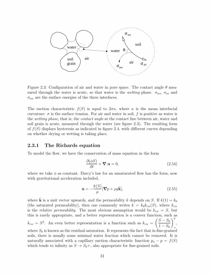
Figure 2.3: Configuration of air and water in pore space. The contact angle θ mea-sured through the water is acute, so that water is the wetting phase. σws, σas andσaw are the surface energies of the three interfaces.

The suction characteristic f(S) is equal to 2σκ, where κ is the mean interfacialcurvature: σ is the surface tension. For air and water in soil, f is positive as water isthe wetting phase, that is, the contact angle at the contact line between air, water andsoil grain is acute, measured through the water (see figure 2.3). The resulting formof f(S) displays hysteresis as indicated in figure 2.4, with different curves dependingon whether drying or wetting is taking place.

2.3.1 The Richards equation

To model the flow, we have the conservation of mass equation in the form

∂(φS)

∂t+∇.u = 0, (2.54)

where we take φ as constant. Darcy’s law for an unsaturated flow has the form, nowwith gravitational acceleration included,

u = −k(S)µ

[∇p+ ρgk], (2.55)

where k is a unit vector upwards, and the permeability k depends on S. If k(1) = k0(the saturated permeability), then one commonly writes k = k0krw(S), where krwis the relative permeability. The most obvious assumption would be krw = S, butthis is rarely appropriate, and a better representation is a convex function, such as

krw = S3. An even better representation is a function such as krw =

(S − S0

1− S0

)3

+

,

where S0 is known as the residual saturation. It represents the fact that in fine-grainedsoils, there is usually some minimal water fraction which cannot be removed. It isnaturally associated with a capillary suction characteristic function pa − p = f(S)which tends to infinity as S → S0+, also appropriate for fine-grained soils.

31

p - p wa

1 S

drying

wetting

Figure 2.4: Capillary suction characteristic. It displays hysteresis in wetting anddrying.

In one dimension, and if we take the vertical coordinate z to point downwards, weobtain the Richards equation

φ∂S

∂t= − ∂

∂z

[k0µkrw(S)

∂f

∂z+ ρg

]. (2.56)

We are assuming pa = constant (and also that the soil matrix is incompressible).

2.3.2 Non-dimensionalisation

We choose scales for the variables as follows:

f =σ

dpψ, z ∼ σ

ρgdp, t ∼ φµz

ρgk0, (2.57)

where dp is grain size and σ is the surface tension, assumed constant. The Richardsequation then becomes, in dimensionless variables,

∂S

∂t= − ∂

∂z

[krw

(∂ψ

∂z+ 1

)]. (2.58)

To be specific, we consider the case of soil wetting due to surface infiltration: ofrainfall, for example. Suitable boundary conditions for infiltration are

S = 1 at z = 0 (2.59)

32

if surface water is ponded, or

krw

(∂ψ

∂z+ 1

)= u∗ =

µu0k0ρwg

=µu0K0

, (2.60)

if there is a prescribed downward flux u0; K0 is the saturated hydraulic conductivity.In a dry soil we would have S → 0 as z → ∞, or if there is a water table at z = zp,S = 1 there.5 For silt with k0 = 10−14 m2, the hydraulic conductivity K0 ∼ 10−7 ms−1 or 3 m y−1, while average rainfall in England, for example, is ≤ 1 m y−1. Thuson average u∗ ≤ 1, but during storms we can expect u∗ ≫ 1. For large values of u∗,the desired solution may have S > 1 at z = 0; in this case ponding occurs (as oneobserves), and (2.60) is replaced by (2.59), with the pond depth being determined bythe balance between accumulation, infiltration, and surface run-off.

2.3.3 Snow melting

An application of the unsaturated flow model occurs in the study of melting snow.In particular, it is found that pollutants which may be uniformly distributed in snow(e. g. SO2 from sulphur emissions via acid rain) can be concentrated in melt water run-off, with a consequent enhanced detrimental effect on stream pollution. The questionthen arises, why this should be so. We shall find that uniform surface melting of adry snowpack can lead to a meltwater spike at depth.

Suppose we have a snow pack of depth d. Snow is a porous aggregate of icecrystals, and meltwater formed at the surface can percolate through the snow pack tothe base, where run-off occurs. (We ignore effects of re-freezing of meltwater). Themodel (2.58) is appropriate, but the relevant length scale is d. Therefore we define aparameter

κ =σ

ρgddp, (2.61)

and we rescale the variables as z ∼ 1/κ, t ∼ 1/κ. To be specific, we will also take

krw = S3, (2.62)

and

ψ(S) =1

S− S, (2.63)

based on typical experimental results.Suitable boundary conditions in a melting event might be to prescribe the melt

flux u0 at the surface, thus

krw

(∂ψ

∂z+ 1

)= u∗ =

u0K 0

at z = 0. (2.64)

5With constant air pressure, continuity of S follows from continuity of pore water pressure.

33

If the base is impermeable, then

krw

(∂ψ

∂z+ 1

)= 0 at z = h. (2.65)

This is certainly not realistic if S reaches 1 at the base, since then ponding must occurand presumably melt drainage will occur via a channelised flow, but we examine theinitial stages of the flow using (2.65). Finally, we suppose S = 0 at t = 0. Again, thisis not realistic in the model (it implies infinite capillary suction) but it is a feasibleapproximation to make.

Simplification of this model now leads to the dimensionless Darcy-Richards equa-tion in the form

∂S

∂t+ 3S2∂S

∂z= κ

∂

∂z

[S(1 + S2)

∂S

∂z

]. (2.66)

If we choose σ = 70 mN m−1, dp = 0.1 mm, ρ = 103 kg m−3, g = 10 m s−2, d = 1m, then κ = 0.07. it follows that (2.66) has a propensity to form shocks, these beingdiffused by the term in κ over a distance O(κ) (by analogy with the shock structurefor the Burgers equation, see chapter 3).

We want to solve (2.66) with the initial condition

S = 0 at t = 0, (2.67)

and the boundary conditions

S3 − κS(1 + S2)∂S

∂z= u∗ on z = 0, (2.68)

and

S3 − κS(1 + S2)∂S

∂z= 0 at z = 1. (2.69)

Roughly, for κ≪ 1, these are

S = S0 at z = 0,

S = 0 at z = 1, (2.70)

where S0 = u∗1/3, which we initially take to be O(1) (and < 1, so that surface pondingdoes not occur).

Neglecting κ, the solution is the step function

S = S0, z < zf ,

S = 0, z > zf , (2.71)

and the shock front at zf advances at a rate zf given by the jump condition

zf =[S3]+−[S]+−

= S20 . (2.72)

34

Z

0S

S

-8 -4 0

0.5

1

Figure 2.5: S(Z) given by (2.78); the shock front terminates at the origin.

In dimensional terms, the shock front moves at speed u0/φS0, which is in fact obvious(given that it has constant S behind it).

The shock structure is similar to that of Burgers’ equation. We put

z = zf + κZ, (2.73)

and S rapidly approaches the quasi-steady solution S(Z) of

−V S ′ + 3S2S ′ = [S(1 + S2)S ′]′, (2.74)

where V = zf ; henceS(1 + S2)S ′ = −S(S2

0 − S2), (2.75)

in order that S → S0 as Z → −∞, and where we have chosen

V = S20 , (2.76)

(as S+ = 0), thus reproducing (2.72). The solution is a quadrature,

∫ S (1 + S2) dS

(S20 − S2)

= −Z, (2.77)

with an arbitrary added constant (amounting to an origin shift for Z). Hence

S − (1 + S20)

2S0ln

[S0 + S

S0 − S

]= Z. (2.78)

The shock structure is shown in figure 2.5; the profile terminates where S = 0at Z = 0. In fact, (2.75) implies that S = 0 or (2.78) applies. Thus when S given

35

by (2.78) reaches zero, the solution switches to S = 0. The fact that ∂S/∂Z isdiscontinuous is not a problem because the diffusivity S(1 + S2) goes to zero whenS = 0. This degeneracy of the equation is a signpost for fronts with discontinuousderivatives: essentially, the profile can maintain discontinuous gradients at S = 0because the diffusivity is zero there, and there is no mechanism to smooth the jumpaway.

Suppose now that k0 = 10−10 m2 and µ/ρ = 10−6 m2 s−1; then the saturatedhydraulic conductivity K0 = k0ρg/µ = 10−3 m s−1. On the other hand, if a metrethick snow pack melts in ten days, this implies u0 ∼ 10−6 m s−1. Thus S3

0 = u0/K0 ∼10−3, and the approximation S ≈ S0 looks less realistic. With

S3 − κS(1 + S2)∂S

∂z= S3

0 , (2.79)

and S0 ∼ 10−1 and κ ∼ 10−1, it seems that one should assume S ≪ 1. We define

S =

(S30

κ

)1/2

s; (2.80)

(2.79) becomes

βs3 − s

[1 +

S30

κs2]∂s

∂z= 1 on z = 0, (2.81)

and we have S30/κ ∼ 10−2, β = (S0/κ)

3/2 ∼ 1.We neglect the term in S3

0/κ, so that

βs3 − s∂s

∂z≈ 1 on z = 0, (2.82)

and substituting (2.80) into (2.66) leads to

∂s

∂τ+ 3βs2

∂s

∂z≈ ∂

∂z

[s∂s

∂z

], (2.83)

if we define t = τ/ (κS30)

1/2. A simple analytic solution is no longer possible, but the

development of the solution will be similar. The flux condition (2.82) at z = 0 allowsthe surface saturation to build up gradually, and a shock will only form if β ≫ 1(when the preceding solution becomes valid).

2.3.4 Similarity solutions

If, on the other hand, β ≪ 1, then the saturation profile approximately satisfies

∂s

∂τ=

∂

∂z

[s∂s

∂z

],

−s∂s∂z

=

1 on z = 0,0 on z = 1.

(2.84)

36

At least for small times, the model admits a similarity solution of the form

s = ταf(η), η = z/τβ , (2.85)

where satisfaction of the equations and boundary conditions requires 2α = β and2β = 1 = α, whence α = 1

3, β = 2

3, and f satisfies

(ff ′)′ − 13(f − 2ηf ′) = 0, (2.86)

with the condition at z = 0 becoming

−ff ′ = 1 at η = 0. (2.87)

The condition at z = 1 can be satisfied for small enough τ , as we shall see, becausethe equation (2.86) is degenerate, and f reaches zero in a finite distance, η0, say, andf = 0 for η > η0. As η = 1/τ 2/3 at z = 1, then this solution will satisfy the no flux

condition at z = 1 as long as τ < η−3/20 , when the advancing front will reach z = 1.

To see why f behaves in this way, integrate once to find

f(f ′ + 23η) = −1 +

∫ η

0

f dη. (2.88)

For small η, the right hand side is negative, and f is positive (to make physical sense),so f decreases (and in fact f ′ < −2

3η). For sufficiently small f(0) = f0, f will reach

zero at a finite distance η = η0, and the solution must terminate. On the other hand,

for sufficiently large f0,

∫ η

0

f dη reaches 1 at η = η1 while f is still positive (and

f ′ = −23η1 there). For η > η1, then f remains positive and f ′ > −2

3η (f cannot reach

zero for η > η1 since

∫ η

0

f dη > 1 for η > η1). Eventually f must have a minimum

and thereafter increase with η. This is also unphysical, so we require f to reach zeroat η = η0. This will occur for a range of f0, and we have to select f0 in order that

∫ η0

0

f dη = 1, (2.89)

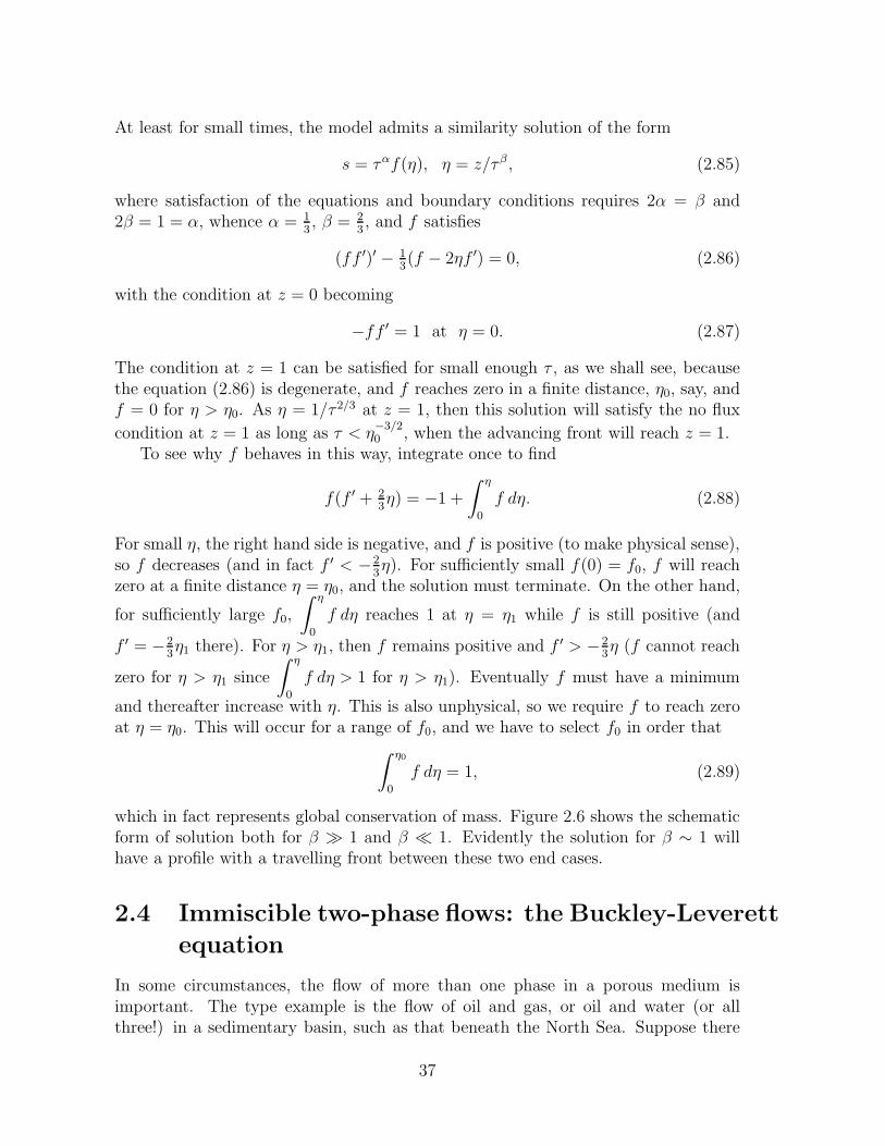
which in fact represents global conservation of mass. Figure 2.6 shows the schematicform of solution both for β ≫ 1 and β ≪ 1. Evidently the solution for β ∼ 1 willhave a profile with a travelling front between these two end cases.

2.4 Immiscible two-phase flows: the Buckley-Leverett

equation

In some circumstances, the flow of more than one phase in a porous medium isimportant. The type example is the flow of oil and gas, or oil and water (or allthree!) in a sedimentary basin, such as that beneath the North Sea. Suppose there

37

s ~1/β2/3 β >> 1

β << 1

z = η0τ2/3 z ~ β1/3τ

s

z

s~1

Figure 2.6: Schematic representation of the evolution of s in (2.83) for both large andsmall β.

are two phases; denote the phases by subscripts 1 and 2, with fluid 2 being the wettingfluid, and S is its saturation. Then the capillary suction characteristic is

p1 − p2 = pc(S), (2.90)

with the capillary suction pc being a positive, monotonically decreasing function ofsaturation S; mass conservation takes the form

−φ∂S∂t

+∇.u1 = 0,

φ∂S

∂t+∇.u2 = 0, (2.91)

where φ is (constant) porosity, and Darcy’s law for each phase is

u1 = −k0µ1

kr1[∇p1 + ρ1gk],

u2 = −k0µ2kr2[∇p2 + ρ2gk], (2.92)

with kri being the relative permeability of fluid i.For example, if we consider a one-dimensional flow, with z pointing upwards, then

we can integrate (2.91) to yield the total flux

u1 + u2 = q(t). (2.93)

38

If we define the mobilities of each fluid as

Mi =k0µikri, (2.94)

then it is straightforward to derive the equation for S,

φ∂S

∂t= − ∂

∂z

[Meff

q

M1+∂pc∂z

+ (ρ1 − ρ2)g

], (2.95)

where the effective mobility is determined by

Meff =

(1

M1

+1

M2

)−1

. (2.96)

-0.05

0

0.05

0.2 0.4 0.6 0.8 1

V

S

Figure 2.7: Graph of dimensionless wave speed V (S) as a function of wetting fluidsaturation, indicating the speed and direction of wave motion (V > 0 means wavesmove upwards) if the wetting fluid is more dense. The viscosity ratio µr (see (2.100))is taken to be 30.

This is a convective-diffusion equation for S. If suction is very small, we obtainthe Buckley-Leverett equation

φ∂S

∂t+

∂

∂z

[Meff

q

M1+ (ρ1 − ρ2)g

]= 0, (2.97)

which is a nonlinear hyperbolic wave equation. As a typical situation, suppose q = 0,and kr2 = S3, kr1 = (1− S)3. Then

Meff =k0S

3(1− S)3

µ1S3 + µ2(1− S)3, (2.98)

39

and the wave speed v(S) is given by

v = −(ρ2 − ρ1)gM′eff(S) = v0V (S), (2.99)

where

v0 =(ρ2 − ρ1)gk0

µ2, V (S) =

χ′(S)

χ(S)2,

χ(S) =µr

(1− S)3+

1

S3, µr =

µ1

µ2. (2.100)

The variation of V with S is shown in figure 2.7. For ρ2 > ρ1 (as for oil and water,where water is the wetting phase), waves move upwards at low water saturation anddownwards at high saturation.

Shocks will form, but these are smoothed by the diffusion term − ∂

∂z

[Meffp

′c

∂S

∂z

],

in which the diffusion coefficient is

D = −Meff p′c. (2.101)

As a typical example, take

pc =p0(1− S)λ1

Sλ2(2.102)

with λi > 0. Then we find

D = k0p0S2−λ2(1− S)2+λ1

[λ1S + λ2(1− S)

µ1S3 + µ2(1− S)3

], (2.103)

and we see that D is typically degenerate at S = 0. In particular, if λ2 < 2, theninfiltration of the wetting phase into the non-wetting phase proceeds at a finite rate,and this always occurs for infiltration of the non-wetting phase into the wetting phase.

A particular limiting case is when one phase is much less dense than the other,the usual situation being that of gas and liquid. This is exemplified by the problemof snow-melt run-off considered earlier. In that case, water is the wetting phase, thusρ2 − ρ1 = ρw − ρa is positive, and also µw ≈ 10−3 Pa s, µa ≈ 10−5 Pa s, whenceµa ≪ µw (µr ≪ 1), so that, from (2.98),

Meff ≈ k0S3

µw, (2.104)

at least for saturations not close to unity. Shocks form and propagate downwards(since ρ2 > ρ1). The presence of non-zero flux q < 0 does not affect this statement.Interestingly, the approximation (2.104) will always break down at sufficiently highsaturation. Inspection of V (S) for µr = 0.01 (as for air and water) indicates that(2.104) is an excellent approximation for S <∼ 0.5, but not for S >∼ 0.6; for S >∼ 0.76,V is positive and waves move upwards. As µr → 0, the right hand hump in figure2.7 moves towards S = 1, but does not disappear; indeed the value of the maximumincreases, and is V ∼ µ

−1/3r . Thus the single phase approximation for unsaturated

flow is a singular approximation when µr ≪ 1 and 1− S ≪ 1.

40

2.5 Consolidation

Consolidation refers to the ability of a granular porous medium such as a soil tocompact under its own weight, or by the imposition of an overburden pressure. Thegrains of the medium rearrange themselves under the pressure, thus reducing theporosity and in the process pore fluid is expelled. Since the porosity is no longerconstant, we have to postulate a relation between the porosity φ and the pore pressurep. In practice, it is found that soils, when compressed, obey a (non-reversible) relationbetween φ and the effective pressure

pe = P − p, (2.105)

where P is the overburden pressure.The concept of effective pressure, or more generally effective stress, is an extremely

important one. The idea is that the total imposed pressure (e. g., the overburdenpressure due to the weight of the rock or soil) is borne by both the pore fluid and theporous medium. The pore fluid is typically at a lower pressure than the overburden,and the extra stress (the effective stress) is that which is applied through grain tograin contacts. Thus the effective pressure is that which is transmitted through theporous medium, and it is in consequence of this that the medium responds to theeffective stress; in particular, the characteristic relation between φ and pe representsthe nonlinear pseudo-elastic effect of compression.

As pe increases, so φ decreases, thus we can write (ignoring irreversibility)

pe = pe(φ), p′e(φ) < 0. (2.106)

Taking fluid density ρ to be constant, we obtain from the conservation of mass equa-tion the nonlinear diffusion equation

φt = ∇.

[k(φ)

µ|p′e(φ) |∇φ

], (2.107)

assuming Darcy’s law with a permeability k, ignoring gravity, and taking P as con-stant. This is essentially the same as the Richards equation for unsaturated soils.

The dependence of the effective pressure on porosity is non-trivial and involveshysteresis, as indicated in figure 2.8. Specifically, a soil follows the normal consolida-

tion line providing consolidation is occurring, i.e pe > 0. However, if at some pointthe effective pressure is reduced, only a partial recovery of φ takes place. When peis increased again, φ more or less retraces its (overconsolidated) path to the normalconsolidation line, and then resumes its normal consolidation path. Here we willignore effects of hysteresis, as in (3.90).

When modelling groundwater flow in a consolidating medium, we must take ac-count also of deformation of the medium itself. In turn, this requires prescription ofa constitutive rheology for the deformable matrix. This is often a complex matter,but luckily in one dimension, the issue does not arise, and a one-dimensional modelis often what is of practical interest. We take z to point vertically upwards, and let

41

ep

φ

normal consolidation line

Figure 2.8: Form of the relationship between porosity and effective pressure. Ahysteretic decompression-reconsolidation loop is indicated. In soil mechanics thisrelationship is often written in terms of the void ratio e = φ/(1− φ), and specificallye = e0 − Cc log pe, where Cc is the compression index.

vl and vs be the linear (or phase-averaged) velocities of liquid and solid, respectively.Then ul = φvl and us = (1− φ)vs are the respective fluxes, and conservation of massof each phase requires

∂φ

∂t+∂(φvl)

∂z= 0,

−∂φ∂t

+∂(1− φ)vs

∂z= 0; (2.108)

Darcy’s law is then

φ(vl − vs) = −kµ

[∂p

∂z+ ρlg

], (2.109)

while the overburden pressure is

P = P0 + [ρs(1− φ) + ρlφ]g(h− z); (2.110)

here z = h represents the ground surface and P0 is the applied load. (2.110) assumesvariations of φ are small. More generally, we would have ∂P/∂z = −[ρs(1−φ)+ρlφ]g.The effective pressure is then just pe = P − p.

We suppose these equations apply in a vertical column 0 < z < h, for whichsuitable boundary conditions are

vl = vs = 0 at z = 0,

p = 0, h = vs at z = h, (2.111)

42

and with an initial condition for p (or φ).The two mass conservation equations imply

vs = − φvl

1− φ. (2.112)

Substituting this into (2.109), we derive, using (2.108),

∂φ

∂t=

∂

∂z

[k

µ(1− φ)

∂p

∂z+ ρlg

]. (2.113)

If we assume the normal consolidation line takes the commonly assumed form (seefigure 2.8)

φ

1− φ= e0 − Cc ln(pe/p

0e), (2.114)

then we derive the consolidation equation

∂pe∂t

=pe

Cc(1− φ)2∂

∂z

[k

µ(1− φ)

∂pe∂z

+∆ρ(1− φ)g

], (2.115)

where ∆ρ = ρs − ρl.If Cc is small (and typical values are in the range Cc ≤ 0.1) then φ varies little,

and the consolidation equation takes the simpler form

∂pe∂t

= cv∂2pe∂z2

, (2.116)

where

cv =k

µ

peCc(1− φ)

(2.117)

is the coefficient of consolidation.Suitable boundary conditions are

∂pe∂z

+∆ρ(1− φ)g = 0 at z = 0,

pe = P0 at z = h, (2.118)

and if the load is applied at t = 0, the initial condition is

pe = ∆ρ(1− φ)g(h− z) at t = 0. (2.119)

The equation is trivially solved. The consolidation time is

tc ∼h2

cv=µCc(1− φ)h2

kpe, (2.120)

and depends primarily on the permeability k. If we take k ∼ 10−14 m2 (silt), Cc = 0.1,φ = 0.3, µ = 10−3 Pa s, P0 = 105 Pa (a small house), then cv ∼ 10−5 m2 s−1, andte ∼ 1 year for h ∼ 10 m.

43

2.6 Compaction

Compaction is the same process as consolidation, but on a larger scale. Other mech-anisms can cause compaction apart from the rearrangement of sediments: pressuresolution in sedimentary basins, grain creep in partially molten mantle (see chapter??). The compaction of sedimentary basins is a problem which has practical con-sequences in oil-drilling operations, since the occurrence of abnormal pore pressurescan lead to blow-out and collapse of the borehole wall. Such abnormal pore pressures(i.e., above hydrostatic) can occur for a variety of reasons, and part of the purpose ofmodelling the system is to determine which of these are likely to be realistic causes.A further distinction from smaller scale consolidation is that the variation in porosity(and, particularly, permeability) is large.

The situation we consider was shown in figure ??. Sediments, both organic andinorganic, are deposited at the ocean bottom and accumulate. As they do so, theycompact under their weight, thus expelling pore water. If the compaction is fast (i.e.,the rate of sedimentation is greater than the hydraulic conductivity of the sediments)then excess pore pressure will occur.

Sedimentary basins, such as the North Sea or the Gulf of Mexico, are typicallyhundreds of kilometres in extent and several kilometres deep. It is thus appropriateto model the compacting system as one-dimensional. A typical sedimentation rate is10−11 m s−1, or 300 m My−1, so that a 10 kilometre deep basin may accumulate in30 My (30 million years). On such long time scales, tectonic processes are important,and in general accumulation is not a monotonic process. If tectonic uplift occurs sothat the surface of the basin rises above sea level, then erosion leads to denudationand a negative sedimentation rate. Indeed, one purpose of studying basin porosityand pore pressure profiles is to try and infer what the previous subsidence historywas — an inverse problem.

The basic mathematical model is that of slow two-phase flow, where the phasesare solid and liquid, and is the same as that of consolidation theory. The effectivepressure pe is related, in an elastic medium, to the porosity by a function pe = pe(φ).In a soil, or for sediments near the surface up to depths of perhaps 500 m, the relationis elastic and hysteretic. At greater depths, more than a kilometre, pressure solutionbecomes important, and an effective viscous relationship becomes appropriate, asdescribed below. At greater depths still, cementation occurs and a stiffer elasticrheology should apply.6 In addition, the permeability is a function k = k(φ) ofporosity, with k decreasing to zero fairly rapidly as φ decreases to zero.

Let us suppose the basin overlies an impermeable basement at z = 0, and that itssurface is at z = h; then suitable boundary conditions are

vs = vl = 0 at z = 0,

pe = 0, h = ms + vs at z = h, (2.121)

6Except that at elevated temperatures, creep deformation will start to occur.

44

where vs and vl are solid and liquid average velocities, and ms is the prescribedsedimentation rate, which we take for simplicity to be constant.

If we assume a specific elastic compactive rheology of the form

pe = p0ln(φ0/φ)− (φ0 − φ), (2.122)

then non-dimensionalisation (using a depth scale d =p0

(ρs − ρl)gand a time scale

d

ms)

and simplification of the model leads to the nonlinear diffusion equation, analogousto (2.113),

∂φ

∂t= λ

∂

∂z

k(1− φ)2

[1

φ

∂φ

∂z− 1

], (2.123)

where the permeability is defined to be

k = k0k(φ), (2.124)

k0 being a suitable scale for k.The dimensionless parameter λ is given by

λ =K0

ms, (2.125)

where K0 = k0(ρs − ρl)g/µ is essentially the surface hydraulic conductivity, and wecan then distinguish between slow compaction (λ≪ 1) and fast compaction (λ≫ 1).Typical values of λ depend primarily on the sediment type. For ms = 10−11 m s−1,we have λ ≈ 0.1 for the finest clay, λ ≈ 109 for coarse sands. In general, therefore,we can expect large values of λ. The associated boundary conditions for the modelbecome

φz − φ = 0 at z = 0,

φ = φ0, h = 1 + λk(1− φ)

[1

φ

∂φ

∂z− 1

]at z = h. (2.126)

Slow compaction, λ≪ 1

When λ is small, overpressuring occurs. A boundary layer analysis is easy to do, andshows that φ ≈ φ0 in the bulk of the (uncompacted) sediment, while a compactingboundary layer of thickness

√λt exists at the base.

Fast compaction, λ≫ 1

The more realistic case of fast compaction is also the more mathematically interesting.Most simply, the solution when λ≫ 1 is the equilibrium profile

φ = φ0 exp[h− z]; (2.127)

45

the exponential decline of porosity with depth is sometimes called an Athy profile,but it only applies while λk ≫ 1. If we assume a power law for the dimensionlesspermeability of the form

k = (φ/φ0)m, (2.128)

then we find that λk reaches one when φ decreases to a value

φ∗ = φ0 exp

[− 1

mlnλ

], (2.129)

and this occurs at a dimensionless depth

Π =1

mlnλ (2.130)

and time

t∗ =Π− φ0(1− e−Π)

1− φ0

. (2.131)

Typical values m = 8, λ = 100, φ0 = 0.5, give values φ∗ = 0.28, Π = 0.58, t∗ = 0.71.In particular, for a reasonable depth scale of 1 km (corresponding to p0 = 2 × 107

Pa = 200 bars), this would correspond to a depth of 580 m. Below this, the profileis not equilibrated, and the pore pressure is elevated. Figure 2.9 shows the resultingdifference in the porosity profiles at t = t∗ and t > t∗, and figure 2.10 shows the effecton the pore pressure, whose gradient changes abruptly from hydrostatic to lithostaticat the critical depth.

If we take φ∗ = O(1) and λ ≫ 1, then formally m ≫ 1, and it is possible toanalyse the profile below the critical depth. One finds that

φ = φ∗ exp

[− 1

mlnm+O(1)

], (2.132)

which can explain the flattening of the porosity profile evident in figure 2.9, and whichis also seen in field data.

Viscous compaction

Below a depth of perhaps a kilometre, pressure solution at intergranular contactsbecomes important, and the resulting dissolution and local reprecipitation leads toan effective creep of the grains (and hence of the bulk medium) in a manner analogousto regelation in ice. For such viscous compaction, the constitutive relation for theeffective pressure becomes

pe = −ξ∇.us. (2.133)

In one dimension, the resulting dimensionless model is

−∂φ∂t

+∂

∂z[(1− φ)u] = 0,

46

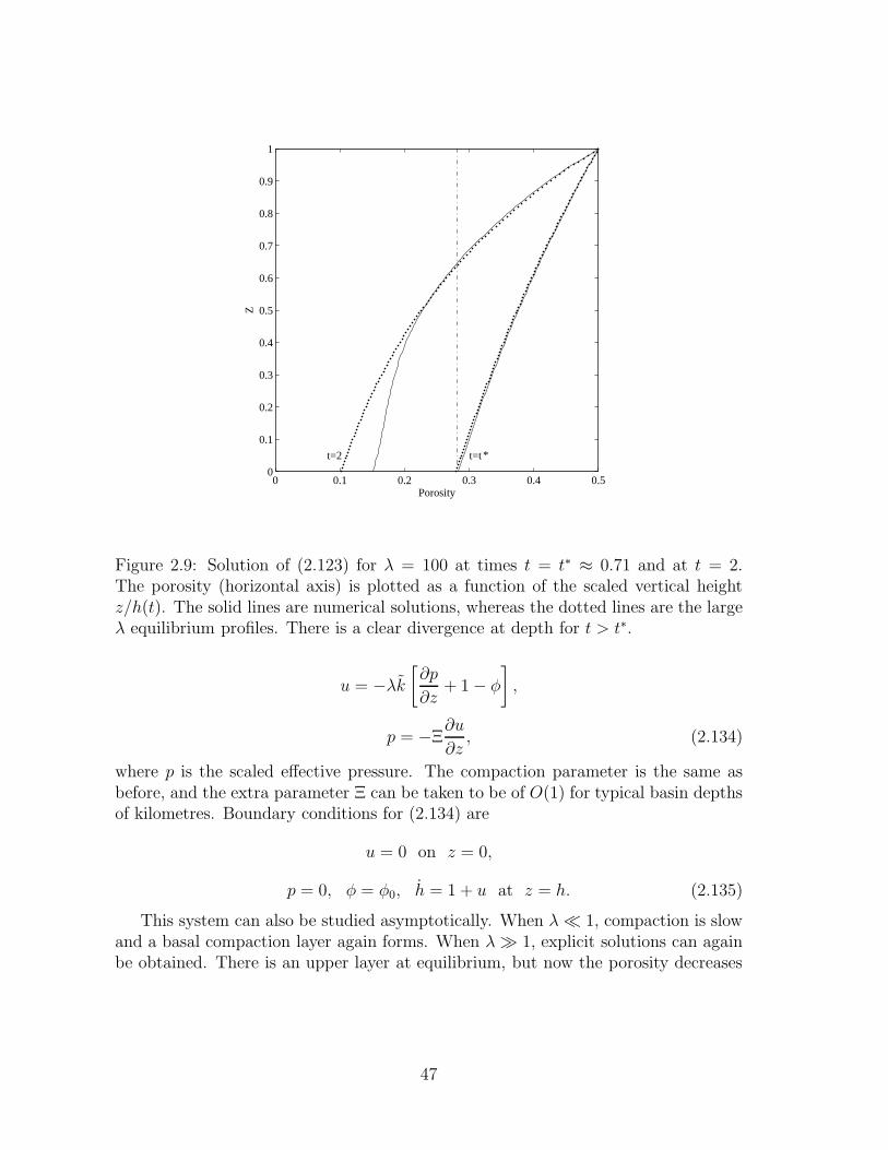
0 0.1 0.2 0.3 0.4 0.50

0.1

0.2

0.3

0.4

0.5

0.6

0.7

0.8

0.9

1

Porosity

Z

t=2 t=t *

Figure 2.9: Solution of (2.123) for λ = 100 at times t = t∗ ≈ 0.71 and at t = 2.The porosity (horizontal axis) is plotted as a function of the scaled vertical heightz/h(t). The solid lines are numerical solutions, whereas the dotted lines are the largeλ equilibrium profiles. There is a clear divergence at depth for t > t∗.

u = −λk[∂p

∂z+ 1− φ

],

p = −Ξ∂u

∂z, (2.134)

where p is the scaled effective pressure. The compaction parameter is the same asbefore, and the extra parameter Ξ can be taken to be of O(1) for typical basin depthsof kilometres. Boundary conditions for (2.134) are

u = 0 on z = 0,

p = 0, φ = φ0, h = 1 + u at z = h. (2.135)

This system can also be studied asymptotically. When λ≪ 1, compaction is slowand a basal compaction layer again forms. When λ≫ 1, explicit solutions can againbe obtained. There is an upper layer at equilibrium, but now the porosity decreases

47

0 0.5 1 1.50

0.1

0.2

0.3

0.4

0.5

0.6

0.7

0.8

0.9

1

pressure

scal

ed h

eigh

t: Z

overburden

pore

hydrostatic

Figure 2.10: Hydrostatic, overburden (lithostatic) and pore pressures at t = 5 andλ = 100, as functions of the scaled height z/h(t). The transition from equilibriumto non-equilibrium compaction at the critical depth is associated with a transitionfrom normal to abnormal pore pressures. The dashed lines represent two distinctapproximations to the pore pressure profile, respectively valid above and below thetransition region.

concavely with depth.7 As before, there is a transition when φ = φ∗, and below this

φ = φ∗ exp

[− 2

mlnm+O(1)

], (2.136)

similar to (2.132).The main distinction between viscous and elastic compaction is thus in the form of

the rapidly compacted equilibrium profile near the surface (figure 2.11). The concaveprofile is not consistent with observations, but we need not expect it to be, as theviscous behaviour of pressure solution only becomes appropriate at reasonable depths.A more general relation which allows for this is a viscoelastic compaction law of theform

∇.us = − 1

Ke

dpedts

− peξ. (2.137)

7In view of chapter ??, we need to be careful here. The function is mathematically concave, i. e.,the rate of decrease of porosity with depth increases as depth increases.

48

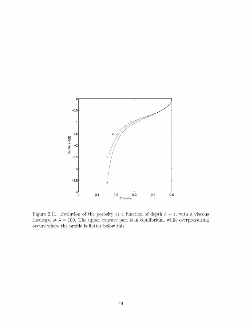
0 0.1 0.2 0.3 0.4 0.5−4

−3.5

−3

−2.5

−2

−1.5

−1

−0.5

0

2

3

5

Porosity

Dep

th: z

−h(

t)

Figure 2.11: Evolution of the porosity as a function of depth h − z, with a viscousrheology, at λ = 100. The upper concave part is in equilibrium, while overpressuringoccurs where the profile is flatter below this.

49

2.7 Notes and references

Flow in porous media is described in the books by Bear (1972) and Dullien (1979).More recent versions, for example by Bear and Bachmat (1990) have developed ataste for more theoretical, deductive treatments based on homogenisation (see below)or averaging, with a concomitant loss of readability. The classic geologists’ book ongroundwater is by Freeze and Cherry (1979) and the classic engineering text is byPolubarinova-Kochina (1962). A short introduction, of geographical style, is by Price(1985). A more mathematical survey, with a variety of applications, is by Bear andVerruijt (1987). The book edited by Cushman (1990) contains a wealth of articles ontopics of varied and current interest, including dispersion, homogenisation, averaging,dual porosity models, multigrid methods and heterogeneous porous media. Furtherinformation on the concepts of soil mechanics can be found in Lambe and Whitman(1979).

Homogenisation

The technique of homogenisation is no more than the technique of averaging in thespatial domain, most often formulated as a multiple scales method. Whole books havebeen written about it, for example those by Bensoussan et al. (1978) and Sanchez-Palencia (1983). For application to porous media, see, for example, Ene’s article inthe book edited by Cushman (1990).

Piping

Many dams are built of concrete, and in this case the problems associated with seepagedo not arise, owing to the virtual impermeability of concrete. Earth and rockfill damsdo exist, however, and are liable to failure by a mechanism called piping. The Darcyflow through the porous dam causes channels to form by eroding away fine particles.The resultant channelisation concentrates the flow, increasing the force exerted bythe flow on the medium and thus increasing the erosion/collapse rate of the channelwall. We can write Darcy’s law as a force balance on the liquid phase,

0 = −φ∇p− φµ

kvl − φρlgk (2.138)

(k being vertically upwards) and φµvl/k is an interactive drag term; then the corre-sponding force balance for the solid phase is

0 = −(1− φ)∇ps +φµ

kvl − (1− φ)ρsgk, (2.139)

where ps is the pressure in the solid. For a granular solid, we can expect grain motionto occur if the interactive force is large enough to overcome friction and cohesion; thetypical kind of criterion is that the shear stress τ satisfies

τ ≥ c+ pe tanφ, (2.140)

50

but in view of the large confining pressure and the necessity of dilatancy for soildeformation, the piping criterion will in practice be satisfied at the toe of the dam(i.e. the front), and piping channels will eat their way back into the dam, in muchthe same way that river drainage channels eat their way into a hillslope. A simplercriterion at the toe then follows from the necessity that the effective pressure on thegrains be positive. A lucid discussion by Bear and Bachmat (1990, p. 153) indicatesthat the solid pressure is related to the effective pressure pe which controls graindeformation by

pe = (1− φ)(ps − p), (2.141)

and in this case the piping criterion at the toe is that pe < 0 in the soil there, or∂pe/∂z > 0. From (2.138), (2.139) and (2.141), this implies piping if

µv

k> (ρs − ρl)(1− φ)g, (2.142)

where v is the vertical component of vl. This criterion is given by Bear (1972). Moregenerally, piping can be expected to occur if pe reaches 0 in the soil interior (ignoringcohesion). Sellmeijer and Koenders (1991) develop a model for piping.

Taylor dispersion

Taylor dispersion is named after its investigation by Taylor (1953), who carried outexperiments on the dispersal of solute in flow down a tube. The dispersion is enabledby the combination of differential axial advection by the down tube velocity, typicallya Poiseuille flow, and the rapid cross stream diffusion which renders the cross-sectionalconcentration profile radially uniform. The theory of Taylor is somewhat heuristic;it was later elaborated by Aris (1956). For a formal derivation using asymptoticmethods, see Fowler (1997, p. 222, exercise 2).

Its application to porous media stems from the conceptual idea that the pore spaceconsists of a network of narrow tubules connected at pore junctions. If the tubes areof radius a and length dp, the latter corresponding to grain size, then the Darcy flux|u| ∼ πφU , while the pore radius a ∼ dp

√φ. This would suggest a Taylor dispersion

coefficient of

DT ≈ a2U2

48D∼

d2p|u|248π2Dφ

, (2.143)

as opposed to the measured values which more nearly have DT ∼ |u|. Taylor dis-persion in porous media has been studied by Saffman (1959), Brenner (1980) andRubinstein and Mauri (1986), the latter using the method of homogenisation.

Biofilm growth

Monod kinetics was described by Monod (1949), by way of analogy with enzymekinetics, where one considers the uptake of nutrients as occurring through a seriesof fast intermediary reactions; when two nutrients control growth, as in respiration,

51

it is usual to take the growth rate as proportional to the product of two Monodfactors (Bader 1978). A variety of enhancements to this simple model have also beenproposed to account for nutrient consumption due to maintenance, inactivation ofcells in adverse conditions, and other observed effects (Beeftink et al. 1990, Wanneret al. 2006).

Bacteria in soils commonly grow as attached biofilms on soil grains, with a thick-ness of the order of 100 µ. A variety of models to describe biofilm growth have beenpresented, with an ultimate view of being able to parameterise the uptake rate ofcontaminant species in soils and other environments (Rittmann and McCarty 1980,Picioreanu et al. 1998, Eberl et al. 2001, Dockery and Klapper 2001, Cogan andKeener 2004).

Remediation sites

The three sites described in section ?? are under study by the Groundwater Restora-tion and Protection Group at the University of Sheffield, led by Professor DavidLerner. The site at Four Ashes is described by Mayer et al. (2001), that at Rexco byHuttmann et al. (2003), and that at St. Alban’s by Wealthall et al. (2001).

The description of the two species reaction front given by (??) is similar to that fora diffusion flame (Buckmaster and Ludford 1982) in combustion, and also corrosionin alloys (Hagan et al. 1986). It is not conceptually difficult to extend this approachto an arbitrary number of reactions, although it may become awkward when multiplereaction fronts are present (see, for example, Dewynne et al. (1993)).

Diagenesis

The first order reaction kinetics (??) for the smectite-illite transition was proposedby Eberl and Hower (1976). Information on solubility limits is given by Aagard andHelgeson (1983) and Sass et al. (1987). The asymptotic approximation called here theweak solubility limit is called solid density asymptotics by Ortoleva (1994). Details ofthe use of the weak solubility approximation can be found in Fowler and Yang (2003).

Compaction

Interest in compaction is motivated by its occurrence in sedimentary basins, and alsoby issues of subsidence due to groundwater or natural gas extraction (see, for example,Bau et al. 2000). The constitutive law used here for effective pressure is that of Smith(1971); it mimics the normal consolidation behaviour of compacting sediments (suchas soils), and is further discussed by Audet and Fowler (1992) and Jones (1994).

Athy’s law comes from the paper by Athy (1930). Smith (1971) advocates the useof the high exponent m = 8 in (2.128). Further details of the asymptotic solutionof the compaction profiles are given by Fowler and Yang (1998). Freed and Peacor(1989) show examples of the flattened porosity profiles at depth.

52

Early work on pressure solution in sedimentary basins was by Angevine and Tur-cotte (1983) and Birchwood and Turcotte (1984). More recently, Fowler and Yang(1999) derived the viscous compaction law. An extension to viscoelastic compactionhas been studied by Yang (2000).

Seals

One process which we have not described is the formation of high pressure seals.In certain circumstances, pore pressures undergo fairly rapid jumps across a ‘seal’,typically at depths of 3000 m. Such jumps cannot be predicted within the confines of asimple compaction theory, and require a mechanism for pore-blocking. Mineralisationis one such mechanism, as some seals are found to be mineralised with calcite andsilica (Hunt 1990). In fact, a generalisation of the clay diagenesis model to allow forcalcite precipitation could be used for this purpose. As it stands, (??) predicts asource for φ, but mineralisation would cause a corresponding sink term. Reductionof φ leads to reduction of diffusive transport, and the feedback is self-promoting.Problems of this type have been studied by Ortoleva (1994), for example.

Exercises

2.1 Show that for a porous medium idealised as a cubical network of tubes, thepermeability is given (approximately) by k = d2pφ

2/72π, where dp is the grainsize. How is the result modified if the pore space is taken to consist of pla-nar sheets between identical cubical blocks? (The volume flux per unit widthbetween two parallel plates a distance h apart is −h3p′/12µ, where p′ is thepressure gradient.)

2.2 A sedimentary rock sequence consists of two type of rock with permeabilitiesk1 and k2. Show that in a unit with two horizontal layers of thickness d1 andd2, the effective horizontal permeability (parallel to the bedding plane) is

k‖ = k1f1 + k2f2,

where fi = di/(d1 + d2), whereas the effective vertical permeability is given by

k−1⊥ = f1k

−11 + f2k

−12 .

Show how to generalise this result to a sequence of n layers of thickness d1, . . . , dn.

Hence show that the effective permeabilities of a thick stratigraphic sequencecontaining a distribution of (thin) layers, with the proportion of layers havingpermeabilities in (k, k + dk) being f(k)dk, are given by

k‖ =

∫ ∞

0

kf(k) dk, k−1⊥ =

∫ ∞

0

f(k) dk

k.

53

2.3 Groundwater flows between an impermeable basement at z = hb(x, y, t) anda phreatic surface at z = zp(x, y, t). Write down the equations governing theflow, and by using the Dupuit approximation, show that the saturated depth hsatisfies

φht =kρg

µ∇.[h∇zp],

where ∇ = (∂/∂x, ∂/∂y). Deduce that a suitable time scale for flows in anaquifer of typical depth h0 and extent l is tgw = φµl2/kρgh0.

I live a kilometer from the river, on top of a layer of sediments 100 m thick(below which is impermeable basement). What sort of sediments would thoseneed to be if the river responds to rainfall at my house within a day; within ayear?

2.4 A two-dimensional earth dam with vertical sides at x = 0 and x = l has areservoir on one side (x < 0) where the water depth is h0, and horizontal dryland on the other side, in x > l. The dam is underlain by an impermeablebasement at z = 0.

Write down the equations describing the saturated groundwater flow, and showthat they can be written in the dimensionless form

u = −px, ε2w = −(pz + 1),

pzz + ε2pxx = 0,

and define the parameter ε. Write down suitable boundary conditions on theimpermeable basement, and on the phreatic surface z = h(x, t).

Assuming ε≪ 1, derive the Dupuit-Forchheimer approximation for h,

ht = (hhx)x in 0 < x < 1.

Show that a suitable boundary condition for h at x = 0 (the dam end) is

h = 1 at x = 0.

Now define the quantity

U =

∫ h

0

p dz,

and show that the horizontal flux

q =

∫ h

0

u dz = −∂U∂x

.

Hence show that the conditions of hydrostatic pressure at x = 0 and constant(atmospheric) pressure at x = 1 (the seepage face) imply that

∫ 1

0

q dx = 12.

54

Deduce that, if the Dupuit approximation for the flux is valid all the way tothe toe of the dam at x = 1, then h = 0 at x = 1, and show that in the steadystate, the (dimensional) discharge at the seepage face is

qD =kρgh202µl

.

Supposing the above description of the solution away from the toe to be valid,show that a possible boundary layer structure near x = 1 can be described bywriting

x = 1− ε2X, h = εH, z = εZ, p = εP,

and write down the resulting leading order boundary value problem for P .

2.5 I get my water supply from a well in my garden. The well is of depth h0 (relativeto the height of the water table a large distance away) and radius r0. Show thatthe Dupuit approximation for the water table height h is

φ∂h

∂t=kρg

µ

1

r

∂

∂r

(rh∂h

∂r

).

If my well is supplied from a reservoir at r = l, where h = h0, and I withdrawa constant water flux q0, find a steady solution for h, and deduce that my wellwill run dry if

q0 >πkρgh20µ ln[l/r0]

.

Use plausible values to estimate the maximum yield (gallons per day) I can useif my well is drilled through sand, silt or clay, respectively.

2.6 A volume V of effluent is released into the ground at a point (r = 0) at time t.Use the Dupuit approximation to motivate the model

φ∂h

∂t=kρg

µ

1

r

∂

∂r

(rh∂h

∂r

),

h = h0 at t = 0, r > 0,∫ ∞

0

r(h− h0)dr = V/2π, t > 0,

where h0 is the initial height of the water table above an impermeable basement.Find suitable similarity solutions in the two cases (i) h0 = 0 (ii) h0 > 0, h−h0 ≪h0, and comment on the differences you find.

2.7 Fluid flows through a porous medium in the x direction at a linear velocity U .At t = 0, a contaminant of concentration c0 is introduced at x = 0. If thelongitudinal dispersivity of the medium is D, write down the equation which

55

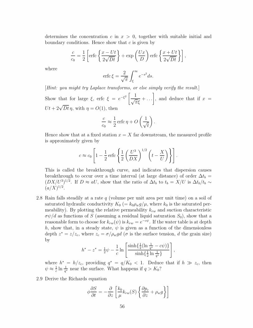
determines the concentration c in x > 0, together with suitable initial andboundary conditions. Hence show that c is given by

c

c0=

1

2

[erfc

x− Ut

2√Dt

+ exp

(Ux

D

)erfc

x+ Ut

2√Dt

],

where

erfc ξ =2√π

∫ ∞

ξ

e−s2

ds.

[Hint: you might try Laplace transforms, or else simply verify the result.]

Show that for large ξ, erfc ξ = e−ξ2

[1√πξ

+ . . .

], and deduce that if x =

Ut + 2√Dtη, with η = O(1), then

c

c0≈ 1

2erfc η +O

(1√t

).

Hence show that at a fixed station x = X far downstream, the measured profileis approximately given by

c ≈ c0

[1− 1

2erfc

1

2

(U3

DX

)1/2(t− X

U

)].

This is called the breakthrough curve, and indicates that dispersion causesbreakthrough to occur over a time interval (at large distance) of order ∆tb =(DX/U3)1/2. If D ≈ aU , show that the ratio of ∆tb to tb = X/U is ∆tb/tb ∼(a/X)1/2.

2.8 Rain falls steadily at a rate q (volume per unit area per unit time) on a soil ofsaturated hydraulic conductivity K0 (= k0ρwg/µ, where k0 is the saturated per-meability). By plotting the relative permeability krw and suction characteristicσψ/d as functions of S (assuming a residual liquid saturation S0), show that areasonable form to choose for krw(ψ) is krw = e−cψ. If the water table is at depthh, show that, in a steady state, ψ is given as a function of the dimensionlessdepth z∗ = z/zc, where zc = σ/ρwgd (σ is the surface tension, d the grain size)by

h∗ − z∗ = 12ψ − 1

cln

[sinh1

2(ln 1

q∗− cψ)

sinh12ln 1

q∗

],

where h∗ = h/zc, providing q∗ = q/K0 < 1. Deduce that if h ≫ zc, thenψ ≈ 1

cln 1

q∗near the surface. What happens if q > K0?

2.9 Derive the Richards equation

φ∂S

∂t= − ∂

∂z

[k0µkrw(S)

∂pc∂z

+ ρwg

]

56

for one-dimensional infiltration of water into a dry soil, explaining the meaningof the terms, and giving suitable boundary conditions when the surface flux qis prescribed. Show that if the surface flux is large compared with k0ρwg/µ,where k0 is the saturated permeability, then the Richards equation can be ap-proximated, in suitable non-dimensional form, by a nonlinear diffusion equationof the form

∂S

∂t=

∂

∂z

[D∂S

∂z

].

Show that, if D = Sm, a similarity solution exists in the form

S = tαF (η), η = z/tβ ,

where α =1

m+ 2, β =

m+ 1

m+ 2, and F satisfies

(FmF ′)′ = αF − βηF ′, FmF ′ = −1 at η = 0, F → 0 as η → ∞.

Deduce that

FmF ′ = −(α + β)

∫ η0

η

Fdη − βηF,

where η0 (which may be ∞) is where F first reaches zero. Deduce that F ′ < 0,and hence that η0 must be finite, and is determined by

∫ η0

0

F dη =1

α + β.

What happens for t > F (0)−1/α?

2.10 Write down the equations describing one-dimensional consolidation of wet sedi-ments in terms of the variables φ, vs, vl, p, pe, these being the porosity, solid andliquid (linear) velocities, and the pore and effective pressures. Neglect the effectof gravity.

Saturated sediments of depth h lie on a rigid but permeable (to water) basement,through which a water flux W is removed. Show that

vs =k

µ

∂p

∂z−W,

and deduce that φ satisfies the equation

∂φ

∂t=

∂

∂z

[(1− φ)

k

µ

∂p

∂z−W

].

If the sediments are overlain by water, so that p = constant (take p = 0) atz = h, and if φ = φ0 + p/K, where the compressibility K is large (so φ ≈ φ0),show that a suitable reduction of the model is

∂p

∂t−W

∂p

∂z= c

∂2p

∂z2,

57

where c = K(1− φ0)k/µ, and p = 0 on z = h, pz = µW/k. Non-dimensionalisethe model using the length scale h, time scale h2/c, and pressure scale µWh/k.Hence describe the solution if the parameter ε = µWh/k is small, and find therate of surface subsidence. What has this to do with Venice?

2.11 Write down a model for vertical flow of two immiscible fluids in a porousmedium. Deduce that the saturation S of the wetting phase satisfies the equa-tion

φ∂S

∂t+

∂

∂z

[Meff

q

Mnw+ g∆ρ

]= − ∂

∂z

[Meff

∂pc∂z

],

where z is a coordinate pointing downwards,

pc = pnw − pw, ∆ρ = ρw − ρnw, M−1eff = (M−1

w +M−1nw ),

q is the total downward flux, and the suffixes w and nw refer to the wetting andnon-wetting fluid respectively. Define the phase mobilities Mi. Give a criterionon the capillary suction pc which allows the Buckley-Leverett approximation tobe made, and show that for q = 0 and µw ≫ µnw, waves typically propagatedownwards and form shocks. What happens if q 6= 0? Is the Buckley-Leverettapproximation realistic — e.g. for air and water in soil? (Assume pc ∼ 2γ/rp,where γ = 70 mN m−1, and rp is the pore radius: for clay, silt and sand, takerp = 1 µ, 10 µ, 100 µ, respectively.)

2.12 A model for snow melt run-off is given by the following equations:

u =k

µ

[∂pc∂z

+ ρlg

],

k = k0S3,

φ∂S

∂t+∂u

∂z= 0,

pc = p0

(1

S− S

).

Explain the meaning of the terms in these equations, and describe the assump-tions of the model.

The intrinsic permeability k0 is given by

k0 = 0.077 d2 exp[−7.8 ρs/ρl],

where ρs and ρl are snow and water densities, and d is grain size. Take d = 1mm, ρs = 300 kg m−3, ρl = 103 kg m−3, p0 = 1 kPa, φ = 0.4, µ = 1.8 × 10−3

Pa s, g = 10 m s−2, and derive a non-dimensional model for melting of a onemetre thick snow pack at a rate (i.e. u at the top surface z = 0) of 10−6 m s−1.Determine whether capillary effects are small; describe the nature of the modelequation, and find an approximate solution for the melting of an initially drysnowpack. What is the (meltwater flux) run-off curve?

58

2.13 Consider the following model, which represents the release of a unit quantity ofgroundwater at t = 0 in an aquifer −∞ < x < ∞, when the Dupuit approxi-mation is used:

ht = (hhx)x,

h = 0 at t = 0, x 6= 0,∫ ∞

−∞

h dx = 1

(i. e., h = δ(x) at t = 0). Show that a similarity solution to this problem existsin the form

h = t−1/3g(ξ), ξ = x/t1/3,

and find the equation and boundary conditions satisfied by g. Show that thewater body spreads at a finite rate, and calculate what this is.

Formulate the equivalent problem in three dimensions, and write down theequation satisfied by the similarity form of the solution, assuming cylindricalsymmetry. Does this solution have the same properties as the one-dimensionalsolution?

2.14 The tensor Dij (i, j = 1, 2, 3) has three invariants

DI = Dii, DII = DijDij, DIII = DijDjkDki.

(Summation over repeated indices is implied.) Show that the invariants of thetensor

Dij = α⊥uδij + (α‖ − α⊥)uiuju,

where u = |u| and δij is the Kronecker delta (= 1 if i = j, = 0 if i 6= j), are thesame as those of the tensor

D =

α‖u 0 00 α⊥u 00 0 α⊥u

.

.

2.15 Suppose that a doubly porous medium consists of a periodic sequence of blocksM with boundaries (fractures) ∂M . The concentration of a chemical reactant cis taken to be a function of the fast space variable X and the slow space variablex = εX, and we assume that c = c(x) + ε2ck(X), where the suffix k refers tofractures (f) or matrix block (m).

Let G(X,Y) be a Green’s function satisfying

∇2YG = δ(X−Y) in M, G = 0 for Y ∈ ∂M,

59

and suppose that

∇2Xψ = 0 in M,

ψ = χ on ∂M.

Show that

ψ =

∫

∂M

∂G(X,Y)

∂NY

χ(Y) dS(Y),

where∂G

∂NY= n.∇YG(X,Y), and hence show that

∂ψ

∂N

∣∣∣∣∂M

=

∫

∂M

K(X,Y)χ(Y) dS(Y),

where

K(X,Y) =∂2G(X,Y)

∂NX∂NY.

Now suppose that the fluctuating matrix and fracture concentrations of thechemical reactant are given by

∇2Xcm = Pe

[∂c

∂t+ um.∇xc

]+ PeΛc−∇2

xc ≡ Rm in M,

subject to cm = cf on ∂M , and

∇2Xcf−

(1− φf)

φf

∂cm∂N

∣∣∣∣∂M

= Pe

[∂c

∂t+ uf .∇xc

]+PeΛc−∇2

xc ≡ Rf on ∂M,

subject to conditions of periodicity with zero mean.

Show that, if we define c∗ to be the solution of

∇2Xc∗ = 1 in M,

withc∗ = 0 on ∂M,

then

cm =

∫

∂M

∂G(X,Y)

∂NYcf (Y) dS(Y) + Rmc

∗,

and deduce that, for X ∈M ,

φf∇2Xcf − (1− φf)

∫

∂M

K(X,Y)cf(Y) dS(Y) = φfRf + (1− φf)Rm∂c∗

∂N

∣∣∣∣∂M

.

By integrating this equation over ∂M , show that the condition of periodicity ofcf implies that the equation to determine c is

Pe

[∂c

∂t+ u.∇xc

]= ∇2

xc− PeΛc,

where u = φfuf + (1− φf)um.

60

2.16 The reaction rates in the reactions

SSr1−→ XL + nH2O,

KFsr2−→ K+L +AlO−L

2 + s SiOL2 ,

K+L +AlO−L2 + fXL r3−→ f IS + SiOL

2 ,

SiOL2

r+4

r−4

Qz,

are related by

r1 ≈ fr3,

r2 ≈ r3,

r+4 − r−4 ≈ (s+ 1)r3.

The reaction rate r3 is given by

r3 = φIR3

[1− fr3

φSR1

]1−

r3

φFR2

θL − 1− (s+ 1)r3

φQR+4

,

where φi are porosities, Rk are rate factors (such that rk ∝ Rk), and the stoi-chiometric constants f and s, and the constant θL, may be taken as O(1) (andθL > 1). Show that r3 can be written explicitly in the form

2

r3=

1

(θL − 1)γF+

s+ 1

(θL − 1)γQ+

f

γS+

1

γI

+

1

(θL − 1)γF+

s+ 1

(θL − 1)γQ+

f

γS+

1

γI

2

+4(s+ 1)

(θL − 1)γQ

(f

γS+

1

γI

)1/2

,

where the coefficients γY represent the porosity weighted rate factors, i. e.,

γI = φIR3, γS = φSR1, γQ = φQR+4 , γF = φFR2.

Deduce that the slowest reaction of the four (as measured by γY ) controls theoverall rate, and give explicit approximations for r3 for each of the consequentfour possibilities.

61

Chapter 3

Convection

Convection is the fluid motion induced by buoyancy; buoyancy is the property of afluid whereby its density depends on external properties. The most common form ofconvection is thermal convection, which occurs due to the dependence of density ontemperature: warm fluid is light, and therefore rises. Everyday examples of this arethe circulation induced by a convector heater, or the motion which can be seen in asaucepan of oil when it is heated. (In the latter case, one can see convection rolls inthe fluid, regular but time-dependent.) Another common form of convection is com-

positional convection, which is induced by density changes dependent on composition.An example of this occurs during the formation of sea ice in the polar regions. Assalty sea water freezes, it rejects the salt (the ice is almost pure water substance),and the resulting salty water is denser than the sea water from which it forms, andthus induces a convective motion below the ice. Below, we discuss three geophysicalexamples from convection, but convection is everywhere: it drives the oceanic circula-tion, it drives the atmospheric circulation, it causes thunderstorms, it occurs in glassmanufacture, in a settling pint of Guinness, in back boilers, in solar panels. And, ithas formed the thematic core of the subject of geophysical fluid dynamics for almosta century.

3.1 Mantle convection

Most people have heard of continental drift, the process whereby the Earth’s conti-nents drift apart relative to each other. The Atlantic Ocean is widening at the rate ofseveral centimetres a year, the crashing of India into Asia over the last 50 My (fiftymillion years) has caused the continuing uplift of the Himalayas, Scotland used tobe joined to Newfoundland. The continents ride, like rafts of debris, on the tectonicplates of the Earth, which separate at mid-ocean ridges and converge at subductionzones. The theory of plate tectonics, which originated with the work of Wegener andHolmes in the early part of the twentieth century, and which was finally acceptedby geophysicists in the ‘plate tectonics revolution of the 1960’s, describes the surfaceof the Earth as being split up into some thirteen major tectonic plates: see figure

62

Figure 3.1: The tectonic plates of the Earth.

3.1. These plates move relative to each other across the surface, and this motionis the surface manifestation of a convective motion in the Earth’s mantle, which isthe part of the Earth from the surface to a depth of about 3,000 kilometres, andwhich consists of an assemblage of polycrystalline silicate rocks. Upwelling occurs atmid-ocean ridges, for example the mid-Atlantic ridge which passes through Iceland,and the East Pacific Rise off the coast of South America, which passes through theGalapagos Islands. The plates sink into the mantle at subduction zones, which ad-join continental boundaries, and which are associated with the presence of oceanictrenches.

The plates are so called because they are conceived of as moving quasi-rigidly.They are in fact the cold upper thermal boundary layers of the convective motion, in-

Figure 3.2: A cartoon of mantle convection. We see plumes, mid-ocean ridges, sub-ducting slabs.

63

dicated schematically in figure 3.2, and are plate-like because the strong temperaturedependence of mantle viscosity renders these relatively cold rocks extremely viscous.One may wonder how the mantle moves at all, consisting as it does of mostly solidpolycrystalline rocks. In fact, solids will deform just as fluids do when subjected tostress. The deformation is enabled by the migration of dislocations within the crys-talline lattice of the solid grains of the rock. The effective viscosity of the Earth’smantle is a whopping 1021 Pa s; this is about eight orders of magnituse greater thanthe viscosity of ice, and twenty-four orders greater than the viscosity of water.

The reason that the mantle convects is that the Earth is cooling. The primordialheat of formation has gradually been lost over the Earth’s history, but the centralcore of the planet is still very hot; some six thousand degrees Celsius at the centreof the planet. This heat from the core is instrumental in heating the mantle frombelow, and driving the convective flow. Radioactive heating also contributes to anextent which is not certain, but which is thought to be significant.

3.2 The Earth’s core

Part of the heat which drives mantle convection is derived from cooling the Earth’score. The core is the part of the Earth which lies between its centre and the mantle.Like the mantle, it is also some three thousand kilometres deep, and consists of amolten outer core of iron, alloyed with some lighter element, usually thought to besulphur or oxygen, in a concentration of some 10%. The inner core is solid (pure)iron, of radius 1,000 km. It is generally thought that the core was initially moltenthroughout, and that the inner core has gradually solidified from the outer core overthe course of geological time. It is the consequent release of latent heat which, atleast partly, powers mantle convection.

One may wonder how the outer core can be liquid, and the inner core solid, if theinner core is hotter (as it must be). The reason for this is that the solidification tem-perature (actually the liquidus temperature, see below) depends on pressure, throughthe Clapeyron effect. This is the effect whereby a pressure cooker works: the boilingtemperature increases with pressure, and similarly, the solidification temperature ofthe outer core iron alloy increases with pressure, and thus also depth. Thus, the innercore can be below the solidification temperature because of the greater pressure there.

The convection in the outer core is partly due to the dependence of density on tem-perature, but the primary dependence is, as often the case when composition varies,due to the dependence of density on the concentration of sulphur (or oxygen). In orderto understand how the solidification of the inner core leads to convection, we need tounderstand the general thermodynamic way in which melting and solidification occurin multi-component materials. This is illustrated in figure 3.3, which indicates howthe solidification temperatures vary with composition in a two-component melt. At agiven temperature, there are two curves which describe the concentrations of the solidand liquid, when these are in thermodynamic equilibrium with each other. These twocurves are called the solidus and liquidus, respectively. Often there are two sets of

64

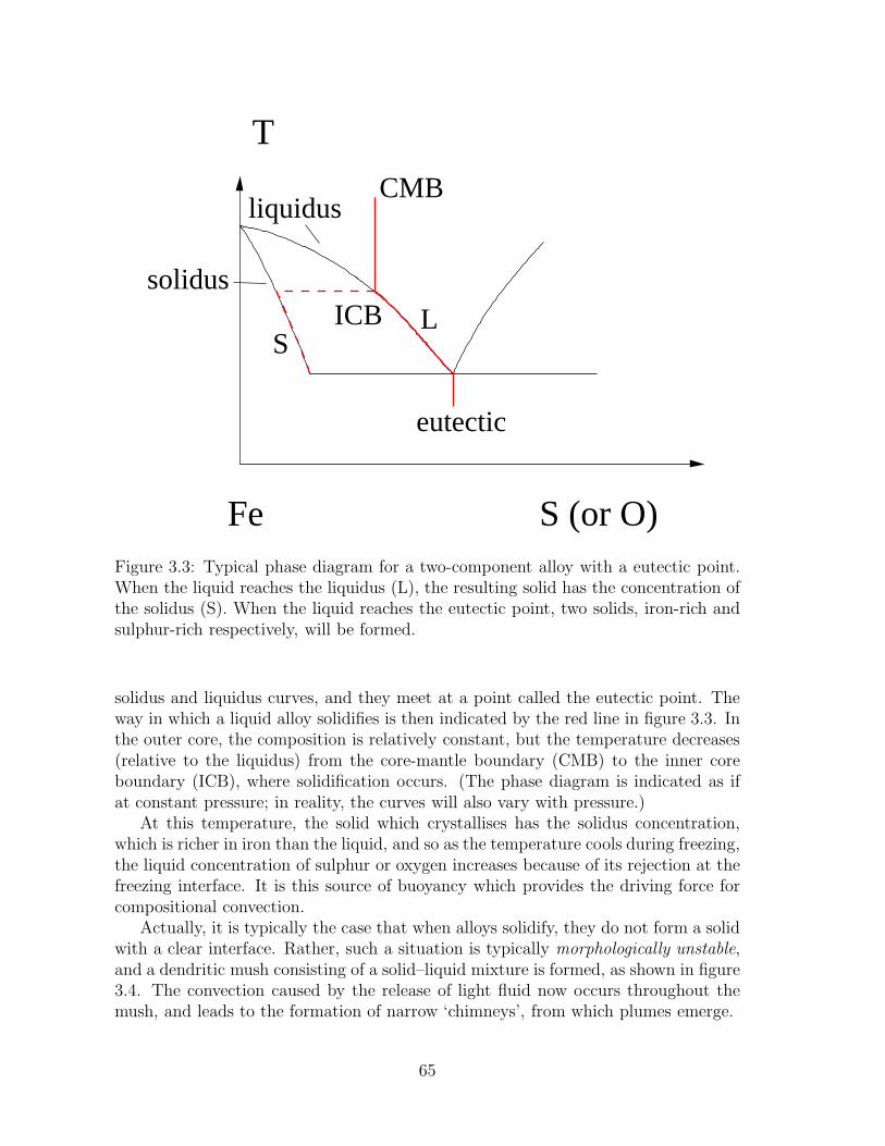
T

Fe S (or O)

liquidus

solidus

CMB

eutectic

SICB L

Figure 3.3: Typical phase diagram for a two-component alloy with a eutectic point.When the liquid reaches the liquidus (L), the resulting solid has the concentration ofthe solidus (S). When the liquid reaches the eutectic point, two solids, iron-rich andsulphur-rich respectively, will be formed.

solidus and liquidus curves, and they meet at a point called the eutectic point. Theway in which a liquid alloy solidifies is then indicated by the red line in figure 3.3. Inthe outer core, the composition is relatively constant, but the temperature decreases(relative to the liquidus) from the core-mantle boundary (CMB) to the inner coreboundary (ICB), where solidification occurs. (The phase diagram is indicated as ifat constant pressure; in reality, the curves will also vary with pressure.)

At this temperature, the solid which crystallises has the solidus concentration,which is richer in iron than the liquid, and so as the temperature cools during freezing,the liquid concentration of sulphur or oxygen increases because of its rejection at thefreezing interface. It is this source of buoyancy which provides the driving force forcompositional convection.

Actually, it is typically the case that when alloys solidify, they do not form a solidwith a clear interface. Rather, such a situation is typically morphologically unstable,and a dendritic mush consisting of a solid–liquid mixture is formed, as shown in figure3.4. The convection caused by the release of light fluid now occurs throughout themush, and leads to the formation of narrow ‘chimneys’, from which plumes emerge.

65

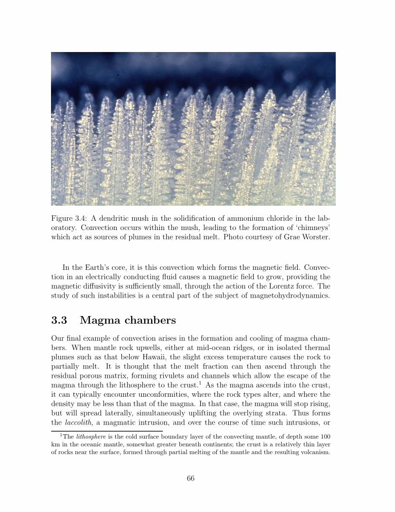
Figure 3.4: A dendritic mush in the solidification of ammonium chloride in the lab-oratory. Convection occurs within the mush, leading to the formation of ‘chimneys’which act as sources of plumes in the residual melt. Photo courtesy of Grae Worster.

In the Earth’s core, it is this convection which forms the magnetic field. Convec-tion in an electrically conducting fluid causes a magnetic field to grow, providing themagnetic diffusivity is sufficiently small, through the action of the Lorentz force. Thestudy of such instabilities is a central part of the subject of magnetohydrodynamics.

3.3 Magma chambers

Our final example of convection arises in the formation and cooling of magma cham-bers. When mantle rock upwells, either at mid-ocean ridges, or in isolated thermalplumes such as that below Hawaii, the slight excess temperature causes the rock topartially melt. It is thought that the melt fraction can then ascend through theresidual porous matrix, forming rivulets and channels which allow the escape of themagma through the lithosphere to the crust.1 As the magma ascends into the crust,it can typically encounter unconformities, where the rock types alter, and where thedensity may be less than that of the magma. In that case, the magma will stop rising,but will spread laterally, simultaneously uplifting the overlying strata. Thus formsthe laccolith, a magmatic intrusion, and over the course of time such intrusions, or

1The lithosphere is the cold surface boundary layer of the convecting mantle, of depth some 100km in the oceanic mantle, somewhat greater beneath continents; the crust is a relatively thin layerof rocks near the surface, formed through partial melting of the mantle and the resulting volcanism.

66

Figure 3.5: Graded layering in the Skaergaard intrusion. Photograph courtesy ofKurt Hollocher.

magma chambers, will solidify, forming huge cauldrons of rock which may later beexposed at the Earth’s surface.

Convection undoubtedly occurs in such chambers, which may be tens of kilome-tres in extent. The hot magma is continuously chilled at the roof and sides of thechamber, and this leads to convective currents continually draining towards the floorof the chamber. There they will accumulate, leading to a cold, crystal-rich layer ly-ing stagnant below the convecting upper portion. This is essentially the filling boxmechanism which is discussed further below.

Magmas are multi-component alloys, and their convective solidification can lead tovarious exotic phenomena. The phase diagram of the type in figure 3.3 causes chemicaldifferentiation on the large scale (in metal alloy castings this is called macrosegrega-tion). For example, in an olivine–plagioclase magma, the heavy olivine will crystalliseout first, and the crystals may settle to the base of the chamber. The residual liquidis then plagioclase-rich and lighter. So the end result would be a chamber having twodistinct layers. Successive injections of magma may then lead to a sequence of suchlayers, as is seen in the Scottish island of Rum, and this has been suggested as anexplanation for these particular layers.

Other magma chambers show layering at a much finer scale, and the origin of theselayers is a mystery. An example is shown in figure 3.5. The layers are reminiscentof double-diffusive layering, which we discuss in section 3.11, but efforts to build atheory round this idea, or indeed any other, have so far not met with success.

67

wx = 0

Tx = 0

u = 0wx = 0

u = 0

Tx = 0

z = d

x = a

z = 0x = 0

p = 0, T = T0, w = 0, uz = 0

T = T0 + ∆T , w = 0, uz = 0

Figure 3.6: Geometry of a convection cell.

3.4 Rayleigh–Benard convection

The simplest model of convection is the classical Rayleigh-Benard model in whicha layer of fluid is heated from below, by application of a prescribed temperaturedifference across the layer. Depending on the nature of the boundaries, one may havea no slip condition or a no shear stress condition applied at the bounding surfaces.For the case of mantle convection, one conceives of both the oceans (or atmosphere)and the underlying fluid outer core as exerting no stress on the extremely viscousmantle, so that no stress conditions are appropriate, and in fact it turns out that thisis the simplest case to consider. The geometry of the flow we consider is shown infigure 3.6. It is convenient to assume lateral boundaries, although in a wide layer,these simply represent the convection cell walls, and can be an arbitrary distanceapart.

The equations describing the flow are the Navier-Stokes equations, allied with theenergy equation and an equation of state, and can be written in the form

ρt +∇. (ρu) = 0,

ρ[ut + (u .∇)u] = −∇p− ρgk+ µ∇2u,

ρcp[Tt + u .∇T ] = k∇2T,

ρ = ρ0[1− α(T − T0)]; (3.1)

in these equations, ρ is the density, u is the velocity, p is the pressure, g is the acceler-ation due to gravity, k is the unit upwards vector, µ is viscosity, cp is the specific heat,T is temperature, k is thermal conductivity, ρ0 is the density at the reference temper-ature T0 at the surface of the fluid layer, and α is the thermal expansion coefficient.The boundary conditions for the flow are indicated in figure 3.6, and correspond to

68

prescribed temperature at top and bottom, no flow through the boundaries, and noshear stress at the boundaries. The lateral boundaries represent stress free ‘walls’,but as mentioned above, these simply indicate the boundaries of the convection cells(across which there is no heat transport, hence the no flux condition for temperature).

To proceed, we non-dimensionalise the variables as follows. We use the convectivetime scale, and a thermally related velocity scale, and use the depth of the box d asthe length scale:

u ∼ κ

d, κ =

k

ρ0cp, t ∼ d2

κ, x ∼ d,

p− [p0 + ρ0g(d− z)] ∼ µκ

d2, T − T0 ∼ ∆T. (3.2)

Here p0 is the (prescribed) pressure at the surface, which we take as constant. Wewould also scale ρ ∼ ρ0, but in the scaled equations below, the density has beenalgebraically eliminated. The scaled equations take the form

−BTt +∇. [(1− BT )u] = 0,1

Pr[1− BT ][ut + (u .∇)u] = −∇p+RaTk+∇2u,

(1− BT )(Tt + u .∇T ) = ∇2T, (3.3)

and the dimensionless parameters are defined as

B = α∆T, Pr =µ

ρ0κ, Ra =

αρ0∆Tgd3

µκ; (3.4)

the parameters Ra and Pr are known as the Rayleigh and Prandtl numbers, respec-tively. The Prandtl number is a property of the fluid; for air it is 0.7, and for waterit is 7. The Rayleigh number is a measure of the strength of the heating. As weshall see, convective motion occurs if the Rayleigh number is large enough, and itbecomes vigorous if the Rayleigh number is large. The parameter B might be termeda Boussinesq number, although this is not common usage.

Suppose we think of values typical for a layer of water in a saucepan. We taked = 0.1 m, µ = 2 × 10−3 Pa s, ∆T = 100 K, α = 3 × 10−5 K−1, ρ0 = 103 kg m−3,κ = 0.3 × 10−6 m2 s−1, g = 9.8 m s−2. Then we have Pr ≈ 7, B ≈ 3 × 10−3, andRa ≈ 5×107. In this case, we have that B ≪ 1 and Ra≫ 1. This is typically the case.We now make the Boussinesq approximation, which says that B ≪ 1, and we ignorethe terms in B in (3.3). In words, we assume that the density is constant, exceptin the buoyancy term. The mathematical reason for this exception is that, althoughRa ∝ B (and so Ra→ 0 as B → 0), the actual numerical sizes of the two parametersare typically very different. The adoption of the Boussinesq approximation leads towhat are called the Boussinesq equations of thermal convection:

∇.u = 0,1

Pr[ut + (u .∇)u] = −∇p+∇2u+RaT k,

Tt + u.∇T = ∇2T, (3.5)

69

with associated boundary conditions for free slip:

T = 1, u.n = τnt = 0 on z = 0,

T = 0, u.n = τnt = 0 on z = 1, (3.6)

where τnt represents the shear stress.

3.4.1 Linear stability

It is convenient to study the problem of the onset of convection in two dimensions(x, z). In this case we can define a stream function ψ which satisfies

u = −ψz , w = ψx. (3.7)

(The sign is opposite to the usual convention; for ψ > 0 this describes a clockwisecirculation.) We eliminate the pressure by taking the curl of the momentum equation(3.5)2, which leads, after some algebra (see also question 3.2), to the pair of equationsfor ψ and T :

1

Pr

[∇2ψt + ψx∇2ψz − ψz∇2ψx

]= RaTx +∇4ψ,

Tt + ψxTz − ψzTx = ∇2T, (3.8)

with the associated boundary conditions

ψ = ∇2ψ = 0 at z = 0, 1,

T = 0 at z = 1,

T = 1 at z = 0. (3.9)

In the absence of motion, u = 0, the steady state temperature profile is linear,

T = 1− z, (3.10)

and the lithostatic pressure is modified by the addition of

p = −Ra2(1− z)2. (3.11)

(Even if Ra is large, this represents a small correction to the lithostatic pressure, ofrelative O(B).) The stream function is just

ψ = 0. (3.12)

We define the temperature perturbation θ by

T = 1− z + θ. (3.13)

70

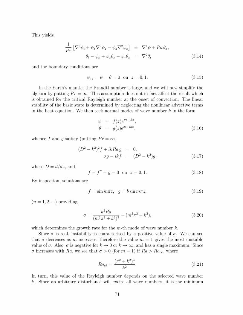
This yields

1

Pr

[∇2ψt + ψx∇2ψz − ψz∇2ψx

]= ∇4ψ +Ra θx,

θt − ψx + ψxθz − ψzθx = ∇2θ, (3.14)

and the boundary conditions are

ψzz = ψ = θ = 0 on z = 0, 1. (3.15)

In the Earth’s mantle, the Prandtl number is large, and we will now simplify thealgebra by putting Pr = ∞. This assumption does not in fact affect the result whichis obtained for the critical Rayleigh number at the onset of convection. The linearstability of the basic state is determined by neglecting the nonlinear advective termsin the heat equation. We then seek normal modes of wave number k in the form

ψ = f(z)eσt+ikx,

θ = g(z)eσt+ikx, (3.16)

whence f and g satisfy (putting Pr = ∞)

(D2 − k2)2f + ikRa g = 0,

σg − ikf = (D2 − k2)g, (3.17)

where D = d/dz, andf = f ′′ = g = 0 on z = 0, 1. (3.18)

By inspection, solutions are

f = sinmπz, g = b sinmπz, (3.19)

(n = 1, 2, ...) providing

σ =k2Ra

(m2π2 + k2)2− (m2π2 + k2), (3.20)

which determines the growth rate for the m-th mode of wave number k.Since σ is real, instability is characterised by a positive value of σ. We can see

that σ decreases as m increases; therefore the value m = 1 gives the most unstablevalue of σ. Also, σ is negative for k → 0 or k → ∞, and has a single maximum. Sinceσ increases with Ra, we see that σ > 0 (for m = 1) if Ra > Rack, where

Rack =(π2 + k2)3

k2. (3.21)

In turn, this value of the Rayleigh number depends on the selected wave numberk. Since an arbitrary disturbance will excite all wave numbers, it is the minimum

71

value of Rack which determines the absolute threshold for stability. The minimum isobtained when

k =π√2, (3.22)

and the resulting critical value of the Rayleigh number is

Rac =27π4

4≈ 657.5; (3.23)

That is, the steady state is linearly unstable if Ra > Rac.For other boundary conditions, the solutions are still exponentials, but the coef-

ficients, and hence also the growth rate, must be found numerically. The resultantcritical value of the Rayleigh number is higher for no slip boundary conditions, forexample, (it is about 1707), and in general, thermal convection is initiated at valuesof Ra >∼ O(103).

3.5 Double-diffusive convection

Double-diffusive convection refers to the motion which is generated by buoyancy, whenthe density depends on two diffusible substances or quantities. The simplest examplesoccur when salt solutions are heated; then the two diffusing quantities are heat andsalt. Double-diffusive processes occur in sea water and in lakes, for example. Othersimple examples occur in multi-component fluids containing more than one dissolvedspecies; convection in magma chambers is one such.

The guiding principle behind double-diffusive convection is still that light fluidrises, and convection occurs in the normal way (the direct mode) when the steady stateis statically unstable (i. e., when the density increases with height), but confoundingfactors arise when, as normally the case, the two substances diffuse at different rates.Particularly when we are concerned with temperature and salt, the ratio of thermalto solutal diffusivity is large, and in this case different modes of convection occurnear the statically neutral buoyancy state: the cells can take the form of long thin‘fingers’, or the onset of convection can be oscillatory. In practice, fingers are seen,but oscillations are not.

A further variant on Rayleigh-Benard convection arises in the form of convec-tive layering. This is a long-lived transient form of convection, in which separatelyconvecting layers form, and is associated partly with the high diffusivity ratio, andpartly with the usual occurrence of no flux boundary conditions for diffusing chemicalspecies.

We pose a model for double-diffusive convection based on a density which is relatedlinearly to temperature T and salt composition c in the form

ρ = ρ0[1− α(T − T0) + βc], (3.24)

where we take α and β to be positive constants; thus the presence of salt makes thefluid heavier. The equation that then needs to be added to (3.1) is that for convective

72

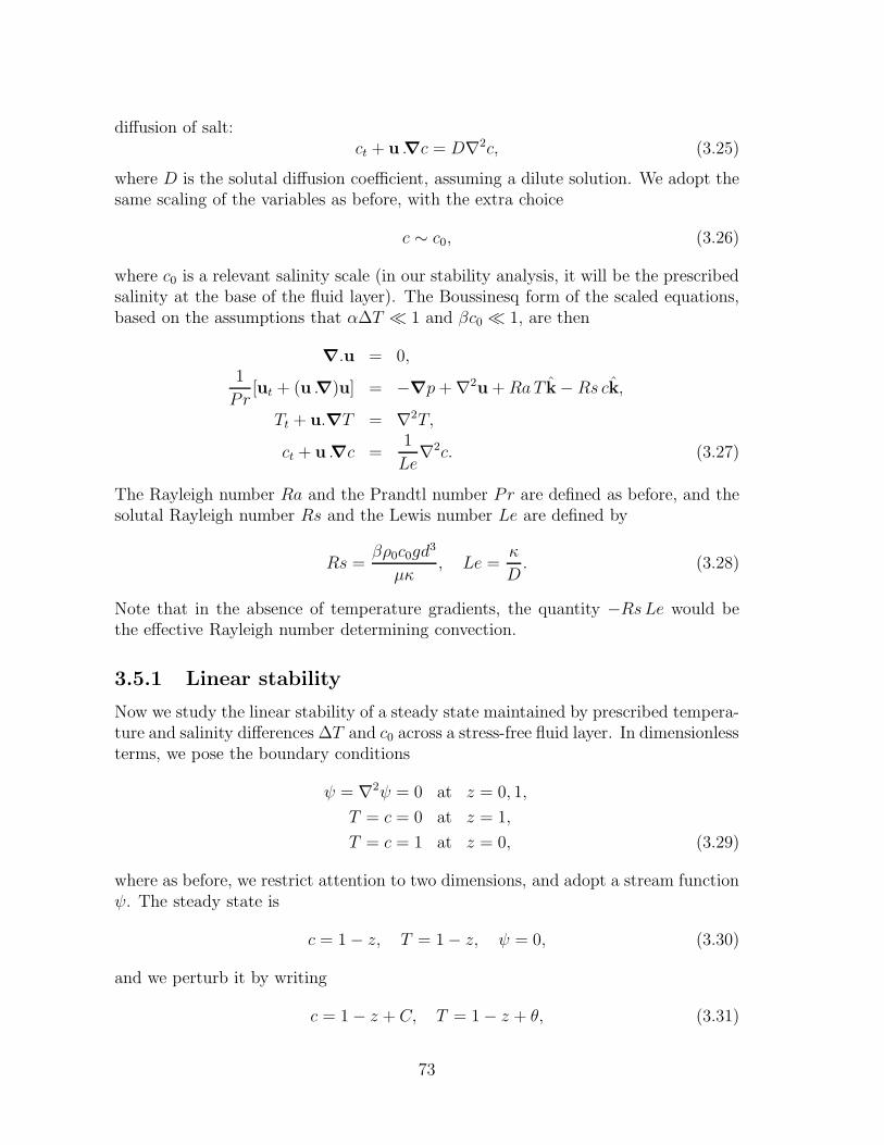
diffusion of salt:ct + u .∇c = D∇2c, (3.25)

where D is the solutal diffusion coefficient, assuming a dilute solution. We adopt thesame scaling of the variables as before, with the extra choice

c ∼ c0, (3.26)

where c0 is a relevant salinity scale (in our stability analysis, it will be the prescribedsalinity at the base of the fluid layer). The Boussinesq form of the scaled equations,based on the assumptions that α∆T ≪ 1 and βc0 ≪ 1, are then

∇.u = 0,1

Pr[ut + (u .∇)u] = −∇p+∇2u+RaT k− Rs ck,

Tt + u.∇T = ∇2T,

ct + u .∇c =1

Le∇2c. (3.27)

The Rayleigh number Ra and the Prandtl number Pr are defined as before, and thesolutal Rayleigh number Rs and the Lewis number Le are defined by

Rs =βρ0c0gd

3

µκ, Le =

κ

D. (3.28)

Note that in the absence of temperature gradients, the quantity −RsLe would bethe effective Rayleigh number determining convection.

3.5.1 Linear stability

Now we study the linear stability of a steady state maintained by prescribed tempera-ture and salinity differences ∆T and c0 across a stress-free fluid layer. In dimensionlessterms, we pose the boundary conditions

ψ = ∇2ψ = 0 at z = 0, 1,

T = c = 0 at z = 1,

T = c = 1 at z = 0, (3.29)

where as before, we restrict attention to two dimensions, and adopt a stream functionψ. The steady state is

c = 1− z, T = 1− z, ψ = 0, (3.30)

and we perturb it by writing

c = 1− z + C, T = 1− z + θ, (3.31)

73

and then linearising the equations on the basis that C, θ, ψ ≪ 1. This leads to

1

Pr∇2ψt ≈ Ra θx − RsCx +∇4ψ,

θt − ψx ≈ ∇2θ,

Ct − ψx ≈ 1

Le∇2C, (3.32)

withC = ψ = ψzz = θ = 0 on z = 0, 1. (3.33)

By inspection, solutions satisfying the temperature and salinity equations are

ψ = exp(ikx+ σt) sinmπz,

θ =ik

σ +K2exp(ikx+ σt) sinmπz,

C =ik

σ +K2

Le

exp(ikx+ σt) sinmπz, (3.34)

where we have writtenK2 = k2 +m2π2. (3.35)

Substituting these into the momentum equation leads to the dispersion relation de-termining σ in terms of k:

(σ +K2Pr)(σ +K2)

(σ +

K2

Le

)+ k2Pr

[(Rs− Ra)σ

K2+Rs− Ra

Le

]= 0. (3.36)

This is a cubic in σ, which can be written in the form

σ3 + aσ2 + bσ + c = 0, (3.37)

where

a = K2

(Pr + 1 +

1

Le

),

b = K4

(Pr +

1

Le+Pr

Le

)+k2

K2Pr(Rs− Ra),

c =K6

LePr + k2Pr

(Rs− Ra

Le

). (3.38)

Instability occurs if any one of the three roots of (3.37) has positive real part.Since Le and Pr are properties of the fluid, we take them as fixed, and study theeffect of varying Ra and Rs on the stability boundaries where Reσ = 0. Firstly, ifRa < 0 and Rs > 0, then a, b and c are all positive. We can then show (see question3.3) that Reσ < 0 for all three roots providing ab > c, and this is certainly the case if

74

Ra

Rs

U

Z

W

V

os illations

ngers

stati ally stable

X

Figure 3.7: Stability diagram for double-diffusive convection.

Le > 1, which is always true for heat and salt diffusion. Thus when both temperatureand salinity fields are stabilising, the state of no motion is linearly stable.

To find regions of instability in the (Rs,Ra) plane, it thus suffices to locate thecurves where Reσ = 0. There are two possibilities. The first is referred to as exchangeof stability, or the direct mode, and occurs when σ = 0. From (3.37), this is when

c = 0, or Rs =Ra

Le− K6

k2Le. This is a single curve (for each k), and since we know that

Reσ < 0 in Ra < 0 and Rs > 0, this immediately tells us that a direct instabilityoccurs if

Ra− LeRs > Rc = mink

K6

k2=

27π4

4. (3.39)

This direct transition is the counterpart of the onset of Rayleigh-Benard convection,and shows that Ra− LeRs is the effective Rayleigh number. This is consistent withthe remark just after (3.28).

The other possibility is that there is a Hopf bifurcation, i. e., a pair of complexconjugate values of σ cross the imaginary axis at ±iΩ, say. The condition for thisis ab = c, which is again a single curve, and one can show (see question 3.4) thatoscillatory instability occurs for

Ra >

(Pr +

1

Le

)Rs

1 + Pr+

(1 +

1

Le

)(Pr +

1

Le

)

PrRc. (3.40)

Direct instability occurs along the line XZ in figure 3.7, while oscillatory insta-bility occurs at the line XW . Between XW and the continuation XU of XZ, there

75

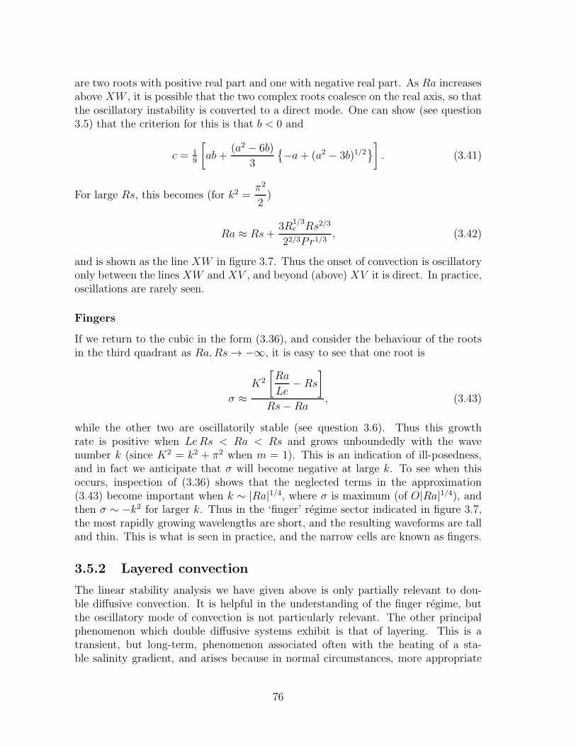
are two roots with positive real part and one with negative real part. As Ra increasesabove XW , it is possible that the two complex roots coalesce on the real axis, so thatthe oscillatory instability is converted to a direct mode. One can show (see question3.5) that the criterion for this is that b < 0 and

c = 19

[ab+

(a2 − 6b)

3

−a + (a2 − 3b)1/2

]. (3.41)

For large Rs, this becomes (for k2 =π2

2)

Ra ≈ Rs+3R

1/3c Rs2/3

22/3Pr1/3, (3.42)

and is shown as the line XW in figure 3.7. Thus the onset of convection is oscillatoryonly between the lines XW and XV , and beyond (above) XV it is direct. In practice,oscillations are rarely seen.

Fingers

If we return to the cubic in the form (3.36), and consider the behaviour of the rootsin the third quadrant as Ra,Rs→ −∞, it is easy to see that one root is

σ ≈K2

[Ra

Le− Rs

]

Rs− Ra, (3.43)

while the other two are oscillatorily stable (see question 3.6). Thus this growthrate is positive when LeRs < Ra < Rs and grows unboundedly with the wavenumber k (since K2 = k2 + π2 when m = 1). This is an indication of ill-posedness,and in fact we anticipate that σ will become negative at large k. To see when thisoccurs, inspection of (3.36) shows that the neglected terms in the approximation(3.43) become important when k ∼ |Ra|1/4, where σ is maximum (of O|Ra|1/4), andthen σ ∼ −k2 for larger k. Thus in the ‘finger’ regime sector indicated in figure 3.7,the most rapidly growing wavelengths are short, and the resulting waveforms are talland thin. This is what is seen in practice, and the narrow cells are known as fingers.

3.5.2 Layered convection

The linear stability analysis we have given above is only partially relevant to dou-ble diffusive convection. It is helpful in the understanding of the finger regime, butthe oscillatory mode of convection is not particularly relevant. The other principalphenomenon which double diffusive systems exhibit is that of layering. This is atransient, but long-term, phenomenon associated often with the heating of a sta-ble salinity gradient, and arises because in normal circumstances, more appropriate

76

boundary conditions for salt concentration are to suppose that there is no flux at thebounding surfaces.

In pure thermal convection, the heating of an initially stably thermally stratifiedfluid will lead to the formation of a layer of convecting fluid below the stable region.This (single) convecting layer will grow in thickness until it fills the entire layer. Thisis essentially the ‘filling box’ which is described in section 3.10. Suppose now we havea stable salinity gradient which is heated from below. Again a convecting layer forms,which mixes the temperature and concentration fields to be uniform within the layer.At the top of the convecting layer, there will be a step down ∆T in temperature, anda step down ∆c in salinity. It is found experimentally that α∆T = β∆c, that is, theboundary layer2 is neutrally stable. However, the disparity in diffusivities (typicallyLe≫ 1) means that there is a thicker thermal conductive layer ahead of the interface.In effect, the stable salinity gradient above the convecting layer is heated by the layeritself, and a second, and then a third, layer forms. In this way, the entire fluid depthcan fill up with a sequence of long-lived, separately convecting layers. The layers willeventually merge and form a single convecting layer over a time scale controlled bythe very slow transport of salinity between the convecting layers. Such layers are verysuggestive of some of the fossilised layering seen in magma chambers, as for examplein figure 3.5, but the association may be a dangerous one.

3.6 High Rayleigh number convection

We have seen that convection occurs if the Rayleigh number is larger than O(103) ingeneral, depending on the precise boundary conditions which apply. In the Earth’smantle, suitable values of the constituent parameters are α = 3 × 10−5 K−1, ∆T =3000 K, ρ0 = 3× 103 kg m−3, g = 10 m s−2, d = 3000 km, η0 = 1021 Pa s, κ0 = 10−6

m2 s−1, and for these values, the Rayleigh number is slightly less than 108. Thus theRayleigh number is much larger than the critical value, and as a consequence we canexpect the convection to be vigorous (if velocities of centimetres per year can be saidto be vigorous).

There are various intuitive ways in which we can get a sense of the likely behaviourof the convective solutions of the Boussinesq equations when Ra≫ 1. Since Ra mul-tiplies the buoyancy term, any O(1) lateral temperature gradient will cause enormousvelocities. One might thus expect the flow to organise itself so that either horizontaltemperature gradients are small, or they are confined to thin regions, or both. SinceO(1) temperature variations are enforced by the boundary conditions, the latter ismore plausible, and thus we have the idea of the thermal plume, a localised upwellingof hot fluid which will be instantly familiar to glider pilots and seabirds.

A mathematically intuitive way of inferring the same behaviour follows from theexpectation that increasing Ra drives increasing velocities; then large Ra shouldimply large velocity, and the conduction term in the heat equation u.∇T = ∇2T iscorrespondingly small. Since the conduction term represents the highest derivative

2For discussion of boundary layers, see section 3.6.1.

77

hot

cold

Figure 3.8: Schematic representation of boundary layer convection

in the equation, its neglect would imply a reduction of order, and correspondingly wewould expect thermal boundary layers to exist at the boundaries of the convectingcell. This is in fact what we will find: a hot thermal boundary layer adjoins the lowerboundary, and a cold one adjoins the upper boundary, and a rapid circulation in theinterior of the cell detaches these as upwelling and downwelling plumes. The generalstructure of the resulting flow is shown in figure 3.8. We analyse this structure in thefollowing sections.

3.6.1 Boundary layer theory

The Boussinesq equations describing thermal convection are written in the followingdimensionless form:

∇.u = 0,

1

Pr

du

dt= −∇p+∇2u+RaT j,

dT

dt= ∇2T, (3.44)

where u is velocity, p is pressure, T is temperature, and the Rayleigh and Prandtlnumbers are defined in (3.4).

By considering only two-dimensional motion in the (x, z) plane, we define thestream function ψ by

u = −ψz , v = ψx; (3.45)

the vorticity is then (0, ω, 0), where ω = −∇2ψ. Taking the curl of the momentumequation, we derive the set

78

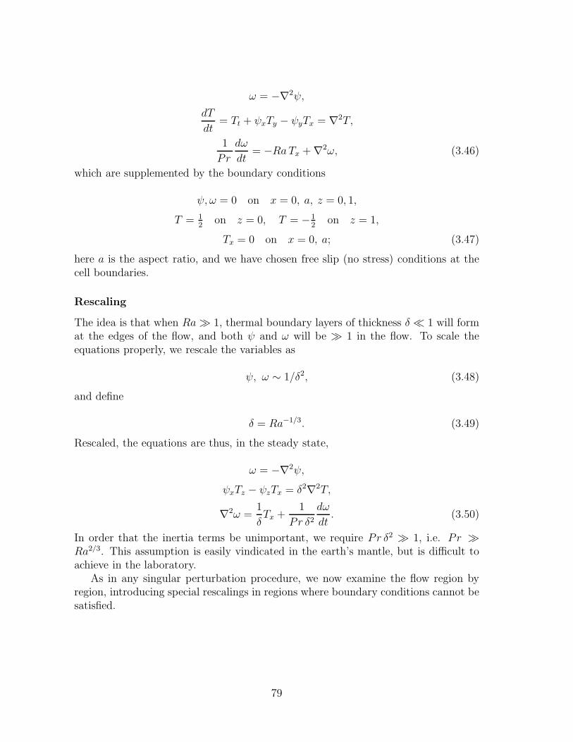
ω = −∇2ψ,

dT

dt= Tt + ψxTy − ψyTx = ∇2T,

1

Pr

dω

dt= −RaTx +∇2ω, (3.46)

which are supplemented by the boundary conditions

ψ, ω = 0 on x = 0, a, z = 0, 1,

T = 12

on z = 0, T = −12

on z = 1,

Tx = 0 on x = 0, a; (3.47)

here a is the aspect ratio, and we have chosen free slip (no stress) conditions at thecell boundaries.

Rescaling

The idea is that when Ra≫ 1, thermal boundary layers of thickness δ ≪ 1 will format the edges of the flow, and both ψ and ω will be ≫ 1 in the flow. To scale theequations properly, we rescale the variables as

ψ, ω ∼ 1/δ2, (3.48)

and define

δ = Ra−1/3. (3.49)

Rescaled, the equations are thus, in the steady state,

ω = −∇2ψ,

ψxTz − ψzTx = δ2∇2T,

∇2ω =1

δTx +

1

Pr δ2dω

dt. (3.50)

In order that the inertia terms be unimportant, we require Pr δ2 ≫ 1, i.e. Pr ≫Ra2/3. This assumption is easily vindicated in the earth’s mantle, but is difficult toachieve in the laboratory.

As in any singular perturbation procedure, we now examine the flow region byregion, introducing special rescalings in regions where boundary conditions cannot besatisfied.

79

Core flow

The temperature equation is linear in T , and implies T = T0(ψ) + O(δ2). For a flowwith closed streamlines, the Prandtl-Batchelor theorem then implies T0 = constant

(this follows from the exact integral

∮

C

∂T

∂nds = 0, where the integral is around a

streamline, whence T ′0(ψ)

∮

C

∂ψ

∂nds = 0); it then follows that T is constant to all

(algebraic) orders of δ, and is in fact zero by the symmetry of the flow. Thus

T = 0,

∇4ψ = 0, (3.51)

and clearly the core flow cannot have ψ = ω = 0 at the boundaries, for non-zero ψ.In fact, ω jumps at the side-walls where the plume buoyancy generates a non-zerovorticity. We examine the plumes next.

Plumes

Near x = 0, for example, we rescale the variables as

x ∼ δ, ψ ∼ δ, (3.52)

and denote rescaled variables by capital letters. At leading order, we then have

ΨXX ∼ 0, (3.53)

whence Ψ ∼ vp(y)X , and to match to the core flow, we define vp = ψx |x=0 as thecore velocity at x = 0. Also

ΨXTy −ΨyTX ∼ TXX ,

ωXX ∼ TX , (3.54)

the latter of which integrates to give

ω =

∫ X

0

T dX, ωp =

∫ ∞

0

T dX, (3.55)

where matching requires ωp to be the core vorticity at x = 0. Integration of (3.54)1gives

∫ ∞

0

T dΨ = C, (3.56)

where C is constant, and it follows that the core flow must satisfy the boundarycondition ωψx = C on x = 0. In summary, the effective boundary conditions for thecore flow are

80

ψ = 0 on x = 0, a; z = 0, 1;

ψzz = 0 on z = 0, 1; (3.57)

ψxψxx = −C on x = 0, ψxψxx = C on x = a,

and the solution can be found as ψ = C1/2ψ, where ψ is determined numerically. Itthus remains to determine C. This requires consideration of the thermal boundarylayers.

Thermal boundary layers

Near the base, for example, we rescale the variables

z ∼ δ, ψ ∼ δ, ω ∼ δ, (3.58)

to find the leading order rescaled equations as

ΨZZ ∼ 0, (3.59)

whence Ψ ∼ ub(x)Z, and −ub is the core value of the basal velocity. Then ΩZZ ∼ Txdetermines Ω (with Ω = 0 on Z = 0, and Ω ∼ ωb(x)Z as Z → ∞, where ωb is thecore value of the basal vorticity), and T satisfies

ΨxTZ −ΨZTX ∼ TZZ . (3.60)

In Von Mises coordinates x,Ψ, the equation is

−Tx ∼∂

∂Ψ

[ΨZ

∂T

∂Ψ

], (3.61)

and putting ξ =

∫ a

x

ub(x)dx (so ξ marches from right to left in the direction of flow),

this is just the diffusion equation

Tξ = TΨΨ, (3.62)

with

T = 12

on Ψ = 0, T → 0 as Ψ → ∞. (3.63)

A quantity of interest is the Nusselt number, defined as

Nu = −∫ 1

0

∂T

∂z(x, 0)dx, (3.64)

and from the above, this can be written as

Nu ∼[∫ ∞

0

T |z=0 dΨ

]x=0

x=a

R1/3. (3.65)

81

Notice that the plume temperature equation can also be written as (3.62), where ξ is

extended as

∫ z

vp(z) dz, etc.

Corner flow

The core flow has a singularity in each corner, where (if r is distance from the corner),then ψ ∼ r3/2, ω ∼ r−1/2, and (for the corner at x = 0, z = 0, for example) x, z ∼ r.There must be a region where this singularity is alleviated by the incorporation of thebuoyancy term. This requires ω/r2 ∼ 1/δr, whence r ∼ δ2/3. Rescaling the variablesas indicated (x, z ∼ δ2/3, ψ ∼ δ, ω ∼ δ−1/3) then gives the temperature equation as

ΨXTZ −ΨZTX ∼ δ∇2T, (3.66)

which shows that (since the ψ scale, δ, is the same as that of the boundary layersadjoining the corner) the boundary layer temperature field is carried through thecorner region. The corner flow has T ∼ T (Ψ), so that

∇4Ψ+ T ′(Ψ)ΨX = 0, (3.67)

with appropriate matching conditions.

Solution strategy

The temperature equation (3.62) must now be solved in the four regions correspondingto the boundary layer at z = 0, plume at x = 0, boundary layer at z = 1, plume atx = a, with T being continuous at each corner, and

T → 0 as Ψ → ∞,

T = 12

on Ψ = 0 [z = 0, base],

∂T

∂Ψ= 0 on Ψ = 0 [x = 0, left],

T = −12

on Ψ = 0 [z = 1, top],

∂T

∂Ψ= 0 on Ψ = 0 [x = a, right];

(3.68)

in addition, T is periodic in ξ. Beginning from x = a, z = 0, denote the values of ξat the corners as ξA (x = 0, z = 0), ξB (x = 0, z = 1), ξC (x = a, z = 1). From thedefinition of ξ, we have ξk = C1/2ξk, where ξk are independent of C. Putting

ξ = C1/2ξ, Ψ = C1/4Ψ, (3.69)

then the problem for T (ξ, Ψ) is independent of C. If we can solve this numerically,then

∫T dΨ = C1/4

∫T dΨ, thus

82

Nu ∼ C1/4

[∫ ∞

0

T dΨ

]ξA

0

R1/3, (3.70)

and lastly, C is determined from

C =

[∫ ∞

0

T dΨ

]4/3, (3.71)

where the integral is evaluated at ξA. Since also −C3/4 =

∫ ∞

0

T dΨ at ξ = 0, (3.70)

can be written as

Nu ∼ 2CRa1/3. (3.72)

No-slip boundary conditions

For no slip boundary conditions, the necessary preliminary rescaling is ψ ∼ 1/δ3,ω ∼ 1/δ3, where δ = Ra−1/5. Thus the Nusselt number Nu ∼ Ra1/5. There is nolonger parity between the thermal boundary layers and plumes, as the former areslowed down by the no slip conditions. The rescaled equations are

ω = −∇2ψ,

ψxTz − ψzTx = δ3∇2T,

∇2ω =1

δ2Tx. (3.73)

The core flow is as before; the thermal boundary layers have ψ ∼ δ2, ω ∼ 1, z ∼ δ, sothat vorticity balances buoyancy (an omission in Roberts’ 1979 paper, precluding hissimilarity solution), and all three equations are necessary to solve for T ; it is still thecase that

∫T dψ is conserved at corners, but now in the plume, x ∼ δ3/2, ψ ∼ δ3/2,

and T ∼ δ1/2. The initial plume profile is effectively a delta function, and the plumetemperature is just the resultant similarity solution. The remainder of the structuremust be computed numerically, something which has not been done.

3.7 Parameterised convection

The boundary layer theory described in section ?? applies to steady state solutionsat high Rayleigh number, but in fact real convection becomes time-varying at suchparameter values. The behaviour becomes first oscillatory, and then becomes in-creasingly irregular, so that at very high Rayleigh numbers, the cellular structure ofconvection in a fluid layer breaks down. The upwelling and downwelling plumes ofthe boundary layer theory still exist, but their detachment is sporadic and irregular.In these circumstances, the theoretical description of convection become, paradoxi-cally, easier. Just as for turbulent shear flows at high Reynolds numbers, one uses

83

Figure 3.9: On the left, a sub-oceanic black smoker issuing from a ventat the ocean floor; on the right, an industrial chimney. Images fromhttp://oceanexplorer.noaa.gov.

empirically-based measures of the fluxes at boundaries to describe the flow. Tur-bulence mixes the fluid, so that, as in the boundary layer theory, the interior of aconvecting cell is taken to be isothermal. In this section, we describe two particularexamples of turbulent convection to illustrate these ideas. The first is that of the tur-bulent convective plume, and the second is a classic example of the use of turbulentconvective theory in the decription of the ‘filling box’.

3.8 Plumes

A plume is an isolated convective upwelling. Examples are the rise of smoke from anindustrial chimney, the formation of cumulus clouds over oceans, ‘black smokers’ atmid-ocean rise vents, and explosive volcanic eruptions. In these examples, a sourceof buoyancy at (essentially) a point drives a convective flow in the fluid above. Assuggested in figure 3.9, the plume forms a turbulent, approximately conical region,with a fairly sharp (but time-varying) boundary. The turbulence causes rapid con-vective mixing, and allows us to conceptualise the plume as a relatively homogeneouscloud of density ρ = ρ0 −∆ρ rising through an ambient medium of density ρ0. If ρ0depends on height z, then the medium is called a stratified medium, and it is stablystratified if ρ′0(z) < 0.

84

Suppose that a cylindrical plume of radius r = b(z) rises at speed w through amedium of density ρ0. We take the density deficit in the plume to be ∆ρ, and definethe reduced gravity to be

g′ =g∆ρ

ρ0. (3.74)

The (constant) buoyancy flux is then defined to be

B = 2π

∫ b

0

rwg′ dr. (3.75)

The boundary of the plume is taken to be such that g′ = w = 0 at r = b.

Self-similarity

If we take ρ0 to be constant, and suppose that the dynamics of the plume dependonly on the reduced gravity and on position, or equivalently on the buoyancy fluxand position, then purely dimensional reasoning leads to the conclusion that we musthave

w = c1

(rb

)B1/3z−1/3,

g′ = c2

(rb

)B2/3z−5/3,

b = βz. (3.76)

The functions c1 and c2 are found experimentally to be well fitted by Gaussians.Note that the volume flux

Q = 2π

∫ b

0

rw dr (3.77)

is then given byQ ∼ B1/3z5/3, (3.78)

so that the plume volume flux increases with height. As a consequence, for thissolution to be appropriate, the plume must entrain ambient fluid.

Entrainment

In fact this is found to be the case. The turbulent eddies of the plume incorporate theambient fluid, and dramatically increase the plume volume flux. If the entrainmentvelocity at the edge of the plume is ue, then we have that

(ru)|b = −bue. (3.79)

The entrainment velocity needs to be constituted, and a common assumption is tosuppose that

ue = αw, (3.80)

where the value of α is found experimentally to be approximately 0.1. It is no longerquite obvious that with this assumption, the similarity solution (3.76) will still beappropriate, but in fact it is (but depends on the fact that (3.80) is linear).

85

Plumes in a stratified environment

If, as for example in the atmosphere, the ambient density decreases with height, thena similarity solution for Q is no longer feasible. To derive a model for such a plume, weconsider a turbulent, cylindrical plume to be described by the inviscid, conductionless(or diffusionless) Boussinesq equations:

uur + wuz = − 1

ρ0pr,

uwr + wwz = − 1

ρ0pz −

ρ

ρ0g,

uρr + wρz = 0,1

r(ru)r + wz = 0, (3.81)

where (r, z) are cylindrical coordinates, (u, w) the corresponding velocity components,p the pressure, ρ the density, ρ0 the reference density, and g is the acceleration dueto gravity. The Boussinesq approximation is based on the assumption that ∆ρ≪ ρ0.

Dissipative processes are ignored in writing (3.81) because in a turbulent flow, themolecular diffusivites are unimportant. There are turbulent diffusivities arising fromvelocity fluctuations (for example Reynolds stresses), but these are also relativelysmall, and are feasibly ignored in a first approximation. The density evolution equa-tion (3.81)3 merits some comment. It indicates the assumption that density dependson a variable such as temperature or composition (or both) which is described by anadvection-diffusion equation, so that when the diffusion term is ignored, we obtainthe purely advective equation indicated, assuming that density depends linearly onthe advected variables (as is typically the case in Boussinesq fluids).

By integrating the equations across the plume, we can derive three equations forthe buoyancy flux B, the volume flux Q, and the momentum flux

M = 2π

∫ b

0

rw2 dr, (3.82)

and these are (see question 3.8)

dB

dz= −N2Q,

dQ

dz= 2παbw,

dM

dz= 2π

∫ b

0

rg′ dr, (3.83)

where N is the Brunt–Vaisala frequency,

N =

(−gρ

′0(z)

ρ0

)1/2

. (3.84)

86

Note that when N = 0, i. e., the ambient fluid is not stratified, then the buoyancyflux is constant, as we assumed.

To progress, we must make closure assumptions about the average fluxes B, Q andM in terms of the plume (average) velocity w and radius b. The simplest assumptionsare based on the notion that the profiles of density and velocity are uniform acrossthe plume (as opposed to the more realistic Gaussians), and this leads to the formulae

B = πb2wg′, Q = πb2w, M = πb2w2; (3.85)

in addition we take

2π

∫ b

0

rg′ dr = πb2g′. (3.86)

Eliminating w and b finally yields the equations (see question 3.9)

dB

dz= −N2Q,

dM

dz=

BQ

M,

dQ

dz= 2π1/2αM1/2. (3.87)

We can see from this that the buoyancy flux continually decreases with height,while the volume flux increases. When B = 0, the plume reaches its level of neutralbuoyancy, but continues to rise because of its momentum. With B < 0, M decreases,and will not rise any further when M reaches 0. According to the equations, thevolume flux is still positive, but in fact the plume spreads out laterally, and the one-dimensional description becomes irrelevant. Thus a plume in a stratified medium willlevel out at a height zs which can be determined from (3.87) in the form (see question3.9)

zs = cB1/40 N−3/4, (3.88)

where B0 is the buoyancy flux at z = 0, and N is assumed constant.

3.9 Turbulent convection

As the Rayleigh number increases in Rayleigh–Benard convection, the convectiverolls which can be seen at the onset of convection bifurcate to three-dimensionalplanforms, typically either square cells or hexagons. In a layer of large horizontalextent, convective rolls tend to be weakly chaotic, because the alignment in differentparts of the layer is different, and thus defects or dislocations are formed in the cellularstructure, and these migrate slowly, sometimes permanently. Three-dimensional cellstend to be more stable, because they are essentially confined, but at higher Rayleighnumber, an oscillatory instability sets in. The thermal boundary layers which migrateacross the base of the cells and detach at the cell boundaries start to prematurelythicken and then thin again before detachment, causing an oscillation which is a

87

manifestation of budding plume development. Eventually, these budding plumes dobegin to detach before reaching the cell walls, and at this point the convection becomestemporally and spatially disordered. Thermal boundary layers thicken and plumesdetach irregularly, and a defined cellular structure disappears, being replaced by ahost of upwelling and downwelling thermal plumes. In fact, a large scale circulationdoes come into existence, but this is on a much larger scale than the typical plumespacing.

A very famous but simple model of turbulent thermal convection was put forwardby Lou Howard in 1964, at the International Congress of Mechanics in Munich. Inhis model, a quiescent thermal boundary layer grows into an isothermal core until itreaches a critical thickness, when it suddenly forms a plume and detaches, mixing thefluid and returning to isothermal conditions. The average heat flux is then determinedby that during the quiescent, conductive phase. The conductive temperature in thegrowing boundary layer is given by the solution of

Tt = κTzz, (3.89)

with

T =∆

2on z = 0,

T → 0 as z → ∞; (3.90)

here we imagine a convecting fluid layer of depth d, across which the prescribed tem-perature difference is ∆T (and thus half across the boundary layers on each surface).Starting from an isothermal state T = 0 (boundary layer of thickness zero), thesolution is

T =∆

2erfc

(z

2√κt

), (3.91)

and thus the average heat flux from the surface z = 0 is

F =1

tc

∫ tc

0

(−k∂T

∂z

)∣∣∣∣z=0

dt, (3.92)

where tc is the time of detachment of the boundary layer. Using (3.91), we then find

F =k∆T

2√κtc

=k∆T

2dc, (3.93)

where dc =√κtc is the thickness of the thermal boundary layer at detachment.

Howard hypothesised that detachment would occur when a locally defined Rayleighnumber, using the boundary layer thickness as the depth scale, became critical, oforder

Rac ∼ 103; (3.94)

thus we define the critical thickness dc via the effective critical Rayleigh numbercondition

αρ0gd3c∆T

2µκ= Rac, (3.95)

88

where the factor 2 allows for the temperature drop of ∆T/2 across the boundarylayer. In terms of the Rayleigh number of the fluid layer

Ra =αρ0gd

3∆T

µκ, (3.96)

we thus have the dimensionless heat flux, called the Nusselt number Nu, given by

Nu =F

(k∆T/d)=

d

dc= cRa1/3, (3.97)

wherec = (2Ra)−1/3 ≈ 0.08. (3.98)

Thus the heat flux can be parameterised as

F = c

(αgcpµ

)1/3

(ρ0k)2/3 ∆T 4/3, (3.99)

which is the famous four-thirds law for turbulent convection. it is reasonably consis-tent with experimental results.

3.10 The filling box

3.11 Double-diffusive layering

3.12 Notes and references

The theory of continental drift was famously published by Alfred Wegener, a Germanmeteorologist, in 1915. An English translation of his book was published later, seeWegener (1924). His ideas were scorned by the geophysical establishment, and inparticular, in Britain, by the colossal figure of Harold Jeffreys. The blind ignorancewith which he and other fellow geologists refuted Wegener’s ideas should serve (buthave not) as a lesson for scientists against the perils of treating science as religion,and hypothesis as dogma. A notable supporter of the thesis of continental drift wasHolmes (1978), who understood that mantle convection was the driving mechanism. Amore modern treatment of geodynamics is the classic book by Turcotte and Schubert(1982), while Davies (1999) gives a readable but technically undemanding account.

The layered magma chamber known as the Skaergaard intrusion was the subject ofa massive memoir by Wager and Brown (1968), who gave painstaking descriptions ofthe series of layered rocks. They made some attempts at a theoretical description, asdid McBirney and Noyes (1979), based on analogous processes in chemical reaction-diffusion theory. Neither of these, nor any subsequent attempts at a theoretical model,have been altogether successful.

Baines and Gill (1969), Turner (1979)

89

Balmforth et al. (2001)The basic description of boundary layer at high Rayleigh number and infinite

Prandtl number was first done successfully by Turcotte and Oxburgh (1967). A morecomplete theory is due to Roberts (1979), although even this is not quite watertight..The necessary numerical results to compute C in (3.57) are given by Roberts (1979)and Jimenez and Zufiria (1987). The results are slightly different, with the latterpaper considering Roberts’ numerical results to be wrong. For a = O(1), then 2C ≈0.1.

Jimenez and Zufiria (1987) claim that the equivalent problem to (3.67) for thecase of no-slip boundary conditions has no solution, but do not adduce details. Theirinference is that the boundary layer approximation fails: this seems a hazardousconclusion.

Linden (2000, Morton et al. (1956).The model of turbulent thermal convection described in section 3.9 is due to

Howard (1966). Baines and Turner (1969).

Exercises

3.1

3.2 A two-dimensional, incompressible fluid flow has velocity u = (u, 0, w), anddepends only on the coordinates x and z. Show that there is a stream functionψ satisfying u = −ψz, w = ψx, and that the vorticity

ω = ∇× u = −∇2ψj,

and thus thatu× ω = (ψx∇2ψ, 0, ψz∇2ψ),

and hence∇× (u× ω) = (ψx∇2ψz − ψz∇2ψx)j.

Use the vector identity (u .∇)u = ∇(12u2)− u× ω to show that

∇× du

dt=[−∇2ψt − ψx∇2ψz + ψz∇2ψx

]j.

Show also that∇× θk = −θxj,

and use the Cartesian identity

∇2 ≡ grad div− curl curl

to show that∇×∇2u = −∇4ψ j,

90

and hence deduce that the momentum equation for Rayleigh–Benard convectioncan be written in the form

1

Pr

[∇2ψt + ψx∇2ψz − ψz∇2ψx

]= Ra θx +∇4ψ.

3.3 Suppose that σ satisfies

p(σ) ≡ σ3 + aσ2 + bσ + c = 0,

and that a, b and c are positive. Suppose, firstly, that the roots are all real.Show in this case that they are all negative.

Now suppose that one root (α) is real and the other two are complex conjugatesβ ± iγ. Show that α < 0. Show also that β < 0 if a > α. Show that a > α ifp(−a) < 0, and hence show that β < 0 if c < ab.

If

a = K2

(Pr + 1 +

1

Le

),

b = K4

(Pr +

1

Le+Pr

Le

)+k2

K2Pr(Rs− Ra),

c =K6

LePr + k2Pr

(Rs− Ra

Le

),

show that a, b, c > 0 if Ra < 0, Rs > 0, and show that if Le > 1, then c < ab.

What does this tell you about the stability of a layer of fluid which is boththermally and salinely stably stratified?

3.4 Suppose that σ satisfies

p(σ) ≡ σ3 + aσ2 + bσ + c = 0,

and that all the roots have negative real part if c < ab. Show that the conditionthat there be two purely imaginary roots ±iΩ is that c = ab, and deduce thatthere are two (complex) roots with positive real part if c > ab. With

a = K2

(Pr + 1 +

1

Le

),

b = K4

(Pr +

1

Le+Pr

Le

)+k2

K2Pr(Rs− Ra),

c =K6

LePr + k2Pr

(Rs− Ra

Le

),

show that this condition reduces to

Ra >

(Pr +

1

Le

)Rs

1 + Pr+

(1 +

1

Le

)(Pr +

1

Le

)

Pr

K6

k2.

91

Assuming K2 = k2+m2π2, where m is an integer, show that the minimum valueof Ra where this condition is satisfied is whenm = 1, and give the correspondingcritical value Raosc.

3.5 On the line XV in figure 3.7, the cubic

p(σ) = σ3 + aσ2 + bσ + c

has two positive real roots β and one negative real root α. Show that thecondition for this to be the case is that

a = α− 2β, b = β2 − 2αβ, c = αβ2,

and deduce thataβ2 + 2bβ + 3c = 0. (1)

Show also that at the double root β,

3β2 + 2aβ + b = 0. (2)

Deduce from (1) and (2) that

β =9c− ab

a2 − 6b,

and hence, using (2), that

β = 13

[−a + a2 − 3b1/2

]. (3)

Explain why the positive root is taken in (3), and why we can assume b < 0.

Use the definitions

a = K2

(Pr + 1 +

1

Le

),

b = K4

(Pr +

1

Le+Pr

Le

)+k2

K2Pr(Rs− Ra),

c =K6

LePr + k2Pr

(Rs− Ra

Le

),

to show that if Ra ∼ Rs ≫ 1, Ra − Rs ≫ 1 and Le ≫ 1, then XV isapproximately given by

Ra ≈ Rs+3K2Rs2/3

(4k2Pr)2/3.

92

3.6 The growth rate σ for finger instabilities is given by

(σ +K2Pr)(σ +K2)

(σ +

K2

Le

)+ k2Pr

[(Rs−Ra)σ

K2+Rs− Ra

Le

]= 0,

and Ra,Rs < 0 with −Ra,−Rs ≫ 1; K is defined by K2 = k2 + π2.

Define Rs = Ra r, and consider the behaviour of the roots when Ra → −∞with r fixed. Show that when k is O(1), one root is given by

σ =

(r − 1

Le

)K2

1− r+O

(1

|Ra|

), (∗)

and that this is positive if1

Le< r < 1.

Show that the other two roots are of O(|Ra|1/2

), and by putting

σ = |Ra|1/2Σ0 + Σ1 + . . . ,

show that they are given by

σ = ±i kK

Pr(Ra−Rs)1/2 − 12K2

Pr +

1− 1

Le1− r

+O

(1

|Ra|1/2),

and thus represent stable modes.

Show further that when k is large, an appropriate scaling when (∗) breaks downis given by

k = |Ra|1/4α, σ = |Ra|1/4Σ,and write down the equation satisfied by Σ in this case. Show also that whenα is large, the three roots are all negative, with Σ ∼ −α2S, and S = Pr, 1, or1

Le.

Deduce that the maximal growth rate for finger instability occurs when k ∼|Ra|1/4.

3.7 The scaled Boussinesq equations for two-dimensional thermal convection at in-finite Prandtl number and large Rayleigh number R in 0 < x < a, 0 < z < 1,can be written in the form

ω = −∇2ψ,

∇2ω =1

δTx,

ψxTz − ψzTx = δ2∇2T,

93

where δ = R−1/3. Explain what is meant by the Boussinesq approximation, andexplain what the equations represent. Explain why suitable boundary condi-tions for these equations which represent convection in a box with stress freeboundaries, as appropriate to convection in the Earth’s mantle, are given by

ψ = 0, ω = 0, on x = 0, a, z = 0, 1,

T = 12

on z = 0, T = −12

on z = 1, Tx = 0 on x = 0, a.

Show that, if δ ≪ 1, there is an interior ‘core’ in which T ≈ 0, ∇4ψ = 0.

By writing 1−z = δZ, ψ = δΨ and ω = δΩ, show that Ψ ≈ us(x)Z, and deducethat the temperature in the thermal boundary layer at the surface is describedby the approximate equation

usTx − Zu′sTZ ≈ TZZ ,

withT = −1

2on Z = 0, T → 0 as Z → ∞.

If us is constant, find a similarity solution, and show that the scaled surfaceheat flux q = ∂T/∂Z|Z=0 is given by

q =1

2

√usπx.

3.8 An isolated turbulent cylindrical plume in a stratified medium of density ρ0(z)is described by the inviscid Boussinesq equations

uur + wuz = − 1

ρ0pr,

uwr + wwz = − 1

ρ0pz −

ρ

ρ0g,

uρr + wρz = 0,

1

r(ru)r + wz = 0,

where (r, z) are cylindrical coordinates, (u, w) the corresponding velocity com-ponents, p the pressure, ρ the density, ρ0 the reference density, and g is theacceleration due to gravity. If ρ = ρ0 − ∆ρ, explain what is meant by theBoussinesq approximation.

Suppose the edge of the plume is at radius r = b, such that w = 0 there.Suppose also that the plume entrains ambient fluid, such that

(ru)|b = −bαw,

94

where w denotes the cross-sectional average value of w. Deduce that the plumevolume flux

Q = 2π

∫ b

0

rw dr

satisfiesdQ

dz= 2παbw.

The momentum flux is defined by

M = 2π

∫ b

0

rw2 dr.

Show that, assuming that∂p

∂z= −ρ0g

throughout the plume, that

dM

dz= 2π

∫ b

0

rg′ dr,

where

g′ =g∆ρ

ρ0.

Why would the hydrostatic approximation be appropriate?

The buoyancy flux is defined by

B = 2π

∫ b

0

rwg′ dr;

assuming g′ = 0 at r = b, show that

dB

dz= −N2Q,

where the Brunt–Vaisala frequency N is defined by

N =

(−gρ

′0(z)

ρ0

)1/2

.

3.9 The buoyancy flux B, momentum fluxM , and mass flux Q of a turbulent plumein a stratified atmosphere satisfy the equations

dB

dz= −N2Q,

dM

dz= 2π

∫ b

0

rg′ dr,

95

dQ

dz= 2παbw,

where w is the plume velocity, b is its radius, g′ is the reduced gravity, N is theBrunt–Vaisala frequency, α ≈ 0.1 is an entrainment coefficient, and r and z areradial and axial coordinates. Assuming that

2π

∫ b

0

rA dr = πb2A

for any plume quantity, assumed to be approximated by a top hat profile, showthat

dB

dz= −N2Q,

dM

dz=BQ

M,

dQ

dz= 2π1/2αM1/2.

Now suppose that B = B0, M = Q = 0 at z = 0. By non-dimensionalising theequations appropriately, show that the level of neutral buoyancy where B = 0is given by

zs =ζs

(2απ1/2)1/2B

1/40

N3/4,

where ζs is a numerical constant (it is approximately measured to be 1.5). Writedown the equations and boundary conditions necessary to determine ζs, and byintegrating them, show that

ζs =

∫ 1

0

db[2

∫ 1

b

(1− β2)1/4 dβ

]1/2 .

If, instead, w = w0 and b = b0 at z = 0, show that the same model to determinezs is valid provided w0 and b0 are small enough, and specifically if

w0 ≪g′

N, b20w0 ≪

g′3

N5.

Show that if the first inequality is satisfied, then the second is also provided

b0 <∼g′

N2.

If the scale height of the medium is h (i. e., ρ′0/ρ ∼ 1/h), show that these twoinequalities take the form

w0 ≪∆ρ

ρ0

√gh, b0 <∼

∆ρ

ρ0h.

96

Chapter 4

Atmospheric and oceanic

circulation

If we had to define what environmental fluid dynamics was about, we might betempted to limit ourselves to physical oceanography and numerical weather pre-diction. The wind and the sea are the most obvious examples of fluids in motionaround us, and the nightly weather forecast is a commonplace in our perception ofour surroundings. Certainly, groundwater levels and river flood forecasting are otherenvironmental fluid flows of concern, but they are more often associated with stochas-tic behaviour and uncertainty, whereas we all know that ocean currents and weathersystems are described, however inexactly, by partial differential equations. The gen-eral idea (which may or may not be correct) is that we know, at least in principle, thegoverning equations. The difficulty with weather prediction is then that the solutionsare chaotic.1

Oceanography and atmospheric sciences, together tagged with the epithet of geo-physical fluid dynamics (GFD), are huge and related subjects which each can and dohave whole books devoted to them. In this chapter we describe briefly some of theprincipal phenomena of GFD with a view to making sense of how the Earth’s oceansand winds operate.

The atmosphere is a layer of thin fluid draped around the Earth. The Earth hasa radius of some 6,370 kilometres, but the bulk of the atmosphere lies in a film only10 kilometres deep. This layer is called the troposphere. The atmosphere extendsabove this, into the stratosphere and then the mesosphere, but the fluid density isvery small in these upper layers (though not inconsequential), and we will simplifythe discussion by conceiving of atmospheric fluid motion as being (largely) confinedto the troposphere.

Atmospheric winds (and thus weather) are driven by heating from the sun. Thesun heats the Earth non-uniformly, because of the curvature of the Earth’s surface,but the outgoing long wave radiation is much more uniform. Consequently, there

1This paradigm, that we know the model but can’t solve it well enough, is one which is a matterof current concern in weather forecasting circles.

97

is an energy imbalance between the equator and the poles. The equator is differen-tially heated, and the poles are differentially cooled. It is important to realise thatthe primary climatic energy balance (which determines the mean temperature of theEarth) is between net incoming short wave radiation and outgoing long wave radia-tion; the Earth’s weather systems and general circulation arise as a consequence ofspatial variation in this balance, and as such are a perturbation to the basic energybalance. Weather is a detail.

The oceans are similar. The fluid is water and not air, but the oceans also lie ina thin layer on the Earth. For various reasons, their motion is more complicated andless well understood. For a start, their motion is baulked by continents. The greatoceans lie in basins, and their global circulation is dictated to some extent by thetopography of these basins. The atmosphere may have to flow over mountains, butit can do so: oceans have to flow round continents.

In addition, the oceans are driven not only by the same differential heating whichdrives the atmosphere, but also by the atmospheric winds themselves; this is the winddriven circulation. It is not even clear whether this is the primary driving force. Afinal complication is that the density of ocean water depends on salinity as well astemperature, so that oceanic convection is double-diffusive in nature. (One mightsay in compensation that cloud formation in the atmosphere means that atmosphericconvection is multi-phase convection, but this is not conceived of as being fundamentalto the nature of atmospheric motion.)

The basic nature of the atmospheric general circulation is thus that it is a con-vecting fluid. Hot air rises, and so the equatorial air will rise at the expense of thecold polar air. In the simplest situation, the Earth’s differential heating would drivea convection cell with warm air rising in the tropics and sinking at the poles; thiscirculation is called the Hadley circulation.

In reality, the hemispheric circulation consists of three cells rather than one. Thetropical cell (terminating at about 30 latitude) is still called the Hadley cell, thenthere is a mid-latitude cell and a polar cell. This basic circulation is strongly distortedby the rotation of the Earth, which as we shall see is rapid, so that the north/southHadley type circulations are flung to the east (at mid-latitudes): hence the prevailingwesterly winds of common European experience.2

This eastwards wind is called the zonal wind. And it is unstable: a phenomenoncalled baroclinic instability causes the uniform zonal wind to form north to southwaves, and these meandering waves form the weather systems which can be seen ontelevision weather forecast charts. At a smaller scale, such instabilities lead to weatherfronts, essentially like shocks, and in the tropics these lead to cyclones and hurricanes.In order to begin to understand how this all works, we need a mathematical model,and this is essentially a model of shallow water theory (or shallow air theory) on arapidly rotating sphere.

2A westerly wind is one coming from the west. It will be less confusing to call such a windeastwards, and vice versa for easterlies, i. e., westwards winds.

98

4.1 Basic equations

The basic equations describing atmospheric (or indeed, oceanic) motion are those ofmass, momentum and energy in a rotating frame, and can be written in the form

dρ

dt+ ρ∇.u = 0,

ρ

du

dt+ 2Ω× u

= −∇p− ρ∇Φ+ F,

ρcpdT

dt− βT

dp

dt= ∇.q+Q. (4.1)

In these equations, ρ is the density, u is the velocity, p is the pressure, T is thetemperature. d/dt is the material derivative following a fluid element, i. e., d/dt =∂/∂t + u .∇. Ω is the angular velocity of the Earth, and the equations have beenwritten with respect to a set of coordinates fixed in the (rotating) Earth.3

q is the heat flux, and is principally due to turbulent thermal conduction (molecu-lar thermal conductivity is negligible) and radiative transport. The latter is awkwardto quantify, but in the limit of an opaque, ‘grey’ atmosphere, it can be approximatedby a Fourier heat conduction law, with an effective ‘radiative’ thermal conductivity

kR =16σT 3

3κρ; (4.2)

here σ is the Stefan–Boltzmann constant, and κ is the radiative absorption coefficient(independent of wavelength in a grey atmosphere). If the eddy thermal conductivityis kT , then we suppose

q = −k∇T, (4.3)

wherek = kR + kT . (4.4)

Φ is called the geopotential; it is the gravitational potential corrected for the effectof centrifugal force, and is defined by

Φ = Φg − 12|Ω× r|2 , (4.5)

where Φg is the gravitational potential. The surface Φ = 0 is called sea level; thesurface of the oceans would be this geopotential surface in the absence of motion. Wetake z to be the coordinate normal to Φ = 0; essentially it is in the radial direction,and to a good approximation we can take Φ = gz, where g is called the gravitationalacceleration (although in fact it includes a small component due to centrifugal force).

3The effect of the rotating coordinate system is that time derivatives of vectors a are transformed

asda

dt

∣∣∣∣fix

=da

dt

∣∣∣∣rot

+Ω× a, because in differentiating a = aiei, both the components ai and the

unit vectors ei change with time, and ei = Ω× ei.

99

(4.1) must be supplemented by an equation of state. In the atmosphere, we takethe perfect gas law

p =ρRT

Ma

, (4.6)

where R is the gas constant and Ma is the molecular weight of dry air.

4.1.1 Eddy viscosity

The force F represents the effects of friction. Molecular viscosity is insignificant inthe atmosphere and oceans, but the flows are turbulent, and the result of this is thatmomentum transport by small scale eddying motion is often modelled by a a diffusivefrictional term of the form ρεT∇2u, where εT is an ‘eddy’ (kinematic) viscosity. Moregenerally, it varies with distance from rough boundaries.4 A complication in theatmosphere is that the vertical motion is much smaller than the horizontal, and thisleads to the idea that different eddy viscosities are appropriate for horizontal andvertical momentum transport. We denote these coefficients as εH and εV , and takethem as constants. To be precise, we then represent the frictional terms in the form

F = ρεH∇2Hu+ ρεV

∂2u

∂z2, (4.7)

where ∇2H =

∂2

∂x2+

∂2

∂y2, and x, y are ‘horizontal’ coordinates, z is the vertical coor-

dinate. In the following chapter, we discuss a more precise definition of the relationof these local cartesian coordinates to the appropriate spherical coordinates of thesystem. Since the friction terms will only be important in boundary layers wherethe sphericity is unimportant, we need not concern ourselves with such niceties indefining F. Frictional effects are generally relatively small. In the atmosphere, theyare confined to a ‘boundary layer’ adjoining the surface, having a typical depth of1000 metres, and bulk motion above this layer is effectively inviscid.

4.2 Geostrophic flow

Two simplifications render the equations (4.1) more tractable. The first follows fromthe fact that the atmosphere is relatively shallow: the length scale of major weathersystems (the synoptic scale) is of the order of thousands of kilometres, whereas thedepth scale of the troposphere is about ten kilometres. Thus the aspect ratio of theflow is large.

A typical consequence of this large aspect ratio is that of lubrication theory:vertical velocities are small, and the pressure field is almost hydrostatic.

The second simplification arises from the observation that on the Earth, one formof the Rossby number

Ro =U

2Ωl(4.8)

4And then, we write F = ∇. τT , τ T = 1

2εT (∇tu +∇tuT ).

100

is small; here U is a typical atmospheric wind speed, Ω is the angular speed of rotationof the Earth, and l is the synoptic length scale. A typical value is Ro ≈ 0.1. Ignoringinertia and friction, the momentum equation in the horizontal is then

2ρΩ× u ≈ −∇Hp. (4.9)

A consequence of this is that u.∇Hp ≈ 0, which implies that horizontal winds areapproximately along isobars. This odd behaviour (we normally expect fluid flow tobe down pressure gradients) is entirely due to the rapid rotation of the planet.

Tis kind of flow is called geostrophic flow. In it the velocity is determined by thepressure field. The question then arises, how to determine the pressure field. Theanswer to this question lies in formalising the geostrophic approximation by meansof an expansion in powers of the Rossby number, and this leads to an equation calledthe quasi-geostrophic equation. Its derivation is sketched in the following chapter.

4.3 The quasi-geostrophic potential vorticity equa-

tion

We now write the equations in terms of spherical polar coordinates. We take r tobe the radius measured from the Earth’s centre, λ to be the angle of latitude, andφ to be the angle of longitude. In terms of the more usual definition of sphericalpolar coordinates (r, θ, φ), r and φ are the same, and λ = π

2− θ. We denote velocity

components in φ, λ, r directions as u, v, w (because we are setting up φ, λ, r, i. e.,east, north, upwards, as future x, y, z cartesian variables), and we denote the vectorvelocity u = (u, v, w).5 Then the material derivative takes the form

d

dt=

∂

∂t+ u .∇, (4.10)

and conservation of mass can be written in the form

dρ

dt+ ρ∇.u = 0, (4.11)

where the definitions of the vector derivatives are

∇.u =1

r cosλ

∂u

∂φ+

1

r cosλ

∂(v cosλ)

∂λ+

1

r2∂

∂r

(r2w

),

∇ =

(1

r cosλ

∂

∂φ,1

r

∂

∂λ,∂

∂r

). (4.12)

5It should be pointed out that the Earth deviates noticeably from being a sphere; it is morenearly an oblate spheroid, whose radius varies by some 20 km between pole and equator. This isof some conceptual importance, since gravity is the most important force, and the use of a purelyspherical coordinate system would yield large ‘horizontal’ forces in the momentum equations. Thecorrect procedure is to define the level ‘horizontal’ surfaces to be geopotential surfaces, so that thereare no horizontal gravitational forces. But the geometric deviation from sphericity is so small thatin effect we regain the form of the equations in spherical polars, as presented here.

101

The momentum equations have the form

du

dt+uw

r− uv

rtanλ− 2Ωv sinλ+ 2Ωw cosλ = − 1

ρr cosλ

∂p

∂φ+Fφρ,

dv

dt+vw

r+u2

rtanλ+ 2Ωu sinλ = − 1

ρr

∂p

∂λ+Fλρ,

dw

dt− (u2 + v2)

r− 2Ωu cosλ = −1

ρ

∂p

∂r− g +

Frρ. (4.13)

The energy equation is

ρcpdT

dt− dp

dt= ∇. (k∇T ) +Qa + ρLC, (4.14)

where we assume that k represents a combined effective radiative and sensible thermalconductivity.

These are awkward equations, but they can be simplified by scaling and approx-imation. One of the features of the Earth’s weather systems is that they have ahorizontal length scale which, though large, is not global in extent. The descriptionof such systems is facilitated by using a local, near cartesian coordinate system.

However, there is a difficulty in doing this. It is necessary to choose a particularlatitude on which to put the cartesian origin, and this then limits the applicability ofthe resulting approximate model to phenomena appropriate to this latitude. Luckily,as we have seen, there is a natural division of the global circulation into three bands(one in each hemisphere): tropical, mid-latitude and polar. We associate these three

latitudes with values of λ near zero, of O(1), and near ±π2. Particularly, the polar

regime is an awkward one, because of the degeneracy of the equations near λ =π

2.

We will concentrate our discussion on mid-latitude phenomena, and take λ = λ0 todefine the x-z plane.

Specifically, we define east, north and vertical coordinates x, y and z by therelations

x = φr cosλ0, y = (λ− λ0)r, z = r − r0, (4.15)

where r0 is the radius at sea level. We then have

1

r cos λ

∂

∂φ= µ

∂

∂x,

1

r

∂

∂λ=

∂

∂y,

∂

∂r=

∂

∂z+

1

r

(x∂

∂x+ y

∂

∂y

), (4.16)

where

µ =cosλ0cos λ

, (4.17)

so that

∇ =

(µ∂

∂x,∂

∂y,∂

∂z

)+

k

r

(x∂

∂x+ y

∂

∂y

),

∇.u = µ∂u

∂x+ µ

∂(v/µ)

∂y+∂w

∂z+

1

r

x∂w

∂x+ y

∂w

∂y+ 2w

. (4.18)

102

The mass and energy equations are still (4.11) and (4.14), and the momentumequations are then

du

dt− 2Ωv sin λ+ 2Ωw cosλ+

1

r[uw − uv tanλ] = −µ

ρ

∂p

∂x+ fx,

dv

dt+ 2Ωu sinλ+

1

r

[vw + u2 tanλ

]= −1

ρ

∂p

∂y+ fy,

dw

dt− 2Ωu cosλ− (u2 + v2)

r= −1

ρ

[∂p

∂z+

1

r

(x∂p

∂x+ y

∂p

∂y

)]− g + fz, (4.19)

where

fx =Fφρ, fy =

Fλρ, fz =

Frρ. (4.20)

Following (4.7), we take the vector f = (fx, fy, fz) as

f = Fu, (4.21)

where

F = εH

(∂2

∂x2+

∂2

∂y2

)+ εV

∂2

∂z2. (4.22)

4.4 Non-dimensionalisation

There are three obvious length scales of immediate relevance. These are the depthh of the troposphere, the radius r0 of the Earth, and the length scale l of horizontalatmospheric motions. We have h = 10 km, r0 = 6370 km, and the largest (synoptic)scales of mid-latitude weather systems are observed to be l = 1000 km. These lengthscombine to form two dimensionless parameters,

δ =h

l, Σ =

l

r0. (4.23)

both of which are small: δ ≈ 0.01, Σ ≈ 0.16. The ideas of lubrication theory, using

the fact that δ ≪ 1, suggest that in the vertical momentum equation,∂p

∂z≈ −ρg, i. e.,

the pressure is approximately hydrostatic, as in our basic state. Lubrication theoryalso suggests that if U is a suitable horizontal velocity scale, then the appropriatevertical velocity scale is hU/l, in order that the material derivative retains verticalacceleration.

Sphericity in the equations is manifested by the terms in 1/r and the trigonometricterms in λ. The terms in 1/r are generally small, of order Σ or less, and serve as aregular perturbation to the cartesian derivative terms, except near the poles, wheretanλ→ ∞ and a different discussion is necessary.

We scale the variables as follows:

x, y ∼ l, z ∼ h, u, v ∼ U, w ∼ δU,

t ∼ l

U, ρ ∼ ρ0, p ∼ p0, T ∼ T0, (4.24)

103

where we choose

p0 =ρ0RT0Ma

= ρ0gh (4.25)

(which actually defines h as the (dry) atmospheric scale height, cf. question 4.2). Thelength scales l and r0 are those we have described, the horizontal wind speed U istypically about 20 m s−1, and the density and temperature scales ρ0 and T0 are theirvalues at sea level. (These are determined by the mass of the atmosphere and theeffective radiative temperature.) For the moment we assume they are constant. Thisis a reasonable approximation for ρ0 but less so for temperature.

We then have dimensionless expressions

∇.u = µ∂u

∂x+

1

cosλ

∂(v cos λ)

∂y+∂w

∂z+ δΣ

x∂w

∂x+ y

∂w

∂y+ 2w

,

d

dt=

∂

∂t+ u .∇ =

∂

∂t+ µu

∂

∂x+ v

∂

∂y+ w

∂

∂z+ δΣw

(x∂

∂x+ y

∂

∂y

), (4.26)

and the momentum equations take the dimensionless form

Rodu

dt− v

(sin λ+ 1

2RoΣv tanλ

)+ δw

(cosλ+ 1

2RoΣu

)= −Ro

F 2

µ

ρ

∂p

∂x+ f ∗

x ,

Rodv

dt+ u

(sinλ+ 1

2RoΣu tanλ

)+ 1

2δRoΣvw = −Ro

F 2

1

ρ

∂p

∂y+ f ∗

y ,

δ

[δRo

dw

dt− u cosλ−RoΣ

(u2 + v2

)]

= −RoF 2

[1

ρ

∂p

∂z+ δΣ

(x∂p

∂x+ y

∂p

∂y

)+ 1

]+ δf ∗

z , (4.27)

in whichλ = λ0 + Σy, (4.28)

f ∗k =

fk2ΩU

for k = x, y, z, (4.29)

and the extra parameters are a form of the Rossby number,

Ro =U

2Ωl, (4.30)

and the Froude number

F =U√gh. (4.31)

For U = 20 m s−1, Ω = 0.7×10−4 s−1, l = 103 km, g = 10 m s−2, h = 10 km, we haveRo ≈ 0.14, F ≈ 0.06, and thus F 2/Ro ≈ 0.03. Evidently the pressure is essentiallyhydrostatic, as we expect for a shallow flow.

104

It is convenient also to define a dimensionless measure of the (vertical) frictionterm. This is the Ekman number, defined by

E =εVfh2

, (4.32)

where εV is the vertical eddy diffusivity defined in (4.22), and f is the Coriolis pa-rameter, given by

f = 2Ω sinλ0. (4.33)

The energy equation is commonly written in terms of the potential temperature,defined as

θ = T

(p0p

)R/Macp

; (4.34)

the use of this variable is that

ρcpTdθ

θ= ρcp dT − dp, (4.35)

so that θ is constant for the dry adiabatic basic state of question 4.2.6 If we scale θas well as T with T0, then the dimensionless definition of θ is

θ =T

pα, (4.36)

in which

α =R

Macp. (4.37)

The equation of state is simply

ρ =p

T. (4.38)

The dimensionless energy equation takes the form

p

θ

dθ

dt=

1

Pe

[∂

∂z

(k∗∂T

∂z

)+O(δ2)

]+Q∗

a + C∗; (4.39)

the reduced Peclet number, internal heating rate and condensation rate are given by

Pe =Uh2

κ0l, Q∗

a =Qal

ρ0cpT0U, C∗ =

LClρ

cpT0U, (4.40)

we have writtenk = k0k

∗ (k∗ = O(1)), (4.41)

and

κ0 =k0ρ0cp

. (4.42)

6Thus s = cp ln θ, where s is entropy.

105

4.5 Parameter estimates

We have already estimated typical values δ ≈ 0.01, Ro ≈ 0.14, F ≈ 0.06, Σ ≈ 0.16,and we need further to estimate values of f ∗

k , Pe, Q∗a and C∗. We estimate the

internal radiative heating Qah ∼ 0.2 qi ∼ 68 W m−2; using values ρ ≈ 1 kg m−3,h ≈ 10 km, cp ≈ 103 J kg−1 K−1, l = 103 km, T0 = 288 K, U = 20 m s−1, we obtainQ∗a ∼ 1.2× 10−3. Internal radiative heating is therefore very small.In order to estimate Pe and f ∗

k , we need estimates of eddy viscosities. A typicalestimate in the horizontal is εH ∼ 0.1Uh ∼ 104 m2 s−1, and a typical estimate in thevertical is εV ∼ 0.1δUh ∼ 102 m2 s−1. Therefore εH∇2

H ∼ 10−8 s−1, εV ∂2/∂z2 ∼ 10−6

s−1, so that the vertical diffusivity is dominant. Then f ∗x,y ∼ εV /2Ωh

2 ∼ 10−2, whilef ∗z ∼ δf ∗

x,y.We already estimated Pe ∼ 20 in question 4.1, based on a radiative effective

thermal conductivity of kR ≈ 105 W m−1 K−1. A corresponding estimate for the(vertical) eddy thermal conductivity is kT ≈ ρcpεV ≈ 105 W m−1 K−1, comparable tothe radiative value. This suggests that k ∼ k0 ≈ 2× 105 W m−1 K−1 is a reasonableestimate, which would then suggest that Pe ∼ 10.

In order to estimate the dimensionless condensation rate C∗, we suppose thatC ≈ −dm/dt, assuming saturation. We use the expression, obtained by solving theClausius–Clapeyron equation,

pSV = p 0SV exp

[a

(1− T0

T

)], (4.43)

where

a =MvL

RT0. (4.44)

Appropriate values are a ≈ 18.8 and p 0SV ≈ 1, 688 Pa.7 From these we find

m =Mvp

0SV

Mapexp

[a

(1− T0

T

)], (4.45)

and in terms of the dimensionless temperature and pressure,

m = νM(T, p), (4.46)

where

M(T, p) =1

pexp

[a

(1− 1

T

)], (4.47)

and

ν =Mvp

0SV

Map0. (4.48)

7This is different from the triple point value of 600 Pa because we use 288 K as the referencetemperature, not 273 K.

106

Approximately, ν ≈ 0.01. In dimensionless terms, we thus have

C∗ = νSt

(−ρdM

dt

), (4.49)

where the Stefan number is

St =L

cpT0. (4.50)

The value of St is 8.7, so that νSt ≈ 0.087. Because a is large and M is O(1),dM/dt ∼ aM , and thus C∗ ∼ O(1) (the value of νSt a is ≈ 1.6).

4.5.1 Basic reference state

Using the definitions ofM in (4.47), and of ρ and T in (4.38) and (4.36), we can writethe energy equation (4.39) in the form

p

θ

[1 +

νSt aM

T 2

]dθ

dt= −νStM(αa − T )

T 2

dp

dt+

1

Pe

[∂

∂z

(k∗∂T

∂z

)], (4.51)

in which we neglect Q∗a and O(δ2Pe).

If we further neglect the conductive term of O(1/Pe), then to leading order, (4.27)and (4.51) can be written as

∂p

∂z= −ρ, p

θ

[1 +

νSt aM

T 2

]dθ

dt= −νStM(αa− T )

T 2

dp

dt, (4.52)

representing a wet adiabatic hydrostatically balanced atmosphere. This tells us thatin such an atmosphere, θ is a well-defined function of p, and hence (because of hy-drostatic balance) also of z. We define this basic wet potential temperature functionas θw(p), and the corresponding pressure and density profiles as pw and ρw. Thus θwand pw are determined by solving the simultaneous differential equations (noting thatρ = p1−α/θ and T = θpα)

dpwdz

= −p1−αw

θw,

dθwdz

=νSt (aα − θwp

αw)M

[θ2wp2αw + νSt aM ]pαw

, (4.53)

with pw = θw = 1 at z = 0. We have α ≈ 0.29, a ≈ 18.8, and thus αa ≈ 5.45,and so dθ/dz > 0. Also ν ≈ 0.01, St ≈ 8.7, so that νSt ≈ 0.087, and the potentialtemperature gradient appears on this basis to be small, of O(Ro). Figure 4.1 showsa numerical solution of (4.53), which shows that pressure decreases approximatelyexponentially (with scale height of about 10 km) and θw increases approximately lin-early, in this model. The numerical solution indicates that the potential temperaturegradient is indeed small, of order 0.1. We associate this with the fact that νSt ≈ 0.087is small. Below, we define a parameter ε (the Rossby number) which is of the sameorder as the wet potential temperature gradient; then θw = 1 + O(ε) defines a wetadiabat, whereas a dry reference state in which the moisture term is absent is simplyθ = 1. Reality is somewhere between the two, though nearer the wet state.

107

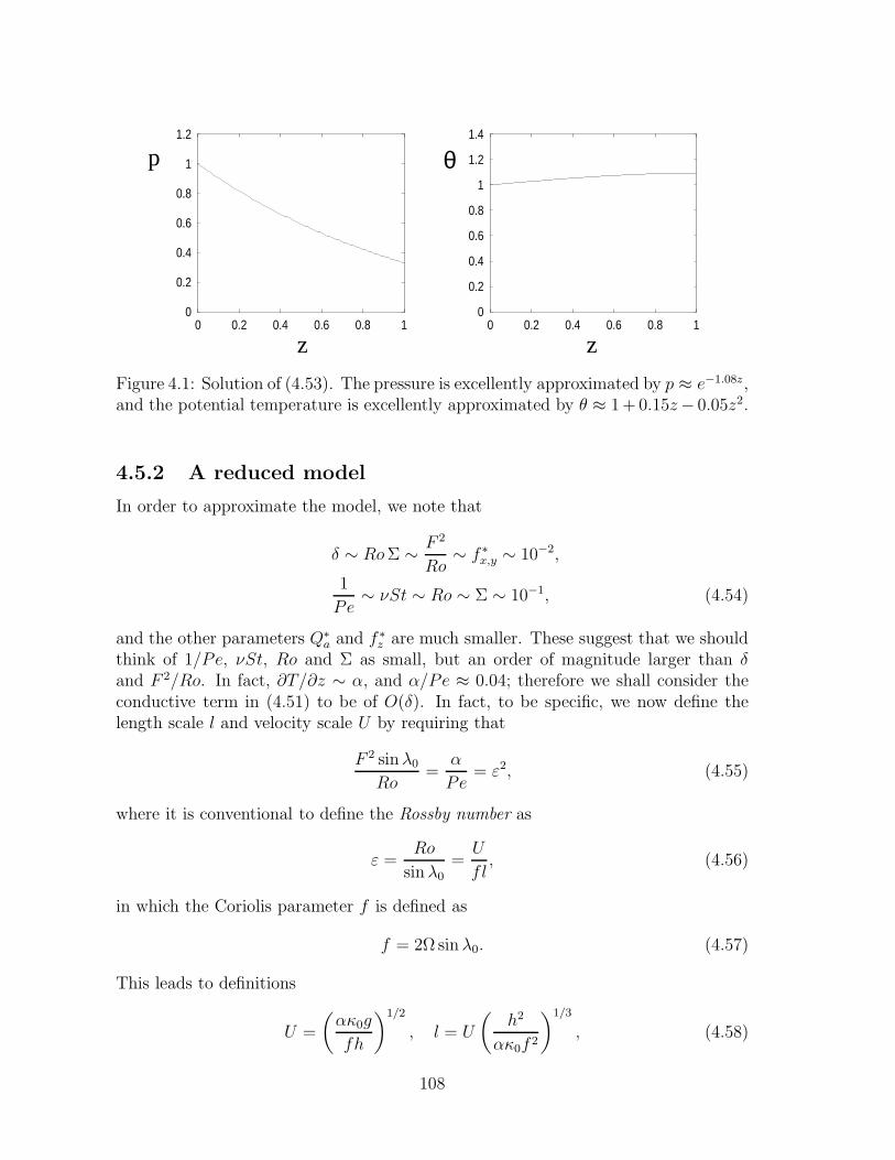
0

0.2

0.4

0.6

0.8

1

1.2

0 0.2 0.4 0.6 0.8 10

0.2

0.4

0.6

0.8

1

1.2

1.4

0 0.2 0.4 0.6 0.8 1

z z

p θ

Figure 4.1: Solution of (4.53). The pressure is excellently approximated by p ≈ e−1.08z,and the potential temperature is excellently approximated by θ ≈ 1+ 0.15z− 0.05z2.

4.5.2 A reduced model

In order to approximate the model, we note that

δ ∼ RoΣ ∼ F 2

Ro∼ f ∗

x,y ∼ 10−2,

1

Pe∼ νSt ∼ Ro ∼ Σ ∼ 10−1, (4.54)

and the other parameters Q∗a and f

∗z are much smaller. These suggest that we should

think of 1/Pe, νSt, Ro and Σ as small, but an order of magnitude larger than δand F 2/Ro. In fact, ∂T/∂z ∼ α, and α/Pe ≈ 0.04; therefore we shall consider theconductive term in (4.51) to be of O(δ). In fact, to be specific, we now define thelength scale l and velocity scale U by requiring that

F 2 sinλ0Ro

=α

Pe= ε2, (4.55)

where it is conventional to define the Rossby number as

ε =Ro

sinλ0=U

fl, (4.56)

in which the Coriolis parameter f is defined as

f = 2Ω sinλ0. (4.57)

This leads to definitions

U =

(ακ0g

fh

)1/2

, l = U

(h2

ακ0f 2

)1/3

, (4.58)

108

and calculation of these using values suggested previously leads to U ≈ 26 m s−1,l ≈ 1290 km.

Next, we adopt the formal asymptotic limits

νSt ∼ Ro ∼ Σ ∼ ε,

δ ∼ RoΣ ∼ f ∗x,y ∼ ε2. (4.59)

Expanding the equations in powers of ε, the vertical momentum equation is

∂p

∂z≈ −ρ+O(ε3), (4.60)

where

ρ =p

T, θ =

T

pα. (4.61)

Also,

∇.u ≈ µ∂u

∂x+

1

µ

∂(v/µ)

∂y+∂w

∂z+O(ε3),

d

dt=

∂

∂t+ u .∇ ≈ ∂

∂t+ µu

∂

∂x+ v

∂

∂y+ w

∂

∂z+O(ε3), (4.62)

the horizontal momentum equations are approximately

ε sinλ0du

dt− v sinλ = −sin λ0

ε2µ

ρ

∂p

∂x+O(ε2),

ε sinλ0dv

dt+ u sinλ = −sin λ0

ε21

ρ

∂p

∂y+O(ε2), (4.63)

and the energy equation is approximately

p

θ

[1 +

νSt aM

T 2

]dθ

dt= −εsM(αa− T )

T 2

dp

dt+ ε2

[∂

∂z

(k∗

α

∂T

∂z

)], (4.64)

where we have writtenνSt = εs (4.65)

to delineate the smallness of νSt (but noting that νSt a ≈ 1.64 is O(1)). Togetherwith the conservation of mass equation

dρ

dt+ ρ∇.u = 0, (4.66)

this completes the basic approximate model, valid locally everywhere except nearthe poles (where µ and tanλ → ∞). There are seven equations in (4.60), (4.61),(4.63), (4.64) and (4.66) for the seven variables θ, ρ, T , p, u, v and w. The frictionalterms f ∗

x,y can be neglected in the main flow, but they are important in the planetaryboundary layer.

109

4.5.3 Geostrophic balance

Geostrophic flow is described by the leading order approximation which considersboth curvature and inertial effects to be small, that is, ε ≪ 1. At leading order, thepressure is hydrostatic, and (4.63) indicates that the correction is of O(ε2). This isconsistent with (4.64), which indicates that θ = θ(z) +O(ε2). We do not yet assumethat θ is equal to the reference state θw defined in (4.53); this would have to bededuced. But we do anticipate that θ′(z) = O(ε) (since also θ′w = O(ε).) We put

p = p(z) + ε2P, (4.67)

where p is the hydrostatic pressure corresponding to θ, and we denote the correspond-ing density and temperature as ρ and T . Then, since µ ≈ 1, λ ≈ λ0 and ρ ≈ ρ, themomentum equations become

ρv ≈ ∂P

∂x,

ρu ≈ −∂P∂y

, (4.68)

and mass conservation reduces to

∂(ρu)

∂x+∂(ρv)

∂y+∂(ρw)

∂z≈ 0. (4.69)

Together (4.68) and (4.69) imply

∂(ρw)

∂z= 0, (4.70)

and thus w is determined by its value on the surface, where it is prescribed by the noflow through boundary condition. In the absence of topography, we have w = 0 atz = 0, so that w = 0 everywhere. The flow is then purely two-dimensional, and thehorizontal velocity vector uH = (u, v) is given by

ρuH = k×∇HP, (4.71)

where ∇H =

(∂

∂x,∂

∂y

). (4.71) defines the geostrophic wind, and shows that u .∇p =

0, i. e., wind velocities are along isobars. In the northern hemisphere, the wind movesanti-clockwise about regions of low pressure (depressions, or cyclones). The closerthe isobars, the higher the wind speed.

The no flow through condition at the ground is modified by the small frictionterms in the momentum equation, which causes the existence of a boundary layer(the planetary boundary layer) to occur. The effect of rotation in this boundary layeris to cause an effective vertical velocity at the top of the layer, proportional to theEkman number E defined by (4.32), and this velocity is often called Ekman pumping(indeed, the viscous boundary layer in a rapidly rotating fluid is called an Ekmanlayer). The Ekman layer modifies the effective no–flow–through condition to be

w =

√E

2

(∂v

∂x− ∂u

∂y

)at z = 0. (4.72)

110

4.6 The quasi-geostrophic approximation

We now return to the problem of finding the pressure for the geostrophic approxima-tion in which (4.71) applies. To do this, we need to carry the approximation to nextorder in ε, and this will allow us to deduce the quasi-geostrophic potential vorticity

equation. The equation of mass conservation (4.66) can be written in the form

∂ρ

∂t+ µ

∂(ρu)

∂x+ µ

∂(ρv/µ)

∂y+∂(ρw)

∂z= O(ε3). (4.73)

Since w = 0 at leading order, we put

w = εW. (4.74)

We also define the perturbed potential temperature Θ by

θ = θ(z) + ε2Θ; (4.75)

evidently θ(z) is the time and space-horizontal average of θ correct to O(ε2), andwe can in fact define it to be the exact such average of θ, without loss of generality.More generally, we might take θ = θ(z, t), but the energy equation then simply impliesthat θt = 0. We might have expected θ to be equal to the wet adiabatic potentialtemperature θw, defined in (4.53), but as we shall see, there is a subtle distinction, andit is necessary to delineate the difference in the equations. Because the hydrostaticcorrection in (4.60) is O(ε3), expansion of that equation toO(ε2) yields the hydrostaticapproximation for the perturbation pressure P , defined in (4.67):

Θ = θ2∂

∂z

[P

p1−α

]. (4.76)

The geostrophic wind approximation (4.68) suggests that we write

P = ρψ, (4.77)

where ψ is the geostrophic stream function, thus

u = −∂ψ∂y, v =

∂ψ

∂x. (4.78)

Bearing in mind that ρ = p1−α/θ, it follows that

Θ = θ2∂

∂z

[ψ

θ

]=∂ψ

∂z+O(ε), (4.79)

on the assumption that θ′(z) = O(ε). This relation, together with the geostrophicwind approximation, gives us the thermal wind equations:

∂u

∂z= −∂Θ

∂y,

∂v

∂z=∂Θ

∂x. (4.80)

111

Next we form an equation for the (vertical) vorticity

ζ =∂v

∂x− ∂u

∂y= ∇2ψ (4.81)

by cross differentiating (4.63) (with some care) to eliminate the pressure derivatives.Using the conservation of mass equation, together with (4.74) and the fact that ρ =ρ(z) +O(ε2), we derive the vorticity equation

Dζ

Dt+ β

∂ψ

∂x=

1

ρ

∂(ρW )

∂z, (4.82)

where D/Dt denotes the horizontal material derivative, and the term in β arises fromthe variation of sin λ with latitude; β is defined by

β =Σcot λ0

ε, (4.83)

and the horizontal material derivative is defined by

D

Dt=

∂

∂t+ u

∂

∂x+ v

∂

∂y=

∂

∂t− ∂ψ

∂y

∂

∂x+∂ψ

∂x

∂

∂y. (4.84)

Next, we consider the energy equation (4.64). Expanding in powers of ε, this canbe written in the form, correct to terms of O(ε2),

εWdθ

dz+ ε2

DΘ

Dt= εW

dθwdz

+ ε2H, (4.85)

where

H =

∂

∂z

(k∗

α∂T∂z

)

p

θ

[1 + νSt aM(T ,p)

T 2

] (4.86)

is the heating term.Now we can see the nature of the assumption about the average potential temper-

ature. Bearing in mind that dθw/dz = O(ε), we see that the ansatz that dθ/dz = O(ε)is indeed correct. However, it is generally not the case that θ = θw. The questionthen arises how to determine it.

Let us denote the stratification function S(z) by

S(z) =1

ε

[dθ

dz− dθw

dz

], (4.87)

and note that by observation (and assumption) it is positive and O(1). It is related tothe Brunt-Vaisala frequency N , which is the frequency of small vertical oscillationsin the atmosphere; in fact S ∝ N2. Positive S (and thus real N) indicates a stably

112

stratified atmosphere. If S were to become negative, the atmosphere would becomeunstably stratified and it would overturn. The energy equation is thus

DΘ

Dt= H −WS. (4.88)

In summary, we have the vorticity ζ and potential temperature Θ defined in termsof the stream function ψ by (4.81) and (4.79). Two separate equations for ζ and Θare then (4.82) and (4.88), from which W and S(z) must also be determined, thelatter by averaging the equations.

By an application of Green’s theorem in the plane, we have that∫ ∫

A

DΓ

DtdS =

∂

∂t

∫ ∫

A

Γ dS −∮

∂A

Γ dψ, (4.89)

where A is any horizontal area at fixed z. In particular, if A is a closed region on theboundaries of which ψ is constant in space, i. e., there is no flow through ∂A, thenthe boundary integral is zero.8 Let an overbar denote a space horizontal average overA. Putting Γ = Θ, it follows that

∂Θ

∂t= H −WS, (4.90)

where W (z) is the horizontal average of W . Applying the same procedure to (4.82),we have

∂ζ

∂t=

1

ρ

∂

∂z[ρW ]. (4.91)

According to the Ekman pumping boundary condition (4.72), the value of W atz = 0 is

W 0 = E∗ζ0, (4.92)

where ζ0 is the space averaged vorticity at the surface, and

E∗ =

√E

2ε2. (4.93)

Integrating (4.91), we have (using ρ = 1 at z = 0)

ρW =

∫ z

0

ρζt dz + E∗ζ0, (4.94)

and it follows from this that the stratification parameter is defined by the relation

ρ

S=

∫ z

0

ρζt dz + E∗ζ0

H − Θt

. (4.95)

8We have in mind that A is the region of zonal mid-latitude flow, bounded to the north by thepolar front, and to the south by the tropical front. We can allow A to be a periodic strip on thesphere also.

113

We can go further if we assume that the solutions are stationary (not necessarilysteady), i. e., a well-defined time average exists.9 The time averages of the timederivative terms are zero, and thus it simply follows (since H , S and ρ are functionsonly of z) that

H = WS, ρW = W0, (4.96)

where W is the time average of W , and the constant W0 is the value of the surfaceboundary value of W at z = 0. The Ekman pumping boundary condition (4.92)implies that

W0 = E∗ζ0, (4.97)

where ζ0 is the space averaged vorticity at the surface.The two equations in (4.96) define S and W , and in particular we find that

ρ

S=E∗ζ0H

. (4.98)

This equation thus defines the stratification function S(z) for a stationary (butnot necessarily steady) atmosphere.10 Evidently, the wet adiabatic profile (S = 0) isobtained (in stationary conditions) only if the heating rate H is zero.

We can now use the identity

∂

∂z

[K(z)

DΘ

Dt

]=

D

Dt

[∂

∂z

(K(z)

∂ψ

∂z

)](4.99)

to show, using (4.88), that

1

ρ

∂

∂z[ρW ] =

1

ρ

∂

∂z

[ρH

S

]− D

Dt

[1

ρ

∂

∂z

(ρ

S

∂ψ

∂z

)], (4.100)

and therefore (4.82) can be written

D

Dt

[∇2ψ + βy +

1

ρ

∂

∂z

(ρ

S

∂ψ

∂z

)]=

1

ρ

∂

∂z

[ρH

S

]. (4.101)

This is one form of the quasi-geostrophic potential vorticity equation. It is a sin-gle equation for the geostrophic stream function ψ, providing the stratification S isknown. In most treatments of its solutions, the stratification parameter S is assumedknown (from measurements), and then the equation (4.101) can be considered on itsown. However, in reality S must be determined from (4.98), which indicates thatthe stratification is determined in terms of the solution of the equation (4.101) itself,which is thus an integro-differential equation for the stream function ψ. This equa-tion is only well-posed if S > 0, i. e., if the time mean surface value of the vorticity

9This is what we would generally expect. Unbounded drift of ψ would indicate breakdown of theperturbation expansion because of the presence of secular terms.

10This derivation is somewhat similar to that of Pedlosky (1979); however, he did not provide anexplicit recipe for S(z). See also question 4.3.

114

ζ0 is positive (assuming also that H > 0), but there seems to be no obvious reasonwhy this should necessarily be the case. If the stratification became negative, theatmosphere would become inherently unstable. It would start to ‘boil’, with severeconvective storms shrouding the planet. The mild, quasi-geostrophic description ofthe weather would no longer be apt, and climate change would be a sudden, dra-matic reality overnight. The day after tomorrow, indeed. The possibility of such acatastrophic scenario appears to have entirely bypassed climate scientists.

4.7 Poincare, Kelvin and Rossby waves

The geostrophic wind given by equation (4.71) is an approximate solution to thegoverning equations which is quasi-static, in the sense that the acceleration terms inthe momentum equation are ignored; implicitly, any more rapid transients have diedout. In this chapter, we consider various classes of wave motion which arise in themodel on this shorter transient time scale.

4.8 Gravity waves

Atmospheric motions are dominated by various kinds of waves. Two particular sortsof waves which are familiar in fluid mechanics are sound waves and gravity waves.Sound waves are associated with compressibility; they travel at a speed (the speedof sound) which depends on density but is independent of wave number: they aremonochromatic. At sea level this speed is about 330 m s−1: much faster than typicalwind speeds; as a consequence, we might expect sound waves to be high frequencyphenomena which are not relevant to common atmospheric motions. If we denotethe sound wave speed as cs, then the dispersion relation relating frequency ω to wavespeed and wave number k is just ω = kcs. When this is written in dimensionlessunits, as in chapter 4, we have

c2s = ghc2, c =

(dp

dρ

)1/2

, (4.102)

and the corresponding dimensionless dispersion relation is just

ω

k=

c

F, (4.103)

where F is the Froude number defined by (4.31). Note from (4.55) that F = ε3/2.Gravity waves are familiar as the waves which propagate on the surface of the sea.

The ingredients of the theory which describes them are mass conservation (wherehorizontal divergence is accommodated by vertical contraction and expansion), accel-eration, gravity, pressure gradient, and a vertical stratification which, in the simplestform of the theory, is manifested by the interface between dense underlying fluid (e. g.,

115

Figure 4.2: Periodic gravity waves in Lapland, Northern Finland, October 2004.

water) and a lighter overlying fluid (e. g., air). Gravity waves can be seen propagat-ing at the interface between two incompressible liquids such as oil and water, andgravity waves will similarly propagate in a continuously stratified fluid contained in avertically confined channel; in this case the waves are less easily visualised, and theyare often called internal waves, or internal gravity waves.

In the sense that the atmosphere consists of a dense troposphere beneath alight stratosphere, we can expect gravity waves to propagate as undulations in thetropopause altitude. More generally, gravity waves will propagate as internal wavesin the stratified atmosphere. Gravity waves can be seen commonly in the atmosphere,because the vertical undulations of the air causes periodic cloud formation as air rises(and thus cools). Figure 4.2 shows a particular striking example from Lapland of lowlying periodic gravity waves.

For the simple case of an incompressible fluid of depth h, the dispersion relationbetween frequency and wavenumber is ω2 = gk tanh kh. In the case of a shallowfluid (such as the atmosphere), the long wave limit kh≪ 1 may be appropriate, andthen the wave speed is constant, and ω ≈ k

√gh. This applies to waves of wavelength

larger than 10 km (the waves in figure 4.2 are of smaller wavelength). In dimensionlessterms, the dispersion relation becomes

ω

k=

1

F. (4.104)

Comparing (4.104) with (4.103), we see that long gravity waves in the atmosphere areessentially the same as sound waves. In an incompressible fluid, density is manifested

116

as fluid column depth, and the pressure is proportional to this, so that the dimen-sionless ‘sound’ speed is equal to one. For internal waves, the height of the columnneed not change, but the common factor is that the height of geopotential surfacespropagates in both types of wave.

We can recover gravity waves from the scaled atmospheric model by focussingon long waves of wavenumber k ∼ O(

√ε), and time scales of O(ε) (i. e., frequencies

ω ∼ O(1/ε)). (Note that then ω/k ∼ 1/ε3/2 = 1/F , consistent with (4.103) and(4.104).) We write

t = ετ, (x, y) = (X, Y )/√ε, P =

Π√ε, (4.105)

and retain leading order terms in equations (4.63) and (4.66), assuming that w ∼ ε.Note that ρ = p1−α/θ, and that ∂θ/∂t ≈ 0, so that

1

ρ

∂ρ

∂t≈(1− α

p

)∂p

∂t. (4.106)

At leading order, mass conservation takes the form

(1− α

p

)∂Π

∂τ+∂u

∂X+∂v

∂Y= 0; (4.107)

compressibility and stratification are manifested by the first term in this equation.At leading order, the momentum equations take the form

∂u

∂τ− v ≈ −1

ρ

∂Π

∂X,

∂v

∂τ+ u ≈ −1

ρ

∂Π

∂Y. (4.108)

We can write these equations in terms of the horizontal divergence ∆ = uX + vY ,the vorticity ζ = vX − uY , and the pressure perturbation Π. We obtain

∂∆

∂τ− ζ = −1

ρ∇2Π,

∂ζ

∂τ+∆ = 0,

∂Π

∂τ+ ρc2∆ = 0, (4.109)

where

c =

[p

(1− α)ρ

]1/2(4.110)

is the dimensionless isentropic sound speed.

117

These are linear equations, and solutions exist of the form

∆ζΠ

= w expi(kX + lY + ωτ, (4.111)

provided

0 1(k2 + l2)

ρ−1 0 0−ρc2 0 0

w = iωw. (4.112)

Solutions to this exist provided either ω = 0, or

ω2 = 1 + (k2 + l2)c2, (4.113)

and this latter equation is the dispersion relation for gravity waves in a stratifiedatmosphere. These waves are called Poincare waves.

Another kind of wave can be found by seeking solutions in which v = 0. Suchwaves are particularly relevant to propagation in a confined zonal channel (for examplein the ocean), where the condition v = 0 at the north and south boundaries forcesv = 0 everywhere. This requires ∂∆/∂Y = −∂ζ/∂X , and substitution into (4.112)then shows that we must have l = −ik/ω, and thus solutions are exponential in y,and

ω = kc; (4.114)

these waves are called Kelvin waves. They are edge waves, because they decay ex-ponentially away from one or other boundary. Together with the geostrophic modeω = 0, Poincare and Kelvin waves form the complete spectrum of waves for the flow.The mode ω = 0 is associated with low frequency waves which emerge in the higherorder quasi-geostrophic approximation (which is derived in the next section); theseslow waves are called Rossby waves, or planetary waves.

The constant term in (4.113) arises from rotation and the Coriolis force. In thehigh frequency limit, we see that ω ≈ kc (for unidirectional waves), and this isconsistent with the long wave limit of gravity wave theory, and the acoustic wavespeed given in (4.103). Gravity waves are essentially long wavelength sound waves,and Poincare waves are their modification by the effects of rotation. The criticallength scale l/

√ε above which rotation becomes important is known as the Rossby

radius of deformation. Using (4.58), it is found to be equal to√gh/f . For atmospheric

motion, it is of order 3000 km, so that rotation is unimportant for smaller scale gravitywaves.

4.9 Rossby waves

We now seek a wave motion corresponding to the zero frequency geostrophic gravitywave mode satisfying (4.112) with ω = 0. This is the Rossby wave, and it is most

118

simply examined by studying (4.101) in the absence of heating, and assuming that thestratification parameter S is prescribed. (Such simplifications are in fact commonlymade in studying the properties of (4.101).) We define a vertical eigenfunction Ψ(z)satisfying the ordinary differential equation

1

ρ

[ ρSΨ′]′= −m2Ψ, (4.115)

where for suitable homogeneous boundary conditions on Ψ, m2 will be positive. WithH = 0, ψ = 0 is a solution of (4.101), and small amplitude solutions of the equationwill satisfy the linearised equation

∂

∂t

[∇2ψ +

1

ρ

∂

∂z

(ρ

S

∂ψ

∂z

)]+ β

∂ψ

∂x= 0. (4.116)

This has solutionsψ = Ψ(z) exp[i(kx+ ly + ωt)], (4.117)

providing

ω =kβ

k2 + l2 +m2. (4.118)

These are Rossby waves. The wave speed −ω/k is negative, so that the waves movewestwards. The sphericity of the Earth (i. e., β > 0) is essential in causing the wavesto move.

4.10 Baroclinic instability

Gravity waves are the sound of the atmosphere. Like a bell which reverberates whenstruck, gravity waves are excited externally. For example, when the atmosphere flowsover mountains, the waves are visualised by the periodic rows of clouds which formin the lee. However, they do not play a prominent part in large scale weather flows,because they are damped fairly rapidly by friction, and they are generated by externaleffects such as topographic forcing, not by internal dynamics.

Rossby waves, on the other hand, do play an important part in the day to dayweather, and this is because they are continually generated by an instability in theunderlying basic zonal flow. This instability is called baroclinic instability, and it isresponsible for the basic wave-like nature of the circulation in mid-latitudes.

We consider the stability of a basic state which is taken to be a purely zonal flow.Because the quasi-geostrophic model is essentially inviscid (and conductionless), thereis no unique such state. In the absence of the heating term H on the right hand side of(4.101), any zonal stream function ψ(y, z) satisfies the QG equation (4.101). However,we would expect that over sufficiently long time scales, the potential temperature Θ ofa zonal flow would become equal to the underlying surface temperature Θ0(y), whichultimately is what drives the flow. A local expansion on the mid-latitude length scale

119

of the global O(ε) variation in θ suggests the prescription of Θ0 = −y at z = 0. Thechoice Θ = −y implies the zonal flow

ψ = k − yz; (4.119)

generally, k = k(z) but we will take it as constant, k = 1. We will use (4.119) as thebasic state whose stability we wish to study.

4.11 The Eady model

The simplest model in which baroclinic instability is manifested is the Eady model.In this model, the tropopause is considered to be a rigid lid, so that we impose

W = 0 at z = 1. (4.120)

Basal friction is ignored, corresponding to E → 0 in (4.72), so that

W = 0 at z = 0. (4.121)

The Earth’s sphericity is ignored by putting β = 0 in (4.101), the heating term H = 0(consistent with the basic state (4.119), and both the density ρ and the stratificationS are taken as constant. The equation to be solved is thus the QG equation in theform

D

Dt

[∇2ψ +

1

S

∂2ψ

∂z2

]= 0, (4.122)

with boundary conditions which derive from (4.88):

D

Dt

(∂ψ

∂z

)= 0 at z = 0, 1, (4.123)

together with the no flow conditions ∂ψ/∂x = 0 on y = ±1. In addition, (4.82)implies that

D

Dt

∫ 1

0

ζ dz = 0. (4.124)

This is automatically satisfied when ψ satisfies (4.122) and (4.123).We write

ψ = 1− yz +Ψ, (4.125)

and linearise for small Ψ to find(∂

∂t+ z

∂

∂x

)[∇2Ψ+

1

S

∂2Ψ

∂z2

]= 0, (4.126)

subject to(∂

∂t+ z

∂

∂x

)∂Ψ

∂z− ∂Ψ

∂x= 0 on z = 0, 1,

Ψ = 0 on y = ±1. (4.127)

120

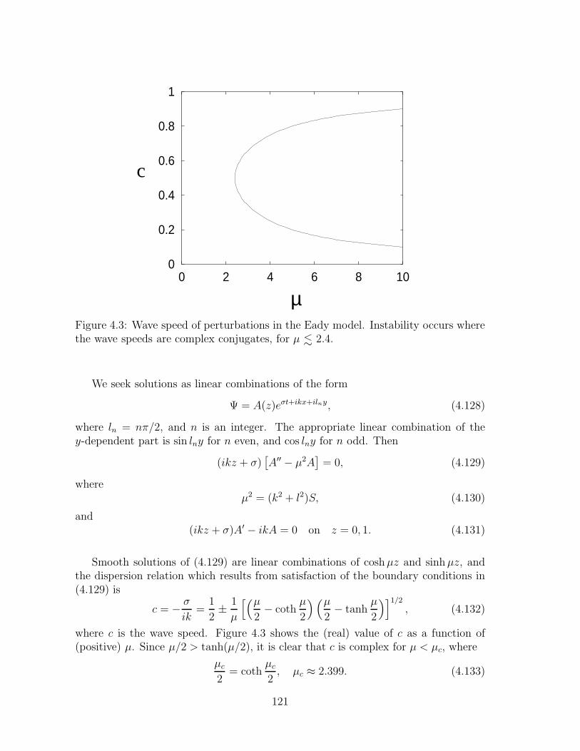
0

0.2

0.4

0.6

0.8

1

0 2 4 6 8 10

µ

c

Figure 4.3: Wave speed of perturbations in the Eady model. Instability occurs wherethe wave speeds are complex conjugates, for µ <∼ 2.4.

We seek solutions as linear combinations of the form

Ψ = A(z)eσt+ikx+ilny, (4.128)

where ln = nπ/2, and n is an integer. The appropriate linear combination of they-dependent part is sin lny for n even, and cos lny for n odd. Then

(ikz + σ)[A′′ − µ2A

]= 0, (4.129)

whereµ2 = (k2 + l2)S, (4.130)

and(ikz + σ)A′ − ikA = 0 on z = 0, 1. (4.131)

Smooth solutions of (4.129) are linear combinations of coshµz and sinhµz, andthe dispersion relation which results from satisfaction of the boundary conditions in(4.129) is

c = − σ

ik=

1

2± 1

µ

[(µ2− coth

µ

2

)(µ2− tanh

µ

2

)]1/2, (4.132)

where c is the wave speed. Figure 4.3 shows the (real) value of c as a function of(positive) µ. Since µ/2 > tanh(µ/2), it is clear that c is complex for µ < µc, where

µc2

= cothµc2, µc ≈ 2.399. (4.133)

121

0

0.1

0.2

0.3

0.4

0.5

0.6

0.7

0 1 2 3 4 5

σ

k

R

Figure 4.4: Growth rate σR of perturbations in the Eady model as a function ofwavenumber k when the stratification S = 0.25. The growth rate is well approximated

by σR ≈ 0.145k(kc − k)1/2, where kc =

õ2c

S− π2

4is the maximum wavenumber for

instability.

Complex conjugate values of c indicate instability, and this occurs for µ < µc.Instability occurs if k2 + l2 < µ2

c/S, and thus is effected by the minimum valuesk = 0, l = π/2, and the Eady instability criterion is

S <4µ2

c

π2≈ 2.218; (4.134)

this is readily satisfied in the Earth’s atmosphere.Evidently, the waves (stable or unstable) move to the east in the northern hemi-

sphere, as is observed. The wave speed of unstable waves is 0.5, and the growth rateis

σR =k

µ

[(coth

µ

2− µ

2

)(µ2− tanh

µ

2

)]1/2. (4.135)

The growth rate goes to zero as k → 0, and also as µ → µc. Since, for the fundamental

mode (n = 1) µ2 =

(k2 +

π2

2

)S increases with k, it appears that the growth rate

is maximum for an intermediate value of k. Indeed, figure 4.4 shows a typical graphof the growth rate plotted as a function of wave number k. Although linear stabilitygives us no information about the eventual form of the growing waves, it is plausiblethat the maximum growth rate at wavenumber km selects the preferred wavelength

122

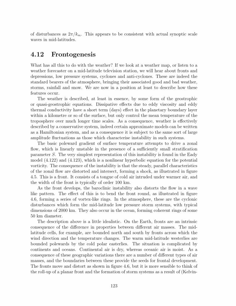
of disturbances as 2π/km. This appears to be consistent with actual synoptic scalewaves in mid-latitudes.

4.12 Frontogenesis

What has all this to do with the weather? If we look at a weather map, or listen to aweather forecaster on a mid-latitude television station, we will hear about fronts anddepressions, low pressure systems, cyclones and anti-cyclones. These are indeed thestandard bearers of the atmosphere, bringing their associated good and bad weather,storms, rainfall and snow. We are now in a position at least to describe how thesefeatures occur.

The weather is described, at least in essence, by some form of the geostrophicor quasi-geostrophic equations. Dissipative effects due to eddy viscosity and eddythermal conductivity have a short term (days) effect in the planetary boundary layerwithin a kilometre or so of the surface, but only control the mean temperature of thetroposphere over much longer time scales. As a consequence, weather is effectivelydescribed by a conservative system, indeed certain approximate models can be writtenas a Hamiltonian system, and as a consequence it is subject to the same sort of largeamplitude fluctuations as those which characterise instability in such systems.

The basic poleward gradient of surface temperature attempts to drive a zonalflow, which is linearly unstable in the presence of a sufficiently small stratificationparameter S. The very simplest representation of this instability is found in the Eadymodel (4.122) and (4.123), which is a nonlinear hyperbolic equation for the potentialvorticity. The consequence of the instability is that the steady, parallel characteristicsof the zonal flow are distorted and intersect, forming a shock, as illustrated in figure4.5. This is a front. It consists of a tongue of cold air intruded under warmer air, andthe width of the front is typically of order 100 km.

As the front develops, the baroclinic instability also distorts the flow in a wavelike pattern. The effect of this is to bend the front round, as illustrated in figure4.6, forming a series of vortex-like rings. In the atmosphere, these are the cyclonicdisturbances which form the mid-latitude low pressure storm systems, with typicaldimensions of 2000 km. They also occur in the ocean, forming coherent rings of some50 km diameter.

The description above is a little idealistic. On the Earth, fronts are an intrinsicconsequence of the difference in properties between different air masses. The mid-latitude cells, for example, are bounded north and south by fronts across which thewind direction and the temperature changes. The warm mid-latitude westerlies arebounded polewards by the cold polar easterlies. The situation is complicated bycontinents and oceans. Continental air is dry, whereas oceanic air is moist. As aconsequence of these geographic variations there are a number of different types of airmasses, and the boundaries between these provide the seeds for frontal development.The fronts move and distort as shown in figure 4.6, but it is more sensible to think ofthe roll-up of a planar front and the formation of storm systems as a result of (Kelvin-

123

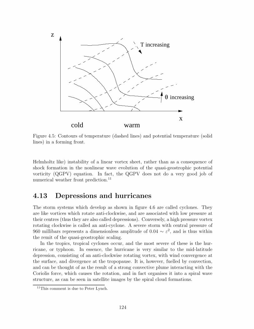
cold warm

z

x

θ

T increasing

increasing

Figure 4.5: Contours of temperature (dashed lines) and potential temperature (solidlines) in a forming front.

Helmholtz like) instability of a linear vortex sheet, rather than as a consequence ofshock formation in the nonlinear wave evolution of the quasi-geostrophic potentialvorticity (QGPV) equation. In fact, the QGPV does not do a very good job ofnumerical weather front prediction.11

4.13 Depressions and hurricanes

The storm systems which develop as shown in figure 4.6 are called cyclones. Theyare like vortices which rotate anti-clockwise, and are associated with low pressure attheir centres (thus they are also called depressions). Conversely, a high pressure vortexrotating clockwise is called an anti-cyclone. A severe storm with central pressure of960 millibars represents a dimensionless amplitude of 0.04 ∼ ε2, and is thus withinthe remit of the quasi-geostrophic scaling.

In the tropics, tropical cyclones occur, and the most severe of these is the hur-ricane, or typhoon. In essence, the hurricane is very similar to the mid-latitudedepression, consisting of an anti-clockwise rotating vortex, with wind convergence atthe surface, and divergence at the tropopause. It is, however, fuelled by convection,and can be thought of as the result of a strong convective plume interacting with theCoriolis force, which causes the rotation, and in fact organises it into a spiral wavestructure, as can be seen in satellite images by the spiral cloud formations.

11This comment is due to Peter Lynch.

124

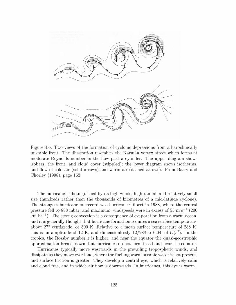
Figure 4.6: Two views of the formation of cyclonic depressions from a baroclinicallyunstable front. The illustration resembles the Karman vortex street which forms atmoderate Reynolds number in the flow past a cylinder. The upper diagram showsisobars, the front, and cloud cover (stippled); the lower diagram shows isotherms,and flow of cold air (solid arrows) and warm air (dashed arrows). From Barry andChorley (1998), page 162.

The hurricane is distinguished by its high winds, high rainfall and relatively smallsize (hundreds rather than the thousands of kilometres of a mid-latiude cyclone).The strongest hurricane on record was hurricane Gilbert in 1988, where the centralpressure fell to 888 mbar, and maximum windspeeds were in excess of 55 m s−1 (200km hr−1). The strong convection is a consequence of evaporation from a warm ocean,and it is generally thought that hurricane formation requires a sea surface temperatureabove 27 centigrade, or 300 K. Relative to a mean surface temperature of 288 K,this is an amplitude of 12 K, and dimensionlessly 12/288 ≈ 0.04, of O(ε2). In thetropics, the Rossby number ε is higher, and near the equator the quasi-geostrophicapproximation breaks down, but hurricanes do not form in a band near the equator.

Hurricanes typically move westwards in the prevailing tropospheric winds, anddissipate as they move over land, where the fuelling warm oceanic water is not present,and surface friction is greater. They develop a central eye, which is relatively calmand cloud free, and in which air flow is downwards. In hurricanes, this eye is warm.

125

Notes and references

Exercises

4.1 Using values d = 10 km, κρd = 0.67, σ = 5.67× 10−8 W m−2 K−4, T = 290 K,show that a representative value of the radiative conductivity kR defined by

kR =16σT 3

3κρ

for an opaque atmosphere is kR ≃ 105 W m−1 K−1. Hence show that a typicalvalue for the effective Peclet number

Pe =ρcpUd

2

kRl

is about 20, if ρ ≈ 1 kg m−3, cp ≈ 103 J kg−1 K−1U ≈ 20 m s−1, l ≈ 1000 km.Explain the import of this in terms of the heat equation

ρcpdT

dt= ∇.[kR∇T ].

4.2 Derive a reference state for a dry atmosphere (no condensation) by using theequation of state

p =ρRT

Ma

,

the hydrostatic pressure∂p

∂z= −ρg,

and the dry adiabatic temperature equation

ρcpdT

dt− dp

dt= 0.

Show thatT = T0 −

gz

cp, p = p0p

∗(z),

where

p∗(z) =

(1− gz

cpT0

)Macp/R

.

Use the typical values cpT0/g ≈ 29 km,Macp/R ≈ 3.4, to show that the pressurecan be adequately represented by

p = p0 exp(−z/H),

where here the scale height is defined as

H =RT0Mag

≈ 8.4 km.

(A slightly better numerical approximation near the tropopause is obtained ifthe scale height is chosen as 7 km.)

126

4.3 Suppose that θ satisfies the equation

Dθ

Dt+ εW

∂θ

∂z= ε2ΓW + ε2H, (∗)

where Γ and H are constants, W =W (x, y) and the horizontal material deriva-tive is given by

D

Dt=

∂

∂t− ∂ψ

∂y

∂

∂x+∂ψ

∂x

∂

∂y,

where ψ is the geostrophic stream function.

The equation is to be solved in the region V : −L < x < L, −1 < y < 1,0 < z < 1, with the boundary condition θ = 1 + ε2Θ0(y) on z = 0, andan initial condition for θ. We can assume without loss of generality that theaverage of Θ0 over y is zero. (Why?) Assume that ψ = ±1 on y = ±1, and thatit is periodic in x (with period 2L). Comment on the suitability of the initialand boundary conditions. Does it matter whether W is positive or negative??

If A is any horizontal section of V , show that∫

A

Dθ

DtdS =

∂

∂t

∫

A

θ dS ,

and deduce that the equationDθ

Dt= g

only has a bounded solution if g(z) = 0, where g is the time average of

∫

A

g dS.

By expanding θ as θ0 + εθ1 + ε2θ2 + . . . and assuming that the solution remainsregular, find the equations satisfied by θi, i = 1, 2, 3, and show that a solutionexists in which θ0 = θ0(z); whence also

θ0 = 1

and θ1 = θ1(z), and θ1 is given by

θ1 =

(Γ +

H

W

)z;

whenceDθ2Dt

= H

(1− W

W

). (†)

Suppose now that θ2 =∂ψ

∂z; show that

D

Dt

[∂θ2∂z

]=

∂

∂z

(Dθ2Dt

), and deduce

that a solution for θ2 can be found in the form θ2 = θ2(z) + Θ(x, y), whereΘ(x, y) is a particular solution of (†), and show that the secularity constraintat O(ε3) implies that we can take θ2 = 0. Deduce that ψ = zΘ(x, y).

127

Suppose now that a diffusion term ε2∂2θ

∂z2is added to the right hand side of (∗).

Show that the preceding discussion still applies, but now Θ represents an outersolution for θ2 away from the boundary z = 0. By writing θ2 = Θ + χ andz = εZ, show that χ satisfies the approximate boundary layer equation

Dχ

Dt+W

∂χ

∂Z=∂2χ

∂Z2,

with boundary conditions

χ → 0 as Z → ∞,

χ = χ0(x, y) = Θ0 −Θ on Z = 0.

For the particular case of a steady zonal flow in whichD

Dt= u

∂

∂x, u = u(y),

W = W (y) and χ0 =∑

k

χk(y)eikx, show that

χ =∑

k

χk(y)eikx−αZ,

where

α =

(W 2

4+ iku

)1/2

− W

2. (‡)

By writingW 2

4+ iku = (p+ iq)2, p > 0, and defining the square root in (‡) as

having p > 0, show that Reα > 0 irrespective of the sign of W . How would youexpect Θ to behave over long time scales in this case?

128

Chapter 5

Two-phase flows

Two-phase flow occurs in numerous situations in industry, as well as in nature. Two-phase flow refers to the coexistence of two phases of a substance in a flow. Typically(though not always) the phases are liquid and gas, as for example in the commonoccurrence of steam-water flows.

In boilers, water is heated as it flows through a bank of channels, until it startsto boil. This leads to a two-phase flow region until dryout occurs, and the flow is ofsuperheated steam. The boundaries which physically divide the various regimes arecalled the boiling boundary and the superheat boundary.

A similar situation occurs in nuclear reactors where liquid sodium is commonlyused as a coolant. Here it is important that dryout does not occur, since the insulatingproperties of vapour reduce the cooling efficiency of the flow. Two-phase flow alsooccurs in condensers, where superheated steam is cooled through the reverse sequenceof two-phase and then sub-cooled regions.

Natural examples of two-phase flows include volcanic eruptions, where a varietyof such flows can occur, for example ash flows (solid/liquid), and vesicular eruptions,where dissolved gases are exsolved as the magma rises (and loses pressure), so thatthe erupting flow is of a gas/liquid mixture.

5.1 Flow regimes

Modelling two-phase flow is complicated by a variety of factors. For a start, the flowis usually turbulent, so that some sort of averaging is necessary to model the meanflow. In addition, the distribution of phases means that averaging must also be doneso that average variables such as void fraction can be defined. (This is analogous tothe definition of variables such as porosity in permeable media.)

A further complication is that two-phase flows can exist in a variety of regimes,all of which will generally occur in a boiling flow. When boiling commences, smallbubbles are nucleated at the wall, detach and are taken up by the fluid. Initially,the liquid away from the walls may still be sub-cooled (below boiling point), so thatheat transfer to the vapour is predominantly at the wall. When the liquid reaches

129

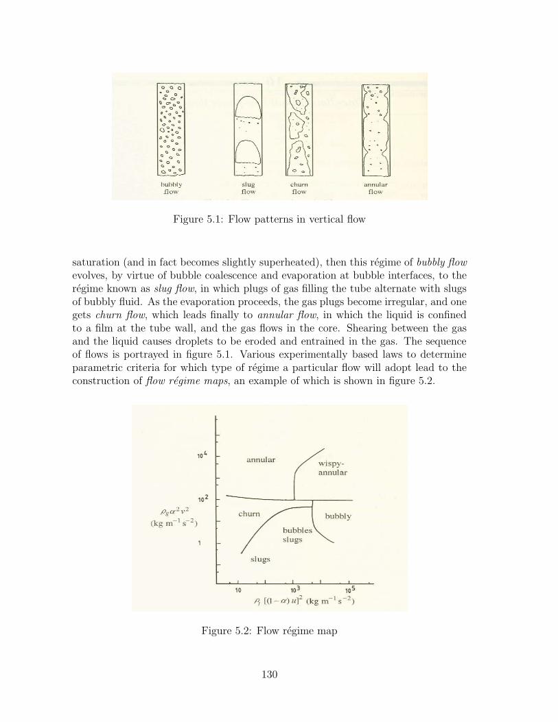
Figure 5.1: Flow patterns in vertical flow

saturation (and in fact becomes slightly superheated), then this regime of bubbly flow

evolves, by virtue of bubble coalescence and evaporation at bubble interfaces, to theregime known as slug flow, in which plugs of gas filling the tube alternate with slugsof bubbly fluid. As the evaporation proceeds, the gas plugs become irregular, and onegets churn flow, which leads finally to annular flow, in which the liquid is confinedto a film at the tube wall, and the gas flows in the core. Shearing between the gasand the liquid causes droplets to be eroded and entrained in the gas. The sequenceof flows is portrayed in figure 5.1. Various experimentally based laws to determineparametric criteria for which type of regime a particular flow will adopt lead to theconstruction of flow regime maps, an example of which is shown in figure 5.2.

Figure 5.2: Flow regime map

130

5.2 A simple two-fluid model

Two-phase flow equations are averaged in various ways: in time, cross-sectionally,in space. For one-dimensional flow in a tube, we seek relations for cross-sectionallyand time averaged variables representing the two fluids. These variables are the voidfraction α, which is the gas volume fraction; u and v, which are the liquid and gasvelocities; and averaged pressures pl and pg for each phase. We concentrate on steam-water or air-water flow, for example, for which the viscous stresses are manifestedthrough the wall-friction, while the internal friction is largely due to Reynolds stresses;both of these terms must be constituted. In writing the simplest model (in order toexamine its structure), we will in fact omit frictional terms for the moment.

Ignoring surface tension, it seems reasonable to take pg = pl = p, and thenequations conserving mass and momentum of each phase (and without change ofphase due to boiling or condensation) are

(αρg)t + (αρgv)z = 0,

ρl(1− α)t + ρl(1− α)uz = 0,

ρg[vt + vvz] = −pz,ρl[ut + uuz] = −pz. (5.1)

These equations can be derived from first principles in the usual way. They representfour equations for the variables α, u, v, p, if we suppose ρg and ρl, the gas and liquiddensities, are given by appropriate equations of state. These are simple generalisationsof Euler’s equations to the case of two-fluid motion.

For heated flows, one requires also two energy or (more usually) enthalpy equationsfor the gas and liquid enthalpies hg and hl. For adiabatic (unheated) flow, theseequations are redundant.

Boundary conditions

From a physical consideration of the system, it seems we could prescribe inlet andoutlet pressures, and the two inlet mass fluxes. The natural boundary conditions arethose of α, u, v at the inlet and p at the outlet (say). Thus if we solve the system forgiven α0 at z = 0, as well as u and v, then we will obtain the pressure drop ∆p asa functional of α0, ∆p = ∆p(α0). Inversion of this relation determines the necessaryα0 to obtain the correct pressure drop.

5.3 Other models

There are two other commonly used two phase flow models. In the homogeneousmodel, both phases are assumed to move at the same velocity, thus u = v and oneconsiders momentum conservation for the mixture, in the (simplest) form

131

ρ[ut + uuz] = −pz, (5.2)

where

ρ = αρg + (1− α)ρl (5.3)

is the mixture density. The homogeneous model should work best for regimes suchas bubbly flow, where there may be little relative motion between the phases.

The drift-flux model allows a relative motion, but rather than have separate mo-mentum equations, it considers total momentum conservation in the form

[αρgv + (1− α)ρlu]t + [αρgv2 + (1− α)ρlu

2]z = −pz , (5.4)

with v being related to u through the drift flux (basically, v − u is constituted as afunction of α). This is rather akin to the status of Darcy’s law.

5.4 Characteristics

The form of the equations ( 5.1) suggests that the system should be hyperbolic. Itcan be written in the form

Aψt +Bψz = 0, (5.5)

where ψ = (α, u, v, p)T and, if ρg and ρl are constant,

A =

1 0 0 0−1 0 0 00 ρl 0 00 0 ρg 0

, B =

v 0 α 0−u 1− α 0 00 ρlu 0 10 0 ρgv 1

. (5.6)

We seek characteristics dz/dt = λ satisfying det(λA − B) = 0; we find that theeigenvalues λ must satisfy

ρg(1− α)(λ− v)2 + ρlα(λ− u)2 = 0, (5.7)

whence

λ =u± isv

1± is, s =

[ρg(1− α)

ρlα

]1/2. (5.8)

It follows that there are two complex characteristics unless u = v, (the other two areinfinite, corresponding to two infinite sound speeds). Consequently, the model is ill-posed as it stands. There is thus a fundamental logical inconsistency, and before wego on to consider more complicated models, it is worth pursuing this further. Noticethat the ellipticity of the model is not due to the neglect of frictional terms: theseare algebraic, and do not affect the characteristics.

132

To see the practical effect of complex characteristics, consider a uniform stateψ = ψ0, subject to small perturbations proportional to exp(σt+ ikz). Such solutionsexist if σ = ikλ = ∓kλI + ikλR, where λ = λR ± iλI represents (5.8). Thus ifλI 6= 0, there are unstable solutions, moreover these grow arbitrarily fast at veryshort wavelengths. These grid scale instabilities are a practical sign of an ill-posedproblem.

5.5 More on averaging

In order to resolve this dilemma, let us examine the process of averaging in greaterdetail. There are many different ways of approaching averaging, and here we followthat outlined by Drew and Wood (1985), or Drew (1983). The idea is to use indicatorfunctions Xk for each phase (labelled by k) such that Xk(x, t) = 1 if x is in phasek at time t, and Xk = 0 otherwise. Averaged equations can then be obtained bymultiplying the pointwise conservation laws for phase k by Xk, and averaging. In sodoing, we consider Xk as a generalised function, which allows us to use integrationby parts.

A typical conservation law has the form

∂

∂t(ρψ) +∇.(ρψv) = −∇.J+ ρf. (5.9)

Multiplying by Xk and averaging (in practice, this is often a time and/or spaceaverage), yields (an overbar denoting the average)

∂

∂t(Xkρψ) +∇.[Xkρψv] = −∇.[XkJ] +Xkρf

+ρψ

∂Xk

∂t+ vi.∇Xk

+ ρψ(v − vi) + J.∇Xk, (5.10)

where we assume that ∇f = ∇f , ∂f/∂t = ∂f/∂t, which will be the case for suffi-ciently well-behaved f . In (5.10), vi is the average interfacial velocity of the boundaryof phase k, and derivatives of Xk are interpreted as generalised functions. In partic-ular, ∂Xk/∂t + vi.∇Xk = 0, since if φ is a smooth test function, then

133

∫ ∫φ

[∂Xk

∂t+ vi.∇Xk

]dV dt

= −∫ ∫

Xk

[∂φ

∂t+ vi.∇φ

]dV dt

−∫ ∞

−∞

∫

Vk(t)

[∂φ

∂t+ vi.∇φ

]dV dt

= −∫ ∞

−∞

d

dt

∫

Vk(t)

φ dV dt

= −[∫

Vk(t)

φ dV

]∞

−∞

= 0, (5.11)

for φ vanishing at large values of |t|.The last term in (5.10) is related to the surface average, since ∇Xk picks out

interfacial values. For a smooth test function vanishing at large x, j.∇Xk is definedvia

∫

V

φj.∇Xk dV = −∫

V

Xk∇.(φj) dV

= −∫

Vk

∇.(φj) dV

= −∫

Sk

φjn dS, (5.12)

where jn is the normal component of j at the interface, pointing away from phase k.This suggests that j.∇Xk can be identified with the surface average of −j.n.

Now put ψ = 1, J = 0, f = 0 in (5.9), corresponding to mass conservation. Thenequations of conservation of mass of each phase are, from (5.10),

∂

∂t(Xkρ) +∇.[Xkρv] = ρ(v − vi).∇Xk. (5.13)

The form of (5.13) suggests that we define the average phase volume, density andvelocity as follows:

αk = Xk, ρk = Xkρ/αk, vk = Xkρv/αkρk, (5.14)

so that (5.13) gives

∂

∂t(αkρk) +∇.[αkρkvk] = Γk, (5.15)

where Γk = ρ(v − vi).∇Xk, and represents a mass source due to phase change (with-out which v = vi at the interface).

134

Next, consider momentum conservation. With appropriate interpretation of tensornotation, we put

ψ = v, J = pI− τ , f = g, (5.16)

where τ is the deviatoric stress tensor, g is gravity. Then

∂

∂t(Xkρv) +∇.[Xkρvv] = ∇.[Xk(−pI+ τ )] +Xkρg

+ρv(v − vi) + (pI− τ ).∇Xk. (5.17)

NowXkρv = αkρkvk, and we would like to haveXkρvv = αkρkvkvk; but evidently thelatter is not the case. Since the flow is normally turbulent, this can be circumventedby separating v (and, more generally ψ) into mean and fluctuating parts, thus v =vk + v′

k, so that

Xkρvv = αkρkvkvk +Xkρv′kv

′k; (5.18)

The second term can be interpreted as the averaged Reynolds stress. The momentumequation can thus be written as

∂

∂t(αkρkvk) +∇.[αkρkvkvk] =

∇.[αk(Tk +T′k)] + αkρkg +Mk + vmkiΓk, (5.19)

where

αkTk = Xk(−pI + τ ),αkT

′k = Xkρv′

kv′k,

Mk = (pI− τ ).∇Xk,

vmki = [ρv(v − vi).∇Xk]/[ρ(v − vi).∇Xk]. (5.20)

Evidently, the average pressure in phase k is pk = Xkp/αk. If we neglect viscousstresses, we can write the interfacial momentum source as

Mk = p∇Xk = pki∇αk +M′k, (5.21)

where

M′k = (p− pki)∇Xk, (5.22)

pki is the average interfacial pressure on phase k, and we use ∇Xk = ∇αk. Thus themomentum equation can be written as

135

∂

∂t(αkρkvk) +∇.[αkρkvkvk] = −αk∇pk − (pk − pki)∇αk

+∇.[αkT′k] + αkρkg +M′

k + vmkiΓk. (5.23)

Commonly, we assume pk = pki and the pressure term is explicitly −αk∇pk, animportant point to consider.

One dimension: profile coefficients

In one-dimensional turbulent flow, it is common to constitute Reynolds stresses viaan eddy viscosity, or equivalently, to define (cf. (5.18))

Xkρvv = Dkαkρkvv, (5.24)

where Dk is known as a profile coefficient. It includes the effects of both the Reynoldsstresses and also the cross-sectional non-uniformity of the flow. Let us consider thesimplest modification to (5.1) which allows Dk 6= 1. A one-dimensional version of(5.1) is, with ρg and ρl constant,

αt + (αv)z = 0,

−αt + [(1− α)u]z = 0,

ρg(αv)t + ρg(Dgαv2)z = −αpz,

ρl[(1− α)u]t + ρl[Dl(1− α)u2]z = −(1− α)pz. (5.25)

It will usually be appropriate to choose Dg = 1, but we allow Dl 6= 1. Then the lasttwo of (5.25) can be written as

ρg[vt + vvz] = −pz,

ρl

[ut + (2Dl − 1)uuz − (Dl − 1)

[u2

1− α

]αz

]= −pz , (5.26)

and the system can be written as (5.5) for ψ = (α, u, v, p)T , with

A =

1 0 0 0−1 0 0 00 ρl 0 00 0 ρg 0

, B =

v 0 α 0−u (1− α) 0 0

−ρl(Dl−1)u2

(1−α)ρl(2Dl − 1)u 0 1

0 0 ρgv 1

. (5.27)

The characteristics dz/dt = λ satisfy det(λA−B) = 0, hence with s defined in (5.8),

(λ− u)2 = δ[u2 + 2u(λ− u)]− s2(λ− v)2, (5.28)

136

where δ = Dl − 1. For small values of s and δ, we see that λ is real provided

δ > s2(u− v)2/u2, (5.29)

so that practically, a very small Reynolds stress (or profile coefficient above one)is sufficient to make the basic system have real characteristics, and hence be well-posed. Other possibilities to render the system well-posed can be chosen. In practice,any realistic model will (and should) be well-posed, otherwise it will be physicallymeaningless.

5.6 A simple model for annular flow

In many two-phase boiling flows, annular flows are significant. Because the gas flowis less impeded by the liquid, the flow velocities are high, and consequently, annularflow regions can occupy large parts of the tube. Moreover, since the gas and liquidvelocities are very different, a two-fluid model is appropriate. If we denote α, β asgas and liquid volume fractions, u, v as liquid and gas velocities, and hg and hl as gasand liquid enthalpies, then a typical one-dimensional set of model equations is givenby

(αρg)t + (αρgv)z = Γ,

(βρl)t + (βρlu)z = −Γ,

(βρlu)t + (Dβρlu2)z = −βpz − Flw + Fli,

(αρgv)t + (αρgv2)z = −αpz + Fgi,

βρl[hlt + uhlz] = Γ(hl − hli) + El +Q/A,

αρg[hgt + vhgz] = Γ(hgi − hg) + Eg,

El + Eg + Γ(hgi − hli) = 0. (5.30)

The first two of these represent conservation of mass, as before. The next tworepresent conservation of momentum, and we have chosen to include the wall frictionFlw on the liquid, and the interfacial friction Fli on the liquid (and Fgi on the gas,Fgi = −Fli). The next two are enthalpy equations. In an annular flow, boiling takesplace at the liquid-gas interface, so that the liquid in particular must be superheated.If the average phasic enthalpy hk is different from the interfacial value hki, then thereis a convective transfer of enthalpy Γ(hki − hk) to that phase associated with thephase change term. In addition, there will be a diffusive transport Ek due to heatconduction. Finally, Q is the external heat supply per unit length per unit time, andA is the cross-sectional area. The final relation then represents the volume averageof the Stefan condition. There are various other terms which could be included butthey can be treated in the same way as below, and are in any case often small.

137

Nondimensionalisation

Our aim is to derive appropriate scaling relationships for the variables and to showhow suitable simplifications can often be made. To do this, we use values of theparameters typical to one particular application, that of a steam turbine.

Firstly, we must choose constitutive forms for the various terms which arisethrough the averaging process. We suppose

Flw =2

dflwρl |u|u,

Fli = −Fgi =2

dfliρg |v − χu| (v − χu) (5.31)

are the friction terms. The numbers flw, fli are friction factors, and are themselvesusually considered to be functions of the phasic Reynolds numbers. Here we takethem to be constant. The coefficient χ in (16.31)2 represents the speed of interfacialwaves; a typical value is χ = 2.

We will assume that the interface is in thermodynamic equilibrium, thus

hgi = hsatg , hli = hsatl , (5.32)

where these are the saturation values of the enthalpies, and L = hsatg − hsatl is thelatent heat. Enthalpies are related to temperature by

hg = hsatg + cpg(Tg − T sat),

hl = hsatl + cpl(Tl − T sat), (5.33)

where T sat is the saturation (boiling) temperature, which we take as constant. Interms of temperature, the interfacial heat transfer terms are

Eg = Hgi(Tgi − Tg)/Ls,

El = Hli(Tli − Tl)/Ls, (5.34)

where Hli and Hgi are heat transfer coefficients, Tgi = Tli = T sat here, and L−1s is the

(average) surface area per unit volume, which for annular flow we take as

L−1s = 4α1/2/d ≈ 4/d. (5.35)

In general, Hki are complicated functions of Reynolds number, etc., but we take themas constant.

Now we scale the variables by writing

z = lz∗, u = Uu∗, v = V v∗, p = p0 + Pp∗, β = Bβ∗,

Γ = GΓ∗, t = (l/U)t∗, hg = hsatg + Lh∗g, hl = hsatl + Lh∗l ; (5.36)

138

we take l to be the tube length, and choose the unknown scales U, V, P, B,G byeffecting the following balances in (5.30):

(αρgv)z ∼ Γ, (βρlu)z ∼ Γ, Flw ∼ Fli, αpz ∼ Fgi, Γ(hl − hli) ∼ Q/A. (5.37)

We take ρg and ρl as constants for simplicity, though in reality ρg will vary by areasonable amount. Specifically, we choose (since α ∼ 1)

ρgV = lG, ρlBU = lG, U/V = (fliρg/flwρl)1/2,

P = 2lflwρlU2/d, G = Q/AL (5.38)

(if Q is constant, or a typical value if it varies). Substitution of these values into theequations, and omitting the asterisks, yields the following:

α = 1− c1β,

c2αt + (αv)z = Γ,

βt + (βu)z = −Γ,

c3[(βu)t +D(βu2)z] = −c1βpz − u2 + (v − χc2u)2,

c4[c2(αv)t + (αv2)z] = −αpz − (v − χc2u)2,

β(hlt + uhlz) = Γhl − hl/c5 + q,

c2αhgt + αvhgz = Γhg − hg/c6,

Γ = hg/c6 + hl/c5, (5.39)

where the parameters are defined by

c1 = B, c2 = U/V, c3 = Bd/2flwl,

c4 = d/2flil, c5 = Gcpl/HliL−1s , c6 = Gcpg/HgiL

−1s , (5.40)

and q = O(1) is the dimensionless heat supply.To estimate the values of the parameters, we choose

l = 10m, ρg = 30 kg m−3, ρl = 760 kg m−3, flw = .004,

fli = .02, d = .014m, A ∼ 1.5× 10−4m2, m = .2 kg s−1,

L−1s = 4/d, cpl = 5.2 kJ kg−1K−1, cpg = 4.6 kJ kg−1K−1,

Hli ∼ 1.7× 105W m−2K−1, Hgi ∼ .7× 105W m−2K−1, (5.41)

where m is the inlet mass flux; this determines Q via Ql ∼ mL, so that G is equiva-lently determined from

139

G = m/Al. (5.42)

These parameters are relevant for steam/water flow at an ambient pressure of 60 bars.We find successively

G ∼ 130 kg m−3 s−1, V ∼ 43 m s−1, U ∼ 19 m s−1,

B ∼ .09, P ∼ 16 bars (1.6× 106 Pa), (5.43)

and thus

c1 ∼ 0.09, c2 ∼ 0.44, c3 ∼ 0.016, c4 ∼ 0.035, c5 ∼ 0.014, c6 ∼ 0.03. (5.44)

The fact that all the parameters are less than one indicates that the balances chosenin (5.38) are correct. In practice, this often has to be done through trial and error.

Analysis

Since all the parameters except c2 in (16.44) are in fact small, the system lends itselfto an asymptotic reduction. Specifically, hg, hl ≪ 1 (thus the fluids are close tothermodynamic equilibrium); adding the two enthalpy equations then gives

Γ ≈ q. (5.45)

Also α ≈ 1, and the gas momentum equation is just a quadrature for p,

0 = −pz − (v − χc2u)2, (5.46)

while the liquid momentum equation is simply a force balance:

u = λv, (5.47)

where

λ = (1 + χc2)−1 ∼ 0.5. (5.48)

The equations thus reduce to

vz ≈ q,

βt + λ(βv)z = −q, (5.49)

which can even be solved explicitly. Thus, if q is constant,

v = v0 + qz, (5.50)

and using characteristics, we find

(1 + λβ) =(1 + λβ0)v0v0 + qz

, (5.51)

140

if v = v0, β = β0 at z = 0. Thus β decreases and reaches zero at z = λβ0v0/q,corresponding to dryout of the liquid film.

The dramatic collapse we have illustrated here is robust, in the sense that evenif a more realistic system is algebraically more intractable (for example, because flwdepends on u, fli depends on v and β, etc.), nevertheless the approximations involvedwill continue to apply. The result is that numerical computations can be greatlysimplified. Simple but accurate models are also of use in establishing parameterdependence of stability characteristics, for example.

In neglecting the parameters c1, c3, c4, c5, c6, we reduce a sixth-order system to athird-order one, two of whose equations are quadratures. All these approximationsare potentially singular, as they involve the neglect of small terms, and we must beconcerned at whether we also lose the ability to satisfy initial/boundary conditions.Insofar as the system will be hyperbolic, we can afford not to worry about loss of timederivatives, since any resulting rapid transients will be washed out of the system.

Inspecting the reduced system, we see that we can specify v and β at the inlet,but not u, as we lose the acceleration terms in the liquid momentum equation. Lossof acceleration in the gas momentum equation does not matter, since the pressuregradient remains, and the equation acts as a quadrature for p. Inspection of theenthalpy equations shows that any initial/boundary condition for hl or hg is quicklyrelaxed. Since, in fact, it is natural to prescribe hl = hg = 0 at the entrance to theannular flow region, there will not actually be any enthalpy boundary layer. The onlycause for worry is thus the inability to prescribe u, and we must forgo this luxury.Strictly, an inlet boundary layer analysis is then necessary to complete the solution.

Two important features about this two-phase flow are these: the pressure gradientdisappears from the liquid momentum equation because β ≪ 1 (in annular flow).Further, acceleration terms will always be small if ρu2 ≪ ∆p, which is inevitably thecase. Thus, it will be a common feature that liquid momentum simply gives a forcebalance, so that the momentum equations can effectively be taken out of the system.

5.7 Density wave oscillations

Density wave oscillations in two phase flow have been of concern in the nuclear in-dustry for a long time. In a steam generating boiler, water in an array of pipes isheated externally, and begins to boil as it flows along the pipes. In certain situations,the resulting two phase flow can be oscillatorily unstable, which is an undesirablefeature in industrial systems. The instability mechanism is the same one that pro-duces chugging in a domestic back boiler, if the pipework to the hot water tank isincorrectly installed (i. e., a section of pipe from fire to hot water tank is inclineddownwards), and also the same that produces geysering in geothermal springs. Amore direct analogy is in certain types of effusive volcanic eruptions, such as that atVillarrica volcano in Chile, where the magma flow in the vent appears to oscillatebetween a bubbly flow regime and a slug flow regime.

The simplest model to describe the instability was posed and analysed by Davies

141

q q

boilingboundary

sub-cooled

two phase

u

Figure 5.3: Geometry of heated flow in a boiler tube.

and Potter (1967). They studied a homogeneous two phase flow model, in which itis assumed that in the two phase region, the liquid and vapour phases move with thesame velocity. This is the simplest assumption, though it is inaccurate, particularlyin the annular flow regime. Nevertheless it appears to capture the essence of theinstability, and serves as a useful starting point.

The geometry of the flow under consideration is shown in Figure 5.3. We denotethe vertical coordinate along the tube as x, so that the tube occupies 0 < x < l. Theflow is supposed turbulent, as is generally the case, and we use a cross-sectionallyaveraged model of the turbulent flow, with the effects of Reynolds stresses modelledby an empirical wall friction factor. Heat is added to the flow at a rate q, and wesuppose that the flow consists of two regimes, a sub-cooled region occupying theinitial part of the tube 0 < x < r(t), and a two-phase region r < x < l, in whichliquid and vapour coexist as a bubbly flow. In practice, such two phase flows passthrough a succession of flow regimes, from bubbly to slug to churn to annular, asthe vapour fraction increases. To model such different regimes at all requires a moresophisticated two fluid model, but it is not known with any theoretical confidencewhat controls the transition between the different regimes, so that the effort involvedmay not be appropriate.

We pose a homogeneous model of the two phase region. We suppose that theflow is driven by a pressure drop ∆p, and that the inlet temperature and pressure(and thus also enthalpy) is prescribed. Equations describing the flow are those of

142

conservation of mass, momentum and energy, and they take the form

ρt + (ρu)x = 0,

ρ(ut + uux) = −px − ρg − 4fρu2

d,

ρdh

dt− dp

dt=

4q

d, (5.52)

where ρ is density (of the liquid in the single phase region, of the mixture in the

two-phase region), u is velocity, p is pressure, and h is enthalpy;d

dtis the material

derivative∂

∂t+ u

∂

∂x, fρu2 is the wall stress, q is the heat input per unit surface area,

g is the gravitational acceleration, and d is the tube diameter. These are to be solvedsubject to the conditions

h = h0 at x = 0,

−∫ l

0

px dx = ∆p. (5.53)

One simplification which we immediately make is to suppose that

∆p

ρgL≪ 1, (5.54)

where ρg is vapour density and L is latent heat. This is well satisfied in industrialcontexts, and guarantees that the adiabatic pressure derivative term in the enthalpyequation can be ignored, which we henceforth do. For steam–water systems, this is agood approximation. For example, ρgL ≈ 270 bars (1 bar = 105 Pa = 105 N m−2) atan operating pressure of 30 bars, and ρgL ≈ 13 bars at atmospheric pressure (wherewe take vapour density at the boiling point).

Sub-cooled region

In the single phase sub-cooled liquid near the inlet, we suppose the liquid is incom-pressible, so that ρ = ρl is constant, and thus u = U(t), and

ht + Uhx =4q

ρld. (5.55)

With the inlet condition (5.53)1, this is easily solved, to find

x =

∫ t

τ

U(θ) dθ,

h =4q

ρld(t− τ) + h0. (5.56)

143

We assume here that q is constant. A more realistic assumption is to have q dependon u, and it is possible to treat this case also, though less easily. We define thesaturation enthalpy of the liquid at the boiling point to be hl, and we define the inletsub-cooling to be

∆h0 = hl − h0; (5.57)

then h = hl defines the location of the boiling boundary x = R(t), and we find

R(t) =

∫ t

t−τ0

U(θ) dθ, (5.58)

where

τ0 =ρld∆h0

4q. (5.59)

Note that (5.58) introduces a delay τ0 into the system: the boiling boundary positionR(t) depends on the history of the inlet velocity U(t).

Two-phase region

In the two phase liquid–vapour region x > R, we define the void fraction α to be thevolume fraction of vapour. We then have the definitions of two phase density andenthalpy:

ρ = ρl(1− α) + ρgα,

ρh = ρlhl(1− α) + ρghgα, (5.60)

where suffixes l and g indicate liquid and gas properties; note that the latent heat is

L = hg − hl. (5.61)

Eliminating α yields h as a function of ρ, and we substitute this into (5.52) to findthat ρ and u in x > R satisfy the equations

ρt + uρx = −uxρ,ρgρlL

∆ρux =

4q

d, (5.62)

where∆ρ = ρl − ρg, (5.63)

subject toρ = ρl, u = U(t) on x = R. (5.64)

When this pair of equations is solved, then the inlet velocity is found by requiringthat

∆p =4f

d

[ρlU

2R +

∫ l

R

ρu2 dx

]+ g

[∫ l

R

ρ dx+ ρlR

]

+ ρu2∣∣l− ρlU

2 +∂

∂t

∫ l

R

ρu dx+ ρlUR. (5.65)

144

Non-dimensionalisation

At this point it is convenient to non-dimensionalise the model. We scale the variablesas follows:

ρ ∼ ρl, x, R ∼ l, t ∼ τ0, u, U ∼ u0 =l

τ0; (5.66)

we then find the dimensionless model to be

R =

∫ t

t−1

U(θ) dθ,

∆p = ∆pf

[U2R +

∫ 1

R

ρu2 dx

]+∆pg

[∫ 1

R

ρ dx+R

]

+∆pi

[ρu2∣∣1− U2 +

∂

∂t

∫ 1

R

ρu dx+ UR

]. (5.67)

where

∆pi = ρlu20, ∆pf =

4flρlu20

d, ∆pg = ρlgl, (5.68)

and ρ and u satisfy

ρt + uρx = −uxρ,εux = 1 (5.69)

in R < x < 1, withu = U, ρ = 1 on x = R, (5.70)

and

ε =ρgL

∆ρ∆h0. (5.71)

For reasons which will emerge, we define the pressure drop scale

∆p0 =∆pfε

=4flρlu

20∆ρ∆h0

ρgLd, (5.72)

and then in terms of the dimensionless parameters

γ =∆pg∆pf

=gd

4fu20, δ =

∆pi∆pf

=d

4fl, (5.73)

the dimensionless pressure drop Π = ∆p/∆p0 is

Π

ε=

[U2R +

∫ 1

R

ρu2 dx

]+ γ

[∫ 1

R

ρ dx+R

]

+δ

[ρu2∣∣1− U2 +

∂

∂t

∫ 1

R

ρu dx+ UR

]. (5.74)

145

The solution for u is evidently

u = U +x−R

ε. (5.75)

The characteristic solution for ρ is then found to be, after some rearrangement andintegration by parts,

x = R(t) + ε

∫ s

0

U1(t− εζ) eζ dζ,

ρ = e−s, (5.76)

whereU1(θ) = U(θ − 1), (5.77)

and note that then

u = U +

∫ s

0

U1(t− εζ) eζ dζ. (5.78)

A reduced model

The model thus reduces to the pair of equations (5.74) and (5.67)1, with the variousintegrals computed using (5.76) and (5.78). Writing them together, these equationsare

R =

∫ t

t−1

U(θ) dθ,

Π

ε=

[U2R +

∫ 1

R

ρu2 dx

]+ γ

[∫ 1

R

ρ dx+R

]

+δ

[ρu2∣∣1− U2 +

∂

∂t

∫ 1

R

ρu dx+ UR

], (5.79)

in which ρ and u are defined by

ρ = e−s,

u = U +

∫ s

0

U1(t− εζ) eζ dζ, (5.80)

and s is defined through

x = R(t) + ε

∫ s

0

U1(t− εζ) eζ dζ. (5.81)

The delay (scaled to be one) in this system is explicitly represented by the delayedfunction U1(t) = U(t− 1), but a second delay is manifested through the dependenceof u and x on the delayed values of U1.

146

The model depends on the four parameters Π, ε, γ and δ. It is common todescribe the behaviour of the system in terms of two dimensionless parameters knownas the sub-cooling number Nsub and the phase change number Npch. In terms of theparameters defined above, these are defined by

Nsub =1

ε, Npch =

1

εU. (5.82)

Stability diagrams are often given in terms of these parameters. (Obviously, assumingthat U is constant, i. e., under steady state conditions.)

It is generally the case that ρg ≪ ρl, and we will suppose that ∆h0 ∼ L, so thatthe inlet water is decently sub-cooled. It then follows that ε ≪ 1, a typical value atan operating pressure of 30 bars being ε ≈ 0.02. As illustrative values, we take u0 = 1m s−1, ρl = 103 kg m−3, l = 10 m, d = 10−2 m, f = 0.01, g ∼ 10 m s−2. From thesewe find γ ≈ 2.5, δ ≈ 0.025. Thus it seems reasonable to suppose that γ ∼ O(1), andδ ∼ ε≪ 1.

We see from (5.76) that if 0 < R < 1 and is not close either to the inlet oroutlet, then s1 ∼ ln(1/ε), where s = s1 when x = 1. Since we then have thatεζ ∼ ε ln(1/ε) ≪ 1, we can expand the integral terms in (5.74), and at leading orderwe then find that s1 is given by

s1 ∼ ln

[1− R

εU1

], (5.83)

and the dimensionless pressure drop Π can be written as

Π ≈ 112U1(1− R)2 + εU2R + εγ

[εU1 ln

(1− R

εU1

)+R

]

+ δ[U1(1−R)− εU2

]+ εδ

[d

dtU1(1− R)+ UR

]. (5.84)

Steady states

Figure 5.4 shows steady states of U as a function of applied pressure drop. Evidentlymultiple steady states occur. The middle branch is unstable, this instability beingknown as Ledinegg instability. In the steady state R = U , so that the Ledinegg values0.44 <∼ U <∼ 0.86 (in Figure 5.4) correspond to situations where the boiling boundaryapproaches the outlet.

Instability and ill-posedness

Oscillatory instabilities can occur as well as the direct Ledinegg instability. To studythese we begin by putting ε = 0 (now we can see why the factor ε was included inthe denominator of the left hand side of (5.84)). At leading order, the model reducesto

Π ≈ 12U1(1−R)2, R =

∫ t

t−1

U(θ) dθ. (5.85)

147

0

0.5

1

0 0.05 0.1 0.15

U

ΠFigure 5.4: Multiple steady states of (5.84) when ε = 0.03, γ = 2.5, δ = 0.025.

This innocuous-looking delay integral equation is ill-posed. (it also appears notto be accurate, at least when U approaches one, since in the steady state Π thenapproaches zero, unlike the full curve shown in Figure 5.4. We can see the ill-posednessas follows. If we define

W =

∫ t

U(θ) dθ, (5.86)

then R =W −W1, and (5.85) is

W1 =2Π

(1−W +W1)2, (5.87)

which is an equation of advanced type, i. e., a delay equation with negative delay.In assessing the instability of the steady state, we then find an infinite number ofunstable states, whose (complex) growth rate σ tends to infinity in the complex planewith Re σ > 0.

To be specific, denote the steady state as R = U = U∗, and linearise the reducedmodel (5.85). The solutions are exponential, thus

U − U∗ = eσt, R − U∗ =1

σ

(1− e−σ

)eσt, (5.88)

and we require σ to satisfy the transcendental equation

g0(σ) =12(1− U∗)2 e−σ − U∗ (1− U∗)

σ

(1− e−σ

)= 0. (5.89)

148

It is straightforward to show that this equation has an infinite number of roots in thecomplex plane, and these tend to the essential singularity at ∞ in the right half plane,Reσ > 0. This accumulation of rapidly growing modes is the signal of an ill-posedequation of advance.

Putting ε = 0 is thus a singular approximation. There are a number of small termsin (5.84) which might regularise the model. The principal suspect in this regard isthe sub-cooled frictional pressure drop. Adding this yields the model

Π ≈ 12U1(1−R)2 + εU2R. (5.90)

This gives an equation of mixed type, and regularises the model if ε is large enough.Linear stability of the steady state yields the equation for the growth rate σ as

gε(σ) = g0(σ) + εU∗2

[2 +

1− e−σ

σ

]= 0. (5.91)

Of concern is the sector where σ → ∞. It is easy to show that Reσ cannot tend to+∞. If Re σ is bounded, then we find

σ ≈ ln

[(1− U∗)2

4εU∗

]± (2n+ 1)iπ (5.92)

for large integer n, and thus the model is regularised if

ε >(1− U∗)2

4U∗. (5.93)

This conditional regularisation of the model is reminiscent of the conditional regu-larisation of two fluid models of bubbly flow for low enough void fraction, associated(perhaps) with flow regime transition boundaries.

The fact that the regularisation is conditional, and in particular does not applyfor sufficiently small ε, suggests that a further regularisation is necessary. The correctterm to include is the derivative term, thus we replace (5.90) by

Π ≈ 12U1(1−R)2 + εU2R + νRU, (5.94)

whereν = εδ. (5.95)

This unequivocally regularises the model. Linear stability of the steady state is de-termined by values of σ for which

gε,ν(σ) = gε(σ) + νU∗σ = 0. (5.96)

Now as σ → ∞, we must have

νU∗σ + 12(1− U∗)2e−σ ≈ 0, (5.97)

149

0

0.2

0.4

0.6

0.8

1

60 65 70 75 80

t

U

Figure 5.5: Solution of (5.99) with γ = 2.5, δ = 0.025, ε = 0.03, Π = 0.08, andν = 0.88.

and it follows from this that

σ ≈ 2niπ − ln 2nπ + . . . (5.98)

for large integer n. The problem is thus regularised, although of course there will bemany unstable modes with smaller |σ|.

To write an approximate model, we retain the regularising term νRU , but ignorethe other term in ν, which allows us to write the model as a pair of delay differentialequations:

νRU = Π− 12U1(1− R)2 − εU2R

−εγ[εU1 ln

(1−R

εU1

)+R

]− δ

[U1(1− R)− εU2

],

R = U − U1. (5.99)

Although it appears that a useful further approximation can be made by putting theterms in ε and δ to zero, this is not numerically accurate, because in practice (seeFigure 5.4) Π is small.

(5.99) has the appearance of a singularly perturbed delay differential equation,and it is challenging to find asymptotic solutions of (5.99). In addition, this systemhas an added twist. If we fix the parameters ε = 0.03, δ = 0.025, γ = 2.5, Π = 0.08,and progressively reduce ν, we find that the steady state at Π = 0.08, U = 0.181(see Figure 5.4) has a Hopf bifurcation to a stable limit cycle as ν is reduced through

150

0.984. As ν decreases, the amplitude grows until at ν = 0.88 the inlet velocitydecreases to zero (see Figure 5.5), and for ν < 0.88, reversed flow occurs. The modelis not applicable for reversed flow, and indeed the numerical solution breaks down inthat case. This appears consistent with theoretical stability results of many authors,which indicate that instability is commonplace at small ε. The twist here is that themodel itself precludes attainment of the relevant asymptotic limit.

Notes and references

Exercises

5.1

151

References

Aldridge and Fowler

Baines, P.G. and A.E. Gill 1969 On thermohaline convection with linear gradients.J. Fluid Mech. 37, 289–306.

Baines, W.D. and J. S. Turner 1969 Turbulent buoyant convection from a source ina confined region. J. Fluid Mech. 37, 51–80.

Balmforth, N. J., A. Provenzale and J.A. Whitehead 2001 The language of patternand form. In: Geomorphological fluid mechanics, eds. N. J. Balmforth and A.Provenzale, pp. 3–33. Springer-Verlag, Berlin.

Batchelor, G.K. 1967 An introduction to fluid dynamics. C.U.P., Cambridge.

Davies, G. F. 1999 Dynamic Earth: plates, plumes and mantle convection. C.U.P.,Cambridge.

Davies and Potter 1967

Delmastro

Drew 1983

Drew and Wood 1985

Holmes, A. 1978 Principles of physical geology. rd edition, revised by Doris Holmes.John Wiley and sons, New York.

Howard, L.N. 1966 Convection at high Rayleigh number. Proc. 11th Int. Cong.Appl. Mech., ed. H.Gortler, pp. 1109–1115. Springer, Berlin.

Jimenez, J. and J.A. Zufiria 1987 A boundary layer analysis of Rayleigh-Benardconvection at large Rayleigh number. J. Fluid Mech. 178, 53–71.

Linden, P. F. 2000 Convection in the environment. In: Perspectives in fluid dy-namics, eds. G.K. Batchelor, H.K. Moffatt and M.G. Worster, pp. 289–345.C.U.P., Cambridge.

McBirney, A.R. and R.M. Noyes 1979 Crystallisation and layering of the Skaergaardintrusion. J. Petrol. 20, 487–554.

Morton, B.R., G. Taylor and J. S. Turner 1956 Turbulent gravitational convectionfrom maintained and instantaneous sources. Proc. R. Soc. Lond. A234, 1–23.

Roberts, G.O. 1979 Fast viscous Benard convection. Geophys. Astrophys. FluidDynamics 12, 235–272.

152

Turcotte, D. L. and E.R. Oxburgh 1967 Finite amplitude convection cells and con-tinental drift. J. Fluid Mech. 28, 29–42.

Turcotte, D. L. and G. Schubert 1982 Geodynamics: applications of continuumphysics to geological problems. John Wiley, New York.

Turner, J. S. 1979 Buoyancy effects in fluids. C.U.P., Cambridge.

Wager, L.R. and G.M. Brown 1968 Layered igneous rocks. Oliver and Boyd, Edin-burgh.

Wegener, A. L. 1924 The origin of continents and oceans. rd ed., trans. J.G.A.Skerl. Methuen, London.

153