


Bahasa
Halaman
Hukum


Exploring the relationship between sampling efficiencyand short-range endemism for groundwater fauna in thePilbara region, Western Australia
STEFAN M. EBERHARD*, 1 , STUART A. HALSE* , 2 , MATTHEW R. WILLIAMS †,
MICHAEL D. SCANLON* , 2 , JAMES COCKING*, 2 AND HARLEY J. BARRON* , 3
*Department of Environment and Conservation, Science Division, Wanneroo, WA, Australia†Department of Environment and Conservation, Science Division, Bentley Delivery Centre, WA, Australia
SUMMARY
1. Identifying the existence of short or narrow range endemic species is an important issue
when planning for conservation of groundwater fauna in the face of threats to
groundwater quantity and quality.
2. Fourteen bores were sampled six times over 3 or 4 years to assess the reliability of net-
hauling sampling in broad-scale survey to collect the groundwater fauna present at a site
and to identify short-range endemic (SRE) species.
3. Species accumulation curves suggested that one sample from a bore collected 23% and
46% of species occurring in low and high abundance, respectively, and two samples
collected 38% and 65% of such species. False-negative rates provided a slightly higher
estimate of the collection probability of species with low abundances.
4. The frequent failure to collect species present at a site means that some apparent short-
range endemism was probably an artefact of low sampling effort. Nevertheless, as is
typical for subterranean fauna, a high proportion of the known species in the Pilbara
region appeared to be SREs. About 55% had probable ranges <10 000 km2, the criterion
proposed by Harvey (2002) for short-range endemism.
5. Consideration of species occurrence patterns, natural barriers and the scale of most
disturbances suggest that 1000 km2 is a more satisfactory threshold for short-range
endemism than 10 000 km2 but, as the threshold is reduced, more intensive sampling is
required to determine whether a species qualifies as an SRE.
6. Extrapolation of the results of regional sampling suggested the Pilbara contains about
500–550 species of groundwater fauna, with the density of species being relatively uniform
across the region. Attempts to use a T-S curve approach (sensu Ugland & Gray, 2004)
highlighted the lack of information about within-population dispersal of these species and
the area of an aquifer that is effectively sampled by a bore.
Keywords: false negative, narrow range endemism, species accumulation, stygofauna, survey design
Introduction
The task of conserving biodiversity in the face of
increasing threat from human activities is a challenge
to biologists worldwide (Danielopol et al., 2003; Mace
et al., 2005; Dudgeon et al., 2006). One of the central
tenets of conservation is that all species should be
prevented from extinction and there is much legisla-
tion to support this aspiration at international,
Correspondence: Dr. Stuart A. Halse, Bennelongia Pty Ltd.,
PO Box 384, Wembley, WA 6913, Australia.
E-mail: [email protected] address: Subterranean Ecology, Scientific
Environmental Services, Greenwood, WA, Australia.2Present address: Bennelongia Pty Ltd, Wembley, WA, Australia.3Present address: Barron, 25 Durack Way, Padbury, WA,
Australia.
Freshwater Biology (2009) 54, 885–901 doi:10.1111/j.1365-2427.2007.01863.x
� 2007 The Authors, Journal compilation � 2007 Blackwell Publishing Ltd 885

national and local scales (Caughley & Gunn, 1996;
Krishnamurthy, 2003). However, legislation requires
the existence of a species to be documented, and its
conservation status assessed, before protection occurs
(e.g. IUCN Red List of Threatened Species). The
conventional approach to such assessment involves
sampling a number of locations to produce a pres-
ence–absence matrix of species occurrence across
spatial units. Inferences are then drawn about species
distributions, abundances and habitat preferences,
with consequential decisions about conservation sta-
tus (e.g. Mace, 1995; Paran et al., 2005; Dole-Olivier
et al., 2009). The obvious importance of reliable survey
data in reaching appropriate conservation decisions
has led to considerable interest in quantifying the
errors associated with species detection.
One approach to calculating detection errors uses
species accumulation curves to measure the relation-
ship between sampling effort and species detection
(see Colwell & Coddington, 1994; Colwell, Mao &
Chang, 2004). More recently, focus has shifted to
explicit calculation of the probability of failing to
collect a species when in fact it is present (MacKenzie
et al., 2002; Tyre et al., 2003). Such false-negative (FN)
records lead to underestimates of species’ ranges and
overestimates of extinction probabilities.
Several studies have documented errors associated
with sampling interstitial and groundwater species
(e.g. Rouch & Danielopol, 1997; Mauclaire, Marmo-
nier & Gibert, 1998; Pipan & Culver, 2005). They show
that sampling error prevents easy translation of the
results of most surveys into conservation planning
(Castellarini et al., 2007a,b) but provide little informa-
tion about the factors affecting species detectability,
nor whether there is any relationship between detect-
ability and conservation status.
Locally restricted species tend to have high conser-
vation status because they are more vulnerable to
extinction, following habitat destruction or environ-
mental change, than are widespread species (Ponder
& Colgan, 2002). The more extreme examples of
locally restricted species are referred to as narrow-
range or short-range endemics (SREs). Harvey (2002)
defined SREs as those species with distributions
covering <10 000 km2. Subterranean faunas usually
contain higher proportions of SREs than nearby
surface communities (Gibert & Deharveng, 2002) so
that issues associated with conservation of SREs are
particularly important below ground.
Identifying SREs is difficult and many highly visible
plant species suspected to comprise small localized
populations remain classified in formal conservation
lists as ‘data deficient’, rather than being assigned to a
category of distribution, because survey effort is
considered inadequate (Coates & Atkins, 2001). Par-
adoxically, despite cryptic occurrence and much less
being known about invertebrate biology and distri-
butions, SRE status is often readily inferred for
invertebrate species known only from a single site.
The chance of error is high, however, when such
assessments are based on only one, or few, surveys of
the region. Many of the species recorded at a single
site may be widespread but occupying poorly sam-
pled habitats, be at the limit of a broader distribution
contiguous with the areas surveyed, or occur only
sporadically (see Halse et al., 2000; Pinder et al., 2004).
The Pilbara region in north-western Australia con-
tains the richest known groundwater fauna in Aus-
tralia, with up to 54 species at individual bores and a
total of about 350 species recorded (Eberhard, Halse &
Humphreys, 2005a; S. A. Halse et al., unpubl. data).
Although the fauna is still being documented, it is
apparent that the Pilbara contains globally significant
numbers of groundwater species (see Culver & Sket,
2000; Gibert & Deharveng, 2002). The Pilbara also
contains the largest concentration of mining in Aus-
tralia, with much of it occurring in open pits that
extend below the watertable and require de-watering
(Johnson & Wright, 2001). Thus, there is potential for
substantial conflict between mining and the conser-
vation requirements of groundwater fauna (Boulton,
Humphreys & Eberhard, 2003; Humphreys, Watts &
Bradbury, 2005).
Early sparse, somewhat clustered sampling of
groundwater fauna in the Pilbara identified many
SREs (e.g. Bradbury, 2000) and strongly suggested
that a systematic, broad-scale survey was needed to
provide a framework for mining, groundwater use
and fauna conservation. Thus, a 4-year survey of the
Pilbara began in 2002 with the aims of (i) mapping
regional patterns of diversity of the groundwater
fauna; (ii) identifying species of conservation signi-
ficance (mostly SREs) and (iii) relating diversity of
groundwater fauna to environmental parameters such
as geology and water chemistry (Eberhard et al.,
2005b).
This paper reports the results of intensive sampling,
undertaken at selected sites within the Pilbara survey,
886 S. M. Eberhard et al.
� 2007 The Authors, Journal compilation � 2007 Blackwell Publishing Ltd, Freshwater Biology, 54, 885–901

to explore the validity of biodiversity patterns
obtained from lower intensity sampling in the
regional survey as a whole. Specific objectives were
(i) to determine the probability of species present at a
site being retrieved in a single sampling event; (ii) to
determine whether that probability was affected by
species abundance and (iii) to examine whether low
sampling intensity may have contributed to the high
proportion of site singletons (and inferred SREs) in
Pilbara groundwater.
Methods
The semi-arid Pilbara region is a geologically complex
and ancient landscape, consisting of five major catch-
ments and covering an area of approximately
178 000 km2 (Fig. 1). Groundwater is predominantly
fresh (total dissolved solids <3000 mg L)1), occurring
in unconsolidated alluvium, chemically deposited
sediments with high secondary porosity (calcrete
and pisolitic limonite) and fractured rocks. Ground-
water fauna occurs in all these deeper groundwater
environments, as well as in shallow ground water in
springs and the hyporheos (Halse, Scanlon & Cocking,
2002; Eberhard et al., 2005a).
The Pilbara contains >3700 bores and wells. A total
of 424 were sampled twice during the Pilbara survey,
once after the wet season (April–July) and once
towards the end of the dry season (August–October)
(Eberhard et al., 2005b). Bores and wells were sampled
by dropping a weighted phreatobiological net to the
bottom of the water column, agitating the net to
disturb bottom sediment, and then retrieving the net.
Nets of varying diameter were used, according to size
of the bore or well. A McCartney vial was fitted to
each net, with the base of the vial ground off and
replaced with 50-lm mesh screen to improve water
flow through nets as they were hauled up.
Each net-haul sampling event consisted of dropping
and retrieving nets six times: the first three hauls were
made with a 150-lm mesh net principally to catch
macrofauna and the second three hauls were made
with a 50-lm mesh net to capture microfauna. After
sampling, nets were washed in a decontaminant (5%
Fig. 1 Pilbara region showing the five major catchments and locations of 14 net-sampling (circles) and 13 combination bores (trian-
gles). (1) Ashburton River Basin, (2) De Grey River Basin, (3) Fortescue River Basin, (4) Port Hedland Coast Basin, (5) Onslow Coast
Basin.
Sampling efficiency and groundwater fauna distributions 887
� 2007 The Authors, Journal compilation � 2007 Blackwell Publishing Ltd, Freshwater Biology, 54, 885–901

solution of Decon 90; Bacto Laboratories, Sydney
Australia) and rinsed with distilled water to reduce
the possibility of faunal contamination between sam-
pling sites.
Net sampling
The data set on which most of the presented analyses
are based came from 14 bores that were sampled by
net hauling on six occasions (three wet season and
three dry season collections) over a 3- or 4-year period
(2002–05) (Table 1). The bores, which were chosen
after initial sampling had occurred at many sites
across the Pilbara, represented a range of hydrogeo-
logical conditions and associated groundwater fauna.
They covered all five major catchments and both
coastal and inland settings (Fig. 1).
Combination sampling
The effectiveness of net-haul sampling was further
investigated at 13 bores by combination sampling,
which consisted of a net-haul sampling event fol-
lowed immediately by pumping three times the bore
volume of groundwater through a 50 lm net. As soon
as the bore refilled, another set of net hauls was taken.
When calculating sampling effort, combination sam-
pling was considered to consist of three sampling
events (one pump sample and two net hauls).
Eleven of the combination sampling bores were
located in alluvial aquifers near the coast; the other
two were inland (Fig. 1 and Table 1). Combination
sampling was undertaken twice at an interval of
2 years at six of the bores and once at the remaining
seven bores. All the bores were sampled with nets
only on at least two other occasions as part of the
standard Pilbara survey protocol.
Sample processing and identification
Each time the net was pulled to the surface, contents
of the McCartney vial were transferred to a 120 mL
polycarbonate container. On completion of the six net
hauls, water was drained off and the sample was
preserved in 100% analytical grade ethanol. Samples
of animals collected in pump water were similarly
preserved.
Prior to sorting specimens under a dissecting
microscope, samples were separated into three size
fractions in the laboratory by sieving through 250, 90
and 53 lm metal Endecott sieves (Endecott Ltd,
London, U.K.). All animals were identified to the
lowest taxonomical rank possible using published and
informal keys, and the numbers of individuals of
each taxon were recorded. Identification frequently
required dissection and examination under a com-
pound microscope. All ostracods were identified by I.
Karanovic or J. Reeves and T. Karanovic identified
copepods collected in 2002 and 2003.
Analyses
Species abundance was categorized in two ways for
the purpose of calculating species accumulation rates.
First, for each species the mean number of individuals
retrieved from all samples in which the species
occurred was calculated and species in the lowest 50
percentiles of abundance were designated ‘rare’ and
others ‘abundant’. In a second analysis, each species
was assigned to an abundance category for each bore,
based on the species’ average abundance only in the
samples from that bore in which it occurred (rare £3
animals and abundant >3 animals). A species was
sometimes classified as rare at one bore and abundant
at another.
Accumulation curves at each bore for rare species,
abundant species and all species were generated
using Colwell’s (2005) ESTIMATESESTIMATES software (version
7.5.1). The total number of species at each bore was
estimated using the Chao2 estimator (or ICE if the
coefficient of variation for incidence was >0.5 and the
ICE estimate was higher) because of the patchy nature
of species recovery through time (Colwell & Codd-
ington, 1994; Foggo et al., 2003). Results from all bores
were combined to examine the general pattern of
accumulation of rare and abundant species, although
it should be emphasized that rates in individual bores
were heterogeneous because of variation in geology
and differences in the biology and behaviour of the
particular species present.
False-negative rates for abundant species, rare
species and all species (based on abundance in all
net-sampled bores) were calculated for each bore from
the six surveys as
FN ¼ 1� no=6S ð1Þ
where no is sum of occurrences of all species at the
bore and S is number of species recorded. If all species
888 S. M. Eberhard et al.
� 2007 The Authors, Journal compilation � 2007 Blackwell Publishing Ltd, Freshwater Biology, 54, 885–901
recorded at a bore were collected during most
sampling events, no will approach 6S and the FN rate
will be low. An important assumption is that all
species present at the bore were collected sometime
during the sequence of sampling events. As with
estimates of species accumulation rates, the FN rates
of all intensively sampled bores were averaged to
estimate overall FN rates for abundant, rare and all
species. Using FN rates, the proportion of species at a
bore collected by several samples was calculated as
f ¼ 1� FNk ð2Þ
where k is number of samples taken.
Species accumulation rates during the first three
sampling events (i.e. two net hauls and one pump
sample) at combination bores, which took place over a
few hours, were compared with rates for three season-
ally separated sampling events at repeat bores to assess
the extent of species turnover between seasons. If
turnover occurred, a higher proportion of species
would be expected in the first sample from combina-
tion than repeat bores, assuming any increased
efficiency of pump sampling was less than the extent
of seasonal turnover. In a further test of whether
groundwater communities exhibited seasonal change,
variations in species richness and abundance at
net-sampled bores were examined using repeated-
measures ANOVAANOVA. Abundance data were logarithmi-
cally transformed [log (x + 1)] to ensure approximate
normality and homoscedasticity of residuals; species
richness data did not require transformation.
Validity of the hypothesis that many apparent SREs
detected during the Pilbara-wide sampling program
were sampling artefacts, because in fact they have
much larger ranges than suggested by sampling
results, was examined by comparing spatial occur-
rences of sites with species recorded at only two or
three sites (site doubletons and tripletons, respectively)
with the spatial distribution of sampling sites. Data
from 397 bores and wells sampled twice were used in
this analysis; the net-sampled and combination sam-
pling bores were excluded. The distance between
records of an SRE species should be closer to the
minimum distance between bores, reflecting localized
distribution, than overall bore spacing (i.e. the average
distance between each bore and every other bore).
The total number of species of groundwater fauna
in the Pilbara was estimated using the ICE estimator
within ESTIMATESESTIMATES (see above) and the more recently
derived T-S curve technique (Ugland, Gray & Elling-
sen, 2003; Ugland & Gray, 2004). The maximum
number of sites that could be processed in the
software available to calculate T-S curves was 240,
so regional survey bores where no species was
recorded were omitted and additional sites were
randomly dropped until only 240 bores or wells and
239 species remained in the data set. Extrapolations
with ESTIMATESESTIMATES were made using both this reduced
data set and the regional data set of 397 bores and
wells. For calculation of T-S curves, sites were strat-
ified according to catchment.
Results
Net sampling
Ninety-three species belonging to 10 higher taxo-
nomic groups were collected: Crustacea (69 species),
Oligochaeta (10), Nematoda (3), Arachnida (3), Rotif-
era (2), Gastropoda (2), Aphanoneura (1), Polychaeta
(1), Hirudinea (1) and Turbellaria (1). Six orders of
Crustacea were collected: Ostracoda (32 species),
Copepoda (20), Amphipoda (7), Isopoda (5), Syncari-
da (4) and Thermosbanacea (1). Cumulative species
richness at individual bores ranged from 0 to 36
(12 ± 3; mean ± SE). The total number of animals
collected per bore ranged from 0 to 1402 (76 ± 24) and
the number of animals per species was 33 ± 10. No
animal was collected from bore PSS056. The three
bores (PSS003, PSS016 and PSS058) with relatively
high species richness (>20 species) also had high
numbers of animals (350–475) but the site with most
animals (PSS032) had only 12 species.
More species were collected in small than large
numbers and the abundance distribution was over-
dispersed (Fig. 2). Twenty-four species were repre-
sented by only one animal in the sample(s) in which
they occurred and 69 species were represented by £5
animals per sample. Forty-seven per cent of all species
were found in only one sample (here referred to as
sample singletons), 24% were recorded in only two
samples (sample doubletons) and only 29% were
recorded more than twice (Fig. 3a). Sample singletons
were usually represented by fewer animals in a
sample than sample doubletons and other more
frequently occurring species (Fig. 3b).
Unsurprisingly, the species that occurred in high
numbers were mostly collected earlier in the sampling
Sampling efficiency and groundwater fauna distributions 889
� 2007 The Authors, Journal compilation � 2007 Blackwell Publishing Ltd, Freshwater Biology, 54, 885–901

Ta
ble
1B
ore
san
dw
ells
sam
ple
d,a
qu
ifer
char
acte
rist
ics
incl
ud
ing
bo
red
epth
(met
res
bel
ow
gro
un
dle
vel
),st
and
ing
wat
erle
vel
(SW
L),
nu
mb
ero
fsa
mp
lin
gev
ents
(net
sam
pli
ng
or
com
bin
atio
nsa
mp
lin
g),
geo
log
yan
dse
lect
edp
hy
sico
chem
ical
par
amet
ers
at)
1m
SW
L(m
ean
of
sam
pli
ng
even
ts)
Hy
dro
gra
ph
ic
bas
in(c
atch
men
t
area
ink
m2)
Aq
uif
ern
ame
Geo
log
y
Sam
pli
ng
typ
e
No
.
even
ts
Bo
re
cod
e
Sp
ecie
s
rich
nes
s
Bo
re
dep
th
(mb
gl)
SW
L
(mb
gl)
Tem
per
atu
re
(�C
)
pH
ran
ge
Sal
init
y
(mg
L)
1)
DO
(mg
L)
1)
1A
shb
urt
on
Riv
er(7
889
3)
Du
ckC
reek
Co
llu
viu
m:
un
con
soli
dat
ed
san
dan
dg
rav
el
Rep
eat
6P
SS
172
167
631
.46.
5–6.
967
82.
0
Tu
ree
Cre
ekA
llu
viu
m:
flu
via
l
san
d,
silt
and
gra
vel
6P
SS
056
049
3931
.56.
6–7.
549
44.
2
6P
SS
058
2710
630
.36.
9–7.
266
03.
3
2D
eG
rey
Riv
er(5
671
7)
Pea
rC
reek
All
uv
ium
:si
lt,
san
dan
dg
rav
el
wit
hca
lcre
te
6P
SS
140
954
532
.06.
4–7.
410
00.
2
Wes
tS
trel
ley
Riv
er
All
uv
ium
:si
lt,
san
dan
dg
rav
el
6P
SS
032
1251
531
.95.
7–7.
250
43.
1
3F
ort
escu
e
Riv
er(4
923
2)
Eth
elC
reek
All
uv
ium
:si
lt,
san
dan
dg
rav
el
wit
hca
lcre
te
6P
SS
003
2223
327
.96.
6–8.
084
41.
5
Wee
liW
oll
i
Cre
ek
All
uv
ium
:
un
con
soli
dat
edsi
lt,
san
d,
gra
vel
and
cob
ble
so
ver
lyin
g
frac
ture
d-r
ock
(Bro
ckm
anir
on
form
atio
n)
6P
SS
006
722
328
.06.
7–7.
228
51.
6
6P
SS
009
234
426
.16.
9–7.
329
51.
8
War
p2
All
uv
ium
:
un
con
soli
dat
ed
silt
,sa
nd
and
gra
vel
6P
SS
044
584
1528
.16.
9–7.
434
84.
4
4P
ort
Hed
lan
d
Co
ast
(35
172)
Bal
laB
alla
Riv
er
Cal
cret
e6
PS
S02
72
4610
30.8
6.4–
7.0
465
1.2
Tab
ba
Tab
ba
Cre
ek
All
uv
ium
:si
lt,
san
dan
dg
rav
el
6P
SS
025
1216
631
.96.
4–7.
762
71.
5
5O
nsl
ow
Co
ast
(15
689)
Can
eR
iver
All
uv
ium
:cl
ay,
san
d,
silt
and
gra
vel
par
tly
calc
rete
d
6P
SS
086
430
1031
.27.
1–8.
025
73.
8
Yar
ralo
ola
Wel
l
Un
con
soli
dat
ed
flu
via
tile
dep
osi
ts
6P
SS
088
1754
1631
.06.
0–6.
327
70.
6
Ro
be
Riv
erA
llu
viu
m,
calc
rete
and
lim
esto
ne
6P
SS
016
3613
631
.16.
7–7.
148
04.
1
890 S. M. Eberhard et al.
� 2007 The Authors, Journal compilation � 2007 Blackwell Publishing Ltd, Freshwater Biology, 54, 885–901

sequence at a bore than those occurring in low
numbers, reflecting a strong relationship between
abundance and detectability (Fig. 4). Based on across-
bore abundance categories and Chao2 estimates of the
true numbers of species at each bore, the first
sampling event collected only 23 ± 6% of rare species
present at a site, 46 ± 7% of abundant species and
33 ± 5% of all species, while six sampling events
collected 79 ± 22%, 92 ± 16% and 82 ± 16, respec-
tively (Fig. 4a). The effect of abundance was even
more pronounced when within-bore abundance cat-
egories were used (Fig. 4b).
Analysis of FN rates provided a similar picture,
although they overestimated the efficiency with which
rare species were recovered. The probability of
collecting a rare species in a single sample was
36 ± 3%, for abundant species 50 ± 3% and for all
species 39 ± 3%. FN rates suggested six samples
would probably collect 95% of all species. The
discrepancies between FN and species accumulation
estimates were mainly the result of FN calculations
overestimating the rate of accumulation of rare spe-
cies.
Combination sampling
Results from combination bores suggested there was
no significant seasonal turnover in species composi-
tion at a site. The first net-hauling event at these bores
collected a smaller proportion (<16%) of all species
collected by the net-pump-net samples than did the
first of three net-hauling events in different seasons at
net-sampled sites (43 ± 8% versus 51 ± 3%). The
probable reason for the first event at combination
bores yielding a lower, rather than similar, proportion
of species to that obtained at net-sampling sites was
that pump sampling was more efficient and inflated
the total species list at combination bores. Pumping
collected on average 6.8 ± 1.5 species compared with
5.4 ± 1.2 from a net-hauling event at the same bores,
although the difference was not significant (P ¼ 0.2,
paired t-test, n ¼ 18) (but see Hancock & Boulton,
2009).
Inclusion of bore PSS0016 in both net and combi-
nation sampling meant that 11 sampling events
occurred at this site, which allowed predictions based
on species accumulation curves and FN rates to be
tested. Cumulative species richness appeared to sta-
bilize after 10 sample events (Fig. 5), which was inTa
ble
1(C
onti
nu
ed)
Hy
dro
gra
ph
ic
bas
in(c
atch
men
t
area
ink
m2)
Aq
uif
ern
ame
Geo
log
y
Sam
pli
ng
typ
e
No
.
even
ts
Bo
re
cod
e
Sp
ecie
s
rich
nes
s
Bo
re
dep
th
(mb
gl)
SW
L
(mb
gl)
Tem
per
atu
re
(�C
)
pH
ran
ge
Sal
init
y
(mg
L)
1)
DO
(mg
L)
1)
5O
nsl
ow
Co
ast
Ro
be
Riv
erA
llu
viu
m,
calc
rete
and
lim
esto
ne
Pu
rge
2P
SS
016
5013
631
.16.
7–7.
148
04.
1
2P
SS
015
2523
831
.86.
3–7.
274
24.
9
2P
SS
017
1216
631
.06.
7–7.
284
04.
3
1P
SS
072
828
731
.87.
1–7.
454
04.
0
1P
SS
075
1020
630
.76.
8–7.
182
53.
8
3F
ort
escu
e
Riv
er
Lo
wer
Fo
rtes
cue
Riv
er
All
uv
ium
,ca
lcre
te,
lim
esto
ne
and
con
glo
mer
ate
Pu
rge
2P
SS
012
249
729
.58.
1–8.
917
40.
4
2P
SS
013
1425
731
.16.
4–6.
844
62.
2
1P
SS
076
470
930
.77.
7–8.
827
80.
4
1P
SS
077
1120
930
.76.
8–7.
153
54.
1
2P
SS
078
1525
830
.66.
8–6.
911
085.
2
1P
SS
447
1316
930
.76.
7–6.
938
34.
4
Co
on
din
er
Cre
ek
All
uv
ium
and
coll
uv
ium
:sa
nd
and
clay
1P
SS
503
257
1130
.36.
7–7.
059
03.
3
Mar
illa
na
Cre
ek
Pis
oli
tic
lim
on
ite
(vu
gg
yp
oro
sity
)
1P
SS
504
1162
–29
.66.
4–6.
541
03.
4
Sampling efficiency and groundwater fauna distributions 891
� 2007 The Authors, Journal compilation � 2007 Blackwell Publishing Ltd, Freshwater Biology, 54, 885–901

0 5 10 15 20 25 30 35 40 45123456789
101112131415161718192021222324252627282930313233343536373839404142434445464748495051525354555657585960616263646566676869707172737475767778798081828384858687888990919293
Mean no. individuals per sample
Fig. 2 Distribution of animal abundances among species from net-sampled bores. Mean abundance was calculated for each species
only from samples in which the species was present. See Appendix for species names according to numbers on y-axis.
892 S. M. Eberhard et al.
� 2007 The Authors, Journal compilation � 2007 Blackwell Publishing Ltd, Freshwater Biology, 54, 885–901

general agreement with predictions of the species
accumulation curves (Fig. 4) other than that the
actual number of species collected was 15% higher
than the prediction generated by Chao2 after six
sampling events.
Abundance and richness patterns
Analysis of patterns of total animal abundance at the
net-sampling bores showed strong differences between
sites but no significant differences between times of
year sampled (Table 2). The same lack of response to
season was apparent in species richness (results not
shown).
Distributional patterns in the Pilbara
Sampling throughout the Pilbara identified about 350
species. The proportions of species represented by
sample singletons and doubletons were 37% and
20%, respectively, and the proportions of species
recorded at only one, two, three or more bores were
44%, 20%, 10% and 26%.
For 29 of the 50 species represented by site double-
tons, both collecting locations were within the same
catchment (Table 3). However, even these 29 species
had average distances between occurrences that were
>50% of the average distance of any bore to any other
within the same catchment, which suggests that many
of the species had catchment-wide ranges that do not
fit with localized distributions expected of SREs. A
similar pattern was obtained for site tripletons,
although only seven of the 25 species recorded at
only three bores appeared to be restricted to single
catchments (Table 3).
Despite the relatively weak evidence of localized
occurrence among site doubletons and tripletons, 28 of
0
20
40
60
80
Singletons Doubletons Tripletons & others
% to
tal s
peci
es
Net sampling
Combination
0
20
40
60
80
100
Singletons Doubletons Tripletons & others
Mea
n no
. ind
ivid
uals
per
sam
ple
(a)
(b)
Fig. 3 Frequency of species occurrence and its relationship with
animal abundance. (a) Mean proportion (±SE) of singletons,
doubletons and other species at net-sampling and combination
bores. (b) Mean animal abundance (±SE) for sample singletons,
doubletons and other species at net-sampling and combination
bores.
0
2
4
6
8
10
12
14
16
Cum
ulat
ive
no. s
peci
es
Rare
Abundant
All
0
2
4
6
8
10
12
14
16
1 2 3 4 5 6
Number of samples
Cum
ulat
ive
no. s
peci
es
(a)
(b)
Fig. 4 Species accumulation curves for rare species, abundant
species and all species, based on averaged data from all net-
sampled bores. (a) Rare ¼ average species abundance across all
bores was in lowest 50 percentiles of abundance. (b) Rare ¼species abundance within bore being sampled was £3 animals
per sample in which the species occurs.
Sampling efficiency and groundwater fauna distributions 893
� 2007 The Authors, Journal compilation � 2007 Blackwell Publishing Ltd, Freshwater Biology, 54, 885–901

the 50 species represented by site doubletons appeared
to meet Harvey’s (2002) criterion for SREs of range
<10 000 km2 if circular ranges were assumed. Eighteen
of the site doubletons appeared to have ranges
<1000 km2. Of the 25 site tripletons, 11 and three had
ranges of <10 000 km2 and <1000 km2 respectively.
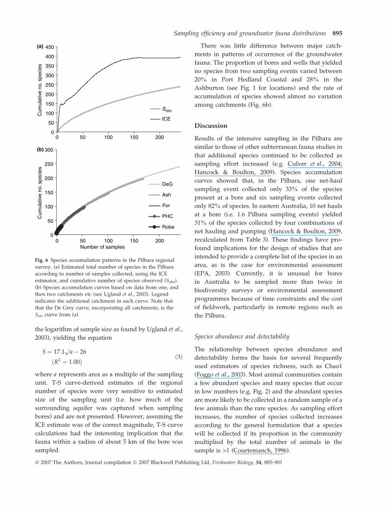
Regional species richness
Using a reduced matrix of 240 bores and wells that
yielded 239 species, the ICE estimator suggested that
about 400 species of groundwater fauna occur in the
Pilbara (Fig. 6a). This estimate omitted several groups
of animals that were excluded from analyses because
they are poorly resolved taxonomically in the Pilbara
and present identification difficulties. Extrapolating
ratio of collected and uncollected taxa (1.67) to the full
number of species known from the 240 bores (320)
provides a more realistic estimate that about 500–550
species occur in the Pilbara. A similar estimate was
obtained using the full regional data set.
The cumulative numbers of species at terminal
points of the catchment plots used to calculate a T-S
curve (Fig. 6b) showed a very strong linear relation-
ship with the square root of sample size (rather than
0
10
20
30
40
50
60
Pre-pumpnet haul
Post-pumpnet haul
Pump Net haul Net haul Net haul Pre-pumpnet haul
Pump Post-pumpnet haul
Net haul Net haul
14/11/02 4/04/03 11/05/04 21/10/04 11/11/04 14/05/05 6/08/05
Cum
ulat
ive
no. s
peci
es
Other species
Sample singletons
Fig. 5 Increase in cumulative number of species recorded at bore PSS016, and decrease in number of species recorded only once at the
site (referred to in legend as sample singletons), as sampling effort increased.
Table 2 Comparison of total groundwater fauna abundance
across sampling season (as month) using mixed-model A N O V AA N O V A
with sampling month being a fixed and site a random effect.
Abundance varied significantly across sites but not months
Source d.f.
Type III
sum of
squares
Mean
squares F P
Site 13 1153 88.7 15.3 <0.001
Month 6 68.5 11.4 1.97 0.08
Error 64 371 5.8
Table 3 Nearest neighbour and average distance to any other bore within each of the five catchments of the Pilbara compared with
distances between occurrences of site doubleton and tripleton species. Weighted averages were used to summarize within-catchment
data
Catchment
Bores and wells
Average inter-bore distances
(km)
Doubletons
Inter-occurrence distances
(km)
Tripletons
Inter-occurrence distances
(km)
n Nearest Average n Average Max. n Average Max.
1 Ashburton 132 7.5 151 11 44 146 1 67 67
2 De Grey River 112 7.0 123 2 22 22 1 47 47
3 Fortescue River 109 6.5 174 7 144 363 1 28 28
4 Port Hedland Coast 76 6.4 108 4 60 118 2 47 90
5 Onslow Coast 40 5.5 60 2 54 94 2 22 38
Within catchments 469 6.8 135 29 72 263 7 40 57
Across catchments 242 21 227 502 18 259 400
894 S. M. Eberhard et al.
� 2007 The Authors, Journal compilation � 2007 Blackwell Publishing Ltd, Freshwater Biology, 54, 885–901
the logarithm of sample size as found by Ugland et al.,
2003), yielding the equation
S ¼ 17:1p
a� 26
ðR2 ¼ 1:00Þð3Þ
where a represents area as a multiple of the sampling
unit. T-S curve-derived estimates of the regional
number of species were very sensitive to estimated
size of the sampling unit (i.e. how much of the
surrounding aquifer was captured when sampling
bores) and are not presented. However, assuming the
ICE estimate was of the correct magnitude, T-S curve
calculations had the interesting implication that the
fauna within a radius of about 5 km of the bore was
sampled.
There was little difference between major catch-
ments in patterns of occurrence of the groundwater
fauna. The proportion of bores and wells that yielded
no species from two sampling events varied between
20% in Port Hedland Coastal and 28% in the
Ashburton (see Fig. 1 for locations) and the rate of
accumulation of species showed almost no variation
among catchments (Fig. 6b).
Discussion
Results of the intensive sampling in the Pilbara are
similar to those of other subterranean fauna studies in
that additional species continued to be collected as
sampling effort increased (e.g. Culver et al., 2004;
Hancock & Boulton, 2009). Species accumulation
curves showed that, in the Pilbara, one net-haul
sampling event collected only 33% of the species
present at a bore and six sampling events collected
only 82% of species. In eastern Australia, 10 net hauls
at a bore (i.e. 1.6 Pilbara sampling events) yielded
31% of the species collected by four combinations of
net hauling and pumping (Hancock & Boulton, 2009,
recalculated from Table 3). These findings have pro-
found implications for the design of studies that are
intended to provide a complete list of the species in an
area, as is the case for environmental assessment
(EPA, 2003). Currently, it is unusual for bores
in Australia to be sampled more than twice in
biodiversity surveys or environmental assessment
programmes because of time constraints and the cost
of fieldwork, particularly in remote regions such as
the Pilbara.
Species abundance and detectability
The relationship between species abundance and
detectability forms the basis for several frequently
used estimators of species richness, such as Chao1
(Foggo et al., 2003). Most animal communities contain
a few abundant species and many species that occur
in low numbers (e.g. Fig. 2) and the abundant species
are more likely to be collected in a random sample of a
few animals than the rare species. As sampling effort
increases, the number of species collected increases
according to the general formulation that a species
will be collected if its proportion in the community
multiplied by the total number of animals in the
sample is >1 (Courtemanch, 1996).
(b)
0
50
100
150
200
250
300
Number of samples
Cum
ulat
ive
no. s
peci
es
DeG
Ash
For
PHC
Robe
(a)
0
50
100
150
200
250
300
350
400
450
0 50 100 150 200
0 50 100 150 200
Cum
ulat
ive
no. s
peci
es
Sobs
ICE
Fig. 6 Species accumulation patterns in the Pilbara regional
survey. (a) Estimated total number of species in the Pilbara
according to number of samples collected, using the ICE
estimator, and cumulative number of species observed (Sobs).
(b) Species accumulation curves based on data from one, and
then two catchments etc (see Ugland et al., 2003). Legend
indicates the additional catchment in each curve. Note that
that the De Grey curve, incorporating all catchments, is the
Sobs curve from (a).
Sampling efficiency and groundwater fauna distributions 895
� 2007 The Authors, Journal compilation � 2007 Blackwell Publishing Ltd, Freshwater Biology, 54, 885–901

We are unaware of previous studies of the relation-
ship between abundance and detectability for subter-
ranean animals, despite the sampling deficiencies and
the small numbers of animals collected in studies of
subterranean environments (e.g. Eberhard et al.,
2005b; Hahn & Matzke, 2005; Schneider et al., 2005),
making them more susceptible to effects on detect-
ability than studies of surface-water fauna. Using only
two abundance categories, this study showed that
species represented by high numbers of animals were
two or three times more likely to be collected in one
sampling event than species occurring at low abun-
dance (Fig. 4). In reality, the difference in collection
probabilities of the most, and least, abundant spe-
cies will be much greater and much of what has
previously been treated as stochastic variation in
species recovery can probably be explained in terms
of species abundances. Recognizing this will improve
our understanding of the structure of groundwater
fauna communities and improve interpretation of
sampling results.
FN rates
ESTIMATESESTIMATES has often been used to provide estimates
of the true number of species at a site, or in a region,
from which sampling efficiency can then be inferred.
Such estimates are unreliable at low sampling efforts
(Foggo et al., 2003) and, therefore, we explored use of
FN rates as an alternative method of examining
sampling efficiency. The FN rate calculated was based
on the assumption that all species present at a bore
were detected in at least one of the six sampling
events. However, this assumption is unlikely to be
correct for subterranean fauna, and other organisms
occurring in low abundance, as shown by this study
and Hancock & Boulton (2009).
A more accurate FN for all species can be calculated
by inserting the observed FN rate (0.392), derived
from eqn 1, into a formula provided by Tyre et al.
(2003) to generate collection probabilities that include
failure to collect a species
Lðyjp; qÞ ¼ pm
y
� �qyð1� qÞm�y
y > 0
ð4Þ
where 1 ) q is the FN rate; p is the probability that the
species utilized the site throughout sampling
(assumed ¼ 1); m is the number of sampling events
(6) and y is the number of times the species was
observed. For the all-species data set, the likelihood of
a species not being recorded in six samples was 0.05,
the revised FN rate was approximately 0.65, and
revised probability of a species being collected in a
single sample was 0.35. This is similar to the estimate
based on species accumulation curves (0.33). How-
ever, a discrepancy remained between estimates of the
detection probability of rare species based on the
revised FN rate and Chao2 (0.30 versus 0.23).
Regional heterogeneity
Species richness often exhibits heterogenous patterns
across regions (Ugland et al., 2003; Culver et al., 2004)
and taking heterogeneity into account when estimat-
ing regional species richness is likely to improve
accuracy. Unfortunately, the T-S curve method pro-
posed by Ugland et al. (2003) proved to be very
sensitive to assumptions about the area of aquifer that
was captured by sampling a bore. There is no
experimental information about the distance over
which groundwater fauna will move into bores but T-
S curve calculations suggested ingress occurs from the
surrounding 50–80 km2 of aquifer. This is a much larger
area than inferred in other studies (e.g. Malard et al.,
1997; Hahn & Matzke, 2005). While independent
confirmation is needed that the mobility suggested by
T-S curves is not a mathematical artefact, such mobility
has considerable ramifications for management of
groundwater fauna. In particular, re-colonization of
de-watered sites from surrounding areas may occur
quickly if animals can move several kilometres.
Colonization of bores
The extent to which the composition of groundwater
fauna in bores accurately reflects faunal composition
in surrounding ground water is an important, unre-
solved issue. Results to date are inconsistent, with
some studies suggesting bores provide biased sam-
ples and others implying a representative selection of
aquifer species is obtained (see Hahn & Matzke, 2005).
Bias may be caused by the differential attraction of
various species to bores because of their feeding and
habitat preferences, or by the physical exclusion of
larger species from bores.
Construction, slotting and screening methods for
bores vary considerably, and are unrecorded for most
896 S. M. Eberhard et al.
� 2007 The Authors, Journal compilation � 2007 Blackwell Publishing Ltd, Freshwater Biology, 54, 885–901

bores in the Pilbara, but bore attributes appear
unlikely to have had much effect on the number of
species collected from bores where net sampling
occurred. Down-hole video recordings showed iso-
pods of the genus Pygolabis, the largest groundwater
invertebrates in the Pilbara and measuring over 1 cm
(Keable & Wilson, 2006), moving freely in and out of
bores through slotting (Fig. 7c). Amphipods were also
observed swimming through slotting. Amphipods
and Pygolabis species were both observed entering
bores through small fissures at the base (Fig. 7a,b) and
below the casing (Fig. 7d) of bores. Furthermore,
Pygolabis or amphipods of the genera Nedsia, Pilbarus
or Chydaekata were recorded from a high proportion of
bores. The above evidence suggests there were few
impediments to colonization by larger species and
that any bias in species composition within bores,
relative to the surrounding aquifer, was more likely
because of factors associated with the enrichment of
bores (Hahn & Matzke, 2005).
Singletons and SREs
One of the defining characteristics of subterranean
fauna globally is the high level of regional and short-
range endemism. In Europe, subterranean fauna
usually comprises >50% SREs, with some regions
having >90% (Gibert & Deharveng, 2002), and high
proportions of SREs have been reported from ground-
water of the Australian arid zone (Cooper et al., 2002;
Harvey, 2002). Survey effort in the Pilbara is insuffi-
cient to make definitive statements about the propor-
tion of groundwater fauna that are SREs but,
nonetheless, it seems likely that very few species
collected at more than three sites in the regional
survey are SREs (range <10 000 km2). Fewer than 30%
of species represented by site tripletons and <50% of
site doubletons are likely to be SREs.
Assessing the proportion of species recorded as site
singletons that are likely to be SREs is difficult. About
85% of them were also sample singletons, which was
similar to the 88% expected if they had an average
collection probability of 0.23 (used in calculations
below). Average density of bores and wells in the
Pilbara survey was about 23/10 000 km2 and species
with a collection probability of 0.23 should have been
collected from more than one bore if their ranges were
‡10 000 km2 (probability of being collected two or three
times was >0.99 and 0.94, respectively). Thus, even
allowing for bore distribution being somewhat irregu-
lar within a catchment, most of the species recorded as
site singletons must have ranges <10 000 km2 and
qualify as SREs according to Harvey’s (2002) criterion,
unless they are restricted to groundwater habitats that
(a) (b)
(c) (d)
Fig. 7 Groundwater species entering
bores in the Pilbara from down-hole video
footage. (a & b) Amphipod (arrowed in a)
entering through small void in base of
bore PSS190 at 35 m depth in the Fortes-
cue Basin. (c) Pygolabis isopod entering
through slot of bore PSS172 at 7 m depth
in the Ashburton Basin. (d) Pygolabis iso-
pods entering under casing of bore PSS179
at 41 m depth in the Ashburton Basin.
Scale bar ¼ 1 cm.
Sampling efficiency and groundwater fauna distributions 897
� 2007 The Authors, Journal compilation � 2007 Blackwell Publishing Ltd, Freshwater Biology, 54, 885–901

we rarely sampled. If our assumptions about collection
probability and distribution of singletons in relation
with bore spacings are correct, then about 55% of
known Pilbara groundwater species are SREs. A true
picture of endemism in the Pilbara, however, must also
take into account the species we failed to collect.
Despite some small gaps in our sampling coverage,
most of these species would have been missed because
their ranges were £10 000 km2, which implies that
about 70% of all Pilbara groundwater species are SREs.
The proportion of SREs is, however, dependent on
the threshold criterion used. Harvey’s (2002) decision
to use a range of 10 000 km2 to define SREs was
arbitrary and we suggest it is rather large. It fails to
distinguish groundwater species with sub-regional
distributions that are secure from range-related
natural and anthropogenic threats from those species
with sufficiently localized distributions that most of
their population may be at risk from an activity such
as de-watering or from a pollution event. No project
involving below water table mining and groundwater
abstraction in the Pilbara has caused significant
groundwater drawdown beyond a 10 km2 radius of
pumping (Johnson & Wright, 2001), which equates to
an impact area of about 350 km2, and in most cases
the impact area has been <100 km2. Therefore, we
suggest that a more appropriate criterion for Pilbara
groundwater SREs is a range of <1000 km2. Mine
de-watering and groundwater extraction are unlikely
to threaten species with distributions at the upper end
of this range but a threshold of 1000 km2 represents a
precautionary approach and is of a scale that matches
natural barriers. Many Pilbara groundwater species
appear to be restricted to sections of hydrographic
basins, or tributaries within them, and to have ranges
of the order of 1000 km2 (see Finston et al., 2006;
Reeves, De Deckker & Halse, 2007).
In conclusion, high regional richness of ground-
water fauna is usually attributed to age of the
landscape, habitat fragmentation, SRE and existence
of suitable habitat (e.g. Christman & Culver, 2001;
Humphreys, 2001; Gibert & Deharveng, 2002). The
Pilbara is an old landscape with geological heteroge-
neity (McPhail & Stone, 2004) and >40% of known
Australian groundwater species have been recorded
from this region (Humphreys et al., 2005). Although
there is much still to be learned about the groundwa-
ter fauna of the Pilbara, the recently completed
regional survey is likely to have identified its major
characteristics and sub-regional hotspots. Results
from the net-sampled bores suggest that, as with
Slovenian caves (Culver et al., 2004), two rounds of
sampling is usually sufficient to identify Pilbara sites
that are rich in groundwater species. Continued
sampling is, however, required to document the full
richness of the sites. This was demonstrated at bore
PSS016 where 11 sampling events yielded three times
more species than collected in two events (Fig. 5).
Acknowledgments
Jessica Reeves and Ivana Karanovic identified all
ostracods in this study; Tom Karanovic identified
many of the copepods. Some species identifications
were confirmed by Adrian Pinder (oligochaetes) and
Buz Wilson (isopods). Advice on other groups was
provided by John Bradbury and Terrie Finston
(amphipods), Mark Harvey (mites) and Peter
Serov (bathynellids). We thank Dave Robertson for
calculating distances between bores, Lesley Gibson
for helpful advice, and Janine Gibert and two
anonymous referees for very constructive criticism
of the manuscript.
References
Boulton A.J., Humphreys W.F. & Eberhard S.M. (2003)
Imperilled subsurface waters in Australia: biodiver-
sity, threatening processes and conservation. Aquatic
Ecosystem Health and Management, 6, 41–54.
Bradbury J.H. (2000) Western Australian stygobiont
amphipods (Crustacea: Paramelitidae) from the Mt
Newman and Millstream regions. Records of the Western
Australian Museum Supplement, 60, 1–102.
Castellarini F., Dole-Oliver M.-J., Malard F. & Gibert J.
(2007a) Modelling the distributions of stygobionts in
the Jura Mountains (eastern France). Implications for
the protection of groundwaters. Diversity and Distribu-
tions, 13, 213–224.
Castellarini F., Dole-Oliver M.-J., Malard F. & Gibert J.
(2007b) Using environmental heterogeneity to assess
stygobiotic species richness in the French Jura region
with a conservation perspective. Fundamental and
Applied Limnology, 169, 69–78.
Caughley G. & Gunn A. (1996) Conservation Biology in
Theory and Practice. Blackwell Science, Oxford, pp. 459.
Christman M.C. & Culver D.C. (2001) The relationship
between cave biodiversity and available habitat. Jour-
nal of Biogeography, 28, 367–380.
898 S. M. Eberhard et al.
� 2007 The Authors, Journal compilation � 2007 Blackwell Publishing Ltd, Freshwater Biology, 54, 885–901

Coates D.J. & Atkins K.A. (2001) Priority setting and the
conservation of Western Australia’s diverse and highly
endemic flora. Biological Conservation, 97, 251–263.
Colwell R.K. (2005) EstimateS: statistical estimation of
species richness and shared species from samples,
version 7. User’s guide and application. (http://viceroy.
eeb.uconn.edu/estimates).
Colwell R.K. & Coddington J.A. (1994) Estimating
terrestrial biodiversity through extrapolation. Philo-
sophical Transactions of the Royal Society of London, Series
B, 345, 101–118.
Colwell R.K., Mao C.X. & Chang J. (2004) Interpolating,
extrapolating, and comparing incidence-based species
accumulation curves. Ecology, 85, 2717–2727.
Cooper S., Hinze S., Leys R., Watts C. & Humphreys W.
(2002) Islands under the desert: molecular systematics
and evolutionary origins of stygobitic water beetles
(Coleoptera: Dytiscidae) from central Western Austra-
lia. Invertebrate Systematics, 16, 589–598.
Courtemanch D.L. (1996) Commentary on the subsam-
pling procedures used for rapid bioassessments.
Journal of the North American Benthological Society, 15,
381–385.
Culver D.C. & Sket B. (2000) Hotspots of subterranean
biodiversity in caves and wells. Journal of Cave and
Karst Studies, 6, 11–17.
Culver D.C., Christman M.C., Sket B. & Trontelj P. (2004)
Sampling adequacy in an extreme environment: spe-
cies richness patterns in Slovenian caves. Biodiversity
and Conservation, 13, 1209–1229.
Danielopol D.L., Griebler C., Gunatilaka A. & Noten-
boom J. (2003) Present state and future prospects for
groundwater ecosystems. Environmental Conservation,
30, 104–130.
Dole-Olivier M.J., Castellarini F., Coineau N., Galassi
D.M.P., Mori N., Valdecasas A. & Gibert J. (2009)
Towards an optimal sampling strategy to
assess groundwater biodiversity: comparison
across six European regions. Freshwater Biology, 54,
777–796.
Dudgeon D., Arthington A.H., Gessner M.O. et al. (2006)
Freshwater biodiversity: importance, threats, status
and conservation challenges. Biological Reviews, 81,
163–182.
Eberhard S.M., Halse S.A. & Humphreys W.F. (2005a)
Stygofauna in the Pilbara region, north-west Western
Australia: a review. Journal of the Royal Society of
Western Australia, 88, 167–176.
Eberhard S.M., Halse S.A., Scanlon M.D., Cocking J.S. &
Barron H.J. (2005b) Assessment and conservation of
aquatic life in the subsurface of the Pilbara region,
Western Australia. In: Proceedings of an International
Symposium on World Subterranean Biodiversity (Ed.
J. Gibert), pp. 61–68. Villeurbanne, France, 8–10
December 2004. University of Lyon, France.
EPA (2003) Guidance for the Assessment of Environmental
Factors: Consideration of Subterranean Fauna in Ground-
water and Caves During Environmental Impact Assessment
in Western Australia. Guidance Statement 54. Western
Australian Environmental Protection Authority, Perth,
Australia.
Finston T.L., Johnson M.S., Humphreys W.F., Eberhard
S.M. & Halse S.A. (2006) Cryptic speciation in two
widespread subterranean amphipod genera reflects
historical drainage patterns in an ancient landscape.
Molecular Ecology, 16, 355–365.
Foggo A., Attrill M.J., Frost M.T. & Rowden A.A. (2003)
Estimating marine species richness: an evaluation of
six extrapolative techniques. Marine Ecology Progress
Series, 248, 15–26.
Gibert J. & Deharveng L. (2002) Subterranean ecosys-
tems: a truncated functional biodiversity. BioScience,
52, 473–481.
Hahn H.J. & Matzke D. (2005) A comparison of stygofa-
una communities inside and outside groundwater
bores. Limnologica, 35, 31–44.
Halse S.A., Scanlon M.D. & Cocking J.S. (2002) Do
springs provide a window to the groundwater fauna of
the Australian arid zone? In: Balancing the Groundwater
Budget: Proceedings of an International Groundwater
Conference, Darwin 2002 (Ed. D. Yinfoo), pp. 1–12.
International Association of Hydrogeologists, Darwin,
Australia.
Halse S.A., Shiel R.J., Storey A.W., Edward D.H.D.,
Lansbury I., Cale D.J. & Harvey M.S. (2000) Aquatic
invertebrates and waterbirds of wetlands and rivers of
the southern Carnarvon Basin, Western Australia.
Records of the Western Australian Museum Supplement,
61, 217–265.
Hancock P.J. & Boulton A.J. (2009) Sampling ground-
water fauna: efficiency of rapid assessment methods
tested in bores in eastern Australia. Freshwater Biology,
54, 902–917.
Harvey M. (2002) Short-range endemism among
the Australian fauna: some examples from non-
marine environments. Invertebrate Systematics, 16,
555–570.
Humphreys W.F. (2001) Groundwater calcrete aquifers
in the Australian arid zone: the context to an unfolding
plethora of stygal biodiversity. Records of the Western
Australian Museum Supplement, 64, 63–83.
Humphreys W.F., Watts C.H.S. & Bradbury J.H. (2005)
Emerging knowledge of diversity, distribution and
origins of some Australian stygofauna. In: Proceedings
of an International Symposium on World Subterranean
Biodiversity (Ed. J. Gibert), pp. 57–60. Villeurbanne,
Sampling efficiency and groundwater fauna distributions 899
� 2007 The Authors, Journal compilation � 2007 Blackwell Publishing Ltd, Freshwater Biology, 54, 885–901

France, 8–10 December 2004. University of Lyon,
France.
Johnson S.L. & Wright A.H. (2001) Central Pilbara
Groundwater Study. Hydrogeological Record Series HG8.
Department of Water, Perth, Australia.
Keable S.J. & Wilson G.D.F. (2006) New species of
Pygolabis Wilson 2003 (Isopoda, Tainisopidae, Crusta-
cea) from Western Australia. Zootaxa, 1116, 1–27.
Krishnamurthy K.V. (2003) Textbook of Biodiversity. Sci-
ence Publishers, Enfield. pp. 260.
Mace G.M. (1995) Classification of threatened species and
its role in conservation planning. In: Extinction Rates
(Eds J.H. Lawton & R.M. May), pp. 197–213. Oxford
University Press, Oxford.
Mace G., Masundire H., Baillie J. et al. (2005) Biodiver-
sity. In: Ecosystems and Human Well-being: Current State
and Trends, Vol. 1. Findings of the Condition and Trends
Working Group of the Millenium Ecosystem Assessment
(Eds R. Hassan, R. Scholes & N. Ash), pp. 77–122.
Island Press, Washington, D.C.
MacKenzie D.I., Nichols J.D., Lachman G.B., Droege S.,
Royle J.A. & Langtimm C.A. (2002) Estimating site
occupancy rates when detection probabilities are less
than one. Ecology, 83, 2248–2255.
Malard F., Reygrobellet J.-L., Laurent R. & Mathieu J.
(1997) Developments in sampling the fauna of deep
water-table aquifers. Archiv fur Hydrobiologie, 138, 401–
432.
Mauclaire L., Marmonier P. & Gibert J. (1998) Sampling
water and sediment in interstitial habitats: a compar-
ison of coring and pumping techniques. Archiv fur
Hydrobiologie, 142, 111–123.
McPhail M.K. & Stone M.S. (2004) Age and palaeoenvi-
ronmental constraints on the genesis of the Yandi
channel iron deposits, Marillana Formation, Pilbara,
northwestern Australia. Australian Journal of Earth
Sciences, 51, 497–520.
Paran F., Malard F., Mathieu J., Lafont M., Galassi D.M.P.
& Marmonier P. (2005) Distribution of groundwater
invertebrates along an environmental gradient in a
shallow water-table aquifer. In: Proceedings of an
International Symposium on World Subterranean Bio-
diversity (Ed. J. Gibert), pp. 99–106. Villeurbanne,
France, 8–10 December 2004. University of Lyon,
France.
Pinder A.M., Halse S.A., McRae J.M. & Shiel R.J. (2004)
Aquatic invertebrate assemblages of wetlands and
rivers in the Wheatbelt region of Western Australia.
Records of the Western Australian Museum Supplement,
67, 7–37.
Pipan T. & Culver D.C. (2005) Estimating biodiversity in
the epikarstic zone of a West Virginia cave. Journal of
Cave and Karst Studies, 67, 103–109.
Ponder W. & Colgan D.J. (2002) What makes a narrow-
range taxon? Insights from Australian freshwater
snails. Invertebrate Systematics, 16, 571–582.
Reeves J., De Deckker P. & Halse S.A. (2007) Ground-
water ostracods from the arid Pilbara region of
northwestern Australia: distribution and water chem-
istry. Hydrobiologia, 585, 99–118.
Rouch R. & Danielopol D.L. (1997) Species richness of
microcrustacea in subterranean freshwater habitats.
Comparative analysis and approximate evaluation.
Internationale Revue der gesamten Hydrobiologie, 82,
121–145.
Schneider K., Culver D.C., Hobbs H.H. & Fong D. (2005)
The blind misleading the blind: false negatives and
estimations of subterranean biodiversity. In: Proceed-
ings of an International Symposium on World Subter-
ranean Biodiversity (Ed. J. Gibert), p. 138.Villeurbanne,
France, 8–10 December 2004. University of Lyon,
France.
Tyre A.J., Tehumberg B., Field S.A., Niejalke D., Parris K.
& Possingham H.P. (2003) Improving precision and
reducing bias in biological surveys by estimating false
negative error rates in presence–absence data. Ecolog-
ical Applications, 13, 1790–1801.
Ugland K.I. & Gray J.S. (2004) Estimation of species
richness: analysis of the methods developed by Chao
and Karakassis. Marine Ecology Progress Series, 284, 1–8.
Ugland K.I., Gray J.S. & Ellingsen K.E. (2003) The
species-accumulation curve and estimation of species
richness. Journal of Animal Ecology, 72, 888–897.
(Manuscript accepted 28 July 2007)
Appendix 1 Taxonomic list of the 93 taxa collected
during repeat sampling of 14 bores in the Pilbara (see
Fig. 2). Many of the identifications are only to
morphospecies level. Species numbers relate to those
in Fig. 2
Species
numbers
Turbellaria
Turbellaria sp. 70
Nematoda
Nematoda sp. 3 24
Nematoda sp. 4 30
Nematoda sp. 11 23
Rotifera
Dissotrocha sp. 72
Gastropoda
Planorbidae sp. 42
Hydrobiidae sp. 22
900 S. M. Eberhard et al.
� 2007 The Authors, Journal compilation � 2007 Blackwell Publishing Ltd, Freshwater Biology, 54, 885–901

Appendix 1 (Continued)
Species
numbers
Oligochaeta
Hirudinea sp. 68
Aeolosoma sp. 3 59
Phreodrilus sp. WA32 26
Phreodrilidae sp. DVC 45
Phreodrilidae sp. SVC 64
Ainudrilus sp. WA27 54
Tubificidae sp. 1 83
Tubificidae sp. 2 29
Tubificidae sp. WA28 27
Dero nivea Aiyer 19
Pristina sp. WA3 69
Enchytraeidae sp. 2 25
Enchytraeidae sp. 1 86
Polychaeta
Nereidae sp. 31
Arachnida
Guineaxonopsis sp. S1 12
Arrenurus n. sp. 2 52
Peza sp. 41
Oribatida sp. 1 53
Ostracoda
Gomphodella hirsuta Karanovic 82
Limnocythere stationis Vavra 16
Limnocythere sp. 1 15
Candonopsis pilbarae Karanovic 88
Deminutiocandona aporia Karanovic 48
Deminutiocandona cf. atope Karanovic 66
Deminutiocandona aenigma Karanovic 44
Deminutiocandona stomachosa Karanovic 62
Humphreyscandona woutersi Karanovic &
Marmonier
80
Humphreyscandona sp. 2 75
Humphreyscandona ventosa Karanovic 67
Notacandona boultoni Karanovic & Marmonier 17
Origocandona posteriorecta Karanovic 18
Pilbaracandona colonia Karanovic & Marmonier 32
Pilbaracandona eberhardi Karanovic & Marmonier 33
Pilbaracandona kosmos Karanovic 85
Pilbaracandona temporaria Karanovic 39
Pilbaracandona rosa Karanovic 43
Areacandona mulgae Karanovic (11)
Areacandona lepte Karanovic 61
Areacandona cylindrata Karanovic 58
Areacandona triangulum Karanovic 55
Areacandona iuno Karanovic 91
Areacandona cf. sp. 1 37
Areacandona sp. 7 38
Areacandona astrepte Karanovic 50
Areacandona atomus Karanovic 10
Leicacandona carinata Karanovic 51
Leicacandona jimi Karanovic 14
Kencandona verrucosa Karanovic 13
Candonidae n. gen. 77
Appendix 1 (Continued)
Species
numbers
Syncarida
Bathynella sp. 21
Notobathynella sp. 47
Chilibathynella sp. 40
Atopobathynella sp. A 20
Thermosbaenacidae
Halosbaena tulki Poore & Humphreys 79
Copepoda
Mesocyclops brooksi De Laurentiis et al. 5
Inermipes sp. 2 4
Diacyclops einslei Karanovic 3
Diacyclops humphreysi s. str.
X unispinosus Karanovic
78
Diacyclops humphreysi humphreysi Karanovic 81
Diacyclops cocking Karanovic 76
Diacyclops scanloni Karanovic 90
Diacyclops sobeprolatus Karanovic 60
Halicyclops (Rochacyclops) rochi Karanovic 87
Orbuscyclops westaustraliensis Karanovic 6
Elaphoidella humphreysi Karanovic 84
Schizopera roberiveri Karanovic 46
Abnitocrella sp. 3 56
Archinitocrella newmanensis Karanovic 92
Parapseudoleptomesochra tureei Karanovic 65
Stygonitocrella bispinosa Karanovic 36
Stygonitocrella trispinosa Karanovic 63
Stygonitocrella unispinosa Karanovic 74
Parastenocaris jane Karanovic 35
Pseudectinosoma galassiae Karanovic 7
Amphipoda
Chydaekata sp. 73
Paramelitidae n. gen. 2
Paramelitidae sp. 9 28
Paramelitidae sp. 2 89
Nedsia sp. 93
Melitidae sp. 1 49
Bogidiellidae sp. 1
Isopoda
Speocirolana n. sp. 1 57
Pygolabis eberhardi Keable & Wilson 71
Pygolabis humphreysi Wilson 34
Pygolabis paraburdoo Keable & Wilson 9
Microcerberidae sp. 8
Sampling efficiency and groundwater fauna distributions 901
� 2007 The Authors, Journal compilation � 2007 Blackwell Publishing Ltd, Freshwater Biology, 54, 885–901
Top Related

Copyright © 2022 FDOKUMEN

