Download - Error analysis in the determination of the electron microscopical contrast transfer function parameters from experimental power Spectra

BioMed CentralBMC Structural Biology

ss
Open AcceMethodology articleError analysis in the determination of the electron microscopical contrast transfer function parameters from experimental power SpectraCarlos Oscar S Sorzano*1,2, Abraham Otero1, Estefanía M Olmos1 and José María Carazo2
Address: 1Escuela Politécnica Superior, Universidad San Pablo-CEU, Campus Urb. Montepríncipe s/n, E-28668 Boadilla del Monte, Madrid, Spain and 2Biocomputig Unit of the National Center of Biotechnology (CSIC), Madrid, Spain

Email: Carlos Oscar S Sorzano* - [email protected]; Abraham Otero - [email protected]; Estefanía M Olmos - [email protected]; José María Carazo - [email protected]

* Corresponding author

AbstractBackground: The transmission electron microscope is used to acquire structural information ofmacromolecular complexes. However, as any other imaging device, it introduces opticalaberrations that must be corrected if high-resolution structural information is to be obtained. Theset of all aberrations are usually modeled in Fourier space by the so-called Contrast TransferFunction (CTF). Before correcting for the CTF, we must first estimate it from the electronmicrographs. This is usually done by estimating a number of parameters specifying a theoreticalmodel of the CTF. This estimation is performed by minimizing some error measure between thetheoretical Power Spectrum Density (PSD) and the experimentally observed PSD. The high noisepresent in the micrographs, the possible local minima of the error function for estimating the CTFparameters, and the cross-talking between CTF parameters may cause errors in the estimated CTFparameters.

Results: In this paper, we explore the effect of these estimation errors on the theoretical CTF.For the CTF model proposed in [1] we show which are the most sensitive CTF parameters as wellas the most sensitive background parameters. Moreover, we provide a methodology to reveal theinternal structure of the CTF model (which parameters influence in which parameters) and toestimate the accuracy of each model parameter. Finally, we explore the effect of the variability inthe detection of the CTF for CTF phase and amplitude correction.

Conclusion: We show that the estimation errors for the CTF detection methodology proposedin [1] does not show a significant deterioration of the CTF correction capabilities of subsequentalgorithms. All together, the methodology described in this paper constitutes a powerful tool forthe quantitative analysis of CTF models that can be applied to other models different from the oneanalyzed here.

Published: 26 March 2009

BMC Structural Biology 2009, 9:18 doi:10.1186/1472-6807-9-18

Received: 18 September 2008Accepted: 26 March 2009

This article is available from: http://www.biomedcentral.com/1472-6807/9/18

© 2009 Sorzano et al; licensee BioMed Central Ltd. This is an Open Access article distributed under the terms of the Creative Commons Attribution License (http://creativecommons.org/licenses/by/2.0), which permits unrestricted use, distribution, and reproduction in any medium, provided the original work is properly cited.

of 16(page number not for citation purposes)

http://www.biomedcentral.com/1472-6807/9/18

http://creativecommons.org/licenses/by/2.0

http://www.ncbi.nlm.nih.gov/entrez/query.fcgi?cmd=Retrieve&db=PubMed&dopt=Abstract&list_uids=19321015

http://www.biomedcentral.com/

http://www.biomedcentral.com/info/about/charter/

BMC Structural Biology 2009, 9:18 http://www.biomedcentral.com/1472-6807/9/18

BackgroundThe transmission electron microscope distorts the struc-tural information contained in the electron micrographsby changing the amplitude of the Fourier coefficients at allspatial frequencies and flipping their phase at certainannular regions [2]. This effect is usually modeled in Fou-rier space by the Contrast Transfer Function (CTF), whichin turn has to be estimated from the electron micrographs.Normally, a theoretical model of the CTF is assumed andthe parameters defining this model are optimized so thatthe experimentally observed PSD and the theoreticallypredicted PSD coincide as much as possible [1,3-10].Therefore, the PSD has to be estimated first. This step istraditionally performed by the fast, although less accurate,periodogram averaging [10-13] or parametric methods,more accurate but much slower to compute [8,12]. Theestimated periodogram can be further enhanced [14] tohighlight the Thon rings and, therefore, facilitate the taskof fitting the parameters of the theoretical model.

Fully two-dimensional models multiply by three thenumber of parameters needed since each parameter isallowed to vary in two dimensions. For instance, the defo-cus is assumed to vary elliptically, thus three parametersare needed for its full description (major axis, minor axis,and the angle between the major axis and the coordinatehorizontal axis); the same applies to all parameters vary-ing in 2D. Moreover, rich physical models like the ones in[1,9,10] need many parameters to account for a pletorahof physical effects. Finally, as shown in [1], rich two-dimensional background models are needed to fullyaccount for the astigmatism introduced not only by theelectron microscope but also by the film scanner.

Overall, theoretical CTF models may end up with manyparameters demanding robust optimization algorithmsthat avoid local minima. Cross-talking between parame-ters cannot be avoided, ie, sometimes the same CTF can beobtained with two different sets of CTF parameters. More-over, the amount of noise present in the electron micro-graphs passes to the PSD estimates, no matter how muchaveraging is performed, and errors in the estimates of theCTF parameters are to be expected. Sensitivity analysis[15] is a branch of mathematics studying how errors at theinput of a mathematical model translate into errors at itsoutput.

In this paper, we propose to use sensitivity analysis toidentify those CTF parameters that have the strongestinfluence in the estimation on the CTF. Knowing this listof "sensitive" parameters, simpler models for the CTF canbe proposed (as will be shown in the Results Section, twoparameters of the CTF model analyzed can be safelyremoved). We also propose the use of bootstrap resam-pling to estimate the accuracy in the estimation of each

individual parameter and to reveal the internal structureof the model: which model parameters influence in agiven parameter, for instance, which are the modelparameters influencing the defoci? The bootstrap resam-pling also allows us to estimate the experimental distribu-tion of each CTF parameter. Confidence intervals for eachCTF parameter can be computed using these experimentaldistributions. We use these confidence intervals to iden-tify which parameters are not significantly different fromzero, and therefore can be omitted from the CTF model.Finally, we use Factor Analysis in order to further clarifythe internal structure of the CTF model (thanks to thisanalysis, the CTF parameters can be divided into differentgroups, each one accounting mainly for a different part ofthe CTF). In this work we apply the general principles ofsensitivity analysis to the identification of the most rele-vant parameters in the CTF model introduced by [1] aswell as their internal relationships and accuracy of theirestimates.

Moreover, we explore the effect of the variability in theestimation of the CTF parameters in subsequent algo-rithms for CTF correction. In particular, we analyzed itseffects on CTF phase correction and CTF amplitude correc-tion using the Iterative Data Refinement (IDR) [16]. Weshow that in our experiments, the estimation errors of theCTF detection performed in [1] does not significantlydeteriorates the CTF correction.

Results and discussionAs described in the Methods section, the average sensitiv-

ity of the CTF with respect to a given parameter ( , Eq.

21) is a measure of how variations in that parameter trans-late into variations of the CTF. In a similar manner we alsodefine the average sensitivity of the PSD and the averagesensitivity of the first zero of the CTF with respect to agiven parameter. In the following sections we present anddiscuss our results.

Results

To estimate the sensitivity of the CTF on the modelparameters we used two sets of experimental images (LTagand GltS) corresponding to samples embedded in ice withno carbon. The LTag images correspond to the Large Tantigen [17,18], while the GltS images correspond to theGlutamate synthase [19]. The LTag images had a samplingrate of 5.6 Å per pixel while the GltS images were digitizedwith a pixel size of 1.59 Å. The two datasets used in thispaper are the same ones used in [1]. In all, we studied thesensitivity of the parameters using a total of 217 micro-graphs. The rationale for employing two distinct datasetsis not to bias the statistical analysis by using a single type

SH



of micrographs. The fact that both datasets have very dif-ferent sampling rates helps in the analysis of the effect ofthe sampling rate. The average sensitivity of the CTF withrespect to a given parameter (Eq. 21) was evaluated as fol-lows. For each micrograph and parameter, the CTF wasstudied with the value estimated by the CTF fitting pro-

gram ( ) [1]. Then, we perturbed each parameter individ-

ually by a small amount ( ) as described in the

Methods section in order to test its influence in the CTF.In particular, we studied variations of -20%, -10%, -5%, -2%, -1%, 1%, 2%, 5%, 10%, and 20% (the expected valuein Eq. 21 was computed for each variation and the result-ing sensitivities were averaged). For a particular variation

of the parameter ( ), we computed the integral in Eq.

21. The set of all perturbations and all micrographs empir-ically defined the statistical distribution of the sensitivityover which an ensemble average was taken.

The analysis carried out in the "Sensitivity analysis" Sec-tion for the CTF can be analogously be performed on thetheoretical PSD (Eq. 1) simply by replacing H in that sec-tion by P S Dtheoretical. The corresponding sensitivity will be

referred to as . In the same way, the sensitive analysis

can also be performed on the first zero of the CTF (that isthe frequency of the first sign change of the CTF; since theCTF is a 2D function, we will measure the sensitivity of theaverage of the first zero along all possible directions in2D). The corresponding sensitivity of this average first

zero will be referred to as . Summarizing, the CTF

sensitivity is analyzed according to three different meas-ures: the average sensitivity of the CTF itself as is com-

puted in the "Sensitivity analysis" Section ( ); the

average sensitivity of the theoretical PSD ( ); and the

average sensitivity of the frequency of the first zero along

all possible directions ( ). The CTF sensitivity results

are summarized in Table 1. In each case, the sensitivityvalues are arranged in decreasing order.

The highest values of sensitivity are found in . Interest-

ingly, within this measure, the most significant parameteris the microscope voltage (V) that is a user suppliedparameter. Not surprisingly, the energy spread of the elec-

trons ( ) is a related magnitude and is also a parameter

with a high sensitivity. The next two most sensitive param-eters are the defoci and the chromatic aberration.

Considering , parameters from the background PSD

(sm, sM, b and KG) are by far the most sensitive. Of the CTF

parameters, only the microscope voltage and the defoci

have a significant weight. As expected, in the case of ,

the most sensitive values defining the first zero of the CTFare the microscope voltage V, the defoci and the fractionof electrons being scattered Q0.

We obtain a relative sensitivity of each parameter dividingeach sensitivity column by its maximum value and multi-plying by 100 (data shown in Table 1). Adding all relativesensitivities (data shown in Table 2) we can have an ideaof which are the most important model parametersregarding the three quantities studied in this article (CTF,PSD and first zero of the CTF). By far the most importantparameters are the microscope voltage and the defoci.Next, we find four parameters defining the backgroundPSD (sm, sM, b and KG). Finally, we have the fraction ofelectrons being scattered Q0 (a parameter affecting the firstzero of the CTF) and the chromatic aberration (a parame-ter mostly affecting the CTF envelope decay). The previousresults seems to point out that there are "redundant" orless important parameters in our PSD model. To test up towhich degree this statement is true, we randomly choseone of the micrographs and estimated several simplifiedPSD models. The full model has 29 parameters out ofwhich 27 have to be estimated (the microscope voltage Vand its spherical aberration Cs are assumed to be given).The different simplified models proceed by removingparameters from the full model following an order indi-cated by ascending sensitiveness: less sensitive parametersare removed first (however, they are removed in "blocks"of related parameters). We explored 3 different simplifiedmodels:

1. Simplified model 1: Since the CTF is usually com-puted on non-drifted images and as shown by the sen-sitivity analysis the PSD is not very sensitive to the driftparameters (ΔF and ΔR), our simplified model 1 doesnot estimate these two parameters and sets them to 0.This model has a total of 25 parameters to be esti-mated.

2. Simplified model 2: The last step of the PSD estima-tion is the computation of the subtractive Gaussianparameters (Kg, cM, cm, θg, gM and gm). In our experiencethis last Gaussian helps to accurately fit the low passfrequencies. However, as shown by the sensitive anal-ysis, the theoretical PSD is not too sensitive to theseparameters, so we also estimated a simplified modelwithout this last Gaussian (and without the parame-ters already removed in the Simplified model 1). Thereis a total of 19 parameters to be estimated.

x̂Δxx

Δxx

SPSD

Szero

SH

SPSD

Szero

SH

ΔVV

SPSD

Szero



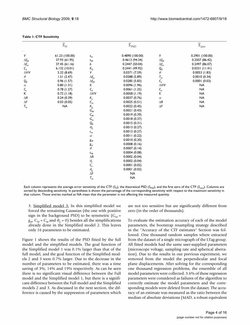
3. Simplified model 3: In this simplified model weforced the remaining Gaussian (the one with positivesign in the background PSD) to be symmetric (GM =gm, CM = Cm and θG = 0) besides all the simplificationsalready done in the Simplified model 2. This leavesonly 16 parameters to be estimated.

Figure 1 shows the results of the PSD fitted by the fullmodel and the simplified models. The goal function ofthe Simplified model 1 was 0.1% larger than that of thefull model, and the goal function of the Simplified mod-els 2 and 3 were 0.7% larger. Due to the decrease in thenumber of parameters to be estimated, there was a timesaving of 3%, 14% and 19% respectively. As can be seenthere is no significant visual difference between the Fullmodel and the Simplified model 1, but there is a signifi-cant difference between the Full model and the Simplifiedmodels 2 and 3. As discussed in the next section, the dif-ference is caused by the suppression of parameters which

are not too sensitive but are significantly different fromzero (in the order of thousands).

To evaluate the estimation accuracy of each of the modelparameters, the bootstrap resampling strategy describedin the "Accuracy of the CTF estimates" Section was fol-lowed. One thousand random samples where extractedfrom the dataset of a single micrograph of the LTag group.All fitted models had the same user-supplied parameters(microscope voltage, sampling rate and spherical aberra-tion). Due to the results in our previous experiment, weremoved from the model the perpendicular and focalplane displacements. After solving for the correspondingone thousand regression problems, the ensemble of allmodel parameters were collected. 3.6% of these regressionparameters were considered as failures of the algorithm tocorrectly estimate the model parameters and the corre-sponding models were deleted from the dataset. The accu-racy of an estimate was measured as the ratio between themedian of absolute deviations (MAD, a robust equivalent

Table 1: CTF Sensitivity

V 61.23 (100.00) sm 0.4890 (100.00) V 0.2901 (100.00)ΔfM 37.93 (61.95) sM 0.4613 (94.34) ΔfM 0.2507 (86.42)Δfm 37.45 (61.16) b 0.2447 (50.04) Δfm 0.2497 (86.07)Ca 6.132 (10.01) KG 0.2441 (49.92) Q0 0.0331 (11.41)ΔV/V 5.32 (8.69) V 0.0371 (7.59) θ 0.0053 (1.83)θ 1.51 (2.47) Δfm 0.0288 (5.89) Tm 0.0010 (0.34)Q0 0.96 (1.57) ΔfM 0.0285 (5.83) Cs 0.0001 (0.03)α 0.80 (1.31) K 0.0096 (1.96) ΔV/V NACs 0.78 (1.27) Ca 0.0061 (1.25) Ca NAK 0.72 (1.18) ΔV/V 0.0058 (1.19) K NAΔR 0.24 (0.39) Ks 0.0037 (0.76) α NAΔF 0.03 (0.05) Cm 0.0025 (0.51) ΔR NATm NA Kg 0.0022 (0.45) ΔF NA

GM 0.0021 (0.43)CM 0.0019 (0.39)Gm 0.0018 (0.37)Q0 0.0015 (0.31)θG 0.0013 (0.27)cm 0.0013 (0.27)α 0.0011 (0.22)gM 0.0010 (0.20)gm 0.0008 (0.16)θ 0.0007 (0.14)cM 0.0004 (0.08)ΔR 0.0002 (0.04)θs 0.0002 (0.04)Cs 0.0001 (0.02)θg 0.0001 (0.02)ΔF NATm NA

Each column represents the average error sensitivity of the CTF (SH), the theoretical PSD (SPSD), and the first zero of the CTF (Szero). Columns are sorted by descending sensitivity. In parenthesis is shown the percentage of the corresponding sensitivity with respect to the maximum sensitivity in that column. Those entries marked as NA mean that the parameter is not affecting the measured quantity.

SH SPSD Szero




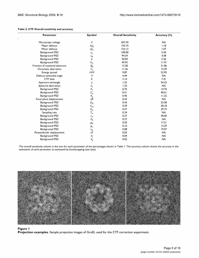
Table 2: CTF Overall sensitivity and accuracy

Parameter Symbol Overall Sensitivity Accuracy (%)

Microscope voltage V 207.59 NAMajor defocus ΔfM 154.19 1.18Minor defocus Δfm 153.13 1.07

Background PSD sm 100.00 5.50Background PSD sM 94.34 4.38Background PSD b 50.04 5.26Background PSD KG 49.92 11.91

Fraction of scattered electrons Q0 13.28 21.86Chromatic aberration Ca 11.26 14.29

Energy spread ΔV/V 9.87 52.95Defocus azimuthal angle θ 4.44 NA

CTF Gain K 3.14 7.41Aperture semiangle α 1.53 54.23Spherical aberration Cs 1.33 NA

Background PSD Ks 0.76 14.70Background PSD Cm 0.51 40.61Background PSD Kg 0.45 11.22

Focal plane displacement ΔR 0.43 NABackground PSD GM 0.43 23.58Background PSD CM 0.39 38.18Background PSD Gm 0.37 29.72

Sampling rate Tm 0.34 NABackground PSD cm 0.27 40.60Background PSD θG 0.27 NABackground PSD gM 0.20 17.51Background PSD gm 0.16 13.29Background PSD cM 0.08 19.07

Perpendicular displacement ΔF 0.05 NABackground PSD θs 0.04 NABackground PSD θg 0.02 NA

The overall sensitivity column is the sum for each parameter of the percentages shown in Table 1. The accuracy column shows the accuracy in the estimation of each parameter as estimated by bootstrapping (see text).

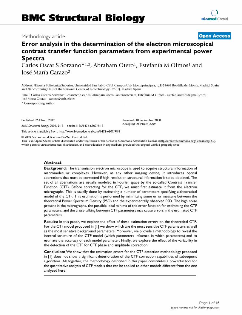
Projection examplesFigure 1Projection examples. Sample projection images of GroEL used for the CTF correction experiment.

BM

C S

truct

ural

Bio

logy

200

9, 9

:18

http

://w

ww

.bio

med

cent

ral.c

om/1

472-

6807

/9/1

8

Page

6 o

f 16

(pag

e nu

mbe

r not

for c

itatio

n pu

rpos

es)

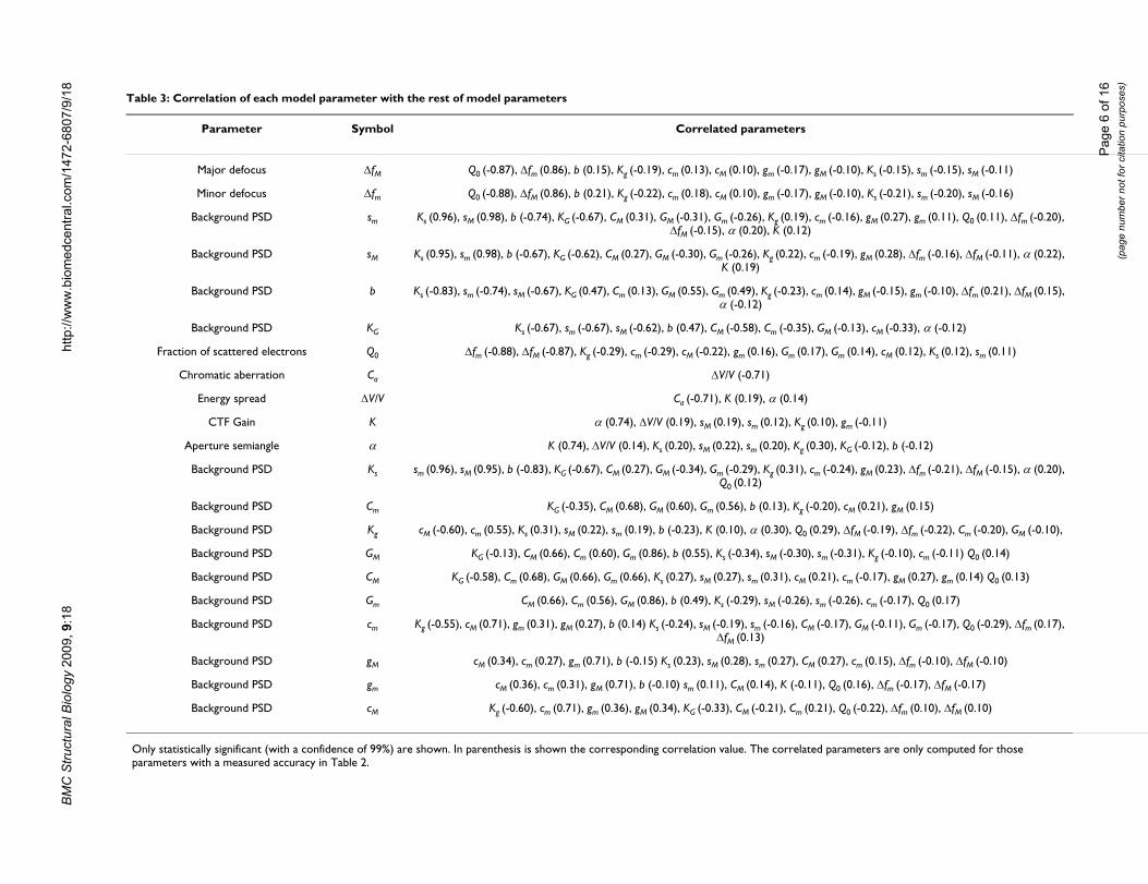
Table 3: Correlation of each model parameter with the rest of model parameters

Parameter Symbol Correlated parameters

Major defocus ΔfM Q0 (-0.87), Δfm (0.86), b (0.15), Kg (-0.19), cm (0.13), cM (0.10), gm (-0.17), gM (-0.10), Ks (-0.15), sm (-0.15), sM (-0.11)

Minor defocus Δfm Q0 (-0.88), ΔfM (0.86), b (0.21), Kg (-0.22), cm (0.18), cM (0.10), gm (-0.17), gM (-0.10), Ks (-0.21), sm (-0.20), sM (-0.16)

Background PSD sm Ks (0.96), sM (0.98), b (-0.74), KG (-0.67), CM (0.31), GM (-0.31), Gm (-0.26), Kg (0.19), cm (-0.16), gM (0.27), gm (0.11), Q0 (0.11), Δfm (-0.20), ΔfM (-0.15), α (0.20), K (0.12)

Background PSD sM Ks (0.95), sm (0.98), b (-0.67), KG (-0.62), CM (0.27), GM (-0.30), Gm (-0.26), Kg (0.22), cm (-0.19), gM (0.28), Δfm (-0.16), ΔfM (-0.11), α (0.22), K (0.19)

Background PSD b Ks (-0.83), sm (-0.74), sM (-0.67), KG (0.47), Cm (0.13), GM (0.55), Gm (0.49), Kg (-0.23), cm (0.14), gM (-0.15), gm (-0.10), Δfm (0.21), ΔfM (0.15), α (-0.12)

Background PSD KG Ks (-0.67), sm (-0.67), sM (-0.62), b (0.47), CM (-0.58), Cm (-0.35), GM (-0.13), cM (-0.33), α (-0.12)

Fraction of scattered electrons Q0 Δfm (-0.88), ΔfM (-0.87), Kg (-0.29), cm (-0.29), cM (-0.22), gm (0.16), Gm (0.17), Gm (0.14), cM (0.12), Ks (0.12), sm (0.11)

Chromatic aberration Ca ΔV/V (-0.71)

Energy spread ΔV/V Ca (-0.71), K (0.19), α (0.14)

CTF Gain K α (0.74), ΔV/V (0.19), sM (0.19), sm (0.12), Kg (0.10), gm (-0.11)

Aperture semiangle α K (0.74), ΔV/V (0.14), Ks (0.20), sM (0.22), sm (0.20), Kg (0.30), KG (-0.12), b (-0.12)

Background PSD Ks sm (0.96), sM (0.95), b (-0.83), KG (-0.67), CM (0.27), GM (-0.34), Gm (-0.29), Kg (0.31), cm (-0.24), gM (0.23), Δfm (-0.21), ΔfM (-0.15), α (0.20), Q0 (0.12)

Background PSD Cm KG (-0.35), CM (0.68), GM (0.60), Gm (0.56), b (0.13), Kg (-0.20), cM (0.21), gM (0.15)

Background PSD Kg cM (-0.60), cm (0.55), Ks (0.31), sM (0.22), sm (0.19), b (-0.23), K (0.10), α (0.30), Q0 (0.29), ΔfM (-0.19), Δfm (-0.22), Cm (-0.20), GM (-0.10),

Background PSD GM KG (-0.13), CM (0.66), Cm (0.60), Gm (0.86), b (0.55), Ks (-0.34), sM (-0.30), sm (-0.31), Kg (-0.10), cm (-0.11) Q0 (0.14)

Background PSD CM KG (-0.58), Cm (0.68), GM (0.66), Gm (0.66), Ks (0.27), sM (0.27), sm (0.31), cM (0.21), cm (-0.17), gM (0.27), gm (0.14) Q0 (0.13)

Background PSD Gm CM (0.66), Cm (0.56), GM (0.86), b (0.49), Ks (-0.29), sM (-0.26), sm (-0.26), cm (-0.17), Q0 (0.17)

Background PSD cm Kg (-0.55), cM (0.71), gm (0.31), gM (0.27), b (0.14) Ks (-0.24), sM (-0.19), sm (-0.16), CM (-0.17), GM (-0.11), Gm (-0.17), Q0 (-0.29), Δfm (0.17), ΔfM (0.13)

Background PSD gM cM (0.34), cm (0.27), gm (0.71), b (-0.15) Ks (0.23), sM (0.28), sm (0.27), CM (0.27), cm (0.15), Δfm (-0.10), ΔfM (-0.10)

Background PSD gm cM (0.36), cm (0.31), gM (0.71), b (-0.10) sm (0.11), CM (0.14), K (-0.11), Q0 (0.16), Δfm (-0.17), ΔfM (-0.17)

Background PSD cM Kg (-0.60), cm (0.71), gm (0.36), gM (0.34), KG (-0.33), CM (-0.21), Cm (0.21), Q0 (-0.22), Δfm (0.10), ΔfM (0.10)

Only statistically significant (with a confidence of 99%) are shown. In parenthesis is shown the corresponding correlation value. The correlated parameters are only computed for those parameters with a measured accuracy in Table 2.


of the standard deviation) and the median of the absolutevalue of the parameter being considered (a robust equiva-lent of the mean). Working with medians is a robust wayof estimating the central position of a distribution. Theaccuracy of the value of the goal function being mini-mized in [1] of the remaining 97.4% bootstrapped sam-ples was 0.5%. This low value indicates that the remainingbootstrapped models were quite homogeneous withrespect to the regression error. The accuracy of eachparameter was estimated and the resulting values arelisted in Table 2. Those entries with NA indicate that theaccuracy was not available in this case because the param-eter is supplied by the user, or the parameter has not beenestimated (displacements), or the parameter is meaning-less in this case (the image used for the example was notastigmatic and therefore the angles of the ellipses involvedin the model can take any value).

The analysis of the empirical distribution of each parame-ter computed by the bootstrap showed that the confi-dence interval of 95% of none of the parameters (exceptthe azimuthal angle) included the zero value. This meansthat we can reject the hypothesis with a 95% confidencelevel that any of the parameters was really null, and there-fore the corresponding parameter could have beenremoved from the regression. The bootstrapped ensemblealso allows the estimation of pairwise correlation coeffi-cients. Tables 3 and 4 show for each model parameter theset of parameters which are significantly correlated to itwith a confidence of 99%. The tables also show the corre-sponding correlation coefficients. It can be seen that thedifferent coefficients can be grouped in subgroups of largecorrelations. To identify these subgroups we used factoranalysis. We used ten factors for the decomposition andkept only the first seven since their associated eigenvaluewas larger than 1. Table 5 shows those factor loadingsgreater than 0.5 for each factor (ie, those CTF parametersthat correlate more than 0.5 with the factor). It can be seenhow the factor loadings create a partition of the modelparameters into subgroups that are strongly correlated

among each other. In the Discussion Section we proposean interpretation of each factor in terms of the differentaspects of the CTF (different kinds of envelopes, the idealCTF, and the different frequency ranges of the backgroundPSD).

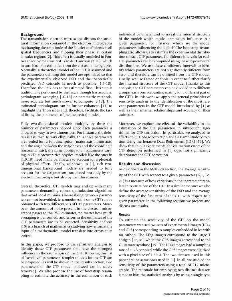
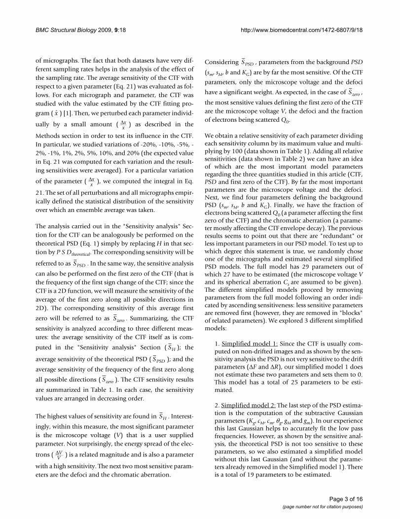
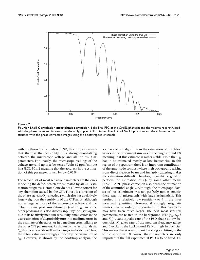
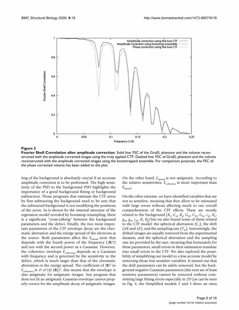
Finally, we used the bootstrapped ensemble to evaluatethe effect of the variability of the CTF detection in the CTFcorrection capabilities of subsequent algorithms, particu-larly, those of CTF phase correction and CTF amplitudecorrection through IDR. For exploring this effect we used97.4% CTFs considered to be non-failures of the CTFdetection algorithm (see description of the bootstrapensemble experiment). One of them was selected to be thetrue underlying CTF, while the rest were used as estimatesof this true CTF. As many projections as good CTF in theensemble were simulated of the GroEl atomic structure[20] (PDB entry code: 1GRL) with a random angular dis-tribution, a sampling rate of 2 Å/pixel. Noise was addedwith a final Signal-to-Noise Ratio (SNR) of 1/3 (see Fig.1). We corrected the CTF phase using the truly appliedCTF and its pretended bootstrap estimates (one differentestimate for each projection). We compared the FourierShell Correlation (FSC, [21]) of the volume reconstructedout of each one of these different corrections with respectto the atomic model (see Fig. 2). We also corrected theCTF amplitude using IDR with a relaxation factor of 1.8.After 10 iterations we did not observe any furtherimpShould we haverovement of the FSC. The FSC of thevolumes reconstructed using the truly applied CTF andthe pretended bootstrap estimates are shown in Fig. 3.Note that in this experiment we used a single defocusvalue in the set of images used for reconstruction. This wasdone with the aim of isolating the effect of the miscor-rected phase flips. The use of more defoci in the datasetwould have translated in results more difficult to interpretsince the zeros of one defocus group would have beenmasked by other defocus groups having a larger CTF valueat that frequency. It is expected that if the effect of miscor-recting the phase of a single defocus groups is negligible,the combined effect of miscorrecting each defocus groupindependently is also negligible on the final reconstruc-tion.

DiscussionFrom the experiments performed, it turns out that themost important parameter when dealing with the CTF isthe microscope voltage. This fact will certainly not cometo a surprise to any practitioner in the field, but it clearlystress the point that small inaccuracies in its provision(and most CTF estimation algorithms rely on the user pro-viding manually this value rather than automatically cal-culating it) result in large variations in the CTF relatedquantities. Since the CTF estimation algorithms try to fitas much as possible the experimentally observed PSD

Table 4: Factor loadings greater than 0.5 for the first seven factors of a factor analysis with ten factors of the bootstrapped ensemble of model parameters

Factor Loadings greater than 0.5

Factor 1 sM (0.98), sm (0.97), Ks (0.96), KG (-0.75), b (-0.73)Factor 2 CM (0.90), GM (0.87), Gm (0.84), Cm (0.72)Factor 3 Q0 (-0.94), ΔfM (0.92), Δfm (0.92)Factor 4 cM (0.83), cm (0.80), Kg (-0.76)Factor 5 K (0.94), α (0.87)Factor 6 gM (0.96), gm (0.74)Factor 7 Ca (-0.99), ΔV/V (0.72)

Each row shows which are the parameters correlating more than 0.5 with the factor heading the row. We show in parenthesis the corresponding correlation.


http://www.rcsb.org/pdb/cgi/explore.cgi?pdbId=1GRL


with the theoretically predicted PSD, this probably meansthat there is the possibility of a strong cross-talkingbetween the microscope voltage and all the rest CTFparameters. Fortunately, the microscope readings of thevoltage are valid up to a few tens of Volts (2 ppm/minutein a JEOL 3011) meaning that the accuracy in the estima-tion of this parameter is well below 0.01%.

The second set of most sensitive parameters are the onesmodeling the defoci, which are estimated by all CTF esti-mation programs. Defoci alone do not allow to correct forany aberration caused by the CTF. For a 1D correction ofthe phase, at least Q0 is needed (which also has a relativelylarge weight on the sensitivity of the CTF zeros, althoughnot as large as those of the microscope voltage and thedefoci). Some programs estimate Q0 although in someother programs it is also directly input by the user. Again,due to its relatively medium sensitivity, small errors in theuser estimation of Q0 probably turn into medium errors inthe estimate of the zeros, or in a medium cross-talking tothe other CTF parameters. As shown by the factor analysis,Q0 changes correlate well with changes in the defoci. Thus,the defoci values are strongly affected by the estimation ofQ0. However, as shown by the bootstrap analysis, the

accuracy of our algorithm in the estimation of the defocivalues in the experiment run was in the range around 1%meaning that this estimate is rather stable. Note that Q0has to be estimated mostly at low frequencies. In thisregion of the spectrum there is an important contributionof the amplitude contrast where high background arisingfrom direct electron beam and inelastic scattering makesthe estimation difficult. Therefore, it might be good toperform the estimation of Q0 by some other means[22,23]. A 2D phase correction also needs the estimationof the azimuthal angle θ. Although, the micrograph data-set of our experiment was not perfectly non-astigmatic,there was no micrograph with large astigmatism. Thisresulted in a relatively low sensitivity to θ in the threemeasured quantities. However, if strongly astigmaticimages were recorded, the sensitivity to this parametermay have been much larger. The next most sensitiveparameters are related to the background PSD (sm, sM, band KG). smand sM take care of the PSD shape at low fre-quencies, KG takes care of the medium frequency range,and b explains the background PSD at high frequencies.This means that it is important to do a good fitting in thewhole spectrum. Of course, these parameters are onlyimportant if the full experimental PSD is to be fitted. Fit-

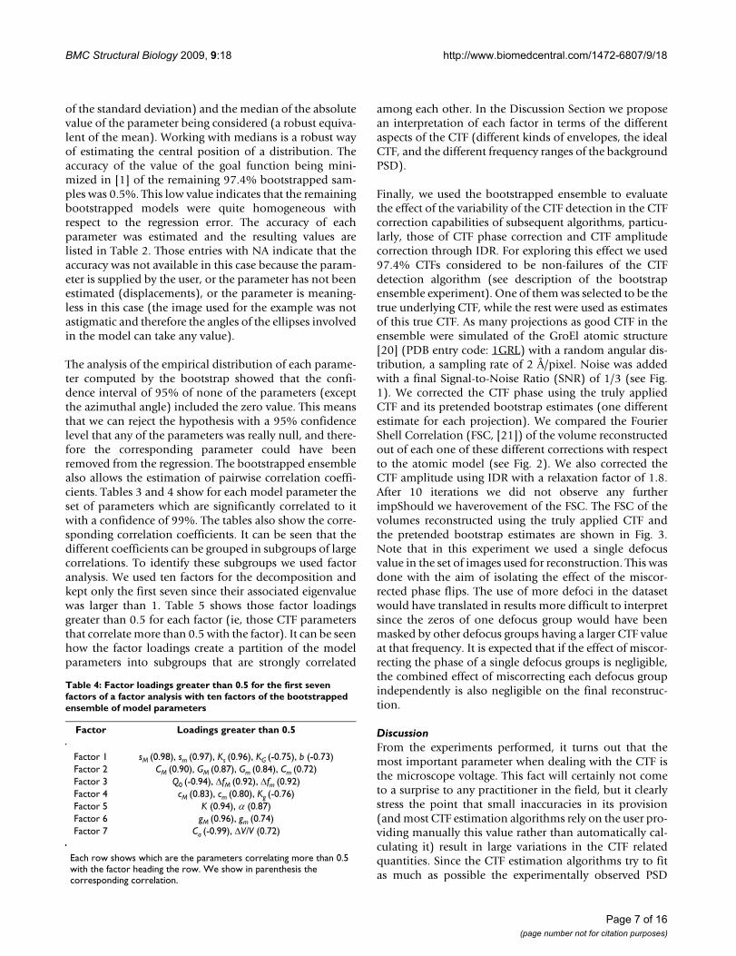
Fourier Shell Correlation after phase correctionFigure 2Fourier Shell Correlation after phase correction. Solid line: FSC of the GroEL phantom and the volume reconstructed with the phase corrected images using the truly applied CTF. Dashed line: FSC of GroEL phantom and the volume recon-structed with the phase corrected images using the bootstrapped ensemble.



ting of the background is absolutely crucial if an accurateamplitude correction is to be performed. The high sensi-tivity of the PSD to the background PSD highlights theimportance of a good background fitting or backgroundsubtraction. Those programs that estimate the CTF zerosby first subtracting the background need to be sure thatthe subtracted background is not modifying the positionsof the zeros. As is shown by the internal structure of theregression model revealed by bootstrap resampling, thereis a significant "cross-talking" between the backgroundparameters and the defoci. Finally, the two most impor-tant parameters of the CTF envelope decay are the chro-matic aberration and the energy spread of the electrons atthe source. Both parameters affect the Espread term thatdepends with the fourth power of the frequency (|R|4)and not with the second power as a Gaussian. However,the coherence envelope Ecoherence depends as a Gaussianwith frequency and is governed by the sensitivity to thedefoci, which is much larger than that of the chromaticaberration or the energy spread. The coefficient of |R|2 inEcoherence is π2 α2|Δf (R)|2, this means that the envelope isalso astigmatic for astigmatic images. Any program thatdoes not fit an astigmatic Gaussian envelope cannot prop-erly correct for the amplitude decay of astigmatic images.

On the other hand, Espread is not astigmatic. According tothe relative sensitivities, Ecoherence is more important thanEspread.

On the other extreme, we have identified variables that arenot so sensitive, meaning that they allow to be estimatedwith large errors without affecting much to our overallcomprehension of the CTF effects. These are mostlyrelated to the background (Ks, Cm, Kg, GM, CM, Gm, cm, θG,gM, gm, cM, θs, θg) but we also found some of them relatedto the CTF model: the spherical aberration (Cs), the drift(ΔR and ΔF), and the sampling rate (Tm). Interestingly, thedrifted images are usually removed from the experimentaldatasets, and the spherical aberration and the samplingrate are provided by the user, meaning that fortunately forthese parameters, small errors in their estimation translateinto small errors in the CTF. We also explored the possi-bility of simplifying our model to a less accurate model byremoving those less sensitive variables. It turned out thatthe drift parameters can be safely removed, but the back-ground negative Gaussian parameters (the next set of leastsensitive parameters) cannot be removed without com-mitting large fitting errors especially in 2D (as can be seenin Fig. 4, the Simplified models 2 and 3 show an extra

Fourier Shell Correlation after amplitude correctionFigure 3Fourier Shell Correlation after amplitude correction. Solid line: FSC of the GroEL phantom and the volume recon-structed with the amplitude corrected images using the truly applied CTF. Dashed line: FSC of GroEL phantom and the volume reconstructed with the amplitude corrected images using the bootstrapped ensemble. For comparison purposes, the FSC of the phase corrected volume has been added to the plot.



Thon ring that is not present in the experimental PSD).The reason for this is that the values of gM and gm are 2,256and 1,432 respectively. Having a low sensitivity meansthat you can commit small errors around the nominal val-ues without committing large errors in the function beingstudied, but it does not mean that the corresponding termcan be completely removed. This is confirmed by the 95%confidence intervals computed through the experimentalparameter distribution estimated by bootstrapping. Sincethe null hypothesis that any of the regression parametersis zero has been rejected for all parameters (except the azi-muthal angle), we conclude that all parameters in ourmodel really explain a part of the PSD behavior. It is alsointeresting to see how a background term as the subtrac-tive Gaussian influences the envelope parameters so thatwhen this Gaussian is removed, the envelope is such thatan extra ring is made visible.

We also explored a methodology to determine the accu-racy in the estimation of each parameter. For this we madeuse of bootstrap resampling to build an empirical distri-bution of each parameter. From this distribution we wereable to estimate the accuracy in each parameter. It is inter-esting to see that under similar fitting conditions (theaccuracy of the goal function of the regression was 0.5%meaning that all the bootrstrapped models were similar inexplanation power), the most important parameters arevery precisely estimated (1% in the case of the defoci, andabout 5% in the case of sm, sM and b). The rest of parame-ters are much less centered around a central value and canvary much more (some of them like the aperture semian-gle can vary up to 54%, without affecting much the regres-sion goal function).

CTF fitting examplesFigure 4CTF fitting examples. Top: 2D representation of the experimental and theoretical PSDs for the Full model (left), and Simpli-fied models 1, 2 and 3. Bottom: Radial average of the fitting for the Full model and the Simplified model 3.



The ensemble of models stemming from the bootstrapresampling also allows to identify which model parame-ters influence a given parameter by means of identifyingstatistically significant correlations. For each modelparameter, a set of significantly correlated parameters iscomputed and shown in Tables 3 and 4. It is interesting tosee that there is a non-negligible correlation between allthe components of the background PSD, meaning thatsimilar explicative power can be attained simply by shift-ing part of the information from one background compo-nent to the other. The sign of the correlation indicateswhether a given parameter must be increased or decreasedif another parameter is increased. It is also important torecognize the non-negligible correlation between the twomost important parameters (defoci) and the PSD modelat low frequencies (explained by Q0, the base line b, theterm headed by Ks and the term headed by Kg). Most ofthese terms correspond to the background estimation.This implies that the background must be carefully esti-mated rather than simply subtracted after a rough estima-tion provided by a low-pass filter of the experimentalPSD. A theoretical model for the background PSD is lack-ing in electron microscopy, and instead we use an arbi-trary model that has been shown to perform well withmicrographs. However, more research should be carriedout in this direction to correctly identify a physically justi-fied model for the background PSD.

The use of Factor Analysis with the bootstrapped ensem-ble of models allowed us to identify those main compo-nents of the regression. Seven groups of parameters wereidentified by keeping only those factor whose associatedeigenvalue was larger than 1. These groups of parametersexplain different aspects of the regression and within eachgroup parameters are strongly correlated with each other.The groups identified were:

• Oscillatory behavior of the CTF: through the param-eters Q0, ΔfM and Δfm

• Amplitude and coherence decay of the CTF: control-led by the parameters K and α.

• Energy spread decay of the CTF: controlled by theparameters Ca and ΔV/V.

• General fitting of the background PSD: particularlythrough the parameters sM, sm, Ks (low-frequency), KG(medium-frequency), b (high-frequency). There is astrong "cross-talking" between all the components.

• Fitting of the background PSD at medium frequen-cies: through the parameters CM, Cm, GM and Gm.

• Fitting of the background PSD at low frequencies:with the parameters cM, cm and Kg controlling theamplitude and location of this low frequency model.

• Fitting of the background PSD at low frequencies:with the parameters gM and gmcontrolling the width ofthis low frequency model. Note that this set of param-eters is not so much correlated to the previous set con-trolling different features of the same part of themodel.

The Factor Analysis reveals the internal structure of thecross-talking between parameters. As can be seen in thefollowing example, cross-talking between parameters isunavoidable. Let us consider, for instance, the groupformed by Ca and ΔV/V. It participates exclusively in theenvelope due to the beam energy spread. It can be easilyseen in Eq. (7) that increases in Ca can be compensated bydecreases in ΔV/V and viceversa (this also explains the dif-ferent signs of these two parameters with respect to Factor7 in Table 5).

Our analysis of the effect of the variability of the CTF esti-mation on the CTF correction either through CTF phasecorrection or CTF amplitude correction shows that in theexperiment performed, there is not a significant differencebetween the FSC of the volume corrected with the trulyapplied CTF and the FSC of the volume using the boot-strap ensemble. This would be pointing out that the dif-ferent estimates around the true value obtained with thealgorithm of [1] can be successfully used for CTF correc-tion.

Finally, although not considered in this work, we wouldlike to comment on the effect of the micrograph recordingsupport (film and film scanner, or CCD camera). To thebest of our knowledge, none of the CTF models publishedso far consider the effect of the Modulation Transfer Func-tion (MTF) of the recording support. They are usually con-sidered to behave as lowpass filters with a relatively flatbandpass region within which the microscopic informa-tion is supposed to fit. If the MTF actually modulated theamplitudes of the microscopic information, this wouldtranslate into variations of the areas of the CTF and thePSD analyzed in this paper, but not in variations in thepositions of the zeros. This means that the MTF has noeffect on the sensitivity analysis performed for the firstzero of the CTF. The effect of a monotonically decayingMTF on the analysis performed in this paper would be adecrease in the overall sensitivity of all the parameters(since all the areas under the CTF and PSD would besmaller).



ConclusionIn this article we have devised a mathematical methodol-ogy to quantitative analyze CTF models. This mathemati-cal framework gives a clue about the sensitivity of eachCTF parameter, the origin of cross-talking between param-eters and which parameters are more likely to inducecross-talking. At the same time, the use of our methodol-ogy also permits the estimation of the accuracy in thedetermination of each CTF parameter. For the CTF andPSD model of [1] we have shown that the most importantparameters are the microscope voltage and the defoci,then a few parameters determining the background PSDrevealing the importance of a good background fitting,and finally Q0 (representing the mixture of amplitude andphase contrast) and the chromatic aberration so thatamplitude correction can be performed.

The bootstrap analysis performed has revealed the accu-racy achieved in the estimation of each parameter. Gener-ally speaking, the most sensitive parameters identified inthe previous section are estimated with higher accuracy. Inparticular the most important parameters, voltage anddefoci, are estimated with accuracies in the order of 0.01%and 1%. The bootstrap analysis also allowed to identifythe internal structure of the model (which parametersinfluence in which). Applying Factor Analysis to the boot-strapped data, we have been able to divide the PSDparameters into seven groups each one accounting for adifferent aspect of the final PSD fitting.

We have also checked that if the PSD is less sensitive to aparameter, it does not mean that it can be safely removedfrom the model (in fact the hypothesis tests performedwith the experimental parameter distribution estimatedby bootstrapping indicate that they cannot be removedfrom the regression without losing modeling power). Itrather means that we are allowed to commit a bigger errorin its estimation without affecting too much the finalresult. Through the estimation of the empirical joint dis-tribution of the model parameters we have shown that thebackground PSD model is crucial in order to have mean-ingful estimates of the CTF parameters.

Finally, we have checked whether the variability observedin the CTF detection affects or not the quality of the CTFcorrection, either phase or amplitude correction. In ourexperiments, the different estimates of the CTF do not sig-nificantly hinder the posterior CTF correction algorithms.

Although we have applied the sensitivity analysis to a sin-gle CTF model, the idea is general and can be applied toother CTF models in order to reveal their most sensitiveparameters as well as the internal structure of the modelas described through the factor analysis and the correla-tion between model parameters.

MethodsIn order to make the paper self-contained we briefly sum-marize the CTF model of [1], and then we proceed withthe sensitivity analysis and the accuracy of the CTF esti-mates.

CTF modelWe assume that the model of image formation in the elec-tron microscope is

where R ∈ �2 denotes the spatial frequency in Å-1. Thestructure of this PSD is formed by two terms. The first oneis the PSD of the noise colored by the CTF (represented byH (R)). The second one is the PSD after CTF and is referredto as "background" PSD.

An ideal microscope has a frequency response given by

Hideal (R) = -(sin(χ (R)) + Q (R) cos(χ (R))), (2)

where Q (R) is the mixture of amplitude and phase con-trast at each frequency. In the model of [1] it is assumedto be constant, Q0. χ (R) determines the shape of the sinu-soidal dependency of the CTF

Cs represents the spherical aberration coefficient. Δf (R) isthe defocus vector described by the ellipse:

Δf (R) = (ΔfM cos(∠R - θ), Δfm sin(∠R - θ)). (4)

∠R is the angle of the 2D frequency R. The major andminor semi-axes of the ellipse are ΔfM and Δfm, respec-tively. The angle of the major semi-axis with respect to thehorizontal axis is θ. λ is the electron wavelength com-puted as

being V the acceleration voltage of the microscope.

A real microscope has a frequency response that is thecombination of the ideal CTF with a damping envelope E(R), which results in a low-pass filtering of the ideally pro-jected 3D object. The model in [1] considers three differ-ent aberration sources: the beam energy spread, the beamcoherence, and the sample drift. Thus, the frequencyresponse of a real microscope is

PSD K H PSDtheoretical na( ) | ( ) | ( ),R R R= +2 2 (1)

χ πλ λ( ) | ( ) || | | | .R R R R= +⎛⎝⎜

⎞⎠⎟

Δf C s2 4 21

2(3)

λ = ⋅ −

+ −1 2310 9

10 6 2.

,V V

(5)



H (R) = Espread (R) Ecoherence (R)Edrift (R) Hideal (R).(6)

The beam energy spread envelope is computed as

where Ca is the chromatic aberration coefficient, and

is the energy spread of the emitted electrons representedas a fraction of the nominal acceleration voltage.

The beam coherence envelope is computed as

Ecoherence (R) = exp (-π2 α2(Cs λ2 |R|3 + |Δf (R)||R|)2),(8)

where α is the semi-angle of aperture.

Finally, the envelope due to the sample shift is computedas

Edrift (R) = J0 (πΔF λ|R|2)sinc(|R|ΔR), (9)

where ΔF is the mechanical displacement perpendicularto the focal plane and ΔR, the displacement in the focalplane (drift).

Summarizing, the parameters required to fully specify theCTF in the model are

The formal model for the background PSD used in [1] is

where

The first term provides a constant baseline; the secondterm is a decaying exponential representing the back-ground PSD behavior; the third and fourth terms of themodel are intended to provide more flexibility in the PSDmodeling process. All terms are assumed to be ellipticallysymmetric accounting for a possible anisotropy of thespectrum after convolution with the Point Spread Func-tion (the real-space counterpart of the CTF). Parametricalmodels of the corresponding ellipses are given in Eq. 12.This model for the background was established purely onempirical basis without any theoretical support. To thebest of the authors' knowledge there is no well-establishedphysical model for the background noise, and the meritsof the proposed models relay in their ability to fit theexperimentally observed PSDs.

To summarize, all the parameters involved in the defini-tion of the background PSD are

(b, Ks, sM, sm, θs, KG, GM, Gm, CM, Cm, θG, Kg, gM, gm, cM, cm, θg). (13)

Sensitivity analysis

The CTF function H (R) depends only on R assuming that

the estimated CTF parameters, , are fixed. However, ifwe consider the CTF parameters to be also variables, then

we could define a new function (R, Θ) such that H (R)

= (R, ). Because of the noise, we assume that the esti-

mated parameters are not exactly the true parameters, Θ*,

but a close approximation, ie, = Θ* + ΔΘ, being ΔΘ asmall displacement around the true parameters.

We consider now which is the error in the CTF by using

the estimated parameters instead of the true parame-

ters Θ*. For doing so, we compute the Taylor series expan-

sion of the function (R, Θ) around the point

We define ΔH (R) = (R, Θ*) - (R, ). For each CTF

parameter, x, we define its variation as Δx = x*- , where

x* is the parameter true value and is our estimate. Withthis notation, we can express Eq. 14 as

ECa

VV

spread( ) explog( )

| | .R R= −

⎛⎝⎜

⎞⎠⎟

⎛

⎝

⎜⎜⎜⎜⎜

⎞

⎠

⎟⎟⎟⎟⎟

π λ4

2

24

Δ

(7)

ΔVV

Θ Δ Δ Δ Δ Δ= ⎛⎝⎜

⎞⎠⎟

K V C f f Q CV

VF Rs M m a, , , , , , , , , , , .θ α0

(10)

PSD b K exp

K exp K

n s

G

a( ) | ( ) | | |

| ( ) |(| | | ( ) |)

R s R R

G R R C R

= + −( )+ − −( ) −2

ggexp − −( )| ( ) |(| | | ( ) |) ,g R R c R 2

(11)

s R R R

C R R

( ) ( cos( ), sin( )),

( ) ( cos( ), sin(

= ∠ − ∠ −= ∠ −

s s

C CM s m s

M G m

θ θθ ∠∠ −

= ∠ − ∠ −= ∠ −

R

G R R R

c R R

θθ θθ

G

M G m G

M

G G

c

)),

( ) ( cos( ), sin( )),

( ) ( cos( gg m g

M g m g

c

g g

), sin( )),

( ) ( cos( ), sin( )).

∠ −

= ∠ − ∠ −

R

g R R R

θ

θ θ

(12)

Θ̂

H

H Θ̂

Θ̂

Θ̂

H Θ̂

H H H O( , ) ( , ) ( , ). ( ).*R R RΘ Θ Θ ΔΘ ΔΘ= + ∇ + 2

(14)

H H Θ̂x̂

x̂

Δ Θ Δ Θ Δ Θ ΔHHK

KHV

VHCs

Cs( ) ( , ) ( , ) ( , ) ...R R R R≈ ∂∂

+ ∂∂

+ ∂∂

+

(15)



This latter equation relates the error committed in the esti-mation of the CTF to the error committed in the estima-tion of all its parameters. Errors in one parameter maycompensate with errors in some other parameter. Withthirteen parameters (K, V, Cs,..., ΔR), the amount of possi-ble combinations is huge. For this reason, parameters areusually studied one by one. Moreover, sensitivity analysisis not as much interested in the sign of the error as in itsmagnitude. For these reasons, for each parameter x of theCTF we study the absolute value of the error in the CTFdue to an error in a single parameter:

The previous equation approximates the absolute errorcommitted in the CTF value when a given absolute errorin the estimation of x is committed. However, it would bemore interesting to compute relative errors of the CTFwith respect to relative errors in x. Therefore, we modifyour previous absolute error estimate to a relative error esti-mate:

Eq. 17 expresses the relative error in the CTF as a functionof the relative error in the parameter estimate. Calling

SH( , R) to , we have

ie, SH ( , R) represents the sensitivity of the CTF at fre-

quency R to variations in the parameter x, specifically

when its value is . Solving for SH ( , R) we have

Eq. 19 provides the sensitivity at a single frequency R. Inorder to obtain a single numerical observer that reflectsthe overall sensitivity over the whole CTF, we average the

sensitivity over the square ,

where Rs is the sampling rate in Å-1:

SH ( ) is a measure of the overall error sensitivity of the

CTF at a particular estimate of the parameter, . However,an ensemble of micrographs may have different values ofthe same parameter. Therefore, it is more reasonable to

have an average sensitivity assuming that the parameter is in fact a random parameter with an underlying distribu-tion that can be estimated from the micrograph ensemble.

where E{·} is the expectation operator with respect to the

distribution of .

We propose to use to sort all CTF parameters accord-

ing to their sensitivity. Parameters with low sensitivitymay be estimated more roughly while the estimation ofmore sensible parameters has to be more careful. The sen-sitivity also reflects indirectly which are the most impor-tant parameters defining the characteristics of a given CTF.The more sensitive is a given parameter, the more impor-tant it is to estimate it correctly.

Accuracy of the CTF estimates

The problem solved in [1] can be regarded as a regressionproblem of the experimentally observed PSD as a functionof the frequency. The model parameters are given by thePSD parameters described in the previous section. Fordetermining the accuracy of each parameter in the model,an empirical distribution of each parameter can be con-structed through bootstrap resampling of the measureddata (the pairs frequency-experimental PSD) [24]. Foreach resampled dataset, the PSD model parameters areestimated producing, thus, an ensemble of parameter esti-mates out of which the empirical distribution of eachparameter is easily estimated. An important consequenceof bootstrap resampling is that the distribution of themodel parameters of the resampled datasets around themodel parameters estimated from the whole dataset is thesame as the distribution of the model parameters from thewhole dataset around the true parameters. This allows toestimate many statistics of the unknown distribution ofthe model parameters estimated from the whole datasetfrom the bootstrapped distribution. In particular, we con-centrate on two aspects: the estimation of the accuracy ofeach model parameter (computed as the percentage ofvariation of that parameter with respect to its nominal

Δ Θ ΔHHx

x( ) ( , )R R≈ ∂∂

(16)

Δ Θ ΔHH

xH

Hx

xx

( )( ) ( )

( , )R

R RR≈ ∂

∂(17)

x̂ ˆ( )

( , ˆ )xH

HxR

R∂∂ Θ

Δ ΔHH

S xx

xH( )

( )( , ) ,

RR

R≈ (18)

x̂

x̂ x̂

S xH

HxxH( , )

( )( )

.RR

R≈ Δ

Δ(19)

Ω ss s s s= − × −[ , ] [ , ]R R R R

2 2 2 2

S xs

S x ds

xx

HH

dH Hs s

( ) ( , )( )

( )= =∫ ∫1

212R

R RR

RR

RΩ ΩΔ

Δ

(20)

x̂

x̂

x̂

S E S xs

Exx

HH

dH Hs

= { } =⎧⎨⎪

⎩⎪

⎫⎬⎪

⎭⎪∫( )( )

( ),

12R

RR

RΔ

ΔΩ

(21)

x̂

SH



value, | |); and the computation of the confidence

interval for each model parameter to test the hypothesisthat each one is significantly different from zero (if theyare, they cannot be removed from the model without los-ing part of the modeling power).

The empirical joint distribution of all parameters can alsobe computed using bootstrapping, and it can be used toestimate the possible cross-talking between model param-eters through the computation of the correlation matrixfrom the bootstrapped ensemble. Statistically significantcorrelations show which parameters have an influence onother parameters: the larger the correlation coefficient inabsolute value, the stronger the influence. In this way, forany model parameter we can construct a list of other vari-ables in the model influencing it.

Careful observation of the influence lists easily pinpointsgroups of variables where all of them influence all the oth-ers, as shown in the Results Section. However, it is notstraightforward to manually identify these variablegroups. For this purpose, we propose the use of factoranalysis [25] to identify the underlying factors explainingthe bootstrapped ensemble. The elements of the loadingmatrix provide an estimate of the correlation between themodel parameters and the identified factors. Only statisti-cally significant correlations are considered. As shown inthe Results Section, each factor mainly correspond to agroup of variables that are strongly interrelated plus a fewof low correlated, although significantly, variables.

Authors' contributionsCOSS designed and implemented most of the experi-ments. AO automated part of the experiments and EMOperformed the experiments and organized the results. JCrevised the manuscript and provided useful suggestionsduring the tests.

AcknowledgementsThe authors would like to thank the collaboration of Dr. Jonic from the Institut de Minéralogie et de Physique des Milieux Condensés (IMPMC, CNRS) in Paris for providing us with the GltS micrographs, and Dr. Núñez from the Centro de Investigaciones Biológicas (CSIC) for providing us with the LTag micrographs.

This work was funded by the European Union (projects FP6-502828 and UE-512092), the 3DEM European network (LSHG-CT-2004-502828) and the ANR (PCV06-142771), the Spanish Ministerio de Educación y Ciencias (CSD2006-0023, BIO2007-67150-C01 and BIO2007-67150-C03), the Spanish Fondo de Investigación Sanitaria (04/0683), Univ. San Pablo CEU (USP-PPC 04/07) and the Comunidad de Madrid (S-GEN-0166-2006). The project described was supported by Award Number R01HL070472 from the National Heart, Lung, And Blood Institute. The content is solely the responsibility of the authors and does not necessarily represent the official views of the National Heart, Lung, And Blood Institute or the National Institutes of Health.

References1. Sorzano COS, Jonic S, Núñez-Ramírez R, Boisset N, Carazo JM: Fast,

robust and accurate determination of transmission electronmicroscopy contrast transfer function. J Struct Biol. 2007,160(2):249-262.

2. Frank J: Three-Dimensional Electron Microscopy of MacromolecularAssemblies: Visualization of Biological Molecules in Their Native State NewYork, USA: Oxford Univ. Press; 2006.

3. Huang Z, Baldwin PR, Mullapudi S, Penczek PA: Automated deter-mination of parameters describing power spectra of micro-graph images in electron microscopy. J Struct Biol. 2003, 144(1-2):79-94.

4. Mallick SP, Carragher B, Potter CS, Kriegman DJ: ACE: AutomatedCTF Estimation. Ultramicroscopy 2005, 104:8-29.

5. Mindell JA, Grigorieff N: Accurate determination of local defo-cus and specimen tilt in electron microscopy. J Struct Biol.2003, 142(3):334-347.

6. Saad A, Ludtke S, Jakana J, Rixon F, Tsuruta H, Chiu W: Fourieramplitude decay of electron cryomicroscopic images of sin-gle particles and effects on structure determination. J StructBiol. 2001, 133(1):32-42.

7. Sander B, Golas MM, Stark H: Automatic CTF correction for sin-gle particles based upon multivariate statistical analysis ofindividual power spectra. J Struct Biol. 2003, 142(3):392-401.

8. Velázquez-Muriel JA, Sorzano COS, Fernández JJ, Carazo JM: Amethod for estimating the CTF in electron microscopybased on ARMA models and parameter adjusting. Ultramicro-scopy 2003, 96:17-35.

9. Zhou ZH, Hardt S, Wang B, Sherman MB, Jakana J, Chiu W: CTFdetermination of images of ice-embedded single particlesusing a graphics interface. J Struct Biol. 1996, 116(1):216-222.

10. Zhu J, Penczek PA, Schröder R, Frank J: Three-DimensionalReconstruction with Contrast Transfer Function Correctionfrom Energy-Filtered Cryoelectron Micrographs: Procedureand Application to the 70S Escherichia coli Ribosome. J StructBiol. 1997, 118(3):197-219.

11. Avila-Sakar AJ, Guan TL, Arad T, Schmid MF, Loke TW, Yonath A,Piefke J, Franceschi F, Chiu W: Electron cryomicroscopy of bacil-lus stearothermophilus 50S ribosomal subunits crystallizedon phospholipid monolayers. J Molecular Biology 1994,239:689-697.

12. Fernández JJ, Sanjurjo J, Carazo JM: A spectral estimationapproach to contrast transfer function detection in electronmicroscopy. Ultramicroscopy 1997, 68:267-295.

13. Welch PD: The use of fast Fourier transform for the estima-tion of power spectra: A method based on time averagingover short, modified periodograms. IEEE Trans. Audio Electroa-coustics 1967, AU-15:70-73.

14. Jonic S, Sorzano COS, Cottevieille M, Larquet E, Boisset N: A novelmethod for improvement of visualization of power spectrafor sorting cryo-electron micrographs and their local areas.J Struct Biol. 2007, 157(1):156-167.

15. Saltelli A, Chan K, Scott EM: Sensitivity analysis Hoboken, New Jersey,USA: Wiley; 2000.

16. Sorzano COS, Marabini R, Herman GT, Censor Y, Carazo JM: Trans-fer function restoration in 3D electron microscopy via itera-tive data refinement. Phys Med Biol. 2004, 49(4):509-522.

17. Gómez-Lorenzo M, Valle M, Frank J, Gruss C, Sorzano COS, ChenXS, Donate LE, Carazo JM: Large T antigen on the simian virus40 origin of replication: a 3D snapshot prior to DNA replica-tion. EMBO Journal 2003, 22:6205-6213.

18. Valle M, Chen XS, Donate LE, Fanning E, Carazo JM: StructuralBasis for the Cooperative Assembly of Large T Antigen onthe Origin of Replication. J Mol Biol. 2006, 357(4):1295-1305.

19. Cottevieille M, Larquet E, Jonic S, Petoukhov MV, Caprini G, ParavisiS, Svergun DI, Vanoni MA, Boisset N: The subnanometer resolu-tion structure of the glutamate synthase 1.2-MDa hexamerby cryoelectron microscopy and its oligomerization behav-ior in solution: functional implications. J Biol Chem 2008,283(13):8237-8249.

20. Braig K, Adams PD, Brunger AT: Conformational Variability inthe Refined Structure of the Chaperonin GroEL at 2.8 Å Res-olution. Nature Structural Biology 1995, 2:1083-1094.

21. Harauz G, van Heel M: Exact filters for general geometry threedimensional reconstruction. Optik 1986, 73:146-156.

Δxx













































Publish with BioMed Central and every scientist can read your work free of charge

"BioMed Central will be the most significant development for disseminating the results of biomedical research in our lifetime."

Sir Paul Nurse, Cancer Research UK

Your research papers will be:

available free of charge to the entire biomedical community

peer reviewed and published immediately upon acceptance

cited in PubMed and archived on PubMed Central

yours — you keep the copyright

Submit your manuscript here:http://www.biomedcentral.com/info/publishing_adv.asp

BioMedcentral

22. Toyoshima C, Unwin NTP: Contrast transfer for frozen-hydrated specimens: Determination from pairs of defocusedimages. Ultramicroscopy 1988, 25:279-292.

23. Toyoshima C, Yonekura K, Sasabe H: Contrast transfer for fro-zen-hydrated specimens II: Amplitude contrast at very lowfrequencies. Ultramicroscopy 1993, 48:165-176.

24. Efron B, Tibshirani R: An introduction to the bootstrap Boca Raton, Flor-ida, USA: Chapman & Hall; 1993.

25. Dillon WR, Goldstein M: Multivariate analysis: Methods and applicationsNew York, USA: John Wiley; 1984.






http://www.biomedcentral.com/info/publishing_adv.asp
