Download - Econometric Effects of Utility Order-Preserving Transformations in Discrete Choice Models

Econometric Effects of Utility Order-PreservingTransformations in Discrete Choice Models

Francisco Javier Amador & Elisabetta Cherchi

Abstract In the random utility modelling context, choice probabilities areunaffected by increasing linear transformations of the systematic utility; hence itsempirical specification is derived on the basis that only differences in utility mattersand that the scale of utility is arbitrary. We argue that choice probabilities remainunchanged if these linear transformations are made under the deterministicperspective of a single individual choosing several times. But, in the random utilitysetting, parameter estimates might be significantly affected by these transformations.In particular we focus on the effect of two order-preserving transformations usuallyapplied in the derivation of the representative utility from the conditional indirectutility function: adding a constant to the utility of all alternatives and multiplyingeach alternative utility by a constant. We concentrate on the two most popularspecifications in transport mode choice: the “wage rate” (Train and McFaddenTransport Res 12:349–353, 1978) and the “expenditure rate” (Jara-Díaz and FarahTransport Res 22B:159–171, 1987) specifications. Using a collection of syntheticdatasets generated in a new fashion directly from the conditional indirect utilityfunction, i.e. before applying any expansion or transformation, we demonstrate howtaking this class of order-preserving transformations could lead to misinterpretationof the econometric results, such as detecting randomly distributed and correlatedparameters and/or income and time effects which are in fact not present.

Keywords Discrete choice models . Ordinal and cardinal utility .

Wage and expenditure rate

F. J. Amador (*)IUDR—Departamento de Análisis Económico, Fac. Cc. Económicas y Empresariales, Universidad deLa Laguna, Campus de Guajara s/n, Casilla 22, 38071 La Laguna, Españae-mail: [email protected]

E. CherchiCRiMM—Dipartimento di Ingegneria del Territorio, Facoltà di Ingegneria, Università di Cagliari,Piazza d’Armi, 16, 09123 Cagliari, Italiae-mail: [email protected]

Netw Spat Econ (2011) 11:419–438DOI 10.1007/s11067-010-9134-7

Published online: 29 May 2010# Springer Science+Business Media, LLC 2010

1 Introduction

As well known (see for example, Ortuzar and Willumsen 2001), two approaches canbe basically adopted for defining the utility function in discrete choice models: thetheoretical approach, whereby the form of the utility function and its variables isderived from the microeconomic theory of consumer choice, and the empiricalapproach, whereby the optimum functional form is the one that best fits the database, after model calibration. In spite of some criticism related to whether peoplereally behave as we can formulate in a microeconomic model, the possibility ofusing an economic theory that suggests, and above all justifies in behavioural terms,how to incorporate variables into the functional form, has rendered the theoreticalapproach far more attractive than the empirical approach.

The conditional indirect utility function (CIUF) is derived from maximizing directutility in all good expect on the specific choice, be that mode or route choice(Jara-Díaz 2007). The passage from the CIUF to the modal or route utility function(i.e. the typical utility function used in the modal or route choice models) is a crucialstep. In fact, in the majority of cases it implies several approximations that yieldutility specifications that are not perfectly consistent with the underlying micro-economic theory. This may lead to erroneous interpretation of the results.

In particular, to render the CIUF operational for the practical purpose of modelestimation, the following steps are commonly made:

1) A Taylor expansion to transform any general CIUF into a linear in theparameters (albeit not in the attributes) utility fuction.

2) Only the truncated utility (i.e. the part of the utility relevant for the choice) isconsidered. This typically consists in applying order-preserving transformationsto the theoretical CIUF, which states that individual preferences are preserved byadding or multiplying each utility by a constant.

Both approximations may have serious consequences in the interpretation ofmodelling results, i.e. when the microeconomic theory is used to justify results fromeconometric estimations. Cherchi and Ortúzar (2001) discussed the first step whenanalysing the effect of using a first order approximations of the CIUF function(under the expenditure rate formulation). They found that omitting second-ordervariables from the utility function altered the error term distribution (the alternativesappearing to be perfectly independent on one another) and could lead to severemisinterpretation of important behavioural issues such as income effect.

Regarding the second step, though habitual in discrete choice random utilitymodels practice, the econometric implications of using the aforementioned trans-formations of utility do not seem to have been fully explored, or at least reporteduntil now. Batley (2008) discusses the order-preserving transformation to demon-strate that marginal utilities and some benefit measurements are affected by thecardinal scale.

In this paper we concentrate on analyzing the effects of assuming an order-preserving transformation to the theoretical CIUF in parameter estimation and hencein their interpretation. In particular we focus on the two most popular specificationsin transport mode choice: the so-called “wage rate” (WR) specification based on thework of Train and McFadden (1978) and the “expenditure rate” (ER) specification

420 F. J. Amador, E. Cherchi

proposed by Jara-Díaz and Farah (1987). In both cases, in fact, in the passage fromthe CIUF to the truncated utility a constant over alternatives (but not overindividuals) is omitted. This passage is not a problem in itself, but it could lead tomisinterpretation of the results when the above microeconomic theory is invoked tojustify some econometric results.

The paper is organized as follow. In section 2 we briefly review the derivation ofthe random utility maximisation (RUM) models highlighting the econometricimplication of the order preserving transformations. In section 3 the microeconomicderivation of the indirect utility function for both the wage and expenditure rateformulations is reviewed and the problem associated with the misinterpretation ofthe econometric results when order preserving transformations are in act is analysed.Section 4 describes the empirical tests performed with simulated data, while insection 5 the results from the model estimations are discussed. Finally section 6summarizes our main conclusions.

2 The order-preserving transformations in the rum

Random utility models are an extension of the Neo-Classical microeconomicconsumer theory to account for variability in individual’s preferences. As in Neo-Classical theory, RUM assumes that individuals exhibit rational behaviour, choosingthe alternative that provides the greatest utility. This guarantees that there exists anordinal utility function that expresses mathematically an individual’s alternativepreference ranking (Debreu 1954). The fact that the derivation of RUM relies onordinal utility establishes the basis for admitting order-preserving transformations ofutility (Ben-Akiva and Lerman 1985), because ordinal utility shows the property thatindividual preferences are invariant to any strictly monotonically increasingfunction. In fact, as well known, all the (utility specifications in the) discrete choicemodels commonly used in practice are based on the assumptions that “onlydifferences in utility matter” and “the scale of utility is arbitrary” (Train 2003).

However, as noted by Batley (2008), the translation of the RUM to practicereveals a problem of compatibility in the analogy between the Neo-Classical andRUM models. This is because, in contrast to its theoretical underpinnings, thespecification of discrete choice RUM models in practice yields models that exhibitthe properties of cardinal utility. The common point between the RUM and thetheory of deterministic choice is that the probability that alternative j will be chosenis equal to the probability that alternative j will be first-ranked:

PðjÞ ¼ P Uj � Ui � . . . � Un

� � � 0 ð1Þwhere Uj is the utility associated to alternative j, and (j,i,…n) is the set of

available alternatives. To make the above statement operational for econometricpurposes, Marschak et al. (1963) first and McFadden (1975)1 later recognized thatwhile the utility (Uj) is known to the decision makers, modellers are always unableto obtain perfect information; hence they treat this utility as a random variable and

1 Batley (2008) notes that McFadden’s work actually dates back to 1968, when it first appeared as anunpublished working paper at the University of California, Berkeley.

Econometric Effects of Utility Order-Preserving Transformations 421

decompose it into a representative utility (Vj), which includes all the observablecharacteristics, and a random error (εj), which measures basically the differencebetween the true and the representative utility. More importantly, in order toimplement RUM in practice, they proved that if there exist constants (V1, …, Vn) anda non-decreasing real-valued function �(k) defined for all real numbers k, such that�(k) is the distribution function of the difference between two random variables, thenthe RUM can be expressed in the following well-known form (see Ortuzar andWillumsen 2001, p. 224):

PðjÞ ¼ Prob Vj � Vi

� � � "i � "j� �� ¼ f Vj � Vi

� � 8i 6¼ j ð2ÞThe problem, as noted by Batley (2008), is that while Eq. (1) is robust to any

strictly monotonic transformation applied to utility, Eq. (2) is robust only to theclass of increasing linear transformations, and precisely this latter propertyexplains that only differences in utility matters and that the scale of utility isarbitrary.

For the purpose of this paper, it is also important to remember that RUM werefirst derived for an individual engaged in repeated choices, where randomness isderived from intraindividual variations in the preference ordering. McFadden (1976)modified the perspective assuming that “a single subject will draw independentutility function in repeated choice settings (…) is equivalent to a model in which theexperimenter draws individuals randomly from a population with differing, butfixed, utility functions, and offers each a single choice”. What we would like tohighlight is that in this context even an increasing linear transformation caninfluence choice probabilities as long as the multiplicative factor implicit in thetransformation differs among individuals.

3 The order preserving transformation in the microeconomic derivationof the representative utility function

The basic concept underlying microeconomic theory is the rationality postulate,according to which the consumer “always chooses the one he prefers from a set ofavailable options” (Varian 1978). According to Lancaster’s (1966) approach theattractiveness of an alternative can be measured in quantitative terms as a function ofits attributes using a scalar defining a single objective function. To each availableoption and hence to each possible choice, the consumer associates a utility functionto the level of satisfaction s/he derives from it.

In the transport context, the basic assumptions are that individuals deriveutility from the quantity of goods they can consume and from the time they canspend on leisure activities, subject to income and time constraints (Jara-Díaz2007). It is usual in this context that individuals face a discrete choice like mode orroute choice. Then the problem of maximizing utility subject to the constraints issolved in two steps. First optimal values for the decision variables are foundedconditional on the discrete choice. Replacing them back into the direct utilityfunction, it yields the conditional indirect utility function (CIUF). In the secondstep the discrete choice is decided by comparison among the CIUF of eachalternative. Hence, the representative utility Vj typically used in discrete choice


models is precisely a CIUF. However, even once specified the particularmicroeconomic problem, the CIUF usually does not have a form that can directlybe used in the model specification.

The first step to render the CIUF operational for practical purposes is the Taylorexpansion that transforms the CIUF into a linear in the parameters function, albeitnot in the attributes. This is a necessary step in almost all the microeconomicformulations, unless the functional form of V (i.e. variables and the way variablesenter in it) coincides with the functional form of the CIUF (as in the Train andMcFadden wage rate formulation).

Once linearized, since only differences in utility matters and the scale of utility isarbitrary, order-preserving transformations (such as adding and/or multiplying theutility of each alternative by a constant) are usually applied. These allow one todisregard the terms that do not vary over the alternatives and hence to consider onlythat portion V of the CIUF that decides the result of the discrete comparison. In fact,the portion of utility that enters the discrete choice models is called truncated utility(Jara-Díaz 2007).

This second step deserves some comment. Firstly the procedure is made under adeterministic approach. However, according to RUM, once the deterministictruncated utility function is defined, a randomly distributed error term is usuallyadded to account for unobserved variables, measurement errors and uncertainty.Secondly, the two order-preserving transformations (i.e. adding a constant to theutility of all alternatives and multiplying each alternative utility by a constant) applyat individual level, but now with the particularity that in both cases constants mayvary over individuals. In fact, applying the first transformation implies adding adifferent constant to each individual utility while applying the second transformationimplies multiplying each individual utility by a different constant.

The key point is that, although both are order-preserving transformations from theperspective of a given individual and would be irrelevant if the model was entirelydeterministic, the use of this kind of transformations has an influence from aneconometric point of view because the modal utility contains a random term and theapplications are based on observations for different individuals rather than repeatedobservations for the same individual exclusively. In other words, what could be aninnocuous order-preserving transformation from a determinist perspective may haverelevant consequences on the parameter estimates in the random utility setting andthus on user benefit measurements and forecasts inferred from the application. Thisissue reflects a limitation for the econometricians to retrieve the parametersunderlying individual behaviour that has been disregarded until now.

In the following sections we will discuss the effects of the order-preservingtransformations for the wage rate and the expenditure rate models, highlightingwhy the passage from the CIUF to the modal utility could lead tomisinterpretation of the results, when microeconomic theory is invoked to justifysome econometric results.

3.1 The wage rate formulation

The classical microeconomic formulation proposed by Train and McFadden (1978)states that an individual derives utility only from the total amount of goods (G) s/he


can purchase and the time s/he can spend in leisure activities (L), subject to incomeand time constraints:

maxU G; Lð Þs:t:

Gþ cj � E þ wWLþW þ tj ¼ T 8j 2 M

ð3Þ

where E is unearned income, ωW represents the income people can earn if they workW hours at a wage rate ω; cj and tj represent respectively travel cost and travel timeby mode j; T is the total time available, excluding the minimum time required tosleep and other life-compulsory activities, and M is the number of discretealternatives.

Solving the continuous problem of the maximum number of hours workedconditional on a given alternative j, and substituting it in the direct utility, theindirect utility function conditional on mode j is obtained. In particular, for a Cobb-Douglas direct utility function with preference parameter β (i.e. U ¼ G1�bLb), anon-linear in travel time and cost CIUF is obtained:

Vj ¼ 1� bð Þ E � cj� �þ w 1� bð Þ T � tj

� �� 1�bb T � tj� �þ b

wE � cj� �� b

ð4Þ

In these cases the standard way to proceed to specify the systematic (modal orroute) utility of a discrete choice model is to linearize the expression through aTaylor expansion. However, it is interesting to note that, in Train and McFaddenformulation all the second and higher derivatives are null (see Cherchi 2003, formore details); thus the linear in the attributes is indeed the only indirect utilityfunction justified2:

Vj ¼ 1� bð Þ1�bbbw�b wT þ Eð Þ|fflfflfflfflfflfflfflfflfflfflfflfflfflfflfflfflfflfflfflfflfflffl{zfflfflfflfflfflfflfflfflfflfflfflfflfflfflfflfflfflfflfflfflfflffl}A

þ 1� bð Þ1�bbb|fflfflfflfflfflfflfflfflffl{zfflfflfflfflfflfflfflfflffl}k

�w�bcj � w1�btj� � ð5Þ

Disregarding the terms that cancel out when comparing Vj and Vi (i≠j), Train andMcFadden (1978) obtain the following systematic utility:

Vj ¼ �k w�bcj þ w1�btj� �

where k ¼ 1� bð Þ1�bbb ð6aÞand in addition they recognize two special cases of this formulation, when βapproaches respectively zero and one, that yield the following expressions for Vj

3:

Vj ¼ �a1 cj þ wtj� � ð6bÞ

Vj ¼ �a2cjwþ tj

ð6cÞ

2 This same result was found for the two log-linear direct utility functions considered in the Train andMcFadden (1978) paper.3 Train and McFadden (1978) derive Eqs. (6b) and (6c) from the following direct utility functions:U ¼ a1 logGþ a2L and U ¼ a1Gþ a2 log L. In maximazing them, respectively α2L and α1G drop out,hence the indirect utilities (6b) and (6c) are obtained, where actually α1 = 1-β and α2 = β.


The value of the parameter β determines different mappings for goods and leisurethat are consistent with a different response to additional unearned income. In theextreme cases, in fact, a value of β=0 implies that all additional income is devoted togoods consumption, while β=1 involves workers responding by reducing the numberof hours worked and not by consuming additional goods.

The paper by Train and McFadden (1978) notably influenced empiricalapplications; however, rather than the general formulation (6a) where β needs tobe explicitly estimated, the following wage rate specification was commonly used:

Vqj ¼ qccqj�wq þ qt tqj þ . . . ð7Þ

where θc, θt are the coefficients to be estimated, and q is the individual. Theargument to do this seems to be provided by the fact that from a deterministicperspective, i.e. if we disregard unobserved factors, the three CIUF forms (6a), (6b)and (6c) yield the same discrete choice. In fact, as both terms A and k in (5) areindependent of alternative j, each form can be viewed as an order-preservingtransformation of each other since they only differ by the scale parameter.4 In fact,Eq. (6b) can be obtained multiplying (6a) by the factor 1� bð Þb�1b1�bwb

q while (6c)is obtained by using the factor 1� bð Þ�bbbwb�1

q (Cherchi 2003). Hence it can beargued that it is irrelevant which one is used to model a given individual’s choice. Inthis sense, Jara-Díaz and Ortúzar (1989, p. 294) claim that “finding the maximum ofVi with i∈M can be easily shown to be equivalent to finding the maximum of(�cj

�w� tj) among other possibilities. This is the foundation of the widely used

cost/wage rate variable in the modal utility in disaggregate models…”.5

Nonetheless, there are some issues/implications in the passage from thedeterministic specification of the representative utility (V) -that is, the CIUF- to thestochastic formulation of the modal utility (U) that must be taken into account wheninterpreting the estimated parameters.

Firstly, it is interesting to note that, from a deterministic perspective, all threeforms (6a), (6b) and (6c) of the wage rate model would imply equal coefficients fortime and cost. Thus, in principle the same parameters should be estimated for timeand cost/wage_rate; i.e. in Eq. (7) we should obtain qc ¼ qt. But this hardly happensin practice. In fact, in an attempt to justify different coefficients for time and costTrain and McFadden (1978) postulated the existence of psychometric weightsreflecting the “relative onerousness or burden of different time or expenditureactivities”. Thus, if the wage rate (WR) model (7) is specified, the estimatedparameters represent the psychometric effects.

4 Note that neither the wage rate nor the direct preference parameter β depends on the discrete alternative.Hence, although β plays a relevant role on the goods/leisure trade-off, under a strictly deterministicapproach it has no influence on the discrete choice. See Cherchi (2003) and Amador (2005) for moredetails.5 They employ a similar reasoning to justify what they called the expenditure rate specification.Nonetheless, some years later Jara-Díaz (1991, p.343) showed that the aforementioned specification wasactually a particular case of the generalized expenditure rate model. On the other hand, Train andMcFadden (1978, p.350) suggest two alternative ways of deriving the CIUF as equivalent approaches andthey explicitly recognize that the CIUF obtained through one manner is the same or a monotonictransformation of the CIUF resulting from the other approach. Thus, they are implicitly accepting the useof order-preserving transformations of the CIUF.


Secondly, it is important to stress that the microeconomic model is derived for anindividual with a given wage rate and direct6 preference parameter β. However, inpractice, we have samples where at least the wage rate differs among individuals andthe so called “wage rate” model has hardly ever been used with homogeneoussamples. On the contrary, it has been used with the main goal of accounting fordifferences in income among individuals. In this case, the WR specification (7) canstill be viewed as an order preserving transformation of (5) since we obtain (7) bydisregarding the term A and multiplying the remaining expression by a factorkwb�1

q

that do not vary among alternatives. Notwithstanding, the key point here is

that the latter factor does vary among individuals. Hence, if the choice wascompletely deterministic this transformation would lead to the same choice as (5),but an econometric use of the WR specification instead of (5) can conduce tomisleading, if not completely incorrect, results since it implies rescaling eachindividual modal utility by a different factor. In fact, if individual behaviour isexplained by (5) but we specify the WR model (7), we actually estimate thefollowing CIUF:

V qj ¼ � kw1�bq

|fflfflfflfflffl{zfflfflfflfflffl}

qc;q

cqjwq

� kw1�bq

|fflfflfflfflffl{zfflfflfflfflffl}

qt;q

tqj ð8Þ

where, to be consistent with the microeconomic theory, the estimated parametersshould be correlated -in fact, they should be equal- and vary across the populationrather than be fixed. As a consequence, it can be argued that the detection ofsignificant random variation in the parameters when the WR specification is usedcould be simply masking differences in wage rate among individuals.

A third issue is also of importance. The key assumption in the microeconomicderivation of the modal/route utility is that the random term is added to the truncatedutility function, i.e. after the order-preserving assumptions are applied. However, this isa questionable assumption. Interestingly, since their first work, Train and McFadden(1978) proposed also a generalisation of their model, including the aforementionedpsychometric effects (δc, δt) and adding to both income and time constraints specificrandom terms to account for unmeasured cost (ηc,qj) and time (ηt,qj) components. It isimportant to highlight that, in contrast with the subsequent literature, as random termsare included in the constraints, they do not appear simply added to the representativeutility, but they are multiplied by a factor k7:

Uqj ¼ �k w�bq dccqj þ w1�b

q dt tqj

� k hc;qj þ ht;qj� � ð9Þ

Train and McFadden (1978) assume that k(ηc,qj+ηt,qj ) is distributed GeneralisedExtreme Value (GEV) type 1, hence the multinomial logit model is estimated. This

6 Note that we use the term direct preference parameter to denote the parameter β influencing the directutility function. This parameter should not be confused with the parameters θ that appear into therepresentative utility function, which also reflects individuals’ preferences.7 The generalization proposed by Train and McFadden (1978) postulates also the existence of differentcomponents of travel time and cost: Uj ¼ �k

Pi¼1;::;N dicw

�bcij � kP

i¼1;...M ditw1�btij � k hcj þ htj

� �.

However, considering only one component of time and cost does not affect our discussion.


assumption is valid if both wage rate and preferences are homogeneous overindividuals.

However, once more, although the WR model (7) can be viewed as an orderpreserving transformation of Eq. (9) from a deterministic perspective, it is not aninnocuous transformation from an econometric perspective, because it impliesrescaling each individual utility by a different factor kwb�1

q

as long as wage rate

varies over individuals. In fact, if the typical wage rate specification, as in Eq. (7),is estimated (i.e. forcing the variables in the utility specification were cqj/ωq andtqj instead of w�b

q cqj andw1�bq tqj), then the parameters q

_

c; q_

t

we actually estimate

are as follows:

Uqj ¼ � kw1�bq dc

|fflfflfflfflfflfflffl{zfflfflfflfflfflfflffl}

qc;q

cqjwq

� kw1�bq dt

|fflfflfflfflfflfflffl{zfflfflfflfflfflfflffl}

qt;q

tqj þ k"qj ð10Þ

Equation (10) is still correct (i.e. consistent with Eq. (9)) as long as a model withcorrelated random parameters q

_

c;q; q_

t;q

is specified. In this case the error term

k"qj ¼ �k hc;qj þ ht;qj� ��

is still homoskedastic and GEV type 1. Note that therandom coefficients in Eq. (10) are induced only by the fact that the wage rate (ωq)varies over the population. Random parameters should also be estimated if weassume that the direct preference parameter and/or the psychometric effects varyover the population.

On the other hand, if we estimate a model forcing the parameters to be constantover the population (this is unfortunately a far more common specification), then theassumption of GEV type 1 additive error term is no longer verified. In fact, a fixparameter model can be obtained simply dividing Eq. (7) by w1�b

q (the psycometriceffects are assumed constant):

U qj ¼ � kdcð Þ|ffl{zffl}qc

cqjwq

� kdtð Þ|ffl{zffl}qt

tqj þ k "qj

.w1�bq

ð11Þ

However, the scale of the model in Eq. (11) varies among individuals inducingheteroskedasticity because its variance is equal to s"k

.w1�bq

2. In this case,

consequences might be also more serious because the error term is correlated withthe explanatory variables, raising problems of endogeneity. Hence, coefficientsmight result inconsistently estimated.

Finally, it is worth mentioning that so far the direct preference parameter wasassumed constant across individuals, which made the utility invariant to the scalefactor k. If this assumption does not hold, random and correlated time and costparameters will also be found even if the correct CIUF in Eq. (9) is specified.

By looking at CIUF (9) it is also possible to understand why income effect can becounfounded with variability in a heterogeneous population. It is easy to show thatthe marginal utility of income in Eq. (9) is given by kw�b

q dc. Hence if individuals’behaviour is consistent with the utility given by expression (9) income effect shouldnot be present because the marginal utility of income does not depend on theresidual income (Eq-cqj). Hence, changes in residual income do not affect individualchoices. However, wrong conclusions could be drawn if, following Jara-Díaz andVidela (1989), we try to detect the presence of income effect by entering a cost-


squared variable in the modal utility, instead of using Eq. (9). In fact, observing asignificant cost-squared coefficient and a diminishing marginal utility of incomewould reflect individual heterogeneity in wage rates and preferences rather thanincome effect.8 Similar conclusions could be drawn if we try to detect income effectby specifying a representative utility as a non-linear function of the residual income.This poses several doubts on the usual tests applied for income effect because in thereal world the researcher does not even know the utility specification underpinningindividuals’ choices.

3.2 The expenditure rate formulation

The expenditure rate model, proposed by Jara-Díaz and Farah (1987), assumes thatindividuals cannot freely choose how many hours to work. Thus income (I) isexogenously determined. Under this assumption, the indirect utility functionconditional on mode j is obtained substituting directly the constraints into the directutility. And considering, for analogy with the previous case, a Cobb-Douglas directutility function, the CIUF is:

Vqj ¼ k Iq � cqj� �1�b

T �Wq � tqj� �b ð12Þ

Here the Taylor expansion terms of second order and higher are not null, thus therounding point also affects the results. In particular, the approximation to the firstorder terms yields the following CIUF:

Vqj ¼ I1�bq T �Wq

� �b|fflfflfflfflfflfflfflfflfflfflffl{zfflfflfflfflfflfflfflfflfflfflffl}

A

� 1� bð ÞI�bq T �Wq

� �b|fflfflfflfflfflfflfflfflfflfflfflfflfflfflfflfflfflfflffl{zfflfflfflfflfflfflfflfflfflfflfflfflfflfflfflfflfflfflffl}

ϑc;q

cqj �bI1�bq T �Wq

� �b�1

|fflfflfflfflfflfflfflfflfflfflfflfflfflfflfflffl{zfflfflfflfflfflfflfflfflfflfflfflfflfflfflfflffl}ϑt;q

tqj ð13Þ

where the time and cost parameters ϑc;q;ϑt;q

� �are expected to be constant only for a

perfectly homogeneous population (i.e. with equal I, T-W, and β). Given that I, T, Wand β do not vary with the alternative, it is easy to show that the followingexpressions are order preserving transformations of (13) from a deterministic pointof view since they all lead to the same maximizing utility alternative (i.e. the samechoice):

Vqj ¼ �a1 1� bð Þcqj�gq þ btqj

� �where a1 ¼ T �Wq

� ��Iq

� �b�1 ð14aÞ

Vqj ¼ �a2 1� bð Þcqj þ btqjgq� �

where a2 ¼ T �Wq

� ��Iq

� �b ð14bÞ

Vqj ¼ �a3 1� bð Þcqj�Iq þ btqj= T �Wq

� �� where a3 ¼ I1�b

q T �Wq

� �b ð14cÞwhere gq ¼ Iq

�T �Wq

� �is the expenditure rate and the terms that cancel out in the

comparison between utilities have been deleted. As can be seen the three expressionsdiffer only by the scale factor.

8 In fact, this argument could partially explain empirical findings by Amador et al. (2008) on confoundingpreference heterogeneity and income effect.


As in the wage rate model, the terms (α) that scale the utilities will not influencethe intra-individual variability but they will influence the inter-individual variability.If the population is not homogeneous both the scale factor and the time and costparameters will depend on the distribution of income, on the free time (T-W) and onthe direct preferences across the population. This leads to the same problem notedabove in the wage rate model. From an empirical perspective it is not irrelevantwhich expression we use since each of them implies rescaling each individual modalutility by a different factor.

As a consequence, if we estimate the typical ER specification (Jara-Díaz andOrtúzar 1989), Vj ¼ qc cj

�g

� �þ qt tj, the parameters are expected to vary randomlyeven when the direct preferences are equal among individuals.

The effect of the assumption on the error term is analogous to the wage rate casesdiscussed in the previous section, but here the error term also accounts for the secondand/or higher order terms that are left out in the Taylor expansion. Thus highlighting theeffects accounted for by the error term in this case might be less clear.

4 Simulated dataset

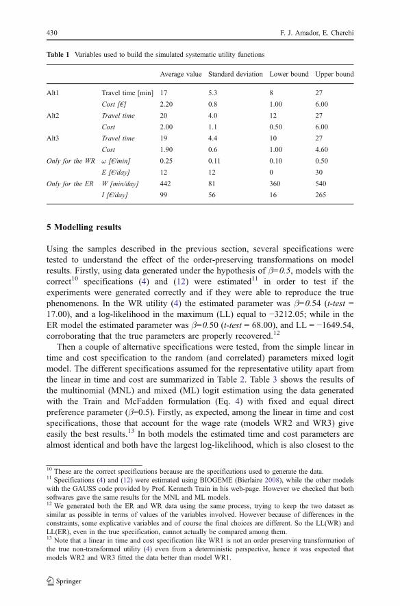
To test the effects of the order-preserving transformations in model estimation, acollection of datasets were generated according to the above microeconomictheories. In contrast to the typical applications of synthetic data (where the modalrandom utility is used), in our application choices were generated from the CIUFbefore applying any expansion and any order-preserving transformations. FollowingWilliams and Ortúzar (1982), different samples were generated according to Eqs. (4)and (12), to which a GEV type 1 error was added. Following Jara-Díaz (1998) it wasalso assumed that individuals made two trips in the reference period. Heterogeneoussamples of 10,000 observations were generated to test segmentation intohomogeneous categories. Three discrete alternatives were considered, with onlytwo level-of-service (LOS) attributes: time and cost. Truncated Normal distributionswere adopted for all the attributes (both LOS and socioeconomic attributes) toguarantee that minimum and maximum values of each attribute did not exceedrealistic values. The reference time T was assumed equal to 10 h (24 h minus14 h for maintenance activities at home and out of home). The final available incomewas computed substracting 20€/day plus 50% of the endowments to live.9 Allattributes were also generated to fulfill the constraints of the microeconomic problem(in both the wage rate and expenditure rate formulations). The main characteristicsof the data are shown in Table 1.

For each formulation (the WR formulation in Eq. (4) and the ER formulation inEq. (12)) two samples were generated keeping the above attributes fixed and varyingthe preferences. In one case the direct preference parameter β was assumed fixedacross the population and equal to 0.5; in the other case it was assumed uniformlydistributed in the range [0–0.5].

9 This is an assumption that might be discussed, but it was based on average real data, in order to generatea fairly realistic choice set. Following Train and McFadden (1978) the endowment represents the incomenot generated by work.


5 Modelling results

Using the samples described in the previous section, several specifications weretested to understand the effect of the order-preserving transformations on modelresults. Firstly, using data generated under the hypothesis of β=0.5, models with thecorrect10 specifications (4) and (12) were estimated11 in order to test if theexperiments were generated correctly and if they were able to reproduce the truephenomenons. In the WR utility (4) the estimated parameter was β=0.54 (t-test =17.00), and a log-likelihood in the maximum (LL) equal to −3212.05; while in theER model the estimated parameter was β=0.50 (t-test = 68.00), and LL = −1649.54,corroborating that the true parameters are properly recovered.12

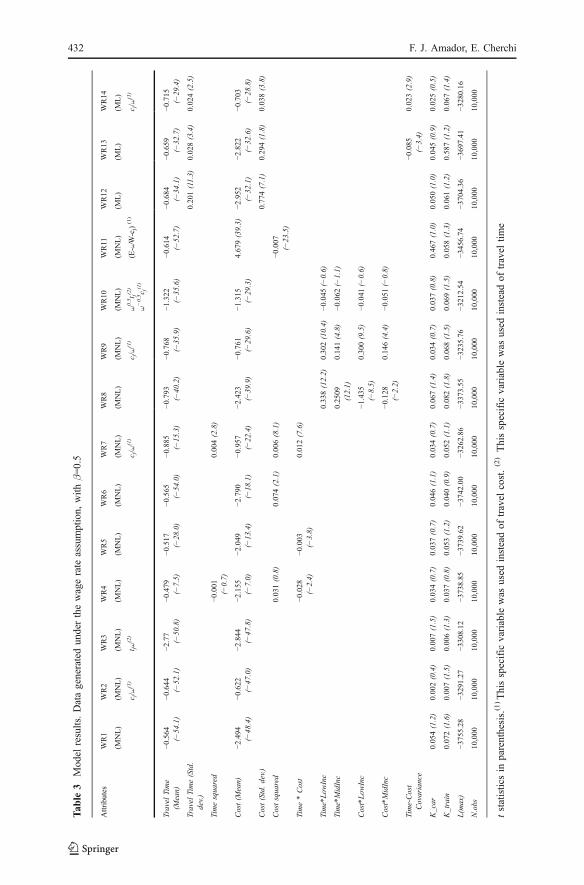
Then a couple of alternative specifications were tested, from the simple linear intime and cost specification to the random (and correlated) parameters mixed logitmodel. The different specifications assumed for the representative utility apart fromthe linear in time and cost are summarized in Table 2. Table 3 shows the results ofthe multinomial (MNL) and mixed (ML) logit estimation using the data generatedwith the Train and McFadden formulation (Eq. 4) with fixed and equal directpreference parameter (β=0.5). Firstly, as expected, among the linear in time and costspecifications, those that account for the wage rate (models WR2 and WR3) giveeasily the best results.13 In both models the estimated time and cost parameters arealmost identical and both have the largest log-likelihood, which is also closest to the

10 These are the correct specifications because are the specifications used to generate the data.11 Specifications (4) and (12) were estimated using BIOGEME (Bierlaire 2008), while the other modelswith the GAUSS code provided by Prof. Kenneth Train in his web-page. However we checked that bothsoftwares gave the same results for the MNL and ML models.12 We generated both the ER and WR data using the same process, trying to keep the two dataset assimilar as possible in terms of values of the variables involved. However because of differences in theconstraints, some explicative variables and of course the final choices are different. So the LL(WR) andLL(ER), even in the true specification, cannot actually be compared among them.13 Note that a linear in time and cost specification like WR1 is not an order preserving transformation ofthe true non-transformed utility (4) even from a deterministic perspective, hence it was expected thatmodels WR2 and WR3 fitted the data better than model WR1.

Table 1 Variables used to build the simulated systematic utility functions

Average value Standard deviation Lower bound Upper bound

Alt1 Travel time [min] 17 5.3 8 27

Cost [€] 2.20 0.8 1.00 6.00

Alt2 Travel time 20 4.0 12 27

Cost 2.00 1.1 0.50 6.00

Alt3 Travel time 19 4.4 10 27

Cost 1.90 0.6 1.00 4.60

Only for the WR ω [€/min] 0.25 0.11 0.10 0.50

E [€/day] 12 12 0 30

Only for the ER W [min/day] 442 81 360 540

I [€/day] 99 56 16 265


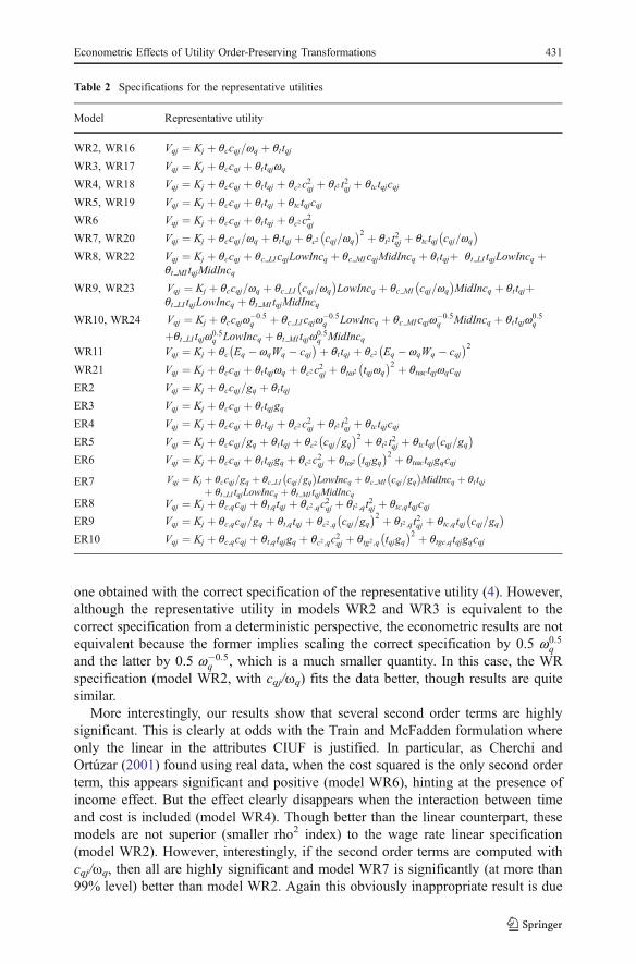
one obtained with the correct specification of the representative utility (4). However,although the representative utility in models WR2 and WR3 is equivalent to thecorrect specification from a deterministic perspective, the econometric results are notequivalent because the former implies scaling the correct specification by 0.5 w0:5

qand the latter by 0.5 w�0:5

q , which is a much smaller quantity. In this case, the WRspecification (model WR2, with cqj/5q) fits the data better, though results are quitesimilar.

More interestingly, our results show that several second order terms are highlysignificant. This is clearly at odds with the Train and McFadden formulation whereonly the linear in the attributes CIUF is justified. In particular, as Cherchi andOrtúzar (2001) found using real data, when the cost squared is the only second orderterm, this appears significant and positive (model WR6), hinting at the presence ofincome effect. But the effect clearly disappears when the interaction between timeand cost is included (model WR4). Though better than the linear counterpart, thesemodels are not superior (smaller rho2 index) to the wage rate linear specification(model WR2). However, interestingly, if the second order terms are computed withcqj/5q, then all are highly significant and model WR7 is significantly (at more than99% level) better than model WR2. Again this obviously inappropriate result is due

Table 2 Specifications for the representative utilities

Model Representative utility

WR2, WR16 Vqj ¼ Kj þ qccqj=wq þ qt tqj

WR3, WR17 Vqj ¼ Kj þ qccqj þ qt tqjwq

WR4, WR18 Vqj ¼ Kj þ qccqj þ qt tqj þ qc2c2qj þ qt2 t

2qj þ qtctqjcqj

WR5, WR19 Vqj ¼ Kj þ qccqj þ qt tqj þ qtctqjcqj

WR6 Vqj ¼ Kj þ qccqj þ qt tqj þ qc2c2qjWR7, WR20 Vqj ¼ Kj þ qccqj=wq þ qt tqj þ qc2 cqj=wq

� �2 þ qt2 t2qj þ qtctqj cqj=wq

� �WR8, WR22 Vqj ¼ Kj þ qccqj þ qc LI cqjLowIncq þ qc MI cqjMidIncq þ qt tqjþ qt LI tqjLowIncq þ

qt MI tqjMidIncq

WR9, WR23 Vqj ¼ Kj þ qccqj=wq þ qc LI cqj=wq

� �LowIncq þ qc MI cqj=wq

� �MidIncq þ qt tqjþ

qt LI tqjLowIncq þ qt MI tqjMidIncq

WR10, WR24 Vqj ¼ Kj þ qccqjw�0:5q þ qc LI cqjw

�0:5q LowIncq þ qc MI cqjw

�0:5q MidIncq þ qt tqjw

0:5q

þqt LI tqjw0:5q LowIncq þ qt MI tqjw0:5

q MidIncqWR11 Vqj ¼ Kj þ qc Eq � wqWq � cqj

� �þ qt tqj þ qc2 Eq � wqWq � cqj� �2

WR21 Vqj ¼ Kj þ qccqj þ qt tqjwq þ qc2c2qj þ qtw2 tqjwq

� �2 þ qtwctqjwqcqj

ER2 Vqj ¼ Kj þ qccqj=gq þ qt tqj

ER3 Vqj ¼ Kj þ qccqj þ qt tqjgq

ER4 Vqj ¼ Kj þ qccqj þ qt tqj þ qc2c2qj þ qt2 t

2qj þ qtctqjcqj

ER5 Vqj ¼ Kj þ qccqj=gq þ qt tqj þ qc2 cqj=gq� �2 þ qt2 t

2qj þ qtctqj cqj=gq

� �ER6 Vqj ¼ Kj þ qccqj þ qt tqjgq þ qc2c

2qj þ qtw2 tqjgq

� �2 þ qtwctqjgqcqj

ER7 Vqj ¼ Kj þ qccqj=gq þ qc LI cqj=gq� �

LowIncq þ qc MI cqj=gq� �

MidIncq þ qt tqjþ qt LI tqjLowIncq þ qt MI tqjMidIncq

ER8 Vqj ¼ Kj þ qc;qcqj þ qt;qtqj þ qc2 ;qc2qj þ qt2;qt

2qj þ qtc;qtqjcqj

ER9 Vqj ¼ Kj þ qc;qcqj=gq þ qt;qtqj þ qc2 ;q cqj=gq� �2 þ qt2 ;qt2qj þ qtc;qtqj cqj=gq

� �ER10 Vqj ¼ Kj þ qc;qcqj þ qt;qtqjgq þ qc2 ;qc

2qj þ qtg2;q tqjgq

� �2 þ qtgc;qtqjgqcqj


Tab

le3

Model

results.Datageneratedunderthewagerate

assumption,

with

β=0.5

Attributes

WR1

WR2

WR3

WR4

WR5

WR6

WR7

WR8

WR9

WR10

WR11

WR12

WR13

WR14

(MNL)

(MNL)

(MNL)

(MNL)

(MNL)

(MNL)

(MNL)

(MNL)

(MNL)

(MNL)

(MNL)

(ML)

(ML)

(ML)

c j/ω

(1)

t jω(2)

c j/ω

(1)

c j/ω

(1)

ω0.5t j(2

)

ω−0.5c j(1)

(E-ωW-c

j)(1)

c j/ω

(1)

Travel

Time

(Mean)

−0.564

(−54.1)

−0.644

(−52.1)

−2.77

(−50.8)

−0.479

(−7.5)

−0.517

(−28.0)

−0.565

(−54.0)

−0.885

(−15.3)

−0.793

(−40.2)

−0.768

(−35.9)

−1.322

(−35.6)

−0.614

(−52.7)

−0.684

(−34.1)

−0.659

(−32.7)

−0.715

(−29.4)

Travel

Time(Std.

dev.)

0.201(11.3)

0.028(3.4)

0.024(2.5)

Timesquared

−0.001

(−0.7)

0.004(2.8)

Cost(M

ean)

−2.494

(−48.4)

−0.622

(−47.0)

−2.844

(−47.8)

−2.155

(−7.0)

−2.049

(−13.4)

−2.790

(−18.1)

−0.957

(−22.4)

−2.423

(−39.9)

−0.761

(−29.6)

−1.315

(−29.3)

4.679(39.3)

−2.952

(−32.1)

−2.822

(−32.6)

−0.703

(−28.8)

Cost(Std.dev.)

0.774(7.1)

0.294(1.8)

0.038(3.8)

Costsquared

0.031(0.8)

0.074(2.1)

0.006(8.1)

−0.007

(−23.5)

Time*Cost

−0.028

(−2.4)

−0.003

(−3.8)

0.012(7.6)

Time*Low

Inc

0.338(12.2)

0.302(10.4)

−0.045

(−0.6)

Time*MidInc

0.2509

(12.1)

0.141(4.8)

−0.062

(−1.1)

Cost*Low

Inc

−1.435

(−8.5)

0.300(9.5)

−0.041

(−0.6)

Cost*MidInc

−0.128

(−2.2)

0.146(4.4)

−0.051

(−0.8)

Time-Cost

Covariance

−0.085

(−3.4)

0.023(2.9)

K_car

0.054(1.2)

0.002(0.4)

0.007(1.5)

0.034(0.7)

0.037(0.7)

0.046(1.1)

0.034(0.7)

0.067(1.4)

0.034(0.7)

0.037(0.8)

0.467(1.0)

0.050(1.0)

0.045(0.9)

0.025(0.5)

K_train

0.072(1.6)

0.007(1.5)

0.006(1.3)

0.037(0.8)

0.053(1.2)

0.040(0.9)

0.052(1.1)

0.082(1.8)

0.068(1.5)

0.069(1.5)

0.058(1.3)

0.061(1.2)

0.587(1.2)

0.067(1.4)

L(m

ax)

−3755.28

−3291.27

−3308.12

−3738.85

−3739.62

−3742.00

−3262.86

−3373.55

−3235.76

−3212.54

−3456.74

−3704.36

−3697.41

−3280.16

N.obs

10,000

10,000

10,000

10,000

10,000

10,000

10,000

10,000

10,000

10,000

10,000

10,000

10,000

10,000

tstatisticsin

parenthesis.(1)Thisspecific

variable

was

used

insteadof

travel

cost.(2)Thisspecific

variable

was

used

insteadof

travel

time


to the application of an order preserving transformation which has an influence onthe choice probabilities and thus on the estimates. In fact, this result reveals that themodel is accounting for the variability of the omitted scale parameters (which inducevariability in both the time and cost parameters) through the second order terms. Inline with this comment and with the theoretical discussion in section 3, all the MixedLogit models (WR12-WR14)14 are significantly (99% level) better than theircounterparts with fixed parameters; also, the variance of the time and costparameters is highly significant (see model WR12). Furthermore, when randomparameters are estimated with the (cqj/5q) specification (model WR14), variance andcovariance are all highly significant although the estimated mean travel time andcost parameters are correctly equal. The ML models estimate a correlation of 0.93between time and cost (model WR12), and a correlation of 0.76 between travel timeand cost/wage rate (model WR14), confirming the discussion in Eq. (10).

Finally, we tested if using the typical specifications to detect and account forincome effect instead of the correct specification might reveal some confoundingeffects. With this purpose, several models accounting for different marginal utilitiesof time and cost depending on the level of income (models WR8-WR10), as well asnon-linear functions on residual income (model WR11), were estimated. Resultsshow that all the parameters are significant (model WR8) reflecting a differentvaluation of travel time and cost among individuals of different income level.According to the sign and size of the cost coefficients, the marginal utility of income(MUI) decreases with income level15, so one could wrongly conclude that incomeeffect exists. Nonetheless, as discussed in section 3, the wage rate formulation doesnot account for income effect. In fact, according to the specification (4), the MUIdepends on the individual wage rate and on the direct preference parameter β, but itis not influenced by income level. As we took β=0.5 for the whole sample, thedifferent marginal utilities of cost for the different income levels do in fact accountfor the variability of the MUI over individuals according to their wage rate.Interestingly, the level of income is indeed highly significant when models areestimated with cqj/ωq (model WR9) while, as expected, it ceases to be significantwhen the correct specification is used, i.e. wq

�0:5cqj and wq0:5tqj (model WR10). The

same misleading effect is observed when a non-linear in residual incomespecification (model WR11) is estimated. This is due to the significance of thesquare of residual income, which would also bring to the incorrect conclusion thatincome effect is actually present.

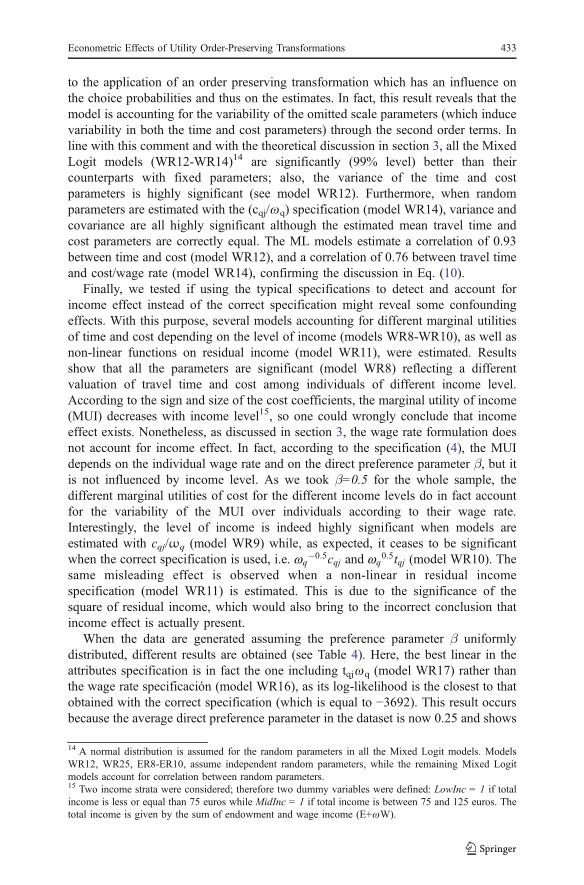
When the data are generated assuming the preference parameter β uniformlydistributed, different results are obtained (see Table 4). Here, the best linear in theattributes specification is in fact the one including tqj5q (model WR17) rather thanthe wage rate specificación (model WR16), as its log-likelihood is the closest to thatobtained with the correct specification (which is equal to −3692). This result occursbecause the average direct preference parameter in the dataset is now 0.25 and shows

14 A normal distribution is assumed for the random parameters in all the Mixed Logit models. ModelsWR12, WR25, ER8-ER10, assume independent random parameters, while the remaining Mixed Logitmodels account for correlation between random parameters.15 Two income strata were considered; therefore two dummy variables were defined: LowInc = 1 if totalincome is less or equal than 75 euros while MidInc = 1 if total income is between 75 and 125 euros. Thetotal income is given by the sum of endowment and wage income (E+5W).ωW).


Tab

le4

Model

estim

ationresults.Datageneratedun

derthewagerate

assumption,

with

β∼Uniform

(0,0.5)

Attributes

WR15

WR16

WR17

WR18

WR19

WR20

WR21

WR22

WR23

WR24

WR25

WR26

WR27

WR28

(MNL)

(MNL)

(MNL)

(MNL)

(MNL)

(MNL)

(MNL)

(MNL)

(MNL)

(MNL)

(ML)

(ML)

(ML)

(ML)

c j/ω

(1)

t jc j/ω

(1)

t j*ω

(2)

c j/ω

(1)

ω0.5t j(2

)

ω−0. *c j

(1)

c j/ω

(1)

t jω(2)

Travel

Time

(Mean)

−0.487

(−55.3)

−0.563

(−54.6)

−2.436

(−52.2)

−0.473

(−8.7)

−0.4487

(−26.9)

−0.8437

(−18.0)

−2.9727

(−23.1)

−0.740

(−36.4)

−0.750

(−37.5)

−1.314

(−35.7)

−0.612

(−33.1)

−0.600

(−29.1)

−0.663

(−30.7)

−2.501

(−29.9)

Travel

Time(Std.

dev.)

0.229(14.1)

0.047(5.6)

0.042(5.3)

0.132(0.9)

Timesquared

0.0005

(0.4)

0.0051

(4.3)

0.0428

(4.3)

Cost(M

ean)

−2.171

(−48.8)

−0.498

(−49.7)

−2.486

(−48.4)

−1.930

(−7.4)

−1.808

(−12.9)

−0.9025

(−33.3)

−3.0110

(−15.7)

−2.167

(−29.7)

−0.737

(−31.3)

−1.307

(−29.5)

−2.554

(−30.9)

−2.502

(−27.3)

−0.656

(−29.5)

−2.53

(−29.5)

Cost(Std.dev.)

0.489(3.4)

0.154(1.7)

0.063(6.7)

0.033(0.2)

Costsquared

0.017(0.5)

0.0068

(15.2)

0.0420

(1.1)

Time*Cost

−0.019

(−2.4)

−0.022

(−3.8)

0.01449

(13.8)

0.0901

(7.6)

Time*Low

Inc

0.434(18.1)

0.436(18.6)

0.399(7.5))

Time*MidInc

0.249(9.9)

0.244(10.0)

0.191(3.8))

Cost*Low

Inc

−0.596

(−4.7)

0.408(15.9)

0.344(6.0)

Cost*MidInc

−0.192

(−1.8)

0.246(9.1)

0.230(3.5)

Time-Cost

Covariance

0.045(0.9)

0.029(4.9)

0.051(0.4)

K_car

0.041(1.0)

0.004(0.1)

0.042(1.0)

−0.019

(−1.9)

0.022(0.5)

0.0142

(0.3)

0.0305

(0.6)

0.045(1.0)

0.208(0.5)

0.026(0.6)

0.034(0.7)

0.031(0.7)

0.003(0.1)

0.041(0.9)

K_train

0.011(0.3)

0.009(0.2)

0.005(0.1)

0.019(0.5)

−0.004

(−0.1)

−0.0096

(−0.2)

0.0055

(0.1)

0.010(0.2)

0.006(0.1)

0.006(0.2)

0.008(0.2)

0.005(0.1)

−0.008

(−0.2)

−0.006

(−0.2)

L(m

ax)

−4235.07

−3954.75

−3713.20

−4231.26

−4231.43

−3860.61

−3702.60

−3831.30

−3762.08

−3705.75

−4184.06

−4182.52

−3897.63

−3712.62

N.obs

10,000

10,000

10,000

10,000

10,000

10,000

10,000

10,000

10,000

10,000

10,000

10,000

10,000

10,000

tstatisticsin

parenthesis.(1

)Thisspecific

variable

was

used

insteadof

travel


variable

was

used

insteadof

travel

time


that using different utility transformations is not innocuous in terms of goodness offit. The formulation including tqj5q and cqj (model WR17) reproduces thephenomenon better than the wage rate specification (model WR16), because, inthis case, the former is consistent with a value of β (β=0), which on average is closerto the true value of β than the one underlying the WR model (β=1).

In contrast with the dataset generated with β=0.5, in this case the second orderterms are significant only when the wage rate is included in the specification (seemodels WR18, WR21 and WR22). But it seems that when there is a preference forgood consumption rather than for leisure time (β<0.5) the cost squared term loosessignificance (see models WR18 and WR21); for example, the cost squared term wasnot significant even when it was the only second order term. It is important tohighlight that these results do not seem to depend on the presence of randomness inthe direct preference parameter. In fact the same results were obtained also with adata set generated with a preference parameter for leisure fixed to 0.25. For reasonsof space we do not report a table with these results. Regarding the incorrect detectionof income effect (models WR22-WR24), results are very similar to those obtainedwith β=0.5 except for model WR24. In this case the cost parameters for the differentincome levels remain significant because this model does not coincide exactly withthe correct specification (i.e. it imposes a fixed value for β rather than accounting foreach individual actual β). This shows that the heterogeneity in the direct preferencesmight induce to detect erroneously the presence of income effect even when thefunctional form and the random term distribution are known with certainty.

Finally, differences appear also in the ML estimation. In fact, in this case Eq. (6a)is quite a good representation of our choice set, thus variances and covariance aresignificant when clearly inappropriate models are estimated (models WR25-WR27)but loose completely their significance when a more adequate specification (i.e. theone including tqj5q, as discussed above) is considered, as in model WR28.

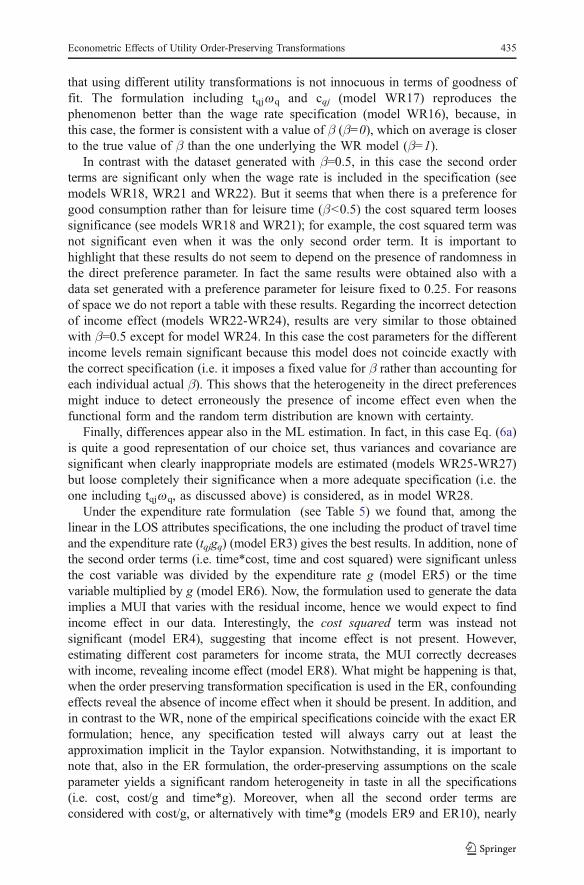
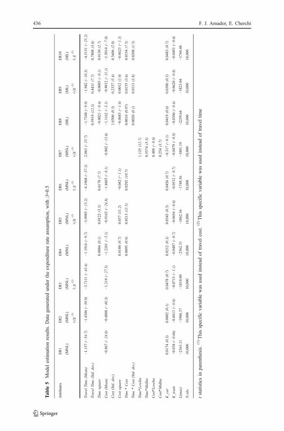
Under the expenditure rate formulation (see Table 5) we found that, among thelinear in the LOS attributes specifications, the one including the product of travel timeand the expenditure rate (tqjgq) (model ER3) gives the best results. In addition, none ofthe second order terms (i.e. time*cost, time and cost squared) were significant unlessthe cost variable was divided by the expenditure rate g (model ER5) or the timevariable multiplied by g (model ER6). Now, the formulation used to generate the dataimplies a MUI that varies with the residual income, hence we would expect to findincome effect in our data. Interestingly, the cost squared term was instead notsignificant (model ER4), suggesting that income effect is not present. However,estimating different cost parameters for income strata, the MUI correctly decreaseswith income, revealing income effect (model ER8). What might be happening is that,when the order preserving transformation specification is used in the ER, confoundingeffects reveal the absence of income effect when it should be present. In addition, andin contrast to the WR, none of the empirical specifications coincide with the exact ERformulation; hence, any specification tested will always carry out at least theapproximation implicit in the Taylor expansion. Notwithstanding, it is important tonote that, also in the ER formulation, the order-preserving assumptions on the scaleparameter yields a significant random heterogeneity in taste in all the specifications(i.e. cost, cost/g and time*g). Moreover, when all the second order terms areconsidered with cost/g, or alternatively with time*g (models ER9 and ER10), nearly


Tab

le5

Model

estim

ationresults.Datageneratedun

dertheexpend

iture

rate

assumption,

with

β=0.5

Attributes

ER1

ER2

ER3

ER4

ER5

ER6

ER7

ER8

ER9

ER10

(MNL)

(MNL)

(MNL)

(MNL)

(MNL)

(MNL)

(MNL)

(ML)

(ML)

(ML)

c j/g

(1)

t jg

(2)

c j/g

(1)

t jg

(2)

c j/g

(1)

c j/g

(1)

t jg

(2)

Travel

Time(M

ean)

−1.157

(−54.7)

−1.4306(−50.9)

−3.7111(−43.4)

−1.1916(−9.7)

−1.9985(−15.2)

−4.1968(−37.3)

2.063(−25.7)

−1.7348(−9.9)

−1.942

(−10.3)

−4.5151(−25.2)

Travel

Time(Std.dev.)

0.5919

(12.3)

0.4411

(7.7)

0.7808

(3.6)

Timesquare

0.0004

(0.1)

0.0122

(3.5)

0.0178

(7.7)

−0.0021(−0.4)

−0.0005(−0.1)

0.0130

(2.7)

Cost(M

ean)

−0.967

(−24.0)

−0.4808(−40.3)

−1.319

(−27.5)

−1.2101(−5.1)

−0.9165(−24.8)

−1.4603(−8.1)

−0.802

(−13.6)

−1.1162(−3.1)

−0.9012(−11.1)

−1.5014(−7.0)

Cost(Std.dev.)

1.0300

(8.3)

0.2337

(5.4)

0.3606

(2.0)

Costsquare

0.0180

(0.7)

0.037(11.2)

−0.042

(−1.1)

−0.0683(−1.4)

0.0012

(1.0)

−0.0623(−1.3)

Time*Cost

0.0095

(0.9)

0.0213

(11.5)

0.0292

(10.7)

0.0010

(0.07)

0.0155

(3.6)

0.0334

(7.5)

Time*Cost(Std.dev.)

0.0020

(0.1)

0.0113

(3.8)

0.0208

(1.5)

Time*Low

Inc

1.125(12.7)

Time*MidInc

0.5574

(5.3)

Cost*Low

Inc

0.488(−8.6)

Cost*MidInc

0.254(3.7)

K_car

0.0174

(0.3)

0.0082

(0.1)

0.0478

(0.7)

0.0212

(0.3)

0.0343

(0.5)

0.0456

(0.7)

−0.317

(−0.1)

0.0419

(0.6)

0.0380

(0.5)

0.0483

(0.7)

K_train

−0.038

(−0.66)

−0.0413(−0.6)

−0.0715(−1.1)

−0.0487(−0.7)

−0.0456(−0.6)

−0.0532(−0.7)

−0.0479(−0.8)

−0.0306(−0.4)

−0.0620(−0.8)

−0.0493(−0.6)

L(m

ax)

−2363.11

−1906.37

−1810.00

−2362.51

−1862.56

−1748.56

−1801.19

−2259.64

−1823.04

−1744.48

N.obs

10,000

10,000

10,000

10,000

10,000

10,000

10,000

10,000

10,000

10,000

tstatisticsin

parenthesis.

(1)Thisspecific

variable

was

used

insteadof

travel


variable

was

used

insteadof

travel

time


all the parameters are randomly distributed and correlated, which is a clear effect ofthe omitted scale factor.

6 Conclusions

To render the CIUF operational for the practical purpose of model estimation severalorder-preserving transformations are usually applied. Nonetheless, we argue that theclass of increasing linear transformations which involves multiplying the utility ofevery alternative by a factor that differs among individuals, does not leave the choiceprobabilities unaltered since this transformation induces a change in the distributionof the random terms. We focus on the effect of two order-preserving transformationsin the derivation of the modal utility from the conditional indirect utility functionboth in the wage rate and expenditure rate formulations. We show that the commonpractice of disregarding the scale factor would not be a problem if the factor implicitin that transformation was equal among individuals. However, as it dependson individual characteristics (preferences and wage or expenditure rate), theMcFadden’s operationalization of the RUM where the randomness derives frominter-individual variability can be valid only if the population under study isperfectly homogeneous, at least for the microeconomic frameworks analysed here.Disregarding this issue will affect the parameter estimates inducing confoundingeffect and a potential misinterpretation of the modelling results.

Using a collection of synthetic datasets generated from the CIUF before applyingany expansion and any order-preserving transformations (differently from the typicalapplications where the modal random utility is used), our results show, for example,that random and correlated parameters might be the simple consequences ofapplying this class of utility transformations. Also time and income effect mightwrongly be detected as a consequence of applying the aforementioned trans-formations.

A couple of general conclusions can be drawn. Firstly, it should be recognisedthat the parameters estimated with the typical WR and ER formulations with fixparameters and additive GEV type 1 random term are not consistent with theunderlying microeconomic theories. This is important in the interpretation of theestimated parameters and in the computation of economic indices. Secondly, lineartransformations of utility involving a multiplicative factor that differs amongindividuals should be avoided or at least recognized and correctly accounted for inthe distribution of the additive error terms. Thirdly, if we believe that individualsbehave according to Train and McFadden or Jara-Díaz and Farah frameworks, oursuggestion is then to specify the utility as in Eqs. (7) and (13), i.e. includingexplicitly all the terms that vary over the population, without applying anytransformations. This would allow one to estimate the direct preference parameter,which is certainly recommended, rather than imposing it a priori as usual. As wesaw, while in the WR formulation the linearisation has no effect, in the ER implies atruncation (to the first or second order terms) of the true CIUF, and this truncation isat the root of problems in interpreting estimation results. Given the progress in theestimation techniques, we could also avoid the linearisation of the CIUF andestimate directly the multiplicative forms.


Acknowledgements This research was partially done during a stay of the second author at La Lagunafunded by the Universidad de La Laguna Programme for Research Support. We would also like to thanksJuan de Dios Ortúzar for his amazing job in improving the clarity of the paper.

References

Amador FJ (2005) Medidas Alternativas de Bienestar Derivadas de un Modelo de Asignación del Tiempoen un Contexto de Elección Discreta: Teoría y Aplicaciones. PhD Thesis. Departamento de AnálisisEconómico. Universidad de La Laguna (in Spanish)

Amador FJ, González RM, Ortúzar J de D (2008) On confounding preference heterogeneity and incomeeffect in discrete choice models. Network Spatial Econ 8:97–108

Batley R (2008) On ordinal utility, cardinal utility, and random utility. Theory Decis 64:37–63Ben-Akiva M, Lerman S (1985) Discrete choice analysis: theory and applications to travel demand. The

MIT, CambridgeBierlaire M (2008) An introduction to BIOGEME Version 1.6, biogeme.epfl.chCherchi E (2003) On the microeconomic derivation of the systematic utility function. Working Paper 09/

03 Crimm, Università di CagliariCherchi E, Ortúzar J de D (2001) Multimodal choice models with mixed RP/SP data: correlation, non-

linearities and income effect. 9th World Conference on Transport Research Selected Proceeding,Pergamon-Elsevier (ed.), Netherlands (on CD)

Debreu G (1954) Representation of a preference ordering by a numerical function. In: Thrall RM, CoombsCH, Davis RL (eds) Decision processes. New York, John Wiley

Jara-Díaz SR (1991) Income and taste in mode choice models: are they surrogates? Transport Res25B:341–350

Jara-Díaz SR (1998) Time and income in travel demand: towards a microeconomic activity-basedtheoretical framework. In: Gärling T, Laitila T, Westin K (eds) Theoretical foundations of travelchoice modelling. Pergamon, Oxford

Jara-Diaz SR (2007) Transport economic theory. Elsevier Science, OxfordJara-Díaz SR, Farah M (1987) Transport demand and user’s benefits with fixed income: the goods/leisure

trade-off revisited. Transport Res 22B:159–171Jara-Díaz SR, Ortúzar J de D (1989) Introducing the expenditure rate in the estimation of mode choice

models. J Transport Econ Pol 23:293–308Jara-Díaz SR, Videla J (1989) Detection of income effect in mode choice: theory and application.

Transport Res 23B:393–400Lancaster KJ (1966) A new approach to consumer theory. J Polit Econ 74:132–57Marschak J, Becker GM, De Groot MH (1963) Stochastic models of choice behavior. Behav Sci 8:41–55McFadden D (1975) The revealed preferences of a government bureaucracy. Bell J Econ Manag Sci

6:401–416McFadden D (1976) Quantal choice analysis: a survey. Ann Econ Soc Meas 5:363–390Ortuzar J de D, Willumsen LG (2001) Modelling transport. Wiley, ChichesterTrain K (2003) Discrete choice methods with simulation. Cambridge University Press, CambridgeTrain K, McFadden D (1978) The goods/leisure trade-off and disaggregate work trip mode choice models.

Transport Res 12:349–353Varian H (1978) Microeconomic analysis. W. W. Norton and Company, New YorkWilliams HCWL, Ortúzar J de D (1982) Behavioural theories of dispersion and the mis-specification of

travel demand models. Transport Res 16B:167–219
