


Bahasa
Halaman
Hukum


INOM EXAMENSARBETE ENERGI OCH MILJÖ,AVANCERAD NIVÅ, 30 HP
, STOCKHOLM SVERIGE 2019
Design and implementation of sensor-based and sensorless control of a PMSM test system
OSKAR GIESECKE
KTHSKOLAN FÖR ELEKTROTEKNIK OCH DATAVETENSKAP
EJ210X - Master Thesis in Electrical Energy Conversion
School of Electrical Engineering and Computer Science
KTH Royal Institute of Technology
Design and implementation of
sensor-based and sensorless control
of a PMSM test system
Oskar Giesecke
Stockholm, Sweden, 2019
Supervisor: Jurgen Mökander
Examiner: Oskar Wallmark

i
Abstract
Transportation of liquids and gasses in industries in forms of pumping and fanning, constitutes a
significant part of the world-wide electric energy consumption. In order to meet global environmental
goals of greenhouse gas emissions and sustainable material usage, the development of efficiency and
technical lifetime of industrial pump and fan technology, are key. Innovative designs of electric
motors, motor control and electronics have improved the energy efficiency and technical lifetime of
residual and wastewater pumps technologies. Mid-sized wastewater submersible pumps are often
used in hazardous environments, where the pumped medium consists of a mixture of water, sludge
and solids. Solids in wastewater such as textiles are prone to get stuck in the impeller of the pump,
thereby halting the motion, lower the efficiency or completely locking the rotor. An aspect of
importance is henceforth the pump’s ability to provide full torque at low or start-up speed to
overcome the blockade of the solids. “Xylem Water Solutions” most modern and advanced waste
water pump consists of a permanent magnet synchronous motor (PMSM) for obtaining a vast
increase of efficiency compared to induction motors traditionally used in wastewater pumping
applications. Also, PMSM’s can provide full torque at zero speed. PMSM’s are commonly controlled
by position-sensorless means. However, obtaining full torque at low- or zero speed is for sensorless
PMSM control extremely challenging.
The thesis project examines sensor-based PMSM control and compares this to conventional
sensorless strategies. This was done both by building and analysing a simulated model in
SIMULINK/MATLAB of both a sensor-based and sensorless drive system. Secondly, a laboratory
test system was implemented with a motor drive platform with programmable motor control
algorithms. This was done partially to grasp the knowledge of implementation and design of motor
control, and partially to enable tests and comparisons between different motor control strategies in a
motor brake bench test rig located at the lab of Xylem Water Solutions Sundbyberg.
The implementation of the motor control platform lab system was successfully implemented and ran
with the vendors pre-configured sensorless control. An own interrupt-driven sensor-based cascaded
motor control algorithm was designed in SIMULINK where all suggestions of design and
implementation are outlined in the report. However, during an early step of the test procedure of
the pre-programmed sensorless control code, the hardware equipment malfunctioned and caused a
breakdown of the current-sensors of the controlled inverter. This led to disabled test equipment and
left the own-written code unverified at the time of the project’s end.
The results from the simulation resulted in a successfully implemented SCVM model and a sensor-
based motor control model. The sensored model was implemented by assuming synchronization at
any given moment, whereas the SCVM finds the position angle by estimating the back-EMF of the
motor. The simulated sensored and SCVM controls performs well for the targeted system application.
Parametric study of the SCVM model suggests that both the stator winding resistance and the
synchronous inductance should be underestimated for guaranteed synchronization at start-up.

ii
Sammanfattning
Förflyttning av vätskor och gaser med hjälp av pumpar och fläktar i industustriella applikationer
står för en signifikant del av den globala konsumtionen av elektrisk energi. För att möta miljömål
med avseende på utsläpp av växthusgaser och hållbar användning av naturresurser är effektivisering
och ökad teknisk livslängd inom industriell pump- och fläktteknologi viktigt. Förbättrad design av
elektriska motorer, motorstyrning och elektronik har ökat energieffektiviteten och den tekniska
livslängden för avloppsvattenpumpar. Medelstora nedsänkta avloppspumpar används ofta i
utmanande miljöer, där det pumpade mediet består av en blandning av vatten, slam och fast
material. Fasta material såsom textilier i avloppsvatten riskerar att orsaka problem för pumpar
genom att fastna i impellern och därmed göra pumprörelsen ojämn, sänka verkningsgraden eller
totalt låsa rotorn. Därför är en viktig egenskap hos en högpresterande och pålitlig pump dess
förmåga att leverera fullt vridmoment vid uppstart och vid låga hastigheter, för att kunna hantera
material som fastnat. “Xylem Water Solutions” modernaste och mest avancerade
avloppsvattenpump har en synkron permanentmagnetmotor (PMSM) vilket ger en betydande
effektivitetsökning jämfört med traditionella induktionsmotorer. Dessutom kan
permanentmagnetmotorer ge fullt vridmoment vid noll hastigheten. PMSM:er styrs vanligen utan
positionsgivare. Dock är det extremt utmanande att uppnå fullt vridmoment vid låg eller noll
hastighet för givarlös PMSM-styrning.
Avhandlingens projekt undersöker givarbaserad PMSM-styrning och jämför detta med
konventionella givarlösa strategier. Detta utfördes för det första genom att konstruera och analysera
en simuleringsmodell i SIMULINK/MATLAB för både en givarbasera och en givarlös drivlina. För
det andra implementerades ett testsystem i laboratorium bestående av en drivlina framtagen för
programmeringsbar motorstyrning. Projektet genomfördes dels för att bygga kunskap om design
och implementering av motorstyrning, dels för att möjliggöra tester och jämförelser mellan olika
strategier för motorstyrning i en befintlig testbänk för motorbromsning i Xylem Water Solutions
laboratorium i Sundbyberg.
Implementering av motorstyrningsplattformen och drivlinan genomfördes framgångsrikt och
kördes med leverantörens förkonfigurerade styrning av givarlös typ. En egen givarbaserad algoritm
för motorstyrning designades i SIMULINK. Alla förslag rörande design och implementering av
denna algoritm summeras i rapporten. Under ett av de tidiga stegen i testproceduren för den
förprogrammerade koden för givarlös styrning fallerade dock hårdvaran och orsakade att
strömgivarna i den styrda växelriktaren havererade. Detta ledde till inaktiverad testutrustning och
lämnade den egenskrivna programkoden overifierad vid tiden för projektets avslutning.
Resultaten från simuleringen gav en framgångsrikt implementerad SCVM (Statiskt kompenserad
spänningsmodell) och en givarbaserad modell för motorstyrning. Den givarbaserade modellen
realiserades genom att anta synkronisering vid varje givet tillfälle, medan SCVM-modellen
bestämmer positionsvinkeln genom att estimera motorns back-EMF. De simulerade
styrmodellerna, den givarbaserade och SCVM, fungerar båda väl för målapplikationen.
Parameterstudier av SCVM-modellen tyder på att både statorns lindningsresistans och den
synkrona induktansen ska estimeras i underkant för att garantera synkronisering vid uppstart.

iii
Keywords
PMSM, Field oriented control, FOC, Sensorless motor control, sensor-based motor control, digital
motor control, Inverter test system, MCU, automatic control, current control, speed control, SCVM,
Synchronization at start-up, Back-EMF observer, optical encoders, C2000 MCU.
Abbreviation
PMSM Permanent magnet synchronous motor
IM Induction machine
BLDC Brush-less direct current machine
EMF Electromotive force
CAN Controller area network
IDE Integrated Development environment
CCS Code composer studio
MCU Microcontroller unit
DSP Digital signal processor
PLC Programmable logic controller
VFD Variable frequency drive
FOC Field oriented control
SVM Space vector modulation
SCVM Statically compensated voltage model
SMO Sliding mode observer
PLL Phase locked loop
IGBT Insulated gate bipolar transistor
PIL Processor in-the-loop
HIL hardware in-the-loop
PWM Pulse width modulation
ADC Analog to digital converter
TI Texas Instruments
PCB Printed circuit board
EMC Electro magnetic compability

iv
Symbol Description
𝑇𝑒𝑚 Electrical torque (Nm)
𝑣𝑠 Stator voltage (V)
𝑣𝛼𝛽 Stator voltage alpha/betha-coordinates (V)
𝑣𝑑𝑞 Stator voltage dq-coordinates (V)
𝑖𝑠 Stator current (A)
𝐿𝑠 Thickness (m)
𝐿𝑑𝑞 Synchronous inductance (H)
ψ𝑠𝑠 Flux linkage (V/rad)
𝜔𝑟 Rotor electrical frequency (rad/s)
𝜔1 Stator electrical frequency (rad/s)
𝜃𝑟 rotor angle (rad)
𝜃𝑟 Rotor angle estimate (rad)
�̃�𝑟 Rotor angle estimation error (rad)
𝜃1 Stator electrical position (rad)
E Back-emf (V)
𝑛𝑝𝑝 number of pole pairs
𝐾 peak-to-peak/RMS compensation constant (-)
𝑇𝑠 Sampling period (s)
𝑓𝑠 Sampling frequency (1/s)
𝛼𝑐 Bandwidth current controller
𝛼𝑠 Bandwidth speed controller
𝛼𝑙 Bandwidth PLL (1/s)
𝑡𝑟𝑐 Rise time current controller (s)
𝑡𝑠𝑐 Rise time speed controller (s)
λ𝑠 Thickness (m)
J Inertia (kg/m2)
𝜏𝑙 External load torque (Nm)
𝑏 Viscous damping constant
𝑅𝑎 Active damping resistance
𝑘𝑖 Integral gain
𝑖𝑠𝑎𝑡 Current saturation limit (A)
𝑣𝑠𝑎𝑡 Voltage saturation limit (V)

Table of Contents
Abstract ................................................................................................................................................ i
Sammanfattning ................................................................................................................................. ii
Keywords ........................................................................................................................................... iii
Abbreviation ...................................................................................................................................... iii
1 Introduction ............................................................................................................................... 1
1.1 Background ....................................................................................................................... 1
1.2 Purpose .............................................................................................................................. 1
1.3 Objectives .......................................................................................................................... 2
1.4 Thesis outline .................................................................................................................... 2
2 Methodology .............................................................................................................................. 3
2.1 Outline ............................................................................................................................... 3
2.2 Simulation study ............................................................................................................... 3
2.3 Test platform .................................................................................................................... 3
2.4 Code Development and Software Environment ......................................................... 4
2.5 Motor brake bench ........................................................................................................... 5
2.6 Limitations ......................................................................................................................... 5
3 Theory Study .............................................................................................................................. 6
3.1 Permanent magnet synchronous motors ...................................................................... 6
3.1.1 PMSM fundamentals ............................................................................................... 6
3.1.2 Field oriented control .............................................................................................. 7
3.1.3 PMSM Voltage Model ............................................................................................. 8
3.2 Motor control ................................................................................................................... 9
3.2.1 Basic AC-motor drive system ................................................................................ 9
3.2.2 Digital Motor Control Basics ............................................................................... 10
3.2.3 Current Controller Design .................................................................................... 11
3.2.4 Space vector modulation ....................................................................................... 13
3.3 Sensor based motor control .......................................................................................... 14
3.3.1 Optical encoders .................................................................................................... 14
3.3.2 Resolvers ................................................................................................................. 15
3.3.3 Hall effect sensors .................................................................................................. 15
3.4 Sensorless motor control .............................................................................................. 16
3.4.1 Statically Compensated Voltage Model .............................................................. 16

3.4.2 Sliding mode observer ........................................................................................... 18
3.4.3 Comments regarding the literature ...................................................................... 19
4 Simulation Study ......................................................................................................................20
4.1 Simulation model implementation ............................................................................... 20
4.1.1 Mechanical model of PMSM ................................................................................ 20
4.1.2 Electrical dynamics model .................................................................................... 21
4.1.3 Current controller .................................................................................................. 21
4.1.4 Speed controller ..................................................................................................... 24
4.1.5 Implementation of SCVM .................................................................................... 25
4.2 Results of Simulation ..................................................................................................... 26
4.2.1 Simulation results sensored control .................................................................... 27
4.2.2 Results of SCVM no-load start up ...................................................................... 28
4.2.3 Parametric study of SCVM .................................................................................. 31
4.2.4 Locked rotor torque and load at start up ........................................................... 35
4.2.5 Discussion of simulation study ............................................................................ 37
5 Test system Implementation ..................................................................................................39
5.1 Hardware and test system ............................................................................................. 39
5.1.1 Motor brake bench ................................................................................................ 39
5.1.2 Servo drive .............................................................................................................. 40
5.1.3 Measuring device .................................................................................................... 40
5.1.4 Position Sensor ....................................................................................................... 40
5.1.5 DAQ monitoring ................................................................................................... 41
5.2 Test platform electrical implementation ..................................................................... 42
5.2.1 Electrical overview ................................................................................................. 42
5.2.2 Encoder index pulse calibration .......................................................................... 44
5.3 Controller Code design and implementation ............................................................. 46
5.3.1 Code generation ..................................................................................................... 46
5.3.2 Top layer build ....................................................................................................... 46
5.3.3 Function FOC ........................................................................................................ 47
5.3.4 Current controller .................................................................................................. 48
5.3.5 PWM synchronization ........................................................................................... 49
5.3.6 ADC Scheduling .................................................................................................... 50
5.3.7 QEP speed position measurement module ....................................................... 51

5.4 Results of tests ................................................................................................................ 52
5.4.1 Results and discussion of Sensorless motor control ......................................... 53
6 Future work ..............................................................................................................................57
7 Conclusions ..............................................................................................................................57
8 Bibliography .............................................................................................................................58

-1-
1 Introduction
1.1 Background
One of the foremost energy demanding activities in industry is transportation of fluids or gasses either in
cooling, processes, or removal of ground water due to for example mining. Industrial pumps and fans are
consuming a considerable amount of the total electric energy worldwide. Consequently, the development
of pump and fan technology is highly impactful both economically and environmentally. Traditionally
industrial pumps and pumps used for private use have been consisting of an induction motor for the electric
energy conversion into mechanical rotational force. However, during recent years permanent magnet
synchronous motors PMSMs have been introduced in order to vastly increase the efficiency of the pump.
Energy optimization, lifetime expectancy and maintenance minimization of industrial pumps and fans may
play a major role for minimized green-house gas emissions, energy savings and less material usage globally.
Submersible pumps are today developing in many directions for energy savings, longer life times and
minimized need of maintenance. By using a PMSM instead of an IM traditionally used in industrial pumps,
one can achieve vast energy savings due to the PMSM high efficiency. However, a PMSM requires a
frequency converter and cannot be started direct online. Therefore, a variable frequency drive is needed in
a PMSM drive system.
The electric energy conversion system may be designed in several different ways, a crucial point of design
is whether the VFD uses a position sensor or sensorless algorithms in order to find the rotor position of
the motor. The position of the rotor is vital for the VFD to control the currents such that torque is produced.
This is also referred to as synchronizing the motor. Sensor based versus sensorless control of synchronous
machines have both benefits and drawbacks. Sensorless control of submersible pumps is commonly used
due to the benefits of less number of components and unreliability of EMC sensitive signals. Sensorless
control strategies are often based upon observing back-emf of the motor. However, during low speeds the
observer becomes blind and therefore the sensorless control algorithm may lose track of the rotor position
hence unable to synchronize the stator voltage output with the rotor magnet position. Thus, a position
sensor may increase the performance significantly during low speeds. However, a sensor may be costly for
the drive and may be prone to exceed its technical life time before the pump’s lifetime.
A sensored solution of a PMSM drive system for submersible pumps may be interesting if the torque
performance is greater to that of a sensorless solution at low speeds. In many applications of wastewater
pumping the impeller may get clogged by solids or sludge and therefore require high starting torque. In this
case of event torque performance at zero or low speed is key to “chew” through the solid material
throughout the outlet of the pump. If a sensorbased control solution provides greater torque performance
for smaller pumps, the increased costs and the risks of more components in the system may be justified.
1.2 Purpose
“Xylem water solutions” has during recent years continuously developed software and hardware solutions
to their pump systems that minimizes maintenance during operation of submersible pumps. In general,
pumps larger than 5 kW often chew through solids such as rags and textiles with low risk of clogging.
However, smaller pumps than 5kW needs as much torque as possible at low speeds to minimize the risk of
a pump failure caused by clogging.
The main goal of this project is to design and implement a control system for both a sensorless and a sensor-
based control algorithm. This is done in order to enable testing and comparison of the two strategies both
in this project but also in the future at the lab of Xylem Sundbyberg. The point of interest is especially the
amount of torque that can be produced at low speeds for a PMSM if a position sensor is used compared to
a sensorless algorithm. Furthermore, this project will outline the aspects of design and implementation of

-2-
algorithms of both sensorless and sensorbased control into a digital signal controller that will carry perform
speed control of a PMSM. To do this both adequate hardware and software is needed.
1.3 Objectives
In this thesis study, an evaluation between position sensorless and sensor-based control for permanent
magnet motors PMSMs will be carried out. The project is carried out with respect to enlighten the field of
PMSM control concepts, both theoretically and practically. This comprises of a literature study of PMSM
control within the field of electric energy conversion, digital control and position sensor techniques present
today. Practically the goal is to design and implement two control algorithms that controls a PMSM
sufficiently at low speeds and analyze and compare the torque performance between the two algorithms.
Thus, this project will outline the necessary steps of implementing code to microprocessor controlling a
motor.
The main goal is to design and implement one sensor-based control algorithm and one sensorless control
system. But before the control code of the laboratory test system will be constructed an analytical evaluation
of two control concepts will be carried out through a simulation study. This will be conducted by first
choosing one sensor-based design concept of a motor control system and one sensorless concept based on
the information gathered in the literature study. The simulation study includes comparisons of two
algorithms, and design and implementation controller parameters related to the hardware that will be used
in the test rig in laboratory. This is done in order to investigate the value of introducing a position sensor to
pump systems that are presently using sensorless control systems with a mathematical approach.
In order to set up the testing environment an appropriate hardware will be acquired. This should consist of
a variable frequency drive that can drive a 8kW PMSM at low speeds. A platform with programmable digital
signal processor is therefore needed.
Adjustments to the existing motor brake bench has to be carried out for the specific device under test. A
position sensor is needed to be installed, calibrated and configured. Data acquisition from the VFD for
measuring currents, position should be measured and equally time stamped with the torque measured from
the measuring devices of the test bench.
1.4 Thesis outline
This paper will first outline the method of procedure to obtain the main goals of the project. In chapter two
the methodology of the project is described. All pieces of hardware that was acquired for the project will be
described. In chapter three the theoretical background of PMSM fundamentals, motor control and sensor
techniques is presented. Chapter four comprises the simulation study of a sensor-based model and one
chosen sensorless-motor control algorithm. The design and implementation of the studied control systems
are presented in detail, followed by results and analysis of the observations shown by the simulations. In
chapter five the implementation, design and results of the electrical test system is described. This includes
the procedure of programming the micro-controller code with MatLAB/SIMULINK code and the physical
configuration and installation of the test rig. Subsequently the results of the testing will be outlined, followed
by analysis and conclusions.

-3-
2 Methodology
In this chapter, the method of the master thesis project will be explained. First the thesis outline will be
explained where each phase of the project will be described briefly. The following section will describe the
simulation study. Next section will describe the hardware test platform that was purchased for this project.
2.1 Outline
The thesis project was carried out in four phases in order to achieve the goals stated in previous section.
The first phase consists of a theoretical overview of PMSM control technologies including, PMSM
fundamentals, automatic control theory and a brief introduction to commonly used control algorithms in
industrial drive applications. The second phase includes theoretical simulation of position-sensored speed
control and one chosen sensorless control strategy which both are simulated and analyzed using
Matlab/Simulink. This is done in order to have theoretical based simulations which will serve as a
complement to the results carried out in lab environment. Phase three consists of implementation and
design of one position-based motor control system. The fourth and last phase of the project consist of lab
environment testing of sensorless and position-sensored motor control.
2.2 Simulation study
The simulation study is carried out in this project to analytically implement and test motor control systems.
This is conducted by choosing one sensorless control algorithm and one sensorbased control and conduct
those two on a simulated motor model. The choice of control strategies is based upon performance at start-
up of a drive. The sensorless strategy must guarantee synchronization at start-up. Additionally, complexity
of implementation is taken into consideration. A too complicated control system cannot be chosen due to
time limitations of the project. The motor model will simulate the real PMSM which is tested with the real
lab equipment in the following phase of the thesis project. Hence, the real parameters of the motor and the
inverter of the test platform are used for the simulation model. The simulation is programmed in
Matlab/Simulink for different test cases.
The first test condition is the no-load start-up. This motor test indicates motor behavior at start up for both
control strategies as well as verify that the motor can be run in the targeted speed for the laboratory test
environment. In the case of sensorless control, this test can be conducted for different starting positions of
the rotor, for analysis if the sensorless controller can synchronize the motor at start-up.
The second part of the simulation study consists of a parametric study regarding the sensorless control
algorithm. Motor control algorithms can be sensitive for faulty input parameters set by the user while
programming the motor control code. In this part the resistance and the inductance are varied for different
starting positions. By doing this one can achieve information of the stability of the controller depending on
the motor parameters.
The third and last part of the of the simulation study consists of a locked rotor simulation where the shaft
load torque is simulated to always keep the rotor in same position no matter the produced electrical torque
from the windings. This test indicates how the implemented sensorless control can compare with the sensor-
based control when the rotor is locked.
2.3 Test platform
A development platform is needed to be acquired to design and implement the control algorithms upon. In
order to save time, it was decided to purchase a development kit from a CPU manufacturer that supplies
hardware for three phase motor control. Several kits were taken into consideration, all rated at 2.0 kW or
below. The hardware that is used for the motor control unit in this project was selected to a Texas
Instrument platform. The high voltage motor control kit allows the user to implement code in CCS and
several examples are given. The platform consists of a variable frequency converter with a dc-link with
maximum 350VDC and an output maximum power of 1,5kW. The board is supplied with 6 IGBTS with

-4-
single shunts current sensors and a slot for TMSf280 control cards of the c2000 family. The TI solution was
chosen mostly due to flexibility when coding and configuring the system. The DSP can be coded directly in
C/C++ environment with code support from TI. The code can also be developed in
MATLAB/SIMULINK environment alongside embedded coder in order to simulate the system and
subsequently compile and load the code with make file approach and flashed directly to the processor.
Table 1. Test equipment hardware specifications
High voltage motor and PFC Developer’s Kit 2 phase PFC stage Max 750W CAN interface 3 phase inverter stage Max 1.5 kW SCI connectivity Output voltage 220 VAC PWM DAC* 4 CH (for oscilloscope) Output power 1.5 kW (unfused) 2 QEP Incremental encoder AC input Voltage 85-132/170-250V 3 CAP Hall sensors AC input power 750 W IPM heatsink DC-bus input Max 400V (with fans) DC Fan Control voltage input 15VDC 15W Emulation JTAG efficiency Up to 90% UART Through SCI and FTDI Switching frequency 200kHz Fuses 4A at AC power input
Table 2. Microcontroller specifications
C2000 TMS320F28069 Clock Frequency 90 MHz (11.11 -ns) PWM 16 CH Flash 256 KB QEP/CAP 2/3 RAM 100 KB DMA 6 -CH 12bit ADC 16-CH 3.46 MSPS I2C 1-CH GPIO 54-CH SCI 2-CH Floating point Native single-prec. SPI 2-CH Timers 3 32bit CPU eCAN 1-CH Clocking 2 Zero pin/watchdog CLA 32-bit match acc
2.4 Code Development and Software Environment
The c2000 microcontroller family are optimized for motion control and can be used with TI’s development
kits for motor control. These digital signal controllers are 32-bits fixed or floating point processors which
offers a variety of software implementation utilities. The IDE, (Integrated Development Environment) CCS
(Code Composer Studio) is the software where code can be written, debugged and compiled into the MCU.
The c2000 family offers several support packages for effective code generation from Simulink into .rtw files
into C/C++ code directly into the IDE. This also offers one to use utilize HIL/PIL simulations in Simulink
when using mathworks Embedded coder. Meaning that coding and developing time may be reduced by using
top layer programming in Simulink.
In this project the “makefile” approach is used. There are code examples based on SIMULINK for c2000
controllers for controlling motors where the code from Simulink is compiled into an .out file which can be
uploaded directly as a project into CCS. When a project is uploaded all includes, headers and executes are
structed for running the code in CCS. Alternatively, one can build, load and run code directly from

-5-
SIMULINK if function “build, load and run” is chosen as a simulation option. Both alternatives are based
on the same “makefile” approach.
Traceability may become an issue when using code language transformations, but in recent years MathWorks
embedded coder has optimized code generation along TI which can assure safe code generation and
traceability reports.
2.5 Motor brake bench
The motor brake bench was designed and implemented by the author and coworkers at Xylem Sundbyberg
prior to this project. The system consists of a of a servo drive system with integrated PLC and serial
communication. The servo drive is used as a braking motor/generator for programmable load curves. The
drive communicates through CANopen protocol with a LABVIEW sequence program, for controlling
speed references and torque allowance. Furthermore, a torque strain gauge and a speed sensor is connected
to the shaft of the servo motor. Torque and speed are measured and observed through a universal
measurement amplifier and software from HBM. More information regarding the configuration of the brake
bench rig can be found in the implementation section. On the other side of the shaft pump motors can be
mounted onto a shaft connector. In this project an 8kW surface mounted, non-salient PMSM is connected
to the brake bench. The test motor will be controlled through a programmable VFD platform which was
described in previous section.
2.6 Limitations
This project has several limitations due to time allocation of both development time and testing in motor
brake bench rig. It is obvious that development of all control systems can be quite time consuming,
especially if the controller should perform with high efficiency. In this project there is not time enough to
optimize the control system. Also, the implementation of a sensorless control algorithm to the
programmable microcontroller was deemed too time consuming for the scope of the project, henceforth
an own-written code will be implemented for a sensor-based control system. The sensorless control
provided by TI “Insta-spin” will be used to compare torque performance during low speed regions of the
motor.

-6-
3 Theory Study
This chapter will include the relevant theoretical background of PMSMs and motor control. It is divided in
to three parts, one of which outlines the core characteristics of PMSMs. The second part will outline the
motor control theory in general and specific control theory adopted for PMSMs. The third part briefly
outlines the core concepts of conventional sensors used in electric machine control.
3.1 Permanent magnet synchronous motors
An electric machine is a set of components which converts electric energy into mechanical motive force and
vice versa. Mainly there are two categories of electrical machines. DC and AC machines. Amongst many
different AC motors topologies, there are namely synchronous machines and induction machines. Induction
machines has been dominating the field of industrial motive applications for the robust and simple
construction and the capability of direct online connection. However, PMSMs are nowadays an interesting
alternative in high-end industrial applications for driving position or speed controlled drives since the
machines have the highest efficiency amongst most machines with up to 97% efficiency, low maintenance
and high power density [1].
3.1.1 PMSM fundamentals
The essentials of all electrical machines are a rotating magnetic field supplied from the stator coils which in
turn interacts with the magnetic field of the rotor. The interaction between magnetic fields creates magnetic
motive force which produces torque on the rotor transferred to the shaft of the machine. In the case of
PMSMs the magnetic field from the rotor is produced from installed high remanence magnets inside or
onto the rotor. This means that there is no need to feed current into rotor windings by induction or
commutators. By doing this one eliminates resistive losses in rotor windings. The magnets can be surface
mounted, placed in openings, or buried inside the rotor. The permanent magnets produce a magnetic flux
in the airgap of the motor. When the flux created by the rotor interacts with the stator created flux, torque
is produced. [2]
Figure 1. Conceptual cross section of a surface mounted 3 pole-paired PMSM
The stator windings are placed inside the stator slots. The windings can be distributed such as sinusoidally
distributed windings which provides smooth sinusoidal back-emf. Or the windings can be designed as
concentrated windings which reduces copper losses and has high performance if the motor has high number
of poles, lowering the harmonic content of the MMF. Several variations of winding layout such as pitching
the end windings, overlapping windings techniques exist for eliminating harmonic distortion of the MMF,
reducing copper/iron losses, cogging torque, higher torque capacity, etc. [3]. The stator and rotor core
materials usually are made out of high remanence, laminated iron stacks which allows high flux with minimal
amount of iron core losses and eddy currents. The maximal torque that can be produced is correlated to the
inverse of the airgap length. Therefore, a small as possible airgap is highly desired [4].

-7-
The rotating field created by the current flow in the stator windings will interact with the permanent magnets
and the rotor will rotate synchronously with the stator field. However, the stator flux has to be oriented
apart from the direction of the rotor magnets. If the stator flux is aligned with the magnet flux, no torque
will be produced and in extreme cases the magnets can get demagnetized [5]. In other words, the stator flux
should be oriented perpendicular to the rotor flux in in order to achieve maximum torque per ampere. This
described in more detail in the section field-oriented control.
3.1.2 Field oriented control
Field oriented control (FOC) or as often referred to vector control is a commonly used control technique
for high performing AC machines. When implementing FOC for a PMSM the rotor field some way
estimated or sensored, in order to produce stator field optimized for torque production. To achieve the
highest torque at any given point, the stator flux created by the windings should be orthogonal to the rotor
flux at the point where the two fluxes interact, in the airgap of the motor that is. Hence the knowledge of
the rotor position where the magnets are located is key for synchronous motor control [2].
In motor control it is convenient to represent current, voltage and flux quantities in synchronous reference
frame. Instead of using three-phase time altering quantities, these are instead decomposed into a two-
component time invariant system. This allow computations to become significantly more simplified.
Analogously with using phasor representation of ac-systems, phase currents are translated into the rotor
reference frame, making the system to act as two dc quantities. The system of three phase voltages seen
from the stator, disregarding the zero-sequence, can be decomposed into an equivalent two-phase system.
This coordination system base change is known as the Clarke transformation.
𝒗𝑠(𝑡) = 𝑣𝑎(𝑡) + 𝑣𝑏(𝑡) + 𝑣𝑐(𝑡) (1)
𝒗𝑠(𝑡) = [
𝑣𝛼(𝑡)
𝑣𝛽(𝑡)] = [𝑅𝑒{𝑣𝑠(𝑡)}
𝐼𝑚 {𝑣𝑠(𝑡)}]
(2)
Figure 2. Vector diagram Clarke transformation
This comprises the concept of space vectors which can be regarded as rotating phasors with the exception
that phasors consist of single frequency component. Complex space vectors may represent multi frequencies
and thus allowing mathematical operation beyond steady state [2].
These may be transformed into synchronous space vectors by the Park transformation or the dq-
transformation that utilizes the rotor position and the direction of the rotor flux orientation.

-8-
𝒗 = [
𝑣𝑑
𝑣𝑞] = [
𝑐𝑜𝑠𝜃1 − 𝑠𝑖𝑛𝜃1
𝑠𝑖𝑛𝜃1 𝑐𝑜𝑠𝜃1] [
𝑣𝛼
𝑣𝛽]
(3)
Figure 3. Vector diagram Park transformation
3.1.3 PMSM Voltage Model
The PMSM has the same stator winding configuration as a IM. For both IMs and PMSM the equation
commonly referred to as the voltage model. According to Faraday’s law of induction Eq. 4 should hold [2]
𝒗𝑠
𝑠 = 𝑅𝑠𝐢𝑠𝑠 +
𝑑 𝛙𝑠𝒔
𝑑𝑡
(4)
The voltage applied to the stator windings creates flux in the stator in one hand and resistive losses in the
other. 𝒊𝑠𝑠 and 𝛙𝑠
𝑠 denotes the stator current and the stator flux linkage. The bold variables indicate space
vectors. In case of a PMSM the stator flux linkage should be equal to
𝛙𝑠𝒔 = 𝐿𝑠𝐢𝑠
𝑠 + 𝛙𝑅𝑠
(5)
Where 𝛙𝑅𝑠 is the rotor flux linkage which is created by the rotor permanent magnets and 𝐿𝑠 is the stator
inductance. The rotor flux linkage is directly connected to the rotation of the rotor, hence can be written in
polar form 𝛙𝑅𝑠 = ψ𝑅𝑒𝑗𝜃 where ψ𝑅 may be assumed constant. By taking the time derivate of Eq. 5 with
the constant yields
𝑑 𝛙𝑠𝒔
𝑑𝑡= 𝐿𝑠
𝑑𝐢𝑠𝑠
𝑑𝑡+ 𝑗𝜔𝑟ψ𝑅𝑒𝑗𝜃
(6)
Combining equation 4 -6 one may express a dynamic model of the round rotor PMSM [2].
𝑳𝑠
𝑑𝐢𝑠𝒔
𝑑𝑡= 𝒗𝑠
𝑠 − 𝑅𝑠𝐢𝑠𝑠 − j𝜔𝑟ψ𝑅 𝑒𝑗𝜃
(7)
This model can be modeled by the equivalent circuit diagram shown in Fig. 4 and is widely used in PMSM
motor control theory for example in [6]. The voltage drop across the righthand side is the modeled back-
emf dissipated by the motor.

-9-
Figure 4. Dynamic equivalent model of round-rotor PMSM
Eq. 7 may be expressed in component form by splitting up 𝑳𝑠 in its direct and quadratic components.
𝑳𝑠 = [
𝐿𝑑 00 𝐿𝑞
] (8)
Consequently the components of Eq. 8 becomes as expressed in Eq. 9 recalling that ψ𝑅 the flux modulus
of the permanent magnets ideally are aligned solely on the d-axis [2].
𝐿𝑑
𝑑𝑖𝑑
𝑑𝑡= 𝑣𝑑 − 𝑅𝑠𝑖𝑑 + 𝜔𝑟𝐿𝑞𝑖𝑞
(9)
𝐿𝑞
𝑑𝑖𝑞
𝑑𝑡= 𝑣𝑞 − 𝑅𝑠𝑖𝑞 − 𝜔𝑟(𝐿𝑑𝑖𝑑 + ψ𝑅)
(10)
A surface mounted permanent magnet machine is often regarded as non-salient. The permeability of high
remanance magnets is close to air, therefore it is often referred to 𝐿𝑑 ≈ 𝐿𝑞 . By using the power dissipated
by the emfs one can express the mechanical power. The back emfs of Eq. 11 and 12 are expressed as.
𝐸𝑑 = −𝜔𝑟𝐿𝑞𝑖𝑞 (11)
𝐸𝑞 = 𝜔𝑟(𝐿𝑑𝑖𝑑 + ψ𝑅) (12)
The mechanical power may be expressed by the back emf multiplied with the currents. Neglecting
harmonics and zero sequence components the electrical torque can be expressed as eq. 13.
𝑃𝑒 =
3
2𝐾2 (𝐸𝑑𝑖𝑑 + 𝐸𝑞𝑖𝑞) =3
2𝐾2𝜔𝑟{ψ𝑅𝑖𝑞 + (𝐿𝑞 − 𝐿𝑑)𝑖𝑞𝑖𝑑}
(13)
Thus, the electrical torque can be found by dividing Eq. 14 with the mechanical speed 𝜔𝑟 = 𝜔𝑟/𝑛𝑝 thus
giving the toruq equation in Eq. 14.
𝜏𝑒 =
3𝑛𝑝
2𝐾2 {ψ𝑅𝑖𝑞 + (𝐿𝑞 − 𝐿𝑑)𝑖𝑞𝑖𝑑}
(14)
In Eq. 14 a torque component in the second term can be seen. This is called the reluctance torque and is a
consequence of saliency in the rotor. With non-salient rotor the term vanquishes since 𝐿𝑞 − 𝐿𝑑 is small or
close to zero.
3.2 Motor control
3.2.1 Basic AC-motor drive system
Since PMSM are synchronous machines, a frequency converter is needed so that the applied stator voltages
to the rotor position. In some applications, line connected PMSM are used without an frequency converter,
instead uses damper windings for asynchronous start-up [2]. The VFD is an AC-AC converter which are
fed from constant frequency grid and converts the frequency and the voltage amplitude of the output to the

-10-
motor side. This is commonly done by rectifying grid side three-phase ac voltage dc to a DC-bus link. The
dc link is connected to a three-phase inverter consisting typically of thyristors, IGBTs or FETs. In most
motor application voltage stiff (capacitive) dc links are used, which is achieved by introducing a shunted
capacitor bank at the dc-link. In this case the voltage stiff VFD can support full bidirectional power flow,
allowing the motor to act as a generator and supply power back to the grid [2]. The VFD control system is
shown in Fig. 5.
Figure 5. Basic concept of a electric circuit diagram of a motor drive system
With controllable thyristor signals for switching the frequency of the motor side can be fully controlled.
Thus speed, current control is achievable alongside dc-link voltage control and field weakening control [2].
Figure 6. Circuit diagram of inverter stage of a VFD with 3 legs two-layer IGBTs
In Fig. 6 the inverter stage’s components and connection to the dc-link and motor is shown. By controlling
the gates of the switches in case of IGBT’s, variable sinusoidal three phase voltage supply to the motor can
be achieved.
3.2.2 Digital Motor Control Basics
Direct online induction motors or scalar controlled induction motors have been dominating industrial
motion up until recent years. However, direct online and scalar controlled induction machines have poor
dynamic performance. The reduction in price and increased efficiency of power electronics, enables the
VFD to be more commonly used in industrial motive applications. Alongside with real time digital
processing, a reliable and dynamically high performing drive solution may be obtained and this configuration
is becoming standard for many industrial applications [7].
Digital processors, analog to digital converters and memory chips are relatively cheap, reliable, and small.
Development of semiconductors have allowed cheap small and reliable system solutions to digital control
and computer engineering [8]. A DSP in a motor control implementation has several tasks; data acquisition,
computation of input control signals and output signal driving [8]. In AC motor control, all these tasks are
computational heavy, demands fast clocking cycles and a reasonable large memory.

-11-
VFDs for PMSMs are often controlled by FOC or DTC (direct torque control) which are closed loop
control systems, and often cascaded current, torque and speed. Consequently the control system requires
fast, accurate simultaneous A/D and sampling of the phase currents that are measured [9]. If sensors are
used for position estimation further computational power is required by the processor.
One major issue when implementing digital control is to address integration math of continuous-time
processors. One common method of integration that is commonly used is Euler discretization with the
“Forward Euler” method. “Forward Euler” can be used to approximate a continuous-time integrator of a
function 𝑦(𝑡) as in eq. 15.
𝑑𝑦(𝑡)
𝑑𝑦= 𝑢(𝑡)
(15)
By using the sampling time of the system and the previous iteration values of 𝑦(𝑡) and 𝑢(𝑡). Henceforth a
discretized integrator is found by Eq. 16, where 𝑇𝑠 is the sampling time.
𝑦𝑘 = 𝑦𝑘−1 + 𝑇𝑠𝑢𝑘−1 (16)
3.2.3 Current Controller Design
In this section, the voltage model of a PMSM was derived. In order to design an appropriate controller for
the electromechanical system Eq. 9 and 10 will be used to describe the open loop electrical dynamics of the
PMSM. A transfer function 𝑮(𝑠) can be formed by taking the Laplace transform of the motor model.
𝑮𝒆(𝑠) =
1
(𝑠 + 𝑗𝜔1)𝐿 + 𝑅
(17)
The transfer function is similar of a DC motor. However, now the system is in complex form with respect
of direct and quadratic axes, meaning that the current controller will consist of a PI-regulator each for the
direct and the quadratic axis current control. It is convenient to use a PI controller since order of the
controller has no need of being higher than the order of the process. Subsequently, the controller is in the
form of Eq. 18 with solely a proportional gain and integral part.
𝑭𝒄(𝑠) = 𝑘𝑝𝑐 +
𝑘𝑖𝑐
𝑠
(18)
The controller is fed by the error signal of the measured current 𝒊 and the desired current 𝒊𝑟𝑒𝑓. By the
method of “direct synthesis” [10] one can express the closed loop transfer function by specifying the rise
time of the current controller to b within the range of a few milliseconds and thereby getting the relation of
the bandwidth since Eq. 19 should hold.
𝑡𝑟𝑐𝛼𝑐 = 𝑙𝑛9 (19)
Where 𝑡𝑟𝑐 is the desired current control risetime and 𝛼𝑐 is the bandwidth of the controlled system. Ideally the
closed loop transfer function should hold the first order Eq. 20.
𝑮𝒄𝒄(𝑠) =𝛼𝑐
𝑠 + 𝛼𝑐
(20)
Subsequently the closed loop current controller can be found by assuming that the control error at steady state
should be zero and realizing the closed loop transfer function as Eq. 21.
𝑮𝒄𝒄(𝑠) =
𝑭𝒄(𝑠)𝑮𝒆(𝑠)
1 + 𝑭𝒄(𝑠)𝑮𝒆(𝑠)
(21)
The control gain parameters can easily be realized by deducing Eq. 20 and 21, yielding Eq. 22.

-12-
𝑭𝒄(𝑠) =
𝛼𝑐
𝑠𝑮𝒆
−1(𝑠) = 𝛼𝑐𝐿 +𝛼𝑐𝑅
𝑠
(22)
Therefore, the proportional and integral gains are suggested to be set accordingly as in Eq. 23.
{𝑘𝑝𝑐 = 𝛼𝑐𝐿
𝑘𝑖𝑐 = 𝛼𝑐𝑅
(23)
Direct synthesis may yield slow dynamics during load disturbances. Consequently, one would prefer to
increase the integral gain, yet limiting overshoots [2]. In [11] a solution is proposed by adding a fictive
resistance as an inner feed-back loop of the current controller. This should decrease the control error yet
minimize the over shoot of a higher integral gain. A two-degrees-of-freedom controller and addition of
fictive resistance do this 𝑅𝑎 as an inner feedback loop of the transfer function to the transfer function. The
fictive resistance and the two degrees of freedom controller transfer function and new closed loop system 𝑮𝒆′(𝑠)
is given by Eq. 24.
𝑮𝒆
′ (𝑠) =𝑮𝒆(𝑠)
1 + 𝑅𝑎𝑮𝒆(𝑠) =
1
𝑠𝐿 + 𝑅 + 𝑅𝑎
(24)
Equivalent to the controller of one degree of freedom the PI controller 𝑭𝒄(𝑠) can be found using direct
synthesis, but with respect to the added fictive resistance, shown in Eq. 25 and the new gain parameters in
Eq. 26.
𝑭𝒄(𝑠) =
𝛼𝑐
𝑠𝑮𝒆
′ −1(𝑠) = 𝛼𝑐
𝑠𝐿 + 𝑅 + 𝑅𝑎
𝑠= 𝑘𝑝𝑐 +
𝑘𝑖𝑐
𝑠
(25)
𝑘𝑝𝑐 = 𝛼𝑐𝐿
𝑘𝑖𝑐 = 𝛼𝑐(𝑅 + 𝑅𝑎)
(26)
The active damping resistance 𝑅𝑎 should be as fast as the closed loop current dynamics, henceforth 𝑅𝑎 should
be chosen so that inner feed-back loop is as fast as the closed loop current controller. In other words it is
beneficial to set (𝑅𝑎 + 𝑅)/𝐿 =𝛼𝑐, [2]. Yielding Eq. 27 for selection of the active damping resistance.
𝑅𝑎 = 𝛼𝑐𝐿 − 𝑅 (27)
Combining Eq. 26 and Eq. 27 the final gain selection of the two degrees of freedom current controller is given
by Eq. 28.
𝑘𝑝𝑐 = 𝛼𝑐𝐿
𝑘𝑖𝑐 = 𝛼𝑐2𝐿
(28)
The bandwidth 𝛼𝑐 of the current controller is proportional to the desired rise time of the electrical dynamics,
shown in Eq. 29. The rise time 𝑡𝑟𝑐 of the current controller is often in the range of a few milliseconds.
𝛼𝑐 = ln(9) /𝑡𝑟𝑐 (29)
A new term 𝑗𝜔1𝐿 is a consequence of the transformation into synchronous coordinates. Hence in the case
of ac motors there are a cross coupling effect caused by 𝜔1𝐿𝑖𝑞 and 𝜔1𝐿𝑖𝑑 [2]. The first action for designing
the current controller is to negate the cross coupling with a cross coupling cancelation term. This is done
by subtracting the term 𝑗𝜔1�̂�𝒊 for both direct and quadratic inner feedback loop of the transfer function.

-13-
3.2.4 Space vector modulation
Space vector modulation SVM is a technique specially adopted for motor control and has some advantages
compared to conventional sinusoidal pulse width modulation. In [12] the authors claim that theoretically,
SVM yields less ripple in torque and lower harmonic distortion. However, SVM control algorithms are more
complex and is more difficult to implement. Nowadays, SVM is state of the art when controlling high
performance vector control of PMSMs.
SVM focuses on creating a constant magnitude rotating magnetic field to the stator windings of the machine,
which also should be manageable for a processor to handle in real-time. The desired output voltage vector
determined by the current controller [12]. In SVM, eight switching states are defined, S0 trough S7. These
states represent all the possible combinations of closed or open switches in the three-legged two-layer
inverter with. In Fig. 7 switching state S0 and S1 are illustrated. S1 refers to switch state (1,0,0) where the
positive switch of phase leg a is closed and the positive switches of phase B and C are open. It should be
noticed that once a switch in one leg is ON the second switch in the same leg should always be OFF. If two
switches of the same phase leg were to be ON at the same time this would short circuit the DC-link and
damage the VFD.
Figure 7. Circuit representation of switching states S0 zero vector (left) and S1(right)
By manipulation of the duty ratios of each transistor, the amplitude of the three output voltages the three-
legged two layered inverter can be controlled in to achieve full control of the hexagon shaped space vector
range, shown in Fig. 8. If the rotor position is known the 𝛼𝛽 coordinates can easily be transformed into
𝑑𝑞-frame of reference, which is strongly advised to be used in motor control.

-14-
Figure 8. Hexagon range of SVM control with three-legged two layered inverter.
3.3 Sensor based motor control
In general motor control for PMSM needs information of rotor position in order to make the correct
commutation switching for aligning the stator currents for maximum torque production. The position
information can either be retrieved by a sensor or using sensorless control algorithms based on back-emf
information or signal injection. Sensored solutions have more components added to the system, therefore
adding more costs and potential hardware failures. However, the sensorless systems requires higher
performance processor and memory. The sensorless motor control algorithms are also more complex,
leading to more design and code generation time, which may lead to higher costs compared to a sensored
system solution [13]. In this section three commonly used sensored techniques of motor control will be
briefly described.
3.3.1 Optical encoders
Optical encoders are frequently used for high servo drive systems where position and speed is key for high
performance in speed or positioning control. The encoder can provide rotor position for the vector control
orientation and may be used for feedback for the speed or torque control loop [14]. There are two types of
optical encoders, incremental and absolute. The traditional absolute encoder provides absolute position as
binary outputs. The rotating unit consists of a disc with coded elements along the surface which is decoded
by a stationary decoding unit. The decoding units reads the element of the rotating disc, allowing position
measurement regardless speed or direction. However, the absolute encoder is expensive and used in
application were precision is of utter most importance, such as robotic arms and surveying apparatus. [15].
Incremental encoders use incremental steps for pulse generation that can be translated to speed and
position. The rotating disc of the encoder has patterns of transparent and impervious sections which
generates pulses when the optical light hits the surface of the disc while the shaft is rotating. There are one
or two pulse incremental encoders. The one pulse encoder does not track position or direction, but only
speed [14]. The two-pulse incremental encoder has two code tracks on the disc which produces binary
square pulses, phase A and B which are 90 degrees separated, see Fig 9.

-15-
Figure 9. Visualization of encoder tracks compared with binary output phases of channel A and B
of incremental encoders
The direction of rotation can be determined depending if phase A leads or lags phase B. The two-pulse
incremental encoder can determine position with a third index pulse or a zero signal. These encoders with
a third pulse are often referred to as quadrate encoders. The index pulse is generated at a specific position
of the rotation, and by tracking this signal and counting the number of pulses from A and B, absolute
position may be found. The Incremental encoder can achieve less number of tracks and is often cheaper
compared to an absolute encoder [14]. The drawback of the incremental encoder is that the rotor has to
start rotating in order to find the index pulse, thereby the position. Whereas the absolute encoder retrieves
the position at startup.
Even if high precision position measurements can be achieved by incremental encoders, they still suffer
from some quantization errors. The resolution, the number of slits per revolution that is, heavily affects the
static quantization error of the encoder. However, the resolution of the encoder also has a large impact on
the prize [16].
3.3.2 Resolvers
Resolver is a form of transducer which is widely used in servo motor application, nonetheless for PMSM
and BLDC motors. Resolvers are known for being robust and reliable in harsh environments and high
temperatures [17]. The resolver works as a transformer with one rotating coil and two stationary coils. The
two stationary coils are 90° mechanically separated. The output signals are generated when the two
stationary coils become energized from induction of the rotating coil. For a rotating shaft the two signals
becomes sinusoidal, the position of the rotor can be calculated by a feedback loop calculating the
trigonometric identity of the two signals and integrating the speed as shown in [17].
3.3.3 Hall effect sensors
Hall sensors are one of the most promising low-cost position sensors for sensor-based motor control.
During recent years, PMSM and BLDC drives with hall position sensors has been targeted for plentiful
research. The most beneficial property of hall elements is the low cost and its small volume. Hall elements
does not require mechanical connection and does not wear down as a resolver or an encoder do [18].
However, the installation of hall elements inside a rotor is sensitive for misplacement and complicated in
terms of motor design and fault tolerant control is preferable for reliable position and speed feedback [19].
The hall sensor is implemented by burying one or more hall elements inside the rotor/stator, departed with
a certain electric angle between. Usually 3 hall elements are installed with a 120° mechanical angle separation
close to the airgap in the stator. The Hall elements emits current signals that are measured by shunt resistors
and the absolute position can be measured as proposed in [13]. The mechanical angle between two signals
are known and therefore the speed of the motor may be calculated for purposes of speed control feedback.

-16-
Hall elements are commonly used in application where max torque is required at start up and close to zero
speeds such as in traction applications. By introducing hall elements computational power may be saved
compared to sensorless algorithms and max torque at start up can be achieved [20].
3.4 Sensorless motor control
Sensors can be expensive, and the risk of malfunction decreases the system reliability. Hence, position
sensors are often avoided when possible. Sensorless control of PMSM has therefore been popular, and the
technology has been developed and matured over a decade [21]. The two major techniques for sensorless
control used in in conventional drives are signal injection type or back-electromagnetic-force (back-emf)
based estimation of the rotor angle. The first can solely be used for salient rotors, where the direct and
quadratic inductance of the rotor are different. Interior mounted magnets and non-round rotors have these
properties. However, with round rotors with surface mounted magnets yields low or zero difference in d-
and q- axis inductances where signal injection no longer can be used. Thus, limiting round rotors- surface
mounted PMSMs only to utilize back-emf or flux-based estimation of the rotor angle, when designing
sensorless control systems [22].
Back-emf based estimation is convenient when the rotor is running. However, when the rotational speed
approaches low speeds or is at standstill, the observer becomes “blind” [23]. Designing a robust back-emf
based sensorless control that manages to synchronize at low and zero speeds, are far from straight forward.
Fortunately, this topic has received quite a lot of research by academies during recent years and a few design
and implementation concepts for non- salient PMSMs.
In coming sections, two conventional techniques of sensorless control design of round rotor PMSM, will
be briefly outlined.
3.4.1 Statically Compensated Voltage Model
The Back-EMF of the PMSM is seldom measured, and mostly estimated through measured phase currents,
reference values and the voltage model in Eq. 7. In the expression of the back-emf the speed of the rotation
is found, and therefore position can be estimated. If the parameters of the motor are known with somewhat
good fault tolerance the back-emf can be predicted by using the reference voltages and current. Once the
back-emf is estimated one can calculate the position by using a phase lock loop (PLL) [24].
The PLL approach was introduced into communication systems in the 1970th and has been widely used
since [25]. In this section, a basic approach of position estimation with the usage of PLL as described in [2],
will be considered.
With the use of a PLL one may estimate an unknown signal by tracking a known signal and synchronizing
both signals [25]. In sensorless control of PMSM the unknown position of the rotor may be deduced from
phase currents and voltages. First, an estimation of the back EMF is outlined in [23] and in [2], where the
back-emf estimate is assumed by utilizing Eq. 7 solved for the stator voltage.
�̂� = (�̃�𝑠 + 𝑗𝜔1�̃�𝑠)𝒊𝒔 + 𝑗𝜔𝑟ψ𝑅𝑗�̃�
(30)
The second term of Eq. 14 is the actual back-emf and if error angle is small one can approximate the actual
currents and voltages as the reference values. That is if the parameter error of the resistance and inductance
small. Then estimation of the back emf could be seen as in Eq. 31 and 32.
�̂�𝒅 = −𝜔𝑟ψ𝑅𝑠𝑖𝑛�̃� ≈ 𝑣𝑑,𝑟𝑒𝑓 + �̂�𝑞�̂�𝑟𝑖𝑞,𝑟𝑒𝑓 − �̂�𝑠𝑖𝑑,𝑟𝑒𝑓
(31)
�̂�𝑞 = 𝜔𝑟ψ𝑅𝑐𝑜𝑠�̃� ≈ 𝑣𝑞,𝑟𝑒𝑓 − �̂�𝑑�̂�𝑟𝑖𝑑,𝑟𝑒𝑓 − �̂�𝑠𝑖𝑞,𝑟𝑒𝑓 (32)

-17-
A PLL may be implemented with respect to the back-emf estimates using a low-pass filter and Euler
discretization of the integrators realized by Eq. 33.
𝜔1 =
𝛼𝑙
𝑝 + 𝛼𝑙(�̂�𝑔 − 𝑘𝑝𝑝𝐸𝑑 + 𝜔𝑖)
(33)
Integral frequency can be neglected, 𝜔𝑖 = 0 since of varying grid frequency �̂�𝑔. Thereby a first order PLL
filter as a phase lock loop with Eq. 34 [2], [6],
�̇�1 = 𝜔1 =
𝛼𝑙
𝑝 + 𝛼𝑙
�̂�𝑞 − λ𝑠�̂�𝑑
ψ̂𝑅
(34)
where λ𝑠 is the dimensionless gain parameter. The selection of the PLL bandwidth is essential for stability.
In [6] it is suggested to select the bandwidth such that the imaginary poles of the linearized second-order
system are equal or smaller than the real part, for good damping. This can be done by selecting the
bandwidth as in Eq. 35.
𝛼𝑙 = 𝛼𝑠 + 2|𝜔1|λ𝑠 (35)
This algorithm is the called the statically compensated voltage model, which is designed to take care of the
lower speed regions where rotor position tracking is difficult. Also, the algorithm has proven be stable for
any starting position of the rotor and should address rotational reversal. The algorithm was introduced in
[6] where the authors claim good start-up dynamics and rotational reversal guaranteed.
λ𝑠 = λsgn𝜔1 λ > 0 𝛼𝑙 ≫ 𝛼𝑠
(36)
The theoretic block schematic of the SCVM can be seen Fig. 10. And the complete estimator algorithm for
continuous time operation for estimating the speed of the motor is shown in Eq. 37
�̇�1 = 𝜔1 = 𝜔1 + 𝑇𝑠𝛼𝑙 [
�̂�𝑞 − λ𝑠�̂�𝑑
ψ̂𝑅
− 𝜔1] (37)
Where the angle can be deduced with a discrete integrator such as in Eq. 16.

-18-
Figure 10. Control diagram of SCVM concept
3.4.2 Sliding mode observer
One approach for estimating the rotor position of a PMSM is by using a sliding mode observer (SMO). This
automatic control concept is based upon forcing a state variable estimate, towards a “sliding surface”. Once
the sliding surface is reached, the observer becomes robust. Subsequently, the rotor position can be deduced
from the model based current observer [26]. In PMSM drives, the phase currents are most often sensed for
closed loop control, and therefore it is convenient to construct a model-based state variable observer based
on phase currents in the 𝛼𝛽- coordinates. Consider the observer with a control generator and current
estimates in 𝛼𝛽- coordinates shown in Eq. 38 and 39.
𝑑𝑖̂𝛼𝑑𝑡
= −𝑅𝑠�̂�𝛼
𝐿𝑠+
𝑉𝛼
𝐿𝑠−
𝑘
𝐿𝑠𝑠𝑔𝑛(�̂�𝛼 − 𝑖𝛼)
(38)
𝑑𝑖�̂�
𝑑𝑡= −
𝑅𝑠�̂�𝛽
𝐿𝑠+
𝑉𝛽
𝐿𝑠−
𝑘
𝐿𝑠𝑠𝑔𝑛(�̂�𝛽 − 𝑖𝛽)
(39)
The control generator in the last term of Eq. 38 and 39, also referred to as a switching function, consists of
a current estimate error, the sign function and a gain parameter 𝑘. A sliding mode surface can be chosen as
in [27].
𝑆(𝑥) = [
�̂�𝛼 − 𝑖𝛼
�̂�𝛽 − 𝑖𝛽]
(40)
The sliding mode surface is reached when 𝑆(𝑥) = 0, meaning that the current estimates and measurements
should be equal 𝑖̂𝛼 = 𝑖𝛼 and 𝑖�̂� = 𝑖𝛽 . This is done by selecting a proper value of 𝑘. In that case taking Eq.
38 and 39, alongside the voltage model Equation Eq. 7, the back-emf estimates can be expressed as Eq. 41
and 42.
�̂�𝛼 = 𝑘𝑠𝑔𝑛(�̂�𝛼 − 𝑖𝛼) (41)
�̂�𝛽 = 𝑘𝑠𝑔𝑛(�̂�𝛽 − 𝑖𝛽) (42)

-19-
Recalling the voltage model and the relationship between back-EMF and rotor position, a position estimate
can be formed by the back-emf estimates from Eq. 41, 42 and the relationship of back-emf and position
Eq. 44, to the position observer Eq. 43 [26, 27].
𝑒𝑠 =
3
2𝑘𝑒𝜔 (
−𝑠𝑖𝑛𝜃𝑐𝑜𝑠𝜃
) (43)
𝜃𝑟 = 𝑎𝑟𝑐𝑡𝑎𝑛 (
−�̂�𝑠𝛼
�̂�𝑠𝛽)
(44)
The Sliding mode observer has proven beneficial for position estimation in terms of stability and robustness
regarding parameter sensitivity. Compared to the extended Kalman Filter for position estimation SMO is
easier to implement hardware-wise [26]. However, the SMO faces problems with “chattering” due to the
discontinuous function of “sgn-function”. In theory a “sgn-function” would give no chattering effects if
the sample time were infinitely small, but in practice this in not achievable. The authors of [27] proposes a
“sigmoid function” which is a continuous function which greatly improved the SMO algorithm regarding
chattering phenomenon.
3.4.3 Comments regarding the literature
Regarding the choice of sensorless control algorithms to be used in the progression of the project, the
studied algorithms have shown different approaches for estimating the position angle of the motor. For this
project an algorithm which can guarantee start-up and rotational reversal is required. Additionally, the
algorithm should be somewhat easy to implement. Taking these requirements to consideration it was
decided to progress with the SCVM as the studied sensorless technique for this project as this algorithm
offers fair implementation complexity and synchronization at start-up.

-20-
4 Simulation Study
In this chapter the simulation study will be outlined. The simulation study is the part of the project where
two control systems for a machine model will be simulated and analyzed. The goal is to gain knowledge in
the field of motor control theory in addition to analytically compare the two control systems. Moreover, the
simulation will test the expected behavior for the test system that is going to be set up in the lab.
The control methods that will be used are PI-controlled sensored FOC and sensorless SCVM. The choice
of sensorless control algorithm was decided from the results of the literature.
4.1 Simulation model implementation
In this chapter the process of implementing the drive model will be outlined. Firstly, a dynamic motor model
is constructed followed by a sensored control loop. Lastly the sensorless SCVM algorithm will be
implemented on the same motor model.
4.1.1 Mechanical model of PMSM
The mechanical dynamics of the motor model will first be considered when constructing the system model.
It is convenient to model a PMSM in dq-coordinates as discussed in the theory chapter. Furthermore, we
assume that the d-axis current does not contribute to any torque and the assumption that there will be none
cogging torque since 𝐿𝑑 ≈ 𝐿𝑞, i.e. the motor is a type non-salient. Henceforth the mechanical dynamics of
Eq. 45 is considered [2].
J
𝜔𝑚
dt=
3𝑛𝑝𝑝
2ψ𝑅𝑖𝑞 − 𝜏𝑙
(45)
The inertia J is the mechanical inertia of the motor and 𝜏𝑙 is the load torque. The load torque can be modeled
as a sum of two component, a viscous part and an external load torque [2]. In this project the simulation
will be done with regard of a pump motor in a pump application. In pump applications the load torque is
proportional to the square of the speed of the motor [28]. Therefore, the load torque consists of the
mechanical speed of the motor times a vicious damping constant and an external load for simulating
disturbances in the load Eq.45, such as solids that get stuck in the pump during operation.
𝜏𝑙 = 𝑏𝜔𝑚2 + 𝜏𝐿 (46)
Eq. 45 and 46 was constructed in SIMULINK with respect to the electric frequency of the rotor 𝜔𝑟,
therefore a factor 𝑛𝑝𝑝 is multiplied to each term. The model can be seen in Fig. 11.

-21-
Figure 11. Simulink simulation of mechanical dynamics,
Seen if Fig. 11 the 𝜔𝑟 is the output signal after the integrator block which also is used to calculate the position
of the position angle 𝜃𝑚. The calculation of the position angle is done by integration of the angular velocity and
wrapping around (0,2𝜋) with the help of the “modulus function”.
4.1.2 Electrical dynamics model
The electrical dynamics of a PMSM was introduced in Eq. 7, where the currents, voltages and inductances
were expressed with dq-frame components. The voltage provided by the drive is at this stage of the
implementation assumed to be equal the reference voltage found by the current controller. Later, this will
not be the case when position angle estimation is introduced. The electrical dynamics is implemented in the
model as in Fig. 12, with respect to Eq. 10 and Eq. 11.
Figure 12. Electrical dynamics of the PMSM simulation in SIMULINK
Seen in Fig. 12 there are 3 inputs to the subsystem; d-axis voltage reference, q-axis voltage reference and
the rotor electrical rotor frequency 𝜔𝑟. The rotor frequency is inherited from the mechanical dynamics from
previous section.
4.1.3 Current controller
A current controller will now be implemented to the system model. Since the mechanical and electrical
dynamics of the machine are implemented, one can implement a closed loop current controller. First,
consider Eq. 25-29 where “back-calculation” was introduced for field oriented current controller. In
component form, this translates to following Eq. 47.

-22-
[𝑣𝑑
𝑟𝑒𝑓
𝑣𝑞𝑟𝑒𝑓] = 𝑘𝑝 [
𝑒𝑑
𝑒𝑞] + 𝑘𝑖 [
𝐼𝑑
𝐼𝑞] − [
𝑖𝑑
𝑖𝑞] [
𝑅𝑎 𝜔1𝐿�̂�
−𝜔1𝐿�̂� 𝑅𝑎
]
(47)
Apart from the PI controller the active resistance and cross coupling cancelation is present in the last term
of Eq. 47. The proportional is the error of desired current and the measured current as in Eq. 48.
𝑒𝑑 = 𝑖𝑑,𝑟𝑒𝑓 − 𝑖𝑑
𝑒𝑞 = 𝑖𝑞,𝑟𝑒𝑓 − 𝑖𝑞
(48)
The integral part is more complicated to implement in a real time controller since integration is not straight
forward. The Euler discretization was mentioned in theory study as a common approach of integration in
continuous time systems. In this simulation it is desired to approach the controller as a continuous time
system. Therefore, a fixed size step equal to the desired sampling frequency of the real controller is used for
solving the modeled system in SIMULINK and Euler discretization integrator is used inside the controller
model. Hence Eq. 49 solves the integral part of the current controller.
𝐼𝑑𝑞,𝑘 = 𝐼𝑑𝑞,𝑘−1 + 𝑇𝑠 [𝑒𝑑 +
1
𝑘𝑝𝑑(𝑖𝑑,𝑟𝑒𝑓 − 𝑖𝑠𝑎𝑡)]
𝐼𝑞,𝑘 = 𝐼𝑞,𝑘−1 + 𝑇𝑠 [𝑒𝑞 +1
𝑘𝑝𝑑(𝑖𝑞,𝑟𝑒𝑓 − 𝑖𝑠𝑎𝑡)]
(49)
The proportional and integral part are implemented in SIMULINK alongside the active damping and the
cross-coupling cancelation. The subsystem of the current controller is shown in Fig. 13. The integral action
with a discrete integrator is shown in Fig. 14.

-23-
Figure 13. Implementation of proposed current controller simulation model.
The current controller in Fig. 13, should now in theory give output reference voltages such that the dq-
currents of the machine reach the reference currents that are given to the controller. The d-current which
is the field oriented current should kept zero for normal operation, therefore a constant zero signal will be
used for idref. The q-current is the torque producing current and will in turn be controlled by the outer
speed/torque control loop, which be outlined in next section.

-24-
Figure. 14 Implementation of I-control subsystem integral current control
4.1.4 Speed controller
The speed control loop of the system is indirectly a torque control loop. The reference speed is set by the
user, and then the controller calculates what needed torque is needed to obtain the reference speed. The
torque of a non-salient PMSM is proportional to the current in q-direction. Hence, the speed controller has
the objective to control the current reference in real time so that the desired rise time of the rotational speed
of the motor is obtained.
The speed controller can be designed with the same approach as the current controller. The transfer
function, back-calculation, and discrete integrator follows the same rules that of the current controller. There
is no need of a cross coupling cancelation since only one variable is controlled. However, the bandwidth of
the speed controller should be selected to be significantly smaller than the bandwidth of the current
dynamics. A rule of thumb is to select the bandwidth of the speed loop at least a thousand times smaller.
Hence, if the current dynamics are designed to have a risetime of a few milliseconds then the speed
controller risetime should be in the range of a few seconds [2].
The control parameters of the speed controller are selected as in Eq. 50. The implementation of the speed
controller model in Simulink can be seen in Fig. 15.
𝛼𝑠 = ln 9 /𝑡𝑟𝑠
𝑘𝑝𝑠 = 𝛼𝑐𝐽/𝑛𝑝𝑝
𝑘𝑖𝑠 = 𝐽2𝛼𝑐/𝑛𝑝𝑝
𝐵𝑎 = 𝐽𝛼𝑐/𝑛𝑝𝑝
(50)

-25-
Figure 15. subsystem of speed control model
The three parts of the basic sensored model is thus far obtained. The dynamic/mechanical model of the
motor, the current controller, and the speed controller. The closed loop system is implemented in
SIMULINK with a step signal for activating a step response in the speed reference which triggers the speed
controller. The system is shown in Fig. 16.
Figure 16. Overview of the closed loop system for sensored PMSM speed-controlled system
4.1.5 Implementation of SCVM
The finished closed loop system of the PMSM was outlined in the previous section where the alignment of
voltage references where considered to be aligned to the actual position for the rotor. In other words, the
model assumes that the optimized position of voltage is true. This may be true for a well calibrated position
sensor, but in this section the model will be improved for cases when the estimated rotor position is
separated from the true rotor position introducing the error angle �̃� = 𝜃𝑟 − 𝜃𝑟.
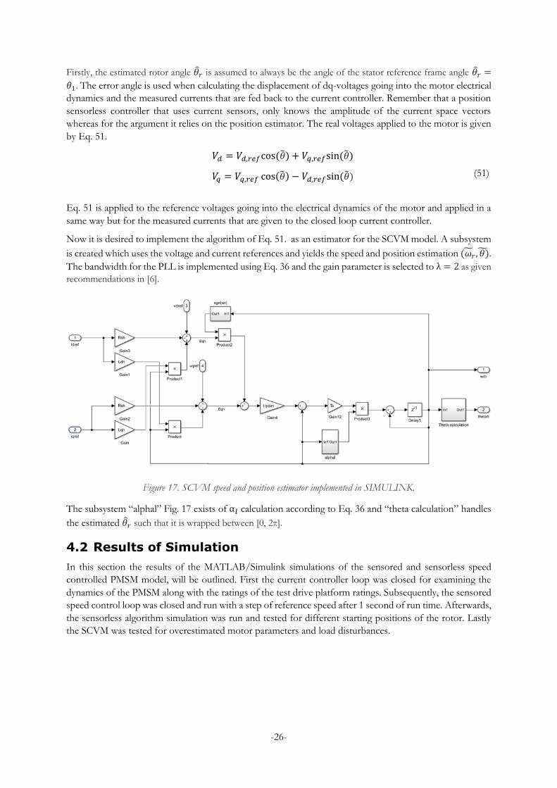
-26-
Firstly, the estimated rotor angle 𝜃𝑟 is assumed to always be the angle of the stator reference frame angle 𝜃𝑟 =
𝜃1. The error angle is used when calculating the displacement of dq-voltages going into the motor electrical
dynamics and the measured currents that are fed back to the current controller. Remember that a position
sensorless controller that uses current sensors, only knows the amplitude of the current space vectors
whereas for the argument it relies on the position estimator. The real voltages applied to the motor is given
by Eq. 51.
𝑉𝑑 = 𝑉𝑑,𝑟𝑒𝑓cos (�̃�) + 𝑉𝑞,𝑟𝑒𝑓sin (�̃�)
𝑉𝑞 = 𝑉𝑞,𝑟𝑒𝑓 cos(�̃�) − 𝑉𝑑,𝑟𝑒𝑓sin (�̃�)
(51)
Eq. 51 is applied to the reference voltages going into the electrical dynamics of the motor and applied in a
same way but for the measured currents that are given to the closed loop current controller.
Now it is desired to implement the algorithm of Eq. 51. as an estimator for the SCVM model. A subsystem
is created which uses the voltage and current references and yields the speed and position estimation (𝜔�̃� , 𝜃)̃.
The bandwidth for the PLL is implemented using Eq. 36 and the gain parameter is selected to λ = 2 as given
recommendations in [6].
Figure 17. SCVM speed and position estimator implemented in SIMULINK.
The subsystem “alphal” Fig. 17 exists of α𝑙 calculation according to Eq. 36 and “theta calculation” handles
the estimated 𝜃𝑟 such that it is wrapped between [0, 2π].
4.2 Results of Simulation
In this section the results of the MATLAB/Simulink simulations of the sensored and sensorless speed
controlled PMSM model, will be outlined. First the current controller loop was closed for examining the
dynamics of the PMSM along with the ratings of the test drive platform ratings. Subsequently, the sensored
speed control loop was closed and run with a step of reference speed after 1 second of run time. Afterwards,
the sensorless algorithm simulation was run and tested for different starting positions of the rotor. Lastly
the SCVM was tested for overestimated motor parameters and load disturbances.

-27-
4.2.1 Simulation results sensored control
Before running the whole speed controlled electric drive system model the current dynamics needs to be
verified to perform as intended. In section 4.2.3, the target rise time of the current dynamics were selected
to 2ms. The current controller of both the sensored model and the SCVM have no differences (apart from
direct current adjustment in SCVM) hence one simulation could verify the rise time of both current
controllers. The simulation was run with closed loop current controller with a step in q-current at time
stamp 1 second to 0.77 p.u.
Figure 18. Closed loop q-quadrant current dynamics of common current controller with q-current
(blue) and q-current reference (blue dashed)
In Fig.18 the current response of the controller is shown. The rise time is defined as the time it takes for a
signal to reach 90% of a new reference. The step response reaches 90% of the reference after 2ms after
initiation. This verifies that the proportional part of the gain selection properly selected given the
requirements. The step response does not give rise to overshoot which implies that the integral part is
selected properly. There is no cross-coupling effect in the d-current which stays at zero during the
simulation.
After the current controller was verified to perform satisfyingly, the speed control loop can be closed. The
test simulation was run by using the step of reference rotational speed and no-load condition. The inertia
of the motor and a small part of the vicious damping is the torque load. As the test are meant to test the
operation in a test bench the damping of pressurized water is not used for this simulation. The reference
speed is set to 100 radians per seconds which corresponds to 190 rpms. The results of the simulation are
shown in Fig. 19 with currents and speed along with reference values.
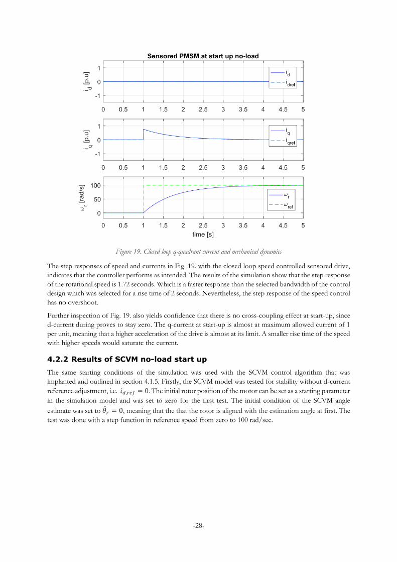
-28-
Figure 19. Closed loop q-quadrant current and mechanical dynamics
The step responses of speed and currents in Fig. 19. with the closed loop speed controlled sensored drive,
indicates that the controller performs as intended. The results of the simulation show that the step response
of the rotational speed is 1.72 seconds. Which is a faster response than the selected bandwidth of the control
design which was selected for a rise time of 2 seconds. Nevertheless, the step response of the speed control
has no overshoot.
Further inspection of Fig. 19. also yields confidence that there is no cross-coupling effect at start-up, since
d-current during proves to stay zero. The q-current at start-up is almost at maximum allowed current of 1
per unit, meaning that a higher acceleration of the drive is almost at its limit. A smaller rise time of the speed
with higher speeds would saturate the current.
4.2.2 Results of SCVM no-load start up
The same starting conditions of the simulation was used with the SCVM control algorithm that was
implanted and outlined in section 4.1.5. Firstly, the SCVM model was tested for stability without d-current
reference adjustment, i.e. 𝑖𝑑,𝑟𝑒𝑓 = 0. The initial rotor position of the motor can be set as a starting parameter
in the simulation model and was set to zero for the first test. The initial condition of the SCVM angle
estimate was set to 𝜃𝑟 = 0, meaning that the that the rotor is aligned with the estimation angle at first. The
test was done with a step function in reference speed from zero to 100 rad/sec.

-29-
Figure 20. SCVM during start-up with no initial angle error and no-load.
The results of the SCVM simulation at start-up in Fig. 20 shows that even though the starting position of
the rotor and the initial value of the angle estimator are equal, the estimator overshoots the angle estimation
once the controller starts. Hence a negative value at timestamp 1 second is shown in the angle error plot in
Fig. 20. Because of the non-zero �̃�𝑟 the current controller outputs a small amount of negative d-axis currents
at start-up and the q-axis current is not able to reach its reference value until the angle error converge to
zero. Also, seen by the speed estimation curve, the green dashed curve of Fig. 20 is overshooting the actual
speed at the 1 second mark. The overshoot in speed estimation is the cause of the overestimated position
once the motor control is started. However, the position estimate converges to zero after about 200ms and
the results of the speed controller is quite satisfying.
The SCVM model was implemented successfully without the d-current adjustment for low-speeds. The d-
current adjustment that is proposed in [6] should compensate erroneous estimation of stator resistance and
inductance, making the controller more reliable for synchronizing at low speeds by set 𝑖𝑑,𝑟𝑒𝑓 = 𝑖𝑞,𝑟𝑒𝑓/λ for
low speeds. Once the speed estimation reaches a stable speed for reliable back-emf information, tentatively
10% of the rated speed, the d-current reference is set to zero again.
The d-current adjustment algorithm was implemented in to the SCVM current controller subsystem as
shown in section 4.1.5 but once tested the system was proving instability, see Fig 21.

-30-
Figure 21. SCVM start-up with d-current reference adjustment
The speed estimator estimates a speed of 100 rad/sec in negative direction at startup which in turn makes
the position estimation error not to converge. Afterwards the speed estimator pulsates between positive and
negative small speeds which the q-current pulsates from negative to positive yielding quick acceleration and
deceleration between 50 to -50 rpm. Quite some time was spent to fix the implementation of the d-current
adjustment algorithm, but due to the time scope of this project it was decided to progress with keeping d-
current at zero throughout all speeds since the results of Fig. 20 were satisfying.
The test of the SCVM model proceeds by sweeping through different starting positions of the rotor. The
simulation is the same that of the startup case of Fig. 20. but for each test the starting rotor position offset
is increased for each test. The angle estimation error is plotted in Fig. 22. for each test iteration.

-31-
Figure 22. SCVM error angle stabilization during no-load start-ups with different starting positions
Fig. 22 verifies that the SCVM position estimation converges towards 0 or 2π for each tested starting
position of the rotor, which in turn verifies that the implemented SCVM will synchronize for the given load
condition and the tested starting positions. Two of starting position seen in Fig.22 clearly has a longer
settling time than the rest of the starting positions. The two starting positions of 2.9 and 2.4 radians has a
longer settling time of 0.8 seconds after start-up. The other starting positions converge towards 0 or 2π
within 0.5 seconds.
4.2.3 Parametric study of SCVM
In this section the tolerance of erroneous estimated motor parameters and torque load disturbance will be
examined. The parametric study concerns the SCVM sensorless control since faulty estimation parameters
may affect the speed and position estimator thus affecting the synchronization of the controller. Hence it is
vital for the sensorless control that motor parameters are considered with care when designing the control
gains.
First consider the stator winding resistance, the real resistance of the motor is kept the same in the electrical
dynamics of the motor model. But for the controller gains, the active damping and the SCVM speed
estimator the stator resistance 𝑅𝑠 is substituted with 𝑅�̂� which is the estimate of the stator resistance such
that 𝑅�̂� = 𝑘𝑅𝑠 where k is a scale factor to adjust the estimation error.
For the first test, the stator resistance was underestimated by 40%. The simulation was run as in previous
test where the simulation was run several times for different starting positions. The results are shown in Fig.
23.

-32-
Figure 23. Error angle during start up with underestimated stator resistance Rsh=0.6Rs
In Fig. 23 the results of the SCVM start up with underestimated stator resistance. The simulation results
show that the error angle approaches 0 or 2π for all tested starting positions. Furthermore, the error angle
converges slightly faster for most starting positions compared to the test where 𝑅�̂� = 𝑅𝑠. The results of the
simulation show that the oscillations are actually dampened by underestimating the stator resistance.
Progressing with analyzing overestimation the stator resistance, with an increase of 10%, with same test
procedure to previous starting position sweep. The results are shown in Fig. 24 and clearly shows that the
time of convergence for 0 or 2π is greatly increased and for 1.9 and 2.2 radians and starting positions the
controller is not able to synchronize at all.
Figure 24. Error angle during start up with overestimated stator resistance 𝑅�̂�=1.1Rs

-33-
The rotor position starting offset which yielded high oscillations were targeted for several of values of 𝑅�̂�.
In fig. 25 the same test conditions were conducted for the SCVM with a starting position of 2.2 radians, and
several values of k for each simulation. The results show that for an overestimated stator resistance the
position estimator turns unstable and oscillating rather than converging towards zero. In the other hand, an
underestimation of the resistance improves the time for convergence. However, the lower value of k the
higher undershoot of the estimation error. Seen by the light blue curve where k=0.1, the fastest zero crossing
appears but also the farthest undershoot. If low under-shoot is desired but as fast synchronization as
possible, the stator resistance in this case could be underestimated to by roughly 20-40% intendedly for this
application.
Figure 25. SCVM startup position error for different estimation errors of stator resistance
The implication of faulty estimated stator resistance was examined. Next parameter to examine was the
synchronous inductance which was tested with same procedure. First the underestimated value of the
inductance was simulated for different starting positions of the rotor. The results of the simulations are
shown by Fig. 26, where the synchronous inductance was set to �̂�𝑑𝑞 = 0.6𝐿𝑑𝑞.

-34-
Figure 26. Error angle during start up with underestimated stator resistance Ldqh=0.6Ldq
The simulation of underestimated inductance in Fig. 26 shows faster convergence compared to the normal
case in Fig. 26, for the most problematic starting positions of the rotor. Like the underestimated resistance,
the underestimated inductance seems to improve the dynamics of the controller for faster synchronization
at start up.
The simulation was run several times for different values of estimated inductance with k varying from 0.5
to 2. The chosen starting position was chosen as for the same test of resistance where 2.2 radians offset was
considered as a problematic starting position of the rotor. The results are shown in Fig. 27.
Figure 27. Simulation of different k values of estimated inductance for no-load start up with 2.2
radians initial rotor position offset.
The results of Fig. 27. shows that neither underestimation or overestimation of the synchronous inductance
affects the stability of the controller. However, different values of k clearly affect the time response of

-35-
convergence for the controller. Seen by the graph the larger the value of k, the longer time it takes for the
angle estimation angle to reach zero. A highly underestimated inductance yields the fastest zero crossing. In
the other hand, a greatly over- or underestimated yields a static error of the angle estimation error as seen
by the 3 seconds mark where the static error spread from -0.1 to 0.1 radians.
4.2.4 Locked rotor torque and load at start up
In this section the results of the locked rotor simulation will be outlined. The simulation test is carried out
for examine SCVM’s ability to produce torque while the rotor is locked in same position and compare this
to the sensored model simulation of the same test conditions. The foremost crucial part of of the SCVM
for deliver torque is to synchronize. But with rotation completely locked at start-up is complicated since the
inputs of the back-emf will be static, currents, voltages, references and estimated rotation that is.
The mechanical load of the motor model was for this test changed such that the external load torque equals
the electrical torque and the viscous damping such that all torque components equals out, making Eq. 47.
equal zero henceforth the speed of the rotor should be zero. The torque load step function stops at the 5
second mark then putting the motor under no-load. The results of the simulation with locked rotor, is
shown by Fig. 28.
Figure 28. Motor dynamics with locked rotor during 5 seconds after sstart-up and initial rotor
position offset of 2.2 radians.
The results of the SCVM locked rotor test in Fig. 28. show that for this case the position estimator is unable
to synchronize during the lock-down of the rotor. The error angle is initially 2.2 electric radians before the
motor starts. Once the speed and current references are set at the 1 second mark the error angle reduces
slightly to 1.76 electric radians but then remains at that static error until the load torque is released. Once
the load is released the motor synchronizes and accelerated whit an overshoot. The q-current in the motor
is during locked rotor is -0.19 p.u while the d- current is almost at maximum limit 0.98 p.u. Still during lock
down the maximum absolute value limit of 1 p.u. is not exceeded
The same simulation was conducted with zero initial rotor position offset to examine the best case scenario
for a sensorless control algorithm. The results are shown in Fig. 29. The error angle goes from zero to -0.07
radians once the controller starts at the 1 second mark. This offsets the q, current from being 1 p.u. to 0.91
p.u.

-36-
Figure 29. SCVM simulation of locked rotor with zero position offset at start-up
Figure 30. Position angle error for increasing torque load.
In Fig. 30 the error angle is plotted for different percentages load torques of the maximum available torque
of the motor. In other words when c=1 the load is equal to the electrical torque. When c=0.1 the load is
10% of the produced torque during the simulation for 5 seconds. This simulation was done to complement
the other test results as an indication where the SCVM starts having difficulties of synchronization with
loaded start-up. One can see that when the load is 60% of the available produced electric torque, the SCVM

-37-
cannot synchronize the motor. But for 50% load the SCVM manages to synchronize after roughly 1.5
seconds.
Lastly the sensored control model was simulated with the same load conditions as in prior tests where the
load torque is equal to the provided torque by the machine for a locked rotor simulation. The results are
shown in Fig. 31, where the q- and d-currents align as controlled by the controller just as in the no-load
simulation of Fig. 31.
Figure 31. Locked rotor simulation of the sensored PMSM control model
4.2.5 Discussion of simulation study
The simulation study achieved a complete model of a PMSMs motor control system both for a position-
sensored control system by assuming direct and reliable rotor position, and a position-sensorless control
system by using the SCVM position and speed estimator. Both models verified that a feasible selections of
gain parameters for the PI-controllers, selected accordingly known methods from previous literature,
resulted in satisfyingly performance for the target motor model. Also, the desired test conditions that would
be used in the lab experiments would not exceed drive platform ratings of 10A and 234V per phase. With
the implemented control design the absolute value of d- and q-currents and voltages never exceeded this
hardware limit with exception of the faulty implementation of d-current reference compensation.
The compensation of d-current reference at low speeds, was unsuccessfully implemented. All the attempts
of using a non-zero d-current reference at start-up made the controller unstable. By inspection of the results
in Fig. 21, one can suspect that there is a sign error at some point in the implementation, since the peaks of
the real speed occurs at same point where the estimated peaks appear but with different signs. Moreover,
the sign function of the speed yields fast switching between positive and negative values for the d-current

-38-
at low speeds which yields fast switching of the output voltage. One further cause of the error could be that
the sign output of Simulink returns zero if the input is zero which leads to division by zero for the d-current
reference calculation seen in Eq. 21. Further error investigation would be needed to solve the dysfunctional
algorithm. However, as pointed out in [6] the d-current reference adjustment can reduce instability due to
estimation errors of the stator resistance and inductance. Conclusively, the d-current adjustment might
improve the implemented algorithm of the simulation study but is not a requirement since the control
algorithm performs satisfyingly according to the results.
The impact of erroneous estimation of parameters has impact on the controlled system. While a slightly
underestimated stator resistance decreases the time of synchronization, an overestimation can make the
synchronization to never happen. Conclusively it is in line by previous literature in [6] and by the results of
this report, that if SCVM is used the user is recommended to underestimate both inductance and stator
resistance for guaranteed synchronization at start up. The results of this study showed with the given motor
dynamics and for different values of the estimated resistance, that the resistance could be underestimated
by up to 40% without giving large undershoots in position error, but still minimizing the time of
synchronization.
The implementation of the SCVM has shortcomings when considering locked rotor torque production.
Shown by the results of the locked rotor tests of the SCVM the position error has in all cases a static fault
when the rotor is completely at standstill. This can be foreseen by Eq.31,32 and 38, since all variables for
the back-emf estimation are at steady state, hence the position estimate will also be static. There are
possibilities to get around this lock up with various techniques when expanding the sensorless functionalities
of the controller, such as “sweeping” through different position estimates sending pulses for chances of
acceleration. Once the motor accelerates the error estimate will be eliminated.
The sensored lock rotor simulation yielded maximum torque while assuming perfect synchronization by the
sensor. The results should not be considered realistic, since sensors in practice have technical limitations
that is not considered by the by simulation. The performance of the sensored drive is affected by the
resolution of the sensor, quantization errors, EMC disturbances, the analogue to digital conversion, software
limitations, mechanical stress etc. The results of the locked rotor test of the sensored control should
henceforth be considered only as a theoretical possibility.

-39-
5 Test system Implementation
5.1 Hardware and test system
A major part of this thesis project is to set up the test system. Prior to this project a brake bench rig was
designed and implemented in the motor test lab at Xylem Sundbyberg. The brake bench test rig contains a
speed-controlled servo drive which allows the user to program and run different braking profiles based on
speed references and maximum torque production of the braking servo motor. The system comprises of
the servo drive, a motor stand bench, braking resistor, a strain gauge torque transducer which also measures
shaft speed and a universal amplifier for real-time data acquisition.
Secondly the test platform for motor control will be implemented electrically. This comprises the AC-DC
supply to the TI platform´s DC-link, where of which the three-phase grid supply has to be rectified, and
also adjustable with a variable ac transformer a.k.a. variac.
5.1.1 Motor brake bench
The motor brake bench rig is basically a speed-controlled servo motor which can be connected to another
motor which is going to be tested. On the servo shaft a torque strain gauge is connected in order to measure
absolute torque applied to the shaft and a two-pulse optical encoder for speed measurement. The test rig is
designed in order to do motor performance tests for smaller motors and testing VFD performance and
software functions for pump applications. The servo drive is speed controlled in order to perform rapid
programmable braking. Data monitoring and programmable load curves can be communicated between
servo drive and a PC through a graphical user interface in LabVIEW. This Communication system was
implemented by the author of this project prior to this master thesis.
Figure 32. Motor brake bench test rig with tested motor (green), braking servo motor (upper red),
resistive load (blue) and servo VFD (bottom red).

-40-
5.1.2 Servo drive
The braking motor drive is a 6.5kW sensored permanent magnet motor controlled by an 8kW VFD. The
drive has a rated torque of 22.5 Nm from 0 to 3000 rpms with a maximum speed of 3000 rpm with flux
weakening control from 3000 rpms to 45000 rpms. The drive’s speed, current, torque states etc. can be
monitored and controlled through CANbus protocol CANopen. This is done via LabVIEW program that
was designed and implemented prior to this project.
5.1.3 Measuring device
The test bench is supplied by a strain gauge torque transducer T40B HBM. The device measures absolute
torque on the shaft up to 100Nm and the speed of the motion.
Figure 33. Coupled shafts of the two motors with strain gauge torque transducer measuring absolute
torque and speed of the motion.
5.1.4 Position Sensor
In chapter three some of the commonly used industrial position sensor technologies were explained. For a
position sensored speed control system one could use any of these that fit for the application. In a
submersible pump application there is limited space for a shaft mounted encoder. Hall elements are much
less space demanding since they are mounted inside the rotor and stator. However, in this project any sensor
could be used since it is carried out in a brake test rig where there are no space limitations. Hall elements
are quite complicated to install and would be time consuming for this thesis project. Subsequently hall
elements were rejected for this project. The TI platform supports either hall elements or quadrate encoder
signals and has interface input signals for either of these. Hence, it was decided to use a quadrate shaft-
encoder. A triple pulse incremental encoder from Heidenhein was purchased alongside a 10 m shielded cable

-41-
with open wiring at one of the cable ends which were going to be connected to the TI platform. The TI
platform uses 4 pins to connect a quadrate encoder, phase A, phase B, reference signal and ground that is.
The mechanical installation of an encoder needs to be carried out with care. The rotor and encoder shafts
need to be aligned when using a rigid shaft connection. If not, the encoder can be mechanically damaged
by vibrations. The pump that was used has an iron housing head that the power electronics usually are
installed. In this project the motor is fed by an external drive. Hence, am empty top housing could be used
to mount the encoder with good alignment to the axial shaft from the motor, see Fig. 34. and the encoder
shaft is mounted to the rotor shaft on the rotor shaft with an adjustable rigid shaft extension.
Figure 34. Top of test motor with shafts connected with a rigid coupling to a incremental encoder.
5.1.5 DAQ monitoring
For measurements of the test rig an HBM QantumX MX840B universal amplifier is used. The amplifier has
8 input channels and can measure analogue and digital signals with a fast sample rate of XX kHz. The
amplifier ships preconfigured for the HBM T40B torque transducer which is handy for setting up real-time
monitoring for lab-based test systems.
The torque and speed of the shaft are directly measured by the torque transducer and are connected to 2 of
the input channels of the amplifier box. Furthermore, the TI platform has 4 pins from the DAC which will
be used to monitor the estimated angle, measured angle and 𝑖𝑑𝑞. The output signals from the DAC pins of
the TI platform pulse widths signals that creates analogue signals between 0 and 3.3 VDC. The DAC of the
TI HV kit is explained in section 2.3. These signals can be sent to the QuantumX amplifier and scaled to
proper values for the application. The cables that were used are three-wire shielded cables with a 15- pole
RS-485 interface. One wire carries the DAC signal and the second one is terminal ground of the TI platform
and QuantumX terminal ground. The cable shield was connected to the housing of the RS-485 interface
housing.
With the HBM Quantum X amplifier one can use a software tool for real-time measuring called CATman.
In catman, the user can set up the measurement system and configure measured signals with ease. Once the
test is running a real-time watch window of measurements can be seen and the user can record the
measurements and save it in different data formats. In this project the raw data was saved and transported
to MATLAB as raw data.

-42-
5.2 Test platform electrical implementation
The TI motor control kit referred to the test platform of this thesis electrical installation and configuration
will be outlined in the following sections.
5.2.1 Electrical overview
The test platform that were chosen for this project to run FOC for the PMSM is the high voltage motor
control kit Revision 1.1 by Texas Instruments. The general specifications for the platform were given in
table 1 in the method chapter. In Fig. 35. the schematics of the electrical layout of the hardware is shown.
Figure 35. Electric schematics of TI test platform
In the upper left corner of the schematics in Fig. 35 one can see the AC stage with AC input power and
PFC stage at notation P1. If single phase AC supply is desired the supply voltage should be 110 to 220 VAC
and maximum 750W. In the upper right corner, the diode rectifying stage AC-to-DC converter, noted (M4)
is located with three small capacitors and diode rectifiers. To the right of the rectifying stage there is input
for DC voltage supply directly to the DC-link of the inverter, noted BS4 and BS6 GND. If this input is used
the DC voltage should exceed no more than 350VDC and maximum 1.5kW.

-43-
Below the larger DC-bus capacitor bank, the inverter stage is located, noted (M5). This is where 6 IGBTs,
current sensors and motor connections are located. The inverter stage can be seen with up close in Fig. 36.
Figure 36. Inverter stage of the TI test platform.
In Fig. 36 the components of the three shunt legs of the inverter can be seen. The six IGBTs are located at
U1 in Fig. 36. The IGBTs consist of a single 3-phase module MOD IPM PS2176 mini-DIP. Six diode
rectifiers are placed at D1-D6. Furthermore, the current sensors that measures the outgoing phase currents
to motor is located at R39, R10 and R11. These 20mOhms, 1% accuracy, with a maximum of 10A of pass
through current. More information regarding the test platform can be found by TI´s open-source literature
and downloadable motorware.
5.2.1.1 Medium voltage installation
The TI platform has two options of medium voltage inputs. The device could either be fed by a single-
phase AC supply, which is then rectified by the rectifier stage of the platform. The platform also in this case
has a PFC stage for power factor correction. However, using this input limits, the output power to the
motor to 750W due to the ratings of the rectifying stage and the PFC stage. If one uses direct DC-supply
to the DC-link of the platform one can utilize the maximum power of the inverter stage which is rated
1.5Kw. Hence, for device safety measures the direct DC supply input will be used.
In order to generate DC voltage an external motor drive will be used to rectify a 3-phase voltage source.
The external drive has a DC-link output positive output and ground output. These two terminals of the
external motor drive will serve as an AC-DC rectifier for the supply to the TI test platform. Moreover, the

-44-
DC-supply need to be variable in order to safe-starting the algorithms of the test platform. For testing motor
control algorithms, it is necessary to start at low voltage and slowly increase the voltage while the algorithm
is run. By doing this, faulty control designs can be detected before it damages the hardware of the inverter.
The high voltage supply to the TI platform will be done by connecting DC voltage directly to the DC-link
of the TI platform. The TI platform could alternatively be fed by single-phase AC power. However, the
rectifying stage of the TI platform is rated for only 750W whereas if direct supply to the DC link offers
operation to maximum 1.5kW. The DC-supply.
Figure 37. System design of voltage supply to test platform and test motor connection.
Figure 38. Picture of electrical installation of TI platform. DC-supply (A), motor phases (B),
Microcontrol-card with USB flash connection (C), encoder interface (D), low voltage-side supply (E)
and DAC monitoring connections (F).
5.2.2 Encoder index pulse calibration
The physical position of the index pulse has to be calibrated and translated to a corresponding electrical
angle. This is done by measuring electrically where the index pulse appears relatively to the electrical angle
of phase A of the PMSM. More precise, how many encoder counts are there between the PMSMs zero
crossing on rising edge are the until an index pulse appears with raising edge. One way to find this is to

-45-
externally rotate the PMSM and measure the back-emf voltage of its output phases alongside the encoder
index pulse with an oscilloscope.
The PMSM has no neutral so the phase A cannot be measured directly between phase A and neutral.
Another way to measure the phase-to-neutral voltage of phase A is to measure the phase-to-phase voltage
between A and B and adding the phase-to-phase voltage between phase A and C. This yields phase A’s
alignment but whit a factor √3 increase in magnitude.
The PMSM was for this test set up so that the servo drive rotates the PMSM with 300 rpm constantly and
the encoder was fed with operating voltage. The oscilloscope is set up with 3 voltage probes, two for line-
to-line voltages of the PMSMs back-emf and on probe for the index pulse of the encoder.
Figure 39. Left figure showing back-emf voltages Vab (red) Vac (green) and Vab+Vac purple,
right figure shows zoom of index pulse
Figure 40. Oscilloscope time capture of index pulse occurring at T and zero crossing of Phase A.
Seen in Fig. 40, the index pulse occurs at captured time zero point of the oscilloscope. Each square is 2.0 𝑚𝑠
which thereby the time between the index pulse and the phase A zero-crossing was measured to be 5.64 𝑚𝑠.
Knowing that the speed of the rotation is 300𝑟𝑝𝑚 2048 encoder tics per mechanical revolution and 5 pole
pairs of the motor, the displacement of the index signal is calculated to be 469 tics. The calibration offset
parameter is henceforth 469𝑡𝑖𝑐 × 4𝑐𝑜𝑛𝑡𝑠
𝑡𝑖𝑐=1876 encoder counts.

-46-
5.3 Controller Code design and implementation
In this chapter the software implementation of the MCU will be described including the procedure of the
coding process as well as the software implementation of the motion sensored motor control algorithm.
5.3.1 Code generation
All coding for the MCU is carried out in SIMULINK/MATLAB with supported by the embedded coder
add-on which enables the user to directly compile, load and run code from SIMULINK to C-code via make
file approach. The code is generated to a .h-file which can be loaded once in the IDE (integrated
development environment) which for C2000 family is TI-s CCS (Code Composer Studio). The IDE has to
be installed to a version that is supported by MathWorks embedded coder in order to be able to convert
Simulink/MATLAB code into C-code. Also, a set of global variables has to be configured on the PC-global
entries. This is done while installing MathWorks embedded coder.
In this project the Matlab2016b is used with embedded coder version 6.11. Additionally, in order to generate
C-code via Simulink to the micro controller, the MathWorks support package “Texas Instruments c2000
processors v.16.2.4” and a compatible IDE version of CCS is needed. CCS v.5.0 was used in this project
since both v.6.xx and v.7.xx were all struggling to successfully compile Simulink generated code to the
microcontroller. The implementation of CCS v.6 and 7 were unsuccessful and the reason is unknown. This
limits some of the access of some features of the newer versions of CCS.
5.3.2 Top layer build
The program code for sensored motor control in Simulink consists of a hardware interrupt which includes
calls for all functions of the complete algorithm. In the top layer build shown in Fig. 41. the hardware
interrupt block (blue) can be seen at the top with a call signal to the main function of field-oriented control
in yellow. The hardware interrupt is configured by creating a vector with four configurable rows. When
several interrupts is needed, the user creates a new column for each configured interrupt. The first row is
corresponding to the CPU number of the interrupt which is set to 1. The second row is corresponding to
the “peripheral interrupts expansion” (PIE) number, which is also set to 1. The third row of the interrupt
vector is “Simulink task priorities” which is set to 30 by default. The fourth and final row allows the user to
set a Preemption flag, where one equals preemptible interrupt and zero equals non-preemptible. A non-
preemptible system is sufficient for the application, hence 0 is chosen. More information regarding the
configuration registers and features for the device is found in the manufacturer product sheet in [29].
This function includes the current and angle measurements, the current control loop, DAC-signalling and
the PWM-signalling. There’s also an outer control loop of speed control. This outer speed loop should
preferably have a bandwidth of hundreds lower than the inner current controller. This is done by using rate
transitions for the outer speed control in Simulink such that the sample time of the speed controller is at
least 1000 times greater than the inner current control sample time [2].

-47-
Figure 41. Top layer build of SIMULINK code to target hardware.
The speed control block includes just a simple PI controller with an adjustable speed reference signal and
the actual measured speed from the sensor as input. The measured speed is calculating from the raw position
counter signal QEP from the function FOC system and is calculated in the Speed calculation block. The
speed control loop could also be driven by a second interrupt by the hardware interrupt module. However,
with the use of rate transition functions one can in a convenient way make sure of the speed controller
always will perform at a certain rate lower than the FOC interrupt. In the rate transition block going into
the speed calculation is set to 0.001 and the rate transition going from the speed controller is set to be
inherited by the input of the block.
5.3.3 Function FOC
The “Function FOC” subsystem has four main functions that are all categorized into own subsystems seen
in fig. 42.
Figure 42. Insight of “Function FOC” main field-oriented motor control subsystem

-48-
The leftmost block in Fig. 42. is the measurements and scaling subsystem. In this subsystem measurements
of phase currents and encoder is performed each sample cycle, and also the scaling into a feasible per-unit
scaling with a fixed-point format. In the current controller subsystem, a PI-regulator controls the scaled
values of the measured quantities. The “to PWM”-block includes the configuration of the PWM dialling of
the calculated reference values from the controller. Lastly the “To DAC” block handles all the values from
the CPU to be sent to the digital to analogue converter for data acquisition purposes.
5.3.4 Current controller
The essential part of the current control subsystem is to handle measured currents and with respect to the
current reference yielded by the speed controller, perform calculations such that new voltage references are
sent to the PWM signals. Therefore, PI-controllers are used in this function with one for the d-quadrate
current and one for the q-quadrate current. Most vitally for standard operation is to control maximum q-
quadrate current since it is the torque providing current of the machine, as described in the theory part in
previous chapter. The d-current reference should always be controlled for zero, hence a fixed-point constant
is used for the reference of d-current seen in Fig. 43.
Figure 43. Inside of current controller subsystem
Firstly, the measured and scaled signals of phase currents a and b is Clarke transformed followed by Park
transformed. This is done with the measured value of rotor angle theta, seen in Fig. 43. Subsequently the
dq-transformed measured currents are sent to the two PI modules. In this program TI libraries functions
are used for PI controllers. These are used since they are pre-made for computation efficiency for the C2000
processor family. Own controllers could also be constructed likewise, but one needs to keep in mind to
prevent data overflow and computational power limits of the processor.
In this stage of the current control design, the active damping and the cross-coupling cancelation is left out
for reasons of not overload the processor. These should however be implemented in a later stage once the
current controller has been tested and proven functional.
The configuration of the PI-controller should be set in accordance to the motor parameters and the desired
performance of the system. For this application a rise-time of the current controller was set to 3ms and
risetime of the outer speed loop was set to 3s as described in the simulation chapter. Nevertheless, the gain
parameters considered during the simulation chapter, must be scaled correctly to the per-unit base same as
the controller code design. A considerable amount of time was spent to try to normalize the gain parameters
using the previous built simulation model. However, the simulation resulted in unstable performance.
Consequently, it was decided to use the gain parameters that are found while running auto tune with TI’s
“Insta-Spin FOC” algorithm which follow the same fix-point format as this implementation. In case of poor
tuning of the parameters, fine-tuning could be done by hand.

-49-
The outgoing signal from the two PI controllers enters a subsystem called saturation seen in Fig. 44. The
function of the saturation is to limit the magnitude of the newly found voltage reference to not exceed the
voltage limit of the inverter, 236.14V that is. This value corresponds to the value of ±1 𝑝. 𝑢 within the fixed-
point base.
Figure 44. Inside of saturation subsystem
Seen in Fig. 44. the signals of voltage references are saturated using a switch. If the magnitude of the two
signals are greater than 1, the former value of previous sample is used instead. This is done with the help of
a unit delay.
Lastly, the voltage references that have gone through the saturation function are to be calculated into raw
duty ratios for the PWM switching. This is done by inverse park transforming the dq- references and project
them into phase reference phase voltages. There is DMC-library blocks for both operations provided by
MathWorks and TI, which ensures correct Q-setting based on the input setting. The implementation of this
in Simulink is shown in Fig. 45.
Figure 45. Inside of space vector generator subsystem
5.3.5 PWM synchronization
In motor control it is vital that the timers of the three PWM modules are synchronized. Firstly, the thyristors
that are directly controlled via the PWM signals must be switched on and off correctly, not allowing short
circuiting of the DC-link. Hence the switching logic should prevent SW1 and SW2 of the same phase leg
(see figure. XX) ever being closed at any moment. Short circuit of the DC-link will damage the hardware
and in catastrophic events lead to injury to people close by the hardware. Moreover, the PWM modules in
this application are also triggering the ADC modules which measures the currents A & B and the encoder
measurements. The timing of the PWMs are there for critical and delicate. The software modules provided
by TI can quite easily be configured for the logic and timing and is therefore used in this project. The ePWM
modules for C200 family in SIMULINK for the usage of IGBT control are preconfigured to prevent phase
leg short circuit. Hence, Swa+ will always be open if Swa- is closed and vice versa. The first ePWM1 module
is configured to output a synchronization signal with counter equals zero. ePWM2 and ePWM3 have a
synchronization action to counter equals zero. This ensures that the periodic counter of the three ePWM
modules are synchronized.

-50-
The ePWMs are first configured for one out of three different compare value wave forms. Often in motor
control literature this is referred to as the carrier wave. By the ePWM module in SIMULINK one can
configure a carrier wave to be either UP, DOWN or UP-DOWN. For symeterical waveforms UP-DOWN
count are used wheras for asymmetrical waveforms can be created by a count UP or count DOWN sawtooth
wave. For a symmetrical sinusoidal waveform UP-DOWN counting mode should be used. The timer base
counter period (TBCTR), according to TI ePWM module documentation (källa) should be chosen as Eq.
51.
TBPRD =
𝐶𝑙𝑜𝑐𝑘 𝑓𝑟𝑒𝑞𝑒𝑢𝑒𝑐𝑦
2 × 𝑆𝑎𝑚𝑝𝑙𝑖𝑛𝑔 𝑓𝑟𝑒𝑞𝑒𝑢𝑛𝑐𝑦=
90 𝑀ℎ𝑧
20𝑘𝐻𝑧= 2250
(51)
The time base counter period is to say the maximum counter compare value of the PWM module. In other
words this if the ingoing counter compare value equals the timer period, the PWM would respond with with
a duty cycle of 100%. And if the ingoing counter compare value equals half of the period it the PWM would
yield a duty cycle with 50%. This Logic is illustrated in Fig. 46.
Figure 46. Inside “To_PWM” subsystem.
5.3.6 ADC Scheduling
The ADC (analogue to digital converter) module is carrying out the requested analogue to digital
conversions from the measurable currents, voltages, and speed/position signals on the board. The needed
signals of this application are; two phase currents Ia and Ib, and the counter value of the encoder QEP. A
third measurement of a phase current is not needed since in three phase electrical systems one often assumes
that the load is balanced. Hence all calculations in the current controller requires only measurements of two
phases to be able to calculate the magnitude and argument of the third one.
The TI ADC module in SIMULINK collects the data gathered from the ADC pins of the processor at a
configurable event. For the current measuring the ADC block configured via simultaneous sample mode
for current A and B with an acquisition window of 7 at the start of the conversion. This is triggered by the
ePWM sync signal which was described in PWM synchronization section. The sample time is inherited,
meaning that the ePWM sample rate is used. Moreover, the interrupt trigger is sent at the end of the
conversion. Configuration and the Simulink blocks can be seen in Fig. 47.

-51-
Figure 47 Simulink block “measurements and scaling” of ADC and eQEP modules (left), ADC
configuration (right).
5.3.7 QEP speed position measurement module
TI offers an enhanced quadrate encoder pulse software module for purposes of measuring speed and
position in motion control systems. This module is embedded in most C2000 processors and can be
implemented in IDE or when coding in SIMULINK. An incremental encoder as mentioned in section
XX uses two or three pulse signals in order to track speed and position. Two pulses accordingly to A and
B are 90 degrees separated and can therefore be used to calculate the speed and direction of the shaft
motion. Depending if the A lags B or vice versa the direction can be determined. The third pulse is a
position index which can be used to determine the absolute position.
The speed and the direction of the motion is straightforward to implement when using TI libraries for the
eQEP module. However, position index for absolute position of the rotor is somewhat more complicated.
One solution to track the index pulse is to use the latch position counter of the eQEP module. It should
be mentioned that the eQEP module is used for decoding of the two-pulse train clocking and the index
pulse, to a counter calue and a latched counter value respectively. The calculation of these signals into
position value in terms of radians are left to the user to implement. However, there are some examples
provided by Mathworks in order to perform these calculations in a real time environment.
Firstly, the configuration of the module will be explained. The position counter mode can be set to
Quadrate-count, direction count, Up-count and Down-count depending on the way the input signals are
encoded. In this project it was chosen to the default of Quadrate-count. The sample time is chosen to be
inherited by the synchronization message created by the PWM1 module once the count equals zero. And a
latch position counter signal is enabled on index event. This is crucial for the sensored system since once
the index signal is sent the position latch signal will be used to track the position of the rotor.

-52-
The first signal incoming to the eQEP scaling block is the counter signal from the pulse train of phase A
and B of the encoder. These are both counter value from the number of tics for a whole mechanical
revolution of the encoder. The counter signal increments by 4 for each rising edge of a pulse from one of
the encoder phases. In turn, this means that the position counter has real-world value between 0 and the
number of slits multiplied of the encoder, 4 × 2048 = 8192. The second ingoing signal is the index latch
signal. This signal has one pulse per revolutions, on its rising edge the encoder the “qposilat” captures the
counter value of the rising edge of the index pulse. By subtracting the index counter value by the
“indexoffset” and counter value the actual mechanical angle can be found by eq. 52.
The electrical angle 𝜃𝑟 is calculated by the position counter value
𝜃𝑟 =
(𝑐𝑜𝑢𝑛𝑡𝑒𝑟 𝑣𝑎𝑙𝑢𝑒 − 𝑖𝑛𝑑𝑒𝑥 𝑐𝑜𝑢𝑛𝑡𝑒𝑟 𝑣𝑎𝑙𝑢𝑒 + 𝑖𝑛𝑑𝑒𝑥 𝑜𝑓𝑓𝑠𝑒𝑡) × 𝑛𝑝𝑝
𝑒𝑛𝑐𝑜𝑑𝑒𝑟 𝑠𝑙𝑖𝑡𝑠
(52)
Figure 48. Inside of subsystem eQEP and scaling
When the program is initially run the position is unknown until the first index signal pulse is received. Hence
a start- up ramp is used as a sweep-through of the motor, which should start to rotate the motor somewhat
which will hit the index pulse position eventually. This in turn yields a non-zero value of the index pulse
and this is captured by the eQEP module of the TI software which captures the counter value of the index
pulse. Seen in the bottom part of Fig. 34 and before the output signal 2 “position” there is a switch that will
use the start-up ramp as the electrical position until “init_latch” is non-zero. Lastly the counter position
signal is scaled to a fixed-point number between 0 and 1 with a Q value of 2.
5.4 Results of tests
In this section the results of the laboratory tests of the vendor’s pre-programmed sensorless motor control
and the implemented SIMULINK code, will be outlined.

-53-
5.4.1 Results and discussion of Sensorless motor control
The TI “Insta-SPIN” sensorless motor control algorithm was decided to be tested beforehand the own
written SIMULINK code. This was decided due to reasons of code safety. The vendor guarantees the Pre-
programmed code to function, and thereby the test system could be run without risks of ill-conditioned
PWM synchronizing or poor ADC scheduling etc.
There are two approaches when using Insta-SPIN for motor control. Either the user can use the code via a
pre-programmed GUI for configuration and operation. Or, the user can use code examples provided by TI
in the IDE CCS. At first the pre-programmed GUI of Insta-spin was run.
The first tab of the “InstaSPIN_FOC” GUI handles motor identification, where the user selects the type
of motor and basic motor parameters that is intended for the application. Subsequently, the user is needed
to run motor identification run where the code will execute a number of actions to find the stator resistance,
synchronous inductances and the flux modulus. In this GUI mode the user is not permitted to use own
motor parameters. This can only be done by using the code examples in CCS.
The identification run was executed, and the parameters were estimated. The first tab of the GUI is shown
in Fig. 49.
Figure 49. Motor identification tab of InstaSPIN_FOC software GUI.
As can be seen in Fig. 49. by the green box, the stator resistance, synchronous inductances and the flux
modulus are estimated to �̂�𝑠 = 0.416 Ω, �̂�𝑑 = 9.98 𝑚𝐻, �̂�𝑞 = 9.98 𝑚𝐻 and �̂�𝑚 = 1.56 𝑉/𝐻𝑧
respectively. The values are in correct order of magnitude, but the stator resistance is over estimated by
more than 10% and the inductances are overestimated by more than 5%.
Once identification of motor parameters is done, the user may operate the motor by either one of the other
function tabs in the GUI. “The speed or torque” tab was used for an initial start-up of the motor, this

-54-
program is suggested by the vendor for initial commissioning. The speed reference was initially set to 100
rpms, with a maximum accelaeration of 108 rpms/s. later ther speed was set to 900 to test functioning
operation at slightly higher speeds. The GUI of the speed or torque program can be seen in Fig. 50 and the
results of the speed, currents and torque measured by the sensoreless algorithm of the insta spin function
in Fig. 51.
Figure 50. Insta-spin FOC GUI of speed or torque control mode with motor running at 900rpm.

-55-
Figure 51. No-load test of insta-spin FOC with 100 rpm speed reference (left) and 900 rpm (right)
Fig. 51. Shows the steady-state performance of the two motor-runs. The motor accelerates to given
reference point for both cases and the d-currents are kept around zero once in steady state. The estimated
speeds, currents and estimated torque fluctuates significantly during operation. The estimate is cycling
between 850 rpm and 960 rpm. The cause of the fluctuations is debatable, but mechanical reasons could be
rejected. The servo drive can provide smooth torque with low ripple, with or without a test motor connected
to the shaft. Therefore, mechanical distortion is unlikely. The most probable cause of the ripple is due to
either software or hardware flaws in the test platform. Previously the over and underestimation of the motor
identification was noted. Whether or not this is the pure cause of the ripple is not known but its probable
that it contributes to the ripple.
At this point of the test procedure of the sensorless control algorithm it was decided to utilize the precise
knowledge of the motor parameters in order to possibly reduce current and torque ripple and also make the
sensorless control algorithm more comparable to the own written code. Henceforth it was decided to set
the parameters manually. The GUI restricts users to use identification run and does not allow own
parameters to be set within the GUI. If the user decides to use own parameter sets, these can be set inside
the C-code examples in CCS as the IDE where the user needs to go through a step-by-step process of
setting up the controller.
Before entering own parameters to the motor the step-by-step process requires a identification run in CCS.
While this was run the serial communication from COM to MCU failed while DC-bus voltage was on. The
user executed the program leaving the IGBTs in a non-safe condition which lead to a current from the DC-
bus to the motor which apparently was too high for current sensors. The current rushing through one of
the three phase legs, lead to an overload and the corresponding current sensor of that phase the blew up.
The burnt current sensor can be seen in Fig. 52 where the damage on the resistor can be seen and some
indication of soot and smoke where the minor explosion took place. No fire was developed, and no parts
flew off since the platform was encapsulated by a protective plastic housing.

-56-
Figure 52. Damaged current sensor of Phase V of the inverter.
The damaged current sensor leaved the platform out of function for the application since the open circuit
of the shunt returns error to the MCU and cannot operate. Other components of the inverter could have
been damaged while this is not tested and should be tested for future restoration of the platform.
The current sensor can be replaced. In a new iteration of the platform the current sensors could be mounted
on a separate card connected to the PCB of the TI platform such that a damaged current sensor is easier to
replace.
Unfortunately, due to the breakdown of the TI platform the own written code of the sensored motor control
could not be tested in the lab. The time scope of the project could not allow a new platform hardware set-
up. Initial testing of the code without load proved at least that the ADC scheduling and PWM modules were
working properly. But if the motor would be to synchronize is still unknown and if the encoder offset
calibration is yet to be verified by measuring the position error and speed error with the use of the
measurements of the torque flange.
-57-
6 Future work
Foremost future work is to actually test the designed motor control algorithms that were created during this
project. The breakdown of the current sensor in this project left the code untested for operation with the
motor. The start-up synchronization and the sensor off-set calibration are yet to be verified.
In regards of Xylem’s research and development of motor control technology the foremost suggested plan
of action is to implement a fully programmable inverter for testing and developing motor control concepts.
This could be the scope of a future master thesis project where the aim is to design and implement the
hardware of an inverter. The TI platform is meant to fulfil this role. However, the ratings of the platform
are under dimensioned for larger motors which Xylem uses. Also, there are other functions in the TI-
platform such as power factor corrector which could be expanded upon but is at this point vastly under
dimensioned for the motors. The under dimensioning of the drive yields risks to the hardware since small
errors in the control can lead to high currents due to low resistance of large motors.
7 Conclusions
During this master thesis project, a simulation study of two PMSM motor control algorithms were
conducted. The two algorithms that were simulated for a PMSM drive, were one with position sensor and
one based on the SCVM position sensorless back-emf estimator. The gain parameters of the closed loop
dynamics were designed analytically for a current rise time of 2ms and a rise time of the speed of 2 seconds
which were verified by simulations. By saturating current reference to the maximum allowed current of each
phase of the inverter the control system stayed within limits during stable conditions during the simulations.
The SCVM was implemented by constantly using a d-current reference equal to zero. This helped the control
system to be stable compared to numerous attempts to using a non-zero d-current reference at start-up of
the motor. The SCVM model resulted in guaranteed synchronization at start-up for any given starting
position if two criteria were hold. First the stator resistance estimate should be equal or less to the actual
stator resistance, secondly the load torque at start up would be equal or less to 50% of maximum torque
delivered by the PMSM.
The sensored simulated PMSM model followed the same gain selection of the sensorless model but assumed
always synchronized operation. While this assumption may not be true in reality, the simulations models
can offer information for a best-case scenario. The sensored drive could deliver maximum torque at start-
up independently of the load torque. If sensored PMSM control is feasible for a submersible pump within
1-5kW range is still to be furtherly investigated. What is needed to study is the costs of implementation and
reliability of position measurements in actual pump station environment.
The laboratory test system was in this project implemented and put into test. An own written code based
on TI literature and code examples was written for the application. A pre-written code for sensorless control
was used for comparison of control systems.
During an early event of the tests, the communication between PC and MCU broke down and as a
consequence, a faulty PWM signal was sent to one of the IGBTs, leaving one phase under load to the motor
and a minor explosion occurred on a current sensor on the inverter PCB. This left the drive platform
damaged and dysfunctional for the remainder of the project. Hence the own-written code for the sensored
PMSM control is still to be tested. In future work for the laboratory equipment at Sundbyberg, it is
recommended to design and implement a controllable inverter stage with properly dimensioned
components such that the risk of damaged hardware is minimized.

-58-
8 Bibliography
[1] S. Derammelaere, M. Haemers, J. D. Viaene, F. Verbelen, and K. Stockman, "A quantitative comparison between BLDC, PMSM, brushed DC and stepping motor technologies," in 2016 19th International Conference on Electrical Machines and Systems (ICEMS), 2016, pp. 1-5.
[2] L. Harnefors, M. Hinkkanen, O. Wallmark, and A. Gomez, Control of Voltage-Spurce Converters and Variable-Speed drives. 2015.
[3] F. Meier, "Permanent-magnet synchronous machines with non-overlapping concentrated windings for low-speed direct-drive applications," Diss. Stockholm : Kungliga Tekniska högskolan, 2008, Stockholm, 2008.
[4] O. Wallmark, AC machine analysis fundamental Theory. Stockholm: KTH - Department of electrical energy conversion, 2015.
[5] S. Ruoho, "Demagnetisation of Permanent Magnets in Electrical Machines," ed. Kuressaare, Estonia: Doctoral school of energy- and geo-technology Helsinki University of Technology, 2007.
[6] M. Jansson, L. Harnefors, O. Wallmark, and M. Leksell, "Synchronization at startup and stable rotation reversal of sensorless nonsalient PMSM drives," IEEE Transactions on Industrial Electronics, vol. 53, no. 2, pp. 379-387, 2006.
[7] H. A. Toliyat and S. G. Campbell, DSP-based electromechanical motion control. CRC press, 2003. [8] N. K. Sinha, Microprocessor-based control systems. Springer Science & Business Media, 2012. [9] M. H. Rashid, Power electronics handbook: devices, circuits and applications. Academic press, 2010. [10] D. Seborg, T. Edgar, D. Mellichamp, and F. Doyle, "Process Dynamics and Control," ed: Wiley,
1989. [11] F. B. d. Blanco, M. W. Degner, and R. D. Lorenz, "Dynamic analysis of current regulators for AC
motors using complex vectors," IEEE Transactions on Industry Applications, vol. 35, no. 6, pp. 1424-1432, 1999.
[12] B. Li and C. Wang, "Comparative analysis on PMSM control system based on SPWM and SVPWM," in 2016 Chinese Control and Decision Conference (CCDC), 2016, pp. 5071-5075.
[13] H. C. Wu, M. Y. Wen, and C. C. Wong, "Speed control of BLDC motors using hall effect sensors based on DSP," in 2016 International Conference on System Science and Engineering (ICSSE), 2016, pp. 1-4.
[14] F. Briz, J. A. Cancelas, and A. Diez, "Speed measurement using rotary encoders for high performance AC drives," in Industrial Electronics, Control and Instrumentation, 1994. IECON '94., 20th International Conference on, 1994, vol. 1, pp. 538-542 vol.1.
[15] S. Das, T. S. Sarkar, B. Chakraborty, and H. S. Dutta, "A Simple Approach to Design a Binary Coded Absolute Shaft Encoder," IEEE Sensors Journal, vol. 16, no. 8, pp. 2300-2305, 2016.
[16] R. Petrella, M. Tursini, L. Peretti, and M. Zigliotto, "Speed measurement algorithms for low-resolution incremental encoder equipped drives: a comparative analysis," in 2007 International Aegean Conference on Electrical Machines and Power Electronics, 2007, pp. 780-787.
[17] W. Kaewjinda and M. Konghirun, "Vector control drive of permanent magnet synchronous motor using resolver sensor," 2007.
[18] J.-U. Kim, S.-Y. Jung, and K.-H. Nam, "PMSM angle detection based on the edge field measurements by hall sensors," Journal of Power Electronics, vol. 10, no. 3, pp. 300-305, 2010.
[19] L. Dong, Y. Huang, J. Jatskevich, and J. Liu, "Improved Fault-Tolerant Control for Brushless Permanent Magnet Motor Drives With Defective Hall Sensors," IEEE Transactions on Energy Conversion, vol. 31, no. 2, pp. 789-799, 2016.
[20] A. Lidozzi, L. Solero, F. Crescimbini, and A. D. Napoli, "SVM PMSM Drive With Low Resolution Hall-Effect Sensors," IEEE Transactions on Power Electronics, vol. 22, no. 1, pp. 282-290, 2007.
[21] A. Consoli, G. Scarcella, and A. Testa, "Industry application of zero-speed sensorless control techniques for PM synchronous motors," IEEE Transactions on Industry Applications, vol. 37, no. 2, pp. 513-521, 2001.
[22] L. Niu, J. Zhai, X. Liu, Y. Wang, and A. K. Gupta, "A smooth and fast transition method for PMSM SMO based sensorless control," in 2016 IEEE 2nd Annual Southern Power Electronics Conference (SPEC), 2016, pp. 1-6.
[23] L. Harnefors, M. Jansson, R. Ottersten, and K. Pietilainen, "Unified sensorless vector control of synchronous and induction motors," IEEE Transactions on Industrial Electronics, vol. 50, no. 1, pp. 153-160, 2003.

-59-
[24] O. Benjak and D. Gerling, "Review of position estimation methods for IPMSM drives without a position sensor part I: Nonadaptive methods," in The XIX International Conference on Electrical Machines - ICEM 2010, 2010, pp. 1-6.
[25] H. Guan-Chyun and J. C. Hung, "Phase-locked loop techniques. A survey," IEEE Transactions on Industrial Electronics, vol. 43, no. 6, pp. 609-615, 1996.
[26] R. A. Walambe, V. A. Joshi, A. A. Apte, J. P. Kolhe, and A. Deshpande, "Study of sensorless control algorithms for a permanent magnet synchronous motor vector control drive," in 2015 International Conference on Industrial Instrumentation and Control (ICIC), 2015, pp. 423-428.
[27] O. Saadaoui, A. Khlaief, M. Abassi, A. Chaari, and M. Boussak, "Position sensorless vector control of PMSM drives based on SMO," in 2015 16th International Conference on Sciences and Techniques of Automatic Control and Computer Engineering (STA), 2015, pp. 545-550.
[28] S. Senty, Motor Control Fundamentals. Cengage Learning, 2012. [29] Texas-Instruments, "Technical Reference Manual TMS320x2806x Piccolo ", Available:
http://www.ti.com/lit/ug/spruh18g/spruh18g.pdf

www.kth.seTRITA-EECS-EX-2019:559
Top Related
Copyright © 2022 FDOKUMEN

