r

lands

n

y

rch ofcation

widthctures

u.nl

Journal of Algorithms 56 (2005) 1–24

www.elsevier.com/locate/jalgo

Cutwidth I: A linear time fixed parameteralgorithm ,

Dimitrios M. Thilikosa,∗, Maria Sernaa, Hans L. Bodlaenderb

a Departament de Llenguatges i Sistemes Informàtics, Universitat Politècnica de Catalunya,Campus Nord – EdificiΩ, c/Jordi Girona Salgado 1-3, 08034 Barcelona, Spain

b Department of Computer Science, Utrecht University, P.O. Box 80.089, 3508 TB Utrecht, The Nether

Received 7 August 2000

Available online 21 February 2005

Abstract

Thecutwidthof a graphG is the smallest integerk such that the vertices ofG can be arranged ia linear layout[v1, . . . , vn] in such a way that, for everyi = 1, . . . , n − 1, there are at mostk edgeswith one endpoint inv1, . . . , vi and the other invi+1, . . . , vn. In this paper we provide, for anconstantk, a linear time algorithm that for any input graphG, answers whetherG has cutwidth atmostk and, in the case of a positive answer, outputs the corresponding linear layout. 2005 Elsevier Inc. All rights reserved.

Keywords:Cutwidth; Treewidth; Pathwidth; Graph layout

DOI of related article: 10.1016/j.jalgor.2004.12.003. The work of all the authors was supported by the EU project ALCOM-FT (IST-99-14186). The resea

the first author was supported by the Spanish CICYT project TIC2000-1970-CE and the Ministry of Eduand Culture of Spain (Resolución 31/7/00 – BOE 16/8/00). This paper is the full version of part of the paper titled “Constructive linear time algorithms for small cutand carving-width” which appeared in: Proceedings of 11th International Conference ISAAC 2000, LeNotes in Comput. Sci., vol. 1969, Springer-Verlag, 2000, pp. 192–203.

* Corresponding author.E-mail addresses:sedthilk@lsi.upc.edu (D.M. Thilikos), mjserna@lsi.upc.edu (M. Serna), hansb@cs.u

(H.L. Bodlaender).

0196-6774/$ – see front matter 2005 Elsevier Inc. All rights reserved.doi:10.1016/j.jalgor.2004.12.001

2 D.M. Thilikos et al. / Journal of Algorithms 56 (2005) 1–24

itiontwidthof any

aph isr, fore

graph6].ich iso

n theirains ave that

ingnor

tion

n set.otndinghe mosttwidth

dhishere

h atthect

s notxplicitaph

1. Introduction

Linear layouts (or vertex orderings) of graphs provide the framework for the definof several graph theoretic parameters with a wide range of applications [11]. The cuof a layout is the maximum number of edges connecting vertices on opposite sidesof the “gaps” between successive vertices in the linear layout. The cutwidth of a grthe minimum cutwidth over all possible layouts of its vertex set. Deciding whethea givenG and an integerk, cutwidth(G) k, is an NP-complete problem known in thliterature as the MINIMUM CUT LINEAR ARRANGEMENT problem [14]. Cutwidth hasbeen extensively examined [8,10,12,13,15,17,22] and it is closely related with othertheoretic parameters like pathwidth, bandwidth, or modified bandwidth [4,8–10,15,1

The results of this paper concern the fixed parameter tractability of cutwidth whclosely related to immersion properties. Recall that a graphH is said to be immersed tG if a graph isomorphic toH can be obtained from a subgraph ofG by a series ofliftoperations. A lift operation replaces two adjacent edgesa, b, b, c by the edgea, c.The main motivation of our research were the results of Robertson and Seymour iGraph minorsseries where, among others, they prove that any set of graphs contfinite number of immersion minimal elements (see [18]). As a consequence, we hafor any classC of graphs the set of graphsnot in C contains afiniteset (we call it immersionobstruction set ofC) of immersion minimal elements. Therefore, we have the followfinite characterization forC: a graphG is in C iff none of the graphs in the immersioobstruction set ofC is immersed toG. Combining this observation with the fact that, fany fixedH , there exists a polynomial time algorithm deciding, givenG as input, whether aH is immersed toG (see [12,19]), we imply the existence of a polynomial time recognialgorithm for any immersion-closed graph class.

Unfortunately, the result of Robertson and Seymour isnon-constructivein the sensethat it does not provide any method of constructing the corresponding obstructioTherefore, it only guarantees theexistenceof a polynomial time algorithm and does nprovide one. However, it gives a strong motivation towards identifying the correspoalgorithms for a wide range of graph classes and parameters. So far, it appears that tpopular class (see [12,13]) that is immersion-closed, is the class of graphs with cubounded by a fixed constant. A direct consequence is that, for any fixedk, there exists apolynomial time algorithm checking whether a graph has cutwidth at mostk.

The first algorithm checking whether cutwidth is at mostk was given by Makedon anSudborough in [10] where aO(nk−1) dynamic programming algorithm is described. Ttime complexity has been considerably improved by Fellows and Langston in [13] wthey provide, for any fixedk, an algorithm that checks whether a graph has cutwidtmost k in O(n3). Furthermore, using a technique introduced in [12] (see also [2])bound can be further reduced toO(n2), while in [1] a general method is given to construa linear time algorithm that decides whether a given graph has cutwidth at mostk, fork constant. However the methodology in [1] gives only a decision algorithm: it doegive any method to construct the corresponding layout. In this paper, we give an edescription, for anyk 1, of a linear time algorithm that checks whether an input grG has cutwidth at mostk and, if this is the case, it furtheroutputsa linear layout ofG of

minimum cutwidth.

D.M. Thilikos et al. / Journal of Algorithms 56 (2005) 1–24 3

om-

priatemposi-ts ofght,

red, weoutse

d (for a

teadary tothanwhiched onlyation

ated[6].r to itsosition.of theumbersation

erefore,

-tewidthh [6].ntionedrsion-

eters as

h andwith thenaly-widthlso as on

At this point, we want to give an informal description of our algorithm. It starts cputing a “nice” path decomposition of bounded width of the input graphG (for a formaldefinition see Section 2.1). The path decomposition allows the definition of an approsequence of subgraphs and the algorithm proceeds from left to right of the path decotion. First, consider the following exponential algorithm, that builds the set of all layoucutwidth at mostk. The algorithm goes through the path decomposition from left to riat each point having in a data structure the set of all layouts of cutwidth at mostk of thesubgraph induced by the vertices encountered so far. When a new vertex is encountetry to insert it at all different spots in all the layouts in the data structure; from the laywe thus obtain, we keep those whose cutwidth is at mostk. Clearly, this algorithm can usexponential time, but solves the problem:G has cutwidth at mostk, if and only if the datastructure contains at least one layout when the whole path decomposition is scannemore detailed analysis of this procedure, see [4]).

In order to decrease the running time of the algorithm, we modify it as follows. Insof storing entire layouts, we only store that information of the layout that is necessdetermine whether inserting a vertex at some spot increases the cutwidth to morek,and to compute the same type of information for the new sequence again. Layoutshave the same such structural information can be deemed to be equivalent, and neone object to have stored in the data structure. The key notion for this structural informis thecharacteristic, used here in a similar fashion as in linear time algorithms for relparameters, like pathwidth and treewidth in [5], linear-width in [7], and branchwidth inIn a few words, a characteristic serves to filter the main data structure of a parameteessential part, a part that can be constructed from node to node of a path decompCharacteristics consist of the sequence in which the vertices in the current nodepath decomposition appear in the layout, plus sequences of integers representing nof edges crossing certain gaps in the layout. As we will see, the size of the informencoded by a characteristic depends on the width of the path decomposition and, thit is constant for graphs with bounded pathwidth.

A consequence of our result is an algorithm that, for anyk, is able to determine the immersion obstruction set for the class of the graphs with cutwidth at mostk. We mention thaoptimal constructive results exist so far only for minor closed parameters such as treand pathwidth [3,5], agile search parameters [7], linear-width [7], and branch-widtBesides the fact that our techniques are motivated by those used in the aforememinor-closed parameters, in our knowledge, our results are the first concerning immeclosed parameters and we believe that our approach is applicable to other paramwell (e.g., MODIFIED CUTWIDTH, 2-D GRID LOAD FACTOR, or BINARY GRID LOAD

FACTOR—see [12]).The paper is organized as follows. Section 2 contains the definitions of cutwidt

pathwidth and several definitions and results on sequences of sequences, finishingdefinition of characteristics. That way, we provide the theoretical framework for the asis of the algorithm. Section 3 describes the algorithm for deciding whether the cutof a graph is at mostk and Section 4 presents the modification needed to compute alayout with small cutwidth when there is one. We conclude with some final remark

Section 5.

4 D.M. Thilikos et al. / Journal of Algorithms 56 (2005) 1–24

encess,

dgestion is

f

ticess

te

2. Definitions and preliminary results

We proceed with a number of definitions and notations, dealing with finite sequ(i.e., ordered sets) of a given finite setO. For our purposes,O can be a set of numbersequences of numbers, vertices, or vertex sets. Letω be a sequence of elements fromOwith lengthr . We use the notation[ω1, . . . ,ωr ] to representω and we defineω[i, j ] as thesubsequence[ωi, . . . ,ωj ] of ω (in casej < i, the result is the empty subsequence[ ]). Wealso denote asω(i) the element ofω indexed byi and byω[i] the sequence[ω(i)].

Given a setS containing elements ofO, we denote asω[S] the subsequence ofω thatcontains only the elements ofω that are inS, respecting their relative positions inω. Giventwo sequencesω1,ω2, defined onO, whereωi = [ωi

1, . . . ,ωiri], i = 1,2, we define the

concatenationof ω1 andω2 as

ω1 · ω2 = [ω1

1, . . . ,ω1r1

,ω21, . . . ,ω

2r2

].

Unless mentioned otherwise, we consider that the first element of a sequenceω is indexedby 1, i.e.,ω = ω[1, |ω|].

All the graphs of this paper are finite, undirected, and without loops or multiple e(our results can be straightforwardly generalized to the case where the last restricaltered). We denote the vertex (edge) set of a graphG byV (G) (E(G)) and setn = |V (G)|.As our graphs will not have multiple edges, we represent an edgee ∈ E(G) by a two vertexsubset.

Let G be a graph andS ⊆ V (G). We call the graph(S,E(G) ∩ x, y | x, y ∈ S)the subgraph ofG induced byS and we denote it byG[S]. For anye ∈ E(G), we setG − e = (V (G),E(G) − e) and for anyN ⊆ V (G) andu /∈ V (G), the graphG +u N

is obtained by adding toG the new vertexu and the edgesu,v | v ∈ N. We denoteby EG(S) the set of edges ofG that have an endpoint inS; we also setEG(v) = EG(v)for any vertexv. If E ⊆ E(G) then we denote asV (E) the set of all the endpoints othe edges inE, i.e., we setV (E) = ⋃

e∈E e. The neighborhood of a vertexv in graphG

is the set of vertices inG that are adjacent tov in G and we denote it asNG(v), i.e.,NG(v) = V (EG(v)) − v. If l is a sequence of vertices, we denote the set of its verasV (l). If x ∈ V (l) then we setl − x = l[V (l) − x]. If l is a sequence of all the verticeof G without repetitions, then we will call itvertex orderingor layoutof G. If l is a vertexordering ofG, therank of a vertexu ∈ V (l) is its position in the ordering, and we denoit by rankl(u).

2.1. Pathwidth

A path decompositionof a graphG is defined as a sequenceX = [X1, . . . ,Xr ] of sub-sets ofV (G) satisfying the following properties.

(1)⋃

i,1ir Xi ⊆ V (G).(2) ∀v,u∈E(G) ∃i,1ir v,u ⊆ Xi .

(3) ∀v∈V (G) ∃i,j,1ijr ∀h,1hr v ∈ Xh ⇔ i h j .

D.M. Thilikos et al. / Journal of Algorithms 56 (2005) 1–24 5

nt

we

e

ions of

ofof, defin-tics

We call the setsX1, . . . ,Xr , thenodesof the path decompositionX. Thewidth of X isequal to max1ir|Xi | − 1 and thepathwidthof a graphG is the minimum width overall path decompositions ofG. We say that a path decompositionX = [X1, . . . ,Xr ] is niceif |X1| = 1 and∀i,2i|X| |(Xi −Xi−1)∪ (Xi−1 −Xi)| = 1. The following lemma followsdirectly from the definitions.

Lemma 1. For some constantk, given a path decomposition of a graphG that has width atmostk andO(|V (G)|) nodes, one can find a nice path decomposition ofG that has widthat mostk and has at most2|V (G)| nodes inO(|V (G)|) time.

We distinguish the three types of nodes in a nice path decompositionX = X1, . . . ,Xr.We say thatXi is an introducenode if |Xi − Xi−1| = 1, while Xi is a forget node if|Xi−1 −Xi | = 1. It is easy to observe that any nodeXi , i 2, of a nice path decompositiois either anintroduceor aforgetnode. We call the first nodeX1 of X, startnode (recall tha|X1| = 1). Notice that if the last nodeXr is a forget node, the node can be removed andstill have a path decomposition. Hence we may assume thatXr is an introduce node.

Finally, for each node in the path decomposition we associate a graphGi , 1 i r ,as follows. We defineVi = ⋃

j,1ji Xj andGi = G[Vi]. Notice that ifXi , i > 1, is anintroduce node thenV (Gi−1) = V (Gi), and we will call the unique vertex inXi −Xi−1 theintroducedvertex ofGi . Notice that ifXi , i > 1, is a forget node thenV (Gi−1) = V (Gi),and we will call the unique vertex inXi−1 − Xi theforgottenvertex ofGi .

2.2. Cutwidth

The cutwidth of a graphG with n vertices is defined as follows. Letl = [v1, . . . , vn]be a layout ofV (G). For i = 1, . . . , n − 1, we define thecut at positioni, denoted byθl,G(i), as the set of crossover edges ofG that have one endpoint inl[1, i] and one inl[i +1, n], i.e.,θl,G(i) = EG(l[1, i])∩EG(l[i +1, n]). Thecutwidth of a layoutl of V (G)

is maxi,1in−1|θl,G(i)|. Thecutwidthof a graph is the minimum cutwidth over all thvertex orderings ofV (G). It is easy to see the following (see also [10]).

Lemma 2. For any graphG, cutwidth(G) pathwidth(G).

If l = [v1, . . . , vn] is a vertex ordering of a graphG, we set

QG,l = [[0], [∣∣θl,G(1)∣∣], . . . , [∣∣θl,G(n − 1)

∣∣], [0]].The above sequence keeps information on the sequence of cuts at different posita layout. We also assume that the indices of the elements ofQG,l start from 0 and finishonn, i.e.,QG,l = QG,l[0, n]. Moreover, in what follows, we will assume that the indicesany sequence of sequences will start from 0. Clearly,QG,l is a sequence of sequencesnumbers each containing only one element. We insist on the, somewhat overloadedition of QG,l in order to make its notation compatible with the definition of characteris

in Section 2.4 (for an example ofQG,l , see Fig. 1).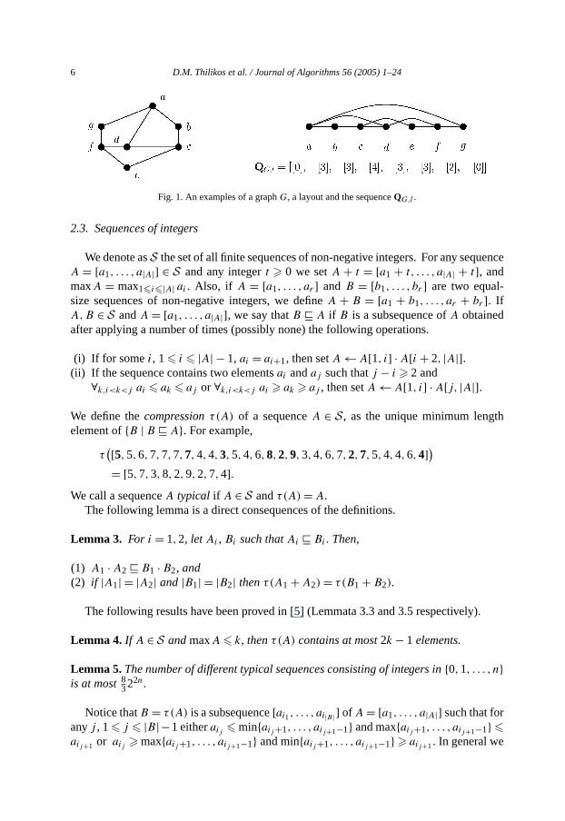

6 D.M. Thilikos et al. / Journal of Algorithms 56 (2005) 1–24

uence

h

.

Fig. 1. An examples of a graphG, a layout and the sequenceQG,l .

2.3. Sequences of integers

We denote asS the set of all finite sequences of non-negative integers. For any seqA = [a1, . . . , a|A|] ∈ S and any integert 0 we setA + t = [a1 + t, . . . , a|A| + t], andmaxA = max1i|A| ai . Also, if A = [a1, . . . , ar ] and B = [b1, . . . , br ] are two equal-size sequences of non-negative integers, we defineA + B = [a1 + b1, . . . , ar + br ]. IfA,B ∈ S andA = [a1, . . . , a|A|], we say thatB A if B is a subsequence ofA obtainedafter applying a number of times (possibly none) the following operations.

(i) If for somei, 1 i |A| − 1, ai = ai+1, then setA ← A[1, i] · A[i + 2, |A|].(ii) If the sequence contains two elementsai andaj such thatj − i 2 and

∀k,i<k<j ai ak aj or ∀k,i<k<j ai ak aj , then setA ← A[1, i] · A[j, |A|].

We define thecompressionτ(A) of a sequenceA ∈ S , as the unique minimum lengtelement ofB | B A. For example,

τ([5,5,6,7,7,7,7,4,4,3,5,4,6,8,2,9,3,4,6,7,2,7,5,4,4,6,4])= [5,7,3,8,2,9,2,7,4].

We call a sequenceA typical if A ∈ S andτ(A) = A.The following lemma is a direct consequences of the definitions.

Lemma 3. For i = 1,2, let Ai , Bi such thatAi Bi . Then,

(1) A1 · A2 B1 · B2, and(2) if |A1| = |A2| and |B1| = |B2| thenτ(A1 + A2) = τ(B1 + B2).

The following results have been proved in [5] (Lemmata 3.3 and 3.5 respectively)

Lemma 4. If A ∈ S andmaxA k, thenτ(A) contains at most2k − 1 elements.

Lemma 5. The number of different typical sequences consisting of integers in0,1, . . . , nis at most8322n.

Notice thatB = τ(A) is a subsequence[ai1, . . . , ai|B| ] of A = [a1, . . . , a|A|] such that foranyj , 1 j |B|−1 eitheraij minaij +1, . . . , aij+1−1 and maxaij +1, . . . , aij+1−1

aij+1 or aij maxaij +1, . . . , aij+1−1 and minaij +1, . . . , aij+1−1 aij+1. In general we

D.M. Thilikos et al. / Journal of Algorithms 56 (2005) 1–24 7

unctioni-

sitions

in

ns of

may have more than one such subsequence. We fix one of them and define the fβA : 1, . . . , |τ(A)| → 1, . . . , |A| whereβA(j) = ij is one of the possible original postions inA of thej th element inτ(A). Consider the sequence of the previous example

A = [5,5,6,7,7,7,7,4,4,3,5,4,6,8,2,9,3,4,6,7,2,7,5,4,4,6,4],then we have

βA(1) = 1, βA(2) = 6 (or 4 or 5 or 7), βA(3) = 10,

βA(4) = 14, βA(5) = 15, βA(6) = 16,

βA(7) = 21, βA(8) = 22, βA(9) = 27.

The following lemma is a direct consequence of the definition ofβ.

Lemma 6. Let A be any sequence inS . Then, for anyi, 1 i < |τ(A)|, we haveτ(A[βA(i), βA(i + 1)]) = [A(βA(i)),A(βA(i + 1))].

Analogously, we define the functionβ−1A : 1, . . . , |A| → 1, . . . , τ (A) such that

β−1A (j) is the uniquei such thatβA(i) = j .

For anyA ∈ S , we defineα(A) in the same way asτ(A) with the difference that onlyoperation (i) is considered, i.e., we remove repetitions of a number on successive poin the sequence. If nowA is a typical sequence, we define theset of extensionsof A as

E(A) = A ∈ S | α(

A) = A

.

We call a sequenceA denseif A ∈ E(τ (A)). If A is dense then all the sequencesE(A) are dense. Finally, notice also that ifA is dense andB A thenB ∈ E(τ (A)). Forexample, the sequences[5,7,7,7,4,8,8,8,8] and[1,7,2,6,4,4,4,4,4] are dense.

Notice that for any typical sequenceA, if B ∈ E(A), B(i) = B(i + 1), andβ−1B (i) = j ,

then the subsequenceB[i, i + 1] represents thej th number change inB.The results in the following two lemmata are direct consequences of the definitio

β andβ−1.

Lemma 7. LetA be a sequence inS, andB ∈ E(τ (A)) then, for anyi,1 i |B|,

(1) A(βA(β−1B (j))) = B(j),

(2) B(j) = B(j + 1) ⇒ β−1B (j + 1) = β−1

B (j) + 1, and(3) B(j) = B(j + 1) ⇒ β−1

B (j + 1) = β−1B (j).

Let A = [a1, . . . , ar1] andB = [b1, . . . , br2] be two sequences inS . We say thatA B

if r1 = r2 and ∀1ir1 ai bi . In general, we say thatA ≺ B if there exist exten-

sionsA ∈ E(A), and B ∈ E(B) such thatA B. For example ifA = [1,7,2,6,4] andB = [5,7,4,8] then A ≺ B becauseB = [5,7,7,7,4,8,8,8,8] is an extension ofB,A = [1,7,2,6,4,4,4,4,4] is an extension ofA, andA B.

The following lemma corresponds to Corollary 3.11 of [5].

Lemma 8. If A andB are two sequences thenA ≺ B if and only ifτ(A) ≺ τ(B).

8 D.M. Thilikos et al. / Journal of Algorithms 56 (2005) 1–24

ey fol-

ctness

e-

fLet

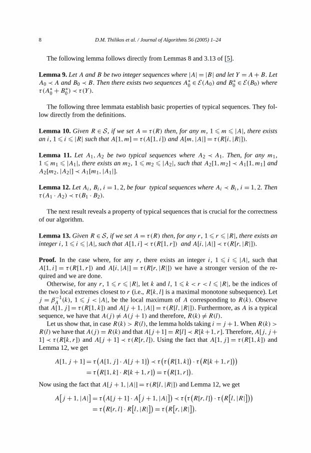
The following lemma follows directly from Lemmas 8 and 3.13 of [5].

Lemma 9. LetA andB be two integer sequences where|A| = |B| and letY = A + B. LetA0 ≺ A andB0 ≺ B. Then there exists two sequencesA∗

0 ∈ E(A0) andB∗0 ∈ E(B0) where

τ(A∗0 + B∗

0) ≺ τ(Y ).

The following three lemmata establish basic properties of typical sequences. Thlow directly from the definitions.

Lemma 10. GivenR ∈ S , if we setA = τ(R) then, for anym, 1 m |A|, there existsan i, 1 i |R| such thatA[1,m] = τ(A[1, i]) andA[m, |A|] = τ(R[i, |R|]).

Lemma 11. Let A1,A2 be two typical sequences whereA2 ≺ A1. Then, for anym1,1 m1 |A1|, there exists anm2, 1 m2 |A2|, such thatA2[1,m2] ≺ A1[1,m1] andA2[m2, |A2|] ≺ A1[m1, |A1|].

Lemma 12. Let Ai , Bi , i = 1,2, be four typical sequences whereAi ≺ Bi , i = 1,2. Thenτ(A1 · A2) ≺ τ(B1 · B2).

The next result reveals a property of typical sequences that is crucial for the correof our algorithm.

Lemma 13. GivenR ∈ S , if we setA = τ(R) then, for anyr , 1 r |R|, there exists anintegeri, 1 i |A|, such thatA[1, i] ≺ τ(R[1, r]) andA[i, |A|] ≺ τ(R[r, |R|]).

Proof. In the case where, for anyr , there exists an integeri, 1 i |A|, such thatA[1, i] = τ(R[1, r]) and A[i, |A|] = τ(R[r, |R|]) we have a stronger version of the rquired and we are done.

Otherwise, for anyr , 1 r |R|, let k and l, 1 k < r < l |R|, be the indices othe two local extremes closest tor (i.e.,R[k, l] is a maximal monotone subsequence).j = β−1

A (k), 1 j < |A|, be the local maximum ofA corresponding toR(k). ObservethatA[1, j ] = τ(R[1, k]) andA[j + 1, |A|] = τ(R[l, |R|]). Furthermore, asA is a typicalsequence, we have thatA(j) = A(j + 1) and therefore,R(k) = R(l).

Let us show that, in caseR(k) > R(l), the lemma holds takingi = j + 1. WhenR(k) >

R(l) we have thatA(j) = R(k) and thatA[j +1] = R[l] ≺ R[k+1, r]. Therefore,A[j, j +1] ≺ τ(R[k, r]) andA[j + 1] ≺ τ(R[r, l]). Using the fact thatA[1, j ] = τ(R[1, k]) andLemma 12, we get

A[1, j + 1] = τ(A[1, j ] · A[j + 1]) ≺ τ

(τ(R[1, k]) · τ(

R[k + 1, r]))= τ

(R[1, k] · R[k + 1, r]) = τ

(R[1, r]).

Now using the fact thatA[j + 1, |A|] = τ(R[l, |R|]) and Lemma 12, we get

A[j + 1, |A|] = τ

(A[j + 1] · A[

j + 1, |A|]) ≺ τ(τ(R[r, l]) · τ(

R[l, |R|]))( [ ]) ( [ ])

= τ R[r, l] · R l, |R| = τ R r, |R| .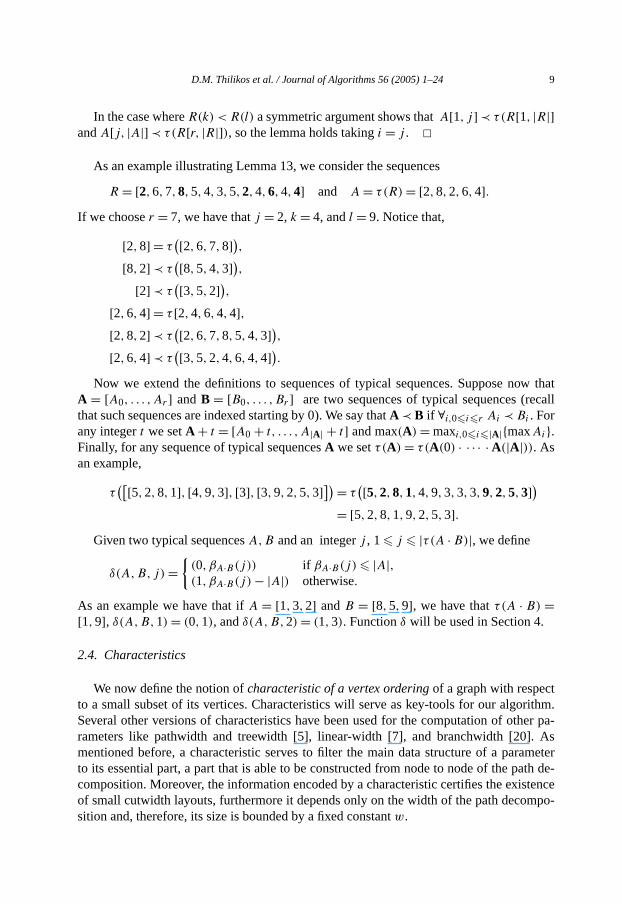

D.M. Thilikos et al. / Journal of Algorithms 56 (2005) 1–24 9

w thatcall

trithm.her pa-As

ameterath de-stencempo-

In the case whereR(k) < R(l) a symmetric argument shows thatA[1, j ] ≺ τ(R[1, |R|]andA[j, |A|] ≺ τ(R[r, |R|]), so the lemma holds takingi = j .

As an example illustrating Lemma 13, we consider the sequences

R = [2,6,7,8,5,4,3,5,2,4,6,4,4] and A = τ(R) = [2,8,2,6,4].If we chooser = 7, we have thatj = 2, k = 4, andl = 9. Notice that,

[2,8] = τ([2,6,7,8]),

[8,2] ≺ τ([8,5,4,3]),

[2] ≺ τ([3,5,2]),

[2,6,4] = τ [2,4,6,4,4],[2,8,2] ≺ τ

([2,6,7,8,5,4,3]),[2,6,4] ≺ τ

([3,5,2,4,6,4,4]).Now we extend the definitions to sequences of typical sequences. Suppose no

A = [A0, . . . ,Ar ] andB = [B0, . . . ,Br ] are two sequences of typical sequences (rethat such sequences are indexed starting by 0). We say thatA ≺ B if ∀i,0ir Ai ≺ Bi . Forany integert we setA + t = [A0 + t, . . . ,A|A| + t] and max(A) = maxi,0i|A|maxAi.Finally, for any sequence of typical sequencesA we setτ(A) = τ(A(0) · · · · · A(|A|)). Asan example,

τ([[5,2,8,1], [4,9,3], [3], [3,9,2,5,3]]) = τ

([5,2,8,1,4,9,3,3,3,9,2,5,3])= [5,2,8,1,9,2,5,3].

Given two typical sequencesA,B and an integerj , 1 j |τ(A · B)|, we define

δ(A,B, j) =

(0, βA·B(j)) if βA·B(j) |A|,(1, βA·B(j) − |A|) otherwise.

As an example we have that ifA = [1,3,2] andB = [8,5,9], we have thatτ(A · B) =[1,9], δ(A,B,1) = (0,1), andδ(A,B,2) = (1,3). Functionδ will be used in Section 4.

2.4. Characteristics

We now define the notion ofcharacteristic of a vertex orderingof a graph with respecto a small subset of its vertices. Characteristics will serve as key-tools for our algoSeveral other versions of characteristics have been used for the computation of otrameters like pathwidth and treewidth [5], linear-width [7], and branchwidth [20].mentioned before, a characteristic serves to filter the main data structure of a parto its essential part, a part that is able to be constructed from node to node of the pcomposition. Moreover, the information encoded by a characteristic certifies the exiof small cutwidth layouts, furthermore it depends only on the width of the path deco

sition and, therefore, its size is bounded by a fixed constantw.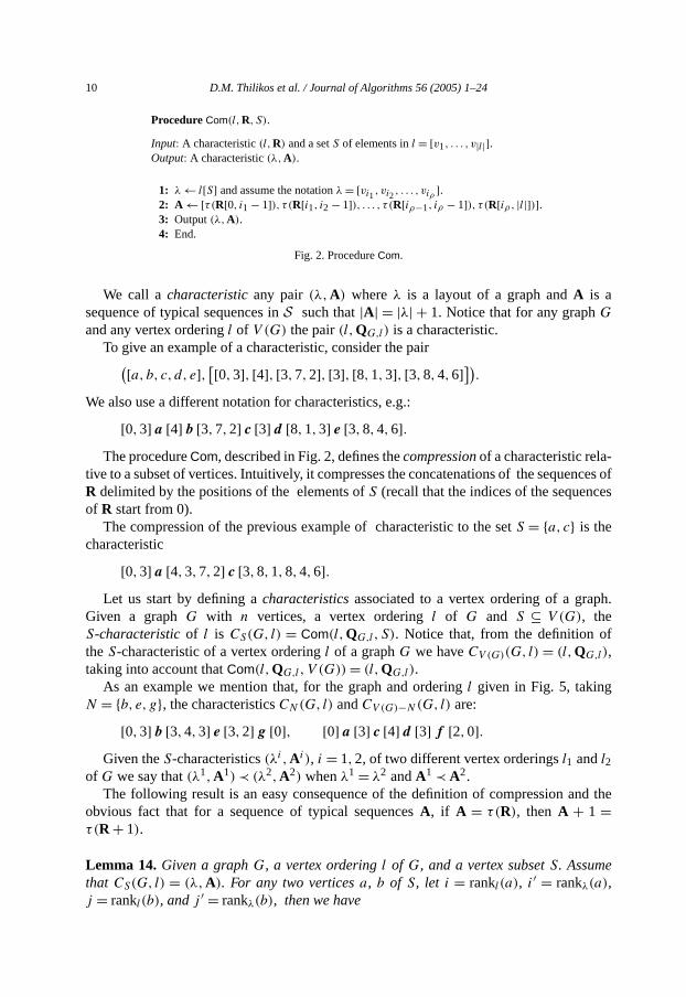

10 D.M. Thilikos et al. / Journal of Algorithms 56 (2005) 1–24

-nces ofes

ph.

f

nd the

Procedure Com(l,R, S).

Input: A characteristic(l,R) and a setS of elements inl = [v1, . . . , v|l|].Output: A characteristic(λ,A).

1: λ ← l[S] and assume the notationλ = [vi1, vi2, . . . , viρ ].2: A ← [τ(R[0, i1 − 1]), τ (R[i1, i2 − 1]), . . . , τ (R[iρ−1, iρ − 1]), τ (R[iρ , |l|])].3: Output(λ,A).4: End.

Fig. 2. ProcedureCom.

We call acharacteristicany pair (λ,A) whereλ is a layout of a graph andA is asequence of typical sequences inS such that|A| = |λ| + 1. Notice that for any graphGand any vertex orderingl of V (G) the pair(l,QG,l) is a characteristic.

To give an example of a characteristic, consider the pair([a, b, c, d, e], [[0,3], [4], [3,7,2], [3], [8,1,3], [3,8,4,6]]).We also use a different notation for characteristics, e.g.:

[0,3] a [4] b [3,7,2] c [3] d [8,1,3] e [3,8,4,6].The procedureCom, described in Fig. 2, defines thecompressionof a characteristic rela

tive to a subset of vertices. Intuitively, it compresses the concatenations of the sequeR delimited by the positions of the elements ofS (recall that the indices of the sequencof R start from 0).

The compression of the previous example of characteristic to the setS = a, c is thecharacteristic

[0,3] a [4,3,7,2] c [3,8,1,8,4,6].Let us start by defining acharacteristicsassociated to a vertex ordering of a gra

Given a graphG with n vertices, a vertex orderingl of G and S ⊆ V (G), theS-characteristicof l is CS(G, l) = Com(l,QG,l, S). Notice that, from the definition otheS-characteristic of a vertex orderingl of a graphG we haveCV (G)(G, l) = (l,QG,l),taking into account thatCom(l,QG,l,V (G)) = (l,QG,l).

As an example we mention that, for the graph and orderingl given in Fig. 5, takingN = b, e, g, the characteristicsCN(G, l) andCV (G)−N(G, l) are:

[0,3] b [3,4,3] e [3,2] g [0], [0] a [3] c [4] d [3] f [2,0].Given theS-characteristics(λi,Ai ), i = 1,2, of two different vertex orderingsl1 andl2

of G we say that(λ1,A1) ≺ (λ2,A2) whenλ1 = λ2 andA1 ≺ A2.The following result is an easy consequence of the definition of compression a

obvious fact that for a sequence of typical sequencesA, if A = τ(R), then A + 1 =τ(R + 1).

Lemma 14. Given a graphG, a vertex orderingl of G, and a vertex subsetS. Assumethat CS(G, l) = (λ,A). For any two verticesa, b of S, let i = rankl (a), i′ = rankλ(a),

j = rankl(b), andj ′ = rankλ(b), then we have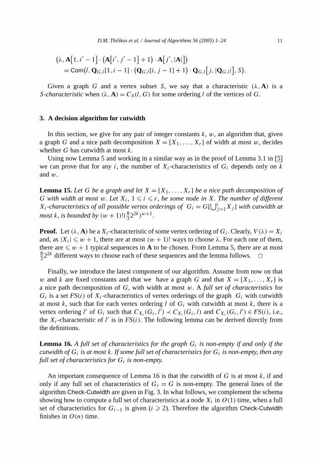

D.M. Thilikos et al. / Journal of Algorithms 56 (2005) 1–24 11

[5]

oft

,ost

that

m

ey

ema

(λ,A

[1, i′ − 1

] · (A[i′, j ′ − 1

] + 1) · A

[j ′, |A|])

= Com(l,QG,l[1, i − 1] · (QG,l[i, j − 1] + 1

) · QG,l

[j, |QG,l |

], S

).

Given a graphG and a vertex subsetS, we say that a characteristic(λ,A) is aS-characteristicwhen(λ,A) = CS(l,G) for some orderingl of the vertices ofG.

3. A decision algorithm for cutwidth

In this section, we give for any pair of integer constantsk, w, an algorithm that, givena graphG and a nice path decompositionX = [X1, . . . ,Xr ] of width at mostw, decideswhetherG has cutwidth at mostk.

Using now Lemma 5 and working in a similar way as in the proof of Lemma 3.1 inwe can prove that for anyi, the number ofXi -characteristics ofGi depends only onkandw.

Lemma 15. Let G be a graph and letX = [X1, . . . ,Xr ] be a nice path decompositionG with width at mostw. Let Xi , 1 i r , be some node inX. The number of differenXi -characteristics of all possible vertex orderings ofGi = G[⋃i

j=1Xj ] with cutwidth atmostk, is bounded by(w + 1)!(8

322k)w+1.

Proof. Let (λ,A) be aXi -characteristic of some vertex ordering ofGi . Clearly,V (λ) = Xi

and, as|Xi | w + 1, there are at most(w + 1)! ways to chooseλ. For each one of themthere are w + 1 typical sequences inA to be chosen. From Lemma 5, there are at m8322k different ways to choose each of these sequences and the lemma follows.

Finally, we introduce the latest component of our algorithm. Assume from now onw andk are fixed constants and that we have a graphG and thatX = [X1, . . . ,Xr ] isa nice path decomposition ofG, with width at mostw. A full set of characteristicsforGi is a setFS(i) of Xi -characteristics of vertex orderings of the graphGi with cutwidthat mostk, such that for each vertex orderingl of Gi with cutwidth at mostk, there is avertex orderingl′ of Gi such thatCXi

(Gi, l′) ≺ CXi

(Gi, l) andCXi(Gi, l

′) ∈ FS(i), i.e.,theXi -characteristic ofl′ is in FS(i). The following lemma can be derived directly frothe definitions.

Lemma 16. A full set of characteristics for the graphGi is non-empty if and only if thcutwidth ofGi is at mostk. If some full set of characteristics forGi is non-empty, then anfull set of characteristics forGi is non-empty.

An important consequence of Lemma 16 is that the cutwidth ofG is at mostk, if andonly if any full set of characteristics ofGr = G is non-empty. The general lines of thalgorithmCheck-Cutwidth are given in Fig. 3. In what follows, we complement the scheshowing how to compute a full set of characteristics at a nodeXi in O(1) time, when a fullset of characteristics forGi−1 is given (i 2). Therefore the algorithmCheck-Cutwidth

finishes inO(n) time.

12 D.M. Thilikos et al. / Journal of Algorithms 56 (2005) 1–24

e

e

g

n

Algorithm Check-Cutwidth(G,X,k).

Input: A graphG, a path decompositionX of G with width w, and an integerk.Output: Whether cutwidth(G) k.

1: Compute a full setF1 of X1-characteristics forG1.2: For anyi, 1< i r , compute a full set ofXi -characteristicsFi for Gi usingFi−1 andXi ’s type.3: If Fr = ∅ then output “cutwidth(G) k”, otherwise output “cutwidth(G) > k”.4: End.

Fig. 3. AlgorithmCheck-Cutwidth.

3.1. A full set for a start node

We first give a full set of characteristics forG1. Clearly,G1 consists only of the uniquvertex inX1 = xstart and a full set of characteristics is[xstart], [[0], [0]].

3.2. A full set for an introduce node

We will now consider the case whereXi is an introducenode. The procedureIns,depicted in Fig. 4, is the basis to compute aXi -characteristic after the insertion of thintroduced vertex and the additional edges that appear inGi at some pointj of a layout forGi−1.

The following lemma is a direct consequence of the definitions ofQG,l , QG′,l′ and theinsertion procedure. Recall that the sequences inQG,l andQG′,l′ are sequences consistinof only one element counting the number of “crossing edges” in the “gaps” ofl and l′respectively.

Lemma 17. LetG be a graph, letl be a layout ofG, and letγ be an integer where0 γ |l|. If G′ = G +u N for someN ⊆ V (G) andu /∈ V (G), thenIns(G,u,V (G),N, l,QG,l,

γ,1) is theV (G′)-characteristic of the layoutl′ = l[1, γ ] · [u] · l[γ + 1, |l|] of G′, thatis Ins(G,u,V (G),N, l,QG,l, γ,1) = (l′,QG′,l′), whereIns is the procedure described iFig. 4.

Procedure Ins(G,u,S,N,λ,A, j,m).

Input: A graphG, a vertexu /∈ V (G), two setsS andN , N ⊆ S ⊆ V (G), aS-characteristic(λ,A) of some layoutof G, an integerj , 0 j |λ|, and an integerm, 1 m |A(j)|.

Output: An (S ∪ u)-characteristic(λ′,A′) of some vertex ordering ofG′ = G +u N where 0 γ |l|.Assume thatλ = [u1, . . . , uρ ], andλ[N ] = [uj1, . . . , ujσ ].

1: (Insertion ofu) Setλ′ = λ[1, j ] · [u] · λ[j + 1, ρ] andA′ = A[0, j − 1] · [A(j)[1,m]] · [A(j)[m, |A(j)|]] ·A[j + 1, ρ].

2: (Insertion of the edges fromu) for h = 1 to σ do(i) If jh j then setA′ ← A′[0, jh − 1] · (A′[jh, j ] + 1) · A′[j + 1, ρ + 1].

(ii) If jh j + 1 then setA′ ← A′[0, j ] · (A′[j + 1, jh] + 1) · A′[jh + 1, ρ + 1].3: Output(λ′,A′).4: End.

Fig. 4. ProcedureIns.

D.M. Thilikos et al. / Journal of Algorithms 56 (2005) 1–24 13

f

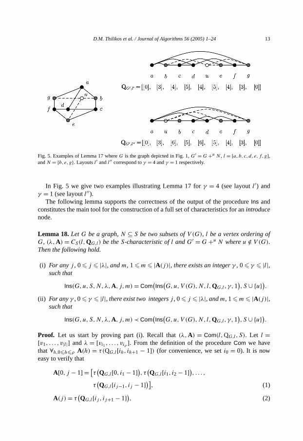
Fig. 5. Examples of Lemma 17 whereG is the graph depicted in Fig. 1,G′ = G +u N , l = [a, b, c, d, e, f, g],andN = b, e, g. Layoutsl′ andl′′ correspond toγ = 4 andγ = 1 respectively.

In Fig. 5 we give two examples illustrating Lemma 17 forγ = 4 (see layoutl′) andγ = 1 (see layoutl′′).

The following lemma supports the correctness of the output of the procedureIns andconstitutes the main tool for the construction of a full set of characteristics for anintroducenode.

Lemma 18. Let G be a graph,N ⊆ S be two subsets ofV (G), l be a vertex ordering oG, (λ,A) = CS(l,QG,l) be theS-characteristic ofl andG′ = G +u N whereu /∈ V (G).Then the following hold.

(i) For anyj , 0 j |λ|, andm, 1 m |A(j)|, there exists an integerγ , 0 γ |l|,such that

Ins(G,u,S,N,λ,A, j,m) = Com(Ins

(G,u,V (G),N, l,QG,l, γ,1

), S ∪ u).

(ii) For anyγ , 0 γ |l|, there exist two integersj , 0 j |λ|, andm, 1 m |A(j)|,such that

Ins(G,u,S,N,λ,A, j,m) ≺ Com(Ins

(G,u,V (G),N, l,QG,l, γ,1

), S ∪ u).

Proof. Let us start by proving part (i). Recall that(λ,A) = Com(l,QG,l, S). Let l =[v1, . . . , v|l|] and λ = [vi1, . . . , viρ ]. From the definition of the procedureCom we havethat ∀h,0hρ A(h) = τ(QG,l[ih, ih+1 − 1]) (for convenience, we seti0 = 0). It is noweasy to verify that

A[0, j − 1] = [τ(QG,l[0, i1 − 1]), τ(

QG,l[i1, i2 − 1]), . . . ,τ(QG,l[ij−1, ij − 1])], (1)( )

A(j) = τ QG,l[ij , ij+1 − 1] , (2)

14 D.M. Thilikos et al. / Journal of Algorithms 56 (2005) 1–24

(10) is

ounte nota-

A[j + 1, ρ] = [τ(QG,l[ij+1, ij+2 − 1]), . . . , τ(

QG,l[iρ−1, iρ − 1]),τ(QG,l

[iρ, |l|])]. (3)

Applying now Lemma 10 to (2), we have that there existsγ , ij γ < ij+1, such that

A(j)[1,m] = τ(Q[ij , γ ]), (4)

A(j)[m,

∣∣A(j)∣∣] = τ

(Q[γ, ij+1 − 1]). (5)

Observe that, asij γ < ij+1, the following hold

l[1, γ ][S] = λ[1, j ], (6)

l[γ + 1, |l|][S] = λ[j + 1, ρ]. (7)

Let (λ′,A′) and (l′,R) be the characteristics constructed by step1 of the proceduresIns(G,u,S,N,λ,A, j,m) and Ins(G,u,V (G),N, l,QG,l, γ,1) respectively. We willprove now that(λ′,A′) = Com((l′,R), S). Notice first thatλ′ = λ[1, j ] · [u] · λ[j + 1, |ρ|]andl′ = l[1, γ ] · [u] · l[γ + 1, |l|]. Using now (6) and (7), it follows thatλ′ = l′[S ∪ u] =[vi1, . . . , vij , u, vij+1, . . . , viρ ]. Notice now that

A′ = A[0, j − 1] · [A(j)[1,m]] · [A(j)[m,

∣∣A(j)∣∣]] · A[j + 1, ρ], (8)

R = QG,l[0, ij − 1] · QG,l[ij , γ ] · QG,l[γ, ij+1 − 1] · QG,l

[ij+1, |l|

]. (9)

Taking now in mind (9) and the fact thatλ′ = [vi1, . . . , vij , u, vij+1, . . . , viρ ], we can con-clude that the sequence of typical sequences in the output ofCom(l,R, S ∪ u) is[

τ(QG,l[0, i1 − 1]), . . . , τ(

QG,l[ij−1, ij − 1]), τ(QG,l[ij , γ ]),

τ(QG,l[γ, ij+1 − 1]), . . . , τ(

QG,l

[iρ, |l|])]. (10)

Using now (1), (3), (4), and (5) we have that the sequence of typical sequences inequal toA′ in the form it is presented in (8).

So far, we have seen that(λ′,A′) = Com((l′,R), S ∪u). In what follows we will provethat this relation is invariant under the transformations applied to(λ′,A′) and(l′,R) duringstep2 of the insertion procedure.

Notice that during step2, no vertex is introduced, only new edges are taken into accand added, therefore the respective vertex orderings do not change. We will use thtion (λ′,A(h)) and(l′,R(h)) for the contents ofA andR at the end of thehth execution ofthe loop in step2 of Ins(G,u,S,N,λ,A, j,m) and Ins(G,u,V (G),N, l,QG,l, γ,1) re-spectively. And for convenience we set(λ′,A′) = (λ′,A(0)), and(l′,R) = (l′,R(0)). To seethat for anyh (λ′,A(h)) = Com((l′,R(h)), S ∪ u) we proceed by induction.

Suppose that(λ′,A(h)) = Com(l′,R(h), S ∪ u) for any h, 0 < h < ξ . It remains toprove that(λ′,A(ξ)) = Com(l′,R(ξ), S ∪ u).

Assume thatµ1 = l[N ∩ V (l[1, γ ])] andµ2 = l[N ∩ V (l[γ + 1, |l|])]. Then we have

rankl (v) = rankl′(v), for v ∈ V (µ1),

rankl(v) + 1= rankl′(v), for v ∈ V (µ2),

rankλ(v) = rankλ′(v), for v ∈ V (µ1),

rankλ(v) + 1= rankλ′(v), for v ∈ V (µ2),

D.M. Thilikos et al. / Journal of Algorithms 56 (2005) 1–24 15

ewith

iffer-se

rankl′(u) = γ + 1,

rankλ′(u) = j + 1,

λ = µ1 · µ2,

λ′ = µ1 · [u] · µ2.

Assume that the vertex to be taken fromN in this step has rankjξ in l and rankξ in λ. Inthe case thatjξ j we have that

R(ξ) = R(ξ−1)[0, jξ − 1] · (R(ξ−1)[jξ , γ ] + 1) · R(ξ−1)

[γ + 1, |l| + 1

], (11)

A(ξ) = A(ξ−1)[0, ξ − 1] · (A(ξ−1)[ξ, j ] + 1) · A(ξ−1)[j + 1, ρ + 1]. (12)

As jξ = rankl′(u), γ + 1= rankλ′(u), ξ = rankl′(ujξ ) andj + 1= rankλ′(ujξ ), Lemma 14implies that(λ(ξ),A(ξ)) = Com(l(ξ−1),R(ξ), S ∪ u). In the casejξ j + 1 we have that

R(ξ) = R(ξ−1)[0, γ ] · (R(ξ−1)[γ + 1, jξ ]) · R(ξ−1)

[jξ + 1, |l| + 1

], (13)

A(ξ) = A(ξ−1)[0, j ] · (A(ξ−1)[j + 1, ξ ] + 1) · A(ξ−1)[ξ + 1, ρ + 1]. (14)

As γ + 1 = rankl′(u), jξ + 1 = rankl′(ujξ ), j + 1 = rankλ′(u), andξ + 1 = rankλ′(ujξ ),Lemma 14 implies that(λ(ξ),A(ξ)) = Com(l(ξ−1),R(ξ), S ∪ u) and this completes thproof of (i). The arguments to prove (ii) are exactly the same as in the proof of (i)the difference that now weaker versions of (1), (3), (4), and (5) are required. As(λ,A) =Com(l,QG,l, S), we can assume again thatl = [v1, . . . , v|l|] andλ = [vi1, . . . , viρ ]. Fromthe definition procedureCom there existsj , 0 j |ρ|, such thatij γ < ij+1 (forconvenience, we seti0 = 0 andiρ+1 = |l| + 1). Notice now that for this choice ofj , (1)–(3) hold and (1) and (3) can be rewritten in the following weaker form.

A[0, j − 1] ≺ [τ(QG,l[0, i1 − 1]), τ(

QG,l[i1, i2 − 1]), . . . ,τ(QG,l[ij−1, ij − 1])], (15)

A[j + 1, ρ] ≺ [τ(QG,l[ij+1, ij+2 − 1]), . . . , (QG,l[iρ−1, iρ − 1]),

τ(QG,l

[iρ, |l|])]. (16)

From Lemma 13 there exists an integerm, 1 m A(j), where

A(j)[1,m] ≺ τ(Q[ij , γ ]), (17)

A(j)[m,

∣∣A(j)∣∣] ≺ τ

(Q[γ, ij+1 − 1]). (18)

Notice that (15), (16), (17), and (18) are the same as (1), (3), (4), and (5) with the dence that “=” has been replaced by “≺”. From this fact, using the same proof as in ca(i), it follows thatIns(G,u,S,N,λ,A, j,m) ≺ Com(Ins(G,u,V (G),N, l,QG,l, γ,1), S∪u).

As an example for Lemma 18, we consider the graphsG andG′ and their vertex or-deringsl, l′ andl′′ as depicted in Fig. 5. If we setS = N ∪ d = b, d, e, g we have thatCS(G, l) = (λ,A) is the characteristic[0,3] b [3,4] d [3] e [3,2] g [0]. Notice that inl′, ifj = 2 andm = 1, Lemma 18(i) givesγ = 4. Moreover, inl′′, if γ = 1, Lemma 18(ii) gives

j = 0 andm = 2.

16 D.M. Thilikos et al. / Journal of Algorithms 56 (2005) 1–24

al

fterl

p

t

is

us

We will now prove some monotonicity properties of the insertion procedure.

Lemma 19. Let (λ,Ai ), i = 1,2, be two characteristics of a graphG where(λ,A2) ≺(λ,A1). LetN,S be subsets ofV (G) and letG′ = G +u N for someu /∈ V (G). Then forany j , 0 j |A1|, and anym1, 1 m1 |A1(j)|, there existsm2, 1 m2 |A2(j)|,such that

Ins(G,u,S,N,λ,A2, j,m2) ≺ Ins(G,u,S,N,λ,A1, j,m1).

Proof. As (λ,A2) ≺ (λ,A1), for any j , we haveA2(j) ≺ A1(j). Therefore, Lemma 11implies that there existsm2, 1 m2 |A2(j)|, such that

A2(j)[1,m2] ≺ A1(j)[1,m1] and A2(j)[m2,

∣∣A2(j)∣∣] ≺ A1(j)

[m1,

∣∣A1(j)∣∣].

Moreover,∀i,0ij−1 A2(i) ≺ A1(i) and∀i,j+1iρ A2(i) ≺ A1(i). Therefore, if

A′i = Ai[0, j − 1] · [Ai (j)[1,mi]

] · [Ai (j)[m1,

∣∣Ai (j)∣∣]] · Ai[j + 1, ρ],

for i = 1,2, then A′2 ≺ A′

1. Observe that,A′1 and A′

2 are the sequences of typicsequences created after step1 of the computation ofIns(G,u,S,N,λ,A1, j,m1) andIns(G,u,S,N,λ,A2, j,m2) respectively. Moreover, the vertex orderings constructed astep1 of Ins(G,u,S,N,λ,A1, j,m1) andIns(G,u,S,N,λ,A2, j,m2) are both identicaand we denote themλ′. It now remains to prove that after step2, A′

2 ≺ A′1. We proceed by

induction.For i = 1,2 let A(h)

i denote the value ofA′i after thehth execution of the loop in ste

2 of the computation ofIns(G,u,S,N,λ,Ai , j,mi), i = 1,2, and setA(0)i = A′

i . Supposethat A(h)

2 ≺ A(h)1 for anyh, 0< h < ξ . It remains to prove thatA(ξ)

2 ≺ A(ξ)1 . Assume tha

the vertex ofN considered in this step has rankjξ in l andξ in λ′. We examine only thecase wherejξ j as the case wherejξ j + 1 is analogous. By induction hypothes

A(ξ−1)2 ≺ A(ξ−1)

1 , therefore

A(ξ−1)2 [0, jξ − 1] ≺ A(ξ−1)

1 [0, jξ − 1], (19)

A(ξ−1)2 [jξ , j ] ≺ A(ξ−1)

1 [jξ , j ], (20)

A(ξ−1)2 [j,ρ + 1] ≺ A(ξ−1)

1 [j,ρ + 1]. (21)

Clearly, (20) is equivalent to

A(ξ−1)2 [jξ , j ] + 1≺ A(ξ−1)

1 [jξ , j ] + 1. (22)

Taking into account that, fori = 1,2,

Aξi = A(ξ−1)

i [0, jξ − 1] · (A(ξ−1)i [jξ , j ] + 1

) · A(ξ−1)i [j,ρ + 1],

we concludeA(ξ)2 ≺A(ξ)

1 as a consequence of (19), (22), and (21).We now give an algorithm (algorithmIntroduce-Node) given in Fig. 6 that, for any

introduce nodeXi , computes a full set of characteristics for the graphGi , given a fullset of characteristics for the graphGi−1. Now we prove the correctness of the previo

algorithm.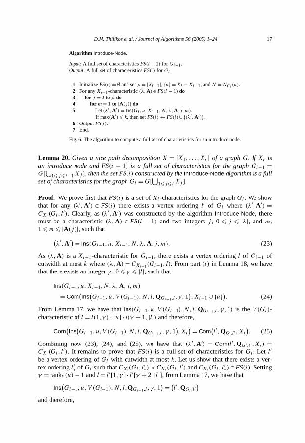

D.M. Thilikos et al. / Journal of Algorithms 56 (2005) 1–24 17

r-

Algorithm Introduce-Node.

Input: A full set of characteristicsFS(i − 1) for Gi−1.Output: A full set of characteristicsFS(i) for Gi .

1: Initialize FS(i) = ∅ and setρ = |Xi−1|, u = Xi − Xi−1, andN = NGi(u).

2: For anyXi−1-characteristic(λ,A) ∈ FS(i − 1) do3: for j = 0 to ρ do4: for m = 1 to |A(j)| do5: Let (λ′,A′) = Ins(Gi ,u,Xi−1,N,λ,A, j,m).

If max(A′) k, then setFS(i) ← FS(i) ∪ (λ′,A′).6: OutputFS(i).7: End.

Fig. 6. The algorithm to compute a full set of characteristics for an introduce node.

Lemma 20. Given a nice path decompositionX = [X1, . . . ,Xr ] of a graphG. If Xi isan introduce node and FS(i − 1) is a full set of characteristics for the graphGi−1 =G[⋃1ji−1 Xj ], then the set FS(i) constructed by theIntroduce-Node algorithm is a fullset of characteristics for the graphGi = G[⋃1ji Xj ].

Proof. We prove first thatFS(i) is a set ofXi -characteristics for the graphGi . We showthat for any(λ′,A′) ∈ FS(i) there exists a vertex orderingl′ of Gi where (λ′,A′) =CXi

(Gi, l′). Clearly, as(λ′,A′) was constructed by the algorithmIntroduce-Node, there

must be a characteristic(λ,A) ∈ FS(i − 1) and two integersj , 0 j |λ|, and m,1 m |A(j)|, such that(

λ′,A′) = Ins(Gi−1, u,Xi−1,N,λ,A, j,m). (23)

As (λ,A) is a Xi−1-characteristic forGi−1, there exists a vertex orderingl of Gi−1 ofcutwidth at mostk where(λ,A) = CXi−1(Gi−1, l). From part(i) in Lemma 18, we havethat there exists an integerγ , 0 γ |l|, such that

Ins(Gi−1, u,Xi−1,N,λ,A, j,m)

= Com(Ins

(Gi−1, u,V (Gi−1),N, l,QGi−1,l , γ,1

),Xi−1 ∪ u). (24)

From Lemma 17, we have thatIns(Gi−1, u,V (Gi−1),N, l,QGi−1,l , γ,1) is theV (Gi)-characteristic ofl = l(1, γ ) · [u] · l(γ + 1, |l|) and therefore,

Com(Ins

(Gi−1, u,V (Gi−1),N, l,QGi−1,l , γ,1

),Xi

) = Com(l′,QG′,l′ ,Xi

). (25)

Combining now (23), (24), and (25), we have that(λ′,A′) = Com(l′,QG′,l′ ,Xi) =CXi

(Gi, l′). It remains to prove thatFS(i) is a full set of characteristics forGi . Let l′

be a vertex ordering ofGi with cutwidth at mostk. Let us show that there exists a vetex orderingl′∗ of Gi such thatCXi

(Gi, l′∗) ≺ CXi

(Gi, l′) andCXi

(Gi, l′∗) ∈ FS(i). Setting

γ = rankl′(u) − 1 andl = l′[1, γ ] · l′[γ + 2, |l|], from Lemma 17, we have that

Ins(Gi−1, u,V (Gi−1),N, l,QGi−1,l , γ,1

) = (l′,QGi,l

′)

and therefore,

18 D.M. Thilikos et al. / Journal of Algorithms 56 (2005) 1–24

s

n

ly

edure

Com(Ins

(Gi−1, u,V (Gi−1),N, l,QGi−1,l , γ,1

),Xi

)= Com(l,QGi,l

′ ,Xi) = CXi

(Gi, l

′). (26)

Set now(λ,A) = CXi(Gi, l). From part (ii) of Lemma 18 we have that there are valuej

andm, 0 j |λ| and 1 m |A(j)|, such that

Ins(Gi−1, u,Xi−1,N,λ,A, j,m)

≺ Com(Ins

(Gi−1, u,V (Gi−1),N, l,QGi−1,l , γ,1

),Xi−1 ∪ u). (27)

As FS(i − 1) is a full set of characteristics, there exists a vertex orderingl∗ of V (Gi−1) forwhich

CXi−1(Gi−1, l∗) ≺ CXi−1(Gi−1, l) and CXi−1(Gi−1, l∗) ∈ FS(i − 1).

Let (λ∗,A∗) = CXi−1(Gi−1, l∗). From Lemma 19, we have that there exists am∗ such that

Ins(Gi−1, u,Xi−1,N,λ∗,A∗, j,m∗) ≺ Ins(Gi−1, u,Xi−1,N,λ,A, j,m). (28)

From part (i) of Lemma 18, there existsγ∗, 0 γ∗ |l∗|, such that

Com(Ins

(Gi−1, u,V (Gi−1),N, l∗,QGi−1,l∗ , γ∗,1

),Xi

)= Ins(Gi−1, u,Xi−1,N,λ∗,A∗, j,m∗). (29)

Defining l′∗ = l∗[1, γ∗] · [u] · l∗[γ∗ + 1, |l∗|] and applying Lemma 17 we have that(l′∗,QGi,l

′∗) = Ins

(Gi−1, u,V (Gi−1),N, l∗,QGi−1,l∗ , γ∗,1

)and therefore,

CXi

(Gi, l

′∗) = Com

(l′∗,QGi,l

′∗ ,Xi

)= Com

(Ins

(Gi−1, u,V (Gi−1),N, l∗,QGi−1,l∗ , γ∗,1

),Xi

). (30)

From (29) and (30) we have thatCXi(Gi, l

′∗) = Ins(Gi−1, u,Xi−1,N,λ∗,A∗, j,m∗).Since (QGi−1, l∗) ∈ FS(i − 1) we obtainCXi

(Gi, l′∗) ∈ FS(i). Finally, combining rela-

tions (26)–(30) we conclude thatCXi(Gi, l

′∗) ≺ CXi(Gi, l

′). 3.3. A full set for a forget node

We now consider the case whereXi is aforgetnode. We provide an algorithm that givea full set of characteristicsFS(i − 1) for Xi−1, computes a full set of characteristicsFS(i)

for Xi . We start by defining the deletion procedureDel (see Fig. 7) that operates inverseto the insertion procedureIns.

The following lemma is a direct consequence of the definitions of the proceduresComandDel.

Lemma 21. Let (l,R) be a characteristic of a given graphG and letV ⊆ V (l). Then, foranyv ∈ V , Com(l,R,V − v) = Del(Com(l,R,V ), v).

Observe that Lemma 21 provides an alternative recursive definition of the procCom, based on the procedureDel.

The following monotonicity result is a direct consequence of Lemma 12.

D.M. Thilikos et al. / Journal of Algorithms 56 (2005) 1–24 19

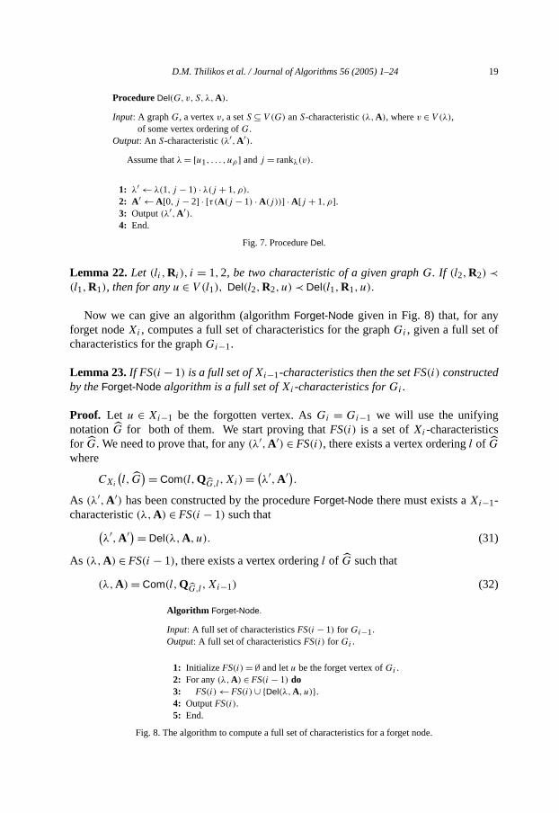
Procedure Del(G,v,S,λ,A).

Input: A graphG, a vertexv, a setS ⊆ V (G) anS-characteristic(λ,A), wherev ∈ V (λ),of some vertex ordering ofG.

Output: An S-characteristic(λ′,A′).

Assume thatλ = [u1, . . . , uρ ] andj = rankλ(v).

1: λ′ ← λ(1, j − 1) · λ(j + 1, ρ).2: A′ ← A[0, j − 2] · [τ(A(j − 1) · A(j))] · A[j + 1, ρ].3: Output(λ′,A′).4: End.

Fig. 7. ProcedureDel.

Lemma 22. Let (li ,Ri ), i = 1,2, be two characteristic of a given graphG. If (l2,R2) ≺(l1,R1), then for anyu ∈ V (l1), Del(l2,R2, u) ≺ Del(l1,R1, u).

Now we can give an algorithm (algorithmForget-Node given in Fig. 8) that, for anyforget nodeXi , computes a full set of characteristics for the graphGi , given a full set ofcharacteristics for the graphGi−1.

Lemma 23. If FS(i − 1) is a full set ofXi−1-characteristics then the set FS(i) constructedby theForget-Node algorithm is a full set ofXi -characteristics forGi .

Proof. Let u ∈ Xi−1 be the forgotten vertex. AsGi = Gi−1 we will use the unifyingnotationG for both of them. We start proving thatFS(i) is a set ofXi -characteristicsfor G. We need to prove that, for any(λ′,A′) ∈ FS(i), there exists a vertex orderingl of G

where

CXi

(l, G

) = Com(l,QG,l ,Xi) = (λ′,A′).

As (λ′,A′) has been constructed by the procedureForget-Node there must exists aXi−1-characteristic(λ,A) ∈ FS(i − 1) such that(

λ′,A′) = Del(λ,A, u). (31)

As (λ,A) ∈ FS(i − 1), there exists a vertex orderingl of G such that

(λ,A) = Com(l,QG,l ,Xi−1) (32)

Algorithm Forget-Node.

Input: A full set of characteristicsFS(i − 1) for Gi−1.Output: A full set of characteristicsFS(i) for Gi .

1: Initialize FS(i) = ∅ and letu be the forget vertex ofGi .2: For any(λ,A) ∈ FS(i − 1) do3: FS(i) ← FS(i) ∪ Del(λ,A, u).4: OutputFS(i).5: End.

Fig. 8. The algorithm to compute a full set of characteristics for a forget node.

20 D.M. Thilikos et al. / Journal of Algorithms 56 (2005) 1–24

in

e

ftics,

ring

and therefore, from (31) and (32) we have(λ′,A′) = Del

(Com(l,QG,l ,Xi−1), u

)(33)

and using (33) and Lemma 21 we have thatCXi(l, G) = Com(l,QG,l ,Xi) = (λ′,A′).

We will now prove thatFS(i) is a full set ofXi -characteristics forG. Let l be a vertexordering ofG of cutwidth at mostk. We will show that there exists a vertex orderingl∗ ofG such that

CXi

(G, l∗

) ≺ CXi

(G, l

)and CXi

(G, l∗

) ∈ FS(i).

From Lemma 21 we have that

CXi

(G, l

) = Com(l,QG,l ,Xi) = Del(Com(l,QG,l ,Xi−1), u

). (34)

As FS(i − 1) is a full set of characteristics, there exists a vertex orderingl∗ of V (G) suchthatCXi−1(G, l∗) ∈ FS(i − 1) andCXi−1(G, l∗) ≺ CXi−1(G, l) or, equivalently,

Com(l∗,QG,l∗ ,Xi−1) ≺ Com(l,QG,l ,Xi−1). (35)

Using now Lemma 22 we can rewrite (35) as follows.

Del(Com(l∗,QG,l∗ ,Xi−1), u

) ≺ Del(Com(l,QG,l ,Xi−1), u

). (36)

Applying again Lemma 21 we have that

CXi

(G, l∗

) = Com(l∗,QG,l∗ ,Xi) = Del(Com(l∗,QG,l∗ ,Xi−1), u

). (37)

Combining now (34), (36), and (37), we have thatCXi(G, l∗) ≺ CXi

(G, l). Finally as

CXi−1

(G, l∗

) = Com(l∗,QG,l∗ ,Xi−1) ∈ FS(i − 1),

the output ofDel(Com(l∗,QG,l∗ ,Xi−1), u) will be one of the characteristics includedFS(i). And we concludeCXi

(G, l∗) ∈ FS(i).

4. Computing a vertex ordering

Suppose now that, given a path decompositionX = [X1, . . . ,Xr ] of G with boundedwidth, after running the algorithmCheck-Cutwidth, described in the previous section, wknow that a graphG has cutwidth at mostk, i.e., the computed setFS(r) is not empty. Wedescribe now a way to further construct a vertex ordering ofG with cutwidth at mostk,and the modifications and additions needed to perform to the algorithmCheck-Cutwidth,we refer to the extended algorithm asLayout-Cutwidth. By observing the execution othe Check-Cutwidth algorithm, it follows that there exist a sequence of characteris(λ1,A1), (λ2,A2), . . . , (λr ,Ar ), that we call awitness path, such that

(1) (λ1,A1) = ([xstart], [[0], [0]]) is the unique characteristic of the unique vertex ordeof G1.

(2) (λr ,Ar ) is some characteristic inFS(r), and

D.M. Thilikos et al. / Journal of Algorithms 56 (2005) 1–24 21

ll

s.

ive

(3) for anyh, 1 h n − 1, the characteristic(λh+1,Ah+1) was constructed after a caof eitherIntroduce-Node or Forget-Node with input (λh,Ah).

Let us show how to compute a layout with cutwidth at mostk, in linear time, given awitness path

(λ1,A1), (λ2,A2), . . . , (λr ,Ar ).

For anyh, 1< h < r , let lh be a vertex ordering such thatCXh(Gh, lh) = (λh,Ah). Assume

that

lh = [vh

1, . . . , vh|lh|

]and

Ah = [Ah

0, . . . ,Ah|Ah|

]whereAh

j = [a

h,j

1 , . . . , ah,j|Ah|

].

Notice that any elementah,jm of Ah

0 · · · · · Ah|Ah| is determined by a pair(j,m) of indices

where 0 j |Ah| and 1 m |Aj |. We denote asPh the set containing all these pairLet κ be the minimum number such thath < κ r andXκ is an introduce node(κ is

well defined asXr is an introduce node andh < r = |X|). We setuh = Xk − Xh andNh = NGκ (u

h). Now we define a mappingφh :Ph → 0,1, . . . , |lh| such thatφh(j,m) =γ implies that

Ins(Gh,u

h,Xh,Nh,λh,Ah, j,m)

= Com(Ins

(Gh,u

h,V (Gh),Nh, lh,QGh,lh , γ,1),Xh

). (38)

Our definition is recursive. We assume that for someh, 1 h r −1, lh andφh are known.We will show thatlh+1, φh+1 can be defined recursively and computed inO(1) time.

We first examine the case where(λh+1,Ah+1) was computed after a call ofIntroduce-Node. This means thatκ = h + 1 and thatuh = Xh+1 − Xh and Nh = NGh+1(u

h).Clearly, (λh+1,Ah+1) = Ins(Gh,u

h,Xh,Nh,λh,Ah, j,m) for some choice ofj and m

where 0 j |λh| and 1 m |A(j)|. From (38) and the proof of Lemma 20, we derthe following:

If γ = φh(j,m), then by settinglh+1 = lh[1, γ ] · [uh] · lh[γ + 1, |lh|], we getCXh+1(Gh+1, lh+1) = (λh+1,Ah+1).

If we now take in mind the rearrangement of the indices occuring during step1 of theprocedureIns as it is applied on(λh,Ah) and(lh,QGh,lh) to (38) we have that

Ph+1 = (0,1), . . . ,

(0,

∣∣Ah0

∣∣) ∪ · · · ∪ (j − 1,1), . . . ,

(j − 1,

∣∣Ahj−1

∣∣)∪

(j,1), . . . , (j,m) ∪

(j + 1,1), . . . ,(j + 1,

∣∣Ahj

∣∣ − m + 1)

∪ (j + 2,1), . . . ,

(j + 2,

∣∣Ahj+1

∣∣) ∪ · · ·( ) ( ∣ ∣)

∪ |Ah| + 1,1 , . . . , |Ah| + 1, ∣Ah|Ah|∣

22 D.M. Thilikos et al. / Journal of Algorithms 56 (2005) 1–24

teristiclso asition

tions

e

ema 2

and, we can defineφh+1 as

φh+1(ν, ξ) =

φh(ν, ξ) if ν < j + 1,

γ + 1 if ν = j + 1 andξ = 1,

φh(j,m + ξ − 1) + 1 if ν = j + 1 andξ > 1,

φh(ν − 1, ξ) + 1 if ν > j + 1

and, therefore the required condition holds.Suppose now that(λh+1,Ah+1) was computed after a call ofForget-Node. Assume

λh = [v1, . . . , vj , . . . , v|λh|]wherevj is the forgotten vertex. Clearly, the new vertex orderinglh+1 is the same aslh.Taking now in mind the outputs ofDel(λh,Ah, vj ) andDel(lh,QGh,lh , vj ), the new indexset is

Ph+1 = (0,1), . . . ,

(0,

∣∣Ah0

∣∣) ∪ · · · ∪ (j − 2,1), . . . ,

(j − 2,

∣∣Ahj−2

∣∣)∪

(j − 1,1), . . . ,(j − 1,

∣∣τ(Ah(j − 1) · Ah(j)

)∣∣)∪

(j,1), . . . ,(j,

∣∣Ahj+1

∣∣) ∪ · · · ∪ (|Ah| − 1,1), . . . ,

(|Ah| − 1,∣∣Ah

|Ah|∣∣)

and the functionφh+1 is obtained by setting

φh+1(ν, ξ) =

φh(ν, ξ) if ν < j − 1,

φh(j − 1+ σ,ψ) if ν = j − 1,

φh(ν + 1, ξ) − 1 if ν > j − 1

where(σ,ψ) = δ((Ah(j − 1),Ah(j)), ξ)). Clearly, the functionφh+1 verifies the requiredconditions.

If at each time a new characteristic is computed, we set up a pointer to the characit was constructed from, we obviously have a suitable structure for constructing awitness path in linear time. We will also maintain a data structure associating the po(determined by the pair(j,m)) of each elementah,j

m of a typical sequenceAhj of Ah with

the valueγ = φh(ah,jm ), 0 γ |lh|. Furthermore, from the definitions,lh+1 andφh+1 can

be computed inO(1) time from lh andφh. Therefore, asl1 = [xstart] andφ1(0,1) = 0 andφ1(1,1) = 1, we are able to construct in time linear in|X|, a vertex orderingl = lr suchthatCXr (Gr, lr ) ∈ FS(r).

Notice that, because of Lemma 15, the algorithmsIntroduce-Node andForget-Node runin O(1) time whenk andw are fixed. We summarize the results of the previous subsecin the following.

Theorem 24. For all k, w 1, theLayout-Cutwidth algorithm, with input a graphG anda path decompositionX = [X1, . . . ,Xr ] of G with width at mostw, computes whether thcutwidth ofG is at mostk and, if so, constructs a vertex ordering ofG with cutwidth atmostk, in O(n + r) time.

According to the results in [7] and [3], one can construct, for anyk, a linear time algo-rithm that decides whether the pathwidth of a graph is at mostk and, in case of a positivanswer, outputs the corresponding path decomposition. Combining this fact with Lem

and Theorem 24, we derive the following:

D.M. Thilikos et al. / Journal of Algorithms 56 (2005) 1–24 23

of

arand

h

.,ny

putshe

f thiss with

marks

Struc-1993,

Appl.

om-

on of

Theorem 25. For all k 0, it is possible to construct an algorithm, that given a graphG,computes whether the cutwidth ofG is at mostk and, if so, constructs a vertex orderingG with minimum cutwidth inO(n) time.

5. Final remarks

It is known (e.g., see [9]) that graphs with maximum degree bounded by∆ and path-width bounded byw have cutwidth bounded byw∆. Therefore, our result implies a linetime algorithm for computing the cutwidth for graphs where both maximum degreepathwidth are bounded by a constant.

Moreover, one can easily observe that, in the more general case where pathwidt(G) isat mostw and the maximum degree ofG is at mostβ · logn, for someβ 0, Lemma 15bounds the number of different characteristics byO((w+1)!(8

3)w+1n2βw(w+1)). The com-plexity of the algorithmIntroduce-Node is O(w3w!(8

3)w+1n2βw(w+1)+1) as step2 requiresO((w+1)!(8

3)w+1n2βw(w+1)) repetitions, step3 requiresO(w) repetitions, step4 requiresO(n) repetitions, and the call of the procedureIns in step5 requiresO(w) steps. Similarly,the complexity of the algorithmForget-Node is O(w2w!(8

3)w+1n2βw(w+1)). Therefore, wecan conclude that for any constantsw andβ there exists a polynomial time algorithm (i.eO(w3w!(8

3)w+1n2βw(w+1)+2 logn)) that outputs a minimum cutwidth linear layout of agraphG with maximum degreeβ · logn, β 0 and pathwidth w, w 0.

In the second part of this work [21] we provide a polynomial time algorithm that outa minimum cutwidth linear layout of any graphG where the maximum degree and ttreewidth are fixed constants. The algorithm uses as subroutines the algorithmsIntroduce-Node andForget-Node and its analysis is based on the definitions and the results opaper. For an analogous result concerning the computation of pathwidth for graphbounded degree, see Section 7 of [5].

Acknowledgment

We wish to thank one of the anonymous referees for his detailed comments and rethat helped us improving the overall presentation of this work.

References

[1] K. Abrahamson, M. Fellows, Finite automata, bounded treewidth and well-quasiordering, in: Graphture Theory, Seattle, WA, 1991, in: Contemp. Math., vol. 147, Amer. Math. Soc., Providence, RI,pp. 539–563.

[2] H.L. Bodlaender, Improved self-reduction algorithms for graphs with bounded treewidth, DiscreteMath. 54 (2–3) (1994) 101–115.

[3] H.L. Bodlaender, A linear-time algorithm for finding tree-decompositions of small treewidth, SIAM J. Cput. 25 (6) (1996) 1305–1317.

[4] H.L. Bodlaender, M.R. Fellows, D.M. Thilikos, Starting with nondeterminism: the systematic derivati

linear-time graph layout algorithms, in: Proc. 26th International Symposium on Mathematical Foundations

24 D.M. Thilikos et al. / Journal of Algorithms 56 (2005) 1–24

2003,

aphs,

Lan-Verlag,

-CS-

Meth-

1989)

blem

) 313–

lems

thms,

s, Free-

.crete

ci. 58

mbin.

heory

eport

e,

985)

of Computer Science, MFCS, 2003, in: Lecture Notes in Comput. Sci., vol. 2747, Springer-Verlag,pp. 239–248.

[5] H.L. Bodlaender, T. Kloks, Efficient and constructive algorithms for the pathwidth and treewidth of grJ. Algorithms 21 (1996) 358–402.

[6] H.L. Bodlaender, D.M. Thilikos, Constructive linear time algorithms for branchwidth, in: Automataguages and Programming, Bologna, 1997, in: Lecture Notes in Comput. Sci., vol. 1256, Springer-Berlin, 1997, pp. 627–637.

[7] H.L. Bodlaender, D.M. Thilikos, Computing small search numbers in linear time, Technical Report UU1998-05, Department of Computer Science, Utrecht University, 1998.

[8] F.R.K. Chung, On the cutwidth and the topological bandwidth of a tree, SIAM J. Algebraic Discreteods 6 (2) (1985) 268–277.

[9] F.R.K. Chung, P.D. Seymour, Graphs with small bandwidth and cutwidth, Discrete Math. 75 (1–3) (113–119.

[10] M.J. Chung, F. Makedon, I.H. Sudborough, J. Turner, Polynomial time algorithms for the MIN CUT proon degree restricted trees, SIAM J. Comput. 14 (1) (1985) 158–177.

[11] J. Díaz, J. Petit, M. Serna, A survey on graph layout problems, ACM Comput. Surveys 34 (3) (2002356.

[12] M.R. Fellows, M.A. Langston, On well-partial-order theory and its application to combinatorial probof VLSI design, SIAM J. Discrete Math. 5 (1) (1992) 117–126.

[13] M.R. Fellows, M.A. Langston, On search, decision, and the efficiency of polynomial-time algoriJ. Comput. System Sci. 49 (3) (1994) 769–779.

[14] M.R. Garey, D.S. Johnson, Computers and Intractability. A Guide to the Theory of NP-Completenesman, San Francisco, CA, 1979.

[15] E. Korach, N. Solel, Tree-width, path-width, and cutwidth, Discrete Appl. Math. 43 (1) (1993) 97–101[16] F.S. Makedon, C.H. Papadimitriou, I.H. Sudborough, Topological bandwidth, SIAM J. Algebraic Dis

Methods 6 (3) (1985) 418–444.[17] B. Monien, I.H. Sudborough, Min cut is NP-complete for edge weighted trees, Theoret. Comput. S

(1–3) (1988) 209–229.[18] N. Robertson, P.D. Seymour, Graph minors. XXII. The Nash–Wiliams immersion conjecture. J. Co

Theory Ser. B, in press.[19] N. Robertson, P.D. Seymour, Graph minors. XIII. The disjoint paths problem, J. Combin. T

Ser. B 63 (1) (1995) 65–110.[20] D.M. Thilikos, H.L. Bodlaender, Constructive linear time algorithms for branchwidth, Technical R

UU-CS-2000-38, Department of Computer Science, Utrecht University, 2000.[21] D.M. Thilikos, M. Serna, H.L. Bodlaender, Cutwidth II: Algorithms for partialw-trees of bounded degre

J. Algorithms 56 (1) (2005) 25–49.[22] M. Yannakakis, A polynomial algorithm for the min-cut linear arrangement of trees, J. ACM 32 (4) (1

950–988.