


Bahasa
Halaman
Hukum

TIFR/TH/15-13
Prepared for submission to JHEP
Constraining brane inflationary magnetic
field from cosmoparticle physics after Planck
Sayantan Choudhurya
aDepartment of Theoretical Physics, Tata Institute of Fundamental Research, Colaba,
Mumbai - 400005, India 1
E-mail: [email protected]
Abstract: In this article, I have studied the cosmological and particle physics con-
straints on a generic class of large field (|∆φ| > Mp) and small field (|∆φ| < Mp)
models of brane inflationary magnetic field from: (1) tensor-to-scalar ratio (r), (2)
reheating, (3) leptogenesis and (4) baryogenesis in case of Randall-Sundrum single
braneworld gravity (RSII) framework. I also establish a direct connection between
the magnetic field at the present epoch (B0) and primordial gravity waves (r), which
give a precise estimate of non-vanishing CP asymmetry (εCP ) in leptogenesis and
baryon asymmetry (ηB) in baryogenesis scenario respectively. Further assuming
the conformal invariance to be restored after inflation in the framework of RSII,
I have explicitly shown that the requirement of the sub-dominant feature of large
scale coherent magnetic field after inflation gives two fold non-trivial characteris-
tic constraints- on equation of state parameter (w) and the corresponding energy
scale during reheating (ρ1/4rh ) epoch. Hence giving the proposal for avoiding the con-
tribution of back-reaction from the magnetic field I have established a bound on
the generic reheating characteristic parameter (Rrh) and its rescaled version (Rsc),
to achieve large scale magnetic field within the prescribed setup and further ap-
ply the CMB constraints as obtained from recently observed Planck 2015 data and
Planck+BICEP2+Keck Array joint constraints. Using all these derived results I
have shown that it is possible to put further stringent constraints on various classes
of large and small field inflationary models to break the degeneracy between various
cosmological parameters within the framework of RSII. Finally, I have studied the
consequences from two specific models of brane inflation- monomial and hilltop, after
applying the constraints obtained from inflation and primordial magnetic field.
Keywords: Inflation, Field Theories in Higher Dimensions, Cosmology of Theories
beyond the Standard Model, Effective field theories, Primordial Magnetic field, CMB.
1Presently working as a Visiting (Post-Doctoral) fellow at DTP, TIFR, Mumbai,
Alternative E-mail: [email protected].
arX
iv:1
504.
0820
6v3
[as
tro-
ph.C
O]
19
Sep
2015
Contents
1 Introduction 1
2 Parametrization of magnetic power spectrum 7
3 Constraint on inflationary magnetic field from leptogenesis and baryo-
genesis 11
4 Brane inflationary magnetic field via reheating 20
4.1 Basic assumptions 20
4.2 Reheating parameter 21
4.3 Evading magnetic back-reaction 23
5 Reheating constraints on brane inflationary magnetic field 25
6 Constraining brane inflationary magnetic field from CMB 30
6.1 Monomial Models 30
6.2 Hilltop Models 43
7 Summary 56
8 Appendix 59
8.1 Inflationary consistency relations in RSII 59
8.2 Evaluation of Iξ(kL, kΛ) integral kernel 60
8.3 Evaluation of J(kL, kΛ) integral kernel 61
1 Introduction
Large scale magnetic fields are ubiquitously present across the entire universe. They
are a major component of the interstellar medium e.g. stars, galaxies and galac-
tic clusters of galaxies 1. It has been verified by different astronomical observa-
tions, but their true origin is a big mystery of cosmology and astro-particle physics
[3–6]. The proper origin and the limits of the magnetic fields within the range
O(5× 10⁻¹⁷− 10−14) Gauss [7] in the intergalactic medium have been recently stud-
ied using combined constraints from the Atmospheric Cherenkov Telescopes and the
Fermi Gamma-Ray Space Telescope on the spectra of distant blazars. The upper
1Magnetic fields in galaxies have a strength , O(5 × 10⁻⁶ − 10−4) Gauss [1] and the detected
strength within clusters of galaxies is, O(10−6 − 10−5) Gauss [2].
– 1 –
bound on primordial magnetic fields could be also obtained from the Cosmic Mi-
crowave Background (CMB) and the Large Scale Structure (LSS) observations, and
the current upper bound is given by O(10−9) Gauss from Faraday rotations [8, 9] and
the lower bound is fixed at O(10−15) Gauss by HESS and Fermi/LAT observations
[10–12]. If the magnetic fields are originated in the early universe, then they mimics
the role of seed for the observed galactic and cluster magnetic field, as well as directly
explain the origin of the magnetic fields present at the interstellar medium. Among
various possibilities, inflationary (primordial) magnetic field is one of the plausible
candidates, through which the origin of cosmic magnetic field at the early universe
can widely be explained. Within this prescribed setup, large scale coherent magnetic
fields and the primordial curvature perturbations are generated from the quantum
fluctuations. However explaining the origin of cosmic magnetic field via inflation-
ary paradigm is not possible in a elementary fashion, as in the context of standard
electromagnetic theory the action 2:
SEM = −1
4
∫d4x√−g gαµgβνFµνFαβ (1.2)
is conformally invariant. Consequently in FLRW cosmological background for a
comoving observer uν the magnetic field:
Bµ = −1
2εµναβuνFαβ = −∗ F µνuν (1.3)
always decrease with the scale factor in a inverse square manner and implies the
rapid decay of magnetic field during inflation. In a flat universe, this issue can be
resolved by breaking the conformal invariance of the electromagnetic theory during
inflationary epoch 3. See refs. [13–26] for the further details of this issue. Due to
the breaking of conformal invariance of the electromagnetic theory the magnetic field
gets amplified. On the other hand, during inflation the back-reaction effect of the
2 In Eq (1.2), Fµν is the electromagnetic field strength tensor, which is defined as,
Fµν = ∂[µAν], (1.1)
where Aµ is the U(1) gauge field.3One of the simplest, gauge invariant model of inflationary magnetogenesis is described by the
following effective action [14]:
SEM = −1
4
∫d4x√−gf2(φ) gαµgβνFµνFαβ (1.4)
where the conformal invariance of the U(1) gauge field Aµ is broken by a time dependent function
f(φ)(∝ aα) of inflaton φ and at the end of inflation
f(φend)→ 1. (1.5)
– 2 –
electromagnetic field spoil the underlying picture. Also the theoretical origin and the
specific technical details of the conformal invariance breaking mechanism makes the
back-reaction effect model dependent. However, in this paper, during the analysis it
is assumed that after the end of inflation conformal invariance is restored in absence
of source and the magnetic field decrease with the scale factor in a inverse square
fashion. Also by suppressing the effect of back-reaction after inflation, in this work,
I derive various useful constraints on- reheating, leptogenesis and baryogenesis in a
model independent way 4.
The prime objective of this paper is to establish a theoretical constraint for
a generic class of large field (|∆φ| > Mp5) and small field (|∆φ| < Mp) model
of inflation to explain the origin of primordial magnetic field in the framework of
Randall-Sundrun braneworld gravity (RSII) [28–36, 39–42] from various probes:
1. Tensor-to-scalar ratio (r),
2. Reheating,
3. Leptogenesis [43, 44, 59] and
4. Baryogenesis [46–49].
Throughout the analysis of the paper I assume:
1. Inflaton field φ is localized in the membrane of RSII set up and also mini-
mally coupled to the gravity sector at the membrane in the absence of any
electromagnetic interaction. In this situation the representative action in RSII
membrane set up can be expressed as:
S =
∫d5x√−G
[M3
5
2R5 − 2Λ5 −
(1
2(∂φ)2 + V (φ)
)+ σ
δ(y)
], (1.8)
4Additionally it is important to mention here that the back-reaction problem is true for some
class of inflationary models. But on the contrary there exist also many inflationary models in
cosmology literature in which back-reaction is not at all a problem [23, 24, 27]. For completeness
it is also mention here that, in the original model proposed as in [14], back-reaction is not an big
issue in the relevant part of the parameter space.5Field excursion of the inflation filed is defined as:
∆φ = φcmb − φend, (1.6)
where φcmb represent the field value of the inflaton at the momentum scale k which satisfies the
equality,
k = aH = −η−1 ≈ k∗, (1.7)
where (a, H, η) represent the scale factor , Hubble parameter, the conformal time and pivot
momentum scale respectively. Also φend is the field value of the inflaton defined at the end of
inflation.
– 3 –
where the extra dimension “y” is non-compact for which the covariant formal-
ism is applicable. Here M5 represents the 5D quantum gravity cut-off scale, Λ5
represents the 5D bulk cosmological constant, φ is the scalar inflaton localized
at the brane and√−G is the determinant of the 5D metric. It is important
to mention that, the scalar inflaton degrees of freedom is embedded on the 3
brane which has a positive brane tension σ and it is localized at the position of
orbifold point y = 0. The exact connecting relationship between M5, Λ5 and σ
is explicitly mentioned in the later section of this article. Also for the sake of
simplicity, in the RSII membrane set-up, during cosmological analysis one can
choose the following sets of parameters to be free:
• 5D bulk cosmological constant Λ5 is the most important parameter of
RSII set up. Only the upper bound of Λ5 is fixed to validate the Effective
Field Theory framework within the prescribed set up. Once I choose the
value of Λ5 below its upper bound value, the other two parameters- 5D
quantum gravity cut-off scale M5 and the brane tension σ is fixed from
their connecting relationship as discussed later. In this paper, I fix the
values of all of these RSII braneworld gravity model parameters by using
Planck 2015 data and Planck+BICEP2/Keck Array joint constraints.
• The rest of the free parameters are explicitly appearing through the struc-
tural form of the inflationary potential V (φ). For example in this article
I have studied the cosmological features from monomial and hilltop po-
tential. For both the cases the characteristic index β, which controls the
structural form of the brane inflationary potential are usually considered
to be the free parameter in the present context. Additionally, for both the
potentials the tunable energy scale V0 is also treated as the free parame-
ter within RSII set up. Finally, the mass parameter µ can also be treated
as the free parameter of hilltop potential. Most importantly, all of these
parameters can be constrained by applying the observational constraints
obtained from Planck 2015 and Planck+BICEP2/Keck Array joint data.
2. Once the contribution from the electromagnetic interaction is switched on at
the RSII membrane, the inflaton field φ gets non-minimally coupled with grav-
ity as well as U(1) gauge fields as depicted in Eq (1.4). But for the clarity
it is important to note that, in this paper I have not explicitly discussed the
exact generation mechanism of inflationary magnetic field within the frame-
work of RSII membrane paradigm. Most precisely, here I explicitly assume a
preexisting magnetic field parametrized by an amplitude, spectral index and
running of the magnetic power spectrum. Consequently the exact structural
form of the non-minimal coupling is not exactly known in terms of the RSII
model parameters. Additionally, it is important to mention here that in the
– 4 –
rest of the paper I assume that the initial magnetic field is originated through
some background mechanism during inflation in RSII membrane set up. Here
the representative action in RSII membrane set up can be modified as:
S =
∫d5x√−G
[M3
5
2R5 − 2Λ5 −
(1
2(∂φ)2 + V (φ)
)+
1
4f 2(φ) gαµgβνFµνFαβ + σ
δ(y)
], (1.9)
where f(φ) plays the role of inflaton field dependent non-minimal coupling in
the present context.
3. The conformal symmetry of the quantized version of the U(1) gauge fields
breaks down in curved space-time through which it is possible to generate
sizable amount of magnetic field during the phase of single field inflation. Con-
formal invariance is restored at the end of inflation such that the magnetic field
decays as inverse square of the scale factor.
4. Slow-roll prescription perfectly holds good for the RSII braneworld version of
the inflationary paradigm.
5. I also assume the instantaneous transitions between inflation, reheating, radi-
ation and matter dominated epoch which involves entropy injection. In the
prescribed framework specifically reheating phenomena is characterized by the
following sets of parameters:
• Instantaneous equation of state parameter:
w(Nb) = P (Nb)/ρ(Nb), (1.10)
where Nb is the number of e-foldings and P (Nb) and ρ(Nb) characterize
the instantaneous pressure and energy density in RSII membrane set up.
• Mean equation of state parameter:
wreh =
∫ Nreh;b
Nend;bw(Nb)dNb∫ Nreh;b
Nend;bdNb
, (1.11)
where Nreh;b and Nend;b represent the number of e-foldings during reheat-
ing epoch and at the end of inflation respectively.
• Reheating energy density ρreh.
• Reheating temperature Treh.
– 5 –
• Reheating parameter and its rescaled version:
Rrad =
(ρrehρend
) 1−3wreh12(1+wreh)
, (1.12)
Rsc = Rrad ×ρ
1/4end
Mp
, (1.13)
where ρend and Mp represent the energy density at the end of inflation
and 4D effective Planck mass.
• Change of relativistic degrees of freedom between reheating and present
epoch is characterized by a parameter Areh, which is explicitly defined in
the later section of this paper.
6. Contribution from the correction coming from the non-relativistic neutrinos
are negligibly small.
7. Initial condition for inflation is guided via the Bunch-Davies vacuum.
8. The effective sound speed during inflation is fixed at cS = 1.
The plan of the paper is as follows.
• In the section 2, I will explicitly mention the various parametrization of mag-
netic power spectrum and its cosmological implications.
• In the section 3, I will explicitly show that for all of these generic class of
inflationary models it is possible to predict the amount of magnetic field at
the present epoch (B0), by measuring non-vanishing CP asymmetry (εCP ) in
leptogenesis and baryon asymmetry (ηB) in baryogenesis or the tensor-to-scalar
ratio.
• In this paper I use various constraints arising from Planck 2015 data on the
amplitude of scalar power spectrum, scalar spectral tilt, the upper bound on
tenor to scalar ratio, lower bound on rescaled characteristic reheating parameter
and the bound on the reheating energy density within 1.5σ−2σ statistical CL.
• I also mention that the GR limiting result (ρ << σ) and the difference between
the high energy limit result (ρ >> σ) of RSII.
• Further assuming the conformal invariance to be restored after inflation in the
framework of Randall-Sundrum single braneworld gravity (RSII), I will show
that the requirement of the sub-dominant feature of large scale magnetic field
after inflation gives two fold non-trivial characteristic constraints- on equation
of state parameter (w) and the corresponding energy scale during reheating
(ρ1/4rh ) epoch in section 3.
– 6 –
• Hence in section 4 and 5, avoiding the contribution of back-reaction from the
magnetic field, I have established a bound on the reheating characteristic pa-
rameter (Rrh) and its rescaled version (Rsc), to achieve large scale magnetic
field within the prescribed setup and apply the Cosmic Microwave Background
(CMB) constraints as obtained from recent Planck 2015 data [50–52] and the
joint constraint obtained from Planck+BICEP2+Keck Array [53].
• Finally in section 6, I will explicitly study the cosmological consequences from
two specific models of brane inflation- monomial (large field) and hilltop (small
field), after applying all the constraints obtained in this paper.
• Moreover, by doing parameter estimation from both of these simple class of
models, I will explicitly show the magneto-reheating constraints can be treated
as one of the probes through which one can distinguish between the prediction
from both of these inflationary models.
2 Parametrization of magnetic power spectrum
A Gaussian random magnetic field for a statistically homogeneous and isotropic
system is described by the equal time two-point correlation function in momentum
space as [23]:
〈B∗i (k, η)Bj(k′, η)〉 = (2π)3δ(3)(k− k
′)Pij(k)
2π2
k3PB(k), (2.1)
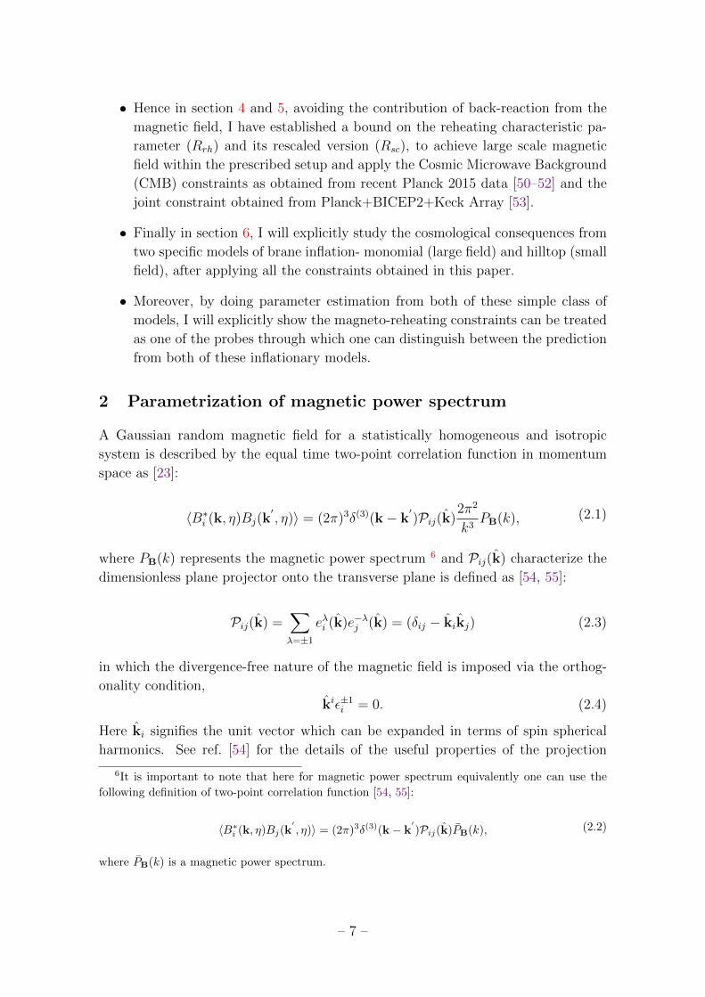
where PB(k) represents the magnetic power spectrum 6 and Pij(k) characterize the
dimensionless plane projector onto the transverse plane is defined as [54, 55]:
Pij(k) =∑λ=±1
eλi (k)e−λj (k) = (δij − kikj) (2.3)
in which the divergence-free nature of the magnetic field is imposed via the orthog-
onality condition,
kiε±1i = 0. (2.4)
Here ki signifies the unit vector which can be expanded in terms of spin spherical
harmonics. See ref. [54] for the details of the useful properties of the projection
6It is important to note that here for magnetic power spectrum equivalently one can use the
following definition of two-point correlation function [54, 55]:
〈B∗i (k, η)Bj(k′, η)〉 = (2π)3δ(3)(k− k
′)Pij(k)PB(k), (2.2)
where PB(k) is a magnetic power spectrum.
– 7 –
tensors of magnetic modes. Additionally, it is worthwhile to mention that in the
present context, PB(k) be the part of the power spectrum for the primordial magnetic
field which will only contribute to the cosmological perturbations for the scalar modes
and the Faraday Rotation at the phase of decoupling 7.
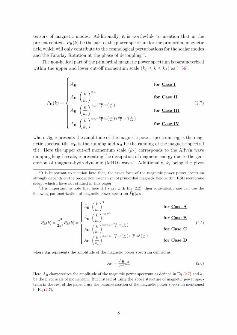
The non-helical part of the primordial magnetic power spectrum is parameterized
within the upper and lower cut-off momentum scale (kL ≤ k ≤ kΛ) as 8 [56]:
PB(k) =
AB for Case I
AB
(k
k∗
)nB
for Case II
AB
(k
k∗
)nB+αB2
ln( kk∗ )
for Case III
AB
(k
k∗
)nB+αB2
ln( kk∗ )+
κB6
ln2( kk∗ )
for Case IV
(2.7)
where AB represents the amplitude of the magnetic power spectrum, nB is the mag-
netic spectral tilt, αB is the running and κB be the running of the magnetic spectral
tilt. Here the upper cut-off momentum scale (kΛ) corresponds to the Alfven wave
damping length-scale, representing the dissipation of magnetic energy due to the gen-
eration of magneto-hydrodynamic (MHD) waves. Additionally, k∗ being the pivot
7It is important to mention here that, the exact form of the magnetic power power spectrum
strongly depends on the production mechanism of primordial magnetic field within RSII membrane
setup, which I have not studied in this paper.8It is important to note that here if I start with Eq (2.2), then equivalently one can use the
following parametrization of magnetic power spectrum PB(k):
PB(k) =k3
2π2PB(k) =
AB
(k
k∗
)3
for Case A
AB
(k
k∗
)nB+3
for Case B
AB
(k
k∗
)nB+3+αB2 ln( k
k∗ )for Case C
AB
(k
k∗
)nB+3+αB2 ln( k
k∗ )+κB6 ln2( k
k∗ )for Case D
(2.5)
where AB represents the amplitude of the magnetic power spectrum defined as:
AB =AB
2π2k3∗. (2.6)
Here AB characterizes the amplitude of the magnetic power spectrum as defined in Eq (2.7) and k∗be the pivot scale of momentum. But instead of using the above structure of magnetic power spec-
trum in the rest of the paper I use the parametrization of the magnetic power spectrum mentioned
in Eq (2.7).
– 8 –
or normalization scale of momentum. Now let me briefly discuss the physical signif-
icance of the above mentioned four possibilities 9:
• Case I stands for a physical situation where the magnetic power spectrum is
exactly scale invariant and it is characterized by nB = 0,
• Case II stands for a physical situation where the magnetic power spectrum
follows power law feature in presence of magnetic spectral tilt nB,
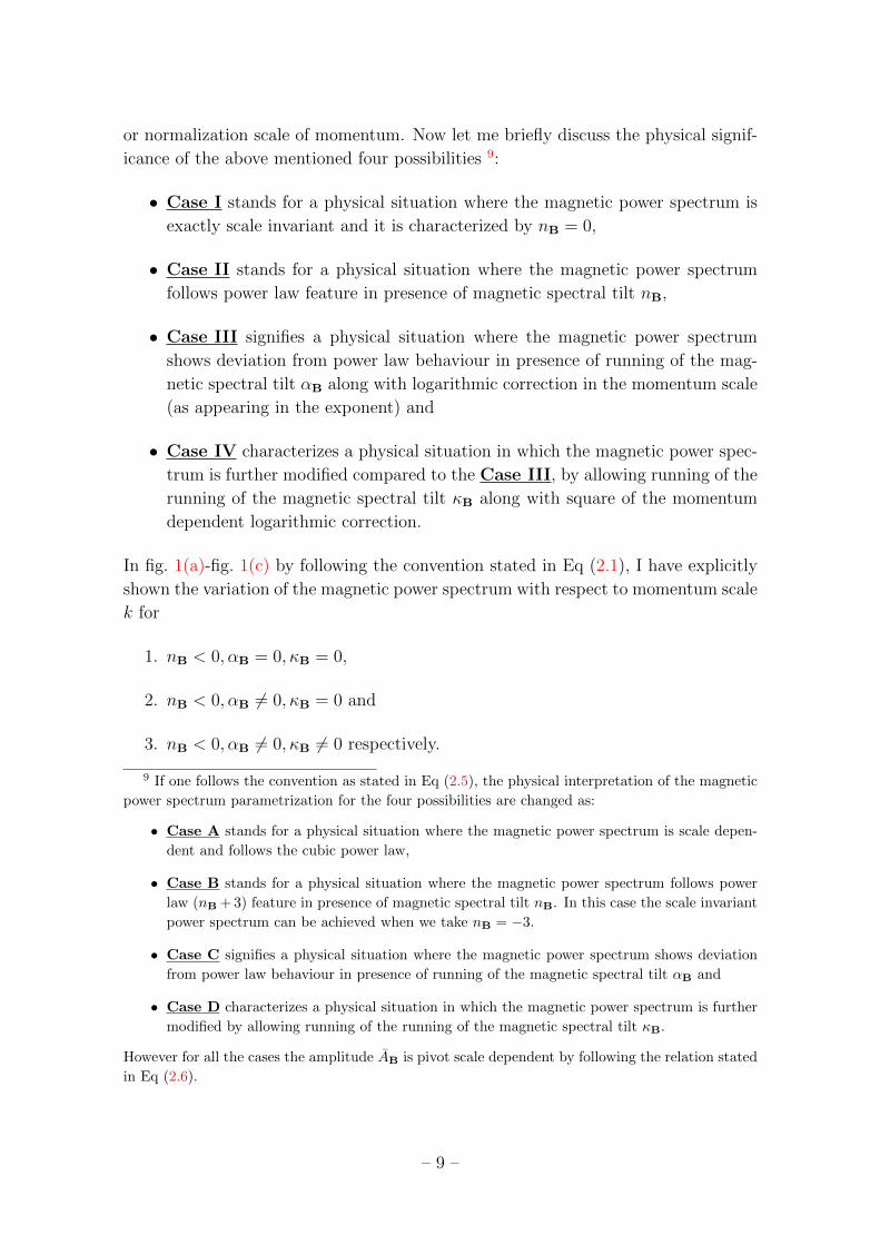
• Case III signifies a physical situation where the magnetic power spectrum
shows deviation from power law behaviour in presence of running of the mag-
netic spectral tilt αB along with logarithmic correction in the momentum scale
(as appearing in the exponent) and
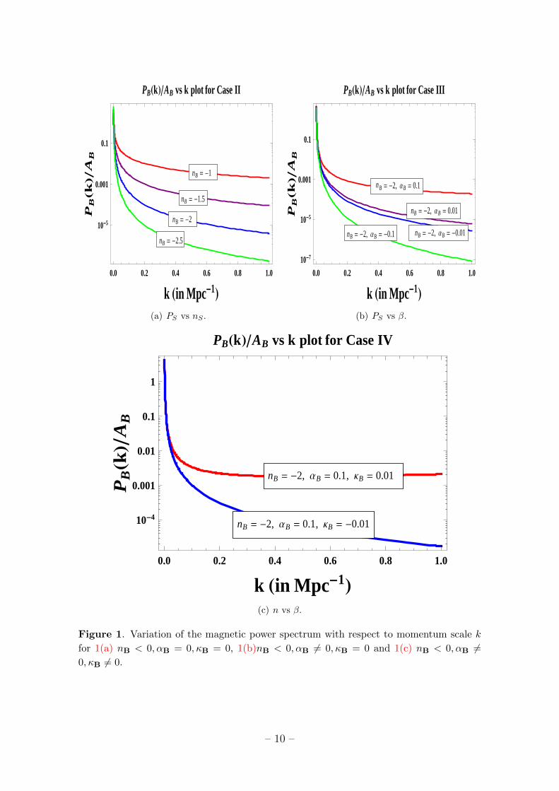
• Case IV characterizes a physical situation in which the magnetic power spec-
trum is further modified compared to the Case III, by allowing running of the
running of the magnetic spectral tilt κB along with square of the momentum
dependent logarithmic correction.
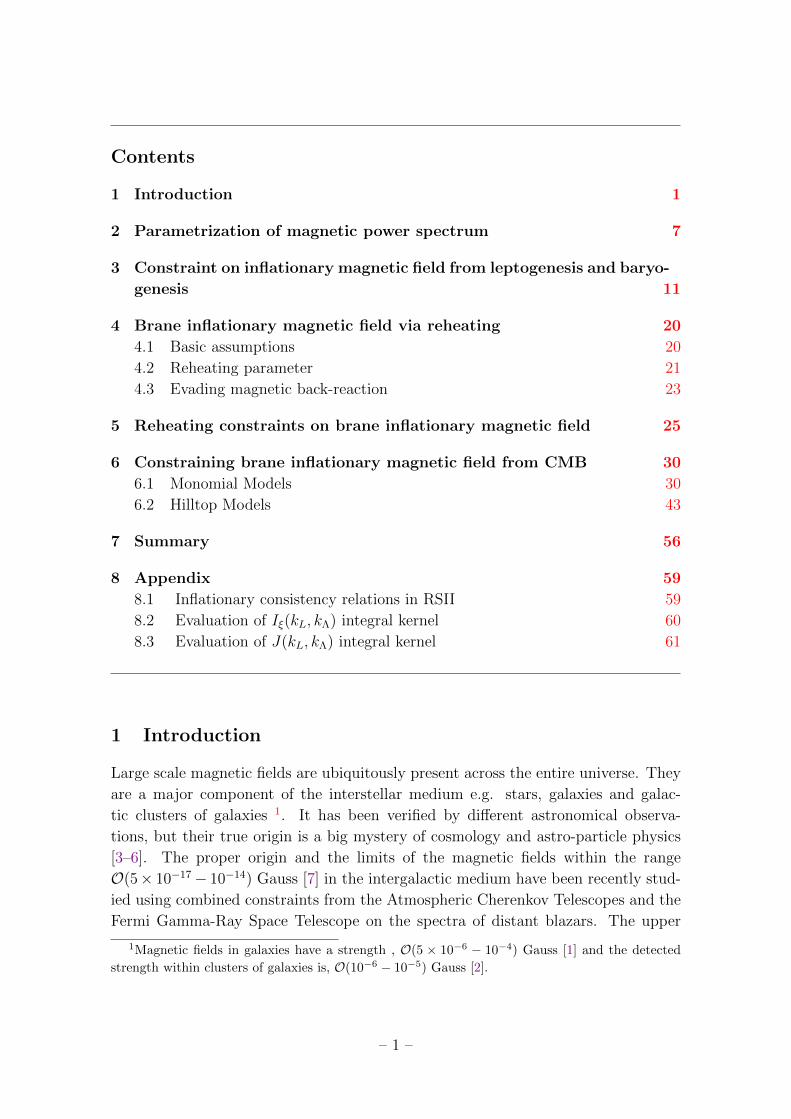
In fig. 1(a)-fig. 1(c) by following the convention stated in Eq (2.1), I have explicitly
shown the variation of the magnetic power spectrum with respect to momentum scale
k for
1. nB < 0, αB = 0, κB = 0,
2. nB < 0, αB 6= 0, κB = 0 and
3. nB < 0, αB 6= 0, κB 6= 0 respectively.
9 If one follows the convention as stated in Eq (2.5), the physical interpretation of the magnetic
power spectrum parametrization for the four possibilities are changed as:
• Case A stands for a physical situation where the magnetic power spectrum is scale depen-
dent and follows the cubic power law,
• Case B stands for a physical situation where the magnetic power spectrum follows power
law (nB + 3) feature in presence of magnetic spectral tilt nB. In this case the scale invariant
power spectrum can be achieved when we take nB = −3.
• Case C signifies a physical situation where the magnetic power spectrum shows deviation
from power law behaviour in presence of running of the magnetic spectral tilt αB and
• Case D characterizes a physical situation in which the magnetic power spectrum is further
modified by allowing running of the running of the magnetic spectral tilt κB.
However for all the cases the amplitude AB is pivot scale dependent by following the relation stated
in Eq (2.6).
– 9 –
nB = -1
nB = -1.5
nB = -2
nB = -2.5
0.0 0.2 0.4 0.6 0.8 1.0
10-5
0.001
0.1
k Hin Mpc-1L
PB
HkL
AB
PBHkLAB vs k plot for Case II
(a) PS vs nS .
nB = -2, ΑB = 0.1
nB = -2, ΑB = 0.01
nB = -2, ΑB = -0.01nB = -2, ΑB = -0.1
0.0 0.2 0.4 0.6 0.8 1.010-7
10-5
0.001
0.1
k Hin Mpc-1LP
BHk
LA
B
PBHkLAB vs k plot for Case III
(b) PS vs β.
nB = -2, ΑB = 0.1, ΚB = 0.01
nB = -2, ΑB = 0.1, ΚB = -0.01
0.0 0.2 0.4 0.6 0.8 1.0
10-4
0.001
0.01
0.1
1
k Hin Mpc-1L
PB
HkL
AB
PBHkLAB vs k plot for Case IV
(c) n vs β.
Figure 1. Variation of the magnetic power spectrum with respect to momentum scale k
for 1(a) nB < 0, αB = 0, κB = 0, 1(b)nB < 0, αB 6= 0, κB = 0 and 1(c) nB < 0, αB 6=0, κB 6= 0.
– 10 –
It is important to note that the most recent observational constraint from CMB
temperature anisotropies on the amplitude and the spectral index of a primordial
magnetic field has been predicted by using Planck 2015 data as 10 [50, 51]
B1 Mpc < 4.4nG (2.8)
with magnetic spectral tilt
nB < 0 (2.9)
at 2σ CL. If, in near future, Planck or any other observational probes can predict
the signatures for αB and κB in the primordial magnetic power spectrum (as already
predicted in case of primordial scalar power spectrum within 1.5− 2σ CL [52]), then
it is possible to put further stringent constraint on the various models of inflation.
3 Constraint on inflationary magnetic field from leptogene-
sis and baryogenesis
In the present section, I am interested in the mean square amplitude of the primordial
magnetic field on a given characteristic scale ξ, on which I smooth the magnetic power
spectrum using a Gaussian filter 11 as given by [55]:
B2ξ = 〈Bi(x)Bi(x)〉ξ =
1
2π2
∫ ∞0
dk
k∗
(k
k∗
)2
PB(k) exp(−k2ξ2
). (3.1)
Here in Case III and Case IV of Eq (2.7) describes a more generic picture where
the magnetic power spectrum deviates from its exact power law form in presence of
logarithmic correction. Consequently, the resulting mean square primordial magnetic
field is logarithmically divergent in both the limits of the integral as presented in
Eq (3.1). But in Case I and Case II of Eq (2.7) no such divergence is appearing. To
remove the divergent contribution from the mean square amplitude of the primordial
magnetic field as appearing in Case III and Case IV of Eq (3.1), I introduce here
cut-off regularization technique in which I have re-parameterized the integral in terms
of regulated UV (high) and IR (low) momentum scales. Most importantly, for the
sake of completeness in all four cases, here I introduce the high and low cut-offs
kΛ and kL are momentum regulators to collect only the finite contributions from
Eq (3.1). Finally I get the following expression for the regularized magnetic field:
B2ξ (kL; kΛ) =
Iξ(kL; kΛ)
2π2AB
(3.2)
10Here B1 Mpc represents the comoving field amplitude at a scale of 1 Mpc.11In standard prescriptions, Gaussian filter is characterized by a Gaussian window function
exp(−k2ξ2
), defined in a characteristic scale ξ.
– 11 –
where
Iξ(kL; kΛ) =
∫ kΛ
kL
dk
k∗exp
(−k2ξ2
)( k
k∗
)2
for Case I∫ kΛ
kL
dk
k∗exp
(−k2ξ2
)( k
k∗
)nB+2
for Case II∫ kΛ
kL
dk
k∗exp
(−k2ξ2
)( k
k∗
)nB+2+αB2
ln( kk∗ )
for Case III∫ kΛ
kL
dk
k∗exp
(−k2ξ2
)( k
k∗
)nB+2+αB2
ln( kk∗ )+
κB6
ln2( kk∗ )
for Case IV.
(3.3)
The exact expression for the regularized integral function Iξ(kL; kΛ) are explicitly
mentioned in the appendix 8.1 for all four cases. It is important to mention here
that, for Case I and Case II, Iξ(kL → 0; kΛ →∞) is finite. But for rest of the two
cases, Iξ(kL → 0; kΛ → ∞) → ∞. On the other hand, in absence of any Gaussian
filter, the magnetic energy density can be expressed in terms of the mean square
primordial magnetic field as [55]:
ρB =1
8π〈Bi(x)Bi(x)〉 =
1
8π2
∫ ∞0
dk
k∗
(k
k∗
)2
PB(k) (3.4)
which is logarithmically divergent in UV and IR end for Case III and Case IV. For
rest of the two cases also the contribution become divergent, but the behaviour of the
divergences are different compared to the Case III and Case IV. After introducing
the momentum cut-offs as mentioned earlier, I get the following expression for the
regularized magnetic energy density as:
ρB(kL; kΛ) =J(kL; kΛ)
8π2AB =
J(kL; kΛ)B2ξ (kL; kΛ)
4Iξ(kL; kΛ)(3.5)
where
J(kL; kΛ) =
∫ kΛ
kL
dk
k∗
(k
k∗
)2
for Case I∫ kΛ
kL
dk
k∗
(k
k∗
)nB+2
for Case II∫ kΛ
kL
dk
k∗
(k
k∗
)nB+2+αB2
ln( kk∗ )
for Case III∫ kΛ
kL
dk
k∗
(k
k∗
)nB+2+αB2
ln( kk∗ )+
κB6
ln2( kk∗ )
for Case IV
(3.6)
where I use Eq (3.2). Here the regularized integral function J(kL; kΛ) are explicitly
written in the appendix 8.2 for all four possibilities.
– 12 –
Now to derive a phenomenological constraint here I further assume the fact that
the primordial magnetic field is made up of relativistic degrees of freedom. In this
physical prescription, the regularized magnetic energy density can be expressed as
[57]:
ρB(kL; kΛ) ∼ π2
30g∗T
4 ∼ O(10−13)× T 4
εCP
(3.7)
where the CP asymmetry parameter εCP is defined as:
εCP =ΓL(NR → LiΦ)− ΓLc(NR → LciΦ
c)
ΓL(NR → LiΦ) + ΓLc(NR → LciΦc)≈ O(|λ|2) sin θCP
(3.8)
for the standard leptogenesis scenario [58, 59] where the Majorana neutrino (NR)
decays through Yukawa matrix interaction (λ) with the Higgs (Φ) and lepton (L)
doublets. Here θCP is the CP-violating phase and for heavy majorana neutrino (NR)
mass
MNR ∼ 1010 GeV (3.9)
the Yukawa coupling is given by,
|λ|2 = O(10−16). (3.10)
Now combining Eq (3.5) and Eq (3.7), I derive the following simplified expression
for the root mean square value of the primordial magnetic field at the present epoch
in terms of the CP asymmetry parameter (εCP) as:
B0 ∼ O(10−14)×
√Iξ(kL = k0; kΛ)
J(kL = k0; kΛ)εCP
Gauss (3.11)
where I use the temperature at the present epoch
T0 ∼ 2× 10⁻⁴ eV (3.12)
and
1 Gauss = 7× 10⁻²⁰ GeV2. (3.13)
In addition, here in this paper, I fix the IR cut-off scale of the momentum at the
present epoch i.e. kL = k0. Consequently the momentum integrals satisfy the fol-
lowing constraint: √Iξ(kL = k0; kΛ)
J(kL = k0; kΛ)∼ 10−8. (3.14)
Further using Eq (8.16) and Eq (8.17) in Eq (3.14) one can write the following
constarints for all four cases of the parametrization of magnetic power spectrum as:
Case I : k∗ ∼ O(8.17× 10⁻⁹)×
√ √ξ [k3
Λ − k3L]√
π [erf(ξkΛ)− erf(ξkL)], (3.15)
– 13 –
Case II :1
ξnB+3∼ O(2× 10⁻¹⁶)×
[knB+3
Λ − knB+3L
](nB + 3)
[Γ(
(nB+3)2
, ξ2k2L
)− Γ
((nB+3)
2, ξ2k2
Λ
)] , (3.16)
Case III :
[√π erf (ξk)
2ξ
1 +Q ln
(k
k∗
)+ P ln2
(k
k∗
)+ k
2P PFQ
[1
2,1
2,1
2
;
3
2,3
2,3
2
;−ξ2k2
]−(Q+ 2P ln
(k
k∗
))PFQ
[1
2,1
2
;
3
2,3
2
;−ξ2k2
]]k=kΛ
k=kL
∼ O(10−16)×k
[(1 + 2P −Q) + (Q− 2P) ln
(k
k∗
)+ P ln2
(k
k∗
)]k=kΛ
k=kL
,
(3.17)
Case IV :
[√π erf (ξk)
2ξk∗
1 +Q ln
(k
k∗
)+ P ln2
(k
k∗
)+ F ln3
(k
k∗
)+
(k
k∗
)−6F PFQ
[1
2,1
2,1
2,1
2
;
3
2,3
2,3
2,3
2
;−ξ2k2
]+ 2
(P + 3F ln
(k
k∗
))PFQ
[1
2,1
2,1
2
;
3
2,3
2,3
2
;−ξ2k2
]−(Q+ 2P ln
(k
k∗
)+ 6F ln2
(k
k∗
))× PFQ
[1
2,1
2
;
3
2,3
2
;−ξ2k2
]]k=kΛ
k=kL
∼ O(10−16)×(
k
k∗
)[(1− 6F + 2P −Q) + (6F − 2P +Q) ln
(k
k∗
)− (3F − P) ln2
(k
k∗
)+ F ln3
(k
k∗
)]k=kΛ
k=kL
,
(3.18)
where
Q = nB + 2, (3.19)
P = αB/2, (3.20)
F = κB/6. (3.21)
The conformal symmetry of the quantized electromagnetic field breaks down in
curved space-time which is able to generate a sizable amount of magnetic field dur-
ing a phase of slow-roll inflation. Such primordial magnetism is characterized by
the renormalized mean square amplitude of the primordial magnetic field at leading
order in slow-roll approximation for comoving observers as [60]:
ρB(kL; kΛ) =1
8π〈Bi(x)Bi(x)〉 ≈ V 4(φ)εb(φ)
8640π3M4pσ
2(3.22)
– 14 –
where V (φ) represents the inflationary potential, σ represents the brane tension of
RSII setup and Mp ∼ 2.43×10¹⁸ GeV be the four dimensional reduced Planck mass.
Within RSII setup the visible brane tension σ can be expressed as [33]:
σ =
√− 3
4πM3
5 Λ5 =
√−24M3
5 Λ5 > 0 (3.23)
where Λ5 be the scaled 5D bulk cosmological constant defined as [33]:
Λ5 =Λ5
32π< 0. (3.24)
Also the 5D quantum gravity cut-off scale can be expressed in terms of 5D cosmo-
logical constant and the 4D effective Planck scale as:
M35 =
3
√−4πΛ5
3M4/3
p =3
√−128π2Λ5
3M4/3
p . (3.25)
In the high energy regime the energy density ρ >> σ the slow-roll parameter εb(φ)
in the visible brane can be expressed as [33]:
εb(φ) ≈2M2
pσ(V′(φ))2
V 3(φ). (3.26)
It is important to note that Eq (3.22) is insensitive to the intrinsic ambiguities of
renormalization in curved space-times. See the appendix where I have mentioned
the inflationary consistency conditions within RSII setup. Around the pivot scale
k = k∗ I can write:
εb(k∗) ≈r(k∗)
24+ · · · , (3.27)
where · · · includes the all the higher order slow-roll contributions. Here r = PT/PSrepresents the tensor-to-scalar ratio. The recent observations from Planck (2013 and
2015) and Planck+BICEP2+Keck Array puts an upper bound on the amplitude of
primordial gravitational waves via tensor-to-scalar ratio. This bounds the potential
energy stored in the inflationary potential within RSII setup as [33]:
4√Vinf ≈ 12
√2π2PS(k∗)r(k∗)M
1/3p σ1/6 . 4
√3
2PS(k∗)r(k∗)π2 Mp
= (1.96× 10¹⁶GeV)×(r(k∗)
0.12
)1/4(3.28)
where PS(k∗) represents the amplitude of the scalar power spectrum. More precisely
Eq (3.28) can be recast as a stringent constraint on the upper bound on the brane
tension in RSII setup during inflation as:
σ <3√
3
4π2PS(k∗)r(k∗)M
4p . (3.29)
– 15 –
It is important to note that, to validate the effective field theory prescription within
the framework of small field models of inflation, the model independent bound on
the brane tension, the 5D cut-off scale and 5D bulk cosmological constant can be
written as [33]:
σ ≤ O(10−9) M4p , M5 ≤ O(0.04− 0.05) Mp, Λ5 ≥ −O(10−15) M5
p .(3.30)
If I go beyond the above mentioned bound on the characteristic parameters of RSII
then one can describe the inflationary paradigm in large field regime. Please see
ref. [33] for further details.
Finally using this constraint along with Eq (3.5) in Eq (3.22) I get the following
simplified expression for the root mean square value of the primordial magnetic field
in terms of the tensor-to-scalar ratio r in RSII setup as 12:
Bξ(kL; kΛ) . O(1035)×(r(k∗)
0.12
)5/2
Σ5/2b (kL, k∗)×
(M4
p
σ
)︸ ︷︷ ︸
Regulator in RSII
×
√Iξ(kL; kΛ)
J(kL; kΛ)Gauss.
(3.34)
At the present epoch the regulating factor Σb(kL = k0, k∗) appearing in Eq (3.34) is
lying within the window,
O(4.77× 10¹³) ≤ Σb(kL = k0, k∗)×(M4
p
σ
)2/5
≤ O(10−17.6), (3.35)
for the tensor-to-scalar ratio,
10−29 ≤ r∗ ≤ 0.12 (3.36)
12In case of the low energy limit of RSII setup i.e. when the energy density of the matter content
(ρm) is much higher compared to the RSII brane tension σ then the actual version of the Friedmann
equations in RSII setup are mapped into the Friedmann equations known for General Relativistic
setup. Technically this statement can be expressed as:
H2 =ρm
3M2p
1 +ρm2σ︸︷︷︸<<1
≈ ρm3M2
p
. (3.31)
In the low energy regime of RSII the lower bound of the CP asymmetry parameter can be written
as [56]:
Bξ(kL; kΛ) . O(1044)×(r(k∗)
0.12
)3/2
Σ3/2(kL, k∗)︸ ︷︷ ︸Regulator in GR
×
√Iξ(kL; kΛ)
J(kL; kΛ)Gauss. (3.32)
where Σ(kL = k0, k∗) plays the GR analogue of the regulator and satisfies the following stringent
constraint:
O(10−2/3) ≤ Σ(kL = k0, k∗) ≤ O(10−30). (3.33)
– 16 –
at the momentum pivot scale, k∗ ∼ 0.002 Mpc−1. Here the “b” subscript is used to
specify the fact that the analysis is done within RSII setup. Now by setting kL = k0
at the present epoch, the estimated numerical value of the primordial magnetic field
from RSII setup turns out to be:
B0 = Bξ(kL = k0; kΛ) ∼ O(10−9) Gauss. (3.37)
Further using Eq (3.11) I get following expression for the lower bound of the CP
asymmetry parameter within RSII setup as 13:
εCP & O(10−98)×(
0.12
r(k∗)
)5
Σ−5b (kL = k0, k∗)×
(σ
M4p
)2
, (3.39)
which is pointing towards the following possibilities within RSII setup:
1. For the large tensor-to-scalar ratio the significant features of CP asymmetry
can be possible to detect in future collider experiments. For an example we
consider a situation where the tensor-to-scalar ratio is,
r(k∗) ∼ 0.12 (3.40)
and in such a case the lower bound of CP asymmetry is given by
εCP & 10−10 (3.41)
in RSII braneworld. For GR one can also compute the lower bound of CP
asymmetry parameter and it turns out to be
εCP & 10−16 (3.42)
for GR limit [56].
2. For very small tensor-to-scalar ratio the CP asymmetry is largely suppressed
and can’t be possible to detect in the particle colliders. For an example if
tensor-to-scalar ratio,
r(k∗) ∼ 10−29 (3.43)
then the lower bound of CP asymmetry is given by
εCP & 10−26 (3.44)
13In case of low energy regime of RSII or equivalently for GR prescribed setup the lower bound
of the CP asymmetry parameter can be written as [56]:
εCP & O(10−116)×(
0.12
r(k∗)
)3
Σ−3(kL = k0, k∗), (3.38)
where Σ(kL = k0, k∗) plays the GR analogue of the regulator.
– 17 –
in RSII braneworld. Similarly the lower bound of CP asymmetry parameter in
GR prescribed setup can be computed as [56],
εCP & 10−30. (3.45)
If, in near future, any direct/indirect observational probe detects the signatures of
primordial gravitational waves by measuring large detectable amount of tensor-to-
scalar ratio then it will follow the first possibility. For a rough estimate for CP
asymmetry in terms of neutrino masses one can write:
εCP ∼3
16π
M1m3
v2∼ 0.1
M1
M3
. (3.46)
This implies that in the first case it is highly possible to achieve the upper bound of
CP asymmetry parameter [56],
εCP . 10−6 (3.47)
for
M1/M3 ∼ mu/mt ∼ 10−5, (3.48)
by tuning the regulating factor as well the brane tension of RSII setup at the pivot
scale k∗ ∼ 0.002 Mpc−1 to the following value 14:
Σb(kL = k0, k∗)×(M4
p
σ
)2/5
. O(4× 10⁻¹⁹), (3.50)
which is required to accommodate mass hierarchy of the heavy Majorana neutrino
at the scale of 1010 GeV. Additionally it is important mention here that the heavy
Majorana neutrino NR is the ideal candidate for baryogenesis as decays to lepton-
Higgs pairs yield lepton asymmetry
〈L〉T 6= 0, (3.51)
partially converted to baryon asymmetry
〈B〉T 6= 0. (3.52)
Also the baryon asymmetry ηB for given CP asymmetry εCP can be expressed as:
ηB =nB − nB
nγ=κ
fc∆εCP (3.53)
14In case of low energy regime of RSII or equivalently for GR prescribed setup the upper bound
on the tuning in the regulator can be expressed as:
Σ(kL = k0, k∗) . O(2.1× 10−37). (3.49)
– 18 –
where f ∼ 102 is the dilution factor which accounts for the increase of the number of
photons in a comoving volume element between baryogenesis and today, c∆ represents
the fraction which is responsible for the conversion of lepton asymmetry to baryon
asymmetry and exactly quantified by the following expression:
c∆ =〈B〉T〈B − L〉T
=1
1− 〈L〉T〈B〉T
. (3.54)
Usually the conversion factor
c∆ ∼ O(1) (3.55)
and in the context of Standard Model
c∆ = 28/79. (3.56)
Also the determination of the washout factor κ requires the details of modified Boltz-
mann equations within RSII setup. But for realistic estimate one can fix
κ ∼ O(10−2 − 10−1). (3.57)
The baryon asymmetry is generated around a temperature
TB ∼ 1010 GeV, (3.58)
which is exactly same as mass scale of the heavy Majorana neutrino and this has
possibly interesting implications for the nature of dark matter. The observed value
of the baryon asymmetry [51],
ηB ∼ 10−9 (3.59)
is obtained as consequence of a large hierarchy of the heavy neutrino masses, leading
to a small CP asymmetry, and the kinematical factors f and κ. In case of RSII setup
using Eq (3.53) the lower bound on baryon asymmetry parameter can be expressed
as 15:
ηB & O(10−101)×(
0.12
r(k∗)
)5
Σ−5b (kL = k0, k∗)×
(σ
M4p
)2
. (3.61)
which implies the following possibilities within RSII setup:
15In case of GR prescribes setup the lower bound of the CP asymmetry parameter can be written
as:
ηB & O(10−119)×(
0.12
r(k∗)
)3
Σ−3(kL = k0, k∗). (3.60)
– 19 –
1. For the large tensor-to-scalar ratio the significant features of baryon asymmetry
can be possible to detect in future. For an example we consider a situation
where the tensor-to-scalar ratio is,
r(k∗) ∼ 0.12 (3.62)
and in such a case the lower bound of baryon asymmetry is given by
ηB & 10−14 (3.63)
in RSII braneworld. This also implies that in this case it is highly possible to
achieve the observed baryon asymmetry parameter,
ηB ∼ 10−9 (3.64)
by adjusting the regulating factor as well the brane tension of RSII setup at
the pivot scale k∗ ∼ 0.002 Mpc−1 by following the upper bound as stated
in Eq (3.50). In case of low energy regime of RSII or equivalently for GR
prescribed setup the lower bound of baryon asymmetry is given by
ηB & 10−26 (3.65)
with tensor to scalar ratio
r(k∗) ∼ 0.12. (3.66)
2. For very small tensor-to-scalar ratio the baryon asymmetry is largely sup-
pressed and can’t be possible to detect via future experiments. For an example
if tensor-to-scalar ratio,
r(k∗) ∼ 10−29 (3.67)
then the lower bound of baryon asymmetry parameter is given by
ηB & 10−30 (3.68)
in RSII braneworld. Similarly in the low energy regime of RSII or in GR limit
the lower bound of baryon asymmetry is given by
ηB & 10−33 (3.69)
with r(k∗) ∼ 0.12.
4 Brane inflationary magnetic field via reheating
4.1 Basic assumptions
Before going to the critical details of the computation, let me first briefly mention
the underlying assumptions and basics of the present setup:
– 20 –
• The primordial magnetic field is created via quantum vacuum fluctuation and
amplified during the epoch of inflation.
• Conformal invariance is restored at the end of inflation such that the magnetic
field subsequently decays as a−2, where a is the cosmological scale factor. Con-
sequently the physical strength of the magnetic field today on the large scale
is given by:
B0 =Bend
(1 + zend)2 . (4.1)
where B0 and Bend are the magnetic field today and at the end of inflation
respectively. Also zend signifies the redshift at the end of inflation and in terms
of scale factor it is defined as:
zend =a0
aend− 1. (4.2)
In this work I will explicitly show that for all classes of the models of originating
brane inflationary magnetic field, the redshift zend depends on the properties of
reheating. During the epoch of inflation the corresponding wave number can
be expressed as:k∗a
=k∗a0
(1 + zend) eNend;b−Nb (4.3)
where the subscript “b” is used to specify the braneworld gravity setup and
exactly consistent with Eq (4.2).
• Further I assume the instantaneous transitions between inflation, reheating,
radiation and matter dominated epoch one can write:
(1 + zend) = (1 + zeq)
(ρrehρeq
)1/4(arehaend
)(4.4)
where the subscript “reh” and “eq” stand for end of reheating and the matter
radiation equality.
• I also assume that at the present epoch the contribution from the correction
coming from the non-relativistic neutrinos are negligibly small and so that I
neglected the contribution from the computation.
4.2 Reheating parameter
Let us first start with the reheating parameter Rrad defined by 16 [61]:
Rrad ≡aendareh
(ρendρreh
)1/4
, (4.5)
16If I fix Rrad = 1 then from Eq (4.5) it implies that ρ ∝ a−4, which exactly mimics the role of
the energy density during radiation dominated era.
– 21 –
where the subscript “reh” can be interpreted as the end of reheating era and also the
beginning of radiation dominated era. More precisely Rrad measures the deviation
between reheating and radiation dominated era. Now using Eq (4.5) in Eq (4.4) one
can write:
(1 + zend) = (1 + zeq)×(aeqareh
)×(arehaend
)=
1
Rrad
(ρendArehργ
)1/4
(4.6)
where in the high energy regime of RSII braneworld the radiation energy density can
be expressed as:
ργ =√
6σΩradH0Mp (4.7)
represents the energy density of radiation at present epoch and
Areh ≡grehg0
(q0
qreh
)4/3
(4.8)
is the measure of the change of relativistic degrees of freedom between the reheating
epoch and present epoch. Also q and g denotes the number of entropy and relativistic
degrees of freedom at the epoch of interest respectively. Here H0 represents the
Hubble parameter at the present epoch and Ωrad signifies the dimensionless density
parameter during radiation dominated era. To proceed further here I start with the
expression for the number of e-foldings at any arbitrary momentum scale] as [62–66]:
Nb(k) = 71.21− ln
(k
k0
)+
1
4ln
V∗M4
p
+1
4ln
V∗ρend
+1− 3wreh
12 (1 + wreh)ln
(ρrehρend
)(4.9)
where ρend is the energy density at the end of inflation, ρreh is an energy scale during
reheating, k0 = a0H0 is the present Hubble scale, V∗ corresponds to the potential
energy when the relevant modes left the Hubble patch during inflation corresponding
to the momentum scale k∗ ≈ kcmb, and wreh characterizes the effective equation of
state parameter between the end of inflation and the energy scale during reheating.
Further using Eq (4.9) one can write:
∆Nb = Nreh;b −Nend;b = ln
(arehaend
)= ln
(kendkreh
). (4.10)
Now using only the energy conservation one can derive the following expression for
the reheating energy density:
ρreh = ρend exp
[−3
∫ Nreh;b
Nend;b(1 + w(Nb)) dNb
]≈ ρend exp
[−3∆Nb (1 + wreh)
](4.11)
where ∆Nb is defined in Eq (4.10) and the mean equation of state parameter wreh is
defined as:
wreh ≡
∫ Nreh;b
Nend;bw(Nb)dNb
∆Nb. (4.12)
– 22 –
where
w(Nb) = P (Nb)/ρ(Nb) (4.13)
represents the instantaneous equation of state parameter. Further using Eq (4.11)
in Eq (4.5) one can derive the following expression for reheating parameter:
Rrad =
(ρrehρend
) 1−3wreh12(1+wreh)
. (4.14)
Here Eq (4.14) also implies that for
wreh = 1/3 (4.15)
the reheating parameter
Rrad = 1. (4.16)
4.3 Evading magnetic back-reaction
To evade magnetic back-reaction on the cosmological background in this paper I
consider the following two physical situations:
1. In the first situation the reheating epoch characterizes by the lower bound
on the equation of state parameter at,
wreh ≥ 1/3 (4.17)
and the corresponding energy density during reheating decays very faster com-
pared to the energy density during radiation dominated era. In this case, the
magnetic back-reaction on the length scales of interest is evaded for the follow-
ing constraint on the ratio of the energy densities [61]:
ρB(zreh)
ρreh=ρB0
ργ< 1 (4.18)
Now further using the Planckian unit system one can write, 1 Gauss ' 3.3 ×10−57 M2
p and using this unit conversion the photon energy density can be
written in terms of the magnetic unit as [61],
ργ ' 5.7× 10−125 M4p = 5.2× 10⁻¹² Gauss2. (4.19)
Using Eq (4.14) one can further show that for wreh ≥ 1/3 the reheating pa-
rameter
Rrad ≥ 1. (4.20)
This clearly implies that magnetic back-reaction effect can evaded using this
constraint.
– 23 –
2. In the second situation the reheating epoch characterizes by
wreh < 1/3 (4.21)
and the corresponding energy density of the magnetic field dominate over the
energy density during reheating epoch. Within this prescription the effect of
magnetic back-reaction can be neglected, provided the magnetic energy density
remains smaller compared to the background total energy density at any epoch
i.e.ρBendρend
< 1. (4.22)
where the magnetic energy density ρBend can be written in terms of the energy
density at the end of inflationary epoch as:
ρBend =B2
0
2R4radργ
ρend. (4.23)
Further substituting Eq (4.23) in Eq (4.22) one can compute the lower bound
on the reheating parameter as [61]:
Rrad >
√B0
(2ργ)1/4. (4.24)
The physical interpretation of the bound on reheating parameter is as follows:
• Firstly it is important to note that the lower bound on reheating param-
eter is true for any models of inflation and completely independent on any
prior knowledge of inflationary models.
• Secondly to hold this bound it necessarily requires that the conformal
invariance has to be satisfied during the decelerating phase of the Universe.
Further using Eq (4.11), eq (4.14) and Eq (4.24) I get the following simplified ex-
pression for the reheating constraint:
√B0
(2ργ)1/4exp
[∆Nb
4(1− 3wreh)
]< 1 (4.25)
from which one can compute the following analytical constraint on the mean equation
of state parameter wreh as:
wreh <1
3
(1 +
4
∆Nbln
( √B0
(2ργ)1/4
))(4.26)
For an example if I fix the magnetic field at the present epoch within
B0 ∼ O(10−15 Gauss− 10−9 Gauss) (4.27)
– 24 –
then the lower bound of the reheating parameter is constrained within
Rrad > O(1.76× 10⁻⁵ − 10−2). (4.28)
Consequently the bound on the mean equation of state parameter wreh can be com-
puted as:
wreh <1
3
(1 +
C∆Nb
)(4.29)
where the numerical factor C ∼ O(18.42 − 43.81) > 0 for B0 ∼ O(10−15 Gauss −10−9 Gauss).
5 Reheating constraints on brane inflationary magnetic field
To derive the expression for the scale of reheating and also its connection with the
inflationary magnetic field within RSII I start with Eq (4.14) and using this input
one can write:
ρreh = ρendR12(1+wreh)
1−3wrehrad . (5.1)
Further using the lower limit of the reheating parameter as stated in Eq (4.24), one
can derive the lower bound of the reheating energy density as:
ρreh > ρend
(B0√2ργ
) 6(1+wreh)
1−3wreh
= ρend
(B0√2ργ
)−2
1+∆Nb
ln
( √B0
(2ργ )1/4
). (5.2)
Now in the high density or high energy regime of RSII, ρ >> σ and using the
Friedmann equation one can write [41, 42]:
H ≈ ρ√6σMp
. (5.3)
where σ is the brane tension in RSII setup. Hence using Eq (5.3) the lower bound
of the reheating energy density can be recast within RSII setup as 17:
ρreh >√
6σMpHend
(B0√2ργ
) 6(1+wreh)
1−3wreh
=√
6σMpHend
(B0√2ργ
)−2
1+∆Nb
ln
( √B0
(2ργ )1/4
)
(5.5)
17In the low density regime of RSII braneworld or equivalently in GR limit the lower bound on
the reheating energy density can be expressed as:
ρreh >√
3MpHend
(B0√2ργ
) 6(1+wreh)
1−3wreh
=√
3MpHend
(B0√2ργ
)−2
1+∆Nb
ln
( √B0
(2ργ )1/4
)
(5.4)
– 25 –
where Hend represents the Hubble parameter at the end of reheating and additionally
Eq (4.29) has to satisfied to avoid magnetic back-reaction. Here Eq (5.5) implies that
if the magnetic field is generated via inflation in braneworld then by knowing the
Hubble scale at the end of inflation as well as the constraint on the brane tension σ
it is possible to constraint the lower bound of the scale of reheating. It is important
to note that if
wreh → 1/3 (5.6)
the equality in Eq (5.5) will not hold at all and also in such a situation the exponent
diverges i.e.6(1 + wreh)
1− 3wreh→∞. (5.7)
This clearly implies that the lower bound of the reheating energy density is zero
and compatible with the understandings of the physics of originating inflationary
magnetic field. In the present context the field value at the end of inflation is deter-
mined by the violation of the slow-roll conditions. See Appendix 8.1 for the details.
Consequently one can derive the following sets of constraints on the generic form of
inflationary potential and its derivatives at the end of inflation as:
V (φend) =(2M2
pσ)1/3
(V′(φend)
)2/3
, (5.8)
V (φend) =(2M2
pσ)1/2
(V′′(φend)
)1/2
, (5.9)
V (φend) =(4M4
pσ2)1/4
(V′(φend)V
′′′(φend)
)1/2
, (5.10)
V (φend) =(8M6
pσ3)1/6
(V′(φend)
)1/3 (V′′′′
(φend))1/6
. (5.11)
For more stringent constraint the system need to satisfy all of the equations as
mentioned in Eq (5.8-5.11) to fix the scale of inflationary potential at the end of
inflation. In this case the derivatives or more precisely the Taylor expansion co-
efficients of the inflationary potential at the end of inflation are not independent at
all. But if the system relaxes any three of the previously mentioned constraints,
then also it possible to constrain the scale of potential at the end epoch of inflation.
Consequently Eq (5.5) can be recast in terms of the generic form of the inflationary
potential as:
ρreh > V (φend)
(B0√2ργ
) 6(1+wreh)
1−3wreh
≈ V (φend)
(B0√2ργ
)−2
1+∆Nb
ln
( √B0
(2ργ )1/4
)
(5.12)
Here it is important to note that during reheating both kinetic and potential con-
tribution play crucial role in the energy density. Later I will explicitly show the
– 26 –
estimation algorithm of V (φend) from a generic as well as for specified form of in-
flationary potential for the determination of the lower bound of the energy density
during reheating.
In the high energy regime of RSII setup during reheating one can write the total
decay width for the decay of heavy Majorana neutrinos as [31, 32]:
Γtotal = ΓL(NR → LiΦ) + ΓLc(NR → LciΦc) = 3H(Treh) ≈
√3
2σ
ρrehMp
(5.13)
where H(Treh) be the Hubble parameter during reheating and ρreh represents the
energy density during reheating. In the context of statistical theormodynamics one
can express the reheating energy density as:
ρreh =π2
30g∗T
4reh (5.14)
where g∗ signifies the effective number of relativistic degrees of freedom. In a more
generalized prescription g∗ can be expressed as:
g∗ = gB∗ +7
8gF∗ (5.15)
where gB∗ and gF∗ are the number of bosonic and fermionic degrees of freedom
respectively. It is worth mentioning that the reheating temperature within RSII
does not depend on the initial value of the inflaton field from where inflation starts
and is solely determined by the elementary particle theory of the early universe.
Further using Eq (5.13) and Eq (5.14) the reheating temperature within the high
energy regime of RSII setup can be expressed as 18 [31, 32]:
Treh =
(30
π2g∗
)1/4
× (ΓtotalMp)1/4 ×
(2σ
3
)1/8
. (5.17)
On the other hand the reheating temperature can be expressed in terms of the tensor-
to-scalar ratio as:
Treh ≈(
30
π2g∗
)1/4
× (1.96× 1016GeV)×(r(k∗)
0.12
)1/4
. (5.18)
18In the low energy regime of RSII or equivalently in the GR limit the reheating temperature can
be expressed as [65, 67, 68]:
Treh =
(30
π2g∗
)1/4
×(
ΓtotalMp√3
)1/2
. (5.16)
– 27 –
Now eliminating reheating temperature from Eq (5.17) and Eq (5.18) one can express
the total decay width in terms of inflationary tensor-to-scalar ratio as 19:
Γtotal = 4.23× 10⁻⁹M3p ×
√3
2σ×(r(k∗)
0.12
). (5.20)
Further combining Eq (4.11) and Eq (5.14) the energy density of inflaton at the end
of inflation can be expressed in terms of tensor-to-scalar ratio as:
ρend ≈ V (φend) = (1.96× 10¹⁶GeV)4 ×(r(k∗)
0.12
)× exp
[3 (1 + wreh) ∆Nb
]. (5.21)
Similarly using Eq (5.21) in Eq (5.12) the reheating energy density or more precisely
the scale of reheating can be expressed in terms of the tensor-to-scalar ratio, mean
equation of reheating wreh and magnetic field at the present epoch as:
ρreh > (1.96× 10¹⁶GeV)4 ×(r(k∗)
0.12
)× exp
[3 (1 + wreh) ∆Nb
]×
(B0√2ργ
) 6(1+wreh)
1−3wreh
. (5.22)
Further applying the constraint in the mean equation of reheating parameter as
stated in Eq (4.26) the lower bound of the scale of reheating energy density can be
recast as:
ρreh > (1.96× 10¹⁶GeV)4 ×(r(k∗)
0.12
)× exp
[4∆Nb
]×
(B0√2ργ
)− 4∆Nb
ln
(B0√2ργ
). (5.23)
Next I will explicitly derive the expression for the density parameter during radiation
dominated epoch (Ωrad) and further I will connect this to the density parameter of
the magnetic field (ΩBend). To serve this purpose I start with the analysis in the high
energy regime of the RSII braneworld in which the dimensionless density parameter
can be expressed as:
Ω =ρ2
ρcρ0
(5.24)
where the critical energy density in RSII braneworld can be written as:
ρc = 2σ (5.25)
and the energy density at the present epoch can be written as:
ρ0 = 3M2pH
20 . (5.26)
19In the low energy regime of RSII or equivalently in the GR limit total decay width of the heavy
Majorana neutrino can be written as:
Γtotal = 1.13× 10⁻⁴Mp ×(r(k∗)
0.12
)1/2
. (5.19)
– 28 –
Now using Eq (4.6) in Eq (4.23) one can write the magnetic energy density in terms
of redshift as:
ρBend =B2
0
2(1 + zeq)
4 exp[∆Nb (1− 3wreh)
](5.27)
and using Eq (5.27) the dimensionless density parameter for magnetic field can be
written as:
ΩBend =B4
0
24σH20M
2p
(1 + zeq)8 exp
[2∆Nb (1− 3wreh)
]. (5.28)
In the high energy regime of RSII braneworld one can write the density parameter
at the end of inflation in terms of the density parameter at the radiation dominated
era and redshift as:
Ωend = (1 + zeq)8 Ωrad. (5.29)
Further substituting Eq (5.31) in Eq (5.30) I get the following constraint relationship:
ΩBend =B4
0Ωend
24σH20M
2pΩrad
exp[2∆Nb (1− 3wreh)
]. (5.30)
Next using Eq (5.21) one can write down the expression for the dimensionless pa-
rameter at the end of inflationary epoch as:
Ωend =M6
p
6σH20
× (1.79× 10−17)×(r(k∗)
0.12
)2
× exp[6 (1 + wreh) ∆Nb
]. (5.31)
Further applying the constraint in the mean equation of reheating parameter as
stated in Eq (4.26) the dimensionless density parameter can be expressed in terms
of the magnetic field at the present epoch as:
Ωend =M6
p
6σH20
×(1.79×10−17)×(r(k∗)
0.12
)2
×exp
[8
(∆Nb + ln
( √B0
(2ργ)1/4
))]. (5.32)
Finally substituting Eq (5.32) in Eq (5.30) I get 20:
ΩBend =B4
0M4p
144σ2H40 Ωrad
× (1.79× 10⁻¹⁷)×(r(k∗)
0.12
)2
× exp[8∆Nb
]. (5.34)
Here the dimensionless density parameter during the epoch of radiation domination
is given by the following expression:
Ωrad =ρ2γ
ρcρ0
=ρ2γ
6σH20M
2p
(5.35)
20In the low energy regime of RSII dimensionless density parameter for magnetic field can be
expressed as:
ΩBend =B2
0
6M2pH
20 Ωrad
× (2.17× 10⁻⁵)×(r(k∗)
0.12
)× exp
[4∆Nb
]. (5.33)
– 29 –
where ργ ' 5.7 × 10−125 M4p = 5.2 × 10⁻¹² Gauss2. Further using Eq (5.35) in
Eq (5.34) I get:
ΩBend =B4
0M6p
24σH20ρ
2γ
× (1.79× 10−17)×(r(k∗)
0.12
)2
× exp[8∆Nb
]. (5.36)
Next using Eq (3.11) in Eq (5.36) finally I get the following relationship between the
density parameter of the magnetic field and the CP asymmetry parameter within
the high energy regime of RSII braneworld as 21:
ΩBend =M6
p
24σH20 ε
2CP
× (6.63× 10−83)×(r(k∗)
0.12
)2
× exp[8∆Nb
]. (5.38)
6 Constraining brane inflationary magnetic field from CMB
Before going to the details of the constraints on the various models of describing the
origin of brane inflationary magnetic field from CMB, let me introduce a rescaled
reheating parameter Rsc defined as [61]:
Rsc ≡ Rrad ×ρ
1/4end
Mp
=
(ρrehρend
) 1−3wreh12(1+wreh)
× ρ1/4end
Mp
=aendareh×
(ρ
1/2end
ρ1/4rehMp
)(6.1)
which is relevant for further analysis. Further using Eq (5.21) the lower bound of the
rescaled reheating parameter can be expressed in terms of the tensor-to-scalar ratio
and the magnetic field at the present epoch as:
Rsc > 8.07× 10⁻³ ×(r(k∗)
0.12
)1/4
× exp[∆Nb
]×
(B0√2ργ
). (6.2)
In the following subsections I will explicitly discuss about the CMB constraints on
two types of models of describing the origin of brane inflationary magnetic field. But
in principle one can carry forward the prescribed methodology for rest of the brane
inflationary models also.
6.1 Monomial Models
In case of monomial models the inflationary potential can be represented by the
following functional form:
V (φ) = V0
(φ
Mp
)β(6.3)
21In the low energy regime of RSII or equivalently in Gr limit the dimensionless density parameter
for magnetic field can be expressed as:
ΩBend =1
2εCP× (4.17× 10−38)×
(r(k∗)
0.12
)× exp
[4∆Nb
]. (5.37)
– 30 –
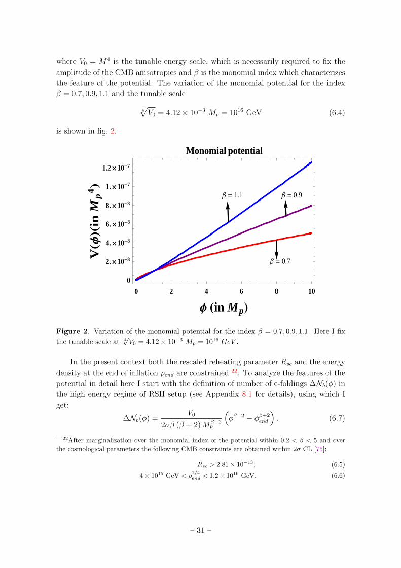
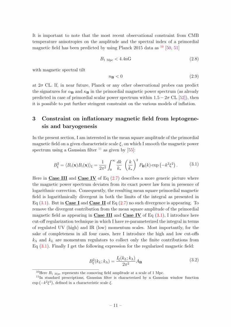
where V0 = M4 is the tunable energy scale, which is necessarily required to fix the
amplitude of the CMB anisotropies and β is the monomial index which characterizes
the feature of the potential. The variation of the monomial potential for the index
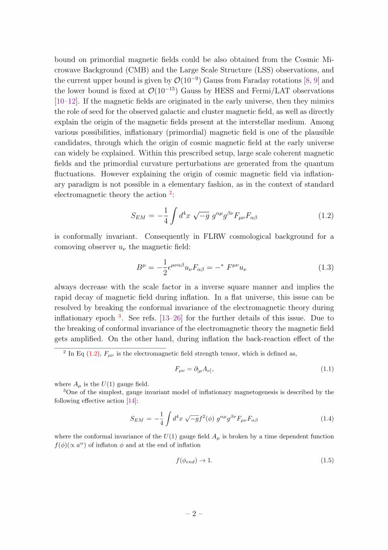
β = 0.7, 0.9, 1.1 and the tunable scale
4√V0 = 4.12× 10⁻³ Mp = 1016 GeV (6.4)
is shown in fig. 2.
Β = 1.1 Β = 0.9
Β = 0.7
0 2 4 6 8 100
2. ´ 10-8
4. ´ 10-8
6. ´ 10-8
8. ´ 10-8
1. ´ 10-7
1.2 ´ 10-7
Φ Hin MpL
VHΦ
LHin
Mp
4L
Monomial potential
Figure 2. Variation of the monomial potential for the index β = 0.7, 0.9, 1.1. Here I fix
the tunable scale at 4√V0 = 4.12× 10⁻³ Mp = 1016 GeV .
In the present context both the rescaled reheating parameter Rsc and the energy
density at the end of inflation ρend are constrained 22. To analyze the features of the
potential in detail here I start with the definition of number of e-foldings ∆Nb(φ) in
the high energy regime of RSII setup (see Appendix 8.1 for details), using which I
get:
∆Nb(φ) =V0
2σβ (β + 2)Mβ+2p
(φβ+2 − φβ+2
end
). (6.7)
22After marginalization over the monomial index of the potential within 0.2 < β < 5 and over
the cosmological parameters the following CMB constraints are obtained within 2σ CL [75]:
Rsc > 2.81× 10⁻¹³, (6.5)
4× 10¹⁵ GeV < ρ1/4end < 1.2× 10¹⁶ GeV. (6.6)
– 31 –
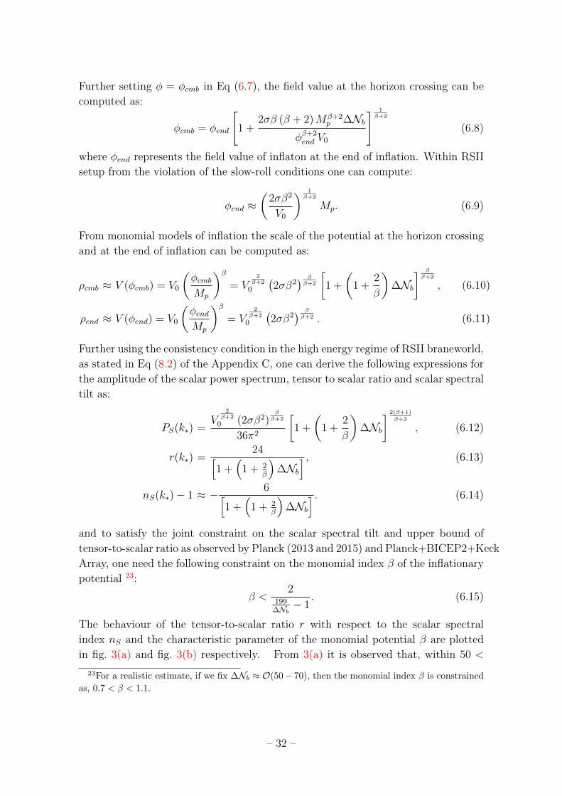
Further setting φ = φcmb in Eq (6.7), the field value at the horizon crossing can be
computed as:
φcmb = φend
[1 +
2σβ (β + 2)Mβ+2p ∆Nb
φβ+2end V0
] 1β+2
(6.8)
where φend represents the field value of inflaton at the end of inflation. Within RSII
setup from the violation of the slow-roll conditions one can compute:
φend ≈(
2σβ2
V0
) 1β+2
Mp. (6.9)
From monomial models of inflation the scale of the potential at the horizon crossing
and at the end of inflation can be computed as:
ρcmb ≈ V (φcmb) = V0
(φcmbMp
)β= V
2β+2
0
(2σβ2
) ββ+2
[1 +
(1 +
2
β
)∆Nb
] ββ+2
, (6.10)
ρend ≈ V (φend) = V0
(φendMp
)β= V
2β+2
0
(2σβ2
) ββ+2 . (6.11)
Further using the consistency condition in the high energy regime of RSII braneworld,
as stated in Eq (8.2) of the Appendix C, one can derive the following expressions for
the amplitude of the scalar power spectrum, tensor to scalar ratio and scalar spectral
tilt as:
PS(k∗) =V
2β+2
0 (2σβ2)ββ+2
36π2
[1 +
(1 +
2
β
)∆Nb
] 2(β+1)β+2
, (6.12)
r(k∗) =24[
1 +(
1 + 2β
)∆Nb
] , (6.13)
nS(k∗)− 1 ≈ − 6[1 +
(1 + 2
β
)∆Nb
] . (6.14)
and to satisfy the joint constraint on the scalar spectral tilt and upper bound of
tensor-to-scalar ratio as observed by Planck (2013 and 2015) and Planck+BICEP2+Keck
Array, one need the following constraint on the monomial index β of the inflationary
potential 23:
β <2
199∆Nb− 1
. (6.15)
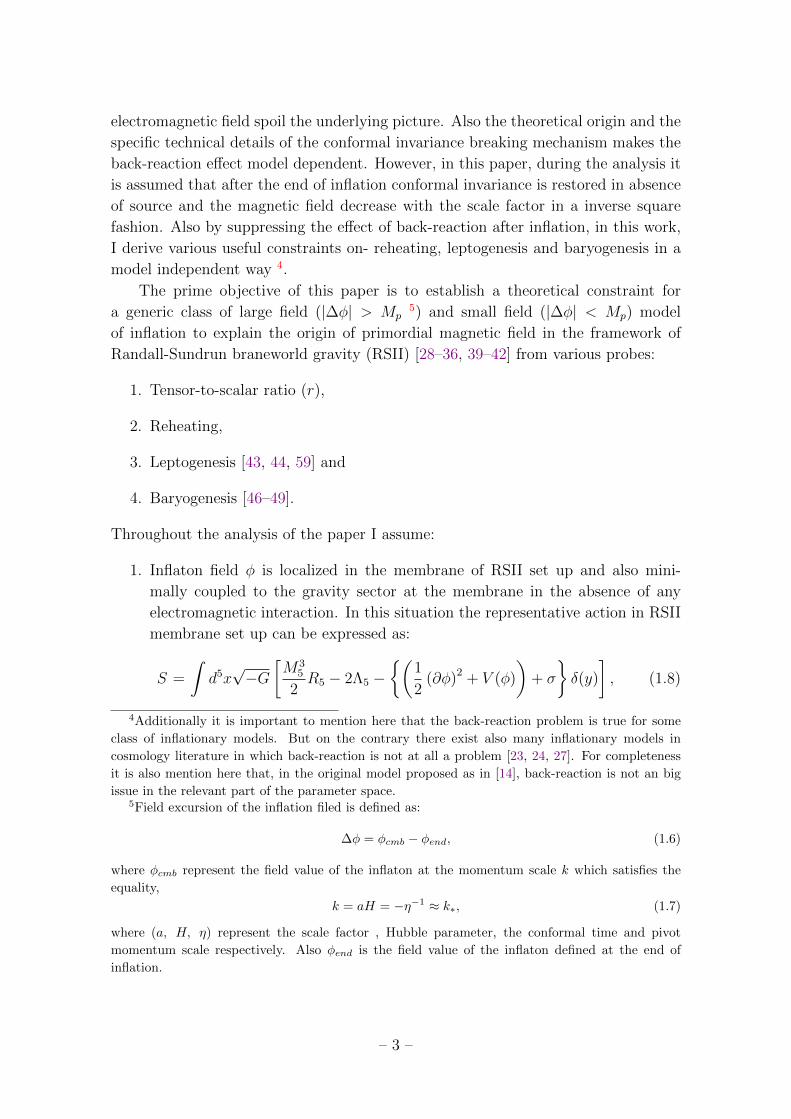
The behaviour of the tensor-to-scalar ratio r with respect to the scalar spectral
index nS and the characteristic parameter of the monomial potential β are plotted
in fig. 3(a) and fig. 3(b) respectively. From 3(a) it is observed that, within 50 <
23For a realistic estimate, if we fix ∆Nb ≈ O(50− 70), then the monomial index β is constrained
as, 0.7 < β < 1.1.
– 32 –
0.94 0.95 0.96 0.97 0.98 0.99 1.00
0.00
0.05
0.10
0.15
0.20
0.25
nS
r
r vs nS plot for Monomial potential
(a) r vs nS .
0.0 0.5 1.0 1.5 2.0
0.04
0.06
0.08
0.10
0.12
0.14
0.16
0.18
Β
r
r vs Β plot for Monomial potential
(b) r vs β.
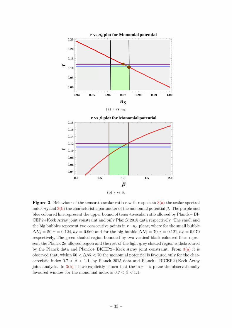
Figure 3. Behaviour of the tensor-to-scalar ratio r with respect to 3(a) the scalar spectral
index nS and 3(b) the characteristic parameter of the monomial potential β. The purple and
blue coloured line represent the upper bound of tenor-to-scalar ratio allowed by Planck+ BI-
CEP2+Keck Array joint constraint and only Planck 2015 data respectively. The small and
the big bubbles represent two consecutive points in r−nS plane, where for the small bubble
∆Nb = 50, r = 0.124, nS = 0.969 and for the big bubble ∆Nb = 70, r = 0.121, nS = 0.970
respectively, The green shaded region bounded by two vertical black coloured lines repre-
sent the Planck 2σ allowed region and the rest of the light grey shaded region is disfavoured
by the Planck data and Planck+ BICEP2+Keck Array joint constraint. From 3(a) it is
observed that, within 50 < ∆Nb < 70 the monomial potential is favoured only for the char-
acteristic index 0.7 < β < 1.1, by Planck 2015 data and Planck+ BICEP2+Keck Array
joint analysis. In 3(b) I have explicitly shown that the in r − β plane the observationally
favoured window for the monomial index is 0.7 < β < 1.1.
– 33 –
0.955 0.960 0.965 0.970 0.975 0.9801.8 ´ 10-9
1.9 ´ 10-9
2. ´ 10-9
2.1 ´ 10-9
2.2 ´ 10-9
2.3 ´ 10-9
2.4 ´ 10-9
2.5 ´ 10-9
2.6 ´ 10-9
nS
PS
PS vs nS plot for Monomial potential
(a) PS vs nS .
0.0 0.5 1.0 1.5 2.01.8 ´ 10-9
2. ´ 10-9
2.2 ´ 10-9
2.4 ´ 10-9
2.6 ´ 10-9
2.8 ´ 10-9
Β
PS
PS vs Β plot for Monomial potential
(b) PS vs β.
0.0 0.5 1.0 1.5 2.00.90
0.92
0.94
0.96
0.98
1.00
Β
nS
nS vs Β plot for Monomial potential
(c) n vs β.
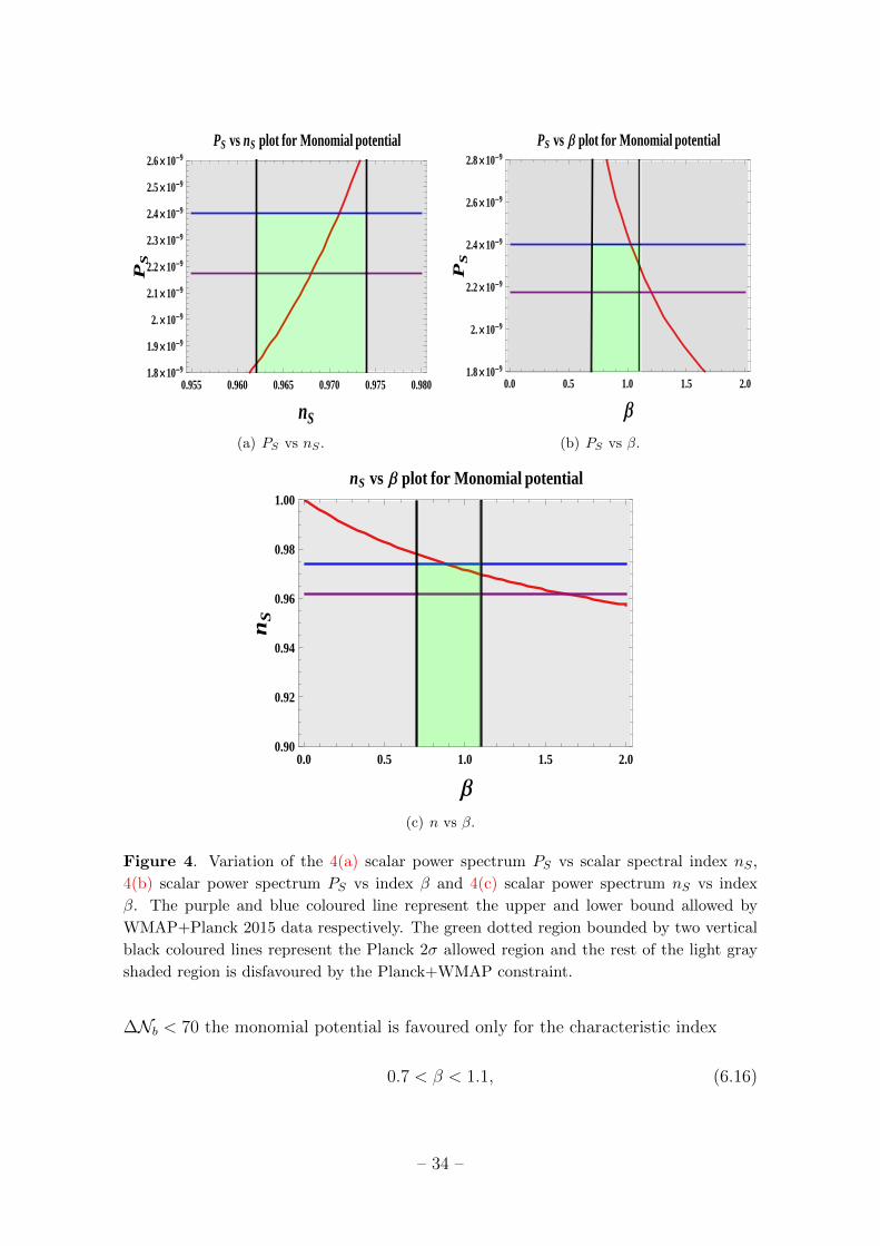
Figure 4. Variation of the 4(a) scalar power spectrum PS vs scalar spectral index nS ,
4(b) scalar power spectrum PS vs index β and 4(c) scalar power spectrum nS vs index
β. The purple and blue coloured line represent the upper and lower bound allowed by
WMAP+Planck 2015 data respectively. The green dotted region bounded by two vertical
black coloured lines represent the Planck 2σ allowed region and the rest of the light gray
shaded region is disfavoured by the Planck+WMAP constraint.
∆Nb < 70 the monomial potential is favoured only for the characteristic index
0.7 < β < 1.1, (6.16)
– 34 –
by Planck 2015 data and Planck+ BICEP2+Keck Array joint analysis. In 3(b) I
have explicitly shown that the in r − β plane the observationally favoured window
for the monomial index is 0.7 < β < 1.1. Additionally it is important to note that,
for monomial potentials embedded in the high energy regime of RSII braneworld,
the consistency relation between tensor-to-scalar ratio r and the scalar spectral nSis given by,
r ≈ 4(1− nS). (6.17)
On the other hand in the low energy regime of RSII braneworld or equivalently in
the GR limiting situation, the consistency relation between tensor-to-scalar ratio r
and the scalar spectral nS is modified as,
r ≈ 8
3(1− nS). (6.18)
This also clearly suggests that the estimated numerical value of the tensor-to-scalar
ratio from the GR limit is different compared to its value in the high density regime
of the RSII braneworld. To justify the validity of this statement, let me discuss a
very simplest situation, where the scalar spectral index is constrained within
0.969 < nS < 0.970, (6.19)
as appearing in this paper. Now in such a case using the consistency relation in
GR limit one can easily compute that the tensor-to-scalar is constrained within the
window,
0.080 < r < 0.083, (6.20)
which is pretty consistent with Planck 2015 result.
Variation of the 4(a) scalar power spectrum PS vs scalar spectral index nS, 4(b)
scalar power spectrum PS vs index β and 4(c) scalar power spectrum nS vs index β.
The purple and blue coloured line represent the upper and lower bound allowed by
WMAP+Planck 2015 data respectively. The green dotted region bounded by two
vertical black coloured lines represent the Planck 2σ allowed region and the rest of the
light gray shaded region is disfavoured by the Planck+WMAP constraint. From the
fig. 4(a)-fig. 4(c) it is clearly observed that the monomial index of the the inflationary
potential is constrained within the window 0.7 < β < 1.1 for the amplitude of the
scalar power spectrum,
2.3794× 10⁻⁹ < PS < 2.3798× 10⁻⁹ (6.21)
and scalar spectral tilt,
0.969 < nS < 0.970. (6.22)
Now using Eq (6.12), Eq (6.13) and Eq (6.14) one can write another consistency
relation among the amplitude of the scalar power spectrum PS, tensor-to-scalar ratio
– 35 –
r and scalar spectral index nS for monomial potentials embedded in the high density
regime of RSII braneworld as:
PS =V
2β+2
0 (2σβ2)ββ+2
36π2
[6
1− nS
] 2(β+1)β+2
=V
2β+2
0 (2σβ2)ββ+2
36π2
[24
r
] 2(β+1)β+2
. (6.23)
Further using Eq (3.28), I get the following stringent constraint on the tunable energy
scale of the monomial models of inflation:
V0 = M4 <
(2.12× 10⁻¹¹ M4
p
)1+β2
(2σβ2)β2
. (6.24)
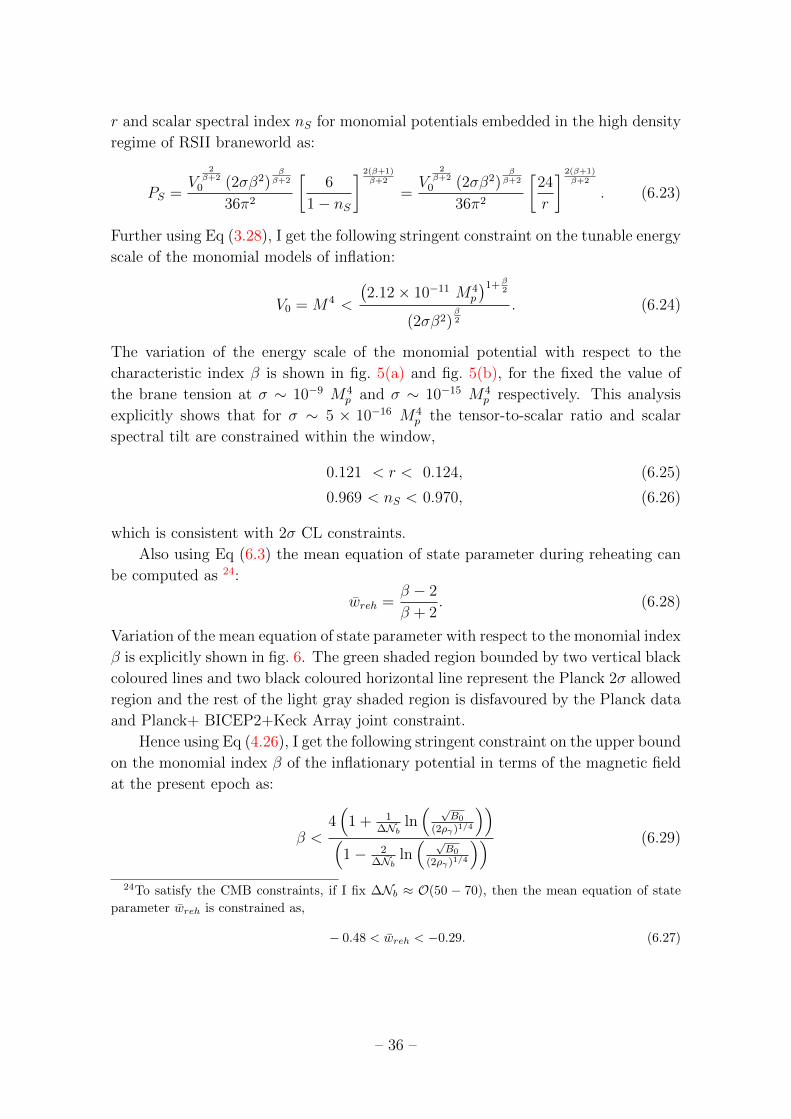
The variation of the energy scale of the monomial potential with respect to the
characteristic index β is shown in fig. 5(a) and fig. 5(b), for the fixed the value of
the brane tension at σ ∼ 10−9 M4p and σ ∼ 10−15 M4
p respectively. This analysis
explicitly shows that for σ ∼ 5 × 10⁻¹⁶ M4p the tensor-to-scalar ratio and scalar
spectral tilt are constrained within the window,
0.121 < r < 0.124, (6.25)
0.969 < nS < 0.970, (6.26)
which is consistent with 2σ CL constraints.
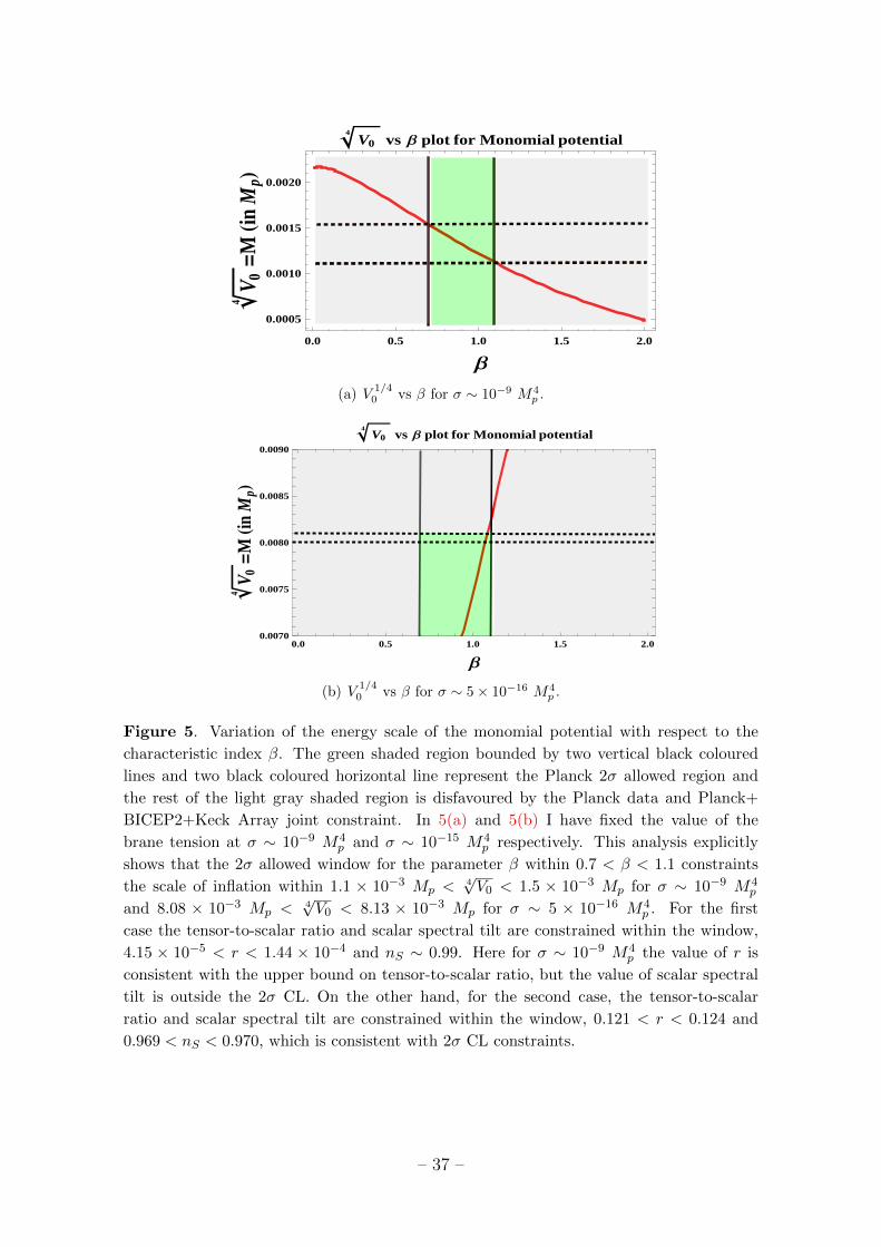
Also using Eq (6.3) the mean equation of state parameter during reheating can
be computed as 24:
wreh =β − 2
β + 2. (6.28)
Variation of the mean equation of state parameter with respect to the monomial index
β is explicitly shown in fig. 6. The green shaded region bounded by two vertical black
coloured lines and two black coloured horizontal line represent the Planck 2σ allowed
region and the rest of the light gray shaded region is disfavoured by the Planck data
and Planck+ BICEP2+Keck Array joint constraint.
Hence using Eq (4.26), I get the following stringent constraint on the upper bound
on the monomial index β of the inflationary potential in terms of the magnetic field
at the present epoch as:
β <4(
1 + 1∆Nb
ln( √
B0
(2ργ)1/4
))(
1− 2∆Nb
ln( √
B0
(2ργ)1/4
)) (6.29)
24To satisfy the CMB constraints, if I fix ∆Nb ≈ O(50 − 70), then the mean equation of state
parameter wreh is constrained as,
− 0.48 < wreh < −0.29. (6.27)
– 36 –
0.0 0.5 1.0 1.5 2.0
0.0005
0.0010
0.0015
0.0020
Β
V 04
=M
HinM
pL
V04
vs Β plot for Monomial potential
(a) V1/40 vs β for σ ∼ 10−9 M4
p .
0.0 0.5 1.0 1.5 2.00.0070
0.0075
0.0080
0.0085
0.0090
Β
V 04
=M
HinM
pL
V04
vs Β plot for Monomial potential
(b) V1/40 vs β for σ ∼ 5× 10⁻¹⁶ M4
p .
Figure 5. Variation of the energy scale of the monomial potential with respect to the
characteristic index β. The green shaded region bounded by two vertical black coloured
lines and two black coloured horizontal line represent the Planck 2σ allowed region and
the rest of the light gray shaded region is disfavoured by the Planck data and Planck+
BICEP2+Keck Array joint constraint. In 5(a) and 5(b) I have fixed the value of the
brane tension at σ ∼ 10−9 M4p and σ ∼ 10−15 M4
p respectively. This analysis explicitly
shows that the 2σ allowed window for the parameter β within 0.7 < β < 1.1 constraints
the scale of inflation within 1.1 × 10⁻³ Mp <4√V0 < 1.5 × 10⁻³ Mp for σ ∼ 10−9 M4
p
and 8.08 × 10⁻³ Mp < 4√V0 < 8.13 × 10⁻³ Mp for σ ∼ 5 × 10⁻¹⁶ M4
p . For the first
case the tensor-to-scalar ratio and scalar spectral tilt are constrained within the window,
4.15 × 10⁻⁵ < r < 1.44 × 10⁻⁴ and nS ∼ 0.99. Here for σ ∼ 10−9 M4p the value of r is
consistent with the upper bound on tensor-to-scalar ratio, but the value of scalar spectral
tilt is outside the 2σ CL. On the other hand, for the second case, the tensor-to-scalar
ratio and scalar spectral tilt are constrained within the window, 0.121 < r < 0.124 and
0.969 < nS < 0.970, which is consistent with 2σ CL constraints.
– 37 –
0.0 0.5 1.0 1.5 2.0
-1.0
-0.8
-0.6
-0.4
-0.2
0.0
Β
w-
reh
w-
reh vs Β plot for Monomial potential
Figure 6. Variation of the mean equation of state parameter with respect to the monomial
index β. The green shaded region bounded by two vertical black coloured lines and two
black coloured horizontal line represent the Planck 2σ allowed region and the rest of the
light gray shaded region is disfavoured by the Planck data and Planck+ BICEP2+Keck
Array joint constraint. It is also observed from the plot that, if I fix the number of e-
foldings within the window, ∆Nb ≈ O(50−70), then the mean equation of state parameter
wreh is constrained as, −0.48 < wreh < −0.29.
where
∆Nb = Nreh;b −Ncmb;b + ∆Nb. (6.30)
Here using Eq (6.15) in Eq one can derive the following constraint on ∆Nb as:
∆Nb <398
∆Nbln
( √B0
(2ργ)1/4
). (6.31)
Further using Eq (5.22) the reheating energy density can be computed as:
ρreh =
(8.46× 10⁻⁷ M4
p
)[1 +
(1 + 2
β
)∆Nb
] × exp
[6β∆Nbβ + 2
]×
(B0√2ργ
)− β(β−4)
(6.32)
and also using the numerical constraint on the energy density at the end of infla-
tion, as stated in Eq (6.6), I get following stringent constraint on the magnetic field
measured at the present epoch in terms of model parameter β for instantaneous
– 38 –
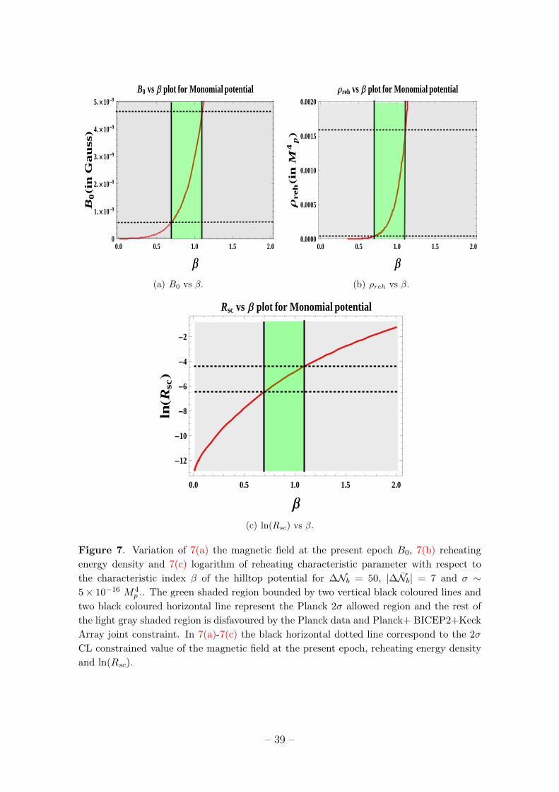
0.0 0.5 1.0 1.5 2.00
1. ´ 10-9
2. ´ 10-9
3. ´ 10-9
4. ´ 10-9
5. ´ 10-9
Β
B0
Hin
Ga
uss
LB0 vs Β plot for Monomial potential
(a) B0 vs β.
0.0 0.5 1.0 1.5 2.00.0000
0.0005
0.0010
0.0015
0.0020
Β
Ρreh
Hin
M4
pL
Ρreh vs Β plot for Monomial potential
(b) ρreh vs β.
0.0 0.5 1.0 1.5 2.0
-12
-10
-8
-6
-4
-2
Β
lnHR
scL
Rsc vs Β plot for Monomial potential
(c) ln(Rsc) vs β.
Figure 7. Variation of 7(a) the magnetic field at the present epoch B0, 7(b) reheating
energy density and 7(c) logarithm of reheating characteristic parameter with respect to
the characteristic index β of the hilltop potential for ∆Nb = 50, |∆Nb| = 7 and σ ∼5× 10⁻¹⁶ M4
p .. The green shaded region bounded by two vertical black coloured lines and
two black coloured horizontal line represent the Planck 2σ allowed region and the rest of
the light gray shaded region is disfavoured by the Planck data and Planck+ BICEP2+Keck
Array joint constraint. In 7(a)-7(c) the black horizontal dotted line correspond to the 2σ
CL constrained value of the magnetic field at the present epoch, reheating energy density
and ln(Rsc).
– 39 –
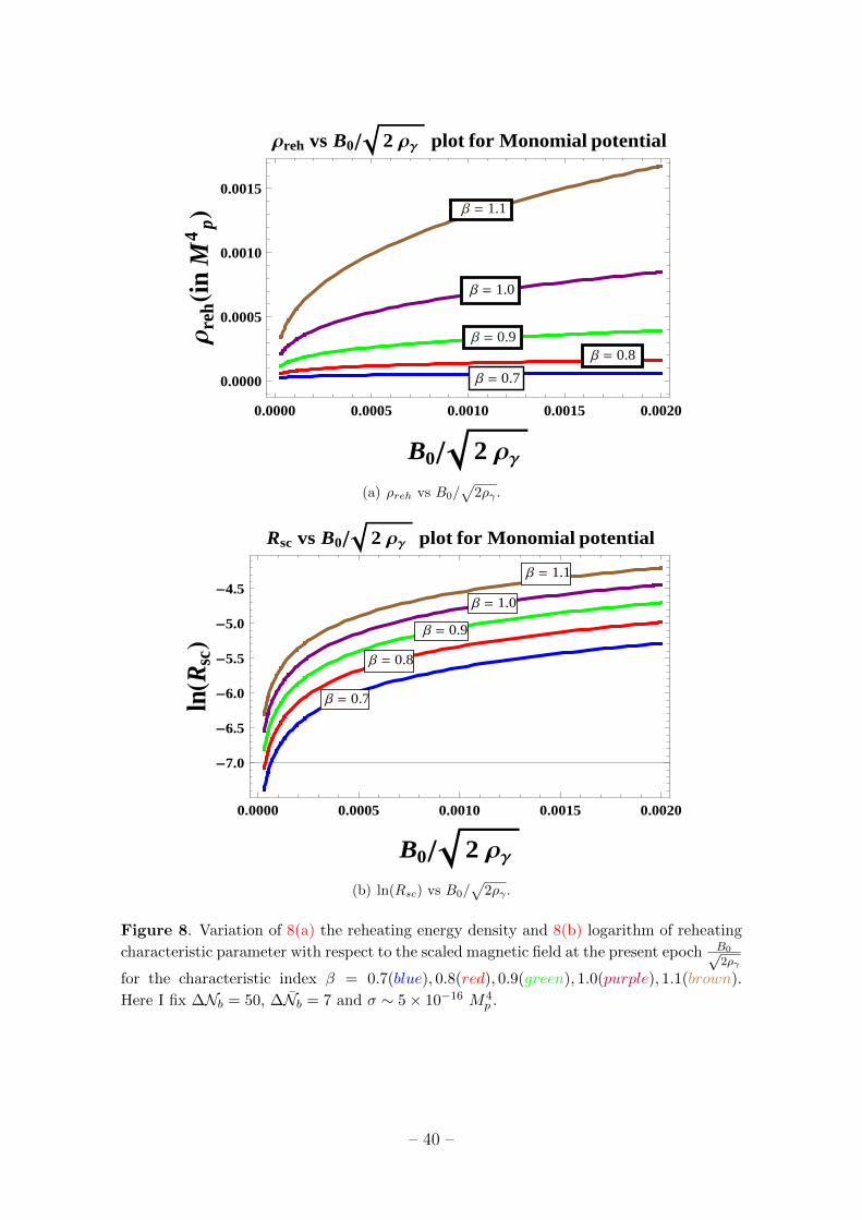
Β = 1.1
Β = 1.0
Β = 0.9Β = 0.8
Β = 0.7
0.0000 0.0005 0.0010 0.0015 0.0020
0.0000
0.0005
0.0010
0.0015
B0 2 ΡΓ
Ρre
hHin
M4
pL
Ρreh vs B0 2 ΡΓ plot for Monomial potential
(a) ρreh vs B0/√
2ργ .
Β = 1.1
Β = 1.0
Β = 0.9
Β = 0.8
Β = 0.7
0.0000 0.0005 0.0010 0.0015 0.0020
-7.0
-6.5
-6.0
-5.5
-5.0
-4.5
B0 2 ΡΓ
lnHR
scL
Rsc vs B0 2 ΡΓ plot for Monomial potential
(b) ln(Rsc) vs B0/√
2ργ .
Figure 8. Variation of 8(a) the reheating energy density and 8(b) logarithm of reheating
characteristic parameter with respect to the scaled magnetic field at the present epoch B0√2ργ
for the characteristic index β = 0.7(blue), 0.8(red), 0.9(green), 1.0(purple), 1.1(brown).
Here I fix ∆Nb = 50, ∆Nb = 7 and σ ∼ 5× 10⁻¹⁶ M4p .
– 40 –
reheating 25 as:
(8.68× 10⁻⁶)4−ββ
[1 +
(1 + 2
β
)∆Nb
] 4−ββ
exp[
6(4−β)∆Nbβ+2
] <B0√2ργ
<(7.02× 10⁻⁴)
4−ββ
[1 +
(1 + 2
β
)∆Nb
] 4−ββ
exp[
6(4−β)∆Nbβ+2
] . (6.33)
Next using Eq (5.36), I get the following constraint on the dimensionless magnetic
density parameter:
ΩBend =B4
0M6p
24σH20ρ
2γ
[1 +
(1 + 2
β
)∆Nb
]2 × (7.16× 10−13)× exp[8∆Nb
]. (6.34)
Finally the rescaled reheating parameter can be expressed in terms of the model
parameters of the monomial models of inflationary potential as:
Rsc =3.03× 10⁻²[
1 +(
1 + 2β
)∆Nb
]1/4× exp
[3β∆Nb2(β + 2)
]×
(B0√2ργ
)1/2
(6.35)
and using the numerical constraint on the rescaled reheating parameter as stated in
Eq (6.5) I get the lower bound on the present value of the magnetic field for the
monomial potentials as:
B0√2ργ
>8.6× 10−23 ×
[1 +
(1 + 2
β
)∆Nb
]1/2
exp[
3β∆Nbβ+2
] (6.36)
In fig. 7(a), fog. 7(b) and in fig. 7(c) I have explicitly shown the variation of the
magnetic field at the present epoch B0, reheating energy density ρreh and logarithm
of reheating characteristic parameter ln(Rsc) with respect to the characteristic index
β of the monomial potential for the number of e-foldings ∆Nb = 50. The green
shaded region bounded by two vertical black coloured lines and two black coloured
horizontal line represent the Planck 2σ allowed region and the rest of the light gray
shaded region is disfavoured by the Planck data and Planck+ BICEP2+Keck Array
joint constraint. Also in fig. 8(a) and in fig. 8(b) I have depicted the behaviour of
the reheating energy density ρreh and logarithm of reheating characteristic parameter
ln(Rsc), with respect to the scaled magnetic field at the present epoch B0/√
2ργ for
the characteristic index 0.7 ≤ β ≤ 1.1.
25For instantaneous reheating the energy density of inflaton at the end of inflation is instanta-
neously converted to the reheating energy density or radiation and the instantaneous transition
occurs at ρend = ρreh. Commonly this physical situation is known as instantaneous entropy gener-
ation scenario [69].
– 41 –
Further using Eq (6.13) in Eq (3.39) and Eq (3.61) finally I get the following
constraints on the regulating factor within RSII setup as 26:
Σb(kL = k0, k∗)×(M4
p
σ
)2/5
≈ O(1.58× 10−21)×[1 +
(1 +
2
β
)∆Nb
](6.38)
which is compatible with the observed/measured bound on CP asymmetry and
baryon asymmetry parameter.
From fig. 7(a), fig. 7(b) and fig. 7(c) I get the following 2σ constraints on magneto
reheating cosmological parameters computed from the monomial inflationary model:
5.969× 10⁻¹⁰ Gauss < B0 =√
Iξ(kL=k0,kΛ)
2π2 AB < 4.638× 10⁻⁹ Gauss, (6.39)
1.940× 10−132 M4p < ρB0 = B2
0/2 < 1.171× 10−130 M4p , (6.40)
4.061× 10⁻⁵ M4p < ρreh < 1.591× 10⁻³ M4
p , (6.41)
6.227× 10⁻⁴ × g−1/4∗ Mp < Treh < 4.836× 10⁻³ × g−1/4
∗ Mp,(6.42)
Γtotal ∼ 0.24 Mp, (6.43)
1.55× 10⁻³ < Rsc < 1.24× 10⁻², (6.44)
εCP ∼ O(10−6), (6.45)
ηB ∼ O(10−9), (6.46)
0.121 < r < 0.124, (6.47)
0.969 < nS < 0.970, (6.48)
2.3794× 10⁻⁹ < PS < 2.3798× 10⁻⁹, (6.49)
8.08× 10⁻³ Mp < 4√V0 < 8.13× 10⁻³ Mp, (6.50)
for the number of e-foldings ∆Nb = 50, |∆Nb| = 7, mean equation of state parameter
−0.48 < wreh < −0.29 and Ωradh2 ∼ 2.5 × 10⁻⁵, along with the following restricted
model parameter space:
0.7 < β < 1.1, (6.51)
σ ∼ 5× 10⁻¹⁶ M4p , (6.52)
M5 ∼(
1.042× 10⁻³² ×M8
p
|Λ5|
)1/3
. (6.53)
It is important to note that, if I choose different parameter space by allowing fine
tuning in–(1) the energy scale of monomial potential V0 = M4, (2) the brane tension
26After fixing ∆Nb ≈ O(50− 70), the regulating factor within RSII can be constrained as,
3.06× 10⁻¹⁹ < Σb(kL = k0, k∗)×
(M4p
σ
)2/5
< 3.13× 10⁻¹⁹, (6.37)
which is consistent with the upper bound mentioned in Eq (3.50).
– 42 –
σ and (3) the characteristic index of the monomial potential β then the overall
analysis and the obtained results suggests that-
• For β < 0.7, the amplitude of the scalar power spectrum PS match the Planck
2015 data and also consistent with the joint constraint obtained from Planck
+BICEP2 +Keck Array. But the allowed range for scalar spectral tilt nS is
outside the observational window. Also in this regime the value of tensor-to-
scalar ratio r is lower compared to the upper bound i.e. r << 0.12. On the
other hand, for very low β the estimated value of the magnetic field at the
present epoch B0 from the monomial model is very very small and can reach
up to the lower bound
B0 > 10−15 Gauss. (6.54)
Similarly for low β, the reheating energy density ρreh or equivalently the re-
heating temperature Treh falls down and also the rescaled reheating parameter
Rsc decrease.
• For 1.1 < β < 1.2, both the amplitude of the scalar power spectrum PS and the
scalar spectral tilt nS are perfectly consistent with the Planck 2015 data and
also consistent with the joint constraint obtained from Planck+BICEP2+Keck
Array. But for β > 1.2 the estimated value of the amplitude of the scalar
power spectrum falls down from its predicted bound from observation. Also for
β > 1.2 region the value of tensor-to-scalar ratio r is very very large compared
to its the upper bound i.e. r >> 0.12. As β increases the estimated value of
the magnetic field at the present epoch B0 exceeds the upper bound i.e.
B0 >> 10−9 Gauss (6.55)
as obtained from Faraday rotation. Additionally in the large β regime the re-
heating energy density ρreh or equivalently the reheating temperature Treh and
the rescaled reheating parameter Rsc are not consistent with the observational
constraints.
6.2 Hilltop Models
In case of hilltop models the inflationary potential can be represented by the following
functional form:
V (φ) = V0
[1−
(φ
µ
)β](6.56)
where V0 = M4 is the tunable energy scale, which is necessarily required to fix the
amplitude of the CMB anisotropies and β is the characteristic index which character-
izes the feature of the potential. In the present context V0 mimics the role of vacuum
energy and the scale of inflation is fixed by this correction term. The variation of the
– 43 –
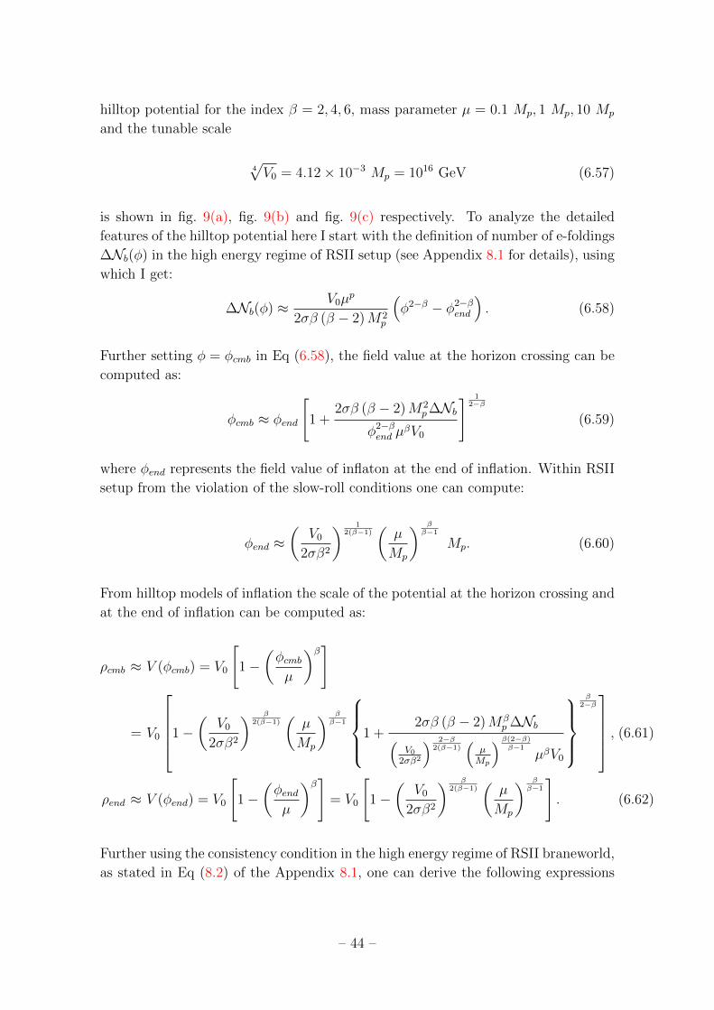
hilltop potential for the index β = 2, 4, 6, mass parameter µ = 0.1 Mp, 1 Mp, 10 Mp
and the tunable scale
4√V0 = 4.12× 10⁻³ Mp = 1016 GeV (6.57)
is shown in fig. 9(a), fig. 9(b) and fig. 9(c) respectively. To analyze the detailed
features of the hilltop potential here I start with the definition of number of e-foldings
∆Nb(φ) in the high energy regime of RSII setup (see Appendix 8.1 for details), using
which I get:
∆Nb(φ) ≈ V0µp
2σβ (β − 2)M2p
(φ2−β − φ2−β
end
). (6.58)
Further setting φ = φcmb in Eq (6.58), the field value at the horizon crossing can be
computed as:
φcmb ≈ φend
[1 +
2σβ (β − 2)M2p∆Nb
φ2−βend µ
βV0
] 12−β
(6.59)
where φend represents the field value of inflaton at the end of inflation. Within RSII
setup from the violation of the slow-roll conditions one can compute:
φend ≈(
V0
2σβ2
) 12(β−1)
(µ
Mp
) ββ−1
Mp. (6.60)
From hilltop models of inflation the scale of the potential at the horizon crossing and
at the end of inflation can be computed as:
ρcmb ≈ V (φcmb) = V0
[1−
(φcmbµ
)β]
= V0
1−(
V0
2σβ2
) β2(β−1)
(µ
Mp
) ββ−1
1 +2σβ (β − 2)Mβ
p ∆Nb(V0
2σβ2
) 2−β2(β−1)
(µMp
)β(2−β)β−1
µβV0
β
2−β , (6.61)
ρend ≈ V (φend) = V0
[1−
(φendµ
)β]= V0
[1−
(V0
2σβ2
) β2(β−1)
(µ
Mp
) ββ−1
]. (6.62)
Further using the consistency condition in the high energy regime of RSII braneworld,
as stated in Eq (8.2) of the Appendix 8.1, one can derive the following expressions
– 44 –
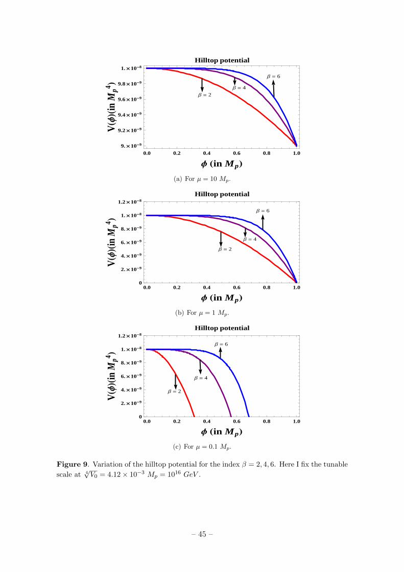
Β = 2
Β = 4
Β = 6
0.0 0.2 0.4 0.6 0.8 1.09. ´ 10-9
9.2 ´ 10-9
9.4 ´ 10-9
9.6 ´ 10-9
9.8 ´ 10-9
1. ´ 10-8
Φ Hin MpL
VHΦL
HinM
p4 L
Hilltop potential
(a) For µ = 10 Mp.
Β = 6
Β = 4
Β = 2
0.0 0.2 0.4 0.6 0.8 1.00
2. ´ 10-9
4. ´ 10-9
6. ´ 10-9
8. ´ 10-9
1. ´ 10-8
1.2 ´ 10-8
Φ Hin MpL
VHΦL
HinM
p4 L
Hilltop potential
(b) For µ = 1 Mp.
Β = 6
Β = 4
Β = 2
0.0 0.2 0.4 0.6 0.8 1.00
2. ´ 10-9
4. ´ 10-9
6. ´ 10-9
8. ´ 10-9
1. ´ 10-8
1.2 ´ 10-8
Φ Hin MpL
VHΦL
HinM
p4 L
Hilltop potential
(c) For µ = 0.1 Mp.
Figure 9. Variation of the hilltop potential for the index β = 2, 4, 6. Here I fix the tunable
scale at 4√V0 = 4.12× 10⁻³ Mp = 1016 GeV .
– 45 –
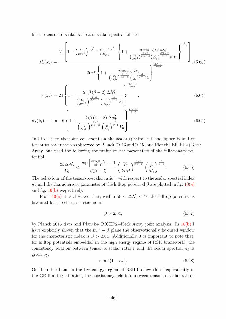
for the tensor to scalar ratio and scalar spectral tilt as:
PS(k∗) =
V0
1−(
V0
2σβ2
) β2(β−1)
(µMp
) ββ−1
1 +2σβ(β−2)Mβ
p ∆Nb(V0
2σβ2
) 2−β2(β−1)
(µMp
)β(2−β)β−1 µβV0
β
2−β
36π2
1 + 2σβ(β−2)∆Nb(V0
2σβ2
) 2−β2(β−1)
(µMp
) ββ−1 V0
2(β−1)
2−β
, (6.63)
r(k∗) = 24
1 +2σβ (β − 2) ∆Nb(
V0
2σβ2
) 2−β2(β−1)
(µMp
) ββ−1
V0
2(β−1)
2−β
, (6.64)
nS(k∗)− 1 ≈ −6
1 +2σβ (β − 2) ∆Nb(
V0
2σβ2
) 2−β2(β−1)
(µMp
) ββ−1
V0
2(β−1)
2−β
. (6.65)
and to satisfy the joint constraint on the scalar spectral tilt and upper bound of
tensor-to-scalar ratio as observed by Planck (2013 and 2015) and Planck+BICEP2+Keck
Array, one need the following constraint on the parameters of the inflationary po-
tential:
2σ∆NbV0
<exp
[2.65(β−2)
(β−1)
]− 1
β(β − 2)
(V0
2σβ2
) 2−β2(β−1)
(µ
Mp
) ββ−1
. (6.66)
The behaviour of the tensor-to-scalar ratio r with respect to the scalar spectral index
nS and the characteristic parameter of the hilltop potential β are plotted in fig. 10(a)
and fig. 10(b) respectively.
From 10(a) it is observed that, within 50 < ∆Nb < 70 the hilltop potential is
favoured for the characteristic index
β > 2.04, (6.67)
by Planck 2015 data and Planck+ BICEP2+Keck Array joint analysis. In 10(b) I
have explicitly shown that the in r − β plane the observationally favoured window
for the characteristic index is β > 2.04. Additionally it is important to note that,
for hilltop potentials embedded in the high energy regime of RSII braneworld, the
consistency relation between tensor-to-scalar ratio r and the scalar spectral nS is
given by,
r ≈ 4(1− nS). (6.68)
On the other hand in the low energy regime of RSII braneworld or equivalently in
the GR limiting situation, the consistency relation between tensor-to-scalar ratio r
– 46 –
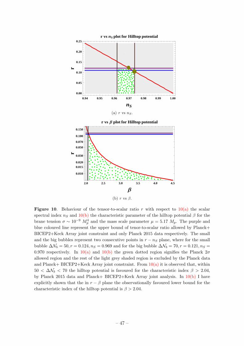
0.94 0.95 0.96 0.97 0.98 0.99 1.00
0.00
0.05
0.10
0.15
0.20
0.25
nS
r
r vs nS plot for Hilltop potential
(a) r vs nS .
2.0 2.5 3.0 3.5 4.0 4.5
0.010
0.100
0.050
0.020
0.030
0.015
0.150
0.070
Β
r
r vs Β plot for Hilltop potential
(b) r vs β.
Figure 10. Behaviour of the tensor-to-scalar ratio r with respect to 10(a) the scalar
spectral index nS and 10(b) the characteristic parameter of the hilltop potential β for the
brane tension σ ∼ 10−9 M4p and the mass scale parameter µ = 5.17 Mp. The purple and
blue coloured line represent the upper bound of tenor-to-scalar ratio allowed by Planck+
BICEP2+Keck Array joint constraint and only Planck 2015 data respectively. The small
and the big bubbles represent two consecutive points in r − nS plane, where for the small
bubble ∆Nb = 50, r = 0.124, nS = 0.969 and for the big bubble ∆Nb = 70, r = 0.121, nS =
0.970 respectively. In 10(a) and 10(b) the green dotted region signifies the Planck 2σ
allowed region and the rest of the light grey shaded region is excluded by the Planck data
and Planck+ BICEP2+Keck Array joint constraint. From 10(a) it is observed that, within
50 < ∆Nb < 70 the hilltop potential is favoured for the characteristic index β > 2.04,
by Planck 2015 data and Planck+ BICEP2+Keck Array joint analysis. In 10(b) I have
explicitly shown that the in r − β plane the observationally favoured lower bound for the
characteristic index of the hilltop potential is β > 2.04.
– 47 –
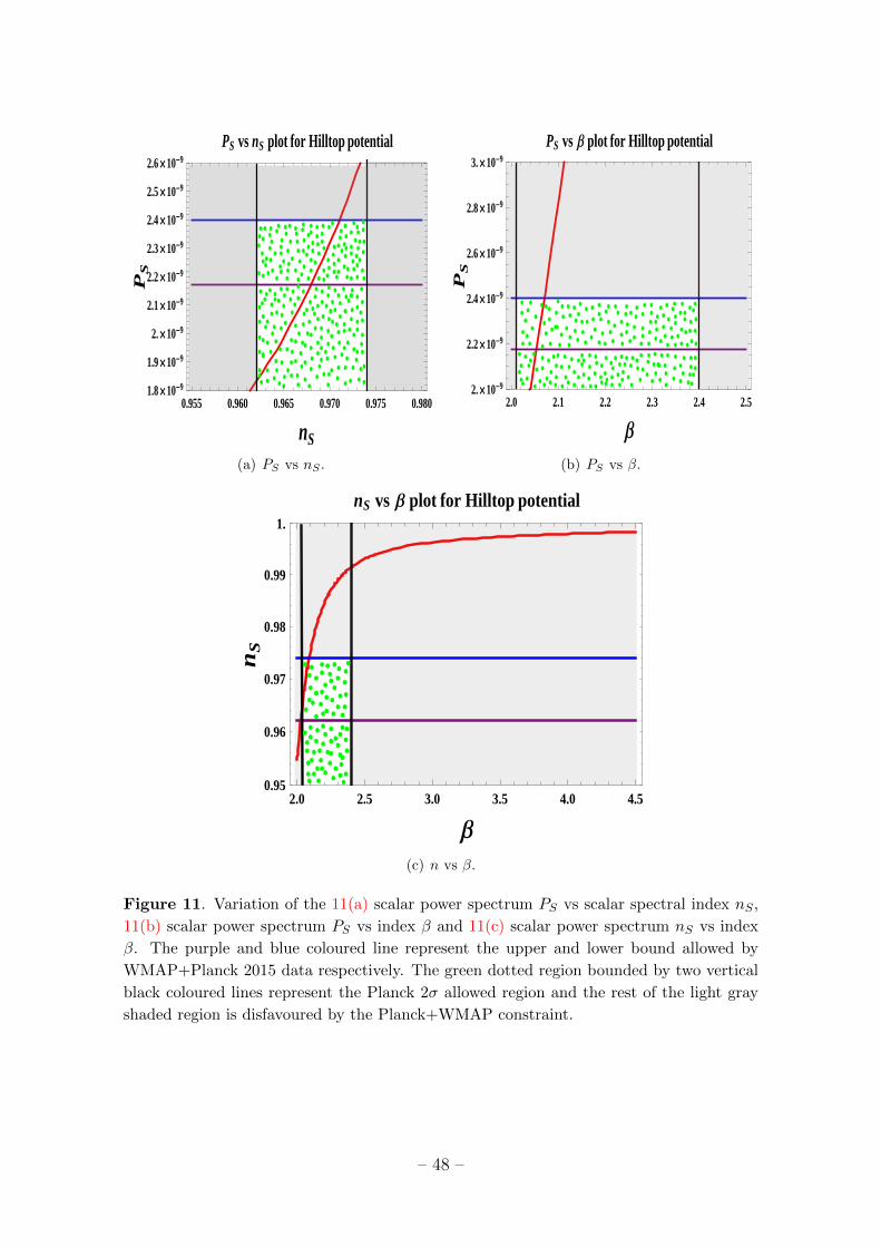
0.955 0.960 0.965 0.970 0.975 0.9801.8 ´ 10-9
1.9 ´ 10-9
2. ´ 10-9
2.1 ´ 10-9
2.2 ´ 10-9
2.3 ´ 10-9
2.4 ´ 10-9
2.5 ´ 10-9
2.6 ´ 10-9
nS
PS
PS vs nS plot for Hilltop potential
(a) PS vs nS .
2.0 2.1 2.2 2.3 2.4 2.52. ´ 10-9
2.2 ´ 10-9
2.4 ´ 10-9
2.6 ´ 10-9
2.8 ´ 10-9
3. ´ 10-9
ΒP
S
PS vs Β plot for Hilltop potential
(b) PS vs β.
2.0 2.5 3.0 3.5 4.0 4.50.95
0.96
0.97
0.98
0.99
1.
Β
nS
nS vs Β plot for Hilltop potential
(c) n vs β.
Figure 11. Variation of the 11(a) scalar power spectrum PS vs scalar spectral index nS ,
11(b) scalar power spectrum PS vs index β and 11(c) scalar power spectrum nS vs index
β. The purple and blue coloured line represent the upper and lower bound allowed by
WMAP+Planck 2015 data respectively. The green dotted region bounded by two vertical
black coloured lines represent the Planck 2σ allowed region and the rest of the light gray
shaded region is disfavoured by the Planck+WMAP constraint.
– 48 –
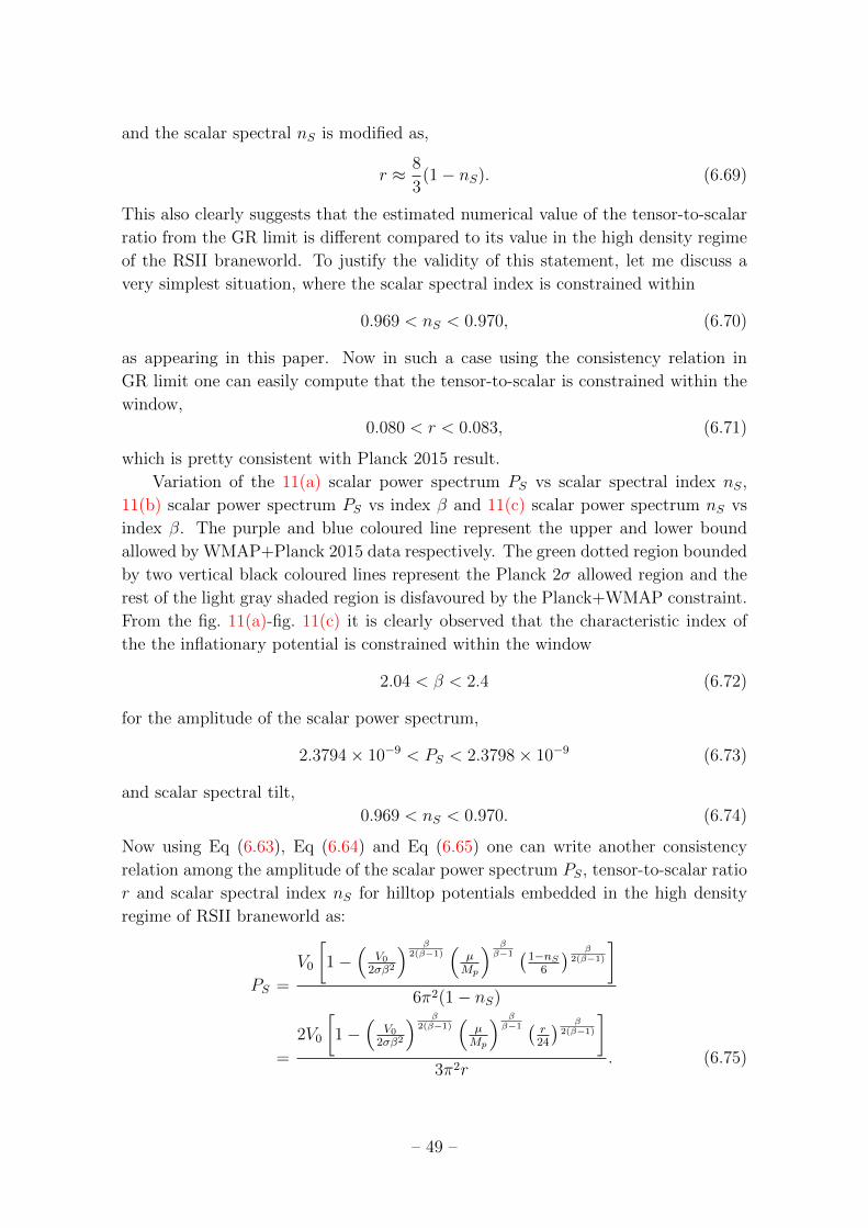
and the scalar spectral nS is modified as,
r ≈ 8
3(1− nS). (6.69)
This also clearly suggests that the estimated numerical value of the tensor-to-scalar
ratio from the GR limit is different compared to its value in the high density regime
of the RSII braneworld. To justify the validity of this statement, let me discuss a
very simplest situation, where the scalar spectral index is constrained within
0.969 < nS < 0.970, (6.70)
as appearing in this paper. Now in such a case using the consistency relation in
GR limit one can easily compute that the tensor-to-scalar is constrained within the
window,
0.080 < r < 0.083, (6.71)
which is pretty consistent with Planck 2015 result.
Variation of the 11(a) scalar power spectrum PS vs scalar spectral index nS,
11(b) scalar power spectrum PS vs index β and 11(c) scalar power spectrum nS vs
index β. The purple and blue coloured line represent the upper and lower bound
allowed by WMAP+Planck 2015 data respectively. The green dotted region bounded
by two vertical black coloured lines represent the Planck 2σ allowed region and the
rest of the light gray shaded region is disfavoured by the Planck+WMAP constraint.
From the fig. 11(a)-fig. 11(c) it is clearly observed that the characteristic index of
the the inflationary potential is constrained within the window
2.04 < β < 2.4 (6.72)
for the amplitude of the scalar power spectrum,
2.3794× 10⁻⁹ < PS < 2.3798× 10⁻⁹ (6.73)
and scalar spectral tilt,
0.969 < nS < 0.970. (6.74)
Now using Eq (6.63), Eq (6.64) and Eq (6.65) one can write another consistency
relation among the amplitude of the scalar power spectrum PS, tensor-to-scalar ratio
r and scalar spectral index nS for hilltop potentials embedded in the high density
regime of RSII braneworld as:
PS =
V0
[1−
(V0
2σβ2
) β2(β−1)
(µMp
) ββ−1 (1−nS
6
) β2(β−1)
]6π2(1− nS)
=
2V0
[1−
(V0
2σβ2
) β2(β−1)
(µMp
) ββ−1 ( r
24
) β2(β−1)
]3π2r
. (6.75)
– 49 –
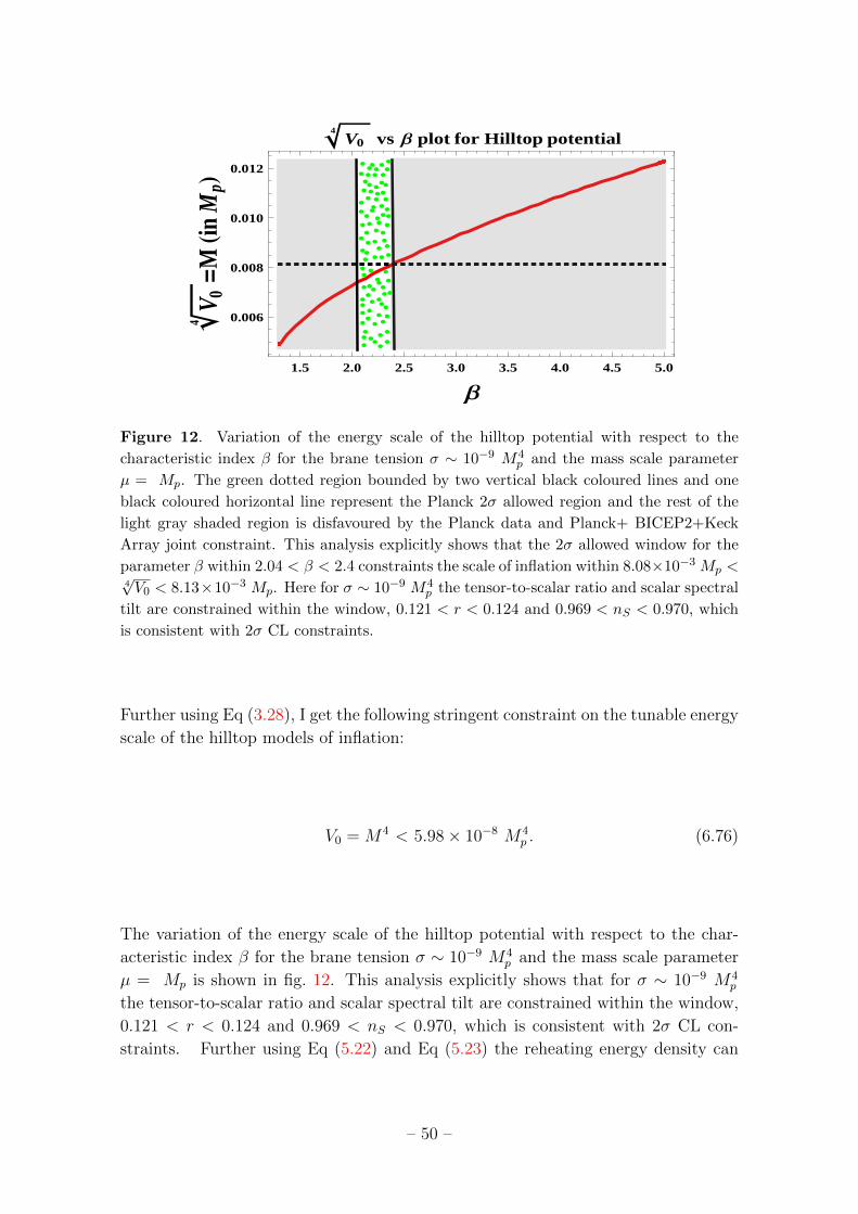
1.5 2.0 2.5 3.0 3.5 4.0 4.5 5.0
0.006
0.008
0.010
0.012
Β
V 04
=M
HinM
pL
V04
vs Β plot for Hilltop potential
Figure 12. Variation of the energy scale of the hilltop potential with respect to the
characteristic index β for the brane tension σ ∼ 10−9 M4p and the mass scale parameter
µ = Mp. The green dotted region bounded by two vertical black coloured lines and one
black coloured horizontal line represent the Planck 2σ allowed region and the rest of the
light gray shaded region is disfavoured by the Planck data and Planck+ BICEP2+Keck
Array joint constraint. This analysis explicitly shows that the 2σ allowed window for the
parameter β within 2.04 < β < 2.4 constraints the scale of inflation within 8.08×10⁻³ Mp <4√V0 < 8.13×10⁻³ Mp. Here for σ ∼ 10−9 M4
p the tensor-to-scalar ratio and scalar spectral
tilt are constrained within the window, 0.121 < r < 0.124 and 0.969 < nS < 0.970, which
is consistent with 2σ CL constraints.
Further using Eq (3.28), I get the following stringent constraint on the tunable energy
scale of the hilltop models of inflation:
V0 = M4 < 5.98× 10⁻⁸ M4p . (6.76)
The variation of the energy scale of the hilltop potential with respect to the char-
acteristic index β for the brane tension σ ∼ 10−9 M4p and the mass scale parameter
µ = Mp is shown in fig. 12. This analysis explicitly shows that for σ ∼ 10−9 M4p
the tensor-to-scalar ratio and scalar spectral tilt are constrained within the window,
0.121 < r < 0.124 and 0.969 < nS < 0.970, which is consistent with 2σ CL con-
straints. Further using Eq (5.22) and Eq (5.23) the reheating energy density can
– 50 –
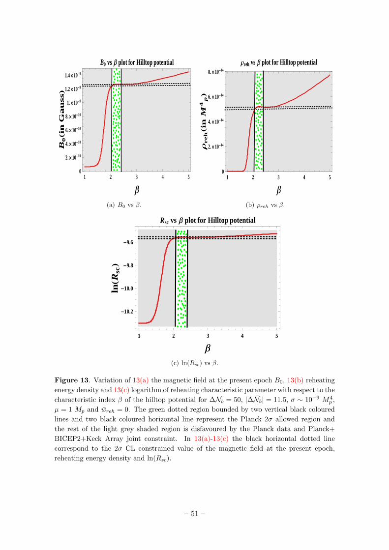
1 2 3 4 50
2. ´ 10-10
4. ´ 10-10
6. ´ 10-10
8. ´ 10-10
1. ´ 10-9
1.2 ´ 10-9
1.4 ´ 10-9
Β
B0
Hin
Gau
ssL
B0 vs Β plot for Hilltop potential
(a) B0 vs β.
1 2 3 4 50
2. ´ 10-14
4. ´ 10-14
6. ´ 10-14
8. ´ 10-14
ΒΡ
reh
Hin
M4
pL
Ρreh vs Β plot for Hilltop potential
(b) ρreh vs β.
1 2 3 4 5
-10.2
-10.0
-9.8
-9.6
Β
lnHR
scL
Rsc vs Β plot for Hilltop potential
(c) ln(Rsc) vs β.
Figure 13. Variation of 13(a) the magnetic field at the present epoch B0, 13(b) reheating
energy density and 13(c) logarithm of reheating characteristic parameter with respect to the
characteristic index β of the hilltop potential for ∆Nb = 50, |∆Nb| = 11.5, σ ∼ 10−9 M4p ,
µ = 1 Mp and wreh = 0. The green dotted region bounded by two vertical black coloured
lines and two black coloured horizontal line represent the Planck 2σ allowed region and
the rest of the light grey shaded region is disfavoured by the Planck data and Planck+
BICEP2+Keck Array joint constraint. In 13(a)-13(c) the black horizontal dotted line
correspond to the 2σ CL constrained value of the magnetic field at the present epoch,
reheating energy density and ln(Rsc).
– 51 –
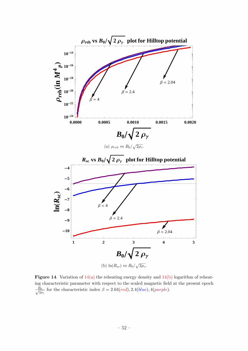
Β = 2.04
Β = 2.4
Β = 4
0.0000 0.0005 0.0010 0.0015 0.002010-24
10-22
10-20
10-18
10-16
10-14
B0 2 ΡΓ
Ρre
hHin
M4
pL
Ρreh vs B0 2 ΡΓ plot for Hilltop potential
(a) ρreh vs B0/√
2ργ .
Β = 4
Β = 2.4
Β = 2.04
1 2 3 4 5
-10
-9
-8
-7
-6
-5
-4
B0 2 ΡΓ
lnHR
scL
Rsc vs B0 2 ΡΓ plot for Hilltop potential
(b) ln(Rsc) vs B0/√
2ργ .
Figure 14. Variation of 14(a) the reheating energy density and 14(b) logarithm of reheat-
ing characteristic parameter with respect to the scaled magnetic field at the present epochB0√2ργ
for the characteristic index β = 2.04(red), 2.4(blue), 4(purple).
– 52 –
be computed as:
ρreh ≥ (8.46× 10⁻⁷ M4p )×
1 +2σβ (β − 2) ∆Nb(
V0
2σβ2
) 2−β2(β−1)
(µMp
) ββ−1
V0
2(β−1)
2−β
×
exp
[3∆Nb
]×
(B0√2ργ
)6
for wreh = 0
exp[4∆Nb
]( B0√2ργ
)− 4∆Nb
ln
(B0√2ργ )
)for wreh 6= 0.
(6.77)
Next using Eq (5.36), I get the following constraint on the dimensionless magnetic
density parameter:
ΩBend =B4
0M6p
24σH20ρ
2γ
×(7.16×10−13)×
1 +2σβ (β − 2) ∆Nb(
V0
2σβ2
) 2−β2(β−1)
(µMp
) ββ−1
V0
4(β−1)
2−β
×exp[8∆Nb
].
(6.78)
Finally the rescaled reheating parameter can be expressed in terms of the model
parameters of the hilltop models of inflationary potential as 27:
Rsc = 3.03× 10−2 ×
1 +2σβ (β − 2) ∆Nb(
V0
2σβ2
) 2−β2(β−1)
(µMp
) ββ−1
V0
β−1
2(2−β)
exp[∆Nb
]×
(B0√2ργ
). (6.80)
and using the numerical constraint on the rescaled reheating parameter as stated in
Eq (6.79) I get the lower bound on the present value of the magnetic field as:
B0√2ργ
>
4.45× 10−12 ×
1 + 2σβ(β−2)∆Nb(V0
2σβ2
) 2−β2(β−1)
(µMp
) ββ−1 V0
2(β−1)3(β−2)
exp[
43∆Nb
] . (6.81)
In fig. 13(a), fig. 13(b) and fig. 13(c) I have explicitly shown the variation of the
magnetic field at the present epoch B0, reheating energy density ρreh and logarithm
of reheating characteristic parameter ln(Rsc) with respect to the characteristic index
27The CMB constraint on the lower bound of the rescaled reheating parameter for hilltop models
within 2σ CL is given by [75]:
Rsc > 9.29× 10⁻¹¹. (6.79)
– 53 –
β of the hilltop potential for the number of e-foldings ∆Nb = 50, |∆Nb| = 11.5, brane
tension σ ∼ 10−9 M4p , mass scale parameter µ = 1 Mp and mean equation of state
parameter wreh = 0. The green dotted region bounded by two vertical black coloured
lines and two black coloured horizontal lines represent the Planck 2σ allowed region
and the rest of the light grey shaded region is disfavoured by the Planck data and
Planck+ BICEP2+Keck Array joint constraint. Also in fig. 14(a) and in fig. 14(b)
I have depicted the behaviour of the reheating energy density ρreh and logarithm of
reheating characteristic parameter ln(Rsc), with respect to the scaled magnetic field
at the present epoch B0/√
2ργ for the characteristic index 2.04 ≤ β ≤ 2.4.
Using Eq (6.64) in Eq (3.39) and Eq (3.61), finally I get the following constraints
on the magnetic regulating factor within RSII setup as 28:
Σb(kL = k0, k∗)×(M4
p
σ
)2/5
≈ O(1.99× 10−21)×
1 +2σβ (β − 2) ∆Nb(
V0
2σβ2
) 2−β2(β−1)
(µMp
) ββ−1
V0
2(β−1)β−2
(6.83)
which is compatible with the observed/measured bound on CP asymmetry and
baryon asymmetry parameter.
From fig. 10(a)-fig. 13(c), I get the following 2σ constraints on cosmological
parameters computed from the hilltop inflationary model:
1.238× 10⁻⁹ Gauss < B0 =√
Iξ(kL=k0,kΛ)
2π2 AB < 1.263× 10⁻⁹ Gauss, (6.84)
8.345× 10−132 M4p < ρB0 = B2
0/2 < 8.685× 10−132 M4p , (6.85)
4.945× 10⁻¹⁴ M4p < ρreh < 5.128× 10⁻¹⁴ M4
p , (6.86)
6.227× 10⁻⁴ × g−1/4∗ Mp < Treh < 6.283× 10⁻⁴ × g−1/4
∗ Mp,(6.87)
Γtotal ∼ 1.7× 10⁻⁴ Mp, (6.88)
7× 10⁻⁵ < Rsc < 7.11× 10⁻⁵, (6.89)
εCP ∼ O(10−6), (6.90)
ηB ∼ O(10−9), (6.91)
0.121 < r < 0.124, (6.92)
0.969 < nS < 0.970, (6.93)
2.3794× 10⁻⁹ < PS < 2.3798× 10⁻⁹, (6.94)
8.08× 10⁻³ Mp < 4√V0 < 8.13× 10⁻³ Mp, (6.95)
28After fixing ∆Nb ≈ O(50− 70), the regulating factor within RSII can be constrained as,
Σb(kL = k0, k∗)×
(M4p
σ
)2/5
< 3.98× 10⁻¹⁹, (6.82)
which is consistent with the upper bound mentioned in Eq (3.50).
– 54 –
for the number of e-foldings ∆Nb = 50, |∆Nb| = 11.5, mean equation of state
parameter wreh = 0 and Ωradh2 ∼ 2.5 × 10⁻⁵, along with the following restricted
model parameter space:
2.04 < β < 2.4, (6.96)
µ ∼ O(Mp), (6.97)
σ ∼ 10−9 M4p , (6.98)
M5 ∼(
4.170× 10⁻²⁰ ×M8
p
|Λ5|
)1/3
. (6.99)
It is important to mention here that, if I choose different parameter space by allowing
fine tuning in-(1) the energy scale of hilltop potential V0 = M4, (2) the mass scale
parameter µ of the hilltop model, (3) the brane tension σ and (4) the characteristic
index of the hilltop potential β then the overall analysis and the obtained results
suggests that-
• For β < 2.04, the amplitude of the scalar power spectrum PS and the scalar
spectral tilt nS match the Planck 2015 data and also consistent with the joint
constraint obtained from Planck+BICEP2+Keck Array. But in this regime
the value of tensor-to-scalar ratio r exceeds the upper bound i.e. r > 0.12. On
the other hand, for very low β the estimated value of the magnetic field at the
present epoch B0 from the hilltop model is very very small and can be able to
reach up to the lower bound
B0 > 10−15 Gauss. (6.100)
Similarly for low β, the reheating energy density ρreh or equivalently the re-
heating temperature Treh falls down and also the rescaled reheating parameter
Rsc decrease.
• For β > 2.4, the amplitude of the scalar power spectrum PS and the scalar
spectral tilt nS are perfectly consistent with the Planck 2015 data and also
consistent with the joint constraint obtained from Planck+BICEP2+Keck Ar-
ray. But in this case the value of tensor-to-scalar ratio r is very very small
compared to its the upper bound i.e. r << 0.12. As β increases the estimated
value of the magnetic field at the present epoch B0 exceeds the upper bound
i.e.
B0 >> 10−9 Gauss (6.101)
as obtained from Faraday rotation. Additionally in the large β regime the re-
heating energy density ρreh or equivalently the reheating temperature Treh and
the rescaled reheating parameter Rsc are not consistent with the observational
constraints.
– 55 –
7 Summary
To summarize, in the present article, I have addressed the following points:
• I have established a theoretical constraint relationship on inflationary magnetic
field in the framework of Randall-Sundrun braneworld gravity (RSII) from: (1)
tensor-to-scalar ratio (r), (2) reheating, (3) leptogenesis and (4) baryogenesis
for a generic large and small field model of inflation with a flat potential, where
inflation is driven by slow-roll.
• For such a class of model it is also possible to predict amount of magnetic field
at the present epoch (B0) by measuring non-vanishing CP asymmetry (εCP ) in
leptogenesis and baryon asymmetry (ηB) in baryogenesis or the tensor-to-scalar
ratio in the inflationary setup.
• Most significantly, once the signature of primordial gravity waves will be pre-
dicted by in any near future observational probes, it will be possible to comment
on the associated CP asymmetry and baryon asymmetry and vice versa.
• In this paper I have used important cosmological and particle physics con-
straints arising from Planck 2015 and Planck+BICEP2/Keck Array joint data
on the amplitude of scalar power spectrum, scalar spectral tilt, the upper bound
on tenor to scalar ratio, lower bound on rescaled characteristic reheating param-
eter and the bound on the reheating energy density within 1.5σ−2σ statistical
CL.
• Further assuming the conformal invariance to be restored after inflation in the
framework of Randall-Sundrum single braneworld gravity (RSII), I have explic-
itly shown that the requirement of the sub-dominant feature of large scale mag-
netic field after inflation gives two fold non-trivial characteristic constraints-
on equation of state parameter (w) and the corresponding energy scale during
reheating (ρ1/4rh ) epoch.
• Hence avoiding the contribution of back-reaction from the magnetic field I
have established a bound on the reheating characteristic parameter (Rrh) and
its rescaled version (Rsc), to achieve large scale magnetic field within the pre-
scribed setup and apply the Cosmic Microwave Background (CMB) constraints
as obtained from recent Planck 2015 data and Planck+BICEP2/Keck Array
joint data.
• To this end I have explicitly shown the cosmological consequences from two spe-
cific models of brane inflation- monomial (large field) and hilltop (small field)
after applying all the constraints obtained from inflationary magnetic field.
For monomial models I get, 5.969 × 10⁻¹⁰ Gauss < B0 < 4.638 × 10⁻⁹ Gauss,
– 56 –
4.061 × 10⁻⁵ M4p < ρreh < 1.591 × 10⁻³ M4
p , 1.940 × 10−132 M4p < ρB0 <
1.171× 10−130 M4p , 6.227× 10⁻⁴× g−1/4
∗ Mp < Treh < 4.836× 10⁻³× g−1/4∗ Mp,
Γtotal ∼ 0.24 Mp, 1.55 × 10⁻³ < Rsc < 1.24 × 10⁻², εCP ∼ O(10−6), ηB ∼O(10−9), 0.121 < r < 0.124, 0.969 < nS < 0.970, 2.3794 × 10⁻⁹ < PS <
2.3798 × 10⁻⁹, 8.08 × 10⁻³ Mp <4√V0 < 8.13 × 10⁻³ Mp for 0.7 < β < 1.1,
−0.48 < wreh < −0.29, ∆Nb = 50, ∆Nb = 7 and σ ∼ 5 × 10⁻¹⁶ M4p . Simi-
larly for hilltop models I get, 1.238× 10⁻⁹ Gauss < B0 < 1.263× 10⁻⁹ Gauss,
4.945 × 10⁻¹⁴ M4p < ρreh < 5.128 × 10⁻¹⁴ M4
p , 8.345 × 10−132 M4p < ρB0 <
8.685× 10−132 M4p , 6.227× 10⁻⁴× g−1/4
∗ Mp < Treh < 6.283× 10⁻⁴× g−1/4∗ Mp,
Γtotal ∼ 1.7 × 10⁻⁴ Mp, 7 × 10⁻⁵ < Rsc < 7.11 × 10⁻⁵, εCP ∼ O(10−6),
ηB ∼ O(10−9), 0.121 < r < 0.124, 0.969 < nS < 0.970, 2.3794 × 10⁻⁹ < PS <
2.3798 × 10⁻⁹, 8.08 × 10⁻³ Mp <4√V0 < 8.13 × 10⁻³ Mp for 2.04 < β < 2.4,
wreh = 0, ∆Nb = 50, ∆Nb = 11.5, σ ∼ 10−9 M4p and µ = 1 Mp.
• The prescribed analysis performed in this paper also shows that the estimated
cosmological parameters for both of the models confronts well with the Planck
2015 data and Planck+BICEP2+Keck Array joint constraint within 2σ CL for
restricted choice of the parameter space of the model parameters within the
framework of Randall-Sundrum single braneworld. Also it is important men-
tion here that by doing parameter estimation from both of these simple class
of models, it is clearly observed that the magneto-reheating constraints serve
the purpose of breaking the degeneracy between the inflationary observables
estimated from both of these inflationary models.
Further my aim is to carry forward this work in a more broader sense, where I will
apply all the derived results to the rest of the inflationary models within RSII setup.
The other promising future prospects of this work are-
1. One can follow the prescribed methodology to derive the cosmological con-
straints in the context of various modified gravity framework i.e. Dvali-Gabadadze-
Porrati (DGP) braneworld [70], Einstein-Hilbert-Gauss-Bonnet (EHGB) grav-
ity [36, 71], Einstein-Gauss-Bonnet-Dilaton (EGBD) gravity [34, 35, 37, 38]
and f(R) theory of gravity [73, 74] etc.
2. Hence using the derived constraints one can constrain various classes of large
and small field inflationary models [68, 76, 77, 77, 79–82] within the framework
of other modified theories of gravity.
3. One can explore various hidden cosmological features of CMB E-mode and
B-mode polarization spectra from the various modified gravity frameworks,
which can be treated as a significant probe to put further stringent constraint
on various classes of large and small field inflationary models.
– 57 –
4. One can study the model independent prescription of describing the origin of
primordial magnetic field by reconstructing inflationary potential [62, 83] from
various cosmological constraints from the observed data.
5. One can also implement the methodology for the alternative theories of in-
flation i.e. bouncing frameworks and related ideas. For an example one can
investigate for the cosmological implications of cosmic hysteresis scenario [84]
in the generation of primordial magnetic field.
6. Explaining the origin of primordial magnetic field in presence of non-standard/
non-canonical kinetic term, using non-minimal inflaton coupling to gravity sec-
tor, multi-field sector and also exploring the highly non-linear regime of field
theory are serious of open issues in this literature. String theory originated DBI
and tachyonic inflationary frameworks are the two prominent and well known
examples of non-standard field theoretic setup through which one can explore
various open questions in this area.
Acknowledgments
SC would like to thank Department of Theoretical Physics, Tata Institute of Funda-
mental Research, Mumbai for providing me Visiting (Post-Doctoral) Research Fel-
lowship. SC take this opportunity to thank sincerely to Prof. Sandip P. Trivedi,
Prof. Shiraz Minwalla, Prof. Varun Sahni, Prof. Soumitra SenGupta, Prof. Sud-
hakar Panda, Prof. Sayan Kar, Prof. Subhabrata Majumdar and Dr. Supratik Pal
for their constant support and inspiration. SC take this opportunity to thank all the
active members and the regular participants of weekly student discussion meet “COS-
MOMEET” from Department of Theoretical Physics and Department of Astronomy
and Astrophysics, Tata Institute of Fundamental Research for their strong support.
SC additionally take this opportunity to thank the organizers of STRINGS, 2015,
International Centre for Theoretical Science, Tata Institute of Fundamental Research
(ICTS,TIFR), Indian Institute of Science (IISC) and specially Prof. Shiraz Minwalla
for giving me the opportunity to participate in STRINGS, 2015 and also providing
the local hospitality during the work. SC also thanks The Inter-University Centre for
Astronomy and Astrophysics (IUCAA), Pune, India and specially Prof. Varun Sahni
for providing the academic visit during the work. Last but not the least, I would
all like to acknowledge our debt to the people of India for their generous and steady
support for research in natural sciences, especially for various areas in theoretical
high energy physics i.e. cosmology, string theory and particle physics.
– 58 –
8 Appendix
8.1 Inflationary consistency relations in RSII
In the context of RSII the spectral tilts (nS, nT ), running of the tilts (αS, αT ) and
running of the running of tilts (κT , κS) at the momentum pivot scale k∗ can be
expressed as:
nS(k∗)− 1 = 2ηb(φ∗)− 6εb(k∗), (8.1)
nT (k∗) = −3εb(k∗) = −r(k∗)8
, (8.2)
αS(k∗) = 16ηb(k∗)εb(k∗)− 18ε2b(k∗)− 2ξ2b (k∗), (8.3)
αT (k∗) = 6ηb(k∗)εb(k∗)− 9ε2b(k∗), (8.4)
κS(k∗) = 152ηb(k∗)ε2b(k∗)− 32εb(k∗)η
2b (k∗)− 108ε3b(k∗)
− 24ξ2b (k∗)εb(k∗) + 2ηb(k∗)ξ
2b (k∗) + 2σ3
b (k∗), (8.5)
κT (k∗) = 66ηb(k∗)ε2b(k∗)− 12εb(k∗)η
2b (k∗)− 54ε3b(k∗)− 6εb(k∗)ξ
2b (k∗). (8.6)
In terms of slow-roll parameters in RSII setup one can also write the following sets
of consistency conditions for brane inflation:
nT (k∗)− nS(k∗) + 1 =
(d ln r(k)
d ln k
)∗
=
[r(k∗)
8− 2ηb(k∗)
], (8.7)
αT (k∗)− αS(k∗) =
(d2 ln r(k)
d ln k2
)∗
=
[(r(k∗)
8
)2
− 20
3
(r(k∗)
8
)+ 2ξ2
b (k∗)
], (8.8)
κT (k∗)− κS(k∗) =
(d3 ln r(k)
d ln k3
)∗
=
[2
(r(k∗)
8
)3
− 86
9
(r(k∗)
8
)2
(8.9)
+4
3
(6ξ2b (k∗) + 5η2
b (k∗))(r(k∗)
8
)+ 2ηb(k∗)ξ
2b (k∗) + 2σ3
b (k∗)
].
Here Eq (8.7-8.9)) represent the running, running of the running and running of the
double running of tensor-to-scalar ratio in RSII brane inflationary setup. Within high
energy limit ρ >> σ the slow-roll parameters in the visible brane can be expressed
– 59 –
as:
εb(φ) ≈2M2
pσ(V′(φ))2
V 3(φ), (8.10)
ηb(φ) ≈2M2
pσV′′(φ)
V 2(φ), (8.11)
ξ2b (φ) ≈
4M4pσ
2V′(φ)V
′′′(φ)
V 4(φ), (8.12)
σ3b (φ) ≈
8M6pσ
3(V′(φ))2V
′′′′(φ)
V 6(φ). (8.13)
and consequently the number of e-foldings can be written as:
∆Nb = Nb(φcmb)−Nb(φe) ≈1
2σM2p
∫ φcmb
φe
dφV 2(φ)
V ′(φ)(8.14)
where φe corresponds to the field value at the end of inflation, which can be obtained
from the following constraint equation:
maxφ=φe
[εb, |ηb|, |ξ2
b |, |σ3b |]
= 1. (8.15)
8.2 Evaluation of Iξ(kL, kΛ) integral kernel
Iξ(kL; kΛ) =
√π
2ξk∗[erf(ξkΛ)− erf(ξkL)] for Case I
1
2 (ξk∗)nB+3
[Γ
((nB + 3)
2, ξ2k2
L
)− Γ
((nB + 3)
2, ξ2k2
Λ
)]for Case II[√
π erf (ξk)
2ξk∗
1 +Q ln
(k
k∗
)+ P ln2
(k
k∗
)+
(k
k∗
)2P PFQ
[1
2,1
2,1
2
;
3
2,3
2,3
2
;−ξ2k2
]−(Q+ 2P ln
(k
k∗
))PFQ
[1
2,1
2
;
3
2,3
2
;−ξ2k2
]]k=kΛ
k=kL
for Case III[√π erf (ξk)
2ξk∗
1 +Q ln
(k
k∗
)+ P ln2
(k
k∗
)+ F ln3
(k
k∗
)+
(k
k∗
)−6F PFQ
[1
2,1
2,1
2,1
2
;
3
2,3
2,3
2,3
2
;−ξ2k2
]+ 2
(P + 3F ln
(k
k∗
))PFQ
[1
2,1
2,1
2
;
3
2,3
2,3
2
;−ξ2k2
]−(Q+ 2P ln
(k
k∗
)+ 6F ln2
(k
k∗
))× PFQ
[1
2,1
2
;
3
2,3
2
;−ξ2k2
]]k=kΛ
k=kL
for Case IV
(8.16)
– 60 –
where Q = nB + 2, P = αB/2 and F = κB/6.
8.3 Evaluation of J(kL, kΛ) integral kernel
J(kL; kΛ) =
1
3
[(kΛ
k∗
)3
−(kLk∗
)3]
for Case I
1
(nB + 3)
[(kΛ
k∗
)nB+3
−(kLk∗
)nB+3]
for Case II(k
k∗
)[(1 + 2P −Q) + (Q− 2P) ln
(k
k∗
)+ P ln2
(k
k∗
)]k=kΛ
k=kL
for Case III(k
k∗
)[(1− 6F + 2P −Q) + (6F − 2P +Q) ln
(k
k∗
)− (3F − P) ln2
(k
k∗
)+ F ln3
(k
k∗
)]k=kΛ
k=kL
for Case IV
(8.17)
where Q = nB + 2, P = αB/2 and F = κB/6.
References
[1] K. T. Chyzy and R. Beck, “Magnetic fields in merging spirals - The Antennae,”
Astron. Astrophys. 417 (2004) 541 [astro-ph/0401157].
[2] C. Vogt and T. A. Ensslin, “Measuring the cluster magnetic field power spectra from
Faraday Rotation maps of Abell 400, Abell 2634 and Hydra A,” Astron. Astrophys.
412 (2003) 373 [astro-ph/0309441].
[3] D. Grasso and H. R. Rubinstein, “Magnetic fields in the early universe,” Phys. Rept.
348 (2001) 163 [astro-ph/0009061].
[4] M. Giovannini, “The Magnetized universe,” Int. J. Mod. Phys. D 13 (2004) 391
[astro-ph/0312614].
[5] A. Kandus, K. E. Kunze and C. G. Tsagas, “Primordial magnetogenesis,” Phys.
Rept. 505 (2011) 1 [arXiv:1007.3891 [astro-ph.CO]].
[6] R. Durrer and A. Neronov, “Cosmological Magnetic Fields: Their Generation,
Evolution and Observation,” Astron. Astrophys. Rev. 21 (2013) 62 [arXiv:1303.7121
[astro-ph.CO]].
[7] W. Essey, S. Ando and A. Kusenko, “Determination of intergalactic magnetic fields
from gamma ray data,” Astropart. Phys. 35 (2011) 135 [arXiv:1012.5313
[astro-ph.HE]].
[8] P. P. Kronberg, “Extragalactic magnetic fields,” Rept. Prog. Phys. 57 (1994) 325.
[9] T. Kahniashvili, A. G. Tevzadze, S. K. Sethi, K. Pandey and B. Ratra, “Primordial
magnetic field limits from cosmological data,” Phys. Rev. D 82 (2010) 083005
[arXiv:1009.2094 [astro-ph.CO]].
– 61 –
[10] F. Tavecchio, G. Ghisellini, L. Foschini, G. Bonnoli, G. Ghirlanda and P. Coppi,
“The intergalactic magnetic field constrained by Fermi/LAT observations of the TeV
blazar 1ES 0229+200,” Mon. Not. Roy. Astron. Soc. 406 (2010) L70 [arXiv:1004.1329
[astro-ph.CO]].
[11] A. Neronov and I. Vovk, “Evidence for strong extragalactic magnetic fields from
Fermi observations of TeV blazars,” Science 328 (2010) 73 [arXiv:1006.3504
[astro-ph.HE]].
[12] K. Dolag, M. Kachelriess, S. Ostapchenko and R. Tomas, “Lower limit on the
strength and filling factor of extragalactic magnetic fields,” Astrophys. J. 727 (2011)
L4 [arXiv:1009.1782 [astro-ph.HE]].
[13] M. S. Turner and L. M. Widrow, “Inflation Produced, Large Scale Magnetic Fields,”
Phys. Rev. D 37 (1988) 2743.
[14] B. Ratra, “Cosmological ’seed’ magnetic field from inflation,” Astrophys. J. 391
(1992) L1.
[15] A. Dolgov and J. Silk, “Electric charge asymmetry of the universe and magnetic field
generation,” Phys. Rev. D 47 (1993) 3144.
[16] A. Dolgov, “Breaking of conformal invariance and electromagnetic field generation in
the universe,” Phys. Rev. D 48 (1993) 2499 [hep-ph/9301280].
[17] B. Ratra and P. J. E. Peebles, “Inflation in an open universe,” Phys. Rev. D 52
(1995) 1837.
[18] O. Tornkvist, A. C. Davis, K. Dimopoulos and T. Prokopec, “Large scale primordial
magnetic fields from inflation and preheating,” AIP Conf. Proc. 555 (2001) 443
[astro-ph/0011278].
[19] K. Subramanian, “The origin, evolution and signatures of primordial magnetic
fields,” arXiv:1504.02311 [astro-ph.CO].
[20] K. Atmjeet, I. Pahwa, T. R. Seshadri and K. Subramanian, “Cosmological
Magnetogenesis From Extra-dimensional Gauss Bonnet Gravity,” Phys. Rev. D 89
(2014) 6, 063002 [arXiv:1312.5815 [astro-ph.CO]].
[21] K. Atmjeet, T. R. Seshadri and K. Subramanian, “Helical cosmological magnetic
fields from extra-dimensions,” arXiv:1409.6840 [astro-ph.CO].
[22] K. Subramanian, “Magnetic fields in the early universe,” Astron. Nachr. 331 (2010)
110 [arXiv:0911.4771 [astro-ph.CO]].
[23] C. T. Byrnes, L. Hollenstein, R. K. Jain and F. R. Urban, “Resonant magnetic fields
from inflation,” JCAP 1203 (2012) 009 [arXiv:1111.2030 [astro-ph.CO]].
[24] R. J. Z. Ferreira, R. K. Jain and M. S. Sloth, “Inflationary magnetogenesis without
the strong coupling problem,” JCAP 1310 (2013) 004 [arXiv:1305.7151 [astro-ph.CO]].
[25] R. J. Z. Ferreira, R. K. Jain and M. S. Sloth, “Inflationary Magnetogenesis without
– 62 –
the Strong Coupling Problem II: Constraints from CMB anisotropies and B-modes,”
JCAP 1406 (2014) 053 [arXiv:1403.5516 [astro-ph.CO]].
[26] R. K. Jain and M. S. Sloth, “Consistency relation for cosmic magnetic fields,” Phys.
Rev. D 86 (2012) 123528 [arXiv:1207.4187 [astro-ph.CO]].
[27] S. Kanno, J. Soda and M. a. Watanabe, “Cosmological Magnetic Fields from
Inflation and Backreaction,” JCAP 0912 (2009) 009 [arXiv:0908.3509 [astro-ph.CO]].
[28] L. Randall and R. Sundrum, “A Large mass hierarchy from a small extra
dimension,” Phys. Rev. Lett. 83 (1999) 3370 [hep-ph/9905221].
[29] L. Randall and R. Sundrum, “An Alternative to compactification,” Phys. Rev. Lett.
83 (1999) 4690 [hep-th/9906064].
[30] S. Choudhury and S. Pal, “Brane inflation in background supergravity,” Phys. Rev.
D 85 (2012) 043529 [arXiv:1102.4206 [hep-th]].
[31] S. Choudhury and S. Pal, “Reheating and leptogenesis in a SUGRA inspired brane
inflation,” Nucl. Phys. B 857 (2012) 85 [arXiv:1108.5676 [hep-ph]].
[32] S. Choudhury and S. Pal, “Brane inflation: A field theory approach in background
supergravity,” J. Phys. Conf. Ser. 405 (2012) 012009 [arXiv:1209.5883 [hep-th]].
[33] S. Choudhury, “Can Effective Field Theory of inflation generate large
tensor-to-scalar ratio within Randall-Sundrum single braneworld?,” Nucl. Phys. B 894
(2015) 29 [arXiv:1406.7618 [hep-th]].
[34] S. Choudhury and S. SenGupta, “Features of warped geometry in presence of
Gauss-Bonnet coupling,” JHEP 1302 (2013) 136 [arXiv:1301.0918 [hep-th]].
[35] S. Choudhury and S. SenGupta, “A step toward exploring the features of
Gravidilaton sector in Randall-Sundrum scenario via lightest Kaluza-Klein graviton
mass,” Eur. Phys. J. C 74 (2014) 11, 3159 [arXiv:1311.0730 [hep-ph]].
[36] S. Choudhury, S. Sadhukhan and S. SenGupta, “Collider constraints on
Gauss-Bonnet coupling in warped geometry model,” arXiv:1308.1477 [hep-ph].
[37] S. Choudhury, J. Mitra and S. SenGupta, “Modulus stabilization in higher curvature
dilaton gravity,” JHEP 1408 (2014) 004 [arXiv:1405.6826 [hep-th]].
[38] S. Choudhury, J. Mitra and S. SenGupta, “Fermion localization and flavour
hierarchy in higher curvature spacetime,” arXiv:1503.07287 [hep-th].
[39] Y. Himemoto and M. Sasaki, “Brane world inflation without inflaton on the brane,”
Phys. Rev. D 63 (2001) 044015 [gr-qc/0010035].
[40] B. Mukhopadhyaya, S. Sen and S. SenGupta, “Does a Randall-Sundrum scenario
create the illusion of a torsion free universe?,” Phys. Rev. Lett. 89 (2002) 121101
[Phys. Rev. Lett. 89 (2002) 259902] [hep-th/0204242].
[41] R. Maartens and K. Koyama, “Brane-World Gravity,” Living Rev. Rel. 13 (2010) 5
[arXiv:1004.3962 [hep-th]].
– 63 –
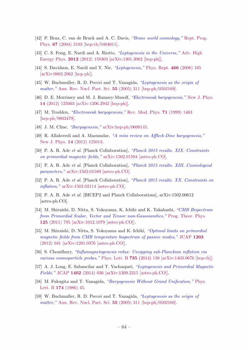
[42] P. Brax, C. van de Bruck and A. C. Davis, “Brane world cosmology,” Rept. Prog.
Phys. 67 (2004) 2183 [hep-th/0404011].
[43] C. S. Fong, E. Nardi and A. Riotto, “Leptogenesis in the Universe,” Adv. High
Energy Phys. 2012 (2012) 158303 [arXiv:1301.3062 [hep-ph]].
[44] S. Davidson, E. Nardi and Y. Nir, “Leptogenesis,” Phys. Rept. 466 (2008) 105
[arXiv:0802.2962 [hep-ph]].
[45] W. Buchmuller, R. D. Peccei and T. Yanagida, “Leptogenesis as the origin of
matter,” Ann. Rev. Nucl. Part. Sci. 55 (2005) 311 [hep-ph/0502169].
[46] D. E. Morrissey and M. J. Ramsey-Musolf, “Electroweak baryogenesis,” New J. Phys.
14 (2012) 125003 [arXiv:1206.2942 [hep-ph]].
[47] M. Trodden, “Electroweak baryogenesis,” Rev. Mod. Phys. 71 (1999) 1463
[hep-ph/9803479].
[48] J. M. Cline, “Baryogenesis,” arXiv:hep-ph/0609145.
[49] R. Allahverdi and A. Mazumdar, “A mini review on Affleck-Dine baryogenesis,”
New J. Phys. 14 (2012) 125013.
[50] P. A. R. Ade et al. [Planck Collaboration], “Planck 2015 results. XIX. Constraints
on primordial magnetic fields,” arXiv:1502.01594 [astro-ph.CO].
[51] P. A. R. Ade et al. [Planck Collaboration], “Planck 2015 results. XIII. Cosmological
parameters,” arXiv:1502.01589 [astro-ph.CO].
[52] P. A. R. Ade et al. [Planck Collaboration], “Planck 2015 results. XX. Constraints on
inflation,” arXiv:1502.02114 [astro-ph.CO].
[53] P. A. R. Ade et al. [BICEP2 and Planck Collaborations], arXiv:1502.00612
[astro-ph.CO].
[54] M. Shiraishi, D. Nitta, S. Yokoyama, K. Ichiki and K. Takahashi, “CMB Bispectrum
from Primordial Scalar, Vector and Tensor non-Gaussianities,” Prog. Theor. Phys.
125 (2011) 795 [arXiv:1012.1079 [astro-ph.CO]].
[55] M. Shiraishi, D. Nitta, S. Yokoyama and K. Ichiki, “Optimal limits on primordial
magnetic fields from CMB temperature bispectrum of passive modes,” JCAP 1203
(2012) 041 [arXiv:1201.0376 [astro-ph.CO]].
[56] S. Choudhury, “Inflamagnetogenesis redux: Unzipping sub-Planckian inflation via
various cosmoparticle probes,” Phys. Lett. B 735 (2014) 138 [arXiv:1403.0676 [hep-th]].
[57] A. J. Long, E. Sabancilar and T. Vachaspati, “Leptogenesis and Primordial Magnetic
Fields,” JCAP 1402 (2014) 036 [arXiv:1309.2315 [astro-ph.CO]].
[58] M. Fukugita and T. Yanagida, “Baryogenesis Without Grand Unification,” Phys.
Lett. B 174 (1986) 45.
[59] W. Buchmuller, R. D. Peccei and T. Yanagida, “Leptogenesis as the origin of
matter,” Ann. Rev. Nucl. Part. Sci. 55 (2005) 311 [hep-ph/0502169].
– 64 –
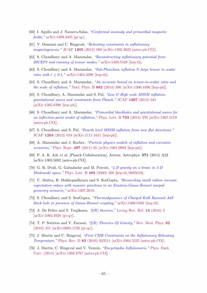
[60] I. Agullo and J. Navarro-Salas, “Conformal anomaly and primordial magnetic
fields,” arXiv:1309.3435 [gr-qc].
[61] V. Demozzi and C. Ringeval, “Reheating constraints in inflationary
magnetogenesis,” JCAP 1205 (2012) 009 [arXiv:1202.3022 [astro-ph.CO]].
[62] S. Choudhury and A. Mazumdar, “Reconstructing inflationary potential from
BICEP2 and running of tensor modes,” arXiv:1403.5549 [hep-th].
[63] S. Choudhury and A. Mazumdar, “Sub-Planckian inflation & large tensor to scalar
ratio with r ≥ 0.1,” arXiv:1404.3398 [hep-th].
[64] S. Choudhury and A. Mazumdar, “An accurate bound on tensor-to-scalar ratio and
the scale of inflation,” Nucl. Phys. B 882 (2014) 386 [arXiv:1306.4496 [hep-ph]].
[65] S. Choudhury, A. Mazumdar and S. Pal, “Low & High scale MSSM inflation,
gravitational waves and constraints from Planck,” JCAP 1307 (2013) 041
[arXiv:1305.6398 [hep-ph]].
[66] S. Choudhury and A. Mazumdar, “Primordial blackholes and gravitational waves for
an inflection-point model of inflation,” Phys. Lett. B 733 (2014) 270 [arXiv:1307.5119
[astro-ph.CO]].
[67] S. Choudhury and S. Pal, “Fourth level MSSM inflation from new flat directions,”
JCAP 1204 (2012) 018 [arXiv:1111.3441 [hep-ph]].
[68] A. Mazumdar and J. Rocher, “Particle physics models of inflation and curvaton
scenarios,” Phys. Rept. 497 (2011) 85 [arXiv:1001.0993 [hep-ph]].
[69] P. A. R. Ade et al. [Planck Collaboration], Astron. Astrophys. 571 (2014) A22
[arXiv:1303.5082 [astro-ph.CO]].
[70] G. R. Dvali, G. Gabadadze and M. Porrati, “4-D gravity on a brane in 5-D
Minkowski space,” Phys. Lett. B 485 (2000) 208 [hep-th/0005016].
[71] U. Maitra, B. Mukhopadhyaya and S. SenGupta, “Reconciling small radion vacuum
expectation values with massive gravitons in an Einstein-Gauss-Bonnet warped
geometry scenario,” arXiv:1307.3018.
[72] S. Choudhury and S. SenGupta, “Thermodynamics of Charged Kalb Ramond AdS
black hole in presence of Gauss-Bonnet coupling,” arXiv:1306.0492 [hep-th].
[73] A. De Felice and S. Tsujikawa, “f(R) theories,” Living Rev. Rel. 13 (2010) 3
[arXiv:1002.4928 [gr-qc]].
[74] T. P. Sotiriou and V. Faraoni, “f(R) Theories Of Gravity,” Rev. Mod. Phys. 82
(2010) 451 [arXiv:0805.1726 [gr-qc]].
[75] J. Martin and C. Ringeval, “First CMB Constraints on the Inflationary Reheating
Temperature,” Phys. Rev. D 82 (2010) 023511 [arXiv:1004.5525 [astro-ph.CO]].
[76] J. Martin, C. Ringeval and V. Vennin, “Encyclopdia Inflationaris,” Phys. Dark
Univ. (2014) [arXiv:1303.3787 [astro-ph.CO]].
– 65 –
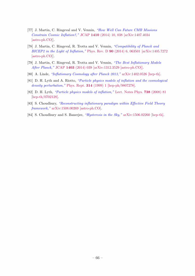
[77] J. Martin, C. Ringeval and V. Vennin, “How Well Can Future CMB Missions
Constrain Cosmic Inflation?,” JCAP 1410 (2014) 10, 038 [arXiv:1407.4034
[astro-ph.CO]].
[78] J. Martin, C. Ringeval, R. Trotta and V. Vennin, “Compatibility of Planck and
BICEP2 in the Light of Inflation,” Phys. Rev. D 90 (2014) 6, 063501 [arXiv:1405.7272
[astro-ph.CO]].
[79] J. Martin, C. Ringeval, R. Trotta and V. Vennin, “The Best Inflationary Models
After Planck,” JCAP 1403 (2014) 039 [arXiv:1312.3529 [astro-ph.CO]].
[80] A. Linde, “Inflationary Cosmology after Planck 2013,” arXiv:1402.0526 [hep-th].
[81] D. H. Lyth and A. Riotto, “Particle physics models of inflation and the cosmological
density perturbation,” Phys. Rept. 314 (1999) 1 [hep-ph/9807278].
[82] D. H. Lyth, “Particle physics models of inflation,” Lect. Notes Phys. 738 (2008) 81
[hep-th/0702128].
[83] S. Choudhury, “Reconstructing inflationary paradigm within Effective Field Theory
framework,” arXiv:1508.00269 [astro-ph.CO].
[84] S. Choudhury and S. Banerjee, “Hysteresis in the Sky,” arXiv:1506.02260 [hep-th].
– 66 –
Top Related
Copyright © 2022 FDOKUMEN

