Classification of wave regimes in excitable systems with linear cross-diffusion

M. A. TsyganovInstitute of Theoretical and Experimental Biophysics, Pushchino, Moscow Region, 142290, Russia

V. N. BiktashevCollege of Engineering, Mathematics and Physical Sciences, University of Exeter, Exeter EX4 4QF, UK

(Dated: November 12, 2014)

We consider principal properties of various wave regimes in two selected excitable systems with linear cross-diffusion in one spatial dimension observed at different parameter values. This includes fixed-shape propagatingwaves, envelope waves, multi-envelope waves, and intermediate regimes appearing as waves propagating fixed-shape most of the time but undergoing restructuring from time to time. Depending on parameters, most of theseregimes can be with and without the “quasi-soliton” property of reflection of boundaries and penetration througheach other. We also present some examples of behaviour of envelope quasi-solitons in two spatial dimensions.

PACS numbers: 82.40.Bj,82.40.Ck, 87.10.-e

I. INTRODUCTION

The progress in the study of self-organization phenomenain physical, chemical and biological systems is dependent onstudy of generation, propagation and interaction of nonlinearwaves in spatially distributed active, e.g. excitable, systemswith diffusion [1]. An important general property of such sys-tems is their ability to generate and conduct self-supportedstrongly nonlinear waves of the change of state of the medium.The shape and speed of such waves in the established regimedoes not depend on initial and boundary conditions and isfully determined by the medium parameters. Until recentlythe results concerning such systems have been focused on sys-tems “reaction+diffusion” with a diagonal diffusivity matrix,e.g. for two reacting components,

∂u

∂t= f(u, v) +Du∇2u,

∂v

∂t= g(u, v) +Dv∇2v, (1)

with non-negative diffusivities Du ≥ 0, Dv ≥ 0, Du +Dv >0. However, a number of applications motivate considera-tion of a more generic class of reaction-diffusion systems,with non-diagonal elements of the diffusivity matrix (“cross-diffusion”), which can produce a number of unusual patternsand wave regimes, see e.g. a review [2]. In this paper weconcentrate on one subclass of such unusual wave regimes,which is associated with soliton-like interaction, i.e. pene-tration of waves upon impact with each other or reflectionfrom non-flux boundaries. This is rather uncharacteristic ofthe waves in (1) with the exception of narrow parametric re-gions on the margins of the excitability [3]. However, in sys-tems with cross-diffusion, such “quasi-soliton’ behaviour canbe observed in large parametric regions [4, 5]. These phe-nomena have been observed in numerical simulations of two-component excitable media with cross-diffusion, both in lin-ear formulation, e.g.

∂u

∂t= f(u, v) +Du∇2u+ h1∇2v,

∂v

∂t= g(u, v) +Dv∇2v − h2∇2u, (2)

and nonlinear, “taxis” formulation,

∂u

∂t= f(u, v) +Du∇2u+ h1∇ (u∇v) ,

∂v

∂t= g(u, v) +Dv∇2v − h2∇ (v∇u) , (3)

where h1 ≥ 0, h2 ≥ 0, h1 + h2 > 0.Quasi-solitons have similarities and differences with the

classical solitons in conservative (fully integrable) systems.The already mentioned similarity is their ability to penetratethrough each other and reflect from boundaries. The differ-ences are:

• The amplitude and speed of a true soliton depend oninitial conditions. For the quasi-soliton, the establishedamplitude and speed depend on the medium parameters.

• The amplitudes of the true solitons do not change afterthe impact. The dynamics of quasi-solitons on impactis often naturally seen as a temporary diminution of theamplitude with subsequent gradual recovery.

Recently we have demonstrated “envelope quasi-solitons”in one-dimensional systems with linear cross-diffusion (2) [6],which share some phenomenology with envelope solitons inthe nonlinear Schrodinger equation (NLS) for a complex fieldw [7],

i∂w

∂t+∇2w + w|w|2 = 0. (4)

Namely, they have the form of spatiotemporal oscillations(“wavelets”) with a smooth envelope, and the velocity of theindividual wavelets (the phase velocity) is different from thevelocity of the envelope (the group velocity). This may be se-rious evidence for some deep relationship between these phe-nomena from dissipative and conservative realms. The linkin this relationship is cross-diffusion, which for NLS is re-vealed if is rewriten as a system for two real fields u and v viaw = u− iv of the form (2) with

h1 = h2 = 1, Du = Dv = 0,

f = u(u2 + v2), g = −v(u2 + v2).

arX

iv:1

408.

3611

v2 [

nlin

.PS]

7 N

ov 2

014

2

Note the signs of the cross-diffusion terms in the component-wise form of NLS and in (2).

Further investigation has revealed a great variety of thetypes of nonlinear waves in excitable cross-diffusion sys-tems. In this paper we present some classification of the phe-nomenologies of such waves.

Our observations are made in two selected two-componentkinetic models, supplemented with cross-diffusion, ratherthan self-diffusion terms; such terms may appear, say, in me-chanical [8], chemical [2, 9], biological and ecological [10,11] contexts. We note that the case of only cross-diffusionterms, with Du = Dv = 0, is special in that the spatial cou-pling is then not dissipative, and all the dissipation in the sys-tem is due to the kinetic terms. So, theoretically speaking, thiscase may present features that are not characteristic for morerealistic models. In practice, however, these worries seem un-founded. Parametric studies done in the past [4, 12] indicatethat the role of the self-diffusion coefficients Du, Dv is notessential if they are small enough. Moreover, we have verifiedthat the results presented below are robust in that respect, too.In other words, regimes observed for Du = Dv = 0 typicallyare qualitatively preserved, even if quantitatively modified,upon adding small Du, Dv . So in this study we limit consid-eration to Du = Dv = 0 to reduce number of parameters andfocus attention on effects of the cross-diffusion terms. Exceptwhere stated otherwise, the values of the cross-diffusion coef-ficients are h1 = h2 = 1. We consider the FitzHugh-Nagumo(FHN) kinetics,

f = u(u− a)(1− u)− k1v, g = εu, (5)

for varied values of parameters a, k1, and ε. As a specificexample of a real-life system, we also consider the Lengyel-Epstein (LE) [13] model of a chlorite-iodide-malonic acid-starch autocatalitic reaction system

f = A− u− 4uv

1 + u2, g = B

(u− uv

1 + u2

). (6)

for varied values of parameters A and B.

II. METHODS

We simulate (2) in one spatial dimension for x ∈ [0, L],L ≤ ∞, with Neumann boundary conditions for both u and v.We use first order time stepping, fully explicit in the reactionterms and fully implicit in the cross-diffusion terms, with asecond-order central difference approximation for the spatialderivatives. Unless stated otherwise, we used steps ∆x =1/10 and ∆t = 1/5000 for FHN kinetics (5) and ∆x = 0.1and ∆t = 1/1000 for LE kinetics (6).

To simulate propagation “on an infinite line”, we did thesimulations on a finite but sufficiently large L (specifiedin each case), and instantanously translated the solution byδx1 = 30 away from the boundary each time the pulse, asmeasured at the level u = u∗, where u∗ = 0.1 for FHN ki-netics and u∗ = 1.5 for LE kinetics, approached the bound-ary to a distance smaller than δx2 = 100, and filled in the

new interval of x values by extending the u and v variablesat levels u = u0, v = v0, where (u0, v0) is the resting state,u0 = v0 = 0 for FHN kinetics and u0 = A/5, v0 = 1+A2/25for LE kinetics.

Initial conditions were set as u(x, 0) = u0 + us Θ(δ − x),v(x, 0) = v0, to initiate a wave starting from the left end ofthe domain. Here Θ() is the Heaviside function, and the waveseed length was typically chosen as δ = 2 or δ = 4. The inter-val length L was chosen sufficiently large, say for the system(2,5) it was typically at least L = 350, to allow wave propa-gation unaffected by boundaries, for some significant time.

To characterize shape of the waves emerging in simulationsand its evolution, we counted significant peaks (wavelets) inthe solutions as the number n of continuous intervals of xwhere u − u0 > 0.1. In some regimes, this number variedwith time, as the shape of enveloped changed while propagat-ing. We also measured the speed of individual wavelets as thespeed of the fore ends of these intervals at short time intervals.To estimate the group velocity, we considered the fore edge ofthe foremost significant peak over a longer time interval, cov-ering several oscillation periods.

To compare the oscillatory front of propagating waves tothe linearized theory, we took the v-component of the givensolution in the interval and selected the connected area in the(x, t) plane where |v(x, t)| < 0.1 ahead of the main wave.We numerically fitted this grid function v(x, t) to (7) usingGnuplot implementation of Marquardt-Levenberg algorithm.The initial guess for parameters C, µ, c, k, x, ω was done“by eye”. The fitting was initially on a small interval in time,smaller than the temporal period of the front oscillations, andthen gradually extended to a long time interval, so that theresult of one fitting was used as the initial guess for the nextfitting.

III. RESULTS

A. Overview of wave types

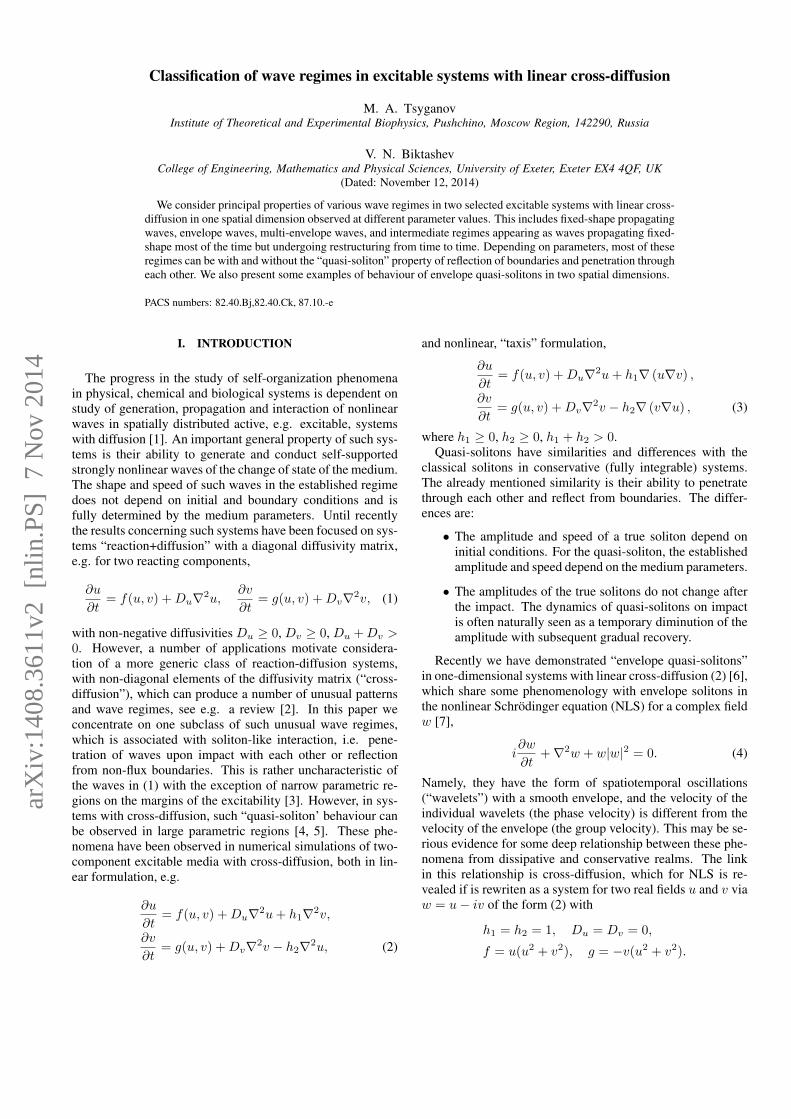
Fig. 1 illustrates the three main types of waves in theexcitable cross-diffusion system (2) with FHN kinetics (5).Fig. 2 explains why these are “main” types. It shows the re-gions in the parametric plane (a, ε), and we see that the solu-tions shown in fig. 1 are represented by large parametric areas.Their common features are quasi-soliton interaction and oscil-latory front, and the differences are in the propagation mode.A simple quasi-soliton (fig. 1(a), abbreviation SFR in fig. 2(a))retains its shape as it propagates. A group, or envelope, quasi-soliton (fig. 1(b), abbreviation SER in fig. 2(a)) does not havea fixed shape; instead it has the form of spatiotemporal os-cillations, whose envelope retains a fixed unimodal shape asit propagates. A multi-envelope quasi-soliton (fig. 1(c,d), ab-breviation MER in fig. 2(a)) is shown at two time moments,to illustrate the dynamics of its formation. At first, the emerg-ing solution looks like an envelope quasi-soliton; however af-ter some time behind it forms another envelope quasi-soliton,then behind that one yet another, and so it continues. The in-terval of time between formation of new envelopes depends

3

0

1

4940 5020

uv

x

a = 0.22

0

1

5760 5840

uv

x

a = 0.12

(a) (b)

0

1

2500 2800

uv

x

a = 0.04, t = 600

0

1

2750 3050

uv

x

a = 0.04, t = 650

(c) (d)

FIG. 1: (color online) Three typical wave regimes in the cross-diffusion system (2,5) with k1 = 10, ε = 0.01 for different values of a. (a)Simple quasi-soliton, a = 0.22. (b) Envelope quasi-soliton, a = 0.12. (c,d) Multi-envelope qausi-soliton, a = 0.04, at two different timemoments.

0

0.06

0 0.6

SER

SEN

MER

N

SFR

SIR

2EN

SFN

MENε

a 0

0.06

0 0.6

ε

a

us = 1, xs = 1us = 2, xs = 4

(a) (b)

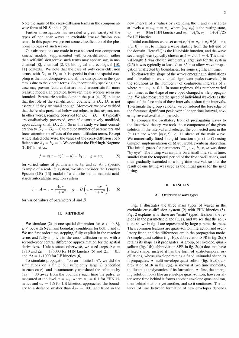
FIG. 2: (a) The parametric regions corresponding to different wave regimes in (2,5) in the (a, ε) plane at k1 = 10, xs = 4, us = 2.The abbreviations in the legend stand for various types of typical wave solutions: SER single envelope reflecting; SEN single envelopenon-reflecting; MER multiple envelope reflecting; MEN multiple envelope non-reflecting; SFR single fixed-shape reflecting; SFN singlefixed-shape non-reflecting; SIR single intermediate (between single shape and envelope) reflecting; 2EN envelope non-reflecting with separateenvelopes at the front and at the back with non-oscillating plateau between them; N no propagation. See Supplementary Material [14] for amovie. (b) Boundaries of the regimes of propagation and decay (of any waves) for different initial conditions.

4

on the parameters, e.g. it becomes smaller for smaller valuesof a.

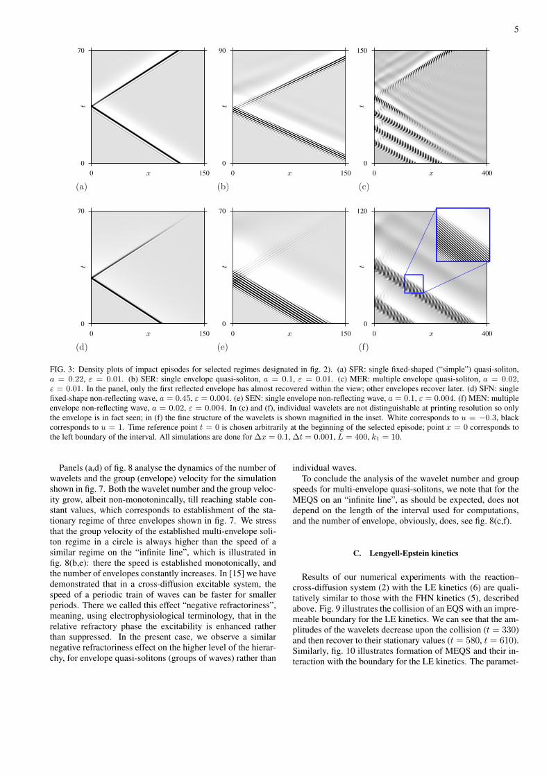
Each of the three types of quasi-solitons shown in fig. 1 hasa counterpart type of solutions of similar propagation mode,but without the quasi-soliton property, i.e. not reflecting uponcollision (abbreviations SFN, SEN, MEN in fig. 2(a)). Densityplots of interaction of the three main types of quasi-solitonsand their non-soliton counterparts are shown in fig. 3. Notethat the non-soliton regimes do not show immediate annihi-lation upon the collision. Rather, the process looks like re-flection with a decreased amplitude, and subsequent decay,see fig. 3(d-f).

Apart from the non-reflecting counterparts to the three maintypes, there are also “non-propagating” counterparts, all ofwhich are denoted by N in fig. 2(a). These regimes correspondto waves that are in fact formed from the standard initial con-ditions, but then decay after some time. Naturally, the successof initiation of a propagating wave does in fact depend on theparameters of the initial conditions: fig. 2(b) shows how theregion of single quasi-soliton differs for two different initialconditions. This is of course expectable for excitable kinetics.

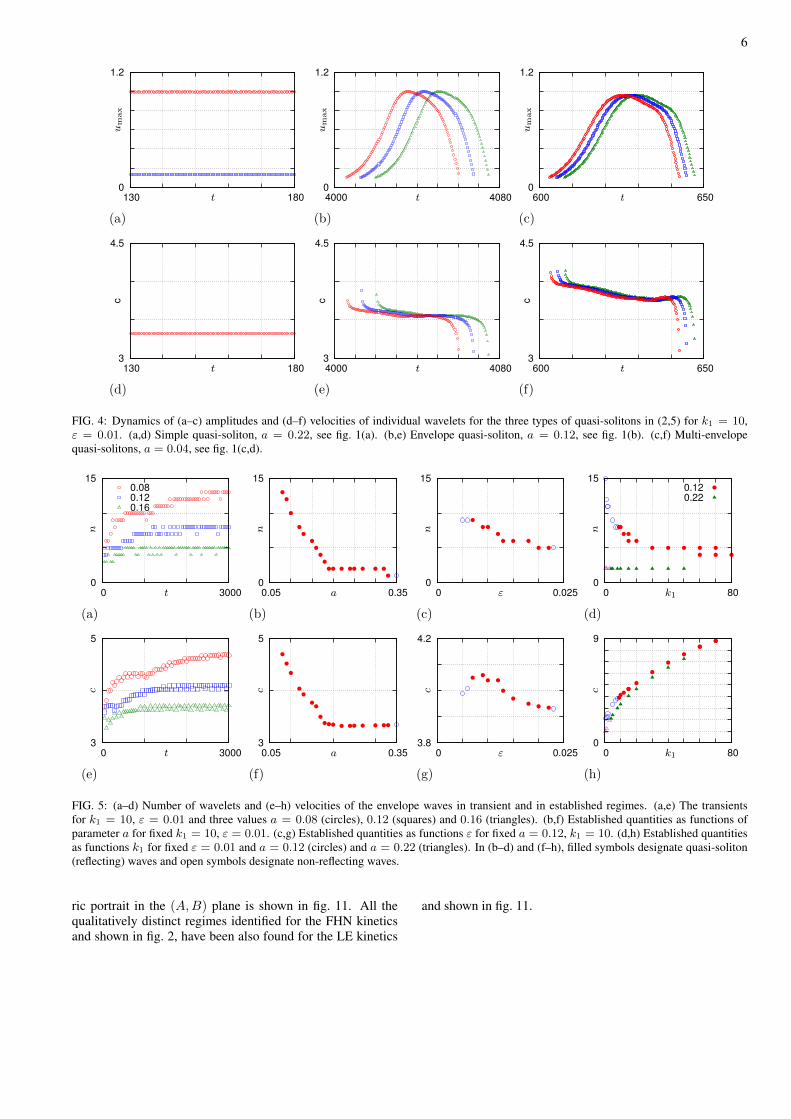
The analysis of the dynamics of the wavelets andwavespeeds for the three main types of quasi-solitons, illus-trated in figures 4 and 5, reveals:

• The amplitude and speed of the simple quasi-solitonsdo not change in time (fig. 4(a,d)).

• For the envelope and multi-envelope quasi-solitons, theamplitudes of individual wavelets during their lifetimefirst grow to a certain maximum and then decreasemonotinically (fig. 4(b,c)). The speed of a wavelet (thephase velocity) is high at first, but the decreases non-monotonically (fig. 4(e,f)).

• In the process of establishment of an envelope quasi-soliton, the number of wavelets in it increases until sat-uration (fig. 5(a)), and so does the speed of the envelope(the group velocity) (fig. 5(e)).

• Fig. 5(b,f) shows that in simple quasi-solitons (a >0.2), the number of wavelets remains the same (n = 2),and their speed remains approximately the same in thatinterval; whereas in envelope quasi-solitons (a < 0.2),both the number of wavelets and their velocities in-crease with the decrease of a.

• Fig. 5(c,g) shows that increase of parameter ε causesdecrease of both the number of wavelets and of theirspeeds.

• Parameter k1 also plays a significant role in defininingthe wave regime and its parameters (fig. 5(d,h)).

The oscillatory character of the fronts of cross-diffusionwaves both for simple quasi-solitons and for envelope quasi-solitons, which is apparent from numerical simulations, is eas-ily confirmed by linearization of (2) around the resting state.

The resting states in both FHN (5) and LE (6) kinetics are sta-ble foci which already shows propensity to oscillations. Tak-ing the solution of the linearized equation in the form[

u− u0v − v0

]≈ Re

(Cve−µ(x−ct)ei(kx−ωt)

), (7)

we need

A(λ, ν)v = 0, v 6= 0, detA = 0, (8)

where

A =

[−a− λ −k1 + ν2

ε− ν2 −λ

],

λ = µc− iω, ν = −µ+ ik.

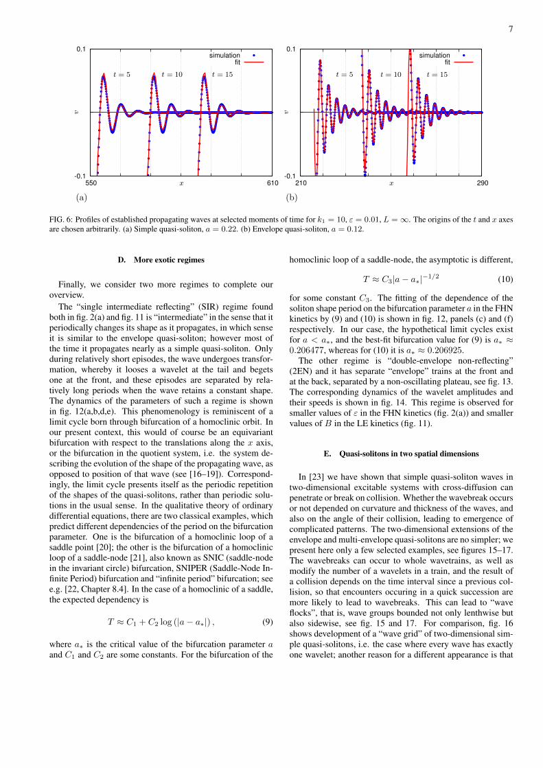
Equation (8) imposes two constraints (for the real and imag-inary parts of the determinant) on the four real quantities µ,c, k and ω, so it is by far insufficient to determine the selec-tion of these parameters, but this equality can be verified forthe numerical simulations, in order to ensure that the observedoscillatory fronts are not a numerical artefact but a true prop-erty of the underlying partial differential equations. Hence wefitted selected simulations around the fronts with the depen-dence (7). The quality of the fitting is illustrated by two ex-amples in fig. 6. The fitted parameters satisfied (8) with goodaccuracy; in both cases, they gave |detA/(TrA)2| < 10−3.

Note that the approximation (7) makes explicit the conceptsof wavelets (the oscillating factor ei(kx−ωt)), the phase veloc-ity (the ratio ω/k), the envelope (in this case the exponentialshape e−µ(x−ct)) and the group velocity (the fitting parameterc). As expected, for the simple quasi-soliton shown in fig. 6(a)the fitted group and phase velocities coincided within the pre-cision of fitting (|c − ω/k| < 10−5). For the envelope quasi-soliton shown in fig. 6(b) they were significantly different:c ≈ 4.077, ω/k ≈ 3.586.

B. Multi-envelope quasi-solitons

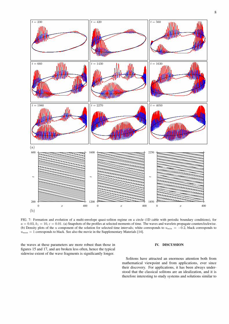
We use the term multiplying envelope quasi-solitons(MEQS) to concisely designate spontaneously multiplying en-velope quasi-solitons. The process of self-multiplication leadsto eventually filling the whole domain, behind the leadingedge of the first group, with what appears as a train of enve-lope quasi-solitons, i.e. a hierarchical, quasi-periodic regime.This is illustrated in fig. 7(a) for periodic boundary condi-tions, the setting that eliminates the “leading edge” complica-tion mentioned above. One envelope quasi-soliton (EQS) pro-duced by the standard initial conditions develops an instabilityat its tail, leading to generation of the second EQS (t = 230).The system of two EQSs generates a third (t = 420). Af-ter forming of a system of five EQSs (t = 600), the inversetransition happens, from five to four envelopes (t = 1430,t = 1630), and then from four to three envelopes (t = 1980,t = 2270), leading to an established, persistent state of threeenvelopes (t = 4050). The same process is represented alsoas a density plot in fig. 7(b).

5

0

70

0 150

t

x

0

90

0 150

t

x

0

150

0 400

t

x

(a) (b) (c)

0

70

0 150

t

x

0

70

0 150

t

x

0

120

0 400

t

x

(d) (e) (f)

FIG. 3: Density plots of impact episodes for selected regimes designated in fig. 2). (a) SFR: single fixed-shaped (“simple”) quasi-soliton,a = 0.22, ε = 0.01. (b) SER: single envelope quasi-soliton, a = 0.1, ε = 0.01. (c) MER: multiple envelope quasi-soliton, a = 0.02,ε = 0.01. In the panel, only the first reflected envelope has almost recovered within the view; other envelopes recover later. (d) SFN: singlefixed-shape non-reflecting wave, a = 0.45, ε = 0.004. (e) SEN: single envelope non-reflecting wave, a = 0.1, ε = 0.004. (f) MEN: multipleenvelope non-reflecting wave, a = 0.02, ε = 0.004. In (c) and (f), individual wavelets are not distinguishable at printing resolution so onlythe envelope is in fact seen; in (f) the fine structure of the wavelets is shown magnified in the inset. White corresponds to u = −0.3, blackcorresponds to u = 1. Time reference point t = 0 is chosen arbitrarily at the beginning of the selected episode; point x = 0 corresponds tothe left boundary of the interval. All simulations are done for ∆x = 0.1, ∆t = 0.001, L = 400, k1 = 10.

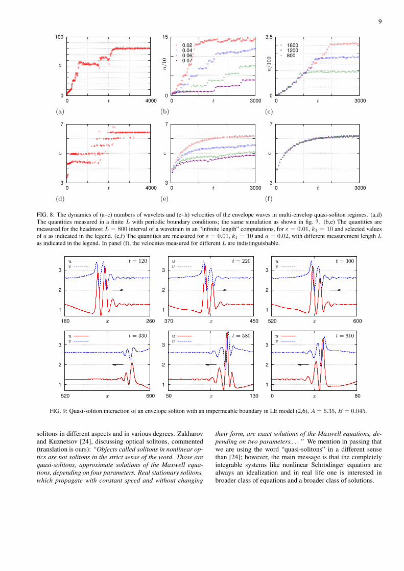
Panels (a,d) of fig. 8 analyse the dynamics of the number ofwavelets and the group (envelope) velocity for the simulationshown in fig. 7. Both the wavelet number and the group veloc-ity grow, albeit non-monotonincally, till reaching stable con-stant values, which corresponds to establishment of the sta-tionary regime of three envelopes shown in fig. 7. We stressthat the group velocity of the established multi-envelope soli-ton regime in a circle is always higher than the speed of asimilar regime on the “infinite line”, which is illustrated infig. 8(b,e): there the speed is established monotonically, andthe number of envelopes constantly increases. In [15] we havedemonstrated that in a cross-diffusion excitable system, thespeed of a periodic train of waves can be faster for smallerperiods. There we called this effect “negative refractoriness”,meaning, using electrophysiological terminology, that in therelative refractory phase the excitability is enhanced ratherthan suppressed. In the present case, we observe a similarnegative refractoriness effect on the higher level of the hierar-chy, for envelope quasi-solitons (groups of waves) rather than

individual waves.To conclude the analysis of the wavelet number and group

speeds for multi-envelope quasi-solitons, we note that for theMEQS on an “infinite line”, as should be expected, does notdepend on the length of the interval used for computations,and the number of envelope, obviously, does, see fig. 8(c,f).

C. Lengyell-Epstein kinetics

Results of our numerical experiments with the reaction–cross-diffusion system (2) with the LE kinetics (6) are quali-tatively similar to those with the FHN kinetics (5), describedabove. Fig. 9 illustrates the collision of an EQS with an impre-meable boundary for the LE kinetics. We can see that the am-plitudes of the wavelets decrease upon the collision (t = 330)and then recover to their stationary values (t = 580, t = 610).Similarly, fig. 10 illustrates formation of MEQS and their in-teraction with the boundary for the LE kinetics. The paramet-

6

0

1.2

130 180

um

ax

t 0

1.2

4000 4080

um

ax

t 0

1.2

600 650

um

ax

t

(a) (b) (c)

3

4.5

130 180

c

t 3

4.5

4000 4080

c

t 3

4.5

600 650

c

t

(d) (e) (f)

FIG. 4: Dynamics of (a–c) amplitudes and (d–f) velocities of individual wavelets for the three types of quasi-solitons in (2,5) for k1 = 10,ε = 0.01. (a,d) Simple quasi-soliton, a = 0.22, see fig. 1(a). (b,e) Envelope quasi-soliton, a = 0.12, see fig. 1(b). (c,f) Multi-envelopequasi-solitons, a = 0.04, see fig. 1(c,d).

0

15

0 3000

0.08

0.12

0.16

n

t 0

15

0.05 0.35

n

a 0

15

0 0.025

n

ε 0

15

0 80

0.12

0.22

nk1

(a) (b) (c) (d)

3

5

0 3000

c

t 3

5

0.05 0.35

c

a 3.8

4.2

0 0.025

c

ε 0

9

0 80

c

k1

(e) (f) (g) (h)

FIG. 5: (a–d) Number of wavelets and (e–h) velocities of the envelope waves in transient and in established regimes. (a,e) The transientsfor k1 = 10, ε = 0.01 and three values a = 0.08 (circles), 0.12 (squares) and 0.16 (triangles). (b,f) Established quantities as functions ofparameter a for fixed k1 = 10, ε = 0.01. (c,g) Established quantities as functions ε for fixed a = 0.12, k1 = 10. (d,h) Established quantitiesas functions k1 for fixed ε = 0.01 and a = 0.12 (circles) and a = 0.22 (triangles). In (b–d) and (f–h), filled symbols designate quasi-soliton(reflecting) waves and open symbols designate non-reflecting waves.

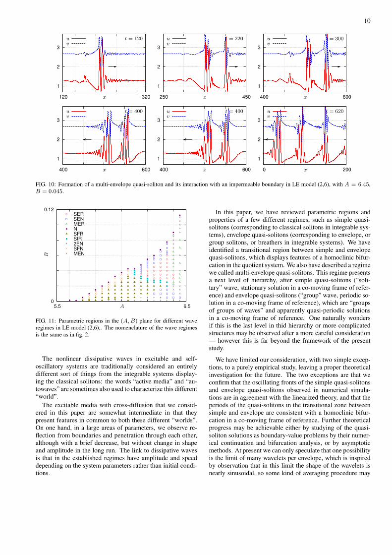
ric portrait in the (A,B) plane is shown in fig. 11. All thequalitatively distinct regimes identified for the FHN kineticsand shown in fig. 2, have been also found for the LE kinetics

and shown in fig. 11.

7

-0.1

0.1

550 610

simulation

fit

x

vt = 5 t = 10 t = 15

-0.1

0.1

210 290

simulation

fit

x

v

t = 5 t = 10 t = 15

(a) (b)

FIG. 6: Profiles of established propagating waves at selected moments of time for k1 = 10, ε = 0.01, L =∞. The origins of the t and x axesare chosen arbitrarily. (a) Simple quasi-soliton, a = 0.22. (b) Envelope quasi-soliton, a = 0.12.

D. More exotic regimes

Finally, we consider two more regimes to complete ouroverview.

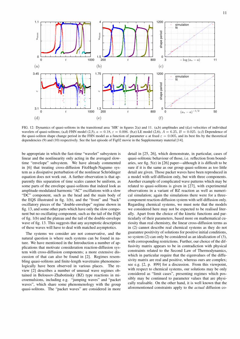
The “single intermediate reflecting” (SIR) regime foundboth in fig. 2(a) and fig. 11 is “intermediate” in the sense that itperiodically changes its shape as it propagates, in which senseit is similar to the envelope quasi-soliton; however most ofthe time it propagates nearly as a simple quasi-soliton. Onlyduring relatively short episodes, the wave undergoes transfor-mation, whereby it looses a wavelet at the tail and begetsone at the front, and these episodes are separated by rela-tively long periods when the wave retains a constant shape.The dynamics of the parameters of such a regime is shownin fig. 12(a,b,d,e). This phenomenology is reminiscent of alimit cycle born through bifurcation of a homoclinic orbit. Inour present context, this would of course be an equivariantbifurcation with respect to the translations along the x axis,or the bifurcation in the quotient system, i.e. the system de-scribing the evolution of the shape of the propagating wave, asopposed to position of that wave (see [16–19]). Correspond-ingly, the limit cycle presents itself as the periodic repetitionof the shapes of the quasi-solitons, rather than periodic solu-tions in the usual sense. In the qualitative theory of ordinarydifferential equations, there are two classical examples, whichpredict different dependencies of the period on the bifurcationparameter. One is the bifurcation of a homoclinic loop of asaddle point [20]; the other is the bifurcation of a homoclinicloop of a saddle-node [21], also known as SNIC (saddle-nodein the invariant circle) bifurcation, SNIPER (Saddle-Node In-finite Period) bifurcation and “infinite period” bifurcation; seee.g. [22, Chapter 8.4]. In the case of a homoclinic of a saddle,the expected dependency is

T ≈ C1 + C2 log (|a− a∗|) , (9)

where a∗ is the critical value of the bifurcation parameter aand C1 and C2 are some constants. For the bifurcation of the

homoclinic loop of a saddle-node, the asymptotic is different,

T ≈ C3|a− a∗|−1/2 (10)

for some constant C3. The fitting of the dependence of thesoliton shape period on the bifurcation parameter a in the FHNkinetics by (9) and (10) is shown in fig. 12, panels (c) and (f)respectively. In our case, the hypothetical limit cycles existfor a < a∗, and the best-fit bifurcation value for (9) is a∗ ≈0.206477, whereas for (10) it is a∗ ≈ 0.206925.

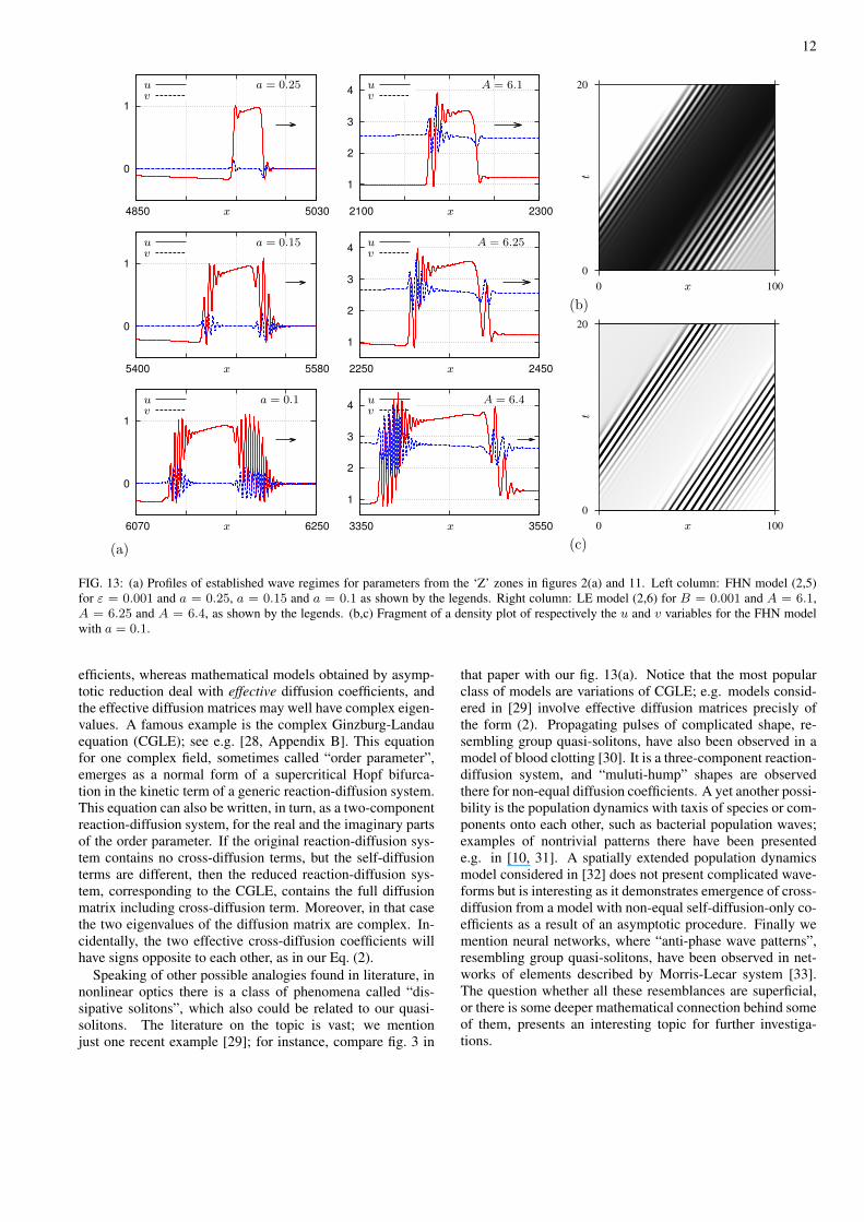
The other regime is “double-envelope non-reflecting”(2EN) and it has separate “envelope” trains at the front andat the back, separated by a non-oscillating plateau, see fig. 13.The corresponding dynamics of the wavelet amplitudes andtheir speeds is shown in fig. 14. This regime is observed forsmaller values of ε in the FHN kinetics (fig. 2(a)) and smallervalues of B in the LE kinetics (fig. 11).

E. Quasi-solitons in two spatial dimensions

In [23] we have shown that simple quasi-soliton waves intwo-dimensional excitable systems with cross-diffusion canpenetrate or break on collision. Whether the wavebreak occursor not depended on curvature and thickness of the waves, andalso on the angle of their collision, leading to emergence ofcomplicated patterns. The two-dimensional extensions of theenvelope and multi-envelope quasi-solitons are no simpler; wepresent here only a few selected examples, see figures 15–17.The wavebreaks can occur to whole wavetrains, as well asmodify the number of a wavelets in a train, and the result ofa collision depends on the time interval since a previous col-lision, so that encounters occuring in a quick succession aremore likely to lead to wavebreaks. This can lead to “waveflocks”, that is, wave groups bounded not only lenthwise butalso sidewise, see fig. 15 and 17. For comparison, fig. 16shows development of a “wave grid” of two-dimensional sim-ple quasi-solitons, i.e. the case where every wave has exactlyone wavelet; another reason for a different appearance is that

8

t = 230 t = 420 t = 560

t = 660 t = 1430 t = 1630

t = 1980 t = 2270 t = 4050

(a)

200

600

0 400

t

x

1200

1600

0 400

t

x

1850

2250

0 400

t

x

(b)

FIG. 7: Formation and evolution of a multi-envelope quasi-soliton regime on a circle (1D cable with periodic boundary conditions), fora = 0.03, k1 = 10, ε = 0.01. (a) Snapshots of the profiles at selected moments of time. The waves and wavelets propagate counterclockwise.(b) Density plots of the u component of the solution for selected time intervals; white corresponds to umin = −0.2, black corresponds toumax = 1 corresponds to black. See also the movie in the Supplementary Materials [14].

the waves at these parameters are more robust than those infigures 15 and 17, and are broken less often, hence the typicalsidewise extent of the wave fragments is significantly longer.

IV. DISCUSSION

Solitons have attracted an enormous attention both frommathematical viewpoint and from applications, ever sincetheir discovery. For applications, it has been always under-stood that the classical solitons are an idealization, and it istherefore interesting to study systems and solutions similar to

9

0

100

0 4000

n

t 0

15

0 3000

0.02

0.04

0.06

0.07

n/10

t 0

3.5

0 3000

1600

1200

800

n/100

t

(a) (b) (c)

3

7

0 4000

c

t 3

7

0 3000

c

t 3

7

0 3000

c

t

(d) (e) (f)

FIG. 8: The dynamics of (a–c) numbers of wavelets and (e–h) velocities of the envelope waves in multi-envelop quasi-soliton regimes. (a,d)The quantities measured in a finite L with periodic boundary conditions; the same simulation as shown in fig. 7. (b,e) The quantities aremeasured for the headmost L = 800 interval of a wavetrain in an “infinite length” computations, for ε = 0.01, k1 = 10 and selected valuesof a as indicated in the legend. (c,f) The quantities are measured for ε = 0.01, k1 = 10 and a = 0.02, with different measurement length Las indicated in the legend. In panel (f), the velocities measured for different L are indistinguishable.

1

2

3

180 260

uv

x

t = 120

1

2

3

370 450

uv

x

t = 220

1

2

3

520 600

uv

x

t = 300

1

2

3

520 600

uv

x

t = 330

1

2

3

50 130

uv

x

t = 580

1

2

3

0 80

uv

x

t = 610

FIG. 9: Quasi-soliton interaction of an envelope soliton with an impermeable boundary in LE model (2,6), A = 6.35, B = 0.045.

solitons in different aspects and in various degrees. Zakharovand Kuznetsov [24], discussing optical solitons, commented(translation is ours): “Objects called solitons in nonlinear op-tics are not solitons in the strict sense of the word. Those arequasi-solitons, approximate solutions of the Maxwell equa-tions, depending on four parameters. Real stationary solitons,which propagate with constant speed and without changing

their form, are exact solutions of the Maxwell equations, de-pending on two parameters.. . . ” We mention in passing thatwe are using the word “quasi-solitons” in a different sensethan [24]; however, the main message is that the completelyintegrable systems like nonlinear Schrodinger equation arealways an idealization and in real life one is interested inbroader class of equations and a broader class of solutions.

10

1

2

3

120 320

uv

x

t = 120

1

2

3

250 450

uv

x

t = 220

1

2

3

400 600

uv

x

t = 300

1

2

3

400 600

uv

x

t = 400

1

2

3

400 600

uv

x

t = 400

1

2

3

0 200

uv

x

t = 620

FIG. 10: Formation of a multi-envelope quasi-soliton and its interaction with an impermeable boundary in LE model (2,6), with A = 6.45,B = 0.045.

0

0.12

5.5 6.5

SER

SEN

MER

N

SFR

SIR

2EN

SFN

MEN

A

B

FIG. 11: Parametric regions in the (A,B) plane for different waveregimes in LE model (2,6),. The nomenclature of the wave regimesis the same as in fig. 2.

The nonlinear dissipative waves in excitable and self-oscillatory systems are traditionally considered an entirelydifferent sort of things from the integrable systems display-ing the classical solitons: the words “active media” and “au-towaves” are sometimes also used to characterize this different“world”.

The excitable media with cross-diffusion that we consid-ered in this paper are somewhat intermediate in that theypresent features in common to both these different “worlds”.On one hand, in a large areas of parameters, we observe re-flection from boundaries and penetration through each other,although with a brief decrease, but without change in shapeand amplitude in the long run. The link to dissipative wavesis that in the established regimes have amplitude and speeddepending on the system parameters rather than initial condi-tions.

In this paper, we have reviewed parametric regions andproperties of a few different regimes, such as simple quasi-solitons (corresponding to classical solitons in integrable sys-tems), envelope quasi-solitons (corresponding to envelope, orgroup solitons, or breathers in integrable systems). We haveidentified a transitional region between simple and envelopequasi-solitons, which displays features of a homoclinic bifur-cation in the quotient system. We also have described a regimewe called multi-envelope quasi-solitons. This regime presentsa next level of hierarchy, after simple quasi-solitons (“soli-tary” wave, stationary solution in a co-moving frame of refer-ence) and envelope quasi-solitons (“group” wave, periodic so-lution in a co-moving frame of reference), which are “groupsof groups of waves” and apparently quasi-periodic solutionsin a co-moving frame of reference. One naturally wondersif this is the last level in thid hierarchy or more complicatedstructures may be observed after a more careful consideration— however this is far beyond the framework of the presentstudy.

We have limited our consideration, with two simple excep-tions, to a purely empirical study, leaving a proper theoreticalinvestigation for the future. The two exceptions are that weconfirm that the oscillating fronts of the simple quasi-solitonsand envelope quasi-solitons observed in numerical simula-tions are in agreement with the linearized theory, and that theperiods of the quasi-solitons in the transitional zone betweensimple and envelope are consistent with a homoclinic bifur-cation in a co-moving frame of reference. Further theoreticalprogress may be achievable either by studying of the quasi-soliton solutions as boundary-value problems by their numer-ical continuation and bifurcation analysis, or by asymptoticmethods. At present we can only speculate that one possibilityis the limit of many wavelets per envelope, which is inspiredby observation that in this limit the shape of the wavelets isnearly sinusoidal, so some kind of averaging procedure may

11

0

1.1

0 1000t

um

ax

1.5

4

200 800t

um

ax

0

1200

3 11

shap

e p

erio

d

simulationfit

− log (a∗ − a)

(a) (b) (c)

3.1

3.45

0 1000t

c

1.3

1.75

200 800t

c

0

1200

0 50

sha

pe p

eriod

simulationfit

(a∗ − a)−1/2

(d) (e) (f)

FIG. 12: Dynamics of quasi-solitons in the transitional area ’SIR’ in figures 2(a) and 11. (a,b) amplitudes and (d,e) velocities of individualwavelets of quasi-solitons; (a,d) FHN model (2,5), a = 0.18, ε = 0.006. (b,e) LE model (2,6), A = 6.25, B = 0.025. (c,f) Dependence ofthe quasi-soliton shape change period in the FHN model as a function of parameter a at fixed ε = 0.005, and its best fits by the theoreticaldependencies (9) and (10) respectively. See the last episode of Fig02 movie in the Supplementary material [14].

be appropriate in which the fast-time “wavelet” subsystem islinear and the nonlinearity only acting in the averaged slow-time “envelope” subsystem. We have already commentedin [6] that treating cross-diffusion FitzHugh-Nagumo sys-tem as a dissipative perturbation of the nonlinear Schrodingerequation does not work out. A further observation is that ap-parently this separation of time scales cannot be uniform, assome parts of the envelope quasi-solitons that indeed look asamplitude-modulated harmonic “AC” oscillations with a slow“DC” component, such as the head and the main body ofthe EQS illustrated in fig. 1(b), and the “front” and “back”oscillatory pieces of the “double-envelope” regime shown infig. 13, and some other parts which have only the slow compo-nent but no oscillating component, such as the tail of the EQSof fig. 1(b) and the plateau and the tail of the double-envelopewave of fig. 13. This suggests that any asymptotic descriptionof these waves will have to deal with matched asymptotics.

The systems we consider are not conservative, and thenatural question is where such systems can be found in na-ture. We have mentioned in the Introduction a number of ap-plications that motivate consideration reaction-diffusion sys-tem with cross-diffusion components; a more extensive dis-cussion of that can also be found in [2]. Regimes resem-bling quasi-solitons and finite-length wavetrains phenomeno-logically have been observed in various places. The re-view [2] describes a number of unusual wave regimes ob-tained in Belousov-Zhabotinsky (BZ) type reactions in mi-croemulsions, including e.g. “jumping waves” and “packetwaves”, which share some phenomenology with the groupquasi-solitons. The “packet waves” are considered in more

detail in [25, 26], which demonstrate, in particular, cases ofquasi-solitonic behaviour of those, i.e. reflection from bound-aries, see fig. 5(e) in [26] paper—although it is difficult to besure if it is the same as our group quasi-solitons as too littledetail are given. Those packet waves have been reproduced ina model with self-diffusion only, but with three components.Another example of complicated wave patterns which may berelated to quasi-solitons is given in [27], with experimentalobservations in a variant of BZ reaction as well as numeri-cal simulation; again the simulations there were for a three-component reaction-diffusion system with self-diffusion only.Regarding chemical systems, we must note that the modelswe considered here may not be expected to be realised liter-ally. Apart from the choice of the kinetic functions and par-ticularly of their parameters, based more on mathematical cu-riosity than real chemistry, the linear cross-diffusion terms asin (2) cannot describe real chemical systems as they do notguarantee positivity of solutions for positive initial conditions,so system (2) can only be considered as an idealization of (3),with corresponding restrictions. Further, our choice of the dif-fusivity matrix appears to be in contradiction with physicalconstraints related to the Second Law of Thermodynamics,which in particular require that the eigenvalues of the diffu-sivity matrix are real and positive, whereas ours are complex;see e.g. [2, p. 899] for a discussion. From this viewpoint,with respect to chemical systems, our solutions may be onlyconsidered as “limit cases”, presenting regimes which pos-sibly may be continued to parameter values that are physi-cally realisable. On the other hand, it is well known that theaforementioned constraints apply to the actual diffusion co-

12

0

1

4850 5030x

uv

a = 0.25

1

2

3

4

2100 2300x

uv

A = 6.1

0

1

5400 5580x

uv

a = 0.15

1

2

3

4

2250 2450x

uv

A = 6.25

0

1

6070 6250x

uv

a = 0.1

1

2

3

4

3350 3550x

uv

A = 6.4

(a)

0

20

0 100

t

x

(b)

0

20

0 100

t

x

(c)

FIG. 13: (a) Profiles of established wave regimes for parameters from the ‘Z’ zones in figures 2(a) and 11. Left column: FHN model (2,5)for ε = 0.001 and a = 0.25, a = 0.15 and a = 0.1 as shown by the legends. Right column: LE model (2,6) for B = 0.001 and A = 6.1,A = 6.25 and A = 6.4, as shown by the legends. (b,c) Fragment of a density plot of respectively the u and v variables for the FHN modelwith a = 0.1.

efficients, whereas mathematical models obtained by asymp-totic reduction deal with effective diffusion coefficients, andthe effective diffusion matrices may well have complex eigen-values. A famous example is the complex Ginzburg-Landauequation (CGLE); see e.g. [28, Appendix B]. This equationfor one complex field, sometimes called “order parameter”,emerges as a normal form of a supercritical Hopf bifurca-tion in the kinetic term of a generic reaction-diffusion system.This equation can also be written, in turn, as a two-componentreaction-diffusion system, for the real and the imaginary partsof the order parameter. If the original reaction-diffusion sys-tem contains no cross-diffusion terms, but the self-diffusionterms are different, then the reduced reaction-diffusion sys-tem, corresponding to the CGLE, contains the full diffusionmatrix including cross-diffusion term. Moreover, in that casethe two eigenvalues of the diffusion matrix are complex. In-cidentally, the two effective cross-diffusion coefficients willhave signs opposite to each other, as in our Eq. (2).

Speaking of other possible analogies found in literature, innonlinear optics there is a class of phenomena called “dis-sipative solitons”, which also could be related to our quasi-solitons. The literature on the topic is vast; we mentionjust one recent example [29]; for instance, compare fig. 3 in

that paper with our fig. 13(a). Notice that the most popularclass of models are variations of CGLE; e.g. models consid-ered in [29] involve effective diffusion matrices precisly ofthe form (2). Propagating pulses of complicated shape, re-sembling group quasi-solitons, have also been observed in amodel of blood clotting [30]. It is a three-component reaction-diffusion system, and “muluti-hump” shapes are observedthere for non-equal diffusion coefficients. A yet another possi-bility is the population dynamics with taxis of species or com-ponents onto each other, such as bacterial population waves;examples of nontrivial patterns there have been presentede.g. in [10, 31]. A spatially extended population dynamicsmodel considered in [32] does not present complicated wave-forms but is interesting as it demonstrates emergence of cross-diffusion from a model with non-equal self-diffusion-only co-efficients as a result of an asymptotic procedure. Finally wemention neural networks, where “anti-phase wave patterns”,resembling group quasi-solitons, have been observed in net-works of elements described by Morris-Lecar system [33].The question whether all these resemblances are superficial,or there is some deeper mathematical connection behind someof them, presents an interesting topic for further investiga-tions.

13

0

1.2

3000 3080t

um

ax

0

0.31

3000 3080t

vm

ax

0

0.31

3000 3080t

vm

ax

(a) (b) (c)

3

4.2

3000 3080t

c ph

3

4.2

3000 3080t

c ph

3

4.2

3000 3080t

c ph

(d) (e) (f)

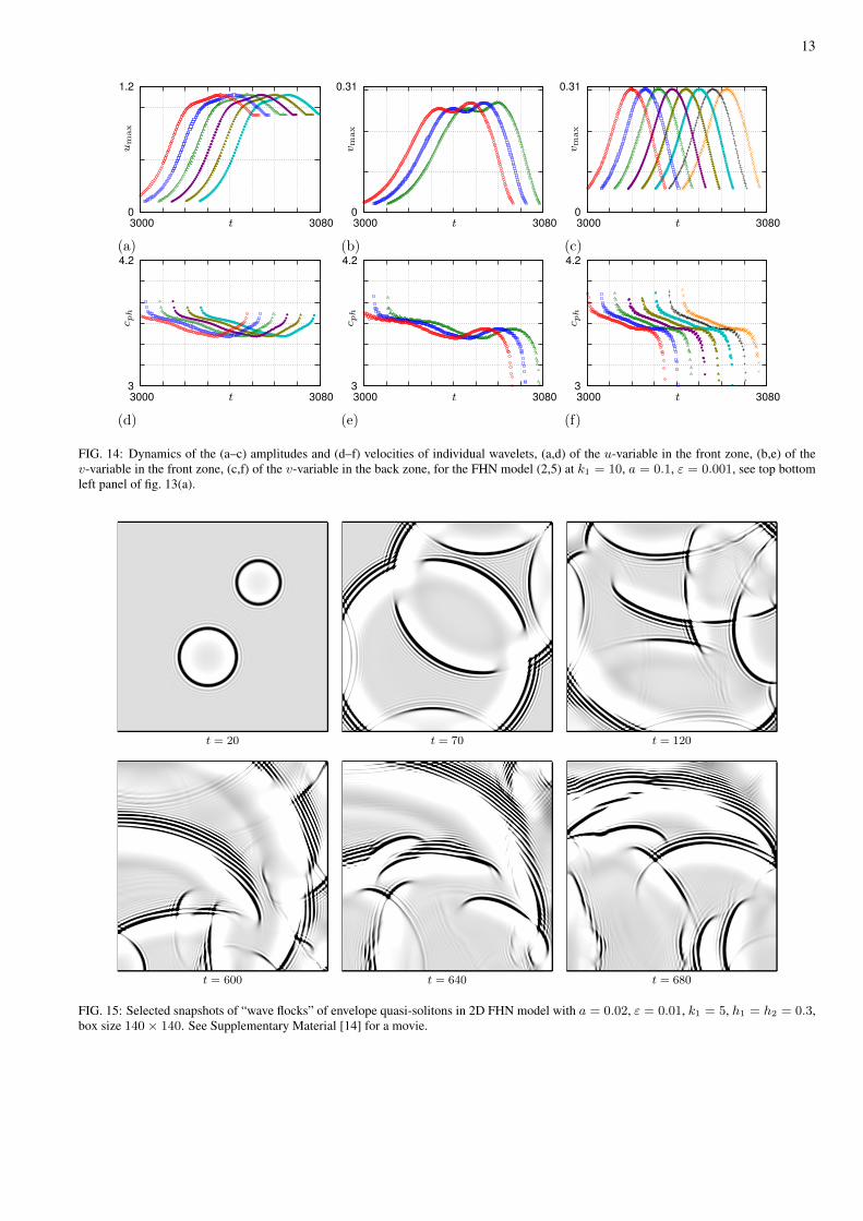
FIG. 14: Dynamics of the (a–c) amplitudes and (d–f) velocities of individual wavelets, (a,d) of the u-variable in the front zone, (b,e) of thev-variable in the front zone, (c,f) of the v-variable in the back zone, for the FHN model (2,5) at k1 = 10, a = 0.1, ε = 0.001, see top bottomleft panel of fig. 13(a).

t = 20 t = 70 t = 120

t = 600 t = 640 t = 680

FIG. 15: Selected snapshots of “wave flocks” of envelope quasi-solitons in 2D FHN model with a = 0.02, ε = 0.01, k1 = 5, h1 = h2 = 0.3,box size 140× 140. See Supplementary Material [14] for a movie.

14

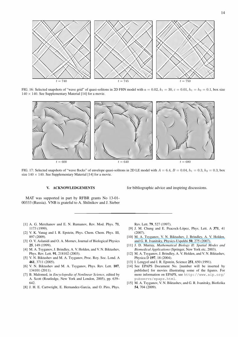
t = 740 t = 745 t = 750

FIG. 16: Selected snapshots of “wave grid” of quasi-solitons in 2D FHN model with a = 0.02, k1 = 30, ε = 0.01, h1 = h2 = 0.1, box size140× 140. See Supplementary Material [14] for a movie.

t = 600 t = 640 t = 680

FIG. 17: Selected snapshots of “wave flocks” of envelope quasi-solitons in 2D LE model with A = 6.4, B = 0.04, h1 = 0.3, h2 = 0.3, boxsize 140× 140. See Supplementary Material [14] for a movie.

V. ACKNOWLEDGEMENTS

MAT was supported in part by RFBR grants No 13-01-00333 (Russia). VNB is grateful to A. Shilnikov and J. Sieber

for bibliographic advice and inspiring discussions.

[1] A. G. Merzhanov and E. N. Rumanov, Rev. Mod. Phys. 71,1173 (1999).

[2] V. K. Vanag and I. R. Epstein, Phys. Chem. Chem. Phys. 11,897 (2009).

[3] O. V. Aslanidi and O. A. Mornev, Journal of Biological Physics25, 149 (1999).

[4] M. A. Tsyganov, J. Brindley, A. V. Holden, and V. N. Biktashev,Phys. Rev. Lett. 91, 218102 (2003).

[5] V. N. Biktashev and M. A. Tsyganov, Proc. Roy. Soc. Lond. A461, 3711 (2005).

[6] V. N. Biktashev and M. A. Tsyganov, Phys. Rev. Lett. 107,134101 (2011).

[7] B. Malomed, in Encyclopedia of Nonlinear Science, edited byA. Scott (Routledge, New York and London, 2005), pp. 639–642.

[8] J. H. E. Cartwright, E. Hernandez-Garcia, and O. Piro, Phys.

Rev. Lett. 79, 527 (1997).[9] J. M. Chung and E. Peacock-Lopez, Phys. Lett. A 371, 41

(2007).[10] M. A. Tsyganov, V. N. Biktashev, J. Brindley, A. V. Holden,

and G. R. Ivanitsky, Physics-Uspekhi 50, 275 (2007).[11] J. D. Murray, Mathematical Biology II: Spatial Modes and

Biomedical Applications (Springer, New York etc, 2003).[12] M. A. Tsyganov, J. Brindley, A. V. Holden, and V. N. Biktashev,

Physica D 197, 18 (2004).[13] I. Lengyel and I. R. Epstein, Science 251, 650 (1991).[14] See EPAPS Document No. [number will be inserted by

publisher] for movies illustrating some of the figures. Formore information on EPAPS, see http://www.aip.org/pubservs/epaps.html.

[15] M. A. Tsyganov, V. N. Biktashev, and G. R. Ivanitsky, Biofizika54, 704 (2009).

15

[16] V. N. Biktashev, A. V. Holden, and E. V. Nikolaev, Int. J. ofBifurcation and Chaos 6, 2433 (1996).

[17] V. N. Biktashev and A. V. Holden, Physica D 116, 342 (1998).[18] P. Chossat, Acta Appplicandae Mathematicae 70, 71 (2002).[19] A. J. Foulkes and V. N. Biktashev, Phys. Rev. E 81, 046702

(2010).[20] L. Shilnikov, Soviet Math. Dokl. 3, 394 (1962), in Russian.[21] L. Shilnikov, Mat. Sbornik 61, 443 (1963), in Russian.[22] S. H. Strogatz, Nonlinear dynamics and chaos : with applica-

tions to physics, biology, chemistry, and engineering (WestviewPress, Cambridge, Mass., 2000).

[23] V. N. Biktashev, J. Brindley, A. V. Holden, and M. A. Tsyganov,Chaos 14, 988 (2004).

[24] V. E. Zakharov and E. A. Kuznetsov, J. Exp. Theor. Phys. 113,1892 (1998).

[25] V. K. Vanag and I. R. Epstein, Phys. Rev. Lett. 88, 088303(2002).

[26] V. K. Vanag and I. R. Epstein, J. Chem. Phys. 121, 890 (2004).[27] N. Manz, B. T. Ginn, and O. Steinbock, Phys. Rev. E 73,

066218 (2006).[28] Y. Kuramoto, Chemical Oscillations, Waves and Turbulence

(Springer-Verlag, Berlin Heidelberg New York Tokyo, 1984).[29] D. A. Korobko, R. Gumenyuk, I. O. Zolotovskii, and O. G.

Okhotnikov, Opt. Fiber Technol. http://dx.doi.org/10.1016/j.yofte.2014.08.011 (2014).

[30] E. S. Lobanova and F. I. Ataullakhanov, 93, 098303 (2004).[31] M. A. Tsyganov, I. B. Kresteva, A. B. Medvinsky, and G. R.

Ivanitsky, Doklady 333, 532 (1993).[32] Y. A. Kuznetsov, M. Antonovsky, V. N. Biktashev, and E. A.

Aponina, J. Math. Biol. 32, 219 (1994).[33] A. S. Dmitrichev, V. I. Nekorkin, R. Behdad, S. Binczak, and

J. M. Bilbault, Eur. Phys. J. Special Topics pp. 2633–2646(2013).