Categorization of 2-photon microscopy images of

human cartilage into states of osteoarthitis

T. Bergmanna,c,∗ , U. Maederb, M. Fiebichb, P. Czermaka, T. Nattkemperd,D. Anselmettic

aUniversity of Applied Sciences Mittelhessen, Institute of Bioprocess Engineering andPharmaceutical Technology, Wiesenstrasse 14, 35390 Giessen, Germany

bUniversity of Applied Sciences Mittelhessen, Institute of Medical Physics andRadiation Protection, Wiesenstrasse 14, 35390 Giessen, Germany

cBielefeld University, Experimental Biophysics, Universitatsstrasse 25, 33615 Bielefeld,Germany

dBielefeld University, Biodata Mining Group, Universitatsstrasse 25, 33615 Bielefeld,Germany

Abstract

The degeneration of articular cartilage is part of the clinical syndrome of os-teoarthritis (OA) and one of the most common causes of pain and disabilityin middle-aged and older people [1]. However, the objective detection of aninitial state of OA is still challenging. In order to categorize cartilage intostates of OA, an algorithm is presented which offers objective categoriza-tion on the basis of 2-photon laser-scanning microscopy (TPLSM) images.The algorithm is based on morphological characteristics of the images andresults in a topographical visualization. This paper describes the algorithmand shows the result of a categorization of human cartilage samples. Theresulting map of the analysis of TPLSM images can be divided into ar-eas which correspond to the grades of the outerbridge categorization. Thealgorithm is able to differentiate the samples in coincidence with the macro-scopic impression. Thus, the method is promising for early OA detectionand categorization. In order to achieve a higher benefit for the physicianthe method must be transferred to an endoscopic setup for an applicationin surgery.

Keywords: cartilage, osteoarthitis, 2-photon microscopy, categorization,wavelet transformation, self-organizing maps

Preprint submitted to Osteoarthritis and Cartilage December 7, 2012

1. Introduction

Articular cartilage lesions generally do not heal or heal partially undercertain biological conditions [2]. Only an early detection of the degener-ation of the extracellular matrix makes it possible to capture retaliatoryaction. Common histologic assessment methods assess poorly early phasesof disease, have wide interobserver variation and are very non-linear overthe range from mild to advanced disease [3]. Macroscopic assessment grad-ing systems are mainly based on the work of Collins [4] and Outerbridge[5] where classification is based on extensive qualitative descriptions of car-tilage surface texture, lesion size and bony changes [3]. The Outerbridgeclassification is recommended for the arthroscopic evaluation of articularcartilage defects [6].

Another common grading system is based on microscopic evaluation ofstained tissue [7]. The study provides a correlation with cartilage biochem-ical changes associated with OA progression.

All these grading systems have in common, that the morphologic appear-ance seen on diagnostic imaging and/or arthroscopy are evaluated by theinvestigator. Nevertheless, a small interobserver variance of investigatorswith varying levels of histopathology experience is worthwhile. Therefore,there is a need for an objective classification tool, which supports the physi-cian by evaluating the diagnostic images.

In order to overcome the lack of objective validation an automated anal-ysis is presented. The analysis is based on fluorescence images which can berecorded via microscope as well as endoscopically. The presented methoduses images taken by a two-photon laser scanning microscope (TPLSM).

Due to the fact, that cartilage is a highly scattering tissue, the penetra-tion depth of optical microscopy techniques is limited. Thus, TPLSM wasused for image acquisition because it is first choice for deep tissue imaging[8]. TPLSM is a 3-dimensional fluorescence microscopy technique and incase of cartilage tissue the fluorescence occurs intrinsically and is thereforecalled autofluorescence. This fact avoids the usage of any staining. Thepenetration depth into tissue is limited to approximately 500 µm becauseof a high scattering coefficient of cartilage tissue. For the detection of early

∗Corresponding authorEmail addresses: thorsten.bergmann@kmub.thm.de (T. Bergmanna,c,∗),

ulf.maeder@kmub.thm.de (U. Maeder), martin.fiebich@kmub.thm.de (M. Fiebich),peter.czermak@kmub.thm.de (P. Czermak), tnattkem@techfak.uni-bielefeld.de(T. Nattkemper), dario.anselmetti@physik.uni-bielefeld.de (D. Anselmetti)

2

changes in the extracellular matrix this limitation does not hamper theanalysis because the first visible signs of OA occur at the surface.

The images of a TPLSM from the cartilage samples of different states ofOA show very varying morphology. They provide a high scalability becausethe macroscopic appearance of the cartilage corresponds well with the mor-phology of the TPLSM images. Thus, a categorization of the images willcorrespond to a categorization of the samples. Nevertheless, it is not thatobvious to transfer the morphology of an image into an objective parameter.For this reason, a classification method with analogies to the classification ofhistopathological images of meningiomas WHO grade I [9] was performed.

In order to characterize the content of an image by numerical imagefeatures, transforms like Fourier or Wavelet Transform are used. Wavelettransform was used for calculation of image features in this analysis. Asa result, each image is represented by a n-dimensional feature vector. Thesubset of feature vectors explores a space of texture features. A Self Organiz-ing Map (SOM) acts as a connector between the texture feature space andthe image characteristics. It is a method that is able to visualize datasets ofhigh dimensionality and furthermore it is able to perform clustering. Theunsupervised learning method reduces the higher dimensional dataset to twodimensions and allocates the images on a map according to their similarityin the feature space.

The success of clustering or categorization depends strongly on the sub-set of selected features. Several features have been analyzed and used forclassification of image textures [10], [11]. Nevertheless, no gold standardof texture features regarding its classification performance was found [12].Thus, the feature selection has to be adapted to each classification problemwith respect to the kind of image, the image morphology and the differencesfor classification.

In this paper, the samples and the image acquisition are described first.Afterwards the feature calculation and selection is shown on basis of thefollowing data visualization and clustering by using SOM. As the final result,a map of the whole dataset is shown, including the classification of thecartilage into states of OA.

2. Methods

2.1. Samples and image acquisition

The cartilage samples originate from a total joint replacement of theknee. The patients were male and female with an age between 50 and

3

80 years. The cartilage samples were transferred to the microscope labfirst after surgery. The samples were categorized by macroscopic investiga-tion into states of OA according to the Outerbridge-Categorization. TheOuterbridge-Categorization consists of five grades. A more comprehensivedescription is given in [13]. A summary of the characteristics of the fivegrades is given in tab. 1.

Samples from every grade could be obtained because the whole kneewas removed during surgery which enabled to get even healthy cartilagesamples. Each sample was categorized macroscopically according to theauthors experience and labeled with the color corresponding to its grade (fig.2). It has to be noticed that the classification algorithm is not based on thisclassification. It helps to understand the allocation of the images withinthe SOM. Grade 4 is left out because the cartilage is nearly completelydegenerated in this state and thus just a very weak fluorescence signal canbe detected. The cartilage samples were imaged via TPLSM as received.They were neither stained nor treated in any other way.

The TPLSM used a 1 W Ti:Sa femtosecond-laser (Tsunami, Spectra-Physics) at 800 nm for the excitation. A beam-multiplexer within a TriM-Scope (LaVision Biotec GmbH) splitted up the beam into 64 single beams.The resulting 64 spots were scanned simultaneously across the sample. Abeamsplitter differentiates the excitation light from the fluorescence lightand a highly sensitive EMCCD-camera (Andor, Ixon) detects the signal(fig. 1). 30 images of every sample were generated, each image representingone z-layer of the tissue with a distance of one µm between each layer.Each image can be treated separately as an individual image. The completedataset consists of 930 individual images.

Grade Outerbridge0 Normal cartilage1 Softening and swelling of the cartilage2 Fragmentation and fissuring in an area 0.5

inches or less in diameter3 Fragmentation and fissuring in an area 0.5

inches or more in diameter4 Erosion of cartilage down to bone

Table 1: Outline of the classification system for OA of the knee (from [13])

4

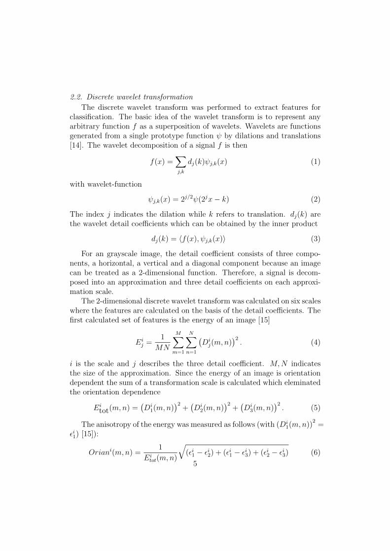
2.2. Discrete wavelet transformation

The discrete wavelet transform was performed to extract features forclassification. The basic idea of the wavelet transform is to represent anyarbitrary function f as a superposition of wavelets. Wavelets are functionsgenerated from a single prototype function ψ by dilations and translations[14]. The wavelet decomposition of a signal f is then

f(x) =∑j,k

dj(k)ψj,k(x) (1)

with wavelet-function

ψj,k(x) = 2j/2ψ(2jx− k) (2)

The index j indicates the dilation while k refers to translation. dj(k) arethe wavelet detail coefficients which can be obtained by the inner product

dj(k) = 〈f(x), ψj,k(x)〉 (3)

For an grayscale image, the detail coefficient consists of three compo-nents, a horizontal, a vertical and a diagonal component because an imagecan be treated as a 2-dimensional function. Therefore, a signal is decom-posed into an approximation and three detail coefficients on each approxi-mation scale.

The 2-dimensional discrete wavelet transform was calculated on six scaleswhere the features are calculated on the basis of the detail coefficients. Thefirst calculated set of features is the energy of an image [15]

Eij =

1

MN

M∑m=1

N∑n=1

(Di

j(m,n))2. (4)

i is the scale and j describes the three detail coefficient. M,N indicatesthe size of the approximation. Since the energy of an image is orientationdependent the sum of a transformation scale is calculated which eleminatedthe orientation dependence

Eitot(m,n) =

(Di

1(m,n))2

+(Di

2(m,n))2

+(Di

3(m,n))2. (5)

The anisotropy of the energy was measured as follows (with (Di1(m,n))

2=

εi1) [15]):

Oriani(m,n) =1

Eitot(m,n)

√(εi1 − εi2) + (εi1 − εi3) + (εi2 − εi3) (6)

5

Thus, the resulting feature vector consists of the following components onsix scales:

Eitot =

1

MN

M∑m=1

N∑n=1

Etot(m,n) (7)

Oriani =1

MN

M∑m=1

N∑n=1

Orian(m,n) (8)

which results in ten features because the Orian(5−6) values were neglected.This set of features is expanded by the normalized mean pixel value

of the original image as an additional feature. The normalization avoidsan intensity measurement rather this feature measures how much cartilagematerial exists within the field of view.

The feature space for the analysis spans a 11-dimensional vector space.

2.3. Self organizing maps

SOM are a kind of artificial neuronal network which organizes itselfunsupervised and was introduced by Kohonen [16]. The SOM defines anelastic net of points that are fitted to the distribution of the training datain the input space [17]. Thus, a multidimensional data set is visualized ona 2-dimensional grid.

The SOM consists of a 2-dimensional lattice of units of artificial neu-rons. First, a model vector mi is created which connects each neuron ofthe lattice with the n-dimensional input space. Afterwards, the trainingphase begins. A winning neuron is evaluated for each input data pointby calculating the distance of the input data point and the neurons of thelattice. Accordingly, the neurons are shifted towards the input data pointcorresponding a weighting function. The winning neuron suffers the longestdistance. This procedure is repeated for every datapoint in every trainingstep. Thus, the map attempts to represent all the available observations xwith optimal accuracy by using the map units as a restricted set of models.During the training phase, the model become ordered on the grid so thatsimilar models are close to and dissimilar models far from each other.

The discrete wavelet analysis produces data and spans a 11-dimensionalvector space which characterizes the input data. Nevertheless, these datahave to be interpreted in a way, that similar images or feature vectors aredetected as one group or cluster. Thus, the first goal of the algorithm isthe correlation between the 11-dimensional input space X ⊂ RN and a

6

set of neurons of a low-dimensional space M ⊂ RM (with M = 1, 2) [18].Second, the algorithm has to work unsupervised and the resulting map hasto represent the input-space topologically correct (3).

The input space consists of 930 data points which corresponds to thenumber of images. Each image is analyzed by discrete wavelet transformand thus a 11-dimensional feature-vector represents each image. After ini-tializing the SOM and training the dataset is represented by the referencevectors (neurons) of the SOM. Each image can be allotted to a accordingneuron and displayed at the corresponding neuron within the map. Thus,a map can be generated where every neuron is represented by the originalimage. This kind of map provides a good overview of the topographicalclustering. Furthermore, the SOM can be displayed by using a hinton dia-gram. Every image which is located at a neuron is displayed as a quad. Themore images fall on this neuron, the bigger the quad gets. By connectingan image to a color, the quad can be displayed with this color. This enablesthe tracking of images and investigation of a group of images.

3. Results

The discrete wavelet analysis was performed with the whole set of 930images. A SOM with 64 neurons was trained in 300 training steps. The dataare displayed in different ways to get an impression of the data structureand the clustering performance of the algorithm.

Figure 4 shows the map as a hinton diagramm. The more data pointsare connected to a neuron, the bigger this neuron is displayed. In orderto visualize the outerbridge classification the data have to be labeled first.This makes it possible to identify the data within the resulting map. Theused color code corresponds to fig. 2. The images of each category are nowvisualized within the hit statistic in the color belonging to the category.Thus, it is possible to locate the individual categories. The result is shownin fig 4. The healthy cartilage (grade 0) is displayed in green and locatedmostly in the lower left corner. Grade 1 in yellow is located basically in thelower right corner, grade 2 in blue in the upper right corner and the mostdegenerated one, grade 3 in red is mainly in the upper left corner. Thismeans, that the progress of the degeneration of the cartilage is documentedon the map from the lower left corner to the upper left corner anti-clockwise.

It becomes apparent that the analysis clusters the images with smoothtransition between the outbridge grades. Thus, the images were integrated

7

into the map to visualize the kind of differentiation of the images. Addition-ally, the winning grade or color was estimated for every neuron of the map.The grade with most images at one neuron wins a neuron and is colored,respectively. The result is shown in figure 5.

It has to be mentioned that the hit-statistic (fig. 4) does not only colorthe winning neuron. In fact, the neurons are colored according a gaussfunction around the winning neuron. As a consequence, the categories aredistributed on a larger area on the map. The reason to represent the datathis way becomes clear by looking at the map in figure 5. There is one emptyframe which corresponds to a neuron which is not connected to an image.Consequently, this neuron can not be labeled with a winning category. Bychoosing the hit statistic in fig. 4 it becomes clear that the red categorywins this neuron.

The structure with the anti-clockwise location of the different grades ismaintained in fig. 5. There are only two neurons in which the winning gradedoes not belong to the expected grade (lower left corner). Nevertheless, alook at the images at this neurons points out that the images are locatedright regarding their morphology.

After the establishment of this classification system it has to be vali-dated. Thus, the classification was proven by comparing the macroscopicdetermined grade of the cartilage and the automatically determined gradeof the TPLSM images. Samples of each grade were chosen and categorized.Afterwards, TPLSM images were generated at the same location at the car-tilage sample and analyzed by using the algorithm. The total amount ofimages for validation was 41. The corresponding images are merged in fig.6.

The main goal of the algorithm based on microscopic images was thedetection of the early changes of the extracellular matrix when an OA be-gins. Thus, the sensitivity and the specificy were determined because theseparameters only take healthy and arthritic cartilage into account. The re-sult of the validation was a sensitivity of 0,88 and a specificy of 0,93. Thesevalues have to be treated carefully because of the small amount of sampleswhich contributed to this calculation.

4. Discussion

In this paper, an algorithm for the classification of cartilage into statesof OA was presented. The algorithm works with TPSLM images und usesdiscrete wavelet transformation to determine image features. Afterwards,

8

SOM‘s were used for dimension reduction and visualization of the multidi-mensional data set.

The result was a data set which represented a wide spectrum of OAstates and the outerbridge classification of the samples were approved. Fur-thermore, the validation of the analysis resulted in good values for the sen-sitivity and specificy. These results are promising for further developmentsfor early OA detection.

The fact that the samples have to be imaged ex-vivo with a 2-photonmicroscope hampers the integration of the method into the daily routineof early OA detection. Nevertheless, there are proposals to get access toendoscopical 2-photon microscope images [19], [20].

The presented analysis method is not restricted to TPLSM images. Dueto the fact, that optical coherence tomography (OCT) provides a high pen-etration depth [21] it is used for arthroscopic diagnosis of early arthritis[22]. Nevertheless, the images of OCT systems typically show the xz-planein comparison to the xy-plane of the TPLSM images, it seems to be possibleto adapt the algorithm to this acquisition technique.

The presented method holds the potential to support the physician inearly OA detection by providing an objective parameter. The parametercould be the automatic determined grade of the cartilage, a position withinthe map or simply a sign whether the cartilage is healthy or not. As men-tioned before, even early states of OA can be detected. This result shouldbe considered as an assistance for the physician in addition to other ex-amination methods and his individual experience. By taking an objectiveparameter into account, the interobserver variance can be minimized. Byintegrating a fiber-based fluorescence microscope into existing arthrosopictools, no additional examination is necessary. Then, the physician gets twoadditional information of the cartilage. One the one hand the TPLSM imageitself (surface and depth information) and on the other hand the objectiveparameter of the automated analysis. The time for the investigation extendsinsignificant. Furthermore, the results are available within seconds.

The results of the presented study are very promising. Nevertheless, themethod has to be proven with a greater amount of samples to fulfill twopurposes. First, the database for the generation of the SOM and thereforethe classification has to be extended. Hence, the classification becomesmore precise and reliable. Second, the validation of the data becomes moredetailed and precise. A prototype with endoscopic imaging would be veryassistant to achieve those objectives.

9

Several endoscopic OCT systems are mentioned in literature e.g. [23]with applications in urology and gastroenterology. These examples show,that the clinical usage of these systems are on the rise. Thus, a clinicalapplication of the presented analysis method is also possible for the nearfuture.

References

[1] J. Buckwalter, H. Mankin, Instr Course Lect. 47 (1998) 487–504.[2] E. Hunziker, Osteoarthritis and Cartilage 10 (2001) 432–463.[3] K. Pritzker, S. Gay, S. Jimenez, K. Ostergaard, J.-P. Pelletier, P. Revell, D. Salter,

W. van den Berg, Osteoarthritis and Cartilage 14 (2006) 13–29.[4] D. Collins, The pathology of articular and spinal disease Edward Arnold & Co,

London (1949) 74–115.[5] R. Outerbridge, A. Ellermann, J Bone Joint Surg Br 43-B (1961) 752–757.[6] L. Boes, A. Ellermann, Arthroskopische Diagnostik (2003).[7] H. Mankin, H. Dorfman, L. Lipiello, A. Zarins, J Bone Joint Surg 53A (1971) 523–

537.[8] F. Helmchen, W. Denk, Nature methods 2 (2005) 932–940.[9] B. Lessmann, N. T.W., H. V.H., D. A, Journal of biomedical informatics 40 (2007)

631–641.[10] T. Chang, C.-C. Kuo, IEEE Transactions on Image Processing 2 (1993) 429–441.[11] G. van de Wouwer, P. Scheunders, D. van Dyck, IEEE Transactions on Image Pro-

cessing 8 (1993) 592–598.[12] T. Randen, J. Husoy, IEEE Transactions on Pettern Analysis and Machine Intelli-

gence 21 (1999) 291–310.[13] B. Brismar, T. Wredmark, T. Movin, J. Leandersson, O. Svensson, J Bone Joint

Surg 84-B (2001) 42–47.[14] H. Li, B. Manjunath, S. Mitra, Graphical models and image processing 57-3 (1995)

235–245.[15] S. Livans, P. Scheunders, D. van de Wouwer, D. Dyck, J. Smets, W. Winkelmanns,

W. Bogaerts, Microscopy, Microanalysis, Microstructures 7 (1996) 1–10.[16] T. Kohonen, Biological Cybernetics 43 (1982) 59–69.[17] J. Laaksonen, M. Kosela, S. Laakso, E. Oja, Pattern Analysis and Applications 23

(2001) 140–152.[18] T. Kohonen, Self-organizing maps, Springer Series in Information Sciences, Berlin

Heidelberg New York, 3. edition, 2001.[19] W. Goebel, J. Kerr, A. Nimmerjahn, F. Helmchen, Optics letters 29 (2004) 2521–

2523.[20] B. Flusberg, E. Cocker, W. Piyawattanametha, J. Jung, E. Cheung, M. Schnitzer,

Nature methods 2 (2005) 941–950.[21] C. Blatter, J. Weingast, A. Alex, B. Grajciar, W. Wieser, W. Drexler, R. Huber,

R. Leitgeb, Biomed. Opt. Express 3 (2012) 2636–2646.[22] A. O Malley, C. Chu, Minimally Inavasive Surgery 2011 (2011) 1–6.[23] E. Zagaynoca, N. Gladkova, N. Shakhova, G. Gelikonov, V. Gelikonov, J. Biopho-

tonics 1 (2008) 114–128.10

Figure 1: Setup of the TPLSM microscope: 1) Ti:Sa-laser; 2) polarizer/analyzer, beamexpander; 3) prism compressor; 4) beam multiplexer; 5) scanning mirrors; 6) beam ex-pander; 7) microscope objective; 8) dichroic mirror; 9) filter-wheel, EMCCD-camera; 10)photomultiplyer

11

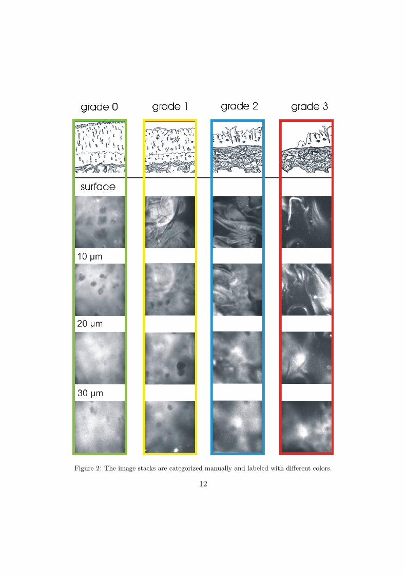
Figure 2: The image stacks are categorized manually and labeled with different colors.

12

Figure 3: Wavelet analysis of the TPLSM images of human cartilage and visualizationwithin the SOM map.

13

Figure 4: The different grades are tracked with a hit-statistic and displayed in congruentcolors. The SOM shows four different cluster, each cluster locataed in approximately onequarter of the map. The degeneration process advance from healthy cartilage (lower leftarea in green) anti-clockwise to grade 3 (upper left area in red).

14

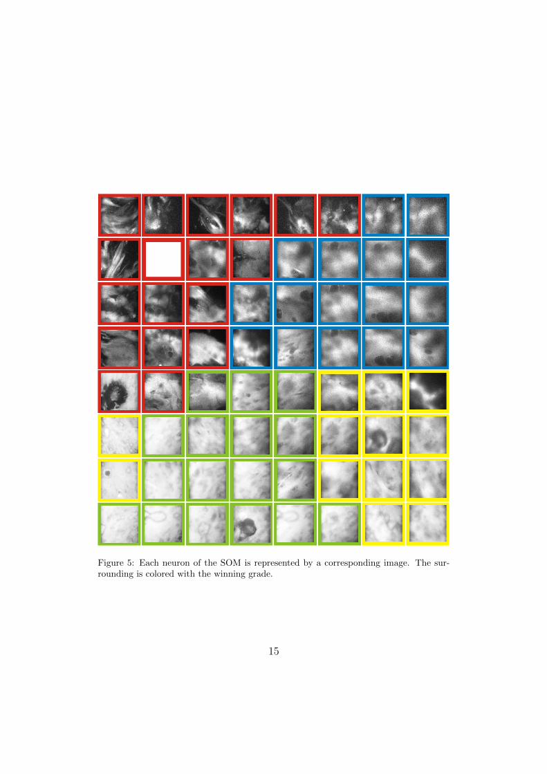
Figure 5: Each neuron of the SOM is represented by a corresponding image. The sur-rounding is colored with the winning grade.

15

Figure 6: The validation shows good compliance of the macroscopic classification andthe automatic classification algorithm.

16