PHYSICAL REVIEW MATERIALS 5, 055603 (2021)

Capillary control of collapse in soft composite columns

Marc Suñé *

Nordita, Royal Institute of Technology and Stockholm University, Hannes Alfvéns väg 12, SE-106 91 Stockholm, Sweden

John S. Wettlaufer †

Yale University, New Haven, Connecticut 06520, USAand Nordita, Royal Institute of Technology and Stockholm University, Hannes Alfvéns väg 12, SE-106 91 Stockholm, Sweden

(Received 28 May 2020; revised 29 January 2021; accepted 23 April 2021; published 20 May 2021)

Euler buckling is the elastic instability of a column subjected to longitudinal compression forces at itsends. The buckling instability occurs when the compressing load reaches a critical value, and an infinitesimalfluctuation leads to a large amplitude deflection. Since Euler’s original study, this process has been extensivelyexamined in homogeneous, isotropic, linear-elastic solids. Here, we examine the nature of the buckling ininhomogeneous soft composite materials. In particular, we consider a soft host with liquid inclusions bothlarge and small relative to the elastocapillarity length, which lead to softening and stiffening, respectively, ofa homogeneous composite. However, by imposing a gradient of the inclusion volume fraction or by varying theinclusion size we can deliberately manipulate the spatial structure of the composite properties of a column andthereby control the nature of Euler buckling.

DOI: 10.1103/PhysRevMaterials.5.055603

I. INTRODUCTION

An elastic beam under a sufficiently large compressible ax-ial load collapses or buckles when an infinitesimal deflectiondestroys the equilibrium. The critical load for the bucklingof homogeneous, isotropic, linear-elastic rods with a constantcross section was derived by Euler in 1744 [1,2], and La-grange analyzed the higher-order modes in 1770 [3]. From themechanical failure of structural elements in civil engineeringto the storage of information through controlled buckling ofnanoscale beams for future nanomechanical computing [4],the buckling of slender structures has been a focus of studiesin engineering, biology, and physics for nearly 300 yr [5].

The macroscopic response of a solid body to an exter-nal force lies at the heart of buckling, the details of whichdepend on the body shape, material composition, and inter-nal structure. A vast range of distinct responses is displayedin materials with geometric inclusions of different elasticmoduli [6], foams modeled by anisotropic Kelvin cells [7],porous and particle-reinforced hyperelastic solids with cir-cular inclusions of variable stiffness [8], fiber-reinforcedelastomers with incompressible Neo-Hookean phases [9],long cylindrical shells with localized imperfections [10],

*marc.sune.simon@su.se†john.wettlaufer@su.se; john.wettlaufer@yale.edu

Published by the American Physical Society under the terms of theCreative Commons Attribution 4.0 International license. Furtherdistribution of this work must maintain attribution to the author(s)and the published article’s title, journal citation, and DOI. Fundedby Bibsam.

finitely strained porous elastomers [11], and hyperelasticcylindrical shells [12] to mention but a few. Attempts todescribe buckling have lead to, among other things, thecelebrated theory of elasticity [5,13] and to finite-elementsimulation methods [14].

Kirchhoff [15,16] and Clebsch [17,18] described the basictheoretical analysis of elastic rods by replacing the stressacting inside a volume element with a resultant force andthe moment vectors attached to a body defining curve. These“Kirchhoff equations” relate the averaged forces and momentsto the curve’s strains, e.g., Ref. [19].

Recent work shows how the elastic response of softmaterials with liquid inclusions is governed by interfacialstresses [20–23] and suggests the possibility that capillaritymay play an important role in buckling instabilities. To thatend, we reformulate the study of compressed rods viewedfrom the perspective of the theory of elasticity [5,13] to ac-count for the surface tension effects of the inclusions. Weincorporate the physics of capillarity into the Kirchhoff equa-tions through the elastic moduli as given by a generalizationof the Eshelby and Peierls theory of inclusions [22–24]. Thetheory of Eshelby and Peierls describes how an inclusion ofone elastic material deforms when it is embedded in an elastichost matrix [25]. However, it has recently been discoveredthat Eshelby and Peierls inclusion theory breaks down whenthe inclusion size R approaches the elastocapillary lengthL ≡ γ /E , where γ is the inclusion/host surface tension and Eis the host Young’s modulus [22–24]. Importantly, when R >

L (R < L) the composite softens (stiffens). This basic physi-cal process, wherein the inclusion size controls the Young’smodulus of the the composite Ec reveals the possibility ofcontrolling the buckling process through the properties anddistribution of the inclusions.

2475-9953/2021/5(5)/055603(13) 055603-1 Published by the American Physical Society

MARC SUÑÉ AND JOHN S. WETTLAUFER PHYSICAL REVIEW MATERIALS 5, 055603 (2021)

A quantitative treatment of how the inclusion size R andvolume fraction φ in soft composites influences their bulkmechanical properties underlies our understanding of theirresponse under loads. In particular, by determining how thespatial variation of R and φ modify Euler buckling weprovide a framework of either tailoring a material responseor explaining observations in naturally occurring soft com-posites. Canonical examples of the latter include slendercomposite structures, such as insect extremities [26,27], plantstems [28,29], bones [30], bacterial biofilaments [31], andplant tendrils [32]. Indeed, these latter systems [31,32] veryoften grow into axisymmetric elongated structures by addingnew material at a small active growing zone located near thetip, creating a varying composition along the growth axis.

Although our analysis is confined to static elastic Kirchhoffrods, our results are clearly of use in interpreting the bucklinginstabilities prompted by tip growth [33,34] as well as thephenomenon of morphoelasticity induced by time-dependentcompression [35,36].

The paper is organized as follows. In Sec. II, we: (i) reviewthe general concepts of the Kirchhoff rod theory and thesmall deflection approximation; (ii) introduce some conceptsof static stability; and (iii) describe the models of compositemechanics that are used throughout the paper. In Sec. III,we outline classical Euler buckling of homogeneous rods,and then in Sec. IV, we examine in detail the buckling ofinhomogeneous composite materials. In particular, we: (i) de-scribe the stability analysis; (ii) study stiffened and softenedcomposites; (iii) quantify the effect of inhomogeneity on thecritical compression; and (iv) consider the case with a “polar”inclusion configuration. Conclusions and implications for ex-perimental examination of our results are presented in Sec. V.

II. PRELIMINARIES

In this section, we formulate the equilibrium configura-tions of inhomogeneous compressed rods in terms of planarelastica, we derive the corresponding approximation of smalldeflections, we introduce the key concepts of static stability ofelastic rods adapted to the particular case at hand, we reviewthe generalized Eshelby and Peierls theories for compositeelastic materials with capillary effects, and we describe thenondimensionalization of the problem.

A. The planar equilibrium

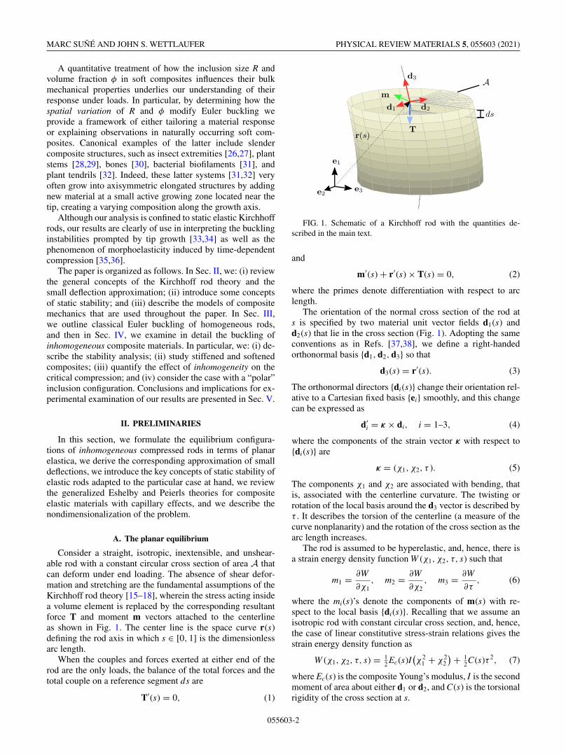
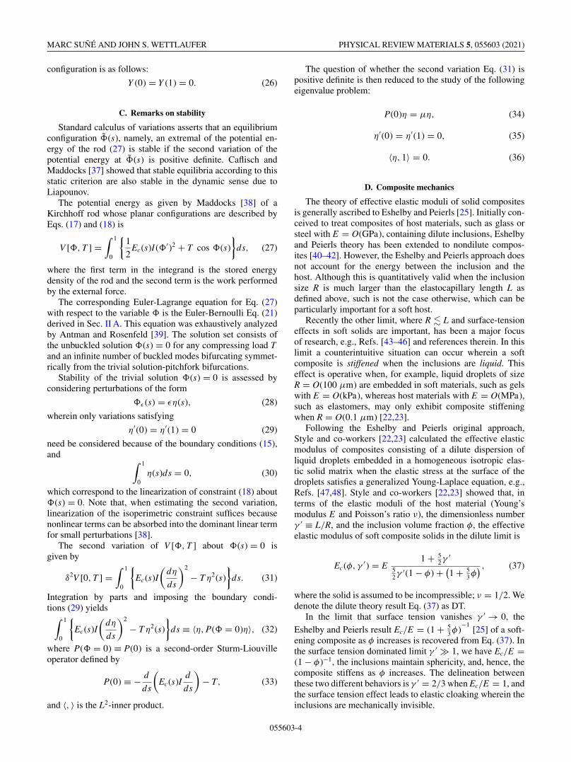
Consider a straight, isotropic, inextensible, and unshear-able rod with a constant circular cross section of area A thatcan deform under end loading. The absence of shear defor-mation and stretching are the fundamental assumptions of theKirchhoff rod theory [15–18], wherein the stress acting insidea volume element is replaced by the corresponding resultantforce T and moment m vectors attached to the centerlineas shown in Fig. 1. The center line is the space curve r(s)defining the rod axis in which s ∈ [0, 1] is the dimensionlessarc length.

When the couples and forces exerted at either end of therod are the only loads, the balance of the total forces and thetotal couple on a reference segment ds are

T′(s) = 0, (1)

FIG. 1. Schematic of a Kirchhoff rod with the quantities de-scribed in the main text.

and

m′(s) + r′(s) × T(s) = 0, (2)

where the primes denote differentiation with respect to arclength.

The orientation of the normal cross section of the rod ats is specified by two material unit vector fields d1(s) andd2(s) that lie in the cross section (Fig. 1). Adopting the sameconventions as in Refs. [37,38], we define a right-handedorthonormal basis {d1, d2, d3} so that

d3(s) = r′(s). (3)

The orthonormal directors {di(s)} change their orientation rel-ative to a Cartesian fixed basis {ei} smoothly, and this changecan be expressed as

d′i = κ × di, i = 1–3, (4)

where the components of the strain vector κ with respect to{di(s)} are

κ = (χ1, χ2, τ ). (5)

The components χ1 and χ2 are associated with bending, thatis, associated with the centerline curvature. The twisting orrotation of the local basis around the d3 vector is described byτ . It describes the torsion of the centerline (a measure of thecurve nonplanarity) and the rotation of the cross section as thearc length increases.

The rod is assumed to be hyperelastic, and, hence, there isa strain energy density function W (χ1, χ2, τ, s) such that

m1 = ∂W

∂χ1, m2 = ∂W

∂χ2, m3 = ∂W

∂τ, (6)

where the mi(s)’s denote the components of m(s) with re-spect to the local basis {di(s)}. Recalling that we assume anisotropic rod with constant circular cross section, and, hence,the case of linear constitutive stress-strain relations gives thestrain energy density function as

W (χ1, χ2, τ, s) = 12 Ec(s)I

(χ2

1 + χ22

) + 12C(s)τ 2, (7)

where Ec(s) is the composite Young’s modulus, I is the secondmoment of area about either d1 or d2, and C(s) is the torsionalrigidity of the cross section at s.

055603-2

CAPILLARY CONTROL OF COLLAPSE IN SOFT … PHYSICAL REVIEW MATERIALS 5, 055603 (2021)

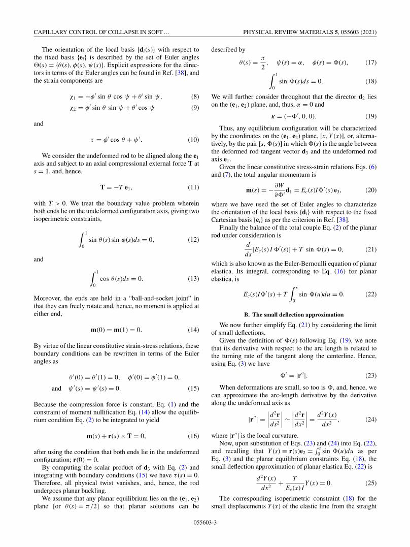
The orientation of the local basis {di(s)} with respect tothe fixed basis {ei} is described by the set of Euler angles�(s) = {θ (s), φ(s), ψ (s)}. Explicit expressions for the direc-tors in terms of the Euler angles can be found in Ref. [38], andthe strain components are

χ1 = −φ′ sin θ cos ψ + θ ′ sin ψ, (8)

χ2 = φ′ sin θ sin ψ + θ ′ cos ψ (9)

and

τ = φ′ cos θ + ψ ′. (10)

We consider the undeformed rod to be aligned along the e1

axis and subject to an axial compressional external force T ats = 1, and, hence,

T = −T e1, (11)

with T > 0. We treat the boundary value problem whereinboth ends lie on the undeformed configuration axis, giving twoisoperimetric constraints,

∫ 1

0sin θ (s) sin φ(s)ds = 0, (12)

and

∫ 1

0cos θ (s)ds = 0. (13)

Moreover, the ends are held in a “ball-and-socket joint” inthat they can freely rotate and, hence, no moment is applied ateither end,

m(0) = m(1) = 0. (14)

By virtue of the linear constitutive strain-stress relations, theseboundary conditions can be rewritten in terms of the Eulerangles as

θ ′(0) = θ ′(1) = 0, φ′(0) = φ′(1) = 0,

and ψ ′(s) = ψ ′(s) = 0. (15)

Because the compression force is constant, Eq. (1) and theconstraint of moment nullification Eq. (14) allow the equilib-rium condition Eq. (2) to be integrated to yield

m(s) + r(s) × T = 0, (16)

after using the condition that both ends lie in the undeformedconfiguration; r(0) = 0.

By computing the scalar product of d3 with Eq. (2) andintegrating with boundary conditions (15) we have τ (s) = 0.Therefore, all physical twist vanishes, and, hence, the rodundergoes planar buckling.

We assume that any planar equilibrium lies on the (e1, e2)plane [or θ (s) = π/2] so that planar solutions can be

described by

θ (s) = π

2, ψ (s) = α, φ(s) = �(s), (17)

∫ 1

0sin �(s)ds = 0. (18)

We will further consider throughout that the director d2 lieson the (e1, e2) plane, and, thus, α = 0 and

κ = (−�′, 0, 0). (19)

Thus, any equilibrium configuration will be characterizedby the coordinates on the (e1, e2) plane, [x,Y (x)], or, alterna-tively, by the pair [s,�(s)] in which �(s) is the angle betweenthe deformed rod tangent vector d3 and the undeformed rodaxis e1.

Given the linear constitutive stress-strain relations Eqs. (6)and (7), the total angular momentum is

m(s) = − ∂W

∂�′ d1 = Ec(s)I�′(s) e3, (20)

where we have used the set of Euler angles to characterizethe orientation of the local basis {di} with respect to the fixedCartesian basis {ei} as per the criterion in Ref. [38].

Finally the balance of the total couple Eq. (2) of the planarrod under consideration is

d

ds[Ec(s) I �′(s)] + T sin �(s) = 0, (21)

which is also known as the Euler-Bernoulli equation of planarelastica. Its integral, corresponding to Eq. (16) for planarelastica, is

Ec(s)I�′(s) + T∫ s

0sin �(u)du = 0. (22)

B. The small deflection approximation

We now further simplify Eq. (21) by considering the limitof small deflections.

Given the definition of �(s) following Eq. (19), we notethat its derivative with respect to the arc length is related tothe turning rate of the tangent along the centerline. Hence,using Eq. (3) we have

�′ = |r′′|. (23)

When deformations are small, so too is �, and, hence, wecan approximate the arc-length derivative by the derivativealong the undeformed axis as

|r′′| =∣∣∣∣d2rds2

∣∣∣∣ ∼∣∣∣∣d2rdx2

∣∣∣∣ = d2Y (x)

dx2, (24)

where |r′′| is the local curvature.Now, upon substitution of Eqs. (23) and (24) into Eq. (22),

and recalling that Y (s) ≡ r(s)e2 = ∫ s0 sin �(u)du as per

Eq. (3) and the planar equilibrium constraints Eq. (18), thesmall deflection approximation of planar elastica Eq. (22) is

d2Y (x)

dx2+ T

Ec(x) IY (x) = 0. (25)

The corresponding isoperimetric constraint (18) for thesmall displacements Y (x) of the elastic line from the straight

055603-3

MARC SUÑÉ AND JOHN S. WETTLAUFER PHYSICAL REVIEW MATERIALS 5, 055603 (2021)

configuration is as follows:

Y (0) = Y (1) = 0. (26)

C. Remarks on stability

Standard calculus of variations asserts that an equilibriumconfiguration �(s), namely, an extremal of the potential en-ergy of the rod (27) is stable if the second variation of thepotential energy at �(s) is positive definite. Caflisch andMaddocks [37] showed that stable equilibria according to thisstatic criterion are also stable in the dynamic sense due toLiapounov.

The potential energy as given by Maddocks [38] of aKirchhoff rod whose planar configurations are described byEqs. (17) and (18) is

V [�, T ] =∫ 1

0

{1

2Ec(s)I (�′)2 + T cos �(s)

}ds, (27)

where the first term in the integrand is the stored energydensity of the rod and the second term is the work performedby the external force.

The corresponding Euler-Lagrange equation for Eq. (27)with respect to the variable � is the Euler-Bernoulli Eq. (21)derived in Sec. II A. This equation was exhaustively analyzedby Antman and Rosenfeld [39]. The solution set consists ofthe unbuckled solution �(s) = 0 for any compressing load Tand an infinite number of buckled modes bifurcating symmet-rically from the trivial solution-pitchfork bifurcations.

Stability of the trivial solution �(s) = 0 is assessed byconsidering perturbations of the form

�ε (s) = εη(s), (28)

wherein only variations satisfying

η′(0) = η′(1) = 0 (29)

need be considered because of the boundary conditions (15),and ∫ 1

0η(s)ds = 0, (30)

which correspond to the linearization of constraint (18) about�(s) = 0. Note that, when estimating the second variation,linearization of the isoperimetric constraint suffices becausenonlinear terms can be absorbed into the dominant linear termfor small perturbations [38].

The second variation of V [�, T ] about �(s) = 0 isgiven by

δ2V [0, T ] =∫ 1

0

{Ec(s)I

(dη

ds

)2

− T η2(s)

}ds. (31)

Integration by parts and imposing the boundary condi-tions (29) yields∫ 1

0

{Ec(s)I

(dη

ds

)2

− T η2(s)

}ds ≡ 〈η, P(� = 0)η〉, (32)

where P(� = 0) ≡ P(0) is a second-order Sturm-Liouvilleoperator defined by

P(0) ≡ − d

ds

(Ec(s)I

d

ds

)− T, (33)

and 〈, 〉 is the L2-inner product.

The question of whether the second variation Eq. (31) ispositive definite is then reduced to the study of the followingeigenvalue problem:

P(0)η = μη, (34)

η′(0) = η′(1) = 0, (35)

〈η, 1〉 = 0. (36)

D. Composite mechanics

The theory of effective elastic moduli of solid compositesis generally ascribed to Eshelby and Peierls [25]. Initially con-ceived to treat composites of host materials, such as glass orsteel with E = O(GPa), containing dilute inclusions, Eshelbyand Peierls theory has been extended to nondilute compos-ites [40–42]. However, the Eshelby and Peierls approach doesnot account for the energy between the inclusion and thehost. Although this is quantitatively valid when the inclusionsize R is much larger than the elastocapillary length L asdefined above, such is not the case otherwise, which can beparticularly important for a soft host.

Recently the other limit, where R � L and surface-tensioneffects in soft solids are important, has been a major focusof research, e.g., Refs. [43–46] and references therein. In thislimit a counterintuitive situation can occur wherein a softcomposite is stiffened when the inclusions are liquid. Thiseffect is operative when, for example, liquid droplets of sizeR = O(100 μm) are embedded in soft materials, such as gelswith E = O(kPa), whereas host materials with E = O(MPa),such as elastomers, may only exhibit composite stiffeningwhen R = O(0.1 μm) [22,23].

Following the Eshelby and Peierls original approach,Style and co-workers [22,23] calculated the effective elasticmodulus of composites consisting of a dilute dispersion ofliquid droplets embedded in a homogeneous isotropic elas-tic solid matrix when the elastic stress at the surface of thedroplets satisfies a generalized Young-Laplace equation, e.g.,Refs. [47,48]. Style and co-workers [22,23] showed that, interms of the elastic moduli of the host material (Young’smodulus E and Poisson’s ratio ν), the dimensionless numberγ ′ ≡ L/R, and the inclusion volume fraction φ, the effectiveelastic modulus of soft composite solids in the dilute limit is

Ec(φ, γ ′) = E1 + 5

2γ ′52γ ′(1 − φ) + (

1 + 53φ

) , (37)

where the solid is assumed to be incompressible; ν = 1/2. Wedenote the dilute theory result Eq. (37) as DT.

In the limit that surface tension vanishes γ ′ → 0, theEshelby and Peierls result Ec/E = (1 + 5

3φ)−1

[25] of a soft-ening composite as φ increases is recovered from Eq. (37). Inthe surface tension dominated limit γ ′ 1, we have Ec/E =(1 − φ)−1, the inclusions maintain sphericity, and, hence, thecomposite stiffens as φ increases. The delineation betweenthese two different behaviors is γ ′ = 2/3 when Ec/E = 1, andthe surface tension effect leads to elastic cloaking wherein theinclusions are mechanically invisible.

055603-4

CAPILLARY CONTROL OF COLLAPSE IN SOFT … PHYSICAL REVIEW MATERIALS 5, 055603 (2021)

Two approaches have been used to treat the nondilutelimit. In the first, Mancarella et al. [49], and Mancarella andWettlaufer [50] used a three-phase generalized self-consistent(GSC) theory, which replaces the actual inclusions by com-posite spheres. In the second, Mancarella et al. [24] (MSW)extended the multiphase scheme of Mori and Tanaka [51] totreat the fluid inclusions in the solid matrix—with isotropicinterfacial tension—as elastic inclusions with no interfacialtension. Although both the GSC and the MSW approachesrecover Eq. (37) in the dilute limit; the results of the formerare too cumbersome for incorporation into the buckling ofcomposite rods we study here. Therefore, we use the MSWapproach for which the effective Young’s modulus of thecomposite is

Ec(φ, γ ′) = E2 − 2φ + γ ′(5 + 3φ)

2 + (4/3) φ + γ ′(5 − 2φ), (38)

in which the transition between stiffening and softening atγ ′ = 2/3 is the same value as for the DT expression Eq. (37).Therefore, we will use the effective composite Young’s mod-uli in Eqs. (37) and (38) in our analysis of the collapse ofcomposite columns.

E. Scaling

We note that because of the inextensibility of the rod, fromthe outset the arc-length s has been dimensionless. In orderto avoid clutter in notation, the other independent variablesmass (m∗), space (x∗), and time (t∗) were not labeled in theusual manner (e.g., with a superscript ∗) to distinguish thatthey carried dimensions. We now render them dimensionlessas follows:

m = m∗

ρ√AI

, x = x∗√

I/Aand t = t∗

√ρI/AE

, (39)

where ρ is the mass per unit reference volume, A denotesthe rod cross-sectional area, and E is the Young’s modulusof the host matrix as above so that the dimensionless com-posite Young’s modulus is Erel(s) = Ec(s)/E and, hence, thedimensionless force is � = T/(E A).

Under this rescaling, the small-deflection equilibriumEq. (25) is given by

d2Y (x)

dx2+ �

Erel(x)Y (x) = 0. (40)

III. BUCKLING OF HOMOGENEOUS COMPOSITE RODS

The classical Euler buckling problem [1] treats a com-pressed homogeneous rod (Erel = constant) as a boundary-value problem for the small-deflection Euler-Bernoulli equa-tion Eq. (40) with Dirichlet boundary conditions. The trivialsolution Y (x) = 0 corresponds to the undeformed rod. How-ever, such a configuration is only stable if the compressingforce � is less than the critical value �cr [1],

�cr = π2Erel, (41)

which corresponds to the smallest nonzero eigenvalue of theDirichlet problem. At the critical compression a first bifurca-tion of the solution is encountered: The unbuckled solution

becomes unstable, and two buckled stable symmetric config-urations appear

Y (x) ∝ ± sin(πx). (42)

Beyond the bifurcation, that is, for � > �cr, the solu-tion can be computed explicitly because the Euler-BernoulliEq. (21) is integrable. The solutions of the nonlinear Kirchhoffequations are beyond the scope of this paper. Here we treatthe isoperimetric linearized planar elastica Eq. (40), whoseeigenvalues,

�(n)cr = (nπ )2Erel, n = 1, 2, . . . (43)

describe the bifurcation points. The associated buckled con-figurations are described by the corresponding eigenfunctions,

Yn(x) ∝ ± sin(nπx). (44)

IV. BUCKLING OF INHOMOGENEOUS COMPOSITES

Given the expressions for the effective Young’s modulus ofa soft composite Eqs. (37) and (38) an axially inhomogeneouselastic modulus can be constructed by varying either the in-clusion volume fraction φ(x) or the ratio of the elastocapillarylength to the inclusion radius γ ′(x) ≡ L/R(x) both of whichwe discuss presently.

A linear inclusion volume fraction profile,

φ(x) = φ0(1 − x), (45)

where φ(x = 0) ≡ φ0 leads to the bulk modulus decreasing(γ ′ > 2/3) or increasing (γ ′ < 2/3) with the distance alongthe column.

A linear variation in γ ′(x),

γ ′(x) = γ ′0 − (γ ′

0 − γ ′1)x, (46)

where γ ′0 and γ ′

1 are the values of γ ′ at x = 0 and x = 1,respectively, leads to the possibility of a polar configurationin which one side of a column will be stiffer than the bulkhost and the other will be softer.

Equipped with Eqs. (45) and (46) in what follows weexamine the nature of the buckling in inhomogeneous soft-composite rods by studying the dimensionless small deviationequilibrium equation (40) with Dirichlet boundary conditionsY (0) = Y (1) = 0. The operator associated with this second-order differential equation is Hermitian for the functionals ofErel(x) given by the DT, Eq. (37), and the MSW, Eq. (38),theories with spatial inhomogeneity introduced through eitherEq. (45) or Eq. (46).

A. Stability analysis for inhomogeneous elastic rods

We follow the framework described in Sec. II C and ana-lyze the stability of the trivial solution Y (x) = 0 of Eq. (40)via the eigenvalue problem given by Eqs. (34)–(36) in whichthe dimensionless version of the operator P(0) Eq. (33) is

P(0) = − d

dx

(Erel(x)

d

dx

)− �, (47)

which is a Hermitian Sturm-Liouville operator on x ∈ [0, 1]with Neumann boundary conditions (35). Note that the small

055603-5

MARC SUÑÉ AND JOHN S. WETTLAUFER PHYSICAL REVIEW MATERIALS 5, 055603 (2021)

deflection approximation of Eq. (24) leads to approximating swith x in (47).

The eigenvalue problem in Eqs. (34)–(36) corresponds tothe first-order approximation in � (i.e., � small) of the Euler-Bernoulli Eq. (21) when μ(�) = 0. Thus, the eigenfunctionη(x, �) associated with μ(�) = 0 constitutes a first-order so-lution of the equilibrium Euler-Bernoulli Eq. (21) and, hence,gives an equilibrium configuration of the rod.

On the other hand, the equilibrium configurations for smalldeformations, also to first order in �, correspond to theeigenfunctions of the eigenvalue problem (40), which are de-termined by the sequence of critical tensions �(n)

cr or loads atwhich the rod is in equilibrium.

Therefore, because equilibrium configurations require both� = �(n)

cr and μ(�) = 0, we have

P(� = 0, � = �(n)

cr

)η(x, �(n)

cr

) = 0, (48)

and, hence, Eq. (34) can be rewritten as(�(n)

cr − �)η = μη. (49)

Namely, eigenvalues μ(n)(�) of operator (47) that each corre-spond to a certain �(n)

cr are

μ(n)(�) = �(n)cr − �, (50)

and, hence, they are positive definite when � < �(n)cr .

As implied by Eq. (11), compression occurs for positivevalues of � and, hence, �(n)

cr > 0, ∀ n > 0. In the case ofno compression, the lowest eigenvalue of Eq. (40) is �(0)

cr =0, whose eigenfunction is the undeformed trivial solutionY (x) = 0. Therefore, the eigenvalue problem (34) with Neu-mann boundary conditions (35) can be integrated to givethe lowest eigenvalue μ(0)(�) = −� and the associated con-stant eigenfunction η(0)(x, �) = 1. However, we note that thissolution does not satisfy the isoperimetric constraint (36).Therefore, the second variation will be positive definite when

μ(1)(�) > 0, (51)

and, hence,

� < �(1)cr , (52)

where �(1)cr denotes the first buckling critical compression

[provided that the corresponding eigenfunction η(1)(x, �)is orthogonal to the first eigenfunction η(0)(x, �)]. Impor-tantly, although �(1)

cr is the first buckling load, it is theforce at which the second eigenvalue of Eq. (34) crosseszero. In consequence, we recover Euler’s classical bucklingresult for a homogeneous column [1]: Namely, the unde-formed equilibrium configuration � = 0 will be stable whenthe compressive force does not exceed �(1)

cr and unstableotherwise.

B. Stiffened inhomogeneous composites

In this section we examine a stiffened composite (γ ′ >

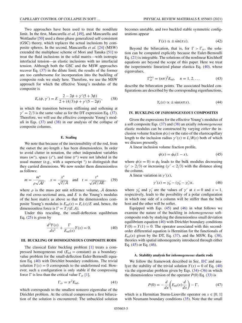
2/3) rod with a linear axial gradient of the liquid contentusing Eq. (45) and the DT expression for the effective Young’smodulus Eq. (37). In this manner we can impose a linearly de-creasing stiffness along the rod. We show in the upper panel ofFig. 2(a) the effective Young’s modulus for this class of com-posite rods as we vary the parameters: γ ′ = 10, 100; φ0 =

FIG. 2. Effective Young’s moduli and buckling modes. The up-per panel of (a) is the relative effective Young’s modulus Eq. (37)as a function of γ ′ and φ. The first (a) (lower panel) and second(b) buckling modes of homogeneous and linearly stiffened soft com-posite columns with the same potential energy. The vertical linesin (a) denote the coordinate x at which the color correspondingcolumn reaches the maximum deflection. The dashed vertical linein (b) denotes the position of the middle of the undeformed rod;x = 1/2.

0.3, 0.6. Clearly, the stiffness of the column Erel(x) de-creases with x as the volume fraction φ(x) decreases from φ0

to 0.The small deviation Euler buckling boundary value prob-

lem for Eq. (40) with Y (0) = Y (1) = 0 takes the form of theAiry equation,

Y ′′(x) + (a + bx)�Y (x) = 0, (53)

where a = 1/Erel(φ = φ0) and b = (φ0/l )(γ ′5/2 − 5/3)/(1 + γ ′5/2), the solutions to which can be written in terms

055603-6

CAPILLARY CONTROL OF COLLAPSE IN SOFT … PHYSICAL REVIEW MATERIALS 5, 055603 (2021)

TABLE I. Critical loads of inhomogeneous stiffened rods with alinear gradient of liquid inclusions Eq. (45) as a function of γ ′ andφ0.

γ ′, φ0 �(1)cr , �(2)

cr

γ ′ = 100, φ0 = 0.3 11.574(4), 46.430(4)γ ′ = 100, φ0 = 0.6 13.929(0), 56.631(0)γ ′ = 10, φ0 = 0.3 11.392(9), 45.676(1)γ ′ = 10, φ0 = 0.6 13.427(4), 54.386(4)

of Airy functions Ai and Bi as

Y (x) = C

Bi(−�cra/| − �crb|2/3)

×[

Ai

(−�cra − �crbx

| − �crb|2/3

)Bi

( −�cra

| − �crb|2/3

)

− Ai

( −�cra

| − �crb|2/3

)Bi

(−�cra − �crbx

| − �crb|2/3

)], (54)

where C is a constant. When the compression exerted onthe ends of the inhomogeneous column exceeds a criticalvalue �cr, the column deflections are given by Eq. (54) as afunction of the strength of the gradient in inclusion volumefraction |φ0|. The values of �cr are now given by the nontrivialsolutions of Eq. (53) and are the roots of the transcendentalequation,

Ai

( −�

| − �b|2/3

)Bi

( −�a

| − �b|2/3

)

= Ai

( −�a

| − �b|2/3

)Bi

( −�

| − �b|2/3

), (55)

which we solve numerically to determine the failure modes.Table I shows the results for the two lowest critical loads [i.e.,the first two nonzero roots of Eq. (55)] of inhomogeneousstiffened rods for a range of γ ′ and φ0.

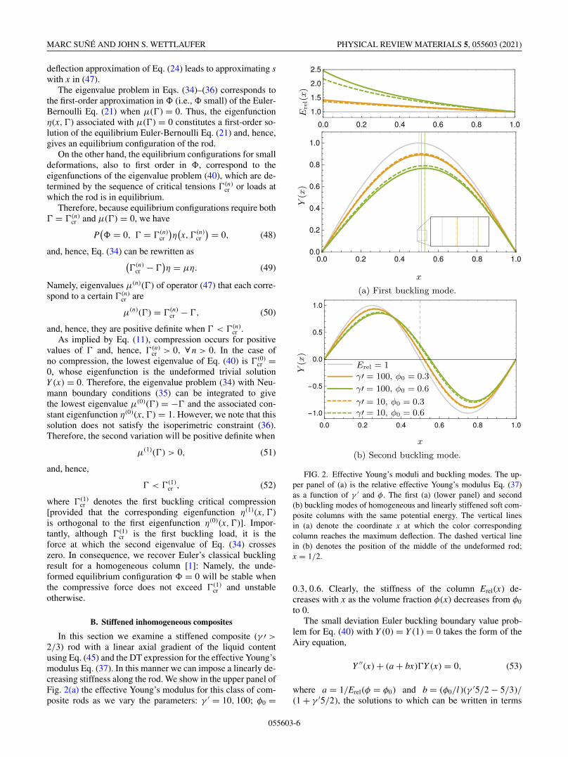
Substituting the critical loads of Table I into Eq. (54),we obtain the first two buckling modes (n = 1, 2), whichwe compare to the corresponding failure configurations ofa column with a constant elasticity given by Eq. (44) [52].Figure 2 shows how the axially varying Young’s modulus,associated with a linear gradient of the liquid volume fraction,breaks the buckling symmetry associated with the Kirchhoffrod. The distinction between the classical homogeneous andthe heterogeneous column is seen in the first buckling mode,through the shift in the apex of the deflection towards the com-pliant end x = 1 as shown in the magnified inset of Fig. 2(a).The distinction between the stiffened and the compliant endsis more striking for the second buckling mode, shown inFig. 2(b), and enhanced when we plot the curvature of theprofile as performed in Fig. 3.

Although we can tailor the response of the stiffened in-homogeneous column by changing γ ′ and φ0, their effectis the same: The more we increase the composite Young’smodulus at the stiffened end either by reducing the inclusionsize (increasing γ ′) or by increasing the liquid volume fractionand gradient φ0, the more asymmetric the response. Moreover,because we are comparing the buckling modes at the same

FIG. 3. Buckling curvature. The second derivative of the secondbuckling modes of homogeneous and linearly stiffened soft com-posite columns with the same potential energy. The dashed verticalline denotes the position of the middle of the naturally straight rod;x = 1/2. The same color legend as in Fig. 2 applies.

potential energy, a larger stiffness implies a smaller deflectionfrom the straight configuration.

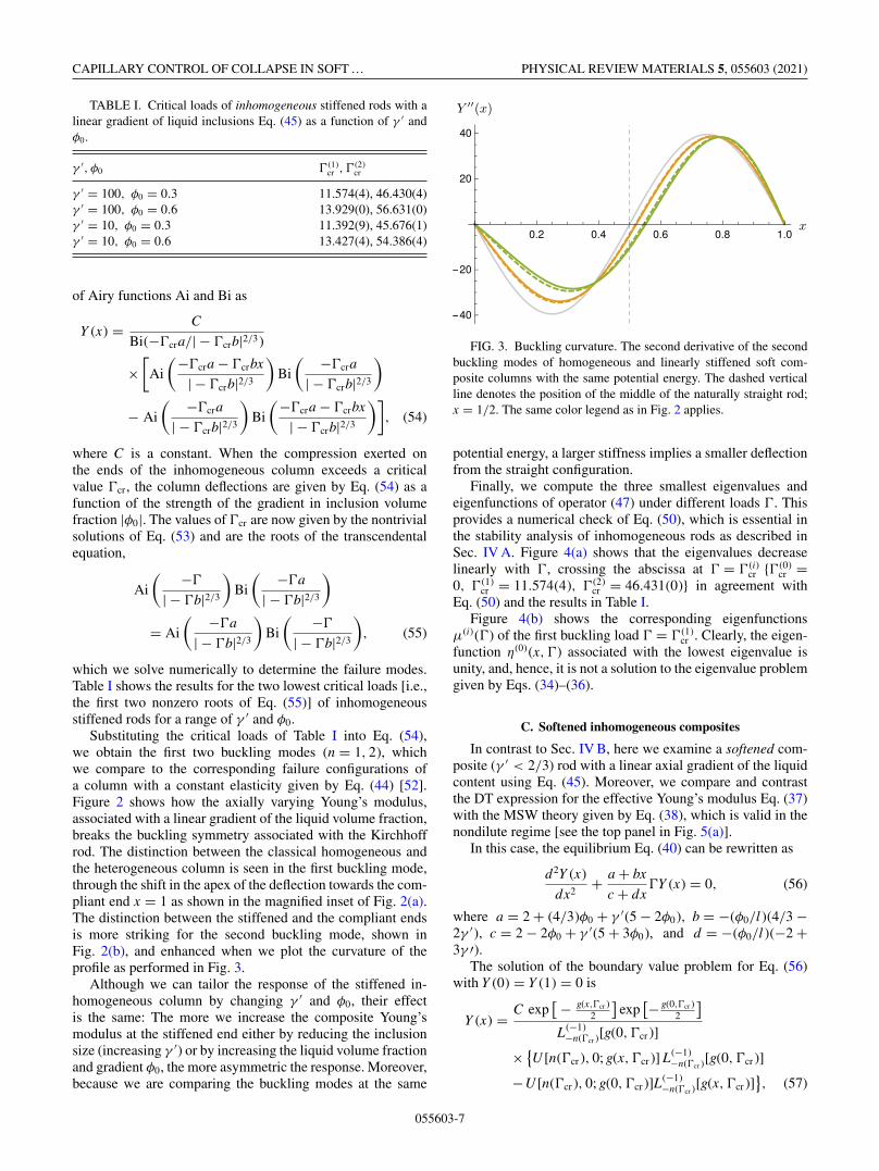
Finally, we compute the three smallest eigenvalues andeigenfunctions of operator (47) under different loads �. Thisprovides a numerical check of Eq. (50), which is essential inthe stability analysis of inhomogeneous rods as described inSec. IV A. Figure 4(a) shows that the eigenvalues decreaselinearly with �, crossing the abscissa at � = �(i)

cr {�(0)cr =

0, �(1)cr = 11.574(4), �(2)

cr = 46.431(0)} in agreement withEq. (50) and the results in Table I.

Figure 4(b) shows the corresponding eigenfunctionsμ(i)(�) of the first buckling load � = �(1)

cr . Clearly, the eigen-function η(0)(x, �) associated with the lowest eigenvalue isunity, and, hence, it is not a solution to the eigenvalue problemgiven by Eqs. (34)–(36).

C. Softened inhomogeneous composites

In contrast to Sec. IV B, here we examine a softened com-posite (γ ′ < 2/3) rod with a linear axial gradient of the liquidcontent using Eq. (45). Moreover, we compare and contrastthe DT expression for the effective Young’s modulus Eq. (37)with the MSW theory given by Eq. (38), which is valid in thenondilute regime [see the top panel in Fig. 5(a)].

In this case, the equilibrium Eq. (40) can be rewritten as

d2Y (x)

dx2+ a + bx

c + dx�Y (x) = 0, (56)

where a = 2 + (4/3)φ0 + γ ′(5 − 2φ0), b = −(φ0/l )(4/3 −2γ ′), c = 2 − 2φ0 + γ ′(5 + 3φ0), and d = −(φ0/l )(−2 +3γ ′).

The solution of the boundary value problem for Eq. (56)with Y (0) = Y (1) = 0 is

Y (x) = C exp[ − g(x,�cr )

2

]exp

[− g(0,�cr )2

]L(−1)

−n(�cr )[g(0, �cr )]

× {U [n(�cr ), 0; g(x, �cr )] L(−1)

−n(�cr )[g(0, �cr )]

−U [n(�cr ), 0; g(0, �cr )]L(−1)−n(�cr )[g(x, �cr )]

}, (57)

055603-7

MARC SUÑÉ AND JOHN S. WETTLAUFER PHYSICAL REVIEW MATERIALS 5, 055603 (2021)

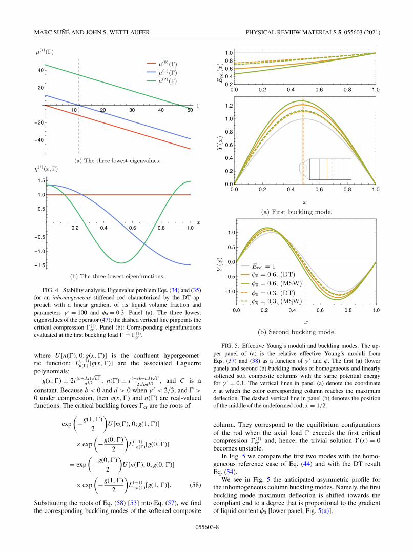
FIG. 4. Stability analysis. Eigenvalue problem Eqs. (34) and (35)for an inhomogeneous stiffened rod characterized by the DT ap-proach with a linear gradient of its liquid volume fraction andparameters γ ′ = 100 and φ0 = 0.3. Panel (a): The three lowesteigenvalues of the operator (47); the dashed vertical line pinpoints thecritical compression �(1)

cr . Panel (b): Corresponding eigenfunctionsevaluated at the first buckling load � = �(1)

cr .

where U [n(�), 0; g(x, �)] is the confluent hypergeomet-ric function; L(−1)

n(�) [g(x, �)] are the associated Laguerrepolynomials;

g(x, �) ≡ 2i (c+dx)√

b�d3/2 , n(�) ≡ i (−cb+ad )

√�

2√

bd3/2 , and C is aconstant. Because b < 0 and d > 0 when γ ′ < 2/3, and � >

0 under compression, then g(x, �) and n(�) are real-valuedfunctions. The critical buckling forces �cr are the roots of

exp

(−g(1, �)

2

)U [n(�), 0; g(1, �)]

× exp

(−g(0, �)

2

)L(−1)

−n(�)[g(0, �)]

= exp

(−g(0, �)

2

)U [n(�), 0; g(0, �)]

× exp

(−g(1, �)

2

)L(−1)

−n(�)[g(1, �)]. (58)

Substituting the roots of Eq. (58) [53] into Eq. (57), we findthe corresponding buckling modes of the softened composite

FIG. 5. Effective Young’s moduli and buckling modes. The up-per panel of (a) is the relative effective Young’s moduli fromEqs. (37) and (38) as a function of γ ′ and φ. The first (a) (lowerpanel) and second (b) buckling modes of homogeneous and linearlysoftened soft composite columns with the same potential energyfor γ ′ = 0.1. The vertical lines in panel (a) denote the coordinatex at which the color corresponding column reaches the maximumdeflection. The dashed vertical line in panel (b) denotes the positionof the middle of the undeformed rod; x = 1/2.

column. They correspond to the equilibrium configurationsof the rod when the axial load � exceeds the first criticalcompression �(1)

cr and, hence, the trivial solution Y (x) = 0becomes unstable.

In Fig. 5 we compare the first two modes with the homo-geneous reference case of Eq. (44) and with the DT resultEq. (54).

We see in Fig. 5 the anticipated asymmetric profile forthe inhomogeneous column buckling modes. Namely, the firstbuckling mode maximum deflection is shifted towards thecompliant end to a degree that is proportional to the gradientof liquid content φ0 [lower panel, Fig. 5(a)].

055603-8

CAPILLARY CONTROL OF COLLAPSE IN SOFT … PHYSICAL REVIEW MATERIALS 5, 055603 (2021)

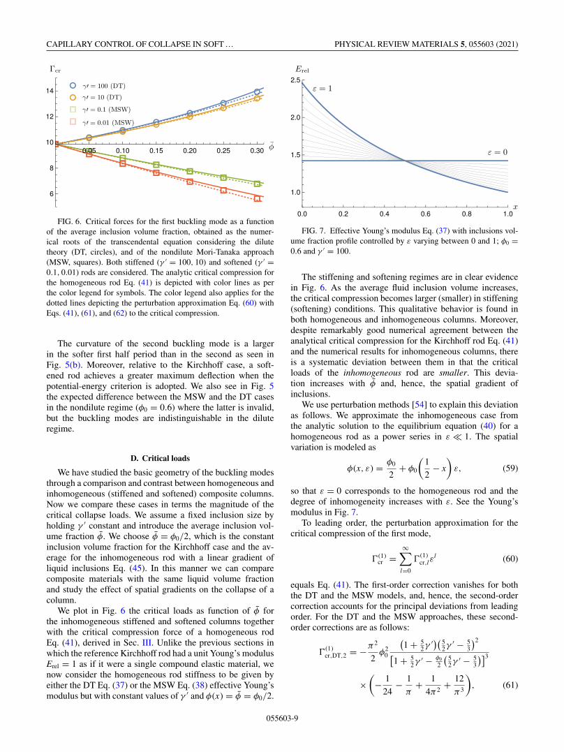
FIG. 6. Critical forces for the first buckling mode as a functionof the average inclusion volume fraction, obtained as the numer-ical roots of the transcendental equation considering the dilutetheory (DT, circles), and of the nondilute Mori-Tanaka approach(MSW, squares). Both stiffened (γ ′ = 100, 10) and softened (γ ′ =0.1, 0.01) rods are considered. The analytic critical compression forthe homogeneous rod Eq. (41) is depicted with color lines as perthe color legend for symbols. The color legend also applies for thedotted lines depicting the perturbation approximation Eq. (60) withEqs. (41), (61), and (62) to the critical compression.

The curvature of the second buckling mode is a largerin the softer first half period than in the second as seen inFig. 5(b). Moreover, relative to the Kirchhoff case, a soft-ened rod achieves a greater maximum deflection when thepotential-energy criterion is adopted. We also see in Fig. 5the expected difference between the MSW and the DT casesin the nondilute regime (φ0 = 0.6) where the latter is invalid,but the buckling modes are indistinguishable in the diluteregime.

D. Critical loads

We have studied the basic geometry of the buckling modesthrough a comparison and contrast between homogeneous andinhomogeneous (stiffened and softened) composite columns.Now we compare these cases in terms the magnitude of thecritical collapse loads. We assume a fixed inclusion size byholding γ ′ constant and introduce the average inclusion vol-ume fraction φ. We choose φ = φ0/2, which is the constantinclusion volume fraction for the Kirchhoff case and the av-erage for the inhomogeneous rod with a linear gradient ofliquid inclusions Eq. (45). In this manner we can comparecomposite materials with the same liquid volume fractionand study the effect of spatial gradients on the collapse of acolumn.

We plot in Fig. 6 the critical loads as function of φ forthe inhomogeneous stiffened and softened columns togetherwith the critical compression force of a homogeneous rodEq. (41), derived in Sec. III. Unlike the previous sections inwhich the reference Kirchhoff rod had a unit Young’s modulusErel = 1 as if it were a single compound elastic material, wenow consider the homogeneous rod stiffness to be given byeither the DT Eq. (37) or the MSW Eq. (38) effective Young’smodulus but with constant values of γ ′ and φ(x) = φ = φ0/2.

FIG. 7. Effective Young’s modulus Eq. (37) with inclusions vol-ume fraction profile controlled by ε varying between 0 and 1; φ0 =0.6 and γ ′ = 100.

The stiffening and softening regimes are in clear evidencein Fig. 6. As the average fluid inclusion volume increases,the critical compression becomes larger (smaller) in stiffening(softening) conditions. This qualitative behavior is found inboth homogeneous and inhomogeneous columns. Moreover,despite remarkably good numerical agreement between theanalytical critical compression for the Kirchhoff rod Eq. (41)and the numerical results for inhomogeneous columns, thereis a systematic deviation between them in that the criticalloads of the inhomogeneous rod are smaller. This devia-tion increases with φ and, hence, the spatial gradient ofinclusions.

We use perturbation methods [54] to explain this deviationas follows. We approximate the inhomogeneous case fromthe analytic solution to the equilibrium equation (40) for ahomogeneous rod as a power series in ε � 1. The spatialvariation is modeled as

φ(x, ε) = φ0

2+ φ0

(1

2− x

)ε, (59)

so that ε = 0 corresponds to the homogeneous rod and thedegree of inhomogeneity increases with ε. See the Young’smodulus in Fig. 7.

To leading order, the perturbation approximation for thecritical compression of the first mode,

�(1)cr =

∞∑l=0

�(1)cr,lε

l (60)

equals Eq. (41). The first-order correction vanishes for boththe DT and the MSW models, and, hence, the second-ordercorrection accounts for the principal deviations from leadingorder. For the DT and the MSW approaches, these second-order corrections are as follows:

�(1)cr,DT,2 = −π2

2φ2

0

(1 + 5

2γ ′)( 52γ ′ − 5

3

)2

[1 + 5

2γ ′ − φ0

2

(52γ ′ − 5

3

)]3

×(

− 1

24− 1

π+ 1

4π2+ 12

π3

), (61)

055603-9

MARC SUÑÉ AND JOHN S. WETTLAUFER PHYSICAL REVIEW MATERIALS 5, 055603 (2021)

and

�(1)cr,MSW,2 = −π2φ2

010

3

(2− 3γ ′)2(2+ 5γ ′)[2+ 2

3φ0+ γ ′(5− φ0)]2[

2− φ0+ γ ′(5+ 32

)]

×[

5

12

(2 + 5γ ′)2 + 2

3φ0 + γ ′(5 − φ0)

(− 1

24− 1

π+ 1

4π2+ 12

π3

)+ 1

24− 1

4π2

], (62)

respectively. Further details of the perturbative calculationscan be found in the Supplemental Material [55].

In Fig. 6 we plot the critical compression fromEqs. (43), (61), and (62) along with perturbation expansionEq. (60). We note that the numerical results of the inhomo-geneous rod—symbols in Fig. 6—correspond to ε → 1 inthe perturbation theory, although the accuracy of the latter isrestricted to ε � 1. Thus, whereas we cannot reproduce theinhomogeneous case with the perturbation theory, the latterprovides valuable insight into the interpretation of the results.In particular, the first nonzero correction to the homogeneouscritical compression in Eq. (60) is negative for any set ofparameters in both the DT and the MSW models. Therefore,spatial gradients in the elastic properties of a column promotesbuckling under smaller loads.

Physically, the fact that an inhomogeneous elastic rodbuckles more easily can be seen in terms of the perturbedYoung’s modulus plotted in Fig. 7. Namely, a gradient in theelasticity gives one-half of the rod with Erel(x) < Erel(φ =φ0/2), which is softened relative to the homogeneous counter-part. This weaker region is sufficient to lead to collapse underlower loads despite the fact that the other half of the rod hasan increased stiffness compared to the homogeneous referencecase.

E. Polar elasticity

In Secs. IV B and IV C we either linearly stiffened orsoftened a column using Eq. (45) for a given ratio of elas-tocapillary length to inclusion radius γ ′. In consequence, thebulk modulus either decreased or increased with distancealong the column. Here we consider a constant inclusionvolume fraction φ and a linear variation in γ ′(x) as in Eq. (46)to create a polar rod that changes from softened to stiffenedalong its axis.

As described in Sec. II D the DT and MSW extensionsof the Eshelby and Peierls theory are equivalent in thedilute limit. However, in the softening (stiffening) regimein the nondilute limit the effective Young’s modulus es-timates of Style and co-workers [22,23] deviate from thethree-phase model of Mancarella and co-workers [49,50] (theMSW method [24]). Here, we solve the equilibrium equationEq. (40) for γ ′(x) as in Eq. (46), φ constant, and use the DTand MSW theories in the dilute limit.

The resulting effective Young’s modulus for both the DTand the MSW models can be expressed as a ratio of twolinear polynomials. The equilibrium equation correspondingto Eq. (40) is, thus, mathematically analogous to Eq. (56),namely, the MSW theory with φ(x) obeying Eq. (45) withconstant γ ′ treated in Sec. IV C. Thus, as in Eq. (57), we canwrite the deflections of a composite polar rod with hinged

ends in terms of the confluent hypergeometric function andthe associated Laguerre polynomials.

The coefficients in Eq. (57) when φ is constant and γ ′obeys the linear gradient of Eq. (46), are as follows: a =(1 + φ5/3) + (1 − φ)γ ′

05/2, b = −(1 − φ)(γ ′0 − γ ′

1)5/2, c =1 + γ ′

05/2, and d = −(γ ′0 − γ ′

1)5/2 for the DT approach;a = 2 + φ4/3 + (5 − 2φ)γ ′

0, b = −(5 − 2φ)(γ ′0 − γ ′

1), c =2 − 2φ + (5 + 3φ)γ ′

0, and d = −(5 + 3φ)(γ ′0 − γ ′

1) for theMSW approach. Parameters b and d for both models arenegative when γ ′

0 > γ ′1 (0 � φ � 1) yielding complex roots

of Eqs. (57) and (58). However, we note that in both of theseequations y1(x) ≡ exp[−g(x, �)/2] U [n(�), 0; g(x, �)] andy2(x) ≡ exp[−g(x, �)/2] L(−1)

−n(�)[g(x, �)] are eigenfunctionsof the linear differential operator acting on Y (x) and haveeigenvalue 0, corresponding to the equilibrium equation (56).We noted at the outset of Sec. IV that for either the DT orthe MSW effective Young’s moduli, the second-order linearoperator of Eq. (40) with Dirichlet boundary conditions isHermitian. Therefore, Eqs. (57) and (58) can be rewritten interms of linear combinations of the real-valued eigenfunctionsy1(x) and y2(x). Hence, since the deflection of a polarcompressed rod given by Eq. (57) is defined up to anundetermined constant without loss of generality we considerthe real part of Eq. (57) for the remainder of this subsection.

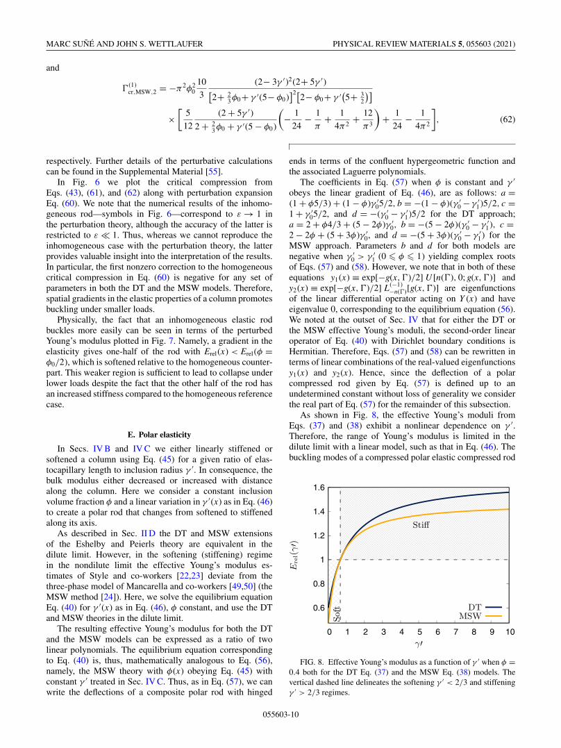
As shown in Fig. 8, the effective Young’s moduli fromEqs. (37) and (38) exhibit a nonlinear dependence on γ ′.Therefore, the range of Young’s modulus is limited in thedilute limit with a linear model, such as that in Eq. (46). Thebuckling modes of a compressed polar elastic compressed rod

FIG. 8. Effective Young’s modulus as a function of γ ′ when φ =0.4 both for the DT Eq. (37) and the MSW Eq. (38) models. Thevertical dashed line delineates the softening γ ′ < 2/3 and stiffeningγ ′ > 2/3 regimes.

055603-10

CAPILLARY CONTROL OF COLLAPSE IN SOFT … PHYSICAL REVIEW MATERIALS 5, 055603 (2021)

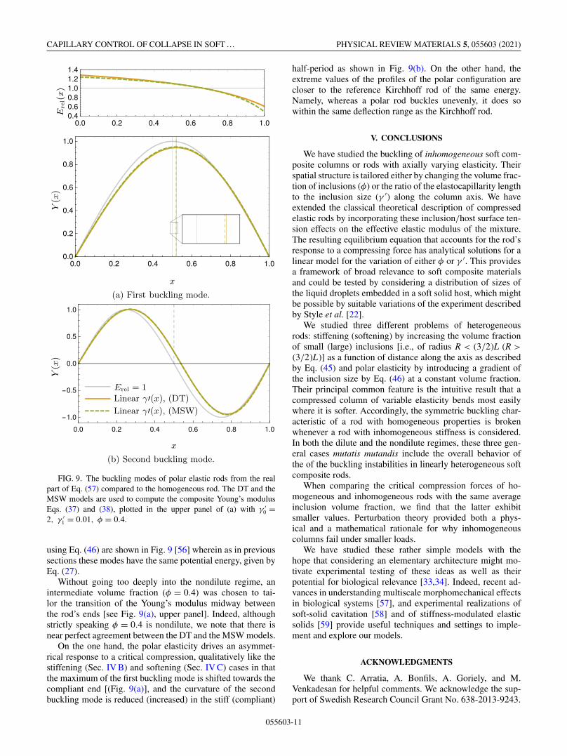
FIG. 9. The buckling modes of polar elastic rods from the realpart of Eq. (57) compared to the homogeneous rod. The DT and theMSW models are used to compute the composite Young’s modulusEqs. (37) and (38), plotted in the upper panel of (a) with γ ′

0 =2, γ ′

1 = 0.01, φ = 0.4.

using Eq. (46) are shown in Fig. 9 [56] wherein as in previoussections these modes have the same potential energy, given byEq. (27).

Without going too deeply into the nondilute regime, anintermediate volume fraction (φ = 0.4) was chosen to tai-lor the transition of the Young’s modulus midway betweenthe rod’s ends [see Fig. 9(a), upper panel]. Indeed, althoughstrictly speaking φ = 0.4 is nondilute, we note that there isnear perfect agreement between the DT and the MSW models.

On the one hand, the polar elasticity drives an asymmet-rical response to a critical compression, qualitatively like thestiffening (Sec. IV B) and softening (Sec. IV C) cases in thatthe maximum of the first buckling mode is shifted towards thecompliant end [(Fig. 9(a)], and the curvature of the secondbuckling mode is reduced (increased) in the stiff (compliant)

half-period as shown in Fig. 9(b). On the other hand, theextreme values of the profiles of the polar configuration arecloser to the reference Kirchhoff rod of the same energy.Namely, whereas a polar rod buckles unevenly, it does sowithin the same deflection range as the Kirchhoff rod.

V. CONCLUSIONS

We have studied the buckling of inhomogeneous soft com-posite columns or rods with axially varying elasticity. Theirspatial structure is tailored either by changing the volume frac-tion of inclusions (φ) or the ratio of the elastocapillarity lengthto the inclusion size (γ ′) along the column axis. We haveextended the classical theoretical description of compressedelastic rods by incorporating these inclusion/host surface ten-sion effects on the effective elastic modulus of the mixture.The resulting equilibrium equation that accounts for the rod’sresponse to a compressing force has analytical solutions for alinear model for the variation of either φ or γ ′. This providesa framework of broad relevance to soft composite materialsand could be tested by considering a distribution of sizes ofthe liquid droplets embedded in a soft solid host, which mightbe possible by suitable variations of the experiment describedby Style et al. [22].

We studied three different problems of heterogeneousrods: stiffening (softening) by increasing the volume fractionof small (large) inclusions [i.e., of radius R < (3/2)L (R >

(3/2)L)] as a function of distance along the axis as describedby Eq. (45) and polar elasticity by introducing a gradient ofthe inclusion size by Eq. (46) at a constant volume fraction.Their principal common feature is the intuitive result that acompressed column of variable elasticity bends most easilywhere it is softer. Accordingly, the symmetric buckling char-acteristic of a rod with homogeneous properties is brokenwhenever a rod with inhomogeneous stiffness is considered.In both the dilute and the nondilute regimes, these three gen-eral cases mutatis mutandis include the overall behavior ofthe of the buckling instabilities in linearly heterogeneous softcomposite rods.

When comparing the critical compression forces of ho-mogeneous and inhomogeneous rods with the same averageinclusion volume fraction, we find that the latter exhibitsmaller values. Perturbation theory provided both a phys-ical and a mathematical rationale for why inhomogeneouscolumns fail under smaller loads.

We have studied these rather simple models with thehope that considering an elementary architecture might mo-tivate experimental testing of these ideas as well as theirpotential for biological relevance [33,34]. Indeed, recent ad-vances in understanding multiscale morphomechanical effectsin biological systems [57], and experimental realizations ofsoft-solid cavitation [58] and of stiffness-modulated elasticsolids [59] provide useful techniques and settings to imple-ment and explore our models.

ACKNOWLEDGMENTS

We thank C. Arratia, A. Bonfils, A. Goriely, and M.Venkadesan for helpful comments. We acknowledge the sup-port of Swedish Research Council Grant No. 638-2013-9243.

055603-11

MARC SUÑÉ AND JOHN S. WETTLAUFER PHYSICAL REVIEW MATERIALS 5, 055603 (2021)

[1] L. Euler, Methodus Inveniendi Lineas Curvas Maximi MinimiveProprietate Gaudentes Sivesolutio Problematis IsoperimetriciLatissimo Sensu Accepti (Marc-Michel Bousquet, Lausanne,Geneva, 1744).

[2] L. Euler, Memoires de l’Académie de Berlin Vol. 13 (Berlin,Germany, 1759), pp. 487–488.

[3] J. L. Lagrange, Miscellanea Taurinensia 5, 123 (1770).[4] S. O. Erbil, U. Hatipoglu, C. Yanik, M. Ghavami, A. B. Ari,

M. Yuksel, and M. S. Hanay, Phys. Rev. Lett. 124, 046101(2020).

[5] S. Timoshenko and J. Gere, Theory of Elastic Stability, seconded. (McGraw-Hill, New York, 1963).

[6] S. Nezamabadi, J. Yvonnet, H. Zahrouni, and M. Potier-Ferry,Comput. Methods Appl. Mech. Eng. 198, 2099 (2009).

[7] L. Gong, S. Kyriakides, and N. Triantafyllidis, J. Mech. Phys.Solids 53, 771 (2005).

[8] N. Triantafyllidis, M. D. Nestorovic, and M. W. Schraad,J. Appl. Mech. 73, 505 (2005).

[9] G. deBotton, I. Hariton, and E. Socolsky, J. Mech. Phys. Solids54, 533 (2006).

[10] M. Jamal, M. Midani, N. Damil, and M. Potier-Ferry, Int. J.Solids Struct. 36, 441 (1999).

[11] J. Michel, O. Lopez-Pamies, P. P. Castañeda, and N.Triantafyllidis, J. Mech. Phys. Solids 55, 900 (2007).

[12] A. Goriely, R. Vandiver, and M. Destrade, Proc. R. Soc. LondonA 464, 3003 (2008).

[13] E. Lifshitz, A. Kosevich, and L. Pitaevskii, Theory of Elasticity,third ed., edited by E. Lifshitz, A. Kosevich, and L. Pitaevskii(Butterworth-Heinemann, Oxford, 1986), pp. 38–86.

[14] P. P. Castañeda and P. Suquet, Nonlinear composites, Advancesin Applied Mechanics Volume 34, edited by E. van der Giessenand T. Y. Wu (Elsevier, 1997), pp. 171–302.

[15] G. Kirchhoff, J. F. Reine. Angew. Math. (Crelle) 56, 285 (1859).[16] G. Kirchhoff, Vorlesungen über Mathematische Physik,

Mechanik (B. G. Teubner, Leipzig, 1876).[17] A. Clebsch, Theorie der Elasticität Fester Körper (B. G. Teub-

ner, Leipzig, 1862).[18] A. Clebsch, Théorie de l’Elasticité des Corps Solides (Trans-

lation of Ref. [17] by Saint-Venant & Flamant, Dunod, Paris,1883).

[19] B. D. Coleman, E. H. Dill, M. Lembo, Z. Lu, and I. Tobias,Arch. Ration. Mech. Anal. 121, 339 (1993).

[20] S. Mora, T. Phou, J.-M. Fromental, L. M. Pismen, and Y.Pomeau, Phys. Rev. Lett. 105, 214301 (2010).

[21] L. Ducloué, O. Pitois, J. Goyon, X. Chateau, and G. Ovarlez,Soft Matter 10, 5093 (2014).

[22] R. W. Style, R. Boltyanskiy, B. Allen, K. E. Jensen, H. P.Foote, J. S. Wettlaufer, and E. R. Dufresne, Nat. Phys. 11, 82(2015).

[23] R. W. Style, J. S. Wettlaufer, and E. R. Dufresne, Soft Matter11, 672 (2015).

[24] F. Mancarella, R. W. Style, and J. S. Wettlaufer, Proc. R. Soc.London A 472, 20150853 (2016).

[25] J. D. Eshelby and R. E. Peierls, Proc. R. Soc. London A 241,376 (1957).

[26] H. Peisker, J. Michels, and S. N. Gorb, Nat. Commun. (2013).[27] M. Schmitt, T. H. Büscher, S. N. Gorb, and H. Rajabi, J. Exp.

Biol. 221, jeb173047 (2018).[28] M. Rüggeberg, T. Speck, O. Paris, C. Lapierre, B. Pollet, G.

Koch, and I. Burgert, Proc. R. Soc. London B 275, 2221 (2008).

[29] T. Speck and I. Burgert, Annu. Rev. Mater. Res. 41, 169 (2011).[30] A. Fritsch and C. Hellmich, J. Theor. Biol. 244, 597 (2007).[31] N. H. Mendelson, Microbiol. Mol. Biol. Rev. 46, 341 (1982).[32] M. J. Jaffe and A. W. Galston, Annu. Rev. Plant Physiol. 19,

417 (1968).[33] A. Goriely, The Mathematics and Mechanics of Biological

Growth (Springer, New York, 2017), pp. 63–96.[34] A. Goriely, The Mathematics and Mechanics of Biological

Growth (Springer, New York, 2017), pp. 97–123.[35] R. E. Goldstein and A. Goriely, Phys. Rev. E 74, 010901(R)

(2006).[36] A. Goriely, The Mathematics and Mechanics of Biological

Growth (Springer, New York, 2017), pp. 125–172.[37] R. E. Caflisch and J. H. Maddocks, Proc.-R. Soc. Edinburgh,

Sect. A: Math. 99, 1 (1984).[38] J. H. Maddocks, Arch. Ration. Mech. Anal. 85, 311354

(1984).[39] S. S. Antman and G. Rosenfeld, SIAM Rev. 20, 513 (1978).[40] Z. Hashin, J. Appl. Mech. 29, 143 (1962).[41] Z. Hashin and S. Shtrikman, J. Mech. Phys. Solids 11, 127

(1963).[42] R. Christensen and K. Lo, J. Mech. Phys. Solids 27, 315

(1979).[43] S. Mora, C. Maurini, T. Phou, J.-M. Fromental, B. Audoly, and

Y. Pomeau, Phys. Rev. Lett. 111, 114301 (2013).[44] R. W. Style, R. Boltyanskiy, Y. Che, J. S. Wettlaufer, L. A.

Wilen, and E. R. Dufresne, Phys. Rev. Lett. 110, 066103(2013).

[45] N. Nadermann, C.-Y. Hui, and A. Jagota, Proc. Natl. Acad. Sci.U.S.A. 110, 10541 (2013).

[46] X. Xu, A. Jagota, and C.-Y. Hui, Soft Matter 10, 4625 (2014).[47] S. Mora, M. Abkarian, H. Tabuteau, and Y. Pomeau, Soft Matter

7, 10612 (2011).[48] R. W. Style and E. R. Dufresne, Soft Matter 8, 7177 (2012).[49] F. Mancarella, R. W. Style, and J. S. Wettlaufer, Soft Matter 12,

2744 (2016).[50] F. Mancarella and J. S. Wettlaufer, Soft Matter 13, 945 (2017).[51] T. Mori and K. Tanaka, Acta Metall. 21, 571 (1973).[52] In order to benchmark our results for heterogeneous elastic rods

against the constant Young’s modulus case, we have to assumean additional constraint associated with the fact that the bendingshapes are defined up to a constant. Here we impose the condi-tion that the reference case Eqs. (44), and the heterogeneouselastic rod Eqs. (55) and (58) have the same potential energy asgiven by Eq. (27).

[53] The critical loads for the buckling modes in Fig. 5,γ ′ = 0.1, are—MSW in the first place, DT second: �(1)

cr =6.785(4), 7.344(9); �(2)

cr = 27.104(2), 29.557(6), for φ0 = 0.6;and �(1)

cr = 8.265(4), 8.427(8); �(2)cr = 33.059(4), 33.778(8)

for φ0 = 0.3.[54] C. Bender and S. Orszag, Advanced Mathematical Methods for

Scientists and Engineers I (Springer-Verlag, New York, 1999).[55] See Supplemental Material at http://link.aps.org/supplemental/

10.1103/PhysRevMaterials.5.055603 for further details of theperturbative calculations.

[56] The numerical results for the critical forces correspond-ing to the first two buckling modes of a polar rod with{γ ′

0 = 2, γ ′1 = 0.01, φ = 0.4} are �(1)

cr = 10.601(6) and �(2)cr =

41.265(1) (DT), and �(1)cr = 10.502(6) and �(2)

cr = 40.549(2)(MSW).

055603-12

CAPILLARY CONTROL OF COLLAPSE IN SOFT … PHYSICAL REVIEW MATERIALS 5, 055603 (2021)

[57] H. Hofhuis, D. Moulton, T. Lessinnes, A.-L. Routier-Kierzkowska, R. J. Bomphrey, G. Mosca, H. Reinhardt,P. Sarchet, X. Gan, M. Tsiantis, Y. Ventikos, S. Walker,A. Goriely, R. Smith, and A. Hay, Cell 166, 222(2016).

[58] J. Y. Kim, Z. Liu, B. M. Weon, T. Cohen, C.-Y. Hui,E. R. Dufresne, and R. W. Style, Sci. Adv. 6, eaaz0418(2020).

[59] E. Riva, M. I. N. Rosa, and M. Ruzzene, Phys. Rev. B 101,094307 (2020).

055603-13