


Bahasa
Halaman
Hukum


Bounds Testing Approaches to the Analysis of Level RelationshipsAuthor(s): M. Hashem Pesaran, Yongcheol Shin, Richard J. SmithSource: Journal of Applied Econometrics, Vol. 16, No. 3, Special Issue in Memory of JohnDenis Sargan, 1924-1996: Studies in Empirical Macroeconometrics (May - Jun., 2001), pp. 289-326Published by: John Wiley & SonsStable URL: http://www.jstor.org/stable/2678547Accessed: 20/07/2009 11:08
Your use of the JSTOR archive indicates your acceptance of JSTOR's Terms and Conditions of Use, available athttp://www.jstor.org/page/info/about/policies/terms.jsp. JSTOR's Terms and Conditions of Use provides, in part, that unlessyou have obtained prior permission, you may not download an entire issue of a journal or multiple copies of articles, and youmay use content in the JSTOR archive only for your personal, non-commercial use.
Please contact the publisher regarding any further use of this work. Publisher contact information may be obtained athttp://www.jstor.org/action/showPublisher?publisherCode=jwiley.
Each copy of any part of a JSTOR transmission must contain the same copyright notice that appears on the screen or printedpage of such transmission.
JSTOR is a not-for-profit organization founded in 1995 to build trusted digital archives for scholarship. We work with thescholarly community to preserve their work and the materials they rely upon, and to build a common research platform thatpromotes the discovery and use of these resources. For more information about JSTOR, please contact [email protected].
John Wiley & Sons is collaborating with JSTOR to digitize, preserve and extend access to Journal of AppliedEconometrics.
http://www.jstor.org
JOURNAL OF APPLIED ECONOMETRICS J. Appl. Econ. 16: 289-326 (2001) DOI: 10.1002/jae.616
BOUNDS TESTING APPROACHES TO THE ANALYSIS OF LEVEL RELATIONSHIPS
M. HASHEM PESARAN,a* YONGCHEOL SHINb AND RICHARD J. SMITHC a
Trinity College, Cambridge CB2 1TQ, UK b
Department of Economics, University of Edinburgh, 50 George Square, Edinburgh EH8 9JY, UK c
Department of Economics, University of Bristol, 8 Woodland Road, Bristol BS8 1TN, UK
SUMMARY This paper develops a new approach to the problem of testing the existence of a level relationship between a dependent variable and a set of regressors, when it is not known with certainty whether the underlying regressors are trend- or first-difference stationary. The proposed tests are based on standard F- and t-statistics used to test the significance of the lagged levels of the variables in a univariate equilibrium correction mechanism. The asymptotic distributions of these statistics are non-standard under the null hypothesis that there exists no level relationship, irrespective of whether the regressors are I(0) or I(1). Two sets of asymptotic critical values are provided: one when all regressors are purely I(1) and the other if they are all purely 1(0). These two sets of critical values provide a band covering all possible classifications of the regressors into purely I(O), purely I(1) or mutually cointegrated. Accordingly, various bounds testing procedures are proposed. It is shown that the proposed tests are consistent, and their asymptotic distribution under the null and suitably defined local alternatives are derived. The empirical relevance of the bounds procedures is demonstrated by a re-examination of the earnings equation included in the UK Treasury macroeconometric model. Copyright © 2001 John Wiley & Sons, Ltd.
1. INTRODUCTION
Over the past decade considerable attention has been paid in empirical economics to testing for the existence of relationships in levels between variables. In the main, this analysis has been based on the use of cointegration techniques. Two principal approaches have been adopted: the two-step residual-based procedure for testing the null of no-cointegration (see Engle and Granger, 1987; Phillips and Ouliaris, 1990) and the system-based reduced rank regression approach due to Johansen (1991, 1995). In addition, other procedures such as the variable addition approach of Park (1990), the residual-based procedure for testing the null of cointegration by Shin (1994), and the stochastic common trends (system) approach of Stock and Watson (1988) have been considered. All of these methods concentrate on cases in which the underlying variables are integrated of order one. This inevitably involves a certain degree of pre-testing, thus introducing a further degree of uncertainty into the analysis of levels relationships. (See, for example, Cavanagh, Elliott and Stock, 1995.)
This paper proposes a new approach to testing for the existence of a relationship between variables in levels which is applicable irrespective of whether the underlying regressors are purely
* Correspondence to: M. H. Pesaran, Faculty of Economics and Politics, University of Cambridge, Sidgwick Avenue, Cambridge CB3 9DD. E-mail: [email protected] Contract/grant sponsor: ESRC; Contract/grant numbers: R000233608; R000237334. Contract/grant sponsor: Isaac Newton Trust of Trinity College, Cambridge.
Copyright © 2001 John Wiley & Sons, Ltd. Received 16 February 1999 Revised 13 February 2001
M. H. PESARAN, Y. SHIN AND R. J. SMITH
I(O), purely I(1) or mutually cointegrated. The statistic underlying our procedure is the familiar Wald or F-statistic in a generalized Dicky-Fuller type regression used to test the significance of lagged levels of the variables under consideration in a conditional unrestricted equilibrium correction model (ECM). It is shown that the asymptotic distributions of both statistics are non-standard under the null hypothesis that there exists no relationship in levels between the included variables, irrespective of whether the regressors are purely I(0), purely I(1) or mutually cointegrated. We establish that the proposed test is consistent and derive its asymptotic distribution under the null and suitably defined local alternatives, again for a set of regressors which are a mixture of 1(0)/I(1) variables.
Two sets of asymptotic critical values are provided for the two polar cases which assume that all the regressors are, on the one hand, purely I(1) and, on the other, purely I(0). Since these two sets of critical values provide critical value bounds for all classifications of the regressors into purely I(1), purely I(0) or mutually cointegrated, we propose a bounds testing procedure. If the computed Wald or F-statistic falls outside the critical value bounds, a conclusive inference can be drawn without needing to know the integration/cointegration status of the underlying regressors. However, if the Wald or F-statistic falls inside these bounds, inference is inconclusive and knowledge of the order of the integration of the underlying variables is required before conclusive inferences can be made. A bounds procedure is also provided for the related cointegration test proposed by Banerjee et al. (1998) which is based on earlier contributions by Banerjee et al. (1986) and Kremers et al. (1992). Their test is based on the t-statistic associated with the coefficient of the lagged dependent variable in an unrestricted conditional ECM. The asymptotic distribution of this statistic is obtained for cases in which all regressors are purely I(1), which is the primary context considered by these authors, as well as when the regressors are purely I(0) or mutually cointegrated. The relevant critical value bounds for this t-statistic are also detailed.
The empirical relevance of the proposed bounds procedure is demonstrated in a re-examination of the earnings equation included in the UK Treasury macroeconometric model. This is a particularly relevant application because there is considerable doubt concerning the order of integration of variables such as the degree of unionization of the workforce, the replacement ratio (unemployment benefit-wage ratio) and the wedge between the 'real product wage' and the 'real consumption wage' that typically enter the earnings equation. There is another consideration in the choice of this application. Under the influence of the seminal contributions of Phillips (1958) and Sargan (1964), econometric analysis of wages and earnings has played an important role in the development of time series econometrics in the UK. Sargan's work is particularly noteworthy as it is some of the first to articulate and apply an ECM to wage rate determination. Sargan, however, did not consider the problem of testing for the existence of a levels relationship between real wages and its determinants.
The relationship in levels underlying the UK Treasury's earning equation relates real average earnings of the private sector to labour productivity, the unemployment rate, an index of union density, a wage variable (comprising a tax wedge and an import price wedge) and the replacement ratio (defined as the ratio of the unemployment benefit to the wage rate). These are the variables predicted by the bargaining theory of wage determination reviewed, for example, in Layard et al. (1991). In order to identify our model as corresponding to the bargaining theory of wage determination, we require that the level of the unemployment rate enters the wage equation, but not vice versa; see Manning (1993). This assumption, of course, does not preclude the rate of change of earnings from entering the unemployment equation, or there being other level relationships between the remaining four variables. Our approach accommodates both of these possibilities.
Copyright © 2001 John Wiley & Sons, Ltd.
290
J. Appl. Econ. 16: 289-326 (2001)
BOUNDS TESTING FOR LEVEL RELATIONSHIPS
A number of conditional ECMs in these five variables were estimated and we found that, if a sufficiently high order is selected for the lag lengths of the included variables, the hypothesis that there exists no relationship in levels between these variables is rejected, irrespective of whether they are purely I(0), purely I(1) or mutually cointegrated. Given a level relationship between these variables, the autoregressive distributed lag (ARDL) modelling approach (Pesaran and Shin, 1999) is used to estimate our preferred ECM of average earnings.
The plan of the paper is as follows. The vector autoregressive (VAR) model which underpins the analysis of this and later sections is set out in Section 2. This section also addresses the issues involved in testing for the existence of relationships in levels between variables. Section 3 considers the Wald statistic (or the F-statistic) for testing the hypothesis that there exists no level relationship between the variables under consideration and derives the associated asymptotic theory together with that for the t-statistic of Banerjee et al. (1998). Section 4 discusses the power properties of these tests. Section 5 describes the empirical application. Section 6 provides some concluding remarks. The Appendices detail proofs of results given in Sections 3 and 4.
The following notation is used. The symbol == signifies 'weak convergence in probability measure', I,,1 'an identity matrix of order m', I(d) 'integrated of order d', Op(K) 'of the same order as K in probability' and op(K) 'of smaller order than K in probability'.
2. THE UNDERLYING VAR MODEL AND ASSUMPTIONS
Let {zt}tl denote a (k + l)-vector random process. The data-generating process for {zt}°l is the VAR model of order p (VAR(p)):
(L)(z,t - - yt) = et, t = 1, 2,... (1)
where L is the lag operator, It and y are unknown (k + 1)-vectors of intercept and trend coefficients, the (k + 1, k + 1) matrix lag polynomial ¢((L) = Ik+l - E1I l iL with {Ci}iP (k + 1, k + 1) matrices of unknown coefficients; see Harbo et al. (1998) and Pesaran, Shin and Smith (2000), henceforth HJNR and PSS respectively. The properties of the (k + 1)-vector error process {Et}i=1 are given in Assumption 2 below. All the analysis of this paper is conducted given the initial observations Zo = (l_p, ..., zo). We assume:
Assumption 1. The roots of |Ik+l - EP=1 (iiZil = 0 are either outside the unit circle Izl = 1 or satisfy z = 1.
Assumption 2. The vector error process {et}tl\ is IN(0, Q), Q positive definite.
Assumption 1 permits the elements of zt to be purely I(1), purely I(0) or cointegrated but excludes the possibility of seasonal unit roots and explosive roots.1 Assumption 2 may be relaxed somewhat to permit {[t}7tl to be a conditionally mean zero and homoscedastic process; see, for example, PSS, Assumption 4.1.
We may re-express the lag polynomial 4(L) in vector equilibrium correction model (ECM) form; i.e.. ¢(L) -HL + 1(L)(I - L) in which the long-run multiplier matrix is defined by HI
1 Assumptions 5a and 5b below further restrict the maximal order of integration of {zt}l1 to unity.
Copyright © 2001 John Wiley & Sons, Ltd.
291
J. Appl. Econ. 16: 289-326 (2001)
M. H. PESARAN, Y. SHIN AND R. J. SMITH
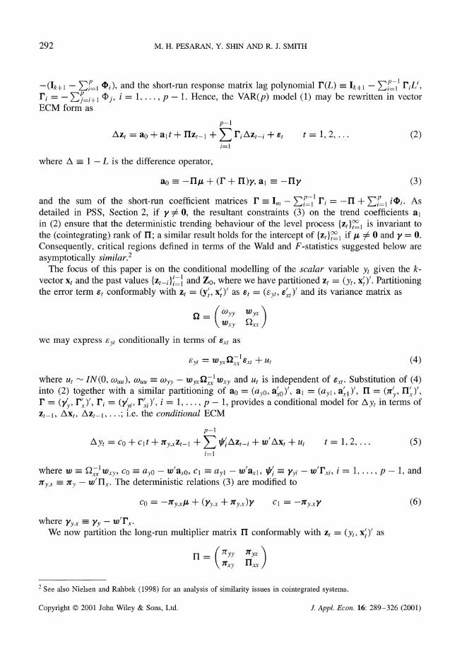
-(Ik+l - =iP-1 (i), and the short-run response matrix lag polynomial r(L) Ik+l - Ei1 riLi, ri = - jil j, i = 1, ..., p- 1. Hence, the VAR(p) model (1) may be rewritten in vector ECM form as
p-1
Azt = ao + alt + rIt + E riAzt i + st t = 1, 2,... (2) i=l
where A - 1 - L is the difference operator,
ao = -nrI + (F + n)y, ai = -Hy (3)
and the sum of the short-run coefficient matrices r' =I - II, f1 ri = - + Ei l i4i. As detailed in PSS, Section 2, if y 7& 0, the resultant constraints (3) on the trend coefficients al in (2) ensure that the deterministic trending behaviour of the level process {zt}°l is invariant to the (cointegrating) rank of II; a similar result holds for the intercept of {zt}lI if it 4 0 and y = 0. Consequently, critical regions defined in terms of the Wald and F-statistics suggested below are asymptotically similar.2
The focus of this paper is on the conditional modelling of the scalar variable Yt given the k- vector xt and the past values {zt-}i=l and Zo, where we have partitioned zt = (Yt, x')'. Partitioning the error term et conformably with t = (Y' x)' as t = (yt, et)' and its variance matrix as
a. _ ( )yy wyX )
(Wxy )xx
we may express Eyt conditionally in terms of ext as
yt = WyxQl-xt + Ut (4)
where ut - IN(O, 0uu), Cw,, = oyy - w wyx l wxy and ut is independent of ext. Substitution of (4) into (2) together with a similar partitioning of ao = (ayo, axO)', a1 =(ay, = ( a, a I = (7r, n)', r = (y/ r), ' ri = (yi, r,i) i = 1,... p- , provides a conditional model for Ayt in terms of zt-_, Axt, Azt-, ...; i.e. the conditional ECM
P-1
Ayt o + clt + 7ry.xt- 1 + Azt-i + w'Axt + ut t = 1, 2,... (5) i=l
where w = 1wx,y, co a= o - w'aao, cl _ ayl - w'al, a - Yyyi - w'rxi, i = 1,..., p - 1, and
7y.x = ry - w'Ix. The deterministic relations (3) are modified to
Co =-7ry.xl + (Yy.x + 7ry.x)Y C1 = -7y.xY (6)
where Yy.x Yv - w'r. We now partition the long-run multiplier matrix rI conformably with t = (yt, x)' as
r = (7tyy 7yx c V rxy nrx x
2 See also Nielsen and Rahbek (1998) for an analysis of similarity issues in cointegrated systems.
Copyright © 2001 John Wiley & Sons, Ltd.
292
J. Appl. Econ. 16: 289-326 (2001)
BOUNDS TESTING FOR LEVEL RELATIONSHIPS
The next assumption is critical for the analysis of this paper.
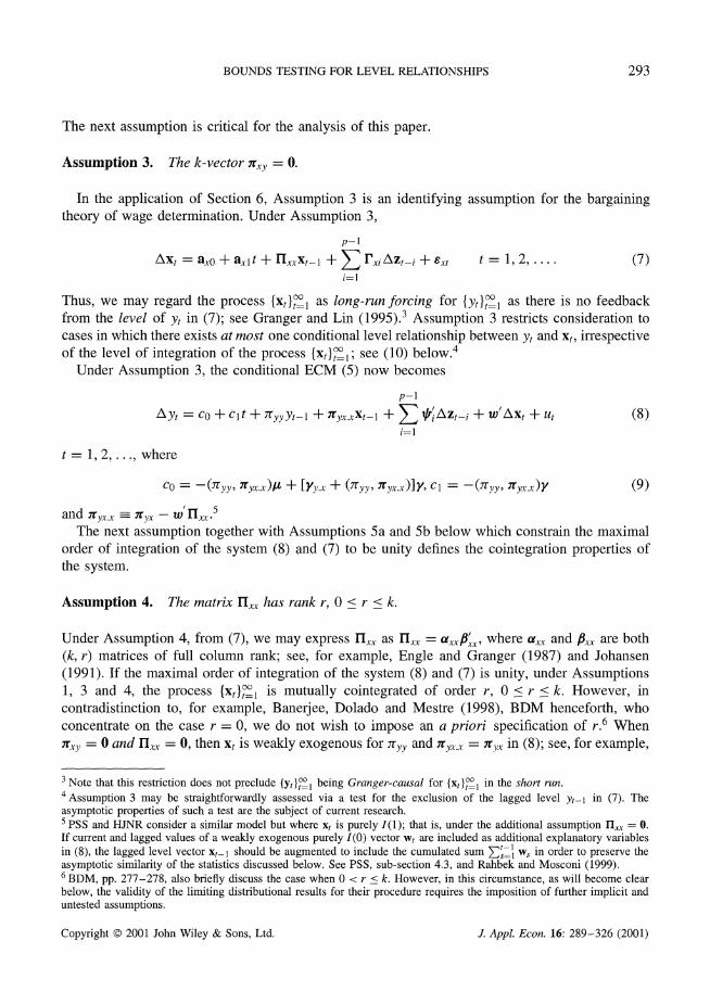
Assumption 3. The k-vector 7xy = 0.
In the application of Section 6, Assumption 3 is an identifying assumption for the bargaining theory of wage determination. Under Assumption 3,
p-1
Axt = axo + axlt + nlxxxt + rxi Azti + xt t = 1, 2,.... (7) i=l
Thus, we may regard the process {xt}°l as long-run forcing for {Yt}li as there is no feedback from the level of Yt in (7); see Granger and Lin (1995).3 Assumption 3 restricts consideration to cases in which there exists at most one conditional level relationship between Yt and xt, irrespective of the level of integration of the process {xt}ll; see (10) below.4
Under Assumption 3, the conditional ECM (5) now becomes
P-1
Ay =co + clt + ryyt + 7yCt-l + 1 Azt-i + w'Axt + Ut (8) i=l
t = 1, 2..., where
C = -(7ryy, 7ryx.x)± + [Yy.x + (7ry, 7. )]Y, C1 = -( 7Tyy, 7ry.x)y (9)
and 7ryx.x -= tyx - lxx^.5 The next assumption together with Assumptions 5a and 5b below which constrain the maximal
order of integration of the system (8) and (7) to be unity defines the cointegration properties of the system.
Assumption 4. The matrix Ixx has rank r, 0 < r < k.
Under Assumption 4, from (7), we may express IIxl as lxx = axxPx, where axx and ,xx are both (k, r) matrices of full column rank; see, for example, Engle and Granger (1987) and Johansen (1991). If the maximal order of integration of the system (8) and (7) is unity, under Assumptions 1, 3 and 4, the process {xt}tl^ is mutually cointegrated of order r, 0 < r < k. However, in contradistinction to, for example, Banerjee, Dolado and Mestre (1998), BDM henceforth, who concentrate on the case r = 0, we do not wish to impose an a priori specification of r.6 When
7y, = 0 and .,x = O, then xt is weakly exogenous for tyy and 7ryx.x = 7Ty in (8); see, for example,
3Note that this restriction does not preclude {Yt }I being Granger-causal for {xt } in the short run. t= i n thotu 4
Assumption 3 may be straightforwardly assessed via a test for the exclusion of the lagged level yt-1 in (7). The asymptotic properties of such a test are the subject of current research. 5 PSS and HJNR consider a similar model but where xt is purely I(1); that is, under the additional assumption lrx = 0. If current and lagged values of a weakly exogenous purely I(0) vector wt are included as additional explanatory variables in (8), the lagged level vector xt- should be augmented to include the cumulated sum s1Wi ws in order to preserve the asymptotic similarity of the statistics discussed below. See PSS, sub-section 4.3, and Rahbek and Mosconi (1999). 6 BDM, pp. 277-278, also briefly discuss the case when 0 < r < k. However, in this circumstance, as will become clear below, the validity of the limiting distributional results for their procedure requires the imposition of further implicit and untested assumptions.
Copyright © 2001 John Wiley & Sons, Ltd.
293
J. Appl. Econ. 16: 289-326 (2001)
M. H. PESARAN, Y. SHIN AND R. J. SMITH
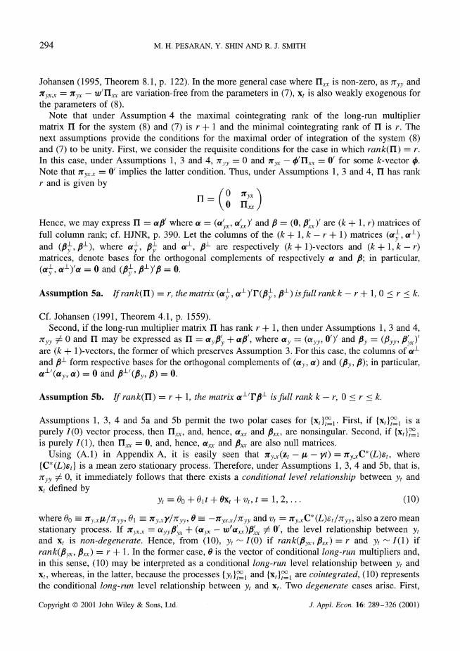
Johansen (1995, Theorem 8.1, p. 122). In the more general case where rIl. is non-zero, as yTYY and
ryx.x = jt,y - w'ilx are variation-free from the parameters in (7), xt is also weakly exogenous for the parameters of (8).
Note that under Assumption 4 the maximal cointegrating rank of the long-run multiplier matrix n for the system (8) and (7) is r + 1 and the minimal cointegrating rank of HI is r. The next assumptions provide the conditions for the maximal order of integration of the system (8) and (7) to be unity. First, we consider the requisite conditions for the case in which rank(J) = r. In this case, under Assumptions 1, 3 and 4, 7ryy = 0 and ryx - 'Inx, = 0' for some k-vector 4. Note that Tyx.x = 0' implies the latter condition. Thus, under Assumptions 1, 3 and 4, rI has rank r and is given by
n (x° x 11 - \Q n,Jx
Hence, we may express II = at' where a = (a x, a')' and fB = (0, B'x)' are (k + 1, r) matrices of full column rank; cf. HJNR, p. 390. Let the columns of the (k + 1, k - r + 1) matrices (al, a') and (fry , pf), where ay , fy1 and a , fB are respectively (k+l 1)-vectors and (k+ , k - r) matrices, denote bases for the orthogonal complements of respectively a and fB; in particular, (al, a')'a = 0 and (I, fBl)'f- = 0.
Assumption 5a. If rank(r ) = r, the matrix (al, al)'r(BIyz, f6) isfull rankk - r + 1, 0 < r < k.
Cf. Johansen (1991, Theorem 4.1, p. 1559). Second, if the long-run multiplier matrix II has rank r + 1, then under Assumptions 1, 3 and 4,
Yyy : 0 and r may be expressed as rI = ay'y + at', where ay = (Oyy, 0')' and By = (/3yy, B )' are (k + 1)-vectors, the former of which preserves Assumption 3. For this case, the columns of al and fBI form respective bases for the orthogonal complements of (ay, a) and (fBy, f); in particular, al'(ay, a) = 0 and Bl'/(Bfy, B) = 0.
Assumption 5b. If rank(r) = r + 1, the matrix al'r"T is full rank k - r, 0 < r < k.
Assumptions 1, 3, 4 and 5a and 5b permit the two polar cases for {x,} l. First, if {xt} 1 is a
purely I(O) vector process, then n^,, and, hence, aXx and ,XX, are nonsingular. Second, if {xt}l is purely I(1), then lxx = 0, and, hence, axx and fxx are also null matrices.
Using (A.1) in Appendix A, it is easily seen that 7ty.x(zt - A - yt) = ry.xC*(L)Et, where {C*(L)Et} is a mean zero stationary process. Therefore, under Assumptions 1, 3, 4 and 5b, that is, 7Tyy A O0, it immediately follows that there exists a conditional level relationship between Yt and xt defined by
Yt = O0 + lt + xt +vt, t = 1,2,... (10)
where -0 -= 7ryX,L/ryy, 01 Tty.xy/ryy, 8 = _- x.x/nyy and vt = 7ryx.C*(L)st/7yy, also a zero mean
stationary process. If 7tyx.. = ayyPyx + (ay - w'atx)xx ) ~ 0f', the level relationship between Yt and xt is non-degenerate. Hence, from (10), Yt - I(0) if rank(Byx, Bxx) = r and Yt -I (1) if
rank(IOyx, fP,) = r + 1. In the former case, 0 is the vector of conditional long-run multipliers and, in this sense, (10) may be interpreted as a conditional long-run level relationship between Yt and xt, whereas, in the latter, because the processes {yt}} i and {xt} I are cointegrated, (10) represents the conditional long-run level relationship between Yt and xt. Two degenerate cases arise. First,
Copyright © 2001 John Wiley & Sons, Ltd.
294
J. Appl. Econ. 16: 289-326 (2001)
BOUNDS TESTING FOR LEVEL RELATIONSHIPS
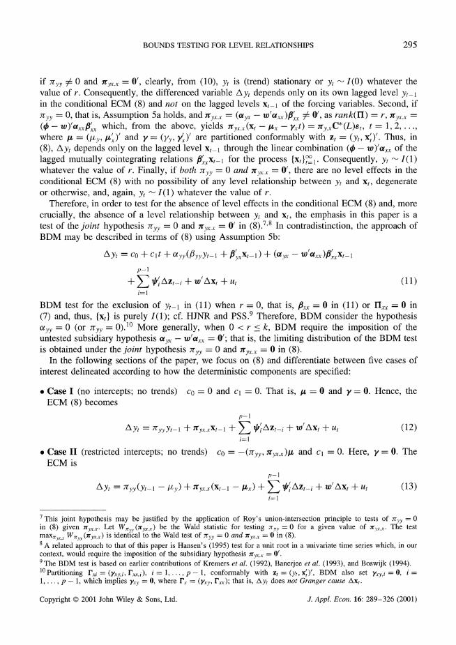
if yryy 0 0 and ryx.x = 0', clearly, from (10), Yt is (trend) stationary or yt - I(0) whatever the value of r. Consequently, the differenced variable Ayt depends only on its own lagged level Yt-l in the conditional ECM (8) and not on the lagged levels xt_l of the forcing variables. Second, if ryy = 0, that is, Assumption 5a holds, and 7tyx.x = (ayx - w'axvx)B'x 7 O', as rank(r) = r, 7rx.x = (0 - w)'ax,Bx which, from the above, yields yx. (xt - ,ux - yxt) = ,ry.xC*(L)t, t = 1, 2,... where /u = (/y, ' ) and y= (y), yx)' are partitioned conformably with zt = (Yt, xt)'. Thus, in (8), Ayt depends only on the lagged level xt_l through the linear combination ( - w)'axx of the lagged mutually cointegrating relations IBxt-I for the process {xt}=1. Consequently, Yt - 1(1) whatever the value of r. Finally, if both rryy = 0 and ryx.x = 0', there are no level effects in the conditional ECM (8) with no possibility of any level relationship between Yt and xt, degenerate or otherwise, and, again, Yt ' 1(1) whatever the value of r.
Therefore, in order to test for the absence of level effects in the conditional ECM (8) and, more crucially, the absence of a level relationship between Yt and xt, the emphasis in this paper is a test of the joint hypothesis yTyy = 0 and 7tyx.x = O' in (8).7,8 In contradistinction, the approach of BDM may be described in terms of (8) using Assumption 5b:
At = co + clt + aoyy(fyyYt-1 + P '
xt-1) + (ay)x - w 'ax)xxxt_
p-1
+ E AZt- i+ 'Axt +ut (11) i=l
BDM test for the exclusion of yt- in (11) when r = 0, that is, fx, = 0 in (11) or Ix = 0 in (7) and, thus, {xt} is purely 1(1); cf. HJNR and PSS.9 Therefore, BDM consider the hypothesis oyy = 0 (or ryy = 0).10 More generally, when 0 < r < k, BDM require the imposition of the untested subsidiary hypothesis ay - w'axx = O'; that is, the limiting distribution of the BDM test is obtained under the joint hypothesis yTyy = 0 and 7ryx.x = 0 in (8).
In the following sections of the paper, we focus on (8) and differentiate between five cases of interest delineated according to how the deterministic components are specified:
* Case I (no intercepts; no trends) co = 0 and cl = 0. That is, ,u = 0 and y= 0. Hence, the ECM (8) becomes
p-1
Ayt = nTyyyt-l + -7yx.xXt-l + E 'iAzt-i + w'Axt + ut (12) i=l
* Case II (restricted intercepts; no trends) co = -(ryy, 7tyx.x)L and cl = 0. Here, y= 0. The ECM is
p-1
Ayt = T7yy(yYt- - y)+ ± yx.x(Xt - I-x) + E /l Azt-i + w'/Axt + ut (13) i=l
7 This joint hypothesis may be justified by the application of Roy's union-intersection principle to tests of ryy = 0 in (8) given ,ryx.. Let W,,,, (yx)) be the Wald statistic for testing 7r,y = 0 for a given value of r:x. The test
maxr',,, W7y (lryx.x) is identical to the Wald test of 7r,y = 0 and ryx.x. = 0 in (8). 8 A related approach to that of this paper is Hansen's (1995) test for a unit root in a univariate time series which, in our context, would require the imposition of the subsidiary hypothesis 7ry.x = 0'. 9 The BDM test is based on earlier contributions of Kremers et al. (1992), Banerjee et al. (1993), and Boswijk (1994). 10Partitioning rxi = (Yxy,i, rxx,i), i = 1, - 1 , , conformably with zt = (yt x, x BDM also set xy,i = 0, i = 1,..., p - 1, which implies y,y = 0, where rx = (Yxy, rxx); that is, AYt does not Granger cause Axt.
295
Copyright © 2001 John Wiley & Sons, Ltd. J. Appl. Econ. 16: 289-326 (2001)
M. H. PESARAN, Y. SHIN AND R. J. SMITH
* Case III (unrestricted intercepts; no trends) co - 0 and cl = 0. Again, y= 0. Now, the intercept restriction co = -(7r)y, ry,. ),t is ignored and the ECM is
p-1
Ay C = co + r- Yy Xt-1, + ±E i AZt -i + w Axt + Ut (14)
i=l
* Case IV (unrestricted intercepts; restricted trends) co ~= 0 and cl = -(7tryy, 7rx.x)y.
ip-1
Ayt = Co + ryy,(Yt- -
yyt) + 7,x(.x(Xt - yxt) + E rAzt-i + w'Axt + ut (15)
i=l
* Case V (unrestricted intercepts; unrestricted trends) co - 0 and cl :7 0. Here, the deterministic trend restriction cl = -(7r)y, 7ryx.x)y is ignored and the ECM is
p-1
AYt = CO + Clt + yy-Yt-i + Ty:.Xrt-1 + E /iAzt-i + W'AXt + ut (16) i-=
It should be emphasized that the DGPs for Cases II and III are treated as identical as are those for Cases IV and V. However, as in the test for a unit root proposed by Dickey and Fuller (1979) compared with that of Dickey and Fuller (1981) for univariate models, estimation and hypothesis testing in Cases III and V proceed ignoring the constraints linking respectively the intercept and trend coefficient, co and cl, to the parameter vector (7ryy, 7rty.) whereas Cases II and IV fully incorporate the restrictions in (9).
In the following exposition, we concentrate on Case IV, that is, (15), which may be specialized to yield the remainder.
3. BOUNDS TESTS FOR A LEVEL RELATIONSHIPS
In this section we develop bounds procedures for testing for the existence of a level relationship between Yt and xt using (12)-(16); see (10). The main approach taken here, cf. Engle and Granger (1987) and BDM, is to test for the absence of any level relationship between Yt and Xt via the exclusion of the lagged level variables yt-l and xt-_ in (12)-(16). Consequently, we define the constituent null hypotheses Ho' :ryy = 0, H " ': T,.x = 0', and alternative hypotheses Hi!': ryy , 0, HI"' : Jtr, 0'. Hence, the joint null hypothesis of interest in (12)-(16) is
given by: Ho= HZo qnH,o (17)
and the alternative hypothesis is correspondingly stated as:
Hi =H H' UH .'. x (18)
However, as indicated in Section 2, not only does the alternative hypothesis H1 of (17) cover the case of interest in which y,,y : 0 and 7ty,. : 0' but also permits 7r),,y, 0, 7t,v.x = 0' and 7r,,, = 0 and 7r,,. 70 0'; cf. (8). That is, the possibility of degenerate level relationships between Yt and xt is admitted under H1 of (18). We comment further on these alternatives at the end of this section.
Copyright © 2001 John Wiley & Sons, Ltd.
296
J. Appl. Econ. 16: 289-326 (2001)
BOUNDS TESTING FOR LEVEL RELATIONSHIPS
For ease of exposition, we consider Case IV and rewrite (15) in matrix notation as
Ay = TcO + Z*_liX + AZ-_ + U (19)
where IT is a T-vector of ones, yAy ..A )', AX = ((Axl, ...,AxT)', AZ_i- (Azi, AZT-i), i=1,..., p-, 1, (w, 1,... _1, AZ- (AX,AZ,,... AZ1i_), Z-1 (TT, Z-), rT (1,...T)', Z_1 (o. ,ZT-o), U (U1,, UT) and
, Ik+l_ (- ) ( 7[ly )
The least squares (LS) estimator of rT*. is given by:
. = - ^Z- *)-* P^- Ay (20) y.x - P _ Z_ IP_ Y _
where Z1-PLZ, AZ_- -PlZ_, Ay=P y, Pl, - IT - lr(tr) - and PZ -IT -
AZ_ (AZ AZ_)-1AZ_. The Wald and the F-statistics for testing the null hypothesis Ho of (17) against the alternative hypothesis H1 of (18) are respectively:
=^, ~ , - ~ W W = r PZ*_P_z Z* _i x/ ,9I, F k2 (21)
where ci,,,, (T - m)- T=1 Uz , m - (k + 1)(p + 1) + 1 is the number of estimated coefficients and ut, t = 1, 2, ..., T, are the least squares (LS) residuals from (19).
The next theorem presents the asymptotic null distribution of the Wald statistic; the limit behaviour of the F-statistic is a simple corollary and is not presented here or subsequently. Let Wk-,-+l(a) = (W, (a), Wk-r (a)')' denote a (k - r + 1)-dimensional standard Brownian motion partitioned into the scalar and (k - r)-dimensional sub-vector independent standard Brownian motions W,,(a) and Wk_, (a), a e [0, 1]. We will also require the corresponding de-meaned (k - r+ 1)-vector standard Brownian motion Wk-,+l (a) Wk-,.+ (a) - f0 Wk-r+1 (a)da, and de- meaned and de-trended (k - r + l)-vector standard Brownian motion Wk-,+l (a) = Wk-,+l (a) - 12 (a - 1) fo (a- 2) W,k_,.+l(a)da, and their respective partitioned counterparts Wk_,.+ (a) =
(W ,,(a), Wk- r(a)')', and Wk-, ++i(a) = (W,l(a), Wk-. (a)')', a E [0, 1].
Theorem 3.1 (Limiting distribution of W) If Assumptions 1-4 and 5a hold, then under Ho: Try) = 0 and rTyv.x = 0 of (17), as T -> oo, the asymptotic distribution of the Wald statistic W of (21) has the representation
1 \I i-1o W X Zz.z + dW,(a)Fk r.+ia) (' , F k-l (a)Fk-l (a)'da Fk-,+l (a)dW,,(a) (22)
where z,. - N(O, I,.) is distributed independently of the second term in (22) and
Wk-r+l(a) Case I >
(Wk-.+l (a)', 1)' Case II Fk-r+l(a) = Wk-r+l(a) Case III
(Wk-+l (a)', a - )' Case IV
Wk-_,+l(a) Case V -
r = 0, ..., k, and Cases I-V are defined in (12)-(16), a e [0, 1].
Copyright © 2001 John Wiley & Sons, Ltd.
297
J. Appl. Econ. 16: 289-326 (2001)
M. H. PESARAN, Y. SHIN AND R. J. SMITH
The asymptotic distribution of the Wald statistic W of (21) depends on the dimension and cointegration rank of the forcing variables {xt}, k and r respectively. In Case IV, referring to (11), the first component in (22), z.zr - X2(r), corresponds to testing for the exclusion of the r- dimensional stationary vector 'xx t_l, that is, the hypothesis ayx - w'ax = 0', whereas the second term in (22), which is a non-standard Dickey-Fuller unit-root distribution, corresponds to testing for the exclusion of the (k - r + 1)-dimensional I(1) vector (gfB, Pl)'zt_l and, in Cases II and IV, the intercept and time-trend respectively or, equivalently, ayy = 0.
We specialize Theorem 3.1 to the two polar cases in which, first, the process for the forcing variables {xt} is purely integrated of order zero, that is, r = k and rlx is of full rank, and, second, the {xt} process is not mutually cointegrated, r = 0, and, hence, the {xt} process is purely integrated of order one.
Corollary 3.1 (Limiting distribution of W if {xt} - I(0)). If Assumptions 1-4 and 5a hold and r = k, that is, {xt} - I(0), then under Ho : 0tyy = 0 and Yfyx.x = O' of (17), as T -> oo, the asymptotic distribution of the Wald statistic W of (21) has the representation
W X: z Zk + (f ° F(a)d W (a))2 (23) (fo F(a)2da)
where Zk ~ N(O, Ik) is distributed independently of the second term in (23) and
W (a) Case I '
(W (a), 1)' Case II
F(a) = W,(a) Case III (W.(a), a-- Case IV
W.(a) Case V,
r = 0, ..., k, where Cases I-V are defined in (12)-(16), a e [0, 1].
Corollary 3.2 (Limiting distribution of W if {xt} I1(1)). If Assumptions 1-4 and 5a hold and r = O, that is, {xt} I1(1), then under Ho : tryy = 0 and ryx.x = O' of (17), as T -+ oo, the asymptotic distribution of the Wald statistic W of (21) has the representation
WX f dW.L(a)Fk+l (a)' Fk+ (a)Fk+1 (a)'da) Fk+l (a)dW,(a)
where Fk+l(a) is defined in Theorem 3.1 for Cases I-V, a e [0, 1].
In practice, however, it is unlikely that one would possess a priori knowledge of the rank r of nl; that is, the cointegration rank of the forcing variables {xt} or, more particularly, whether {xt} - I(O) or {xtl 1 I(1). Long-run analysis of (12)-(16) predicated on a prior determination of the cointegration rank r in (7) is prone to the possibility of a pre-test specification error; see, for example, Cavanagh et al. (1995). However, it may be shown by simulation that the asymptotic critical values obtained from Corollaries 3.1 (r = k and {xt} - I(O)) and 3.2 (r = 0 and {xt} - I(1)) provide lower and upper bounds respectively for those corresponding to the general case considered in Theorem 3.1 when the cointegration rank of the forcing variables
298
Copyright © 2001 John Wiley & Sons, Ltd. J. Appl. Econ. 16: 289-326 (2001)
BOUNDS TESTING FOR LEVEL RELATIONSHIPS
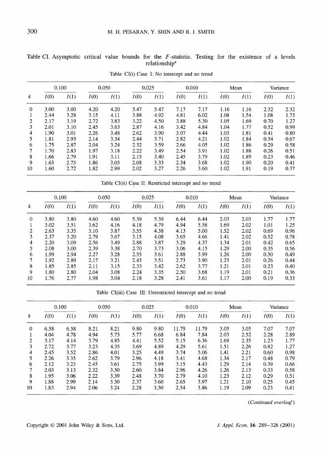
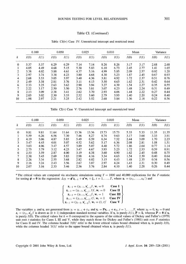
{xt} process is 0 < r < k.11 Hence, these two sets of critical values provide critical value bounds covering all possible classifications of {xt} into I(0), I(1) and mutually cointegrated processes. Asymptotic critical value bounds for the F-statistics covering Cases I-V are set out in Tables CI(i)-CI(v) for sizes 0.100, 0.050, 0.025 and 0.010; the lower bound values assume that the forcing variables {xt} are purely I(0), and the upper bound values assume that {xt} are purely 1(1).12
Hence, we suggest a bounds procedure to test Ho : ryy = 0 and ryx.x = 0' of (17) within the conditional ECMs (12)-(16). If the computed Wald or F-statistics fall outside the critical value bounds, a conclusive decision results without needing to know the cointegration rank r of the {xt} process. If, however, the Wald or F-statistic fall within these bounds, inference would be inconclusive. In such circumstances, knowledge of the cointegration rank r of the forcing variables {xt} is required to proceed further.
The conditional ECMs (12)-(16), derived from the underlying VAR(p) model (2), may also be interpreted as an autoregressive distributed lag model of orders (p, p, ..., p) (ARDL(p, ..., p)). However, one could also allow for differential lag lengths on the lagged variables Yt-i and xt-i in (2) to arrive at, for example, an ARDL(p, 1, ..., Pk) model without affecting the asymptotic results derived in this section. Hence, our approach is quite general in the sense that one can use a flexible choice for the dynamic lag structure in (12)-(16) as well as allowing for short-run feedbacks from the lagged dependent variables, Ayt-i, i = 1, ..., p, to Axt in (7). Moreover, within the single-equation context, the above analysis is more general than the cointegration analysis of partial systems carried out by Boswijk (1992, 1995), HJNR, Johansen (1992, 1995), PSS, and Urbain (1992), where it is assumed in addition that _xn = 0 or xt is purely I(1) in (7).
To conclude this section, we reconsider the approach of BDM. There are three scenarios for the deterministics given by (12), (14) and (16). Note that the restrictions on the deterministics' coefficients (9) are ignored in Cases II of (13) and IV of (15) and, thus, Cases II and IV are now subsumed by Cases III of (14) and V of (16) respectively. As noted below (11), BDM impose but do not test the implicit hypothesis at - w'ax = 0'; that is, the limiting distributional results given below are also obtained under the joint hypothesis Ho : tyy = 0 and Vyx.x = 0' of (17). BDM test y,, = 0 (or H 'Ttyy = 0) via the exclusion of Yt-1 in Cases I, III and V. For example, in Case V, they consider the t-statistic
-1P - t - A y A 1/2 /
- ^
1/2 t Oiiu (Y^-lP I _I (24)
where ctuU, is defined in the line after (21), Ay =P-1 _ P1,y_i y-i (Yo, .., YT-1), X-1 -Pt X_1, X-1 (Xp, v,XT-)i,) AZ_ APATZ-_, PT,TT - P,,
PTtT( TQTPTTT) tP,tT PI - =PPZ -P z- X1(X P-Z X_ 1) X Pz and PZ-
IT - AZ-(AZ AZ- )-'AZZ
1 The critical values of the Wald and F-statistics in the general case (not reported here) may be computed via stochastic simulations with different combinations of values for k and 0 < r < k. 12 The critical values for the Wald version of the bounds test are given by k + 1 times the critical values of the F-test in Cases I, III and V, and k + 2 times in Cases II and IV.
Copyright © 2001 John Wiley & Sons, Ltd.
299
J. Appl. Econ. 16: 289-326 (2001)
M. H. PESARAN, Y. SHIN AND R. J. SMITH
Table CI. Asymptotic critical value bounds for the F-statistic. Testing for the existence of a levels
relationshipa
Table CI(i) Case I: No intercept and no trend
0.100
k 1(0) 1(1)
0.050 0.025 0.010 Mean Variance
I(o) I(1) I(o) I(1) i(o) ( (1) ( (o) ( (1) ( (o) () )
0 3.00 3.00 4.20 4.20 5.47 5.47 7.17 7.17 1.16 1.16 2.32 2.32 1 2.44 3.28 3.15 4.11 3.88 4.92 4.81 6.02 1.08 1.54 1.08 1.73 2 2.17 3.19 2.72 3.83 3.22 4.50 3.88 5.30 1.05 1.69 0.70 1.27 3 2.01 3.10 2.45 3.63 2.87 4.16 3.42 4.84 1.04 1.77 0.52 0.99 4 1.90 3.01 2.26 3.48 2.62 3.90 3.07 4.44 1.03 1.81 0.41 0.80 5 1.81 2.93 2.14 3.34 2.44 3.71 2.82 4.21 1.02 1.84 0.34 0.67 6 1.75 2.87 2.04 3.24 2.32 3.59 2.66 4.05 1.02 1.86 0.29 0.58 7 1.70 2.83 1.97 3.18 2.22 3.49 2.54 3.91 1.02 1.88 0.26 0.51 8 1.66 2.79 1.91 3.11 2.15 3.40 2.45 3.79 1.02 1.89 0.23 0.46 9 1.63 2.75 1.86 3.05 2.08 3.33 2.34 3.68 1.02 1.90 0.20 0.41
10 1.60 2.72 1.82 2.99 2.02 3.27 2.26 3.60 1.02 1.91 0.19 0.37
Table CI(ii) Case II: Restricted intercept and no trend
0.100 0.050 0.025 0.010 Mean Variance
k I(o) I(1) I(O) I(1) I(O) I(1) I(O) I(1) I(O) I(1) I(O) I(1)
0 3.80 3.80 4.60 4.60 5.39 5.39 6.44 6.44 2.03 2.03 1.77 1.77 1 3.02 3.51 3.62 4.16 4.18 4.79 4.94 5.58 1.69 2.02 1.01 1.25 2 2.63 3.35 3.10 3.87 3.55 4.38 4.13 5.00 1.52 2.02 0.69 0.96 3 2.37 3.20 2.79 3.67 3.15 4.08 3.65 4.66 1.41 2.02 0.52 0.78 4 2.20 3.09 2.56 3.49 2.88 3.87 3.29 4.37 1.34 2.01 0.42 0.65 5 2.08 3.00 2.39 3.38 2.70 3.73 3.06 4.15 1.29 2.00 0.35 0.56 6 1.99 2.94 2.27 3.28 2.55 3.61 2.88 3.99 1.26 2.00 0.30 0.49 7 1.92 2.89 2.17 3.21 2.43 3.51 2.73 3.90 1.23 2.01 0.26 0.44 8 1.85 2.85 2.11 3.15 2.33 3.42 2.62 3.77 1.21 2.01 0.23 0.40 9 1.80 2.80 2.04 3.08 2.24 3.35 2.50 3.68 1.19 2.01 0.21 0.36
10 1.76 2.77 1.98 3.04 2.18 3.28 2.41 3.61 1.17 2.00 0.19 0.33
Table CI(iii) Case III: Unrestricted intercept and no trend
0.100 0.050 0.025 0.010 Mean Variance
k I(O) I(1) i(O) I(1) I(O) I(1) I(O) I(1) I(O) I(1) I(O) I(1)
0 6.58 6.58 8.21 8.21 9.80 9.80 11.79 11.79 3.05 3.05 7.07 7.07 1 4.04 4.78 4.94 5.73 5.77 6.68 6.84 7.84 2.03 2.52 2.28 2.89 2 3.17 4.14 3.79 4.85 4.41 5.52 5.15 6.36 1.69 2.35 1.23 1.77 3 2.72 3.77 3.23 4.35 3.69 4.89 4.29 5.61 1.51 2.26 0.82 1.27 4 2.45 3.52 2.86 4.01 3.25 4.49 3.74 5.06 1.41 2.21 0.60 0.98 5 2.26 3.35 2.62 3.79 2.96 4.18 3.41 4.68 1.34 2.17 0.48 0.79 6 2.12 3.23 2.45 3.61 2.75 3.99 3.15 4.43 1.29 2.14 0.39 0.66 7 2.03 3.13 2.32 3.50 2.60 3.84 2.96 4.26 1.26 2.13 0.33 0.58 8 1.95 3.06 2.22 3.39 2.48 3.70 2.79 4.10 1.23 2.12 0.29 0.51 9 1.88 2.99 2.14 3.30 2.37 3.60 2.65 3.97 1.21 2.10 0.25 0.45
10 1.83 2.94 2.06 3.24 2.28 3.50 2.54 3.86 1.19 2.09 0.23 0.41
(Continued overleaf)
Copyright © 2001 John Wiley & Sons, Ltd.
300
J. Appl. Econ. 16: 289-326 (2001)
BOUNDS TESTING FOR LEVEL RELATIONSHIPS 301
Table CI. (Continued)
Table CI(iv) Case IV: Unrestricted intercept and restricted trend
0.100 0.050 0.025 0.010 Mean Variance
k I(O) I(1) I(O) I(1) I(O) I(1) I(O) I(1) I(O) I(1) I(O) I(1)
0 5.37 5.37 6.29 6.29 7.14 7.14 8.26 8.26 3.17 3.17 2.68 2.68 1 4.05 4.49 4.68 5.15 5.30 5.83 6.10 6.73 2.45 2.77 1.41 1.65 2 3.38 4.02 3.88 4.61 4.37 5.16 4.99 5.85 2.09 2.57 0.92 1.20 3 2.97 3.74 3.38 4.23 3.80 4.68 4.30 5.23 1.87 2.45 0.67 0.93 4 2.68 3.53 3.05 3.97 3.40 4.36 3.81 4.92 1.72 2.37 0.51 0.76 5 2.49 3.38 2.81 3.76 3.11 4.13 3.50 4.63 1.62 2.31 0.42 0.64 6 2.33 3.25 2.63 3.62 2.90 3.94 3.27 4.39 1.54 2.27 0.35 0.55 7 2.22 3.17 2.50 3.50 2.76 3.81 3.07 4.23 1.48 2.24 0.31 0.49 8 2.13 3.09 2.38 3.41 2.62 3.70 2.93 4.06 1.44 2.22 0.27 0.44 9 2.05 3.02 2.30 3.33 2.52 3.60 2.79 3.93 1.40 2.20 0.24 0.40
10 1.98 2.97 2.21 3.25 2.42 3.52 2.68 3.84 1.36 2.18 0.22 0.36
Table CI(v) Case V: Unrestricted intercept and unrestricted trend
0.100 0.050 0.025 0.010 Mean Variance
k I(O) I(1) I(O) I(1) I(O) I(1) I(O) (1 ) i(O ) (1 ) i(O) i(1)
0 9.81 9.81 11.64 11.64 13.36 13.36 15.73 15.73 5.33 5.33 11.35 11.35 1 5.59 6.26 6.56 7.30 7.46 8.27 8.74 9.63 3.17 3.64 3.33 3.91 2 4.19 5.06 4.87 5.85 5.49 6.59 6.34 7.52 2.44 3.09 1.70 2.23 3 3.47 4.45 4.01 5.07 4.52 5.62 5.17 6.36 2.08 2.81 1.08 1.51 4 3.03 4.06 3.47 4.57 3.89 5.07 4.40 5.72 1.86 2.64 0.77 1.14 5 2.75 3.79 3.12 4.25 3.47 4.67 3.93 5.23 1.72 2.53 0.59 0.91 6 2.53 3.59 2.87 4.00 3.19 4.38 3.60 4.90 1.62 2.45 0.48 0.75 7 2.38 3.45 2.69 3.83 2.98 4.16 3.34 4.63 1.54 2.39 0.40 0.64 8 2.26 3.34 2.55 3.68 2.82 4.02 3.15 4.43 1.48 2.35 0.34 0.56 9 2.16 3.24 2.43 3.56 2.67 3.87 2.97 4.24 1.43 2.31 0.30 0.49
10 2.07 3.16 2.33 3.46 2.56 3.76 2.84 4.10 1.40 2.28 0.26 0.44
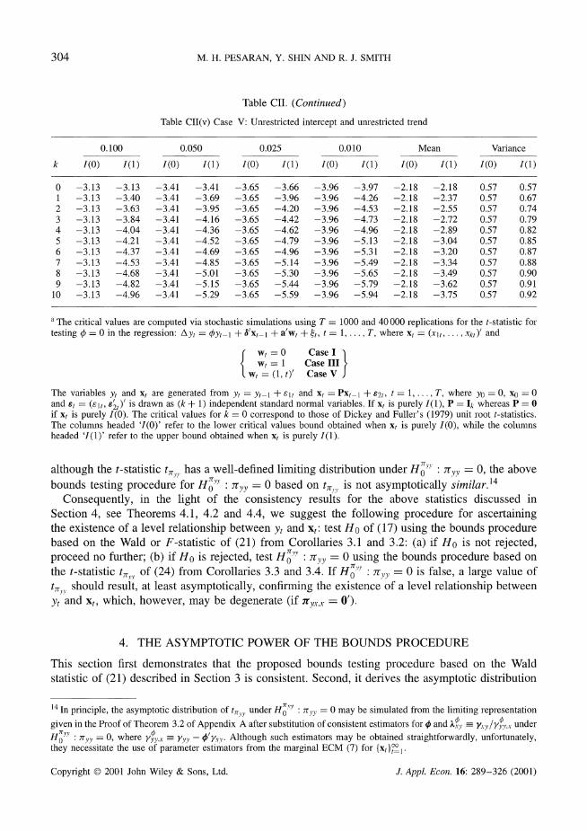
a The critical values are computed via stochastic simulations using T = 1000 and 40,000 replications for the F-statistic for testing q = 0 in the regression: Ayt = -'z-_l + a'wt + 4t, t 1..., T, where xt = (xlt, Xkt') and
zt-i = (Yt-1, Xt_), wt =0 Case I zt- = (Yt-I, x, i)', wt =0 Case II
zt-i = - (Yt- ), xt1, wt = 1 Case III
Zt-1 = (Yt-1, xt-1, t), wt = 1 Case IV
zt- = (Yt -, t_i), wt = (1, t)' Case V
The variables yt and xt are generated from Yt = Yt-l + Eit and xt = Pxt-I + 82t, t = 1 ..., T, where yo = 0, xo = 0 and Et = (lt, e2t)' is drawn as (k + 1) independent standard normal variables. If xt is purely I(1), P = Ik whereas P = 0 if xt is purely I(0). The critical values for k = 0 correspond to the squares of the critical values of Dickey and Fuller's (1979) unit root t-statistics for Cases I, III and V, while they match those for Dickey and Fuller's (1981) unit root F-statistics for Cases II and IV. The columns headed 'I(0)' refer to the lower critical values bound obtained when xt is purely I(0), while the columns headed 'I(1)' refer to the upper bound obtained when xt is purely I(1).
Copyright © 2001 John Wiley & Sons, Ltd. J. Appl. Econ. 16: 289-326 (2001)
M. H. PESARAN, Y. SHIN AND R. J. SMITH
Theorem 3.2 (Limiting distribution of t,,,). If Assumptions 1-4 and 5a hold and Yxy = 0, where Tx = (Yxy, rr), then under Ho: 7ryy = 0 and tyx.x = O' of (17), as T -> oo, the asymptotic distribution of the t-statistic t,y, of (24) has the representation
dWu(a)Fk_,r(a) Fk_-r(a)2 da) (25)
where
W,(a) - f1 W,(a)Wk_,(a)' da (fo Wk-_(a)Wk- (a)' da) Wk_-r(a) Case I
Fkr(a) = u(a) - fo WI,a)Wk_,(a)'da ( Wk-,r(a)Wk-, (a)'da) Wk ,(a) Case III
< W(a) - f Wu,(a)Wk r(a)'da (f1 Wk _r(a)Wk_ (a)' da)l Wkr(a) Case V
r = 0, .., k, and Cases I III and V are defined in (12), (14) and (16), a e [0, 1].
The form of the asymptotic representation (25) is similar to that of a Dickey-Fuller test for a unit root except that the standard Brownian motion W,,(a) is replaced by the residual from an asymptotic regression of W (a) on the independent (k - r)-vector standard Brownian motion Wkr_ (a) (or their de-meaned and de-meaned and de-trended counterparts).
Similarly to the analysis following Theorem 3.1, we detail the limiting distribution of the t- statistic t,y in the two polar cases in which the forcing variables {xt} are purely integrated of order zero and one respectively.
Corollary 3.3 (Limiting distribution of t,y if {xt) - I(0)). If Assumptions 1-4 and 5a hold and r = k, that is, {xt} - I(0), then under Ho : 7ryy = 0 and ryx.x = 0' of (17), as T -> oo, the
asymptotic distribution of the t-statistic t,,y, of (24) has the representation
p\ / \ \-1/2
d dWu(a)F(a) F(a2da o \Jo( )
where where W, (a) Case I
F(a) = Wu(a) Case III I W,(a) Case V )
and Cases I, III and V are defined in (12), (14) and (16), a e [0, 1].
Corollary 3.4 (Limiting distribution of t,y: if {Xt} - 1(1)). If Assumptions 1-4 and 5a hold, Yxy = 0, where rI = (Yxy, ,), and r = O, that is, {xt} - I(1), then under Ho'r' yy = 0, as T -> oo, the asymptotic distribution of the t-statistic t,,y of (24) has the representation
r1 / /ll -1/2
j dW,(a)Fk(a) ( Fk(a)2
da
where Fk(a) is defined in Theorem 3.2 for Cases I, III and V, a e [0, 1].
As above, it may be shown by simulation that the asymptotic critical values obtained from Corollaries 3.3 (r = k and {xt} is purely I(O)) and 3.4 (r = 0 and {xt} is purely I(1)) provide
Copyright © 2001 John Wiley & Sons, Ltd.
302
J. Appl. Econ. 16: 289-326 (2001)
BOUNDS TESTING FOR LEVEL RELATIONSHIPS
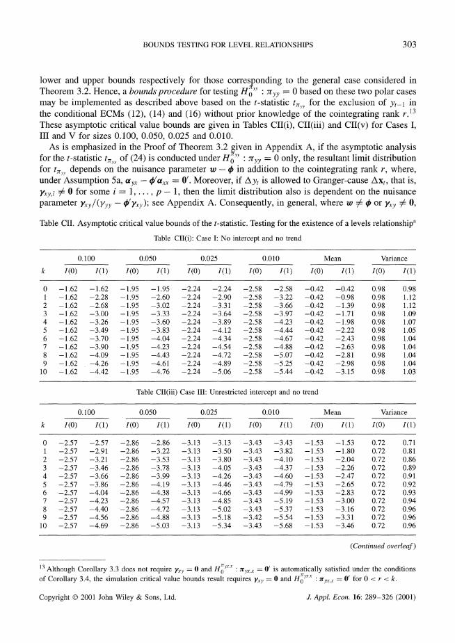
lower and upper bounds respectively for those corresponding to the general case considered in Theorem 3.2. Hence, a bounds procedure for testing H': y = 0 based on these two polar cases may be implemented as described above based on the t-statistic t,,, for the exclusion of yt-_ in the conditional ECMs (12), (14) and (16) without prior knowledge of the cointegrating rank r.13 These asymptotic critical value bounds are given in Tables CII(i), CII(iii) and CII(v) for Cases I, III and V for sizes 0.100, 0.050, 0.025 and 0.010.
As is emphasized in the Proof of Theorem 3.2 given in Appendix A, if the asymptotic analysis for the t-statistic t,Y of (24) is conducted under HoY : yy = 0 only, the resultant limit distribution for t,: depends on the nuisance parameter w - 0 in addition to the cointegrating rank r, where, under Assumption 5a, ayx - 0'acx = 0'. Moreover, if Ayt is allowed to Granger-cause Axt, that is, Yxy,i a 0 for somee i = p - , then the limit distribution also is dependent on the nuisance parameter yAy/(yyy - 'Yxy); see Appendix A. Consequently, in general, where w Z / or y,y y 0,
Table CII. Asymptotic critical value bounds of the t-statistic. Testing for the existence of a levels relationshipa
Table CII(i): Case I: No intercept and no trend
0.100
k I(0) I(1)
0 -1.62 -1.62 1 -1.62 -2.28 2 -1.62 -2.68 3 -1.62 -3.00 4 -1.62 -3.26 5 -1.62 -3.49 6 -1.62 -3.70 7 -1.62 -3.90 8 -1.62 -4.09 9 -1.62 -4.26
10 -1.62 -4.42
0.050 0.025 0.010 Mean Variance
I(0) I(1) I() I(1) I(0) I(1) I(0) I(1) I(0) I(1)
-1.95 -1.95 -2.24 -2.24 -2.58 -2.58 -0.42 -0.42 0.98 0.98 -1.95 -2.60 -2.24 -2.90 -2.58 -3.22 -0.42 -0.98 0.98 1.12 -1.95 -3.02 -2.24 -3.31 -2.58 -3.66 -0.42 -1.39 0.98 1.12 -1.95 -3.33 -2.24 -3.64 -2.58 -3.97 -0.42 -1.71 0.98 1.09 -1.95 -3.60 -2.24 -3.89 -2.58 -4.23 -0.42 -1.98 0.98 1.07 -1.95 -3.83 -2.24 -4.12 -2.58 -4.44 -0.42 -2.22 0.98 1.05 -1.95 -4.04 -2.24 -4.34 -2.58 -4.67 -0.42 -2.43 0.98 1.04 -1.95 -4.23 -2.24 -4.54 -2.58 -4.88 -0.42 -2.63 0.98 1.04 -1.95 -4.43 -2.24 -4.72 -2.58 -5.07 -0.42 -2.81 0.98 1.04 -1.95 -4.61 -2.24 -4.89 -2.58 -5.25 -0.42 -2.98 0.98 1.04 -1.95 -4.76 -2.24 -5.06 -2.58 -5.44 -0.42 -3.15 0.98 1.03
Table CII(iii) Case III: Unrestricted intercept and no trend
0.100
k I(0) I(1)
0 -2.57 -2.57 1 -2.57 -2.91 2 -2.57 -3.21 3 -2.57 -3.46 4 -2.57 -3.66 5 -2.57 -3.86 6 -2.57 -4.04 7 -2.57 -4.23 8 -2.57 -4.40 9 -2.57 -4.56
10 -2.57 -4.69
0.050 0.025 0.010 Mean Variance
I(0) I(1) I(0) I(1) I(0 ) () (0) I(1) I(O) I(1)
-2.86 -2.86 -3.13 -3.13 -3.43 -3.43 -1.53 -1.53 0.72 0.71 -2.86 -3.22 -3.13 -3.50 -3.43 -3.82 -1.53 -1.80 0.72 0.81 -2.86 -3.53 -3.13 -3.80 -3.43 -4.10 -1.53 -2.04 0.72 0.86 -2.86 -3.78 -3.13 -4.05 -3.43 -4.37 -1.53 -2.26 0.72 0.89 -2.86 -3.99 -3.13 -4.26 -3.43 -4.60 -1.53 -2.47 0.72 0.91 -2.86 -4.19 -3.13 -4.46 -3.43 -4.79 -1.53 -2.65 0.72 0.92 -2.86 -4.38 -3.13 -4.66 -3.43 -4.99 -1.53 -2.83 0.72 0.93 -2.86 -4.57 -3.13 -4.85 -3.43 -5.19 -1.53 -3.00 0.72 0.94 -2.86 -4.72 -3.13 -5.02 -3.43 -5.37 -1.53 -3.16 0.72 0.96 -2.86 -4.88 -3.13 -5.18 -3.42 -5.54 -1.53 -3.31 0.72 0.96 -2.86 -5.03 -3.13 -5.34 -3.43 -5.68 -1.53 -3.46 0.72 0.96
(Continued overleaf )
13 Although Corollary 3.3 does not require Yyy = 0 and HO x : TAx.x = 01 is automatically satisfied under the conditions of Corollary 3.4, the simulation critical value bounds result requires Yyx) = 0 and H" : 7.x = 0' for 0 < r < k.
Copyright © 2001 John Wiley & Sons, Ltd.
303
J. Appl. Econ. 16: 289-326 (2001)
M. H. PESARAN, Y. SHIN AND R. J. SMITH
Table CII. (Continued)
Table CII(v) Case V: Unrestricted intercept and unrestricted trend
0.100 0.050 0.025 0.010 Mean Variance
k i(o) I(1) I(O) I(1) I(0) I(1) I(0) I(1) I(O) I(1) I(O) I(1)
0 -3.13 -3.13 -3.41 -3.41 -3.65 -3.66 -3.96 -3.97 -2.18 -2.18 0.57 0.57 1 -3.13 -3.40 -3.41 -3.69 -3.65 -3.96 -3.96 -4.26 -2.18 -2.37 0.57 0.67 2 -3.13 -3.63 -3.41 -3.95 -3.65 -4.20 -3.96 -4.53 -2.18 -2.55 0.57 0.74 3 -3.13 -3.84 -3.41 -4.16 -3.65 -4.42 -3.96 -4.73 -2.18 -2.72 0.57 0.79 4 -3.13 -4.04 -3.41 -4.36 -3.65 -4.62 -3.96 -4.96 -2.18 -2.89 0.57 0.82 5 -3.13 -4.21 -3.41 -4.52 -3.65 -4.79 -3.96 -5.13 -2.18 -3.04 0.57 0.85 6 -3.13 -4.37 -3.41 -4.69 -3.65 -4.96 -3.96 -5.31 -2.18 -3.20 0.57 0.87 7 -3.13 -4.53 -3.41 -4.85 -3.65 -5.14 -3.96 -5.49 -2.18 -3.34 0.57 0.88 8 -3.13 -4.68 -3.41 -5.01 -3.65 -5.30 -3.96 -5.65 -2.18 -3.49 0.57 0.90 9 -3.13 -4.82 -3.41 -5.15 -3.65 -5.44 -3.96 -5.79 -2.18 -3.62 0.57 0.91
10 -3.13 -4.96 -3.41 -5.29 -3.65 -5.59 -3.96 -5.94 -2.18 -3.75 0.57 0.92
a The critical values are computed via stochastic simulations using T = 1000 and 40000 replications for the t-statistic for testing 0 = 0 in the regression: Ayt = Pyt- + 8'xt- + a'wt + -t, t = 1, ..., T, where xt = (xlt, ..., Xkt)' and
wt = 0 Case I wt = 1 Case III
wt =(1, t)' Case V
The variables Yt and xt are generated from Yt = Yt-_ + 8lt and xt = Pxt_l + s2t, t = 1 ..., T, where yo = 0, xo = 0 and st = (Elt, s2t)' is drawn as (k + 1) independent standard normal variables. If xt is purely I(1), P = Ik whereas P = 0 if xt is purely I(0). The critical values for k = 0 correspond to those of Dickey and Fuller's (1979) unit root t-statistics. The columns headed 'I(0)' refer to the lower clitical values bound obtained when xt is purely I(0), while the columns headed 'I(1)' refer to the upper bound obtained when xt is purely I(1).
although the t-statistic t, has a well-defined limiting distribution under H ' = 0, the above IT - ~yy - 0, the above
bounds testing procedure for Hor : r,,,, = 0 based on t=,. is not asymptotically similar.14
Consequently, in the light of the consistency results for the above statistics discussed in Section 4, see Theorems 4.1, 4.2 and 4.4, we suggest the following procedure for ascertaining the existence of a level relationship between Yt and xt: test Ho of (17) using the bounds procedure based on the Wald or F-statistic of (21) from Corollaries 3.1 and 3.2: (a) if Ho is not rejected, proceed no further; (b) if Ho is rejected, test Ho'' : 7,y = 0 using the bounds procedure based on the t-statistic t,, of (24) from Corollaries 3.3 and 3.4. If H ' y = 0 is false, a large value of
t,!! should result, at least asymptotically, confirming the existence of a level relationship between
Yt and xt, which, however, may be degenerate (if yr,. = 0').
4. THE ASYMPTOTIC POWER OF THE BOUNDS PROCEDURE
This section first demonstrates that the proposed bounds testing procedure based on the Wald statistic of (21) described in Section 3 is consistent. Second, it derives the asymptotic distribution
14 In principle, the asymptotic distribution of t,V,, under H"!' : Ty,, = 0 may be simulated from the limiting representation
given in the Proof of Theorem 3.2 of Appendix A after substitution of consistent estimators for 0 and ,, _ y- y/y/,y.x under
Ho' y = 0, where yY,x Y /y - /Xy. Although such estimators may be obtained straightforwardly, unfortunately, they necessitate the use of parameter estimators from the marginal ECM (7) for {xt}t°l
Copyright © 2001 John Wiley & Sons, Ltd.
304
J. Appl. Econ. 16: 289-326 (2001)
BOUNDS TESTING FOR LEVEL RELATIONSHIPS
of the Wald statistic of (21) under a sequence of local alternatives. Finally, we show that the bounds procedure based on the t-statistic of (24) is consistent.
In the discussion of the consistency of the bounds test procedure based on the Wald statistic of (21), because the rank of the long-run multiplier matrix H may be either r or r + 1 under the alternative hypothesis H1 = H
' U H of (18) where H"' : yy 7 0 and H. , = 0', it is
necessary to deal with these two possibilities. First, under H 'Y' ty 7 0, the rank of n is r + 1 so Assumption 5b applies; in particular, a,yy O. Second, under H z = 0, the rank of H is r so Assumption 5a applies; in this case, H l': rtyx O' holds and, in particular, aty - w'a / O7'.
Theorem 4.1 (Consistency of the Wald statistic bounds testprocedure under H ' "). IfAssumptions 1-4 and 5b hold, then under H '!Y: t,, Zy 0 of (18) the Wald statistic W (21) is consistent against H1: trryy 0 in Cases I-V defined in (12)-(16).
Theorem 4.2 (Consistency of the Wald statistic bounds test procedure under H ' I Ht). If Assumptions 1-4 and 5a hold, then under H '": 7r x. 0 of(18) and H" : · = 0 of(17) the Wald statistic W (21) is consistent against H> ' : nr,..x = 0/ in Cases I-V defined in (12)-(16).
Hence, combining Theorems 4.1 and 4.2, the bounds procedure of Section 3 based on the Wald statistic W (21) defines a consistent test of Ho = Ho"' n, H"H' of (17) against H1 = H>!' U Hlr of (18). This result holds irrespective of whether the forcing variables {xt} are purely I(O), purely I(1) or mutually cointegrated.
We now turn to consider the asymptotic distribution of the Wald statistic (21) under a suitably specified sequence of local alternatives. Recall that under Assumption 5b, t7rV,v[= (vy,,,, yx.)] =
(ayytyy, ayalfiy + (aoty -W - w/a)/5x). Consequently, we define the sequence of local alternatives
H1T 7: y.xT[= (7ryy, T r.xT)] = (T-l yyaS)y, T-1 , + 1/2(, - w')B ) (26)
Hence, under Assumption 3, defining
niT ( ('y,T ZyT-T
and recalling Hn = ap', where (1, -w')a = a, - w'ax = 0', we have
II - T-r= lT S'a,, + T-/2 )1v (27)
In order to detail the limit distribution of the Wald statistic under the sequence of local alterna- tives HIT of (26), it is necessary to define the (k - r + l)-dimensional Ornstein-Uhlenbeck pro- cess Jk_- (a) = ( Ja) (la),(a), ')' which obeys the stochastic integral and differential equations, Jk-.+l (a) = Wk-r+1 (a) + ab' f Jk- +l (r) dr and dJk_.+l (a) = dWk-,+l (a) + ab Jk-,+ (a) da, where Wk-,+l (a) is a (k - r + 1)-dimensional standard Brownian motion, a = [(ay, aol)'n(aOy, a1)]-1/2(ol, oL)'a)y, b = [(a- , a')'(a', a1)]l/2[(-L l)Tr(a I, a1)]-1 I(S, 1 )ty,,, together
k, ), ( with the de-meaned and de-meaned and de-trended counterparts J_,.+(a) = (J* (a), Jk _(a)')'
and J_,+l (a) = (J*(a) Jk_,.(a)')' partitioned similarly, a e [0, 1]. See, for example, Johansen (1995, Chapter 14, pp. 201-210).
Copyright © 2001 John Wiley & Sons, Ltd.
305
J. Appl. Econ. 16: 289-326 (2001)
M. H. PESARAN, Y. SHIN AND R. J. SMITH
Theorem 4.3 (Limiting distribution of W under H ir). If Assumptions 1 -4 and 5a hold, then under H1T : ry.x = T y-lyyfy + T-1/2(8y - w'8xx)' of (26), as T -- oo, the asymptotic distribution of the Wald statistic W of (21) has the representation
W = z;z, + 0 dJ *(a)Fk -r+(a)' (7 Fk-r+l(a)Fk ,+1(a)'da) Fk_,+i(a)dJ(a) (28) JO \Jo } o
where z, N (Q1/2I, I,), Q[= Q1/2,Q1/2] = plimrToo(r- T fiZ_1P^, Z_i), ) (yx - w' xx)', is distributed independently of the second term in (28) and
Jkr.+i(a) Case I (Jk-r+l (a)', 1)' Case II Case II
Fk-r+l(a)= < Jk+i(a) Case III
(J_.l (a)', a- 1/2)' Case IV
Jkr+l(a) Case V
r = 0, ..., k, and Cases I-V are defined in (12)-(16), a E [0, 1].
The first component of (28) z'.z,. is non-central chi-square distributed with r degrees of freedom and non-centrality parameter Yt'QYt and corresponds to the local alternative H,7>' nryxxT = T- /2(8 - W'8xx)'xx under HO' : ty = 0. The second term in (28) is a non-standard yx.xT = xx 0 . 71'y y Dickey-Fuller unit-root distribution under the local alternative H'' = T-lay/yy and yx - w'Sxx = O'. Note that under Ho of (17), that is, ayy = 0 and 8yx - w'S^ = 0', the limiting
representation (28) reduces to (22) as should be expected. The proof for the consistency of the bounds test procedure based on the t-statistic of (24)
requires that the rank of the long-run multiplier matrix nI is r + 1 under the alternative hypothesis H 'ry : ryy 0. Hence, Assumption 5b applies; in particular, ayy % 0.
Theorem 4.4 (Consistency of the t-statistic bounds test procedure under H 1' ). If Assumptions 1-4 and 5b hold, then under H>' . yy :7 0 of (18) the t-statistic t,,~, (24) is consistent against H1 ': tyy 0 in Cases I, III and V defined in (12), (14) and (16).
As noted at the end of Section 3, Theorem 4.4 suggests the possibility of using ty,, to discriminate between HO!: yy = 0 and H 7y: Ty 1 0, although, if H': = O' is false, the bounds procedure given via Corollaries 3.3 and 3.4 is not asymptotically similar.
AN APPLICATION: UK EARNINGS EQUATION
Following the modelling approach described earlier, this section provides a re-examination of the earnings equation included in the UK Treasury macroeconometric model described in Chan, Savage and Whittaker (1995), CSW hereafter. The theoretical basis of the Treasury's earnings equation is the bargaining model advanced in Nickell and Andrews (1983) and reviewed, for example, in
Layard et al. (1991, Chapter 2). Its theoretical derivation is based on a Nash bargaining framework where firms and unions set wages to maximize a weighted average of firms' profits and unions'
Copyright © 2001 John Wiley & Sons, Ltd.
306
J. Appl. Econ. 16: 289-326 (2001)
BOUNDS TESTING FOR LEVEL RELATIONSHIPS
utility. Following Darby and Wren-Lewis (1993), the theoretical real wage equation underlying the Treasury's earnings equation is given by
Prodt t =1 + f(URt)(1 - RRt)/Uniont
(29)
where Wt is the real wage, Prodt is labour productivity, RRt is the replacement ratio defined as the ratio of unemployment benefit to the wage rate, Uniont is a measure of 'union power', and f(URt) is the probability of a union member becoming unemployed, which is assumed to be an increasing function of the unemployment rate URt. The econometric specification is based on a log-linearized version of (29) after allowing for a wedge effect that takes account of the difference between the 'real product wage' which is the focus of the firms' decision, and the 'real consumption wage' which concerns the union.15 The theoretical arguments for a possible long-run wedge effect on real wages is mixed and, as emphasized by CSW, whether such long-run effects are present is an empirical matter. The change in the unemployment rate (A URt) is also included in the Treasury's wage equation. CSW cite two different theoretical rationales for the inclusion of A URt in the wage equation: the differential moderating effects of long- and short-term unemployed on real wages, and the 'insider-outsider' theories which argue that only rising unemployment will be effective in significantly moderating wage demands. See Blanchard and Summers (1986) and Lindbeck and Snower (1989). The ARDL model and its associated unrestricted equilibrium correction formulation used here automatically allow for such lagged effects.
We begin our empirical analysis from the maintained assumption that the time series properties of the key variables in the Treasury's earnings equation can be well approximated by a log-linear VAR(p) model, augmented with appropriate deterministics such as intercepts and time trends. To ensure comparability of our results with those of the Treasury, the replacement ratio is not included in the analysis. CSW, p. 50, report that '... it has not proved possible to identify a significant effect from the replacement ratio, and this had to be omitted from our specification'.16 Also, as in CSW, we include two dummy variables to account for the effects of incomes policies on average earnings. These dummy variables are defined by
D7475t = 1, over the period 1974ql - 1975q4, 0 elsewhere
D7579t = 1, over the period 1975ql - 1979q4, 0 elsewhere
off' dummy variables.17 Let zt = (wt, Prodt, URt, Wedget, Uniont)' = (wt, x')'. Then, using the analysis of Section 2, the conditional ECM of interest can be written as
p-l
Aw, = Co + clt + c2D7475t + c3D7579t + 7r,,,,wt- + Tx.Xxt- + E Azt-i + 8'Axt + Ut i=1
(30)
15 The wedge effect is further decomposed into a tax wedge and an import price wedge in the Treasury model, but this decomposition is not pursued here. 16 It is important, however, that, at a future date, a fresh investigation of the possible effects of the replacement ratio on real wages should be undertaken. 17 However, both the asymptotic theory and associated critical values must be modified if the fraction of periods in which the dummy variables are non-zero does not tend to zero with the sample size T. In the present application, both dummy variables included in the earning equation are zero after 1979, and the fractions of observations where D7475t and D7579t are non-zero are only 7.6% and 19.2% respectively.
Copyright © 2001 John Wiley & Sons, Ltd.
307
J. Appl. Econ. 16: 289-326 (2001)
M. H. PESARAN, Y. SHIN AND R. J. SMITH
Under the assumption that lagged real wages, wt1_, do not enter the sub-VAR model for xt, the above real wage equation is identified and can be estimated consistently by LS.18 Notice, however, that this assumption does not rule out the inclusion of lagged changes in real wages in the unemployment or productivity equations, for example. The exclusion of the level of real wages from these equations is an identification requirement for the bargaining theory of wages which permits it to be distinguished from other alternatives, such as the efficiency wage theory which postulates that labour productivity is partly determined by the level of real wages.19 It is clear that, in our framework, the bargaining theory and the efficiency wage theory cannot be entertained simultaneously, at least not in the long run.
The above specification is also based on the assumption that the disturbances ut are serially uncorrelated. It is therefore important that the lag order p of the underlying VAR is selected appropriately. There is a delicate balance between choosing p sufficiently large to mitigate the residual serial correlation problem and, at the same time, sufficiently small so that the conditional ECM (30) is not unduly over-parameterized, particularly in view of the limited time series data which are available.
Finally, a decision must be made concerning the time trend in (30) and whether its coefficient should be restricted.20 This issue can only be settled in light of the particular sample period under consideration. The time series data used are quarterly, cover the period 1970ql-1997q4, and are seasonally adjusted (where relevant).21 To ensure comparability of results for different choices of p, all estimations use the same sample period, 1972ql-1997q4 (T = 104), with the first eight observations reserved for the construction of lagged variables.
The fiveve variables in the earnings equation were constructed from primary sources in the fol- lowing manner: wt = ln(ERPRt/PYNONGt), Wedget = ln(l + TEt) + ln(l - TDt) - ln(RPIXt/ PYNONGt), URt = ln(100 x ILOUt/(ILOUt + WFEMPt)), Prodt = ln((YPROMt + 278.29 x YMFt)/(EMFt + ENMFt)), and Uniont = ln(UDENt), where ERPRt is average private sector earnings per employee (£), PYNONGt is the non-oil non-government GDP deflator, YPROM is output in the private, non-oil, non-manufacturing, and public traded sectors at constant fac- tor cost (f million, 1990), YMFt is the manufacturing output index adjusted for stock changes (1990 = 100), EMFt and ENMFt are respectively employment in UK manufacturing and non- manufacturing sectors (thousands), ILOUt is the International Labour Office (ILO) measure of unemployment (thousands), WFEMPt is total employment (thousands), TEt is the average employers' National Insurance contribution rate, TDt is the average direct tax rate on employ- ment incomes, RPIXt is the Retail Price Index excluding mortgage payments, and UDENt is union density (used to proxy 'union power') measured by union membership as a percentage of
employment.22 The time series plots of the five variables included in the VAR model are given in
Figures 1-3.
18 See Assumption 3 and the following discussion. By construction, the contemporaneous effects Axt are uncorrelated with the disturbance term ut and instrumental variable estimation which has been particularly popular in the empirical wage equation literature is not necessary. Indeed, given the unrestricted nature of the lag distribution of the conditional ECM (30), it is difficult to find suitable instruments: namely, variables that are not already included in the model, which are uncorrelated with Ut and also have a reasonable degree of correlation with the included variables in (30). 19 For a discussion of the issues that surround the identification of wage equations, see Manning (1993). 20 See, for example, PSS and the discussion in Section 2. 21 We are grateful to Andrew Gurney and Rod Whittaker for providing us with the data. For further details about the sources and the descriptions of the variables, see CSW, pp. 46-51 and p. 11 of the Annex. 22 The data series for UDEN assumes a constant rate of unionization from 1980q4 onwards.
Copyright © 2001 John Wiley & Sons, Ltd.
308
J. Appl. Econ. 16: 289-326 (2001)
BOUNDS TESTING FOR LEVEL RELATIONSHIPS 309
(a) 4.0-
3.5- _ __^-----~~~~~~~~~~~- ~ ~ ~~~/ Real Wages
3.0.~.~~-~
-a)
co 2.5-
_
2.0-
1.5- ~
A... . ........ / Productivity o . 0..
1 .0 I I I I I I I I I I 1972Q1 1974Q3 1977Q1 1979Q3 1982Q1 1984Q3 1987Q1 1989Q3 1992Q1 1994Q3 1997Q1
Quarters
(b) 0.04-
0.03-
0.02 /, ! Real Wage
0.00
-0.01
-0.02 I I0.03-0.04~ /
t,
Productivity
-0.03
-0.0 4 I I I I I I I I I I I 1972Q1 1974Q3 1977Q1 1979Q3 1982Q1 1984Q3 1987Q1 1989Q3 1992Q1 1994Q3 199701
Quarters
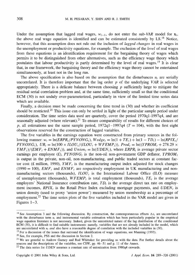
Figure 1. (a) Real wages and labour productivity. (b) Rate of change of real wages and labour productivity
It is clear from Figure 1 that real wages (average earnings) and productivity show steadily rising trends with real wages growing at a faster rate than productivity.23 This suggests, at least initially, that a linear trend should be included in the real wage equation (30). Also the application of unit root tests to the five variables, perhaps not surprisingly, yields mixed results with strong evidence in favour of the unit root hypothesis only in the cases of real wages and productivity. This does not necessarily preclude the other three variables (UR, Wedge, and Union) having levels impact on real wages. Following the methodology developed in this paper, it is possible to test for the existence of a real wage equation involving the levels of these five variables irrespective of whether they are purely I(O), purely I(1), or mutually cointegrated.
23 Over the period 1972ql-97q4, real wages grew by 2.14% per annum as compared to labour productivity that increased by an annual average rate of 1.54% over the same period.
Copyright © 2001 John Wiley & Sons, Ltd.
_A_
J. Appl. Econ. 16: 289-326 (2001)
M. H. PESARAN, Y. SHIN AND R. J. SMITH
I O Q I I I I I I I I I I I
1972Q1 1974Q3 1977Q1 1979Q3 1982Q1 1984Q3 1987Q1 1989Q3 1992Q1 1994Q3 1997Q1 Quarters
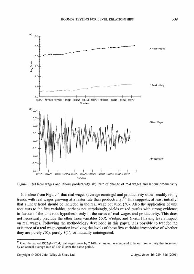
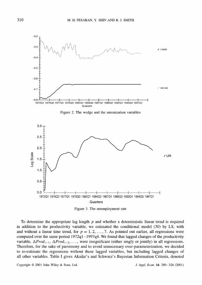
Figure 2. The wedge and the unionization variables
I I I I I I I I I
3.0-
2.5-
2.0-
1.5-
1.0-
0.5-
I I I I I I I I I I
*~ ~ I l l l l
1972Q1 1974Q3 1977Q1 1979Q3 1982Q1 1984Q3 1987Q1 1989Q3 1992Q1 1994Q3 1997Q1
Quarters
Figure 3. The unemployment rate
To determine the appropriate lag length p and whether a deterministic linear trend is required in addition to the productivity variable, we estimated the conditional model (30) by LS, with and without a linear time trend, for p = 1, 2,..., 7. As pointed out earlier, all regressions were computed over the same period 1972ql-1997q4. We found that lagged changes of the productivity variable, AProdt-l, AProdt2, ..., were insignificant (either singly or jointly) in all regressions. Therefore, for the sake of parsimony and to avoid unnecessary over-parameterization, we decided to re-estimate the regressions without these lagged variables, but including lagged changes of all other variables. Table I gives Akaike's and Schwarz's Bayesian Information Criteria, denoted
310
-0.2
-0.3 -
-0.4 -
-0.5 -
-0.6-
-0.7-
_
.(
/ UNION
WEDGE
Q) 0 o 0
,_1
/ UR
·I·L·L_
I n n
Copyright © 2001 John Wiley & Sons, Ltd. J. Appl. Econ. 16: 289-326 (2001)
BOUNDS TESTING FOR LEVEL RELATIONSHIPS
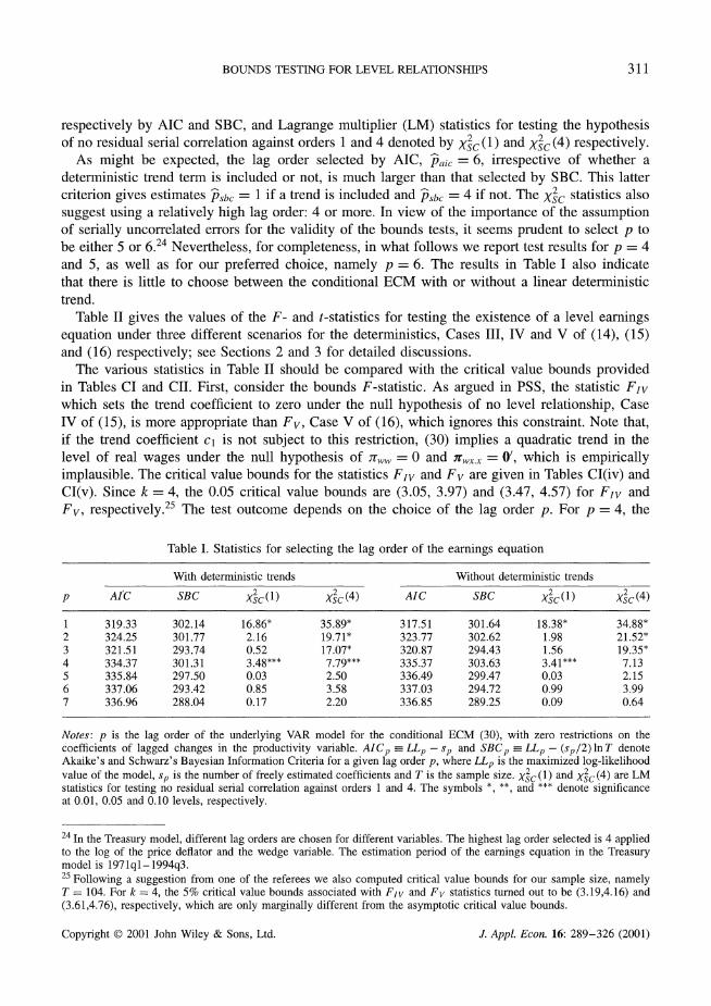
respectively by AIC and SBC, and Lagrange multiplier (LM) statistics for testing the hypothesis of no residual serial correlation against orders 1 and 4 denoted by XS2c(1) and X 2c(4) respectively.
As might be expected, the lag order selected by AIC, 7paic = 6, irrespective of whether a deterministic trend term is included or not, is much larger than that selected by SBC. This latter criterion gives estimates Psbc = 1 if a trend is included and psbc = 4 if not. The Xsc statistics also suggest using a relatively high lag order: 4 or more. In view of the importance of the assumption of serially uncorrelated errors for the validity of the bounds tests, it seems prudent to select p to be either 5 or 6.24 Nevertheless, for completeness, in what follows we report test results for p = 4 and 5, as well as for our preferred choice, namely p = 6. The results in Table I also indicate that there is little to choose between the conditional ECM with or without a linear deterministic trend.
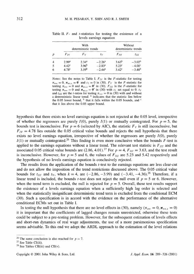
Table II gives the values of the F- and t-statistics for testing the existence of a level earnings equation under three different scenarios for the deterministics, Cases III, IV and V of (14), (15) and (16) respectively; see Sections 2 and 3 for detailed discussions.
The various statistics in Table II should be compared with the critical value bounds provided in Tables CI and CII. First, consider the bounds F-statistic. As argued in PSS, the statistic Fly which sets the trend coefficient to zero under the null hypothesis of no level relationship, Case IV of (15), is more appropriate than Fv, Case V of (16), which ignores this constraint. Note that, if the trend coefficient cl is not subject to this restriction, (30) implies a quadratic trend in the level of real wages under the null hypothesis of nr,, = 0 and r,,x.x = 0', which is empirically implausible. The critical value bounds for the statistics Flv and Fv are given in Tables CI(iv) and CI(v). Since k = 4, the 0.05 critical value bounds are (3.05, 3.97) and (3.47, 4.57) for Fly and Fv, respectively.25 The test outcome depends on the choice of the lag order p. For p = 4, the
Table I. Statistics for selecting the lag order of the earnings equation
With deterministic trends Without deterministic trends
p C SC ) AIC SBC x2 XC S (1) XSC(4)
1 319.33 302.14 16.86* 35.89* 317.51 301.64 18.38* 34.88* 2 324.25 301.77 2.16 19.71* 323.77 302.62 1.98 21.52* 3 321.51 293.74 0.52 17.07* 320.87 294.43 1.56 19.35* 4 334.37 301.31 3.48*** 7.79*** 335.37 303.63 3.41*** 7.13 5 335.84 297.50 0.03 2.50 336.49 299.47 0.03 2.15 6 337.06 293.42 0.85 3.58 337.03 294.72 0.99 3.99 7 336.96 288.04 0.17 2.20 336.85 289.25 0.09 0.64
Notes: p is the lag order of the underlying VAR model for the conditional ECM (30), with zero restrictions on the coefficients of lagged changes in the productivity variable. AICp = LLp - sp and SBCp = LLp - (sp/2) n T denote Akaike's and Schwarz's Bayesian Information Criteria for a given lag order p, where LLp is the maximized log-likelihood value of the model, sp is the number of freely estimated coefficients and T is the sample size. Xsc(1) and Xsc(4) are LM statistics for testing no residual serial correlation against orders 1 and 4. The symbols *, **, and *** denote significance at 0.01, 0.05 and 0.10 levels, respectively.
24 In the Treasury model, different lag orders are chosen for different variables. The highest lag order selected is 4 applied to the log of the price deflator and the wedge variable. The estimation period of the earnings equation in the Treasury model is 1971ql-1994q3. 25 Following a suggestion from one of the referees we also computed critical value bounds for our sample size, namely T = 104. For k = 4, the 5% critical value bounds associated with FIr and Fv statistics turned out to be (3.19,4.16) and (3.61,4.76), respectively, which are only marginally different from the asymptotic critical value bounds.
Copyright © 2001 John Wiley & Sons, Ltd.
311
J. Appl. Econ. 16: 289-326 (2001)
M. H. PESARAN, Y. SHIN AND R. J. SMITH
Table II. F- and t-statistics for testing the existence of a levels earnings equation
With Without deterministic trends deterministic trends
p F F t F tv Fi tll
4 2.99a 2.34a -2.26a 3.63b -3.02b 5 4.42C 3.96b -2.83a 5.23C -4.00C 6 4.78c 3.59b -2.44a 5.42C -3.48b
Notes: See the notes to Table I. Fly is the F-statistic for testing 2tYvV = 0, ,,,wx,- = 0' and cl = 0 in (30). Fv is the F-statistic for testing rtww = 0 and 7w,,x. = 0' in (30). FlI is the F-statistic for testing trvw = 0 and 7r,,.x = 0' in (30) with cl set equal to 0. tv and tlm are the t-ratios for testing 7rvv = 0 in (30) with and without a deterministic linear trend. a indicates that the statistic lies below the 0.05 lower bound, b that it falls within the 0.05 bounds, and c
that it lies above the 0.05 upper bound.
hypothesis that there exists no level earnings equation is not rejected at the 0.05 level, irrespective of whether the regressors are purely I(O), purely I(1) or mutually cointegrated. For p = 5, the bounds test is inconclusive. For p = 6 (selected by AIC), the statistic Fv is still inconclusive, but Flv = 4.78 lies outside the 0.05 critical value bounds and rejects the null hypothesis that there exists no level earnings equation, irrespective of whether the regressors are purely I(0), purely I(1) or mutually cointegrated.26 This finding is even more conclusive when the bounds F-test is applied to the earnings equations without a linear trend. The relevant test statistic is F111 and the associated 0.05 critical value bounds are (2.86, 4.01).27 For p = 4, F111 = 3.63, and the test result is inconclusive. However, for p = 5 and 6, the values of F111 are 5.23 and 5.42 respectively and the hypothesis of no levels earnings equation is conclusively rejected.
The results from the application of the bounds t-test to the earnings equations are less clear-cut and do not allow the imposition of the trend restrictions discussed above. The 0.05 critical value bounds for t/ll and tv, when k = 4, are (-2.86, -3.99) and (-3.41, -4.36).28 Therefore, if a linear trend is included, the bounds t-test does not reject the null even if p = 5 or 6. However, when the trend term is excluded, the null is rejected for p = 5. Overall, these test results support the existence of a levels earnings equation when a sufficiently high lag order is selected and when the statistically insignificant deterministic trend term is excluded from the conditional ECM (30). Such a specification is in accord with the evidence on the performance of the alternative conditional ECMs set out in Table I.
In testing the null hypothesis that there are no level effects in (30), namely (7,,, = 0, 7r,^.. = 0) it is important that the coefficients of lagged changes remain unrestricted, otherwise these tests could be subject to a pre-testing problem. However, for the subsequent estimation of levels effects and short-run dynamics of real wage adjustments, the use of a more parsimonious specification seems advisable. To this end we adopt the ARDL approach to the estimation of the level relations
26 The same conclusion is also reached for p = 7. 27 See Table CI(iii). 28 See Tables CII(iii) and CII(v).
Copyright © 2001 John Wiley & Sons, Ltd.
312
J. Appl. Econ. 16: 289-326 (2001)
BOUNDS TESTING FOR LEVEL RELATIONSHIPS
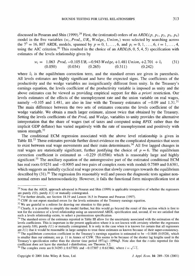
discussed in Pesaran and Shin (1999).29 First, the (estimated) orders of an ARDL(p, pi, P2, P3, P4) model in the five variables (wt, Prodt, URt, Wedget, Uniont) were selected by searching across the 75 = 16, 807 ARDL models, spanned by p = 0, 1,..., 6, and pi = 0, 1,..., 6, i = 1,..., 4, using the AIC criterion.30 This resulted in the choice of an ARDL(6, 0, 5, 4, 5) specification with estimates of the levels relationship given by
wt = 1.063 Prodt -0.105 URt -0.943 Wedget +1.481 Uniont +2.701 + vt (31) (0.050) (0.034) (0.265) (0.311) (0.242)
where vt is the equilibrium correction term, and the standard errors are given n parenthesis. All levels estimates are highly significant and have the expected signs. The coefficients of the productivity and the wedge variables are insignificantly different from unity. In the Treasury's earnings equation, the levels coefficient of the productivity variable is imposed as unity and the above estimates can be viewed as providing empirical support for this a priori restriction. Our levels estimates of the effects of the unemployment rate and the union variable on real wages, namely -0.105 and 1.481, are also in line with the Treasury estimates of -0.09 and 1.31.31 The main difference between the two sets of estimates concerns the levels coefficient of the wedge variable. We obtain a much larger estimate, almost twice that obtained by the Treasury. Setting the levels coefficients of the Prodt and Wedget variables to unity provides the alternative interpretation that the share of wages (net of taxes and computed using RPIX rather than the implicit GDP deflator) has varied negatively with the rate of unemployment and positively with union strength.32
The conditional ECM regression associated with the above level relationship is given in Table III.33 These estimates provide further direct evidence on the complicated dynamics that seem to exist between real wage movements and their main determinants.34 All five lagged changes in real wages are statistically significant, further justifying the choice of p = 6. The equilibrium correction coefficient is estimated as -0.229 (0.0586) which is reasonably large and highly significant.35 The auxiliary equation of the autoregressive part of the estimated conditional ECM has real roots 0.9231 and -0.9095 and two pairs of complex roots with moduli 0.7589 and 0.6381, which suggests an initially cyclical real wage process that slowly converges towards the equilibrium described by (31).36 The regression fits reasonably well and passes the diagnostic tests against non- normal errors and heteroscedasticity. However, it fails the functional form misspecification test at
29 Note that the ARDL approach advanced in Pesaran and Shin (1999) is applicable irrespective of whether the regressors are purely I(0), purely 1(1) or mutually cointegrated. 30 For further details, see Section 18.19 and Lesson 16.5 in Pesaran and Pesaran (1997). 31 CSW do not report standard errors for the levels estimates of the Treasury earnings equation. 32 We are grateful to a referee for drawing our attention to this point. 33
Clearly, it is possible to simplify the model further, but this would go beyond the remit of this section which is first to test for the existence of a level relationship using an unrestricted ARDL specification and, second, if we are satisfied that such a levels relationship exists, to select a parsimonious specification. 34 The standard errors of the estimates reported in Table III allow for the uncertainty associated with the estimation of the levels coefficients. This is important in the present application where it is not known with certainty whether the regressors are purely 1(0), purely 1(1) or mutually cointegrated. It is only in the case when it is known for certain that all regressors are 1(1) that it would be reasonable in large samples to treat these estimates as known because of their super-consistency. 35 The equilibrium correction coefficient in the Treasury's earnings equation is estimated to be -0.1848 (0.0528), which is smaller than our estimate; see p. 11 in Annex of CSW. This seems to be because of the shorter lag lengths used in the Treasury's specification rather than the shorter time period 1971ql-1994q3. Note also that the t-ratio reported for this coefficient does not have the standard t-distribution; see Theorem 3.2. 36 The complex roots are 0.34293 + 0.67703i and -0.17307 + 0.61386i, where i = 1-T.
Copyright © 2001 John Wiley & Sons, Ltd.
313
J. Appl. Econ. 16: 289-326 (2001)
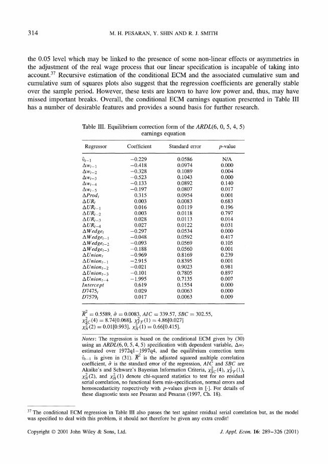
M. H. PESARAN, Y. SHIN AND R. J. SMITH
the 0.05 level which may be linked to the presence of some non-linear effects or asymmetries in the adjustment of the real wage process that our linear specification is incapable of taking into account.37 Recursive estimation of the conditional ECM and the associated cumulative sum and cumulative sum of squares plots also suggest that the regression coefficients are generally stable over the sample period. However, these tests are known to have low power and, thus, may have missed important breaks. Overall, the conditional ECM earnings equation presented in Table III has a number of desirable features and provides a sound basis for further research.
Table III. Equilibrium correction form of the ARDL(6, 0, 5, 4, 5) earnings equation
Regressor Coefficient Standard error p-value
Vt- -0.229 0.0586 N/A Awt- 1 -0.418 0.0974 0.000 Awt-2 -0.328 0.1089 0.004 Awt-3 -0.523 0.1043 0.000 Awt-4 -0.133 0.0892 0.140 Awt-5 -0.197 0.0807 0.017 AProdt 0.315 0.0954 0.001 A URt 0.003 0.0083 0.683 AURt-1 0.016 0.0119 0.196 AURt-2 0.003 0.0118 0.797 AURt-3 0.028 0.0113 0.014 AURt-4 0.027 0.0122 0.031 AWedget -0.297 0.0534 0.000 AWedget- -0.048 0.0592 0.417 AWedget-2 -0.093 0.0569 0.105 AWedget-3 -0.188 0.0560 0.001 AUniont -0.969 0.8169 0.239 AUniont_l -2.915 0.8395 0.001 AUniont-2 -0.021 0.9023 0.981 AUniont-3 -0.101 0.7805 0.897 A Uniont-4 -1.995 0.7135 0.007 Intercept 0.619 0.1554 0.000 D7475t 0.029 0.0063 0.000 D7579t 0.017 0.0063 0.009
R2 = 0.5589, - = 0.0083, AIC = 339.57, SBC = 302.55, X2c(4) = 8.74[0.068], X2(1) = 4.86[0.027] X2(2) = 0.01[0.993], XH(1) = 0.66[0.415].
Notes: The regression is based on the conditional ECM given by (30) using an ARDL(6, 0, 5, 4, 5) specification with dependent variable, Awt estimated over 1972ql-1997q4, and the equilibrium correction term
vt-1 is given in (31). R2 is the adjusted squared multiple correlation coefficient, & is the standard error of the regression, AIC and SBC are Akaike's and Schwarz's Bayesian Information Criteria, XSc(4), X2F(1), X2(2), and X2 (1) denote chi-squared statistics to test for no residual serial correlation, no functional form mis-specification, normal errors and homoscedasticity respectively with p-values given in [.]. For details of these diagnostic tests see Pesaran and Pesaran (1997, Ch. 18).
37 The conditional ECM regression in Table III also passes the test against residual serial correlation but, as the model was specified to deal with this problem, it should not therefore be given any extra credit!
Copyright © 2001 John Wiley & Sons, Ltd.
314
J. Appl. Econ. 16: 289-326 (2001)
BOUNDS TESTING FOR LEVEL RELATIONSHIPS
6. CONCLUSIONS
Empirical analysis of level relationships has been an integral part of time series econometrics and pre-dates the recent literature on unit roots and cointegration.38 However, the emphasis of this earlier literature was on the estimation of level relationships rather than testing for their presence (or otherwise). Cointegration analysis attempts to fill this vacuum, but, typically, under the relatively restrictive assumption that the regressors, xf, entering the determination of the dependent variable of interest, yt, are all integrated of order 1 or more. This paper demonstrates that the problem of testing for the existence of a level relationship between Yt and xf is non-standard even if all the regressors under consideration are I(0) because, under the null hypothesis of no level relationship between Yt and xt, the process describing the Yt process is I(1), irrespective of whether the regressors xt are
purely I(0), purely I(1) or mutually cointegrated. The asymptotic theory developed in this paper provides a simple univariate framework for testing the existence of a single level relationship between Yt and xt when it is not known with certainty whether the regressors are purely I(0), purely I(1) or mutually cointegrated.39 Moreover, it is unnecessary that the order of integration of the underlying regressors be ascertained prior to tesg te sting the existence of a level relationship between yt and xt. Therefore, unlike typical applications of cointegration analysis, this method is not subject to this particular kind of pre-testing problem. The application of the proposed bounds
testing procedure to the UK earnings equation highlights this point, where one need not take an a priori position as to whether, for example, the rate of unemployment or tt ohe union density variable are I(1) or I(0).
The analysis of this paper is based on a single-equation approach. Consequently, it is inappropri- ate in situations where there may be more than one level relationship involving yt. An extension of this paper and those of HJNR and PSS to deal with such cases is part of our current research, but the consequent theoretical developments will require the computation of further tables of critical values.
APPENDIX A: PROOFS FOR SECTION 3
We confine the main proof of Theorem 3.1 to that for Case IV and briefly detail the alterations
necessary for the other cases. Under Assumptions 1-4 and 5a, the process {zt}ll has the infinite
moving-average representation,
z, = C/L+ yt + Cst + C*(L)Et (Al)
where the partial sum st = E1, 4(z)C(z) = C(z)4'(z) = (1 - )Ik+, ¢(z)- I+i -
4iz', C(z) Ik+i + E Cizl = C + (1 - z)C*(z), t = 1, 2...; see Johansen (1991) and PSS. Note that C = (g, 'l)[(al, a'r(B , )]-a o,al)'; see Johansen (1991, (4.5), p. 1559). Define the (k + 2, r) and (k + 2, k - r + 1) matrices ,* and 8 by
p =f-IB + ) ( P and 8 I+ ) (l, P)
38 For an excellent review of this early literature, see Hendry et al. (1984). 39 Of course, the system approach developed by Johansen (1991, 1995) can also be applied to a set of variables containing possibly a mixture of 1(0) and 1(1) regressors.
Copyright © 2001 John Wiley & Sons, Ltd.
315
J. Appl. Econ. 16: 289-326 (2001)
M. H. PESARAN, Y. SHIN AND R. J. SMITH
where (gB, fBI) is a (k + 1, k- r + 1) matrix whose columns are a basis for the orthogonal complement of f. Hence, (f, , B) is a basis for Zk+l. Let 4 be the (k + 2)-unit vector (1, 0')'. Then, (P,,, , 8) is a basis for Rk+2. It therefore follows that
T-1/28/Z* T/2Z/2(L ( )/, = T-1/2(p l, _ _)/'CS[Ta] + (f2, )' T-1/2C*(L)E[Ta]
= (P', PI)/CBk+l (a)
where zt* = (t, z),) Bk+l (a) is a (k + 1)-vector Brownian motion with variance matrix Q and [Ta] denotes the integer part of Ta, a e [0, 1]; see Phillips and Solo (1992, Theorem 3.15, p. 983). Also, T-l'zt* = T-lt = a. Similarly, noting that B'C = 0, we have that ft*,zt = Pt'/ + ItC*(L)Et = Op(l). Hence, from Phillips and Solo (1992, Theorem 3.16, p. 983), defining V Z- P,Z* and AZ_ - P,AZ_, it follows that
T-l ' = Op(l), T-lZ*AZ = Op(l), T-1'Z_AZ = Op(l) Z1 f , Z_
T-lBZ*-1 -,B* = Op(1), T-BTZ*lAZ_ = Op(l) (A2)
where BT (8, T-1/2k). Similarly, defining ui P,u,
T- /2p' Z*' = Op(l), T-1/2'Z i = Op(l) (A3)
Cf. Johansen (1991, Lemma A.3, p. 1569) and Johansen (1995, Lemma 10.3, p. 146). The next result follows from Phillips and Solo (1992, Theorem 3.15, p. 983); cf. Johansen
(1991, Lemma A.3, p. 1569) and Johansen (1995, Lemma 10.3, p. 146) and Phillips and Durlauf (1986).
Lemma A.1 Let BT (8, T-1/25) and define G(a) = (G (a)', G2(a))', where GI (a) (f,L, BI)' CBk+ (a), Bk+1(a)[= (B1(a)', Bk(a)')'] = Bk+1(a) - f0 Bk+1(a)da, and G2(a) a - 2, a e [0,1]. Then
T- 2B'* Z* 1Br =T J G(a)G(a)'da, T-'1BTZ* G(a)dB*(a) Jo Jo
where B*(a) - 1 (a) - w'Bk(a) and Bk(a) = (B (a), Bk(a)')', a E [0, 1]
Proof of Theorem 3.1 Under Ho of (17), the Wald statistic W of (21) can be written as
~-uW = U'P^Z * 1 (* P^Z- )-1 ZP^ (tuW = - -1 up _ -1 1P_ PT_fi
= i'P Z1A (AZ' P Z* A) A Z*'1P^Z Z A T TZ_ -1 T T - _
where AT = T-1/2 (f, T-1/2BT). Consider the matrix ATZ*iP^ Z-1AT It follows from (A2) and Lemma A. 1 that
ATZP -1 n 1 T 0 -2B
' B 1 ()
T -,.T. _ -_ _iT
316
Copyright © 2001 John Wiley & Sons, Ltd. J. Appl. Econ. 16: 289-326 (2001)
BOUNDS TESTING FOR LEVEL RELATIONSHIPS
Next, consider A,,Z*' P_ ii. From (A3) and Lemma A. 1,
(T-1/2fl/ '*'pl--i
A' P u+ (A5) - \ T lBZ* fi + op() (A5)
Finally, the estimatorfor the error variance cou, (defined in the line after (21)),
~/ _ -- * A-* --Z* -1 A/,~.*/ - ] wuu = (T - m)-1 [u'f
- i'P Z1AT(AZP^ Z -1iA) -AZP^
= (T - m)-ii + op(1) = ( o+ + op(1) (A6)
From (A4)-(A6) and Lemma A.I,
W = T-1i'P- Z*-1fi (T 1Z 1P z* )-1 -z*_,p
P~-_ _ BT T- ' ~ --z B ' (A7) + T -2UZi'B [rT BZ.Z. Br BZ*UiB B _i/)oIu + op(1) (A7) T -1 T -I
We consider each of the terms in the representation (A7) in turn. A central limit theorem allows us to state
(T-l/z2*p z* fi1) -1/2 T /2 ii/o1/ 2 = : Zr N(O, I,) T - 1-PT -_
- 1/* T - _ -PT-N ,_
Hence, the first term in (A7) converges in distribution to z.z,., a chi-square random variable with r degrees offreedom; that is,
T- 1 'P Z* (1 i(T- Z 1Z iP Z* ) Z IPAz_P U/C),,, = Z .Z, - X2(r) (A8)
From Lemma A.], the second term in (A7) weakly converges to
dB*(a)G(a)' ( G(a)G(a)'dr) Gk+l(a)dB,*(a)/w,,,
which, as C = (g, jBl)[(a, a' )'(P, )]-1 (, a')', may be expressed as
dB* ( )da)(a) 1 1 a-U 1 a 1 a- 2O a \Jo a 2/
X,/ (( 1ay B al )'Bkl l(a) d(a a I
Now, noting that under Ho of (17) we may express a^ = (1, -w')' and al = (0, aA'Y where ax'a = O, we define the (k - r + 1)-vector of independent de-meaned standard Brownian motions,
[(~et e )~-1/2 2_ ]Rk+l(a) Wk_r++l(a)[= (W a(a), Wk_r(a)')] [(a, al)'Q(ay, a)]-/(a, aL)' (a)
-( Ct)o-1/2B1, (a)
Copyrig(aht © 2001 John Wiley & Sons, Ltd. J. (a). Ecn. 16: 289-326 (2001)
Copyright © 2001 John Wiley & Sons, Ltd. J. Appl. Econ. 16: 289-326 (2001)
317
M. H. PESARAN, Y. SHIN AND R. J. SMITH
where B*(a) = B1(a) - w'Bk(a) is independent of Bk(a) and Bk+1(a) = (B1(a), Bk(a)')' is par- titioned according to z, = (Yt, x)', a e [0, 1]. Hence, the second term in (A7) has the following asymptotic representation:
dW,(a 1 (a I 1 da aJ- a- - a- - jd lW (a) (Wk ± (a)) 0 (I ( -+l
(a)) (Wk+l (a) )da)
x /l ( + (a-2 ) dl,(a) (A9)
Note that dWu(a) in (A9) may be replaced by dW, (a), a e [0, 1]. Combining (A8) and (A9) gives the result of Theorem 3.1.
For the remaining cases, we need only make minor modifications to the proof for Case IV. In Case I, 8 = (fyir, 'il) with (P, fyi, ) a basis for Rk+1 and Br = 8. For Case II, where
-1 = (tr, Z 1)', we have
Ik+ and, consequently, we define ~ as in Case IV,
8= Ik+l (fyl(, B) and B =(8, ).
Case III is similar to Case I as is Case V. E
Proof of Corollary 3.1 Follows immediately from Theorem 3.1 by setting r = k.
Proof of Corollary 3.2 Follows immediately from Theorem 3.1 by setting r = O.E
Proof of Theorem 3.2 We provide a prooffor Case V which may be simply adapted for Cases I and III. To emphasize the potential dependence of the limit distribution on nuisance parameters, the proof is initially conducted under Assumptions 1-4 together with Assumption 5a which implies Ho'' tyy = 0 but not necessarily HO ' =rV.xX 0'; in particular, note that we may write ay =
(1, -o')' for some k-vector 0. The t-statistic for Ho'"! ' y = 0 may be expressed as the square root of
Ay P _, Z-_A1AT ATZ/P- Z_iA -A ^Z/'P Ay/8; (A 10)
where AT T-1/2(, T-1/2BT) and BT = (yL, pl). Note that only the diagonal element of the inverse in (A10) corresponding to yL is relevant, which implies that we only need to consider the blocks T2B'ZP 1P Z1BT and T-1B'Z' P Ay in (A10). Therefore, using (A2) and
(A3), (A10) is asymptotically equivalent to
T--UPlB( 2BT T --B'' I 21B B T) T-1BT ' A0111 Tr-lP_iZiBr (T Z ZiBr)1 T -TZ ^P i/r- (All)
where Px : '- ITX- 1I - x xx -1 x )X-fiX) iX' Now,
1 I_ a I._I I I T fi- X X[Ta] (, flX fiL)[(ayi a.Lr r , k._ 1 (a)
= (Ix PAx)[a , (r. - y, - )fia ] a -1 B (a) o- rxg © [2x0 Jhxx Wi xy yS..x pxx k (2)
318
Copyright © 2001 John Wiley & Sons, Ltd. J. Appl. Econ. 16: 289-326 (2001)
BOUNDS TESTING FOR LEVEL RELATIONSHIPS
where, for convenience, but without loss of generality, we have set y = (p1 y, 0')' and ti =
(0, y), ) y = Yxy /Yy.x, Yy. Yyy - Yx y y. Yyx - 0 x and (a) B (a) Bk(a) - xy (a),
B,(a) = B1(a) - 0/Bk(a), a e [0, 1]. Hence, (All) weakly converges to
- / ,{ B(a)dWit(a)-(o B-(a)B(a)da a a B ( a) Boa 'daa
x al' ( (J B(a) B(a)'da) aax aj (j/ B"(a)B"(a)da)
Under the conditions of the theorem, 0 = w and Xy =0 and, therefore, BO(a)[= B*(a)] =
x axx u \UIUk xx
012W1 (a) and ax'B(a)[= a Bk (a)] (a), a e [0, 1].
Proof of Corollary 3.3 Follows immediately from Theorem 3.2 by setting r = k.
Proof of Corollary 3.4 Follows immediately from Theorem 3.2 by setting r = O.E
APPENDIX B: PROOFS FOR SECTION 4
Proof of Theorem 4.1 Again, we consider Case IV; the remaining Cases I-III and V may be dealt with similarly. Under H
' : .7r,y / 0, Assumption Sb holds and, thus, n = ay py + ap' where
ay = (a, 0')' and fy = (Pyy, Px)'; see above Assumption 5b. Under Assumptions 1-4 and 5b, the process {zt]lz has the infinite moving-average representation, zt = /i + yt + Cst + C*(L)st, where now C - '[a "'p1]-la '. We redefine P* and 8 as the (k + 2, r + 1) and (k + 2, k - r) matrices,
and , 8 (Y -f )1
1jk+1/
where is a (k + 1, k - r) matrix whose columns are a basis for the orthogonal complement of (fly, j). Hence, (y, , (y, , ) is a basis for Z k+1 and, thus, (I*, , 8) a basis for Zk+2, where again 4 is the (k + 2)-unit vector (1, 0')'. It therefore follows that
T- 1/28/ = T- 1/2p/I + T- 112 ICS[Ta] + p'T- l/2C*(L)e8[Ta] = "CB (a)
Also, as above, T-10'z* = T-1t = a and P*z7 = (fy, P)Itt + (fy, 8)'C*(L)st = Op(l). The Wald statistic (21) multiplied by eui may be written as
(B1) (B 1) Copyright © 2001 John Wiley & Sons, Ltd.
319
J. Appl. Econ. 16: 289-326 (2001)
M. H. PESARAN, Y. SHIN AND R. J. SMITH
where , (, a)'(1, -w')', AT - T-1/2(, T-1/2B) and Br - (, T-1/2k). Note that (A6) continues to hold under H!'' 71
T y k O. A similar argument to that in the Proof of Theorem 3.1 demonstrates that the first term in (Bl) divided by w,,c has the limiting representation
z. l + j dWI(a)Fk -r(a)' ( Fk_,(a)Fk ,(a)'da) Fk,r(a)dW,(a) (B2)
where z,.+ 1 N(O, I,+i), Fk_,(a) = (Wk_,(a)', a - ) and Wk_ (a) (a 'Qa )- 1/2aB(a) is a (k - r)-vector of de-meaned independent standard Brownian motions independent of the standard Brownian motion W,(a), a e [0, 1]; cf (22). Now, fo Fk_,(a)dW,(a) is mixed normal with conditional variance matrix fo Fk_,-(a)Fk_,(a)'da. Therefore, the second term in (B2) is unconditionally distributed as a X2(k - r) random variable and is independent of the first term; cf: (A4). Hence, the first term in (Bl) divided by Iw,i has a limiting X2(k + 1) distribution.
The second term in (Bl) may be written as
2(1, -w')(ay, a)pZ P u = 2T1/2(, -w')(a a) (Tr- / Z Z*' P ) = O(T12), (B3)
and the third term as
(1, -w')(ay, a)p'* IPz_ Z* _(al,a), a)'(1,-w')'
=T(1, -w')(ay, a) (T-1B Z* P Z*fi) (a,, a)'(1, -w')' = Op(T) (B4)
as T- ' Z*P- Z-* 1 f converges in probability to a positive definite matrix. Moreover, as
(1, -w')(ay, a) k 0' under H1 : tyy 0, the Theorem is proved.
Proof of Theorem 4.2 A similar decomposition to (Bl) for the Wald statistic (21) holds under
HIV n Ho-'- except that f, and 8 are now as defined in the Proof of Theorem 3.1. Although H 7ryy = 0 holds, we have Hl' ' Jryx, O'. Therefore, as in Theorem 3.2, note that we may
write al = (1, -')' for some k-vector 0 = w. Consequently, the first term divided by w,, may be written as
T-1i/- 2* ~Ifi T-1 ~ *P * 1 P */ l/ T-pz_ U Z1 ,- ,V -1P^Z zz_1fi* - 1P^A_fi/O)
+T-2UiZ* 1BT [T-2B/rTZ* lZ- iB B'Z- i/,,1 + op(l) (B5) -1 T T -1
cf (A7). As in the Proof of Theorem 3.1, the first term of (B5) has the limiting representation z'.z,. where z,. ~ N(0, I,.); cf (22). The second term of (B5) has the limiting representation
/ ( Bf(a) /' Bf(a) I Bf(a) ' -1
Jo a1i Xk(a) jo\ aX 1 /
[I 7(/% Bk(a) \ x ( cx^Bk(a) dB(a)/w,,, = Op(1)
JO \ a--
Coyrgh ©201 on ily Sns td J Api Eon 6:28-36 201
320
Copyright © 2001 John Wiley & Sons, Ltd. J. Appl. Econ. 16: 289-326 (2001)
BOUNDS TESTING FOR LEVEL RELATIONSHIPS
where B (a) Bl(a) - 'Bk(a), a e [0, 1]; cf. Proof of Theorem 3.2. The second term of (BI) becomes
2(1, -w')a Z* lP--_u = 2T12(1, -w')a (Tr-/2' Pz ) = Op(T )
and the third term
(1,-w')iZ*_iP _Z* ,B a' (1, -w') = T(1,-w')a
x (T-ljB,Z*iP - Zi ) a'(1, -uw') = Op(T)
The Theoremfollows as (1, -w')a , 0' under H :r = O and Hr r : O .
Proof of Theorem 4.3 We concentrate on Case IV; the remaining Cases I-III and V are proved by a similar argument. Let {ztr}lI denote the process under HIT of (26). Hence, 41(L)(ztT - L -yt) = StT, where tT - (fT - n)[z(t-_)T - - y(t - 1)] + Et and nT - n is
given in (27). Therefore, A(ztT - / - yt) = C tT+ C*(L)AtT, C(z) = C + (1 - z)C*(z) and C = (fi-, B')[(a, a')'F(fl, al')] -(a, a1)', and thus,
[Ik+l - (Ik+1 + T- Ca,fy'y)L](ztT - - t) = CetT + C*(L)A tT (B6)
where
etT =T-1 (2 f i [Z(t)r - - y(t - 1)] + t, t = 1, ..., T, T = 1, 2, ...
Inverting (B6) yields
s-1
ZtT = (Ik+1 + Tr Cai)(ZST - - ys) + -t + Yt + (I+l + T- Ca, 1) i=0
x[Cs(t-i)T + C*(L)AU(t-i)T]
Note that ArT = (tri - n)A[z(t-_ ) - t - y(t - 1)] + Ast. It thereforefollows that T- /28'ZT]T
( (g,, B )'CJk+l(a), where 8 is defined above Lemma A.1 and zt* = (t, z'T', Jk+l (a) = fo exp {ayfi,C(a - r)dBk+l (r) is an Ornstein-Uhlenbeck process and Bk+l (a) is a (k + 1)-vector Brow- nian motion with variance matrix Q, a E [0, 1]; cf Johansen (1995, Theorem 14.1, p. 202).
Similarly to (A4),
T ',Z*<-P1T * Ifi o0,
r -1_ -- 1 rT A'Z_' P Z iA = (T T
IBA_*B ) +op(1)
Therefore, expression (Bl) for the Wald statistic (21) multiplied by ,,,, is revised to
c T- oaWyP Z*- A1 * (T- 1 P/Z* Pjz Z- 1 i) * +T z BT [T BT*1*BT BZ*PZ y+op(1) (B7) I <y,,,,W T-2 !i --,-! )1
- r-2a'yP" -I ~ B- T, B'Z ^,Br] B rZ!P _ Ay + op(1) (B7) AP IZ T -1 -1 1P _
Copyright © 2001 John Wiley & Sons, Ltd.
321
J. Appl. Econ. 16: 289-326 (2001)
M. H. PESARAN, Y. SHIN AND R. J. SMITH
The first term in (B7) may be written as
+ 2T'i'Pz Z2* f(T l-' /Z* P^ Z-1 ) p Z* P Z*< rfiP--1 ~ T ,- ~ z -1 ,
yT -1 T, -1 yT_ +wT r 1z(laP^z 2* ( (TZ-1 P^zl f-1) i-_P '^Z-_-, (B8)
where T T- 1auTyyfi' + T1/2( - w'~S,)P. Defining n (8), - w'82)', consider
T 2pl/2 /*1P' 2*i<_-T1/2Z/ 2*' p Z* 22 rT-/2* P*'-z Z*- 1T, = T /2 lP-- Z* (, _lPayyT- + *T- 2)
= T-lf*Z*lPAzZ* + op(l) (B9)
where we have made use of T- 112jy*z[Ta]T =^ ' CJk+l (a). Therefore, (B8) divided by oi,,i may be re-expressed as
[(T //*ZpI f) + Qr] Q1 [(T Z Pz u) + Qr1] /o)Iu + op(l) = z,.z, + op(l)
(B9) 12,-1 B* -- Z* * ' where Q plimT,, (T-1'Z*iP_ _ Z* I) and z, - N(Q1/2, I,).
As PAZ_ y = PA (Z_-I 7r + u), T-1 Bf1PAZ = T BZ PAZ (ZiX1 ,+ Ui).
Consider the second term in (B7), in particular, T- 1B/Z*' P * T which after substitution for 7*y becomes
B/ZlT-2B'P ZL-Y*ay + T-32BT* P Z- = '* ,T-B + o1 ) =_Z T7-1 ' , _cif,P~_Z*_,y + op(l))
1 ( fy, fi )CJk+l (a) JT+fl ( La) ayyda
Therefore,
T- iBTZ* 1PXZ_ Ay I )C (a) ( dWi, (a)+ Jk+1 (a)'C' yl)yyda)
Consider
;k-,-+l(a)[= (J(a), JK,-) [(aO, )'Q(aa, )]-12c k a I ) (a)
=( cC- 1/2 J((a) \ *I -'1 . )-1/2 - k (axxQ ab 1 /2 a.x'Jk(a) J
where Ju(a) = J1(a) - W'Jk(a) is independentf k(a) and o k+l(a) (Ji(a), Jk(a)')', a e [0, 1]. Now , Jk r+l(a) satisfies the stochastic integral and differential equations, Jk*-,+l (a) = Wk-r+ (a) + ab' Jo Jk- + (r) dr and dJk.+ 1 (a) = dWk-,.+1 (a) + ab'Jl .+1 (a) da, where a = [(a, a)'
(af, al)]-1/2(f, a)'a and b = [(aL, a)'Q)(al, a')]1/2 x [(f, Bly)'r(al, a)]-( Y )
fy; cf. Johansen (1995, Theorem 14.4, p. 207). Note that the first element of Jk*-_+l (a) satisfies J(a) = Wu(a) + wouu-/2ayb' f i Jk- ( (r) dr and dJ( = dW(a) = d +(a)C + 1/2 ' 1 (a) da.
~T- r__P~ y= f0 ' 1
U\L~~t/ u\U/
Copyright © 2001 John Wiley & Sons, Ltd.
322
J. Appl. Econz. 16: 289-326 (2001)
BOUNDS TESTING FOR LEVEL RELATIONSHIPS
Therefore,
T- B lB Z*P j ((IY, CJk+l (a) ) )1/2 d(a) T-1B *'IP-_AY :=o d1*( T -J I \ a I ^
Hence, the second term in (B7) weakly converges to
W, I dJ) (a) 'Fk_, +l k )Fk(a) kr 'da Fk-,+l(a)FdJ(a) (B10)
where Fk-r+l (a) = (Jk-r+ (a)', a -
Combining (B9) and (BO1) gives the result stated in Theorem 4.3 as o,,, - w,, = Op(1) under
H1T of (26) and noting dJ*(a) may be replaced by dJ*(a).E
Proof of Theorem 4.4 We consider Case V; the remaining Cases I and III may be dealt with similarly. Under H y: tyy # 0, from (10), Y-1 = X_10 + v_i, where v-1 - P^ _,V- and
__ A A_Z
V-1 = (O, V1,..., VT-)'. Therefore, yP' P A, y = y ' V1P -_ AY and ' 1P l-i = v'lP AZ-.X l-1 1 AZY- 1X
'~1P~'~_, -
_ V-
1· As in Appendix A,
T-1/2PX[Ta] = T-1/2 x1fx + T-1 2x YXt + T- (x (f rxx)()l r 1P S[Ta
+ (0, ,B ')T- 1/2C*(L)e[Ta]
and noting that = 0, -8tXx = T-l/2f' + T-1/24xxy xt + (0, pB')C*(L)st. Consequently,
A i P/fxX _ 1 -0P " _^ tT 01
x
where AX - T- 1/2 (BX, T- /2 ) Now, because T- 1 Bx ̂ v/ = Op(l), T- BlXX' AZ = Op(l), T-'AZ_AZ_ = Op(l) and
T-1 AZ_v-i = Op(l), hence T- BXX' 1P vi = Op(l ). Also because T-l1 -LX' i = Op(l) xX-P-_ v_t-^-I = O-M
and T-1 '^/XZ' 1A = Op(l), hence T-l xx'X' P- V_i = Op(l); cf: (A3). Hence, noting that
T- 1 X' P X - rlxx = Op(l) and T-2ix' P^ X-i = O,(l),
where 1P X_ A , P -P X 1 1 1frx 1 X 1 and
i (P^X_i ' l /X' P^- X i) 1X'1 . Therefore, as T- v' iv_1 = Op(l),
T- yi 1P^ x_Y- = Op(l) (Bll)
The numerator of tf_ of (24) may be written as Ty' _P^" Ay = v'_iP^ .u + vi P^( )
2_1i, where X (Py, B)(ay, a)'(1, -w')'. Because T -'/2B Xt' = Op(l) and T-/2AZ u =
Copyright © 2001 John Wiley & Sons, Ltd.
323
J. Appl. Econ. 16: 289-326 (2001)
M. H. PESARAN, Y. SHIN AND R. J. SMITH
Op(l), T- /2 Xi 1P^ u = Op(l), and, as T- 1A 'X' uI = Op(l), T- 'X' P u = Op (1). Therefore,
T-1/2vlPZXu = ^T-1/2v/ -lP - T-/2/ -P fli + Op(1)
-l/2v_P^ , u + op(l) = Op(l)
noting T-1/2v u = Op(l). Similarly, as (1 - )(, a) 7 0', T-/Z'' 1AZ_ = Op(1), T-'1Z'2 X- iPxx_ = Op(l) and T-1''J IX_ i-l = Op(l). Therefore,
T-' 1i"' P Z 1=T 1 P, x 1X- T P_ X X_ + op(1) T'B',P 1PAZXZ-^ I
T-1PAZXA,i_lI -A1Z V-1 AZ_X.Z-f + (D
= T-'vip' 1P_' z-_ i + op(1)= op(l) _ 1 AZ_,-_ip..r
noting T- ' 1Z _1 = Op(l). Thus,
T-1/2vP' 1 Z_1- = Op(T12). (B12)
Because i),, - w,, = op(1), combining (Bll) and (B12) yields the desired result.
ACKNOWLEDGEMENTS
We are grateful to the Editor (David Hendry) and three anonymous referees for their helpful comments on an earlier version of this paper. Our thanks are also owed to Michael Binder, Peter
Burridge, Clive Granger, Brian Henry, Joon-Yong Park, Ron Smith, Rod Whittaker and seminar
participants at the University of Birmingham. Partial financial support from the ESRC (grant Nos R000233608 and R000237334) and the Isaac Newton Trust of Trinity College, Cambridge, is
gratefully acknowledged. Previous versions of this paper appeared as DAE Working Paper Series, Nos. 9622 and 9907, University of Cambridge.
REFERENCES
Banerjee A, Dolado J, Galbraith JW, Hendry DF. 1993. Co-Integration, Error Correction, and the Econo- metric Analysis of Non-Stationary Data. Oxford University Press: Oxford.
Banerjee A, Dolado J, Mestre R. 1998. Error-correction mechanism tests for cointegration in single-equation framework. Journal of Time Series Analysis 19: 267-283.
Banerjee A, Galbraith JW, Hendry DF, Smith GW. 1986. Exploring equilibrium relationships in economet- rics through static models: some Monte Carlo Evidence. Oxford Bulletin of Economics and Statistics 48: 253-277.
Blanchard OJ, Summers L. 1986. Hysteresis and the European Unemployment Problem. In NBER Macroe- conomics Annual 15-78.
Boswijk P. 1992. Cointegration, Identification and Exogeneity: Inference in Structural Error Correction Models. Tinbergen Institute Research Series.
Boswijk HP. 1994. Testing for an unstable root in conditional and structural error correction models. Journal of Econometrics 63: 37-70.
Boswijk HP. 1995. Efficient inference on cointegration parameters in structural error correction models. Journal of Econometrics 69: 133-158.
Cavanagh CL, Elliott G, Stock JH. 1995. Inference in models with nearly integrated regressors. Econometric Theory 11: 1131-1147.
Copyright © 2001 John Wiley & Sons, Ltd.
324
J. Appl. Econ. 16: 289-326 (2001)
BOUNDS TESTING FOR LEVEL RELATIONSHIPS
Chan A, Savage D, Whittaker R. 1995. The new treasury model. Government Economic Series Working Paper No. 128, (Treasury Working Paper No. 70).
Darby J, Wren-Lewis S. 1993. Is there a cointegrating vector for UK wages? Journal of Economic Studies 20: 87-115.
Dickey DA, Fuller WA. 1979. Distribution of the estimators for autoregressive time series with a unit root. Journal of the American Statistical Association 74: 427-431.
Dickey DA, Fuller WA. 1981. Likelihood ratio statistics for autoregressive time series with a unit root. Econometrica 49: 1057-1072.
Engle RF, Granger CWJ. 1987. Cointegration and error correction representation: estimation and testing. Econometrica 55: 251-276.
Granger CWJ, Lin J-L. 1995. Causality in the long run. Econometric Theory 11: 530-536. Hansen BE. 1995. Rethinking the univariate approach to unit root testing: using covariates to increase power.
Econometric Theory 11: 1148-1171. Harbo I, Johansen S, Nielsen B, Rahbek A. 1998. Asymptotic inference on cointegrating rank in partial
systems. Journal of Business Economics and Statistics 16: 388-399. Hendry DF, Pagan AR, Sargan JD. 1984. Dynamic specification. In Handbook of Econometrics (Vol. II)
Griliches Z, Intriligator MD (des). Elsevier: Amsterdam. Johansen S. 1991. Estimation and hypothesis testing of cointegrating vectors in Gaussian vector autoregres-
sive models. Econometrica 59: 1551-1580. Johansen S. 1992. Cointegration in partial systems and the efficiency of single-equation analysis. Journal of
Econometrics 52: 389-402. Johansen S. 1995. Likelihood-Based Inference in Cointegrated Vector Autoregressive Models. Oxford Uni-
versity Press: Oxford. Kremers JJM, Ericsson NR, Dolado JJ. 1992. The power of cointegration tests. Oxford Bulletin of Economics
and Statistics 54: 325-348. Layard R, Nickell S, Jackman R. 1991. Unemployment. Macroeconomic Performance and the Labour
Market. Oxford University Press: Oxford. Lindbeck A, Snower D. 1989. The Insider Outsider Theory of Employment and Unemployment, MIT Press:
Cambridge, MA. Manning A. 1993. Wage bargaining and the Phillips curve: the identification and specification of aggregate
wage equations. Economic Journal 103: 98-118. Nickell S, Andrews M. 1983. Real wages and employment in Britain. Oxford Economic Papers 35: 183-206. Nielsen B, Rahbek A. 1998. Similarity issues in cointegration analysis. Preprint No. 7, Department of
Theoretical Statistics, University of Copenhagen. Park JY. 1990. Testing for unit roots by variable addition. In Advances in Econometrics: Cointegration,
Spurious Regressions and Unit Roots, Fomby TB, Rhodes RF (eds). JAI Press: Greenwich, CT. Pesaran MH, Pesaran B. 1997. Working with Microfit 4.0: Interactive Econometric Analysis, Oxford Univer-
sity Press: Oxford. Pesaran MH, Shin Y. 1999. An autoregressive distributed lag modelling approach to cointegration analysis.
Chapter 11 in Econometrics and Economic Theory in the 20th Century: The Ragnar Frisch Centennial Symposium, Strom S (ed.). Cambridge University Press: Cambridge.
Pesaran MH, Shin Y, Smith RJ. 2000. Structural analysis of vector error correction models with exogenous I(1) variables. Journal of Econometrics 97: 293-343.
Phillips AW. 1958. The relationship between unemployment and the rate of change of money wage rates in the United Kingdom, 1861-1957. Economica 25: 283-299.
Phillips PCB, Durlauf S. 1986. Multiple time series with integrated variables. Review of Economic Studies 53: 473-496.
Phillips PCB, Ouliaris S. 1990. Asymptotic properties of residual based tests for cointegration. Econometrica 58: 165-193.
Phillips PCB, Solo V. 1992. Asymptotics for linear processes. Annals of Statistics 20: 971-1001. Rahbek A, Mosconi R. 1999. Cointegration rank inference with stationary regressors in VAR models. The
Econometrics Journal 2: 76-91. Sargan JD. 1964. Real wages and prices in the U.K. Econometric Analysis of National Economic Planning,
Hart PE Mills G, Whittaker JK (eds). Macmillan: New York. Reprinted in Hendry DF, Wallis KF (eds.) Econometrics and Quantitative Economics. Basil Blackwell: Oxford; 275-314.
Copyright © 2001 John Wiley & Sons, Ltd.
325
J. Appl. Econ. 16: 289-326 (2001)
M. H. PESARAN, Y. SHIN AND R. J. SMITH
Shin Y. 1994. A residual-based test of the null of cointegration against the alternative of no cointegration. Econometric Theory 10: 91-115.
Stock J, Watson MW. 1988. Testing for common trends. Journal of the American Statistical Association 83: 1097-1107.
Urbain JP. 1992. On weak exogeneity in error correction models. Oxford Bulletin of Economics and Statistics 52: 187-202.
Copyright © 2001 John Wiley & Sons, Ltd.
326
J. Appl. Econ. 16: 289-326 (2001)
Copyright © 2022 FDOKUMEN

