


Bahasa
Halaman
Hukum

A SYNTACTIC APPROACH AND VLSI ARCHITECTURES
FOR SEISMIC SIGNAL CLASSIFICATION
Hsi-Ho Liu and K. S. FuSchool of Electrical Engineering
Purdue UniversityWest Lafayette, Indiana 47907
January 1983
ffThis work was supported by ONR Contract N00014-79-C-0574 and the~NSF-Grant
ECS~80-16580.

SECURITY CLASSIFICATION OF THIS. PAGE (When Date,Entered)
REPORT DOCUMENTAriON PAGE READ INSTJ<UCTIONSBEFORE COMf'LFTINC FORM
RECIPIENT'S CATALOG NUMBER1. REPORT NUMBER 12~_GOVT ACCESSION NO.3.
1fI0-,L}/;;1/ 3 iJr---------- ..L--=--'-~!Zl'_L_=_L_''''_+---.--.----.----------... • __
4. TITLE (and Subtitle) 5. TYPE'. OF REPORT [; PEI·HOD COVERf-n
A SYNTACTIC APPROACH AND VLSI ARCHITECTURESFOR SEISMIC SIGNAL CLASSIFICATION. Technical)
r-6 .-P-E-R-F-O-R-M-IN-G-O-"-G'r;-[:-p-O-R-T-N-UM-S-E-R---
t-------------.------------------.--+-=-----~_________,c_=_.__ccc____----.-----._.--- -- ...-7. AUTHOR(s) 8. CONTRACT OR GRANT NUMBER(s)
Hsi-Ho Liu and K. S. Fu ONR N00014-79-C-0574)
9. PERFORMING ORGANIZATION NAME AND ADDRESS
Purdue UniversitySchool of Electrical EngineeringWest Lafayette, IN 47907
10. PROGRAM ELEMENT. PROJECT. TAS~-'--AREA I} WORK UNIT NUMBERS
,1. CONTROLLING OFFICE NAME AND ADDRESS
Department of the NavyOffice of Naval ResearchArlington, VA 22217
13. NUMBER OF PAGES -~-----'-------,
208 I
""';-;"4-.7':'M::-:ON7':'I:::cTO=OR::-:-:IN::-:G::-A:-:G::-::E::":"N"::::CY~NA:-:M:-::E~&;-:-:AD::-::D:-::R-::-ES::-:Sc:-:-(i:-f d7.'if;-;-fe-re-nt:-:l-ro-m--:::C-on-:-tr-:ol-:7lin--:i/-;O:-:-:Il::---;c--:C)---+7;:,S:-.-;:S~EC:::-:-U-;-;:R~IT~Y:-:C-::-:L-:-A::-;SS:-. ~("~l-:-,"7";"-'e·.-'''--,,-:-t)--·------
unclassified
16. DISTRIBUTION STATEMENT (ollhi" Reporl)
Approved for pUblic release:
"" ~",fct,it'," A' '0' noWN'" 'O:"l
distribution unlimited. . _ __.1
17. DISTRIBUTION STATEMENT (01 tI", a1,strwl onte""lln B1"ck :W. II diller""t from U"I'"rl) 1I
Approved for pUblic release: distribution unlimited.
--------------- ---·--·118. SUPPLEMENT ARY NOTES ~
Ii
_. . . .._.__________ i19, KEY WORDS (Continue on rf.'verse side if necessary lind identify by block nurnher) 1
I-----------------_._----------------~._------------_. -20. ABSTRACT ((~Otltl!HH' on rOV('!SI' _"jdt, Jf fH'.-("." ,';llTV lIl1d hlt'nUly t,y h}o('k lluHd}pr)
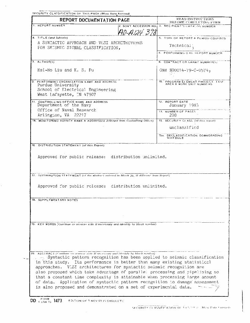
Syntactic pattern recognition has been applied to seismic classificationin this study. Its performance is better than many existing statisticalapproaches. VLSI architectures for syntactic seismic recognition arealso proposed which take advantage of parallel processing and pipelining sothat a constant time complexity is attainable when processing large amount Iof data. Application of syntactic pattern recognition to damage assessment ~
is also proposed and demonstrated on a set of experimental data. - - --<)) J!
______________________/___.14,
DD FORM1 JAN 73 1473 EDITION OF '1 NOV 65 IS OIJSOLLTL
--_..__ .. -.._----_._._.._---- -t;FCIJRITY Cl IV:Jr)IF1CA11()N ()!- rH"- 1'/\',1 ,WfWf! }1,1//I I "I.',.,."

SECURITY CLASSIFICATION OF THIS PAGE(Wl".n Dat .. Entered)
)·Seismic waveforms are represented by strings of primitives, i.e.,sentences, in this study. String-to-string similarity measures based onboth distance and likelihood concepts are discussed along with the symmetricproperty and the hierarchy. A fixed-length segmentation is used in theexperiment. Encouraging results comparable to those of the best statisticalapproaches are obtained with only two very simple features, namely, zerocrossing count and log energy. Primitives are automatically selected usinga hierarchical clustering procedure and two decision criteria.
Nearest-neighbor decision rule and finite-state error-correctingparsers are used for classification. For error-correcting parsing, finitestate grammars are first inferred from the training samples. These twoapproaches have same performance in the experiment? whereas the nearestneighbor rule is faster in speed. ?---
Attributed grammar and its parsing are also proposed for seismicrecognition, which could reduce the complexity and increase the descriptiveflexibility of the pattern gramamrs. VLSI architectures are proposed forfast recognition of seismic waveforms. Three systolic arrays perform thefeature selection, primitive recognition and string distance computation.These individual units can be used in other similar applications.
Although this study is on seismic classification, it can be extendedor modified to tackle other signal recognition problems.
SECURITY CLASSII"ICATIOf4 01" Tu,r AGE(When D,,'. Enl",ed)
iv
TABLE OF CONTENTS
Page
LIST OF TABLE vii
LIST OF FIGURES viii
ABSTRACT....................... xi
CHAPTER I - INTRODUCTION................................................................ 1
1.1 Statement of the Problem 1.1. 2 Literature Survey..................................................................... 7
1.2.1 Syntactic Pattern Recognition andDigital Signal Processing...................... 7
1.2.2 Pattern Recognition andSeismic Signal Analysis 13
1.3 Organization of Thesis 17
CHAPTER II - SIMILARIIT MEASURES AND RECOGNITIONPROCEDURES FOR STRING PATTERNS 19
2.1 Introduction 192:2 Similarity Measures of Strings 21
2.2.1 Similarity Measures Based on Distance Concept 212.2.2 Similarity Measures Based on Likelihood Concept 41
2.3 Error-Correcting Parsing 452.3.1 Minimum-Distance Error-Correcting Parsing
Algorithm 462.3.2 Maximum-Likelihood Error-Correcting Parsing
Algorithm 522.4 Recognition Procedures for Syntactic Patterns 562.5 Conclusion 58
v
CHAPTER III - APPLICATION OF SYNTACTIC PATTERNRECOGNITION TO SEISMIC CLASSIFICATION ; 59
3.1 Introduction , 593.2 Preprocessing , 613.3 Automatic Clustering Procedure for Primitive Selection 68
3.3.1 Pattern Segmentation 683.3.2 Feature Selection 703.3.3 Primitive Recognition 71
3.4 Syntax Analysis , 773.4.1 Nearest-Neighbor Decision Rule 773.4.2 Error-Correcting Finite-State Parsing 77
3.5 Experimental Results on Seismic Discrimination 823.6 An Application of Syntactic Seismic Recognition
to Damage Assesment 963.7 Conclusion 107
CHAPTER IV - INFERENCE AND PARSING OF ATTRIBUTED GRAMMARFOR SEISMIC SIGNAL RECOGNITION 110
4.1 Introduction 1104.2 Inference of Attributed Grammar for Seismic Signal
Recognition 1134.3 Error-Correcting Parsing of Attributed Seismic Grammar 1214.4 Stochastic Attributed Grammar and Parsing for
Seismic Analysis 1254.5 Experimental Results and Discussion 129
CHAPTER V - VLSI ARCHITECTURES FOR SYNTACTIC SEISMICPATTERN RECOGNITION 134
5.1 Introduction 1345.2 VLSI Architectures for Feature Extraction 1375.3 VLSl Architectures for Primitive Recognition 1435.4 VLSI Architectures for String Matching
Based on Levenshtein Distance 1505.4.1 Levenshtein Distance 1535.4.2 Weighted Levenshtein Distance 161
5.5 Simulation and Performance Varification 1675.6 Concluding Remarks 173
vi
CHAPTER VI - SUMMARY, CONCLUSIONS, AND RECOMMENDATIONS .... 176
6.1 Summary 1766.2 Conclusions 1796.3 Recommendations 180
LIST OF REFERENCES 182
APPENDICES
Appendix A: Flow Chart for the Simulations 190Appendix B: Step-by-Step Simulation Results 195
VITA 209


vii
LIST OF TABLES
Table Page
3.1 The criterion function, increments of criterionfunction and the classification results ofdifferent cluster number selections 83
3.2 The center of the 13 clusters, the number of membersin each cluster and the primitive symbol of each cluster 88
3.3 Weights for substitution error ,. 92
3.4 Classification results using nearest-neighbor decision rule 93
3.5 The number of nonterminals, productions and negativesamples accepted by the inferred grammars 94-
3.6 The average parsing time and percentage of correctclassification of the error-correcting parsers ,. 95
4-.1 The recognition results, computation time, andmemory used for seismic recognition using an attributedcfg and a nonattributed fsg 132
5.1 Computation time of sequential algorithm, simulatedcomputation time for VLSI arrays using sequentialcomputer, real speedups, theoretical speedups andspeedup ratio 168
AppendixTable
B.1 The intermediate results of feature extraction at eachtime interval for one seismic segment 198
B.2 The intermediate results of primitive recognition ateach time interval for one unknown feature vector 203
B.3 The intermediate results of string matching at eachtime interval between two strings 20C.i

viii
LIST OF FIGURES
Figure Page
1.1 An example of two typical seismic records '" 3
1.2 An example of extreme case 4
1.3 Another example of extreme case 5
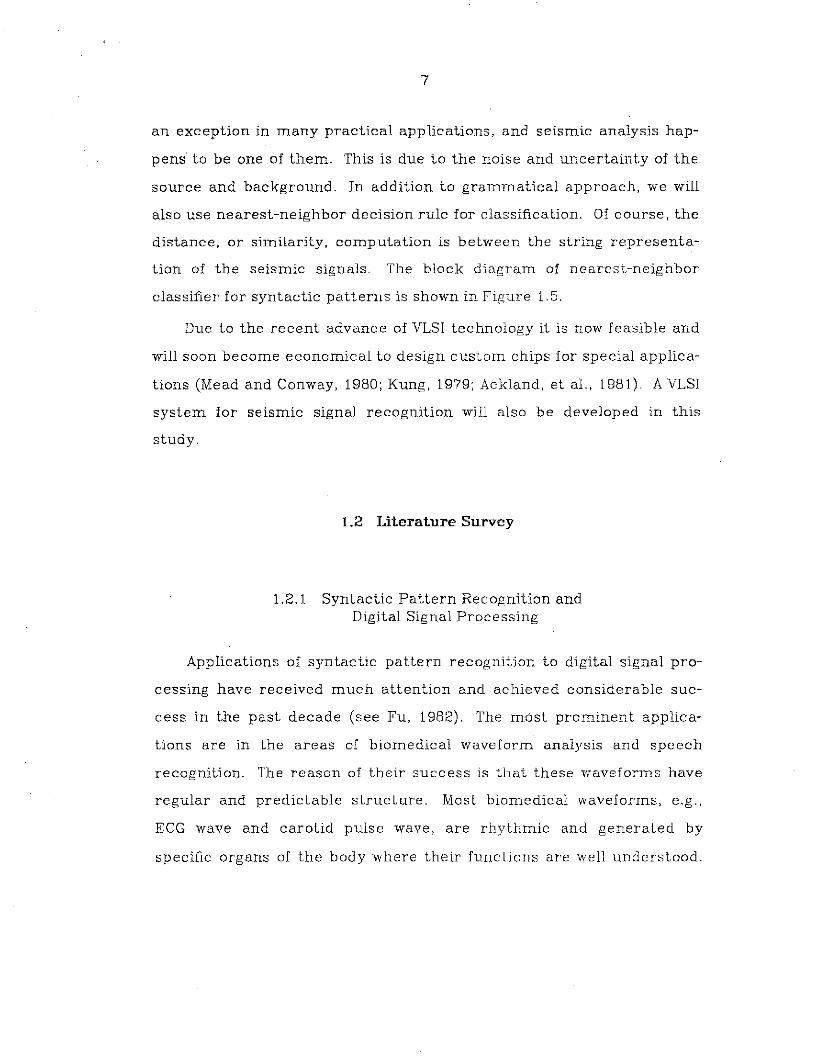
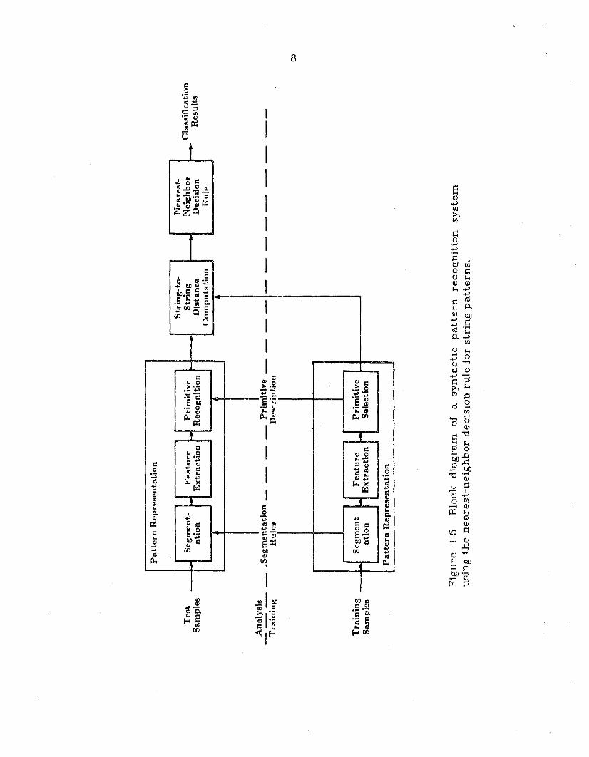
1.4 Block diagram of a syntactic pattern recognition system 61.5 Block diagram of a syntactic pattern recognition system using
the nearest-neighbor decision rule for string pattern 8
2.1 The transformation from string 'aabaab' to 'ababb' 24
2.2 The partial distance 6[i,j] is computed from6[i,j-1], 6[i-1,j-1] and 6[i-1,j] 25
2.3 An example of global path constraint 26
2.4 Computation of partial distance for (a) type 1, (b)type 2 and (c) type 3 WLD 34
2.5 An example of dynamic time warping 36
2.6 Examples of some seismic recordings in structuraldamage assesment 37
2.7 Examples of slope constraints and corresponding localdistance function of modified time warping distance 40
2.8 computation of partial distance for stochastic models 43
3.1 (a) An example of seismic signal with pulse noise(glitch). (b) The same waveform after local filtering 63
3.2 (a) Another example of seismic signal with severalpulse noise (glitches) 64
ix
3.3 (a) An original seismic signal. (b) With zero-lineadded for comparison. (c) After global adjustment.(d) After local adjustment 66
3.4 Another example of seismic signaL 67
3.5 tr SB increases as the number of clusters increases 85
3.6 tr Sw decreases as the number of clusters increases 86
3.7 The PFS curve where the maximum valueoccurs at number 13 87
3.8 Cluster centers of the 13 clusters in thetwo-dimensional feature plane 89
3.9 Examples of the seismic waveforms andcorresponding strings 90
3.10Top level displacement and basement acceleration 98
3.11 Basement displacement of the seven test runs 100
3.12 Top level displacement of the seven test runs 101
3.13 Diagram of slope constraints and local distancefunction for string distance computation in damageassesment application 102·
3.14 Distance between the basement displacement'. waveform and the top level displacementwaveform of each run 105
4.1 A flow chart of the inference algorithm (Algorithm 4.1) 118
4.2· A flow chart of the parsing algorithm (Algorithm 4.2) 124
4.3 A flow chart of the parsing algorithm (Algorithm 4.3) 128
4.4 A flow chart of the parsing algorithm (Algorithm 4.4) 131
5.1 The special-purpose processor is attached toa host computer as a peripheral processor : 136
5.2 The internal architecture of the special-purposeprocessor 138
5.3 Data setup for (a) feature extraction, (b) primitiverecognition and (c) string matching 139
5.4 Processor array, data movement and operationsof each processor for feature extraction 140
x
5.5 The internal structure of the processor forfeature extraction " 142
5.6 Processor arrays and data movement forprimitive recognition 144
5.7 Data flow and operations of each (a) 'compute'processor and (b) 'compare' processor 148
5.8 Internal structure and register transfer of (a) 'compute'and (b) 'compare' processors 149
5.9 (a) Portions of dynamic programming diagram and(b) corresponding processor array 154
5.10 Internal structure and register transfer ofPE Pi,j at stage 1, 2 and 3 156
5.11 Data movement between PE's 158
5.12 Processors at the same diagonal perform thesame operation; three diagonals are requiredfor one string (a), and strings can be pipelined (b) 159
5.13 Processor array and data movement forcomputing Levenshtein distance 160
5.14 PLA implementation of a simple weight table 162
5.15 A PLA implementation of the weight tablefor seismic recognition 164
5.16 Internal structure of the PE for weighted stringdistance computation 165
5.17 An implementation of feature extraction with20 PE's and 60 points in each segment. 171
AppendixFigure
A.l Flow chart for the simulation of feature extraction 191
A.2 Flow chart for the simulation of primitive recognition 192
A.3 Flow chart for the simulation of string matching 194
B.l Seismic segment (60 points) used in the simulation 197


xi
ABSTRACT
Syntactic pattern recognition has been applied to seismic
classification in this study. Its performance is better than many exist
ing statistical approaches. VLSI architectures for syntactic seismic
recognition are also proposed which t.ake advantage of I=arallel process
ing and pipelining so that a constant time complexity is attainable when
processing large amount of data. Application of syntactic pattern
recognition to damage assesment is also proposed and demonstrated on
a set of experimental data.
Seismic waveforms are represented by strings of primitives, Le.,
sentences, in this study. String-to-string similarity mensures based on
both distance and likelihood concepts are discussed along with the
symmetric property and the hierarchy. A flxed-lengt.h :;cgmentatiori is
used in the experiment. Encouraging results comparc:.ble to those of
the best statistical approaches are obtained with only two very simple
features, namely, zero-crossing count and log energy. Primitives are
automatically selected using a hierarchical clustering procedure and
two decision criteria.
xii
Nearest-neighbor decision rule and finite-state error-correcting
parsers aTe used for classification. For error-correcting parsing,
finite-state grammars are first inferred from the training samples.
These two approaches have same performance in the experiment,
whereas the nearest-neighbor rule is faster in speed.
Attributed grammar and its parsing are also proposed for seismic
recognition, which could reduce the complexity and increase the
descriptive flexibility of the pattern grammars. VLSI architectures are
proposed for fast recognition of seismic waveforms. Three· systolic
arrays perform the feature selection, primitive recogn:.tion and string
distance computation. These individual units can be used in other simi
lar applications.
Although this study is on seismic classification, it can be extended
or modified to tackle other signal recognition problems.
1
CHAPTER I
INTRODUCTION
1.1 Statement of the Problem
In the past, seismic wave analyses were all retained within the geo
physical field. Underground structure and earthquake analyses are the
most important topics. The major parameters computed from the
recorded seismograms are the location, time, depth and magnitude of
the event and so forth.
In the 1960's, a new problem arose when the idea of the
comprehensive nuclear test ban treaties were proposed. The problem is
how to discriminate between the natural earthquake and the secret
underground nuclear explosion by seismological methods, which in turn
are based on the seismic wave recordings (Bolt, 1976; Dahlman and
Israelson, 1977). Traditional methods use the informations like time,
location, depth, magnitude, complexity, ratio of body wave magnitude
to surface wave magnitude and usually interaction of human experts.
However, these methods are not reliable for small events and require
the involvement of many seismic stations. Recently, pattern recogni
tion has been applied to the discrimination between these two
categories (see Chen, 1978).
2
It is sometimes very difficult to distinguish between some earth
quakes and explosions just by looking at the seismic signals only. Even
for experienced analyst additional informations are needed in order to
make correct classification. According to the source mechanism, the
explosion signal should look more like pulse and contain higher fre
quency than earthquake, while the earthquake signal should last longer
and look more complex. However it is not always true since the depth
of the source, distance and geophysical configuration of the path will
change the waveform significantly. Here are some examples. The
difference between explosion and earthquake is very clear in Figure 1.1,
but not so in Figure 1.2 and Figure 1.3 where neither frequency nor
complexity can tell the difference. In pattern recognition terminology
these two classes are overlapped.
All the existing pattern recognition applications use statistical
approach. Since the complexity and structural information play an
important role in seismic analysis, it is thus natural to pursue syntactic
(structural) approach in seismic pattern analysis. In oil exploration.
the structure of the seismic reflection indicates the underground struc
ture. In earthquake / explosion classification, the structural informa
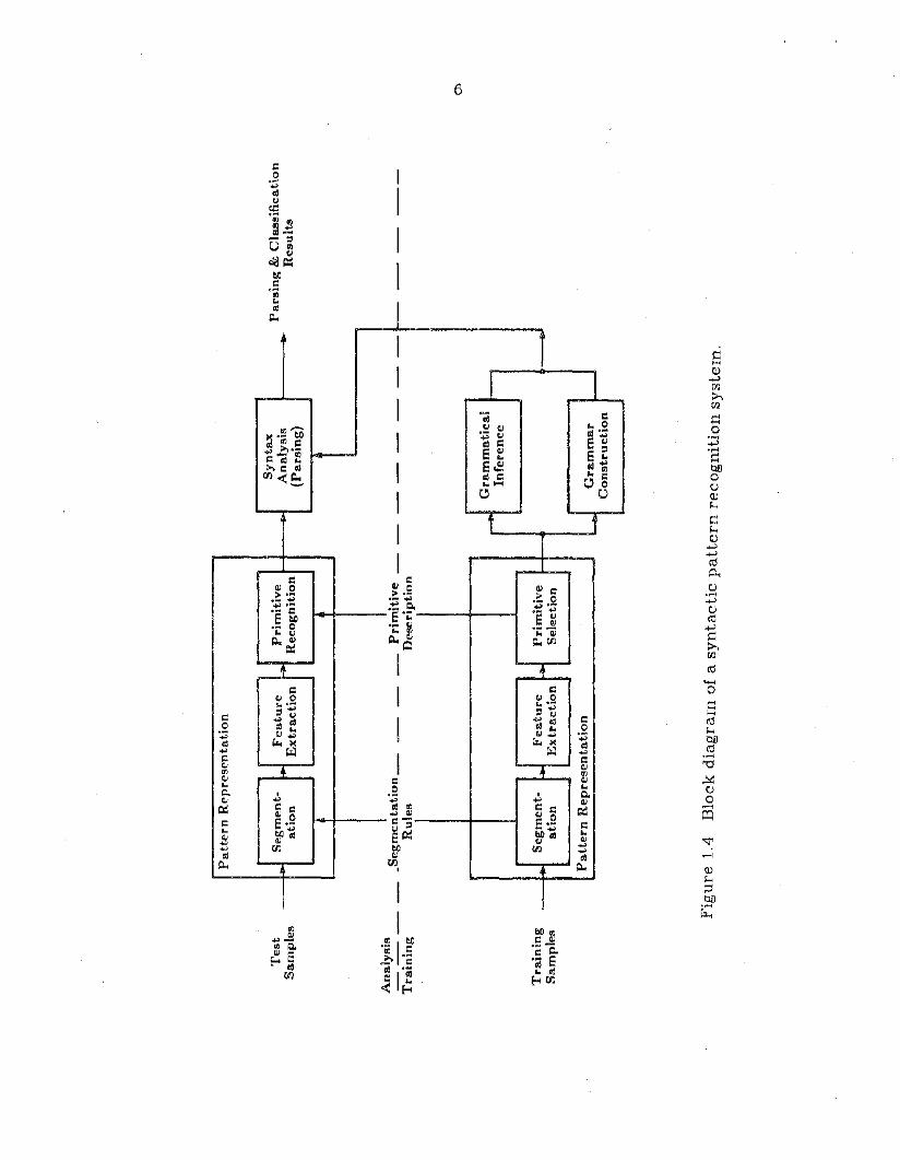
tion is the most important feature. The block diagram of a typical syn
tactic pattern recognition system is shown in Figure 1.4. Due to the
unknown characteristic about the source and environment, seismic
grammar is usually difficult to construct manually. Therefore, gram
matical inference techniques will be applied to infer the pattern gram
mar from a set of training samples. An error-correcting parser will also
be used because the chance that a testing sample is perfectly accepted
by the inferred grammar is very slim. This is usually a rule rather than

3
Figure 1.1 An example of two typical seismic records. The top one is anexplosion; the bottom one is an earthquake.

4
Figure 1.2 An example of extreme case. The top one is a typical explosion waveform; the bottom one is an earthquake record which looks likean explosion.

5
Figure 1.3 Another example 01 extreme ease. The bottom one is a typicalearthquake wavelorm; the top one is an explosion record which looks likean earthquake.
Test
Sam
ple
s
An
aly
sis
Tra
inin
g
Tra
inin
gS
amp
les
Patt
ern
Rep
rese
nta
tio
n
Pri
mit
ive
Sy
nta
xS
egm
ent-
i-"F
eatu
ref-a
An
aly
sis
ati
on
Ex
tracti
on
Rec
og
nit
ion
(Pars
ing
)
__
_S
egm
enta
tio
n_
_-
__
Pri
mit
ive
__
__
----
----
----
--R
ule
sD
escr
ipti
on
.-G
ram
mati
cal
t--
Infe
ren
ce
Seg
men
t-F
eatu
reP
rim
itiv
e--
...f+
ati
on
Ex
tracti
on
Sel
ecti
on
Patt
ern
Rep
rese
nta
tio
n4
Gra
mm
ar
I---
Co
nst
ructi
on
Fig
ure
1.4
Blo
ckd
iag
ram
ofa
syn
tacti
cp
att
ern
reco
gn
itio
nsy
stem
.
rsin
g&
Cla
ssif
icat
ion
Res
ult
s
CJ)
7
an exception in many practical applications, and seismic analysis hap
pens to be one of them. This is due to the noise and uncertainty of the
source and background. In addition to grammatical approach, we will
also use nearest-neighbor decision rule for classification. Of course, the
distance, or similarity, computation is between the string representa
tion of the seismic signals. The block diagram of nearest-neighbor
classifier for syntactic patterns is shown in Figure 1.5.
Due to the recent advance of VLSI technology it is now feasible and
will soon become economical to design custom chips for special applica-
tions (Mead and Conway, 1980; Kung, 1979; Ackland, et aI., 1981). A VLSI
system for seismic signal recognition will also be developed in this
study.
1.2 Literature Survey
1.2.1 Syntactic Pattern Recognition andDigital Signal Processing
Applications of syntactic pattern recognition to digital signal pro
cessing have received much attention and achieved considerable suc
cess in the past decade (see Fu, 1982). The most prominent applica-
tions are in the areas of biomedical waveform analysis and speech
recognition. The reason of their success is that these waveforms have
regular and predictable structure. Most biomedical waveforms, e.g.,
ECG wave and carotid pulse wave, are rhythmic and generated by
specific organs of the body where their functions are well understood.
Test
Sam
ple
s
An
aly
sis
Tra
inin
g
Tra
inin
gS
amp
les
Patt
ern
Rep
rese
nta
tio
n
Str
ing
-to
-N
eare
st-
Seg
men
t-~
Featu
re~
Pri
mit
ive
Str
ing
Nei
gh
bo
rati
on
Ex
tracti
on
Rec
og
nit
ion
Dis
tan
ceD
ecis
ion
Co
mp
uta
tio
nR
ule
__
.Seg
men
tati
on
_--
__
__
Pri
mit
ive
__
__
__
_--
----
----
---
Ru
les
Des
crip
tio
n
Seg
men
t-..
Featu
rei-to
-P
rim
itiv
eati
on
Ex
tracti
on
Sel
ecti
on
Patt
ern
Rep
rese
nta
tio
n
Fig
ure
1.5
Blo
ckd
iag
ram
of
asy
nta
cti
cp
att
ern
reco
gn
itio
nsy
stem
usi
ng
the
neare
st-n
eig
hb
or
decis
ion
rule
for
stri
ng
patt
ern
s.
Cla
ssif
icat
ion
Res
ult
s
en
9
It is thus easy to write a grammar for these waveforms based on their
functions. Horowitz (1975, 1977) developed a syntactic algorithm to
detect the peaks of ECG waves. Albus (1977) used a stochastic finite
state model to interpret ECG signals. Giese, et a1., (1979) proposed a
syntactic method to analyze EEG signals. Stockman, et 0.1., (1976)
applied a syntactic method to analyze carotid pulse waveforms. The
major problem in biomedical waveform analysis is the noise which could
be generated by muscles or other sources (Albus, 1977).
It has been shown that speech patterns are related to linguistic
items by a complex set of rules belonging to "grammar of speech"
(DeMori, 1977). Therefore, the most effective way of detecting and
recognizing speech patterns is by syntactic method. DeMori (1972) has
shown a syntactic method to recognize spoken Italian digits. The major
problem in speech recognition IS the variability of the speech patterns.
They are speaker-dependent as well as context-dependent. Even for the
same speaker and the same word, the features extracted from different
utterances are usually not the same.
We will review in this section some of the existing syntactic
methods applied to signal processing. Although preprocessing is also
important, we do not include this part here, because it is case depen
dent and is usually not related to the recognition stage. However, we
will discuss the preprocessing procedure later in our experiments of
seismic signal recognition. We will now concentrate on the major parts
of syntactic pattern recognition system, i.e., segmentation, feature
extraction, primitive selection, grammatical inference or construction,
and syntax analysis.

10
A waveform must be converted into a string of primitives (tree OT
graph for high dimensional representation) before grammatical infer
ence and syntax analysis can take place. Since a waveform is a one
dimensional signal, it is most natural to represent it by a string of
primitives. Various series expansion, for example, Fourier series, and
spectral analysis techniques have been used to approximate the whole
waveform. However, they are not suitable for syntactic analysis
because the relationships among one part of the waveform and the oth
ers are significant in syntactic analysis. Although they can be used to
feature waveform segment, they are subject to the constraint of seg
ment length and characteristics of the waveform. Pavlidis (1971, 1973,
1974) proposed a linguistic waveform analysis algorithm in which he
partitioned the waveform into several segments by using linear approxi
mation. The basic idea is to minimize the number of segments by
merging and splitting while the error norm of each segment is retained
below the error tolerance. Horowitz (1975, 1977) extended this idea
and added peak detection algorithm. He gave a syntactic definition to
the positive peak - a positive slope followed by a negative slope or posi
tive slope followed by zero slope and then followed by negative slope. A
negative peak can be defined in a similar way. He further constructed a
deterministic context-free grammar to recognize positive and negative
peaks. This approach is useful in waveform shape analysis because of
its simplicity. However, the curvature informations are not included.
Another interesting representation of waveform is by tree struc
ture. It was first introduced by Ehrich and Foith (1976). The peaks and
valleys of the waveform are detected and connected by a relational
tree. Sankar and Rosenfeld (1979) extended this idea by using the
11
concepts of fuzzy connectedness. This method converts one
dimensional waveform into two-dimensional tree structure. It is useful
for unipolar waveform analysis such as terrain analysis, but not so help
ful for the analysis of bipolar waveforms such as ECG wave and random
waveforms such as EEG and seismic waves. Another well-known method
of converting one-dimensional signal into two-dimensional image is
called spectrogram which is used very often in speech analysis
(Flanagan, 1972). The spectrogram of a waveform is the plot of energy
as a function of time and frequency. Time and frequency are the hor
izontal and vertical axes of the picture. Energy is represented by gray
level intensity. This method needs special facilities to convert a small
segment of time-domain signal into frequency-domain representation
efficiently. Automatic interpretation of the two-dimensional image is
still a subject for studies.
Giese et al. (1979) proposed a syntactic method to analyze EEG sig
nal. The EEG recording is divided into fixed-length segments, each seg
ment is equal to i-second period. Seventeen features are computed
from the spectral of each segment. A linear classifier is applied to clas
sify the segments into seven categories. An EEG grammar is manually
constructed and a bottom-up parser without backtracking is used for
syntax analysis.
Stockman et al. (1976) proposed a syntactic pattern recognition
system for carotid pulse wave analysis. A set of thirteen primitives
including various type of line segments and parabolas are used. The
subpattern and primitive extraction starts from the most prominent
substructure, e.g., long line segment, and then less prominent struc
tures with respect to the more prominent ones, in a prespecified order.
12
A context-free grammar is manually constructed and a top-down parser
is used for syntax analysis.
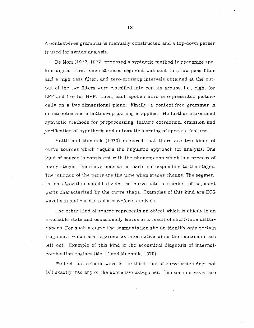
De Mori (1972, 1977) proposed a syntactic method to recognize spo
ken digits. First, each 20-msec segment was sent to a low pass filter
and a high pass filter, and zero-crossing intervals obtained at the out
put of the ~wo filters were classified into certain groups, Le., eight for
LPF and five for HPF. Then, each spoken word is represented pic tori
cally on a two-dimensional plane. Finally, a context-free grammar is
constructed and a bottom-up parsing is applied. He further introduced
syntactic methods for preprocessing, feature extraction, emission and
verification of hypothesis and automatic learning of spectral features."
MotU' and Muchnik (1979) declared that there are two kinds of
curve sources which require the linguistic approach for analysis. One
kind of source is consistent with the phenomenon which is a process of
many stages. The curve consists of parts corresponding to the stages.
The junction of the parts are the time when stages change. The segmen
tation algorithm should divide the curve into a number of adjacent
parts characterized by the curve shape. Examples of this kind are ECG
waveform and carotid pulse waveform analysis.
The other kind of source represents an object which is chiefly in an
invariable state and occasionally leaves as a result of short-time distur
bances. For such a curve the segmentation should identify only certain
fragments which are regarded as informative while the remainder are
left out. Example of this kind is the acoustical diagnosis of internal
combustion engines (Mottl' and Muchnik, 1979).
We feel that seismic wave is the third kind of curve which does not
fall exactly into any of the above two categories. The seismic waves are

13
influenced largely by background as well as by source. Sometimes we
are interested in the background, e.g., oil exploration; ~ometimes we
are interested in the source, e.g., nuclear test detection. This will be
discussed in the next section.
1.2.2 Pattern Recognition andSeismic Signal Analysis
The major studies of seismic waves can be classified into the follow
ing areas (Bath, 1979):
1. Seismic prospecting. This is the most attractive topic in these
days. Seismic methods are applied to exploration for occurrences of
oil, are bodies, minerals, etc. The reflection method and the refraction
method are two major methods in use. It should be noted that it is not
possible, at least by now, to detect oil, etc., by seismic or any other
geophysical methods. It is only possible to discover geological forma
tion which may indicate the occurrence of oil, etc.
2. 1fi-bration measurements. The effect of vibraions, cue to mining,
traffic, etc., on various structures and human beings is dudied. Such
measurements are usually made with accelerographs.
3. Stress measurements. Measurements of absolute stress have
been used to investigate the strength of building materials and stability
in rnines.
4. Earthquake engineering. This field studies the effects of earth
quakes on all kinds of building structures, especially on crucial struc
ture such as nuclear power plant.
14
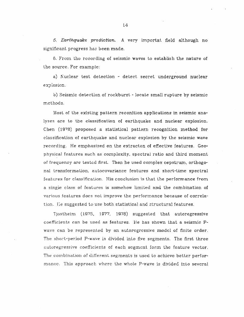
5. Earthqualce prediction. A very importat field although no
significant progress has been made.
6. From the recording of seismic waves to establish the nature of
the source. For example:
a) Nuclear test detection - detect secret underground nuclear
explosion.
b) Seismic detection of rockburst - locate small rupture by seismic
methods.
Most of the existing pattern reconition applications in seismic ana
lyses are to the classification of earthquake and nuclear explosion.
Chen (1978) proposed a statistical pattern recognition method for
classification of earthquake and nuclear explosion by the seismic wave
recording. He emphasized on the extracton of effective features. Geo
physical features such as complexity, spectral ratio and third moment
of frequency are tested first. Then he used complex cepstrum, orthogo
nal transformation, auiocovariance features and short-time spectral
features for classification. His conclusion is that the performance from
a single class of features is somehow limited and the combination of
various features does not improve the performance because of correla
tion. He suggested to use both statistical and structural features.
Tjostheim (1975, 1977, 1978) suggested that autoregressive
coefficients can be used as features. He has shown that a seismic P
wave can be represented by an autoregressive model of finite order.
The short-period P-wave is divided into five segments. The first three
autoregressive coefficients of each segment form the feature vector.
The combination of different segments is used to achieve better perfor
mance. This approach where the whole P-wave is divided into several
15
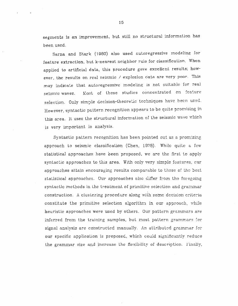
segments is an improvement, but still no structural information has
been used.
Sarna and Stark (1980) also used autoregressive modeling for
feature extraction, but k-nearest neighbor rule for classification. When
applied to artificial data, this procedure gave excellent results; how
ever, the results on real seismic / explosion data are very poor. This
may indicate that autoregressive modeling is not suitable for real
sei:;;mic waves. Most of these studies concentrated on feature
selection. Only simple decision-theoretic techniques have been used.
However, syntactic ps.ttern recognition appears to be quite promising in
this area. It uses the structural information of the seismic wave which
is very important in analysis.
Syntactic pattern recognition has been pointed out as a promising
approach to seismic classification (Chen, 1978). While quite a few
statistical approaches have been proposed, we are the first to apply
syntactic approaches to this area. With only very simple features, our
approaches attain encouraging results comparable to those of the best
statistical approaches. Our approaches also differ from the foregoing
syntactic methods in the treatment of primitive selection and grammar
construction. A clustering procedure along with some decision criteria
constitute the primitive selection algorithm in our approach, while
heuristic approaches were used by others. Our pattern grammars are
inferred from the training samples, but most pattern grammars for
signal analysis are constructed manually. An attributed grammar for
our specific application is proposed, which could significantly reduce
the grammar size and increase the flexibility of description. Finally,

16
18
between the two reserviors is determined by the distribution of the two
clusters. Since the nature of the reservior is characterized by the
seismic traces, it is possible to compare the seismic traces of the two
reserviors directly.
Levenshtein distance has recently been applied to speech recogni
tion (Okuda, Tanaka and KasaL 1976; Ackroyd, 1980). It can be used to
correct the letter or phoneme sequences that are generated by the
recognition machine, or can be built directly into the recognition pro
cedures. Our VLSI string matcher can be applied to both cases. Futh
ermore, our primitive recognizer can also be applied to the case in Ack
royd (l980). Mottl' and Muchnik (1979) proposed a linguistic approach
to the analysis of experimental curves where a special-purpose
language is constructed to describe the pattern. The distance between
two strings is defined as the minimum number of insertion and deletion
of symbols, which is in essence equivalent to Levenshtein distance.

19
CHAPTER II
SIMILARITY MEASURES AND RECOGNITIONPROCEDURES FOR STRING PATTERNS
2.1 Introduction
One important premise in pattern recognition is that we can meas
ure the similarities between patterns. We say that a pattern belongs to
one class if and only if that pattern is more similar to the members of
this class than the members of other classes. These measures can be
nominal where numbers used only as names, or ordinal where only rank
orders have meaning, or interval where seperation between numbers is
meaningful, or ratios where a natural zero exists. Distance is a popular
candidate for simlarity measure. If the pattern is represented by a
vector, as in the case of statistical approach, the Euclidean distance is
usually used as a similarity measure. The Euclidean di:;;tance has many
nice properties, for example, symmetric and invariant under transla
tion and rotation.
In syntactic approach, patterns are represented by strings, trees
or graphs, therefore similarity measures must be available for these
syntactic patterns. Several similarity measures have been proposed to
tackle this problem (Fu, 1977; Lu and Fu, 1977, 1978b). Since our major
interest is string patterns, we will review some well-knovvll string simi
larity measures, discuss their properties and defme u hierarchy of

20
string distanc es.
String similarity measure can be applied to string-matchi.ng in
information storage and retrieval (Hall and Dowling, 1980), speech
recognition (Sakoe and Chiba, 1978), clustering of string patterns (Fu
and Lu, 1977) and nearest-neighbor decision rule for string
classification. It is also used in error-correcting parsing. Given a string
y and a language L (G), an error-correcting parser (ECP) generates a
parse for string x, where x E: L (G) and x is most similar to y.
Section 2 of this chapter discusses various types of string similarity
measures, including both nonstochastic and stochastic models. String
distances are classified into general string distances and special string
distances. General string distances are based on the principles of
insertion, deletion and substitution transformations. Special string dis
tances are those not based on the above principles. One example is the
time warping distance in speech analysis. We propose another special
distance computation for damage assesment. A hierarchy of general
string distances are also defined. Section 3 describes error-correcting
parsing algorithms which do not require expanded grammars. Section
4 discusses and compares two recognition procedures, namely, the
error-correcting parsing and the nearest-neighbor rule, for syntactic
patterns, and Section 5 gives the conclusion.
This chapter emphasizes the symmetric property of string similar
ity measures. This is not a problem when we use Euclidean distance as
the similarity measure, since Euclidean distance is always symmetric.
But this is not true when we define string similarity measures, espe
cially when using weighted distance. The error-correcting parsing algo
rithms using symmetric string similarity measures are also given which
21
car. not be solved by any other existing parsing algorithm.
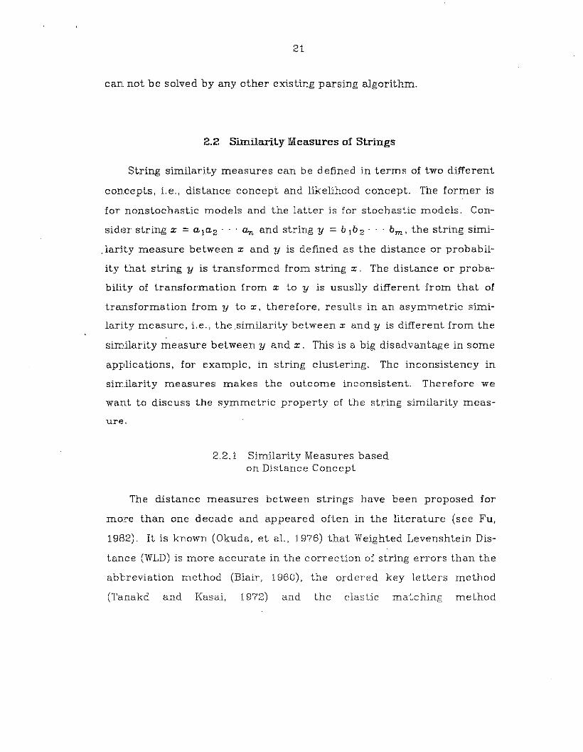
2.2 Similarity Measures of Strings
String similarity measures can be defined in terms of two different
concepts, i.e., distance concept and likelihood concept. The former is
for nonstochastic models and the latter is for stochastic models. Con-
sider string x = a 1az ... CLn and string y = b 1b z ... b m , the string simi
.larity measure between x and y is defined as the distance or probabil
ity that string y is transformed from string x. The distance or proba
bility of transformation from x to y is ususlly different from that of
transformation from y to x, therefore, results in an asymmetric simi
larity measure, i.e., the similarity between x and y is different from the
similarity measure between y and x. This is a big disadvantage in some
applications, for example, in string clustering. The inconsistency in
sim.ilarity measures makes the outcome inconsistent. Therefore we
want to discuss the symmetric property of the string similarity meas-
ure.
2.2.1 Similarity Measures basedon Distance Concept
The distance measures between strings have been proposed for
more than one decade and appeared often in the literature (see Fu,
1982). It is known (Okuda, et al., 1976) that Weighted Levenshtein Dis
tance (WLD) is more accurate in the correction of string errors than the
abbreviation method (Blair, 1960), the ordered key letters method
(Tanakd and Kasai, 1972) and the elastic matching method
22
(Levenshtein, 1966), where all of these apply substitution, insertion and
deletion to string symbols. Fu and Lu (1977) have classified the weight
metrics into three categories, but did not consider the symmetric pro·
perty of the metric. We would like to further extend this idea and
include the discussion of symmetric property.
A. General String Distances
One of the primitive string distance definitions is called the
Levenshtein distance (Levenshtein, 1966). The Levenshtein distance
between strings x and y, x, Y E: I: ", denoted as d L (x ,y), is defined as
the smallest number of transformations required to derive string y
from string x. The transformations include insertion, deletion and sub
stitution of terminal symbols.
Definition 2.1 For any two strings x, y E: I: v, we can define a sequence
of transformations J=!T1, T2 , ..• , Tn!. n ~ 0, Ti E: ~Ts, TD • TI~ for 1 ~ i
~ n, such that y E: J(x). The transformations Ts, TD and TI are
defined as follows:
(1) substitution transformation, Ts
(2) deletion transformation. TD
(3) insertion transformation, T1
23
Definition 2.2 The Levenshtein distance d L (x ,y) is defined as
where k j , Tnj and nj are respectively the number of substitution, dele
tion and insertion transformations in J.
Definition 2.3 A distance between two strings x, y E: 2;., d(x,y) is sym
metric if and only if d(x,y) =d(y,x).
Since all the insertion, substitution and deletion transformations
are: counted equally, the Levenshtein distance is symmetric. It is
equivalent to assigning weight 1 to each of the transformation. We call
these weights type 0 weights.
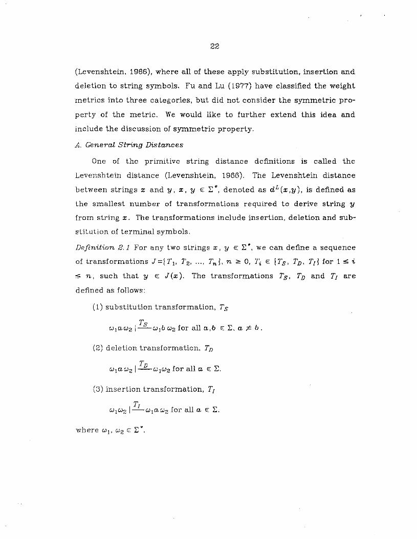
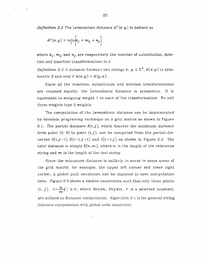
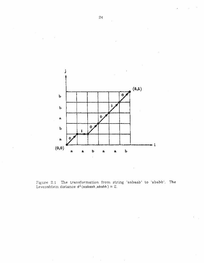
The computation of the Levenshtein distance can be implemented
by dynamic programing technique on a grid matrix as shown in Figure
2.1. The partial distance o[ i ,j J, which denotes the minimum distance
from point (0, 0) to point (i,j), can be computed from the partial dis
tances o[ i ,j -lJ o[ i -1 ,j -lJ and o[i -l ,j J as shown in Figure 2.2. The
total distance is simply o[n ,m.. J, where n is the length of the reference
string and Tn is the length of the test string.
Since the minumum distance is unlikely to occur in some areas of
the grid matrix, for example, the upper left corner and lower right
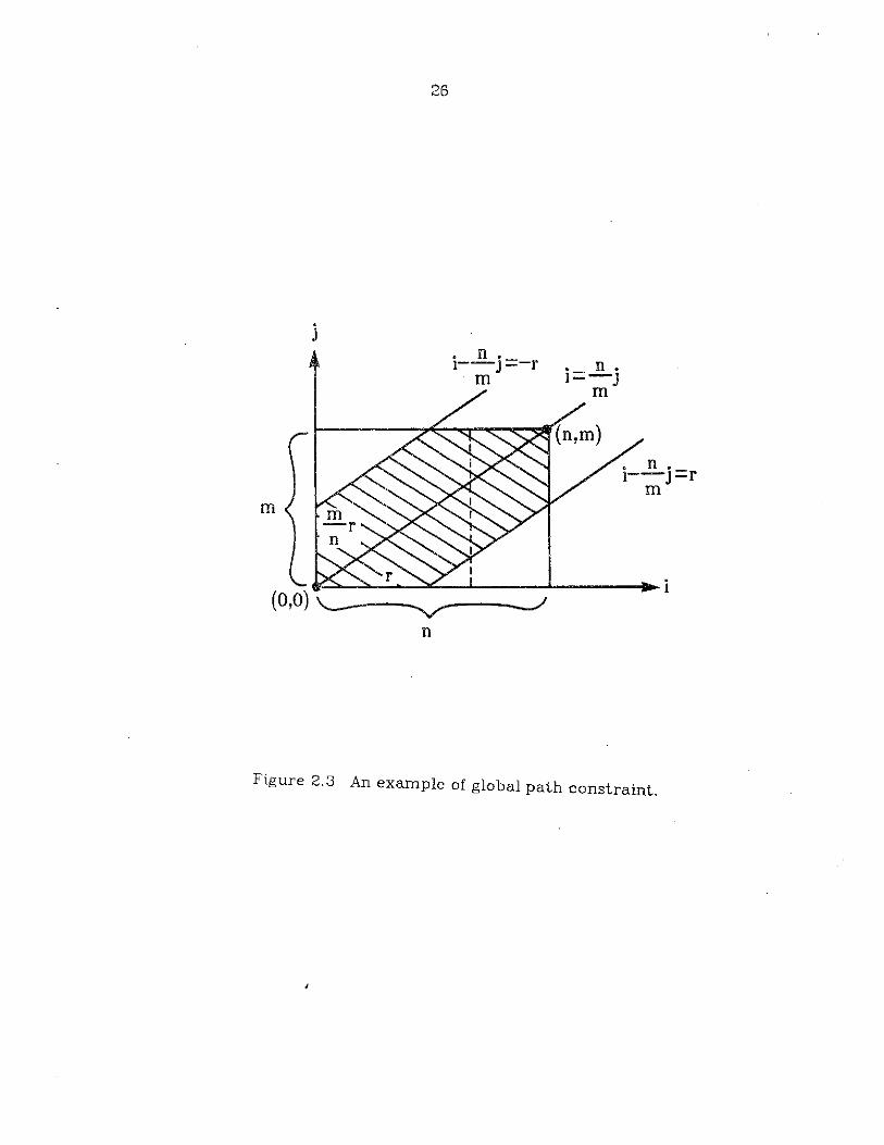
corner, a globol path constraint can be imposed to save computation
time. Figure 2.3 shows a window constraints such that only those points
(i, n, li-~ I ~ r, where O~i~n, O~j~Tn, r is a selected constant,Tn
are subject to distance computation. Algorithm 2.1 is for general string
distance computation with global path constraint.
24
.J
(6,6)
YY
VI'1 Y
Y
b
b
a
b
a
(0,0)a a b a b
i
Figure 2.1 The transformation from string 'aabaab' to 'ababb'. TheLevenshtein distance d L (aabaab ,ababb) =2.
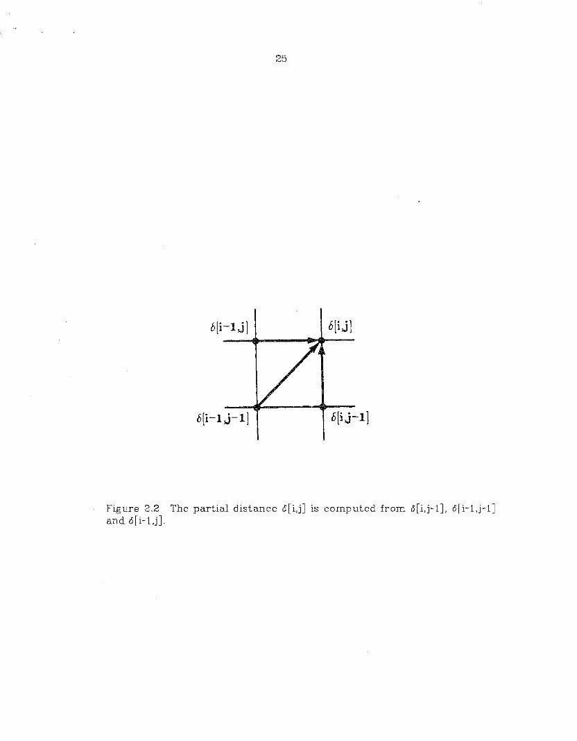
6[i-lj]
6[i-lJ-ll
25
o[iJl
o[iJ-ll
Figv.re 2.2 The partial distance 6[i,j] is computed from 6[i,j-l], 6!i-l,j-l]and 6[i-l,j].
26
J
n
Figure 2.3 An example of global path constraint.
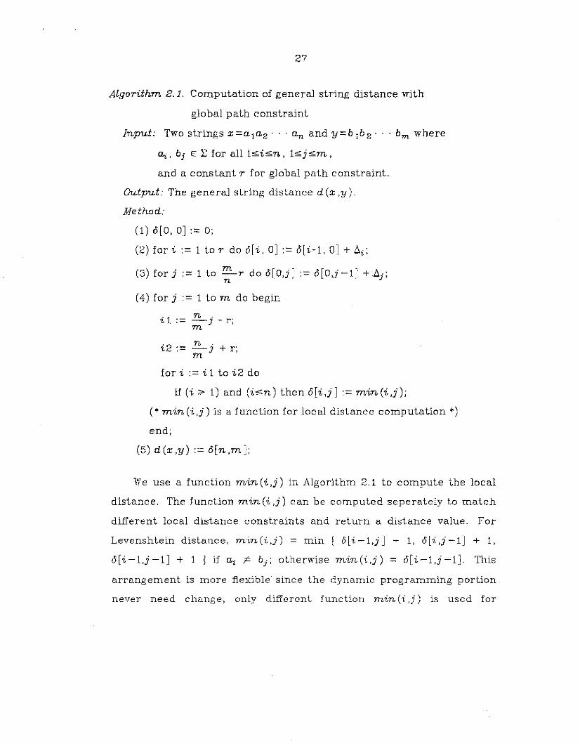
27
Algorithm 2.1. Computation of general string distance with
global path constraint
Input: Two strings x=ala2' . , an and y=b 1b2' .. bm where
eLi, , bj E: l: for all l~i~n, l'5,j~m ,
and a constant r for global path constraint.
Output: The general string distance d (x ,y),
Method:
(1) 0[0, OJ := 0;
(2) for i := 1 to r do o[i, OJ := o[i-1, OJ + D. i ;
(3) for j ,- 1 to m r do 0[O,1J := 0[O,j-1J +D.j ;n
(4) for j .- 1 to m do begin.
i 1 := :!!:- j - r;m
i2 := :!!:- j + r;m
for i := i 1 to i2 do
if (i ~ 1) and (i~n) then o[i,j J := min (i ,j);
('" min (i ,j) is a function for local distance computation *)
end;
(5) d(x,y) := o[n,mJ;
We use a function min (i,j) in Algorithm 2.1 to compute the local
distance. The function min (i ,j) can be computed seperately to match
different local distance constraints and return a distance value. For
Levenshtein distance, min(i,j) = min f o[i-1,jJ + 1, 0[i,j-1J + 1,
0[i-l,j-1J + 1 l if ai j:. bj ; otherwise min(i,j) = o[i-1,j-1]. This
arrangement is more flexible since the dynamic programming portion
never need change, only different function min(i,j) is used for
28
different applications.
The Levenshtein distance appears to be not powerful enough for
many pattern recognition applications. However, it may be sufficient
for string matching in information retrieval (Hall and Dowling, 1980).
Fu and Lu (1977) have proposed a weighted Levenshtein distance (WLD)
where different weights are associated with different transformation
and terminals.
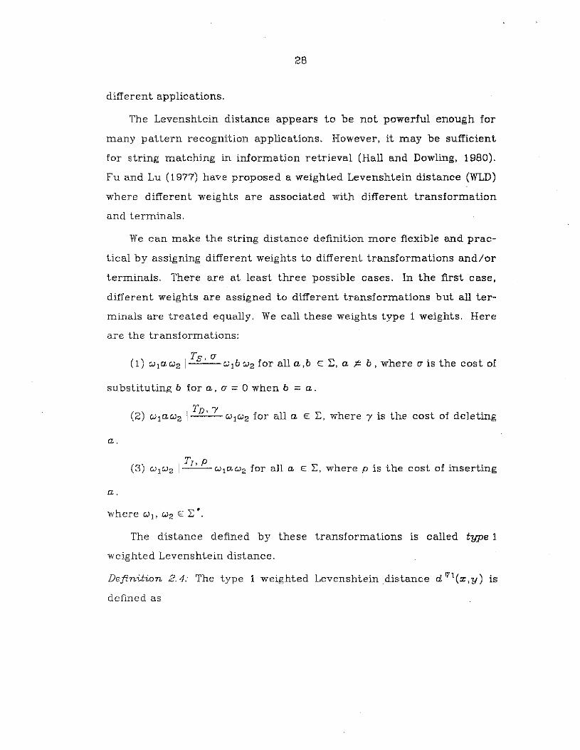
We can make the string distance definition more flexible and prac
tical by assigning different weights to different transformations and/or
terminals. There are at least three possible cases. In the first case,
different weights are assigned to different transformations but all ter
minals are treated equally. We call these weights type 1 weights. Here
are the transformations:
( ) I
Ts, a-1 W1aw2 W1bwZ for all a,b E: 2:, a ;t:. b, where a- is the cost of
substituting b for a, a- = 0 when b = a.
(2) w1aw2 I TD' 'Y W1 w2 for all a E: 2:, where 'Y is the cost of deleting
a.
(3) W1w2 I TI, P CJ1aw2 for all a E: 2:, where p is the cost of inserting
a.
The distance defined by these transformations is called type 1
weighted Levenshtein distance.
Definition 2.4: The type 1 weighted Levenshtein distance d fl'l(x ,y) is
defined as

29
where k j , mj and nj are defined the same as in Definition 2.3.
Theorem 2.1 d W1 (x,y) is symmetric, i.e., d W1 (x,y) = d W1 (y,x), if and
only if y =p.
The WLD d Wl(x ,y) can be computed by Algorithm 2.1 where
m1:n(i,j) = min fo[i,j-1] + p, o[i-1,j-l] + (J, o[i-l,j] + yl as shown in
Figure 2.4(a). The weights in step (2) and (3) should also be changed.
In the second case, different weights are assigned to different
transformations and terminals, but the weights associated with the ter
minals are context-indepentent. We call these weights type 2 weights.
We have the following transformations:
Ts , S(o.,b)(1) '" 1a "'2 I '" 1b "'2 for all a, b E: ~, a 1= b , where S (a, b) is
the cost of substituting b for a, S (a ,a) =O.
( ) l
TD, D(o.) )2 "'10."'2 "'1"'2 for all a E: 2:, where D (a is the cost of
deleting o..
Tf ,1(a)(3) "'1"'2 I "'10."'2 for all a E: 2:, where 1(0.) is the cost of
inserting a.
The distance defined by these transformations is called type 2
weighted Levenshtein distance.
Definition 2.5: The type 2 weighted Levenshtein distance d W2(x, y) is
de:fined as
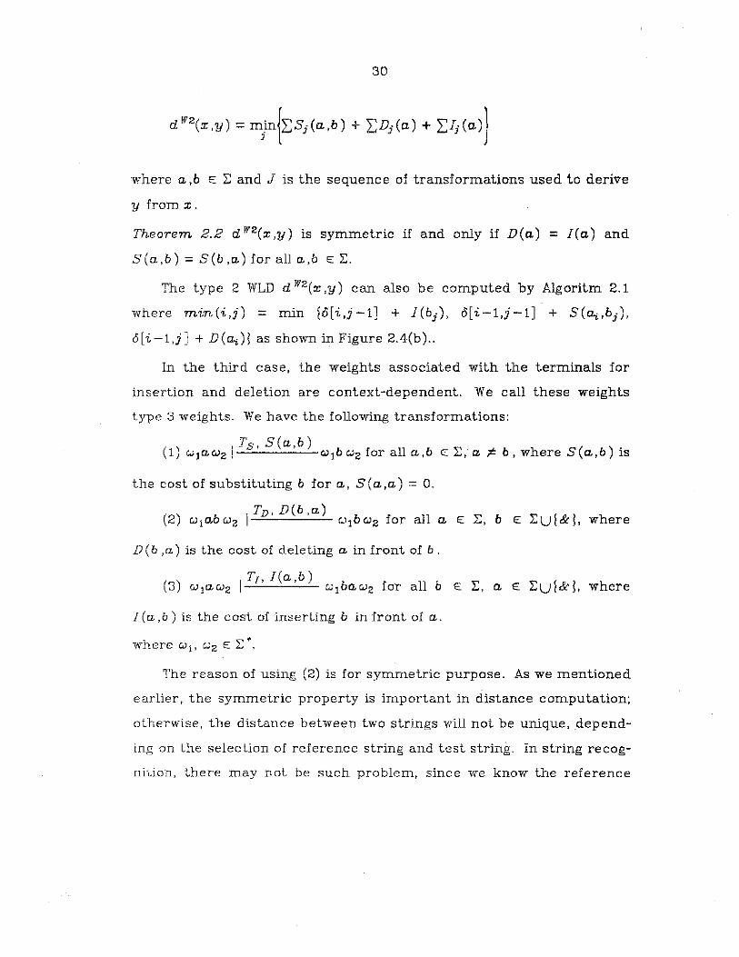
30
where a ,b E: L: and J is the sequence of transformations used to derive
y from x.
Theorem 2.2 d W2(x,y) is symmetric if and only if D(a) = 1(a) and
S(a,b) = S(b ,a) for all a,b E: 2:.
The type 2 WLD d W2(x ,y) can also be computed by Algoritm 2.1
where min(i,j) = min ~o[i,j-l] + 1(bj ), o[i-l,j-1] + S(~,bj)'
o[i-l,j] + D(~)l as shown in Figure 2.4(b) ..
In the third case, the weights associated with the terminals for
insertion and deletion are context-dependent. We call these weights
type 3 weights. We have the following transformations:
ITs,S(a,b) ( )
(1) c.J 1a""2 ""lb c.J2 for all a,b E: 2:, a ji:. b, where S a,b is
the cost of substituting b for (2, S(a,a) =O.
D (b ,a) is the cost of deleting a in front of b .
1(a ,b) is the cost of inserting b in front of a.
where ""1' CJ2 E: ~ "'.
The reason of using (2) is for symmetric purpose. As we mentioned
earlier, the symmetric property is important in distance computation;
otherwise, the distance between two strings will not be unique, depend
ing on the selection of reference string and test string. In string recog
nition, there may not be such problem, since we know the reference
31
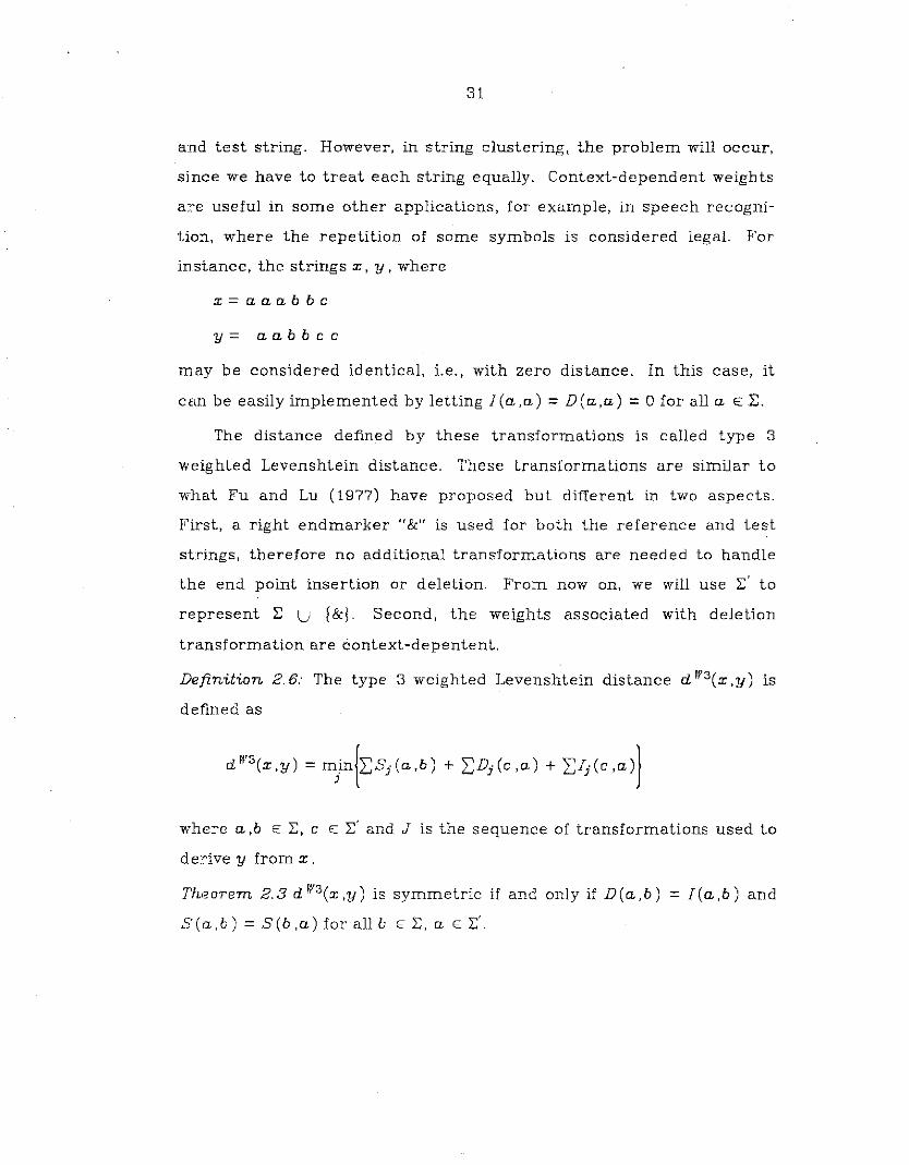
and test string. However, in string clustering, the problem will occur,
since we have to treat each string equally. Context-dependent weights
are useful in some other applications, for example, in speech recogni
tion, where the repetition of some symbols is considered legal. For
instance, the strings x, y, where
x=aaabbc
y= aabbcc
may be considered identical, Le., with zero distance. In this case, it
can be easily implemented by letting J(a,a) =D(a,a) =0 for all a E:2:.
The distance defined by these transformations is called type 3
weighted Levenshtein distance. These transformations are similar to
what Fu and Lu (1977) have proposed but different in two aspects.
First, a right endmarker "&" is used for both the reference and test
strings, therefore no additional transformations are needed to handle
the end point insertion or deletion. From now on, we will use z:;' to
represent z:; U f&l. Second, the weights associated with deletion
transformation are context-depentent.
Definition 2.6: The type 3 weighted Levenshtein distance d W3(x ,y) is
defined as
where a ,b E: Z:;, C E: z:;' and J is the sequence of transformations used to
derive y from x.
Theorem 2.3 d W3 (x,y) is symmetric if and only if D(a,b) = J(a,b) and
5(I':L,6) =5(b ,a) for all b E: Z:;, a E: Z:;'.
32
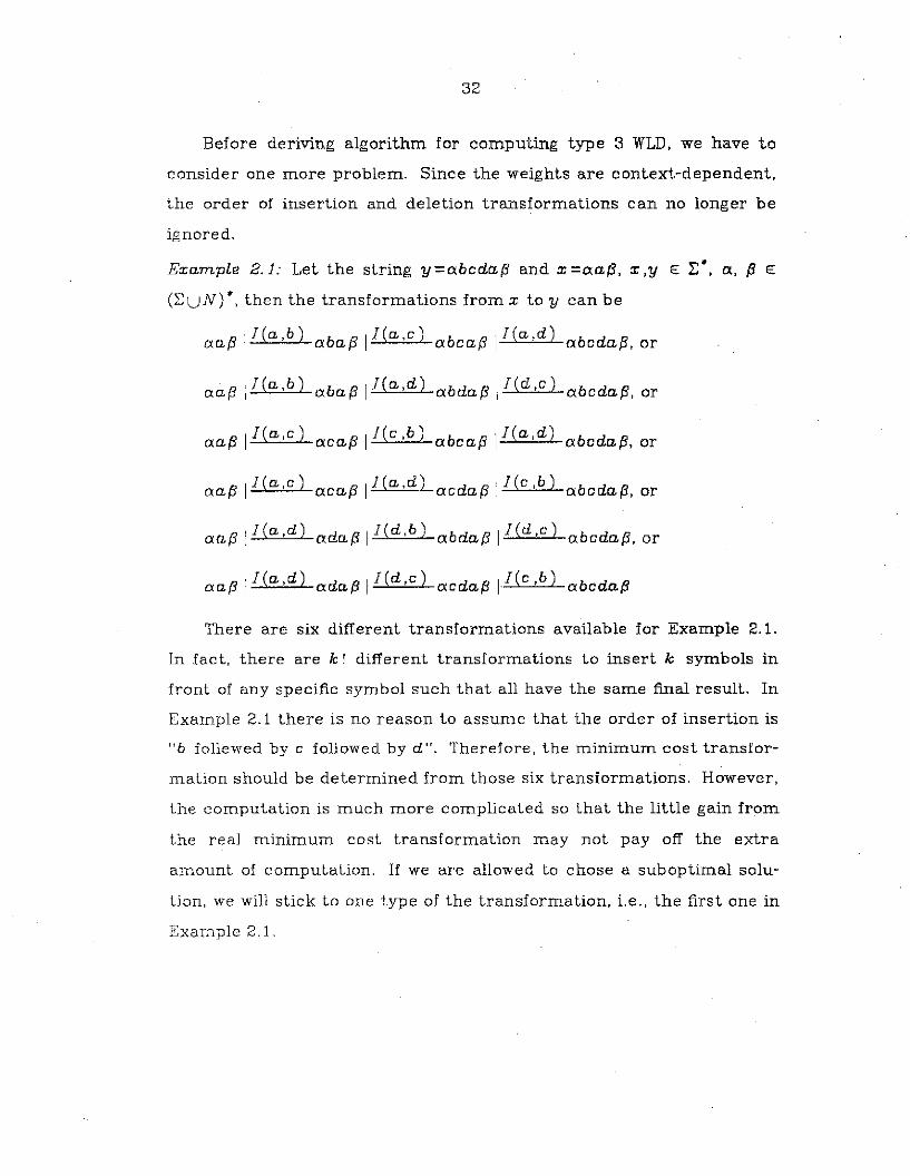
Before deriving algorithm for computing type 3 WLD, we have to
consider one more problem. Since the weights are context-dependent,
the order of insertion and deletion transformations can no longer be
ignored.
Example 2.1: Let the string y=o.bcda(3 and x=o.a(3, x,y e: 2;", a., (3 e:
('f, UN)", then the transformations from x to y can be
o.a(3I I (a,b ) aba(3 II(a,c) abca(3I I (a,d) o.bcda{3, or
o.a(3I I (a,b) aba(3I I (a,d) a bda (3 11 (d ,c ) abcda(3, or
o.a(3 II(a,c) o.ca(3 II(c ,b) cxbca(3I I (a,d) cxbcda(3, or
o.a(3 II(a,c) o.ca(3I I (a,d) acda(3 II(c ,b) o.bcda(3, or
a. a (3 II (a ,d) ada (3 II(d ,b) a. bda (3 I I (d ,c ) o.bcda(3, or
a. a (3 I I (a ,d) a. da (3 I I (d ,c) 01. c da (3 11 (c ,b ) cxbcda(3
There are six different transformations available for Example 2.1.
In fact, there are k! different transformations to insert k symbols in
front of any specific symbol such that all have the same final result. In
Example 2.1 there is no reason to assume that the order of insertion is
"b follewed by c followed by d". Therefore, the minimum cost transfor
mation should be determined from those six transformations. However,
the computation is much more complicated so that the little gain from
the real minimum cost transformation may not payoff the extra
amount of computation. If we are allowed to chose a suboptimal solu
tion, we will stick to one type of the transformation, Le., the first one in
Example 2.1.

33
The cases for deletion are similar to those for insertion. Consider
Example 2.1, the transformation from y to x corresponding to the first
one is as follows:
abcdaP>ID(a,d) abcaP>ID(a,c) abaP>ID(a,b) aap>
It is noted that the symmetric property is preserved here.
We can use Algorithm 2.1 to compute the type 3 WLD d W3(x ,y)
where min(i,j) = min f 0[i,j-1J + l(ai+l,bj ), 0[i-1,j-1J + S(~,bj),
0[£-1,jJ + D(bj+1,ai) I as shown in Figure 2.4(c). The weights in step
(2) and (3) should also be modified.
We can define a hierarchy on the four types of distances, i.e., type 0
distance is a proper subset of type 1 distance; type 1 distance is a
proper subset of type 2 distance, and type 2 distance is a proper subset
of type 3 distance. They are capable of computing all the general string
distances based on the concepts of insertion, deletion and substitution
transformations. However, there are some exceptions of distance
measurements which do not base on the idea of insertion, deletion and
subtitution transformations. We will call them the special string dis
tances.
B. Special String Distance
The special string distances mean that these distances can only be
applied to some specific applications, also they are not based on the
idea of insertion, deletion and substitution transformations. One exam
ple is the dynamic time warping for speech recognition, the other is the
modified dynamic time warping for damage assesment.
In spoken word recognition, the recorded speech signal from
different utterance is different even for the same word by the same

o[i-
l,j]I
JIo
[i,j]
o[i-
l,j]I
D(a
j)Io[
i,j]
o[i-
l,j]
D(b
j+1,
aj)l
b[i,j
]-
b·p
b·I(
bj)
b·I(
ai+
1,b j
)J
JJ
o[i-
l,j-
l]o[
i,j-l
)b[
i-l,
j-l]
o[i,j
-l]
o[i-l
,j-l]
o[i,j
-t]
c.J
a·a·
a·*'"
II
I
(a)
(b)
(c)
Fig
ure
2.4
Co
mp
uta
tio
nof
parti~l
dis
tan
ce
for
(a)
typ
e1.
(b)
typ
e2
an
d(c
)ty
pe
3W
LD.
35
perso,n. Meanwhile, the time difference between speech patterns is
nonlinear, therefore a nonlinear matching algorithm is requiered in
order to obtain good recognition results. A special technique called
time warping has been proposed by Sakoe and Chiba (1978). An exam
ple is shown in Figure 2.5 where x = a 1a2 ... an is the reference pattern
and y = bIb 2 ... bm is the test pattern. Each component ~, bJ· of string
x, y can be a feature vector or a scalar which represents a signal seg
ment. (The position of each component ~, b j in the grid matrix is
slightly different from what we have used previously.)
Definition 2.7 The time warping distance between strings x and y is
KdTW(x, y) = 2:: d(c (k))
k=l
where
d (c (k ))=d (i (k) ,j (k)) = 11~(k) - bj(k)11
and k is the index of common time axis.
Two major differences between time warping and the general
string-to-string distance can be pointed out immediately. First, one
component, i.e., symbol, in warping function can be used more than
once. For example, component a4 in Figure 2.6 has been used to com
pared with b 3 and b 4' Second, the components may be skipped without
any cost. Although the general string distance can be modified by let
ting l(a,a)=O and D(a,b )=0 for a,b E: 2:, to simulate time warping,
there are other restrictions on the time warping function, for example,
slope constraint. Slope constraint will eliminate excessively steep or
gentle gradient from the warping function. For details of slope con
straints and computation of time warping distance, see (Sakoe and
Chiba, 1978). The weights used for time warping are difIercnt from

36
J
hm • • .. • • • •· • •· • • • •·h4 It •h3 • • • •h2 • • • •hI • • • •
....
Figure 2.5 An example of dynamic time warping.

37
c a
d b
Figure 2.6 Examples of some seismic recordings in structural damageassesment.
38
those for insertion, deletion and substitution, and can be tailored to fit
specific applications.
A path constraint similar to that of general string distance (see Fig
2.3) can also be applied here, i.e.,
li(k)-~(k)1 ~rm
where r is the path width. This will prevent warping function from hav
ing unrealistic matches. Sakoe and Chiba (1978) proposed a path con
straint
li(k)-j(k)1 ~r
This window is along the diagonal axis i (k )=j (k). Since the dynamic
programming proceeds from point (0,0) to point (n ,m), the window
should be along the diagonal axis i (k) = .:!!:....j (k) as shown in Figure 2.3.m
It has been shown by Sakoe and Chiba (1978) that the symmetric time
warping distance has higher recognition accuracy than asymmetric
time warping distance.
In so.me applications, specifically string distance computation for
damage assesment, one component in one string is equivalent to the
summation of several components in another string. For example, in
Figure 2.6 the top two segments may come from the seismic recordings
of a buildings without damage while the bottom two segments may
come from the same building with certain degree of damage. If we con
sider each component in Figure 2.6 as an appropriate measurement
then b 3 =a3 + a4 + a 5 + a6 + a7 and d 2 = c 2 + c 3 + c 4' since b 3 is a dis
tortion of a3' a4' a5' a6 and a7' and d 2 is a distortion of c 2, c 3 and c 4'
39
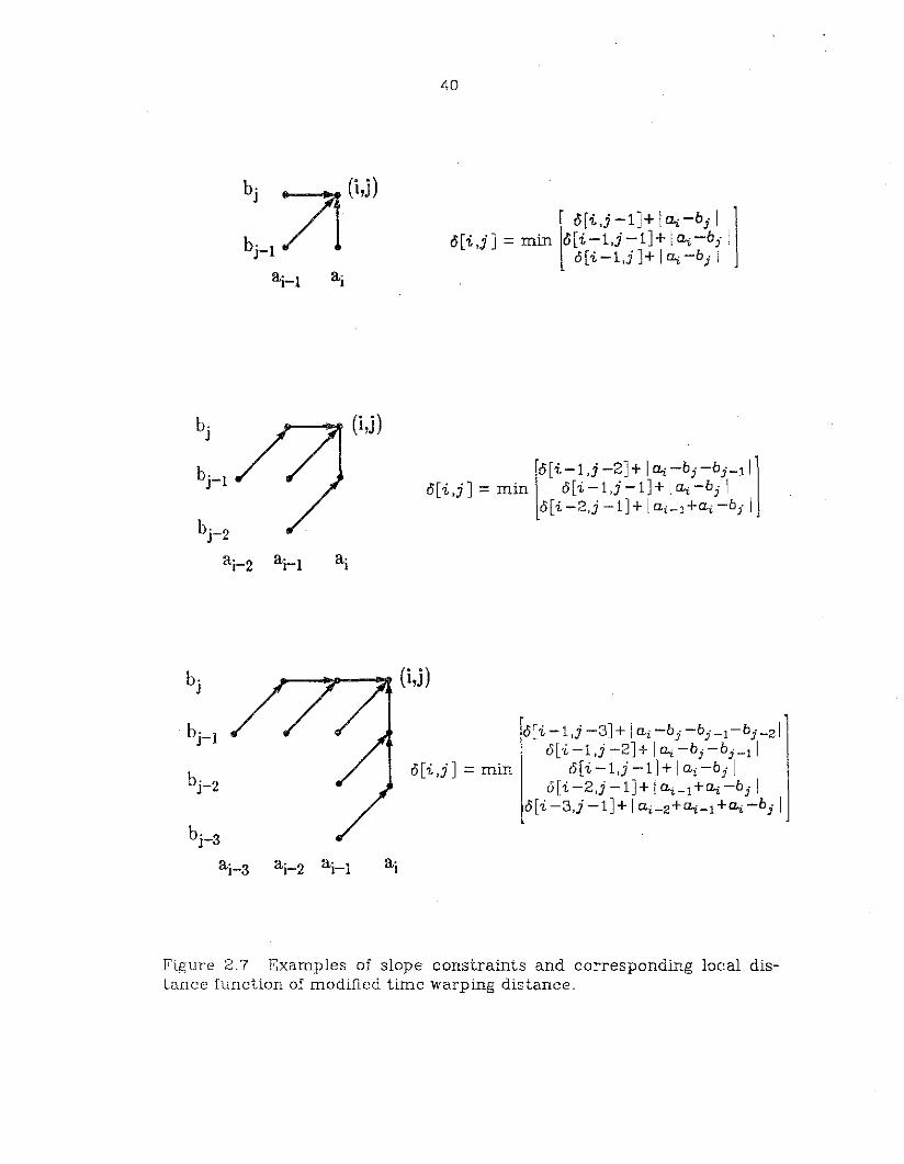
Therefore we can modify the slope constraints and local distance func
tions in Sakoe and Chiba (1978) and use them for distance computation.
The modified slope constraints are shown in Figure 2.7. Since the local
distance functions min (i ,j) are symmetric, the modified time warping
distance is also symmetric. The local distance functions min (i,j) are
chang able as we will see in chapter III.
C. Normalized Distance
All the distance measures discussed so far are absolute distances..
For example, consider two pairs of strings Xl' Yl and X2 and Y2'
X I =aaabbbcccddd
YI = acabbbcccdbd
X2 = ad
Y2 = cb
The distance between Xl and YI is two (substitution errors). The dis
tance between X2 and Y2 is also two (substitution errors). However,
when taking the whole string length into consideration, string pair X I
and Yl are more similar than string pair x2 and Y2' This shows that
equal absolute distance does not necessarily indicate equal similarity.
Sakoe and Chiba (1978) have proposed a normalized distance for
dynamic time warping, which is equal to division of the absolute dis
tance by the total length of the strings. When absolute distances are
equal, the normalized distances tend to favor longer strings. This same
idea can be applied to general string distance computation with inser
tion, deletion and substitution.
40
a·I
ro[i-1,j -2J+ IfL£ -bj-bj-11]o[i,jJ =min l o[i-1,j-1J+ I~-bj I
o[i-2,j -lJ+ 1 ai-l +ai -b,i I
...--~ (i,j)
bj - 2
aj-2 aj-l aj
b·J
ro[i -l,j -3J + Iai -bj -b,i -l-b,i -216[i-1,j -2J+ 1 ~ -b j -b j - 1 1
o[i -1 ,j -1 J+ 1 ai -bj 1
6[i-2,j -lJ+ Iai-l+ a i -b,i Io[i -3,j -lJ+ 1 ai-2+~-1+ai -bj I
o[i,j J =min
"'-'~P--~ (i,j)
bj - 3
aj-3 aj-2 aj-l aj
b·J
Figure 2.7 Examples of slope constraints and corresponding local distance function of modified time warping distance.
41
2.2.2 Similarity Measures Basedon Likelihood Concept
The string distance measures discussed in the previous section are
for nonstochastic models. In stochastic language, every string is asso
ciated with a probability (Fu and Huang, 1972). Therefore, we use pro
bability, instead of weight, to characterize the transformation. Some of
the stochastic context-dependent transformations have been proposed,
for example, substitution has been proposed by Fung and Fu (1975),
substitution and insertion have been proposed by Lu and Fu (1977b).
Here we add context-dependent deletion transformation. We still use
Ts , TI and TD to represent substitution, insertion and deletion
transformation respectively. Associated with Ts , TI and TD we use Ps ,
PI and PD for transformation probabilities. Transformations with
context-dependent probabilities are defined as follows:
probability of substituting b for a.
PD(b lab) is the probability of deleting a in front of b.
PI(ba Ia) is the probability of inserting b in front of a.
for all a E: 2:.
42
The probability associated with the transformation of one string
from another is called stochastic similarity. A higher transformation
probability between two strings means they are more similar. Similar
to the various weights for nonstochastic cases in Section 2.2.1, we can
also define many different types of transformation probabilities, for
example, context independent, terminal independent or transformation
independent. Since they are the simplified versions of the one just
defined, we will only use the above one as an example in the following.
Definition 2.8 The stochastic similarity between strings x and y ,
d S (x ,y), is defined as
where
gj (y Ix) is the probability of transfomations J which derives y from
x.
The transformation probability p (y Ix) is the maximum probability
among those associated with all the possible transformations from x to
y.
Theorem 2.4 dS(x,y) is symmetric if and only if PD(a Iba) =P/(ba 10.)
and Ps(b [e) =Ps(e Ib) for all b ,e E: 2:, a E: 2:'.
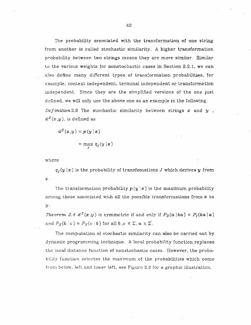
The computation of stochastic similarity can also be carried out by
dynamic programming technique. A local probability function replaces
the local distance function of nonstochastic cases. However, the proba
bility function selectes the maximum of the probabilities which come
from below, left and lower left, see Figure 2.8 for a graphic illustration.

43
e5!i-lJ]
6[i-lJ-l]
6[iJ]
o[iJ-l]
Figure 2.8 Computation of partial distance for stochastic models.

44
Algorithm 2.3 Computation of stochastic string similarity
Input: Two strings x =ala2 '" Clnan +1 and y =b Ib 2 .. , bmbm +1
where CJ.;., bj E: l; for alll:;:;i:;:;n, l:;:;j:;:;m, ~+l =&,
bm + 1 =&, and the probabilities associated with transformations
on terminals in 2: and f& j.
Output: stochastic similarity dS(x,y).
Method:
(1) 0[0, OJ:= 1;
(2) for i := 1 to n do 0[i ,0 J := 0[i - 1,OJ· PD ( b 1 ICJ.;. b 1);
(3) for j := 1 to m do o[O,j J := o[O,j -lJ . P1(bjall al);
(4) for i := 1 to n do
for j := 1 to m do begin
o[i,jJ:= max /o[i,j-1J· P1(bjai+llCJ.;.+1),
o[i-1,j-1]' Ps(bj lai), o[,i,-l,j]' PD(bj+ll~bj+l)l;
end;
(5) dS(x,y) := o[n,mJ;
We can also use a global path constraint here to speed up .the com
putation.
Similarity measure is one of the fundamental constituent of pat
tern recognition. In some applications, for example, string-matching,
the recognition accuracy relies almost entirely on the accuracy of simi
larity measure. Even the error-correcting parsing is closely related to
similarity measures. We will discuss the relation between EC (error
correcting) parsing and similarity measure in the next section. The dis
tance measures defined in this chapter are not metric. They have the
properties of positivity and symmetry, but do not necessarily have the
property of triangle inequality. The accuracy of actual similarity
45
measure depends on many parameters. The most significant one is the
assignment of weights and probabilities. The weights and probabilities
assignment is case-dependent and usually heuristic. Previous
knowledges and statistics may guide the assignment in some cases.
2.3 Error-Correcting Parsing
Error-correcting parser (ECP) has been proposed in the areas of
compiler design (Aho and Peterson, 1972) and syntactic pattern recog
nition (Fu, 1977). When a conventional parser fails to parse a string, it
will terminate and reject the string. An error-correcting parser pro
duces same results as a conventional one when the string is syntacti
cally correct. However, it also generates a parse for the string even
when it has minor syntax errors. The significance of error-correcting
parsing in compiler design is still controversial since it may misinter
prete the programmer's intention. However, its significance in syntac
tic pattern recognition is unquestionable. The most important reason
is the noise problem. The noise may come from sensor device, environ
ment or data communication. These will cause segmentation error and
primitive recognition error, and therefore result in syntax error. In
m.any cases, the pattern grammars are constructed from a finite set of
training samples, and then used to recognize a larger set of test sam
ples. Therefore, it is not surprising that the conventional parsers usu
ally fail to work.
The error-correcting parsing algorithms can be classified into two
categories, one uses minimum-distance criterion the other uses
rnaximum-likelihood criterion. The minimum-distance error-correcting
46
parser (MDECP) is for nonstochastic models where string similarity is
measured by distance. The maximum-likelihood error-correcting
parser (MLECP) is for stochastic model where string similarity is meas
ured by probability.
The ECP in this chapter is different from other existing ECP's in
two aspects; first, it uses symmetric similarity measures, second, it
does not use expanded grammar.
2.3.1 Minimum-Distance Error-Correcting Parsing Algorithm
For the purpose of generality we will discuss context-free grammar
(CFG) throughout this chapter. Since finite-state laguage (FSL) is a
subset of context-free language, all the principles described here can
be applied to FSL as well. Of course, the implementation can be
modified to increase the efficiency. Given a CFG G and an input string
y E: 2:", a minimum-distance error-correcting parser (MDECP) gen
erates a parse for some string x E: L (G) such that the distance between
x and y, d (x ,y) is as small as possible. Since we have defined several
different string distance, therefore different error-correcting parsers
can be constructed.
Aho and Peterson (1972) have shown a minimum-distance error
correcting parsing algorithm which uses the Levenshtein distance. We
will call their algorithm "Algorithm A" for short. They first transformed
the original grammar into an expanded grammar which includes all the
possible error productions. Then, they modified the Earley's parsing
algorithm so that the number of error productions used is stored in the
item list. The productions of the expanded grammar, p', is constructed
from P as follows:

47
(1) For each production in P, replace all terminals a E: 2: by
by a new nonterminal Ea and add these productions to p'.
(2) Add to p' the productions
a) S· -) S
b) S· -) SH
c) H -) HI
d) H -) I
(3) For each a E: ~, add to p' the productions
a) E a -) a
b) Ea -) 6 for all 6 in~, 6 j:. a
c) Ea -) Ha
d) I -) a
e) E a -) A, A is the empty string
In step (3), the productions Ea. -) 6, I -) a and Ea. -) A are called
terminal error productions. The production Ea. -) b introduces a sub
stituition error. I -) a intorduces an insertion error. Ea. -) A introduces
a deletion error. For the Levenshtein distance, a constant weight, e.g.,
1, is associated with each of these productions. It will also handle the
type 1 WLD d Wl(x ,y) and type 2 WLD d W2(x ,y) in a similar way. For the
type 1 WLD, weight a is associated with production Ea. -) b, weight '( with
E a -) A and weight p with I -) a. For the type 2 WLD, weight S (a ,6) is
associated with production Ea -) 6, weight D (a) with Ea. -) A and weight
I(CL) with I -) a. However, the problem will occur when it comes to type
3 YfLD d W3(x ,y). In order to maintain the symmetric property we must
have D (a ,6) = I (a ,6) for all b E: 2:, a E: 2:' as mentioned in Theorem 2.3.
The expanded grammar will have difficulty in handling context
dependent transformation weight.
48
Although we can modify this expanded grammar to handle insertion
weights, as did in Fu (1982), it still can not handle the deletion weights.
Since the productions associated with context-dependent deletion
weights will be something like bEa ~ Ea , D(a,b), but this is not a
context-free production rule, even not a context-sensitive production
rule. While the expanded grammars seem unable to solve the sym
metric problem, we can implement the ECP without the expanded
grammar. This idea of ECP without expanded grammar has appeared in
Lyon (1974) where type a distance is used. His main concern is for
practical reasons: to save space and execution time. Our proposed ECP
using type 3 WLD is a modified Earley's parsing algorithm where the
substitution, insertion and deletion transformations are examined dur
ing the parsing.
Algorithm 2.4. Minimum-Distance Error-Correcting Parsing Algorithm
Input: A grammar G = (N,'L.,P,S), an input string
y =b Ib 2 ... bm in 'L.", and the weights of transformations
between symbols.
Output: The parse lists 1o, I1, ... ,Im' and d(x,y) where
x is the minimum-distance correction of y, x E: L (G).
Method:
(1) Set j =O. Add [5 ~ . a,O,OJ to Ii if 5 -'10'. is a production in P.
(2) Repeat step (3) and (4) until no new items can be added to I j .
(3) If [A-,;cx' B(3,i,~J is in Ij,and B~I is a production in P, then add
item [B ~ . 'Y,j ,0] to Ii'
(4) If [A->cx . ,i,~J is in Ii and [B->(3 . ky,k ,(J is in Ii, and if no item
of the form [B ->(3A . 'Y,lc ,cp J can be found in Ii' then add an item
49
[B~iJA . 'Y,k ,~+(J to Ii' Store with this item two pointers. The first
points to item [B~iJ' A'Y,k .(J in Ii; the second points to item
[A~cx' ,i,tJ in Ii' If [B~iJA . 'Y,Ic,II?J is already in Ii' then replace II? by
t+( together with the pointers if lI?>t+(.
(5) For each [B~cx . aiJ.i.~J in Ij , add [B~cxa . iJ.i,~+D(bj,a)J to Ii'
Store with this item a pointer to item [B~cx . a{3,i.~J in Ii' If no more
new item of this form can be found. go to step (6); otherwise, go to step
(2) .
(6) If j=m, go to step (9); otherwise j=j+1.
(7) For each item [B-l>cx . a{3,i,~J in Ij - l add [B~cxa . (3,i,t+S(a,bi)J
to Ii' Store with this item a pointer to item [B--)cx . a{3,i,tJ in Ij - l .
(8) For each item [B~cx . a{3,i,t] in Ij - l add [B~cx . a{3.i.t+I(a,bj)]
to Ii' Store with this item a pointer to item [B~cx . a{3.i,tJ in Ii-I' Go to
(2) .
(9) If item [S ~cx . ,0.tJ is in 1m , then d (x ,y) = t. If there are more
than one such items, then choose one with the smallest t. Exit.
In this algorithm, step (5) examines deletion transformations, step
(7) examines substitution transformations and step (8) examines inser
tion transformations.
The right parse of the input string can be constructed from the
parse lists. Since we use error-correcting parsing, it is possible that
there may exist several parses associated with one input string. but we
only choose the one with minimum distance.
Algorithm 2. 5. Construction of a right parse from the parse lists
Input.' 10 , II"'"1m , the parse lists for string y =61°2' .. bm
O'tLtput.' A parse 1T for x, x Eo: L (G), and the distance
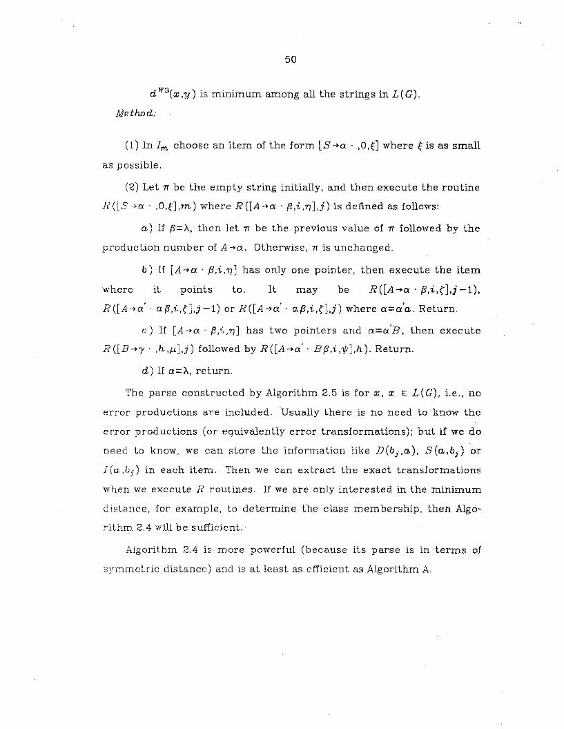
50
d W3( X,y) is minimurn among all the strings in L ( G) .
Method:
(1) In 1m choose an item of the form [3 4 0:: . ,O,~J where ~ is as small
as possible.
(2) Let 7T be the empty string initially, and then execute the routine
R([S40:: . ,O,~],m) where R([A 4 0:: . {3,i,7J],j) is defined as follows:
a) If {3=I\, then let 7T be the previous value of 7T followed by the
production number of A 40::. Otherwise, 7T is unchanged.
b) If [A 4 0::' {3,i,7JJ has only one pointer, then execute the item
where it points to. It may be R([A 4 0:: . (5,i,(],j-l),
R ([A 40::' . a{3,i,(],j -1) or R ([A 40::' . a{3,i ,(],j) where 0::= 0:: 'a . Return.
c) If [A~o::' (5,i,7J] has two pointers and 0:: = o::'B , then execute
R([B4!,' ,h,f.L],j) followed by R([A 4 0::'. B{3,i,'l/J],h). Return.
d) If 0::=1\, return.
The parse constructed by Algorithm 2.5 is for x, x E: L(G), Le., no
error productions are included. Usually there is no need to know the
error productions (or equivalently error transformations); but if we do
need to know, we can store the information like D(bj,a), S(a,bj ) or
I (a ,b j ) in each item. Then we can extract the exact transformations
when we execute R routines. If we are only interested in the minimum
distance, for example, to determine the class membership, then Algo
rithm 2.4 will be sufficient.·
Algorithm 2.4 is more powerful (because its parse is in terms of
symmetric distance) and is at least as efficient as Algorithm A.

51
Lemma2.1: The time complexity of Algorithm 2.4 is O(n 3) where n is
the length of the input string.
The proof of lemma 2.1 is similar to that of (Aho and Peterson,
1972). Since each item list I j takes time O(j2) to complete, therefore
the total time is O(n 3 ). We can also show that the number of produc
tions and the number of items in item lists of Algorithm 2.4 are less
than those of Algorithm A. Therefore, less numbers of productions and
items have to be considered when we add new items to item lists. For
eaeh item [B-loO'.· a(3,i,~J in 1;-1 in Algorithm 2.4 there is an item
[B-loa . Ea,{3,i,~] in 1;-1 in Algorithm A. Let us consider the following
transformations:
(1) Substitition. There is an item [Ea-lo' b,j-l,S(a,b)] in 1;-1
where b=b; and [Ea-lob . ,j-l,S(a,b)J, [B-loaEa · (3,i,~+S(a,b)J in I; in
Alg~rithm A. There is only one item [B-loaa . (3,i,~+S(a,bj)] in I j in
Algorithm 2.4.
(2) Deletion. There is an item [Ea-lo . A, j-1, D(a)J and [B-loaEa . (3,
i, ~+D(a)J in 1j - 1 in Algorithm A. There is only one item
[B-loaa . (3,i,~+D(bj,a)J in Ij - 1 in algorithm 2.4.
(3) Insertion. There are items [Ea -loHa ,j -1,OJ, [H -lo • I,j -1 ,OJ and
[I-~ . b, j -1, I(b)J where b =b j in I j - 1 and items [I -lob . ,j -i,l(b )],
[H-loI· ,j-i, I(b)J and [Ea-loH· a,j-i,l(b)J in1j inAlgorithmA. There
is only one item [B -loa . a (3 ,i, ~+1 (a ,b j )] in Ij in Algorithm 2.4.
Since all the other items not involving error transformations are
unchanged, therefore we can see that the time complexity of Algorithm
2.4 is no more than that of Algorithm A, i.e., the time complexity of
Algorithm 2.4 is O(n 3 ).
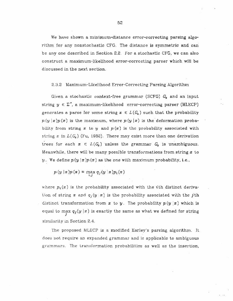
52
We have shown a minimum-distance error-correcting parsing algo
rithm for any nonstochastic CFG. The distance is symmetric and can
be anyone described in Section 2.2. For a stochasti.c CFG, we can also
construct a maximum-likelihood error-correcting parser which will be
discussed in the next section.
2.3.2 Maximum-Likelihood Error-Correcting Parsing Algorithm
Given a stochastic context-free grammar (SCFG) Gs and an input
string y E: L:", a maximum-likelihood error-correcting parser (MLECP)
generates a parse for some string x E.: L (Gs ) such that the probability
P (y Ix)p (x) is the maximum, where P (y Ix) is the deformation proba
bility from string x to y and p (x) is the probability associated with
string x in L (Gs ) (Fu, 1982). There may exist more than one derivation
trees for each x E: ·L (Gs ) unless the grammar Gs is unambiguous.
Meanwhile, there will be many possible transformations from string x to
y. We definep(y Ix)p(x) as the one with maximum probability, Le.,
where Pi (x) is the probability associated with the ith distinct deriva
tion of string x and 9j (y Ix) is the probability associated with the j th
distinct transformation from x to y. The probability p (y Ix) which is
equal to m?-x qj (y Ix) is exactly the same as what we defined for stringJ
similarity in Section 2.4.
The proposed MLECP is a modified Earley's parsing algorithm. It
does not require an expanded grammar and is applicable to ambiguous
grammars. The transformation probabilities as well as the insertion,
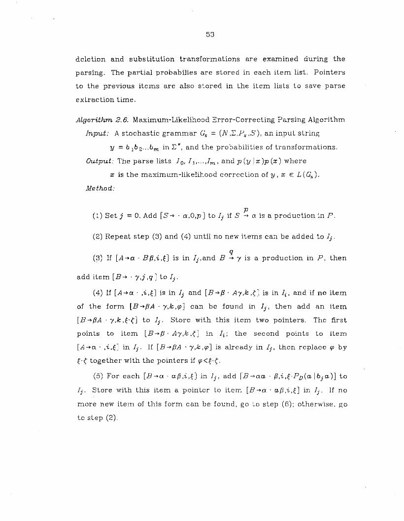
53
deletion and substitution transformations are examined during the
parsing. The partial probabilies are stored in each item list. Pointers
to the previous items are also stored in the item lists to save parse
extraction time.
Algorithm 2.6. Maximum-Likelihood Error-Correcting Parsing Algorithm
Input: A stochastic grammar Gs = (N ,r"Ps .5). an input string
y = b lb2 ... bm in r,., and the probabilities of transformations.
Output: The parse lists 10 • I 1.... ,Im. andp(y Ix)p(x) where
x is the maximum-likelihood correction of y, x E: L (Gs )'
Method:
p(1) Set j =a. Add [5 -l> • 0: ,a,p J to I j if 5 -l> 0: is a production in P.
(2) Repeat step (3) and (4) until no new items can be added to I j .
q(3) If [A-l>O: . B(3,i,~J is in Ij,and B -+ 1 is a production in P, then
add item [B-+ . 1,j ,q] to I j .
(4) If [A-l>O: . ,i,~J is in Ij and [B-l>(3 . A1,1c ,(] is in Ii' and if no item
of the form [B -+(3A . 1,k ,9'] can be found in I j , then add an item
[B->(3A . 'i,k '~'(J to I j . Store with this item two pointers. The first
points to item [B-+(3· A'i,lc ,(J in Ii; the second points to item
[A-+o:' ,i,~J in I j . If [B-l>(3A . 'i.k,9'J is already in I j , then replace 9' by
~.~- together with the pointers if 9'<~.(.
(5) For each [B-l>O: . a(3,i,~] in I j , add [B->o:a . (3,i'~'PD(a Ibja)] to
Ij. Store with this item a pointer to item [B-l>O: . a{5,i,~] in Ij . If no
more new item of this form can be found, go to step (6); otherwise, go
to step (2).
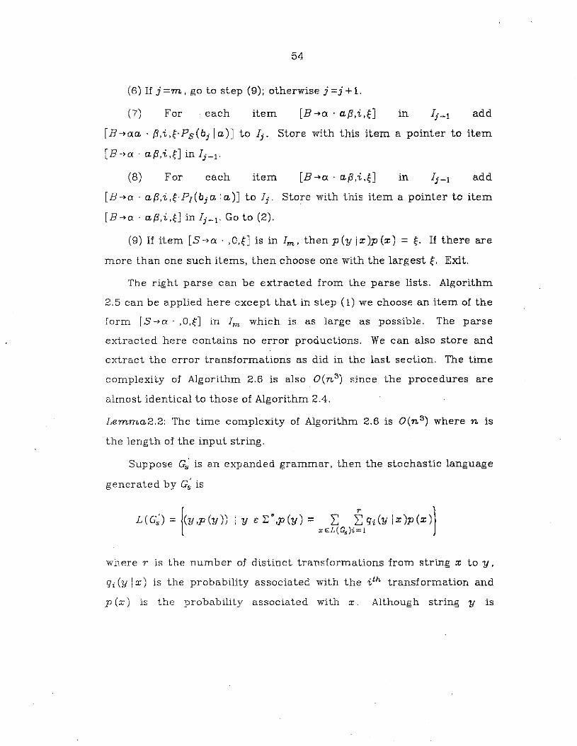
54
(6) If j =m, go to step (9); otherwise j =j + 1.
(7) For each item [B ~cx . ap',i,~J in . Ij - 1 add
[B~cxa . P',i,(Ps(b j la)J to I j • Store with this item a pointer to item
[B~cx . ap',i,tJ in 1j - 1 .
(8) For each item [B ~cx . ap',i ,~J in 1j - 1 add
[B-t-o:· ap',i'~'PI(bjala)J to I j . Store with this item a pointer to item
[B~o: . ap',i,~J in I j - 1 . Go to (2).
(9) If item [5 ~a. . ,O,~J is in 1m , then p (y Ix)p (x) = ~. If there are
more than one such items, then choose one with the largest~. Exit.
The right parse can be extracted from the parse lists. Algorithm
2.5 can be applied here except that in step (1) we choose an item of the
form [5~a.· ,o,t] in 1m which is as large as possible. The parse
extracted here contains no error productions. We can also store and
extract the error transformations as did in the last section. The time
complexity of Algorithm 2.6 is also O(n 3) since the procedures are
almost identical to those of Algorithm 2.4.
Lemma2.2: The time complexity of Algorithm 2.6 is O(n 3 ) where n is
the length of the input string.
Suppose G~ is an expanded grammar, then the stochastic language
generated by G; is
where r is the number of distinct transformations from string x to y,
qi (y Ix) is the probability associated with the i th transformation and
p (x) is the probability associated with x. Although string y is
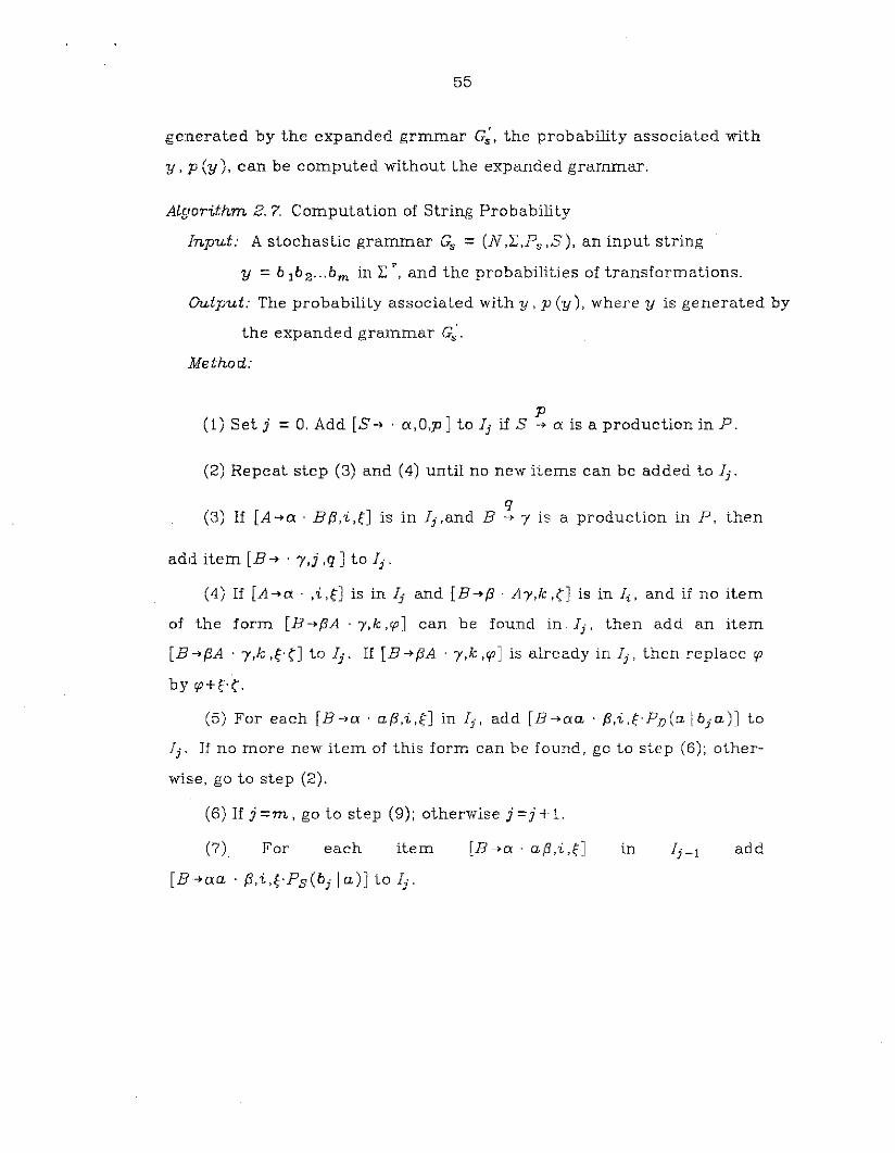
55
generated by the expanded grmmar C;, the probability associated with
y, p (y), can be computed without the expanded grammar.
Algorithm 2.7. Computation of String Probability
Input: A stochastic grammar Cs =(N ,L"Ps ,5), an input string
y =b Ib 2 ... bm in L,", and the probabilities of transformations.
Output: The probability associated with y, P (y), where y is generated by
the expanded grammar C;.Method:
p(1) Set j = O. Add [5 ~ . o.,O,p] to Ij if S -;. 0. is a production in P.
(2) Repeat step (3) and (4) until no new items can be added to I j .
g(3) If [A-.o. . B(i,i,~] is in Ij,and B --Jo /' is a production in P, then
add item [B ~ . I',j ,g] to Ii'
(4) If [A~o. . ,i,~J is in Ii and [B--Jo(i . ky,k ,c:-J is in Ii, and if no item
of the form [B ~{3A . /"k ,rp] can be found in Ii' then add an item
[B-'{3A' 7,k,~·c:-J to Ij . If [B~{3A . 7,k,rpJ is already in Il' , then replace rp
by rp+~'c:-.
(5) For each [B --)0. . a{3 ,i ,tJ in I j , add [B -;'0. a . (i,i ,~. P D (a Ibl' a)J to
I j . If no more new item of this form can be found, go to step (6); other
wise, go to step (2).
(6) If j=m, go to step (9); otherwise j=j+1.
(7) For each item
[B~o.a . (i,i,~·Ps(bl' la)] to Il' .
in add
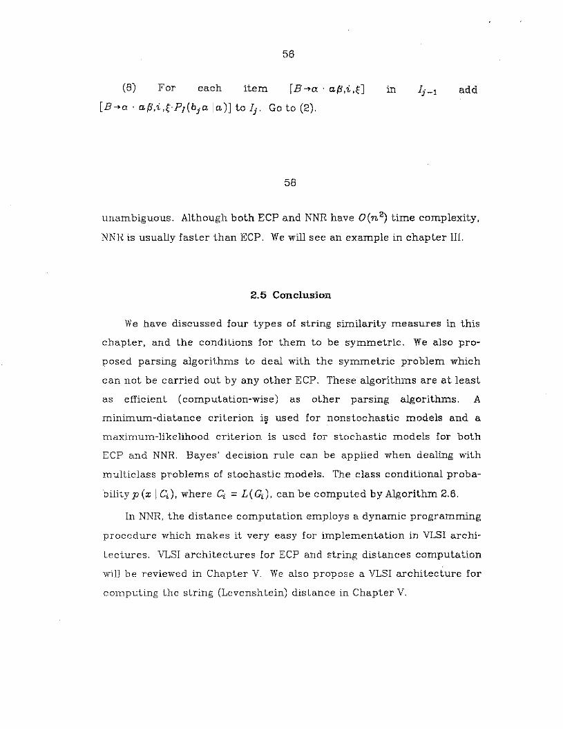
56
(8) For each item [B -)u . af3 ,i ,t]
[B-)u· af3,i,t'P/(bja la)J to I j . Go to (2).
58
in I j - 1 add
unambiguous. Although both ECP and NNR have O(n 2) time complexity,
NNR is usually faster than ECP. We will see an example in chapter III.
2.5 Conclusion
We have discussed four types of string similarity measures in this
chapter, and the conditions for them to be symmetric. We also pro
posed parsing algorithms to deal with the symmetric problem which
can not be carried out by any other ECP. These algorithms are at least
as efficient (computation-wise) as other parsing algorithms. A
minimum-diatance criterion is used for nonstochastic models and a.maximum-likelihood criterion is used for stochastic models for both
ECP and NNR. Bayes' decision rule can be applied when dealing with
multiclass problems of stochastic models. The class conditional proba
bility p (x 1 Ci ), where Ci =L(Gi ), can be computed by Algorithm 2.6.
In NNR, the distance computation employs a dynamic programming
procedure which makes it very easy for implementation in VLSI archi
tectures. VLSI architectures for ECP and string distances computation
will be reviewed in Chapter V. We also propose a VLSI architecture for
computing the string (Levenshtein) distance in Chapter V.
59
CHAPTER III
APPUCATIONS OF SYNTACTIC PATIERNRECOGNITION TO SEISMIC CLASSIfiCATION
3.1 Introduction
In this chapter we apply syntactic approaches to two real seismic
classification problems. One is the seismic discrimination between
nuclear explosion and natural earthquake, the other is the seismic
classification in structural damage assesment. These waveforms have
been sampled and digitized before we obtain the data. However, vari
ous noises exist in both cases. Certain prepocessing procedures there-
fore must be imposed to remove those noises. Section 2 to 5 discuss
application to seismic discrimination, and Section 6 shows application
to damage assesment.
Seismological methods are so far the most effective and practical
methods for detecting nuclear explosions, especially for underground
explosions. Position, depth and origin time of the seismic events are
useful information for discrimination; so are the body wave magnitude
and surface wave magnitude of the seismic wave (Bolt, 1976; Dahlman
and Israelson, 1977). Unfortunately, they are not always applicable and
reliable for small events. It would be very helpful if the discrimination
is based on the short-period waves alone. The application of pattern
recognition techniques to seismic wave analysis has been studied
60
extensively in the last few years (Chen, 1978; Tjostheim, 1978; Sarna
and Stark, 1980). They all use short-period waves only for discrimina
tion. Most of these studies concentrated on feature selection. Only
simple decision-theoretic techniques have been used. However, syntac
tic pattern recognition appears to be quite promising in this area. It
uses the structural information of the seismic wave which is very
important in analysis. Seismic records are one-dimensional waveforms.
Although there exist several alternatives (Ehrich and Foith, 1976; San
kar and Rosenfeld, 1979) for representing one-dimensional waveforms,
it is most natural to represent them by sentences, Le., strings of primi
tives. In order to make it easy for analysis we divide the pattern
representation procedure into three steps, namely, pattern segmenta
tion, feature selection and primitive recognition, though they are corre
lated.
In this chapter, we apply two different methods of syntactic
approach to the recognition of seismic waves. One uses the nearest
neighbor decision rule, the other uses the error-correcting parsing. In
the first method, a pattern representation sybsystem converts the
seismic waveforms into strings of primitives. The string-to-string dis
tances between the test sample and all the training samples are com
puted and then the nearest-neighbor decision rule is applied. The
second method contains pattern representation, automatic grammati
cal inference and error-correcting parsing. The pattern representation
subsystem performs pattern segmentation, feature selection and primi
tive recognition so as to convert the seismic wave into a string of primi
tives. The auLomatic grammatical inference subsystem infers a finite
sLaLe (regular) grammar from a finite set of training samples. The
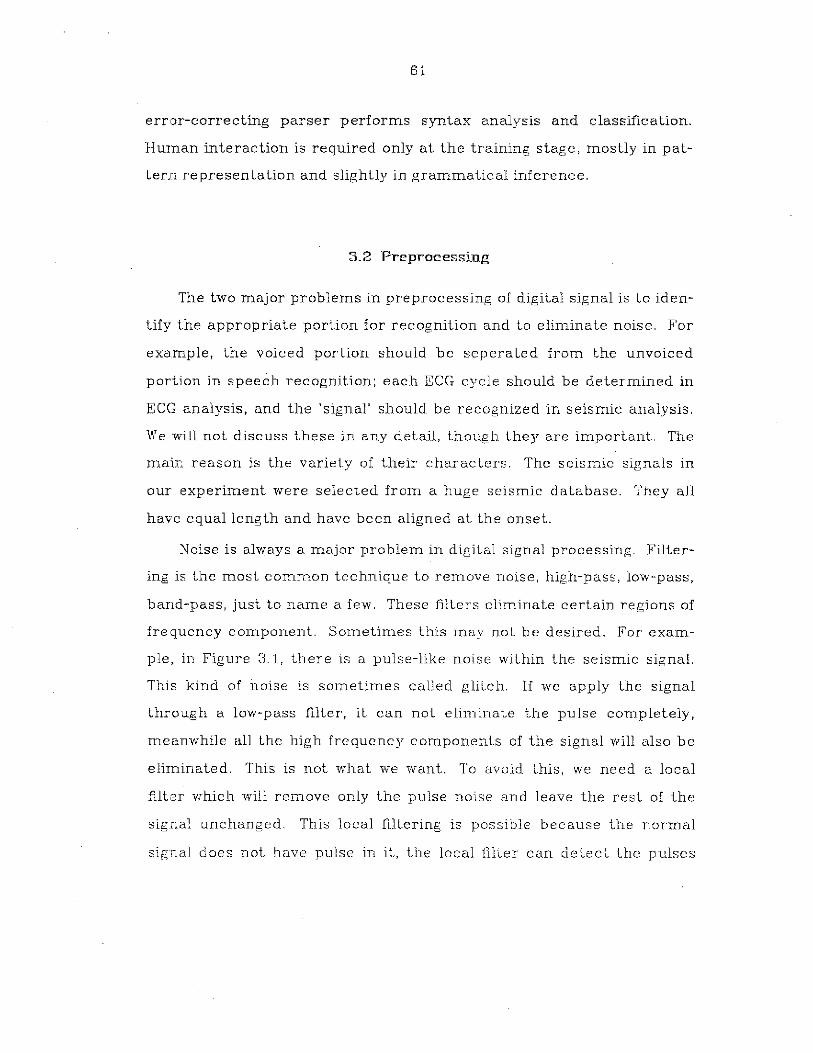
61
error-correcting parser performs syntax analysis and classification.
Human interaction is required only at the training stage, mostly in pat
tern representation and slightly in grammatical inference.
3.2 Preprocessing
The two major problems in preprocessing of digital signal is to iden
tify the appropriate portion for recognition and to eliminate noise. For
example, the voiced portion should be seperated from the unvoiced
portion in speech recognition; each ECG cycle should be determined in
ECG analysis, and the 'signal' should be recognized in seismic analysis.
'Ne will not discuss these in any detail, though they are important. The
main reason is the variety of their characters. The seismic signals in
our experiment were selected from a huge seismic database. They all
have equal length and have been aligned at the onset.
Noise is always a major problem in digital signal processing. Filter
ing is the most common technique to remove noise, high-pass, low-pass,
band-pass, just to name a few. These filters eliminate certain regions of
frequency component. Sometimes this may not be desired. For exam
ple, in Figure 3.1, there is a pulse-like noise within the seismic signal.
This kind of noise is sometimes called glitch. If we apply the signal
through a low-pass filter, it can not eliminate the pulse completely,
meanwhile all the high frequency components of the signal will also be
eliminated. This is not what we want. To avoid this, we need a local
filter which will remove only the pulse noise and leave the rest of the
signal unchanged. This local filtering is possible because the normal
signal does not have pulse in it, the local filter can detect the pulses
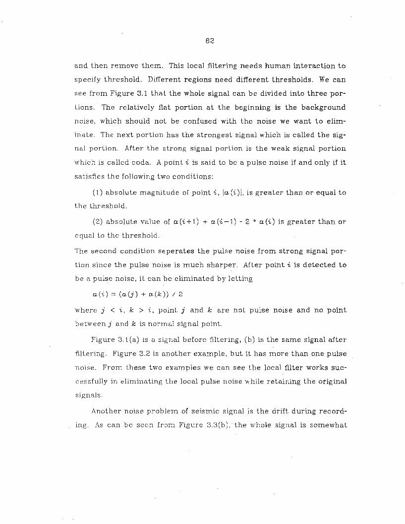
62
and then remove them. This local filtering needs human interaction to
specify threshold. Different regions need different thresholds. We can
see from Figure 3.1 that the whole signal can be divided into three por
tions. The relatively fiat portion at the beginning is the background
noise, which should not be confused with the noise we want to elim
inate. The next portion has the strongest signal which is called the sig
nal portion. After the strong signal portion is the weak signal portion
"which is called coda. A point i is said to be a pulse noise if and only if it
satisfies the following two conditions:
(1) absolute magnitude of point i, la(i)l, is greater than or equal to
the threshold.
(2) absolute value of a (i + 1) + a (i -1) - 2 * a (i) is greater than or
equal to the threshold.
The second condition seperates the pulse noise from strong signal por
tion since the pulse noise is much sharper. After point i is detected to
be a pulse noise, it can be eliminated by letting
a (i) := (a (j) + a (Ie )) / 2
where j < i, Ie > i, point j and Ie are not pulse noise and no point
between J' and Ie is normal signal point.
Figure 3.1 (a) is a signal before filtering, (b) is the same signal after
filtering. Figure 3.2 is another example, but it has more than one pulse
noise. From these two examples we can see the local filter works suc
cessfully in eliminating the local pulse noise while retaining the original
signals.
Another noise problem of seismic signal is the drift during record
ing. As can be seen from Figure 3.3(b), the whole signal is somewhat
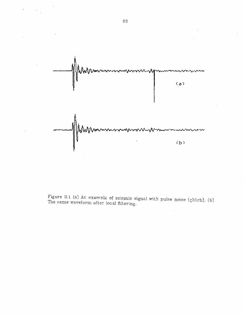
63
Figure 3.1 (a) An example of seismic signal with pulse noise (glitch). (b)The same waveform after local filtering.
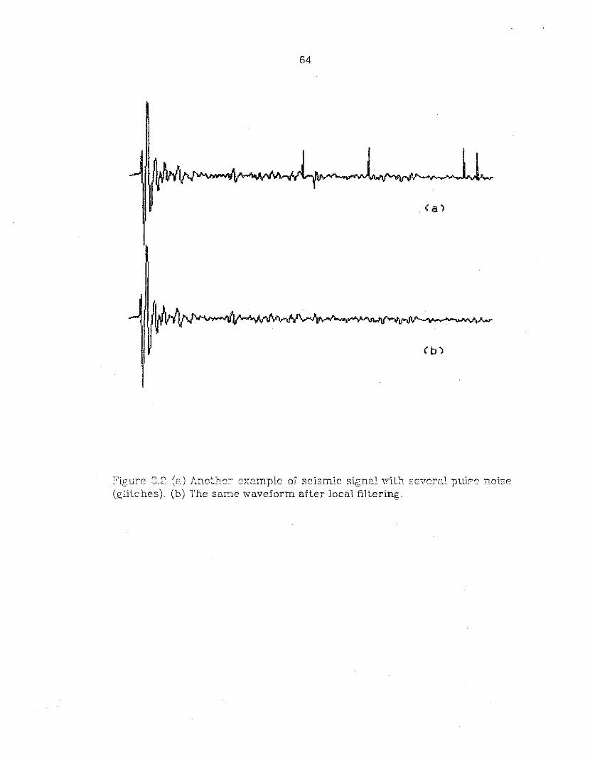
64
Tl'1"a1·lr n '" ? ("," Ann+hn~ ""'""'mn1e of sPl'smic sl'gn~l ""Tl'th '='cver",l n"I~"" n"i"""".;.. C.l L. \.....- ·.J.I......t \G\} l:l. V-'-L ......~ ....... ..: .... 1..... .l:- - ............... _ .. u_~. "-'.' (.",~ 1: "-l._ •• .~......_v~...)r",::::
(glitches). (b) The same waveform after local filtering.
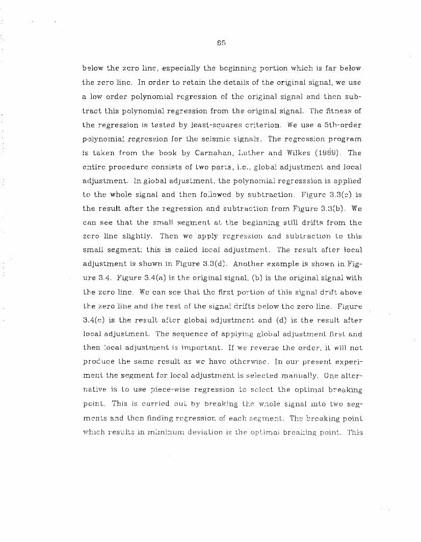
65
below the zero line, especially the beginning portion which is far below
the zero line. In order to retain the details of the original signal, we use
a low order polynomial regression of the original signal and then sub
tract this polynomial regression from the original signal. The fitness of
the regression is tested by least-squares criterion. We use a 5th-order
polynomial regression for the seismic signals. The regression program
is taken from the book by Carnahan, Luther and Wilkes (1969). The
entire procedure consists of two parts, i.e., global adjustment and local
adjustment. In global adjustment, the polynomial regresssion is applied
to the whole signal and then followed by subtraction. Figure 3.3(c) is
the result after the regression and subtraction from Figure 3.3(b). We
can see that the small segment at the beginning still drifts from the
zero line slightly. Then we apply regression and subtraction La this
small segment; this is called local adjustment. The result after local
adjustment is shown in Figure 3.3(d). Another example is shown in Fig
ure 3.4. Figure 3.4(a) is the original signal, (b) is the original signal with
the zero line. We can see that the first portion of this signal drift above
the zero line and the rest of the signal drifts below the zero line. Figure
3.4(c) is the result after global adjustment and (d) is the result after
local adjustment. The sequence of applying global adjustment first and
then local adjustment is important. If we reverse the order, it will not
produce the same result as we have otherwise. In our present experi
ment the segment for local adjustment is selected manually. One alter
DEltive is to use piece-wise regression to select the optimal breaking
point. This is carried out by breaking Lhe \lrhole signal into two seg
ments and then fmding regression of each segment. The breaking point
'wlLich results in miminum deviation is the optimal breaking point. This
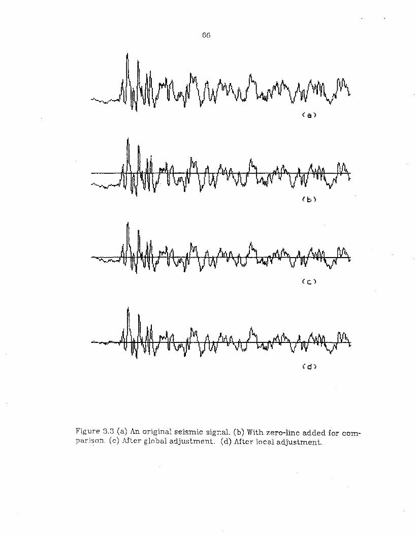
66
(c.)
Figure 3.3 (a) An original seismic signal. (b) With zero-line added for comparison. (c) After global adjustment. (d) After local adjustment.
67
""
Figure 3.4 (a) Another example of seismic signal. (b) Zero-line is addedfor comparison. (c) After global adjustment. (d) After local adjustment.
68
must be done on a section of contiguous points. It is time consuming
and therefore is excluded from our experiment. After the above
preprocessing procedures we can perform segmentation and primitive
selection.
3.3 Automatic Clustering Procedurefor Primitive Selection
It has been mentioned in Fu (1982) that the pattern primitives
should serve as basic pattern elements in describing the structural
relations and they should be easily extractable, usually by nonsyntactic
methods. The selection of primitives depends largely on the type of
waveforms. In some applications, the primitives are prespecified by
human expert, e.g., in Giese, et 0.1. (1979). We would like to investigate
the possibility of nonsupervised learning in primitive selection, there
fore, we use an automatic clustering procedure to select the pattern
primitives. This is important because human selection of pattern prim
itive may not always be available, besides, it may be unreliable.
3.3.1 Pattern Segmentation
A digitized waveform to be processed by a digital computer is usu
ally sampled from a continuous waveform which represents the
phenomena of a source plus external noise. For some cases, such as
ECG and carotid pulse wave analysis (Horowitz, 1975; Stockman, et 0.1.,
1976), every single peak and valley are significant, therefore these
waveforms can be segmented according to the shape. For others, like
EEG (Giese, et 0.1., 1979) and seismic vmve analysis in our case, a single
69
peak or valley does not contain significant information, especially when
the signal to noise ratio is low, therefore they should be segmented by
length, either a fixed length or a variable length. A variable-length seg
mentation is more efficient and precise in representation, but it is usu
ally very difficult and time consuming to find an appropriate segmenta
tion. A fixed-length segmentation is much easier to implement. If the
length is well selected it will be adequate to represent the original
waveform. There is a compromise between the representation accu
racy and analysis efficency. The shorter the segmentation is, the more
accurate the representation will be. But the analysis becomes more
inefficient since the string is longer and the computation time is pro
portional to string length. Another problem is the noise. If the segmen
tation is too short, it will be very sensitive to noise.
Pattern segmentation is closely related to primitive selection. The
segment length in speech analysis is 20 milliseconds (DeMori, 1972,
lSI77), and 1 second in EEG analysis (Giese, et a1., 1979). For short
period seismic signal, a segment length of around 6 seconds is a good
choice. A segment of this length contains adequate information and has
been used by many other researchers (Chen, 1978; Tojstheim, 1975).
Since the sampling frequency of our data set is 10 Hz, a 6-second period
contains 60 points.
We have done experiments on other segment lengths, they are 40
points and 80 points. We selected 41 explosion records out of 111 and
58! earthquake records out of 210 as training samples. The recognition
result for 60-point segment length is 91.0%, i.e., 20 misclassifications
out of 221. When we chose 40 points as segment length, according to
the primitive selection procedure in Section 3.4 the best selecton for
70
primitive number is 18. For primitive number 18, the recognition
result is 72.9%, i.e., GO misclassifications out of 221. If we chose primi
Live number 13 as we did in GO-point segment length, the recognition
result is still 72.9%, though the detail of classification is different. When
we chose 80 points as segment length, the primitive number selection is
14 and the recognition result is 73.8%, i.e., 58 misc1assifications out of
221.
Although this experiment is by no means conclusive, it does show
that a segment length of GO points is an appropriate selection for
short-period seismic signal. A shorter segment is too sensitive to noise
and a longer segment is too complicated for a primitive. The selection
of segment length is ususlly a subjective judegment and depends on the
characteristic of the signal waveform.
3.3.2 Feature Selection
Any linear or nonlinear mapping of the original measurements can
be considered as features provided they have discriminating capability.
Both time-domain features and frequency-domain features have been
used for seismic discrimination. For example, complexity and autore
gressive models are features in time domain; spectral ratio and third
moment of frequency are features in frequency domain (Dahlman and
Israelson, 19(7). Since we segment the seismic wave, complexity and
spectral ratio features are implicitely contained in the string structure.
Furthermore, the segment may be too short for a model estimation if
we use shorter segment. Therefore, we selected a pair of commonly
used features, i.e., zero crossing count and log energy of each segment,
which are easy to compute and contain significant information. Easy to
71
compute is a desired property for primitive extraction in syntactic
approach. Zero crossing count roughly represents the major frequency
component of the signal and log energy indicates the magnitude of the
signal. These two features should be able to characterize the signal
segment. Other features may also serve as good candidates. An advan
tage of syntactic approach is that feature selection is simpler since
features are extracted from smaller segments, and feature selection is
not that critical as is in statistical approach. Since there is no optimal
feature selection algorithm, features are usually subjectively selected.
Although there are criteria such as between cluster and within cluster
scatterness, they have no direct relation to final recognition results.
While other features, including K -L expansion, do not show any
superiority in recognition results in our preliminary experiments, we
will stick to the zero crossing count and log energy.
Since we are experimenting a new approach for seismic discrimina
tion, we do not particularly emphasize feature selection. In fact, simple
features like these give favorable result in our experiment. This indi
cates that syntactic approach utilizes structural information instead of
sophisticated feature measurement.
3.3.3 Primitive Recognition
The selection of primitives varies very largely in digital signal
recognition. Line segments from linear approximation of signals have
been used in ECG analysis (Horowitz, 1975, 1977). Parabola and line
segment have been used in carotid pulse wave analysis (Stockman, et
al., 1976). These primitives are mainly used to describe the shape of
the signal waveform. When the shape of the signal wavefonn is not

72
important, other types of primitives must be selected. For example in
spoken word recognition (DeMori, 1972, 1977), silence interval, stable
zone and lines are used as primitives. In EEG analysis (Giese, et aI.,
1979), a group of seven primitives has been specified and a linear
classifier is used to recognize the testing segments. What should we do
if the signal on hand is not as predictable as speech signal, nor can we
specify the primitives as in EEG analysis. One possible solution is by
clustering procedure. A clustering procedure will classify any number
of signal segments into certain number of clusters in an optimal way,
which means minimization of some criterion function.
If the number of primitives, i.e., the number of clusters, has been
selected then any typical clustering technique, e.g., K-means algo
rithm, can find the optimal clustering. Now the difficult part is how to
select an appropriate primitive number. For example in EEG analysis,
how do we know seven is the best selection. Is there any other better
selection? How does the selection of primitive number affect the final
recognition results? We will discuss all of these questions in this sec
tion.
Without lost of generality we assume that each signal segment is
represented by a vector of features x =[Xl, X2' ... , XkJt . It is noted that
we use decision-theoretic approach for primitive selection. Other
representations may also serve the purpose as long as the similarity
between signal segments can be computed. If the feature space is iso
tropic, then the Euclidean distance can be used as a measure of simi
larity and it is invariant under translation or rotation. However, the
invariance can be attained by normalizing the data before clustering.
73
Suppose we want to partition n samples xl, x 2, ... , x n into k dis
joint subsets C l' C2 , ... , Ck . Each subset represents a cluster. The sam-
pIes in the same cluster are more similar than the samples in different
clusters. One typical approach is to define a criterion function that
measures the clustering quality of any partition of the samples. Then
the problem is to minimize of maximize the criterion function. One of
the most well-known criterion function is the sum-of-squared-error cri
terion (Duda and Hart, 1973). Let ni be the number of samples in clus
ter Ci and TTLi be the mean of those samples, where
The sum-of-squared-error criterion is defined as
k
J fJ = I; I; I Ix - TTLi I [2i=l :Z:£Ci
Another set of criterion functions are derived from scatter matrice.
First, let us introduce some definitions.
Mean vector for i th cluster:
Total mean vector:
1-I; xn C
1 k- '" n· TTL·LJ 1 1n i=l
Scatter matrix for ith cluster:

74
Si = I: (x -mi)(x -mi)tXEq
Within-cluster scatter matrix:
Between-cluster scatter matrix:
kS B 2: ni (mi - m ) (mi - m ) t
i =1
Total scatter matrix:
ST = I: (x -m)(x -mlx EC
It follows obviously that Sr =Sw + SB
We define the optimal partition as one that minimizes Sw or max
imizes SB' In doing so we need a scalar measure of the size of a scatter
matrix. The trace of Sw is the simplest measures. Other well-known
measures are the determinant of Sw and the trace of SilSB' For the
sake of computational simplicity we will only consider the trace of Sw
as criterion function. The trace criterion is defined as:
lc
tr Sw 2: tr Sii=l
k
2: I: II x - mi 112 = Je
i=l XECi
which is exactly the same as the sum-of-squared-error criterion. Since
lr Sr = tr SB + tr Sw and tr Sr is independent of how the samples are
partitioned, therefore minimizing tr S w is equivalent to maximizing
tr SE' Where
75
ktr SB 2:: ni II ffii - m 11
2
i=l
If the number of cluster is known, then the K-means algorithm can
be applied to find a clustering which minimizes the criterion function,
i.e., the sum-of-squared-error Je . When the number of clusters is unk
nown, at least two approaches can be used to determine the optimal
cluster number. These two approaches turn out to have similar results
in our experiment.
Both approaches use a bottom-up hierarchical clustering pro
cedure. This algorithm repeats the clustering procedure for Ie = U, Ie =U - 1 , ... , Ie = L, where U and L are the specified upper and lower bound
respectively. The first approach selects the optimal cluster number by
examining how the criterion function Je changes with Ie. If these n
sa.mples are really grouped into p well seperated clusters, then J e
should increase slowly until Ie =p and then increase much more rapidly
thereafter. The algorithm for bottom-up clustering procedure is shown
a~; follows:
Algorithm 3.1 Bottom-Up Hierarchical Clustering
Input: A set of n unclassified samples, an upper bound U
and a lower bound L.
Output: A sequence of optimal clusterings for the number
of clusters between U and L.
Method:
(1) Let lc = U, Ie is the number of clusters, and arbitrarily
assign cluster membership.
(2) Reassign membership using J(-means algorithm. If
76
Ie -::;,L, stop.
(3) Find the nearest pair of clusters, say Ci and Cj , i "1= j.
(4) Merge Ci and Cj , delete Cj and decrease Ie by one,
go to step 2.
The distance between two clusters is defined by
where mi' mj are the mean vectors of clusters i ,j respectively.
Just as F-statistics can be used in univariate case to test the
significance of group seperation, a pseudo F-statistics (PFS) can be
applied in multivariate case provided that a single measurement of
similarity between samples, e.g., Euclidean distance, is assumed (Vogel
and 'Nong, 1978). A pseudo F-statistics is defined as:
PFStT 58 (n - k)
tT Sw (k - 1)
As the number of clusters increases, tT 58 will always increase while
tT Sw will always decrease. However, the PFS value will not monotoni
cally increase due to the effect of (n-k) / (k-l) which is smaller as k
becomes larger. Therefore, there will be a peak of PFS value some
where in the middle. Since, like F-statistics, the PFS shows the
significance of group seperation, therefore a larger PFS value means
the clusters are more compact and well seperated. The crietrion here
is to select the maximum PFS value; the corresponding cluster number
will be optimal. For example, in Figure 3.7, the maximum PFS value
appears at cluster number 13, therefore 13is the optimal selection for
cluster nurnber.

77
3.4 Syntax Analysis
If the classification is all we need, then the nearest-neighbor deci
sion rule is preferred because of its computational efficiency. On the
other hand, if a complete description of the waveform structure is
needed, we have to use parsing (or error-correcting parsing). An error
correcting parser (instead of conventional parser) is required for most
practical pattern recognition applications. Since noise and distortion
usually cause conventional parsers to fail. It is not unusual that even a
noise-free, distortion-free pattern can not be recognized by a conven
tional parser, since the pattern grammar is often inferred from a small
set of training samples.
3.4.1 Nearest-Neighbor Decision Rule
The concept of nearest-neighbor decision rule in syntactic
approach is similar to that in decision-theoretic approach. The only
di:fference is in distance calculation. Four types of string distances
hcwe been discussed in chapter two, and they can be computed using
dynamic programming method (e.g., Algorithm 2.1).
3.4.2 Error-Correcting Finite-State Parsing
Before parsing can take place we must have a grammar, which can
be either heuristically constructed or inferred from a set of training
samples. In order to study the learning capability of the syntactic
method, we choose the grammatical inference approach.
Phrase structure grammars have been used to describe patterns in
syntactic pattern recognition (see Fu, 1982). Each pattern is
78
represented by a string of primitives which corresponds to a sentence.
in a language (tree or graph in high dimensional grammars). All strings
which belong to the same class are generated by one grammar.
79
a source grammar which generates a language and we want to infer the
source grammar or automaton based on the observed samples. In the
second case the exact nature of the source grammar is unknown, the
only information we have are some sentences generated by the source.
We assume that the source grammar falls into a particular class and
infer a grammar which generates all the training samples, and hope
fully will generate some samples belonging to the same class. If a nega
tive sample set is given, the inferred grammar must not generate any
sarnple in the negative sample set. Grammars more complex than
finite-state grammars and restricted context-free grammars (in Chom
sky hierarchy) can not be inferred efficiently without human interac
tion. Furthermore, there exists no obvious self-embedding property in
seismic waves, finite-state grammars will be sufficient in generating
power. Therefore we choose finite-state grammars to describe the
sei:smic waves.
The inference of regular grammars has been studied extensively.
The k -tail algorithm finds the canonical grammar and then merges the
states which are k -tail equivalent. This algorithm is adjustable, the
value of k controls the size of the inferred grammar. Another algorithm
called tail-clustering algorithm (Miclet, 1980) also finds the canonical
grammar, but then merges the states which have common tails. The
original algorithm is not as flexible as the k -tail algorithm, but will infer
a grammar which is closer to the source grammar in some cases. We
can modify the merge criterion to make it more flexible. Since the
grammar is inferred from a small set of training samples, we can only
expect that the inferred grammar generates all the training samples
and will generate other strings which are similar to the training
80
samples. The generating power of the inferred grammar relies entirely
on the merge procedure. If no merge occurs at all, then the inferred
grammar generates exactly the same training set, no more no less.
Since all the seismic records have the same length and alignment in
our experiment, the sentences representing these signals also have the
same length.
Error-Carre c ting Parsing
After a grammar is available, either by automatic inference or by
manaul construction, the next step is to design a recognizer which will
recognize the patterns generated by the grammar. If the grammar G is
finite-state, a deterministic finite-state automaton can be constructed
to recognize the strings generated by G.
Segmentation and primitives recognition errors due to noise and
distortion usually occur in practice. Conventional parsing algorithms
can not handle these situations, therefore, an error-correcting parser
must be used (Fu, 1977).
Since all the sentences in our example have the same length, only
the substitution error needs to be considered. For each production A -)
aB and A ..... a in the original grammar we add A ..... bB and A ..... b
respectively to the covering grammar, where A,B E: N, a,b E: 1:, b ;t::. a,
N is a set of nonterminal symbols and 2: is a set of terminal symbols.
Different weights can be assigned to different error productions, there
fore, result in a minimum-cost error-correcting parser. The assignment
of weights is a crucial problem. We have used the distance between
clusters a and b as the weight for substituting a by b and vise versa.
Since a finite-state grammar can be represented by a transition
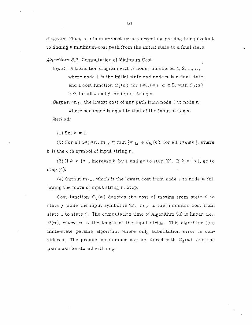
Is I, go to
81
diagram. Thus, a minimum-cost error-correcting parsing is equivalent
to finding a minimum-cost path from the initial state to a final state.
Algorithm 3.2. Computation of Minimum-Cost
Input: A transition diagram with n nodes numbered 1, 2, . __ , n,
where node 1 is the initial state and node n is a final state,
and a cost function Cij(a), for l~i,j~n, a E: 2:, with Cil'(a)
~ 0, for all i and j. An input string s.
Output: m In the lowest cost of any path from node 1 to node n
whose sequence is equal to that of the input string s .
.Method:
(1) Set k = 1.
(2) For all l~j ~n, mIl' =min 1m lk + Ckl' (b), for all l~k~n L where
b is the k th symbol of input string s.
(3) If k < Is I, increase k by 1 and go to step (2). If k
step (4).
(4) Output mIn, which is the lowest cost from node 1 to node n fol
low'ing the move of input string s _ Stop.
Cost function Cij (a) denotes the cost of moving from state i to
state j while the input symbol is 'a'. mIl' IS the minimum cost from
state 1 to state j. The computation time of Algorithm 3.2 is linear, i.e.,
G (n), where n is the length of the input string. This algorithm is a
finite-state parsing algorithm where only substitution error is con
sidered. The production number can be stored with Cil' (a), and the
parse can be stored with m Ij'
82
If insertion and deletion errors are to be considered, then the
parser is still similar except that we have to compute and store the
information V(T, S, a) which is the minimum cost of changing character
'a' into some string which can change the state of the automaton from
state T to S (Wagner, 1974). The inclusion of insertion and deletion
errors makes the error correction more complete, but assigning
appropriate weights to insertion and deletion error is even more
difficult.
3.5 Experimental Results on Seismic Discrimination
The seismic data used in our experiments are provided by Profes
sor C. H.Chen of Southeastern Massachusetts University. The data
were recorded at LASA in Montana. Each record contains 1200 points;
the sampling frequency is 10 points per second. The original data con
tains 323 records. Due to some technical problems in data conversion
only 321 records were received. Among them 111 records are nuclear
explosions and 210 records are earthquakes.
We have selected forty-one earthquake records and fifty-nine explo
sion records as training samples. Each record is divided into 20 seg
ments where each segment contains 60 points. Two features, i.e., zero
crossing count and log energy, are computed from each segment.
Table 3.1 shows the criterion function Je and its increment from cluster
number 16 down to 2, which are the results of applying Algorithm 3.1 to
the training segments. We can see that the increment of Jr:. is small
before and until cluster number is equal to 13 and then becomes much
larger thereafter. Therefore, we say that 13 is an optimal selection of
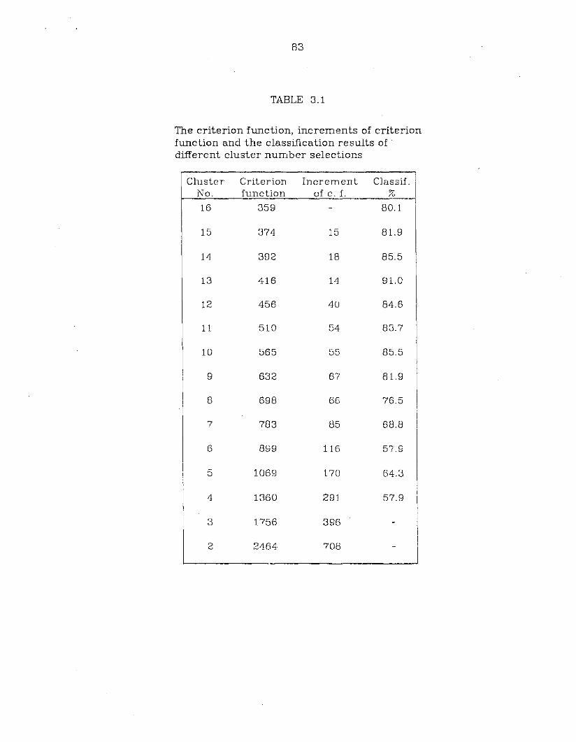
83
TABLE 3.1
The criterion function, increments of criterionfunction and the classification results of .different cluster number selections
Cluster Criterion Increment Classif.No. function of c. f. %
16 359 80.1
15 374 15 81.9
14 392 18 85.5
13 416 14 91.0
12 456 40 84.6
11 510 54 83.7
10 565 55 85.5
9 632 67 81.9
8 698 66 76.5
7 783 85 68.8
6 899 116 57.9
5 1069 170 64.3
4 1360 291 57.9
3 1756 396
2 2464 708
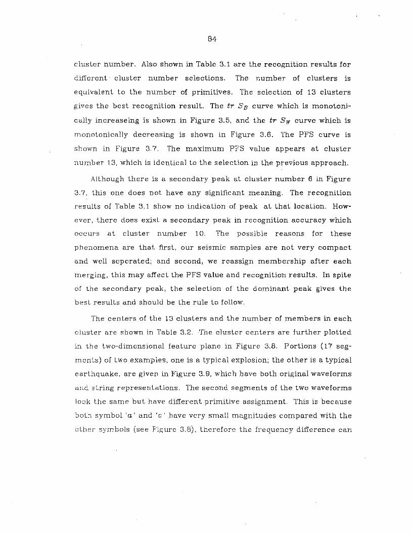
84
cluster number. Also shown in Table 3.1 are the recognition results for
different cluster number selections. The number of clusters is
equivalent to the number of primitives. The selection of 13 clusters
gives the best recognition result. The tr 5 s curve which is monotoni
cally increaseing is shown in Figure 3.5, and the tr 5 w curve which is
monotonically decreasing is shown in Figure 3.6. The PFS curve is
shown in Figure 3.7. The maximum PFS value appears at cluster
number 13, which is identical to the selection in the previous approach.
Although there is a secondary peak at cluster number 6 in Figure
3.7, this one does not have any significant meaning. The recognition
results of Table 3.1 show no indication of peak at that location. How
ever, there does exist a secondary peak in recognition accuracy which
occurs at cluster number 10. The possible reasons for these
phenomena are that first, our seismic samples are not very compact
and well seperated; and second, we reassign membership after each
merging, this may affect the PFS value and recognition results. In spite
of the secondary peak, the selection of the dominant peak gives the
best results and should be the rule to follow.
The centers of the 13 clusters and the number of members in each
cluster are shown in Table 3.2. The cluster centers are further plotted
in the two-dimensional feature plane in Figure 3.8. Portions (17 seg
ments) of two examples, one is a typical explosion; the other is a typical
earthquake, are given in Figure 3.9, which have both original waveforms
and string representations. The second segments of the two waveforms
look the same but have different primitive assignment. This is because
both symbol 'a' and 'e' have very small magnitudes compared with the
oUler symbols (see Figure 3.8), therefore the frequency difference can
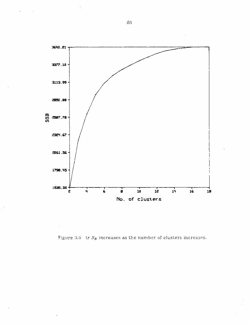
85
:36IJO.21 -r----------------------=::::::;;:oo-----,
:3377.10
:U13.99
1!8S0.88
CJ:IU) 157.78(f)
l!32'+.67
i!D61.56
:1798.&15
18161&112108:lS3S.3S of-----r---..-----.----r-----,------.,----,-----4
2
No. of clusters
Figure 3,5 tr SB increases as the number of clusters increases.
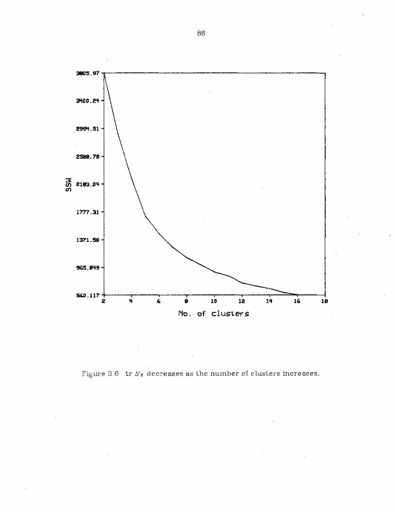
86
3805.97 _r_----------------------------,
181612108
1'777.31
1371.58
2588.78
5GO .117 +-----.----..-----...----,r----v-----.-.-.;;;;:::::._---12
965."9
299'f.51
3't00.2&+
No. of clusters
Figure 3.6 tr Sw decreases as the number of clusters increases.
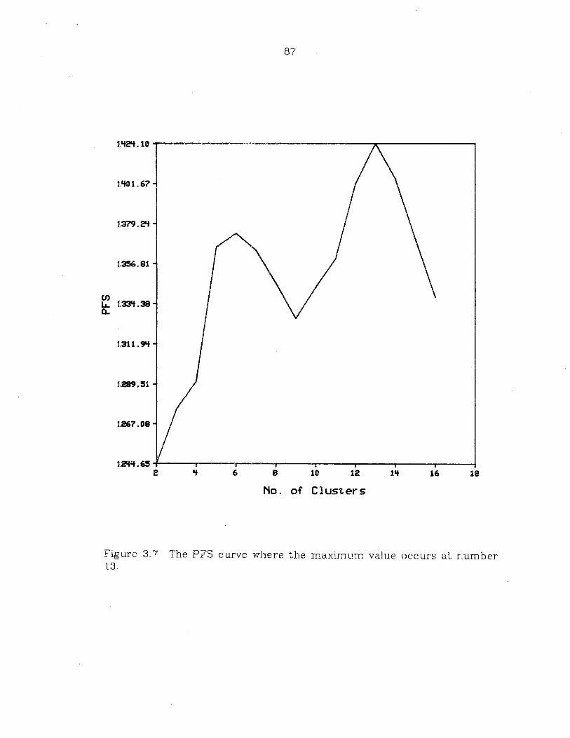
87
2.'t2'+.10 -------------------x~------__,
1. 'to 1.67
1.379.2'+
1.356.81
(J)u.. 1.33'+ .38n.
1.311.9'+
U!89.51
1.267.08
18161210861.2't1t.6S -J---...."..----.----r----...,-----.,.---,.----r----!
2
No. of Clusters
Figure 3.7 The PFS curve where the maximum value occurs at Lumber13.
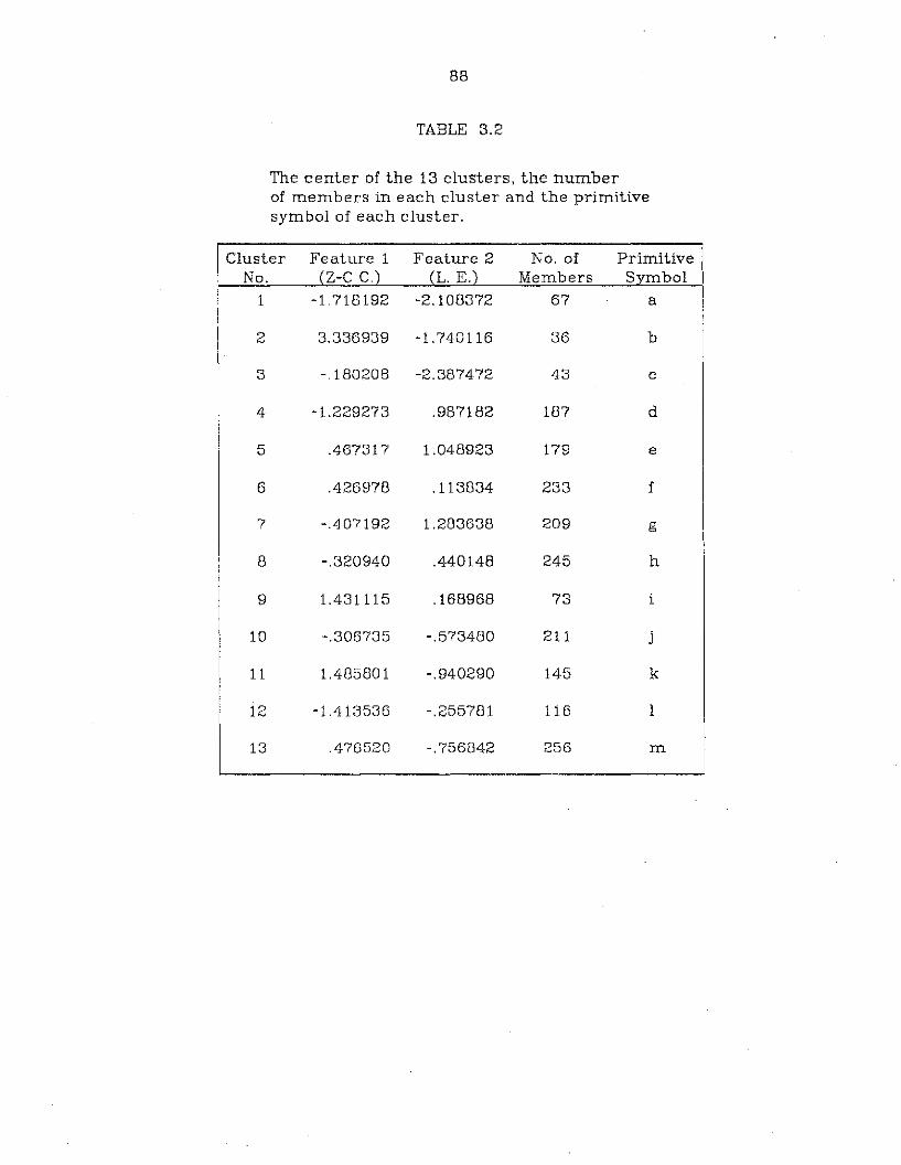
88
TABLE 3.2
The center of the 13 clusters, the numberof members in each cluster and the primitivesymbol of each cluster.
Cluster Feature 1 Feature 2 No. of PrimitiveNo. (Z-C C.) (1. E.) Members Symbol
1 -1.718192 -2.108372 67 a
2 3.336939 -1.740116 36 b
3 -.180208 -2.387472 43 c
4 -1.229273 .987182 187 d
5 .467317 1.048923 179 e
6 .426978 .113834 233 f
7 -.407192 1.283638 209 g
8 -.320940 .440148 245 h
9 1.431115 .168968 73 i
10 -.306735 -.573480 211 j
11 1.485801 -.940290 145 k
12 -1.413536 -.255781 116 1
13 .476520 -.756842 256 m
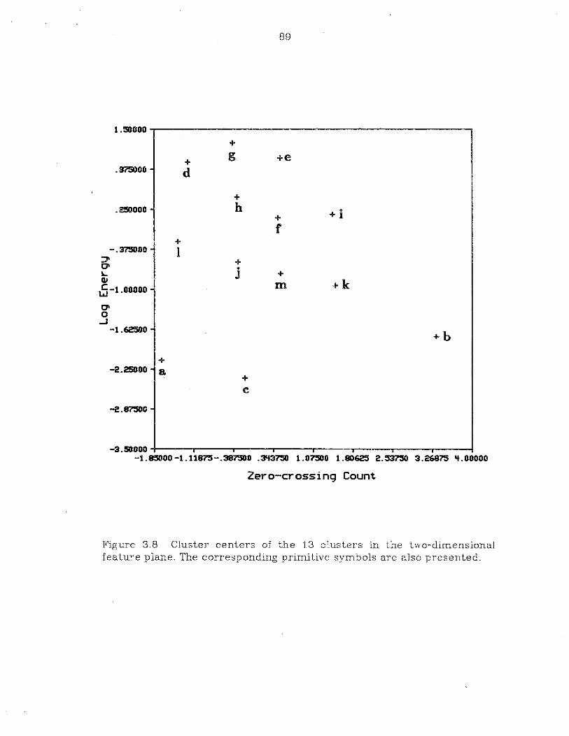
89
1.50000
+
+g +e
.:B75000· d
+.25)000 h +i+
r+
-.375000 I::J' +0' e
"- J +CIJ +kt5 -1.00000 m
C'0
.-J-1.62'S00 .
+b
+-2.25000· a
+c
-2.87500
-3.:50000 +----r---T"""'--...,----r---..,....----,:----...,.----i-1.8S000 -1.11875-.387300 .3'f37S0 1.07500 1.8062'5 2.537S0 3.26875 It.ooooo
Zero-crossing Count
Figure 3.8 Cluster centers of the 13 clusters in the two-dimensionalfeature plane. The corresponding primitive symbols are also presented.
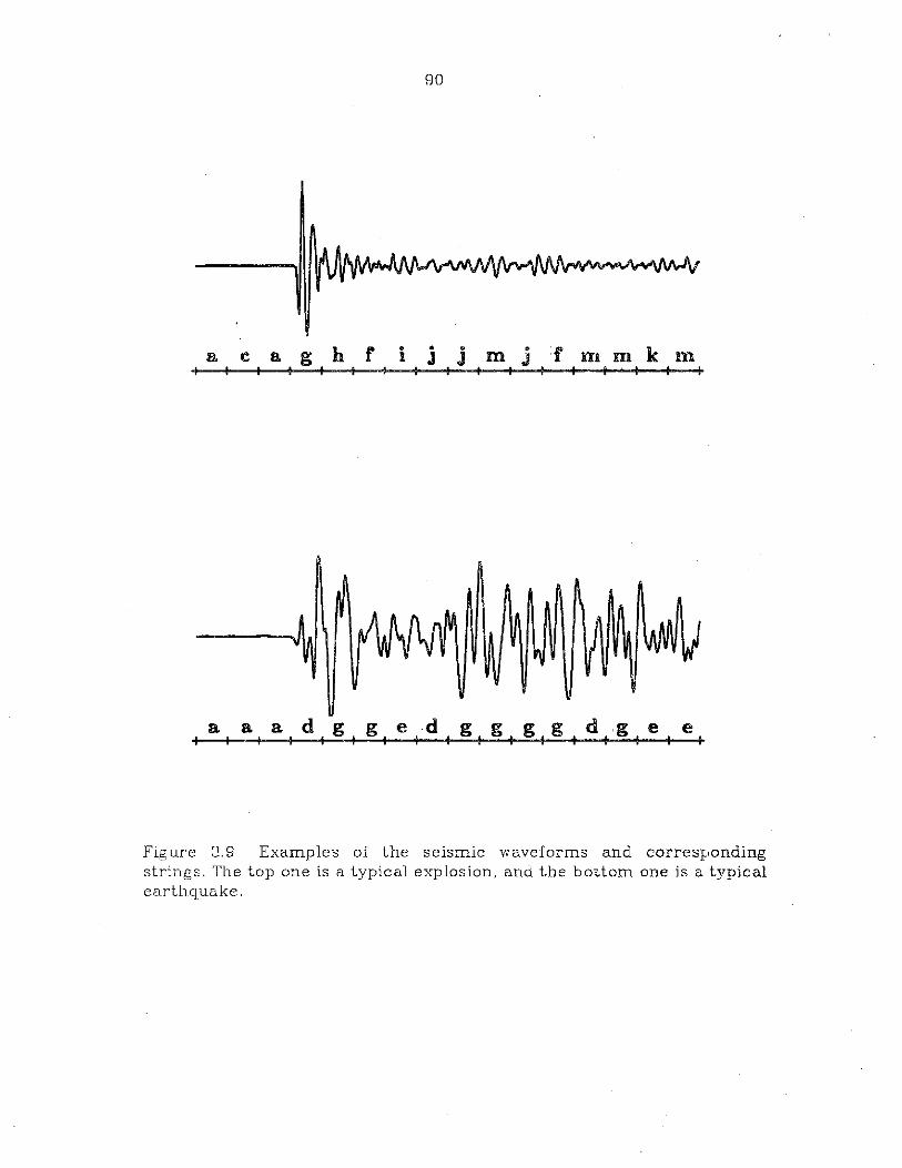
90
e a g h rI
i j j "m JI
:f m m k mi . I I
a a I a d gig I e I· d I gig I gig I d I ,g Ie I e I
Figure 3.9 Examples of the seismic waveforms and correspondingstrings. The top one is a typical explosion, and the bottom one is a typicalearthquake.
91
not be seen due to the resolution of the drawing. Algorithm 2.1 is
applied for string distance computation, and the nearest-neighbor deci
sion rule is used for classification. Since all the records have equal
length and alignment, only substitution errors are considered. The
weights for substitution errors are given in Table 3.3. The weight
between pattern primitives is defined as the normalized distance
between corresponding clusters. Classification results and computation
time of the 221 test samples are shown in Table 3.4 where 201 records
are correctly classified, i.e., 91% correct rate, with an average time of
0.07 sec for each record. The experiments were run on a VAX 111780
computer using Pascal programming language.
We use the Ie -tail finite-state inference algorithm to infer pattern
grammars for the seismic waves. When Ie ~ 19, the inferred grammar is
exactly the same as the canonical grammar. When Ie < 19, some
equivalent states will be merged, therefore, result in fewer number of
states and productions. The number of states and productions for vari
ous values of Ie is shown in Table 3.5; it is getting smaller as Ie gets
smaller. Average parsing time of one string and percentage of correct
classification for different Ie are given in Table 3.6. The parsing time is
shorter when Ie is smaller. This is due to the smaller number of produc
tions and states. On the other hand, the correct perentage is also
srnaller when Ie is smaller. This is because derived grammars generate
strings which do not belong to the positive sample set. Another reason
of worse performance is that in our case only those states with longest
tails are merged. In terms of transition diagram, this means only those
states which are close to the initial state are merged. Because the le
tails of those states are empty, and only are they lc -equivalent. This is
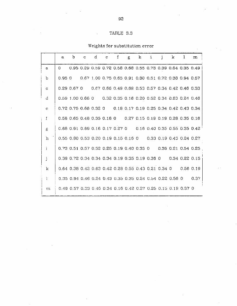
92
TABLE 3.3
Weights for substitution error
a b c d e f g h i k 1 m
a o 0.95 0.29 0.59 0.72 0.58 0.68 0.55 0.73 0.39 0.64 0.35 0.49
b 0.95 0 0.67 1.00 0.75 0.65 0.91 0.80 0.51 0.72 0.38 0.94 0.57
c 0.29 0.67 0 0.67 0.66 0.49 0.69 0.53 0.57 0.34 0.42 0.46 0.33
d 0.59 1.00 0.66 0 0.32 0.35 0.16 0.20 0.52 0.34 0.63 0.24 0.46
e 0.72 0.75 0.66 0.32 0 0.18 0.17 0.19 0.25 0.34 0.42 0.43 0.34
f 0.58 0.65 0.48 0.35 0.18 0 0.27 0.15 0.19 0.19 0.28 0.35 0.16
g 0.68 0.91 0.69 0.16 0.17 0.27 0 0.16 0.40 0.35 0.55 0.35 0.42
h 0.55 0.80 0.53 0.20 0.19 0.15 0.16 0 0.33 0.19 0.43 0.24 0.27
i 0.73 0.51 0.57 0.52 0.25 0.19 0.40 0.33 0 0.36 0.21 0.54 0.25
j 0.39 0.72 0.34 0.34 0.34 0.19 0.35 0.19 0.36 0 0.34 0.22 0.15
k 0.64 0.38 0.42 0.63 0.42 0.28 0.55 0.43 0.21 0.34 0 0.56 0.19
1 0.35 0.94 0.46 0.24 0.43 0.35 0.35 0.24 0.54 0.22 0.56 0 0.37
ill 0.49 0.57 0.33 0.46 0.34 0.16 0.42 0.27 0.25 0.15 0.19 0.37 0
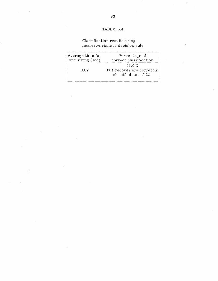
93
TABLE 3.4
Classification results usingnearest-neighbor decision rule
Average time forone strinR: (sec)
0.07
Percentage ofcorrect classification
91.0 %201 records are correctly
classified out of 221
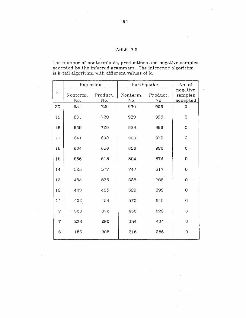
94
TABLE 3.5
The number of nonterminals, productions and negative samplesaccepted by the inferred grammars. The inference algorithmis k-tail algorithm with different values of k.
Explosion Earthquake No. of
knegative
Nonterm. Product. Nonterm. Product. samplesNo. No. No. No. accepted
20 681 720 939 996 0
19 681 720 939 996 0
18 669 720 928 996 0
17 641 692 900 970 0
16 604 656 856 926 0
15 566 618 804 874 0
14 525 577 747 817 0
13 484 536 688 758 0
12 443 495 629 699 0
11 402 454 570 640 0
9 320 372 452 522 0
7 238 290 334 404 0
5 156 208 216 286 0
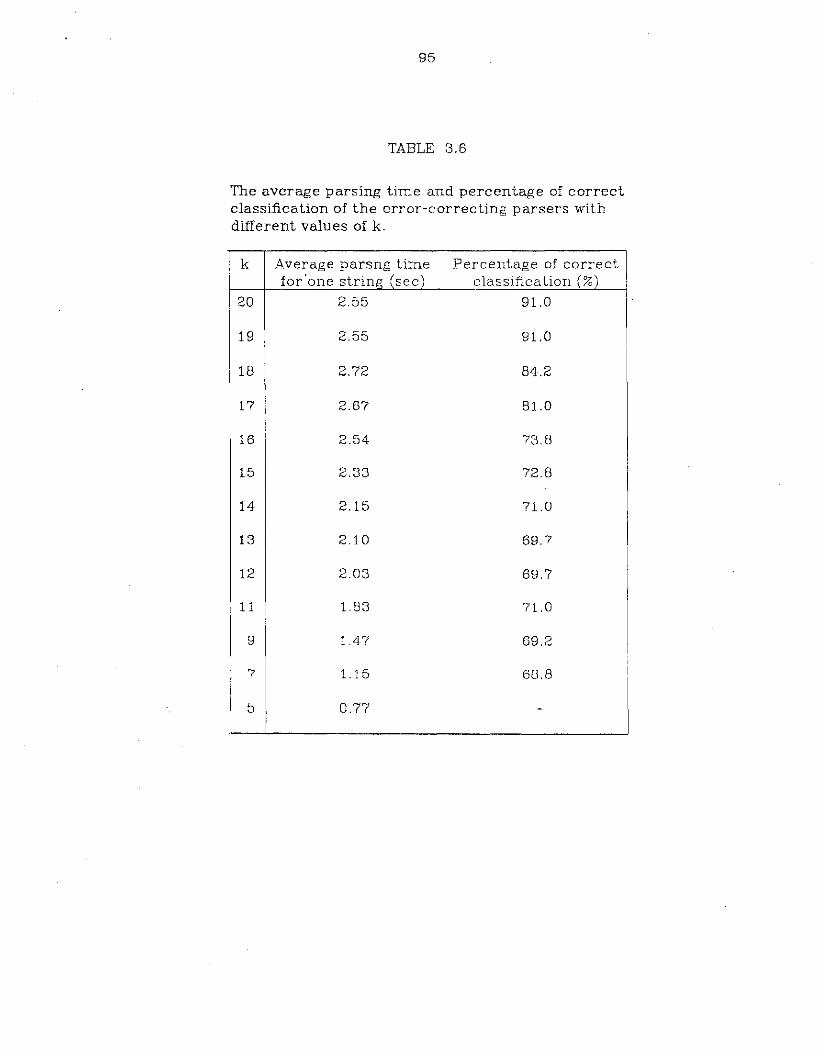
95
TABLE 3.6
The average parsing time and percentage of correctclassification of the error-correcting parsers withdifferent values of k.
k Average parsng time Percentage of correctfor'one string (sec) classification (%)
20 2.55 91.0
19 2.55 91.0
18 2.72 84.2
17 2.67 81.0
16 2.54 73.8
15 2.33 72.8
14 2.15 71.0
13 2.10 69.7
12 2.03 69.7
11 1.83 71.0
9 1.47 69.2
7 1.15 68.8
5 0.77 -
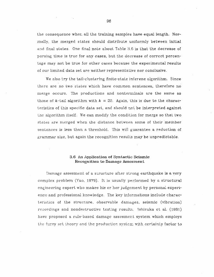
96
the consequence when all the training samples have equal length. Nor
mally, the merged states should distribute uniformly between initial
and final states. One final note about Table 3.6 is that the decrease of
parsing time is true for any cases, but the decrease of correct percen
tage may not be true for other cases because the experimental results
of our limited data set are neither representative nor conclusive.
We also try the tail-clustering finite-state inferene algorithm. Since
there are no two states which have common sentences, therefore no
merge occurs. The productions and nonterminals are the same as
those of k -tail algorithm with k = 20. Again, this is due to the charac
teristics of this specific data set, and should not be interpreted against
the algorithm itself. We can modify the condition for merge so that two
states are merged when the distance between some of their member
sentences is less than a threshold. This will guarantee a reduction of
grammar size, but again the recognition results may be unpredictable.
3.6 An Application of Syntactic SeismicRecognition to Damage Assesment
Damage assesment of a structure after strong earthquake is a very
complex problem (Yao, 1979). It is usually performed by a structural
engineering expert who makes his or her judgement by personal experi
ence and professional knowledge. The key informations include charac
teristics of the structure, observable damages, seismic (vibration)
recordings and nondestructive testing results. Ishizuka et al. (1981)
have proposed a rule-based damage assesment system which employs
the fuzzy set t.heory and the production system with certainty factor to
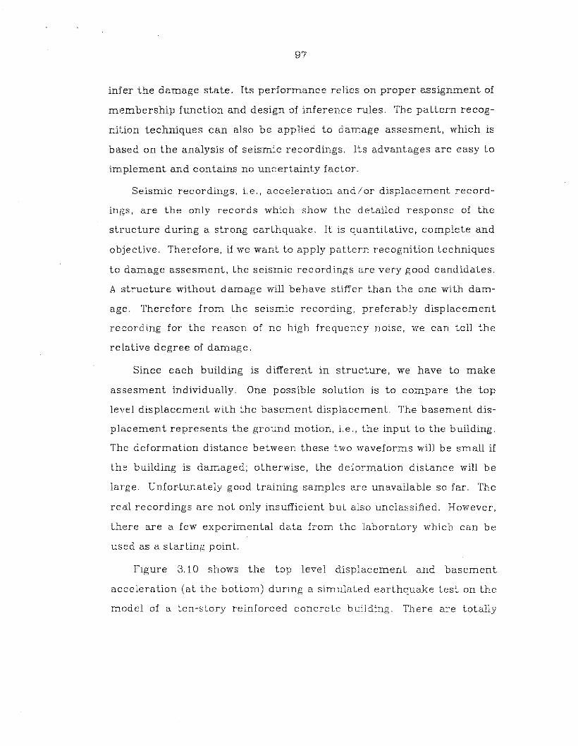
97
infer the damage state. Its performance relies on proper assignment of
membership function and design of inference rules. The pattern recog
nition techniques can also be applied to damage assesment, which is
based on the analysis of seismic recordings. Its advantages are easy to
implement and contains no uncertainty factor.
Seismic recordings, i.e., acceleration and/or displacement record
ings, are the only records which show the detailed response of the
structure during a strong earthquake. It is quantitative, complete and
objective. Therefore, if we want to apply pattern recognition techniques
to damage assesment, the seismic recordings are very good candidates.
A structure without damage will behave stiffer than the one with dam
age. Therefore from the seismic recording, preferably displacement
recording for the reason of no high frequency noise, we can tell the
relative degree of damage.
Since each building is different in structure, we have to make
assesment individually. One possible solution is to compare the top
level displacement with the basement displacement. The basement dis
placement represents the ground motion, i.e., the input to the building.
The deformation distance between these two waveforms will be small if
the building is damaged; otherwise, the deformation distance will be
large. Unfortunately good training samples are unavailable so far. The
rea.l recordings are not only insufficient but also unclassified. However,
there are a few experimental data from the laboratory which can be
used as a starting point.
Figure 3.10 shows the top level displacement and basement
acceleration (at the bottom) during a simulated earthquake test on the
model of a ten-'story reinforced concrete building. There are totally
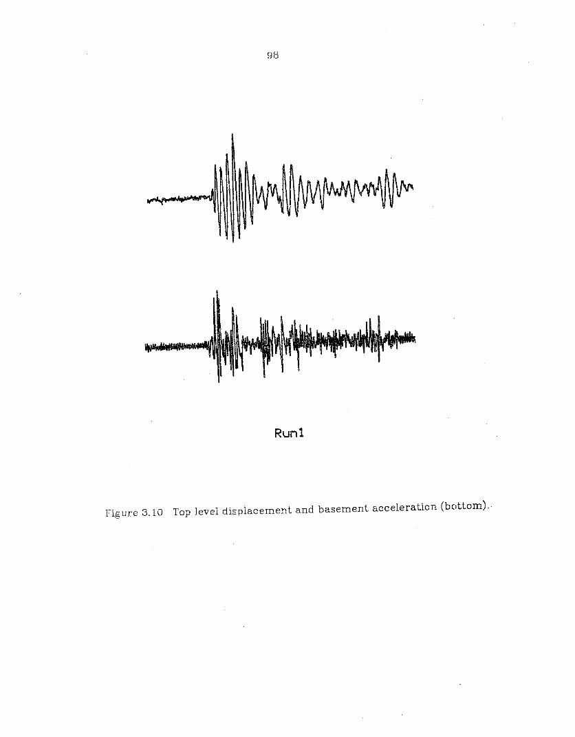
98
Runl
Figure 3.10 Top level displacement and basement acceleration (bottom).

99
seven test runs. It is obvious from Figure 3.10 that the accleration
waveform is much more complicated than the displacement waveform.
Since they are convertible, we chose displacement seismogram for
cornparison.
Since only the basement accleralions are available, we have to
compute displacements using numerical integration. The basement
displacements of the seven runs are all the same as shown in Figure
3.11, only the magnitudes are intensified from run to run so as to
assure more damage after more runs. The top level displacements are
shown in Figure 3.12. It is not diflucult to see that the top level dis
placement of run seven is more similar in figuration to basement dis
placement than the top level displacement of run one is. This shows
thc\t the building structure becomes softer due to the cracks, breaks
and other implicit damages. Some potential damages may not be seen
from the appearence of the building, but they will be shown on the
seismic recording since it reflects the actual structure response. This
is one of the reasons why the analysis of seismic recording is important.
The other reason is that we can compute the similarity, or deformation
distance on the other hand, between the waveforms which can be
further used in a knowledge-based damage assesment system.
Computation of the deformation distance between the seismic
waveforms are based on the modified dynamic time warping distance in
Section 2.2. Comparing Figure 2.6 with Figure 3.12 we will find that the
waveforms in Figure 2.6 are actually taken from those in Figure 3.12.
The slope constraints and local distance functions are shown in Figure
3.13.
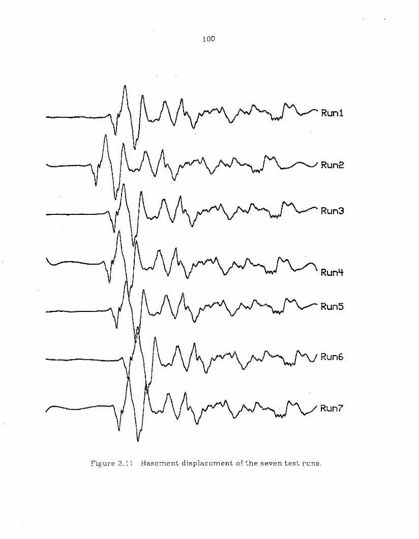
100
Run1
Run2
Run3
Runlf
RunS
RunG
Run?
Figure 3.11 Basement displacement of the seven test runs.
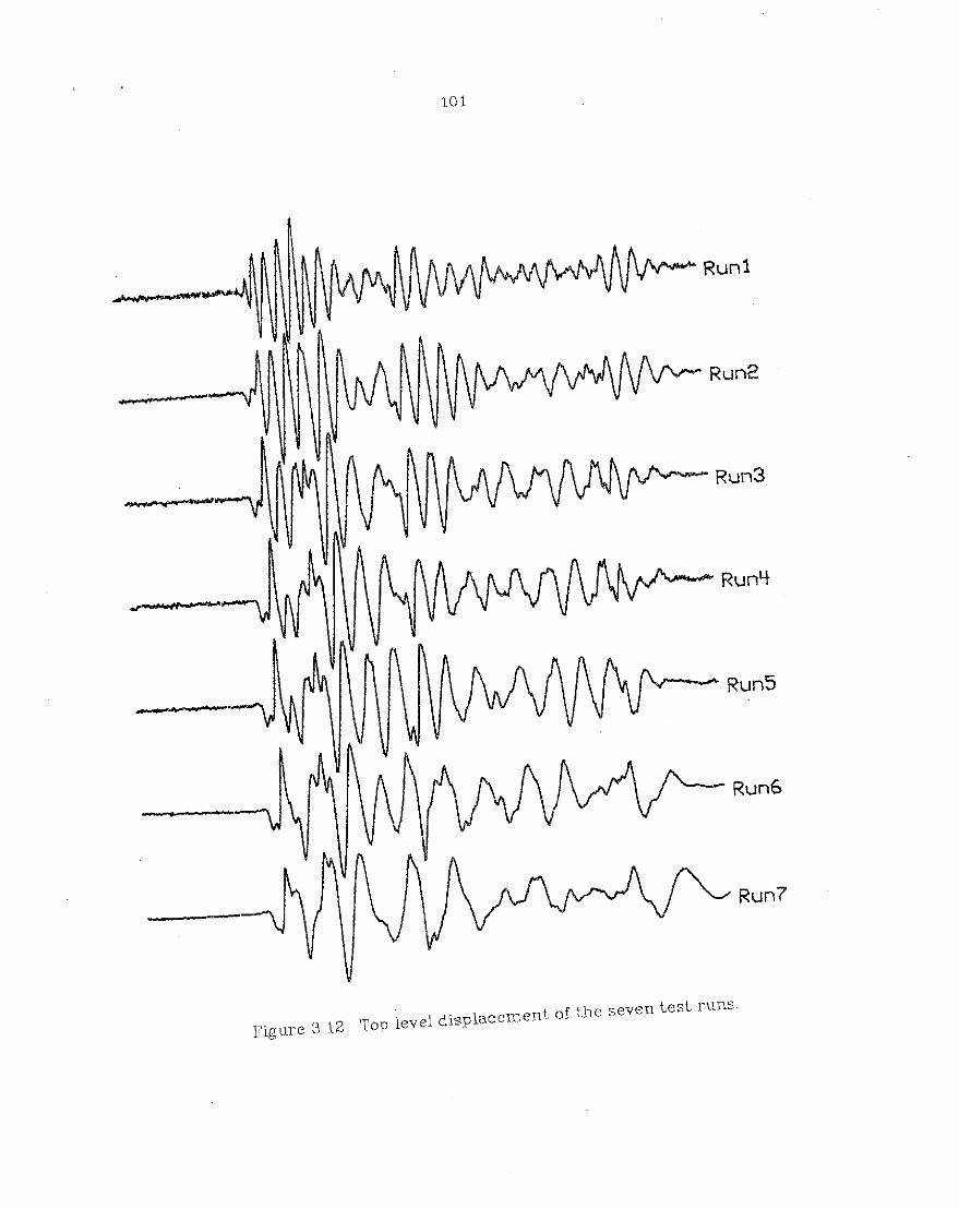
lito,. ,.... 'Iv &11'
..., . "-
....
101
Runl
Rune
Run3
Run't
Run5
RunG
Run?
Figure 3.12 Top level displacement of the seven test runs.
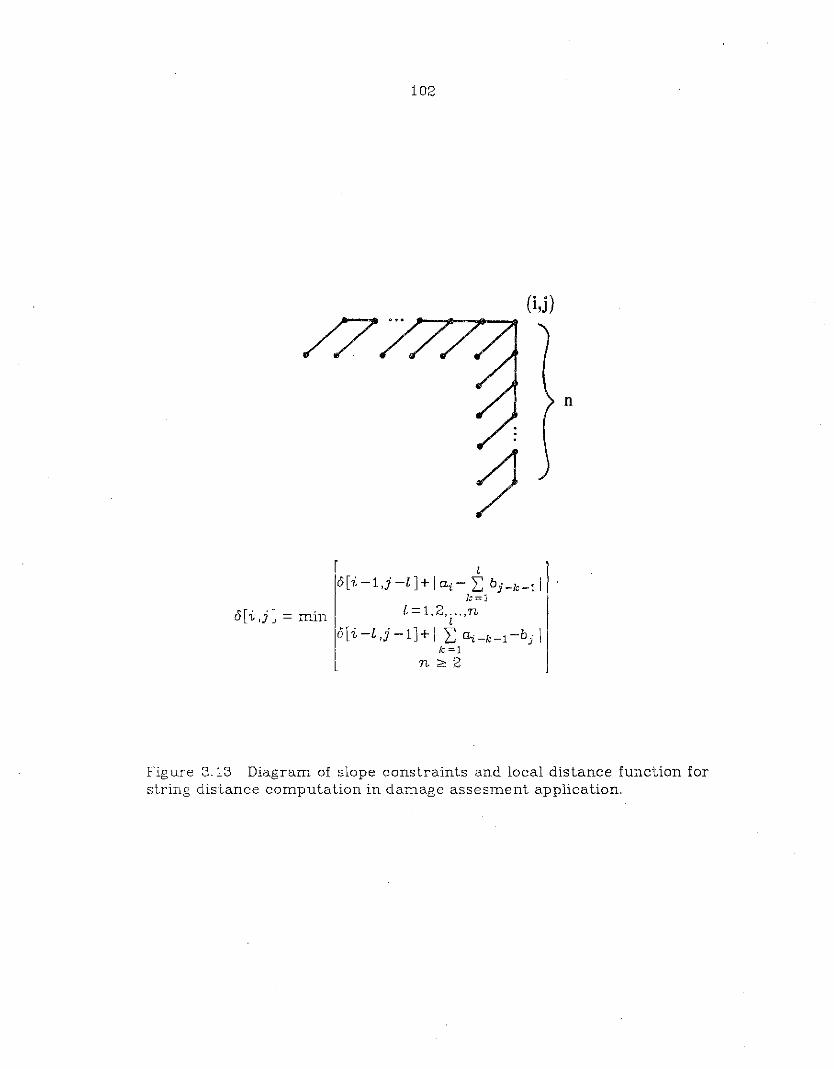
102
(i,j)
/7'"n
o[i,j J =min
r l
o[i -i.j -l J+ Iai - I:; b j -lc -1 Ik=l
l = 1,2, ...•nl
o[i -l ,j -lJ+ I I: ~-k-1-bj Ik =1
n;;;:: 2
Figure 3.13 Diagram of slope constraints and local distance function forstring distance computation in damage assesment application.
103
The selection of string representation and the selection of compu
tational algorithm for string deformation distance are correlated. We
observed from the waveforms in Figure 3.12 that several local peaks are
deformed and merge into a large peak. Therefore, we consider each
peak as a component, i.e., primitive or symbol, of string representation.
The next problem is how to describe each peak. Of course, shape and
geometric properties can describe a peak, they are far complicated
than what is needed. Besides, it is difficult to implement these features
in distance computation. The area of each peak contains the informa-
tions about the duration and amplitude of the peak. Since different
cOlnbinations of duration and amplitude may have same area, area
alone is ambiguous. But we don't need to worry about this problem
since we are dealing with recordings from the same structure, such
randomly contrast shapes will not occur. We developed a special string
deformation distance computation for this application, which is a
modified dynamic time warping distance as shown in Section 2.2.1. The
type of this deformation distance is ordinal, i.e., rank orders have
meaning, and interval, i.e., seperation between numbers is meaningful.
However, the lower and upper bounds of this distance is open, i.e., the
distance is in the interval (0, M) where .M is the summation of the total
area of the two strings. For example, if x =a1a2... am, and y = b lb 2... b n
then
M
Each seismic waveform x is converted into a string of real
numbers, x = ala2'''D.n, Ui > 0, such that the ith component of the
string, ai, represents the area of the i th peale The definition of the

104
peak here is the segment between two adjacent zero-crossing points.
Therefore one peak may contain many local maxima and minima. It
often happens that small ripples and zero-crossings may exist due to
the noise. These noisy ripples can be removed by setting a threshold T.
Only those peaks whose areas are larger than threshold T are con
sidered as effective components. The waveforms are scanned from both
side until a peak larger than T is reached on each direction. The left
most peak larger than T will be the first component of the string and
the rightmost peak larger than T will be the last component of the
string. This process will eliminate the noisy ripple before and after the
signal. The noisy ripples within the signal are combined with the
nearest peak which is greater than T. Therefore, only the significat
peaks are converted into components of the string. The algorithm for
computing string deformation distance is similar to that of Sakoe and
Chiba's. only the slope constraints and local distance functions are
different.
The deformation distance between the basement displacement and
the top level displacement of each run is plotted in Figure 3.14. Since
each run of the test adds some damage to the structure, the degree of
damage is proportional to the number of tests. Greater damage makes
the structure softer. consequently the deformation distance between
the basement waveform and top level waveform is smaller. It can be
seen from Figure 3.14 that the deformation distance is getting smaller
after more runs of tests. Figure 3.14 also shows that large damage
occurs during the first three runs since the differences of the deforma
tion distance, i.e., the slope, are larger than those of the later runs.

105
],71.8'iO ~----------------------------.
],55.766
139.&92
123.619
Q1UCI1J 107.&15~
Ifl.o-f
~
51.1f712
75.3975
987:321f3.2500 +-----r---"'T"""----,r-----r---or---~---.,__--__f
1
59.3237
Run
Figure 3,14 Distance between the basement displacement waveform andthe top level displacement waveform of each run.
106
In order to normalize the length of the strings come from different
event, the deformation distance in Figure 3.14 can be divided by the
length of the basement waveform so that the deformation distance of
different event can be compared. The domain of damage can be divided
into several intervals, for example, negligible, slight, moderate, s~vere,
etc. The deformation distance is used for classification of damage
degree. The classification depends on which category the deformation
distance of one event falls into. Other informations such as human
observations and system identification results are usuful auxilary infor
mations, for example, to resolve the conflict when the distance falls at
the boundary. But system identification is a very complicated matter,
it is mainly for the study of system characteristics. Visual informations
are easy to obtain and are helpful in resolving conflict and ambiguity.
The proposed system does not have the opportunity to test real
data because of the lack of data. The research in damage assesment is
only in its infancy. No organization or individual has been working on
the collection and classification of the real datEl. We must understand
that appropriate samples for damage assesment are rather difficult to
obtain. The structure must be equipped with recording devices, subject
to strong earthquake and bear certain degree of damage. Therefore,
the demonstration of the proposed method is based on experimental
data only. It attempts to show the feasibility instead of practicability of
the proposed method.
The segmentation of waveform employs some structural (contex
tual) information. Peak extraction needs structural information,
merge of small peaks with the nearest large peak also needs structural
information. In our demonstration, only the top level recordings are

107
used for comparison. Intermediate levels are similar to top level but
with smallar amplitude.
3.7 Conclusion
In this chapter, syntactic pattern recognition has been applied to
the discrimination of earthquake and nuclear explosion based on
seismic waveforms. The waveforms are segmented by a fixed length. A
clustering procedure classifies these segments and a symbol is assigned
to leach cluster. Finite-state grammars are inferred from the training
set using k -tail inference algorithm. An error-correcting parser and a
nearest-neighbor rule are compared with respect to their performance
in recognition speed and accuracy. Although the classification results
seem to be encouraging, there is plenty of room for improvement. The
selection of a set of distinguishing features is the most important part
in practical pattern recognition applications. The difficulty increases
when the classes are somewhat overlapped. Most of the features which
are effective in decision-theoretic approach can also be used in the syn
tactic approach for primitive recognition. The number of features
selected should be kept as small as possible for the sake of computa
tional efficiency.
In string distance computation, the assignment of weights for
transformation errors is a difficult subject especially when insertion,
deletion and substitution are all included. The seperation between clus
ters can be used as the substitution weights between corresponding
primitives as we did in our experiment. The distance from a cluster
center to the origin can be used as the insertion and/or deletion v{eight

108
of that primitive. Heuristic information may be necessary and helpful
in most cases.
Syntactic approach can be modified to deal with stochastic models
if the probabilities associated with pattern classes and training samples
can be easily determined. In this case, there will be stochastic gram
mar, stochastic language and maximum-likelihood parsing (see Fu,
1982). We did not apply the stochastic approach because the class and
string probabilities are unavailable. This must be done from the
analysis of the previous records. If the probabilities can be determined
precisely, which can be made to a certain degree, the class-overlap
problem can be solved. Syntactic approach can be made more flexible
by adding numerical information (attribute) to the primitives.
Meanwhile, it can also make the pattern grammar less complex. We will
discuss an attributed seismic grammar and its parsing in Chapter IV.
At the present stage, our experiments show that the nearest
neighbor decision rule is faster than the error-correcting parsing.
Although the speed of error-correcting parsing depends on the struc
ture of the grammar, the nearest-neighbor rule is faster in general.
VLSI architectures have been recently applied to both string matching
and recognition (by parsing), which will be discussed in Chapter V.
Decision between simple, faster classification and sophisticated, slower
syntax analysis should be made according to application requirements.
Syntactic pattern recognition has also been applied to damage
assesment where the seismic recordings are the physical measure
ments. Strings of various length are constructed from the seismic
waveforms. A modified dynamic time warping is developed for comput
ing the string distance. The segmentation of waveform in syntactic
109
pattern recognition usually uses shape information. Tbe shape informa
tion appears to be not important for seismic signal. Besides, it does not
have much discrimination capability. The enveloI: s of the signal
appears to be very good features in some cases, for example, consider
ing Figure 1.2, but not so in other cases, for example, when Figure 1.3
and 1.4 are compared with Figure 1.2. The application to damage asses
ment shows that special algorithm for string distance computation
must be developed for some applications when the general string dis
tances seem unable to solve the problem.


110
CHAPTER IV
INFERENCE AND PARSING OF ATTRffiUTED GRAMMARFOR SEISMIC SIGNAL RECOGNITION
401 Introduction
Attributed grammars were first formulated by Knuth (1968) where
"meaning" can be assigned to a string in a context-::ree language by
defining "attributes" of the symbols in a derivation tree for that string.
The attributes are defined by functions associated with each production
in the grammar. Although the idea of attributed grammar is due to
Irons (see Knuth, 1968), Knuth included inherited attributes as well as
synthesized attributes which often leads to significant simplification.
WItile attributed grammars were originally proposed 'or programming
languages, they have been applied to pattern recognition recently and
increasingly. Tang and Huang (1979) used attributE d grammars for
image understanding. You and Fu (1978, 1979), Tsai and Fu (19BO) and
Tai and Fu (1981) have applied attributed grammars 1.0 shape recogni
tion and transformation, Shi and Fu (1982) proposed an efficient
er:~or-correcting parser for attributed tree grammar::: where semantic
information are associated with each terminal but no semantic rule is
associated with the production. Leung (1982) also proposed an error-
correcting parser for attributed grammars vlith applications to charac
ter recognition. Knuth's formal semantics can also be app lied to
111
patterns described by picture description language (PDL) expressions
(Fu, 1982).
The advantages of using attributed grammars for pattern recogni
tion are twofold. The inclusion of semantic information increases the
flexibility in pattern description; in the meantime, it reduces the syn
tactic complexity of the pattern grammar. We may notice that all the
above applications are essentially to pictorial shape recognition where
length and angle are useful semantic informations. This same set of
attributes can also be used in waveform shape recognition, e.g., ECG
analysis, where shape information is very important in recognition.
However, they can not be applied to the signals, e.g., EEG, seismic and
speech, where shape informations are not particularly important. The
segmentation of these signals usually corresponds to a short, fixed- or
variable-length time period. In order not to overlook any transition,
the time periods are usually kept relatively short. Therefore, it is very
common that the same primitive may last for several periods. This
often makes the pattern strings and the inferred grammars unneces
sarily complicated. The numbers of productions and nonterminal sym
bols are usually very large as we can see from the experimental results
in Section 3.5. Instead of keeping track of all these identical primitives,
we can use one syntactic symbol to represent the tYPt~ of the primitive
with an attribute to indicate the length of the primitive. This leads to
the application of length attribute to seismic and other similar digital
signal analysis.
A pattern primitive a can be represented by a 2-h.:ple
a=(s,x)
112
wJJ.ere s is a syntactic symbol denoting the primitive structure of a,
and x = (xl,X2,""Xm ), m 2.": 0, is an m-dimensional semantic vect.or with
each xi, i = 1, 2, ... , Tn, denoting a numerical measurement. A pattern
string can be represented by ala2a3... ak, where ai = (Si, li)' li is the
length of primitive ai, lsisk. For a fixed-length segmentation, li = C
for all i, where c is a constant. For a variable-length segmentation, li
mayor may not equal t.o lj when i j:. j. In our case, li = c for lsis20,
.where c = 60 points. For simiplicity, wit.h constant IE ngth in mind, we
can eliminate the semantic part. For example, a pattern string may
look like
aaadgggegggggggegeeg
where these are syntactic symbols. It can be further simplified by
merging identical symbols, therefore the above string becomes
adgegegeg
31317 1 121
where the numbers are numbers of unit lengths; eacb unit length con
tains 60 points in our case. This idea shows some storage improvement
in string representation, and it will show significant. improvement in
g::ammatical inference as we will see in the next. section. Although we
used finite-state grammars to describe the seismic patterns in Chapter
III, we will use attributed cfg's here. This is because attributed fsg's do
not have much reduction in t.he number of productions and nont.ermi
nals. Only attribut.ed cfg's can drastically reduce t.he production
number, t.herefore make the recognition more efficient. An error
correcting parser for attributed context.-free grammar is given in Sec
tion 4.3. St.ochastic attributed grammar and parsing will be discussed
in Section 4.4.
113
4.2 Inference of Attributed Grammarfor Seismic Signal Recognition
An attributed context-free grammar is a 4-tuple G = (VN • Vr, P, S)
where each production rule contains two parts, one is a syntactic rule,
the other is a semantic rule (Knuth, 1968). Each symbol X E: (VN U VT )
is associated with a finite set of attributes A (X); and A(X) is partitioned
into two disjoint sets, the synthesized attribute set Ao(X) and the inher
ited attributed set A 1(X). The syntactic rule has the following form
where k means the k th production. The sematic rule maps values of
certain attributes of XkO , Xk1 , ... , Xknk into the value of some attribute of
Xkj . The evaluation of synthesized attributes is based on the attributes
of the descendents of the nonterminal symbol, therefore it is a
bottom-up fashion in the tree structure. On the contrary, the evalua
tion of inherited attributed is based on the attributes of the ancestors,
therefore it is a top-down fashion in the tree structure.
In Chapter III, we have chosen a set of 41 explosio:J. seismic records
as training samples. Each record has been converted :.nto a string of 20
primitives. If we use the k-tail algorithm to infer a finite-state gram
mar for the pattern class with a value of k = 20, the total number of
productions will be 720 and the number of nonterminal symbols will be
681. In order to reduce the size of the grammar we use one length
attribute, i.e., the number of unit lengths. The input strings are attri
buted strings, and the production rule of the gramme.r has a syntactic
part as well as a semantic part which contains both synthesized and
inherited attributes. The type of grammar is also Llpgraded into a
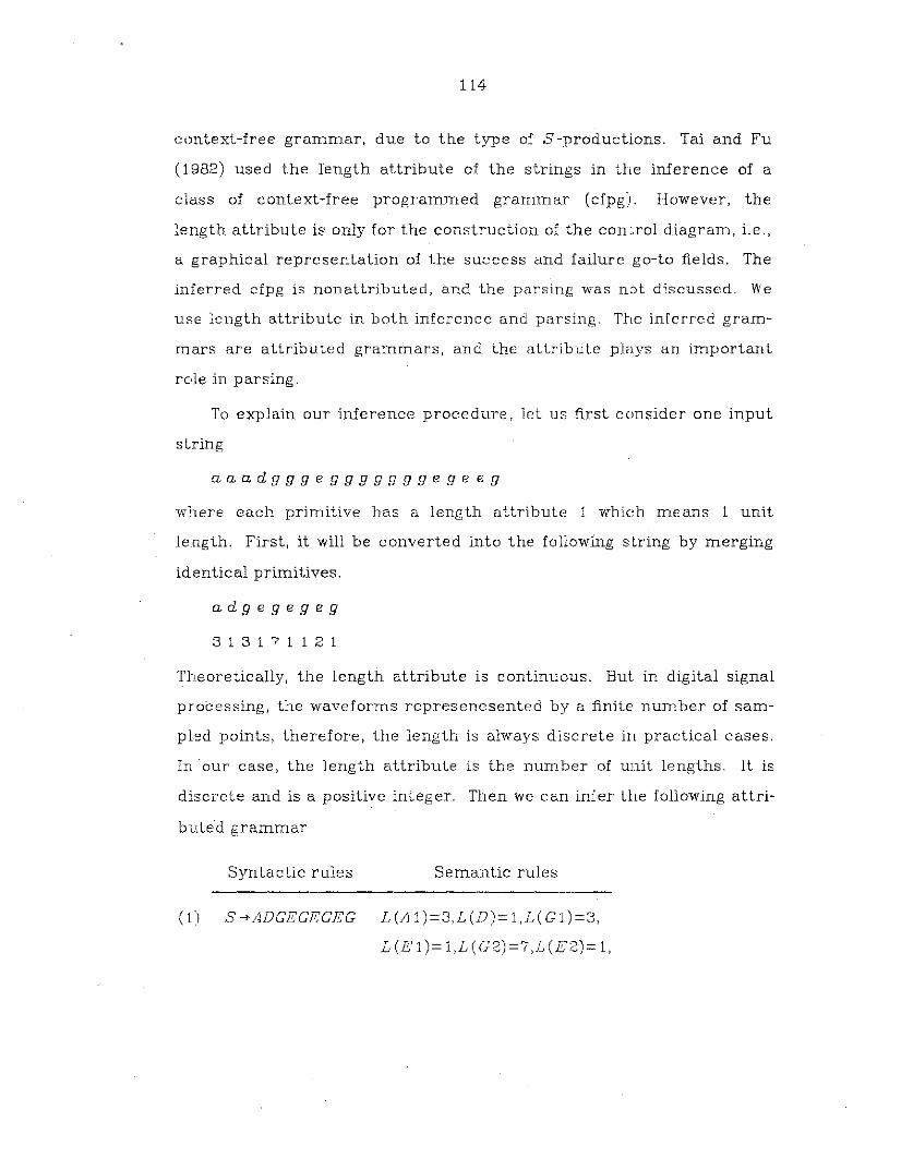
114
context-free grammar, due to the type of S-productions. Tai and Fu
(1982) used the length attribute of the strings in the inference of a
class of context-free programmed grammar (cfpg:l. However, the
length attribute is only for the construction of the con~rol diagram, i.e.,
a graphical representation of the success and failure go-to fields. The
inferred cfPg is nonattributed, and the parsing was n:::>t discussed. We
use length attribute in both inference and parsing. The inferred gram
mars are attributed grammars, and the attribute plnys an important
role in parsing.
To explain our inference procedure, let us first consider one input
string
aaadgggegggggggegeeg
where each primitive has a length attribute 1 which means 1 unit
length. First, it will be converted into the following string by merging
identical primitives.
adgegegeg
3 1 3 171 121
Trteoretically, the length attribute is continuous. But. in digital signal
processing, the waveforms represenesented by a finite number of sam
pled points, therefore, the length is always discrete in practical cases.
In our case, the length attribute is the number of unit lengths. It is
discrete and is a positive integer. Then we can infer the following attri
buted grammar
Syntactic rules Semantic rules
(1) S~ADGEGEGEG L(A1)=3,L(D)=l,L(Gl)=3,
L (E 1)= 1,L (G2)=7,L (£2)= 1,
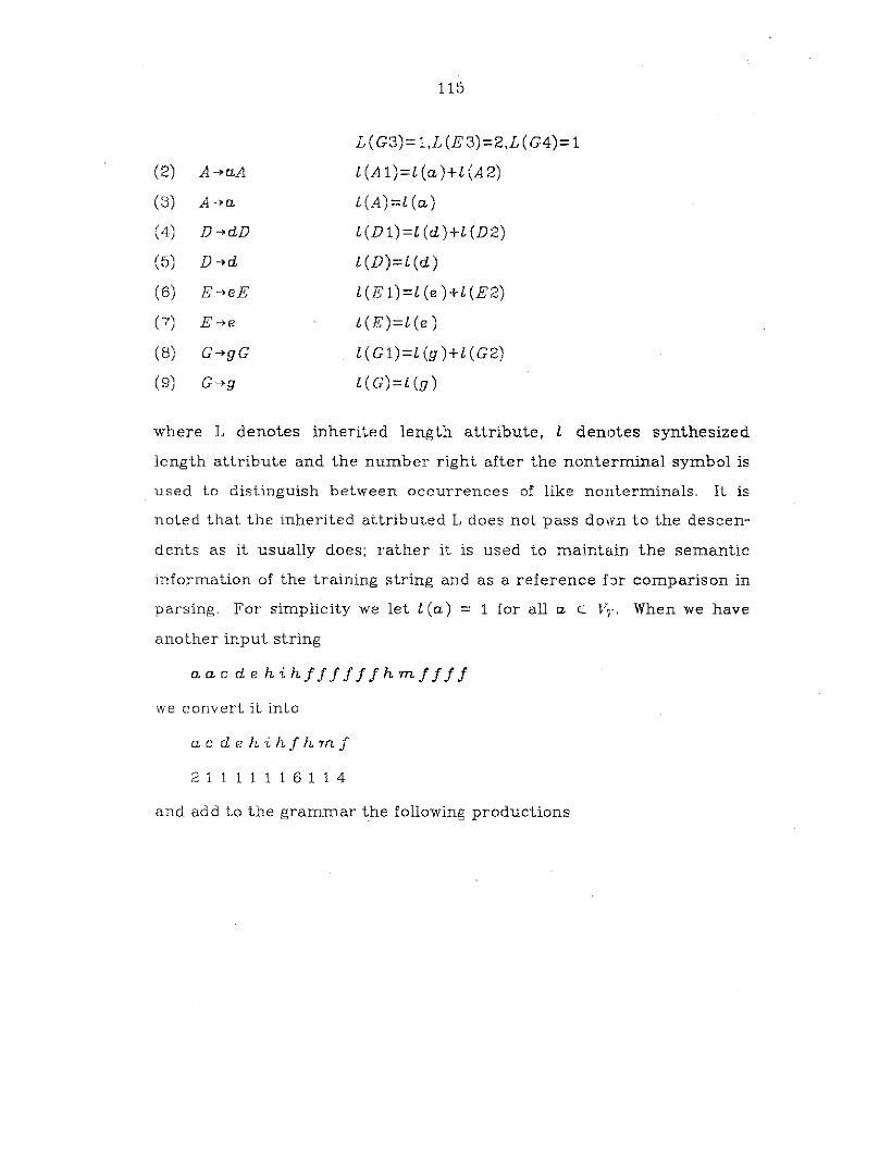
115
L (G3)= 1,L (E3)=2,L (G4)= 1
(2) A~aA l(Al)=l(a)+l(A2)
(3) A~a l(A)=l(a)
(4) D~dD l (D l)=l (d )+l (D2)
(5) D~d l (D)=l (d)
(6) E~eE l(E1)=l(e)+l(E2)
(7) E~e l (E)=l (e )
(8) G~gG l ( G 1) =l (g )+l (G 2)
(9) G~g l(G)=l(g)
where L denotes inherited length attribute, l denotes synthesized
length attribute and the number right after the nonterminal symbol is
. used to distinguish between occurrences of like nonterminals. It is
noted that the inherited attributed L does not pass down to the descen
dents as it usually does; rather it is used to maintain the semantic
information of the training string and as a reference hI' comparison in
parsing. For simplicity we let l (a) = 1 for all a E: V2" When we have
another input string
a a c de hi hjJ f f f J h m J f J J
we convert it into
acdehihfhmJ
21111 1 161 1 4
and add to the grammar the following productions
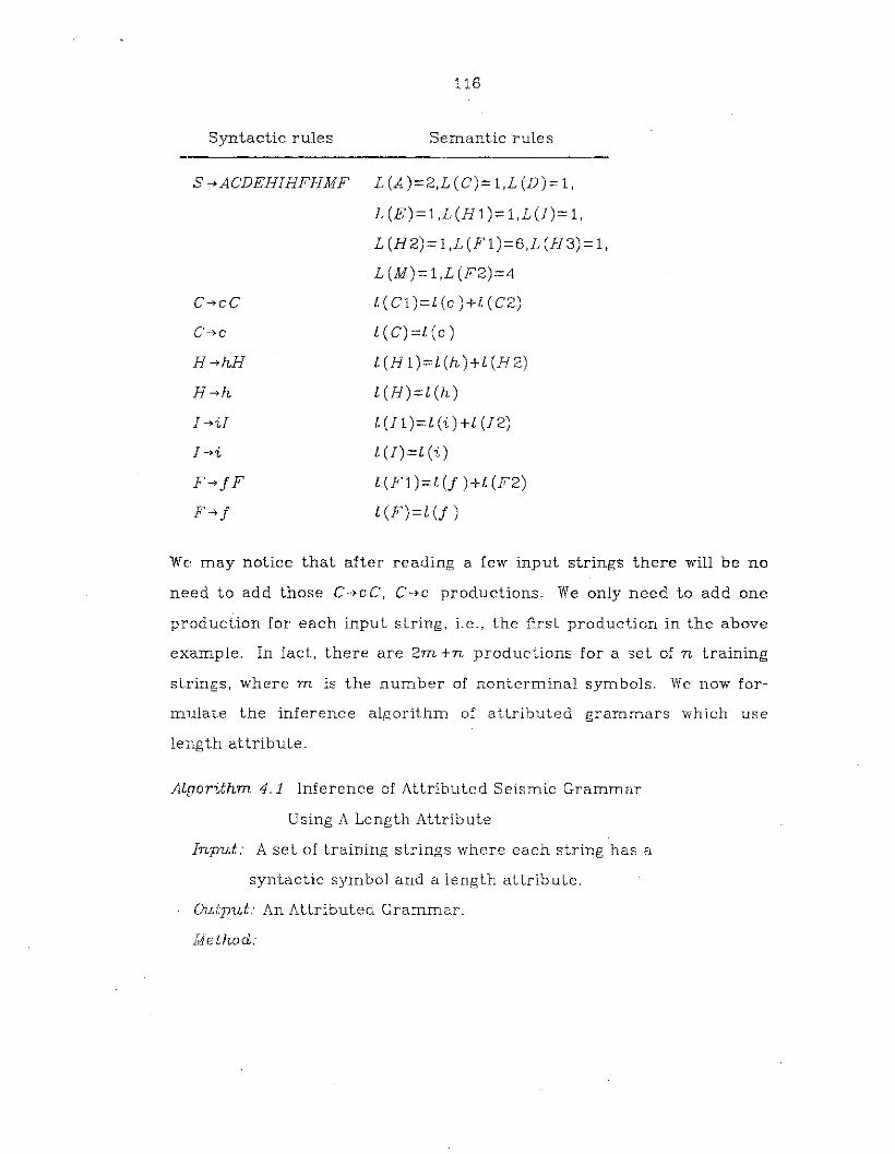
Syntactic rules
S -'>ACDEHIHFHMF
H-+hH
H -'>h
I -'>iI
I -'>i
116
Semantic rules
L (A )=2,L (C)= 1,L (D) =1,
L (E)= 1,L (H 1)= 1,L(I)= 1,
L (H2)= 1,L (F 1)=6,L (H3)= 1,
L (M) =1 ,L (F2)=4
l(Cl)=l(c)+l(C2)
l(C)=l(c)
l (H l)=l (h )+l (H2)
l(H)=l(h)
l (I 1)=l (i) +l (I2)
l(I)=l(i)
l (Fl)=l (j )+l (F2)
l (F)=l (j )
WE' may notice that after reading a few input strings there will be no
need to add those C-'>cC, C-,>c productions. We only need to add one
production for each input string, i.e., the first production in the above
example. In fact, there are 2m +n productions for a set of n training
strings, where m is the number of nonterminal symbols. We now for
mulate the inference algorithm of attributed grammars which use
length attribute.
Algorithm 4.1 Inference of Attributed Seismic Grammar
Using A Length Attribute
Input: A set of training strings where each string has a
syntactic symbol and a length attribute.
Output: An Attributed Grammar.
Method:
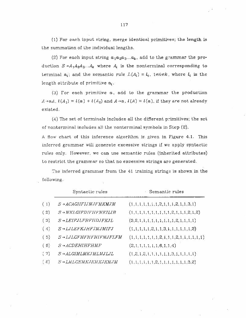
117
(1) For each input string, merge identical primitives; the length is
the summation of the individual lengths.
(2) For each input string ala2aS... ak, add to the grammar the pro
duction S -l>A 1A 2A s...Ak where ~ is the nonterminal corresponding to
terminal C4.; and the semantic rule L (Ai) =Li , l:::;;i:=;k. where Li is the
length attribute of primitive C4..
(3) For each primitive a, add to the grammar the production
A-l>aA, L(A l ) ::: lea) + l(A 2) and A-l>a, L(A) = l(a), if they are not already
existed.
(4) The set of terminals includes all the different pJ~imitives; the set
of nonterminal includes all the nonterminal symbols in Step (2).
A flow chart of this inference algorithm is given in Figure 4.1. This
inferred grammar will generate excessive strings if we apply syntactic
rules only. However, we can use semantic rules (inherited attributes)
to restrict the grammar so that no excessive strings ar'2 generated.
The inferred grammar from the 41 training strings is shown in the
following.
( 1)
( 2)
( 3)
( 4)
( 5)
( 6)
( 7)
( 8)
Syntactic rules
S -l> ACA GHF1J MJ F MKMJ M
S -l>MKLGIFDIFHFMKILIB
S -l> LEIFJLFBFHDJFKJL
S -l> LJLEFKJHFJ M JMIF J
S-l>LJLGFHFHFHIFMJFLFM
S -l>ACDEHIHFHMF
S -l> ALGIMLMKJMLMJ LJL
S -l>LMLGEMKJKMKJKMJM
Semantic rules
(1,1,1,1,1,1.1,2,1,1,1,2,1,1,3,1)
(1, 1. 1. 1,1, 1,1, 1, 1,1,2,1. 1,1,2,1, 2)
(3,2,1,1, 1. 1, 1, 1,1, 1, 1,2, 1,1,1,1)
(1,1, 1,1,1,2,1,1,3,1,1,1,1,1,1,2)
(1,1, 1,1,1, 1,1,2,1,1,1,2,1,1,1,1,1,1)
(2,1,1,1,1,1,1,6,1,1,4)
(1,2,1,2,1,1,1,1,1,1,3,1,1,1,1,1)
(1,1.1,1.1,1,2,1,1,1,1,1,1,1,3,2)
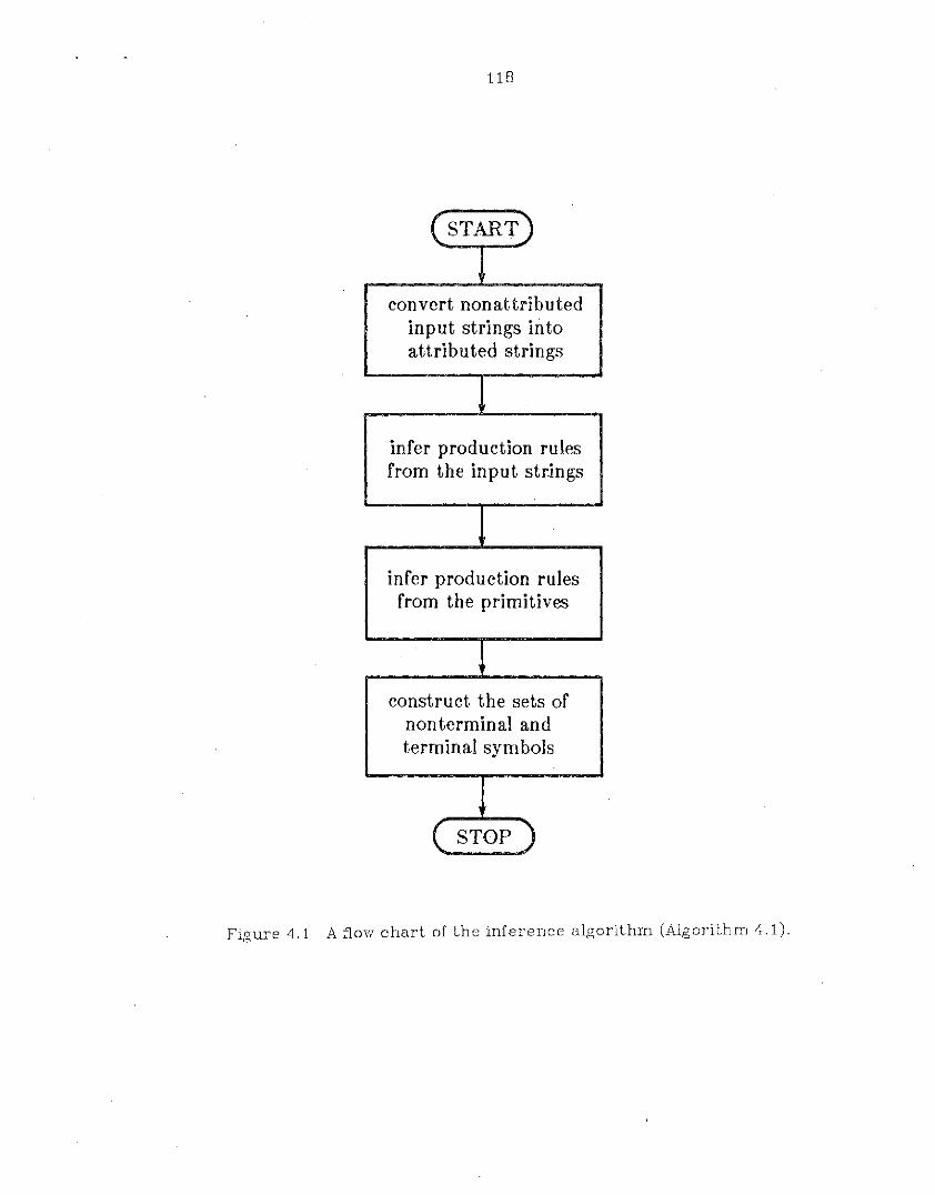
118
(START
convert nonattributedinput strings in toattributed strings
infer production rulesfrom the input strings
infer production rulesfrom the primitives
construct the sets ofnonterminal andterminal symbols
( STOP
Figure 4.1 A flow chart of the inference algorithm (Algorithm 4.1).
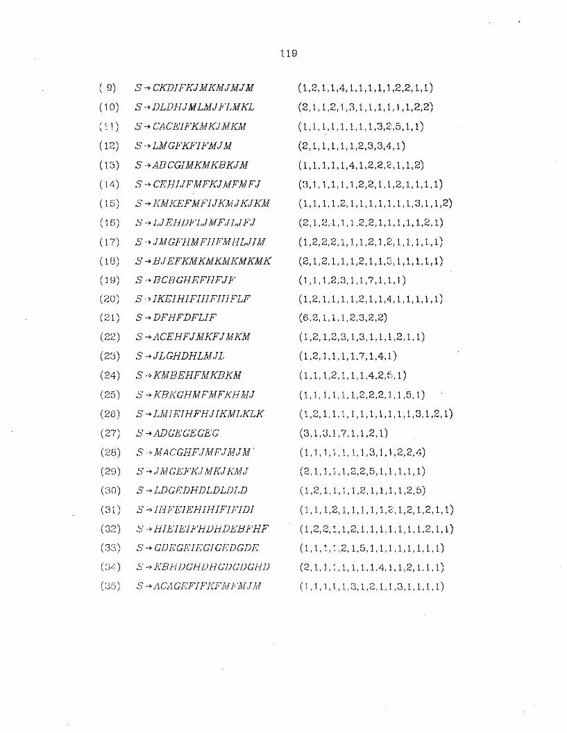
119
( 9) S~CKDIFKJMKMJMJM (1,2,1,1,4,1,1,1,1,1,2,2,1,1)
(10) S ~DLDHJMLMJFLMKL (2,1,1,2,1,3,1,1,1,1,1,1,2,2)
(11) S -'> CACEIFKMKJMKM ( 1, 1, 1, 1, 1, 1, 1, 1,3,2:,5,1, 1)
(12) S -,>LMGPXFIFMJM (2,1,1,1,1,1,2,3,3,4,1)
(13) S-'>ABCGIMKMKBKJM (1,1,1,1,1,4,1,2,2,2,1,1,2)
(14) S -'> CEHIJFMFKJMFMFJ (3,1,1,1,1,1,2,2,1,1,2,1,1,1,1)
(15) S -'>KMKEFMFIJKMJKJKM (1,1,1,1,2,1,1,1,1,1,1,1,3,1,1,2)
(16) S -'> LJEHDFLJMF JLJF J (2,1,2,1,1,1,2,2,1,1,1,1,1,2,1)
(17) S -'>JMGFHMFHFMHLJIM (1,2,2,2,1,1,1,2,1,2,1,1,1,1,1)
(18) S -'> BJEFKMKMKMKMKMK (2,1,2,1,1,1,2,1,1,3,1,1,1,1,1)
(19) S-'>BCBGHEFHFJF 0,1,1,2,3,1, 1,7,1,1,1)
(20) S -'>IKEIHIFIHFIHFLF (1,2, 1,1,1, 1,2,1,1,4,1,1,1,1,1)
(21 ) S -'>DFHFDFLIF (6,2,1,1,1,2,3,2,2)
(22) S-'>ACEHFJMKFJMKM (1,2,1,2,3,1,3,1,1,1,2,1,1)
(23) S ~JLGHDHLMJL ( 1,2, 1, 1,1, 1,7, 1,4,1 )
(24) S-'>KMBEHFMKBKM (1,1,1,2,1,1,1,4,2,5,1)
(25) S -'>KBKGHMFMFKHMJ (1,1,1,1,1,1,2,2,2,1,1,5,1)
(26) S -'>LMIEIHFHJIKMLKLK (1,2,1,1,1,1,1,1,1,1,1,1,3,1,2,1)
(27) S -'>ADGEGEGEG (3,1,3,1,7,1,1,2,1)
(28) S 4>MACGHFJMFJMJM' (1,1,1,1,1,1, 1,3,1,1,2,2,4)
(29) S -'>JlvlGEFKJlvlKJKMJ (2,1,1,1,1,2,2,5,1,1,1, 1,1)
(30) S 4> LDGEDHDLDLDLD (1,2,1,1,1,1,2,1,1,1,1,2,5)
(31 ) S -'>IHFEIEHIHIFIFIDI (1,1,1,2,1,1,1,1,1,2:,1,2,1,2,1,1)
(32) S -)HIEIEIFHDHDEBFHF (1,2,2,1,1,2,1,1,1,1,1,1, 1,2,1,1)
(33) S -'> GDEGEIEGIGEDGDE (1, 1, 1, 1,2, 1,5,1,1,1,1,1, 1, 1, 1)
(34) S -'>KBHDGHDHGDGDGHD (2,1, 1, 1,1,1,1, 1,4,1,1,2,1, 1, 1)
(35) S ..."ACAGEFIFKFlv[FlvlJM (1,1,1,1,1,3,1,2,1,1,3,1,1,1,1)
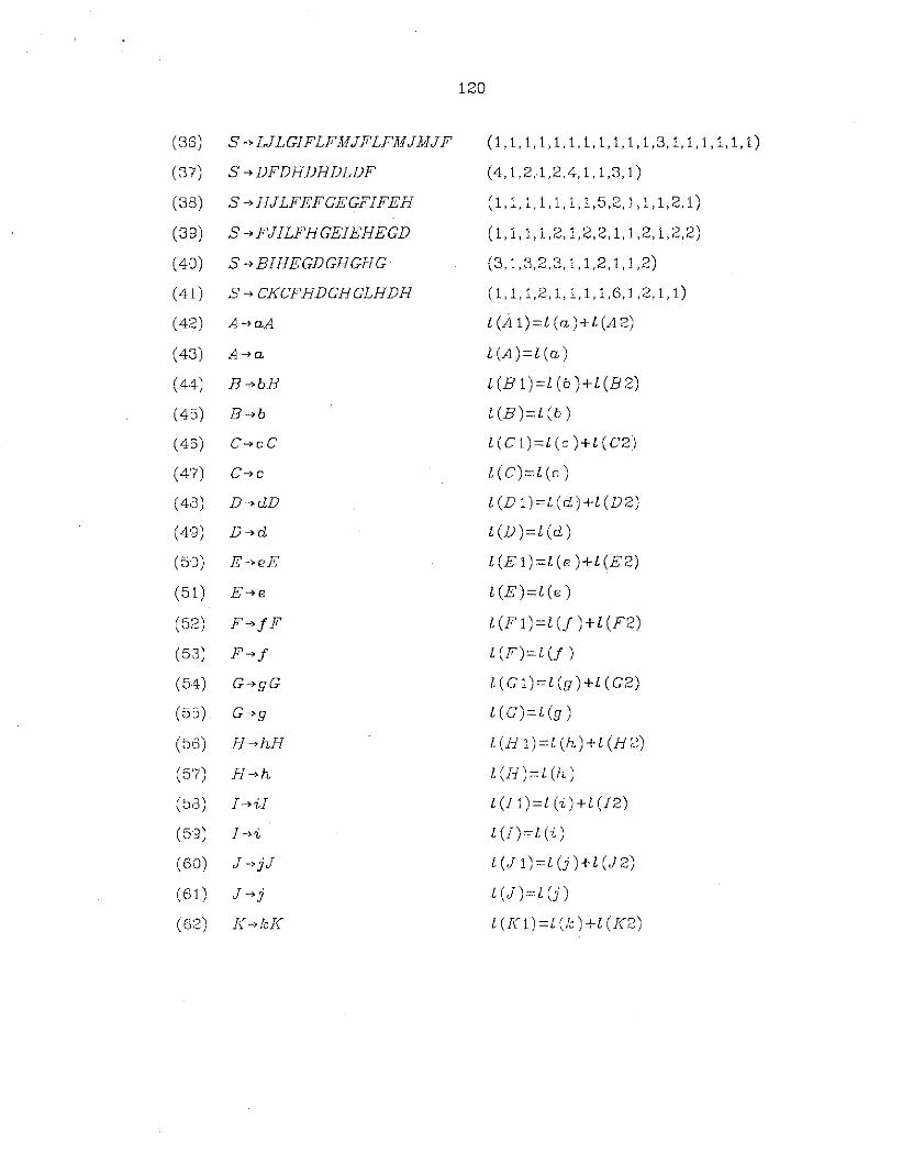
120
(36) S ~LJLGIFLFMJFLFMJMJF (1,1, 1,1,1, 1,1,1,1,1,1,3,1,1,1,1,1,1)
(37) S ~DFDHDHDLDF (4,1,2 c1,2,4,1,1,3,1)
(38) S~HJLFEFGEGFIFEH (1,1,1,1,1,1,1,5,2,1,1,1,2,1)
(39) S ~FJILFHGEIEHEGD (1,1,1,1,2,1,2,2,1,1,2,1,2,2)
(40) S ~BIHEGDGHGHG (3,1,3,2,3,1,1,2,1,1,2)
(41 ) S~CKCFHDGHGLHDH (1,1,1,2,1,1,1,1,6,1,2,1,1)
(4:8) A~aA l(Al)=:l(a)+l(A2)
(4:3) A~a l(A)=:l(a)
(44) B~bB l(B1)=l(b)+l(B2)
(4:5) B~b l(B)=:l(b)
(4;3) C~cC l ( C 1) =: l (c ) + l ( C2"
(4'7) C~c l(C)=:l(c)
(4,3) D~dD l(D 1)=l(d)+l(D2)
(49) D~d l(D)=l(d)
(50) E~eE l(E1)=l(e)+l(E2)
(51 ) E~e l (E)=l (e)
(52) F~fF l(Fl)=l(j)+l(F2)
(5:3) F~f l(F)=l(j)
(54) G~gG l(Gl)=l(g)+l(G2)
(55) G~g l (G) =l (g)
(56) H~hH l (H 1) =l (h) +l (H ~~)
(5'7) H~h l(I-J)=l(h,)
(5,3) I~il l(I1)=l(i)+l(J2)
(59) l~i l(I)=l(i)
(60) J~jJ l (J 1) = l (j )+ l (J 2)
(61 ) J~j l(J)=l(]")
( 6'::>~ /( ->!c/( l (I( 1) =l (lc) +l (/(2)'v)
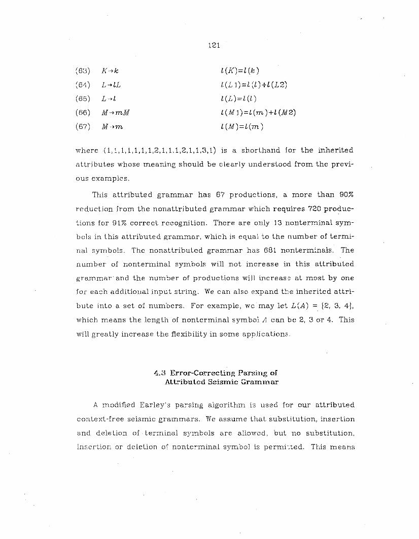
(63) K--"k
(64) L--"lL
(65) L~l
(66) M--"mM
(67) M--,>m
121
l (K)=l (k)
l(L l)=l (l)+l(L2)
l(L)=l(l)
l (M l)=l (m )+l (M2)
l(M)=l(m)
where (1,1,1,1,1,1,1,2,1,1,1,2,1,1,3,1) is a shorthand for the inherited
attributes whose meaning should be clearly understood from the previ-
ous examples.
This attributed grammar has 67 productions, a more than 90%
reduction from the nonattributed grammar which requires 720 produc
tions for 91% correct recognition. There are only 13 nonterminal sym
bols in this attributed grammar, which is equal to the number of termi
nal symbols. The nonattributed grammar has 681 nonterminals. The
number of nonterminal symbols will not increase in this attributed
grammar and the number of productions will increase at most by one
for each additional input string. We can also expand the inherited attri
bute into a set of numbers. For example, we may let L(A) = (2, 3, 4L
which means the length of nonterminal symbol A can be 2, 3 or 4. This
will greatly increase the flexibility in some applicatiom.
4.3 Error-Correcting Parsing ofAttributed Seismic Grammar
A modified Earley's parsing algorithm is used for our attributed
context-free seismic grammars. We assume that substitution, insertion
and deletion of terminal symbols are allo'wed, but no substitution,
insertion or deletion of nonterminal symbol is permi-~ted. This means

122
the length of the local segment is variable, even local :claise is tolerable,
but the whole local segment can not be deleted entirely. The local seg
ment means a segment of identical terminal symbols. The item of this
parsing algorithm has the form [A ~ex . (3, 7], ~, iJ where 7] is a counter
for local syntactic deformation which accumulates the total cost of sub
stitution of terminal symbols. l; is used for two different purposes.
When A ;t:. 5, l; is used as synthesized attribute of A. On the other hand,
if A = 5 then ~ is used as a counter for semantic deformation which
records the total length variation of nonterminal symbols, and i is the
se.me pointer as a conventional Earley's parser. A parsing algorithm for
expanded attributed grammar using length attribut.e has been pro
posed by Leung (1982). As usual, we don't need an expanded grammar.
All the deformations are examined during the parsing while errors are
recorded in appropriate counters. The parsing algorithm is shown in
the following.
Algorithm 4.2 Minimum-Distance Error-Correcting Parsing Algorithm
for Attributed Context-Free Seismic Granmar.
Input: An attributed seismic grammar G = (VN , Vr,P ,5) and an
input string y = bIb 2 ...bm in V;.Output: The parse lists 1 o, II, ... ,lm' and decision whether y is
accepted by the grammar G together with the syntacic and semantic
deformation distances.
Method:
(1) Set j = O. Add [5~ . ex, 0, 0, OJ to Ij if 5~ex is a production in P.
(2) Repeat step (3) and (4) until nO new items can be added to I j .
123
(3) If [A -'>(X • B {3, 71, ~,i ] is in Ii ,and B -'>7 is a production in P, then
add item [B -'> . 7, 0, O. n to Ii'
(4) (a) If [A-l>(X' .712, ~2,iJ is in Ij and [A-'>a 'A,7I1, ~l.kJ is in Ii,
then add an item [A--)aA . , 711+712. ~1+~2,1cJ to Ii' (There is no need to
check collision here. since there will be no other item of the form
[A ~ aA . . 71, ~,k] in I j .)
(b) If [A-l>(X·. 712, ~2,i] in Ii and [S-'>{3' A7, 711. ~l,k] is in h, then
add an item [S--){3A . 7, 711+712. ~1+(L(A)-~2),kJ to I j , where L(A) is the
inherited attributed of the nonterminal symbol A.
(5) If j =m, go to st.ep (7); otherwise j =j + 1.
(6) For each item [A-'> . a{3. 71. ~.iJ in I j - 1 add [A-,>a . (3, 7I+S(a,bj),
t+L(bj), i] to I j . where L(b j ) is the synthesized attribute of bj . For sim
plicit.y, we may let l(b j ) = 1 for all j. S(a,b j ) is substitution cost, and
S(a,bj ) =0 when a =bj . Go to (2).
(7) If item [5 -'>(X • , 71. ~, OJ is in 1m , then string y is accepted by
grammar G where 71 is the syntactic deformation distance and ~ is the
semantic deformation distance; otherwise, string y i~ not accepted by
grammar G. Exit.
A flow chart of this parsing algorithm is given in Figure 4.2. It is
noted that (1) The parse extraction is straightforward once the first S
production is identified, therefore we do not include the parse extrac
tion algorithm. This is obvious. Since we use attributes, the syntactic
part will be much simpler than that of a nonattributed (context-free)
grammar. (2) Deformation of any type on terminal symbols will be
accepted. For a simple example, the string 'aaadgggegggggggegeeg'
v{ill be accepted by our seiSlnic grammar voiith no error; the string
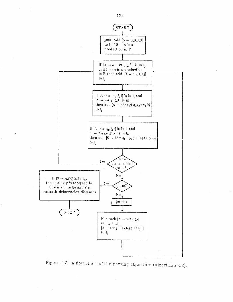
124
( START
!j =0. Add [S -+ Q,O,O,O]to Ij if S -+ Q is aproduction in P
If [A -+ Q • B,B, 1J,~, i ] is in Ij ,and B -+ "I is a productionin P then add [8 -> • "I,O,O,j]to Ij
If [A -+ Q ',I]2'~2,i] is in Ij and[A -+ a'A,fll'€I,kj is in Ij ,
then add [A -+ aA',I]l +1J2'~1 +x2,k)to I j
If fA --> Q',fJ2,~2,i] is in Ij and[S ~ ,B'A"I,I]I'~I,kl is in II.
then add IS -+ ,BA'VII +1J2,€1 +(L(A)-€2l,k]to Ij
If IS -+',I],~,OI is in 1m,
then string y is accepted byG, I] is syntactic and ~ is
semantic deformation distances
!( STOP
YesNew
items addedto I j ?
No
j=m?
No
I j=j+l I
For each [A -+ 'a,B"I,~,i]
in Ij~l and[A -+ a',B,I]+S(a,bj),~+I(bj),il
to Ij
Figure 4,2 A fiow chart of the parsing algorithm (Algorithm L1.2),
125
'aadgggeg .. .' will be accepted with semantic error of one unit length on
'A'; and the string 'abadgggeg .. .' will also be accepted with a syntactic
substitution error S(a,b).
The time complexity of Algorithm 4.2 is O(n 2 ) where n is the length
of the input string, since each item list Ii takes time O(j) to complete.
However, since we only considered substitution error in the seismic
recognition problem in Section 3.5, a simplified ven;ion of Algorithm
4.2, i.e., Algorithm 4.4, can be applied. This special parser is faster
than Algorithm 3.2. The experimental results are given in Section 4.5.
The question about how much advantage we can take by using attri
butes depends on the selection and characters of the training samples.
If the training samples are very much alike, then there are great possi
bilities that less syntactic rules are needed; instead, attributes will be
used to distinguish between different patterns. An attributed grammar
can also be constructed manually based on the knowledge about pat
tern sources. This may sometimes be a great advantage.
4.4 Stochastic Attributed Grammarand Parsing for Seismic Analysis
Although we do not know the probability distribution of the training
samples at this moment, it is possible to estimate it if more samples
are available. If the probability distribution of the training samples is
known, then we can infer the production probability using the algo
rithm described in Lee and Fu (1972b). Therefore, we also include a
parsing algorithm for stochastic attributed seismic grammar in this
section. A stochastic version of the attributed grammar shown in
126
Section 4.2 can be formulated as follows. First, a probability is associ
ated with each production. Second, a probability distribution is associ
ated with all the possible attributes. For example, if originally L (A) =13,4, 5l, now it may become L(A) = 1(3,0.25), (4,0.5), (5, 0.25)L where
0.25 = ?rob iL(A)=3l. Finally, probabilities instead of costs are used to
characterize substitution transformations. The probability associated
with each S-production will be the probability of occurrence of the
training string which contributes to that production.
The parsing algorithm of stochastic attributed seismic grammar is
very similar to Algorithm 4.2 except for the following changes. First, 77
is now the probability of syntactic substitution deformation. Second, ~
is still used as a synthesized attribute of A when A j::. S, however, when
A = S, ~ will be the probability of semantic deformations.
Algorithm 4.3 Error-Correcting Parsing Algorithm for
Stochastic Attributed Seismic Grammar
Input: An attributed seismic grammar G = (VN , Vr ,? ,S) and an
input string y =b lb 2 ... b m in V;.
Output: The parse lists I o, I1> ... ,Im, and decision whether y is
accepted by the grammar G together with the synta,:::ic and semantic
deformation probabilities.
Method:
(1) Set j = O. Add [S-J> . ex, 1, 1, OJ to I j if S-J>(X is a production in P.
(2) Repeat step (3) and (4) until no new items can be added to I j .
(3) If [A-J>(X· B(J, 77, ~,iJ is in Ij,and B->-y is a production in P, then
add item [B-J> . ;', 1, 1, jJ to IJ·•

127
(4) (a) If [A-4cx . ,7)2, ~2,iJ is in 11' and [A-4a . A, 7)1' ~l,1cJ is in h,
then add an item [A -4aA . ,7)1 . 7)2, ~1 +~2,k J to Ij . (There is no need to
check collision here, since there will be no other Lem of the form
[A -) aA . , 7), t k J in Ij . )
(b) If [A-)cx· ,7)2, ~2,iJ in Ij and [3-4,6' ky, 7)1. b.kJ is in Ii. then
add an item [3-),6A . "1,7)1' 772, ~1' Prob /~2Lk] to Ij , where 'L(A) is the
inherited attributed of the nonterminal symbol A.
(5) If j =m. go to step (7); otherwise j =j + 1.
(6) For each item [A-)· a,6, 7), ~,i] in Ij - 1 add [A-4a',6,
7)' Ps(b j la), ~+l(bj)' i] to Ij , where l(b j ) is the synthesized attribute
of bj . For simplicity, we may let l (b j ) = 1 for all j. P s (b j Ia) is substi
tution probability. Go to (2).
(7) If item [3 -40: . , 7), ~, OJ is in 1m , then stringi'l is accepted by
grammar G where 7) is the syntactic deformation probability and t is
the semantic deformation probability; otherwise, string y is not
accepted by grammar G. Exit.
A flow chart of this parsing algorithm is given in Figure 4.3. Due to
the error-correcting characteristics there may be more than one item
of the form [S -)cx " 7). ~, OJ in 1m . In that case, a decision should be
made based on 7) and E,. Weights can be assigned to 7) and t. Neverthe
less, this is a rather subjective judgement, and is always a problem
when using both syntactic and semantic informations.

128
(START)
~
j=O. Add [S - '0:,1,1,0]to Ij if S --> 0: is aproduction in P
If [A --> 0: 'B,B, '7, 0] is in I j
and B --> "I is a production in Pthen add [B --> '''I,l,l,j) to Ij
If [A --> 0:"'72,';2,ij is in Ij and[A --> a'A,'7t,';!kj is in Ii' then add[A --> aA','7,''72'';' +';2,k) to Ij
If IA- O:','72,';2,iJ is in I j andIS --> ,B·A"I,'7t,';"kj is in Ii' then add[S --> ,BA'''I,tl,''72,';!' Prob{';2},k] to Ij
NewYes
L.- .....:_< items addedto Ij?
iif IS --> 0:','7,';,0] is in 1m ,
then string y is accepted by G,I] is syn tactic and'; is seman ticdeformation distances
Yes
No
j=m?
1STOP
I j=j+l I
For each [A --> 'a,B,'7,~,i) in Ij_1 add[A --> a',B,'7'Ps(bjla),';+I(bj),i]to Ij
Figure 4.3 A flow chart of the parsing algoriLhm (Algorithm 4.3).

129
4.5 Experimental Results and Discussion
In this chapter we have shown an attributed seismic grammar
which has only 67 productions and 13 nonterminal symbols compared
to the 720 productions and 681 nonterminal symbols of a nonattributed
finite-state grammar. An error-correcting parser (Algoritm 4.2) is also
proposed for this attributed grammar. Since the error-correcting
parser of Algorithm 3.2 considered only the substitution error, a
simplified version of Algorithm 4.2 which ignores the length variation
can be used to greatly increase the processing speed. This is shown in
Algorithm 4.4.
Algorithm 4.4 Top-Down No-Backtrack Error-Correcting Parsing
Algorithm for Attributed Seismic Grammar.
Input: An attributed seismic grammar G = (VN , Vr,P ,S) and an
input string y = b 1b 2 •.. bm in V;.
Output: The minimum distance between y and L (G) where only sub
stitution error is considered.
Method:
(1) Set N = the number of S-productions, min-distance = a
sufficiently large number.
(2) Set 'I- = 1.
(3) The ith S-production has the form Si ~ Ai1 A i2 ' .. ~Mi' where
Jv['i is the number of nonterminals at the right-hand side of the ith S
production, Aij E: VN , 1 :S j :S Mi'
(4)Setdist=O,1c =l,l =1.
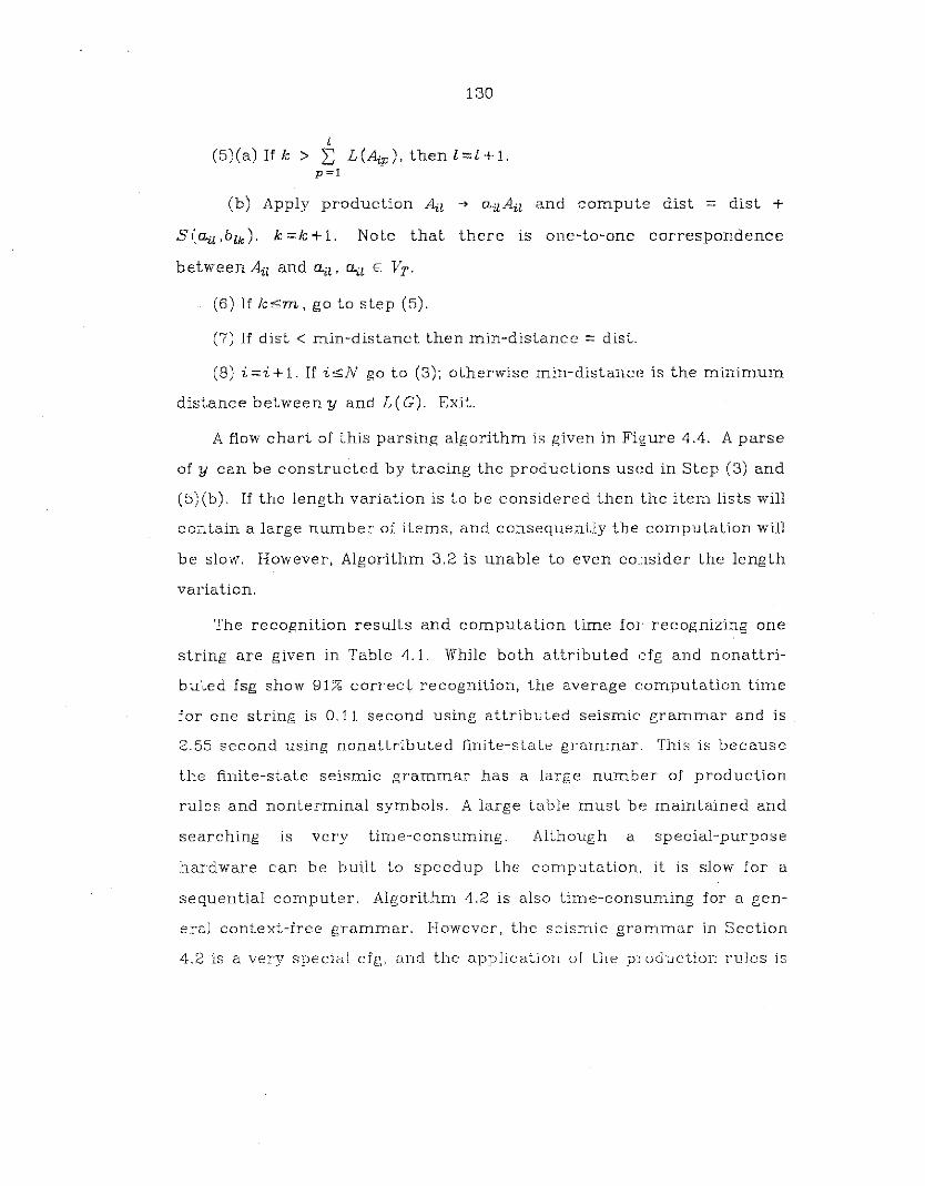
130
l(5)(a) If k > 2: L(~p), then l=l+1.
p =1
(b) Apply production ~l -) ail~l and compute dist = dist +
S(~l,blk)' k=k+1. Note that there is one-to-one correspondence
between ~l and C4l, ~l E: VT ·
(6) If 1c~m, go to step (5).
(7) If dist < min-distanct then min-distance =dist.
(8) i =i + 1. If i~N go to (3); otherwise min-distance is the minimum
distance between y and L (G). Exit.
A flow chart of this parsing algorithm is given in Figure 4.4. A parse
of y can be constructed by tracing the productions used in Step (3) and
(5)(b). If the length variation is to be considered then the item lists will
contain a large number of items, and consequently the computation will
be slow. However, Algorithm 3.2 is unable to even cO:1sider the length
variation.
The recognition results and computation time for recognizing one
string are given in Table 4.1. While both attributed cfg and nonattri
buted fsg show 91% correct recognition, the average computation time
for one string is 0.11 second using attributed seismic grammar and is
2.55 second using nonattributed finite-state grammar. This is because
the finite-state seismic grammar has a large number of production
rules and nonterminal symbols. A large table must be maintained and
searching IS very time-consuming. Although a special-purpose
hardware can be built to speedup the computation, it is slow for a
sequential computer. Algorithm 4.2 is also time-consuming for a gen-
eral context-free grammar. However, the seismic grammar in Section
4.2 is a very special cfg, and the application of the production rules is
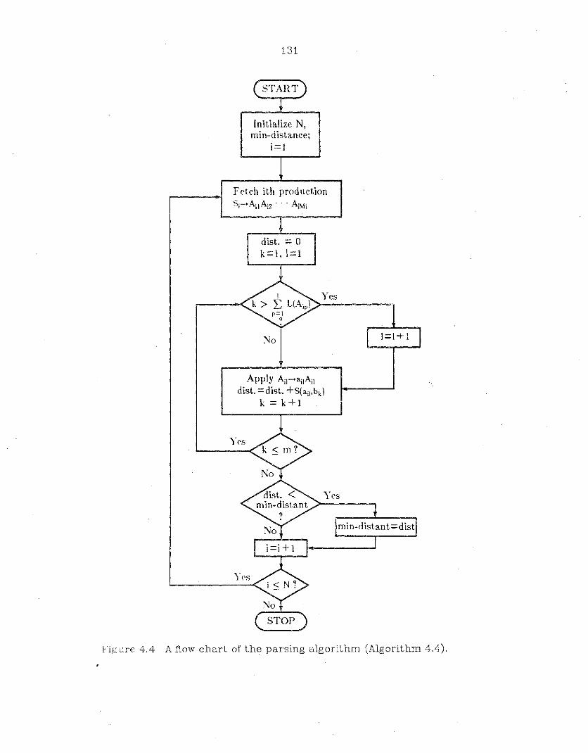
131
Initialize N,min-distance;
i=l
Fetch ith productionSj--AiJ A i2 ' .. A iMi
dist. == 0k=l,l=l
Yes
No
Apply Ail--ailAildist.=dist. +S(ail,bk)
k = k+l
Yes
Figure 4.4 A flow chart of the parsing algorithm (Algorithm 4.4).
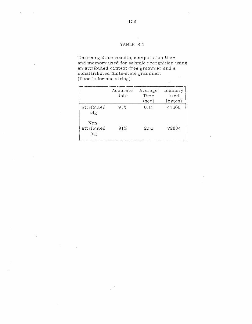
132
TABLE 4.1
The recognition results, computation time,and memory used for seismic recognition usingan attributed context-free grammar and anonattributed finite-state grammar.(Time is for one string)
Accurate Average memoryRate Time used
(sec; (bvtes;
Attributed 91% 0.11 41360cfg
Non-attributed 91% 2.55 72804
fsg
133
very straightforward. The actual storage used in computer is also given
in Table 4.1.
We mentioned earlier that substitution, insertion and deletion of
terminal symbols are allowed but no substitution, insertion or deletion
of nonterminal symbol is permitted. As a matter of fad, substitution of
nonterminal symbols can be attained in terms of substitution of termi
nal symbols. Therefore, only insertion or deletion of nonterminal sym
bols is not allowed. The reason is that if the training samples are well
selected, the grammar should be able to recogniZE! any reasonable
strings. If the test string needs insertion or deletion of nonterminal
symbols in order to be accepted, it is either severely distorted or miss
ing some string segments. If insertion and deletion of nonterminal
sylubols are to be considered then this becomes a structural
deformation problem (Tsai and Fu, 1979). 'We can add insertion and
deletion error transformations in Step(6) of Algoritm 4.2 as we did in
Algorithm 2.4. This will make the algorithm more complicated. A dis
tance threshold should be imposed to eliminate unrealistic parses so
that the item list will not become unmanagable.
134
CHAPTER V
VLSI ARCHITECTURES FOR SYNTACTICSEISMIC PATTERN RECOGNITION
5.1 Introduction
Some computational algorithms, for example, matrix multiplication
a.nd inversion in numeric computation and string Dlatching in non-
numeric computation, are very time-consuming so that an efficient
implementation is usually not feasible and economical. However, this
~:ituation has been changed due to the advances in hardware technol-
ogy, i.e., the development of high-speed, high-density and low-cost elec
tronic devices. Hardware implementation (particularly parallel and/or
pipeline processing) of software algorithm has become an affordable
solution to increase the processing speed because the cost of hardware
is decreasing. Advance in VLSI technology makes it possible to pack
luore components into one chip at a lower price than ever before (Mead
and Conway, 1980). This revolutionary impact sUmulEltes considerable
interest to develop parallel algorithms for VLSI implementation and
build special-purpose chips for specific applications (Kung, 1979, 1980).
A whole book (Bowen and Brown, 1982) has been devoted to VLSI sys
tems design for digital signal processing. Many computers and proces
sors have been developed for signal processing. The recent trend is to
135
use attached signal processors, e.g. ,Lincoln Laboratory Fast Digital
Processor (FDP) and Data Genaral AP /130 array processor, instead of
supercomputers as ILLIAC-rv and Advanced Scientific Processor (ASC)
(Bowen and Brown, 1982). More specialized applications for matrix mul
tiplication, convolution and solving linear equations can be found in
Kung (1979, 1982), Kulkarni and Yen (1982), Hwang and Cheng (1981). A
recent example of special-purpose VLSI architecture is an integrated
multiprocessing array for time warping pattern matching which is used
in speech recognition (Ackland, Weste and Burr, 1981). Pattern m.atch
ing is the most time-consuming stage in speech reco&;nition especially
when the dictionary is large. Using parallel processing improves the
speed 200 times faster, t.herefore make the real-time application possi
ble.
Like dynamic time warping, all the string distance computation and
string matching are time consuming. Hardware implementation has
been proposed by Okuda, Tanaka and Kasai (1976) for computing
Levenshtein distance even before VLSI technology is available. They
used delay circuits to implement insertion, deletion and substitution
weights.
We propose in this chapter a VLSI architeet~re for seismic
classification using syntactic approach, which include:, feature extrac
tion, primitive recognition and string matching. Our string matching
implementation is more complicated than Okuda, et a1.'s, where
different weights are assigned to different symbols in our case. This
special-purpose processor is designed to be aUachecc to a host com
puter, for example, a minicomputer as shown in Figure 5.1, therefore it
'works like a perihperal processor. Three systolic arrays are proposed

136
SYSTEM BUS
(~llN SPECIAL TAPE I/Oi:EMORY
CPUPURPOSE DISC DEVICEPROCESSOR
I
[
Figure 5.1 The special-purpose processor is attached to a host computeras a peripheral processor.
137
to perform feature extraction, primitive recognition and string match
ing respectively. Several memory units are required for holding the
intermediate results and for data setup. Figure 5.2 shows the architec
ture of our special-purpose processor. All these three systolic arrays
perform in time 0 (1), i.e., results can be produced at a constant rate
provided that input data are supplied properly in a pipelined fashion.
The formations of input data are given in Figure 5.3 where (a) is for
feature extraction, (6) is for primitive recognition and (c) is for string
matching. Section 5.2 discusses VLSI architectures for feature extrac
tion. Section 5.3 discusses VLSI architectures for primitive recognition.
Section 5.4 discusses VLSI architectures for string matching. Section
5.5 shows some simulation results and performance verification. Sec
tion 5.6 gives the concluding remarks.
5.2 VLSI Architectures for Feature Extraction
The systolic array for feature extraction is linearly connected as
shown in Figure 5.4. The input data, which are the digitized and quan
tized signal waveform coded in binary form, are stored in seperate
memeory modules in a skewed format as shown in Figure 5.3(a) and
Figure 5.4(a). Each memory module is delay by on,~ unit time, i.e.,
time required to process one data element, from left to right. Each
memory module contains a sequence of words, i.e., discrete signal
points and is connected to a processing element (PE:) of the systolic
array. The data are transferred into the PE's bit by bit, and all the
memory modules are read parallelly. Two features, zero-crossing count
and sum of absolute magnitudes are computed. Absolute sum instead
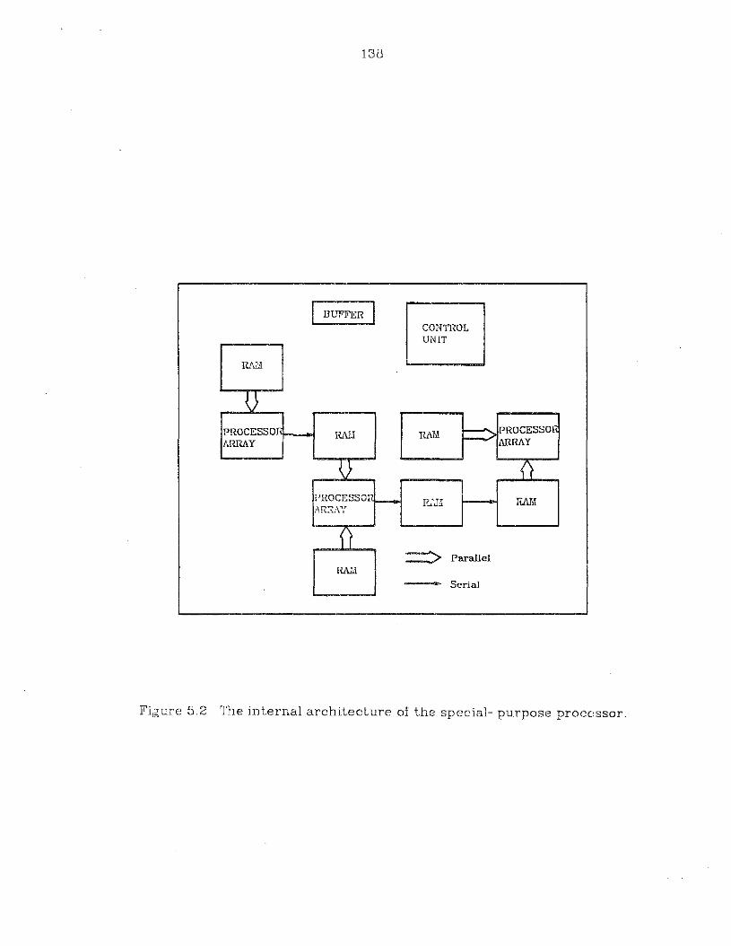
138
I BUFFER I CONTROLUNIT
RfJ.:l.
T}PROCESSOr. ~ PROCESSOIiRMl RAMAI~RAY -- Mr~AY
~> {)
PROCESSOEI-- I(..:.Ii RM,I/\RRAY
1)==> Parallel
RMI - Serial
Fil;;,;ure 5.2 The internal architecture of the special- purpose processor.
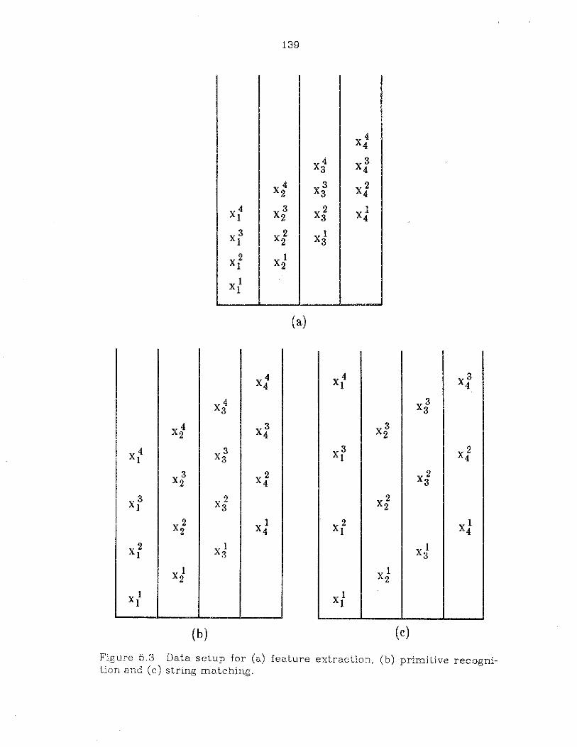
139
(a)
x4 X4 X34 1 4
X4 X33 3
X 4 X3 X32 4 2
X 4 X3 X3 X 21 3 1 4
X; X2 X 24 3
xl x 2 X 23 2
x 2 xl x 2 xl2 1 4
X2XJ Xl
1 3
Xl Xl2 2
Xl Xl1 1
(b) (c)
F'igure 5.3 Data setup for (a) feature extraction, (b) primitive recogni-tion and (c) string matching.

140
.-
------0-
......
(a)
a
b
S
C
!
(b)
x
Yd
y .-- S + lal
d +- C + (sgn(a) @ sgn(b))
Figure 5.4 Processor array, data movement and operations of each processor for feature extraction.
141
of log energy is used here for the simplicity of implementation. Loga
rithmic function can be approximated by taking a series expansion (see
Ackland, et al., 1981). Zero-crossing is detected by checking the signs
of every two consecutive points. Any sign change is counted as one
zero-crossing. An exclusive-OR circuit is used for detection of sign
change. Figure 5.4(b) shows the operation of each PE. The internal
structures are given in Figure 5.5. All the n FE's compute the two
features simultaneously and pass the partial results to the next FE's.
Each general-purpose register A, B, C, E and S is i6-bit long. The
micro-operations of each FE are as follows.
(1) (a) Transfer (serially) input data into Register A from external
storage.
(b) Transfer (serially) input data into Register B from Register A of
the left FE.
(c) Transfer (serially) partial result into Register C from Register C
of the left FE.
(d) Transfer (serially) partial result into Register ::: from Register S
of the left FE.
(e) C t- C + (sgn(A) + sgn(B)).
(2) E <- IAI.
(3) S t- S + E.
Steps (l)(a) to (l)(e) can be executed in parallel, therefore can be
completed in 16 machine cycles. Step (2) and step (3) can each be
completed in one machine cycle. The entire operations (1), (2) and (3)
take 18 machine cycles to complete. The time for e;3.ch processor to
complete its entire operations, i.e. 18 machine cycles here, is call a unit
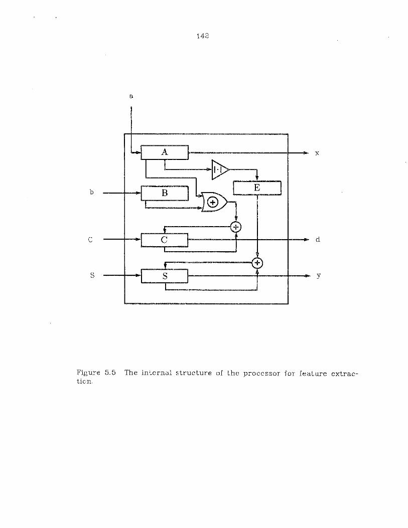
142
a
b
c
B
"...-------'i+
x
d
.r----------(+
S y
Figure 5.5 The internal structure of the processor for feature extraction.
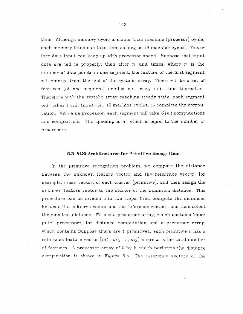
143
time. Although memory cycle is slower than machine (procesor) cycle,
each memory fetch can take time as long as 18 machine cycles. There
fore data input can keep up with processor speed. Suppose that input
data are fed in properly, then after n unit times, where n is the
number of data points in one segment, the feature of the first segment
will emerge from the end of the systolic array. There will be a set of
features (of one segment) coming out every unit time thereafter.
Therefore with the systolic array reaching steady state, each segment
only takes 1 unit times, i.e., 18 machine cycles, to complete the compu
tation. With a uniprocessor, each segment will take O(n) computations
and comparisons. The speedup is n, which is equal to the number of
processors.
5.3 VISI Architectures for Primitive Recognition
In the primitive recognition problem, we compute the distance
between the unknown feature vector and the reference vector, for
example, mean vector, of each cluster (primitive), and then assign the
unknown feature vector to the cluster of the minimUJTI distance. This
procedure can be divided into two steps; first, compute the distances
between the unknown vector and the reference vectors, and then select
the smallest distance. We use a processor array, which contains 'com
pute' processors, for distance computation and a processor array,
which contains Suppose there are l primitives; each :ximitive i has a
reference feature vector [m\, mk, ... , m/~J where k is Lhe total number
of features. A processor array of l by Ie 'which perfo:~ms the distance
computation is shown in Figure 5.6. The reference vectors of the
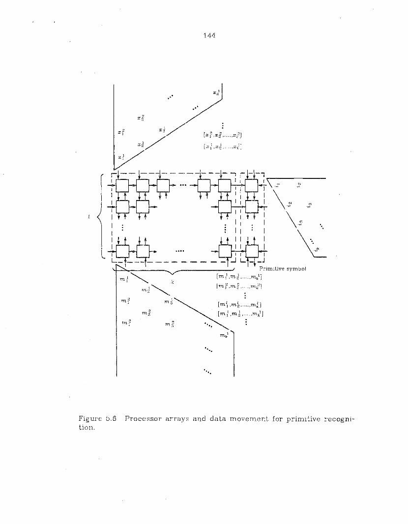
144
,,'
ml............. ,............. .C
md~m 2 mdI
mim 3
m~I
[xf.xi.· ....xlJ
Primitive symbol
[ml.md mkIJ
[mf'.mJ m/]
[m\ .m~ m~J
[ml.m~ mln
" '.
".
Figure 5.6 Processor arrays and data movement for primitive recognition.

145
primitives ent.er from the bottom and move up while the unknown
feat.ure vect.ors ent.er from the top and move down. The partial sums
move from left. t.o right.. The dat.a must be properly skewed as shown in
Figure 5.6 and Figure 5.3(b). Since the two data streams move in oppo
sit.e direction, t.hey must be separated by one unit t.irr~e which is shown
by one space in Figure 5.6; otherwise, some data will just pass instead
of meeting each other.
The unknown feat.ure vect.ors are assumed to come in continuously.
The reference vectors must also repeat their cycles continuously, i.e.,
with the first primitive vector coming right after t.he l th primitive vec
t.or. After initiation, t.he feat.ure vect.ors will be delayed for l-l unit.
times so that the first feat.ure vector and the first primit.ive vector will
meet at. t.he first. row of t.he processor array. The sum, which is equal to
zero initially, will be the distance at. the end of computation. The func
tional diagram of each 'compute' processor is shown in Figure 5.7(a),
where x is a component of the unknown feature vect.or, U is a com
ponent of t.he primitive vector and a is the partial sum. For simplicit.y,
we use the absolute-value distance here. Euclidean dist.ance computa
tion will t.ake more space and time.
The internal st.ruct.ure and data movement are shown in Figure
5.8(a). Each 'compute' processor contains an arithmetic and logic unit
(ALU), and four 16-bit registers A, B, U and X. The micro-operations are
shown as follows.
(1) (a) Transfer data (serially) into register X from the above PE.
146
(b) Transfer data (serially) into register U from the lower FE.
(c) Transfer partial sum (serially) into register A from the left FE.
(2) B ~ X - U.
(3) B ~ IBI.
(4) A~A+B.
Step (1) takes 16 clock cycles to transfer one word of 16 bits; step (2),
(3) and (4) takes 1 clock cycle each. The entire operations take 19
clock cycles. The unit time here is 19 clock cycles.
After computation of the corresponding components between the
reference vector and the unknown feature vector, the partial sum
moves to the right. When the partial sum passes the k th processor of
the first row. the output will be the distance between vectors [x 1, xJ •
... , xJl] and [m f. mJ, ... , mk1], then it enters the rightmost column of
processors. which are the 'compare' processors. Since the data
streams are seperated by one unit time, the processors on alternate
diagonals (from lower left to upper right) are idle. When vector [x f ,xd • ... , xAf] enters the second row of the processor array. it will meet
vector [m f. m~ ..... mn. When vector [xl, x~ . .... x{1 enters the third
row, it will meet vector [m r. m~ mk3 ]; meanwhilE. vector [x r. x~ .
... , Xk2] will meet vector [m r. mf mk2] at row one. We can see from
the above and Figure 5.6 that vector [xl, xi, .... Xk1 ] is compared with
HIe reference vectors in the sequence 1. 2, ... , l, vector [x f. xf, , Xk2]
is compared with the reference vectors in the seque;:1ce 2, 3 , l, 1,
and so forth. These operations are overlapped, i.e., pipelined, in a way
that every processor is doing part of the computation and pass the data
and results to the neighbor processors.
147
The functional diagram of the 'compare' processor is shown in Fig
ure 5. 7(b) where a is the minimum distance computed so far with prim
itive identifier c, b is the distance just computed and d is the
corresponding primitive identifier input externally. The internal struc
ture and data movement are shown in Figure 5.8(b). Each 'compare'
processor contains an ALD, two 8-bit registers B, D and two 16-bit regis
ters A, C. The micro-operations are as follows.·
(1) (a) Transfer partial sum (serially) into register A from C of the
above PE.
(b) Transfer partial sum (serially) into register C from the left PE.
(c) Transfer primitive identifier (serially) into reg:lster B from D of
the above PE.
(d) Transfer primitive identifier (serially) into register D from
external input.
(2) E (- A-C.
(3) If a < c then Ie (- A; D ~ Bl.
Step (1) takes 16 cycles to complete, step (2) takes 1 and step (3)
takes 1. These three steps take 18 cycles, which is 1 cycle shorter than
the 'compute' processor, therefore the 'compare' processcir must be
idle for one cycle in order to synchronize with the 'compute' processor.
The 'compare' processors compare the current dista::l.ce coming from
the left with the distance coming from the above, and pass the smaller
one to the lower processor. Primitive identifiers are fed in from the
right in a similar format as those for data streams. The identifier
streams should be delayed for l +1c -1 unit times so that the first
identifier i 1 enters the flrst 'compare' processor at the same time as
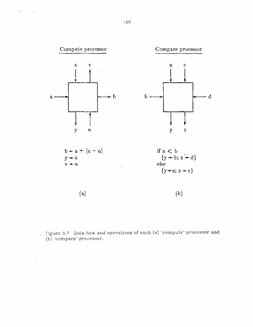
Compute processor
148
Compare processor
x v a c
a--~ b ~ d
y u y z
b~a+ Ix-uly~x
v~u
(a)
if a < b{y~ b; z -::..- d}
else --
{y~a; z ~c}
(b)
Figure 5.7 Data flow and operations of each (a) 'compute' processor and(b) 'compare' processor.
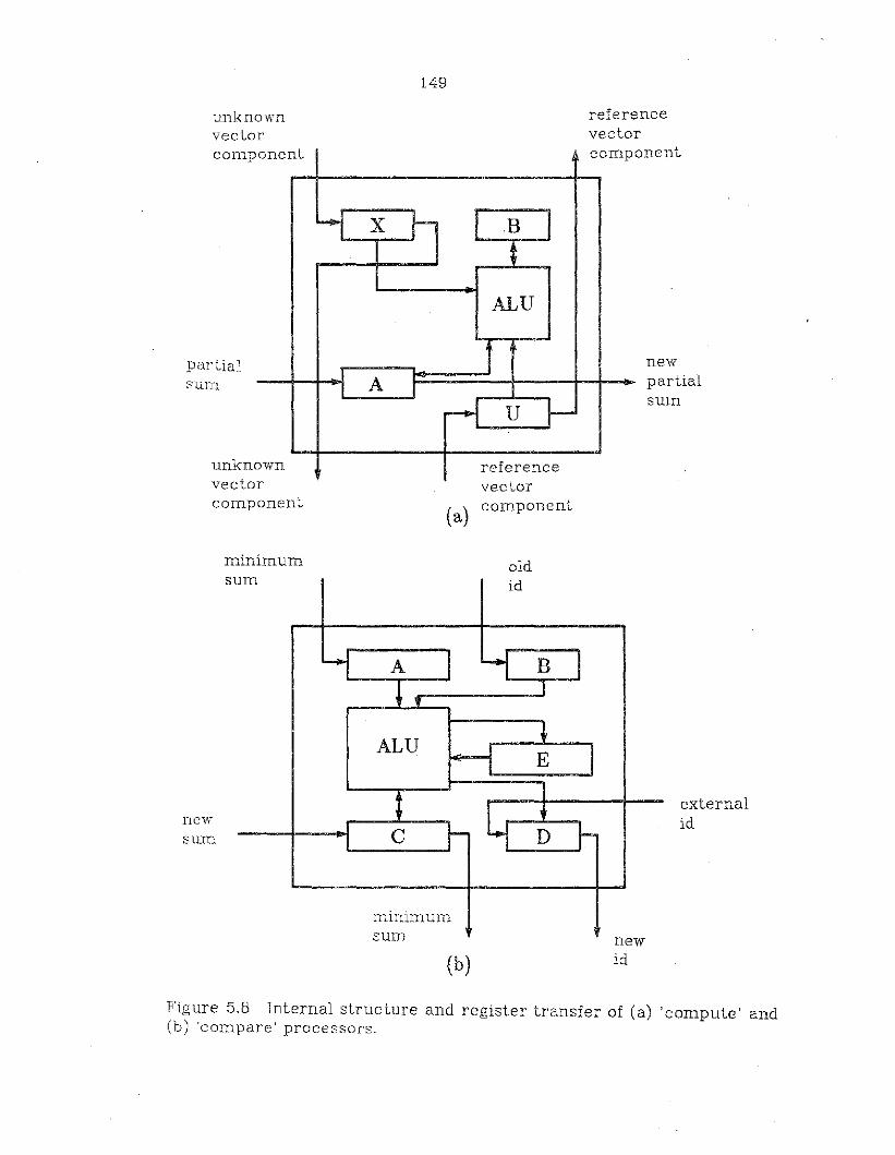
149
newpartialSUln
referencevector
anent
vectorcomponent(a)
anent camp
X r- .B
ALU
I iAI r
r--1 u r--own reference
unknownvectorcamp
unknvectorcom.ponent
partialsum.
minimumsum
oldid
newsum
ALU
externalid
minimum~um
(b)newid
Figure 5.8 Internal structure and register transfer of (a) 'compute' and(b) 'compare' processors.
150
the distance between [x I, xJ, ... , Xl}] and [m I, mJ, ... , m,}], In order
to assign right identifier to right distance, the identifier streams must
be arranged as shown in Figure 5.6.
With a uniprocessor, the primitive recognition procedure of one
feature vector will take lxk computations and l-l comparisons in our
present example. With the processor array of Figure :5.6, the primitive
recognition procedure of a single feature vector needs l x1c + 1 unit
times. However, a processor array is not designed for the processing of
one single datum, instead, it is for a stream of data. In that case, a new
result will come out every 2 unit times in Figure 5.6. Given l reference
vectors and a feature vectors of dimension k, the array processor will
te,ke 2 unit times to get one result in steady state, while a uniprocessor
te.kes O(l xk) time to complete the computation. The speedup is
l >:k /2. In Figure 5.6, the results contain both the minimum distance
and the primitive identifier, therefore no other proces~ing is required.
Primitive recognizer is essentially a vector pattern matcher.
Therefore it can be used in many other applications, and can be used
indepent of feature extraction and string matching.
5.4 VLSI Architectures for String M:atch:ngBased on Levenshtein Distance
Nonnumeric computation has become more important and
demanded more hardware algorithms, i.e., algorithms specially
designed for hardware implementations, and architectures recently
dve to the increasing applications in artificial intelligence, database,
in:'ormation retrieval, language translation, pattern recognition, etc.,
151
One of the most important categories in nonnumeric computation is
string pattern matching. Character string matching is very important
in information retrieval and dictionary look up (Hall and Dowling, 1980).
The problem of string pattern matching can generally be classified into
two kinds. We call them exact matching and approximate matching.
For exact matcing, a single string is matched against a set of strings,
usually this particular string is embeded as a substring of the reference
strings. Hardware algorithms for exact matching has been proposed by
Mukhopadhyay (1979), where the test pattern resides in an array of
cells and the reference text is broadcasted to all the cells simultane
ously character by character. Foster and Kung (1980) designed a VLSI
chip for exact pattern matching with wild card capability, where the
test pattern enters from one end and the reference text enters from
the other end of the linear array. By constrast, for approximate
matching, we want to find a string from a finite set of strings which
approximately matches the test string. Certainly we will also find the
string which exactly matches the test string if it does exist. A good sur
vey of approximate string matching can be found in Hall and Dowling
(1980). This section concentrates exclusively on approximate match
ing. Approximate string matching is based on the dea of insertion,
deletion and substitution of terminal symbols. An application example
of approximate string matching which cannot be performed by exact
string matching is thestrj.ng clustering problems, for example, in Lu
and Fu (1978). Wagner and Fischer (1974) proposed a dynamic pro
gramming method for the computation. Okuda, Tanaka and Kasai
(1976) proposed an algorithm and hardware implementation for garbled
word recognition based on the Levenshtein Nietric. We propose in this

152
section a VLSI architecture for approximate string matching. The dis
tance measure is (weighted) Levenshtein distance using dynamic pro
gramming method. Although it is using the minim.lm-distance cri
te:C'ion in deterministic cases; it can be easily modified to the
maximum-likelihood criterion in probabilistic cases.
Chiang and Fu (1979) studied several parallel architectures,
namely, SIMD, dedicated SIMD and MIMD, for string and tree distance
computation. Each node on the same diagonal of the dynamic program
ming matrix is computed simultaneously. The time complexity of these
specific parallel systems is O(n+rn), where nand rn are the lengthes
of the two strings under comparison. Our system, differs from theirs in
that we use a systolic array, i.e., a square array of PE's as in Ackland, et
al. (1981) and pipelined data flow for the computation. Therefore we
can obtain the results at a constant rate, i.e., one result after each unit
time.
It is well-known that Levenshtein distance can be computed by
dynamic programming. Therefore, it can be implemented by parallel
processing on VLSI architectures. In this case, parallel computation
and pipeline data flow are combined to process continuously a large
amount of data at a very high speed. The dynamic programming algo
rithm recursively computes the optimal path from point (1,1) to (rn ,n)
based on its subpaths. In dynamic time warping, there are many slope
constraint.s for selecting subpat.hs. Ackland et al. (1981) chose t.he sim
plest constraint, i.e.,
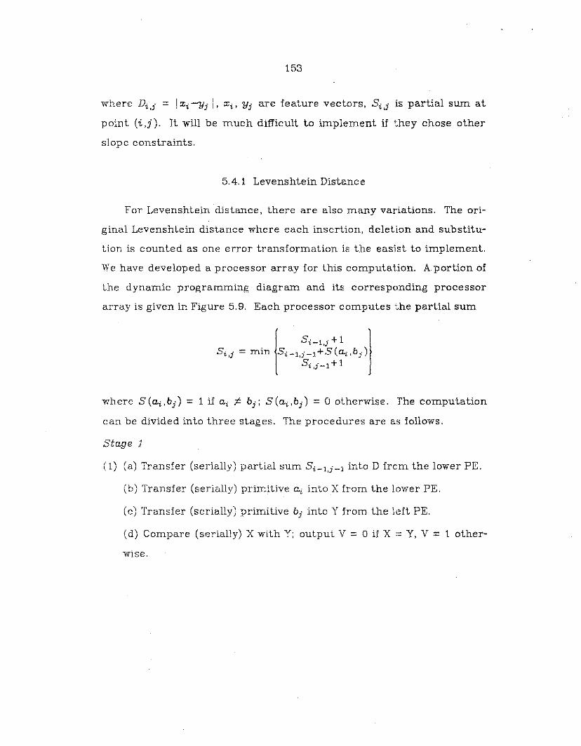
153
where Di,j = Ixi -Yj I, Xi, Yj are feature vectors, Si,f is partial sum at
point (i,i). It will be much difficult to implement if ~~hey chose other
slope constraints.
5.4.1 Levenshtein Distance
For Levenshtein distance, there are also many variations. The ori
ginal Levenshtein distance where each insertion, deletion and substitu
tion is counted as one error transformation is the easist to implement.
We have developed a processor array for this computation. Aportion of
the dynamic programming diagram and its corresponding processor
array is given in Figure 5.9. Each processor computes ,~he partial sum
where S(ai,bj ) = 1 if ai ;t:. bj ; S(ai,bj ) =0 otherwise. The computation
can be divided into three stages. The procedures are as follows.
stage 1
(1) (a) Transfer (serially) partial sum Si-l,j-l into D frcm the lower PE.
(b) Transfer (serially) primitive Cl.j, into X from the lower PE.
(c) Transfer (serially) primitive bj into Y from the left PE.
(d) Compare (serially) X with Y; output V = 0 if X := y, V = 1 other-
wise.
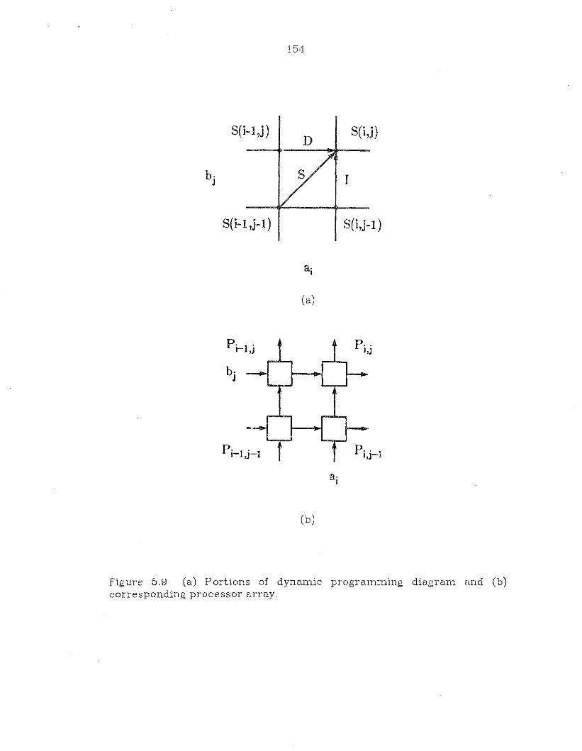
b·J
S(i-l,j)
S(i-l,j-l)
b·J
Pi-l,j-l
154
D
a·I
(a)
a·I
(b)
S(i,j)
I
S(i,j-l)
p..I,J
Figure 5.9 (a) Portions of dynamic programming diagram and (b)corresponding processor array.

155
(2) D ~ D + V.
Stage 2
(1) (a) Transfer (serially) partial sum Si-l,j into B from the left PE.
(b) Transfer (serially) partial sum Si,j-l into C from the lower PE.
(c) Send (serially) partial sum Si-l,j to D of the above PE.
(d) Compare (serially) B with C, A <- min(B, C).
(e) Send (serailly) contents of X to X of the above PE.
(f) Send (serially) contents of Y to Y of the right PE.
(2) A <- A + 1.
(3) Compare (parallelly) A with D, R <- min(A, D).
Stage 3
(1) (a) Send (serially) partial sum R to B of the left PE.
(b) Send (serially) partial sum R to C of the above PE.
Stage 1 takes 17 clock cycles to complete (16 for step (1) and 1 for step
(2)); stage 2 takes 18 (16 for step (1), 1 for step (2) and 1 for step (3)),
and stage 3 takes 16. Figure 5.10 shows the internal slructure and the
operations of processor element Pi,;" at stage 1, 2 and 3. Each PE con
tains a set of registers, an ALD, a control unit and some other combina
tional logic. Registers A, B, C, D, V and R are general-purpose registers
which are 16-bit long and connected to the ALD. Regi~:ters X and Yare
8-bit long, which are used to store primitives. In our seismic case, we
have 13 primitives; therefore, 4 bits should be enol.,gh to represent
them. In fact, 4 bits, which have 16 combinations, should be sufficient
for many practical applications. However, in order to make our system
more flexible and compatible with other systems which use ASCII code,

156
Stage 1
Primitive
a·I
b·J
v
Si-l,j-l
PartialSum
,.......-------1+
Stap;e 2 & 3
PartialSums
LSi-l,j B I +1
[Si,j-l C ]
Figure 5.10 Internal structure and register transfer of PE Pi,j at :stage 1,2 and 3.
157
we let registers X and Y hold 8 bits. This generalization will be able to
recognize character strings where each character is in ASCII code, for
example, A ='01000001', B ='01000010', C ='01000011', and so forth.
Figure 5.11 shows the data movement between 4 neighboring PE's
shown in Figure 5.9. All the processors at the same diagonal performs
the same computation as shown in Figure 5.11 and 5.12(a). This format
will move forward one step every 18 clock cycles. Since each string
only needs three diagonals at any time, the other processors can be
used to compute distances of other strings. Therefore, data fiow can be
pipelined as shown in Figure 5.12(b). If we are matc:t:.ing a test string
against a number of reference strings, the distance between the test
string and the first reference string will emerge after p x 18 clock
cycles, where p is the number of diagonals in the array. After that,
there will be one string distance coming out every 3x 18 = 54 clock
cycles. Since stage 1 and 3 have no conflict, they can be ovelapped, Le.,
one diagonal of the array can be used to perform stage 3 of one string
and stage 1 of the next string at the same time, to increase the
throughput.
The structure of processor array and data flow are shown in Figure
5.13. The reference strings enter from the left; the t,~st string enters
from the bottom. The test string must repeat itself continuously in
order to compare with all the reference strings. Both test and refer
ence strings must be properly skewed and separated as shown in Figure
5.13 so that they will arrive at the right processors aL the right time.
The bookkeeping and selection of minimum distance can be done by a
special-purpose processor or the host computer. One practical prob
lem is about the dimension of the processor array. The number of rows

1v
xl
Ir-----
.,----
Sta
ge1
ryl
H-+
rIyIF
:-txt------
Ix~
stag
e2
i
" 1
rI
1I
i RI
r
J(+
D 1>
-'"
()l
co
y
Sta
ge2
Q Iy
t4
Sta
ge3
Lx
]I
yI
R
ID
II
RI I
tI
HB
I
rlT·~
I===
C='
:=:..
..J
I~
Fig
ure
5.1
1D
ata
mo
vem
en
tb
etw
een
PE
's.
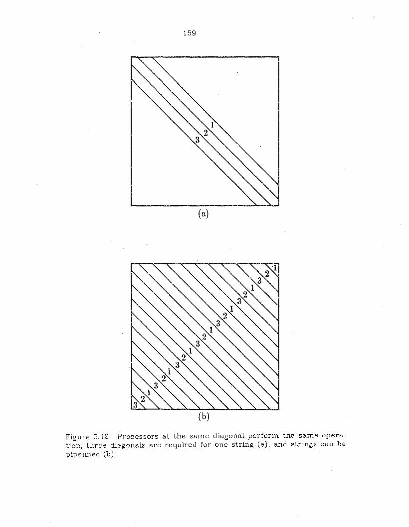
159
(a)
Figure 5.12 Processors at the same diagonal perform the same operation; three diagonals are required for one string (a), and strings can bepipelined (b).
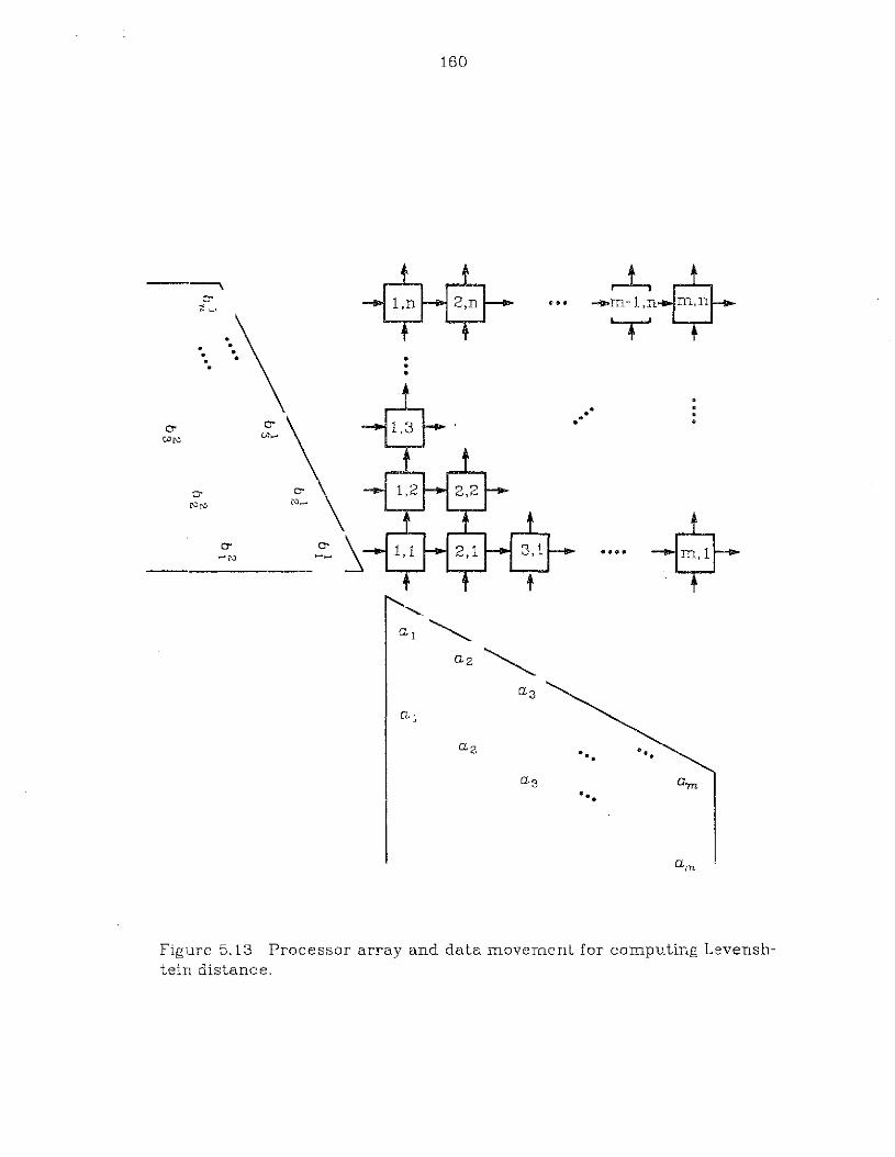
160
....
.... .....
... -$~
Figure 5.13 Processor array and data movement for computing Levenshtein distance.

161
can be set to the maximum length of the reference strings. Since the
length of the test string is unknown, the number of column can be set
arbitrarily. If a test string exceeds the array size, it should be handled
by the host computer or preprocessor. Because the interruption of the
regular computation pattern in a VLSI array will greatly reduce its
efficiency. This situation can be kept to minimum by selecting a
reasonablly large array size. A shorter string will be padded out with
blank to make it equal to the array dimension.
Suppose both the reference and the test string:3 have length l.
With a uniprocessor, the matching process for one unknown string will
take 0 (l Xl) unit operations. With the array processor, it only takes 3
unit times.
5.4.2 Weighted Levenshtein Distances
Since a weighted Levenshtein distance is usually more favorable in
practical application, we now propose a VLSI architec',~ore for its com
putation. The major problem here is to store all the weights in each
processor, which must be easy to implement and fast for access. For
tunately, a programmable logic array (PLA) can be used (Mead and Con
way, 1980). It is a special type of read-only memory, and easy to imple
ment in a VLSI system. A simple example will illustrate how a PLA
works. Figure 5.14 shows a simple weights table and its PLA implemen
tation. A PLA consists of two parts, the left part is called the AND
plane, the right part is called the OR plane. Input lines A, B have the
combinations (0,0), (0,1), (1,0), (1,1) which represent the entries of the
weight table. The output XYZ indicate the values of the entries, which
range from 0 to 7. The circles indicate connections. Since we only have
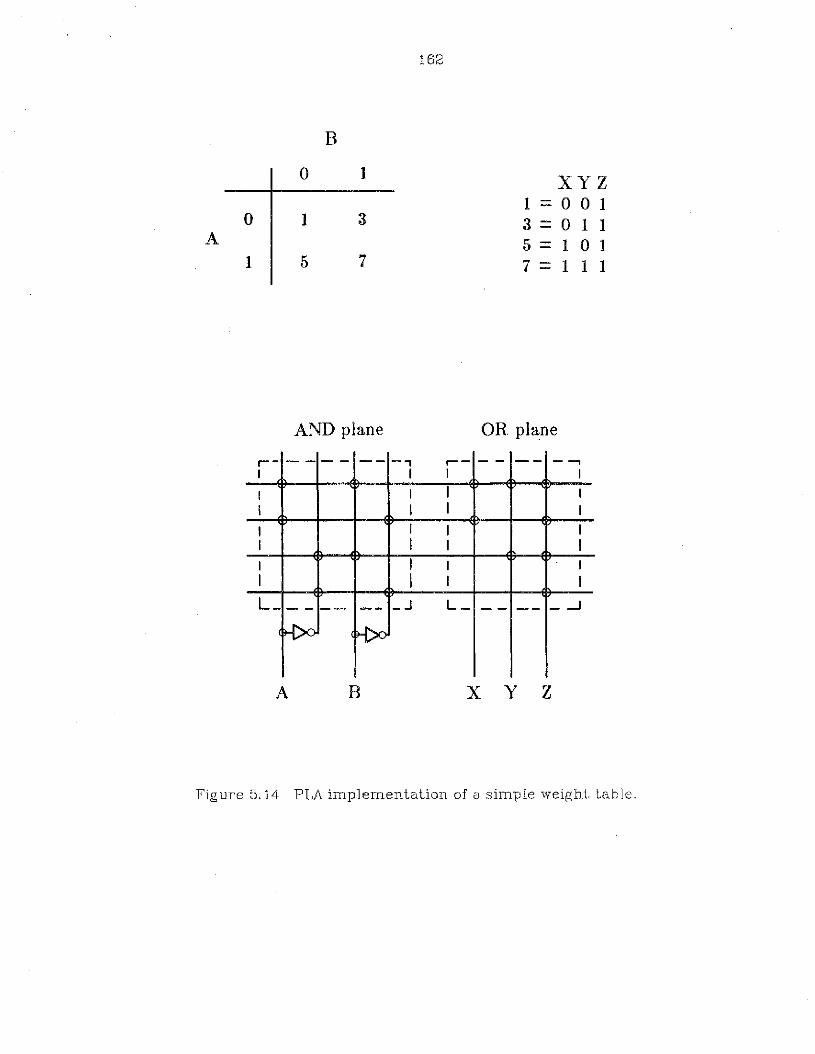
162
B
0 1 XYZ1 = 0 0 1
0 1 3 3 = 0 1 1A 5 = 1 0 1
1 5 7 7 = 1 1 1
AND plane OR pl~ne
,- -- - - -- -, r-- - - -- -....,I I I I
I I I II I I I
I I I II I I II I I II I I IL_ -- -- -- _ .J L _ -- -- _-oJ
4>0 K>o
A B x Y Z
Figure 5.14 PLA implementation of a simple weight table.

163
13 primitives, 4 bits will be enough for discrimination. We take the 4
least-significant bits (LSB) from the primitives for our internal compu
tation, for example, a = '0001', b ='0010', C = '0011', and so forth. We
need more bits for recognition of character strings. Figure 5.15 shows
the PLA implementation of weight table for substituti:m, insertion and
deletion in our seismic case. There is an input register to the AND
plane and an output register from the OR-plane; both are 8-bit long.
Register X contains primitive 'a', and register Y contains primitive 'b';
(a, b) is the entry of the weight table. Here the symbols X, Y, A and B
are registers which should not be confused with those in Figure 5.14.
The pair (X = a, Y = b) represents the substitution of 'b ' for 'a'. The
pair (X =a, Y =0000) represents the deletion of 'a'. The pair (X =0000,
Y = 6) means the insertion of 'b ' . The access tilne is very fast, only two
clock cycles; one is needed for input register, the other is for output
register.
Except for the weight table, the computation procedure is similar
to the previous one. The internal structure of the PE's is given in Fig
ure 5.16. Each PE has an ALD, a PLA (With registers Q and S), a control
unit, two 8-bit registers X, Y and three 16-bit registers B, C, and D.
Register Z contains constant '0000' as symbol A. The clata movement is
similar to that in Figure 5.11.
Stage 1
(1) (a) Transfer (serially) partial sum Si-l,j-l into D from the lower PE.
(b) Transfer (serially) primitive ~ into X from the lower PE.
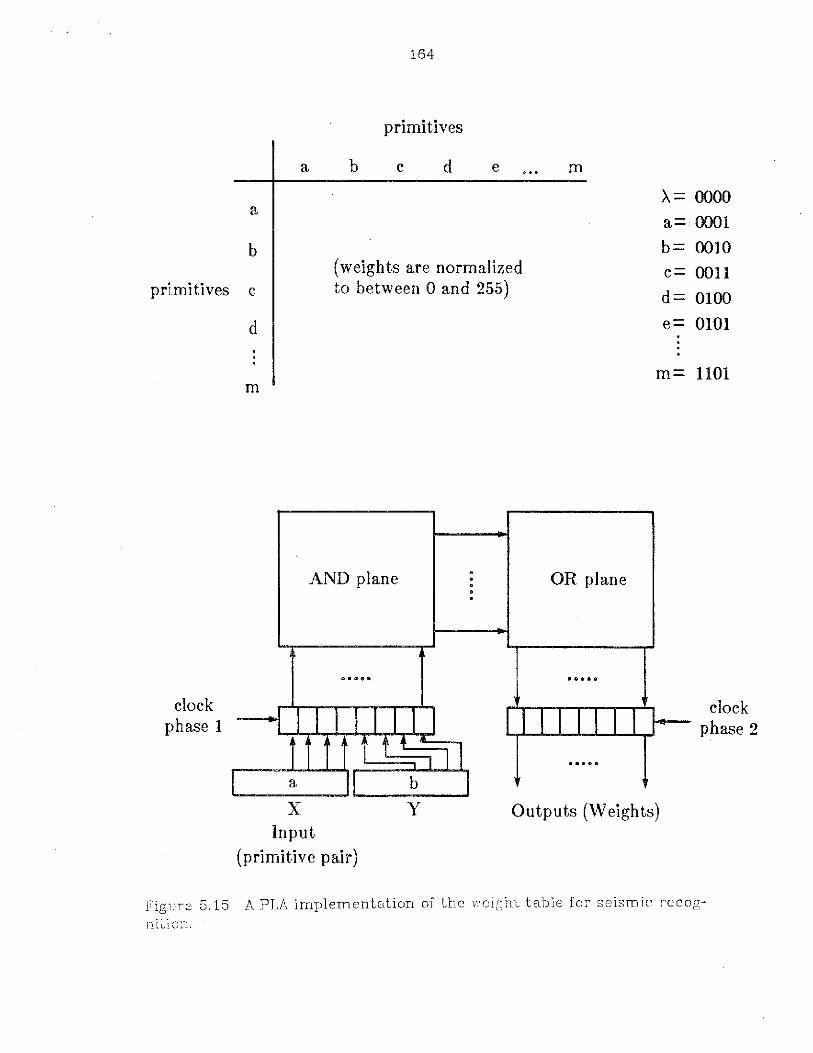
164
primitives
a b c d e m
a
b
primitives c
d
m
(weights are normalizedto between 0 and 255)
A= 0000
a= 0001
b= 0010
c= 0011
d= 0100
e= 0101
m= 1101
clockphase 1
AND plane
XInput
(primitive pair)
··oo·OR plane
Outputs (Weights)
clockphase 2
Figure 5.15 A PLA implementation of thewcighL table for seismic reeog-
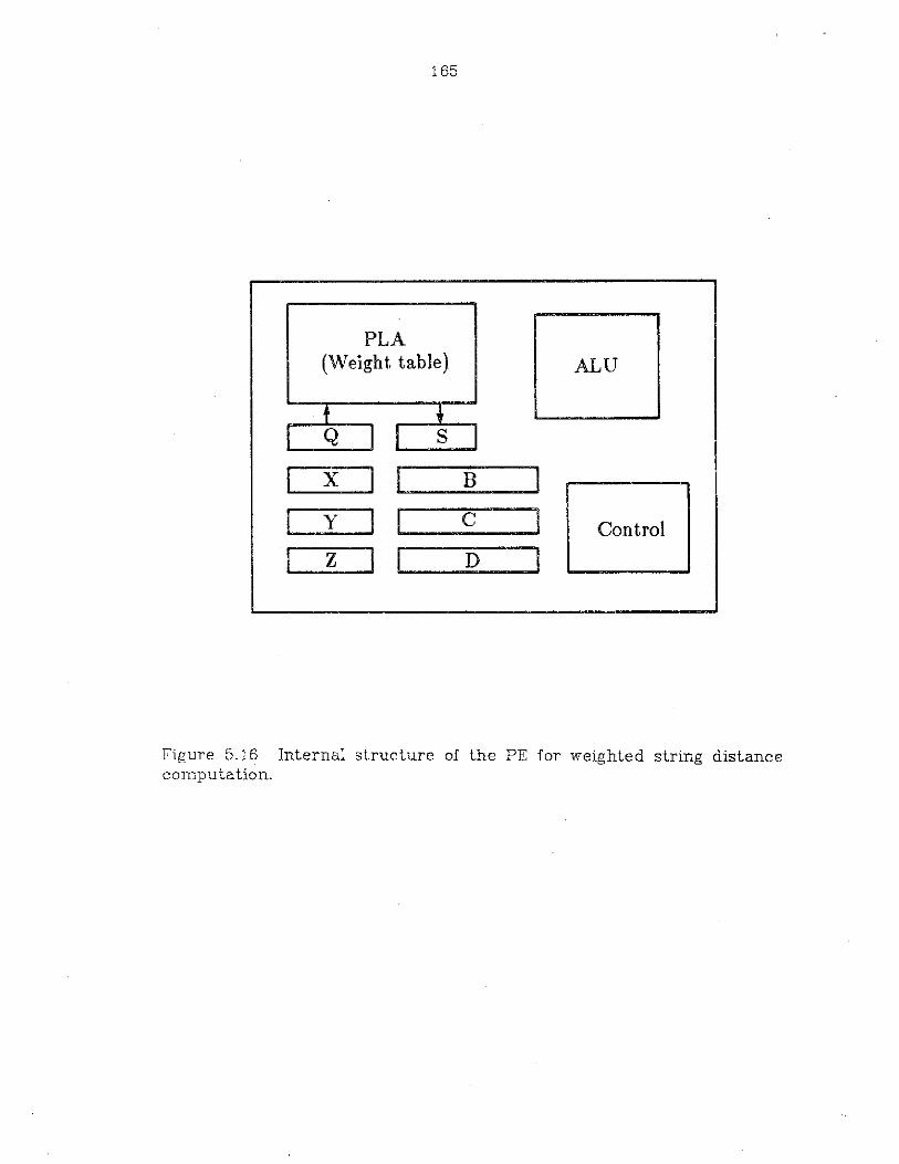
165
PLA(Weight table) ALU
t TQ I I s
I X I [ B II y I [ c ] Control_.
I z I I D I
Figure 5.16 Internal structure of the PE for weighted string distancecomputation.
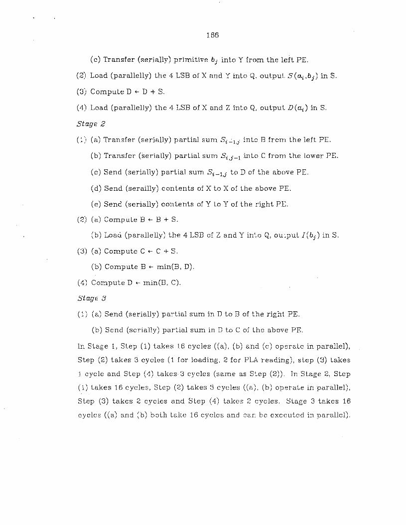
166
(c) Transfer (serially) primitive b j into Y from the left PE.
(2) Load (parallelly) the 4 LSB of X and Y into Q, output S (CLj, ,bJ.) in S.
(3) Compute D ~ D + S.
(4) Load (parallelly) the 4 LSB of X and Z into Q, output D (CLj,) in S.
stage 2
(1) (a) Transfer (serially) partial sum Si';"l,j into B from the left PE.
(b) Transfer (serially) partial sum Si,j-l into C from the lower PE.
(c) Send (serially) partial sum Si-l,j to D of the above PE.
(d) Send (serailly) contents of X to X of the above PE.
(e) Send (serially) contents of Y to Y of the right PE.
(2) (a) Compute B ~ B + S.
(b) Load (parallelly) the 4 LSB of Z and Y into Q, ousput l(b j ) in S.
(3) (a) Compute C ~ C + S.
(b) Compute B ~ min(B, D).
(4) Compute D ~ min(B, C).
Stage 3
(1) (a) Send (serially) partial sum in D to B of the right PE.
(b) Send (serially) partial sum in D to C of the above PE.
In Stage 1, Step (1) takes 16 cycles ((a), (b) and (c) operate in parallel),
Step (2) takes 3 cycles (1 for loading, 2 for PLA reading), step (3) takes
1 cycle and Step (4) takes 3 cycles (same as Step (2)). In Stage 2, Step
(1) takes 16 cycles, Step (2) takes 3 cycles ((a), (b) operate in paralle!),
Step (3) takes 2 cycles and Step (4) takes 2 cycles. Stage 3 takes 16
cycles ((a) and (b) both take 16 cycles and can be executed in parallel).
167
Therefore, Stage 1 takes 23 cycles, Stage 2 takes 23 cycles, and Stage 3
takes 16 cycles. As usual, stage 3 can be overlapped. with stage 1 to
save processing time. Due to the weight computation, this system
takes longer time than the previous one.
5.5 Simulations and Performance Verrnc,3.tion
Simulations have been performed for the three systolic arrays:
feature extraction array, primitive recognition array and string match
ing array. The flow charts for the simulations are given in Appendix A.
The same seismic data as those used in Section 3.5 :lre tested in the
simulations. The results of the simulations are exactly the same as
those of the sequential computer in Section 3.5. Therefore the design
of the systolic arrays are correct and the operations are as expected.
Step-by-step simulation results using sample seismic waveforms are
given in Appendix B. The computation time in our simulation is shown
in Table 5.1. The computation time using a sequential computer is also
given for comparison. it is noted that the listed comp.ltation time is an
average and approximate time which should be used for comparison
only. Suppose that we are dealing with a large amout of data. Similar
to the definition of speedup for multioperation computer in Kuck
(1978), we define the theoretical speedup (TS) of a (systolic) processor
array as
TS =time interval between consecutive
results using a sequential computertime interval between consecutive
results using a processor array

TA
BL
E5
.1
Co
mp
uta
tio
nti
me
of
seq
uen
tial
alg
ori
thm
,si
mu
late
dco
mp
uta
tio
nti
me
for
VL
SI
arr
ay
su
sin
gse
qu
en
tial
co
mp
ute
r,re
al
speed
up
s,th
eo
reti
cal
speed
up
san
dsp
eed
up
rati
o.
(All
co
mp
uta
tio
ns
are
for
on
ese
ism
icre
co
rdo
req
uiv
ale
nt
on
est
rin
g)
Seq
uen
tial
Sim
ula
ted
Rea
lT
heo
reti
cal
Sp
eed
up
Alg
ori
thm
VL
SI
arr
ay
sS
peed
up
Sp
eed
up
Rate
I>
-' m(s
ec.)
(sec.)
co
Featu
re0
.30
.00
56
06
010
0%E
xtr
acti
on
Pri
mit
ive
0.1
0.0
06
17
.41
9.5
89%
Reco
gn
itio
n
Str
ing
0.0
70
.01
54
.67
6.6
770
%M
atc
hin
g

169
Therefore the 1'8 for feature extraction is 60/1 = 60, for primitive
recognition is 39/2 = 19.5 and for string matching is 20/3 = 6.67. The
numerators are the numbers of operations for getting one result using
a sequential computer, and the denominators are the time intervals
between consecutive results for VL8I arrays as shown in the previous
sections. Note that the 1'8 for string matching in our experiment is
20/3 = 6.67 instead of 20x20/3 = 133. This is because we only consider
substitution errors, therefore the number of operatioJ:'ls is proportional
to string length, i.e., 20. If insertion and deletion errors are to be con
sidered, then the whole dynamic programming matrix as shown in Fig
ure 2.1 should be considered. In the seismic recognition problem the
size of the matrix is 20x20.
The real speedup in our simulations for featLre extraction is
approximately the same as the maximum theoretical speedup. This is
due to the simple structure and data flow of the linearly connected sys
tolic array. The real speedup (17.4) for primitive recognition is slightly
less than the 1'8 (19.5), which is 89% of the TS. The reason for this is the
increasing complexity of array structure and data flow. More time is
spent on data movement. The real speedup (4.67) for string matching
is also less than the 1'3 (6.67), which is 70% of the 1'3. This is because
the array structure and data flow are even more complicated. The
increasing complexity can be seen from the the desigrs in previous sec
tions. The theoretical speedup is the upper bound where the real
speedup in simulation is a function of the computations performed and
the underlying architectures.
The simulations are performed on a sequential computer (VAX
11/780). In order to compare the simulation results vrith the results in
170
Chapter III we use the same high level languages (C, Fortran and Pas
cal). Therefore, there are many overhead in language translation and
program execution. These are some of the reasons for low speedup.
Another reason is data movement which can be performed in parallel
with the computation in VLSI arrays, but can not be done in a sequen
tial computer. One can not accurately simulate the VLSI system even
using an assembly language. Since most systolic arrays are hardwired,
Le., unprogrammable, there is no instruction decoding or memory
fetch and storage for each instruction. Besides, the parallelism can not
be fully simulated on a sequential computer. The real computation
speeds of the proposed VLSI arrays when fabricated should stay close to
the analytical results as shown in the previous sections, i.e., 1 unit time
for feature extraction, 2 unit times for primitive recol5nition and 3 unit
times for string matcing using WLD.
We would like to consider some problems about actual implementa
tion and give some examples about the performancE' of our proposed
system. In Section 5.2 we assumed that the length of '"he linear systolic
array is the same as the number of points in each segment. Although a
linear array can be expanded easily, it is sometimes necessary to use
small array to process data of larger size. For example, in the seismic
recognition problem, the number of points in each segment is 60. We
can use a linear array consisting of 60 PE's, or we can use less PE's, for
example, 20 PE's. The implementation using 20 PE's is shown in Figure
5.17, where the data points in each segment are folded into three rows.
This will take three unit times to compute the features for each seg
ment. Suppose there are 20 PE's with machine cycle 200 ns, then the
time required for feature extraction of 2,000 segments (after it reaches
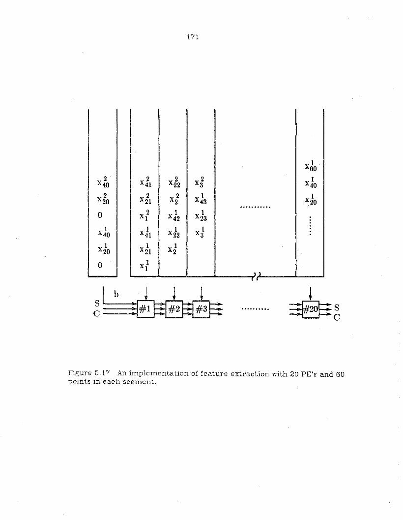
171
IX60
2 2 2 xl IX40 X 41 X22 X40
2 2 X 2 I 1X20 X21 2 X43 X20
a •• e.lt"~3O.
0 X 2 1 I1 X42 X23
I 1 I xiX40 X41 X22
I I XlX20 X21 2
0 Xl1 ,,
c (
~lb
E~ ~~•• 0 •••• "a.
Figure 5.17 An implementation of feature extraction with 20 PE'~ and 60points in each segment.
172
steady-state) is equal to 3 x 18 x 2000 x 200 ns =21.6 ms. The time for
reaching steady-state is 20 unit times, which is equal to 20 x 18 cycles
x 200 ns/cycle = 72 f..lS. Since the processing speed of feature extrac
tion (18 cycles) is faster than that of primitive recognition (19 cycles),
the output of the former can be used directly by the hUeI'. Recall that
the input data for primitive recognition are interleaved by one space
(Figure 5.3(b )). The feature vector of the next segm,~nt is not needed
until after 2 x 19 cycles = 38 cycles. Therefore 30 PE s can be used for
feature extraction and produce a feature vector every 2 x 18 cycles =36 cycles. Because 30 PE's take 2 unit times to produce a result and
each unit time is equal to 18 cycles. These two opera.tions can be exe
cuted in parallel to save a half of the total processing time.
Consider string matching using Levenshtein di~;tance, the com
pa.rison of one test string with each reference string takes 3 x 18 x 200
ns = 10.8 f..lS. With one hundred reference strings, it takes 1.08 ms to
classify each test string, and each test string is exec·~ted sequentially.
Using a systolic array it is possible to make real-time string matching.
Our system can match approximately 90,000 strings per second (10.8
f..lS for one string).
oNe assume in the previous discussion that all strings, test and
reference, have the same length. This is not true in many other appli
ca.tions. Reference strings are different in length; dmensions of pro
cessor array can not fit exactly the string size. It is required to make
processor array larger than the string size and pad the string with
blank at the end. If we let the weight of insertion, deletion and substi
tution of blanks be zero, then we can solve the problem of length
variety and still maintain the regular, synchronous data fiovV' pattern.
173
Long strings and larger array size do not degrade the steady-state
throughput. As usual, results can be obtained every 3x18 =54 cycles.
It only takes longer time, i.e., F x 18 cycles where F is the number of
diagonals, to reach steady-state. Usually the time to reach steady
state is negligible compared with the total processing time.
The system bus as shown in Figure 5.1 is similar to the Unibus of
DEC PDP-i1 (Kuck, 19(8). The Unibus has a maximum data rate of
4Xi07 bits/sec operating in an interlocked way, Le., the sender waits
until the receiver acknowledges receipt of a word before sending
another word. In our experiment, each seismic record has 1200 points,
and each point is coded into a i6-bit binary number. Therefore, each
seismic record needs 16x 1200 = 19200 bits of storage. It is easy to see
that the system bus can transmit one seismic record from disc to
special-purpose processor in 0.48 ms. However, the typical operating
speed of magnetic disc is from 2.4Xi05 bits/sec to 1.2X107 bits/sec
(Stone, 1980). Therefore the actual time for sending a seismic record
from disc to special-purpose processor is from 80 ms to 1.6 ms. The
output from the special-purpose processor is the classification results,
which use one word (16 bits) for each seismic record to indicate class
membership. The transmission time is 0.4 f..lS for one record.
5.6 Concluding Remarks
We have proposed special-purpose array processors for seismic sig
nal classification, which can be attached to a general-purpose computer
as shown in Figure 5.1. The host computer can retrieve any intermedi
ate data frorna special-purpose processor and store them in its own
174
storage, as well as send data to any memory unit of th2 special-purpose
processor. For example, the host computer can retrieve and store the
string representation of the signals for display or for later use. The
host computer can also use anyone of the systolic arrays, for example,
feature extraction array, only.
The design correctness and speedup have been verified by simula
tions in Section 5.5. From the simulation results it is safe to predict
that the real speedup of the fabricated VLSI processor arrays will be
close to the theoretical speedup. Computer-aided design has greatly
reduce the design cost (Swerling, 1982). The cosUper'ormance ratio of
special-purpose processors will eventually be justified.
Recently, VLSI architectures have been applied to syntactic pattern
re2ognition and to implement parallel computation. Guibas, et al.
(U379) proposed two VLSI arrays for the implementation of combina
todal algorithms, one is for a subset of dynamic programming prob
lems, i.e., optimal parenthesization problems which include context
free language recognition, the other is for transitive closure problems
wt.ich include finite-state language recognition. Based on the array
structure of Guibas, et al., Chu and Fu (1981) proposed VLSI architec
tures for finite-state language recognition and context-free language
recognition using CYK's algorithm. Chiang and Fu (19132) also proposed
a VLSI systems for context-free language recogniticn using Earley's
algorithm. Ackland et al. (1981) developed a VLSI systems to imple
ment dynamic time warping for spoken word recognltion. Our string
matcher can be applied to any problem where the Levenshtein di.stance
computation is required. It can be used for string matching in our
selsmic recognition, for character string matchinr in information
175
retrieval (Hall and Dowling, 1980) or for pattern matching in shape
analysis if the object can be represented by a string, ,faT example,
using chain codes (see Fu, 1982). Our primitive recognizer can also be
applied to any minimum-distance recognition problem and vector pat
tern matching.
176
CHAPTER VI
SUMMARY, CONCLUSIONS, AND RECOMI~ENDATIONS
6.1 SummaIy
We have studied the application of syntactic pattern recognition to
sE'ismic signal classification and proposed special-purpose VL::iI archi
tectures for the implementation. Our studies concentrate on the
waveforms where shape information is not important or useful, like
seismic signals. EEG and speech signals have similar characteristic as
seismic signal. Chapter I defines the problem of study, oun.nes the
approach to the problem and gives relevent literature survey. Chapter
II discusses string similarity (distance) measures and recognition pro
cedures. String distances have been classified into two categoLes: gen
eral string distances which are based on the concept of insertion, dele
tion and substitution transformations and special string distances.
General string distances are further classified into a hierarchy of four
levels. Symmetric property of string distance has also been di:3cussed.
Recognition can be carried out by either nearest-neighbor decision rule
or error-correcting parsing. We use a modified Earley's parsing algo
rLhm which does not require an expanded grammar and is able to use
symmetric distance.
177
Chapter III demonstrates the experimental results of seismic
discrimination and damage assesment. If shape is not the major
feature, pattern segmentation is often simpler. We only need to con-.
sider fixed-length segmentation. When shape information is the dom
inant feature, pattern segmentation is usually associated with primitive
recognition. Generally speaking, a fixed-length segmentation :',s easier
to perform; a variable-length segmentation is more efficient in
representation. However, a variable-length segmentation usually takes
more time in determining the optimal boundary. Furthermore, a
variable-length segmentation sometimes starts from fixed-length seg
mentation and then merges or splits based on a preset criterion. In
general, we are in favor of fixed-length segmentation provided a. proper
length can be easily selected. Feature selection is problem-dependent;
therefore we did not emphasize on this subject. Primitive recognition
is our first major topic in practical applications. Without any knowledge
about the data, we use a clustering procedure to find the optimal
number of clusters. Two criteria, increment of merge distance and
pseudo F-statistic (PFS), have been used to select cluster number and
they show identical results. Finite-state grammars are inferred from
. the training patterns using the k-tail inference algorithm.. Unless the
patterns are really generated by a finite-state grammar, chosing small
values of k usually worsens the classification result. Our experiments
show that uneven merge of states makes the inferred grammar perform
ing poorly in recognition. Whenlthe inferred grammar is the canonical
grammar, the recognition results of using NN rule and ECP are the
saIne. According to our experiment, the NN rule takes however much
less computer time than ECP. A modified dynamic time-warping
178
system has been used to measure the distance between the seismic
waveforms of the building during a strong earthquake. This measure
rnent can be used for damage assesmenL
Chapter N introduces an attributed grammar and parsing for sig
nal recognition in general, and seismic recognition in particular. If we
use a canonical grammar as the pattern grammar, it usually contains a
large number of production rules and nonterminal symbols. Using
attributes will increase the descriptive power of the grammar as well as
simplify the syntactic rules of the grammar. We use a length attribute
for seismic grammar, which reduces more than 90% of the number of
productions and nonterminals from the nonattributed grammar. Attri
buted seismic grammars also increase the recognition speed while
maintaining the same recognition accuracy.
Chapter V contains VLSI architectures for string matching, primi
tive recognition and feature extraction. Although some special'-purpose
chips have been developed for signal recognition, for example, spoken
word recognition, we are making our systems as general as possible.
This is to say our string matcher and primitive recognizer with the
exception of feature extractor can be applied to any other pattern
recognition problem. They employ parallel processing and pipeline
data flow so that very fast throughput can be achieved. This improve
ment of speed makes real-time pattern recognition possible.
179
6.2 Conclusions
Syntactic pattern recognition has been pointed out as a promising
approach to seismic classification (Chen, 1978). While quite a few sta
tistical approaches have been proposed, we are the first to apply syn
tactic approaches to this problem. With two simple features, our
approaches attain better results (91% correct rate) than most of the
existing statistical approaches (Tjostheim, 1975; Sarna and Stark,
1980). Our approaches also differ from the syntactic methods in
Chapter I in the treatment of primitive selection and grammar con
struction. A clustering procedure along with two decision criteria con
stitute the primitive selection algorithm in our approach, while heuris
tic approaches were used by others, e.g., in Stockman, et al., (1976).
Our pattern grammars are inferred from training samples, but most
pattern grammars for signal analysis are constructed manually. An
attributed grammar for the seismic application is proposed, which
could significantly reduce the grammar size and increase the recogni
tion speed. Finally, VLSI architectures are proposed for seismic
classification, which include feature extraction, primitive recognition
and string matching using (weighted) Levenshtein distance. Our string
matcher is different from many contemparory implementations, i.e.,
exact matching (e.g., in Foster and Kung, 1980), which are not suitable
for pattern recognition applications because of the noise and other
problems, for example, segmentation and primitive recognition errors;
the detail is discussed in chapter V. The computational results can be
produced at a constant rate, i.e., constant time corn.plexity, when using
our VLS1 architectures with pipelined data flow. Although these VLS1
systems are developed for seismic classification, they can be applied to
180
other similar applications.
6.3 Recommendations
Future works about syntactic seismic signal recognition can be
divided into two parts, one is algorithm development, the other is high
speed implementation. (This can also be applied to other signal recog
nition problems.) In algorithm development, the possibility of using
variable-length segmentation should be explored. Stochastic grammars
and parsing should be applied when probabilistic information is avail
able. The inclusion of semantic information in pattern primitive is
another approach (Tsai and Fu, 1980). A conventional pattern
re:oresentation contains only syntactic symbols. A typical speech pat
tern for dynamic time warping contains only numerical infomation. A
combination of these two will have both syntactic and semantic infor
mation. The distance computation and parsing of such patterns can be
separated into syntactic deformation and semantic deformation, and
different weights can be assigned to these two deformations. Feature
extraction also needs further studies; linear predictive coefficients and
feEtures from power spectrum are good candidates.
After the algorithms are developed, they can often be implemented
on a parallel architecture, particularly on VLSI architectures. In our
string matcher, a global path constraint can be imposed, therefore
reduce the number of processors. Those special-purpose chips can be
arranged in such a way that the output of one chip is used directly as
the input of another chip. Of course, this can happen only wher all the
chips have the sarne processing speed; oUlCcwisc, buflen: or luLchcs are

181
required between the chips. Although these chips are for special pur
poses, flexibility should also be considered. The more fiexible the chips
are, the more applications they have; therefore, makes their manufac
turing cheaper. This combination of algorithm development and tech
nology advance will make many pattern recognition applications practi
cal in both cost and speed.
The application of attributed grammar using length attri'aute to
speech recognition should also be investigated. Suppose two strings
x =aaaaaabbbccc and y =aaaabbcc represent different utterances of
the same word. If we use string matching and NNR for classification,
then d (x ,y) 1= 0 regardless that we use the conventional Levensh
tein distance or weighted Levenshtein distance. Ackroyd (1980) sug
gested a modified WLD which is computed by subtracting II -J IdID
from the WLD, where I, J are the lengths of the two strings respectively
and dID is the weigth for insertion and deletion. Although this modified
WLD can make d (x ,y) =0, it will cause other problems, for example,
d (y ,z) = 0 for z =aaa. The type 3 WLD proposed in Chapter 2 can solve
this problem by letting D(a,a) = l(a,a) = 0 for all a E:~. However,
there exists one drawback, i.e., there is no restriction on the number of
insertions or deletions. An attributed grammar using length attribute
can be used to solve this problems without side effects. For example, if
string x is .the training sample, then the attributed grammar has pro
d uction S -)ABC with inherited length attribute (l6,4L f3,2l, f3,2D for
(A,B,C). This attributed grammar will accept both string x and y, but
not z.
182
LI;3T OF REFERENCES
[( Ackland, B., Weste, N. and Burr, D.J., 1981. "An integrated multiprocessing array for time warping pattern matching," Proc. 8thAnnu. Symp. on Comput. Archil. May 12-14, Minneapolis, pp.197-215.
[2J Ackroyd, M. H., 1980. "Isolated word recognition using theweighted Levenshtein distance," IEEE Trans. Acous. Speech, Signal Processing, vol. ASSP-28, no. 2, pp. 243-244.
[3~ Aho, A.V. and Peterson, T.G., 1972. "A minimum distance errorcorrecting parser for context-free languages," SIAM J. Comput.,voL 1, no. 4, pp. 305-312.
[4] Aho, A.V. and Ullman, J.D., 1972. The Theory of Parsing, Translation and Compiling, Prentice-Hall, Inc., vol. 1,542 pp.
[5] Albus, J.E., 1977. "Electrocardiogram interpretation using a stochastic finite state model," in Syntactic Pattern RecognitionApplication, ed. by Fu, K.S., Springer-Verlag, pp. 51-64.
[6] Allen, R.V., 1978. "Automatic earthquake recognition and timingfrom single traces," Bull. Seismol. Soc. Amer., vol. 68, no. 5, pp.1521-1532.
[7] Anderson, K.R., 1978. "Automatic Analysis of Microearthquake Network Data," Geoexplor, vol. 16, pp. 159-175.
[8] Atal, B.S. and Hanauer, S.L., 1971. "Speech analysis and synthesisby linear prediction of the speech wave," J. Acoust. Soc. Am., vol.50, no. 2, pp. 637-655.
[9] Bath, M., 1977. Spectral Analysis in Geophysics, Elsevier, NewYork, 563 pp.
[10] Bath, M., 1979. Introduction to Seismology, Birkhauser Berlag,Boston, 428 pp.
[l1J Biermann, A.W. and Feldman, J.A., 1972. "On the synthesis offinite-state machine," IEEE Trans. Compnt., vol. C-21, pp. 592597.
183
[12J Blair, C. R., 1960. "A program for correcting spelling errors,"Inform. Contr., vol. 3, pp. 60-67.
[13J Bois, P., 1981. "Reservior recognition in petroleum prospectionconsidered as an application of close man-machine communication," Froc. 2nd Int. Symp. on Comput. Aided Seismic Analysisand Discrimination, North Dartmouth, Massachusetts, pp. 42-47.
[14J Bolt, B.A., 1976. Nuclear Explosions and Earthquakes, The PartedVeil., W. H. Freeman and Co., San Francisco, 309 pp.
[15J Booth, T.1., 1967. Sequential Machines and Automata Theory,Wiley, New York.
[16J Bowen, B. A. and Brown, W. R., 1982. VLSI Systems Design ForDigital Signal Processing. Prentice-Hall, Inc., New Jersey.
[17J Box, G.E.P. and Jenkins, G.M., 1976. Time Series Analysis -forecasting and control, Holden-Day Inc., San Francisco, 575 pp.
[18J Carnahan, B., Luther, H. A. and Wilkes, J. 0., 1969. Applied Numerical Methods, John Wiley & Sons, Inc., New York.
[19J Chen, C.H., 1978. "Seismic Pattern Recognition," Geoexplor, vol.16, no. 1/2, pp. 133-146.
[20J Chiang, Y. and Fu, K. S., 1981. "Parallel processing for d'.stancecomputation in syntactic pattern recognition," Proc. IEEEWorkshop on CAPAIDM. Nov. 11-13, Hot Springs, VA.
[21J Chiang, Y. and Fu, K. S., 1982. "A VLSI architecture for fastcontext-free language recognition (Earley'S algorithm) ,It 3rd Int.Conj. Distributed Computing Systems. Oct. 12-15, Ft. Lauderdale, FL.
[22J Chou, S.M. and Fu, K.S., 1975. "Transition networks for patternrecognition," Tech. Rept., TR-EE 75-39, Purdue Universiey, Indiana.
[23J Crespi-Reghizzi, S., 1971. "An effective model for grammar inference," Proc. IFfP Congress, Aug., Yugoslavia, pp. 524-529.
[24J Crespi-Reghizzi, S., 1971. "Reduction of enumeration in gra.mmaracquisition," Proc. 2nd Int. Joint conj. Artij. Intel., Sept. 1-3,London, England, pp: 564-552.
[25J Dahlman, O. and Israelson, H., 1977. Monitoring UndergroundNuclear Explosions, Elsevier Scientific Publishing Co., Amsterdam, the Netherlands.
184
[26J DeMori, R., 1972. "A descriptive technique for automatic speechrecognition," IEEE Trans. Audio Eleetroacoustic, AU-21, pp.89100.
[27J DeMori, R, 1977. "Syntactic recognition of speech patterns," inSyntactic Pattern Recognition Application, ed. by Fu, KS.,Springer-Verlag, New York, pp. 65-94.
[28J Duda, R.D. and Hart, P.E., 1973. Pattern Classification and SceneAnalysis, Wiley, New York, 482 pp.
[29J Earley, J., 1970. "An efficient context-free parsing algorithm,"CACM vol. 13, pp. 94-102.
[30J Ehrich, R.W. and Foith, J.P., 1976. "Representation of randomwaveforms by relational trees," IEEE Trans. Comput., vol. C-25,no. 7, pp.725-736.
[31J Flanagan, J.1., 1972. Speech Analysis, Synthesis and Perception,2nd Ed., Springer-Verlag, New York.
[32J Foster, M. J. and Kung, H. T., 1980. "The desssign of specialpurpose V1S1 chips," Computer, vol. 13, no. 1, pp. 26-40.
[33J Fu, K.S., 1973. "Stochastic languages for picture analysis," Computer Graphics and Image Processing, vol. 2, pp. 433 ..A53.
[34J Fu, KS., 1977. "Error-correcting parsing for syntactic patternrecognition," in Data Structure, Computer Graphics and PatternRecognition, ed. by Klinger, A., et al., Acdemic Press, pp. 449-492.
[35J Fu, K.S., ed., 1977. Syntactic Pattern Recognition Application,Springer-Verlag, New York.
[36J Fu, KS., 1978. "Syntactic pattern recognition and its applicationto signal processing," Proceedings oj the NATO Advanced StudyInstitute on Pattern Recognition and Signal Processing, Series E,Applied Science, no. 29, Sijthoff & Noordhoff International Publishers, The Netherland.
[37J Fu, K.S., 1982. Syntactic Pattern Recognition and Applications,Prentice-Hall, Inc., New Jersey, 596 pp.
[38J Fu, K.S. and Huang, T., 1972. "Stochastic grammars andlanguages," Intern. Journal oj Comput. and Inform. Sci., vol. 1,no. 2, pp. 135-170.
[39J Fu, K.S. and Booth, T.L., 1975. "Grammatical inference- introduction and survey," IEEE Trans. Syst., Man, CybeTn., vol. SMC-5, no1, pp. 95-111, no. 4, pp. 409-423.
lS5
[40J Fu, KS. and Lu, S.Y., 1977. "A clustering procedure for syntacticpatterns," IEEE Trans. Sys., Man and Cybern, vol. SMC-7, no. 10,pp. 734-742.
[41J Fu, KS. and Yao, J.T.P., 1979. "Pattern recognition and d.amageassesment," The ASCE EMD Specialty Conference Austin, Texas.
[42J Fukunaga, K., 1972. Introduction to Statistical Pattern Recognition, Academic Press, New York.
[43J Fukunaga, K and Koontz, W.1.G., 1970. "A criterion and algorithmfor grouping data," IEEE Trans. Comput., vol. C-19, pp. 917-:923.
[44J Fung, 1.W. and Fu, KS., 1975. "Stochastic syntactic decoding forpattern classification," IEEE Trans. Comput., vol.· C-24, pp. 662669.
[45J Giese, D.A., Bourne, J.R. and Ward, J.W., 1979. "Syntactic analysisof the electroencephalogram," IEEE Tran. Syst., Man., Oybern.,vol.9, no.S, pp.429-435.
[46J Guibas, 1. J., Kung, H. T. and Thompson, C. D., 1979. "Direct VLSIimplementation of combinatorial algorithms," Caltech ConJ. onVLSI, Jan., pp. 509-525.
[47J Hall, P.A.V. and Dowling, G.R., 1980. "Approximate string matching," ACM Comput. Surveys, vol. 12, no. 4, pp. 381-402.
[48J Horowitz, S.1., 1975. "A syntactic algorithm for peak detection inwaveforms with applications to cardiography," CACM, vol. 18,no.5, pp. 281-285.
[49J Horowitz, S.1., 1977. "Peak recognition in waveforms," in Syntactic Pattern Recognition Application, ed. by Fu, KS., SpringerVerlag, pp. 31-49.
[50J Hwang, K and Cheng, Y. H., 1981. "Partioned matrix algcrithmsand VLSI structures for large scale matrix computations," 5thSymp. Comput. Arithmetic, May 18-19, Ann Arbor, Mich., pp. 222232.
[51J Ishizuka, M., Fu., K.S. and Yao, J.T.P., 1981. "Inexact inference forrule-based damage assesment of existing structure," Tech. Rep.,CE-STR-81-5, Purdue University, Indiana.
[52J Joshi, A.K., 1973. "Remarks on some aspects of language structureand their relevance to pattern analysis," Pattern Recognition, vol.5, no. 4.
[53J Knuth, D.E., 1968. "Semantics of context-free languages," J. Math.Sys. Theory, vol. 2, pp. 127-146.

186
[54J Kuck, D. J., 1978. The Structure of Computers and Computations. John-Wiley and Sons, New York.
[55J Kulkarni, A. V. and Yen, D. W. L., 1982. "Systolic processing and animplementation for signal and image processing," IEEE Trans.Comput., vol. C-31, no. 10, pp. 1000-1009.
[5 13J Kung, H.T., 1979. "Let's design algorithm for VLSI systems," Proc.Caltech Conj. on VLSI, Jan., Pasadena, CA, pp. 65-90.
[5'7J Kung, H. T., 1982. "Why systolic architectures ?" Computer, vol.15, no. 1, pp. 37-46.
[53J Lee, H.C. and Fu, K.S., 1972. "A stochastic syntax analysis procedure and its application to pattern classification," IEEE Trans.Comput., vol. C-21, pp. 660-666.
[59J Lee, H.C. and Fu, K.S., 1972. "A syntactic pattern recognition system with learning capability," Froc. Int. Symp. Comput. andInform. Sci. Dec. 14-16, Miami Beach, Florida.
[60J Lee, B.C. and Fu, KS., 1972. "Stochastic linguistics for patternrecognition," Tech. Rep., TR-EE 72-17, Purdue Universiry, Lafayette, Indiana.
[61J Levenshtein, V.I., 1966. "Binary codes capable of correcting deletions, insertions, and reversals," Sov. Phys. Do1cL., vol. 10, pp.707-710.
[62J Lozano-Peiez, T., 1977. "Parsing Intensity Profile," ComputerGraphics and Image Processing, vol. 6, pp. 43-60.
[6~3J Lu, S.Y. and Fu, KS., 1977. "Stochastic error-correcting syntaxanalysis for recognition of noisy pattern," IEEE Trans. CoTnput. ,vol. C-26, no. 12., pp.1268-1276.
[64-J Lu, S.Y. and Fu, K.S., 1978a. "A syntactic approach to textureanalysis," Computer Graphics and Irnage Processing, vol. 7, no. 3,pp. 303-330.
[65J Lu, S.Y. and Fu, KS., 1978b. "Error-correcting tree automata forsyntactic pattern recognition," IEEE Trans. Comput., vo. C-27,Nov., pp. 1040-1053.
[6 13J Lu, S.Y. and Fu, K.S., 1979. "Stochastic tree grammar inferencefor texture analysis and discrimination," Computer Graph1.cs andImage Processing, vol. 9, pp. 234-245.
[6'7J Lyon, G., 1974. "Syntax-directed least-error analysis for contextfree languages: a practical approach," CACM, vol. 17, no. 1 pp. 314.
187
[68J Mead, C.A. and Conway, L.A., 1980. Introduction to VLSI Systems,Addison-Wesley, 396 pp.
[69J Miclet, L., 1980. "Regular inference with a tail-clustering method,"IEEE Trans. Syst., Man., Cybern., vol. SMC-l0, pp. 737-743.
[70J Mottl', V.V. and Muchnik, LB.. 1979. "Linguistic analysis of experimental curves," Froc. IEEE, vol. 67, no. 5, pp. 714-736.
[71J Mukhopadhyay, A., 1979. "Hardware algorithm for nonnumericcomputation," IEEE Trans. Comput., vol. C-28, no. 6, pp.384-394.
[72J Okuda, T, Tanaka, E and Kasai, T, 1976. "A method for the correction of garbled words based on the Levenshtein metric," IEEETrans. Comput., vol. C-25, pp. 172-178.
[73J Oppenheim, A.V., 1970. "Speech spectrograms using the fastfourier transform," IEEE Spectrum, vol. 7, pp. 57-62.
[74J Oppenheim, A.V. and Schafer, R.W., 1975. Digital Signal Processing, Prentice-Hall Inc., Englewood Cliffs, New Jersey.
[75J Pavlidis, T., 1971. "Linguistic analysis of waveforms," in SoftwareEngineering, ed. by Tou, J. T., vol. 2, Acdemic, New Yor, pp.203225.
[76J Pavlidis, T., 1973. "Waveform segmentation through functionalapproximation," IEEE Trans. Comput., vol. C-22, pp.689-697.
[77J Pavlidis, T. and Horowitz, S.L., 1974. "Segmentation of planecurves," IEEE Trans. Comput., vol. C-23, pp.860-870.
[78J Reddy, D.R., ed., 1975. Speech Recognition, Acdemic Press, NewYork.
[79J Sakoe, H. and Chiba, S., 1978. "Dynamic programming algorithmoptimization for spoken word recognition," IEEE Trans. Acoust.,Speech, Signal Processing, vol. ASSP-26, pp. 43-49.
[80J Sandvin, O. and Tjostheim, D., 1978. "Multivariate autoregressiverepresentation of seismic P-wave signals with application toshort-period discrimination," Bull. Seism. Soc. Am., vol. 68, pp.735-756.
[81J Sankar, P.V. and Rosenfeld, A., 1979. "Hierarchical representationof waveforms," IEEE Trans. Patt. Analy. and Mach. Intd., vol.PAMI-l, no. 1, pp. 73-79.
[82J Sa.rna C.S. and Stark H., 1980. "Pattern recognition of waveformsusing modern spectral estimation techniques and its applicationto earthquake / explosion data," Froc. 5th Intl. Conf. on PatternRecognition, Dec. 1-4, Miami Beach, FL.

188
[B3J Schafer, R.W. and Rabiner, L.R., 1975. "Digital representation ofspeech signa}," Froc. IEEE, vol. 63, pp. 662-677.
[B4J Stewart, S.W., 1977. "Real-time detection and location c,f localseismic events in central California," Bull. Seism. Soc. Am., vol.67, pp. 433-452.
[B5J Stockman, G., Kanel, L.N. and Kyle, M.C., 1976. "Structural patternrecognition of carotid pulse waves using a general waveforrn parsing system," CACM, vol. 19, no. 12, pp. 688-695.
[B6J Stone, H. S., ed., 1980. Introduction to Computer Architecture.Science Research Associates, Inc., Chicago.
[E17J Swerling, S. 1982. "Computer-aided engineering," IEEE Spectrum,vol. 19, no. 1.1, pp. 37-41.
[EI8J Tanaka, E. and Kasai, T., 1972. "A correcting method of garbledlanguages using ordered key letters," Trans Inst. Elec. Commun.·Eng. (Japan), vol. 55-D, pp. 363-370.
[EI9J Tai, J.W. and Fu, K.S., 1981. "Semantic syntax-directed translationfor ipet.orial pattern recognition," Tech. Rep., TR-EE 81-38, Purdue University.
[tIOJ Tai, J. W. and Fu, K. S., 1982. "Inference of a class of CF'PG bymeans of semantic rules," Int'l J. of Comput. and Inf. Sci., vol.1.1,no. l,pp. 1-23.
[~HJ Tang. G.Y. and Huang, T.S., 1979. "A syntactic-semantic approachto image understanding and creation," IEEE Trans. Patt. Anal.Mach. Intel., vol. PAMI-1..
[£2J Thomason, M.G. and Gonzalez, R.C., 1975. "Error detection andclassification in syntactic pattern structures," IEEE Trans. Comput., vol. C-24.
[93J Thomason, M.G. and Gonzalez, R.C., 1975. "Syntactic recognition ofimperfectly specified patterns," IEEE Trans. Comput., vol. C-24,no. 1, pp. 93-95.
[94J Tjostheim, D., 1975. "Autoregressive representation of sei;::mic Pwave signals with an application to the problem of shori-perioddiscriminants," Geophys. J. R. Astr. Soc., vol. 43, pp. 269-291.
[95J Tjostheim, D., 1977. "Recognition of waveforms using autoregressive feature extraction," IEEE Trans. Comput., vol. C-26, pp. 268270.
[96J Tjostheim, D., 1978. "Improved seismic discrimination using pattern recognition," Phys. Earth Planet, inter., vol. 16, pp. 85-108.

189
[97J Tjostheim, D. and Sandvin, 0., 1979. "Multivariate AutoregressiveFeature Extraction and the Recognition of MultichannelWaveforms," IEEE Tra:ns. Fatt. Analys. and Mach. Intell., vol.PAMI-l, no. 1, pp.80-86.
[98J Tomek, 1., 1975. "More on Piecewise Linear Approximation," Comput. Biomed. Res., vol. 8, pp.568-572.
[99J Tsai, W.H. and Fu, KS., 1979. "A pattern deformation model andBayes error-correcting recognition system," IEEE Tran~l. Sys.Man and Cyber., vol. SMC-9, no. 12,pp. 745-756.
[100J Tsai, W.H. and, Fu, K.S., 1980. "Attributed grammar-a tool forcombing syntactic and statistical approach to pattern recognition," IEEE Trans. Sys. Man and Cyber., vol. SMC-l0, no. 12, pp.873-885.
[10 1J Vogel, M.A. and Wong, A.KC., 1978. "PFS Clustering Method," IEEETrans. Patt. Analy. Mach. Intel., vol. PAMI-1, no. 3, pp. 237-:245.
[102J Wagner, R.A., 1974. "Order-n correction of regular languages,"CACM, vol. 17, no. 5, pp. 265-268.
[103J Wagner, R.A. and F'ischer, M.J., 1974. "The string-io-string correction problem," J. ACM vol. 21, no. 1, pp. 168-178.
[104J Yao, J.T.P., 1979. "Damage assessment and reliability evaluation ofexisting structures," Eng. Struct., vol. 1, pp. 245-251.
[105J You, KC., 1978. "Syntactic shape recognition using attributedgrammars," Tech. Rep., TR-EE 78-38, Purdue University, Indiana.
[106J You, KC. and· F'u, KS., 1979. "A syntactic approach to shaperecognition using attributed grammar," IEEE Trans. Sy8. Manand Cyber., vol. SMC-9, no. 6, pp. 334-345.
190
APPENDIX A
FLOW CHARTS FOR THE SIMULATIONS
Appendix A gives the ft.ow charts for the simulations in Section 5.5.
Figure A.l is the ft.ow chart for feature extraction, Figure A.2 is the ft.ow
chart for primitive recognition, and Figure A.3 is the ft.ow chart for
string matching.
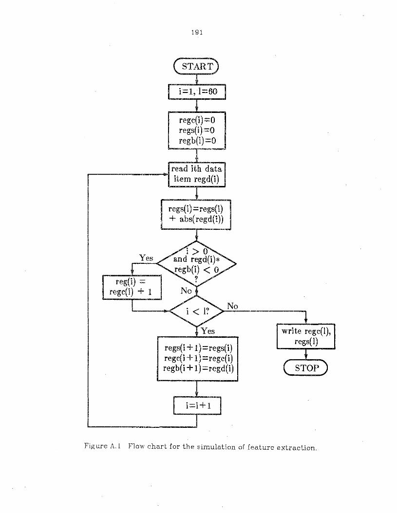
191
regc(i)=Oregs(i)=0regb(i)=O
read ith data...-------~ item regd(i)
regs(i)=regs(i)+ abs( regd(i))
reg(i) =regc(i) + 1
No
regs(i +1) =regs(i)regc(i + l)=regc(i)regb(i +1)=regd(i)
write regc{l),regs(l)
Figure A.1 Flow chart for the simulation of feature extraction.
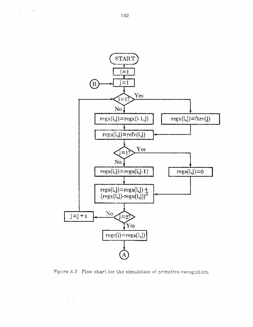
j=j+1
192
regx(i,j) = regx (i-I ,j)
regu(i,j) = refv(i,j)
Yes
rega(i,j)=rega(i,j) 1(regx(i,j)-regu(i,j))
regx(i,j) =ftrv(j)
rega(i,j)=O
Figure A.2 Flow chart for the simulation of primitive recognition.
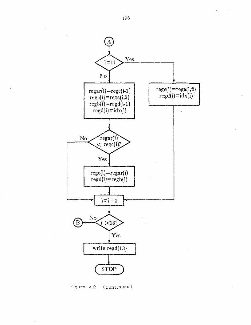
193
Yes
No
No
regar(i) =regc(i-l)regc(i) =rega(i,2)regb(i)=regd(i-l)
regd(i) =idx(i)
Yes
regc(i) =regar(i)regd(i) =regb(i)
regc(i) =rega(i,2)regd(i)=idx(i) .
Yes
write regd( 13)
Figure A.2 (Continued)
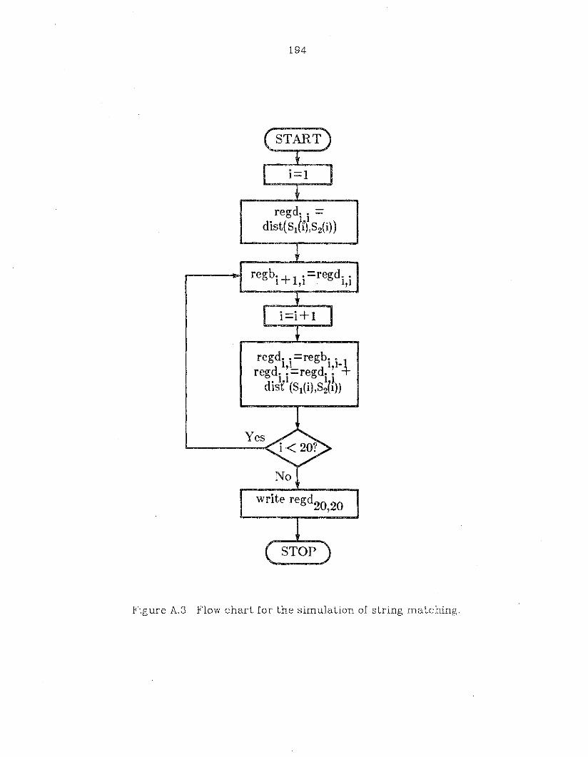
194
regd.. =dist(sifl,S2(i))
regb. + 1 . =regd..1 ,I. 1,1
regd.. =regb.. 4-1,1 1,1-
regd.. =regd..• 1 1 1)
dls~ (Sl(i),S2(1))
Yes
write regd20,20
Figure A.3 Flow chart for the simulation of string matching.

195
APPENDIXB
STEP-BY-STEP SIMULATION RESULTS
Table B.1 shows the intermediate results of feature extraction at
each time interval for the seismic signal shown in Figure B.lo The sym
b:)ls a.b ,S.e.x.y and d are described in Figure 5.4(b). We use a
linearly-connected array of 60 processors. Therefore. for a specific
seismic segment, it takes 60 unit times to pass through the processor
array. Since the data can be pipelined, it takes only one unit time to
extract the feature from each segment. The inputs to Table B.2 are the
outputs from Table B.1 after normalization. Table B.2 shows the inter
mediate results of primitive recognition at each time interval. At time
nand 2n. n = 1, 2 13, the simulation executes 'compute' operation.
At time 3n, n = 1, 2 13, the simulation executes 'compare' opera-
tion. The symbols a.x ,u.b ,y and v of 'compute' operation are
described in Figure 5.7(0.). The symbols a.b ,e ,d ,y and z of 'compare'
operation are described in Figure 5.7(b). A specific feature vector
takes 39 unit times to pass through the processor array. Since the
feature vectors can be pipelined. it takes two unit times to assign a
primitive to each feature vector. The output 'g' from Table B.2 is the
4th symbol of the second string in Table B.3. Table B.3 shows the inter
mediate results of string matching using the weighted Levenstein dis
tance. Since only substitution errors are considered. the computation
is straightforward. The syrnbols x ,Y ,d and b represent the rc['isLers as
196
described in Figure 5.16. A specific pair of strings take 39 unit times to
pass through the processor array. Since the strings can be pjpelined, it
takes 3 unit times to compute the distance between an unknown and a
reference string. The recognition results will not be known until we
compare against all the (100) reference strings.
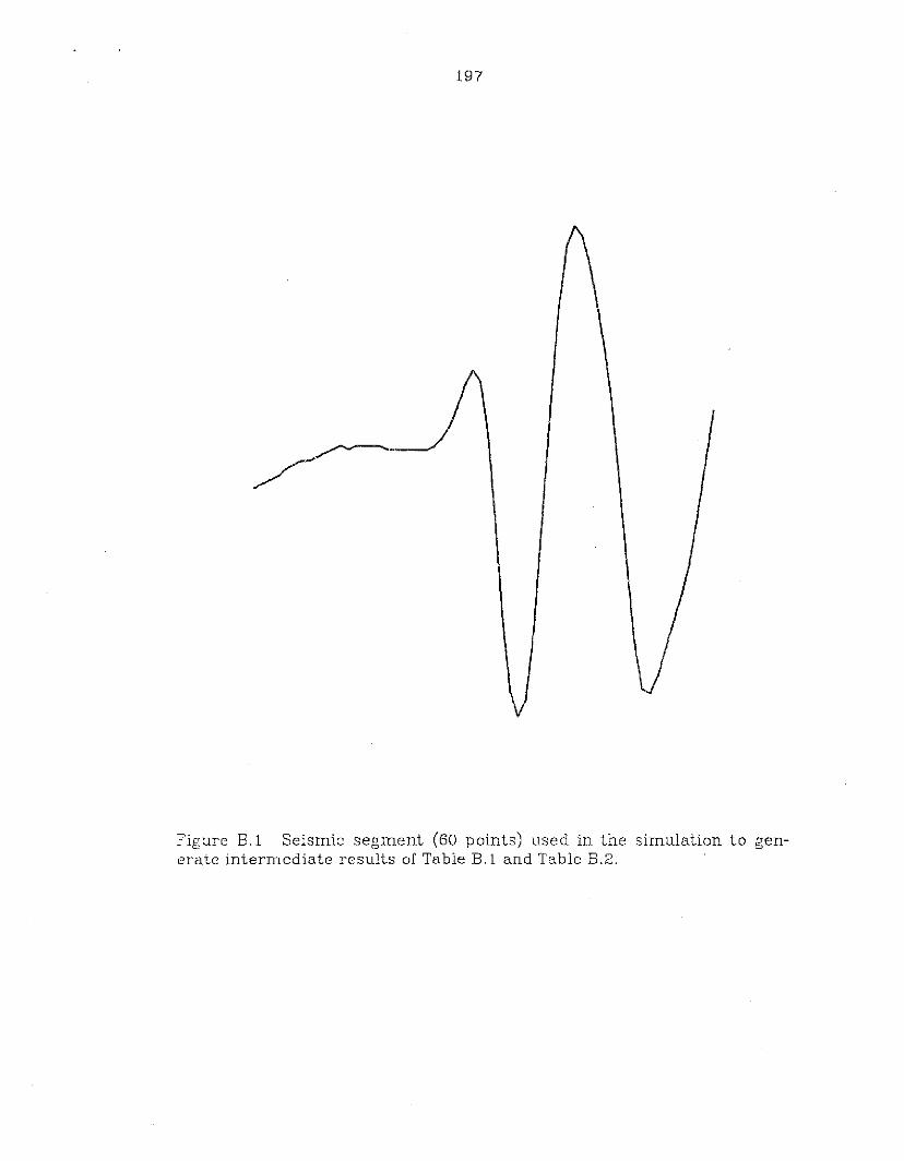
197
Figure B.1 Seismic segment (60 points) used in the simulation to generate intermediate results of Table B.1 and Table B.2.
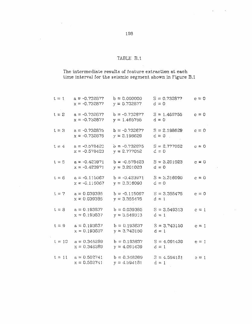
198
TABLE B.l
The intermediate results of feature extraction at eachtime interval for the seismic segment shown in Figure B.l
t = 1 a = -0.732877 b = 0.000000 S = 0.732877 c=Ox = -0.732877 Y = 0.732877 d := 0
t=2 a = -0.732877 b = -0.732877 S = 1.465755 c=Ox = -0.732877 Y = 1.465755 d=O
t::: 3 a = -0.732875 b =-0.732877 S = 2.198629 c = 0x = -0.732875 y=2.198629 d=O
t=4 a = -0.578423 b = -0.732875 S :.:: 2.777052 c=Ox :.:: -0.578423 y = 2.777052 d:::O
t :.:: 5 a = -0.423971 b = -0.578423 S = 3.201023 c = 0x = -0.423971 Y = 3.201023 d=O
t = 6 a = -0.115067 b :.:: -0.423971 S = 3.316090 c=Ox=-0.115067 y = 3.316090 d = 0
t = 7 a:.:: 0.039385 b :.:: -0.115067 S :.:: 3.355475 c = 0x = 0.039385 y = 3.355475 d = 1
t :.:: 8 a :.:: 0.193837 b = 0.039385 S :.:: 3.549313 c = 1x:.:: 0.193837 y = 3.549313 d = 1
t:.:: 9 a = 0.193837 b = 0.193837 S = 3.743150 c = 1x = 0.193837 Y = 3.743150 d = 1
t = 10 a = 0.348289 b :.:: 0.193837 S = 4.091439 c = 1x = 0.348289 Y = 4.091439 d = 1
t :.:: 11 a = 0.502741 b = 0.348289 S = 4.594181 c :.:: 1x:.:: 0.502741 y = 4.594181 d :.:: 1
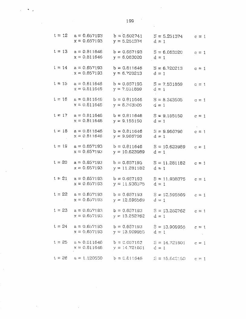
199
t = 12 a =0.657193 b =0.502741 S =5.251374 c = 1x =0.657193 y =5.251374 d = 1
t = 13 a =0.811646 b =0.657193 S =6.063020 c = 1x == 0.811646 y =6.063020 d = 1
t = 14 a =0.657193 b =0.811646 S =6.720213 c = 1x =0.657193 y = 6.720213 d = 1
t = 15 a = 0.811646 b =0.657193 S = 7.531859 c = 1x = 0.811646 y =7.531859 d = 1
t = 16 a =0.811646 b =0.811646 S = 8.343505 c = 1x =0.811646 y = 8.343505 d = 1
t = 17 a = 0.811646 b =0.811646 S = 9.155150 c = 1x = 0.811646 y=9.155150 d = 1
t = 18 a = 0.811646 b = 0.811646 S =9.966796 c = 1x = 0.811646 y = 9.966796 d == 1
t = 19 a = 0.657193 b = 0.811646 S = 10.623989 c == 1x = 0.657193 y = 10.623989 d = 1
t = 20 a =0.657193 b =0.657193 S = 11.281182 c = 1x = 0.657193 y = 11.281182 d = 1
t = 21 a =0.657193 b =0.657193 S = 11. 938375 c = 1x =0.657193 y = 11. 938375 d == 1
t = 22 a = 0.657193 b =0.657193 S = 12.595569 c = 1x = 0.657193 Y = 12.595569 d == 1
t == 23 a == 0.657193 b == 0.657193 S == 13.252762 c == 1x = 0.657193 Y = 13.252762 d = 1
t = 24 a = 0.657193 b =0.657193 S = 13.909955 c = 1x = 0.657193 Y == 13.909955 d = 1
t == 25 a = 0.811646 b == 0.657193 S = 14.721601 c = 1x = 0.811646 y = 14.721601 d = 1
t = 26 a = 1.120550 b=0.811646 S = 15.8421.50 c = 1
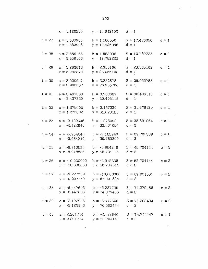
200
x = 1.120550 Y = 15.842150 d = 1
t = 27 a = 1.583906 b = 1.120550 S == 17.426056 c =1x == 1.583906 Y = 17.426056 d == 1
t = 28 a = 2.356166 b = 1.583906 S = 19.782223 c =1x == 2.356166 y == 19.782223 d = 1
t == 29 a = 3.282878 b =2.356166 S = 23.065102 c =1x = 3.282878 Y = 23.065102 d == 1
t == 30 a == 3.900687 b == 3.282878 S == 26.965788 c = 1x = 3.900687 Y == 26.965788 d == 1
t == 31 a = 3.437330 b = 3.900687 S = 30.403118 c = 1x = 3.437330 y = 30.403118 d = 1
t = 32 a == 1.275002 b == 3.437330 S == 31.678120 c =1x == 1.275002 y =31.678120 d = 1
t == 33 a == -2.122946 b = 1.275002 S = 33.801064 c =1x == -2.122946 y = 33.801064 d=2
t == 34 a =-5.984246 b == -2.122946 S = 39.785309 c=2x = -5.984246 y = 39.785309 d=2
t == 35 a == -8.918835 b = -5.984246 S == 48.704144 c == 2x = -8.918835 y == 48.704144 d==2
t = 36 a = -10.000000 b = -8.918835 S = 58.704144- c = 2x = -10.000000 y == 58.704144- d == 2
t == 37 a = -9.227739 b = -10.000000 S == 67.931885 c == 2x == -9.227739 Y = 67,931885 d == 2
t == 38 a == -6.447603 b = -9.227739 S == 74.379486 c = 2x = -6.447603 Y = 74.379486 d==2
t == 39 a = -2.122946 b = -6.44-7603 S = 76.502434 c = 2x = -2.122946 Y == 76.502434 d =2
t = 40 a = 2.201714 b = -2.122946 S = 78.704147 c = 2:::=2.201714- y == 78.704147 d == 3
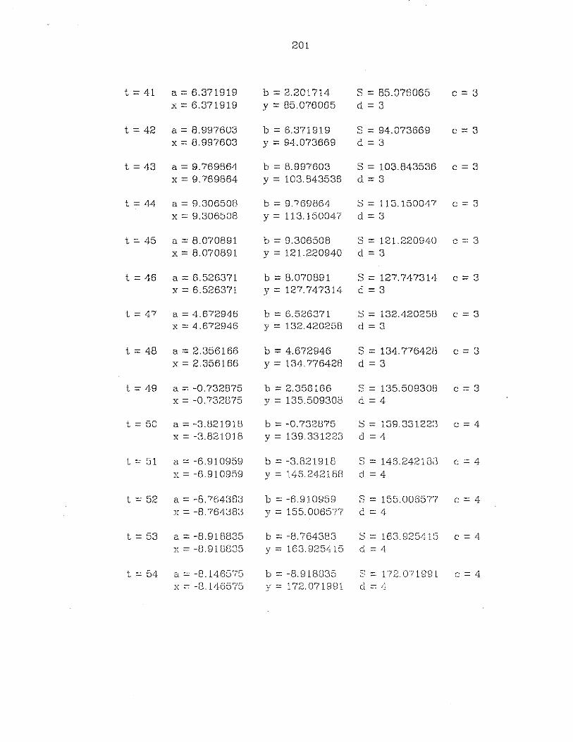
201
t = 41 a = 6.371919 b =2.201714 S = 85.076065 c = 3x =6.371919 Y = 85.076065 d = 3
t = 42 a = 8.997603 b = 6.371919 S = 94.073669 c = 3x = 8.997603 Y = 94.073669 d=3
t = 43 a = 9.769864 b = 8.997603 S = 103.843536 c = 3x =9.769864 y= 103.843536 d=3
t = 44 a = 9.306508 b = 9.769864 S = 113.150047 c = 3x = 9.306508 Y = 113.150047 d=3
t = 45 a = 8.070891 b = 9.306508 S = 121.220940 c = 3x = 8.070891 y= 121.220940 d = 3
t = 46 a = 6.526371 b = 8.070891 S = 127.747314 c = 3x =6.526371 Y = 127.747314 d =3
t =47 a = 4.672946 b = 6.526371 S = 132.4202513 c = 3x = 4.672946 y = 132.420258 d = 3
t = 48 a = 2.356166 b = 4.672946 S = 134.7764213 c = 3x = 2.356166 Y = 134.776428 d=3
t = 49 a = -0.732875 b = 2.356166 S = 135.5093013 c = 3x = -0.732875 y = 135.509308 d=4
t = 50 a = -3.821918 b = -0.732875 S = 139.33122:3 c=4x = -3.821918 Y = 139.331223 d=4
t = 51 a = -6.910959 b = -3.821918 S = 146.2421813 c=4x = -6.910959 Y = 146.242188 d = 4
t = 52 a = -8.764383 b = -6.910959 S = 155.006577 c = 4x = -8.764383 y = 155.006577 d=4
t = 53 a = -8.918835 b =-8.764383 S = 163. 92541~5 c=4x = -8.918835 Y = 163.925415 d=4
t = 54 a = -8.146575 b = -8.918835 S = 172.07199l c = 4x = -8.146575 y= 172.071991 d=4
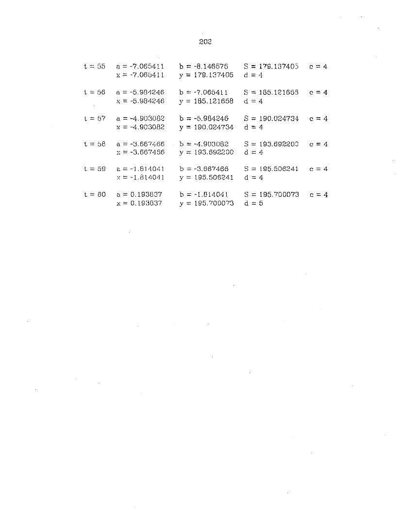
202
t = 55 a = -7.065411 b = -8.146575 S = 179.137405 c=4x =-7.065411 Y = 179.137405 d=4
t = 56 a =-5.984246 b = -7.065411 S = 185.121659 c=4x =-5.984246 Y = 185.121658 d=4
t = 57 a = -4.903082 b = -5.984246- S = 190.024734 c=4x = -4.903082 Y = 190.024734 d=4
t = 58 a =-3.667466 b = -4.903082 S = 193.692200 c=4x = -3.667466 Y = 193. (392200 d=4
t = 59 a = -1.814041 b = -3.667466 S = 195.506241 c=4x = -1.814041 y = 195.506241 d=4
t = 60 a = 0.193837 b = -1.814041 S = 195.700073 c=4x = 0.193837 Y = 195.700073 d=5

203
TABLE B.2
The intermediate results of primitive recognition ateach time interval for the feature vector from Table B.lafter normalization.
t = 1 a = .000 x = -.161 u=-1.718b = 2A26 y=-.161 v=-1.718
t = 2 a = 2.426 x= 19.252 u=-2.108b=458.711 y= 19.252 v = -2.108
t = 3 a= ********** b = 458.711 c = ,*, d = 'a'y=458.711 z = 'a'
t=4 a = .000 x=-.161 u = 3.337b= 12.232 y=-.161 v = 3.337
t = 5 a= 12.232 x= 19.252 u = -1. 740b = 452.920 y= 19.252 v = -1.740
t = 6 a = 458.711 b = 452.920 c = 'a' d = 'b'y =452.920 z = 'b'
t = 7 a = .000 x=-.161 u=-.180b = .000 y = -.161 v = -.180
t = 8 a = .000 x= 19.252 u = -2.387b = 468.287 y= 19.252 v = -2.387
t = 9 a = 452.920 b = 468.287 c = 'b' d = 'c'y = 452.920 z = 'b'
t = 10 a = .000 x = -.161 u=-1.229b = 1.142 y=-.161 v = -1.229
t = 11 a= 1.142 x= 19.252 u = .987b = 334.762 y= 19.252 v = .987
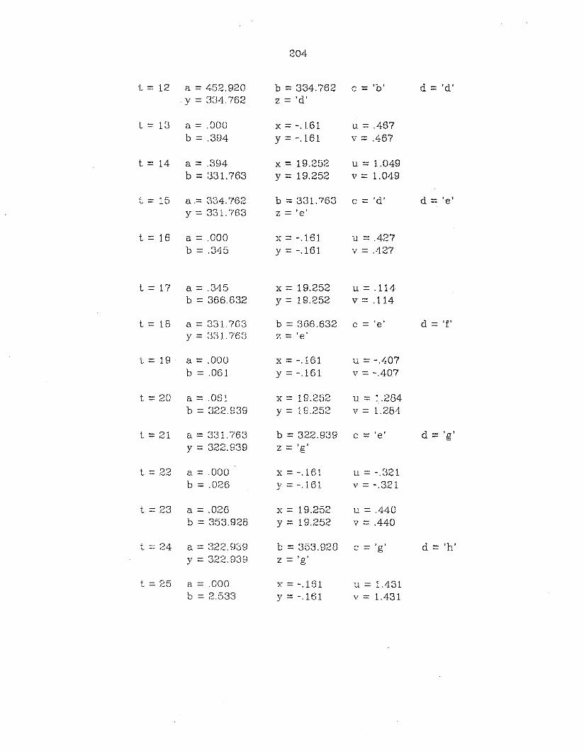
204
t= 12 a = 452.920 b = 334.762 c = 'b' d = 'd'y = 334.762 z = 'd'
t = 13 a = .000 x = -.161 u = .467b = .384 y = -.161 v = .467
t= 14 a = .394 x= 19.252 u =1.049b = 331.763 y= 19.252 v= 1.049
t= 15 a= 334.762 b =3~31.763 c = 'd' d = 'e'y = 331.763 z = 'e'
t= 16 a = .000 x = -.161 u = .427b = .345 Y = -.161 v = .427
t = 17 a = .345 x= 19.252 u = .114b = 366.632 y= 19.252 v = .114
t =18 a = 331.763 b = 366.632 c = 'e' d = 'f'y=331.763 z = 'e'
t = 19 a = .000 x = -.161 u = -.407b = .061 y=-.161 v = -.407
t = 20 a = .061 x= 19.252 u= 1.284b = 322.939 y= 19.252 v= 1.284
t = 21 a = 331.763 b = 322.939 c = 'e' d = 'g'y = 322.939 z = 'g'
t = 22 a = .000 x = -.161 u = -.321b = .026 Y = -.161 v = -.321
t = 23 a = .026 x= 19.252 u = .440b = 353.928 y= 19.252 v = .440
t = 24 a = 322.939 b = 353.928 c = 'g' d = 'h'y = 322.939 z = 'g'
t = 25 a = .000 x=-.161 u= 1.431b = 2.533 Y = -.161 v= 1.431
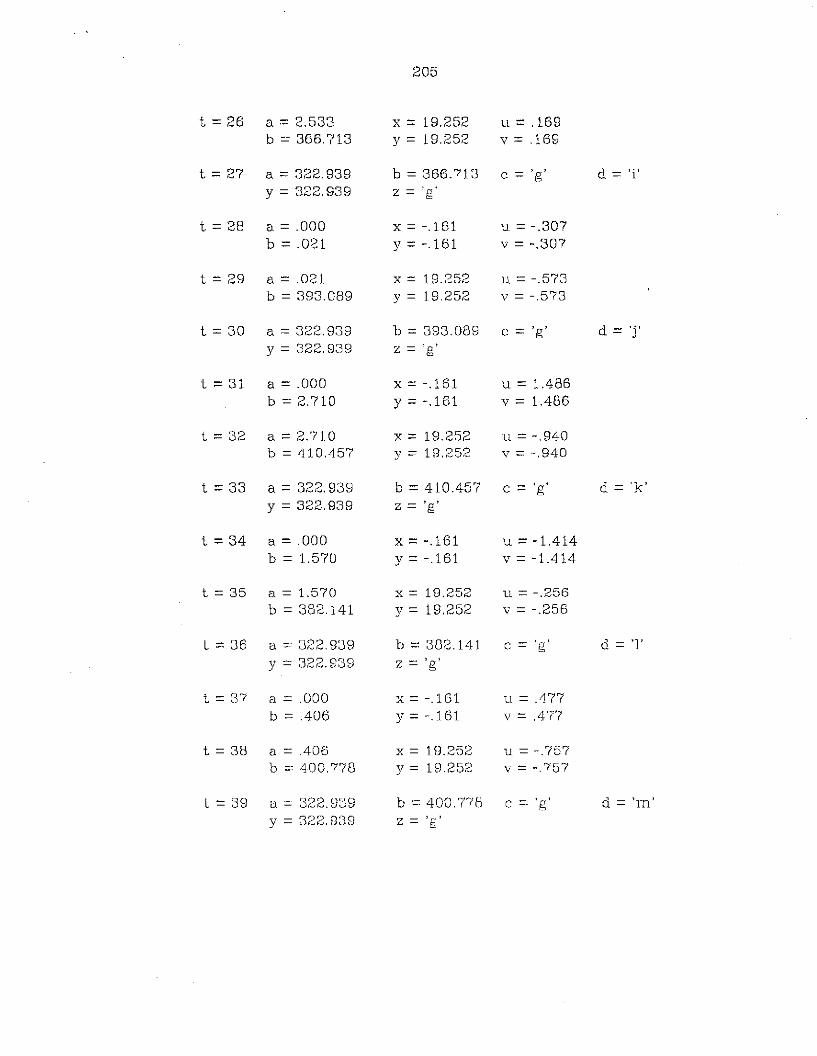
205
t = 26 a = 2.533 x= 19.252 u = .169b == 366.713 y= 19.252 v = .169
t = 27 a = 322.939 b = 366.713 c = 'g' d = 'i'Y = 322.939 z = 'g'
t = 28 a = .000 x = -.161 u = -.307b = .021 y=-.161 v = -.307
t = 29 a = .021 x= 19.252 u = -.573b = 393.089 y= 19.252 v = -.573
t = 30 a = 322.939 b = 393.089 c = 'g' d = 'j'y = 322.939 z = 'g'
t = 31 a = .000 x=-.161 u = 1.486b = 2.710 Y = -.161 v= 1.486
t = 32 a = 2.710 x= 19.252 u = -.940b = 410.457 y= 19.252 v = -.940
t =33 a =322.939 b = 410.457 c = 'g' d = 'k'y = 322.939 z = 'g'
t = 34 a = .000 x =-.161 u=-1.414b = 1.570 y=-.161 v = -1.414
t = 35 a= 1.570 x= 19.252 u = -.256b = 382.141 y= 19.252 v =-.256
t = 36 a ::: 322.939 b=382.141 c = 'g' d='l'y = 322.939 z = 'g'
t = 37 a ::: .000 X = -.161 u = .477b = .406 y=-.161 v = .477
t = 38 a ::: .406 x= 19.252 u = -.757b =: 400.778 y= 19.252 v = -.757
t = 39 a = 322.939 b = 400.778 c = 'g' d = 'm'y = 322.939 z = 'g'
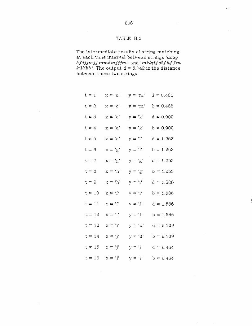
206
TABLE B.3
The intermediate results of string matchingat each time interval between strings 'acaghfijjmjjmmkmjjjm' and 'mlclgijdifhf1mIcillibb '. The output d = 5.742 is the distancebetween these two strings.
t= 1 v - 'a' y= 'm' d == 0.485£>. -
t=2 x= 'c' y= 'm' b = 0.485
t=3 x== 'c' y= 'k' d = 0.900
t=4 x= 'a' y= 'k' b =0.900
t = 5 x= 'a' y= '1' d = 1.253
t= 6 x= 'g' y= '1 ' b = 1.253
t=7 x= 'g' y= 'g' d = 1.253
t= 8 x= 'h' y= 'g' b = 1.253
t= 9 x= 'h' Y = 'i ' d = 1.586
t= 10 x== 'f' y= 'i' b = 1.586
t= 11 li = 'f' y= 'f' d = 1.586
t= 12 x== 'it y= 'f' b = 1.586
t= 13 x= 'i' y= 'd' d = 2.109
t= 14 v - 'j' y= 'd' b = 2.109"' -
t= 15 v - 'j' y= 'i J d = 2.464"' -
t= 16 y- 'j' y= 'i' b = 2.464, -
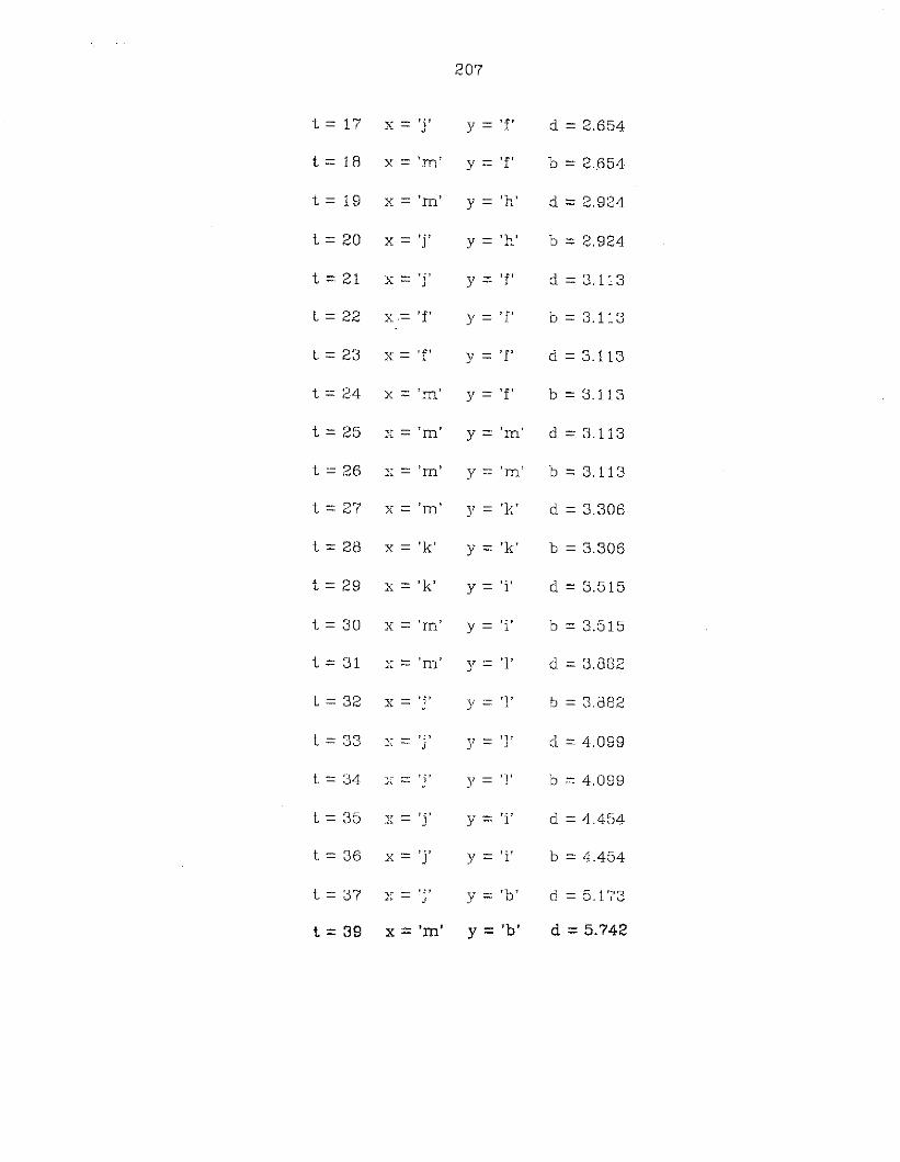
207
t= 17 x- 'j' y= 'f' d = 2.654. -
t= 18 x= 'm' y= 'f' b = 2.654
t= 19 x= 'm' y= 'h' d = 2.924
t= 20 x= 'j' y= 'h' b = 2.924
t= 21 ;( = 'j' y= 'f' d = 3.113
t = 22 x= 'f' y= 'f' b = 3.113
t= 23 x= 'f' y= 'f' d = 3.113
t = 24 x= 'm' y= 'f' b = 3.113
t = 25 y- 'm' y= 'm' d = 3.113' -
t= 26 x- 'm' y= 'm' b = 3.113. -
t = 27 x= 'm' y = 'k' d = 3.306
t = 28 x= 'k' y= 'k' b = 3.306
t = 29 x= 'k' y= 'i' d = 3.515
t = 30 x= 'm' y= 'i' b =3.515
t= 31 v - 'm' y= '1' d = 3.882.. -
t= 32 x=: 'j' y=: '1' b =3.882
t =: 33 :x = 'j' y = '1 ' d = 4.099
t= 34 v - 'j' y= '1 ' b = 4.099.l'l. -
t=: 35 y- 'j' y= 'i' d = 4.454. -
t= 36 x= ' j' y= 'i' b =: 4.454
t =: 37 v - 'j' y= 'b' d =: 5.173L·l-- -
t = 39 x= '.m' y= 'b' d = 5.742

Top Related
Copyright © 2022 FDOKUMEN

