ELSEVIER Computer Physics Communications 88 (1995) 195-210

Computer Physics Communications

A new multivariate technique for top quark search Lasse Holmstr6m a'1'2, Stephan R. Sain a,3, Hannu E. Miettinen b

a Department of Statistics, Rice University, Houston, Texas 77251, USA b Physics Department, Rice University, Houston, Texas 77251, USA

Received 1 February 1995

Abstract

We present a new multivariate event classifier, the PDE classifier, which can be used to identify rare signals in the presence of large backgrounds. The classifier is based on a discriminant function which uses kernel density estimates of the signal and background event densities. The PDE method offers the flexibility of a neural network but is conceptually simpler, theoretically better understood, and easier to optimize in practice. The technique is tested on Monte Carlo data using processes t~ --* e + Et + jets as signal and W + jets --~ e + Et + jets as background. The performance of the PDE classifier is similar to that of a neural network. Both methods outperform conventional analysis.

1, Introduct ion

The Standard Model of particle physics [ 1 ] requires the existence of the top quark, the weak isospin partner of the bottom quark, and the heaviest of the six quarks. Direct experimental evidence for top quark production in p/~ collisions at v/s = 1.8 TeV has recently been presented by the CDF Collaboration [2] . The DO experiment [3] has reported a signal consistent with the CDF result, but does not interpret it as conclusive evidence. It appears that more data and/or new, more efficient analysis methods are required for a compelling discovery.

The top quark signal is masked by large backgrounds arising from conventional electroweak and QCD processes. These backgrounds are normally reduced by imposing a set of one-dimensional cuts on selected variables characterizing the events of interest. Such cuts are usually determined by examining the relevant single variable probability densities for (Monte Carlo generated) signal and background events. However, it seems natural that better results could be obtained by employing mul t i var ia t e techniques, which are more flexible and allow for exploiting correlations among variables. Feed-forward Neural Networks (NN) represent one such approach, and they have indeed been applied successfully to many pattern recognition problems in high energy physics [4] . In this paper we propose a new method based on direct comparison of the

On a visit from Rolf Nevanlinna Institute, University of Helsinki, Finland. 2Correspondence to L. HolmstrSm, Rolf Nevanlinna Institute, P.O.Box 26, SF-00014, University of Helsinki, Finland. E-mail:

llh@ rolf.helsinki.fi 3 Currently at the Applied Physics Center, Pacific Northwest Laboratory, Richland, WA, 99352, USA.

Elsevier Science B.V. SSDI 0010-4655(95)00040-2

196 L. Holmstri~m et al. / Computer Physics Communications 88 (1995) 195-210

multivariate probability densities for signal and background events. Our PDE (Probability Density Estimation) event classifier estimates the unknown densities by using the so-called kernel method. In principle at least the kernel estimates can represent arbitrary event class boundaries, and while the NN classifier requires non-linear optimization in high-dimensional spaces, the PDE classifier is optimized by tuning just one real parameter.

We begin by reviewing some relevant features of multivariate event classification and neural networks in Section 2. The PDE classifier is introduced in Section 3. The simulated data sets are described in Section 4 and variable selection is discussed in Section 5. Our results are summarized in Section 6. We find that the PDE and NN classifiers perform similarly in terms of attainable signal-to-background ratios and signal efficiencies. Both methods compare favorably with conventional analysis which relies on one-dimensional cuts.

The PDE event classifier described in this article is being used by the DO Collaboration to search for top quark production in p/~ collisions.

2. Fcedforward neural networks and probability densities in classification

2.1. Event classification

Let us suppose that d physical variables xl . . . . . Xd have been chosen to describe the events of interest. In the framework of statistical discrimination the row vector

x = (Xl . . . . . xd)

is regarded as a particular value of a random vector X = (X1 . . . . . Xd). Associated with each event is also a class label, "s" for a signal and "b" for a background event. This is described by a random variable 69 with the two possible values s and b. The design of a classifier is based on a set of training vectors xi with known labels /9i. In actual use the classifier must then guess the unknown label /9 of an event using the information contained in x only.

An effective event classifier has two properties. First, among the events accepted as signals, the signal-to- background ratio (ratio of true signal events to background events) should be high. Second, the classifier should have a high signal efficiency, i.e. it should accept as signals as many of the true signal events as possible. The signal-to-background ratio among the accepted events is formally defined as

P (69 = s i x accepted) S/ B = p(69 = b---~ accepted) ' ( 1 )

where P( . [ . ) stands for conditional probability. Signal efficiency is defined as

E = P ( X accepted [ 69 = s). (2)

The goal in the present work was to design a classifier that would improve the "trigger-level" signal-to- background ratio by a factor of 10-100 with a signal efficiency of at least 0.5 (see Section 4).

S / B and E were estimated by counting the number of events classified as signals and background. If N signal events are available for efficiency estimation and Ns of them are accepted by the classifier, then E is estimated by

f: Ns N

Let Ps = P(69 = s) and Pb = P(69 = b) be the probabilities that an event to be classified is a signal event and a background event, respectively. Then S / B can also be written as

S / B Ps P ( X accepted]O = s) = Pbb P ( X accepted169 = ~ "

L. Holmstr6m et al. / Computer Physics Communications 88 (1995) 195-210 197

X l O _

w 1 X2 • W 2 g ,w 0

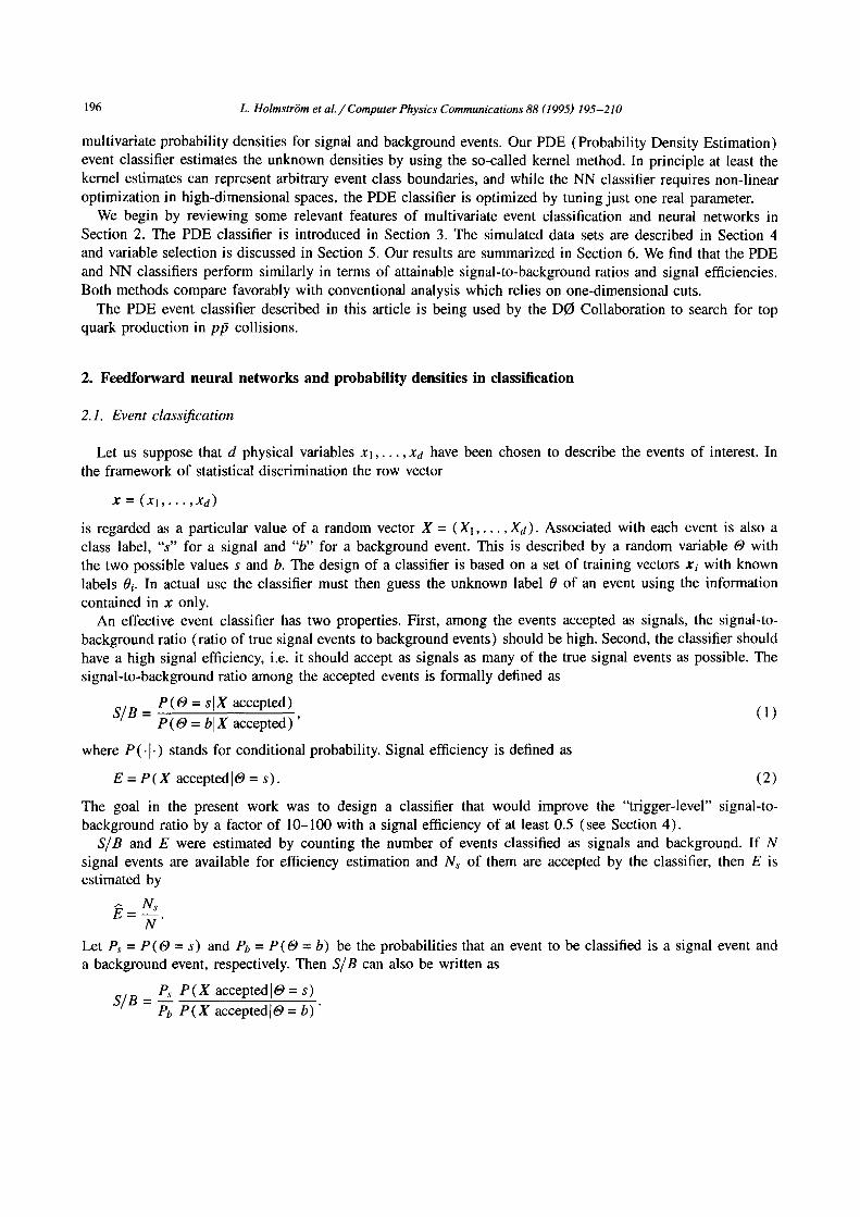
Fig. 1.

- Oo >OO-y ~2 o . " ~ - -~ . ( -~ . ' ~ - ~ . r - ' ~ ~ y~

Fig. 2.

Fig. I. A formal neuron.

Fig. 2. A feedforward layered neural network with one hidden layer.

In the present context we have Ps/Pb = 4~ (see Section 4). When equal numbers of signal and background events are used to estimate S /B we therefore have

I Ns S /B - 41 Nb'

where N, signal and Nv background events are accepted by the classifier.

2.2. Neural networks and probability density functions

Artificial neural networks are computational tools that can be used to tackle problems such as statistical pattern recognition. The most popular NN by far has been the feedforward layered network, or the "multilayer perceptron" [5]. The basic unit of this network is the formal neuron depicted in Fig. 1. The neuron receives inputs x = (xl . . . . . xd) and computes the output y = g (w0+wxT) . Here w denotes the vector w = (wl . . . . . wd) of the "connection weights" of the neuron, x T is the transpose of x, w0 is a threshold parameter, and g is a monotonically increasing function such as

1 g ( x ) = 1 + e -x" (3)

In a feedforward layered network such formal neurons are arranged in consecutive layers, each neuron in a layer receiving its input from all neurons in the previous layer. Fig. 2 shows a network with one "hidden layer" between the input and output layers. In general, the network therefore defines a mapping y = G ( x , w ) of d input variables xl . . . . . xd to m output variables Yl . . . . . ym. In this notation, the weights of all the formal neurons in the network are collected in the single parameter vector w.

A feedforward NN can be used to model a complicated input-output relationship by optimizing the network parameters with the aid of known examples of desired input-output pairs x i ,Yr This optimization is called "training", and often the quadratic error function

1 N 7~(w) = -~ ~_, [ [ G ( x , , w ) - y, II 2 (4)

i=1

is minimized to find an optimal parameter vector w*. In the context of event classification one can try to design a network with a single ouput which maps signal events to 1 and background events to 0. Classification of events is then based on a threshold value c~ placed on the output of the network:

198 L. Holmstr6m et al. / Computer Physics Communications 88 (1995) 195-210

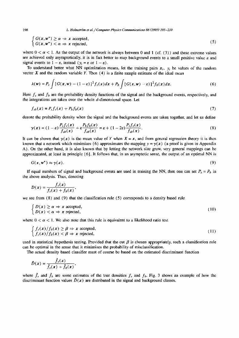
G ( x , w * ) >_ a ~ x accepted, G ( x , w * ) < a ~ x rejected, (5)

where 0 < a < 1. As the output of the network is always between 0 and 1 (cf. (3) ) and these extreme values are achieved only asymptotically, it is in fact better to map background events to a small positive value e and signal events to 1 - e, instead ( y i = e o r 1 - e ) .

To understand better what NN optimization means, let the training pairs xi, Yi be values of the random vector X and the random variable Y. Then (4) is a finite sample estimate of the ideal mean

A(w) Ps

Here f s and fb are the probability density functions of the signal and the background events, respectively, and the integrations are taken over the whole d-dimensional space. Let

fsb(X) = Ps f~(x) + Pbfb(X) (7)

denote the probability density when the signal and the background events are taken together, and let us define

Psfs(X) Pbfb(X) Psfs(X) T(x ) = (1 - e ) - - + e = e + (1 - 2 e ) - - (8)

f sb (x ) f sb (x ) f sb (x ) "

It can be shown that y ( x ) is the mean value of Y when X = x, and from general regression theory it is then known that a network which minimizes (6) approximates the mapping y = y ( x ) (a proof is given in Appendix A). On the other hand, it is also known that by letting the network size grow, very general mappings can be approximated, at least in principle [6]. It follows that, in an asymptotic sense, the output of an optimal NN is

G ( x , w * ) ,~ y ( x ) . (9)

If equal numbers of signal and background events are used in training the NN, then one can set Ps = Pb in the above analysis. Thus, denoting

f s ( x ) n ( x ) = f ~ ( x ) + f o ( x ) '

we see from (8) and (9) that the classification rule (5) corresponds to a density based rule

D ( x ) _> a ~ x accepted, D ( x ) < a ~ x rejected, (10)

where 0 < a < 1. We also note that this rule is equivalent to a likelihood ratio test

f s ( X ) / f b ( X ) >_ fl ::~ X accepted, f ~ ( x ) / f b ( x ) </3 => x rejected, (11)

used in statistical hypothesis testing. Provided that the cut/3 is chosen appropriately, such a classification rule can be optimal in the sense that it minimizes the probability of misclassification.

The actual density based classifier must of course be based on the estimated discriminant function

t ) (x) = L ( x ) L(x) + }o(x)'

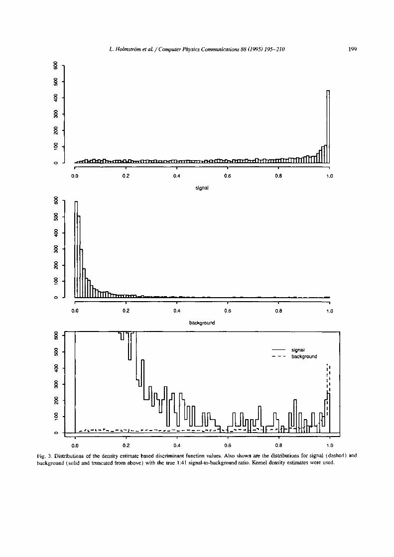
where f s and fo are some estimates of the true densities f s and f0. Fig. 3 shows an example of how the discriminant function values /5(x) are distributed in the signal and background classes.

L. Holmstrbm et al. / Computer Physics Communications 88 (1995) 195-210 199

i

u u ! ! u u

0,0 0.2 0.4 0.6 0.8 1.0

signal

lU ! u ! ! u

0.0 0.2 0.4 0.6 0.8 1.0

g

Q

l j . - i

background

signal background

I i I

I ] J/l I I l .

-U ]Jl~ l~ I]l]nnJ I~ nl~i u u u u i v

0.0 0.2 0.4 0.6 0,8 1.0

Fig. 3. Distributions o f the density estimate based discfiminant function values. Also shown am the distributions for signal (dashed) and background (sol id and truncated from above) with the true ! :41 signal-to-background ratio. Kernel density estimates were used.

200 L. HolmstrOm et al. / Computer Physics Communications 88 (1995) 195-210

By choosing different mathematical forms for the estimates fs and fb, different types of event classifiers can be proposed. A classical approach is to assume that the two classes have multivariate normal or "Gaussian" distributions,

1 f s (X) = ~/(27r)ddet(,Ss)

1 fb(X) = ¥/(27r)ddet(2b )

exp ( -½ ( x - las) .Ssl(x - / . t s )T) ,

exp ( - -½ ( x - l.tb).,~bl ( x - Pb) T) . (12)

Here /x s, Pb and Z~, ~b are the means and the covariance matrices of the signal and the background classes,

ps= f Xf~(x)dx, s=/(X--ps)T(x--ps)fs(x)dx, and similarly for the background. To get density estimates f~ and fb one estimates the unknown means Ps, ['tb and covariance matrices Z~, 27b from training data. If there are N signal training vectors the usual estimates are

1 1 ~s = -~ Z xi, .Y,s - N - 1 Z (xi - pt s) T (xi _ ~s) ,

signals signals (13)

and similarly for the background. By writing the rule ( 11 ) in terms of l o g ( f s ( x ) / f b ( X ) ) one easily sees that (12) leads to a classifier that attempts to separate the signal and background event classes using a d - 1 dimensional quadratic surface. When Z, = 27b, a simpler linear classifier results. In connection with top quark analysis, such Gaussian classifiers were first suggested in [7,8] (see also [9] ). Gaussian classifiers are also being currently used at DO [ 10]. While these classifiers are relatively easy to use, their power to model optimal non-linear boundaries between the signal and background classes is limited.

3. The PDE e v e n t c lass i f i er

3.1. Kernel estimates

The event classifier that we propose uses the rule (10) with the densities fs and fb estimated by multivariate kernel estimates. In the one-dimensional case the kernel estimate can be derived as follows. Consider a random variable X with density f and suppose that Xl . . . . . XN is a set of randomly drawn values of X. To estimate f on the basis of Xl . . . . . XN, consider the cumulative distribution function

F ( x ) = P ( X < x) = x f (u )du . - - 0 0

The probability F(x) can be estimated by counting the number of points xi to the left of x,

F(x) ~ P(x ) def ~#{Xi ] Xi ~ X}.

On the other hand, since f ( x ) = F~(x), we can estimate f ( x ) by choosing an h > 0 and setting

f ( x ) ~ + h ) - P ( x - h ) ) = # { x i l - h < x i - x < _ h } d ~ f f ( x ) . (14)

L. HolmstrOm et al. / Computer Physics Communications 88 (1995) 195-210

If K is the uniform density function on the interval -1 _< u < 1,

½, - l _ < . < l , K(u) = O, elsewhere ,

then j~(x) can also be written as

2 0 1

/ ( x ) = ~/-/~ Z K i=1

(15)

This formula defines the kernel estimate of f with kernel K and smoothing parameter h. In a general kernel estimate the kernel function K is any probability density function, a common choice being the standard Gaussian, K ( x ) = ~ e x p ( - x 2 / 2 ) .

The simplest multivariate generalization of (15) is straightforward,

) ( x ) = i=1

where xl . . . . . XN is a random sample from the random vector X and, in the Gaussian case,

K ( x ) - 1 (2~_) a/2 exp( - ½1Ix] ]2). (16)

Fig. 4 shows examples of kernel estimates for signal and background densities when two variables are used. The variables in question are described in Section 5.

In a multivariate setting it is desirable that the covariance or the "shape" of the kernel K reflects the covariance of the density f being estimated [ 11, Sec 6.1]. To accomplish this, one could transform a simple kernel such as (16) to match its covariance with that of f . Alternatively, one can transform the data so that its covariance matches that of the kernel used. We have adopted this latter approach. Let Xs and Xb denote the covariance matrices of X in the signal and background classes, respectively. It is in general impossible to transform the data so that the signal and background classes would have equal covariance matrices. However, it is well known from linear algebra that one can construct a matrix A such that the transformed random vector yT = AX T has a unit covariance matrix in one class and a diagonal covariance matrix in the other class. The details of this transformation are given in Appendix B. The transformed variables Y = ( Y I . . . . . Yd) are then uncorrelated within the two classes. Changing the names of variables Y back to X, the transformed event densities are then naturally estimated by using the multivariate product kernel I~jdl h f l K ( x j / h j ) , where K is a one-dimensional Gaussian and h) are d smoothing parameters. Our PDE classifier thus uses an event density estimate

f ( x ) - N h l . . .ha ~= j=l K ~. , (17)

where x = ( X l . . . . . Xd) and xi = (Xil . . . . . Xid) , i = 1 . . . . . N, denotes the value of X for the ith event in the training sample.

We note that a simple PDE-style classifier which uses multivariate histograms was considered in [8 ]. The LVQ-trained nearest neighbor classifier of [ 12] shares features of both a neural network classifier and the PDE classifier.

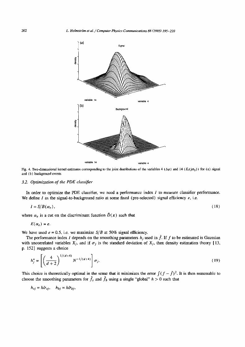
(a) Signal

"o

202 L. Holmstr6m et al. / Computer Physics Communications 88 (1995) 195-210

variable 14 variable 4

(b) Background

variable 14 vadable 4

Fig. 4. Two-dimensional kernel estimates corresponding to the joint distributions of the variables 4 (A~p) and 14 (Et(jets)) for (a) signal and (b) background events.

3.2. Optimization o f the PDE classifier

In order to optimize the PDE classifier, we need a performance index I to measure classifier performance. We define I as the signal-to-background ratio at some fixed (pre-selected) signal efficiency e, i.e.

l = S / B ( a e ) , (18)

where o~ e is a cut on the discriminant funct ion/5(x) such that

E ( a e ) = e.

We have used e = 0.5, i.e. we maximize S /B at 50% signal efficiency. The performance index 1 depends on the smoothing parameters hj used in f . If f to be estimated is Gaussian

with uncorrelated variables Xj, and if o-j is the standard deviation of Xj, then density estimation theory [ 13, p. 152] suggests a choice

* [ ( d - - - ~ ) l/(d+4) ] hj = N -U(a+4) o'j. (19)

This choice is theoretically optimal in the sense that it minimizes the error f ( f - f )2 . It is then reasonable to choose the smoothing parameters for fs and fb using a single "global" h > 0 such that

hsj = h~rsj, hbj = hO'bj,

L. HolmstriJm et al. / Computer Physics Communications 88 (1995) 195-210 203

where Osj and bbj are the estimated standard deviations of the jth variable for the signal and background classes, respectively. The performance index 1 then becomes a function 1 (h) = S/B (Ore (h ) ) of a single real parameter h, and we maximized l ( h ) by examining values of h in a neighborhood of the reference value

h* ( d ~ 2 ) 1/(d+4) = N-l~(d+4)

obtained by setting o-j = 1 in (19). Compared with the multivariate optimization necessary with NN training, optimizing the single parameter h

of the PDE classifier is conceptually and technically much simpler, and the optimization process is very easy to carry out in practice.

4. Signal and background data sets

In p/~ collisions the top quark is produced mostly in pairs through q~ annihilation: q# ~ t?. The t? pair decays almost exclusively as

tT ~ Wb + W[~,

and each of the two W bosons further decays as

{ e / g / r + u (1 /3 ) , W ~ q#-- . 2jets (2 /3) ,

while the b and b quarks produce two jets. Thus the tf final state contains 6 jets, a lepton + Et + 4 jets, or 2 leptons + Et + 2 jets. Here Et stands for the missing transverse energy arising from undetected neutrinos. The 6-jet final state has the largest branching ratio (4/9 = 44%), but the huge QCD multijet background makes it very difficult to isolate the top quark signal in this decay mode. The final states with two leptons have very small branching ratios. Experimentally the most accessible final states are

t t --~ e / tz + Et + 4 jets,

each of which has a branching ratio of 4/27 = 15%. In this paper we concentrate on the "e + Et +jets" mode for simplicity.

The leading physics background for this mode arises from the production of a single W in association with QCD jets. We refer to this background as "W +jets". Another significant background arises from QCD multijet events where one jet fakes an electron in the detector and a significant Et is due to mismeasurements of jet energies. We ignore such "fake electrons" and other instrumental backgrounds in this study.

The signal and background events were generated with the Monte Carlo program PYTHIA version 5.6 [ 14]. The top quark mass was taken to be 150 GeV. PYTHIA cross sections for the signal and background processes were 10.6 pb and 27.2 rib, respectively. A jetfinder (LUCELL) was applied to the generated events, using a "detector" with ]r/I < 4.0 (r/ is pseudorapidity) divided into bins of size 0.1 x 0.1 in the r/~o-space. A cone algorithm with cone radius R = 0.7 was used to find jets and determine their 4-momenta. The generated events were "triggered" by imposing the following selection criteria:

(i) An electron with Et > 20 GeV. (ii) No other leptons with Et 3> 5 GeV.

(iii) Missing Et > 20 GeV. (iv) At least 4 jets with Et > 10 GeV. The trigger efficiencies were 5.6 % for signal events and 0.09 % for background events. The signal-to- background ratio in the triggered event population is therefore 1:41.

204 L. HolmstrOm et al. / Computer Physics Communications 88 (1995) 195-210

A total of 10 4 triggered events were separated into training and testing samples of 5000 events each, equally divided between signal and background events. All classifiers were designed using the training data only and their performance was estimated using the independent testing data.

5. Variable selection

One might think that the performance of a classifier always improves with more input variables since more information is made available. This is indeed true if one has an infinite training sample of signal and background events but, as shown below, it is not true with a finite training sample. In practice, then, a sensible strategy entails trying to find the best combination of a modest number of "good" variables which are effective in discriminating between signal and background events.

We consider the following 14 variables, all commonly used for description of top quark candidate (and other interesting) events: (1) Electron transverse energy Et. (2) Electron pseudorapidity r/. (3) Missing transverse energy Et. (4) Aq~, the azimuthal angle between the electron and the Et vector. (5) xt = ~ E t / v G for particles within Inl < 4.0, exluding muons and neutrinos. (6) Centrality C = ~ - ] E t / ~ E for particles within Ir/I < 4.0, excluding muons and neutrinos. (7) Planarity P, calculated using jet momenta rather than particle momenta. (8) Sphericity S, calculated using jet momenta. (9) Aplanarity A, calculated using jet momenta. ( 10)-(14) Transverse energies of the 5 leading jets, including the electron. The first four variables contain complete information about the electron and Et, the next five characterize the entire event, and the last five contain partial information about jets. The exact definitions of these variables can be found in [ 14].

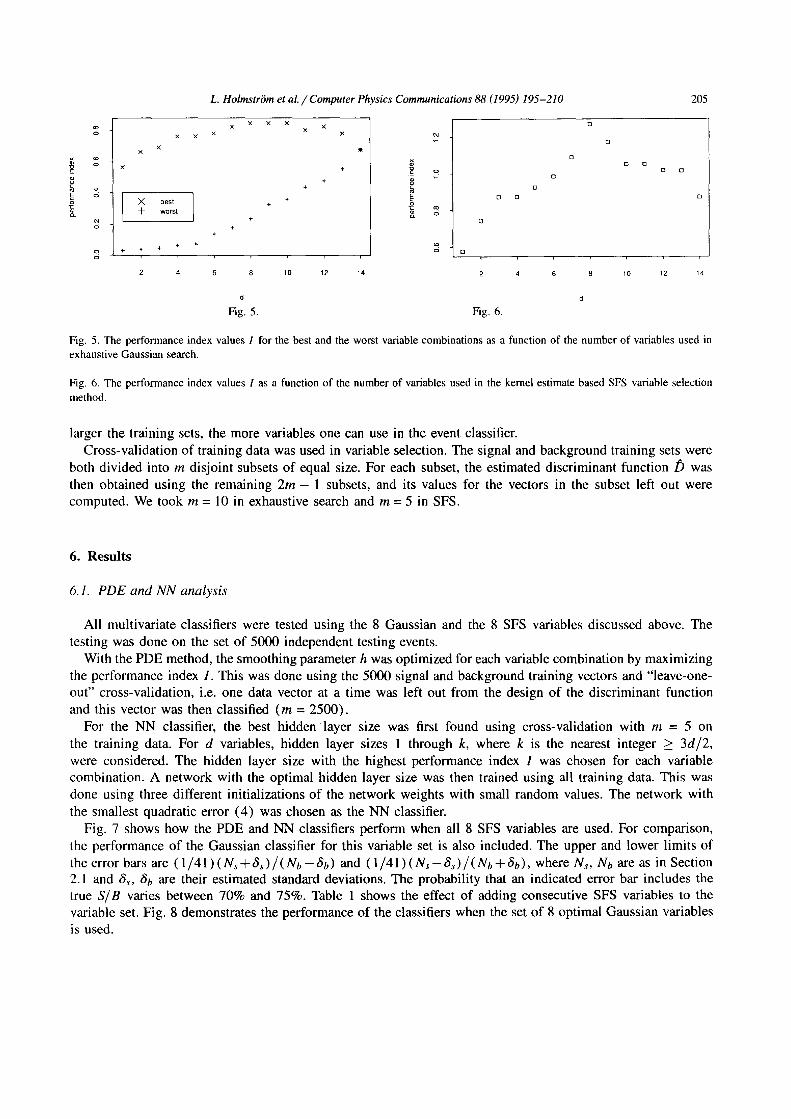
A simple variable selection strategy is to evaluate all combinations of the 14 variables. However, both the PDE and the NN classifiers are computationally too heavy to use in such an exhaustive search, and we used a Gaussian classifier based on multivariate Gaussians (12) instead. For a fixed d, each combination of d variables was evaluated by computing the index I and the combination with the highest 1 was considered as the best set of variables. Fig. 5 shows the performance index for the best and the worst combinations as a function of d. Clearly, different combinations can perform very differently. Notice how the performance does not appear to improve beyond 8 variables. The 8 best of these "Gaussian" variables were Et, Et,xt ,C, P, S, Et(jet4), and Et(jets), but, as many combinations ranked near the top, there are no grounds for claiming that they represent a truly optimal variable set.

In addition to the exhaustive search with the Gaussian classifier, the PDE classifier based on kernel estimates (17) was used in a simple suboptimal search strategy. This strategy, called Sequential Forward Selection (SFS), first finds the best single variable, then finds a variable which in combination with the best gives the best two- variable performance, and so on [ 15, Section 5.6]. Fig. 6 shows that the performance index appears to peak at 8 variables. In the order of preference the SFS variables were xt, A, P, Aq~, C, Et, Et(jets), and Et(jet.2).

The existence of a maximum in the performance index 1 can be understood in the following way [ 16] : for the ideal classifier (10) I is theoretically monotone, i.e. it increases with the number of variables and begins to level off as increasingly unimportant variables are added. Thus the performance index of the estimated classifier, which cannot exceed the index of the ideal classifier, may in fact decrease for large values of d. This happens when a point has been reached where estimation errors in the sparsely populated x-space overshadow extra information offered by additional variables. In our case the optimum number of variables is about 8, but, of course, this number depends crucially on the size of the available signal and background training sets. The

E c~

e~ c~

x x x

x x

L. Holmstr6m et al. / Computer Physics Communications 88 (1995) 195-210

x x x x x

x ×

X best +

-~- worst +

÷ +

+ + + +

+

+

4-

4-

g

o ~o

O

171

205

13

0

o D 12

o o o

o

o

2 4 6 8 10 12 14 2 4 6 8 10 12 14

d

Fig. 5. Fig. 6.

Fig. 5. The performance index values 1 for the best and the worst variable combinations as a function of the number of variables used in exhaustive Gaussian search.

Fig. 6. The performance index values I as a function of the number of variables used in the kernel estimate based SFS variable selection method.

larger the training sets, the more variables one can use in the event classifier. Cross-validation of training data was used in variable selection. The signal and background training sets were

both divided into m disjoint subsets of equal size. For each subset, the estimated discriminant funct ion/~ was then obtained using the remaining 2 m - 1 subsets, and its values for the vectors in the subset left out were computed. We took m = 10 in exhaustive search and m = 5 in SFS.

6. Results

6.1. PDE and N N analysis

All multivariate classifiers were tested using the 8 Gaussian and the 8 SFS variables discussed above. The testing was done on the set o f 5000 independent testing events.

With the PDE method, the smoothing parameter h was optimized for each variable combination by maximizing the performance index 1. This was done using the 5000 signal and background training vectors and "leave-one- out" cross-validation, i.e. one data vector at a time was left out from the design of the discriminant function and this vector was then classified (m = 2500).

For the NN classifier, the best hidden layer size was first found using cross-validation with m = 5 on the training data. For d variables, hidden layer sizes 1 through k, where k is the nearest integer > 3d/2, were considered. The hidden layer size with the highest performance index 1 was chosen for each variable combination. A network with the optimal hidden layer size was then trained using all training data. This was done using three different initializations of the network weights with small random values. The network with the smallest quadratic error (4) was chosen as the NN classifier.

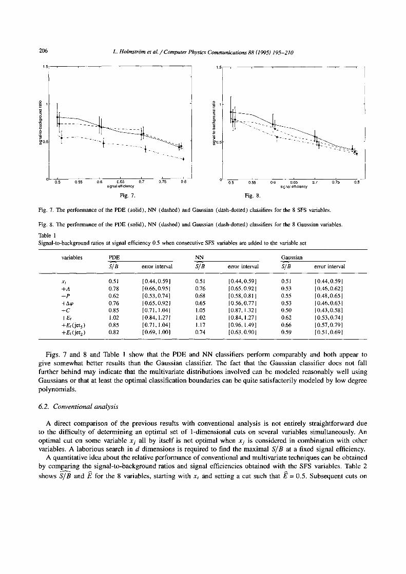
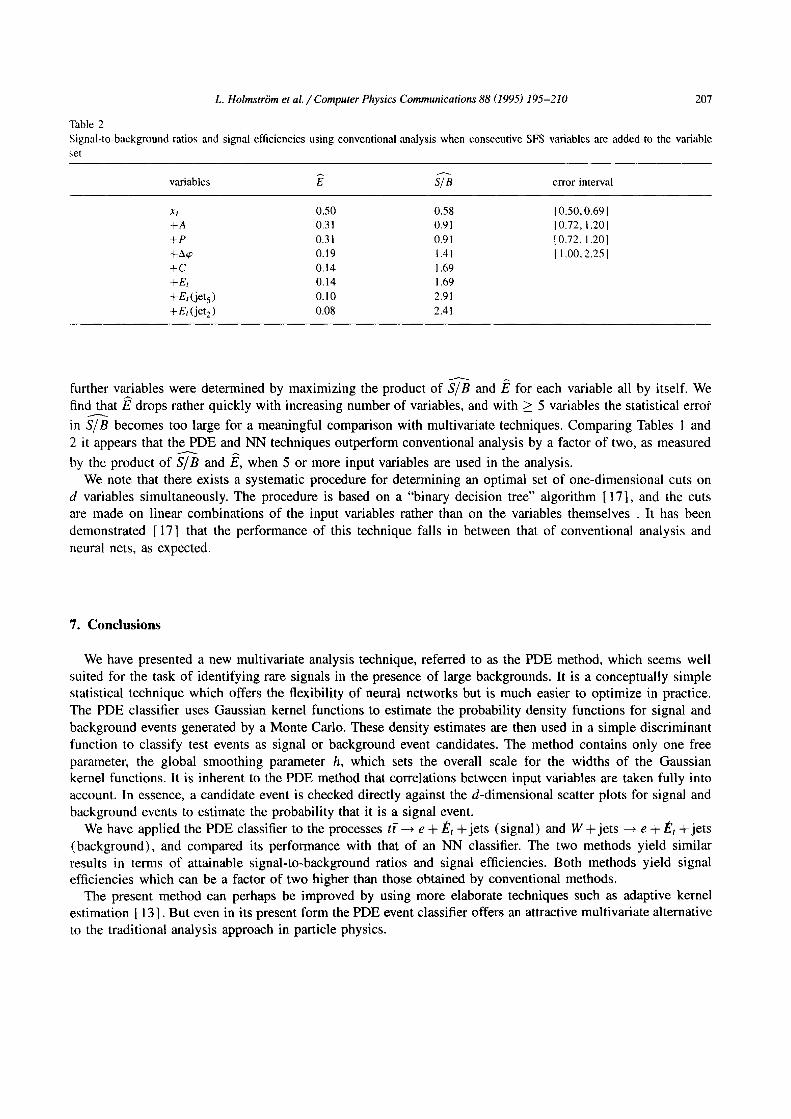
Fig. 7 shows how the PDE and NN classifiers perform when all 8 SFS variables are used. For comparison, the performance of the Gaussian classifier for this variable set is also included. The upper and lower limits of the error bars are ( 1/41 ) ( Ns + 6s) / ( Nb -- 6b) and ( 1/41 ) ( Ns - Ss) / ( Nb + 6b), where Ns, Nb are as in Section 2.1 and 6s, 6b are their estimated standard deviations. The probability that an indicated error bar includes the true S / B varies between 70% and 75%. Table 1 shows the effect of adding consecutive SFS variables to the variable set. Fig. 8 demonstrates the performance of the classifiers when the set of 8 optimal Gaussian variables is used.

206 L. HolmstriSm et aL / Computer Physics Communications 88 (1995) 195-210

1.5

.(2-

6

.~0.5

1.5

o

-9 , o " r

i i i i i _ _ o'.~ o.ss o'.~ o.6s o'.~ o.~ 0~.8 o'.~ o.E~ o'.~ o.~ o'.~ o3s o.8 signal efficiency signal efficiency

Fig. 7. Fig. 8.

Fig. 7. The performance of the PDE (solid), NN (dashed) and Gaussian (dash-dotted) classifiers for the 8 SFS variables.

Fig. 8. The performance of the PDE (solid), NN (dashed) and Gaussian (dash-dotted) classifiers for the 8 Gaussian variables.

Table 1 Signal-to-background ratios at signal efficiency 0.5 when consecutive SFS variables are added to the variable set

variables PDE NN Gaussian S/B error interval S/B error interval S/B error interval

xt 0.51 [ 0.44, 0.59 ] 0.51 [ 0.44, 0.59 ] 0.51 [ 0.44, 0.59 l +A 0.78 [ 0.66, 0.951 0.76 10.65, 0.92 [ 0.53 l 0.46, 0.62 ] +P 0.62 [0.53, 0.74] 0.68 [0.58, 0.811 0 . 5 5 I0.48,0.651 +A~ 0.76 [ 0.65,0.92 [ 0.65 10.56, 0.771 0.53 [ 0.46, 0.63 ] +C 0.85 [ 0.71,1.04 ] 1.05 [ 0.87, 1.32 ] 0.50 [ 0.43, 0.58 ] +Et 1.02 [0.84, 1.27] 1.02 [0.84, 1.27] 0 . 6 2 [0.53,0.741 +Et(jet 5) 0.85 [0.71, 1.04] 1.17 [0.96, 1.49] 0 . 6 6 10.57,0.79] +Et (jet 2) 0.82 [0.69, 1.001 0.74 [0.63, 0.901 0 . 5 9 [0.51,0.691

Figs. 7 and 8 and Table 1 show that the PDE and NN classifiers perform comparably and both appear to give somewhat better results than the Gaussian classifier. The fact that the Gaussian classifier does not fall further behind may indicate that the multivariate distributions involved can be modeled reasonably well using Gaussians or that at least the optimal classification boundaries can be quite satisfactorily modeled by low degree polynomials .

6.2. Conventional analysis

A direct comparison of the previous results with conventional analysis is not entirely straightforward due to the difficulty of determining an optimal set of 1-dimensional cuts on several variables simultaneously. An optimal cut on some variable Xy all by itself is not optimal when xj is considered in combination with other variables. A laborious search in d dimensions is required to find the maximal S /B at a fixed signal efficiency.

A quantitative idea about the relative performance of conventional and multivariate techniques can be obtained by comparing the signal- to-background ratios and signal efficiencies obtained with the SFS variables. Table 2 shows S/---B and if7 for the 8 variables, starting with xt and setting a cut such that if? = 0.5. Subsequent cuts on

L. Holmstr6m et al. / Computer Physics Communications 88 (1995) 195-210 207

Table 2 Signal-to-background ratios and signal efficiencies using conventional analysis when consecutive SFS variables are added to the variable set

variables E S/"~B error interval

xt 0.50 0.58 +A 0.31 0.91 +P 0.31 0.91 +A~o 0.19 1.41 +C 0.14 1.69 + Et 0.14 1.69 +Et(jets) 0.10 2.91 + Et (jet 2 ) 0.08 2.41

[ 0.50, 0.69 I 10.72, 1.201 I 0.72, 1.201 I 1.00, 2.251

further variables were determined by maximizing the product of S/-B and ffS for each variable all by itself. We find that/~ drops rather quickly with increasing number of variables, and with >_ 5 variables the statistical error

A

in S/B becomes too large for a meaningful comparison with multivariate techniques. Comparing Tables 1 and 2 it appears that the PDE and NN techniques outperform conventional analysis by a factor of two, as measured by the product of S/'-'-B and if2, when 5 or more input variables are used in the analysis.

We note that there exists a systematic procedure for determining an optimal set of one-dimensional cuts on d variables simultaneously. The procedure is based on a "binary decision tree" algorithm [ 17], and the cuts are made on linear combinations of the input variables rather than on the variables themselves . It has been demonstrated [ 17] that the performance of this technique falls in between that of conventional analysis and neural nets, as expected.

7. C o n c l u s i o n s

We have presented a new multivariate analysis technique, referred to as the PDE method, which seems well suited for the task of identifying rare signals in the presence of large backgrounds. It is a conceptually simple statistical technique which offers the flexibility of neural networks but is much easier to optimize in practice. The PDE classifier uses Gaussian kernel functions to estimate the probability density functions for signal and background events generated by a Monte Carlo. These density estimates are then used in a simple discriminant function to classify test events as signal or background event candidates. The method contains only one free parameter, the global smoothing parameter h, which sets the overall scale for the widths of the Gaussian kernel functions. It is inherent to the PDE method that correlations between input variables are taken fully into account. In essence, a candidate event is checked directly against the d-dimensional scatter plots for signal and background events to estimate the probability that it is a signal event.

We have applied the PDE classifier to the processes t? --~ e + Et +jets (signal) and W+je t s ---, e + Et +jets (background), and compared its performance with that of an NN classifier. The two methods yield similar results in terms of attainable signal-to-background ratios and signal efficiencies. Both methods yield signal efficiencies which can be a factor of two higher than those obtained by conventional methods.

The present method can perhaps be improved by using more elaborate techniques such as adaptive kernel estimation [ 13], But even in its present form the PDE event classifier offers an attractive multivariate alternative to the traditional analysis approach in particle physics.

208

Acknowledgements

L. Holmstrfm et al. / Computer Physics Communications 88 (1995) 195-210

We thank David Scott and Dennis Cox for useful discussions. This research was supported in part by the U.S. Department of Energy, by a grant no. 8001726 from the

Academy of Finland, grants from the Emil Aaltonen Foundation, the Rolf Nevanlinna Institute, and grant no. DMS-9306658 from the National Science Foundation.

Appendix A

The following computation shows that a neural network that minimizes (6) approximates the function (8) optimally in a least squares sense. First,

,'~ iI~(.~,.,) -(,-~)J~fs(.~),~,, : ,'s l ie(x, , , ) - , , , (x) l~f ,(x) , , , ,

+e~ f ~G(.~,w) - r ( ~ ) ] [ r ( ~ ) - (1 - ~,) ]f~(. , , )dx + P~ i t ' r ( ~ ) - ( ~ - ,~) J: f~(x)d., , , ( i . 1 ) J J

and

Pb i[c,(x, , , ,) - e]2 fb(x)dx = P~, i [G(x ,w) - r ( x ) ]2D,(x)dx

+Pb S [ G ( x , w ) - )'(x) ] [ y ( x ) - - e ] f b ( X ) d x + Pb i [ ~ / ( X ) - - e ] 2 f b ( X ) d x .

Now (7) implies that

y(x) - (1 - e ) = ( 2 e - 1) - -

and since

y(x) - e = (1 - 2 e ) - -

Pbfb(X) f s b ( X ) '

(A.2)

P s f s ( x ) f s b ( x ) '

the second integrals on the right sides of (A.1) and (A.2) cancel out. The third integrals do not depend on w so one has to minimize only

,'~ f t~(~,,,,) - ~(x) ~i~(.,,),,x + ,>~ f lc(,,,w) - ~(.,,)1~i,,(,,),,,,

= f t G ( x , w) - ~,(x) ]2fsb(X)dX.

Thus, the optimal network indeed tries to approximate the mapping y = y(x) in a least squares sense.

Appendix B

We describe here the transformation that was used to diagonalize the signal and background covariance matrices simultaneously. Let 2~s and Xb denote the signal and background covariance matrices. The symmetric (real Hermitian) matrix 2~b has an eigenvalue decomposition

Xb = UAU T,

L. Holmstri~m et al. / Computer Physics Communications 88 (1995) 195-210 209

where U is an orthogonal (real unitary) matrix and A = diag(A1 . . . . . Ad) is a diagonal matrix of the eigenvalues of 2b. Let M = UA-I /2uT, where A -1/2 = diag(A~ -1/2 . . . . . A-~1/2). Then MZ~M is a symmetric matrix, and hence it also has an eigenvalue decomposition,

M£, .M = VDV T,

where D is diagonal and V is orthogonal. A linear transformation of the desired type is then defined by the matrix

A = VTM = VTUA-I/2u T.

To check this, let Id denote the d × d unit matrix. Then

A~YbA T = VTMZbMTV

= VTUA- 1/2 ( U T ZbU) A- 1/2uT V

= VTUA- U2AA- 1/2uT V

= vTU][dUTV

= VTIdV = v T v

=Id,

and

A ~ s A T = VTM2sMTV

= V T ( M ~ ? s M ) V

= vT (VDVT) V

= ( v T v ) D ( V T V )

= IdDId

--D.

Consequently, if X is transformed as yT = AX T, then Y has covariance matrices A~VsA T and AZbA T in the signal and background classes, respectively, and they are both diagonal.

References

[ 1 S.L. Glashow, Nucl. Phys. 22 (1961) 579. S. Weinberg, Phys. Rev. Lett. 19 (1967) 1264. A. Salam, in: Elementary Particle Theory: Relativistic Groups and Analyticity, N. Svartholm, ed., Nobel Symposium No. 8 (Almqvist and Wiksell, Sweden, 1968) p. 367.

12 E Abe et al., CDF Collaboration, Phys. Rev. Lett. 73 (1994) 225; Fermilab Preprint FERMILAB-PUB-94/097-E, Phys. Rev. D, submitted.

13 S. Abachi et al., DO Collaboration, Search for high mass top quark production in pp collisions at v'~ = 1.8 TeV, Phys. Rev. Lett., submitted.

141 C. Peterson and T. Rognvaldsson, An Introduction to Artificial Neural Networks, Lectures given at the 1991 CERN School of Computing, University of Lund preprint LU TP 91-23, September 1991. B. Denby, Neural Computation 5 (1993) 505.

151 J. Hertz et al., Introduction to the Theory of Neural Computation (Addison-Wesley, Redwood City, CA, 1991 ).

210 L. Holmstri~m et al. / Computer Physics Communications 88 (1995) 195-210

[6] G. Cybenko, Math. Contr. Sign. Syst. 2 (1989) 303. [7] R. Odorico, Phys. Lett. B 120 (1983) 219. [8] G. Ballochi and R. Odorico, Nucl. Phys. B 229 (1983) 1. {91 A. Cherubini and R. Odorico, Z. Phys. C 47 (1990) 547.

[ 10] R. Raja, DO Note 1992, September 1991, unpublished; private communication. [ I0] K. Fukunaga, Introduction to Statistical Pattern Recognition, second edition (Academic Press, San Diego, CA, 1991 ). [11] A. Cherubini and R. Odorico, Z. Phys. C 53 (1992) 139. [12] D.W. Scott, Multivariate Density Estimation. Theory, Practice, and Visualization (Wiley, New York, 1992). [ 13] T. Sjostrand, PYTHIA 5.6 and JETSET 7.3 Physics Manual, CERN preprint CERN-TH.6488/92, May 1992. [ 14] P.A. Devijver and Kittler, Pattern Recognition: A Statistical Approach (Prentice-Hall, London, 1982). [ 15] L. HolmstrOm and S. Sain, Searching for the Top Quark Using Multivariate Density Estimates, Rice University Department of

Statistics Technical Report 93-3, December 1993. [161 D. Bowser-Chao and D.L. Dzialo, Phys. Rev. D 47 (1993) 1900.