


Bahasa
Halaman
Hukum


Worcester Polytechnic InstituteDigital WPI
Masters Theses (All Theses, All Years) Electronic Theses and Dissertations
2018-04-26
EMG Site: A MATLAB-based Application forEMG Data Collection and EMG-based ProstheticControlWilliam J. BoydWorcester Polytechnic Institute
Follow this and additional works at: https://digitalcommons.wpi.edu/etd-theses
This thesis is brought to you for free and open access by Digital WPI. It has been accepted for inclusion in Masters Theses (All Theses, All Years) by anauthorized administrator of Digital WPI. For more information, please contact [email protected].
Repository CitationBoyd, William J., "EMG Site: A MATLAB-based Application for EMG Data Collection and EMG-based Prosthetic Control" (2018).Masters Theses (All Theses, All Years). 351.https://digitalcommons.wpi.edu/etd-theses/351

EMG Site: A MATLAB-based Application for EMG Data
Collection and EMG-based Prosthetic Control
by
William J. Boyd
A Thesis
Submitted to the Faculty
of the
WORCESTER POLYTECHNIC INSTITUTE
in partial fulfillment of the requirements for the
Degree of Master of Science
in
Electrical & Computer Engineering
April 2018
APPROVED:
Prof. Edward A. Clancy, Research Advisor
Prof. Xinming Huang
Dr. Moin Bhuiyan

2 | P a g e
Abstract:
This thesis describes the system design of EMG Site, a MATLAB-based application for
collection and visualization of surface electromyograms (EMGs) and the real-time control of an
upper limb prosthesis, including details pertaining to the design of the software and the
graphical user interface (GUI). The application consists of features that aid in the visualization of
the collected EMG data and the control of a prosthesis. Visualization of the collected EMG data
is handled in one of two ways: an oscilloscope-like view showing the raw EMG data collected
with respect to time, or a radial plot showing the processed EMG data collected with respect to
the site of EMG data collection on the arm. The control of a hand-wrist prosthesis is primarily
regulated through the use of signal processing designed to relate EMG to torque and is
visualized in the tracking window – a plotting window showing both a user-control cursor and
an either static (or dynamic) computer-controlled target. This thesis concludes with a
description of the real-time capabilities of the application regarding both the visualization of
the collected EMG data as well as the control of a prosthesis.

3 | P a g e
Contents 1.0 Introduction ............................................................................................................................................ 6
2.0 Background ............................................................................................................................................. 7
2.1 Electromyogram .................................................................................................................................. 7
2.2 MATLAB ............................................................................................................................................... 7
2.2.1 Computation Levels in MATLAB ................................................................................................... 8
2.3 EMG Site .............................................................................................................................................. 9
3.0 System Design ....................................................................................................................................... 10
3.1 GUI Design ......................................................................................................................................... 10
3.1.1 GUI: Menu Bar............................................................................................................................ 10
3.1.2 GUI: Scope View ......................................................................................................................... 11
3.1.3 GUI: Radial Plot .......................................................................................................................... 12
3.1.4 GUI: Multi-Purpose Tracking Window ....................................................................................... 13
3.2 Software Design ................................................................................................................................ 14
3.2.1 First Phase: Initialization ............................................................................................................ 15
3.2.1.1 Initialization: GUI and DAQ Session .................................................................................... 15
3.2.1.2 Initialization: Signal Processing and Updates ..................................................................... 17
3.2.2 Second Phase: Background Loop ............................................................................................... 17
3.2.2.1 Data Collection .................................................................................................................... 17
3.2.2.2 Sending ADC Data to the Foreground ................................................................................. 18
3.2.3 Third Phase: Foreground Functions ........................................................................................... 18
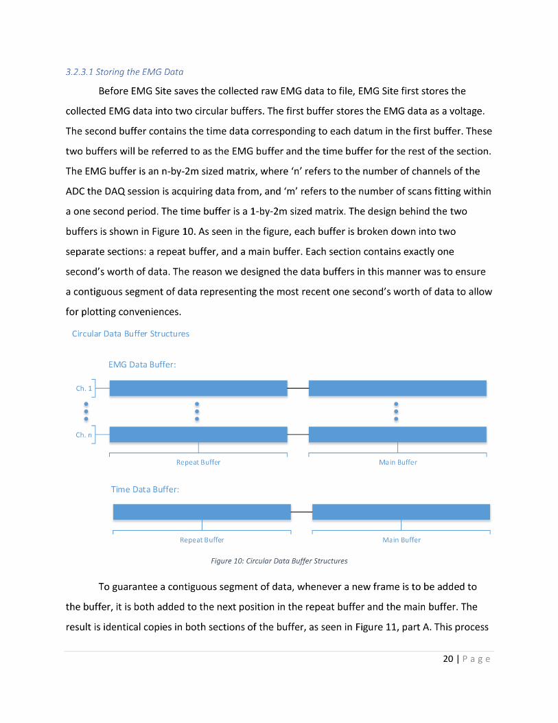
3.2.3.1 Storing the EMG Data ......................................................................................................... 20
3.2.3.2 Saving the EMG Data .......................................................................................................... 21
3.2.3.1 Plotting: Raw EMG Time Plots ............................................................................................ 22
3.2.3.2 Plotting: EMG Standard Deviation Radial Plot .................................................................... 24
3.2.3.3 Plotting: Multi-purpose Tracking window .......................................................................... 26
3.2.3.4 Generation of Control Signals ............................................................................................. 31
3.3 Filtering ............................................................................................................................................. 32
3.3.1 Filter Design Techniques ............................................................................................................ 32
3.3.1.1 The Problem of Quantization .............................................................................................. 32
3.3.1.2 tf2mos() ............................................................................................................................... 34
3.3.1.3 Critically Damped Filters ..................................................................................................... 35
3.3.2 Filter Implementation ................................................................................................................ 36

4 | P a g e
4.0 Results ................................................................................................................................................... 39
4.1 Timing Results ................................................................................................................................... 39
4.1.1 Sampling Rate of 1000 Hz .......................................................................................................... 41
4.1.2 Sampling Rate of 2000 Hz .......................................................................................................... 42
4.1.3 Sampling Rate of 4000 Hz .......................................................................................................... 43
4.1.4 Overall Timing Results ................................................................................................................ 44
4.2 Target Tracking Usage Data .............................................................................................................. 44
4.2.1 Bandlimited Random Values ...................................................................................................... 44
4.2.2 Uniform Random Values ............................................................................................................ 47
5.0 Discussion .............................................................................................................................................. 49
5.1 Adding Additional GUI Elements ....................................................................................................... 49
5.2 Changing Number of Active Channels .............................................................................................. 54
5.2.1 Adding/Removing Points to Radial Plot ..................................................................................... 54
5.2.2 Adding/Remove Plots in Scope View ......................................................................................... 55
6.0 Conclusion ............................................................................................................................................. 58
References .................................................................................................................................................. 59
Appendix A (Written by Edward A. Clancy, Included with permission) ...................................................... 60
Figure 1: Main menu bar of EMG Site (1) ................................................................................................... 10
Figure 2: Main menu bar of EMG Site (2) ................................................................................................... 10
Figure 3: Scope View ................................................................................................................................... 11
Figure 4: EMG Standard Deviation Radial Plot............................................................................................ 12
Figure 5: Multi-Purpose Tracking Window ................................................................................................. 13
Figure 6: EMG Site Phase Flow diagram ..................................................................................................... 15
Figure 7: EMG Site Phase 1 Flow Diagram .................................................................................................. 15
Figure 8: Background Loop Flow Diagram .................................................................................................. 18
Figure 9: ADC_ISR/Foreground Flow Diagram ............................................................................................ 19
Figure 10: Circular Data Buffer Structures .................................................................................................. 20
Figure 11: Data Position in Buffers. ............................................................................................................ 21
Figure 12: Plotting Time Plots Algorithm .................................................................................................... 24
Figure 13: Calculation of EMG Standard Deviation..................................................................................... 25
Figure 14: Generation of Correlated Uniform Random Values .................................................................. 27
Figure 15: Target/Cursor Generation Flow Diagram .................................................................................. 29
Figure 16: Block Diagram: Filter Sectioning. ............................................................................................... 34
Figure 17: Direct Form I IIR Filter Implementation. .................................................................................... 37
Figure 18: Power Spectrum Density of x-position, Window size = 2000 samples ...................................... 45
5 | P a g e
Figure 19: Power Spectrum Density of y-position, Window size = 2000 samples ...................................... 45
Figure 20: Power Spectrum Density of Rotation, Window size = 2000 samples ........................................ 46
Figure 21: Power Spectrum Density of Size, Window size = 2000 samples ................................................ 46
Figure 22: Histogram of x-position Values .................................................................................................. 47
Figure 23: Histogram of y-position Values .................................................................................................. 47
Figure 24: Histogram of Rotation Values .................................................................................................... 48
Figure 25: Histogram of Size Values ............................................................................................................ 48
Table 1: PC Specs ........................................................................................................................................ 40
Table 2: EMG Site Timing Results (fs = 1000 Hz) ......................................................................................... 41
Table 3: EMG Site Timing Results (fs = 2000 Hz) ......................................................................................... 42
Table 4: EMG Site Timing Results (fs = 4000 Hz) ......................................................................................... 43
Equation 1: Cutoff Frequency vs. Decimate Rate ....................................................................................... 25
Equation 2: Cubic Polynomial Interpolation. .............................................................................................. 27
Equation 3: Calculation of Rotation Angle .................................................................................................. 30
Equation 4: Rotation Transformation ......................................................................................................... 30
Equation 5: Translation Transformation ..................................................................................................... 30
Equation 6: Zero-Pole-Gain Form of a Transfer Function. .......................................................................... 34
Equation 7: Corrected frequency cutoff for a critically damped filter. ...................................................... 36
Equation 8: Angular frequency cutoff for a critically damped filter. .......................................................... 36
Equation 9: Filter coefficient equations. ..................................................................................................... 36

6 | P a g e
1.0 Introduction
In this thesis, we will describe the system design of EMG Site, a MATLAB-based
application for the collection and visualization of surface electromyograms (EMGs) and the real-
time control of an upper limb prosthetic. In this discussion, we will describe the design of the
software, the graphical user interface (GUI), as well as the signal processing techniques used
with EMG Site. The features and design of EMG Site it based on the needs of those using it at
the time and will contain features similar to a preexisting system written in LABVIEW, with the
intent of future additions being made in the future as the needs arise.
The current application being used for the collection and visualization of surface EMGs
is written and designed in LabVIEW – a programming language largely unfamiliar to those using
EMG Site. However, within the current lab, there is a large pool of knowledge and experience
with MATLAB; as such, the recreation of EMG Site in MATLAB allows for more freedom in the
software design and features for the current lab members, especially in present studies
concerning EMG.
EMG Site, to fulfill the needs and requirements of the lab needs to contain an EMG data
collection system allowing for the collection of surface EMG from a multitude of sites of a test
subject. This collection is desired to be USB-based and wired. In addition, EMG Site needs to be
able to save the collected data to the local computer for future analysis and visualization, to be
able to visualize the collected EMG, and to be able to support the control of a hand/wrist
prosthetic.
This thesis will begin its discussion with the presentation of background information on
topics related to EMG Site and EMG data, followed by a detailed description of the system
design. This system design will include information concerning the software design of EMG Site,
the design of the GUI, as well as the signal processing techniques used. After the discussion on
the system design, we will discuss the usage results of EMG Site with respect to the
performance of the different features as well as the performance of the tracking system, used
in part of the control of a hand/wrist prosthetic. Following the results, we will discuss various
ways of improving EMG Site in the future as well as the methods on would take to make certain
additions to the GUI, before concluding the thesis.

7 | P a g e
2.0 Background
In this section, we present the relevant background information needed to fully
understand the topics discussed in later sections. Firstly, we provide basic descriptions of
electromyograms and of MATLAB, including brief histories of each. Afterwards, we discuss the
purposes behind the EMG Site, and the reasons leading to its development.
2.1 Electromyogram
As defined in the Oxford Dictionary of Biology, an electromyogram is A e o di g of the
electrical activity of muscle fibre Hine, 2016). What the electromyogram records is the action
potential of individual muscle units. The action potential refers to transmission along muscle
fibers through electrochemical pulses caused by changes in the electrical potential between the
interior and exterior of a muscle fiber cell membrane (Lerner, 2014). It is these changes that are
then amplified and recorded as an electromyogram. A common process by which clinical
electromyograms are acquired involves the insertion of electrodes within the muscle(s) to be
observed (Hine, 2016). For many biomechanics-related studies and tasks however, EMGs are
recorded at the skin surface. EMG recorded at the skin surface are called surface EMG or sEMG
(Staudenmann, 2010). The EMG recorded and collected by EMG Site will consist of sEMG.
The discovery of electricity generated by muscles was first documented by Italian
physician Francesco Redi who observed electricity generated by specialized muscle of the
electric ray fish (Reaz, 2006). It as t u til 1890 when this electrical activity was first recorded,
and the term electromyogram coined (Reaz, 2006). However, due to the stochastic nature of
myoelectric signals, it as t u til u h late that EMG ould e used li i all ‘eaz, .
EMG recorded at the forearm, the primary source of EMG for this application, has a
typical bandwidth ranging from 20-500 Hz (Clancy, 2006). The voltage of EMG tends to range up
to the scale of millivolts (Kilic, 2017), and is usually gained up to larger ranges prior to analog-
to-digital conversion.
2.2 MATLAB
Cleve Moler designed the first version of MATLAB in the late 1970s to allow his students
at the time at the University of New Mexico to have access to portions of EISPACK and LINPACK,

8 | P a g e
two Fortran libraries containing useful methods for matrix eigenvalue computation and solving
linear equations (MathWorks). This initial release of MATLAB contained 80 functions, a fraction
of what is available today. With the a ou e e t of IBM s fi st PC i , MATLAB was
ep og a ed i C, addi g i a featu es that a e o o pla e i toda s MATLAB, such as
m-files. In 1984 in California, MathWorks was founded by Cleve Moler, Jack Little, and Steve
Bangert. Today, MATLAB has several different toolboxes covering applications from several
different disciplines including computer vision, signal processing, and control systems, to name
a few (MathWorks).
2.2.1 Computation Levels in MATLAB
Within the MATLAB environment, every basic process is handled in one of two places:
the foreground or the background. Couple these two levels of processing with a GUI/keyboard
inputs, and that gives any MATLAB application a total of three different levels of computation
and users access. The main functional level of computation is the foreground. The foreground
level is where all functions and basic commands are processed in MATLAB. Using the DAQ (Data
Acquisition) toolbox, MATLAB allows for certain processes to run behind the foreground in the
background. Events occurring in the foreground will not block these processes from executing
in the background. In return, the processes in the background will also not prevent any function
from being executed in the foreground. The GUI/keyboard level consists of a collection of
interactable elements such as buttons, switches, and text boxes. Every time a GUI element is
interacted with, if there is an associated callback function, that function will attempt to
execute. If a process is already in process, the execution of the callback function is either added
to a queue or is ignored. This decision is decided upon by the creator of the GUI and cannot be
changed dynamically. If there is no callback function associated with a particular event, then
that event will be ignored; this holds true for both events originating from the GUI and events
originating from the background.
The priority of processing events in MATLAB does not rely on where the event has come
from, but when the event has occurred. Whether the event is the press of a button on a GUI or
the acquisition of data from a data acquisition device, the event simply calls a function. If

9 | P a g e
another function is currently running, the new function is either ignored or queued up, waiting
for its turn to execute.
2.3 EMG Site
EMG Site is intended to be a stand-alone application capable of handling many of the
tasks performed during experiments where EMG is collected including the acquisition of
EMG data from one or many electrodes, the storage of said EMG to a local memory location,
and a real-time EMG display with an option to control a hand-wrist prosthetic. With a similar
application, written in LabVIEW, already working, and being used in current experiments, the
necessity for EMG Site arose due to the collective experience programming of the current lab
members in MATLAB as compared to LabVIEW. This collective experience allows for easier
adjustments and additions to be made. With an application already designed in LabVIEW, much
of the functionality of EMG Site is modeled after its LabVIEW counterpart. Design choices made
with EMG Site considered which features the lab desired to retain and which features the lab
would no longer need in the future.

10 | P a g e
3.0 System Design
In this section, we focus the discussion on the overall system design of EMG Site. We
first discuss the design of the GUI and highlight many of the key features of EMG Site. Secondly,
we discuss the software design of EMG Site, focusing on the basic flow of the program and how
EMG Site handles all its tasks, as well as the techniques it uses to maximize its processing
efficiency. Lastly, we discuss the signal processing techniques used throughout EMG Site
including the different filter design techniques used as well as the different methods of
implementing the different filters throughout EMG Site.
3.1 GUI Design
The overall GUI design of EMG Site consists of four main components: three panels
corresponding to the main functional units of EMG Site and a menu bar. In the following
sections, we discuss each o po e t s desig as ell as p o ide e a ples as to ho ea h
component is used within EMG Site. First, we discuss the menu bar.
3.1.1 GUI: Menu Bar
Figure 1: Main menu bar of EMG Site (1)
Figure 2: Main menu bar of EMG Site (2)
Figures 1 and 2 above display the main menu bar of EMG Site Menu Bar. The menu bar
can be broken up into four different sections. The first section consists of a series of buttons
that controls the current window, of which there are four different active options – Scope,
Radial, Task, and Settings. Three of these options will be discussed in further detail in the
following sections. The second section focuses on the file path and file name used to save the
data ei g olle ted du i g a DAQ sessio . The File Path te t o allo s the use to sele t the
destination folder on the local machine in which EMG Site will save the data it collects. The
T ial a d “u je t text boxes allow for the user to modify the file name of the data being

11 | P a g e
saved during each DAQ session, allowing for integer input. The resulting filename is of the form
s[su je t#]_t[t ial#]. i . The third section consists of three buttons: ‘e o d, “ta t Data
Colle tio , a d “top Data Colle tio . The fi st button starts a DAQ session and saves all data
that is collected. The second button also starts a DAQ session but does not save any data. The
third button manually stops any active DAQ session. The fourth section of the main menu bar
consists of text boxes, one editable and the other greyed out. The first text box allows for the
user to enter in the desired duration of the next DAQ session. This value can be any real,
positi e i tege , o i f , representing an infinite duration. The greyed-out text box displays the
current time elapsed since the start of the DAQ session.
3.1.2 GUI: Scope View
Figure 3: Scope View: Each MATLAB plot shows the raw EMG data collected from each of the 16 connected channels.
The first of three main screens of EMG Site, the scope view contains a total of 16
different two-dimensional time plots, each one corresponding with a different analog input
channel of the ADC, as seen above in Figure 3. Each of these time plots is designed to display
the last-collected data from the ADC and back a set period. The result is a scrolling-time plot.
Alongside the 16 time plots, the scope view also contains two other sections of note. The first
of these sections contains two text boxes controlling the axis limits of all 16 time plots. The
topmost text box sets the desired horizontal axis, representing the time window (in seconds)
12 | P a g e
displayed in each plot. The default value for this is a one-second window. The bottommost text
box sets the desired vertical axis, representing the voltage of the EMG. The default for this is +/-
10 V (as presented to the ADC). The second section contains an array of text boxes, labeled 1) –
16), corresponding to each of the 16 time plots. The values in these text boxes represent
channel gains that are applied post-ADC, but before plotting. More details about the plotting
process are discussed in section 3.2.3.1.
3.1.3 GUI: Radial Plot
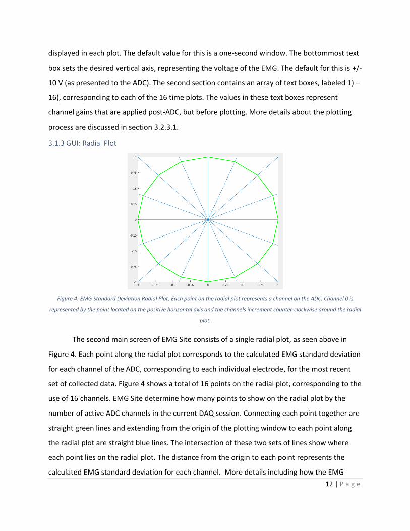
Figure 4: EMG Standard Deviation Radial Plot: Each point on the radial plot represents a channel on the ADC. Channel 0 is
represented by the point located on the positive horizontal axis and the channels increment counter-clockwise around the radial
plot.
The second main screen of EMG Site consists of a single radial plot, as seen above in
Figure 4. Each point along the radial plot corresponds to the calculated EMG standard deviation
for each channel of the ADC, corresponding to each individual electrode, for the most recent
set of collected data. Figure 4 shows a total of 16 points on the radial plot, corresponding to the
use of 16 channels. EMG Site determine how many points to show on the radial plot by the
number of active ADC channels in the current DAQ session. Connecting each point together are
straight green lines and extending from the origin of the plotting window to each point along
the radial plot are straight blue lines. The intersection of these two sets of lines show where
each point lies on the radial plot. The distance from the origin to each point represents the
calculated EMG standard deviation for each channel. More details including how the EMG

13 | P a g e
standard deviation is calculated and how this plot is generated is discussed further in section
3.2.3.2.
3.1.4 GUI: Multi-Purpose Tracking Window
Figure 5: Multi-Purpose Tracking Window
The last of the three main screens of EMG Site is the tracking window and can be seen in
Figure 5 above. The tracking window is broken up into three sections. The first section is the
large plot in the center containing two triangular objects. The x-axis and y-axis both represent
the %MVC (maximum voluntary contractions) for the flexion/extension movements and the
ulnar/radial deviation movements, respectively. The blue object represents the computer-
o t olled ta get, and the red object represents the user- o t olled u so . The next two
sections correspond to the allowed degrees of freedom (DoF) of both the target and the cursor
objects. The set of buttons to the left of the plot, la eled Cu so DoF allo the use to sele t
or de-select which DoFs to use while plotting the red cursor. For each option selected, another
DoF is allo ed. The set of utto s to the ight of the plot, la eled Ta get DoF a t i a si ila
manner, allowing the user to select which DoFs are used to plot the target. Above the set of
buttons is a set of two radio buttons that allow the user to toggle between a static target or a


16 | P a g e
The init_plots() function goal is to generate the initial data EMG Site displays on start-up
and to set the default parameter configurations of the plots a es. Function init_plots() further
brakes up this process into multiple sections relating to each of the different type of plots
within EMG Site, consisting of time plots, a radial plot, and a multi-purpose tracking window.
For each of the different types of plots, init_plots() performs two basic tasks. Firstly, init_plots()
defines the properties of the axes object contained within each plot, such as the axis limits and
the tick values along the two axes. Secondly, init_plots() creates the initial data to be populated
within the different plots for both the time plots and the radial plot. For the tracking window,
the initial data set generated at this step is not immediately utilized but is instead saved for
later use. The details of how this data set is created and used will be discussed with the third
phase of EMG Site, in Section 3.2.3.3.
With the initialization of the different plots and the initial data to populate each plot,
init() calls its second child function, init_timer(). The init_timer() fu tio s ole is to defi e a
timer object with a period of one second. The timer object allows for the implementation of a
stopwatch that counts to, or a timer that counts down from, the set duration of the DAQ
session with a resolution of one second. A period of one second was chosen to give the user an
accurate representation of the elapsed time while not diverting too much of the computational
time needed by the other functions. The purpose of the timer is to give the user information
concerning the running-time of the current DAQ session or how much time may be left in the
current session, if a set duration is specified.
The final primary child function that init() calls is init_daq(). This function handles the
initialization of the communication link between MATLAB and the ADC, as well as sets the
default values related to the input and output DAQ sessions used by EMG Site. Function
init_daq() first defines the initial parameters of the input DAQ session such as the sampling rate
of the ADC and the size of the frame of data to be passed to the main processing function of
EMG Site. A description and discussion of these parameters is located below in Section 3.2.2.
Secondly, init_daq() establishes the link between the ADC and MATLAB by specifying the ADC to
connect with, if there are multiple ADC systems recognized by MATLAB, and which channels to
use for both the input and output sessions.

17 | P a g e
3.2.1.2 Initialization: Signal Processing and Updates
With the plots, the timer, and the DAQ sessions for both input and output created, the
first of the two primary responsibilities of the initialization phase concludes and is not repeated
for the entirety of the current instance of the application. With the initialization of EMG Site
completed, control of the GUI is given to the user. Before the start of a DAQ session, the user
can edit the parameters of the DAQ session, as well as certain properties of the plots, such as
the sampling rate for the input DAQ session and the axis limits for the time plots.
The second responsibility of the initialization phase of EMG Site occurs just before the
start of a DAQ session. The specific tasks that need to be accomplished include: initializing the
filters and buffers used by EMG Site in the processing of the incoming EMG data, updating the
DAQ session with any modifications that the user may have made, and readying the individual
plots for the new incoming data. Each of these three tasks is handled by startDAQ(). More
information detailing the filters used and how they are created is discussed below in Section
3.3.
3.2.2 Second Phase: Background Loop
In this section, we discuss the specifics of the background loop within EMG Site. We first
discuss how EMG Site collects the EMG data from the ADC. Secondly, we discuss how those
data are then handled through the background and up to the foreground.
3.2.2.1 Data Collection
When a DAQ session is started, the process of collecting data in the background begins
and follows the flow of events described in Figure 8. As part of the initialization phase, the DAQ
session has been initialized to collect a certain number of scans of the original EMG signal
before triggering the data to begin to be processed. The number of scans to collect is
determined by the size of the frame of data to be sent to the foreground. A frame of data
consists of a matrix with columns representing the different channels of the ADC being read
from and rows representing the different scans of the original EMG signal. The number of scans
is determined based on the set sampling frequency of the ADC and how often a completed
frame is desired. For example, if the ADC is set to sample at a rate of 2000 Hz and a new frame
of data is desired at a rate of 100 Hz, each frame would have 20 scans.


22 | P a g e
The native numeric data type in MATLAB is a floating-point double, consisting of 64 bits
worth of data. To increase the speed of writing the collected EMG data to file, before the data
are written, they are casted to floating-point single precision, following IEEE Standard 754. After
being casted to single precision, each datum is then written to a binary file (.BIN), using the
fwrite() function.
3.2.3.1 Plotting: Raw EMG Time Plots
With the data collected from the ADC saved and stored within the data buffers, the data
are then passed into one of three different functions, corresponding to the current view of the
GUI. In this section, we discuss the process in which EMG Site plots the time plots displaying the
raw EMG with respect to time. To display all the data collected from the ADC, EMG Site has 16
different time plots, one for each channel of the ADC, shown above in Figure 3. To ease the
burden of plotting to 16 different plots, EMG Site utilizes two basic ideas: strategically skipping
plotting certain plots each iteration and updating the smallest amount of data each iteration.
Plotting Object Hierarchy in MATLAB
To better understand how EMG Site plots all its plots, we must first investigate the
object hierarchy created by the plotting functions within MATLAB. Each plot that is displayed
within MATLAB consists of three layers, with each layer being a different MATLAB object. The
first that encompasses all others is a figure object. The figure object provides the framework
that allows for a plot to exist. Without a figure object to exist in, a plot would not be able to be
displayed. The second layer consists of an axes object. Different types of plots in MATLAB use
different objects to represent the display of the data being plotted. The axes object allows for
the data to be displayed on Cartesian axes. The third layer contains the actual data to be
displayed within the plot. For an axes object, the data being displayed is contained within line
objects. The line object contains all the details of the data and how it is plotted, such as the
color of the line or the width of the line. For EMG Site, for each axes object, a total of two line
objects are required. One is for the EMG data being displayed and the second is for the zero-
line displayed on every time plot. When a plotting function, such as plot(), is called for the first
time, all three layers are created and initialized with the parameters from the plotting function.

23 | P a g e
The problem for EMG Site arises in the processing time for each call to the plot()
function. For simplicity, for the rest of this discussion, we only consider the objects used within
EMG Site. If a user would call the plotting function again, the plotting function will use the pre-
existing figure object and create and initialize new axes and line objects. If this procedure of
plotting to a pre-existing figure object is repeated, the actions of creating and initialization the
different layers becomes very time-consuming. If EMG Site tries to plot using the built-in
MATLAB plotting functions every time new data arrives to the foreground, with a frame rate of
100 Hz and a total of 16 time plots, EMG Site will need to create and initialize 1,600 axes
objects and 3,200 line objects every second. For practical purposes, plotting to all 16 plots is
impossible to achieve every iteration of the ADC loop.
Methods to Reduce Time to Plot
One of the methods EMG Site uses to reduce the processing time of plotting the 16 time
plots is by strategically skipping certain plots every iteration of the ADC loop. Specifically, for
every iteration of the ADC loop, EMG Site only updates four plots, as shown below in Figure 12.
With a total of 16 plots, EMG Site takes four iterations of the ADC loop to update all 16 plots,
resulting in a plot refresh rate that is a quarter of the frame rate. This lower refresh rate
reduces the 4,800 objects being created down to 1,200. However, this reduction in refresh
rates does not come without a price. Firstly, the plots being updated in the current iteration of
the ADC loop eed to at h up also plotti g the data that as skipped i p e ious
iterations; this results in a chunkier plot as more data points are being appended every
iteration. Even with this reduction in the number of plots being updated each iteration, the
process of creating and initializing 1,200 objects is still practically impossible to achieve.


25 | P a g e
High Pass @ 15 Hz
Calculation of EMG Standard
Deviation
Low Pass Low Pass @ 1 HzDownsampleRectify
Figure 13: Calculation of EMG Standard Deviation
Calculating EMG Standard Deviation
The process of calculating the EMG standard deviation consists of four steps. The
process is shown in detail in Figure 13. The first step is to pass the data through a high-pass
filter. The reason we send the data through a high-pass filter is to remove any disturbances
caused by the EMG recording device. The high-pass filter we used is a 4th order Butterworth
filter with a cutoff of 15 Hz. The second step is to rectify the signal, to force a positive value out
of the calculation. After sending the data though the high-pass filter and a rectifier, to calculate
the EMG standard deviation, we want to send the signal through a low-pass filter to smooth the
signal. The desired cutoff frequency for this low-pass filter is defaulted to 1 Hz but remains
programmable to fit the need for the current situation. However, with a sampling rate of up to
4 kHz, filtering at 1Hz is quite difficult. To make this process easier, EMG Site first decimates the
data down to the frame rate before performing the final pass through the low-pass filter at 1
Hz. The low-pass filters used during decimation are 9th order Chebyshev Type 1 filters, and the
final low-pass filter is designed as a 2nd order critically damped IIR filter. The decimation process
itself consists of a loop of two steps. The first step is a low-pass filter, whose cutoff frequency is
dependent on the desired rate of decimation. The relationship between the cutoff frequency
and the rate of decimation is shown below in Equation 1. = .�
Equation 1: Cutoff Frequency vs. Decimate Rate
where is the cutoff frequency of the filter and � is the desired rate of decimation. The second
step in the decimation process is to down-sample the signal to the desired sampling rate. This is

26 | P a g e
done by removing samples in the filtered signal, leaving only every � ℎ point in the signal. For
decimation rates greater than 13, the decimation process is broken up into two jumps to
increase the reliability of the decimation, hence the loop shown in Figure 13.
With the EMG standard deviation for each channel of EMG data calculated, a simple
transform is applied to the data to transform the data from Cartesian coordinates into polar
coordinates. The angles for each channel are determined based on the number of channels
being used for plotting and are calculated to allow the points on the radial plot to be evenly
distributed.
3.2.3.3 Plotting: Multi-purpose Tracking window
The last of the three main functions occurring in the foreground, and the focus of this
section, is the tracking window. The primary function of the tracking window is to perform
target-tracking with a randomly-generated target object and a user-controlled cursor object.
The other primary function of the tracking window is a 2-DoF dynamic calibration that guides a
user to attempt to control the cursor object to follow the target object along a pre-defined
path.
Generation of band-Limited Uniform Random Values
The randomly-generated target object has four degrees of freedom: the x-position, the
y-position, the rotation about its origin, and its size. Each degree of freedom corresponds to an
independent movement on the hand-wrist, corresponding to the flexion/extension of the wrist,
the ulnar/radial deviation of the wrist, the pronation/supination of the wrist, and the
opening/closing of the hand, respectively. The process of generating the random values consists
of three steps: generating Gaussian random deviates, interpolating the random deviates, and
applying a static transform to covert the deviates from a Gaussian distribution to a Uniform
distribution (Clancy). More details on this procedure can be found in Appendix A. This process is
shown in Figure 14. The ultimate reason for this process is to create correlated Uniform random
numbers. Normally, a random number generator will produce independent Gaussian random
numbers.


28 | P a g e
where , , , and represent the coefficients of the cubic polynomial used for the
interpolation process of , and [・] represents the four most recent random values that
are being interpolated between. Using the middle two points allows for continuity between
each of the generated deviates as new points are added over time. The resulting values at this
point are band-limited correlated Gaussian random values. The final step is to transform the
random values using the Gaussian CDF function, transforming the random values from a
Gaussian distribution to a Uniform distribution. The result of this process is an array of
correlated Uniform random values representing the trajectory of the target on the tracking
window.
Target Object Generation
With the generation of the Uniform random values described in the previous section,
EMG Site then handles the generation of the target object within the tracking window. The
process by which EMG Site generates the target and the other functions of the tracking window
are shown below in Figure 15.


30 | P a g e
is applying a vertical and horizontal translation to the target moving the target to the desired x
and y positions of the tracking window. This process is defined below in Equations 3, 4, and 5.
Let be a 2x10 matrix, where each 2x2 block represents a single line making up the target
object located centered at the origin. The first row represents the x-coordinates of the
endpoints of the line and the second row represents the y-coordinates of the endpoints of the
line. � = � − �
Equation 3: Calculation of Rotation Angle
where � is the desired rotation of the target and � is the rotation angle required to
achieve the desired orientation, assuming a default orientation of �
. = (cos � − sin �sin � cos � ) ∗
Equation 4: Rotation Transformation
where is a 2x10 matrix containing the line information of the target rotated around the
origin to the desired orientation. = + ( )
Equation 5: Translation Transformation
where is a 2x10 matrix containing the line information of the target rotated and then
translated into the desired orientation and position, and and are the desired x-
coordinate and y-coordinate of the center of the target.
The generation of the target object in a static state is even simpler. The user, after
selecting the desire to generate a static target, is given access to four input boxes on the GUI.
Within these four input boxes, the user can enter in the desired size, rotation, x-position, and y-
position of the target within the tracking window. Using the same coordinate transformations
as described above, EMG Site plots the static target object within the tracking window.
2-DoF Dynamic Calibration
The goal of the 2-DoF dynamic calibration is to ascertain a set of channel gains to allow
for a 2-DoF control, utilizing the opening/closing of the hand and one additional DoF (degree of

31 | P a g e
freedom) such as the ulnar/radial deviation of the wrist. The calibration process consists of the
tracking of a target along the x and y axes of the tracking window. The target moves a slow,
constant speed moving away from the origin along each axis in turn before returning to the
origin. One implementation that EMG Site utilizes has the time for the target to travel from the
origin to a pre-determined point at the end of one axis to take a total of five seconds, resulting
in ten seconds per axis and forty seconds for the entire calibration process.
3.2.3.4 Generation of Control Signals
As can be seen in Figure 9 after the desired foreground function has finished execution,
the next step in the procedure is the generation of the control signals, using the collected EMG
data as input. EMG Site generates a total of three control signals to send out: one signal ranging
from 0V to 5V controlling the rotation of the wrist and two signals ranging from 0 V to 4 V
controlling the opening and closing of the hand.
The control signal for the wrist is a bi-directional control signal, spinning in one direction
continuously while the signal ranges from 0 V to just under 2.5 V. At 2.5 V is a dead-band,
resulting in the wrist remaining stationary. From just after 2.5 V to 5 V, the wrist spins
continuously in the opposite direction. The two control signals for the hand are proportional
and correspond to different motions – one for opening and the other for closing the hand. At 0
V, the hand remains in its current position. As the control signal increases from 0 V to 4 V, the
hand changes its position with speed relative to the control signal. Due to the nature of the
contradicting motions of opening and closing a hand, when one signal is high, the other signal is
set to 0 V.
1-DoF Control: 2 Channel Proportional Open/Close
The first-created control scheme EMG Site has is a single degree of freedom control
controlling just the opening and closing of the hand, leaving the wrist stationary. The wrist
control signal is set to the dead-band of 2.5 V to keep it stationary. The process of generating
the proportional control signals for the hand control signals consists of three steps. The first
step is taking the EMG standard deviation of the raw EMG data for each channel. The second
step is taking the larger standard deviation estimate and taking the difference between that
number and the smaller standard deviation estimate. The final step is multiplying the resulting

32 | P a g e
difference by a static gain. The gained difference then is set as the control signal for the motion
tied with the larger standard deviation estimate, while the other motion is set to 0 V.
Control Signal Output
With the three control signals generated, EMG Site s last task efo e p epa i g fo the
next iteration of data from the ADC is to output the th ee o t ol sig als th ough the ADC s
analog output channels. As mentioned is section 3.1.1, during the initialization phase, EMG Site
creates two DAQ sessions: an input session and an output session. The input session is set to
scan the incoming analog signal at a given sampling frequency and send the collected data to
EMG Site at a given refresh rate. The output session, to synchronize with the input session, is
not tied with any set rate to output data. Instead, EMG Site calls the outputSingleScan()
function at the end of the ADC_ISR() function after the control signals have been generated.
This output is updated once per frame of data received by the ADC.
3.3 Filtering
Throughout EMG Site, we implemented a total of six different IIR (infinite impulse
response) filters to process the raw EMG data. The goal of this section is to describe and discuss
the filtering process used in conjunction with these six filters. The first topic that we discuss will
be the design of and the techniques used to design these six filters. The second topic that we
discuss will be the implementation of the different filters within EMG Site. The third topic will
be a quick description of the different filters used and their roles.
3.3.1 Filter Design Techniques
In this section, we discuss the different methodologies we used to design the digital
filters within EMG Site. The first methodology uses the prebuilt MATLAB functions, butter(),
cheby1(), and iirnotch(). The second methodology uses a technique to design a 2nd order low
pass filter. In addition to discussing these methodologies, we will discuss one of the limitations
that can arise while designing large-order digital filters, quantization, as well as the techniques
we used to minimize this problem.
3.3.1.1 The Problem of Quantization
With MATLAB using a floating-point processor for its calculations, the traditional
problem of fixed-point processors of overflow is less of a concern, when compared to the

33 | P a g e
problem stemming from the machine epsilon. In simple terms, the machine epsilon represents
the distance from a reference to the next largest value a machine can represent. Due to the
nature of floating-point values, the larger or smaller the reference, the larger the machine
epsilon with respect to the reference. This loss of precision in the values represented by the bits
is commonly referred to as quantization. So, while the problem of overflow is of little worry
with floating-point processors, the problem of quantization is something that needs to be
cognizant of. As a reference, in MATLAB, the machine epsilon can be found using the eps()
function, which using a reference value of returns . − , using a reference of .
returns , and using a reference of . − returns . − . As one can see, as the
reference gets farther away from 0 in either direction, the next nearest representable value
becomes larger.
All the prebuilt filter design functions in MATLAB, including butter(), cheby1(), and
iirnotch(), have two outputs in common: the A coefficients representing the poles of the filter
and the B coefficients representing the zeros of the filter and the overall gain of the filter. With
the incorporation of the gain into the B coefficients, it is common to find that the B coefficients
become quite small when compared to the A coefficients. The amount by which the B
coefficients grow smaller increases with the order of the filter. If the B coefficients become too
small, the precision of the output of the filter could be compromised, leading to incorrect
results.
Of the five filters we created using the prebuilt functions, the filters created using
butter() and iirnotch() were of order four. The B coefficients that the function returned were on
the order of magnitude of − , not nearly small enough to be of concern for the precision of
the output. The filters created using cheby1() were of order 9, much higher than that of the
filters created using butter(). The B coefficients that cheby1() returned were on the order of
magnitude of − . We determined that these coefficients were starting to get too small to
guarantee precise results. To circumvent this problem, we decided to use the technique of
sectioning the filters designed with cheby1().

34 | P a g e
H(z)
H1(z) H2(z) Y(z)U(z)
U(z) Y(z)
Figure 16: Block Diagram: Filter Sectioning.
where represents the input to the system, � represents the output of the system, and � represents the sections of the filter implementation. The basic principles of filter sectioning
involve converting a higher-order filter implementation into a series of sequential biquadratic
filters, or filters with only two poles and two zeroes. Figure 16 shows the block diagram of a
digital filter, H(z), being broken down into two sequential filters. In order to minimize the
problem of quantization seen in the implementation of the 9th order filters created using
cheby1() while not limiting ourselves to biquadratic filters, we decided to create a new function,
tf2mos(), that would take in as input the B and A coefficients of a filter and the number of
desired sections into which the filter is to be broken up into and output a matrix containing the
filter coefficients for each sequential filter.
3.3.1.2 tf2mos()
The tf2mos() function that we created goes through a process of five steps to convert a
single-segmented filter implementation into a sequential string of multiple filters. The first step
the function takes is to covert the transfer function of the input filter consisting of the B and A
coefficients into the zero-pole-gain form of the system as shown below in Equation 6. To
accomplish this step, we used the MATLAB function tf2zpk(). This function returns as output a
vector containing the system zeroes, a vector of the system poles, and the gain of the system. � = ∗ ∏ − −∏ − −
Equation 6: Zero-Pole-Gain Form of a Transfer Function.
where represents the zeroes of the transfer function, � , represents the poles of the
transfer, and represents the overall gain of the transfer function. The second step tf2mos()
takes is to re-arrange the poles and zeros to ensure that all complex conjugate pairs are kept

35 | P a g e
together. This step is crucial to maintain real values as output of our filter implementation. To
accomplish this step, we used the MATLAB function cplxpair(). This function returns as output a
re-arranged vector of the input where the conjugate pairs are paired together, if any, and
placed at the beginning of the vector with any real-values being stored at the end of the vector.
The third step is to ascertain the number of poles and zeroes that each section will
contain. To keep the logic simple, the function first finds the total number of poles in the
system, with the assumption that this number also reflects the number of zeroes in the system,
which is always true using the MATLAB filter functions. Next, the function finds the ideal
number of poles to place in each section by dividing the number of poles with the number of
sections. If the result is not an integer, the function rounds the result to the nearest even
number, guaranteeing that all complex conjugate pairs are keep together. This value will be
efe ed to as the ase u e of poles to e i ea h se tio .
The fourth step is break down the transfer function into the desired number of sections.
The first � − se tio s o sist of poles a d ze os u e i g the sa e as the ase alue
found in the prior step. The final section of the system contains all the remaining poles and
zeros.
The final step is to convert the individual sections back into transfer functions that
contain the B and A filter coefficients for each section. The MATLAB function zp2tf() handles
this conversion taking in as input the poles, zeroes, and the gain of the system. The overall gain
of the system found in the first step is split into equal parts and is applied to each section of the
system. With each section being converted to the corresponding B and A coefficients, tf2mos()
populates a matrix in which each row corresponds to a different section containing the filter
coefficients. All of the filter design occurs immediately before the start of a DAQ session, in
order to account for any changes that may be made between consecutive DAQ sessions.
3.3.1.3 Critically Damped Filters
For the low-pass filter used after decimation during the calculation of the EMG standard
deviation, as shown in section 3.2.3.2, we decided to design it such that the time response of
the filter was critically-damped, with no overshoot. To accomplish this, we created a new
function that would take in as input the desired frequency cutoff and the sampling frequency

36 | P a g e
and return as output the B and A filter coefficients of a 2nd order low-pass IIR filter (Robertson,
2003).
The first step the function takes is the calculation of a correction factor to apply to the
cutoff frequency. This correction is shown in Equation 4. The second step is to convert this
corrected frequency cutoff to an angular frequency. This process is shown in Equation 5. = √ −
Equation 7: Corrected frequency cutoff for a critically damped filter.
where represents the desired frequency cutoff of the critically damped filter. � represents the
desired number of passes through the filter to reach the desired response. � represents the
corrected frequency cutoff for a critically damped implementation.
ωc = tan (� )
Equation 8: Angular frequency cutoff for a critically damped filter.
where � represents the corrected frequency cutoff for a critically damped filter.
represents the sampling frequency of the data being filtered. � represents the angular
frequency cutoff for a critically damped filter. The final step is to use the angular frequency
cutoff calculated in the previous step and to calculate the values of the B and A coefficients.
These equations are shown in Equation 8.
B = �+ � + � = B =
A = = − (� − ) A = − + + + −
Equation 9: Filter coefficient equations.
where � represents the angular frequency cutoff for a critically damped filter.
3.3.2 Filter Implementation
To be able to filter in real-time and to accommodate the different filter designs that
EMG Site employs, we need to create two separate filter functions. The first function takes in as

37 | P a g e
input two vectors containing the B and A filter coefficients, a matrix containing the data to be
filtered, and two matrices containing two buffers corresponding to the previous inputs and the
previous outputs. The first and only dimension of the two vectors containing the B and A filter
coefficients corresponds to the time delay of the digital filter. For the matrix containing the
data to be filtered, each column represents a vector of data to be filtered. For the two matrices
containing the input and output buffers, as with the input matrix, the columns represent the
past inputs and outputs of the corresponding column in the input matrix.
The second function takes in as input a matrix containing the B and A filter coefficients
of sequential sections of a filter, such as the matrices returned by the function tf2mos(), a
matrix containing the data to be filtered, and two three-dimensional matrices containing the
two buffers corresponding to the previous inputs and the previous outputs for each section of
the system. For the matrix containing the filter coefficients, each row represents a different
section of the system, where each row contains the B filter coefficients concatenated with the
A filter coefficients. The matrix containing the data to be filtered is structured in the same way
as with filterRT(). The two matrices containing the input and output buffers are also structured
similarly. However, to accommodate the different sections, we added a third dimension. For
these matrices, each slice with respect to the third dimension corresponds with a different
section of the total system. Both filter functions utilize the Direct Form I of an IIR filter. The
block diagram of the Direct Form I is shown in Figure 17.
Figure 17: Direct Form I IIR Filter Implementation.

38 | P a g e
where represent the A filter coefficients, represents the B filter coefficients, �
represents the input to the filter, and � represents the output of the filter (Smith, 2007).
EMG Site has two different filtering functions, both taking in filters of different forms. filterRT()
takes in a single-sectioned filter, or a single section of a multiple-sectioned filter. filterMOS()
takes in a filter with multiple-ordered sections, and calls filterRT() on each section.
filterRT() implements the Direct Form I IIR filter realization using two for loops. The first
for loop performs a convolution of the B filter coefficients and the current and past inputs. The
second for loop then performs a convolution of the last � − A filter coefficients and the
past outputs. The output of this convolution is then subtracted from the output of the first
convolution. This difference is then returned as the output of the function. In addition, the
previous input and output buffers are updated to include the most recent data points.
The filterMOS() function implements the filter represented by the filter coefficient
matrices, such as those generated by tf2mos(). filterMOS() utilizes a for-loop to sequentially
take each set of filter coefficients and input/output buffers and passes the input data through
filterRT().

39 | P a g e
4.0 Results
In this section, we focus on the results of EMG Site and a discussion of the results. The
results of EMG Site are broken into two sections. The first section explains how well EMG Site
performs in real-time, with respect to the different parameters that the user can set. The
second section explains the ability of EMG Site to generate accurately bandlimited correlated
uniform random values, used for the purpose of generating the computer target object in the
tracking window, a tool primarily used for the control of a hand/wrist prosthetic.
4.1 Timing Results
As EMG Site is a real-time application, one of the most important result is whether the
application can run in real-time or not, and at what speeds does the system start to break-
down. When discussing the computational speed and power of an application, one must look at
both the software and the hardware used within the system. Before we discuss the results, we
must first present the hardware specifications in order provide a better sense of the actual
capabilities of EMG Site. Table 1 below shows the specifications of the PC used to run EMG Site.
The real-time aspect of EMG Site is completely encapsulated within the function
ADC_ISR(). Within this function occurs all the processes that rely on the collected data. These
processes include the process of saving the data, plotting the data, and the generation of the
control signals. Table 2 below shows the time EMG Site takes to fully process o e f a e s o th
of data with respect to the refresh rate of the ADC at a sampling rate of 1000 Hz. Table 3 below
shows the time EMG Site takes with a sampling rate of 2000 Hz, and Table 4 shows the time
EMG Site takes with a sampling rate of 4000 Hz. Within each table, we compare the time
ADC_ISR() takes at both 100 Hz and 200 Hz frame rates, and the rate at which ADC_ISR()
executes during a DAQ session. Therefore, to run in real-time, EMG Site must be able to
execute ADC_ISR() in 10 ms with a frame rate of 100 Hz and in 5 ms with a frame rate of 200 Hz.

40 | P a g e
Table 1: PC Specs
Component: Name:
Operating System Windows 10 Enterprise 64-bit
System Manufacturer Dell Inc.
System Mode OptiPlex 5050
Processor I tel® Co e™ i -7700 CPU @ 3.60 GHz
Memory 16384 MB RAM
Graphics Card Name NVIDIA GeForce GTX 1050
In each of the three tables below, each row corresponds to a separate instance of EMG
Site consisting of a 30-second DAQ session or a 40-second calibration DAQ session. To capture
the most processing-intensive scenarios, the processes of saving the collected data to file and
generating the control signals for a proportional 1-DoF control scheme were completed during
each instance. In addition, each instance of EMG Site utilized all 16 ADC channels. The timing
values were collected using the profiling tool within MATLAB. The values returned by the
profiling tool contain the overhead caused by the profiling tool itself but is consistent
throughout each instance. The first six rows correspond to the foreground function of plotting
raw EMG time plots, described in section 3.2.3.1. The next two rows correspond to the
foreground function of plotting the radial plot, described in section 3.2.3.2. The last six rows
correspond to the foreground functions using the multi-purpose tracking window, described in
section 3.2.3.3.

41 | P a g e
4.1.1 Sampling Rate of 1000 Hz
Table 2: EMG Site Timing Results (fs = 1000 Hz)
Time (ms) Time (% of Real-Time Limit) Frame Rate (Hz) Function
4.26 42.6 100 2 Time Plot
3.45 69.0 200 2 Time Plots
4.28 42.8 100 4 Time Plots
3.44 68.8 200 4 Time Plots
5.05 50.5 100 16 Time Plots
4.35 87.0 200 16 Time Plots
4.69 46.9 100 Radial Plot
3.72 74.4 200 Radial Plot
4.71 47.1 100 Static Target
3.73 74.6 200 Static Target
4.88 48.8 100 Dynamic Target
3.80 76.0 200 Dynamic Target
4.24 42.4 100 Calibration
3.59 71.8 200 Calibration
For each different plotting configuration, the time to complete ADC_ISR() is faster while
EMG Site has the frame rate at 200 Hz. This can be explained by examining the relationship
between the sampling rate and the frame rate. With a constant sampling rate, an increase in
the frame rate will increase the rate at which frames of data arrive to the foreground, but with
each frame having fewer scans of the original signal. However, when looking at the percentage
time compared to the real-time time limit of 5 ms and 10 ms, EMG Site at a frame rate of 100
Hz takes less time, averaging at 45.87% compared to 74.51% at a frame of 200 Hz. The quickest
plotting EMG Site performs is 3.44 ms at 200 Hz and 4.26 ms at 100 Hz, for the plotting of 2
time plots and 4 time plots, respectively. The longest plotting EMG Site performs is 4.35 ms at
200 Hz and 5.05 ms at 100 Hz, for the plotting on 16 time plots.

42 | P a g e
The timing data shown in Table 2 shows the perceived time EMG Site takes to execute
ADC_ISR() by the MATLAB profiler tool. What this does not include is the time by the GPU
(Graphics Processing Unit) to display the data within the various plots on the screen as well as
the overhead due to the profiler tool. Couple this with the constant need to save the data
collected periodically every second, and the visual smoothness of the plotting of the different
plots a appea hopp hile ai tai i g a real-time operating speed.
4.1.2 Sampling Rate of 2000 Hz
Table 3: EMG Site Timing Results (fs = 2000 Hz)
Time (ms) Time (% of Real-Time Limit) Frame Rate (Hz) Comments
4.79 47.9 100 2 Time Plot
3.59 71.8 200 2 Time Plots
4.76 47.6 100 4 Time Plots
3.61 72.2 200 4 Time Plots
5.83 58.3 100 16 Time Plots
4.75 95.0 200 16 Time Plots
5.96 59.6 100 Radial Plot
4.04 80.8 200 Radial Plot
5.48 54.8 100 Static Target
3.96 79.2 200 Static Target
5.54 55.4 100 Dynamic Target
4.02 80.4 200 Dynamic Target
5.27 52.7 100 Calibration
3.84 76.8 200 Calibration
Similarly to the results with EMG Site at a sampling rate of 1000 Hz, every plotting
configuration takes less time to execute at the higher frame rate, but at a higher percentage of
the real-time time limit. When compared to a sampling rate of 1000 Hz, the time taken each

43 | P a g e
iteration of ADC_ISR() is greater. This can be explained by the fact that at a higher sampling rate
the total number of scans being processed is increased by a factor proportional to the gain in
the sampling rate. Specifically, when increasing the sampling rate from 1000 Hz to 2000 Hz, the
number of scans sent to the foreground each iteration of ADC_ISR() is increased by a factor of
2; that is an increase of 100% in terms of the raw number of scans being processed.
4.1.3 Sampling Rate of 4000 Hz
Table 4: EMG Site Timing Results (fs = 4000 Hz)
Time (ms) Time (% of Real-Time Limit) Frame Rate (Hz) Comments
5.30 53.0 100 2 Time Plot
3.97 79.4 200 2 Time Plots
5.50 55.0 100 4 Time Plots
4.06 81.2 200 4 Time Plots
7.36 73.6 100 16 Time Plots
5.70 114.0 200 16 Time Plots
7.64 76.4 100 Radial Plot
5.23 104.6 200 Radial Plot
6.87 68.7 100 Static Target
4.80 96.0 200 Static Target
6.91 69.1 100 Dynamic Target
4.89 97.8 200 Dynamic Target
6.57 65.7 100 Calibration
4.49 89.9 200 Calibration
Just as the sampling rate of 1000 Hz and 2000 Hz, the sampling rate of 4000 Hz shows
similar patterns the time EMG Site takes to execute ADC_ISR(). As expected, the amount of time
has again increased when compared to the processing time at a sampling rate of 2000 Hz. One

44 | P a g e
observation to note is the fact that the average time for plotting 16 time plots and the radial
plot at a frame rate of 200 Hz both take over the 5ms limit for being able to run in real-time.
4.1.4 Overall Timing Results
To operate in real-time, the processing time of the function ADC_ISR() needs to be
smaller than the time between function calls. The time between function calls is tied directly to
the frame rate. The number of scans being processed each iteration of ADC_ISR() is tied to both
the screen refresh rate and the sampling rate. Therefore, to make conclusions concerning the
timing performance of EMG Site, one must consider both the screen refresh rate as well as the
sampling rate. Sections 4.1.1 – 4.1.3 showed the timing results for six different combinations
consisting of three different sampling rates and two different screen refresh rates. Based on the
results gathered, at a screen refresh rate of 100 Hz, EMG Site has few problems processing all
its data up to a sampling rate of 4000 Hz. At a screen refresh rate of 200 Hz however, EMG Site
starts to show its processing limitations for some of the plotting configurations at 2000 Hz and
exceeds them at 4000 Hz.
4.2 Target Tracking Usage Data
For the computer-generated target object used for tracking, we desired to have
bandlimited, correlated random values, with each DoF being independent from each other. In
order to prove the quality of these random values, we need to prove three properties: 1) the
values for each DoF are bandlimited from 0 Hz to 1 Hz, 2) the values for each DoF are uniformly
distributed, and 3) the values between each DoF are independent and uncorrelated. The next
two sections will show the procedure we used to prove that the first two properties hold as
well as present the results of these procedures. The third property can be assumed to be true
by the fact that each DoF was calculated through individual calls to the MATLAB function rand(),
which produces independent, uncorrelated Gaussian random values. The data analyzed was
collected over a period of one hour, total 360,000 samples for each DoF.
4.2.1 Bandlimited Random Values
In order to verify that the random values generated for each DoF are bandlimited, we
calculated the power spectrum density (PSD) for each of the four DoFs. In order to remove the
DC bias from each channel, the mean value of the collected data for each DoF was subtracted

45 | P a g e
from every datum in the set of collected data. Due to the large sample size over a long period of
time, the P“D as al ulated usi g MATLAB s pwelch() function with a window size of 2000
samples, using the default Hamming window. Figures 18-21 show the PSD from 0 Hz to 2 Hz for
each DoF.
Figure 18: Power Spectrum Density of x-position, Window size = 2000 samples
Figure 19: Power Spectrum Density of y-position, Window size = 2000 samples

46 | P a g e
Figure 20: Power Spectrum Density of Rotation, Window size = 2000 samples
Figure 21: Power Spectrum Density of Size, Window size = 2000 samples
From the above plots, one can see that most of the power is approximately flat across from 0
Hz to 1 Hz. While not perfectly flat, this can be explained by the use of interpolation – which
has the effect of low-pass filter.

47 | P a g e
4.2.2 Uniform Random Values
The next property that we want to prove is the uniformity of each DoF. This is done by
visually analyzing a histogram containing all of the points for each DoF. Each histogram was
chosen to have 100 bins. Figures 22-25 show the histograms for each of the four DoFs.
Figure 22: Histogram of x-position Values
Figure 23: Histogram of y-position Values

48 | P a g e
Figure 24: Histogram of Rotation Values
Figure 25: Histogram of Size Values

49 | P a g e
5.0 Discussion
In this section, we will discuss the approaches and procedures one might use to modify
EMG Site to better fit the current needs of its users. First, we will discuss the procedure of
adding various additional GUI elements, such as additional views, edit boxes, and buttons.
Second, we will discuss different methods one might modify the active number of channels
used for plotting.
5.1 Adding Additional GUI Elements
Adding additional GUI elements to the GUI of EMG Site is performed through the use of
MATLAB s GUIDE – a builder for MATLAB applications, and the one use to create EMG Site.
Below, we will list out the different steps one needs to take from start to finish to successfully
add GUI elements to EMG Site.
1. Open MATLAB by any means.
2. “et the Cu e t Folde to the folde o tai i g EMG_“ite.fig – the figure file
containing the GUI of EMG Site.
3. Right-click the figure file a d sele t Ope i GUIDE.
4. Navigate to the view to add GUI element to
a. To switch views, right-click on current view and

50 | P a g e
b. “ele t “e d to Ba k
c. Repeat steps a. and b. until desired view has been reached.
5. Left-click and drag desired GUI element to required location from the toolbar on the
left-hand side of the screen.
a. Desired GUI Elements by EMG Site feature
i. View: Panel
ii. Radio Buttons: Button Group -> Radio Button(s)
iii. Button: Push Button
iv. Toggle Switch: Toggle Button
v. Edit Box: Edit Text
vi. Static Text Box: Static Text
vii. Plot: Axes

51 | P a g e
6. Adjust size of GUI element and adjust location if needed
a. For an additional view, follow these steps below
i. Double-click the text in the upper left-hand corner of the newly added
panel. This will open the Inspector Window for the panel.
ii. Na igate to the Lo atio a d “ize se tio
iii. “et u its to pi els
iv. E pa d Positio
v. “et to . , to - . , idth to . , a d height to . .

52 | P a g e
b. For any other element, it is easier to copy and paste existing elements to match
the size of any existing elements.
7. Open the Inspector Window (See 6.a.i for details on how to open the Inspector
Window)
8. Navigate to Te t. He e ou a ha ge the pla e e t of te t ithi the GUI ele e t
as well as change its default text.
9. Na igate to Ide tifie s. He e ou a ha ge the tag of the ele e t. This is the a e
you will use to refer to the GUI element within the MATLAB code.

53 | P a g e
10. Control and Callbacks.
a. For all user-interactions with GUI, you will find the callback definitions within
the I te a ti e Co t ol se tio .
b. Additio al all a ks a e auto ati all defi ed ith the C eatio a d
Deletio Co t ol se tio . If ot desi ed, ou a delete these allback function
definitions.
11. Na igate to Call a k E e utio Co t ol. He e ou a ha ge ho MATLAB ha dles
repeated calls to the callback function and set whether the callback can be interrupted
or not.

54 | P a g e
With the above procedure completed, you can save any changes to the figure file by using the
save icon in the upper left hand corner of the screen.
5.2 Changing Number of Active Channels
By default, EMG Site is configured to handle 16 ADC channels for all of its plotting
functions. If there comes a time when a different number of channels is desired, there are a
couple of different methods one can go about to add/remove any number of channels. This
section will briefly cover the thought processes behind each method while listing any benefits
or detriments. We will first discuss how one could add or remove points to the radial plot.
Second, we will discuss how one could add or remove plots from the scope view. Lastly, we will
discuss methods of adding or removing ADC channels from a DAQ session.
5.2.1 Adding/Removing Points to Radial Plot
By default, the radial plot is well equipped in dealing with atypical numbers of channels.
The current method EMG Site uses takes the matrix of raw EMG data and calculates the EMG
standard deviation. The resultant data is a single row vector, where each column represents a
different channel. EMG Site then uses the size of this row vector in determining the spacing
between each point as it is plotted on the radial plot. Thus, if the data presented to plotting
function contains data only from four channels, the spacing will automatically be set to
radians. If the data comes from seven channels, the spacing will be set to radians. Therefore,
in order to reduce the number of points on the radial plot, one only needs to modify the DAQ

55 | P a g e
session handling the data collection. To provide a possible solution to this, we will discuss two
valid options.
The first option is to, at the start of EMG Site, before the start of the initialization phase,
grant the user access to a screen with a collection of toggle buttons, allowing the user to toggle
on or off each channel. With this information, EMG Site could then add those channels the user
desired. In addition, this screen could remain reachable throughout the current instantiation of
EMG Site, perhaps within the settings screen. With access to this collection of toggle buttons,
the user could add or remove channels at will. The benefit of this method is accurate and
precise control over which channels can be used at any time, allowing the user to add or
remove channels between trials or collections without having to restart EMG Site every time. A
detriment to this method is the amount of re-initialization that will need to be performed every
time a change has been made, primarily the new DAQ session object and any other objects that
may rely on the DAQ session.
The second option is always use all 16 channels, but allow the user to, post-ADC,
remove individual columns in the collected data. This method, quite similar to the first method
discussed, can be controlled with a collection of toggle button in the settings page as well.
Ideally, at the start of ADC_ISR(), EMG Site would perform a check to see which toggle buttons
are inactive and forcefully remove those columns that correspond to undesired channels. The
benefit for this method over the first, is when the data is removed. If EMG Site waits until just
before the EMG data gets pushed to the different plotting functions, all 16 channels of data can
be saved if desired. Another benefit is the lack of any re-initialization of the DAQ session with
respect to desired and undesired ADC channels. A detriment to this method is the fact that
EMG “ite ould eed to he k the status of ea h ha el s toggle utto to determine whether
o ot to delete that ha el s olu of data fo ea h f a e of data olle tio , up to
times a second. This can be mitigated however, by not allowing dynamic changes to be made to
the active channels during a DAQ session.
5.2.2 Adding/Remove Plots in Scope View
Matching the default number of ADC channels, the scope view, by default, contains 16
time plots. Whereas EMG Site determines the number of points on the radial plot by the size of

56 | P a g e
data, due to the time required to generate a significant number of plots, EMG Site
automatically generates all 16 plots during the initialization of the application. Due to the
automatic generation of the 16 time plots, and the structure of the plotting function, EMG Site
is always looking for the raw data from 16 channels, and will throw an error if less or more
channels are present. Thus, the number of physical plots on the screen and the number of
channels are linked and must remain equal, given the current state of EMG Site. In section
5.2.1, we discuss different methods of adding and removing ADC channels to a DAQ session.
As mentioned above in section 3.2.3.1, for each time plot in the scope view, there is a
hierarchy of objects, starting with a figure object. Inside the figure object is an axis object, and
within an axis object are two line objects. We will first discuss how one could go about adding
plots, a d the dis uss the ethod to e o e plots. Withi GUIDE, MATLAB s appli atio
builder, one of the selectable GUI elements that one can place o the GUI is A es. I o de to
add a plot, o e ust add a A es to the GUI. With the a es i pla e, e ha e asse led the
top two layers of the object hierarchy – the figure object and the axes object. All that remains is
establishing the two line objects. This is done during the initialization phase of EMG Site within
the init_plots() function.
“ta ti g o li e is the i itializatio of all the ze o li es that ill e e tuall populate
each of the time plots. By default, there will be 16 references to a pre-defined line object –
nullLine. One must add additional references to the nullLine object. Second, starting on line 19
is the definition of a row vector containing the handles to all of the time plots in the scope view:
add to this vector the handles of any axes object you created. With this done, EMG Site then
handles the initialization of the rest of the parameters required. If a plot is desired to be
removed, follow the same steps; however, instead of adding references or handles, one must
delete them.
Another method that may be considered is to dynamically add GUI elements in real-
time, either at the start of EMG Site or during. To do this, one will need to pre-determine where
each plot would go, as well as any parameters that need to set, such as the handle name of the
axes object, the location and size, the object hierarchy, etc. This method while convenient may
result in a lot of empty space in the GUI if there are many undesired channels – for example, if

57 | P a g e
only channels 1 and 32 are desired, the places where channels 2 through 31 would still need to
e ese ed if added late . Addi g a la e of o ple it , o e ould set EMG “ite to fill-i p e-
determined locations in the GUI with the desired plots, ignoring unique plot locations.

58 | P a g e
6.0 Conclusion
In this thesis, we described the system design of EMG Site, a MATLAB-based application
for the collection and visualization of surface electromyograms (EMGs) and the real-time
control of an upper limb prosthetic. This discussed included details on the design of the
software, the design of the GUI, as well as an overview of the signal processing techniques used
by EMG Site. As a part of EMG Site, the EMG data visualization includes multiple different
views, including a scope view showing the raw EMG collected from each of the connected
channels with respect to the time at which EMG Site collected the data, a radial plot showing
the processed EMG data in the form of the EMG standard deviation from each of the connected
channels with respect to the collection site on the test subject, and a tracking window showing
the estimated forces for each motion of the hand/wrist, including: flexion/extension,
ulnar/radial deviation, pronation/supination, and the opening/closing of the hand.
A requirement of EMG Site was that the MATLAB-based application needs to be able to
operate in real-time. This requires the many features of EMG Site to execute in a time bounded
above by the time between new frames of data. The testing of EMG Site and the presentation
of the results show that at large sampling rates and large frame rates, EMG Site cannot
currently keep up with the influx of new data. However, at slower rates, such as sampling at
2000 Hz with a frame rate of 00 Hz, EMG Site can indeed operate in real-time with the
specifications of the current computer used in lab.
Another requirement of EMG Site was the ability to support the control of a hand/wrist
prosthetic using a tracking window. The generation of the band-limited correlated uniform
random values used to control the computer target relies of the quality of the random values.
The target data collection and analysis proved that the random values EMG Site generated are
adequately uniform and correlated.

59 | P a g e
References Hine, R., & Martin, E.(Eds.). (2016). A Dictionary of Biology: Oxford
University Press. Retrieved from
http://www.oxfordreference.com.ezproxy.wpi.edu/view/10.1093/acref/978019871437
8.001.0001/acref-9780198714378.
Kilic, E., & Dogan, E. (2017). Design and fuzzy logic control of an active wrist orthosis. Journal of
Engineering in Medicine, 231(8), 728-746. https://doi.org/10.1177/0954411917705408.
Lerner, K. L., & Lerner, B. W.(Eds.). (2014). Action potential.
The Gale Encyclopedia of Science (5th ed.). Farmington Hills, MI: Gale.
Retrieved from
http://libraries.state.ma.us/login?gwurl=http://link.galegroup.com/apps/doc/CV264403
0021/SCIC?u=mlin_c_worpoly&xid=119be4ef
Moler, C. (2004). The Origins of MATLAB. Retrieved from
https://www.mathworks.com/company/newsletters/articles/the-origins-of-
matlab.html.
Raez, M. B. I., Hussain, M. S., & Mohd-Yasin, F. (2006). Techniques of EMG signal analysis:
detection, processing, classification and applications. Biological Procedures Online, 8(1),
11–35. http://doi.org/10.1251/bpo115
Robertson, D.G., Dowling, J.J., (2003). Design and responses of Butterworth and critically
damped digital filters. Journal of Electromyography and Kinesiology, 13(6), 569-573.
Staudenmann, D., Roeleveld, K., Stegeman, D. F., & van Dieën, J. H. (2010). Methodological
aspects of SEMG recordings for force estimation – A tutorial and review. Journal of
Electromyography and Kinesiology, 20(3), 375-387.
https://doi.org/10.1016/j.jelekin.2009.08.005.

60 | P a g e
Appendix A (Written by Edward A. Clancy, Included with permission)
Documentation of the LabView Software for “2DoF”
Generating Band-Limited Uniform Random Values
For some time, we have been generating band-limited uniform random values for real-
time experimental work by generating independent Gaussian random variables at a rate that
satisfies the desired statistical bandwidth, interpolating these values up to the target update rate
and converting the distribution to uniform via a cumulative Gaussian density transformation.
This procedure is shown below in black-box diagram form, and the details follow.
Generate Gaussian
Random Deviates:
G(0, 1.14)
N per second, with
N = 2∙Bs∙T,
where Bs is the desired
statistical bandwidth (Hz)
and T = 1 s.
Interpolate
(Upsample) to Display
Frequency
Cubic polynomial
interpolation, using the
past four independent
random numbers.
Static Transformation
to Uniform Density
Achieved via mapping
specified by the Gaussian
CDF.
Band-
limited
Uniform
Overall black-box diagram of the method for generating band-limited uniform random values.
Generate Gaussian Random Deviates: G(0, 1.14)
It is a challenge to produce correlated random numbers whenever the desired PDF is non-
Gaussian. The above technique uses a multi-rate process to produce values that are uniform and
have equal power over a frequency range from zero to the desired frequency. Bendat and Piersol
give the equivalent number of independent samples (N) from a Gaussian density extending over
a specified bandwidth (Bs, in Hz) during a time duration (T, in s) as: TBN s 2 . In our case,
we are trying to determine the number of deviates to create per second, over a 1 Hz bandwidth
(Bendat and Pierson defined bandwidth only considering the positive-valued frequencies), thus:
2s1Hz12 N . Hence, a new deviate is required every 0.5 s.
Most random number generators produce independent, Gaussian, zero-mean, unit-
variance random numbers. And, the final step in this process (static transformation to uniform
density) assumes a Gaussian distribution with unit standard deviation. However, the

61 | P a g e
interpolation step (described in detail below) is a form of lowpass filtering of the sequence. As
such, some of the sequence power is lost—which reduces the standard deviation. In particular,
the cubic interpolation described below is supplied independent, unit-variance deviates, but
produces correlated deviates with a standard deviation of approximately 0.88. (Found by
producing one million deviates using this method within MATLAB.) A simple correction is to
scale the values produced by the Gaussian random number generator by a factor of 1/0.88 = 1.14.
Thus, the Gaussian deviates produced in this step should be zero mean with a standard deviation
of 1.14: G(0, 1.14).
Interpolate (Upsample) to Display Frequency
Our display screen was updated at a rate of 200 Hz. Since the Gaussian random deviates
were produced at a rate of 2 Hz (one every 0.5 s), these deviates had to be interpolated (up-
sampled) by a factor of 100. The four most recent Gaussian deviates were used to do so. These
deviates were considered to define the up-sampled stochastic process at the four relative times
t0=0 s, t1=1 s, t2=2 s and t3=3 s. The current time interval was considered as between times t1 and
t2. Thus, the curve was interpolated between these two times, as illustrated in the figure below.
When time t2 was reached, the Gaussian values were shifted left (backwards) in time and one
new Gaussian deviate assigned to time t3. The process then repeated interpolation between
(shifted) times t1 and t2. This process could continue indefinitely.

62 | P a g e
Time (s)
t0 t1 t2 t3
XX
X
X
X
X
X
X
X
XX
Upsampling scheme. Blue circles depict the available independent Gaussian deviates, the red
line depicts the interpolated curve and the black “x” markers depict the interpolated values.
(In practice, many more interpolated values are produced between times t1 and t2.
By always interpolating between times t1 and t2, the interpolation avoids edge effects in
the interpolator. The interpolation utilized was a cubic polynomial, which obeys the general
equation:
3
3
2
210 tatataay ,
where a0–a3 are the interpolator fit parameters and yi denotes the four independent Gaussian
deviates, respectively.
In this case, four time-series values are known, denoted: (t0, y0), (t1, y1), (t2, y2) and (t3, y3). The
four fit parameters can be found by solving this system of four linear equations in four
unknowns. The solution is found to be (this solution can be verified via substitution):

63 | P a g e
32103
32102
32101
00
336
1
4522
1
2918116
1
yyyya
yyyya
yyyya
ya
.
As noted above, the interpolation process is a form of lowpass filter (albeit applied as a
multi-rate technique). Thus, some amount of signal power is attenuated by the filter. Via a
MATLAB simulation of this process, it was found that an input (2 Hz) Gaussian signal with
standard deviation of 1.14 would produce and output (200 Hz) band-limited Gaussian signal with
standard deviation of 1 (see figure below). On output standard deviation of 1 is required in order
for proper transformation to a uniform PDF.
Histogram of one million random values after the interpolation stage (100 bins used for
histogram resolution). This sequence had a sample standard deviation of 1.017.

64 | P a g e
Static Transformation to Uniform Density
The final step is performed at the up-sampled rate of 200 Hz. Each individual random
value is transformed by the static non-linear mapping defined by the Gaussian CDF (zero-mean,
unit-variance). By definition, a CDF is equal to zero at negative infinity, one at positive infinity
and increases across this range as a monotonically non-decreasing function. A Gaussian CDF
applied to a Gaussian random process produces a uniform random process.
Histogram of one million random values after the transformation stage (100 bins used for
histogram resolution). Same data as from prior figure. This sequence had a mean value of
0.498.
Top Related
Copyright © 2022 FDOKUMEN

