


Bahasa
Halaman
Hukum

Contents lists available at ScienceDirect
Signal Processing
Signal Processing 107 (2015) 238–245
http://d0165-16
E-mjtrujill@martynyfjvc@fct
journal homepage: www.elsevier.com/locate/sigpro
A generalized power series and its application in the inversionof transfer functions
Manuel D. Ortigueira a, Juan J. Trujillo b, Valery I. Martynyuk c,Fernando J.V. Coito a
a UNINOVA and DEE of Faculdade de Ciências e Tecnologia da UNL, Campus da FCT da UNL, Quinta da Torre, 2829 – 516 Caparica, Portugalb Departamento de Análisis Matemático, Universidad de La Laguna, 38271 La Laguna, Tenerife, Spainc Khmelnytskiy National University, Faculty of Programming, Computer and Telecommunication System,Department of Radio Engineering and Communication, Khmelnytskiy, Ukraine
a r t i c l e i n f o
Article history:Received 2 December 2013Received in revised form18 March 2014Accepted 19 April 2014Available online 28 April 2014
Keywords:Laplace transform inversionGeneralized Taylor series
x.doi.org/10.1016/j.sigpro.2014.04.01884/& 2014 Published by Elsevier B.V.
ail addresses: [email protected] (M.D. Ortigueirullmat.es (J.J. Trujillo),[email protected] (V.I. Martynyuk),.unl.pt (F.J.V. Coito).
a b s t r a c t
The paper proposes a new approach to compute the impulse response of fractional orderlinear time invariant systems. By applying a general approach to decompose a Laplacetransform into a Laurent like series, we obtain a power series that generalizes the Taylorand MacLaurin series. The algorithm is applied to the computation of the impulseresponse of causal linear fractional order systems. In particular for the commensuratecase we propose a table to obtain the coefficients of the MacLaurin series. Through whatwe call the correspondence principle we show that it is possible to obtain a fractionalorder Laplace transform solution from the integer one. Some examples are presented.
& 2014 Published by Elsevier B.V.
1. Introduction
1.1. On the Taylor series
The importance of the Taylor and MacLaurin series isunquestionable. This motivated the search for generalizationsto the fractional case. The first attempt was made by Riemannleading to what is known as the Riemann–Taylor series [15,6].This approach was retaken by Osler [13] which worked in thecomplex domain. A similar approach was followed by Camposthat proposed several generalizations to the Taylor, Lagrange,Laurent and Teixeira series [2]. However, the series resultingfrom these attempts were not satisfactory enough whichmotivated the appearance of new proposals. The first wasdone by Dzherbashyan and Nersesian [4,5] and later by
a),
Trujillo et al. [17] which presented a fractional Taylor seriesdifferent from the Riemann–Taylor series, but which appearedas a more natural generalization. In the same line of reasoningother formulations appeared, but while Trujillo et al. used theRiemann–Liouville derivative definition, Odibat and Shawag-feh [10] used the Caputo derivative. Another differentapproach was proposed by Jumarie [8] which is also similarto the classic integer order series and is based on the modifiedRiemann–Liouville derivative.
We may wonder about the reason that leads us to proposea new formulation alternative to the above-referred seriesexpansions. As is well known the classic Taylor (MacLaurin)series converges in a circle on the complex plane or on asymmetric interval around the centre point. When we go intothe fractional setup this is not the situation, because we aredealing with derivatives that exhibit causality.1 This meansthat the convergence domain will be a half-circle or a left or
1 We will be anware of the two-sided derivatives.
M.D. Ortigueira et al. / Signal Processing 107 (2015) 238–245 239
right part of the symmetric interval. On the other hand wework frequently with functions that have infinite duration. So,our convergence domain must be a half plane or the left orright half axis. We need a very general formulation.
1.2. The inversion of the transfer function of linear systems
A linear system is characterized by the impulseresponse and its Laplace transform called transfer functionof the system. This can be obtained directly from thedifferential equation describing the system. So, we mustperform a Laplace transform inverse computation. Ingeneral we must use the inversion integral, but the taskmay be very difficult, because the poles may be unknownand we may have branch points. For example the solutionof the general non-commensurate fractional differentialequations has been considered as a non-simple task andonly particular cases have been considered. Podlubny [14]proposed a general rather complicated formula that isvalid for equations without derivatives over the input. Thesame subject was also considered by Diethelm [3] in thecontext of the Caputo derivative, but he did not presentexplicitly a general formula for the solution, except for thetwo-term case. Among the most interesting cases we mustconsider the commensurate case. The transfer functioncorresponding to this case is a rational function of sα that isnormally decomposed into partial fractions which needsthe knowledge of the poles.
1.3. Proposed solution
In this paper we will present a simple algorithm fordecomposing a given transfer function, not necessarily arational function of sα, but can assume very generalaspects, as is the case of the function arctan(1/s).
Here we will propose a simple approach based on anegative power series expansion of the transfer function.The term by term Laplace transform inversion of suchseries leads to a power series that generalizes well-knownpower series: MacLaurin, Taylor, and Puiseaux [7]. Thecorresponding Taylor-like series is easily obtained. Thisseries is really a Dirichlet series because the power may beuncommensurate.
1.4. Outline of the paper
The paper is outlined as follows. In the next section wewill revise some important aspects of the Laplace trans-form and its use in studying linear systems. In Section 3we present an outline of previous more important general-izations of the Taylor series. In Section 4 we show how byusing the initial value theorem we can obtain a Laurentlike series for the transfer function of a linear system. Fromit we obtain general MacLaurin and Taylor series. Someexamples are presented to illustrate the proposed theory.This is particularized in Section 5 to the commensurateorders case where a simple implementation algorithm ispresented. In Section 6 we show how to obtain thegeneralized Taylor series from the normal integer orderseries through what we call the correspondence principle.At last we present some conclusions.
2. On the Laplace transform
2.1. Relations between this transform and the linear timeinvariant systems
The importance of the Laplace transform in the study ofthe linear time invariant (LTI) systems is unquestionable.Many books enhance such facts [11,16].
For these kinds of systems, the input–output relation isgiven by the convolution [16]
yðtÞ ¼Z þ1
�1hðτÞxðt�τÞ dτ ð1Þ
where xðtÞ is the input signal and hðtÞ is the impulseresponse. Consider a particular input xðtÞ ¼ est for tAR andsAC. As is easy to understand, the output is given byyðtÞ ¼HðsÞest provided HðsÞ exists. This is given by
HðsÞ ¼Z þ1
�1hðtÞe� st dt ð2Þ
and called a transfer function. As we see HðsÞ is the bilateral(two-sided) Laplace transform of the impulse response ofthe system. We showed that the exponentials, defined on R,are the eigenfunctions of the continuous-time LTI systems. Thisshows why we must use the two-sided Laplace transform,although the one-sided transform has greater popularity.However, the exponentials used in this transform are noteigenfunctions of the LTI systems. Even if the signal to betransformed is causal seeming we recover the one-sided LTwe shall be using the two-sided and the correspondingproperties, in particular LT½f ðαÞ� ¼ sαFðsÞ. In the following wewill be in this situation, since we will be dealing with theimpulse response of causal linear systems. We will not putany restriction on the format of such transfer functions inorder to include a broader class of functions. In particular weshall be interested in functions with the format
G sð Þ ¼∑Mk ¼ 0bks
βk
∑Nk ¼ 0aks
αkð3Þ
where the αk and βk are increasing sequences of positive reals.This implies the use of a fractional derivative definition suchthat Dαest ¼ sαest , for tAR. Without losing generality we shallbe using the Grünwald–Letnikov derivative.
Concerning the behaviour of the time functions weshall be working with exponential order functions toguarantee the existence of the Laplace transform. Thisdoes not mean that the obtained results are not useful forother functions.
2.2. The general initial value theorem
The Abelian initial value theorem [19] is a very impor-tant result in dealing with the Laplace transform. Thistheorem relates the asymptotic behaviour of a causalsignal, ϕðtÞ, as t-0þ to the asymptotic behaviour of itsLaplace transform, ΦðsÞ ¼ LT ½ϕðtÞ�, as s¼ ReðsÞ-1
Theorem 1 (The initial-value theorem). Assume that ϕðtÞ isa causal signal such that in some neighbourhood of the originis a regular distribution corresponding to an integrablefunction and its Laplace transform is ΦðsÞ with region of
M.D. Ortigueira et al. / Signal Processing 107 (2015) 238–245240
convergence defined by ReðsÞ40. Also, assume that there is areal number β4�1 such that limt-0þ ϕðtÞtβ exists and is afinite complex value. Then
limt-0þ
ϕðtÞtβ
¼ lims-1
sβþ1ΦðsÞΓðβþ1Þ ð4Þ
For proof see [19, Section 8.6, pp. 243–248].As referred above, LT ½f ðαÞ� ¼ sαFðsÞ for ReðsÞ40 (see for
instance [11]). On the other hand attending to the currentinitial value theorem
f ð0þÞ¼ lims-1
sFðsÞ
we can write
limt-0þ
ϕðtÞtβ
¼ limt-0þ
ϕðβÞ tð Þ ¼ lims-1
sβþ1Φ sð Þ ð5Þ
Corollary 1.1. Let �1oαoβ. Then
limt-0þ
ϕðtÞtα
¼ 0
If α4β
limt-0þ
ϕðtÞtα
¼1
To prove the first part we only have to write
limt-0þ
ϕðtÞtα
¼ limt-0þ
ϕðtÞtβ
tβ
tα¼ 0
and realize that the first factor has a finite limit given in (5)and the second has zero as the limit. The second part isimmediately evident.
This means that the function, ϕðtÞ, has the behaviourϕðβÞð0þÞtβ near the origin.
3. Past generalizations of the Taylor series
The first attempt to generalize the Taylor series was doneby Riemann leading to what is known as the Riemann–Taylor series [15,6]. This approach was retaken by Osler [13]which worked in the complex domain. A similar approachwas followed by Campos that proposed several general-izations to the Taylor, Lagrange, Laurent and Teixeira series[2]. However, the series resulting from these attempts werenot satisfactory enough which motivated the rise of newproposals. Here we revise the most interesting one.
3.1. Riemann–Liouville and Caputo derivatives
Most formulations of the fractional Taylor series wereobtained using the Riemann–Liouville or Caputo [9,14]derivatives.2 We make here a brief presentation of thesederivatives.
2 The algorithm we present in this paper is incompatible with thesederivatives.
The forward Riemann–Liouville derivative of the orderα40 is defined by
RLDαaþ f
� �tð Þ ¼ 1
Γðn�αÞddt
� �n Z x
a
f ðτÞ dτðt�τÞα�nþ1 n¼ α½ �þ1ð Þ:
ð6ÞWe can rewrite this relation in the form
RLDαaþ f
� �tð Þ ¼ d
dt
� �n
In�αaþ f
� �tð Þ; ð7Þ
where Iαaþ is a forward Riemann–Liouville integral of theorder α40
Iαaþ f� �
tð Þ ¼ 1ΓðαÞ
Z x
a
f ðτÞ dτðt�τÞ1�α
x4að Þ ð8Þ
The Caputo fractional derivative of the order α isdefined by
CDαaþ f
� �tð Þ ¼ In�α
aþddt
� �n
f� �
tð Þ; ð9Þ
where Iαaþ is a forward Riemann–Liouville integral (8) ofthe order α40.
As the Taylor series involves the computation of deri-vatives that are multiples of a given α and in general3
ðCDαaþ
CDαaþ f ÞðtÞaðCD2α
aþ f ÞðtÞthe coefficients of the fractional Taylor series can be foundby repeated differentiation.
3.2. Riemann formal version of the generalized Taylor series
The Riemann formal version of the generalized Taylorseries [15,6] is
f tð Þ ¼ ∑þ1
m ¼ �1
ðRLDαþma f Þðt0Þ
Γðαþmþ1Þ ðt�t0Þαþm; ð10Þ
where RLDαa for α40 is the Riemann–Liouville fractional
derivative, and RLDαa ¼ I�α
a for αo0 is the Riemann–Liou-ville fractional integral of the order jαj.
3.3. Fractional Taylor series in the Riemann–Liouville form
Let f(t) be a real-value function such that the derivativeðRLDαþm
aþ f ÞðtÞ is integrable. Then the following analogue ofthe Taylor formula holds (see [18, Chapter 1, Section 2.6]):
f tð Þ ¼ ∑m�1
j ¼ 0
ðRLDαþ jaþ f ÞðaþÞ
Γðαþ jþ1Þ ðt�aÞαþ jþRm tð Þ α40ð Þ; ð11Þ
where Dαþ jaþ are forward Riemann–Liouville derivatives,
and
RmðtÞ ¼ ðIαþmaþ
RLDαþmaþ f ÞðtÞ: ð12Þ
Trujillo et al. also obtained the following generalizedTaylor formula [17]:
f tð Þ ¼ ∑m
j ¼ 0
cjΓððjþ1ÞαÞðt�aÞðjþ1Þα�1þRm t; að Þ; ð13Þ
3 As we use the Grünwald–Letnikov derivative, this problem doesnot set.
4 Meaning that the error in time is less than tαn =Γðαnþ1Þ.
M.D. Ortigueira et al. / Signal Processing 107 (2015) 238–245 241
where αA ½0;1�, andcj ¼ ΓðαÞ½ðt�aÞ1�αðRLDα
a Þjf ðtÞ�ðaþÞ; ð14Þ
Rm t; að Þ ¼ ððRLDαa Þmþ1f ÞðξÞ
Γððmþ1Þαþ1Þ ðt�aÞðmþ1Þα; ξA a; t½ �: ð15Þ
3.4. Fractional Taylor series in the Dzherbashyan–Nersesianform
Let αk ðk¼ 0;1;…;mÞ be an increasing sequence of realnumbers such that
0oαk�αk�1r1; α0 ¼ 0; k¼ 1;2;…;m: ð16ÞWe introduce the notation [4,5] (see also [18, Section
2.8])
DðαkÞ ¼ I1�ðαk �αk� 1Þ0þ D1þαk� 1
0þ : ð17ÞIn general, DðαkÞaRLDαk
0þ . Fractional derivative DðαkÞ differsfrom the Riemann–Liouville derivative RLDαk
0þ by a finitesum of power functions (see [9, Eq. 2.68]), but coincideswith the Grünwald–Letnikov derivative if the Liouvillederivative is used [11, Chap. 2].
The generalized MacLaurin formula proposed by Dzher-bashyan and Nersesian reads as [4,5]
f ðtÞ ¼ ∑m�1
k ¼ 0Akt
αk þRmðtÞ ðt40Þ: ð18Þ
where
Ak ¼ðDðαkÞf Þð0þ ÞΓðαkþ1Þ ;
Rm tð Þ ¼ 1Γðαmþ1Þ
Z x
0ðt�τÞαm �1 DðαkÞf
� �τð Þ dτ: ð19Þ
3.5. Fractional Taylor series in the Odibat–Shawagfeh form
The fractional Taylor series is a generalization of theTaylor series for fractional derivatives, where α is thefractional order of differentiation, 0oαo1. The fractionalTaylor series with Caputo derivatives [10] has the form
f tð Þ ¼ f að ÞþðCDαaþ f ÞðaÞ
Γðαþ1Þ ðt�aÞαþðCDαaþ
CDαaþ f ÞðaÞ
Γð2αþ1Þ ðt�aÞ2αþ⋯;
ð20Þwhere CDα
aþ is the Caputo fractional derivative of the order α.
3.6. Fractional Taylor series with the modified Riemann–Liouville derivative
Another formulation was proposed by Jumarie [8]. Itcan be stated as follows: Assume that f(t) is defined in Rand has modified Riemann–Liouville derivative of anyorder αk; kAZþ and 0oαo1; then the following relationholds:
f tþhð Þ ¼ ∑1
¼ 0
hkα
Γðkαþ1ÞfðkαÞ tð Þ ð21Þ
4. The transfer function series representation
Let H(s) be a transfer function and its associated regionof convergence be ReðsÞ40. We are going to use the initialvalue theorem to obtain a decomposition of H(s) into asum of negative power functions plus an error term. Let usdo it:
1.
Define R0ðsÞ ¼HðsÞ with inverse r0ðtÞ. 2. Let γ0 be the real value such thatlims-1
sγ0HðsÞ ¼ A0
where A0 is finite and non-null. Then, if
R1ðsÞ ¼HðsÞ�A0s� γ0 ;
as is clear lims-1sγ0R1ðsÞ ¼ 0 and A0 ¼ limt-0þ r0ðtÞ ¼hðγ0 �1Þð0þ Þ.
3.
Now, repeat the process. Let γ1 be the real value suchthatlims-1
sγ1R1ðsÞ ¼ A1;
where A1 is finite and non-null. Again introduce
R2ðsÞ ¼HðsÞ�A0s� γ0 �A1s� γ1
with lims-1sγ1R2ðsÞ ¼ 0 and A1 ¼ limt-0þ rðγ1 �1Þ1 ðtÞ,
with r1ðtÞ as the inverse of R1ðsÞ.
4. In general, let γn be the real value such thatlims-1
sγnRnðsÞ ¼ An
where An is finite and non-null. We arrive at thefunction
RnðsÞ ¼HðsÞ� ∑n�1
0Aks
� γk ð22Þ
and lims-1sγnRnðsÞ ¼ 0. As above An ¼ limt-0þ rðγn �1Þn�1
ðtÞ ¼ rðαnÞn�1ð0þ Þ is coherent with the initial value theo-rem γn ¼ αnþ1, for nAZþ
0 .
We can write
HðsÞ ¼ ∑n�1
0Aks
� γk þRnðsÞ ð23Þ
leading us to conclude that HðsÞ can be expanded into aLaurent like power series.
Theorem 2 (The generalized Laurent series). As is easy toconclude jRnðsÞj ¼ oðj1=sγ jÞ4 with γ4γn, allowing us to writewhat we consider a generalized Laurent series
HðsÞ ¼ ∑1
0rðαkÞk ð0þ Þs� γk ð24Þ
In the general case it is not easy to state the conver-gence of this series. If the αk ¼ kα, we can apply the theoryof Z transform [16]. In this case, if the sequenceAk ¼ rðkαÞk ð0þ Þ is also of exponential order, the series in(24) converges in the region that is the exterior of a circlewith the centre at s¼0.
M.D. Ortigueira et al. / Signal Processing 107 (2015) 238–245242
According to the development we did above, the succes-sive functions rðαkÞk ðtÞ come from hðtÞ by removing the inversesof rðαmÞm ð0þ Þs� γm for mok. As is easy to verify, the order αkderivative of such terms is singular at the origin. So, the termsrðαkÞk ðtÞ are equal to the analytic part of hðαkÞðtÞ. When thederivative orders are positive integers, this does not happenbecause the derivatives of the removed terms are zero or thederivatives of the impulse δðtÞ null for t ¼ 0þ . In the followingwe will represent them by hðαkÞa ðtÞ.
Theorem 3 (The generalized MacLaurin series). Let hðtÞ bethe impulse response corresponding to H(s). Then
h tð Þ ¼ ∑1
0hðγk �1Þa 0þ� �tγk �1
ΓðγkÞε tð Þ ð25Þ
where εðtÞ is the Heaviside unit step function that can bewritten as
h tð Þ ¼ ∑1
0hðαkÞa 0þ� � tαk
Γðαkþ1Þε tð Þ ð26Þ
This formulation generalizes the Dzherbashyan andNersesian result in the sense that our approach does notneed the restriction (16).
In the commensurate case, αk ¼ αk, for kAZþ0 , we
obtain easily
h tð Þ ¼ ∑1
0hðαkÞa 0þ� � tαk
Γðαkþ1Þε tð Þ ð27Þ
With α¼1 we obtain the traditional MacLaurin series.
Theorem 4 (The generalized Taylor theorem). Let a be anyreal and gðtÞ ¼ 0, for toa. We have
g tð Þ ¼ ∑1
0gðαkÞa aþ� � ðt�aÞαk
Γðαkþ1Þε t�að Þ ð28Þ
To prove this result it is enough to make gðtÞ ¼ f ðt�aÞ.
4.1. Examples
1.
HðsÞ ¼ sα�β=ðsαþ1Þ.It is the Laplace transform of the generalized Mittag–Leffler function. We are going to proceed as pointedout above. We haveA0 ¼ 1 and γ0 ¼ β
A1 ¼ �1 and γ1 ¼ αþβ
Repeating the process we obtain
Rn sð Þ ¼ ð�1Þn 1sβþn�αðsαþ1Þ
with
An ¼ ð�1Þn and γn ¼ n � αþβ
This leads to
HðsÞ ¼ s�β ∑1
0ð�1Þns�nα
Its inverse is easily obtained
h tð Þ ¼ ∑1
0ð�1Þn t
nαþβ�1
ΓðnαþβÞ � ε tð Þ
in agreement with well-known results [9].
2. HðsÞ ¼ arctanð1=sÞ.We are going to proceed as above, but as the functionis more involved, we are going to do all the steps withmore details. We have
lims-1
s � arctan 1=s� �¼ lim
s-1arctanð1=sÞ
1=s
¼ limv-0
arctanðvÞv
¼ limv-0
11þv2
1¼ 1
Then A0 ¼ 1 and γ0 ¼ 1 and R0ðsÞ ¼ arctanð1=sÞ�1=s. Inthe second step, we obtain
lims-1
s2½s � arctanð1=sÞ�1=s� ¼ 0
So,
lims-1
s3 arctan 1=s� ��1=s
� ¼ limv-0
arctanðvÞ�vv3
¼ limv-0
D3½arctanðvÞ�3!
¼ limv-0
D2½ 11þv2
�3!¼ �2!
3!¼ �13
We obtain A1 ¼ �1=3 and γ1 ¼ 3 and R1ðsÞ ¼arctanð1=sÞ�1=sþ1=ð3s3Þ. In the third step, we obtainas above
lims-1
s4½arctanð1=sÞ�1=sþ1=ð3s3Þ� ¼ 0
leading us to try the next power
lims-1
s5 arctan 1=s� ��1=sþ1= 3s3
� �� ¼ lim
v-0
arctanðvÞ�vþðv3Þ=3v5
¼ limv-0
D5½arctanðvÞ�5!
¼ limv-0
D4 11þv2
�5!
¼ �4!5!
¼ �15
leading to A2 ¼ �1=5 and γ2 ¼ 5 and R2ðsÞ ¼arctanð1=sÞ�1=sþ1=ð3s3Þ�1=ð5s5Þ. Generalizing andassuming that we proceed indefinitely we obtain
H sð Þ ¼ ∑1
0ð�1Þn 1
2nþ1s�2n�1
The inverse Laplace transform gives
h tð Þ ¼ ∑1
0ð�1Þn 1
2nþ1t2n
ð2nÞ! � ε tð Þ ¼∑1
0 ð�1Þn t2nþ1
ð2nþ1Þ!t
�ε tð Þ ¼ sin ðtÞt
� ε tð Þ
that is the result shown in [1].
3. The following example illustrates a very difficultsituation although without practical applications. LetHðsÞ ¼ 1=ðs
ffiffi3
pþs
ffiffi2
pþ1Þ.
The coefficients of the generalized Laurent series are
An ¼ ð�1Þn
5
M.D. Ortigueira et al. / Signal Processing 107 (2015) 238–245 243
and the powers
γn ¼ ðnþ1Þffiffiffi3
p�n
ffiffiffi2
p
for n¼0,1,….Although this is an academic example it is not difficultto devise similar situations with rational powers. Forthat purpose it is enough to use rational approxima-tions for the square roots.
5. The rational format commensurate case
In this section we will consider a special particular casethat is very useful in applications. It is the case of transferfunctions corresponding to commensurate fractional linearequations with constant coefficients that have the format
G sð Þ ¼∑Mk ¼ 0bks
αk
∑Nk ¼ 0aks
αkð29Þ
where α is a positive real. We will assume that MrN andnormalize aN to 1.
In the following we particularize the above algorithmfor this case. We start by introducing a modified sequenceof the numerator coefficients
b0N� i ¼bM� i; irM0; i4M
(i¼ 0;…;N ð30Þ
and represent the denominator in (29) by D(s).It is not difficult to conclude that
A0 ¼ bM and γ0 ¼ ðN�MÞα ð31ÞOn the other hand the repetition of the above-describedalgorithm leads to
Rn sð Þ ¼ ∑N�1k ¼ 0b
nks
αk
sðNþn�MÞαDðsÞ ð32Þ
where
bnN�k ¼ bn�1N�1�k�An�1 � aN�1�k; k¼ 0;…;N�15 ð33Þ
and
An ¼ bnN and γn ¼ ðNþn�Mþ1Þα ð34Þ
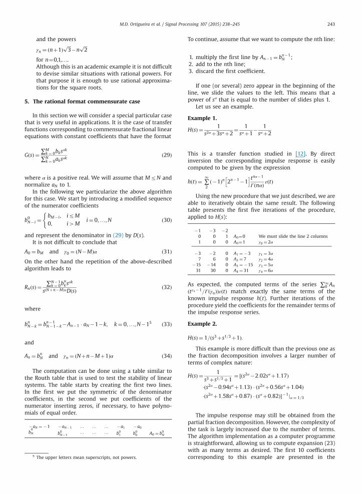
The computation can be done using a table similar tothe Routh table that is used to test the stability of linearsystems. The table starts by creating the first two lines.In the first we put the symmetric of the denominatorcoefficients, in the second we put coefficients of thenumerator inserting zeros, if necessary, to have polyno-mials of equal order.
The upper
letters me an su perscr ipts, n ot powe rs.�aN ¼ �1
�aN�1 … … … �a1 �a0 bN0b0N�1
… … … b01 b00 A0 ¼ b0NTo continue, assume that we want to compute the nth line:
1.
multiply the first line by An�1 ¼ bn�1N ;2.
add to the nth line; 3. discard the first coefficient.If one (or several) zero appear in the beginning of theline, we slide the values to the left. This means that apower of sα that is equal to the number of slides plus 1.
Let us see an example.
Example 1.
H sð Þ ¼ 1s2αþ3sαþ2
¼ 1sαþ1
� 1sαþ2
This is a transfer function studied in [12]. By directinversion the corresponding impulse response is easilycomputed to be given by the expression
h tð Þ ¼ ∑1
2ð�1Þn 2n�1�1
h itnα�1
ΓðnαÞ ε tð Þ
Using the new procedure that we just described, we areable to iteratively obtain the same result. The followingtable presents the first five iterations of the procedure,applied to H(s):
�1
�3 �2 0 0 1 A0¼0 We must slide the line 2 columns 1 0 0 A0¼1 γ0 ¼ 2α�3
�2 0 A1 ¼ �3 γ1 ¼ 3α 7 6 0 A2 ¼ 7 γ2 ¼ 4α�15
�14 0 A3 ¼ �15 γ3 ¼ 5α 31 30 0 A4 ¼ 31 γ4 ¼ 6αAs expected, the computed terms of the series ∑10 An
ðtγn �1=ΓðγnÞÞεðtÞ match exactly the same terms of theknown impulse response h(t). Further iterations of theprocedure yield the coefficients for the remainder terms ofthe impulse response series.
Example 2.
HðsÞ ¼ 1=ðs3þs1=3þ1Þ:This example is more difficult than the previous one as
the fraction decomposition involves a larger number ofterms of complex nature:
H sð Þ ¼ 1s3þs1=3þ1
¼ ½ðs2α�2:02sαþ1:17Þ
�ðs2α�0:94sαþ1:13Þ � ðs2αþ0:56sαþ1:04Þ�ðs2αþ1:58sαþ0:87Þ � ðsαþ0:82Þ��1jα ¼ 1=3
The impulse response may still be obtained from thepartial fraction decomposition. However, the complexity ofthe task is largely increased due to the number of terms.The algorithm implementation as a computer programmeis straightforward, allowing us to compute expansion (23)with as many terms as desired. The first 10 coefficientscorresponding to this example are presented in the
M.D. Ortigueira et al. / Signal Processing 107 (2015) 238–245244
following table where α¼ 13
� �. The full computation of
these coefficients is presented as an Appendix.
n
0 1 2 3 4 5 6 7 8 9γn¼
9α 17α 18α 25α 26α 27α 33α 34α 35α 36α An¼ 1 �1 �1 1 2 1 �1 �3 �3 �16. The correspondence principle
The above development showed that the algorithm hastwo steps:
�
Expand the transfer function in negative powers of sα. � Invert the series term by term.On the other hand the examples showed that it can beused for both integer or fractional orders. This leads us tothink of the possibility of obtaining the fractional solutionfrom the integer one (and the reverse). In fact this ispossible through what we call the correspondence principlethat we state in the following theorem.
Theorem 5 (Correspondence principle). Let H(s) be theLaplace transform of the impulse response h(t) of a causalcommensurate linear system. The correspondence principlestates the following:The substitution of sα for s in the transfer function
corresponds to the substitution of tnα�1=ΓðnαÞ fortn�1=ΓðnÞ in the series associated with the impulseresponse.
For proof, consider a given integer order transfer function,H(s), of a causal exponential order function, h(t). According tothe development presented in Section 4, we can write
HðsÞ ¼ ∑1
1hðkÞð0þ Þs�k�1
As shown previously the successive coefficients are com-puted using the initial value theorem and hðtÞ is obtainedthrough a term by term inversion leading to (27).
Substitute sα for s in the series for H(s) to obtain theseries of a new transfer function, HαðsÞ. The above state-ment says that the corresponding series for hαðtÞ can beobtained from the series of h(t) using the above substitu-tion. To see whether this is true, write
HαðsÞ ¼ ∑1
1Aks
�αk
Its inversion gives
hα tð Þ ¼ ∑1
1Ak
tnα�1
ΓðnαÞε tð Þ
As known,
Dα tmα�1
ΓðmαÞ
�¼ tðm�1Þα�1
Γððm�1ÞαÞ
The results presented in Section 2.2 show that whencomputing the limit as t goes to zero, all the terms of an
order less than m go to infinite and so they must beremoved as we did in the computation of the series forHðsÞ. The terms with an order greater than m go to zero.We conclude immediately that Am ¼ hðm�1Þ
a ð0þ Þ.A comparison of the two series shows that with the
above substitution we obtain really the correct series.However, the coefficients must be reinterpreted: they areno longer order k derivatives, but order αk derivatives. Thecoefficients hðαkÞð0þ Þ are really independent of α. This is arather surprising result.
Let us see a simple example.The inverse Laplace transform of HðsÞ ¼ 1=ðsþaÞ for
ReðsÞ40 is given by hðtÞ ¼ e�atεðtÞ. Suppose we want tocompute the inverse of HαðsÞ ¼ 1=ðsαþaÞ for ReðsÞ40 usingthe correspondence principle. Begin by rewriting h(t) in aseries format:
h tð Þ ¼ ∑1
0ð�aÞnt
n
n!ε tð Þ ¼ ∑
1
0ð�aÞn tn
Γðnþ1Þε tð Þ
¼ ∑1
1ð�aÞn�1t
ðn�1Þ
ΓðnÞ ε tð Þ
Perform the above substitution to obtain
hα tð Þ ¼ ∑1
1ð�aÞn�1t
ðnα�1Þ
ΓðnαÞ ε tð Þ
The corresponding transform is
Hα sð Þ ¼ ∑1
1ð�aÞn�1s�nα ¼ s�α 1
1þas�α
¼ 1sαþa
¼H sαð Þ
confirming the above statement.
7. Conclusions
We presented a general approach to decompose aLaplace transform into a Laurent like series. From it weobtained a general power series. This result was applied tothe computation of the impulse response of causal linearsystems. In particular, we considered the commensuratecase and proposed a table to obtain the coefficients of theMacLaurin series. Some examples were presented.
Acknowledgements
This work was partially funded by the National Fundsthrough the Foundation for Science and Technology ofPortugal, under the Project PEst-OE/EEI/UI0066/2011 andby project MTM2010-16499 from the Government ofSpain.
Appendix A. Transfer function decomposition forExample 2
Here we deal with the decomposition of the transferfunction HðsÞ ¼ 1=ðs3þs1=3þ1Þ ¼ 1=ðs9αþsαþ1Þjα ¼ 1=3 asseries of the form HðsÞ ¼∑n�1
0 Aks� γk þRnðsÞ. The next table
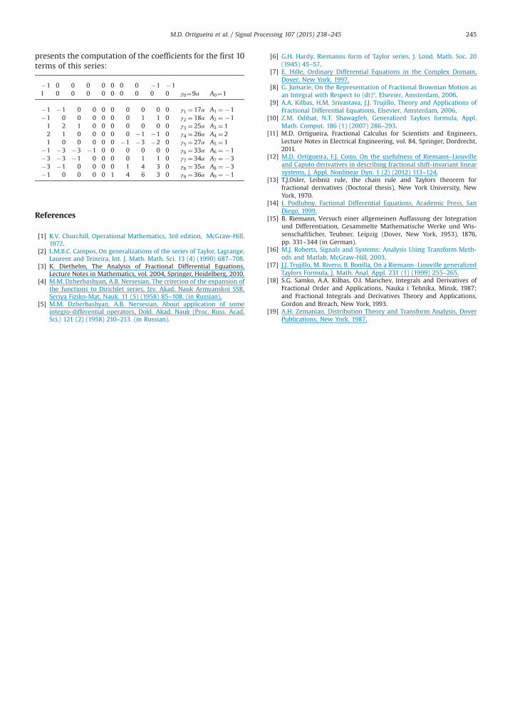
M.D. Ortigueira et al. / Signal Processing 107 (2015) 238–245 245
presents the computation of the coefficients for the first 10terms of this series:
�1
0 0 0 0 0 0 0 �1 �1 1 0 0 0 0 0 0 0 0 0 γ0¼9α A0¼1�1
�1 0 0 0 0 0 0 0 0 γ1 ¼ 17α A1 ¼ �1 �1 0 0 0 0 0 0 1 1 0 γ2 ¼ 18α A2 ¼ �1 1 2 1 0 0 0 0 0 0 0 γ3 ¼ 25α A3 ¼ 1 2 1 0 0 0 0 0 �1 �1 0 γ4 ¼ 26α A4 ¼ 2 1 0 0 0 0 0 �1 �3 �2 0 γ5 ¼ 27α A5 ¼ 1�1
�3 �3 �1 0 0 0 0 0 0 γ6 ¼ 33α A6 ¼ �1 �3 �3 �1 0 0 0 0 1 1 0 γ7 ¼ 34α A7 ¼ �3 �3 �1 0 0 0 0 1 4 3 0 γ8 ¼ 35α A8 ¼ �3 �1 0 0 0 0 1 4 6 3 0 γ9 ¼ 36α A9 ¼ �1References
[1] R.V. Churchill, Operational Mathematics, 3rd edition, McGraw-Hill,1972.
[2] L.M.B.C. Campos, On generalizations of the series of Taylor, Lagrange,Laurent and Teixeira, Int. J. Math. Math. Sci. 13 (4) (1990) 687–708.
[3] K. Diethelm, The Analysis of Fractional Differential Equations,Lecture Notes in Mathematics, vol. 2004, Springer, Heidelberg, 2010.
[4] M.M. Dzherbashyan, A.B. Nersesian, The criterion of the expansion ofthe functions to Dirichlet series, Izv. Akad. Nauk Armyanskoi SSR.Seriya Fiziko-Mat. Nauk. 11 (5) (1958) 85–108. (in Russian).
[5] M.M. Dzherbashyan, A.B. Nersesian, About application of someintegro-differential operators, Dokl. Akad. Nauk (Proc. Russ. Acad.Sci.) 121 (2) (1958) 210–213. (in Russian).
[6] G.H. Hardy, Riemanns form of Taylor series, J. Lond. Math. Soc. 20(1945) 45–57.
[7] E. Hille, Ordinary Differential Equations in the Complex Domain,Dover, New York, 1997.
[8] G. Jumarie, On the Representation of Fractional Brownian Motion asan Integral with Respect to (dt)α, Elsevier, Amsterdam, 2006.
[9] A.A. Kilbas, H.M. Srivastava, J.J. Trujillo, Theory and Applications ofFractional Differential Equations, Elsevier, Amsterdam, 2006.
[10] Z.M. Odibat, N.T. Shawagfeh, Generalized Taylors formula, Appl.Math. Comput. 186 (1) (2007) 286–293.
[11] M.D. Ortigueira, Fractional Calculus for Scientists and Engineers,Lecture Notes in Electrical Engineering, vol. 84, Springer, Dordrecht,2011.
[12] M.D. Ortigueira, F.J. Coito, On the usefulness of Riemann–Liouvilleand Caputo derivatives in describing fractional shift-invariant linearsystems, J. Appl. Nonlinear Dyn. 1 (2) (2012) 113–124.
[13] T.J.Osler, Leibniz rule, the chain rule and Taylors theorem forfractional derivatives (Doctoral thesis), New York University, NewYork, 1970.
[14] I. Podlubny, Factional Differential Equations, Academic Press, SanDiego, 1999.
[15] B. Riemann, Versuch einer allgemeinen Auffassung der Integrationund Differentiation, Gesammelte Mathematische Werke und Wis-senschaftlicher, Teubner, Leipzig (Dover, New York, 1953), 1876,pp. 331–344 (in German).
[16] M.J. Roberts, Signals and Systems: Analysis Using Transform Meth-ods and Matlab, McGraw-Hill, 2003.
[17] J.J. Trujillo, M. Rivero, B. Bonilla, On a Riemann–Liouville generalizedTaylors Formula, J. Math. Anal. Appl. 231 (1) (1999) 255–265.
[18] S.G. Samko, A.A. Kilbas, O.I. Marichev, Integrals and Derivatives ofFractional Order and Applications, Nauka i Tehnika, Minsk, 1987;and Fractional Integrals and Derivatives Theory and Applications,Gordon and Breach, New York, 1993.
[19] A.H. Zemanian, Distribution Theory and Transform Analysis, DoverPublications, New York, 1987.
Top Related
Copyright © 2022 FDOKUMEN

