Download - A Finite Element Method for Domain Decompo - sition with Non - Matching Grids

Mathematical Modelling and Numerical Analysis ESAIM: M2AN

Modelisation Mathematique et Analyse Numerique M2AN, Vol. 37, No 2, 2003, pp. 209–225

DOI: 10.1051/m2an:2003023

A FINITE ELEMENT METHOD FOR DOMAIN DECOMPOSITIONWITH NON-MATCHING GRIDS

Roland Becker1, Peter Hansbo

2and Rolf Stenberg

3

Abstract. In this note, we propose and analyse a method for handling interfaces between non-matching grids based on an approach suggested by Nitsche (1971) for the approximation of Dirichletboundary conditions. The exposition is limited to self-adjoint elliptic problems, using Poisson’s equa-tion as a model. A priori and a posteriori error estimates are given. Some numerical results areincluded.

Mathematics Subject Classification. 65N30, 65N55.

Received: September 3, 2001. Revised: October 21, 2002.

1. Introduction

In any domain decomposition method, one has to define how the continuity between the subdomains is tobe enforced. Different approaches have been proposed:

• Iterative procedures, enforcing that the approximate solution or its normal derivative or combinationsthereof should be continuous across interfaces. This forms the basis for the standard Schwarz alternatingmethod as defined, e.g., by Lions [16].

• Direct procedures, using Lagrange multiplier techniques to achieve continuity. Different variants havebeen proposed, e.g., by Le Tallec and Sassi [15], and Bernadi et al. [8].

The multiplier method has the advantage of directly yielding a solvable global system. However, in the lattermethod, new unknowns (the multipliers) must be introduced and solved for. The method must then eithersatisfy the inf-sup condition, which necessitates special choices of multiplier spaces (such as mortar elements,cf. [8]), or then stabilization techniques (cf. [3, 4, 9]) must be used.

In this paper, we consider a third possibility, i.e. Nitsche’s method [17], which was originally introduced forthe purpose of solving Dirichlet problems without enforcing the boundary conditions in the definition of thefinite element spaces. This method has later been used by Arnold [2] for the discretization of second order ellipticequations by discontinuous finite elements. In earlier papers [18, 19] we have pointed out the close connectionbetween Nitsche’s method and stabilized methods and proposed it as a mortaring method. In this paper wewill give a more detailed analysis of this domain decomposition technique where independent approximations

Keywords and phrases. Nitsche’s method, domain decomposition, non-matching grids.

1 Institute of Applied Mathematics, University of Heidelberg, INF 294, 69120 Heidelberg, Germany.2 Department of Applied Mechanics, Chalmers University of Technology, 412 96 Goteborg, Sweden.e-mail: [email protected] Institute of Mathematics, Box 1100, 02015 Helsinki University of Technology, Finland.

c© EDP Sciences, SMAI 2003

210 R. BECKER ET AL.

are used on the different subdomains. The continuity of the solution across interfaces is enforced weakly, but insuch a way that the resulting discrete scheme is consistent with the original partial differential equation. Undersome regularity assumptions we derive both a priori and a posteriori error estimates. We also give numericalresults obtained with the method.

Although we discuss its application to domain decomposition, the same technique is also suited for otherapplications, e.g.,

• to handle diffusion terms in the discontinuous Galerkin method [2, 6];• to simplify mesh generation (different parts can be meshed independently from each other);• finite element methods with different polynomial degree on adjacent elements;• new finite element methods such as linear approximations on quadrilaterals.

2. The domain decomposition method

In this section we will introduce the mortaring method based on the classical method of Nitsche. We willperform a classical stability and a priori error analysis. For simplicity, we consider the model Poisson problem,i.e. of solving the partial differential equation

−∆u = f in Ω,

u = 0 on ∂Ω,(1)

where Ω is a bounded domain in two or three space dimensions and f ∈ L2(Ω).Likewise for ease of presentation, we consider only the case where Ω is divided into two non-overlapping

subdomains Ω1 and Ω2, Ω1 ∪ Ω2, with interface Γ = Ω1 ∩ Ω2. We further assume that the subdomains arepolyhedral (or polygonal in R

2) and that Γ is polygonal (or a broken line).This equation can be written in weak form as: find u ∈ H1

0 (Ω) such that

a(u, v) = (f, v), ∀v ∈ H10 (Ω), (2)

where

a(u, v) =∫

Ω

∇u · ∇v dx, (f, v) =∫

Ω

f v dx, (3)

and H10 (Ω) is the space of square-integrable functions, with square-integrable first derivatives, that vanish on

the boundary ∂Ω of Ω.Our discrete method for the approximate solution of (1) is a nonconforming finite element method which is

continuous within each Ωi and discontinuous across Γ. We start by rewriting the original problem (1) as twoequations and the interface conditions:

−∆ui = f in Ωi, i = 1, 2,

ui = 0 on ∂Ω ∩ Ωi, i = 1, 2,

u1 − u2 = 0 on Γ, (4)∂u1

∂n1+

∂u2

∂n2= 0 on Γ.

Here, ni is the outward unit normal to ∂Ωi.We will perform our analysis under the following regularity assumption.

Assumption 2.1. The solution of (2) satisfies u ∈ Hs(Ω), with s > 3/2.

A FINITE ELEMENT METHOD FOR DOMAIN DECOMPOSITION WITH NON-MATCHING GRIDS 211

With this assumption it holds ∂ui/∂ni ∈ L2(Γ) and the two problems (1) and (4) are equivalent (see forexample [1]) with:

u|Ωi = ui, i = 1, 2. (5)In the following we will therefore write u = (u1, u2) ∈ V1 × V2 with the continuous spaces

Vi =vi ∈ H1(Ωi) : ∂vi/∂ni ∈ L2(Γ), vi|∂Ω∩∂Ωi = 0

, i = 1, 2.

To formulate our method, we suppose that we have regular finite element partitionings T ih of the subdomains

Ωi into shape regular simplexes. These two meshes induce “trace” meshes on the interface

Gih = E : E = K ∩ Γ, K ∈ T i

h· (6)

By hK and hE we denote the diameter of element K ∈ T ih and E ∈ Gi

h, respectively. For the purpose of thea priori analysis, we also define

h = maxhK , hE : K ∈ T ih , E ∈ Gi

h, i = 1, 2·

In our analysis we will need the following assumption.

Assumption 2.2. There exists positive constants C1, C2 such that

C1 hE1 ≤ hE2 ≤ C2 hE1

holds for all pairs (E1, E2) ∈ T 1h × T 2

h , with E1 ∩ E2 = ∅.

We seek the approximation uh = (u1,h, u2,h) in the space V h = V h1 × V h

2 , where

V hi =

vi ∈ Vi : vi|K is a polynomial of degree p for all K ∈ T i

h

,

choosing for simplicity p constant on all subdomains. On the interface we will use the notation

[[v]] := v1 − v2 (7)

for the jump,

v :=12v1 +

12v2 (8)

for the average and

〈v, w〉S :=∫

S

v w ds, for S ∈ Gih, or S = Γ. (9)

Finally, we denoten := n1 = −n2. (10)

With this notation we have ∂v

∂n

=

12

∂v1

∂n1− 1

2∂v2

∂n2(11)

and hence ∂u

∂n

=

∂u

∂n=

∂u1

∂n1= −∂u2

∂n2· (12)

The methods of Nitsche [17] and Arnold [2] now give the following domain decomposition method.

Mortar method. Find uh ∈ V h such that

ah(uh, v) = fh(v) ∀v ∈ V h, (13)


with

ah(w, v) :=2∑

i=1

[(∇wi,∇vi)Ωi + γ

∑E∈Gi

h

h−1E 〈[[w]] , [[v]]〉E

](14)

−⟨

∂w

∂n

, [[v]]

⟩Γ

−⟨

∂v

∂n

, [[w]]

⟩Γ

and

fh(v) :=2∑

i=1

(f, vi)Ωi , (15)

where γ > 0 is chosen sufficiently large, see Lemma 2.6 below.

The first observation is that this formulation gives a consistent method.

Lemma 2.3. The solution u = (u1, u2) to (4) satisfies

ah(u, v) = fh(v) ∀v ∈ V. (16)

Proof. Multiplying the first equation in (4) with vi, integrating over Ωi, using Greens formula and the rela-tions (12) yields

fh(v) =2∑

i=1

(f, vi)Ωi =2∑

i=1

[(∇ui,∇vi)Ωi −

⟨∂ui

∂ni, vi

⟩Γ

]

=2∑

i=1

(∇ui,∇vi)Ωi −⟨

∂u

∂n

, [[v]]

⟩Γ

· (17)

Since [[u]] = 0 on Γ we have

0 = −⟨

∂v

∂n

, [[u]]

⟩Γ

+ γ

2∑i=1

∑E∈Gi

h

h−1E 〈[[u]] , [[v]]〉E . (18)

Adding (17) and (18) the gives the claim. For the stability analysis below we need the following mesh-dependent dual norms. To emphasize that Γ is

to be considered as a part of ∂Ωi we write Γi.

‖v‖21/2,h,Γi

=∑

E∈Gih

h−1E ‖v‖2

L2(E) (19)

and‖v‖2

−1/2,h,Γi=∑

E∈Gih

hE ‖v‖2L2(E) , (20)

which satisfy| 〈v, w〉Γ | ≤ ‖v‖1/2,h,Γi

‖w‖−1/2,h,Γi. (21)

The analysis will be performed using the norms

‖v‖21,h =

2∑i=1

(‖∇vi‖2

L2(Ωi)+ ‖[[v]]‖2

1/2,h,Γi

)(22)


and

|‖v‖|21,h = ‖v‖21,h +

2∑i=1

∥∥∥∥ ∂vi

∂ni

∥∥∥∥2

−1/2,h,Γi

· (23)

The following estimate is readily proved by local scaling.

Lemma 2.4. There is a positive constant CI such that

∥∥∥∥ ∂vi

∂ni

∥∥∥∥2

−1/2,h,Γi

≤ CI ‖∇vi‖2L2(Ωi)

∀vi ∈ V hi . (24)

For linear elements ∇v is constant on each element and then it is particularly easy to give a bound for theconstant CI, see Remark 2.12 below.

A immediate consequence of the above lemma is the equivalence of norms in the finite element subspace.

Lemma 2.5. The norms ‖ · ‖1,h and |‖ · ‖|1,h are equivalent on the subspace V h.

The stability of the method can now be proved.

Lemma 2.6. Suppose that γ > CI/4. Then it holds

ah(v, v) ≥ C|‖v‖|21,h ∀v ∈ V h.

Proof. From the definition (14), the relation (11), and the preceding lemmas we get

ah(v, v) =2∑

i=1

[‖∇vi‖2

L2(Ωi)+ γ ‖[[v]]‖2

1/2,h,Γi

]− 2

⟨[[v]] ,

∂v

∂n

⟩Γ

=2∑

i=1

[‖∇vi‖2

L2(Ωi)+ γ ‖[[v]]‖2

1/2,h,Γi

]−⟨

[[v]] ,∂v1

∂n1

⟩Γ

+⟨

[[v]] ,∂v2

∂n2

⟩Γ

≥2∑

i=1

[‖∇vi‖2

L2(Ωi)+ γ ‖[[v]]‖2

1/2,h,Γi−∣∣∣∣⟨

[[v]] ,∂vi

∂ni

⟩Γ

∣∣∣∣]

≥2∑

i=1

[‖∇vi‖2

L2(Ωi)+ γ ‖[[v]]‖2

1/2,h,Γi− ‖[[v]]‖1/2,h,Γi

∥∥∥∥ ∂vi

∂ni

∥∥∥∥−1/2,h,Γi

]

≥2∑

i=1

[(1 − CI

2ε

)‖∇vi‖2

L2(Ωi)+(γ − ε

2

)‖[[v]]‖2

1/2,h,Γi

]

≥ C1‖v‖21,h

≥ C2|‖v‖|21,h,

for γ > ε/2 and choosing ε > CI/2. The following interpolation estimates holds, cf. [20].

Lemma 2.7. Suppose that u ∈ Hs(Ω), with 3/2 < s ≤ p + 1. Then it holds

infv∈V h

‖u − v‖1,h ≤ Chs−1 ‖u‖Hs(Ω) (25)

andinf

v∈V h|‖u − v‖|1,h ≤ Chs−1 ‖u‖Hs(Ω) . (26)


We are now able to prove the following a priori error estimate.

Theorem 2.8. Suppose γ > CI/4. Then it holds

|‖u − uh‖|1,h ≤ C infv∈V h

|‖u − v‖|1,h.

If u ∈ Hs(Ω), for 3/2 < s ≤ p + 1, then

|‖u − uh‖|1,h ≤ Chs−1 ‖u‖Hs(Ω) .

Proof. Since the bilinear form ah is bounded with respect to the norm |‖ · ‖|1,h, the first inequality followsfrom the stability estimate of Lemma 2.6 and the triangle inequality. The second estimate then follows fromLemma 2.7.

Remark 2.9. As [[u]] = 0 on Γ the error estimate gives ‖ [[uh]] ‖−1/2,h,Γi= O(hs−1). For quasi-uniform meshes

it then holds ‖ [[uh]] ‖L2(Γ) = O(hs−1/2).

Remark 2.10. The presented method resembles a mesh-dependent penalty method, but with added consistencyterms involving normal derivatives across the interface. Note that the formulation allows us to deduce optimalorder error estimates with preserved condition number of O(h−2) for a quasiuniform mesh. Pure penaltymethods, in contrast, are not consistent, and optimal error estimates require degrading the condition numberfor higher polynomial approximation (cf. [5]).

Remark 2.11. The form ah(·, ·) in (14) is symmetric and positive definite, which is natural as the problem tobe approximated has the same properties. With this there exists fast solvers, such as preconditioned conjugategradients, for the resulting matrix problem. If the bilinear form is changed to

ah(w, v) :=2∑

i=1

[(∇wi,∇vi)Ωi + γ

∑E∈Gi

h

h−1E 〈[[w]] , [[v]]〉E

](27)

−⟨

∂w

∂n

, [[v]]

⟩Γ

+⟨

∂v

∂n

, [[w]]

⟩Γ

,

then one obtains a method which is stable for all positive values of γ:

ah(v, v) ≥ C|‖v‖|21,h ∀v ∈ V h, ∀γ > 0.

If the Laplace operator is a part of a problem which is not symmetric, then it might be practical to use thisnonsymmetric bilinear form. See [10, 11] for applications to convection diffusion problems.

Remark 2.12. For linear elements ∇vi (vi ∈ V hi ) is constant on each element and hence for K ∈ T i

h with thebase E ∈ Gi

h we have ∥∥∥∥ ∂vi

∂ni

∥∥∥∥2

0,E

= meas(E)∣∣∣ ∂vi

∂ni

∣∣∣2 (28)

and

‖∇vi‖20,K ≥

∥∥∥∥ ∂vi

∂ni

∥∥∥∥2

0,K

= meas(K)∣∣∣ ∂vi

∂ni

∣∣∣2 (29)

and hence it holds

hE

∥∥∥∥ ∂vi

∂ni

∥∥∥∥2

0,E

≤ hE meas(E)meas(K)

‖∇vi‖20,K . (30)


Hence, once the shape regularity of the mesh is specified, one has a bound for CI. In a practical implementationeasier would be to replace the weight γh−1

E in (14) with a parameter

αK = αmeas(E)meas(K)

, (31)

with α > 1/4 fixed. With this all results of the paper hold.

Remark 2.13. We have performed our analysis assuming that the solution is sufficiently smooth, i.e. thatu ∈ Hs(Ω) with s > 3/2. The analysis can be extended for less regular solutions if the corner and transmissionsingularities are carefully taken into account, cf. the recent papers [12, 13].

3. A POSTERIORI error estimates

We will first consider control of the error e = u− uh in the mesh dependent energy norm |‖ · ‖|1,h. We definethe local and global estimators as

EK(uh)2 = h2K ‖f + ∆uh‖2

L2(K) + hK

∥∥∥∥[[

∂uh

∂nK

]]∥∥∥∥2

L2(∂K)

+ h−1K ‖[[uh]]‖2

L2(∂K) (32)

and

E(uh) =[ ∑

K∈Th

EK(uh)2]1/2

. (33)

To be able to control the normal derivatives across the interface, we are forced to introduce a “saturation”assumption. This assumption is consistent with the Assumption 2.1 on the regularity of the solution and theinterpolation estimates of Theorem 2.7.

Assumption 3.1. There is a constant C such that

|‖u − uh‖|1,h ≤ C‖u − uh‖1,h. (34)

We also remark that an analog assumption is used in the context of a posteriori error estimates for the mortarelement method, see Wohlmuth [21].

The a posteriori estimate is now the following.

Theorem 3.2. Suppose that the Assumption 3.1 is valid. Then there is a positive constant C such that

|‖u − uh‖|1,h ≤ CE(uh). (35)

Proof. We denote e = u − uh. By Lemma 2.3 we have

‖e‖21,h = ah(e, e) + 2

⟨[[e]] ,

∂e

∂n

⟩Γ

+ (1 − γ)2∑

i=1

∑E∈Gi

h

h−1E 〈[[e]] , [[e]]〉E

:= R1 + R2, (36)

withR1 := ah(e, e),

and

R2 := 2⟨

[[e]] ,

∂e

∂n

⟩Γ

+ (1 − γ)2∑

i=1

‖[[e]]‖21/2,h,Γi

.


Since [[e]] |Γ = [[uh]] |Γ Assumption 3.1 gives

R2 =⟨

[[uh]] ,∂e1

∂n1

⟩Γ

−⟨

[[uh]] ,∂e2

∂n2

⟩Γ

+ (1 − γ)2∑

i=1

‖[[e]]‖21/2,h,Γi

≤ C

2∑i=1

(‖[[uh]]‖1/2,h,Γi

∥∥∥∥ ∂ei

∂ni

∥∥∥∥−1/2,h,Γi

+ ‖[[uh]]‖1/2,h,Γi‖[[e]]‖1/2,h,Γi

)

≤ C‖e‖1,h

(2∑

i=1

‖[[uh]]‖1/2,h,Γi

)≤ C‖e‖1,hE(uh). (37)

Next, let πhe be the Clement interpolant to e, which satisfies

( ∑K∈Th

(h−2

K ‖e − πhe‖2L2(K) + h−1

K ‖e − πhe‖2L2(∂K)

))1/2

≤ C‖e‖1,h (38)

and‖e − πhe‖1,h ≤ C‖e‖1,h. (39)

From the consistency (2.3) we have ah(e, πhe) = 0. Hence

R1 = ah(e, e) = ah(e, e − πhe)

=2∑

i=1

(∇ei,∇(ei − πhei))Ωi + γ

∑E∈Gi

h

h−1E 〈[[e]] , [[e − πhe]]〉E

−⟨

∂e

∂n

, [[e − πhe]]

⟩Γ

−⟨

∂(e − πhe)∂n

, [[e]]

⟩Γ

:= S1 + S2 + S3 + S4. (40)

Integrating by parts on each K ∈ Th yields

S1 =2∑

i=1

(∇ei,∇(ei − πhei))Ωi (41)

=∑

K∈Th

(−(∆e, e − πhe)K +

⟨∂e

∂nK, e − πhe

⟩∂K

)

:= T1 + T2.

Since on K ∈ Th it holds −∆e = −∆u + ∆uh = f + ∆uh, the first term above is estimated using (38)

T1 = −∑

K∈Th

(∆e, e − πhe)K (42)

≤( ∑

K∈Th

h2K ‖∆uh + f‖2

L2(K)

)1/2( ∑K∈Th

h−2K ‖e − πhe‖2

L2(K)

)1/2

≤( ∑

K∈Th

h2K ‖∆uh + f‖2

L2(K)

)1/2

‖e‖1,h.


Let Ih be the collection of element sides in the interiors of the subdomains Ωi. The boundary integrals in (41)above we now split into those in Ih and those lying on the interface Γ:

T2 =∑

K∈Th

⟨∂e

∂nK, e − πhe

⟩∂K

(43)

=∑

E∈Ih

⟨∂e

∂nE, e − πhe

⟩E

+⟨

∂e1

∂n1, e1 − πhe1

⟩Γ

+⟨

∂e2

∂n2, e2 − πhe2

⟩Γ

·

The integrals over the interior sides can now be grouped together two by two yielding the estimate

∣∣∣∣∣∑

E∈Ih

⟨∂e

∂nE, e − πhe

⟩E

∣∣∣∣∣ ≤ C

[ ∑K∈Th

hK

∥∥∥∥[[

∂uh

∂nK

]]∥∥∥∥2

L2(∂K)

]1/2 [ ∑K∈Th


L2(∂K)

]1/2

(44)

≤ C

[ ∑K∈Th

hK

∥∥∥∥[[

∂uh

∂nK

]]∥∥∥∥2

L2(∂K)

]1/2

‖e‖1,h,

where (38) was used.Using the definition (11) we have

S3 = −⟨

∂e

∂n

, [[e − πhe]]

⟩Γ

= −⟨

12

∂e1

∂n1+

12

∂e2

∂n2, e1 − πhe1 − (e2 − πhe2)

⟩Γ

= −⟨

12

∂e1

∂n1− 1

2∂e2

∂n2, e1 − πhe1

⟩Γ

+⟨

12

∂e1

∂n1− 1

2∂e2

∂n2, (e2 − πhe2)

⟩Γ

· (45)

Combining these terms with two last terms in (43) gives

⟨∂e1

∂n1, e1 − πhe1

⟩Γ

+⟨

∂e2

∂n2, e2 − πhe2

⟩Γ

−⟨

∂e

∂n

, [[e − πhe]]

⟩Γ

=⟨(

1 − 12

)∂e1

∂n1+

12

∂e2

∂n2, e1 − πhe1

⟩Γ

+⟨

12

∂e1

∂n1+(

1 − 12

)∂e2

∂n2, (e2 − πhe2)

⟩Γ

=12

⟨∂e1

∂n1+

∂e2

∂n2, e1 − πhe1

⟩Γ

+12

⟨∂e1

∂n1+

∂e2

∂n2, e2 − πhe2

⟩Γ

=12

⟨∂(e1 − e2)

∂n, e1 − πhe1

⟩Γ

+12

⟨∂(e1 − e2)

∂n, e2 − πhe2

⟩Γ

=12

⟨[[∂e

∂n

]], e1 − πhe1

⟩Γ

+12

⟨[[∂e

∂n

]], e2 − πhe2

⟩Γ

(46)

=12

⟨[[∂uh

∂n

]], e1 − πhe1

⟩Γ

+12

⟨[[∂uh

∂n

]], e2 − πhe2

⟩Γ

≤ 12E(uh)

[ ∑K∈Th


L2(∂K)

]1/2

≤ CE(uh)‖e‖1,h.

From (41) to (46) we now getS1 + S3 ≤ C‖e‖1,hE(uh). (47)


From the Clement estimate (38) have

S2 = γ

2∑i=1

∑E∈Gi

h

h−1E 〈[[e]] , [[e − πhe]]〉E ≤ C‖e‖1,hE(uh).

To estimate the last term S4 we use Lemma 2.4 and the Assumption 3.1

S4 = −⟨

∂(e − πhe)∂n

, [[e]]

⟩Γ

= −⟨

∂e

∂n

, [[e]]

⟩Γ

+⟨

∂πhe

∂n

, [[e]]

⟩Γ

≤ C‖e‖1,hE(uh). (48)

Hence, collecting the estimates (40) to (48) yields

R1 ≤ C‖e‖1,hE(uh), (49)

which together with (37) proves the estimate

‖u − uh‖1,h = ‖e‖1,h ≤ CE(uh). (50)

The claim then follows from (34).

Next, we consider the error in the L2-norm. This is measured with the estimator

L(uh) =

[ ∑K∈Th

h2KEK(uh)2

]1/2

. (51)

For the a posteriori estimate we as usual, need the H2-regularity but not Assumption 3.1.

Theorem 3.3. Let z be the solution to the problem

−∆z = g in Ω,

z = 0 on ∂Ω,(52)

and suppose that the shift theorem

‖z‖H2(Ω) ≤ C ‖g‖L2(Ω) (53)

is valid. Then there is a positive constant C such that

‖u − uh‖L2(Ω) ≤ CL(uh). (54)

Proof. We again write z = (z1, z2) and note that

∂z1

∂n1+

∂z2

∂n2= 0 and

∂z

∂n

=

∂z1

∂n1= − ∂z2

∂n2·


Choosing g = u − uh in (52) we then get

‖u − uh‖2L2(Ω) =

2∑i=1

[(∇zi,∇(ui − ui,h))Ωi −

⟨∂zi

∂ni, ui − ui,h

⟩Γi

]

=2∑

i=1

[(∇zi,∇(ui − ui,h))Ωi +

⟨∂zi

∂ni, ui,h

⟩Γi

](55)

=2∑

i=1

(∇zi,∇(ui − ui,h))Ωi +⟨

∂z

∂n

, [[uh]]

⟩Γ

·

We let πhz ∈ V h be the Clement interpolant to z satisfying

( ∑K∈Th

(h−4

K ‖z − πhz‖2L2(K) + h−3

K ‖z − πhz‖2L2(∂K) + h−1

K

∥∥∥∥∂(z − πhz)∂nK

∥∥∥∥2

L2(∂K)

))1/2

≤ C ‖z‖H2(Ω) . (56)

From the consistency condition we have ah(u−uh, πhz) = 0, and since [[z]] = 0, [[u]] = 0, on the interface, we get

0 = ah(u − uh, πhz) (57)

=2∑

i=1

(∇(ui − ui,h),∇πhzi)Ωi + γ

∑E∈Gi

h

h−1E 〈[[u − uh]] , [[πhz]]〉E

−⟨

∂(u − uh)∂n

, [[πhz]]

⟩Γ

−⟨

∂πhz

∂n

, [[u − uh]]

⟩Γ

=2∑

i=1

(∇(ui − ui,h),∇πhzi)Ωi + γ

∑E∈Gi

h

h−1E 〈[[ uh]] , [[z − πhz]]〉E

+⟨

∂(u − uh)∂n

, [[z − πhz]]

⟩Γ

+⟨

∂πhz

∂n

, [[uh]]

⟩Γ

·

Substracting (57) from (55) gives

‖u − uh‖2L2(Ω) =

2∑i=1

(∇(zi − πhz,∇(ui − ui,h))Ωi − γ

∑E∈Gi

h

h−1E 〈[[ uh]] , [[z − πhz]]〉E

−⟨

∂(u − uh)∂n

, [[z − πhz]]

⟩Γ

+⟨

∂(z − πhz)∂n

, [[uh]]

⟩Γ

(58)

:= R1 + R2 + R3 + R4.


Using Schwarz inequality and the Clement estimate (56) we get

R2 + R4 ≤ C

( ∑K∈Th

(h−3

K ‖z − πhz‖2L2(∂K) + h−1

K

∥∥∥∥∂(z − πhz)∂nK

∥∥∥∥2

L2(∂K)

))1/2∑

E∈Gih

hE ‖[[uh]]‖L2(E)

1/2

≤ C ‖z‖H2(Ω) L(uh) ≤ C ‖u − uh‖L2(Ω) L(uh).

Integrating by parts yields

R1 + R3 =2∑

i=1

[(∇(zi − πhz,∇(ui − ui,h))Ωi

−⟨

∂(u − uh)∂n

, [[z − πhz]]

⟩Γ

=∑

K∈Th

(z − πhz, ∆(uh − u))K

+⟨

∂(u − uh)∂nK

, z − πhz

⟩∂K

−⟨

∂(u − uh)∂n

, [[z − πhz]]

⟩Γ

=∑

K∈Th

(z − πhz, ∆uh + f)K

+∑

E∈Ih

⟨∂(u − uh)

∂nE, z − πhz

⟩E

+2∑

i=1

⟨∂(ui − ui,h)

∂ni, zi − πhzi

⟩Γ

−⟨

∂(u − uh)∂n

, [[z − πhz]]

⟩Γ

·

The boundary terms in the second term above are grouped together two by two yielding jump terms in thenormal derivative. This gives the estimate

∑K∈Th

(z − πhz, ∆uh + f)K +∑

E∈Ih

⟨∂(u − uh)

∂nE, z − πhz

⟩E

(59)

≤ C

( ∑K∈Th

(h−4

K ‖z − πhz‖2L2(K) + h−3

K ‖z − πhz‖2L2(∂K)

))1/2

×( ∑

K∈Th

h4K ‖f + ∆uh‖2

L2(K) + h3K

∥∥∥∥[[

∂uh

∂nK

]]∥∥∥∥2

L2(∂K)

)1/2

≤ C ‖z‖H2(Ω) L(uh)

≤ C ‖u − uh‖L2(Ω) L(uh).


The remaining two terms are estimated as follows

2∑i=1

⟨∂(ui − ui,h)

∂ni, zi − πhzi

⟩Γ

−⟨

∂(u − uh)∂n

, [[z − πhz]]

⟩Γ

=2∑

i=1

⟨∂ui

∂ni, zi − πhzi

⟩Γ

−2∑

i=1

⟨∂ui,h

∂ni, zi − πhzi

⟩Γ

−⟨

∂u

∂n, [[z − πhz]]

⟩Γ

+⟨

∂uh

∂n

, [[z − πhz]]

⟩Γ

= −2∑

i=1

⟨∂ui,h

∂ni, zi − πhzi

⟩Γ

+⟨

∂uh

∂n

, [[z − πhz]]

⟩Γ

= −⟨

∂u1,h

∂n1, z1 − πhz1

⟩Γ

−⟨

∂u2,h

∂n2, z2 − πhz2

⟩Γ

+12

⟨∂u1,h

∂n1, z1 − πhz1

⟩Γ

− 12

⟨∂u1,h

∂n1, z2 − πhz2

⟩Γ

−12

⟨∂u2,h

∂n2, z1 − πhz1

⟩Γ

+12

⟨∂u2,h

∂n2, z2 − πhz2

⟩Γ

= −12

⟨∂u1,h

∂n1, z1 − πhz1

⟩Γ

− 12

⟨∂u2,h

∂n2, z2 − πhz2

⟩Γ

− 12

⟨∂u1,h

∂n1, z2 − πhz2

⟩Γ

− 12

⟨∂u2,h

∂n2, z1 − πhz1

⟩Γ

(60)

= −12

⟨∂u1,h

∂n1+

∂u2,h

∂n2, z1 − πhz1

⟩Γ

− 12

⟨∂u1,h

∂n1+

∂u2,h

∂n2, z2 − πhz2

⟩Γ

= −12

⟨[[∂uh

∂n

]], z1 − πhz1

⟩Γ

− 12

⟨[[∂uh

∂n

]], z2 − πhz2

⟩Γ

≤ CL(uh)( ∑

K∈Th

h−3K ‖z − πhz‖2

L2(∂K)

)1/2

≤ CL(uh) ‖z‖H2(Ω) ≤ CL(uh) ‖u − uh‖L2(Ω) .

Combining (59) and (60) givesR1 + R3 ≤ CL(uh) ‖u − uh‖L2(Ω)

which together with (59) and (58) proves the claim.

4. Numerical examples

4.1. Numerical verification of the a priori estimates

To verify the a priori estimates, we choose the model problem of a unit square with exact solution

u = x y (1 − x) (1 − y)

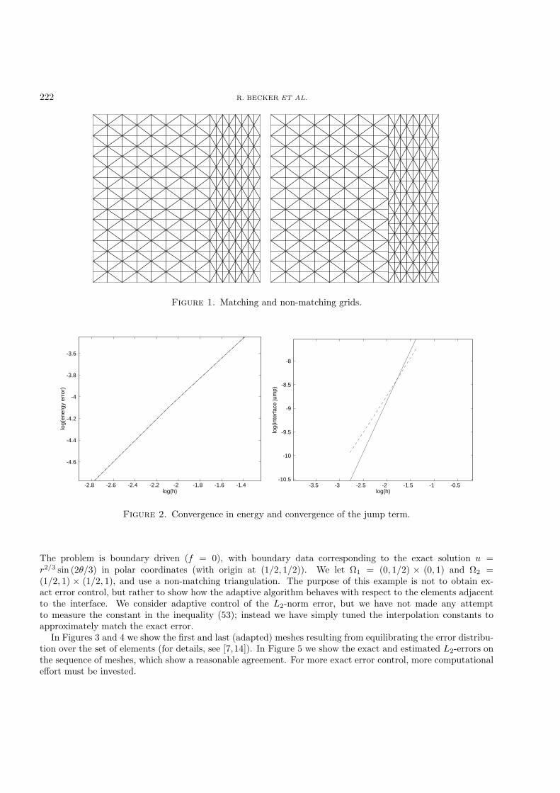
corresponding to a right-hand side of f = 2(x−x2 +y−y2). The domain is divided by a vertical slit at x = 0.7.Two different triangulations were used: one matching and one non-matching (see Fig. 1).

In Figure 2 (left-hand side) we give the convergence in the broken energy norm. The dashed line is thenon-matching grid computation. Both meshes show the same convergence with slope 0.95. which is close tothe theoretical value of 1. On the right-hand side we show the convergence of the L2-norm of the jump term(dashed line for the non-matching grid). Here we obtain a better convergence (slope 2.15) for the matchinggrids than for the non-matching grids (slope 1.57, close to the theoretical value of 3/2).

4.2. Adaptive computations

We present results of adaptive computations on the L-shaped domain

Ω = (0, 1) × (0, 1) \ (1/2, 1)× (0, 1/2).


Figure 1. Matching and non-matching grids.

-2.8 -2.6 -2.4 -2.2 -2 -1.8 -1.6 -1.4

-4.6

-4.4

-4.2

-4

-3.8

-3.6

log(h)

log(

ener

gy e

rror

)

-3.5 -3 -2.5 -2 -1.5 -1 -0.5-10.5

-10

-9.5

-9

-8.5

-8

log(h)

log(

inte

rfac

e ju

mp)

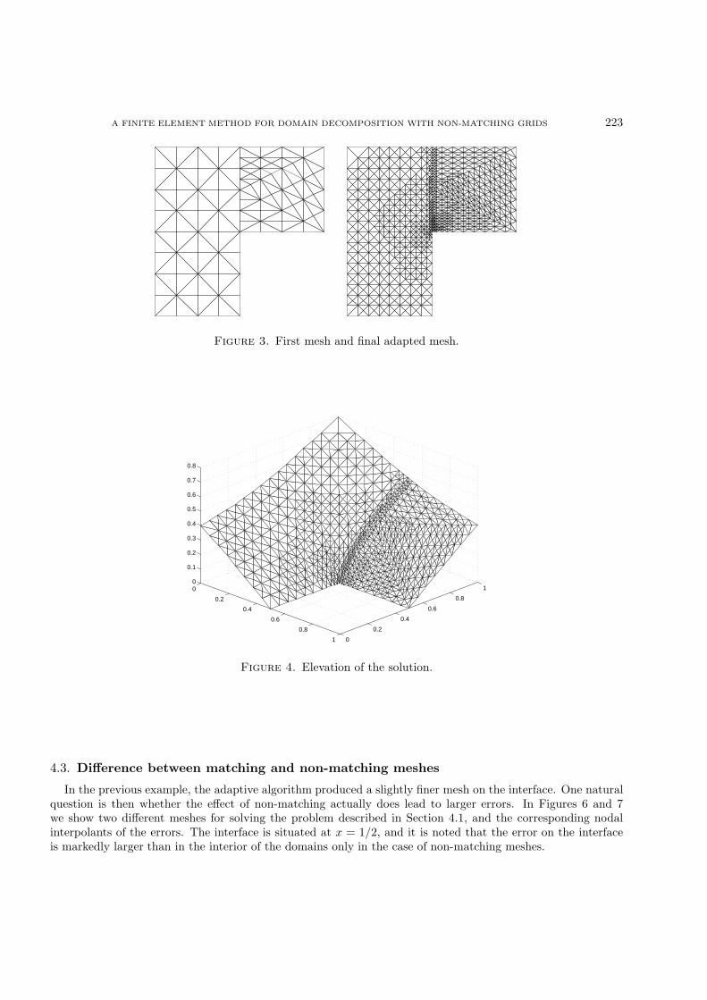
Figure 2. Convergence in energy and convergence of the jump term.

The problem is boundary driven (f = 0), with boundary data corresponding to the exact solution u =r2/3 sin (2θ/3) in polar coordinates (with origin at (1/2, 1/2)). We let Ω1 = (0, 1/2) × (0, 1) and Ω2 =(1/2, 1) × (1/2, 1), and use a non-matching triangulation. The purpose of this example is not to obtain ex-act error control, but rather to show how the adaptive algorithm behaves with respect to the elements adjacentto the interface. We consider adaptive control of the L2-norm error, but we have not made any attemptto measure the constant in the inequality (53); instead we have simply tuned the interpolation constants toapproximately match the exact error.

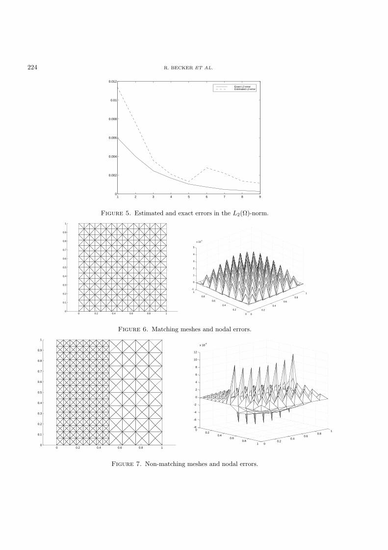
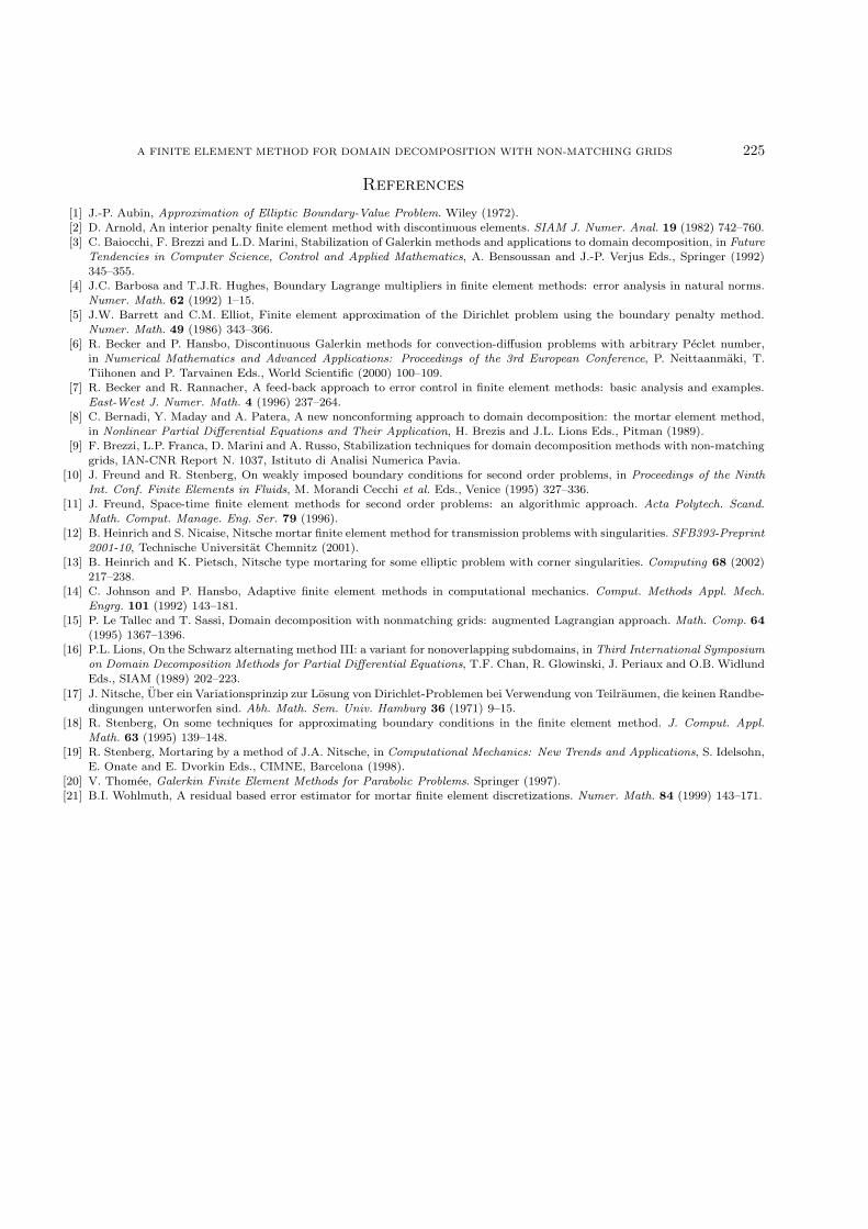
In Figures 3 and 4 we show the first and last (adapted) meshes resulting from equilibrating the error distribu-tion over the set of elements (for details, see [7,14]). In Figure 5 we show the exact and estimated L2-errors onthe sequence of meshes, which show a reasonable agreement. For more exact error control, more computationaleffort must be invested.


Figure 3. First mesh and final adapted mesh.

0

0.2

0.4

0.6

0.8

1 0

0.2

0.4

0.6

0.8

10

0.1

0.2

0.3

0.4

0.5

0.6

0.7

0.8

Figure 4. Elevation of the solution.

4.3. Difference between matching and non-matching meshes

In the previous example, the adaptive algorithm produced a slightly finer mesh on the interface. One naturalquestion is then whether the effect of non-matching actually does lead to larger errors. In Figures 6 and 7we show two different meshes for solving the problem described in Section 4.1, and the corresponding nodalinterpolants of the errors. The interface is situated at x = 1/2, and it is noted that the error on the interfaceis markedly larger than in the interior of the domains only in the case of non-matching meshes.


1 2 3 4 5 6 7 8 90

0.002

0.004

0.006

0.008

0.01

0.012

Exact L2-errorEstimated L2-error

Figure 5. Estimated and exact errors in the L2(Ω)-norm.

0 0.2 0.4 0.6 0.8 10

0.1

0.2

0.3

0.4

0.5

0.6

0.7

0.8

0.9

1

0

0.2

0.4

0.6

0.8

1

0

0.2

0.4

0.6

0.8

1-1

0

1

2

3

4

5

x 10-4

Figure 6. Matching meshes and nodal errors.

0 0.2 0.4 0.6 0.8 10

0.1

0.2

0.3

0.4

0.5

0.6

0.7

0.8

0.9

1

00.2

0.40.6

0.81 0

0.20.4

0.60.8

1-8

-6

-4

-2

0

2

4

6

8

10

12

x 10-4

Figure 7. Non-matching meshes and nodal errors.


References

[1] J.-P. Aubin, Approximation of Elliptic Boundary-Value Problem. Wiley (1972).[2] D. Arnold, An interior penalty finite element method with discontinuous elements. SIAM J. Numer. Anal. 19 (1982) 742–760.[3] C. Baiocchi, F. Brezzi and L.D. Marini, Stabilization of Galerkin methods and applications to domain decomposition, in Future

Tendencies in Computer Science, Control and Applied Mathematics, A. Bensoussan and J.-P. Verjus Eds., Springer (1992)345–355.

[4] J.C. Barbosa and T.J.R. Hughes, Boundary Lagrange multipliers in finite element methods: error analysis in natural norms.Numer. Math. 62 (1992) 1–15.

[5] J.W. Barrett and C.M. Elliot, Finite element approximation of the Dirichlet problem using the boundary penalty method.Numer. Math. 49 (1986) 343–366.

[6] R. Becker and P. Hansbo, Discontinuous Galerkin methods for convection-diffusion problems with arbitrary Peclet number,in Numerical Mathematics and Advanced Applications: Proceedings of the 3rd European Conference, P. Neittaanmaki, T.Tiihonen and P. Tarvainen Eds., World Scientific (2000) 100–109.

[7] R. Becker and R. Rannacher, A feed-back approach to error control in finite element methods: basic analysis and examples.East-West J. Numer. Math. 4 (1996) 237–264.

[8] C. Bernadi, Y. Maday and A. Patera, A new nonconforming approach to domain decomposition: the mortar element method,in Nonlinear Partial Differential Equations and Their Application, H. Brezis and J.L. Lions Eds., Pitman (1989).

[9] F. Brezzi, L.P. Franca, D. Marini and A. Russo, Stabilization techniques for domain decomposition methods with non-matchinggrids, IAN-CNR Report N. 1037, Istituto di Analisi Numerica Pavia.

[10] J. Freund and R. Stenberg, On weakly imposed boundary conditions for second order problems, in Proceedings of the NinthInt. Conf. Finite Elements in Fluids, M. Morandi Cecchi et al. Eds., Venice (1995) 327–336.

[11] J. Freund, Space-time finite element methods for second order problems: an algorithmic approach. Acta Polytech. Scand.Math. Comput. Manage. Eng. Ser. 79 (1996).

[12] B. Heinrich and S. Nicaise, Nitsche mortar finite element method for transmission problems with singularities. SFB393-Preprint2001-10, Technische Universitat Chemnitz (2001).

[13] B. Heinrich and K. Pietsch, Nitsche type mortaring for some elliptic problem with corner singularities. Computing 68 (2002)217–238.

[14] C. Johnson and P. Hansbo, Adaptive finite element methods in computational mechanics. Comput. Methods Appl. Mech.Engrg. 101 (1992) 143–181.

[15] P. Le Tallec and T. Sassi, Domain decomposition with nonmatching grids: augmented Lagrangian approach. Math. Comp. 64(1995) 1367–1396.

[16] P.L. Lions, On the Schwarz alternating method III: a variant for nonoverlapping subdomains, in Third International Symposiumon Domain Decomposition Methods for Partial Differential Equations, T.F. Chan, R. Glowinski, J. Periaux and O.B. Widlund

Eds., SIAM (1989) 202–223.

[17] J. Nitsche, Uber ein Variationsprinzip zur Losung von Dirichlet-Problemen bei Verwendung von Teilraumen, die keinen Randbe-dingungen unterworfen sind. Abh. Math. Sem. Univ. Hamburg 36 (1971) 9–15.

[18] R. Stenberg, On some techniques for approximating boundary conditions in the finite element method. J. Comput. Appl.Math. 63 (1995) 139–148.

[19] R. Stenberg, Mortaring by a method of J.A. Nitsche, in Computational Mechanics: New Trends and Applications, S. Idelsohn,E. Onate and E. Dvorkin Eds., CIMNE, Barcelona (1998).

[20] V. Thomee, Galerkin Finite Element Methods for Parabolic Problems. Springer (1997).[21] B.I. Wohlmuth, A residual based error estimator for mortar finite element discretizations. Numer. Math. 84 (1999) 143–171.