Zpectrometer commissioning report, Fall 2006

A. Harris, S. Zonak, K. Rauch, A. Baker, G. Watts, K. O’Neil,

R. Creager, B. Garwood, P. Marganian18 April 2007

1 Overview

This report covers the first commissioning phase of the Zpectrometer project in the Fall of20061. All functional aspects of the commissioning were successful: the interfaces betweenthe receiver, correlators, data acquisition system, and calibration systems are compatible andare nearly complete. We were able to make demonstration observations of strong astronomicalsources. Laboratory testing revealed systematic instrumental effects that limit the astronomicalperformance of the overall system, however, and systematic spectral structure precluded deepspectroscopic observations.

Much of this report covers the characterization of the systematics and their origins. Insummary, it appears that differential loss in the circuits at the very front of the receiver leavesan effective temperature imbalance that causes a nonzero signal at the correlator outputs.Ideally, the correlation receiver perfectly differences the signals at its two inputs, producingan output of zero when both inputs view the same temperature. This property reduces thesensitivity to amplifier gain fluctuations: zero scaled by a fluctuation is still zero. Non-zerooffset signals are amplified by fluctuating gains, adding relatively large and unstable spectralbaseline structure to the spectra. Improving the spectral baselines will involve reducing thedifferential loss and improving the gain stability. Sections 3 and 4 cover these topics in detail.Section 5 covers the spectral range limit imposed by the calibration signal generator.

2 The Zpectrometer and some first results

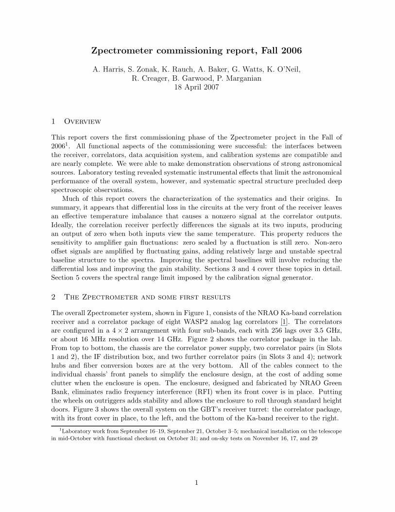
The overall Zpectrometer system, shown in Figure 1, consists of the NRAO Ka-band correlationreceiver and a correlator package of eight WASP2 analog lag correlators [1]. The correlatorsare configured in a 4 × 2 arrangement with four sub-bands, each with 256 lags over 3.5 GHz,or about 16 MHz resolution over 14 GHz. Figure 2 shows the correlator package in the lab.From top to bottom, the chassis are the correlator power supply, two correlator pairs (in Slots1 and 2), the IF distribution box, and two further correlator pairs (in Slots 3 and 4); networkhubs and fiber conversion boxes are at the very bottom. All of the cables connect to theindividual chassis’ front panels to simplify the enclosure design, at the cost of adding someclutter when the enclosure is open. The enclosure, designed and fabricated by NRAO GreenBank, eliminates radio frequency interference (RFI) when its front cover is in place. Puttingthe wheels on outriggers adds stability and allows the enclosure to roll through standard heightdoors. Figure 3 shows the overall system on the GBT’s receiver turret: the correlator package,with its front cover in place, to the left, and the bottom of the Ka-band receiver to the right.

1Laboratory work from September 16–19, September 21, October 3–5; mechanical installation on the telescopein mid-October with functional checkout on October 31; and on-sky tests on November 16, 17, and 29

1

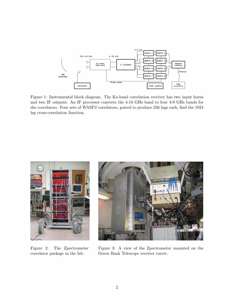
Figure 1: Instrumental block diagram. The Ka-band correlation receiver has two input hornsand two IF outputs. An IF processor converts the 4-18 GHz band to four 4-8 GHz bands forthe correlators. Four sets of WASP2 correlators, paired to produce 256 lags each, find the 1024lag cross-correlation function.

Figure 2: The Zpectrometercorrelator package in the lab.

Figure 3: A view of the Zpectrometer mounted on theGreen Bank Telescope receiver turret.

2

2.1 Interfaces

Planning for the interfaces to the GBT system started early in the project, and the implemen-tation went smoothly. The Zpectrometer provides two signals that drive the Ka-band receiver’sphase switches in quadrature for an effective switch frequency of 10.4 kHz2. Two 0.141′′ di-ameter conformable cables, matched in length and about 1 m long, carry the 4–18 GHz IFsignals from the receiver to the correlator. Over this band, the receiver output power is about−20 dBm. Power across the band is flat to about 10 dB, and we trim the average for eachcorrelator sub-band with attenuators. We measured the slope across the individual bands, andhave ordered gain equalizers to compensate.

By the end of the test period we had completed all software integration with the GBTsystem. Manager and Astrid scripts set up and control configurations and integrations. A setof GBTIDL scripts form the beginning stages of a full data reduction package. Although real-time monitoring of data and spectra is not yet possible, it should be implemented in summer2007.

Apart from the usual startup and teething problems, we had two noteworthy computer-related problems. First, one of the Zpectrometer’s internal microcontrollers hung once duringtesting on the telescope, and had to be manually reset. This is very unusual, occurring oncein the month or so that the system was on the telescope, and never in the lab. We havechanged the microcontroller code to deal with combined packets; if the telescope network isvery busy, it is possible that two commands are sent to the microcontrollers in one packet, butthe microcontrollers expected a single command. The other problem was that the GBT system’srequests failed to trigger data collection from all of the microcontrollers for a period of about anhour on the last night of observation. This was likely a Manager configuration problem, since ithappened after reconfiguration for pointing. It appeared that the Manager did not request themicrocontrollers to set up hardware or to start integrating. Simple communication problemscan be ruled out as the cause of the problem since the Zpectrometer control software did notgenerate errors and the microcontrollers all returned monitor data to the monitor file and to aterminal through this period.

2.2 First results

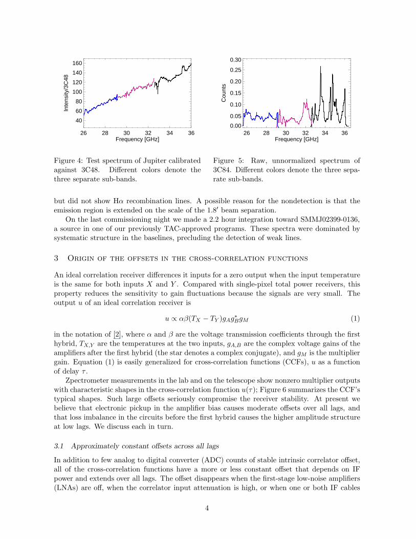
Figure 4 is our first spectrum of Jupiter, taken during the second on-sky commissioning pe-riod. It includes data from three of the four correlator sub-bands; the power level from thephase calibration source drops rapidly beyond 37 GHz (see Sec. 5). This power drop, possiblycombined with deteriorating receiver sensitivity, makes the top 3 GHz of the band difficult toobserve at present. We divided the spectrum of Jupiter by the spectrum of the quasar 3C48(∼ 1 Jy, z = 0.367) to remove the passband gain, but made no other corrections. The sub-bandedges match well, indicating that the receiver and spectrometer systems are very linear. Thespectral index across the 26–36 GHz spectrum is +3, which plausibly matches an index of +2(blackbody) for Jupiter and −1 for 3C48. Figure 5 is the raw, unnormalized spectrum of 3C48.After full reduction, a spectrum of the Orion A Hii region had considerable baseline structure

2Tests with lower frequency switching did not change the CCF’s shape or offset within fluctuations, but therms of the difference from the standard increases slightly with decreasing switch frequency. For correlator #2, thevariance of the residual was 1.2 counts at 10.4 kHz (Scans 12097–12100, 10/4/06). The variance of the residualwas 2.9 counts for a 6.25 kHz frequency and 7.0 for 4.17 kHz (Scans 12101–12104 and 12105-12108 comparedwith 12109-12112, 10/4/06). Based on these few data points, it seems that switching frequencies above 6 kHzare necessary for optimum sensitivity.

3

26 28 30 32 34 36Frequency [GHz]

40

60

80

100

120

140

160In

tens

ity/3

C48

Figure 4: Test spectrum of Jupiter calibratedagainst 3C48. Different colors denote thethree separate sub-bands.

26 28 30 32 34 36Frequency [GHz]

0.00

0.05

0.10

0.15

0.20

0.25

0.30

Cou

nts

Figure 5: Raw, unnormalized spectrum of3C84. Different colors denote the three sepa-rate sub-bands.

but did not show Hα recombination lines. A possible reason for the nondetection is that theemission region is extended on the scale of the 1.8′ beam separation.

On the last commissioning night we made a 2.2 hour integration toward SMMJ02399-0136,a source in one of our previously TAC-approved programs. These spectra were dominated bysystematic structure in the baselines, precluding the detection of weak lines.

3 Origin of the offsets in the cross-correlation functions

An ideal correlation receiver differences it inputs for a zero output when the input temperatureis the same for both inputs X and Y . Compared with single-pixel total power receivers, thisproperty reduces the sensitivity to gain fluctuations because the signals are very small. Theoutput u of an ideal correlation receiver is

u ∝ αβ(TX − TY )gAg∗BgM (1)

in the notation of [2], where α and β are the voltage transmission coefficients through the firsthybrid, TX,Y are the temperatures at the two inputs, gA,B are the complex voltage gains of theamplifiers after the first hybrid (the star denotes a complex conjugate), and gM is the multipliergain. Equation (1) is easily generalized for cross-correlation functions (CCFs), u as a functionof delay τ .

Zpectrometer measurements in the lab and on the telescope show nonzero multiplier outputswith characteristic shapes in the cross-correlation function u(τ); Figure 6 summarizes the CCF’stypical shapes. Such large offsets seriously compromise the receiver stability. At present webelieve that electronic pickup in the amplifier bias causes moderate offsets over all lags, andthat loss imbalance in the circuits before the first hybrid causes the higher amplitude structureat low lags. We discuss each in turn.

3.1 Approximately constant offsets across all lags

In addition to few analog to digital converter (ADC) counts of stable intrinsic correlator offset,all of the cross-correlation functions have a more or less constant offset that depends on IFpower and extends over all lags. The offset disappears when the first-stage low-noise amplifiers(LNAs) are off, when the correlator input attenuation is high, or when one or both IF cables

4

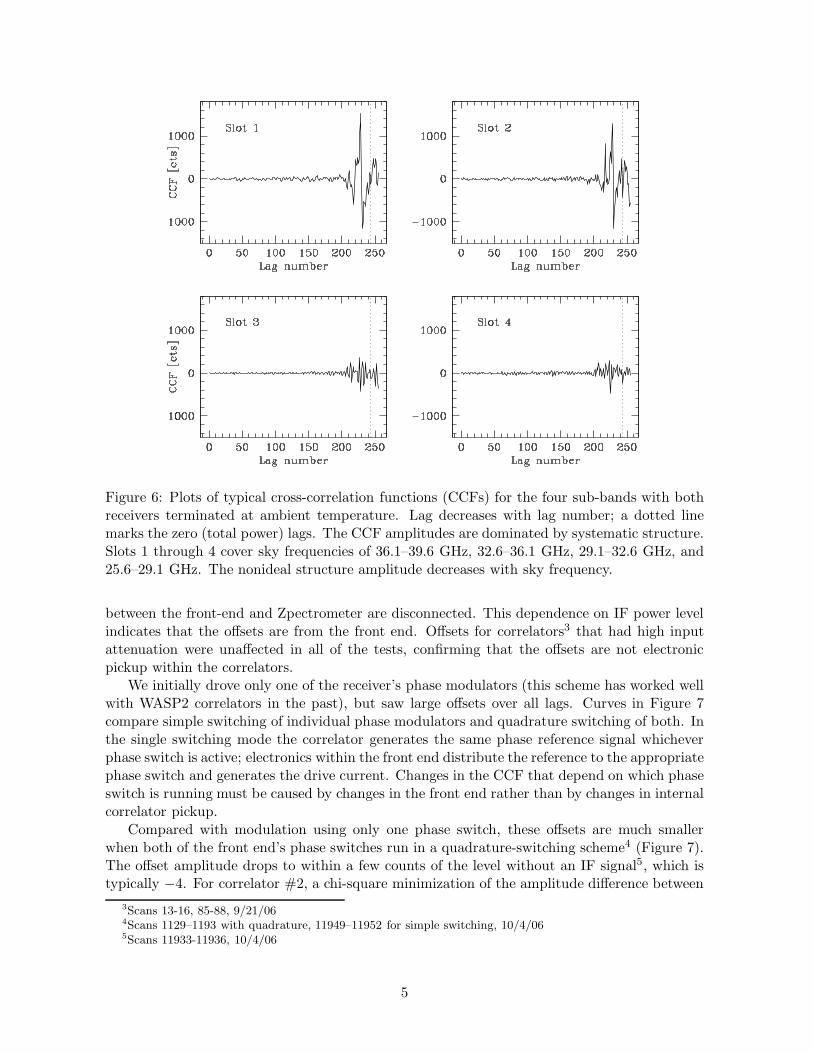
Figure 6: Plots of typical cross-correlation functions (CCFs) for the four sub-bands with bothreceivers terminated at ambient temperature. Lag decreases with lag number; a dotted linemarks the zero (total power) lags. The CCF amplitudes are dominated by systematic structure.Slots 1 through 4 cover sky frequencies of 36.1–39.6 GHz, 32.6–36.1 GHz, 29.1–32.6 GHz, and25.6–29.1 GHz. The nonideal structure amplitude decreases with sky frequency.

between the front-end and Zpectrometer are disconnected. This dependence on IF power levelindicates that the offsets are from the front end. Offsets for correlators3 that had high inputattenuation were unaffected in all of the tests, confirming that the offsets are not electronicpickup within the correlators.

We initially drove only one of the receiver’s phase modulators (this scheme has worked wellwith WASP2 correlators in the past), but saw large offsets over all lags. Curves in Figure 7compare simple switching of individual phase modulators and quadrature switching of both. Inthe single switching mode the correlator generates the same phase reference signal whicheverphase switch is active; electronics within the front end distribute the reference to the appropriatephase switch and generates the drive current. Changes in the CCF that depend on which phaseswitch is running must be caused by changes in the front end rather than by changes in internalcorrelator pickup.

Compared with modulation using only one phase switch, these offsets are much smallerwhen both of the front end’s phase switches run in a quadrature-switching scheme4 (Figure 7).The offset amplitude drops to within a few counts of the level without an IF signal5, which istypically −4. For correlator #2, a chi-square minimization of the amplitude difference between

3Scans 13-16, 85-88, 9/21/064Scans 1129–1193 with quadrature, 11949–11952 for simple switching, 10/4/065Scans 11933-11936, 10/4/06

5

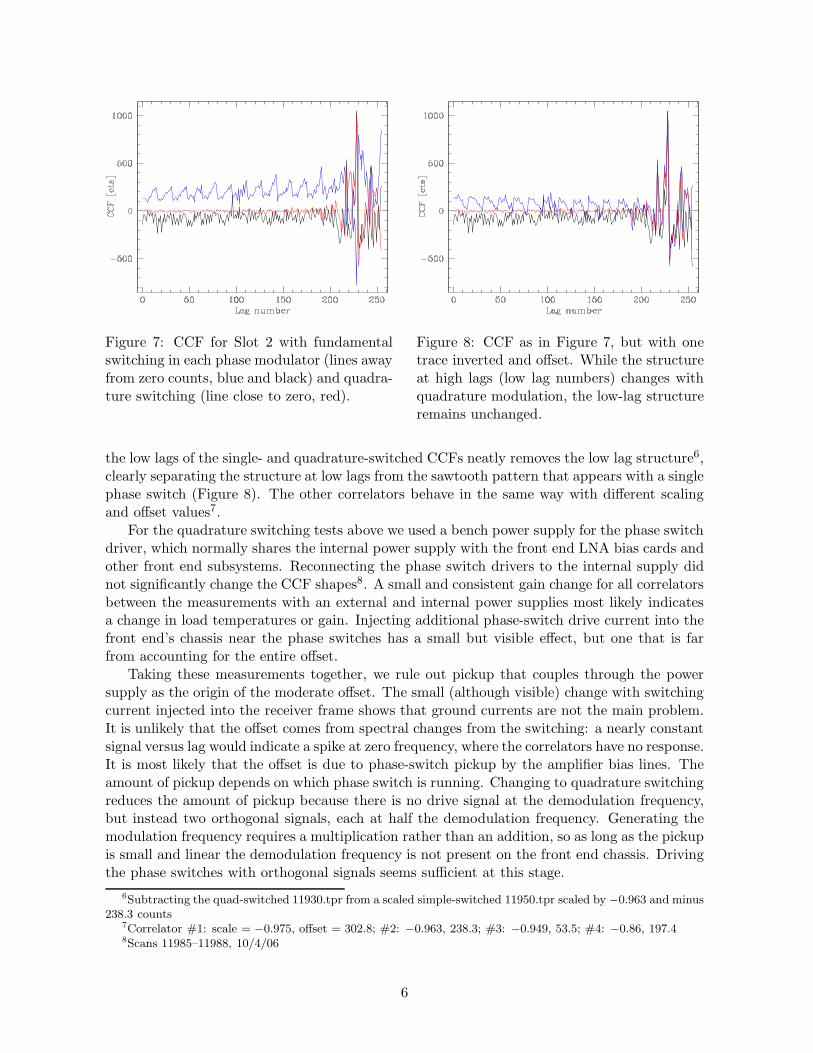
Figure 7: CCF for Slot 2 with fundamentalswitching in each phase modulator (lines awayfrom zero counts, blue and black) and quadra-ture switching (line close to zero, red).

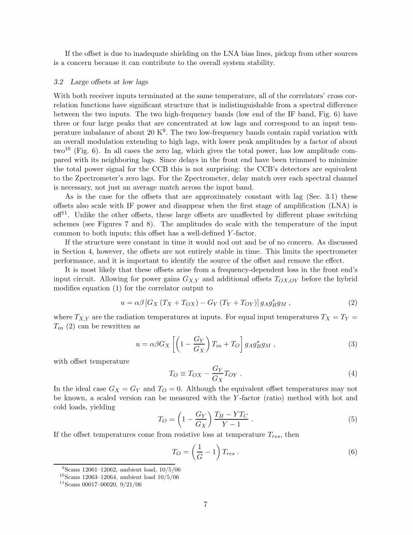
Figure 8: CCF as in Figure 7, but with onetrace inverted and offset. While the structureat high lags (low lag numbers) changes withquadrature modulation, the low-lag structureremains unchanged.

the low lags of the single- and quadrature-switched CCFs neatly removes the low lag structure6,clearly separating the structure at low lags from the sawtooth pattern that appears with a singlephase switch (Figure 8). The other correlators behave in the same way with different scalingand offset values7.

For the quadrature switching tests above we used a bench power supply for the phase switchdriver, which normally shares the internal power supply with the front end LNA bias cards andother front end subsystems. Reconnecting the phase switch drivers to the internal supply didnot significantly change the CCF shapes8. A small and consistent gain change for all correlatorsbetween the measurements with an external and internal power supplies most likely indicatesa change in load temperatures or gain. Injecting additional phase-switch drive current into thefront end’s chassis near the phase switches has a small but visible effect, but one that is farfrom accounting for the entire offset.

Taking these measurements together, we rule out pickup that couples through the powersupply as the origin of the moderate offset. The small (although visible) change with switchingcurrent injected into the receiver frame shows that ground currents are not the main problem.It is unlikely that the offset comes from spectral changes from the switching: a nearly constantsignal versus lag would indicate a spike at zero frequency, where the correlators have no response.It is most likely that the offset is due to phase-switch pickup by the amplifier bias lines. Theamount of pickup depends on which phase switch is running. Changing to quadrature switchingreduces the amount of pickup because there is no drive signal at the demodulation frequency,but instead two orthogonal signals, each at half the demodulation frequency. Generating themodulation frequency requires a multiplication rather than an addition, so as long as the pickupis small and linear the demodulation frequency is not present on the front end chassis. Drivingthe phase switches with orthogonal signals seems sufficient at this stage.

6Subtracting the quad-switched 11930.tpr from a scaled simple-switched 11950.tpr scaled by −0.963 and minus238.3 counts

7Correlator #1: scale = −0.975, offset = 302.8; #2: −0.963, 238.3; #3: −0.949, 53.5; #4: −0.86, 197.48Scans 11985–11988, 10/4/06

6

If the offset is due to inadequate shielding on the LNA bias lines, pickup from other sourcesis a concern because it can contribute to the overall system stability.

3.2 Large offsets at low lags

With both receiver inputs terminated at the same temperature, all of the correlators’ cross cor-relation functions have significant structure that is indistinguishable from a spectral differencebetween the two inputs. The two high-frequency bands (low end of the IF band, Fig. 6) havethree or four large peaks that are concentrated at low lags and correspond to an input tem-perature imbalance of about 20 K9. The two low-frequency bands contain rapid variation withan overall modulation extending to high lags, with lower peak amplitudes by a factor of abouttwo10 (Fig. 6). In all cases the zero lag, which gives the total power, has low amplitude com-pared with its neighboring lags. Since delays in the front end have been trimmed to minimizethe total power signal for the CCB this is not surprising: the CCB’s detectors are equivalentto the Zpectrometer’s zero lags. For the Zpectrometer, delay match over each spectral channelis necessary, not just an average match across the input band.

As is the case for the offsets that are approximately constant with lag (Sec. 3.1) theseoffsets also scale with IF power and disappear when the first stage of amplification (LNA) isoff11. Unlike the other offsets, these large offsets are unaffected by different phase switchingschemes (see Figures 7 and 8). The amplitudes do scale with the temperature of the inputcommon to both inputs; this offset has a well-defined Y -factor.

If the structure were constant in time it would nod out and be of no concern. As discussedin Section 4, however, the offsets are not entirely stable in time. This limits the spectrometerperformance, and it is important to identify the source of the offset and remove the effect.

It is most likely that these offsets arise from a frequency-dependent loss in the front end’sinput circuit. Allowing for power gains GX,Y and additional offsets TOX,OY before the hybridmodifies equation (1) for the correlator output to

u = αβ [GX (TX + TOX) − GY (TY + TOY )] gAg∗BgM , (2)

where TX,Y are the radiation temperatures at inputs. For equal input temperatures TX = TY =Tin (2) can be rewritten as

u = αβGX

[(

1 −

GY

GX

)

Tin + TO

]

gAg∗BgM , (3)

with offset temperature

TO ≡ TOX −

GY

GXTOY . (4)

In the ideal case GX = GY and TO = 0. Although the equivalent offset temperatures may notbe known, a scaled version can be measured with the Y -factor (ratio) method with hot andcold loads, yielding

TO =

(

1 −

GY

GX

)

TH − Y TC

Y − 1. (5)

If the offset temperatures come from resistive loss at temperature Tres, then

TO =

(

1

G− 1

)

Tres . (6)

9Scans 12061–12062, ambient load, 10/5/0610Scans 12063–12064, ambient load 10/5/0611Scans 00017–00020, 9/21/06

7

Some algebra gives the input gain ratio GY /GX in terms of the measured correlator outputswith combinations of hot–hot, cold–cold, and hot–cold loads at the inputs (uHH , uCC , uHC ;Y = uHH/uCC):

GY

GX=

uHC

uHHY (TH − TC) − (TH − Y TC) − (Y − 1)TH

uHC

uHHY (TH − TC) − (TH − Y TC) − (Y − 1)TC

. (7)

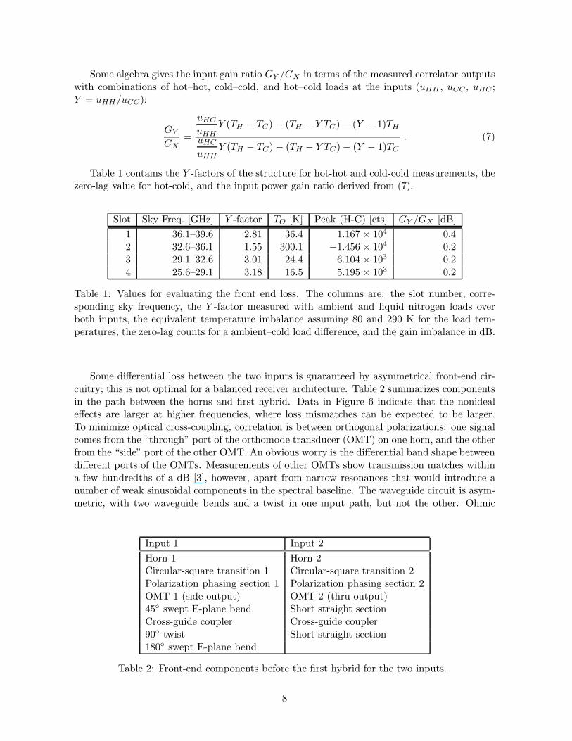
Table 1 contains the Y -factors of the structure for hot-hot and cold-cold measurements, thezero-lag value for hot-cold, and the input power gain ratio derived from (7).

Slot Sky Freq. [GHz] Y -factor TO [K] Peak (H-C) [cts] GY /GX [dB]

1 36.1–39.6 2.81 36.4 1.167 × 104 0.42 32.6–36.1 1.55 300.1 −1.456 × 104 0.23 29.1–32.6 3.01 24.4 6.104 × 103 0.24 25.6–29.1 3.18 16.5 5.195 × 103 0.2

Table 1: Values for evaluating the front end loss. The columns are: the slot number, corre-sponding sky frequency, the Y -factor measured with ambient and liquid nitrogen loads overboth inputs, the equivalent temperature imbalance assuming 80 and 290 K for the load tem-peratures, the zero-lag counts for a ambient–cold load difference, and the gain imbalance in dB.

Some differential loss between the two inputs is guaranteed by asymmetrical front-end cir-cuitry; this is not optimal for a balanced receiver architecture. Table 2 summarizes componentsin the path between the horns and first hybrid. Data in Figure 6 indicate that the nonidealeffects are larger at higher frequencies, where loss mismatches can be expected to be larger.To minimize optical cross-coupling, correlation is between orthogonal polarizations: one signalcomes from the “through” port of the orthomode transducer (OMT) on one horn, and the otherfrom the “side” port of the other OMT. An obvious worry is the differential band shape betweendifferent ports of the OMTs. Measurements of other OMTs show transmission matches withina few hundredths of a dB [3], however, apart from narrow resonances that would introduce anumber of weak sinusoidal components in the spectral baseline. The waveguide circuit is asym-metric, with two waveguide bends and a twist in one input path, but not the other. Ohmic

Input 1 Input 2

Horn 1 Horn 2Circular-square transition 1 Circular-square transition 2Polarization phasing section 1 Polarization phasing section 2OMT 1 (side output) OMT 2 (thru output)45◦ swept E-plane bend Short straight sectionCross-guide coupler Cross-guide coupler90◦ twist Short straight section180◦ swept E-plane bend

Table 2: Front-end components before the first hybrid for the two inputs.

8

Figure 9: Total power from all correlators ver-sus time for the receiver on the sky and thetelescope in its service position. Correlatoroutputs have been scaled and shifted for com-parison.

Figure 10: Continuation of time series in Fig-ure 9 after a brief break.

loss sets a minimum of 0.11 dB loss at 26.5 GHz to 0.08 dB loss at 37 GHz for copper WR-28waveguide of this length [4, Ch. 8.02]. Since the CCF nonideal structure is larger at high fre-quencies and the loss is not ohmic (compare Table 1 and Eq. (6)), reflection loss may dominate.Ohmic and reflection loss mismatches between the horns, transitions, phasing sections (whichhave significant internal structure), and cross-guide couplers also be important. An fluctuatingoffset from differential coupling to radiation modes within the cryostat cavity is an additionalsource of potential offsets [5], especially if the coupling is via the LNAs.

4 Consequences of the structure in the cross-correlation function

Even large offsets would not be a problem if they were stable on the timescale of a telescopenod, and subtracted out. Figures 9 and 10 show that the offsets are not stable, however. Eachfigure shows a time series of data from a lag with a large offset in each of the four correlators.The outputs have been scaled to simplify comparison. While we typically saw waveforms similarto Fig. 9 in the laboratory, Fig. 10 also captures a period with low fluctuations.

The figures show that outputs from the four correlators share a common waveform, implyinga common origin to the structure. Since the individual correlators and much of the electronicsin the channelizing downconverter are independent, the common structure must come from thereceiver’s output power or from the correlator or IF processor power supplies. We can rule outthe correlator power supply since the correlator electronics use the power supply as a referenceto convert the bipolar correlation function into a unipolar signal for the ADCs, and in theabsence of microwave input power the offsets are small and nearly constant. It is possible butunlikely that one of the amplifiers in the downconverter is damaged and unstable. Stability isa problem for Ka band observations with the Zpectrometer, the Spectrometer, and the CCB,however; all of these point to an unstable front end.

Instabilities persist but retain a basic shape over longer time periods. Figure 11 is a water-fall image of 263 raw (undifferenced) cross-correlation functions from Correlator #2 with the

9

telescope tracking SMMJ02399-0136 for 3.33 hr of elapsed time12. We chose a short integrationtime of 30 s for individual integrations as a balance between rapid switching and integrationefficiency. With 15 s of overhead for each scan, the observing efficiency was 66%. The verticalstripes in the image show that the data are dominated by a nearly fixed pattern structure.Differencing successive scans reduces the structure’s amplitude by a factor of about 500, butstill leaves substantial structure in the correlation function (heavy line in Fig. 12). Much ofthe high amplitude structure is close to the zero lag (lag numbers above 200 in the figure), andlooks like a scaled version of the raw data. This indicates imperfect subtraction due to relativelysmall variations in the structure’s amplitude with time. Subtracting a least-squares fit of thesummed data to the differenced data (light dotted line in (Fig. 12)) reduces the structure in thehigh-amplitude lags by a further factor of a few, but still leaves substantial structure. While thefit matches much of the structure, it does not fit in detail, indicating that band shape changesslightly in time.

Figure 13 is a waterfall plot of 131 differenced pairs of data from Fig. 11, each with aleast-squares fit of the summed data from each pair removed. This image shows the imper-fect subtraction of the systematic structure as a function of time: there are times when thesubtraction is successful, leaving little structure in the low lags toward the right of the image,and other times when the subtraction leaves residual structure. We saw no relationship withantenna elevation or other activity with the degree of instability. Figure 14 is a companionimage to Fig. 13, showing the differenced data’s covariance matrix. In the case of CCFs com-posed of uncorrelated random noise, this matrix would contain a series of uniformly bright spotsalong the diagonal, indicating each function’s variance, and off-diagonal elements that wouldbe zero within statistical uncertainty. While the spots along the diagonal are somewhat visiblein the upper left part of the figure, considerable horizontal and vertical striping dominates theimage. This shows the degree of covariance (mutual variance, unnormalized correlation) be-tween different differenced correlation functions. White denotes positive correlation, and blacknegative correlation. The covariance between different differenced functions is strong when thestructure within a correlation fiction is large: the horizontal and vertical stripes are strongestwhen the diagonal spot is brightest. An absence of localized sets of striping shows that thestructure within the correlation functions varies in amplitude, but not in basic shape for all ofthe data. A principal components analysis of the differenced and fit data confirms that most ofthe structure is common-mode, as expected from the structure of Figure 14. Almost all (85%)of the variance is in the first principal component, and essentially all (90%) of the variance iswithin the first four components. The shape of the first principal component is similar to theundifferenced data at lags away from the zero lag. A spectrum of the first principal componentshows lumpy baseline structure with typical widths of 300–400 MHz across the band.

4.1 Allan variance noise spectrum characterization

We used Allan variance calculations to quantify our measurement of the system stability. TheAllan variance was invented to characterize the stability of frequency standards [6, 7, 8].Schieder and collaborators [9, 10] popularized and extended its use for in radio astronomy.The Allan variance is the variance computed from differences of successively larger subsets oftime-series data; this is exactly the fluctuation one is most interested in for finding efficientchopping or nodding rates.

A plot of the Allan variance versus integration time T for the subsamples often follows a

12from 20:57 on 29 Nov 2006 to 00:36 on 30 Nov 2006

10

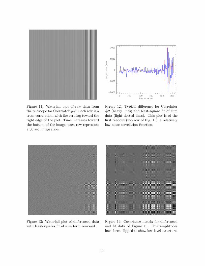
Figure 11: Waterfall plot of raw data fromthe telescope for Correlator #2. Each row is across-correlation, with the zero lag toward theright edge of the plot. Time increases towardthe bottom of the image; each row representsa 30 sec. integration.

Figure 12: Typical difference for Correlator#2 (heavy lines) and least-square fit of sumdata (light dotted lines). This plot is of thefirst readout (top row of Fig. 11), a relativelylow noise correlation function.

Figure 13: Waterfall plot of differenced datawith least-squares fit of sum term removed.

Figure 14: Covariance matrix for differencedand fit data of Figure 13. The amplitudeshave been clipped to show low-level structure.

11

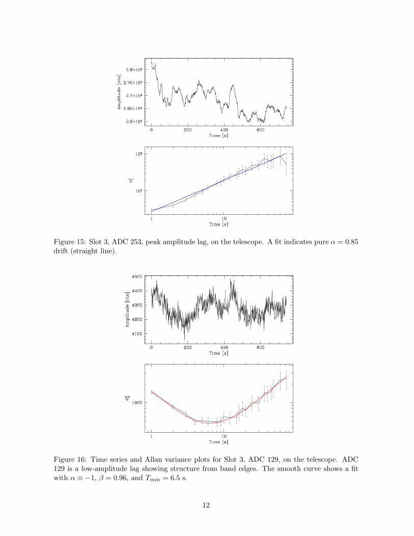
Figure 15: Slot 3, ADC 253, peak amplitude lag, on the telescope. A fit indicates pure α = 0.85drift (straight line).

Figure 16: Time series and Allan variance plots for Slot 3, ADC 129, on the telescope. ADC129 is a low-amplitude lag showing structure from band edges. The smooth curve shows a fitwith α ≡ −1, β = 0.96, and Tmin = 6.5 s.

12

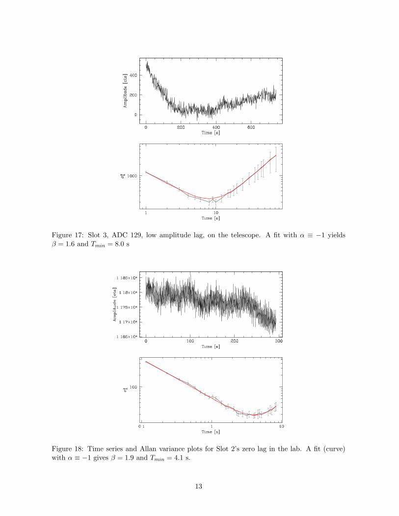
Figure 17: Slot 3, ADC 129, low amplitude lag, on the telescope. A fit with α ≡ −1 yieldsβ = 1.6 and Tmin = 8.0 s

Figure 18: Time series and Allan variance plots for Slot 2’s zero lag in the lab. A fit (curve)with α ≡ −1 gives β = 1.9 and Tmin = 4.1 s.

13

formσ2

A(T ) = aTα + bT β , (8)

where α = −1 represents the ideal case where the deviation integrates down as the square rootof integration time and a and b are the values for each power law term at a time of one second.For some devices β = 0, representing 1/f noise, but most receiver systems show “drift noise”,correlated noise and drift with β usually between 1 and 2. Curves following expression (8)have a minimum at the time when the decreasing radiometric and increasing nonideal noise areequal.

We wish to observe with switching times that are firmly in the radiometric noise regime, ortimes of about one third of this minimum in the Allan variance versus integration time. Withtelescope and software overheads of 15 to 20 s per integration, reasonable efficiency dictates anod-side time of 60 s. Ideally, then, we would like to push the Allan variance time to about180 s.

Figure 18 contains data from lab measurements with an ambient temperature absorberacross both horns. The upper panel is amplitude versus time, showing white noise fluctuationssuperposed on an underlying slowly varying signal. The lower panel shows the Allan varianceversus time, with the dark line a least-squares fit to (8) with α constrained to −1. The noise isradiometric to a few seconds, with a minimum in the Allan variance at an integration time of4.1 seconds and a drift slope power law of β = 1.9.

Solving (8) for the time at the minimum variance, Tmin, gives

Tmin =

(

−

βb

αa

)1/(α−β)

. (9)

Assuming that the input power is as high as possible while preserving linearity, a will be as largeas possible, so increasing the time to the minimum requires reducing the drift noise amplitude,b, by minimizing system gain variations. For α = −1 and a typical value of β = 1.5, the timeto minimum scales as Tmin ∝ b−0.4.

For comparison, a fit to the Allan variance for the −4 counts average correlator offsets withno microwave input signal gives α ∼ −0.95 to more than 70 s. In operation, the additionalreceiver noise brings σ2

A(1s) = 150 counts2 even at high lags, so input signals will alwaysdominate the stability.

We see the same characteristic time of a few seconds in the lab and on the sky. Figures 15,16, and 17 are the peak amplitude lag, mid-lag, and high-lag Allan variance plots of the time-series data of Fig. 9 for Slot 3. The time series for all lags show some identical underlyingstructure, but the higher lags contain noticeably more uncorrelated (white) noise. While thezero lag shows pure drift with β = 0.85, the higher lags have minimum variance times are 6 to8 s with β = 1–1.6.

Although the stability measurements in the lag domain cover the full band, we are moreinterested in the stability on bandwidths comparable to a few times a typical galaxy widths.The minimum time increases with decreasing bandwidth as [10]

Tmin2 = Tmin1

(

B1

B2

)1/(β+1)

. (10)

Scaling the stability results from the ∼ 200 spectral channels implied by the full-bandwidthmeasurements in the lag domain to the 10 or so channels that include a galaxy’s emission andsome baseline gives an increase in stability time by a factor of about 200.4

≈ 3, or about 15 s.This still falls well short of stability times that allow efficient integrations.

14

Figure 19: Correlator card internal temperatures (top panel) and package orientation informa-tion (bottom panel) versus time.

One open question is still why, given the pure drift of the zero lag, the average differencebaselines are so close to zero (e.g. Figure 4). The answer may well be that the fractional driftis large but the absolute drift amplitude is small.

5 Frequency calibration and bandwidth

The Zpectrometer has small internal phase shifts, so a simple Fourier transform would producea distorted spectrum. We obtain the coefficients for a discrete Fourier transform by injectingmonochromatic signals at known frequencies across the band [1]. This phase calibration isneeded only occasionally, when the system changes. Changes in temperature affect the cable andmicrostrip delays, but measurements show that temperature changes with elevation (Figure 19)are small enough that a single calibration at a representative temperature is sufficient.

A falloff in power from the doubler that generates the continuous wave (CW) calibrationtone sets the limits on the spectral bandwidth and spectral coverage. At present approximatelythree quarters of the band is usable, from about 27 to 37 GHz (zCO1−0 = 2.1 to 3.3). Someregions within this bands also have low calibration power levels, which makes them difficult touse for high signal-to-noise calibrations. We found that some of the low power regions comefrom loss in the cross-guide couplers. Work in this area is still in the early stages and we expectimprovement.

15

References

[1] A. Harris and J. Zmuidzinas, “A wideband lag correlator for heterodyne spectroscopy ofbroad astronomical and atmospheric spectral lines,” Rev. Sci. Inst., vol. 72, pp. 1531–1538,Feb. 2001.

[2] A. Harris, “Spectroscopy with multichannel correlation radiometers,” Rev. Sci. Inst.,vol. 76, pp. 4503–+, May 2005.

[3] E. Wollack, W. Grammer, and J. Kingsley, “The Bøifot orthodmode junction.” ALMAMemo 425, 2002.

[4] S. Ramo, J. R. Whinnery, and T. van Duzer, Fields and waves in communication electron-

ics. New York: John Wiley & Sons, Inc., 1965.

[5] R. Norrod, “Cryostat cavity noise and the impact on spectral baselines.” NRAO ElectronicsDivision Internal Report No. 318, 2007.

[6] D. W. Allan, “Statistics of atomic frequency standards,” Proc. IEEE, vol. 54, pp. 221–230,1966.

[7] J. A. Barnes, “Atomic timekeeping and the statistics of precision signal generators,” Proc.

IEEE, vol. 54, pp. 207–220, 1966.

[8] J. Rutman and F. Walls, “Characterization of frequency stability in precision frequencysources,” Proc. IEEE, vol. 79, pp. 952–960, 1991.

[9] R. Schieder, G. Rau, and B. Vowinkel, “Characterization and measurement of systemstability,” in Instrumentation for submillimeter spectroscopy (E. Kollberg, ed.), vol. 598 ofProc. SPIE, pp. 189–192, Society of Photo-Optical Instrumentation Engineers, Bellingham,WA, 1986.

[10] R. Schieder and C. Kramer, “Optimization of heterodyne observations using Allan variancemeasurements,” Astron. Astrophys., vol. 373, pp. 746–756, 2001.

16