X-ray Spectroscopy and Pulse Radiolysis of Aqueous Solutions

By

Alice Heller England

A dissertation submitted in partial satisfaction of the

requirements for the degree of

Doctor of Philosophy

in

Chemistry

in the

Graduate Division

of the

University of California, Berkeley

Committee in charge:

Professor Richard J. Saykally, ChairProfessor Daniel M. Neumark

Professor Teresa Head-Gordon

Fall 2011

Abstract

X-ray Spectroscopy and Pulse Radiolysis of Aqueous Solutions

by

Alice Heller England

Doctor of Philosophy in Chemistry

University of California, Berkeley

Professor Richard J. Saykally, Chair

The interaction of radiation and matter plays a crucial role in studies of aqueous solutions. Depending on the type of radiation, it can either be used a probe or as a source of excitation. With X-ray spectroscopy, high-energy photons are tuned to excite core electrons, giving insight into electronic structure and the local chemical environment of both the solvent and solute. In pulse radiolysis, an accelerated electron beam is used as an excitation source to create transient radiolytic products. Here, I present detailed studies using both X-rays and electron beams to investigate aqueous solutions and phenomena.

In Chapter 2, I discuss the probing of the pH-dependent aqueous carbonate system by soft X-rays. Spectral changes between carbonate, bicarbonate, carbonic acid, and carbon dioxide are analyzed by comparison with theoretically computed spectra. I also give an introduction to Near Edge X-ray Absorption Fine Structure (NEXAFS) spectroscopy and discuss experimental details for the design and employment of liquid microjets.

Chapter 3 describes a variety of different projects aimed at expanding the capabilities of the X-ray absorption experiments. These new directions include characterizing free radicals in solution, developing a new detection technique, exploring X-ray induced damage to solid biomolecules, and potentially investigating unusual nitrogen compounds.

In Chapter 4, I explore the interaction of high-energy electrons (8 MeV) with aqueous nickel (II) solutions. Pulse radiolysis combined with UV-visible absorption spectroscopy is used to investigate the kinetics of Ni2+ with water radiolysis products. The rate constant for the solvated electron reaction with Ni2+ is measured up to 300°C, and the electronic spectrum for the monovalent nickel ion is also recorded at high temperatures.

1

Acknowledgements

! I would like to first acknowledge my advisor, Richard Saykally, for providing the opportunity to work in his research group. I am especially thankful for his support and ongoing passion for scientific research. I also greatly appreciate being able to work with David Prendergast, who was always willing to spend the extra time helping me to navigate the calculations and to understand the basic concepts behind the code. My gratitude to the entire Saykally group, especially the X-ray side (Andrew, Craig, Janel, Orion, Greg, Kaitlin, and Jacob) for help and guidance in my experiments and calculations. My research at the Notre Dame Radiation Laboratory would not have been possible without the financial and scientific support of David Bartels, and I am thankful for that opportunity to expand my graduate research.! My research was supported by the Director, Office of Basic Energy Sciences, Office of Science, U.S. Department of Energy under Contract No. DE-AC02-05CH11231 through Lawrence Berkeley National Laboratory’s Chemical Sciences Division; experiments were performed at the Advanced Light Source, with theory, interpretation, and analysis provided through a User Project at the Molecular Foundry, and high performance computing resources provided by the National Energy Research Scientific Computing Center. Additional computing resources were provided by the Molecular Graphics and Computation Facility (College of Chemistry, University of California, Berkeley) under NSF grants CHE-0233882 and CHE-0840505. I would also like to acknowledge financial support from the Office of Civilian Radioactive Waste Management Graduate Fellowship, administered by Oak Ridge Institute for Science and Education under a contract between the U.S. Department of Energy and the Oak Ridge Associated Universities.! I am also grateful for the moral support of family and friends throughout my time in graduate school. Thank you to my parents for always supporting my academic pursuits, and especially to my father for sparking my scientific interest from an early age. Finally, Mike - you have been my best friend through this whole process and I couldn’t have done it without you.

i

Table of Contents

Chapter 1 - Introduction References

13

Chapter 2 - X-ray Absorption Spectroscopy of the Aqueous Carbonate System 4

2.1 Introduction 2.2 Experimental Methods NEXAFS Spectroscopy Experimental Details 2.3 Calculations Molecular Dynamics Simulations Simulated NEXAFS Spectra 2.4 Results and Discussion Experimental Results Acidic pH: Carbonic Acid vs CO2 Carbonate Structural Effects Spectral Fingerprints and Bond Lengths Relative Hydration Strength Ion Effects 2.5 Conclusions and Future Work 2.6 References

4668

101010111111162024263032

Chapter 3 - New Directions in NEXAFS 35 3.1 Introduction 3.2 Radicals Introduction Hydroxyl Radical Production NEXAFS of Hydroxyl Radicals Conclusions and Future Work 3.3 Streaming Current Detection Introduction Experimental Methods Results and Discussion Conclusions and Future Work 3.4 Radiation Damage Introduction Experimental Methods Results and Discussion Conclusions and Future Work

35353538424445454546494949505053

ii

3.5 Liquid Nitrogen Introduction Experimental Methods Results and Discussion Conclusions and Future Work 3.6 References

535353545657

Chapter 4 - High Temperature Radiolysis of Aqueous Nickel (II) Solutions 60

4.1 Introduction Radiation Chemistry Pulse Radiolysis Nickel (II) Chemistry 4.2 Experimental Methods Linear Electron Accelerator Samples High Temperature Flow Cell Optical Spectroscopy 4.3 Data Treatment Data Collection Kinetic Modeling 4.4 Results and Discussion Experimental Results Nickel (II) and Solvated Electron Reaction Nickel (I) Spectrum Nickel (I) and Hydroxyl Radical Reaction 4.5 Conclusions and Future Work 4.6 Appendix Electron and Nickel (II) Reaction Fit Parameters Nickel (I) Decay Fit Parameters 4.7 References

60606264656566666768686870707075778284848688

iii

Chapter 1 - Introduction! Ionizing radiation is classified as having sufficient energy to remove an electron from an atom or molecule. Depending on the type of particle and the energy of the radiation, a variety of chemical processes can occur after the initial ionization. Photons in the vacuum UV spectral region (> 6.5 eV) have enough energy to excite and ionize water molecules1, 2. Higher energy soft X-rays (250-600 eV) can selectively excite core electrons on carbon, oxygen, and nitrogen atoms as a probe of electronic structure and the intermolecular environment3. However, excess exposure to X-rays in this energy range can ultimately result in the decomposition of the samples being measured4. At even higher energies, ionizing radiation (such as accelerated MeV electron beams), induces distinct changes in the absorbing medium, resulting in the production of many excited species after the initial ionization processes5. Radiolysis of aqueous systems has been studied extensively with various solutes to characterize the kinetic behavior of the transient products. These various types of high energy radiation can be utilized either as an excitation source to produce a desired species, or as a measurement tool to investigate their behavior in certain conditions, or both.! In Chapter 2, I describe the use of X-rays as a probe to explore the behavior of dissolved carbonate, bicarbonate, carbonic acid, and carbon dioxide in aqueous solutions. Near Edge X-ray Absorption Fine Structure (NEXAFS) spectroscopy is an element-specific technique that measures core-level excitations in the soft X-ray region. For over a decade, the Saykally research group has employed NEXAFS to study a variety of aqueous systems containing carbon, nitrogen, boron, and oxygen6-11. Recent developments in the theoretical calculations of NEXAFS spectra, through a collaboration with David Prendergast (Lawrence Berkeley National Laboratory), has become increasingly important for our ability to interpret condensed phases spectra12-17. My research into the aqueous carbonate system has engendered the first measurements and/or predictions of X-ray absorption features of carbonate, bicarbonate, carbonic acid, and carbon dioxide. This work was recently published as a feature article in Chemical Physics Letters18. We have gained valuable insight into the relative hydration of each species, explored interactions with counterions, interpreted the spectral changes resulting from variations in molecular structure, and explored the vibronic coupling in a carbon dioxide Rydberg transition. The collaboration between experiment and theory provides an important fundamental perspective on the behavior of these fundamental carbon species in water. ! In the third chapter, I discuss several experiments that encompass new directions in NEXAFS spectroscopy. For two studies, an excimer laser at 157 nm is used to create excited species in liquid microjets, that can then be probed with NEXAFS spectroscopy. Coupling a vacuum UV (VUV) laser to the X-ray experiments can provide the opportunity to study a whole new range of high energy molecules that were previously inaccessible by solution chemistry. One important class of molecules to be explored with this method is free radicals. Specifically, I investigated the hydroxyl radical (•OH), an extremely reactive species, which can be produced with VUV photolysis of liquid water2. The hydration of this ubiquitously important transient molecule is still not well understood, and NEXAFS can potentially better characterize its behavior in aqueous

1

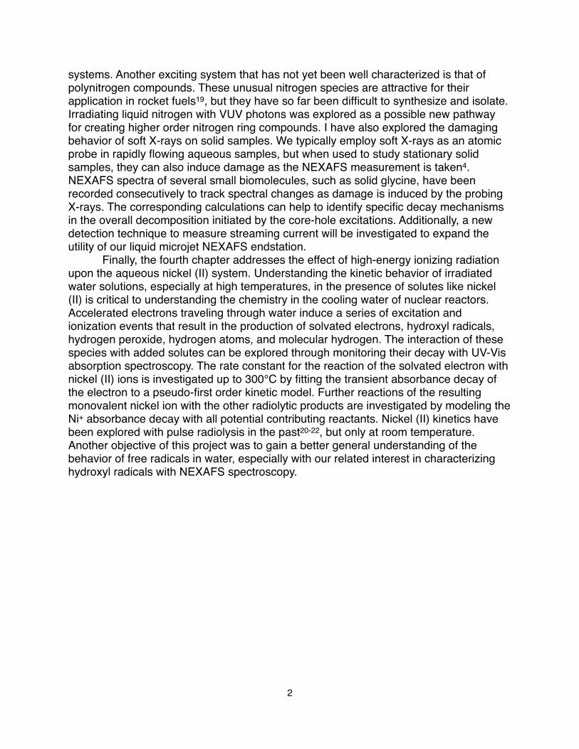
systems. Another exciting system that has not yet been well characterized is that of polynitrogen compounds. These unusual nitrogen species are attractive for their application in rocket fuels19, but they have so far been difficult to synthesize and isolate. Irradiating liquid nitrogen with VUV photons was explored as a possible new pathway for creating higher order nitrogen ring compounds. I have also explored the damaging behavior of soft X-rays on solid samples. We typically employ soft X-rays as an atomic probe in rapidly flowing aqueous samples, but when used to study stationary solid samples, they can also induce damage as the NEXAFS measurement is taken4. NEXAFS spectra of several small biomolecules, such as solid glycine, have been recorded consecutively to track spectral changes as damage is induced by the probing X-rays. The corresponding calculations can help to identify specific decay mechanisms in the overall decomposition initiated by the core-hole excitations. Additionally, a new detection technique to measure streaming current will be investigated to expand the utility of our liquid microjet NEXAFS endstation.! Finally, the fourth chapter addresses the effect of high-energy ionizing radiation upon the aqueous nickel (II) system. Understanding the kinetic behavior of irradiated water solutions, especially at high temperatures, in the presence of solutes like nickel (II) is critical to understanding the chemistry in the cooling water of nuclear reactors. Accelerated electrons traveling through water induce a series of excitation and ionization events that result in the production of solvated electrons, hydroxyl radicals, hydrogen peroxide, hydrogen atoms, and molecular hydrogen. The interaction of these species with added solutes can be explored through monitoring their decay with UV-Vis absorption spectroscopy. The rate constant for the reaction of the solvated electron with nickel (II) ions is investigated up to 300°C by fitting the transient absorbance decay of the electron to a pseudo-first order kinetic model. Further reactions of the resulting monovalent nickel ion with the other radiolytic products are investigated by modeling the Ni+ absorbance decay with all potential contributing reactants. Nickel (II) kinetics have been explored with pulse radiolysis in the past20-22, but only at room temperature. Another objective of this project was to gain a better general understanding of the behavior of free radicals in water, especially with our related interest in characterizing hydroxyl radicals with NEXAFS spectroscopy.!

2

References

1.! Crowell, R. A., Bartels, D. M., J. Phys. Chem. 100, 17940 (1996).2.! Elles, C. G., Jailaubekov, A. E., Crowell, R. A., Bradforth, S. E., J. Chem. Phys.

125, (2006).3.! Stöhr, J., NEXAFS Spectroscopy. (Springer, New York, 1996).4.! Zubavichus, Y. et al., Radiat. Res. 161, 346 (2004).5.! Spinks, J. W. T., Woods, R. J., An Introduction to Radiation Chemistry. (John

Wiley & Sons, Inc., New York, ed. 3rd, 1990).6.! Cappa, C. D., Smith, J. D., Messer, B. M., Cohen, R. C., Saykally, R. J., J. Phys.

Chem. B 110, 1166 (2006).7.! Cappa, C. D., Smith, J. D., Messer, B. M., Cohen, R. C., Saykally, R. J., J. Phys.

Chem. B 110, 5301 (2006).8.! Smith, J. D. et al., J. Phys. Chem. B 110, 20038 (2006).9.! Uejio, J. S. et al., Proc. Natl. Acad. Sci. USA 105, 6809 (2008).10.! Wilson, K. R. et al., J. Phys. Chem. B 105, 3346 (2001).11.! Wilson, K. R. et al., Rev. Sci. Instrum. 75, 725 (2004).12.! Duffin, A. M. et al., J. Chem. Phys. 134, 154503 (2011).13.! Duffin, A. M. et al., Phys. Chem. Chem. Phys. 13, 17077 (2011).14.! Schwartz, C. P., Saykally, R. J., Prendergast, D., J. Chem. Phys. 133, 044507

(2010).15.! Schwartz, C. P., Uejio, J. S., Saykally, R. J., Prendergast, D., J. Chem. Phys.

130, 184109 (2009).16.! Uejio, J. S. et al., J. Phys. Chem. B 114, 4702 (2010).17.! Uejio, J. S., Schwartz, C. P., Saykally, R. J., Prendergast, D., Chem. Phys. Lett.

467, 195 (2008).18.! England, A. H. et al., Chem. Phys. Lett. 514, 187 (2011).19.! Butler, R., Chem. Ind., 24 (2009).20.! Buxton, G. V., Sellers, R. M., J. Chem. Soc. Faraday Trans. 1 71, 558 (1975).21.! Kelm, M., Lilie, J., Henglein, A., Janata, E., J. Phys. Chem. 78, 882 (1974).22.! Meyerstein, D., Mulac, W. A., J. Phys. Chem. 72, 784 (1968).

3

Chapter 2 - X-ray Absorption Spectroscopy of the Aqueous Carbonate System*The majority of the work presented in this chapter has been published as a feature article in Chemical Physics Letters1.

2.1 Introduction

! The hydrolysis of carbon dioxide (CO2) to form carbonic acid and the subsequent speciation to bicarbonate and carbonate is a fundamental process that has been studied extensively. From a geological perspective, carbonic acid is the most abundant terrestrial acid, while bicarbonate and carbonate are the primary contributors to total alkalinity in natural waters. These dissolved carbonate species participate in numerous reactions that have vital implications in rock weathering, mineral precipitation, ocean acidification and climate change. New technologies are emerging to mitigate global warming by exploiting methods for capture and storage of excess CO2, such as the metal-organic-frameworks (MOFs) developed to selectively trap CO2 gas2 or pumping CO2 into underground salt-water reservoirs3.! Aqueous carbonate chemistry not only governs the terrestrial carbon cycle, but it also maintains the delicate pH balance required in mammalian biological systems. The carbonate/bicarbonate/CO2 buffer system regulates blood pH, and is also responsible for CO2 transport in the body and ion mobility across cell membranes. The importance of calcium carbonate in biomineralization processes has led to extensive study of its nucleation and precipitation dynamics in supersaturated solutions4, 5. Seawater carbonate chemistry dictates the uptake of CO2 in surface waters, and the consequent carbonate saturation plays a major role in the calcification of ocean organisms and ecosystems6. Furthermore, the influence of the aqueous carbonate system extends to the astronomical realm. Upon irradiation, CO2-H2O deposits in outer space are converted to carbonic acid, which has also been identified as a possible species present on several planetary surfaces7.! Understanding the molecular-scale details of carbonate, bicarbonate, carbonic acid, and CO2 behavior in these various environments is critical to the development and success of future strategies aimed at maintaining or mitigating these natural carbon processes. The overall reactions8 for carbon dioxide dissolution, hydrolysis, and equilibrium are:

CO2 (g) + H2O ↔ CO2 (aq)! ! ! ! ! ! ! (1.1) ! CO2 (aq) + H2O ↔ H2CO3! (Keq = 2.6 x 10-3 at 25 °C)! ! ! (1.2) ! H2CO3 ↔ H+ + HCO3-! (pKa = 6.35) ! ! ! ! ! (1.3)

HCO3- ↔ H+ + CO32- ! (pKa = 10.33)!! ! ! ! (1.4)Based on Reactions 1.1-1.4 and the associated equilibrium constants, the speciation diagram is plotted in Figure 2.1.

4

Keq = 2.6 x 10-3

H2CO3

HCO3-

CO32-

CO2 (aq)

2 4 6 8 10 120

0.2

0.4

0.6

1

0.8

pH

Mol

e Fr

actio

n

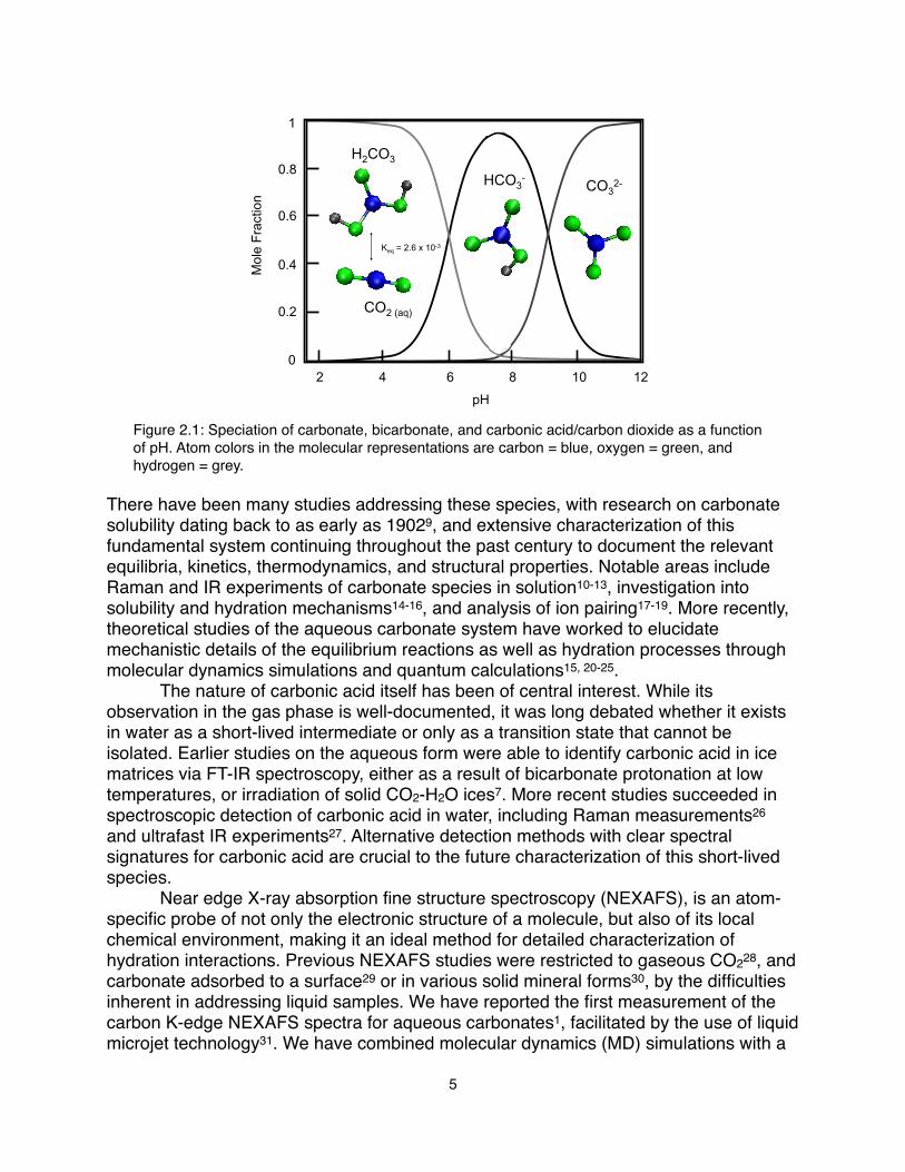
Figure 2.1: Speciation of carbonate, bicarbonate, and carbonic acid/carbon dioxide as a function of pH. Atom colors in the molecular representations are carbon = blue, oxygen = green, and hydrogen = grey.

There have been many studies addressing these species, with research on carbonate solubility dating back to as early as 19029, and extensive characterization of this fundamental system continuing throughout the past century to document the relevant equilibria, kinetics, thermodynamics, and structural properties. Notable areas include Raman and IR experiments of carbonate species in solution10-13, investigation into solubility and hydration mechanisms14-16, and analysis of ion pairing17-19. More recently, theoretical studies of the aqueous carbonate system have worked to elucidate mechanistic details of the equilibrium reactions as well as hydration processes through molecular dynamics simulations and quantum calculations15, 20-25.! The nature of carbonic acid itself has been of central interest. While its observation in the gas phase is well-documented, it was long debated whether it exists in water as a short-lived intermediate or only as a transition state that cannot be isolated. Earlier studies on the aqueous form were able to identify carbonic acid in ice matrices via FT-IR spectroscopy, either as a result of bicarbonate protonation at low temperatures, or irradiation of solid CO2-H2O ices7. More recent studies succeeded in spectroscopic detection of carbonic acid in water, including Raman measurements26 and ultrafast IR experiments27. Alternative detection methods with clear spectral signatures for carbonic acid are crucial to the future characterization of this short-lived species. ! Near edge X-ray absorption fine structure spectroscopy (NEXAFS), is an atom-specific probe of not only the electronic structure of a molecule, but also of its local chemical environment, making it an ideal method for detailed characterization of hydration interactions. Previous NEXAFS studies were restricted to gaseous CO228, and carbonate adsorbed to a surface29 or in various solid mineral forms30, by the difficulties inherent in addressing liquid samples. We have reported the first measurement of the carbon K-edge NEXAFS spectra for aqueous carbonates1, facilitated by the use of liquid microjet technology31. We have combined molecular dynamics (MD) simulations with a

5

first principles density functional theory (DFT) method to model and interpret the measured NEXAFS spectra32, 33, gaining new and detailed insights into the nature of aqueous carbonate species. ! The majority of the work presented in this chapter has been published in Chemical Physics Letters1; specifically the material in the Introduction, the Experimental Methods, and the Results and Discussion sections: Acidic pH: Carbonic Acid vs CO2, Carbonate Structural Effects, Spectral Fingerprints and Bond Lengths, and Relative Hydration Strength. Figures 2.7, 2.8, 2.9, 2.10, 2.12, 2.14, 2.15, and Table 2.1 are replicated directly from the article. The discussion on Ion Effects is the only section that was not included in the article.

2.2 Experimental Methods

NEXAFS Spectroscopy

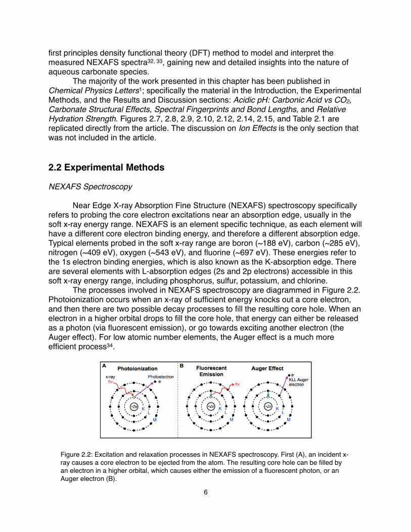
! Near Edge X-ray Absorption Fine Structure (NEXAFS) spectroscopy specifically refers to probing the core electron excitations near an absorption edge, usually in the soft x-ray energy range. NEXAFS is an element specific technique, as each element will have a different core electron binding energy, and therefore a different absorption edge. Typical elements probed in the soft x-ray range are boron (~188 eV), carbon (~285 eV), nitrogen (~409 eV), oxygen (~543 eV), and fluorine (~697 eV). These energies refer to the 1s electron binding energies, which is also known as the K-absorption edge. There are several elements with L-absorption edges (2s and 2p electrons) accessible in this soft x-ray energy range, including phosphorus, sulfur, potassium, and chlorine. ! The processes involved in NEXAFS spectroscopy are diagrammed in Figure 2.2. Photoionization occurs when an x-ray of sufficient energy knocks out a core electron, and then there are two possible decay processes to fill the resulting core hole. When an electron in a higher orbital drops to fill the core hole, that energy can either be released as a photon (via fluorescent emission), or go towards exciting another electron (the Auger effect). For low atomic number elements, the Auger effect is a much more efficient process34.

Figure 2.2: Excitation and relaxation processes in NEXAFS spectroscopy. First (A), an incident x-ray causes a core electron to be ejected from the atom. The resulting core hole can be filled by an electron in a higher orbital, which causes either the emission of a fluorescent photon, or an Auger electron (B).

6

! When in condensed phases, the inelastic scattering of the primary photoelectrons and Auger electrons result in an electron cascade as shown in Figure 2.3. The primary and Auger electrons typically have mean free paths of less than 10 Å, and so only when the electron cascade occurs within this distance of the surface will those electrons escape into the vacuum to be measured. This limits electron detection methods to an effective escape depth of about 10 Å, since electrons that are generated deeper within the bulk will not have sufficient energy to escape35. Typically NEXAFS is considered a surface technique given this small escape depth, but in some liquid samples, like water, this distance is sufficient to probe bulk properties.

Figure 2.3: X-ray photons penetrate liquid water ~5-10 µm (at 530 eV), but only electrons generated within 10 Å of the surface will have sufficient energy to escape out of the sample. The diagram is based on a similar figure by Stöhr35, with depths altered to appropriate values for liquid water.

! The K-shell spectra represents transitions of the core electrons up to states near the vacuum level, and therefore near the ionization potential (IP). Characteristic resonances include π*, σ*, and Rydberg states. π* resonances are typically sharp features and are the lowest energy peaks in the K-shell spectrum. These transitions occur below the IP due to the Coulombic shift of the outer orbitals resulting from the presence of the core hole. A π* resonance is of course only observed for molecules with π bonding, and the natural width is determined by the lifetime of the excited state. The sharp but weak resonances occurring in between the π* energy and the IP correspond to Rydberg states. Above the IP, the broad features represent transitions to continuum states, or σ* resonances. The natural width of the σ* features is determined by the lifetime of the excited state, but they are also broadened by the vibrational motions in the molecule35.! NEXAFS not only characterizes the electronic structure of a molecule, but it also probes the local chemical environment around the absorbing atom. The core electron is excited to antibonding states which are large and diffuse, and therefore can be greatly affected by the proximity of and interaction with nearby molecules. For example, the NEXAFS spectrum of the oxygen K-edge in water drastically changes from the vapor to liquid phase due to the increased hydrogen bonding of the water molecules. One can

7

investigate relative shifts or changes in shape of the K-shell spectra features to characterize the effect of different environments on a given absorbing atom.

Experimental Details! Sodium and potassium carbonate were obtained commercially from EMD Chemicals in the crystalline form with a purity of 99.0%. A 1 M solution was prepared for each with 18 MΩ/cm resistivity water, with an initial pH of approximately 12. To access the lower pH regions, the carbonate solutions were mixed with appropriate ratios of 1 M HCl in a dual syringe pump system (Teledyne-Isco) by adjusting the flow rates. A 1:1 ratio of carbonate to acid resulted in pH=8, where bicarbonate is the predominant species. Similarly, a 1:2 ratio yielded pH=3 to produce H2CO3 (aq)/CO2 (aq). Based on Reactions 1.1-1.4 and associated equilibrium constants, the basic solution at pH=12 contained 98% carbonate and 2% bicarbonate. The mid-range solution (pH=8.5) was comprised of 98% bicarbonate and 2% carbonic acid/CO2. Finally, for the acidic range, at pH=3, the speciation indicates the solution contained 100% carbonic acid/CO2.! The NEXAFS experiments were conducted at Beamline 8.0.1 at the Advanced Light Source (Lawrence Berkeley National Labs, Berkeley, CA). Beamline 8.0.1 is an undulator beamline that is tunable over 80-1250 eV with a maximum flux of 6x1015 photons/second and resolving power of 6000 E/ΔE. The carbon K-edge energy range was accessed by using the first harmonic of the middle energy grating in the monochromator. The Saykally group endstation is connected to the beamline via a differential pumping section that maintains pressures of 10-8 – 10-9 torr with three small turbo pumps (Varian Turbo V-70). The main experimental chamber is coupled windowlessly to the differential pumping section by a small pinhole, which is just large enough to pass the x-ray beam. A pressure-sensitive shutter is also employed to protect the beamline from any backflow pressure in the main chamber.! The samples are introduced into the main vacuum chamber via a liquid microjet36. A free vacuum surface of a volatile liquid can be achieved due to the high velocity and small surface area of these jets. These conditions result in collision-free evaporation, which allows for measurement of the liquid with minimal interference from any vapor jacket around the jet. Additionally, the flowing jet prevents potential sample damage from the incident x-ray beam. In this experiment, the liquid microjet stream was produced by a 30 μm fused silica capillary tip pressurized with the dual syringe pump (Teledyne-Isco). Typical flow rates range from 0.8 to 1.0 mL/min with backing pressures around 80 atm. Under similar conditions, it has been determined that the jet temperature is near 20°C31, 36-39.! Shortly after the sample leaves the jet tip, it is intersected with the tunable X-rays from the beamline (~50 µm spot size) over the carbon K-edge energy range (280-320 eV). The liquid microjet is trapped with a skimmer and liquid nitrogen trap to help reduce vacuum pressures in the chamber. An additional liquid nitrogen trap along with a turbo pump (Turbotronik NT-20) and roughing pump keep the main chamber pressures down to ~9x10-5 torr. Figure 2.4 shows a diagram of the experimental setup. A complete description of the endstation has been published previously31.

8

X-ray Beam

Electrical feedthrough

LN2 trap

LN2 trapTurbo pump

XYZ stage

Microjet feedthrough

(connected to syringe pumps)

To rough pump

(connect copper electrode to battery box)

Figure 2.4: A schematic of the NEXAFS endstation. The tunable x-ray beam intersects the liquid microjet sample perpendicularly and the core excitations are detected by TEY with a biased copper electrode at 2.1 kV. The jet is aligned to the beam using the x-y-z stage and vacuum pressures are maintained with the multiple pumps and liquid nitrogen traps. The connection to the beamline with the differential pumping section is not shown.

! The total electron yield (TEY) was collected with a 2.1 kV biased copper electrode placed about 1 cm from the jet as a function of the incident photon energy. The signal current is then passed through a Keithley current amplifier (model 428) before it is recorded by the beamline data acquisition software. While TEY is not a direct measurement x-ray absorption, it is representative of the process. As the absorption edge is reached, the excitation of the high-energy core electrons spurs a cascade of Auger and secondary electrons (from inelastic scattering of the primary electrons) to be emitted from the sample (Figure 2.3). Therefore, measuring this surge of electrons is indicative of the absorption of x-rays that promote the core electrons to different excited states. The TEY signal is limited to the effective electron escape depth since those generated deeper in the sample will not have sufficient energy to escape to the surface and into the vacuum35. In this case, the average escape depth of electrons in water is near 10 Å, which is far enough to describe excitations occurring in the bulk liquid (radial distribution functions for water reach a uniform distribution by 10 Å).! The jet is mounted on an x-y-z stage for alignment with the x-ray beam. There is a large TEY signal enhancement when the x-ray beam is directly on the jet due to the higher concentration of molecules in the liquid. As the jet is moved above or below the x-ray beam, the TEY signal decreases significantly as a result of the much lower concentration of gas molecules.! Each TEY measurement was normalized to the I0 detected on a gold mesh located up-beam of the chamber. The beamline energy was calibrated to the energy of the carbon dips measured on the I0 signal. The vapor spectra were measured by detecting the TEY signal off of the jet for each sample. The vapor signal was then subtracted from the on-jet scans as a background subtraction. Additionally, a baseline correction was performed if necessary. In order to compare the spectra of the different pH ranges, the first intense peak of each were area normalized. All data analysis was completed using IGOR Pro 6.00.

9

2.3 Calculations

! Interpretation of x-ray spectra of condensed phases is inherently difficult due to the broadening of NEXAFS features by the large range of molecular motions and intramolecular interactions. Comparison with calculated spectra can provide great insight into the molecular-scale details that affect the NEXAFS spectral features. A combination of molecular dynamics with a first-principles electronic structure approach to calculating core electron excitations has allowed us to gain insight into not only this carbonate system but to many other aqueous systems as well32, 33, 40-43.

Molecular Dynamics Simulations! AMBER 944 was used to perform classical MD simulations for gaseous and dissolved CO2, and Quantum Mechanic/Molecular Mechanics (QM/MM) trajectories for carbonate, bicarbonate, and carbonic acid. Classical MD calculations employed the default ff99SB force field while the PM3 method was used for the semi-empirical QM/MM calculations. For all systems, ~90 TIP3P waters were added and for carbonate and bicarbonate sodium counterions were also added to balance the total charge. The MD simulations were run in periodic boundary conditions for 10 ns. 100 uncorrelated snapshots were chosen from each trajectory to represent a sufficient sampling of molecular motions. Additionally, first principles molecular dynamics (FPMD), within the Born-Oppenheimer approximation, was performed on carbonate to verify the accuracy of the QM/MM simulation. We used the Quantum-ESPRESSO package45, sampling the dynamics of the electronic ground state for 2.5 ps using the Perdew-Burke-Ernzerhof form of the generalized-gradient approximation (PBE GGA functional)46.

Simulated NEXAFS Spectra! X-ray absorption cross sections were calculated from transition probabilities within Fermi’s Golden Rule35, using DFT. The initial state was derived from a ground state DFT calculation. The lowest energy final state was approximated as the self-consistent electronic response of a given molecular configuration to the presence of a core-hole on the excited carbon atom (modeled using a suitably modified pseudopotential) and the inclusion of an excited electron in the first available empty state [eXcited state Core Hole (XCH) approximation]47. The resulting excited state self-consistent field was used to generate subsequent higher excited states non-self-consistently. Transition matrix elements were computed using individual Kohn-Sham states (the ground state 1s atomic orbital and the spectrum of eigenvalues from the approximate final state). All DFT calculations were obtained using the PBE GGA functional46. Plane-wave pseudopotential calculations employed ultrasoft pseudopotentials and a kinetic energy cut-off of 25 Ry. A modified form of the Quantum-ESPRESSO package45 was used to generate the Kohn-Sham eigenspectrum while the Shirley interpolation scheme48 was employed to accelerate numerical convergence of computed spectra. Because there is no absolute energy reference in pseudopotential calculations, further spectral alignment was necessary for meaningful comparisons between chemically or structurally different systems. Details of the alignment scheme are described further in the Results and Discussion section. Isosurfaces were calculated with Quantum-ESPRESSO and rendered in VMD49.

10

2.4 Results and Discussion

Experimental Results! The full carbon edge spectra are shown in Figure 2.5 for the three different pH ranges. All exhibit an intense feature around 290 eV, which is representative of the first allowed transition of the carbon 1s electron to the lowest unoccupied molecular orbital (LUMO), a π* antibonding state. These peaks appear at energies within the expected range for C=O π* transitions. This feature shifts to higher energies as the carbonate solution is acidified. The broader, higher energy features represent transitions to σ* antibonding final states. There is more variation in the shape and position of these features than the π* peaks.

Tota

l Ele

ctro

n Y

ield

(TE

Y)

320315310305300295290Incident Photon Energy (eV)

Basic pH Neutral pH Acidic pH

Figure 2.5: Experimental carbon K-absorption spectra for the 3 different pH carbonate solutions. Blue is the basic solution, red is the mid-range pH, and green is the acidic solution.

! Interpretation of the acidic pH range based on comparison with calculated spectra will be addressed first, followed by a discussion on the difficulties encountered when modeling the carbonate anion, and then by an overall analysis of the spectral fingerprints for each species. Finally the relative hydration strengths and the effects of different cations are examined.

Acidic pH: Carbonic Acid vs CO2! The carbonate speciation in the acidic pH range indicates the presence of three possible species: carbonic acid, dissolved carbon dioxide, and carbon dioxide gas. As described in the experimental section, the acidic solution was achieved by mixing a 2:1 ratio of equal molarity HCl and sodium carbonate in the dual syringe pumps. Depending on the carbonic acid/dissolved CO2 equilibrium and then the extent to which the CO2 evaporates out of the liquid microjet, we could potentially observe one dominant species or some combination of multiple species in the NEXAFS spectrum. As previously mentioned, an off-jet scan is taken to measure the contribution of any vapor to the spectra. Usually, the off-jet scans are much less intense and typically do not exhibit

11

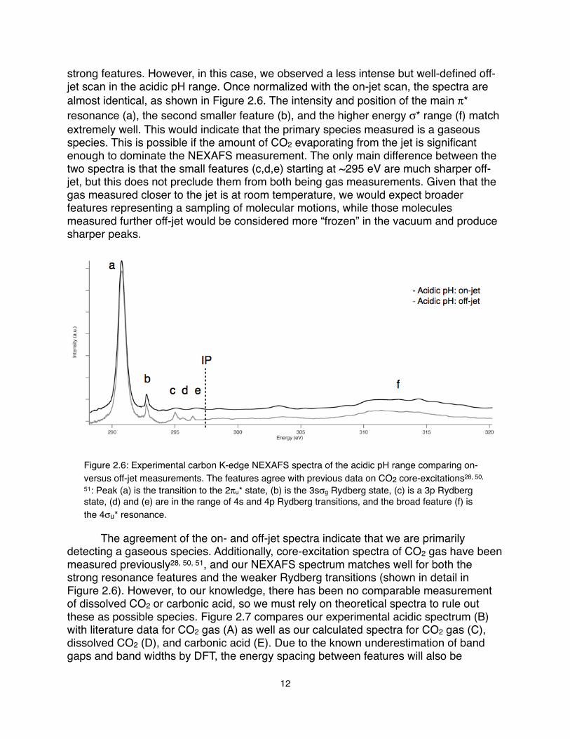
strong features. However, in this case, we observed a less intense but well-defined off-jet scan in the acidic pH range. Once normalized with the on-jet scan, the spectra are almost identical, as shown in Figure 2.6. The intensity and position of the main π* resonance (a), the second smaller feature (b), and the higher energy σ* range (f) match extremely well. This would indicate that the primary species measured is a gaseous species. This is possible if the amount of CO2 evaporating from the jet is significant enough to dominate the NEXAFS measurement. The only main difference between the two spectra is that the small features (c,d,e) starting at ~295 eV are much sharper off-jet, but this does not preclude them from both being gas measurements. Given that the gas measured closer to the jet is at room temperature, we would expect broader features representing a sampling of molecular motions, while those molecules measured further off-jet would be considered more “frozen” in the vacuum and produce sharper peaks.

Figure 2.6: Experimental carbon K-edge NEXAFS spectra of the acidic pH range comparing on- versus off-jet measurements. The features agree with previous data on CO2 core-excitations28, 50,

51: Peak (a) is the transition to the 2πu* state, (b) is the 3sσg Rydberg state, (c) is a 3p Rydberg state, (d) and (e) are in the range of 4s and 4p Rydberg transitions, and the broad feature (f) is the 4σu* resonance.

! The agreement of the on- and off-jet spectra indicate that we are primarily detecting a gaseous species. Additionally, core-excitation spectra of CO2 gas have been measured previously28, 50, 51, and our NEXAFS spectrum matches well for both the strong resonance features and the weaker Rydberg transitions (shown in detail in Figure 2.6). However, to our knowledge, there has been no comparable measurement of dissolved CO2 or carbonic acid, so we must rely on theoretical spectra to rule out these as possible species. Figure 2.7 compares our experimental acidic spectrum (B) with literature data for CO2 gas (A) as well as our calculated spectra for CO2 gas (C), dissolved CO2 (D), and carbonic acid (E). Due to the known underestimation of band gaps and band widths by DFT, the energy spacing between features will also be

12

underestimated compared to experiment. All spectra exhibit a sharp feature around 290.7 eV, which represents the excitation of the carbon 1s electron to the LUMO 2πu* antibonding molecular states. This feature is similar in all spectra and therefore not useful in determining the dominant species in experiment. Carbonic acid has two broad σ* resonances spanning 294-305 eV that are absent from experiment. Both CO2 species have broader σ* features representing the 4σu* resonance centered at 310 eV that match experiment, but only gaseous CO2 exhibits the small peak observed at 292.3 eV, representing the 3sσg Rydberg state. Furthermore, the peak positions for the 2πu*, 3sσg, and 4σu* peaks in the experimental spectra (Figure 2.7B) match extremely well with those observed in previous CO2 gas electron-energy-loss spectra51 and NEXAFS measurements28. Transitions to additional 3p, 4s, and 4p Rydberg states in CO2 gas are weakly detected in the 295-297 eV range, yet these features are not resolved in our plane-wave supercell theoretical spectra due to their diffuse nature. Calculations with a larger box size will be necessary to resolve such fine structure for higher energy Rydberg states. All of the above factors clearly indicate that the dominant species in our acidic pH experiment is CO2 gas, but it is also important to understand the chemical origin of this distinctive 3sσg Rydberg peak.

One would assume that the disappearance of the 3sσg feature upon hydration is simply due to the presence of water. However, slight changes in the shape of CO2 can also impact the position and intensity of features in the computed spectrum. There were negligible differences in the bond distances and angles between gaseous and dissolved CO2, but to confirm the effect of hydration versus molecular shape on the spectrum, additional fictitious core-excited state calculations were performed on the CO2 molecules with the effect of the water removed from the spectra. This constrained model maintains the structural effects of the solvent while removing the electronic confinement and hybridization effects. The constrained CO2 gas spectrum for the 2πu* and 3sσg states is compared with its dissolved counterpart and the original gaseous CO2 spectrum in Figure 2.8A. It is now clear that the spectroscopic disappearance of the 3sσg feature is a direct result of hydration, while the small differences in molecular shape between CO2 gas and its constrained form lead to a slight blue-shift in the position of the 2πu*. To gain further insight into the reason why the 3sσg peak is only present in the gas phase, the states for corresponding snapshots in the dissolved and constrained CO2 are imaged in Figure 2.8B – 2.8E. The 2πu* state is very similar in each and localized on the CO2, therefore it should be unaffected by hydration. The 3sσg state for the gas is very large and diffuse, but upon hydration it hybridizes with the surrounding water to form a band of states that have mixed CO2 3sσg and water character. The formation of this energy dispersive band, together with the reduced overlap with the carbon 1s orbital due to its large spatial extent, leads to the eradication of the peak from the solvated phase spectrum.

13

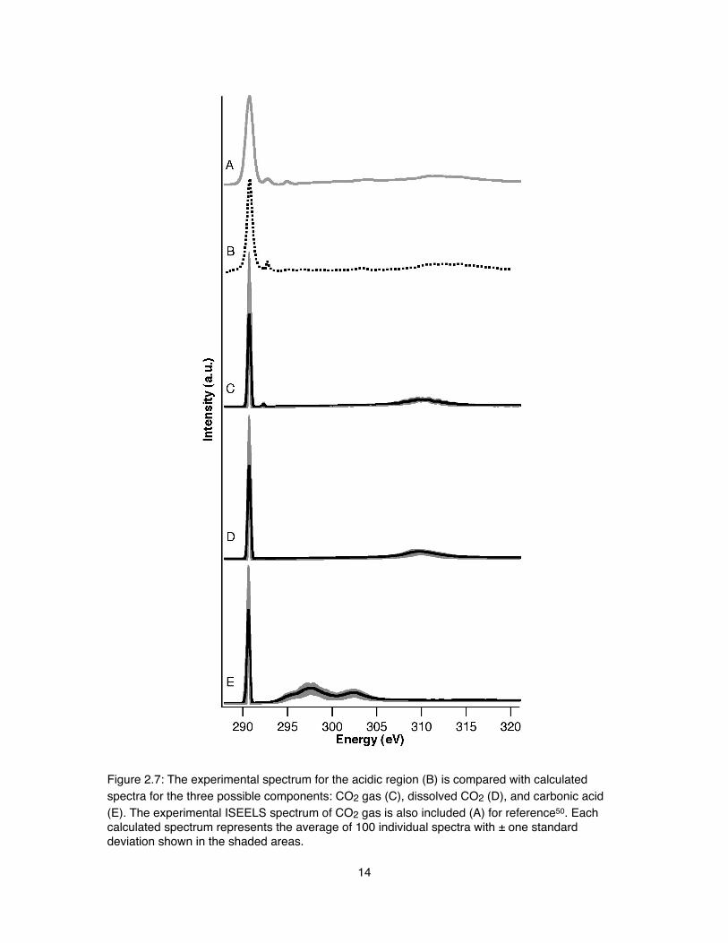
Figure 2.7: The experimental spectrum for the acidic region (B) is compared with calculated spectra for the three possible components: CO2 gas (C), dissolved CO2 (D), and carbonic acid (E). The experimental ISEELS spectrum of CO2 gas is also included (A) for reference50. Each calculated spectrum represents the average of 100 individual spectra with ± one standard deviation shown in the shaded areas.

14

Figure 2.8: Spectra and isosurfaces for gaseous and dissolved CO2. Panel A shows detail of the average calculated spectra for the carbon 1s transition to the 2πu* and 3sσg states for CO2 gas (solid line), constrained CO2 gas (dotted line), and dissolved CO2 (dashed line). Isosurfaces for a representative snapshot of constrained CO2 gas are plotted in B (2πu*) and C (3sσg); and those for dissolved CO2 in D (2πu*) and E (3sσg). Atom colors are aqua for carbon, red for oxygen, and white for hydrogen.

! Upon closer inspection of the final 3sσg Rydberg state shown for one CO2 gas snapshot (Figure 2.8C), there is electron density around but not actually on the carbon atom itself, which would imply that there should be no feature observed for this state in the carbon K-edge spectrum. Further research into the literature revealed that the carbon 1s(σg) → 3sσg transition is dipole-forbidden (σg → σg), but becomes dipole-allowed upon the inclusion of nuclear motion. We have previously encountered this issue of sampling the nuclear degrees of freedom accessible, either from zero-point motion or finite temperature, in order to accurately predict NEXAFS spectral features42,

43, 52. Here, we found the appearance of the 3sσg Rydberg state for CO2 gas dependent on the bending vibration, which is consistent with previous predictions in the literature53-55. Vibronic coupling with the CO2 bending mode along with the intensity-lending π* resonance makes this the strongest observed Rydberg transition for CO2.

15

The correlation between O-C-O bond angle and the 3sσg peak is illustrated in Figure 2.9A for all 100 snapshots contributing to the average CO2 spectrum. As expected, those closer to 180° show little or no intensity, while those with smaller angles display increasingly more intense peaks. This is due to stronger vibronic coupling as the molecule bends and the linear symmetry is broken. Furthermore, the spectra and isosurfaces for three representative snapshots are shown in Figure 2.9B. These illustrate the increasing p-character on the carbon atom as the CO2 molecule bends away from the linear configuration. This demonstrates the importance of MD sampling in order to accurately predict the experimental spectrum. If only the relaxed linear CO2 molecule was used for the gas phase calculation, then we would be missing this important Rydberg feature that is not only sensitive to CO2 configuration but to the presence of water as well.

Figure 2.9: CO2 3sσg Rydberg vibronic state angular dependence. In panel A, the 3sσg feature for all 100 individual CO2 gas spectra is plotted versus energy (x-axis) and O-C-O angle (y-axis), with the peak intensity represented by rainbow color. Because this feature is vibronically coupled to the bending mode, the intensity increases as the CO2 angle decreases from 180°. Panel B shows three spectra representing snapshots over a range of CO2 linearity, with their bond angles indicated and corresponding isosurfaces plotted to the side. The atom size in the isosurface plots has been minimized in order to see localization of electron density on the carbon atom.

Carbonate Structural Effects! The basic and mid-range pH solutions are not nearly as complicated in experiment because the speciation clearly indicates carbonate and bicarbonate as the dominant species, respectively. However, we found it necessary to employ quantum mechanical methods to accurately model the structure and dynamics of carbonate, bicarbonate, and carbonic acid. In particular, the carbonate spectrum calculated using classical MD did not agree with experiment (Figure 2.10A) as a direct result of excessive flexibility in the molecular configuration. As shown in detail in Figure 2.11, the large variation in the position and intensity of the π* transitions from the individual

16

snapshots result in a broad asymmetrical peak for the average calculated spectrum instead of the sharp singular peak seen in experiment.

Figure 2.10: Carbonate and bicarbonate NEXAFS spectra. The experimental spectrum for the basic pH region is compared to the calculated spectra for carbonate (panel A), and the mid-range pH to bicarbonate (panel B). Experimental spectra are plotted as dotted lines, with the calculated spectra shown as solid lines (QM/MM=black and classical MD=gray). All calculated spectra represent the average of 100 individual spectra. For both carbonate and bicarbonate, the spectrum computed from QM/MM is in better agreement with experiment than the classically derived spectrum.

Inte

nsity

(a.

u.)

-2 -1 0 1Energy Shift (eV)

co3Na

Figure 2.11: The average calculated NEXAFS spectrum for the carbonate π* feature (black) and the 100 spectra from the individual snapshots (red) that make up the average. The x-axis represents a relative energy alignment across molecular configurations, not an absolute alignment with experiment.

17

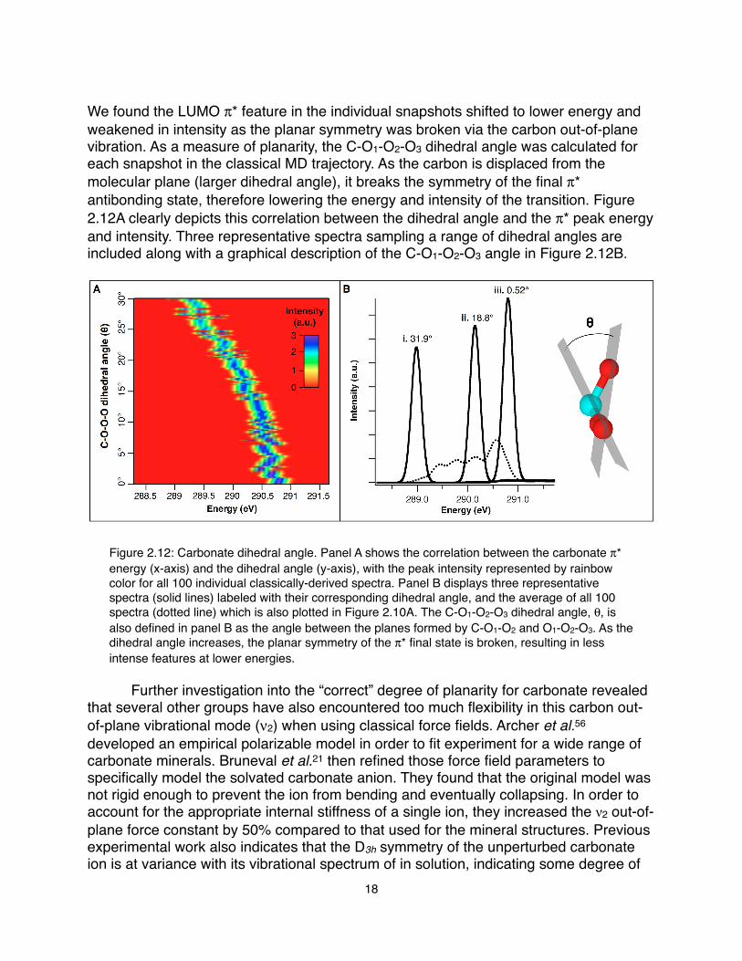
We found the LUMO π* feature in the individual snapshots shifted to lower energy and weakened in intensity as the planar symmetry was broken via the carbon out-of-plane vibration. As a measure of planarity, the C-O1-O2-O3 dihedral angle was calculated for each snapshot in the classical MD trajectory. As the carbon is displaced from the molecular plane (larger dihedral angle), it breaks the symmetry of the final π* antibonding state, therefore lowering the energy and intensity of the transition. Figure 2.12A clearly depicts this correlation between the dihedral angle and the π* peak energy and intensity. Three representative spectra sampling a range of dihedral angles are included along with a graphical description of the C-O1-O2-O3 angle in Figure 2.12B.

Figure 2.12: Carbonate dihedral angle. Panel A shows the correlation between the carbonate π* energy (x-axis) and the dihedral angle (y-axis), with the peak intensity represented by rainbow color for all 100 individual classically-derived spectra. Panel B displays three representative spectra (solid lines) labeled with their corresponding dihedral angle, and the average of all 100 spectra (dotted line) which is also plotted in Figure 2.10A. The C-O1-O2-O3 dihedral angle, θ, is also defined in panel B as the angle between the planes formed by C-O1-O2 and O1-O2-O3. As the dihedral angle increases, the planar symmetry of the π* final state is broken, resulting in less intense features at lower energies.

! Further investigation into the “correct” degree of planarity for carbonate revealed that several other groups have also encountered too much flexibility in this carbon out-of-plane vibrational mode (ν2) when using classical force fields. Archer et al.56 developed an empirical polarizable model in order to fit experiment for a wide range of carbonate minerals. Bruneval et al.21 then refined those force field parameters to specifically model the solvated carbonate anion. They found that the original model was not rigid enough to prevent the ion from bending and eventually collapsing. In order to account for the appropriate internal stiffness of a single ion, they increased the ν2 out-of-plane force constant by 50% compared to that used for the mineral structures. Previous experimental work also indicates that the D3h symmetry of the unperturbed carbonate ion is at variance with its vibrational spectrum of in solution, indicating some degree of

18

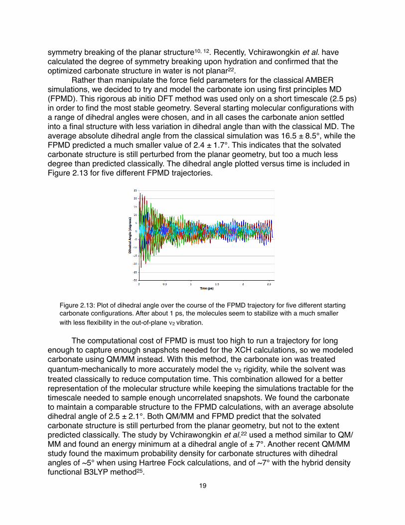
symmetry breaking of the planar structure10, 12. Recently, Vchirawongkin et al. have calculated the degree of symmetry breaking upon hydration and confirmed that the optimized carbonate structure in water is not planar22.! Rather than manipulate the force field parameters for the classical AMBER simulations, we decided to try and model the carbonate ion using first principles MD (FPMD). This rigorous ab initio DFT method was used only on a short timescale (2.5 ps) in order to find the most stable geometry. Several starting molecular configurations with a range of dihedral angles were chosen, and in all cases the carbonate anion settled into a final structure with less variation in dihedral angle than with the classical MD. The average absolute dihedral angle from the classical simulation was 16.5 ± 8.5°, while the FPMD predicted a much smaller value of 2.4 ± 1.7°. This indicates that the solvated carbonate structure is still perturbed from the planar geometry, but too a much less degree than predicted classically. The dihedral angle plotted versus time is included in Figure 2.13 for five different FPMD trajectories.

Figure 2.13: Plot of dihedral angle over the course of the FPMD trajectory for five different starting carbonate configurations. After about 1 ps, the molecules seem to stabilize with a much smaller with less flexibility in the out-of-plane ν2 vibration.

! The computational cost of FPMD is must too high to run a trajectory for long enough to capture enough snapshots needed for the XCH calculations, so we modeled carbonate using QM/MM instead. With this method, the carbonate ion was treated quantum-mechanically to more accurately model the ν2 rigidity, while the solvent was treated classically to reduce computation time. This combination allowed for a better representation of the molecular structure while keeping the simulations tractable for the timescale needed to sample enough uncorrelated snapshots. We found the carbonate to maintain a comparable structure to the FPMD calculations, with an average absolute dihedral angle of 2.5 ± 2.1°. Both QM/MM and FPMD predict that the solvated carbonate structure is still perturbed from the planar geometry, but not to the extent predicted classically. The study by Vchirawongkin et al.22 used a method similar to QM/MM and found an energy minimum at a dihedral angle of ± 7°. Another recent QM/MM study found the maximum probability density for carbonate structures with dihedral angles of ~5° when using Hartree Fock calculations, and of ~7° with the hybrid density functional B3LYP method25.

19

! The NEXAFS spectrum computed from the QM/MM trajectory is in excellent agreement with the experimental spectrum (Figure 2.10A), indicating a much more accurate sampling of the carbonate structure with regards to the ν2 vibrational mode. Furthermore, the bond lengths predicted by QM/MM are also in better agreement with the literature for carbonate, bicarbonate and carbonic acid. The bicarbonate spectra derived from classical MD and QM/MM are compared with experiment in Figure 2.10B. While we did not encounter the same problem with planarity for the bicarbonate π* feature, the agreement with experiment was improved with QM/MM due to the more accurate prediction of bond lengths. The carbon dioxide spectra are the only ones derived from classical MD trajectories, since the predicted bond lengths and structures correspond with literature values.!Spectral Fingerprints and Bond Lengths! It is important to note that the calculated spectra are not simply aligned empirically to the corresponding experimental absorption onset energies, but, rather, relative to a simulated atomic carbon excitation energy. This allows us to accurately predict relative spectral energy alignment, and provides accurate absolute energies for aqueous carbonate species when aligned with an established standard measurement, such as the position of the 2πu* peak in gaseous CO2. Relative alignment of calculated spectra is a pervasive problem both for simulations of isolated clusters when using pseudopotentials (which neglect explicit calculation of core-electronic states) and for accurate simulations of condensed phases using periodic boundary conditions (in which the energy reference is necessarily determined by the mathematical requirement that the potential in each repeated cell must average to zero). To overcome these limitations, we can shift the energy scale of the computed DFT eigenvalues such that relative energies between different systems are meaningful and such that we have alignment with an experimental reference. We have previously documented a scheme for spectral alignment across different molecular configurations within a given system42, but the alignment of different systems relative to a common reference (i.e. the carbon atom excitation) is a new scheme developed for this project.! For a given chemical system X with a molecular configuration i (sampled from a molecular dynamics trajectory), we shift the energy scale used in the absorption cross section, σ (E) , as follows:! E E − εN +1

XCH (i) + ΔEatomicC (i) + Δexpt ,!! ! ! ! ! (1.5)

where εN +1XCH (i) is the (N+1)th eigenvalue of the lowest energy core-excited state of

configuration i, i.e., corresponding to the Kohn-Sham eigenvalue of the first available state that the excited electron could occupy above the existing N valence electrons (the LUMO energy); ΔEatomic

C (i) is the relative excitation energy of X(i) with respect to that of an isolated C atom (we only consider carbon core-level excitations in this work), computed as:! ΔEatomic

C (i) = EtotXCH (i) − EC

XCH (i)⎡⎣ ⎤⎦ − EtotGS (i) − EC

GS (i)⎡⎣ ⎤⎦ ! ! ! (1.6)where these are DFT total energy differences between the total system X and the isolated atom in ground and excited states. Note that the dependence of the atomic

20

energies on snapshot i is not necessarily unique for each snapshot, but appears only through the same choice of periodic boundary conditions (lattice vectors, cell volume, etc.). Finally the alignment with experiment is performed once and only once for a given reference calculation through the constant Δexpt . In our case, only the spectrum of isolated CO2 was aligned to the corresponding gas-phase experiment and all other simulated spectra were aligned relative to that. A similar alignment approach has been documented by Hamann and Muller for electron energy loss near-edge spectra57. This is a key step towards using an efficient first-principles theory to accurately predict x-ray absorption spectra of novel condensed phases. ! Based on this scheme, the relative energy positioning of in the calculated carbonate spectra is in excellent agreement with the experimental results, as shown in detail for the LUMO π* feature in Figure 2.14A. The relative ordering is reproduced correctly, and the position of carbonate matches well. The bicarbonate π* feature is predicted to be 0.08 eV higher than experiment, but since the experimental resolution is 0.1 eV, this difference is reasonable.

Figure 2.14: Experimental and calculated NEXAFS spectra for all three pH regions. The experimental spectra are presented with the corresponding calculated spectra for carbonate (blue), bicarbonate (red), and carbon dioxide gas (green). The calculated spectrum of carbonic acid (dotted black) is included for comparison. The figure is split to show the detailed alignment of the π* features in panel A, and the σ* resonances in panel B. Panel B is plotted on a smaller scale y-axis for better visualization of the higher-energy features. Features within the areas marked 1 and 2 in panel B represent transitions to σ* states localized on the C=O and C-OH bonds, respectively. Calculated spectra represent the average of 100 individual snapshots.

21

! Given that the x-ray excitation is localized on the carbon atom, the NEXAFS spectra are highly sensitive to its immediate surroundings, in particular to the nature of its bonds with oxygen. The C-O bond length will have significant impact on the energies of bonding and antibonding states in a molecule. A shorter bond will result in a stronger bonding interaction and consequently a higher energy antibonding state relative to a longer C-O bond. This correlation between intramolecular bond lengths and the position of K-shell resonances (especially σ* resonances) has been documented previously for a variety of gas phase molecules58. A thorough analysis of the bond lengths in these molecules becomes critical to understanding the subtle differences in the spectra.! There are two types of bonds present in these molecules: C=O (or C-O-) and C-OH. The ordering of the calculated average C=O bond lengths follow the sequence: CO2 (1.166 Å) < H2CO3 (1.224 Å) < HCO3- (1.261 Å) < CO32- (1.285 Å), which correlates with the relative positions of the LUMO π* carbonyl peaks (Figure 2.14A) and the σ* carbonyl peaks (Figure 2.14B, feature 1). Additionally, C-OH bonds are present in bicarbonate (1.356 Å) and carbonic acid (1.339 Å), which introduces a third peak (Figure 2.14B, feature 2) in the σ* range. The C-OH bonds are longer than the C=O bonds overall, so they appear at lower energies. All bond lengths are compiled and compared with literature values in Table 2.1. For further confirmation, the states of each feature were imaged for individual snapshots to verify that they were indeed localized on the C=O or C-OH bonds, with the appropriate π* or σ* character (Figure 2.15).

This workThis work LiteratureLiterature

C=O (Å) C-OH (Å) C=O (Å) C-OH (Å)

CO2 (g)

1.166 ± 0.021 1.162a

CO2 (g)1.165 ± 0.020 1.162a

CO2 (aq)

1.171 ± 0.021 1.167b

CO2 (aq)1.171 ± 0.024 1.167b

H2CO3 (aq)

1.224 ± 0.021 1.342 ± 0.029 1.220b 1.335b

H2CO3 (aq)1.336 ± 0.025 1.335b

HCO3- (aq) (Na+)1.263 ± 0.021 1.356 ± 0.027 1.259b 1.397b

HCO3- (aq) (Na+)1.259 ± 0.022 1.255b

CO32- (aq) (2Na+)

1.293 ± 0.024 1.302b

CO32- (aq) (2Na+) 1.284 ± 0.022 1.302bCO32- (aq) (2Na+)

1.279 ± 0.023 1.302b

a Reference 59.

b Reference 20.

Table 2.1: Average C-O bond lengths. The bond lengths (Å) calculated for this work are the averages of 100 snapshot MD trajectories with an error of one standard deviation. The literature values for CO2 gas are experimental bond lengths, while those for the aqueous species are calculated at the B3LYP level using a polarizable continuum model for the solvent.

22

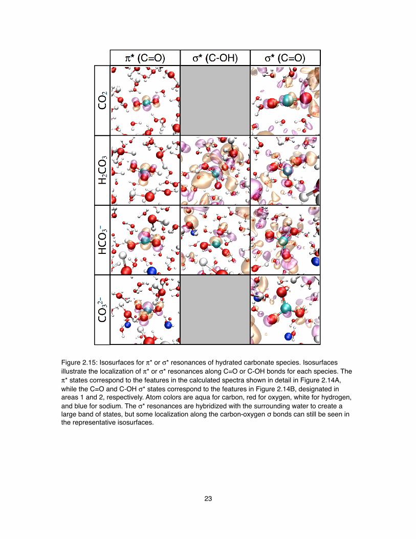
Figure 2.15: Isosurfaces for π* or σ* resonances of hydrated carbonate species. Isosurfaces illustrate the localization of π* or σ* resonances along C=O or C-OH bonds for each species. The π* states correspond to the features in the calculated spectra shown in detail in Figure 2.14A, while the C=O and C-OH σ* states correspond to the features in Figure 2.14B, designated in areas 1 and 2, respectively. Atom colors are aqua for carbon, red for oxygen, white for hydrogen, and blue for sodium. The σ* resonances are hybridized with the surrounding water to create a large band of states, but some localization along the carbon-oxygen σ bonds can still be seen in the representative isosurfaces.

23

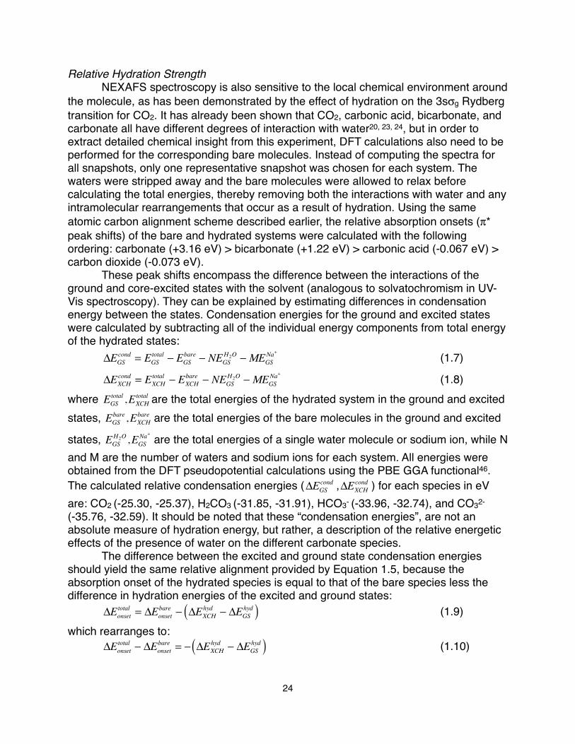
Relative Hydration Strength! NEXAFS spectroscopy is also sensitive to the local chemical environment around the molecule, as has been demonstrated by the effect of hydration on the 3sσg Rydberg transition for CO2. It has already been shown that CO2, carbonic acid, bicarbonate, and carbonate all have different degrees of interaction with water20, 23, 24, but in order to extract detailed chemical insight from this experiment, DFT calculations also need to be performed for the corresponding bare molecules. Instead of computing the spectra for all snapshots, only one representative snapshot was chosen for each system. The waters were stripped away and the bare molecules were allowed to relax before calculating the total energies, thereby removing both the interactions with water and any intramolecular rearrangements that occur as a result of hydration. Using the same atomic carbon alignment scheme described earlier, the relative absorption onsets (π* peak shifts) of the bare and hydrated systems were calculated with the following ordering: carbonate (+3.16 eV) > bicarbonate (+1.22 eV) > carbonic acid (-0.067 eV) > carbon dioxide (-0.073 eV). ! These peak shifts encompass the difference between the interactions of the ground and core-excited states with the solvent (analogous to solvatochromism in UV-Vis spectroscopy). They can be explained by estimating differences in condensation energy between the states. Condensation energies for the ground and excited states were calculated by subtracting all of the individual energy components from total energy of the hydrated states:

ΔEGScond = EGS

total − EGSbare − NEGS

H2O − MEGSNa+ ! ! ! ! ! (1.7)

! ΔEXCHcond = EXCH

total − EXCHbare − NEGS

H2O − MEGSNa+ ! ! ! ! ! (1.8)

where EGStotal ,EXCH

total are the total energies of the hydrated system in the ground and excited states, EGS

bare,EXCHbare are the total energies of the bare molecules in the ground and excited

states, EGSH2O ,EGS

Na+ are the total energies of a single water molecule or sodium ion, while N and M are the number of waters and sodium ions for each system. All energies were obtained from the DFT pseudopotential calculations using the PBE GGA functional46. The calculated relative condensation energies (ΔEGS

cond ,ΔEXCHcond ) for each species in eV

are: CO2 (-25.30, -25.37), H2CO3 (-31.85, -31.91), HCO3- (-33.96, -32.74), and CO32- (-35.76, -32.59). It should be noted that these “condensation energies”, are not an absolute measure of hydration energy, but rather, a description of the relative energetic effects of the presence of water on the different carbonate species. ! The difference between the excited and ground state condensation energies should yield the same relative alignment provided by Equation 1.5, because the absorption onset of the hydrated species is equal to that of the bare species less the difference in hydration energies of the excited and ground states:! ΔEonset

total = ΔEonsetbare − ΔEXCH

hyd − ΔEGShyd( ) ! ! ! ! ! ! (1.9)

which rearranges to:! ΔEonset

total − ΔEonsetbare = − ΔEXCH

hyd − ΔEGShyd( ) !! ! ! ! ! (1.10)

24

If the negative value is incorporated into the hydration energies (the total energy decreases as a result of stabilization by hydration), then we can write:! ΔEonset

total − ΔEonsetbare = ΔEXCH

hyd − ΔEGShyd( ) ! ! ! ! ! ! (1.11)

Equation 1.11 demonstrates the equality between the change in relative absorption onset for the bare and hydrated systems with the difference in ground and excited state condensation energies. This relationship is illustrated in Figure 2.16.

Figure 2.16: Diagram of the relationship between absorption onset energies for bare and hydrated systems with the changes in excited and ground state energies upon hydration. The absolute differences between energy states were chosen arbitrarily for this illustration.

! If both the ground and excited states were stabilized by the solvent to the same degree, then we would expect no peak shift between the bare and hydrated systems. However, we find that the ground and excited states have differing degrees of interaction with the surrounding water. The ground state of carbonate is the most stabilized upon hydration and bicarbonate to a lesser degree. This is expected, given the double and single overall negative charge on these ions, respectively. The corresponding excited states are less stabilized, given that the solvent is in equilibrium with the solute ground state and cannot rearrange on the x-ray absorption timescale to accommodate the excited state before it decays. This difference in stabilization leads to an opening of the gap between ground and excited states, resulting in a blue-shift of the absorption onset. The neutral species, carbonic acid and CO2, both exhibit comparatively weak interactions with water. However, their diffuse and polarizable excited states are more stabilized due to electronic screening by the solvent, leading to a small overall red-shift. ! Furthermore, these energetic arguments are in accord with the number of coordinating water molecules derived from radial distribution functions of the MD trajectories. The relative ordering of ΔEGS

cond values, CO2 > H2CO3 > HCO3- > CO32-, representative of increasing hydration strength through the series, matches with the number of coordinated waters up to 2.5 Å: CO2 (0.56) < H2CO3 (3.17) < HCO3- (4.26) < CO32- (5.55). The radial distribution functions for the carbonyl oxygen to water

25

hydrogens illustrating this trend are shown in Figure 2.17. This trend in hydration strength and number of coordinating waters for each species is in agreement with other theoretical studies20, 23, 24 as well as with experiment for carbonate60. It should be noted, however, that our water coordination numbers are lower overall for bicarbonate and carbonate when compared to the literature, which is due to the inclusion of sodium counterions in our MD simulations.

Figure 2.17: Radial distribution functions for the carbonyl oxygen to water hydrogens for each species. Carbonate is blue, bicarbonate is red, carbonic acid is black, and carbon dioxide is green. Carbonate and bicarbonate simulations include sodium counterions in addition to water.

Ion Effects! We found that both sodium ions were located very close to carbonate (~2.7 Å from the carbon), resulting in a large decrease in the number of waters in the first solvation shell (9.09 to 5.55). Sodium was also localized near bicarbonate (~3 Å from the carbon), but not as strongly associated as with carbonate. The effect of sodium on bicarbonate hydration number was less pronounced (5.41 to 4.26) since only one sodium ion was present and positioned near the same distance as the first hydration shell.! Additionally, MD simulations were run with potassium counterions; the radial distribution functions are plotted in Figure 2.18. The potassium ions are also localized close to carbonate, but slightly farther than sodium (~0.3 Å farther from the carbon), comparable to the difference in ionic radii (Na+=1.16 Å, K+= 1.52 Å). The number of coordinated waters in the potassium case is slightly higher (6.55) than for sodium (5.55), but upon inspection of the radial distribution functions in Figure 2.18, we see that

26

sodium clearly displaces water from carbonate’s first solvation shell, while potassium does not (nearly the same g(r) for carbonate with or without potassium). The relative distances of the water and ions indicate that carbonate forms contact ion pairs (CIP) with sodium, and either solvent shared ion pairs (SIP) or solvent separated ion pairs (2SIP) with potassium. The overall decrease in coordinated waters with potassium is then likely due to the larger size of the ion and it positioning near the first water shell. For bicarbonate, the potassium had a similar effect on the total coordinated waters (4.85) as with sodium (4.26). There are only small changes in g(r) for C-water upon the inclusion of the counterions, which indicates a weaker solute-ion interaction, only a SIP or 2SIP.

Figure 2.18: Radial distribution functions, g(r), for carbonate and bicarbonate. g(r) for the carbon to water (solid lines) and counterions (dashed lines) are included for each species in only water (blue), and in water with sodium cations (black) or potassium cations (green).

! For a closer look at the association between carbonate with water and counterions, spatial distribution functions were calculated, and are shown in Figure 2.19. Sodium and potassium tend to localize in the plane of the carbonate molecule, but not above or below. The ions sit in between the oxygens but not directly at the end of the C=O bonds. These images also illustrate the nature of the ion pairing with carbonate: CIP for sodium, and SIP or 2SIP for potassium.

27

Figure 2.19: Spatial distribution functions for carbonate in water (A), in water with sodium (B,C), and in water with potassium (D,E). (B) and (D) depict both the water and ion distributions, while (C) and (E) show only the ion distributions. Water is depicted in gray with sodium in yellow and potassium in green.

The ions have similar spatial distribution functions for bicarbonate, shown for sodium in Figure 2.20, although they are rarely found near the C-OH end of the molecule. Additionally, we see some water positioned closer to the bicarbonate than sodium, indicating the ion pairing is not CIP but rather SIP or 2SIP, which in in agreement with the radial distribution functions.

Figure 2.20: Spatial distribution functions for bicarbonate in water (A) and in water with sodium (B,C). The spatial distribution functions for water and sodium are shown in (B) while only that for sodium is shown in (C). Water is depicted in gray with sodium in yellow.

28

! To our knowledge, there have been no published theoretical studies of these aqueous carbonate species that specifically compare the effect of sodium versus potassium; most do not include counterions at all. However, there has been research on stronger carbonate-ion interactions, like with calcium (both sodium and potassium are considered as having weak interactions with carbonate since both Na2CO3 and K2CO3 are water soluble). In the MD study by Bruneval et al.21, it was determined that Ca2+ forms heteroion pairs (or bound ion pairs) with carbonate, while potassium does not. This conclusion was based on the fact that no bound state was predicted within the gas-phase equilibrium bonding distance for KCO3- (2.8 Å). A similar study on site-binding in polyacrylates in water determined that calcium ions are strongly coordinated to the carboxylate groups while sodium ions display weaker interactions. The free energy describing sodium coordination has a shallower minima than that of calcium, and also indicates that the preferred interaction is an indirect coordination involving a water molecule between of the COO- group and the sodium ion61. ! While not specifically looking at carbonate ions, another theoretical study has investigated the weak interactions of sodium and potassium with protein surfaces. Through MD simulations and quantum chemical calculations it was found that sodium binds at least twice as strongly as potassium to the charged carboxylic groups on the protein surface, and the study also indicated preferential pairing of the smallest carboxylate anions (formate and acetate) with sodium over potassium62. Radial distribution functions for these protein carboxylate groups had peaks in similar positions to our simulations, with sodium at 2.3 Å and potassium at 2.7 Å. They also calculated that sodium pairing was favored by >2 kcal/mol over potassium for both acetate and formate. The Law of Matching Water Affinities63 has been used to explain this Na+/K+ ion specificity with carbonate. This concept suggests that cations and anions with similar hydration energies tend to form contact ion pairs in water. Sodium matches carbonate and carboxylate groups better than potassium in surface charge density, and therefore is more likely to form contact ion pairs.! Because both sodium and potassium exhibit relatively weak interactions with carbonate and bicarbonate, these are difficult to characterize experimentally. A variety of Raman and potentiometric studies have indicated some degree of ion pairing between sodium and potassium with carbonate12, 18, 19, 64-66, and also weaker outer-sphere ion pairing12, 19 or non-existent interactions66 for bicarbonate. Previous research in our group has investigated the selective binding of alkali cations to acetate and formate with NEXAFS, where relative shifts in the carbonyl π* feature indicated a preferential interaction of sodium over potassium67.! Similarly, we can track the NEXAFS spectral changes in Na2CO3 and K2CO3 to further explore the favored sodium interaction. Only the π* feature can be monitored because potassium exhibits L-edge features from 294-298 eV that interfere with the σ* region. However, we found no discernible shift in the π* feature between sodium and potassium carbonate. In the previous NEXAFS study, sodium acetate was blue-shifted only ~0.05 eV compared to potassium acetate, while no shift was measured between sodium and potassium formate67. The carbon absorption edge may not be the ideal probe of carbonate-cation interactions in this case because it appears that the cations are more directly interacting with the oxygens based on our MD simulations. The

29

oxygen edge was also measured, but at only 1M carbonate concentration it is indistinguishable from the bulk water spectrum.! NEXAFS spectra were also calculated for potassium carbonate, and for carbonate with no counterions present. The average spectrum for each is plotted in Figure 2.21A along with the original sodium carbonate calculated spectrum. The spectra exhibit very little change upon the inclusion of sodium or potassium. A closer look at the π* feature (Figure 2.21B) reveals that the carbonate ion in water π* feature is positioned at a slightly higher energy than with either counterion (~0.05 eV). There is no distinguishable difference in the absorption onset predicted between sodium and potassium carbonate (<0.01 eV), which matches the experimental observation. Again, it appears that the carbon NEXAFS spectra are not sensitive to these weak ion interactions, although the MD simulations show a slight preference for sodium over potassium binding with carbonate.

Figure 2.21: Panel A shows the calculated carbon NEXAFS spectra for carbonate in water (blue), carbonate in water with sodium (red), and carbonate in water with potassium (green). They are plotted on a relative energy scale for comparison. Panel B details the π* feature.

2.5 Conclusions and Future Work

! The distinct spectra measured and calculated for carbonate, bicarbonate, and carbon dioxide gas, combined with the calculated spectra for carbonic acid and dissolved CO2 give us a complete picture of the x-ray absorption properties of this fundamental carbon system.! It was determined that the experimental NEXAFS spectrum of the acidic carbonate solution is dominated by CO2 gas, but we have identified key spectral differences between CO2 gas, dissolved CO2, and carbonic acid in the calculated spectra. The sensitivity of the 3sσg Rydberg state to both CO2 molecular shape (vibronic coupling with the bending mode) and to environment (gaseous versus hydrated) makes

30

it an ideal marker to probe the behavior of CO2 in systems relevant to carbon sequestration, such as in brine aquifers or MOFs. While the present experiment did not actually detect aqueous carbonic acid, the characteristic calculated spectrum provides an important starting point for future NEXAFS studies.! Although incorrect, the unrealistic flexibility of carbonate in our classical model has allowed us to sample a larger range of geometries not accessible in our experiment and therefore has actually revealed the sensitivity of the carbon K-edge NEXAFS spectrum to the carbon out-of-plane motion in carbonate’s nominally trigonal planar geometry. Future experiments to confirm this could include monitoring the change in the π* feature with specific excitation of the ν2 mode, or investigating the carbonate ion in different chemical environments or reactions where coordination contributes to symmetry degradation68.! The calculated spectra for the species observed in these experiments (carbonate, bicarbonate, CO2 gas) agree well in both shape and relative alignment, which demonstrates the predictive capability of our first principles, electronic structure approach for calculating NEXAFS spectra. Although not actually measured here, the relative position of carbonic acid transitions are well-predicted, given the C–O bond length analysis of all hydrated species. Furthermore, the relative condensation energies extracted from the calculated spectra match the trends previously described in the literature.! While the MD simulations predict stronger ion pairing for sodium carbonate compared to potassium carbonate, our experimental NEXAFS spectra of these were indistinguishable and a <0.01 eV difference was calculated for the π* feature energy between the two systems. The carbon K-absorption edge appears to be insensitive to carbonate ion pairing, probably because the cation does not directly interact with the carbon atom.! Future work to further characterize the carbonate system could include probing dissolved CO2 experimentally, which would require trying a different experimental approach, perhaps with a controlled cooling method (CO2 solubility increases at lower temperatures), or using a flow cell to prevent CO2 from escaping the solution. With our current experimental set-up, we are not likely to probe carbonic acid in water due to the long time (~25 seconds) between the solution mixing and measurement. The endstation could be altered so that the syringe pump lines (containing the carbonate and acid solutions) meet right before the jet tip, therefore allowing us to probe the solution immediately after mixing. This may allow for detection of the distinct carbonic acid σ* region to differentiate from CO2 gas.

31

2.6 References

1.! England, A. H. et al., Chem. Phys. Lett. 514, 187 (2011).2.! Vaidhyanathan, R. et al., Science 330, 650 (2010).3.! Pau, G. S. H. et al., Advances in Water Resources 33, 443 (2010).4.! Gebauer, D., Verch, A., Borner, H. G., Colfen, H., Cryst. Growth Des. 9, 2398

(2009).5.! Raiteri, P., Gale, J. D., J. Am. Chem. Soc. 132, 17623 (2010).6.! de Putron, S. J., McCorkle, D. C., Cohen, A. L., Dillon, A. B., Coral Reefs 30, 321

(2011).7.! Loerting, T., Bernard, J., ChemPhysChem 11, 2305 (2010).8.! Langmuir, D., Aqueous Environmental Geochemistry. (Prentice Hall, New

Jersey, 1997).9.! Cameron, F. K., Seidell, A., J. Phys. Chem. 6, 50 (1902).10.! Davis, A. R., Oliver, B. G., J. Solution Chem. 1, 329 (1972).11.! Falk, M., Miller, A. G., Vib. Spectrosc. 4, 105 (1992).12.! Rudolph, W. W., Fischer, D., Irmer, G., Appl. Spectrosc. 60, 130 (2006).13.! Garand, E. et al., J. Am. Chem. Soc. 132, 849 (2010).14.! Sato, H., Matubayasi, N., Nakahara, M., Hirata, F., Chem. Phys. Lett. 323, 257

(2000).15.! Nguyen, M. T. et al., J. Phys. Chem. A 112, 10386 (2008).16.! Wang, X. G., Conway, W., Burns, R., McCann, N., Maeder, M., J. Phys. Chem. A

114, 1734 (2010).17.! Sipos, P., Bolden, L., Hefter, G., May, P. M., Aust. J. Chem. 53, 887 (2000).18.! Perrot, M., Guillaume, F., Rothschild, W. G., J. Phys. Chem. 87, 5193 (1983).19.! Capewell, S. G., Hefter, G., May, P. M., J. Solution Chem. 27, 865 (1998).20.! Rustad, J. R., Nelmes, S. L., Jackson, V. E., Dixon, D. A., J. Phys. Chem. A 112,

542 (2008).21.! Bruneval, F., Donadio, D., Parrinello, M., J. Phys. Chem. B 111, 12219 (2007).22.! Vchirawongkwin, V., Sato, H., Sakaki, S., J. Phys. Chem. B 114, 10513 (2010).23.! Kumar, P. P., Kalinichev, A. G., Kirkpatrick, R. J., J. Phys. Chem. B 113, 794

(2009).24.! Leung, K., Nielsen, I. M. B., Kurtz, I., J. Phys. Chem. B 111, 4453 (2007).25.! Tongraar, A., Yotmanee, P., Payaka, A., Phys. Chem. Chem. Phys. 13, 16851

(2011).26.! Falcke, H., Eberle, S. H., Water Res. 24, 685 (1990).27.! Adamczyk, K., Premont-Schwarz, M., Pines, D., Pines, E., Nibbering, E. T. J.,

Science 326, 1690 (2009).28.! Sham, T. K., Yang, B. X., Kirz, J., Tse, J. S., Phys. Rev. A 40, 652 (1989).29.! Bader, M., Hillert, B., Puschmann, A., Haase, J., Bradshaw, A. M., Europhys.

Lett. 5, 443 (1988).30.! Brandes, J. A., Wirick, S., Jacobsen, C., J. Synchrotron Radiat. 17, 676 (2010).31.! Wilson, K. R. et al., Rev. Sci. Instrum. 75, 725 (2004).32.! Schwartz, C. P. et al., Proc. Natl. Acad. Sci. USA 107, 14008 (2010).33.! Uejio, J. S. et al., J. Phys. Chem. B 114, 4702 (2010).

32

34.! Attwood, D., Soft X-Rays and Extreme Ultraviolet Radiation: Principles and Applications. (Cambridge University Press, 1999).

35.! Stöhr, J., NEXAFS Spectroscopy. (Springer, New York, 1996).36.! Faubel, M., Schlemmer, S., Toennies, J. P., Z. Phys. D: At., Mol. Clusters 10, 269

(1988).37.! Smith, J. D., Cappa, C. D., Drisdell, W. S., Cohen, R. C., Saykally, R. J., J. Am.

Chem. Soc. 128, 12892 (2006).38.! Smith, J. D. et al., J. Phys. Chem. B 110, 20038 (2006).39.! Wilson, K. R. et al., J. Phys. Chem. B 105, 3346 (2001).40.! Duffin, A. M. et al., J. Chem. Phys. 134, 154503 (2011).41.! Duffin, A. M. et al., Phys. Chem. Chem. Phys. 13, 17077 (2011).42.! Schwartz, C. P., Uejio, J. S., Saykally, R. J., Prendergast, D., J. Chem. Phys.

130, 184109 (2009).43.! Schwartz, C. P., Saykally, R. J., Prendergast, D., J. Chem. Phys. 133, 044507

(2010).44.! Case, D. A. et al. (University of California, San Francisco, 2006).45.! Giannozzi, P. et al., J. Phys.: Condens. Matter 21, 395502 (2009).46.! Perdew, J. P., Burke, K., Ernzerhof, M., Phys. Rev. Lett. 77, 3865 (1996).47.! Prendergast, D., Galli, G., Phys. Rev. Lett. 96, 215502 (2006).48.! Shirley, E. L., Phys. Rev. B 54, 16464 (1996).49.! Humphrey, W., Dalke, A., Schulten, K., J. Mol. Graphics 14, 33 (1996).50.! Hitchcock, A. P., Mancini, D. C., J. Electron. Spectrosc. Relat. Phenom. 67, 1

(1994).51.! Eustatiu, I. G. et al., Phys. Rev. A 61, 042505 (2000).52.! Uejio, J. S., Schwartz, C. P., Saykally, R. J., Prendergast, D., Chem. Phys. Lett.

467, 195 (2008).53.! Adachi, J., Kosugi, N., Shigemasa, E., Yagishita, A., J. Phys. Chem. 100, 19783

(1996).54.! Kosugi, N., J. Electron. Spectrosc. Relat. Phenom. 79, 351 (1996).55.! Prince, K. C., Avaldi, L., Coreno, M., Camilloni, R., de Simone, M., J. Phys. B: At.,

Mol. Opt. Phys. 32, 2551 (1999).56.! Archer, T. D. et al., Phys. Chem. Miner. 30, 416 (2003).57.! Hamann, D. R., Muller, D. A., Phys. Rev. Lett. 89, 126404 (2002).58.! Sette, F., Stohr, J., Hitchcock, A. P., Chem. Phys. Lett. 110, 517 (1984).59.! Pauling, L., Nature of the Chemical Bond. (Cornell University Press, New York,

ed. 3, 1960).60.! Kameda, Y., Sasaki, M., Hino, S., Amo, Y., Usuki, T., Physica B-Condensed

Matter 385, 279 (2006).61.! Bulo, R. E. et al., Macromolecules 40, 3437 (2007).62.! Vrbka, L., Vondrasek, J., Jagoda-Cwiklik, B., Vacha, R., Jungwirth, P., Proc. Natl.

Acad. Sci. USA 103, 15440 (2006).63.! Collins, K. D., Biophys. Chem. 119, 271 (2006).64.! Rudolph, W. W., Irmer, G., Konigsberger, E., Dalton Trans., 900 (2008).65.! Capewell, S. G., Buchner, R., Hefter, G., May, P. M., Phys. Chem. Chem. Phys.

1, 1933 (1999).66.! Oliver, B. G., Davis, A. R., Can. J. Chem. 51, 698 (1973).

33

67.! Uejio, J. S. et al., Proc. Natl. Acad. Sci. USA 105, 6809 (2008).68.! Healy, P. C., White, A. H., Spectrochim. Acta, Part A 29, 1191 (1973).

34

Chapter 3 - New Directions in NEXAFS Spectroscopy

3.1 Introduction

! A significant amount of research was conducted to explore various new directions in NEXAFS spectroscopy. In this chapter, I discuss several projects that expand on our existing X-ray experiments by probing previously unmeasured species, by developing a new method for X-ray absorption detection, and by investigating the damage incurred to stationary samples from synchrotron radiation. First, I present our efforts to measure the oxygen K-absorption edge of hydroxyl radicals in water. Second, an alternative detection method exploiting streaming current is discussed. Third, our results probing the radiation damage to several solid biomolecule samples are analyzed, and finally, I examine the possibility of creating unusual nitrogen compounds for eventual NEXAFS measurements.

3.2 Radicals

Introduction! The hydroxyl radical is considered to be the most reactive of the oxy-radicals in aqueous conditions1. •OH is the primary oxidant in the atmosphere2, where it reacts rapidly with volatile organic compounds to render them less hazardous. With UV treatment, organic pollutants are removed from wastewater by reacting with •OH3. In biological systems, the hydroxyl radical is very reactive and has been shown to damage tissues and kill mammalian cells through oxidation and cleavage of proteins and nucleic acids4, 5. It has been specifically linked to the mechanism responsible for cell death in the development of neurodegenerative diseases like Alzheimer’s and Parkinson’s disease6. As a primary product of water radiolysis, hydroxyl radicals play an important role in aqueous reactions in the cooling water of nuclear reactors, as well as in ground water in nuclear waste repositories. Although •OH has ubiquitous importance, the hydration properties of this transient molecule are still not well understood.! In water, hydroxyl radicals react with most solutes at diffusion-controlled rates. Its lifetime ranges from nanoseconds to microseconds depending on the type and concentration of solutes present in the solution5, 7-10. Based on recombination kinetics, it has been suggested that geminate hydroxyl radicals are weakly interacting in water, which implies strong caging by the solvent molecules11. There have been several theoretical studies aimed at understanding the hydration structure of •OH and its behavior in water8, 12-14, yet the inherent difficulty in measuring the transient species has limited the corresponding experimental research. Characterizing the behavior of •OH in aqueous conditions, specifically solvation structure, energetics, and dynamics, is crucial to the fundamental understanding of how •OH affects various environmental, biological, and nuclear energy systems15. The objective for the work presented in this section is to investigate the hydration structure of the hydroxyl radical using NEXAFS spectroscopy.! Hydroxyl radicals have been studied with core-level spectroscopies in the gas phase16, 17. The Χ2Πi ground state of •OH (1σ22σ23σ21π3) is excited to the 2Σ+ state

35

(1σ12σ23σ21π4) on the oxygen K-absorption edge. An oxygen 1s electron is promoted up to the 1π orbital, which is nonbonding in character and consists of an oxygen 2pπ atomic orbital. High-resolution photoabsorption experiments have measured this transition at 525.85 eV 17, and it has been theoretically calculated at 526.04 eV with ab initio methods18. •OH has been detected with NEXAFS in crystalline ice films after extended exposure to synchrotron radiation19. The peak at 526 eV is attributed to •OH, which is distinctly separated from peaks for other water radiolysis products (•O, HO2, O2, H2O2) and from bulk water (which begins ~ 534 eV). While •OH has not been probed with NEXAFS in liquid water, we can refer to this water ice experiment as a starting point and look for the •OH transition near 526 eV. Because the liquid sample in our experiments is not stationary, we cannot easily take advantage of using the synchrotron X-rays to produce the radicals as was done in the ice study.! Hydroxyl radicals can be produced by several different methods. They are a major product of water radiolysis and photolysis, or they can be produced by chemical pathways1. When water is exposed to high-energy ionizing radiation, •OH is formed among several other primary radicals and molecular products. The process of water radiolysis is discussed in further detail in Chapter 4. •OH can also be produced by photolysis of liquid water in the vacuum UV (VUV) spectral domain, or by photolysis of hydrogen peroxide at UV wavelengths. Chemical production of •OH by Fenton-type reactions has been used for over a century20. In the classic Fenton reaction, hydrogen peroxide oxidizes a ferrous ion to produce the transient •OH, which is then consumed by a second ferrous ion. Fenton’s reagents have been well-characterized for •OH production as well as further reactions of •OH with other additives present21. ! For this experiment, we chose to exploit the VUV photolysis of liquid water to produce hydroxyl radicals, given the availability of a laser in the appropriate wavelength range: 157 nm. VUV photolysis of water has been studied extensively due to its applications in the fabrication of microelectronics and the oxidative treatment of waste water. There are two distinct VUV-induced reactions that have been characterized for photolysis with wavelengths shorter than 190 nm. The dissociation pathway leads to homolysis of the water, resulting in a hydrogen atom and the hydroxyl radical. Ionization of water is the other possibility, which produces an electron and proton in addition to •OH22. These reactions are diagrammed in Figure 3.1. The •OH quantum yield (Φ) , or number of •OH produced per photon absorbed into the water, is wavelength-dependent for homolysis: Φ = 0.33 at 184.9 nm; Φ = 0.42 at 172 nm; Φ = 0.7 at 147.9 nm; and Φ ~ 1 at 123.6 nm 23.!

Figure 3.1: Vacuum UV photolysis of liquid water. When irradiated with incident photons of greater than 6.5 eV, liquid water will photolyze via two different pathways: ionization or dissociation. Hydroxyl radicals are formed in both cases, and the yield is wavelength dependent.

36

! The kinetics of the VUV photolysis of liquid water have been well-characterized with transient absorption spectroscopy of the hydroxyl radicals and solvated electrons produced by two-photon excitation24-26. From these experiments, it was determined that the decay mechanism is also wavelength-dependent. The dissociation decay channel is the primary mechanism at 8.3 eV, ionization is the dominant process at 12.4 eV, and at 9.3 eV the two decay pathways occur with equal probability24.! The 157 nm photons for our experiment are 7.9 eV, which falls in the domain of the dissociation channel. This wavelength also achieves a fairly high quantum yield, Φ = 0.6, which was calculated by extrapolation from the values reported by Getoff and Schenck23. To our knowledge, there has not been any characterization of the production of hydroxyl radicals specifically by the 157 nm photolysis of liquid water, but water ice has been studied at this wavelength. Photodissociation dynamics have been monitored after 157 nm irradiation of solid amorphous water by tracking hydrogen atom formation with time-of-flight mass spectrometry27, and by measuring •OH desorption experimentally with REMPI28 and theoretically with MD simulations29. Because there is no benchmark for liquid water photolysis at 157 nm (one-photon excitation), we must first quantify our production of •OH before attempting the NEXAFS experiments.! Instead of directly probing the hydroxyl radical, which would require time-dependent UV absorption spectroscopy on the nanosecond timescale, the reaction with coumarin was used to quantify the yield of radicals produced. Coumarin (C9H6O2, shown in Figure 3.2) has long been used as a chemical dosimeter in radiolysis experiments because of its fast reaction with •OH and the formation of a stable fluorescent product. Coumarin is an excellent scavenger of •OH, reacting with a rate constant of 2 x 109 (M-1 s-1)30. Figure 3.2 shows this reaction, which forms several hydroxylated products through a complicated mechanism. Only one of these products, 7-hydroxycoumarin (7OHC), is fluorescent, and it accounts for roughly one third of the total products31.

Figure 3.2: Coumarin reaction with hydroxyl radicals to form 7-hydroxycoumarin (7OHC). Hydroxylated products on the #3-8 carbons are all formed, with 5OHC being the major product. 7OHC is the only fluorescent product and accounts for ~1/3 of the total products31.

! 7OHC is a stable product that fluoresces in the visible region, easily accessible by any commercial fluorimeter. When excited at 332 nm, it fluoresces with a maximum near 455-460 nm30-32. Additionally, low concentrations of 7OHC can be detected (~10-8 M), which makes it a very useful probe for the small amount of •OH produced from radiolysis or VUV photolysis of liquid water. Quantification of •OH will take place in two parts. First, aqueous coumarin solutions will be irradiated with 157 nm photons; and

37

second, the fluorescence of those solutions will be analyzed to determine the amount of 7OHC, and therefore the concentration of •OH produced.! I will first address the quantification of •OH produced by 157 nm photolysis of liquid water (via the coumarin reaction and 7OHC fluorescence), and then I will describe the initial NEXAFS experiments on the oxygen K-edge for the irradiated liquid microjets. Each section will contain information on the experimental details and the results.

Hydroxyl Radical Production! The VUV photolysis of liquid water was performed using a 157 nm F2 excimer laser (Coherent Xantos XS 500). Lasing is initiated by an electrical discharge in the gas media, which is supplied from an integrated gas cylinder containing 0.2% F2 (in helium). An excimer laser (short for “excited dimer”) typically operates with inert noble gas dimers or complexes with halogens. The excited bound state of the excimer (induced by an electrical discharge) relaxes to a repulsive ground state wherein the two atoms dissociate, providing the population inversion necessary for lasing33. The primary wavelength for an F2 excimer is 157 nm, but atomic fluorine also emits radiation in in the 624 - 755 nm range34, 35, which accounts for < 10% of the total pulse energy. The Coherent Xantos XS laser is pulsed at a repetition rate variable up to 500 Hz, with 5 ns pulses of up to 25 mJ energy. VUV photons are strongly absorbed in air, specifically by O236, and therefore a vacuum environment or nitrogen gas purge is required to propagate the 157 nm beam. Any effect of the atomic fluorine lines on the samples can be tested by repeating all of the VUV irradiations in air, which will absorb the 157 nm photons but allow the red radiation to reach the sample.! Coumarin (Sigma Aldrich, Co.) and 7OHC (Supleco, 99.5% purity) were obtained commercially in the solid form. A 10-5 M aqueous coumarin solution was prepared to undergo irradiation by the excimer laser. 7OHC standard solutions were prepared in 10-5 M aqueous coumarin to create a fluorescence calibration curve, at concentrations of 5 x 10-9, 1 x 10-8, 5 x 10-8, 1 x 10-7, 3 x 10-7, and 5 x 10-7 M 7OHC.! A diagram of the irradiation experiments is shown in Figure 3.3. The pulsed 157 nm beam from the F2 excimer laser enters the nitrogen gas purge box, and is directed downward with a vacuum UV aluminum mirror (CVI) into an open 20 mL glass scintillation vial containing 200 µL of the 10-5 M aqueous coumarin solution. Allowing the photons to directly hit the solution avoids the problem of transmission loss through a sample container. Alignment of the laser beam was verified by placing a paper card over the vial, which was removed prior to the sample irradiation. Samples were irradiated under a variety of conditions. The effect of the atomic fluorine lines from the laser was tested by irradiating each sample under the nitrogen gas purge and in air, where the 157 nm photons will be absorbed before reaching the sample. The irradiations were performed both with and without a CaF2 rectangular cylinderical lens (CVI). The energy per pulse of the laser was varied from 10 mJ up to 25 mJ, and the samples were irradiated with single shots as well as multiple shots. The extended irradiations were tested by varying the repetition rate (up to 500 Hz) and total irradiation time.

38

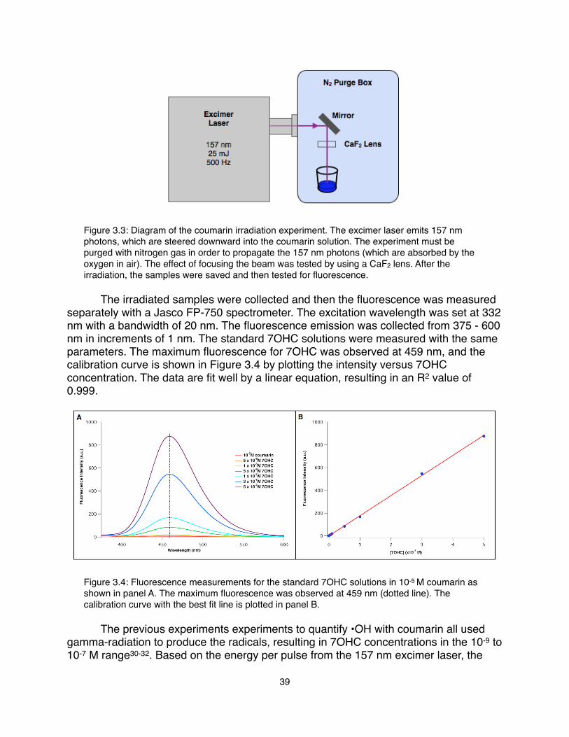
Figure 3.3: Diagram of the coumarin irradiation experiment. The excimer laser emits 157 nm photons, which are steered downward into the coumarin solution. The experiment must be purged with nitrogen gas in order to propagate the 157 nm photons (which are absorbed by the oxygen in air). The effect of focusing the beam was tested by using a CaF2 lens. After the irradiation, the samples were saved and then tested for fluorescence.

! The irradiated samples were collected and then the fluorescence was measured separately with a Jasco FP-750 spectrometer. The excitation wavelength was set at 332 nm with a bandwidth of 20 nm. The fluorescence emission was collected from 375 - 600 nm in increments of 1 nm. The standard 7OHC solutions were measured with the same parameters. The maximum fluorescence for 7OHC was observed at 459 nm, and the calibration curve is shown in Figure 3.4 by plotting the intensity versus 7OHC concentration. The data are fit well by a linear equation, resulting in an R2 value of 0.999.

Figure 3.4: Fluorescence measurements for the standard 7OHC solutions in 10-5 M coumarin as shown in panel A. The maximum fluorescence was observed at 459 nm (dotted line). The calibration curve with the best fit line is plotted in panel B.

! The previous experiments experiments to quantify •OH with coumarin all used gamma-radiation to produce the radicals, resulting in 7OHC concentrations in the 10-9 to 10-7 M range30-32. Based on the energy per pulse from the 157 nm excimer laser, the

39

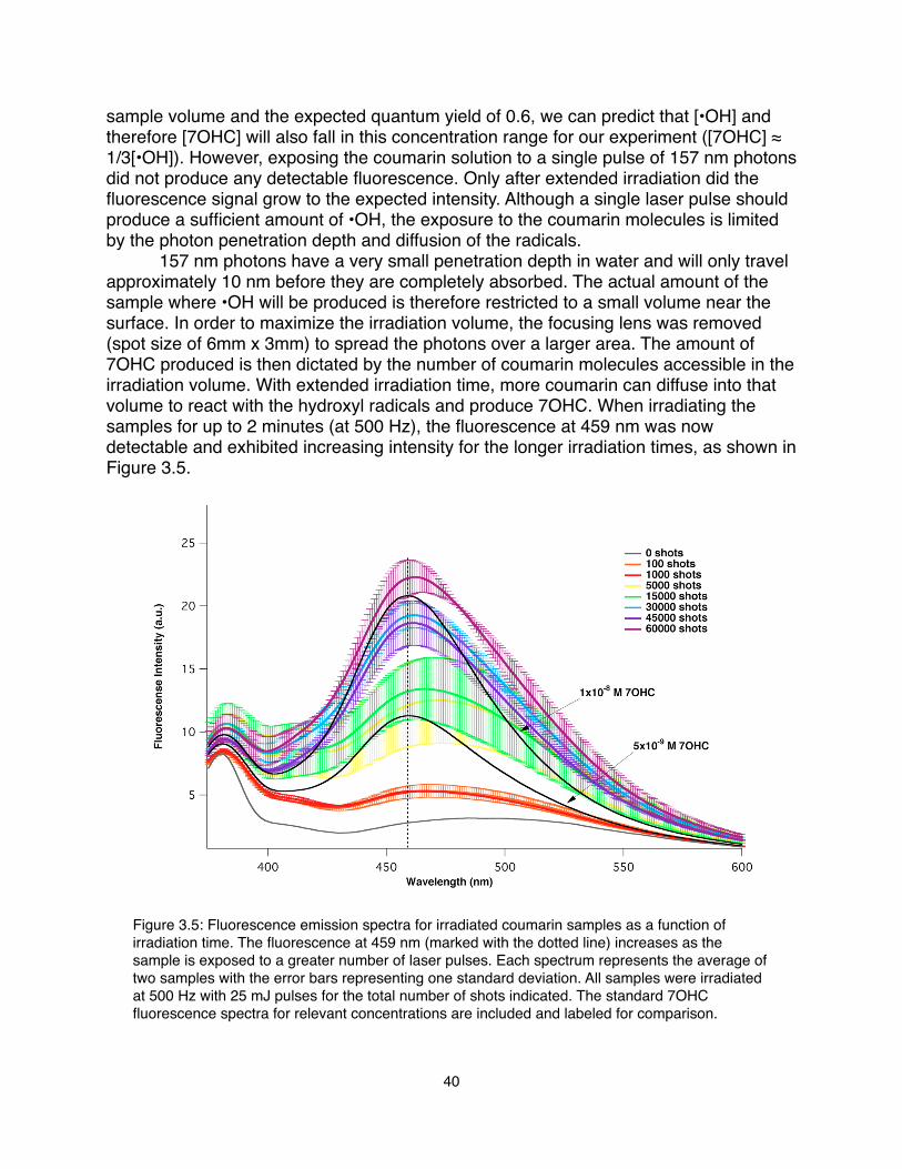
sample volume and the expected quantum yield of 0.6, we can predict that [•OH] and therefore [7OHC] will also fall in this concentration range for our experiment ([7OHC] ≈ 1/3[•OH]). However, exposing the coumarin solution to a single pulse of 157 nm photons did not produce any detectable fluorescence. Only after extended irradiation did the fluorescence signal grow to the expected intensity. Although a single laser pulse should produce a sufficient amount of •OH, the exposure to the coumarin molecules is limited by the photon penetration depth and diffusion of the radicals. ! 157 nm photons have a very small penetration depth in water and will only travel approximately 10 nm before they are completely absorbed. The actual amount of the sample where •OH will be produced is therefore restricted to a small volume near the surface. In order to maximize the irradiation volume, the focusing lens was removed (spot size of 6mm x 3mm) to spread the photons over a larger area. The amount of 7OHC produced is then dictated by the number of coumarin molecules accessible in the irradiation volume. With extended irradiation time, more coumarin can diffuse into that volume to react with the hydroxyl radicals and produce 7OHC. When irradiating the samples for up to 2 minutes (at 500 Hz), the fluorescence at 459 nm was now detectable and exhibited increasing intensity for the longer irradiation times, as shown in Figure 3.5.

Figure 3.5: Fluorescence emission spectra for irradiated coumarin samples as a function of irradiation time. The fluorescence at 459 nm (marked with the dotted line) increases as the sample is exposed to a greater number of laser pulses. Each spectrum represents the average of two samples with the error bars representing one standard deviation. All samples were irradiated at 500 Hz with 25 mJ pulses for the total number of shots indicated. The standard 7OHC fluorescence spectra for relevant concentrations are included and labeled for comparison.

40

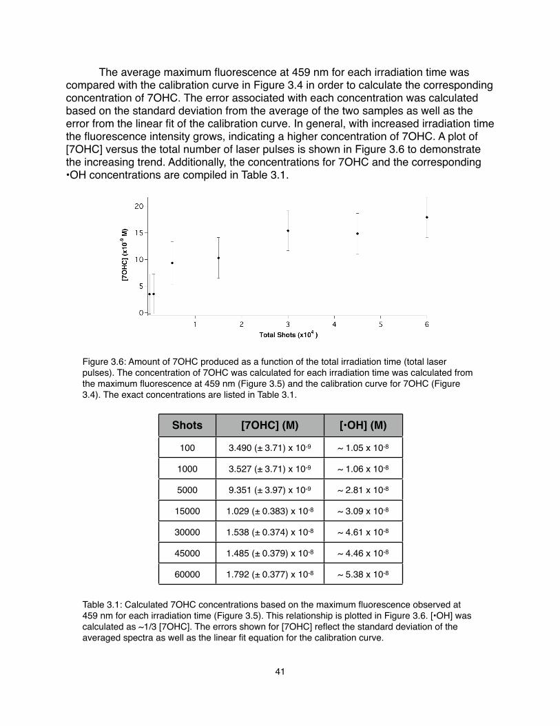
! The average maximum fluorescence at 459 nm for each irradiation time was compared with the calibration curve in Figure 3.4 in order to calculate the corresponding concentration of 7OHC. The error associated with each concentration was calculated based on the standard deviation from the average of the two samples as well as the error from the linear fit of the calibration curve. In general, with increased irradiation time the fluorescence intensity grows, indicating a higher concentration of 7OHC. A plot of [7OHC] versus the total number of laser pulses is shown in Figure 3.6 to demonstrate the increasing trend. Additionally, the concentrations for 7OHC and the corresponding •OH concentrations are compiled in Table 3.1.

Figure 3.6: Amount of 7OHC produced as a function of the total irradiation time (total laser pulses). The concentration of 7OHC was calculated for each irradiation time was calculated from the maximum fluorescence at 459 nm (Figure 3.5) and the calibration curve for 7OHC (Figure 3.4). The exact concentrations are listed in Table 3.1.

Shots [7OHC] (M) [•OH] (M)

100 3.490 (± 3.71) x 10-9 ~ 1.05 x 10-8

1000 3.527 (± 3.71) x 10-9 ~ 1.06 x 10-8

5000 9.351 (± 3.97) x 10-9 ~ 2.81 x 10-8

15000 1.029 (± 0.383) x 10-8 ~ 3.09 x 10-8

30000 1.538 (± 0.374) x 10-8 ~ 4.61 x 10-8

45000 1.485 (± 0.379) x 10-8 ~ 4.46 x 10-8

60000 1.792 (± 0.377) x 10-8 ~ 5.38 x 10-8

Table 3.1: Calculated 7OHC concentrations based on the maximum fluorescence observed at 459 nm for each irradiation time (Figure 3.5). This relationship is plotted in Figure 3.6. [•OH] was calculated as ~1/3 [7OHC]. The errors shown for [7OHC] reflect the standard deviation of the averaged spectra as well as the linear fit equation for the calibration curve.

41

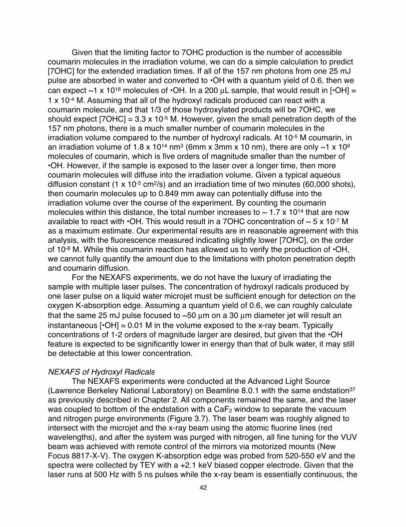
! Given that the limiting factor to 7OHC production is the number of accessible coumarin molecules in the irradiation volume, we can do a simple calculation to predict [7OHC] for the extended irradiation times. If all of the 157 nm photons from one 25 mJ pulse are absorbed in water and converted to •OH with a quantum yield of 0.6, then we can expect ~1 x 1016 molecules of •OH. In a 200 µL sample, that would result in [•OH] = 1 x 10-4 M. Assuming that all of the hydroxyl radicals produced can react with a coumarin molecule, and that 1/3 of those hydroxylated products will be 7OHC, we should expect [7OHC] = 3.3 x 10-5 M. However, given the small penetration depth of the 157 nm photons, there is a much smaller number of coumarin molecules in the irradiation volume compared to the number of hydroxyl radicals. At 10-5 M coumarin, in an irradiation volume of 1.8 x 1014 nm3 (6mm x 3mm x 10 nm), there are only ~1 x 109 molecules of coumarin, which is five orders of magnitude smaller than the number of •OH. However, if the sample is exposed to the laser over a longer time, then more coumarin molecules will diffuse into the irradiation volume. Given a typical aqueous diffusion constant (1 x 10-5 cm2/s) and an irradiation time of two minutes (60,000 shots), then coumarin molecules up to 0.849 mm away can potentially diffuse into the irradiation volume over the course of the experiment. By counting the coumarin molecules within this distance, the total number increases to ~ 1.7 x 1014 that are now available to react with •OH. This would result in a 7OHC concentration of ~ 5 x 10-7 M as a maximum estimate. Our experimental results are in reasonable agreement with this analysis, with the fluorescence measured indicating slightly lower [7OHC], on the order of 10-8 M. While this coumarin reaction has allowed us to verify the production of •OH, we cannot fully quantify the amount due to the limitations with photon penetration depth and coumarin diffusion.! For the NEXAFS experiments, we do not have the luxury of irradiating the sample with multiple laser pulses. The concentration of hydroxyl radicals produced by one laser pulse on a liquid water microjet must be sufficient enough for detection on the oxygen K-absorption edge. Assuming a quantum yield of 0.6, we can roughly calculate that the same 25 mJ pulse focused to ~50 µm on a 30 µm diameter jet will result an instantaneous [•OH] ≈ 0.01 M in the volume exposed to the x-ray beam. Typically concentrations of 1-2 orders of magnitude larger are desired, but given that the •OH feature is expected to be significantly lower in energy than that of bulk water, it may still be detectable at this lower concentration.

NEXAFS of Hydroxyl Radicals! The NEXAFS experiments were conducted at the Advanced Light Source (Lawrence Berkeley National Laboratory) on Beamline 8.0.1 with the same endstation37 as previously described in Chapter 2. All components remained the same, and the laser was coupled to bottom of the endstation with a CaF2 window to separate the vacuum and nitrogen purge environments (Figure 3.7). The laser beam was roughly aligned to intersect with the microjet and the x-ray beam using the atomic fluorine lines (red wavelengths), and after the system was purged with nitrogen, all fine tuning for the VUV beam was achieved with remote control of the mirrors via motorized mounts (New Focus 8817-X-V). The oxygen K-absorption edge was probed from 520-550 eV and the spectra were collected by TEY with a +2.1 keV biased copper electrode. Given that the laser runs at 500 Hz with 5 ns pulses while the x-ray beam is essentially continuous, the

42

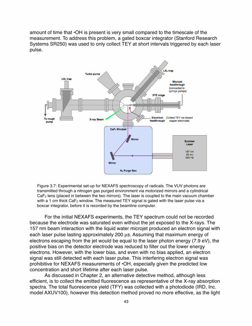
amount of time that •OH is present is very small compared to the timescale of the measurement. To address this problem, a gated boxcar integrator (Stanford Research Systems SR250) was used to only collect TEY at short intervals triggered by each laser pulse.

Figure 3.7: Experimental set-up for NEXAFS spectroscopy of radicals. The VUV photons are transmitted through a nitrogen gas purged environment via motorized mirrors and a cylindrical CaF2 lens (placed in between the two mirrors). The laser is coupled to the main vacuum chamber with a 1 cm thick CaF2 window. The measured TEY signal is gated with the laser pulse via a boxcar integrator, before it is recorded by the beamline computer.

! For the initial NEXAFS experiments, the TEY spectrum could not be recorded because the electrode was saturated even without the jet exposed to the X-rays. The 157 nm beam interaction with the liquid water microjet produced an electron signal with each laser pulse lasting approximately 200 µs. Assuming that maximum energy of electrons escaping from the jet would be equal to the laser photon energy (7.9 eV), the positive bias on the detector electrode was reduced to filter out the lower energy electrons. However, with the lower bias, and even with no bias applied, an electron signal was still detected with each laser pulse. This interfering electron signal was prohibitive for NEXAFS measurements of •OH, especially given the predicted low concentration and short lifetime after each laser pulse. ! As discussed in Chapter 2, an alternative detective method, although less efficient, is to collect the emitted fluorescence as representative of the X-ray absorption spectra. The total fluorescence yield (TFY) was collected with a photodiode (IRD, Inc. model AXUV100), however this detection method proved no more effective, as the light

43

from the laser also saturated the photodiode prior to any NEXAFS measurements. To filter out the light from the laser, a thin film of aluminum (150 nm) was applied to the photodiode (IRD, Inc. model AXUV100Al) in order to block the 157 nm photons while allowing the fluorescent X-ray photons to reach the detector. Nominally, the maximum transmittance was 5 x 10-8 in the UV-Vis spectral region (for both the 157 nm photons and the red atomic fluorine lines), and ~70% transmission in the oxygen K-edge region should be achievable with this thickness of aluminum. Even with this aluminum filter, some signal was still detected from the laser pulse. With the already less efficient TFY (compared to TEY), the spectra collected for bulk water was too noisy, implying that this method will definitely not be appropriate for detecting the low concentration, short-lived hydroxyl radical.! Further NEXAFS experiments will first require a better characterization of the processes involved in the VUV photolysis of a liquid water microjet by the 157 nm excimer laser. Understanding how the electrons are produced will be essential in order to use TEY as a viable detection method for hydroxyl radicals. Although the dominant decay pathway for water excited at 157 nm is homolysis instead of ionization, it has been shown that, even at this energy, solvated electrons can be produced. Crowell and Bartels38 found that at above 6 eV, excess energy in the homolysis reaction goes into the hydrogen atom, which can then react with a neighboring water molecule to produce hydronium and a solvated electron. At 4 eV, they found electrons produced in the two photon absorption of liquid water have an escape probability of 0.44. Therefore, even though the initial photodissociation of water at 157 nm should not produce a significant amount of electrons, there are ensuing reactions that will produce low-energy solvated electrons. This production of electrons may be responsible for the signal interfering with our NEXAFS measurements. It will therefore be essential to better characterize the electrons produced by the 157 nm excitation of a liquid water microjet. Energy analysis of the ejected electrons may provide particularly useful information, especially in learning how to block those electrons during the NEXAFS experiments.

Conclusions and Future Work! The characterization of hydroxyl radicals in aqueous conditions is critical to understanding their behavior in various biological, environmental, and nuclear energy systems. We were able to verify the production of hydroxyl radicals in water by VUV photolysis at 157 nm by the reaction with coumarin to produce the stable, fluorescent product 7-hydroxycoumarin. However, production of 7OHC was limited to the amount of coumarin available to react in the limited irradiation volume, due to the short penetration depth of the 157 nm photons in water.! NEXAFS experiments to detect •OH in water were not successful due to a significant electron signal appearing with each excimer laser pulse, which interfered with the TEY detection of the oxygen K-absorption edge. Attempts to detect TFY were also unsuccessful because of saturation by the laser light, even with filters placed over the photodiode. Further characterization of the electrons created by the VUV photolysis of liquid water at 157 nm will be required before TEY can be used to detect the NEXAFS spectra. One possibility is to perform an energy analysis of the ejected electrons (by Auger spectroscopy) and then find an appropriate way to filter out those electrons for the NEXAFS experiments. Alternatively, another detection method for X-ray absorption,

44

such as measuring the current in the jet instead of TEY may be a better option. This will be discussed in the next section.! Given the short lifetime of the hydroxyl radical and the difficulty of detecting its low concentration relative to bulk water on the oxygen K-absorption edge, a different radical can be chosen as an easier starting point for NEXAFS characterization of open-shell systems. For example, the carbonate radical, with a lifetime in the microsecond range, could be detected on the carbon K-absorption edge. The carbonate radicals could be produced by the same method: VUV photolysis of an aqueous carbonate solution would produce •OH that, in turn, reacts quickly with the carbonate anions to produce carbonate radicals. However, exploring other radicals with NEXAFS spectroscopy will not be feasible until the electron production from water VUV photolysis is better understood.

3.3 Streaming Current Detection

Introduction! The streaming current produced from a pressurized liquid water microjet has been well-characterized previously in the Saykally research group. Andrew Duffin found that hydroxide ions are selectively adsorbed to a metal jet nozzle while the corresponding protons were swept away, resulting in a positively charged water jet39, 40. Monitoring the jet streaming current, and any changes in that current, upon excitation on the oxygen K-absorption edge could prove to be useful in further characterizing the streaming current, as well as developing a new detection method for our NEXAFS measurements. This section outlines some initial tests with streaming current detection of oxygen 1s excitations in liquid water microjets.

Experimental Methods! The same NEXAFS experimental set-up37 was used as previously described for carbonate project in Chapter 2. For this preliminary work, we only measured the NEXAFS spectrum of liquid water, therefore the incident x-ray energy spanned from 520 through 550 eV to excite the oxygen K-absorption edge. 18 MΩ water was loaded into the dual syringe pumps (Teledyne-Isco) and flowed through a 30 µm fused silica capillary to create the liquid microjet in the vacuum chamber. It was then intersected at 90° by the x-ray beam. The biased copper electrode used for TEY detection remained in place, but a piece of foil was added downstream of the microjet to detect the jet current. It was placed in the path of the microjet, directly in front of the liquid nitrogen cold trap, as diagrammed in Figure 3.8.

45

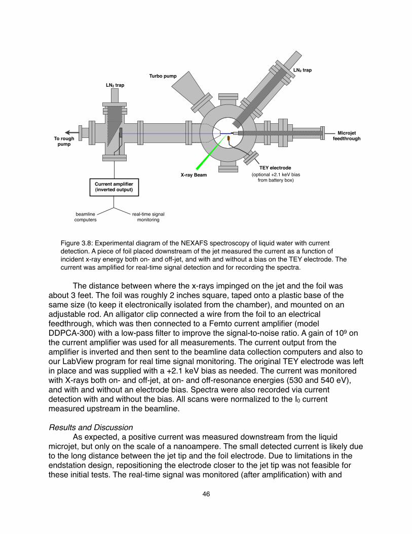
X-ray BeamTEY electrode

LN2 trap

LN2 trapTurbo pump

Microjet feedthroughTo rough

pump

(optional +2.1 keV bias from battery box)

beamline computers

Current amplifier (inverted output)

real-time signal monitoring

Figure 3.8: Experimental diagram of the NEXAFS spectroscopy of liquid water with current detection. A piece of foil placed downstream of the jet measured the current as a function of incident x-ray energy both on- and off-jet, and with and without a bias on the TEY electrode. The current was amplified for real-time signal detection and for recording the spectra.

! The distance between where the x-rays impinged on the jet and the foil was about 3 feet. The foil was roughly 2 inches square, taped onto a plastic base of the same size (to keep it electronically isolated from the chamber), and mounted on an adjustable rod. An alligator clip connected a wire from the foil to an electrical feedthrough, which was then connected to a Femto current amplifier (model DDPCA-300) with a low-pass filter to improve the signal-to-noise ratio. A gain of 109 on the current amplifier was used for all measurements. The current output from the amplifier is inverted and then sent to the beamline data collection computers and also to our LabView program for real time signal monitoring. The original TEY electrode was left in place and was supplied with a +2.1 keV bias as needed. The current was monitored with X-rays both on- and off-jet, at on- and off-resonance energies (530 and 540 eV), and with and without an electrode bias. Spectra were also recorded via current detection with and without the bias. All scans were normalized to the I0 current measured upstream in the beamline.

Results and Discussion! As expected, a positive current was measured downstream from the liquid microjet, but only on the scale of a nanoampere. The small detected current is likely due to the long distance between the jet tip and the foil electrode. Due to limitations in the endstation design, repositioning the electrode closer to the jet tip was not feasible for these initial tests. The real-time signal was monitored (after amplification) with and

46

without irradiating by the X-rays to look for changes in the streaming current. Both on- and off-resonance energies were tested. Upon opening the shutter to 530 eV X-rays (off-resonance), the current did not change. This was the case for both with and without applying a +2.1 kV bias to the TEY electrode. When exposing the jet to resonant energy X-rays (540 eV), the measured current increased by 50% and 10% with and without the TEY electrode bias, respectively. These observations are summarized in Table 3.2 for easy reference. For the off-jet scans, there was zero change in current upon opening and closing the X-ray shutter in all cases (on and off resonance energy, with and without TEY electrode bias).

+ 2.1 keV bias NO bias

530 eV NO change NO change

540 eV increase by ~50% increase by ~10%

Table 3.2: Changes in streaming current observed downstream of the liquid microjet for on (540 eV) and off (530 eV) resonance energies. The current was also monitored as a function of applied bias to the TEY electrode. These observations are all for on-jet positioning of the X-rays. All corresponding off-jet measurements recorded no change in current.

! Exposing the liquid water microjet to energies over the oxygen K-absorption edge will eject oxygen 1s electrons from the water molecules and create the corresponding positive ions. Although more charged species are thenpresent compared to the unexcited microjet, it would be expected that the streaming current will not change significantly because the electrons and ions will be created in equal amounts. However, if a strong positive bias is applied to the existing TEY electrode, that will draw out the electrons from the core excitations and leave the remaining positive ions to flow with the jet and reach the current-detecting electrode. This can explain our observation of a much greater change in streaming current at 540 eV with the +2.1 kV bias applied.! Oxygen K-absorption edge spectra were recorded for water and compared with TEY results to determine if this streaming current detection could be a viable method for collecting NEXAFS spectra. On- and off-jet scans were measured with the same parameters as the TEY spectra, both with and without the applied positive bias. Figure 3.9 summarizes these results. The original TEY detection method for water (Figure 3.9A) produces both on- and off-jet spectra with good signal-to-noise and distinct spectral features. Current detection with the TEY bias still applied resulted in a similar on-jet spectra (Figure 3.9B), although noisier, but the off-jet spectra did not match those for water vapor from TEY. Finally the spectra collected from current detection without the applied bias (Figure 3.9C) are very noisy. The on-jet scans suggest the general shape of the bulk water spectrum, and the off-jet does not record any significant signal. While the amplitude of the on-jet spectrum is small, it is reproducibly larger than the off-jet.

47

Figure 3.9: Comparison of on-jet (red) and off-jet (blue) NEXAFS spectra for TEY and current detection. Panel A shows the bulk water spectrum as measured by the traditional TEY method. The spectra collected from streaming current measurements downstream of the jet tip are shown for when a +2.1 keV bias is applied to the TEY electrode (panel B), and when no bias is applied (panel C).

48

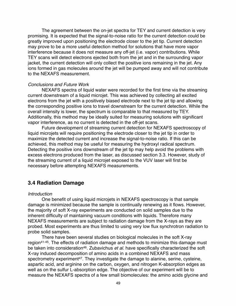
! The agreement between the on-jet spectra for TEY and current detection is very promising. It is expected that the signal-to-noise ratio for the current detection could be greatly improved upon positioning the electrode closer to the jet tip. Current detection may prove to be a more useful detection method for solutions that have more vapor interference because it does not measure any off-jet (i.e. vapor) contributions. While TEY scans will detect electrons ejected both from the jet and in the surrounding vapor jacket, the current detection will only collect the positive ions remaining in the jet. Any ions formed in gas molecules around the jet will be pumped away and will not contribute to the NEXAFS measurement.

Conclusions and Future Work! NEXAFS spectra of liquid water were recorded for the first time via the streaming current downstream of a liquid microjet. This was achieved by collecting all excited electrons from the jet with a positively biased electrode next to the jet tip and allowing the corresponding positive ions to travel downstream for the current detection. While the overall intensity is lower, the spectrum is comparable to that measured by TEY. Additionally, this method may be ideally suited for measuring solutions with significant vapor interference, as no current is detected in the off-jet scans.! Future development of streaming current detection for NEXAFS spectroscopy of liquid microjets will require positioning the electrode closer to the jet tip in order to maximize the detected current and increase the signal-to-noise ratio. If this can be achieved, this method may be useful for measuring the hydroxyl radical spectrum. Detecting the positive ions downstream of the jet tip may help avoid the problems with excess electrons produced from the laser, as discussed section 3.3. However, study of the streaming current of a liquid microjet exposed to the VUV laser will first be necessary before attempting NEXAFS measurements.

3.4 Radiation Damage

Introduction! One benefit of using liquid microjets in NEXAFS spectroscopy is that sample damage is minimized because the sample is continually renewing as it flows. However, the majority of soft X-ray experiments are conducted on solid samples due to the inherent difficulty of maintaining vacuum conditions with liquids. Therefore many NEXAFS measurements are subject to radiation damage from the X-rays as they are probed. Most experiments are thus limited to using very low flux synchrotron radiation to probe solid samples.! There have been several studies on biological molecules in the soft X-ray region41-45. The effects of radiation damage and methods to minimize this damage must be taken into consideration46. Zubavichus et al. have specifically characterized the soft X-ray induced decomposition of amino acids in a combined NEXAFS and mass spectrometry experiment47. They investigate the damage to alanine, serine, cysteine, aspartic acid, and arginine on the carbon, oxygen, and nitrogen K-absorption edges as well as on the sulfur L-absorption edge. The objective of our experiment will be to measure the NEXAFS spectra of a few small biomolecules: the amino acids glycine and

49

L-threonine, and the nucleobases uracil and cytosine. Their structures are illustrated in Figure 3.10. We will also model these damaged systems with our XCH code (as discussed in detail in Chapter 2) in order to understand possible decomposition pathways and products.

Figure 3.10: Molecular structures for (A) glycine, (B) L-threonine, (C) uracil, and (D) cytosine.

Experimental Methods! Glycine, L-threonine, uracil, and cytosine were obtained commercially by Sigma-Aldrich in the crystalline form. The powdered samples were lightly pressed into Indium foil and then attached to the sample holder with carbon tape, and any excess powder was brushed away before loading them into the vacuum environment. Each sample was roughly 5 mm x 10 mm in size.! The solid NEXAFS measurements were completed on Beamline 8.0.1 at the Advanced Light Source (Lawrence Berkeley National Laboratory) using the soft X-ray fluorescence spectrometer endstation. Briefly, the prepared samples were loaded into a vacuum chamber where they were positioned to intersect the X-ray beam (~100 µm spot size) at a 45° angle. Both the total electron yield (TEY) and total fluorescence yield (TFY) were measured simultaneously. The sample holder position was adjusted as needed to irradiate fresh portions of each sample as well as to switch between different samples. Ten consecutive spectra were recorded in order to investigate spectral changes over extended irradiation time. Each scan took roughly 3 minutes to complete. The measurements were also repeated on a fresh spot while severely attenuating the X-ray flux to monitor any subtle spectral changes with lower irradiation. All spectra were normalized to the photon flux measured in the beamline by a gold mesh.! To simulate the X-ray induced damages, the crystal structures were first built from the Cambridge Structure Database and then relaxed with ab initio MD using the Quantum-ESPRESSO package48. A core hole was placed on the desired atom with the XCH approximation49 and the transition matrix elements were calculated with the same methods and parameters as described in detail in Chapter 2. The forces resulting from the core excitation were imaged with XCrySDen50 for final states where the excited electron is included (LUMO state) and ejected (ionization).

Results and Discussion! The first NEXAFS spectra recorded on each edge already showed some changes when compared to the “pristine” (undamaged) samples for glycine41, 43, 45, L-

50

threonine41, and uracil and cytosine42, 44. I will only present the data for glycine as an example of the radiation damage induced by soft X-rays over the carbon, nitrogen, and oxygen K-absorption edges. The carbon edge (Figure 3.11A) shows an initial strong π* feature at ~289 eV that disappears in the later spectra. A lower energy peak appears around 285 eV and grows with increased irradiation time. According to the decomposition analysis by Zubavichus et al.47 on a similar molecule, cytseine, these changes signify decarboxylation (decreasing π*) and the formation of C-C or C-N higher order bonds as hydrogens are detached from the molecules (the new lower energy features) over time. The very small peak at ~290 eV that only appears in the middle time intervals could be indicative of CO2 gas forming and desorbing from the sample. On the nitrogen edge, we observe a similar pattern. In the nitrogen spectral region (Figure 3.11B), the main σ* feature at ~407 eV gradually decreases over time while several lower energy peaks grow with longer total irradiation exposure. As seen in the carbon spectrum, this indicates the loss of hydrogen to form C-N double and triple bonds (growth of lower energy peaks), and an overall deamination (decrease in main σ* peak). The oxygen edge (Figure 3.11C) shows an overall decrease in signal and slight changes (relative size and energy) in the peaks over time. The decrease in intensity of the first feature, the sharp π* transition for C=O, is indicative of the loss of the carbonyl group. This is in agreement with the the disappearance of the carbonyl peak in the carbon edge spectrum. An overall decrease in signal on the oxygen edge can signify the general loss of oxygen through water or CO2 desorption47.

Figure 3.11: Glycine NEXAFS spectra on the K-absorption edges of carbon (A), nitrogen (B), and oxygen (C). Spectral changes over time (greater total irradiation exposure) are represented by plotting the earliest spectrum in red at the bottom, with the subsequent spectra in rainbow colors stacked above. The time intervals are approximately 3 minutes (the time required to record a full spectrum over the specified energy range).

51

! While Zubavichus et al.47 were able to monitor NEXAFS spectral changes and detect molecular products from the decomposition with mass spectrometry, we hope to gain further insight into this radiation damage process by simulating the core excitations and tracking the ensuing molecular changes. For example, with a core hole placed on a carbon in glycine, we observe substantial amounts of force on the system after the 1s electron excitation. The forces on the glycine system for a final state representing a transition of the electron to the LUMO (Figure 3.12A) are significantly different than those for ionization (Figure 3.12B), where the electron is completely ejected from the system. In both cases the forces are localized on the carbon with the core hole, but the different directionality and magnitude indicates that the atomic and molecular motion following the excitation is dependent on the final destination of the excited electron.

Figure 3.12: Illustration of the resulting forces in the presence of a core hole on one carbon in solid glycine. Panel A shows the forces when the carbon 1s electron is promoted to the first excited state, and panel B depicts the forces resulting from ionization when the core electron is ejected from the system completely. Atom colors are yellow for carbon, red for oxygen, blue for nitrogen, and aqua for hydrogen.

! If these forces were allowed to propagate through the system, more MD simulations could provide insight into decomposition pathways involving specific atomic motion, leading to bond breaking, new bond formation, and desorption of molecular products from the system. However, it will take careful consideration to systematically sample the motion of the excited system over time while keeping the calculations tractable, both for the MD trajectories and the spectral calculations. Propagating the molecular motion after the core excitation may provide insight into specific decay mechanisms, but it will not be an accurate representation of the entire process because we do not take the relaxation of the core hole into account. Given that the core hole relaxation will take place on the scale of femtoseconds51, it will precede any movement of the atoms or molecules. Therefore, the large scale calculations required to model the damage in thee systems will be delayed until the core hole decay is incorporated into the model.

52

Conclusions and Future Work! NEXAFS spectra on the oxygen, carbon, and nitrogen K-absorption edges were measured repeatedly on solid sample of glycine, L-threonine, uracil, and cytosine in order to explore X-ray induced decay of biological compounds. Spectral changes over increased irradiation time for glycine indicate the loss of the carbonyl and amine groups, and the formation of higher order carbon-nitrogen bonds as a result of hydrogen detachment or desorption of water and CO2. Initial calculations on glycine indicate significantly different forces after the core excitation to the LUMO compared to the case when ionization has occurred. In order to adequately sample the possible scenarios after the forces are allowed to propagate through the system, it will require a systematic approach and an extensive amount of computational time. This work will not be pursued at the present time because the calculations do not take the core hole relaxation into account. While it may shed light onto specific steps in the decomposition mechanisms, we cannot currently provide a simulation that is representative of the entire process. This work can be resumed at a future time if the core hole decay can be incorporated into the calculations.

3.5 Liquid Nitrogen

Introduction! There has long been interest in proving the existence of polynitrogen molecules. These elusive molecules are unstable and explosive, and have become particularly attractive because of their potential as energy sources (High Energy Density Materials - HDEMs)52. The US Air Force Office of Scientific Research has been investigating these unusual nitrogen molecules as a possible new rocket fuel53. There has been limited success in proving the existence of polynitrogen compounds because of their instability. One example is pentazole, a five-membered nitrogen ring (HN5), that has been produced experimentally54 and confirmed theoretically55 through a complicated synthesis from aryl-pentazoles (R-N5).! An easier approach to producing such interesting polynitrogen molecules could involve exposing stable nitrogen compounds (such as liquid nitrogen or azide solutions) to high-energy radiation. If these compounds could be synthesized in a liquid microjet, then we would have the ability to probe them with NEXAFS spectroscopy on the nitrogen K-absorption edge, where they should have a spectral signature distinctly different from that of the reactants. Our approach to creating polynitrogen rings will be to subject liquid nitrogen samples to extended irradiation from a vacuum-UV photon source, a 157 nm excimer laser.

Experimental Methods! Liquid nitrogen (LN2) was acquired from the campus supply and used without any further purification. The sample to be irradiated was poured into a 20 mL glass scintillation vial. In order to keep the LN2 sample cool during the experiment, the vial was submerged partially into a Dewar containing LN2. This minimized bubbling of the sample and evaporation of the nitrogen. A picture of the vial and dewar is shown in

53

Figure 3.13. The 157 nm photons from the fluorine excimer laser (Coherent Xantos XS-500, previously described in Section 3.1) enter the nitrogen gas purge box and are steered by a VUV aluminum mirror (CVI), then focused by a cylindrical CaF2 lens (CVI) onto the surface of the LN2 sample. An iris was used between the lens and the sample to check alignment of the beam. The diagram of the experiment is shown in Figure 3.13. The box was purged with nitrogen gas for a minimum of 10 minutes before beginning irradiation in order to get rid of any oxygen from the air (which strongly absorbs 157 nm photons).

Figure 3.13: Experimental diagram of the liquid nitrogen irradiation and picture of the sample container. The 157 nm beam is directed by one mirror through the nitrogen gas purge box and focused into a vial of liquid nitrogen. The vial is kept in a dewar of liquid nitrogen by a wire support frame to keep the sample cold and minimize any evaporation.

! The excimer laser was operated at the maximum repetition rate (500 Hz) and at the maximum energy per pulse (~25 mJ). The LN2 samples were irradiated in two minute intervals (60,000 shots from the laser) and checked for visual changes, such as color and condensate formation, in between each interval.

Results and Discussion! Given that this experiment has no precedent, we were unsure as to how the liquid nitrogen might change upon irradiation with vacuum-UV photons. After exposing the LN2 sample to 157 nm photons for about 6 minutes total (180,000 shots from the laser), the sample started to turn a light blue color, which darkened to a deeper blue upon further irradiation. There were some small white solids floating in the sample, but they were present before the irradiation as well, so it is assumed that they are ice pieces from water impurities in the sample. After the irradiation was stopped, the vial was removed from the dewar and allowed to thaw. As it came up to room temperature, the LN2 all evaporated, leaving behind a blue residue on the inner surfaces of the vial. The residue immediately turned white, and then completely disappeared once the vial reached room temperature. Based on these observations, there is either a blue liquid or solid species forming (or both) as a result of the LN2 irradiation. This product can be some new nitrogen species, or an excited species formed in the nitrogen by reaction with any impurities, such as oxygen or water ice. The first assumption, given the blue

54

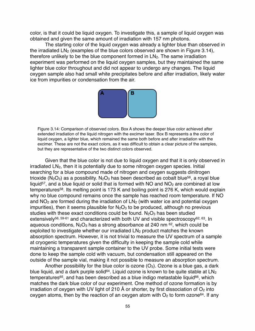
color, is that it could be liquid oxygen. To investigate this, a sample of liquid oxygen was obtained and given the same amount of irradiation with 157 nm photons.! The starting color of the liquid oxygen was already a lighter blue than observed in the irradiated LN2 (examples of the blue colors observed are shown in Figure 3.14), therefore unlikely to be the blue component formed in LN2. The same irradiation experiment was performed on the liquid oxygen samples, but they maintained the same lighter blue color throughout and did not appear to undergo any changes. The liquid oxygen sample also had small white precipitates before and after irradiation, likely water ice from impurities or condensation from the air.

Figure 3.14: Comparison of observed colors. Box A shows the deeper blue color achieved after extended irradiation of the liquid nitrogen with the excimer laser. Box B represents a the color of liquid oxygen, a lighter blue, which remained the same both before and after irradiation with the excimer. These are not the exact colors, as it was difficult to obtain a clear picture of the samples, but they are representative of the two distinct colors observed.

! Given that the blue color is not due to liquid oxygen and that it is only observed in irradiated LN2, then it is potentially due to some nitrogen oxygen species. Initial searching for a blue compound made of nitrogen and oxygen suggests dinitrogen trioxide (N2O3) as a possibility. N2O3 has been described as cobalt blue56, a royal blue liquid57, and a blue liquid or solid that is formed with NO and NO2 are combined at low temperatures58. Its melting point is 173 K and boiling point is 276 K, which would explain why no blue compound remains once the sample has reached room temperature. If NO and NO2 are formed during the irradiation of LN2 (with water ice and potential oxygen impurities), then it seems plausible for N2O3 to be produced, although no previous studies with these exact conditions could be found. N2O3 has been studied extensively56, 59-61 and characterized with both UV and visible spectroscopy62, 63. In aqueous conditions, N2O3 has a strong absorbance at 240 nm 62, which could be exploited to investigate whether our irradiated LN2 product matches the known absorption spectrum. However, it is not trivial to measure the UV spectrum of a sample at cryogenic temperatures given the difficulty in keeping the sample cold while maintaining a transparent sample container to the UV probe. Some initial tests were done to keep the sample cold with vacuum, but condensation still appeared on the outside of the sample vial, making it not possible to measure an absorption spectrum.! Another possibility for the blue color is ozone (O3). Ozone is a blue gas, a dark blue liquid, and a dark purple solid64. Liquid ozone is known to be quite stable at LN2 temperatures65, and has been described as a blue indigo metastable liquid66, which matches the dark blue color of our experiment. One method of ozone formation is by irradiation of oxygen with UV light of 210 Å or shorter, by first dissociation of O2 into oxygen atoms, then by the reaction of an oxygen atom with O2 to form ozone64. If any

55

oxygen from the air remains near the LN2 surface during the irradiation then it could create ozone on the LN2 sample. Additionally, the VUV photolysis of water ice (present as an impurity) creates oxygen atoms which can also contribute to ozone formation67, 68. However, it seems that in this case, ozone would also form upon the irradiation of liquid oxygen, which was not observed to change color. Ozone also absorbs in the UV near 250 nm and may be difficult to distinguish between N2O3, but it also has distinct absorption bands from 350 - 800 nm65, 66, 69. However, the same problems would occur in measuring the absorption spectrum while keeping the sample at cryogenic temperatures.

Conclusions and Future Work! Extended irradiation of liquid nitrogen with vacuum UV photons (157 nm) has created a blue colored final product in the liquid nitrogen. It is likely that this product is either dinitrogen trioxide (that has formed from nitrogen-oxygen compounds in the irradiated LN2 with oxygen and water ice impurities) or liquid ozone (produced by VUV photolysis of oxgyen and water ice). The dark blue color change was not observed in irradiated liquid oxygen. In this case, N2O3 would not form due to the lack of nitrogen in the sample, but ozone would be expected to form given that its production is from the presence of oxygen and water ice in the sample.! Given the difficulties in characterizing the absorption spectrum of a sample at cryogenic temperatures, it may be easier to characterize the irradiated N2 with a different method. Mass spectrometry would be a useful tool and could distinguish between N2O3 and ozone, or other polynitrogen compounds. However it would require allowing the sample to thaw to room temperature while trapping the evaporating gasses, and then analyzing the gas with mass spectrometry.! The initial motivation for this project was to explore the formation of nitrogen rings, but it seems more likely that we have instead created ozone or N2O3. Until the product can be analyzed, we have no strong evidence that irradiation by 157 nm photons is a viable method for producing nitrogen rings in liquid nitrogen. If the irradiated product does contain ozone or N2O3, then purifying the liquid nitrogen sample to get rid of any water ice or oxygen from the air near the sample surface will be important for further attempts in producing polynitrogen molecules. Only after characterization of the irradiated product can this study progress to the next step of measuring the nitrogen rings with NEXAFS spectroscopy.

56

3.6 References:

1.! Active Oxygen in Chemistry. C. S. Foote, J. S. Valentine, A. Greenberg, J. F. Liebman, Eds., (Blackie Academy & Professional, London, 1995).

2.! Finlayson-Pitts, B. J., Pitts Jr., J. N., Chemistry of the Upper and Lower Atmosphere. (Academic Press, New York, 2000).

3.! Legrini, O., Oliveros, E., Braun, A. M., Chem. Rev. 93, 671 (1993).4.! Oxygen radicals in biological systems. Part B Oxygen Radicals and Antioxidants.

L. Packer, A. N. Glazer, Eds., Methods Enzymol. (Academic Press, New York, 1990), vol. 186.

5.! Roots, R., Okada, S., Radiat. Res. 64, 306 (1975).6.! Olanow, C. W., Annals of Neurology 32, S2 (1992).7.! Pryor, W. A., Annu. Rev. Physiol. 48, 657 (1986).8.! Khalack, J. M., Lyubartsev, A. P., J. Phys. Chem. A 109, 378 (2005).9.! Laverne, J. A., Radiat. Res. 118, 201 (1989).10.! Janik, I., Bartels, D. M., Jonah, C. D., J. Phys. Chem. A 111, 1835 (2007).11.! Crowell, R. A., Lian, R., Sauer, M. C., Oulianov, D. A., Shkrob, I. A., Chem. Phys.

Lett. 383, 481 (2004).12.! Cabral do Couto, P., Guedes, R. C., Costa Cabral, B. J., Martinho Simoes, J. A.,

J. Chem. Phys. 119, 7344 (2003).13.! Schofield, D. P., Kjaergaard, H. G., J. Chem. Phys. 120, 6930 (2004).14.! Chipman, D. M., J. Phys. Chem. A 112, 13372 (2008).15.! Garrett, B. C. et al., Chem. Rev. 105, 355 (2005).16.! Barr, J. D. et al., J. Chem. Phys. 110, 345 (1999).17.! Stranges, S., Richter, R., Alagia, M., J. Chem. Phys. 116, 3676 (2002).18.! Hjelte, I. et al., Chem. Phys. Lett. 334, 151 (2001).19.! Laffon, C., Lacombe, S., Bournel, F., Parent, P., J. Chem. Phys. 125, (2006).20.! Fenton, H. J. H., Jackson, H., J. Chem. Soc. (London) 75, 1 (1899).21.! Walling, C., Acc. Chem. Res. 8, 125 (1975).22.! Gonzalez, M. G., Oliveros, E., Worner, M., Braun, A. M., J. Photoch. Photobio. C

5, 225 (2004).23.! Getoff, N., Schenck, G. O., Photochem. Photobiol. 8, 167 (1968).24.! Elles, C. G., Shkrob, I. A., Crowell, R. A., Bradforth, S. E., J. Chem. Phys. 126,

(2007).25.! Sander, M. U., Luther, K., Troe, J., J. Phys. Chem. 97, 11489 (1993).26.! Elles, C. G., Jailaubekov, A. E., Crowell, R. A., Bradforth, S. E., J. Chem. Phys.

125, (2006).27.! Yabushita, A., Kanda, D., Kawanaka, N., Kawasaki, M., Ashfold, M. N. R., J.

Chem. Phys. 125, (2006).28.! Hama, T., Yabushita, A., Yokoyama, M., Kawasaki, M., Andersson, S., J. Chem.

Phys. 131, (2009).29.! Andersson, S. et al., Phys. Chem. Chem. Phys. 13, 15810 (2011).30.! Gopakumar, K. et al., Radiat Eff. Defects Solids 32, 199 (1977).31.! Louit, G. et al., Radiat. Phys. Chem. 72, 119 (2005).32.! Ashawa, S. C., Kini, U. R., Madhvanath, U., Int J Appl Radiat Is 30, 7 (1979).

57

33.! Van Hecke, G. R., Karukstis, K. K., A Guide to Lasers in Chemistry. (Jones and Bartlett Publishers, Boston, 1998).

34.! Sumida, S., Obara, M., Fujioka, T., J. Appl. Phys. 50, 3884 (1979).35.! Kakehata, M., Uematsu, T., Kannari, F., Obara, M., IEEE J. Quantum Elec. 27,

2456 (1991).36.! Blake, A. J., Carver, J. H., Haddad, G. N., J. Quant. Spectrosc. Radiat. Transfer

6, 451.37.! Wilson, K. R. et al., Rev. Sci. Instrum. 75, 725 (2004).38.! Crowell, R. A., Bartels, D. M., J. Phys. Chem. 100, 17940 (1996).39.! Duffin, A. M., Saykally, R. J., J. Phys. Chem. C 111, 12031 (2007).40.! Duffin, A. M., Saykally, R. J., J. Phys. Chem. C 112, 17018 (2008).41.! Zubavichus, Y., Shaporenko, A., Grunze, M., Zharnikov, M., J. Phys. Chem. A

109, 6998 (2005).42.! Zubavichus, Y., Shaporenko, A., Korolkov, V., Grunze, M., Zharnikov, M., J. Phys.

Chem. B 112, 13711 (2008).43.! Zubavichus, Y., Zharnikov, M., Schaporenko, A., Grunze, M., J. Electron.

Spectrosc. Relat. Phenom. 134, 25 (2004).44.! Fujii, K., Akamatsu, K., Muramatsu, Y., Yokoya, A., Nuc. Instrum. Meth. B 199,

249 (2003).45.! Boese, J., Osanna, A., Jacobsen, C., Kirz, J., J. Electron. Spectrosc. Relat.

Phenom. 85, 9 (1997).46.! Zubavichus, Y., Shaporenko, A., Grunze, M., Zharnikov, M., Nuc. Instrum. Meth.

A 603, 111 (2009).47.! Zubavichus, Y. et al., Radiat. Res. 161, 346 (2004).48.! Giannozzi, P. et al., J. Phys.: Condens. Matter 21, 395502 (2009).49.! Prendergast, D., Galli, G., Phys. Rev. Lett. 96, 215502 (2006).50.! Anton, K., J. Mol. Graphics Modell. 17, 176.51.! Stöhr, J., NEXAFS Spectroscopy. (Springer, New York, 1996).52.! Butler, R., Chem. Ind., 24 (2009).53.! Bartlett, R. J., Chem. Ind., 140 (2000).54.! Butler, R. N., Hanniffy, J. M., Stephens, J. C., Burke, L. A., J. Org. Chem. 73,

1354 (2008).55.! Perera, S. A., Gregusova, A., Bartlett, R. J., J. Phys. Chem. A 113, 3197 (2009).56.! Markovits, G. Y., Schwartz, S. E., Newman, L., Inorg. Chem. 20, 445 (1981).57.! Austin, A. T., Brit J Anaesth 39, 345 (1967).58.! Nour, E. M., Chen, L. H., Laane, J., The Journal of Physical Chemistry 87, 1113

(1983).59.! Nour, E. M., Chen, L. H., Laane, J., J. Phys. Chem. 87, 1113 (1983).60.! Beattie, I. R., in Prog. Inorg. Chem. (John Wiley & Sons, Inc., 2007), pp. 1-26.61.! Beattie, I. R., Bell, S. W., Vosper, A. J., J. Chem. Soc., 4796 (1960).62.! Shaw, A. W., Vosper, A. J., J. Chem. Soc., Dalton Trans., 961 (1972).63.! Vosper, A. J., J. Chem. Soc. A, 1759 (1966).64.! Ardon, M., Oxygen: Elementary Forms and Hydrogen Peroxide. (W.A. Benjamin,

New York, 1965).65.! Hearn, A. G., Proceedings of the Physical Society 78, 932 (1961).66.! Brion, J. et al., Journal of Atmospheric Chemistry 30, 291 (1998).

58

67.! Hama, T., Yabushita, A., Yokoyama, M., Kawasaki, M., Watanabe, N., J. Chem. Phys. 131, 114510 (2009).

68.! Hama, T., Yabushita, A., Yokoyama, M., Kawasaki, M., Watanabe, N., J. Chem. Phys. 131, 114511 (2009).

69.! Inn, E. C. Y., Tanaka, Y., J. Opt. Soc. Am. 43, 870 (1953).

59

Chapter 4 - High Temperature Pulse Radiolysis of ! ! Aqueous Nickel (II) Solutions*This work was performed at the Notre Dame Radiation Laboratory (Notre Dame, IN) under the direction and support of Professor David M. Bartels.

4.1 Introduction

Radiation Chemistry! Radiation chemistry is the study of the interaction of ionizing radiation with matter. Types of radiation include accelerated beams of particles (electrons, protons, deuterons, alpha and other heavy particles), the decay of radioactive nuclei (α,β,and γ radiation), and high-energy photons (x-ray or bremsstrahlung radiation). The study of chemical effects resulting from absorption of ionizing radiation dates back to the discovery of X-rays by Roentgen in 1895, Becquerel’s discovery of uranium radioactivity in 1896 shortly after, and the Curies’ discovery of radioactive polonium and radium in 18981. The availability of these new radiation sources prompted extensive research to characterize their interactions with different types of matter.! The term “radiolysis” specifically refers to radiation-induced changes following the initial irradiation of molecules by the high-energy, ionizing radiation. The process typically includes a mixture of reactive intermediates such as ions, excited molecules, and free radicals depending on the radiation source and material. While gas samples can be irradiated with any type of ionizing radiation, bulk liquid or solid samples require a more penetrating radiation such as a beam of high-energy electrons (MeV range). For example, a 10 MeV electron beam will travel 52 mm in liquid water, while the equivalent energy proton and deuterium beams will only penetrate 1.2 and 0.72 mm, respectively2. As this experiment employs an electron beam for the radiation source, I will only focus on the radiolytic processes specific to electron irradiation.! Accelerated electrons lose energy upon interacting with matter by two major pathways: by radiation, or by inelastic/elastic collisions. Electrons lose energy as they are decelerated when passing the nuclei in the stopping material, resulting in the emission of electromagnetic radiation (bremsstrahlung radiation). For electrons, bremsstrahlung radiation is the predominant mode of energy loss at energies between 10 and 100 MeV 2. At lower energies, electrons are instead slowed primarily by elastic and inelastic scattering through Coulomb interactions with the atomic electrons in the stopping material. ! When a moving charged particle is slowed down, energy is deposited into the medium, creating a trail of excited and ionized atoms and molecules in the particle’s trajectory. The distribution of energy loss events is called the track structure, which is diagrammed in Figure 4.1. Nearly half of the energy loss events occur along the primary electron path3, creating “spurs” of excited and ionized species. The formation of these spurs represent an energy loss of 100 eV or less by the penetrating electron, and they typically contain 2 to 3 ion pairs2. If the secondary electrons have sufficient energy to ionize surrounding atoms, then “blobs” (100 to 500 eV) or “short tracks” (500 to 5000 eV) are produced by overlapping spurs. Secondary electrons with energy above 5 keV

60

are able to travel further from the original ionization track and create “branch tracks” of their own.

Figure 4.1: Track structure of a moving charged particle. Electrons deposit energy into spurs (<100 eV), blobs (100-500 eV), short tracks (500-5000 eV) and branch tracks (>5000 eV). The partitioning of energy into the different tracks is dependent on the incident electron energy. The small open circles represent positive ions formed, each associated with an electron and one or more excited molecules. This diagram is recreated from one already published by Spinks2.

! The amount of energy deposited into the different track structures is dependent on the original energy of the incident electron beam. Mozumder and Magee4 calculated the partitioning of the electron energy loss into the different track structures using Monte Carlo methods. In water, they found the energy of a 1 MeV electron to be distributed 67% in spurs, 11% in blobs, and 22% in short tracks. However, some improvements to the calculation, such as including the effect of elastic collisions, redistribute that energy to 75% in spurs, 12% in blobs, and 13% in short tracks5.! The primary products formed as a result of the energy deposition into a given material include electrons, ions, free radicals, and other excited species. When water is exposed to high-energy electrons, it will either ionize or be excited to an upper electronic state which can then dissociate, auto-ionize, or return back to the ground state. Those ions and excited species produced in the spurs can then further react or dissociate out of the spurs. These general reactions are diagrammed in Figure 4.2 along with the timescale at which each event occurs. The initial ionization takes place on the same timescale as an electronic transition. If the electron released does not have sufficient energy to cause further ionization, it will lose energy instead by exciting vibrational and rotational modes of the solvent, and becomes solvated by 10-13 seconds. The other radical or molecular fragments formed by dissociation of the excited species also appear on this timescale. Because these species are clustered in the spurs, they now can diffuse and react with each other or escape to the bulk solution. This “spur expansion” is over by 10-7 seconds, resulting in the products listed at the bottom of Figure 4.2, which marks the end of the radiation chemical stage3.

61

Figure 4.2: Reactions and events in water radiolysis, and the timescale on which they occur. This figure is adapted from the scheme presented by Buxton3. The final species listed at the bottom are considered the primary radiolysis products for liquid water.

The primary products, ensuing reactions, and their rate constants have been well characterized for the radiolysis of liquid water1-3. At room temperature, the primary yields of the radiolysis products6 are! H2O ⇝ 2.63 eaq

− + 2.80 iOH + 0.57 iH + 0.65H2O2 + 0.45H2 ! ! (4.1)

The blue numbers are the G-values for each species, which represent the number of molecules formed per 100 eV of energy absorbed into the water. G-values are dependent on temperature, pH, and the type of ionizing radiation6. Of these products, the solvated electron (eaq-) and the hydrogen atom (•H) are considered to be strongly reducing, while the hydroxyl radical (•OH) is the strongest oxidizer. To achieve totally oxidizing conditions, N2O gas can be added to scavenge the solvated electron and create more hydroxyl radicals in the process. If reducing conditions are desired instead, organic solutes are commonly added to react with •OH, converting them into less reactive reducing radicals7. The ability to tailor the conditions make water radiolysis an effective tool to study many different chemical systems.

Pulse Radiolysis! As many of the primary water radiolysis products are unstable and short-lived, it is essential to use a measurement technique that both produces high concentration of the species and has the ability to detect them in a time-dependent manner. Pulse radiolysis is the radiation-chemical equivalent of flash photolysis, and is sensitive on the same timescale (microsecond to nanosecond range)2. With this method, a short pulse of radiation is delivered instead of a continuous beam, allowing for higher doses and therefore higher concentration of the radiolysis products. After the invention of pulse radiolysis in 1963 by Boag and Hart8 and Keene9, the solvated electron became one of the most highly studied chemical reagents10. Soon after, this powerful tool was adapted more generally to study other chemical species like organic and inorganic free radicals, or metal ion complexes.

62

! The transients produced by pulse radiolysis can be detected by a variety of techniques including optical absorption, polarography, conductivity, electron paramagnetic resonance, or nuclear magnetic resonance. Optical absorption is a common technique to monitor the formation and decay of transients, and is especially useful to detect the solvated electron, which has a strong absorption near 700 nm. Even at low concentrations, the solvated electron is easily detectable optically, and with a half life of 2.1 x 10-4 seconds2, it’s decay kinetics can be tracked within the timescale of the experiment. If the electron absorption coefficient, ε, is known, then the electron concentration can be determined from absorption measurements in accordance with Beer’s Law (see Equation 4.13). Furthermore, the absorbance can be related to the initial energy dose by the accelerated electron beam,! A = dose ⋅ g eaq

−( ) ⋅ ε ,! ! ! ! ! ! ! ! (4.2)

where A is the absorbance, and g(eaq-) is the G-value for the electron. This relationship allows for calculation of the radiation dose if the absorption coefficient and G-value are known for the appropriate temperature. Once the dose and electron concentration are known, then the yields of the other primary radiolysis products can be determined. The electron extinction coefficient has been well-characterized, and has recently been measured up to 300°C11, 12.! Metal ions in aqueous solution have been studied extensively with pulse radiolysis to investigate unusual oxidation states of the ions and their complexes13-15. For the most part, the reduction of metal ions (M2+) by hydrated electrons has been the main focus:! M2+ + eaq

− →M+ ! ! ! ! ! ! ! ! (4.3)Alkali and alkaline earth metals are unreactive towards the hydrated electron, but more reactive ions like Cu2+ and Ag+ are readily reduced by hydrated electrons and hydrogen atoms. The divalent ions Cd2+, Pd2+, Zn2+, Co2+, and Ni2+ are also easily reduced by hydrated electrons but unreactive with hydrogen atoms15. Reaction 4.3 can be tracked by measuring the hydrated electron optical absorption, and the formation and decay of the reduced metal ions is observable by UV absorption spectroscopy (near 300 nm)13.! Pulse radiolysis of these transient metal species has been traditionally conducted at room temperature; however, measuring the kinetics at higher temperatures has become more important recently, especially when characterizing possible reactions in the cooling water of nuclear reactors. The cooling water is routinely exposed to the radiation produced by nuclear reactors, and its temperature increases to accommodate cooling of the reactor. The measurement of radiolysis reactions at higher temperatures is thus critical to further understanding the water chemistry in nuclear reactors. The reactions with metals are particularly important because of the metal ions present from the stainless steel containment vessels, and changes in the metal reactions will have implications for corrosion of the walls of the cooling water system16, 17. The initial research in the 1970s was conducted at room temperature, and only recently have new pulse radiolysis studies attempted to investigate these systems at increased temperatures and pressures.

63

Nickel (II) Chemistry! The nickel (II) ion is a good starting point to study the radiolysis of metal ions in water at higher temperatures because its speciation is straightforward. Other metal ions relevant in corrosion chemistry, like iron, magnesium, and chromium, have more complicated speciation and have the potential to precipitate out of solution depending on the oxidation state. Pulse radiolysis of nickel (II) solutions at room temperature has been studied by several groups13-15, 18, 19 in the 1960s and 1970s, but no recent attempts have been made to further elucidate the Ni+ decay kinetics or to study higher temperature solutions.! After radiolysis, the Ni2+ ion will react very quickly with the hydrated electrons as (analogous to Reaction 4.3): ! Ni2+ + eaq

− → Ni+ ! ! ! k ~ 2 x 1010 (M-1 s-1)! ! ! (4.4)

Baxendale et al.15 measured a rate constant of 2.2 x 1010 (M-1 s-1), and Buxton and Sellers recorded both 2.2 x 1010 (M-1 s-1) and 1.4 x 1010 (M-1 s-1) (corrected to 1.7 x 1010 (M-1 s-1) to include ion pairing) in separate publications13, 14.! Other possible competing reactions with the hydroxyl radical or the hydrogen atom are estimated to be much slower (k < 5 x 105 M-1 s-1)14, 20 and therefore not significantly contributing to the decay of the nickel (II) ion. After Reaction 4.4 has produced the monovalent nickel ion, it can further react with other radiolysis products or itself:! Ni

+ + iOH→ NiOH+ !! ! k ~ 2 x 1010 (M-1 s-1) 18! ! (4.5)

! Ni+ + H2O2 → Ni2+ + iOH + OH− ! k ~ 4.3 x 107 (M-1 s-1) 19! ! (4.6)! Ni+ + Ni+ → Ni2+ + Ni0 ! ! ! ! ! ! ! (4.7)Reaction 4.5 is predicted to be the major reaction, which is approximately diffusion controlled and has been estimated at room temperature in the past. The reaction with hydrogen peroxide (Reaction 4.6) may be significant, but only at longer timescales. While the dismutation reaction (Reaction 4.7) has been important for other metals, it has not yet been observed for nickel18. These reactions have all been proposed, but the specifics of how they each contribute to the Ni+ ion decay kinetics is not yet fully understood. The objective of the work described in this chapter is to investigate the radiolysis kinetics of these nickel species in water by monitoring the optical absorption signals over time for both the hydrated electron and for the Ni+ ion. These measurements will be used to determine the extent that these different reactions contribute to the Ni+ decay, and then to explore how increasing temperature will affect the rate constants.! ! !

64

4.2 Experimental Methods

Linear Electron Accelerator! The radiation source for the aqueous nickel (II) radiolysis experiments was a high-energy electron beam produced by a linear accelerator (linac) at the Notre Dame Radiation Laboratory (Notre Dame, IN). The linac, manufactured by Titan Beta, produces a beam of 8 MeV electrons in pulses ranging from 2 ns up to 1.5 µs. A 130 kV electron gun produces a beam of electrons that are then accelerated through a waveguide consisting of a series of Helmholtz coils powered by a pulsed RF source (2.586 GHz klystron). The 8 MeV beam exits the acceleration section with a maximum current of 4 amps and a diameter of approximately 5 mm. The linac can be operated at 1-10 Hz pulse frequency or in a single shot mode. Figure 4.3A shows a general diagram of the linac components.! For this experiment, we used a range of pulse widths between 4 and 15 ns to sample different solvated electron concentrations. The radiation dose of each pulse can be calculated from the solvated electron optical absorbance by using the appropriate G-value and extinction coefficient, as described in Equation 4.2.

Figure 4.3: Experimental Diagram. Panel A shows the linear accelerator components that produce the high energy electron beam for radiolysis. Panel B includes the sample flow diagram as well as the xenon arc lamp for optical absorption spectroscopy. Panel C depicts the detection end for the optical absorption measurements, which is located in a different room to minimize interference from the linac.

!

65

Samples! Once the accelerated electron beam exits the linac, it intersects with the aqueous nickel solution. A 1 mM stock solution was made from solid nickel perchlorate hexahydrate (Ni(ClO4)2•6H2O). The nickel solution and a solution of pure water were each stirred and bubbled with argon for an hour to purge out any oxygen (which will react with solvated electrons), and then loaded into a dual syringe pump system (Teledyne-Isco). The total flow rate was 3 mL/min, and the two pump outputs were mixed in appropriate ratios to sample a range of nickel concentrations: 0, 0.25, 0.5, 0.75, and 1 mM. The pump system, along with the sample containers for argon bubbling are shown in Figure 4.4A.

Figure 4.4: Photographs of the liquid sample components diagrammed in Figure 4.3B. Panel A shows the dual syringe pump system (while not connected to the experiment). The Ni2+ solution and pure water solutions are purged with Argon gas sufficiently (and stirred on a magnetic stir plate) before they are loaded into the syringe pumps. The pumps inject the solutions into the high temperature cell shown in Panel B.

High Temperature Flow Cell! Room temperature pulse radiolysis experiments can be carried out using a simple quartz flow cell, but measurements at higher temperatures and pressure require a much more complex sample container because quartz and silica both dissolve in supercritical water. The high temperature, high pressure flow cell21, 22 is made of the Hastelloy 276C alloy with 3 mm thick sapphire windows. The cylindrical flow cell has an inner diameter of 4 mm, a volume of 0.13 mL, and a path length of 1.1 cm. The alloy is thinned to 2 mm where the electron pulse intersects the cell in order to ensure uniform irradiation. A picture of the cell is shown in Figure 4.4B.! The flow path for the sample is diagrammed in Figure 4.3B. The liquid solution travels at 3 mL/min from the dual syringe pump system into the flow cell, and then through a controlled water bath before dumping into a waste container. Each nickel sample was run from room temperature up through 300°C in 50°C increments. To maintain a desired temperature, the sample first passes through a preheater immediately before entering the cell. Both the preheater and the cell are insulated with a 2.5 cm thick calcium sulfate board. The preheater does the majority of the sample

66

heating, but another heater is located in the cell to counteract any heat loss into the insulation. Thermocouples are used to measure the temperature of the solution as it enters and exits the flow cell. The temperature difference must be less than 0.5°C to avoid problems with excessive scattered light. The exiting sample then travels through a 316 stainless steel capillary tube coil in a water bath to maintain a desired pressure. By heating the water bath, the solution viscosity will change and affect the temperature. As the bath temperature is increased, the pressure will decrease. Typically the experiments were run with a water bath of ~ 40°C, resulting in a pressure of 250 bar. After flowing through the water bath, the solution is dumped into a waste container. However, it is possible to instead collect the irradiated solution and further characterize the products if desired.!Optical Spectroscopy! The time dependent decay of the solvated electron and Ni+ are monitored by optical absorption spectroscopy. A 75 Watt xenon arc lamp (PTI A1010 lamp housing) is pulsed (typically ~300 µs) to coincide with the electron beam pulse. The light path travels through the sapphire windows of the flow cell, perpendicular to the direction of the electron beam. The light transmitted through the sample is collimated, steered, and focused into a monochomator, then detected with a PMT. The detection system is separated from the rest of the experiment by two concrete walls in order to minimize any interference or noise produced by the linac pulses. Furthermore, all data acquisition is performed in a separate control room, and so all adjustments to the experiments (changes in temperature, nickel concentration, pulse width, etc.) must de done remotely. The components of the optical spectroscopy system are diagrammed in Figure 4.3B and 4.3C. The solvated electron absorption was measured at 700 nm and the Ni+ absorption was monitored at 300 nm. For the electron measurements, a Corning 2-58 filter was used to block all light below 620 nm. Because the Ni+ absorbance has not been well-characterized, we will also measure its spectrum with increasing temperature.! There are two major factors that interfere with the absorbance measurements and must be taken into account. First, if a charged particle is traveling fasted than the speed of light in a given medium (> 2.25 x 108 m/s for water), then it will disrupt the electrons in the atoms along its path through the medium. The electromagnetic radiation that is emitted as a result of the displaced electrons is called Çerenkov radiation1. The light emitted is typically in the UV range3, and the short, intense pulse can saturate the detectors. While this well-defined light pulse can be useful in some measurements, in this case is must be subtracted out so that it doesn’t interfere with the decay analysis at short timescales. The subtraction procedure it outlined in the Data Treatment section. The other possible interference is the absorption of UV light by the sapphire windows in the flow cell, especially at higher temperatures23. To account for window interference, especially for the Ni+ measurements that were also in UV region, we repeated each measurement with argon flowing through the cell instead of the nickel solution. The window absorption was recorded for each dose at each temperature, then subtracted from the Ni+ traces if they were substantial.

67

4.3 Data Treatment

Data Collection! For each optical absorption decay measurement there were actually four individual traces recorded. First, the signal is measured when both the linac and the arc lamp were pulsed to measure the transient decay trace (Figure 4.5A); then only the lamp was fired to account for any absorption without the transient species present (Figure 4.5B); then only the linac is fired to detect Çerenkov radiation (Figure 4.5C); and finally, the trace is recorded with neither the lamp nor the linac in order to measure any background signal (Figure 4.5D). The four measurements are then treated by Equation 4.8 to produce the final trace, which is also depicted in Figure 4.5. This treatment is incorporated into the data collection software and is done automatically for each measurement taken. Additionally, measurements were repeated several times and averaged if necessary, depending on the signal-to-noise ratio.

! Trace =LINAC + LAMP( ) − (LINAC ONLY )⎡⎣ ⎤⎦

LAMP ONLY( ) − (DARK )⎡⎣ ⎤⎦! ! ! ! (4.8)

Figure 4.5: The four-step measurement process. A time-dependent trace is recorded for a given solution at the chosen wavelength while (A) the linac and lamp are pulsed, (B) the lamp only is pulsed, (C) the linac only is pulsed, and (D) neither the linac nor lamp are pulsed. The traces are treated according to Equation 4.8 to produce the final trace. The example traces shown here are for the hydrated electron optical absorbance at 700 nm.

Kinetic Modeling! The rate of decay of the hydrated electron can be tracked directly by monitoring its strong optical absorption near 700 nm. In the presence of a sufficient amount of solute, the decay kinetics can be modeled with a pseudo-first-order approximation2. The general hydrated electron reaction:

68

! eaq− + solute → products rate constant, k ! ! ! ! (4.9)

can be described by the following rate expression:

!−d eaq

−⎡⎣ ⎤⎦dt

= k[solute] eaq−⎡⎣ ⎤⎦ ! ! ! ! ! ! ! (4.10)

If the concentration of the solute is high compared to that of the hydrated electron, then a pseudo-first order approximation can be made by treating k[solute] as a constant and the rate expression reduces to

!−d eaq

−⎡⎣ ⎤⎦dt

= k ' eaq−⎡⎣ ⎤⎦ ,! ! ! ! ! ! ! ! (4.11)

where k ' = k[solute] . Now Equation 4.11 is a first-order rate expression which can be integrated with respect to time to give:! eaq

−⎡⎣ ⎤⎦t = eaq−⎡⎣ ⎤⎦0 e

−k 't ,! ! ! ! ! ! ! ! (4.12)

where eaq−⎡⎣ ⎤⎦0 and eaq−⎡⎣ ⎤⎦t are the hydrated electron concentrations at time 0 and time t,

respectively. Assuming that the products do not also absorb significantly at the hydrated electron wavelength, Beer’s Law can be used to relate the electron concentration and absorption signal! A = ε ⋅ eaq

−⎡⎣ ⎤⎦ ⋅ l !,! ! ! ! ! ! ! ! (4.13)

where A is the absorption (or optical density, O.D.), ε is the absorption coefficient, and l is the length of the reaction cell. Since neither ε nor l will change during the course of the reaction, we can rewrite Equation 4.12 as! At = A0e

−k 't ! ! ! ! ! ! ! ! ! (4.14)A plot of the O.D. measured at 700 nm versus time can be fitted exponentially to give k’. Recalling that k ' = k[solute] , the experiment can be repeated with varying solute concentrations, and then a plot of k’ versus [solute] will yield a slope of k, the overall rate constant for the reaction shown in Equation 4.9.! For this work, the electron optical absorption was monitored over a range of nickel (II) concentrations to measure the rate constant of the hydrated electron with Ni2+ (Reaction 4.4). These measurements were then repeated while increasing the solution temperature in order to extract the rate constant for this reaction over a range of temperatures.! The ensuing reactions of the Ni+ ion with the other radiolysis products is much more complicated and not yet fully characterized. Possible reactions have already been listed in the Introduction (Equations 4.5-4.7), and they will all need to be incorporated into an advanced fitting model to fully understand the decay of the Ni+ optical absorption signal at 300 nm, which will be described in detail in the Results and Discussion section. All kinetic modeling and curve fitting were completed with IGOR 6.0 (WaveMetrics, Inc.).

69

4.4 Results and Discussion

Experimental Results! To illustrate the data presented in this chapter, I will first give a general description of the absorbance measurements. Figure 4.6A plots traces from both 300 nm and 700 nm to show the time-dependent absorbance of both the solvated electron and the Ni+ species. Figure 4.6B focuses on a shorter timescale to show more detail in the rise and decay of each species. The electron trace decays very quickly (< 0.5 µs), and corresponds with the rise of the Ni+ signal, which makes sense given that the electrons produced by radiolysis are reacting with the nickel (II) ions to form Ni+ (Reaction 4.4). The Ni+ traces takes much longer to decay and may have a much more complicated decay mechanism involving several different reactions.! The objective of this research is to first characterize the nickel (II) and solvated electron reaction by calculating the rate constant at various temperatures; second to measure the Ni+ spectrum with increasing temperature; and finally to investigate the Ni+ decay mechanism with kinetic modeling and scavenger reactions.

Figure 4.6: The entire timescale is shown in Panel A for the electron (red) and Ni+ (blue) decay traces for a solution of 0.25 mM Ni(ClO4)2 irradiated with 15 ns electron pulses. Panel B focuses only on the first few microseconds in order to show the rise and decay for each species in more detail.

Nickel (II) and Solvated Electron Reaction! As described in the previous section on kinetic modeling, the rate constant for Reaction 4.4 can be approximated with pseudo-first-order decay kinetics of the hydrated electron. Therefore, in order to fully characterize this reaction versus temperature, we will measure the electron decay both as a function of dose (electron concentration), and nickel concentration. Electron absorbance was measured at temperatures of 22°C, 100°C, 200°C, and 300°C.! An example of the electron decay traces in Figure 4.7 depicts the electron absorbance with increasing nickel concentration at room temperature and 4 ns linac

70

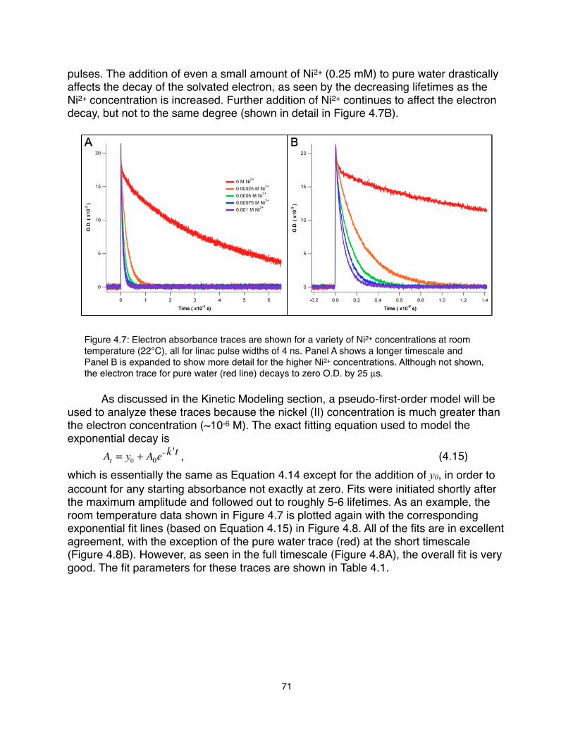
pulses. The addition of even a small amount of Ni2+ (0.25 mM) to pure water drastically affects the decay of the solvated electron, as seen by the decreasing lifetimes as the Ni2+ concentration is increased. Further addition of Ni2+ continues to affect the electron decay, but not to the same degree (shown in detail in Figure 4.7B).

Figure 4.7: Electron absorbance traces are shown for a variety of Ni2+ concentrations at room temperature (22°C), all for linac pulse widths of 4 ns. Panel A shows a longer timescale and Panel B is expanded to show more detail for the higher Ni2+ concentrations. Although not shown, the electron trace for pure water (red line) decays to zero O.D. by 25 µs.

! As discussed in the Kinetic Modeling section, a pseudo-first-order model will be used to analyze these traces because the nickel (II) concentration is much greater than the electron concentration (~10-6 M). The exact fitting equation used to model the exponential decay is! At = y0 + A0e

−k 't ,! ! ! ! ! ! ! ! (4.15)which is essentially the same as Equation 4.14 except for the addition of y0, in order to account for any starting absorbance not exactly at zero. Fits were initiated shortly after the maximum amplitude and followed out to roughly 5-6 lifetimes. As an example, the room temperature data shown in Figure 4.7 is plotted again with the corresponding exponential fit lines (based on Equation 4.15) in Figure 4.8. All of the fits are in excellent agreement, with the exception of the pure water trace (red) at the short timescale (Figure 4.8B). However, as seen in the full timescale (Figure 4.8A), the overall fit is very good. The fit parameters for these traces are shown in Table 4.1.

71

Figure 4.8: Electron absorbance traces are shown again for a variety of Ni2+ concentrations at room temperature (22°C), all for linac pulse widths of 4 ns, with the corresponding exponential fit curves plotted on top. Panel A depicts the entire measurement timescale, while Panel B focuses on the first 1.5 µs to show more detail for the fits of the higher Ni2+ concentration solutions.

[Ni2+] (M) y0 A0 k’ χ2

0 1.60 x 10-4 1.59 x 10-2 2.31 x 105 1.28 x 10-3

0.00025 8.49 x 10-5 1.90 x 10-2 4.16 x 106 9.11 x 10-5

0.0005 4.16 x 10-5 1.83 x 10-2 7.51 x 106 7.22 x 10-5

0.00075 8.17 x 10-5 1.91 x 10-2 1.07 x 107 5.81 x 10-5

0.001 4.29 x 10-6 1.88 x 10-2 1.34 x 107 4.19 x 10-6

Table 4.1: Fitting parameters for electron decay at room temperature with 4 ns linac pulses. k’ is the pseudo-first-order rate constant which will be used to determine the overall rate constant for the electron and nickel (II) reaction. More detailed parameters (including fit errors) can be found in the Appendix (Table A4.1).

! Recalling that k ' = k[solute] , we can plot the pseudo-first-order rate constant k’ obtained from the exponential fits versus the nickel (II) concentration in order to calculated the overall rate constant for the reaction. This plot is shown in Figure 4.9A for room temperature. A linear fit will yield a slope equal to the overall rate constant. For room temperature, the average overall rate constant (taking both linac pulse widths into account) is 1.37 (± 0.0347) x 1010 (M-1 s-1). This value matches well with the rate constants in the literature: 2.2 x 1010 (M-1 s-1)15, 2.2 x 1010 (M-1 s-1)13 and 1.7 x 1010 (M-1 s-1)14, indicating that our experiment and exponential fitting method are appropriate.! As mentioned previously, this experiment had not yet been carried out at temperatures higher than room temperature. Data for 100°C, 200°C, and 300°C were

72

obtained, similar to what was shown in Figure 4.7 for room temperature, and exponentials fits were performed in the same manner.!To simplify, I have only shown the k’ versus [Ni2+] plots in Figure 4.9 to illustrate the temperature dependence of the overall rate constant.!

Figure 4.9: Plots of the pseudo-first-order rate constant, k’, versus [Ni2+] for 22°C (A), 100°C (B), 200°C (C) and 300°C (D). Linear fits yield a slope equal to the overall rate constant for each temperature. More details on the fitting parameters are included in the Appendix (Table A4.2).

! While the linear fits for room temperature (Figure 4.9A) are in good agreement with the data, those for the higher temperatures do not fit as well. This is partially due to the fact that at higher temperatures, the maximum absorbance for the solvated electron shifts making the overall absorbance signal weaker, and the signal-to-noise will also be lower. However, once taking all of the data into account for each temperature, we still calculate overall rate constants that are reasonable, with errors of at least an order of magnitude smaller. The average rate constants are summarized in Table 4.2.!

73

Temperature (°C) k (M-1s-1)

22 1.37 (±0.035) x 1010

100 6.56 (±0.49) x 1010

200 3.98 (±0.19) x 1011

300 1.12 (±0.083) x 1012

Table 4.2: Rate constants for the solvated electron and nickel (II) reaction (Equation 4.4) at various temperatures. The errors from the exponential and linear fits were propagated through to calculate the final error (see Table A4.2 in the Appendix for the errors associated with each fit).

! The relationship between a reaction rate constant and temperature can be expressed by the Arrhenius equation

! k = A ⋅ e−EaRT ,! ! ! ! ! ! ! ! ! (4.16)

where A is the prefactor, Ea is the activation energy for the reaction, and R is the universal gas constant (8.314 J/mol•K).

! ln(k) = ln(A) − Ea

R1T

⎛⎝⎜

⎞⎠⎟! ! ! ! ! ! ! (4.17)

This second form of the equation, which expresses the variables in a linear form, is very useful. A plot of ln(k) versus 1/T will yield a slope equal to -Ea/R and a y-intercept of A. Based on the rate constant and temperature values listed in Table 4.2, the Arrhenius plot for the solvated electron and Ni2+ reaction is shown in Figure 4.10. The linear fit of this plot results in values of A = 1.18 (± 0.188) x 1014, and Ea = 22.5 (±1.30) kJ/mol.

Figure 4.10: Arrhenius plot for the reaction of Ni2+ and the solvated electron based on the rate constants (and error bars) and temperatures tabulated in Table 4.2. The fit yields values for the prefactor, A, and the activation energy, Ea.

74

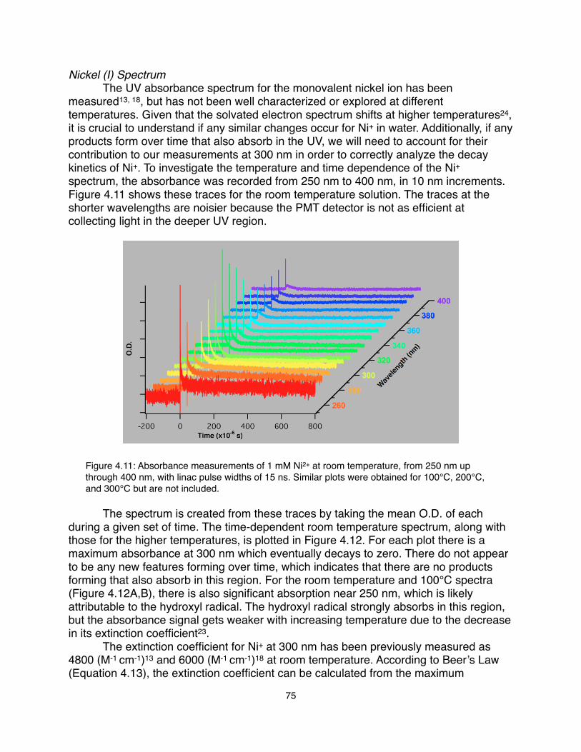
Nickel (I) Spectrum! The UV absorbance spectrum for the monovalent nickel ion has been measured13, 18, but has not been well characterized or explored at different temperatures. Given that the solvated electron spectrum shifts at higher temperatures24, it is crucial to understand if any similar changes occur for Ni+ in water. Additionally, if any products form over time that also absorb in the UV, we will need to account for their contribution to our measurements at 300 nm in order to correctly analyze the decay kinetics of Ni+. To investigate the temperature and time dependence of the Ni+ spectrum, the absorbance was recorded from 250 nm to 400 nm, in 10 nm increments. Figure 4.11 shows these traces for the room temperature solution. The traces at the shorter wavelengths are noisier because the PMT detector is not as efficient at collecting light in the deeper UV region.

Figure 4.11: Absorbance measurements of 1 mM Ni2+ at room temperature, from 250 nm up through 400 nm, with linac pulse widths of 15 ns. Similar plots were obtained for 100°C, 200°C, and 300°C but are not included.

! The spectrum is created from these traces by taking the mean O.D. of each during a given set of time. The time-dependent room temperature spectrum, along with those for the higher temperatures, is plotted in Figure 4.12. For each plot there is a maximum absorbance at 300 nm which eventually decays to zero. There do not appear to be any new features forming over time, which indicates that there are no products forming that also absorb in this region. For the room temperature and 100°C spectra (Figure 4.12A,B), there is also significant absorption near 250 nm, which is likely attributable to the hydroxyl radical. The hydroxyl radical strongly absorbs in this region, but the absorbance signal gets weaker with increasing temperature due to the decrease in its extinction coefficient23.! The extinction coefficient for Ni+ at 300 nm has been previously measured as 4800 (M-1 cm-1)13 and 6000 (M-1 cm-1)18 at room temperature. According to Beer’s Law (Equation 4.13), the extinction coefficient can be calculated from the maximum

75

absorption, the solute concentration, and the path length. In this case the Ni+ concentration is not known directly, but given that it is only produced by Reaction 4.4, and assuming that all solvated electrons will quickly react with Ni2+ to form Ni+, we can approximate the Ni+ concentration as equal to that of the solvated electron. The Ni+ extinction coefficient, ε

Ni+, can then be calculated as

! εNi+

=A300nmeaq−⎡⎣ ⎤⎦ ⋅ l

!,! ! ! ! ! ! ! ! (4.18)

where A300nm is the maximum absorbance at 300 nm and l is the path length (1.1 cm).The electron concentration, [eaq-], is calculated from the maximum absorbance measured at 700 nm and the temperature dependent extinction coefficient from the literature12. For each temperature, the electron concentrations were calculated for four different linac pulse widths, and the resulting Ni+ extinction coefficients for each were averaged together. These values (compiled in Table 4.3) show that the extinction coefficient drops significantly, especially at 200°C and 300°C. The room temperature value falls between the two values estimated previously in the literature.

Figure 4.12: Ni+ absorbance spectra as a function of time for room temperature (A), 100°C (B), 200°C (C), and 300°C (D). After the solution is irradiated (time = 0), the spectra decrease over time. O.D. values were selected from the decay traces at approximately Time1 = 0.6 µs (red), Time2 = 2.0 µs (orange), Time3 = 8.0 µs (yellow), Time4 = 40 µs (green), Time5 = 80 µs (blue), and Time6 = 300 µs (purple). No evidence of other absorbing products forming over time is observed.

76

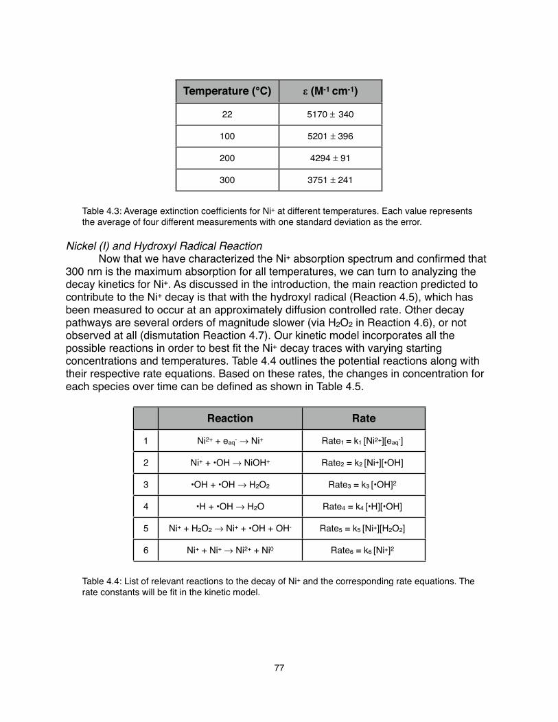
Temperature (°C) ε (M-1 cm-1)

22 5170 ± 340

100 5201 ± 396

200 4294 ± 91

300 3751 ± 241

Table 4.3: Average extinction coefficients for Ni+ at different temperatures. Each value represents the average of four different measurements with one standard deviation as the error.

Nickel (I) and Hydroxyl Radical Reaction! Now that we have characterized the Ni+ absorption spectrum and confirmed that 300 nm is the maximum absorption for all temperatures, we can turn to analyzing the decay kinetics for Ni+. As discussed in the introduction, the main reaction predicted to contribute to the Ni+ decay is that with the hydroxyl radical (Reaction 4.5), which has been measured to occur at an approximately diffusion controlled rate. Other decay pathways are several orders of magnitude slower (via H2O2 in Reaction 4.6), or not observed at all (dismutation Reaction 4.7). Our kinetic model incorporates all the possible reactions in order to best fit the Ni+ decay traces with varying starting concentrations and temperatures. Table 4.4 outlines the potential reactions along with their respective rate equations. Based on these rates, the changes in concentration for each species over time can be defined as shown in Table 4.5.

Reaction Rate

1 Ni2+ + eaq- → Ni+ Rate1 = k1 [Ni2+][eaq-]

2 Ni+ + •OH → NiOH+ Rate2 = k2 [Ni+][•OH]

3 •OH + •OH → H2O2 Rate3 = k3 [•OH]2

4 •H + •OH → H2O Rate4 = k4 [•H][•OH]

5 Ni+ + H2O2 → Ni+ + •OH + OH- Rate5 = k5 [Ni+][H2O2]

6 Ni+ + Ni+ → Ni2+ + Ni0 Rate6 = k6 [Ni+]2

Table 4.4: List of relevant reactions to the decay of Ni+ and the corresponding rate equations. The rate constants will be fit in the kinetic model.

77

Species (X) d[X]/dt

eaq- -Rate1

•OH -Rate2 - 2Rate3 - Rate4 + Rate5

Ni+ +Rate1 - Rate2 - Rate5 - Rate6

•H -Rate4

H2O2 +Rate3 - Rate5

NiOH+ +Rate2

Ni0 +Rate6

Table 4.5: Differential equations for the change in concentration of each species over time used in the fitting model for Ni+ decay. These are based on the rate equations defined in Table 4.4.

! The starting concentration of Ni2+ is known from the original Ni(ClO4)2 solution, and the solvated electron concentration is calculated based on the maximum absorbance at 700 nm (as described in the previous section). For the doses used in this experiment, the initial electron concentration is in the range of 10-7 - 10-6 M, which is typical for pulse radiolysis with a linac. [•OH]0, [•H]0, and [H2O2]0 can be found based on the electron concentration. As discussed in the introduction, relative yields of water radiolysis products have been well-defined based on temperature. The following reactions describe these relationships of the relative G-values6:! g eaq

−( ) = 2.56 + 3.40 ×10−3T ! ! ! ! ! ! ! (4.19)

! g iOH( ) = 2.64 + 7.17 ×10−3T ! ! ! ! ! ! (4.20)

! g iH( ) = 0.54 +1.28 ×10−3T ! ! ! ! ! ! ! (4.21)! g H2O2( ) = 0.72 −1.49 ×10−3T ! ! ! ! ! ! (4.22)Here T is the temperature in °C. The relative starting concentrations for each species compared to the solvated electron based on the relative G-values are compiled in Table 4.6. Given that Ni+, NiOH+, and Ni0 are formed during the course of the experiment, their initial concentrations input into the fitting model were zero.

78

Temp (°C) [•OH]0 [•H]0 [H2O2]0

25 1.06275 x [eaq-]0 0.21584 x [eaq-]0 0.25992 x [eaq-]0

100 1.15586 x [eaq-]0 0.23034 x [eaq-]0 0.1969 x [eaq-]0

200 1.25432 x [eaq-]0 0.24568 x [eaq-]0 0.13025 x [eaq-]0

300 1.33408 x [eaq-]0 0.2581 x [eaq-]0 0.07626 x [eaq-]0

Table 4.6: Relative starting concentrations for water radiolysis products relevant to Ni+ decay. The G-values for each species are calculated relative to that of the solvated electron based on Equations 4.19 through 4.22. The initial electron concentration is determined from the maximum absorbance at 700 nm.

! The fitting model incorporates the rate equations (Table 4.4), the starting concentrations, and solves the differential equations for changing concentrations over time (Table 4.5) while fitting the rate constants. The Ni+ concentration output is then used to calculate the optical density (absorbance) versus time according to Beer’s law,! At = [Ni

+ ]t ⋅ l ⋅ εNi+ ! ! ! ! ! ! ! ! (4.23)for comparison with our absorbance measurements at 300 nm. Although we have already calculated the Ni+ extinction coefficient from the absorbance spectra, it will also be determined from a fit to allow for more flexibility in the kinetic model.! For each temperature, there were four linac pulse widths used to vary the starting concentrations of the radiolysis products. These four traces were fit simultaneously in our model using a global fit procedure. Rate constants for the hydroxyl radical recombination and reaction with the hydrogen atom (Rate3 and Rate4 in Table 4.4) have been well characterized6, 23, 25, 26 at temperatures up to 350°C and will be held constant in the fitting model. Although already measured by the electron decay kinetics, the electron and Ni2+ reaction rate constant will be fit by the formation kinetics of Ni+ for comparison. The remaining rate constants, as well as the Ni+ extinction coefficient, are the only remaining parameters to fit.! The fitting procedure evolved through three different distinct models. First, we chose the only Ni+ decay pathway as the reaction with •OH, so the model neglected any significant contributions from decay by the H2O2 or dismutation reactions. We found that this did not accurately model the measured Ni+ decay, so the H2O2 reaction was included in the model, although previous data predicted the rate constant to be several orders of magnitude smaller than that for the •OH reaction. While this model seemed to fit the data fairly well and resulted in a rate constant for the •OH reaction comparable to the literature18 at room temperature (2.4 x 1010 M-1 s-1), a reasonable extinction coefficient based on our earlier calculations from the Ni+ spectra (5557 M-1 cm-1), the rate constant for the Ni+ decay by H2O2 was two orders of magnitude larger than predicted by previous experiments18, 19 (2.0 x 109 M-1 s-1). Hence, although the dismutation reaction has not previously been observed for nickel18, we decided to include it as an alternative decay pathway, given that it has been shown to be significant for other metals and that the nickel research is not very extensive.

79

! The four decay traces for the room temperature solution and are shown with their corresponding fit curves in Figure 4.13. The fit of the decay curve during the first 10 µs is in agreement with experiment for each of the four pulse widths. Over the entire timescale, the fit is still good, except for the shortest pulse width at longer times. The experimental measurement does not flatten out over time, but instead seems to increase again at the end. As this trend is not observed for the other pulse widths, it is likely an artifact of the window subtraction, rather than being indicative of Ni+ growing in concentration. One important finding is that the Ni+ traces do not decay completely to zero. Although our measurements were limited to measuring only 150 µs (due to issues with the arc lamp stability), previous work has determined that the decay trace still retains about 25% of its value until after 1 ms, before slowly decaying to zero in the 10-2 s range18. The authors attribute the initial fast decay of Ni+ to its reaction with •OH, and then the longer timescale decay to the slower reaction with H2O2. Their measured rate constant for the H2O2 reaction agrees well with that of Meyerstein and Mulac19. Given our earlier problems with fitting this rate constant, it was instead held fixed in the model at 4.3 x 107 M-1 s-1 based on the values obtained from the literature. Then the only rate constants to be fit are the electron and Ni2+ reaction (Rate1), the Ni+ reaction with •OH (Rate2) and the dismutation reaction (Rate6). The initial guess put into the model for k2 was based on the literature (2 x 1010 M-1s-1), and that for k6 was estimated as 7.4 x 108 M-1s-1. This estimate is based on the fact that any Ni+ remaining after •OH is used up will need to decay appropriately until the H2O2 reaction takes over at longer times (> 1 ms).

Figure 4.13: Decay traces measured at 300 nm for four different linac pulse widths. The full timescale (A) and a detail of the first 10 µs (B) show good agreement between the modeled decay curves and experiment for all four different pulse widths. The darker solid lines represent the fit lines for each experimental trace of the same color.

! The only parameters fit in this room temperature example were the rate constants for the electron and Ni2+ reaction (k1), the Ni+ reactions with •OH (k2) and with itself (k6), and the extinction coefficient. The results from the global fit were k1 = 2.04 x 1010 M-1 s-1, k2 = 1.52 x 1010 M-1 s-1, and k6 = 6.17 x 108 M-1 s-1. More information on the

80

model parameters can be found in the Appendix (Tables A4.3 and A4.4). The electron rate constant is slightly larger but matches well overall with that predicted by the electron decay kinetics. The •OH reaction rate constant is slightly less than in the literature, but still within the same order of magnitude. The dismutation reaction rate constant was close to our initial guess, but it is still fairly large considering that it has not been a proposed decay pathway before. By necessity, it fits well within our model, but it may not be an accurate reflection of experiment. If the dismutation reaction is significant, then the solid nickel product should be observable in experiment. We did not detect any problems in the flow cell that would be indicative of precipitates forming, and the collected waste solution did not show any visible precipitate. However, the actual concentration of solid nickel formed may not be very large. Upon analysis of the concentrations predicted by the fitting model (plotted in Figure 4.14), the nickel precipitated by the dismutation reaction should only amount to ~ 3 x 10-8 M, which may not be enough to disrupt our measurements. Therefore, decay via this pathway by the rate predicted in our model can be a plausible addition to the description of Ni+ decay kinetics.

Figure 4.14: Calculated concentrations of all relevant species for Ni+ decay over the full experimental timescale (A) and the first 10 µs (B) from the kinetic model: solvated electron (red), Ni+ (black), NiOH+ (orange), Ni0 (purple), •OH (blue), H2O2 (aqua), and •H (green). The Ni+ curve (black) is used to calculate the optical density and compare with the absorbance measurements at 300 nm.

! The goal for this project was also to extend these measurements to higher temperatures because the Ni+ transient absorbance has not yet been studied in these conditions. We measured the Ni+ kinetics up to 350°C (in 25°C increments), but we did not attempt to model the Ni+ traces due to problems in resolving the room temperature kinetics. The H2O2 rate constant was fixed in order to achieve the fits at room temperature, but we do not have a value for the higher temperatures to incorporate into our model. Although we did not fit the higher temperature data, the Ni+ traces appear to decay faster with increasing temperature just by visual inspection (Figure 4.15).

81

Figure 4.15: Absorbance at 300 nm measured as a function of temperature for radiolysis of 1 mM Ni2+ with 15 ns linac pulses. The decay time of the Ni+ traces decreases significantly at higher temperatures.

! Overall, our model of Ni+ decay kinetics matches well with experiment and what has previously been published in the literature, except for the inclusion of the dismutation reaction. It would be helpful to measure the absorbance on a longer timescale to further investigate the H2O2 reaction, but due to issues with the arc lamp stability we were not able to probe the > 1 ms region. Furthermore, the subtraction of the window absorbances is still a difficult task and poses problems especially at higher temperatures. Given all of these circumstances, our confidence in the long time Ni+ decay behavior is not as high as desired. We can conclude that the reaction with •OH is still the major decay pathway for Ni+, but we can’t make any further claims for certain regarding the other contributing reactions (H2O2 or the dismutation reaction).

4.5 Conclusions and Future Work

! Pulse radiolysis experiments were performed on aqueous nickel (II) solutions to investigate the kinetics of nickel ions with the transient radiolysis products. Absorbance measurements at 700 nm and 300 nm were analyzed to characterize the decay behavior of the solvated electron and the kinetics of the Ni+ ion. The electron decay traces indicated a rate constant of 1.37 (±0.035) x 1010 M-1 s-1 for the reaction with Ni2+ at room temperature, which is in good agreement with the literature. Our measurements for this reaction up to 300°C follow Arrhenuis behavior with an activation energy of 22.5 (±1.30) kJ/mol. This value is reasonable, given that activation energy of many other solvated electron reactions are on the same order of magnitude.! We have characterized the transient Ni+ absorbance spectrum from 250-400 nm over a range of temperatures. The maximum absorbance remains at 300 nm even at higher temperatures, and we found no evidence of new products forming over long

82

times. The extinction coefficients calculated from the spectra match well with the literature and show a decreasing trend as the temperature increases.! Our global model for the room temperature measurements at 300 nm fits the experimental data well and predicts the dominant decay pathway for Ni+ as the reaction with •OH. Our calculated rate constant for this reaction (1.52 x 1010 M-1s-1) agrees with the literature. We found it necessary to include another decay pathway to accurately model the traces, so we added the dismutation reaction with a rate constant fit at 6.17 x 108 M-1 s-1. While this reaction was discounted in the past, we find it to be a reasonable pathway given that the actual amount of solid nickel produced is negligible (~10-8 M). Because our measurements are made on a shorter timescale, we were not able to fully investigate the H2O2 reaction with Ni+, which is proposed to become significant at times greater than 1 ms. Further characterization of this reaction will help to develop a more complete picture of the Ni+ decay kinetics, but our model is a promising start given our current measurements. While the higher temperature data were not fit with the model, we can see that the Ni+ decays faster with increasing temperature by visual inspection. It is expected that the rate constants will increase at higher temperatures.! The next steps for this project would be to repeat the absorbance measurements on longer timescales, assuming the problems with the arc lamp stability are fixed. Additionally, any impurities in the sample could affect the experiment and our analysis, so future work should be careful to start with the purest possible chemicals. Another common method for investigating transient kinetics with pulse radiolysis is to use scavengers to further characterize a given reaction. We took some initial measurements with added methanol to scavenge the •OH radicals and to monitor the changes in absorbance at 300 nm. The competition kinetics with the methanol scavenger have already been studied at room temperature18 and more measurements need to be taken with our experimental set up to investigate the temperature dependence. ! In addition to further characterization of the nickel system, future studies might include exploration of other relevant aqueous metal systems with pulse radiolysis. Currently, the Bartels group is looking into the iron and magnesium systems, which are also relevant to the corrosion of stainless steel at supercritical temperatures.

83

4.6 Appendix

Electron and Nickel (II) Reaction Fit ParametersTable A4.1: Exponential fitting parameters for the decay of the electron absorbance measured at 700 nm. k’ is the pseudo-first order rate constant for the solvated electron and nickel (II) reaction.

Temp (°C)

Pulse width

[Ni2+] (mM) y0 A0 k’ χ2

22

4 ns

0 1.60 (±0.0197) x 10-4 1.59 (±0.000007) x 10-2 2.31 (±0.00179) x 105 1.28 x 10-3

22

4 ns

0.25 8.49 (±0.246) x 10-5 1.90 (±0.00002) x 10-2 4.16 (±0.000528) x 106 9.11 x 10-5

22

4 ns 0.5 4.16 (±0.193) x 10-5 1.83 (±0.00004) x 10-2 7.51 (±0.00128) x 106 7.22 x 10-5

22

4 ns

0.75 8.17 (±0.167) x 10-5 1.91 (±0.00004) x 10-2 1.07 (±0.00210) x 107 5.81 x 10-5

22

4 ns

1 4.29 (±1.84) x 10-6 1.88 (±0.00006) x 10-2 1.34 (±0.000376) x 107 4.19 x 10-6

22

8 ns

0 8.92 (±0.130) x 10-4 9.15 (±0.00075) x 10-2 3.90 (±0.00489) x 105 8.29 x 10-422

8 ns

0.25 3.03 (±0.188) x 10-4 1.12 (±0.000086) x 10-1 4.59 (±0.000586) x 106 3.03 x 10-3

22

8 ns 0.5 4.37 (±0.138) x 10-4 1.13 (±0.000101) x 10-1 8.20 (±0.00110) x 106 4.37 x 10-4

22

8 ns

0.75 2.95 (±0.116) x 10-4 1.13 (±0.000107) x 10-1 1.16 (±0.00159) x 107 1.72 x 10-4

22

8 ns

1 2.69 (±0.137) x 10-4 1.15 (±0.000148) x 10-1 1.48 (±0.000269) x 107 2.69 x 10-4

100

8 ns

0 9.94 (±0.236) x 10-4 3.75 (±0.0171) x 10-2 8.51 (±0.0543) x 105 1.57 x 10-2

100

8 ns

0.25 1.56 (±0.105) x 10-3 7.14 (±0.182) x 10-2 2.51 (±0.0620) x 107 7.80 x 10-4

100

8 ns 0.5 7.83 (±0.974) x 10-4 9.78 (±0.470) x 10-2 4.52 (±0.154) x 107 7.74 x 10-4

100

8 ns

0.75 4.08 (±1.23) x 10-4 1.08 (±0.0981) x 10-1 5.74 (±0.318) x 107 1.27 x 10-4

100

8 ns

1 9.61 (±1.18) x 10-4 1.18 (±0.136) x 10-1 6.66 (±0.421) x 107 1.20 x 10-3

100

15 ns

0 2.58 (±0.0531) x 10-3 9.54 (±0.0404) x 10-2 2.03 (±0.0117) x 106 1.67 x 10-2100

15 ns

0.25 1.49 (±0.155) x 10-3 1.92 (±0.0465) x 10-1 2.62 (±0.0465) x 107 9.66 x 10-4

100

15 ns 0.5 1.56 (±0.158) x 10-3 2.52 (±0.0722) x 10-1 4.44 (±0.0828) x 107 6.28 x 10-4

100

15 ns

0.75 2.18 (±0.175) x 10-3 3.06 (±0.152) x 10-1 5.78 (±0.155) x 107 8.25 x 10-4

100

15 ns

1 2.14 (±0.152) x 10-3 3.45 (±0.308) x 10-1 6.83 (±2.58) x 106 6.33 x 10-4

200 6 ns

0 -8.19 (±1.61) x 10-5 1.64 (±0.0121) x 10-2 1.24 (±0.0127) x 106 4.84 x 10-3

200 6 ns

0.0625 1.42 (±1.51) x 10-4 3.21 (±0.310) x 10-2 3.51 (±0.264) x 107 1.17 x 10-4

200 6 ns 0.125 1.06 (±1.23) x 10-4 4.95 (±0.947) x 10-2 6.68 (±0.676) x 107 1.24 x 10-4200 6 ns

0.188 8.79 (±0.104) x 10-5 5.20 (±1.29) x 10-2 7.87 (±0.908) x 107 9.39 x 10-5

200 6 ns

0.25 6.53 (±1.04) x 10-4 6.12 (±1.925) x 10-2 1.06 (±0.146) x 108 1.05 x 10-4

84

Temp (°C)

Pulse width

[Ni2+] (mM) y0 A0 k’ χ2

200

200 (cont.)

8 ns

0 6.19 (±2.24) x 10-5 2.92 (±0.0153) x 10-2 1.79 (±0.0133) x 106 3.21 x 10-3

200

200 (cont.)

8 ns

0.0625 2.24 (±1.10) x 10-4 5.62 (±0.267) x 10-2 3.53 (±0.130) x 107 1.74 x 10-4

200

200 (cont.)

8 ns 0.125 1.76 (±0.758) x 10-4 7.75 (±0.713) x 10-2 6.21 (±0.295) x 107 1.03 x 10-4

200

200 (cont.)

8 ns

0.188 3.95 (±0.849) x 10-4 1.21 (±0.294) x 10-1 9.43 (±0.788) x 107 1.40 x 10-4

200

200 (cont.)

8 ns

0.25 4.24 (±0.868) x 10-4 1.38 (±0.279) x 10-1 1.08 (±0.0846) x 108 1.54 x 10-4

200

200 (cont.)

15 ns

0 1.07 (±0.0662) x 10-3 7.36 (±0.0338) x 10-2 3.51 (±0.0201) x 106 2.92 x 10-3

200

200 (cont.)

15 ns

0.0625 3.53 (±1.14) x 10-4 1.60 (±0.0412) x 10-1 3.66 (±0.620) x 107 1.58 x 10-4

200

200 (cont.)

15 ns 0.125 1.37 (±0.101) x 10-3 2.36 (±0.146) x 10-1 6.07 (±0.167) x 107 1.54 x 10-4

200

200 (cont.)

15 ns

0.188 7.77 (±1.09) x 10-4 2.57 (±0.385) x 10-1 7.47 (±0.398) x 107 1.88 x 10-4

200

200 (cont.)

15 ns

0.25 9.96 (±0.968) x 10-5 3.71 (±0.434) x 10-1 9.51 (±0.385) x 107 1.62 x 10-4

300

6 ns

0 1.28 (±0.0247) x 10-4 1.02 (±0.0209) x 10-2 6.43 (±0.174) x 106 1.81 x 10-3

300

6 ns

0.0156 5.20 (±0.226) x 10-4 1.31 (±0.0708) x 10-2 2.49 (±0.118) x 107 7.74 x 10-4

300

6 ns 0.0313 -2.18 (±0.0259) x 10-3 1.21 (±0.173) x 10-2 3.84 (±0.383) x 107 1.06 x 10-3

300

6 ns

0.0469 8.73 (±2.42) x 10-5 2.86 (±0.586) x 10-2 8.57 (±0.808) x 107 9.87 x 10-4

300

6 ns

0.0625 -6.11 (±0.465) x 10-4 6.15 (±0.459) x 10-2 2.82 (±2.59) x 105 8.64 x 10-4

300 8 ns

0 3.20 (±1.54) x 10-5 1.85 (±0.0202) x 10-2 7.07 (±0.102) x 105 4.39 x 10-3

300 8 ns

0.0625 7.08 (±0.223) x 10-4 2.35 (±0.0645) x 10-2 2.91 (±0.0745) x 107 5.45 x 10-4

300 8 ns 0.125 3.26 (±0.338) x 10-4 2.85 (±0.143) x 10-2 4.55 (±0.173) x 107 6.40 x 10-4300 8 ns

0.188 -3.65 (±0.309) x 10-4 2.69 (±0.172) x 10-2 5.50 (±0.257) x 107 5.47 x 10-4

300 8 ns

0.25 4.94 (±0.306) x 10-4 2.84 (±0.233) x 10-2 6.45 (±0.352) x 107 5.45 x 10-4

300

15 ns

0 2.80 (±0.183) x 10-4 4.96 (±0.0348) x 10-2 1.11 (±3.57) x 107 4.03 x 10-3

300

15 ns

0.0625 7.22 (±0.335) x 10-4 6.51 (±0.0928) x 10-2 2.91 (±0.0357) x 107 6.11 x 10-4

300

15 ns 0.125 9.71 (±0.364) x 10-4 8.19 (±0.247) x 10-2 4.70 (±0.0932) x 107 7.79 x 10-4

300

15 ns

0.188 7.39 (±0.334) x 10-4 1.10 (±0.0485) x 10-1 6.53 (±0.152) x 107 6.75 x 10-4

300

15 ns

0.25 2.92 (±0.325) x 10-4 1.06 (±0.0633) x 10-1 7.29 (±0.214) x 107 6.46 x 10-4

85

Table A4.2: Linear fit parameters (y = ax + b) for plots of k’ versus [Ni2+] to find the overall rate constant for the solvated electron and nickel (II) reaction for each temperature.

Temp (°C)

Pulse width

a(y-intercept)

b(slope)

Average b(rate constant in M-1 s-1)

224 ns 6.33 (±3.24) x 105 1.31 (±0.0529) x 1010

1.37 (±0.0347) x 1010228 ns 7.58 (±2.75) x 105 1.43 (±0.0449) x 1010

1.37 (±0.0347) x 1010

1008 ns 6.26 (±4.56) x 106 6.55 (±0.745) x 1010

6.56 (±0.488) x 101010015 ns 6.92 (±3.87) x 106 6.56 (±0.632) x 1010

6.56 (±0.488) x 1010

200

6 ns 6.87 (±5.40) x 106 4.06 (±0.353) x 1011

3.98 (±0.189) x 1011200 8 ns 5.99 (±4.79) x 106 4.35 (±0.313) x 1011 3.98 (±0.189) x 1011200

15 ns 9.85 (±4.85) x 106 3.54 (±0.317) x 1011

3.98 (±0.189) x 1011

300

6 ns 3.53 (±8.16) x 106 1.46 (±0.211) x 1012

1.12 (±0.0834) x 1012300 8 ns 1.23 (±0.409) x 107 8.88 (±1.06) x 1011 1.12 (±0.0834) x 1012300

15 ns 1.34 (±0.319) x 107 1.01 (±0.0828) x 1012

1.12 (±0.0834) x 1012

Nickel (I) Decay Fit ParametersTable A4.3: Initial concentrations for each species in the global fit program to model the Ni+ decay kinetics at room temperature for each linac pulse width. Ni+, NiOH+, and Ni0 start at zero concentration. The starting electron concentration is calculated from the absorbance measured at 700 nm for each dose. The hydroxyl radical, hydrogen atom, and peroxide concentrations are calculated relative to the electron concentration based on the G-value relationships for water radiolysis products at room temperature.

Species (X)

[X]0 (M)[X]0 (M)[X]0 (M)[X]0 (M)Species (X) 5 ns 8 ns 11 ns 15 ns

eaq- 1.5873 x 10-6 3.8927 x 10-6 5.8354 x 10-6 8.6837 x 10-6

•OH 1.844 x 10-6 4.523 x 10-6 6.779 x 10-6 1.009 x 10-5

Ni+ 0 0 0 0

•H 3.422 x 10-7 8.393 x 10-7 1.258 x 10-6 1.872 x 10-6

H2O2 4.140 x 10-7 1.015 x 10-6 1.522 x 10-6 2.265 x 10-6

NiOH+ 0 0 0 0

Ni0 0 0 0 0

86

Table A4.4: Values for the fit parameters in the global fit model. Parameters were fit simultaneously to the decay traces for the four different linac pulses. Those noted as “fixed” were held constant as those rate constants have already been measured (as described in the Results and Discussion).

Reaction Fit Parameter Fit or Fixed Value

Ni2+ + eaq- → Ni+ k1 Fit 2.048 (±0.0021) x 1010 M-1 s-1

Ni+ + •OH → NiOH+ k2 Fit 1.527 (±0.0013) x 1010 M-1 s-1

•OH + •OH → H2O2 k3 Fixed 4 x 109 M-1 s-1

•H + •OH → H2O k4 Fixed 3.69 x 1010 M-1 s-1

Ni+ + H2O2 → Ni+ + •OH + OH- k5 Fixed 4.3 x 107 M-1 s-1

Ni+ + Ni+ → Ni2+ + Ni0 k6 Fit 6.175 (±0.005) x 108 M-1 s-1

Ni+ extinction coefficient εNi+ Fit 5022.5 (±1.39) M-1 cm-1

87

4.7 References

1.! Mozumder, A., Fundamentals of Radiation Chemistry. (Academic Press, San Diego, 1999).

2.! Spinks, J. W. T., Woods, R. J., An Introduction to Radiation Chemistry. (John Wiley & Sons, Inc., New York, ed. 3rd, 1990).

3.! Radiation Chemistry: Principles and Applications. Farhataziz, M. A. J. Rodgers, Eds., (VCH Publishers, New York, 1987).

4.! Mozumder, A., Magee, J. L., J. Chem. Phys. 45, 3332 (1966).5.! Pimblott, S. M., LaVerne, J. A., Mozumder, A., J. Phys. Chem. 100, 8595 (1996).6.! Elliot, A. J., Rate Constants and G-Values for the Simulation of the Radiolysis of

Light Water over the Range 0-300°C. Report AECL-11073 (Atomic Energy of Canada Limited, Chalk River, Ontario, 1994).

7.! The Study of Fast Processes of Transient Species by Electron Pulse Radiolysis. J. H. Baxendale, F. Busi, Eds., Proceedings of the NATO Advanced Study Institute held at Capri, Italy, 7-18 September, 1981 (D. Reidel Publishing Company, Dordrecht, Holland, 1982).

8.! Boag, J. W., Hart, E. J., Nature 197, 45 (1963).9.! Keene, J. P., Nature 197, 47 (1963).10.! Pulse Radiolysis. Y. Tabata, Ed., (CRC Press, Boca Raton, Florida, 1991).11.! Hare, P. M., Price, E. A., Bartels, D. M., J. Phys. Chem. A 112, 6800 (2008).12.! Hare, P. M., Price, E. A., Stanisky, C. M., Janik, I., Bartels, D. M., J. Phys. Chem.

A 114, 1766 (2010).13.! Buxton, G. V., Sellers, R. M., J. Chem. Soc. Faraday Trans. 1 71, 558 (1975).14.! Buxton, G. V., Sellers, R. M., Coord. Chem. Rev. 22, 195 (1977).15.! Baxendale, J. H., Fielden, E. M., Keene, J. P., Proceedings of the Royal Society

of London Series A, Mathematical and Physical Sciences 286, 320 (1965).16.! Kritzer, P., J. Supercrit. Fluids 29, 1 (2004).17.! Kritzer, P., Boukis, N., Dinjus, E., J. Supercrit. Fluids 15, 205 (1999).18.! Kelm, M., Lilie, J., Henglein, A., Janata, E., J. Phys. Chem. 78, 882 (1974).19.! Meyerstein, D., Mulac, W. A., J. Phys. Chem. 72, 784 (1968).20.! Hayon, E., Moreau, M., J Chim Phys 62, 391 (1965).21.! Bonin, J., Janik, I., Janik, D., Bartels, D. M., J. Phys. Chem. A 111, 1869 (2007).22.! Takahashi, K., Cline, J. A., Bartels, D. M., Jonah, C. D., Rev. Sci. Instrum. 71,

3345 (2000).23.! Janik, I., Bartels, D. M., Jonah, C. D., J. Phys. Chem. A 111, 1835 (2007).24.! Bartels, D. M., Takahashi, K., Cline, J. A., Marin, T. W., Jonah, C. D., J. Phys.

Chem. A 109, 1299 (2005).25.! Buxton, G. V., Elliot, A. J., J. Chem. Soc. Faraday Trans. 89, 485 (1993).26.! Elliot, A. J., Mccracken, D. R., Buxton, G. V., Wood, N. D., J. Chem. Soc.

Faraday Trans. 86, 1539 (1990).

88