X-ray focusing by the system of refractive lens(es) placed inside asymmetric channel-cut crystals
16
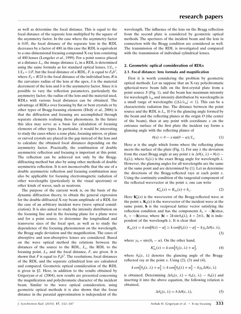
research papers 332 doi:10.1107/S0909049510003754 J. Synchrotron Rad. (2010). 17, 332–347 Journal of Synchrotron Radiation ISSN 0909-0495 Received 23 January 2009 Accepted 30 January 2010 # 2010 International Union of Crystallography Printed in Singapore – all rights reserved X-ray focusing by the system of refractive lens(es) placed inside asymmetric channel-cut crystals Arshak H. Grigoryan, a,b Minas K. Balyan c * and Albert H. Toneyan d a Center for the Advancement of Natural Discoveries Using Light Emission (CANDLE), Research Institute at YSU, Armenia, b Department of Solid State Physics, Faculty of Physics, Yerevan State University, Armenia, c Solid State Physics Research Laboratory, Department of Solid State Physics, Faculty of Physics, Yerevan State University, Armenia, and d Web AM LLC, Armenia. E-mail: [email protected] An X-ray one-dimensionally focusing system, a refracting–diffracting lens (RDL), composed of Bragg double-asymmetric-reflecting two-crystal plane parallel plates and a double-concave cylindrical parabolic lens placed in the gap between the plates is described. It is shown that the focal length of the RDL is equal to the focal distance of the separate lens multiplied by the square of the asymmetry factor. One can obtain RDLs with different focal lengths for certain applications. Using the point-source function of dynamic diffraction, as well as the Green function in a vacuum with parabolic approximation, an expression for the double-diffracted beam amplitude for an arbitrary incident wave is presented. Focusing of the plane incident wave and imaging of a point source are studied. The cases of non-absorptive and absorptive lenses are discussed. The intensity distribution in the focusing plane and on the focusing line, and its dependence on wavelength, deviation from the Bragg angle and magnification is studied. Geometrical optical considerations are also given. RDLs can be applied to focus radiation from both laboratory and synchrotron X-ray sources, for X-ray imaging of objects, and for obtaining high-intensity beams. RDLs can also be applied in X-ray astronomy. Keywords: X-ray dynamical diffraction; X-ray refraction; X-ray optics; X-ray imaging; X-ray astronomy. 1. Introduction Nowadays, X-ray focusing is considered to be an important aspect of studies in physics. Focusing is necessary for the imaging of objects (including those not transparent in the visible spectrum), the creation of X-ray microscopes, for X-ray astronomy and other physical studies. Lenses can be used as the focusing element. However, the focal distances of X-ray lenses are very large (refractive indices are very close to 1), and their application meets principle difficulties. It becomes essential to have systems which have focusing distances (of 1 m order) appropriate for application. An X-ray focusing system has been suggested (Grigoryan et al., 2004) that consists of (+n, n) asymmetric-reflecting two-crystal plane parallel plates with a double-concave cylindrical parabolic lens (refractive index < 1) placed in the gap between the plates (Fig. 1). The axis of the parabolic cylinder is perpendicular to the diffraction plane, and the beam diffracted from the first plate in the diffraction plane falls perpendicularly onto the lens. This system is called a refractive–diffractive lens (RDL). Grigoryan et al. (2004) show the focusing principle capability of a double-diffracted beam with its trajectory approximation, Figure 1 The general focusing scheme in the RDL. S: X-ray point source; Ox; Oz: coordinate axes; RP: reflecting planes; : glancing angle formed by the reflecting planes and the incident beam; : angle between the reflecting planes and the entrance surface; RL: refractive cylindrical parabolic lens with variables L and $ p and their directions of increase, parallel and perpendicular to the double-diffracted beam, respectively, and O 0 their origin; FP: focal plane perpendicular to the double-diffracted beam; f : focus.
-
Upload
independent -
Category
Documents
-
view
3 -
download
0
Transcript of X-ray focusing by the system of refractive lens(es) placed inside asymmetric channel-cut crystals

research papers
332 doi:10.1107/S0909049510003754 J. Synchrotron Rad. (2010). 17, 332–347
Journal of
SynchrotronRadiation
ISSN 0909-0495
Received 23 January 2009
Accepted 30 January 2010
# 2010 International Union of Crystallography
Printed in Singapore – all rights reserved
X-ray focusing by the system of refractive lens(es)placed inside asymmetric channel-cut crystals
Arshak H. Grigoryan,a,b Minas K. Balyanc* and Albert H. Toneyand
aCenter for the Advancement of Natural Discoveries Using Light Emission (CANDLE), Research
Institute at YSU, Armenia, bDepartment of Solid State Physics, Faculty of Physics, Yerevan State
University, Armenia, cSolid State Physics Research Laboratory, Department of Solid State Physics,
Faculty of Physics, Yerevan State University, Armenia, and dWeb AM LLC, Armenia.
E-mail: [email protected]
An X-ray one-dimensionally focusing system, a refracting–diffracting lens
(RDL), composed of Bragg double-asymmetric-reflecting two-crystal plane
parallel plates and a double-concave cylindrical parabolic lens placed in the gap
between the plates is described. It is shown that the focal length of the RDL is
equal to the focal distance of the separate lens multiplied by the square of the
asymmetry factor. One can obtain RDLs with different focal lengths for certain
applications. Using the point-source function of dynamic diffraction, as well as
the Green function in a vacuum with parabolic approximation, an expression for
the double-diffracted beam amplitude for an arbitrary incident wave is
presented. Focusing of the plane incident wave and imaging of a point source
are studied. The cases of non-absorptive and absorptive lenses are discussed.
The intensity distribution in the focusing plane and on the focusing line, and its
dependence on wavelength, deviation from the Bragg angle and magnification is
studied. Geometrical optical considerations are also given. RDLs can be applied
to focus radiation from both laboratory and synchrotron X-ray sources, for
X-ray imaging of objects, and for obtaining high-intensity beams. RDLs can also
be applied in X-ray astronomy.
Keywords: X-ray dynamical diffraction; X-ray refraction; X-ray optics; X-ray imaging;X-ray astronomy.
1. Introduction
Nowadays, X-ray focusing is considered to be an important
aspect of studies in physics. Focusing is necessary for the
imaging of objects (including those not transparent in the
visible spectrum), the creation of X-ray microscopes, for X-ray
astronomy and other physical studies. Lenses can be used as
the focusing element. However, the focal distances of X-ray
lenses are very large (refractive indices are very close to 1),
and their application meets principle difficulties. It becomes
essential to have systems which have focusing distances (of
1 m order) appropriate for application. An X-ray focusing
system has been suggested (Grigoryan et al., 2004) that
consists of (+n,�n) asymmetric-reflecting two-crystal plane
parallel plates with a double-concave cylindrical parabolic lens
(refractive index < 1) placed in the gap between the plates
(Fig. 1). The axis of the parabolic cylinder is perpendicular to
the diffraction plane, and the beam diffracted from the first
plate in the diffraction plane falls perpendicularly onto the
lens. This system is called a refractive–diffractive lens (RDL).
Grigoryan et al. (2004) show the focusing principle capability
of a double-diffracted beam with its trajectory approximation,
Figure 1The general focusing scheme in the RDL. S: X-ray point source; Ox; Oz:coordinate axes; RP: reflecting planes; �: glancing angle formed by thereflecting planes and the incident beam; �: angle between the reflectingplanes and the entrance surface; RL: refractive cylindrical parabolic lenswith variables L and �p and their directions of increase, parallel andperpendicular to the double-diffracted beam, respectively, and O 0 theirorigin; FP: focal plane perpendicular to the double-diffracted beam;f : focus.
as well as determine the focal distance. This is equal to the
focal distance of the separate lens multiplied by the square of
the asymmetry factor. In the case where the asymmetry factor
is 0.05, the focal distance of the separate lens in the RDL
decreases by a factor of 400; in this case the RDL is equivalent
to a one-dimensional focusing compound X-ray lens consisting
of 400 lenses (Lengeler et al., 1999). For a point source placed
at a distance Ls, the image distance Lf in a RDL is determined
using the same formula as for standard optical lenses, 1/Ls +
1/Lf = 1/F, but the focal distance of a RDL, F, is equal to F0b2,
where F0 = R/2� is the focal distance of the individual lens, R is
the curvature radius of the lens at the apex, � is the material
decrement of the lens and b is the asymmetry factor. Since it is
possible to vary the reflection parameters, particularly the
asymmetry factor, the radius of the lens and the material used,
RDLs with various focal distances can be obtained. The
advantage of RDLs over focusing by flat or bent crystals or by
other types of Bragg-focusing elements (Hrdy et al., 2006) is
that the diffraction and focusing are accomplished through
separate elements realising these phenomena. In the future
this idea may serve as a basis for calculation of focusing
elements of other types. In particular, it would be interesting
to study the cases where a zone plate, focusing mirror, or plane
or curved crystals are placed in the gap instead of the lens and
to calculate the obtained focal distances depending on the
asymmetry factor. Practically, the combination of double
asymmetric reflection and focusing is important at this point.
The reflection can be achieved not only by the Bragg-
diffracting method but also by using other methods of double
asymmetric reflection. It is not inconceivable that the use of a
double asymmetric reflection and focusing combination may
also be applicable for focusing electromagnetic radiation of
other wavelengths (particularly in the visual spectrum) or
other kinds of waves, such as neutrons.
The purpose of the current work is, on the basis of the
dynamic diffraction theory, to obtain the general expression
for the double-diffracted X-ray beam amplitude of a RDL for
the case of an arbitrary incident wave (wave optical consid-
eration). It is also aimed to study the intensity distribution on
the focusing line and in the focusing plane for a plane wave
and for a point source, to determine the longitudinal and
transverse sizes of the focal spot, as well as to study the
dependence of the focusing phenomenon on the wavelength,
the Bragg angle deviation and the magnification. The cases of
absorptive and non-absorptive lenses are considered. Based
on the wave optical method the relations between the
distances of the source to the RDL, Ls, the RDL to the
focusing point, Lf, and the focal distance, F, are given. It is
shown that F is equal to F0b2. The resolutions, focal distances
of the RDL and the separate cylindrical lens are calculated
and compared. Geometric optical consideration of the RDL
is given in x2. Here, in addition to the results obtained by
Grigoryan et al. (2004), new results are presented concerning
the magnification and polychromatic character of the incident
beam. Similar to the wave optical consideration, using
geometric optical methods it is also shown that the focus
distance in the paraxial approximation is independent of the
wavelength. The influence of the lens on the Bragg reflection
from the second plate is considered by geometric optical
methods. The apertures of the incident beam and the lens in
connection with the Bragg condition are considered as well.
The transmission of the RDL is investigated and compared
with the transmission of individual cylindrical lenses.
2. Geometric optical consideration of RDLs
2.1. Focal distance: lens formula and magnification
First it is worth considering the problem by geometric
optical methods. Let us suppose that an X-ray polychromatic
spherical-wave beam falls on the first-crystal plate from a
point source S (Fig. 1), and the beam has maximum intensity
for wavelength �m and intensity distribution by wavelengths in
a small range of wavelengths (|��/�m| << 1). This can be a
characteristic radiation line. The distance between the point
source and the RDL is Ls. If � is the glancing angle formed by
the beam and the reflecting planes at the origin O (the center
of the beam), then at any point with coordinate x on the
entrance surface of the first plate the incident ray forms a
glancing angle with the reflecting planes of
�ðxÞ ¼ � � x sinð� � �Þ=Ls: ð1Þ
Here � is the angle which forms where the reflecting plane
meets the surface of the plate (Fig. 1). For any � the deviation
from the exact Bragg angle at any point x is ��(x, �) = �(x) �
�0(�), where �0(�) is the exact Bragg angle for wavelength �.
However, the glancing angles for all wavelengths are the same
at the same point and are determined by (1). Let us determine
the directions of the Bragg-reflected rays at each point x.
Using the continuity condition of the tangential component of
the reflected wavevector at the point x, one can write
KehxðxÞ ¼ K0xðxÞ þ hx: ð2Þ
Here KehðxÞ is the wavevector of the Bragg-reflected wave at
the point x, K0ðxÞ is the wavevector of the incident wave at the
same point, h is the reciprocal lattice vector satisfying the
reflection condition and has the components hx = �|h| sin�,
hz = �|h| cos�, where |h| = 2ksin�0(�), k = 2�/�. |h| is inde-
pendent of the wavelength �. It is clear that
K0xðxÞ ¼ k cos½�ðxÞ � �� ’ k cos½�0ð�Þ � �� � k�0��ðx; �Þ;
ð3Þ
where �0 = sin(�0 � �). On the other hand,
KehxðxÞ ¼ k cos �hðx; �Þ þ �
� �; ð4Þ
where �h(x, �) denotes the glancing angle of the Bragg-
reflected ray at the point x. Using (2), (3) and (4),
k cos �hðx; �Þ þ �� �
’ k cos �0ð�Þ þ �� �
� k�0��ðx; �Þ
is obtained. Determining ��h(x, �) = �h(x, �) � �0(�) and
inserting it into the above equation, the following relation is
obtained,
��hðx; �Þ ¼ b��ðx; �Þ; ð5Þ
research papers
J. Synchrotron Rad. (2010). 17, 332–347 Arshak H. Grigoryan et al. � X-ray focusing 333
where b = �0 /�h is the asymmetry factor, �h = sin(�0 + �), and
��h(x, �) is a function of �. This means that at each point on
the entrance surface of the first plate the directions of the
reflected rays differ for various �. It follows from (5) that
�hðx; �Þ ¼ �0ð�Þ þ b��ðx; �Þ ¼ �ðxÞ þ ðb� 1Þ��ðx; �Þ: ð6Þ
It is assumed that the lens is perpendicular to the direction
which forms the glancing angle (� + �) with the entrance
surface of the first plate (Fig. 1). The direction determined by
the glancing angle (� + �) does not depend on wavelength.
Then it is obvious from (6) that the ray reflected at the point
x = 0 (at the origin O) is deviated from the center of the lens by
Dh� ���0, where Dh is the characteristic size of the gap along the
direction of the reflected rays and � ���0 is an average deviation
from the exact Bragg condition. If � ���0 ’ 10�4 and Dh ’
10 mm then the deviation is 1 mm. This deviation must be
neglected as the diffracted rays have geometrical sizes much
greater than 1 mm. At the other points x these deviations can
be neglected for all wavelengths. Below it becomes clear that
these deviations are negligible because the difference between
the refraction angles in the lens at the points x and xþDh� ���0
is also negligible. Therefore, all the rays pass through the lens
having the same parameter x, which they have on the entrance
surface of the first plate. Coordinate xsin(� + �) ’ x�h on the
entrance surface of the lens corresponds to the parameter x on
the entrance surface of the first plate. The formula for the
surface of the lens is x2�h2/2R + constant, where R is the radius
of the parabolic lens at the apex. The derivative of this formula
by the variable x�h gives the tangent of the angle which forms
the two normals to the parabola at the points O and x�h.
Therefore,
tan ’ ¼ x�h=R: ð7Þ
According to Snell’s law,
sin ’= sinð’þ�’Þ ¼ n ¼ 1� �; ð8Þ
where ’ + �’ gives the angle of the refracted ray, formed with
the normal to the lens surface at the point x�h, n is the
refractive index of the lens material and � is the decrement. It
is assumed that the rays falling on the lens surface are parallel
to the lens axes. The contributions of the deviations of the
directions from the parallel to the axes of the lens direction
in �’ are negligible. Since � and �’ are small, a linear
approximation can be used and, from (8), �’ = � tan’ = x��h /
R. After passing the second surface of the lens, the ray changes
its direction by
�’t ¼ 2x��h=R: ð9Þ
Now, from (9) it is clear that if the shift of x is �x = Dh� ���0 =
1 mm, for � ’ 10�6, �h ’ 0.3R ’ 1 mm, the corresponding
deviation of �’t is �6 � 10�10. This means that the change of
x can be neglected when the reflected ray passes the distance
from the entrance surface of the first plate to the entrance
surface of the lens. Taking into account (6) and (9), the
glancing angles of the rays falling on the surface of the second
plate are determined as
� 0hðx; �Þ ¼ �0ð�Þ þ b��ðx; �Þ þ 2x��h=R
¼ �0ð�Þ þ b��ð0; �Þ þ bx�0ð1=F � 1=LsÞ; ð10Þ
where F = F0b2 and F0 = R/2� is the focal distance of the
individual lens. For �� 0hðx; �Þ = � 0hðx; �Þ � �0(�) from (10) it
follows
�� 0hðx; �Þ ¼ b��ð0; �Þ þ bx�0ð1=F � 1=LsÞ: ð11Þ
The x parameter of the rays falling on the surface of the
second plate slightly differs from that falling on the second
surface of the lens. This difference is �x ’ 1 mm and is
negligible because after the Bragg reflection of the rays from
the surface of the second plate this difference is �0�x ’
0.02 mm (�0 ’ 0.02) in the double-diffracted beam cross
section. It follows from (5) that after Bragg reflection from the
second plate the deviations of the rays are
�� 0ðx; �Þ ¼ �� 0hðx; �Þ=b
¼ ��ð0; �Þ þ x�0ð1=F � 1=LsÞ: ð12Þ
Since �0(�) + ��(0, �) = � is independent of �, then
� 0ðxÞ ¼ �0ð�Þ þ�� 0ðx; �Þ ð13Þ
does not depend on wavelength. Here x is calculated from the
point O 0 (Fig. 1). The rays are reflected from the second plate
at the glancing angles (13) to the reflecting planes and at the
glancing angles � 0(x)� � to the entrance surface of the second
plate. The central reflected ray and the ray reflected at the
point x form the angle �� 0(x, �)��� 0(0, �) = x�0(1/F� 1/Ls)
and are intersected on the central line at the distance L(x)
from the point O 0 determined from the expression
x�0=LðxÞ ¼ �� 0ðx; �Þ ��� 0ð0; �Þ
¼ x�0ð1=F � 1=LsÞ: ð14Þ
This relation gives the focusing distance L = Lf. It follows from
(14) that Lf is independent of x and �,
1=Ls þ 1=Lf ¼ 1=F: ð15Þ
As follows from (13)–(15), the coordinates (�p = 0, L = Lf)
(Fig. 1) of the double-diffracted beam focus point do not
depend on wavelength, i.e. the image of a point chromatic
source has no chromatic aberrations and is still a point.
If R ’ 1 mm, � ’ 10�6, b ’ 0.05, then F0 ’ 500 m, F ’ 1 m
and the focal distance of the RDL is equivalent to the focal
distance of a compound lens containing 400 cylindrical para-
bolic lenses. As follows from (15), when Ls!1, then Lf = F.
This is the case of the incident plane wave. When Ls = F, then
Lf ! 1, i.e. the source is placed at the focal distance and a
plane wave is formed by the RDL. This is obvious from (12)
too. In the case Ls = F, �� 0(x, �) = ��(0, �) is independent of
x, i.e. all the rays reflected from the second plate are parallel to
the central ray.
Now let us consider another point source S1 which is at the
same distance Ls and deviated from the first point source S
perpendicular to the propagation direction of the incident
wave by ��s. The beam emitted from this point source falls on
the RDL at the glancing angle �1 to the reflecting planes. In
paraxial approximation the perpendicularity of the lens to the
research papers
334 Arshak H. Grigoryan et al. � X-ray focusing J. Synchrotron Rad. (2010). 17, 332–347

reflecting rays from this point source is also true. All formulae
obtained for the first point source are also true for the second
one. However, the rays of the second point source are focused
on the central line of the double-reflected beam of the second
source, i.e. the focusing line for the second point source forms
angle (�1 � �) with the focusing line of the first point source.
Therefore, the reversed image is formed. The images are
formed at the same distance, but are deviated by
��f ¼ Lfð�1 � �Þ ¼ ���sLf =Ls: ð16Þ
Hence the magnification is determined as
M ¼ Lf=Ls: ð17Þ
It can be seen from (15) that if F � Ls � 2F, then Lf � 2F and
M � 1. In the case where Ls > 2F it follows that F � Lf < 2F
and M < 1.
2.2. Amplitudes of diffracted beams: influence of the lens onthe Bragg condition
Now let us consider the amplitudes of the rays reflected
from the first and the second crystals. At the point x the
deviation from the exact Bragg angle is given by (1). For any
deviation the amplitude coefficient of reflection of a Bragg-
reflected ray (Pinsker, 1982) is well known,
�1ðx; �Þ ¼ � h= �hh
� �1=2�0=�hð Þ
1=2��
k��ðx; �Þ�0 þ 0
þ
nhk��ðx; �Þ�0 þ 0
i2
� 2o1=2�
; ð18Þ
where 2 = k2h �hh�0�h= sin2 2�0, 0 = k0 cos �=2 cos �0 and
0; h; �hh are the crystal dielectric susceptibility Fourier
components corresponding to the zero and h reflection. It
follows from (18) that the dimension of the region on the
entrance surface of the first crystal, where the Bragg reflection
takes place, is determined from the condition
��cðx; �Þ � h
�h=�0ð Þ1=2= sin 2�0; ð19Þ
where ��cðx; �Þ = � 0 þ��ðx; �Þ is the deviation from the
Bragg-corrected angle �cð�Þ = �0ð�Þ þ 0 and 0 =
0
ð1þ �h=�0Þ=2 sin 2�0. Let us consider the case when
��cð0; �Þ = 0, i.e. the beam falls at the Bragg-corrected angle
for �. It can be �m . In this case ��cðx; �mÞ = �x�0=Ls. Using
(19) the following estimation is obtained,
x�0=Ls
� � ; ð20Þ
where � is the right-hand side of (19). Assuming that jhj ’
1.9� 10�6, sin 2�0 ’ 0.36, �0 ’ 0.017, �h ’ 0.35, b ’ 0.05, Ls’
1 m, � = 2.3 � 10�5, |x| ’ 1.3 mm is obtained. If the
projection of the falling beam on the entrance surface of the
first plate is 2R0x = 6 mm, then it is equal to more than two
whole rocking curves ð4� Þ in real space. The transverse size
of the incidence beam is 6�0 (mm) ’ 105 mm. The transverse
size of the Bragg-reflected beam is 6�h (mm) ’ 2 mm. The
aperture 2R0 of the lens must be 2R0 � 2 mm.
Similarly to (18), the amplitude reflection coefficient of the
reflected beam from the second plate is
�2ðx; �Þ ¼ � �hh=h
� �1=2�h=�0ð Þ
1=2��
k�� 0hðx; �Þ�h þ 0
þ
nk�� 0hðx; �Þ�h þ 0
� �2�2
o1=2�: ð21Þ
Now the influence of the lens on the reflection condition can
be estimated. In the case where the wave component corre-
sponding to �m falls at the Bragg-corrected angle, as is seen
from (20) the component of the reflected beam for �m is
strongly reflected at the point x if
x�0ð1=F � 1=LsÞ ¼ x�0=Lf
� � : ð22Þ
This estimation must be considered in combination with (20),
which is fulfilled. If Lf � Ls (M � 1) then (22) is fulfilled in
the same region of x as (20). In the case when Lf < Ls (M < 1)
the region of strong reflection on the surface of the first plate
increases, and the region of strong reflection on the surface of
the second plate decreases. From (22) it is obvious that the
minimal value jxminj = F� =�0 = 1.15 mm of the strong
reflection region on the surface of the second plate for M < 1 is
achieved for Lf = F, and the maximal value jxmaxj ’ 2.3 mm for
M < 1 is achieved for Lf ’ 2F. Using (18) the distances Ls for
which the plane-wave approximation is valid can also be
estimated,
��cðx; �Þ � : ð23Þ
From (23) it follows that the plane-wave approximation is
valid when
Ls xj j�0=� : ð24Þ
Taking xj j = 3 mm from (24), then Ls 2.6 m is found. If a
plane parallel beam falls at the appropriate angle, the whole
region on the first plate (6 mm) is a region of strong reflection,
while the second plate is strongly reflected in the region given
by the estimation (22), i.e. about 2jxminj = 2.3 mm. Combining
(18) and (21) the whole reflection amplitude at any point x can
be found as
�ðx; �Þ ¼ �1ðx; �Þ�2ðx; �Þ: ð25Þ
It is easy to calculate the reflection amplitude at any point
using (25) and to obtain the graphic of j�j2 for any wave-
length, incident angle and distance Ls. For each case the
region for which the intensity value of the double-reflected
beam on the surface of the second plate does not vanish will be
seen in the graphic.
It is interesting to note that the formula (25) is sufficient for
calculating the double-diffracted field amplitude in a vacuum
after reflection from the second plate. For this, it is necessary
to write the phase of (25) and find the amplitude of the
double-diffracted beam at any distance from the RDL in a
vacuum using the Huyghens–Fresnel principle. In the focusing
plane this operation gives the same result as Fraunhofer
diffraction at the glancing angle (� � �) on the slit with the
same aperture as of the projection of the lens on the surface of
the second plate and with the amplitude transmission coeffi-
cient �. The final result for the amplitude Ee0hf of the double-
diffracted wave on the focusing plane is
research papers
J. Synchrotron Rad. (2010). 17, 332–347 Arshak H. Grigoryan et al. � X-ray focusing 335
Ee0hf ¼ expð�i�=4ÞðF=2�Þ1=2 sinð� � �Þ=LfLs
� �� exp iky2=2ðLf þ LsÞ
� �expð�k �
T0Þ
�RR0x
�R0x
�ðx0; �Þ exp �k�1x0 2�20=2Fð Þ exp �ikxx0�2
0=Lfð Þ dx0
where �1 = j�=�j, the refractive index of the lens is n =
1� �� i� and T0 is the thickness of the lens at the apex.
For the large lens the limits of integration can be taken
ð�1;þ1Þ. The validity of this approximation will be given in
x4.1. However, more accurate consideration of this problem
will be carried out using wave optical methods and dynamical
diffraction theory.
2.3. Transmission
The losses in RDLs are determined by absorption both in
the lens and in the plates and by the Bragg strong reflecting
common region of the first and the second crystals. For a lens
the absorption effect is small and it can be omitted by choosing
appropriate material for the lens. The absorption in the plates
in the Bragg case for more reflections [the example of Si(220)
(Mo K�) is considered] is small. However, for any wavelength
the losses owing to the change of the Bragg reflection condi-
tion by the lens are more important. The whole flux reflected
from the RDL for each wavelength is determined by the
square module of (25) multiplied by the size of the common
region of the strong Bragg reflection of two crystalline plates
and the lens. So, the transmission of the RDL can be deter-
mined as the ratio of the reflected beam flux on the surface of
the second crystal to the flux of the Bragg reflection from the
surface of the first-plate beam. It is equal to the ratio of the
common Bragg-reflection region to the reflection region from
the first plate and is multiplied by j�ð�xx; �Þj2, where �xx is the
middle point coordinate of the common region of the Bragg
reflection for the whole system. This is equal to 0.94 for the
Si(220) (Mo K�) reflection, and the transmission connected
only with absorption in the plates is 0.94 ’ 1. It is more
difficult to estimate the ratio of the size of the common
reflecting region to the size of the reflection region on the
surface of the first plate. This estimation has been given [see
(20), (22)] for the wavelength for which the deviation from the
Bragg-corrected angle is zero at the origin. Let us take another
�. It is true to see from (1) and (11) that
��cðx; �Þ ¼ ��� tan �=�� x�0=Ls;
�� 0hcðx; �Þ ¼ �b�� tan �=�þ bx�0=Lf;ð26Þ
where ��cðx; �Þ and �� 0hcðx; �Þ are the deviations from the
corrected Bragg angle at the point x for the wavelength � for
the first and the second crystals, respectively. For the first
crystal, x is calculated from O, and, for the second crystal,
from O 0, �� = �� �m and ��cð0; �mÞ = 0. It is seen from (26)
that the regions of Bragg reflection are concentrated around
the points
x0ð�Þ ¼ �ðLs=�0Þ�� tan �=�;
xhð�Þ ¼ ðLf=�0Þ�� tan �=�ð27Þ
on the surfaces of the first and the second crystal, respectively.
The intervals around the points x0ð�Þ and xhð�Þ, where the
Bragg reflection takes place, are
x0ð�Þ � ðLs=�0Þ� ; x0ð�Þ þ ðLs=�0Þ� � �
;
xhð�Þ � ðLf=�0Þ� ; xhð�Þ þ ðLf=�0Þ� � �
:ð28Þ
These two intervals have no common points when
j�� tan �=�j > � . Therefore, the components with the
wavelengths
�� tan �=� < � ð29Þ
are effectively reflected.
The following cases can be derived from (27)–(29):
(a) The interval of xh is included in the interval of x0. In this
case
Ls � 2F=ð1��=� Þ; ð30Þ
where � = j��j tan �=�. Obviously the size of the common
region of the Bragg reflection is 2ðLf=�0Þ� . If the interval
around x0 includes the region of the first crystal 2R0x = 2R0=�h,
then the transmission � = Lf=Ls � 1. Equality to 1 corre-
sponds to the case [(� = 0), (Ls = Lf = 2F)]. If the interval of x0
is larger than the aperture 2R0x , but the interval of xh is
smaller than 2R0x, then � = Lf� =�0R0x � 1. If these two
intervals are larger than 2R0x , then � = 1.
(b) The interval of x0 is included in the interval of xh . This
case is realised when
F � Ls � 2F=ð1þ�=� Þ: ð31Þ
The dimensions of the common Bragg-reflecting region is
equal to 2Ls� =�0. � = 1 in this case.
(c) The intervals of x0 and xh are particularly intersected.
This case is realised if 2F/(1 + �/� ) < Ls < 2F=ð1��=� Þ.The dimension of the common Bragg-reflection region is
ðLs þ LfÞð� ��Þ=�0 . If Ls� =�0 < R0x, then � =
ðLs þ LfÞð1��=� Þ=2Ls � 1. If the two intervals of x0 and
xh are larger than 2R0x , then � = 1. � = 1 is also the case when
the interval of xh is included in the aperture but the interval of
x0 includes the aperture 2R0x . In comparison with the indivi-
dual lens it must be noted that for a non-absorbing lens the
losses are zero, i.e. � = 1.
If the absorption losses in the lens are taken into account,
the transmission is determined as
�ð��;LsÞ ¼ exp �2k � T0
� ��
RR0x
�R0x
�j j2 exp �k�1x2�20=Fð Þ dx �0
=RR0x
�R0x
�1
2 dx �h:
If D2 and D1 are the sizes of the regions of the common Bragg
reflection on the surface of the second crystal and the Bragg
reflection on the surface of the first crystal, respectively, and at
the same time the absorption in the lens is small and the
reflection coefficients are close to 1, then transmission takes
the following form,
research papers
336 Arshak H. Grigoryan et al. � X-ray focusing J. Synchrotron Rad. (2010). 17, 332–347

�ð��;LsÞ ¼ exp �2k � T0
� � RD2
exp �k�1x2�20=Fð Þ dx=D1
’ D2ð��;LsÞ=D1ð��;LsÞ:
The analysis of the situation where the absorption in the lens is
neglected is given by (22) for the cases (a)–(c). However, the
transmission of the RDL can be introduced as the ratio of the
reflected flux to the flux of the incidence wave, i.e.
�t ��;Lsð Þ ¼ exp �2k � T0
� ��
RR0x
�R0x
�j j2expð�k�1x2�20=FÞ dx=ð2R0xÞ:
For the individual absorbing lens the transmission is defined as
�l ¼ expð�2k � T0Þ
RR0
�R0
exp �k�1x2=F0ð Þ dx=ð2R0Þ:
Here T0 is the thickness of the lens at the apex. When the
absorption is neglected, �l is equal to 1. In Figs. 2 and 3,
�tð��;LsÞ dependences are shown for the cases �� = 0 and
Ls = 3F/2 for lenses made of beryllium and silicon, with R =
1 mm, R0 = 3 mm, T0 = 0.1 mm, b = 0.05. For beryllium F =
1.14 m and for silicon F = 0.8 m. For the lens made of beryl-
lium �l = 0.98, and �l = 0.56 for that made of silicon. The
Si(220) Mo K� reflection is used. The refractive indices of
beryllium and silicon are given in x4.1 and x4.2, respectively.
As can be seen from Figs. 2 and 3, the transmission of the RDL
can be close to 1, and �ð��;LsÞ � �tð��;LsÞ. Note that for
the compound lens the transmission can be up to 0.3 (Lengeler
et al., 1999) if the number of lenses is �40 and R0 = 450 mm,
R = 200 mm. The advantage of the RDL is the small focal
distance when a lens is used, and the curvature radius and the
aperture of the lens can be 1–10 mm. The compound lens with
400 lenses and R = 1 mm, R0 = 1 mm equivalent to a RDL with
b = 0.05 will have a longitudinal size of more than 0.4 m and
negligible transmission, thus it will be practically useless.
In summary, one-dimensional focusing can be achieved with
a RDL. It is clear that for obtaining two-dimensional focusing
it is necessary to use two RDLs. One of them will focus in the
meridional plane and the other, placed after the first, in the
plane perpendicular to the meridional plane. The vector of
diffraction of the first RDL lies in the plane ðK; ezÞ, the vector
of diffraction of the second RDL h2 lies in the plane ðK; eyÞ,
where ey is the unit vector perpendicular to the plane XOZ,
and K is the wavevector of the incidence beam. If the asym-
metry factors of these two RDLs are the same, two-dimen-
sional point focusing is achieved, and the formula of that lens
is the same as (15), with the same F. At the distance Lf the
stigmatic image of a point source is formed. The calculation of
(15) for two RDLs can be carried out using geometric optical
methods, as represented in this section. The formulae (16) and
(17) for magnification stay unchanged. In the current work,
wave theory is given only for one-dimensional focusing, since
the wave optical consideration of two-dimensional focusing
with two RDLs is more complicated.
3. Wave optical consideration: derivation of thegeneral formula of double-diffracted beam amplitude
Consideration of the RDL by wave optical methods is
necessary. The formulae for the intensity distribution in the
focusing plane and on the focusing line, the longitudinal and
transverse sizes of the focal spot, and for the resolution of the
lens and object imaging can be correctly obtained only by
using wave optical methods. First the wave optical consid-
research papers
J. Synchrotron Rad. (2010). 17, 332–347 Arshak H. Grigoryan et al. � X-ray focusing 337
Figure 2Transmission of the RDL and its dependence on Ls for �� = 0. (a) Lensmade of beryllium, F = 1.14 m; (b) lens made of silicon, F = 0.8 m. F �Ls � 20F.
Figure 3Transmission of the RDL and its dependence on �� for Ls = 3F/2. (a)Lens made of beryllium, F = 1.14 m; (b) lens made of silicon, F = 0.8 m.

eration of this problem for an arbitrary incident wave is given.
Then the main formula obtained for the amplitude of the
double-diffracted beam is applied for the case of an incident
plane wave and for the case of point-source imaging.
The electric field of an arbitrary non-polarized incident
wave is described as Eið!; rÞ expðiKrÞ, where Ei is the slowly
varying amplitude, and the exponent space period is of the
order of interatomic spacing, and ! is the frequency corre-
sponding to wavelength �. K are wavevectors of different
lengths, K2 = ð2�=�Þ2, and K corresponding to different
wavelengths have the same direction. The glancing angle
formed by K and the entrance surface of the first crystal is
(� � �), where � is the glancing angle formed by K and the
reflecting atomic planes, and � is the angle formed by the
atomic planes and the entrance surface (Fig. 1). The field of
any frequency in the crystal is represented by a two-wave
approximation as
E ¼ E0 exp iK0rð Þ þ Eh exp iKhrð Þ;
where K0 and Kh = K0 þ h vectors are the wavevectors of the
transmitted and diffracted fields, respectively, which satisfy the
Bragg exact condition for a certain wavelength, and K20 = K2
h =
ð2�=�Þ2, E0, Eh are the amplitudes of the electric fields of the
transmitted and diffracted waves for the same wavelength.
The amplitudes satisfy Takagi’s equations of dynamic
diffraction (Takagi, 1969),
2ik cos �0 � �ð Þ@=@xþ sin �0 � �ð Þ@=@z� �
E0 þ k20E0
þ k2 �hhCEh ¼ 0;
2ik cos �0 þ �ð Þ@=@x� sin �0 þ �ð Þ@=@z� �
Eh þ k20Eh
þ k2hCE0 ¼ 0:
ð32Þ
Here C is the polarization factor; C = 1 for -polarization and
C = cos 2�0 for �-polarization. Hereinafter the polarization
factor is omitted. On the first-crystal entrance surface the E0
field corresponding to any polarized state satisfies the conti-
nuity condition
E0ðx; yÞ ¼ E iðx; yÞ exp �ik���0xð Þ: ð33Þ
Here �� = � � �0 is the deviation of the wavevector K from
the exact Bragg angle for a certain wavelength, and the linear
approximation by that deviation is used. It is known that in the
Bragg case the diffracted field amplitude at the crystal
entrance surface can be expressed by the convolution of the
point-source function and the incident wave amplitude
(Uragami, 1969),
Ehðx; y; 0Þ ¼Rþ1�1
Gh0ðx� x0ÞE0ðx0; y; 0Þ dx0; ð34Þ
where
Gh0ðxÞ ¼ ih
�hh
�1=2�0
�h
�1=2J1ðxÞ
xexp i0xð ÞHðxÞ ð35Þ
is the first-crystal point-source function, J1 is the first-order
Bessel function, HðxÞ is the step function; HðxÞ = 1 when x > 0
and HðxÞ = 0 when x < 0. After reflection from the first plate
the beam falls onto the lens. The lens is placed perpendicular
to the diffracted beam. Since the case of a polychromatic beam
is discussed, if it is assumed that the lens is placed perpendi-
cular to Kh, the direction of which depends on the wavelength,
then clearly the perpendicularity condition of the lens to the
diffracted beam will be broken for another wavelength, that is
not suitable for calculations. Since the directions of the
diffracted waves for different wavelengths together form
angles of �2000, it is assumed that the lens is placed perpen-
dicular to the direction which forms angle (� þ �) with the
entrance surface of the first crystal. Such a choice does not
depend on the wavelength and is defined only by the direction
of the incident beam. So, both in the lens and in the gap the
electric field corresponding to any polarization state and any
frequency in the form E0h expðikshrÞ is represented, where sh =
½cosð� þ �Þ;� sinð� þ �Þ� is a unit vector, the direction of
which does not depend on the wavelength. The lens is placed
perpendicular to the direction defined by vector sh . If LG
Ls , where LG is the characteristic size of the gap in the
direction of sh, and Ls is the characteristic distance between
the source and the system, then E 0h in the gap and in the lens
propagates by xþ zc tanð� þ �Þ = constant characteristics
parallel to sh , acquiring an additional phase in the lens. In the
gap and in the lens the field amplitude propagates according to
the following equations, respectively,
2ik cosð� þ �Þ@E 0h=@x� sinð� þ �Þ@E 0h=@z� �
¼ 0;
2ik cosð� þ �Þ@E 0h=@x� sinð� þ �Þ@E 0h=@z� �
þ k20lE0h ¼ 0;
ð36Þ
where 0l is the dielectric susceptibility of the lens and is
related to the refractive index of the lens by the relation n =
1þ 0l=2. The first equation of (36) can be obtained from the
second equation of (32) by replacing 0 = h = 0, and the
second equation of (36) can be obtained from the second
equation of (32) by replacing 0 = 0l, h = 0. In both cases �must be taken instead of �0 . The amplitude E 0h satisfies the
continuity conditions on both surfaces of the lens and on the
surface of the first plate. Using (36) the amplitude on the exit
surface of the lens is
E 0hðx; y; zÞ ¼ E 0hð�h; y; 0Þ exp ik0l
2
�2h
R
�exp ik
0l
2T0
� �; ð37Þ
where �h = x sinð� þ �Þ þ z cosð� þ �Þ and T0 is the lens
thickness at the apex. The entrance and exit surfaces
of the lens are given by �h ent = Lh � ð�2h=2RÞ and �h ex =
Lh þ T0 þ ð�2h=2RÞ, respectively. Here �h = x cosð� þ �Þ �
z sinð� þ �Þ and Lh is the distance of the apex of the lens from
the origin O. Taking into account that after the lens the wave
amplitude propogates according to the first equation of (36)
and satisfies the continuity condition on the exit surface of the
lens, the amplitude in the gap after the lens is represented as
research papers
338 Arshak H. Grigoryan et al. � X-ray focusing J. Synchrotron Rad. (2010). 17, 332–347

E 0hðx; y; zÞ ¼ Eh½xþ zc tanð� þ �Þ; y; 0�
� exp ik���h xþ zc tanð� þ �Þ½ ��
ð38Þ
� exp ikð0l=2ÞT0
� �� exp ik
0l sin2ð� þ �Þ
2
½xþ zc tanð� þ �Þ�2
R
� �:
Passing through the lens and the gap the wave falls on the
second plate. In the second plate the field also satisfies
Takagi’s equations (32) and the continuity conditions
E 0h expðikshrÞ = Eh expðiKhrÞ on the surface of the second plate
(z = �D), where D is the size of the gap in the z direction.
Once again applying the formula (34) but with the point-
source function of the second crystal,
G0hðxÞ ¼ i �hh
h
�1=2�h
�0
�1=2J1ðxÞ
xexp i0xð ÞHðxÞ; ð39Þ
the amplitude of the double diffracted beam on the surface of
the second crystal is represented as
E0ðx; y;�DÞ ¼R
G0h x� x0ð ÞEh x0; y;�Dð Þ dx0; ð40Þ
where
Eh ¼ E 0h exp �ik���hxð Þ exp �i kshz � Khz
� �D
� �: ð41Þ
Later the constant phase exponent in (41) can be omitted,
since it has no effect on the final result. Inserting (41) and (38)
into (40) for the double-diffracted wave amplitude on the
surface of the second plate, the following equation is obtained,
E0ðx; y;�DÞ ¼ exp ik0l
2T0
� � ZZG0hðx� x0Þ
�Gh0 x0 �Dc tanð� þ �Þ � x00½ �E0ðx00; y; 0Þ
� exp ik0l sin2 � þ �ð Þ
2
x0 �Dc tanð� þ �Þ½ �2
R
� �� dx0 dx00
¼ exp ik0l
2T0
� � ZZG0h x�Dc tanð� þ �Þ � x0½ �
�Gh0ðx0� x00Þ exp ik
0l sin2ð� þ �Þ
2
x0 2
R
� �� E0ðx
00; y; 0Þ dx0 dx00: ð42Þ
The double-diffracted field We0h propagating in the vacuum
is represented in the form We0h = Ee
0h expðiKrÞ. It satisfies the
Helmholtz equation
@2We0h
@x2þ@2We
0h
@y2þ@2We
0h
@z2þ k2We
0h ¼ 0:
From this equation we can find the propagation equation for
Ee0h,
@2Ee0h
@x2þ@2Ee
0h
@y2þ@2Ee
0h
@z2
þ 2ik cosð� � �Þ@
@xþ sinð� � �Þ
@
@z
� �Ee
0h ¼ 0: ð43Þ
Since the first derivatives in (43) are large in comparison with
the second derivatives, in parabolic approximation from (43)
one can write the shortened propagation equation,
1
sin2ð� � �Þ
@2Ee0h
@x2þ@2Ee
0h
@y2
þ 2ik cosð� � �Þ@
@xþ sinð� � �Þ
@
@z
� �Ee
0h ¼ 0: ð44Þ
Equation (44) can be obtained by making the Fourier trans-
formation of (43), writing the obtained dispersion equation in
parabolic approximation. After making the inverse Fourier
transformation of this approximated dispersion equation, (44)
is obtained. The wave amplitude in a vacuum can be repre-
sented by means of the Green function corresponding to that
equation. According to the definition, the Green function
should satisfy the differential equation
1
sin2ð� � �Þ
@2G
@x2þ@2G
@y2� 2ik cosð� � �Þ
@
@xþ sinð� � �Þ
@
@z
� �G
¼ 2ik sinð� � �Þ�ðr� rpÞ; ð45Þ
where �ðr� rpÞ is the Dirac three-dimensional �-function. The
coefficient �2ik sinð� � �Þ is introduced for convenience.
Taking a volume Qv restricted with the surface Q, multiplying
(44) by G, then adding (45) multiplied by�Ee0h and integrating
the result in the volume Qv using the Gauss theorem, one can
obtain the amplitude Ee0h at the point rp of the volume Qv
represented by means of the Green function,
1
sin2ð� � �Þ
IG@Ee
0h
@x� Ee
0h
@G
@x
�dQx
þ
IG@Ee
0h
@y� Ee
0h
@G
@y
�dQy þ 2ik cosð� � �Þ
�
IGEe
0h dQx þ 2ik sinð� � �Þ
IGEe
0h dQz
¼ �2ik sinð� � �ÞEe0hðrpÞ: ð46Þ
For representation of the amplitude in the form (46) it is
necessary to find the Green function. Solving (45) by Fourier
methods the following is obtained,
G xp � x; yp � y; zp � z� �
¼
�ik
2�
sin2ð� � �Þ
ðzp � zÞexp ik
�0p � �0
� �2sinð� � �Þ
2ðzp � zÞ
" #
� exp iky� yp
� �2sinð� � �Þ
2 zp � z� �
" #H zp � z� �
; ð47Þ
where �0 = ½x� zc tanð� � �Þ� sinð� � �Þ and �0p =
½xp � zpc tanð� � �Þ� sinð� � �Þ. Now the amplitude of the
double-diffracted wave can be represented as an integral over
the surface of the second plate if the surface of the second
plate is taken as part of the integration surface in (46). On the
infinite surface, which closes the volume Qv with the surface of
the second plate, the integral for the physical waves tends to
zero. For the surface of the second plate, all components dQi
are zero, instead of dQz = �dx dy. Therefore, from (46),
research papers
J. Synchrotron Rad. (2010). 17, 332–347 Arshak H. Grigoryan et al. � X-ray focusing 339

Ee0hðrpÞ ¼
RGðxp � x; yp � y; zp þDÞEe
0hðx; y;�DÞ dx dy:
ð48Þ
Ee0hðx; y;�DÞ can be found from the continuity conditions on
the surface of the second plate,
Ee0hðx; y;�DÞ expðiKrÞ ¼ E0ðx; y;�DÞ expðiK0rÞ:
From this condition,
Ee0hðx; y;�DÞ ¼ E0ðx; y;�DÞ exp i K0 � Kð Þr
� �¼ E0ðx; y;�DÞ
� exp ik cosð�0 � �Þ � cosð� � �Þ� �
x�
� exp �ik sin �0 � �ð Þ � sinð� � �Þ� �
D�
:
Again omitting the non-essential constant phase exponents
Ee0hðx; y;�DÞ = E0ðx; y;�DÞ expðik���0xÞ, then inserting this
expression into (48), the following can be written,
Ee0h rp
� �¼R
G xp � x; yp � y; zp þD� �
E0ðx; y;�DÞ
� exp ik���0xð Þ dx dy: ð49Þ
Now using (42) and (49) the amplitude of the double-
diffracted beam can be represented as
Ee0h rp
� �¼ exp ik
0l
2T0
� � ZG xp � x; yp � y; zp þD� �
�G0h x�Dc tanð� þ �Þ � x0½ �Gh0ðx0� x00Þ
� exp ik0l sin2
ð� þ �Þ
2
x0 2
R
� �E0ðx
00; y; 0Þ
� exp ik���0xð Þ dx dx0 dx00 dy: ð50Þ
Making the following series of transformation of variables in
integral (50), x0 � x00 ! x00, x�Dc tanð� þ �Þ � x0 ! x0,
x�Dc tanð� þ �Þ � x0 ! x,
Ee0h rp
� �¼ exp ik
0l
2T0
� � Zdx0
ZRox�x0
�Rox�x0
dx
�
ZG xp �Dc tanð� þ �Þ � x� x0; yp � y; zp þD� �
�G0hðx0ÞGh0ðx
00Þ exp ik0l sin2
ð� þ �Þ
2
x2
R
� �� E0ðx� x00; y; 0Þ exp ik���0ðxþ x0Þ
� �dx00 dy:
Here the non-essential constant phase exponents are omitted.
Taking into account that R0x 1=r [1=r is the half width of
G0hðx0Þ], the limits of integration ð�R0x � x0;R0x þ x0Þ by x can
be taken independent of x0 as ð�R0x;R0xÞ. Then, the amplitude
of the double-diffracted beam can be represented as
Ee0h rp
� �¼ exp ik
0l
2T0
� � ZRox
�Rox
dx
�
ZG xp �Dc tanð� þ �Þ � x� x0; yp � y; zp þD� �
�G0hðx0ÞGh0ðx
00Þ exp ik
0l sin2ð� þ �Þ
2
x2
R
� �� E0ðx� x00; y; 0Þ exp½ik���0ðxþ x0Þ� dx0 dx00 dy:
ð51Þ
Here the limits of integration by x are shown; the inner
integrals are taken in the limits ð�1;1Þ. Denoting
xp � xp �Dc tanð� þ �Þ, zp � zp þD, �p =
½xp � zpc tanð� � �Þ� sinð� � �Þ, � = x sinð� � �Þ, �0 =
x0 sinð� � �Þ, L = zp= sinð� � �Þ, from (51) one can obtain
Ee0h rp
� �¼ exp ik
0l
2T0
� �
�
ZRox
�Rox
ZG xp � x� x0; yp � y; zp
� �
�G0hðx0ÞGh0ðx
00Þ exp ik0l sin2
ð� þ �Þ
2
x2
R
� �� E0ðx� x00; y; 0Þ exp ik���0ðxþ x0Þ
� �dx dx0 dx00 dy
ð52Þ
where
G ¼ �ik sinð� � �Þ
2�Lexp ik
ð�p � �0 � �Þ2
2L
" #exp ik
ðyp � yÞ2
2L
" #:
ð53Þ
According to the obtained formula, the amplitude is a function
of variables �p and L, which are calculated from the point O 0
(see Fig. 1). -polarized waves are considered, and for �-
polarization h and �hh should be multiplied by cos 2�0.
Hereafter, for the integrals taken in the limits ð�1;þ1Þ, the
limits are not indicated.
Formula (52) is the main formula for the amplitude of the
double-diffracted beam for an arbitrary incident wave. Taking
the incident wave amplitude for various cases and inserting
into (52), the amplitude for the double-diffracted beam can be
obtained. In this paper this procedure will be carried out for
incident plane and spherical waves. The second case corre-
sponds to imaging of a point source by the RDL. The focus
point properties are considered by means of (52). The results
for focusing distance and magnification are also obtained in a
wave optical consideration.
4. Plane-wave focusing
One of the cases of interest from a physical aspect is the case
when the distance between the X-ray source and the RDL is
very large. Then in the phase of the incident wave the quad-
ratic term can be neglected. The plane-wave approximation
condition is given by (24). Leaving only the linear term, the
research papers
340 Arshak H. Grigoryan et al. � X-ray focusing J. Synchrotron Rad. (2010). 17, 332–347
plane-wave approximation is used. Taking E iðx; yÞ = constant
= E i in the boundary condition (33) and inserting it into (52),
then integrating by y, the amplitude has the following
expression,
Ee0h rp
� �¼ E i exp ik
0l
2T0
� �
�
ZRox
�Rox
dx
ZGx xp � x� x0;L0
� �G0hðx
0ÞGh0ðx
00Þ
� exp ik0l sin2
ð� þ �Þ
2
x2
R
� �� exp ik���0ðx
0 þ x00Þ� �
dx0 dx00; ð54Þ
where
Gx xp � x� x0;L0
� �¼ �0 expð�i�=4Þ k=2�Lð Þ
1=2
� exp ikð�p � � � �0Þ
2=2L� �
: ð55Þ
In this case the reflection from the first crystal forms a plane
wave. The integration describing this phenomenon is made by
x00. Using the well known Fourier representation of the plane-
wave solution by the point-source function (Gabrielyan et al.,
1989), the following formula is obtained,RGh0ðx
00Þ exp ik���0x00ð Þ dx00 ¼
�h
�hh
�1=2�0
�h
�1=2
k���0 þ 0 þ k���0 þ 0ð Þ2�2
� �1=2: ð56Þ
The next step is to integrate by x. Equation (55) is inserted into
(54) and, instead of integrating by x, integration is made by the
variable � = x sinð� � �Þ,
ZR0x�0
�R0x�0
exp ik�2
2
1
Lþ 0l
sin2ð� þ �Þ
sin2ð� � �Þ
1
R
� �� ikð�p � �
0Þ
L�
� �d�:
ð57Þ
It is appropriate to discuss the cases of absorptive and non-
absorptive lenses separately.
4.1. Non-absorptive lens
For a non-absorptive lens, 0l is real. It is clear that when the
limits of integration are taken ð�1;þ1Þ, the integral value
of (57) is infinite when
L ¼ F ¼ F0b2; �p ¼ �0; ð58Þ
where b = sinð� � �Þ= sinð� þ �Þ and F0 = �R=0l is the focal
distance of the separately taken lens. So, the RDL focal
distance is determined by the formula (58), which is obtained
in x2 in the geometric optical sense [formula (15)]. At
the focal distance defined by (58) the integral (57)
gives 2 sin½kð�p � �0ÞR0x�0=F�=½kð�p � �
0Þ=F�. If its half-
width is smaller than the first zero of G0hð�0=�0Þ, i.e.
3:8ð�0=rÞ=½2F=ðk�0R0xÞ� > 1, where r is the real part of , it
can be replaced by the �-function 2�F�ð�p � �0Þ=k. This is the
case for a large lens. For the Si(220) (Mo K�) reflection and
for a lens made of beryllium (� = 1.118� 10�6, see below) with
R = 1 mm, R0 = 1 mm, R0x = 3 mm, it follows that
3:8ð�0=rÞ=½2F=ðk�0R0xÞ� ’ 3.7. This approximation will be
more correct if R0 is greater. For example, when R0 = 2 mm,
then 3:8ð�0=rÞ=½2F=ðk�0R0xÞ� ’ 7.53. Taking R0x >
2Fr=3:8k�20 and replacing 2 sin½kð�p � �
0ÞR0x�0=F�/
½kð�p � �0Þ=F� by 2�F�ð�p � �
0Þ=k, and inserting it, as well as
(55) and (56), into (54), the amplitude value on the focal plane
is obtained,
Ee0h rp
� �¼ � E i expði�=4Þ exp ik
0l
2T0
� ��ð��Þ
�2�F
k
�1=2 J1ð�p=�0Þ
�p
expði0�p=�0Þ
� exp ik���p
� �H �p
� �; ð59Þ
where
�ð��Þ ¼
k���0 þ 0 þ k���0 þ 0ð Þ2�2
� �1=2:
Note that in (59), and later on, wherever the difference of �0
and sinð� � �Þ, as well as �h and sinð� þ �Þ, is insignificant, �0
is written instead of sinð� � �Þ and �h instead of sinð� þ �Þ.From (59) it follows that the RDL plane-wave focusing in
the focal plane for the amplitude E e0h gives the point-source
function of the Bragg case. From this point of view, like in
optics [theory of Abbe (Born & Wolf, 1968)], in the micro-
scope case, the second-crystal surface wavefield can be
considered as an object imaged through a lens on the focal
plane (Fourier transform of the Bragg-reflected incident plane
wave). From the expression defined by (59) one can see that
the field is focused at the point �pf = 0. Therefore, summarizing
the obtained results, the focal distance and coordinate of the
focus point on the focal plain are
F ¼ F0b2; �pf ¼ 0: ð60Þ
Both the focal distance and the focus coordinate do not
depend on the wavelength. The components corresponding to
all the wavelengths of the polychromatic plane wave are
focused at the same point. However, their intensities depend
on the deviation from the Bragg condition corresponding to
each wavelength.
Formula (59) allows the focus size on the focal plane to be
evaluated. It is determined from the condition r��pf=�0 ’ 1
as
��pf ’ �0=r: ð61Þ
Here r is the real part of . Taking �0 = 0.017, �h = 0.36 from
(61) for Si(220) (Mo K�) radiation, ��pf ’ 0.5 mm is esti-
mated.
Then the value of the intensity at the focus for a certain
wavelength is
Ifð0;FÞ ¼ Ee0fð0;FÞ
2¼ E i 2 �ð��Þ
2 2�F
k
2�0
2
: ð62Þ
research papers
J. Synchrotron Rad. (2010). 17, 332–347 Arshak H. Grigoryan et al. � X-ray focusing 341

Taking the same parameters and a lens made of beryllium,
Ifð0;FÞ = 84jE ij2 is estimated from (62).
4.1.1. Angular resolution. Note that plane waves falling at
different angles � are focused at different distances, and on the
focal plane the focus lies in the central direction, which makes
an angle (� � �) with the second-crystal surface. Since plane
waves which form angles in the small-angle range are
considered, the focal distance difference can be neglected, and
in the general focal plane the absolute value of the distance
between two arbitrary plane-wave foci calculated in the
direction perpendicular to the double-reflected beam in the
diffraction plane is j�pf1 � �pf2j = Fj�1 � �2j, while the reversed
image appears for the corresponding plane-wave sources.
There is a possibility of using RDLs in X-ray astronomy. From
(59) the angular resolution of a RDL can be estimated. From
(59), according to the Rayleigh criterion, two plane waves are
angularly resolved when Fj�1 � �2j ’ 3:8�0=r . Here, 3.8 is the
first zero of the point-source function in (59). Therefore for
the resolved angle the following estimation is true,
�1 � �2
’ 3:8�0= r Fð Þ: ð63Þ
For the case considered in x2 [Si220 (Mo K�) radiation, lens
made of beryllium], one can estimate j�1 � �2j ’ 1.83� 10�6 =
0.3700. Now it is interesting to compare the resolution of the
RDL with the resolution of the individual cylindrical lens with
the same parameters as for the lens placed in the gap.
The intensity distribution of a cylindrical lens in the focal
plane is given by the Fraunhofer diffraction formula on
a slit with the same aperture as of the lens, IfðxÞ =
4R20ðk=2�F0Þ½sinðkxR0=F0Þ=ðkxR0=F0Þ�
2, where x is a coordi-
nate in the focal plane. The first zero of this distribution is at
kxR0=F0 = �. The two plane waves are resolved if j�1 � �2j ’
�=ðkR0Þ. For Mo K� radiation, k’ 1011 m�1, and if R0 = 1 mm
then j�1 � �2j ’ 10�8� = 0.00600, i.e. it is two orders smaller
than that for the RDL. However, the advantage of the RDL is
the small focal distance; the focal distance of the RDL is
smaller by a factor of 400 than that of the individual lens,
which makes the RDL appropriate for applications (F ’ 1 m).
The focal distance of the individual lens is so large, F0 ’
500 m, that its application encounters principle difficulties.
4.1.2. Fourier method. For investigation of the intensity
distribution on the focusing line of RDLs it is more convenient
to refer to the expression of the Fourier representation of the
amplitude, because in the focal plane the �-function appears.
Using table integrals, the convolution Fourier analysis
theorem and (56),
Ee0hðrpÞ ¼ � E i expð�i�=4Þ exp ik
0l
2T0
� � F
2�k�20
�1=2
�ð��Þ
�
Zexp �iq2ðL� FÞ=2kþ iq�p
� �q0 � q0 2 � 2=�2
0
� �1=2dq; ð64Þ
where q0 = q� ð0=�0Þ � k��. It is easy to note that (59) is
obtained from (64) in the focal plane.
By using (64) and the integral calculation stationary phase
method, the directions of the trajectories can be determined.
The sub-integral exponent phase is designated by �ðqÞ =
q�p � q2ðL� FÞ=2k. According to the stationary phase
method the stationary points are defined by the condition
d�ðqÞ=dq = 0, which in our case gives �p � ðL� FÞq=k = 0. It
follows that the trajectories determined by different q values
represent straight lines, which at the distance L = F pass
through the point �p = 0 independently of q. The point ð0;FÞ is
where all the trajectories intersect, i.e. the focus, after which
the trajectories diverge. The coordinates of this point are
independent of the wavelength, and again all the wavelengths
are gathered in one point. This stationary phase method is
equivalent to the geometric optical method, described in x2 for
an incident plane wave.
4.1.3. Example. Let us discuss a particular case, the Si(220)
Mo K�1 reflection (�m = 0.709 A). The non-absorptive lens is
made of beryllium. The index of refraction of the lens is
defined as n = 1þ 0l=2 = 1þ 0lr=2þ i0li=2 = 1� �� i�.
Here, 0lr and 0li are the real and imaginary parts of the lens
susceptibility. It is assumed that R = 1 mm and the lens aper-
ture is 2 mm. In this case the largest thickness of the lens is
T ’ 1 mm if T0 = 0.1 mm. The intensity absorption in the lens
takes place according to the expð� TÞ rule, where =
4�j�j=� is the linear absorption coefficient of the lens. Taking
the absorption coefficient by mass =� = 0.0257 m2 kg�1 and
the beryllium density � = 1850 kg m�3 from the http://
lipro.msl.titech.ac.jp/eindex.html (Materials and Structures
Laboratory, University of Tokyo) website, the linear absorp-
tion coefficient = 47.6 m�1 for Mo K�1 radiation is calcu-
lated. Now we can estimate T ’ 0.05. Therefore, the
absorption in the lens can be neglected. Using the relation
between and �, �=�2.69� 10�10 is obtained. � is calculated
using the well known formula (Lengeler et al., 1999).
According to the above-mentioned website, the dispersion
correction with the third digit accuracy f 0 = 0. Using these
data, � = 1.118 � 10�6. For the Si(220) Mo K�1 asymmetric
reflection, �0 = 10.626�. If � = 9.626�, then �0 = 0.0175, �h =
0.346, b = 0.05, F = 1.14 m, F0 = R=2� = 448.43 m.
In the spectrum of the polychromatic beam there is a
wavelength satisfying the Bragg-corrected condition, i.e.
k���0 þ 0r = 0 for this wave [see the expression for �ð��Þ].It is natural to assume that the beam falls at the Bragg-
corrected angle for the wave component with maximum
intensity. In this case, k��m�0 þ 0r = 0, where ��m =
� � �0ð�mÞ, and �� = � � �0ð�Þ = � � �0ð�mÞ + �0ð�mÞ � �0ð�Þ =��m � ð��=�mÞ tan �. Using this relation between �� and ��,
one can refer to the wavelength dependence in the �ð��Þfunction,
�ð��Þ ¼
1ð��Þ þ 1ð��Þ2� 2
� �1=2;
where 1ð��Þ = i0i � k�0 tan �ð��=�mÞ. From this expression
it follows that these wavelengths reflect effectively, and
j��=�mj � rc tan �=k�0 . For the case under consideration this
range is�10�4. If the wavelength � = �m is fixed and the beam
angular deviation is calculated as ��c = � � �cð�mÞ, where
�cð�mÞ is the Bragg-corrected angle determined from the
condition k½�cð�mÞ� �0ð�mÞ��0 + 0r = 0, then, taking into
research papers
342 Arshak H. Grigoryan et al. � X-ray focusing J. Synchrotron Rad. (2010). 17, 332–347

account �� = ��c + �cð�mÞ � �0ð�mÞ, one can refer to the ��c
dependence in the �ð��Þ function,
�ð��cÞ ¼
1ð��cÞ þ 1ð��cÞ2� 2
� �1=2;
where 1ð��cÞ = k��c�0 + i0i. The j�ð��Þj2 and j�ð��cÞj2
dependences have the same behavior. This is why the intensity
distributions given by (59) on the focal plane are presented
only for different ��=�m (Fig. 4).
The curve of the intensity dependence of L on the �! +0
focal line can be obtained by means of the numerical inte-
gration of formula (64) (Fig. 5).
4.2. Absorptive lens
In the case of an absorptive lens, 0l is a complex number.
Instead of the integral (57), the table integral can be written as
ZR0x�0
�R0x�0
exp �k� F�þ i
1
F�
1
L
�� ��2=2� ik �p � �
0� �
�=L
� �d�:
The case of a large lens is considered, where the limits can be
taken as ð�1;1Þ. In this case kðj�j=F�ÞðR0x�0Þ2=2 � 1. This
case is realised for a lens made of silicon with R = 1 mm, R0 =
1.5 mm, R0x = 4.3 mm. Then kðj�j=F�ÞðR0x�0Þ2=2 = 1.65. For
the case R0 = 1 mm, one can find kðj�j=F�ÞðR0x�0Þ2=2 ’ 0.8.
For a lens made of silicon, F = 0.8 m, F0 = R=2� = 316.26 m and
F0=F = 400. The silicon data 0r =�3.162� 10�6, 0i = 0.165�
10�7, hr = �hhr = � 1.901 � 10�6, hi = �hhi = 0.159 � 10�7 are
derived from Pinsker (1982).
After taking the limits of integration ð�1;þ1Þ and
integrating, the amplitude has the following expression,
Ee0hð�;LÞ ¼ � E i expði�=4Þ exp ik
0l
2T0
� ��ð��ÞðF=LÞ
1=2
��
� ð1þ i�Þ
" #1=2Zexpð�Þ
J1ð�0=�0Þ
�0Hð�0Þ d�0;
ð65Þ
where
� ¼�
� 1�
F
L
�;
� ¼ ikð�p � �
0Þ2
2L� sð�p � �
0Þ
2þ
i0�0
�0
þ ik���0;
s ¼kF
2L2 � =�� �
þ i 1� ðF=LÞ½ �� :
Since j�j is much smaller than � for X-ray radiation, all the
essential conclusions made for the non-absorptive lens are
true for this case.
For a lens made of silicon, Fig. 6 shows the intensity
distribution using formula (65) on the focal plane for three
different wavelengths (R0 � 1 mm). The wavelengths are the
same as in the non-absorptive case (see Fig. 4). The L curve of
the intensity dependence on the focal line for the case � = �m ,
� = �cð�mÞ , is presented in Fig. 7 [numerical integration using
formula (65)].
5. Formation of a point-source image
A point source emits a spherical wave
E ¼ exp ikRsð Þ=Rs;
where Rs is the distance between the point source and the
observation point. In the parabolic approximation on the
entrance surface of the first plate,
Eðx; y; !Þ ¼ E iðx; y; !Þ expðiKrÞ ð66Þ
with amplitude
E iðx; y; !Þ ¼expðikLsÞ
Ls
exp ikx2 sin2ð� � �Þ=2Ls
� �� exp iky2=2Ls
� �: ð67Þ
Here Ls is the distance between the point source and the
origin O, and x is also calculated from O. From the continuity
condition on the entrance surface of the first plate,
E0ðx; y; !Þ ¼ E iðx; y; !Þ exp �ik���0xð Þ:
Inserting it into (52),
research papers
J. Synchrotron Rad. (2010). 17, 332–347 Arshak H. Grigoryan et al. � X-ray focusing 343
Figure 5The intensity distribution on the � ! +0 focal line in a RDL with aberyllium lens. Incident plane monochromatic wave, ��=�m = 0, ��c = 0.Numerical integration is performed using formula (64). Absorption in thelens is neglected.
Figure 4The double-diffracted beam intensity distribution on the focal plane inthe RDL with a beryllium lens. Shown are the cases corresponding to��=�m = 0 (a), ��=�m = 1.5 � 10�4 (b), ��=�m = �1.9 � 10�4 (c). Thebeam falls at the Bragg-corrected angle corresponding to the wave with��=�m = 0. Absorption in the lens is neglected. Incident plane wave.

Ee0hðrÞ ¼ exp ik
0l
2T0
� ��
ZG x� x0 � x00; y� y0; zð ÞG0h x00ð ÞGh0 x000ð Þ
� exp ik0l sin2
ð� þ �Þ
2
x0 2
R
� �E i x0 � x000; y0ð Þ
� exp ik���0 x00 þ x000ð Þ� �
dx0 dx00 dx000 dy0: ð68Þ
Here r is used instead of rp . Using the well known table
integral the integration over y0 can be made, after which the
expression of the amplitude takes the form
Ee0hðrÞ ¼ A0
ZG� � � �
0 � �00; y; zð ÞG0h �00=�0ð ÞGh0 �
000=�0ð Þ
� exp ik0l
2
�0 2
Rb2
�E i �0 � �000ð Þ
� exp ik�� �00 þ �000ð Þ½ � d�0 d�00 d�000; ð69Þ
where
A0 ¼ expð�i�=4Þ exp ik0lT0=2ð Þ exp ikLsð Þ=Ls�20 ;
G� � � �0 � �00; y; zð Þ ¼ exp iky2=2 Lþ Lsð Þ
� �� kLs=2�L Lþ Lsð Þ� �1=2
� exp ik � � �0 � �00ð Þ2=2L
h i;
E i �0 � �000ð Þ ¼ exp ik �0 � �000ð Þ2=2Ls
h i:
The non-absorptive and absorptive cases of the refractive lens
must be considered separately.
5.1. Non-absorptive lens
In the case of a non-absorptive lens, 0l is real. In this case
the integral over �0 in (69) takes the formRexp ik�0ð Þ d�0= sinð� � �Þ; ð70Þ
where �0 = A1�0 2 + B1�
0 and A1 = ð1=Lþ 1=Ls + 0l=Rb2Þ=2,
B1 = ½ð�00 � �Þ=L� �000=Ls�, b2 = sin2ð� � �Þ= sin2
ð� þ �Þ. For
large lenses, integral (70) gives 2��½ð�00 � �Þ=Lf � �000=Ls�=k at
the focusing distance L = Lf defined from the expression
1=Ls þ 1=Lf ¼ 1=F; ð71Þ
where F = �Rb2=0l = F0b2 is the focal distance of the RDL
and F0 = �R=0l is the focal distance of the individual lens.
The distance Lf is the distance where the image of the point
source is formed. Using the obtained �-function and inte-
grating for the distance Lf in (69) over the variable �00 for the
amplitude of the double-diffracted beam, one obtains
Ee0h ¼ A0ð2�F=kÞ
1=2 exp ik�1ð ÞR
exp ik�1ð Þ
�G0h � þ �000Lf=Lsð Þ=�0
� �Gh0 �
000=�0ð Þ d�000: ð72Þ
Here �1 = ��� + y2=2ðLf + LsÞ, �1 = ð1=2FÞðLf=LsÞ�000 2 +
�000��ð1þ Lf=LsÞ.
Using the �-function obtained from (70), the integration by
�000 in (69) can also be made and the expression of the ampli-
tude as an integral over the variable �00 is obtained,
Ee0h ¼ A0ðLs=LfÞð2�F=kÞ1=2 exp ik�2ð Þ
Rexp ik�2ð ÞG0h �
00=�0ð Þ
�Gh0 Ls=Lfð Þ �00 � �ð Þ=�0
� �d�00; ð73Þ
where �2 = ����ðLs=LfÞ + y2=2ðLf + LsÞ, �2 =
ð1=2FÞðLs=LfÞð�00 � �Þ2 + ��ð1þ Ls=LfÞ�
00. In the form (72)
for the amplitude, the point �000 of the first plate is imaged to
the observation point � = �ðLf=LsÞ�000 of the focusing plane,
while in the form (73) the point �00 of the second plate is
imaged to the point � = �00. Formulae (72) and (73) are
equivalent. The intensity in the focusing plane (L = Lf) is
represented as
If ¼ Ee0h
2= Ej j2; ð74Þ
where E = exp½ikðLf þ LsÞ�=ðLf þ LsÞ is the amplitude of the
point-source wave at the distance (Lf + Ls) without any
focusing or diffracting system in the path of the wave. This
representation provides the possibility to not only describe the
intensity distribution but also to find the intensity increase in
comparison with the intensity from a point source at the same
distance (gain). From the obtained formulae it is obvious that
research papers
344 Arshak H. Grigoryan et al. � X-ray focusing J. Synchrotron Rad. (2010). 17, 332–347
Figure 6The intensity distribution of the focused beam on the focal plane in aRDL with a silicon lens. Shown are the cases corresponding to ��=�m = 0(a), ��=�m = 1.5 � 10�4 (b), ��=�m = �1.9 � 10�4 (c). The beam falls atthe Bragg-corrected angle corresponding to ��=�m = 0. Absorption inthe lens is taken into account. Computer calculation performed usingformula (65). Incident plane wave.
Figure 7The intensity distribution on the focal line in a RDL with silicon lens.Plane monochromatic wave, ��=�m = 0, ��c = 0. Absorption in the lens istaken into account. Computer calculation performed using formula (65).

If is a function of � and Lf=Ls . It is easy to see that Lf=Ls is the
magnification factor of the RDL. Let us consider two point
sources placed at a distance Ls from the RDL. If j��sj is the
distance between the two points and the glancing angles of
waves emitted from these two points are ð�1 � �Þ and ð�2 � �Þ,then for each point the double-diffracted wave with the
surface of the second plate forms the glancing angle ð�1 � �Þand ð�2 � �Þ. Therefore at the distance (Lf1 + Lf2)/2 ’ Lf , the
reversed image of these two points is formed. It is obvious that
j�1 � �2jLf = j��fj, where ��f is the distance between the
images of the point sources. The magnification M is deter-
mined as
M ¼ ��f
= ��s
¼ Lf=Ls: ð75Þ
This result is obvious also from expression (72), because the
maximum value of the function G0h½ð� + �000Lf=LsÞ=�0� takes
place at the point � = ��000ðLs=LfÞ. Introducing M into (73),
If ¼ ð1þMÞ2ð2�F=kÞ
�
Z expð�3ÞJ1ð�
00=�0Þ
�00J1½ð�
00 � �Þ=M�0�
�00 � �
�Hð�00 � �ÞHð�00Þ d�002; ð76Þ
where �3 = ik½ð1=2FMÞð�00 � �Þ2 + �00��cð1þ 1=MÞ� � �000i=�0
� ð�00 � �Þ0i=M�0 , 0i is the imaginary part of 0 , and ��c =
� � �c is the deviation from the Bragg-corrected angle �c =
�0 � 0r=k�0 , where 0r is the real part of 0 .
Based on (76), by numerical integration for various M and
for � = �m (�m is the wavelength corresponding to the
maximum amplitude component in the incident wave) and
��cð�mÞ = 0, the intensity distribution on the focusing plane
L = Lf is calculated. Let us take a lens made of beryllium. For
the Si(220) Mo K�1 reflection (�m = 0.709 A) the intensity
distributions for various values of M are shown in Fig. 8. The
refractive index of a material is represented as n = 1 � � � i�.
In the case under consideration, � = 1:118� 10�6 and � =
�2:69� 10�10, �0 = 10.626�, � = 9.626�, �0 = 0.0175, �h = 0.346,
b = 0.05, F0 = R=2� = 448.43 m, F = F0b2 = 1.14 m. It is
supposed that the radius of the lens R = 1 mm, T0 = 0.1 mm
and the aperture of the lens is 2R0 > 2 mm. Tmax =
(4�j�j=�ÞTmax � 0.05 1 can be estimated, where is the
linear absorption coefficient of the lens and Tmax is the
maximal thickness of the lens. Therefore, the formula (76) can
be used where the absorption of the lens is neglected. In (76),
from ��c one can pass to �� = �� �m taking into account that
��c ¼ ��c �mð Þ � ��=�mð Þ tan �0: ð77Þ
Supposing that ��cð�mÞ = � � �cð�mÞ = 0 and inserting (77)
into (76), one can refer to the �� dependence of the intensity.
Using the obtained expression and numerical integration, the
intensity distributions for various ��=�m for the case M = 1
are shown in Fig. 9. The parameters of the reflection and the
lens in Figs. 9 and 8 are the same.
5.2. Absorptive lens
For an absorptive lens, 0l = 0lr þ i0li is a complex number.
In this case the intensity distribution not only on the focusing
plane but also along the focusing line must be studied. In (70),
B1 = kð1=L� 1=Lf + i0li=Rb2Þ=2. Denoting
� ¼ 1=L� 1=Lf ð78Þ
and using the relation 0li =�2�, B1 can be represented as B1 =
kði�� j�j=F�Þ=2. For a large lens, making the integration in
(70) the amplitude is written as
Ee0hðrÞ ¼ Aa
Rexp �að Þ J1 �
00=�0ð Þ=�00� �
J1 �000=�0ð Þ=�000
� ��H �00ð ÞH �000ð Þ d�00 d�000; ð79Þ
where
Aa ¼ expði�Þ F= LLs Lþ Lsð Þð �=� � i�FÞ
� �� ;
� ¼ kLs þ k0lT0=2� �=4þ ky2=2 Lþ Lsð Þ;
�a ¼ ik � � �00ð Þ2=Lþ �000 2=Ls
h iþ ik��c �
00 þ �000ð Þ � 0i �00 þ �000ð Þ=�0
� kF �000=Ls � �00 � �ð Þ=L� �2
=2 �=� � iF�� �
:
research papers
J. Synchrotron Rad. (2010). 17, 332–347 Arshak H. Grigoryan et al. � X-ray focusing 345
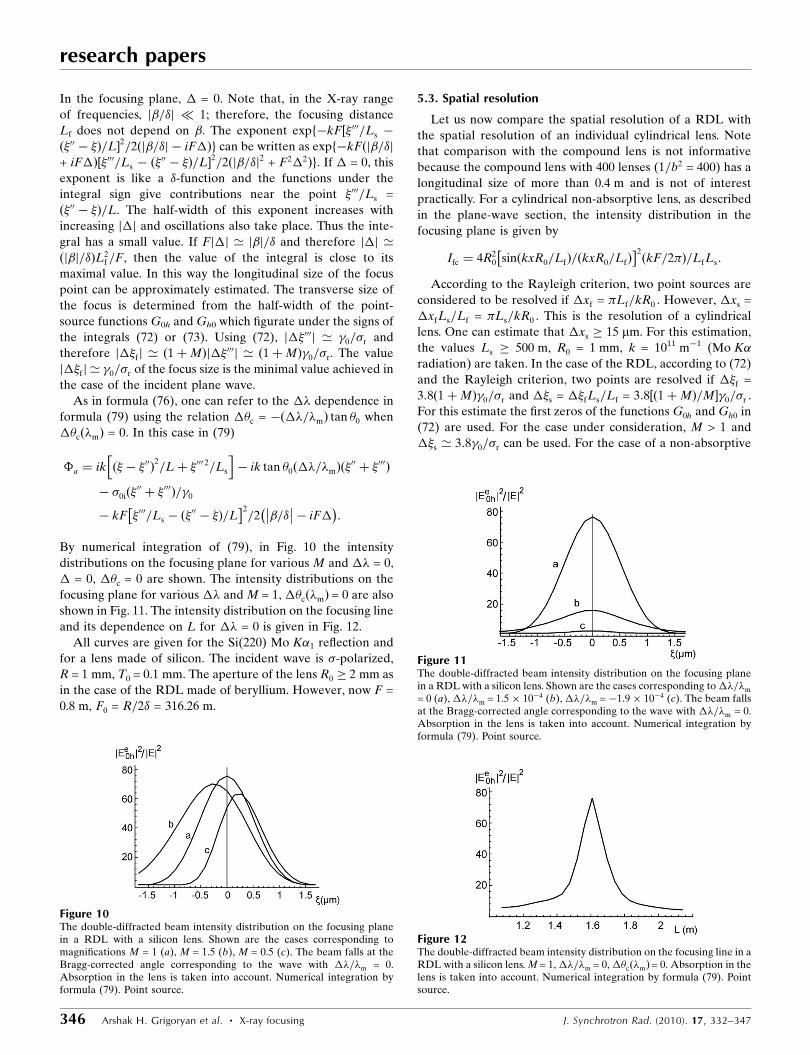
Figure 9The double-diffracted beam intensity distribution on the focusing planein a RDL with a beryllium lens. Shown are the cases corresponding to��=�m = 0 (a), ��=�m = 1.5 � 10�4 (b), ��=�m = �1.9 � 10�4 (c). Thebeam falls at the Bragg-corrected angle corresponding to the wave with��=�m = 0. Absorption in the lens is neglected. M = 1. Numericalintegration by formula (76). Point source.
Figure 8The double-diffracted beam intensity distribution on the focusing planein a RDL with a beryllium lens. Shown are the cases corresponding tomagnifications M = 1 (a), M = 1.5 (b), M = 0.5 (c). The beam falls at theBragg-corrected angle corresponding to the wave with ��=�m = 0.Absorption in the lens is neglected. Numerical integration by formula(76). Point source.
In the focusing plane, � = 0. Note that, in the X-ray range
of frequencies, j�=�j 1; therefore, the focusing distance
Lf does not depend on �. The exponent expf�kF½�000=Ls �
ð�00 � �Þ=L�2=2ðj�=�j � iF�Þg can be written as expf�kFðj�=�j+ iF�Þ½�000=Ls � ð�
00 � �Þ=L�2=2ðj�=�j2 + F2�2Þg. If � = 0, this
exponent is like a �-function and the functions under the
integral sign give contributions near the point �000=Ls =
ð�00 � �Þ=L. The half-width of this exponent increases with
increasing j�j and oscillations also take place. Thus the inte-
gral has a small value. If Fj�j ’ j�j=� and therefore j�j ’ðj�j=�ÞL2
f =F, then the value of the integral is close to its
maximal value. In this way the longitudinal size of the focus
point can be approximately estimated. The transverse size of
the focus is determined from the half-width of the point-
source functions G0h and Gh0 which figurate under the signs of
the integrals (72) or (73). Using (72), j��000j ’ �0=r and
therefore j��fj ’ ð1þMÞj��000j ’ ð1þMÞ�0=r. The value
j��fj ’ �0=r of the focus size is the minimal value achieved in
the case of the incident plane wave.
As in formula (76), one can refer to the �� dependence in
formula (79) using the relation ��c = �ð��=�mÞ tan �0 when
��cð�mÞ = 0. In this case in (79)
�a ¼ ik � � �00ð Þ2=Lþ �000 2=Ls
h i� ik tan �0 ��=�mð Þ �00 þ �000ð Þ
� 0i �00þ �000ð Þ=�0
� kF �000=Ls � �00 � �ð Þ=L� �2
=2 �=� � iF�� �
:
By numerical integration of (79), in Fig. 10 the intensity
distributions on the focusing plane for various M and �� = 0,
� = 0, ��c = 0 are shown. The intensity distributions on the
focusing plane for various �� and M = 1, ��cð�mÞ = 0 are also
shown in Fig. 11. The intensity distribution on the focusing line
and its dependence on L for �� = 0 is given in Fig. 12.
All curves are given for the Si(220) Mo K�1 reflection and
for a lens made of silicon. The incident wave is -polarized,
R = 1 mm, T0 = 0.1 mm. The aperture of the lens R0 � 2 mm as
in the case of the RDL made of beryllium. However, now F =
0.8 m, F0 = R=2� = 316.26 m.
5.3. Spatial resolution
Let us now compare the spatial resolution of a RDL with
the spatial resolution of an individual cylindrical lens. Note
that comparison with the compound lens is not informative
because the compound lens with 400 lenses (1=b2 = 400) has a
longitudinal size of more than 0.4 m and is not of interest
practically. For a cylindrical non-absorptive lens, as described
in the plane-wave section, the intensity distribution in the
focusing plane is given by
Ifc ¼ 4R20 sin kxR0=Lfð Þ= kxR0=Lfð Þ� �2
ðkF=2�Þ=LfLs:
According to the Rayleigh criterion, two point sources are
considered to be resolved if �xf = �Lf=kR0 . However, �xs =
�xfLs=Lf = �Ls=kR0 . This is the resolution of a cylindrical
lens. One can estimate that �xs � 15 mm. For this estimation,
the values Ls � 500 m, R0 = 1 mm, k = 1011 m�1 (Mo K�radiation) are taken. In the case of the RDL, according to (72)
and the Rayleigh criterion, two points are resolved if ��f =
3:8ð1þMÞ�0=r and ��s = ��fLs=Lf = 3:8½ð1þMÞ=M��0=r .
For this estimate the first zeros of the functions G0h and Gh0 in
(72) are used. For the case under consideration, M > 1 and
��s ’ 3:8�0=r can be used. For the case of a non-absorptive
research papers
346 Arshak H. Grigoryan et al. � X-ray focusing J. Synchrotron Rad. (2010). 17, 332–347
Figure 10The double-diffracted beam intensity distribution on the focusing planein a RDL with a silicon lens. Shown are the cases corresponding tomagnifications M = 1 (a), M = 1.5 (b), M = 0.5 (c). The beam falls at theBragg-corrected angle corresponding to the wave with ��=�m = 0.Absorption in the lens is taken into account. Numerical integration byformula (79). Point source.
Figure 11The double-diffracted beam intensity distribution on the focusing planein a RDL with a silicon lens. Shown are the cases corresponding to ��=�m
= 0 (a), ��=�m = 1.5� 10�4 (b), ��=�m =�1.9� 10�4 (c). The beam fallsat the Bragg-corrected angle corresponding to the wave with ��=�m = 0.Absorption in the lens is taken into account. Numerical integration byformula (79). Point source.
Figure 12The double-diffracted beam intensity distribution on the focusing line in aRDL with a silicon lens. M = 1, ��=�m = 0, ��cð�mÞ= 0. Absorption in thelens is taken into account. Numerical integration by formula (79). Pointsource.

lens made of beryllium, for Si220 (Mo K�) radiation and �0 =
0.02 one can estimate ��s = 1.8 mm, i.e. approximately ten
times smaller than for the cylindrical lens with the same
parameters. Here note also that with increasing M the reso-
lution of the RDL stays almost unchanged.
6. Conclusions
The results obtained in this paper can be summarized as
follows.
(i) A one-dimensional focusing X-ray element is proposed.
This element includes two plane parallel asymmetric-cut
crystalline plates and a cylindrical parabolic double-concave
lens placed in the gap between the plates.
(ii) Using the geometric optical method it is shown that the
focal distance of this element is equal to the focal distance of a
separately taken lens multipled by the square of the asym-
metry factor: F ¼ F0b2.
(iii) If b < 1, then F < F0. A practically useful focal distance
can be achieved by taking an appropriate b. For example,
when F0 ’ 400 m and b = 0.05, then F ’ 1 m. In this sense the
RDL is equivalent to an X-ray compound lens with 400 lenses.
(iv) The focus distance of a point source is determined by
the well known thin lens formula 1=Ls þ 1=Lf = 1=F. For two
point sources the reversed image is formed. The magnification
M is determined by the well known optics expression for a thin
lens M = Lf=Ls .
(v) In paraxial approximation the focus point does not
depend on wavelength. The focus distance and focus coordi-
nate on the focusing plane are the same for all wavelengths.
(vi) A one-dimensional focusing RDL can be upgraded to a
two-dimensional focusing element. The use of two RDLs, each
of which focus the beam perpendicular to each other, can
realise two-dimensional focusing. The diffraction vectors h of
the RDLs must lie in the ðK; ezÞ and ðK; eyÞ planes. Here K is
the wavevector of the incident wave, ey is the unit vector,
perpendicular to the plane XOZ. The focus distance and
magnification are defined by the same formulae as described
in (iv).
(vii) For determination of the longitudinal and transverse
sizes of the focus spot, the intensity distribution on the
focusing plane and on the focusing line, and for describing the
imaging of objects, a wave optical theory is necessary. The
wave optical theory for the amplitude of the double-diffracted
beam is given when an arbitrary wave falls on the system.
(viii) This theory is applied for two cases: plane-wave
focusing and imaging of point sources. The formulae obtained
confirm the results (iv) and (v). In addition, it is shown that the
focus size is �1 mm. The angular and spatial resolutions are
given and compared with the resolution of a separately taken
lens.
(ix) The intensity at the point of observation can increase by
two orders.
(x) The losses are determined by absorption in the lens and
in the plates. Besides, the lens can affect the Bragg reflection
from the second plate. The analysis of the transmission coef-
ficient and its dependence on wavelength and other para-
meters is given. It is shown that waves with wavelengths
j��j=� ’ 10�4 can effectively pass through the RDL. The
transmission of the RDL can be close to unity. Note that the
transmission can be up to 0.3 for a compound lens.
(xi) RDLs can be used in X-ray astronomy for imaging of
objects and in X-ray microscopy. They can be used as a
collimator if a point source is placed at the distance F from
the RDL.
In the future it is planned to continue the investigation of
RDLs, particularly the influence of the finite size of the lens on
the focusing, and object imaging will be considered.
References
Born, M. & Wolf, E. (1968). Principles of Optics. Oxford: Pergamon.Gabrielyan, K. T., Chuckhovskii, F. N. & Piskunov, D. I. (1989). J.
Exp. Theor. Phys. 96, 834–846. (In Russian.)Grigoryan, A. H., Balyan, M. K., Gasparyan, L. G. & Agasyan, M. M.
(2004). Proc. Natl Acad. Sci. Armen. 39, 262–265. (In Russian.)Hrdy, J., Mocella, V., Oberta, P., Peverini, L. & Potlovskiy, K. (2006).
J. Synchrotron Rad. 13, 392–396.Lengeler, B., Schroer, C., Tummler, J., Benner, B., Richwin, M.,
Snigirev, A., Snigireva, I. & Drakopoulos, M. (1999). J. SynchrotronRad. 6, 1153–1167.
Pinsker, Z. G. (1982). X-ray Crystalloptics. Moscow: Nauka. (InRussian.)
Takagi, S. (1969). J. Phys. Soc. Jpn, 26, 1239–1248.Uragami, T. (1969). J. Phys. Soc. Jpn, 27, 147–154.
research papers
J. Synchrotron Rad. (2010). 17, 332–347 Arshak H. Grigoryan et al. � X-ray focusing 347