arX

iv:0

911.

0189

v1 [

astr

o-ph

.SR

] 1

Nov

200

9

X-ray Emission and Corona of the Young Intermediate Mass

Binary θ1 Ori E

David P. Huenemoerder1,

Norbert S. Schulz1,

Paola Testa2,

Anthony Kesich3,

& Claude R. Canizares1

Received ; accepted

1Massachusetts Institute of Technology, Kavli Institute for Astrophysics and Space Re-

search, 70 Vassar St., Cambridge, MA, 02139

2Harvard-Smithsonian Center for Astrophysics, 60 Garden St., Cambridge, MA, 02138

3University of California - Davis, One Shields Ave., Davis, CA 95616

– 2 –

ABSTRACT

θ1 Ori E is a young, moderate mass binary system, a rarely observed case of

spectral-type G-giants of about 3 Solar masses, which are still collapsing towards

the main sequence, where they presumably become X-ray faint. We have obtained

high resolution X-ray spectra with Chandra and find that the system is very

active and similar to coronal sources, having emission typical of magnetically

confined plasma: a broad temperature distribution with a hot component and

significant high energy continuum; narrow emission lines from H- and He-like

ions, as well as a range of Fe ions, and relative luminosity, Lx/Lbol = 10−3,

at the saturation limit. Density, while poorly constrained, is consistent with

the low density limits, our upper limits being ne < 1013 cm−3 for Mg xi and

ne < 1012 cm−3 for Ne ix. Coronal elemental abundances are sub-Solar, with

Ne being the highest at about 0.4 times Solar. We find a possible trend in

Trapezium hot plasmas towards low relative abundances of Fe, O, and Ne, which

is hard to explain in terms of the dust depletion scenarios of low-mass young stars.

Variability was unusually low during our observations relative to other coronally

active stars. Qualitatively, the emission is similar to post main-sequence G-

stars. Coronal structures could be compact, or comparable to the dimensions

of the stellar radii. From comparison to X-ray emission from similar mass stars

at various evolutionary epochs, we conclude that the X-rays in θ1 Ori E are

generated by a convective dynamo, present during contraction, but which will

vanish during the main-sequence epoch, and possibly to be resurrected during

post main-sequence evolution.

Subject headings: stars: individual (tet01 Ori E); stars: coronae; stars: pre-main

sequence; X-rays: stars

– 3 –

1. Introduction

Intermediate mass pre-main sequence (PMS) stars, like their massive cousins, are

difficult to study because of their rapid evolutionary time scales. Though not as short as

stars above 8 M⊙ which take less than 105 years to reach the main sequence, intermediate

mass stars between 2M⊙ and 8M⊙ may only take 10–20 Myr. In both cases the accretion

time scales dominate the evolution time to the zero-age main sequence (ZAMS), in contrast

to the low-mass T Tauri stars for which PMS contraction times are longest. Intermediate

mass PMS stars are also not easily found and identified, and most existing studies focus on

Herbig Ae and Be (HAeBe) stars. Herbig stars (Herbig 1960) are recognized as such once

they already contracted to high enough photospheric temperatures to be optically identified

as A and B stars and are thus already close to the ZAMS. Herbig stars mark the transition

between formation mechanisms of low-mass and high-mass stars (Baines et al. 2006).

Herbig Ae stars seem more similar to the low-mass T Tauri stars (Waters & Waelkens

1998; Vink et al. 2005). Herbig Be stars are more similar to embedded young massive stars

(Drew et al. 1997). Both the Ae and Be stars are all already in fairly late PMS stages.

Most studies of Herbig stars use infrared and optical wavelengths to probe their

circumstellar disks and dusty environments. Recent studies suggest that specifically in

HAe stars there is evidence not only for circumstellar disks (Mannings & Sargent 1997;

Grady et al. 1999) but also indications of dust shadowing and settling indicative of dust

grain growth and planetesimal formation (Acke & Waelkens 2004; Dullemond & Dominik

2004; Grady et al. 2005). Some studies also suggest that magnetospheric accretion

analogous to classical T Tauri stars is possible (Muzerolle et al. 2004; Grady et al. 2004;

Guimaraes et al. 2006). Recent modeling of 37 Herbig Ae/Fe stars using UV spectra

revealed that all but one show indications of accretion with accretion rates in many cases

substantially exceeding 10−8 M⊙yr−1 (Blondel & Djie 2006).

– 4 –

Binarity also seems to be an important attribute in the formation and evolution of

intermediate mass stars. In a sample of 28 HAeBe stars, Baines et al. (2006) find a binarity

fraction of almost 70% with a higher binary frequency in HBe stars than in HAe stars. HAe

stars with close companions also seem to lack circumstellar disks (Grady et al. 2005).

X-ray studies of young intermediate mass stars are still quite rare and to date

also focus almost entirely on HAe stars. Systematic studies have shown that these

are moderately bright in X-rays (Damiani et al. 1994; Zinnecker & Preibisch 1994;

Hamaguchi, Yamauchi & Koyama 2005; Stelzer et al. 2006b). This fact is already quite

remarkable since main sequence A-stars lack strong winds or coronae and it suggests

that the physical characteristics of HAe stars stars differ from those of main sequence

A- and B-stars. Mechanisms suggested range from active accretion to coronal activity to

some other form of plasma confinement. It is also possible, given the high frequency of

binaries among HAeBe stars, that some X-ray sources could be due to late-type companions

(Stelzer et al. 2006a,b). A detailed summary can be found in a recent Chandra high

resolution spectroscopic study of the HAe star HD 104237 in the ǫ Chamaeleontis Group

(Testa et al. 2008).

In this paper we focus on X-ray emission from θ1 Ori E, which was recently determined

to be an intermediate mass binary star. The Orion Trapezium is generally known for its

ensemble of the nearest and youngest massive stars (Schulz et al. 2001, 2003; Stelzer et al.

2005). Recent studies now suggest the presence of several intermediate mass stars. θ2 Ori

A harbors the second most massive O-star of the Trapezium, but also two unidentified

intermediate mass stars both between 3M⊙ and 7M⊙ (Preibisch et al. 1999). The system

is particularly interesting in X-rays for its high luminosity and hard spectral properties

as well as giant hard X-ray outbursts (Feigelson et al. 2002; Schulz et al. 2006). Plasma

temperatures during these outbursts exceed 108K (Schulz et al. 2006). While the latter

– 5 –

authors suggested a possible link of these outbursts to binary interactions involving the

closer intermediate mass companion, there is also some evidence that these may be

connected to the more distant companion (M. Gagne, private communication).

θ1 Ori E is another system now known to contain young intermediate mass stars. It was

long misidentified as B5 to B8 spectral type (Parenago 1954; Herbig 1960). Herbig & Griffin

(2006) obtained optical spectroscopic radial velocity measurements and identified the

system as a binary containing two G III type stars of masses of about 3–4 M⊙ in a 9.9

day orbit. Evolutionary tracks constrain the age of the system to 0.5–1.0 Myr making the

components of θ1 Ori E some of the youngest intermediate mass PMS stars known and far

younger than stars in the HAeBe phase. θ1 Ori E is not among the optically brightest stars

in the Trapezium, but has long been recognized as the second brightest Trapezium source

in X-rays (Ku, Righini-Cohen & Simon 1982; Gagne & Caillault 1994; Schulz et al. 2001).

The Chandra Orion Ultradeep Project (COUP) observed θ1 Ori E (COUP 732) for a total

exposure of about 10 days over a time period of 3 weeks and found a low level of variability

including one moderate X-ray flare (Stelzer et al. 2005). Its luminosity during COUP was

determined to be log Lx[ergs s−1] = 32.4; early Chandra High Energy Transmission Grating

(HETG) spectra indicated plasma temperatures of up to 50 MK (Schulz et al. 2003).

The HETG Orion Legacy Project has now accumulated almost 4 days of total exposure

of θ1 Ori E allowing for an in depth study of its X-ray spectral properties. The following

analysis of θ1 Ori E’s high resolution X-ray spectrum is aimed to characterize its coronal

nature. The existence of coronal X-rays confirms predictions that very young intermediate

mass stars of less than 4M⊙ are not fully radiative (Palla & Stahler 1993) and may possess

some form of magnetic dynamo. We also compare these properties with the ones observed

in θ2 Ori A, various T Tauri stars including the relatively massive T Tauri star, SU Aur

(2M⊙), active coronal sources, and post-main sequence evolved G-type giants. The optical

– 6 –

and binary system parameters of θ1 Ori E can be found in Herbig & Griffin (2006).

2. Observations and Analysis

2.1. Observations, Data Processing

As part of the HETGS Orion Legacy Project, we have observed θ1 Ori E on 11

separate occasions from 1999 through 2007, mostly within our HETG Guaranteed Time

program, with individual exposure times ranging from about 10 to 50 ks. The HETGS

(Canizares et al. 2005) is an objective transmission grating spectrometer with two channels

optimized for high and medium energies (HEG and MEG, respectively). The HEG and

MEG spectra of each point source in the field form a shallow “×” centered on the zeroth

order image. Since the Orion Trapezium field is crowded, we had to take special care to

avoid source confusion when possible, and to assess contamination and reject spectra when

not. The range in spacecraft roll angles, the redundancy provided by multiple gratings and

orders, the narrow point-spread-function, and the efficiency of order-sorting with the CCD

energy resolution all help to provide a reliable spectrum.

We processed the data with CIAO 3.4 (Fruscione et al. 2006) taking care to fine-tune

the zero order detection to accurately center on θ1 Ori E. Response files were made with the

most recent calibration database available at the time (version 3.4). Further analysis was

done using ISIS (Houck & Denicola 2000), an Interactive Spectral Interpretation System for

high resolution X-ray spectroscopy, developed especially for scriptable, extensible analysis

of Chandra high resolution spectra.

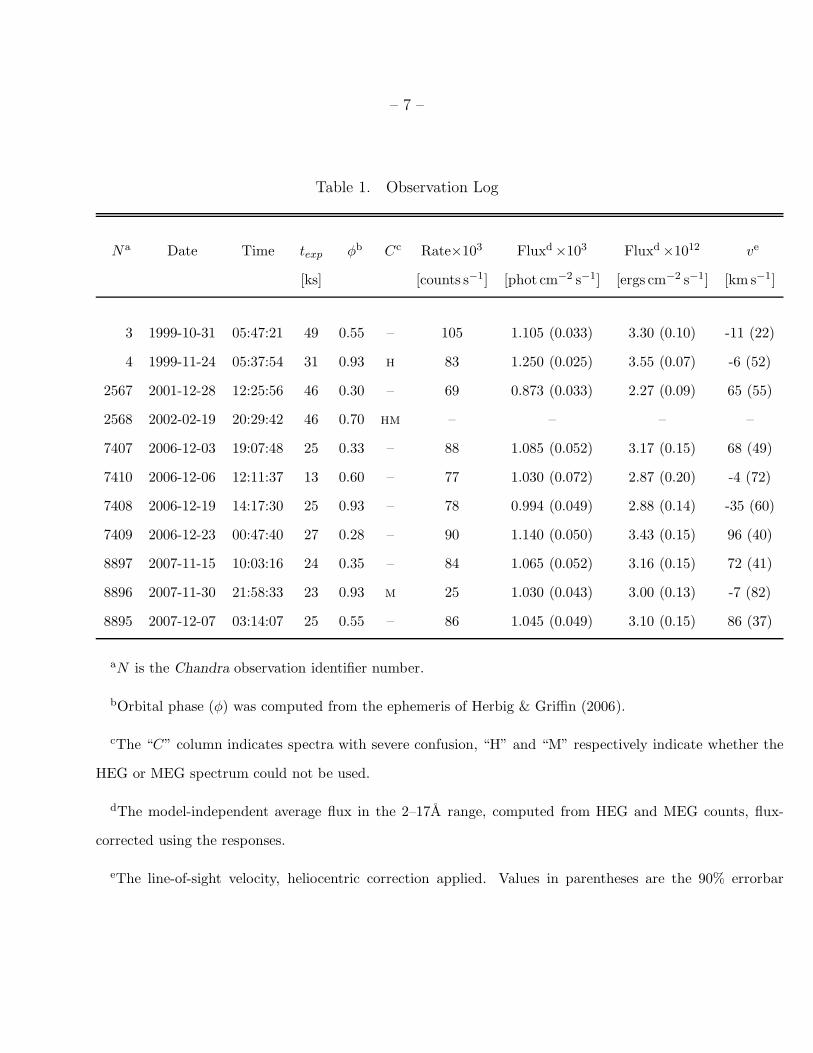
We give an observing log in Table 1, along with ancillary information and some derived

properties of each observation.

– 7 –

Table 1. Observation Log

Na Date Time texp φb Cc Rate×103 Fluxd ×103 Fluxd ×1012 ve

[ks] [counts s−1] [phot cm−2 s−1] [ergs cm−2 s−1] [km s−1]

3 1999-10-31 05:47:21 49 0.55 – 105 1.105 (0.033) 3.30 (0.10) -11 (22)

4 1999-11-24 05:37:54 31 0.93 h 83 1.250 (0.025) 3.55 (0.07) -6 (52)

2567 2001-12-28 12:25:56 46 0.30 – 69 0.873 (0.033) 2.27 (0.09) 65 (55)

2568 2002-02-19 20:29:42 46 0.70 hm – – – –

7407 2006-12-03 19:07:48 25 0.33 – 88 1.085 (0.052) 3.17 (0.15) 68 (49)

7410 2006-12-06 12:11:37 13 0.60 – 77 1.030 (0.072) 2.87 (0.20) -4 (72)

7408 2006-12-19 14:17:30 25 0.93 – 78 0.994 (0.049) 2.88 (0.14) -35 (60)

7409 2006-12-23 00:47:40 27 0.28 – 90 1.140 (0.050) 3.43 (0.15) 96 (40)

8897 2007-11-15 10:03:16 24 0.35 – 84 1.065 (0.052) 3.16 (0.15) 72 (41)

8896 2007-11-30 21:58:33 23 0.93 m 25 1.030 (0.043) 3.00 (0.13) -7 (82)

8895 2007-12-07 03:14:07 25 0.55 – 86 1.045 (0.049) 3.10 (0.15) 86 (37)

aN is the Chandra observation identifier number.

bOrbital phase (φ) was computed from the ephemeris of Herbig & Griffin (2006).

cThe “C” column indicates spectra with severe confusion, “H” and “M” respectively indicate whether the

HEG or MEG spectrum could not be used.

dThe model-independent average flux in the 2–17A range, computed from HEG and MEG counts, flux-

corrected using the responses.

eThe line-of-sight velocity, heliocentric correction applied. Values in parentheses are the 90% errorbar

– 8 –

(∼ 1.6σ). See Section 2.4.1 for explanation.

– 9 –

2.2. Source Confusion

To assess confusion in detail, we used two techniques. For field source zeroth-order

coincidence with the diffracted spectra of θ1 Ori E, we used the COUP (Getman et al.

2005) source list, and for each observation we transformed the list’s celestial coordinates to

the diffraction coordinate system for θ1 Ori E. We did not find any source on the spectral

regions with significant counts.

The second technique assessed the contamination from sources near the zeroth order,

such that their diffracted spectra would overlap with the HEG or MEG spectra of θ1 Ori E,

and so close to the zeroth order that the order-sorting by CCD energy would distinguish

orders. For this, it was crucial to inspect the events’ distribution as selected from the

θ1 Ori E default binning region (cross-dispersion region half width of 6.6 × 10−4 deg) in

diffraction distance versus energy (the CCD blurred energy) coordinates in which zeroth

orders appear as vertical distributions and diffracted photons as hyperbolas. Here we found

significant contamination for a few observations and had to reject all or some orders.

The useful exposure from which we can extract spectra, light curves, and line fluxes

totals to 260 ks. Rejected orders or observations are flagged in Table 1. A cumulative

counts spectrum is shown in Figure 1.

2.3. Light Curves, Variability

There was little variability of any significance within any observation. The MEG rate

was about 0.05 counts/s. Variations within each observation were consistent with statistical

uncertainties — no abrupt increases or slow decays characteristic of coronal flares occurred.

Observation to observation, there was also no variability, except for one which had a

significantly lower count rate than the others. We show the mean flux rate per observation

– 10 –0

2×10

−4

4×10

−4

6×10

−4

8×10

−4

Phot

ons

cm−

2 s−

1 Å

−1

5 10 15

−2

02

χ

Wavelength (Å)

Fe

XV

II

Fe

XV

II

Fe

XX

IVF

e X

XIV

Ar

XV

II

O V

III

O V

III O

VIII

Si X

IVS

i XIV

Si X

III

Fe

XX

VF

e X

XV

Fe

XIX

Fe

XIX

Fe

XX

II

Fe

XX

IIF

e X

XF

e X

X

Mg

XII

Mg

XII

Mg

XI

Ne

X

Ne

XN

e X

Ne

IX

S X

VI

S X

V

Fe

XX

I

Fe

XX

I

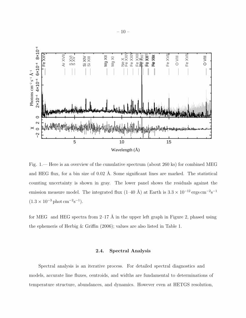
Fig. 1.— Here is an overview of the cumulative spectrum (about 260 ks) for combined MEG

and HEG flux, for a bin size of 0.02 A. Some significant lines are marked. The statistical

counting uncertainty is shown in gray. The lower panel shows the residuals against the

emission measure model. The integrated flux (1–40 A) at Earth is 3.3 × 10−12 ergs cm−2s−1

(1.3 × 10−3 phot cm−2s−1).

for MEG and HEG spectra from 2–17 A in the upper left graph in Figure 2, phased using

the ephemeris of Herbig & Griffin (2006); values are also listed in Table 1.

2.4. Spectral Analysis

Spectral analysis is an iterative process. For detailed spectral diagnostics and

models, accurate line fluxes, centroids, and widths are fundamental to determinations of

temperature structure, abundances, and dynamics. However even at HETGS resolution,

– 11 –

we are dependent upon plasma models for accurate estimation of the continuum and for

assessment of blending. We base our spectral models on the Astrophysical Plasma Emission

Database (APED; Smith et al. 2001), ionization balance of Mazzotta et al. (1998), and

abundances of Anders & Grevesse (1989). We begin by fitting a one-temperature component

model to the short wavelength continuum, then add one or two more components to get

a reasonable match to the continuum throughout the spectrum, ignoring strong lines in

the process. Next we fit about 100 lines parametrically with unresolved Gaussians folded

through the instrumental response, using the line-free plasma model for the local continuum.

To improve the statistic per bin, we group the spectra by 2–4 bins and we combined the

MEG first orders and combined the HEG first orders, both over all observations, then

fit the MEG and HEG jointly. (The default binning oversamples the HEG and MEG

resolutions by a factor of two, or 0.0025 A and 0.005 A, respectively.) Combination of

spectra is done dynamically — each effective area and redistribution matrix are distinct,

and summed counts are compared with the summed folded models to compute the statistic.

We adopted an interstellar absorption column of NH = 2 × 1021 cm−2 as determined by

Schulz et al. (2001). For some weak lines, we froze the wavelength at the theoretical value.

This allows us to obtain a limit on the flux which can provide important constraints on

emission measure and abundance reconstruction.

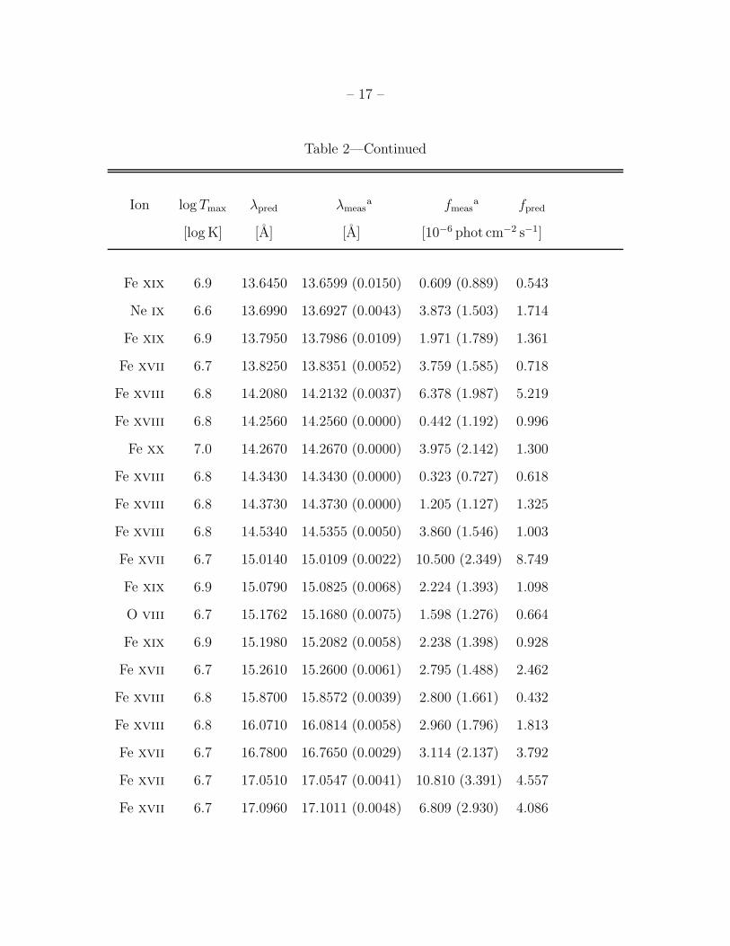
After we have mean line fluxes and centroids for a variety of elements and ions (see

Table 2), we can reconstruct the emission measure distribution assuming that the plasma

has uniform abundances and is in collisional ionization equilibrium. We use a uniform

logarithmic temperature grid and minimize the line flux residuals by adjusting the weights

in each temperature bin as well as the elemental abundances. Since this is an ill-conditioned

problem, we impose a smoothness on the emission measure by using its sum-squared second

derivative in a penalty function.

– 12 –

Emission measure reconstruction is also an iterative process. First we ignore lines with

large wavelength residuals relative to their preliminary identification based on expectations

of a baseline plasma model, since they are likely misidentified or blended. Then we

reconstruct a trial emission measure distribution. Lines with large flux residuals are

rejected, since they may be symptomatic of unresolved blends or inaccurate emissivities

due to uncertainties in the underlying atomic data. We repeat the fit with the accepted

lines. We use the emission measure and abundance model to generate a synthetic spectrum

and compare to the observed spectrum. Here we can adjust the line-to-continuum ratio

by adjusting the normalizations of the emission measure and relative abundances. If the

continuum model was improved, we start over by fitting the lines with the improved

continuum. Finally, we perform a Monte-Carlo series of fits in which we let the measured

line flux vary randomly according to its measured uncertainty. This provides an estimate of

the uncertainty on the emission measure and the abundances.

– 13 –2

2.5

33.

54

Flu

x [1

0−12

erg

s/cm

2 /s]

0 0.2 0.4 0.6 0.8 1−10

0−

500

5010

0V

eloc

ity [k

m/s

]

Orbital Phase

0 2×10−4 4×10−4

010

020

030

0

∆ v/c

v turb [k

m/s

]

high ∆ v

low ∆ v

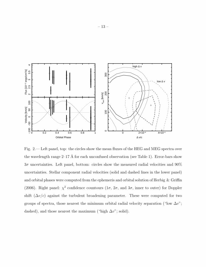
Fig. 2.— Left panel, top: the circles show the mean fluxes of the HEG and MEG spectra over

the wavelength range 2–17 A for each unconfused observation (see Table 1). Error-bars show

3σ uncertainties. Left panel, bottom: circles show the measured radial velocities and 90%

uncertainties. Stellar component radial velocities (solid and dashed lines in the lower panel)

and orbital phases were computed from the ephemeris and orbital solution of Herbig & Griffin

(2006). Right panel: χ2 confidence countours (1σ, 2σ, and 3σ, inner to outer) for Doppler

shift (∆v/c) against the turbulent broadening parameter. These were computed for two

groups of spectra, those nearest the minimum orbital radial velocity separation (“low ∆v”;

dashed), and those nearest the maximum (“high ∆v”; solid).

– 14 –

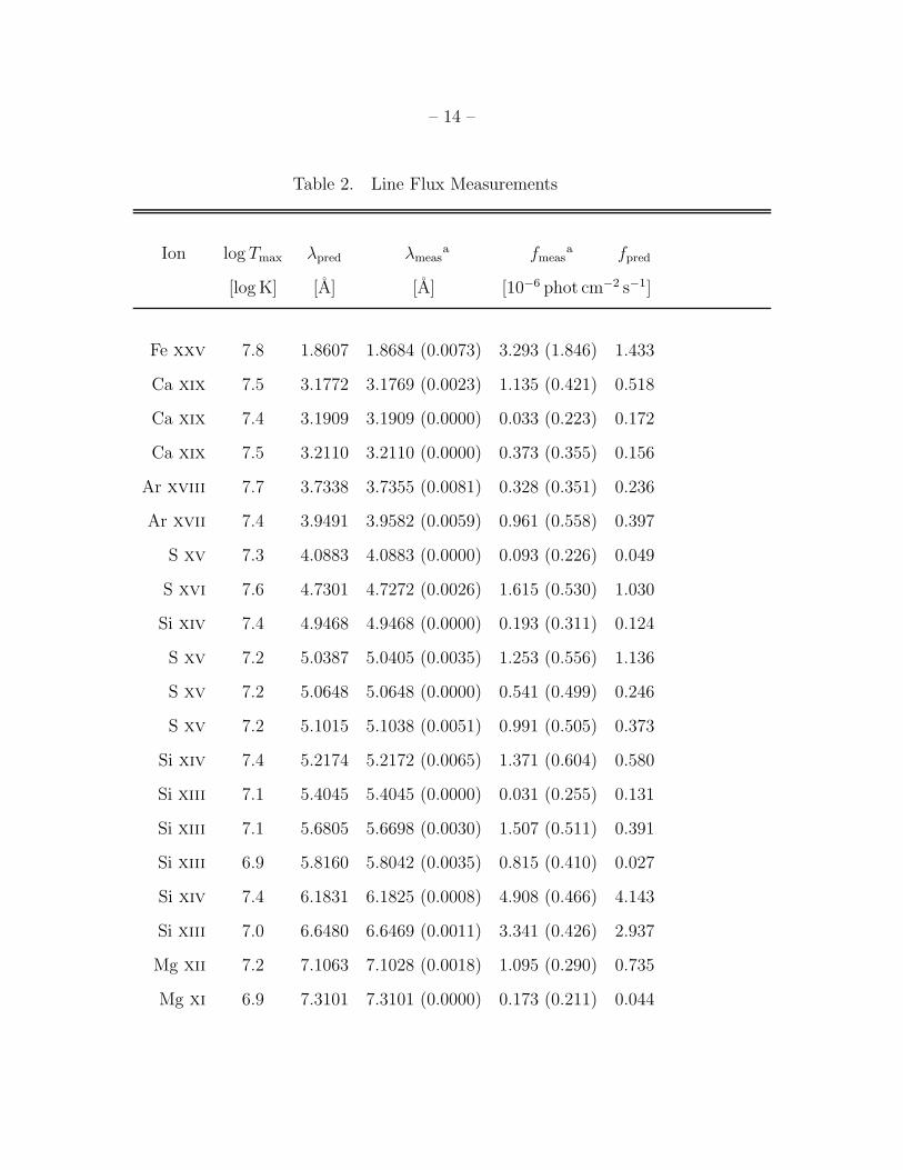
Table 2. Line Flux Measurements

Ion log Tmax λpred λmeasa fmeas

a fpred

[log K] [A] [A] [10−6 phot cm−2 s−1]

Fe xxv 7.8 1.8607 1.8684 (0.0073) 3.293 (1.846) 1.433

Ca xix 7.5 3.1772 3.1769 (0.0023) 1.135 (0.421) 0.518

Ca xix 7.4 3.1909 3.1909 (0.0000) 0.033 (0.223) 0.172

Ca xix 7.5 3.2110 3.2110 (0.0000) 0.373 (0.355) 0.156

Ar xviii 7.7 3.7338 3.7355 (0.0081) 0.328 (0.351) 0.236

Ar xvii 7.4 3.9491 3.9582 (0.0059) 0.961 (0.558) 0.397

S xv 7.3 4.0883 4.0883 (0.0000) 0.093 (0.226) 0.049

S xvi 7.6 4.7301 4.7272 (0.0026) 1.615 (0.530) 1.030

Si xiv 7.4 4.9468 4.9468 (0.0000) 0.193 (0.311) 0.124

S xv 7.2 5.0387 5.0405 (0.0035) 1.253 (0.556) 1.136

S xv 7.2 5.0648 5.0648 (0.0000) 0.541 (0.499) 0.246

S xv 7.2 5.1015 5.1038 (0.0051) 0.991 (0.505) 0.373

Si xiv 7.4 5.2174 5.2172 (0.0065) 1.371 (0.604) 0.580

Si xiii 7.1 5.4045 5.4045 (0.0000) 0.031 (0.255) 0.131

Si xiii 7.1 5.6805 5.6698 (0.0030) 1.507 (0.511) 0.391

Si xiii 6.9 5.8160 5.8042 (0.0035) 0.815 (0.410) 0.027

Si xiv 7.4 6.1831 6.1825 (0.0008) 4.908 (0.466) 4.143

Si xiii 7.0 6.6480 6.6469 (0.0011) 3.341 (0.426) 2.937

Mg xii 7.2 7.1063 7.1028 (0.0018) 1.095 (0.290) 0.735

Mg xi 6.9 7.3101 7.3101 (0.0000) 0.173 (0.211) 0.044

– 15 –

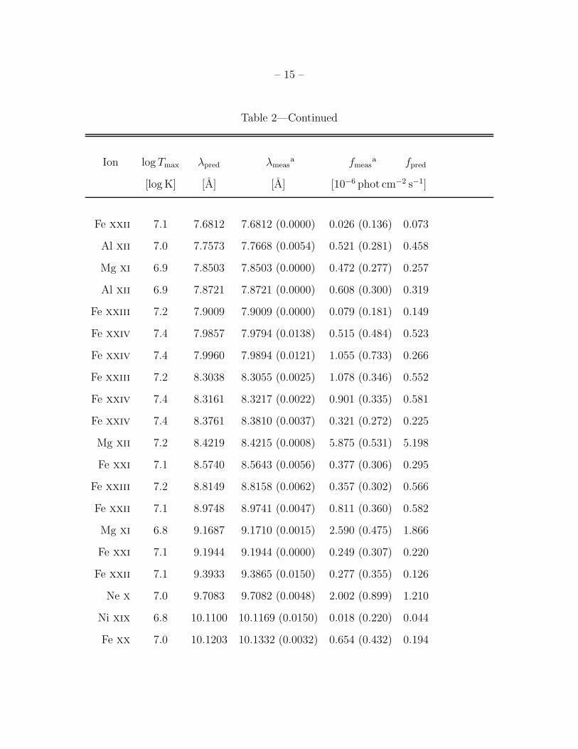
Table 2—Continued

Ion log Tmax λpred λmeasa fmeas

a fpred

[log K] [A] [A] [10−6 phot cm−2 s−1]

Fe xxii 7.1 7.6812 7.6812 (0.0000) 0.026 (0.136) 0.073

Al xii 7.0 7.7573 7.7668 (0.0054) 0.521 (0.281) 0.458

Mg xi 6.9 7.8503 7.8503 (0.0000) 0.472 (0.277) 0.257

Al xii 6.9 7.8721 7.8721 (0.0000) 0.608 (0.300) 0.319

Fe xxiii 7.2 7.9009 7.9009 (0.0000) 0.079 (0.181) 0.149

Fe xxiv 7.4 7.9857 7.9794 (0.0138) 0.515 (0.484) 0.523

Fe xxiv 7.4 7.9960 7.9894 (0.0121) 1.055 (0.733) 0.266

Fe xxiii 7.2 8.3038 8.3055 (0.0025) 1.078 (0.346) 0.552

Fe xxiv 7.4 8.3161 8.3217 (0.0022) 0.901 (0.335) 0.581

Fe xxiv 7.4 8.3761 8.3810 (0.0037) 0.321 (0.272) 0.225

Mg xii 7.2 8.4219 8.4215 (0.0008) 5.875 (0.531) 5.198

Fe xxi 7.1 8.5740 8.5643 (0.0056) 0.377 (0.306) 0.295

Fe xxiii 7.2 8.8149 8.8158 (0.0062) 0.357 (0.302) 0.566

Fe xxii 7.1 8.9748 8.9741 (0.0047) 0.811 (0.360) 0.582

Mg xi 6.8 9.1687 9.1710 (0.0015) 2.590 (0.475) 1.866

Fe xxi 7.1 9.1944 9.1944 (0.0000) 0.249 (0.307) 0.220

Fe xxii 7.1 9.3933 9.3865 (0.0150) 0.277 (0.355) 0.126

Ne x 7.0 9.7083 9.7082 (0.0048) 2.002 (0.899) 1.210

Ni xix 6.8 10.1100 10.1169 (0.0150) 0.018 (0.220) 0.044

Fe xx 7.0 10.1203 10.1332 (0.0032) 0.654 (0.432) 0.194

– 16 –

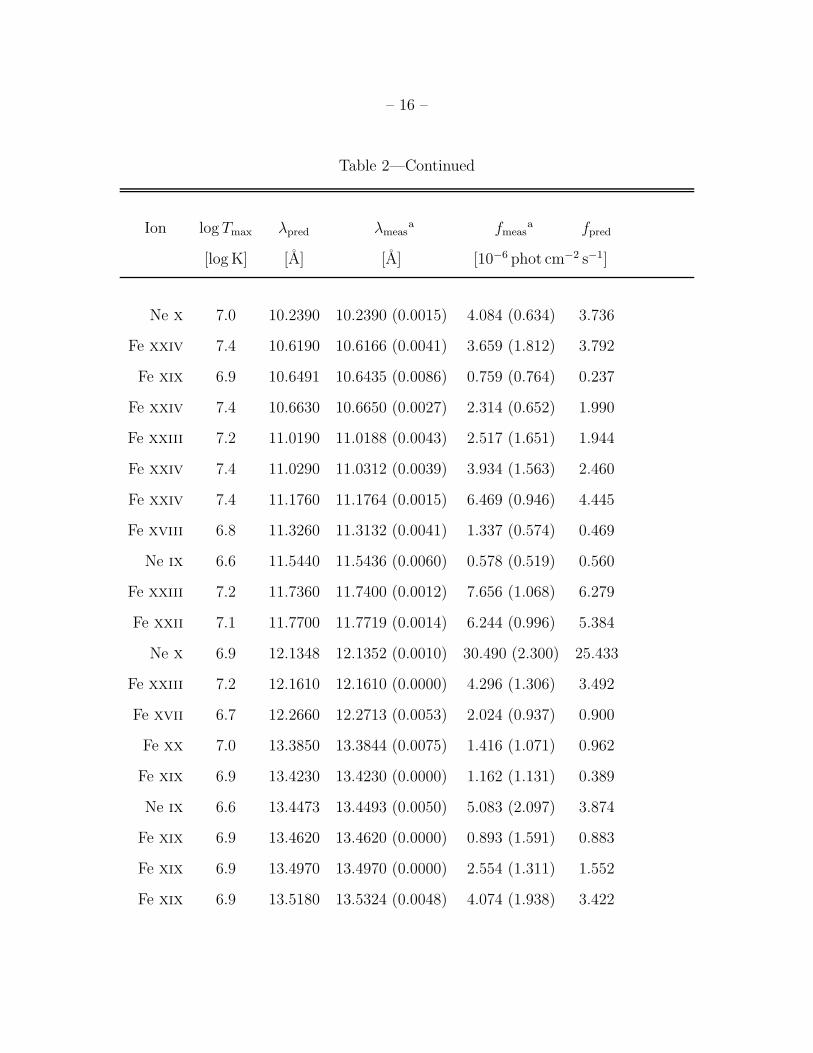
Table 2—Continued

Ion log Tmax λpred λmeasa fmeas

a fpred

[log K] [A] [A] [10−6 phot cm−2 s−1]

Ne x 7.0 10.2390 10.2390 (0.0015) 4.084 (0.634) 3.736

Fe xxiv 7.4 10.6190 10.6166 (0.0041) 3.659 (1.812) 3.792

Fe xix 6.9 10.6491 10.6435 (0.0086) 0.759 (0.764) 0.237

Fe xxiv 7.4 10.6630 10.6650 (0.0027) 2.314 (0.652) 1.990

Fe xxiii 7.2 11.0190 11.0188 (0.0043) 2.517 (1.651) 1.944

Fe xxiv 7.4 11.0290 11.0312 (0.0039) 3.934 (1.563) 2.460

Fe xxiv 7.4 11.1760 11.1764 (0.0015) 6.469 (0.946) 4.445

Fe xviii 6.8 11.3260 11.3132 (0.0041) 1.337 (0.574) 0.469

Ne ix 6.6 11.5440 11.5436 (0.0060) 0.578 (0.519) 0.560

Fe xxiii 7.2 11.7360 11.7400 (0.0012) 7.656 (1.068) 6.279

Fe xxii 7.1 11.7700 11.7719 (0.0014) 6.244 (0.996) 5.384

Ne x 6.9 12.1348 12.1352 (0.0010) 30.490 (2.300) 25.433

Fe xxiii 7.2 12.1610 12.1610 (0.0000) 4.296 (1.306) 3.492

Fe xvii 6.7 12.2660 12.2713 (0.0053) 2.024 (0.937) 0.900

Fe xx 7.0 13.3850 13.3844 (0.0075) 1.416 (1.071) 0.962

Fe xix 6.9 13.4230 13.4230 (0.0000) 1.162 (1.131) 0.389

Ne ix 6.6 13.4473 13.4493 (0.0050) 5.083 (2.097) 3.874

Fe xix 6.9 13.4620 13.4620 (0.0000) 0.893 (1.591) 0.883

Fe xix 6.9 13.4970 13.4970 (0.0000) 2.554 (1.311) 1.552

Fe xix 6.9 13.5180 13.5324 (0.0048) 4.074 (1.938) 3.422

– 17 –

Table 2—Continued

Ion log Tmax λpred λmeasa fmeas

a fpred

[log K] [A] [A] [10−6 phot cm−2 s−1]

Fe xix 6.9 13.6450 13.6599 (0.0150) 0.609 (0.889) 0.543

Ne ix 6.6 13.6990 13.6927 (0.0043) 3.873 (1.503) 1.714

Fe xix 6.9 13.7950 13.7986 (0.0109) 1.971 (1.789) 1.361

Fe xvii 6.7 13.8250 13.8351 (0.0052) 3.759 (1.585) 0.718

Fe xviii 6.8 14.2080 14.2132 (0.0037) 6.378 (1.987) 5.219

Fe xviii 6.8 14.2560 14.2560 (0.0000) 0.442 (1.192) 0.996

Fe xx 7.0 14.2670 14.2670 (0.0000) 3.975 (2.142) 1.300

Fe xviii 6.8 14.3430 14.3430 (0.0000) 0.323 (0.727) 0.618

Fe xviii 6.8 14.3730 14.3730 (0.0000) 1.205 (1.127) 1.325

Fe xviii 6.8 14.5340 14.5355 (0.0050) 3.860 (1.546) 1.003

Fe xvii 6.7 15.0140 15.0109 (0.0022) 10.500 (2.349) 8.749

Fe xix 6.9 15.0790 15.0825 (0.0068) 2.224 (1.393) 1.098

O viii 6.7 15.1762 15.1680 (0.0075) 1.598 (1.276) 0.664

Fe xix 6.9 15.1980 15.2082 (0.0058) 2.238 (1.398) 0.928

Fe xvii 6.7 15.2610 15.2600 (0.0061) 2.795 (1.488) 2.462

Fe xviii 6.8 15.8700 15.8572 (0.0039) 2.800 (1.661) 0.432

Fe xviii 6.8 16.0710 16.0814 (0.0058) 2.960 (1.796) 1.813

Fe xvii 6.7 16.7800 16.7650 (0.0029) 3.114 (2.137) 3.792

Fe xvii 6.7 17.0510 17.0547 (0.0041) 10.810 (3.391) 4.557

Fe xvii 6.7 17.0960 17.1011 (0.0048) 6.809 (2.930) 4.086

– 18 –

Table 2—Continued

Ion log Tmax λpred λmeasa fmeas

a fpred

[log K] [A] [A] [10−6 phot cm−2 s−1]

Fe xviii 6.8 17.6230 17.6080 (0.0025) 4.326 (2.586) 1.323

O vii 6.4 17.7680 17.7680 (0.0000) 0.300 (0.315) 0.041

O vii 6.4 18.6270 18.6270 (0.0000) 0.900 (0.926) 0.123

O viii 6.7 18.9698 18.9744 (0.0043) 17.680 (5.846) 13.292

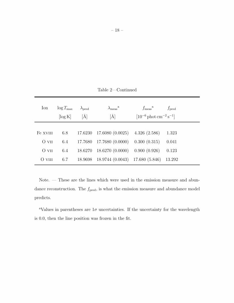
Note. — These are the lines which were used in the emission measure and abun-

dance reconstruction. The fpred, is what the emission measure and abundance model

predicts.

aValues in parentheses are 1σ uncertainties. If the uncertainty for the wavelength

is 0.0, then the line position was frozen in the fit.

– 19 –

We have applied this technique to several other spectra (e.g., see Huenemoerder et al.

2007, and references therein). Given the form of the problem there is no unique solution.

However, results can be useful for comparison of emission measures derived with similar

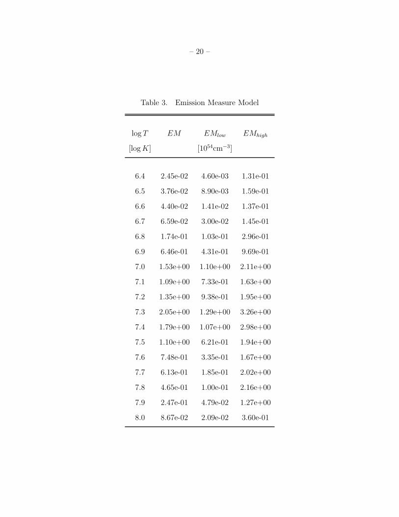
methods. Figure 3 shows our reconstructed emission measure distribution whose values are

also given in Table 3. The corresponding abundances are shown in Figure 4 and are listed

in Table 4.

– 20 –

Table 3. Emission Measure Model

log T EM EMlow EMhigh

[log K] [1054cm−3]

6.4 2.45e-02 4.60e-03 1.31e-01

6.5 3.76e-02 8.90e-03 1.59e-01

6.6 4.40e-02 1.41e-02 1.37e-01

6.7 6.59e-02 3.00e-02 1.45e-01

6.8 1.74e-01 1.03e-01 2.96e-01

6.9 6.46e-01 4.31e-01 9.69e-01

7.0 1.53e+00 1.10e+00 2.11e+00

7.1 1.09e+00 7.33e-01 1.63e+00

7.2 1.35e+00 9.38e-01 1.95e+00

7.3 2.05e+00 1.29e+00 3.26e+00

7.4 1.79e+00 1.07e+00 2.98e+00

7.5 1.10e+00 6.21e-01 1.94e+00

7.6 7.48e-01 3.35e-01 1.67e+00

7.7 6.13e-01 1.85e-01 2.02e+00

7.8 4.65e-01 1.00e-01 2.16e+00

7.9 2.47e-01 4.79e-02 1.27e+00

8.0 8.67e-02 2.09e-02 3.60e-01

– 21 –

Note. — The reconstructed emission mea-

sure over the temperature range of sensitive

features. The “low” and “high” values are the

logarithmic 1σ boundaries from Monte-Carlo

iterations.

– 22 –

6.5 7 7.5 8

01

23

Log T

Em

issi

on M

easu

re [1

054 c

m−

3 ]

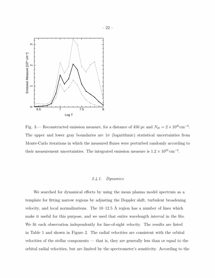
Fig. 3.— Reconstructed emission measure, for a distance of 450 pc and NH = 2× 1021cm−2.

The upper and lower gray boundaries are 1σ (logarithmic) statistical uncertainties from

Monte-Carlo iterations in which the measured fluxes were perturbed randomly according to

their measurement uncertainties. The integrated emission measure is 1.2 × 1055 cm−3.

2.4.1. Dynamics

We searched for dynamical effects by using the mean plasma model spectrum as a

template for fitting narrow regions by adjusting the Doppler shift, turbulent broadening

velocity, and local normalizations. The 10–12.5 A region has a number of lines which

make it useful for this purpose, and we used that entire wavelength interval in the fits.

We fit each observation independently for line-of-sight velocity. The results are listed

in Table 1 and shown in Figure 2. The radial velocities are consistent with the orbital

velocities of the stellar components — that is, they are generally less than or equal to the

orbital radial velocities, but are limited by the spectrometer’s sensitivity. According to the

– 23 –

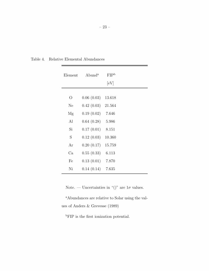
Table 4. Relative Elemental Abundances

Element Abunda FIPb

[eV]

O 0.06 (0.03) 13.618

Ne 0.42 (0.03) 21.564

Mg 0.19 (0.02) 7.646

Al 0.64 (0.28) 5.986

Si 0.17 (0.01) 8.151

S 0.12 (0.03) 10.360

Ar 0.20 (0.17) 15.759

Ca 0.55 (0.33) 6.113

Fe 0.13 (0.01) 7.870

Ni 0.14 (0.14) 7.635

Note. — Uncertainties in “()” are 1σ values.

aAbundances are relative to Solar using the val-

ues of Anders & Grevesse (1989)

bFIP is the first ionization potential.

– 24 –

105 20

0.1

10.

050.

20.

52

FIP [eV]

Rel

ativ

e A

bund

ance

O

Ne

Mg

Al

Si

S

Ar

Ca

Fe

Ni

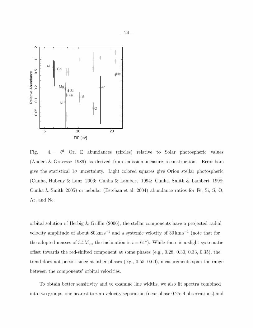
Fig. 4.— θ1 Ori E abundances (circles) relative to Solar photospheric values

(Anders & Grevesse 1989) as derived from emission measure reconstruction. Error-bars

give the statistical 1σ uncertainty. Light colored squares give Orion stellar photospheric

(Cunha, Hubeny & Lanz 2006; Cunha & Lambert 1994; Cunha, Smith & Lambert 1998;

Cunha & Smith 2005) or nebular (Esteban et al. 2004) abundance ratios for Fe, Si, S, O,

Ar, and Ne.

orbital solution of Herbig & Griffin (2006), the stellar components have a projected radial

velocity amplitude of about 80 km s−1 and a systemic velocity of 30 km s−1 (note that for

the adopted masses of 3.5M⊙, the inclination is i = 61◦). While there is a slight systematic

offset towards the red-shifted component at some phases (e.g., 0.28, 0.30, 0.33, 0.35), the

trend does not persist since at other phases (e.g., 0.55, 0.60), measurements span the range

between the components’ orbital velocities.

To obtain better sensitivity and to examine line widths, we also fit spectra combined

into two groups, one nearest to zero velocity separation (near phase 0.25; 4 observations) and

– 25 –

the other nearest to maximum velocity separation (near phase 0.5 or 1.0; 6 observations).

We computed contour maps in line-of-sight and turbulent broadening velocities. The

point of this is not that we necessarily expect turbulent broadening, but that there could

be broadening due to binary orbital effects, and fitting turbulent broadening is simply a

useful parameterization of this. For instance, for equally X-ray bright stars, the X-ray

line’s measured radial velocity could always be zero (or the systemic value), but the lines

could broaden and narrow, modulated by the orbital radial velocity. If only one star

were the X-ray source, the lines could shift but maintain constant width. Since we are

photon-limited, we need to group spectra in order to obtain significant counting statistics.

The resulting confidence contours are shown in Figure 2. We see the radial velocity

offset towards a small positive velocity as we should in the low-∆v group at a level of

about 30–120 km s−1 (or ∆v/c ∼ 1–4 × 10−4; 90% confidence limits), while the high-∆v

group range is −60 to 60 km s−1. Broadening is marginally significant with 90% confidence

contours of 60 – 300 km s−1 for the high-∆v group and 0 – 200 km s−1 for the low-∆v group

(with a 1σ lower limit of 20 km s−1).

2.4.2. He-like Triplets

The HETGS bandpass includes the He-like triplet lines of Mg xi, Ne ix, and O vii,

which are useful diagnostics of density in the coronal regime (Gabriel & Jordan 1969, 1973).

Due to the absorption towards Orion and the low sensitivity of the HETGS at 22 A, we

have no useful data on O vii, but we do have spectra of Mg xi and Ne ix. By fitting the

line ratios of the resonance (r), intercombination (i), and forbidden (f) lines we are able to

put upper limits on the coronal electron density. In our fits, we constrained the relative

positions of the triplet components and included blends as estimated from the emission

measure model spectrum. The Ne x Lyman series converges near the Mg xi i-line (9.230

– 26 –

A). We included relevant lines of this series by providing an initial guess for their strengths

by scaling fluxes according to their relative f -values from the isolated and well detected

Ly-γ and δ lines, since APED does not contain lines with upper levels n > 5. The locations

of the weaker and blended features are 9.215 A (Ne x Ly-α series n = 9 to n = 1 transition),

9.246 A (Ne x 8-to-1 transition), and 9.194 A (Fe xxi). The weakest (Fe xxi) line’s position

was frozen, while the others positions and fluxes were left free and gave reasonable fitted

wavelengths. While this is not a complete and accurate plasma model for the region, it is a

useful parameterization to obtain ratios for the interesting features.

There are Fe blends in the Ne ix triplet region, but since the Ne:Fe abundance ratio is

high (see Table 4), these are not severe.

The continuum in each region was evaluated from the plasma model and not governed

by free parameters.

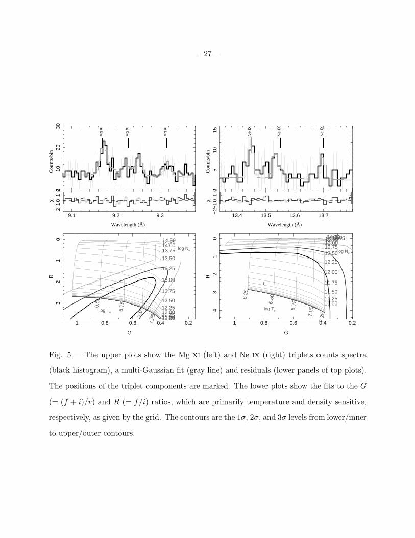
Results for both triplets are consistent with low density. In Figure 5 we show the

spectra and confidence contours of the G and R ratios, defined as G = (f + i)/r and

R = f/i. G is primarily a function of temperature, and R of density. The density and

temperature dependence are from APEC calculations (Smith et al. 2001).1

1Data for the lines are available from http://cxc.harvard.edu/atomdb/features/denHETG.ps

– 27 –0

1020

30C

ount

s/bi

n

9.1 9.2 9.3−2−

10

12

χ

Wavelength (Å)

Mg

XI

Mg

XI

Mg

XI

1 0.8 0.6 0.4 0.2

32

10

G

R

6

.50

6

.75

7

.00

7

.25 11.0011.2511.5011.7512.00

12.2512.50

12.75

13.00

13.25

13.50

13.7514.0014.2514.50

log Te

log Ne

05

1015

Cou

nts/

bin

13.4 13.5 13.6 13.7−2−

10

12

χ

Wavelength (Å)

Ne

IX

Ne

IX

Ne

IX1 0.8 0.6 0.4 0.2

43

21

0

G

R

6

.25

6

.50

6

.75

7

.00

7

.25

11.0011.2511.50

11.75

12.00

12.25

12.5012.7513.0013.2513.5013.7514.0014.2514.50

log Te

log Ne

Fig. 5.— The upper plots show the Mg xi (left) and Ne ix (right) triplets counts spectra

(black histogram), a multi-Gaussian fit (gray line) and residuals (lower panels of top plots).

The positions of the triplet components are marked. The lower plots show the fits to the G

(= (f + i)/r) and R (= f/i) ratios, which are primarily temperature and density sensitive,

respectively, as given by the grid. The contours are the 1σ, 2σ, and 3σ levels from lower/inner

to upper/outer contours.

– 28 –

2.4.3. Abundance Ratios

By forming appropriately weighted flux ratios of line pairs, we can obtain relatively

temperature-insensitive abundance ratios. This is achieved by relating a linear combination

of emissivities of He and H-like resonance lines for one element to a similar linear

combination of another element, so as to minimize fluctuations with temperature in

their ratio. If this ratio is constant, then the analogous combination of line fluxes gives

the abundance ratio. This technique was explained in detail by Liefke et al. (2008) and

described generally by Garcıa-Alvarez et al. (2005).

We define the ratio in the following way:

r =F1,1 + a1F1,2

F2,1 + a2F2,2=

A1a0

A2

∫

[ǫ1,1(T ) + a1ǫ1,2(T )]D(T ) dT∫

[ǫ2,1(T ) + a2ǫ2,2(T )]D(T ) dT(1)

in which subscripts i, j on F refer to the line j from element i, F is the observed flux, ǫ(T )

is the emissivity, D(T ) the emission measure, and Ai the abundance of element i. The

parameters, an are to-be-determined. It is clear that if the terms in square brackets within

the integrals are identical in numerator and denominator for all T , then the integrals cancel

and we are left with the abundance ratio (parameters a1 and a2 serve to flatten the ratio,

and a0 normalizes it). We determined the parameters by minimizing the variation in the

ratios using H-like and He-like line emissivities from the APED database. Re-writing in

terms of the abundance ratio for these lines, we have

A1

A2

=

(

1

a0

)

F1,H + a1F1,He

F2,H + a2F2,He(2)

in which subscripts H and He represent the hydrogen-like Lyman-α doublet and the

helium-like Lyman-α resonance line, respectively. We tabulate coefficients for a few useful

ratios in Table 5 as derived from APED for units of F in [phot cm−2s−1] and abundances

relative to Solar. Minimization of the ratio variances were restricted to temperature ranges

where the emissivities were greater than 1% of their maximum. In Table 6 we give the

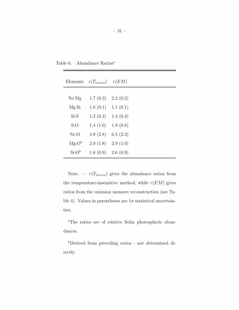
– 29 –

abundance ratios derived from the temperature-insensitive ratios along with values from

emission measure modeling. The ratios from each method are in very good agreement. This

means that abundance ratios can be derived fairly easily, without resorting to emission

measure reconstruction.

– 30 –

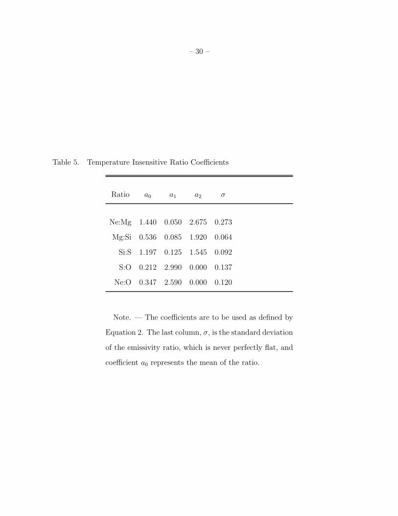
Table 5. Temperature Insensitive Ratio Coefficients

Ratio a0 a1 a2 σ

Ne:Mg 1.440 0.050 2.675 0.273

Mg:Si 0.536 0.085 1.920 0.064

Si:S 1.197 0.125 1.545 0.092

S:O 0.212 2.990 0.000 0.137

Ne:O 0.347 2.590 0.000 0.120

Note. — The coefficients are to be used as defined by

Equation 2. The last column, σ, is the standard deviation

of the emissivity ratio, which is never perfectly flat, and

coefficient a0 represents the mean of the ratio.

– 31 –

Table 6. Abundance Ratiosa

Elements r(Tinsens) r(EM)

Ne:Mg 1.7 (0.3) 2.2 (0.2)

Mg:Si 1.0 (0.1) 1.1 (0.1)

Si:S 1.2 (0.2) 1.4 (0.4)

S:O 1.4 (1.0) 1.9 (0.8)

Ne:O 4.9 (2.8) 6.5 (2.3)

Mg:Ob 2.9 (1.8) 2.9 (1.0)

Si:Ob 1.8 (0.9) 2.6 (0.9)

Note. — r(Tinsens) gives the abundance ratios from

the temperature-insensitive method, while r(EM) gives

ratios from the emission measure reconstruction (see Ta-

ble 4). Values in parentheses are 1σ statistical uncertain-

ties.

aThe ratios are of relative Solar photospheric abun-

dances.

bDerived from preceding ratios - not determined di-

rectly.

– 32 –

3. Discussion, Interpretation

The recent determination by Herbig & Griffin (2006) that θ1 Ori E is a moderate mass

pre-main-sequence spectroscopic binary is very important in the context of stellar evolution

and X-ray activity. When θ1 Ori E arrives on the main sequence, we expect it to be faint

or non-detectable in soft X-rays. Yet at the age of 0.5 Myr, it is the second-brightest steady

X-ray source in the Orion Trapezium. The binary system has Lx = 1.2 × 1032 ergs s−1, and

given an optical luminosity of 29L⊙ (Herbig & Griffin 2006) it thus has Lx/Lbol = 10−3

for the pair. This value is near the saturation limit of coronally active stars (Prosser et al.

1996). The X-ray emission is similar to other magnetically active stars, having a broad

temperature distribution and narrow emission lines. Hence we surmise that θ1 Ori E has

dynamo activity and probably has strong convection zones. This is also in accordance with

evolutionary models of stellar interiors (Siess, Dufour & Forestini 2000) which indicate a

substantial convection zone for stars like the θ1 Ori E components (also see Figure 1 of

Stelzer et al. 2005).

Prior to the Herbig & Griffin (2006) determination that θ1 Ori E is a binary of G-type

stars, θ1 Ori E was considered to be a B5-star. Schulz et al. (2003) considered the X-rays

to be a hybrid of wind shock emission and magnetically confined winds, but they did note a

striking similarity to active coronal sources. Stelzer et al. (2005) interpreted the emission as

from a weak wind, but noted unusual emission characteristics, such as due to an extended

magnetosphere and magnetically confined wind shocks. It is now clear in hindsight, given

the spectral types, that emission is coronal in nature.

θ1 Ori E did not show any distinct flares during our observations, which is somewhat

unusual for coronally active stars. This lack of activity is consistent, however, with the

long intervals of constant flux seen by Stelzer et al. (2005). There was one observation in

which the flux was lower than our average (see Figure 2), and examination of the spectra

– 33 –

shows that this is manifested in diminished short wavelength flux (below about 10A). This

variation between observations cannot be attributed to rotational phase dependence since it

does not repeat. We also found no significant variability within any of our observations. It

is possible that the system is so coronally active that a significant proportion of the average

flux is from continuously visible flares, which would also give rise to the dominant emission

measure peak at log T = 7.3, but one observation had a bit less flaring.

The HETGS flux was about half that reported by Stelzer et al. (2005) from heavily

piled, low resolution spectra. The HETGS flux calibration is accurate to about 5%.

Since flux for our observations was effectively constant and spans the time of the COUP

observations, the difference in flux without obvious flares is unusual. Since the Stelzer et al.

(2005) analysis was made difficult by the high photon pile-up in the core of θ1 Ori E, they

resorted to spectral analysis of photons only from the wings of the point-spread-function.

We reanalyzed spectra for θ1 Ori E from one of the COUP datasets, observation ID 4373,

for which the flux was constant. We used an extraction radius of 2.25 arcsec centered on

the source, including piled photons and made standard responses for the region. To fit the

spectrum, we used the pileup model of Davis (2001) as implemented in ISIS. Pileup is a

very non-linear process; there can be multiple solutions since the count-rate first saturates

with increasing fluence, then can decrease as events are rejected from telemetry. Finally, for

extremely high pileup, the count rate can again increase when the core is fully saturated

and the wings grow. We used two-temperature component, absorbed APED plasma

models, similar to those of Stelzer et al. (2005), and used Monte-Carlo techniques to explore

parameter space, given the multi-valued nature of pileup fitting and the possibly degenerate

nature of the models. While we found solutions with fluxes similar to those presented by

Stelzer et al. (2005), we found equally acceptable solutions (reduced χ2 < 1.3 ) with fluxes

comparable to our HETGS-derived values. Incidentally, all our fits to this one spectrum

preferred NH & 3 × 1021cm−2, a bit larger than our adopted value of 2 × 1021cm−2. We

– 34 –

conclude that the Stelzer et al. (2005) flux is probably in error and the source is probably

steady outside of distinct flares with a flux of about 3 × 10−12 ergs cm−2s−1.

The radial velocities determined from lines are consistent with the orbital dynamics.

Given a peak-to-peak orbital radial velocity amplitude of 160 km s−1, we have marginal

sensitivity for detection of the orbital modulation if emission were dominated by one stellar

component (see the confidence limits in Table 1 and Figure 2). Variability over the time

period of observations could destroy any orbital systematic radial velocities in X-ray lines

if the relative activity level of the two stellar components changed. Our phase coverage is

also poor, but the lack of significant velocity offsets at phases of maximum orbital velocity

separation suggests that both stellar components are roughly equal in X-ray emission. The

marginal detection of line broadening, particularly at these same phases, is consistent with

the broadening being due to orbital velocity effects. We conclude that the lines are similar

to other coronal sources - narrow, and effectively unresolved.

The absolute abundances are rather low when compared to other coronal sources.

If we compare θ1 Ori E to the abundances derived from low-resolution COUP spectra

of Maggio et al. (2007), they are not only lower by a factor of 5 or more in general, the

ratios are also different — they are, in fact, uncorrelated. This probably has as much to

do with different methods and spectral resolutions than with intrinsic differences between

θ1 Ori E and average Orion stars. Maggio et al. (2007) use two temperature component

fits, and these cannot accurately reproduce abundances and emission measures for realistic,

continuous emission measure distribution plasmas. If a fitted temperature component is off

the peak of some ion’s temperature of peak emissivity, and there is actually plasma at that

temperature, then a two-temperature model will artificially increase the abundance of that

element in order to reproduce the flux. Comparison of low and high resolution results with

different modeling approach is in general not meaningful.

– 35 –

3.1. Loop Sizes

The geometric structure of stellar coronae is largely an open question, and is relevant

to energetics, variability, and likelihood of interactions with stellar companions or disks.

While there are many uncertain parameters, we can provide order-of-magnitude estimates

via several methods to show that loops could be compact (small fraction of the stellar radii

of 7R⊙; see Table 7), or comparable to the stellar radii and thus a significant fraction of the

stellar separation (the semi-major axis is about 2.5R∗; see Herbig & Griffin (2006)).

If we assume that the X-ray emission originates in an ensemble of identical semi-circular

loops, we can estimate the order of magnitude of the loops’ radius. The loop radius (or

height if vertically oriented) relative to the stellar radius can be expressed as

h = E1/351 R−1

10 n−2/310 N

−1/32 α

−2/3−1 (3)

in which E is the volume emission measure, R the stellar radius, N the number of identical

loops, n the electron density, and α is the loop aspect ratio (cross sectional radius to

height, ≤ 1), and the subscripts indicate the power of 10 scale factor (all cgs or unit-less

quantities). Only two of these parameters are well determined, E = 1.2 × 1055 cm−3 from

our X-ray spectral modeling, and R ∼ 5 × 1011 cm from the radial velocity curve analysis

of Herbig & Griffin (2006). Densities are poorly constrained; we will adopt 1012 cm−3 for

argument (see Figure 5). From Solar loops, α is about 0.1, and given the lack of variability

in θ1 Ori E (to about 10% accuracy; see Figure 2), we will let N = 100. If we assume that

the emission is divided equally between the two binary stellar components, then with these

parameters we obtain h ∼ 0.02, implying that the coronae are compact. For a density of

1010 cm−3, this height increases by a factor of 20 to about 0.4, a significant fraction of the

orbital separation.

We can also estimate loop parameters using hydrodynamical models from the flare

– 36 –

temporal and spectral properties. Assuming that a single flaring loop dominates the

emission, Reale (2007) expressed the loop size (his Equation 12) as L9 ∼ 3(T0/TM)2 T1/20,7 τM,3.

Here L9 is the loop half-length in units of 109 cm, T0 is the maximum temperature during

the flare (and T0,7 is the same in units of 107 K), TM is the temperature at which maximum

density occurs, and τM,3 is the time from flare start (in ks) at which maximum density

occurs. To apply such a model in detail, we would need the evolution of emission measure

(a proxy for density) and temperature (from time-resolved spectra) from the rise to the

decay of a flare. We do not have such, so we will make some reasonable approximations to

obtain an order-of-magnitude hydrodynamical loop size.

The COUP observation of θ1 Ori E detected a flare (Stelzer et al. 2005); from this,

we estimate that τm,3 = 25. We have an emission measure distribution; we assume that

the hotter peak and hot tail represents the integrated history over many flares. From

time-resolved analyses of other stars, we have seen that such a hot peak can be directly

attributed to flaring (Huenemoerder, Canizares & Schulz 2001; Gudel et al. 2004). We will

thus assume that the flare mean temperature of maximum density (or maximum emission

measure) corresponds to our strongest peak, or log TM = 7.3 (see Figure 3). We will assume

that the hot tail of the EMD represents the maximum flare temperature. This is less well

defined, and we adopt log T0 = 7.8, which is where there is an inflection in our EMD. From

these parameters we find a relative loop half-length of about 3.8 stellar radii, or a height

(for semi-circular vertical loops) of 2.4 stellar radii.

We can also adopt flare parameters from other giant stars, such as HR 9024 (Testa et al.

2007) (also see Table 7), for which log T0 = 7.9 and T0/TM = 1.4. Thus, if θ1 Ori E flare

temperatures and densities are similar to those on HR 9024, the loop half-length is about 1

stellar radius (or a height of 0.6 stellar radii).

Since these are order-of-magnitude estimates, we conclude that flare loops can be of

– 37 –

order the stellar radius. In sum, an origin of the emission from magnetically confined coronal

loops is not unreasonable. To better determine the coronal geometry, more information is

needed, such as more stringent constraints on density, detection of rotational modulation,

or time-resolved spectroscopy of a large flare.

4. Comparison to Other Stars

To understand the nature of the X-ray emission from θ1 Ori E, we must examine it

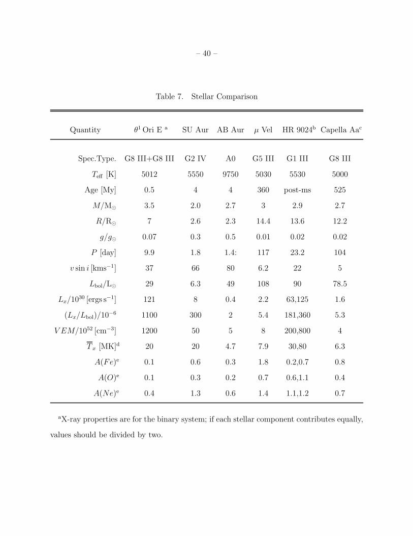
in the evolutionary context of stars of similar mass. We have collected information for

several other stars, both pre-main-sequence and post-main-sequence, with masses ranging

from 2 to 3.5M⊙. Information and sources are listed in Table 7 and in Figure 6 we show

the objects on a temperature-luminosity diagram along with evolutionary tracks. Of the

sample, θ1 Ori E has the highest relative X-ray luminosity, being as high in Lx/Lbol as

“saturated” short period active binaries (Vilhu & Rucinski 1983; Cruddace & Dupree 1984;

Prosser et al. 1996), even though its period is somewhat longer than those systems. If we

look to the future of θ1 Ori E’s evolution and consider AB Aur, we see that Lx/Lbol may

become much smaller; we expect main-sequence A-type stars to be very faint or undetected

in X-rays (for reference, a spectral type A0 V star has a mass of ∼ 2M⊙, and a B5 V of

∼ 6M⊙).

Stellar rotation is well known to be a key factor in magnetic dynamo generation. If

we compare the sample’s X-ray activity as a function of period (Figure 7), excluding AB

Aur, we see a strong anti-correlation which holds for both pre- and post-main-sequence

objects. This is similar to the behavior of active giants, binaries, or main sequence late-type

stellar coronae (Walter & Bowyer 1981; Pizzolato et al. 2003; Gondoin 2005). AB Aur,

in spite of its short period, has very low activity; it is approaching the low-activity

main-sequence era of its life, and may have a radically different emission mechanism, such

– 38 –

as from wind or accretion affects, with lower Lx and X-ray temperatures (Telleschi et al.

2007). It’s convective zone, necessary for magnetic dynamo generation, is quite small,

being less than 1% of the stellar radius, compared to about 20% for the other stars

(Siess, Dufour & Forestini 2000; Stelzer et al. 2005, their Figure 1), so it is reasonable to

exclude it from period-activity relations of stars with significant convective regions.

θ1 Ori E has a very hot corona, characterized by an emission measure distribution

with a strong peak at about 20 MK (see Figure 3). It is similar to SU Aur and

HR 9024 (see Table 7), two objects which displayed strong flares during their X-ray

observations. A hot emission measure peak has been directly identified with flares

(Huenemoerder, Canizares & Schulz 2001; Gudel et al. 2004). In this context, it is

curious that during all the COUP and HETG exposures, only one distinct flare was seen

(Stelzer et al. 2005). We can only speculate that perhaps θ1 Ori E is so active that the flare

rate is so high that they are nearly always superimposed and create a nearly constant flux.

Such was found plausible for Orion’s low-mass stars by Caramazza et al. (2007). Our single

low-flux HETGS observation (see Figure 2) did have a relative deficit in short wavelength

flux (< 5 A), a region sensitive to the highest temperature plasmas; it is consistent with

diminished flare activity. To sustain continuous flaring, there has to be a continuous source

of erupting magnetic fields and their reconnection. The pressure scale-height for a hot,

low-density plasma is a significant fraction of the binary stellar separation of θ1 Ori E.

There could be star-to-star magnetic reconnections sustained at a fairly high level by the

binary proximity and dynamo action generating sufficiently large loops.

The presence of a very hot corona and the low probability of distinct flares is common

to several evolved giants, such as HR 9024, µ Vel, 31 Com, or IM Peg (Testa et al.

2007; Testa, Drake & Peres 2004; Ayres, Hodges-Kluck & Brown 2007). While this is not

understood, it could be a significant trait of the coronal heating mechanisms.

– 39 –

Another distinguishing characteristic of θ1 Ori E is the relatively low mean metal

abundance. Table 4 shows relative elemental abundances from the EMD analysis. All

abundances are significantly below unity with oxygen at an extremely low value. When

compared to abundances deduced in a similar analysis of θ1 Ori C (Schulz et al. 2003), its

massive neighbor within the Orion Trapezium, then there are a few remarkable differences

to note. Values for Ne, Al, and Ca seem very similar within uncertainties, while Mg, Si,

S, and Ar are very different, being near or above unity in θ1 Ori C; values for O and

Fe are even lower than in θ1 Ori C. Figure 4 also compares coronal with average Orion

stellar photospheric and nebular values. Since the photospheric and nebular abundances

are all near unity, it seems that abundances from the hot X-ray plasmas are fundamentally

different. A two-temperature modeling of θ1 Ori C could reconcile deficient O and Ne

values by requiring a significantly higher column density (Gagne et al. 2005), as would

forcing the Ne/O ratio to be similar to other coronae (Drake & Testa 2005), though Fe

would still remain low. In the case of θ1 Ori E, the application of a higher column will

not change the low values for Mg and higher-Z elements, but also not enough for O, which

at A(O) = 0.06 is extremely low. We also find that multi-temperature plasmas more

accurately describe the spectra in both stars and thus see trends in Orion Trapezium stars

which include some neon deficiency but clearly hot plasmas with low iron and oxygen

abundances. For pre-main-sequence stars, depletion of metals has been explained by

formation of dust in the disk, and the remaining gas, seen heated to X-ray temperatures in

an accretion shock, is the metal-poor material (Drake, Testa & Hartmann 2005). Magnetic

coronae generally show low metals, but tend to have higher Ne and O (e.g., II Peg,

Huenemoerder, Canizares & Schulz (2001), or HR 1099, Drake et al. (2001)). Hot plasmas

of Orion’s stars, if the two studied are representative, seem to be different. There is no

theoretical explanation for coronal abundances, but these differences may be clues to

fractionation mechanisms.

– 40 –

Table 7. Stellar Comparison

Quantity θ1 Ori E a SU Aur AB Aur µ Vel HR 9024b Capella Aac

Spec.Type. G8 III+G8 III G2 IV A0 G5 III G1 III G8 III

Teff [K] 5012 5550 9750 5030 5530 5000

Age [My] 0.5 4 4 360 post-ms 525

M/M⊙ 3.5 2.0 2.7 3 2.9 2.7

R/R⊙ 7 2.6 2.3 14.4 13.6 12.2

g/g⊙ 0.07 0.3 0.5 0.01 0.02 0.02

P [day] 9.9 1.8 1.4: 117 23.2 104

v sin i [kms−1] 37 66 80 6.2 22 5

Lbol/L⊙ 29 6.3 49 108 90 78.5

Lx/1030 [ergs s−1] 121 8 0.4 2.2 63,125 1.6

(Lx/Lbol)/10−6 1100 300 2 5.4 181,360 5.3

V EM/1052 [cm−3] 1200 50 5 8 200,800 4

T x [MK]d 20 20 4.7 7.9 30,80 6.3

A(Fe)e 0.1 0.6 0.3 1.8 0.2,0.7 0.8

A(O)e 0.1 0.3 0.2 0.7 0.6,1.1 0.4

A(Ne)e 0.4 1.3 0.6 1.4 1.1,1.2 0.7

aX-ray properties are for the binary system; if each stellar component contributes equally,

values should be divided by two.

– 41 –

bWhen two quantities are given they are for quiescent and flare states, respectively.

cX-ray properties assume that component Aa dominates.

dA qualitative temperature of the high energy emission measure distribution, adopted

from visual inspection of published curves or few-T fits.

eAbundances are relative to Solar.

Note. — Sources: θ1 Ori E: Herbig & Griffin (2006); this paper. SU Aur:

Franciosini et al. (2007); Robrade & Schmitt (2006); DeWarf et al. (2003). AB Aur:

Telleschi et al. (2007). µ Vel: Ayres, Hodges-Kluck & Brown (2007); Wood et al.

(2005). HR 9024: Ayres, Hodges-Kluck & Brown (2007); Testa et al. (2007). Capella:

Ishibashi et al. (2006); Canizares et al. (2000); Hummel et al. (1994); Ness et al. (2003);

Gu et al. (2006).

– 42 –

104 5000

1010

010

00

Teff [K]

L bol/L

sun

θ1 Ori E

SU Aur

AB Aur

µ VelHR 9024

Capella Aa

2 Msun

3 Msun

4 Msun

ZAMS

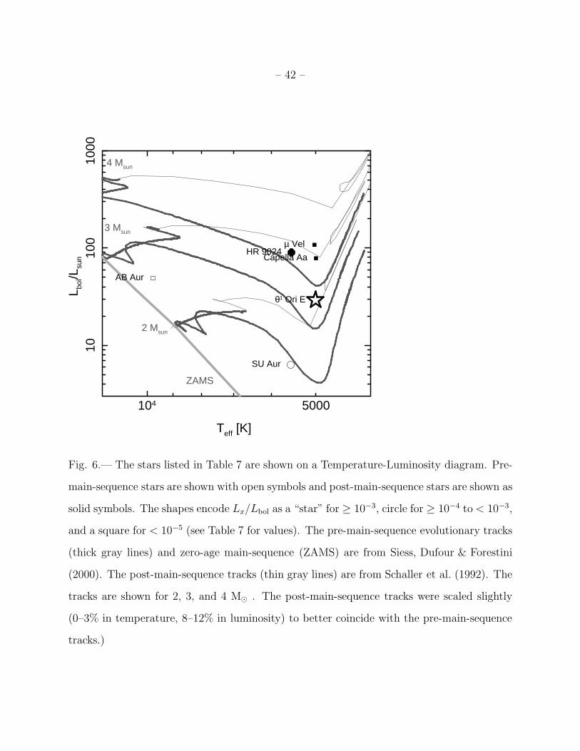
Fig. 6.— The stars listed in Table 7 are shown on a Temperature-Luminosity diagram. Pre-

main-sequence stars are shown with open symbols and post-main-sequence stars are shown as

solid symbols. The shapes encode Lx/Lbol as a “star” for ≥ 10−3, circle for ≥ 10−4 to < 10−3,

and a square for < 10−5 (see Table 7 for values). The pre-main-sequence evolutionary tracks

(thick gray lines) and zero-age main-sequence (ZAMS) are from Siess, Dufour & Forestini

(2000). The post-main-sequence tracks (thin gray lines) are from Schaller et al. (1992). The

tracks are shown for 2, 3, and 4 M⊙ . The post-main-sequence tracks were scaled slightly

(0–3% in temperature, 8–12% in luminosity) to better coincide with the pre-main-sequence

tracks.)

– 43 –

1 10 100

110

100

1000

P [day]

106

L x / L

bol

θ1 Ori E

SU Aur

AB Aur

µ Vel

HR 9024−Q

HR 9024−F

Capella Aa

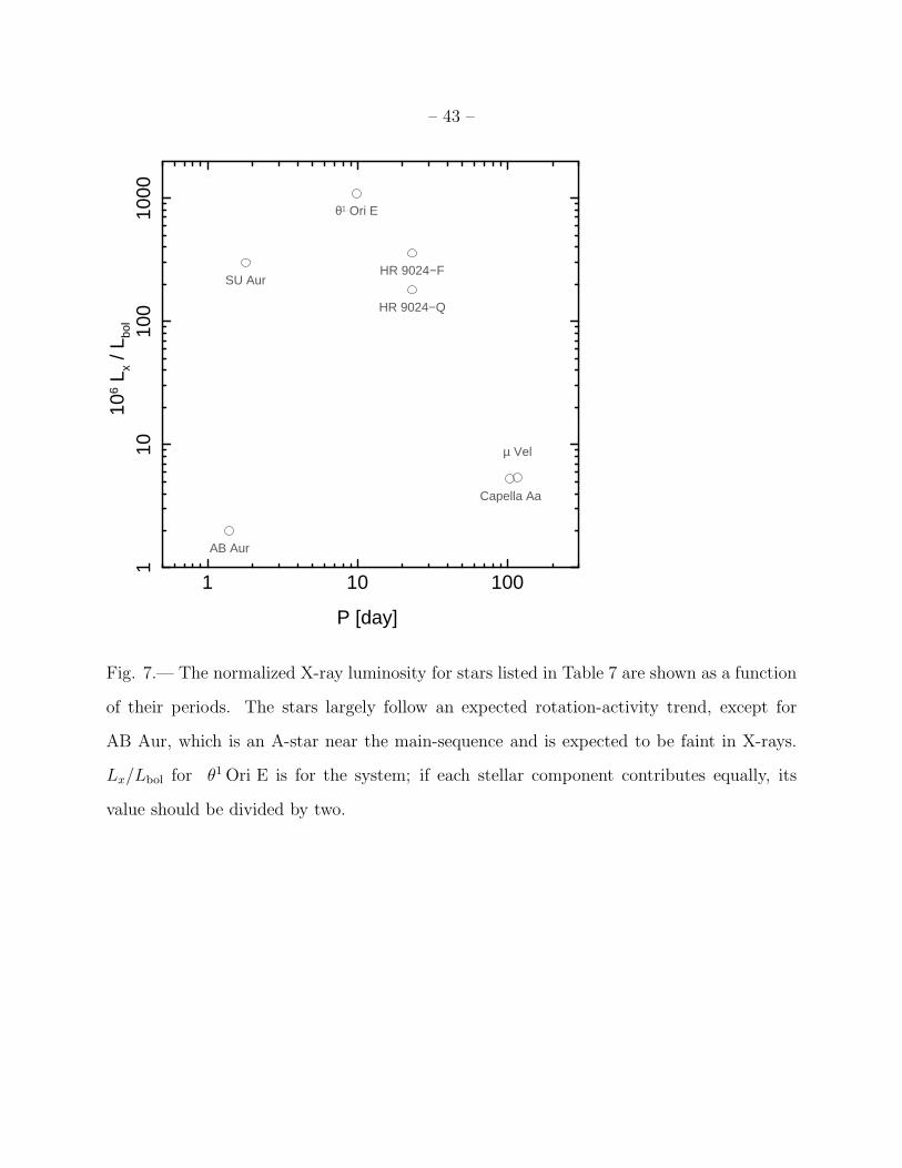
Fig. 7.— The normalized X-ray luminosity for stars listed in Table 7 are shown as a function

of their periods. The stars largely follow an expected rotation-activity trend, except for

AB Aur, which is an A-star near the main-sequence and is expected to be faint in X-rays.

Lx/Lbol for θ1 Ori E is for the system; if each stellar component contributes equally, its

value should be divided by two.

– 44 –

5. Conclusions

θ1 Ori E is perhaps the only case known of a pre-main-sequence 3 Solar mass G-star

binary. As such, it holds an important place in our understanding of X-ray dynamo

generation and evolution. We believe that when it reaches the main sequence, it will emit

a negligible fraction of its luminosity in X-rays. Yet now it is the second brightest X-ray

source in the Trapezium. Furthermore, its relative X-ray luminosity (Lx/Lbol) makes it as

strong as any of the coronally active binaries. Thus we conclude that as moderate mass stars

collapse toward the main sequence, they go through a phase of strong magnetic dynamo

generation, very similar or identical to that of coronally active late-type stars which sustain

a convective zone and shear-generated magnetic dynamo. Since A-stars are dark or at most

quite faint in X-rays (Schroder & Schmitt 2007), at some point, the dynamo vanishes, and

the magnetic fields dissipate. AB Aur, which is near the main sequence and relatively faint

in X-rays, is a possible future state of θ1 Ori E. It is also clear from the post-main-sequence

objects that a dynamo can be generated as stars of this mass evolve into giants.

Hot plasma abundances of θ1 Ori E (as well as of θ1 Ori C) are different from coronally

active stars. θ1 Ori E is hot and has fairly steady X-ray emission. The high temperature is

either due to unresolved flares, or to an unknown mechanism which also may be common

to other active G-giants. The temperature structure, abundances, and low variability may

be clues to plasma heating mechanisms. Continuing high-resolution spectroscopic studies of

Orion stars will show us if some of these patterns are common in the Orion Nebular Cluster.

Facilities: CXO (HETGS)

Acknowledgments Support for this work was provided by the National Aeronautics

and Space Administration through the Smithsonian Astrophysical Observatory contract

– 45 –

SV3-73016 to MIT for Support of the Chandra X-Ray Center, which is operated by the

Smithsonian Astrophysical Observatory for and on behalf of the National Aeronautics

Space Administration under contract NAS8-03060.

– 46 –

REFERENCES

Acke, B., & Waelkens, C., 2004, A&A, 427, 1009

Anders, E., & Grevesse, N., 1989, Geochim. Cosmochim. Acta, 53, 197

Ayres, T. R., Hodges-Kluck, E., & Brown, A., 2007, ApJS, 171, 304

Baines, D., Oudmaijer, R. D., Porter, J. M., & Pozzo, M., 2006, MNRAS, 367, 737

Blondel, P. F. C., & Djie, H. R. E. T. A., 2006, A&A, 456, 1045

Canizares, C. R., et al., 2005, PASP, 117, 1144

Canizares, C. R., et al., 2000, ApJ, 539, L41

Caramazza, M., Flaccomio, E., Micela, G., Reale, F., Wolk, S. J., & Feigelson, E. D., 2007,

A&A, 471, 645

Cruddace, R. G., & Dupree, A. K., 1984, ApJ, 277, 263

Cunha, K., Hubeny, I., & Lanz, T., 2006, ApJ, 647, L143

Cunha, K., & Lambert, D. L., 1994, ApJ, 426, 170

Cunha, K., & Smith, V. V., 2005, ApJ, 626, 425

Cunha, K., Smith, V. V., & Lambert, D. L., 1998, ApJ, 493, 195

Damiani, F., Micela, G., Sciortino, S., & Harnden, Jr., F. R., 1994, ApJ, 436, 807

Davis, J. E., 2001, ApJ, 562, 575

DeWarf, L. E., Sepinsky, J. F., Guinan, E. F., Ribas, I., & Nadalin, I., 2003, ApJ, 590, 357

Drake, J. J., Brickhouse, N. S., Kashyap, V., Laming, J. M., Huenemoerder, D. P., Smith,

R., & Wargelin, B. J., 2001, ApJ, 548, L81

– 47 –

Drake, J. J., & Testa, P., 2005, Nature, 436, 525

Drake, J. J., Testa, P., & Hartmann, L., 2005, ApJ, 627, L149

Drew, J. E., Busfield, G., Hoare, M. G., Murdoch, K. A., Nixon, C. A., & Oudmaijer,

R. D., 1997, MNRAS, 286, 538

Dullemond, C. P., & Dominik, C., 2004, A&A, 421, 1075

Esteban, C., Peimbert, M., Garcıa-Rojas, J., Ruiz, M. T., Peimbert, A., & Rodrıguez, M.,

2004, MNRAS, 355, 229

Feigelson, E. D., Broos, P., Gaffney, III, J. A., Garmire, G., Hillenbrand, L. A., Pravdo,

S. H., Townsley, L., & Tsuboi, Y., 2002, ApJ, 574, 258

Franciosini, E., Scelsi, L., Pallavicini, R., & Audard, M., 2007, A&A, 471, 951

Fruscione, A., et al., 2006, in Society of Photo-Optical Instrumentation Engineers (SPIE)

Conference Series, Vol. 6270

Gudel, M., Audard, M., Reale, F., Skinner, S. L., & Linsky, J. L., 2004, A&A, 416, 713

Gabriel, A. H., & Jordan, C., 1969, MNRAS, 145, 241

Gabriel, A. H., & Jordan, C., 1973, ApJ, 186, 327

Gagne, M., & Caillault, J.-P., 1994, ApJ, 437, 361

Gagne, M., Oksala, M. E., Cohen, D. H., Tonnesen, S. K., ud-Doula, A., Owocki, S. P.,

Townsend, R. H. D., & MacFarlane, J. J., 2005, ApJ, 628, 986

Garcıa-Alvarez, D., Drake, J. J., Lin, L., Kashyap, V. L., & Ball, B., 2005, ApJ, 621, 1009

Getman, K. V., et al., 2005, ApJS, 160, 319

– 48 –

Gondoin, P., 2005, A&A, 444, 531

Grady, C. A., Woodgate, B., Bruhweiler, F. C., Boggess, A., Plait, P., Lindler, D. J.,

Clampin, M., & Kalas, P., 1999, ApJ, 523, L151

Grady, C. A., et al., 2004, ApJ, 608, 809

Grady, C. A., et al., 2005, ApJ, 630, 958

Gu, M. F., Gupta, R., Peterson, J. R., Sako, M., & Kahn, S. M., 2006, ApJ, 649, 979

Guimaraes, M. M., Alencar, S. H. P., Corradi, W. J. B., & Vieira, S. L. A., 2006, A&A,

457, 581

Hamaguchi, K., Yamauchi, S., & Koyama, K., 2005, ApJ, 618, 360

Herbig, G. H., 1960, ApJS, 4, 337

Herbig, G. H., & Griffin, R. F., 2006, AJ, 132, 1763

Houck, J. C., & Denicola, L. A., 2000, in ASP Conf. Ser. 216: Astronomical Data Analysis

Software and Systems IX, Vol. 9, 591

Huenemoerder, D. P., Canizares, C. R., & Schulz, N. S., 2001, ApJ, 559, 1135

Huenemoerder, D. P., Kastner, J. H., Testa, P., Schulz, N. S., & Weintraub, D. A., 2007,

ApJ, 671, 592

Hummel, C. A., Armstrong, J. T., Quirrenbach, A., Buscher, D. F., Mozurkewich, D., Elias,

II, N. M., & Wilson, R. E., 1994, AJ, 107, 1859

Ishibashi, K., Dewey, D., Huenemoerder, D. P., & Testa, P., 2006, ApJ, 644, L117

Ku, W. H.-M., Righini-Cohen, G., & Simon, M., 1982, Science, 215, 61

– 49 –

Liefke, C., Ness, J. ., Schmitt, J. H. M. M., & Maggio, A., 2008, A&A, 000, (in press)

Maggio, A., Flaccomio, E., Favata, F., Micela, G., Sciortino, S., Feigelson, E. D., & Getman,

K. V., 2007, ApJ, 660, 1462

Mannings, V., & Sargent, A. I., 1997, ApJ, 490, 792

Mazzotta, P., Mazzitelli, G., Colafrancesco, S., & Vittorio, N., 1998, A&AS, 133, 403

Muzerolle, J., D’Alessio, P., Calvet, N., & Hartmann, L., 2004, ApJ, 617, 406

Ness, J., Brickhouse, N. S., Drake, J. J., & Huenemoerder, D. P., 2003, ApJ, 598, 1277

Palla, F., & Stahler, S. W., 1993, ApJ, 418, 414

Parenago, P. P., 1954, Trudy Gosudarstvennogo Astronomicheskogo Instituta, 25, 1

Pizzolato, N., Maggio, A., Micela, G., Sciortino, S., & Ventura, P., 2003, A&A, 397, 147

Preibisch, T., Balega, Y., Hofmann, K.-H., Weigelt, G., & Zinnecker, H., 1999, New

Astronomy, 4, 531

Prosser, C. F., Randich, S., Stauffer, J. R., Schmitt, J. H. M. M., & Simon, T., 1996, AJ,

112, 1570

Reale, F., 2007, A&A, 471, 271

Robrade, J., & Schmitt, J. H. M. M., 2006, A&A, 449, 737

Schaller, G., Schaerer, D., Meynet, G., & Maeder, A., 1992, A&AS, 96, 269

Schroder, C., & Schmitt, J. H. M. M., 2007, A&A, 475, 677

Schulz, N. S., Canizares, C., Huenemoerder, D., Kastner, J. H., Taylor, S. C., & Bergstrom,

– 50 –

Schulz, N. S., Canizares, C., Huenemoerder, D., & Tibbets, K., 2003, ApJ, 595, 365

Schulz, N. S., Testa, P., Huenemoerder, D. P., Ishibashi, K., & Canizares, C. R., 2006, ApJ,

653, 636

Siess, L., Dufour, E., & Forestini, M., 2000, A&A, 358, 593

Smith, R. K., Brickhouse, N. S., Liedahl, D. A., & Raymond, J. C., 2001, ApJ, 556, L91

Stelzer, B., Flaccomio, E., Montmerle, T., Micela, G., Sciortino, S., Favata, F., Preibisch,

T., & Feigelson, E. D., 2005, ApJS, 160, 557

Stelzer, B., Huelamo, N., Micela, G., & Hubrig, S., 2006a, A&A, 452, 1001

Stelzer, B., Micela, G., Hamaguchi, K., & Schmitt, J. H. M. M., 2006b, A&A, 457, 223

Telleschi, A., Gudel, M., Briggs, K. R., Skinner, S. L., Audard, M., & Franciosini, E., 2007,

A&A, 468, 541

Testa, P., Drake, J. J., & Peres, G., 2004, ApJ, 617, 508

Testa, P., Huenemoerder, D. P., Schulz, N. S., & Ishibashi, K., 2008, ApJ, 687, 579

Testa, P., Reale, F., Garcia-Alvarez, D., & Huenemoerder, D. P., 2007, ApJ, 663, 1232

Vilhu, O., & Rucinski, S. M., 1983, A&A, 127, 5

Vink, J. S., Drew, J. E., Harries, T. J., Oudmaijer, R. D., & Unruh, Y., 2005, MNRAS,

359, 1049

Walter, F. M., & Bowyer, S., 1981, ApJ, 245, 671

Waters, L. B. F. M., & Waelkens, C., 1998, ARA&A, 36, 233

Wood, B. E., Redfield, S., Linsky, J. L., Muller, H.-R., & Zank, G. P., 2005, ApJS, 159, 118

– 51 –

Zinnecker, H., & Preibisch, T., 1994, A&A, 292, 152

This manuscript was prepared with the AAS LATEX macros v5.2.