Workload models of spam and legitimate e-mails

Performance Evaluation 64 (2007) 690–714www.elsevier.com/locate/peva

Workload models of spam and legitimate e-mails

Luiz Henrique Gomes, Cristiano Cazita, Jussara M. Almeida∗, Virgılio Almeida,Wagner Meira Jr.

Department of Computer Science, Federal University of Minas Gerais, Belo Horizonte, Brazil

Received 15 April 2005; received in revised form 4 November 2006Available online 27 December 2006

Abstract

This article presents an extensive characterization of a spam-infected e-mail workload. The study aims at identifying andquantifying the characteristics that significantly distinguish spam from non-spam (i.e., legitimate) traffic, assessing the impact ofspam on the aggregate traffic, providing data for creating synthetic workload models, and drawing insights into more effectivespam detection techniques.

Our analysis reveals significant differences in the spam and non-spam workloads. We conjecture that these differences areconsequence of the inherently different mode of operation of the e-mail senders. Whereas legitimate e-mail transmissions aredriven by social bilateral relationships, spam transmissions are a unilateral spammer-driven action.c© 2006 Elsevier B.V. All rights reserved.

Keywords: Workload characterization; SPAM; E-mail traffic; Performance

1. Introduction

E-mail has become a de facto means to disseminate information to millions of users in the Internet. However, thevolume of unsolicited e-mails containing, typically, commercial content, also known as spam, is increasing at a veryfast rate. In January 2003, 24% of all Internet e-mails were spams. By March 2005, this fraction had increased to83% [1]. A report from October 2003 shows that, in North America, a business user received on average 10 spamsper day, and that this number is expected to grow by a factor of four by 2008 [2]. Furthermore, AOL and MSN, twolarge ISPs, report blocking, daily, a total of 2.4 billion spams from reaching their customers’ in-boxes. This trafficcorresponds to about 80% of daily incoming e-mails at AOL [3].

This rapid increase in spam traffic is beginning to take its toll on end users, business corporations and systemadministrators. Results from a survey in March 2004, with over 2000 American e-mail users, report that over 60%of them are less trusting of e-mail systems, and over 77% of them believe being online has become unpleasant orannoying due to spam [4]. The impact of spam traffic on the productivity of workers of large corporations is alsoalarming. Research firms estimate the yearly cost per worker at anywhere from US$ 50 to US$ 1400, and the total

∗ Corresponding author.E-mail addresses: [email protected] (L.H. Gomes), [email protected] (C. Cazita), [email protected] (J.M. Almeida),

[email protected] (V. Almeida), [email protected] (W. Meira Jr.).

0166-5316/$ - see front matter c© 2006 Elsevier B.V. All rights reserved.doi:10.1016/j.peva.2006.11.001

http://www.elsevier.com/locate/peva

mailto:[email protected]





http://dx.doi.org/10.1016/j.peva.2006.11.001

L.H. Gomes et al. / Performance Evaluation 64 (2007) 690–714 691

annual cost associated with spam to American businesses in the range of US$ 10 billion to US$ 87 billion [3]. Finally,estimates of the cost of spam must also take into account the costs of computing and network infra-structure upgradesas well as quantitative measures of its impact on the quality of service available to traditional non-spam e-mail trafficand other “legitimate” Internet applications.

A number of approaches have been proposed to alleviate the impact of spam. These approaches can be categorizedinto pre-acceptance and post-acceptance methods, based on whether they detect and block spam before or afteraccepting the e-mail [5]. Examples of pre-acceptance methods are black lists [6] and gray lists or temp-failing [7].Pre-acceptance approaches based on server authentication [8,9], economic disincentives [10] and accountability [11]have also been proposed. Examples of post-acceptance methods include Bayesian filters [12,13], collaborativefiltering [14], e-mail prioritization [5], and recent techniques that exploit properties of the relationship establishedbetween spammers and spam recipients [15–17].

Although existing spam detection and filtering techniques have, reportedly, very high success rates (up to 97%of spams are detected [14]), they suffer from one key limitation. The rate of false positives, i.e., legitimate e-mailsclassified as spams, can be as high as 15% [18], incurring costs that are hard to mensurate.

Despite the large number of reports on spam cost and the plethora of previously proposed spam detection andfiltering methods, the efforts towards analyzing the characteristics of this type of traffic have been somewhat limited.In addition to some previous e-mail workload characterizations [19,20], we are aware of only a few limited analysesof spam traffic in the literature [5,8,21–24].

This paper takes an innovative approach towards addressing the problems caused by spam and presents an extensivecharacterization of a spam traffic. Our goal is to develop a deep understanding of the fundamental characteristics ofspam traffic and spammer’s behavior, in the hope that such knowledge can be used, in the future, to drive the designof more effective techniques for detecting and combating spams.

Our characterization is based on an eight-day log of over 360 thousand incoming e-mails to a large university inBrazil. Standard spam detection techniques are used to classify the e-mails into two categories, namely, spam andnon-spam (i.e., legitimate e-mail). For each of the two resulting workloads, as well as for the aggregate workload,we analyze a set of parameters, based on the information available in the e-mail headers. We aim at identifying thequantitative and qualitative characteristics that significantly distinguish spam from non-spam traffic, assessing theimpact of spam on the aggregate traffic by evaluating how the latter deviates from the non-spam traffic, and providingdata for generating realistic synthetic spam-infected e-mail workloads.

Our key findings are:

• Unlike traditional non-spam e-mail traffic, which exhibits clear weekly and daily patterns, with load peaks duringthe day and on weekdays, the numbers of spam e-mails, spam bytes, distinct active spammers and distinct spame-mail recipients are roughly insensitive to the period of measurement, remaining mostly stable during the wholeday, for all days analyzed.

• Spam and non-spam arrivals follow Poisson processes. However, whereas the spam arrival rates remain roughlystable across all periods analyzed, the arrival rates of non-spam e-mails vary by as much as a factor of five in thesame periods.

• E-mail sizes in the three workloads follow Lognormal distributions. However, the average size of a non-spam e-mail is from six to eight times larger than the average size of a spam, in our workload. Moreover, the coefficientof variation (CV) of the sizes of non-spam e-mails is around three times higher than the CV of spam sizes. Thus,the impact of spam on the aggregate traffic is a decrease on the average e-mail size but an increase in the sizevariability.

• The distribution of the number of recipients per e-mail is more heavy-tailed in the spam workload. Whereas only5% of non-spam e-mails are addressed to more than one user, 15% of spams have more than one recipient. In theaggregate workload, the distribution is heavily influenced by the spam traffic, deviating significantly from the oneobserved in the non-spam workload.

• Regarding daily popularity of e-mail senders and recipients, the main distinction between spam and non-spame-mail traffic comes up in the distribution of the number of e-mails per recipient. Whereas in the non-spam andaggregate workloads, the distribution is well modeled by a single Zipf-like distribution plus a constant probabilityof a user receiving only one e-mail per day, the distribution of the number of spams a user receives per day is moreaccurately approximated by the concatenation of two Zipf-like distributions, in addition to the constant single-message probability.

692 L.H. Gomes et al. / Performance Evaluation 64 (2007) 690–714

• There are two distinct and non-negligible sets of non-spam recipients: those with very strong temporal locality andthose who receive e-mails only sporadically. These two sets are not clearly defined in the spam workload. In fact,temporal locality is, on average, much weaker among spam recipients and even weaker among recipients in theaggregate workload. Similar trends are observed for the temporal locality among e-mail senders.

• The distributions of contact list sizes for senders and recipients are much more skewed towards smaller sizes inthe non-spam workload. In fact, a typical spammer sends e-mails to twice as many distinct recipients as a typicallegitimate e-mail sender. Moreover, a typical spam recipient receives spams from a number of distinct spammersthat is almost three times the number of non-spam senders a typical recipient has contact with. Furthermore, thespam traffic significantly impacts the distribution of contact list sizes for senders and recipients in the aggregatetraffic.

Therefore, our characterization reveals significant differences between the spam and non-spam workloads. Thesedifferences are possibly due to the inherent distinct nature of e-mail senders and their connections with e-mailrecipients in each group. Whereas a non-spam e-mail transmission is the result of a bilateral relationship, typicallyinitiated by a human being, driven by some social relationship, a spam transmission is basically a unilateral action,typically performed by automatic tools and driven by the spammer’s will to reach as many targets as possible,indiscriminately, without being detected.

The remaining of this paper is organized as follows. Section 2 discusses related work. Our e-mail workloads andthe characterization methodology are described in Section 3. Section 4 analyzes temporal variation patterns in theworkloads. E-mail traffic characteristics are discussed in Section 5. E-mail recipients and senders are analyzed inSection 6. Finally, Section 7 presents conclusions and directions for future work.

2. Related work

Developing a clear understanding of the workload is a key step towards the design of efficient and effectivedistributed systems and applications. A number of characterization studies of different workload types that ledto valuable insights into system design are available in the literature, including the characterization of Webworkloads [25], streaming media workloads [26–28] and, recently, peer-to-peer [29] and chat room workloads [30]. Tothe best of our knowledge, previous efforts towards characterizing spam traffic have been very limited. In particular,an initial and preliminary version of this study is presented in [23]. Next we discuss previous characterizations andanalysis of e-mail and spam workloads.

In [19,20], the authors provide an extensive characterization of several e-mail server workloads, analyzing e-mailinter-arrival times, e-mail sizes, and number of recipients per e-mail. They also analyze user accesses to e-mail servers(through the POP3 protocol), characterizing inter-access times, number of e-mails per user mailboxes, mailbox sizesand size of deleted e-mails, and propose user behavior models. In this paper, in contrast, we characterize not only ageneral e-mail workload, but also a spam workload, in particular, aiming at identifying a signature of spam traffic,which can be used in the future for developing more effective spam-controlling techniques. In Sections 4 and 5, wecontrast our characterization results for non-spam e-mails with those reported in [19,20].

Twining et al. [5] present a simpler server workload characterization, as the starting point for investigating theeffectiveness of novel techniques for detecting and controlling junk e-mails (i.e., virus and spams). They analyze thelogs of two e-mail servers that include a virus checker and a spam filter, and characterize the arrival process of eachtype of e-mail on a per-sender basis, the percentage of servers that send only junk e-mails, only good e-mails, anda mixture of both. A major conclusion of the paper is that popular spam detection mechanisms such as blacklisting,temp-failing, and rate-limiting are rather limited in handling the problem. This paper presents a much more thoroughcharacterization of spam traffic, and contrasts, whenever appropriate, our findings to those reported in [5].

In [8], the authors analyze the temporal distribution of spam arrivals and spam content at selected sites from theAT&T and Lucent backbones. They also discuss the factors that make users and domains more likely to receive spamsand the reasons that lead to the use of spam as a communication and marketing strategy. The paper also includes abrief discussion of the pros and cons of several anti-spam strategies.

In [22], the authors analyze two sets of SMTP packet traces and identify a significant increase in the use of DNSblack lists over a four-year period. Furthermore, they also show that the distribution of the number of connectionsper spam sender, although not Zipf-like in the older set, does exhibit a heavy-tailed Zipf-like behavior in the second


set, collected four years later. In contrast, the characterization presented in this paper covers a much broader range ofworkload aspects. Nevertheless, we compare our results with those presented in [22] whenever appropriate.

Ramachandran and Feamster [24] study the network-level behavior of spammers, including the IP address rangesfrom which a significant fraction of spams are sent, common spamming modes (e.g., BGP route hijacking, bots), howpersistent across time each spamming host is, and characteristics of spamming botnets. Their main findings are thatmost spams are sent from a few regions of IP address space and that spammers use transient bots that send a few piecesof emails over short periods of time. Furthermore, they found that spammers use short-lived BGP routes, typically forhijacked prefixes, to send a non-negligible number of spams. In contrast, we found almost 2 times more spam senderdomains than non-spam sender domains in our workload. Moreover, we found a skewed distribution of spams oversender domains and recipient users and conclude that the use of sender/recipient blacklisting and whitelisting can bevery effective for combating spam.

Other recent studies focus on deriving graph-based models of spam and legitimate e-mail traffic [15,16,21,17]. Thestructural characteristics of the relationships established between senders and recipients of spams and legitimate e-mails have been used as basis for the design of new spam detection techniques in [15–17]. In [21], the authors analyzea variety of properties of e-mail graphs, identifying characteristics that strongly distinguish spam from non-spamrelationships. This paper, on the other hand, takes a complementary approach, focusing mainly on the characteristicsof each traffic separately, analyzing a variety of workload aspects that distinguish one from the other.

3. E-mail workload

This section introduces the e-mail workload analyzed in this paper. Section 3.1 describes the data source andcollection architecture. The methodology used in the characterization process is presented in Section 3.2. Section 3.3provides an overview of our e-mail workload.

3.1. Data source

Our e-mail workload consists of anonymized SMTP logs of incoming e-mails to a large university, with around 22thousand students, in Brazil. The logs are collected at the central Internet-facing e-mail server of the university. Thisserver handles all e-mails coming from the outside and addressed to the vast majority of students, faculty and staff withe-mail addresses under the major university domain name. Only e-mails addressed to two out of over 100 universitysub-domains (i.e., departments, research labs, research groups) do not pass through and, thus, are not logged by, thecentral server.

The central e-mail server runs the Exim e-mail software [31], the AMaViS virus scanner [32] and the Trend microVscan anti-virus tool [33]. It also runs a set of pre-acceptance spam filters, including local black lists and localheuristics for detecting suspicious senders. These filters block on average 50% of all daily SMTP connection arrivals.The server also runs Spam Assassin [34], a popular spam filtering software, over all e-mails that are accepted. SpamAssassin detects and filters spams based on a set of user-defined rules. These rules assign scores to each receivede-mail based on the presence in the subject or in the e-mail body of one or more pre-categorized keywords taken froma constantly changing list. Highly ranked e-mails are flagged as spams. Spam Assassin also uses size-based rules,which categorize e-mails larger than a pre-defined size as non-spam.1 E-mails that are neither flagged as spam noras virus-infected are forwarded to the appropriate local servers, indicated by the sub-domain names of the recipientusers.

We analyze an eight-day log collected by the AMaViS software at the central e-mail server, during the universityacademic year. Our logs store the header of each e-mail that passes the pre-acceptance filters, along with the resultsof the tests performed by Spam Assassin and the virus scanners. In other words, for each e-mail that is accepted bythe server, the log contains the arrival time, the size, the sender e-mail address, a list of recipient e-mail addresses andflags indicating whether the e-mail was classified as spam and whether it was detected to be infected with a virus.Fig. 1 shows the overall data collection architecture at the central e-mail server.

1 We note that this rule was applied to only 4% of all e-mails in our log.


Fig. 1. Data collection the central e-mail server.

E-mails flagged with virus or addressed to recipients in a domain name outside the university, for which the centrale-mail server is a published relay, are not included our analysis. These e-mails correspond to only 0.8% of all loggeddata.

Note that the central server does not perform any test on the existence of the recipient addresses of the acceptede-mails. Such tests are performed by the local servers. Thus, some of the recipient e-mail addresses in our logs maynot actually exist. These recipient addresses could be result of honest mistakes or the consequence of dictionaryattacks [35], a technique used by some spammers to automatically generate a target distribution list with a largenumber of potential e-mail addresses.

Finally we note that, even though our analysis is performed over an e-mail workload collected at an universityenvironment, we do expect our results to be representative of workloads in other general settings. In fact, as wewill point out in Sections 4–6, most of our results closely agree with those reported in the literature for other datasources [21,5,19,20,8,36,22], some of which collected at enterprise environments [19,20,8,5].

3.2. Characterization methodology

As a basis for our characterization, we first group the e-mails logged by AMaViS into two categories, namely,spam and non-spam (also referred to as “ham” in the literature [37]), based on whether the e-mail was flagged bySpam Assassin. Three distinct workloads are then defined:

• Spam — only e-mails flagged as spam by Spam Assassin.• Non-spam — only e-mails not flagged as spam by Spam Assassin.• Aggregate — all e-mails logged by AMaViS.

Several studies report SpamAssassin correctly classifies spams in more than 90% of the cases, with a rate of falsepositives (i.e., non-spam e-mails misclassifieds as spam) typically under 1% [38,39]. Thus, even though the use ofSpamAssassin classification to generate the workloads analyzed may somewhat impact our quantitative results, we donot expected this impact to qualitatively bias our conclusions.

We characterize each workload separately. The purpose is fourfold. First, we can compare and validate our findingsfor the non-spam workload with those reported in previous analysis of traditional (non-spam) e-mail traffic [5,19,20,36]. Second, we are able to identify the characteristics that significantly distinguish spam from non-spam traffic. Third,we are also able to assess the quantitative and qualitative impact of spam on the overall e-mail traffic, by evaluatinghow the aggregate workload deviates from the non-spam workload. Finally, we provide useful data for generatingsynthetic spam and non-spam workloads, which in turn can be used in an experimental evaluation of alternative spamdetecting techniques.

Our characterization focuses on the information available in the e-mail headers, logged by AMaViS. In otherwords, we characterize the e-mail arrival process, distribution of e-mail sizes, distribution of the number of recipientsper e-mail, distribution of contact list sizes, popularity and temporal locality among e-mail recipients and senders.Characterization of e-mail content is left for future work.

Each workload aspect is analyzed separately for each day in our eight-day log, recognizing that their statisticalcharacteristics may vary with time. The e-mail arrival process is analyzed during periods of approximately stablearrival rate, as daily load variations may also impact the aggregate distribution.


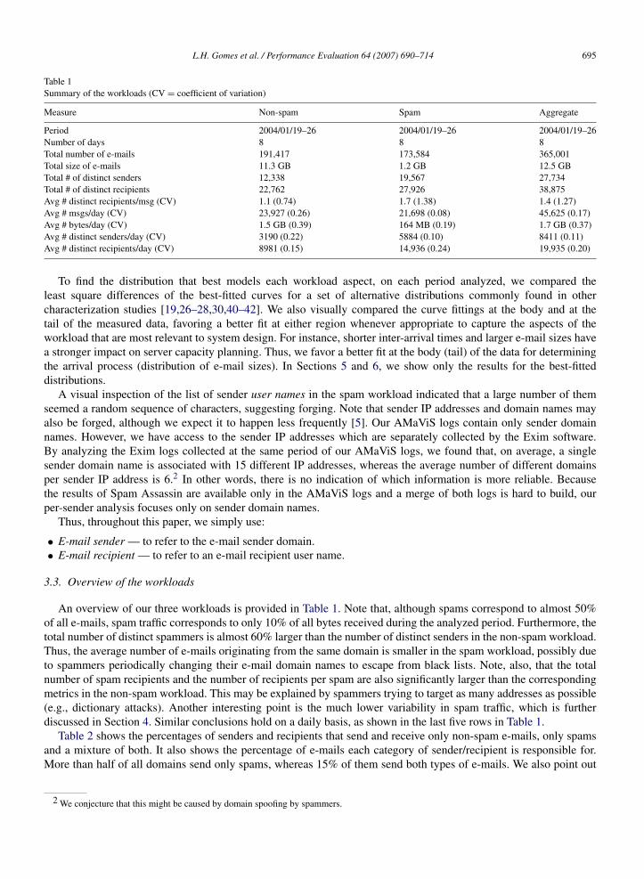
Table 1Summary of the workloads (CV = coefficient of variation)

Measure Non-spam Spam Aggregate

Period 2004/01/19–26 2004/01/19–26 2004/01/19–26Number of days 8 8 8Total number of e-mails 191,417 173,584 365,001Total size of e-mails 11.3 GB 1.2 GB 12.5 GBTotal # of distinct senders 12,338 19,567 27,734Total # of distinct recipients 22,762 27,926 38,875Avg # distinct recipients/msg (CV) 1.1 (0.74) 1.7 (1.38) 1.4 (1.27)Avg # msgs/day (CV) 23,927 (0.26) 21,698 (0.08) 45,625 (0.17)Avg # bytes/day (CV) 1.5 GB (0.39) 164 MB (0.19) 1.7 GB (0.37)Avg # distinct senders/day (CV) 3190 (0.22) 5884 (0.10) 8411 (0.11)Avg # distinct recipients/day (CV) 8981 (0.15) 14,936 (0.24) 19,935 (0.20)

To find the distribution that best models each workload aspect, on each period analyzed, we compared theleast square differences of the best-fitted curves for a set of alternative distributions commonly found in othercharacterization studies [19,26–28,30,40–42]. We also visually compared the curve fittings at the body and at thetail of the measured data, favoring a better fit at either region whenever appropriate to capture the aspects of theworkload that are most relevant to system design. For instance, shorter inter-arrival times and larger e-mail sizes havea stronger impact on server capacity planning. Thus, we favor a better fit at the body (tail) of the data for determiningthe arrival process (distribution of e-mail sizes). In Sections 5 and 6, we show only the results for the best-fitteddistributions.

A visual inspection of the list of sender user names in the spam workload indicated that a large number of themseemed a random sequence of characters, suggesting forging. Note that sender IP addresses and domain names mayalso be forged, although we expect it to happen less frequently [5]. Our AMaViS logs contain only sender domainnames. However, we have access to the sender IP addresses which are separately collected by the Exim software.By analyzing the Exim logs collected at the same period of our AMaViS logs, we found that, on average, a singlesender domain name is associated with 15 different IP addresses, whereas the average number of different domainsper sender IP address is 6.2 In other words, there is no indication of which information is more reliable. Becausethe results of Spam Assassin are available only in the AMaViS logs and a merge of both logs is hard to build, ourper-sender analysis focuses only on sender domain names.

Thus, throughout this paper, we simply use:

• E-mail sender — to refer to the e-mail sender domain.• E-mail recipient — to refer to an e-mail recipient user name.

3.3. Overview of the workloads

An overview of our three workloads is provided in Table 1. Note that, although spams correspond to almost 50%of all e-mails, spam traffic corresponds to only 10% of all bytes received during the analyzed period. Furthermore, thetotal number of distinct spammers is almost 60% larger than the number of distinct senders in the non-spam workload.Thus, the average number of e-mails originating from the same domain is smaller in the spam workload, possibly dueto spammers periodically changing their e-mail domain names to escape from black lists. Note, also, that the totalnumber of spam recipients and the number of recipients per spam are also significantly larger than the correspondingmetrics in the non-spam workload. This may be explained by spammers trying to target as many addresses as possible(e.g., dictionary attacks). Another interesting point is the much lower variability in spam traffic, which is furtherdiscussed in Section 4. Similar conclusions hold on a daily basis, as shown in the last five rows in Table 1.

Table 2 shows the percentages of senders and recipients that send and receive only non-spam e-mails, only spamsand a mixture of both. It also shows the percentage of e-mails each category of sender/recipient is responsible for.More than half of all domains send only spams, whereas 15% of them send both types of e-mails. We also point out

2 We conjecture that this might be caused by domain spoofing by spammers.


Table 2Distribution of senders and recipients

Group Senders Recipients% % Msg % % Msg

Only non-spam 29 31 25 10Only spam 56 23 38 20Mixture 15 46 37 70

(a) Non-spam. (b) Spam. (c) Aggregate.

Fig. 2. Daily load variation (normalization parameters: Max # E-mails/h = 51,226; Max # Bytes/h 2.24 GB).

that, on average, six out of the ten most active spam senders on each day send only spams. Nevertheless, the spam-onlyservers are responsible for only 23% of all e-mails, whereas 46% of the e-mails originate from domains that send amixture of spams and non-spams. These results may be explained by spammers frequently “forging” new domains.In [5], the authors also found a large fraction of senders who send only junk (i.e., virus, spam) e-mails. However, theyfound those senders accounted for a larger fraction of the e-mails in their workloads.

Table 2 also shows that whereas 25% of all recipients are not target of spam, around 38% of them appear only in thespam workload and receive 20% of all e-mails, in our log. Furthermore, we found that around 50% of the spam-onlyrecipients received fewer than 5 e-mails during the whole log, and that a number of them seemed forged (e.g., randomlygenerated sequence of characters). These observations led us to speculate that many spam-only recipients are the resultof two frequent spammer actions: dictionary attacks and removal of recipients from their target list after finding theydo not exist (i.e., after receiving a “not a user name” SMTP answer). They also illustrate a potentially harmful side-effect of spam, namely the use of network and computing resources for transmitting and processing a significantnumber of e-mails that are addressed to non-existent users and, thus, that will be discarded only once they reach thelocal e-mail servers they are addressed to.

4. Temporal variation patterns in e-mail traffic

This section discusses temporal variation patterns in each of our three e-mail workloads, namely, spam, non-spamand aggregate workloads. Section 4.1 analyzes daily and hourly variations in load intensity. Temporal variations inthe numbers of distinct e-mail recipients and senders are discussed in Section 4.2.

4.1. Load intensity

Fig. 2 shows daily load variations in the number of e-mails and number of bytes, for non-spam, spam and aggregateworkloads, respectively. The graphs show load measures normalized by the peak daily load observed in the aggregatetraffic. The normalization parameters are shown in the caption of the figure.

Fig. 2(a) shows that daily load variations in the non-spam e-mail traffic exhibit the traditional bell-shape behavior,typically observed in other web workloads [26,28,27], with load peaks during weekdays and a noticeable decrease inload intensity over the weekend (days six and seven). On the other hand, Fig. 2(b) shows that spam traffic does notpresent any significant daily variation. In fact, the daily numbers of e-mails and bytes are roughly uniformly distributedover the whole week. This stability in the daily spam traffic was previously observed in [8] for a much lighter spam


(a) Non-spam. (b) Spam.

(c) Aggregate.

Fig. 3. Hourly load variation (normalization parameters: Max # E-mails/h = 2768; Max # Bytes/h 197 MB).

Table 3Summary of hourly load variation

Traffic Metric Minimum Maximum Average CV

Non-spam# E-mails/hour 232–435 703–4676 513–1213 0.20–0.74# MBytes/hour 4–11 46–349 23–86 0.45–0.98

Spam# E-mails/hour 194–776 1081–2086 781–1007 0.12–0.36# MBytes/hour 1.7–5.7 6.1–18.4 4.3–8.0 0.15–0.45

Aggregate# E-mails/hour 500–1210 1681–6762 1294–2134 0.13–0.55# MBytes/hour 8.7–16.8 50–367 29–93 0.36–0.93

workload, including only 5% of all e-mails received. Fig. 2(c) shows that the impact of this distinct behavior on theaggregate traffic is a smoother variation in the number of e-mails per day. On the other hand, the variations in theaggregate number of bytes and in the number of non-spam bytes have very similar patterns, as shown in Fig. 2(c).This is because non-spam e-mails account for over 90% of all bytes received (see Table 1).

The same overall behavior is observed for the hourly load variations, as illustrated in Fig. 3, for a typical day. Likein [19,20], traditional non-spam e-mail traffic (Fig. 3(a)) presents two distinct and roughly stable regions: a high loaddiurnal period, typically from 7 AM to 7 PM, (i.e., working hours), during which the central server receives between65% and 73% of all daily non-spam e-mails, and a low load period covering the evening, night and early morning.On the other hand, the intensity of spam traffic (Fig. 3(b)) is roughly insensitive to the time of the day: the fractionof spams that arrives during a typical diurnal period is between 50% and 54%. Fig. 3(c) shows that, as observed fordaily load variations, the impact of spam on the aggregate traffic is a less pronounced hourly variation of the numberof e-mails received.

Table 3 summarizes the observed hourly load variation statistics. For each workload, it presents the ranges forminimum, maximum, average and coefficient of variation of the numbers of e-mails and bytes received per hour, oneach day. Note the higher variability in the numbers of e-mails and bytes in the non-spam workload. Moreover, forany of the three workloads, a higher coefficient of variation is observed in the number of bytes, because of the inherentvariability of e-mail sizes. Note that these results are consistent with the daily variations in the numbers of e-mails and



(c) Aggregate.

Fig. 4. Daily variation of number of senders and recipients (normalization parameters: Max # Senders/day = 10,089; Max # Recipients/day =

25,218).

bytes (see Table 1). Qualitative similar results were also found for load variations on a minute basis. The coefficientsof variation of the number of e-mails per minute vary in the ranges of 0.45–0.78 and 0.46–0.91 for the spam andnon-spam workloads, respectively. The coefficients of variation of the number of bytes per minute are in the ranges of0.70–1.03 and 1.37–1.75, in the two workloads.

One key conclusion is that, on various time scales, whereas traditional e-mail traffic is concentrated on diurnalperiods, the arrival rate of spam e-mails is roughly stable over time. One question that comes up is whether thisdifference is also observed on a per-sender basis. We analyzed the hourly traffic generated by each of the 50 mostactive spam-only senders and strictly non-spam senders. We found that each of the 50 strictly spam senders sent, onaverage, 53% of its daily e-mails during the day. In contrast, the strictly non-spam senders selected send, on average,63% of their e-mails during the same period. Similar results were obtained for the 100, 200 and 500 most active sendersin each group. Thus, each spammer independently sends almost half of its e-mails over night, when computing andnetworking resources are mostly idle. We conjecture that, by using automatic tools, spammers try to maximize theirshort-term throughput, sending at the fastest rate they can get through without being noticed, throughout the day.

4.2. Distinct senders and recipients

This section analyzes temporal variations in the numbers of distinct senders and recipients. Daily variations andhourly variations for a typical day are shown in Figs. 4 and 5, respectively. As before, we show normalized measures,expressed as fractions of the peak aggregate numbers of senders and recipients in the period. The normalizationparameters are given in the captions of the figures.

As observed in the load variation, temporal variations in the number of distinct e-mail senders in the spam workloadpresent significantly different behavior from those observed in the non-spam e-mail workload. Whereas the numberof distinct legitimate e-mail senders does present weekly patterns, the number of distinct spammers is roughly stableover the eight days (with a slight increase by the 7th day), as shown in Fig. 4(a) and (b). This difference is even morestriking on a hourly basis, as shown in Fig. 5(a) and (b). Again, we speculate that the inherently different nature of thee-mail senders in each workload (automatic tools versus human beings) are responsible for it. In the aggregate traffic,



(c) Aggregate.

Fig. 5. Hourly variation of number of senders and recipients (normalization parameters: Max # Senders/h = 956; Max # Recipients/h = 2802).

Table 4Summary of hourly variation of number of distinct recipients and senders

Traffic Metric Minimum Maximum Average CV

Non-spam# Recipients/hour 228–383 589–2883 411–978 0.21–0.58# Senders/hour 107–136 225–937 160–332 0.14–0.61

Spam# Recipients/hour 485–1174 1397–4095 955–2371 0.15–0.41# Senders/hour 147–406 548–925 433–577 0.10–0.24

Aggregate# Recipients/hour 828–1672 2480–6580 1505–3179 0.20–0.41# Senders/hour 256–541 828–1614 623–885 0.12–0.33

the significant variations observed in the non-spam e-mail traffic are somewhat smoothed out by the roughly stablenumber of spammers, as shown in Figs. 4(c) and 5(c).

Regarding the daily variations in the number of distinct recipients, shown in Fig. 4, no clear distinction betweenspam and non-spam traffic is observed. We found that the number of distinct spam recipients actually decreasessignificantly by the fourth day. We could not find any reason to explain this weird behavior and plan to look furtherinto that as future work. However, on a hourly basis, we found that whereas the number of distinct recipients of non-spam e-mails is higher during the day, the number of distinct spam recipients is roughly stable over time, as illustratedin Fig. 5, for a typical day. These results are summarized in Table 4, which shows, for each of the three workloads, theobserved ranges for the minimum, maximum, average and coefficient of variation of the number of distinct recipientsand number of distinct senders per hour.

For each workload, on each day, we also measured the statistical correlation [43] between the number of distinctsenders (si ) and the number of distinct recipients (ri ) for each hour i = 1 . . . 24. In other words, we computedthe coefficient of correlation ρ =

n∑n

i=1 si ri −∑n

i=1 si∑n

i=1 ri√n

∑ni=1 s2

i −(∑n

i=1 si )2√

n∑n

i=1 r2i −(

∑ni=1 ri )2

, where n = 24. We found coefficients of

correlation between 0.90 and 0.99 in the non-spam, and between 0.58 and 0.89 in the spam workload during theeight days. The lower correlation seems to indicate that there is a larger overlap in the distribution lists of typicalspammers. This overlap may be the result of spammers using similar automatic tools to create their targets, trading



Fig. 6. Distribution of inter-arrival times.

their distribution lists to extend their reach or obtaining the same distribution list from existing web services [44]. Thesharing of recipients among traditional e-mail senders is most probably due to the fixed number of recipients, who aremembers of a somewhat closed university community.

In summary, our results show that, unlike traditional non-spam e-mail traffic, which exhibits clear daily patterns,with load peaks during the day, the numbers of spam e-mails, spam bytes, distinct active spammers and distinct spamrecipients are roughly insensitive to the period of measurement, remaining mostly stable during the whole day, for alldays analyzed.

The fundamental differences between spam and non-spam traffic discussed in this section may be explained by theinherently distinct nature of their sources. Spammers are driven by the goal of reaching as many targets as possible,without being detected. To do so, they use automatic tools to (roughly) uniformly spread the flooding of e-mailsover time to avoid being noticed. Thus, a spam transmission is basically a unilateral action. The transmission of anon-spam e-mail, on the other hand, is the result of a bilateral relationship [21,45,40,41]. It is typically initiated by ahuman being, driven by some social reason (i.e., work, leisure), during his/her active hours.

5. E-mail traffic characteristics

This section analyzes the characteristics of e-mail traffic for the spam, non-spam and aggregate workloads. Thee-mail arrival process is characterized in Section 5.1. The distributions of e-mail sizes and number of recipients pere-mail are analyzed in Sections 5.2 and 5.3, respectively. For each workload characteristic, we discuss the differencesbetween spam and non-spam, pointing out the impact of the former on the aggregate workload.

5.1. E-mail arrival process

In this section, the e-mail arrival process in each workload is characterized during periods of roughly stable arrivalrate, in order to avoid spurious effects due to data aggregation. In the spam workload, such periods are typically wholedays, whereas in the non-spam and aggregate workloads, different stable periods are observed during the day and overnight.

We found that e-mail inter-arrival times are exponentially distributed in all three workloads, as illustrated inFig. 6(a), (b) and (c), for typical periods of stable arrival rate in the non-spam, spam and aggregate workloads,respectively. To evaluate the sensitivity of the distribution to the period of measurement, we looked into the distributionof inter-arrival times observed in different periods. Fig. 7 presents the cumulative distributions of inter-arrival timesfor two distinct periods, one during the day (from 7 AM to 7 PM) and the other during the evening (comprising theinterval between 7 PM up to 7 AM of the following day), for each workload. Fig. 7(a) shows that non-spam e-mailarrivals are burstier during the day, with around 86% of all inter-arrival times within 5 seconds. During the evening,only 40% of non-spam inter-arrival times are under 5 seconds. On the other hand, the distributions are the same in bothperiods in the spam workload, as shown in Fig. 7(b). Fig. 7(c) shows somewhat intermediate results for the aggregateworkload.

We next evaluate whether the assumptions of independent e-mail arrivals and, thus Poisson arrival processes, holdin our workloads. As in [36], we measured the statistical auto-correlation with lag one [43] of the inter-arrival times



Fig. 7. Sensitivity of inter-arrival time distribution to the period analyzed.

Table 5Summary of the distribution of inter-arrival times

Workload Inter-arrival times ExponentialMean (s) CV parameter λ

Non-spam 2.1–9.7 1.12–1.90 0.10–0.48Spam 3.6–4.9 1.08–1.99 0.21–0.26Aggregate 1.3–3.2 1.07–1.73 0.31–0.75

Exponential (PDF): pX (x) = λe−λx .

Table 6Summary of the statistic auto-correlation of inter-arrival times

Workload Mean auto-correlation CV

Non-spam 0.0659 0.6969Spam 0.0567 0.6062Aggregate 0.0435 0.5032

for all periods analyzed. Table 6 shows the mean and the coefficient of variation of the auto-correlation found for allthree workloads. Clearly, for all periods analyzed in all three workloads, the mean auto-correlation is very close tozero, with very low coefficient of variation. These results are an indication of independent inter-arrival times. Thus,we can conclude that e-mail arrivals follow Poisson processes in all three workloads.

Table 5 summarizes our findings. It shows the ranges of the mean and coefficient of variation of the inter-arrivaltimes measured in seconds as well as the range values of the λ parameter (e-mail arrival rate) of the best-fittedexponential distribution, for all periods analyzed, in each workload. Note that λ remains roughly stable across allperiods analyzed in the spam workload. In fact, the peak arrival rate is only 36% higher than the minimum. On theother hand, the non-spam arrival rates vary by as much as a factor of 5 across the periods analyzed. Aggregate trafficexhibits somewhat lower variations, as discussed in Section 4.

Our results are in contrast with prior work, which found that the distribution of e-mail inter-arrival times at foure-mail servers is a combination of a Weibull and a Pareto distributions [19,20]. However, like in our workloads (seeTable 5), the reported CV of their inter-arrival times was close to 1. Moreover, our results are in close agreementwith other previous work which found a non-stationary Poisson process to model with reasonable accuracy SMTPconnection arrivals [36].

5.2. E-mail size

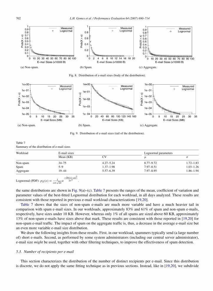
As proposed in Section 3.2, in order to analyze e-mails sizes, we fitted the body and the tail of the probabilitydistribution function separately. We found that the distribution of e-mail sizes is most accurately approximated, bothat the body and at the tail of the distribution, by a Lognormal distribution, in all three workloads, as illustrated inFigs. 8 and 9, for a typical day. Fig. 8(a)–(c) show the complementary cumulative distribution functions of the dataand fitted Lognormal distributions for the non-spam, spam and aggregate workloads, respectively. Semi-log plots of



Fig. 8. Distribution of e-mail sizes (body of the distribution).


Fig. 9. Distribution of e-mail sizes (tail of the distribution).

Table 7Summary of the distribution of e-mail sizes

Workload E-mail sizes Lognormal parametersMean (KB) CV µ σ

Non-spam 34–75 4.27–5.24 8.77–9.72 1.72–1.83Spam 5–9 1.37–1.98 7.97–8.51 1.03–1.26Aggregate 19–44 5.57–6.39 7.97–8.95 1.86–1.94

Lognormal (PDF): pX (x) =1

xσ√

2πe

−(ln(x)−µ)2

2σ2 .

the same distributions are shown in Fig. 9(a)–(c). Table 7 presents the ranges of the mean, coefficient of variation andparameter values of the best-fitted Lognormal distribution for each workload, in all days analyzed. These results areconsistent with those reported in previous e-mail workload characterizations [19,20].

Table 7 shows that the sizes of non-spam e-mails are much more variable and have a much heavier tail incomparison with spam e-mail sizes. In our workloads, approximately 83% and 61% of spam and non-spam e-mails,respectively, have sizes under 10 KB. However, whereas only 1% of all spams are sized above 60 KB, approximately13% of non-spam e-mails have sizes above that mark. These results are consistent with those reported in [19,20] fornon-spam e-mail traffic. The impact of spam on the aggregate traffic is, thus, a decrease in the average e-mail size butan even more variable e-mail size distribution.

We draw the following insights from these results. First, in our workload, spammers typically send (a large numberof) short e-mails. Second, as performed by some system administrators (including our central server administrator),e-mail size might be used, together with other filtering techniques, to improve the effectiveness of spam detection.

5.3. Number of recipients per e-mail

This section characterizes the distribution of the number of distinct recipients per e-mail. Since this distributionis discrete, we do not apply the same fitting technique as in previous sections. Instead, like in [19,20], we subdivide


Fig. 10. Distribution of number of recipients per e-mail.

each distribution into k buckets. Each bucket is characterized with an average probability, calculated over the eightdays analyzed. Jointly, these probabilities represent the distribution of the number of recipients per e-mail. For eachworkload, we choose a value of k so as to limit the probability of an e-mail with more than k recipients per e-mail tobelow 0.002 [19,20]. The values of k for the non-spam, spam and aggregate workloads are knon-spam = 8, kspam = 16and kaggregate = 16, respectively.

Fig. 10 shows the cumulative distributions for the three workloads. As mentioned in Section 3.3, spams are typicallyaddressed to a larger number of recipients. Whereas, on average, 95% of all non-spams are addressed to one recipient,86% of spams have a single destination. Furthermore, the distribution is heavier tailed in the spam workload, possiblydue to the use of automatic tools. Since almost half of all e-mails are spams, the distribution of the number of recipientsper e-mail in the aggregate workload is strongly influenced by their heavy tailed behavior. The authors of [19,20] foundan even heavier tail in the distribution of the number of recipients per e-mail. In that study, even though 94% of alle-mails are addressed to a single recipient, 20 buckets were necessary to cover 99.8% of all e-mails.

6. Analyzing e-mail senders and recipients

This section further analyzes e-mail senders and recipients. Popularity of e-mail recipients and senders is analyzedin Section 6.1. Section 6.2 analyzes temporal locality among e-mail recipients and senders. Finally, Section 6.3analyzes the sizes of sender and recipient contact lists, i.e., the sizes of the lists of contacts each sender (recipient)exchanges e-mail with.

6.1. Popularity

Popularity of objects has been repeatedly modeled with a Zipf-like distribution (Prob(access object with rank i)= C/ iα , where α > 0 and C is a normalizing constant [46]) in many contexts, including web, e-mail and streamingmedia [26–28,40]. A Zipf-like distribution appears as a straight line in the log–log plot of popularity versus objectrank. However, two roughly linear regions have been observed in the log–log plots of some streaming media andpeer-to-peer workloads [27–29,47]. The concatenation of two Zipf-like distributions has been suggested as a goodmodel in such cases [27,28].

In the next sections, we analyze the log–log plots of e-mail recipient and sender popularity, measured in terms ofnumber of e-mails and bytes received and sent. To assess the accuracy of our proposed models, we measure the R2

factor of the linear regression [43] for each single Zipf-like distribution found. In our models, the values of R2 areabove 0.95 in all cases. An R2

= 1 means perfect agreement.

6.1.1. Recipient popularityThis section analyzes the popularity of e-mail recipients in our three workloads. A characterization of the number

of e-mails per recipient is presented first. The distribution of the number of bytes per recipient is discussed later inthis section.

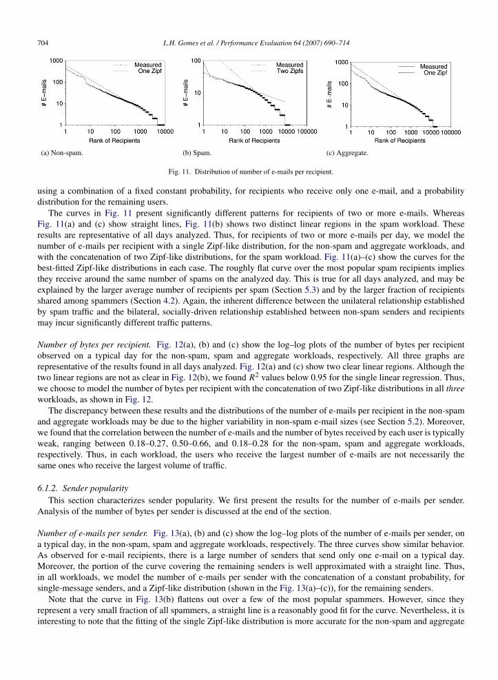
Number of e-mails per recipient. Fig. 11(a), (b) and (c) show the log–log plots of the number of e-mails per recipientfor the non-spam, spam and aggregate workloads, respectively, on a typical day. Given the large fraction of users whoreceive only one e-mail per day in all three workloads, we choose to characterize the number of e-mails per recipient



Fig. 11. Distribution of number of e-mails per recipient.

using a combination of a fixed constant probability, for recipients who receive only one e-mail, and a probabilitydistribution for the remaining users.

The curves in Fig. 11 present significantly different patterns for recipients of two or more e-mails. WhereasFig. 11(a) and (c) show straight lines, Fig. 11(b) shows two distinct linear regions in the spam workload. Theseresults are representative of all days analyzed. Thus, for recipients of two or more e-mails per day, we model thenumber of e-mails per recipient with a single Zipf-like distribution, for the non-spam and aggregate workloads, andwith the concatenation of two Zipf-like distributions, for the spam workload. Fig. 11(a)–(c) show the curves for thebest-fitted Zipf-like distributions in each case. The roughly flat curve over the most popular spam recipients impliesthey receive around the same number of spams on the analyzed day. This is true for all days analyzed, and may beexplained by the larger average number of recipients per spam (Section 5.3) and by the larger fraction of recipientsshared among spammers (Section 4.2). Again, the inherent difference between the unilateral relationship establishedby spam traffic and the bilateral, socially-driven relationship established between non-spam senders and recipientsmay incur significantly different traffic patterns.

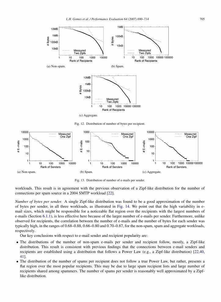
Number of bytes per recipient. Fig. 12(a), (b) and (c) show the log–log plots of the number of bytes per recipientobserved on a typical day for the non-spam, spam and aggregate workloads, respectively. All three graphs arerepresentative of the results found in all days analyzed. Fig. 12(a) and (c) show two clear linear regions. Although thetwo linear regions are not as clear in Fig. 12(b), we found R2 values below 0.95 for the single linear regression. Thus,we choose to model the number of bytes per recipient with the concatenation of two Zipf-like distributions in all threeworkloads, as shown in Fig. 12.

The discrepancy between these results and the distributions of the number of e-mails per recipient in the non-spamand aggregate workloads may be due to the higher variability in non-spam e-mail sizes (see Section 5.2). Moreover,we found that the correlation between the number of e-mails and the number of bytes received by each user is typicallyweak, ranging between 0.18–0.27, 0.50–0.66, and 0.18–0.28 for the non-spam, spam and aggregate workloads,respectively. Thus, in each workload, the users who receive the largest number of e-mails are not necessarily thesame ones who receive the largest volume of traffic.

6.1.2. Sender popularityThis section characterizes sender popularity. We first present the results for the number of e-mails per sender.

Analysis of the number of bytes per sender is discussed at the end of the section.

Number of e-mails per sender. Fig. 13(a), (b) and (c) show the log–log plots of the number of e-mails per sender, ona typical day, in the non-spam, spam and aggregate workloads, respectively. The three curves show similar behavior.As observed for e-mail recipients, there is a large number of senders that send only one e-mail on a typical day.Moreover, the portion of the curve covering the remaining senders is well approximated with a straight line. Thus,in all workloads, we model the number of e-mails per sender with the concatenation of a constant probability, forsingle-message senders, and a Zipf-like distribution (shown in the Fig. 13(a)–(c)), for the remaining senders.

Note that the curve in Fig. 13(b) flattens out over a few of the most popular spammers. However, since theyrepresent a very small fraction of all spammers, a straight line is a reasonably good fit for the curve. Nevertheless, it isinteresting to note that the fitting of the single Zipf-like distribution is more accurate for the non-spam and aggregate



(c) Aggregate.

Fig. 12. Distribution of number of bytes per recipient.


Fig. 13. Distribution of number of e-mails per sender.

workloads. This result is in agreement with the previous observation of a Zipf-like distribution for the number ofconnections per spam source in a 2004 SMTP workload [22].

Number of bytes per sender. A single Zipf-like distribution was found to be a good approximation of the numberof bytes per sender, in all three workloads, as illustrated in Fig. 14. We point out that the high variability in e-mail sizes, which might be responsible for a noticeable flat region over the recipients with the largest numbers ofe-mails (Section 6.1.1), is less effective here because of the larger number of e-mails per sender. Furthermore, unlikeobserved for recipients, the correlation between the number of e-mails and the number of bytes for each sender wastypically high, in the ranges of 0.68–0.88, 0.66–0.80 and 0.70–0.87, for the non-spam, spam and aggregate workloads,respectively.

Our key conclusions with respect to e-mail sender and recipient popularity are:

• The distributions of the number of non-spam e-mails per sender and recipient follow, mostly, a Zipf-likedistribution. This result is consistent with previous findings that the connections between e-mail senders andrecipients are established using a distribution that follows a Power Law (e.g., a Zipf-like distribution) [22,40,41].

• The distribution of the number of spams per recipient does not follow a true Power Law, but rather, presents aflat region over the most popular recipients. This may be due to large spam recipient lists and large number ofrecipients shared among spammers. The number of spams per sender is reasonably well approximated by a Zipf-like distribution.



(c) Aggregate.

Fig. 14. Distribution of number of bytes per sender.

Table 8Summary of distributions of recipient popularity

Traffic Popularity % receive/send Zipf % Data Prob. α

metric one e-mail/day model

Non-spam# E-mails 48–62 Single 100 1 0.52–0.68

# Bytes –1st 3–21 0.05–0.26 0.62–0.852nd 79–97 0.74–0.95 1.67–3.20

Spam# E-mails 29–59

1st 2–3 0.05–0.08 0.22–0.302nd 97–98 0.92–0.95 0.47–0.64

# Bytes –1st 4–62 0.05–0.66 0.34–0.562nd 38–96 0.34–0.95 1.10–3.87

Aggregate# E-mails 29–49 Single 100 1 0.95–0.97

# Bytes –1st 3–85 0.05–0.88 0.64–1.322nd 15–94 0.13–0.95 1.85–8.62

• In all three workloads, the number of bytes per recipient is most accurately modeled by two Zipf-like distributions.In the case of the non-spam and aggregate workloads, this is probably due to the high variability in e-mail size.The distribution of the number of bytes per sender is well modeled by a single Zipf-like distribution in all threeworkloads.

Tables 8 and 9 summarize our findings. Table 8 presents the ranges of the observed percentage of recipients thatreceive only one e-mail on a typical day. It also shows the range of parameter values for the Zipf-like distributionsthat best fit the data for the remaining recipients. For the cases where two Zipf-like distributions are the best model, itshows, for each single distribution, the total probability and percentage of recipients that fall within the correspondingregion of the curve and the value of the α parameter. Table 9 shows similar data for the distributions of senderpopularity.

We point out that the skewed distributions of the number of e-mails and bytes per sender and per recipient suggestthat sender and recipient popularity could be used to improve the effectiveness of spam detection techniques. Forinstance, on a typical day, on average, 53% of the spams and 63% of the spam bytes originate from only 3% of allstrictly spam senders. Furthermore, around 40% of these spammers are among the most active throughout the eightdays covered by our log. Thus, the insertion of these popular spammers into black lists could significantly reduce the


Table 9Summary of distributions of sender popularity

Workload Popularity % receive/send α

mzetric one e-mail/day

Non-spam# E-mails 54–68 0.993–1.251# Bytes – 1.72–2.08

Spam# E-mails 55–67 0.781–0.996# Bytes – 0.915–1.192

Aggregate# E-mails 53–61 0.937–0.987# Bytes – 1.185–1.775


Fig. 15. Histograms of recipient stack distances.

number of spams accepted by the server. Similar results are observed for the strictly non-spam senders, suggesting theuse of white lists to reduce the overhead of e-mail scanning. Finally, the concentration of spams into a small fraction ofrecipients, who remain among the most popular through several days, suggests that spam detection techniques mightbenefit from the use of the e-mail destination.

6.2. Temporal locality

Temporal locality in a object reference stream implies that objects that have been recently referenced are morelikely to be referenced again in the near future [42]. A previously proposed method to assess the temporal localitypresent in a reference stream is by means of the distribution of stack distances [42]. A stack distance measures thenumber of references between two consecutive references to the same object in the stream. Shorter stack distancesimply stronger temporal locality.

This section analyzes temporal locality among recipients and among senders in our three workloads, bycharacterizing the distribution of stack distances in the streams of e-mail recipients and e-mail senders. These streamsare built from each workload as follows. We start by creating one e-mail stream for each workload and day analyzed,preserving the order of e-mail arrivals in the corresponding workload and day. For each such stream, we replace eache-mail by its corresponding recipient list, thus creating a recipient stream. The distributions of stack distances in therecipient streams are then determined. Similarly, to assess the temporal locality among senders, we characterize thedistribution of stack distances in the sender streams, created by replacing each e-mail in the original streams by itssender.

Section 6.2.1 analyzes temporal locality among recipients. Temporal locality among senders is discussed inSection 6.2.2.

6.2.1. Temporal locality among recipientsFig. 15(a), (b) and (c) show histograms of recipient stack distances, for distances shorter than 150, observed on a

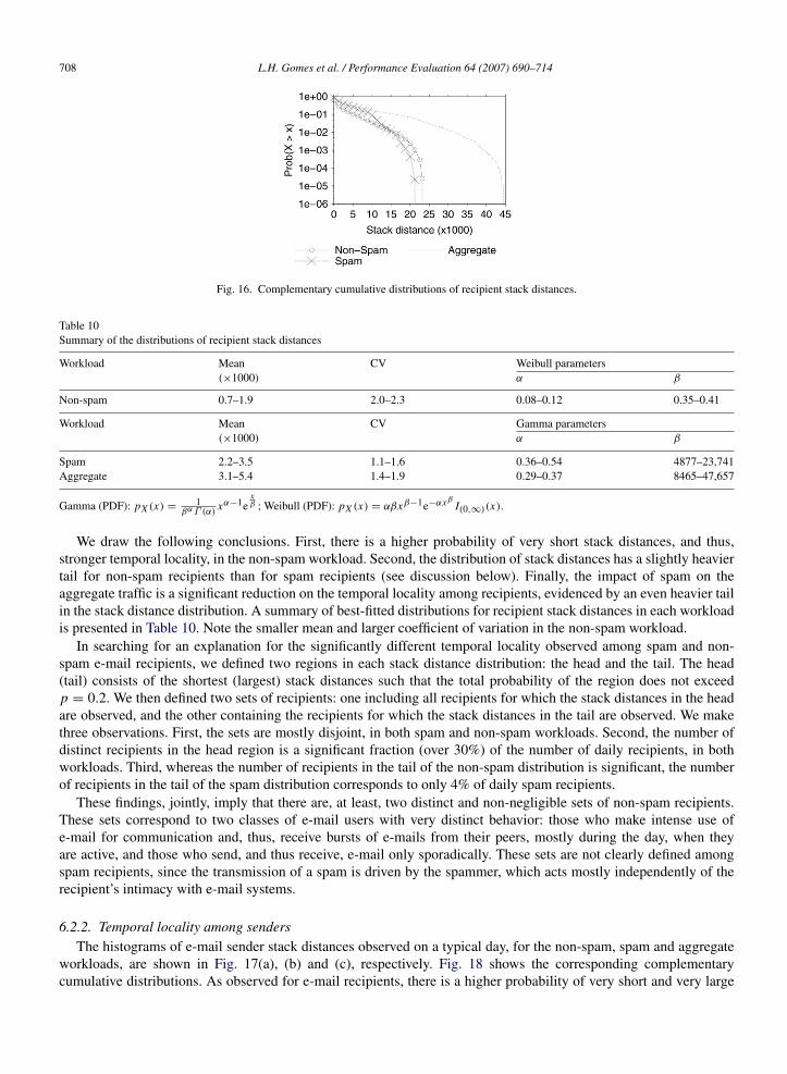
typical day in the non-spam, spam and aggregate workloads, respectively. The complementary cumulative distributionsof recipient stack distances, measured on the same day, are shown in Fig. 16. Note the log scale on the y-axis in Fig. 16.


Fig. 16. Complementary cumulative distributions of recipient stack distances.

Table 10Summary of the distributions of recipient stack distances

Workload Mean CV Weibull parameters(×1000) α β

Non-spam 0.7–1.9 2.0–2.3 0.08–0.12 0.35–0.41

Workload Mean CV Gamma parameters(×1000) α β

Spam 2.2–3.5 1.1–1.6 0.36–0.54 4877–23,741Aggregate 3.1–5.4 1.4–1.9 0.29–0.37 8465–47,657

Gamma (PDF): pX (x) =1

βαΓ (α)xα−1e

xβ ; Weibull (PDF): pX (x) = αβxβ−1e−αxβ

I(0,∞)(x).

We draw the following conclusions. First, there is a higher probability of very short stack distances, and thus,stronger temporal locality, in the non-spam workload. Second, the distribution of stack distances has a slightly heaviertail for non-spam recipients than for spam recipients (see discussion below). Finally, the impact of spam on theaggregate traffic is a significant reduction on the temporal locality among recipients, evidenced by an even heavier tailin the stack distance distribution. A summary of best-fitted distributions for recipient stack distances in each workloadis presented in Table 10. Note the smaller mean and larger coefficient of variation in the non-spam workload.

In searching for an explanation for the significantly different temporal locality observed among spam and non-spam e-mail recipients, we defined two regions in each stack distance distribution: the head and the tail. The head(tail) consists of the shortest (largest) stack distances such that the total probability of the region does not exceedp = 0.2. We then defined two sets of recipients: one including all recipients for which the stack distances in the headare observed, and the other containing the recipients for which the stack distances in the tail are observed. We makethree observations. First, the sets are mostly disjoint, in both spam and non-spam workloads. Second, the number ofdistinct recipients in the head region is a significant fraction (over 30%) of the number of daily recipients, in bothworkloads. Third, whereas the number of recipients in the tail of the non-spam distribution is significant, the numberof recipients in the tail of the spam distribution corresponds to only 4% of daily spam recipients.

These findings, jointly, imply that there are, at least, two distinct and non-negligible sets of non-spam recipients.These sets correspond to two classes of e-mail users with very distinct behavior: those who make intense use ofe-mail for communication and, thus, receive bursts of e-mails from their peers, mostly during the day, when theyare active, and those who send, and thus receive, e-mail only sporadically. These sets are not clearly defined amongspam recipients, since the transmission of a spam is driven by the spammer, which acts mostly independently of therecipient’s intimacy with e-mail systems.

6.2.2. Temporal locality among sendersThe histograms of e-mail sender stack distances observed on a typical day, for the non-spam, spam and aggregate

workloads, are shown in Fig. 17(a), (b) and (c), respectively. Fig. 18 shows the corresponding complementarycumulative distributions. As observed for e-mail recipients, there is a higher probability of very short and very large



Fig. 17. Histograms of e-mail sender stack distances.

Fig. 18. Complementary cumulative distributions of e-mail sender stack distances.

Table 11Summary of the distributions of e-mail senders stack distances

Workload Mean CV Weibull parametersµ σ

Non-spam 287–644 3.35–3.78 4.34–6.63 1.58–1.70Spam 960–1567 1.88–2.51 5.52–7.80 1.23–1.42Aggregate 1403–2189 2.32–3.23 6.03–7.91 1.36–1.56

stack distances for non-spam e-mail senders. The distribution for the aggregate workload has an even heavier tail,implying a significant reduction on temporal locality among e-mail senders due to spam. A summary of the best-fitteddistributions for e-mail sender stack distances is given in Table 11.

6.3. Contact lists

This section analyzes the contacts established between senders and recipients through e-mail in the spam, non-spamand aggregate workloads. Our basic assumption is that, in both spam and non-spam traffic, and thus in the aggregatetraffic as well, users (i.e., senders/recipients) have a defined list of peers they often have contact with (i.e., theysend/receive an e-mail to/from) [21]. In non-spam traffic, contact lists are consequence of social relationships onwhich users’ communications are based. In spam traffic, on the other hand, the lists used by spammers to distributetheir solicitations are created for business interest and, generally, do not reflect any form of social interaction.

In each workload, the contact list of sender s is defined as the set of recipients to which s sent at least one e-mail (spam, non-spam or either one, in the aggregate workload) in the period analyzed. Similarly, the contact list ofrecipient r is defined as the set of senders from which r received at least one e-mail in the period analyzed. The sizeof a sender/recipient contact list is given by the number of recipients/senders in its contact list.

A sender/recipient contact list is built dynamically, over time, as new e-mails are exchanged. Moreover, contactlists certainly may change over time. However, we expect them to be much more stable than other workload aspects


Fig. 19. Cumulative distribution of size of sender contact lists.

Table 12Distribution of sizes of sender contact lists

Workload Sizes of sender contact listsMean CV Size = 1 (%) Size < 8 (%) Size < 400 (%)

Non-spam 6.9 9.0 58 92 99.8Spam 13.8 3.2 29 72 99.6Aggregate 12.6 4.7 37 77 99.6

such as e-mail inter-arrival times and sender popularity. Thus, in contrast to other analysis presented in this paper,this section analyzes the distribution of the sizes of recipient and sender contact lists in each of our three workloadsconsidering the entire eight-day log. The distribution of the size of sender contact lists is analyzed in Section 6.3.1.Section 6.3.2 analyzes the size of recipient contact lists.

6.3.1. Sender contact listsFig. 19 shows the cumulative distribution of the sizes of sender contact lists in each workload, for list sizes varying

from 1 to 100, which account for more than 98% of all senders in our three workloads. Note that the distribution ismuch more skewed towards shorter contact lists among non-spam senders. In other words, typical spammers sende-mails indiscriminately to a much larger number of distinct recipients. Dictionary attacks certainly contribute togenerating large contact lists. Non-spam senders, on the other hand, have, on average, a smaller number of contacts,established through some sort of social relationship they might have. Note that the longer contact lists of spammerssignificantly impact the distribution in the aggregate traffic.

Table 12 shows the mean and coefficient of variation of sender contact list sizes in the non-spam, spam andaggregate workloads. It also shows the percentage of senders that fall into different ranges of list sizes. On average,spammers have contact to twice as many distinct recipients than non-spam senders. Furthermore, the fraction of sendercontact lists with only one recipient over the eight-day period analyzed is significantly higher in the non-spam traffic.In fact, only 8% of non-spam sender contact lists have sizes greater than 8, whereas 28% of spammer contact listshave size above that mark. Nevertheless, it is interesting to note the high variability in the contact list sizes amongnon-spam senders. This reflects the natural variability in the behavior of legitimate e-mail users: some have (e-mail)contact to a much larger number of people than others.

Therefore, the sizes of spammer contact lists are larger, on average, but much less variable. Furthermore, the cleardistinction between the distributions of contact list sizes among spammers and non-spam senders significantly impactthe distribution in the aggregate traffic.

6.3.2. Recipient contact listsFig. 20 shows the cumulative distribution of the sizes of recipient contact lists in each workload, for list sizes

varying from 1 to 100, which account for more than 99% of all recipients. As observed among senders, the distributionof contact list sizes is much more skewed towards shorter lists among non-spam recipients. The impact of spam onthe aggregate traffic is clear: the aggregate distribution is much more heavy tailed than the non-spam distribution.

Table 13 shows the mean and coefficient of variation of recipient contact list sizes in the non-spam, spam andaggregate workloads. It also shows the percentage of recipients that fall into different ranges of list sizes. Note


Fig. 20. Cumulative distribution of size of recipient contact lists.

Table 13Distribution of sizes of recipient contact lists

Workload Sizes of recipient contact listsMean CV Size = 1 (%) Size < 6 (%) Size < 30 (%)

Non-spam 3.7 1.4 44 81 99.5Spam 9.6 1.3 18 45 95.2Aggregate 9.5 1.5 23 49 95.1

that, on average, the number of distinct spammers with whom recipients have contact is almost three times thenumber of contacts of non-spam recipients. Furthermore, the fraction of recipient contact lists with only one senderis significantly higher in the non-spam traffic. In fact, only 19% of non-spam recipient contact lists have sizes greaterthan 5, whereas 55% of spam recipient contact lists have sizes above that mark.

In summary, the analysis presented in this section showed that the sizes of contact lists can strongly distinguishnon-spam and spam traffic, and that they strongly impact the distributions observed in the aggregate traffic. An attemptto exploit this distinction for clustering senders and recipients into communities that share similar contact lists, anduse such communities for detecting spam is presented in [17].

7. Conclusion and future work

This paper provides an extensive analysis of a spam traffic, uncovering characteristics that significantly distinguishit from traditional non-spam traffic and assessing how the aggregate traffic is affected by the presence of a largenumber of spams.

Our characterization, based on the information available on the e-mail headers, revealed that the e-mail arrivalprocess, e-mail sizes, number of recipients per e-mail, popularity and temporal locality among recipients and thesizes of sender and recipient contact lists are key workload aspects where spam traffic significantly deviates fromtraditional non-spam traffic. We believe that such discrepancies are consequence of the inherently different natureof e-mail senders in each traffic. Traditional e-mail senders are usually human beings who use e-mails to interact orsocialize with their peers. Spammers typically use automatic tools to generate and send their e-mails to a multitude of“potential”, mostly unknown, users.

Possible directions for future work include: (1) validation of our results over time and for workloads from differentenvironments; (2) characterization of e-mail content; (3) design and evaluation of new spam detection and filteringtechniques that exploit the distinctions observed in this paper for spam and non-spam traffic; and (4) design andimplementation of a spam-infected e-mail synthetic workload generator to be used in the experimental evaluation ofnew spam detection strategies.

Acknowledgments

The authors would like to thank Fernando Frota, from CECOM/ UFMG, for the helpful and inspiring discussions.They are also thankful to Marcio Bunte and Fernando Frota for providing the logs analyzed in this paper. L.H.


Gomes was supported by the Central Bank of Brazil. J.M. Almeida, V. Almeida and W. Meira Jr. were supportedby CNPq/Brazil.

References

[1] Message Labs Home Page, http://www.messagelabs.co.uk/.[2] M. Nelson, Anti-spam for business and ISPs: Market size 2003–2008, Tech. rep., Ferris Research Inc. 408 Columbus Ave., Suite 1, San

Francisco, CA, April 2003.[3] D. Fallows, Spam: How it is hurting email and degrading life on the internet, Tech. rep., Pew and Internet American Life Project 1100

Connecticut Avenue, NW-Suite 710 Washington, D.C. 20036, October 2003.[4] L. Rainie, D. Fallows, The can-spam act has not helped most email users so far, Tech. rep., Pew and Internet American Life Project 1100

Connecticut Avenue, NW-Suite 710 Washington, D.C. 20036, March 2004.[5] R.D. Twining, M.M. Williamson, M. Mowbray, M. Rahmouni, Email prioritization: Reducing delays on legitimate mail caused by Junk Mail,

in: Proceedings of the Usenix Annual Technical Conference, Boston, MA, 2004, pp. 45–58.[6] MAPS—mail abuse prevention system home page, http://mail-abuse.org/rbl/getoff.html.[7] E. Harris, The next step in the spam control war: Greylisting, http://projects.puremagic.com/greylisting.[8] L.F. Cranor, B.A. LaMacchia, Spam!, Communications of the ACM 41–8 (1998) 74–83.[9] H.P. Baker, Authentication approaches, in: Proceedings of the 56th IETF Meeting, San Francisco, CA, 2003.

[10] B. Krishnamurthy, SHRED: Spam harassment reduction via economic disincentives, in: Proceedings of the 56th IETF Meeting, San Francisco,CA, 2003.

[11] H.P. Brandmo, Solving spam by establishing a platform for sender accountability, in: Proceedings of the 56th IETF Meeting, San Francisco,CA, 2003.

[12] M. Sahami, S. Dumais, D. Heckerman, E. Horvitz, A Bayesian approach to filtering junk e-mail, Tech. Rep. WS-98-05, AAAI Workshop onLearning for Text Categorization, Madison, WI, July 1998.

[13] T. Fawcett, In vivo spam filtering: A challenge problem for KDD, SIGKDD Explor. Newsl. 5 (2) (2003) 140–148.[14] F. Zhou, L. Zhuang, B. Zhao, L. Huang, A. Joseph, J. Kubiatowicz, Approximate object location and spam filtering on peer-to-peer systems,

in: Proceedings of the Middleware, Rio de Janeiro, Brazil, 2003, pp. 1–20.[15] P.O. Boykin, V. Roychowdhury, Leveraging social networks to fight spam, IEEE Computer 38 (4) (2005) 61–68.[16] P. Desikan, J. Srivastava, Analyzing network traffic to detect e-mail spamming machines, in: Proceedings of the ICDM Workshop on Privacy

and Security Aspects of Data Mining, Brighton, UK, 2004, pp. 67–76.[17] L.H. Gomes, F.D.O. Castro, R.B. Almeida, L.M.A. Bettencourt, V.A.F. Almeida, J.M. Almeida, Improving spam detection based on structural

similarity, in: Steps to Reducing Unwanted Traffic on the Interne Workshop, July 2005.[18] S. Atkins, Size and cost of the problem, in: Proceedings of the 56th IETF Meeting, San Francisco, CA, 2003.[19] L. Bertolotti, M.C. Calzarossa, Workload characterization of mail servers, in: Proceedings of the SPECTS 2000, Elsevier Science Publishers

B. V., Vancouver, Canada, 2000, pp. 301–307.[20] L. Bertolotti, M.C. Calzarossa, Models of mail server workloads, Performance Evaluation 46 (2–3) (2001) 65–76.[21] L.H. Gomes, R.B. Almeida, L.M.A. Bettencourt, V.A.F. Almeida, J.M. Almeida, Comparative graph theoretical characterization of networks

of spam and regular email, in: Second Conference on Email and Anti-Spam, July 2005.[22] J. Jung, E. Sit, An empirical study of spam traffic and the use of DNS black lists, in: Proceedings of the 4th ACM SIGCOMM Conference on

Internet Measurement, ACM Press, Taormina, Italy, 2004, pp. 370–375.[23] L.H. Gomes, C. Cazita, J. Almeida, V.A.F. Almeida, W. Meira Jr., Characterizing a spam traffic, in: Proceedings of the 4th ACM SIGCOMM

Conference on Internet Measurement, ACM Press, Taormina, Italy, 2004, pp. 356–369.[24] A. Ramachandran, N. Feamster, Understanding the network level behavior of spammers, in: Proceedings of the 4th ACM SIGCOMM

Conference on Internet Measurement, ACM Press, Pisa, Italy, 2006, pp. 293–302.[25] M. Arlitt, C. Williamson, Web server workload characterization: The search of invariants, in: Proceedings of the 1996 Sigmetrics Conference

on Measurement of Computer Systems, ACM Press, Philadelphia, PA, 1996, pp. 126–137.[26] E. Veloso, V. Almeida, W. Meira, A. Bestavros, S. Jin, A hierarchical characterization of a live streaming media workload, in: Proceedings of

the Second ACM SIGCOMM Workshop on Internet Measurement, ACM Press, Marseille, France, 2002, pp. 117–130.[27] J.M. Almeida, J. Krueger, D.L. Eager, M.K. Vernon, Analysis of educational media server workloads, in: Proceedings of the 11th Int’l,

Workshop on Network and Operating System Support for Digital Audio and Video, ACM Press, Port Jefferson, New York, NY, 2001,pp. 21–30.

[28] C. Costa, I. Cunha, A. Borges, C. Ramos, M. Rocha, J. Almeida, B. Ribeiro-Neto, Analyzing client interativity in streaming media,in: Proceedings of the 13th World Wide Web Conference — WWW 2004, ACM Press, New York, NY, 2004, pp. 534–543.

[29] K.P. Gummadi, R.J. Dunn, S. Saroiu, S.D. Gribble, H.M. Levy, J. Zahorjan, Measurement, modeling, and analysis of a peer-to-peer file-sharing workload, in: Proceedings of the 19th ACM Symposium on Operating Systems Principles, ACM Press, Bolton Landing, NY, 2003,pp. 151–160.

[30] C. Dewes, A. Wichmann, A. Feldmann, An analysis of internet chat systems, in: Proceedings of the 2003 ACM SIGCOMM Conference onInternet Measurement, ACM Press, Miami Beach, FL, 2003, pp. 51–64.

[31] Exim Internet Mailer Home Page, http://www.exim.org.[32] AMaViS — home page, http://www.amavis.org.[33] Trend micro home page, http://www.trendmicro.com.

http://www.messagelabs.co.uk/

http://mail-abuse.org/rbl/getoff.html

http://projects.puremagic.com/greylisting

http://www.exim.org

http://www.amavis.org

http://www.trendmicro.com


[34] SpamAssassin home page, http://www.spamassassin.org.[35] What is a dictionary attack? http://www.filterpoint.com/help/dictionary.html.[36] V. Paxson, S. Floyd, Wide area traffic: The failure of Poisson modeling, IEEE/ACM Transactions on Networking 3 (3) (1995) 226–244.[37] B. Massey, M. Thomure, R.B.S. Long, Learning spam: simple techniques for freely-available software, in: Proceedings of the 2003 Usenix

Annual Technical Conference, San Antonio, TX, 2003.[38] W. Gansterer, M. Ilger, P. Lechner, R. Newmayer, J. Straub, Anti-spam methods — state-of-the-art, Tech. Rep. FA 384108 — Spam-Abwehr,

Institute of Distributed and Multimedia Systems, Faculty of Computer Science. University of Vienna, Austria, March 2005.[39] A.K. Seewald, A close look at current approaches in spam filtering, Tech. Rep. TR-2005-04, Austrian Research Institute for Artificial

Intelligence, Freyung 6/6, A-1010 Vienna, Austria, April 2005.[40] H. Ebel, L.-I. Mielsch, S. Bornhold, Scale-free topology of e-mail networks, Physical Review E 66-035103(R) (2002) 1–3.[41] M.E. Newman, S. Forrest, J. Balthrop, Email networks and the spread of computer viruses, Physical Review E 66-035101(R) (2002) 1–4.[42] V. Almeida, A. Bestavros, M. Crovella, A. de Oliveira, Characterizing reference locality in the WWW, in: Proceedings of the IEEE Conference

on Parallel and Distributed Information Systems (PDIS), Miami Beach, FL, 1996, pp. 92–103.[43] K.S. Trivedi, Probability and Statistics with Reliability, Queuing, and Computer Science Applications, John Wiley & Sons, New York, NY,

2001.[44] The list guy home page, http://www.listguy.com/email-sent.html.[45] J.P. Eckmann, E. Moses, D. Sergi, Entropy of dialogs creates coerent structures in e-mail traffic, PNAS — Proceedings of the National

Academy of Sciences 101-14333 (40) (2004) 333–337.[46] G.K. Zipf, Human Behavior and the Principle of Least-Effort, Addison-Wesley, Cambridge, MA, 1949.[47] L. Cherkasova, G. Ciardo, Characterizing temporal locality and its impact on web server performance, in: Proceedings of the Int’l Conf. on

Computer Communications and Networks, IEEE, Las Vegas, NV, 2000, pp. 16–18.

Luiz Henrique Gomes is a PhD student of the Computer Science Department at the Federal University of Minas Gerais,Brazil. His research interests include performance evaluation and complex networks.

Cristiano Cazita received his BSc degree in Computer Science from the Federal University of Minas Gerais, Brazil, in2004. He currently works as a system analyst for the Brazilian Federal Government.

Jussara M. Almeida has been an Associate Professor of the Computer Science Department at the Federal University ofMinas Gerais, Brazil, since 2004. She received BSc and MSc degrees from the Federal University of Minas Gerais, as wellas MSc and PhD degrees from the University of Wisconsin-Madison, US, all in Computer Science.

Her research interests include performance analysis and modeling of large-scale distributed systems as well asworkload and user behavior characterization.

Virgılio Almeida is a professor of the Computer Science Department at the Federal University of Minas Gerais,Brazil. His research interests include performance evaluation and modeling large scale distributed systems. He has heldvisiting professor positions at Boston University and the Polytechnic University of Catalunya in Barcelona, and visitingappointments at Xerox PARC and Hewlett-Packard Research Laboratory. He is a full member of the Brazilian Academyof Sciences.

http://www.spamassassin.org

http://www.filterpoint.com/help/dictionary.html

http://www.listguy.com/email-sent.html


Wagner Meira Jr. is an associate professor in the computer science department at the Federal University of MinasGerais, Brazil. His research focuses on scalability and efficiency of large-scale parallel and distributed systems frommassively parallel to Internet-based configurations. More recently he has been working on data mining algorithms andtheir parallelization, and application to areas such as information retrieval, bioinformatics, and e-governance. Meira has aPhD in computer science from the University of Rochester.

Workload models of spam and legitimate e-mails

Documents

Transcript of Workload models of spam and legitimate e-mails