WORKING WITH XML - Bangalore Branch of SIRC of ICAI
141
WORKING WITH XML 1.1 Introduction Imagine CFO of a company who regularly looks at financial data. He wants to specify a range of dates and then get aggregate financial data relating to those periods. He wants to see Financial Figures, Revenue streams, Costs summarized by weeks within the specified range. He wants to see the raw data as well as charts showing these trends for the specified date range. To achieve this some staff, has to sift through lots of data and create separate spreadsheet reports for the different scenarios. The load on IT is huge in the sense that they have to cater to demands of not only CFO but whole lot of diverse departments like Sales, Procurement etc. A more viable alternative would be where we have an Excel spreadsheet that could adapt itself to deliver the various reports the CFO needs as well as one that other departments could reuse and adjust for their similar needs. The way out is XML, but let’s first understand what XML is. 1.2 Understanding XML XML is a technology that is designed for managing and sharing structured data in a human-readable text file. XML follows industry-standard guidelines and can be processed by a variety of databases and applications. Using XML, application designers can create their own customized tags, data structures, and schemas. In short, XML greatly eases the definition, transmission, validation, and interpretation of data between databases, applications, and organizations. CHAPTER 1 LEARNING OBJECTIVES To gain understanding of XML To understand XML in Excel To understand Creating XML Maps from Excel file To understand Exporting & Importing XML data To understand working with XML tables To understand refreshing data from XML
-
Upload
khangminh22 -
Category
Documents
-
view
0 -
download
0
Transcript of WORKING WITH XML - Bangalore Branch of SIRC of ICAI
WORKING WITH XML
1.1 Introduction Imagine CFO of a company who regularly looks at financial data. He wants to specify a range of dates and then get aggregate financial data relating to those periods. He wants to see Financial Figures, Revenue streams, Costs summarized by weeks within the specified range. He wants to see the raw data as well as charts showing these trends for the specified date range.
To achieve this some staff, has to sift through lots of data and create separate spreadsheet reports for the different scenarios. The load on IT is huge in the sense that they have to cater to demands of not only CFO but whole lot of diverse departments like Sales, Procurement etc.
A more viable alternative would be where we have an Excel spreadsheet that could adapt itself to deliver the various reports the CFO needs as well as one that other departments could reuse and adjust for their similar needs.
The way out is XML, but let’s first understand what XML is.
1.2 Understanding XML XML is a technology that is designed for managing and sharing structured data in a human-readable text file. XML follows industry-standard guidelines and can be processed by a variety of databases and applications. Using XML, application designers can create their own customized tags, data structures, and schemas. In short, XML greatly eases the definition, transmission, validation, and interpretation of data between databases, applications, and organizations.
CHAPTER
1 LEARNING OBJECTIVES
To gain understanding of XML
To understand XML in Excel
To understand Creating XML Maps from Excel file
To understand Exporting & Importing XML data
To understand working with XML tables
To understand refreshing data from XML
ADVANCED MS-EXCEL
4 ADVANCED INFORMATION TECHNOLOGY
XML was designed to transport and store data.
XML stands for EXtensible Markup Language
XML is a markup language much like HTML
XML was designed to carry data, not to display data
XML tags are not predefined, we must define our own tags
XML is designed to be self-descriptive
XML is a W3C Recommendation
The simplest way to explain XML is as a structured way of storing information.
The difference between an XML document and a database (which is also a way of storing structured information) is:
1. A database is a heavy system in that a lot of software goes into creating and maintaining a database; an XML document is based on tags, similar to a HTML document; the difference is that the tags can even be user defined, which means we can store data the way we want, as long as we create the software which can decipher what the data stands for.
2. Even a browser can interpret common XML documents which rely on standard tags.
3. Every database system is proprietary in the sense that even though each can interface with another through defined protocols, the internals are all hidden; an XML document is defined by tags which are within the document, so it is totally open.
XML stands for
EXtensible
XML is extensible. It lets us define our own tags, the order in which they occur, and how they should be processed or displayed.
Markup
The most recognizable feature of XML is its tags, or elements
Language
XML is a language that’s very similar to HTML, but much more flexible.
XML does not DO anything. XML was created to structure, store, and transport information.
The following example is a note to Sachin, from Mahendra, stored as XML:
<?xml version="1.0" encoding="ISO-8859-1"?>
<note>
<to>Sachin</to> <from>Mahendra</from> <heading>Reminder</heading> <body>Meet me at IPL!</body>
</note>
WORKING WITH XML
ADVANCED INFORMATION TECHNOLOGY 5
The note above is self-descriptive. It has sender and receiver information, it also has a heading and a message body.
Honestly, XML document does not DO anything. It is just information wrapped in tags. To send, receive or display it, software would be needed.
XML allows the author to write their own Tags and their own data structure.
XML documents form a tree structure that starts at "the root" and branches to "the leaves".
The first line is the XML declaration. It defines the XML version (1.0) and the encoding used (ISO-8859-1 = Latin-1/West European character set).
The next line describes the root element of the document (like saying: "this document is a note"):
<note>
The next 4 lines describe 4 child elements of the root (to, from, heading, and body):
<to>Sachin</to> <from>Mahendra</from> <heading>Reminder</heading> <body>Meet me at IPL!</body>
And finally the last line defines the end of the root element:
</note>
This XML document contains a note to Sachin from Mahendra
XML Documents Form a Tree Structure
<root> <child> <subchild>.....</subchild> </child> </root>
The syntax rules of XML are very simple and logical
Every bit of data has to start and end with an identical tag: <TagName>Data</TagName>
Tag names are case sensitive. <Body> and </body> are NOT valid tags because the capitalization in the end tag is not the same as the capitalization in the begin tag.
The XML file must begin and end with a root tag. There can only be one root tag in a file. In the example above, the root tag is <Note>.
We can have an empty tag - put the slash at the end of the tag instead of the beginning: <TagName/>
If we nest tags, we must close the inner tag before closing the outer tag. <Item><a>data</a></Item> will work, but <Item><a>data</Item></a>will not.
XML Attribute Values must be put within quotes.
Whether XML File is Valid or not can be checked at http://www.stg.brown.edu/service/xmlvalid/
XML Element
ADVANCED MS-EXCEL
6 ADVANCED INFORMATION TECHNOLOGY
An XML element is everything from (including) the element's start tag to (including) the element's end tag.
An element can contain:
other elements
text
attributes
or a mix of all of the above...
XML allows us to separate information from presentation
An element consists of an opening tag, its attributes, any content, and a closing tag.
A tag – either opening or closing – is used to mark the start or end of an element.
A node is a part of the hierarchical structure that makes up an XML document. "Node" is a generic term that applies to any type of XML document object, including elements, attributes, comments, processing instructions, and plain text.
XML Attributes
Attributes often provide information that is not part of the data
XML Schema
To ensure that everyone plays by the rules, we need a Document Type Definition (DTD), which is called XML Schema, whose purpose is to define the structure of an XML document. It’s a lot like a rule book that states which tags are legal, and where.
1.3 XML in Excel Microsoft Office Excel makes it easy to import Extensible Markup Language (XML) data that is created from other databases and applications, to map XML elements from an XML schema to worksheet cells, and to export revised XML data for interaction with other databases and applications. Think of these XML features as turning Office Excel into an XML data file generator with a familiar user interface.
Excel works primarily with two types of XML files:
XML data files (.xml), which contain the custom tags and structured data.
Schema files (.xsd), which contain schema tags that enforce rules, such as data type and validation.
The following are key scenarios that the XML features are designed to address:
Extend the functionality of existing Excel templates by mapping XML elements onto existing cells. This makes it easier to get XML data into and out of our templates without having to redesign them.
Use XML data as input to existing calculation models by mapping XML elements onto existing worksheets.
Import XML data files into a new workbook.
WORKING WITH XML
ADVANCED INFORMATION TECHNOLOGY 7
Import XML data from a Web service into Excel worksheet.
Export data in mapped cells to XML data files independent from other data in the workbook.
1.4 XML Maps XML schemas in Excel are called XML maps. XML maps link the cells in a worksheet to the elements (items) in an XML schema. We must build our maps from XML schemas. Because schemas don't contain data, our mapped cells remain blank until we import or otherwise load data into them.
Inferred Schemas
If there is no schema, Excel has a great facility where it infers one from the structure of the tags in an XML data file.
Xml Data File Format vs. XML Spreadsheet Format
The XML Data format allows us to save our data to standard XML data files. The XML Spreadsheet format is proprietary, and requires Excel 2002 or later.
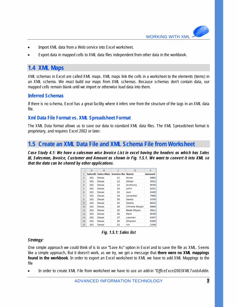
1.5 Create an XML Data File and XML Schema File from Worksheet Case Study 4.1: We have a salesman wise Invoice List in excel having the headers as which has Sales Id, Salesman, Invoice, Customer and Amount as shown in Fig. 1.5.1. We want to convert it into XML so that the data can be shared by other applications.
Fig. 1.5.1: Sales list
Strategy:
One simple approach we could think of is to use “Save As” option in Excel and to save the file as XML. Seems like a simple approach, But it doesn’t work, as we try, we get a message that there were no XML mappings found in the workbook. In order to export an Excel worksheet to XML we have to add XML Mappings to the file
In order to create XML File from worksheet we have to use an add-in “OfficeExcel2003XMLToolsAddin.

ADVANCED MS-EXCEL
8 ADVANCED INFORMATION TECHNOLOGY
exe” which is downloadable from Microsoft’s site http://www.microsoft.com/en-us/download/details.aspx?id=3108.
When downloaded.
Run that exe file which will install at c:\Office Samples\OfficeExcel2003XMLToolsAddin.
Then to install add-in, we go to File> Option>Add-ins>Excel add-in and browse to locate the file which will be at c:\Office Samples\OfficeExcel2003XMLToolsAddin select the file XmlTools.xla.
Thereafter, the add-in would be available for installation as shown in Fig. 1.5.2. select XMLTools
XML Tools would be available in add-Ins Ribbon
Fig. 1.5.2.: Add-in Dialog Box
Select the XML tools in the Add-Ins Tab and 'Convert range to an XML list'.
Fig. 1.5.3:XML Tools
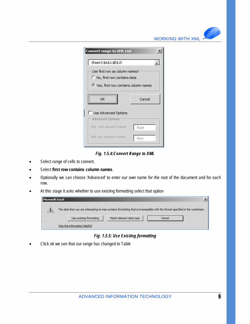
We get a Convert range to an XML List dialog box as shown in Fig. 1.5.4
WORKING WITH XML
ADVANCED INFORMATION TECHNOLOGY 9
Fig. 1.5.4:Convert Range to XML
Select range of cells to convert.
Select first row contains column names.
Optionally we can choose 'Advanced' to enter our own name for the root of the document and for each row.
At this stage it asks whether to use existing formatting select that option
Fig. 1.5.5: Use Existing formatting
Click ok we see that our range has changed to Table
ADVANCED MS-EXCEL
10 ADVANCED INFORMATION TECHNOLOGY
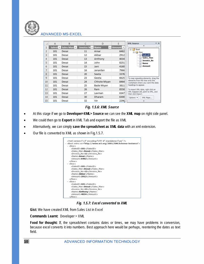
Fig. 1.5.6: XML Source
At this stage if we go to Developer>XML> Source we can see the XML map on right side panel.
We could then go to Export in XML Tab and export the file as XML
Alternatively, we can simply save the spreadsheet as XML data with an xml extension.
Our file is converted to XML as shown in Fig.1.5.7.
Fig. 1.5.7: Excel converted to XML
Gist: We have created XML from Sales List in Excel
Commands Learnt: Developer > XML
Food for thought: If, the spreadsheet contains dates or times, we may have problems in conversion, because excel converts it into numbers. Best approach here would be perhaps, reentering the dates as text field.
WORKING WITH XML
ADVANCED INFORMATION TECHNOLOGY 11
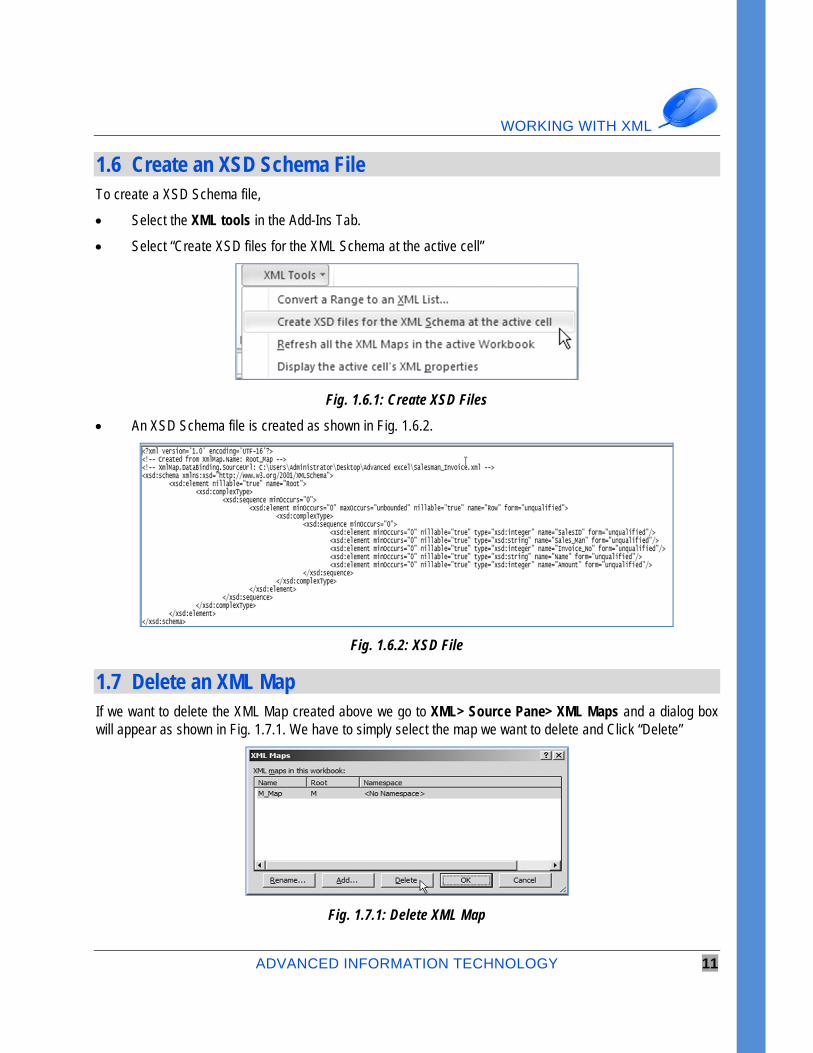
1.6 Create an XSD Schema File To create a XSD Schema file,
Select the XML tools in the Add-Ins Tab.
Select “Create XSD files for the XML Schema at the active cell”
Fig. 1.6.1: Create XSD Files
An XSD Schema file is created as shown in Fig. 1.6.2.
Fig. 1.6.2: XSD File
1.7 Delete an XML Map If we want to delete the XML Map created above we go to XML> Source Pane> XML Maps and a dialog box will appear as shown in Fig. 1.7.1. We have to simply select the map we want to delete and Click “Delete”
Fig. 1.7.1: Delete XML Map
ADVANCED MS-EXCEL
12 ADVANCED INFORMATION TECHNOLOGY
1.8 Working with XML Tables By using XML maps, we can easily add, identify, and extract specific pieces of business data from Excel documents. For example, an invoice that contains the name and address of a customer. We can easily import this information from databases and applications, revise it, and export it to the same or other databases and applications.
Excel creates a map for us automatically when we open the XML data file as a Table. Excel uses every element in the schema, and we have no control over the map or the amount of data that Excel loads into the worksheet.
The map becomes part of the workbook, and Excel saves any changes or new data to the workbook in the standard Excel file format (.xlsx). We can only save the workbook as an xlsx file.
We can't export the data from the Table, but we can import new or changed data into the list.
Case Study 4.2: We have an XML file Salesman Invoice.xml from which we want to create Table.
Strategy:
We open Excel and on the File menu, click Open.
In the Files of type list, select XML files (*.xml).
In the Look in list, navigate to the file Salesman Invoice.xml.
Click Open.
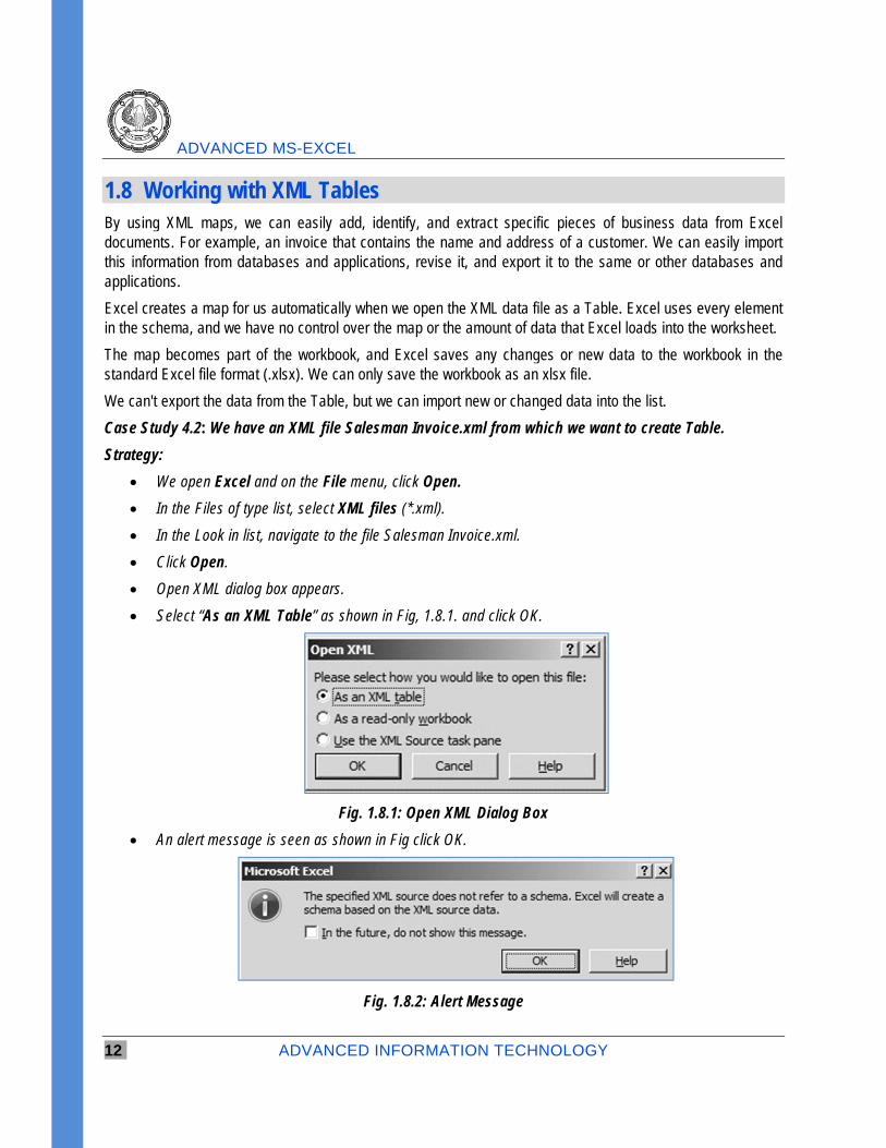
Open XML dialog box appears.
Select “As an XML Table” as shown in Fig, 1.8.1. and click OK.
Fig. 1.8.1: Open XML Dialog Box
An alert message is seen as shown in Fig click OK.
Fig. 1.8.2: Alert Message
WORKING WITH XML
ADVANCED INFORMATION TECHNOLOGY 13
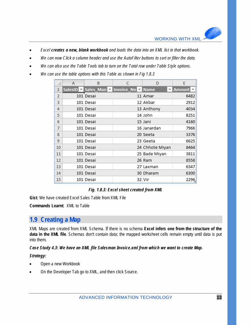
Excel creates a new, blank workbook and loads the data into an XML list in that workbook.
We can now Click a column header and use the AutoFilter buttons to sort or filter the data.
We can also use the Table Tools tab to turn on the Total row under Table Style options.
We can use the table options with this Table as shown in Fig 1.8.3
Fig. 1.8.3: Excel sheet created from XML
Gist: We have created Excel Sales Table from XML File
Commands Learnt: XML to Table
1.9 Creating a Map XML Maps are created from XML Schema. If there is no schema Excel infers one from the structure of the data in the XML file. Schemas don't contain data; the mapped worksheet cells remain empty until data is put into them.
Case Study 4.3: We have an XML file Salesman Invoice.xml from which we want to create Map.
Strategy:
Open a new Workbook
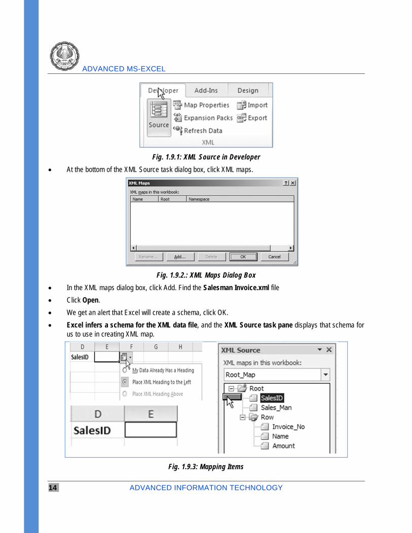
On the Developer Tab go to XML, and then click Source.
ADVANCED MS-EXCEL
14 ADVANCED INFORMATION TECHNOLOGY
Fig. 1.9.1: XML Source in Developer
At the bottom of the XML Source task dialog box, click XML maps.
Fig. 1.9.2.: XML Maps Dialog Box
In the XML maps dialog box, click Add. Find the Salesman Invoice.xml file
Click Open.
We get an alert that Excel will create a schema, click OK.
Excel infers a schema for the XML data file, and the XML Source task pane displays that schema for us to use in creating XML map.
Fig. 1.9.3: Mapping Items
WORKING WITH XML
ADVANCED INFORMATION TECHNOLOGY 15
On the worksheet we start by mapping items that occur only once in the data file. Under Sales ID we drag Sales ID from the task pane to cell E1. Excel surrounds the mapped cell with a Black border, and it displays the Header Options smart tag. Select “Place XML Heading to the left”
When we click another cell, the border becomes thinner and turns blue as shown in Fig. 1.9.3
Now drag Sales_man to cell B1.
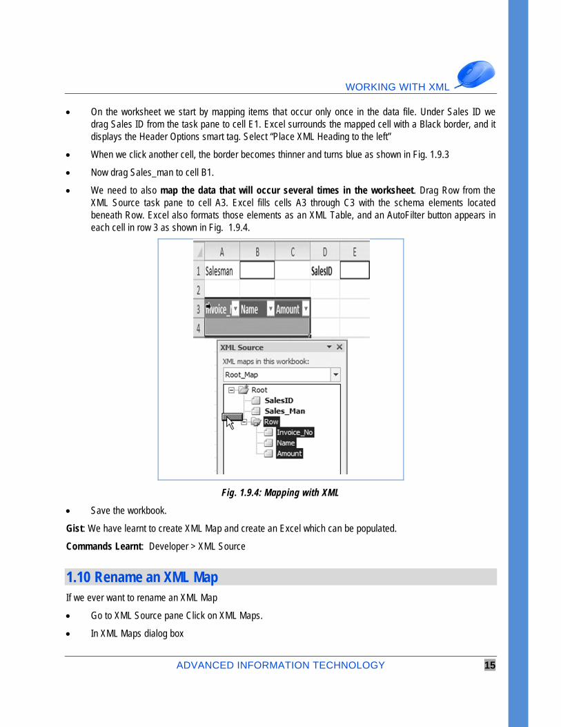
We need to also map the data that will occur several times in the worksheet. Drag Row from the XML Source task pane to cell A3. Excel fills cells A3 through C3 with the schema elements located beneath Row. Excel also formats those elements as an XML Table, and an AutoFilter button appears in each cell in row 3 as shown in Fig. 1.9.4.
Fig. 1.9.4: Mapping with XML
Save the workbook.
Gist: We have learnt to create XML Map and create an Excel which can be populated.
Commands Learnt: Developer > XML Source
1.10 Rename an XML Map If we ever want to rename an XML Map
Go to XML Source pane Click on XML Maps.
In XML Maps dialog box
ADVANCED MS-EXCEL
16 ADVANCED INFORMATION TECHNOLOGY
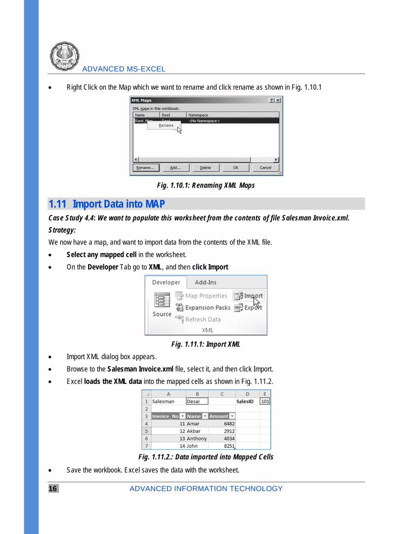
Right Click on the Map which we want to rename and click rename as shown in Fig. 1.10.1
Fig. 1.10.1: Renaming XML Maps
1.11 Import Data into MAP Case Study 4.4: We want to populate this worksheet from the contents of file Salesman Invoice.xml.
Strategy:
We now have a map, and want to import data from the contents of the XML file.
Select any mapped cell in the worksheet.
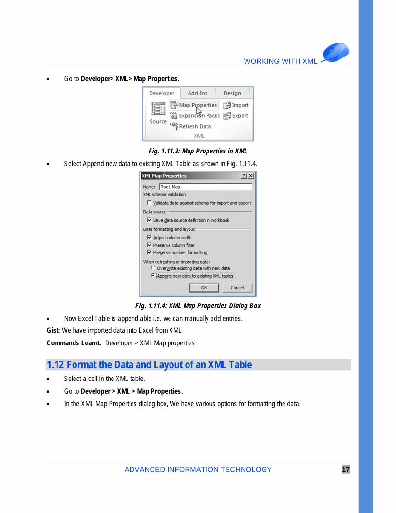
On the Developer Tab go to XML, and then click Import
Fig. 1.11.1: Import XML
Import XML dialog box appears.
Browse to the Salesman Invoice.xml file, select it, and then click Import.
Excel loads the XML data into the mapped cells as shown in Fig. 1.11.2.
Fig. 1.11.2.: Data imported into Mapped Cells
Save the workbook. Excel saves the data with the worksheet.
WORKING WITH XML
ADVANCED INFORMATION TECHNOLOGY 17
Go to Developer> XML> Map Properties.
Fig. 1.11.3: Map Properties in XML
Select Append new data to existing XML Table as shown in Fig. 1.11.4.
Fig. 1.11.4: XML Map Properties Dialog Box
Now Excel Table is append able i.e. we can manually add entries.
Gist: We have imported data into Excel from XML
Commands Learnt: Developer > XML Map properties
1.12 Format the Data and Layout of an XML Table Select a cell in the XML table.
Go to Developer > XML > Map Properties.
In the XML Map Properties dialog box, We have various options for formatting the data
ADVANCED MS-EXCEL
18 ADVANCED INFORMATION TECHNOLOGY
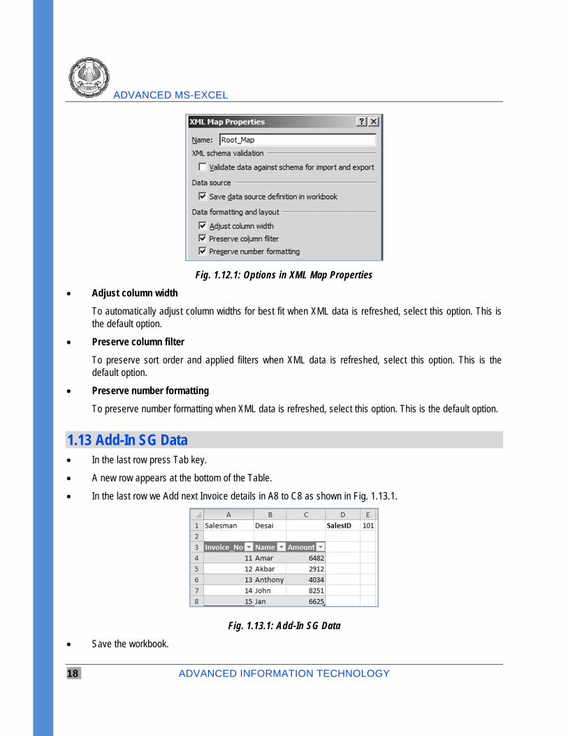
Fig. 1.12.1: Options in XML Map Properties
Adjust column width
To automatically adjust column widths for best fit when XML data is refreshed, select this option. This is the default option.
Preserve column filter
To preserve sort order and applied filters when XML data is refreshed, select this option. This is the default option.
Preserve number formatting
To preserve number formatting when XML data is refreshed, select this option. This is the default option.
1.13 Add-In SG Data In the last row press Tab key.
A new row appears at the bottom of the Table.
In the last row we Add next Invoice details in A8 to C8 as shown in Fig. 1.13.1.
Fig. 1.13.1: Add-In SG Data
Save the workbook.
WORKING WITH XML
ADVANCED INFORMATION TECHNOLOGY 19
1.14 Export Mapped Data After making the changes we can also export the Data. In the export process only the data in the mapped cells of the worksheet are exported.
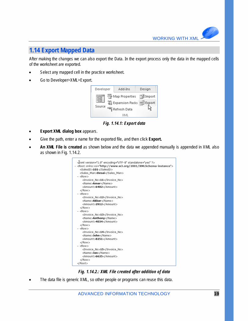
Select any mapped cell in the practice worksheet.
Go to Developer>XML>Export.
Fig. 1.14.1: Export data
Export XML dialog box appears.
Give the path, enter a name for the exported file, and then click Export.
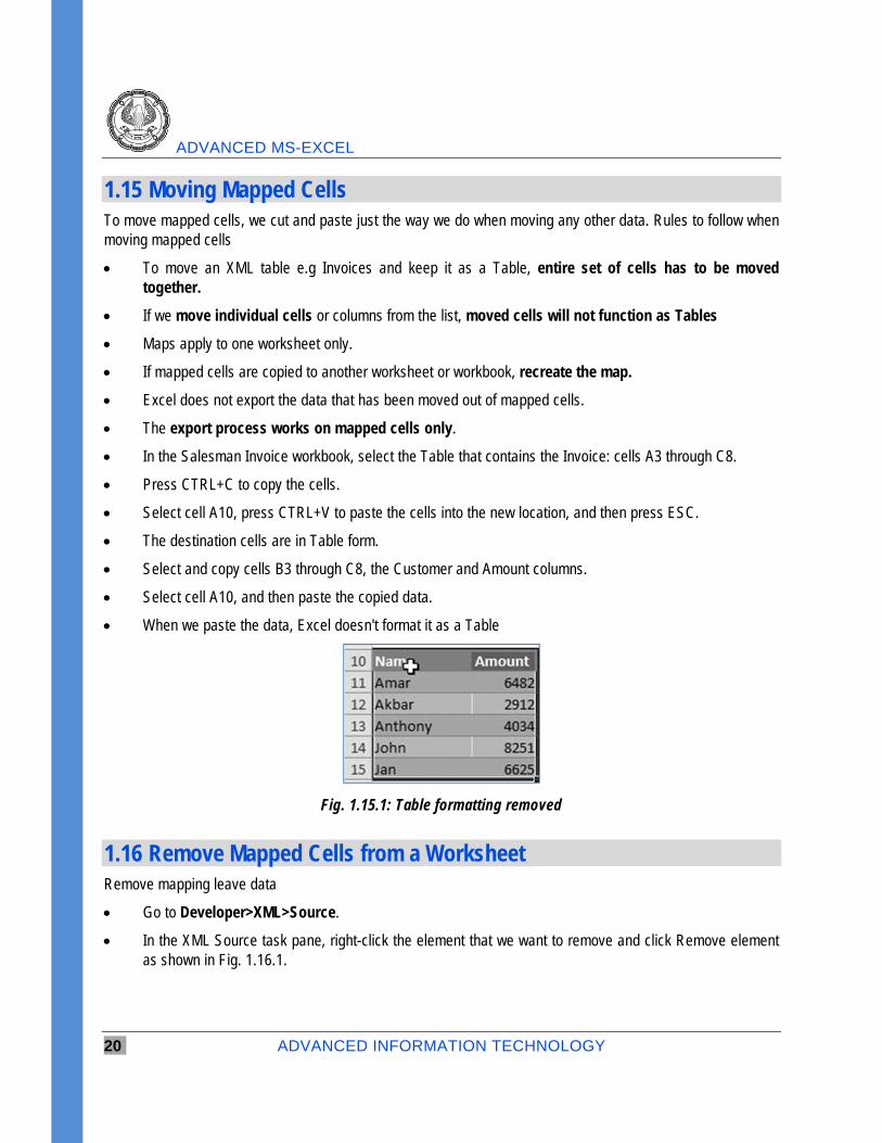
An XML File is created as shown below and the data we appended manually is appended in XML also as shown in Fig. 1.14.2.
Fig. 1.14.2.: XML File created after addition of data
The data file is generic XML, so other people or programs can reuse this data.
ADVANCED MS-EXCEL
20 ADVANCED INFORMATION TECHNOLOGY
1.15 Moving Mapped Cells To move mapped cells, we cut and paste just the way we do when moving any other data. Rules to follow when moving mapped cells
To move an XML table e.g Invoices and keep it as a Table, entire set of cells has to be moved together.
If we move individual cells or columns from the list, moved cells will not function as Tables
Maps apply to one worksheet only.
If mapped cells are copied to another worksheet or workbook, recreate the map.
Excel does not export the data that has been moved out of mapped cells.
The export process works on mapped cells only.
In the Salesman Invoice workbook, select the Table that contains the Invoice: cells A3 through C8.
Press CTRL+C to copy the cells.
Select cell A10, press CTRL+V to paste the cells into the new location, and then press ESC.
The destination cells are in Table form.
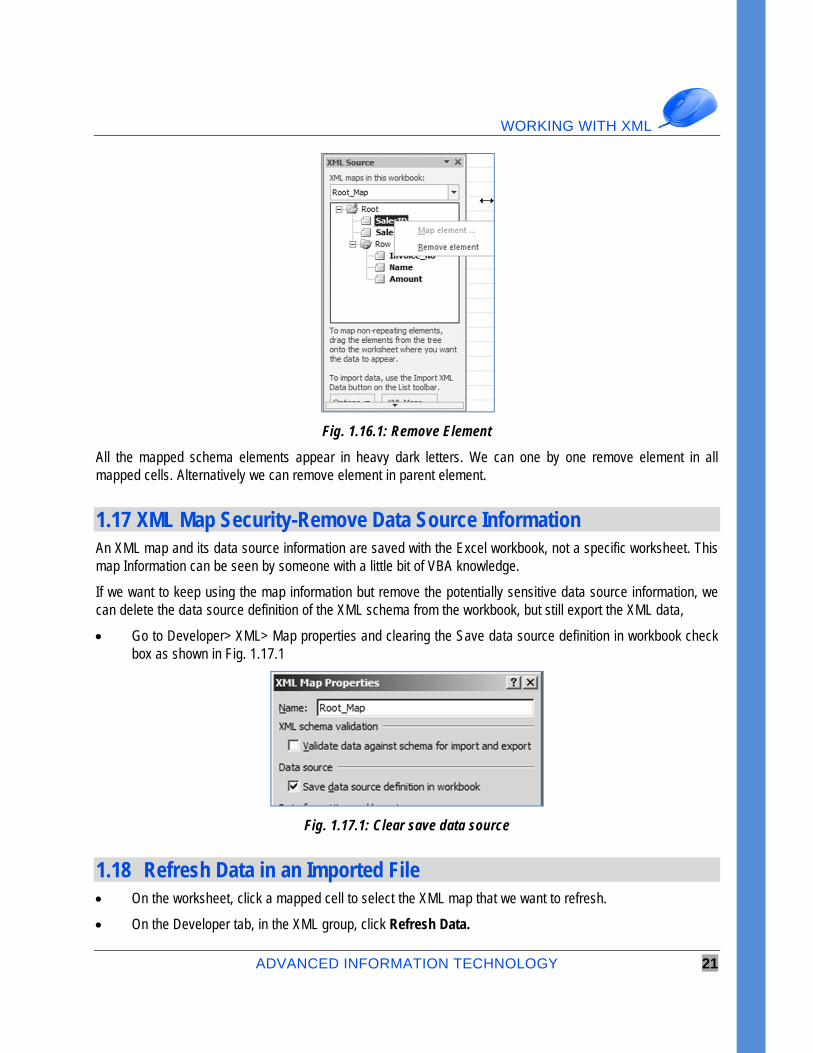
Select and copy cells B3 through C8, the Customer and Amount columns.
Select cell A10, and then paste the copied data.
When we paste the data, Excel doesn't format it as a Table
Fig. 1.15.1: Table formatting removed
1.16 Remove Mapped Cells from a Worksheet Remove mapping leave data
Go to Developer>XML>Source.
In the XML Source task pane, right-click the element that we want to remove and click Remove element as shown in Fig. 1.16.1.
WORKING WITH XML
ADVANCED INFORMATION TECHNOLOGY 21
Fig. 1.16.1: Remove Element
All the mapped schema elements appear in heavy dark letters. We can one by one remove element in all mapped cells. Alternatively we can remove element in parent element.
1.17 XML Map Security-Remove Data Source Information An XML map and its data source information are saved with the Excel workbook, not a specific worksheet. This map Information can be seen by someone with a little bit of VBA knowledge.
If we want to keep using the map information but remove the potentially sensitive data source information, we can delete the data source definition of the XML schema from the workbook, but still export the XML data,
Go to Developer> XML> Map properties and clearing the Save data source definition in workbook check box as shown in Fig. 1.17.1
Fig. 1.17.1: Clear save data source
1.18 Refresh Data in an Imported File On the worksheet, click a mapped cell to select the XML map that we want to refresh.
On the Developer tab, in the XML group, click Refresh Data.
ADVANCED MS-EXCEL
22 ADVANCED INFORMATION TECHNOLOGY
Fig. 1.18.1: Refresh data
If we want to refresh data automatically every time a workbook is opened.
Go To Data Tab >Connections, click the arrow next to Refresh, and then click Connection Properties as shown in Fig. 1.18.2.
Fig. 1.18.2: Automatically refresh data
Under Usage > Refresh control set the preferences like “Refresh data when opening the file”.
1.19 Validate Data against Schema for Import and Export If we want to ensure that the XML data that we are importing or exporting conforms to the XML schema. Excel provides us with a facility to validate data against the XML map when Importing/Exporting data.
Go to Developer> XML> Map properties and click the Validate Data Against Schema For Import And Export check box as shown in Fig. 1.19.1
Fig. 1.19.1: Validating Data against schema
WORKING WITH XML
ADVANCED INFORMATION TECHNOLOGY 23
1.20 Summary XML is a great way of Exchanging information between Computer applications
Excel is a great tool which allows us to import from or export to XML.
In this chapter, we learned how to install XML Tool add-Ins from Microsoft, we learned basics of XML, converting XML to Excel and vice versa, creating an XML data File & Schema file. Create, rename, remove XML Map are important when we want to Add Data from XML and export it to XML.
We have also learnt to refresh data from XML manually, or automatically
References [1] Matthew MacDonald, ‘Excel 2010, THE MISSING MANUAL, O’Reilly Media, Inc, 2010
[2] http://office.microsoft.com
[3] http://www.sitepoint.com/really-good-introduction-xml/
ADVANCES IN MACROS
2.1 Introduction We all want shortcuts and to avoid the chore of doing monotonous work like data entry or some formatting which we want done every time. Excel offers us excellent options to automate in the form of Macros which are basically small programs which automatically perform repetitious steps.
2.2 What is a Macro Programming of Macros is done in programming Language VBA (Visual Basic for Applications) but we can use Macros even if we do not know VBA since Excel gives us a wonderful tool in the form of Macro Recorder. A macro records our mouse clicks and keystrokes while we work and play them back later
Macros can be written in two ways
Writing a Macro using VBA Code
Recording a macro using Excel Macro recorder
2.3 Recording a Macro If we have to store Macros it is not possible in .xlsx files. Fortunately excel has a file extension .xlsm which are macro enabled workbooks. Excel gives macro-enabled workbooks a different icon, with a superimposed exclamation mark. This icon enables us to recognize a macro-enabled workbook.
Some tips to record a macro
Excel records every keystroke & every command we run, so something we don’t want should not be done while recording Macro.
We don’t need to work fast, i.e., Macro just records our actions, so if we are just browsing, that is not recorded it is only specific actions which get recorded.
Try to be generic, since we’d want that macro to run in various situations & scenarios.
CHAPTER
2 LEARNING OBJECTIVES
To gain understanding of Macros
To understand Recording of Macros
To understand Assigning a button to Macros
To understand Absolute & Relative references in Macros
ADVANCES IN MACROS
ADVANCED INFORMATION TECHNOLOGY 25
2.3.1 Enabling Macro Security
On the Developer tab, click Macro Security in the Code group.
The Security dialog appears.
In the Security dialog, change the Macro Settings to Disable All Macros with Notification.
With this setting, Excel alerts us whenever we open a workbook that has macros attached.
When we open a document and get the warning that the document has macros attached, if this is a document that we wrote and we expect macros to be there, click Enable Content to enable the macros
2.3.2 Where Macros Are Stored
Macros can be stored in either of two locations, as follows:
The workbook we are using, or
Our Personal Macro Workbook (which by default is hidden from view)
If our macro applies to all workbooks, then store it in the Personal Macro Workbook so it will always be available in all of our Excel workbooks; otherwise we store it in our current workbook
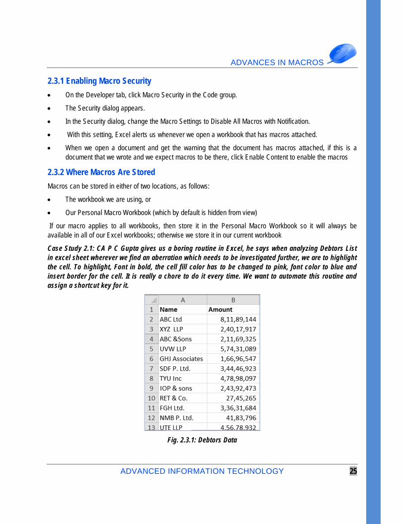
Case Study 2.1: CA P C Gupta gives us a boring routine in Excel, he says when analyzing Debtors List in excel sheet wherever we find an aberration which needs to be investigated further, we are to highlight the cell. To highlight, Font in bold, the cell fill color has to be changed to pink, font color to blue and insert border for the cell. It is really a chore to do it every time. We want to automate this routine and assign a shortcut key for it.
Fig. 2.3.1: Debtors Data

ADVANCED MS-EXCEL
26 ADVANCED INFORMATION TECHNOLOGY
Strategy:
We can automate this boring task using Macros in Excel
We can record a Macro in 3 different ways
In Excel 2010 Macros are in Developer Tab, which is not there by default.
To activate it we have to go to File> Options as shown in Fig. 2.3.2
Fig 2.3.2: Options in File Tab
Under Options > Customize the Ribbon > On the right of the window, a large box lists all the tabs that are currently shown in the ribbon. Near the bottom, we see an unchecked item named Developer as shown in Fig. 2.3.3. To show the Developer tab, check this box, and then click OK.
Fig 2.3.3: Customize ribbon in options

ADVANCES IN MACROS
ADVANCED INFORMATION TECHNOLOGY 27
Macros are under Developer tab as shown in Fig. 2.3.4
Fig. 2.3.4: Macros in Developer tab
Recording a Macros is also available in View> Macros as shown in Fig. 2.3.5
Fig. 2.3.5: Macros under view
There is one more option to record macro in status bar as shown in Fig. 2.3.6
Fig. 2.3.6: Record a macro in status Bar
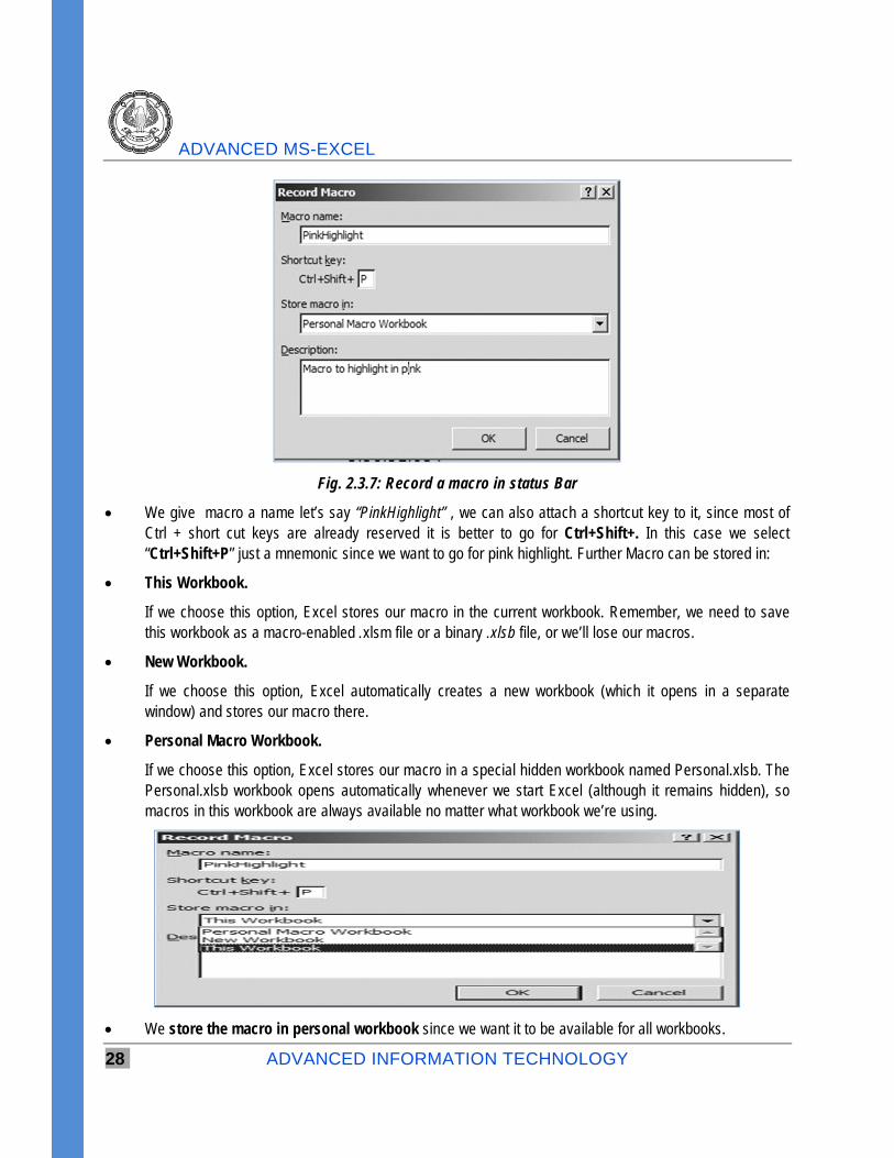
Using any of the above methods we start recoding a Macro, a macro dialog box appears as shown in Fig. 2.3.7
ADVANCED MS-EXCEL
28 ADVANCED INFORMATION TECHNOLOGY
Fig. 2.3.7: Record a macro in status Bar
We give macro a name let’s say “PinkHighlight” , we can also attach a shortcut key to it, since most of Ctrl + short cut keys are already reserved it is better to go for Ctrl+Shift+. In this case we select “Ctrl+Shift+P” just a mnemonic since we want to go for pink highlight. Further Macro can be stored in:
This Workbook.
If we choose this option, Excel stores our macro in the current workbook. Remember, we need to save this workbook as a macro-enabled .xlsm file or a binary .xlsb file, or we’ll lose our macros.
New Workbook.
If we choose this option, Excel automatically creates a new workbook (which it opens in a separate window) and stores our macro there.
Personal Macro Workbook.
If we choose this option, Excel stores our macro in a special hidden workbook named Personal.xlsb. The Personal.xlsb workbook opens automatically whenever we start Excel (although it remains hidden), so macros in this workbook are always available no matter what workbook we’re using.
We store the macro in personal workbook since we want it to be available for all workbooks.

ADVANCES IN MACROS
ADVANCED INFORMATION TECHNOLOGY 29
We also give the macro a description “Macro to highlight in pink”.
As we begin recording we see that record macro button has changed to “stop recording” in both header & status bar as shown in Fig. 2.3.8
Fig. 2.3.8: Stop recording in developer tab & status Bar
Now we perform the recording of action
we select B10 which we need to highlight in pink and
go through the desired steps on Home Tab first we make the font Bold,
next we change the font colour to Blue,
Change the fill to Pink &
Insert a border for the cell.
We now click the stop recording Button
Our macro is now ready, to execute on any cell press Ctrl+Shift+P and we find that the cell gets the desired formatting
Fig. 2.3.9: Macro is executed on pressing Ctrl+Shift+P
Gist: We have recorded a macro to give the desired pink highlighting to a cell to Excel both in static format as well as dynamic format
Commands Learnt: Record a Macro
ADVANCED MS-EXCEL
30 ADVANCED INFORMATION TECHNOLOGY
2.4 Assigning a Button to Macro We have seen that Macros make our repetitive job a lot easier to perform but it would be extremely useful if we can run macro with a simple click on button, rather than running it manually. By creating macro-buttons we will be able to associate macros with buttons, and show them on the worksheet for performing different tasks we have recorded with macro. Excel enables us to create custom buttons to link macros with them, the following case study will elaborate how to create macros and associate buttons with them.
Case Study 2.2: In case study 6.1 we wish to assign a button in Quick Access Toolbar & also make a button on the worksheet for one touch macro execution.
Strategy:
We can assign Buttons for macros in many ways we will discuss two of them.
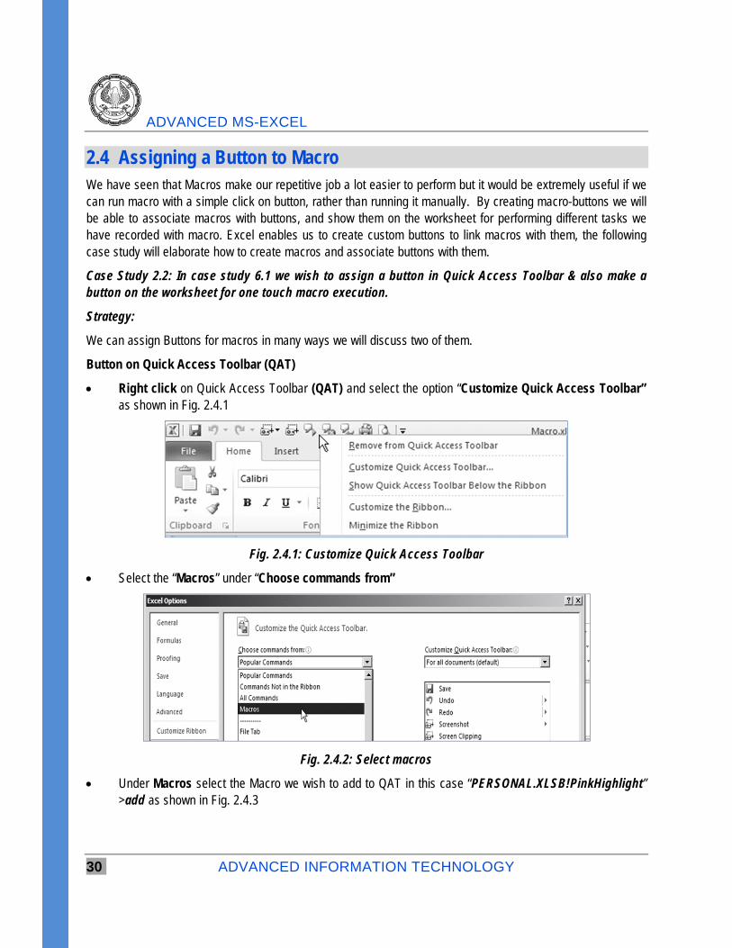
Button on Quick Access Toolbar (QAT)
Right click on Quick Access Toolbar (QAT) and select the option “Customize Quick Access Toolbar” as shown in Fig. 2.4.1
Fig. 2.4.1: Customize Quick Access Toolbar
Select the “Macros” under “Choose commands from”
Fig. 2.4.2: Select macros
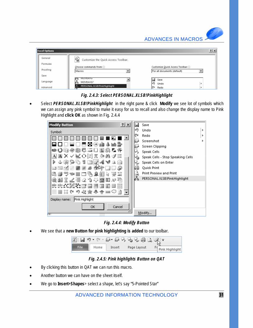
Under Macros select the Macro we wish to add to QAT in this case “PERSONAL.XLSB!PinkHighlight” >add as shown in Fig. 2.4.3
ADVANCES IN MACROS
ADVANCED INFORMATION TECHNOLOGY 31
Fig. 2.4.3: Select PERSONAL.XLSB!PinkHighlight
Select PERSONAL.XLSB!PinkHighlight in the right pane & click Modify we see lot of symbols which we can assign any pink symbol to make it easy for us to recall and also change the display name to Pink Highlight and click OK as shown in Fig. 2.4.4
Fig. 2.4.4: Modify Button
We see that a new Button for pink highlighting is added to our toolbar.
Fig. 2.4.5: Pink highlights Button on QAT
By clicking this button in QAT we can run this macro.
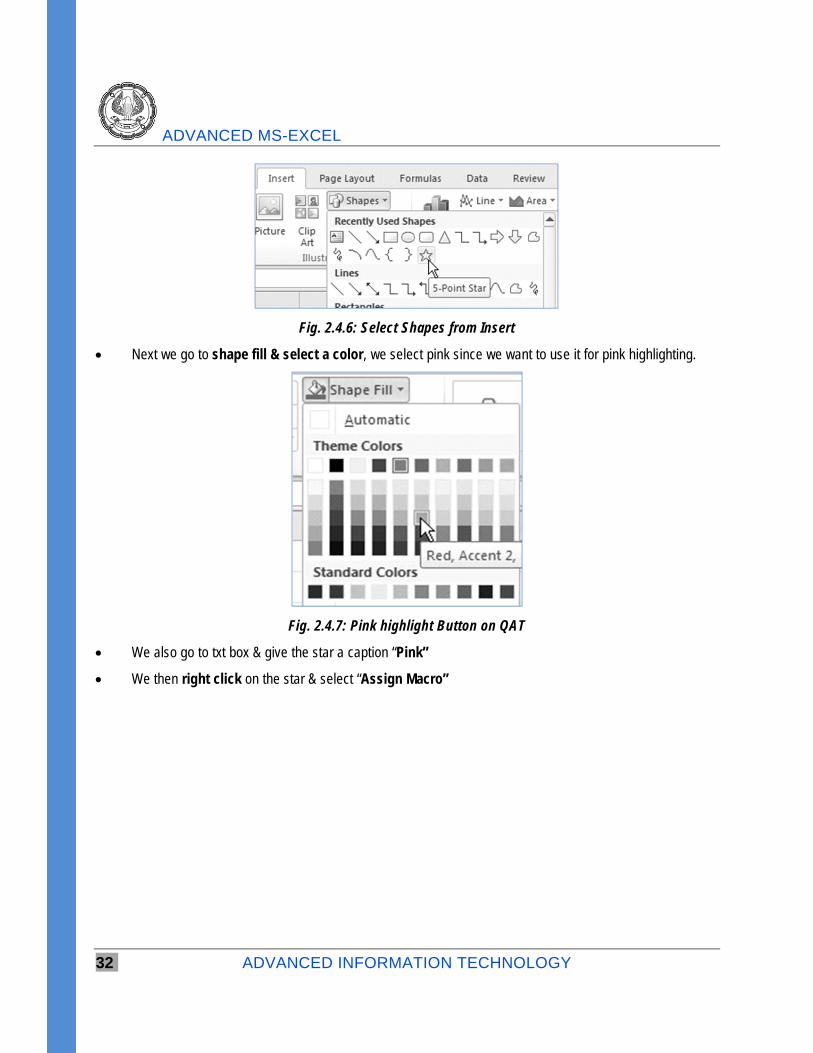
Another button we can have on the sheet itself.
We go to Insert>Shapes> select a shape, let’s say “5-Pointed Star”
ADVANCED MS-EXCEL
32 ADVANCED INFORMATION TECHNOLOGY
Fig. 2.4.6: Select Shapes from Insert
Next we go to shape fill & select a color, we select pink since we want to use it for pink highlighting.
Fig. 2.4.7: Pink highlight Button on QAT
We also go to txt box & give the star a caption “Pink”
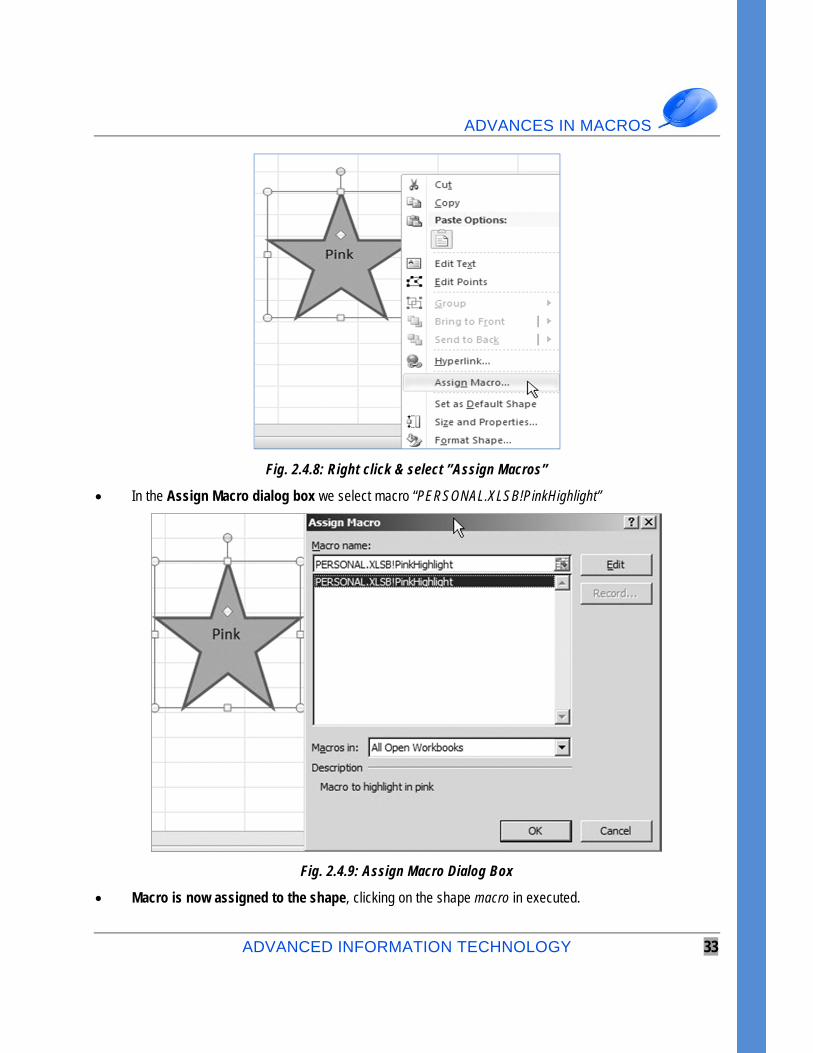
We then right click on the star & select “Assign Macro”
ADVANCES IN MACROS
ADVANCED INFORMATION TECHNOLOGY 33
Fig. 2.4.8: Right click & select ”Assign Macros”
In the Assign Macro dialog box we select macro “PERSONAL.XLSB!PinkHighlight”
Fig. 2.4.9: Assign Macro Dialog Box
Macro is now assigned to the shape, clicking on the shape macro in executed.
ADVANCED MS-EXCEL
34 ADVANCED INFORMATION TECHNOLOGY
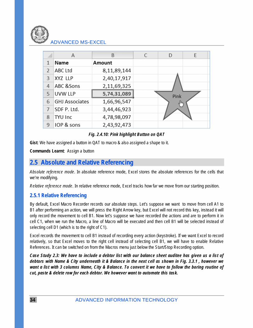
Fig. 2.4.10: Pink highlight Button on QAT
Gist: We have assigned a button in QAT to macro & also assigned a shape to it.
Commands Learnt: Assign a button
2.5 Absolute and Relative Referencing Absolute reference mode. In absolute reference mode, Excel stores the absolute references for the cells that we’re modifying.
Relative reference mode. In relative reference mode, Excel tracks how far we move from our starting position.
2.5.1 Relative Referencing
By default, Excel Macro Recorder records our absolute steps. Let’s suppose we want to move from cell A1 to B1 after performing an action, we will press the Right Arrow key, but Excel will not record this key, instead it will only record the movement to cell B1. Now let’s suppose we have recorded the actions and are to perform it in cell C1, when we run the Macro, a line of Macro will be executed and then cell B1 will be selected instead of selecting cell D1 (which is to the right of C1).
Excel records the movement to cell B1 instead of recording every action (keystroke). If we want Excel to record relatively, so that Excel moves to the right cell instead of selecting cell B1, we will have to enable Relative References. It can be switched on from the Macros menu just below the Start/Stop Recording option.
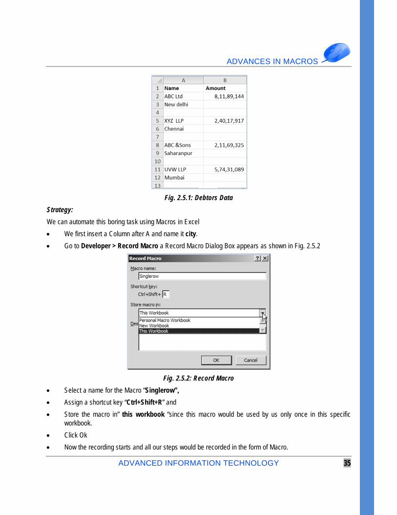
Case Study 2.3: We have to include a debtor list with our balance sheet auditee has given us a list of debtors with Name & City underneath it & Balance in the next cell as shown in Fig. 3.3.1 , however we want a list with 3 columns Name, City & Balance. To convert it we have to follow the boring routine of cut, paste & delete row for each debtor. We however want to automate this task.
ADVANCES IN MACROS
ADVANCED INFORMATION TECHNOLOGY 35
Fig. 2.5.1: Debtors Data
Strategy:
We can automate this boring task using Macros in Excel
We first insert a Column after A and name it city.
Go to Developer > Record Macro a Record Macro Dialog Box appears as shown in Fig. 2.5.2
Fig. 2.5.2: Record Macro
Select a name for the Macro “Singlerow”,
Assign a shortcut key “Ctrl+Shift+R” and
Store the macro in” this workbook “since this macro would be used by us only once in this specific workbook.
Click Ok
Now the recording starts and all our steps would be recorded in the form of Macro.
ADVANCED MS-EXCEL
36 ADVANCED INFORMATION TECHNOLOGY
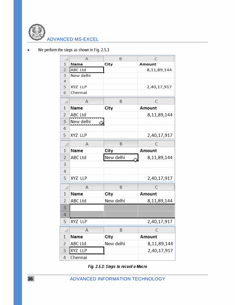
We perform the steps as shown in Fig. 2.5.3
Fig. 2.5.3: Steps to record a Macro
ADVANCES IN MACROS
ADVANCED INFORMATION TECHNOLOGY 37
We start
at Cell A2
Move to Cell A3.
Cut Cell A3 and paste to Cell B2.
Delete Rows 3 through 4.
Go to Cell A3
Stop Recording.
Our Macro is now recorded.
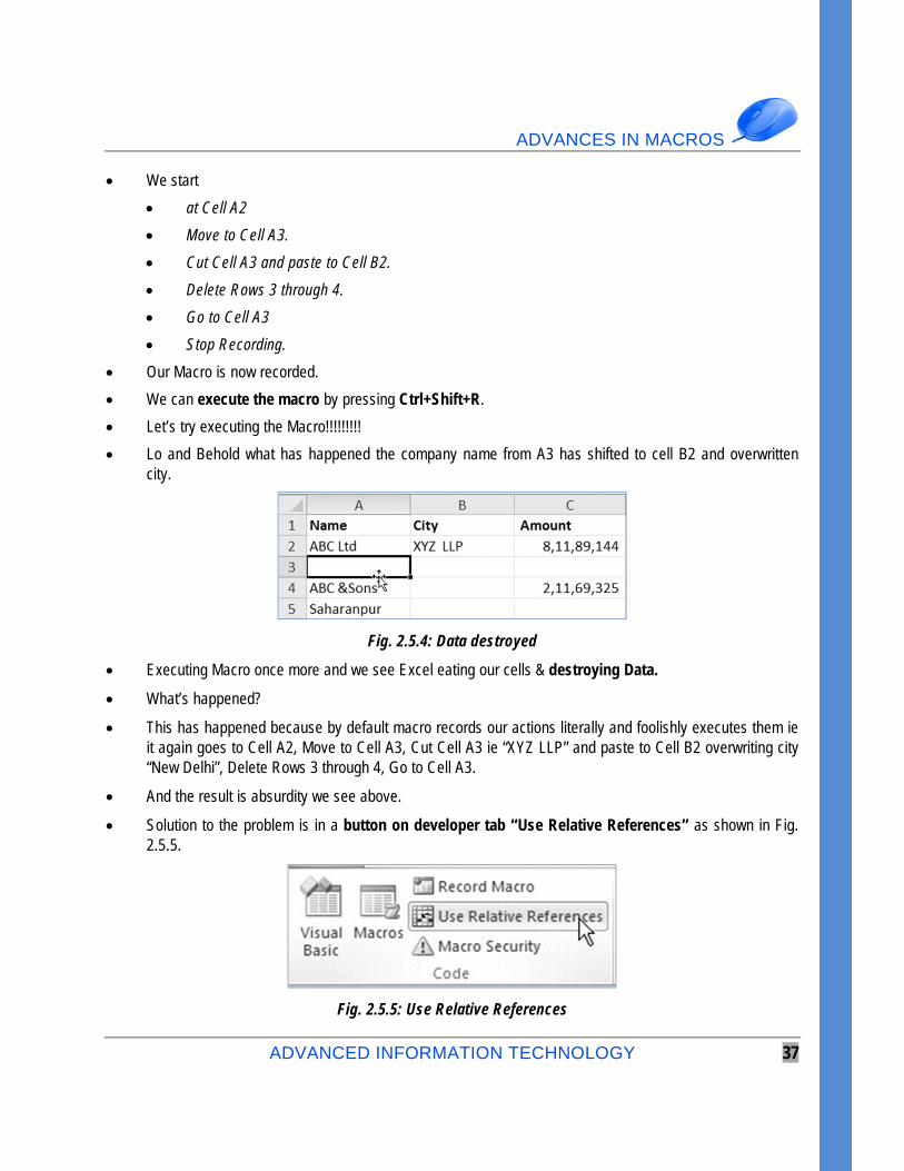
We can execute the macro by pressing Ctrl+Shift+R.
Let’s try executing the Macro!!!!!!!!!
Lo and Behold what has happened the company name from A3 has shifted to cell B2 and overwritten city.
Fig. 2.5.4: Data destroyed
Executing Macro once more and we see Excel eating our cells & destroying Data.
What’s happened?
This has happened because by default macro records our actions literally and foolishly executes them ie it again goes to Cell A2, Move to Cell A3, Cut Cell A3 ie “XYZ LLP” and paste to Cell B2 overwriting city “New Delhi”, Delete Rows 3 through 4, Go to Cell A3.
And the result is absurdity we see above.
Solution to the problem is in a button on developer tab “Use Relative References” as shown in Fig. 2.5.5.
Fig. 2.5.5: Use Relative References
ADVANCED MS-EXCEL
38 ADVANCED INFORMATION TECHNOLOGY
Now before starting recording of the above macro we should have activated “Use Relative References” and proceeded to record the Macro.
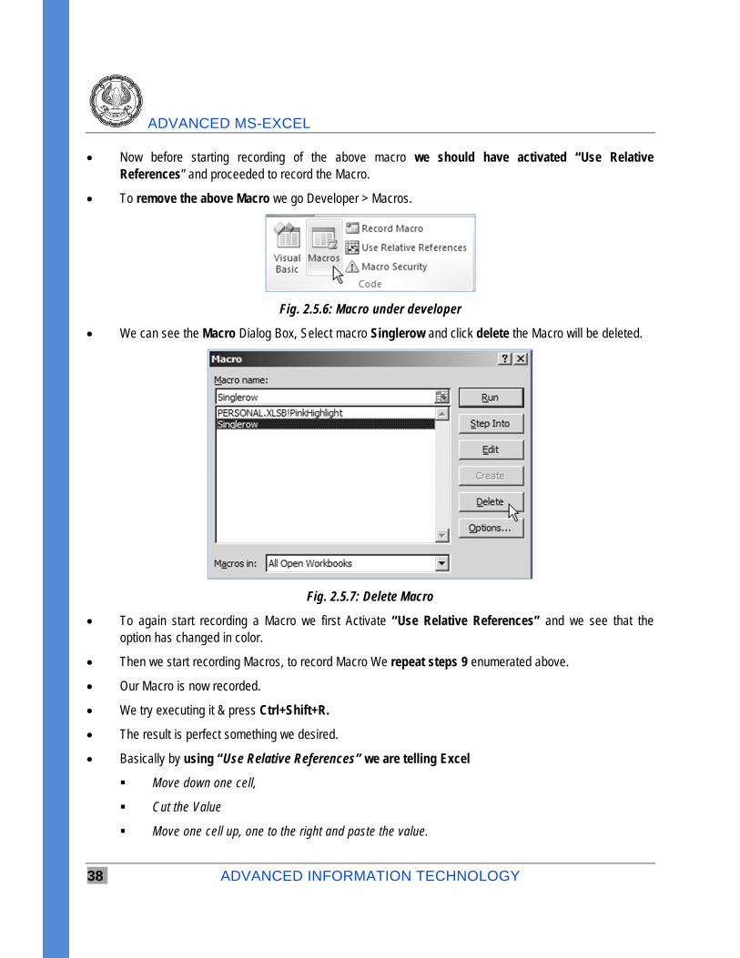
To remove the above Macro we go Developer > Macros.
Fig. 2.5.6: Macro under developer
We can see the Macro Dialog Box, Select macro Singlerow and click delete the Macro will be deleted.
Fig. 2.5.7: Delete Macro
To again start recording a Macro we first Activate “Use Relative References” and we see that the option has changed in color.
Then we start recording Macros, to record Macro We repeat steps 9 enumerated above.
Our Macro is now recorded.
We try executing it & press Ctrl+Shift+R.
The result is perfect something we desired.
Basically by using “Use Relative References” we are telling Excel
Move down one cell,
Cut the Value
Move one cell up, one to the right and paste the value.
ADVANCES IN MACROS
ADVANCED INFORMATION TECHNOLOGY 39
Move two cells left.
Move Two cells Under select the two rows
Delete the rows
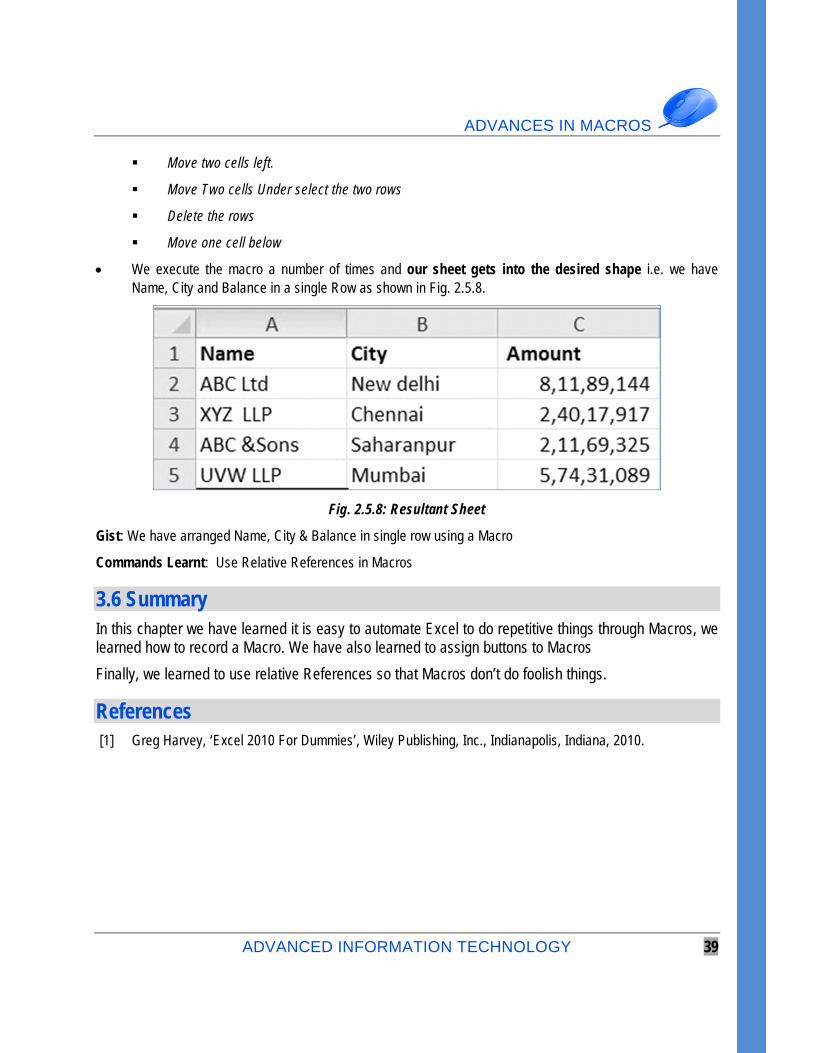
Move one cell below
We execute the macro a number of times and our sheet gets into the desired shape i.e. we have Name, City and Balance in a single Row as shown in Fig. 2.5.8.
Fig. 2.5.8: Resultant Sheet
Gist: We have arranged Name, City & Balance in single row using a Macro
Commands Learnt: Use Relative References in Macros
3.6 Summary In this chapter we have learned it is easy to automate Excel to do repetitive things through Macros, we learned how to record a Macro. We have also learned to assign buttons to Macros
Finally, we learned to use relative References so that Macros don’t do foolish things.
References [1] Greg Harvey, ‘Excel 2010 For Dummies’, Wiley Publishing, Inc., Indianapolis, Indiana, 2010.
APPLIED FINANCIAL ANALYSIS AND FORECASTING FINANCIAL STATEMENTS
3.1 Introduction One of the most important features of excel is its number crunching ability. This is the reason it is used in almost every organization. Most Finance management or accounting packages allow us to export data into Excel format. Thus data analysis and reporting becomes an easier task.
Excel allows us to use various functions and even simple mathematical calculations can be performed for financial analysis, equity analysis, leasing decisions and the list goes on. However before we proceed, we need to know certain basic things about excel formulae:
3.1.1 Elements of a Formula
A Formula can have the following elements:
Arithmetic Operators: These include symbols such as + (for addition) and / (for division)
Conditional Operators: These include symbols such as > (greater than) ; <= ( less than equalto); <> (not equal to)
Cell References: These include references such as C4, =Sheet2!C4 (reference to other sheets)or references to other workbooks.
Range References: These include references such as A1:A4, A1:D1, A1:D6
Named References: These are named ranges or references created by the user to refer to aparticular range of cells. Ex: Range name “Data” referring to a range “A1:D100”
Values or Strings: These are values such as 10 or10.5 (values) or “State wise Sales” (String).
Strings are to be always enclosed in double quotes when used in a formula.
LEARNING OBJECTIVES
To understand Financial Analysis
To understand Du-Pont Analysis
To understand Leasing decisions
To understand Financial Shenanigans
To understand Equity Analysis
To learn Chart creation
Scenarios and Case Studies
CHAPTER
3
APPLIED FINANCIAL ANALYSIS AND FORECASTING FINANCIAL STATEMENTS
ADVANCED INFORMATION TECHNOLOGY 41
Worksheet functions: A formula may consist of multiple functions and each function shall haveits own set of arguments and parameters.
Parentheses: Every formula has its own set of arguments which are written in parentheses.Parentheses are also used to change the order of calculation.
Note: Excel colours the range addresses and the cells that you enter in a formula. This helps as a visual aid to spot the range used in the formula to either understand its working or to spot errors.
3.1.2 What is a Function?
A worksheet function is a built in tool that you use in a formula. Worksheet functions allow you to perform calculations or operations that would otherwise be too cumbersome or impossible altogether.
3.1.3 Arguments of a Function
A function may have:
No arguments Ex: =TODAY()
TODAY function gives you system date which changes daily. This function doesn’t require an argument.
One argument Ex: =ABS(-4)
ABS function gives you absolute value of a number, number without its sign. This function accepts only one argument.
A fixed number of arguments Ex: =MOD(100,3)
MOD function returns the remainder after a number is divided by a divisor. It mandatorily requires two arguments: number and divisor.
Optional arguments
Ex: =INDEX (Salesdata, 5)
INDEX function returns value from a given data range based on row and column.
However in this function, “column number” is optional thus the function will work even without column number provided appropriate data has been selected.
3.1.4 Function Categories
Following function categories are available in excel:
Financial Date & Time
Math & Trig Statistical
Lookup & Reference Database
Text Logical
Information & Compatibility User defined
Engineering Cube
ADVANCED MS-EXCEL
42 ADVANCED INFORMATION TECHNOLOGY
3.1.5 Show Formula Mode
You can often understand an unfamiliar workbook by displaying the formulas rather than the results of the formulas. To toggle the display of formulas, choose Formulas > Formula Auditing > Show Formulas.
You can also use Ctrl+` ( ~ the accent grave key, usually located above the Tab key) to toggle between Formula view and Normal view.
3.2 Financial Analysis Usually potential investors analyze financial statements of companies they want to invest in. This is because financial statements reveal about the current and future financial condition of the company. Financial analysis often involves comparison between companies in the same industry, companies against external benchmarks and analysis of internal performance trends. Analysis also includes forecast based on historical performance. Before we move into the analytics we need to understand the balance sheet.
3.2.1 Understanding the balance sheet.
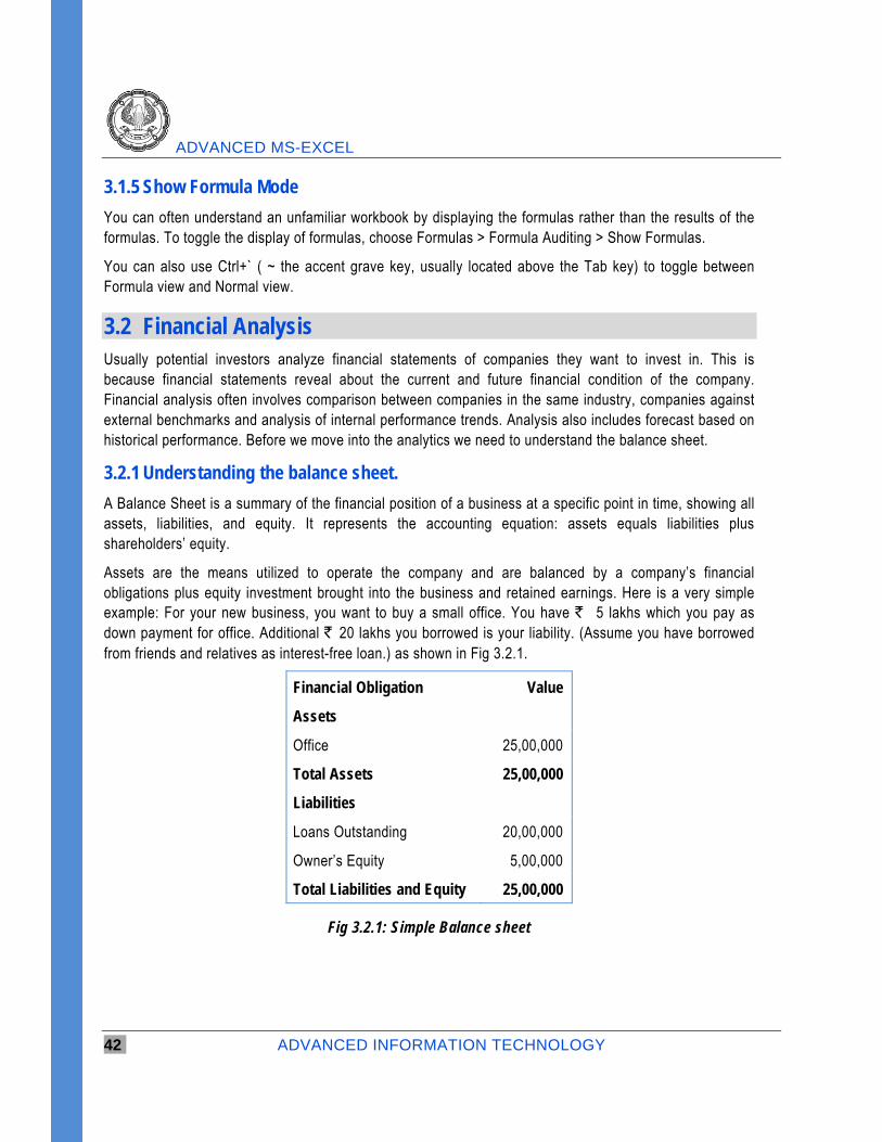
A Balance Sheet is a summary of the financial position of a business at a specific point in time, showing all assets, liabilities, and equity. It represents the accounting equation: assets equals liabilities plus shareholders’ equity.
Assets are the means utilized to operate the company and are balanced by a company’s financial obligations plus equity investment brought into the business and retained earnings. Here is a very simple example: For your new business, you want to buy a small office. You have ` 5 lakhs which you pay as down payment for office. Additional ` 20 lakhs you borrowed is your liability. (Assume you have borrowed from friends and relatives as interest-free loan.) as shown in Fig 3.2.1.
Financial Obligation Value
Assets
Office 25,00,000
Total Assets 25,00,000
Liabilities
Loans Outstanding 20,00,000
Owner’s Equity 5,00,000
Total Liabilities and Equity 25,00,000
Fig 3.2.1: Simple Balance sheet
APPLIED FINANCIAL ANALYSIS AND FORECASTING FINANCIAL STATEMENTS
ADVANCED INFORMATION TECHNOLOGY 43
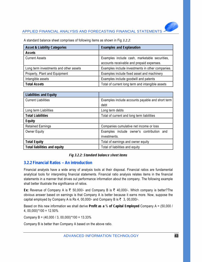
A standard balance sheet comprises of following items as shown in Fig 3.2.2:
Asset & Liability Categories Examples and Explanation
Assets
Current Assets Examples include cash, marketable securities, accounts receivable and prepaid expenses.
Long term investments and other assets Examples include investments in other companies.
Property, Plant and Equipment Examples include fixed asset and machinery
Intangible assets Examples include goodwill and patents
Total Assets Total of current long term and intangible assets
Liabilities and Equity
Current Liabilities Examples include accounts payable and short term debt
Long term Liabilities Long term debts
Total Liabilities Total of current and long term liabilities
Equity
Retained Earnings Companies cumulative net income or loss
Owner Equity Examples include owner’s contribution and investments.
Total Equity Total of earnings and owner equity
Total liabilities and equity Total of liabilities and equity
Fig 3.2.2: Standard balance sheet items
3.2.2 Financial Ratios – An introduction
Financial analysts have a wide array of analysis tools at their disposal. Financial ratios are fundamental analytical tools for interpreting financial statements. Financial ratio analysis relates items in the financial statements in a manner that drives out performance information about the company. The following example shall better illustrate the significance of ratios.
Ex: Revenue of Company A is ` 50,000/- and Company B is ` 40,000/-. Which company is better?The obvious answer based on earnings is that Company A is better because it earns more. Now, suppose the capital employed by Company A is Rs 4, 00,000/- and Company B is ` 3, 00,000/-.
Based on this new information we shall derive Profit as a % of Capital Employed Company A = (50,000 / 4, 00,000)*100 = 12.50%
Company B = (40,000 / 3, 00,000)*100 = 13.33%
Company B is better than Company A based on the above ratio.
ADVANCED MS-EXCEL
44 ADVANCED INFORMATION TECHNOLOGY
Thus ratios help us to convert figures into logical percentages which can then be compared with ratios from some other companies or a company’s own past performance and appropriate conclusions can be drawn.
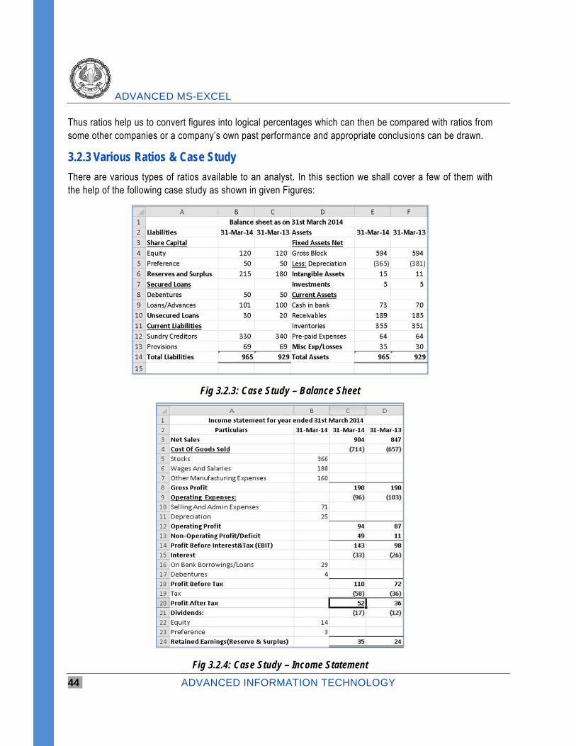
3.2.3 Various Ratios & Case Study
There are various types of ratios available to an analyst. In this section we shall cover a few of them with the help of the following case study as shown in given Figures:
Fig 3.2.3: Case Study – Balance Sheet
Fig 3.2.4: Case Study – Income Statement
APPLIED FINANCIAL ANALYSIS AND FORECASTING FINANCIAL STATEMENTS
ADVANCED INFORMATION TECHNOLOGY 45
3.2.3.1 Liquidity Ratios
These ratios shows the ability of a company to pay its current financial obligations. Company should not be selling its assets at a loss to meet its financial obligations. In a worst scenario company will be forced into liquidation.
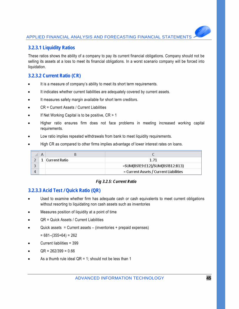
3.2.3.2 Current Ratio (CR)
It is a measure of company’s ability to meet its short term requirements.
It indicates whether current liabilities are adequately covered by current assets.
It measures safety margin available for short term creditors.
CR = Current Assets / Current Liabilities
If Net Working Capital is to be positive, CR > 1
Higher ratio ensures firm does not face problems in meeting increased working capital requirements.
Low ratio implies repeated withdrawals from bank to meet liquidity requirements.
High CR as compared to other firms implies advantage of lower interest rates on loans.
Fig 3.2.5: Current Ratio
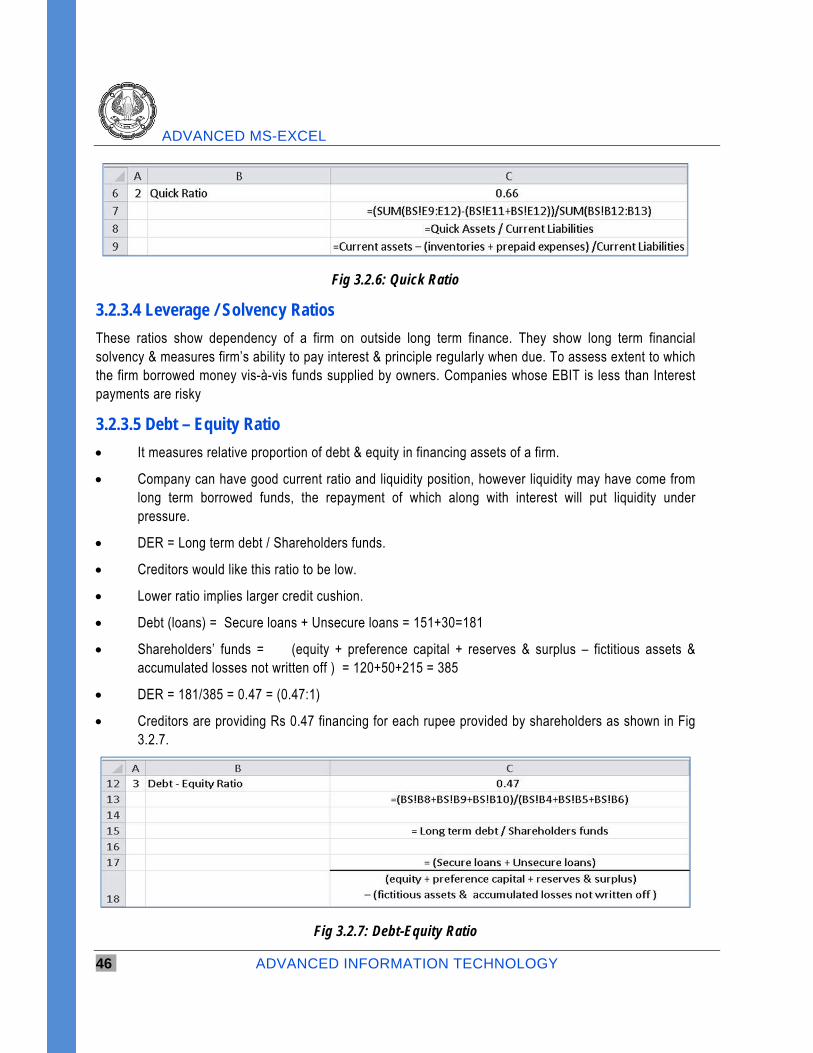
3.2.3.3 Acid Test / Quick Ratio (QR)
Used to examine whether firm has adequate cash or cash equivalents to meet current obligations without resorting to liquidating non cash assets such as inventories
Measures position of liquidity at a point of time
QR = Quick Assets / Current Liabilities
Quick assets = Current assets – (inventories + prepaid expenses)
= 681–(355+64) = 262
Current liabilities = 399
QR = 262/399 = 0.66
As a thumb rule ideal QR = 1; should not be less than 1
ADVANCED MS-EXCEL
46 ADVANCED INFORMATION TECHNOLOGY
Fig 3.2.6: Quick Ratio
3.2.3.4 Leverage / Solvency Ratios
These ratios show dependency of a firm on outside long term finance. They show long term financial solvency & measures firm’s ability to pay interest & principle regularly when due. To assess extent to which the firm borrowed money vis-à-vis funds supplied by owners. Companies whose EBIT is less than Interest payments are risky
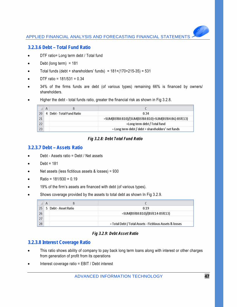
3.2.3.5 Debt – Equity Ratio
It measures relative proportion of debt & equity in financing assets of a firm.
Company can have good current ratio and liquidity position, however liquidity may have come from long term borrowed funds, the repayment of which along with interest will put liquidity under pressure.
DER = Long term debt / Shareholders funds.
Creditors would like this ratio to be low.
Lower ratio implies larger credit cushion.
Debt (loans) = Secure loans + Unsecure loans = 151+30=181
Shareholders’ funds = (equity + preference capital + reserves & surplus – fictitious assets & accumulated losses not written off ) = 120+50+215 = 385
DER = 181/385 = 0.47 = (0.47:1)
Creditors are providing Rs 0.47 financing for each rupee provided by shareholders as shown in Fig 3.2.7.
Fig 3.2.7: Debt-Equity Ratio
APPLIED FINANCIAL ANALYSIS AND FORECASTING FINANCIAL STATEMENTS
ADVANCED INFORMATION TECHNOLOGY 47
3.2.3.6 Debt – Total Fund Ratio
DTF ratio= Long term debt / Total fund
Debt (long term) = 181
Total funds (debt + shareholders’ funds) = 181+(170+215-35) = 531
DTF ratio = 181/531 = 0.34
34% of the firms funds are debt (of various types) remaining 66% is financed by owners/ shareholders.
Higher the debt - total funds ratio, greater the financial risk as shown in Fig 3.2.8.
Fig 3.2.8: Debt Total Fund Ratio
3.2.3.7 Debt – Assets Ratio
Debt - Assets ratio = Debt / Net assets
Debt = 181
Net assets (less fictitious assets & losses) = 930
Ratio = 181/930 = 0.19
19% of the firm’s assets are financed with debt (of various types).
Shows coverage provided by the assets to total debt as shown In Fig 3.2.9.
Fig 3.2.9: Debt Asset Ratio
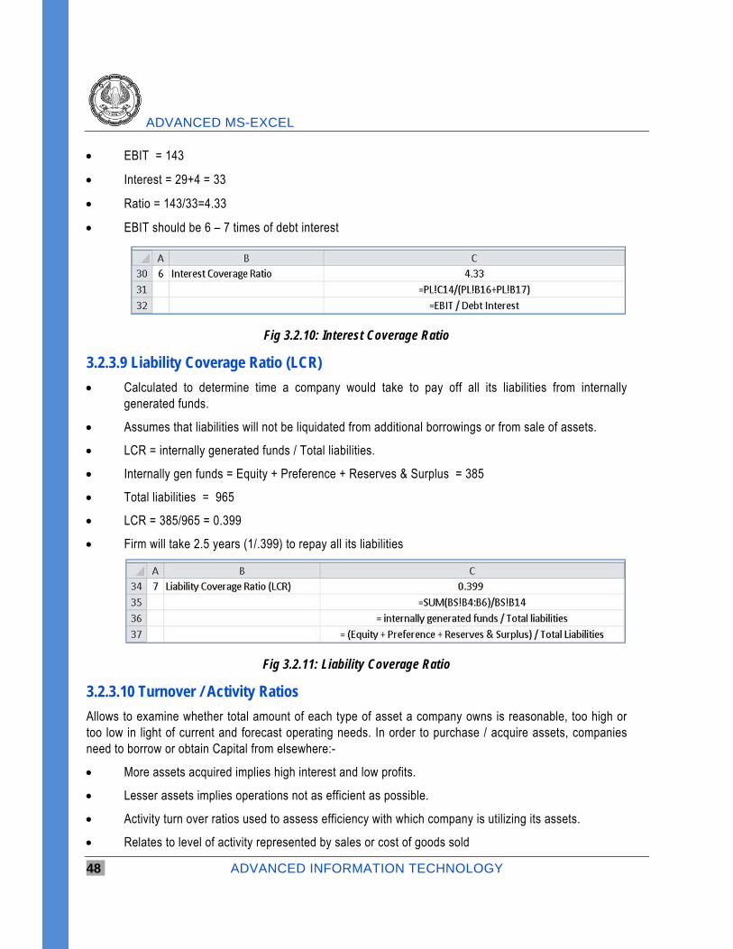
3.2.3.8 Interest Coverage Ratio
This ratio shows ability of company to pay back long term loans along with interest or other charges from generation of profit from its operations
Interest coverage ratio = EBIT / Debt interest
ADVANCED MS-EXCEL
48 ADVANCED INFORMATION TECHNOLOGY
EBIT = 143
Interest = 29+4 = 33
Ratio = 143/33=4.33
EBIT should be 6 – 7 times of debt interest
Fig 3.2.10: Interest Coverage Ratio
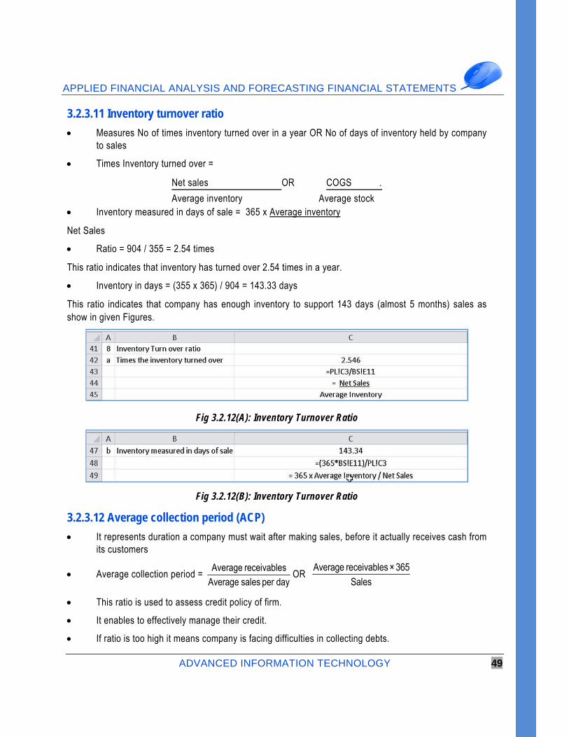
3.2.3.9 Liability Coverage Ratio (LCR)
Calculated to determine time a company would take to pay off all its liabilities from internally generated funds.
Assumes that liabilities will not be liquidated from additional borrowings or from sale of assets.
LCR = internally generated funds / Total liabilities.
Internally gen funds = Equity + Preference + Reserves & Surplus = 385
Total liabilities = 965
LCR = 385/965 = 0.399
Firm will take 2.5 years (1/.399) to repay all its liabilities
Fig 3.2.11: Liability Coverage Ratio
3.2.3.10 Turnover / Activity Ratios
Allows to examine whether total amount of each type of asset a company owns is reasonable, too high or too low in light of current and forecast operating needs. In order to purchase / acquire assets, companies need to borrow or obtain Capital from elsewhere:-
More assets acquired implies high interest and low profits.
Lesser assets implies operations not as efficient as possible.
Activity turn over ratios used to assess efficiency with which company is utilizing its assets.
Relates to level of activity represented by sales or cost of goods sold
APPLIED FINANCIAL ANALYSIS AND FORECASTING FINANCIAL STATEMENTS
ADVANCED INFORMATION TECHNOLOGY 49
3.2.3.11 Inventory turnover ratio
Measures No of times inventory turned over in a year OR No of days of inventory held by company to sales
Times Inventory turned over =
Net sales OR COGS .
Average inventory Average stock Inventory measured in days of sale = 365 x Average inventory
Net Sales
Ratio = 904 / 355 = 2.54 times
This ratio indicates that inventory has turned over 2.54 times in a year.
Inventory in days = (355 x 365) / 904 = 143.33 days
This ratio indicates that company has enough inventory to support 143 days (almost 5 months) sales as show in given Figures.
Fig 3.2.12(A): Inventory Turnover Ratio
Fig 3.2.12(B): Inventory Turnover Ratio
3.2.3.12 Average collection period (ACP)
It represents duration a company must wait after making sales, before it actually receives cash from its customers
Average collection period = Average receivables
Average sales per dayOR
Average receivables × 365Sales
This ratio is used to assess credit policy of firm.
It enables to effectively manage their credit.
If ratio is too high it means company is facing difficulties in collecting debts.
ADVANCED MS-EXCEL
50 ADVANCED INFORMATION TECHNOLOGY
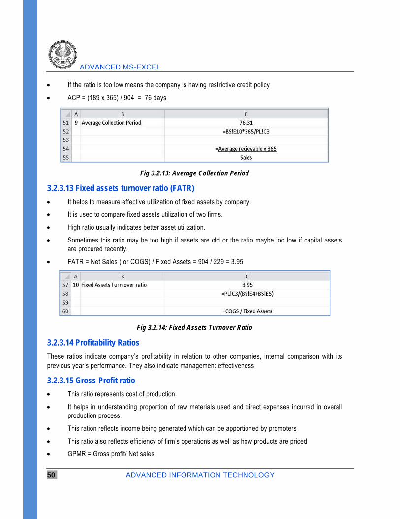
If the ratio is too low means the company is having restrictive credit policy
ACP = (189 x 365) / 904 = 76 days
Fig 3.2.13: Average Collection Period
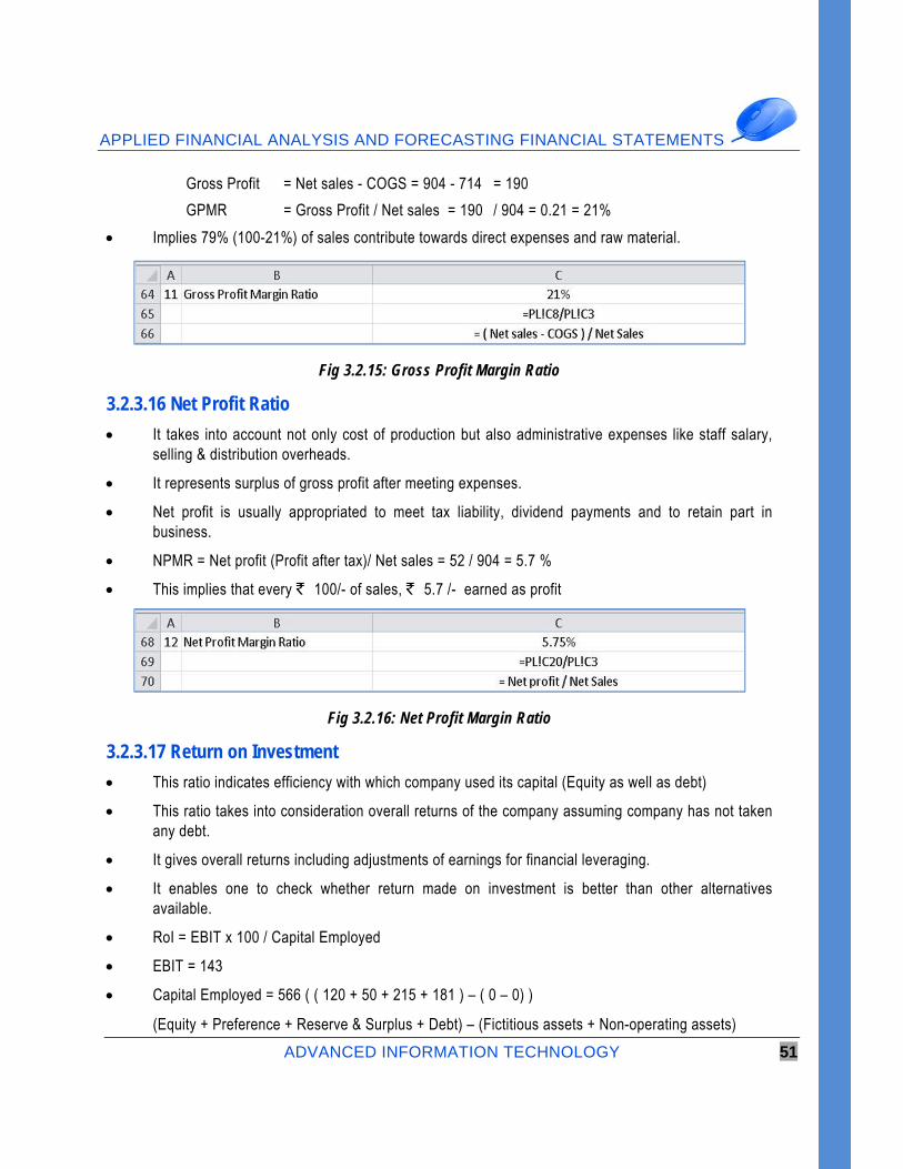
3.2.3.13 Fixed assets turnover ratio (FATR)
It helps to measure effective utilization of fixed assets by company.
It is used to compare fixed assets utilization of two firms.
High ratio usually indicates better asset utilization.
Sometimes this ratio may be too high if assets are old or the ratio maybe too low if capital assets are procured recently.
FATR = Net Sales ( or COGS) / Fixed Assets = 904 / 229 = 3.95
Fig 3.2.14: Fixed Assets Turnover Ratio
3.2.3.14 Profitability Ratios
These ratios indicate company’s profitability in relation to other companies, internal comparison with its previous year’s performance. They also indicate management effectiveness
3.2.3.15 Gross Profit ratio
This ratio represents cost of production.
It helps in understanding proportion of raw materials used and direct expenses incurred in overall production process.
This ration reflects income being generated which can be apportioned by promoters
This ratio also reflects efficiency of firm’s operations as well as how products are priced
GPMR = Gross profit/ Net sales
APPLIED FINANCIAL ANALYSIS AND FORECASTING FINANCIAL STATEMENTS
ADVANCED INFORMATION TECHNOLOGY 51
Gross Profit = Net sales - COGS = 904 - 714 = 190
GPMR = Gross Profit / Net sales = 190 / 904 = 0.21 = 21%
Implies 79% (100-21%) of sales contribute towards direct expenses and raw material.
Fig 3.2.15: Gross Profit Margin Ratio
3.2.3.16 Net Profit Ratio
It takes into account not only cost of production but also administrative expenses like staff salary, selling & distribution overheads.
It represents surplus of gross profit after meeting expenses.
Net profit is usually appropriated to meet tax liability, dividend payments and to retain part in business.
NPMR = Net profit (Profit after tax)/ Net sales = 52 / 904 = 5.7 %
This implies that every ` 100/- of sales, ` 5.7 /- earned as profit
Fig 3.2.16: Net Profit Margin Ratio
3.2.3.17 Return on Investment
This ratio indicates efficiency with which company used its capital (Equity as well as debt)
This ratio takes into consideration overall returns of the company assuming company has not taken any debt.
It gives overall returns including adjustments of earnings for financial leveraging.
It enables one to check whether return made on investment is better than other alternatives available.
RoI = EBIT x 100 / Capital Employed
EBIT = 143
Capital Employed = 566 ( ( 120 + 50 + 215 + 181 ) – ( 0 – 0) )
(Equity + Preference + Reserve & Surplus + Debt) – (Fictitious assets + Non-operating assets)
ADVANCED MS-EXCEL
52 ADVANCED INFORMATION TECHNOLOGY
ROI = 143 / 566 x 100 = 25.26 %
The company has earned a profit of ` 25.26 paisa on every ` 100 reinvested as shown in Fig 3.2.17
Fig 3.2.17: Return on Investment
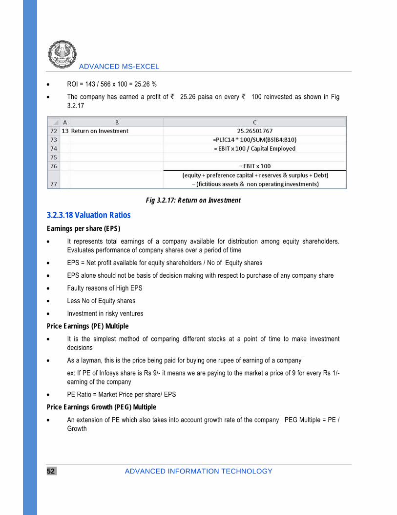
3.2.3.18 Valuation Ratios
Earnings per share (EPS)
It represents total earnings of a company available for distribution among equity shareholders. Evaluates performance of company shares over a period of time
EPS = Net profit available for equity shareholders / No of Equity shares
EPS alone should not be basis of decision making with respect to purchase of any company share
Faulty reasons of High EPS
Less No of Equity shares
Investment in risky ventures
Price Earnings (PE) Multiple
It is the simplest method of comparing different stocks at a point of time to make investment decisions
As a layman, this is the price being paid for buying one rupee of earning of a company
ex: If PE of Infosys share is Rs 9/- it means we are paying to the market a price of 9 for every Rs 1/- earning of the company
PE Ratio = Market Price per share/ EPS
Price Earnings Growth (PEG) Multiple
An extension of PE which also takes into account growth rate of the company � PEG Multiple = PE / Growth
APPLIED FINANCIAL ANALYSIS AND FORECASTING FINANCIAL STATEMENTS
ADVANCED INFORMATION TECHNOLOGY 53
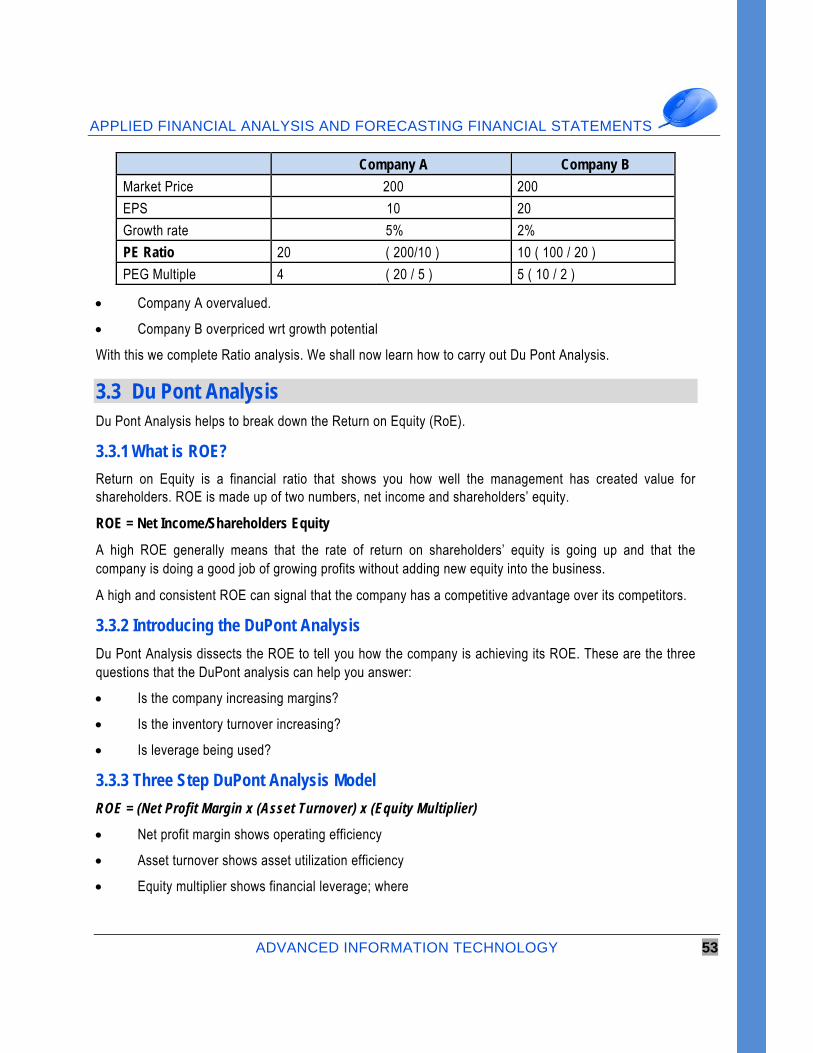
Company A Company B
Market Price 200 200
EPS 10 20
Growth rate 5% 2%
PE Ratio 20 ( 200/10 ) 10 ( 100 / 20 )
PEG Multiple 4 ( 20 / 5 ) 5 ( 10 / 2 )
Company A overvalued.
Company B overpriced wrt growth potential
With this we complete Ratio analysis. We shall now learn how to carry out Du Pont Analysis.
3.3 Du Pont Analysis Du Pont Analysis helps to break down the Return on Equity (RoE).
3.3.1 What is ROE?
Return on Equity is a financial ratio that shows you how well the management has created value for shareholders. ROE is made up of two numbers, net income and shareholders’ equity.
ROE = Net Income/Shareholders Equity
A high ROE generally means that the rate of return on shareholders’ equity is going up and that the company is doing a good job of growing profits without adding new equity into the business.
A high and consistent ROE can signal that the company has a competitive advantage over its competitors.
3.3.2 Introducing the DuPont Analysis
Du Pont Analysis dissects the ROE to tell you how the company is achieving its ROE. These are the three questions that the DuPont analysis can help you answer:
Is the company increasing margins?
Is the inventory turnover increasing?
Is leverage being used?
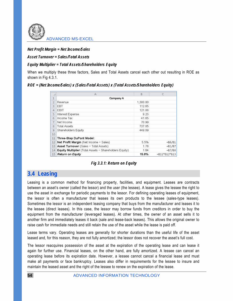
3.3.3 Three Step DuPont Analysis Model
ROE = (Net Profit Margin x (Asset Turnover) x (Equity Multiplier)
Net profit margin shows operating efficiency
Asset turnover shows asset utilization efficiency
Equity multiplier shows financial leverage; where
ADVANCED MS-EXCEL
54 ADVANCED INFORMATION TECHNOLOGY
Net Profit Margin = Net Income/Sales
Asset Turnover = Sales/Total Assets
Equity Multiplier = Total Assets/Shareholders Equity
When we multiply these three factors, Sales and Total Assets cancel each other out resulting in ROE as shown in Fig 4.3.1.
ROE = (Net Income/Sales) x (Sales/Total Assets) x (Total Assets/Shareholders Equity)
Fig 3.3.1: Return on Equity
3.4 Leasing Leasing is a common method for financing property, facilities, and equipment. Leases are contracts between an asset’s owner (called the lessor) and the user (the lessee). A lease gives the lessee the right to use the asset in exchange for periodic payments to the lessor. For defining operating leases of equipment, the lessor is often a manufacturer that leases its own products to the lessee (sales-type leases). Sometimes the lessor is an independent leasing company that buys from the manufacturer and leases it to the lessee (direct leases). In this case, the lessor may borrow funds from creditors in order to buy the equipment from the manufacturer (leveraged leases). At other times, the owner of an asset sells it to another firm and immediately leases it back (sale and lease-back leases). This allows the original owner to raise cash for immediate needs and still retain the use of the asset while the lease is paid off.
Lease terms vary. Operating leases are generally for shorter durations than the useful life of the asset leased and, for this reason, they are not fully amortized; the lessor does not recover the asset’s full cost.
The lessor reacquires possession of the asset at the expiration of the operating lease and can lease it again for further use. Financial leases, on the other hand, are fully amortized. A lessee can cancel an operating lease before its expiration date. However, a lessee cannot cancel a financial lease and must make all payments or face bankruptcy. Leases also differ in requirements for the lessee to insure and maintain the leased asset and the right of the lessee to renew on the expiration of the lease.
APPLIED FINANCIAL ANALYSIS AND FORECASTING FINANCIAL STATEMENTS
ADVANCED INFORMATION TECHNOLOGY 55
Leasing a car for a day or week during a vacation trip is an example of a short-term lease. Leasing trucks, factory machinery, computers, or airplanes for a number of years are examples of long-term financial leases that are involved in capital budgeting. Such leases are the most common method of financing equipment.
For the lessee, the choices are to buy or to lease. For the lessor, the problem is to identify the highest rental rate that would be acceptable to a lessee.
The following case study is for a long-term financial lease of operating equipment from the standpoint of the lessee. It shows how to identify whether it is better for a company to lease or buy operating equipment. Note the treatment of depreciation, the firm’s cost of capital or discount rate, the lessor’s rental rate, and taxes. As the owner of the asset leased, the lessor gets a tax shield for the asset’s depreciation. The lessee can claim the lease payments as an operating expense. The benefits generated by the equipment and such expenses as maintenance, repair, and insurance are assumed to be the same regardless of whether the equipment is leased or purchased.
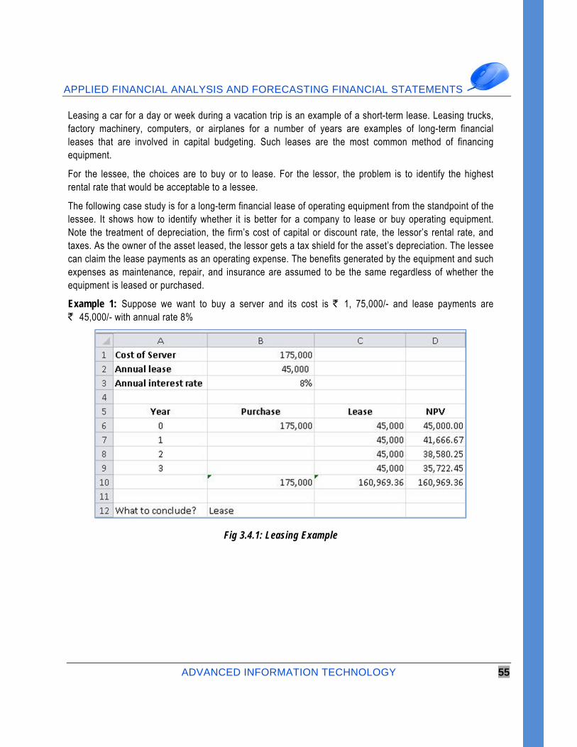
Example 1: Suppose we want to buy a server and its cost is ` 1, 75,000/- and lease payments are ` 45,000/- with annual rate 8%
Fig 3.4.1: Leasing Example
ADVANCED MS-EXCEL
56 ADVANCED INFORMATION TECHNOLOGY
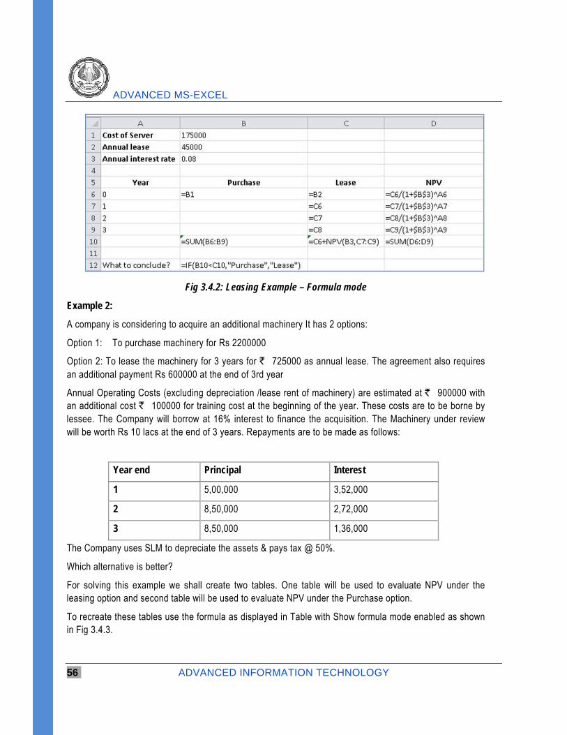
Fig 3.4.2: Leasing Example – Formula mode
Example 2:
A company is considering to acquire an additional machinery It has 2 options:
Option 1: To purchase machinery for Rs 2200000
Option 2: To lease the machinery for 3 years for ` 725000 as annual lease. The agreement also requires an additional payment Rs 600000 at the end of 3rd year
Annual Operating Costs (excluding depreciation /lease rent of machinery) are estimated at ` 900000 with an additional cost ` 100000 for training cost at the beginning of the year. These costs are to be borne by lessee. The Company will borrow at 16% interest to finance the acquisition. The Machinery under review will be worth Rs 10 lacs at the end of 3 years. Repayments are to be made as follows:
Year end Principal Interest
1 5,00,000 3,52,000
2 8,50,000 2,72,000
3 8,50,000 1,36,000
The Company uses SLM to depreciate the assets & pays tax @ 50%.
Which alternative is better?
For solving this example we shall create two tables. One table will be used to evaluate NPV under the leasing option and second table will be used to evaluate NPV under the Purchase option.
To recreate these tables use the formula as displayed in Table with Show formula mode enabled as shown in Fig 3.4.3.
APPLIED FINANCIAL ANALYSIS AND FORECASTING FINANCIAL STATEMENTS
ADVANCED INFORMATION TECHNOLOGY 57
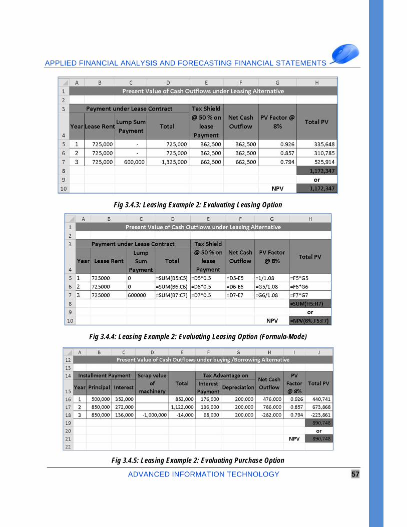
Fig 3.4.3: Leasing Example 2: Evaluating Leasing Option
Fig 3.4.4: Leasing Example 2: Evaluating Leasing Option (Formula-Mode)
Fig 3.4.5: Leasing Example 2: Evaluating Purchase Option
ADVANCED MS-EXCEL
58 ADVANCED INFORMATION TECHNOLOGY
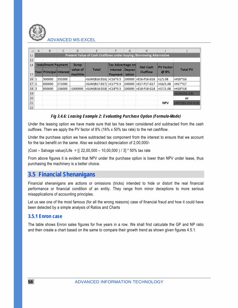
Fig 3.4.6: Leasing Example 2: Evaluating Purchase Option (Formula-Mode)
Under the leasing option we have made sure that tax has been considered and subtracted from the cash outflows. Then we apply the PV factor of 8% (16% x 50% tax rate) to the net cashflow.
Under the purchase option we have subtracted tax component from the interest to ensure that we account for the tax benefit on the same. Also we subtract depreciation of 2,00,000/-
(Cost – Salvage value)/Life = [( 22,00,000 – 10,00,000 ) / 3] * 50% tax rate
From above figures it is evident that NPV under the purchase option is lower than NPV under lease, thus purchasing the machinery is a better choice.
3.5 Financial Shenanigans Financial shenanigans are actions or omissions (tricks) intended to hide or distort the real financial performance or financial condition of an entity. They range from minor deceptions to more serious misapplications of accounting principles.
Let us see one of the most famous (for all the wrong reasons) case of financial fraud and how it could have been detected by a simple analysis of Ratios and Charts
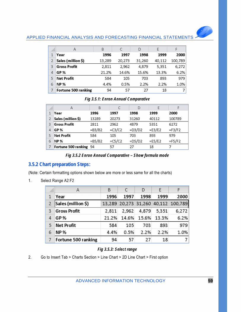
3.5.1 Enron case
The table shows Enron sales figures for five years in a row. We shall first calculate the GP and NP ratio and then create a chart based on the same to compare their growth trend as shown given figures 4.5.1.
APPLIED FINANCIAL ANALYSIS AND FORECASTING FINANCIAL STATEMENTS
ADVANCED INFORMATION TECHNOLOGY 59
Fig 3.5.1: Enron Annual Comparative
Fig 3.5.2 Enron Annual Comparative – Show formula mode
3.5.2 Chart preparation Steps:
(Note: Certain formatting options shown below are more or less same for all the charts)
1. Select Range A2:F2
Fig 3.5.3: Select range
2. Go to Insert Tab > Charts Section > Line Chart > 2D Line Chart > First option
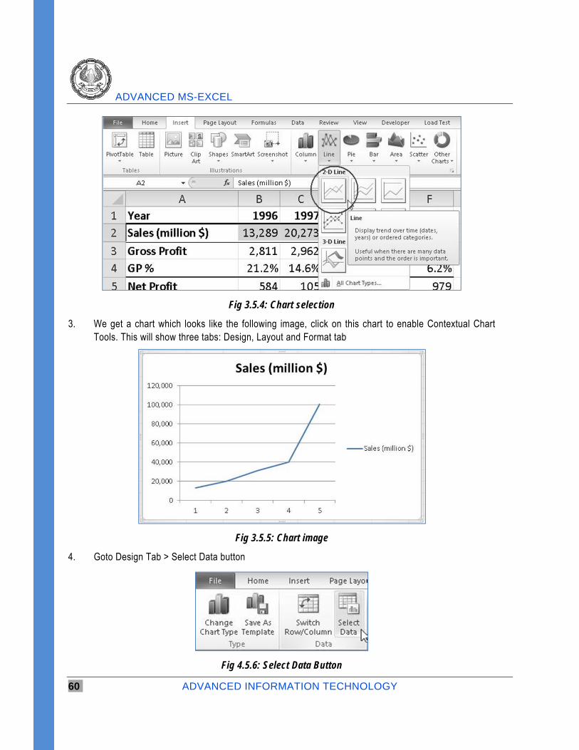
ADVANCED MS-EXCEL
60 ADVANCED INFORMATION TECHNOLOGY
Fig 3.5.4: Chart selection
3. We get a chart which looks like the following image, click on this chart to enable Contextual Chart Tools. This will show three tabs: Design, Layout and Format tab
Fig 3.5.5: Chart image
4. Goto Design Tab > Select Data button
Fig 4.5.6: Select Data Button
APPLIED FINANCIAL ANALYSIS AND FORECASTING FINANCIAL STATEMENTS
ADVANCED INFORMATION TECHNOLOGY 61
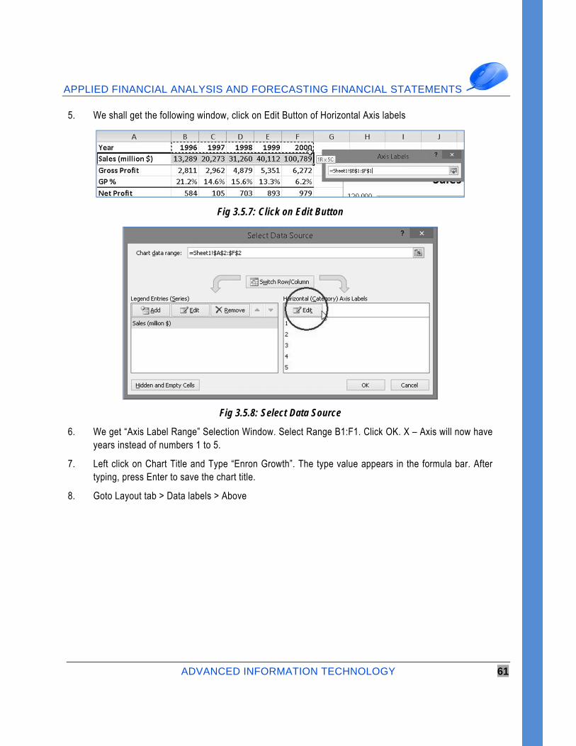
5. We shall get the following window, click on Edit Button of Horizontal Axis labels
Fig 3.5.7: Click on Edit Button
Fig 3.5.8: Select Data Source
6. We get “Axis Label Range” Selection Window. Select Range B1:F1. Click OK. X – Axis will now have years instead of numbers 1 to 5.
7. Left click on Chart Title and Type “Enron Growth”. The type value appears in the formula bar. After typing, press Enter to save the chart title.
8. Goto Layout tab > Data labels > Above
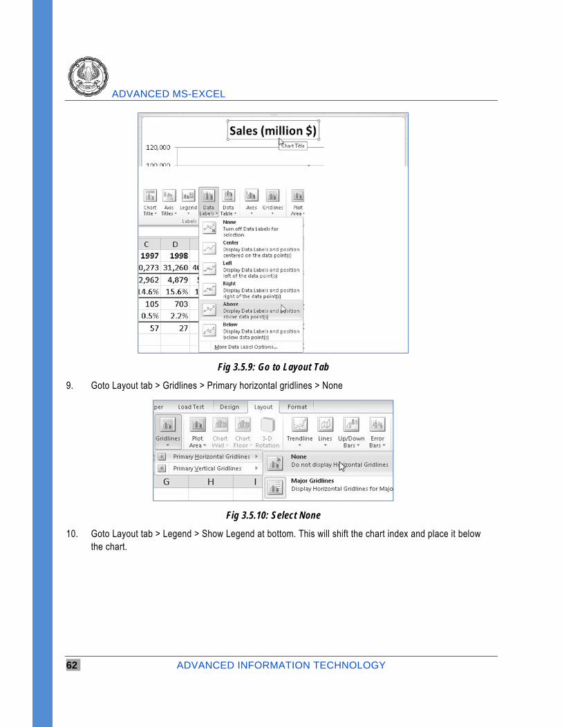
ADVANCED MS-EXCEL
62 ADVANCED INFORMATION TECHNOLOGY
Fig 3.5.9: Go to Layout Tab
9. Goto Layout tab > Gridlines > Primary horizontal gridlines > None
Fig 3.5.10: Select None
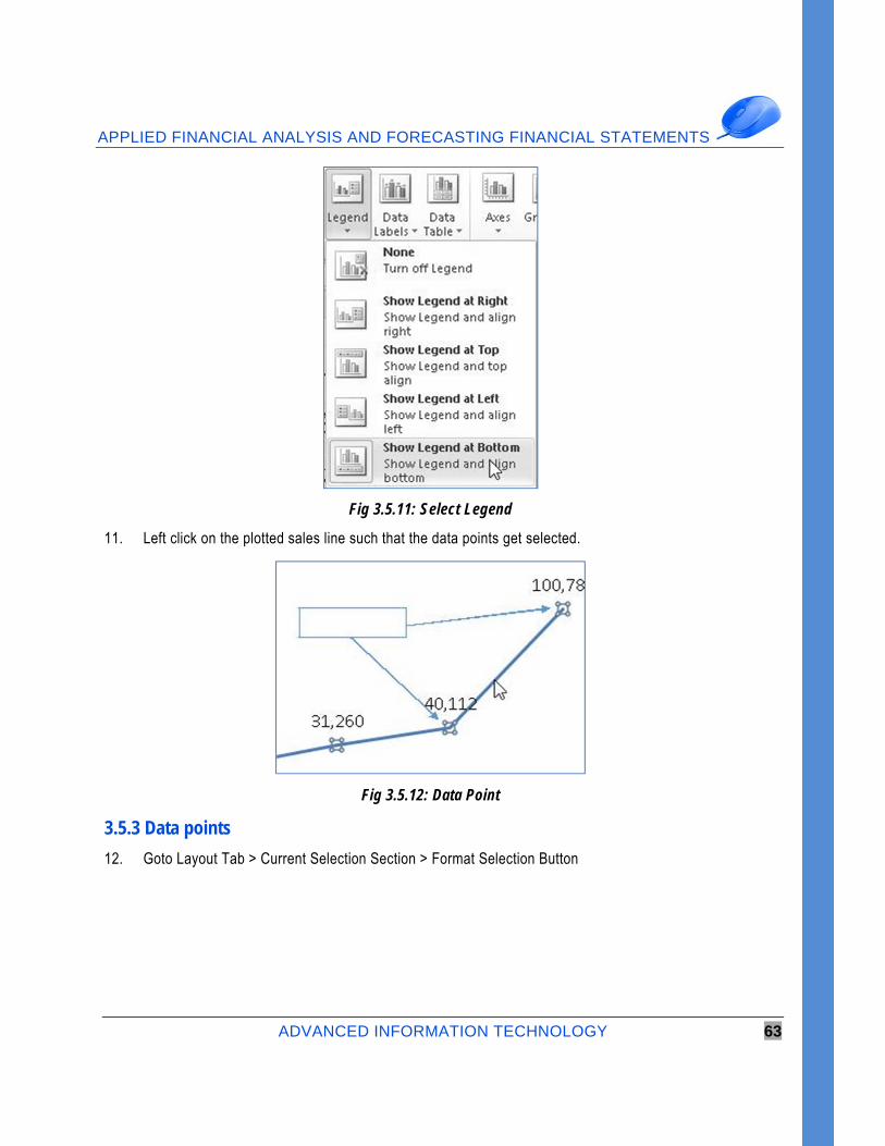
10. Goto Layout tab > Legend > Show Legend at bottom. This will shift the chart index and place it below the chart.
APPLIED FINANCIAL ANALYSIS AND FORECASTING FINANCIAL STATEMENTS
ADVANCED INFORMATION TECHNOLOGY 63
Fig 3.5.11: Select Legend
11. Left click on the plotted sales line such that the data points get selected.
Fig 3.5.12: Data Point
3.5.3 Data points
12. Goto Layout Tab > Current Selection Section > Format Selection Button
ADVANCED MS-EXCEL
64 ADVANCED INFORMATION TECHNOLOGY
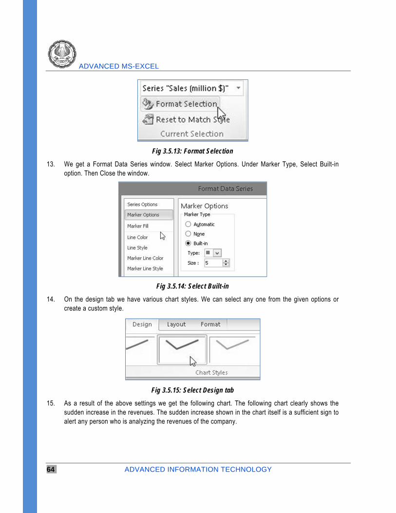
Fig 3.5.13: Format Selection
13. We get a Format Data Series window. Select Marker Options. Under Marker Type, Select Built-in option. Then Close the window.
Fig 3.5.14: Select Built-in
14. On the design tab we have various chart styles. We can select any one from the given options or create a custom style.
Fig 3.5.15: Select Design tab
15. As a result of the above settings we get the following chart. The following chart clearly shows the sudden increase in the revenues. The sudden increase shown in the chart itself is a sufficient sign to alert any person who is analyzing the revenues of the company.
APPLIED FINANCIAL ANALYSIS AND FORECASTING FINANCIAL STATEMENTS
ADVANCED INFORMATION TECHNOLOGY 65
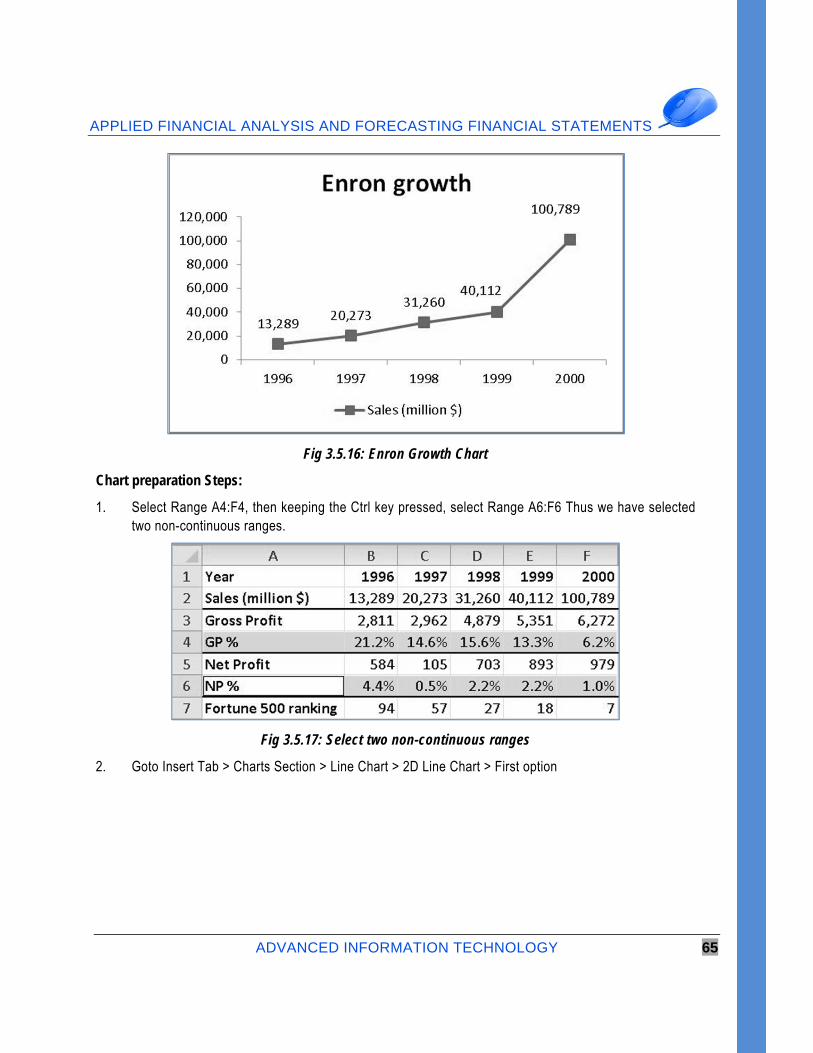
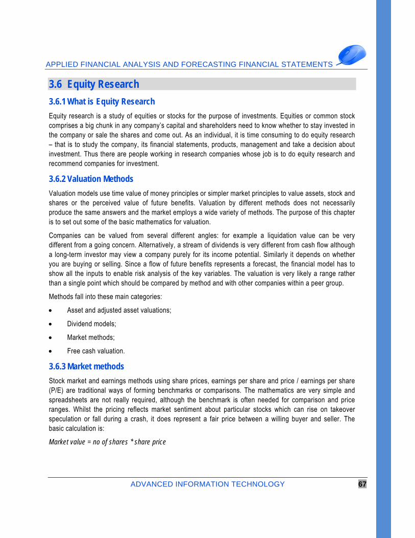
Fig 3.5.16: Enron Growth Chart
Chart preparation Steps:
1. Select Range A4:F4, then keeping the Ctrl key pressed, select Range A6:F6 Thus we have selected two non-continuous ranges.
Fig 3.5.17: Select two non-continuous ranges
2. Goto Insert Tab > Charts Section > Line Chart > 2D Line Chart > First option
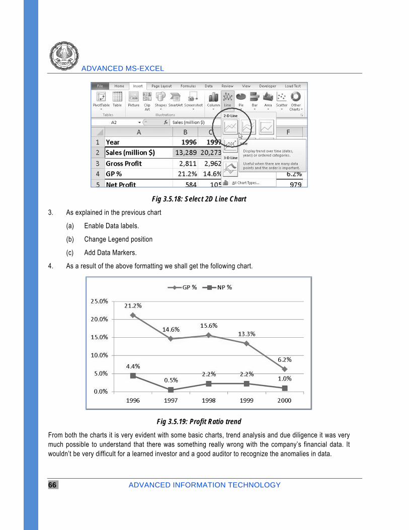
ADVANCED MS-EXCEL
66 ADVANCED INFORMATION TECHNOLOGY
Fig 3.5.18: Select 2D Line Chart
3. As explained in the previous chart
(a) Enable Data labels.
(b) Change Legend position
(c) Add Data Markers.
4. As a result of the above formatting we shall get the following chart.
Fig 3.5.19: Profit Ratio trend
From both the charts it is very evident with some basic charts, trend analysis and due diligence it was very much possible to understand that there was something really wrong with the company’s financial data. It wouldn’t be very difficult for a learned investor and a good auditor to recognize the anomalies in data.
APPLIED FINANCIAL ANALYSIS AND FORECASTING FINANCIAL STATEMENTS
ADVANCED INFORMATION TECHNOLOGY 67
3.6 Equity Research
3.6.1 What is Equity Research
Equity research is a study of equities or stocks for the purpose of investments. Equities or common stock comprises a big chunk in any company’s capital and shareholders need to know whether to stay invested in the company or sale the shares and come out. As an individual, it is time consuming to do equity research – that is to study the company, its financial statements, products, management and take a decision about investment. Thus there are people working in research companies whose job is to do equity research and recommend companies for investment.
3.6.2 Valuation Methods
Valuation models use time value of money principles or simpler market principles to value assets, stock and shares or the perceived value of future benefits. Valuation by different methods does not necessarily produce the same answers and the market employs a wide variety of methods. The purpose of this chapter is to set out some of the basic mathematics for valuation.
Companies can be valued from several different angles: for example a liquidation value can be very different from a going concern. Alternatively, a stream of dividends is very different from cash flow although a long-term investor may view a company purely for its income potential. Similarly it depends on whether you are buying or selling. Since a flow of future benefits represents a forecast, the financial model has to show all the inputs to enable risk analysis of the key variables. The valuation is very likely a range rather than a single point which should be compared by method and with other companies within a peer group.
Methods fall into these main categories:
Asset and adjusted asset valuations;
Dividend models;
Market methods;
Free cash valuation.
3.6.3 Market methods
Stock market and earnings methods using share prices, earnings per share and price / earnings per share (P/E) are traditional ways of forming benchmarks or comparisons. The mathematics are very simple and spreadsheets are not really required, although the benchmark is often needed for comparison and price ranges. Whilst the pricing reflects market sentiment about particular stocks which can rise on takeover speculation or fall during a crash, it does represent a fair price between a willing buyer and seller. The basic calculation is:
Market value = no of shares * share price
ADVANCED MS-EXCEL
68 ADVANCED INFORMATION TECHNOLOGY
The model needs:
Earnings after tax and interest (NPAT)
Number of shares
Calculate earnings per share (EPS)
Price earnings per share (P/E) ratio
Current market price of share / EPS
The valuation can be derived from either:
P/E * earnings per share = share price
Share price * no of shares = market value
The net income and number of shares is on the Data sheet and from this the earnings per share can be calculated as approximately 0.07. The current share price is 5.0 so the price / earnings per share ratio is 71.43.
The valuation is therefore P/E * Net earnings: 71.43 * 3.50 = 250.
The data table in Figure 14.3 shows the sensitivity to the P/E ratio. This is a high figure and there are perhaps some problems relating to the variables used. The formula is:
Value of equity = sustainable earnings * approx P/E ratio + value of non-operating assets
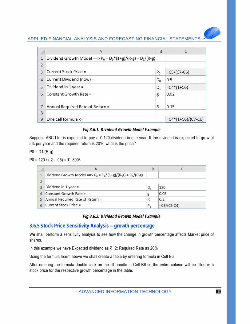
3.6.4 Dividend Growth model
Suppose Big D, Inc. just paid a dividend of ` 30. It is expected to increase its dividend by 2% per year. If the market requires a return of 15% on assets of this risk, how much should the stock be selling for?
D (1� g) D
P �
0
�
1
0
R - g
R - g
P0 = D0(1+g)/(R-g)
P0 = 30 * (1+.02) / (.15 - .02) = Rs 235. 2
APPLIED FINANCIAL ANALYSIS AND FORECASTING FINANCIAL STATEMENTS
ADVANCED INFORMATION TECHNOLOGY 69
Fig 3.6.1: Dividend Growth Model Example
Suppose ABC Ltd. is expected to pay a ` 120 dividend in one year. If the dividend is expected to grow at 5% per year and the required return is 20%, what is the price?
P0 = D1/(R-g)
P0 = 120 / (.2 - .05) = ` 800/-
Fig 3.6.2: Dividend Growth Model Example
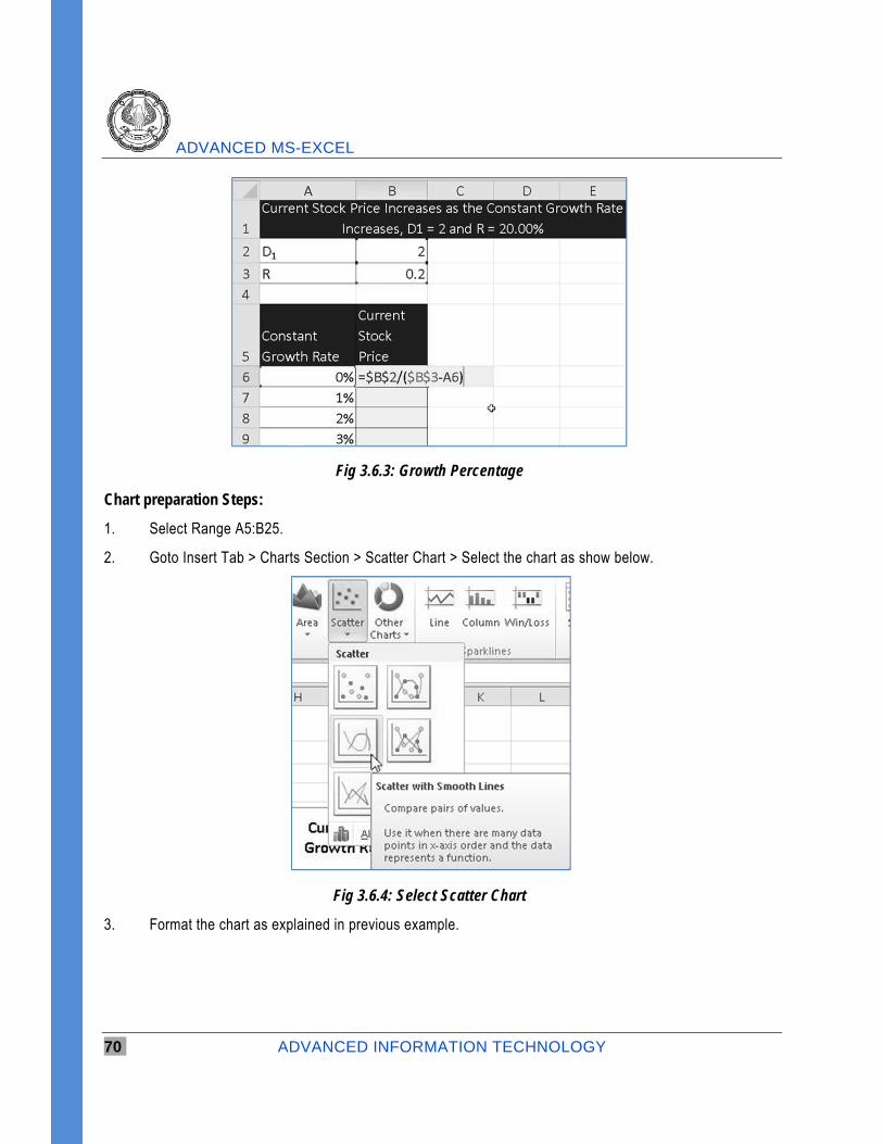
3.6.5 Stock Price Sensitivity Analysis – growth percentage
We shall perform a sensitivity analysis to see how the change in growth percentage affects Market price of shares.
In this example we have Expected dividend as ` 2; Required Rate as 20%
Using the formula learnt above we shall create a table by entering formula in Cell B6
After entering the formula double click on the fill handle in Cell B6 so the entire column will be filled with stock price for the respective growth percentage in the table.
ADVANCED MS-EXCEL
70 ADVANCED INFORMATION TECHNOLOGY
Fig 3.6.3: Growth Percentage
Chart preparation Steps:
1. Select Range A5:B25.
2. Goto Insert Tab > Charts Section > Scatter Chart > Select the chart as show below.
Fig 3.6.4: Select Scatter Chart
3. Format the chart as explained in previous example.
APPLIED FINANCIAL ANALYSIS AND FORECASTING FINANCIAL STATEMENTS
ADVANCED INFORMATION TECHNOLOGY 71
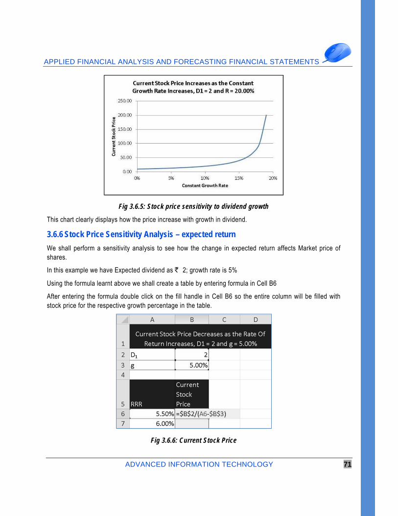
Fig 3.6.5: Stock price sensitivity to dividend growth
This chart clearly displays how the price increase with growth in dividend.
3.6.6 Stock Price Sensitivity Analysis – expected return
We shall perform a sensitivity analysis to see how the change in expected return affects Market price of shares.
In this example we have Expected dividend as ` 2; growth rate is 5%
Using the formula learnt above we shall create a table by entering formula in Cell B6
After entering the formula double click on the fill handle in Cell B6 so the entire column will be filled with stock price for the respective growth percentage in the table.
Fig 3.6.6: Current Stock Price
ADVANCED MS-EXCEL
72 ADVANCED INFORMATION TECHNOLOGY
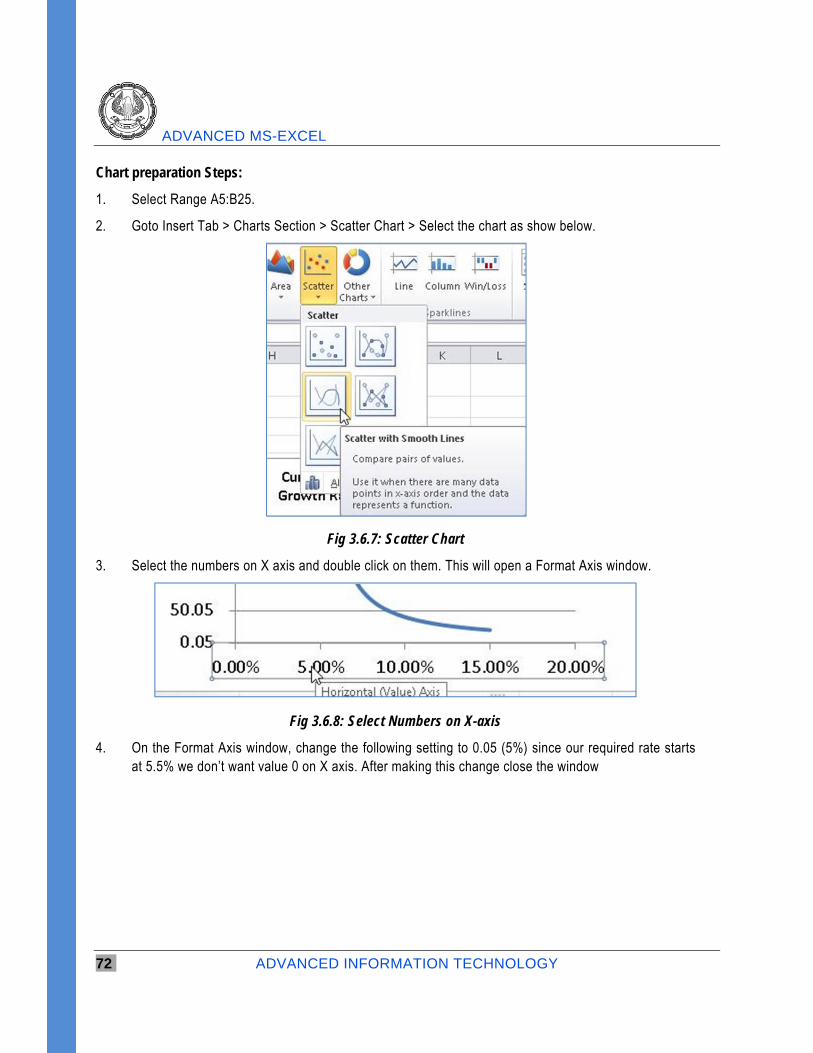
Chart preparation Steps:
1. Select Range A5:B25.
2. Goto Insert Tab > Charts Section > Scatter Chart > Select the chart as show below.
Fig 3.6.7: Scatter Chart
3. Select the numbers on X axis and double click on them. This will open a Format Axis window.
Fig 3.6.8: Select Numbers on X-axis
4. On the Format Axis window, change the following setting to 0.05 (5%) since our required rate starts at 5.5% we don’t want value 0 on X axis. After making this change close the window
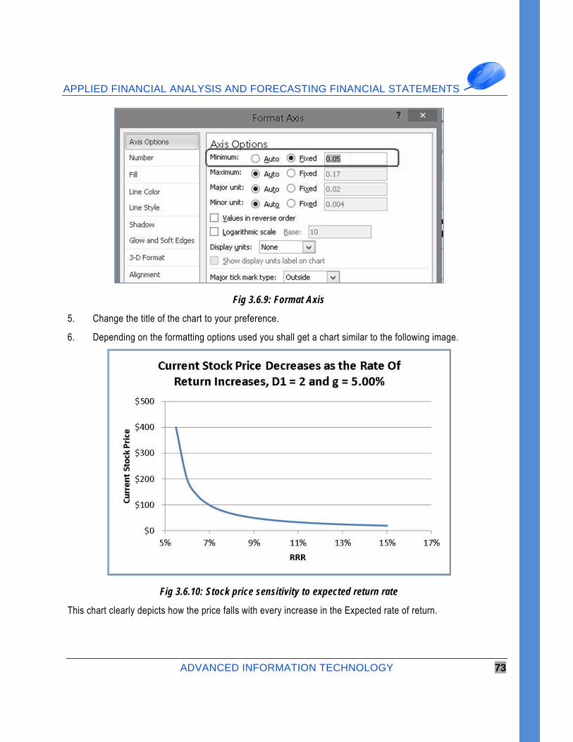
APPLIED FINANCIAL ANALYSIS AND FORECASTING FINANCIAL STATEMENTS
ADVANCED INFORMATION TECHNOLOGY 73
Fig 3.6.9: Format Axis
5. Change the title of the chart to your preference.
6. Depending on the formatting options used you shall get a chart similar to the following image.
Fig 3.6.10: Stock price sensitivity to expected return rate
This chart clearly depicts how the price falls with every increase in the Expected rate of return.
ADVANCED MS-EXCEL
74 ADVANCED INFORMATION TECHNOLOGY
3.7 Summary Excel is an invaluable tool for data analysis. In this chapter, we learnt how to apply simple formula and functions that allow us to analyze financial data. We learnt to create and format charts. Charts are one of the most important visual analysis tools available in excel. We learnt how to use Du-pont analysis in excel by proper data structuring and simple functions. We also learnt decision making like whether it was feasible to Lease a machinery or should it be purchased. In addition, we also learnt how to use charts to analyze trends and recognize the possibility of a fraud.
References [1] Excel 2010 Formulas; John Walkenbach; Wiley Publishing
[2] Financial Shenanigans; Howard Shilit; Mc Graw Hill.
MATHEMATICAL AND STATISTICAL TOOLS FOR FINANCIAL ANALYSIS
4.1 Introduction This chapter focuses on the statistical features of Excel application. The primary goal of this chapter is not to impart knowledge of statistics as a subject, thus basic knowledge of statistics is presumed.
A “Statistic” can be a numerical fact, like Google has a 5% return last month or a test average in a class was 79 points.
Statistics as a discipline = It is an art and science of collecting, presenting and interpreting data.
It’s an Art because the presentation of your analysis matters a lot.
It’s a science because we must use the scientific methods of experiment and probability.
Data means chunks of some values. It can be any value first name, last name, month names etc. Information is data represented in a useful way.
Interpretation of data means that we make useful information from data, using statistics or any tool, so that we can take decisions. Since future is always uncertain we try to use statistics on the past data in an attempt to predict the future and take decisions important decisions.
4.2 Enable Data Analysis Toolpak Go to File menu – Options – Add-ins Section as shown in Fig 4.2.1
LEARNING OBJECTIVES
To learn statistical features of excel
To learn Testing of hypothesis
To learn confidence interval
To learn level of confidence and level of significance
To learn ANOVA
To learn Regression Analysis
CHAPTER
4
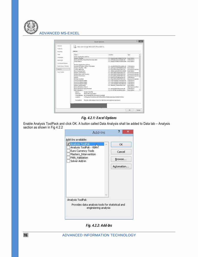
ADVANCED MS-EXCEL
76 ADVANCED INFORMATION TECHNOLOGY
Fig. 4.2.1: Excel Options
Enable Analysis ToolPack and click OK. A button called Data Analysis shall be added to Data tab – Analysis section as shown in Fig 4.2.2
Fig. 4.2.2: Add-Ins
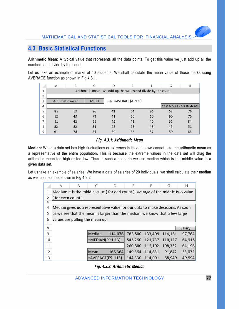
MATHEMATICAL AND STATISTICAL TOOLS FOR FINANCIAL ANALYSIS
ADVANCED INFORMATION TECHNOLOGY 77
4.3 Basic Statistical Functions Arithmetic Mean: A typical value that represents all the data points. To get this value we just add up all the numbers and divide by the count.
Let us take an example of marks of 40 students. We shall calculate the mean value of those marks using AVERAGE function as shown in Fig 4.3.1.
Fig. 4.3.1: Arithmetic Mean
Median: When a data set has high fluctuations or extremes in its values we cannot take the arithmetic mean as a representative of the entire population. This is because the extreme values in the data set will drag the arithmetic mean too high or too low. Thus in such a scenario we use median which is the middle value in a given data set.
Let us take an example of salaries. We have a data of salaries of 20 individuals, we shall calculate their median as well as mean as shown in Fig 4.3.2
Fig. 4.3.2: Arithmetic Median
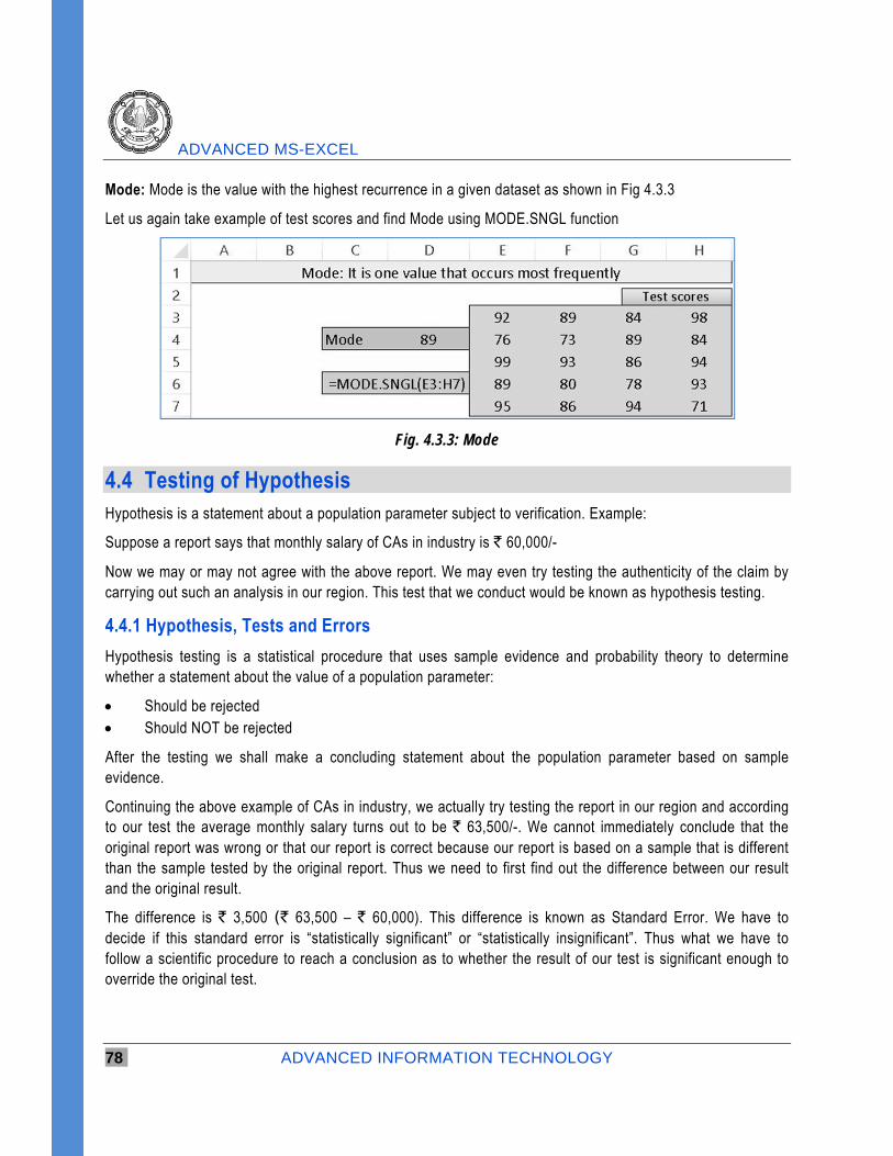
ADVANCED MS-EXCEL
78 ADVANCED INFORMATION TECHNOLOGY
Mode: Mode is the value with the highest recurrence in a given dataset as shown in Fig 4.3.3
Let us again take example of test scores and find Mode using MODE.SNGL function
Fig. 4.3.3: Mode
4.4 Testing of Hypothesis Hypothesis is a statement about a population parameter subject to verification. Example:
Suppose a report says that monthly salary of CAs in industry is ` 60,000/-
Now we may or may not agree with the above report. We may even try testing the authenticity of the claim by carrying out such an analysis in our region. This test that we conduct would be known as hypothesis testing.
4.4.1 Hypothesis, Tests and Errors
Hypothesis testing is a statistical procedure that uses sample evidence and probability theory to determine whether a statement about the value of a population parameter:
Should be rejected Should NOT be rejected
After the testing we shall make a concluding statement about the population parameter based on sample evidence.
Continuing the above example of CAs in industry, we actually try testing the report in our region and according to our test the average monthly salary turns out to be ` 63,500/-. We cannot immediately conclude that the original report was wrong or that our report is correct because our report is based on a sample that is different than the sample tested by the original report. Thus we need to first find out the difference between our result and the original result.
The difference is ` 3,500 (` 63,500 – ` 60,000). This difference is known as Standard Error. We have to decide if this standard error is “statistically significant” or “statistically insignificant”. Thus what we have to follow a scientific procedure to reach a conclusion as to whether the result of our test is significant enough to override the original test.
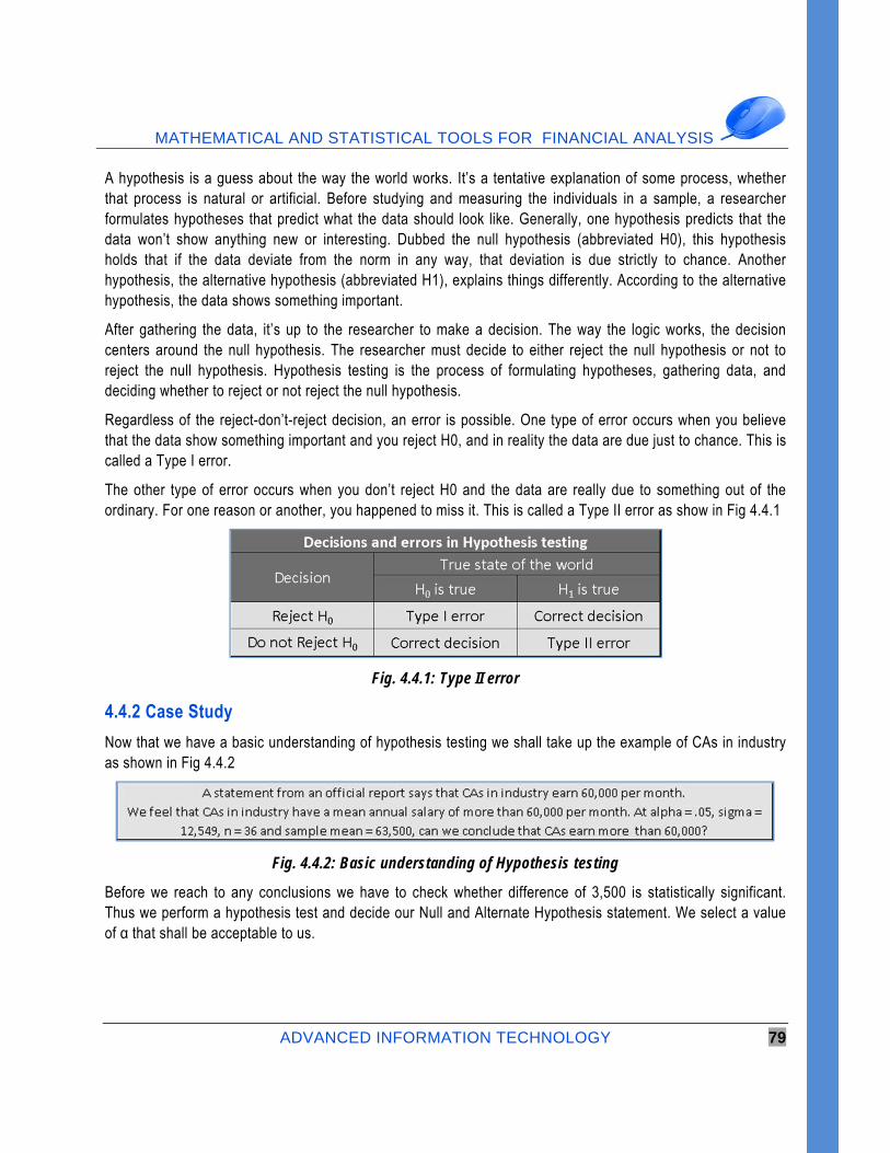
MATHEMATICAL AND STATISTICAL TOOLS FOR FINANCIAL ANALYSIS
ADVANCED INFORMATION TECHNOLOGY 79
A hypothesis is a guess about the way the world works. It’s a tentative explanation of some process, whether that process is natural or artificial. Before studying and measuring the individuals in a sample, a researcher formulates hypotheses that predict what the data should look like. Generally, one hypothesis predicts that the data won’t show anything new or interesting. Dubbed the null hypothesis (abbreviated H0), this hypothesis holds that if the data deviate from the norm in any way, that deviation is due strictly to chance. Another hypothesis, the alternative hypothesis (abbreviated H1), explains things differently. According to the alternative hypothesis, the data shows something important.
After gathering the data, it’s up to the researcher to make a decision. The way the logic works, the decision centers around the null hypothesis. The researcher must decide to either reject the null hypothesis or not to reject the null hypothesis. Hypothesis testing is the process of formulating hypotheses, gathering data, and deciding whether to reject or not reject the null hypothesis.
Regardless of the reject-don’t-reject decision, an error is possible. One type of error occurs when you believe that the data show something important and you reject H0, and in reality the data are due just to chance. This is called a Type I error.
The other type of error occurs when you don’t reject H0 and the data are really due to something out of the ordinary. For one reason or another, you happened to miss it. This is called a Type II error as show in Fig 4.4.1
Fig. 4.4.1: Type II error
4.4.2 Case Study
Now that we have a basic understanding of hypothesis testing we shall take up the example of CAs in industry as shown in Fig 4.4.2
Fig. 4.4.2: Basic understanding of Hypothesis testing
Before we reach to any conclusions we have to check whether difference of 3,500 is statistically significant. Thus we perform a hypothesis test and decide our Null and Alternate Hypothesis statement. We select a value of α that shall be acceptable to us.
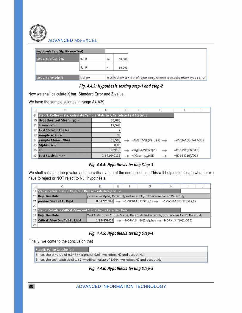
ADVANCED MS-EXCEL
80 ADVANCED INFORMATION TECHNOLOGY
Fig. 4.4.3: Hypothesis testing step-1 and step-2
Now we shall calculate X bar, Standard Error and Z value.
We have the sample salaries in range A4:A39
Fig. 4.4.4: Hypothesis testing Step-3
We shall calculate the p-value and the critical value of the one talied test. This will help us to decide whether we have to reject or NOT reject to Null hypothesis.
Fig. 4.4.5: Hypothesis testing Step-4
Finally, we come to the conclusion that
Fig. 4.4.6: Hypothesis testing Step-5
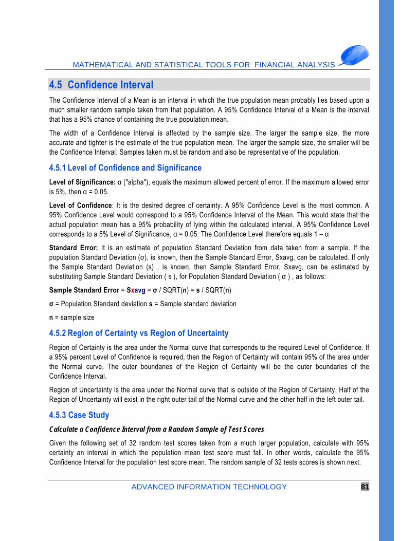
MATHEMATICAL AND STATISTICAL TOOLS FOR FINANCIAL ANALYSIS
ADVANCED INFORMATION TECHNOLOGY 81
4.5 Confidence Interval The Confidence Interval of a Mean is an interval in which the true population mean probably lies based upon a much smaller random sample taken from that population. A 95% Confidence Interval of a Mean is the interval that has a 95% chance of containing the true population mean.
The width of a Confidence Interval is affected by the sample size. The larger the sample size, the more accurate and tighter is the estimate of the true population mean. The larger the sample size, the smaller will be the Confidence Interval. Samples taken must be random and also be representative of the population.
4.5.1 Level of Confidence and Significance
Level of Significance: α ("alpha"), equals the maximum allowed percent of error. If the maximum allowed error is 5%, then α = 0.05.
Level of Confidence: It is the desired degree of certainty. A 95% Confidence Level is the most common. A 95% Confidence Level would correspond to a 95% Confidence Interval of the Mean. This would state that the actual population mean has a 95% probability of lying within the calculated interval. A 95% Confidence Level corresponds to a 5% Level of Significance, α = 0.05. The Confidence Level therefore equals 1 – α
Standard Error: It is an estimate of population Standard Deviation from data taken from a sample. If the population Standard Deviation (σ), is known, then the Sample Standard Error, Sxavg, can be calculated. If only the Sample Standard Deviation (s) , is known, then Sample Standard Error, Sxavg, can be estimated by substituting Sample Standard Deviation ( s ), for Population Standard Deviation ( σ ) , as follows:
Sample Standard Error = Sxavg = σ / SQRT(n) = s / SQRT(n)
σ = Population Standard deviation s = Sample standard deviation
n = sample size
4.5.2 Region of Certainty vs Region of Uncertainty
Region of Certainty is the area under the Normal curve that corresponds to the required Level of Confidence. If a 95% percent Level of Confidence is required, then the Region of Certainty will contain 95% of the area under the Normal curve. The outer boundaries of the Region of Certainty will be the outer boundaries of the Confidence Interval.
Region of Uncertainty is the area under the Normal curve that is outside of the Region of Certainty. Half of the Region of Uncertainty will exist in the right outer tail of the Normal curve and the other half in the left outer tail.
4.5.3 Case Study
Calculate a Confidence Interval from a Random Sample of Test Scores
Given the following set of 32 random test scores taken from a much larger population, calculate with 95% certainty an interval in which the population mean test score must fall. In other words, calculate the 95% Confidence Interval for the population test score mean. The random sample of 32 tests scores is shown next.
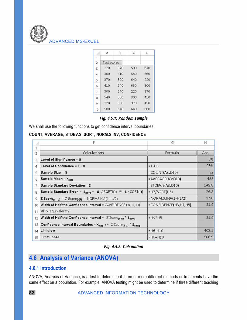
ADVANCED MS-EXCEL
82 ADVANCED INFORMATION TECHNOLOGY
Fig. 4.5.1: Random sample
We shall use the following functions to get confidence interval boundaries:
COUNT, AVERAGE, STDEV.S, SQRT, NORM.S.INV, CONFIDENCE
Fig. 4.5.2: Calculation
4.6 Analysis of Variance (ANOVA)
4.6.1 Introduction
ANOVA, Analysis of Variance, is a test to determine if three or more different methods or treatments have the same effect on a population. For example, ANOVA testing might be used to determine if three different teaching
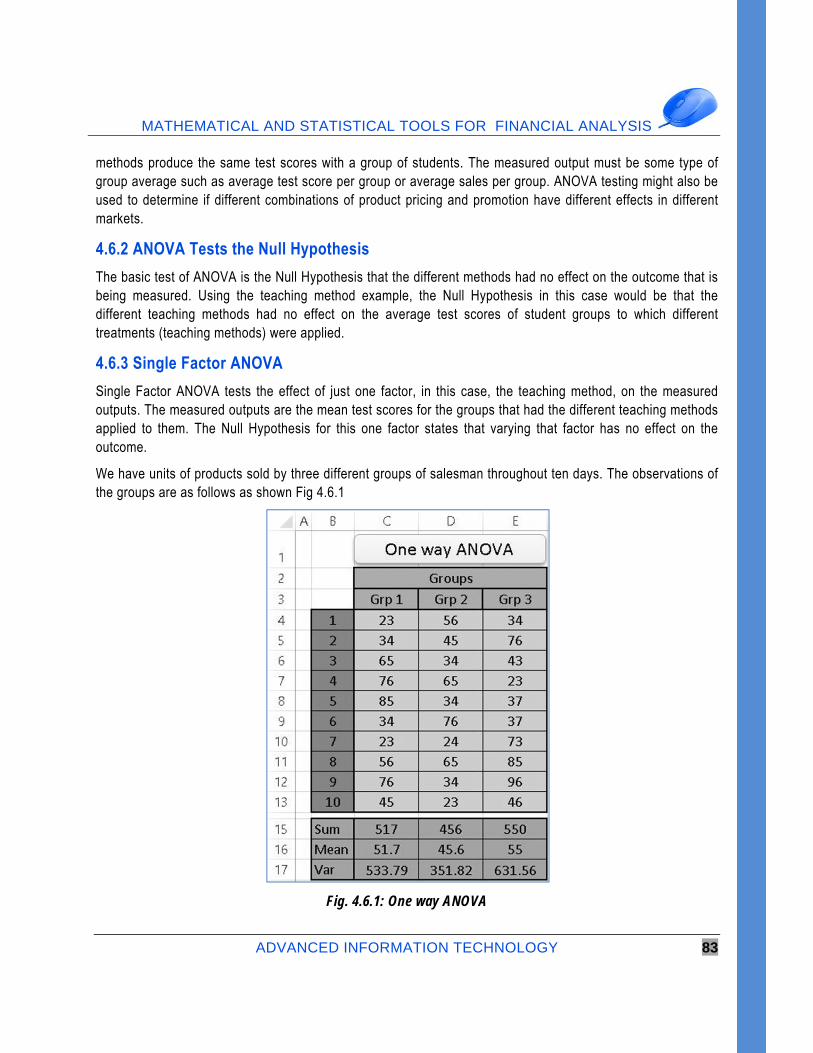
MATHEMATICAL AND STATISTICAL TOOLS FOR FINANCIAL ANALYSIS
ADVANCED INFORMATION TECHNOLOGY 83
methods produce the same test scores with a group of students. The measured output must be some type of group average such as average test score per group or average sales per group. ANOVA testing might also be used to determine if different combinations of product pricing and promotion have different effects in different markets.
4.6.2 ANOVA Tests the Null Hypothesis
The basic test of ANOVA is the Null Hypothesis that the different methods had no effect on the outcome that is being measured. Using the teaching method example, the Null Hypothesis in this case would be that the different teaching methods had no effect on the average test scores of student groups to which different treatments (teaching methods) were applied.
4.6.3 Single Factor ANOVA
Single Factor ANOVA tests the effect of just one factor, in this case, the teaching method, on the measured outputs. The measured outputs are the mean test scores for the groups that had the different teaching methods applied to them. The Null Hypothesis for this one factor states that varying that factor has no effect on the outcome.
We have units of products sold by three different groups of salesman throughout ten days. The observations of the groups are as follows as shown Fig 4.6.1
Fig. 4.6.1: One way ANOVA
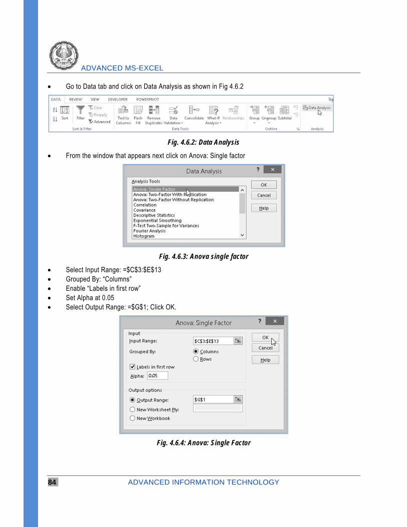
ADVANCED MS-EXCEL
84 ADVANCED INFORMATION TECHNOLOGY
Go to Data tab and click on Data Analysis as shown in Fig 4.6.2
Fig. 4.6.2: Data Analysis
From the window that appears next click on Anova: Single factor
Fig. 4.6.3: Anova single factor
Select Input Range: =$C$3:$E$13 Grouped By: “Columns” Enable “Labels in first row” Set Alpha at 0.05 Select Output Range: =$G$1; Click OK.
Fig. 4.6.4: Anova: Single Factor
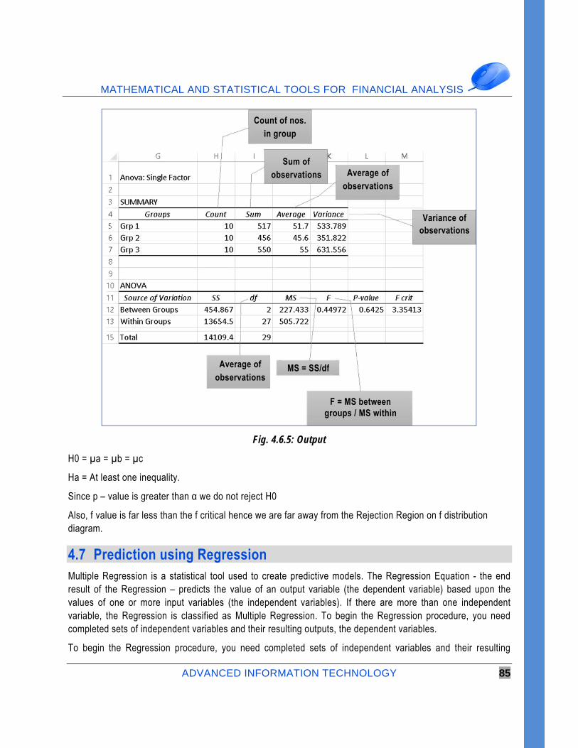
MATHEMATICAL AND STATISTICAL TOOLS FOR FINANCIAL ANALYSIS
ADVANCED INFORMATION TECHNOLOGY 85
Fig. 4.6.5: Output
H0 = µa = µb = µc
Ha = At least one inequality.
Since p – value is greater than α we do not reject H0
Also, f value is far less than the f critical hence we are far away from the Rejection Region on f distribution diagram.
4.7 Prediction using Regression Multiple Regression is a statistical tool used to create predictive models. The Regression Equation - the end result of the Regression – predicts the value of an output variable (the dependent variable) based upon the values of one or more input variables (the independent variables). If there are more than one independent variable, the Regression is classified as Multiple Regression. To begin the Regression procedure, you need completed sets of independent variables and their resulting outputs, the dependent variables.
To begin the Regression procedure, you need completed sets of independent variables and their resulting
Count of nos. in group
Sum of observations Average of
observations
Variance of observations
Average of observations
MS = SS/df
F = MS between groups / MS within
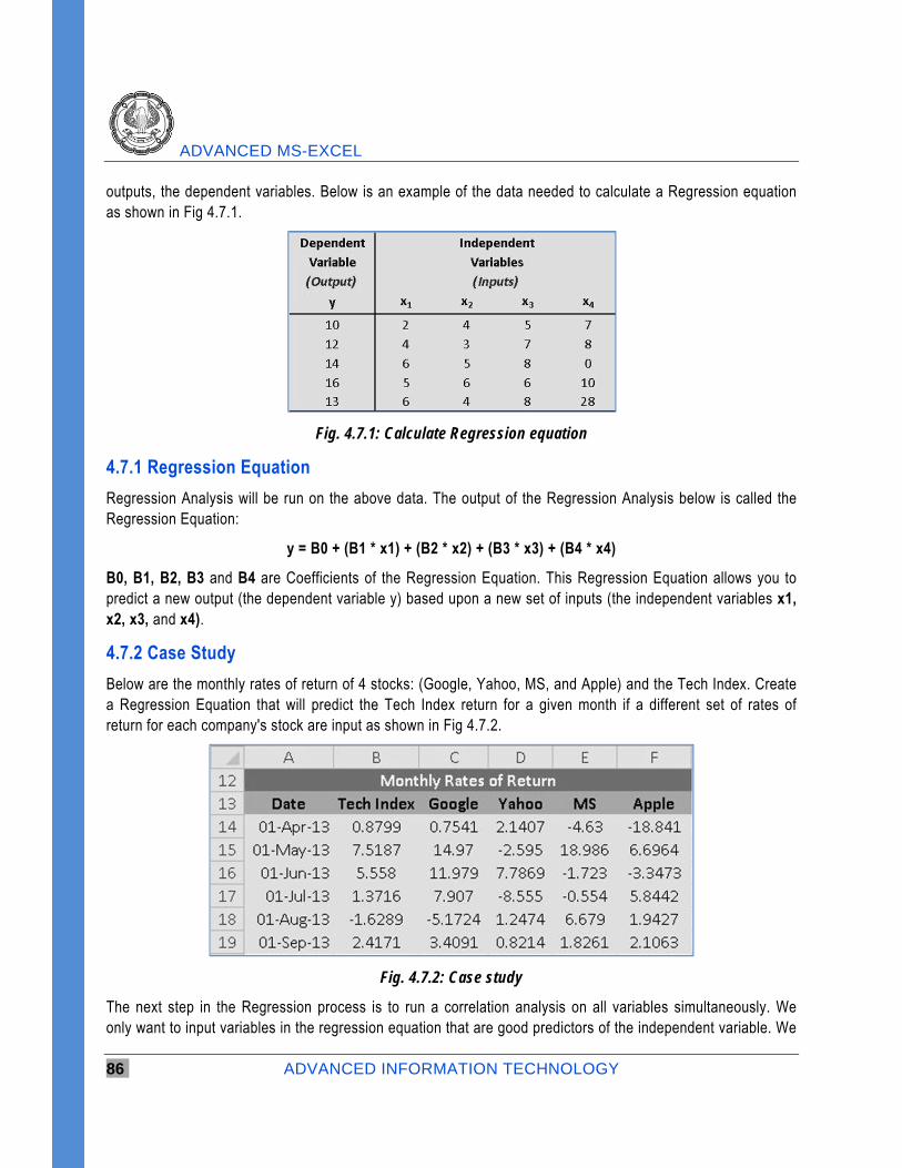
ADVANCED MS-EXCEL
86 ADVANCED INFORMATION TECHNOLOGY
outputs, the dependent variables. Below is an example of the data needed to calculate a Regression equation as shown in Fig 4.7.1.
Fig. 4.7.1: Calculate Regression equation
4.7.1 Regression Equation
Regression Analysis will be run on the above data. The output of the Regression Analysis below is called the Regression Equation:
y = B0 + (B1 * x1) + (B2 * x2) + (B3 * x3) + (B4 * x4)
B0, B1, B2, B3 and B4 are Coefficients of the Regression Equation. This Regression Equation allows you to predict a new output (the dependent variable y) based upon a new set of inputs (the independent variables x1, x2, x3, and x4).
4.7.2 Case Study
Below are the monthly rates of return of 4 stocks: (Google, Yahoo, MS, and Apple) and the Tech Index. Create a Regression Equation that will predict the Tech Index return for a given month if a different set of rates of return for each company's stock are input as shown in Fig 4.7.2.
Fig. 4.7.2: Case study
The next step in the Regression process is to run a correlation analysis on all variables simultaneously. We only want to input variables in the regression equation that are good predictors of the independent variable. We
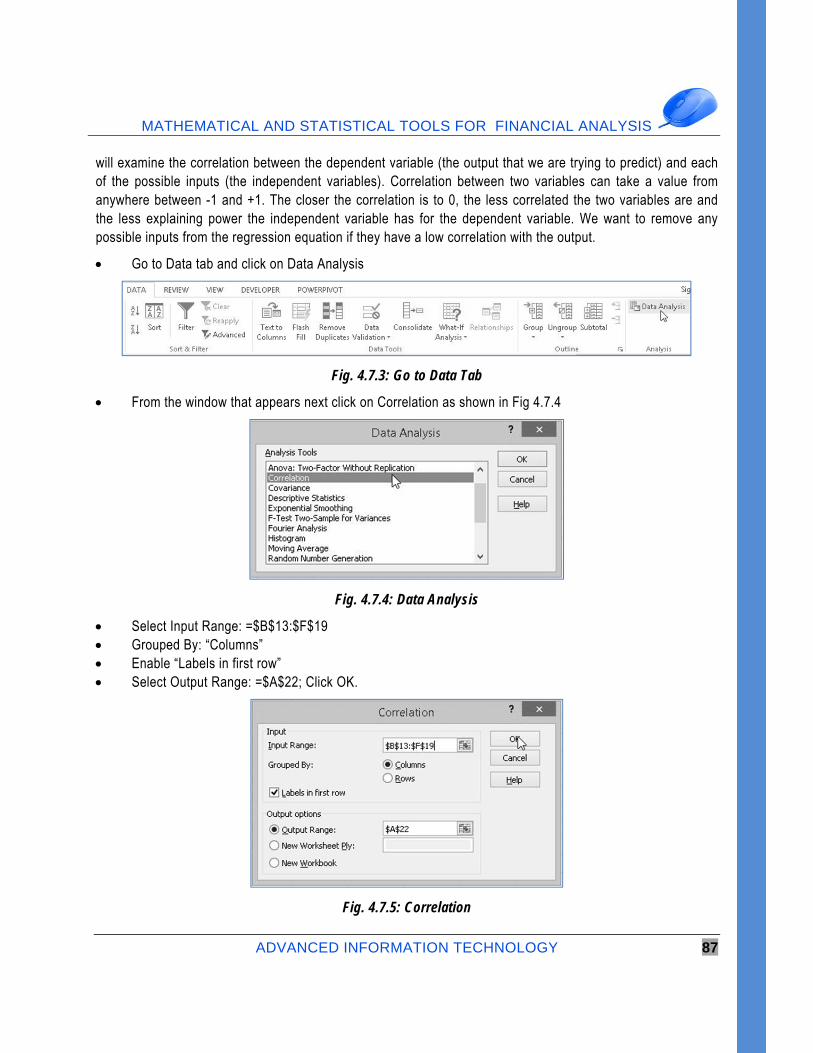
MATHEMATICAL AND STATISTICAL TOOLS FOR FINANCIAL ANALYSIS
ADVANCED INFORMATION TECHNOLOGY 87
will examine the correlation between the dependent variable (the output that we are trying to predict) and each of the possible inputs (the independent variables). Correlation between two variables can take a value from anywhere between -1 and +1. The closer the correlation is to 0, the less correlated the two variables are and the less explaining power the independent variable has for the dependent variable. We want to remove any possible inputs from the regression equation if they have a low correlation with the output.
Go to Data tab and click on Data Analysis
Fig. 4.7.3: Go to Data Tab
From the window that appears next click on Correlation as shown in Fig 4.7.4
Fig. 4.7.4: Data Analysis
Select Input Range: =$B$13:$F$19 Grouped By: “Columns” Enable “Labels in first row” Select Output Range: =$A$22; Click OK.
Fig. 4.7.5: Correlation
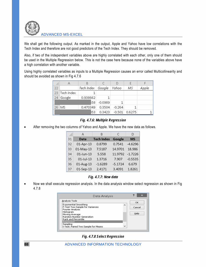
ADVANCED MS-EXCEL
88 ADVANCED INFORMATION TECHNOLOGY
We shall get the following output. As marked in the output, Apple and Yahoo have low correlations with the Tech Index and therefore are not good predictors of the Tech Index. They should be removed.
Also, if two of the independent variables above are highly correlated with each other, only one of them should be used in the Multiple Regression below. This is not the case here because none of the variables above have a high correlation with another variable.
Using highly correlated variables as inputs to a Multiple Regression causes an error called Multicollinearity and should be avoided as shown in Fig 4.7.6
Fig. 4.7.6: Multiple Regression
After removing the two columns of Yahoo and Apple. We have the new data as follows.
Fig. 4.7.7: New data
Now we shall execute regression analysis. In the data analysis window select regression as shown in Fig 4.7.8
Fig. 4.7.8 Select Regression
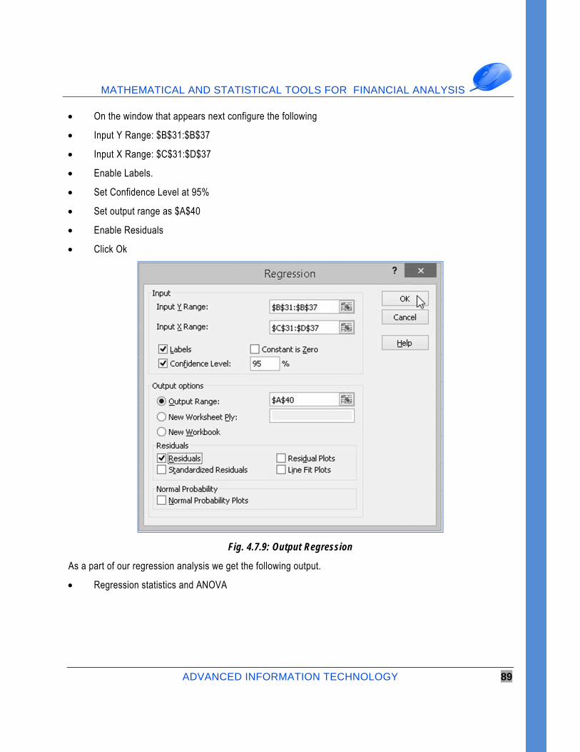
MATHEMATICAL AND STATISTICAL TOOLS FOR FINANCIAL ANALYSIS
ADVANCED INFORMATION TECHNOLOGY 89
On the window that appears next configure the following
Input Y Range: $B$31:$B$37
Input X Range: $C$31:$D$37
Enable Labels.
Set Confidence Level at 95%
Set output range as $A$40
Enable Residuals
Click Ok
Fig. 4.7.9: Output Regression
As a part of our regression analysis we get the following output.
Regression statistics and ANOVA
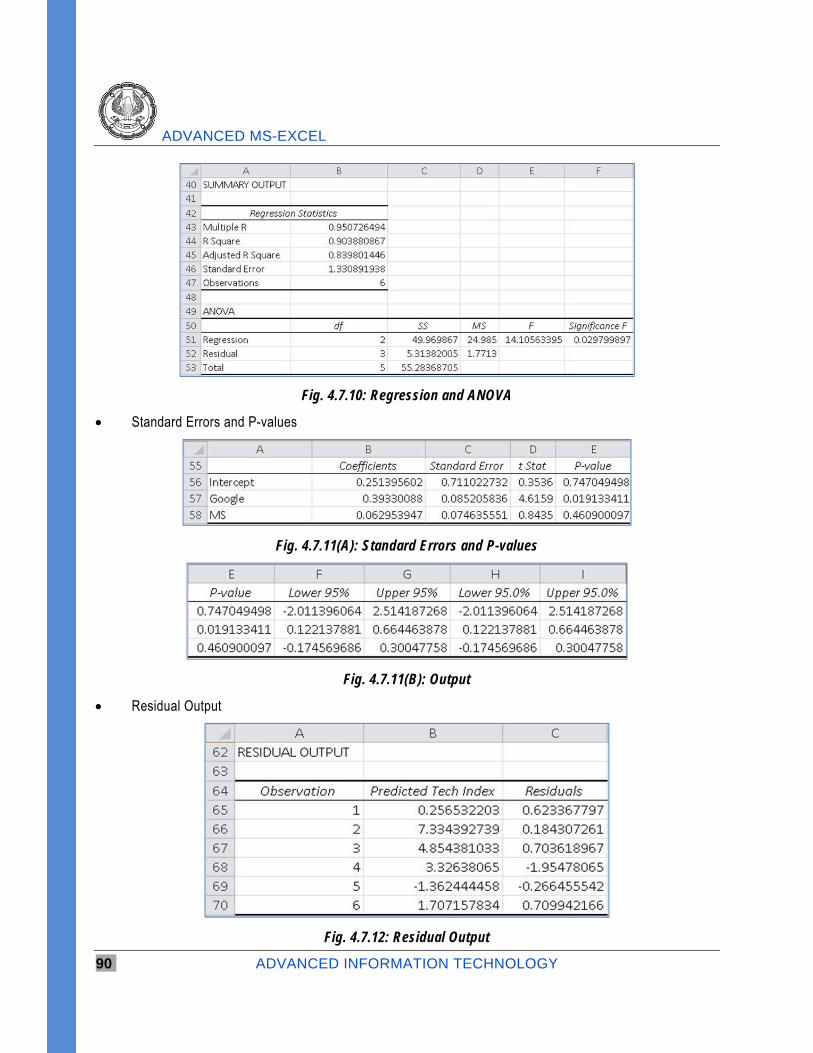
ADVANCED MS-EXCEL
90 ADVANCED INFORMATION TECHNOLOGY
Fig. 4.7.10: Regression and ANOVA
Standard Errors and P-values
Fig. 4.7.11(A): Standard Errors and P-values
Fig. 4.7.11(B): Output
Residual Output
Fig. 4.7.12: Residual Output
MATHEMATICAL AND STATISTICAL TOOLS FOR FINANCIAL ANALYSIS
ADVANCED INFORMATION TECHNOLOGY 91
Let’s take a look at the meaning of the output derived.
First and foremost we check the overall accuracy of the regression which is determined by R-square and adjusted R-square.
R-square is 90% which means that 90% of the variance of the output variable can be explained by the variance of input variable. Adjusted R-square is more conservative and more accurate.
Secondly, we check the probability that the regression output was not obtained by chance (co-incidence)
This can be determined by significance of F for the regression which in our case is 2.8%. Thus there is 2.8% chance that our regression output is mere co-incidence.
Third, we check the reliability of coefficients and y intercepts. This will be determined by the p-values. Smaller p-values means these values are not a result of co-incidence/chance.
Lastly, residuals are difference between actual tech index and predictive value of dependent variable. Thus the equation we get is: Tech Index = 0.251 + 0.393 * Google + 0.063 * MS
4.7.3 Using Regression equation to predict an output
Predict the Tech Index if Google = 7 and MS = 4.
Tech Index = (0.251) + (0.393)*(Google) + (0.063)*(MS)
Tech Index predicted = (0.251) + (0.393)*(7) + (0.063)*(4) = 3.25
4.7.4 The Confidence Interval of the Output Variable
The Confidence Interval was set at 95%. This is the default setting.
It could have been set to any desired confidence level.
The 95% Confidence Interval is interval in which the output variable, Tech Index, should fall with 95% certainty.
The 95% Confidence Interval = Tech Index predicted +/- Z Score95% * (Standard Error)
Z score Calculation
Level of Confidence = 95% = 1 – α; Level of Significance = α = 0.05
Z Score 95% = Z Scoreα=0.05 = NORMSINV (0.975) = 1.96
The cell containing the Overall Standard Error for the Regression Equation = 1.33
The 95% Confidence Interval = 3.25 +/- (1.96) * (1.33) = 0.64 to 5.86
This means that there is a 95% chance the actual Tech Index return will fall within 0.64 and 5.86 for inputs Google = 7 and MS = 4.
ADVANCED MS-EXCEL
92 ADVANCED INFORMATION TECHNOLOGY
4.8 Summary In this chapter we have glanced through some of the statistical features of excel. We have learn how to calculate and interpret ANOVA. We have learnt how to identify our Null and Alternate hypothesis.
We have also learnt how to calculate basic statistical values like mean, median and mode. We have seen how to get a regression equation using regression analysis tools. Based on the derived equation we have learnt to predict an output. We have also learnt how to calculate the confidence interval of the output variable. Thus in this chapter we have touched upon various aspects of statistics as a subject and a few of its use cases in Excel.
References [1] Statistical Analysis Microsoft Excel 2010 – Conard Carlberg
[2] Excel Data Analysis Modeling and Simulation – Hector Guerrero
APPLICATION OF MS - EXCEL
5.1 Introduction Excel is a powerful tool available in the hands of users. Application of excel functions are unlimited. It depends on the imagination of the user only, how a function can be used in a particular situation. In this section we are going to discuss about some of the functions relating to accounting and finance.
When excel was not there, still people used to analyze financial data using traditional tools with lot of limitation. After the availability of excel in the hands of the user, analysis of huge amount of data is possible at an absolutely great speed.
In this section, we are going to discuss financial functions relating to depreciation calculation, marginal costing, cash budgeting, discounting, tax calculations, EMI calculations, capital budgeting, risk analysis and investment, financial planning, etc.
In today’s era of technology, it is directly / indirectly compulsory for an accounting professional to learn these financial functions in excel to ensure his/her existence in this competitive world. Knowledge of these technological tools gives us an added advantage of handling huge amount of data at a great speed.
So, let us start understanding one by one some of the useful functions in excel relating to accounting and finance.
5.2 Depreciation Accounting Depreciation stands for reduction in value of fixed assets. Value of fixed assets is generally reduced over the
period of time due to any of the following reasons.
(a) Wear & Tear
(b) Change in taste of people
(c) Change in technology.
CHAPTER
5 LEARNING OBJECTIVES
To know about the various tools available in excel regarding costing and finance.
To know how to use these tools in practical situations.
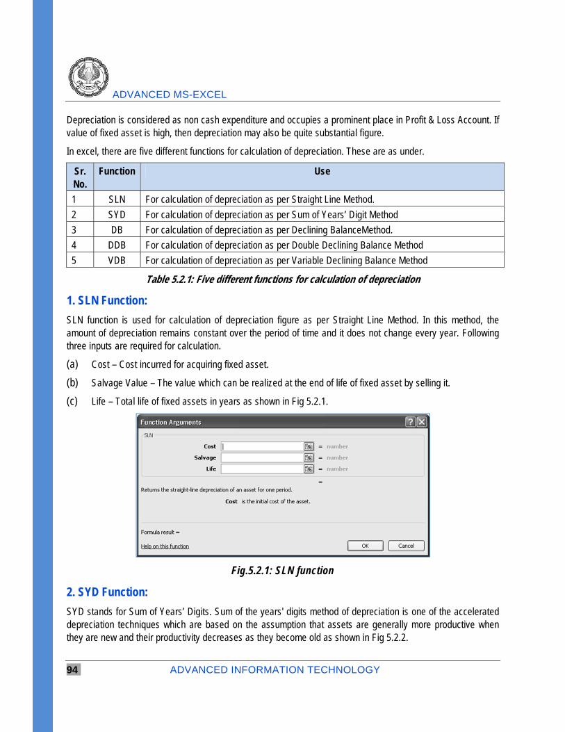
ADVANCED MS-EXCEL
94 ADVANCED INFORMATION TECHNOLOGY
Depreciation is considered as non cash expenditure and occupies a prominent place in Profit & Loss Account. If value of fixed asset is high, then depreciation may also be quite substantial figure.
In excel, there are five different functions for calculation of depreciation. These are as under.
Sr. No.
Function Use
1 SLN For calculation of depreciation as per Straight Line Method.
2 SYD For calculation of depreciation as per Sum of Years’ Digit Method
3 DB For calculation of depreciation as per Declining BalanceMethod.
4 DDB For calculation of depreciation as per Double Declining Balance Method
5 VDB For calculation of depreciation as per Variable Declining Balance Method
Table 5.2.1: Five different functions for calculation of depreciation
1. SLN Function:
SLN function is used for calculation of depreciation figure as per Straight Line Method. In this method, the amount of depreciation remains constant over the period of time and it does not change every year. Following three inputs are required for calculation.
(a) Cost – Cost incurred for acquiring fixed asset.
(b) Salvage Value – The value which can be realized at the end of life of fixed asset by selling it.
(c) Life – Total life of fixed assets in years as shown in Fig 5.2.1.
Fig.5.2.1: SLN function
2. SYD Function:
SYD stands for Sum of Years’ Digits. Sum of the years' digits method of depreciation is one of the accelerated depreciation techniques which are based on the assumption that assets are generally more productive when they are new and their productivity decreases as they become old as shown in Fig 5.2.2.
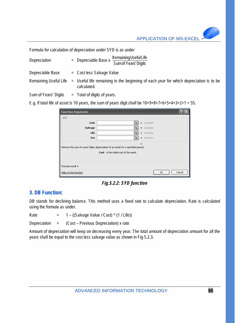
APPLICATION OF MS-EXCEL
ADVANCED INFORMATION TECHNOLOGY 95
Formula for calculation of depreciation under SYD is as under
Depreciation = Depreciable Base x Remaining Useful LifeSum of Years’ Digits
Depreciable Base = Cost less Salvage Value
Remaining Useful Life = Useful life remaining in the beginning of each year for which depreciation is to be calculated.
Sum of Years’ Digits = Total of digits of years.
E.g. if total life of asset is 10 years, the sum of years digit shall be 10+9+8+7+6+5+4+3+2+1 = 55.
Fig.5.2.2: SYD function
3. DB Function:
DB stands for declining balance. This method uses a fixed rate to calculate depreciation. Rate is calculated using the formula as under.
Rate = 1 – ((Salvage Value / Cost) ^ (1 / Life))
Depreciation = (Cost – Previous Depreciation) x rate
Amount of depreciation will keep on decreasing every year. The total amount of depreciation amount for all the years shall be equal to the cost less salvage value as shown in Fig 5.2.3.
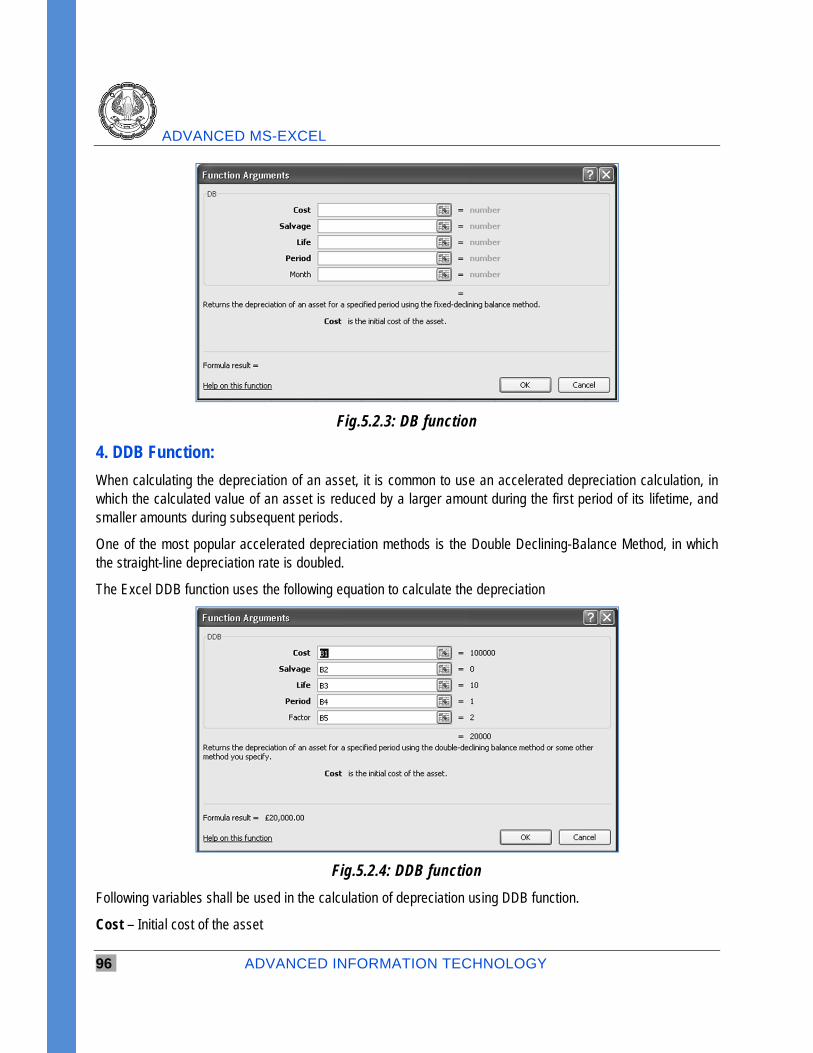
ADVANCED MS-EXCEL
96 ADVANCED INFORMATION TECHNOLOGY
Fig.5.2.3: DB function
4. DDB Function:
When calculating the depreciation of an asset, it is common to use an accelerated depreciation calculation, in which the calculated value of an asset is reduced by a larger amount during the first period of its lifetime, and smaller amounts during subsequent periods.
One of the most popular accelerated depreciation methods is the Double Declining-Balance Method, in which the straight-line depreciation rate is doubled.
The Excel DDB function uses the following equation to calculate the depreciation
Fig.5.2.4: DDB function
Following variables shall be used in the calculation of depreciation using DDB function.
Cost – Initial cost of the asset
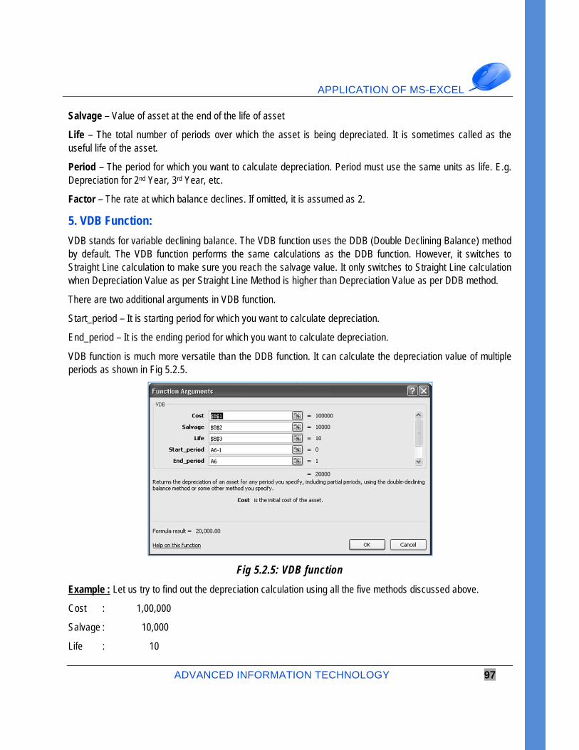
APPLICATION OF MS-EXCEL
ADVANCED INFORMATION TECHNOLOGY 97
Salvage – Value of asset at the end of the life of asset
Life – The total number of periods over which the asset is being depreciated. It is sometimes called as the useful life of the asset.
Period – The period for which you want to calculate depreciation. Period must use the same units as life. E.g. Depreciation for 2nd Year, 3rd Year, etc.
Factor – The rate at which balance declines. If omitted, it is assumed as 2.
5. VDB Function:
VDB stands for variable declining balance. The VDB function uses the DDB (Double Declining Balance) method by default. The VDB function performs the same calculations as the DDB function. However, it switches to Straight Line calculation to make sure you reach the salvage value. It only switches to Straight Line calculation when Depreciation Value as per Straight Line Method is higher than Depreciation Value as per DDB method.
There are two additional arguments in VDB function.
Start_period – It is starting period for which you want to calculate depreciation.
End_period – It is the ending period for which you want to calculate depreciation.
VDB function is much more versatile than the DDB function. It can calculate the depreciation value of multiple periods as shown in Fig 5.2.5.
Fig 5.2.5: VDB function
Example : Let us try to find out the depreciation calculation using all the five methods discussed above.
Cost : 1,00,000
Salvage : 10,000
Life : 10
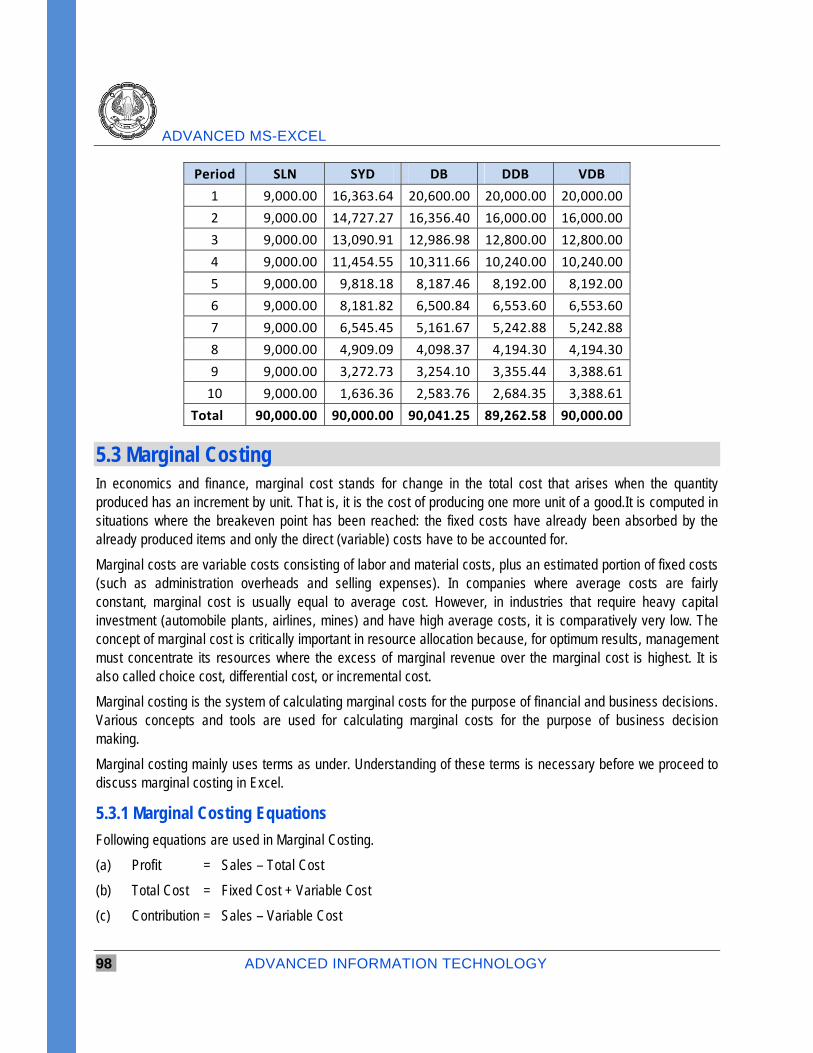
ADVANCED MS-EXCEL
98 ADVANCED INFORMATION TECHNOLOGY
Period SLN SYD DB DDB VDB 1 9,000.00 16,363.64 20,600.00 20,000.00 20,000.00 2 9,000.00 14,727.27 16,356.40 16,000.00 16,000.00 3 9,000.00 13,090.91 12,986.98 12,800.00 12,800.00 4 9,000.00 11,454.55 10,311.66 10,240.00 10,240.00 5 9,000.00 9,818.18 8,187.46 8,192.00 8,192.00 6 9,000.00 8,181.82 6,500.84 6,553.60 6,553.60 7 9,000.00 6,545.45 5,161.67 5,242.88 5,242.88 8 9,000.00 4,909.09 4,098.37 4,194.30 4,194.30 9 9,000.00 3,272.73 3,254.10 3,355.44 3,388.61
10 9,000.00 1,636.36 2,583.76 2,684.35 3,388.61 Total 90,000.00 90,000.00 90,041.25 89,262.58 90,000.00
5.3 Marginal Costing In economics and finance, marginal cost stands for change in the total cost that arises when the quantity produced has an increment by unit. That is, it is the cost of producing one more unit of a good.It is computed in situations where the breakeven point has been reached: the fixed costs have already been absorbed by the already produced items and only the direct (variable) costs have to be accounted for.
Marginal costs are variable costs consisting of labor and material costs, plus an estimated portion of fixed costs (such as administration overheads and selling expenses). In companies where average costs are fairly constant, marginal cost is usually equal to average cost. However, in industries that require heavy capital investment (automobile plants, airlines, mines) and have high average costs, it is comparatively very low. The concept of marginal cost is critically important in resource allocation because, for optimum results, management must concentrate its resources where the excess of marginal revenue over the marginal cost is highest. It is also called choice cost, differential cost, or incremental cost.
Marginal costing is the system of calculating marginal costs for the purpose of financial and business decisions. Various concepts and tools are used for calculating marginal costs for the purpose of business decision making.
Marginal costing mainly uses terms as under. Understanding of these terms is necessary before we proceed to discuss marginal costing in Excel.
5.3.1 Marginal Costing Equations
Following equations are used in Marginal Costing.
(a) Profit = Sales – Total Cost
(b) Total Cost = Fixed Cost + Variable Cost
(c) Contribution = Sales – Variable Cost
APPLICATION OF MS-EXCEL
ADVANCED INFORMATION TECHNOLOGY 99
The whole idea of marginal costing revolves around a simple equation as under.
Fixed Cost + Profit = Sales – Variable Cost
(a) Fixed Costs: As the name suggest, these cost remain fixed irrespective of level of production. Fixed cost need to be incurred even if there is no production. Examples of fixed cost can be Salary of administrative staff, office rent, audit fees, etc.
Fixed Cost = Sales – Variable Cost – Profit
Fixed Cost = (Sales x PV Ratio) – Profit
(b) Variable Costs: As the name suggest, these cost vary according the volume of production. Total variable cost changes after every unit of production. But variable cost per unit remain the same. All direct costs are variable costs. E.g. raw material cost, commission to salesman, etc. are variable cost.
Variable Cost = Sales – Fixed Cost – Profit
Variable Cost = Sales x Variable Cost Ratio
(Variable Cost Ratio = 1 – PV Ratio)
(c) Sales: This is the amount generated from selling of products. Total sales can be obtained by multiplying selling price per unit with number of products sold.
(d) Contribution: It is the difference between sales and variable cost. As the sales and variable cost can be calculated for each unit, it also possible to calculate contribution per unit using the simple formula as under.
Contribution per unit = Selling Price per Unit - Variable Cost per Unit
Or
Contribution per unit = Total Sales Value – Total Variable Cost
No. of units sold
(e) PV Ratio: Profit Volume Ratio expresses mathematical relationship between two variables, i.e. Profit and Volume of sales. It can be calculated by using any formula as stated below.
PV Ratio = (Contribution / Sales) x 100
PV Ratio = [(Sales – Variable Cost) / Sales] x 100
PV Ratio = 1 – Variable Cost Ratio
PV Ratio = (Change in Profit / Change in Sales) x 100
(f) BEP: Break Even Point is the point of no profit or no loss. It may be expressed in terms of sales value or sales unit. It can be calculated as under.
BEP (Value) = Fixed CostPV Ratio
BEP (Units) = Fixed Cost
Contribution per Unit
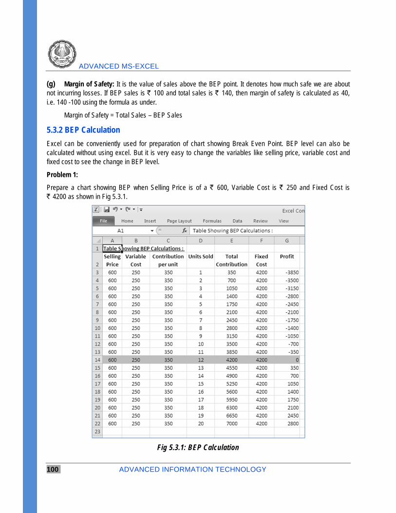
ADVANCED MS-EXCEL
100 ADVANCED INFORMATION TECHNOLOGY
(g) Margin of Safety: It is the value of sales above the BEP point. It denotes how much safe we are about not incurring losses. If BEP sales is ` 100 and total sales is ` 140, then margin of safety is calculated as 40, i.e. 140 -100 using the formula as under.
Margin of Safety = Total Sales – BEP Sales
5.3.2 BEP Calculation
Excel can be conveniently used for preparation of chart showing Break Even Point. BEP level can also be calculated without using excel. But it is very easy to change the variables like selling price, variable cost and fixed cost to see the change in BEP level.
Problem 1:
Prepare a chart showing BEP when Selling Price is of a ` 600, Variable Cost is ` 250 and Fixed Cost is ` 4200 as shown in Fig 5.3.1.
Fig 5.3.1: BEP Calculation
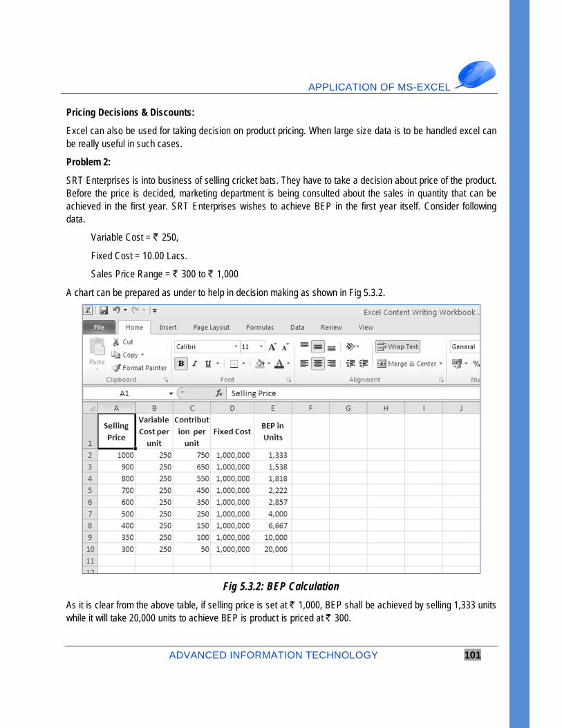
APPLICATION OF MS-EXCEL
ADVANCED INFORMATION TECHNOLOGY 101
Pricing Decisions & Discounts:
Excel can also be used for taking decision on product pricing. When large size data is to be handled excel can be really useful in such cases.
Problem 2:
SRT Enterprises is into business of selling cricket bats. They have to take a decision about price of the product. Before the price is decided, marketing department is being consulted about the sales in quantity that can be achieved in the first year. SRT Enterprises wishes to achieve BEP in the first year itself. Consider following data.
Variable Cost = ` 250,
Fixed Cost = 10.00 Lacs.
Sales Price Range = ` 300 to ` 1,000
A chart can be prepared as under to help in decision making as shown in Fig 5.3.2.
Fig 5.3.2: BEP Calculation
As it is clear from the above table, if selling price is set at ` 1,000, BEP shall be achieved by selling 1,333 units while it will take 20,000 units to achieve BEP is product is priced at ` 300.
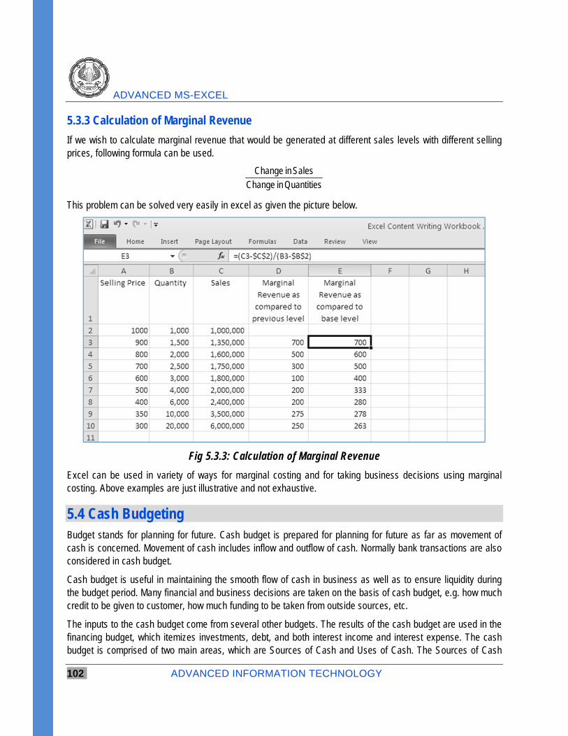
ADVANCED MS-EXCEL
102 ADVANCED INFORMATION TECHNOLOGY
5.3.3 Calculation of Marginal Revenue
If we wish to calculate marginal revenue that would be generated at different sales levels with different selling prices, following formula can be used.
Change in SalesChange in Quantities
This problem can be solved very easily in excel as given the picture below.
Fig 5.3.3: Calculation of Marginal Revenue
Excel can be used in variety of ways for marginal costing and for taking business decisions using marginal costing. Above examples are just illustrative and not exhaustive.
5.4 Cash Budgeting Budget stands for planning for future. Cash budget is prepared for planning for future as far as movement of cash is concerned. Movement of cash includes inflow and outflow of cash. Normally bank transactions are also considered in cash budget.
Cash budget is useful in maintaining the smooth flow of cash in business as well as to ensure liquidity during the budget period. Many financial and business decisions are taken on the basis of cash budget, e.g. how much credit to be given to customer, how much funding to be taken from outside sources, etc.
The inputs to the cash budget come from several other budgets. The results of the cash budget are used in the financing budget, which itemizes investments, debt, and both interest income and interest expense. The cash budget is comprised of two main areas, which are Sources of Cash and Uses of Cash. The Sources of Cash
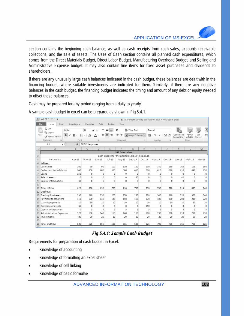
APPLICATION OF MS-EXCEL
ADVANCED INFORMATION TECHNOLOGY 103
section contains the beginning cash balance, as well as cash receipts from cash sales, accounts receivable collections, and the sale of assets. The Uses of Cash section contains all planned cash expenditures, which comes from the Direct Materials Budget, Direct Labor Budget, Manufacturing Overhead Budget, and Selling and Administrative Expense budget. It may also contain line items for fixed asset purchases and dividends to shareholders.
If there are any unusually large cash balances indicated in the cash budget, these balances are dealt with in the financing budget, where suitable investments are indicated for them. Similarly, if there are any negative balances in the cash budget, the financing budget indicates the timing and amount of any debt or equity needed to offset these balances.
Cash may be prepared for any period ranging from a daily to yearly.
A sample cash budget in excel can be prepared as shown in Fig 5.4.1.
Fig 5.4.1: Sample Cash Budget
Requirements for preparation of cash budget in Excel:
Knowledge of accounting
Knowledge of formatting an excel sheet
Knowledge of cell linking
Knowledge of basic formulae
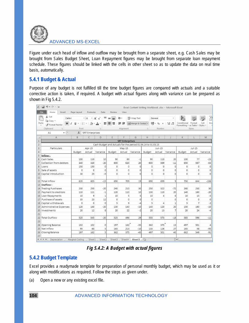
ADVANCED MS-EXCEL
104 ADVANCED INFORMATION TECHNOLOGY
Figure under each head of inflow and outflow may be brought from a separate sheet, e.g. Cash Sales may be brought from Sales Budget Sheet, Loan Repayment figures may be brought from separate loan repayment schedule. These figures should be linked with the cells in other sheet so as to update the data on real time basis, automatically.
5.4.1 Budget & Actual
Purpose of any budget is not fulfilled till the time budget figures are compared with actuals and a suitable corrective action is taken, if required. A budget with actual figures along with variance can be prepared as shown in Fig 5.4.2.
Fig 5.4.2: A Budget with actual figures
5.4.2 Budget Template
Excel provides a readymade template for preparation of personal monthly budget, which may be used as it or along with modifications as required. Follow the steps as given under.
(a) Open a new or any existing excel file.
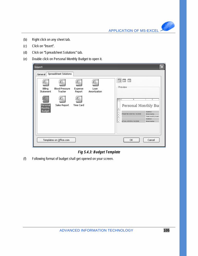
APPLICATION OF MS-EXCEL
ADVANCED INFORMATION TECHNOLOGY 105
(b) Right click on any sheet tab.
(c) Click on “Insert”.
(d) Click on “Spreadsheet Solutions” tab.
(e) Double click on Personal Monthly Budget to open it.
Fig 5.4.3: Budget Template
(f) Following format of budget shall get opened on your screen.
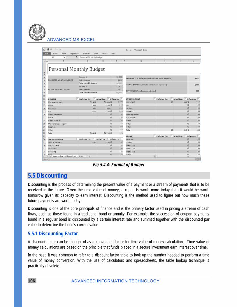
ADVANCED MS-EXCEL
106 ADVANCED INFORMATION TECHNOLOGY
Fig 5.4.4: Format of Budget
5.5 Discounting Discounting is the process of determining the present value of a payment or a stream of payments that is to be received in the future. Given the time value of money, a rupee is worth more today than it would be worth tomorrow given its capacity to earn interest. Discounting is the method used to figure out how much these future payments are worth today.
Discounting is one of the core principals of finance and is the primary factor used in pricing a stream of cash flows, such as those found in a traditional bond or annuity. For example, the succession of coupon payments found in a regular bond is discounted by a certain interest rate and summed together with the discounted par value to determine the bond's current value.
5.5.1 Discounting Factor
A discount factor can be thought of as a conversion factor for time value of money calculations. Time value of money calculations are based on the principle that funds placed in a secure investment earn interest over time.
In the past, it was common to refer to a discount factor table to look up the number needed to perform a time value of money conversion. With the use of calculators and spreadsheets, the table lookup technique is practically obsolete.
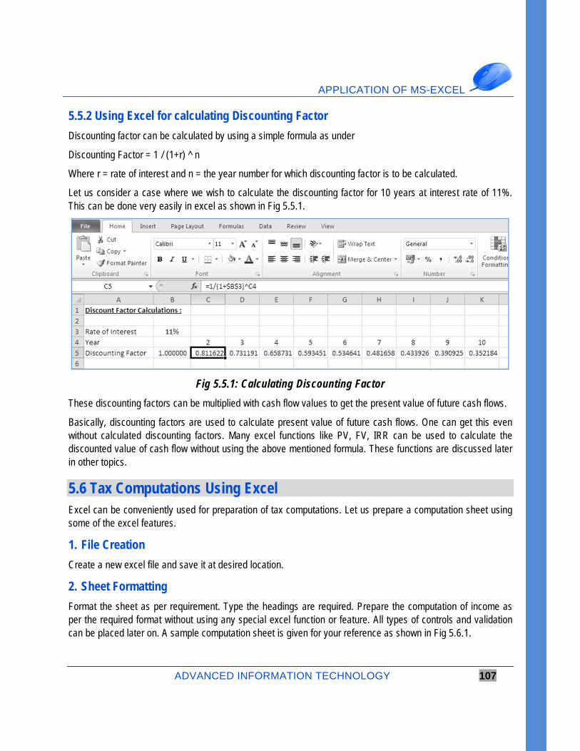
APPLICATION OF MS-EXCEL
ADVANCED INFORMATION TECHNOLOGY 107
5.5.2 Using Excel for calculating Discounting Factor
Discounting factor can be calculated by using a simple formula as under
Discounting Factor = 1 / (1+r) ^ n
Where r = rate of interest and n = the year number for which discounting factor is to be calculated.
Let us consider a case where we wish to calculate the discounting factor for 10 years at interest rate of 11%. This can be done very easily in excel as shown in Fig 5.5.1.
Fig 5.5.1: Calculating Discounting Factor
These discounting factors can be multiplied with cash flow values to get the present value of future cash flows.
Basically, discounting factors are used to calculate present value of future cash flows. One can get this even without calculated discounting factors. Many excel functions like PV, FV, IRR can be used to calculate the discounted value of cash flow without using the above mentioned formula. These functions are discussed later in other topics.
5.6 Tax Computations Using Excel Excel can be conveniently used for preparation of tax computations. Let us prepare a computation sheet using some of the excel features.
1. File Creation
Create a new excel file and save it at desired location.
2. Sheet Formatting
Format the sheet as per requirement. Type the headings are required. Prepare the computation of income as per the required format without using any special excel function or feature. All types of controls and validation can be placed later on. A sample computation sheet is given for your reference as shown in Fig 5.6.1.
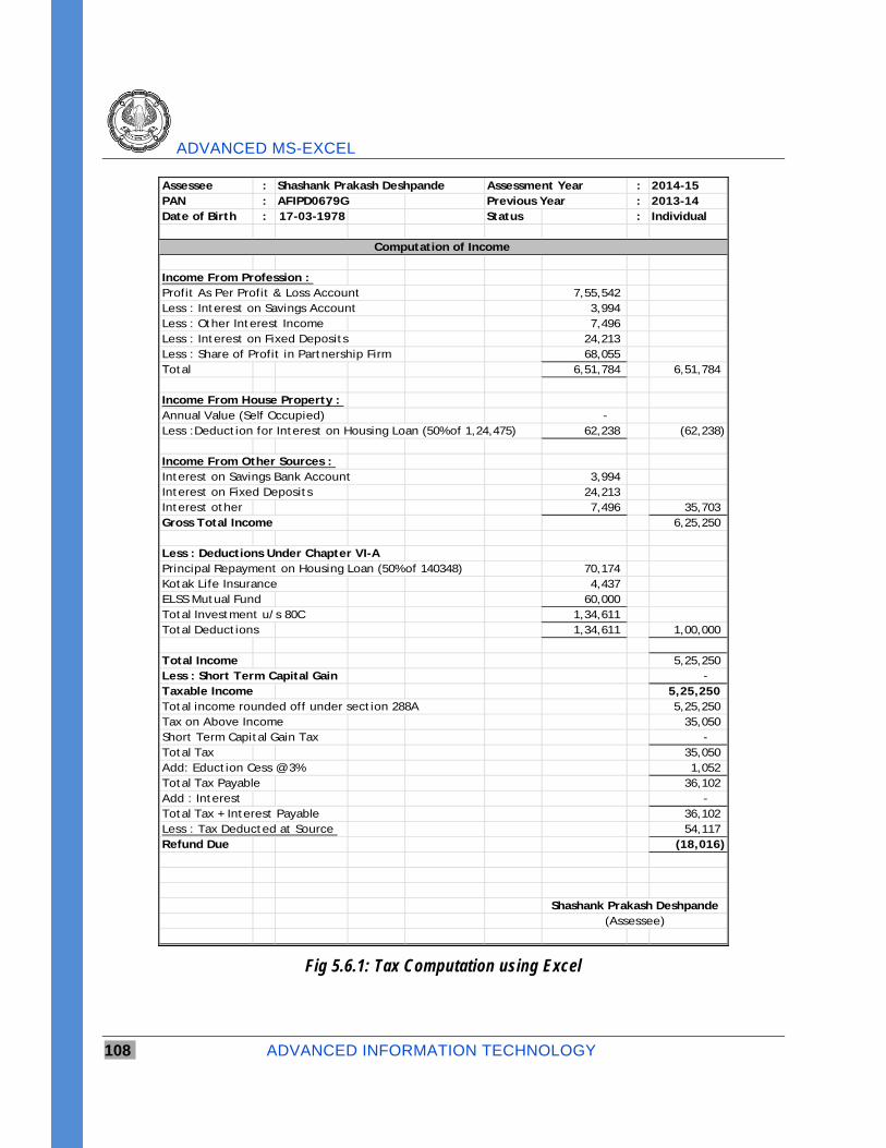
ADVANCED MS-EXCEL
108 ADVANCED INFORMATION TECHNOLOGY
Assessee : Shashank Prakash Deshpande Assessment Year : 2014-15PAN : AFIPD0679G Previous Year : 2013-14Date of Birth : 17-03-1978 Status : Individual
Income From Profession : Profit As Per Profit & Loss Account 7,55,542 Less : Interest on Savings Account 3,994 Less : Other Interest Income 7,496 Less : Interest on Fixed Deposits 24,213 Less : Share of Profit in Partnership Firm 68,055 Total 6,51,784 6,51,784
Income From House Property : Annual Value (Self Occupied) - Less :Deduction for Interest on Housing Loan (50% of 1,24,475) 62,238 (62,238)
Income From Other Sources : Interest on Savings Bank Account 3,994 Interest on Fixed Deposits 24,213 Interest other 7,496 35,703 Gross Total Income 6,25,250
Less : Deductions Under Chapter VI-APrincipal Repayment on Housing Loan (50% of 140348) 70,174 Kotak Life Insurance 4,437 ELSS Mutual Fund 60,000 Total Investment u/s 80C 1,34,611 Total Deductions 1,34,611 1,00,000
Total Income 5,25,250 Less : Short Term Capital Gain - Taxable Income 5,25,250 Total income rounded off under section 288A 5,25,250 Tax on Above Income 35,050 Short Term Capital Gain Tax - Total Tax 35,050 Add: Eduction Cess @ 3% 1,052 Total Tax Payable 36,102 Add : Interest - Total Tax + Interest Payable 36,102 Less : Tax Deducted at Source 54,117 Refund Due (18,016)
Computation of Income
Shashank Prakash Deshpande(Assessee)
Fig 5.6.1: Tax Computation using Excel
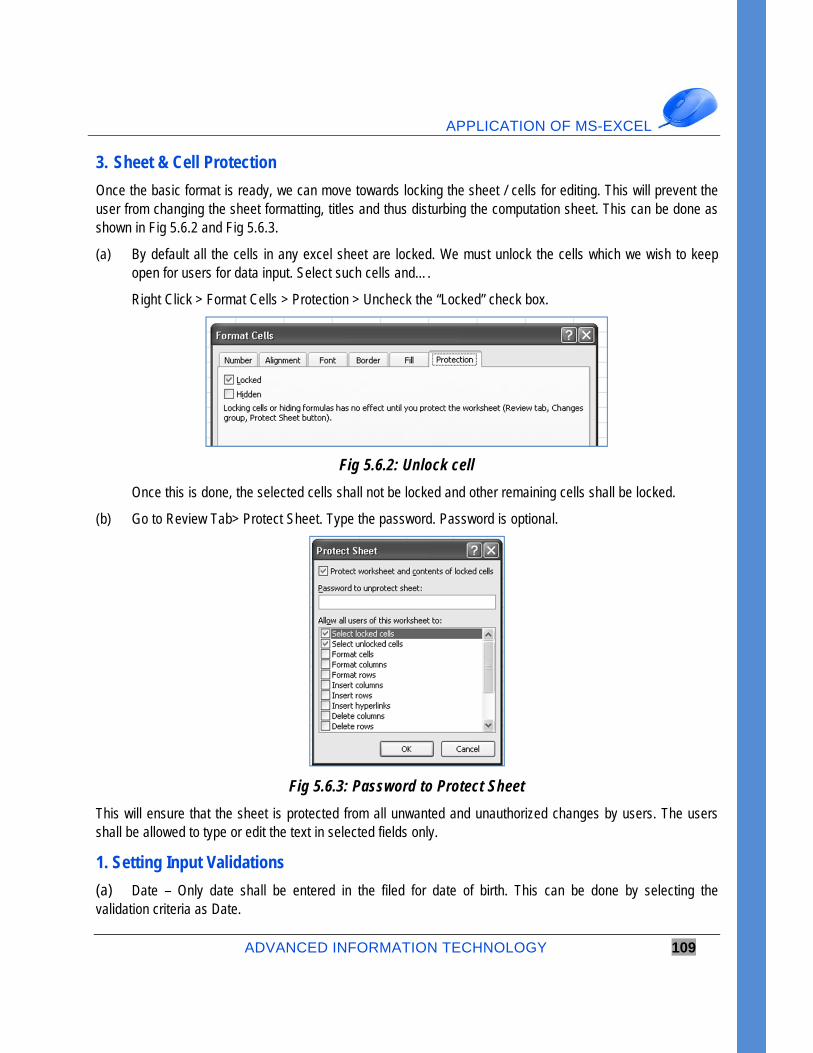
APPLICATION OF MS-EXCEL
ADVANCED INFORMATION TECHNOLOGY 109
3. Sheet & Cell Protection
Once the basic format is ready, we can move towards locking the sheet / cells for editing. This will prevent the user from changing the sheet formatting, titles and thus disturbing the computation sheet. This can be done as shown in Fig 5.6.2 and Fig 5.6.3.
(a) By default all the cells in any excel sheet are locked. We must unlock the cells which we wish to keep open for users for data input. Select such cells and….
Right Click > Format Cells > Protection > Uncheck the “Locked” check box.
Fig 5.6.2: Unlock cell
Once this is done, the selected cells shall not be locked and other remaining cells shall be locked.
(b) Go to Review Tab> Protect Sheet. Type the password. Password is optional.
Fig 5.6.3: Password to Protect Sheet
This will ensure that the sheet is protected from all unwanted and unauthorized changes by users. The users shall be allowed to type or edit the text in selected fields only.
1. Setting Input Validations
(a) Date – Only date shall be entered in the filed for date of birth. This can be done by selecting the validation criteria as Date.
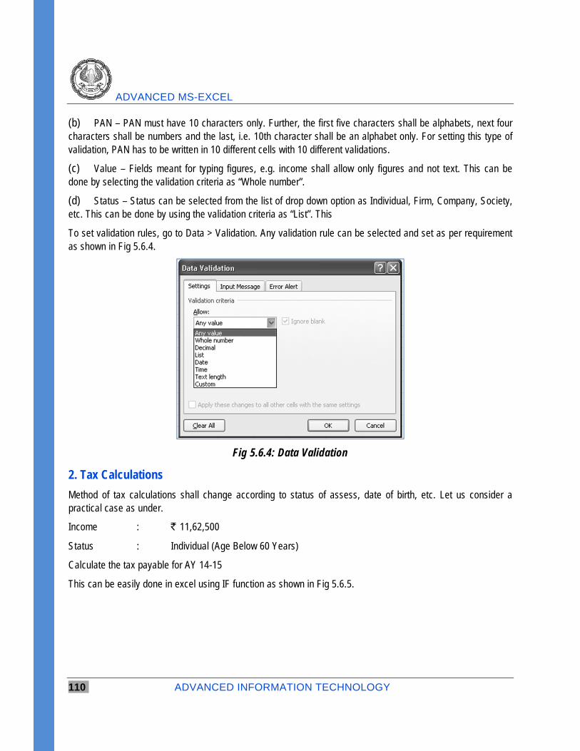
ADVANCED MS-EXCEL
110 ADVANCED INFORMATION TECHNOLOGY
(b) PAN – PAN must have 10 characters only. Further, the first five characters shall be alphabets, next four characters shall be numbers and the last, i.e. 10th character shall be an alphabet only. For setting this type of validation, PAN has to be written in 10 different cells with 10 different validations.
(c) Value – Fields meant for typing figures, e.g. income shall allow only figures and not text. This can be done by selecting the validation criteria as “Whole number”.
(d) Status – Status can be selected from the list of drop down option as Individual, Firm, Company, Society, etc. This can be done by using the validation criteria as “List”. This
To set validation rules, go to Data > Validation. Any validation rule can be selected and set as per requirement as shown in Fig 5.6.4.
Fig 5.6.4: Data Validation
2. Tax Calculations
Method of tax calculations shall change according to status of assess, date of birth, etc. Let us consider a practical case as under.
Income : ` 11,62,500
Status : Individual (Age Below 60 Years)
Calculate the tax payable for AY 14-15
This can be easily done in excel using IF function as shown in Fig 5.6.5.
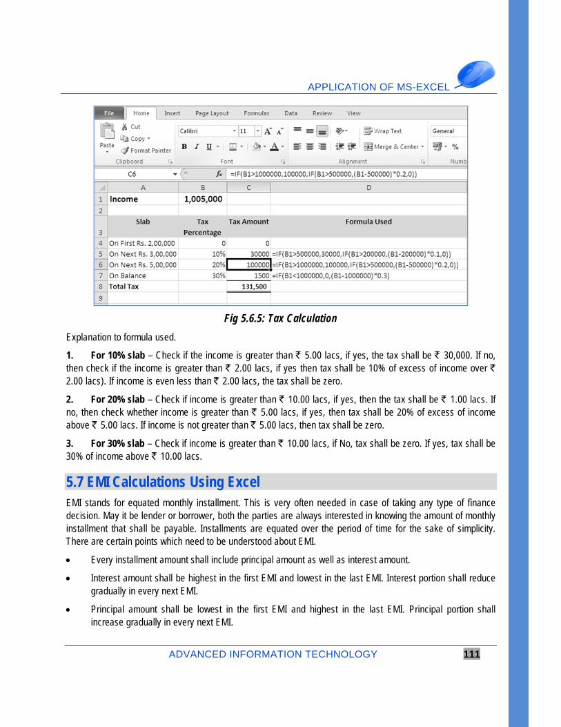
APPLICATION OF MS-EXCEL
ADVANCED INFORMATION TECHNOLOGY 111
Fig 5.6.5: Tax Calculation
Explanation to formula used.
1. For 10% slab – Check if the income is greater than ` 5.00 lacs, if yes, the tax shall be ` 30,000. If no, then check if the income is greater than ` 2.00 lacs, if yes then tax shall be 10% of excess of income over ` 2.00 lacs). If income is even less than ` 2.00 lacs, the tax shall be zero.
2. For 20% slab – Check if income is greater than ` 10.00 lacs, if yes, then the tax shall be ` 1.00 lacs. If no, then check whether income is greater than ` 5.00 lacs, if yes, then tax shall be 20% of excess of income above ` 5.00 lacs. If income is not greater than ` 5.00 lacs, then tax shall be zero.
3. For 30% slab – Check if income is greater than ` 10.00 lacs, if No, tax shall be zero. If yes, tax shall be 30% of income above ` 10.00 lacs.
5.7 EMI Calculations Using Excel EMI stands for equated monthly installment. This is very often needed in case of taking any type of finance decision. May it be lender or borrower, both the parties are always interested in knowing the amount of monthly installment that shall be payable. Installments are equated over the period of time for the sake of simplicity. There are certain points which need to be understood about EMI.
Every installment amount shall include principal amount as well as interest amount.
Interest amount shall be highest in the first EMI and lowest in the last EMI. Interest portion shall reduce gradually in every next EMI.
Principal amount shall be lowest in the first EMI and highest in the last EMI. Principal portion shall increase gradually in every next EMI.
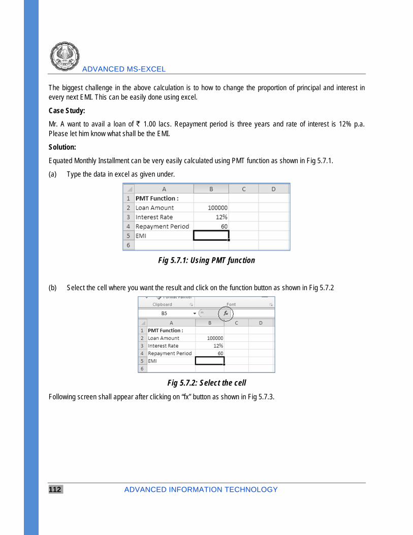
ADVANCED MS-EXCEL
112 ADVANCED INFORMATION TECHNOLOGY
The biggest challenge in the above calculation is to how to change the proportion of principal and interest in every next EMI. This can be easily done using excel.
Case Study:
Mr. A want to avail a loan of ` 1.00 lacs. Repayment period is three years and rate of interest is 12% p.a. Please let him know what shall be the EMI.
Solution:
Equated Monthly Installment can be very easily calculated using PMT function as shown in Fig 5.7.1.
(a) Type the data in excel as given under.
Fig 5.7.1: Using PMT function
(b) Select the cell where you want the result and click on the function button as shown in Fig 5.7.2
Fig 5.7.2: Select the cell
Following screen shall appear after clicking on “fx” button as shown in Fig 5.7.3.
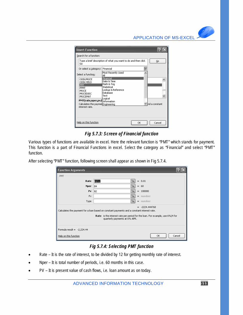
APPLICATION OF MS-EXCEL
ADVANCED INFORMATION TECHNOLOGY 113
Fig 5.7.3: Screen of Financial function
Various types of functions are available in excel. Here the relevant function is “PMT” which stands for payment. This function is a part of Financial Functions in excel. Select the category as “Financial” and select “PMT” function.
After selecting “PMT” function, following screen shall appear as shown in Fig 5.7.4.
Fig 5.7.4: Selecting PMT function
Rate – It is the rate of interest, to be divided by 12 for getting monthly rate of interest.
Nper – It is total number of periods, i.e. 60 months in this case.
PV – It is present value of cash flows, i.e. loan amount as on today.

ADVANCED MS-EXCEL
114 ADVANCED INFORMATION TECHNOLOGY
All the above values can be typed or liked with cells in excel sheet for real time updation. As soon as all the values are entered / linked correctly, formula result is displayed at the bottom as ` 2,224.44. It is displayed as a negative figure just because excel considers all outflows are considered as negative figure. After clicking on OK button, the result shall be generated in the desired cell as shown in Fig 5.7.5.
Fig 5.7.5: Result of PMT function
PPMT Function
This function is used to calculate the principal portion in every installment. This function requires one additional input, i.e. the installment number. The principal amount shall increase after every installment. Hence, principal amount shall be different in every EMI.
Continuing with the above example, the following figure shows calculation of principal and interest component in each EMI. Installment number is denoted by “Per” in excel.
For the calculation of interest component in each EMI, excel has IPMT function. Both the functions are used in the following figure.

APPLICATION OF MS-EXCEL
ADVANCED INFORMATION TECHNOLOGY 115
Fig 5.7.6: PPMT function
Loan Amortization Sheet
Excel provides a readymade solution for the EMI calculation. This can be simply done by following steps as shown in Fig 5.6.7.
(a) Open any excel file
(b) Right click on sheet tab.
(c) Select “Insert” option.
(d) Go to “Spreadsheet Solutions” tab
(e) Select “Loan Amortization” and click OK button.
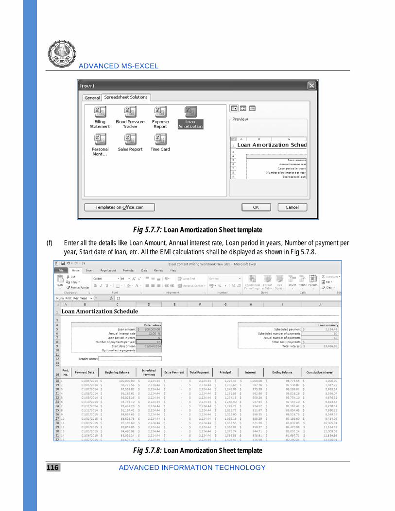
ADVANCED MS-EXCEL
116 ADVANCED INFORMATION TECHNOLOGY
Fig 5.7.7: Loan Amortization Sheet template
(f) Enter all the details like Loan Amount, Annual interest rate, Loan period in years, Number of payment per year, Start date of loan, etc. All the EMI calculations shall be displayed as shown in Fig 5.7.8.
Fig 5.7.8: Loan Amortization Sheet template
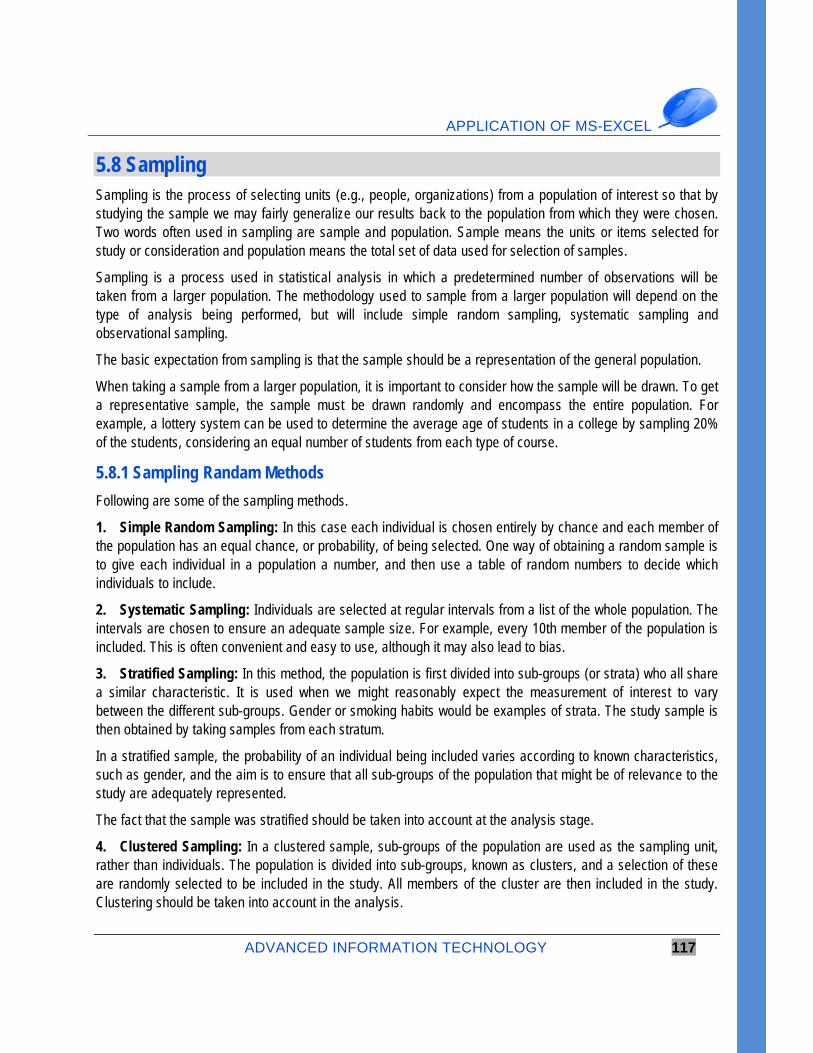
APPLICATION OF MS-EXCEL
ADVANCED INFORMATION TECHNOLOGY 117
5.8 Sampling Sampling is the process of selecting units (e.g., people, organizations) from a population of interest so that by studying the sample we may fairly generalize our results back to the population from which they were chosen. Two words often used in sampling are sample and population. Sample means the units or items selected for study or consideration and population means the total set of data used for selection of samples.
Sampling is a process used in statistical analysis in which a predetermined number of observations will be taken from a larger population. The methodology used to sample from a larger population will depend on the type of analysis being performed, but will include simple random sampling, systematic sampling and observational sampling.
The basic expectation from sampling is that the sample should be a representation of the general population.
When taking a sample from a larger population, it is important to consider how the sample will be drawn. To get a representative sample, the sample must be drawn randomly and encompass the entire population. For example, a lottery system can be used to determine the average age of students in a college by sampling 20% of the students, considering an equal number of students from each type of course.
5.8.1 Sampling Randam Methods
Following are some of the sampling methods.
1. Simple Random Sampling: In this case each individual is chosen entirely by chance and each member of the population has an equal chance, or probability, of being selected. One way of obtaining a random sample is to give each individual in a population a number, and then use a table of random numbers to decide which individuals to include.
2. Systematic Sampling: Individuals are selected at regular intervals from a list of the whole population. The intervals are chosen to ensure an adequate sample size. For example, every 10th member of the population is included. This is often convenient and easy to use, although it may also lead to bias.
3. Stratified Sampling: In this method, the population is first divided into sub-groups (or strata) who all share a similar characteristic. It is used when we might reasonably expect the measurement of interest to vary between the different sub-groups. Gender or smoking habits would be examples of strata. The study sample is then obtained by taking samples from each stratum.
In a stratified sample, the probability of an individual being included varies according to known characteristics, such as gender, and the aim is to ensure that all sub-groups of the population that might be of relevance to the study are adequately represented.
The fact that the sample was stratified should be taken into account at the analysis stage.
4. Clustered Sampling: In a clustered sample, sub-groups of the population are used as the sampling unit, rather than individuals. The population is divided into sub-groups, known as clusters, and a selection of these are randomly selected to be included in the study. All members of the cluster are then included in the study. Clustering should be taken into account in the analysis.
ADVANCED MS-EXCEL
118 ADVANCED INFORMATION TECHNOLOGY
The General Household survey, which is undertaken annually in England, is a good example of a cluster sample. All members of the selected households/ clusters are included in the survey.
5. Quota Sampling: This method of sampling is often used by market researchers. Interviewers are given a quota of subjects of a specified type to attempt to recruit. For example, an interviewer might be told to go out and select 20 adult men and 20 adult women, 10 teenage girls and 10 teenage boys so that they could interview them about their television viewing. There are several flaws with this method, but most importantly it is not truly random.
6. Convenience Sampling: Convenience sampling is perhaps the easiest method of sampling, because participants are selected in the most convenient way, and are often allowed to chose or volunteer to take part. Good results can be obtained, but the data set may be seriously biased, because those who volunteer to take part may be different from those who choose not to.
7. Snowball Sampling: This method is commonly used in social sciences when investigating hard to reach groups. Existing subjects are asked to nominate further subjects known to them, so the sample increases in size like a rolling snowball. For example, when carrying out a survey of risk behavior amongst intravenous drug users, participants may be asked to nominate other users to be interviewed.
5.8.2 Simple Random Sampling in Excel
Consider a small case of analysis of customer feedback about a product. Let us assume that we have a population of 1000 customer feedback forms. We need to analyze the feedback pattern of 5% customer, .i.e. 50 customers.
This can be done easily by following steps as under shown in Fig 5.8.1.
(a) Write Column heading in Cell A1 as Customer IDs and write customer codes / IDs in Cell A2, A3,A4, and so on.
(b) Go the cell B1 and write the column heading as Random Numbers.
(c) Go to cell B2 and type “Rand()” and press ENTER. This is a function for generating random numbers in any particular cell. After pressing ENTER, a random number shall be generated in cell B2.
(d) Copy Cell B2 and paste it in the Cells B3, B4, B5, etc. Now in-front of every customer ID, there is a random number.
(e) Sort both columns according to random numbers

APPLICATION OF MS-EXCEL
ADVANCED INFORMATION TECHNOLOGY 119
Fig 5.8.1: Simple Random Sampling
(f) Select the first 50 customers. Now these 50 customers are the randomly selected customers and represent the complete data.
5.8.3 Using Sampling Feature
Excel has got a built in feature for sampling of data. This can be used as under.
(a) Type the data regarding roll number of students in Cell A2, A3, A4, and so on.
(b) To get a sample of five students, go to Data > Data Analysis
Fig 5.8.2: Sampling Feature
(c) Select “Sampling” from the list and click OK.
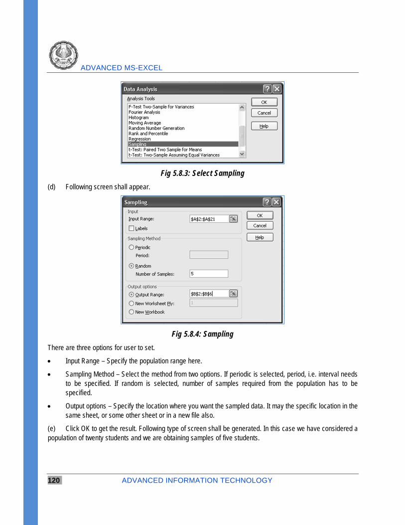
ADVANCED MS-EXCEL
120 ADVANCED INFORMATION TECHNOLOGY
Fig 5.8.3: Select Sampling
(d) Following screen shall appear.
Fig 5.8.4: Sampling
There are three options for user to set.
Input Range – Specify the population range here.
Sampling Method – Select the method from two options. If periodic is selected, period, i.e. interval needs to be specified. If random is selected, number of samples required from the population has to be specified.
Output options – Specify the location where you want the sampled data. It may the specific location in the same sheet, or some other sheet or in a new file also.
(e) Click OK to get the result. Following type of screen shall be generated. In this case we have considered a population of twenty students and we are obtaining samples of five students.
APPLICATION OF MS-EXCEL
ADVANCED INFORMATION TECHNOLOGY 121
Fig 5.8.5: Obtained Sampling
5.9 Summary Summary reports are useful for quick reading and easy understanding, particularly for top management. When excel is used for preparation of reports in similar formats, it can be used for consolidation of reports into a master report or a summary report. Additional operations like average, count, sum can be done while preparing summary reports.
To summarize and report results from data on separate worksheets, you can consolidate the data from each separate worksheet into one worksheet (or master worksheet). The worksheets you consolidate can be in the same workbook as the master worksheet or in other workbooks. When you consolidate data in one worksheet, you can more easily update and aggregate it on a regular or ad hoc basis.
For example, if you have a worksheet of expense figures for each of your regional offices, you might use data consolidation to roll up these figures into a corporate expense worksheet. This master worksheet might contain sales totals and averages, current inventory levels, and highest selling products for the entire enterprise.
Example:
Let us consider a case where the data about debtors for two months is stored in two different sheets. We wish to consolidate the data in third sheet.
Solution:
Let us assume that names of debtors are stored in Cell A2, A3, A4, and so on and monthly purchases by them are recorded in Cells B2, B3, B4, and so on. Data for the month of April is stored in Sheet1 and data for May is stored in Sheet2. Let us consolidate the data in Sheet3.
(a) Create a new sheet and rename it as Summary.
(b) Go to Data > Consolidate (Under Data Tools Group)
(c) Following type of screen shall appear as shown in Fig 5.9.1.
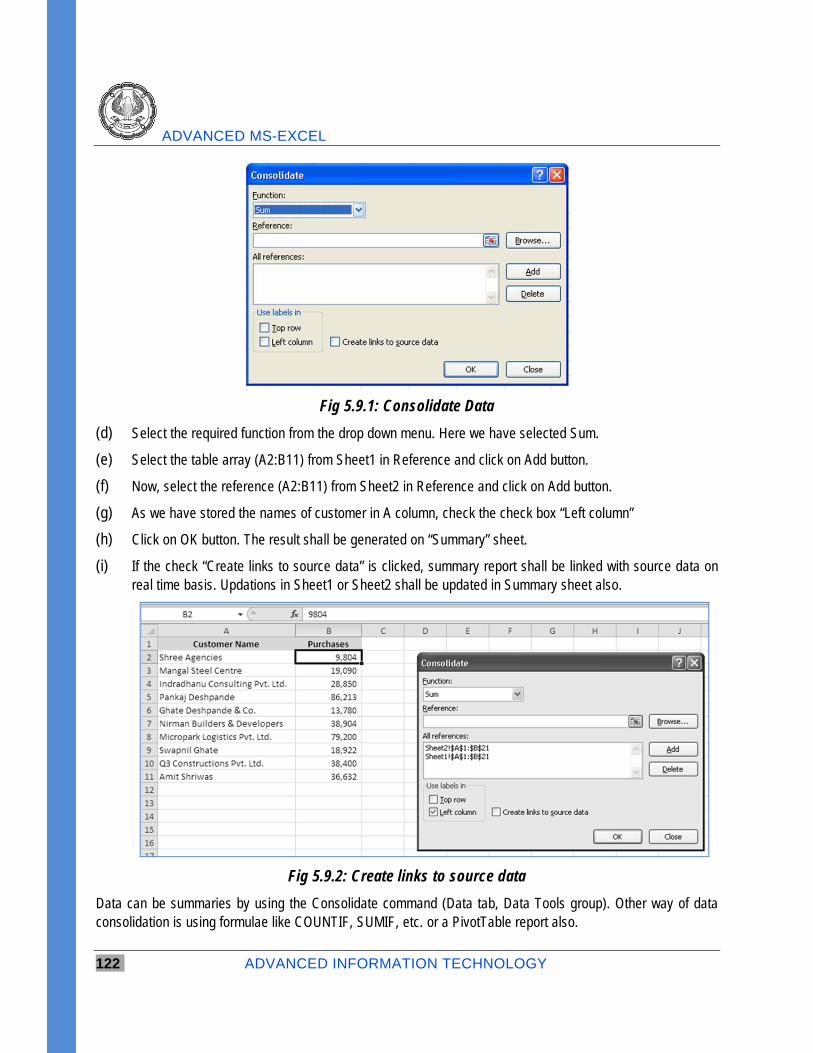
ADVANCED MS-EXCEL
122 ADVANCED INFORMATION TECHNOLOGY
Fig 5.9.1: Consolidate Data
(d) Select the required function from the drop down menu. Here we have selected Sum.
(e) Select the table array (A2:B11) from Sheet1 in Reference and click on Add button.
(f) Now, select the reference (A2:B11) from Sheet2 in Reference and click on Add button.
(g) As we have stored the names of customer in A column, check the check box “Left column”
(h) Click on OK button. The result shall be generated on “Summary” sheet.
(i) If the check “Create links to source data” is clicked, summary report shall be linked with source data on real time basis. Updations in Sheet1 or Sheet2 shall be updated in Summary sheet also.
Fig 5.9.2: Create links to source data
Data can be summaries by using the Consolidate command (Data tab, Data Tools group). Other way of data consolidation is using formulae like COUNTIF, SUMIF, etc. or a PivotTable report also.
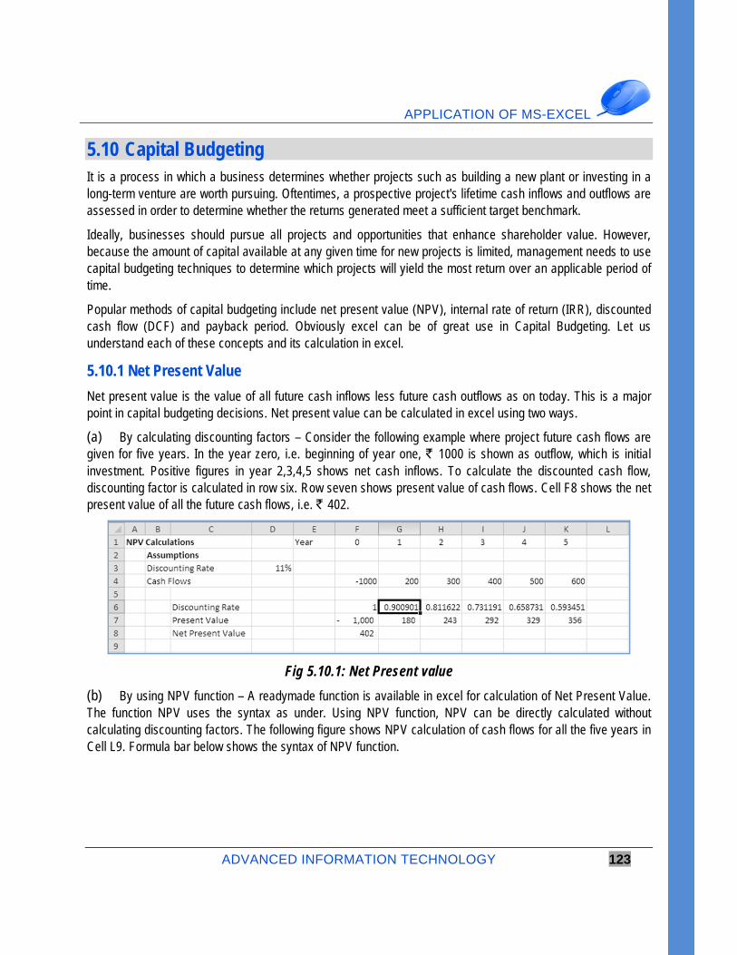
APPLICATION OF MS-EXCEL
ADVANCED INFORMATION TECHNOLOGY 123
5.10 Capital Budgeting It is a process in which a business determines whether projects such as building a new plant or investing in a long-term venture are worth pursuing. Oftentimes, a prospective project's lifetime cash inflows and outflows are assessed in order to determine whether the returns generated meet a sufficient target benchmark.
Ideally, businesses should pursue all projects and opportunities that enhance shareholder value. However, because the amount of capital available at any given time for new projects is limited, management needs to use capital budgeting techniques to determine which projects will yield the most return over an applicable period of time.
Popular methods of capital budgeting include net present value (NPV), internal rate of return (IRR), discounted cash flow (DCF) and payback period. Obviously excel can be of great use in Capital Budgeting. Let us understand each of these concepts and its calculation in excel.
5.10.1 Net Present Value
Net present value is the value of all future cash inflows less future cash outflows as on today. This is a major point in capital budgeting decisions. Net present value can be calculated in excel using two ways.
(a) By calculating discounting factors – Consider the following example where project future cash flows are given for five years. In the year zero, i.e. beginning of year one, ` 1000 is shown as outflow, which is initial investment. Positive figures in year 2,3,4,5 shows net cash inflows. To calculate the discounted cash flow, discounting factor is calculated in row six. Row seven shows present value of cash flows. Cell F8 shows the net present value of all the future cash flows, i.e. ` 402.
Fig 5.10.1: Net Present value
(b) By using NPV function – A readymade function is available in excel for calculation of Net Present Value. The function NPV uses the syntax as under. Using NPV function, NPV can be directly calculated without calculating discounting factors. The following figure shows NPV calculation of cash flows for all the five years in Cell L9. Formula bar below shows the syntax of NPV function.
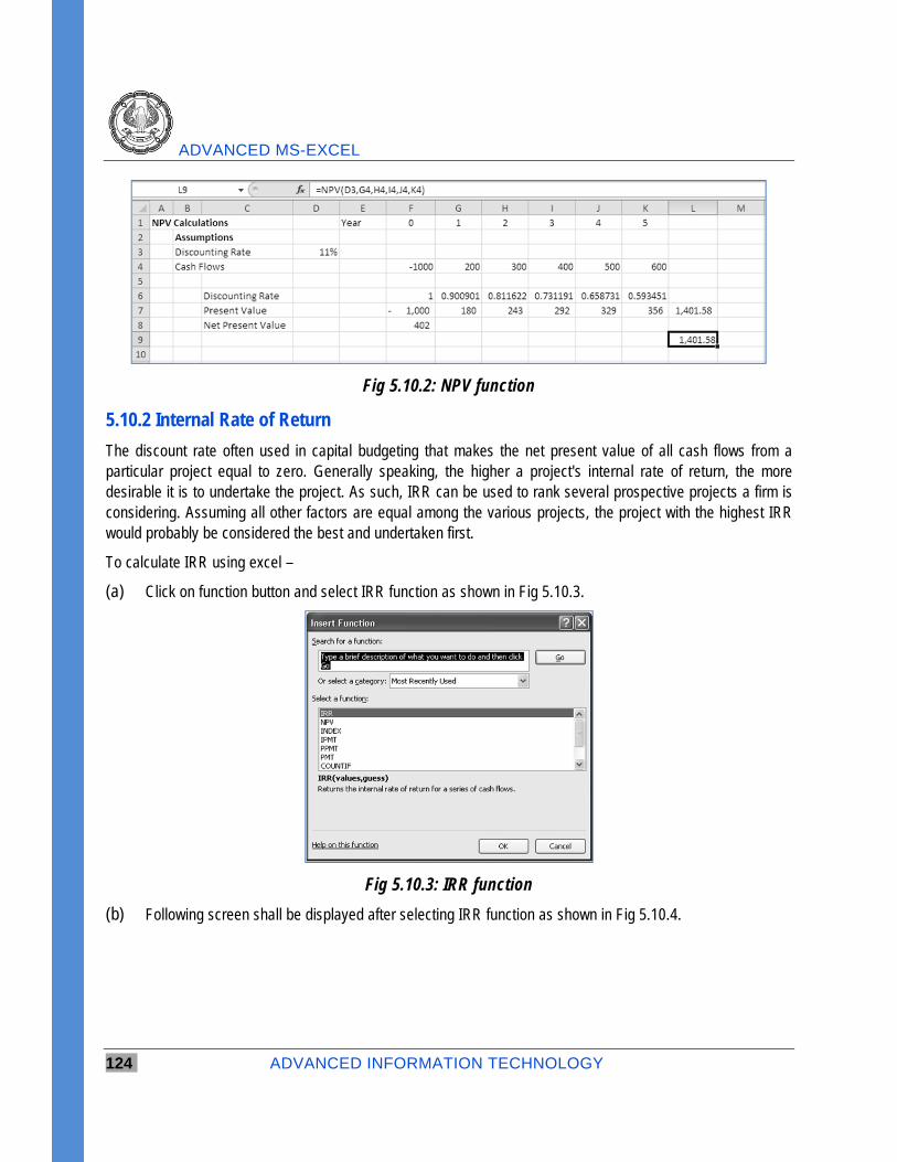
ADVANCED MS-EXCEL
124 ADVANCED INFORMATION TECHNOLOGY
Fig 5.10.2: NPV function
5.10.2 Internal Rate of Return
The discount rate often used in capital budgeting that makes the net present value of all cash flows from a particular project equal to zero. Generally speaking, the higher a project's internal rate of return, the more desirable it is to undertake the project. As such, IRR can be used to rank several prospective projects a firm is considering. Assuming all other factors are equal among the various projects, the project with the highest IRR would probably be considered the best and undertaken first.
To calculate IRR using excel –
(a) Click on function button and select IRR function as shown in Fig 5.10.3.
Fig 5.10.3: IRR function
(b) Following screen shall be displayed after selecting IRR function as shown in Fig 5.10.4.
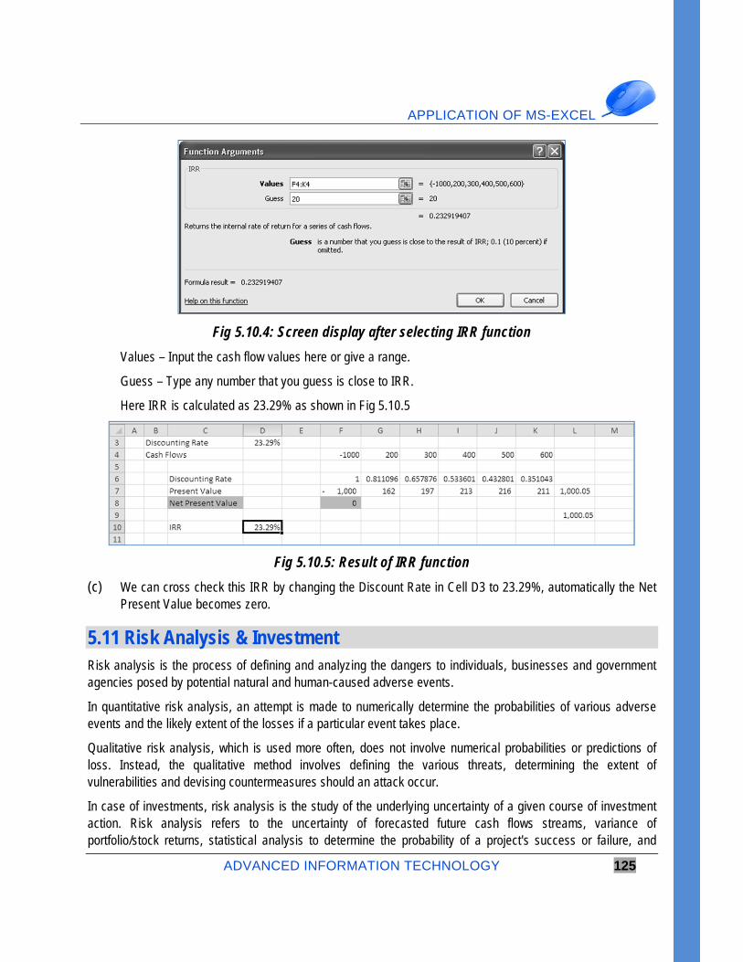
APPLICATION OF MS-EXCEL
ADVANCED INFORMATION TECHNOLOGY 125
Fig 5.10.4: Screen display after selecting IRR function
Values – Input the cash flow values here or give a range.
Guess – Type any number that you guess is close to IRR.
Here IRR is calculated as 23.29% as shown in Fig 5.10.5
Fig 5.10.5: Result of IRR function
(c) We can cross check this IRR by changing the Discount Rate in Cell D3 to 23.29%, automatically the Net Present Value becomes zero.
5.11 Risk Analysis & Investment Risk analysis is the process of defining and analyzing the dangers to individuals, businesses and government agencies posed by potential natural and human-caused adverse events.
In quantitative risk analysis, an attempt is made to numerically determine the probabilities of various adverse events and the likely extent of the losses if a particular event takes place.
Qualitative risk analysis, which is used more often, does not involve numerical probabilities or predictions of loss. Instead, the qualitative method involves defining the various threats, determining the extent of vulnerabilities and devising countermeasures should an attack occur.
In case of investments, risk analysis is the study of the underlying uncertainty of a given course of investment action. Risk analysis refers to the uncertainty of forecasted future cash flows streams, variance of portfolio/stock returns, statistical analysis to determine the probability of a project's success or failure, and

ADVANCED MS-EXCEL
126 ADVANCED INFORMATION TECHNOLOGY
possible future economic states. Risk analysts often work in tandem with forecasting professionals to minimize future negative unforeseen effects.
Almost all sorts of businesses require a minimum sort of risk analysis. For example, commercial banks need to properly hedge foreign exchange exposure of oversees loans while large department stores must factor in the possibility of reduced revenues due to a global recession. Risk analysis allows professionals to identify and mitigate risks, but not avoid them completely. Proper risk analysis often includes mathematical and statistical software programs.
5.11.1 Risk Analysis & Excel
Excel being spreadsheet software can be very effectively used for analysis of any type of data and risk analysis cannot be an exception. There can variety of ways of using excel for risk analysis.
5.11.2 Risk Analysis Using Charts
Charts are generally used to present information in a simple and better way. Charts can also be used to analyse the risk in a better way. Following figure shows how project, probability and its consequence can be explain in a simple and user friendly way using a chart as shown in Fig 5.11.1.
Fig 5.11.1: Risk Analysis using Charts
5.11.3 Probability
Probability is a measure of the likeliness that an event will occur.
Probability is used to quantify an attitude of mind towards some proposition of whose truth we are not certain. The proposition of interest is usually of the form "Will a specific event occur?" The attitude of mind is of the form "How certain are we that the event will occur?" The certainty we adopt can be described in terms of a numerical measure and this number, between 0 and 1 (where 0 indicates impossibility and 1 indicates certainty), we call probability. Thus,higher the probability of an event, the more certain we are that the event will occur. A simple example would be the toss of a fair coin. Since the 2 outcomes are deemed equi-probable, the probability of
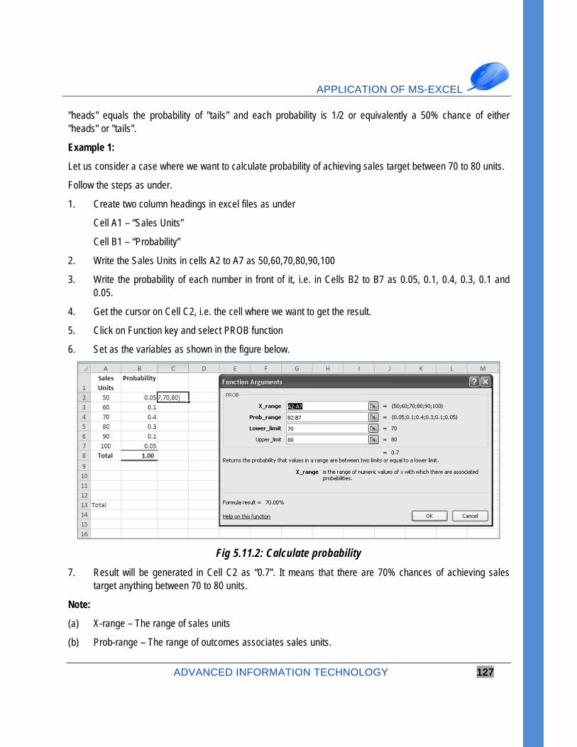
APPLICATION OF MS-EXCEL
ADVANCED INFORMATION TECHNOLOGY 127
"heads" equals the probability of "tails" and each probability is 1/2 or equivalently a 50% chance of either "heads" or "tails".
Example 1:
Let us consider a case where we want to calculate probability of achieving sales target between 70 to 80 units.
Follow the steps as under.
1. Create two column headings in excel files as under
Cell A1 – “Sales Units”
Cell B1 – “Probability”
2. Write the Sales Units in cells A2 to A7 as 50,60,70,80,90,100
3. Write the probability of each number in front of it, i.e. in Cells B2 to B7 as 0.05, 0.1, 0.4, 0.3, 0.1 and 0.05.
4. Get the cursor on Cell C2, i.e. the cell where we want to get the result.
5. Click on Function key and select PROB function
6. Set as the variables as shown in the figure below.
Fig 5.11.2: Calculate probability
7. Result will be generated in Cell C2 as “0.7”. It means that there are 70% chances of achieving sales target anything between 70 to 80 units.
Note:
(a) X-range – The range of sales units
(b) Prob-range – The range of outcomes associates sales units.
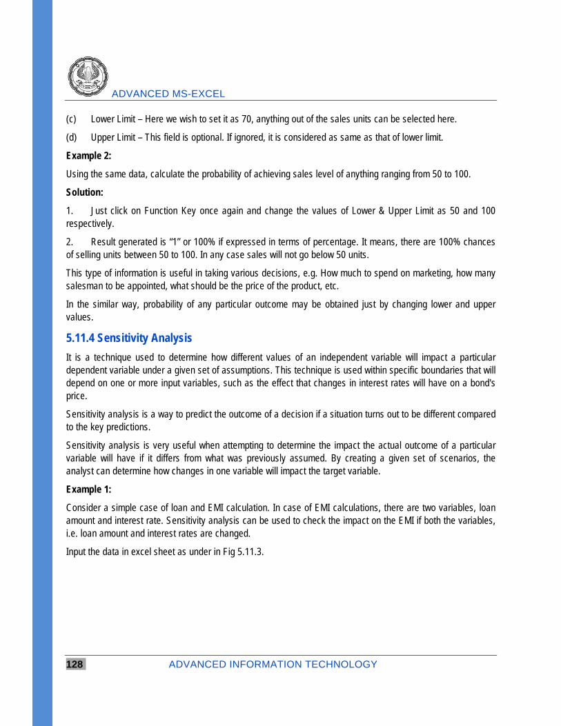
ADVANCED MS-EXCEL
128 ADVANCED INFORMATION TECHNOLOGY
(c) Lower Limit – Here we wish to set it as 70, anything out of the sales units can be selected here.
(d) Upper Limit – This field is optional. If ignored, it is considered as same as that of lower limit.
Example 2:
Using the same data, calculate the probability of achieving sales level of anything ranging from 50 to 100.
Solution:
1. Just click on Function Key once again and change the values of Lower & Upper Limit as 50 and 100 respectively.
2. Result generated is “1” or 100% if expressed in terms of percentage. It means, there are 100% chances of selling units between 50 to 100. In any case sales will not go below 50 units.
This type of information is useful in taking various decisions, e.g. How much to spend on marketing, how many salesman to be appointed, what should be the price of the product, etc.
In the similar way, probability of any particular outcome may be obtained just by changing lower and upper values.
5.11.4 Sensitivity Analysis
It is a technique used to determine how different values of an independent variable will impact a particular dependent variable under a given set of assumptions. This technique is used within specific boundaries that will depend on one or more input variables, such as the effect that changes in interest rates will have on a bond's price.
Sensitivity analysis is a way to predict the outcome of a decision if a situation turns out to be different compared to the key predictions.
Sensitivity analysis is very useful when attempting to determine the impact the actual outcome of a particular variable will have if it differs from what was previously assumed. By creating a given set of scenarios, the analyst can determine how changes in one variable will impact the target variable.
Example 1:
Consider a simple case of loan and EMI calculation. In case of EMI calculations, there are two variables, loan amount and interest rate. Sensitivity analysis can be used to check the impact on the EMI if both the variables, i.e. loan amount and interest rates are changed.
Input the data in excel sheet as under in Fig 5.11.3.
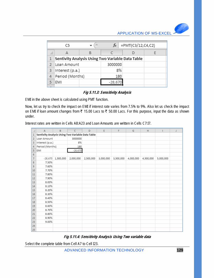
APPLICATION OF MS-EXCEL
ADVANCED INFORMATION TECHNOLOGY 129
Fig 5.11.3: Sensitivity Analysis
EMI in the above sheet is calculated using PMT function.
Now, let us try to check the impact on EMI if interest rate varies from 7.5% to 9%. Also let us check the impact on EMI if loan amount changes from ` 15.00 Lacs to ` 50.00 Lacs. For this purpose, input the data as shown under.
Interest rates are written in Cells A8:A23 and Loan Amounts are written in Cells C7:I7.
Fig 5.11.4: Sensitivity Analysis Using Two variable data
Select the complete table from Cell A7 to Cell I23.
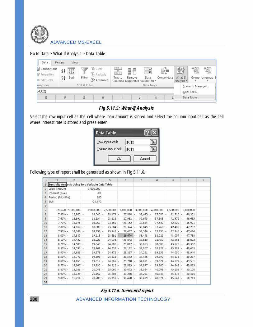
ADVANCED MS-EXCEL
130 ADVANCED INFORMATION TECHNOLOGY
Go to Data > What-If Analysis > Data Table
Fig 5.11.5: What-If Analysis
Select the row input cell as the cell where loan amount is stored and select the column input cell as the cell where interest rate is stored and press enter.
Following type of report shall be generated as shown in Fig 5.11.6.
Fig 5.11.6: Generated report
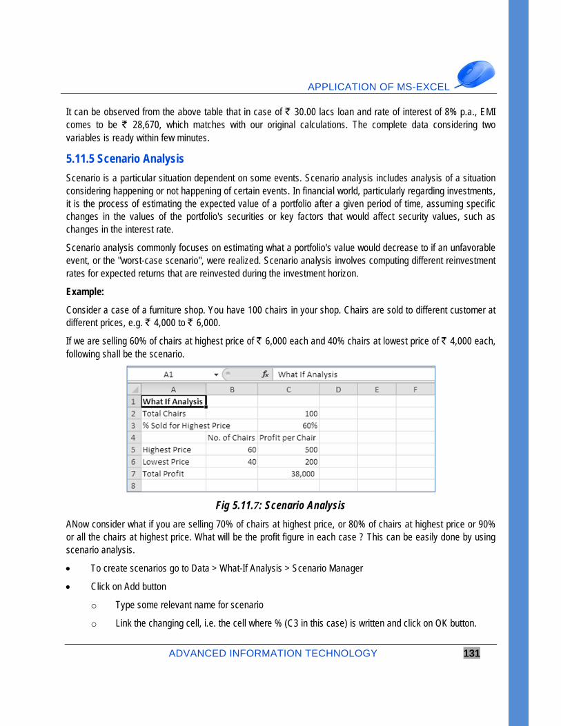
APPLICATION OF MS-EXCEL
ADVANCED INFORMATION TECHNOLOGY 131
It can be observed from the above table that in case of ` 30.00 lacs loan and rate of interest of 8% p.a., EMI comes to be ` 28,670, which matches with our original calculations. The complete data considering two variables is ready within few minutes.
5.11.5 Scenario Analysis
Scenario is a particular situation dependent on some events. Scenario analysis includes analysis of a situation considering happening or not happening of certain events. In financial world, particularly regarding investments, it is the process of estimating the expected value of a portfolio after a given period of time, assuming specific changes in the values of the portfolio's securities or key factors that would affect security values, such as changes in the interest rate.
Scenario analysis commonly focuses on estimating what a portfolio's value would decrease to if an unfavorable event, or the "worst-case scenario", were realized. Scenario analysis involves computing different reinvestment rates for expected returns that are reinvested during the investment horizon.
Example:
Consider a case of a furniture shop. You have 100 chairs in your shop. Chairs are sold to different customer at different prices, e.g. ` 4,000 to ` 6,000.
If we are selling 60% of chairs at highest price of ` 6,000 each and 40% chairs at lowest price of ` 4,000 each, following shall be the scenario.
Fig 5.11.7: Scenario Analysis
ANow consider what if you are selling 70% of chairs at highest price, or 80% of chairs at highest price or 90% or all the chairs at highest price. What will be the profit figure in each case ? This can be easily done by using scenario analysis.
To create scenarios go to Data > What-If Analysis > Scenario Manager
Click on Add button
o Type some relevant name for scenario
o Link the changing cell, i.e. the cell where % (C3 in this case) is written and click on OK button.
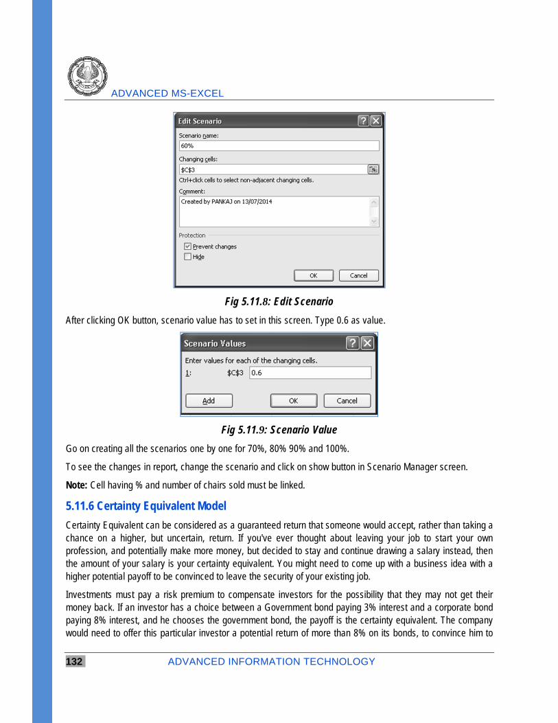
ADVANCED MS-EXCEL
132 ADVANCED INFORMATION TECHNOLOGY
Fig 5.11.8: Edit Scenario
After clicking OK button, scenario value has to set in this screen. Type 0.6 as value.
Fig 5.11.9: Scenario Value
Go on creating all the scenarios one by one for 70%, 80% 90% and 100%.
To see the changes in report, change the scenario and click on show button in Scenario Manager screen.
Note: Cell having % and number of chairs sold must be linked.
5.11.6 Certainty Equivalent Model
Certainty Equivalent can be considered as a guaranteed return that someone would accept, rather than taking a chance on a higher, but uncertain, return. If you've ever thought about leaving your job to start your own profession, and potentially make more money, but decided to stay and continue drawing a salary instead, then the amount of your salary is your certainty equivalent. You might need to come up with a business idea with a higher potential payoff to be convinced to leave the security of your existing job.
Investments must pay a risk premium to compensate investors for the possibility that they may not get their money back. If an investor has a choice between a Government bond paying 3% interest and a corporate bond paying 8% interest, and he chooses the government bond, the payoff is the certainty equivalent. The company would need to offer this particular investor a potential return of more than 8% on its bonds, to convince him to
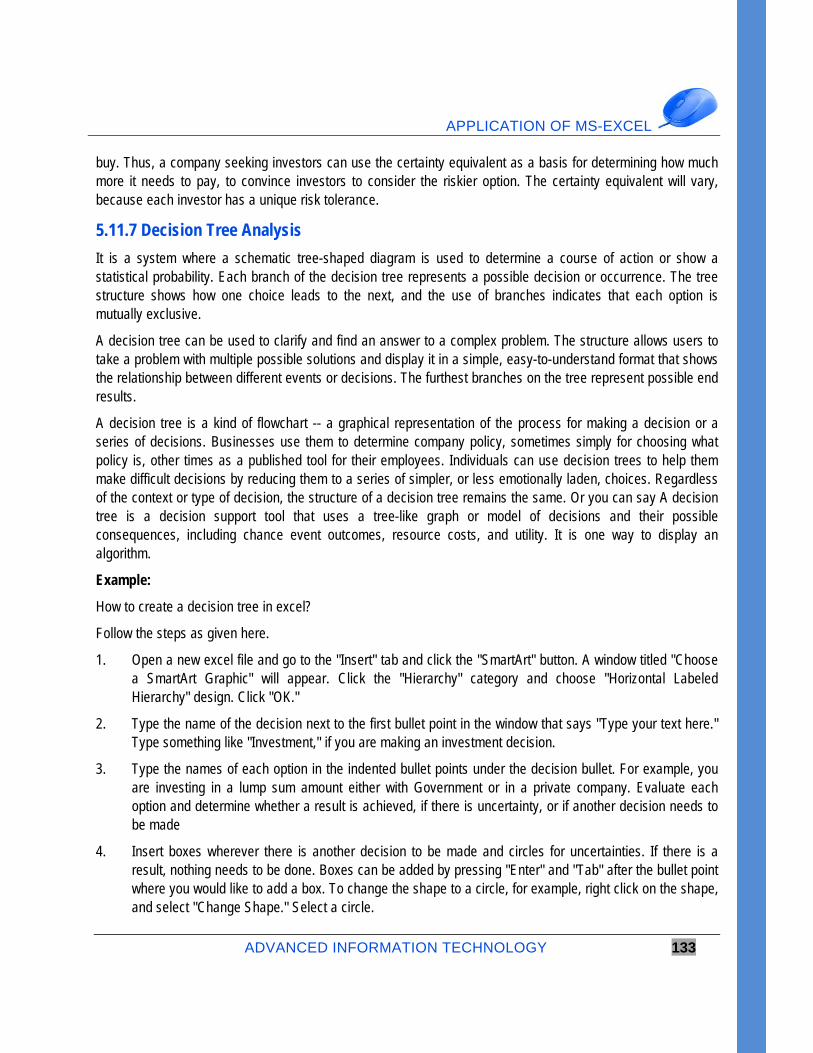
APPLICATION OF MS-EXCEL
ADVANCED INFORMATION TECHNOLOGY 133
buy. Thus, a company seeking investors can use the certainty equivalent as a basis for determining how much more it needs to pay, to convince investors to consider the riskier option. The certainty equivalent will vary, because each investor has a unique risk tolerance.
5.11.7 Decision Tree Analysis
It is a system where a schematic tree-shaped diagram is used to determine a course of action or show a statistical probability. Each branch of the decision tree represents a possible decision or occurrence. The tree structure shows how one choice leads to the next, and the use of branches indicates that each option is mutually exclusive.
A decision tree can be used to clarify and find an answer to a complex problem. The structure allows users to take a problem with multiple possible solutions and display it in a simple, easy-to-understand format that shows the relationship between different events or decisions. The furthest branches on the tree represent possible end results.
A decision tree is a kind of flowchart -- a graphical representation of the process for making a decision or a series of decisions. Businesses use them to determine company policy, sometimes simply for choosing what policy is, other times as a published tool for their employees. Individuals can use decision trees to help them make difficult decisions by reducing them to a series of simpler, or less emotionally laden, choices. Regardless of the context or type of decision, the structure of a decision tree remains the same. Or you can say A decision tree is a decision support tool that uses a tree-like graph or model of decisions and their possible consequences, including chance event outcomes, resource costs, and utility. It is one way to display an algorithm.
Example:
How to create a decision tree in excel?
Follow the steps as given here.
1. Open a new excel file and go to the "Insert" tab and click the "SmartArt" button. A window titled "Choose a SmartArt Graphic" will appear. Click the "Hierarchy" category and choose "Horizontal Labeled Hierarchy" design. Click "OK."
2. Type the name of the decision next to the first bullet point in the window that says "Type your text here." Type something like "Investment," if you are making an investment decision.
3. Type the names of each option in the indented bullet points under the decision bullet. For example, you are investing in a lump sum amount either with Government or in a private company. Evaluate each option and determine whether a result is achieved, if there is uncertainty, or if another decision needs to be made
4. Insert boxes wherever there is another decision to be made and circles for uncertainties. If there is a result, nothing needs to be done. Boxes can be added by pressing "Enter" and "Tab" after the bullet point where you would like to add a box. To change the shape to a circle, for example, right click on the shape, and select "Change Shape." Select a circle.
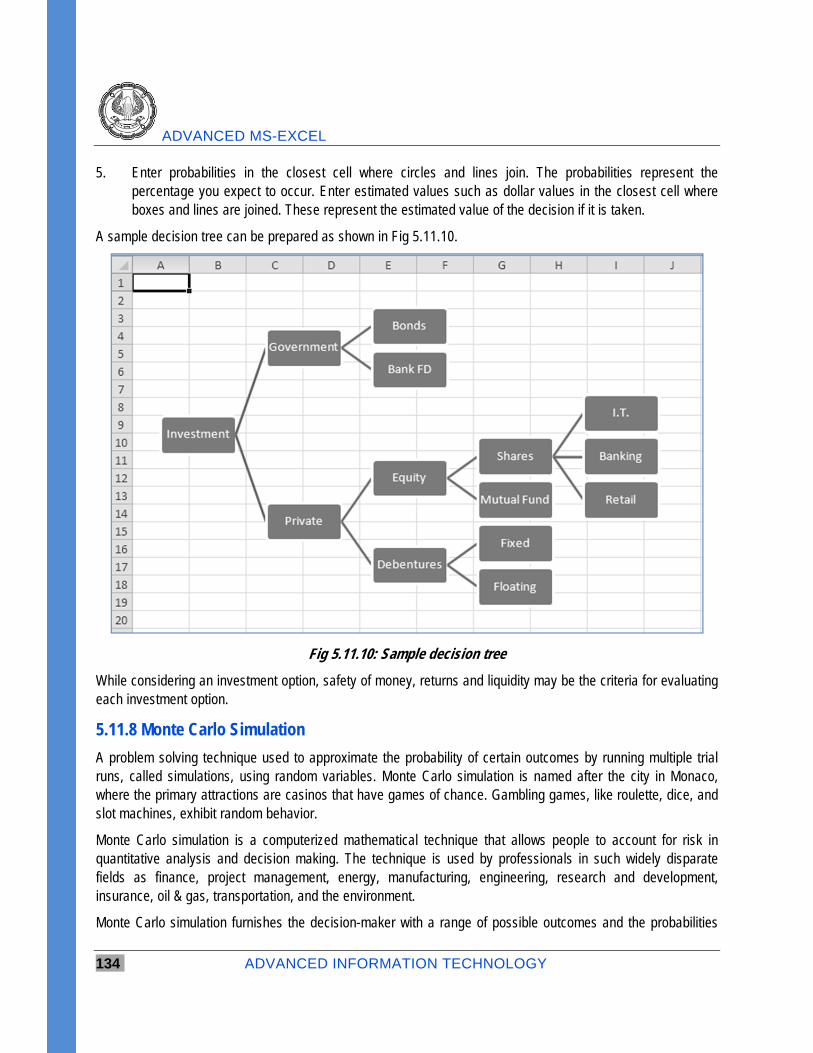
ADVANCED MS-EXCEL
134 ADVANCED INFORMATION TECHNOLOGY
5. Enter probabilities in the closest cell where circles and lines join. The probabilities represent the percentage you expect to occur. Enter estimated values such as dollar values in the closest cell where boxes and lines are joined. These represent the estimated value of the decision if it is taken.
A sample decision tree can be prepared as shown in Fig 5.11.10.
Fig 5.11.10: Sample decision tree
While considering an investment option, safety of money, returns and liquidity may be the criteria for evaluating each investment option.
5.11.8 Monte Carlo Simulation
A problem solving technique used to approximate the probability of certain outcomes by running multiple trial runs, called simulations, using random variables. Monte Carlo simulation is named after the city in Monaco, where the primary attractions are casinos that have games of chance. Gambling games, like roulette, dice, and slot machines, exhibit random behavior.
Monte Carlo simulation is a computerized mathematical technique that allows people to account for risk in quantitative analysis and decision making. The technique is used by professionals in such widely disparate fields as finance, project management, energy, manufacturing, engineering, research and development, insurance, oil & gas, transportation, and the environment.
Monte Carlo simulation furnishes the decision-maker with a range of possible outcomes and the probabilities
APPLICATION OF MS-EXCEL
ADVANCED INFORMATION TECHNOLOGY 135
they will occur for any choice of action.. It shows the extreme possibilities—the outcomes of going for broke and for the most conservative decision—along with all possible consequences for middle-of-the-road decisions.
The technique was first used by scientists working on the atom bomb; it was named for Monte Carlo, the Monaco resort town renowned for its casinos. Since its introduction in World War II, Monte Carlo simulation has been used to model a variety of physical and conceptual systems.
5.12 Finance Planning Planning is considered to be the primary requirement for moving towards any goal. Financial planning is the process of meeting the financial goals through the proper management of finances. Proper management of finances includes deciding the source and application of funds along with it timing. It is common for anybody to face financial setbacks at some point. One way to avoid or reduce the impact of such setbacks in the future is through careful financial planning. Financial goals can include buying a home, saving for your child’s education or planning for retirement. The financial planning process involves the following steps:
There are two basic rules in any type of financial planning.
(a) Earlier the better – Money received today is always better than money received tomorrow.
(b) Bigger the better – More money received is always better than less money received.
5.12.1 Five Ds of Finance Planning:
1. Deciding the Objective : This is the first step in financial planning. One has to be clear about the objective of finance planning. This is basic step which decides and impacts all the future steps.
2. Data Collection : Once the objective is decided and clear, the next step is to collect the required data for analysis. Data can be obtained in any form, but mostly it will be in figures. Excel can be used for storing the data of any size very easily.
3. Data Analysis : This is a very important step in the overall process. This step requires huge amount of efforts and expertise. Excel can be very effectively used for analysis of data of any size and that too with great amount of ease. Data is evaluated as per the direction of financial objective.
4. Drawing Inference :This step invovles human intervention. Many a times this step is ignored. Every individual may have his/her own set of rules for drawing inferences. Two different individuals may draw two different inferences using the same set of data.
5. Decision Making : Once the inferenace is drawn, decision has to be taken about financial planning. Decision making involves taking action on the basis of four earlier steps.
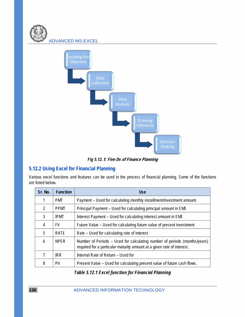
ADVANCED MS-EXCEL
136 ADVANCED INFORMATION TECHNOLOGY
Fig 5.12.1: Five Ds of Finance Planning
5.12.2 Using Excel for Financial Planning
Various excel functions and features can be used in the process of financial planning. Some of the functions are listed below.
Sr. No. Function Use
1 PMT Payment – Used for calculating monthly installment/investment amount.
2 PPMT Principal Payment – Used for calculating principal amount in EMI
3 IPMT Interest Payment – Used for calculating interest amount in EMI
4 FV Future Value – Used for calculating future value of present investment
5 RATE Rate – Used for calculating rate of interest
6 NPER Number of Periods – Used for calculating number of periods (months/years) required for a particular maturity amount at a given rate of interest.
7 IRR Internal Rate of Return – Used for
8 PV Present Value – Used for calculating present value of future cash flows.
Table 5.12.1 Excel function for Financial Planning
Deciding the Objective
Data Collection
Data Analysis
Drawing Inference
Decision Making
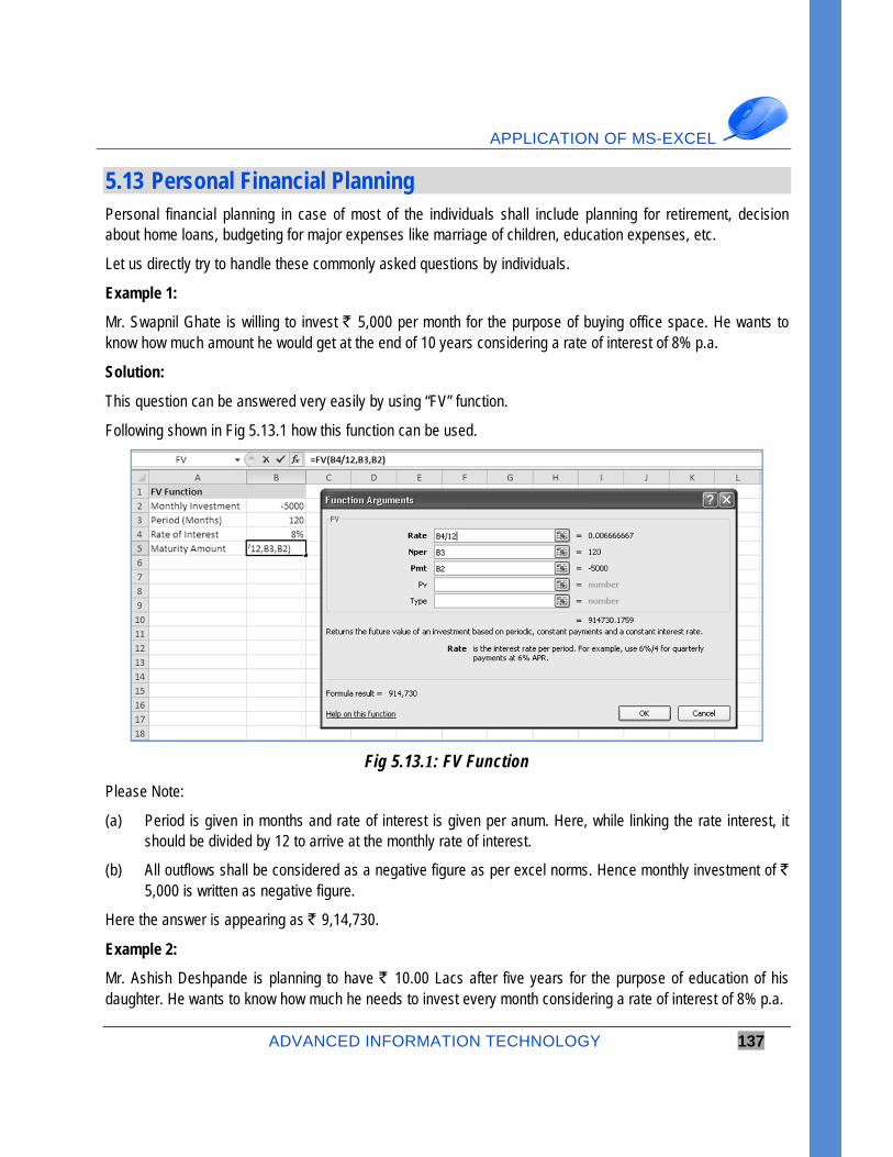
APPLICATION OF MS-EXCEL
ADVANCED INFORMATION TECHNOLOGY 137
5.13 Personal Financial Planning Personal financial planning in case of most of the individuals shall include planning for retirement, decision about home loans, budgeting for major expenses like marriage of children, education expenses, etc.
Let us directly try to handle these commonly asked questions by individuals.
Example 1:
Mr. Swapnil Ghate is willing to invest ` 5,000 per month for the purpose of buying office space. He wants to know how much amount he would get at the end of 10 years considering a rate of interest of 8% p.a.
Solution:
This question can be answered very easily by using “FV” function.
Following shown in Fig 5.13.1 how this function can be used.
Fig 5.13.1: FV Function
Please Note:
(a) Period is given in months and rate of interest is given per anum. Here, while linking the rate interest, it should be divided by 12 to arrive at the monthly rate of interest.
(b) All outflows shall be considered as a negative figure as per excel norms. Hence monthly investment of ` 5,000 is written as negative figure.
Here the answer is appearing as ` 9,14,730.
Example 2:
Mr. Ashish Deshpande is planning to have ` 10.00 Lacs after five years for the purpose of education of his daughter. He wants to know how much he needs to invest every month considering a rate of interest of 8% p.a.
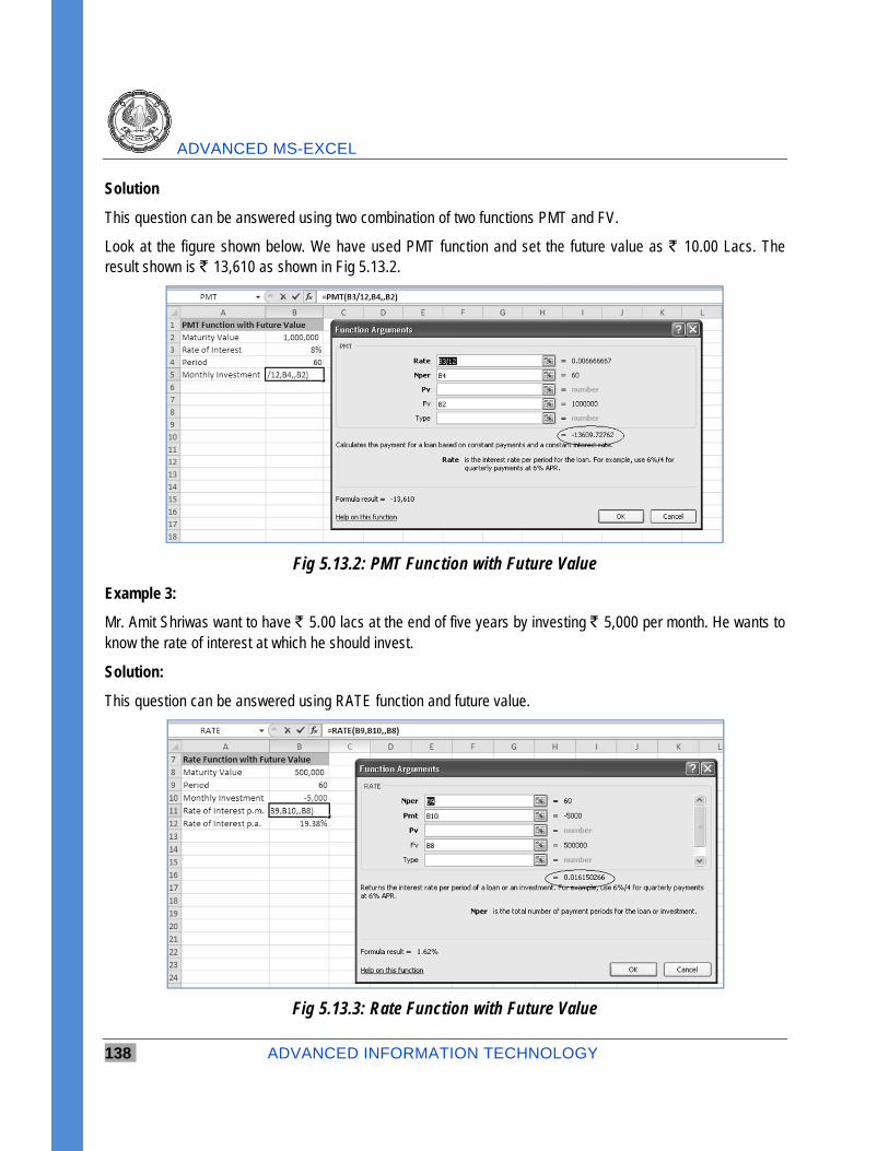
ADVANCED MS-EXCEL
138 ADVANCED INFORMATION TECHNOLOGY
Solution
This question can be answered using two combination of two functions PMT and FV.
Look at the figure shown below. We have used PMT function and set the future value as ` 10.00 Lacs. The result shown is ` 13,610 as shown in Fig 5.13.2.
Fig 5.13.2: PMT Function with Future Value
Example 3:
Mr. Amit Shriwas want to have ` 5.00 lacs at the end of five years by investing ` 5,000 per month. He wants to know the rate of interest at which he should invest.
Solution:
This question can be answered using RATE function and future value.
Fig 5.13.3: Rate Function with Future Value
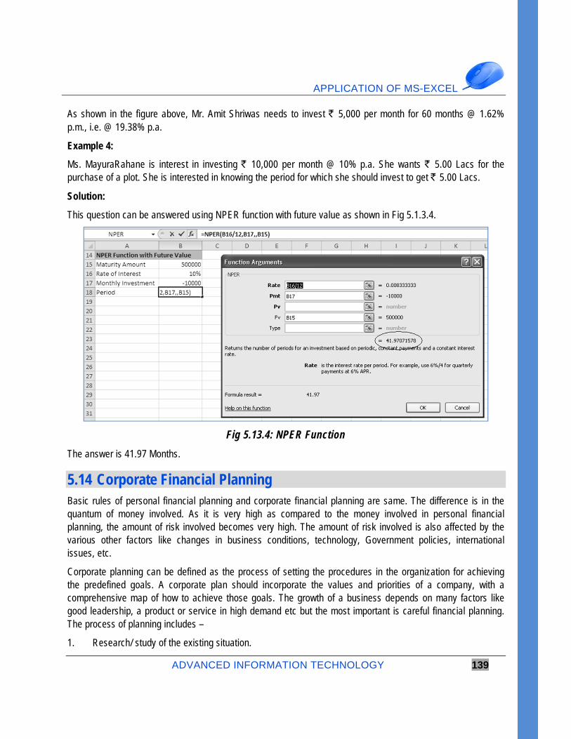
APPLICATION OF MS-EXCEL
ADVANCED INFORMATION TECHNOLOGY 139
As shown in the figure above, Mr. Amit Shriwas needs to invest ` 5,000 per month for 60 months @ 1.62% p.m., i.e. @ 19.38% p.a.
Example 4:
Ms. MayuraRahane is interest in investing ` 10,000 per month @ 10% p.a. She wants ` 5.00 Lacs for the purchase of a plot. She is interested in knowing the period for which she should invest to get ` 5.00 Lacs.
Solution:
This question can be answered using NPER function with future value as shown in Fig 5.1.3.4.
Fig 5.13.4: NPER Function
The answer is 41.97 Months.
5.14 Corporate Financial Planning Basic rules of personal financial planning and corporate financial planning are same. The difference is in the quantum of money involved. As it is very high as compared to the money involved in personal financial planning, the amount of risk involved becomes very high. The amount of risk involved is also affected by the various other factors like changes in business conditions, technology, Government policies, international issues, etc.
Corporate planning can be defined as the process of setting the procedures in the organization for achieving the predefined goals. A corporate plan should incorporate the values and priorities of a company, with a comprehensive map of how to achieve those goals. The growth of a business depends on many factors like good leadership, a product or service in high demand etc but the most important is careful financial planning. The process of planning includes –
1. Research/ study of the existing situation.
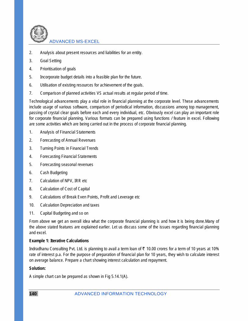
ADVANCED MS-EXCEL
140 ADVANCED INFORMATION TECHNOLOGY
2. Analysis about present resources and liabilities for an entity.
3. Goal Setting
4. Prioritisation of goals
5. Incorporate budget details into a feasible plan for the future.
6. Utilisation of existing resources for achievement of the goals.
7. Comparison of planned activities VS actual results at regular period of time.
Technological advancements play a vital role in financial planning at the corporate level. These advancements include usage of various software, comparison of periodical information, discussions among top management, passing of crystal clear goals before each and every individual, etc. Obviously excel can play an important role for corporate financial planning. Various formats can be prepared using functions / feature in excel. Following are some activities which are being carried out in the process of corporate financial planning.
1. Analysis of Financial Statements
2. Forecasting of Annual Revenues
3. Turning Points in Financial Trends
4. Forecasting Financial Statements
5. Forecasting seasonal revenues
6. Cash Budgeting
7. Calculation of NPV, IRR etc
8. Calculation of Cost of Capital
9. Calculations of Break Even Points, Profit and Leverage etc
10. Calculation Depreciation and taxes
11. Capital Budgeting and so on
From above we get an overall idea what the corporate financial planning is and how it is being done.Many of the above stated features are explained earlier. Let us discuss some of the issues regarding financial planning and excel.
Example 1: Iterative Calculations
Indradhanu Consulting Pvt. Ltd. is planning to avail a term loan of ` 10.00 crores for a term of 10 years at 10% rate of interest p.a. For the purpose of preparation of financial plan for 10 years, they wish to calculate interest on average balance. Prepare a chart showing interest calculation and repayment.
Solution:
A simple chart can be prepared as shown in Fig 5.14.1(A).
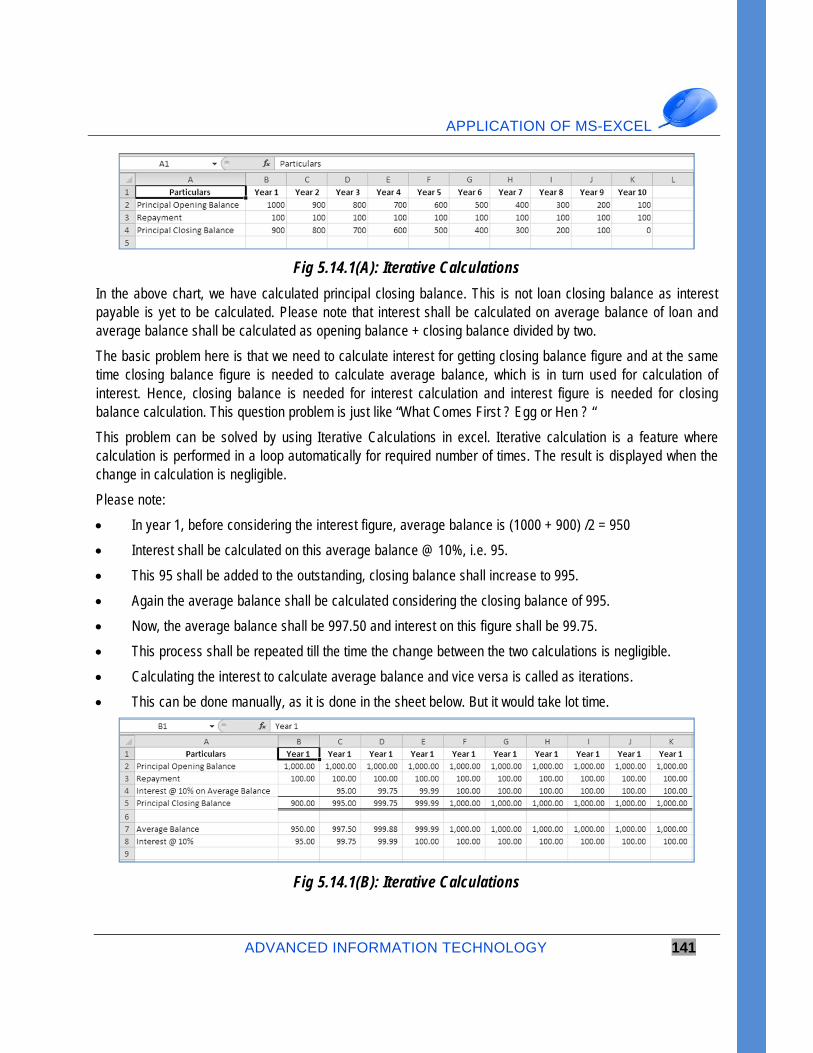
APPLICATION OF MS-EXCEL
ADVANCED INFORMATION TECHNOLOGY 141
Fig 5.14.1(A): Iterative Calculations
In the above chart, we have calculated principal closing balance. This is not loan closing balance as interest payable is yet to be calculated. Please note that interest shall be calculated on average balance of loan and average balance shall be calculated as opening balance + closing balance divided by two.
The basic problem here is that we need to calculate interest for getting closing balance figure and at the same time closing balance figure is needed to calculate average balance, which is in turn used for calculation of interest. Hence, closing balance is needed for interest calculation and interest figure is needed for closing balance calculation. This question problem is just like “What Comes First ? Egg or Hen ? “
This problem can be solved by using Iterative Calculations in excel. Iterative calculation is a feature where calculation is performed in a loop automatically for required number of times. The result is displayed when the change in calculation is negligible.
Please note:
In year 1, before considering the interest figure, average balance is (1000 + 900) /2 = 950
Interest shall be calculated on this average balance @ 10%, i.e. 95.
This 95 shall be added to the outstanding, closing balance shall increase to 995.
Again the average balance shall be calculated considering the closing balance of 995.
Now, the average balance shall be 997.50 and interest on this figure shall be 99.75.
This process shall be repeated till the time the change between the two calculations is negligible.
Calculating the interest to calculate average balance and vice versa is called as iterations.
This can be done manually, as it is done in the sheet below. But it would take lot time.
Fig 5.14.1(B): Iterative Calculations
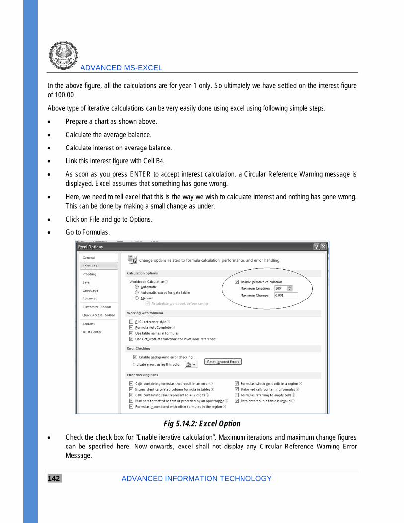
ADVANCED MS-EXCEL
142 ADVANCED INFORMATION TECHNOLOGY
In the above figure, all the calculations are for year 1 only. So ultimately we have settled on the interest figure of 100.00
Above type of iterative calculations can be very easily done using excel using following simple steps.
Prepare a chart as shown above.
Calculate the average balance.
Calculate interest on average balance.
Link this interest figure with Cell B4.
As soon as you press ENTER to accept interest calculation, a Circular Reference Warning message is displayed. Excel assumes that something has gone wrong.
Here, we need to tell excel that this is the way we wish to calculate interest and nothing has gone wrong. This can be done by making a small change as under.
Click on File and go to Options.
Go to Formulas.
Fig 5.14.2: Excel Option
Check the check box for “Enable iterative calculation”. Maximum iterations and maximum change figures can be specified here. Now onwards, excel shall not display any Circular Reference Warning Error Message.
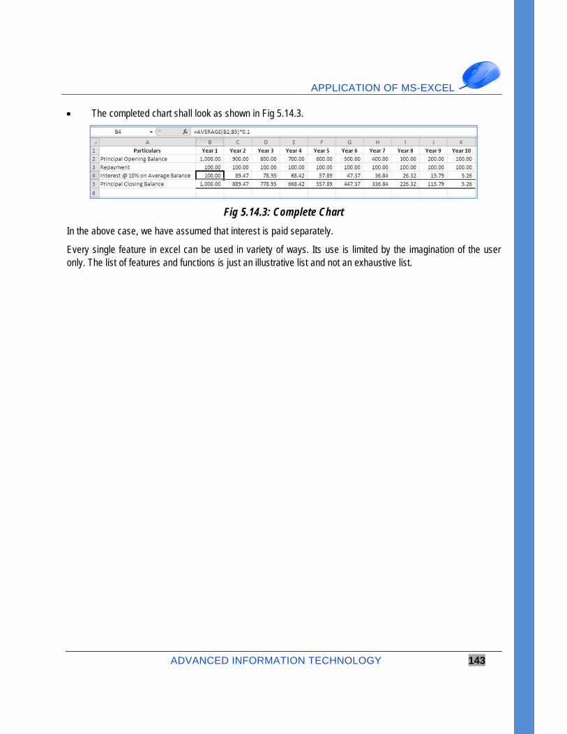
APPLICATION OF MS-EXCEL
ADVANCED INFORMATION TECHNOLOGY 143
The completed chart shall look as shown in Fig 5.14.3.
Fig 5.14.3: Complete Chart
In the above case, we have assumed that interest is paid separately.
Every single feature in excel can be used in variety of ways. Its use is limited by the imagination of the user only. The list of features and functions is just an illustrative list and not an exhaustive list.